Flexible Kernel Memory

Flexible Kernel MemoryDimitri Nowicki1,2*, Hava Siegelmann1,3

1 Biologically Inspired Neural and Dynamical Systems (BINDS) Lab, Department of Computer Science, University of Massachusetts Amherst, Amherst, Massachusetts,

United States of America, 2 Institute of Mathematical Machines and Systems Problems of Ukraine National Academy of Science (IMMSP NASU), Center for Cybernetics,

Kiev, Ukraine, 3 Program on Evolutionary Dynamics, Harvard University, Cambridge, Massachusetts, United States of America

Abstract

This paper introduces a new model of associative memory, capable of both binary and continuous-valued inputs. Based onkernel theory, the memory model is on one hand a generalization of Radial Basis Function networks and, on the other, is infeature space, analogous to a Hopfield network. Attractors can be added, deleted, and updated on-line simply, withoutharming existing memories, and the number of attractors is independent of input dimension. Input vectors do not have toadhere to a fixed or bounded dimensionality; they can increase and decrease it without relearning previous memories. Amemory consolidation process enables the network to generalize concepts and form clusters of input data, whichoutperforms many unsupervised clustering techniques; this process is demonstrated on handwritten digits from MNIST.Another process, reminiscent of memory reconsolidation is introduced, in which existing memories are refreshed and tunedwith new inputs; this process is demonstrated on series of morphed faces.

Citation: Nowicki D, Siegelmann H (2010) Flexible Kernel Memory. PLoS ONE 5(6): e10955. doi:10.1371/journal.pone.0010955

Editor: Pedro Antonio Valdes-Sosa, Cuban Neuroscience Center, Cuba

Received September 7, 2009; Accepted March 23, 2010; Published June 11, 2010

Copyright: � 2010 Nowicki, Siegelmann. This is an open-access article distributed under the terms of the Creative Commons Attribution License, which permitsunrestricted use, distribution, and reproduction in any medium, provided the original author and source are credited.

Funding: This work was supported by the Office of Naval Research grant #109-0138R (www.onr.navy.mil). The funder had no role in study design, datacollection and analysis, decision to publish, or preparation of the manuscript.

Competing Interests: The authors have declared that no competing interests exist.

* E-mail: [email protected]

Introduction

Memory experiments demonstrated persistent activity in several

structures in the lower mammal, primate, and human brains

including the hippocampus [1,2], prefrontal [3], visual [4] and

oculomotor cortex [5], basal ganglia [6], etc. Persistent dynamics is

believed to emerge as attractor dynamics (see also [7]–[13]).

Currently, the leading paradigm in attractor neural networks

memory models is the Hopfield model [14] with possible variations,

including activation functions, neural firing, density of the neural

connections, and the memory loading paradigms [15]–[22].

In this paper, we introduce a memory model, in which its

memory attractors do not lie in the input or neural space as in

classical models but rather in a feature space with large or

infinite dimension. This model is isomorphic to a symmetric

Hopfield network in the kernels’ -space, giving rise to a

Lyapunov function in the dynamics of associative recalls, which

enables the analogy to be drawn between memories and

attractors in the kernel space.

There are several advantages to our novel kernel approach to

attractor memory. The input space can be composed of either

continuous-valued or binary vectors. The number of attractors m

is independent of the input dimension n, thus posing a saturated-

free model, which does not suffer corrupted memories with

memory overload. Attractors can be efficiently loaded, deleted,

and updated on-line, something that has previously been only a

property of symbolic computer-memory models. Furthermore, for

the first time in neural memory models, we have demonstrated a

method allowing input dimension not to be constrained to a fixed

size or be a priori bounded; dimension can change with time,

similar to organic memory allocation for memories of greater

importance or increased detail. These attributes may be very

beneficial in psychological modeling.

The process of kernel memory consolidation results in attractors

in feature space and Voronoi-like diagrams that can be projected

efficiently to the input space. The process can also describe

clusters, which enables the separation of even very close-by

attractors. Another re-consolidation process enables tracking

monotonic updates in inputs including moving and changing

objects.

Generalizing Radial-Basis-Function NetworksOur network can be thought of as generalizing Radial Basis

Function (RBF) networks [23]. These are 2-layered feed-forward

networks with the first layer of neurons having linear activation

and the second layer consisting of neurons with RBF activation

function. Recurrent versions of the RBF networks [24,25] add

time-delayed feedback from the second to the first layer. Our

network enables a more generalized structure, both in terms of

number of layers and in allowing for many more general activation

functions.

Unlike previous RBF networks, our activation functions are

chosen from a large variety of kernels that allow us to distinguish

attractors that are similar or highly correlated. Furthermore,

unlike any previous RBF network with its fixed architecture and

activation functions, our selected neural kernel functions can

change during learning to reflect the memory model’s changing

properties, dimension, or focus. We go on to prove that the

attractors are either fixed points or 2-cycles, unlike general

recurrent RBF networks that may have arbitrary chaotic

attractors [26,27]; regular attractors are advantageous for a

memory system.

PLoS ONE | www.plosone.org 1 June 2010 | Volume 5 | Issue 6 | e10955

Synaptic plasticity and Memory ReconsolidationReconsolidation is a process occurring when memory becomes

liable during retrieval and can then be updated. This process is

implicated in learning and flexible memories when healthy; it leads to

amnesia and compulsive disorders when corrupted. Reconsolidation

is observed both in neurophysiological and psychological studies

([28]–[33]) and has been modeled in artificial neural systems as well

([19,34]). While the actual processes underlying reconsolidation are

still being studied, the property of dependance on sample ordering

has been established in both electrophysiology of CA3 neurons [13]

and in psychophysics [35]. In reconsolidation, memory representa-

tions are sensitive to the order of sample data: when samples change

in an orderly manner, the reconsolidation process learns and updates

effectively. When samples are shuffled and consistent direction of

change is lost, existing memories do not update. We show here that

the importance of input ordering is inherent in any update processes,

reminiscent of reconsolidation. We also demonstrate how reconso-

lidation works in flexible environments and with large-scale data

beyond the model shown in [19].

Our flexible model assumes global memory update. This is an

interesting approach for a few reasons. First, it results in more

stable and robust updates: in other models the ‘‘closest’’ attractor

may be selected incorrectlyly due to noise. Second, it enables a

direct analogy to an existing neural model of reconsolidation [19]

since there the whole synaptic matrix is adjusted, not simply a

chosen attractor. Moreover with global updates our memory can

demonstrate phenomena analogous to the gang effect [36]. While

we have taken a global update approach our model retains the

property in which the retrieved attractor (the attractor closest to

the current input) is most affected.

Kernel Based Algorithms and MemoriesThe memory system introduced here takes advantage of

developments introduced in Support Vector Machine (SVM)

[37], Least-Square SVM [38] and Support Vector Clustering

[39], where kernel functions enable data handling in higher

feature spaces for richer boundaries, yet do so efficiently and

cheaply. Our support-vector-like memory system incorporates

the realistic property of flexible attractors with high dimensional

feature spaces, while being tractable and implementable by

neural units.

Zhang et al. [40] introduced a feedforward network with

particular kernels in the form of wavelet and Radial Basis

Functions (RBF) that were fit to perform a face recognition task

efficiently. The kernel heteroassociative memories were organized

into the modular network. Our architecture can be recurrent,

which is more powerful than the feedforward method, can handle

discrete and analog inputs, and the kernels we use can change

online adding increased flexibility and capability.

Caputo [41] explored analogies from associative memory to

‘‘kernel spin glass’’ and demonstrated an attractor network,

loading bipolar inputs and using generalized Hebbian learning

to load non-flexible memories with greater memory capacity than

the Hopfield network. In this work, a kernel algorithm generalized

the Hebbian rule and the energy function of Hopfield networks,

while capacity estimations generalized Amit’s approach [1]. This

method built in the free energy function in addition to the

Hamiltonian. Our system, by comparison, allows for both binary

and continuous inputs, is far more flexible in that the kernels adapt

themselves over time and that attractors and features can be added

and removed. Further, our system is more practical in that it has

the added capability to cluster data.

Support vector memory by Casali et al. [42] utilized support

vectors to find the optimal symmetric Hopfield-like matrix for a set

of binary input vectors. Their approach is very different from ours

despite the similar title, in that it considers only binary symmetric

case and has bounded attraction space. Support-vector optimiza-

tion is used to find optimal matrix W for given m|n matrix X of

etalons. This matrix must satisfy relationship sign(WX)~sign(X).Support vectors are found to provide optimal margins of WX.

Kernels are not used in this work and hence the name is somewhat

confusing. Our kernel memory is far richer: the number of

memory attractors is not bounded by input dimension -

accomplished by varying the input space; our encoding is more

efficient, our memory can use discrete or analog space, one-shot

learning, and overall is more flexible.

In support vector clustering [39], clusters are formed when a

sphere in the -space spanned by the kernels is projected

efficiently to input space. Here the clustering is a side effect of

the created memories that are formed as separated fixed points

in the -space, and where the Voronoi polyhedron is projected

on a formation of clusters in the input space. Formation of

memories is local, sharing this concept with the Localist

Attractor Network [43] and the Reconsolidation Attractor

Network [34].

OrganizationThis work will be presented as follows: At first, the model of

kernel heteroassociative memory is introduced, followed by the

special case of auto-associative memory where attractors emerge.

A neural representation is layered, and robustness (attraction

radius) is estimated. We then introduce a technique that allows

adding and removing attractors to the existing kernel associative

network, and follow by introducing another technique that adds or

removes input dimensionality on line. We next show a procedure

of consolidating data into representing attractors, and demonstrate

clusters emerging on handwritten digits and conclude by

introducing the functional level of reconsolidation in memory

and applications to morphed faces.

Results and Discussion

2.1 Our Kernel Heteroassociative Memory ModelA general framework of heteroassociative memory can be

defined on the input Ex and output Ey spaces, with dimension-

alities n and p respectively, and with m pairs of vectors

xi[Ex, yi[Ey, i~1 . . . m to be stored. The input vectors in the

space Ex can be written as columns of matrix X (n|m) and

associated vectors in the output space Ey as columns of matrix Y(p|m). A projective operator ~BB : EX?EY such that ~BBxi~yi can

be written in a matrix form ~BB with

~BBX~Y ð1Þ

and be solved as

B~YXz ð2Þ

with ‘‘z’’ stands for the Moore-Penrose pseudoinverse of X [44]. If

the columns of X are linearly independent, the pseudoinverse

matrix can be calculated by

Xz~(XT X){1XT : ð3Þ

Let us define matrix ~SS, (m|m), where the elements ~ssij are the

pairwise scalar products of the memorized vectors, that is

Flexible Kernel Memory


~ssij~(xi,xj), or in matrix notation:

~SS~XT X:

Then ~BB can be written as:

~BB~Y~SS{1XT : ð4Þ

We propose to formulate the pseudoinverse memory association

(recall) by calculating for each input vector x[Ex the output by:

y~~BBx~Y~SS{1z;

z~XT x;

zi~(xi,x):

ð5Þ

This is a ‘‘one-pass’’ non-iterative linear associative memory. It has

the property that if two input samples are close to each other, then

the two outputs will be close to each other as well:

y0{yk kƒ Bk k: x0{xk k.2.1.1 Memory in Feature Space. In order to overcome the

common dependence of memory capacity on input dimension, we

transform the input space EX to a new input space E which we

call feature space, whose dimensionality can be far greater than

the dimension of EX , n (it could even be an infinite-dimensional

Hilbert space). The transformation : EX?E is considered to be

transferring from input to feature space.

The respective associative memory algorithm can now be

defined as follows:

B (X)~Y ð6Þ

B~Y½ (X)�z ð7Þ

½ (X)�z~(½ (X)�T (X)){1½ (X)�T ð8Þ

Analogously writing S as

S~½ (X)�T (X)

sij~( (xi), (xj)),ð9Þ

the memory loads by:

B~YS{1½ (X)�T : ð10Þ

and the association (recall) procedure is calculated by:

y~Bx~YS{1z;

z~½ (X)�T (x);

zi~( (xi), (x)):

ð11Þ

Remark 1 Linear independence of the vectors (xi) in the -

space is required in order to use identity (3) for the Moore-Penrose

pseudoinverse (see [44]). It is achieved as we will see below by

using piece-wise Mercer kernels, and does not limit the number of

attractors. This identity is used to bring equation (7) to the form of

(8) and to introduce S.

We note that during both loading (10) and recall (11)

procedures, the function appears in the pair ( (xi), (xj)). We

can thus define a Kernel function over Ex|Ex and gain

computational advantage.

Let us denote a scalar product in the feature space E by

K(u,v)~( (u), (v)). This is a symmetric, real-valued, and

nonnegative-definite function over Ex|Ex called a kernel [37].

We now can write S and z using the Kernel K :

sij~K(xi,xj); i,j~1:::m

zi~K(xi,x):ð12Þ

The value of the Kernel function is scalar. Thus even if was a

function of high dimension the calculation of the multiplication is a

scalar and thus fast to calculate.

Mercer kernels as used in Support Vector Machines [37] are

not sufficient for creating the associative memory we introduce,

since our memories also require that all attractors are linearly

independent in the feature space. To enable such independence

we define the piece-wise Mercer kernels and in Section ‘‘Piece-

wise Mercer Kernels’’ of Materials and Methods (MM) we prove

that they can always be found and always lead to independence.

As opposed to Hebbian learning that requires O(n2m) multiplica-

tions, we need O(m3znm2) arithmetic operations over real scalars.

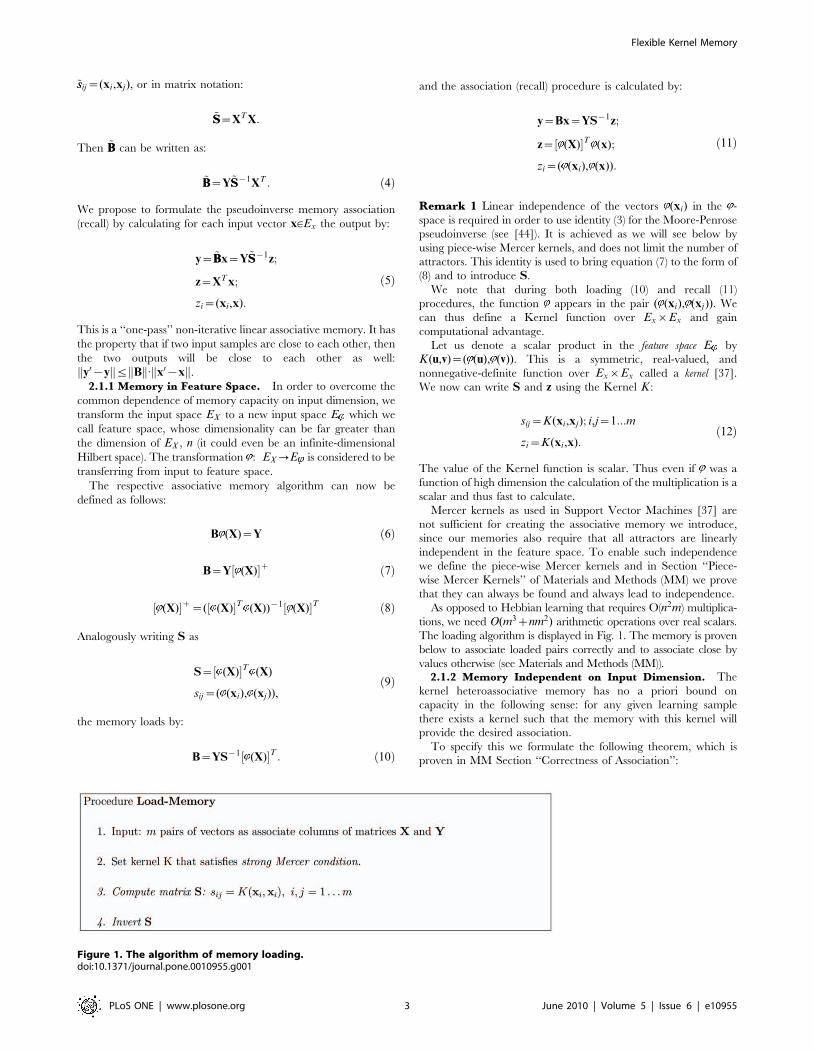
The loading algorithm is displayed in Fig. 1. The memory is proven

below to associate loaded pairs correctly and to associate close by

values otherwise (see Materials and Methods (MM)).2.1.2 Memory Independent on Input Dimension. The

kernel heteroassociative memory has no a priori bound on

capacity in the following sense: for any given learning sample

there exists a kernel such that the memory with this kernel will

provide the desired association.

To specify this we formulate the following theorem, which is

proven in MM Section ‘‘Correctness of Association’’:

Figure 1. The algorithm of memory loading.doi:10.1371/journal.pone.0010955.g001



Theorem 1 For any memory size m, let (xi,yi)[Ex|Ey, i~1 . . . m

be a learning sample consisting of m input-output pairs. Then there exists a

piece-wise Mercer kernel K such that the associative memory that has this

kernel and governed by equations (9)–(11) assigns xi to yi for all i~1 . . . m.

Remark 2 For the correct association, the memories have to

be linearly independent in the feature space. As we have shown

here this does not pose a memory limit, because for any given

learning sample we can find a (piece-wise Mercer) kernel that

guarantees such independence.

2.2 The Kernel Autoassociative Memory ModelWe next focus on the special case where Ex~Ey, and the stored

vectors xm~ym:jm, m~1 . . . m. Here the loading algorithm is the

same as in Fig. 1, and recall is facilitated by the iterative form:

xtz1~f (yt): ð13Þ

The activation function f (x) is applied by coordinates and constitutes

a bounded monotonically increasing real-valued function over R such

that limx?{?

f (x)~a, and limx?z?

f (x)~b, bwa.

The scheme of kernel auto-associative memory working in recall

mode is shown in Fig. 2. We prove (in lemma 4 in MM Section

‘‘Proving Convergence of the Autoassociative Recall Algorithm’’)

that the recall procedure always converges and that the attractors

are either fixed points or 2-limit cycles. Joining all operations to a

single equation we get:

x(tz1)~fXm

m,n~1

jmssm,nK(jn,x)

!ð14Þ

Here by ssm,n we denote the elements of S{1. In coordinate form

this equation is:

xi(tz1)~fXm

m,n~1

jmi ssm,nK(jn,x)

!ð15Þ

The pseudocode of the associative recall is shown in the Fig. 3.

As will be shown in the next section, the double nonlinearity of the

recall dynamics does not reduce the biological plausibility since the

kernel memory can be designed as a layered neural network with

only one nonlinear operation per neuron.

In Materials and Methods, Section ‘‘Example of the associative

recall’’, we provide an explicit example of kernel autoassociative

memory with Ex~R3 and E ~R6. We demonstrate there how a

set of five vectors is memorized and how the iterative recall works.

2.3 Kernel Associative Memory as a Neural NetworkThe autoassociative kernel memory can be directly implement-

ed in a recurrent layered neural network (Fig. 4a): The network

has n inputs. The first layer has m neurons that perform kernel

calculations; the i-th neuron computes zi~K(x,xi). In the special

case where the kernel is a radial-basis function K(u,v)~R( u{vk k)these neurons are the common RBF neurons [23]. The second

layer has m neurons, its weight matrix is S{1. The neurons of the

second layer can be either linear or have a generalized sigmoid

activation function.

The third layer also has n neurons, its weight matrix is XT . Its

activation function can be linear, generalized sigmoid or the even

more general sigmoid from Equation (15) above. The network has

‘‘one-to-one’’ feedback connections from the last layer to the

inputs. In recall mode it works in discrete time, like Hopfield

networks.

Definition 1 A monotonic bounded piecewise-differentiable function

f : R?R such that f (0)~0, f (1)~1, and f ’vhv1 in certain

neighborhoods of 0 and 1 is called generalized sigmoid.

Theorem 2 Suppose that the kernel associative memory has a generalized

sigmoid activation function in the second layer. Then the attractors emerging by

the iterative recall procedure are either fixed points or 2-cycles.

Proof appears in Material and Methods Section ‘‘Proving

Convergence of the Autoassociative Recall Algorithm’’.

2.3.1 The Attraction Radius. A key question for any neural

network or learning machine is how robust it is in the presence of

noise. In attractor networks, the stability of the associative

retrieval and the robustness to noise can be measured by the

attraction radius.

Definition 2 Suppose the input to an attractor network belongs to the

metric space with distance r. For an attractor jm of the network let Rm be

the largest positive real number such that if r(jm,x)vRm the dynamics of the

associative recall with starting point x will converge to jm. The value

R~ minm

Rm is called the attraction radius of the network (AR).

When inputs and memorized patterns belong to a normed

vector space, if the additive noise does not exceed the attraction

radius in this norm then all memories will be retrieved correctly

during the associative recall.

The attraction radius can be estimated in the following special

case:

Theorem 3 Suppose that a kernel associative memory has identity

activation function in the output layer and a generalized sigmoid f in the hidden

layer. Suppose also the kernel K satisfies the global Lipschitz condition on a

certain domain D5Rn, i.e., there exists L such that Vx1,x2,y[EK(x1,y){K(x2,y)DƒLEx1{x2E. Then the stored patterns are

attractors, and the memory attraction radius is

R§

c

ES{1E:L

where c is a constant that depends only on f .

The proof of this theorem is given in Materials and Methods

Sec. Proof of Theorem 3.

We further made a series of experiments of direct measurement

of attraction radius for a dataset of 30|30 gray-scale face images.

Results of this experiment are represented in Fig. 5.Figure 2. Scheme of the kernel autoassociative memory.doi:10.1371/journal.pone.0010955.g002



Remark 3 We have also proven that under the conditions of

Theorem 3 all stored patterns are attractors. Yet, the memory was

not proven to be free from spurious equilibria. However, spurious

attractors were never observed in numerical experiments. The

typical situation is that all the input domain is divided into

attraction basins of the memorized vectors. The basins look like

Voronoi polyhedra as depicted in Fig. 6.

2.3.2 Bounded Synaptic Weight Range. There is a

connection between a bound on the values of the synapses (see

[45]) and the kernel function defining the network.

Proposition 1 Let the kernel memory have input data such that every

two inputs Exi{xjE§d, Vi,j~1 . . . m, i=j and the piece-wise Mercer

kernel K with this d and certain m. Then the synapses defined by matrix S{1

are bounded and the following bound holds:

Dssi,j Dƒm{1

Proof. From the proof of Lemma 3.2 in Material and Methods

we know that S could be written as S~S0zmI, where S

0§0 is a

positive semidefinite matrix. By linear algebra we have

ES{1Eƒm{1. Finally ES{1Emax:maxij

Dssi,j DƒES{1E by matrix

norm equivalence in finite-dimensional space.

2.3.3 Maximizing Capacity. The kernel associative memory

works as a symmetric network in an abstract feature space is used

only in implicit way. Any implementation of the kernel associative

memory with neural computational units requires a recurrent

layered structure (Fig. 4). We can maximize the network capacity

by using the approximation S&I . This approximation is suitable if

the stored patterns are sufficiently distant in the kernel view, see

Remark 5. With this approximation one can save m3 connections

without significant loss of association quality by eliminating the

middle layer in Fig 4a and the other two layers will have weight

matrices X and XT , identical with respect to transposition; see

Fig. 4b. So, to store m vectors of Rn we would need m|n real

numbers only (lossless coding).

The definition of memory capacity and connections/neurons

ratio now leads to

max(m,n)

min(m,n)§1:

Remark 4 The approximation S&I is suitable if the stored

patterns are almost orthogonal in the feature space. For localized

kernels (e.g. RBF) this means that the patterns are distant enough

from each other (comparing to the characteristic scale of the

kernel). Because the condition of orthogonality is applied in the

feature space, not in the input space, this condition does not imply

any relative size of m versus n:With this optimization the kernel-memory network can be made

arbitrarily sparse by choosing a sparse kernel, i.e., a kernel that

explicitly depends only on a (small) portion of the coordinates of its

argument vectors. The non-zero weights will correspond to the

inputs that the sparse kernel depends on. The attractors will have a

sparse structure analogous to the kernel as well. If our goal is to

memorize arbitrary dense data we can still use the sparse network

as long as encoding and decoding layers are externally added to it.

2.4 Flexibility of the Memory2.4.1 Flexibility in the Attractor Space. The kernel

associative memory can be made capable of adding and

removing attractors explicitly.

To add a new attractor to the network we create a new neuron in

the S matrix layer. The dimension of matrix S is increased from m to

mz1. To do so we compute si,mz1~K(xi,xmz1) and we update the

inverse S{1 efficiently using the linear-algebra identity [46]:

(AzB){1~A{1{A{1B(IzA{1B)A{1 ð16Þ

where A~Sm 0

0 smz1,mz1

� �and

Figure 3. Algorithm of Associative Recall. An iterative procedure converges to an attractor.doi:10.1371/journal.pone.0010955.g003



B~

s1,mz1

0m|m...

sm,mz1

smz1,1 . . . smz1,m 0

0BBBB@

1CCCCA

Calculation using (16) takes O(m2) operations since S{1 is already

known.

Similarly one can delete an attractor by reducing the dimension

of S. Here

AzB~Sm{1 0

0 sm,m

� �A~Sm

B~

{s1,m

0(m{1)|(m{1)...

{sm{1,m

{sm,1 . . . {sm,m{1 0

0BBBB@

1CCCCA

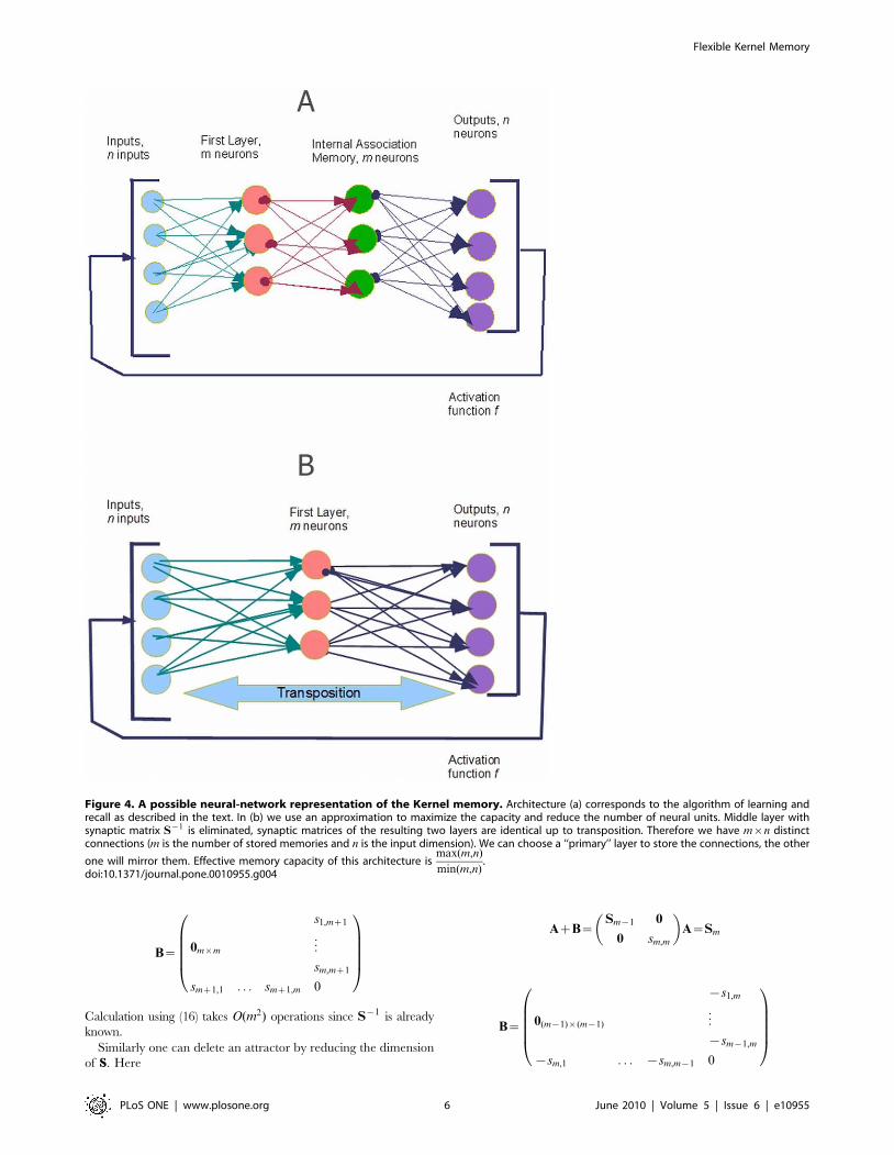
Figure 4. A possible neural-network representation of the Kernel memory. Architecture (a) corresponds to the algorithm of learning andrecall as described in the text. In (b) we use an approximation to maximize the capacity and reduce the number of neural units. Middle layer withsynaptic matrix S{1 is eliminated, synaptic matrices of the resulting two layers are identical up to transposition. Therefore we have m|n distinctconnections (m is the number of stored memories and n is the input dimension). We can choose a ‘‘primary’’ layer to store the connections, the other

one will mirror them. Effective memory capacity of this architecture ismax(m,n)

min(m,n).

doi:10.1371/journal.pone.0010955.g004



To receive Sm{1, the last column and last row from matrix AzBwill be removed.

This results in the two algorithms of Fig. 7.

Remark 5 In the case where S is approximately a diagonal

matrix, its inverse can be calculated by the approximation

S~lIzeS1 for small e, and S&lI, which does not change

during updates.

Remark 6 The procedure Add-Attractor (see Fig. 7) is local in

time. To store a new pattern in the memory we only have to know

the new attractor and the current connection matrix S{1.

In Fig. 6 we display an example of adding an attractor.

2.4.2 Flexibility in Input and Feature Spaces. External

inputs may come with more or fewer features than previously,

causing the input dimensionality to change with time. We propose a

mechanism that enables the network to handle such heterogeneity of

dimension with no need to relearn the previously learned inputs.

Assume that the current dimension in the input space consists of

the ‘‘initial dimension’’ n and ‘‘new’’ q dimensions; denote this as

x~ xa; xbð Þ. We will allow the change of dimensionality by

changing the kernel itself: from the kernel Kn that considers the

first n dimensions to kernel Knzq that depends on all dimensions.

The change of kernel requires the recalculation of S{1.

However, this need not require O(m3) operations if we constrain

to kernels that can be written in an additive form:

Knzq(x,y)~Kn(xa,ya)zKq(xb,yb)

zKint(xa,yb)zK�int(xb,ya)ð17Þ

where Kint describes the interaction of n and q. An explicit kernel with

this property is the polynomial kernel (see Section ‘‘Variable Kernel

and Dimensionality’’). Algorithms for dimensionality control appear

in Fig. 8. An example is given in Example 3 in the next section.

We also prove Lemma 4 in Materials and Methods Section

‘‘Variable Kernel and Dimensionality’’, stating that a small

alteration to the kernels enables changing input dimensionality

without loosing previously learnt attractors.

2.5 Memory Consolidation and ClusteringThe memory system with its loading algorithm enables

consolidation of inputs into clusters using the competitive learning

method. Suppose we have a learning sample of N vectors x1, . . . xN

and m clusters have to be created. Random vectors initiate the mattractors. When a new input is provided, the recall procedure is

performed and the attractor of convergence x�k is updated by

x�k/(1{an)x�kzanxn. Parameter sequence an is selected in order to

provide better convergence of attractors: for instance, we can take an

such that limn??

an~0 butP

nan??. This step is repeated until all

attractors stabilize.

We tested the consolidation algorithm using the MNIST

database of handwritten digits [47]. The data consists of ten

different classes of grayscale images (from ‘0’ to ‘9’, each of 28|28pixels in size) together with their class labels.

Experiment 1: Clustering with the Kernel Memory. The goal of this

experiment is to demonstrate performance of memory clustering. For

this purpose memory was trained on the learning sample in order to

form attractors. Then attractors were assigned to classes, and

classification rate was measured on an independent test sample.

For the MNIST data we used principal-component (PC)

preprocessing. We took the first d~200 PCs which contain

96.77% of the variance. The learning sample contained 10000

digits, 1000 from each class. The kernel was chosen in the form:

K(x,y)~exp{a

2R2

Xd

k~1

wk(xk{yk)2

!ð18Þ

where R2~Pd

k~1

wk, and a is a parameter. This is a Gaussian

kernel depending on weighted metric. Weights were chosen as:

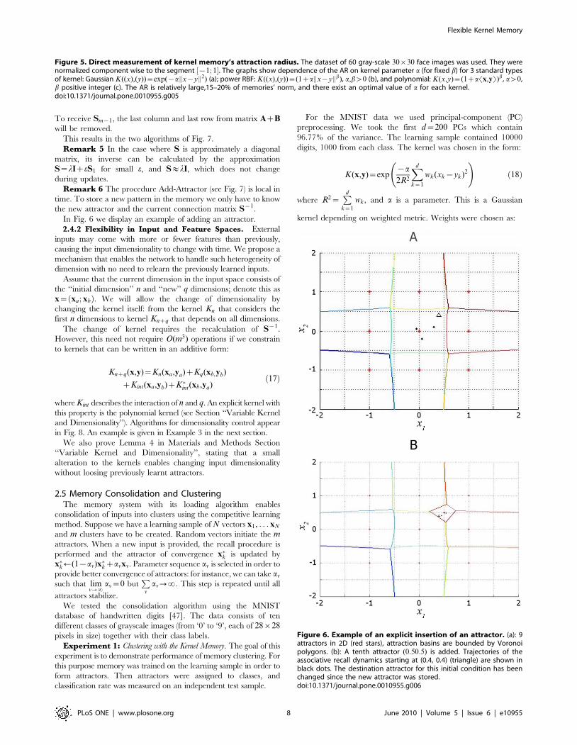
Figure 6. Example of an explicit insertion of an attractor. (a): 9attractors in 2D (red stars), attraction basins are bounded by Voronoipolygons. (b): A tenth attractor (0:50:5) is added. Trajectories of theassociative recall dynamics starting at (0.4, 0.4) (triangle) are shown inblack dots. The destination attractor for this initial condition has beenchanged since the new attractor was stored.doi:10.1371/journal.pone.0010955.g006

Figure 5. Direct measurement of kernel memory’s attraction radius. The dataset of 60 gray-scale 30|30 face images was used. They werenormalized component wise to the segment ½{1; 1�. The graphs show dependence of the AR on kernel parameter a (for fixed b) for 3 standard typesof kernel: Gaussian K((x),(y))~exp({aEx{yE2) (a); power RBF: K((x),(y))~(1zaEx{yEb), a,bw0 (b), and polynomial: K(x,y)~(1zaSx,yT)b, aw0,b positive integer (c). The AR is relatively large,15–20% of memories’ norm, and there exist an optimal value of a for each kernel.doi:10.1371/journal.pone.0010955.g005



wk~STD(xk)

1

Q

XQ

l~1

STDl(xk)

{1

0BBBB@

1CCCCA

2

ð19Þ

We also tried the formula:

wk~1

Q

XQ

l~1

(Elxk{Exk)2 ð20Þ

where El and STDl are expectation and standard deviation over

the l-th class, and Q is the quantity of classes. However formula

(19) gave better results.

Because of the complexity of the MNIST data, we chose to have

multiple clusters per class. Table 1 summarizes the classification rates

for different amounts of attractors in the memory. The classification is

slightly superior to other unsupervised clustering techniques (even

that the goal of the memory system is not directly in clustering). The

number of memory attractors required for good clustering is also

smaller than other techniques, e.g. [48]. Figure 9.a) provides an

example of typical memory attractors of each class.

We also made a series of experiments with wk~sk

R; R~

ffiffiffiffiffiffiffiffiffiffiffiffiffiXs2

k

q,

where sk is an STD of k-th principal component. This weighting

does not depend on class labels in any way. We can see (last row of

table 1) that results are poor for small number of attractors per class,

but for higher number of attractors classification rate is even better.

Experiment 2. Clustering under changing input dimensionality. This

experiment demonstrates clustering while input dimensionality

increases and the kernel is being changed. For this purpose, the

resolution of the original images was reduced twice, to 14|14 (Fig. 9).

Then the images were passed through a linear transformation in

order to use the kernel (19). The memory was trained on 10,000 such

digit images, forming 100 attractors. The recognition quality

obtained was 76.4%. Then the kernel was extended in order to

work with the original size (28|28), and another 10,000 digits were

added, now in full-size. This second session of learning started from

the previous set of attractors, without retraining. The final

classification rate was enhanced to 85.4%.

Experiment 3. Explicit example of adding input dimension.

Consider the R2 data where points lie on two Archimedes’ spirals:

x1~k cos( )

x2~k sin( )ð21Þ

and

x1~k cos( zp)

x2~k sin( zp)ð22Þ

We chose angle range [½p=5 : 8p� for both classes. The initial

kernel was K2~exp({(u1{v1)2z(u2{v2)2

2s22

). Then we add 3-d

coordinate x3~l1,2

ffiffiffiffiffiffiffiffiffiffiffiffiffiffix2

1zx22

q, where l1~1 and l2~1:5 for first

and second class. For R3 the additive kernel will be K3~K2zK1,

where K1~exp({(u3{v3)2

2s21

), an interaction term is not neces-

sary in this example. We took s1~0:25 and s2~0:2. At first, the

network was loaded with the 40 data points in R2. Each point was

labeled and a classification was executed. The recognition quality

on an independent test sample was 86:4%. Then the training was

continued with the additional 40 inputs in R3 and the final

classification rate increased to 97:5%.

2.6 Synaptic Plasticity and Memory ReconsolidationReconsolidation is a storage process distinct from the one time

loading by consolidation. It serves to maintain, strengthen and

modify existing memories shortly after their retrieval [49]. Being a

key process in learning and adaptive knowledge, problems in

reconsolidation have been implicated in disorders such as Post

Figure 7. Procedures of adding and removing attractors in kernel autoassociative memory.doi:10.1371/journal.pone.0010955.g007



Traumatic Stress disorder (PTSD), Obsessive Compulsive disorder

(OCD), and even addiction. Part of the recent growing interest in

the reconsolidation process is the hope that controlling it may

assist in psychiatric disorders such as PTSD [50] or in permanent

extinction of fears [51].

2.6.1 Current Model of Reconsolidation in Hopfield

Networks. A model of reconsolidation was introduced in [19].

It contains a learning mechanism that involves novelty-facilitated

modifications, accentuating synaptic changes proportionally to the

difference between network input and stored memories. The formula

updating the weight matrix C is based on the Hebbian rule:

Ctz1~(1{wm)Ctz(wmzgH)xtxTt ð23Þ

Here t is the time of the reconsolidation process, wm is a weight

parameter defining learning rate, xt is the current input stimulus,

H is a Hamming distance from xt to the set of network’s

attractors, and g is the sensitivity to the novelty of stimuli. This

formula differs from the original Hebbian rule by having both

weight decay and Hamming-distance terms affecting the learning.

The model predicts that memory representations should be

sensitive to learning order.

2.6.2 Our Reconsolidation Algorithm. In the case of

Hebbian learning, the network’s synaptic matrix is composed of

a linear space. In our kernel associative memory, on the other

hand, the corresponding space is no longer linear but rather is a

Riemannian manifold, see Materials and Methods Section 3.7.

Additions and multiplications by a scalar are not defined in this

space and thus formula (23) cannot no longer be applied.

To remedy the situation we define a Riemannian distance (see

Material and Methods Section 3.7) and a geodesics which enables

the memory to change gradually as new but close stimuli arrive

[52]: a point on a geodesic between x1 and x2 that divides the path

in ratio a=(1{a) is a generalization of the convex combination

ax1z(1{a)x2. Suppose, initially we have a memory X0 that

contains m attractors x0,1,x0,2 . . . x0,m. Then we obtain X1 by

replacing one attractor by a new stimulus: x0,1?x1,1. The distance

between X0 and X1 can be thought of as a measure of ‘‘surprise’’

that the memory experience when meets new stimuli. To track the

changes, the memory moves slightly on the manifold from X0 to

X1. See algorithm in Fig. 10.

2.6.3 Numerical Experiments. We exemplify the power

enabled to us by the reconsolidation with the following experiments.

Experiment 4. Morphed faces. The goal of this experiment is

both to show the performance of the reconsolidation process we

describe on large-scale data and to compare its properties with the

recent psychological study [35].

Morphed faces were created by Joshua Goh at the University of

Illinois. The faces were obtained from the Productive Aging Lab

Face Database [53] and other volunteers (All the face images used

in our research were taken from the Productive Aging Lab’s Face

Table 1. Experiment 3.

Attractors per class 1 10 20 50 100

Classification rate, % 52.4 80.4 82.2 87.8 91.1

Classification rate, wk~sk=R, % 34.5 74.48 82.3 89.09 91.38

MNIST digits clustering. Classification rate vs. number of concepts.doi:10.1371/journal.pone.0010955.t001

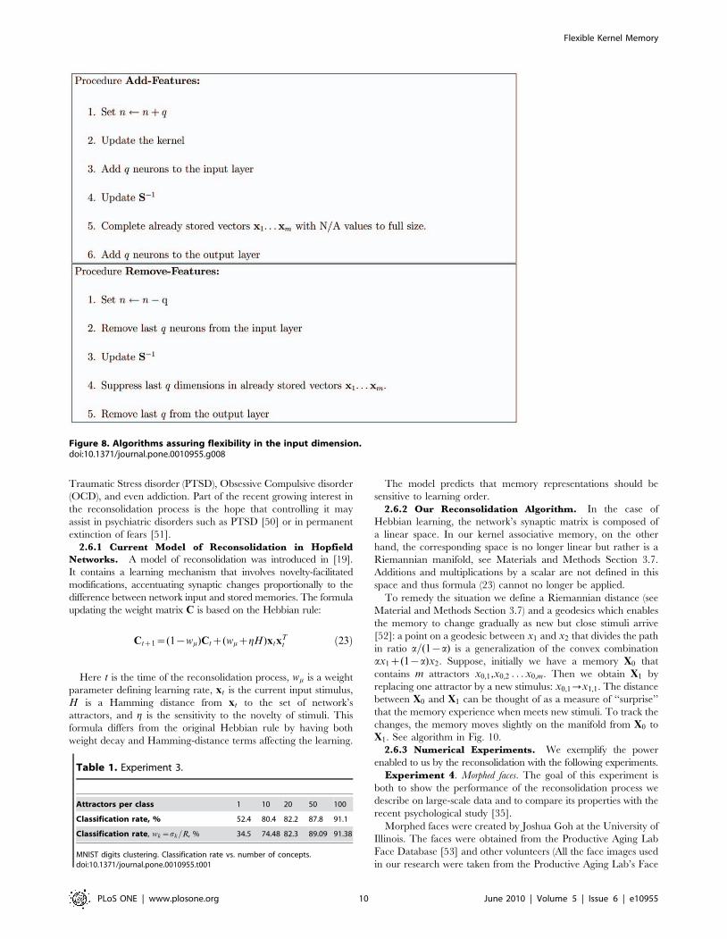
Figure 8. Algorithms assuring flexibility in the input dimension.doi:10.1371/journal.pone.0010955.g008



Database, Morphed face dataset. This dataset is freely accessible

from https://pal.utdallas.edu/facedb/request/index/Morph).

They contain a mix of young, old, Asian, Western, male, and

female faces. They are gray-scale with luminance histogram

equated. Faces were morphed using the software Sqirlz morph.

Original size of all images was 640|480. Useful area falls in the

Figure 9. The MNIST experiment. (a): Ten typical attractors, one for each class out of 100 attractors. (b): An example of 10 downscaled digits. Eachdigit in (b) is a 14|14~196-dimensional vector. Experiment 2 demonstrates work of the algorithm of adding features. we started learning with10000 downscaled images. To continue training we used another 10000 images, and we had to add 784–196 = 588 features.doi:10.1371/journal.pone.0010955.g009



rectangle 320|240, images were cropped to this size before

entering to the network. The database contains 150 morph

sequences, each of them consists of 100 images.

In our simulations we created a network with 16 attractors

representing 16 different faces; it had 76800 input and output neurons,

and two middle layers of 16 neurons each. Four arbitrarily selected

network’s attractors are depicted in Fig. 11. A Gaussian kernel was

chosen in order to simplify calculations with large scale data.

Attractors were initialized with first images from 16

arbitrarily selected morph sequences. When the learning order

followed image order in the morphing sequence, attractors

changed gradually and consistently. The ability to recognize the

initial set of images gradually decreased when attractors tended

to the final set. In case of random learning order attractors

quickly became senseless, and the network was not able to

distinguish faces.

This experiment generalizes the result shown in [19] but is done

on real images demonstrating the efficiency of the reconsolidation

process in kernel memories for high dimension and multi-scale

data. In accordance with [35], the formation of ‘‘good’’ dynamic

attractors occurred only when morphed faces were presented in

order of increasing distance from the source image. Also, as shared

also with [34,19]: the magnitude of the synaptic update due to

exposure to a stimulus depends not only on the current stimulus (as

in Hebbian learning) but also on the previous experience, captured

by the existing memory representation.

Experiment 5. Tracking Head Movement. This example focuses

on rotating head images for reconsolidation based on the

VidTIMIT dataset [54], and it demonstrates our algorithm on a

more applied example of faces and computer vision. The

VidTIMIT dataset is comprised of video and corresponding audio

recordings of 43 people. The recordings include head rotation

sequences. The recording was done in an office environment using

a broadcast quality digital video camera. The video of each person

is stored as a numbered sequence of JPEG images with a

resolution of 512|384 pixels.

The ability to track and recognize faces was tested on the sets of

15 last frames from each sequence. Example of attractors during

the reconsolidation in this experiments is depicted in the Fig. 12.

With reconsolidation and ordered stimuli the obtained recognition

rate was 95.2%. If inputs were shuffled randomly, attractors got

messy after 30–50 updates, and the network did not demonstrate

significant recognition ability.

Experiment 6. Tracking The Patriot Missiles. The following

experiment takes the reconsolidation model into a practical

technology that follows trajectories in real time in complex

dynamic environments.

We analyzed videos of Patriot missile launches with resolution

320|240, originally in RGB color, and transformed them to

grayscale. The memory was loaded with vector composed of two

40|40-pixel regions (windows) around the missile taken from two

consequent frames and a two-dimensional shift vector indicating

how the missile center has moved between these frames. Optimal

number of attractors was found to be 16–20.

Using memory reconsolidation algorithm we were able to calculate

velocity vector every time, and therefore track the missile with great

precision, with only average error of 5.2 pixels (see Fig. 13).

2.7 ConclusionsWe have proposed a novel framework of kernel associative

memory as an attractor neural network with a high degree of

flexibility. It has no explicit limitation, either on the number of

stored concepts or on the underlying metric for association, since

the metric is based on kernel functions. Kernels can be slightly

changed as needed during memory loading without damaging

existing memories. Also due to the kernel properties, the input

dimension does not have to be fixed. Unlike most other

associative memories our model can both store real -valued

patterns and allow for analogous attractor-based dynamic

associative recall.

We endowed our memory with a set of algorithms that insure

flexibility, enabling it to add/delete attractors as well as features

(dimensions) without need to retrain the network. Current

implementation of our memory is based on a simple competitive

clustering algorithm and consolidates memories in a spirit similar

to the localist attractor networks [43]. We have experimentally

tested the memory algorithms on the MNIST database of

handwritten digits, a common benchmark for learning machines.

The obtained clustering rate for this database (91.2%) is slightly

better than the best known result for unsupervised learning

Figure 10. Algorithm of Geodesic Update.doi:10.1371/journal.pone.0010955.g010



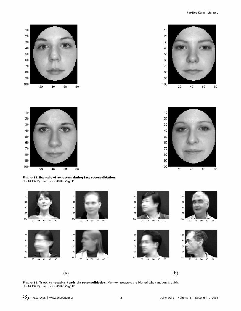
Figure 11. Example of attractors during face reconsolidation.doi:10.1371/journal.pone.0010955.g011

Figure 12. Tracking rotating heads via reconsolidation. Memory attractors are blurred when motion is quick.doi:10.1371/journal.pone.0010955.g012



algorithms on this benchmark. The model further allows the

process of reconsolidation after memory is stored when retrieval by

similar patterns is activated. We demonstrated the properties of

reconsolidation on gray scale large image faces in morphing

experiments. Based on the theoretical and experimental research

made in the present paper we conclude that the proposed kernel

associative memory is promising both as a biological model and a

computational method.

Materials and Methods

3.1 Piece-wise Mercer KernelsThe classical Kernels K(x,y) introduced by Vapnik to the field

of Machine Learning had the Mercer condition. That is, for all

square integrable functions g(x) the kernel satisfied:

ððK(x,y)g(x)g(y)§0: ð24Þ

The Mercer theorem states that if K satisfies the Mercer condition

there exists a Hilbert space H with basis e1,e2, . . . en . . . and a

function : Ex?H, (x)~P?

k~1kek, where 1, 2 . . . : Ex?R, such

that

K(u,v)~X?n~1

an n(u) n(v) ð25Þ

and all anw0. That is, K is a scalar product of (u) and (v)

General Mercer kernels are not sufficient for creating the

associative memory since our kernel memories require that all

attractors are linearly independent in the feature space, and some

Mercer kernels do not assure it, such as the basic scalar-product

kernel K(u,v)~vu,vw. As shown in Lemma 2, linear indepen-

dence of attractors in the feature space is needed to provide correct

association in our system. The piece-wise Mercer kernels as we

define next have this desired property.

Definition 3 A kernel K(u,v) is said to satisfy the piece-wise Mercer

condition if there exist dw0, mw0, and a Mercer kernel K0(u,v) such

that:

K ’(u,v)~K(u,v), u{vk k§d

K(u,v){m, u~v

�ð26Þ

and

K ’(u,v)ƒK(u,v), u{vk kƒd: ð27Þ

The piece-wise Mercer kernel is an extension of strictly positive

definite (SPD) kernels. These kernels have some internal property

of regularization. For usual Mercer kernels, e.g. common scalar

product there are still situations when Gram matrix of certain

vector set in the feature space will be degenerate. In contrast to

this, the m{d piece-wise Mercer kernel can guarantee that for any

finite set of vectors their Gramian will be full-rank and even

greater than mI.

Lemma 1 If K is a piece-wise Mercer Kernel, it also satisfies the Mercer

condition.

Proof. Indeed, for all square integrable functions g(x) : Ex?R,

the Mercer condition and inequality (26–27) give:

ððK(u,v)g(u)g(v)dudv§

ððK0(u,v)g(u)g(v)dudv§0

and the Mercer condition for K is fulfilled.

Remark 7 There is following relation between our definition of

piece-wise Mercer kernel and standard notion of strictly positive

definite (SPD) kernel (which is formulated by replacing ‘‘§’’ with

‘‘w’’ in (24): any piece-wise Mercer kernel is also SPD and for any

continuous SPD kernel K there exist certain m and d such that K is

m{d piece-wise Mercer.

Figure 13. Patriot missile example. Original frame (a) and a processed frame with tracking marker (b).doi:10.1371/journal.pone.0010955.g013



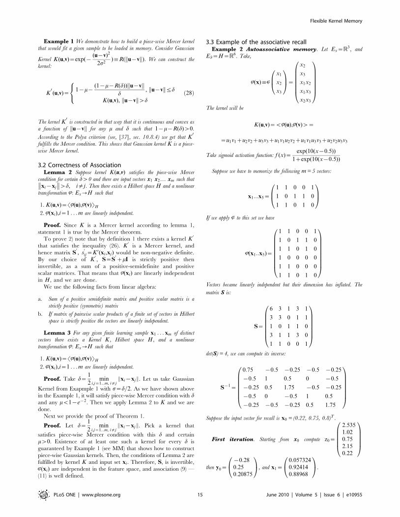
Example 1 We demonstrate how to build a piece-wise Mercer kernel

that would fit a given sample to be loaded in memory. Consider Gaussian

Kernel K(u,v)~exp({(u{v)2

2s2):R( u{vk k). We can construct the

kernel:

K0(u,v)~

1{m{(1{m{R(d)) u{vk k

d, u{vk kƒd

K(u,v), u{vk kwd

8<: ð28Þ

The kernel K0

is constructed in that way that it is continuous and convex as

a function of u{vk k for any m and d such that 1{m{R(d)w0.

According to the Polya criterion (see, [37], sec. 10.8.4) we get that K0

fulfills the Mercer condition. This shows that Gaussian kernel K is a piece-

wise Mercer kernel.

3.2 Correctness of AssociationLemma 2 Suppose kernel K(u,v) satisfies the piece-wise Mercer

condition for certain dw0 and there are input vectors x1 x2… xm such that

xi{xj

�� wd, i=j. Then there exists a Hilbert space H and a nonlinear

transformation : Ex?H such that

1. K(u,v)~S (u), (v)TH

2. (xi),i~1 . . . m are linearly independent.

Proof. Since K is a Mercer kernel according to lemma 1,

statement 1 is true by the Mercer theorem.

To prove 2) note that by definition 1 there exists a kernel K0

that satisfies the inequality (26). K0

is a Mercer kernel, and

hence matrix S0, s

0

ij~K 0(xi,xj) would be non-negative definite.

By our choice of K0, S~S

0zmI is strictly positive then

invertible, as a sum of a positive-semidefinite and positive

scalar matrices. That means that (xi) are linearly independent

in H, and we are done.

We use the following facts from linear algebra:

a. Sum of a positive semidefinite matrix and positive scalar matrix is a

strictly positive (symmetric) matrix

b. If matrix of pairwise scalar products of a finite set of vectors in Hilbert

space is strictly positive the vectors are linearly independent.

Lemma 3 For any given finite learning sample x1 . . . xm of distinct

vectors there exists a Kernel K , Hilbert space H , and a nonlinear

transformation : Ex?H such that

1. K(u,v)~S (u), (v)TH

2. (xi),i~1 . . . m are linearly independent.

Proof. Take d~1

2min

i,j~1...m, i=jExi{xjE. Let us take Gaussian

Kernel from Exapmple 1 with s~d=2. As we have shown above

in the Example 1, it will satisfy piece-wise Mercer condition with dand any mv1{e{2. Then we apply Lemma 2 to K and we are

done.

Next we provide the proof of Theorem 1.

Proof. Let d~1

2min

i,j~1...m, i=jExi{xjE. Pick a kernel that

satisfies piece-wise Mercer condition with this d and certain

mw0. Existence of at least one such a kernel for every d is

guaranteed by Example 1 (see MM) that shows how to construct

piece-wise Gaussian kernels. Then, the conditions of Lemma 2 are

fulfilled by kernel K and input set xi. Therefore, S, is invertible,

(xi) are independent in the feature space, and association (9) —

(11) is well defined.

3.3 Example of the associative recallExample 2 Autoassociative memory. Let Ex~R3, and

Eq~H~R6. Take,

(x):

x1

x2

x3

0B@

1CA~

x2

x3

x1x2

x1x3

x2x3

0BBBBBB@

1CCCCCCA

The kernel will be

K(u,v)~v (u), (v)w~

~u1v1zu2v2zu3v3zu1v1u2v2zu1v1u3v3zu2v2u3v3

Take sigmoid activation function: f (x)~exp(10(x{0:5))

1zexp(10(x{0:5))

Suppose we have to memorize the following m = 5 vectors:

x1:::x5~

1 1 0 0 1

1 0 1 1 0

1 1 0 1 0

0B@

1CA

If we apply to this set we have

(x1::x5)~

1 1 0 0 1

1 0 1 1 0

1 1 0 1 0

1 0 0 0 0

1 1 0 0 0

1 1 0 1 0

0BBBBBBBB@

1CCCCCCCCA

Vectors became linearly independent but their dimension has inflated. The

matrix S is:

S~

6 3 1 3 1

3 3 0 1 1

1 0 1 1 0

3 1 1 3 0

1 1 0 0 1

0BBBBBB@

1CCCCCCA

det(S) = 4, we can compute its inverse:

S{1~

0:75 {0:5 {0:25 {0:5 {0:25

{0:5 1 0:5 0 {0:5

{0:25 0:5 1:75 {0:5 {0:25

{0:5 0 {0:5 1 0:5

{0:25 {0:5 {0:25 0:5 1:75

0BBBBBB@

1CCCCCCA

Suppose the input vector for recall is x0 = (0.22, 0.75, 0.8)T .

First iteration. Starting from x0 compute z0~

2:535

1:020:75

2:15

0:22

0BBBB@

1CCCCA

then y0~

{0:28

0:25

0:20875

0@

1A, and x1~

0:057324

0:92414

0:88968

0@

1A.



Second iteration leads to y1~

0:057324

0:924140:85957

0@

1A and x2~

0:011812

0:985820:97329

0@

1A.

So, the process converges to attractor (0,1,1).

3.4 Proving Convergence of the Autoassociative RecallAlgorithm

Lemma 4 Suppose we have an autoassociative memory with kernel K ,

stored vectors x1…xm forming columns of matrix X, and a matrix S with

elements:

sij~K(xi,xj)

The dynamical system corresponding to the associative recall is:

z(i)t ~ K(xi,xt)

yt ~ XT S{1z

xtz1 ~ f (yt)

ð29Þ

Suppose kernel K(u,v) is continuous, and it satisfies the piece-wise Mercer

condition for a certain dw0 such that the stored vectors x1 x2… xm satisfy

xi{xj

�� wd for i=j. Then attractors of the dynamical system (29) are

either fixed points or 2-cycles.

Proof:

We will prove that lim(t??

xtz1{xt{1)~0. For this we construct

an energy function in a way that is analogous to Hopfield-like

networks:

Et~{1

2K(xt,yt{1) ð30Þ

Step 1. Show that the energy has lower bound. Because

f is bounded, the closure of the co domain of f in (29) is a certain

compact set Q. So, xt will remain in Q for all t§1. The energy

(30) is bounded over Q|Q as a continuous function over a

compact set.

Step 2. Show that there exists a projective self-conjugated operator C : E ?E such that C (xi) = (xi),

i = 1…m. By theorem 1 there exists a feature space H:Esuch that the kernel gives a scalar product in this space.

For every finite set of vectors (xi),i~1 . . . m in H we can

construct a projective operator C that projects to the subspace

spanned with (xi). Indeed, applying Gram-Schmidt orthogo-nalization to (xi) (see, e.g. [55]) we can build an orthonormal

set (basis) of vectors xi,i~1 . . . m.

Then define an operator as follows:

C(u)~Xm

k~1

vxk,uwxk

This C is projective, and it projects to the finite-dimensional

subspace vjiw~v (xi)w. (Here by vjiw we denote a

subspace spanned with all xi,i~1 . . . m).

Step 3. Show that energy decreases monotonicallyevery 2 steps.

Applying properties of the scalar product in Ex

and symmetry

of C we get:

Et{Etz1~1

2K(yt,xtz1){K(yt{1,xt)ð Þ~

~1

2S (yt), (xtz1)T{S (yt{1), (xt)Tð Þ~

~1

2S (xt), (xtz1)T{SC (xt{1), (xt)Tð Þ~

~1

2S (xt), (xtz1)T{S (xt{1),C (xt)Tð Þ

~1

2S (yt), (xtz1)T{S (xt{1), (yt)Tð Þ~

~1

2K(yt,xtz1){K(yt,xt{1)ð Þ§0

ð31Þ

Because xtz1~f (yt), xtz1 is closer to yt than any other point on

the trajectory, and the kernel is monotonic with respect to distance

between x and y, the expression (31) will be non-negative.

Moreover, is Et{Etz1§0; it is zero if and only if a fixed point is

reached.

Step 4. Show that the total amount of energy decreaseis finite if and only if sequences x2k and x2kz1 converge.Suppose the energy lower bound is {E�.

Et{Etz1~1

2v (xtz1), (yt)w{v (xt{1), (yt)wð Þ

~1

2v (xtz1){ (xt{1), (yt)w~

~ (xtz1){ (xt{1)k k: (yt)k k: cos h

ð32Þ

So, there exists mw0 such that Et{Etz1§m (xtz1){ (xt{1)k k.

ThenP?

t~t0

x0tz1{x0t{1

�� ƒP?t~t0

1

m(Et{Etz1)~

1

m(E�zEt0

). The

sum on the left hand of this equation will be finite if and only if

sequences x2k and x2kz1 converge, and we are done.

Remark 8 By Theorem 3 and Remark 2 we have proven that (all) stored

patterns are attractors. This means that Et~const if x equals one of stored vectors.

We next prove Theorem 2.

Proof. The proof is analogous to the proof of lemma 4. Note

that if the k-th attractor is reached zk zi~0, i=k. Activation

function in the form of generalized sigmoid brings z closer to an

attractor. So, where in the proof of lemma 4 the linear activation

function is replaced with a generalized sigmoid, convergence to an

attractor can only be fasted reached.

3.5 Variable Kernel and DimensionalityFor polynomial kernel of degree d we have:

K(x,y)~1

3((1zvxa,yaw)dz(1zvxb,ybw)dz

z((1zvxa,yaw)(1zvxb,ybw))d ’),

d 0~td=2s

ð33Þ

For such decomposed kernels, the matrix S{1 can be efficiently

(O(m2)) updated using formula (16).

Lemma 5 If the kernel K is a linear combination of basis functions, there

exists an additive kernel K1 having the same feature space E (x).

Having the same feature space is important because it leads to

identical behavior of two kernel memories with these to kernels.

We note that as before, if S is an approximately diagonal



matrix, the inverse S{1 can be estimated efficiently. A diagonal

matrix appears for example in the Radial-Basis-Function-like

kernels. In this situation the approximations are given by

S~lIzgS1.3.5.1 Memory Stability with Changing Kernels. Sup-

pose all vectors submitted for learning and recall belong to a

certain compact set Q. Let us define the norm for kernels:

Kk k2~

ð ðQ|Q

K2(u,v)dudv

Proposition 2 For given space Enzq and a compact set Q in it there

exists a constant Mw0 such that if Knzq{Kn

�� ƒM Knk k for any set of

vectors x1…xm stored in the memory with Kn these vectors remain in

attraction basins of corresponding attractors for the memory with kernel Knzq

whose attractors expand x1 . . . xm to dimension nzq.

Proof. The proof directly follows from the norm definition and

direct estimation of attractor shift when the kernel is changed.

3.6 Proof of Theorem 3Lemma 6 Let f : R?R be a generalized sigmoid. Suppose t[½0; 1�

and variable N takes two values 0 and 1. Then there exist constants c and hin (0; 1) such that if Dt{N Dvc, Df (t){N DƒhDt{N D

Proof. By definition 1 there exist c and h in (0,1) such that

Df0(s)Dvh if Ds{N Dvc. Estimate:

jf (t){f (N )j~ðtN

f0(s)dsjƒhjt{N

��

Here we prove Theorem 3.

Proof. Select one of stored patterns xi0 and denote it as

x0:xi0 . Consider the vector f~S{1z. If x is equal to, one of

stored vectors, corresponding vector f0~S{1z0 has all zero

coordinates except f(0)i0

~1, equivalently f(0)i ~di,i0 .

Estimate the norm Ef{f0E?.

Ef{f0E?ƒEf{f0EƒES{1E:Ez{z0EƒES{1E:L:Ex{x0E

If Ef{f0E?vc, Ef (f){f (f0)EvhEf{f0E? according to lemma

6. So, if

Ex{x0Eƒ

c

ES{1E:L

iterations of the recall will make f converge to f0 with exponential

velocity, that immediately implies convergence of xt to x0, and we

are done.

3.7 Reconsolidation and Riemannian Distance3.7.1 Riemannian Metric. Riemannian manifold is a

smooth, at least twice differentiable manifold (see [52,56], or any

textbook on Riemannian Geometry), which has a scalar product at

every point. The scalar product, or Riemannian Metric, is defined

in a tangent space of a point as a positive quadratic form.

Riemannian metrics enables to measure curve length and

introduce geodesics: trajectories of a free particle attached to the

manifold. Between every two points there exist at least one

geodesic that have minimal length among all curves joining these

two points. Length of this geodesic gives Riemannian distance over

the manifold.

There is following Riemannian distance between two kernel

associative memories:

r(X ,Y )2~2(m{tr(S{1=2QxyT{1=2)) ð34Þ

Here X and Y are two memories with the same m,n, and K . They

have S-matrices S and T respectively and Q is the ‘‘cross-matrix’’:

qij~K(xi,yj), i,j~1 . . . m.

3.7.2 Geodesic Update. To find a point analogous to convex

combination of X0 and X1 we build a geodesic cX1

X0joining these to

points, and take a point X �1 ~cX1

X0(t). Here t[½0,1� is a step

parameter related to size of a shift during each update. For t~0we stay at X0, for t = 1 the point is changed to X1. Repeatedly, we

track from X1 to X2 when a stimulus x1,2 appears, etc.

The algorithm of memory update using geodesics uses the

property of kernel memory that an arbitrary attractor can be

added or removed to the network in O(m2zn) operations with no

impact to all other attractors.

Acknowledgments

We express our appreciation to Eric Goldstein for helping to edit this paper

as well as to Yariv Levy, Megan Olsen, David Cooper, and Kun Tu for

helpful discussions and their continuous support.

Author Contributions

Conceived and designed the experiments: DN HS. Performed the

experiments: DN. Wrote the paper: DN HS.

References

1. Amit D (1989) Modeling Brain function. The world of attractor networks

Cambridge Univ. Press. 528 p.

2. Leutgeb JK, Leutgeb S, Treves A, Meyer R, Barnes CA, et al. (2005) Progressive

transformation of hippocampal neuronal representations in morphed environ-

ments. Neuron 48: 345–358.

3. Chafee MV, Goldman-Rakic PS (1998) Matching patterns of activity in primate

prefrontal area 8a parietal area 7ip neurons during a spatial working memory

task. J Neurophysiol 1998: 2919–2940.

4. Li Z (2001) Computational design and nonlinear dynamics of a recurrent network

model of the primary visual cortex. Neural Computation 13: 1749–1780.

5. Seung HS (1998) Continuous attractors and oculomotor control. Neural

Networks 11: 1253–1258.

6. Wang XJ (2001) Synaptic reverberation underlying mnemonic persistent

activity. Trends Neuroscience 24: 455–463.

7. Fuster JM, Alexande G (1971) Neuron activity related to short-term memory.

Neuron 14: 477–485.

8. Miyashita Y (1988) Neuronal correlate of visual associative longterm memory in

the primate temporal cortex. Nature 335: 817–820.

9. Miyashita Y, Chang HS (1988) Neuronal correlate of pictorial short-term

memory in the primate temporal cortex. Nature 331: 68–70.

10. Kay LM, Lancaster LR, Freeman WJ (1996) Reafference and attractors in the

olfactory system during odor recognition. Int J Neural Systems 7: 489–

495.

11. Ericson C, Desimone R (1999) Responses of macaque perirhinal neurons during

and after visual stimulus association learning. J Neurosci 19: 10404–

10416.

12. Compte A, Brunel N, Goldman-Rakic PS, Wang XJ (2000) Synaptic

mechanisms and network dynamics underlying spatial working memory in a

cortical network model. Cerebral Cortex 10: 910–923.

13. Wills TJ, Lever C, Cacucci F, Burgess N, O’Keefe J (2005) Attractor dynamics in

the hippocampal representation of the local environment. Science 308: 873–876.

14. Hopfield JJ (1982) Neural networks and physical systems with emergent

collective computational abilities. Proc Natl Acad Sci USA 79: 2554–2558.

15. McNaughton BL, Morris RGM (1987) Hippocampal synaptic enhancement and

information storage within a distributed memory system. Trends Neurosci 10:

408–415.



16. Treves A, Rolls ET (1992) Computational constraints suggest the need for two

distinct input systems to the hippocampal ca3 network. Hippocampus 2: 189–199.

17. Hasselmo ME, Schnell E, Barkai E (1995) Dynamics of learning and recall at

excitatory recurrent synapses and cholinergic modulation in rat hippocampal

region ca3. J Neurosci 15: 5249–5262.

18. Durstewitz D, Seamans JK, Sejnowski TJ (2000) Dopamine mediated

stabilization of delay-period activity in a network model of prefrontal cortex.

J Neurophysiol 83: 1733–1750.

19. Blumenfeld B, Preminger S, Sagi D, Tsodyks M (2006) Dynamics of memory

representations in networks with novelty-facilitated synaptic plasticity. Neuron

52: 383–394.

20. Gruber AJ, Dayan P, Gutkin BS, Solla SA (2006) Dopamine modulation in the

basal ganglia locks the gate to working memory. J Comput Neurosci 20:

153–166.

21. Treves A (1990) Graded-response neurons and information encodings in

autoassociative memories. Phys Rev A 42: 2418–2430.

22. Lengyel M, Kwag J, Paulsen O, Dayan P (2005) Matching storage and recall:

hippocampal spike–timing–dependent plasticity and phase response curves.

Nature Neuroscience 8: 1677–1683.

23. Poggio T, Girosi F (1990) Regularization algorithms for learning that are

equivalent to multilayer networks. Science 247: 978–982.

24. Billings SA, Fung CF (1995) Recurrent radial basis function networks for

adaptive noise cancellation. Neural Networks 8: 273–290.

25. Cheung YM (2002) A new recurrent radial basis function network. Neural

Information Processing, ICONIP ‘02 Proc of the 9th International Conference

on 2: 1032–1036.

26. Miyoshi T, Ichihashi H, Okamoto S, Hayakawa T (1995) Learning chaotic

dynamics in recurrent rbf network. Neural Networks, Proc IEEE International

Conference on. pp 588–593.

27. Sun J, Zhang T, Liu H (2004) Modelling of chaotic systems with novel weighted

recurrent least squares support vector machines. Lecture Notes in Computer

Science 3173: 578–585.

28. Dudai Y (1997) Time to remember. Neuron 18: 179–182.

29. Eichenbaum H (2006) The secret life of memories. Neuron 50: 350–352.

30. Dudai Y, Eisenberg M (2004) Rite of passage of the engram: Reconsolidation

and the lingering consolidation hypothesis. Neuron 44: 93–100.

31. Nader K, Schafe GE, LeDoux JE (2000) Fear memories require protein synthesis

in the amygdala for reconsolidation after retrieval. Nature 406: 722–726.

32. Lee JLC, Everitt BJ, Thomas KL (2004) Independent cellular processes for

hippocampal memory consolidation and reconsolidation. Science 304: 839–843.

33. Medina JH, Bekinschtein P, Cammarota M, Izquierdo I (2008) Do memories

consolidate to persist or do they persist to consolidate? Behavioural Brain

Research. pp 61–69.

34. Siegelmann HT (2008) Analog-symbolic memory that tracks via reconsolidation.

Physica D 237: 1207–1214.

35. Preminger S, Sagi D, Tsodyks M (2005) Morphing visual memories through

gradual associations. Perception Suppl 34: 14.36. McClelland JL, Rumelhart DE (1981) An interactive activation model of context

effects in letter perception: Part i. an account of basic findings. Psychological

Review 88: 375–407.37. Vapnik V (1998) Statistical Learning Theory. NY: John Wiley & Sons. 736 p.

38. Cucker F, Smale S (2002) On the mathematical foundations of learning. Bulletinof American Mathematical Society 39: 1–49.

39. Ben-Hur A, Horn D, Siegelmann HT, Vapnik V (2001) Support vector

clustering. Journal of Machine Learning Research 2: 125–137.40. Zhang BL, Zhang H, Ge SS (2004) Face recognition by applying wavelet

subband representation and kernel associative memory. IEEE Trans NeuralNetworks 15: 166–177.

41. Caputo B, Niemann H (2002) Storage capacity of kernel associative memories.In: Artificial Neural Networks — ICANN 2002. Heidelberg: Springer Berlin. pp

134–143.

42. Casali D, Constantini G, Perfetti R, Ricci E (2006) Associative memory designusing support vector machines. IEEE Trans on Neural Networks 17: 1165–1174.

43. Zemel RS, Mozer MC (2001) Localist attractor networks. Neural Computation13: 1045–1064.

44. Albert A (1972) Regression and the Moore-Penrose pseudoinverse. NY-London:

Academic Press. 180 p.45. Fusi S, Abbott LF (2007) Limits on the memory storage capacity of bounded

synapses. Nature Neuroscience 10: 485–493.46. Petersen KB, Pedersen MS (2008) The Matrix Cookbook. Available: http://

matrixcookbook.com/.47. LeCun Y, Botton L, Bengio Y, Haffner P (1998) Gradient-based learning

applied to document recognition. Proc IEEE 86: 2278–2324.

48. Zhang R, Rudnicky AI (2002) A large scale clustering scheme for kernel k-means. 16th International Conference on Pattern Recognition (ICPR’02) 4:

40289.49. Tronson NC, Taylor JR (2007) Molecular mechanisms of memory reconsolida-

tion. Nature Reviews Neuroscience 8: 262–275.

50. Singer E (2009) Manipulation memory. Technology Review 46: 138–139.51. Monfils MH, Cowansag KK, Klann E, LeDoux JE (2009) Extinction-

reconsolidation boundaries: Key to persistent attenuation of fear memories.Science 324: 951–955.

52. do Carmo MP (1992) Riemannian Geometry. Brikhauser. 300 p.53. Minear M, Park DC (2004) A lifespan database of adult facial stimuli. Behavior

Research Methods, Instruments, & Computers 36: 630–633.

54. Sanderson C (2008) Biometric Person Recognition: Face, Speech and Fusion.VDM-Verlag. 156 p.

55. Golub GH, Van Loan CF (1996) Matrix computations (3rd ed.). Baltimore,MD, USA: Johns Hopkins University Press. 694 p.

56. Petersen P (2006) Riemannian Geometry. Graduate Texts in Mathematics.

Springer. 408 p.



Flexible Kernel Memory

Documents

Transcript of Flexible Kernel Memory