Journal of Global Optimization manuscript No.(will be inserted by the editor)

ON NUMERICAL OPTIMIZATION THEORY OFINFINITE KERNEL LEARNING

S. Ozogur-Akyuz · G.-W. Weber

Received: date / Accepted: date

Abstract In Machine Learning algorithms, one of the crucial issues is the represen-

tation of the data. As the given data source become heterogeneous and the data are

large-scale, multiple kernel methods help to classify “nonlinear data”. Nevertheless, the

finite combinations of kernels are limited up to a finite choice. In order to overcome this

discrepancy, a novel method of “infinite” kernel combinations is proposed in [12,16]

with the help of infinite and semi-infinite programming regarding all elements in kernel

space. Looking at all infinitesimally fine convex combinations of the kernels from the

infinite kernel set, the margin is maximized subject to an infinite number of constraints

with a compact index set and an additional (Riemann-Stieltjes) integral constraint due

to the combinations. After a parametrization in the space of probability measures, it

becomes semi-infinite. We adapt well-known numerical methods to our infinite kernel

learning model and analyze the existence of solutions and convergence for the given

algorithms. We implement our new algorithm called ”infinite” kernel learning (IKL) on

heterogenous data sets by using exchange method and conceptual reduction method,

which are well known numerical techniques from solve semi-infinite programming. The

results show that our IKL approach improves the classifaction accuracy efficiently on

heterogeneous data compared to classical one-kernel approaches.

This study is partially done at Instiute of Applied Mathematics, Middle East Technical Uni-versity, Ankara, Turkey and Faculty of Engineering and Natural Sciences, Sabancı University,Istanbul, Turkey

S. Ozogur-AkyuzDepartment of Mathematics and Computer Science,Bahcesehir University, Istanbul, TurkeyTel.: +90 212 381 0310E-mail: sureyya.akyuz@bahcesehir.edu.tr

G.-W. WeberInstitute of Applied Mathematics,Middle East Technical University, METU, Ankara, TurkeyFaculty of Economics, Management Science and LawUniversity of Siegen, GermanyE-mail: gweber@metu.edu.tr

2

Keywords machine learning · infinite kernel learning · semi-infinite optimiza-

tion · infinite programming · support vector machines · continuous optimization ·discretization · exchange method · conceptual reduction · triangulation.

1 Introduction

In classical kernel learning methods, a single kernel is used to map the input space

to a higher dimensional feature space. But for large scale and heterogeneous data in

real-world applications [17,19], multiple kernel learning (MKL) is developed [4,21]. The

main intuition behind multiple kernel learning is to combine finitely many pre-chosen

kernels in a convex combination [21]

kβ(xi,xj) :=

K∑κ=1

βκkκ(xi,xj). (1)

In this paper, we shall basically refine the sum in (1) by an integral, as we shall closely

explain. In [4], a multiple kernel reformulation is modeled by semi-definite program-

ming for selecting the optimum weights of corresponding kernels. This reformulation

has some drawbacks in computation time because of semi-definite programming and

this reformulation is developed in [21] by semi-infinite linear programming with the

following optimization model:

maxθ,β

θ (θ ∈ R,β ∈ RK)

such that β � 0,

K∑κ=1

βκ = 1,

K∑κ=1

βκSκ(α) � θ ∀α ∈ Rl,

0 � α � C1 and

l∑i=1

yiαi = 0,

(2)

where 1 = (1, 1, 1, . . . , 1)T ∈ Rl.

The finite combinations of kernels are limited up to a finite choice. This limitation

does not always allow to represent the similarity or dissimilarity of data points, specif-

ically highly nonlinearly distributed and large-scaled ones. A finite combination may

fail, here. In order to overcome this, with the motivation of previous studies [3,12–14],

a combination of infinitely many kernels in Riemann-Stieltjes integral form is proposed

to allow an infinite wealth of possible choices of kernels in the kernel space which is

called infinite kernel learning (IKL) [12,15,16]. This makes the problem infinite in both

its dimension and its number of constraints; which is so-called infinite programming

(IP). The mathematical foundations of IKL is established by mathematical analysis

and the theory of semi-infinite programming in [12,15,16]. An infinite combination is

represented by the following formula:

kβ(xi,xj) :=

∫Ω

k(xi,xj , ω)dβ(ω), (3)

where ω ∈ Ω is a kernel parameter and β is a monotonically increasing function of inte-

gral 1, or just a probability measure on Ω. Furthermore, the kernel function k(xi,xj , ω)

3

is assumed to be a twice continuously differentiable function with respect to ω, i.e.,

k(xi,xj , ·) ∈ C2. The infinite combination can be, e.g., a combination of Gaussian ker-

nels with different widths from a set Ω, i.e., kβ(xi,xj) =∫Ω exp(−ω

∥∥xi − xj

∥∥22)dβ(ω).

It is obvious that the Gaussian kernel is from a family of twice continuously differen-

tiable functions of the variable ω. Hereby, the wealth of infinitely many kernels is used

to overcome the limitation of the kernel combination given by finitely many pre-chosen

kernels. The questions on which combination of kernels and on the structure of the

mixture of kernels can be considered and optimized, and it may, e.g., be answered by

homotopies [12,15,16].

With this new formulation, we have the opportunity of recording (“scanning”) all

possible choices of kernels from the kernel space and, hence, the uniformity is also

preserved. Let us note that infinitely many kernels correspond to infinitely many co-

efficients. Kernel coefficients are defined through an increasing monotonic function by

means of positive measures [15,16].

The IKL formulation is given in [12,15,16] by

maxθ,β

θ (θ ∈ R, β : a positive measure on Ω)

such that θ − ∫ΩT (ω,α)dβ(ω) � 0 (α ∈ A),∫

Ω dβ(ω) = 1,

(4)

where T (ω,α) := S(ω,α) − ∑li=1 αi, S(ω,α) := 1

2

∑li,j=1 αiαjyiyjk(xi,xj , ω) and

Ω := [0, 1] and A := {α ∈ Rl | 0 � α � C1 and

∑li=1 αiyi = 0} are our index sets.

We note that there are infinitely many inequality constraints because of the in-

equality constraint which are uniform in α ∈ A, and the state variable β is from an

infinite dimensional space. Thus, our problem is a one of infinite programming (IP) [1].

The dual of (4) can be written as

minσ,ρ

σ (σ ∈ R, ρ : a positive measure on A)

such that σ − ∫AT (ω,α)dρ(α) � 0 (ω ∈ Ω),∫

A dρ(α) = 1.

(5)

Because of the conditions∫Ω dβ(ω) = 1 and

∫A dρ(α) = 1, positive measures β (or ρ)

are probability measures and these measures are parametrized in this paper via the

probability density functions as in [15,16].

We note that the primal IKL formulation (4) and the dual IKL formulation (5)

are very similar, where minimization is swapped with maximization, the direction of

inequalities in the constraints are changed in (5), the index sets A, Ω and the variables

α, ω are replaced with each other such that both index sets are compact and the

objective functions, θ, σ, of both the dual and the primal are continuous. Thus, similar

formulations, definitions and the theorems (covergence, discretizations etc.) written for

the primal problem can be expressed for the dual problem in terms of the variables and

the index set of the dual problem. However, we observe that the primal and the dual

problem are different as far as the way how the sets of inequality constraints are defined.

In fact, there can be problems with nondegeneracy (that can be related with instability)

just for one of the problems, not for the other. In [11,12,15,16], it is explained that

the LICQ condition is violated because of the linear dependency of the equality and

the inequality constraints on the lower level problem of the primal problem. In order

to overcome this degenerate case, we perturbed the equality constraint of (2) with

4

a monotonically decreasing sequence (ξν)ν∈N such that ξν → 0 (ν → ∞), where,∑li=1 αiyi = ξν .

Corollary 1 [15,16]. Let us assume that there exist (β, θ) and (ρ, σ) which are feasible

for their respective problems, and are complementary slack, i.e.,

σ =

∫A

T (ω,α)dρ(α) and θ =

∫A

T (ω,α)dβ(ω).

Then, β has measure only where σ =∫A T (ω,α)dρ(α) and ρ has measure only where

θ =∫ΩT (ω,α)dβ(ω) which implies that both solutions are optimal for their respective

problems.1

In this study, we restrict ourselves to probability measures, which constitute our

subspace of positive measures, and we use parametrized models of IKL given by prob-

ability density functions (pdfs) in [15,16]. Throughout this study, we assume that we

are given pdf function fP (ω; ·) for our primal problem. We do not need to write

the equality constraint∫Ω dβ(ω) = 1, since we assume that our measures are prob-

ability measures. Then, we parametrize these measures via pdfs fP = fP (ω;℘P ),

taking the place of positive measures β. Let us denote the parameters of a pdf by

℘P = (℘P1 , ℘P

2 , . . . , ℘PιP )T for the primal problem. It is constrained and elements of a

suitable parameter set can be written as follows:

PP := {℘P ∈ RιP

∣∣∣ uPi (℘P) = 0 (i ∈ IP ), vP

j (℘P) ≥ 0 (j ∈ JP )}.

We note that after a parametrization, our primal (or dual) problem has variables in

finite dimension since instead of optimizing with respect to measure β which is in

an infinite dimensional space, we minimize with respect to the pdf parameter vector

℘P . This parametrization allows us to define our infinite programming problem by

semi-infinite programming (SIP) since the variables are in a finite dimension and there

are infinitely many inequality constraints. Hence, our primal problem turns into the

following SIP with additional constraint functions uPi (℘P ) and vPj (℘P ), coming from

the definition of the parameter sets related to the specific pdf function of the primal

problem [15,16]:

(Primal SIP ) minθ,℘P

−θ

such that∫Ω T (ω,α)fP (ω;℘P )d(ω)− θ ≥ 0 (α ∈ A),

uPi (℘P) = 0 (i ∈ IP),

vPj (℘P) ≥ 0 (j ∈ JP ).

(6)

2 Numerical Analysis of IKL

One of the early methods mostly used to solve SIP problems in practice, e.g., in en-

gineering applications, is discretization [7]. It is based on a selection of finitely many

points from the infinite index set of inequality constraints. In our study, these infinite

index sets are A and Ω for the primal and the dual problems, respectively.

1 Communication with E.J. Anderson

5

The discretized primal SIP problem of (6) can be written by the following formu-

lations:

P (Ak) minθ,℘P

−θ

subject to gP((θ,℘P ),α) :=∫Ω T (ω,α)fP (ω;℘P )dω − θ � 0 (α ∈ Ak),

uPi (℘P ) = 0 (i ∈ IP ),

vPj (℘P ) ≥ 0 (j ∈ JP ).

(7)

Here, by the symbol P (·) we denote the primal, k is the iteration step, and the dis-

cretized set Ak will be discussed within Strategy I and Strategy II in Section 3. It is

obvious that Ωk can be defined by a one-dimensional uniform grid2. Hereby, k should

not be confused with our kernel function.

Let vP (Ak), MP (Ak) and GP (Ak) denote the minimal value, the feasible set

and the set of (global) minimizers of our primal problem (6) with A replaced by Ak.

Under suitable regularity conditions (reduction ansatz) [7], the optimal solutions of the

lower level problems depend locally on the parameters, i.e., measures. Furthermore, the

relation with the pdfs has been established with a dual pairing and by the pdfs as test

kind of functions from the dual space.

Let d1 be the Hausdorff distance d1(Ak, A) between A and Ak, which is given by

d1(Ak, A) := maxy∈A

miny′∈Ak

∥∥y − y′∥∥2.

Now, with the Hausdorff distance, we will introduce the discretizability notion for our

problems based on the definitions in [22]. In these problems, y = α and y′ = α′ for theprimal case. In the following definitions, the distance to the solution (θ∗,℘P∗

) of the

primal SIP will be defined by the Hausdorff distance, too. We note that the optimal

solution of the primal problem exists because of the continuity of the objective functions

and inequality constraints, and compactness of the feasible sets which is proposed

subsequently in Closer Explanation 1 [24]. Here, we employ Theorem of Weierstrass.

We denote the distance functions d1 for the primal problem as dP1 .

Definition 1 The primal problem (6) is called finitely reducible if there is a finite

set Ak0 ⊂ A for some k = k0 such that vP (Ak0) = vP (A), and (Ak)k∈N0strictly

isotonically increases3 as k → ∞.

Definition 2 The primal problem (6) is called weakly discretizable if there exists a

sequence of discretizations (Ak)k∈N0such that vP (Ak) → vP (A) (k → ∞).

We note that we have vP (Ak1) ≤ vP (Ak2) if Ak1 ⊂ Ak2 for our primal problem. Let us

recall that we consider the standard form of primal SIP problems, i.e., a minimization

problems. In closer detail, as the infinite index set grows, the number of inequality

constraints increases. This forces the feasible set to become smaller at each iteration

k. Thus, the minimum of the objective function increases (see Figure 1).

2 A uniform grid is discretization of a considered set where all elements x = (x1, x2, . . . , xl)T

have same spacing with respect to their i-th coordinate (i = 1, 2, . . . , l). For example in R2, all

rows have the same spacing and all of the columns have the same spacing (but not necessarilythe same as the row spacing).

3 A sequence (Ak)k∈N0is called strictly isotonically increasing if Ak

⊂�=Ak+1 (k ∈ N0).

6

Fig. 1 Symbolic illustration of the minimum values with respect to different feasible setscorresponding different discretizations; an example.

Definition 3 The primal problem, (6) is called discretizable if for each sequence of

finite grids Ak ⊂ A (k ∈ N0) satisfying dP1 (Ak, A) → 0 (k → ∞), where dP1 (Ak, A) =:

maxα∈A

minα′∈Ak

∥∥α−α′∥∥2, there exist solutions (θk, ℘

Pk )k∈N0

of the discretized primal

problems (7) such that the following relations hold:

min(θ,℘P)∈GP(A)

∥∥∥(θk, ℘Pk )− (θ,℘P )

∥∥∥2→ 0 (8)

and vP (Ak) → vP (A) (k → ∞).

Corollary 2 If the primal problem (6) is finitely reducible, then it is weakly discretiz-

able.

Proof Let us assume that (6) is finitely reducible. Then, by definition, there exist a

k0 ∈ N0 and finite sets Ak0 ⊂ A such that vP (Ak0) = vP (A). Then, it is obvious that

vP (Ak) → vP (A) (k → ∞).

Under the discretizability notion established above, we introduce the conceptual

discretization algorithm in the following section.

3 Conceptual Discretization Method

The conceptual discretization method is based on an update of the discretization ac-

cording to some stopping criterion for the convergence of the optimal solution. We

7

adapt the conceptual discretization method [7,8,22] to our primal problem in Algo-

rithm 1.

Algorithm 1 Primal Conceptual Discretization Method (PCDM)

Input:δ positive number, i.e., δ > 0fP probability density functionPP the set where pdf parameters lie

Output:θ unknown variable for minimization, to be evaluated℘P the parameter vector of the pdf

PCDM(θ,℘P , A, δ, fP , PP)

1: k := 02: Initialize a discretization Ak ⊂ A.3: DO Compute a solution (θk ,℘

Pk ) of

minθ∈R,℘P

(−θ)

subject to gP ((θ,℘P ),α) � 0 (α ∈ Ak),uPi (℘P ) = 0 (i ∈ IP ),

vPj (℘P ) ≥ 0 (j ∈ JP ).

4: if gP ((θk ,℘Pk ),α) ≥ −δ (α ∈ A) then

5: STOP6: else7: Ak+1 := Ak ∪ {any finitely many further points from A}8: k := k + 19: end if10: END DO

In Algorithm 1, the stopping criterion is theoretically established since one needs to

check, e.g., gP ((θk,℘Pk ),α) ≥ −δ (α ∈ A). Alternatively, we introduce some stopping

criterion based on the idea of a Cauchy sequence.

Generally speaking, in our problem and many real-world situations, an optimal so-

lution is not known. In order to stop at a sufficiently close approximately optimal solu-

tion, the increment between the steps has to be small enough, i.e., ‖xk+1 − xk‖2 < ε0for a fixed ε0 > 0 which comes from the definition of “Cauchy sequence” evaluated

at the k-th iteration for a fixed ε0 > 0. A second alternative stopping criterion is

based on the idea of a Cauchy sequence again, but on the value of the objective

function F ; it is determined by looking at the decrement of the objective function

at iterations by (F (xk) − F (xk+1)) < ε1 for a fixed ε1 > 0. As a third alterna-

tive, the first and the second criteria are both integrated in a single criterion by

(F (xk)− F (xk+1)) ‖xk − xk+1‖−12 < ε2 for a fixed ε2 > 0.

In our problems, the objective functions are FP(θ,℘P ) := −θ and FD(σ,℘D) := σ

for the primal and the dual problems, respectively. With this notion, we establish our

stopping criteria in different forms. In the following, we refer to one of the stopping

criteria for the primal and the dual problems:

8

Stopping Criteria for the Primal Problem:∥∥∥(θk+1,℘Pk+1)− (θk,℘

Pk )

∥∥∥2< ε0 for a fixed ε0 > 0,

|−θk − (−θk+1)| < ε1 for a fixed ε1 > 0, (9)

(−θk − (−θk+1))∥∥∥(θk,℘P

k )− (θk+1,℘Pk+1)

∥∥∥−1

2< ε2 for a fixed ε2 > 0.

Next, we will give an important assumption for the following Theorem 2.

Assumption 1: The feasible set MP (A) is compact.

Closer Explanation 1 In fact, our (feasible) set satisfies compactness on the lower

level but not on the upper level. Indeed, on the upper level, θ ∈ R is unbounded for the

primal problem (6). Let us recall that we parametrized β. We need a compact feasible

set to have convergence of subsequences towards the optimal solution guaranteed, and

also for the discretizability given in the following theorem. We encounter this problem by

transversally intersecting the feasible set with sufficiently large transversal families of

elementary geometrical sets (squares, boxes, cylinders or balls); this compactification

is introduced in [18,24].

In an implicitly defined way, this corresponds to the following feasible subset of the

primal SIP with some nonnegative (semi-continuous) functions GP :

MPcomp(A) := {(θ,℘P)

∣∣∣ θ ∈ R, gP ((θ,℘P),α) ≥ 0 (α ∈ A),

(gP −GP )((θ,℘P ),α) ≤ 0 (α ∈ A)}, (10)

where gP((θ,℘P ),α) denotes the inequality constraint function of the primal problem.

We note that the latter function may also be vector-valued.

Besides of this theoretical approach by function GP , a more practical one consists of

the idea of transversally cutting with a cube. This can be geometrically illustrated by

the cube in Figure 2:

Remark 1 When performing the transversal sections, it is important to take into ac-

count any priori information given about where a possible global solution, minimizer

or maximizer, of our regarded optimization problem is located. Let us recall that we

look at the primal and dual problems after parametrization, such that the parameters

themselves become new decision variables. So we choose the intersecting parallelpipe

large enough in order to include such an expected global solution. Of course, to gain

that a priori knowledge, a careful analytical investigation may be helpful and should

be done, e.g., in terms of growth behaviour and convexity kind of properties. In fact,

for the ease of exposition, we just think of minimization rather than both minimization

and maximization.

As a first, simple but important class of problems we mention such ones with a

strictly convex graph (given by the constraints), i.e., an epigraph with the form of a

potential, e.g., a paraboloid. In any such a case, we know that the lower level set with

respect some arbitrary and sufficiently large level is nonempty and compact. Then,

we can choose and raise our transversally cutting parallelpipe so that, in a projective

sense, the lower level set and, hence, as an element, the global minimizer is contained

in the parallelpipe and, therefore, in the excised subset of the epigraph.

9

Fig. 2 Transversal intersection (excision) of the feasible set with a box; an example taken from[18,24]. (The surface may come from an equality constraint; the figure implies perturbationalarguments of [24].)

This treatment and careful geometrical arrangement guarantees the equality of

set of minimizers of the original problem, GP (A), and the set of minimizers after

compactification, GPcomp(A), i.e., GP (A) = GP

comp(A) which is illustrated in Figure 3.

Let us underline that our strict convexity is not guaranteed in general. In fact,

the fulfillment of this property on the one hand depends on how the kernel functions

are chosen and how the kernel matrices are evaluated at the input data. On the other

hand, it depends on how the parameters are involved into the density functions and

how the possible nonlinearity can be characterized by convexity and the growth kinds

of conditions, e.g., in terms of Morse indices [9].

We can adopt this idea to our problem in order to transversally cut around our

height function on the boundary of the epigraph with a cube, as shown by Figure 3.

Under our Closer Explanation 1, we obtain a general convergence result for this

method based on Theorem 13 in [22].

Theorem 2 Let Assumption 1, after the compactification introduced in Closer Expla-

nation 1 be satisfied, and let the primal problem and the sequences of discretizations

(Ak)k∈N0and (Ωk)k∈N0

satisfy

A0 ⊂ Ak (k ∈ N0) and dP1 (Ak, A) → 0 for k → ∞.

10

Fig. 3 Illustration of the transversal cutting around the height function with a box; an ex-ample.

Based on possible compactifications, we may from now on suppose that M(A0) and

M(Ω0) are compact. Then, the primal problem, (6) is discretizable, i.e., the problem

P (Ak) (k ∈ N0) has solutions (θk,℘Pk ), and such sequences of iterative solutions satisfy

min(θ∗,℘P∗

)∈GP(A)

∥∥∥(θk,℘Pk )− (θ∗,℘P∗

)∥∥∥2→ 0 (k → ∞). (11)

We refer to [22] for the proof of Theorem 2. By this theorem, we guarantee the con-

vergence of approximate solutions to optimal solutions for sufficiently large k with

(11).

Closer Explanation 3 We note that the assumptions of Theorem 2 should be satisfied

before we discretize our infinite index set. We know that our index set A is compact,

and we assume that our sequences of discretized set Ak (k ∈ N0) converge to A. Then,

our semi-infinite problem is discretizable.

We also note that the minima which are stated in the theorem exist since the Eu-

clidean norm is continuous and bounded from below, and, indeed, always nonnegative.

Other properties used here are the existence of optimal solution (θ∗,℘P∗), i.e., the set

of minimizers GP (A) exists for the primal problem, since our feasible set is compact

and the objective function is continuous, and we use that the set GP is compact, too,

Theorem of Weierstrass (see [2]).

Next, we give the definition for the local primal which is defined around some open

neighbourhoods of the local minimizers.

11

Definition 4 [22]. Given a local minimizer (θ, ℘P ) of the primal problem (6), the

primal SIP is called locally discretizable at (θ, ℘P ) if the discretizability relation

holds locally, i.e., if there exist neighbourhoods U(θ,℘P ) of (θ, ℘P ) such that the locally

discretized problem P loc(A) for the primal problem, namely,

P loc(A) : min(θ,℘P)∈U

(θ,℘P )

−θ

subject to∫Ω T (ω,α)fP (ω,℘P )dω − θ � 0 (α ∈ A),

uPi (℘P) = 0 (i ∈ IP ),

vPj (℘P) ≥ 0 (j ∈ JP )

obtained as the restriction of P (A) to open neighbourhood U(θ,℘P), is discretizable.

The following Theorem 4 is based on Theorem 15 given in [22], and it gives a conver-

gence result for the discretization method applied to our problems. Let us recall the

definition of a local minimum of order p before giving the result.

Definition 5 A feasible point x is called a local minimizer of order p > 0 of the

problem to minimize f(x) on a feasible set M ⊆ Rn if with suitable constants ε >

0 and M > 0, the following relation holds:

f(x)− f(x) ≥ M ‖x− x‖p2 for all x ∈ M with ‖x− x‖2 < ε.

Theorem 4 Let (θ, ℘P) be a local minimizer of the primal problem (6) of order p,

and let sets M(Ak), M(A), be restricted to a compact subset K ⊂ Rn. We further

suppose that the Mangasarian-Fromovitz Constraint Qualification (MFCQ) (see [7])

holds at (θ, ℘P ). Then, the problem (6) is locally discretizable at (θ, ℘P). In closer

detail: There is some ςP > 0 such that for any sequences of grids (Ak)k∈N0∈ AN0

with dP1 (Ak, A) → 0 (k → ∞) and for any sequences of solutions (θk,℘Pk )k∈N0

of the

locally restricted problem P loc(A), the following relation holds:∥∥∥(θk,℘Pk )− (θ, ℘P)

∥∥∥2≤ ςPdP1 (Ak)

1/p (k → ∞)

.

Closer Explanation 5 The result of Theorem 4 is true for the global minimization

problem (6) since the sets M(Ak) and M(A) are restricted to a compact subset [22].

We note that after compactification by transversally intersecting the feasible set with

sufficiently large transversal elementary geometrical sets (see Closer Explanation 1),

we satisfy the compactness assumption for Theorem 4.

Let us observe that the sets A and Ω are compact. We recall that the discretization

of Ω may simply be a one-dimensional grid, and the elements of the discretized set

of A may consist of a combination of its corner points, which will be explained later

in this section. All the discretized sets are further refined based on the previous sets,

i.e., Ak ⊂ Ak+1 (k ∈ N0). The refinement of the following iterations depends on

the type and the dimension of the set. For example, if the index set Y is an interval

Ω := [a, b], then a one-dimensional grid Y can be chosen such that the distance between

neighbouring grid points is defined by Δyi :=b−ak0

(i = 0, 1, . . . , k0) for some k0 ∈ N,

and with the grid Y := {yi | yi = a+ iΔy, i = 0, 1, . . . , k0 } ⊂ [a, b]. We can refine Y

by updating k0 such that k1 = k0 + 1.

12

Until now, we have provided theorems which guarantee convergence of the dis-

cretization method under some assumptions. If the dimension of the continuous index

variable is larger than 2, then the computational complexity of the discretization grows

exponentially. In fact, we need an (l−1)-dimensional grid of the index set. For example,

we use a grid of [0, C]l for the vector α in our primal problem for the discretization

of the index set A. The size of the mesh grows fastly as the dimension l increases. In

closer detail: For our primal problem (6), the infinite index variable α is lying in an

l-dimensional underlying space. Moreover, the dimension of the elements in A is the

same as the number of the training points used in our SVM which forces the index vari-

able to a high dimension as the number of the training points increases. This makes the

discretization algorithmically more difficult. Let us observe that the set A is an (l−1)-

dimensional polytope, indeed, it is the intersection of the hyperplane∑l

i=1 αiyi = 0

with the box constraints 0 ≤ αi ≤ C (i = 1, 2, . . . , l), as we learn from the definition

of A.

We propose two strategies to find a discretization of the set A. The first Strategy

I is based on an interpretation of the set A by the combination of its corner points.

In this way, we can discretize the standard simplex instead of the set A directly. The

second Strategy II is based on the linearization of the set A, which is established on

theoretical foundations [24].

Strategy I [10] (Triangulation):

In this first strategy, we use Lemma of Carathedory given to represent the elements

of A by its corner points. Furthermore, we apply a triangulation for some standard

simplex ΔN and, hence, a discretization of A will be inherited via ΔN . To do this,

we transform the polytope A to the standard simplex and doing a normalization by

representing the coordinates of A with its barycentric coordinates. After Example 1,

we will explain how the triangulation is refined stepwise in an algorithmic way. Let us

define the standard simplex and the relation with barycentric coordinates:

Definition 6 For any N ∈ N0, let the standard N-simplex (or unit N-simplex) be

given by

ΔN :=

{a ∈ R

N+1

∣∣∣∣∣ ai ≥ 0 (i = 1, 2, . . . , N + 1),

N+1∑i=1

ai = 1

}.

The simplex ΔN is lying in the affine hyperplane obtained by removing the restric-

tions ai ≥ 0 (i = 1, 2, . . . , N + 1) in the above definition.

The vertices of the standard N-simplex are the standard unit-vectors (points)

e0 = (1, 0, 0, . . . , 0)T ,

e1 = (0, 1, 0, . . . , 0)T ,

...

eN = (0, 0, 0, . . . , 1)T .

There is a canonical map from the standard N-simplex to an arbitrary N-simplex

(polytope) ΔN with vertices v1, v2, . . . ,vN , given by

a �→ a :=

N+1∑i=1

aivi (a = (a1, a2, . . . , aN+1)T ∈ ΔN ).

13

Fig. 4 Illustration of the 2-simplex in R3.

The coefficients ai are called the barycentric coordinates of a point a in the N-

simplex ΔN (i = 1, 2, . . . , N+1). The standard 2-simplex in R3 is illustrated in Figure

4.

Closer Explanation 6 In order to apply the canonical mapping with barycentric co-

ordinates, we assume A = ΔN , N +1 is the number of vertices of A and all vertices of

A have entries never different from 0 and C. Then, we can benefit from representing

the points α ∈ A by its barycentric coordinates and by the vertices of standard simplex

or, as we will use below, we may assume all components αi (i = 1, 2, . . . , l) to be 0 or

C, respectively [10].

Let us fix yi ∈ {±1} (i = 1, 2, . . . , l) being the output data (labels) and recall the

index set A ={α ∈ R

l∣∣∣ 0 ≤ αi ≤ C (i = 1, 2, . . . , l) and

∑li=1 αiyi = 0

}.

Without loss of generality, we assume that there is some i0 ∈ {1, 2, . . . , l− 1} such

that y1 = . . . = yi0 = 1 and yi0+1 = . . . = yl = −1. Furthermore, as prepared in

our Closer Explanation 6 for simplicity, we take C = 1 for this strategy. (We could

also choose C different than 1; in fact, we can apply the same procedure below.) Since∑li=1 αiyi = 0, we have the following equation from the definition of the set A:

α1 + . . .+ αi0 = αi0+1+ . . .+ αl, (12)

where αi ∈ {0, 1} (i ∈ {1, 2, . . . , l}). Specifically, the trivial solution to the equation

(12) is a vertex of our polytope A. By this intuition, we will consider the elements of

polytope A by the combination of its binary vertices.

Remark 2 The polytope A has finitely many corner points. In particular, let r :=

min{i0, l − i0}. Then, A has∑r

i=0

(i0r

)(l−i0r

)corner points.

Example 1 Let l = 6, y1 = y2 = 1, y3 = . . . = y6 = −1. Then,

α1 + α2 = α3 + α4 + α5 + α6. (13)

There are 15 different corner points. The trivial one is (0, 0, . . . , 0)T , which corresponds

to the number(20

)(40

)= 1.

14

Fig. 5 Illustration of the algorithmic way of finding corner points of A; an easy example forl = 3 (in R

3).

We observe that we must have corner points with 2 nonzero elements or 4 nonzero

elements to satisfy equation (13). Let us start with the corners having 2 nonzero ele-

ments:

(1, 0, 1, 0, 0, 0), (1, 0, 0, 1, 0, 0), (14)

(1, 0, 0, 0, 1, 0), (1, 0, 0, 0, 0, 1), (15)

(0, 1, 1, 0, 0, 0), . . . , (0, 1, 0, 0, 0, 1), (16)

(1, 1, 1, 1, 0, 0), . . . , (1, 1, 0, 0, 1, 1), (17)

where (14), (15) and (16) represent(21

)(41

)= 8 many points, and (17) corresponds to(2

2

)(42

)= 6 many ones. Then, the total number of corner points is 1 + 2 · 4+ 1 · 6 = 15.

Algorithmic Way to Find all Vertices (or Corner Points) of A:

Let p ∈ A be any point. Indeed, for the ease and completeness of explanation,

we may assume that p is an interior point of A, especially, not a corner point. Now,

we choose a line d through p in A. We take two points q1 and q2 on d which lie on

the opposite sides of p and maximize the distance to p. Then, q1 and q2 must be on

same hypersurfaces (hyperfaces) bounding the convex region A. Next, choose a line d2through q1 which lies in the hypersurface containing q1. This line intersects that face

into two parts. The face has one more codimension (one less dimension). The point

q1 is a convex combination of the two new intersection points. Continuing this way

finishes the construction principle.

We illustrate the intuition of this algorithmic way of finding corners of polytope A

with Figure 5. Obviously, p is a convex combination of q3, q4 and q5, the vertices of

A.

Now, let N :=∑r

i=0

(i0r

)(l−i0r

). Then, we can discretize the standard simplex in R

N+1

and finally map it onto A to discretize A. More formally, we firstly recall Definition 6,

ΔN =

{a ∈ R

N+1

∣∣∣∣∣ ai ≥ 0 (i = 1, 2, . . . , N + 1),

N+1∑i=1

ai = 1

}. (18)

15

Now, let us define a mapping

T : ΔN −→ A with T (a) :=

N+1∑i=1

aivi ∈ A (a = (a1, a2, . . . , aN+1)T ∈ ΔN ),

where the set {v1,v2, . . . ,vN+1} consists of the vertices of A. By this methodology,

we can find the elements of this discretization Ak of A which are represented by a

combination of vertices of the simplex. This can be mathematically formulated as

follows. Any point p ∈ A can be represented by

p =

N+1∑i=1

aivi, (19)

where the set {v1,v2, . . . ,vN+1} is the collection of vertices of A and ai (i = 1, 2, . . . , N+

1) are the barycentric coordinates for A (see Definition 6). To be able to write a point

p from A as in (19), we need to find the coordinates ai (i = 1, 2, . . . , N + 1) from the

standard N-simplex. Hence, the simplex ΔN has to be discretized.

One of the main advantages of this strategy consists in working with the standard

simplex and its vertices. However, the discretization of the simplex is not uniform

because of the unsymmetries of the grid points. As it is clear from Figure 6, the

distances of the neighbouring mesh points are nonuniform, i.e., Δ1 �= Δ2 �= Δ3 �= Δ4.

Fig. 6 Nonuniform sampling of a standard simplex ΔN ; an example in R3, Δ1 �= Δ2 �= Δ3 �=

Δ4.

In order to overcome nonuniformity, we propose a method which transforms the

barycentric coordinates of polytopes to a sphere as shown by Figure 7 (for closer

information, see [25]). Let us consider a particular face F of some polytope and its

corresponding spherical face F ′ as shown in Figure 7. Each point in F can be described

by barycentric coordinate systems induced by vertices of F after the triangulation as

given above. Let us assume that we create a distribution of points inside F . We can

obtain each of the points in this distribution by a linear interpolation between the

vertices of our barycentric coordinates system. Similarly, the distribution on F ′ can be

16

obtained through the same steps of interpolation between the vertices of barycentric

coordinate systems on the sphere [25]. Since we have a uniform sampling over a sphere

(see Figure 8), we achieve a uniformly discretized set of points of our polytope A.

Fig. 7 Transformation of the barycentric coordinates of a polytope to a sphere [25].

Fig. 8 Discretization of the sphere; an example [25].

Remark 3 It is important to observe the computational intractability of Strategy I

because of the exponential growth of the corner points, as the dimension of α, i.e.,

the number of data points, increases. It is clear from the example that the number of

binary vectors grows exponentially, namely, in the way of 2l, which makes the algorithm

impractical. To make the algorithm practical, we do not search for all corners but

we generate random corners in our implementations for exchange method which is

introduced in Section 6.

We also propose a theoretically prepared second strategy which is based on a lin-

earization procedure, and the implementation is left to future study.

Next, we propose a second strategy which is more theoretical.

Strategy II (Linearization):

The second strategy is based on the linearization of A in some open neighbourhood

17

U(θ,℘P), locally around a given point α ∈ A, e.g., a vertex of A. [24]. Mathematically,

we define z = T (α) as follows:

T :

⎧⎪⎪⎪⎪⎪⎪⎪⎪⎪⎪⎨⎪⎪⎪⎪⎪⎪⎪⎪⎪⎪⎩

z1 := u(α),

z2 := v�1(α),...

zk+1 := v�k(α),

zk+2 := ζ1T (α− α),

...

zl := ζl−1−kT (α− α),

(20)

where k is the cardinality |L0(α)| of L0(α) := {� ∈ L | v�(α) = 0}, L = {1, 2, . . . , 2l}.Let L0(α) = {�1, �2, . . . , �k}, u(α) and v(α) be defining equality and inequality con-

straints of the index set A defined by u(α) :=∑l

i=1 αiyi and vr(α) := αr, vs(α) :=

−αl−s+C (r ∈ {1, 2, . . . , l}, s ∈ {l+1, l+2, . . . , 2l}), and let the vectors ζν ∈ Rl (ν =

1, 2, . . . , l− 1− k) complete the set {∇u(α)} ∪ {∇v�(α) | � ∈ L0(α)} to a basis of Rl.

Indeed, we assume that the Linear Independent Constraint Qualification (LICQ) con-

dition which requires the linear independency of the equality and the inequality con-

straints, is satisfied for the lower level problem of (6). Here, we refer to our analysis

from Subsection 5.3.3 in [11], including the perturbation theory (if needed) as being

presented there. Then, by means of Inverse Function Theorem applied at α on T ,

we conclude that there exist open and bounded neighbourhoods U1 ⊆ Rι, U2 ⊆ R

l

around ((θ, ℘P ), α) such that T := T|U1×U2 : U1 × U2 → W := T (U1 × U2)

is a C1-diffeomorphism. Shrinking U1, we can guarantee that W is an axis parallel

open box around ((θ, ℘P),0l) ∈ Rι × R

l. Then, for each (θ,℘P ) ∈ U1, the mapping

Φ(θ,℘P) :=(T ((θ,℘P ), ·)

)|U2

: U2 → S2 is a C1-diffeomorphism which transforms

the (relative) neighbourhood A ∩ U2 of α on the (relative) neighbourhood

({0} ×Hk × R

l−1−k) ∩ S2 ⊆ Rl

of 0, where S2 = S(0, δ) stands for the open square around 0 = 0l with a half side of

length δ. Here, Hk denotes the nonnegative orthant of Rk:

Hk := {z ∈ R

k | z� ≥ 0 (� ∈ {1, 2, . . . , k)}.

We call Φ(θ,℘P) a canonical local change of coordinates of α. By this strategy, we

locally transform A into a rectangular manifold with corners and edges where the

discretization will takes place in. More generally, a discretization point z from the

discretized set (regular grid) Hk corresponds to a discretization point

α = T−1(z) (21)

from the set A by the back transformation T−1, implicitly represented by:

18

T−1 :

⎡⎢⎢⎢⎢⎢⎢⎢⎢⎢⎢⎣

α1

α2

...

αk+1

αk+2...

αl

⎤⎥⎥⎥⎥⎥⎥⎥⎥⎥⎥⎦:= T−1

⎡⎢⎢⎢⎢⎢⎢⎢⎢⎢⎢⎣

z1z2...

zk+1

zk+2...

zl

⎤⎥⎥⎥⎥⎥⎥⎥⎥⎥⎥⎦. (22)

The geometric illustration is shown in Figure 9. The details of this method can be

found in [24].

Fig. 9 Illustration of the local discretization in Hk, P (f, g0,ν , uP , vP ) is the discretized prob-lem and P (f, gP , uP , vP , u, v) is the primal SIP problem, where ν is the number of grid points,f is the objective function and gP is the inequality constraint of the SIP problem; an example[24].

In the case of our problem, A is already given by linear equalities and inequalities.

For this reason, we can perform the linearization more easily. Indeed, we go from any

vertex α to the neighbouring vertices and, by this, find a relative neighbourhood of α

in A of “triangular” shape (cf. Figure 10). Herewith, we obtain a linearization, but we

do not guarantee 900 inscribed at α. However, it can be achieved by the transformation

described above (if being wished).

Note 1 Strategy II is more theoretical, but we can perform it more practically: it aims

at finding how to compute “local” (neighbourhoods). In our problems, u and v are

linear, so that the transformation T is linear and that inverse transformation, T−1,

is linear, too. However, since A has the special form of a polytope, one can use the

neighbourhoods by the (relative) interiors of sub-polytopes (generated by neigbouring

vertices), as being shown in Figure 10. If we do this for all vertices α, then only

interior points remain, which constitute an (interior sub-) polyhedron that is

19

often relatively small, especially, if the number of vertices is not too high. This interior

sub-polyhedron is shown by the shaded region in Figure 10. With such a polyhedron

we can proceed in our way again, and we continue, until the sub-polyhedron remaining

is small enough, indeed. Now, all subdividing sets can be discretized by some scheme

(e.g., by some canonical grids or by a uniform sampling on a sphere after transforming

barycentric coordinates inside of the sub-polyhedron).

Fig. 10 Illustration of the (local) linearization of A, with linear u and v [11].

4 Exchange Method

Another concept which is more powerful than discretization is the exchange method [6,

7,22,23]. It is, in terms of refinement and complexity of the algorithm, located between

discretization and the reduction ansatz. Given a discretization Ak, the discretized upper

level problem P (Ak) (7) is solved approximately, whereby the solution of the lower level

problem

minα

g((θ, β),α) (23)

subject to α ∈ A

is obtained, firstly. In a next iteration, the discretization points of Ak are updated, until

the algorithm terminates according to some stopping criterion. The adapted exchange

algorithm to our primal problem is given by Algorithm 2.

As it is discussed in Section 3, we can use anyone of the alternatives from (9) as a

stopping criterion.

In this section, we apply the exchange algorithm to our SIP problem which is

parametrized by a well known so-called uniform continuous density function from

20

Algorithm 2 Primal Exchange Method (PEM)

Input:δ positive number, i.e., δ > 0fP probability density functionPP the set where pdf parameters lie

Output:θk unknown variable for minimization, to be evaluated℘P

k the parameter vector of the pdfαk dual variable of SVM (support vectors)

PEM(θk,℘

Pk ,αk, A, δ, fP , PP)

1: k := 02: Initialize a discretization Ak ⊂ Ω.3: DO Compute a solution (θk ,℘

Pk ) of

minθ∈R,℘P

−θ

subject to gP ((θ,℘P ),α) :=∫ΩT (ω,α)fP (ω;℘P )dω − θ � 0 (α ∈ Ak),

uPi (℘P ) = 0 (i ∈ IP ),

vPj (℘P ) ≥ 0 (j ∈ JP ).

4: Compute local solutions αik (i = 1, 2, . . . , ik) of the reduced problem such that one of

them, say αi0k , is a global solution, i.e.,

gP ((θk ,℘Pk ),αi0

k ) = minα∈A

gP ((θk ,℘Pk ),α).

5: if gP ((θk ,℘Pk ),αi0

k ) ≥ −δ with a solution (θ, ℘P ) ≈ (θk,℘Pk ), then

6: STOP7: else8: Ak+1 := Ak ∪ {

αik | i = 1, 2, . . . , ik

}

9: k := k + 110: end if11: END DO

probabibilty theory [20]. Before constructing the algorithm, we find constraints of our

density function in the following example.

Example 2 We assume that the objective and the constraint functions, f, h, g, u, v,

respectively, are two times continuously differentiable C2 functions. Now, the global

continuity can fail for our function g, depending on the parametrization of the corre-

sponding pdf. As an example, we choose a uniform continuous density function with

parameter vector ℘P = (a, b) (a ≤ b) [20]. Let us recall that the pdf of the uniform

continuous density is

fP (ω; (a, b)) =

{1

b−a , a � ω � b,

0, ω < a or ω > b.(24)

We observe that the term 1b−a makes the function g (cf. (6)) discontinuous, actually,

undefined at a = b. On the other hand, we need an inequality constraint, e.g., of the

form “≤”, such as in a ≤ b. To encounter this, let us introduce a sufficiently small

positive number ε > 0 such that the following relation is requested:

a+ ε ≤ b.

Then, we prevent from equality of a and b with this small positive number and, hence,

from discontinuity, by the additional inequality constraint functions. In the following,

21

the algorithm of exchange method for solving our primal problem parametrized by a

function (24), is presented.

Algorithm 3 Primal Exchange Method (PEM) Parametrized by Uniform

Continuous Density function

Input:A an infinite index setδ positive number, i.e., δ > 0ε positive number, i.e., ε > 0

Output:θk unknown variable for minimization, to be evaluatedak a parameter of the pdfbk a parameter of the pdfαk dual variable of SVM (support vectors)

PEM(θk, ak, bk,αk, A, δ, ε)

1: k := 02: Initialize a discretization Ak ⊂ A.3: DO Compute a solution (θk , ak , bk) of

minθ∈R,a∈R,b∈R

−θ

subject to gP ((θ, a, b),α) :=∫Ω T (ω,α)fP (ω; a, b)dω − θ � 0 (α ∈ Ak),

a+ ε ≤ b.

4: Compute local solutions αik (i = 1, 2, . . . , ik) of the reduced problem such that one of

them, say αi0k , is global solution, i.e.,

gP ((θk , ak, bk),αi0k ) = min

α∈AgP ((θk , ak, bk),α).

5: if gP ((θk , ak , bk),αi0k ) ≥ −δ with a solution (θ, a, b) ≈ (θk , ak , bk), then

6: STOP7: else8: Ak+1 := Ak ∪ {

αik | i = 1, 2, . . . , ik

}.

9: k := k + 110: end if11: END DO

22

The convergence of the exchange method applied on our primal problem by Algorithm

3 is presented through the following theorem [22].

Theorem 7 [22]. We refer to MPcomp(A) which is obtained by the compactification

of feasible set MP (A), by transversally intersection of original feasible set with simple

geometrical bodies (e.g., parallelpipes) provided by Closer Explanation 1. Then, the

exchange method (with δ = 0) either stops at some iteration k0 ∈ N0 with a solution

(θ, ℘P ) = (θk0,℘P

k0) of (6) or the sequence (θk,℘

Pk )k∈N0

of solutions of (7) satisfies

min(θ,℘P)∈GP(A)

∥∥∥(θk,℘Pk )− (θ,℘P )

∥∥∥2→ 0 (k → ∞).

Proof We prove the theorem by contradiction. Let us assume that the algorithm

does not stop with a minimizer of (6). As in the proof of Theorem 2 given in [22],

by our assumptions, a solution (θk,℘Pk ) of (6) exists, (θk, ℘

Pk ) ∈ MP

comp(A0), and

with a suitable, existing subsequence (θkν,℘P

kν)ν∈N0 and a vector (θ, ℘P ) such that

(θkν,℘P

kν) → (θ, ℘P ) (ν → ∞), where the solution is in the compact elementary

geometrical body (parallelpipe or so) C (see Closer Explanation 1), (θ, ℘P ) ∈ C and

℘P ∈ PP , and we find

−θ ≤ v(A).

Again, we must show (θ, ℘P) ∈ MPcomp(A) or, equivalently, ϕ(θ, ℘P ) ≥ 0 (α ∈ A) for

the value function ϕ(θ,℘P) of lower level problem, i.e., ϕ(θ,℘P ) = minα∈A

g((θ,℘P ),α).

In view of ϕ(θk,℘Pk ) = g((θk,℘

Pk ),α1

k), we can write

ϕ(θ, ℘P ) = ϕ(θk,℘Pk )+ϕ(θ, ℘P )−ϕ(θk,℘

Pk ) = g((θk,℘

Pk ),α1

k)+ϕ(θ, ℘P )−ϕ(θk,℘Pk ).

Since α1k ∈ Ak+1, we have g((θk+1,℘

Pk+1),α

1k) ≥ 0 and by continuity of g and ϕ, we

find

ϕ(θ, ℘P ) ≥(g((θk,℘

Pk ),α1

k)− g((θk+1,℘Pk+1),α

1k+1)

)+(ϕ(θ, ℘P)− ϕ(θk,℘

Pk )

)→ 0

for k → ∞, which concludes the proof. We refer to [7] for detailed explanation.

5 Conceptual Reduction Method

The conceptual reduction method is based on local reduction which starts with an arbi-

trary point x∗ (not necessarily feasible) for the SIP problem and solves the lower level

problem at that point, i.e., it solves Q(x∗) to find all the local minima y1,y2, . . . ,yr

of Q(x∗) (finiteness of local minnima is assumed):

Q(x) miny

g(x,y)

such that uk(y) = 0 (k ∈ K) and v�(y) ≥ 0 (� ∈ L).(25)

We note that our infinite index sets are compact, and the differentiability, nonde-

generacy and continuity assumptions of our model defining functions hold. Then, by

Theorem of Heine-Borel there are finitely many local minima of the lower level problem

Q(x) indeed (cf. [24]).

It finds the optimal solution for the reduced finite problem which has r many

constraints, and the iteration continues until the stopping criterion given by line 4 of

23

Algorithm 4 Primal Conceptual Reduction Method (PCRM)

Input:(θ0,℘P

0 ) initial guess for the optimal solution which is not necessarily feasibleε sufficiently small positive number to be used for one of the stopping criteria given by (9)fP probability density functionPP the set where the pdf parameters lie

Output:θk unknown variable for minimization, to be evaluated℘P

k the parameter vector of the pdfαk dual variable of SVM (support vectors) (i = 1, 2, . . . , r)

PCRM(θk,℘

Pk ,αk, θ0,℘

P0 , δ, fP , PP)

1: k := 02: Determine all local minima α1

k,α2k, . . . ,α

rk of

minα∈A

gP ((θk ,℘Pk ),α).

3: DO Compute a solution (θ∗,℘P∗) of

minθ∈R,℘P

−θ

subject to gP ((θ,℘P ),αlk) :=

∫Ω T (ω,α)fP (ω;℘P )dω − θ � 0 (l = 1, 2, . . . , r),

uPi (℘P ) = 0 (i ∈ IP ),

vPj (℘P ) ≥ 0 (j ∈ JP ).

4: if One of the stopping criteria given by (9) is satisfied, then5: STOP6: else7: (θk+1,℘

Pk+1) := (θ∗,℘P∗)

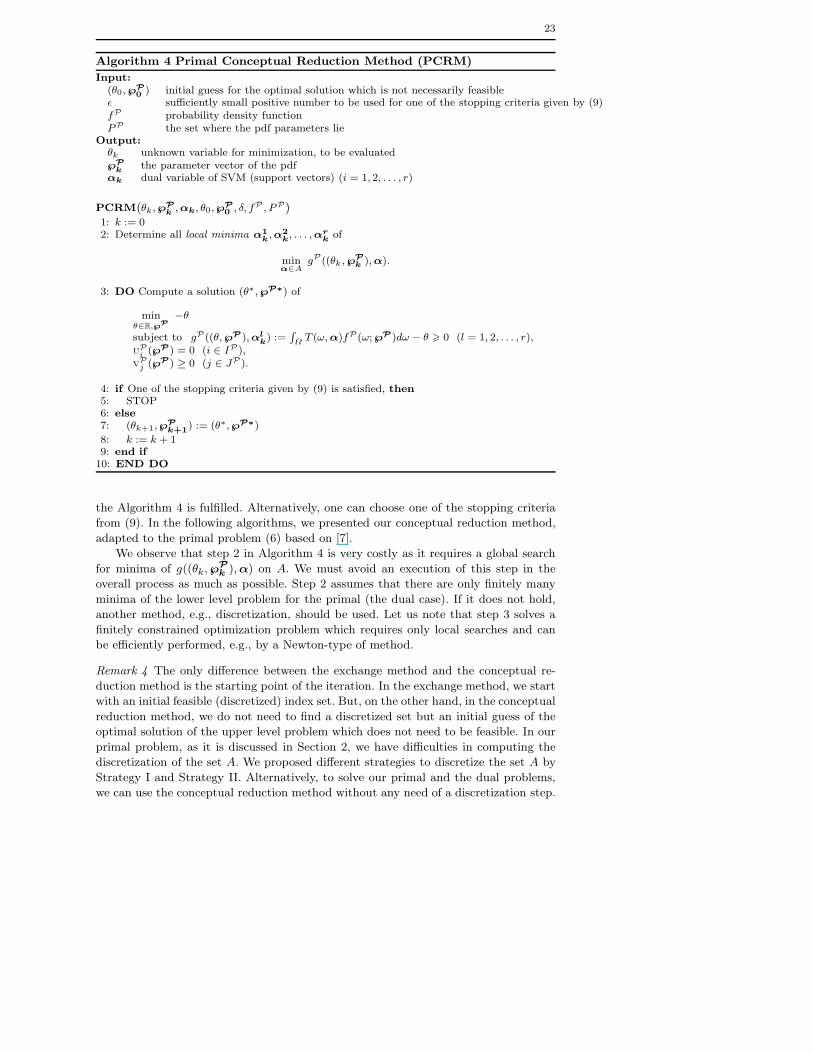
8: k := k + 19: end if10: END DO

the Algorithm 4 is fulfilled. Alternatively, one can choose one of the stopping criteria

from (9). In the following algorithms, we presented our conceptual reduction method,

adapted to the primal problem (6) based on [7].

We observe that step 2 in Algorithm 4 is very costly as it requires a global search

for minima of g((θk,℘Pk ),α) on A. We must avoid an execution of this step in the

overall process as much as possible. Step 2 assumes that there are only finitely many

minima of the lower level problem for the primal (the dual case). If it does not hold,

another method, e.g., discretization, should be used. Let us note that step 3 solves a

finitely constrained optimization problem which requires only local searches and can

be efficiently performed, e.g., by a Newton-type of method.

Remark 4 The only difference between the exchange method and the conceptual re-

duction method is the starting point of the iteration. In the exchange method, we start

with an initial feasible (discretized) index set. But, on the other hand, in the conceptual

reduction method, we do not need to find a discretized set but an initial guess of the

optimal solution of the upper level problem which does not need to be feasible. In our

primal problem, as it is discussed in Section 2, we have difficulties in computing the

discretization of the set A. We proposed different strategies to discretize the set A by

Strategy I and Strategy II. Alternatively, to solve our primal and the dual problems,

we can use the conceptual reduction method without any need of a discretization step.

24

6 Implemantation of IKL

We tested our IKL problem based on Algorithm 3 and Algorithm 4 for two kinds of

data sets. The discretization of the index set is obtained by random search of corner

points.

We first implemented our method on votes data which is a homogeneous data set

and secondly, we tested our method on bupa data set4 which is a heterogeneous data

set. Data descriptions are given in Table 1.

Data set # instances # attributes attribute characteristicsVotes 52 16 categoricalBupa 345 6 integer, real and categorical

Table 1 Data set description.

We compared our results with the single kernel SVM model introduced in Section

1. Furthermore, we considered a single kernel SVM for the comparison with our IKL

because of its simplicity. Let us note that single kernel is a special case of multiple kernel

learning, i.e., the upper limit of multiple combination of kernel is taken as K = 1.

For both single kernel SVM and IKL, we selected the regularization constant of

SVM, C, by 5-fold cross validation from the search set

{2−5, 2−3, 2−1, 2, 23, 25, 27, 29, 211, 213}.The results are interpreted by the accuracy percentage which is computed by the

ratio of correct classification to total number of test points. Further, we used LibSVM

package [5] for single kernel SVM and the parameter of Gaussian kernel is chosen by 5

fold cross validation over a search set of {0, 0.1, 0.2, 0.3, 0.4, 0.5, 0.6, 0.7, 0.8, 0.9, 1}. We

implemented our IKL model by Algorithm 4 with a Gaussian kernel, and the search

space for a Gaussian kernel width is chosen as Ω = [0, 1]. All the implementations are

done in Matlab 7.0.4. In order to have finitely many local minima in the lower level

problem and to use Heine Borel Theorem, the domain of our variable θ is restricted to

a compact set, e.g., [−100, 100]. We used the fmincon function of Matlab Optimization

toolbox to implement both the exchange and the conceptual reduction method.

As our IKL aims to help for the classification of heterogeneous data, the results

given by Table 2 show that IKL increased the accuracy by 27% on bupa data whereas

it could not be successful for homogenous data. The results for homogeneous data can

be improved if different kernels are chosen and different numerical methods are used.

This will be a subject of our future study.

7 Conclusion

By means of new ideas, we developed well-known numerical methods of semi-infinite

programming for our new kernel machine. We improved the discretization method for

4 available from http : //archive.ics.uci.edu/ml/

25

Data set Single kernel SVM IKL by Exchange Method IKL by PCRMVotes 92% 75% 91%Bupa 73% 99% 99%

Table 2 Percentage of the Accuracy.

our specific model and proposed two new algorithms (see Strategy I and Strategy II).

The advantage of these methods were discussed and the intuition behind these al-

gorithms were visualized by figures and examples. We stated the convergence of the

numerical methods with theorems and we analyzed the conditions and assumptions of

these theorems such as optimality and convergence. We implemented our novel kernel

learning algorithm called IKL by two well-known numerical methods for SIP, i.e., ex-

change method and conceptual discretization method. We achieved very satisfactory

accuracy for heterogeneous data and we also got promising accuracy for homogeneous

data. As it was claimed by us that IKL was developed to help classification of hetero-

geneous data, these results validated our proposal. The accuracy results for exchange

method on votes data is not promising due to the discretization step at the exchange

method

In addition, we intend to study infinite programming and investigate primal-dual

methods instead of reducing the infinite problem into semi-infinite programming. Fur-

thermore, we will investigate our works with MFCQ and strong stability of all Karush-

Kuhn-Tucker (KKT) points [7] in the reduction ansatz.

Acknowledgements The authors cordially thank to three anonymous referees for their con-structive critisim, and to the professors E. Anderson, U. Capar, M. Goberna, and Y. Ozan fortheir valuable advices.

References

1. E.J. Anderson and P. Nash. Linear Programming in Infinite-Dimensional Spaces. JohnWiley and Sons Ltd, 1987.

2. T.M. Apostol. Mathematical Analysis: A Modern Approach to Advanced Calculus. Addi-son Wesley, 1974.

3. A. Argyriou, R. Hauser, C. Micchelli, and M. Pontil. A dc-programming algorithm for ker-nel selection. In Proceedings of the 23rd International Conference on Machine Learning,Pittsburgh, PA, 2006.

4. F.R. Bach and G.R.G. Lanckriet. Multiple kernel learning, conic duality, and the smoalgorithm. In Proceedings of the 21st International Conference on Machine Learning,2004.

5. C.-C. Chang and C.-J. Lin. Libsvm: a library for support vector machines. Softwareavailable at http://www.csie.ntu.edu.tw/cjlin/libsvm, 2001.

6. R. Hettich and H.Th. Jongen. Semi-infinite programming: conditions of optimality andapplications. In J. Stoer, editor, Optimization Techniques 2, Lecture notes in Control andInformation Sci. Springer, Berlin, Heidelberg, /New York, 1978.

7. R. Hettich and O. Kortanek. Semi-infinite programming: Theory, methods and applica-tions. SIAM Review, 35, 3:380–429, 1993.

8. R. Hettich and P. Zencke. Numerische Methoden der Approximation und semi-infinitenOptimierung. Tuebner, Stuttgart, 1982.

9. H.Th. Jongen, P. Jonker, and F. Twilt. Nonlinear Optimization in Finite Dimensions- Morse Theory, Chebyshev Approximation, Transversality, Flows, Parametric Aspects.Springer Verlag, 2000.

26

10. Y. Ozan. Scientific discussion with Yıldıray Ozan, Department of Mathemetics, METU,Turkey, 2008.

11. S. Ozogur-Akyuz. A Mathematical Contribution of Statistical Learning and ContinuousOptimization Using Infinite and Semi-Infinite Programming, To Computational Statistics(submitted). PhD thesis, Middle East Technical University, Insitiute of Applied Mathe-matics, Department of Scientific Computing, February, 2009.

12. S. Ozogur-Akyuz and G.W.-Weber. Modelling of kernel machines by infinite and semi-infinite programming. In Proceedings of the Second Global Conference on Power Controland Optimization, AIP Conference Proceedings 1159, Bali, Indonesia, Subseries: Mathe-matical and Statistical Physics; ISBN 978-0-7354-0696-4 (August 2009); A.H. Hakim, P.Vasant and N. Barsoum, guest eds., pages 306–313, 1-3 June 2009.

13. S. Ozogur-Akyuz, Z. Hussain, and J. Shawe-Taylor. Prediction with the svm using testpoint margins. In S. Lessmann, editor, in Annals of Information Systems (to appear).Springer, 2009.

14. S. Ozogur-Akyuz, J. Shawe-Taylor, G.-W. Weber, and Z.B. Ogel. Pattern analysis for theprediction of eukoryatic pro-peptide cleavage sites. Discrete Applied Mathematics, 157(10):2388–2394, 2009.

15. S. Ozogur-Akyuz and G.-W. Weber. Learning with infinitely many kernels via infinite andsemi-infinite programming. accepted to to Optimization Methods and Software.

16. S. Ozogur-Akyuz and G.-W. Weber. Learning with infinitely many kernels via semi-infinite programming. In Continuous Optimization and Knowledge Based Technologies,20th EURO Mini conference, Lithunia, pages 342–348, 2008.

17. P.M. Pardalos and P. Hansen (Eds). Data Mining and Mathematical Programming, volumeCRM 45. American Mathematical Society, 2008.

18. J.-J. Ruckmann and G.-W Weber. Semi-infinite optimization: Excisional stability of non-compact feasible sets. Sibirskij Mathematicheskij Zhurnal, 39:129–145, 1998.

19. O. Seref, O.E. Kundakcioglu, and P.M. Pardalos (Eds). Data Mining, Systems Analysis,and Optimization in Biomedicine. Springer, 2007.

20. A. N. Shiryaev. Probability. Springer, 1995.21. S. Sonnenburg, G. Raetsch, C. Schafer, and B. Scholkopf. Large scale multiple kernel

learning. J. Machine Learning Research, 7:1531–1565, 2006.22. G. Still. Semi-infinite programming: An introduction, preliminary version. Technical

report, University of Twente Department of Applied Mathematics, Enschede, The Nether-lands, 2004.

23. A.I.F. Vaz, E.M.G.P. Fernandes, and M.P.S.F. Gomes. Discretization methods for semi-infinite programming. Investigac ao Operacional, 21 (1), 2001.

24. G.-W. Weber. Generalized Semi-Infinite Optimization and Related Topics, volume 29 ofResearch and Exposition in Mathematics. Heldermann Verlag, Germany, 2003.

25. A. Yershova and S.M. LaVelle. Deterministic sampling methods for spheres and so(3). InIEEE International Conference on Robotics and Automation (ICRA), 2004.