Thermoelastic waves in an anisotropic infinite plate

Thermoelastic waves in an anisotropic infinite plateHussain Al-Qahtani and Subhendu K. Dattaa)

Department of Mechanical Engineering, University of Colorado, Boulder, Colorado 80309-0427

(Received 25 March 2004; accepted 2 June 2004)

An analysis of the propogation of thermoelastic waves in a homogeneous, anisotropic, thermallyconducting plate has been presented in the context of the generalized Lord-Shulman theory ofthermoelasticity. Three different methods are used in this analysis: two of them are exact and thethird is a semianalytic finite element method(SAFE). In our exact analysis, two different approachesare used. The first one, which is applicable to transversely isotropic plate, is based on introducingdisplacement potential functions, whereas in the second approach, which is applicable to anytriclinic material, we rewrite the governing equations and boundary conditions in a matrix form.Finally, in the SAFE method, the plate is discretized along its thickness usingN parallel,homogeneous layers, which are perfectly bonded together. Frequency spectrum and dispersioncurves are obtained using the three methods and are shown to agree well with each other. The effectsof thermal relaxation time and coupling term are also investigated. Numerical calculations havebeen presented for a silicon nitridesSi3N4d plate. However, the methods can be used for othermaterials as well. ©2004 American Institute of Physics. [DOI: 10.1063/1.1776323]

I. INTRODUCTION

During the second half of the 20th century, nonisother-mal problems of the theory of elasticity have been investi-gated extensively. This is due mainly to their many applica-tions in widely diverse fields. First, in the field ofnondestructive evaluation, laser-generated waves have at-tracted great attention owing to their potential application tononcontact and nondestructive evaluation of sheet materials.Second, the high velocities of modern aircraft give rise toaerodynamic heating, which produces intense thermalstresses, reducing the strength of the aircraft structure. Third,in the nuclear field, the extremely high temperatures andtemperature gradients originating inside nuclear reactors in-fluence their design and operations.1 Moreover, it is wellrecognized that the investigation of the thermal effects onelastic wave propogation has bearing on many seismologicaland astrophysical problems.2

Most materials undergo appreciable changes of volumewhen subjected to variations of the temperature. If thermalexpansions or contractions are not freely admitted, tempera-ture variations give rise to thermal stresses. Conversely achange of volume is attended by a change of the temperature.When a given element is compressed or dilated, these vol-ume changes are accompanied by heating and cooling, re-spectively. The study of the influence of the temperature ofan elastic solid upon the distribution of stress and strain, andof the inverse effect of the deformation upon the temperaturedistribution is the subject of thermoelasticity.3

The classical theory of heat conduction in solids restsupon the hypothesis that the flux of heat is proportional tothe gradient of the temperature distribution. As a conse-quence of this hypothesis, the equation is governed by aparabolic partial differential equation, which predicts that the

application of a thermal disturbance in a body instanta-neously affects all points of the body. This assumption ofinfinite speed is contrary to physical phenomenon. To re-move this paradox inherent in the classical theory, a theoryof generalized thermoelasticity was developed. This general-ized theory accounts for the short time required to establish asteady state heat conduction when a temperature gradient issuddenly produced in the solid. This short time is called thethermal relaxation time. The concept of generalized ther-moelasticity has led to a wide range of extensions of theclassical theory of thermoelasticity. Various generalizationinclude the following.

(i) Thermoelasticity proposed by Lord and Shulman in1967 (L–S model),4 in which, in comparison to theclassical theory, the Fourier law of heat conduction ismodified by taking into consideration a single relax-ation time.

(ii ) Thermoelasticity introduced by Green and Lindsay in1972 (G–L model),5 in which the constitutive rela-tions for the stress tensor and the entropy are gener-alized by introducing two different relaxation times.

(iii ) Thermoelasticity without energy dissipation, proposedby Green and Naghdi in 1992(G–N model),6 inwhich, the Fourier law is replaced by a heat fluxrates–temperature gradient relaxation.

These generalization are the most important ones. Forother variations, one can refer for instance to Hetnarski andIgnaczk.7

Guided thermoelastic waves were considered by severalresearchers. Nayfeh and Nemat-Nasser,8 Sinha and Sinha,9

Agarwal,10 Sherief and Helmy,11 and Abd-alla and Al-dawy12

studied isotropic thermoelastic Rayleigh waves. Massalas,13

Daimaruya and Naioth,14 Massalas and Kalpakidis,15

Sharma, Singh, and Kumar,16 considered the propagation ofa)Author to whom correspondence should be addressed; electronic mail:[email protected]

JOURNAL OF APPLIED PHYSICS VOLUME 96, NUMBER 7 1 OCTOBER 2004

0021-8979/2004/96(7)/3645/14/$22.00 © 2004 American Institute of Physics3645

Downloaded 22 Jun 2005 to 212.26.1.29. Redistribution subject to AIP license or copyright, see http://jap.aip.org/jap/copyright.jsp

http://dx.doi.org/10.1063/1.1776323

guided thermoelastic waves in an isotropic plate. Sharma andSharma17 studied the free vibration of a thermoelastic cylin-drical panel.

In contrast, little work has been reported on thermoelas-tic waves in anisotropic plates. The main focus of our workwill be on the laser-generated waves in thermoelastic aniso-tropic plate. As mentioned above, the technique of laser-generated waves has potential application to noncontact andnondestructive evaluation and characterization of sheet ma-terials in industry. It was demonstrated that the thickness ofand moduli of thin plates can be measured experimentallyusing laser-generated waves.18 In the first part of our work,dispersion relations for thermoelastic anisotropic plate willbe studied. These relations are investigated first because oftheir importance in calculating elastic and thermal propertiesof materials. Moreover, using dispersion relations, it is thenpossible to analyze transient response of a plate heated by alaser pulse which will be the subject of our future investiga-tion. The study is carried out in the context of Lord-Shulman(L–S) theory of thermoelasticity using single relaxation time.Two different methods have been used to model the problem.The first is an exact analysis using two different approaches(Secs. II A and II A 2) and a semianalytic finite elementmethod(SAFE) (Sec. II B). Numerical results and discussionare presented in Sec. III. This work concludes with a discus-sion of possible future work.

II. THEORETICAL FORMULATIONS

We consider an infinite homogeneous transversely iso-tropic thermally conducting elastic plate at a uniform tem-peratureT0 in the undisturbed state having a thicknessH, seeFig. 1. The motion is assumed to take place in three dimen-sionssx,y,zd. The displacements in thex, y, andz directionsareu,v, andw, respectively.

A. Exact analysis

In the absence of body forces and internal heat sourcethe generalized L–S thermoelasticity governing equations are

si j ,j = rui , s1d

qi,j = − T0rh, s2d

si j = cijklekl − bi jT, s3d

rh = bi j ei j +rCE

T0T, s4d

ei j = 12sui,j + uj ,id, s5d

qi + t0qi = − KijT,j . s6d

In the above equations, a comma followed by a suffix de-notes spatial derivative and a superposed dot denotes thederivative with respect to time.

Various physical variables and material constants ap-pearing in the above equations are the following:si j , thecomponents of stress tensor;qi, the components of heat fluxvector;ei j , the components of strain tensor;r, mass density;Kij , the coefficients of thermal conductivity;t, time; cijkl , theelastic constants;h, entropy density;bi j , the thermal coeffi-cients;CE, the specific heat at constant deformation; T, tem-perature perturbation;t0, thermal relaxation time;ui, thecomponents of displacement vector;T0, reference tempera-ture si , j ,k, l =1,2,3d. It is assumed thatuT/T0u !1.

In transversely isotropic material and assuming that thexaxis is the axis of symmetry of the material, the stresses canbe written in terms of the displacements and temperaturevariation as

sxx = c11u,x + c12v,y + c12w,z − bxxT, s7d

syy = c12u,x + c22v,y + c23w,z − byyT, s8d

szz= c12u,x + c23v,y + c22w,z − byyT, s9d

syz= c44sv,z + w,yd, s10d

sxz= c55su,z + w,xd, s11d

sxy = c55su,y + v,xd, s12d

where

c44 = 12sc22 − c23d

and

bxx = c11axx + 2c12ayy, byy = c12axx + sc22 + c23dayy.

s13d

Here, axx and ayy are the coefficients of linear thermal ex-pansions inx andy directions, respectively.

By substitution of the foregoing expressions into Eqs.(1)–(6), one can write the governing equations in terms ofdisplacement and temperature,

c11u,xx + c12v,xy + c12w,xz

+ c55su,yy + v,xyd + c55su,zz+ w,xzd − bxxT,x = ru, s14d

c55su,xy + v,xxd + c12u,xy + c22v,yy + c23w,yz

+ c44sv,zz+ w,yzd − byyT,y = rv, s15d

c55su,xz+ w,xxd + c44sv,yz+ w,yyd + c12u,xz

+ c23u,yz+ c22w,zz− byyT,z = rw, s16d

FIG. 1. Geometry of the problem.

3646 J. Appl. Phys., Vol. 96, No. 7, 1 October 2004 H. AL-Qahtani and S. K. Datta


KxxT,xx + KyyT,yy + KyyT,zz− rCEsT + t0Td

= T0fbxxsu,x + t0u,xd

+ byysv,y + t0v,yd + byysw,z + t0w,zdg. s17d

Note that Eq.(17) reduces to the classical coupled ther-moelasticity equation for heat conduction ift0=0.

We define the following nondimensional quantities:

x * =vx

kxx, y * =

vx

kxy, z* =

vx

kxz, t * =

vx2

kxt,

u * =vx

3r

kxbxxT0u, v* =

vx3r

kxbxxT0v,

w* =vx

3r

kxbxxT0w, T * =

T

T0,

c1 =c12

c11, c2 =

c55

c11, c3 =

c22

c11, c4 =

c23

c11,

c5 =c44

c11, d = c1 + c2, b =

byy

bxx, K =

Kyy

Kxx,

t0* =

vx2

kxt0, « =

bxx3 T0

r2CEvx2 ,

where vx=Îc11/r is the velocity of compressional waves,kx=Kxx/rCE is the thermal diffusivity in thex direction, and« is the thermoelastic coupling constant. Using the abovenondimensional quantities, the governing equations are nowwritten as

u,xx + c1v,xy + c1w,xz+ c2su,yy + v,xyd + c2su,zz+ w,xzd − T,x = u,

s18d

c2su,xy + v,xxd + c1u,xy + c3v,yy + c4w,yz+ c5sv,zz+ w,yzd − bT,y

= v, s19d

c2su,xz+ w,xxd + c5su,yz+ w,yyd + c1u,xz+ c4v,yz+ c3w,zz

− bT,z = w, s20d

T,xx + KT,yy + KT,zz− sT + t0Td = «fsu,x + t0u,xd

+ bsv,y + t0v,yd + bsw,z + t0w,zdg. s21d

Generally, the coupling term« is small for most materials.19

Table I gives numerical values of some constants for threedifferent materials, namely, aluminium, zinc, and silicon ni-tride. In the following two sections, two approaches will be

introduced to solve the above exact formulation.

1. First approach

For convenience, the asterisk will be suppressed fromnow on. The displacement can be written in terms of threepotential functions as in Buchwald20 in the form

u =] Q

] x, s22d

u =] F

] y+

] C

] z, s23d

w =] F

] z−

] C

] y. s24d

Eliminating the displacements from the equations of mo-tion produces

Fc2]2

] x2 + c5¹2 −

]2

] t2G¹2C = 0, s25d

d]2

] x2¹2F + Fc2¹2 +

]2

] x2 −]2

] t2G ]2Q

] x2 −]2T

] x2 = 0, s26d

d]2

] x2¹2Q + Fc3¹2 + c2

]2

] x2 −]2

] t2G¹2F − b¹2T = 0, s27d

«F ]2

] x2sQ + t0Qd + b¹2sF + t0FdG −]2T

] x2 − K¹2T

+ sT + t0Td = 0, s28d

where

¹2 =]2

] z2 +]2

] y2 .

It can be noted that the first equation is decoupled from oth-ers. Since we are interested in propagating waves in theplane ofx,y, potentials and temperature are written in theform

Q = g1szdeiskx+jy−vtd, s29d

F = g2szdeiskx+jy−vtd, s30d

T = g3szdeiskx+jy−vtd, s31d

C = g4szdeiskx+jy−vtd, s32d

wherek,j, andv are, respectively, the nondimentional wavenumber in thex direction, the nondimensional wave number

TABLE I. Some numerical constants for different materials.

Material vxm/s kxm2/s K b «

Aluminum alloy 3.883103 1.02310-11 1 1 2.56310-3

Zinc 4.773103 4.45310-5 1 0.882 2.16310-2

Silicon nitride 1.343104 2.58320-5 0.786 0.843 2.49310-3

J. Appl. Phys., Vol. 96, No. 7, 1 October 2004 H. AL-Qahtani and S. K. Datta 3647


in the y direction, and nondimentional frequency.By substitution of these assumed potentials into Eq.(25),

we get a second-order ordinary differential equation ing4szdand a second-order system of differential equation ing1szd,g2szd, andg3szd. It can be shown that the solutions have thefollowing forms:

g1 = F1V1 + G1V2 + H1V3, s33d

g2 = F2V1 + G2V2 + H2V3, s34d

g3 = F3V1 + G3V2 + H3V3, . s35d

g4 = F4V4. s36d

Here,

V1 = B11eis1z + B12e

is1sH−zd, s37d


is2sH−zd, s38d


is3sH−zd, s39d

V4 = B41eirz + B42e

ir sH−zd. s40d

Using Eqs.(29)–(32) and the expression forg1szd, g2szd,andg3szd in Eqs.(25)–(28), we get for nontrivial soltion

r =Îv2 − c2k2 − c5j2

c5s41d

and the determinant of the following matrix must vanish,

3− c2X − k2 + v2 − dX − 1

− dk2 − c3X − c2k2 + v2 − b

«tk2b«tX k2 + KX − t

4 ,

s42d

where

X = ss2 + ,2d

and

t = siv + t0v2d,

ands is the nondimensional wave number in thez-direction.This results in the following cubic equation:

X3 + A1X2 + A2X + A3 = 0, s43d

whereA1, A2, andA3 are defined in Appendix A. Solving Eq.(43) yields the following three roots fors2:

s12 = − j2 −

A1

3−

Î32L

3sY + Î4L3 + Y2d1/3

+sY + Î4L3Y2d1/3

3Î32, s44d

s22 = − j2 −

A1

3−

s1 + iÎ3Ld

3Î32sY + Î4L3 + Y2d1/3

−s1 − iÎ3dsY + Î4L3 + Y2d1/3

6Î32, s45d

s32 = − j2 −

A1

3−

s1 − iÎ3Ld

3Î32sY + Î4L3 + Y2d1/3

−s1 + iÎ3dsY + Î4L3 + Y2d1/3

6Î32, s46d

where L=3A2−A12 and Y=−2A1

3+9A1A2−27A3. The con-stants appearing in Eqs.(33)–(36) may be taken as shown inAppendix A. Now, the temperature gradient and the stressesof interest are

szz= mzzDv, s47d

sxz= mxzDv, s48d

syz= myzDv, s49d

Tz = mTDv, s50d

where the row vectorsmzz, mxz, myz, andmT are defined inAppendix A. The matrixD is a diagonal matrix such that

diagfDg

= feis1z,eis2z,eis3z,eirz,eis1sH−zd,eis2sH−zd,eis3sH−zd,eir sH−zdg

s51d

and the generalized coefficients vector can be written as

v = hB11 B21 B31 B41 B12 B22 B32 B42jT. s52d

The boundary conditions are that stresses and temperaturegradient on the surfaces of the plate should vanish. Hence,we demand that

T,z = szz= szx= szy= 0. s53d

Using boundary conditions(53) in the resulting stresses andtemperature gradient yields eight equations involving thevector v. In order for the eight boundary conditions to besatisfied simultaneously, the determinant of the coefficient ofthe arbitrary constants in Eq.(52) must vanish. This gives anequation for the frequency of the guided wave for a givenwave number.

2. Second approach

For an infinite plate one can use Fourier transformationin space and time domais represented by the following inte-gral:

Fsk,j,z;vd =E−`

` E−`

` E−`

`

Fsx,y,z;tdeiskx+jy−vtddx dy dt.

s54d

Here,k,j are the wave numbers inx andy directions, respec-tively, and v the circular frequency. Applying the Fourier



transformation(54) to the governing equations will yield thefollowing eigenvalue problem:

fAgS,z = fBgS, s55d

wereS,z=dS/dz and

Sszd = fu v w T szx syz szzT,zgT. s56d

The general solution can be obtained by determining the eigenvalues and the eigenvectors of Eq.(55). Here S is thedisplacement-temperature-traction vector and matrices A and B are defined as

A = 3. . . − 1 . . . .

. . − c3 . . . . .

. − c5 . . . . . .

− c2 . . . . . . .

. . ic1k . 1 . . .

. . ic4j . . 1 . .

. . . . . . 1 .

. . b«t . . . . K

4 , s57d

B = 3. . . . . . . − 1

ic1k ic4j . − b . . − 1 .

. . ic5j . . − 1 . .

. . ic2k . − 1 . . .

k2 + c2j2 − v2 kjsc1 + c2d . ik . . . .

kjsc1 + c2d c2k2 + c3j2 − v2 . ibj . . . .

. . − v2 . − ik − ij . .

− i«kt − ib«t . k2 + Kj2 − t . . . .

4 , s58d

wheret= iv+t0v2.The general solution to Eq.(55) can be written as

Sszd = fQEghCj, s59d

where Q is the resulting eigenvectors matrix from Eq.(55), C are generalized coefficients, and E is a diagonal matrix,

E = diagfeis1z,eis2z,eis3z,eis4z,eis1sH−zd,eis2sH−zd,eis3sH−zd,eis4sH−zdg, s60d

where 1, . . . ,4isp,sp=1,2,3d are the resulting eigenvalues ofthe characteristics equations(55), with Imsspdù0. The firstfour elements of Eq.(60) represent the wave propagationalong the positivez axis, while the last four elements repre-sent the wave propagation along the negativez axis.

The boundary conditions are that tractions and tempera-ture gradient in thez direction on the surfaces of the plateshould vanish. Applying these boundary conditions yieldsthe dispersion relation for the infinite plate.

B. Finite element method

We rewrite the governing equations in vector form,

hsj = fCgh«j − hbjT, s61d

rh = hbjTh«j +rCE

T0T, s62d



hqj + t0hqj = − fKghT8j, s63d

whereT8=T,j.The plate is divided intoN parallel, homogeneos, and

anisotropic layers, which are perfectly bonded together. Aglobal rectangular coordinate systemsX,Y,Zd is adoptedsuch thatX andY axes lie in the midplane of the plate, andZaxis parallel to the thickness direction of the plate. To ana-lyze the guided wave propagation in such an infinite plate,we discretize the thickness of the plate using three-noded barelements, each of which has associated with it a local coor-dinate axessx,y,zd, which are parallel to the global coordi-nate axes.

Two sets of shape functions are introduced to approxi-mate the displacement and temperature fields on the elementlevel,

usx,y,z,td = N1eszduesx,y,td, s64d

Tsx,y,z,td = N2eszdTesx,y,td, s65d

where

N1e = 3N1 0 0 N2 0 0 N3 0 0

0 N1 0 0 N2 0 0 N3 0

0 0 N1 0 0 N2 0 0 N34 s66d

and

N2eT= hN1N2N3j. s67d

Nodal displacements and temperatures are stored in the twovectorsue andue, respectively. Using generalized linear ther-moelasticity the strain tensor and temperature vector is de-rived from the kinematic equaitons,

e = D1u,xe + D2u,y

e + D3ue, s68d

T8 = B1T ,xe + B2T ,y

e + B3Te, s69d

whereB1, B2, B3, D1, D2, andD3 are defined in Appendix B.The variational forms of Eqs.(68) and (69) are

de = D1du,xe + D2du,y

e + D3due, s70d

dT8 = B1dT ,xe + B2dT ,y

e + B3dTe. s71d

Considering the body forcefe, the virtual displacementprinciple can be written as the following form:

Et0

t1EV

fd«Ts − dT8TKT8 − dT8Tsqi + t0qidgdV dt

=Et0

t1EV

duTsf − ruddV dt. s72d

Substituting the constitutive relations, Eqs.(61)–(63), intothe variational form, Eq.(72), leads to the following terms:

Et0

t1EV

d«TsdV dt =Et0

t1EV

d«TsC« − bTddV dt

=Et0

t1EV

fsdu,xeTD1

T + du,yeTD2

T + dueTD3TdCsD1du,x

e + D2du,ye + D3

Tdued − su,xeTD1

T + u,yeTD2

T

+ ueTD3TdbN2

eTTegdV dt

=Et0

t1EyE

x

dueTf− k11e u,xx

e −k12e u,xy

e − k13e u,x

e − k21e u,xy

e − k22e u,yy

e − k23e u,y

e + k31e u,x

e + k32e u,y

e + k33e u,yy

e

+ km01e T ,x

e + km02e T ,y

e − km03e T ,x

e gdx dy dt, s73d

where the elemental matrices appearing in the last equationare defined in Appendix B. The second term in Eq.(72) canbe written as

Et0

t1

EV

dsTeTd8K sTed8dV dt

=Et0

t1

EV

sdT ,xe TB1

T + dT ,yeTB2

T + dTeTB3Td

3K sB1T ,xe + B2T ,y

e + B3TeddV dt

=Et0

t1

EyE

x

dTeTsg11e T ,xx

e + g22e T ,yy

e − g33e Teddx dy dt, s74d

whereg11, g22, andg33 are defined as

g11e =E

z

B1TKB 1dz, g22

e =Ez

B2TKB 2dz,

g33e =E

z

B3TKB 3dz.

The third term of Eq.(72) is



Et0

t1

EV

dsTeTd8sq + t0qddV dt

= −Et0

t1

EV

dTeTsq8 + t0q8ddV dt

=Et0

t1

EV

dTeTsT0rh + t0T0rhddV dt

=Et0

t1

EyE

x

dTeTfsf1eu,x

e + f2eu,y

e + f3eue + muu

e Td

+ t0sf1u,xe + f2u,y

e + f3ue + muu

e Tddx dy dt, s75d

whereq8=q,i and

muue =E

z

N2erN2

eTdz, f1e =E

z

T0N2ebD1dz,

f2e =E

z

T0N2ebD2dz, f3

e =Ez

T0N2ebD3dz

The right-hand side of Eq.(72) is written as

Et0

t1

EV

duTsf − ruddV dt

=Et0

t1

EV

dueTN1eTsf − rN1

eueddV dt

=Et0

t1

EyE

x

dueTsfe − meueddx dy dt, s76d

where

fe =Ez

N1eTfdz, m =E

z

rN1eTN1

edz.

Equating the coefficient ofdue in Eq. (72) to zero yields

k11e u,xx

e + k12e u,xy

e + k13e u,x

e + k21e u,xy

e + k22e u,yy

e + k23e u,y

e

− k31e u,x

e − k32e u,y

e − k33e ue − km01

e T ,xe − km02

e T ,ye + km03

e Te

− meue = 0. s77d

Similarly, equating the coefficient ofdTe in Eq. (72) yields

t0muue Te + muu

e Te + t0f1eu,x

e + t0f2eu,y

e + t0f3eue + f1

eu,xe

+ f2eu,y

e + f3eue − g11

e T ,xxe − g22

e T ,yye + g33

e Te = 0. s78d

Rewriting the last two equations[Eqs.(77) and(78)] in vec-tor formats yields

f− M A 0g5 ue

¯

Te6 + fK 11 A 0g5u,xxe

¯

T ,xxe 6 + fK 12 + K 21 A 0g5u,xy

e

¯

T ,xye 6

+ fK 13 − K 31 A − K m01g5u,xe

¯

T ,xe 6 + fK 22 A 0g5u,yy

e

¯

T ,yye 6

+ fK 23 − K 32 A − K m02g5u,ye

¯

T ,ye 6 + f− K 33 A K m03g5ue

¯

Te6 = 0.

s79d

and

ft0F3 A t0Fuug5 ue

¯

Te6 + ft0F1 A 0g5 u,xe

¯

T ,xe 6 + ft0F2 A 0g5 u,y

e

¯

T ,ye 6

+ fF1 A 0g5 u,xe

¯

T ,xe 6 + fF2 A 0g5 u,y

e

¯

T ,ye 6 + fF3 A M uug5 ue

¯

Te6+ f0 A − G11g5u,xx

e

¯

T ,xxe 6 + f0 A − G22g5u,yy

e

¯

T ,yye 6 + f0 A − G33g

35ue

¯

Te6 = 0. s80d

We assemble the element matrices into the global matri-ces in the standard manner to yield the equations of motion,

H1V + H2V ,x + H3V ,y + H4V ,x + H5V ,y + H6V + H7V ,xx

+ H8V ,xy + H9V ,yy + H10V ,x + H11V ,y + H12V = 0, s81d

where the matricesH i are defined in Appendix B andV isthe column vector of assembled nodal displacements andtemperatures.

For a wave propagating in theXY plane, we take theFourier transform ofVsX,Y,td as

Vskx,ky,vd =E−`

`

E−`

`

E−`

`

VsX,Y,tdeiskxX+kyY−vtddX dY dt.

s82d

Applying the Fourier transform to Eq.(81) leads to the fol-lowing expression:

fv2H1 + iv2kxH2 + iv2kyH3 − vkxH4 − vkyH5 + ivH6

+ kx2H7 + kxkyH8 + ky

2H9 − ikxH10 − ikyH11 − H12gV = 0,

s83d

wherev is the circular frequency andkx andky are the wavenumbers in theX andY directions. For wave propagating inarbitrary direction in thexy plane making an angleu with X



axis i.e.,kx=k cosu, andky=k sin u, Eq. (83) is written as

sk2M + kC + K dV = 0, s84d

wherek is the wave number of the wave in the propagationdirection, and

M = − cos2uH7 − cosu sin uH8 − sin2uH9, s85d

C = − iv2cosuH2 − iv2sin u H3 + v cosuH4

+ v sin uH5 + i cosuH10 + i sin uH11, s86d

K = − v2H1 − ivH6 + H12. s87d

Solving the eigenvalue problem represented by Eq.(84)will determine the dispersion for guided thermoelastic wavesin infinite plates.

III. RESULTS AND DISCUSSION

With the view of illustrating the numerical results ob-tained by methods presented in the preceding sections, thematerial chosen for the plate is silicon nitridesSi3N4d, thephysical data for which is given in Table II. Elastic stiffnessconstants can be found in Ref. 21, whereas thermal proper-ties are collected from Swiftet al.,22 Kitayamaet al.,23 andYakota and Ibukiyama.24

The dimensional speed of the thermal wave in thex di-rection for unbounded medium is

yt =Î Kxx

rCEt0. s88d

We recall that the relaxation timet0 is introduced to accountfor the finite speed of thermal wave. To the best of ourknowledge, no experimental values fort0 have been re-ported. However, some researchers suggested different waysof calculating it. Chester25 approximates the speed of thethermal wave according to the following equation:

yt =yx

Î3. s89d

Using this approximation, the dimensional relaxation time isobtained as

t0 =3Kxx

CEC11. s90d

Hence, for silicon nitride, t0 is approximately 4.322310−13 s st0−nondim=3.0d. Prevost and Tao26 andKhadrawi, Al-Nimr, and Hammad27 approximated the relax-ation time by restricting the speed of the thermal wave to be

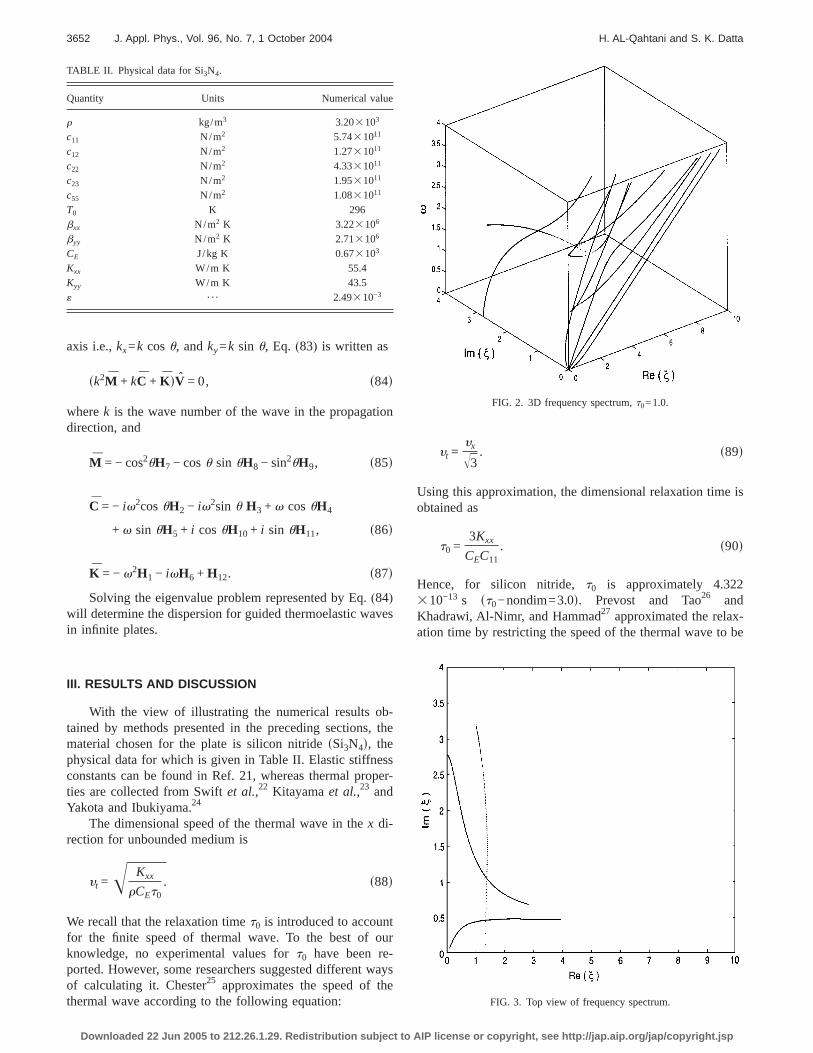
FIG. 2. 3D frequency spectrum,t0=1.0.

FIG. 3. Top view of frequency spectrum.

TABLE II. Physical data for Si3N4.

Quantity Units Numerical value

r kg/m3 3.203103

c11 N/m2 5.7431011

c12 N/m2 1.2731011

c22 N/m2 4.3331011

c23 N/m2 1.9531011

c55 N/m2 1.0831011

T0 K 296bxx N/m2 K 3.223106

byy N/m2 K 2.713106

CE J/kg K 0.673103

Kxx W/m K 55.4Kyy W/m K 43.5« ¯ 2.49310−3



equal to the speed of the longitudinal wave giving the fol-lowing formula for the relaxation time:

t0 =Kxx

CEC11. s91d

This gives a valuet0 to be 1.440310−13 s st0−nondim=1.0d for silicon nitride. The two cases will be considered inour analysis.

Numerical results are presented in the form of three-dimensional view of frequency spectrum. These are obtainedby keepingv real and lettingk to be complex. Then, thephase velocity is defined asc=v /Reskd, and the imaginarypart of thek is a measure of the attenuation of the wave in

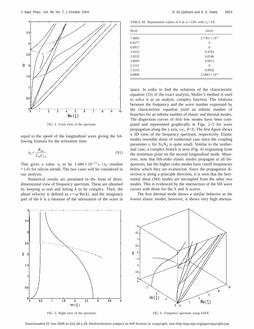
space. In order to find the solutions of the characteristicequation(53) of the exact analysis, Muller’s method is usedto solve it as an analytic complex function. The relationsbetween the frequency and the wave number expressed bythe characteristic equation yield an infinite number ofbranches for an infinite number of elastic and thermal modes.The dispersion curves of first few modes have been com-puted and represented graphically in Figs. 2–5 for wavepropagation along the x axis, i.e.,u=0. The first figure showsa 3D view of the frequency spectrum, respectively. Elasticmodes resemble those of isothermal case since the couplingparameter« for Si3N4 is quite small. Similar to the isother-mal case, a complex branch is seen(Fig. 4) originating fromthe minimum point on the second longitudinal mode. More-over, note that 0th-order elastic modes propagate at all fre-quencies, but the higher order modes have cutoff frequenciesbelow which they are evanescent. Since the propagation di-rection is along a principle direction, it is seen that the hori-zontal shear(SH) modes are uncoupled from the other twomodes. This is evidenced by the intersection of the SH wavecurves with those for the S and A waves.

The first thermal mode shows a similar behavior as thelowest elastic modes; however, it shows very high attenua-

TABLE III. Representive values ofk at v=3.00, witht0=3.0.

Resjd Imsjd

7.4603 3.7701310-5

6.9277 06.0917 03.0555 0.47832.8532 0.01462.8093 0.00132.1112 01.5155 0.99320.8800 3.5483310-4

FIG. 4. Front view of the spectrum.

FIG. 5. Right view of the spectrum. FIG. 6. Frequency spectrum using SAFE.



tion compared to elastic modes. Other thermal modes origi-nate with higher imaginary values of wave numbers andeventually approach the first thermal mode. In order to seethe attenuation associated with thermal modes and someelastic modes, we pick some numerical values from the fre-quency spectrum as shown in Table III. It is observed thatsome elastic modes exhibit attenuation expressed by theimaginary value of wave numbers. Points where the imagi-nary values are relatively high correspond to thermal modes.

Frequency spectrum was also computed by the SAFEmethod and graphically shown in Fig. 6. Excellent agree-ment between SAFE and analytic solution results is observedby comparing Fig. 6 with Fig. 2. Convergent results of SAFEanalysis can be attained by relatively small number of ele-ments(ten elements) indicating that the FEM is a powerful

and efficient technique for analyzing thermoelastic problems.Another advantage is the ease with which layered plates canbe considered.

In order to see the effect of the coupling term in the heatequation, the frequency spectrum was computed for twocases, namely,e=0 and e=2.94310−3. The correspondingfrequency spectra are plotted in Fig. 7. The figure shows thatthe two spectra are undistinguishable, therefore the couplingterm may be neglected without affecting the results. Doingso simplifies the exact analysis considerably because the heatequation gets decoupled from the other elastic equations.Hence Eq.(43) becomes now quadratic instead of cubic.

In Figs. 8–10 dispersion curves(normalized phase ve-locity vs normalized frequency) were computed and plottedalong different propagation directions, namely, 0° ,45°, and

FIG. 7. Coupling effect on frequency spectrum.

FIG. 8. Dispersion curves alongu=0°.





90°. The figures show the effect of anisotropy of the plate ondispersion curves. For instance, the phase velocities of theelastic and thermal modes decrease as the wave travels from0° to 90° direction. For all directions, it is seen that all ther-mal modes except the lowest one start with a finite phasespeed and eventually approach the speed of the first thermalmode, which originates with vanishing phase speed.

Finally, the effect of relaxation time on frequency spec-trum is investigated. Frequency spectrum was computed forthe two values of relaxation times that resulted from usingthe two different formulas Eqs.(90) and(91). Figures 11 and12 show frequency spectra for the thermoelastic plate for thetwo relaxation times. By examining the figure, it is noticedthat influence of changing relaxation time was mainly onthermal modes. Increasing the relaxation time causes thermalmodes to have more attenuation. Besides, it results in fastconvergence of higher thermal modes toward the lowest one.As expected, the velocity of thermal modes increases as therelaxation time decreases.

IV. CONCLUSIONS

Propagation of guided thermoelastic waves in a homo-geneous, transversely isotropic, thermally conducting platewas investigated within the framework of the generalizedtheory of thermoelasticity proposed by Lord and Shulman.This theory includes a thermal relaxation time in the heatconduction equation in order to model the finite speed of thethermal wave. Three different methods were used to modelthe guided wave dispersion. These include an exact analysis

incorporating two different solution approches and a SAFEmethod. The results obtained by these methods were found toagree very well.

The results show that both elastic and thermal modes areattenuated, the thermal modes exhibit much larger attenua-tion than the elastic modes. The attenuation of the former isquite small. The results agree with previous observations byHawwa and Nayfeh.28

The coupling term is generally small for all materialsand can be neglected. Neglecting the coupling term simpli-fies the analysis without noticeable effect on the frequencyspectrum as we saw earlier.

Because of the small relaxation time exhibited by thematerials under consideration the thermal wave modes havemuch larger phase speeds than the elastic modes. The effectof increasing the relaxation time is to lower the speeds of thethermal modes.

The effect of anisotropy of the material is quite pro-nounced on waves propagating in different directions alongthe plate. Thus, it is important to consider the anisotropy ofthe material in order to accurately model the propagationcharacteristics for material characterization and transient re-sponse.

While this paper dealt with the modal dispersion ofguided waves, the transient response of a plate due to a laserpulse will be reported in a subsequent paper. The latter isinvestigated by using the modal sum and a fast Fouriertransform.

APPENDIX A: EXACT ANALYSIS

A1 =1

c2c3Kfsc2c3 + c2

2K + c3K − d2Kdk2 − sc2c3 + c2b«dt − sc2 + c3dKv2g,

FIG. 12. Top view of Fig. 11.

FIG. 11. The effect of relaxation time,t01=3.0, t02=1.0.



A2 =1

c2c3Kfsc2

2 + c3 + c2K − d2dk4 + sd2 + 2bd« − c22 − c3 − c3« + b2«dtk2 − sc2 + c3 + K − c2Kdk2v2 + sc2 + c3 + b2«dtv2

+ Kv4g,

A3 =1

c2c3Kfsc2k

6 − s1 − «dc2tk4 − s1 − c2dk4v2 + s1 + c2 + «dtk2v2 + sk2 − tdv4g,

F1 = G1 = H1 = F4 = 1,

F2 =sd − bdk2 + bfv2 − c2ss1

2 + j2dg

v2 − c2k2 − sc3 − bddss1

2 + j2d,

F3 =fk2 + c2ss1

2 + j2d − v2gfc2k2 + c3ss1

2 + j2 − v2dg − d2k2ss12 + j2d


2 + j2d,

G2 =sd − bdk2 + bfv2 − c2ss2

2 + j2dg


2 + j2d,

G3 =fk2 + c2ss2

2 + j2d − v2gfc2k2 + c3ss2

2 + j2 − v2dg − d2k2ss22 + j2d


2 + j2d,

H2 =sd − bdk2 + bfv2 − c2ss3

2 + j2dg


2 + j2d

G3 =fk2 + c2ss3

2 + j2d − v2gfc2k2 + c3ss3

2 + j2 − v2dg − d2k2ss32 + j2d


2 + j2d,

mzz=5− c1k

2F1 − sc3s12 + c4j2dF2 − bF3

− c1k2G1 − sc3s2

2 + c4j2dG2 − bG3

− c1k2H1 − sc3s3

2 + c4j2dH2 − bH3

c3rjF4 − c4gjF4

− c1k2F1 − sc3s1

2 + c4j2dF2 − bF3

− c1k2G1 − sc3s2

2 + c4j2dG2 − bG3

− c1k2H1 − sc3s3

2 + c4j2dH2 − bH3

c3rjF4 − c4gjF4

6T

,

mzx= c2h− ks1sF1 + F2d,− ks2sG1 + G2d,− ks3sH1 + H2d,kjF4,ks1sF1 + F2d,ks2sG1 + G2d,ks3sH1 + H2d,− kjF4j,

mzy= c5h− 2s1jF2,− 2s2jG2,− 2s3jH2,sj2 − r2dF4,2s1jF2,2s2jG2,2s3jH2,− sj2 − r2dF4j,

mT = his1F3,is2G3,is3H3,0,− is1F3,− is2G3,− is3H3,0j.



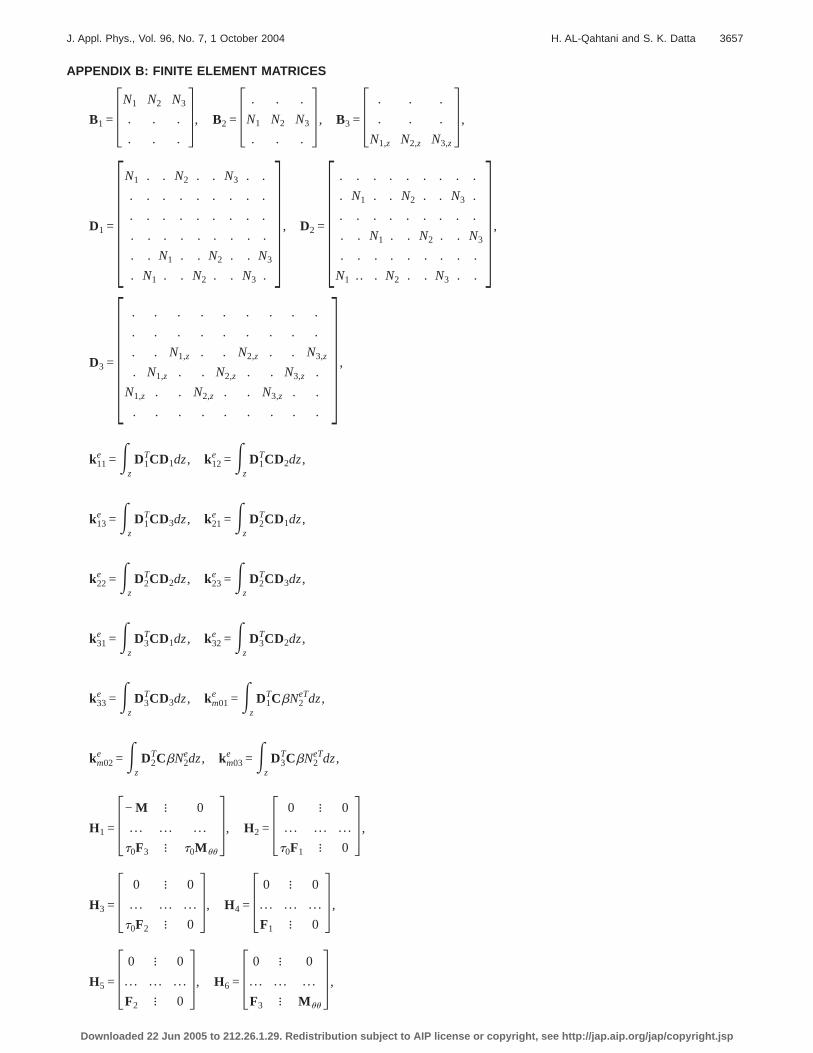
APPENDIX B: FINITE ELEMENT MATRICES

B1 = 3N1 N2 N3

. . .

. . .4, B2 = 3 . . .

N1 N2 N3

. . .4 , B3 = 3 . . .

. . .

N1,z N2,z N3,z4 ,

D1 = 3N1

.

.

.

.

.

.

.

.

.

.

N1

.

.

.

.

N1

.

N2

.

.

.

.

.

.

.

.

.

.

N2

.

.

.

.

N2

.

N3

.

.

.

.

.

.

.

.

.

.

N3

.

.

.

.

N3

.

4 , D2 = 3.

.

.

.

.

N1

.

N1

.

.

.

..

.

.

.

N1

.

.

.

.

.

.

.

N2

.

N2

.

.

.

.

.

.

.

N2

.

.

.

.

.

.

.

N3

.

N3

.

.

.

.

.

.

.

N3

.

.

4 ,

D3 = 3.

.

.

.

N1,z

.

.

.

.

N1,z

.

.

.

.

N1,z

.

.

.

.

.

.

.

N2,z

.

.

.

.

N2,z

.

.

.

.

N2,z

.

.

.

.

.

.

.

N3,z

.

.

.

.

N3,z

.

.

.

.

N3,z

.

.

.

4 ,

k11e =E

z

D1TCD1dz, k12

e =Ez

D1TCD2dz,

k13e =E

z

D1TCD3dz, k21

e =Ez

D2TCD1dz,

k22e =E

z

D2TCD2dz, k23

e =Ez

D2TCD3dz,

k31e =E

z

D3TCD1dz, k32

e =Ez

D3TCD2dz,

k33e =E

z

D3TCD3dz, km01

e =Ez

D1TCbN2

eTdz,

km02e =E

z

D2TCbN2

edz, km03e =E

z

D3TCbN2

eTdz,

H1 = 3− M A 0

. . . . . . . . .

t0F3 A t0M uu

4, H2 = 3 0 A 0

. . . . . . . . .

t0F1 A 04 ,

H3 = 3 0 A 0

. . . . . . . . .

t0F2 A 04, H4 = 3 0 A 0

. . . . . . . . .

F1 A 04 ,

H5 = 3 0 A 0

. . . . . . . . .

F2 A 04, H6 = 3 0 A 0

. . . . . . . . .

F3 A M uu

4 ,



H7 = 3K 11 A 0

. . . . . . . . .

0 A − G114, H8 = 3K 12 + K 21 A 0

. . . . . . . . .

0 A 04 ,

H9 = 3K 22 A 0

. . . . . . . . .

0 A − G224 , H10 = 3K 13 − K 31 A − K mu1

. . . . . . . . .

0 A 04 ,

H11 = 3K 23 − K 32 A − K mu2

. . . . . . . . .

0 A 04 , H12 = 3− K 33 A − K mu3

. . . . . . . . .

0 A G334 .

1J. Nowinski, Theory of thermoelasticity with Applications(Sijthoff &Noordhoff International, Alphen Aan Den Rign, 1978).

2A. N. Abd-alla and A. A. S. Al-dawy, Int. J. Math. Math. Sci.23, 529(2000).

3J. D. Achenbach,Wave Propagation in Elastic Solids(Elsevier, New York,North-Holland, Amsterdam, 1975).

4H. W. Lord and Y. Shulman, J. Mech. Phys. Solids15, 229 (1967).5A. E. Green and K. A. Lindsay, J. Elast.2, 1 (1972).6A. E. Naghdi and K. A. Lindsay, J. Therm. Stresses15, 253 (1992).7R. B. Hetnarski and J. Ignaczk, J. Therm. Stresses22, 451 (1999).8A. H. Nayfeh and S. Nemat-Nasser, Acta Mech.12, 53 (1971).9H. Sinha and S. B. Sinha, Acta Mech.23, 159 (1975).

10Y. Agarwal, J. Elast.8, 171 (1978).11H. H. Sherief and K. A. Helmy, J. Therm. Stresses22, 897 (1999).12A. N. Abd-alla and A. A. S. Al-dawy, J. Therm. Stresses24, 367 (2001).13C. V. Massalas, Acta Mech.65, 51 (1986).14M. Daimaruya and M. Naitoh, J. Sound Vib.117, 511 (1987).15C. V. Massalas and V. K. Kalpakidis, Int. J. Eng. Sci.25, 1207(1987).16J. N. Sharma, D. Singh, and R. Kumar, J. Acoust. Soc. Am.108, 848

(2000).17J. N. Sharma and P. K. Sharma, J. Therm. Stresses25, 169 (2002).18J. C. Cheng and S. Y. Zhang, Appl. Phys. Lett.74, 2087(1999).19Y. C. Fung and P. Tong,Classical and Computational Solid Mechanics

(World Scientific, Singapore, 2001).20V. T. Buchwald, Q. J. Mech. Appl. Math.14, 35 (1961).21R. Vogelgesang, M. Grimsditch, and J. S. Wallace, Appl. Phys. Lett.76,

982 (2000).22G. A. Swift, E. Üstündag, M. A. M. Bourke Bjorn Clausen, and H. -T. Lin,

Appl. Phys. Lett.82, 1039(2003).23M. Kitayama, K. Hirao, M. Toriyama, and S. Kanzaki, J. Am. Ceram. Soc.

82, 3105(1999).24H. Yokota and M. Ibukiyama, J. Am. Ceram. Soc.86, 197 (2003).25M. Chester, Phys. Rev.131, 2013(1963).26J. H. Prevost and D. Tao, J. Appl. Mech.50, 817 (1983).27A. F. Khadrawi, M. A. Al-Nimr, and M. Hammad, Int. J. Thermophys.23,

581 (2002).28M. A. Hawwa and A. H. Nayfeh, J. Appl. Phys.80, 2733(1996).



https://www.researchgate.net/publication/50335309_Wave_Propagation_In_Elastic_Solids?el=1_x_8&enrichId=rgreq-9599496f77f387f33cd2bbc9442e0d45-XXX&enrichSource=Y292ZXJQYWdlOzIyNDQ5MjE5MTtBUzoxMTg5MTYyMTQ5NTYwMzRAMTQwNTM2MzI0Mzk3MQ==

https://www.researchgate.net/publication/50335309_Wave_Propagation_In_Elastic_Solids?el=1_x_8&enrichId=rgreq-9599496f77f387f33cd2bbc9442e0d45-XXX&enrichSource=Y292ZXJQYWdlOzIyNDQ5MjE5MTtBUzoxMTg5MTYyMTQ5NTYwMzRAMTQwNTM2MzI0Mzk3MQ==

Thermoelastic waves in an anisotropic infinite plate

Documents

Transcript of Thermoelastic waves in an anisotropic infinite plate