ARTICLE IN PRESS

Journal of the Mechanics and Physics of Solids

55 (2007) 1889–1921

0022-5096/$ -

doi:10.1016/j

�CorrespoE-mail ad

www.elsevier.com/locate/jmps

Size-dependent effective thermoelastic properties ofnanocomposites with spherically anisotropic phases

H. Le Quang, Q.-C. He�

Laboratoire de Mecanique (LaM), Universite de Marne-la-Vallee, 5 Boulevard Descartes,

77454 Marne-la-Vallee Cedex 2, France

Received 21 November 2006; received in revised form 30 January 2007; accepted 10 February 2007

Abstract

Composites made of semi-crystalline polymers and nanoparticles have a spherulitic microstructure

which can be reasonably represented by a spherically anisotropic volume element. Due to the high

surface-to-volume ratio of a nanoparticle, the particle–matrix interface stress, usually neglected in

determining the effective elastic moduli of particle-reinforced composites, may have a non-negligible

effect. To account for the latter in estimating the effective thermoelastic properties of a composite

consisting of nanoparticles embedded in a semi-crystalline polymeric matrix, this work adopts a

coherent interface model for the nanoparticle–matrix interface and proposes an extended version of

the classical generalized-self consistent method. In particular, Eshelby’s formulae widely used to

calculate the elastic energy change of a homogeneous medium due to the introduction of an

inhomogeneity are extended to the thermoelastic case. The nanoparticle size effect on the effective

thermoelastic moduli of the composite are theoretically shown and numerically illustrated.

r 2007 Elsevier Ltd. All rights reserved.

Keywords: A. Voids and inclusions; B. Anisotropic material; B. Particulate reinforced material; B. Polymeric

material; Spherical anisotropy

1. Introduction

Nanocomposites of semi-crystalline polymers are recently a subject of intenseinvestigations (see, e.g., Kim et al., 2001; Liu et al., 2003; Nowacki et al., 2004; Causin

see front matter r 2007 Elsevier Ltd. All rights reserved.

.jmps.2007.02.005

nding author. Tel.: +33160 957 786; fax: +33 160 957 799.

dress: he@univ-mlv.fr (Q.-C. He).

ARTICLE IN PRESSH.L. Quang, Q.-C. He / J. Mech. Phys. Solids 55 (2007) 1889–19211890

et al., 2006; Hadal et al., 2006). Semi-crystalline polymers, such as polyethylene andpolypropylene, consist of spherulites which are formed of crystalline and amorphousregions arranged approximately in a spherically symmetric way (Bassett, 1981).Nanocomposites have been obtained by using semi-crystalline polymers as the matrixand nano-sized particles as the reinforcement. These composites often exhibit improvedmechanical and physical properties compared to the conventional composites reinforcedwith micron-sized particles. In particular, clay is a preferred reinforcement mineral tosynthesize nanocomposite because clay enhances mechanical and thermal properties, fireresistance and barrier characteristics of semi-crystalline polymers without significantlyincreasing the mass density nor altering the optical behavior. A nanocomposite made of asemi-crystalline polymer reinforced by nanoparticles has a microstructure which can beapproximately represented by a spherically anisotropic volume element.The problem of estimating the effective thermoelastic properties and conductivity of

composites with spherically anisotropic microstructures was studied by Dryden (1988), Chen(1993), He and Cheng (1996), Milton (2002), and He and Benveniste (2004). In these studies,only the micron-sized particles were considered so that the effect of the matrix–particleinterface energy (or stress) on the effective behavior of composites is small enough to benegligible. However, when nano-sized particles are involved as in the aforementioned semi-crystalline polymer nanocomposites, the matrix-particle interface energy can no longer beneglected in determining the effective moduli, because the interface-to-volume ratio is veryhigh in a representative volume element of a composite with nanoparticles. This fact hasbeen emphasized and exploited in recent investigations on nanomaterials and nano-sizedstructural elements (see, e.g., Miller and Shenoy, 2000; Sharma and Dasgupta, 2002;Dingreville et al., 2005; Duan et al., 2005a, b; Chen et al., 2007; Duan and Karihaloo, 2007).The objective of the present work is to estimate the effective thermoelastic properties ofnanocomposites with spherically anisotropic microstructures, a semi-crystalline polymerreinforced with clay nanoparticles being taken as prototype.To achieve our objective, a generalized-self consistent method is proposed in this work,

extending the classical generalized-self consistent model (GSCM) of Kerner (1956), Vander Poel (1958), Smith (1974, 1975), Christensen and Lo (1979) (see also Christensen, 1990)in the following three directions:

�

First, GSCM is broadened to thermoelasticity. In doing so, the energy self-consistencycondition is formulated in the thermoelastic context by deriving an equationgeneralizing a formula of Eshelby (1956) largely invoked to calculate the elastic energychange of a homogeneous medium due to the introduction of an inhomogeneity. � Second, the extended thermoelastic version of GSCM is implemented for phases of

spherically transverse isotropy. This implementation hinges upon the solution of anauxiliary elastic problem in which a hollow sphere consisting of an elastic material ofspherically transverse isotropy is subjected to uniform isotropic or simple shear loadingon its inner and outer surfaces. When isotropic surface loading is concerned, thecomplete solution to this auxiliary problem is available (Dryden, 1988; Chen, 1993; Heand Benveniste, 2004). However, when simple shear surface loading is considered, theexisting solution given by Dryden (1988) and Chen (1993) to the auxiliary problem is inour opinion incomplete, since the positive definiteness of the elastic stiffness tensor hasnot fully been used to deal with the relevant fourth-order polynomial characteristicequation (31). The last point is remedied in the present work.

ARTICLE IN PRESSH.L. Quang, Q.-C. He / J. Mech. Phys. Solids 55 (2007) 1889–1921 1891

�

Third, to account for the nanoparticle–matrix interface energy effect, a coherentinterface model (Shuttleworth, 1950; Povstenko, 1993; Bottomley and Ogino, 2001) isadopted in the extended thermoelastic version of GSCM.

All the effective thermoelastic moduli of an isotropic nanocomposite with a sphericallyanisotropic microstructure are thus estimated in an explicit analytical way. As expected,the nanoparticles have non-negligible size-dependent effects on the effective thermoelasticmoduli. Apart from their theoretical value, the method elaborated and the results obtainedin this work are believed to be directly useful for estimating the effective properties of semi-crystalline polymers reinforced by nanoparticles.

The paper is organized as follows. In Section 2, the phase transversely isotropicthermoelastic laws, the coherent interface model and the effective isotropic thermoelasticrelations are specified. In Section 3, GSCM is formulated in the thermoelastic context withthe help of an equation derived in Appendix A and generalizing a relevant Eshelby’s one.Section 4 is dedicated to obtaining a closed-form estimation for the effective elastic shearmodulus. In completely and rigorously solving the elastic problem of a hollow sphereundergoing axisymmetric loading on its inner and outer surfaces, several inequalities areestablished by exploiting the positive definiteness of the elastic stiffness tensor. In Section5, all the remaining effective thermoelastic moduli are determined by consideringappropriate isotropic boundary conditions and by invoking an elastic solution given inHe and Benveniste (2004). The interface and nanoparticle size effects on the effectivemoduli are discussed and numerically illustrated in Section 6.

2. Setting of the problem

The composite under consideration consists of a matrix reinforced by nanoparticles. Letðx; y; zÞ be a Cartesian coordinate system associated with an orthonormal basis fex; ey; ezg.For later use, it is convenient to introduce the system of spherical coordinates ðr; y;jÞ with

r ¼ffiffiffiffiffiffiffiffiffiffiffiffiffiffiffiffiffiffiffiffiffiffiffiffiffix2 þ y2 þ z2

p; tan y ¼

ffiffiffiffiffiffiffiffiffiffiffiffiffiffiffix2 þ y2

p=z; tanj ¼ y=x (1)

and the corresponding spherical orthonormal basis fer; ey; ejg:

er ¼ sin yðcosjex þ sinjeyÞ þ cos yez,

ey ¼ cos yðcosjex þ sinjeyÞ � sin yez,

ej ¼ � sinjex þ cosjey. ð2Þ

The matrix and particle phases are assumed to be linearly thermoelastic, sphericallyanisotropic. Precisely, relative to the spherical orthonormal basis fer; ey; ejg thethermoelastic law of the particles or that of the matrix takes the following form

sij ¼ Lijpq�pq þ sijW; �z ¼ sij�ij � c�W, (3)

where sij and �ij , respectively, stand for the matrix components of the Cauchy stress andinfinitesimal strain tensors in the spherical coordinate system; z and W are, respectively, theentropy increase and the temperature change from a stress-free state where the temperatureis uniform and equal to T0; Lijpq are the components of the fourth-order elastic stiffnesstensor L, sij are the components of the second-order thermal stress tensor s, and c� is thespecific heat at constant strain. Due to the hypothesis that the particles and matrix are

ARTICLE IN PRESSH.L. Quang, Q.-C. He / J. Mech. Phys. Solids 55 (2007) 1889–19211892

spherically anisotropic, all the material parameters Lijpq, sij and c� are independent of thespherical coordinates ðr; y;jÞ. In other words, the particles and matrix are sphericallyhomogeneous but heterogeneous with respect to the Cartesian coordinates ðx; y; zÞ. Asusual, Lijpq and sij have the symmetries:

Lijpq ¼ Ljipq ¼ Lpqij ; sij ¼ sji. (4)

In this work, we assume that the particles and matrix are spherically transversely isotropic.More precisely, in the spherical coordinate system, using the two-to-one subscriptidentification rr � 1, yy � 2, jj � 3, yj � 4, jr � 5 and ry � 6, the thermoelastic law (3)takes the following matrix form:

srr

syysjjffiffiffi2p

syjffiffiffi2p

sjrffiffiffi2p

sry

26666666664

37777777775¼

L11 L12 L12 0 0 0

L12 L22 L23 0 0 0

L12 L23 L22 0 0 0

0 0 0 L22 � L23 0 0

0 0 0 0 2L55 0

0 0 0 0 0 2L55

26666666664

37777777775

�rr

�yy

�jjffiffiffi2p

�yjffiffiffi2p

�jrffiffiffi2p

�ry

26666666664

37777777775þ

s1

s2

s2

0

0

0

2666666664

3777777775W, (5)

�z ¼ s1�rr þ s2�yy þ s2�jj � c�W. (6)

The stiffness tensor L is required to be positive definite. This requirement is satisfied if andonly if

L1140; L5540; L22 � L2340,

L11L22 � L21240; ðL22 þ L23ÞL11 � 2L2

1240. ð7Þ

Concerning the interface between the nanoparticles and the matrix, we use the coherentinterface model first proposed by Shuttleworth (1950) and then extended by Gurtin andMurdoch (1975) and Cahn (1980). According to this model, the interface between ananoparticle and the matrix is an oriented material surface G across which thedisplacement vector field and the tangential part of the strain tensor field are continuous.In addition, the surface G is considered as a two-dimensional deformable body in a three-dimensional Euclidean space. More specifically, the strain and stress states of every pointof G are characterized by the surface infinitesimal strain tensor es and the surface Cauchystress tensor rs. The material behavior of G is taken to be linearly thermoelastic, so that thetwo-dimensional thermoelastic laws for G read (see, e.g., Murdoch, 1976, 2005; Bottomleyand Ogino, 2001; Duan and Karihaloo, 2007):

rs ¼ Lses þ ssW, (8)

�zs¼ ss : es � cs

�W, (9)

where Ls is the two-dimensional fourth-order elastic stiffness tensor of G; ss the second-order thermal stress tensor of G whose importance to the effective thermoelastic propertiesof nanomaterials has been underlined in Pathak and Shenoy (2005) and Duan andKarihaloo (2007), zs the entropy increase of G, and cs

� the specific heat of G at constantstrain. Recently, Bouby et al. (2007) have derived a general imperfect curved thermoelasticinterface model by applying asymptotic analysis to a thin thermoelastic interphase between

ARTICLE IN PRESSH.L. Quang, Q.-C. He / J. Mech. Phys. Solids 55 (2007) 1889–1921 1893

two thermoelastic media. This model includes (8) and (9) as a particular case where theinterphase is much stiffer than the media.

In what follows, we are concerned with spherical nanoparticles. Thus, the interface G is aspherical surface whose unit normal vector corresponds to er and whose tangential plane isspanned by the tangential hoop vectors ey and ej. Assuming the interface G to bespherically transversely isotropic, the thermoelastic interface constitutive laws (8) and (9)can be written in the matrix forms:

ssyy

ssjj

ssyj

264

375 ¼

ks þ ms ks � ms 0

ks � ms ks þ ms 0

0 0 2ms

264

375

�syy

�sjj

�syj

264

375þ

ss

ss

0

264

375W, (10)

�zs¼ ssð�

syy þ �

sjjÞ � cs

�W, (11)

where ks, ms and ss designate the area, shear moduli and thermal stress of the sphericalinterface G. Finally, the equilibrium of the interface G gives rise to the generalizedYoung–Laplace equations (see, e.g., Povstenko, 1993):

½½srr��er þ ½½sry��ey þ ½½srj��ej ¼ �rs � rs, (12)

where ½½��� represents the jump of a quantity � across the interface G and rs � rs stands for

the surface divergence of the surface stress tensor rs. In the case where G is a sphericalsurface, rs � r

s has the following explicit expression (see, e.g., Duan et al., 2005a):

rs � rs ¼ �

ðssyy þ ss

jjÞer

rþ

ey

r

qssyy

qyþ

1

sin y

qssyj

qjþ ðss

yy � ssjjÞ cot y

� �

þej

r

qssyj

qyþ

1

sin y

qssjj

qjþ 2ss

yj cot y� �

. ð13Þ

Note that, in the coherent interface model, the traction vector across G is not continuousand its jump is governed by the equilibrium equations (12).

At the macroscopic scale, the composite under consideration is assumed to bestatistically isotropic. The corresponding effective thermoelastic behavior is characterizedby

r ¼ L�eþ s�W; L� ¼ k�I� Iþ 2m�ðI� 13I� IÞ, (14)

�z ¼ s� : e� c��W; s� ¼ s�I. (15)

Here, I is the second-order identity tensor; I is the fourth-tensor identity tensor on thespace Sym of second-order symmetric tensors; overbar denotes the volume average over arepresentative volume element; L� is the effective stiffness tensor; k� and m� are the effectivebulk and shear moduli; s� denotes the effective thermal stress; c�� is the effective heat atconstant strain.

3. Description of the model

In order to determine the effective thermoelastic properties of the isotropic compositematerial under consideration, a generalized self-consistent model is now proposed. Thismodel is an extension to spherically anisotropic thermoelastic phases with interface stress

ARTICLE IN PRESSH.L. Quang, Q.-C. He / J. Mech. Phys. Solids 55 (2007) 1889–19211894

of the classical GSCM which was initiated by Kerner (1956) Van der Poel (1958), improvedby Smith (1974, 1975) and completed by Christensen and Lo (1979).We first consider an infinite body O made of the effective homogeneous medium whose

thermoelastic behavior is characterized by Eqs. (14) and (15). Let O now be subjected tothe following uniform thermoelastic boundary conditions in the Cartesian coordinatesystem ðx; y; zÞ:

uðxÞ ¼ e0x; WðxÞ ¼ W0, (16)

where x belongs to the boundary qO of O, e0 is a constant macroscopic strain tensor and W0is a constant temperature. Within the framework of uncoupled thermoelasticity and in thesteady state, the foregoing thermomechanical loading give rises to the followingdisplacement, temperature, strain and stress in O:

uðxÞ ¼ e0x; WðxÞ ¼ W0,

eðxÞ ¼ e0; rðxÞ ¼ r0 ¼ L�e0 þ s�W0. ð17Þ

Under the condition (16), the free energy of O is given by

U0ðe0Þ ¼ 1

2volðOÞ½e0 : L�e0 þ 2s� : e0W0 � c��W

20�. (18)

Next, we cut a sphere out of the foregoing infinite effective medium and substitute back acomposite sphere o while imposing the same boundary condition on qO as before. Theinterface between the composite sphere and outside medium is assumed perfectly bonded.The core of this composite sphere is made of the inclusion phase, referred to as phase 1 andsurrounded by a concentric shell consisting of the matrix phase, denoted by phase 2(Fig. 1). The core and outer coating consist of two spherically anisotropic materials whosethermoelastic behavior are characterized by Eqs. (5) and (6) relative to a sphericalcoordinates system ðr; y;jÞ. The radii of the core and coating, symbolized by r1 and r2, arechosen so as to be compatible with the prescribed phase volume fraction:

c1 ¼ 1� c2 ¼r31r32. (19)

Fig. 1. GSCM with spherically anisotropic thermoelastic constituents.

ARTICLE IN PRESSH.L. Quang, Q.-C. He / J. Mech. Phys. Solids 55 (2007) 1889–1921 1895

The spherical interface G between the matrix and inclusion is formulated by the coherentsurface model as described in Section 2.

Due to the presence of the composite sphere in the effective medium, the initiallyuniform strain and stress fields of the latter are disturbed. Under the conditions (16), it isshown in Appendix A that the free energy Uðe0Þ of O after inserting the composite sphere ois given by the following formula:

U ¼ U0 þ1

2

Zqoðt � u0 � t0 � uÞdS þ

1

2

Zoðs : eW0 � c�W

20ÞdV

þ1

2

ZGðss : esW0 � cs

�W20ÞdS þ

1

2ðc��W

20 � s� : e0W0ÞvolðoÞ. ð20Þ

Here, qo denotes the surface of o; u0 and t0 are the initial traction and displacementvectors on qo; u and t are the traction and displacement vectors on qo when the compositesphere has been introduced; eðxÞ and sðxÞ are the strain field and thermal stress tensor inthe composite sphere, respectively; es and ss are the interface strain and thermal stressfields.

Alternatively, if the uniform thermoelastic boundary conditions

tðxÞ ¼ t0; WðxÞ ¼ W0 (21)

are imposed instead of (16), it can be shown that

U ¼ U0 �1

2

Zqoðt � u0 � t0 � uÞdS �

1

2

Zoðs : eW0 � c�W

20ÞdV

�1

2

ZGðss : esW0 � cs

�W20ÞdS �

1

2ðc��W

20 � s� : e0W0ÞvolðoÞ. ð22Þ

This formula is different from (20) only in that the terms following U0 in the right-handside have the negative sign. Compared with the classical formulas of Eshelby (1956), Eqs.(20) and (22) can be viewed as a thermoelastic extension. As in the GSCM of Christensenand Lo (1979), the effective thermoelastic properties of the effective medium are requiredto be such that the presence of the composite sphere does not change the initial free energy.Thus, the self-consistency condition readsZ

qoðt � u0 � t0 � uÞdS þ

Zoðs : eW0 � c�W

20ÞdV þ

ZGðss : esW0 � cs

�W20ÞdS

þ ðc��W20 � s� : e0W0ÞvolðoÞ ¼ 0. ð23Þ

Note that when W0 ¼ 0, the self-consistency condition (23) reduces to that of Christensenand Lo (1979).

4. Axisymmetric elastic loading

To evaluate the effective shear modulus m�, the infinite medium O is now subjected to thefollowing uniform axisymmetric strain boundary condition:

uðxÞ ¼ �g0xex � g0yey þ 2g0zez, (24)

ARTICLE IN PRESSH.L. Quang, Q.-C. He / J. Mech. Phys. Solids 55 (2007) 1889–19211896

where x 2 qO and g0 is a constant strain. In the corresponding spherical coordinate system,Eq. (24) takes the equivalent form:

urðr; y;jÞ ¼ g0rð3 cos2 y� 1Þ,

uyðr; y;jÞ ¼ �3g0r sin y cos y,

ujðr; y;jÞ ¼ 0. ð25Þ

Under the boundary condition (25), we conjecture that the displacement solution to theproblem previously formulated would have the form:

uðiÞr ðxÞ ¼ f ðiÞðrÞð3 cos2 y� 1Þ,

uðiÞy ðxÞ ¼ �3gðiÞðrÞ sin y cos y,

uðiÞj ðxÞ ¼ 0, ð26Þ

where f ðiÞ and gðiÞ are two scalar functions of r and the superscript i ð¼ 1; 2; eÞ refers to thecore inclusion, coating matrix and the external effective medium, respectively. Thecorresponding spherical non-zero strain components are give by

�ðiÞrr ¼df ðiÞ

drð3 cos2 y� 1Þ; �ðiÞyy ¼

1

rðf ðiÞ � 2gðiÞÞð3 cos2 y� 1Þ þ

gðiÞ

r,

�ðiÞjj ¼1

rðf ðiÞ � gðiÞÞð3 cos2 y� 1Þ �

gðiÞ

r,

�ðiÞry ¼ 3gðiÞ

2r�

f ðiÞ

r�

dgðiÞ

2dr

!sin y cos y. ð27Þ

Next, using the stress–strain relation (5) with W ¼ W0 ¼ 0, the non-zero stress componentshave the expressions

sðiÞrr ¼ LðiÞ11

df ðiÞ

drþ

LðiÞ12

rð2f ðiÞ � 3gðiÞÞ

" #ð3 cos2 y� 1Þ,

sðiÞyy ¼ LðiÞ12

df ðiÞ

drþ ðL

ðiÞ22 þ L

ðiÞ23Þ

f ðiÞ

r� ð2L

ðiÞ22 þ L

ðiÞ23Þ

gðiÞ

r

" #ð3 cos2 y� 1Þ þ ðL

ðiÞ22 � L

ðiÞ23Þ

gðiÞ

r,

sðiÞjj ¼ LðiÞ12

df ðiÞ

drþ ðL

ðiÞ22 þ L

ðiÞ23Þ

f ðiÞ

r� ðL

ðiÞ22 þ 2L

ðiÞ23Þ

gðiÞ

r

" #ð3 cos2 y� 1Þ þ ðL

ðiÞ23 � L

ðiÞ22Þ

gðiÞ

r,

sðiÞry ¼ �3LðiÞ55

rrdgðiÞ

drþ 2f ðiÞ � gðiÞ

� �sin y cos y. ð28Þ

Inserting these expressions into the equilibrium equations and after direct but quitecumbersome manipulations, it turns out that the variable y can be eliminated and that thedifferential equations governing the scalar functions f ðiÞ and gðiÞ take the following form:

r2d2f ðiÞ

dr2þ 2r

df ðiÞ

drþ BðiÞ1 r

dgðiÞ

drþ RðiÞ1 f ðiÞ þ$

ðiÞ1 gðiÞ ¼ 0,

r2d2gðiÞ

dr2þ 2r

dgðiÞ

drþ BðiÞ2 r

df ðiÞ

drþ RðiÞ2 gðiÞ þ$ðiÞ2 f ðiÞ ¼ 0. ð29Þ

ARTICLE IN PRESSH.L. Quang, Q.-C. He / J. Mech. Phys. Solids 55 (2007) 1889–1921 1897

The dimensionless material parameters entering these equations are defined by

BðiÞ1 ¼ �3ðLðiÞ12 þ L

ðiÞ55Þ

LðiÞ11

; BðiÞ2 ¼2ðLðiÞ12 þ L

ðiÞ55Þ

LðiÞ55

,

RðiÞ1 ¼2ðLðiÞ12 � 3L

ðiÞ55 � L

ðiÞ22 � L

ðiÞ23Þ

LðiÞ11

; RðiÞ2 ¼�ðL

ðiÞ55 þ 5L

ðiÞ22 þ L

ðiÞ23Þ

LðiÞ55

,

$ðiÞ1 ¼3ðLðiÞ55 þ L

ðiÞ22 þ L

ðiÞ23 � L

ðiÞ12Þ

LðiÞ11

; $ðiÞ2 ¼2ð2L

ðiÞ55 þ L

ðiÞ22 þ L

ðiÞ23Þ

LðiÞ55

. ð30Þ

It can be shown that only four of the six parameters in Eq. (30) are independent. Thesolution to the differential equations (29) depends on the roots of the characteristicequation

r4 þ 2r3 þ pðiÞr2 þ ðpðiÞ � 1Þr2 þ qðiÞ ¼ 0. (31)

Above, pðiÞ and qðiÞ are related to the material dimensionless constants defined by Eq. (30)as follows

pðiÞ ¼ 1þ RðiÞ1 þ RðiÞ2 � BðiÞ1 BðiÞ2 ; qðiÞ ¼ RðiÞ1 RðiÞ2 �$ðiÞ1 $

ðiÞ2 . (32)

In the general case, the roots of Eq. (31) are provided by the following expressions:

rðiÞ1 ¼ �12½1þ

ffiffiffiffiffiffiffiffiffiffiffiffiffiffiffiffiffiffiffiffiffiffiffiffiffiffiffiffiffiffiffiffiffiffiffiffiffiffiffiffiffiffiffiffiffiffiffiffiffiffiffiffiffiffiffiffiffiffiffiffiffiffiffiffi3� 2pðiÞ þ 2

ffiffiffiffiffiffiffiffiffiffiffiffiffiffiffiffiffiffiffiffiffiffiffiffiffiffiffiffiffiffiffiffiffiffiðpðiÞ � 1Þ2 � 4qðiÞ

qr�,

rðiÞ2 ¼ �12½1þ

ffiffiffiffiffiffiffiffiffiffiffiffiffiffiffiffiffiffiffiffiffiffiffiffiffiffiffiffiffiffiffiffiffiffiffiffiffiffiffiffiffiffiffiffiffiffiffiffiffiffiffiffiffiffiffiffiffiffiffiffiffiffiffiffi3� 2pðiÞ � 2

ffiffiffiffiffiffiffiffiffiffiffiffiffiffiffiffiffiffiffiffiffiffiffiffiffiffiffiffiffiffiffiffiffiffiðpðiÞ � 1Þ2 � 4qðiÞ

qr�,

rðiÞ3 ¼ �12½1�

ffiffiffiffiffiffiffiffiffiffiffiffiffiffiffiffiffiffiffiffiffiffiffiffiffiffiffiffiffiffiffiffiffiffiffiffiffiffiffiffiffiffiffiffiffiffiffiffiffiffiffiffiffiffiffiffiffiffiffiffiffiffiffiffi3� 2pðiÞ � 2

ffiffiffiffiffiffiffiffiffiffiffiffiffiffiffiffiffiffiffiffiffiffiffiffiffiffiffiffiffiffiffiffiffiffiðpðiÞ � 1Þ2 � 4qðiÞ

qr�,

rðiÞ4 ¼ �12½1�

ffiffiffiffiffiffiffiffiffiffiffiffiffiffiffiffiffiffiffiffiffiffiffiffiffiffiffiffiffiffiffiffiffiffiffiffiffiffiffiffiffiffiffiffiffiffiffiffiffiffiffiffiffiffiffiffiffiffiffiffiffiffiffiffi3� 2pðiÞ þ 2

ffiffiffiffiffiffiffiffiffiffiffiffiffiffiffiffiffiffiffiffiffiffiffiffiffiffiffiffiffiffiffiffiffiffiðpðiÞ � 1Þ2 � 4qðiÞ

qr�. ð33Þ

Three cases have to be distinguished according to the value of the discriminantðpðiÞ � 1Þ2 � 4qðiÞ. For each of the three cases, the solution to Eq. (29) can be finallywritten as

f ðiÞðrÞ ¼ AðiÞ1 fðiÞ1 þ A

ðiÞ2 fðiÞ2 þ A

ðiÞ3 fðiÞ3 þ A

ðiÞ4 fðiÞ4 ,

gðiÞðrÞ ¼ BðiÞ1 fðiÞ1 þ B

ðiÞ2 fðiÞ2 þ B

ðiÞ3 fðiÞ3 þ B

ðiÞ4 fðiÞ4 , ð34Þ

where fðiÞj ðj ¼ 1; 2; 3; 4Þ is function of r and the constants AðiÞj and B

ðiÞj are related by

AðiÞ1 ¼ dðiÞ1 B

ðiÞ1 þ iðiÞ1 B

ðiÞ2 ; A

ðiÞ2 ¼ dðiÞ2 B

ðiÞ2 þ iðiÞ2 B

ðiÞ1 ,

AðiÞ3 ¼ dðiÞ3 B

ðiÞ3 þ iðiÞ3 B

ðiÞ4 ; A

ðiÞ4 ¼ dðiÞ4 B

ðiÞ4 þ iðiÞ4 B

ðiÞ3 . ð35Þ

In these equations, the way in which the constants dðiÞj and iðiÞj depend on the materialparameters varies according as the case is considered. Furthermore, it is shown in

ARTICLE IN PRESSH.L. Quang, Q.-C. He / J. Mech. Phys. Solids 55 (2007) 1889–19211898

Appendix B that the positive definiteness of the elastic stiffness tensor LðiÞ implies that

5=44pðiÞ � 4qðiÞ, ð36Þ

ðpðiÞ � 1Þ2 � 4qðiÞo0 whenever pðiÞ41, ð37Þ

45=44pðiÞ4�1; 14qðiÞ4�1. ð38Þ

With the help of these inequalities which have not been established in the previous relevantworks (Dryden, 1988; Chen, 1993), the three cases in question can be characterized andtreated as follows.

Case 1: This case is characterized by

ðpðiÞ � 1Þ2 � 4qðiÞ40. (39)

Under this condition, it follows that all the four roots given by Eq. (33) are real anddistinct. Moreover, note that: (i) rðiÞ1 and rðiÞ2 are negative; (ii) rðiÞ3 is positive or negativeaccording as qðiÞ is positive or negative; (iii) rðiÞ4 is positive. Thus, the associatedcharacteristic functions take the following form:

fðiÞj ¼ rrðiÞj . (40)

The constants dðiÞj and iðiÞj are given by

iðiÞ1 ¼ iðiÞ2 ¼ iðiÞ3 ¼ iðiÞ4 ¼ 0,

dðiÞj ¼3½ðL

ðiÞ12 þ L

ðiÞ55Þr

ðiÞj þ L

ðiÞ12 � L

ðiÞ22 � L

ðiÞ23 � L

ðiÞ55�

LðiÞ11½ðr

ðiÞj Þ

2þ rðiÞj � þ 2ðL

ðiÞ12 � L

ðiÞ22 � L

ðiÞ23 � 3L

ðiÞ55Þ

. ð41Þ

In the special case where phase i is isotropic, then pðiÞ ¼ �13 and qðiÞ ¼ 24. Correspond-ingly, rðiÞ1 ¼ �4, r

ðiÞ2 ¼ �2, r

ðiÞ3 ¼ 1 and rðiÞ4 ¼ 3. The expressions for dðiÞj reduce to

dðiÞ1 ¼ �3

2; dðiÞ2 ¼

3ðki þ miÞ

2mi

; dðiÞ3 ¼ 1; dðiÞ4 ¼9ki � 6mi

15ki þ 11mi

. (42)

Case 2: This case is defined by the condition

ðpðiÞ � 1Þ2 � 4qðiÞ ¼ 0. (43)

Consequently, Eq. (31) has two identical real positive roots and two identical real negativeroots:

rðiÞ1 ¼ rðiÞ2 ¼ �12½1þ

ffiffiffiffiffiffiffiffiffiffiffiffiffiffiffiffiffi3� 2pðiÞ

p� ¼ lio0,

rðiÞ3 ¼ rðiÞ4 ¼ �12½1�

ffiffiffiffiffiffiffiffiffiffiffiffiffiffiffiffiffi3� 2pðiÞ

p� ¼ ui40. ð44Þ

The corresponding characteristic functions are given by

fðiÞ1 ¼ r�li ; fðiÞ2 ¼ r�li ln r; fðiÞ3 ¼ rui ; fðiÞ4 ¼ rui ln r. (45)

ARTICLE IN PRESSH.L. Quang, Q.-C. He / J. Mech. Phys. Solids 55 (2007) 1889–1921 1899

The constants dðiÞi and iðiÞi have the expressions

dðiÞj ¼3½ðL

ðiÞ12 þ L

ðiÞ55Þr

ðiÞj þ L

ðiÞ12 � L

ðiÞ22 � L

ðiÞ23 � L

ðiÞ55�

LðiÞ11½ðr

ðiÞj Þ

2þ rðiÞj � þ 2ðL

ðiÞ12 � L

ðiÞ22 � L

ðiÞ23 � 3L

ðiÞ55Þ; j ¼ 1; 2; 3; 4,

iðiÞj ¼3ðLðiÞ12 þ L

ðiÞ55Þ � djþ1ð2r

ðiÞj þ 1ÞL

ðiÞ11

LðiÞ11½ðr

ðiÞj Þ

2þ rðiÞj � þ 2ðL

ðiÞ12 � L

ðiÞ22 � L

ðiÞ23 � 3L

ðiÞ55Þ; j ¼ 1; 3,

iðiÞ2 ¼ iðiÞ4 ¼ 0. ð46Þ

Case 3: This case corresponds to the condition

ðpðiÞ � 1Þ2 � 4qðiÞo0. (47)

Then it follows from Eq. (33) that Eq. (31) has two pairs of complex conjugate roots:

rðiÞ1 ¼ �li � 1� ui

ffiffiffiffiffiffiffi�1p

; rðiÞ2 ¼ �li � 1þ ui

ffiffiffiffiffiffiffi�1p

,

rðiÞ3 ¼ li � ui

ffiffiffiffiffiffiffi�1p

; rðiÞ4 ¼ li þ ui

ffiffiffiffiffiffiffi�1p

, ð48Þ

where ui and li are defined by

li ¼ �12þ 1

2

ffiffiffiffiffiffiffiffiffiffiffiffiffiffiffiffiffiffiffiffiffiffiffiffiffiffiffiffiffiffiffiffiffiffiffiffiffiffiffiffiffiffiffiffiffiffiffiffiffiffiffiffiffiffiffiffiffiffiffiffiffiffiffiffiffiffiffiffiffiffiffiffiffiffiffiffiffiffiffiffi4qðiÞ � pðiÞ þ 5

4

qþ 3

2� pðiÞ

r; ui ¼

12

ffiffiffiffiffiffiffiffiffiffiffiffiffiffiffiffiffiffiffiffiffiffiffiffiffiffiffiffiffiffiffiffiffiffiffiffiffiffiffiffiffiffiffiffiffiffiffiffiffiffiffiffiffiffiffiffiffiffiffiffiffiffiffiffiffiffiffiffiffiffiffiffiffiffiffiffiffiffiffiffi4qðiÞ � pðiÞ þ 5

4

qþ pðiÞ � 3

2

r.

Consequently, the characteristic functions are given by

fðiÞ1 ¼ r�li�1 cosðui ln rÞ; fðiÞ2 ¼ r�li�1 sinðui ln rÞ,

fðiÞ3 ¼ rli cosðui ln rÞ; fðiÞ4 ¼ rli sinðui ln rÞ. ð49Þ

Note that �li � 1 in these expressions is negative while li is positive or negative accordingas ð4qðiÞ þ 1Þ � ðpðiÞÞ2 is positive or negative. The constants dðiÞi and iðiÞi in this case arespecified by

dðiÞ1 ¼aðiÞeðiÞ � bðiÞd ðiÞ

ðaðiÞÞ2 þ ðbðiÞÞ2; iðiÞ1 ¼

aðiÞd ðiÞ þ bðiÞeðiÞ

ðaðiÞÞ2 þ ðbðiÞÞ2; dðiÞ2 ¼

�bðiÞeðiÞ � aðiÞd ðiÞ

ðaðiÞÞ2 þ ðbðiÞÞ2,

dðiÞ3 ¼aðiÞcðiÞ þ bðiÞd ðiÞ

ðaðiÞÞ2 þ ðbðiÞÞ2; iðiÞ3 ¼

aðiÞd ðiÞ � bðiÞcðiÞ

ðaðiÞÞ2 þ ðbðiÞÞ2; dðiÞ4 ¼

bðiÞcðiÞ � aðiÞdðiÞ

ðaðiÞÞ2 þ ðbðiÞÞ2,

iðiÞ2 ¼aðiÞeðiÞ � bðiÞdðiÞ

ðaðiÞÞ2 þ ðbðiÞÞ2; iðiÞ4 ¼

aðiÞcðiÞ þ bðiÞd ðiÞ

ðaðiÞÞ2 þ ðbðiÞÞ2, ð50Þ

with

aðiÞ ¼ LðiÞ11ðl

2i þ li � u2i Þ þ 2ðL

ðiÞ12 � L

ðiÞ22 � L

ðiÞ23 � 3L

ðiÞ55Þ,

bðiÞ ¼ LðiÞ11ð2li þ 1Þui; dðiÞ ¼ 3ðL

ðiÞ12 þ L

ðiÞ55Þui,

cðiÞ ¼ 3½ðLðiÞ12 þ L

ðiÞ55Þli þ ðL

ðiÞ12 � L

ðiÞ22 � L

ðiÞ23 � L

ðiÞ55Þ�,

eðiÞ ¼ �3½ðLðiÞ12 þ L

ðiÞ55Þðli þ 1Þ � ðL

ðiÞ12 � L

ðiÞ22 � L

ðiÞ23 � L

ðiÞ55Þ�. ð51Þ

ARTICLE IN PRESSH.L. Quang, Q.-C. He / J. Mech. Phys. Solids 55 (2007) 1889–19211900

Concerning the outside medium which is homogeneous and isotropic, the expressions forf ðeÞ and gðeÞ are simply

f ðeÞ ¼ AðeÞ1 r�4 þ A

ðeÞ2 r�2 þ A

ðeÞ3 rþ A

ðeÞ4 r3,

gðeÞ ¼ BðeÞ1 r�4 þ B

ðeÞ2 r�2 þ B

ðeÞ3 rþ B

ðeÞ4 r3, ð52Þ

with

BðeÞ1 ¼ �

2

3AðeÞ1 ; B

ðeÞ2 ¼

2m�

3ðk� þ m�ÞAðeÞ2 ; B

ðeÞ3 ¼ A

ðeÞ3 ; B

ðeÞ4 ¼

15k� þ 11m�

9k� � 6m�AðeÞ4 .

(53)

By combining Eqs. (52)–(53) with Eq. (26) and by accounting for the boundary conditionsEq. (25) with r!1, we have

AðeÞ3 ¼ B

ðeÞ3 ¼ g0; B

ðeÞ4 ¼ A

ðeÞ4 ¼ 0. (54)

In regard to the core of the composite sphere, a root of the characteristic Eq. (31) is physicallysound if its real part is positive (see, e.g., Chen, 1993). This is because the displacement must

be bounded at r ¼ 0. This implies that the negative rðiÞ1 and rðiÞ2 in all the three cases cannot be

involved and that the constants Að1Þ1 , A

ð1Þ2 , B

ð1Þ1 and B

ð1Þ2 vanish. In addition, for rðiÞ3 to be

positive in case 1, the situation where qðiÞo0 has to be avoided; for the real parts of rðiÞ3 and

rðiÞ4 to be positive in case 3, the situation where 4qðiÞ þ 1oðpðiÞÞ2 is to be disregarded. When

such care is taken, the corresponding expressions of f ð1Þ and gð1Þ can be written as

f ð1Þ ¼ Að1Þ3 fð1Þ3 þ A

ð1Þ4 fð1Þ4 ; gð1Þ ¼ B

ð1Þ3 fð1Þ3 þ B

ð1Þ4 fð1Þ4 . (55)

Next, the continuity conditions of the displacement vector and of the tangential part of thestrain tensor across the interface at r ¼ r1 between the core and coating read

uð1Þr ¼ uð2Þr , ð56Þ

uð1Þy ¼ u

ð2Þy , ð57Þ

�syy ¼ �

ð2Þyy ; �s

jj ¼ �ð2Þjj; �s

yj ¼ �ð2Þyj. ð58Þ

It follows from (12) and (13) that the traction at the interface r ¼ r1 must satisfy the followingjump conditions (see also Duan et al., 2005b):

sð2Þrr � sð1Þrr ¼ssyy þ ss

jj

r1, ð59Þ

sð2Þry � sð1Þry ¼ �1

r1

qssyy

qy�ðss

yy � ssjjÞ

r1cot y, ð60Þ

where ssyy and ss

jj are given by (10).

Finally, to determine the eight unknown constants BðeÞ1 , B

ðeÞ2 , B

ð2Þ1 , B

ð2Þ2 , B

ð2Þ3 , B

ð2Þ4 , B

ð1Þ3 and

Bð1Þ4 , we use the fact that the displacements ur and uy and stresses srr and sry are continuous

ARTICLE IN PRESSH.L. Quang, Q.-C. He / J. Mech. Phys. Solids 55 (2007) 1889–1921 1901

across the interface at r ¼ r2 and we account for the interface conditions (56), (57), (59)and (60) at r ¼ r1. These conditions yield a system of eight linear equations which can bewritten in the matrix form:

Ab ¼ c, (61)

where the matrix A and the vectors b and c are given by

A ¼

3

2

1

r42�3ðk� þ m�Þ

2m�1

r22a13 a14 a15 a16 0 0

�1

r42�1

r22a23 a24 a25 a26 0 0

0 0 a33 a34 a35 a36 a37 a38

0 0 a43 a44 a45 a46 a47 a48

�12m�

r42

9k� þ 4m�

r22a53 a54 a55 a56 0 0

8m�

r42�3k�

r22a63 a64 a65 a66 0 0

0 0 a73 a74 a75 a76 a77 a78

0 0 a83 a84 a85 a86 a87 a88

266666666666666666666664

377777777777777777777775

, (62)

b ¼ ½BðeÞ1 B

ðeÞ2 B

ð2Þ1 B

ð2Þ2 B

ð2Þ3 B

ð2Þ4 B

ð1Þ3 B

ð1Þ4 �

T, (63)

c ¼ ½ g0r2 g0r2 0 0 2g0m�r2 2g0m

�r2 0 0 �T. (64)

The components aij of A are specified in Appendix C. Remark that aij depend on theinterface properties and the core size.

The effective shear modulus m� is evaluated by exploiting the self-consistency condition(23) where the components of the initial displacement and traction vectors u0 ¼

ðu0r ; u

0y; u

0jÞ

T and t0 ¼ ðs0rr; s0ry;s

0rjÞ

T have the following respective expressions:

u0r ¼ g0rð3 cos2 y� 1Þ; u0

y ¼ �3g0r sin y cos y; u0j ¼ 0, ð65Þ

s0rr ¼ 2m�g0ð3 cos2 y� 1Þ; s0ry ¼ �6m

�g0 sin y cos y; s0rj ¼ 0, ð66Þ

and the components of the displacement and traction vectors u ¼ ðuðeÞr ; uðeÞy ; u

ðeÞj Þ

T and t ¼

ðsðeÞrr ;sðeÞry ;s

ðeÞrjÞ

T after inserting the composite sphere are given by (26) and (28) in which weset i ¼ e and account for (52) and (53).

Using the expressions of u, t, u0 and t0 and taking W0 ¼ 0 in Eq. (23), we obtain thesimple consistency condition

BðeÞ2 ¼ 0. (67)

By solving Eq. (61) to obtain BðeÞ2 and by letting B

ðeÞ2 be equal to zero, we derive the

following quadratic equation for the effective shear modulus m�:

F ðm�Þ ¼ A2ðm�Þ2þ A1m� þ A0 ¼ 0, (68)

ARTICLE IN PRESSH.L. Quang, Q.-C. He / J. Mech. Phys. Solids 55 (2007) 1889–19211902

where the determinant F ðm�Þ is specified by

F ðm�Þ ¼

3 1 a13 a14 a15 a16 0 0

�2 1 a23 a24 a25 a26 0 0

0 0 a33 a34 a35 a36 a37 a38

0 0 a43 a44 a45 a46 a47 a48

�24m� 2m� a53 a54 a55 a56 0 0

16m� 2m� a63 a64 a65 a66 0 0

0 0 a73 a74 a75 a76 a77 a78

0 0 a83 a84 a85 a86 a87 a88

�������������������

�������������������

(69)

and the coefficients Ai are given by

A2 ¼12½F ð1Þ þ F ð�1Þ� � F ð0Þ; A1 ¼

12½F ð1Þ � F ð�1Þ�; A0 ¼ F ð0Þ. (70)

The effective shear modulus m� is determined as the positive root of Eq. (68). This result isan extension of the well-known GSCM of Christensen and Lo (1979) and of the relevantresult of Le Quang and He (2004) to the spherically anisotropic phases with interfacestress. The effective shear modulus m� determined by (68) is dependent on the interfaceproperties because so are the components aij.In the particular case where phase 2 consists of pores, we have a porous material.

Correspondingly, the continuity conditions and interface conditions (61) at r ¼ r2 andr ¼ r1 become

~A~b ¼ ~c, (71)

where

~A ¼

3

2

1

r42�3ðk� þ m�Þ

2m�1

r22a13 a14 a15 a16

�1

r42�1

r22a23 a24 a25 a26

�12m�

r42

9k� þ 4m�

r22a53 a54 a55 a56

8m�

r42�3k�

r22a63 a64 a65 a66

0 0 a73 a74 a75 a76

0 0 a83 a84 a85 a86

2666666666666666664

3777777777777777775

, (72)

~b ¼ ½BðeÞ1 B

ðeÞ2 B

ð2Þ1 B

ð2Þ2 B

ð2Þ3 B

ð2Þ4 �

T, (73)

~c ¼ ½ g0r2 g0r2 0 0 2g0m�r2 2g0m

�r2 �T. (74)

Using the same consistency condition BðeÞ2 ¼ 0 as before, we obtain another quadratic

equation for m�:

~F ðm�Þ ¼ ~A2ðm�Þ2þ ~A1m� þ ~A0 ¼ 0, (75)

ARTICLE IN PRESSH.L. Quang, Q.-C. He / J. Mech. Phys. Solids 55 (2007) 1889–1921 1903

where the determinant ~F ðm�Þ is given by

~F ðm�Þ ¼

3 1 a13 a14 a15 a16

�2 1 a23 a24 a25 a26

�24m� 2m� a53 a54 a55 a56

16m� 2m� a63 a64 a65 a66

0 0 a73 a74 a75 a76

0 0 a83 a84 a85 a86

��������������

��������������(76)

and the coefficients ~Ai are specified by

~A2 ¼12½ ~F ð1Þ þ ~F ð�1Þ� � ~F ð0Þ; ~A1 ¼

12½ ~F ð1Þ � ~F ð�1Þ�; ~A0 ¼ ~F ð0Þ. (77)

The effective shear modulus m� of the porous material is calculated as the positive root ofEq. (75).

5. Isotropic thermoelastic loading

To evaluate the effective bulk modulus k�, thermal stress coefficient s� and specific heatc�� at constant strain of the composite described above, we let O undergo the followingboundary conditions on its external surface qO:

uðxÞ ¼ �0x; WðxÞ ¼ W0, (78)

where x 2 qO, �0 and W0 are constant strain and temperature, respectively.Using the system of spherical coordinates ðr; y;jÞ, the condition (78) can be equivalently

rewritten as

urðxÞ ¼ �0r; uyðxÞ ¼ ujðxÞ ¼ 0; WðxÞ ¼ W0; x 2 qO. (79)

Owing to the spherical symmetry of the problem, the solution for the displacementfield in the composite sphere and in the outside homogeneous medium is necessarilyradial. More precisely, using the material parameters defined by He and Benveniste(2004) as

ai ¼13½1þ 8ðL

ðiÞ22 þ L

ðiÞ23 � L

ðiÞ12Þ=L

ðiÞ11�

1=2,

tðiÞ1 ¼13ðLðiÞ11 þ 2L

ðiÞ12Þ; tðiÞ2 ¼

13ðLðiÞ12 þ L

ðiÞ22 þ L

ðiÞ23Þ,

ki ¼16LðiÞ11ð3ai � 1Þ þ 2

3LðiÞ12; mi ¼

18LðiÞ11ð3ai þ 1Þ � 1

2LðiÞ12,

Zi ¼1

6LðiÞ12ð3ai � 1Þ þ

1

3ðLðiÞ22 þ L

ðiÞ23Þ; xi ¼

sðiÞ2 tðiÞ1 � s

ðiÞ1 tðiÞ2

tðiÞ1 � tðiÞ2,

di ¼sðiÞ2 � s

ðiÞ1

3ðtðiÞ1 � tðiÞ2 Þ; gi ¼ �

1

4LðiÞ12ð3ai þ 1Þ þ

1

2ðLðiÞ22 þ L

ðiÞ23Þ, ð80Þ

with i ¼ 1 referring to the core, i ¼ 2 to the outer coating and i ¼ e to the external effectivemedium, the expressions for the non-zero spherical displacement, strain and stress

ARTICLE IN PRESSH.L. Quang, Q.-C. He / J. Mech. Phys. Solids 55 (2007) 1889–19211904

components are those obtained by He and Benveniste (2004):

uðiÞr ¼ airð3ai�1Þ=2 þ bir

�ð3aiþ1Þ=2 þ dirW0;

�ðiÞrr ¼12aið3ai � 1Þr3ðai�1Þ=2 � 1

2bið3ai þ 1Þr�3ðaiþ1Þ=2 þ diW0;

(81)

�ðiÞyy ¼ �ðiÞjj ¼ air

3ðai�1Þ=2 þ bir�3ðaiþ1Þ=2 þ diW0;

sðiÞrr ¼ 3aikir3ðai�1Þ=2 � 4bimir

�3ðaiþ1Þ=2 þ xiW0;(82)

sðiÞyy ¼ sðiÞjj ¼ 3aiZir3ðai�1Þ=2 þ 2bigir

�3ðaiþ1Þ=2 þ xiW0. ð83Þ

Here, ai and bi are constants to be determined from the boundary and interface conditionstogether with a condition avoiding the displacement singularity in the core of thecomposite sphere. Recall that the material parameters ki and mi given by Eq. (80) cannot,in general, be interpreted as the bulk and shear moduli. However in the particular case ofan isotropic material, we have ai ¼ 1 and ki and mi correspond to the bulk and shearmoduli, respectively. He and Benveniste (2004) have shown that ai, ki and mi are real andstrictly positive.In the core of the composite sphere, the requirement of finiteness of the displacement at

r ¼ 0 demands that b1 ¼ 0. Thus, the non-zero spherical displacement, strain and stresscomponents in the core of composite sphere are reduced to

uð1Þr ¼ a1rð3a1�1Þ=2 þ d1rW0;

�ð1Þrr ¼12a1ð3a1 � 1Þr3ða1�1Þ=2 þ d1W0;

(84)

�ð1Þyy ¼ �ð1Þjj ¼ a1r3ða1�1Þ=2 þ d1W0;

sð1Þrr ¼ 3a1k1r3ða1�1Þ=2 þ x1W0;(85)

sð1Þyy ¼ sð1Þjj ¼ 3a1Z1r3ða1�1Þ=2 þ x1W0. ð86Þ

For later use, under the boundary condition (78), it is convenient to write the resultingstrain field in the composite sphere o as

�ijðxÞ ¼ AijðxÞ�0 þ BijðxÞW0. (87)

Here the influence functions AijðxÞ and BijðxÞ can be expressed as

AðxÞ ¼X

i¼1;2;s

wðiÞðxÞAðiÞ; BðxÞ ¼X

i¼1;2;s

wðiÞðxÞBðiÞ, (88)

where wðiÞðxÞ ði ¼ 1; 2; sÞ is the characteristic function of phase i such that wðiÞðxÞ ¼ 1 if x isin phase i and wðiÞðxÞ ¼ 0 if x is outside phase i. The non-zero components of AðiÞ and BðiÞ

are given by

Að1Þyy ¼ Að1Þjj ¼ a

ð�Þ1

r

r1

� �3ða1�1Þ=2

,

Að1Þrr ¼1

2að�Þ1 ð3a1 � 1Þ

r

r1

� �3ða1�1Þ=2

, ð89Þ

ARTICLE IN PRESSH.L. Quang, Q.-C. He / J. Mech. Phys. Solids 55 (2007) 1889–1921 1905

Bð1Þyy ¼ Bð1Þjj ¼ a

ðWÞ1

r

r1

� �3ða1�1Þ=2

þ d1,

Bð1Þrr ¼1

2aðWÞ1 ð3a1 � 1Þ

r

r1

� �3ða1�1Þ=2

þ d1, ð90Þ

AðsÞyy ¼ AðsÞjj ¼ a

ð�Þ1 , ð91Þ

BðsÞyy ¼ BðsÞjj ¼ a

ðWÞ1 þ d1, ð92Þ

Að2Þyy ¼ Að2Þjj ¼ a

ð�Þ2

r

r2

� �3ða2�1Þ=2

þ bð�Þ2

r

r2

� ��3ða2þ1Þ=2,

Að2Þrr ¼1

2að�Þ2 ð3a2 � 1Þ

r

r2

� �3ða2�1Þ=2

�1

2bð�Þ2 ð3a2 þ 1Þ

r

r2

� ��3ða2þ1Þ=2, ð93Þ

Bð2Þyy ¼ Bð2Þjj ¼ a

ðWÞ2

r

r2

� �3ða2�1Þ=2

þ bðWÞ2

r

r2

� ��3ða2þ1Þ=2þ d2,

Bð2Þrr ¼aðWÞ2

2ð3a2 � 1Þ

r

r2

� �3ða2�1Þ=2

�bðWÞ2

2ð3a2 þ 1Þ

r

r2

� ��3ða2þ1Þ=2þ d2, ð94Þ

where the expressions of að�Þ1 , a

ðWÞ1 , a

ð�Þ2 , a

ðWÞ2 , b

ð�Þ2 and b

ðWÞ2 are specified below.

Concerning the outside isotropic medium, we have ae ¼ 1, de ¼ 0, Ze ¼ k�, ge ¼ m�,sðeÞ1 ¼ s

ðeÞ2 ¼ s�, xe ¼ s� and the constant ae, determined by the boundary condition Eq. (79)

with r!1, is given by ae ¼ �0. The corresponding non-zero spherical displacement,strain and stress components take the simple expressions

uðeÞr ¼ �0rþ ber�2;

�ðeÞrr ¼ �0 � 2ber�3;(95)

�ðeÞyy ¼ �ðeÞjj ¼ �0 þ ber�3;

sðeÞrr ¼ 3�0k� � 4bem�r�3 þ s�W0;(96)

sðeÞyy ¼ sðeÞjj ¼ 3�0k� þ 2bem�r�3 þ s�W0. ð97Þ

At the interface between the core and the coating, the displacement vector and thetangential part of the strain tensor are continuous, so that

a1rð3a1�1Þ=21 þ d1r1W0 ¼ a2r

ð3a2�1Þ=21 þ b2r

�ð3a2þ1Þ=21 þ d2r1W0, ð98Þ

�syy ¼ �

sjj ¼ �

ð2Þyy ¼ �

ð2Þjj ¼ a2r

3ða2�1Þ=21 þ b2r

�3ða2þ1Þ=21 þ d2W0,

�syj ¼ �

ð2Þyj ¼ 0. ð99Þ

Under the boundary condition (79), the surface conditions (12) at the interface between thecore and the coating can be specified by accounting for Eqs. (10), (99), ð86Þ1 and ð83Þ1 withi ¼ 2 and reduced to the following one:

sð2Þrr � sð1Þrr ¼ 3a2k2r3ða2�1Þ=21 � 4b2m2r

�3ða2þ1Þ=21 � 3a1k1r

3ða1�1Þ=21 þ ðx2 � x1ÞW0

¼ 4a2ksrð3a2�5Þ=21 þ 4b2ksr

�ð3a2þ5Þ=21 þ 4d2ksr

�11 W0 þ 2ssr

�11 W0. ð100Þ

ARTICLE IN PRESSH.L. Quang, Q.-C. He / J. Mech. Phys. Solids 55 (2007) 1889–19211906

At the same time, the interface at r ¼ r2 between the coating matrix and outside effectivemedium is perfectly bonded. Thus, the continuity conditions of the displacement ur andstress srr across the interface at r ¼ r2 are expressed as

�0r2 þ ber�22 ¼ a2r

ð3a2�1Þ=22 þ b2r

�ð3a2þ1Þ=22 þ d2r2W0, ð101Þ

3�0k� � 4bem�r�32 þ s�W0 ¼ 3a2k2r3ða2�1Þ=22 � 4b2m2r

�3ða2þ1Þ=22 þ x2W0. ð102Þ

First, to determine the effective bulk modulus k�, we take W0 ¼ 0 in the self-consistency condition (23). Since the initial displacement and traction vectors u0 and t0

read

u0 ¼ ð�0r; 0; 0ÞT; t0 ¼ ð3k��0; 0; 0Þ

T (103)

and the displacement and traction vectors u and t after inserting composite sphere aregiven by

u ¼ ð�0rþ bð�Þe r�2; 0; 0ÞT; t ¼ ð3�0k� � 4bð�Þe m�r�3; 0; 0ÞT, (104)

the self-consistency condition (23) results in the simple condition

bð�Þe ¼ 0. (105)

Substituting W0 ¼ 0 and bð�Þe ¼ 0 into Eqs. (98), (100), (101), and (102), we obtain a systemof four homogeneous linear equations for the four unknowns a

ð�Þ1 , a

ð�Þ2 and b

ð�Þ2 and �0. A

non-trivial solution to this system exists if and only if the determinant of the relevant 4 4matrix is equal to zero. This necessary and sufficient condition yields the expression for theeffective bulk modulus

k� ¼ k2 þca21 ðk1 � k2 þ 4ks=3r1Þð3k2 þ 4m2Þ

3k2 þ 4m2 þ 3ð1� ca21 Þðk1 � k2 þ 4ks=3r1Þ. (106)

The non-trivial solution of að�Þ1 , a

ð�Þ2 and b

ð�Þ2 can be expressed in terms of �0

að�Þ1 ¼ a

ð�Þ1 r

3ð1�a1Þ=21 �0; a

ð�Þ2 ¼ a

ð�Þ2 r

3ð1�a2Þ=22 �0; b

ð�Þ2 ¼ b

ð�Þ2 r

3ða2þ1Þ=22 �0, (107)

with

að�Þ1 ¼ð4m2 þ 3k�Þcða2�1Þ=21 þ 3ðk2 � k�Þc�ða2þ1Þ=21

4m2 þ 3k2

að�Þ2 ¼

4m2 þ 3k�

4m2 þ 3k2; b

ð�Þ2 ¼

3ðk2 � k�Þ4m2 þ 3k2

. ð108Þ

It is interesting to note that when ks ¼ 0, the expression (106) of k� reduces to theformula (3.22) of He and Benveniste (2004) without interface stress. In the particular casewhere the matrix and inclusion phases and the interface between them are isotropic,we set a1 ¼ a2 ¼ 1, write ks ¼ ls þ ms in terms of the surface Lame constants ls and ms

and interpret ki and mi as the bulk and shear moduli of phase i in (106) to recoverthe corresponding expression of effective bulk modulus k� obtained by Chen et al.(2007).Next, the effective thermal stress s� and specific heat c�� are determined by considering

�0a0 and W0a0 and using the self-consistency condition (23) where the initial

ARTICLE IN PRESSH.L. Quang, Q.-C. He / J. Mech. Phys. Solids 55 (2007) 1889–1921 1907

displacement and traction vectors u0 and t0 are given by

u0 ¼ ð�0r; 0; 0ÞT; t0 ¼ ð3k��0 þ s�W0; 0; 0Þ

T (109)

and the displacement and traction vectors u and t after inserting composite sphere take theform

u ¼ ð�0rþ bðWÞe r�2; 0; 0ÞT; t ¼ ð3k��0 � 4bðWÞe m�r�3 þ s�W0; 0; 0ÞT. (110)

Substituting Eqs. (109), (110) and (87) into (23), it is shown in Appendix D that

s� ¼1

4pr32

Zoðs : AÞdV þ

1

4pr32

ZGðss : AðsÞÞdS � bðWÞe r�32 ð3k

� þ 4m�Þ=W0, (111)

c�� ¼3

4pr32

Zoðc� � s : BÞdV þ

3

4pr32

ZGðcs� � ss : BðsÞÞdS þ 3bðWÞe s�r�32 =W0. (112)

Here the contribution of the interface is included in the form of a surface integral.Introducing Eq. (111) into Eq. (102) together with Eqs. (98), (100) and (101) and

setting �0 ¼ 0, we get once more a system of four linear equations for the four

unknowns aðWÞ1 , a

ðWÞ2 , b

ðWÞ2 and bðWÞe . Starting from this system of four linear equation, it can be

checked that

bðWÞe ¼ 0. (113)

Thus, the expression of s� can be obtained by combining Eq. (111) with Eqs. (113), (108),(89), (91) and (93). On the other hand, using condition (113), the system of four linearequations (98), (100), (101) and (102) with �0 ¼ 0 has a non-trivial solution if and only ifthe determinant of the relevant 4 4 matrix is equal to zero. This necessary and sufficientcondition yields the following expression of s�:

s� ¼ x2 � 3d2k�

þcð1�a2Þ=21 ð4m2 þ 3k2Þ½x1 � x2 � ð3k1 þ 4ks=r1Þðd1 � d2Þ þ ð4d1ks þ 2ssÞ=r1�

3ðk2 � k1 � 4ks=3r1Þ þ c�a21 ð4m2 þ 3k1 þ 4ks=r1Þ.

ð114Þ

The effective thermal expansion coefficient b� is determined in the terms of s� and k� by

b� ¼ �s�

3k�

¼ d2 �x23k�

�cð1�a2Þ=21 ð4m2 þ 3k2Þ½x1 � x2 � ð3k1 þ 4ks=r1Þðd1 � d2Þ þ ð4d1ks þ 2ssÞ=r1�

9ðk2 � k1 � 4ks=3r1Þk� þ 3c�a21 ð4m2 þ 3k1 þ 4ks=r1Þk�.

ð115Þ

when ks ¼ 0 and ss ¼ 0, the formula (114) of s� is reduced to the expression (3.23) obtainedby He and Benveniste (2004) for the composite sphere assemblage model with no interfacestresses. In the particular case where the interface, matrix and inclusion phases are

isotropic, by setting a1 ¼ a2 ¼ 1, d1 ¼ d2 ¼ 0, x1 ¼ sð1Þ, x2 ¼ sð2Þ, ss ¼ 0 and ks ¼ ls þ ms

ARTICLE IN PRESSH.L. Quang, Q.-C. He / J. Mech. Phys. Solids 55 (2007) 1889–19211908

and by considering ki and mi as the bulk and shear moduli of phase i, it is easy to check thatb� given by (115) verifies the exact connection (31) between the effective thermal expansion

coefficient b� and bulk modulus k�, which is obtained by Chen et al. (2007) as ageneralization of Levin’s relation (1967) to including surface effects. Recently, Duan andKarihaloo (2007) have further generalized Levin’s relation by accounting for the interfacethermal expansion coefficient or stress.It is interesting to note that bð�Þe ¼ 0 and bðWÞe ¼ 0 when the effective bulk modulus k� and

thermal stress s� are given by Eqs. (106) and (114), respectively. This means that thestrain and stress fields in the effective external medium are uniform. Thus, the compositesphere can be considered as a neutral inclusion (see, e.g. Torquato, 2001; Milton, 2002).So, under isotropic thermoelastic loading (78), using GSCM or the concept ofneutral inclusions to determine the effective bulk modulus and thermal stress leads tothe same results.Finally, to estimate the effective specific heat constant c�� , it is necessary to determine the

matrix B. We consider again the case where the medium O is subjected to the uniformboundary condition (78) with �0 ¼ 0. Substituting �0 ¼ 0 and bðWÞe ¼ 0 into Eqs. (98), (100),(101) and (102) with k� and s� given by Eqs. (106) and (114) and posing

aðWÞ1 ¼ a

ðWÞ1 r

3ð1�a1Þ=21 W0; a

ðWÞ2 ¼ a

ðWÞ2 r

3ð1�a2Þ=22 W0; b

ðWÞ2 ¼ b

ðWÞ2 r

3ða2þ1Þ=22 W0, (116)

we get a system of four homogeneous linear equations whose non-trivial solution is givenby

aðWÞ2 ¼

s� � x2 � 4m2d2

4m2 þ 3k2; b

ðWÞ2 ¼ �a

ðWÞ2 � d2,

aðWÞ1 ¼ a

ðWÞ2 cða2�1Þ=21 þ b

ðWÞ2 c�ða2þ1Þ=21 þ d2 � d1. ð117Þ

With these definitions, Eq. (112) with bðWÞe ¼ 0 allows us to determine the effective specificheat constant c�� :

c�� ¼ c1½cð1Þ� � ðs

ð1Þ1 þ 2s

ð1Þ2 Þd1� þ c2½c

ð2Þ� � ðs

ð2Þ1 þ 2s

ð2Þ2 Þd2�

�c1½ð3a1 � 1Þs

ð1Þ1 þ 4s

ð1Þ2 �

1þ a1aðWÞ1 �ð1� c

ða2þ1Þ=21 Þ½ð3a2 � 1Þs

ð2Þ1 þ 4s

ð2Þ2 �

1þ a2aðWÞ2

�ð1� c

ð1�a2Þ=21 Þ½4s

ð2Þ2 � ð3a2 þ 1Þs

ð2Þ1 �

1� a2bðWÞ2 þ

3c1½cs� � 2ða

ðWÞ1 þ d1Þss�

r1. ð118Þ

Formulae (68), (106) (114), (115) and (118) constitute the spherically anisotropicthermoelastic generalization of the relevant elastic results obtained by Duan et al.(2005b) using GSCM for homogeneous isotropic constituents with interface stress. Theseresults can be with no difficulties generalized as well to spherically cubic, tetragonal,trigonal constituents with interface effects. The details of this generalization areomitted here.

6. Numerical examples

To numerically illustrate the features of the effective thermoelastic properties obtainedabove, we now consider a semi-crystalline polymer weakened by spherical nanovoids of

ARTICLE IN PRESS

Table 1

The matrix elastic properties

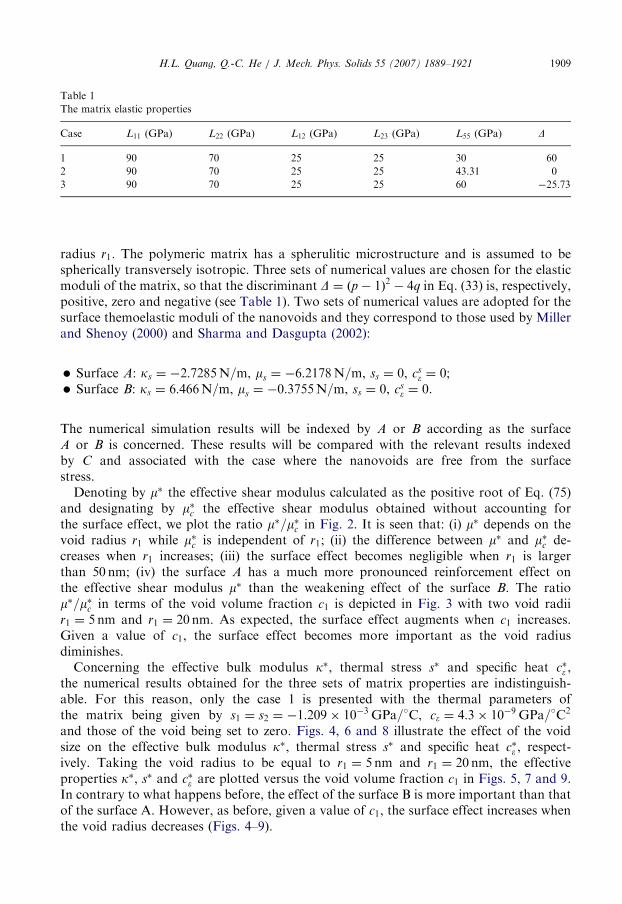
Case L11 (GPa) L22 (GPa) L12 (GPa) L23 (GPa) L55 (GPa) D

1 90 70 25 25 30 60

2 90 70 25 25 43.31 0

3 90 70 25 25 60 �25.73

H.L. Quang, Q.-C. He / J. Mech. Phys. Solids 55 (2007) 1889–1921 1909

radius r1. The polymeric matrix has a spherulitic microstructure and is assumed to bespherically transversely isotropic. Three sets of numerical values are chosen for the elasticmoduli of the matrix, so that the discriminant D ¼ ðp� 1Þ2 � 4q in Eq. (33) is, respectively,positive, zero and negative (see Table 1). Two sets of numerical values are adopted for thesurface themoelastic moduli of the nanovoids and they correspond to those used by Millerand Shenoy (2000) and Sharma and Dasgupta (2002):

�

Surface A: ks ¼ �2:7285N=m, ms ¼ �6:2178N=m, ss ¼ 0, cs� ¼ 0;

�

Surface B: ks ¼ 6:466N=m, ms ¼ �0:3755N=m, ss ¼ 0, cs� ¼ 0.

The numerical simulation results will be indexed by A or B according as the surfaceA or B is concerned. These results will be compared with the relevant results indexedby C and associated with the case where the nanovoids are free from the surfacestress.

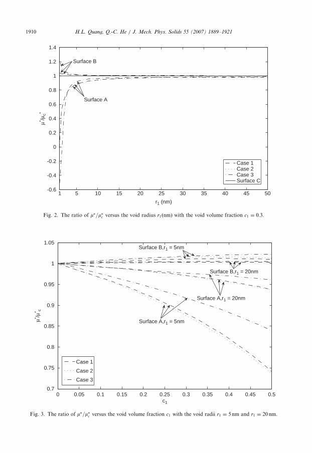
Denoting by m� the effective shear modulus calculated as the positive root of Eq. (75)and designating by m�c the effective shear modulus obtained without accounting forthe surface effect, we plot the ratio m�=m�c in Fig. 2. It is seen that: (i) m� depends on thevoid radius r1 while m�c is independent of r1; (ii) the difference between m� and m�c de-creases when r1 increases; (iii) the surface effect becomes negligible when r1 is largerthan 50 nm; (iv) the surface A has a much more pronounced reinforcement effect onthe effective shear modulus m� than the weakening effect of the surface B. The ratiom�=m�c in terms of the void volume fraction c1 is depicted in Fig. 3 with two void radiir1 ¼ 5 nm and r1 ¼ 20 nm. As expected, the surface effect augments when c1 increases.Given a value of c1, the surface effect becomes more important as the void radiusdiminishes.

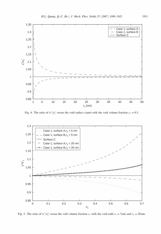
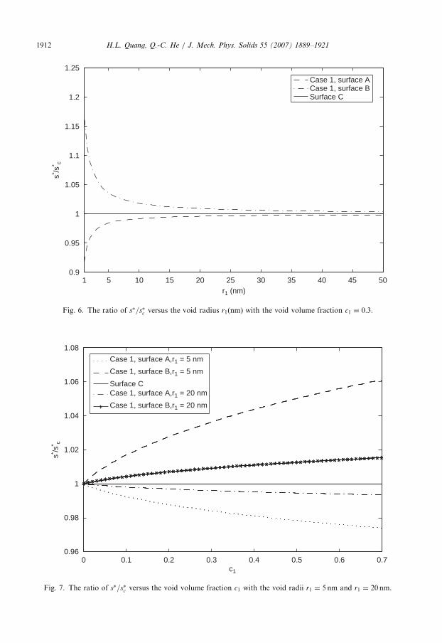
Concerning the effective bulk modulus k�, thermal stress s� and specific heat c�� ,the numerical results obtained for the three sets of matrix properties are indistinguish-able. For this reason, only the case 1 is presented with the thermal parameters ofthe matrix being given by s1 ¼ s2 ¼ �1:209 10�3 GPa=C, c� ¼ 4:3 10�9 GPa=C2

and those of the void being set to zero. Figs. 4, 6 and 8 illustrate the effect of the voidsize on the effective bulk modulus k�, thermal stress s� and specific heat c�� , respect-ively. Taking the void radius to be equal to r1 ¼ 5 nm and r1 ¼ 20 nm, the effectiveproperties k�, s� and c�� are plotted versus the void volume fraction c1 in Figs. 5, 7 and 9.In contrary to what happens before, the effect of the surface B is more important than thatof the surface A. However, as before, given a value of c1, the surface effect increases whenthe void radius decreases (Figs. 4–9).

ARTICLE IN PRESS

0 0.05 0.1 0.15 0.2 0.25 0.3 0.35 0.4 0.45 0.50.7

0.75

0.8

0.85

0.9

0.95

1

1.05

c1

μ* /μ* c

Case 1

Case 2

Case 3

Surface A,r1 = 5nm

Surface A,r1 = 20nm

Surface B,r1 = 20nm

Surface B,r1 = 5nm

Fig. 3. The ratio of m�=m�c versus the void volume fraction c1 with the void radii r1 ¼ 5 nm and r1 ¼ 20 nm.

1 5 10 15 20 25 30 35 40 45 50-0.6

-0.4

-0.2

0

0.2

0.4

0.6

0.8

1

1.2

1.4

r1 (nm)

μ* /μc*

Case 1Case 2Case 3Surface C

Surface A

Surface B

Fig. 2. The ratio of m�=m�c versus the void radius r1ðnmÞ with the void volume fraction c1 ¼ 0:3.

H.L. Quang, Q.-C. He / J. Mech. Phys. Solids 55 (2007) 1889–19211910

ARTICLE IN PRESS

1 5 10 15 20 25 30 35 40 45 500.85

0.9

0.95

1

1.05

1.1

1.15

1.2

1.25

1.3

1.35

r1 (nm)

κ* /κc*

Case 1, surface ACase 1, surface BSurface C

Fig. 4. The ratio of k�=k�c versus the void radius r1ðnmÞ with the void volume fraction c1 ¼ 0:3.

0 0.1 0.2 0.3 0.4 0.5 0.6 0.70.85

0.9

0.95

1

1.05

1.1

1.15

1.2

1.25

1.3

c1

κ* /κ* c

Case 1, surface A,r1 = 5 nm

Case 1, surface B,r1 = 5 nm

Surface CCase 1, surface A,r1 = 20 nm

Case 1, surface B,r1 = 20 nm

Fig. 5. The ratio of k�=k�c versus the void volume fraction c1 with the void radii r1 ¼ 5nm and r1 ¼ 20 nm.

H.L. Quang, Q.-C. He / J. Mech. Phys. Solids 55 (2007) 1889–1921 1911

ARTICLE IN PRESS

1 5 10 15 20 25 30 35 40 45 500.9

0.95

1

1.05

1.1

1.15

1.2

1.25

r1 (nm)

s* /s* c

Case 1, surface ACase 1, surface BSurface C

Fig. 6. The ratio of s�=s�c versus the void radius r1ðnmÞ with the void volume fraction c1 ¼ 0:3.

0 0.1 0.2 0.3 0.4 0.5 0.6 0.70.96

0.98

1

1.02

1.04

1.06

1.08

c1

s* /s* c

Case 1, surface A,r1 = 5 nm

Case 1, surface B,r1 = 5 nm

Surface CCase 1, surface A,r1 = 20 nm

Case 1, surface B,r1 = 20 nm

Fig. 7. The ratio of s�=s�c versus the void volume fraction c1 with the void radii r1 ¼ 5 nm and r1 ¼ 20nm.

H.L. Quang, Q.-C. He / J. Mech. Phys. Solids 55 (2007) 1889–19211912

ARTICLE IN PRESS

1 5 10 15 20 25 30 35 40 45 500.9

0.92

0.94

0.96

0.98

1

1.02

1.04

1.06

r1 (nm)

c ε* /c

εc*

Case 1, surface ACase 1, surface BSurface C

Fig. 8. The ratio of c�� =c��c versus the void radius r1ðnmÞ with the void volume fraction c1 ¼ 0:3.

0 0.1 0.2 0.3 0.4 0.5 0.6 0.7 0.8 0.9 10.97

0.975

0.98

0.985

0.99

0.995

1

1.005

1.01

1.015

c1

c ε* /c

εc*

Case 1, surface A,r1 = 5 nm

Case 1, surface B,r1 = 5 nmSurface CCase 1, surface A,r1 = 20 nm

Case 1, surface B,r1 = 20 nm

Fig. 9. The ratio of c�� =c��c versus the void volume fraction c1 with the void radii r1 ¼ 5nm and r1 ¼ 20 nm.

H.L. Quang, Q.-C. He / J. Mech. Phys. Solids 55 (2007) 1889–1921 1913

ARTICLE IN PRESSH.L. Quang, Q.-C. He / J. Mech. Phys. Solids 55 (2007) 1889–19211914

Appendix A. Derivation of Eq. (20)

This appendix consists in showing that the free energy Uðe0Þ of a homogeneous mediumO after inserting an inhomogeneity o is given by Eq. (20).First, we write Eq. (20) in the equivalent form

2ðU �U0Þ ¼ þ

Zqoðt � u0 � t0 � uÞdS þ

Zoðs : eW0 � c�W

20ÞdV

þ

ZGðss : esW0 � cs

�W20ÞdS þ ðc��W

20 � s� : e0W0Þ volðoÞ. ðA:1Þ

Next, the free energy of O containing an inhomogeneity o takes by definition the followingform:

Uðe0Þ ¼1

2

ZOðe : Leþ 2s : eW0 � c�W

20ÞdV þ

1

2

ZGðes : Lses þ 2ss : esW0 � cs

�W20ÞdS.

(A.2)Using Eqs. (18) and (A.2), it is immediate that

2ðU �U0Þ ¼

ZOðe : Leþ 2s : eW0 � c�W

20ÞdV

þ

ZGðes : Lses þ 2ss : esW0 � cs

�W20ÞdS �

ZOðe0 : L�e0 þ 2s� : e0W0 � c��W

20ÞdV

¼

ZOðr : eþ s : eW0 � c�W

20ÞdV þ

ZGðrs : es þ ss : esW0 � cs

�W20ÞdS

�

ZOðr0 : e0 þ s� : e0W0 � c��W

20ÞdV

¼

ZOðr : e� r0 : e0ÞdV þ

ZG

rs : es dS þ

ZGðss : esW0 � cs

�W20ÞdS

þ

ZOðs : eW0 � c�W

20 � s� : e0W0 þ c��W

20ÞdV

¼

ZOðr0 þ rÞ : ðe� e0ÞdV þ

ZGðrs : es � rs : Du0ÞdS

þ

ZOðr : e0 � r0 : eÞdV þ

ZOðs : eW0 � c�W

20 � s� : e0W0 þ c��W

20ÞdV

þ

ZGðss : esW0 � cs

�W20ÞdS þ

ZG

rs : Du0 dS. ðA:3Þ

In this expression, Du0 denotes the tangential derivative of the displacement field u0. Underthe boundary condition (16), it follows from the divergence theorem and the equilibriumequations r � r ¼ 0 and r � r0 ¼ 0 thatZ

Oðr0 þ rÞ : ðe� e0ÞdV þ

ZGðrs : es � rs : Du0ÞdS

¼

ZqOðt0 þ tÞ � ðu� u0ÞdS

¼

ZqOðt0 þ tÞ � ðe0x� e0xÞdS ¼ 0. ðA:4Þ

ARTICLE IN PRESSH.L. Quang, Q.-C. He / J. Mech. Phys. Solids 55 (2007) 1889–1921 1915

Accounting for Eq. (A.4) in Eq. (A.3), we obtain

2ðU �U0Þ ¼

ZOðr : e0 � r0 : eÞdV þ

ZGðss : esW0 � cs

�W20ÞdS

þ

ZG

rs : Du0 dS þ

ZOðs : eW0 � c�W

20 � s� : e0W0 þ c��W

20ÞdV

¼

Zoðr : e0 � r0 : eÞdV þ

ZOnoðr : e0 � r0 : eÞdV

þ

Zoðs : eW0 � c�W

20 � s� : e0W0 þ c��W

20ÞdV

þ

ZOnoðs : eW0 � c�W

20 � s� : e0W0 þ c��W

20ÞdV

þ

ZGðss : esW0 � cs

�W20ÞdS þ

ZG

rs : Du0 dS. ðA:5Þ

Recall that the effective outside medium Ono is homogeneous with the effectiveconstitutive laws and thermoelastic properties given by

r ¼ L�eþ s�W0; r0 ¼ L�e0 þ s�W0; c� ¼ c�� . (A.6)

Introducing Eq. (A.6) into Eq. (A.5) and using the divergence theorem together with theequilibrium equations r � r ¼ 0 and r � r0 ¼ 0 again for the integral calculus over thedomain o, Eq. (A.5) reduces to Eq. (A.1). Thus, the free energy Uðe0Þ of the effectivemedium with the composite sphere can be expressed as Eq. (20).

Appendix B. Derivation of inequalities (36)–(38)

The matrix and inclusion phases are assumed linearly thermoelastic and sphericallytransverse isotropic. In this case, it is convenient to use the moduli of Hill (1964) defined as

k ¼ 12ðL22 þ L23Þ; m ¼ 1

2ðL22 � L23Þ; n ¼ L11; l ¼ L12; s ¼ L55, (B.1)

where the superscript denoting phase i is omitted. The elastic stiffness tensor L is positivedefinite if and only if the following inequalities hold

k40; m40; s40; nk4l2. (B.2)

First, substituting Eqs. (B.1) and (30) into Eq. ð32Þ1, the material parameter p is given by

p ¼45

4�ð2

ffiffiffikp� 7

2

ffiffiffinpÞ2þ 14ð

ffiffiffiffiffiffinkp� lÞ

nþ

6ðnk � l2Þ þ 4nm

ns

" #. (B.3)

Since (B.2) and owing to the fact that ð2ffiffiffikp� 7

2

ffiffiffinpÞ240,

ffiffiffiffiffiffinkp� l40, nk � l240, n40,

m40 and s40, it is seen that

45=44p. (B.4)

If s! 0þ, it follows from (B.3) that p!�1. In addition, when m! 0, k! 49n=16 andnk! l2, then p! 45=4. Thus,

45=44p4�1, (B.5)

which corresponds to (38).

ARTICLE IN PRESSH.L. Quang, Q.-C. He / J. Mech. Phys. Solids 55 (2007) 1889–19211916

Next, combining Eqs. (B.1), (30) and ð32Þ2 gives the expression of q

q ¼8mð2k � lÞ

nsþ

8ðl þ k þ 3mÞ

n. (B.6)

With k, l, s, n and m verifying conditions (B.2) and by varying the value of n such thatn 2�0;þ1½, the value of q given by Eq. (B.6) can be changed from �1 to þ1 because2k � l can be positive, negative or vanished. This means that q is not subjected to anyrestrictions.Calculating p� 4q with p and q given by (B.3) and ((B.6), we obtain

p� 4q ¼5

4�

18ðnþ 16k þ 8lÞ þ 768m

8n�

6ðnk � l2Þ þ 4mðnþ 16k � 8lÞ

ns. (B.7)

Using the fact that n40 and k40 from (B.2), and applying the inequality a2 þ b2X2ab to

a ¼ffiffiffinp

and b ¼ffiffiffiffiffiffiffiffi16kp

, we can write

nþ 16kX8ffiffiffiffiffiffinkp

. (B.8)

Combining (B.8) with (B.2) yields

nþ 16kX8ffiffiffiffiffiffinkp

48ffiffiffiffil2

p¼ 8jlj (B.9)

and nþ 16k � 8jlj40. It results from (B.7) and (B.2) that

5=44p� 4q. (B.10)

Thus, inequality (36) is demonstrated.We now consider the case of p41. With this condition, inequalities (B.2) can be written

as

m40; n40;45þ

ffiffiffiffiffiffiffiffiffiffi2009p

8n4k4

45�ffiffiffiffiffiffiffiffiffiffi2009p

8n,

ffiffiffiffiffiffinkp

4l42k þ n

7; s4s0, ðB:11Þ

with

s0 ¼2mnþ 3ðnk � l2Þ

7l � 2k � n40. (B.12)

In order to prove that

ðp� 1Þ2 � 4q ¼4ðAs2 þ Bsþ CÞ

n2s2o0 (B.13)

with

A ¼ 49l2 � ð28k þ 22nÞl þ ð2k � nÞ2 � 24mn, (B.14)

B ¼ 12nk2þ 42l3 þ 4n2mþ 6n2k � 8nmk � 42nkl � 20nml � 12kl2 � 6nl2, (B.15)

C ¼ ð3nk � 3l2 þ 2mnÞ2, (B.16)

it is necessary to show that

f ðsÞ ¼ As2 þ Bsþ Co0. (B.17)

ARTICLE IN PRESSH.L. Quang, Q.-C. He / J. Mech. Phys. Solids 55 (2007) 1889–1921 1917

Here f ðsÞ is a quadratic function of s with f ð0Þ ¼ C40. Concerning the value of A, wedetermine

A2k þ n

7

� �¼ �

8

7nð21mþ 9k þ nÞo0. (B.18)

and

AðffiffiffiffiffiffinkpÞ ¼ �24mn� n2gðtÞ, (B.19)

where

gðtÞ ¼ �4t4 þ 28t3 � 45t2 þ 22t� 1, (B.20)

with

1

2ffiffiffi2p

ffiffiffiffiffiffiffiffiffiffiffiffiffiffiffiffiffiffiffiffiffiffiffiffiffi45�

ffiffiffiffiffiffiffiffiffiffi2009p

qot ¼

ffiffiffik

n

ro

1

2ffiffiffi2p

ffiffiffiffiffiffiffiffiffiffiffiffiffiffiffiffiffiffiffiffiffiffiffiffiffi45þ

ffiffiffiffiffiffiffiffiffiffi2009p

q. (B.21)

Furthermore, it can be shown that gðtÞ is positive for any t described by (B.21). Since m40,n40 and gðtÞ40, it follows from (B.19) that Að

ffiffiffiffiffiffinkpÞo0.

Therefore, A given by Eq. (B.14) is a concave parabola whose values associated with

l ¼ ð2k þ nÞ=7 and l ¼ffiffiffiffiffiffinkp

are negative. This implies that A is negative for any

l 2�ð2k þ nÞ=7;ffiffiffiffiffiffinkp½.

Calculating f ðs0Þ yields

f ðs0Þ ¼ �32nð3nk � 3l2 þ 2mnÞ

ð7l � 2k � nÞ2½3ðkn� l2Þðl þ k þ 3mÞ þ 6nm2 þmhðlÞ�, (B.22)

where

hðlÞ ¼ �7l2 þ ð3nþ 16kÞl � 4k2. (B.23)

Substituting l ¼ ð2k þ nÞ=7 and l ¼ffiffiffiffiffiffinkp

into (B.23), we have

hðð2k þ nÞ=7Þ ¼ 27nð9k þ nÞ40, ðB:24Þ

hðffiffiffiffiffiffinkpÞ ¼ n2rðtÞ, ðB:25Þ

where

rðtÞ ¼ �4t4 þ 16t3 � 7t2 þ 3t (B.26)

with t given by (B.21). It can be checked that rðtÞ is positive for any t given by (B.21).

Consequently, both hðffiffiffiffiffiffinkpÞ and hðð2k þ nÞ=7Þ are positive. Thus, the quadratic function

hðlÞ defined by (B.23) is positive for all l 2�ð2k þ nÞ=7;ffiffiffiffiffiffinkp½. Using the conditions (B.11)

together with hðlÞ40 yields f ðs0Þo0.To summarize, the quadratic function f ðsÞ ¼ As2 þ Bsþ C where Ao0, f ð0Þ ¼ C40

and f ðs0Þo0 with s040. This shows that f ðsÞo0 for s4s0. Thus, the proof of (37) iscompleted. &

ARTICLE IN PRESSH.L. Quang, Q.-C. He / J. Mech. Phys. Solids 55 (2007) 1889–19211918

Appendix C. The expressions for the constants aij in (62)

The components aij in Eq. (62) are specified by following expressions with the primedenoting the derivative with respect to r:

a13 ¼ dð2Þ1 fð2Þ1 ðr2Þ þ ið2Þ2 fð2Þ2 ðr2Þ; a14 ¼ dð2Þ2 fð2Þ2 ðr2Þ þ ið2Þ1 fð2Þ1 ðr2Þ,

a15 ¼ dð2Þ3 fð2Þ3 ðr2Þ þ ið2Þ4 fð2Þ4 ðr2Þ; a16 ¼ dð2Þ4 fð2Þ4 ðr2Þ þ ið2Þ3 fð2Þ3 ðr2Þ,

a23 ¼ fð2Þ1 ðr2Þ; a24 ¼ fð2Þ2 ðr2Þ; a25 ¼ fð2Þ3 ðr2Þ; a26 ¼ fð2Þ4 ðr2Þ,

a33 ¼ dð2Þ1 fð2Þ1 ðr1Þ þ ið2Þ2 fð2Þ2 ðr1Þ; a34 ¼ dð2Þ2 fð2Þ2 ðr1Þ þ ið2Þ1 fð2Þ1 ðr1Þ,

a35 ¼ dð2Þ3 fð2Þ3 ðr1Þ þ ið2Þ4 fð2Þ4 ðr1Þ; a36 ¼ dð2Þ4 fð2Þ4 ðr1Þ þ ið2Þ3 fð2Þ3 ðr1Þ,

a37 ¼ �dð1Þ3 fð1Þ3 ðr1Þ � ið1Þ4 fð1Þ4 ðr1Þ; a38 ¼ �d

ð1Þ4 fð1Þ4 ðr1Þ � ið1Þ3 fð1Þ3 ðr1Þ,

a43 ¼ fð2Þ1 ðr1Þ; a44 ¼ fð2Þ2 ðr1Þ; a45 ¼ fð2Þ3 ðr1Þ,

a46 ¼ fð2Þ4 ðr1Þ; a47 ¼ �fð1Þ3 ðr1Þ; a48 ¼ �f

ð1Þ4 ðr1Þ,

a53 ¼ Lð2Þ11 r2½d

ð2Þ1 fð2Þ01 ðr2Þ þ ið2Þ2 fð2Þ02 ðr2Þ� þ L

ð2Þ12 ½ð2d

ð2Þ1 � 3Þfð2Þ1 ðr2Þ þ 2ið2Þ2 fð2Þ2 ðr2Þ�,

a54 ¼ Lð2Þ11 r2½d

ð2Þ2 fð2Þ02 ðr2Þ þ ið2Þ1 fð2Þ01 ðr2Þ� þ L

ð2Þ12 ½ð2d

ð2Þ2 � 3Þfð2Þ2 ðr2Þ þ 2ið2Þ1 fð2Þ1 ðr2Þ�,

a55 ¼ Lð2Þ11 r2½d

ð2Þ3 fð2Þ03 ðr2Þ þ ið2Þ4 fð2Þ04 ðr2Þ� þ L

ð2Þ12 ½ð2d

ð2Þ3 � 3Þfð2Þ3 ðr2Þ þ 2ið2Þ4 fð2Þ4 ðr2Þ�,

a56 ¼ Lð2Þ11 r2½d

ð2Þ4 fð2Þ04 ðr2Þ þ ið2Þ3 fð2Þ03 ðr2Þ� þ L

ð2Þ12 ½ð2d

ð2Þ4 � 3Þfð2Þ4 ðr2Þ þ 2ið2Þ3 fð2Þ3 ðr2Þ�,

a63 ¼ Lð2Þ55 ½r2f

ð2Þ01 ðr2Þ þ ð2d

ð2Þ1 � 1Þfð2Þ1 ðr2Þ þ 2ið2Þ2 fð2Þ2 ðr2Þ�,

a64 ¼ Lð2Þ55 ½r2f

ð2Þ02 ðr2Þ þ ð2d

ð2Þ2 � 1Þfð2Þ2 ðr2Þ þ 2ið2Þ1 fð2Þ1 ðr2Þ�,

a65 ¼ Lð2Þ55 ½r2f

ð2Þ03 ðr2Þ þ ð2d

ð2Þ3 � 1Þfð2Þ3 ðr2Þ þ 2ið2Þ4 fð2Þ4 ðr2Þ�,

a66 ¼ Lð2Þ55 ½r2f

ð2Þ04 ðr2Þ þ ð2d

ð2Þ4 � 1Þfð2Þ4 ðr2Þ þ 2ið2Þ3 fð2Þ3 ðr2Þ�,

a73 ¼ Lð2Þ11 r1½d

ð2Þ1 fð2Þ01 ðr1Þ þ ið2Þ2 fð2Þ02 ðr1Þ� þ L

ð2Þ12 �

2ks

r1

� �½ð2dð2Þ1 � 3Þfð2Þ1 ðr1Þ þ 2ið2Þ2 fð2Þ2 ðr1Þ�,

a74 ¼ Lð2Þ11 r1½d

ð2Þ2 fð2Þ02 ðr1Þ þ ið2Þ1 fð2Þ01 ðr1Þ� þ L

ð2Þ12 �

2ks

r1

� �½ð2dð2Þ2 � 3Þfð2Þ2 ðr1Þ þ 2ið2Þ1 fð2Þ1 ðr1Þ�,

a75 ¼ Lð2Þ11 r1½d

ð2Þ3 fð2Þ03 ðr1Þ þ ið2Þ4 fð2Þ04 ðr1Þ� þ L

ð2Þ12 �

2ks

r1

� �½ð2dð2Þ3 � 3Þfð2Þ3 ðr1Þ þ 2ið2Þ4 fð2Þ4 ðr1Þ�,

a76 ¼ Lð2Þ11 r1½d

ð2Þ4 fð2Þ04 ðr1Þ þ ið2Þ3 fð2Þ03 ðr1Þ� þ L

ð2Þ12 �

2ks

r1

� �½ð2dð2Þ4 � 3Þfð2Þ4 ðr1Þ þ 2ið2Þ3 fð2Þ3 ðr1Þ�,

a77 ¼ �Lð1Þ11 r1½d

ð1Þ3 fð1Þ03 ðr1Þ þ ið1Þ4 fð1Þ04 ðr1Þ� � L

ð1Þ12 ½ð2d

ð1Þ3 � 3Þfð1Þ3 ðr1Þ þ 2ið1Þ4 fð1Þ4 ðr1Þ�,

a78 ¼ �Lð1Þ11 r1½d

ð1Þ4 fð1Þ04 ðr1Þ þ ið1Þ3 fð1Þ03 ðr1Þ� � L

ð1Þ12 ½ð2d

ð1Þ4 � 3Þfð1Þ4 ðr1Þ þ 2ið1Þ3 fð1Þ3 ðr1Þ�,

ARTICLE IN PRESSH.L. Quang, Q.-C. He / J. Mech. Phys. Solids 55 (2007) 1889–1921 1919

a83 ¼ Lð2Þ55 ½r1f

ð2Þ01 ðr1Þ þ ð2d

ð2Þ1 � 1Þfð2Þ1 ðr1Þ þ 2ið2Þ2 fð2Þ2 ðr1Þ�

þ2ks

r1½ð2dð2Þ1 � 3Þfð2Þ1 ðr1Þ þ 2ið2Þ2 fð2Þ2 ðr1Þ� �

4ms

r1fð2Þ1 ðr1Þ,

a84 ¼ Lð2Þ55 ½r1f

ð2Þ02 ðr1Þ þ ð2d

ð2Þ2 � 1Þfð2Þ2 ðr1Þ þ 2ið2Þ1 fð2Þ1 ðr1Þ�

þ2ks

r1½ð2dð2Þ2 � 3Þfð2Þ2 ðr1Þ þ 2ið2Þ1 fð2Þ1 ðr1Þ� �

4ms

r1fð2Þ2 ðr1Þ,

a85 ¼ Lð2Þ55 ½r1f

ð2Þ03 ðr1Þ þ ð2d

ð2Þ3 � 1Þfð2Þ3 ðr1Þ þ 2ið2Þ4 fð2Þ4 ðr1Þ�

þ2ks

r1½ð2dð2Þ3 � 3Þfð2Þ3 ðr1Þ þ 2ið2Þ4 fð2Þ4 ðr1Þ� �

4ms

r1fð2Þ3 ðr1Þ,

a86 ¼ Lð2Þ55 ½r1f

ð2Þ04 ðr1Þ þ ð2d

ð2Þ4 � 1Þfð2Þ4 ðr1Þ þ 2ið2Þ3 fð2Þ3 ðr1Þ�

þ2ks

r1½ð2dð2Þ4 � 3Þfð2Þ4 ðr1Þ þ 2ið2Þ3 fð2Þ3 ðr1Þ� �

4ms

r1fð2Þ4 ðr1Þ,

a87 ¼ �Lð1Þ55 ½r1f

ð1Þ03 ðr1Þ þ ð2d

ð1Þ3 � 1Þfð1Þ3 ðr1Þ þ 2ið1Þ4 fð1Þ4 ðr1Þ�,

a88 ¼ �Lð1Þ55 ½r1f

ð1Þ04 ðr1Þ þ ð2d

ð1Þ4 � 1Þfð1Þ4 ðr1Þ þ 2ið1Þ3 fð1Þ3 ðr1Þ�.

Appendix D. Derivation of the expressions of s� and c�� given by Eqs. (111) and (112)

Consider the general case where the domain O is subjected to the boundary condition(78). The initial displacement and traction vectors u0 and t0 are given by

u0 ¼ ð�0r; 0; 0ÞT; t0 ¼ ð3k��0 þ s�W0; 0; 0Þ

T (D.1)

and the displacement and traction vectors u and t after inserting a composite sphere takethe form

u ¼ ð�0rþ ½bð�Þe �0 þ bðWÞe W0�r; 0; 0Þ

T,

t ¼ ð3k��0 � 4½bð�Þe �0 þ bðWÞe W0�m� þ s�W0; 0; 0ÞT. ðD:2Þ

Introducing Eqs. (D.1), (D.2) and (87) into (23) yields the following equality:

bð�Þe �20ð4m

� þ 3k�Þ

�1

3W20 c�� �

3

4pr32

Zoðc� � s : BÞdV �

3

4pr32

ZGðcs� � ss : BðsÞÞdS � 3bðWÞe s�

� �

þ �0W0 s� �1

4pr32

Zoðs : AÞdV �

1

4pr32

ZGðss : AðsÞÞdS þ s�bð�Þe

�

þbðWÞe ð4m� þ 3k�Þ

�¼ 0 ðD:3Þ

ARTICLE IN PRESSH.L. Quang, Q.-C. He / J. Mech. Phys. Solids 55 (2007) 1889–19211920

for any �0 and W0. Due to the fact that m�40 and k�40, it is deduced from (D.3) that

bð�Þe ¼ 0, ðD:4Þ

s� �1

4pr32

Zoðs : AÞdV �

1

4pr32

ZGðss : AðsÞÞdS þ bðWÞe ð4m

� þ 3k�Þ ¼ 0. ðD:5Þ

c�� �3

4pr32

Zoðc� � s : BÞdV �

3

4pr32

ZGðcs� � ss : BðsÞÞdS � 3bðWÞe s� ¼ 0, ðD:6Þ

Substituting bðWÞe ¼ bðWÞe r�32 =W0 into Eqs. (D.5) and (D.6) yields Eqs. (111) and (112),respectively.

References

Bassett, D.C., 1981. Principles of Polymer Morphology. Cambridge University Press, London.

Bottomley, D.J., Ogino, T., 2001. Alternative to the Shuttleworth formulation of solid surface stress. Phys. Rev. B

63, 165412-1–165412-5.

Bouby, C., He, Q.-C., Gu, S.-T., Pensee, V., 2007. Coordinate-free derivation of a thermoelastic curved interface

model, submitted for publication.

Cahn, J.W., 1980. Surface stress and the chemical equilibrium of small crystals-I. The case of the isotropic surface.

Acta Metall. 28, 1333–1338.

Causin, V., Marega, C., Marigo, A., Ferrara, G., Idiyatullina, G., Fantinel, F., 2006. Morphology, structure and

properties of a poly(1-butene)/montmorillonite nanocomposite. Polymer 47, 4773–4780.

Chen, T., 1993. Thermoelastic properties and conductivity of composites reinforced by spherically particles.

Mech. Mater. 14, 257–268.

Chen, T., Dvorak, G.J., Yu, C.C., 2007. Solids containing spherical nano-inclusions with interface stress: effective

properties and thermal-mechanical connections. Int. J. Solids Struct. 44, 941–955.

Christensen, R.M., 1990. A critical evaluation for a class of micromechanics models. J. Mech. Phys. Solids 38,

379–404.

Christensen, R.M., Lo, K.H., 1979. Solutions for effective shear properties in three phase sphere and cylinder

models. J. Mech. Phys. Solids 27, 315–330.

Dingreville, R., Qu, J., Cherkaoui, M., 2005. Surface free energy and its effect on the elastic behavior of nano-

sized particles, wires and films. J. Mech. Phys. Solids 8, 1827–1854.

Dryden, J.R., 1988. Elastic constants of spherulitic polymer. J. Mech. Phys. Solids 36, 477–498.

Duan, H.L., Karihaloo, B.L., 2007. Thermoelastic properties of heterogeneous materials with imperfect

interfaces: generalized Levins’s formula and Hill’s connections. J. Mech. Phys. Solids, in press, doi:10.1016/

j.jmps.2006.10.006.

Duan, H.L., Wang, J., Huang, Z.P., Karihaloo, B.L., 2005a. Eshelby formalism for nano-inhomogeneities. Proc.

R. Soc. A 461, 3335–3353.

Duan, H.L., Wang, J., Huang, Z.P., Karihaloo, B.L., 2005b. Size-dependent effective elastic constants of solids

containing nano-inhomogeneities with interface stress. J. Mech. Phys. Solids 53, 1574–1596.

Eshelby, J.D., 1956. The continuum theory of lattice defects. In: Seitz, F., Turnbull, D. (Eds.), Prog. Solid State

Phys, vol. 3. Academic Press Inc., New York, pp. 79–144.

Gurtin, M.E., Murdoch, A.I., 1975. A continuum theory of elastic material surfaces. Arch. Ration. Mech. Anal.

57, 291–323 and 59, 389–390.

Hadal, R., Yuan, Q., Jog, J.P., Misra, R.D.K., 2006. On stress whitening during surface deformation in clay-

containing polymer nanocomposites: a microstructural approach. Mater. Sci. Eng. A 418, 268–281.

He, L.-H., Cheng, Z.-Q., 1996. Correspondence relations between the effective thermoelastic properties of

composites reinforced by spherically particles. Int. J. Eng. Sci. 34, 1–8.

He, Q.-C., Benveniste, Y., 2004. Exactly solvable spherically anisotropic thermoelastic microstructures. J. Mech.

Phys. Solids 52, 2661–2682.

Hill, R., 1964. Theory of mechanical properties of fibre-strengthened materials: I. Elastic behaviour. J. Mech.

Phys. Solids 12, 199–212.

Kerner, E.H., 1956. The elastic and thermoelastic properties of composite media. Proc. Phys. Soc. B. 69, 808–813.

ARTICLE IN PRESSH.L. Quang, Q.-C. He / J. Mech. Phys. Solids 55 (2007) 1889–1921 1921

Kim, G., Han, C.C., Libera, M., Jackson, C.L., 2001. Crystallization within melt ordered semicrystalline block

copolymers: exploring the coexistence of microphase-separated and spherulitic morphologies. Macromolecules

34, 7336–7342.

Le Quang, H., He, Q.-C., 2004. Micromechanical estimation of the shear modulus of a composite consisting of

anisotropic phases. J. Mater. Sci. Technol. 20, 6–10.

Levin, V.M., 1967. Thermal expansion coefficients of heterogeneous media. Mekhanika Tverdogo Tela. 2, 88–94

English version, Mech. Solids, 11, 58–61.

Liu, Z., Chen, K., Yan, D., 2003. Crystallization, morphology, and dynamic mechanical properties of

poly(trimethylene terephthalate)/clay nanocomposites. Eur. Polym. J. 39, 2359–2366.

Miller, R.E., Shenoy, V.B., 2000. Size-dependent elastic properties of nanosized structural elements.

Nanotechnology 11, 139–147.

Milton, G.W., 2002. The Theory of Composites. Cambridge University Press, London.

Murdoch, A.I., 1976. A thermodynamical theory of elastic-material interfaces. Q. J. Mech. Appl. Math. 29,

245–275.

Murdoch, A.I., 2005. Some fundamental aspects of surface modelling. J. Elasticity 80, 33–52.

Nowacki, R., Monasse, B., Piorkowska, E., Galeski, A., Haudin, J.M., 2004. Spherulite nucleation in isotactic

polypropylene based nanocomposites with montmorillonite under shear. Polymer 45, 4877–4892.

Pathak, S., Shenoy, V.B., 2005. Size dependence of thermal expansion of nanostructures. Phys. Rev. B 72, 113404.

Povstenko, Y.Z., 1993. Theoretical investigation of phenomena caused by heterogeneous surface tension in solids.

J. Mech. Phys. Solids 41, 1499–1514.

Sharma, P., Dasgupta, A., 2002. Average elastic fields and scale-dependent overall properties of hetero

geneous micropolar materials containing spherical and cylindrical inhomogeneities. Phys. Rev. B 66, 224110-

1–224110-10.

Shuttleworth, R., 1950. The surface tension of solid. Proc. Phys. Soc. A 63, 444–457.

Smith, J.C., 1974. Correction and extension of van der Poel’s method for calculating the shear modulus of a

particulate composite. J. Res. Nat. Bur. Stand. 78A, 355–361.

Smith, J.C., 1975. Simplification of van der Poel’s formula for the shear modulus of a particulate composite.

J. Res. Nat. Bur. Stand. 79A, 419–423.

Torquato, S., 2001. Random Heterogeneous Materials: Microstructure and Macroscopic Properties. Springer,

Berlin.

Van der Poel, C., 1958. On the rheology of concentrated suspensions. Rheol. Acta 1, 198–205.