arX

iv:g

r-qc

/960

4016

v1 8

Apr

199

6

Nonlinear Connections in Superbundles

and Locally Anisotropic Supergravity

Sergiu I. Vacaru

Institute of Applied Physics, Academy of Sciences,

5 Academy str., Chisinau–028, Moldova

(February 7, 2008)

Abstract

The theory of locally anisotropic superspaces (supersymmetric generaliza-

tions of various types of Kaluza–Klein, Lagrange and Finsler spaces) is laid

down. In this framework we perform the analysis of construction of the su-

pervector bundles provided with nonlinear and distinguished connections and

metric structures. Two models of locally anisotropic supergravity are pro-

posed and studied in details.

c©S.I.Vacaru

PACS numbers: 04.65.+e, 04.90.+e, 12.10.+g, 02.40.+k, 04.50.+h, 02.90.+p

Typeset using REVTEX

1

I. INTRODUCTION

Differential geometric techniques plays an important role in formulation and mathemati-

cal formalization of models of fundamental interactions of physical fields. In the last twenty

years there has been a substantial interest in the construction of differential supergeometry

with the aim of getting a framework for the supersymmetric field theories (the theory of

graded manifolds [1-4] and the theory of supermanifolds [5-9]). Detailed considerations of

geometric and topological aspects of supermanifolds and formulation of superanalysis are

contained in [10-16].

Spaces with local anisotropy are used in some divisions of theoretical and mathematical

physics [17-20] (recent applications in physics and biology are summarized in [21,22]). The

first models of locally anisotropic (la) spaces (la–spaces) have been proposed by P.Finsler

[23] and E.Cartan [24]. Early approaches and modern treatments of Finsler geometry and its

extensions can be found in [25-30]. We shall use the general approach to the geometry of la–

spaces, developed by R.Miron and M.Anastasiei [26,27], as a starting point for our definition

of superspaces with local anisotropy and formulation of la–supergravitational models.

In different models of la–spaces one considers nonlinear and linear connections and met-

ric structures in vector and tangent bundles on locally isotropic space–times ((pseudo)–

Riemannian, Einstein–Cartan and more general types of curved spaces with torsion and

nonmetricity). It seems likely that la–spaces make up a more convenient geometric back-

ground for developing in a selfconsistent manner classical and quantum statistical and field

theories in non homogeneous, dispersive media with radiational, turbulent and random pro-

cesses.In [31-35] some variants of Yang–Mills, gauge gravity and the definition of spinors on

la–spaces have been proposed. In connection with the above mentioned the formulation of

supersymmetric extensions of classical and quantum field theories on la–spaces presents a

certain interest

In works [36–38] a new viewpoint on differential geometry of supermanifolds is discussed.

The author introduced the nonlinear connection (N–connection) structure and developed a

2

corresponding distinguished by N–connection supertensor covariant differential calculus in

the frame of De Witt [5] approach to supermanifolds, by considering the particular case of

superbundles with typical fibres parametrized by noncommutative coordinates. This is the

first example of superspace with local anisotropy. But up to the present we have not a gen-

eral, rigorous mathematical, definition of locally anisotropic superspaces (la–superspaces).

In this paper we intend to give some contributions to the theory of vector and tangent

superbundles provided with nonlinear and distinguished connections and metric structures

(a generalized model of la–superspaces). Such superbundles contain as particular cases the

supersymmetric extensions of Lagrange and Finsler spaces. We shall also formulate and

analyze two models of locally anisotropic supergravity.

The plan of the work is the following: After giving in Sec. II the basic terminology on

supermanifolds and superbundles, in Sec.III we introduce nonlinear and linear distinguished

connections in vector superbundles.The geometry of the total space of vector superbundles

will be studied in Sec.IV by considering distinguished connections and their structure equa-

tions. Generalized Lagrange and Finsler superspaces will be defined in Sec.V. In Sec.VI the

Einstein equations on the la–superspaces are written and analyzed. A version of gauge like

la–supergravity will be also proposed. Concluding remarks and discussion are contained in

Sec.VII.

II. SUPERMANIFOLDS AND SUPERBUNDLES

In this section we outline some necessary definitions, concepts and results on the theory

of supermanifolds (s–manifolds) [5–14].

The basic structures for building up s–manifolds (see [6,9,14]) are Grassmann algebra

and Banach space. Grassmann algebra is considered a real associative algebra Λ (with unity)

possessing a finite (canonical) set of anticommutative generators βA, [βA, βB]+ = βAβC +

βCβA = 0, where A, B, ... = 1, 2, ..., L. This way it is defined a Z2-graded commutative

algebra Λ0 + Λ1, whose even part Λ0 (odd part Λ1) represents a 2L−1–dimensional real

3

vector space of even (odd) products of generators βA.After setting Λ0 = R + Λ0′, where R

is the real number field and Λ0′ is the subspace of Λ consisting of nilpotent elements, the

projections σ : Λ → R and s : Λ → Λ0′ are called, respectively, the body and soul maps.

A Grassmann algebra can be provided with both structures of a Banach algebra and

Euclidean topological space by the norm [6]

‖ξ‖ = ΣAi|aA1...Ak|, ξ = ΣL

r=0aA1...ArβA1

...βAr.

A superspace is defined as a product

Λn,k = Λ0×...×Λ0︸ ︷︷ ︸

n

×Λ1×...×Λ1︸ ︷︷ ︸

k

.

This represents the Λ-envelope of a Z2-graded vector space V n,k = V0⊗V1 = Rn⊕Rk, which

is obtained by multiplication of even (odd) vectors of V by even (odd) elements of Λ. The

superspace (as the Λ-envelope) posses (n + k) basis vectors βi, i = 0, 1, ..., n − 1, and

βi, , i = 1, 2, ...k. Coordinates of even (odd) elements of V n,k are even (odd) elements

of Λ. On the other hand, a superspace V n,k forms a (2L−1)(n + k)-dimensional real vector

spaces with a basis βi(Λ), βi(Λ).

Functions of superspaces, differentiation with respect to Grassmann coordinates ,super-

smooth (superanalytic) functions and mappings are defined by analogy with the ordinary

case, but with a glance to certain specificity caused by changing of real (or complex) number

field into Grassmann algebra Λ. Here we remark that functions on a superspace Λn,k which

takes values in Grassmann algebra can be considered as mappings of the space R(2(L−1))(n+k)

into the space R2L. Functions being differentiable with regard to Grassmann coordinates

can be rewritten via derivatives on real coordinates, which obey a generalized version of

Cauchy-Riemann conditions.

A (n, k)-dimensional s-manifold M is defined as a Banach manifold (see, for example,

[39]) modelled on Λn,k endowed with an atlas ψ = U(i), ψ(i) : U(i) → Λn,k, (i) ∈ J whose

transition functions ψ(i) are supersmooth [6,9]. Instead of supersmooth functions we can use

G∞-functions [6] and define G∞-supermanifolds (G∞ denotes the class of superdifferentiable

4

functions). The local structure of a G∞-supermanifold can be built very much as on a C∞-

manifold. Just as a vector field on a n-dimensional C∞-manifold can be expressed locally

as

Σn−1i=0 fi(x

j)∂

∂xi,

where fi are C∞-functions, a vector field on an (n, k)-dimensional G∞-supermanifold M can

be expressed locally on an open region U⊂M as

Σn−1+kI=0 fI(x

J)∂

∂xI=

Σn−1i=0 fi(x

j , θj)∂

∂xi+ Σk

i=1fi(x

j , θj)∂

∂θi,

where x = (x, θ) = xI = (xi, θi) are local (even, odd) coordinates. We shall use indices

I = (i, i), J = (j, j), K = (k, k), ... for geometric objects on M . A vector field on U is

an element X⊂End[G∞(U)] (we can also consider supersmooth functions instead of G∞-

functions) such that

X(fg) = (Xf)g + (−)|f ||X|fXg,

for all f, g in G∞(U), and

X(af) = (−)|X||a|aXf,

where |X| and |a| denote correspondingly the parity (= 0, 1) of values X and a and for

simplicity in this work we shall write (−)|f ||X| instead of (−1)|f ||X|.

A super Lie group (sl-group) [7] is both an abstract group and a s-manifold, provided that

the group composition law fulfils a suitable smoothness condition (i.e. to be superanalytic,

for short,sa [9]).

In our further considerations we shall use the group of automorphisms of Λ(n,k), denoted

as GL(n, k,Λ), which can be parametrized as the super Lie group of invertible matrices

Q =

A B

C D

,

where A and D are respectively (n×n) and (k×k) matrices consisting of even Grassmann

elements and B and C are rectangular matrices consisting of odd Grassmann elements.

5

A matrix Q is invertible as soon as maps σA and σD are invertible matrices.A sl-group

represents an ordinary Lie group included in the group of linear transforms GL(2L−1(n +

k),R). For matrices of type Q one defines [1-3] the superdeterminant,sdetQ, supertrace,

strQ, and superrank,srankQ.

One calls Lie superalgebra (sl-algebra) any Z2-graded algebra A = A0⊕A1 endowed with

product [, satisfying the following properties:

[I, I ′ = −(−)|I||I′|[I ′, I,

[I, [I ′, I ′′ = [[I, I ′, I ′′ + (−)|I||I′|[I ′[I, I ′′,

I∈A|I|, I ′∈A|I′|, where |I|, |I ′| = 0, 1 enumerates, respectively, the possible parity of ele-

ments I, I ′. The even part A0 of a sl-algebra is a usual Lie algebra and the odd part A1

is a representation of this Lie algebra.This enables us to classify sl–algebras following the

Lie algebra classification [40]. We also point out that irreducible linear representations of

Lie superalgebra A are realized in Z2-graded vector spaces by matrices

A 0

0 D

for even

elements and

0 B

C 0

for odd elements and that, roughly speaking, A is a superalgebra of

generators of a sl-group.

An sl–module W (graded Lie module) [7] is a Z2-graded left Λ-module endowed with

a product [, which satisfies the graded Jacobi identity and makes W into a graded-

anticommutative Banach algebra over Λ. One calls the Lie module G the set of the left-

invariant derivatives of a sl-group G.

One constructs the supertangent bundle (st-bundle) TM over a s-manifoldM , π : TM →

M in a usual manner (see, for instance,[39]) by taking as the typical fibre the superspace

Λn,k and as the structure group the group of automorphisms, i.e. the sl-group GL(n, k,Λ).

A s-manifold and a st-bundle TM may be represented as a certain 2L−1(n+k)-dimensional

real manifold and the tangent bundle over it whose transition function obey the special

conditions of Cauchy-Riemann type.

6

Let us denote E a vector superspace (vs-space) of dimension (m, l) (with respect to a

chosen base we parametrize an element y ∈ E as y = (y, ζ) = yA = (ya, ζ a), where

a = 1, 2, ..., m and a = 1, 2, ..., l). We shall use indices A = (a, a), B = (b, b), ... for objects

on vs-spaces. A vector superbundle (vs-bundle) E over base M with total superspace E,

standard fibre F and surjective projection πE : E→M is defined (see details and variants in

[11,16]) as in the case of ordinary manifolds (see, for instance, [39,26,27]). A section of E is

a supersmooth map s : U→E such that πE·s = idU .

A subbundle of E is a triple (B, f, f ′), where B is a vs-bundle on M , maps f : B→E

and f ′ : M→M are supersmooth, and (i) πEf = f ′πB; (ii) f : π−1B (x)→π−1

E f ′(x) is a

vs-space homomorphism.

We denote by u = (x, y) = (x, θ, y, ζ) = uα = (xI , yA) = (xi, θi, ya, ζ a) = (xi, xi, ya, ya)

the local coordinates in E and write their transformations as

xI′ = xI′(xI), srank(∂xI′

∂xI) = (n, k), (1)

yA′

= MA′

A (x)yA, where MA′

A (x)∈G(m, l,Λ).

For local coordinates and geometric objects on ts-bundle TS we shall not distinguish

indices of coordinates on the base and in the fibre and write, for instance, u = (x, y) =

(x, θ, y, ζ) = uα = (xI , yI) = (xi, θi, yi, ζ i) = (xi, xi, yi, y i).

Finally, in this section, we remark that to simplify considerations in this work we shall

consider only locally trivial super fibre bundles.

III. NONLINEAR CONNECTIONS IN VECTOR SUPERBUNDLES

The concept of nonlinear connection (N-connection) was introduced in the framework of

Finsler geometry [24,41,42].The global definition of N-connection is given in [43]. In works

[26,27] nonlinear connection structures are studied in details. In this section we shall present

the notion of nonlinear connection in vs-bundles and its main properties in a way necessary

for our further considerations.

7

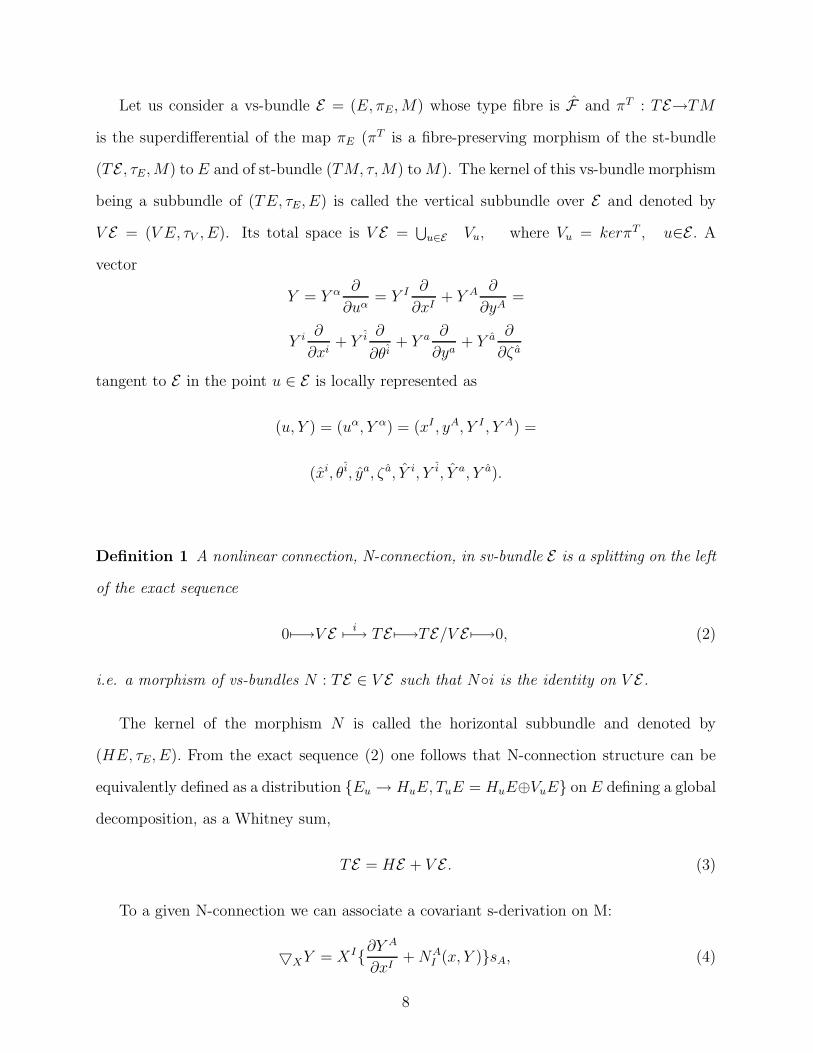
Let us consider a vs-bundle E = (E, πE,M) whose type fibre is F and πT : TE→TM

is the superdifferential of the map πE (πT is a fibre-preserving morphism of the st-bundle

(TE , τE,M) to E and of st-bundle (TM, τ,M) toM). The kernel of this vs-bundle morphism

being a subbundle of (TE, τE, E) is called the vertical subbundle over E and denoted by

V E = (V E, τV , E). Its total space is V E =⋃

u∈E Vu, where Vu = kerπT , u∈E . A

vector

Y = Y α ∂

∂uα= Y I ∂

∂xI+ Y A ∂

∂yA=

Y i ∂

∂xi+ Y i ∂

∂θi+ Y a ∂

∂ya+ Y a ∂

∂ζ a

tangent to E in the point u ∈ E is locally represented as

(u, Y ) = (uα, Y α) = (xI , yA, Y I , Y A) =

(xi, θi, ya, ζ a, Y i, Y i, Y a, Y a).

Definition 1 A nonlinear connection, N-connection, in sv-bundle E is a splitting on the left

of the exact sequence

0 7−→V Ei

7−→ TE 7−→TE/V E 7−→0, (2)

i.e. a morphism of vs-bundles N : TE ∈ V E such that Ni is the identity on V E .

The kernel of the morphism N is called the horizontal subbundle and denoted by

(HE, τE, E). From the exact sequence (2) one follows that N-connection structure can be

equivalently defined as a distribution Eu → HuE, TuE = HuE⊕VuE on E defining a global

decomposition, as a Whitney sum,

TE = HE + V E . (3)

To a given N-connection we can associate a covariant s-derivation on M:

XY = XI∂Y A

∂xI+NA

I (x, Y )sA, (4)

8

where sA are local independent sections of E , Y = Y AsA and X = XIsI .

S-differentiable functions NAI from (4) written as functions on xI and yA, NA

I (x, y),

are called the coefficients of the N-connection and satisfy these transformation laws under

coordinate transforms (1) in E :

NA′

I′∂xI′

∂xI= MA′

A NAI −

∂MA′

A (x)

∂xIyA.

If coefficients of a given N-connection are s- differentiable with respect to coordinates

yA we can introduce (additionally to covariant nonlinear s-derivation (4)) a linear covariant

s-derivation D (which is a generalization for sv-bundles of the Berwald connection [44]) given

as follows:

D( ∂

∂xI )(∂

∂yA) = NB

AI(∂

∂yB), D( ∂

∂yA )(∂

∂yB) = 0,

where

NABI(x, y) =

∂NAI(x, y)

∂yB(5)

and

NABC(x, y) = 0.

For a vector field on E Z = ZI ∂∂xI + Y A ∂

∂yA and B = BA(y) ∂∂yA being a section in the

vertical s-bundle (V E, τV , E) the linear connection (5) defines s-derivation (compare with

(4)):

DZB = [ZI(∂BA

∂xI+ NA

BIBB) + Y B ∂B

A

∂yB]∂

∂yA.

Another important characteristic of a N-connection is its curvature:

Ω =1

2ΩA

IJdxI ∧ dxJ ⊗

∂

∂yA

with local coefficients

ΩAIJ =

∂NAI

∂xJ− (−)|IJ |∂N

AJ

∂xI+NB

I NABJ − (−)|IJ |NB

J NABI ,

where for simplicity we have written (−)|K||J | = (−)|KJ|.

9

We note that linear connections are particular cases of N-connections, when NAI (x, y) are

parametrized as NAI (x, y) = KA

BI(x)xIyB, where functions KA

BI(x), defined on M, are called

the Christoffel coefficients.

IV. GEOMETRY OF THE TOTAL SPACE OF A SV-BUNDLE

The geometry of the sv- and st-bundles is very rich.It contains a lot of geometrical objects

and properties which could be of great importance in theoretical physics. In this section we

shall present the main results from geometry of total spaces of sv-bundles.In order to avoid

long computations and maintain the geometric meaning the notion of nonlinear connections

will systematically used in a manner generalizing to s-spaces the classical results [26,27].

A. Distinguished tensors and connections in sv-bundles

In sv-bundle E we can introduce a local basis adapted to the given N-connection:

δα =δ

δuα= (δI =

δ

δxI= ∂I −NA

I (x, y)∂

∂yA, ∂A), (6)

where ∂I = ∂∂xI and ∂A = ∂

∂yA are usual partial s-derivations. The dual to (6) basis is defined

as

δα = δuα =

(δI = δxI = dxI , δA = δyA = dyA +NAI (x, y)dxI). (7)

By using adapted bases (6) and (7) one introduces algebra DT (E) of distinguished tensor

s-fields (ds-fields, ds-tensors, ds-objects) on E , T = T prqs , which is equivalent to the tensor

algebra of sv-bundle πd : HE⊕V E→E , hereafter briefly denoted as Ed. An element Q∈T prqs ,

, ds-field of type

p r

q s

, can be written in local form as

Q = QI1...IpA1...Ar

J1...JqB1...Bs(x, y)δI1 ⊗ . . .⊗ δIp ⊗ dxJ1 ⊗ . . .⊗

10

dxJq ⊗ ∂A1 ⊗ . . .⊗ ∂Ar ⊗ δyB1 ⊗ . . .⊗ δyBs. (8)

In addition to ds-tensors we can introduce ds-objects with various s-group and coordinate

transforms adapted to global splitting (3).

Definition 2 A linear distinguished connection, d- connection, in sv- bundle E is a linear

connection D on E which preserves by parallelism the horizontal and vertical distributions

in E .

By a linear connection of a s-manifold we understand a linear connection in its tangent

bundle.

Let denote by Ξ(M) and Ξ(E), respectively, the modules of vector fields on s-manifold

M and sv-bundle E and by F(M) and F(E), respectively, the s-modules of functions on M

and on E .

It is clear that for a given global splitting into horizontal and vertical s-subbundles (3) we

can associate operators of horizontal and vertical covariant derivations (h- and v-derivations,

denoted respectively as D(h) and D(v)) with properties:

DXY = (XD)Y = DhXY +DvXY,

where

D(h)X Y = DhXY, D

(h)X f = (hX)f

and

D(v)X Y = DvXY, D

(v)X f = (vX)f,

for every f ∈ F(M) with decomposition of vectors X, Y ∈ Ξ(E) into horizontal and vertical

parts, X = hX + vX and Y = hY + vY.

The local coefficients of a d- connection D in E with respect to the local adapted frame

(6) separate into four groups. We introduce local coefficients (LIJK(u), LA

BK(u)) of D(h)

such that

D(h)

( δ

δxK )

δ

δxJ= LI

JK(u)δ

δxI,

11

D(h)

( δ

δxK )

∂

∂yB= LA

BK(u)∂

∂yA,

D(h)

( δ

δxk)f =

δf

δxK=

∂f

∂xK−NA

K(u)∂f

∂yA,

and local coefficients (CIJC(u), CA

BC(u)) such that

D(v)

( ∂

∂yC )

δ

δxJ= CI

JC(u)δ

δxI, D

(v)

( ∂

∂yC )

∂

∂yB= CA

BC

∂

∂yA,

D(v)

( ∂

∂yC )f =

∂f

∂yC,

where f ∈ F(E). The covariant d-derivation along vector X = XI δδxI +Y A ∂

∂yA of a ds-tensor

field Q of type

p r

q s

, see (8), can be written as

DXQ = D(h)X Q+D

(v)X Q,

where h-covariant derivative is defined as

D(h)X Q = XKQIA

JB|KδI⊗∂A⊗dxI⊗δyA,

with components

QIAJB|K =

δQIAJB

δxK+ LI

HKQHAJB + LA

CKWICJB − LH

JKWIAHB − LC

BKWIAJC ,

and v-covariant derivative is defined as

D(v)X Q = XCQIA

JB⊥CδI⊗∂A⊗dxI⊗δyB,

with components

QIAJB⊥C =

∂QIAJB

∂yC+ CI

HCQHAJB + CA

DCQIDJB − CH

JCQIAHB − CD

BCQIAJD.

The above presented formulas show that

DΓ = (L, L, C, C) =

(LAJK(u), LA

BK(u), CIJA(u), CA

BC(u))

12

are the local coefficients of the d-connection D with respect to the local frame ( δδxI ,

∂∂ya ). If

a change (1) of local coordinates on E is performed, by using the law of transformation of

local frames under it

( δα = (δI , ∂A) 7−→ δα′ = (δI′, ∂A′), (9)

where

δI′ =∂xI

∂xI′δI , ∂A′ = MA

A′(x)∂A ),

we obtain the following transformation laws of the local coefficients of a d-connection:

LI′

J ′K ′ =∂xI′

∂xI

∂xJ

∂xJ ′

∂xK

∂xK ′LI

JK +∂xI′

∂xK

∂2xK

∂xJ ′∂xK ′, (10)

LA′

B′K ′ = MA′

A MBB′

∂xK

∂xK ′LA

BK +MA′

C

∂MCB′

∂xK ′,

and

CI′

J ′C′ =∂xI′

∂xI

∂xJ

∂xJ ′MC

C′CIJC , C

A′

B′C′ = MA′

A MBB′MC

C′CABC .

As in the usual case of tensor calculus on locally isotropic spaces the transformation laws

(10) for d-connections differ from those for ds-tensors, which are written (for instance, we

consider transformation laws for ds-tensor (8)) as

QI′1...A′

1...

J ′

1...B′

1... =∂xI′1

∂xI1. . .M

A′

1A1. . .∂xJ1

∂xJ ′

1. . .MB1

B′

1. . .QI1...A1...

J1...B1....

We note that defined distinguished s-tensor algebra and d-covariant calculus in sv-bundles

provided with N-connection structure is a supersymmetric generalization of the correspond-

ing formalism for usual vector bundles presented in [26,27]. To obtain Miron and Anastasiei

local formulas we have to restrict us with even components of geometric objects by changing,

formally, capital indices (I, J,K, ...) into (i, j, k, a, ..) and s-derivation and s-commutation

rules into those for real number fields on usual manifolds. For brevity, in this work we shall

omit proofs and cumbersome computations if they will be simple supersymmetric general-

izations of those presented in the just cited monographs.

13

B. Torsion and curvature of the distinguished connection in sv-bundle

Let E = (E, πE ,M) be a sv–bundle endowed with N-connection and d-connection struc-

tures. The torsion of d-connection is introduced into usual manner:

T (X, Y ) = [X,DY − [X, Y , X, Y⊂Ξ(M).

The following decomposition is possible by using h– and v–projections (associated to N):

T (X, Y ) = T (hX, hY ) + T (hX, vY ) + T (vX, hX) + T (vX, vY ).

Taking into account the skewsupersymmetry of T and the equation h[vX, vY = 0 we can

verify that the torsion of a d-connection is completely determined by the following ds-tensor

fields:

hT (hX, hY ) = [X(D(h)h)Y − h[hX, hY ,

vT (hX, hY ) = −v[hX, hY ,

hT (hX, vY ) = −D(v)Y hX − h[hX, vY ,

vT (hX, vY ) = D(h)X vY − v[hX, vY ,

vT (vX, xY ) = [X(D(v)v)Y − v[vX, vY ,

where X, Y ∈ Ξ(E). In order to get the local form of the ds-tensor fields which determine

the torsion of d-connection DΓ (the torsions of DΓ) we use equations

[δ

δxJ,δ

δxK = RA

JK

∂

∂yA,

where

RAJK =

δNAJ

δxK− (−)|KJ| δN

AK

δxJ,

[δ

δxJ,∂

∂yA =

∂NAJ

∂yB

∂

∂yA,

and introduce notations

hT (δ

δxK,δ

δxJ) = T I

JK

δ

δxI, vT (

δ

δxK,δ

δxJ) = TA

JK

∂

∂yA, (11)

14

hT (∂

∂yA,∂

∂xJ) = P I

JB

δ

δxI, vT (

∂

∂yB,δ

δxJ) = PA

JB

∂

∂yA,

vT (∂

∂yB,∂

∂yB) = SA

BC

∂

∂yA.

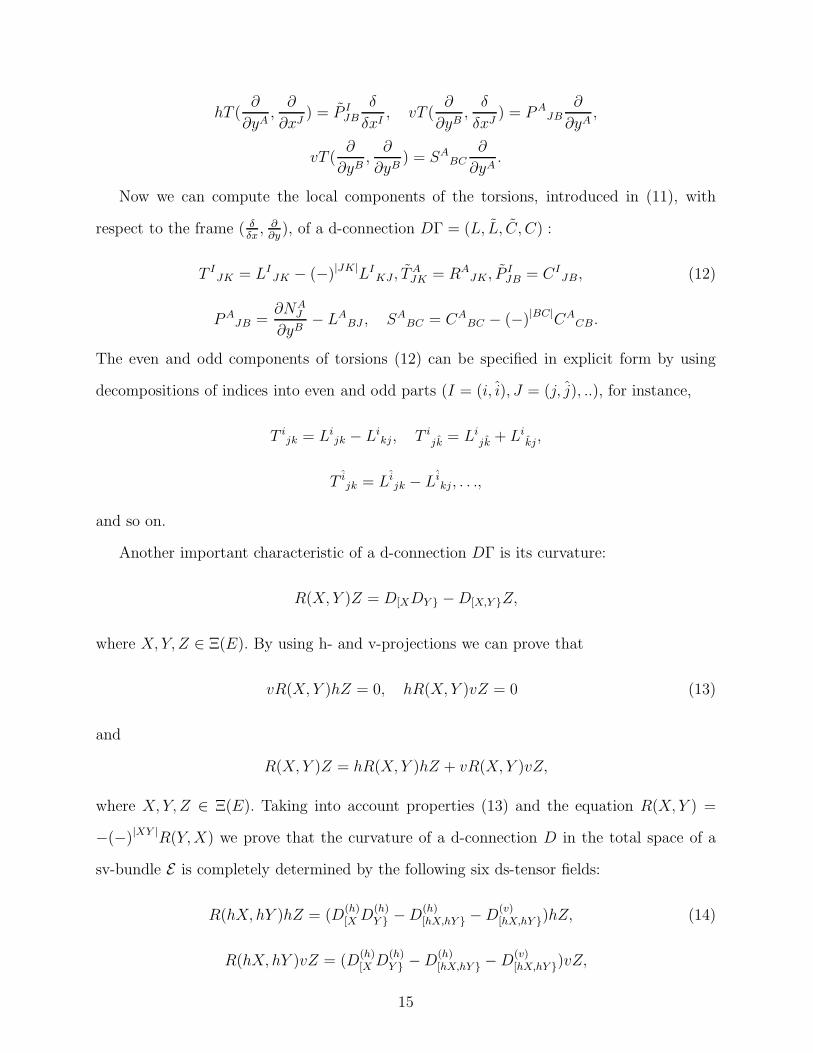
Now we can compute the local components of the torsions, introduced in (11), with

respect to the frame ( δδx, ∂

∂y), of a d-connection DΓ = (L, L, C, C) :

T IJK = LI

JK − (−)|JK|LIKJ , T

AJK = RA

JK , PIJB = CI

JB, (12)

PAJB =

∂NAJ

∂yB− LA

BJ , SABC = CA

BC − (−)|BC|CACB.

The even and odd components of torsions (12) can be specified in explicit form by using

decompositions of indices into even and odd parts (I = (i, i), J = (j, j), ..), for instance,

T ijk = Li

jk − Likj, T i

jk = Lijk + Li

kj,

T ijk = Li

jk − Likj, . . .,

and so on.

Another important characteristic of a d-connection DΓ is its curvature:

R(X, Y )Z = D[XDY −D[X,Y Z,

where X, Y, Z ∈ Ξ(E). By using h- and v-projections we can prove that

vR(X, Y )hZ = 0, hR(X, Y )vZ = 0 (13)

and

R(X, Y )Z = hR(X, Y )hZ + vR(X, Y )vZ,

where X, Y, Z ∈ Ξ(E). Taking into account properties (13) and the equation R(X, Y ) =

−(−)|XY |R(Y,X) we prove that the curvature of a d-connection D in the total space of a

sv-bundle E is completely determined by the following six ds-tensor fields:

R(hX, hY )hZ = (D(h)[X D

(h)Y −D

(h)[hX,hY −D

(v)[hX,hY )hZ, (14)

R(hX, hY )vZ = (D(h)[X D

(h)Y −D

(h)[hX,hY −D

(v)[hX,hY )vZ,

15

R(vX, hY )hZ = (D(v)[XD

(h)Y −D

(h)[vX,hY −D

(v)[vX,hY )hZ,

R(vX, hY )vZ = (D(v)[XD

(h)Y −D

(h)[vX,hY −D

(v)[vX,hY )vZ,

R(vX, vY )hZ = (D(v)[XD

(v)Y −D

(v)[vX,vY )hZ,

R(vX, vY )vZ = (D(v)[XD

(v)Y −D

(v)[vX,vY )vZ,

where

D(h)[X D

(h)Y = D

(h)X D

(h)Y − (−)|XY |D

(h)Y D

(h)X ,

D(h)[X D

(v)Y = D

(h)X D

(v)Y − (−)|XY |D

(v)Y D

(h)X

and

D(v)[XD

(h)Y = D

(v)X D

(h)Y − (−)|XY |D

(h)Y D

(v)X .

We introduce the local components of ds-tensor fields (14) as follows:

R(δK , δJ)δH = RHIJKδI , R(δK , δJ)∂B = R·A

B·JK∂A, (15)

R(∂C , δK)δJ = P ·IJ ·KCδI , R(∂C , δK)∂B = PB

AKC∂A,

R(∂C , ∂B)δJ = S ·IJ ·BCδI , R(∂D, ∂C)∂B = SB

ACD∂A.

Putting the components of a d-connection DΓ = (L, L, C, C) in (15), by a direct computa-

tion, we obtain these locally adapted components of the curvature (curvatures):

RHIJK = δKL

IHJ − (−)|KJ |δJL

IHK + LM

HJLIMK − (−)|KJ |LM

HKLIMJ + CI

HARA

JK ,

R·AB·JK = δKL

ABJ − (−)|KJ |δJL

ABK + LC

BJLA

CK − (−)|KJ |LCBKL

AKJ + CA

BCRC

JK ,

P ·IJ ·KA = ∂AL

IJK − CI

JA|K + CIJBP

BKA, (16)

PBA

KC = ∂CLA

BK − CABC|K + CA

BDPD

KC,

S ·IJ ·BC = ∂CC

IJB − (−)|BC|∂BC

IJC + CH

JB − (−)|BC|CHJCC

IHB,

SBA

CD = ∂DCA

BC − (−)|CD|∂CCA

BD + CEBCC

AED − (−)|CD|CE

BDCA

EC.

16

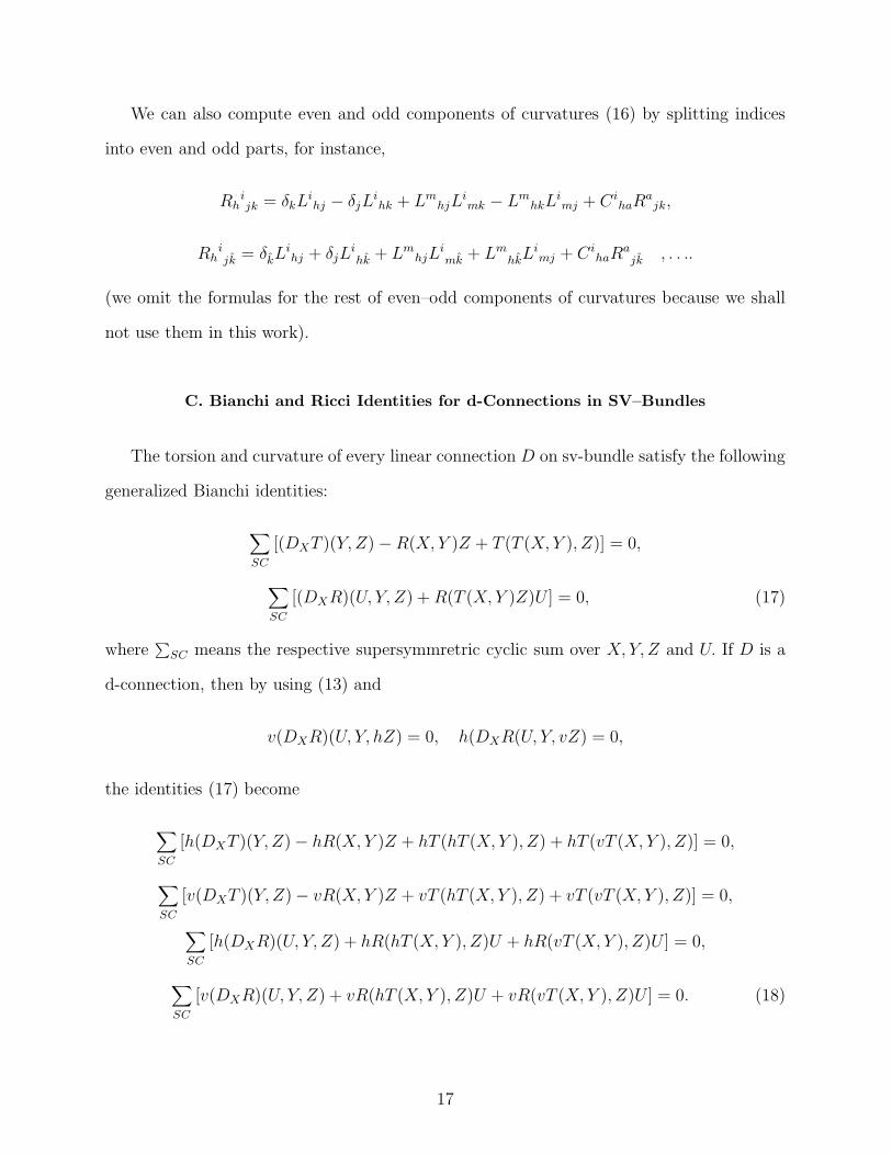
We can also compute even and odd components of curvatures (16) by splitting indices

into even and odd parts, for instance,

Rhijk = δkL

ihj − δjL

ihk + Lm

hjLimk − Lm

hkLimj + Ci

haRajk,

Rhijk = δkL

ihj + δjL

ihk + Lm

hjLimk + Lm

hkLimj + Ci

haRajk , . . ..

(we omit the formulas for the rest of even–odd components of curvatures because we shall

not use them in this work).

C. Bianchi and Ricci Identities for d-Connections in SV–Bundles

The torsion and curvature of every linear connection D on sv-bundle satisfy the following

generalized Bianchi identities:

∑

SC

[(DXT )(Y, Z) −R(X, Y )Z + T (T (X, Y ), Z)] = 0,

∑

SC

[(DXR)(U, Y, Z) +R(T (X, Y )Z)U ] = 0, (17)

where∑

SC means the respective supersymmretric cyclic sum over X, Y, Z and U. If D is a

d-connection, then by using (13) and

v(DXR)(U, Y, hZ) = 0, h(DXR(U, Y, vZ) = 0,

the identities (17) become

∑

SC

[h(DXT )(Y, Z) − hR(X, Y )Z + hT (hT (X, Y ), Z) + hT (vT (X, Y ), Z)] = 0,

∑

SC

[v(DXT )(Y, Z) − vR(X, Y )Z + vT (hT (X, Y ), Z) + vT (vT (X, Y ), Z)] = 0,

∑

SC

[h(DXR)(U, Y, Z) + hR(hT (X, Y ), Z)U + hR(vT (X, Y ), Z)U ] = 0,

∑

SC

[v(DXR)(U, Y, Z) + vR(hT (X, Y ), Z)U + vR(vT (X, Y ), Z)U ] = 0. (18)

17

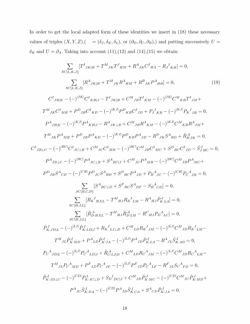
In order to get the local adapted form of these identities we insert in (18) these necessary

values of triples (X, Y, Z),( = (δJ , δK , δL), or (∂D, ∂C , ∂B),) and putting successively U =

δH and U = ∂A. Taking into account (11),(12) and (14),(15) we obtain:

∑

SC[L,K,J

[T IJK|H + TM

JKTJ

HM +RAJKC

IHA − RJ

IKH ] = 0,

∑

SC[L,K,J

[RAJK|H + TM

JKRA

HM +RBJKP

AHB] = 0, (19)

CIJB|K − (−)|JK|CI

KB|J − T IJK|B + CM

JBTIKM − (−)|JK|CM

KBTIJM+

TMJKC

IMB + PD

JBCIKD − (−)|KJ |PD

KBCIJD + PJ

IKB − (−)|KJ |PK

IJB = 0,

PAJB|K − (−)|KJ |PA

KB|J −RAJK⊥B + CM

JBRA

KM − (−)|KJ |CMKBR

AJM+

TMJKP

AMB + PD

JBPA

KD − (−)|KJ |PDKBP

AJD − RD

JKSA

BD + R·AB·JK = 0,

CIJB⊥C − (−)|BC|CI

JC⊥B + CMJCC

IMB − (−)|BC|CM

JBCIMC + SD

BCCIJD − S ·I

J ·BC = 0,

PAJB⊥C − (−)|BC|PA

JC⊥B + SABC|J + CM

JCPA

MB − (−)|BC|CMJBP

AMC+

PDJBS

ACD − (−)|CB|PD

JCSA

BD + SDBCP

AJD + PB

AJC − (−)|CB|PC

AJB = 0,

∑

SC[B,C,D

[SABC⊥D + SF

BCSA

DF − SBA

CD] = 0,

∑

SC[H,J,L

[RKIHJ |L − TM

HJRKILM − RA

HJ P·IK·LA] = 0,

∑

SC[H,J,L

[R·AD·HJ |L − TM

HJR·AD·LM − RC

HJPDA

LC ] = 0,

P ·IK·JD|L − (−)|LJ |P ·I

K·LD|J +RKILJ⊥D + CM

LDRKIJM − (−)|LJ |CM

JDRKILM−

TMJLP

·IK·MD + PA

LDP·IK·JA − (−)|LJ |PA

JDP·IK·LA − RA

JLS·IK·AD = 0,

PCA

JD|L − (−)|LJ |PCA

LD|J + R·AC·LJ |D + CM

LDRCA

JM − (−)|LJ |CMJDRC

ALM−

TMJLPC

AMD + P F

LDPCA

JF − (−)|LJ |P FJDPC

ALF − RF

JLSCA

FD = 0,

P ·IK·JD⊥C − (−)|CD|P ·I

K·JC⊥D + SDIDC|J + CM

JDP·IK·MC − (−)|CD|CM

JCP·IK·MD+

PAJCS

·IK·DA − (−)|CD|PA

JDS·IK·CA + SA

CDP·IK·JA = 0,

18

PBA

JD⊥C − (−)|CD|PBA

JC⊥D + SBA

CD|J + CMJDPB

AMC − (−)|CD|CM

JCPBA

MD+

P FJCSB

ADF − (−)|CD|P F

JDSBA

CF + SFCDPB

AJF = 0,

∑

SC[B,C,D

[SKIBC⊥D − SA

BCS·IK·DA] = 0,

∑

SC[B,C,D

[SFA

BC⊥D − SEBCSF

ADE] = 0,

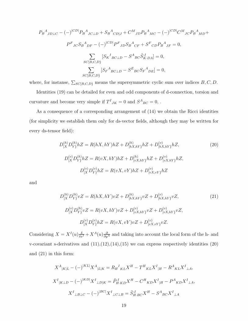
where, for instanse,∑

SC[B,C,D means the supersymmetric cyclic sum over indices B,C,D.

Identities (19) can be detailed for even and odd components of d-connection, torsion and

curvature and become very simple if T IJK = 0 and SA

BC = 0, .

As a consequence of a corresponding arrangement of (14) we obtain the Ricci identities

(for simplicity we establish them only for ds-vector fields, although they may be written for

every ds-tensor field):

D(h)[X D

(h)Y hZ = R(hX, hY )hZ +D

(h)[hX,hY hZ +D

(v)[hX,hY hZ, (20)

D(v)[XD

(h)Y hZ = R(vX, hY )hZ +D

(h)[vX,hY hZ +D

(v)[vX,hY hZ,

D(v)[XD

(v)Y hZ = R(vX, vY )hZ +D

(v)[vX,vY hZ

and

D(h)[X D

(h)Y vZ = R(hX, hY )vZ +D

(h)[hX,hY vZ +D

(v)[hX,hY vZ, (21)

D(v)[XD

(h)Y vZ = R(vX, hY )vZ +D

(v)[vX,hY vZ +D

(v)[vX,hY vZ,

D(v)[XD

(v)Y hZ = R(vX, vY )vZ +D

(v)[vX,vY vZ.

Considering X = XI(u) δδxI +XA(u) ∂

∂yA and taking into account the local form of the h- and

v-covariant s-derivatives and (11),(12),(14),(15) we can express respectively identities (20)

and (21) in this form:

XA|K|L − (−)|KL|XA

|L|K = RHIKLX

H − THKLX

I|H − RA

KLXI⊥A,

XI|K⊥D − (−)|KD|XI

⊥D|K = P ·IH·KDX

H − CHKDX

I|H − PA

KDXI⊥A,

XI⊥B⊥C − (−)|BC|XI

⊥C⊥B = S ·IH·BCX

H − SABCX

I⊥A

19

and

XA|K|L − (−)|KL|XA

|L|K = RBS

KLXB − TH

KLXA|H − RB

KLXA⊥B,

XA|K⊥B − (−)|BC|XA

⊥B|K = PBA

KBXC − CH

KBXA|H − PD

KBXA⊥B,

XA⊥B⊥C − (−)|CB|XA

⊥C⊥B = SDA

BCXD − SD

BCXA⊥D.

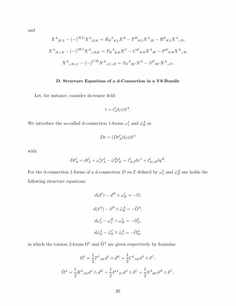
D. Structure Equations of a d-Connection in a VS-Bundle

Let, for instance, consider ds-tensor field:

t = tIAδI⊗δA.

We introduce the so-called d-connection 1-forms ωIJ and ωA

B as

Dt = (DtIA)δI⊗δA

with

DtIA = dtIA + ωIJt

JA − ωB

A tIB = tIA|Jdx

J + tIA⊥BδyB.

For the d-connection 1-forms of a d-connection D on E defined by ωIJ and ωA

B one holds the

following structure equations:

d(dI) − dH ∧ ωIH = −Ω,

d(δA) − δB ∧ ωAB = −ΩA,

dωIJ − ωH

J ∧ ωIH = −ΩI

J ,

dωAB − ωC

B ∧ ωAC = −ΩA

B ,

in which the torsion 2-forms ΩI and ΩA are given respectively by formulas:

ΩI =1

2T I

JKdJ ∧ dK +

1

2CI

JKdJ ∧ δC ,

ΩA =1

2RA

JKdJ ∧ dK +

1

2PA

JCdJ ∧ δC +

1

2SA

BCδB ∧ δC ,

20

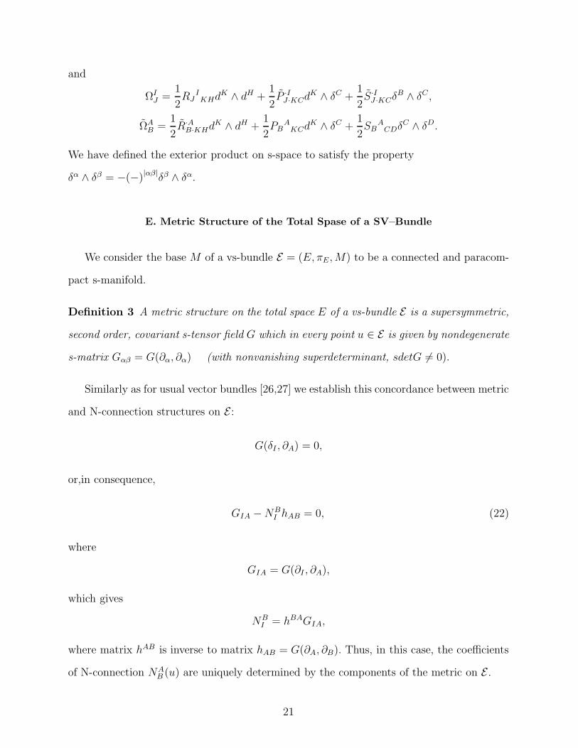
and

ΩIJ =

1

2RJ

IKHd

K ∧ dH +1

2P ·I

J ·KCdK ∧ δC +

1

2S ·I

J ·KCδB ∧ δC ,

ΩAB =

1

2R·A

B·KHdK ∧ dH +

1

2PB

AKCd

K ∧ δC +1

2SB

ACDδ

C ∧ δD.

We have defined the exterior product on s-space to satisfy the property

δα ∧ δβ = −(−)|αβ|δβ ∧ δα.

E. Metric Structure of the Total Spase of a SV–Bundle

We consider the base M of a vs-bundle E = (E, πE ,M) to be a connected and paracom-

pact s-manifold.

Definition 3 A metric structure on the total space E of a vs-bundle E is a supersymmetric,

second order, covariant s-tensor field G which in every point u ∈ E is given by nondegenerate

s-matrix Gαβ = G(∂α, ∂α) (with nonvanishing superdeterminant, sdetG 6= 0).

Similarly as for usual vector bundles [26,27] we establish this concordance between metric

and N-connection structures on E :

G(δI , ∂A) = 0,

or,in consequence,

GIA −NBI hAB = 0, (22)

where

GIA = G(∂I , ∂A),

which gives

NBI = hBAGIA,

where matrix hAB is inverse to matrix hAB = G(∂A, ∂B). Thus, in this case, the coefficients

of N-connection NAB (u) are uniquely determined by the components of the metric on E .

21

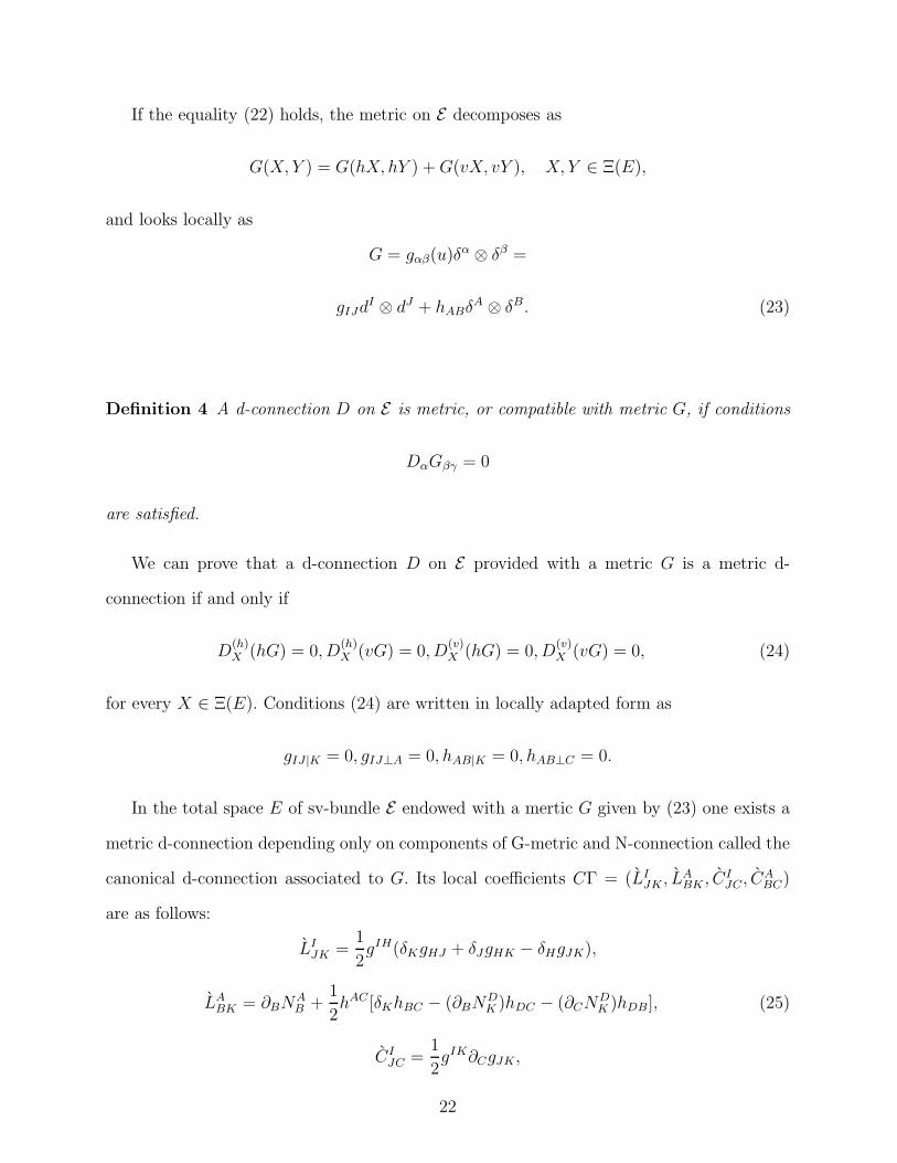
If the equality (22) holds, the metric on E decomposes as

G(X, Y ) = G(hX, hY ) +G(vX, vY ), X, Y ∈ Ξ(E),

and looks locally as

G = gαβ(u)δα ⊗ δβ =

gIJdI ⊗ dJ + hABδ

A ⊗ δB. (23)

Definition 4 A d-connection D on E is metric, or compatible with metric G, if conditions

DαGβγ = 0

are satisfied.

We can prove that a d-connection D on E provided with a metric G is a metric d-

connection if and only if

D(h)X (hG) = 0, D

(h)X (vG) = 0, D

(v)X (hG) = 0, D

(v)X (vG) = 0, (24)

for every X ∈ Ξ(E). Conditions (24) are written in locally adapted form as

gIJ |K = 0, gIJ⊥A = 0, hAB|K = 0, hAB⊥C = 0.

In the total space E of sv-bundle E endowed with a mertic G given by (23) one exists a

metric d-connection depending only on components of G-metric and N-connection called the

canonical d-connection associated to G. Its local coefficients CΓ = (LIJK , L

ABK , C

IJC, C

ABC)

are as follows:

LIJK =

1

2gIH(δKgHJ + δJgHK − δHgJK),

LABK = ∂BN

AB +

1

2hAC [δKhBC − (∂BN

DK )hDC − (∂CN

DK )hDB], (25)

CIJC =

1

2gIK∂CgJK,

22

CABC =

1

2hAD(∂ChDB + ∂BhDC − ∂DhBC).

We point out that, in general, the torsion of CΓ–connection (25) das not vanish (see formulas

(12)).

It is very important to note that on sv-bundles provided with N-connection and d-

connection and metric structures realy it is defined a multiconnection d-structure, i.e. we

can use in an equivalent geometric manner different variants of d- connections with various

properties. For example, for modeling of some physical processes we can use the Berwald

type d–connection (see (5))

BΓ = (LIJK , ∂BN

AK , 0, C

ABC), (26)

where LIJK = LI

JK and CABC = CA

BC , which is hv-metric, i.e. satisfies conditions:

D(h)X hG = 0

and

D(v)X vG = 0,

for every X ∈ Ξ(E), or in locally adapted coordinates,

gIJ |K = 0

and

hAB⊥C = 0.

As well we can introduce the Levi-Civita connection

α

βγ =

1

2Gαβ(∂βGτγ + ∂γGτβ − ∂τGβγ),

constructed as in the Riemann geometry from components of metric Gαβ by using partial

derivations ∂α = ∂∂uα = ( ∂

∂xI ,∂

∂yA ) which is metric but not a d-connection.

Another metric d-connection can be defined as

Γαβγ =

1

2Gατ (δβGτγ + δγGτβ − δτGβγ), (27)

23

with components CΓ = (LIJK , 0, 0, C

ABC), where coefficients LI

JK and CABC are computed

as in formulas (26). We call the coefficients (27) the generalized Christofell symbols on vs-

bundle E .

For our further considerations it is useful to express arbitrary d-connection as a defor-

mation of the background d-connection (26):

Γαβγ = Γα

·βγ + P αβγ, (28)

where P αβγ is called the deformation ds-tensor. Putting splitting (29) into (12) and (16)

we can express torsion T αβγ and curvature Rβ

αγδ

of a d-connection Γαβγ as respective de-

formations of torsion T αβγ and torsion R·α

β·γδ for connection Γαβγ :

T αβγ = T α

·βγ + T α·βγ (29)

and

Rβα

γδ= R·α

β·γδ + R·αβ·γδ, (30)

where

T αβγ = Γα

βγ − (−)|βγ|Γαγβ + wα

γδ, T αβγ = Γα

βγ − (−)|βγ|Γαγβ,

and

R·αβ·γδ = δδΓ

αβγ − (−)|γδ|δγΓ

αβδ + Γϕ

βγΓαϕδ − (−)|γδ|Γϕ

βδΓαϕγ + Γα

βϕwϕ

γδ,

R·αβ·γδ = DδP

αβγ − (−)|γδ|DγP

αβδ + P ϕ

βγPα

ϕδ − (−)|γδ|P ϕβδP

αϕγ + P α

βϕwϕ

γδ,

the nonholonomy coefficients wαβγ are defined as

[δα, δβ = δαδβ − (−)αβδβδα = wταβδτ .

Finally, in this section we remark that if from geometric point of view all considered d-

connections are ”equal in rights” , the construction of physical models on la-spaces requires

an explicit fixing of the type of d-connection and metric structures.

24

V. SUPERSYMMETRIC EXTENSIONS OF GENERALIZED LAGRANGE AND

FINSLER SPACES

Let us fix our attention to the st-bundle TM.The aim of this section is to formulate

some results in the supergeometry of TM and to use them in order to develop the geometry

of Finsler and Lagrange superspaces (classical and new approaches to Finsler geometry, its

generalizations and applications in physics are contained,for example, in [20-30].

All presented in the previous section basic results on sv-bundles provided with N-

connection, d-connection and metric structures hold good for TM. In this case the dimension

of the base space and typical fibre coincides and we can write locally, for instance, s-vectors

as

X = XIδI + Y I∂I = XIδI + Y (I)∂(I),

where uα = (xI , yJ) = (xI , y(J)).

On st-bundles we can define a global map

J : Ξ(TM) → Ξ(TM) (31)

which does not depend on N-connection structure:

J(δ

δxI) =

∂

∂yI

and

J(∂

∂yI) = 0.

This endomorphism is called the natural (or canonical) almost tangent structure on TM ; it

has the properties:

1)J2 = 0, 2)ImJ = KerJ = V TM

and 3) the Nigenhuis s-tensor,

NJ(X, Y ) = [JX, JY − J [JX, Y − J [X, JY ]

(X, Y ∈ Ξ(TN))

identically vanishes, i.e. the natural almost tangent structure J on TM is integrable.

25

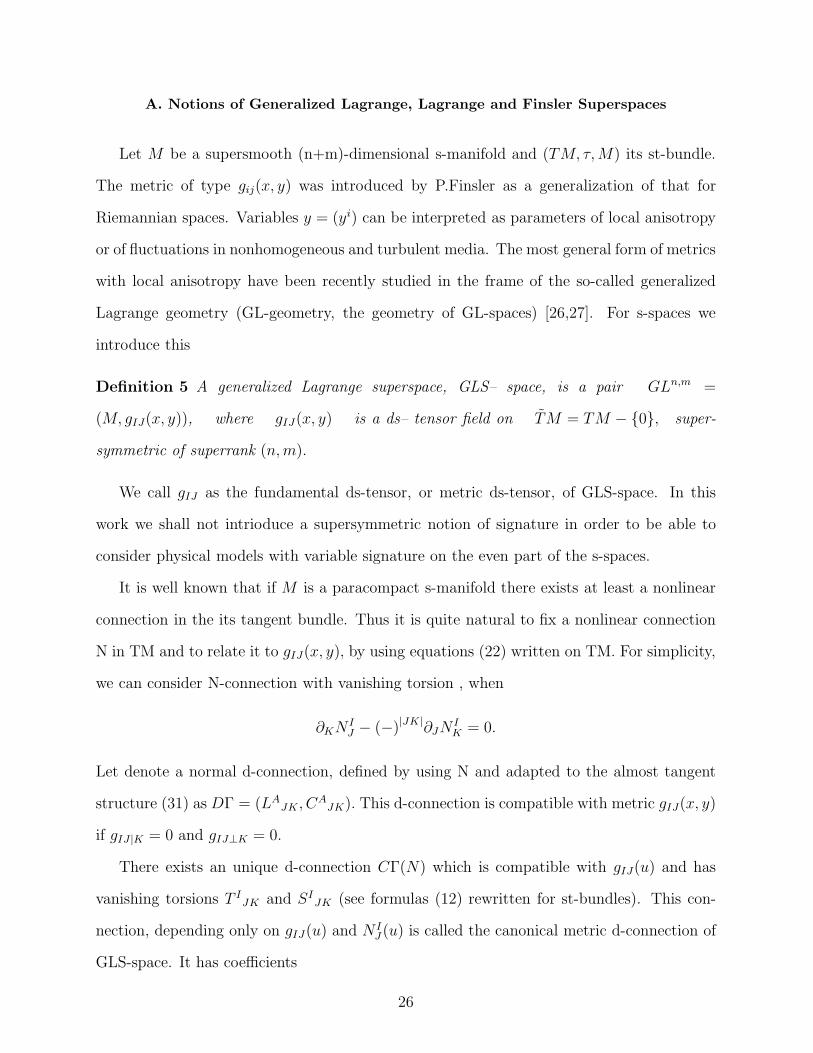
A. Notions of Generalized Lagrange, Lagrange and Finsler Superspaces

Let M be a supersmooth (n+m)-dimensional s-manifold and (TM, τ,M) its st-bundle.

The metric of type gij(x, y) was introduced by P.Finsler as a generalization of that for

Riemannian spaces. Variables y = (yi) can be interpreted as parameters of local anisotropy

or of fluctuations in nonhomogeneous and turbulent media. The most general form of metrics

with local anisotropy have been recently studied in the frame of the so-called generalized

Lagrange geometry (GL-geometry, the geometry of GL-spaces) [26,27]. For s-spaces we

introduce this

Definition 5 A generalized Lagrange superspace, GLS– space, is a pair GLn,m =

(M, gIJ(x, y)), where gIJ(x, y) is a ds– tensor field on TM = TM − 0, super-

symmetric of superrank (n,m).

We call gIJ as the fundamental ds-tensor, or metric ds-tensor, of GLS-space. In this

work we shall not intrioduce a supersymmetric notion of signature in order to be able to

consider physical models with variable signature on the even part of the s-spaces.

It is well known that if M is a paracompact s-manifold there exists at least a nonlinear

connection in the its tangent bundle. Thus it is quite natural to fix a nonlinear connection

N in TM and to relate it to gIJ(x, y), by using equations (22) written on TM. For simplicity,

we can consider N-connection with vanishing torsion , when

∂KNIJ − (−)|JK|∂JN

IK = 0.

Let denote a normal d-connection, defined by using N and adapted to the almost tangent

structure (31) as DΓ = (LAJK , C

AJK). This d-connection is compatible with metric gIJ(x, y)

if gIJ |K = 0 and gIJ⊥K = 0.

There exists an unique d-connection CΓ(N) which is compatible with gIJ(u) and has

vanishing torsions T IJK and SI

JK (see formulas (12) rewritten for st-bundles). This con-

nection, depending only on gIJ(u) and N IJ (u) is called the canonical metric d-connection of

GLS-space. It has coefficients

26

LIJK =

1

2gIH(δJgHK + δHgJK − δHgJK), (32)

CIJK =

1

2gIH(∂JgHK + ∂HgJK − ∂HgJK).

Of course, metric d-connections different from CΓ(N) may be found. For instance, there is

a unique normal d-connection DΓ(N) = (LI·JK , C

I·JK) which is metric and has a priori given

torsions T IJK and SI

JK . The coefficients of DΓ(N) are the following ones:

LI·JK = LI

JK −1

2gIH(gJRT

RHK + gKRT

RHJ − gHRT

RKJ),

CI·JK = CI

JK −1

2gIH(gJRS

RHK + gKRS

RHJ − gHRS

RKJ),

where LIJK and CI

JK are the same as for the CΓ(N)–connection (32).

The Lagrange spaces were introduced [46] in order to geometrize the concept of La-

grangian in mechanics. The Lagrange geometry is studied in details in [26,27]. For s-spaces

we present this generalization:

Definition 6 A Lagrange s-space, LS-space, Ln,m = (M, gIJ), is defined as a particular case

of GLS-space when the ds-metric on M can be expressed as

gIJ(u) =1

2

∂2L

∂yI∂yJ, (33)

where L : TM → Λ, is a s-differentiable function called a s-Lagrangian on M.

Now we consider the supersymmetric extension of the Finsler space:

A Finsler s-metric on M is a function FS : TM → Λ having the properties:

1. The restriction of FS to ˜TM = TM \0 is of the class G∞ and F is only supersmooth

on the image of the null cross–section in the st-bundle to M.

2. The restriction of F to ˜TM is positively homogeneous of degree 1 with respect to (yI),

i.e. F (x, λy) = λF (x, y), where λ is a real positive number.

3. The restriction of F to the even subspace of ˜TM is a positive function.

4. The quadratic form on Λn,m with the coefficients

gIJ(u) =1

2

∂2F 2

∂yI∂yJ(34)

defined on ˜TM is nondegenerate.

27

Definition 7 A pair F n,m = (M,F ) which consists from a supersmooth s-manifold M and

a Finsler s-metric is called a Finsler superspace, FS-space.

It’s obvious that FS-spaces form a particular class of LS-spaces with s-Lagrangian L = F 2

and a particular class of GLS-spaces with metrics of type (34).

For a FS-space we can introduce the supersymmetric variant of nonlinear Cartan con-

nection [24,25]:

N IJ (x, y) =

∂

∂yJG∗I ,

where

G∗I =1

4g∗IJ(

∂2ε

∂yI∂xKyK −

∂ε

∂xJ), ε(u) = gIJ(u)yIyJ ,

and g∗IJ is inverse to g∗IJ(u) = 12

∂2ε∂yI∂yJ . In this case the coefficients of canonical metric d-

connection (32) gives the supersymmetric variants of coefficients of the Cartan connection

of Finsler spaces. A similar remark applies to the Lagrange superspaces.

B. The Supersymmetric Almost Hermitian Model of the GLS–Space

Consider a GLS–space endowed with the canonical metric d-connection CΓ(N). Let

δα = (δα, ∂I) be a usual adapted frame (6) on TM and δα = (∂I , δI) its dual. The linear

operator

F : Ξ( ˜TM) → Ξ( ˜TM),

acting on δα by F (δI = −∂I , F (∂I) = δI , defines an almost complex structure on ˙TM.

We shall obtain a complex structure if and only if the even component of the horizontal

distribution N is integrable. For s-spaces, in general with even and odd components, we

write the supersymmetric almost Hermitian property (almost Hermitian s-structure) as

F αβ F

βδ = −(−)|αδ|δα

β .

The s-metric gIJ(x, y) on GLS-spaces induces on ˙TM the following metric:

G = gIJ(u)dxI ⊗ dxJ + gIJ(u)δyI ⊗ δyJ . (35)

28

We can verify that pair (G,F ) is an almost Hermitian s-structure on ˙TM with the associated

supersymmetric 2-form

θ = gIJ(x, y)δyI ∧ dxJ .

The almost Hermitian s-space H2n,2mS = (TM,G, F ), provided with a metric of type (35)

is called the lift on TM, or the almost Hermitian s-model, of GLS-space GLn,m. We say

that a linear connection D on ˙TM is almost Hermitian supersymmetric of Lagrange type

if it preserves by parallelism the vertical distribution V and is compatible with the almost

Hermitian s-structure (G,F ), i.e.

DXG = 0, DXF = 0, (36)

for every X ∈ Ξ(TM).

There exists an unique almost Hermitian connection of Lagrange type D(c) having h(hh)-

and v(vv)–torsions equal to zero. We can prove (similarly as in [26,27]) that coefficients

(LIJK , C

IJK) ofD(c) in the adapted basis (δI , δJ) are just the coefficients (32) of the canonical

metric d-connection CΓ(N) of the GLS-space GL(n,m). Inversely , we can say that CΓ(N)–

connection determines on ˜TN and supersymmetric almost Hermitian connection of Lagrange

type with vanishing h(hh)- and v(vv)-torsions. If instead of GLs-space metric gIJ in (34)

the Lagrange (or Finsler) s-metric (32) (or (33)) is taken, we obtain the almost Hermitian

s-model of Lagrange (or Finsler) s-spaces Ln,m (or F n,m).

We note that the natural compatibility conditions (36) for the metric (35) and CΓ(N)–

connections on H2n,2m–spaces plays an important role for developing physical models on

la–superspaces. In the case of usual locally anisotropic spaces geometric constructions and

d–covariant calculus are very similar to those for the Riemann and Einstein–Cartan spaces.

This is exploited for formulation in a selfconsistent manner the theory of spinors on la-spaces

[35], for introducing a geometric background for locally anisotropic Yang–Mills and gauge

like gravitational interactions [31,32] and for extending the theory of stochastic processes

and diffusion to the case of locally anisotropic spaces and interactions on such spaces [47]. In

29

a similar manner we shall use in this work N–lifts to sv- and st-bundles in order to investigate

supergravitational la–models.

VI. SUPERGRAVITY ON LOCALLY ANISOTROPIC SUPERSPACES

In this section we shall introduce a set of Einstein and (equivalent in our case) gauge like

gravitational equations, i.e. we shall formulate two variants of la–supergravity, on the total

space E of a sv-bundle E over a supersmooth manifold M. The first model will be a variant of

locally anisotropic supergravity theory generalizing the Miron and Anastasiei model [26,27]

on vector bundles (they considered prescribed components of N-connection and h(hh)- and

v(vv)–torsions, in our approach we shall introduce algebraic equations for torsion and its

source). The second model will be a la–supersymmetric extension of constructions for gauge

la-gravity [31,32] and affine–gauge interpretation of the Einstein gravity [55,56]. There are

two ways in developing supergravitational models. We can try to maintain similarity to

Einstein’s general relativity (see in [48,49] an example of locally isotropic supergravity) and

to formulate a variant of Einstein–Cartan theory on sv–bundles, this will be the aim of the

subsection A, or to introduce into consideration supervielbein variables and to formulate

a supersymmetric gauge like model of la-supergravity (this approach is more accepted in

the usual locally isotropic supergravity, see as a review [45]). The last variant will be

analysed in subsection B by using the s-bundle of supersymmetric affine adapted frames

on la-superspaces. For both models of la–supergravity we shall consider the matter field

contributions as giving rise to corresponding sources in la-supergravitational field equations.

A detailed study of supersymmetric of la–gravitational and matter fields is a matter of our

further investigations [58].

30

A. Einstein–Cartan Equations on SV–Bundles

Let consider a sv–bundle E = (E, π,M) provided with some compatible nonlinear con-

nection N, d–connection D and metric G structures.For a locally N-adapted frame we write

D( δδuγ )

δ

δuβ= Γα

βγ

δ

δuα,

where the d-connection D has the following coefficients:

ΓIJK = LI

JK ,

ΓIJA = CI

JA,ΓIAJ = 0,ΓI

AB = 0,ΓAJK = 0,ΓA

JB = 0,ΓABK = LA

BK ,ΓA

BC = CABC .

(37)

The nonholonomy coefficients wγαβ, defined as [δα, δβ = wγ

αβδγ, are as follows:

wKIJ = 0, wK

AJ = 0, wKIA = 0, wK

AB = 0, wAIJ = RA

IJ ,

wBAI = −(−)|IA|∂N

BA

∂yA, wB

IA =∂NB

A

∂yA, wC

AB = 0.

By straightforward calculations we can obtain respectively these components of torsion,

T (δγ, δβ) = T α·βγδα, and curvature, R(δβ , δγ)δτ = R·α

β·γτδα, ds-tensors:

T I·JK = T I

JK , TI·JA = CI

JA, TI·JA = −CI

JA, TI·AB = 0, (38)

T A·IJ = RA

IJ , TA·IB = −PA

BI , TA·BI = PA

BI , TA·BC = SA

BC

and

R·JI·KL = RJ

IKL,R

·JB·KL = 0,R·A

J ·KL = 0,R·AB·KL = R·A

B·KL, (39)

R·IJ ·KD = PJ

IKD,R

·AB·KD = 0,R·A

J ·KD = 0,R·AB·KD = PB

AKD,

R·IJ ·DK = −PJ

IKD,R

·IB·DK = 0,R·A

J ·DK = 0,R·HB·DK = −PB

AKD,

R·IJ ·CD = SJ

ICD,R

·IB·CD = 0,R·A

J ·CD = 0,R·AB·CD = SB

ACD

(for explicit dependencies of components of torsions and curvatures on components of d-

connection see formulas (12) and (16)).

31

The locally adapted components Rαβ = Ric(D)(δα, δβ) (we point that in general on

st-bundles Rαβ 6= (−)|αβ|Rβα) of the Ricci tensor are as follows:

RIJ = RIK

JK ,RIA = −(2)PIA = −P ·KI·KA (40)

RAI = (1)PAI = P ·BA·IB,RAB = SA

CBC = SAB.

For scalar curvature, R = Sc(D) = GαβRαβ , we have

Sc(D) = R + S, (41)

where R = gIJRIJ and S = hABSAB.

The Einstein–Cartan equations on sv-bundles are written as

Rαβ −1

2GαβR + λGαβ = κ1Jαβ, (42)

and

T α·βγ +Gβ

αT τγτ − (−)|βγ|Gγ

αT τβτ = κ2Q

αβγ , (43)

where Jαβ and Qαβγ are respectively components of energy-momentum and spin-density of

matter ds–tensors on la-space, κ1 and κ2 are the corresponding interaction constants and

λ is the cosmological constant. To write in a explicit form the mentioned matter sources

of la-supergravity in (42) and (43) there are necessary more detailed studies of models of

interaction of superfields on la–superspaces (see first results for Yang–Mills and spinor fields

on la-spaces in [31,32,35] and, from different points of view, [28,29,38]). We omit such

considerations in this paper.

Equations (42), specified in (x,y)–components,

RIJ −1

2(R + S − λ)gIJ = κ1JIJ ,

(1)PAI = κ1(1)JAI , (44)

SAB −1

2(S +R− λ)hAB = κ2JAB,

(2)PIA = −κ2(2)JIA,

are a supersymmetric, with cosmological term, generalization of the similar ones presented

in [26,27], with prescribed N-connection and h(hh)– and v(vv)–torsions. We have added

32

algebraic equations (43) in order to close the system of s–gravitational field equations (really

we have also to take into account the system of constraints (22) if locally anisotropic s–

gravitational field is associated to a ds-metric (23)).

We point out that on la–superspaces the divergence DαJα does not vanish (this is a

consequence of generalized Bianchi and Ricci identities (17),(19) and (20),(21)). The d-

covariant derivations of the left and right parts of (42), equivalently of (44), are as follows:

Dα[R·αβ −

1

2(R − 2λ)δ·αβ ] =

[RJI − 1

2(R + S − 2λ)δJ

I ]|I

+ (1)PAI⊥A = 0,

[SBA − 1

2(R + S − 2λ)δB

A]⊥A

− (2)P IB|I = 0,

where

(1)PAJ = (1)PBJh

AB, (2)P IB = (2)PJBg

IJ , RIJ = RKJg

IK, SAB = SCBh

AC ,

and

DαJα·β = Uα, (45)

where

DαJα·β =

J I·J |I + (1)J A

·J⊥A = 1κ1UI ,

(2)J I·A|I + J B

·A⊥B = 1κ1UA,

and

Uα =1

2(GβδR·γ

δ·ϕβTϕ·αγ − (−)|αβ|GβδR·γ

δ·ϕαTϕ·βγ + Rβ

·ϕTϕ·βα). (46)

¿From the last formula it follows that ds-vector Uα vanishes if d-connection (37) is torsionless.

No wonder that conservation laws for values of energy–momentum type, being a conse-

quence of global automorphisms of spaces and s–spaces, or, respectively, of theirs tangent

spaces and s–spaces (for models on curved spaces and s–spaces), on la–superspaces are

more sophisticated because, in general, such automorphisms do not exist for a generic local

anisotropy. We can construct a la–model of supergravity, in a way similar to that for the

Einstein theory if instead an arbitrary metric d–connection the generalized Christoffel sym-

bols Γα·βγ (see (27)) are used. This will be a locally anisotropic supersymmetric model on

33

the base s-manifold M which looks like locally isotropic on the total space of a sv-bundle.

More general supergravitational models which are locally anisotropic on the both base and

total spaces can be generated by using deformations of d-connections of type (28). In this

case the vector Uα from (46) can be interpreted as a corresponding source of generic local

anisotropy satisfying generalized conservation laws of type (45).

More completely the problem of formulation of conservation laws for both locally isotropic

and anisotropic supergravity can be solved in the frame of the theory of nearly autoparallel

maps of sv-bundles (with specific deformation of d-connections (28), torsion (29) and cur-

vature (30)), which have to generalize our constructions from [33,34,51]. This is a matter of

our further investigations.

We end this subsection with the remark that field equations of type (42), equivalently

(44), and (43) for la-supergravity can be similarly introduced for the particular cases of

GLS–spaces with metric (35) on ˜TM with coefficients parametrized as for the Lagrange,

(33), or Finsler, (34), spaces.

B. Gauge Like Locally Anisotropic Supergravity

The great part of theories of locally isotropic s-gravity are formulated as gauge super-

symmetric models based on supervielbein formalism (see [45,51–53]). Similar approaches

to la-supergravity on vs-bundles can be developed by considering an arbitrary adapted to

N-connection frame Bα(u) = (BI(u), BC(u)) on E and supervielbein, s-vielbein, matrix

Aαα(u) =

AII(u) 0

0 ACC

⊂ GLm,ln,k(Λ) =

GL(n, k,Λ) ⊕GL(m, l,Λ)

for which

δ

δuα= Aα

α(u)Bα(u),

34

or, equivalently, δδxI = AI

I(x, y)BI(x, y) and ∂∂yC = AC

CBC(x, y), and

Gαβ(u) = Aαα(u)Aβ

β(u)ηαβ ,

where, for simplicity, ηαβ is a constant metric on vs-space V n,k ⊕ V l,m.

We denote by LN(E) the set of all adapted frames in all points of sv-bundle E . Con-

sidering the surjective s-map πL from LN(E) to E and treating GLm,ln,k(Λ) as the structural

s-group we define a principal s–bundle,

LN(E) = (LN(E), πL : LN(E) → E , GLm,ln,k(Λ)),

called as the s–bundle of linear adapted frames on E .

Let denote the canonical basis of the sl-algebra Gm,ln,k for a s-group GLm,l

n,k(Λ) as Iα, where

index α = (I , J) enumerates the Z2 –graded components. The structural coefficients fαβγ

of Gm,ln,k satisfy s-commutation rules

[Iα, Iβ = fαβγIγ .

On E we consider the connection 1–form

Γ = Γαβγ(u)I

βαduγ, (47)

where

Γαβγ(u) = Aα

αAβ

βΓαβγ + Aα δ

δuγAα

β(u),

Γαβγ are the components of the metric d–connection (37), s-matrix Aβ

β is inverse to

the s-vielbein matrix Aββ, and I

αβ =

IIJ 0

0 IAB

is the standard distinguished basis in

SL–algebra Gm,ln,k .

The curvature B of the connection (47),

B = dΓ + Γ ∧ Γ = R·β

α·γδIαβ δu

γ ∧ δuδ (48)

has coefficients

R·β

α·γδ = Aαα(u)Aβ

β(u)R·βα·γδ,

35

where R·βα·γδ are the components of the ds–tensor (39).

Aside from LN(E) with vs–bundle E it is naturally related another s–bundle, the bundle

of adapted affine frames EN(E) = (AN(E), πA : AN(E) → E , AFm,ln,k(Λ)) with the structural

s–group ANm,ln,k(Λ) = GLm,l

n,k(Λ) ⊙ Λn,k ⊕ Λm,l being a semidirect product (denoted by

⊙ ) of GLm,ln,k(Λ) and Λn,k ⊕ Λm,l. Because as a linear s-space the LS–algebra Afm,l

n,k of s–

group AFm,ln,k (Λ), is a direct sum of Gm,l

n,k and Λn,k ⊕ Λm,l we can write forms on AN(E)

as Θ = (Θ1,Θ2), where Θ1 is the Gm,ln,k –component and Θ2 is the (Λn,k ⊕ Λm,l)–component

of the form Θ. The connection (47) in LN(E) induces a Cartan connection Γ in AN(E)

(see, for instance, in [55] the case of usual affine frame bundles ). This is the unique

connection on s–bundle AN(E) represented as i∗Γ = (Γ, χ), where χ is the shifting form and

i : AN(E) → LN(E) is the trivial reduction of s–bundles. If B = (Bα) is a local adapted

frame in LN(E) then B = i B is a local section in AN(E) and

Γ = BΓ = (Γ, χ), (49)

B = BB = (B, T ),

where χ = eα⊗Aα

αduα, eα is the standard basis in Λn,k⊕Λm,l and torsion T is introduced

as

T = dχ+ [Γ ∧ χ = Tα·βγeαdu

β ∧ duγ,

Tα·βγ = Aα

αTα·βγ are defined by the components of the torsion ds–tensor (38).

By using metric G (35) on sv–bundle E we can define the dual (Hodge) operator ∗G :

Λq,s

(E) → Λn−q,k−s

(E) for forms with values in LS–algebras on E (see details, for instance,

in [52]), where Λq,s

(E) denotes the s–algebra of exterior (q,s)–forms on E .

Let operator ∗−1G be the inverse to operator ∗ and δG be the adjoint to the absolute

derivation d (associated to the scalar product for s–forms) specified for (r,s)–forms as

δG = (−1)r+s∗−1G d ∗G.

Both introduced operators act in the space of LS–algebra–valued forms as

∗G(Iα ⊗ φα) = Iα ⊗ (∗Gφα)

36

and

δG(Iα ⊗ φα) = Iα ⊗ δGφα.

If the supersymmetric variant of the Killing form for the structural s–group of a s–bundle

into consideration is degenerate as a s–matrix (for instance, this holds for s–bundle AN(E)

) we use an auxiliary nondegenerate bilinear s–form in order to define formally a metric

structure GA in the total space of the s–bundle. In this case we can introduce operator

δE acting in the total space and define operator ∆.= H δA, where H is the operator of

horizontal projection. After H–projection we shall not have dependence on components of

auxiliary bilinear forms.

Methods of abstract geometric calculus, by using operators ∗G, ∗A, δG, δA and ∆, are

illustrated, for instance, in [54-57] for locally isotropic, and in [32] for locally anisotropic,

spaces. Because on superspaces these operators act in a similar manner we omit tedious

intermediate calculations and present the final necessary results. For ∆B one computers

∆B = (∆B,Rτ + Ri),

where Rτ = δGJ + ∗−1G [Γ, ∗J and

Ri = ∗−1G [χ, ∗GR = (−1)n+k+l+mRαµG

ααeαδuµ. (50)

Form Ri from (50) is locally constructed by using the components of the Ricci ds–tensor

(40) as it follows from the decomposition with respect to a locally adapted basis δuα (7).

Equations

∆B = 0 (51)

are equivalent to the geometric form of Yang–Mills equations for the connection Γ (see (49)).

In [55–57] it is proved that such gauge equations coincide with the vacuum Einstein equations

if as components of connection form (47) are used the usual Christoffel symbols. For spaces

with local anisotropy the torsion of a metric d–connection in general is not vanishing and we

37

have to introduce the source 1–form in the right part of (51) even gravitational interactions

with matter fields are not considered [32].

Let us consider the locally anisotropic supersymmetric matter source J constructed by

using the same formulas as for ∆B when instead of Rαβ from (50) is taken κ1(Jαβ−12GαβJ )−

λ(Gαβ −12GαβG

·ττ ). By straightforward calculations we can verify that Yang–Mills equations

∆B = J (52)

for torsionless connection Γ = (Γ, χ) in s-bundle AN(E) are equivalent to Einstein equations

(42) on sv–bundle E . But such types of gauge like la-supergravitational equations, completed

with algebraic equations for torsion and s–spin source, are not variational in the total space

of the s–bundle AL(E). This is a consequence of the mentioned degeneration of the Killing

form for the affine structural group [55,56] which also holds for our la-supersymmetric gen-

eralization. We point out that we have introduced equations (52) in a ”pure” geometric

manner by using operators ∗, δ and horizontal projection H.

We end this section by emphasizing that to construct a variational gauge like supersym-

metric la–gravitational model is possible, for instance, by considering a minimal extension

of the gauge s–group AFm,ln,k (Λ) to the de Sitter s–group Sm,l

n,k (Λ) = SOm,ln,k(Λ), acting on space

Λm,ln,k ⊕R, and formulating a nonlinear version of de Sitter gauge s–gravity (see [57] for lo-

cally isotropic gauge gravity and [32] for a locally anisotropic variant). Such s–gravitational

models will be analyzed in details in [58].

VII. DISCUSSION AND CONCLUSIONS

In this paper we have formulated the theory of nonlinear and distinguished connections

in sv–bundles which is a framework for developing supersymmetric models of fundamental

physical interactions on la-superspaces. Our approach has the advantage of making man-

ifest the relevant structures of supersymmetric theories with local anisotropy and putting

great emphasis on the analogy with both usual locally isotropic supersymmetric gravita-

38

tional models and locally anisotropic gravitational theory on vector bundles provided with

compatible nonlinear and distinguished linear connections and metric structures.

The proposed supersymmetric differential geometric techniques allows us a rigorous

mathematical study and analysis of physical consequences of various variants of supergrav-

itational theories (developed in a manner similar to the Einstein theory, or in a gauge like

form). As two examples we have considered in details two models of locally anisotropic

supergravity which have been chosen to be equivalent in order to illustrate the efficience and

particularities of applications of our formalism in supersymmetric theories of la–gravity.

We emphasize that there are a number of arguments for taking into account effects of

possible local anisotropy of both the space–time and fundamental interactions. For exam-

ple, it’s well known the result that a selfconsistent description of radiational processes in

classical field theories requiers adding of higher derivation terms (in classical electrodynam-

ics radiation is modelated by introducing a corresponding term proportional to the third

derivation on time of coordinates). A very important argument for developing quantum

field models on the tangent bundle is the unclosed character of quantum electrodynamics.

The renormalized amplitudes in the framework of this theory tend to ∞ with values of

momenta p → ∞. To avoid this problem one introduces additional suppositions, modifica-

tions of fundamental principles and extensions of the theory, which are less motivated from

physical point of view. Similar constructions, but more sophisticated, are in order for mod-

elling of radiational dissipation in all variants of classical and quantum (super)gravity and

(supersymmetric) quantum field theories with higher derivations. It is quite possible that

the Early Universe was in a state with local anisotropy caused by fluctuations of quantum

space-time ”foam”.

The above mentioned points to the necessity to extend the geometric background of some

models of classical and quantum field interactions if a careful analysis of physical processes

with non–negligible beak reaction, quantum and statistical fluctuations, turbulence, random

dislocations and disclinations in continuous media and so on.

39

ACKNOWLEDGMENTS

The author would like express his gratitude to officials of the Romanian Ministry of

Research and Technology for their support of investigations on theoretical physics in the

Republic of Moldova and to Academician R.Miron and Professor M.Anastasiei for useful

discussions on generalized Lagrange geometry and locally anisotropic gravity.

40

REFERENCES

[1] F. A. Berezin and D. A. Leites, Doklady Academii Nauk SSSR 224, 505 (1975); Sov.

Math. Dokl. 16, 1218.

[2] D. A. Leites, Usp.Math.Nauk 35, 3 (1980).

[3] D. A. Leites, The Theory of Supermanifolds (Petrozavodsk, URSS, 1980) (in Russian).

[4] B.Konstant, in Differential Geometric Methods in Mathematical Physics, in Lecture Notes

in Mathematics 570, 177 (1977).

[5] B. DeWitt, Supermanifolds (London: Cambridge University Press, 1984).

[6] A. Rogers, J. Math. Phys. 21, 1352 (1980).

[7] A. Rogers, J. Math. Phys. 22, 939 (1981).

[8] C. Bartocci, U. Bruzzo, and D. Hermandes–Ruiperez, The Geometry of Supermanifolds

(Kluwer,Dordrecht, 1991).

[9] A. Jadczic and K. Pilch, Commun. Math. Phys. 78, 373 (1981).

[10] R. Cianci, Introduction to Supermanifolds (Napoli: Bibliopolis, 1990).

[11] U. Bruzzo and R. Cianci, Class. Quant. Grav. 1, 213 (1984).

[12] Yu. I. Manin, Gauge Fields and Complex Geometry (Nauka, Moscow, 1984), (in Russian).

[13] J. Hoyos, M. Quiros, J. Ramirez Mittelbrunn, and F. J. De Uries, J. Math. Phys. 25, 833;

841; 847 (1984).

[14] V. S. Vladimirov and I. V. Volovich, Theor. Math. Phys. 59, 317 (1984),(in Russian).

[15] V. S. Vladimirov and I. V. Volovich, Theor. Math. Phys. 60, 743 (1984),(in Russian).

[16] I. V. Volovich, Doklady Academii Nauk SSSR 269, 524 (1975), (in Russian).

[17] A. A. Vlasov, Statistical Distribution Functions (Nauka, Moscow, 1966), (in Russian).

41

[18] R. S. Ingarden, Tensor N.S. 30, 201 (1976).

[19] H. Ishikawa, J. Math. Phys. 22, 995 (1981).

[20] R. Miron and T. Kavaguchi, Int. J. Theor. Phys. 30, 1521 (1991).

[21] Mathematical and Computer Modelling, 20, N 415, edited by A. Antonelli and T. Zas-

tavneak (Plenum Press, 1994).

[22] Lagrange and Finsler Geometry, Applications to Physics and Biology, edited by Peter L.

Antonelli and Radu Miron (Kluwer, Dordrecht, 1996).

[23] P. Finsler Uber Kurven und Flachen in Allgemeiner Ramen(Dissertation, Gottingen,

1918); reprinted (Birkhauser, Basel, 1951).

[24] E. Cartan Exposes de Geometrie in Series Actualites Scientifiques et Industrielles,79;

reprinted (Herman, Paris, 1971).

[25] H. Rund The Differential Geometry of Finsler Spaces (Springer–Verlag, Berlin, 1959).

[26] R. Miron and M. Anastasiei Vector Bundles. Lagrange Spaces. Application in Relativity

(Academiei, Romania, 1987), (in Romanian).

[27] R. Miron and M. Anastasiei The Geometry of Lagrange Spaces: Theory and Applications

(Kluwer, Dordrecht, 1994).

[28] G. S. Asanov Finsler Geometry, Relativity and Gauge Theories (Reidel, Boston, 1985).

[29] G. S. Asanov and S. F. Ponomarenko Finsler Bundle on Space–Time.Associated Gauge

Fields and Connections (Stiinta, Chisinau, 1988),(in Russian).

[30] M. Matsumoto Foundations of Finsler Geometry and Special Finsler Spaces (Kai-

sisha,Shigaken, 1986).

[31] S. Vacaru, Buletinul Academiei de Stiinte a Republicii Moldova, Fizica si Tehnica, 2, 51

(1995).

42

[32] S. Vacaru and Yu. Goncharenko, Int. J. Theor. Phys. 34, 1955 (1995).

[33] S. Vacaru, S. Ostaf, A. Doina, and Yu. Goncharenko, Buletinul Academiei de Stiinte a

Republicii Moldova, Fizica si Tehnica, 3, 42 (1994).

[34] S. Vacaru and S. Ostaf, in [22].

[35] S. Vacaru, J. Math. Phys. 37, 508 (1996).

[36] A. Bejancu A New Viewpoint on Differential Geometry of Supermanifolds, I

(Timisoara University Press, Romania, 1990).

[37] A. Bejancu A New Viewpoint on Differential Geometry of Supermanifolds, II (Timisoara

University Press, Romania, 1991).

[38] A. Bejancu Finsler Geometry and Applications (Ellis Horwood, Chichester, England,

1990).

[39] S. Leng Differential Manifolds (Reading, Mass, Addison–Wesley, 1972).

[40] V. Kac, Commun. Math. Phys. 53, 31 (1977).

[41] E. Cartan Les Espaces de Finsler (Hermann, Paris, 1935).

[42] A. Kawaguchi, Tensor N. S. 6, 596 (1956).

[43] W. Barthel, J. Reine Angew. Math. 212, 120 (1963).

[44] L. Berwald, Math. Z. 25, 40 (1926).

[45] Supergravities in Diverse Dimensions, edited by A.Salam and E.Sezgin, vol. 1 and 2 (Word

Scientific, Amsterdam, Singapore, 1989).

[46] J. Kern, Arch. Math. 25, 438 (1974).

[47] S. Vacaru, Stochastic Processes and Diffusion on Spaces with Local Anisotropy (in prepa-

ration) .

43

[48] R. Arnowitt, P. Nath, and B. Zumino, Phys. Lett. 56B, 81 (1975).

[49] P. Nath, R. Arnowitt, Phys. Lett. 56B, 177 (1975); 78B, 581 (1978).

[50] S.Vacaru, Romanian J.Phys. 39, 37 (1994).

[51] J.Wess and J.Bagger Supersymmetry and Supergravity (Princeton University Press, 1983).

[52] P. West Introduction to Supersymmetry and Supergravity (World Scientific, 1986).

[53] P. van Nieuwenhuizen and P. West Principles of Supersymmetry and Supergravity (Cam-

bridge University Press, 1986).

[54] R. D. Bishop and R. J. Crittenden Geometry of Manifolds (Academic Press, 1964).

[55] D. A. Popov, Theor. Math. Phys. 24, 347 (1975) (in Russian).

[56] D. A. Popov and L. I. Dikhin, Doklady Academii Nauk SSSR 225, 347 (1975) (in

Russian).

[57] A. Tseitlin, Phys. Rev. D 26, 3327 (1982).

[58] S.Vacaru, Nonlinear Locally Anisotropic Gauge Supergravity (in preparation).

44