Locally adaptable mathematical morphology

using distance transformations

Olivier Cuisenaire

Signal Processing Institute (ITS)

Swiss Federal Institute of Technology (EPFL)

CH-1015 Lausanne, Switzerland

Phone: +41 21 6934712

Fax: +41 21 6937600

Abstract

We investigate how common binary mathematical morphology operators can be

adapted so that the size of the structuring element can vary across the image pixels.

We show that when the structuring elements are balls of a metric, locally adaptable

erosion and dilation can be efficiently implemented as a variant of distance trans-

formation algorithms. Opening and closing are obtained by a local threshold of a

distance transformation, followed by the adaptable dilation.

Key words: mathematical morphology, distance transformation, adaptive filtering

Email address: olivier.cuisenaire@epfl.ch (Olivier Cuisenaire).URL: itswww.epfl.ch/∼cuisenai (Olivier Cuisenaire).

Preprint submitted to Pattern Recognition 25 July 2005

1 Introduction

Mathematical morphology [1–3] on binary images is a set oriented approach

to image processing. Typically, it relies on a small set B of pixel locations,

called structuring element (SE), that is translated over the image I. Logical

operations about whether the pixels in the translated B belong or not to an

object X define operations such as the dilation X⊕B, erosion XªB, opening

XB and closing XB.

Defined this way, mathematical morphology operators have translation invari-

ance, notwithstanding boundary effects. But, as Serra points out in [4], trans-

lation invariance is more cumbersome than helpful, and theoretically useless.

A typical example - from chapter 4 of [3] - is the analysis of images from traffic

control cameras. Because of the perspective effect, vehicles at the bottom of

the image are closer and appear larger than those higher in the image. Hence,

the SE size should be modulated by the perspective function, i.e. vary linearly

with the vertical position in the image.

More complex variations of the relevant structuring element size are possi-

ble. In [5], Roerdink considers a photograph of the trees in a forest, taken by

putting the camera at ground level and aiming towards the sky. This case,

explicitly excluded in [2] from the application field of Euclidean morphology,

requires a polar structure and SE sizes increasing with the distance to the

center of the image. Verly [6] applies mathematical morphology to range im-

agery, a modality where the value of each pixel is the distance to the imaging

device. Thus, in order to take perspective into account the SE size should be

adapted locally to the image content.

2

In [7], Chen considers using structuring elements of variable sizes to filter a

one-dimensional signal. Statistical analysis shows that such a method outper-

forms morphological filters with a space-invariant SE. Masayasu [8] defines

morphological operators on grey-level images with constant SE support but

uses non-flat structuring elements for which the SE function can vary accord-

ing to the image content. While these operators prove useful to process ultra-

sound images, they do not respect all the required properties of morphological

filters.

Roerdink has published several papers laying down the theoretical background

for a mathematical morphology that is not based on translation-invariant

transformations of the Euclidean space. He defines polar morphology [5], con-

strained perspective morphology, spherical morphology, translation-rotation

morphology, projective morphology and differential morphology. All those

morphologies are brought together in the general framework of group mor-

phology [9].

Finally, Charif-Chefchaouni and Schonfeld [10] propose a comprehensive the-

ory of spatially-variant binary mathematical morphology where the structur-

ing elements can vary both in size and shape. While they prove important

theoretical properties of these operators, they offer no efficient way to imple-

ment them.

Indeed, while much work has been spent on developing the mathematical tools

to handle the above problems, relatively little has been done on developing

efficient implementations of these tools, a fundamental issue in order to ensure

their practical use. In this paper we focus explicitly on implementability. We

define morphological operators with structuring elements whose size can vary

3

over the image without any constraint. On the other hand, the SE shape

is identical for the whole image plane and has to be a ball of a distance

metric. This SE shape constraint allows us to propose efficient algorithms for

size-adaptable erosion, dilation, opening and closing, at a computational cost

similar to the most efficient Euclidean distance transformation algorithms.

Fig. 1 shows an example of locally adaptable morphological operations where

the size of the structuring elements varies.

This paper is organized as follows. In section 2, we recall how classical mathe-

matical morphology can be implemented using a distance transformation when

structuring elements are balls of a metric. Section 3 extends this approach to

balls of varying size and proposes an algorithm for the adaptable dilation and

erosion operators. Section 4 shows that the algorithm does reach the desired

result. Section 5 considers closings and openings. It shows that combining an

adaptable dilation with an adaptable erosion does not necessarily give a clos-

ing, but offers an alternative method that replaces the first adaptable dilation

by the threshold of a distance map. Section 6 proves that this operator is in-

deed a closing. Furthermore, is shows that replacing the dilation part was an

arbitrary choice and that another closing can be defined where the adaptable

erosion is replaced by the threshold of a distance map. Section 7 analyses the

computational complexity of the algorithms and compares experimental CPU

time measures with the brute force alternative. Section 8 considers how these

methods can be extended to images in more than 2 dimensions, as well as

to grey-scale images. Finally, section 9 discusses how the operators defined in

this paper relate to Charif-ChefChaouni’s and Roerdink’s works, as well as

possible applications.

4

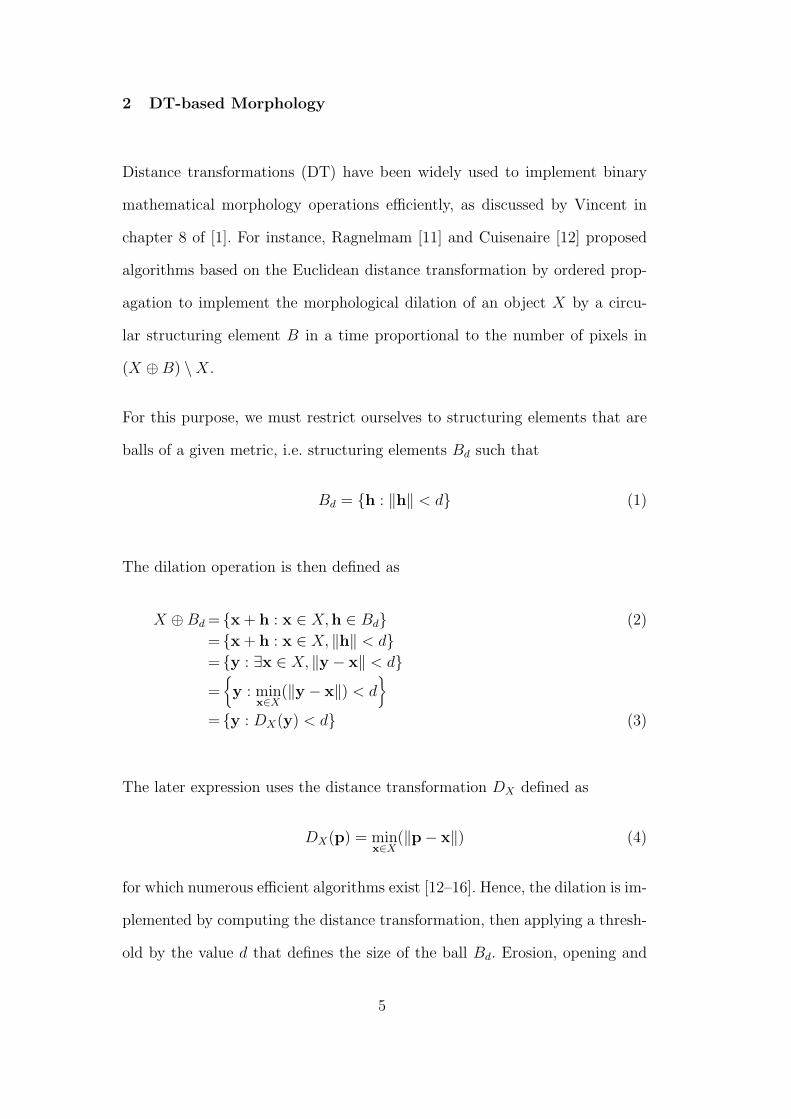
2 DT-based Morphology

Distance transformations (DT) have been widely used to implement binary

mathematical morphology operations efficiently, as discussed by Vincent in

chapter 8 of [1]. For instance, Ragnelmam [11] and Cuisenaire [12] proposed

algorithms based on the Euclidean distance transformation by ordered prop-

agation to implement the morphological dilation of an object X by a circu-

lar structuring element B in a time proportional to the number of pixels in

(X ⊕B) \X.

For this purpose, we must restrict ourselves to structuring elements that are

balls of a given metric, i.e. structuring elements Bd such that

Bd = {h : ‖h‖ < d} (1)

The dilation operation is then defined as

X ⊕Bd = {x + h : x ∈ X,h ∈ Bd} (2)

= {x + h : x ∈ X, ‖h‖ < d}= {y : ∃x ∈ X, ‖y − x‖ < d}=

{y : min

x∈X(‖y − x‖) < d

}

= {y : DX(y) < d} (3)

The later expression uses the distance transformation DX defined as

DX(p) = minx∈X

(‖p− x‖) (4)

for which numerous efficient algorithms exist [12–16]. Hence, the dilation is im-

plemented by computing the distance transformation, then applying a thresh-

old by the value d that defines the size of the ball Bd. Erosion, opening and

5

closing are obtained by combining dilations with set complementations.

In what follows, we consider the Euclidean distance transformation and there-

fore balls that are circular, i.e. the metric is

‖v‖ =√

v2x + v2

y (5)

Nevertheless, other shapes of structuring elements can be obtained using dif-

ferent definitions of the distance. Indeed, the city-block metric

‖v‖ = |vx|+ |vy| (6)

defines balls of diamond shape. The chessboard metric

‖v‖ = max(|vx|, |vy|) (7)

defines square balls. The chamfer metric [17]

‖v‖ = max(|vx|, |vy|) +1

3min(|vx|, |vy|) (8)

defines octagonal balls. Also, anisotropic metrics can be used to define rectan-

gular or ellipsoidal balls. All considerations that follow can easily be extended

to any of these metrics and ball shapes.

3 Dilation and Erosion

In this paper, we extend the above method to allow the size of the ball used as

structuring element to vary over the image. Instead of using the same ball Bd

for all pixels, we consider different balls BS(x) with varying radiuses defined

in an image S of local structuring element sizes. Extending (2), we define the

adaptable dilation of object X by this image S of SE sizes as

6

X ⊕ S ={x + h : x ∈ X, ‖h‖ ∈ BS(x)

}

= {x + h : x ∈ X, ‖h‖ < S(x)} (9)

It can be implemented as efficiently as before using a modified distance mea-

sure. Indeed, similarly to (3), we have

X ⊕ S = {x + h : x ∈ X, ‖h‖ − S(x) < 0}= {y : DX,S(y) < 0} (10)

where we define DX,S as

DX,S(p) = minx∈X

(‖p− x‖ − S(x)) (11)

Note that DX,S is not a distance stricto sensu since in general it respects none

of the axioms of a metric. Computing DX,S is relatively straightforward. The

algorithm, illustrated at Fig. 2, takes two inputs. First, the binary image I in

which resides an object X (Fig. 2.1). Secondly the image of structural element

sizes S (Fig. 2.2). We aim to compute DX,S for all pixels p ∈ I, and a vectorial

image V such that V(p) is the object pixel that minimizes this expression,

i.e.

V(p) = arg minx∈X

(‖p− x‖ − S(x)) (12)

V is the Voronoi partition of the image for the modified distance DX,S.

Firstly, we initialize (Fig. 2.3) all objects pixels with DX,S(p) = −S(p) and

V(p) = p. For background pixels, we should set DX,S(p) to ∞ and leave

V(p) unassigned. Practically, we set DX,S(p) to 0 for background pixels and

compute min(DX,S, 0), which limits the amount of computations and does not

affect the final computation of X⊕S which involves a threshold by 0 anyway.

Secondly, we propagate this information from neighbor to neighbor. The values

7

of DX,S and V at pixel p are modified by its neighbor p + n if we have

‖p−V(p + n)‖ − S(V(p + n)) < DX,S(p) (13)

There are several ways to implement this propagation. The most intuitive

method would be to use a dynamic list of propagating pixels to scan the

image by order of increasing values of DX,S(p), adapting the algorithms of

Ragnelmam [18,11] or Cuisenaire [14] for the Euclidean DT. Nevertheless,

this is needlessly complex. Instead, we adapt the original 4SED Euclidean DT

algorithm of Danielsson [19] which uses a particular type of raster scanning.

The first scan operates line by line from top to bottom. Each line is first

scanned from left to right considering the up and left direct neighbors, then

from right to left considering the right neighbor. The second scan operates

similarly from bottom to top and from right to left. Algorithm 1 formalizes

the method for an image of size M ×N .

As in the case of classical mathematical morphology, the erosion is the dual

operation of dilation and can be obtained as

X ª S = (Xc ⊕ S)c (14)

where Xc = {x : x /∈ X} is the complement set of X.

4 Analysis of the algorithm

In the special case where S has a constant value for all pixels, algorithm 1

is identical to Danielsson’s Euclidean DT [19] followed by a threshold. The

rationale for Danielsson’s algorithm is that while the definition (4) of the DT

8

for all p ∈ I do

if p ∈ X then

DX,S(p) ← −S(p) ; V(p) ← p

else

DX,S(p) ← 0 ; V(p) ← (∞,∞)

for py = 1 → N do

for px = 1 → M do

check((px, py), (−1, 0))

check((px, py), (0,−1))

for px = M → 1 do

check((px, py), (1, 0))

for py = N → 1 do

for px = M → 1 do

check((px, py), (1, 0))

check((px, py), (0, 1))

for px = 1 → M do

check((px, py), (−1, 0))

for all p ∈ I do

if DX,S(p) < 0 then

p ∈ X ⊕ S

else

p ∈ (X ⊕ S)c

procedure check(p,n)

if p + n ∈ I then

v ← V(p + n)

if v 6= (∞,∞) then

d ← ‖p− v‖ − S(v)

if d < DX,S(p) then

DX,S(p) ← d ; V(p) ← v

Algorithm 1: computes X ⊕ S

9

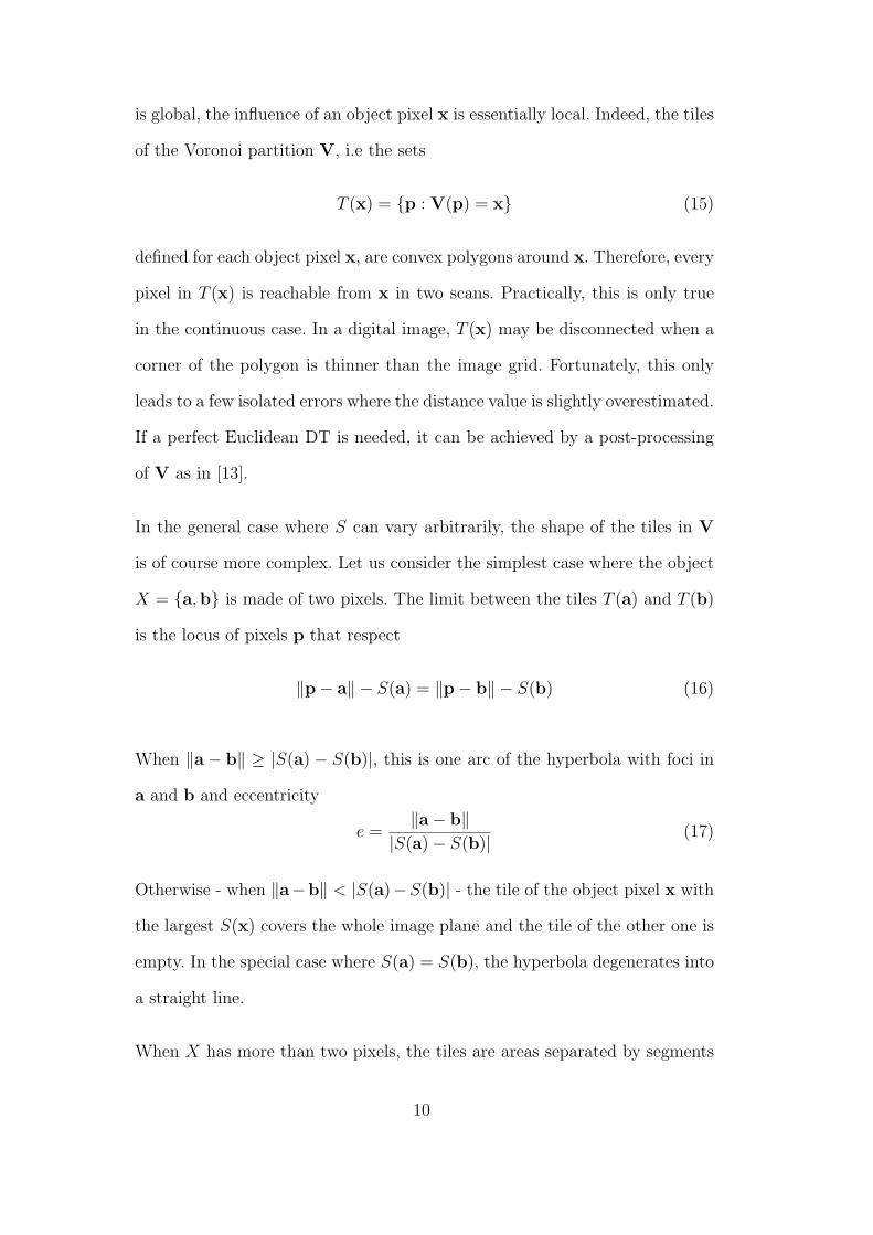
is global, the influence of an object pixel x is essentially local. Indeed, the tiles

of the Voronoi partition V, i.e the sets

T (x) = {p : V(p) = x} (15)

defined for each object pixel x, are convex polygons around x. Therefore, every

pixel in T (x) is reachable from x in two scans. Practically, this is only true

in the continuous case. In a digital image, T (x) may be disconnected when a

corner of the polygon is thinner than the image grid. Fortunately, this only

leads to a few isolated errors where the distance value is slightly overestimated.

If a perfect Euclidean DT is needed, it can be achieved by a post-processing

of V as in [13].

In the general case where S can vary arbitrarily, the shape of the tiles in V

is of course more complex. Let us consider the simplest case where the object

X = {a,b} is made of two pixels. The limit between the tiles T (a) and T (b)

is the locus of pixels p that respect

‖p− a‖ − S(a) = ‖p− b‖ − S(b) (16)

When ‖a − b‖ ≥ |S(a) − S(b)|, this is one arc of the hyperbola with foci in

a and b and eccentricity

e =‖a− b‖

|S(a)− S(b)| (17)

Otherwise - when ‖a−b‖ < |S(a)−S(b)| - the tile of the object pixel x with

the largest S(x) covers the whole image plane and the tile of the other one is

empty. In the special case where S(a) = S(b), the hyperbola degenerates into

a straight line.

When X has more than two pixels, the tiles are areas separated by segments

10

of lines or hyperbolae. Thus, the tiles are not necessarily convex, the basic

assumption for Danielsson’s algorithm. Fortunately, we can prove a weaker

property that is sufficient for the propagation to reach all pixels in the tiles.

The tiles are star-shaped, i.e.

p ∈ T (x) ⇒ ∀α ∈ [0, 1],x + α.(p− x) ∈ T (x) (18)

Indeed, let us consider a pixel p ∈ T (x). For any other object pixel y ∈ X,

we have

‖p− x‖ − S(x) ≤ ‖p− y‖ − S(y) (19)

Let us then consider a pixel q = x + α.(p− x). By the triangular inequality,

we have

‖p− y‖ ≤ ‖p− q‖+ ‖q− y‖ (20)

The definition of q also gives

‖p− q‖ = ‖p− x− α.(p− x)‖

= (1− α).‖p− x‖ if α ≤ 1 (21)

‖q− x‖ = α.‖p− x‖ if α ≥ 0 (22)

= ‖p− x‖ − ‖p− q‖ if 0 ≤ α ≤ 1 (23)

By adding (19) and (20), then using (23), we get

‖p− x‖ − ‖p− q‖ − S(x) ≤ ‖q− y‖ − S(y)

‖q− x‖ − S(x) ≤ ‖q− y‖ − S(y) (24)

which is valid for any object pixel y, and therefore we have q ∈ T (x).

In the continuous image plane, this property guarantees that there is a direct

11

propagation path from x to all the pixels in T (x). Similarly to Danielsson’s

algorithm, there is no such guarantee in the discrete case when the corner of a

tile can be thinner than the grid step. This can lead to occasional small errors

where DX,S is slightly overestimated. Thus, a few pixels at the edge of X ⊕ S

can be mistakenly considered as belonging to (X⊕S)c. In most practical cases

this is of no consequence, and it can be partially corrected by using a larger

neighborhood in the raster scanning algorithm, as Danielsson [19] does with

the 8SED algorithm.

5 Opening and Closing

In Euclidean morphology [5], the closing XB and opening XB of an object X

by a structuring element B are defined respectively as

XB = (X ⊕ B)ªB (25)

XB = (X ª B)⊕B (26)

where B = {−b : b ∈ B} is the reflected set of B. In the case of a symmetric

structuring element, we have B = B.

When it comes to locally adaptable opening and closing, things are more

complicated. In (9), S is not a set of pixel locations, but an image of SE sizes.

Thus, there is no obvious way to compute a reflected S which would give

X ⊕ S = {x + h : x ∈ X, ‖h‖ < S(x)} (27)

A naive approach would be to consider that since the circular balls we use are

12

symmetric, we can assume S = S and define the closing XS as

(X ⊕ S)ª S (28)

Unfortunately, if we do so, the resulting operations do not respect important

properties of opening and closing. In particular, we do not have idempotence,

nor the extensivity of XS and anti-extensivity of XS, i.e.

XS ⊆ X ⊆ XS (29)

as illustrated at the top of Fig. 3. The problem with (28) is that at the dilation

step, we consider values S(p) at pixels p ∈ X, while at the erosion step, we

use values S(p) at different pixels p ∈ (X⊕S)c. Thus, the dilation and erosion

steps use different local structuring element sizes, which leads to the problems

of Fig. 3. In general, it is impossible to define a reflected S. Fortunately, it is

instead possible to define a reflected dilation operation ⊕ as

X ⊕ S = {y : ∃ y − h ∈ X, ‖h‖ < S(y)} (30)

This expression is very similar to (27), but instead of considering the value of

an hypothetical S for the pixels in X, we use the value of S itself on the pixels

of the result X ⊕ S. From this, we can compute the closing as

XS = (X ⊕ S)ª S (31)

as illustrated at the bottom of Fig. 3 Implementing the closing is straightfor-

ward once we notice that (30) can be written as

X ⊕ S = {y : DX(y) < S(y)} (32)

13

Compute DX(p) = minx∈X(‖p− x‖) using the Euclidean DT algorithm in

[13]

for all p ∈ I do

if DX(p) < S(p) then

p ∈ Y = X ⊕ S

else

p ∈ Y c = (X ⊕ S)c

Compute XS = (Y c ⊕ S)c using algorithm 1

Algorithm 2: computes XS

which uses the classical distance transform DX defined as

DX(p) = minx∈X

(‖p− x‖) (33)

For city-block or chessboard metrics, this is easily computed with simple al-

gorithms [20]. For the Euclidean metric, it can also be computed efficiently,

as in [13] for instance. Finally, from Y = X ⊕ S, we compute XS = Y ª S

using the algorithm of the previous section. This is summarized in algorithm

2. The opening is obtained by duality.

XS = ((Xc)S)c (34)

6 Properties

In order to check that XS and XS are respectively a morphological closing

and opening, we need to check that XS is increasing, i.e.

X1 ⊆ X2 ⇒ XS1 ⊆ XS

2 (35)

14

anti-extensive, i.e.

X ⊆ XS (36)

and idempotent, i.e.

(XS)S = XS (37)

Similarly, the opening XS is increasing, extensive and idempotent. These prop-

erties are proved in appendix A.

Let us note that the choice of the order of operations in algorithm 2 is arbitrary.

Instead of computing the distance transformation, comparing DX(p) to S(p),

then applying the adaptable erosion, one could apply an adaptable dilation,

then compute the DT from (X ⊕S)c and finally compare D(X⊕S)c(p) to S(p)

for all pixels. This leads to an alternative definition of XS

XS∗ = (X ⊕ S) ª S (38)

with the reflected erosion ª defined as

X ª S = (Xc ⊕ S)c (39)

One can prove that this operation is also a closing, i.e. that it is increasing,

anti-extensive and idempotent. On the other hand, it leads to a different result

than XS for non trivial S. Fig. 4, with the extreme example of a white random

S, illustrates that choosing the definition of the previous section leads to a

much more intuitive result.

15

X ⊕ S = Ø

for all x ∈ X do

for all h ∈ BS(x) do

(X ⊕ S) 3 (x + h)

Algorithm 3: Brute-force computation of X ⊕ S

7 Computational Complexity

The computational complexity of the algorithms presented here is very low.

The core of algorithm 1 requires two scans over the image for a total of 6 com-

parisons per pixel. Furthermore, as long as the size of a line is small enough to

fit entirely in cache memory, pixels are only fetched twice from the main mem-

ory. On the other hand, for the circular balls that use the Euclidean metric,

each comparison also requires the computation of a square root operation. For

openings and closings, the exact Euclidean distance transform [13] requires 3

scans of the image, and has a complexity similar to the dilation algorithm.

Initializations and set complementations add a negligible overhead.

Typically, the closings that illustrate this paper require approximately 130 ms

for a 512 × 512 image on a 1.8 GHz pentium 4 computer. CPU time scales

linearly with the number of pixels in the image and are independent of the

size of the local structuring elements used. This should be compared with the

brute force approach which implements the following equations

X ⊕ S = {x + h | x ∈ X,h ∈ BS(x)} (40)

X ⊕ S = {x | ∃ h ∈ BS(x),x + h ∈ X} (41)

Algorithm 3 summarizes the brute force approach for the adaptable dilation,

and similarly algorithm 4 implements the reflected dilation.

16

X ⊕ S = X

for all x ∈ Xc do

for all h ∈ BS(x) do

if (x + h) ∈ X then

(X ⊕ S) 3 x

jump to next x

Algorithm 4: Brute-force computation of X ⊕ S

The two approaches are compared at Fig. 5 for the 512× 512 synthetic image

used throughout this paper and randomly sized circular structuring elements

with a mean radius that varies between 1 and 50 pixels. Apart from the trivial

case of radius 1, the DT-based approach is always significantly faster - up to

50 times faster in this example - than the brute force alternative. Fig. 5 also

illustrates that the computational cost of the DT-based approach does not

depend on the size of the structuring elements used.

The comparative advantage of the DT-based approach is even more dramatic

in the 3D case discussed in the next section. For a typical application - the

closing of a 512× 512× 198 CT image of 0.42× 0.42× 0.8 mm3 voxel size by

structuring elements of average radius 15mm - the DT-based approach of this

paper typically requires 2 minutes, while the brute force algorithm takes more

than 13 hours to complete, which makes it approximately 400 times slower.

8 Extensions

8.1 Higher dimensional images

While the methods here have been described for 2D images, extending them to

3 or more dimensions is relatively straightforward. Appropriate neighborhoods

17

and scanning directions for algorithm 1 can be found in [21]. It includes a 4

scans algorithm for 3D images and 2D scans algorithms for D dimensions.

For the openings and closings, the Euclidean DT algorithm in [13] cannot be

used on images of more than 2 dimensions, but there are other linear time

algorithms [15,16] that work in 3 and higher dimensions.

8.2 Gray-level images

There are two conceptual approaches to develop gray-level MM from binary

MM. The first consists of using local maximum and minimum operators for

the dilation and erosion. The second consists of considering an image with G

gray-levels as G−1 binary images, applying the binary MM operators on each

of these images, then recombining the results into a gray-level image. Both

approaches give equivalent results.

Using the first approach, we get the following definitions for the adaptable

dilation δS and the erosion εS of a gray-level image I by a map of structuring

element sizes S, as well as the other operators.

δS(I)(p) = max(I(p + h) : ‖h‖ < S(p + h)) (42)

εS(I)(p) = min(I(p + h) : ‖h‖ < S(p + h)) (43)

δS(I)(p) = max(I(p + h) : ‖h‖ < S(p)) (44)

εS(I)(p) = min(I(p + h) : ‖h‖ < S(p)) (45)

IS = εS(δS(I)) (46)

IS = δS(εS(I)) (47)

Let us note that these definitions are equivalent to equations (9) and (30) if

the image I is binary and defined such that I(p) = 1 if p ∈ X and I(p) = 0

otherwise.

18

for all p ∈ I do

δS(I)(p) ← −∞for all p ∈ I do

for all h ∈ BS(p) do

if δS(I)(p + h) < I(p) then

δS(I)(p + h) ← I(p)

Algorithm 5: Brute-force grey-level dilation δS(I)

for all p ∈ I do

δS(I)(p) ← −∞for all p ∈ I do

for all h ∈ BS(p) do

if δS(I)(p) < I(p + h) then

δS(I)(p) ← I(p + h)

Algorithm 6: Brute-force grey-level reversed dilation δS(I)

One can implement these operators by directly implementing their definitions.

For this purpose, equations (42) and (43) must be implemented using a write-

mechanism, as in algorithm 5. On the other hand, equations (44) and (45) must

be implemented using a read-mechanism, as in algorithm 6. The computational

cost of this approach is obviously ◦(∑p∈I S(p)D) for D dimensional images

since at each pixel we consider the ◦(S(p)D) neighbors in the ball BS(p) around

p. This becomes unpractical when using large local structuring elements.

An alternative method consists of decomposing the gray-level image in as many

binary images as there are gray levels, then applying binary morphological

operators on each binary image and then recombining the gray-level image

from the resulting level sets. For a gray-level image with G levels, i.e. with a

range of [0, G− 1], we have G− 1 images I1 to IG−1 defined as

Ig(p) = (I(p) ≥ g) (48)

19

The gray-level dilation is computed from the G− 1 binary dilations as

δS(I)(p) =G−1∑

g=1

(Ig ⊕ S)(p) (49)

The computational cost of this method is approximately G times the compu-

tational cost of the binary algorithm. It becomes relevant for heavily quantized

images for which G is small, or for large structuring elements, i.e. in all cases

where

∑

p∈I

S(p)D À ∑

p∈I

G (50)

9 Discussion

The mathematical morphology operators defined in this paper have strong

links with previous works by Charif-Chefchaouni [10] and Roerdink [5,9], as

discussed hereafter.

9.1 Link with Charif-Chefchaouni’s work

In [10], Charif-Chefchaouni and Schonfeld propose a general framework for

spatially varying mathematical morphology. The structuring element around

a pixel p is the set θ(p) and the spatially-varying erosion εθ, dilation δθ,

opening Γθ and closing Φθ are defined as

εθ(X) = { p : θ(p) ∈ X } (51)

δθ(X) = { p : θ(p) ∩X 6= ∅ } (52)

Γθ(X) = δθ′(εθ(X)) (53)

Φθ(X) = εθ′(δθ(X)) (54)

20

with

θ′(q) = { p : q ∈ θ(p) } (55)

The operators defined in this paper can be expressed using the same formalism

provided we choose

θ(p) = { q : ‖p− q‖ < S(p) } (56)

and

θ′(q) = { p : q ∈ θ(p) } (57)

= { p : ‖p− q‖ < S(p) } (58)

Let us note that this actually leads to the alternative definition of the opening

and closing of equation (38). For the more intuitive operators defined here, one

needs to swap θ and θ′ in equations (53) and (54). Nevertheless, all properties

proved in [10] also hold for the operators of this paper.

Also, while (55) provides a way to computed the reflected variable structuring

elements, we still need both algorithms 1 and 2 for fast implementations of

openings and closings, since choosing θ such that θ(p) respects (1) for all pixels

- a necessary condition to use algorithm 1 for dilations - does not guarantee

that θ′ will.

9.2 Link with Roerdink’s work

The methods and algorithms of this paper can be used as efficient implemen-

tation of several of Roerdink’s mathematical morphologies on non Euclidean

spaces. For instance, in [5], he develops mathematical morphology on a po-

lar structure. When points are described by their polar coordinates (r, θ), the

21

group operation is

(r1, θ1) ∗ (r2, θ2) = (r1.r2, θ1 + θ2) (59)

He considers dilations by structuring element B, a circle of center (1, 0) and

radius δ. The reflected structuring element B used to define closings is the

circle centered on ((1−δ2)−1, 0) of radius δ.(1−δ2)−1. In appendix B, we show

that these operations are strictly identical to those described in this paper

when we specify

S(p) = δ.‖p‖ (60)

Obviously the methods of this paper can also be applied to implement some

of the other group morphologies defined in [9].

9.3 Applications

There is a vast area of possible application fields where the image acquisition

process involves a projection of the imaged object onto the image plane that is

not properly modelled as a parallel projection along an axis perpendicular to

this plane. This includes applications mentioned in the introduction such as

traffic control cameras, but also others such as weather satellite images where

the curvature of the earth is not negligible.

A major advantage of the method of this paper over those of Roerdink is

that one does not need to develop a new brand of morphology adapted to the

projection geometry for each new problem. Also, it does not require that we

22

have an analytical description of the projection geometry from which we derive

an analytical description of S. Instead, S can be calibrated experimentally by

imaging objects of a know size.

Because there is no constraint on S, it can be made dependent on the image

content. This becomes adaptive mathematical morphology for which range im-

agery is an obvious application. In medical imaging, prior anatomical knowl-

edge could be used to specify S appropriately.

Ultimately, this paper does not say how S should be chosen, but states that

whatever the choice, it can be used to define morphological operators that can

be computed efficiently. Finding the optimal S is an open issue that needs to

be addressed on an application dependent basis.

10 Conclusion

In this work, we have defined morphological operators using structuring el-

ements with a fixed shape, but sizes S(p) that can vary arbitrarily at each

pixel location p. We have presented efficient algorithms using two raster scans

for the adaptable dilation and erosion, and using five raster scans for opening

and closing. We have presented a few applications where S is defined by the

image acquisition process or the image content, but ultimately left the optimal

choice of S an open question.

23

References

[1] E. R. Dougherty, Mathematical Morphology in Image Processing, Marcel

Dekker, Inc., New York, 1992.

[2] J. Serra, Image Analysis and Mathematical Morphology, Academic Press, New

York, 1982.

[3] J. Serra, Image Analysis and Mathematical Morphology. Vol 2: Theoretical

Advances, Academic Press, New York, 1988.

[4] J. Serra, Morphological filtering: an overview, Signal Processing 38.

[5] J. Roerdink, H. Heijmans, Mathematical morphology for structures without

translation symmetry, Signal Processing 15 (3) (1988) 271–277.

[6] J. G. Verly, R. L. Delanoy, Adaptive mathematical morphology for range

imagery, IEEE Transactions on Image Processing 2 (2) (1993) 272–275.

[7] C. S. Chen, J. L. Wu, Y. P. Hung, Statistical analsysis of space-varying

morphological openings with flat structuring elements, IEEE Transactions on

Signal Processing 44 (4) (1996) 1010–1014.

[8] I. Masayasu, T. Masayoshi, N. Akira, Morphological operations by locally

variable structuring elements and their applications to region extraction in

ultrasound images, Systems and Computers in Japan 34 (3) (2003) 33–43.

[9] J. B. T. M. Roerdink, Group morphology, Pattern Recognition 33 (2000) 877–

895.

24

[10] M. Charif-Chefchaouni, D. Schonfeld, Spatially-variant mathematical

morphology, in: IEEE International Conference on Image Processing, 1994, pp.

555–559.

[11] I. Ragnelmam, Fast erosion and dilation by contour processing and thresholding

of distance maps, Pattern Recognition Letters 13 (1992) 161–166.

[12] O. Cuisenaire, Distance transformations: fast algorithms and applications to

medical image processing, Ph.D. thesis, Universite catholique de Louvain

(UCL), Louvain-la-Neuve, Belgium (October 1999).

[13] O. Cuisenaire, B. Macq, Fast and exact signed euclidean distance

transformation with linear complexity, in: Proc. IEEE Int. Conference on

Acoustics, Speech and Signal Processing (ICASSP99), Vol. 6, Phoenix (AZ),

1999, pp. 3293–3296.

[14] O. Cuisenaire, B. Macq, Fast euclidean distance transformation by propagation

using multiple neighborhoods, Computer Vision and Image Understanding

76 (2) (1999) 163–172.

[15] C. R. Maurer Jr, R. Qi, V. Raghavan, A linear time algorithm for computing

exact euclidean distance transforms of binary images in arbitrary dimensions,

IEEE Transactions on Pattern Analysis and Machine Intelligence 25 (2) (2003)

265–270.

[16] A. Meijster, J. B. T. M. Roerdink, W. H. Hesselink, A general algorithm

for computing distance transforms in linear time, in: J. Goutsias, L. Vincent,

D. Bloomberg (Eds.), Mathematical Morphology and its applications to image

and signal processing, 2000, pp. 331–340.

25

[17] G. Borgefors, Distance transformations in digital images, Computer Vision,

Graphics, and Image Processing 34 (1986) 344–371.

[18] I. Ragnelmam, Neighborhoods for distance transformations using ordered

propagation, CVGIP, Image Understanding 56 (3) (1992) 399–409.

[19] P. E. Danielsson, Euclidean distance mapping, Computer Graphics and Image

Processing 14 (1980) 227–248.

[20] A. Rosenfeld, J. L. Pfaltz, Distance functions on digital pictures, Pattern

Recognition 1 (1) (1968) 33–61.

[21] I. Ragnelmam, The euclidean distance transformation in arbitrary dimensions,

Pattern Recognition Letters 14 (1993) 883–888.

26

About the author

OLIVIER CUISENAIRE was born in Lobbes, Belgium, in 1973. He received

the M.S. and Ph.D. degrees in electrical engineering from Universite catholique

de Louvain (UCL), Louvain-la-Neuve, Belgium, in 1995 and 1999, respectively.

His Ph.D. thesis focused on efficient implementations of the Euclidean dis-

tance transformation and its applications to medical image processing. He

was a Visiting Student at the Universitat Politecnica de Catalunya (UPC),

Barcelona, Spain in spring 1995, and at the Surgical Planning Laboratory,

Harvard Medical School, Boston, MA, in the summer of 1999. He then joined

the Signal Processing Institute at the Swiss Federal Institute of Technology

(EPFL), Lausanne, Switzerland in 2000 as Postdoctoral Researcher, and was

appointed First Assistant in 2001 and Lecturer in 2003.

27

Fig. 1. (top-left) Original image I of size 512 × 512 with object X in black.

(bottom-left) Structuring element image S chosen as S(p) = (512 − px)/14.

(top-center) Dilation X⊕S. (bottom-center) Erosion XªS (top-right) Clos-

ing XS (bottom-right) Opening XS .

28

0 100 200 300 400 500 600 700 800 900 1000−0.2

0

0.2

0.4

0.6

0.8

1

x ∈

X

0 100 200 300 400 500 600 700 800 900 10000

20

40

60

80

S(x

)

0 100 200 300 400 500 600 700 800 900 1000

−60

−40

−20

0

D0(p

)

0 100 200 300 400 500 600 700 800 900 1000

−60

−40

−20

0

D(p

)

0 100 200 300 400 500 600 700 800 900 1000−0.2

0

0.2

0.4

0.6

0.8

1

x ∈

(X

⊕ S

)

Fig. 2. Adaptive dilation algorithm in one dimension. (1) Object X. (2) Local

structuring element sizes S. (3) Initialization of DX,S (4) DX,S after raster scan

propagation (5) Resulting X ⊕ S

29

Fig. 3. (top-left) Original image I of size 512 × 512 with object X in black.

(bottom-left) Structuring element image S chosen as S(p) = (512 − px)/10.

(top-center) Naive implementation of the closing: (X⊕S)ªS. (bottom-center)

Proper implementation of the closing XS = (X ⊕ S) ª S. (top-right)

X \ ((X ⊕S)ªS). Black pixels belong to X but not (X ⊕S)ªS. (bottom-right)

X \XS . All pixels in X also belong to XS .

30

Fig. 4. (left) Original image I of size 512×512 with object X in black. S is a random

image where each pixel is chosen independently and uniformly between 0 and 50

(center) Closing XS = (X ⊕ S)ªS (right) Alternative closing XS∗ = (X⊕S) ª S.

31

0 5 10 15 20 25 30 35 40 45 50

10−1

100

mean SE radius (pixels)

CP

U ti

me

(sec

)

DT−based algorithmBrute force algorithm

Fig. 5. Computational times for the adaptable closing of the 512×512 synthetic im-

age of the previous figures using uniformly distributed random structuring element

sizes of mean radius between 2 and 50 pixels.

32

A XS is a closing

In order to prove that the XS operation (31) is a closing, we need to show

that it is increasing, anti-extensive and idempotent, i.e

X1 ⊆ X2⇒XS1 ⊆ XS

2 (A.1)

X ⊆ XS (A.2)

(XS)S = XS (A.3)

A.1 XS is increasing

First, let us prove that both the adaptable dilation X ⊕ S and the reflected

dilation X ⊕ S are increasing. We consider two objects X1 and X2 such that

X1 ⊆ X2. We have

X1 ⊕ S = {x + h : x ∈ X1, ‖h‖ < S(x)}⊆{x + h : x ∈ X2, ‖h‖ < S(x)}= X2 ⊕ S (A.4)

and

X1 ⊕ S = {p : minx∈X1

‖p− x‖ < S(x)}⊆{p : min

x∈X2

‖p− x‖ < S(x)}= X2 ⊕ S (A.5)

The corresponding erosions are also increasing. Indeed, using the property

that X1 ⊆ X2 ⇒ Xc1 ⊇ Xc

2, we have

33

X1 ⊆ X2

⇒ Xc1 ⊇ Xc

2

⇒ Xc1 ⊕ S ⊇ Xc

2 ⊕ S

⇒ (Xc1 ⊕ S)c ⊆ (Xc

2 ⊕ S)c

⇒ X1 ª S ⊆ X2 ª S (A.6)

and a similar proof for the reflected erosion X ª S. It follows immediately

that

X1 ⊆ X2

⇒ X1 ⊕ S ⊆ X2 ⊕ S

⇒ (X1 ⊕ S)ª S ⊆ (X2 ⊕ S)ª S

⇒ XS1 ⊆ XS

2 (A.7)

A.2 XS is anti-extensive

Let us suppose that X is not a subset of XS. Then, there exists a pixel x such

that x ∈ X and x ∈ (XS)c. We consider the pixels y that do not belong to

X ⊕ S, i.e. the set Y = (X ⊕ S)c. By the definition of X ⊕ S (30), x ∈ X

implies that

∀y ∈ Y, ‖x− y‖ ≥ S(y) (A.8)

On the other hand, we have x ∈ (XS)c = Y ⊕ S. By the definition of the

adaptive dilation (9), this means that

∃y ∈ Y, ‖x− y‖ < S(y) (A.9)

Since this contradicts (A.8), no pixel x can belong to both X and (XS)c, and

34

therefore X ⊆ XS.

A.3 XS is idempotent

In order to prove idempotence, we first notice that since XS is anti-extensive,

we have

XS ⊆ (XS)S (A.10)

It remains to be proven that

(XS)S ⊆XS (A.11)

(XS ⊕ S)ª S⊆ (X ⊕ S)ª S (A.12)

Since adaptable erosion is increasing, it is sufficient to prove that

XS ⊕ S ⊆ X ⊕ S (A.13)

Let us proceed ab absurdo. Suppose there is a pixel y ∈ (XS ⊕ S) and

y ∈ (X ⊕ S)c. By the definition of the reflected dilation (30), y ∈ (XS ⊕ S)

means that

DXS(y) = minx∈XS

(‖x− y‖) < S(y) (A.14)

or in other words,

∃x ∈ XS : ‖x− y‖ < S(y) (A.15)

35

On the other hand, according to the definition of the adaptable dilation (9),

since (XS)c = (X ⊕ S)c ⊕ S, y ∈ (X ⊕ S)c means that

∀x ∈ XS : ‖x− y‖ ≥ S(y) (A.16)

Since this contradicts (A.15), no pixel y can belong to both (XS ⊕ S) and

(X ⊕ S)c, we have XS ⊕ S ⊆ X ⊕ S and thus (XS)S ⊆ XS.

B Polar morphology

In this annex we show that by specifying

S(p) = δ.‖p‖ (B.1)

we get an operation that is equivalent to Roerdink’s polar morphology. In [5],

points are described by their polar coordinates (r, θ), the group operation is

(r1, θ1) ∗ (r2, θ2) = (r1.r2, θ1 + θ2) (B.2)

Roerdink considers dilations by structuring element B, a circle of center (1, 0)

and radius δ < 1. If we consider an object X = {p} that consists of a single

pixel p, the dilation X ⊕ B is the disk of center p and radius δ.‖p‖. This is

clearly equivalent to X ⊕ S with S defined above.

In [5], the reflected structuring element B used to define the closing

36

XB = (X ⊕ B)ªB (B.3)

is the disk B centered on ((1− δ2)−1, 0) of radius δ.(1− δ2)−1. It results that,

for the single pixel X above, the dilation X ⊕ B is the disk of center

c =1

1− δ2p (B.4)

and radius

R =δ

1− δ2‖p‖ (B.5)

Let us consider the pixels q in this disk. They respect

‖q− c‖<R (B.6)

‖q− 1

1− δ2p‖<

δ

1− δ2‖p‖ (B.7)

Expressed in cartesian coordinates, the square of this expression is

(qx − 1

1− δ2px)

2 + (qy − 1

1− δ2py)

2 <δ2

(1− δ2)2(p2

x + p2y) (B.8)

By expanding the squares and multiplying by 1− δ2, then grouping the terms

in p2x and p2

y, we get

(1− δ2)q2x − 2pxqx + p2

x + (1− δ2)q2y − 2pyqy + p2

y < 0

q2x − 2pxqx + p2

x + q2y − 2pyqy + p2

y <δ2q2x + δ2q2

y

(qx − px)2 + (qy − py)

2 <δ2(q2x + q2

y)

‖q− p‖<δ‖q‖DX(q) <S(q) (B.9)

37

This is clearly the definition of X ⊕ S with S(p) = δ.‖p‖. Having proved that

both approaches are equivalent for an object X made of any single pixel p in

the image, we have proven the equivalence for all objects since we have

(X ∪ Y )⊕B = (X ⊕B) ∪ (Y ⊕B) (B.10)

and similar properties for set B and operation ⊕.

38