Laplace Transformations I
96
Engineering Mathematics - I Semester – 1 By Dr N V Nagendram UNIT – IV Laplace Transformations Class 1 Section I Introduction The knowledge of Laplace Transformations has in recent years became an essential part of Mathematical background required of engineers and scientists. This is because the transform methods provide an easy and effective means for the solution of many problems arising in engineering. This subject originated from the operational methods applied by the English engineer Oliver Heaviside (1850 – 1925) to problems in electrical engineering. Unfortunately, Heaviside’s treatment was unsystematic and lacked rigour, which was placed on sound mathematical footing by Bromwich and carson during 1916 – 1917. It was found that Heaviside’s operational calculus is best introduced by means of a particular type of definite integrals called “Laplace Transforms”. The method of Laplace Transforms has the advantage of directly giving the solution of differential equations with given boundary values without the necessary of first finding the general solution and then evaluating from it the arbitrary constants. Moreover, the ready tables of Laplace Transforms reduce the problems of solving differential equations to mere algebraic manipulation. Definition: Integral transform
-
Upload
independent -
Category
Documents
-
view
0 -
download
0
Transcript of Laplace Transformations I

Engineering Mathematics - I Semester – 1 By Dr N VNagendram
UNIT – IV Laplace Transformations Class 1
Section I
Introduction
The knowledge of Laplace Transformations has in recent yearsbecame an essential part of Mathematical background requiredof engineers and scientists.
This is because the transform methods provide an easy and effective means for the solution of many problems arising in engineering.
This subject originated from the operational methods appliedby the English engineer Oliver Heaviside (1850 – 1925) toproblems in electrical engineering.
Unfortunately, Heaviside’s treatment was unsystematic andlacked rigour, which was placed on sound mathematical footingby Bromwich and carson during 1916 – 1917.
It was found that Heaviside’s operational calculus is bestintroduced by means of a particular type of definite integralscalled “Laplace Transforms”.
The method of Laplace Transforms has the advantage of directlygiving the solution of differential equations with givenboundary values without the necessary of first finding thegeneral solution and then evaluating from it the arbitraryconstants.
Moreover, the ready tables of Laplace Transforms reduce theproblems of solving differential equations to mere algebraicmanipulation.
Definition: Integral transform

Let K(s, t) be a function of two variables s and t where s isa parameter [s R or C] independent of t. Then the functionf(s) defined by an Integral which is convergent. i.e.,
is called the Integral Transform of thefunction F(t) and is denoted by [T{F(t)], K(s, t) is kernel ofthe transformation.
If kernel K(s, t) is defined as
then
is called “Laplace
Transform” of the function F(t) and is also denoted by L{ F(t)} or .
L { F(t) } = =
Definition: Laplace Transformation
P f(P)
f is real valued /complex valued function
Domain Range
Let F(t) be a real or complex valued function defined on [0,
). Then the function f(s) defined by is
called Laplace Transformation of F(t) if the integral existsand f(s) = L{ F(t) }.
Note: If L { F(t) } = F(t) = L-1 { }. Then F(t) iscalled the inverse Laplace Transform of which transformsF(t) into is called “The Laplace Transforms Operator”.
Linearity Property of Laplace Transformation:
A transformation T is said to be linear if a1, a2 constantsand F1(t), F2(t) be any functions of F. Then L{ a1 F1(t) + a2
F2(t) } = a1 L{ F1(t) + a2 L{ F2(t) } or F1(t), F2(t), F3(t) thereexists a1, a2, a3 constants such thatL {a1 F1(t) + a2 F2(t) – a3 F3(t)} = a1 L{ F1(t) + a2 L{ F2(t) } –a3 L{ F3(t)}.
Theorem: Laplace transformation is a linear transformationi.e., a1, a2 constants L{ a1 F1(t) + a2 F2(t) } = a1 L{ F1(t) +a2 L{ F2(t) }.
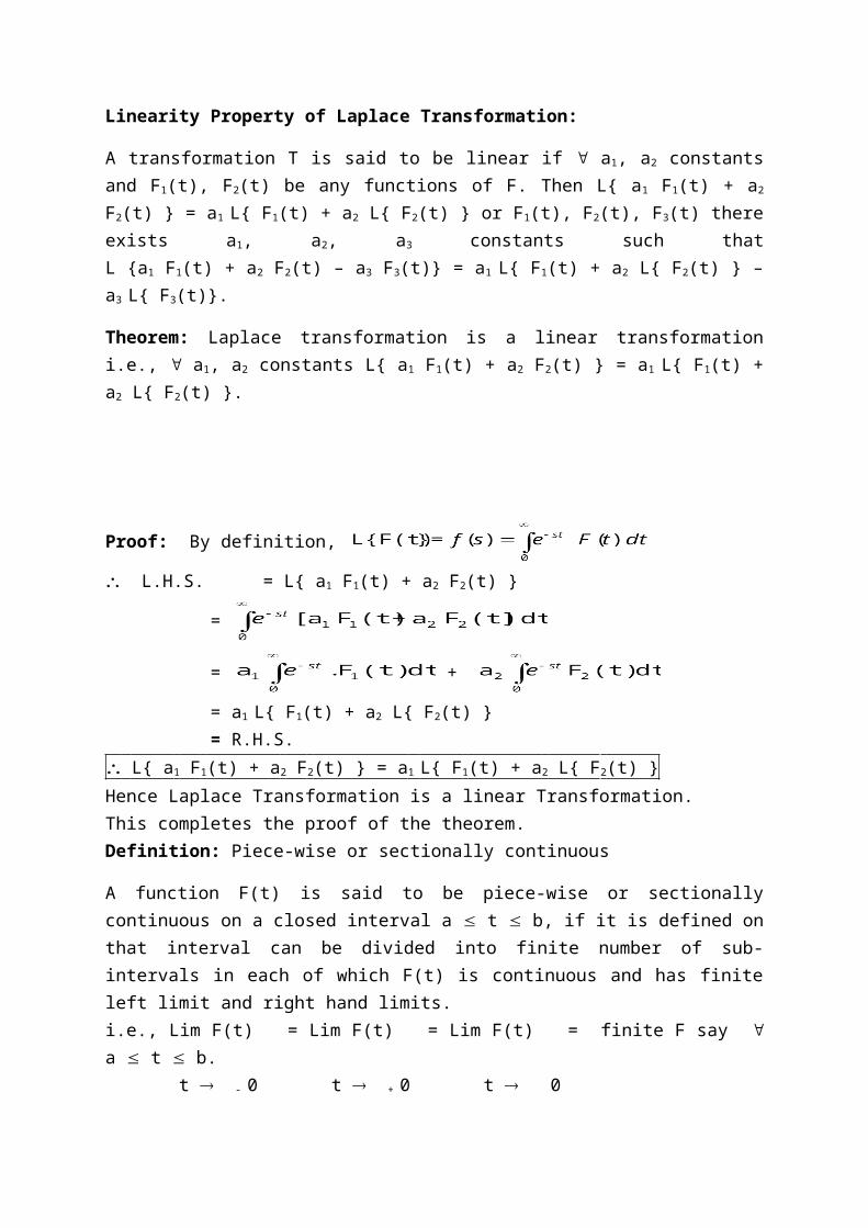
Proof: By definition,
L.H.S. = L{ a1 F1(t) + a2 F2(t) }
=
= +
= a1 L{ F1(t) + a2 L{ F2(t) }= R.H.S.
L{ a1 F1(t) + a2 F2(t) } = a1 L{ F1(t) + a2 L{ F2(t) }Hence Laplace Transformation is a linear Transformation.This completes the proof of the theorem.Definition: Piece-wise or sectionally continuous
A function F(t) is said to be piece-wise or sectionallycontinuous on a closed interval a t b, if it is defined onthat interval can be divided into finite number of sub-intervals in each of which F(t) is continuous and has finiteleft limit and right hand limits.i.e., Lim F(t) = Lim F(t) = Lim F(t) = finite F say
a t b. t - 0 t + 0 t 0

therefore, F is continuous.
Geometrically: F(t)
0 a t1 t2 t3 bt I1 I2 I3 I4
Figure. piece-wise or sectionally continuous.
Engineering Mathematics - I Semester – 1 By Dr N VNagendram
UNIT – IV Laplace Transformations Class 2
Definition: Functions of an Exponential order
A function F(t) is said to be an exponential order as ttends to if there exist a positive real number M a number
and a finite number t0 such that | F(t) | < M e t or | e-t
F(t) | < M, t t0.

Note: If a function F(t) is of an exponential order . It isalso of such that > .
Definition: A function of class A
A function which is piece-wise continuous or sectionallycontinuous on every finite interval in the range t 0 and isof an exponential order , as t is known as “A function ofclass A”.
Theorem: Existence of Laplace Transformation
If F(t) is a function which is piecewise or sectionallycontinuous on every interval (finite) in the range t 0 andsatisfies | F(t) | M. eat, t 0 where a and M areconstants. Then the Laplace Transform exists for every s > a.
Proof:

- 0 t t0 t1
|---------------0-------|------I1--------|---------- I2---------------|
By definition,
= +
....................... (1)
exists and piece-wise continuous in interval 0
t t0 so that
(since, |F(t) M eat)
= (since, s > a implies s – a
> 0 0)
=
for any s > a
If t0 is too large then R.H.S. is too small or infinite small therefore L{ F(t) } exists for s > a.
This completes the proof of the theorem.
Engineering Mathematics - I Semester – 1 By Dr N VNagendram

UNIT–IV Table of General Properties of Laplace Transform Class 3
F(s) =
S No. Name Laplace Transform Inverse Laplace Transform
01. Definition L{f(t)} = f(s) L-1{f(s)} = f(t)02. Linearity af1(t) +b f2(t) a f1(s)+bf2(s)
03. Change of scale f(at)
04. First shifting Th. eat f(t) f(s-a)05. second shifting u(t-a) = { e-as f(s)06. Derivative (multiply by s) f (t)
sf(s)-f(0)07. Second derivative (multiply by s2) f (t) s2f(s) – s f(0) - f (0)08. n th derivative (multiply by sn) f (n)(t) snf(s) – sn-1 f(0) - sn-2
f (0).....– f n-1(0)
09.Integral(division by s)
10. Multiple integral
(division by sn)11. Multiply by t - t f(t) f (s)12. Multiply by t2 t2 f(t) f (s)

13. Multiply by tn (-1)n tn f(t) f n(s)
14. Division by t
15. Convolution f(t) * g(t) =
=
f(s)*g(s)=L(f * g)= L-1(f(s) g(s)}
16. f-periodic with period p f(t) = f(t + p)
Table of some Important Laplace Transforms By Dr N V Nagendram
________________________________________________________________S No. Laplace Transform Inverse Laplace Transform01. L{f(t)} = f(s) L-
1{f(s)} = f(t)
02. 1
03. t
04. t2
05. tn n = 0,1,2,3,...
06. eat
07. e-at
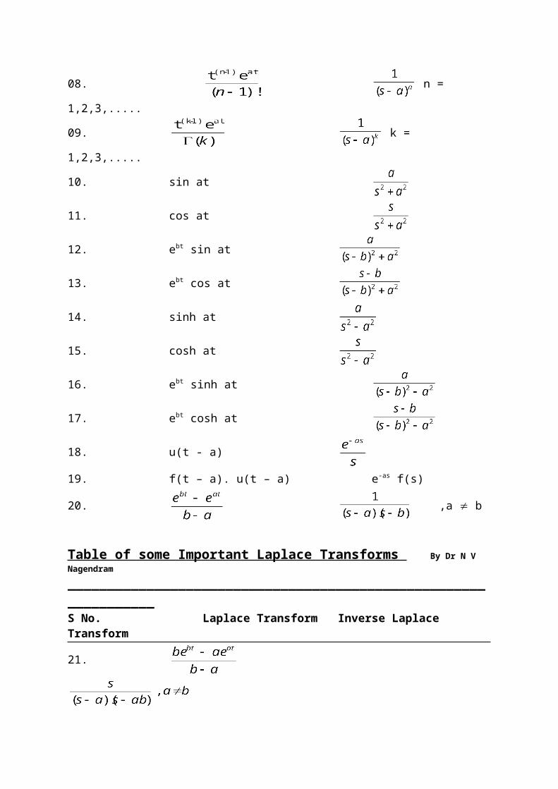
08. n =
1,2,3,.....
09. k =
1,2,3,.....
10. sin at
11. cos at
12. ebt sin at
13. ebt cos at
14. sinh at
15. cosh at
16. ebt sinh at
17. ebt cosh at
18. u(t - a)
19. f(t – a). u(t – a) e-as f(s)
20. ,a b
Table of some Important Laplace Transforms By Dr N V Nagendram________________________________________________________________S No. Laplace Transform Inverse Laplace Transform
21.

22.
23.
24.
25.
26. t cos at
27.
28.
29. (sinh at + at cosh at)/ 2a
30. (cosh at + 1/2at sinh at)
31. t cosh at
32.
33.
34.
35.
36.
37.
38. (1) – log t
Engineering Mathematics - I Semester – 1 By Dr N VNagendram

UNIT–IV Laplace Transformations and its applicationsClass 4
Definition: Laplace Transform of Periodic function
A function f(t) is said to be a periodic function of period T > 0 if F(t) = f(T + t) = f(2T + t) = f(3T + t ) = ..... = f(nT + t).
Sin t , cos t are periodic functions of period 2.
The Laplace transform of a piecewise periodic function f(t) with period p is
L{ f(t) } = ; s > 0
Note: (1) = , ( ) = ,( ) =( +1) = ( ) = ,
,( ) =( +1) = ( ) = and (- ) =(- ) =
-2.

Engineering Mathematics - I Semester – 1 By Dr N VNagendram
UNIT–IV Problems Vs Solutions on Laplace transformationsClass 5
Problem Solution
01. L{ 3t - 5}
02. L{ 2t3 – 6t + 8 }
03. L { 6 sin 2t – 5 cos 2t }
04. L { 3 cosh 5t – 4 sinh 5t }
05. L{ (t2 + 1)2 }
06. L[ cos2 t }
07. L{ 3t4-2t3 + 4 e-3t – 2 sin 5t + 3 cos 2t }
08. L{ sin2 at }
09. L{ 2 e3t – e-3t }
10. L{ sin 5t + cos 3t }
11. L{ e-2t – e-3t }

12. L{ F(t) } if F(t) =
13. L{ F(t) } if F(t) =
14. L{ F(t) } if F(t) =
15. L{ F(t) } if F(t) =
16. L{ F(t) } if F(t) =
17. L{ F(t) } if F(t) =
18. L{
19. L{ e2t + 4 t3 – 2 sin 3t + 3 cos 3t }
20. L{ 1 + 2 +3 }
21. L{ cosh at – cos at }
22. L{ cos (at+b) }
23. L{ (sint – cos t)2 }
24. L{ sin 2t cos 3t }

25. L{ sin at sin bt }
Engineering Mathematics - I Semester – 1 By Dr N VNagendram
UNIT–IV Problems Vs Solutions on Laplace transformationsClass 6
Section II

. First shifting / Translation Lemma
. Second shifting / Translation Lemma
. Change of scale property
. Multiplication by tn
. Problems Vs Solutions

Engineering Mathematics - I Semester – 1 By Dr N VNagendram
UNIT – IV Laplace TransformationsClass 6
Section II
Lemma: First shifting / Translation Lemma.
If L ( F(t) ) where s > then L ( eat F(t) )
, s > a or If is a Laplace transformation ofF(t) then is a Laplace transformation of e
at F(t).
Proof: Y
O L ( eat F(t) ) L
( F(t) ) X
Figure
Given is a Laplace transformation. Then =
= L { F(t) }
So, = = = eat
= eat

= eat since, = = L
{ F(t) }
is a Laplace transformation of eat L{ F(t) }.
This completes the proof of the theorem.
Lemma: Second Translation / shifting Lemma.
If L { F(t) } and G(t) = then, L{ G(t) } e-a s .
Proof:
a
|------------------------ t < a ------------|0------|--- t > a -----|
Given = = L { F(t) } and given G(t) =
So that, = =
Put t – a = x implies dt = dx , since da/dx = 0 implies a = c.
= = = e-a s = e – a s

This completes the proof of lemma.
Note: for every x (a, ) such that x (0, ) and for everyt (0, ), a = 0
=
For any t, e-as
L { G(t) } = e-as L { F(t) }
e-as = L { G(t) } since, =
L { G(t) } = e-as
L { G(t) } = e-as L { F(t) }
This completes the proof of lemma.
Lemma: Change of scale property
If L { F(t) } then L { F(at) } = .
Proof: Given = = L { F(t) }
Let us consider L { F(at) } =
Put at = x implies t = x/a so dt = (1/a) dx
L { F(at) } = =

=
= [since,
]
= [since, =
]
L { F(at) } = or L { F(at) } =
This completes the proof of the lemma.
Lemma: Multiplication by tn
If L { F(t) } then L { tn F(t) } (-1)n
for n = 1,2,3,………………We have =

On differentiation w.r.t. s, = { }
By Leibnitz principle for differentiation under integral sign,
= { } = { }
= { }
for n = m, = ( 1)m { }
This completes the proof of lemma on multiplication by tn.Lemma: Division by t
If L { F(t) } then L { F(t) }
provided integral exists.
Proof: since =
On integrating both sides w.r.t. s from s we get,
=
= = here, since t
is independent of s
= = = L { F(t) } by
definition of Laplace transformation.
L { F(t) }
This completes the proof of lemma.
Engineering Mathematics - I Semester – 1 By Dr N VNagendram

UNIT – IV Laplace TransformationsClass 7
Section II
Problems Vs Solutions
Problem #1: Find L { t sin at }
Problem #2: Find L { t2 sin at }
Problem #3: Find L { t3 e
-3t }
Problem #4: Find L { t e-t sin 3t
}
Problem #5: Find L
Problem #6: Find L
Problem #7: Find and evaluate at s = 2
*Problem #8: Find

Problem #9: Find L
Problem #1: Find L { t sin at }
Solution: Since L { sin at } =
L { t sin at } = { } =
L { t sin at } = is required solution.
Problem #2: Find L { t2 sin at }
Solution: Since L { sin at } =
L { t2 sin at } = ( 1)2 { }

= =
= =
= = =
= =
L { t2 sin at } = = is required solution.
Problem #3: Find L { t3 e
-3t }
Solution: since, L { e-3t } =
L { t3 e
-at } = ( 1)3
= -
= -

= -
= -
=
L { t3 e
-at } = is required solution.
Problem #4: Find L { t e-t
Sin 3t }
Solution: since, L { Sin 3t } =
And L { t Sin 3t } = - =
So, L { t e-t
Sin 3t } =
L { t e-t
Sin 3t } = is required solution.
Problem #5: Find L
Solution: since L { 1- et } = =

Now L = = =
=
=
=
L = is required solution.
Problem #6: Find L
Solution : since L { Cos at – Cos bt } =
L = =
=
= 0 =
L = is required solution.
Problem #7: Find and evaluate at s = 2

Solution : Let
= = - 1. = at s = 2
=
= and s = 2 value is Is required
solution.
Problem #8: Find
Solution: L { Sin mt } =
Now =
= as s 0
= if m > 0
= if m < 0
= is required solution.
Problem #9: Find L

Solution: since L { } =
L { } =L { et Cot
-1s} = Cot
-1 (s – 1)
[ by shifting lemma ]
L = .Cot-1 (s 1). Hence the solution.
Engineering Mathematics - I Semester – 1 By Dr N VNagendram
UNIT – IV Laplace TransformationsClass 8
Section II
Problems Vs SolutionsS
NO
F(t) L { F(t) } Solution
01 Sin t Cos t L{Sin t Cos t}
= ½ L{ 2 sin t cos t}
= ½ L { Sin 2t }
, for s>|2|
02 Cosh2 2t L{Cosh2 2t }
= ½. L{1+Cosh 4t} ,s > 0
03 Sinh at – Sin at L{Sinh at – Sin at}, for s>|a|
04 Sin (at + b) L{ Sin (at+b) }
=L{Sin at cos b + ,
Cos at Sin b} for s>|a|
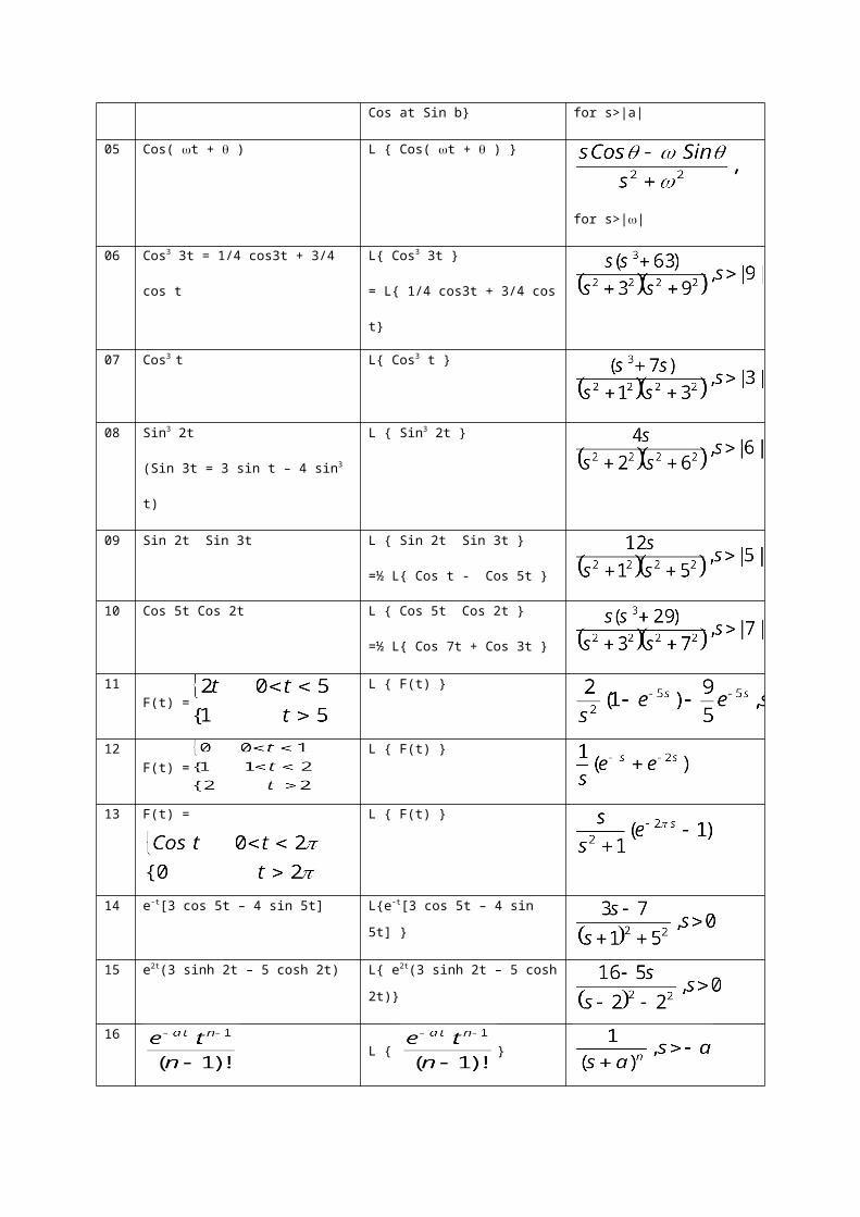
05 Cos( t + ) L { Cos( t + ) }
for s>||
06 Cos3 3t = 1/4 cos3t + 3/4
cos t
L{ Cos3 3t }
= L{ 1/4 cos3t + 3/4 cos
t}
07 Cos3 t L{ Cos3 t }
08 Sin3 2t
(Sin 3t = 3 sin t – 4 sin3
t)
L { Sin3 2t }
09 Sin 2t Sin 3t L { Sin 2t Sin 3t }
=½ L{ Cos t - Cos 5t }
10 Cos 5t Cos 2t L { Cos 5t Cos 2t }
=½ L{ Cos 7t + Cos 3t }
11F(t) =
L { F(t) }
12F(t) =
L { F(t) }
13 F(t) = L { F(t) }
14 e-t[3 cos 5t – 4 sin 5t] L{e-t[3 cos 5t – 4 sin
5t] }
15 e2t(3 sinh 2t – 5 cosh 2t) L{ e2t(3 sinh 2t – 5 cosh
2t)}
16L { }

17 e-t cos2 t L (e-t cos2 t } =
L { e-t }
18 e-at Sin bt L { e-at Sin bt }
19 Cosh at – Cos at L { Cosh at – Cos at }
20 ( 1 + t e-t )3 L { ( 1 + t e-t )3 }
21 t e-4t Sin 3t L [t e-4t Sin 3t }
22 (t-1)3[u(t – 1) L { (t-1)3 [u(t – 1) }6
23 eat [ u( t – a ) } L [eat [ u( t – a ) }
24 e-2t {1- u(t – 1) } L { e-2t } – L { e-2t (1-
u(t – 1) )}
25 If L { F(t) }
then
L { F(t/a) } a. Change of scale
property.
26 If L [ F(t) } L[3e2t sin
t – 4 e2t cos 4t }
L[ F(3t) }
27If L { } Tan-1 L { } Tan-1
28 F(t) L { F(t) }
29 F(t) L { F(t) }

30 F(t) t2 at b L { F(t) }
31 F(t) t3 5 Cos t L { F(t) }
32. Evaluate [Ans. L{
}
33. Evaluate [Ans. L{
}
34. Evaluate [Ans. L{ }
35. Evaluate [Ans. L{ }
36. Evaluate [Ans. L{ }
36. Evaluate [Ans. L{ }

37. Evaluate [Ans. L{ }
Engineering Mathematics - I Semester – 1 By Dr N VNagendram
UNIT – IV Inverse Laplace Transformations Class 9
Section III
Having found Laplace Transformation of a new functions let us
now determine the inverse Laplace Transformations of given
functions of S.
We have seen L { F(t) } is an algebraic function which is rational.
Hence to find inverse laplace transforms, we have to express the
given function of S into partial fractions which will, then to
recognize as one of the following standard forms:
Sl Inverse Laplace Function Solution

.
NO
1 L-1 { } 1
2 L-1 { } e
at
3 L-1 { } n1,2,3
..
4 L-1 { } e
atn1,2
,3..
5 L-1 { }
6 L-1 { }
7 L-1 { }
8 L-1 { }
9 L-1 { }
Cosh at
10 L-1 { } e
at Cos bt

11 L-1 { }
12 L-1 { }
Note: Reader is strongly advised to commit these results to
memory.

Engineering Mathematics - I Semester – 1 By Dr N VNagendram
UNIT – IV Inverse Laplace Transformations Class 10
Section III
Problems Vs Solutions
Problem #1: Evaluate L-1
Problem #02: Evaluate L-1
Problem #03: Evaluate L-1
Problem #04: Evaluate L-1

Problem #05: Evaluate L-1
Problem #06: Evaluate L-1
Problem #07: Evaluate L-1
Problem #08: Evaluate L-1
Problem #09: Evaluate L-1
Problem #10: Evaluate L-1
Problem #11: Evaluate L-1
Problem #1: Evaluate L-1
Solution: L-1
L-1
L-1
L-1
L-1

L-1
L-1
L-1
1 – 3 t 4
L-1
1 – 3 t 4 is required solution.
Problem #02: Evaluate L-1
Solution: L-1
L-1
L-1
L-1
L-1
L-1
is required solution.

Problem #03: Evaluate L-1
Solution: L-1
By using synthetic division method, we can get factors as
S3 s
2 s c
S - 1 1 - 6 11 - 6
0 1 -5 6
1 -5 6 0
S 2 0 2 - 6
1 - 3 0
(S – 1) (S – 2) (S – 3) factor so by partialfractions

on solving We get A ½, B
-1, C 5/2
L-1 L
-1- L
-1 L
-1
½ et - e
-2t 5/2 e
3t
L-1 ½ e
t - e
-2t 5/2 e
3t is required
solution.
Problem #04: Evaluate L-1
Solution: To find L-1 by using partial fractions
4s5 A( s – 1 ) ( s 2 ) B ( s 2 )Put s 1 9 3B B 3 and co efficient of s
2, 0 A –
1/3 A 1/3
L-1 L
-1

L-1
L-1 L-1
1/3 et 3 t e
t – 1/3 e
-2t
L-1 1/3 e
t 3 t e
t – 1/3 e
-2t is required
solution.
Problem #05: Evaluate L-1
Solution: L-1
5s 3 A (s 1)( )
On solving we get, s 1 8 8A A 1
s 0 3 5A C C 2
L-1 L
-1
L-1 L
-1 L-1
et - e
- t Cos 2t 3/2 e
-t Sin 2t

L-1 e
t - e
- t Cos 2t 3/2 e
-t Sin 2t
Is required solution.
Problem #06: Evaluate L-1
Solution: To find L-1
For that by known formula, s4 4a
4 (s
22a
2)2-
(2as)2(s
22a
22as)(s
22a
2-2as)
By partial fractions
s (As b) (Cs d) Co efficient of s3 A – C 0Co efficient of s2 B D 0
Co efficient of s A C 0 and on solving, B ; D
– B so D
L-1 L
-1 L
-1
L-1 e-a t sin at ea t sin at is required
solution.
Problem #07: Evaluate L-1

Solution: L-1 L
-16 L
-1 3 L
-1
6
L-1 6 Is required
solution.
Problem #08: Evaluate L-1
Solution: L-1
L-1 L
-1
L-1
Is required solution.

Problem #09: Evaluate L-1
Solution: L-1
L-1
L-1
L-1
[Since, L-1
e-3t Cos 2t - 3/2 e
-3t Sin 2t
L-1
e-3t Cos 2t - 3/2 e
-3t Sin 2t is required
solution.
Problem #10: Evaluate L-1
Solution: L-1
L-1

L-1
L-1
3 e-t Cosh 3t 3. .Sinh 3t.e
-t
3 e-t
e-t
e-t
L-1
is required solution.

Problem #11: Evaluate L-1
Solution: L-1
L-1
L-1
L-1
10 L-1
3 et 6 Sinh 2t
5 L
-1
3 et 5 Sinh 2t e
t
3 5
L-1
is required solution.

Engineering Mathematics - I Semester – 1 By Dr N VNagendram
UNIT – IV Inverse Laplace Transformations Class 11
Section III
Problems Vs Solutions
Problem #12: Evaluate L-1
Problem #13: Evaluate L-1
Problem #14: Evaluate L-1

Problem #15: Evaluate L-1
Problem #16: Evaluate L-1
Problem #17: Evaluate L-1
Problem #18: Evaluate L-1
Problem #19: Evaluate L-1
Problem #20: Evaluate L-1
Problem #21: Evaluate L-1
Problem #22: Evaluate L-1
Problem #23: Evaluate L-1
Problem #24: Evaluate L-1
Problem #25: Evaluate L-1

Problem #26: Evaluate L-1
Problem #27: Evaluate L-1
Problem #28: Evaluate L-1
Problem #29: Evaluate L-1
Problem #30: Evaluate L-1
Problem #31: Evaluate L-1
Problem #32: Evaluate L-1
Problem #33: Evaluate L-1
Problem #34: Evaluate L-1
Problem #35: Evaluate L-1
Problem #36: Evaluate L-1

Engineering Mathematics - I Semester – 1 By Dr N VNagendram
UNIT – IV Inverse Laplace Transformations Class 11
Section III
Problems Vs Solutions
Problem #12: Evaluate L-1
Solution: To find L-1
By partial fractions, L-1
L-1
L-1
L-1
We get A = ; B = ; C =
L-1
L-1
L-1
L-1
L-1
L-1
L-1
e-3t
e2t

L-1
e-3t
e2t is required
solution.
Problem #13: Evaluate L-1
Solution: L-1
L-1
By partial fractions =
We get, A = ; B = 2 ; C =
L-1
L-1
+ 2 L-1
L-1

L-1
L-1
+ 2 L-1
L-1
e7t + 2 e
3t e
2t
L-1
e7t + 2 e
3t e
2t is required
solution.

Problem #14: Evaluate L-1
Solution: L-1 L
-1
L-1 L
-1
L-1 L
-1
= L-1 L
-1
= t et - t e-t
L-1 = t et - t e-t is required solution.

Problem #15: Evaluate L-1
Solution: L-1 = L
-1
= L-1 L
-1
= L-1 L
-1 = L
-1 L
-1
= L-1 -L
-1 L
-1 -L
-1

= L-1 - L
-1 L
-1 - L
-1
= L-1 - L
-1 L
-1 - L
-1
= t et - t e-2t
L-1 = = t et - t e-2t is required
solution.
Problem #16: Evaluate L-1
Solution: To find L-1

By partial fractions =
Put s = 3 A =
Put s = 0 C =
Put s = 1 B =
L-1 L
-1 L
-1
L-1 L
-1 L
-1
L-1 L
-1 L
-1
= L-1 L
-1 L
-1
= e3t Cos 2t Sin 2t
L-1 = e
3t Cos 2t Sin 2t is
required solution.

Problem #17: Evaluate L-1
Solution: L-1 = L
-1
= L-1
= L-1 L
-1
= L-1 L
-1
= L-1 L
-1
= Sin t - t e-t
L-1 = Sin t - t e-t is required solution.

Problem #18: Evaluate L-1
Solution: L-1 = L
-1
= L-1
= L-1 + L
-1
= L-1 + L
-1
= Cosh at + Cos at

L-1 = Cosh at + Cos at is required solution.
Problem #19: Evaluate L-1

Solution: L-1 = L
-1 = L
-1
L-1 = L
-1 by partial
fractions
Here 1= A[(s-a)2+3as] + (Bs + c) (s-a) ; Put s = a A = ;
Put s = 0 C = ; Put s = 1 B =
L-1 = L
-1
= L-1
= L-1 + L
-1 - L
-1
= + L-1 L
-1
= + L-1 L
-1 L
-1
+ L-1
= e-at t e-at e-at t e-at Cos
at

L-1 = e
-at t e-at e-at
t e-at Cos at
Is required solution.
Problem #20: Evaluate L-1
Solution: L-1
= L-1
= L-1
+ L-1
+ L-1
= L-1
+ L-1
+ L-1
= L-1
+ L-1
+ L-1
= L-1
+ L-1
+ L-1
L-1

= L-1
+ L-1
+ L-1
L-1
= Sin 2t + Sin t + Sin t - Sin 2t
= Sin 2t + Sin t + Sin t - Sin 2t
= Sin t - Sin 2t
= [5 Sin t - Sin 2t]
L-1
= [5 Sin t - Sin 2t] is required
solution.
Problem #21: Evaluate L-1
Solution: L-1
= L-1
= L-1
= L-1
L-1

= L-1
L-1
= 2 e-2t Cos 3t 7 e
-2t sin 3t
L-1
= 2 e-2t Cos 3t 7 e
-2t sin 3t is required
solution.
Problem #22: Evaluate L-1
Solution: L-1
= L-1
= e-2t Cos t
L-1
= e-2t Cos t is required solution.

Problem #23: Evaluate L-1
Solution: L-1
= L-1
= L-1
= L-1
+ L-1
- L-1
= L-1
+ L-1
- 3 L-1
= Sin t + e-t Sin t - 3 L
-1
L-1
= Sin t + e-t Sin t - 3 L
-1
Is required solution.

Problem #24: Evaluate L-1
Solution: L-1
= L-1
= L-1
=
= L-1
L-1

= e-1/2t
Cos e-1/2t
Sin
L-1
= e-1/2t
Cos e-1/2t
Sin
is required solution.
Problem #25: Evaluate L-1
Solution: L-1
= L-1
= L-1
L-1

= L-1
L-1
=a Cos 2a2t a Sin 2a
2t
L-1
=a Cos 2a2t a Sin 2a
2t is required solution.
Problem #26: Evaluate L-1
Solution: L-1 = L
-1
= L-1
= L-1 + L
-1 + L
-1
= L-1 + L
-1 + L
-1
= e2t + 4 t e
2t + 4 t
2 e
2t
L-1 = e
2t + 4 t e
2t + 4 t
2 e
2t is required solution.

Problem #27: Evaluate L-1
Solution: L-1 = L
-1
= L-1 = L
-1 +L
-1
= e2t Cos 3t + 5/3 e
2t Sin 3t
L-1 = e
2t Cos 3t + 5/3 e
2t Sin 3t is required
solution.
Problem #28: Evaluate L-1
Solution: Since, L-1 =
L-1 = = =
L-1 = is required solution.

Problem #29: Evaluate L-1
Solution: L-1 = L
-1 = e
-at L
-1
Here we have, L-1
= = ;
L-1
= = and
L-1
= =

L-1 = =
L-1 = is required
solution.
Problem #30: Evaluate L-1
Solution: Let F (t) = L-1
Hence, L = = = since,
after applying limits. So, = =
L-1 = is required solution.
Problem #31: Evaluate L-1
Solution: L-1

= L-1
=
=
=
=
=
L-1 = is required solution.

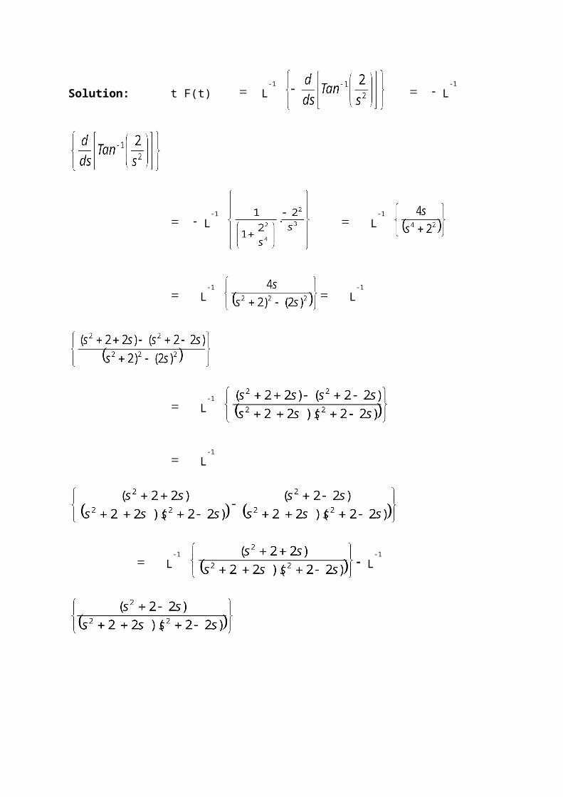
Problem #32: Evaluate L-1
Solution: Let F (t) = L-1
So, t. F(t) = - L-1
= - L-1
= - L-1
= - L-1 + L
-1
= - L-1 + L
-1
= - e-t
+ et
t. F(t) = - e-t
+ et

F(t) = L-1 =2 is required solution.
Problem #33: Evaluate L-1
Solution: t. F(t) L-1
L-1
L-1 L
-1 L
-1

L-1 L
-1 L
-1
t. F(t) 2 Cos t 1 t e-t
F(t) e-t
F(t) is required solution.
Problem #34: Evaluate L-1
Solution: t F(t) L-1 L
-1
L-1 L
-1
L-1 L
-1
L-1
L-1
L-1 L
-1

L-1 L
-1 L
-1 L
-1
et Sin t e
- t Sin t 2 Sin t 2 sinh
t sin t
t F(t) 2 Sinh t sin t
F(t) is required solution.
Problem #35: Evaluate L-1
Solution: Let t F(t) L-1
L-1

L-1
t F(t) Sin 2t
F(t) is required solution.
Engineering Mathematics - I Semester – 1 By Dr N VNagendram

UNIT – IV Inverse Laplace Transformations Class 12
Section III
Convolution theorem:
If L-1{ } F(t) and L
-1{ } G(t) then L
-1{ }
F * G is called the convolution or falting of F
and G.
u
u t
tu t
O u 0
t
Let, (t)

L{ (t) }
here put t-u v
then dv dt
F * G.
L-1{ } F * G
This completes the proof of the theorem.
Exercises: Try yourself….. By Dr N V
Nagendram
Problem #01 Evaluate L-1 [Ans. t Sin at
]
Problem #02 Evaluate L-1 [Ans. t Sin at
]

Problem #03 Evaluate L-1
[Ans.
]
Problem #04 Evaluate L-1
[Ans.
]
Problem #05 Evaluate L-1 [Ans. Cos t
]
Problem #06 Evaluate L-1 [Ans. ( t- Sin
at) ]
Problem #07 Evaluate L-1 [Ans.
]
Problem #08 Evaluate L-1 [Ans. e
-at(1 – at)
]
Problem #09 Evaluate L-1 [Ans.
]
Problem #10 Evaluate L-1 [Ans. e-at
]
Problem #11 Evaluate L-1 [Ans. (1 - e-at)
]
Problem #12 Evaluate L-1 [Ans. (e-b t - e-at)
]
Problem #13 Evaluate L-1 [Ans. e
- t e-2t
e-3t ]

Problem #14 Evaluate L-1 [Ans. (Cos at – Cos
bt) ]
Problem #15 Evaluate L-1 [Ans. (1 – Cosh
at) ]
Problem #16 Evaluate L-1 [Ans. (et – Cos
t) ]
Problem #17 Evaluate L-1 [Ans.
]
Problem #18 Evaluate L-1 [Ans.
]
Problem #19 Evaluate L-1 [Ans.
]
Problem #1 Evaluate L-1
Solution: L-1 = L
-1
[Since, L-1 and L
-1 ]
By convolution theorem,

L-1 = =
=
L-1 = = t Sin at
L-1 = t Sin at is required solution.
Problem #2 Evaluate L-1
Solution: To find L-1
Since, L-1 and L
-1
by convolution theorem,
L-1 = L
-1

= =
=
=
=
L-1 = is required
solution.

Engineering Mathematics - I Semester – 1 By Dr N VNagendram
UNIT – IV Application of Laplace Transform Class 13
Section III
Application of Laplace Transform to differential equations
with constant coefficients:
Laplace transform is especially suitable to obtain thesolution of linear non-homogeneous ordinary differentialequations with constant coefficients, when all the boundaryconditions are specified for the unknown function and itsderivatives at a single point.
Consider the initial value problem
………………………….. (1)
y(t = 0) = k0, y1(t=0) = k1 ………………………………………………………………… (2)
Where a,b,k0,k1 are all constants and r(t) is a function of t.
Method of Solution to differential equation (D.E) by Laplace Transform (L.T.):
1. Apply Laplace transform on both sides of the given differential equation (1), resulting in a subsidiary equation as
[s2Y – s y(0) - y(0)] +a[sY-y(0)]+bY = R(s) …………………………………………. (3) where Y = L{y(t)} and R(s) = L{r(t)}.
Replace y(0), y(0) using given initial conditions (2).
2. Solve (3) algebraically for Y(s), usually to a sum ofpartial fractions.

3. Apply inverse Laplace transform to Y(s) obtained in 2. Thisyields the solution of O.D.E. (1) satisfying the initialconditions (2) as y(t) = L-1[Y(s)].
Problem #1 Solve the differential equation by using Laplacetransformation y-2y-8y = 0, y(0) = 3, y(0) = 6.
Solution: On applying Laplace transform (s2Y - 3s - 6) – 2( sY– 3 ) - 8Y = 0
On solving, Y(s) = =
By using partial fractions, Y(s) = +
Applying 1 L.T. y(t) = L-1(Y(s)) = 2 L-1 +L-1 = 2
e4t + e-2t.
y(t) = 2 e4t + e-2t is required solution.

Problem #2 Solve the differential equation by using Laplacetransformation y+2y+5y = e-t Sin t, y(0) = 0, y(0) = 1.
Solution: Using L.T. On applying Laplace transform we get thegiven differential equation as, (s2Y - 0 - 1) + 2( sY – 0 ) =
L{ e-t Sin t } =
On solving Y =
By partial fractions, = +
= (As + B) ( )+ (Cs + D ) ( )= s3(A + C) + s2 (2A + 2C + B + D ) + s (2A + 5C + 2B
+ 2D )+ 2B + 5DEquating coefficients of s on either side,A + C = 0 ; 2A + 2C + B + D = 1; 2A + 5C + 2B + 2D = 2; 2B +5D = 3
A = 0, B = , C = 0, D =

Y(s)= + = +
Applying I.T. y(t) = L-1{Y}= L-1 + L-1
using first shifting theorem, y(t)= e-t L-1 + e-t L-1
y(t)= is required solution.
Problem #3 Solve the differential equation by using Laplacetransformation y+n2y = a Sin (nt+2), y(0) = 0, y(0) = 0.
Solution: y+n2y = a Sin (nt+2)
= a [Sin nt Cos 2 + Cos nt Sin 2]
Applying L.T. L{ y} + n2 L { y } = a cos 2. L{Sin nt} + a Sin2 L{Cos nt}
Using L.T. On applying Laplace transform we get the givendifferential equation as,

[s2Y – sy(0) - y(0)] + n2Y = .a.Cos 2 + .a. Sin 2
Solving Y, Y(s) = .a. Cos 2 + .a. Sin 2
Applying I.T. we get
y(t) = n. a. Cos 2. L-1 + a. Sin 2. L-1 …… (1)
From I.L.T. tables, we know that 2nd term in R.H.S.
L-1 = ……………………………………………………………… (2) to find
first term in R.H.S.
L-1 =L-1 = =
….(3)
Thus substituting (2) and (3) in (1), we get
y(t) = a.n. Cos 2. + a Sin 2
= [ + Cos 2. Sin nt + nt. Sin 2 .
Sin nt]
= [ ]
= [ ]
y(t) = [ ] is required
solution.

Problem #4 Find the general solution of the differentialequation by using Laplace transformation y - 3y +3y - y=t2 et, y(0) = 1, y(0) = 0,y(0) = - 2.
Solution: Since the initial conditions are arbitrary assumey(0) = a, y(0) =b, y(0) =c.
Then Using L.T. On applying Laplace transform we get the givendifferential equation as, (s2Y – as2 – bs - c) - 3( s2Y – as -b
) + 3(sY – a) - Y =
Y =
By partial fractions Y = where c1,
c2, c3 are constants depending on a, b, c.
Applying I.T. and using first shifting theorem
y(t) = c1 et + c2 t et + c3 et + is required
solution.

Problem #5 Solve the differential equation by using Laplacetransformation y - 3y +3y - y =t2 et, y(0) = 1, y(0) =0,y(0) = - 2.
Solution: Applying L.T. to D.E. L{ y - 3y +3y - y} =L{ t2
et }
L{ y} - 3L{ y} +3 L { y} - L{ y} =L{ t2
et }
[s3Y – s2y(0) - sy(0) - y(0) ] – 3 [s2Y – sy(0) - y(0)] +
3[sY – y(0)] – Y =
Using the initial condition y(0) = 1, y(0) = 0,y(0) = - 2,and solving for Y
(s3 – 3a2 + 3s – 1)Y – s2 + 3s – 1=
Y = = =
Y =
On applying I L.T. we get
y(t) = L-1 { Y } = L-1 L-1 L-1 +2 L-1

y(t) = L-1 { Y } = et t et + is required
solution.
Engineering Mathematics - I Semester – 1 By Dr N VNagendram
UNIT – IV Application of Laplace Transform Class 14
Section III Exercise Try yourself……..
Use L.T. to solve each of the following I.V.P. consisting of aD.E. with I.C.
01. , general solution [Ans. Assume y(0)=0=A=constant;y=Aet]02. [Ans. y=(3et +e3t)/2 ]03. [Ans.G.S. y=C + De-t, C=A + B,D= B ]04. [Ans.G.S. y=et+ Cos t + Sin t ]

05. [Ans.G.S. y=(3t + 2)e3t
]
06. [Ans.G.S. y=
]
07. [Ans.G.S. y=e-2t-2e-3t+e-5t
]
08. [Ans.G.S.
y=4e2t+3te2t+3e3t-2e5t ]09. [Ans.G.S. y=
]
10. [Ans. y=
]
11. [Ans.G.S. y=
]
12. [Ans.y=
]
13. [Ans.y=e-2t + 2e-t -2te-t
– Cos t +2 Sin t]14. [
]
15. [Ans.G.S. y= 2(Sin 2t –
Sin t ]

Engineering Mathematics - I Semester – 1 By Dr N VNagendram
UNIT – IV Application of Laplace Transform Class 14
Section IV
Application of Laplace Transform to system of simultaneous
differential equations:
Laplace transform can also be used to solve a system or familyof m simultaneous equations in m dependent variables which arefunctions of the independent variable t. consider a family oftwo simultaneous differential equations in the two dependentvariables x, y which are functions of t.
……………………………………….. (1)
……………………………………….. (2)
Initial conditions x(0) = c1; y(0) = c2; x(0) = c3; y(0) = c4
………………………… (3)
Here a1, a2, a3, a4, a5, a6,b1, b2, b3, b4, b5, b6 and c1, c2, c3, c4
are all constants and R1(t), R2(t) are functions of t.
Method of solution to system of differential equation (D.E.):
I. Apply Laplace transform on both sides of each of the twodifferential equation (1) and (2) above. This reduces (1) and

(2) to two algebraic equations in X(s) and Y(s) where X(s) =L{ x(t) } and Y(s) = L{ y(t) }. a1[s
2X-sx(0) - x(0)] + a2[ s2Y – sy(0) - y(0)] + a3[sX – x(0) ] + a4[sY- y(0)]+ a5 X + a6 Y = Q1(s)…..(4)
b1[s2X-sx(0) - x(0)] + b2[ s2Y – sy(0) - y(0)] + b3[sX – x(0) ] + b4[sY- y(0)
]+ b5 X + b6 Y = Q2(s)… (5)
use the initial conditions (3) and substitute for x(0) ,y(0) , x(0) , y(0). II. Solve (4) and (5) for X(s) and Y(s).
III. The required solution is obtained by taking the inverseLaplace Transform of X(s) and Y(s) as
x(t) = L-1{ X(s) } and y(t) = L-1 { Y(s) }.
Problem #1 Solve ;
x(0) = 0; y(0) = 6.5; x(0) = 0;
Solution: Taking Laplace Transformation of the givendifferential equation we have
[s2X-sx(0) - x(0)] -3 [sX – x(0) ] - [sY- y(0) ]+ 2Y = 14 +3
[sX – x(0) ] – 3X + [sY- y(0) ] =
Use given initial conditions (I.C.) x(0) = 0; y(0) = 6.5=13/2;x(0) = 0;
S(s - 3)X +(2 – s)Y = and (s – 3 )X + sY =

On solving we get Y(s) = and X(s) =
Taking inverse Laplace Transform y(t) = L-1{Y(s)} = L-1
= L-1
= L-1
y(t) = 7t + 5 – et + e-2t
Similarly, x(t) = L-1{X(s)} = L-1 by partial
fractions
= L-1
= 2 et e3t e-2t
x(t) =2 et e3t e-2t Is required solution.
Problem #2 Solve ;
x(0) = 2; y(0) = 1;

Solution: Taking Laplace Transformation of the givendifferential equation we have
2[sX(s) - x(0)] + sY(s)- y(0) –X(s)- Y(s) =
sX(s) – x(0) + sY(s) - y(0)+ 2 X(s) + Y(s) =
Use given initial conditions (I.C.) x(0) = 2; y(0) = 1.
(2s - 1)X(s) +(s – 1)Y(s) = and (s + 2 )X(s) +
(s+1)Y(s) =
On solving we get Y(s) = =
and X(s) =
Taking inverse Laplace Transform y(t) = L-1{Y(s)} = L-1
= Cos t – 13 Sin t +Sinh t
y(t) = Cos t – 13 Sin t + Sinh t
Similarly, x(t) = L-1{X(s)} = L-1 by partial fractions
= 2 Cos t + 8 Sin t
x(t) =2 Cos t + 8 Sin t Is required solution.

Engineering Mathematics - I Semester – 1 By Dr N VNagendram
UNIT – IV Application of Laplace Transform Class 15
Exercise Solve the following system ofequations Try yourself ……..
01. ; , x(0) = 8, y(0) = 3
[Ans. x(t) = 5 e-t + 3 e4t; y(t) = 5 e-t – 2 e4t]
02. ; ,
x(0) = 35,y(0) = 27; x(0) = -48,y(0) = -55.
[Ans. x(t) = 30 Cos t – 15 Sin 3t + 3 e-t + 2 Cos 2t; y(t) = 30 Cos t – 60 Sin t - 3 e-t + Sin 2t]
03. ; , x(0) = y(0) = 1; x(0) =
y(0) = 0
[Ans. x(t) = ;
y(t) = ]
04. ; , x(0) = 1, y(0) = 0
[Ans. x(t) = ; y(t) =
]

05. ; , x(0) = 3, y(0) = 0
[Ans.x(t)= ; y(t) = ]
06. ; , x(0) = y(0)= y(0) = 0
[Ans. x(t)=1+ e-t – e-at-e-bt; y(t)=1+e-t– be-at a e-bt ]
Note: a = ; b =
07. ; , x(0) = 0, x(0) =
0[Ans. x(t) = 22e-t (1+t); y(t) = 2t-2e-t (1+t)]
08. ; , x(0) =1, y(0) =0
[Ans. x(t) = e-2t - t et; y(t) = et +tet ]
09. ; ,x(0) =-1, y(0) = 0
[Ans. x(t) = -2 et + e4t; y(t)= et + e4t]
10. ; , x(0) = 2, y(0) = 0
[Ans. x(t)=e-t + et = 2Cosh t; y(t)=Sin t – 2 Sinh t]