arX

iv:n

lin/0

5020

06v1

[nl

in.S

I] 3

Feb

200

5

Elementary Darboux transformations and factorization

F.Musso♯ and A.Shabat♭

February 8, 2008

♯ Dipartimento di Fisica E. Amaldi, Universita degli Studi di Roma Treand

Istituto Nazionale di Fisica Nucleare, Sezione di Roma TreVia della Vasca Navale 84, 00146, Rome, Italy 1

♭Landau Institute for Theoretical Physics, Chernogolovka, Russiaand

Dipartimento di Fisica E. Amaldi, Universita degli Studi di Roma TreVia della Vasca Navale 84, 00146, Rome, Italy 2

Abstract

A general theorem on factorization of matrices with polynomial entries is provenand it is used to reduce polynomial Darboux matrices to linear ones. Some newexamples of linear Darboux matrices are discussed.

1 Introduction

In the continuous case, for spectral problems with m×m matrix potentials U polynomialin λ

d

dxΨ = U(x, λ)Ψ (1)

the construction of Darboux transformation

Ψ → Ψ = Q(x, λ)Ψ,d

dxQ = UQ−QU ⇒

d

dxΨ = U(x, λ)Ψ (2)

can be based on the elementary Darboux transformations, for which

Q(x, λ) = (λ− α)P (x) + (λ− β)(E − P (x)), P 2 = P. (3)

Here, E denotes the identity matrix and the projector P is uniquely defined by the null-spaces of Q :

KerQ|λ=α = ImP = M, KerQ|λ=β = KerP = N

1E-mail:musso@fis.uniroma3.it2E-mail:shabat@fis.uniroma3.it

If v(x) ∈ M and w(x) ∈ N , then the following equations have to be satisfied:

d

dxv(x) = U(x, α)v(x),

d

dxw(x) = U(x, β)w(x). (4)

The zeroes of the determinant define the eigenvalues λ = α, β introduced by the Darbouxtransformation (3). In particular, for the Zakharov-Shabat spectral problems (see, e.g.,[1]),

U = λσ + q(x), q(x) = [σ, q(x)], (5)

where σ is a constant matrix with simple eigenvalues, the function Ψ satisfies the equation(1) with the potential

U = U + [Q, σ].

The caseβ = α, P ∗ = P (6)

where ∗ means hermitian conjugation, corresponds to the self-adjoint potentials

U∗(x, λ) = U(λ, x), q∗ = q.

Main Theorem in Section 2 3 formulates the necessary and sufficient conditions on theNth degree matrix polynomial A(λ) to be represented as the product of N first orderpolynomials (3), (6).

In application to Darboux transformations this factorization A = QN · · ·Q1 gives risethe sequence of spectral problems (1)

d

dxΨj = Uj(x, λ)Ψj, Ψj+1 = Qj(x, λ)Ψj, (7)

related with each other by the transformations (2),(3). Observe that the composition ofDarboux transformations Ψj+1 = BjΨj is also a Darboux transformation since (Cf. (2))

Bj,x = Uj+1Bj − BjUj , Bdef= Bn · · ·B1 ⇒ Bx = Un+1B − BU1. (8)

For a scalar differential operator A, the elementary Darboux transformation Ψ → Ψis defined by the first order differential operator:

AΨ = λΨ, Ψ = (D − f)Ψ, AΨ = λΨ A = (D − f)A(D − f)−1.

For the operator A of order N , an analog of Main Theorem yields the relation

AΨ =< ϕ1, . . . , ϕN ,Ψ >

< ϕ1, . . . , ϕN >= (D − fN) · · · (D − f2)(D − f1)Ψ, (9)

where ϕj ∈ KerA and

< ϕ1, . . . , ϕl >def= det(Dk−1(ϕj)), j, k = 1, . . . , l, D =

d

dx.

3An analog of this theorem was recently used by [7] in order to construct an approximate solution ofRiemann-Hilbert problem. See also [6].

2

The proof of (9) is obtained by induction (Cf. Main Theorem) based upon the identityvalid for any smooth functions ϕj :

< ϕ1, . . . , ϕm >= ϕ1 < ϕ2, . . . , ϕm >, ϕj = (D − f1)ϕj, f1 = D logϕ1.

In eq. (9) the factors D−fj are irreducible (they are first order differential operators).Such property appears to be crucial in the theory of dressing chains [2], [3], [4], wherethe functions fj are used as basic dynamical variables. On the other hand, the Darbouxtransformation (3) can be factorized into the composition of two more elementary oneswith null spaces KerP and ImP, respectively. This factorization reformulated in termsof the corresponding matrices B1 and B2 gives rise to the following equations:

Ψ(m+ 1, n) = B1(m,n)Ψ(m,n), Ψ(m,n+ 1) = B2(m,n)Ψ(m,n),

Ψ(m+ 1, n+ 1) = Q(m,n)Ψ(m,n), Q = B1 ◦B2,

where by definition

Q = B1 ◦B2 ⇔ Q(m,n) = B1(m,n+ 1)B2(m,n) = B2(m+ 1, n)B1(m,n). (10)

Equations (10) show that, unlike the continuous case (8), the Darboux transformationsand the original discrete spectral problem have the same nature and it is possible toreplace one with the other.

Thus, the problem of factorization of (3), considered in Section 3, brings up the discretespectral problems with potentials linear in the spectral parameter λ. In the examples,we will restrict ourself to the simplest 2 × 2 case but without the assumption that Q isfactorized through orthogonal projectors (see (3)). In our considerations, the continuousindependent variable x will play the role of a parameter .

In the last subsection we consider solutions of the Yang-Baxter equation linear in thespectral parameter λ.

2 Main Theorem

In order to prove that the Darboux transformations (3) are generic ones, it sufficies toprove that the product of N matrices (3) yields an N -th degree polynomial in λ of ageneral form. We will use the characteristic property of the polynomials (3) as follows

Qαβdef= (λ− α)P + (λ− β)(E − P ) ⇒ QαβQβα = (λ− α)(λ− β)E. (11)

In case (6), we haveQ(λ)∗Q(λ) = (λ− α)(λ− α)E

, and such property holds, obviously, for the product of matrices (3) with the orthogonalprojectors P ∗ = P.

3

Theorem. Let A(λ) be an m ×m matrix with polynomial entries in λ satisfying theconditions:

A(λ)∗A(λ) =N∏

j=1

(λ− αj)(λ− αj)E, (12)

limλ→∞

A(λ)

λN= E. (13)

Then A(λ) can be factorized as

A(λ) =N∏

j=1

((λ− αj)Pαj

+ (λ− αj)(E − Pαj)), (14)

where the Pαjare Hermitian projectors.

Proof: We proceed by induction on N . If N = 0, then from (13) and the Liouvilletheorem it follows that A(λ) = E.

Now we show that if the statement of our theorem holds for N − 1, it holds for N aswell. From (12) and (13) it follows:

det(A(λ)) =N∏

j=1

(λ− αj)kj(λ− αj)

m−kj . (15)

We select a zero αj of det(A(λ)); from (15) it follows:

dim(Ker(A(αj))) = kj ,

dim(Ker(A(αj))) = m− kj .(16)

Let |vi〉kj

i=1 and |wi〉N−kj

i=1 be an orthonormal basis for Ker(A(αj)) and Ker(A(αj)), respec-tively. We denote by Pαj

and Pαjthe Hermitian projectors

Pαj≡

kj∑

i=1

|vi〉〈vi|, (17)

Pαj≡

m−kj∑

i=1

|wi〉〈wi|. (18)

Let us prove thatPαj

= (E − Pαj). (19)

To prove (19) is equivalent to proving that Cm admits an orthogonal decomposition

Cm = Ker(A(αj)) ⊕ Ker(A(αj)). (20)

From (12) it follows:A(αj)A(αj)

∗ = 0, (21)

that isIm(A(αj)

∗) ⊂ Ker(A(αj)); (22)

4

but from (16) we have:

dim(Im(A(αj)∗)) = m− dim(Ker(A(αj))) = kj,

dim(Ker(A(αj))) = kj,

whence it follows:Im(A(αj)

∗) = Ker(A(αj)). (23)

Equation (23) is equivalent to

Ker(A(αj)) = Im(A(αj)∗) (24)

whence it follows

Cm = Ker(A(αj)) ⊕ Im(A(αj)

∗) = Ker(A(αj)) ⊕ Ker(A(αj)).

Now the matrixA(λ)

[(λ− αj)Pαj

+ (λ− αj)(E − Pαj)]

(25)

vanishes at λ = αj and λ = αj. Consequently, we have:

A(λ)[(λ− αj)Pαj

+ (λ− αj)(E − Pαj)]

= (λ− αj)(λ− αj)A(λ) (26)

for a certain matrix A(λ). Then

A(λ) = A(λ)[(λ− αj)Pαj

+ (λ− αj)(E − Pαj)]

(27)

Since Pαjis Hermitian, it follows that A(λ) satisfies

A(λ)∗A(λ) =N∏

k 6=j

(λ− αk)(λ− αk)E. (28)

Moreover,

limλ→∞

A(λ)

λN= limλ→∞

A(λ)

λN−1= E. (29)

In the case of distinct zeroes αj 6= αk, the orthogonal projectors Pαjin (14) are

uniquely defined by the subspaces

Mjdef= KerA(λ)|λ=αj

(30)

and an ordering of zeroes α1, . . . , αN . Indeed, for instance, for N = 2, we have

A(λ) = Q1(λ)Q2(λ), Qj(λ) = (λ− αj)Pαj+ (λ− αj)(E − Pαj

), j = 1, 2;

with P ∗αj

= Pαjand

ImPα2= Ker(E − Pα2

) = KerQ2(α2) = KerQ1(α2)Q2(α2) = M2

5

, since detQ1(α2) 6= 0. Similarly

ImPα1= Q2(α1)M1, since M1 = Ker(E − Pαj

)Q2(α1). (31)

In order to construct a dressing chain, we have to factorize (see the next section) thebasic Darboux transformation (11) further:

Qαβ(λ) = (λ− α)Pαβ + (λ− β)(E − Pαβ) = B2(λ)B1(λ) (32)

where these two factors Bj(λ) = σjλ+ bj are linear in λ and

detQαβ(λ) = (λ− α)k(λ− β)m−k ⇒ detB1 = (λ− α)k, detB2 = (λ− β)m−k.

Evidently,KerB1(β) = ImB2(α) = KerPαβ , (33)

since, due to (32) and the fact that detB1(α) 6= 0, we have

Qαβ(α) = (α− β)(E − Pαβ) = B2(α)B1(α) ⇒ ImB2(α) = Im(E − Pαβ) = KerPαβ.

3 2 × 2 case

In this section we consider some interesting, from our point of view, classes of 2×2 matriceslinear in λ related with (3). First, let us consider the chain of matrices Bj, j ∈ Z :

Bj =

(λ+ hj

1

2uj

1

2vj+1 1

), hj =

1

4ujvj+1 − βj for j odd, (34)

Bj =

(1 −1

2uj+1

−1

2vj λ+ hj

), hj =

1

4vjuj+1 − βj for j even. (35)

ThusdetBj = λ− βj for all j

and (Cf (33)) it easy to see that

KerB1|λ=β1= ImB2|λ=β2

, KerB2|λ=β2= ImB3|λ=β3

, . . .

Moreover, these matrices satisfy the consistency conditions (10) (see Lemma below) and

B2B1 = λ− β1 + β12P12, B3B2 = λ− β2 + β23P23, . . . , βijdef= βi − βj,

where P 2ij = Pij are projectors. In particular,

β12P12 =

(1

4v2u13

1

2u13

1

2v2(β12 −

1

4v2u13) β12 −

1

4v2u13

), u13

def= u1 − u3,

β23P23 =

(β23 + 1

4u2v42

1

2u3(β32 + 1

4u2v24)

1

2v42

1

4u3v24

), vij

def= vi − vj .

6

Thus these matrices provide us with a factorization of elementary Darboux transforma-tions (3). Observe that, for odd i, the product BjBi, where j = i + 1, depends only onvj , uij = ui − uj for i odd and on the difference vi+2 − vi+1 and ui+1 for i even.

In comparison with the factorization defined by main Theorem, the entries of matrices(34) and (35) are expressed directly in terms of the potentials

Uj =

(λ uj

vj −λ

)= λσ + qj

of the 2 × 2 Zakharov-Shabat spectral problem

ψ1

x − λΨ1 = uΨ2, Ψ2

x + λΨ2 = vΨ1, or Ψx = UΨ. (36)

Thus, the substitution of matrices (34) and (35) into the equations (8) yields the dressingchain for the spectral problem (36):

(D + 2βj)vj+1 + 2vj =1

2ujv

2

j+1, (D − 2βj)uj − 2uj+1 = −1

2u2

jvj+1, (37)

(D − 2βj)uj+1 − 2uj = −1

2u2

j+1vj, (D + 2βj)vj + 2vj+1 =1

2uj+1v

2

j . (38)

The first case corresponds to (34) and the second one to (35).

Remark. In the case of the general Zakharov-Shabat spectral problem (5) one couldconsider the following Darboux transformations (8)

Bj = λσj + bj , Uj = λσ + qj.

Collecting quadratic and linear terms in λ in (8) one finds

[σ, σj ] = 0, σj,x = [σ,Aj ] + qj+1σj − σjqj

That implies that σj,x = 0 since the potentials qj are off-diagonal in the basis where thematrix σ is diagonal. Thus, the matrices σj should be x−independent and could be anydiagonal matrix in that basis.

Coming back to the spectral problem (36) we will show how, starting with (u1, v1),one construct a chain of Darboux matrices Bj , transforming the equation (36) with thepotential Uj into one with the potential Uj+1, using the solution to the correspondingspectral problem Riccati equation:

ρx = 2λρ− vjρ2 + uj, ρ

def=

Ψ1

Ψ2. (39)

This should highlight a similarity with the dressing chain considered in [2].

7

Proposition. There is a one-to-one correspondence between the matrices (34), (35) andsolutions of the Riccati equation (39) with λ = βj .

Proof: At the first step we have to find the potentials u2 and v2. The function v2 isdefined by (37) as solution of ODE

(D + 2β1)v2 + 2v1 =1

2u1v

2

2

which is reduced by rescaling v2 = 2ρ to (39) with λ = β1. For the function u2, we obtainnow the exact formula

2u2 = u1,x − 2β1u1 +1

2u2

1v2.

At the next step, we find u3 = 2ρ−1 by solving (39) with λ = β2. It satisfies thecorresponding equation (38):

(D − 2β2)u3 − 2u2 =1

2u2

3v2

while v3 is defined by the second equation in (38). Thus in both cases the system ofequations (37) and (38) are reduced to the Riccati equation (39).

Consistency problem. We will ignore now the dependence on the continuous indepen-dent variable x and consider more general (as comparised with (34), (35)) matrices linearin λ and satisfying conditions analogous to (10). Having applications in mind, we willdenote one of the matrices in (10) as A(n, λ) and consider the second one as a Darbouxtransformation for the discrete spectral problem defined by A :

Ψn+1 = A(n, λ)Ψn, A =

(λ+ c a

b α

), Ψ = BΨ, Ψn+1 = A(n, λ)Ψ. (40)

If the spectral problem in (40) is a “good” one, 4 then there should exist nontrivialDarboux transformations with

B =

(ε f

g h− λ

)(41)

and the consistency equations T1 ◦ T2 = T2 ◦ T1, where T1Ψ = AΨ, T2Ψ = BΨ (Cf. (10))yield

(λ+ c)ε+ ga = ε′(λ+ c) + f ′b, (λ+ c)f + a(h− λ) = ε′a+ f ′α

εb+ αg = (λ+ c)g′ + b(h′ − λ), α(h− λ)ε+ f b = α(h′ − λ) + g′a

where B′ def= T1(B) and A

def= T2(A). We see that

g′ = T1(g) = b, a = T2(a) = f, ε′ = ε, α = α

and thus the consistency equations are reduced to{b(h′ + c) = εb+ αg, ε(c− c) = f ′g′ − fg

a(h+ c) = εa+ αf ′, α(h′ − h) = ab− ab. (42)

It is easy to verify now4The particular case of A with α = 0 is related with Toda chain.

8

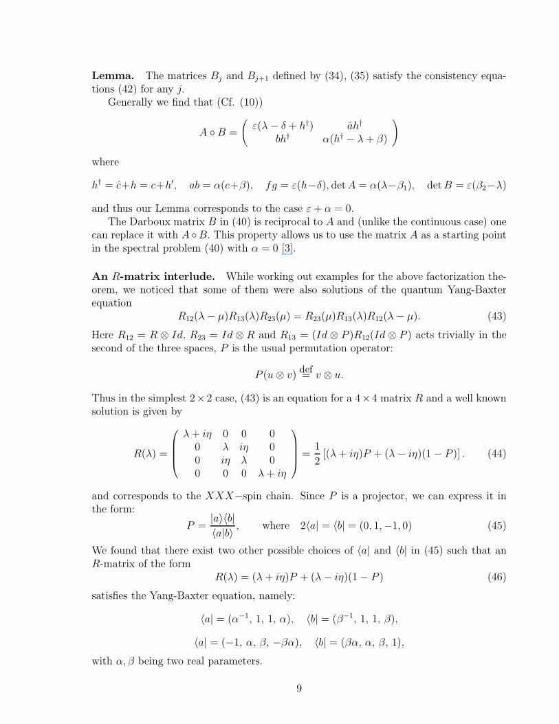
Lemma. The matrices Bj and Bj+1 defined by (34), (35) satisfy the consistency equa-tions (42) for any j.

Generally we find that (Cf. (10))

A ◦B =

(ε(λ− δ + h†) ah†

bh† α(h† − λ+ β)

)

where

h† = c+h = c+h′, ab = α(c+β), fg = ε(h−δ), detA = α(λ−β1), detB = ε(β2−λ)

and thus our Lemma corresponds to the case ε+ α = 0.The Darboux matrix B in (40) is reciprocal to A and (unlike the continuous case) one

can replace it with A ◦B. This property allows us to use the matrix A as a starting pointin the spectral problem (40) with α = 0 [3].

An R-matrix interlude. While working out examples for the above factorization the-orem, we noticed that some of them were also solutions of the quantum Yang-Baxterequation

R12(λ− µ)R13(λ)R23(µ) = R23(µ)R13(λ)R12(λ− µ). (43)

Here R12 = R ⊗ Id, R23 = Id ⊗ R and R13 = (Id ⊗ P )R12(Id ⊗ P ) acts trivially in thesecond of the three spaces, P is the usual permutation operator:

P (u⊗ v)def= v ⊗ u.

Thus in the simplest 2×2 case, (43) is an equation for a 4×4 matrix R and a well knownsolution is given by

R(λ) =

λ+ iη 0 0 00 λ iη 00 iη λ 00 0 0 λ+ iη

=

1

2[(λ+ iη)P + (λ− iη)(1 − P )] . (44)

and corresponds to the XXX−spin chain. Since P is a projector, we can express it inthe form:

P =|a〉〈b|

〈a|b〉, where 2〈a| = 〈b| = (0, 1,−1, 0) (45)

We found that there exist two other possible choices of 〈a| and 〈b| in (45) such that anR-matrix of the form

R(λ) = (λ+ iη)P + (λ− iη)(1 − P ) (46)

satisfies the Yang-Baxter equation, namely:

〈a| = (α−1, 1, 1, α), 〈b| = (β−1, 1, 1, β),

〈a| = (−1, α, β, −βα), 〈b| = (βα, α, β, 1),

with α, β being two real parameters.

9

Having two new solutions of the Yang-Baxter equation, we can construct the associ-ated Lax matrices and, finally, two monodromy matrices out of them. Then, taking thetraces of the monodromy matrices we obtain two sets of commuting quantum observables.Unfortunately the elements of each set are functionally dependent. Hence, these two newsolutions do not give rise to new quantum integrable systems.

Further investigations on Quantum Yang–Baxter equation showed that, if we gen-eralize the R–matrix form (46) dropping the normalization condition (13), then othersolutions, linear in the spectral parameter λ, can be found. We notice that R can thenbe expressed in the form R = λA + B, where A and B must be solutions to the two-dimensional constant quantum Yang-Baxter equation; all such solutions have been foundby J. Hietarinta [5].

An example of solution that we believe could be of some interest is the following one:

R(λ) =

η 0 0 λ

0 0 λ+ η 00 λ+ η 0 0λ 0 0 η

, R−1 =

1

λ2 − η2

−η 0 0 λ

0 0 λ− η 00 λ− η 0 0λ 0 0 −η

Work is in progress on this topic.

Acknowledgements We would like to thank Decio Levi and Antonio Degasperis foruseful discussions and the interest shown in this paper.

This work was partially supported by Russian Foundation for Basic Research, grantsNo. 04-01-00403 and Nsh 1716.2003.1.

References

[1] V.Zakharov and A.Shabat, “A Scheme for integration the nonlinear equations ofmathematical physics by the method of the inverse scattering problem, II”, Funct.

Anal. Appl. 13: 166–74, 1979.

[2] A.P. Veselov and A.B. Shabat “Dressing chain and spectral theory of Schrodingeroperator”, Funkts. Anal. Prilozen., 27(2): 1–21, 1993.

[3] A.B. Shabat, “Third version of the dressing method” Theor. Math. Phys., 121(1):1397–408, 1999.

[4] V.E.Adler, V.G. Marikhin, A.B.Shabat, “Canonical Backlund transformations andLagrangian chains,” Theor. Math. Phys., 129(2): 163-183, 2001.

[5] J. Hietarinta, “Solving the two-dimensional constant quantum Yang-Baxter equa-tion” J. Math. Phys., 34(5): 1725–1756, 1993.

[6] I.T.Habibullin, A.Shagalov, “Numerical realization of the IS,” Theor. Math. Ph.,83(3): 565-73 (323-33), 1990.

[7] A.V.Domrin, “On a version of the Riemann problem in the theory of integrablesystems,” Dokl. Ross. Akad. Nauk, 390: 301-303, 2003.

10