Online Nonnegative Matrix Factorization With Robust Stochastic Approximation
13
IEEE TRANSACTIONS ON NEURAL NETWORKS AND LEARNING SYSTEMS, VOL. 23, NO. 7, JULY 2012 1087 Online Nonnegative Matrix Factorization With Robust Stochastic Approximation Naiyang Guan, Dacheng Tao, Senior Member, IEEE , Zhigang Luo, and Bo Yuan Abstract— Nonnegative matrix factorization (NMF) has become a popular dimension-reduction method and has been widely applied to image processing and pattern recognition problems. However, conventional NMF learning methods require the entire dataset to reside in the memory and thus cannot be applied to large-scale or streaming datasets. In this paper, we propose an efficient online RSA-NMF algorithm (OR-NMF) that learns NMF in an incremental fashion and thus solves this problem. In particular, OR-NMF receives one sample or a chunk of samples per step and updates the bases via robust stochastic approximation. Benefitting from the smartly chosen learning rate and averaging technique, OR-NMF converges at the rate of O(1/ √ k) in each update of the bases. Furthermore, we prove that OR-NMF almost surely converges to a local optimal solution by using the quasi-martingale. By using a buffering strategy, we keep both the time and space complexities of one step of the OR-NMF constant and make OR-NMF suitable for large- scale or streaming datasets. Preliminary experimental results on real-world datasets show that OR-NMF outperforms the existing online NMF (ONMF) algorithms in terms of efficiency. Experimental results of face recognition and image annotation on public datasets confirm the effectiveness of OR-NMF compared with the existing ONMF algorithms. Index Terms— Nonnegative matrix factorization (NMF), online NMF (ONMF), robust stochastic approximation. I. I NTRODUCTION N ONNEGATIVE matrix factorization (NMF) [1] has been widely applied to image processing and pattern recog- nition applications because these nonnegativity constraints on both the basis vectors and the combination coefficients allow only additive, not subtractive, combinations and lead to naturally sparse and parts-based representations. Since NMF does not allow negative entries in both basis vectors and coefficients, only additive combinations are allowed and such combinations are compatible with the intuitive notion Manuscript received July 23, 2011; accepted April 20, 2012. Date of publication May 22, 2012; date of current version June 8, 2012. This work was supported in part by the Australian Research Council Discovery Project with number DP-120103730, the National Natural Science Foundation of China under Grant 91024030/G03, and the Program for Changjiang Scholars and Innovative Research Team in University under Grant IRT1012. N. Guan and Z. Luo are with the School of Computer Science, National University of Defense Technology, Changsha 410073, China (e-mail: ny [email protected]; [email protected]). D. Tao is with the Center for Quantum Computation & Intelligent Systems and the Faculty of Engineering & Information Technology, University of Technology, Sydney, NSW 2007, Australia (e-mail: [email protected]). B. Yuan is with the Department of Computer Science and Engineer- ing, Shanghai Jiao Tong University, Shanghai 200240, China (e-mail: [email protected]). Color versions of one or more of the figures in this paper are available online at http://ieeexplore.ieee.org. Digital Object Identifier 10.1109/TNNLS.2012.2197827 of combining parts to form a whole, i.e., NMF learns parts- based representation. As the basis images are nonglobal and contain several versions of mouths, noses, and other facial parts, the basis images are sparse. Since any given face does not use all the available parts, the coefficients are also sparse. NMF learns sparse representation, but it is different from sparse coding because NMF learns low rank representation while sparse coding usually learns the full rank representation. Recently, several NMF-based dimension reduction algorithms have been proposed [2]–[6] and a unified framework [7] has been proposed to intrinsically understand them. Several algorithms including the multiplicative update rule [8], [9], projected gradient descent [10], alternating nonnega- tive least squares [11], active set methods [12], and NeNMF [13] have been utilized to learn NMF. The multiplicative update rule iteratively updates the two matrix factors by the gradient descent method, whereby the learning rates are carefully chosen to guarantee the nonnegativity. Lin [10] applied the projected gradient descent method to NMF, which iteratively optimizes each matrix factor by descending along its projected gradient direction and the learning rate is chosen by Armjo’s rule. Berry et al. [11] proposed to learn NMF by iteratively projecting the least-squares solution of each matrix factor onto the nonnegative orthant. Kim and Park [12] proposed to learn NMF by utilizing the active set method to iteratively optimize each matrix factor. Recently, Guan et al. [13] proposed an efficient NeNMF solver. These algorithms have been widely used to learn NMF and its extensions [8], [5], [14]. However, they share the following drawbacks: 1) the entire dataset resides in memory during the optimization procedure and 2) the time overheads are proportional to the product of the size of the dataset and number of iterations, and the number of iterations usually increases as the size of dataset increases. These drawbacks prohibit the use of NMF with large-scale problems, e.g., image search [15] and multiview learning [16], due to the high computational cost. In addition, these algorithms exclude NMF from streaming datasets because it is necessary to restart NMF on the arrival of new data. In this paper, we propose an efficient online algorithm to learn NMF on large-scale or streaming datasets. By treating NMF as a stochastic optimization problem, we utilize a robust stochastic approximation (RSA) method to update the bases in an incremental manner. We term this method “online RSA-NMF,” or OR-NMF for short in the remainder of this paper. In particular, OR-NMF receives one sample at each step and projects it onto the learned subspace and then updates the 2162–237X/$31.00 © 2012 IEEE
-
Upload
independent -
Category
Documents
-
view
0 -
download
0
Transcript of Online Nonnegative Matrix Factorization With Robust Stochastic Approximation

IEEE TRANSACTIONS ON NEURAL NETWORKS AND LEARNING SYSTEMS, VOL. 23, NO. 7, JULY 2012 1087
Online Nonnegative Matrix Factorization WithRobust Stochastic Approximation
Naiyang Guan, Dacheng Tao, Senior Member, IEEE, Zhigang Luo, and Bo Yuan
Abstract— Nonnegative matrix factorization (NMF) hasbecome a popular dimension-reduction method and has beenwidely applied to image processing and pattern recognitionproblems. However, conventional NMF learning methods requirethe entire dataset to reside in the memory and thus cannotbe applied to large-scale or streaming datasets. In this paper,we propose an efficient online RSA-NMF algorithm (OR-NMF)that learns NMF in an incremental fashion and thus solves thisproblem. In particular, OR-NMF receives one sample or a chunkof samples per step and updates the bases via robust stochasticapproximation. Benefitting from the smartly chosen learningrate and averaging technique, OR-NMF converges at the rateof O(1/
√k) in each update of the bases. Furthermore, we prove
that OR-NMF almost surely converges to a local optimal solutionby using the quasi-martingale. By using a buffering strategy,we keep both the time and space complexities of one step ofthe OR-NMF constant and make OR-NMF suitable for large-scale or streaming datasets. Preliminary experimental resultson real-world datasets show that OR-NMF outperforms theexisting online NMF (ONMF) algorithms in terms of efficiency.Experimental results of face recognition and image annotation onpublic datasets confirm the effectiveness of OR-NMF comparedwith the existing ONMF algorithms.
Index Terms— Nonnegative matrix factorization (NMF), onlineNMF (ONMF), robust stochastic approximation.
I. INTRODUCTION
NONNEGATIVE matrix factorization (NMF) [1] has beenwidely applied to image processing and pattern recog-
nition applications because these nonnegativity constraintson both the basis vectors and the combination coefficientsallow only additive, not subtractive, combinations and leadto naturally sparse and parts-based representations. SinceNMF does not allow negative entries in both basis vectorsand coefficients, only additive combinations are allowed andsuch combinations are compatible with the intuitive notion
Manuscript received July 23, 2011; accepted April 20, 2012. Date ofpublication May 22, 2012; date of current version June 8, 2012. This work wassupported in part by the Australian Research Council Discovery Project withnumber DP-120103730, the National Natural Science Foundation of Chinaunder Grant 91024030/G03, and the Program for Changjiang Scholars andInnovative Research Team in University under Grant IRT1012.
N. Guan and Z. Luo are with the School of Computer Science,National University of Defense Technology, Changsha 410073, China (e-mail:ny [email protected]; [email protected]).
D. Tao is with the Center for Quantum Computation & Intelligent Systemsand the Faculty of Engineering & Information Technology, University ofTechnology, Sydney, NSW 2007, Australia (e-mail: [email protected]).
B. Yuan is with the Department of Computer Science and Engineer-ing, Shanghai Jiao Tong University, Shanghai 200240, China (e-mail:[email protected]).
Color versions of one or more of the figures in this paper are availableonline at http://ieeexplore.ieee.org.
Digital Object Identifier 10.1109/TNNLS.2012.2197827
of combining parts to form a whole, i.e., NMF learns parts-based representation. As the basis images are nonglobal andcontain several versions of mouths, noses, and other facialparts, the basis images are sparse. Since any given face doesnot use all the available parts, the coefficients are also sparse.NMF learns sparse representation, but it is different fromsparse coding because NMF learns low rank representationwhile sparse coding usually learns the full rank representation.Recently, several NMF-based dimension reduction algorithmshave been proposed [2]–[6] and a unified framework [7] hasbeen proposed to intrinsically understand them.
Several algorithms including the multiplicative update rule[8], [9], projected gradient descent [10], alternating nonnega-tive least squares [11], active set methods [12], and NeNMF[13] have been utilized to learn NMF. The multiplicativeupdate rule iteratively updates the two matrix factors bythe gradient descent method, whereby the learning rates arecarefully chosen to guarantee the nonnegativity. Lin [10]applied the projected gradient descent method to NMF, whichiteratively optimizes each matrix factor by descending alongits projected gradient direction and the learning rate is chosenby Armjo’s rule. Berry et al. [11] proposed to learn NMFby iteratively projecting the least-squares solution of eachmatrix factor onto the nonnegative orthant. Kim and Park [12]proposed to learn NMF by utilizing the active set method toiteratively optimize each matrix factor. Recently, Guan et al.[13] proposed an efficient NeNMF solver. These algorithmshave been widely used to learn NMF and its extensions[8], [5], [14]. However, they share the following drawbacks:1) the entire dataset resides in memory during the optimizationprocedure and 2) the time overheads are proportional to theproduct of the size of the dataset and number of iterations,and the number of iterations usually increases as the sizeof dataset increases. These drawbacks prohibit the use ofNMF with large-scale problems, e.g., image search [15] andmultiview learning [16], due to the high computational cost.In addition, these algorithms exclude NMF from streamingdatasets because it is necessary to restart NMF on the arrivalof new data.
In this paper, we propose an efficient online algorithm tolearn NMF on large-scale or streaming datasets. By treatingNMF as a stochastic optimization problem, we utilize a robuststochastic approximation (RSA) method to update the basesin an incremental manner. We term this method “onlineRSA-NMF,” or OR-NMF for short in the remainder of thispaper. In particular, OR-NMF receives one sample at each stepand projects it onto the learned subspace and then updates the
2162–237X/$31.00 © 2012 IEEE

1088 IEEE TRANSACTIONS ON NEURAL NETWORKS AND LEARNING SYSTEMS, VOL. 23, NO. 7, JULY 2012
bases. Assuming the samples are distributed independently,the objective of updating the bases can be considered as astochastic optimization problem and the problem is convex. Itnaturally motivates us to adopt Nemirovski’s robust stochasticapproximation method [17] to optimize the bases. In oper-ations research, the robust stochastic approximation method[17] solves the stochastic optimization problem and guaran-tees a convergence rate of O(1/
√k) by using an averaging
technique and smartly choosing the learning rates. By provingminimums of the objective functions to be a quasi-martingale,we prove the convergence of OR-NMF. To keep the spacecomplexity of OR-NMF constant, we introduce a buffer tostore a limited number of samples, which makes OR-NMFto update the bases in constant time cost and storage at eachstep. Therefore, OR-NMF could be applied to large-scale orstreaming datasets. We show that OR-NMF can be naturallyextended to handle l1-regularized and l2-regularized NMF,NMF with the box constraint, and Itakura–Saito divergence-based NMF. Preliminary experiments on real-world datasetsshow that OR-NMF converges much faster than representativeonline NMF (ONMF) algorithms. Experimental results of facerecognition and image annotation on public datasets show thatthe performance of OR-NMF is superior to those of otherONMF algorithms.
II. ONLINE RSA-NMF
Given n samples {�v1, . . . , �vn} ∈ Rm+ distributed in the
probabilistic space P ∈ Rm+, NMF learns a subspace Q ⊂ P
spanned by r � min{m, n} bases { �w1, . . . , �wr } ∈ Rm+ to
represent these samples, the problem can be written as
minW∈Rm×r+
fn(W ) = 1
n
n∑
i=1
l(�vi , W ) (1)
where the matrix W contains all the bases and
l(�vi , W ) = min�hi∈Rr+
1
2
∥∥∥�vi −W �hi
∥∥∥2
2(2)
where �hi denotes the coefficient of �vi . According to [18],one is usually not interested in minimizing the empirical costfn(W ), but instead in minimizing the expected cost
minW∈Rm×r+
f (W ) = E�v∈P(l(�v, W )) (3)
where E�v∈P denotes the expectation over P.This section proposes an efficient online algorithm to opti-
mize (3), namely, it receives one sample, or a chunk ofsamples, at a time and incrementally updates the bases onthe arrival of each sample or chunk.
A. Algorithm
Since (3) is nonconvex, it is impractical to solve it directly.Similar to most NMF algorithms, we solve it by recursivelyoptimizing (2) with W fixed and optimizing (3) with �hi s fixed.In particular, at step t ≥ 1, on the arrival of sample �v t , weobtain the corresponding coefficient �ht by using
min�ht∈Rr+
1
2
∥∥∥�v t − W t−1�ht∥∥∥
2
2(4)
where W t−1 is the previous basis matrix and W 0 is randomlyinitialized, followed by updating W t
W t = arg minW∈Rm×r+ E�v∈Pt
(1
2
∥∥∥�v − W �h∥∥∥
2
2
)(5)
where Pt ⊂ P is the probabilistic subspace spanned bythe arrived samples {�v1, . . . , �v t }. Note that the correspondingcoefficients {�h1, . . . , �ht } are available in the previous t steps.To simplify the following derivations, we denote Gt (W, �v) =(1/2)‖�v − W �h‖22 (�v ∈ Pt ), and then the objective function of(5) can be rewritten as
E�v∈Pt
(1
2
∥∥∥�v −W �h∥∥∥
2
2
)= E�v∈Pt (Gt (W, �v)) � gt (W ) (6)
where Gt (W, �v) is convex with respect to W and gt(W ) isbounded. According to [19], we have
∇W gt(W ) = E�v∈Pt (∇W Gt (W, �v)) (7)
where ∇W gt(W ) and ∇W Gt (W, �v) are the gradient of gt(W )and the subgradient of Gt (W, �v), respectively.
Based on (7), we adopt the robust stochastic approximation(RSA) method to optimize (6). Recent results [17] in opera-tions research show that the robust stochastic approximationmethod guarantees the convergence rate of O(1/
√k) by
smartly choosing the learning rates and making use of theaveraging technique. RSA randomly generates N i.i.d. samples{�v1, . . . , �vN } and recursively updates W according to
Wk+1 = �C(Wk − rk∇W Gt (Wk , �vk)), k = 1, . . . , N (8)
where Wk is the generated sequence and W1 = W t−1, rk isthe learning rate, and �C(·) denotes the orthogonal projectoronto the domain C. With the aim of eliminating the invarianceof W �h under the transformation W ← W� and �h ← �−1 �h,where � is any positive diagonal matrix, we constrain eachcolumn of W to be a point on the simplex. Thus we haveC = {W = [ �w1, . . . , �wr ], ‖ �w j‖1 = 1, �w j ∈ R
m+, j =1, . . . , r}. Since it is often difficult to obtain such i.i.d samples�v1, . . . , �vN , they are approximated by cycling on a randomlypermuted sequence of the existing samples �v1, . . . , �v t inpractice, where their coefficients �h1, . . . , �ht are obtained inthe previous t steps. According to [17], the average solutionW k = ∑k
j=1 r j W j/∑k
j=1 r j converges almost surely to theoptimal solution of (6) by using the following learning rateschema rk = θ t DW /M∗
√k, wherein DW = maxW∈C ‖W −
W1‖F and M∗ = supW∈C E (1/2)�v (‖∇W Gt (W, �v)‖2F ), and θ t
is a positive scaling constant of the learning rate at the t-thupdate. According to [17], DW is the diameter of C and M∗ isestimated in the following section. The statistical optimizationmethod has been applied to NMF [20] for finding a localoptimal solution, but it was designed for the batch NMF. Tothe best of our knowledge, this is the first attempt to introducethe statistical optimization method to learn NMF in an onlinefashion.
We summarize the proposed online RSA-NMF algorithm(OR-NMF) in Algorithm 1, and the procedure of updatingbasis matrix in Algorithm 2. To store the arrived samples andtheir coefficients, we introduce a set B in Algorithm 1 andinitialize it to be empty (see Statement 1). On the arrival of the
GUAN et al.: ONLINE NONNEGATIVE MATRIX FACTORIZATION 1089
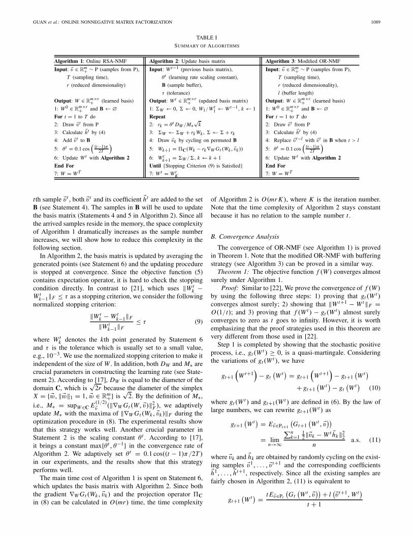
TABLE I
SUMMARY OF ALGORITHMS
Algorithm 1: Online RSA-NMF Algorithm 2: Update basis matrix Algorithm 3: Modified OR-NMF
Input: �v ∈ Rm+ ∼ P (samples from P), Input: Wt−1 (previous basis matrix), Input: �v ∈ R
m+ ∼ P (samples from P),
T (sampling time), θ t (learning rate scaling constant), T (sampling time),
r (reduced dimensionality) B (sample buffer), r (reduced dimensionality),
τ (tolerance) l (buffer length)
Output: W ∈ Rm×r+ (learned basis) Output: Wt ∈ R
m×r+ (updated basis matrix) Output: W ∈ Rm×r+ (learned basis)
1: W0 ∈ Rm×r+ and B← ∅ 1: �W ← 0, �← 0, W1/Wt
1 ← Wt−1, k ← 1 1: W0 ∈ Rm×r+ and B← ∅
For t = 1 to T do Repeat For t = 1 to T do
2: Draw �v t from P 2: rk = θ t DW /M∗√
k 2: Draw �v t from P
3: Calculate �ht by (4) 3: �W ← �W + rk Wk , �← � + rk 3: Calculate �ht by (4)
4: Add �v t to B 4: Draw �vk by cycling on permuted B 4: Replace �v t−l with �v t in B when t > l
5: θ t = 0.1 cos(
(t−1)π2T
)5: Wk+1 = �C(Wk − rk∇W Gt (Wk , �vk )) 5: θ t = 0.1 cos
((t−1)π
2T
)
6: Update Wt with Algorithm 2 6: Wtk+1 = �W /�, k ← k + 1 6: Update Wt with Algorithm 2
End For Until {Stopping Criterion (9) is Satisfied} End For
7: W = W T 7: Wt = WtK 7: W = W T
tth sample �v t , both �v t and its coefficient �ht are added to the setB (see Statement 4). The samples in B will be used to updatethe basis matrix (Statements 4 and 5 in Algorithm 2). Since allthe arrived samples reside in the memory, the space complexityof Algorithm 1 dramatically increases as the sample numberincreases, we will show how to reduce this complexity in thefollowing section.
In Algorithm 2, the basis matrix is updated by averaging thegenerated points (see Statement 6) and the updating procedureis stopped at convergence. Since the objective function (5)contains expectation operator, it is hard to check the stoppingcondition directly. In contrast to [21], which uses ‖W t
k −W t
k−1‖F ≤ τ as a stopping criterion, we consider the followingnormalized stopping criterion:
‖W tk − W t
k−1‖F
‖W tk−1‖F
≤ τ (9)
where W tk denotes the kth point generated by Statement 6
and τ is the tolerance which is usually set to a small value,e.g., 10−3. We use the normalized stopping criterion to make itindependent of the size of W . In addition, both DW and M∗ arecrucial parameters in constructing the learning rate (see State-ment 2). According to [17], DW is equal to the diameter of thedomain C, which is
√2r because the diameter of the simplex
X = { �w, ‖ �w‖1 = 1, �w ∈ Rm+} is
√2. By the definition of M∗,
i.e., M∗ = supW∈C E (1/2)�v (‖∇W Gt (W, �v)‖2F ), we adaptively
update M∗ with the maxima of ‖∇W Gt (Wk , �vk)‖F during theoptimization procedure in (8). The experimental results showthat this strategy works well. Another crucial parameter inStatement 2 is the scaling constant θ t . According to [17],it brings a constant max{θ t , θ−1} in the convergence rate ofAlgorithm 2. We adaptively set θ t = 0.1 cos((t − 1)π/2T )in our experiments, and the results show that this strategyperforms well.
The main time cost of Algorithm 1 is spent on Statement 6,which updates the basis matrix with Algorithm 2. Since boththe gradient ∇W Gt (Wk , �vk) and the projection operator �Cin (8) can be calculated in O(mr) time, the time complexity
of Algorithm 2 is O(mr K ), where K is the iteration number.Note that the time complexity of Algorithm 2 stays constantbecause it has no relation to the sample number t .
B. Convergence Analysis
The convergence of OR-NMF (see Algorithm 1) is provedin Theorem 1. Note that the modified OR-NMF with bufferingstrategy (see Algorithm 3) can be proved in a similar way.
Theorem 1: The objective function f (W ) converges almostsurely under Algorithm 1.
Proof: Similar to [22], We prove the convergence of f (W )by using the following three steps: 1) proving that gt (W t )converges almost surely; 2) showing that ‖W t+1 − W t‖F =O(1/t); and 3) proving that f (W t ) − gt (W t ) almost surelyconverges to zero as t goes to infinity. However, it is worthemphasizing that the proof strategies used in this theorem arevery different from those used in [22].
Step 1 is completed by showing that the stochastic positiveprocess, i.e., gt (W t ) ≥ 0, is a quasi-martingale. Consideringthe variations of gt(W t ), we have
gt+1
(W t+1
)− gt
(W t ) = gt+1
(W t+1
)− gt+1
(W t )
+ gt+1(W t )− gt
(W t ) (10)
where gt (W t ) and gt+1(W t ) are defined in (6). By the law oflarge numbers, we can rewrite gt+1(W t ) as
gt+1(W t ) = E�v∈Pt+1
(Gt+1
(W t , �v))
= limn→∞
∑nk=1
12‖�vk −W t �hk‖22
na.s. (11)
where �vk and �hk are obtained by randomly cycling on the exist-ing samples �v1, . . . , �v t+1 and the corresponding coefficients�h1, . . . , �ht+1, respectively. Since all the existing samples arefairly chosen in Algorithm 2, (11) is equivalent to
gt+1(W t ) = t E�v∈Pt
(Gt
(W t , �v))+ l
(�v t+1, W t)
t + 1

1090 IEEE TRANSACTIONS ON NEURAL NETWORKS AND LEARNING SYSTEMS, VOL. 23, NO. 7, JULY 2012
= tgt(W t
)+ l(�v t+1, W t
)
t + 1a.s. (12)
where �v t+1 is the newly arrived sample at the t+1th step. Bysubstituting (12) into (10) and using some algebra, we have
gt+1
(W t+1
)− gt
(W t ) = gt+1
(W t+1
)− gt+1
(W t )
+ l(�v t+1, W t
)− gt(W t
)
t + 1. (13)
Since W t+1 minimizes gt+1(W ) on C, gt+1(W t+1) ≤gt+1(W t ). By filtering the past information Ft = {�v1, . . . , �v t ;�h1, . . . , �ht } and taking the expectation over both sides of (13),we have
E[gt+1
(W t+1
)− gt
(W t ) |Ft
]
≤ E[l(�v t+1, W t
) |Ft]− gt
(W t
)
t + 1
≤ f(W t
)− ft(W t
)
t + 1≤
∥∥ f(W t
)− ft(W t
)∥∥∞t + 1
(14)
where ft (W t ) signifies the empirical approximation of f (W t ),i.e., ft (W t ) = (
∑ti=1 l(�v i , W t )/t), and the second inequality
comes from the fact
gt(W t ) = limn→∞
∑nk=1
12
∥∥∥�vk −W t �hk
∥∥∥2
2
n
≥ limn→∞
∑nk=1 l(�vk , W t )
n≥ ft (W t )
where (1/2)‖�vk − W t �hk‖22 ≥ l(�vk , W t ) according to (4).Since l(�v, W ) is Lipschitz-continuous and bounded andE�v [l2(�v, W )] is uniformly bounded [22], according to thecorollary of the Donsker theorem [23], we have
E[‖√t( f (W t )− ft (W t ))‖∞
] = O(1). (15)
By taking expectation over both sides of (14) and combiningit with (15), there exists a constant K1 > 0 such that
E[E[gt+1(W t+1)− gt (W t )|Ft ]+
] ≤ K1√t(t + 1)
. (16)
By letting t →∞ and summing up all the inequalities derivedfrom (16), we arrive at
∞∑
t=1
E
[E
[gt+1
(W t+1
)− gt
(W t ) |Ft
]+]
=∞∑
t=1
E[δt
(gt+1
(W t+1
)− gt
(W t ))]
=∞∑
t=1
K1√t (t + 1)
<∞
where δt is defined as in [24]. Since gt (W t ) > 0, according to[24], we prove that gt (W t ) is a quasi-martingale and convergesalmost surely. As a byproduct, we have
∞∑
t=1
∣∣∣∣E
[gt+1
(W t+1
)− gt
(W t )
∣∣∣∣Ft
] ∣∣∣∣ <∞ a.s. (17)
In order to prove f (W t ) converges in Step 3, we first prove‖W t+1−W t‖F = O(1/t) in this step (2). For the convenienceof presentation, we denote the variation of gt(W ) as
ut (W ) = gt(W ) − gt+1(W ).
Since gt+1(W t+1) ≤ gt+1(W t ), we have
gt
(W t+1
)−gt
(W t )
= gt
(W t+1
)− gt+1
(W t+1
)+ gt+1
(W t+1
)− gt+1
(W t )
+gt+1(W t )− gt
(W t )
≤ gt
(W t+1
)− gt+1
(W t+1
)+ gt+1
(W t )− gt
(W t )
= ut
(W t+1
)− ut
(W t ). (18)
Considering the gradient of ut (W )
∇W ut (W ) = ∇W gt (W )−∇W gt+1(W )
= 1
t
(∑ti=1 �vi �hT
i − t �vt+1 �hTt+1
t + 1
−W
∑ti=1�hi �hT
i − t �ht+1 �hTt+1
t + 1
). (19)
Since W ∈ C, ‖W‖F <√
r . By the triangle inequality, (19)implies
‖∇W ut (W )‖F ≤ 1
t
(∥∥∥∑t
i=1 �vi �hTi − t �vt+1 �hT
t+1
t + 1
∥∥∥F
+√r∥∥∥∑t
i=1�hi �hT
i − t �ht+1 �hTt+1
t + 1
∥∥∥F
)= Lt
where Lt = O(1/t). Therefore, ut (W ) is Lipschitz-continuouswith constant Lt . By the triangle inequality, from (18), wehave
∥∥∥gt
(W t+1
)− gt
(W t )
∥∥∥F≤ Lt
∥∥∥W t+1 − W t∥∥∥
F. (20)
Note that gt(W ) is convex, it is reasonable to further assumethat its Hessian has a low bound K2
∥∥∥gt(W t+1)− gt(W t )∥∥∥
F≥ K2‖W t+1 − W t‖2F . (21)
By combining (20) and (21), we arrive at
‖W t+1 −W t‖F ≤ Lt
K2. (22)
Therefore, we prove that ‖W t+1 −W t‖F = O(1/t).Step 3 proves that f (W t )−gt(W t ) almost surely converges
to zero as t goes to infinity. From (13), we get
gt (W t )− ft (W t )
t + 1≤ gt(W t )− gt+1(W t+1)
+ l(�v t+1,W t )− ft (W t )t+1 . (23)
By taking expectation and absolute over both sides of (23)and summing up all the inequalities derived from (23) as tgoes to infinity, we have∞∑
t=1
gt (W t )− ft (W t )
t + 1<
∑∞t=1
∣∣E[gt+1(W t+1)− gt(W t )Ft
]∣∣

GUAN et al.: ONLINE NONNEGATIVE MATRIX FACTORIZATION 1091
+∑∞t=1‖ f (W t )− ft (W t )‖∞
t+1 (24)
where the inequality comes from the triangle inequality andgt (W t ) ≥ ft (W t ). From (15), (17), and (24), we conclude that
∞∑
t=1
gt(W t )− ft (W t )
t + 1<∞ a.s. (25)
Since both gt (W ) and ft (W ) are Lipschitz continuous, thereexists a constant K3 > 0 such that
∣∣∣gt+1
(W t+1
)− ft+1
(W t+1
)− (
gt(W t )− ft
(W t ))
∣∣∣
≤ K3‖W t+1 − W t‖F . (26)
Since ‖W t+1 − W t‖F = O(1/t) (see Step 2), according to[25], (25) and (26) imply that
gt(W t )− ft (W t )→ 0 (t →∞), a.s.
Since f (W t ) − ft (W t ) → 0 (t → ∞), a.s., we prove thatf (W t ) converges almost surely. It completes the proof.
C. Buffering Strategy
Since the space complexity of Algorithm 1, i.e., O(mt +r t +mr), increases dramatically as t increases to infinity, it isunacceptable especially for large-scale or streaming datasetsbecause there is insufficient memory in practice to retain theexisting samples in set B. Therefore, we regard B as a bufferand make it store the l most recently arrived samples and thusreduce the space complexity of Algorithm 1. In particular, atstep t , we update the buffer B by replacing the oldest sample�v t−l with the new coming sample �v t when t > l, wherein l isthe prefixed buffer length. By using this strategy, we reducethe space complexity of Algorithm 1 to O(ml+ rl+mr). Wesummarize the modified OR-NMF (MOR-NMF) in Algorithm3 by replacing Statement 4 in Algorithm 1.
As the space complexity of Algorithm 3 stays constant,it performs efficiently in practice especially on large-scaleor streaming datasets. Empirical experiments on real-worlddatasets show that Algorithm 3 converges and works wellin various applications. In addition, the buffer length l isa critical parameter in Algorithm 3. It should be selectedin a reasonable range for the following two reasons: 1) lcannot be too large because it controls the space complexityof Algorithm 3 and 2) l should be set large enough to makethe buffer B provide sufficient samples �v t−l+1, . . . , �v t for thepermutation procedure in Statement 4 in Algorithm 2. In ourexperiments, we empirically select l by using the strategyl = min{�(n/10)�, 20}, wherein �x� signifies the smallestinteger larger than x .
D. Mini-Batch Extension
We can improve the convergence speed of the proposedAlgorithm 1 by receiving a chunk of samples instead of asingle one, i.e., a total of j samples �v(t−1) j+1, . . . , �v t j aredrawn from the distribution P in iteration t . Their coefficients�h(t−1) j+1, . . . , �ht j are obtained by optimizing the followingobjective:
minHt≥0
1
2‖V t −W t−1 H t‖2F (27)
where V t = [�v(t−1) j+1, . . . , �v t j ] and H t = [�h(t−1) j+1, . . . ,�ht j ]. Many methods, such as the projected gradient descent[10] and block principal pivoting [12] whose complexi-ties are not linear in j , can be applied to efficientlysolve (27). In this case, the proposed Algorithm 1 canbe conveniently extended by calculating the coefficients ofthe sample chunk by optimizing (27) instead of (4) inStatement 3 and adding this sample chunk to set B in State-ment 4. We call this extension as “window-based OR-NMF”(WOR-NMF). In addition, Algorithm 3 can also be conve-niently extended in this case by replacing the oldest samplechunk �v j (t−1)− j l+1, . . . , �v j (t−1)− j l+ j with the new comingsample chunk when t > l.
III. OR-NMF FOR NMF EXTENSIONS
This section shows that OR-NMF can be convenientlyadopted for handling l1-regularized and l2-regularized NMF,NMF with box constraint, and Itakura–Saito (IS) divergence-based NMF.
A. l1-Regularized NMF
Although NMF obtains sparse representation, this sparsity isnot explicitly guaranteed. Hoyer [26] proposed incorporatingthe l1-regularization on the coefficients. The objective is
minW∈Rm×r+
fn(W ) = 1
n
n∑
i=1
l1(�vi , W ) (28)
where l1(�vi , W ) = min�h∈Rr+(1/2)‖�vi − W �h‖22 + λ‖�h‖1 andλ is the tradeoff parameter. The problem (28) can be easilyoptimized by extending OR-NMF, with Statement 3 in Algo-rithm 1 replaced by �ht = arg min�h∈Rr+(1/2)‖�vt − Wt �h‖22 +λ‖�h‖1.
B. l2-Regularized NMF
The l2-regularization, i.e., Tikhonov regularization, is usu-ally utilized to control the smoothness of the solution in NMF[14]. The objective function can be written as
minW∈Rm×r+
fn(W ) = 1
n
n∑
i=1
l2(�vi , W ) (29)
where l2(�vi , W ) = min�h∈Rr+((1/2)‖�vi−W �h‖22+(α/2)‖W‖2F+(β/2)‖�h‖22, and ‖ · ‖F is the matrix Frobenius norm andα, β are tradeoff parameters. The problem (29) can besolved by naturally extending OR-NMF. On the arrivalof sample �vt , its coefficient �ht can be optimized by�ht = arg min�h∈Rr+(1/2)‖�vt − Wt �h‖22 + (β/2)‖�h‖22. Givensamples {�v1, . . . , �vt } and their corresponding coefficients{�h1, . . . , �ht }, the basis matrix Wt+1 is optimized by W t+1 =arg minW∈Rm×r+ g2(W ) = E�v (G2(W, �v)), wherein G2(W, �v) =(1/2)‖�v−W �h‖22+(α/2)‖W‖2F . It is obvious that G2(W, �v) isconvex, and thus OR-NMF can be extended to solve (29) byreplacing ∇W G(Wk, �vk) in Statement 5 in Algorithm 2 with∇W G2(Wk , �vk).

1092 IEEE TRANSACTIONS ON NEURAL NETWORKS AND LEARNING SYSTEMS, VOL. 23, NO. 7, JULY 2012
C. NMF With Box Constraint
Although OR-NMF is designed to solve NMF, it can benaturally extended to solve the box-constrained optimizationproblem [25]
minL≤W≤U
fn(W ) = 1
n
n∑
i=1
lb(�vi , W ) (30)
where both L and U have the same dimensionality as Wand the constraint means Li j ≤ Wij ≤ Uij . By replacingthe feasible set C in (8) with Cb = {W |Li j ≤ Wij ≤Uij ,∀i j}, the basis matrix Wt+1 is obtained by W t+1 =arg minW∈Cb
g(W ) = E�v (G(W, �v)). It is obvious that G(W, �v)is convex on Cb, and thus OR-NMF can be extended tosolve (30) by slightly modifying the projection operator (seeStatement 5 in Algorithm 2).
Beside the l1 and l2-regularizations and box constraint,OR-NMF can also be extended to handle other regularizations,e.g., manifold regularization [27], [28] and regularizationsfor transfer learning [29], [31], for data representation. Withthe aim of acceleration, the active learning based manifoldregularization [32] can also be applied to OR-NMF. Due tolimitations of space, we postpone these discussions to futurepublications.
D. IS Divergence-Based NMF
OR-NMF uses the l2-norm to measure the approximationerror. This section shows that OR-NMF can also be extendedto optimize the IS divergence-based NMF [33]
minW∈Rm×r+
1
n
n∑
j=1
lI S(�v j , W ) (31)
where lI S(�v j , W ) = min�h j∈Rr+ dI S(�v j , W �h j ) and the IS diver-gence is defined by
dI S(�x, �y) =m∑
i=1
( �xi
�yi− log
�xi
�yi− 1
). (32)
When the sample number increases to infinity, (31) becomes anexpectation of the form minW∈Rm×r+ E�v∈P(lI S(�v, W )), whichcan be solved in an incremental manner by using OR-NMF.
On the arrival of the sample �vt , its coefficient �ht can beoptimized by
�ht = arg min�ht∈Rr+dI S(�vt , Wt �ht ). (33)
According to [33], the problem (33) can be solved by iter-atively updated �ht from a random initial point through thefollowing multiplicative rule until convergence: �ht ← �ht ⊗(W T
t ×(�vt/(Wt �ht )2))/(W T
t ×(1/Wt �ht )), where ⊗ signifies theelement-wise product. Given samples {�v1, . . . , �vt } and theircorresponding coefficients {�h1, . . . , �ht }, the basis matrix isupdated by
Wt+1 = arg minW∈Rm×r+ E�v∈P(dI S(�v, W �h)). (34)
Since dI S(�v, W �h) is convex with respect to W , (34) is convexwith respect to W , and thus OR-NMF can be extended tosolve (34). We call such extended algorithm for IS-NMF as
“OR-NMF-IS.” In particular, OR-NMF-IS replaces the State-ment 4 in Algorithms 1 and 3 with (33), and replaces∇W Gt (Wt , �vt ) in the Statement 5 in Algorithm 2 with∇W dI S(�vt , Wt �ht ) = ((Wt �ht − �vt )/(Wt �ht )
2)× �hTt .
Note that Lefèvre et al. [21] proposed the ONMF-IS algo-rithm to incrementally learn IS-NMF, which will be reviewedin the following section. OR-NMF-IS is different fromONMF-IS and the experimental results show that OR-NMF-ISoutperforms ONMF-IS in terms of efficiency.
IV. RELATED WORKS
This section briefly reviews the existing ONMF algorithmsincluding ONMF [34], ONMF-IS [21], incremental NMF [35],[36], and online matrix factorization [22], [37] and presentstheir differences from the proposed OR-NMF.
A. ONMF
Cao et al. [34] proposed an ONMF which finds the twomatrix factors, i.e., W and H , to approximate the wholedata matrix [V , U ] ∈ R
m×n+ , wherein m and n denote thedimensionality and number of samples, respectively, and Vand U are the old and new sample matrix, respectively. ONMFassumes that V is approximated by Wold Hold. The problem isto find W ∈ R
m×r+ and H ∈ Rr×n+ such that
[V , U ] ≈ W H � W [H1, H2]. (35)
Based on the relation W H1 ≈ Wold Hold, Cao et al. [34] provedthat a matrix � exists that satisfies W = Wold�
−1, H1 =�Hold. ONMF smartly carries out NMF on [Wold�, U ],wherein � is positive diagonal matrix
[Wold�, U ] ≈ Wnew[H 1
new, H 2new
](36)
which implies Wold ≈ Wnew H 1new�−1 and U ≈ Wnew H 2
new.By setting W = Wnew and � = H 1
new�−1, we have
W = Wnew, H = [H 1
new�−1 Hold, H 2new
]. (37)
It is suggested that � be calculated by � j j = ‖�h jold‖2, wherein
�h jold is the j th column of Hold [34].Because the time overhead of (36) is much lower than that
of (35), ONMF performs well in practice. However, the spacecomplexity of ONMF, O(mn+rn), increases dramatically as nincreases. Thus it cannot be applied to large-scale or streamingdatasets due to the memory limitation.
B. ONMF-IS
Lefèvre et al. [21] proposed ONMF-IS to incrementallylearn IS divergence based NMF. The objective function is
minW≥0
Lt (W ) = 1
t
t∑
j=1
dI S(�v j , W �h j ) (38)
where dI S is the IS divergence defined in (32), andthe infinite sequences {�v1, . . . , �vt , . . . } and {�h1, . . . , �ht , . . . }contain samples and their corresponding coordinates obtainedas �ht = arg min�hdI S(�vt , Wt �h).

GUAN et al.: ONLINE NONNEGATIVE MATRIX FACTORIZATION 1093
By extending the batch algorithm for IS-NMF, (38) isoptimized by recursively updating the following rules:
At = At−1 +( �vt
(Wt−1 �ht )2�hT
t
)⊗W 2
t−1
Bt = Bt−1 + 1
Wt−1�ht× �hT
t , Wt =√
At
Bt
where W0, A0, and B0 are randomly initialized. ONMF-IS issimple and scalable for processing long-time audio sequences.However, we are not sure how to use ONMF-IS to optimizethe Frobenius-norm-based NMF.
C. Incremental Nonnegative Matrix Factorization (INMF)
Bucak and Gunsel [35] proposed an INMF for learning theNMF problem. On arrival of the (k + 1)th sample, INMFupdates the basis matrix Wk+1 by optimizing the followingobjective function:
minWk+1≥0,�hk+1≥0
Sold1
2‖Vk − Wk+1 Hk‖22
+ Snew1
2‖�vk+1 −Wk+1 �hk+1‖22 (39)
where Vk = [�v1, . . . , �vk ] contains the old samples, Hk =[�h1, . . . , �hk] contains their coefficients, and �vk+1 denotes thenewly arrived sample. As a byproduct, (39) obtains the coef-ficient �hk+1 of �vk+1. In (39), Sold and Snew are the weights tobalance the contributions of the old samples and new sample,and Sold + Snew = 1. To solve (39), INMF iteratively updates�hk+1 and Wk+1 with the following rule until convergence:
�hk+1 ← �hk+1 ⊗W T
k+1�vk+1
W Tk+1Wk+1 �hk+1
Wk+1 ← Wk+1⊗SoldVk H T
k + Snew�vk+1 �hTk+1
SoldWk+1 Hk H Tk + SnewWk+1 �hk+1 �hT
k+1
.
(40)
Since both Vk H Tk and Hk H T
k can be calculated in anincremental manner as Vk+1 H T
k+1 = Vk H Tk + �vk+1 �hT
k+1 andHk+1 H T
k+1 = Hk H Tk + �hk+1 �hT
k+1, respectively, the spacecomplexity of (40) stays constant. The time complexity of(40) is O(mr + mr2) × K , where K is the iteration number.Although INMF works well in practice, the multiplicativeupdate rules (40) suffer from slow convergence, which makes(40) time consuming. In addition, it may fail if some elementsin the denominators become zero.
D. Incremental Nonnegative Matrix Factorization With VolumeConstraint (INMF-VC)
Zhou et al. [36] proposed an INMF-VC to control theuniqueness
minW∈C,H≥0
Dt+1 � 1
2‖V − W H‖2F + μ ln | det W |. (41)
Minimizing the determinant of W steers (41) toward theunique solution, and the tradeoff parameter μ balances theapproximation error of NMF and the volume constraint. In
order to steer (41) toward the global solution, INMF-VC setsμ = δ exp−τ t , where δ and τ are both positive constants andμ decreases to zero with increasing sample number t . To learnW and H in an incremental manner, Zhou et al. proposed touse the amnesic average method by rewriting (41) into thefollowing two parts given a new sample �vt+1:
Dt+1 ≈ αDt + βdt+1 (42)
where dt+1 = (1/2)‖�vt+1 − Wt+1�ht+1‖22 + μ ln | det Wt+1| −μ ln | det Wt |, and α and β are the moving smooth parameterswhich are set to α = 1 − L/t and β = L/t , where L ∈{1, 2, 3, 4} is the amnesic average parameter. As t tends toinfinity, α and β get close to 1 and 0, respectively.
Since (42) is nonconvex, it first updates the coordinate�ht+1 of �vt+1 with the basis Wt fixed, and then updates thebasis Wt+1. Both �ht+1 and Wt+1 are updated by using themultiplicative update rule. INMF-VC performs well in blind-source separation and requires W to be square.
E. Online Matrix Factorization Algorithm (OMF)
Recently, Mairal et al. [22] proposed an OMF whichincludes NMF as a special case. Unlike ONMF and INMF,OMF learns the basis matrix W to adapt it to specific data byminimizing an expected cost
minW
f (W ) = E�v (l(�v, W )) (43)
where l(�v, W ) = min�h∈Rr+(1/2)‖�v − W �h‖22. OMF efficientlysolves (43) by minimizing a quadratic local surrogate ft (W ) =(1/t)
∑ti=1 l(�vi , W ). In particular, on arrival of the tth sample,
OMF updates the basis matrix by
Wt = arg minW∈C1
t
(1
2tr(W T W At )− tr(W T Bt )
)(44)
where At = ∑tj=1�h j �hT
j and Bt = ∑tj=1 �v j �hT
j and they are
incrementally updated by At = At−1+�ht �hTt and Bt = Bt−1+
�vt �hTt , respectively. OMF solves (44) by iteratively updating the
columns of W with the following rule until convergence:
�w j ← �C
(�w j − 1
[At ] j j(W �a j − �b j )
)(45)
where �a j , �b j , and �w j are the j th column of At , Bt , and W ,respectively. Note that the learning rate of (45) is the diagonalof the approximated Hessian inverse.
Similar to INMF [35], OMF only stores matrices At andBt . Thus OMF consumes constant memory and scales upgracefully to large-scale datasets. However, (45) convergesslowly because the learning rates [At ] j j , 1 ≤ j ≤ r ignoremost off-diagonal information.
F. OMF-Diagonal Approximation (DA)
Wang et al. [37] proposed to use the second-order projectedgradient descent method to optimize (44), in which the basismatrix Wt is updated by iterating the following rule untilconvergence: W k+1
t = �C (W kt −H−1
t (W kt )∇t (W k
t )), whereink ≥ 1 is the iteration counter and W k
t is the kth search point

1094 IEEE TRANSACTIONS ON NEURAL NETWORKS AND LEARNING SYSTEMS, VOL. 23, NO. 7, JULY 2012
TABLE II
SUMMARY OF THE USED DATASETS
Datasets Efficiency comparison Face recognition Image annotation
m n r sp #TR #TS r #TR #TS #VC #KD
CBCL 361 500 10/50 .131 30/50/70 470/450/430 10–80 — — — —
ORL 1024 400 10/50 .042 120/200/280 280/200/120 10–150 — — — —
IAPR TC12 100 500 50/80 .745 — — — 17 825 1980 291 4.7
m: sample dimensionality. n: sample number. r: reduced dimensionality. sp: sparseness. TR: training set. TS: test set.
VC: vocabulary; KD: keywords.
initialized to Wt−1, and ∇t (W kt ) and Ht (W k
t ) are the gradientand the Hessian of (44) at W k
t , respectively.Since the exact calculation of the inverse of Hessian
matrix is time consuming especially when r increased,Wang et al. presented two strategies to approximate theHessian inverse: 1) DA, which uses only the diagonalof the Hessian matrix to approximate the whole one and2) conjugate gradient (CG), which approximates the last term,i.e., H−1
t (W kt )∇t (W k
t ), with the least-squares solutions ofHt (W k
t )Q = ∇t (W kt ) obtained by using the conjugate gradient
method.DA ignores all of the off-diagonal information in the
Hessian matrix, and thus suffers from numerical instabilityespecially when the dataset is sparse. Although CG approxi-mates the Hessian inverse, the conjugate gradient procedure istime consuming. Thus we focused on the DA strategy in thispaper and call this method OMF-DA.
The proposed OR-NMF overcomes the aforementioneddrawbacks of ONMF, ONMF-IS, INMF, INMF-VC, OMF,and OMF-DA. The experimental results on real-world datasetsshow that OR-NMF outperforms the existing ONMF algo-rithms in terms of efficiency, and the experimental results ofvarious applications confirm the effectiveness of OR-NMF.
V. EXPERIMENTS
This section evaluates the efficiency and effectiveness ofthe OR-NMF by comparing it with representative ONMFalgorithms including ONMF [34], ONMF-IS [21], INMF [35],OMF [22], and OMF-DA [37]. The efficiency is evaluated ontwo face-image datasets, i.e., CBCL [38] and ORL [39], andone popular image dataset, i.e., IAPR TC12 [40]. The effec-tiveness is evaluated by two applications: 1) face recognitionon both CBCL and ORL datasets and 2) image annotation onthe IAPR TC12 dataset. We summarize the datasets used inthis experiment in Table II and use the following settings.
1) Projection Operator: Based on the definition of thefeasible set C [see (8)], the projection operator �C(·) playsan important role in Algorithm 1. In all our experiments, weapply the method in [41] to project the columns of W ontothe simplex in O(mr) time.
2) Nonnegative Least Squares: To obtain the coefficient ofthe new sample (see Statement 3 in Algorithm 1), we use thelsnonneg method (MATLAB build-in implementation) to solvethe nonnegative least-squares problem (4).
3) Algorithmic Schemes: In our experiments, we utilizethe well-known multiplicative update rule [8] to obtain the
coefficient in INMF. In addition, we set the weights in (39)to Sold = Snew = 1 for fair comparison. Note that ONMFreceives one chunk of samples at each step, here, we set thechunk size to the reduced dimensionality r .
4) Reduced Dimensionalities: The reduced dimensionalityis set to 10, 50, and 80 in the efficiency comparison exper-iments and varies from 10 to 150 in steps of 10 for evalu-ating face recognition performance. In addition, the reduceddimensionality for the image annotation experiments varies ina range of {10%, . . . , 90%} ×min{m, 200}, wherein m is thedimensionality of the visual image features.
A. Efficiency Comparison
To evaluate the efficiency of OR-NMF, we compare itsobjective values with those of other ONMF algorithms.Since it is difficult to directly calculate the expected cost(3), similar to [22] we instead utilize the empirical costft (W t ) = (1/t)
∑ti=1(1/2)‖�vi − W t �hi‖22. In the remainder
of this section, we compare OR-NMF and MOR-NMF withthe existing ONMF algorithms in terms of efficiency on twodense datasets, i.e., CBCL [38] and ORL [39]. For evaluatingthe proposed algorithms on sparse datasets, we compare themwith the existing ONMF algorithms on the sparse dataset, i.e.,IAPR TC12 [40]. We compared the efficiency of WOR-NMFwith that of ONMF. In this part, all algorithms were appliedto two epochs of the permuted training set. We carried out thistrial 10 times with different initial points because the objectivefunction (3) is nonconvex. In each trial, all algorithms startfrom an identical initial point for fair comparison.
1) Dense Datasets: The CBCL dataset [38] contains2429 face images collected from 10 subjects. Fig. 1(a) (firstrow) shows some examples of the CBCL dataset. By reshapinga face image to a vector, we get 2429 training samples inR
361 and randomly selected 500 samples for online training.Fig. 2 gives the mean and deviation of the objective valuesversus the sample numbers and CPU seconds of the OR-NMF,MOR-NMF, OMF, OMF-DA, and INMF algorithms. It showsthat both OR-NMF and MOR-NMF reduce the objectivefunction faster than other algorithms.
The Cambridge ORL dataset [39] is composed of400 images collected from 40 individuals. Fig. 1(a) (sec-ond row) depicts some examples of the ORL dataset.The training set contains 400 samples in R
1,024. Fig. 3shows that both OR-NMF and MOR-NMF outperform OMF,OMF-DA, and INMF in terms of both objective values andCPU seconds.

GUAN et al.: ONLINE NONNEGATIVE MATRIX FACTORIZATION 1095
(a) (b) (c) (d) (e) (f) (g) (h)
Fig. 1. (a) Image examples, (b) learned bases by OR-NMF, (c) MOR-NMF, (d) OMF, (e) OMF-DA, (f) INMF, (g) WOR-NMF, and (h) ONMF of CBCL(first row) and ORL (second row) dataset.
200 400 600 800 100010-2
10-1
100
(a)Sample Numbers
Obj
ectiv
e V
alue
s
50 100 15010-2
10-1
100
(b)CPU Seconds
Obj
ectiv
e V
alue
s OMFOMF-DAINMFMOR-NMFOR-NMF
200 400 600 800 100010-3
10-2
10-1
100
(c)Sample Numbers
Obj
ectiv
e V
alue
s
0 500 1000 1500 200010-3
10-2
10-1
100
(d)CPU Seconds
Obj
ectiv
e V
alue
s
OMFOMF-DAINMFMOR-NMFOR-NMF
Fig. 2. Objective values versus iteration numbers and CPU seconds ofOR-NMF, MOR-NMF, OMF, OMF-DA, and INMF on the CBCL datasetwith reduced dimensionality. (a) and (b) r = 10. (c) and (d) r = 50.
200 400 600 80010-2
10-1
100
(a)Sample Numbers
Obj
ectiv
e V
alue
s
0 200 400 60010-2
10-1
100
(b)CPU Seconds
Obj
ectiv
e V
alue
s OMFOMF-DAINMFMOR-NMFOR-NMF
200 400 600 800
10-2
10-1
100
(c)Sample Numbers
Obj
ectiv
e V
alue
s
0 1000 2000 3000
10-2
10-1
100
(d)CPU Seconds
Obj
ectiv
e V
alue
s
Fig. 3. Objective values versus iteration numbers and CPU seconds ofOR-NMF, MOR-NMF, OMF, OMF-DA, and INMF on the ORL dataset withreduced dimensionality. (a) and (b) r = 10. (c) and (d) r = 50.
Figs. 4 and 5 present the mean and deviation of theobjective values versus the sample numbers and CPU secondsof both WOR-NMF and ONMF on both CBCL and ORLdatasets. It shows that WOR-NMF outperforms ONMF interms of both objective values and CPU seconds on these densedatasets.
2) Sparse Datasets: The IAPR TC12 [40] dataset hasbecome popular for image annotation. There are 20 000 images
200 400 600 800 1000
10-2
100
(a)Sample Numbers
Obj
ectiv
e V
alue
s
0 5 10 15 20 25
10-2
100
(b)CPU Seconds
Obj
ectiv
e V
alue
s ONMFWOR-NMF
500 1000 1500 2000
10-2
(c)Sample Numbers
Obj
ectiv
e V
alue
s
0 20 40 60 80
10-2
(d)CPU Seconds
Obj
ectiv
e V
alue
s
Fig. 4. Objective values versus iteration numbers and CPU seconds ofWOR-NMF and ONMF on the CBCL dataset with reduced dimensionality.(a) and (b) r = 10. (c) and (d) r = 50.
0 200 400 600 800
10-2
100
(a)Sample Numbers
Obj
ectiv
e V
alue
s
0 10 20 30
10-2
100
(b)CPU Seconds
Obj
ectiv
e V
alue
s
ONMFWOR-NMF
0 500 1000 150010-3
10-2
10-1
(c)Sample Numbers
Obj
ectiv
e V
alue
s
0 50 100 15010-3
10-2
10-1
(d)CPU Seconds
Obj
ectiv
e V
alue
s
Fig. 5. Objective values versus iteration numbers and CPU seconds ofWOR-NMF and ONMF on the ORL dataset with reduced dimensionality.(a) and (b) r = 10. (c) and (d) r = 50.
in the IAPR TC12 dataset. In this experiment, the sparsedataset was built by arranging the 100-D “DenseHue” featuresof 500 randomly selected images into columns. Thus thissparse dataset contains 500 samples in R
100. Based on thesparseness defined in [42], we compare the averaged sparse-ness of the used datasets in Table II. It shows that the IAPRTC12 dataset is much sparser than both the CBCL and ORLdatasets.

1096 IEEE TRANSACTIONS ON NEURAL NETWORKS AND LEARNING SYSTEMS, VOL. 23, NO. 7, JULY 2012
200 400 600 800 1000
10-1
100
(a)Sample Numbers
Obj
ectiv
e V
alue
s
0 500 1000 1500
10-1
100
(b)CPU Seconds
Obj
ectiv
e V
alue
s200 400 600 800 1000
10-1
100
(c)Sample Numbers
Obj
ectiv
e V
alue
s
0 500 1000 1500 2000 2500
10-1
100
(d)CPU Seconds
Obj
ectiv
e V
alue
s
OMFOMF-DAINMFMOR-NMFOR-NMF
Fig. 6. Objective values versus iteration numbers and CPU seconds ofOR-NMF, MOR-NMF, OMF, OMF-DA, and INMF on the IAPR TC12 datasetwith reduced dimensionality. (a) and (b) r = 50. (c) and (d) r = 80.
0 500 1000 1500 20000
0.1
0.2
0.3
Sample Numbers
Obj
ectiv
e V
alue
s
0 10 20 300
0.1
0.2
0.3
CPU Seconds
Obj
ectiv
e V
alue
s ONMFWOR-NMF
0 1000 2000 3000 40000
0.5
1
1.5
2
Sample Numbers
Obj
ectiv
e V
alue
s
0 10 20 30 40 500
0.5
1
1.5
2
CPU Seconds
Obj
ectiv
e V
alue
s
(a) (b)
(c) (d)
Fig. 7. Objective values versus iteration numbers and CPU seconds ofWOR-NMF and ONMF on the IAPR TC12 dataset with reduced dimension-ality. (a) and (b) r = 50. (c) and (d) r = 80.
Fig. 6 gives the mean and deviation of the objective val-ues of OR-NMF, MOR-NMF, OMF, OMF-DA, and INMF.It shows that OR-NMF outperforms OMF, OMF-DA, andINMF in terms of both objective values and CPU seconds.In addition, Fig. 6 shows that MOR-NMF may get higherobjective values when the reduced dimensionality is low. Thatis because MOR-NMF discards old samples in the buffer andthus cannot incorporate sufficient information from such fewand sparse samples to update the basis. However, the bufferstrategy used in MOR-NMF largely saves storages, and thusit is much more suitable for streaming datasets.
Fig. 7 presents the mean and deviation of the objective val-ues of both MOR-NMF and ONMF. It shows that WOR-NMFoutperforms ONMF in terms of objective values. AlthoughONMF sometimes costs less CPU seconds especially whenthe reduced dimensionality is relatively high [Fig. 7(b) and(d)], it suffers from a serious nonconvergence problem. Fig. 7shows that WOR-NMF works well on this sparse dataset.
3) OR-NMF-IS Versus ONMF-IS: For evaluating the capac-ity of OR-NMF algorithms to optimize IS-NMF [33], wecompared OR-NMF-IS with ONMF-IS on the dense datasets.In this experiment, we did not apply these algorithms to thesparse dataset because the IS divergence is ill-posed on thatdataset. Figs. 8 and 9 give the mean and deviation of
200 400 600 800 10000
50
100
150
(a)Sample Numbers
Obj
ectiv
e V
alue
s
0 20 40 60 80 1000
50
100
150
(b)CPU Seconds
Obj
ectiv
e V
alue
s INMF-ISOR-NMF-IS
200 400 600 800 10000
50
100
150
(c)Sample Numbers
Obj
ectiv
e V
alue
s
0 100 200 3000
50
100
150
(d)CPU Seconds
Obj
ectiv
e V
alue
s
Fig. 8. Objective values versus iteration numbers and CPU seconds ofOR-NMF-IS and ONMF-IS on the CBCL dataset with reduced dimensionality.(a) and (b) r = 10. (c) and (d) r = 50.
200 400 600 8000
50
100
150
200
250
Sample NumbersO
bjec
tive
Val
ues
0 100 200 3000
50
100
150
200
250
CPU Seconds
Obj
ectiv
e V
alue
s INMF-ISOR-NMF-IS
200 400 600 8000
50
100
150
200
Sample Numbers
Obj
ectiv
e V
alue
s
0 200 400 600 800 10000
50
100
150
200(a) (b)
(c) (d)CPU Seconds
Obj
ectiv
e V
alue
s
Fig. 9. Objective values versus iteration numbers and CPU seconds ofOR-NMF-IS and ONMF-IS on the ORL dataset with reduced dimensionality.(a) and (b) r = 10. (c) and (d) r = 50.
the objective values of both algorithms on the CBCL andORL datasets. It shows that OR-NMF-IS reduces the objectivefunction more rapidly than ONMF-IS and it confirms thatOR-NMF can be applied to incrementally optimizing IS-NMF.
B. Face Recognition
By comparing the bases learned by OR-NMF with thoselearned by other ONMF algorithms in Fig. 1, it can beconcluded that both OR-NMF and MOR-NMF work well inlearning parts-based representation on the CBCL [38] andORL [39] datasets. To further evaluate the effectiveness ofsuch parts-based representation, we compare its face recog-nition accuracy with those of the existing ONMF algorithms.Different numbers (3, 5, 7) of images were randomly selectedfrom each individual to constitute the training set, and the restof the images to form the test set. The training set was usedto learn basis for the low-dimensional space. The test set wasused to report the accuracy in the learned low-dimensionalspace. The accuracy was calculated as the percentage ofsamples in the test set that were correctly classified using theNN rule. These trails were independently conducted 10 timesand both mean and deviation of accuracy are reported.
1) CBCL Dataset: The CBCL [38] dataset contains 2429face images taken from 10 subjects. On average, 243 images

GUAN et al.: ONLINE NONNEGATIVE MATRIX FACTORIZATION 1097
20 40 60 8010
20
30
40
50
60
70
80
Dimensionality
Acc
urac
y (%
)
(a)
OMFOMF-DAONMFINMFOR-NMFMOR-NMFWOR-NMF
20 40 60 8010
20
30
40
50
60
70
80
90
Dimensionality
Acc
urac
y (%
)
(b)
OMFOMF-DAONMFINMFOR-NMFMOR-NMFWOR-NMF
20 40 60 8010
20
30
40
50
60
70
80
90
Dimensionality
Acc
urac
y (%
)
(c)
OMFOMF-DAONMFINMFOR-NMFMOR-NMFWOR-NMF
Fig. 10. Mean and deviation of accuracy versus reduced dimensionality ofOR-NMF, MOR-NMF, WOR-NMF, OMF, OMF-DA, ONMF, and INMF onthe CBCL dataset whereby the training set was composed of (a) three, (b) five,and (c) seven images selected from each individual.
50 100 15030
35
40
45
50
55
60
65
70
75
80
Dimensionality
Acc
urac
y (%
)
(a)
OMFOMF-DAONMFINMFOR-NMFMOR-NMFWOR-NMF
50 100 15030
40
50
60
70
80
90
Dimensionality
Acc
urac
y (%
)
(b)
OMFOMF-DAONMFINMFOR-NMFMOR-NMFWOR-NMF
50 100 15030
40
50
60
70
80
90
Dimensionality
Acc
urac
y (%
)
(c)
OMFOMF-DAONMFINMFOR-NMFMOR-NMFWOR-NMF
Fig. 11. Mean and deviation of accuracy versus reduced dimensionality ofOR-NMF, MOR-NMF, WOR-NMF, OMF, OMF-DA, ONMF, and INMF onthe ORL dataset whereby the training set is composed of (a) three, (b) five,and (c) seven images selected from each individual.
were taken for each subject with a variety of illuminations,poses (up to about 30 degrees of rotation in depth), andbackgrounds. All face images were aligned according to theeye position and normalized to a 19×19 pixel array. Since themaximum size of the training set in this experiment was 70,we varied the reduced dimensionality from 10 to 80, wherebythe step is 10. Fig. 10 depicts the mean and deviation of facerecognition accuracies of OR-NMF, MOR-NMF, WOR-NMF,OMF, OMF-DA, ONMF, and INMF on different test sets.
Fig. 10 shows that both OR-NMF and MOR-NMF out-perform the other algorithms. Although ONMF and INMFperform well on some reduced dimensionalities, their accura-cies decrease when the reduced dimensionality becomes high.OR-NMF, MOR-NMF, and WOR-NMF overcome this prob-lem and perform robustly on all the reduced dimensionalities.
2) ORL Dataset: The Cambridge ORL dataset [39] iscomposed of 400 images collected from 40 individuals. Thereare 10 images for each individual with various lighting,facial expressions, and facial details (with glasses or withoutglasses). All images were taken against the same dark back-ground, and each image was normalized to a 32 × 32 pixelarray and reshaped to a long vector. We varied the reduced
dimensionality from 10 to 150, whereby the step is 10. Fig. 11shows the face recognition accuracies of OR-NMF, MOR-NMF, WOR-NMF, OMF, OMF-DA, ONMF, and INMF ondifferent test sets and it gives the same observation as Fig. 10.
C. Image Annotation
To annotate a given image, the joint equal contributionmodel (JEC) [43] transfers keywords from the training imagesas an annotation in a greedy manner. In particular, JEC sortsthe training images according to a joint distance calculatedby a linear combination of the distances based on differentfeatures and denotes these sorted training images as I1, . . . , In .By sorting the keywords of the nearest neighbor I1 accordingto their frequency in the training set, it picks up the top kkeywords to annotate the given image. If |I1| < k, wherein|I1| denotes the keyword number in I1, and JEC sorts thekeywords in the remaining neighbors I2, . . . , In and picks upk − |I1| top keywords to complete the annotation. Refer to[43] for detailed discussion. In this experiment, we fixed thenumber of obtained keywords k to 5.
Unlike [43], we project the visual features in both thetraining set and the test set onto the semantic space learnedby OR-NMF, MOR-NMF, WOR-NMF, ONMF, INMF, OMF,and OMF-DA by using �hi = W †�vi , wherein �vi denotes thevisual feature and replaces the distance between �vi and �v j
with that between �hi and �h j . In this experiment, two typesof visual features, i.e., the 100-D “DenseHue” and the 100-D“HarrisHue” were used for the tested image datasets. Notethat other visual features, e.g., color [44], luminance [45],and synthetic 3-D features [46], can be used to enhance theperformance. Here we use only two of them because thisexperiment focuses on the effectiveness of OR-NMF comparedwith those of the competitive ONMF algorithms. Similar to[43], we utilize the greedy label transfer approach to assignkeywords to the test image. Three metrics are used to evaluatethe performance of the image annotation, namely accuracy(AC), recall (RC), and normalized score (NS) [47] defined asAC = r/(r + w), RC = r/n, and N S = r/n − w/(N − n),wherein r and w denote the number of correctly and wronglyannotated keywords, respectively, and n and N the number ofkeywords in the test image and vocabulary, respectively.
1) IAPR TC12 Dataset: The IAPR TC12 dataset [40] con-tains 20000 images of natural scenes including different sportsand actions, photographs of people, animals, cities, landscapesand many other aspects of life. By extracting keywords withthe Tree Tagger part-of-speech tagger, a vocabulary including291 keywords and an average of 4.7 keywords per image isobtained [43]. The training set contains 17825 images and thetest set is formed by the remaining images.
Fig. 12 compares the proposed OR-NMF, MOR-NMF, andWOR-NMF with ONMF, INMF, OMF, and OMF-DA onthe IAPR TC12 dataset. It shows that both OR-NMF andWOR-NMF outperform the representative ONMF algorithms,especially when the reduced dimensionality is high.
Table III gives the predicted and manually annotatedkeywords for example images from the IAPR TC12 dataset.It shows that all the keywords in these images were predicted.
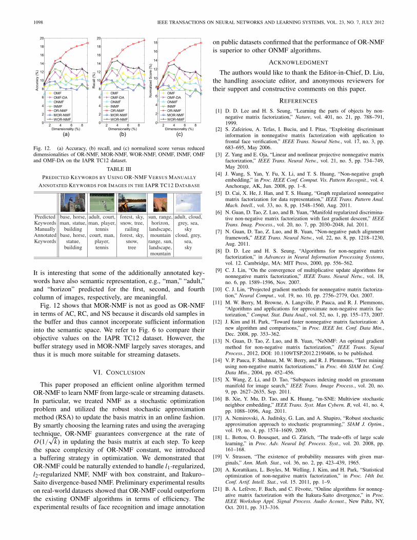
1098 IEEE TRANSACTIONS ON NEURAL NETWORKS AND LEARNING SYSTEMS, VOL. 23, NO. 7, JULY 2012
2 4 6 80
2
4
6
8
10
12
14
16
18
20
(a)Dimensionality (%)
Acc
urac
y (%
)
OMFOMF-DAONMFINMFOR-NMFMOR-NMFWOR-NMF
2 4 6 80
2
4
6
8
10
12
14
16
18
20
(b)Dimensionality (%)
Rec
all (
%)
OMFOMF-DAONMFINMFOR-NMFMOR-NMFWOR-NMF
2 4 6 80
2
4
6
8
10
12
14
16
18
(c)Dimensionality (%)
Nor
mal
ized
Sco
re (%
)
OMFOMF-DAONMFINMFOR-NMFMOR-NMFWOR-NMF
Fig. 12. (a) Accuracy, (b) recall, and (c) normalized score versus reduceddimensionalities of OR-NMF, MOR-NMF, WOR-NMF, ONMF, INMF, OMFand OMF-DA on the IAPR TC12 dataset.
TABLE III
PREDICTED KEYWORDS BY USING OR-NMF VERSUS MANUALLY
ANNOTATED KEYWORDS FOR IMAGES IN THE IAPR TC12 DATABASE
It is interesting that some of the additionally annotated key-words have also semantic representation, e.g., “man,” “adult,”and “horizon” predicted for the first, second, and fourthcolumn of images, respectively, are meaningful.
Fig. 12 shows that MOR-NMF is not as good as OR-NMFin terms of AC, RC, and NS because it discards old samples inthe buffer and thus cannot incorporate sufficient informationinto the semantic space. We refer to Fig. 6 to compare theirobjective values on the IAPR TC12 dataset. However, thebuffer strategy used in MOR-NMF largely saves storages, andthus it is much more suitable for streaming datasets.
VI. CONCLUSION
This paper proposed an efficient online algorithm termedOR-NMF to learn NMF from large-scale or streaming datasets.In particular, we treated NMF as a stochastic optimizationproblem and utilized the robust stochastic approximationmethod (RSA) to update the basis matrix in an online fashion.By smartly choosing the learning rates and using the averagingtechnique, OR-NMF guarantees convergence at the rate ofO(1/√
k) in updating the basis matrix at each step. To keepthe space complexity of OR-NMF constant, we introduceda buffering strategy in optimization. We demonstrated thatOR-NMF could be naturally extended to handle l1-regularized,l2-regularized NMF, NMF with box constraint, and Itakuro–Saito divergence-based NMF. Preliminary experimental resultson real-world datasets showed that OR-NMF could outperformthe existing ONMF algorithms in terms of efficiency. Theexperimental results of face recognition and image annotation
on public datasets confirmed that the performance of OR-NMFis superior to other ONMF algorithms.
ACKNOWLEDGMENT
The authors would like to thank the Editor-in-Chief, D. Liu,the handling associate editor, and anonymous reviewers fortheir support and constructive comments on this paper.
REFERENCES
[1] D. D. Lee and H. S. Seung, “Learning the parts of objects by non-negative matrix factorization,” Nature, vol. 401, no. 21, pp. 788–791,1999.
[2] S. Zafeiriou, A. Tefas, I. Buciu, and I. Pitas, “Exploiting discriminantinformation in nonnegative matrix factorization with application tofrontal face verification,” IEEE Trans. Neural Netw., vol. 17, no. 3, pp.683–695, May 2006.
[3] Z. Yang and E. Oja, “Linear and nonlinear projective nonnegative matrixfactorization,” IEEE Trans. Neural Netw., vol. 21, no. 5, pp. 734–749,May 2010.
[4] J. Wang, S. Yan, Y. Fu, X. Li, and T. S. Huang, “Non-negative graphembedding,” in Proc. IEEE Conf. Comput. Vis. Pattern Recognit., vol. 4.Anchorage, AK, Jun. 2008, pp. 1–8.
[5] D. Cai, X. He, J. Han, and T. S. Huang, “Graph regularized nonnegativematrix factorization for data representation,” IEEE Trans. Pattern Anal.Mach. Intell., vol. 33, no. 8, pp. 1548–1560, Aug. 2011.
[6] N. Guan, D. Tao, Z. Luo, and B. Yuan, “Manifold regularized discrimina-tive non-negative matrix factorization with fast gradient descent,” IEEETrans. Imag. Process., vol. 20, no. 7, pp. 2030–2048, Jul. 2011.
[7] N. Guan, D. Tao, Z. Luo, and B. Yuan, “Non-negative patch alignmentframework,” IEEE Trans. Neural Netw., vol. 22, no. 8, pp. 1218–1230,Aug. 2011.
[8] D. D. Lee and H. S. Seung, “Algorithms for non-negative matrixfactorization,” in Advances in Neural Information Processing Systems,vol. 12. Cambridge, MA: MIT Press, 2000, pp. 556–562.
[9] C. J. Lin, “On the convergence of multiplicative update algorithms fornonnegative matrix factorization,” IEEE Trans. Neural Netw., vol. 18,no. 6, pp. 1589–1596, Nov. 2007.
[10] C. J. Lin, “Projected gradient methods for nonnegative matrix factoriza-tion,” Neural Comput., vol. 19, no. 10, pp. 2756–2779, Oct. 2007.
[11] M. W. Berry, M. Browne, A. Langville, P. Pauca, and R. J. Plemmons,“Algorithms and applications for approximate non-negative matrix fac-torization,” Comput. Stat. Data Anal., vol. 52, no. 1, pp. 155–173, 2007.
[12] J. Kim and H. Park, “Toward faster nonnegative matrix factorization: Anew algorithm and comparisons,” in Proc. IEEE Int. Conf. Data Min.,Dec. 2008, pp. 353–362.
[13] N. Guan, D. Tao, Z. Luo, and B. Yuan, “NeNMF: An optimal gradientmethod for non-negative matrix factorization,” IEEE Trans. SignalProcess., 2012, DOI: 10.1109/TSP.2012.2190406, to be published.
[14] V. P. Pauca, F. Shahnaz, M. W. Berry, and R. J. Plemmons, “Text miningusing non-negative matrix factorizations,” in Proc. 4th SIAM Int. Conf.Data Min., 2004, pp. 452–456.
[15] X. Wang, Z. Li, and D. Tao, “Subspaces indexing model on grassmannmanifold for image search,” IEEE Trans. Image Process., vol. 20, no.9, pp. 2627–2635, Sep. 2011.
[16] B. Xie, Y. Mu, D. Tao, and K. Huang, “m-SNE: Multiview stochasticneighbor embedding,” IEEE Trans. Syst. Man Cybern. B, vol. 41, no. 4,pp. 1088–1096, Aug. 2011.
[17] A. Nemirovski, A. Juditsky, G. Lan, and A. Shapiro, “Robust stochasticapproximation approach to stochastic programming,” SIAM J. Optim.,vol. 19, no. 4, pp. 1574–1609, 2009.
[18] L. Bottou, O. Bousquet, and G. Zürich, “The trade-offs of large scalelearning,” in Proc. Adv. Neural Inf. Process. Syst., vol. 20. 2008, pp.161–168.
[19] V. Strassen, “The existence of probability measures with given mar-ginals,” Ann. Math. Stat., vol. 36, no. 2, pp. 423–439, 1965.
[20] A. Korattikara, L. Boyles, M. Welling, J. Kim, and H. Park, “Statisticaloptimization of non-negative matrix factorization,” in Proc. 14th Int.Conf. Artif. Intell. Stat., vol. 15. 2011, pp. 1–9.
[21] B. A. Lefèvre, F. Bach, and C. Fèvotte, “Online algorithms for nonneg-ative matrix factorization with the Itakura-Saito divergence,” in Proc.IEEE Workshop Appl. Signal Process. Audio Acoust., New Paltz, NY,Oct. 2011, pp. 313–316.

GUAN et al.: ONLINE NONNEGATIVE MATRIX FACTORIZATION 1099
[22] J. Mairal, F. Bach, J. Ponce, and G. Sapiro, “Online learning for matrixfactorization and sparse coding,” J. Mach. Learn. Res., vol. 11, pp. 19–60, Mar. 2010.
[23] A. W. Van der Vaart, Asymptotic Statistics. Cambridge, U.K.: CambridgeUniv. Press, 1998.
[24] D. L. Fisk, “Quasi-martingales,” Trans. Amer. Math. Soc., vol. 120, no.3, pp. 359–388, 1965.
[25] D. Bertsekas, Nonlinear Programming, 2nd ed. Nashua, NH: AthenaScientific, 1999.
[26] P. O. Hoyer, “Non-negative sparse coding,” in Proc. 12th IEEE WorkshopNeural Netw. Signal Process., Nov. 2002, pp. 557–565.
[27] X. He, D. Cai, Y. Shao, H. Bao, and J. Han, “Laplacian regularizedGaussian mixture model for data clustering,” IEEE Trans. Knowl. DataEng., vol. 23, no. 9, pp. 1406–1418, Sep. 2011.
[28] B. Geng, D. Tao, C. Xu, L. Yang, and X. Hua, “Ensemble manifoldregularization,” IEEE Trans. Pattern Anal. Mach. Intell., vol. 34, no. 6,pp. 1227–1233, Jun. 2012.
[29] S. Si, D. Tao, and B. Geng, “Bregman divergence based regularizationfor transfer subspace learning,” IEEE Trans. Knowl. Data Eng., vol. 22,no. 7, pp. 929–942, Jul. 2010.
[30] M. Song, D. Tao, C. Chen, X. Li, and C. Chen, “Color to gray: Visualcue preservation,” IEEE Trans. Pattern Anal. Mach. Intell., vol. 32, no.9, pp. 1537–1552, Sep. 2010.
[31] X. Tian, D. Tao, and Y. Rui, “Sparse transfer learning for interactivevideo search reranking,” ACM Trans. Multimedia Comput. Commun.Appl., 2012, arXiv:1103.2756v3, to be published.
[32] X. He, “Laplacian regularized D-optimal design for active learning andits application to image retrieval,” IEEE Trans. Image Process., vol. 19,no. 1, pp. 254–263, Jan. 2010.
[33] C. Fèvotte, N. Bertin, and J. L. Durrieu, “Nonnegative matrix fac-torization with the Itakura-Saito divergence: With application tomusic analysis,” Neural Comput., vol. 21, no. 3, pp. 793–830, Mar.2009.
[34] B. Cao, D. Shen, S. J. Tao, X. Wang, Q. Yang, and Z. Chen, “Detectand track latent factors with online nonnegative matrix factorization,” inProc. 20th Int. Joint Conf. Artif. Intell., San Francisco, CA, 2007, pp.2689–2694.
[35] S. S. Bucak and B. Gunsel, “Incremental subspace learning via non-negative matrix factorization,” Pattern Recognit., vol. 42, no. 5, pp. 788–797, 2009.
[36] G. Zhou, Z. Yang, and S. Xie, “Online blind source separation usingincremental nonnegative matrix factorization with volume constraint,”IEEE Trans. Neural Netw., vol. 22, no. 4, pp. 550–560, Apr. 2011.
[37] F. Wang, C. Tan, A. C. Knoig, and P. Li, “Efficient document clusteringvia online nonnegative matrix factorization,” in Proc. SIAM Int. Conf.Data Min., 2011, pp. 1–12.
[38] B. Weyrauch, J. Huang, B. Heisele, and V. Blanz, “Component-basedface recognition with 3-D morphable models,” in Proc. IEEE WorkshopFace Process. Video, Jun. 2004, p. 85.
[39] F. Samaria and A. Harter, “Parameterisation of a stochastic model forhuman face identification,” in Proc. IEEE Workshop Appl. Comput. Vis.,Sarasota, FL, Dec. 1994, pp. 138–142.
[40] M. Grubinger, P. D. Clough, M. Henning, and D. Thomas, “The IAPRbenchmark: A new evaluation resource for visual information systems,”in Proc. Int. Conf. Lang. Resour. Evaluat., Genoa, Italy, 2006, pp. 1–10.
[41] J. Duchi, S. Shalev-Schwartz, Y. Singer, and T. Chandra, “Efficientprojections onto the l1-ball for learning in high dimensions,” in Proc.25th Int. Conf. Mach. Learn., Helsinki, Finland, Jul. 2008, pp. 1–8.
[42] P. O. Hoyer, “Non-negative matrix factorization with sparseness con-straints,” J. Mach. Learn. Res., vol. 5, pp. 1457–1469, Dec. 2004.
[43] A. Makadia, V. Pavlovic, and S. Kumar, “A new baseline for imageannotation,” in Proc. 10th Eur. Conf. Comput. Vis., vol. 3. Berlin,Germany, 2008, pp. 316–329.
[44] M. Song, D. Tao, C. Chen, X. Li, and C. Chen, “Color to gray: Visualcue preservation,” IEEE Trans. Pattern Anal. Mach. Intell., vol. 32, no.9, pp. 1537–1552, Sep. 2010.
[45] M. Song, D. Tao, C. Chen, J. Luo, and C. Zhang, “Probabilistic exposurefusion,” IEEE Trans. Image Process., vol. 21, no. 1, pp. 341–357, Jan.2012.
[46] M. Song, D. Tao, X. Huang, C. Chen, and J. Bu, “Three-dimensionalface reconstruction from a single image by a coupled RBF network,”IEEE Trans. Image Process., vol. 21, no. 5, pp. 2887–2897, May2012.
[47] K. Barnard, P. Duygulu, N. Freitas, D. Forsyth, D. Blei, and M. Jordan,“Matching words and pictures,” J. Mach. Learn. Res., vol. 3, pp. 1107–1135, Mar. 2003.
[48] P. Duygulu, N. Freitas, K. Barnard, and D. A. Forsyth, “Object recog-nition as machine translation: Learning a lexicon for a fixed imagevocabulary,” in Proc. 7th Eur. Conf. Comput. Vis., vol. 4. 2002, pp.97–112.
Naiyang Guan received the B.S. and M.S. degreesfrom the National University of Defense Technology(NUDT), Changsha, China. He is currently pursuingthe Ph.D. degree with the School of ComputerScience, NUDT.
He was a Visiting Student with the School ofComputer Engineering, Nanyang Technological Uni-versity, Singapore, from October 2009 to October2010. He is currently a Visiting Scholar with theCentre for Quantum Computation and InformationSystems and the Faculty of the Engineering and
Information Technology, University of Technology, Sydney, Australia. Hiscurrent research interests include computer vision, image processing, andconvex optimization.
Dacheng Tao (M’07–SM’12) is a Professor ofcomputer science with the Centre for QuantumComputation and Intelligent Systems and the Fac-ulty of Engineering and Information Technology,University of Technology, Sydney, Australia. Hemainly applies statistics and mathematics for dataanalysis problems in data mining, computer vision,machine learning, multimedia, and video surveil-lance. He has authored or co-authored more than100 scientific articles, including the IEEE TRANS-ACTIONS ON PATTERN ANALYSIS AND MACHINE
INTELLIGENCE, TRANSACTIONS ON NEURAL NETWORKS AND LEARNING
SYSTEMS, TRANSACTIONS ON IMAGE PROCESSING, Artificial Intelligenceand Statistics, International Conference on Data Mining (ICDM), ComputerVision and Pattern Recognition, and European Conference on ComputerVision.
He received the Best Theory/Algorithm Paper Runner Up Award in IEEEICDM in 2007.
Zhigang Luo received the B.S., M.S., and Ph.D.degrees from the National University of DefenseTechnology (NUDT), Changsha, China, in 1981,1993, and 2000, respectively.
He is currently a Professor with the School ofComputer Science, NUDT. His current researchinterests include parallel computing, computer sim-ulation, and bioinformatics.
Bo Yuan received the Bachelors degree from PekingUniversity Medical School, Beijing, China, in 1983,the M.S. degree in biochemistry and the Ph.D.degree in molecular genetics from the Universityof Louisville, Louisville, KY, in 1990 and 1995,respectively.
He is currently a Professor with the Department ofComputer Science and Engineering, Shanghai JiaoTong University (SJTU), Shanghai, China. Beforejoining SJTU in 2006, he was a tenure-track Assis-tant Professor with Ohio State University (OSU),
Columbus, while serving as a Co-Director for the OSU Program in Phar-macogenomics. At OSU, he was the Founding Director for OSU’s GenomeInitiative from the early 2000s, leading one of the only three independentefforts in the world (besides the Human Genome Project and the Celeracompany), having assembled and deciphered the entire human and mousegenomes. His current research interests include biological networks, net-work evolution, stochastic processes, biologically inspired computing, andbioinformatics, particularly the potential impact of these frameworks on thedevelopment of intelligent algorithms and systems.