BRANE SOLUTIONS IN SUPERGRAVITY

K.S. STELLE

The Blackett Laboratory, Imperial College,

Prince Consort Road, London SW7 2BZ, UK

This review covers p-brane solutions to supergravity theories, by which we shallmean solutions whose lowest energy configuration, in a class determined byasymptotic boundary conditions, contains a (p+1)-dimensional Poincare-invariant“worldvolume” submanifold. The most important such solutions also possess par-tially unbroken supersymmetry, i.e. they saturate Bogomol’ny-Prasad-Sommerfield(BPS) bounds on their energy densities with respect to the p-form charges that theycarry. These charges also appear in the supersymmetry algebra and determine theBPS bounds. Topics covered include the relations between mass densities, chargedensities and the preservation of unbroken supersymmetry; interpolating-solitonstructure; κ-symmetric worldvolume actions; diagonal and vertical Kaluza-Kleinreductions; the four elementary solutions of D = 11 supergravity and the multiple-charge solutions derived from combinations of them; duality-symmetry multiplets;charge quantization; low-velocity scattering and the geometry of worldvolume su-persymmetric σ-models; and the target-space geometry of BPS instanton solutionsobtained by dimensional reduction of static p-branes.

Contents

1 Introduction 3

2 The p-brane ansatz 8

2.1 Single-charge action and field equations . . . . . . . . . . . . . 8

2.2 Electric and magnetic ansatze . . . . . . . . . . . . . . . . . . . 8

2.3 Curvature components and p-brane equations . . . . . . . . . . 102.4 p-brane solutions . . . . . . . . . . . . . . . . . . . . . . . . . . 12

3 D = 11 examples 14

3.1 D = 11 Elementary/electric 2-brane . . . . . . . . . . . . . . . 15

3.2 D = 11 Solitonic/magnetic 5-brane . . . . . . . . . . . . . . . . 19

3.3 Black branes . . . . . . . . . . . . . . . . . . . . . . . . . . . . 22

4 Charges, Masses and Supersymmetry 23

4.1 p-form charges . . . . . . . . . . . . . . . . . . . . . . . . . . . 23

4.2 p-brane mass densities . . . . . . . . . . . . . . . . . . . . . . . 27

4.3 p-brane charges . . . . . . . . . . . . . . . . . . . . . . . . . . . 27

4.4 Preserved supersymmetry . . . . . . . . . . . . . . . . . . . . . 28

1

5 The super p-brane worldvolume action 32

6 Kaluza-Klein dimensional reduction 39

6.1 Multiple field-strength solutions and the single-charge truncation 416.2 Diagonal dimensional reduction of p-branes . . . . . . . . . . . 466.3 Multi-center solutions and vertical dimensional reduction . . . 466.4 The geometry of (D − 3)-branes . . . . . . . . . . . . . . . . . 506.5 Beyond the (D − 3)-brane barrier: Scherk-Schwarz reduction

and domain walls . . . . . . . . . . . . . . . . . . . . . . . . . . 52

7 Intersecting branes and scattering branes 60

7.1 Multiple component solutions . . . . . . . . . . . . . . . . . . . 607.2 Intersecting branes and the four elements in D = 11 . . . . . . 617.3 Brane probes, scattering branes and modulus σ-model geometry 66

8 Duality symmetries and charge quantisation 71

8.1 An example of duality symmetry: D = 8 supergravity . . . . . 728.2 p-form charge quantisation conditions . . . . . . . . . . . . . . 748.3 Charge quantisation conditions and dimensional reduction . . . 778.4 Counting p-branes . . . . . . . . . . . . . . . . . . . . . . . . . 798.5 The charge lattice . . . . . . . . . . . . . . . . . . . . . . . . . 83

9 Local versus active dualities 85

9.1 The symmetries of type IIB supergravity . . . . . . . . . . . . . 879.2 Active duality symmetries . . . . . . . . . . . . . . . . . . . . . 90

10 Non-compact σ-models, null geodesics, and harmonic maps 94

11 Concluding remarks 99

2

1 Introduction

Let us begin from the bosonic sector of D = 11 supergravity,1

I11 =

∫d11x

√−g(R − 148F

2[4])− 1

6F[4] ∧ F[4] ∧ A[3]

. (1.1)

In addition to the metric, one has a 3-form antisymmetric-tensor gauge po-tential A[3] with a gauge transformation δA[3] = dΛ[2] and a field strengthF[4] = dA[3]. The third term in the Lagrangian is invariant under the A[3] gaugetransformation only up to a total derivative, so the action (1.1) is invariantunder gauge transformations that are continuously connected to the identity.This term is required, with the coefficient given in (1.1), by the D = 11 localsupersymmetry that is required of the theory when the gravitino-dependentsector is included.

The equation of motion for the A[3] gauge potential is

d ∗F[4] +12F[4] ∧ F[4] = 0 ; (1.2)

this equation of motion gives rise to the conservation of an “electric” typecharge 2

U =

∫

∂M8

(∗F[4] +12A[3] ∧ F[4]) , (1.3)

where the integral of the 7-form integrand is over the boundary at infinity ofan arbitrary infinite spacelike 8-dimensional subspace of D = 11 spacetime.Another conserved charge relies on the Bianchi identity dF[4] = 0 for its con-servation,

V =

∫

∂M5

F[4] , (1.4)

where the surface integral is now taken over the boundary at infinity of aspacelike 5-dimensional subspace.

Charges such as (1.3, 1.4) can occur on the right-hand side of the super-symmetry algebra,a3

Q,Q = C(ΓAPA + ΓABUAB + ΓABCDEVABCDE) , (1.5)

aAlthough formally reasonable, there is admittedly something strange about this algebra.For objects such as black holes, the total momentum terms on the right-hand side have a well-defined meaning, but for extended objects such as p-branes, the U and V terms on the right-hand side have meaning only as intensive quantities taken per spatial unit worldvolume. Thisforces a similar intensive interpretation also for the momentum, requiring it to be consideredas a momentum per spatial unit worldvolume. Clearly, a more careful treatment of thissubject would recognize a corresponding divergence in the Q,Q anticommutator on theleft-hand side of (1.5) in such cases. This would then require then an infinite normalizationfactor for the algebra, whose removal requires the right-hand side to be reinterpreted in anintensive (i.e. per spatial unit worldvolume) as opposed to an extensive way.

3

where C is the charge conjugation matrix, PA is the energy-momentum 11-vector and UAB and VABCDE are 2-form and 5-form charges that we shall findto be related to the charges U and V (1.3, 1.4) above. Note that since thesupercharge Q in D = 11 supergravity is a 32-component Majorana spinor,the LHS of (1.5) has 528 components. The symmetric spinor matrices CΓA,CΓAB and CΓABCDE on the RHS of (1.5) also have a total of 528 independentcomponents: 11 for the momentum PA, 55 for the “electric” charge UAB and462 for the “magnetic” charge VABCDE .

Now the question arises as to the relation between the charges U and V in(1.3, 1.4) and the 2-form and 5-form charges appearing in (1.5). One thing thatimmediately stands out is that the Gauss’ law integration surfaces in (1.3, 1.4)

are the boundaries of integration volumes M8, M5 that do not fill out a whole10-dimensional spacelike hypersurface in spacetime, unlike the more familiarsituation for charges in ordinary electrodynamics. A rough idea about theorigin of the index structures on UAB and VABCDE may be guessed from the2-fold and 5-fold ways that the corresponding 8 and 5 dimensional integrationvolumes may be embedded into a 10-dimensional spacelike hypersurface. Weshall see in Section 4 that this is too naıve, however: it masks an importanttopological aspect of both the electric charge UAB and the magnetic chargeVABCDE . The fact that the integration volume does not fill out a full spacelikehypersurface does not impede the conservation of the charges (1.3, 1.4); thisonly requires that no electric or magnetic currents are present at the boundaries∂M8, ∂M5. Before we can discuss such currents, we shall need to consider insome detail the supergravity solutions that carry charges like (1.3, 1.4). Thesimplest of these have the structure of p + 1-dimensional Poincare-invarianthyperplanes in the supergravity spacetime, and hence have been termed “p-branes” (see, e.g. Ref.4). In Sections 2 and 3, we shall delve in some detailinto the properties of these solutions.

Let us recall at this point some features of the relationship between super-gravity theory and string theory. Supergravity theories originally arose fromthe desire to include supersymmetry into the framework of gravitational mod-els, and this was in the hope that the resulting models might solve some ofthe outstanding difficulties of quantum gravity. One of these difficulties wasthe ultraviolet problem, on which early enthusiasm for supergravity’s promisegave way to disenchantment when it became clear that local supersymmetryis not in fact sufficient to tame the notorious ultraviolet divergences that arisein perturbation theory.b Nonetheless, supergravity theories won much admira-tion for their beautiful mathematical structure, which is due to the stringent

bFor a review of ultraviolet behavior in supergravity theories, see Ref.5

4

constraints of their symmetries. These severely restrict the possible terms thatcan occur in the Lagrangian. For the maximal supergravity theories, such asthose descended from the D = 11 theory (1.1), there is simultaneously a greatwealth of fields present and at the same time an impossibility of coupling anyindependent external field-theoretic “matter.” It was only occasionally noticedin this early period that this impossibility of coupling to matter fields does not,however, rule out coupling to “relativistic objects” such as black holes, stringsand membranes.

The realization that supergravity theories do not by themselves constituteacceptable starting points for a quantum theory of gravity came somewhatbefore the realization sunk in that string theory might instead be the sought-after perturbative foundation for quantum gravity. But the approaches ofsupergravity and of string theory are in fact strongly interrelated: supergravitytheories arise as long-wavelength effective-field-theory limits of string theories.To see how this happens, consider the σ-model action10 that describes a bosonicstring moving in a background “condensate” of its own massless modes (gMN ,AMN , φ):

I =1

4πα′

∫d2z

√γ [γij∂ix

M∂jxNgMN(x)

+iǫij∂ixM∂jx

NAMN(x) + α′R(γ)φ(x)] . (1.6)

Every string theory contains a sector described by fields (gMN , AMN , φ); theseare the only fields that couple directly to the string worldsheet. In superstringtheories, this sector is called the Neveu-Schwarz/Neveu-Schwarz (NS–NS) sec-tor.

The σ-model action (1.6) is classically invariant under the worldsheet Weylsymmetry γij → Λ2(z)γij . Requiring cancellation of the anomalies in thissymmetry at the quantum level gives differential-equation restrictions on thebackground fields (gMN , AMN , φ) that may be viewed as effective equations ofmotion for these massless modes.11 This system of effective equations may besummarized by the corresponding field-theory effective action

Ieff =

∫dDx

√−ge−2φ[(D − 26)− 3

2α′(R + 4∇2φ− 4(∇φ)2

− 112FMNPF

MNP +O(α′)2], (1.7)

where FMNP = ∂MANP + ∂NAPM + ∂PAMN is the 3-form field strength for theAMN gauge potential. The (D−26) term reflects the critical dimension for thebosonic string: flat space is a solution of the above effective theory only forD = 26. The effective action for the superstring theories that we shall consider

5

in this review contains a similar (NS–NS) sector, but with the substitution of(D−26) by (D−10), reflecting the different critical dimension for superstrings.

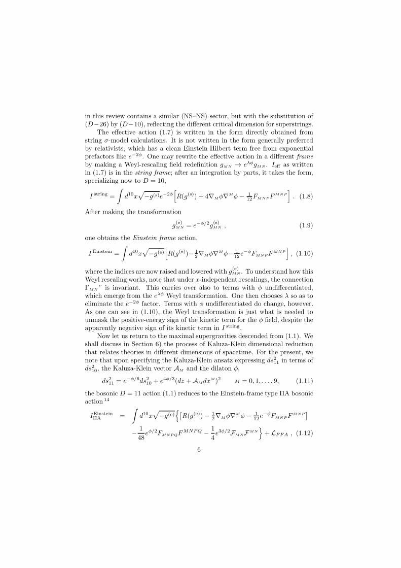
The effective action (1.7) is written in the form directly obtained fromstring σ-model calculations. It is not written in the form generally preferredby relativists, which has a clean Einstein-Hilbert term free from exponentialprefactors like e−2φ. One may rewrite the effective action in a different frameby making a Weyl-rescaling field redefinition gMN → eλφgMN . Ieff as writtenin (1.7) is in the string frame; after an integration by parts, it takes the form,specializing now to D = 10,

I string =

∫d10x

√−g(s)e−2φ

[R(g(s)) + 4∇Mφ∇Mφ− 1

12FMNPFMNP

]. (1.8)

After making the transformation

g(e)MN = e−φ/2g

(s)MN , (1.9)

one obtains the Einstein frame action,

I Einstein =

∫d10x

√−g(e)

[R(g(e))− 1

2∇Mφ∇Mφ− 112e

−φFMNPFMNP

], (1.10)

where the indices are now raised and lowered with g(e)MN . To understand how this

Weyl rescaling works, note that under x-independent rescalings, the connectionΓMN

P is invariant. This carries over also to terms with φ undifferentiated,which emerge from the eλφ Weyl transformation. One then chooses λ so as toeliminate the e−2φ factor. Terms with φ undifferentiated do change, however.As one can see in (1.10), the Weyl transformation is just what is needed tounmask the positive-energy sign of the kinetic term for the φ field, despite theapparently negative sign of its kinetic term in I string.

Now let us return to the maximal supergravities descended from (1.1). Weshall discuss in Section 6) the process of Kaluza-Klein dimensional reductionthat relates theories in different dimensions of spacetime. For the present, wenote that upon specifying the Kaluza-Klein ansatz expressing ds211 in terms ofds210, the Kaluza-Klein vector AM and the dilaton φ,

ds211 = e−φ/6ds210 + e4φ/3(dz +AMdxM)2 M = 0, 1, . . . , 9, (1.11)

the bosonic D = 11 action (1.1) reduces to the Einstein-frame type IIA bosonicaction 14

IEinsteinIIA =

∫d10x

√−g(e)

[R(g(e))− 1

2∇Mφ∇Mφ− 112e

−φFMNPFMNP

]

− 1

48eφ/2FMNPQF

MNPQ − 1

4e3φ/2FMNFMN

+ LFFA , (1.12)

6

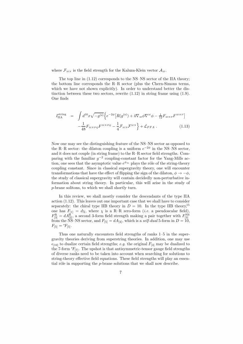
where FMN is the field strength for the Kaluza-Klein vector AM .

The top line in (1.12) corresponds to the NS–NS sector of the IIA theory;the bottom line corresponds the R–R sector (plus the Chern-Simons terms,which we have not shown explicitly). In order to understand better the dis-tinction between these two sectors, rewrite (1.12) in string frame using (1.9).One finds

IstringIIA =

∫d10x

√−g(s)

e−2φ

[R(g(s)) + 4∇Mφ∇Mφ− 1

12FMNPFMNP

]

− 1

48FMNPQF

MNPQ − 1

4FMNFMN

+ LFFA . (1.13)

Now one may see the distinguishing feature of the NS–NS sector as opposed tothe R–R sector: the dilaton coupling is a uniform e−2φ in the NS–NS sector,and it does not couple (in string frame) to the R–R sector field strengths. Com-paring with the familiar g−2 coupling-constant factor for the Yang-Mills ac-tion, one sees that the asymptotic value eφ∞ plays the role of the string-theorycoupling constant. Since in classical supergravity theory, one will encountertransformations that have the effect of flipping the sign of the dilaton, φ→ −φ,the study of classical supergravity will contain decidedly non-perturbative in-formation about string theory. In particular, this will arise in the study ofp-brane solitons, to which we shall shortly turn.

In this review, we shall mostly consider the descendants of the type IIAaction (1.12). This leaves out one important case that we shall have to considerseparately: the chiral type IIB theory in D = 10. In the type IIB theory,15

one has F[1] = dχ, where χ is a R–R zero-form (i.e. a pseudoscalar field),FR[3] = dAR

[2], a second 3-form field strength making a pair together with FNS[3]

from the NS–NS sector, and F[5] = dA[4], which is a self-dual 5-form in D = 10,F[5] =

∗F[5].

Thus one naturally encounters field strengths of ranks 1–5 in the super-gravity theories deriving from superstring theories. In addition, one may useǫ[10] to dualize certain field strengths; e.g. the original F[3] may be dualized tothe 7-form ∗F[7]. The upshot is that antisymmetric-tensor gauge field strengthsof diverse ranks need to be taken into account when searching for solutions tostring-theory effective field equations. These field strengths will play an essen-tial role in supporting the p-brane solutions that we shall now describe.

7

2 The p-brane ansatz

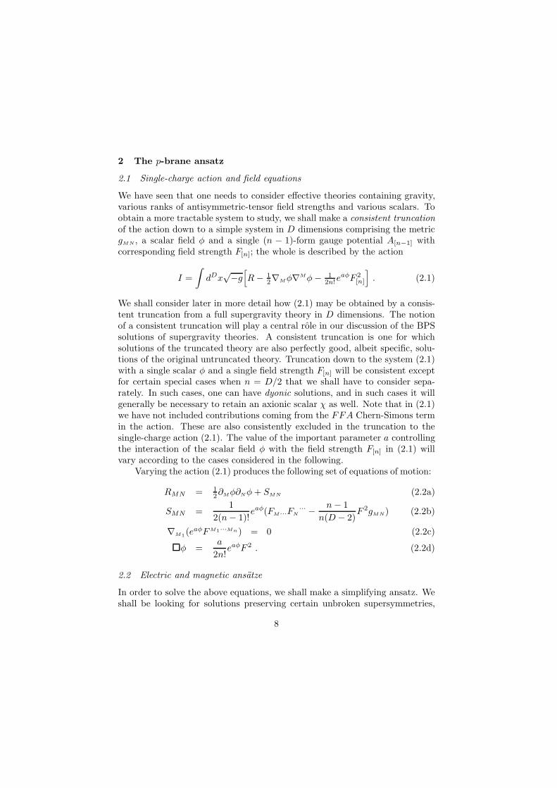
2.1 Single-charge action and field equations

We have seen that one needs to consider effective theories containing gravity,various ranks of antisymmetric-tensor field strengths and various scalars. Toobtain a more tractable system to study, we shall make a consistent truncationof the action down to a simple system in D dimensions comprising the metricgMN , a scalar field φ and a single (n − 1)-form gauge potential A[n−1] withcorresponding field strength F[n]; the whole is described by the action

I =

∫dDx

√−g[R− 1

2∇Mφ∇Mφ− 12n!e

aφF 2[n]

]. (2.1)

We shall consider later in more detail how (2.1) may be obtained by a consis-tent truncation from a full supergravity theory in D dimensions. The notionof a consistent truncation will play a central role in our discussion of the BPSsolutions of supergravity theories. A consistent truncation is one for whichsolutions of the truncated theory are also perfectly good, albeit specific, solu-tions of the original untruncated theory. Truncation down to the system (2.1)with a single scalar φ and a single field strength F[n] will be consistent exceptfor certain special cases when n = D/2 that we shall have to consider sepa-rately. In such cases, one can have dyonic solutions, and in such cases it willgenerally be necessary to retain an axionic scalar χ as well. Note that in (2.1)we have not included contributions coming from the FFA Chern-Simons termin the action. These are also consistently excluded in the truncation to thesingle-charge action (2.1). The value of the important parameter a controllingthe interaction of the scalar field φ with the field strength F[n] in (2.1) willvary according to the cases considered in the following.

Varying the action (2.1) produces the following set of equations of motion:

RMN = 12∂Mφ∂Nφ+ SMN (2.2a)

SMN =1

2(n− 1)!eaφ(FM···FN

··· − n− 1

n(D − 2)F 2gMN) (2.2b)

∇M1(eaφFM1···Mn) = 0 (2.2c)

φ =a

2n!eaφF 2 . (2.2d)

2.2 Electric and magnetic ansatze

In order to solve the above equations, we shall make a simplifying ansatz. Weshall be looking for solutions preserving certain unbroken supersymmetries,

8

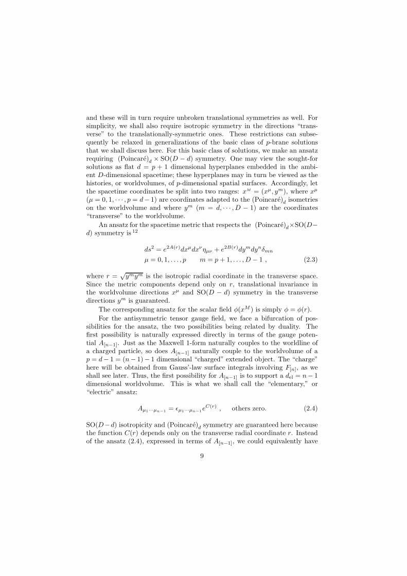
and these will in turn require unbroken translational symmetries as well. Forsimplicity, we shall also require isotropic symmetry in the directions “trans-verse” to the translationally-symmetric ones. These restrictions can subse-quently be relaxed in generalizations of the basic class of p-brane solutionsthat we shall discuss here. For this basic class of solutions, we make an ansatzrequiring (Poincare)d × SO(D − d) symmetry. One may view the sought-forsolutions as flat d = p + 1 dimensional hyperplanes embedded in the ambi-ent D-dimensional spacetime; these hyperplanes may in turn be viewed as thehistories, or worldvolumes, of p-dimensional spatial surfaces. Accordingly, letthe spacetime coordinates be split into two ranges: xM = (xµ, ym), where xµ

(µ = 0, 1, · · · , p = d− 1) are coordinates adapted to the (Poincare)d isometrieson the worldvolume and where ym (m = d, · · · , D − 1) are the coordinates“transverse” to the worldvolume.

An ansatz for the spacetime metric that respects the (Poincare)d×SO(D−d) symmetry is 12

ds2 = e2A(r)dxµdxνηµν + e2B(r)dymdynδmn

µ = 0, 1, . . . , p m = p+ 1, . . . , D − 1 , (2.3)

where r =√ymym is the isotropic radial coordinate in the transverse space.

Since the metric components depend only on r, translational invariance inthe worldvolume directions xµ and SO(D − d) symmetry in the transversedirections ym is guaranteed.

The corresponding ansatz for the scalar field φ(xM ) is simply φ = φ(r).

For the antisymmetric tensor gauge field, we face a bifurcation of pos-sibilities for the ansatz, the two possibilities being related by duality. Thefirst possibility is naturally expressed directly in terms of the gauge poten-tial A[n−1]. Just as the Maxwell 1-form naturally couples to the worldline ofa charged particle, so does A[n−1] naturally couple to the worldvolume of ap = d− 1 = (n− 1)− 1 dimensional “charged” extended object. The “charge”here will be obtained from Gauss’-law surface integrals involving F[n], as weshall see later. Thus, the first possibility for A[n−1] is to support a del = n− 1dimensional worldvolume. This is what we shall call the “elementary,” or“electric” ansatz:

Aµ1···µn−1 = ǫµ1···µn−1eC(r) , others zero. (2.4)

SO(D−d) isotropicity and (Poincare)d symmetry are guaranteed here becausethe function C(r) depends only on the transverse radial coordinate r. Insteadof the ansatz (2.4), expressed in terms of A[n−1], we could equivalently have

9

given just the F[n] field strength:

F(el)mµ1···µn−1 = ǫµ1···µn−1∂me

C(r) , others zero. (2.5)

The worldvolume dimension for the elementary ansatz (2.4, 2.5) is clearly del =n− 1.

The second possible way to relate the rank n of F[n] to the worldvolumedimension d of an extended object is suggested by considering the dualizedfield strength ∗F , which is a (D − n) form. If one were to find an underlyinggauge potential for ∗F (locally possible by courtesy of a Bianchi identity), thiswould naturally couple to a dso = D − n− 1 dimensional worldvolume. Sincesuch a dualized potential would be nonlocally related to the fields appearingin the action (2.1), we shall not explicitly follow this construction, but shallinstead take this reference to the dualized theory as an easy way to identifythe worldvolume dimension for the second type of ansatz. This “solitonic”or “magnetic” ansatz for the antisymmetric tensor field is most convenientlyexpressed in terms of the field strength F[n], which now has nonvanishing valuesonly for indices corresponding to the transverse directions:

F(mag)m1···mn = λǫm1···mnp

yp

rn+1, others zero, (2.6)

where the magnetic-charge parameter λ is a constant of integration, the onlything left undetermined by this ansatz. The power of r in the solitonic/mag-netic ansatz is determined by requiring F[n] to satisfy the Bianchi identity.c

Note that the worldvolume dimensions of the elementary and solitonic casesare related by dso = del ≡ D−del−2; note also that this relation is idempotent,

i.e. (d) = d.

2.3 Curvature components and p-brane equations

In order to write out the field equations after insertion of the above ansatze,one needs to compute the Ricci tensor for the metric.13 This is most easilydone by introducing vielbeins, i.e., orthonormal frames,16 with tangent-spaceindices denoted by underlined indices:

gMN = eMEeN

FηE F . (2.7)

cSpecifically, one finds ∂qFm1···mn = r−(n+1)(

ǫm1···mnq − (n+1)ǫm1···mnpypyq/r2)

; upon

taking the totally antisymmetrized combination [qm1 · · ·mn], the factor of (n+1) is evenedout between the two terms and then one finds from cycling a factor

∑

m ymym = r2, thusobtaining cancellation.

10

Next, one constructs the corresponding 1-forms: eE = dxMeME. Splitting up

the tangent-space indices E = (µ,m) similarly to the world indices M = (µ,m),we have for our ansatze the vielbein 1-forms

eµ = eA(r)dxµ , em = eB(r)dym . (2.8)

The corresponding spin connection 1-forms are determined by the condi-tion that the torsion vanishes, deE + ωE

F ∧ eF = 0, which yields

ωµν = 0 , ωµn = e−B(r)∂nA(r)eµ

ωmn = e−B(r)∂nB(r)em − e−B(r)∂mB(r)en . (2.9)

The curvature 2-forms are then given by

RE F

[2] = dωE F + ωE D ∧ ωDF . (2.10)

From the curvature components so obtained, one finds the Ricci tensor com-ponents

Rµν = −ηµνe2(A−B)(A′′ + d(A′)2 + dA′B′ +(d+ 1)

rA′)

Rmn = −δmn(B′′ + dA′B′ + d(B′)2 +(2d+ 1)

rB′ +

d

rA′) (2.11)

−ymyn

r2(dB′′ + dA′′ − 2dA′B′ + d(A′)2 − d(B′)2 − d

rB′ − d

rA′) ,

where again, d = D − d− 2, and the primes indicate ∂/∂r derivatives.Substituting the above relations, one finds the set of equations that we

need to solve to obtain the metric and φ:

A′′+d(A′)2+dA′B′+ (d+1)r A′ = d

2(D−2)S2 µν

B′′+dA′B′+d(B′)2+ (2d+1)r B′+ d

rA′ = − d

2(D−2)S2 δmn

dB′′+dA′′−2dA′B′+d(A′)2−d(B′)2

− drB

′− drA

′+ 12 (φ

′)2 = 12S

2 ymynφ′′+dA′φ′+dB′φ′+ (d+1)

r φ′ = − 12 ςaS

2 φ(2.12)

where ς = ±1 for the elementary/solitonic cases and the source appearing onthe RHS of these equations is

S =

(e

12aφ−dA+C)C′ electric: d = n− 1, ς = +1

λ(e12aφ−dB)r−d−1 magnetic: d = D − n− 1, ς = −1.

(2.13)

11

2.4 p-brane solutions

The p-brane equations (2.12, 2.13) are still rather daunting. Before we embarkon solving these equations, let us first note a generalization. Although Eqs(2.12) have been specifically written for an isotropic p-brane ansatz, one mayrecognize more general possibilities by noting the form of the Laplace operator,which for isotropic scalar functions of r is

∇2φ = φ′′ + (d+ 1)r−1φ′ . (2.14)

We shall see later that more general solutions of the Laplace equation thanthe simple isotropic ones considered here will also play important roles in thestory.

In order to reduce the complexity of Eqs (2.12), we shall refine the p-brane ansatz (2.3, 2.5, 2.6) by looking ahead a bit and taking a hint from therequirements for supersymmetry preservation, which shall be justified in moredetail later on in Section 4. Accordingly, we shall look for solutions satisfyingthe linearity condition

dA′ + dB′ = 0 . (2.15)

After eliminating B using (2.15), the independent equations become 17

∇2φ = − 12 ςaS

2 (2.16a)

∇2A =d

2(D − 2)S2 (2.16b)

d(D − 2)(A′)2 + 12 d(φ

′)2 = 12 dS

2 , (2.16c)

where, for spherically-symmetric (i.e. isotropic) functions in the transverse(D − d) dimensions, the Laplacian is ∇2φ = φ′′ + (d+ 1)r−1φ′.

Equations (2.16a,b) suggest that we now further refine the ansatze byimposing another linearity condition:

φ′ =−ςa(D − 2)

dA′ . (2.17)

At this stage, it is useful to introduce a new piece of notation, letting

a2 = ∆− 2dd

(D − 2). (2.18)

With this notation, equation (2.16c) gives

S2 =∆(φ′)2

a2, (2.19)

12

so that the remaining equation for φ becomes ∇2φ + ς∆2a (φ

′)2 = 0, which canbe re-expressed as a Laplace equation,d

∇2eς∆2a φ = 0 . (2.20)

Solving this in the transverse (D − d) dimensions with our assumption oftransverse isotropicity (i.e. spherical symmetry) yields

eς∆2a φ ≡ H(y) = 1 +

k

rdk > 0 , (2.21)

where the constant of integration φ|r→∞has been set equal to zero here for

simplicity: φ∞ = 0. The integration constant k in (2.21) sets the mass scaleof the solution; it has been taken to be positive in order to ensure the absenceof naked singularities at finite r. This positivity restriction is similar to theusual restriction to a positive mass parameterM in the standard Schwarzschildsolution.

In the case of the elementary/electric ansatz, with ς = +1, it still remainsto find the function C(r) that determines the antisymmetric-tensor gauge fieldpotential. In this case, it follows from (2.13) that S2 = eaφ−2dA(C′eC)2.Combining this with (2.19), one finds the relation

∂

∂r(eC) =

−√∆

ae−

12aφ+dAφ′ (2.22)

(where it should be remembered that a < 0). Finally, it is straightforwardto verify that the relation (2.22) is consistent with the equation of motion forF[n]:

∇2C + C′(C′ + dB′ − dA′ + aφ′) = 0 . (2.23)

In order to simplify the explicit form of the solution, we now pick valuesof the integration constants to make A∞ = B∞ = 0, so that the solution tendsto flat empty space at transverse infinity. Assembling the result, starting fromthe Laplace-equation solution H(y) (2.21), one finds 7,13

ds2 = H−4d

∆(D−2) dxµdxνηµν +H4d

∆(D−2) dymdym (2.24a)

eφ = H2aς∆ ς =

+1, elementary/electric−1, solitonic/magnetic

(2.24b)

H(y) = 1 +k

rd, (2.24c)

dNote that Eq. (2.20) can also be more generally derived; for example, it still holds if onerelaxes the assumption of isotropicity in the transverse space.

13

and in the elementary/electric case, C(r) is given by

eC =2√∆H−1 . (2.25)

In the solitonic/magnetic case, the constant of integration is related to themagnetic charge parameter λ in the ansatz (2.6) by

k =

√∆

2dλ . (2.26)

In the elementary/electric case, this relation may be taken to define the pa-rameter λ.

The harmonic function H(y) (2.21) determines all of the features of a p-brane solution (except for the choice of gauge for the A[n−1] gauge potential).It is useful to express the electric and magnetic field strengths directly in termsof H :

Fmµ1...µn−1 =2√∆ǫµ1...µn−1∂m(H−1) m = d, . . . , D − 1 electric(2.27a)

Fm1...mn = − 2√∆ǫm1...mnr∂rH m = d, . . . , D − 1 magnetic,(2.27b)

with all other independent components vanishing in either case.

3 D = 11 examples

Let us now return to the bosonic sector of D = 11 supergravity, which hasthe action (1.1). In searching for p-brane solutions to this action, there aretwo particular points to note. The first is that no scalar field is present in(1.1). This follows from the supermultiplet structure of the D = 11 theory,in which all fields are gauge fields. In lower dimensions, of course, scalars doappear; e.g. the dilaton in D = 10 type IIA supergravity emerges out of theD = 11 metric upon dimensional reduction from D = 11 to D = 10. Theabsence of the scalar that we had in our general discussion may be handledhere simply by identifying the scalar coupling parameter a with zero, so thatthe scalar may be consistently truncated from our general action (2.1). Sincea2 = ∆− 2dd/(D − 2), we identify ∆ = 2 · 3 · 6/9 = 4 for the D = 11 cases.

Now let us consider the consistency of dropping contributions arising fromthe FFA Chern-Simons term in (1.1). Note that for n = 4, the F[4] antisym-metric tensor field strength supports either an elementary/electric solutionwith d = n − 1 = 3 (i.e. a p = 2 membrane) or a solitonic/magnetic solution

14

with d = 11 − 3 − 2 = 6 (i.e. a p = 5 brane). In both these elementary andsolitonic cases, the FFA term in the action (1.1) vanishes and hence this termdoes not make any non-vanishing contribution to the metric field equations forour ansatze. For the antisymmetric tensor field equation, a further check isnecessary, since there one requires the variation of the FFA term to vanish inorder to consistently ignore it. The field equation for A[3] is (1.2), which whenwritten out explicitly becomes

∂M

(√−gFMUV W)+

1

2(4!)2ǫUV Wx1x2x3x4y1y2y3y4Fx1x2x3x4Fy1y2y3y4 = 0 . (3.1)

By direct inspection, one sees that the second term in this equation vanishesfor both ansatze.

Next, we shall consider the elementary/electric and the solitonic/magneticD = 11 cases in detail. Subsequently, we shall explore how these particularsolutions fit into wider, “black,” families of p-branes.

3.1 D = 11 Elementary/electric 2-brane

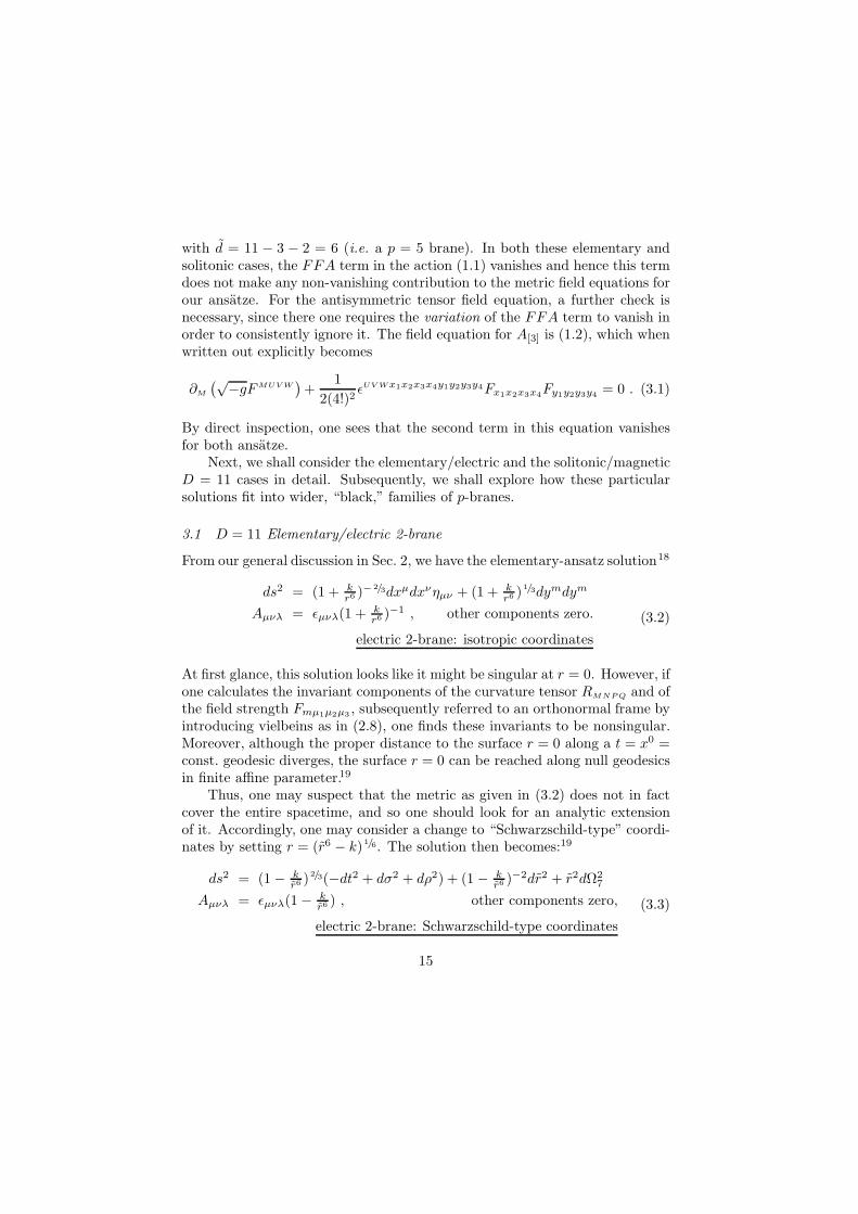
From our general discussion in Sec. 2, we have the elementary-ansatz solution18

ds2 = (1 + kr6 )

−2/3dxµdxνηµν + (1 + kr6 )

1/3dymdym

Aµνλ = ǫµνλ(1 +kr6 )

−1 , other components zero.

electric 2-brane: isotropic coordinates

(3.2)

At first glance, this solution looks like it might be singular at r = 0. However, ifone calculates the invariant components of the curvature tensor RMNPQ and ofthe field strength Fmµ1µ2µ3 , subsequently referred to an orthonormal frame byintroducing vielbeins as in (2.8), one finds these invariants to be nonsingular.Moreover, although the proper distance to the surface r = 0 along a t = x0 =const. geodesic diverges, the surface r = 0 can be reached along null geodesicsin finite affine parameter.19

Thus, one may suspect that the metric as given in (3.2) does not in factcover the entire spacetime, and so one should look for an analytic extensionof it. Accordingly, one may consider a change to “Schwarzschild-type” coordi-nates by setting r = (r6 − k)1/6. The solution then becomes:19

ds2 = (1 − kr6 )

2/3(−dt2 + dσ2 + dρ2) + (1 − kr6 )

−2dr2 + r2dΩ27

Aµνλ = ǫµνλ(1− kr6 ) , other components zero,

electric 2-brane: Schwarzschild-type coordinates

(3.3)

15

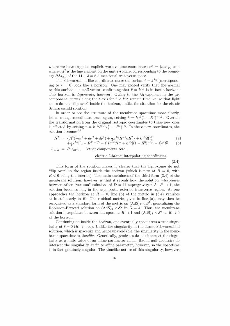
where we have supplied explicit worldvolume coordinates xµ = (t, σ, ρ) andwhere dΩ2

7 is the line element on the unit 7-sphere, corresponding to the bound-ary ∂M8T of the 11− 3 = 8 dimensional transverse space.

The Schwarzschild-like coordinates make the surface r = k 1/6 (correspond-ing to r = 0) look like a horizon. One may indeed verify that the normalto this surface is a null vector, confirming that r = k 1/6 is in fact a horizon.This horizon is degenerate, however. Owing to the 2/3 exponent in the g00component, curves along the t axis for r < k 1/6 remain timelike, so that lightcones do not “flip over” inside the horizon, unlike the situation for the classicSchwarzschild solution.

In order to see the structure of the membrane spacetime more clearly,let us change coordinates once again, setting r = k 1/6(1 − R3)−1/6. Overall,the transformation from the original isotropic coordinates to these new onesis effected by setting r = k 1/6R 1/2/(1 − R3)1/6. In these new coordinates, thesolution becomes 19

ds2 =R2(−dt2 + dσ2 + dρ2) + 1

4k1/3R−2dR2

+ k 1/3dΩ2

7 (a)

+ 14k

1/3[(1−R3)−7/3 − 1]R−2dR2 + k 1/3[(1−R3)−1/3 − 1]dΩ27 (b)

Aµνλ = R3ǫµνλ , other components zero.

electric 2-brane: interpolating coordinates

(3.4)This form of the solution makes it clearer that the light-cones do not

“flip over” in the region inside the horizon (which is now at R = 0, withR < 0 being the interior). The main usefulness of the third form (3.4) of themembrane solution, however, is that it reveals how the solution interpolatesbetween other “vacuum” solutions of D = 11 supergravity.19 As R → 1, thesolution becomes flat, in the asymptotic exterior transverse region. As oneapproaches the horizon at R = 0, line (b) of the metric in (3.4) vanishesat least linearly in R. The residual metric, given in line (a), may then berecognized as a standard form of the metric on (AdS)4 × S7, generalizing theRobinson-Bertotti solution on (AdS)2 × S2 in D = 4. Thus, the membranesolution interpolates between flat space as R → 1 and (AdS)4 × S7 as R → 0at the horizon.

Continuing on inside the horizon, one eventually encounters a true singu-larity at r = 0 (R → −∞). Unlike the singularity in the classic Schwarzschildsolution, which is spacelike and hence unavoidable, the singularity in the mem-brane spacetime is timelike. Generically, geodesics do not intersect the singu-larity at a finite value of an affine parameter value. Radial null geodesics dointersect the singularity at finite affine parameter, however, so the spacetimeis in fact genuinely singular. The timelike nature of this singularity, however,

16

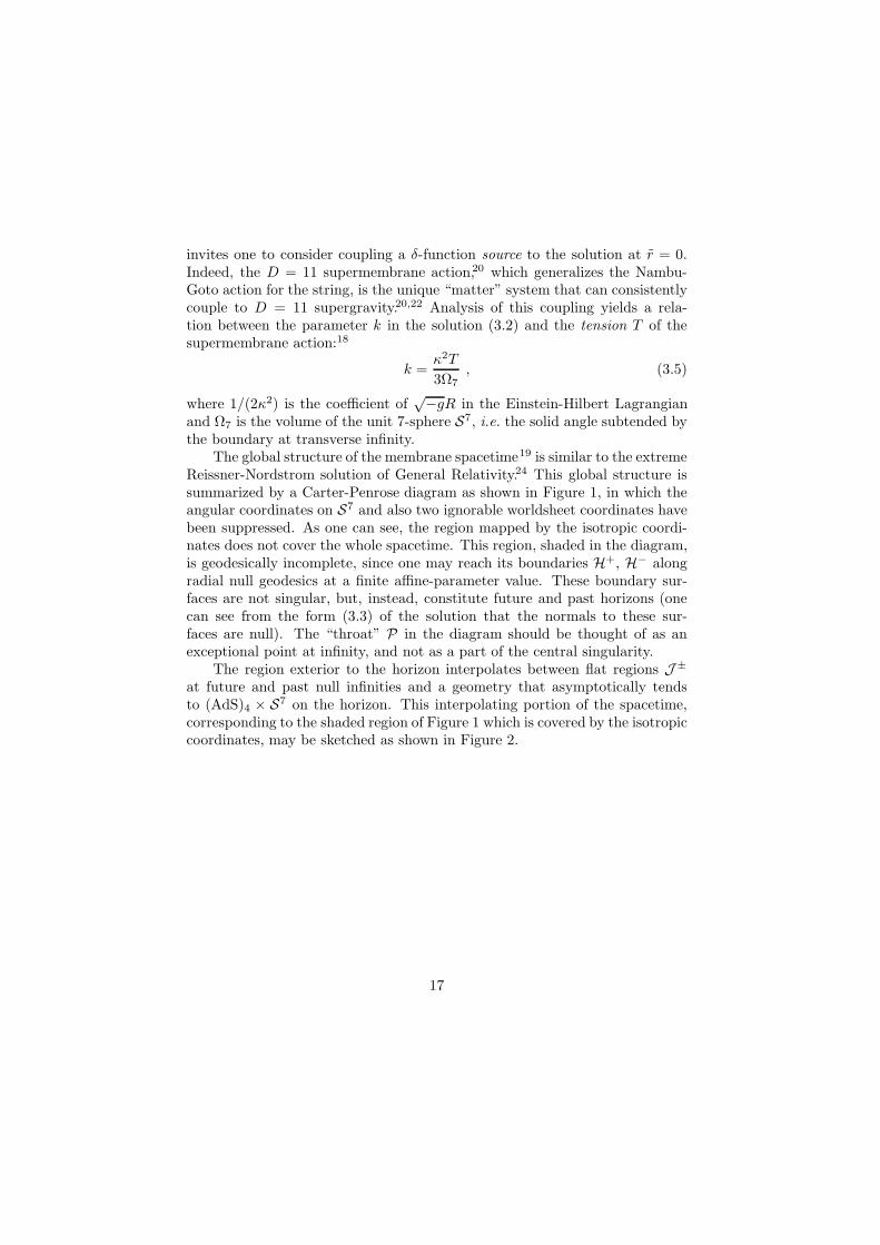
invites one to consider coupling a δ-function source to the solution at r = 0.Indeed, the D = 11 supermembrane action,20 which generalizes the Nambu-Goto action for the string, is the unique “matter” system that can consistentlycouple to D = 11 supergravity.20,22 Analysis of this coupling yields a rela-tion between the parameter k in the solution (3.2) and the tension T of thesupermembrane action:18

k =κ2T

3Ω7, (3.5)

where 1/(2κ2) is the coefficient of√−gR in the Einstein-Hilbert Lagrangian

and Ω7 is the volume of the unit 7-sphere S7, i.e. the solid angle subtended bythe boundary at transverse infinity.

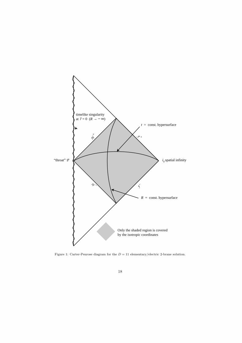
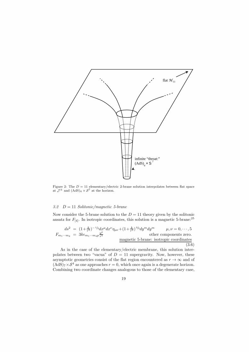
The global structure of the membrane spacetime19 is similar to the extremeReissner-Nordstrom solution of General Relativity.24 This global structure issummarized by a Carter-Penrose diagram as shown in Figure 1, in which theangular coordinates on S7 and also two ignorable worldsheet coordinates havebeen suppressed. As one can see, the region mapped by the isotropic coordi-nates does not cover the whole spacetime. This region, shaded in the diagram,is geodesically incomplete, since one may reach its boundaries H+, H− alongradial null geodesics at a finite affine-parameter value. These boundary sur-faces are not singular, but, instead, constitute future and past horizons (onecan see from the form (3.3) of the solution that the normals to these sur-faces are null). The “throat” P in the diagram should be thought of as anexceptional point at infinity, and not as a part of the central singularity.

The region exterior to the horizon interpolates between flat regions J ±

at future and past null infinities and a geometry that asymptotically tendsto (AdS)4 × S7 on the horizon. This interpolating portion of the spacetime,corresponding to the shaded region of Figure 1 which is covered by the isotropiccoordinates, may be sketched as shown in Figure 2.

17

J +

H –

H +

J–

“throat” P

R = const. hypersurface

t = const. hypersurface

timelike singularityat r = 0 (R → − ∞)

i spatial infinity0

Only the shaded region is coveredby the isotropic coordinates

~

Figure 1: Carter-Penrose diagram for the D = 11 elementary/electric 2-brane solution.

18

flat M 11

infinite “throat:”(AdS) × S

4

7

Figure 2: The D = 11 elementary/electric 2-brane solution interpolates between flat spaceat J± and (AdS)4 × S7 at the horizon.

3.2 D = 11 Solitonic/magnetic 5-brane

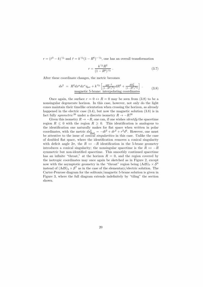
Now consider the 5-brane solution to the D = 11 theory given by the solitonicansatz for F[4]. In isotropic coordinates, this solution is a magnetic 5-brane:25

ds2 = (1+ kr3 )

−1/3dxµdxνηµν+(1+ kr3 )

2/3dymdym µ, ν = 0, · · · , 5Fm1···m4 = 3kǫm1···m4p

yp

r5 other components zero.magnetic 5-brane: isotropic coordinates

(3.6)As in the case of the elementary/electric membrane, this solution inter-

polates between two “vacua” of D = 11 supergravity. Now, however, theseasymptotic geometries consist of the flat region encountered as r → ∞ and of(AdS)7×S4 as one approaches r = 0, which once again is a degenerate horizon.Combining two coordinate changes analogous to those of the elementary case,

19

r = (r3 − k)1/3 and r = k 1/3(1−R6)−1/3, one has an overall transformation

r =k 1/3R2

(1−R6)1/3. (3.7)

After these coordinate changes, the metric becomes

ds2 = R2dxµdxνηµν + k 2/3[

4R−2

(1−R6)8/3dR2 +

dΩ24

(1−R6)2/3

].

magnetic 5-brane: interpolating coordinates(3.8)

Once again, the surface r = 0 ↔ R = 0 may be seen from (3.8) to be anonsingular degenerate horizon. In this case, however, not only do the lightcones maintain their timelike orientation when crossing the horizon, as alreadyhappened in the electric case (3.4), but now the magnetic solution (3.8) is infact fully symmetric 26 under a discrete isometry R→ −R.26

Given this isometry R → −R, one can, if one wishes identify the spacetimeregion R ≤ 0 with the region R ≥ 0. This identification is analogous tothe identification one naturally makes for flat space when written in polarcoordinates, with the metric ds2flat = −dt2 + dr2 + r2d2. However, one mustbe attentive to the issue of conical singularities in this case. Unlike the caseof doubled flat space, where the identification removes a conical singularitywith deficit angle 2π, the R ↔ −R identification in the 5-brane geometryintroduces a conical singularity; the nonsingular spacetime is the R ↔ −Rsymmetric but non-identified spacetime. This smoothly continued spacetimehas an infinite “throat,” at the horizon R = 0, and the region covered bythe isotropic coordinates may once again be sketched as in Figure 2, exceptnow with the asymptotic geometry in the “throat” region being (AdS)7 × S4

instead of (AdS)4 × S7 as in the case of the elementary/electric solution. TheCarter-Penrose diagram for the solitonic/magnetic 5-brane solution is given inFigure 3, where the full diagram extends indefinitely by “tiling” the sectionshown.

20

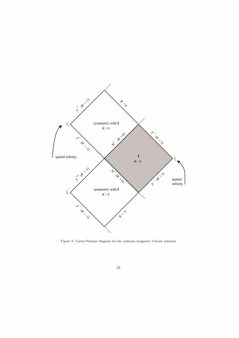
R = 0

R > 0

I

R < 0

symmetric with I

R < 0

symmetric with I

J (R = 1)

+

J

(R =

1)

–

H

(R =

0)

+

H (R = 0)

–

J

(R =

-1)

'

J

(R =

-1)

"+

J (R = -1)

'

J (R = -1)

"

R = 0

i 0

spatial infinity

spatial infinity

'i 0

"i0

–

–

+

Figure 3: Carter-Penrose diagram for the solitonic/magnetic 5-brane solution.

21

The electric and magnetic D = 11 solutions discussed here and in theprevious subsection are “nondilatonic” in that they do not involve a scalar field,since the bosonic sector of D = 11 supergravity (1.1) does not even contain ascalar field. Similar solutions occur in other situations where the parametera (2.18) for a field strength supporting a p-brane solution vanishes, in whichcases the scalar fields may consistently be set to zero; this happens for (D, d) =(11, 3), (11,5), (10,4), (6,2), (5,1), (5,2) and (4,1). In these special cases, thesolutions are nonsingular at the horizon and so one may analytically continuethrough to the other side of the horizon. When d is even for “scalarless”solutions of this type, there exists a discrete isometry analogous to the R →−R isometry of the D = 11 5-brane solution (3.8), allowing the outer andinner regions to be identified.26 When d is odd in such cases, the analytically-extended metric eventually reaches a timelike curvature singularity at r = 0.

When a 6= 0 and the scalar field associated to the field strength supportinga solution cannot be consistently set to zero, then the solution has a singularityat the horizon, as can be seen directly in the scalar solution (2.21) itself (wherewe recall that in isotropic coordinates, the horizon occurs at r = 0)

3.3 Black branes

In order to understand better the family of supergravity solutions that we havebeen discussing, let us now consider a generalization that lifts the degeneratenature of the horizon. Written in Schwarzschild-type coordinates, one findsthe generalized “black brane” solution 27,28

ds2 = − Σ+

Σ1− 4d

∆(D−2)−

dt2 +Σ4d

∆(D−2)

− dxidxi

+Σ

2a2

∆d−1

−Σ+

dr2 + r2Σ2a2

∆d− dΩ2

D−d−1

eς∆2aφ = Σ−1

− Σ± = 1−( r±r

)d.

black brane: Schwarzschild-type coordinates

(3.9)

The antisymmetric tensor field strength for this solution corresponds to a

charge parameter λ = 2d/√∆(r+r−)d/2, either electric or magnetic.

The characteristic feature of the above “blackened” p-branes is that theyhave a nondegenerate, nonsingular outer horizon at r = r+, at which the lightcones “flip over.” At r = r−, one encounters an inner horizon, which, however,coincides in general with a curvature singularity. The singular nature of thesolution at r = r− is apparent in the scalar φ in (3.9). For solutions with p ≥ 1,

22

the singularity at the inner horizon persists even in cases where the scalar φ isabsent.

The extremal limit of the black brane solution occurs for r+ = r−. Whena = 0 and scalars may consistently be set to zero, the singularity at the hori-zon r+ = r− disappears and then one may analytically continue through thehorizon. In this case, the light cones do not “flip over” at the horizon becauseone is really crossing two coalesced horizons, and the coincident “flips” of thelight cones cancel out.

The generally singular nature of the inner horizon of the non-extremesolution (3.9) shows that the “location” of the p-brane in spacetime shouldnormally be thought to coincide with the inner horizon, or with the degeneratehorizon in the extremal case.

4 Charges, Masses and Supersymmetry

The p-brane solutions that we have been studying are supported by anti-symmetric tensor gauge field strengths that fall off at transverse infinity like

r−(d+1), as one can see from (2.5, 2.25, 2.6). This asymptotic falloff is slowenough to give a nonvanishing total charge density from a Gauss’ law flux in-tegral at transverse infinity, and we shall see that, for the “extremal” class ofsolutions that is our main focus, the mass density of the solution saturates a“Bogomol’ny bound” with respect to the charge density. In this Section, weshall first make more precise the relation between the geometry of the p-branesolutions, the p-form charges UAB and VABCDE and the scalar charge magni-tudes U and V (1.3, 1.4); we shall then discuss the relations between thesecharges, the energy density and the preservation of unbroken supersymmetry.

4.1 p-form charges

Now let us consider the inclusion of sources into the supergravity equations.The harmonic function (2.21) has a singularity which has for simplicity beenplaced at the origin of the transverse coordinates ym. As we have seen inSections 3.1 and 3.2, whether or not this gives rise to a physical singularityin a solution depends on the global structure of that solution. In the electric2-brane case, the solution does in the end have a singularity.26 This singularityis unlike the Schwarzschild singularity, however, in that it is a timelike curve,and thus it may be considered to be the wordvolume of a δ-function source.The electric source that couples to D = 11 supergravity is the fundamental

23

supermembrane action,20 whose bosonic part is

Isource = Qe

∫

W3

d3ξ[√

− det(∂µxM∂νxNgMN (x))

+1

3!ǫµνρ∂µx

M∂νxN∂ρx

RAMNR(x)]. (4.1)

The source strength Qe will shortly be found to be equal to the electric chargeU upon solving the coupled equations of motion for the supergravity fields anda single source of this type. Varying the source action (4.1) with δ/δA[3], oneobtains the δ-function current

JMNR(z) = Qe

∫

W3

δ3(z − x(ξ))dxM ∧ dxN ∧ dxR . (4.2)

This current now stands on the RHS of the A[3] equation of motion:

d( ∗F[4] +12A[3] ∧ F[4]) =

∗J[3] . (4.3)

Thus, instead of the Gauss’ law expression for the charge, one may insteadrewrite the charge as a volume integral of the source,

U =

∫

M8

∗J[3] =1

3!

∫

M8

J0MNd8SMN , (4.4)

where d8SMN is the 8-volume element on M8, specified within a D = 10spatial section of the supergravity spacetime by a 2-form. The charge derivedin this way from a single 2-brane source is thus U = Qe as expected.

Now consider the effect of making different choices of the M8 integrationvolume within the D = 10 spatial spacetime section, as shown in Figure 4. Letthe difference between the surfaces M8 and M′

8 be infinitesimal and be givenby a vector field vN (x). The difference in the electric charges obtained is thengiven by

δU =

∫

M8

Lv∗J[3] =1

3!

∫

∂M8

J0MNvRd7SMNR , (4.5)

where Lv is the Lie derivative along the vector field v. The second equality in(4.5) follows using Stokes’ theorem and the conservation of the current J[3].

Now a topological nature of the charge integral (1.3) becomes apparent;similar considerations apply to the magnetic charge (1.4). As long as thecurrent J[3] vanishes on the boundary ∂M8, the difference (4.5) between thecharges calculated using the integration volumes M8 and M′

8 will vanish.This divides the electric-charge integration volumes into two topological classes

24

J[3]

M8

M8'

v(x)

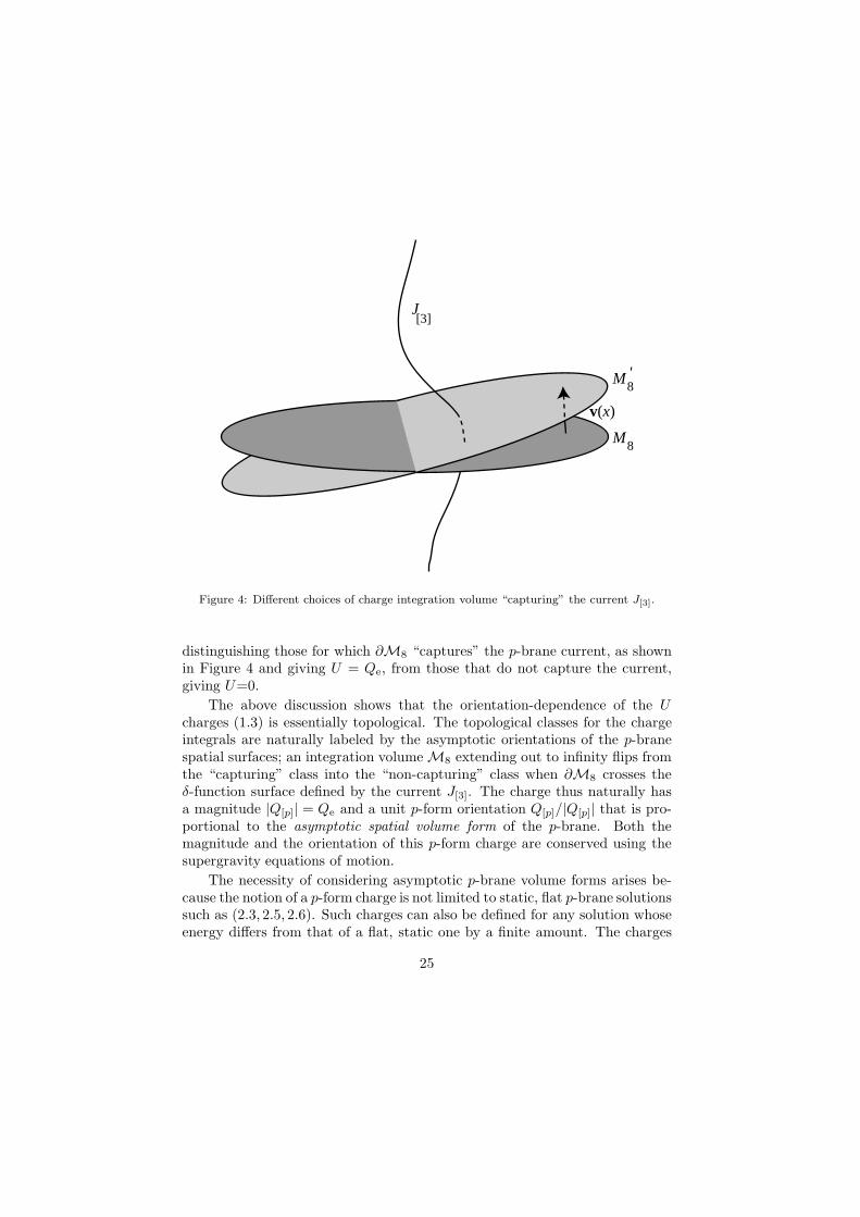
Figure 4: Different choices of charge integration volume “capturing” the current J[3].

distinguishing those for which ∂M8 “captures” the p-brane current, as shownin Figure 4 and giving U = Qe, from those that do not capture the current,giving U=0.

The above discussion shows that the orientation-dependence of the Ucharges (1.3) is essentially topological. The topological classes for the chargeintegrals are naturally labeled by the asymptotic orientations of the p-branespatial surfaces; an integration volume M8 extending out to infinity flips fromthe “capturing” class into the “non-capturing” class when ∂M8 crosses theδ-function surface defined by the current J[3]. The charge thus naturally hasa magnitude |Q[p]| = Qe and a unit p-form orientation Q[p]/|Q[p]| that is pro-portional to the asymptotic spatial volume form of the p-brane. Both themagnitude and the orientation of this p-form charge are conserved using thesupergravity equations of motion.

The necessity of considering asymptotic p-brane volume forms arises be-cause the notion of a p-form charge is not limited to static, flat p-brane solutionssuch as (2.3, 2.5, 2.6). Such charges can also be defined for any solution whoseenergy differs from that of a flat, static one by a finite amount. The charges

25

for such solutions will also appear in the supersymmetry algebra (1.5) for suchbackgrounds, but the corresponding energy densities will not in general sat-urate the BPS bounds. For a finite energy difference with respect to a flat,static p-brane, the asymptotic orientation of the p-brane volume form musttend to that of a static flat solution, which plays the role of a “BPS vacuum”in a given p-form charge sector of the theory.

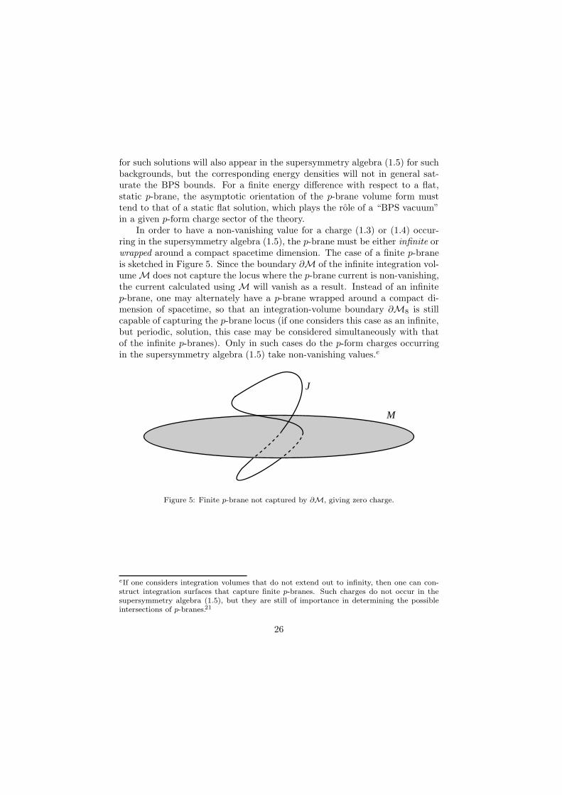
In order to have a non-vanishing value for a charge (1.3) or (1.4) occur-ring in the supersymmetry algebra (1.5), the p-brane must be either infinite orwrapped around a compact spacetime dimension. The case of a finite p-braneis sketched in Figure 5. Since the boundary ∂M of the infinite integration vol-ume M does not capture the locus where the p-brane current is non-vanishing,the current calculated using M will vanish as a result. Instead of an infinitep-brane, one may alternately have a p-brane wrapped around a compact di-mension of spacetime, so that an integration-volume boundary ∂M8 is stillcapable of capturing the p-brane locus (if one considers this case as an infinite,but periodic, solution, this case may be considered simultaneously with thatof the infinite p-branes). Only in such cases do the p-form charges occurringin the supersymmetry algebra (1.5) take non-vanishing values.e

J

M

Figure 5: Finite p-brane not captured by ∂M, giving zero charge.

eIf one considers integration volumes that do not extend out to infinity, then one can con-struct integration surfaces that capture finite p-branes. Such charges do not occur in thesupersymmetry algebra (1.5), but they are still of importance in determining the possibleintersections of p-branes.21

26

4.2 p-brane mass densities

Now let us consider the mass density of a p-brane solution. Since the p-branesolutions have translational symmetry in their p spatial worldvolume direc-tions, the total energy as measured by a surface integral at spatial infinitydiverges, owing to the infinite extent. What is thus more appropriate to con-sider instead is the value of the density, energy/(unit p-volume). Since weare considering solutions in their rest frames, this will also give the value ofmass/(unit p-volume), or tension of the solution. Instead of the standard spa-tial dD−2Σa surface integral, this will be a d(D−d−1)Σm surface integral overthe boundary ∂MT of the transverse space.

The ADM formula for the energy density written as a Gauss’-law integral(see, e.g., Ref.16) is, dropping the divergent spatial dΣµ=i integral,

E =

∫

∂MT

dD−d−1Σm(∂nhmn − ∂mhbb) , (4.6)

written for gMN = ηMN +hMN tending asymptotically to flat space in Cartesiancoordinates, and with a, b spatial indices running over the values µ = i =1, . . . , d − 1; m = d, . . . , D − 1. For the general p-brane solution (2.24), onefinds

hmn =4kd

∆(D − 2)rdδmn , hbb =

8k(d+ 12 d)

∆(D − 2)rd, (4.7)

and, since d(D−d−1)Σm = rdymdΩ(D−d−1), one finds

E =4kdΩD−d−1

∆, (4.8)

where ΩD−d−1 is the volume of the SD−d−1 unit sphere. Recalling that k =√∆λ/(2d), we consequently have a relation between the mass per unit p volume

and the charge parameter of the solution

E =2λΩD−d−1√

∆. (4.9)

By contrast, the black brane solution (3.9) has E > 2λΩD−d−1/√∆, so

the extremal p-brane solution (2.24) is seen to saturate the inequality E ≥2λΩD−d−1/

√∆.

4.3 p-brane charges

As one can see from (4.8, 4.9), the relation (2.26) between the integrationconstant k in the solution (2.24) and the charge parameter λ implies a deep

27

link between the energy density and certain electric or magnetic charges. Inthe electric case, this charge is a quantity conserved by virtue of the equationsof motion for the antisymmetric tensor gauge field A[n−1], and has generallybecome known as a “Page charge,” after its first discussion in Ref.2 To bespecific, if we once again consider the bosonic sector of D = 11 supergravitytheory (1.1), for which the antisymmetric tensor field equation was given in(3.1), one finds the Gauss’-law form conserved quantity 2 U (1.3).

For the p-brane solutions (2.24), the∫A ∧ F term in (1.3) vanishes. The∫ ∗F term does, however, give a contribution in the elementary/electric case,

provided one picks M8 to coincide with the transverse space to the d = 3membrane worldvolume, M8T. The surface element for this transverse spaceis dΣm(7), so for the p = 2 elementary membrane solution (3.2), one finds

U =

∫

∂M8T

dΣm(7)Fm012 = λΩ7 . (4.10)

Since the D = 11 F[4] field strength supporting this solution has ∆ = 4, themass/charge relation is

E = U = λΩ7 . (4.11)

Thus, like the classic extreme Reissner-Nordstrom black-hole solution to whichit is strongly related (as can be seen from the Carter-Penrose diagram given inFigure 1), the D = 11 membrane solution has equal mass and charge densities,saturating the inequality E ≥ U .

Now let us consider the charge carried by the solitonic/magnetic 5-branesolution (3.6). The field strength in (3.6) is purely transverse, so no electriccharge (1.3) is present. The magnetic charge (1.4) is carried by this solution,however. Once again, let us choose the integration subsurface so as to coincidewith the transverse space to the d = 6 worldvolume, i.e. M5 = M5T. Then,we have

V =

∫

∂M5T

dΣm(4)ǫmnpqrFnpqr = λΩ4 . (4.12)

Thus, in the solitonic/magnetic 5-brane case as well, we have a saturation ofthe mass-charge inequality:

E = V = λΩ4 . (4.13)

4.4 Preserved supersymmetry

Since the bosonic solutions that we have been considering are consistent trun-cations of D = 11 supergravity, they must also possess another conserved

28

quantity, the supercharge. Admittedly, since the supercharge is a Grassma-nian (anticommuting) quantity, its value will clearly be zero for the class ofpurely bosonic solutions that we have been discussing. However, the func-tional form of the supercharge is still important, as it determines the form ofthe asymptotic supersymmetry algebra. The Gauss’-law form of the super-charge is given as an integral over the boundary of the spatial hypersurface.For the D = 11 solutions, this surface of integration is the boundary at infinity∂M10 of the D = 10 spatial hypersurface; the supercharge is then 1

Q =

∫

∂M10

Γ0bcψcdΣ(9)b . (4.14)

One can also rewrite this in fully Lorentz-covariant form, where dΣ(9)b =dΣ(9)0b → dΣ(9)AB:

Q =

∫

∂M10

ΓABCψCdΣ(9)AB . (4.15)

After appropriate definitions of Poisson brackets, the D = 11 supersym-metry algebra for the supercharge (4.14, 4.15) is found to be given 29 by (1.5)Thus, the supersymmetry algebra wraps together all of the conserved Gauss’-law type quantities that we have discussed.

The positivity of the Q2 operator on the LHS of the algebra (1.5) is at theroot of the Bogomol’ny bounds 30,26,32

E ≥ (2/√∆)U electric bound (4.16a)

E ≥ (2/√∆)V magnetic bound (4.16b)

that are saturated by the p-brane solutions.The saturation of the Bogomol’ny inequalities by the p-brane solutions

is an indication that they fit into special types of supermultiplets. All ofthese bound-saturating solutions share the important property that they leavesome portion of the supersymmetry unbroken. Within the family of p-branesolutions that we have been discussing, it turns out 32 that the ∆ values ofsuch “supersymmetric” p-branes are of the form ∆ = 4/N , where N is thenumber of antisymmetric tensor field strengths participating in the solution(distinct, but of the same rank). The different charge contributions to thesupersymmetry algebra occurring for different values of N (hence different ∆)affect the Bogomol’ny bounds as shown in (4.16).

In order to see how a purely bosonic solution may leave some portion ofthe supersymmetry unbroken, consider specifically once again the membranesolution of D = 11 supergravity.18 This theory 1 has just one spinor field, the

29

gravitino ψM . Checking for the consistency of setting ψM = 0 with the sup-position of some residual supersymmetry with parameter ǫ(x) requires solvingthe equation

δψA|ψ=0= DAǫ = 0 , (4.17)

where ψA = eAMψM and

DAǫ = DAǫ −1

288(ΓA

BCDE − 8δABΓCDE)FBCDEǫ

DAǫ = (∂A + 14ωA

BCΓBC)ǫ . (4.18)

Solving the equation DAǫ = 0 amounts to finding a Killing spinor field in thepresence of the bosonic background. Since the Killing spinor equation (4.17) islinear in ǫ(x), the Grassmanian (anticommuting) character of this parameteris irrelevant to the problem at hand, which thus reduces effectively to solving(4.17) for a commuting quantity.

In order to solve the Killing spinor equation (4.17) in a p-brane background,it is convenient to adopt an appropriate basis for the D = 11 Γ matrices. Forthe d = 3 membrane background, one would like to preserve SO(2, 1)× SO(8)covariance. An appropriate basis that does this is

ΓA = (γµ ⊗ Σ9, 1l(2) ⊗ Σm) , (4.19)

where γµ and 1l(2) are 2 × 2 SO(2, 1) matrices; Σ9 and Σm are 16 × 16 SO(8)matrices, with Σ9 = Σ3Σ4 . . .Σ10, so Σ2

9 = 1l(16). The most general spinor fieldconsistent with (Poincare)3 × SO(8) invariance in this spinor basis is of theform

ǫ(x, y) = ǫ2 ⊗ η(r) , (4.20)

where ǫ2 is a constant SO(2, 1) spinor and η(r) is an SO(8) spinor dependingonly on the isotropic radial coordinate r; η may be further decomposed intoΣ9 eigenstates by the use of 1

2 (1l± Σ9) projectors.Analysis of the the Killing spinor condition (4.17) in the above spinor basis

leads to the following requirements 12,18 on the background and on the spinorfield η(r):

1) The background must satisfy the conditions 3A′ + 6B′ = 0 and C′eC =3A′e3A. The first of these conditions is, however, precisely the linearity-condition refinement (2.15) that we made in the p-brane ansatz; thesecond condition follows from the ansatz refinement (2.17) (consideredas a condition on φ′/a) and from (2.22). Thus, what appeared previouslyto be simplifying specializations in the derivation given in Section 2 turnout in fact to be conditions required for supersymmetric solutions.

30

2) η(r) = H−1/6(y)η0 = eC(r)/6η0, where η0 is a constant SO(8) spinor.Thus, the surviving local supersymmetry parameter ǫ(x, y) must takethe form ǫ(x, y) = H−1/6ǫ∞, where ǫ∞ = ǫ2 ⊗ η0. Note that, afterimposing this requirement, at most a finite number of parameters canremain unfixed in the product spinor ǫ2 ⊗ η0; i.e. the local supersym-metry of the D = 11 theory is almost entirely broken by any particularsolution. So far, the requirement (4.17) has cut down the amount of sur-viving supersymmetry from D = 11 local supersymmetry (i.e. effectivelyan infinite number of components) to the finite number of independentcomponents present in ǫ2 ⊗ η0. The maximum number of such rigid un-broken supersymmetry components is achieved for D = 11 flat space,which has a full set of 32 constant components.

3) (1l + Σ9)η0 = 0, so the constant SO(8) spinor η0 is also required tobe chiral.f This cuts the number of surviving parameters in the productǫ∞ = ǫ2⊗η0 by half: the total number of surviving rigid supersymmetriesin ǫ(x, y) is thus 2·8 = 16 (counting real spinor components). Since this ishalf of the maximum rigid number (i.e. half of the 32 for flat space), onesays that the membrane solution preserves “half” of the supersymmetry.

In general, the procedure for checking how much supersymmetry is pre-served by a given BPS solution follows steps analogous to points 1) – 3) above:first a check that the conditions required on the background fields are satisfied,then a determination of the functional form of the supersymmetry parameterin terms of some finite set of spinor components, and finally the imposition ofprojection conditions on that finite set. In a more telegraphic partial discus-sion, one may jump straight to the projection conditions 3). These must, ofcourse, also emerge from a full analysis of equations like (4.17). But one canalso see more directly what they will be simply by considering the supersym-metry algebra (1.5), specialized to the BPS background. Thus, for example,in the case of a D = 11 membrane solution oriented in the 012 directions,one has, after normalizing to a unit 2-volume,

1

2-volQα, Qβ = −(CΓ0)αβE + (CΓ12)αβU12 . (4.21)

Since, as we have seen in (4.11), the membrane solution saturating the Bogo-mol’ny bound (4.16a) with E = U = U12, one may rewrite (4.21) as

1

2-volQα, Qβ = 2EP012 P012 = 1

2 (1l + Γ012) , (4.22)

fThe specific chirality indicated here is correlated with the sign choice made in the elemen-tary/electric form ansatz (2.4); one may accordingly observe from (1.1) that a D = 11 paritytransformation requires a sign flip of A[3].

31

where P012 is a projection operator (i.e. P 2012 = P012) whose trace is trP012 =

12 · 32; thus, half of its eigenvalues are zero, and half are unity. Any survivingsupersymmetry transformation must give zero when acting on the BPS back-ground fields, and so the anticommutator Qα, Qβ of the generators must givezero when contracted with a surviving supersymmetry parameter ǫα. From(4.22), this translates to

P012 ǫ∞ = 0 , (4.23)

which is equivalent to condition 3) above, (1l + Σ9)η0 = 0. Thus, we onceagain see that the D = 11 supermembrane solution (3.2) preserves half ofthe maximal rigid D = 11 supersymmetry. When we come to discuss thecases of “intersecting” p-branes in Section 7, it will be useful to have quickderivations like this for the projection conditions that must be satisfied bysurviving supersymmetry parameters.

More generally, the positive semi-definiteness of the operator Qα, Qβis the underlying principle in the derivation 30,26,32 of the Bogomol’ny bounds(4.16). A consequence of this positive semi-definiteness is that zero eigenvaluescorrespond to solutions that saturate the Bogomol’ny inequalities (4.16), andthese solutions preserve one component of unbroken supersymmetry for eachsuch zero eigenvalue.

Similar consideration of the solitonic/magnetic 5-brane solution 25 (3.6)shows that it also preserves half the rigid D = 11 supersymmetry. In the 5-brane case, the analogue of condition 2) above is ǫ(x, y) = H−1/12(y)ǫ∞, andthe projection condition following from the algebra of preserved supersymme-try generators for a 5-brane oriented in the 012345 directions is P012345 ǫ∞ =0, where P012345 = 1

2 (1l + Γ012345).

5 The super p-brane worldvolume action

We have already seen the bosonic part of the action for a supermembrane inbackground gravitational and 3-form fields in Eq. (4.1). We shall now want toextend this treatment to the full set of bosonic and fermionic variables of animportant class of super p-branes. This class consists of those branes whoseworldvolume variables are just the bosonic and fermionic coordinates of thesuper p-brane in the target superspace. In the early days of research on superp branes, this was the only class known, but it is now recognized that moregeneral kinds of worldvolume multiplets can also occur, such as those involvinghigher form fields, requiring a generalization of the formalism that we shall nowpresent.

Let us reformulate in Howe-Tucker form the bosonic part of the p-braneaction coupled to gravity alone, by introducing an independent worldvolume

32

metric γij :33

IHT = 12

∫dp+1ξ

√− detγ

[γij∂ix

m∂jxngmn − (p− 1)

], (5.1)

where the index ranges are i = 0, 1, . . . , p andm = 0, 1, . . . , D−1. The equationof motion following from (5.1) for the worldvolume position variables xm is

γij(∂i∂jx

m −k

ij

(γ) ∂kx

m + ∂ixp∂jx

qΓmpq(g)

)= 0 , (5.2)

wherekij

(γ) and Γmpq(g) are the Christoffel connections for the worldvolume

metric γij(ξ) and the spacetime metric gmn(x) respectively. The γ field equa-tion is

γij = ∂ixm∂jx

ngmn(x) , (5.3)

which states that γij is equal to the metric induced from the spacetime metricgmn through the embedding xm(ξ). Inserting (5.3) into (5.2), one obtainsthe same equation as that following from the Nambu-Goto form action thatgeneralizes (4.1)

ING =

∫dp+1ξdet1/2 (∂ix

m∂jxngmn(x)) , (5.4)

thus demonstrating the classical equivalence of (5.1) and (5.4). Note the es-sential appearance here of a “cosmological term” in the worldvolume actionfor p 6= 1. The absence of this term in the specific case of the string, p = 1,is at the origin of the worldvolume Weyl symmetry which is obtained only inthe string case.

Now generalize the target space to superspace ZM = (xm, θα) and describethe supergravity background by vielbeins EAM (Z) and a superspace (p+1) formB = [(p+1)!]−1EA1 . . . EAp+1BAp+1...A1 , where E

A = dZMEAM are superspacevielbein 1-forms. The superspace world indices M and tangent space indices Arun both through bosonic values m, a = 0, 1, . . . (D − 1) and fermionic valuesα appropriate for the corresponding spinor dimensionality.

The p-brane worldvolume is a map zM (ξ) from the space of the world-volume parameters ξi to the target superspace; this map may be used to pullback forms to the worldvolume: EA = dξiEAi , where E

Ai = ∂iz

M (ξ)EAM (z(ξ).Using these, one may write the super p-brane action in Green-Schwarz form:

I =

∫dp+1ξ

12

√−γ[γijEai Ebjηab − (p− 1)]

+1

(p+ 1)!ǫi1···ip+1EA1

i1· · ·EAp+1

ip+1BAp+1···A1

, (5.5)

33

where γ is the traditional shorthand for det γij .

Writing the super p-brane action in this manifestly target-space supersym-metric form raises the question of how the expected supersymmetric balance ofbosonic and fermionic degrees of freedom can be achieved on the worldvolume.For example, in the case of the D = 11, p = 2 supermembrane 20, the D = 11spinor dimensionality is 32, while the bosonic coordinates take only 11 val-ues. Now, in order to compare correctly the worldvolume degrees of freedom,one should first remove the worldvolume gauge degrees of freedom, which thussubtracts from the above account three worldvolume reparameterizations forthe ξi, leaving 11− 3 = 8 bosonic non-gauge degrees of freedom. The fermionsare not in fact expected to match this number, because they are expectedto satisfy first-order equations of motion on the worldvolume, as opposed tothe second-order equations expected for the bosons. But, multiplying by 2 inorder to take account of this difference, one would still be expecting to have16 active worldvolume fermionic degrees of freedom, instead of the a priori32. The difference can only be accounted for by an additional fermionic gaugesymmetry.

This fermionic gauge symmetry is called “κ symmetry” and its generalimplementation remains something of a mystery. In some formalisms, it canbe related to a standard worldvolume supersymmetry,34 but this introducesadditional twistor-like variables that obscure somewhat the physical contentof the theory. The most physically transparent formalism is the original oneof Ref.35, where the κ symmetry parameter has a spacetime spinor index justlike the spinor variable θ, but the κ transformation involves a projector thatreduces the number of degrees of freedom removed from the spectrum by 1

2 .Let δzA = dzMEAM and consider a transformation such that

δza = 0 , δzα = (1 + Γ)αβκβ(ξ) , (5.6)

where κβ(ξ) is an anticommuting spacetime spinor parameter and

Γ =(−1)

(p+1)(p−2)4

(p+ 1)!√γǫi1...ip+1Ea1i1 . . . E

ap+1

ip+1

(Γa1...ap+1

), (5.7)

where Γa1...ap+1 is the antisymmetrized product of (p + 1) gamma matrices,taken “strength one,” i.e. with a normalization factor 1

(p+1)! . In order to see

the projection property of 12 (1+Γ), let γij be given by the solution to its field

equation, i.e. γij = Eai Ebjηab, from which one obtains Γ2 = 1, so that 1

2 (1+Γ)is indeed a projector.

Detailed analysis of the conditions for κ-invariance 35 show that the super

34

p-brane action (5.5) is κ-invariant provided the following conditions hold:g

i) The field strength H = dB = 1(p+1)!E

Ap+1 · · ·EA1HA1···Ap+1 satisfies theconstraints

Hαap+1···a1 = 0 (5.8a)

Hαβγap−1···a1 = 0 (5.8b)

Hαβap···a1 =(−1)p+

14 (p+1)(p−2)

2p!(Γa1···ap)αβ , (5.8c)

where we are using a notation in which the spinor indices on (Γa1···ap)αβare raised and lowered by the charge conjugation matrix (e.g. (Γa)αβ =(Γa)α

γCγβ).

ii) The superspace torsion satisfies

ηc(aTcb)α = 0 (5.9a)

T aαβ = (Γa)αβ . (5.9b)

iii) H is closed.

Now observe a remarkable consequence of the conditions (5.8,5.9) in a max-imally supersymmetric theory (e.g. D = 11 supergravity or one of the D = 10N = 2 superstring theories): in a general background, these constraints im-ply the supergravity equations of motion. This is a dramatic link between thesuper p-branes and their parent supergravity theories – these supersymmetricextended objects are, on the one hand, the natural sources for the correspond-ing supergravities, and on the other hand their consistent propagation (i.e.preservation of κ symmetry) requires the backgrounds in which they move tosatisfy the supergravity equations of motion. This is a link between supersym-metric objects and the corresponding parent supergravities that is even moredirect than that found in quantized string theories, where the beta functionconditions enforcing the vanishing of worldvolume conformal anomalies imposea set of effective field equations on the background. For the super p-branes ofmaximal supergravities, this link arises already at the classical level.h

gStrictly speaking, what one learns from the requirements for κ symmetry allows for termsinvolving a spinor Λα on the RHS of Eqs. (5.8a) and (5.9a), but this spinor can then be setto zero by a judicious choice of the conventional superspace constraints.22hThis observation in turn poses an unresolved question. The beta function conditions forvanishing of the string conformal anomalies naturally generate quantum corrections to theeffective field equations, but it is not fully understood how the preservation of κ symmetryis achieved in the presence of quantum corrections.

35

To understand the import of κ-symmetry better, note that in flat super-space, conditions i) and ii) apply automatically. Moreover, in flat superspace,one has

EA = (dxm − iθΓmdΘ)δam, dθµδaµ (5.10)

so that condition iii), the closure of H , requires

(dθΓadθ)(dθΓab1···bp−1dθ) = 0 . (5.11)

Noting that the differential dθ is commuting and that for consistency withthe H constraints (5.8), one must have (Γab1···bp−1)αβ symmetric in (αβ), itfollows that the second factor dθΓab1···bp−1dθ in (5.11) does not vanish of itsown accord. Consequently, what one requires for (5.11) to hold is the gammamatrix condition

(ΓaP )(αβ(Γab1···bp−1P )γδ) = 0 , (5.12)

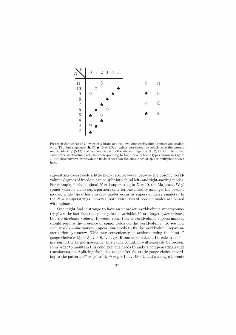
where P is a chirality projector that is required if the spinor coordinate θ isMajorana-Weyl, but is the unit matrix otherwise. Analysis36 of this constraintshows it to hold in the (D, p) spacetime/worldvolume dimensions shown in Fig-ure 6). The (D, p) cases in which (5.12) holds are also related to the existenceof “two-component notations” over the various division algebras R,C,H,O.Examples of this may be seen in the p = 1, D = 3, 4, 6, 10 superstring cases:in D = 3, the Lorentz group is SL(2,R), while in D = 4 it is SL(2,C) and inD = 6 it is SL(2,H); in D = 10, there is an analogous relation between theLorentz group and the quaternions O, although the non-associative nature ofthe quaternions makes this rather more cumbersome. Writing out the gammamatrix identity (5.12) in these cases using two-component notation makes itsproof relatively transparent, as a moment’s consideration of the D = 3 caseshows, keeping in mind that the dθα fermionic one-forms are commuting, whilethe SL(2,R) invariant tensor ǫαβ that would be needed to contract indices isantisymmetric. Similar considerations apply to the p = 0, superparticle cases.36

It should be noted that the superparticle and superstring cases allow for min-imal and also extended supersymmetries. This possibility arises because thereexist corresponding extended worldvolume multiplets constructed from spinorsand scalars alone.

An essential import of the κ symmetry for the super p-brane actions is thatit allows one to gauge away half of the spinor variables, allowing thus gaugechoices of the form θ = (S, 0). After this reduction by half in the numberof non-gauge fermion worldvolume fields, one can achieve a balance betweenthe worldvolume bosonic and fermionic degrees of freedom, as required bythe residual unbroken supersymmetry. The counting of degrees of freedom in

36

D

p

11

10

9

8

7

6

5

4

3

2

0 1 2 3 4 5

♦

♦

♦

♠

♠

♠

♠

♠

♠

♥

♥

♥

♥

♣

♣

♣

♦

♠

♥

♣

H

C

R

O

Figure 6: Sequences of k-invariant p-brane actions involving worldvolume spinors and scalarsonly. The four sequences ♣, ♥, ♠, ♦ of (D, p) values correspond to solutions to the gammamatrix identity (5.12) and are associated to the division algebras R, C, H, O. There alsoexist other worldvolume actions, corresponding to the different brane types shown in Figure7, but these involve worldvolume fields other than the simple scalar-spinor multiplets shownhere.

superstring cases needs a little more care, however, because the bosonic world-volume degrees of freedom can be split into chiral left- and right-moving modes.For example, in the minimal N = 1 superstring in D = 10, the Majorana-Weylspinor variable yields superpartners only for one chirality amongst the bosonicmodes, while the other chirality modes occur as supersymmetry singlets. Inthe N = 2 superstrings, however, both chiralities of bosonic modes are pairedwith spinors.

One might find it strange to have an unbroken worldvolume supersymme-try given the fact that the spinor p-brane variables θα are target-space spinors,but worldvolume scalars. It would seem that a worldvolume supersymmetryshould require the presence of spinor fields on the worldvolume. To see howsuch worldvolume spinors appear, one needs to fix the worldvolume reparam-eterization symmetry. This may conveniently be achieved using the “static”gauge choice xi(ξ) = ξi, i = 0, 1, . . . , p. If one now makes a Lorentz transfor-mation in the target spacetime, this gauge condition will generally be broken,so in order to maintain this condition one needs to make a compensating gaugetransformation. Splitting the index range after the static gauge choice accord-ing to the pattern xm = (xi, xm), m = p+1, . . . , D− 1, and making a Lorentz

37

transformation with parameters (Lij , Lim, L

mn), a combined Lorentz trans-

formation and worldvolume reparameterization (with parameter ηi(ξ)) on thexi variables takes the form

δxi = ηj(ξ)∂jXi + Lijx

j + Limxm . (5.13)

Demanding that δxi = 0 for xi = ξi requires the compensating reparameteri-zation to be given by ηi = −Lijξj−Limxm. Then the combined transformation

for the remaining bosonic variables xm is

δxm = −Lkjξj∂kxm + Lmnxn − Lknx

n∂kxm . (5.14)

This combined transformation remains linearly realized (i.e. “unbroken”) fora subgroup SO(p, 1)×SO(D−p− 1), but the remaining generators of SO(D−1, 1) become nonlinearly realized. The linearly realized SO(p, 1) becomes theworldvolume Lorentz group, according to which the xm transform as a set ofD − p − 1 scalars (although they transform as a vector with respect to theremaining SO(D − p − 1) factor, which is an “internal symmetry” from theworldvolume point of view). Now consider the effect of the linearly realizedSO(p, 1) on the θ(ξ) variables:

δθ = −Lijξj∂iθ + 14LijΓ

ijθ . (5.15)

The matrices Γij provide a spinor representation (in general reducible) of the“worldvolume” SO(p, 1) algebra, so that θ can now be identified, after gaugefixing, as a worldvolume spinor.35

Similar considerations apply to supersymmetry after κ symmetry fixing.Preserving the κ symmetry gauge requires a similar compensating κ symme-try transformation, causing some of the original target-space supersymmetryto become nonlinearly realized, but leaving still a linearly realized subgroup,which may be identified as the unbroken worldvolume supersymmetry. Forthe simple p-brane actions that we have been considering in this section, thefraction of unbroken supersymmetry is 1

2 . A classic example of a worldvolumesupermultiplet with respect to such a worldvolume supersymmetry is providedby the D = 11, p = 2 supermembrane: the xm, m = 3, . . . , 11 and the Sresidual spinor (32/2 = 16 components) form a worldvolume scalar-spinormultiplet with respect to the unbroken worldvolume supersymmetry. Thismultiplet contains 8 + 8 bosonic + fermionic degrees of freedom, transform-ing under 16 unbroken supercharges (it also has an unbroken SO(8) “internal”symmetry). The existence of such a large multiplet of scalars and spinors is aspecific feature of the unbroken d = 3, “N = 8” supersymmetry.

38

6 Kaluza-Klein dimensional reduction

Let us return now to the arena of purely bosonic field theories, and considerthe relations between various bosonic-sector theories and the correspondingrelations between p-brane solutions. It is well-known that supergravity theoriesare related by dimensional reduction from a small set of basic theories, thelargest of which being D = 11 supergravity. The spinor sectors of the theoriesare equally well related by dimensional reduction, but in the following, we shallrestrict our attention to the purely bosonic sector.

In order to set up the procedure, let us consider a theory in (D + 1)dimensions, but break up the metric in D-dimensionally covariant pieces:

ds2 = e2αϕds2 + e2βϕ(dz +AMdxM)2 (6.1)

where carets denote (D+1)-dimensional quantities corresponding to the (D+1)-dimensional coordinates xM = (xM , z); ds2 is the line element in D dimen-sions and α and β are constants. The scalar ϕ in D dimensions emerges fromthe metric in (D + 1) dimensions as (2β)−1 ln gzz. Adjustment of the con-stants α and β is necessary to obtain desired structures in D dimensions. Inparticular, one should pick β = −(D−2)α in order to arrange for the Einstein-frame form of the gravitational action in (D+ 1) dimensions to go over to theEinstein-frame form of the action in D dimensions.

The essential step in a Kaluza-Klein dimensional reduction is a consistenttruncation of the field variables, generally made by choosing them to be inde-pendent of the reduction coordinate z. By a consistent truncation, we alwaysunderstand a restriction on the variables that commutes with variation of theaction to produce the field equations, i.e. a restriction such that solutions tothe equations for the restricted variables are also solutions to the equations forthe unrestricted variables. This ensures that the lower-dimensional solutionswhich we shall obtain are also particular solutions to higher-dimensional su-pergravity equations as well. Making the parameter choice β = −(D − 2)α topreserve the Einstein-frame form of the action, one obtains

√−gR(g) = √−g

(R(g)−(D−1)(D−2)α2∇Mϕ∇Mϕ− 1

4e−2(D−1)αϕFMNFMN

)

(6.2)where F = dA. If one now chooses α2 = [2(D − 1)(D − 2)]−1, the ϕ kineticterm becomes conventionally normalized.

Next, one needs to establish the reduction ansatz for the (D + 1)-dimen-sional antisymmetric tensor gauge field F[n] = dA[n−1]. Clearly, among the

n − 1 antisymmetrized indices of A[n−1] at most one can take the value z, so

39

we have the decomposition

A[n−1] = B[n−1] +B[n−2] ∧ dz . (6.3)

All of these reduced fields are to be taken to be functionally independent of z.For the corresponding field strengths, first define

G[n] = dB[n−1] (6.4a)

G[n−1] = dB[n−2] . (6.4b)

However, these are not exactly the most convenient quantities to work with,since a certain “Chern-Simons” structure appears upon dimensional reduction.The metric in (D+1) dimensions couples to all fields, and, consequently, dimen-sional reduction will produce some terms with undifferentiated Kaluza-Kleinvector fields AM coupling to D-dimensional antisymmetric tensors. Accord-ingly, it is useful to introduce

G′[n] = G[n] −G[n−1] ∧ A , (6.5)

where the second term in (6.5) may be viewed as a Chern-Simons correctionfrom the reduced D-dimensional point of view.

At this stage, we are ready to perform the dimensional reduction of ourgeneral action (2.1). We find that

I =:

∫dD+1x

√−g[R(g)− 1

2∇Mφ∇Mφ− 1

2n!eaφF 2

[n]

](6.6)

reduces to

I =

∫dDx

√−g[R− 1

2∇Mφ∇Mφ− 12∇Mϕ∇Mϕ− 1

4e−2(D−1)αϕF2

[2]

− 1

2n!e−2(n−1)αϕ+αφG′2

[n] −1

2(n− 1)!e2(D−n)αϕ+aφG2

[n−1]

]. (6.7)

Although the dimensional reduction (6.7) has produced a somewhat compli-cated result, the important point to note is that each of the D-dimensionalantisymmetric-tensor field strength terms G′2

[n] and G2[n−1] has an exponential

prefactor of the form earφr , where the φr, r = (n, n − 1) are SO(2)-rotatedcombinations of ϕ and φ. Now, keeping just one while setting to zero the othertwo of the three gauge fields (A[1], B[n−2], Bn−1]), but retaining at the sametime the scalar-field combination appearing in the corresponding exponentialprefactor, is a consistent truncation. Thus, any one of the three field strengths

40

(F[2], G[n−1], G′[n]), retained alone together with its corresponding scalar-field

combination, can support p-brane solutions in D dimensions of the form thatwe have been discussing.

An important point to note here is that, in each of the earφ prefactors, thecoefficient ar satisfies

a2r = ∆− 2drdr(D − 2)

= ∆− 2(r − 1)(D − r − 1)

(D − 2)(6.8)

with the same value of ∆ as for the “parent” coupling parameter a, satisfying

a2r = ∆− 2d(n)d(n)

((D + 1)− 2)= ∆− 2(n− 1)(D − n)

(D − 1(6.9)

in D+1 dimensions. Thus, although the individual parameters ar are both D-and r-dependent, the quantity ∆ is preserved under Kaluza-Klein reduction forboth of the “descendant” field-strength couplings (to G′2

[n] or to G2[n−1]) coming

from the original term eaφF 2[n]. The 2-form field strength F[2] = dA, on the

other hand, emerges out of the gravitational action in D + 1 dimensions; itscoupling parameter corresponds to ∆ = 4.

If one retains in the reduced theory only one of the field strengths (F[2],G[n−1], G

′[n]), together with its corresponding scalar-field combination, then

one finds oneself back in the situation described by our general action (2.1), andthen the p brane solutions obtained for the general case in Sec. 2 immediatelybecome applicable. Moreover, since retaining only one field strength & scalarcombination in this way effects a consistent truncation of the theory, solutionsto this simple truncated system are also solutions to the untruncated theory,and indeed are also solutions to the original (D+ 1)-dimensional theory, sincethe Kaluza-Klein dimensional reduction is also a consistent truncation.

6.1 Multiple field-strength solutions and the single-charge truncation

After repeated single steps of Kaluza-Klein dimensional reduction fromD = 11down to D dimensions, the metric takes the form 31,32

ds211 = e23~a·

~φ ds2D +∑

i

e(23~a−~ai)·

~φ (hi)2 (6.10a)

hi = dzi +Ai[1] +Aij

[0] dzj , (6.10b)

where the AiMare a set of (11−D) Kaluza-Klein vectors generalizing the vector

AM in (6.1), emerging from the higher-dimensional metric upon dimensional

41

reduction. Once such Kaluza-Klein vectors have appeared, subsequent dimen-sional reduction also gives rise to the zero-form gauge potentials Aij

[0] appearing

in (6.10b) as a consequence of the usual one-step reduction (6.3) of a 1-formgauge potential.

We shall also need the corresponding reduction of the F[4] field strength i

(where hatted quantities refer to the original, higher, dimension) and, for laterreference, we shall also give the reduction of its Hodge dual ∗F[4]:

F[4] = F[4]+Fi[3]∧hi+ 1

2Fij[2]∧hi∧hj+ 1

6Fijk[1] ∧hi∧hj∧hk (6.11a)

∗F[4] = e~a·~φ ∗F[4]∧v+e~ai·

~φ ∗F i[3]∧vi+ 12e~aij ·~φ ∗F ij[2]∧v

ij+ 16e~aijk·~φ ∗F ijk[1] ∧vijk ,

(6.11b)

(noting that, since the Hodge dual is a metric-dependent construction, expo-

nentials of the dilatonic vectors ~φ appear in the reduction of ∗F[4]) where theforms v, vi, vij and vijk appearing in (6.11b) are given by

v = 1(11−D)!ǫi1···i11−D h

i1 ∧ · · · ∧ hi11−D

vi = 1(10−D)!ǫii2···i11−D h

i2 ∧ · · · ∧ hi11−D

vij = 1(9−D)!ǫiji3···i11−D h

i3 ∧ · · · ∧ hi11−D

vijk = 1(8−D)!ǫijki4 ···i11−D h

i4 ∧ · · · ∧ hi11−D . (6.12)

Using (6.10, 6.11a), the bosonic sector of maximal supergravity (1.1) nowreduces to 31,32

ID =

∫dDx

√−g[R− 1

2 (∂~φ)2 − 1

48e~a·~φF 2

[4] − 112

∑

i

e~ai·~φ(F i[3])

2

− 14

∑

i<j

e~aij ·~φ(F ij[2])

2 − 14

∑

i

e~bi·φ(F i

[2])2 (6.13)

− 12

∑

i<j<k

e~aijk·~φ(F ijk[1] )

2 − 12

∑

ij

e~bij ·φ(F ij

[1])2]+ LFFA ,

where i, j = 1, . . . , 11−D, and field strengths with multiple i, j indices may betaken to be antisymmetric in those indices since these “internal” indices arisein the stepwise reduction procedure, and two equal index values never occurin a multi-index sum. From (6.11), one sees that the “straight-backed” field

iNote that the lower-dimensional field strengths F[n] include “Chern-Simons” corrections

similar to those in (6.5).

42

strengths F[4], Fi[3], F

ij[2] and F ijk[1] are descendants from F[4] in D = 11. The

“calligraphic” field strengths F i[2], on the other hand, are the field strengths for

the Kaluza-Klein vectors AiM appearing in (6.10b). Similarly, one also has a set

of 1-form field strengths F ij[1] for the Kaluza-Klein zero-form gauge potentials

Aij[0] appearing in (6.10b).

The nonlinearity of the original D = 11 action (1.1) in the metric ten-sor produces a consequent nonlinearity in the (11 −D) dilatonic scalar fields~φ appearing in the exponential prefactors of the antisymmetric-tensor kineticterms in (6.13). For each field-strength kinetic term in (6.13), there is a cor-responding “dilaton vector” of coefficients determining the linear combinationof the dilatonic scalars appearing in its exponential prefactor. For the 4-, 3-,2- and 1-form “straight-backed” field strengths emerging from F[4] in D = 11,these coefficients are denoted correspondingly ~a, ~ai, ~aij and ~aijk; for the “cal-ligraphic” field strengths corresponding to Kaluza-Klein vectors and zero-formgauge potentials emerging out of the metric, these are denoted~bi and~bij . How-ever, not all of these dilaton vectors are independent; in fact, they may all beexpressed in terms of the 4-form and 3-form dilaton vectors ~a and ~aij :

31,32

~aij = ~ai + ~aj − ~a bi = −~ai + ~a

~aijk = ~ai + ~aj + ~ak − 2~a ~bij = −~ai + ~aj .(6.14)

Another important feature of the dilaton vectors is that they satisfy the fol-lowing dot-product relations:

~a · ~a =2(11−D)

D − 2

~a · ~ai =2(8−D)

D − 2(6.15)

~ai · ~aj = 2δij +2(6−D)

D − 2.

Throughout this discussion, we have emphasized consistent truncations inmaking simplifying restrictions of complicated systems of equations, so thatthe solutions of a simplified system are nonetheless perfectly valid solutionsof the more complicated untruncated system. With the equations of motionfollowing from (6.13) we face a complicated system that calls for analysis insimplified subsectors. Accordingly, we now seek a consistent truncation downto a simplified system of the form (2.1), retaining just one dilatonic scalarcombination φ and one rank-n field strength combination F[n] constructed outof a certain number N of “retained” field strengths Fα [n], α = 1, . . . , N , (this

43

could possibly be a straight-backed/calligraphic mixture) selected from thoseappearing in (6.13), with all the rest being set to zero.32 Thus, we let

~φ = ~nφ+ ~φ⊥ , (6.16)

where ~n · ~φ⊥ = 0; in the truncation we then seek to set consistently ~φ⊥ = 0.We shall see that consistency for the retained field strengths Fα [n] requires

them all to be proportional.32 We shall let the dot product matrix for thedilaton vectors of the retained field strengths be denoted Mαβ =: ~aα · ~aβ .Consistency of the truncation requires that the φ⊥ field equation be satisfied:

~φ⊥ −∑

α

Π⊥ · ~aα(Fα [n])2 = 0 , (6.17)

where Π⊥ is the projector into the dilaton-vector subspace orthogonal to theretained dilaton direction ~n. Setting ~φ⊥ = 0 in (6.17) and letting the retainedFα [n] be proportional, one sees that achieving consistency is hopeless unless

all the e~aα·~φ prefactors are the same, thus requiring

~aα · ~n = a ∀α = 1, . . . , N , (6.18)

where the constant a will play the role of the dilatonic scalar coefficient in thereduced system (2.1). Given a set of dilaton vectors for retained field strengths

satisfying (6.18), consistency of (6.17) with the imposition of ~φ⊥ = 0 requires

Π⊥ ·∑

α

~aα(Fα [n])2 = 0 . (6.19)

This equation requires, for every point xM in spacetime, that the combination∑α ~aα(Fα [n])

2 be parallel to ~n in the dilaton-vector space. Combining thiswith the requirement (6.18), one has

∑

α

~aα(Fα [n])2 = a~n

∑

α

(Fα [n])2 . (6.20)

Taking then a dot product of this with ~aβ, one has∑

α

Mβα(Fα [n])2 = a2

∑

α

(Fα [n])2 . (6.21)

Detailed analysis 32 shows it to be sufficient to consider the cases where Mαβ

is invertible, so by applying M−1αβ to (6.21), one finds

(Fα [n])2 = a2

∑

β

M−1αβ

∑

γ

(Fγ [n])2 , (6.22)

44

and, indeed, we find that the Fα [n] must all be proportional. Summing on α,one has

a2 = (∑

α,β

M−1αβ )

−1 ; (6.23)

one then defines the retained field-strength combination F[n] so that

(Fα [n])2 = a2

∑

β

M−1αβ (F[n])

2 . (6.24)

The only remaining requirement for consistency of the truncation down tothe simplified (gMN , φ, F[n]) system (2.1) arises from the necessity to ensurethat the variation of the LFFA term in (6.13) is not inconsistent with settingto zero the discarded dilatonic scalars and gauge potentials. In general, thisimposes a somewhat complicated requirement. In the present review, however,we shall concentrate mainly on either purely-electric cases satisfying the ele-mentary ansatz (2.4) or purely-magnetic cases satisfying the solitonic ansatz(2.6). As one can see by inspection, for pure electric or magnetic solutionsof these sorts, the terms that are dangerous for consistency arising from thevariation of LFFA all vanish. Thus, for such solutions one may safely ignorethe complications of the LFFA term. This restriction to pure electric or mag-netic solutions does, however, leave out the very interesting cases of dyonicsolutions that exist in D = 8 and D = 4, upon which we shall comment lateron in Section 8.

After truncating down to the system (2.1), the analysis proceeds as inSection 2. It turns out 32 that supersymmetric p-brane solutions arise whenthe matrix Mαβ for the retained Fα [n] satisfies

Mαβ = 4δαβ − 2dd

D − 2, (6.25)

and the corresponding ∆ value for F[n] is

∆ =4

N, (6.26)

where we recall that N is the number of retained field strengths. A gener-alization of this analysis leads to a classification of solutions with more thanone independent retained scalar-field combination.32 We shall see in Section 7that the N > 1 solutions to single-charge truncated systems (2.1) may alsobe interpreted as special solutions of the full reduced action (6.13) containingN constituent ∆ = 4 brane components that just happen to have coincidentcharge centers. Consequently, one may consider only the N = 1, ∆ = 4 solu-tions to be fundamental.

45

6.2 Diagonal dimensional reduction of p-branes

The family of p-brane solutions is ideally suited to interpretation as solutionsof Kaluza-Klein reduced theories, because they are naturally independent ofthe “worldvolume” xµ coordinates. Accordingly, one may let the reductioncoordinate z be one of the xµ. Consequently, the only thing that needs to bedone to such a solution in order to reinterpret it as a solution of a reducedsystem (6.7) is to perform a Weyl rescaling on it in order to be in accordancewith the form of the metric chosen in the Kaluza-Klein ansatz (6.10), whichwas adjusted so as to maintain the Einstein-frame form of the gravitationalterm in the dimensionally reduced action.

Upon making such a reinterpretation, elementary/solitonic p-branes in(D+1) dimensions give rise to elementary/solitonic (p−1)-branes in D dimen-sions, corresponding to the same value of ∆, as one can see from (6.8, 6.9). Notethat in this process, the quantity d is conserved, since both D and d reduce byone. Reinterpretation of p brane solutions in this way, corresponding to stan-dard Kaluza-Klein reduction on a worldvolume coordinate, proceeds diagonallyon a D versus d plot, and hence is referred to as diagonal dimensional reduc-tion. This procedure is the analogue, for supergravity field-theory solutions,of the procedure of double dimensional reduction 22 for p-brane worldvolumeactions, which can be taken to constitute the δ-function sources for singularp-brane solutions, coupled in to resolve the singularities, as we discussed insubsection 4.1.

6.3 Multi-center solutions and vertical dimensional reduction

As we have seen, translational Killing symmetries of p-brane solutions allow asimultaneous interpretation of these field configurations as solutions belongingto several different supergravity theories, related one to another by Kaluza-Klein dimensional reduction. For the original single p-brane solutions (2.24),the only available translational Killing symmetries are those in the worldvol-ume directions, which we have exploited in describing diagonal dimensionalreduction above. One may, however, generalize the basic solutions (2.24) byreplacing the harmonic function H(y) in (2.21) by a different solution of theLaplace equation (2.20). Thus, one can easily extend the family of p-branesolutions to multi-center p-brane solutions by taking the harmonic function tobe

H(y) = 1 +∑

α

kα

|~y − ~yα|dkα > 0 . (6.27)

46

Once again, the integration constant has been adjusted to make H |∞= 1 ↔

φ|∞= 0. The generalized solution (6.27) corresponds to parallel and similarly-

oriented p-branes, with all charge parameters λα = 2dkα/√∆ required to be

positive in order to avoid naked singularities. The “centers” of the individual“leaves” of this solution are at the points y = yα, where α ranges over anynumber of centers. The metric and the electric-case antisymmetric tensorgauge potential corresponding to (6.27) are given again in terms of H(y) by(2.24a,2.25). In the solitonic case, the ansatz (2.6) needs to be modified so asto accommodate the multi-center form of the solution:

Fm1...mn = −d−1ǫm1...mnp∂p∑

α

λα

|~y − ~yα|d, (6.28)

which ensures the validity of the Bianchi identity just as well as (2.6) does.The mass/(unit p-volume) density is now

E =2ΩD−d−1√

∆

∑

α

λα , (6.29)

while the total electric or magnetic charge is given by ΩD−d−1

∑λα, so the

Bogomol’ny bounds (4.16) are saturated just as they are for the single-centersolutions (2.24). Since the multi-center solutions given by (6.27) satisfy thesame supersymmetry-preservation conditions on the metric and antisymmetrictensor as (2.24), the multi-center solutions leave the same amount of super-symmetry unbroken as the single-center solution.

From a mathematical point of view, the multi-center solutions (6.27) existowing to the properties of the Laplace equation (2.20). From a physical pointof view, however, these static solutions exist as a result of cancellation betweenattractive gravitational and scalar-field forces against repulsive antisymmetric-tensor forces for the similarly-oriented p-brane “leaves.”

The multi-center solutions given by (6.27) can now be used to preparesolutions adapted to dimensional reduction in the transverse directions. Thiscombination of a modification of the solution followed by dimensional reductionon a transverse coordinate is called vertical dimensional reduction23 because itrelates solutions vertically on a D versus d plot.j In order to do this, we needfirst to develop translation invariance in the transverse reduction coordinate.This can be done by “stacking” up identical p branes using (6.27) in a periodicarray, i.e. by letting the integration constants kα all be equal, and aligning the

jSimilar procedures have been considered in a number of articles in the literature; see, e.g.Refs.37

47

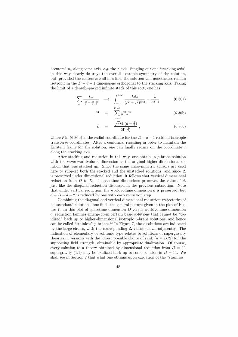
“centers” yα along some axis, e.g. the z axis. Singling out one “stacking axis”in this way clearly destroys the overall isotropic symmetry of the solution,but, provided the centers are all in a line, the solution will nonetheless remainisotropic in the D − d− 1 dimensions orthogonal to the stacking axis. Takingthe limit of a densely-packed infinite stack of this sort, one has

∑

α

kα

|~y − ~yα|d−→

∫ +∞

−∞

kdz

(r2 + z2)d/2=

k

rd−1(6.30a)

r2 =

D−2∑

m=d

ymym (6.30b)

k =

√πkΓ(d− 1

2 )

2Γ(d), (6.30c)

where r in (6.30b) is the radial coordinate for the D− d− 1 residual isotropictransverse coordinates. After a conformal rescaling in order to maintain theEinstein frame for the solution, one can finally reduce on the coordinate zalong the stacking axis.

After stacking and reduction in this way, one obtains a p-brane solutionwith the same worldvolume dimension as the original higher-dimensional so-lution that was stacked up. Since the same antisymmetric tensors are usedhere to support both the stacked and the unstacked solutions, and since ∆is preserved under dimensional reduction, it follows that vertical dimensionalreduction from D to D − 1 spacetime dimensions preserves the value of ∆just like the diagonal reduction discussed in the previous subsection. Notethat under vertical reduction, the worldvolume dimension d is preserved, butd = D − d− 2 is reduced by one with each reduction step.

Combining the diagonal and vertical dimensional reduction trajectories of“descendant” solutions, one finds the general picture given in the plot of Fig-ure 7. In this plot of spacetime dimension D versus worldvolume dimensiond, reduction families emerge from certain basic solutions that cannot be “ox-idized” back up to higher-dimensional isotropic p-brane solutions, and hencecan be called “stainless” p-branes.13 In Figure 7, these solutions are indicatedby the large circles, with the corresponding ∆ values shown adjacently. Theindication of elementary or solitonic type relates to solutions of supergravitytheories in versions with the lowest possible choice of rank (n ≤ D/2) for thesupporting field strength, obtainable by appropriate dualization. Of course,every solution to a theory obtained by dimensional reduction from D = 11supergravity (1.1) may be oxidized back up to some solution in D = 11. Weshall see in Section 7 that what one obtains upon oxidation of the “stainless”

48

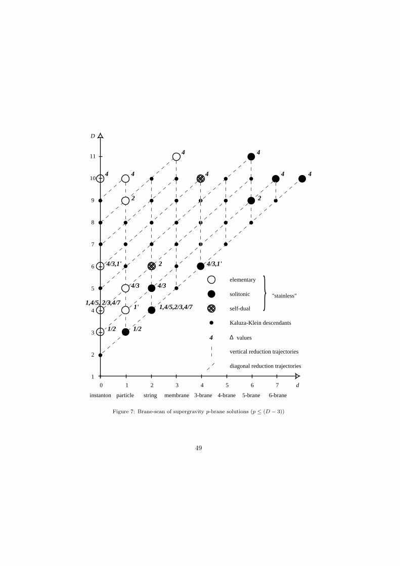
1

2

3

4

5

6

7

8

9

10

11

D

d1 2 3 4 5 6 70

particle string membrane 3-brane 4-brane 5-brane 6-braneinstanton

4 4 4 4 4

44

2 2

4/3,1' 4/3,1'2

4/3 4/3

1,4/5,2/3,4/71,4/5, 2/3,4/7

1'

1/2 1/2

elementary

solitonic

Kaluza-Klein descendants

4 ∆ values

self-dual

vertical reduction trajectories

diagonal reduction trajectories

"stainless"

Figure 7: Brane-scan of supergravity p-brane solutions (p ≤ (D − 3))

49

solutions in Figure 7 falls into the interesting class of “intersecting branes”built from four basic “elemental” solutions of D = 11 supergravity.

6.4 The geometry of (D − 3)-branes

The process of vertical dimensional reduction described in the previous sub-section proceeds uneventfully until one makes the reduction from a (D, d =D − 3) solution to a (D − 1, d = D − 3) solution.k In this step, the integral(6.30) contains an additive divergence and needs to be renormalized. Thisis easily handled by putting finite limits ±L on the integral, which becomes∫ L−L dz(r

2 + z2)−1/2, and then by subtracting a divergent term 2 lnL beforetaking the limit L → ∞. Then the integral gives the expected ln r harmonicfunction appropriate to two transverse dimensions.

Before proceeding any further with vertical dimensional reduction, let usconsider some of the specific properties of (D − 3)-branes that make the nextvertical step down problematic. Firstly, the asymptotic metric of a (D − 3)-brane is not a globally flat space, but only a locally flat space. This distinctionmeans that there is in general a deficit solid angle at transverse infinity, whichis related to the total mass density of the (D − 3)-brane.38 This means thatany attempt to stack up (D− 3)-branes within a standard supergravity theorywill soon consume the entire solid angle at transverse infinity, thus destroyingthe asymptotic spacetime in the construction.

In order to understand the global structure of the (D− 3)-branes in somemore detail, consider the supersymmetric string in D = 4 dimensions.12 InD = 4, one may dualize the 2-form Aµν field to a pseudoscalar, or axion,field χ, so such strings are also solutions to dilaton-axion gravity. The p-braneansatz gives a spacetime of the form M4 = M2 × Σ2, where M2 is D = 2Minkowski space. Supporting this string solution, one has the 2-form gaugefield Aµν and the dilaton φ. These fields give rise to a field stress tensor of theform

Tµν(A, φ) = − 116 (a

2 + 4)∂mK∂mKηµν

Tmn(A, φ) = 18 (a

2 − 4)(∂mK∂nK − 12δmn(∂pK∂pK)) , (6.31)

where a is as usual the dilaton coupling parameter and e−K = H = 1 −8GT ln(r), with r =

√ymym, m = 2, 3. If one now puts in an elementary

string source action, with the string aligned along the µ, ν = 0, 1 subspace, so

kSolutions with worldvolume dimension two less than the spacetime dimension will be re-ferred to generally as (D − 3)-branes, irrespective of whether the spacetime dimension is Dor not.

50

that Tmn (source) = 0, then one has the source stress tensor

Tµν (source) =−T√−g

∫d2ξ

√−γγij∂iXµ∂jXνe− 1

2aφδ(x−X) . (6.32)

By inspection of the field solution, one has Tmn(A, φ) = 0, while the contri-butions to Tµν from the Aµν and φ fields and also from the source (6.32) areboth of the form diag(ρ,−ρ). Thus, the overall stress tensor is of the formTMN = diag(ρ,−ρ, 0, 0).

Consequently, the Einstein equation in the transversem, n indices becomesRmn − 1

2gmnR = 0, since the transverse stress tensor components vanish.This equation is naturally satisfied for a metric satisfying the p-brane ansatz,because, as one can see from (2.11) with d = A′ = 0, this causes the transversecomponents of the Ricci tensor to be equal to the Ricci tensor of a D = 2spacetime, for which Rmn − 1

2gmnR ≡ 0 is an identity, corresponding to thefact that the usual Einstein action,

√−gR, is a topological invariant in D = 2.Accordingly, in the transverse directions, the equations are satisfied simply byby 0 = 0.

In the world-sheet directions, the equations become

− 12Rηµν = −8πGρηµν , (6.33)

or justR = 16πGρ , (6.34)

and as we have already noted, R = Rmm. Owing to the fact that the D = 2Weyl tensor vanishes, the transverse space Σ2 is conformally flat; Eq. (6.34)gives its conformal factor. Thus, although there is no sensible Einstein action inthe transverse D = 2, space, a usual form of the Einstein equation nonethelessapplies to that space as a result of the symmetries of the p-brane ansatz.

The above supersymmetric string solution may be compared to the cosmicstrings arising in gauge theories with spontaneous symmetry breaking. There,the Higgs fields contributing to the energy density of the string are displacedfrom their usual vacuum values to unbroken-symmetry configurations at astationary point of the Higgs potential, within a very small transverse-spaceregion that may be considered to be the string “core.” Approximating thisby a delta function in the transverse space, the Ricci tensor and hence thefull curvature vanish outside the string core, so that one obtains a conicalspacetime, which is flat except at the location of the string core. The totalenergy is given by the deficit angle 8πGT of the conical spacetime. In contrast,the supersymmetric string has a field stress tensor Tµν(A, φ) which is not justconcentrated at the string core but instead is smeared out over spacetime.

51

The difference arises from the absence of a potential for the fields Aµν , φsupporting the solution in the supersymmetric case. Nonetheless, as one cansee from the behavior of the stress tensor Tmn in Eq. (6.31), the transversespace Σ2 is asymptotically locally flat (ALF), with a total energy density givenby the overall deficit angle measured at infinity. For multiple-centered stringsolutions, one has

H = 1−∑

i

8GTi ln |~y − ~yi| . (6.35)

Consequently, when considered within the original supergravity theory, the in-definite stacking of supersymmetric strings leads to a destruction of the trans-verse asymptotic space.

A second problem with any attempt to produce (D − 2)-branes in ordi-nary supergravity theories is simply stated: starting from the p-brane ansatz(2.3, 2.6) and searching for (D − 2) branes in ordinary massless supergravitytheories, one simply doesn’t find any such solutions.

6.5 Beyond the (D−3)-brane barrier: Scherk-Schwarz reduction and domainwalls

Faced with the above puzzles about what sort of (D − 2)-brane could resultby vertical reduction from a (D− 3)-brane, one can simply decide to be brave,and to just proceed anyway with the established mathematical procedure ofvertical dimensional reduction and see what one gets. In the next step of ver-tical dimensional reduction, one again encounters an additive divergence: the

integral∫ L−L dz ln(y

2+z2) needs to be renormalized by subtracting a divergentterm 4L(lnL − 1). Upon subsequently performing the integral, the harmonicfunction H(y) becomes linear in the one remaining transverse coordinate.

While the mathematical procedure of vertical dimensional reduction so asto produce some sort of (D − 2)-brane proceeds apparently without seriouscomplication, an analysis of the physics of the situation needs some care.39

Consider the reduction from a (D, d = D − 2) solution (a p = (D − 3) brane)to a (D − 1, d = D − 3) solution (a p = (D − 2) brane). Note that both the(D− 3) brane and its descendant (D− 2)-brane have harmonic functions H(y)that blow up at infinity. For the (D − 3)-brane, however this is not in itselfparticularly remarkable, because, as one can see by inspection of (2.24) for thiscase, the metric asymptotically tends to a locally flat space as r → ∞, andalso in this limit the antisymmetric-tensor one-form field strength

Fm = −ǫmn∂nH (6.36)

52

tends asymptotically to zero, while the dilatonic scalar φ tends to its modulusvalue φ∞ (set to zero for simplicity in (2.24)). The expression (6.36) for the fieldstrength, however, shows that the next reduction step down to the (D− 1, d =D− 2) solution has a significant new feature: upon stacking up (D− 3) branesprior to the vertical reduction, thus producing a linear harmonic function inthe transverse coordinate y,

H(y) = const. +my , (6.37)

the field strength (6.36) acquires a constant component along the stacking axis↔ reduction direction z,

Fz = −ǫzy∂yH = m , (6.38)

which implies an unavoidable dependence l of the corresponding zero-formgauge potential on the reduction coordinate:

A[0](x, y, z) = mz + χ(x, y) . (6.39)

From a Kaluza-Klein point of view, the unavoidable linear dependenceof a gauge potential on the reduction coordinate given in (6.39) appears tobe problematic. Throughout this review, we have dealt only with consistentKaluza-Klein reductions, for which solutions of the reduced theory are alsosolutions of the unreduced theory. Generally, retaining any dependence on areduction coordinate will lead to an inconsistent truncation of the theory: at-tempting to impose a z dependence of the form given in (6.39) prior to varyingthe Lagrangian will give a result different from that obtained by imposing thisdependence in the field equations after variation.

The resolution of this difficulty is that in performing a Kaluza-Klein re-duction with an ansatz like (6.39), one ends up outside the standard set ofmassless supergravity theories. In order to understand this, let us again focuson the problem of consistency of the Kaluza-Klein reduction. As we have seen,consistency of any restriction means that the restriction may either be imposedon the field variables in the original action prior to variation so as to derivethe equations of motion, or instead may be imposed on the field variables inthe equations of motion after variation, with an equal effect. In this case, so-lutions obeying the restriction will also be solutions of the general unrestrictedequations of motion.

lNote that this vertical reduction from a (D − 3)-brane to a (D − 2)-brane is the first casein which one is forced to accept a dependence on the reduction coordinate z; in all higher-dimensional vertical reductions, such z dependence can be removed by a gauge transforma-tion. The zero-form gauge potential in (6.39) does not have the needed gauge symmetry,however.

53

The most usual guarantee of consistency in Kaluza-Klein dimensional re-duction is obtained by restricting the field variables to carry zero charge withrespect to some conserved current, e.g. momentum in the reduction dimen-sion. But this is not the only way in which consistency may be achieved. Inthe present case, retaining a linear dependence on the reduction coordinate asin (6.39) would clearly produce an inconsistent truncation if the reduction co-ordinate were to appear explicitly in any of the field equations. But this doesnot imply that a truncation is necessarily inconsistent just because a gauge po-tential contains a term linear in the reduction coordinate. Inconsistency of aKaluza-Klein truncation occurs when the original, unrestricted, field equationsimply a condition that is inconsistent with the reduction ansatz. If a particulargauge potential appears in the action only through its derivative, i.e. throughits field strength, then a consistent truncation may be achieved provided thatthe restriction on the gauge potential implies that the field strength is inde-pendent of the reduction coordinate. A zero-form gauge potential on whichsuch a reduction may be carried out, occurring in the action only through itsderivative, will be referred to as an axion.

Requiring axionic field strengths to be independent of the reduction coor-dinate amounts to extending the Kaluza-Klein reduction framework so as toallow for linear dependence of an axionic zero-form potential on the reductioncoordinate, precisely of the form occurring in (6.39). So, provided A[0] is an ax-ion, the reduction (6.39) turns out to be consistent after all. This extension ofthe Kaluza-Klein ansatz is in fact an instance of Scherk-Schwarz reduction.40,41

The basic idea of Scherk-Schwarz reduction is to use an Abelian rigid symme-try of a system of equations in order to generalize the reduction ansatz byallowing a linear dependence on the reduction coordinate in the parameterof this Abelian symmetry. Consistency is guaranteed by cancellations orches-trated by the Abelian symmetry in field-equation terms where the parameterdoes not get differentiated. When it does get differentiated, it contributes onlya term that is itself independent of the reduction coordinate. In the presentcase, the Abelian symmetry guaranteeing consistency of (6.39) is a simple shiftsymmetry A[0] → A[0] + const.

Unlike the original implementation of the Scherk-Schwarz reduction idea,40

which used an Abelian U(1) phase symmetry acting on spinors, the Abelianshift symmetry used here commutes with supersymmetry, and hence the reduc-tion does not spontaneously break supersymmetry. Instead, gauge symmetriesfor some of the antisymmetric tensors will be broken, with a correspondingappearance of mass terms. As with all examples of vertical dimensional re-duction, the ∆ value corresponding to a given field strength is also preserved.Thus, p-brane solutions related by vertical dimensional reduction, even in the

54

enlarged Scherk-Schwarz sense, preserve the same amount of unbroken super-symmetry and have the same value of ∆.

It may be necessary to make several redefinitions and integrations by partsin order to reveal the axionic property of a given zero-form, and thus to pre-pare the theory for a reduction like (6.39). This is most easily explained by anexample, so let us consider the first possible Scherk-Schwarz reductionm in thesequence of theories descending from (1.1), starting in D = 9 where the firstaxion field appears.39 The Lagrangian for massless D = 9 maximal supergrav-ity is obtained by specializing the general dimensionally-reduced action (6.13)given in Section 2 to this case:

L9 =√−g

[R− 1

2 (∂φ1)2− 1

2 (∂φ2)2− 1

2e−3

2φ1+√

72 φ2(∂χ)2− 1

48e~a·~φ(F[4])

2

− 12e~a1·~φ(F (1)

[3] )2− 1

2e~a2·~φ(F (2)

[3] )2− 1

4e~a12·~φ(F (12)

[2] )2− 14e~b1·~φ(F (1)

[2] )2

− 14e~b2·~φ(F (2)

[2] )2]− 1

2 F[4]∧ F[4]∧A(12)[1] − F (1)

[3] ∧ F(2)[3] ∧A[3] , (6.40)

where χ = A(12)[0] and ~φ = (φ1, φ2).

Within the scalar sector (~φ, χ) of (6.40), the dilaton coupling has beenmade explicit; in the rest of the Lagrangian, the dilaton vectors have the generalstructure given in (6.14, 6.15). The scalar sector of (6.40) forms a nonlinear σ-model for the manifold GL(2,R)/SO(2). This already makes it appear that onemay identify χ as an axion available for Scherk-Schwarz reduction. However,account must still be taken of the Chern-Simons structure lurking inside thefield strengths in (6.11, 6.40). In detail, the field strengths are given by

F[4] = F[4] − F(1)[3] ∧ A(1)

[1] − F(2)[3] ∧ A(2)

[1]

+χF(1)[3] ∧ A(2)

[1] − F(12)[2] ∧ A(1)

[1] ∧ A(2)[1] (6.41a)

F(1)[3] = F

(1)[3] − F

(12)[2] ∧ A(2)

[1] (6.41b)

F(2)[3] = F

(2)[3] + F

(12)[2] ∧ A(1)

[1] − χF(1)[3] (6.41c)

F(12)[2] = F

(12)[2] F (1)

[2] = F (1)[2] − dχ ∧ A(2)

[1] (6.41d)

F (2)[2] = F (2)

[2] F (12)[1] = dχ , (6.41e)

where the field strengths carrying tildes are the naıve expressions withoutChern-Simons corrections, i.e. Fn] = dA[n−1]. Now the appearance of undiffer-

mA higher-dimensional Scherk-Schwarz reduction is possible 41 starting from type IIB su-pergravity in D = 10, using the axion appearing in the SL(2,R)/SO(2) scalar sector of thattheory.

55

entiated χ factors in (6.41a,c) makes it appear that a Scherk-Schwarz reductionwould be inconsistent. However, one may eliminate these undifferentiated fac-tors by making the field redefinition

A(2)[2] −→ A

(2)[2] + χA

(1)[2] , (6.42)

after which the field strengths (6.41a,c) become

F[4] = F[4] − F(1)[3] ∧ A(1)

[1] − F(2)[3] ∧ A(2)

[1]

−dχ ∧ A(1)[2] ∧A(2)

[1] − F(12)[2] ∧ A(1)

[1] ∧A(2)[1] (6.43a)

F(2)[3] = F

(2)[3] + F

(12)[2] ∧ A(1)

[1] + dχ ∧ A(1)[2] , (6.43c)

the rest of (6.41) remaining unchanged.

After the field redefinitions (6.42), the axion field χ = A(12)[0] is now ready

for application of the Scherk-Schwarz reduction ansatz (6.39). The coefficientof the term linear in the reduction coordinate z has been denoted m because itcarries the dimensions of mass, and correspondingly its effect on the reducedaction is to cause the appearance of mass terms. Applying (6.39) to the D = 9Lagrangian, one obtains a D = 8 reduced Lagrangiann

L8 ss =√−g

[R− 1

2 (∂φ1)2 − 1

2 (∂φ2)2 − 1

2 (∂φ3)2

− 12e~b12·~φ(∂χ−mA(3)

[1] )2 − 1

2e~b13·~φ(∂A(13)

[0] − ∂χA(23)[0] +mA(2)

[1] )2

− 12e~b23·~φ(∂A(23)

[0] )2 − 12e~a123·~φ(∂A(123)

[0] )2

− 148e

~a·~φ(F[4] −mA(1)[2] ∧A(2)

[1] ∧ A(3)[1] )

2 − 112e

~a1·~φ(F (1)[3] )

2

− 112e

~a2·~φ(F (2)[3] −mA

(1)[2] ∧ A(3)

[1] )2 − 1

12e~a3·~φ(F (3)

[3] +mA(1)[2] ∧A(2)

[1] )2

− 14e~a12·~φ(F (12)

[2] )2 − 14e~a13·~φ(F (13)

[2] )2 − 14e~a23·~φ(F (23)

[2] +mA(1)[2] )

2

− 14e~b1·~φ(F (1)

[2] −mA(2)[1] ∧ A(3)

[1] )2 − 1

4e~b2·~φ(F (2)

[2] )2 − 1

4e~b3·~φ(F (3)

[2] )2

− 12m

2e~b123·~φ

]+mF

(1)[3] ∧ A(1)

[2] ∧ A[3] + LFFA , (6.44)

where the dilaton vectors are now those appropriate for D = 8; the term LFFAcontains only m-independent terms.

nI am grateful to Marcus Bremer for help in correcting some errors in the original expressionof Eq. (6.44) given in Ref.39

56

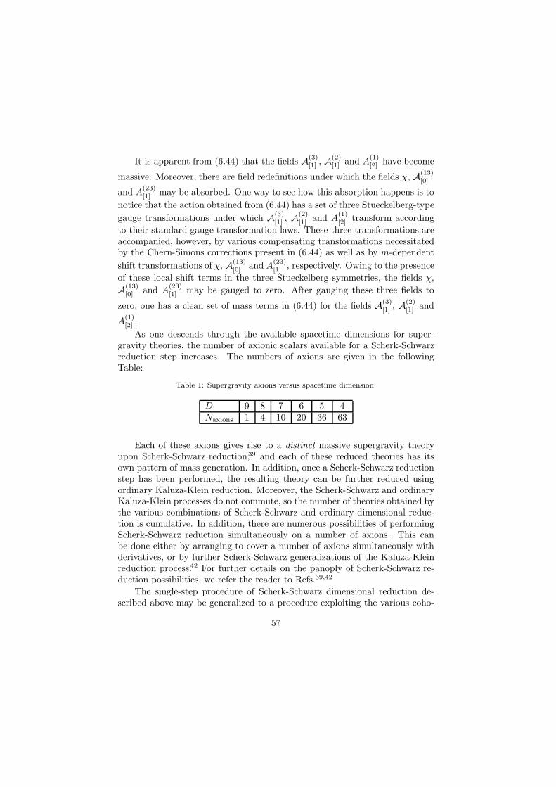
It is apparent from (6.44) that the fields A(3)[1] , A

(2)[1] and A

(1)[2] have become

massive. Moreover, there are field redefinitions under which the fields χ, A(13)[0]

and A(23)[1] may be absorbed. One way to see how this absorption happens is to

notice that the action obtained from (6.44) has a set of three Stueckelberg-type

gauge transformations under which A(3)[1] , A

(2)[1] and A

(1)[2] transform according

to their standard gauge transformation laws. These three transformations areaccompanied, however, by various compensating transformations necessitatedby the Chern-Simons corrections present in (6.44) as well as by m-dependent

shift transformations of χ, A(13)[0] and A

(23)[1] , respectively. Owing to the presence

of these local shift terms in the three Stueckelberg symmetries, the fields χ,

A(13)[0] and A

(23)[1] may be gauged to zero. After gauging these three fields to

zero, one has a clean set of mass terms in (6.44) for the fields A(3)[1] , A

(2)[1] and

A(1)[2] .

As one descends through the available spacetime dimensions for super-gravity theories, the number of axionic scalars available for a Scherk-Schwarzreduction step increases. The numbers of axions are given in the followingTable:

Table 1: Supergravity axions versus spacetime dimension.

D 9 8 7 6 5 4Naxions 1 4 10 20 36 63

Each of these axions gives rise to a distinct massive supergravity theoryupon Scherk-Schwarz reduction,39 and each of these reduced theories has itsown pattern of mass generation. In addition, once a Scherk-Schwarz reductionstep has been performed, the resulting theory can be further reduced usingordinary Kaluza-Klein reduction. Moreover, the Scherk-Schwarz and ordinaryKaluza-Klein processes do not commute, so the number of theories obtained bythe various combinations of Scherk-Schwarz and ordinary dimensional reduc-tion is cumulative. In addition, there are numerous possibilities of performingScherk-Schwarz reduction simultaneously on a number of axions. This canbe done either by arranging to cover a number of axions simultaneously withderivatives, or by further Scherk-Schwarz generalizations of the Kaluza-Kleinreduction process.42 For further details on the panoply of Scherk-Schwarz re-duction possibilities, we refer the reader to Refs.39,42

The single-step procedure of Scherk-Schwarz dimensional reduction de-scribed above may be generalized to a procedure exploiting the various coho-

57

mology classes of a multi-dimensional compactification manifold.43 The key tothis link between the Scherk-Schwarz generalized dimensional reduction andthe topology of the internal Kaluza-Klein manifold K is to recognize that thesingle-step reduction ansatz (6.39) may be generalized to

A[n−1](x, y, z) = ω[n−1] +A[n−1](x, y) , (6.45)

where ω[n−1] is an (n− 1) form defined locally on K, whose exterior derivativeΩ[n] = dω[n−1] is an element of the cohomology class Hn(K,R). For example,in the case of a single-step generalized reduction on a circle S1, one has Ω[1] =mdz ∈ H1(S1,R), reproducing our earlier single-step reduction (6.39).

As another example, consider a generalized reduction on a 4-torus T 4

starting in D = 11, setting A[3](x, y, z) = ω[3] + A[3](x, y) with Ω[4] = dω[3] =

mdz1 ∧ dz2 ∧ dz3 ∧ dz4 ∈ H4(T 4,R). In this example, one may choose to write

ω[3] locally as ω[3] = mz1dz2 ∧ dz3 ∧ dz4. All of the other fields are reducedusing the standard Kaluza-Klein ansatz, with no dependence on any of the zicoordinates. The theory resulting from this T 4 reduction is a D = 7 massivesupergravity with a cosmological potential, analogous to the D = 8 theory(6.44). The same theory (up to field redefinitions) can also be obtained 39 byfirst making an ordinary Kaluza-Klein reduction from D = 11 down to D = 8on a 3-torus T 3, then making an S1 single-step generalized Scherk-Schwarzreduction (6.39) from D = 8 to D = 7. Although the T 4 reduction examplesimply reproduces a massive D = 7 theory that can also be obtained via thesingle-step ansatz (6.39), the recognition that one can use any of the Hn(K,R)cohomology classes of the compactification manifold K significantly extendsthe scope of the generalized reduction procedure. For example, it allows oneto make generalized reductions on manifolds such as K3 or on Calabi-Yaumanifolds.43

For our present purposes, the important feature of theories obtained byScherk-Schwarz reduction is the appearance of cosmological potential termssuch as the penultimate term in Eq. (6.44). Such terms may be consideredwithin the context of our simplified action (2.1) by letting the rank n of thefield strength take the value zero. Accordingly, by consistent truncation of(6.44) or of one of the many theories obtained by Scherk-Schwarz reduction inlower dimensions, one may arrive at the simple Lagrangian

L =√−g

[R − 1

2∇Mφ∇Mφ− 12m

2eaφ]. (6.46)

Since the rank of the form here is n = 0, the elementary/electric type of solutionwould have worldvolume dimension d = −1, which is not very sensible, but

58

the solitonic/magnetic solution has d = D − 1, corresponding to a p = D − 2brane, or domain wall, as expected. Relating the parameter a in (6.46) to thereduction-invariant parameter ∆ by the standard formula (2.18) gives ∆ =a2−2(D−1)/(D−2); taking the corresponding p = D−2 brane solution from(2.24), one finds

ds2 = H4

∆(D−2) ηµν dxµdxν +H

4(D−1)∆(D−2) dy2 (6.47a)

eφ = H−2a/∆ , (6.47b)

where the harmonic function H(y) is now a linear function of the single trans-verse coordinate, in accordance with (6.37).o The curvature of the metric(6.47a) tends to zero at large values of |y|, but it diverges if H tends to zero.This latter singularity can be avoided by taking H to be

H = const. +M |y| (6.48)

where M = 12m

√∆. With the choice (6.48), there is just a delta-function

singularity at the location of the domain wall at y = 0, corresponding to thediscontinuity in the gradient of H .

The domain-wall solution (6.47, 6.48) has the peculiarity of tending asymp-totically to flat space as |y| → ∞, within a theory that does not naturallyadmit flat space as a solution (by “naturally,” we are excluding the caseaφ → −∞). Moreover, the theory (6.46) does not even admit a non-flatmaximally-symmetric solution, owing to the complication of the cosmologicalpotential. The domain-wall solution (6.47, 6.48), however, manages to “can-cel” this potential at transverse infinity, allowing at least asymptotic flatnessfor this solution.

This brings us back to the other facets of the consistency problem for ver-tical dimensional reduction down to (D− 2)-branes as discussed in subsection6.4. There is no inconsistency between the existence of domain-wall solutionslike (6.47, 6.48) and the inability to find such solutions in standard supergrav-ity theories, or with the conical-spacetime character of (D−3)-branes, becausethese domain walls exist only in massive supergravity theories like (6.44), witha vacuum structure different from that of standard massless supergravities.Because the Scherk-Schwarz generalized dimensional reduction used to obtainthem was a consistent truncation, such domain walls can be oxidized backto solutions of higher-dimensional massless supergravities, but in that case,they have the form of stacked solutions prepared for vertical reduction, withnon-zero field strengths in the reduction directions, as in our example (6.38).

oDomain walls solutions such as (6.47) in supergravity theories were found for the D = 4case in Ref.44 and a review of them has been given in Ref.45

59

7 Intersecting branes and scattering branes

7.1 Multiple component solutions

Given the existence of solutions (6.24) with several active field strengths Fα[n],but with coincident charge centers, it is natural to try to find solutions wherethe charge centers for the different Fα[n] are separated.46 This will lead us toa better understanding of the ∆ 6= 4 solutions shown in Figure 7. Considera number of field strengths that individually have ∆ = 4 couplings, but nowlook for a solution where ℓ of these field strengths are active, with centers ~yα,α = 1, . . . , ℓ. Let the charge parameter for Fα be λα. Thus, for example, inthe magnetic case, one sets

Fαm1,...,mn= λαǫm1,...,mnp

yp

|~y − ~yα|n+1. (7.1)

In both the electric and the magnetic cases, the λα are related to the integrationconstants kα appearing in the metric by kα = λα/d. Letting ς = ±1 in theelectric/magnetic cases as before, the solution for the metric and the active

dilatonic combinations eς~aα·~φ is given by

ds2 =

ℓ∏

α=1

H−d

D−2α dxµdxµ +

ℓ∏

α=1

Hd

D−2α dymdym

eς~aα·~φ = H2α

ℓ∑

β1

H−ddD−2

β (7.2)

Hα = 1 +kα

|~y − ~yα|d.

The non-trivial step in verifying the validity of this solution is the check thatthe non-linear terms still cancel in the Einstein equations, even with the mul-tiple centers.46

Now consider a solution with two field strengths (F 1[n], F

2[n]) in which the

two charge parameters are taken to be the same, λα = λ, while the chargecenters are allowed to coalesce. When the charge centers have coalesced, theresulting solution may be viewed as a single-field-strength solution for a fieldstrength rotated by π/4 in the space of field strengths (F 1

[n], F2[n]). Since the

charges add vectorially, the net charge parameter in this case will be λ =√2λ, and the net charge density will be U =

√2λΩD−d−1/4. On the other

hand, the total mass density will add as a scalar quantity, so E = E1 + E2 =2λΩD−d−1/4 =

√2U . Thus, the coalesced solution satisfies E = 2U/

√∆ with

60

∆ = 2. Direct comparison with our general p-brane solution (2.24) shows thatthe coalesced solution agrees precisely with the single-field-strength ∆ = 2solution. Generalizing this construction to a case with N separate ∆ = 4components, one finds in the coincident limit a ∆ = 4/N supersymmetricsolution from the single-field-strength analysis. In the next subsection, weshall see that as one adds new components, each one separately charged withrespect to a different ∆ = 4 field strength, one progressively breaks more andmore supersymmetry. For example, the above solution (7.2) leaves unbroken1/4 of the original supersymmetry. Since the ∆ = 4/N solutions may inthis way be separated into ∆ = 4 components while still preserving somedegree of unbroken supersymmetry, and without producing any relative forcesto disturb their equilibrium, they may be considered to be “bound states atthreshold.”46 We shall shortly see that the zero-force property of such multiple-component solutions is related to their managing still to preserve unbroken acertain portion of rigid supersymmetry, even though this portion is reducedwith respect to the half-preservation characterizing single-component ∆ = 4solutions.

7.2 Intersecting branes and the four elements in D = 11

The multiple-charge-center solutions (7.2) to the dimensionally reduced the-ory (6.13) may automatically be interpreted as solutions of any one of thehigher-dimensional theories descending from the D = 11 theory (1.1). Thisautomatic “oxidation” is possible because we have insisted throughout on con-sidering only consistent truncations. Although all lower-dimensional solutionsmay automatically be oxidized in this way into solutions of higher-dimensionalsupergravity theories, it is not guaranteed that these oxidized branes alwaysfall into the class of isotropic p-brane solutions that we have mainly been dis-cussing. For example, in D = 9, one has a two-black-hole solution of the form(7.2), supported by a 1-form gauge potential A12

[1] descending from the D = 11

gauge potential A[3] and also by another 1-form gauge potential, e.g. A2[1],

emerging from the metric as a Kaluza-Klein vector field. Upon oxidizing thetwo-black-hole solution back to D = 11, one finds the solution

ds211= H131 (y)

[H−1

1 (y)−dt2+dρ2+dσ2+(H2(y)−1)(dt+dρ)2+dymdym]

A[3] = H−11 (y)dt∧dρ∧dσ , m = 3, . . . , 10, wave‖2-brane (7.3)

which depends on two independent harmonic functionsH1(y) andH2(y), wherethe ym are an 8-dimensional set of “overall transverse” coordinates.

Although the solution (7.3) clearly falls outside the class of p-brane ormultiple p-brane solutions that we have considered so far, it nonetheless has

61

two clearly recognizable elements, associated to the two harmonic functionsH1(y) and H2(y). In order to identify these two elements, we may use thefreedom to trivialize one or the other of these harmonic functions by setting itequal to unity. Thus, setting H2 = 1, one recovers

ds211 = H13 (y)

[H−1(y)−dt2 + dρ2 + dσ2 + dymdym

]

A[3] = H−1(y)dt ∧ dρ ∧ dσ, m = 3, . . . , 10, 2-brane (7.4)

which one may recognized as simply a certain style of organizing the harmonic-function factors in the D = 11 membrane solution 18 (3.2), generalized toan arbitrary harmonic function H(y) ↔ H1(y) in the membrane’s transversespace.

Setting H1 = 1 in (7.3), on the other hand, produces a solution of D = 11supergravity that is not a p-brane (i.e. it is not a Poincare-invariant hyperplanesolution). What one finds for H1 = 1 is a classic solution of General Relativityfound originally in 1923 by Brinkmann,47 the pp wave:

ds211 = −dt2 + dρ2 + (H(y)− 1)(dt+ dρ)2+ dymdym

A[3] = 0 , m = 2, . . . , 10, pp wave (7.5)

where for a general wave solution, H(y) could be harmonic in the 9 dimensionsym transverse to the two lightplane dimensions t, ρ in which the wave propa-gates; for the specific case obtained by setting H1 = 1 in (7.3), H(y) ↔ H2(y)is constant in one of these 9 directions, corresponding to the coordinate σ in(7.3).

The solution (7.3) thus may be viewed as a D = 11 pp wave superposed ona membrane. Owing to the fact that the harmonic function H2(y) depends onlyon the overall transverse coordinates ym, m = 3, . . . , 10, the wave is actually“delocalized” in the third membrane worldvolume direction, i.e. the solution(7.3) is independent of σ as well as of its own lightplane coordinates. Of course,this delocalization of the wave in the σ direction is just what makes it possibleto perform a dimensional reduction of (7.3) on the ρ, σ coordinates down toa D = 9 configuration of two particles of the sort considered in (7.2), i.e. thewave in (7.3) has already been stacked up in the σ direction as is necessary inpreparation for a vertical dimensional reduction. Another point to note about(7.3) is that the charge centers of the two harmonic functions H1 and H2 maybe chosen completely independently in the overall transverse space. Thus,although this is an example of an “intersecting” brane configuration, it shouldbe understood that the two components of (7.3) need not actually overlap onany specific subspace of spacetime. The term “intersecting” is generally taken

62

to mean that there are shared worldvolume coordinates, in this case the t, ρoverlap between the membrane worldvolume and the lightplane coordinates.48

A very striking feature of the family of multiple-component p-brane solu-tions is that their oxidations up to D = 11 involve combinations of only 4 basic“elemental” D = 11 solutions. Two of these we have just met in the oxidizedsolution (7.3): the membrane and the pp wave. The two others are the “duals”of these: the 5-brane 25 and a solution describing the oxidation to D = 11 ofthe “Kaluza-Klein monopole.”49 The 5-brane may be written in a style similarto that of the membrane (7.4):

ds211 = H23 (y)

[H−1(y)−dt2 + dx21 + . . .+ dx25+ dymdym

]

F[4] = ∗dH(y), m = 6, . . . , 10, 5-brane (7.6)

where the H(y) is a general harmonic function in the 5-dimensional transversespace.

The Kaluza-Klein monopole oxidized up to D = 11 is the solution

ds211 = −dt2 + dx21 + . . .+ dx26 + ds2TN(y)

A[3] = 0 (7.7a)

ds2TN = H(y)dyidyi +H−1(y)(dψ + Vi(y)dyi)2 , i = 1, 2, 3,

~∇× ~V = ~∇H , Taub-NUT (7.7b)

where ds2TN is the Taub-NUT metric, a familiar four-dimensional Euclideangravitational instanton. The harmonic function H in (7.7) is a function onlyof the 3 coordinates yi, and not of the coordinate ψ, which plays a specialrole. Generally, the solution (7.7) has a conical singularity on the hyperplaneyi = 0, but this becomes a mere coordinate singularity, similar to that for flatspace in polar coordinates, providing the coordinate ψ is periodically identified.For a single-center harmonic function H(y) = 1 + k/(|y|), the appropriateidentification period for ψ is 4πk.

Thus, the Taub-NUT solution naturally invites interpretation as a com-pactified solution in one less dimension, after reduction on ψ. In the case ofthe original Kaluza-Klein monopole,49 the starting solution had 4+1 dimen-sions, giving rise after compactification to a magnetically-charged particle inD = 4 dimensions. The solution (7.7) has an additional 6 spacelike worldvol-ume dimensions x1, . . . , x6, so after reduction on the ψ coordinate one has amagnetically-charged 6-brane solution in D = 10.

The relation ∆ψ = 4πk between the compactification period of ψ andthe charge-determining integration constant k in the harmonic function Hof the solution (7.7) gives rise to a quantisation condition at the quantum

63

level involving the magnetic charge of the dimensionally-reduced D = 10 6-brane descending from (7.7) and the electric charge of the extreme black holeparticle obtained by reducing the pp wave (7.5). This quantisation conditionis nothing other than an ordinary quantisation of momentum for Fourier wavecomponents on a compact space, in this case the compact ψ direction. In termsof the electric and magnetic charges U and V of the dimensionally reducedparticle and 6-brane, one finds UV = 2πκ210n, with n ∈ Z (where κ210 occursbecause the charges U and V as defined in (1.3, 1.4) are not dimensionless).This is precisely of the form expected for a Dirac charge quantisation condition.In Section 8 we shall return to the subject of charge quantisation conditionsmore generally for the charges carried by p-branes.

Let us now return to the question of supersymmetry preservation andenquire whether intersecting branes like (7.3) can also preserve some portionof unbroken rigid supersymmetry. All four of the elemental D = 11 solutions(7.4 – 7.7) preserve half theD = 11 rigid supersymmetry. We have already seenthis for the membrane solution in subsection 4.4. As another example, one mayconsider the supersymmetry preservation conditions for the pp wave solution(7.5). We shall skip over points 1) and 2) of the discussion analogous to that ofsubsection 4.4 and shall instead concentrate just on the projection conditionsthat must be satisfied by the surviving rigid supersymmetry parameter ǫ∞.Analogously to our earlier abbreviated discussion using just the supersymmetryalgebra, consider this algebra in the background of a pp wave solution (7.5)propagating in the 01 directions of spacetime, with normalization to unitlength along the wave’s propagation direction:

1

lengthQα, Qβ = 2EP01 P01 = 1

2 (1l + Γ01) , (7.8)

where P01 is again a projection operator with half of its eigenvalues zero, halfunity. Consequently, the pp wave solution (7.5) preserves half of the D = 11rigid supersymmetry.

Now let us apply the projection-operator analysis to the wave‖2-brane so-lution (7.3). Supersymmetry preservation in a membrane background orientedparallel to the 012 hyperplane requires the projection condition P012ǫ∞ = 0(4.23), while supersymmetry preservation in a pp wave background with a 01lightplane requires P01ǫ∞ = 0. Imposing these two conditions simultaneouslyis consistent because these projectors commute,

[P012, P01] = 0 . (7.9)

Since tr(P012P01) =14 · 32, the imposition of both projection conditions on ǫ∞

cuts the preserved portion of rigid D = 11 supersymmetry down to 14 .

64

Now, let’s consider another example of an intersecting-brane solution, con-taining as elements a D = 11 membrane, 5-brane pair. The solution is

ds2 = H131 (y)H

232 (y)

[H−1

1 (y)H−12 (y)(−dt2 + dx21) 2 ⊥ 5(1)

+H−11 (y)(dx22) +H−1

2 (y)(dx23 + . . .+ dx26)

+dymdym]

m = 7, . . . , 10 (7.10a)

Fm012 = ∂m(H−11 ) F2mnp = −ǫmnpq∂qH2 , (7.10b)

where as in the wave-on-a-membrane solution (7.3), the harmonic functionsH1(y) and H2(y) depend only on the overall transverse coordinates. By con-sidering special cases where H2 = 1 or H1 = 1, one identifies the membraneand 5-brane elements of the solution (7.10); as before, these elements are delo-calized in (i.e., independent of) the “relative transverse” directions, by whichone means the directions transverse to one element’s worldvolume but belong-ing to the worldvolume of the other element, i.e. the directions 2; 3, . . . , 6for the solution (7.10). Note that both the membrane and 5-brane elementsshare the worldvolume directions 01; these are accordingly called “overallworldvolume” directions. Considering this “intersection” to be a string (butrecall, however, that the overall-transverse charge centers of H1 and H2 neednot coincide, so there is not necessarily a true string overlap), the solution(7.10) is denoted 2 ⊥ 5(1).

The forms of the wave‖2-brane solution (7.3) and the 2 ⊥ 5(1) solution(7.10) illustrate the general structure of intersecting-brane solutions. For atwo-element solution, there are four sectors among the coordinates: overallworldvolume, two relative transverse sectors and the overall transverse sector.One may make a sketch of these relations for the 2 ⊥ 5(1) solution (7.10):

0 1 2 3 4 5 6 7 8 9 10x x xx x x x x x

W25 W2T5 W5T2 T25

The character of each coordinate is indicated in this sketch: W2 and W5 indi-cating worldvolume coordinates with respect to each of the two elements andT2 and T5 indicating transverse coordinates with respect to each of the twoelements. Thus, the overall worldvolume coordinates are the W25 coordinatesand the overall transverse coordinates are the T25 coordinates. Having estab-lished this coordinate classification, the general structure of the intersectingbrane metric is as follows. For each element, one puts an overall conformal

65

factor Hd/(D−2)i (y) for the whole metric, and then in addition one puts a fac-

tor H−1i (y) in front of each dx2 term belonging to the worldvolume of the ith

element. One may verify this pattern in the structure of (7.10). This patternhas been termed the harmonic function rule.48

This summary of the structure of intersecting brane solutions does notreplace a full check that the supergravity equations of motion are solved, andin addition one needs to establish which combinations of the D = 11 elementsmay be present in a given solution. For a fuller review on this subject, we referthe reader to Ref.50 For now, let us just check point 3) in the supersymmetry-preservation analysis for the 2 ⊥ 5(1) solution (7.10). For each of the twoelements, one has a projection condition on the surviving rigid supersymme-try parameter ǫ∞: P012ǫ∞ = 0 for the membrane and P013456ǫ∞ = 0 forthe 5-brane. These may be consistently imposed at the same time, because[P012, P013456] = 0, similarly to our discussion of the wave‖2-brane solution.The amount of surviving supersymmetry in the 2 ⊥ 5(1) solution is 1

4 , becausetr(P012P013456) =

14 · 32.

7.3 Brane probes, scattering branes and modulus σ-model geometry

The existence of static configurations such as the wave‖2-brane solution (7.3)or the 2 ⊥ 5(1) intersecting-brane solution (7.10) derives from the proper-ties of the transverse-space Laplace equation (2.20) arising in the process ofsolving the supergravity equations subject to the p-brane ansatze (2.3–2.6).The Laplace equation has the well-known property of admitting multi-centersolutions, which we have already encountered in Eq. (6.27). Physically, theexistence of such multi-center solutions corresponds either to a cancellation ofattractive gravitational and dilatonic forces against repulsive antisymmetric-tensor forces, or to the fact that one brane couples to the background super-gravity fields with a conformal factor that wipes out the effects of the otherbrane. In order to see such cancellations more explicitly, one may use a sourcecoupling analogous to the D = 11 bosonic supermembrane action (4.1) in orderto treat the limiting problem of a light brane probe moving in the backgroundof a heavy brane.18,51 In this limit, one may ignore the deformation of theheavy-brane background caused by the light brane. The use of the brane-probe coupling is a simple way to approximately treat time-dependent braneconfigurations. For a p-brane probe of this sort coupled to a D-dimensionalsupergravity background, the probe action is

Iprobe = −Tα∫dp+1ξ (− det(∂µx

m∂νxngmn(x))

12 e

12 ς

pr~aα·~φ +Qα

∫Aα[p+1]

(7.11a)

66

Aα[p+1] = [(p+ 1)!]−1∂µ1xm1 · · ·∂µp+1x

mp+1Aαm1···mp+1dξµ1 ∧ · · · ∧ dξµp+1 .

(7.11b)

The dilaton coupling in (7.11a) occurs because one needs to have the correctsource for the D-dimensional Einstein frame, i.e. the conformal frame in whichthe D-dimensional Einstein-Hilbert action is free from dilatonic scalar factors.Requiring that the source match correctly to a p-brane (probe) solution de-

mands the presence of the dilaton coupling e12 ς

pr~aα·~φ, where ςpr = ±1 accordingto whether the p-brane probe is of electric or magnetic type and where ~aα isthe dilaton vector appearing in the kinetic-term dilaton coupling in (6.13) forthe gauge potential Aα[p+1], to which the p brane probe couples.

As a simple initial example of such a brane probe, one may take a lightD = 11 membrane probe in the background of a parallel and similarly-orientedheavy membrane.18 In this case, the brane-probe action (7.11) becomes justthe D = 11 supermembrane action (4.1). If one takes the form of the heavy-membrane background from the electric ansatz (2.3, 2.4), and if one choosesthe “static” worldvolume gauge ξµ = xµ, µ = 0, 1, 2, then the bosonic probeaction becomes

Iprobe = −T∫d3ξ

(√− det(e2A(y)ηµν + e2B(y)∂µym∂νym)− eC(y)

).

(7.12)Expanding the square root in (7.12), one finds at order (∂y)0 the effectivepotential

Vprobe = T (e3A(y) − eC) . (7.13)

Recalling the condition (2.22), which becomes just e3A(y) = eC(y) for the mem-brane background, one has directly Vprobe = 0, confirming the absence of staticforces between the two membrane components.

Continuing on in the expansion of (7.12) to order (∂y)2 in the probe ve-locity, one has the effective probe σ-model

I(2)probe = −T

2

∫d3ξe3A(y)e2(B(y)−A(y)∂µy

m∂νymηµν , (7.14)

but, recalling the supersymmetry-preservation condition (2.17) characterizingthe heavy-membrane background, the probe σ-model metric in (7.14) reducessimply to

γmn = eA(y)+2B(y)δmn = δmn , (7.15)

i.e., the membrane-probe σ-model metric is flat.

67

The flatness of the membrane-probe σ-model metric (7.15) accords pre-cisely with the degree of rigid supersymmetry that survives in the underlyingsupergravity solution with two parallel, similarly oriented D = 11 membranes,which we found in subsection 4.4 to have 1

2 · 32 components, i.e. d = 2 + 1,N = 8 probe-worldvolume supersymmetry. This high degree of surviving su-persymmetry is too restrictive in its constraints on the form of the σ-modelto allow for anything other than a flat metric, precisely as one finds in (7.15).Continuing on with the expansion of (7.12), one first finds a nontrivial in-teraction between the probe and the heavy membrane background at order(∂y)4 (odd powers being ruled out by time-reversal invariance of the D = 11supergravity equations).

Now consider a brane-probe configuration with less surviving supersym-metry, and with correspondingly weaker constraints on the probe worldvolumeσ-model. Corresponding to the wave‖2-brane solution (7.3), one has, afterdimensional reduction down to D = 9 dimensions, a system of two black holessupported by different ∆ = 4, D = 9 vector fields: one descending from theD = 11 3-form gauge potential and one descending from the metric.

Now repeat the brane-probe analysis for the two-black-hole configuration,again choosing a static gauge on the probe worldvolume, which in the presentcase just becomes ξ0 = t. Again expand the determinant of the induced metric

in (7.11). At order (∂y)0, this now gives Vprobe = eAe− 3

2√

7φ, but this potential

turns out to be just a constant because the heavy-brane background satisfiesA = 3

2√7φ. Thus, we confirm the expected static zero-force condition for the

14 supersymmetric two-black-hole configuration descending from the wave‖2-brane solution (7.3). This zero-force condition arises not so much as a result ofa cancellation between different forces but as a result of the probe’s coupling tothe background with a dilatonic factor in (7.11) that wipes out the conformalfactor occurring in the heavy brane background metric.

Proceeding on to (velocity)2 order, one now obtains a non-trivial probeσ-model, with metric

γmn = Hback(y)δmn , (7.16)

whereHback is the harmonic function controlling the heavy brane’s backgroundfields; for the case of two black holes in D = 9, the harmonic function Hback

has the structure (1 + k/r6).

The above test-brane analysis for two D = 9 black holes is confirmed bya more detailed study of the low-velocity scattering of supersymmetric blackholes performed by Shiraishi.52 The procedure is a standard one in solitonphysics: one promotes the moduli of a static solution to time-dependent func-tions and then substitutes the resulting generalized field configuration back

68

into the original field equations. This leads to a set of differential equations onthe modulus variables which may be viewed as effective equations for the mod-uli. In the general case of multiple black hole scattering, the resulting systemof differential equations may be quite complicated. The system of equations,however, simplifies dramatically in cases corresponding to the scattering ofsupersymmetric black holes, e.g. the above pair of D = 9 black holes, wherethe result turns out to involve only 2-body forces. These two-body forces maybe derived from an effective action involving the position vectors of the twoblack holes. Separating the center-of-mass motion from the relative motion,one obtains the same modulus metric (7.16) as that found in the brane-probeanalysis above, except for a rescaling which replaces the brane-probe mass bythe reduced mass of the two-black-hole system.

Now we should resolve a puzzle of how this non-trivial d = 1 scatteringmodulus σ-model turns out to be consistent with the surviving supersymme-try.53 The modulus variables of the two-black-hole system are fields in onedimension, i.e. time. The N -extended supersymmetry algebra in d = 1 is

QI , QJ = 2δIJH I = 1, . . . , N , (7.17)

where H is the Hamiltonian. A d = 1, N = 1 σ-model is specified by atriple (M, γ, A[3]), where M is the Riemannian σ-model manifold, γ is themetric on M and A[3] is a 3-form on M which plays the role of torsion in

the derivative operator acting on fermions, ∇(+)t = ∂tx

i∇(+)i , where ∇(+)

i λj =∇iλ

j + 12A

jikλ

k. The σ-model action may be written using N = 1 superfieldsxi(t, θ) (where xi(t) = xi|θ=0

, λi(t) = Dxi|θ=0) as

I = − 12

∫dtdθ(iγijDx

i d

dtxj +

1

3!AijkDx

iDxjDxk) . (7.18)

One may additionally 54 have a set of spinorial N = 1 superfields ψa, withLagrangian − 1

2habψa∇tψ

b, where hab is a fibre metric and ∇t is constructedusing an appropriate connection for the fibre corresponding to the ψa. How-ever, in the present case we shall not include this extra superfield. In orderto have extended supersymmetry in (7.18), one starts by positing a secondset of supersymmetry transformations of the form δxi = ηIijDx

j , and thenrequires these transformations to close to form the N = 2 algebra (7.17); thenone also requires that the action (7.18) be invariant. In this way, one obtainsthe equations

I2 = −1l (7.19a)

N ijk ≡ Ii[j,k] = 0 (7.19b)

69

γklIkiIlj = γij (7.19c)

∇(+)(i Ikj) = 0 (7.19d)

∂[i(ImjA|m|kl])− 2Im[i∂[mAjkl]]) = 0 , (7.19e)

where (7.19a,b) follow from requiring the closure of the algebra (7.17) and(7.19c-e) follow from requiring invariance of the action (7.18). Conditions(7.19a,b) imply that M is a complex manifold, with Iij as its complex struc-ture.

The structure of the conditions (7.19) is more complicated than might havebeen expected. Experience with d = 1 + 1 extended supersymmetry 54 mighthave lead one to expect, by simple dimensional reduction, just the condition

∇(+)i Ijk = 0. Certainly, solutions of this condition also satisfy (7.19c–e), but

the converse is not true, i.e. the d = 1 extended supersymmetry conditionsare “weaker” than those obtained by dimensional reduction from d = 1 + 1,even though the d = 1 + 1 minimal spinors are, as in d = 1, just real single-component objects. Conversely, the d = 1 + 1 theory implies a “stronger”condition; the difference is explained by d = 1 + 1 Lorentz invariance: notall d = 1 theories can be “oxidized” up to Lorentz-invariant d = 1 + 1 the-ories. In the present case with two D = 9 black holes, this is reflected inthe circumstance that after even one dimensional oxidation from D = 9 upto D = 10, the solution already contains a pp wave element (so that we havea D = 10 “wave-on-a-string” solution), with a lightplane metric that is notPoincare invariant.

Note also that the d = 1 “torsion” A[3] is not required to be closed in(7.19). d = 1 supersymmetric theories satisfying (7.19) are analogous to (2,0)chiral supersymmetric theories in d = 1 + 1, but the weaker conditions (7.19)warrant a different notation for this wider class of models; one may call them2b supersymmetric σ-models.53 Such models are characterized by a Kahlergeometry with torsion.

Continuing on to N = 8, d = 1 supersymmetry, one finds an 8b general-ization53 of the conditions (7.19), with 7 independent complex structures builtusing the octonionic structure constants p ϕab

c: δxi = ηaIaijDx

j , a = 1, . . . 7,with (Ia)

8b = δab, (Ia)

b8 = −δba, (Ia)bc = ϕa

bc, where the octonion multipli-

cation rule is eaeb = −δab+ϕabcec. Models satisfying such conditions have an

“octonionic Kahler geometry with torsion,” and are called OKT models.53

Now, are there any non-trivial solutions to these conditions? Evidently,from the brane-probe and Shiraishi analyses, there must be. For our twoD = 9

pWe let the conventional octonionic “0” index be replaced by “8” here in order to avoidconfusion with a timelike index; the E8 transverse space is of Euclidean signature.

70

black holes with a D = 8 transverse space, one may start from the ansatzds2 = H(y)ds2(E8), Aijk = Ωijk

ℓ∂ℓH , where Ω is a 4-form on E8. Then,from the 8b generalization of condition (7.19d) one learns Ω8abc = ϕabc andΩabcd = −∗ϕabcd; from the 8b generalization of condition (7.19e) one learnsδij∂i∂jH = 0. Thus we recover the familiar dependence of p-brane solutionson transverse-space harmonic functions, and we reobtain the brane-probe orShiraishi structure of the black-hole modulus scattering metric with

Hrelative = 1 +kred

|y1 − y2|6, (7.20)

where kred determines the reduced mass of the two black holes.

8 Duality symmetries and charge quantisation

As one can see from our discussion of Kaluza-Klein dimensional reduction inSection 6, progression down to lower dimensions D causes the number of dila-tonic scalars ~φ and also the number of zero-form potentials of 1-form fieldstrengths to proliferate. When one reaches D = 4, for example, a total of 70such spin-zero fields has accumulated. In D = 4, the maximal (N = 8) super-gravity equations of motion have a linearly-realizedH = SU(8) symmetry; thisis also the automorphism symmetry of the D = 4, N = 8 supersymmetry alge-bra relevant to the (self-conjugate) supergravity multiplet. In formulating thissymmetry, it is necessary to consider complex self-dual and anti-self-dual combi-nations of the 2-form field strengths, which are the highest-rank field strengthsoccurring in D = 4, higher ranks having been eliminated in the reduction orby dualization. Using two-component notation for the D = 4 spinors, these

combinations transform as F[ij]αβ and Fαβ [ij], i, j = 1, . . . , 8, i.e. as a complex

28-dimensional dimensional representation of SU(8). Since this complex repre-sentation can be carried only by the complex field-strength combinations andnot by the 1-form gauge potentials, it cannot be locally formulated at the levelof the gauge potentials or of the action, where only an SO(8) symmetry isapparent.

Taking all the spin-zero fields together, one finds that they form a ratherimpressive nonlinear σ-model with a 70-dimensional manifold. Anticipatingthat this manifold must be a coset space with H = SU(8) as the linearly-realized denominator group, Cremmer and Julia 55 deduced that it had to bethe manifold E7(+7)/SU(8); since the dimension of E7 is 133 and that of SU(8)is 63, this gives a 70-dimensional manifold. Correspondingly, a nonlinearly-realized E7(+7) symmetry also appears as an invariance of the D = 4, N = 8maximal supergravity equations of motion. Such nonlinearly-realized symme-

71

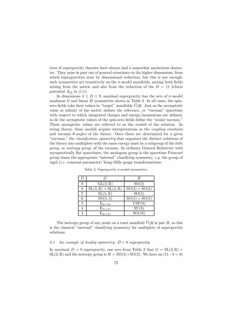
tries of supergravity theories have always had a somewhat mysterious charac-ter. They arise in part out of general covariance in the higher dimensions, fromwhich supergravities arise by dimensional reduction, but this is not enough:such symmetries act transitively on the σ-model manifolds, mixing both fieldsarising from the metric and also from the reduction of the D = 11 3-formpotential A[3] in (1.1).

In dimensions 4 ≤ D ≤ 9, maximal supergravity has the sets of σ-modelnonlinear G and linear H symmetries shown in Table 2. In all cases, the spin-zero fields take their values in “target” manifolds G/H. Just as the asymptoticvalue at infinity of the metric defines the reference, or “vacuum” spacetimewith respect to which integrated charges and energy/momentum are defined,so do the asymptotic values of the spin-zero fields define the “scalar vacuum.”These asymptotic values are referred to as the moduli of the solution. Instring theory, these moduli acquire interpretations as the coupling constantsand vacuum θ-angles of the theory. Once these are determined for a given“vacuum,” the classification symmetry that organizes the distinct solutions ofthe theory into multiplets with the same energy must be a subgroup of the littlegroup, or isotropy group, of the vacuum. In ordinary General Relativity withasymptotically flat spacetimes, the analogous group is the spacetime Poincaregroup times the appropriate “internal” classifying symmetry, e.g. the group ofrigid (i.e. constant-parameter) Yang-Mills gauge transformations.

Table 2: Supergravity σ-model symmetries.

D G H

9 GL(2,R) SO(2)8 SL(3,R)× SL(2,R) SO(3)× SO(2)7 SL(5,R) SO(5)6 SO(5, 5) SO(5)× SO(5)5 E6(+6) USP(8)4 E7(+7) SU(8)3 E8(+8) SO(16)

The isotropy group of any point on a coset manifold G/H is just H , so thisis the classical “internal” classifying symmetry for multiplets of supergravitysolutions.

8.1 An example of duality symmetry: D = 8 supergravity

In maximal D = 8 supergravity, one sees from Table 2 that G = SL(3,R) ×SL(2,R) and the isotropy group is H = SO(3)×SO(2). We have an (11−3 = 8)

72

vector of dilatonic scalars as well as a singlet F ijk[1] and a triplet F ij[1] (i, j, k =

1, 2, 3) of 1-form field strengths for zero-form potentials. Taken all together, wehave a manifold of dimension 7, which fits in precisely with the dimension of the(SL(3,R)× SL(2,R))/(SO(3)× SO(2)) coset-space manifold: 8+3−(3+1) = 7.

Owing to the direct-product structure, we may for the time being dropthe 5-dimensional SL(3,R)/SO(3) sector and consider for simplicity just the

2-dimensional SL(2,R)/SO(2) sector. Here is the relevant part of the action:56

ISL(2)8 =

∫d8x

√−g[R− 1

2∇Mσ∇Mσ − 12e

−2σ∇Mχ∇Mχ

− 1

2 · 4!eσ(F[4])

2 − 1

2 · 4!χF[4]∗F[4]

](8.1)

where ∗FMNPQ = 1/(4!√−g)ǫMNPQx1x2x3x4Fx1x2x3x4 (the ǫ

[8] is a density, hencepurely numerical).

On the scalar fields (σ, χ), the SL(2,R) symmetry acts as follows: letλ = χ+ ieσ; then

Λ =

(a bc d

)(8.2)

with ab−cd = 1 is an element of SL(2,R) and acts on λ by the fractional-lineartransformation

λ −→ aλ+ b

cλ+ d. (8.3)

The action of the SL(2,R) symmetry on the 4-form field strength gives usan example of a symmetry of the equations of motion that is not a symmetryof the action. The field strength F[4] forms an SL(2,R) doublet together with

G[4] = eσ∗F[4] − χF[4] , (8.4)

i.e., (F[4]

G[4]

)−→ (ΛT)−1

(F[4]

G[4]

). (8.5)

One may check that these transform the F[4] field equation

∇M(eσFMNPQ + χ∗FMNPQ) = 0 (8.6)

into the corresponding Bianchi identity,

∇M∗FMNPQ = 0 . (8.7)

Since the field equations may be expressed purely in terms of F[4], we have agenuine symmetry of the field equations in the transformation (8.5), but since

73

this transformation cannot be expressed locally in terms of the gauge potentialA[3], this is not a local symmetry of the action. The transformation (8.3, 8.5) isaD = 8 analogue of ordinary Maxwell duality transformation in the presence ofscalar fields. Accordingly, we shall refer generally to the supergravity σ-modelsymmetries as duality symmetries.

The F[4] field strength of the D = 8 theory supports elementary/electricp-brane solutions with p = 4 − 2 = 2, i.e. membranes, which have a d = 3dimensional worldvolume. The corresponding solitonic/magnetic solutions inD = 8 have worldvolume dimension d = 8 − 3 − 2 = 3 also. So in this case,F[4] supports both electric and magnetic membranes. It is also possible in thiscase to have solutions generalizing the purely electric or magnetic solutionsconsidered so far to solutions that carry both types of charge, i.e. dyons.56

This possibility is also reflected in the combined Bogomol’ny bound q for thissituation, which generalizes the single-charge bounds (4.16):

E2 ≥ e−σ∞(U + χ∞V )2 + eσ∞V 2 , (8.8)

where U and V are the electric and magnetic charges and σ∞ and χ∞ are themoduli, i.e. the constant asymptotic values of the scalar fields σ(x) and χ(x).The bound (8.8) is itself SL(2,R) invariant, provided that one transforms boththe moduli (σ∞, χ∞) (according to (8.3)) and also the charges (U, V ). For thesimple case with σ∞ = χ∞ = 0 that we have mainly chosen in order to simplifythe writing of explicit solutions, the bound (8.8) reduces to E2 ≥ U2+V 2, whichis invariant under an obvious isotropy group H = SO(2).

8.2 p-form charge quantisation conditions

So far, we have discussed the structure of p-brane solutions at a purely classicallevel. At the classical level, a given supergravity theory can have a continuousspectrum of electrically and magnetically charged solutions with respect to anyone of the n-form field strengths that can support the solution. At the quantumlevel, however, an important restriction on this spectrum of solutions entersinto force: the Dirac-Schwinger-Zwanziger (DSZ) quantisation conditions forparticles with electric or magnetic or dyonic charges.57,58 As we have seen,however, the electric and magnetic charges carried by branes and appearingin the supersymmetry algebra (1.5) are forms, and the study of their charge-quantisation properties involves some special features not seen in the D = 4Maxwell case.59

qIn comparing (8.8) to the single-charge bounds (4.16), one should take note that for F[4] in

(8.1) we have ∆ = 4, so 2/√∆ = 1.

74

We shall first review a Wu-Yang style of argument,57 (for a Dirac-stringargument, see Ref.58,60) considering a closed sequence W of deformations ofone p-brane, say an electric one, in the background fields set up by a dual,magnetic, p = D−p−4 brane. After such a sequence of deformations, one seesfrom the supermembrane action (4.1) that the electric p-brane wavefunctionpicks up a phase factor

exp

(iQe

(p+ 1)!

∮

WAM1...Mp+1dx

M1 ∧ . . . ∧ dxMp+1

), (8.9)

where A[p+1] is the gauge potential set up (locally) by the magnetic p-branebackground.

A number of differences arise in this problem with respect to the ordinaryDirac quantisation condition for D = 4 particles. One of these is that, aswe have seen in subsection 4.1, objects carrying p-form charges appearing inthe supersymmetry algebra (1.5) are necessarily either infinite or are wrappedaround compact spacetime dimensions. For infinite p-branes, some deformationsequences W will lead to a divergent integral in the exponent in (8.9); suchdeformations would also require an infinite amount of energy, and so shouldbe excluded from consideration. In particular, this excludes deformations thatinvolve rigid rotations of an entire infinite brane. Thus, at least the asymptoticorientation of the electric brane must be preserved throughout the sequence ofdeformations. Another way of viewing this restriction on the deformations isto note that the asymptotic orientation of a brane is encoded into the electricp-form charge, and so one should not consider changing this p-form in thecourse of the deformation any more than one should consider changing themagnitude of the electric charge in the ordinary D = 4 Maxwell case.

We shall see shortly that another difference with respect to the ordinaryD = 4 Dirac quantisation of particles in Maxwell theory will be the existenceof “Dirac-insensitive” configurations, for which the phase in (8.9) vanishes.

Restricting attention to deformations that give non-divergent phases, onemay use Stoke’s theorem to rewrite the integral in (8.9):

Qe

(p+ 1)!

∮

WAM1...Mp+1dx

M1 ∧ . . . ∧ dxMp+1 =

Qe

(p+ 2)!

∫

MW

FM1...Mp+2dxM1 ∧ . . . ∧ dxMp+2 = QeΦMW , (8.10)

where MW is any surface “capping” the closed surface W , i.e. a surface suchthat ∂MW = W ; ΦMW is then the flux through the cap MW . Choosing thecapping surface in two different ways, one can find a flux discrepancy ΦM1 −

75

ΦM2 = ΦM1∩M2 = ΦMtotal(taking into account the orientation sensitivity of

the flux integral). Then if Mtotal = M1 ∩ M2 “captures” the magnetic p-brane, the flux ΦMtotal

will equal the magnetic charge Qm of the p-brane; thusthe discrepancy in the phase factor (8.9) will be simply exp(iQeQm). Requiringthis to equal unity gives,57 in strict analogy to the ordinary case of electric andmagnetic particles in D = 4, the Dirac quantisation condition

QeQm = 2πn , n ∈ Z . (8.11)

The charge quantisation condition (8.11) is almost, but not quite, the fullstory. In deriving (8.11), we have not taken into account the p-form characterof the charges. Taking this into account shows that the phase in (8.9) vanishesfor a measure-zero set of configurations of the electric and magnetic branes.59

This is easiest to explain in a simplified case where the electric and mag-netic branes are kept in static flat configurations, with the electric p-brane ori-ented along the directions xM1 . . . xMp. The phase factor (8.9) then becomes

exp(iQe

∮W AM1...MpR

∂xR/∂σ), where σ is an ordering parameter for the closedsequence of deformations W . In making this deformation sequence, we recallfrom the above discussion that one should restrict the deformations to pre-serve the asymptotic orientation of the deformed p-brane. For simplicity, onemay simply consider moving the electric p-brane by parallel transport aroundthe magnetic p-brane in a closed loop. The accrued phase factor is invariantunder gauge transformations of the potential A[p+1]. This makes it possible tosimplify the discussion by making use of a specially chosen gauge. Note thatmagnetic p-branes have purely transverse field strengths like (2.27b); there isaccordingly a gauge in which the gauge potential A[p+1] is also purely trans-verse, i.e. it vanishes whenever any of its indices point along a worldvolumedirection of the magnetic p-brane. Consideration of more general deformationsequences yields the same result.59

Now one can see how the Dirac-insensitive configurations arise: the phasein (8.9) vanishes whenever there is even a partial alignment between the electricand the magnetic branes, i.e. when there are shared worldvolume directionsbetween the two branes. This measure-zero set of Dirac-insensitive configura-tions may be simply characterized in terms of the p and p charges themselvesby the condition Qel

[p] ∧ Qmag[p] = 0. For such configurations, one obtains no

Dirac quantisation condition. To summarize, one may incorporate this ori-entation restriction into the Dirac quantisation condition (8.11) by writing a(p+ p)-form quantisation condition

Qel[p] ∧Qmag

[p] = 2πnQel

[p] ∧Qmag[p]

|Qel[p]| |Q

mag[p] | , n ∈ Z , (8.12)

76

which reduces to (8.11) for all except the Dirac-insensitive set of configurations.

8.3 Charge quantisation conditions and dimensional reduction

The existence of Dirac-insensitive configurations may seem to be of only pe-ripheral importance, given that they constitute only a measure-zero subsetof the total set of asymptotic brane configurations. However, their relevancebecomes more clear when one considers the relations existing between the p-form charges under dimensional reduction. Let us recall the relations (6.11)between the field strengths in different dimensions. Now, the electric and mag-netic charges carried by branes in D dimensions take the forms

Qe =

∫ (e~c·

~φ ∗F + κ(A))

(8.13a)

Qm =

∫F , (8.13b)

where F = dA, F = F + (Chern-Simons modifications) (i.e. modificationsinvolving lower-order forms arising in the dimensional reduction similar tothose in the D = 9 case (6.41)) and ~c is the dilaton vector corresponding toF in the dimensionally-reduced action (6.13). The term κ(A) in (8.13a) isthe analogue of the term 1

2A[3] ∧ F[4] in (1.3). From the expressions (6.11) forthe reduced field strengths and their duals, one obtains the following relationsbetween the original charges in D = 11 and those in the reduced theory:

Table 3: Relations between Q11 and QD

F[4] F i[3] F ij[2] F ijk[1]

Electric Q11e = QD

e V QDeVLi

QDe

VLi Lj

QDe

VLi Lj Lk

Magnetic Q11m = QD

m QDm Li QD

m Li Lj QDm Li Lj Lk

where Li =∫dzi is the compactification period of the reduction coordinate

zi and V =∫d11−Dz =

∏11−Di=1 Li is the total compactification volume. Note

that the factors of Li cancel out in the various products of electric and magneticcharges only for charges belonging to the same field strength in the reduceddimension D.

Now consider the quantisation conditions obtained between the various di-mensionally reduced charges shown in Table 3. We need to consider the variousschemes possible for dimensional reduction of dual pairs of (p,p) branes. We

77

have seen that for single-element brane solutions, there are two basic schemes,as explained in Section 6: diagonal, which involves reduction on a worldvolumecoordinate, and vertical, which involves reduction on a transverse coordinateafter preparation by “stacking up” single-center solutions so as to generate atransverse-space translation invariance needed for the dimensional reduction.

For the dimensional reduction of a solution containing two elements, thereare then four possible schemes, depending on whether the reduction coordinatez belongs to the worldvolume or to the transverse space of each brane. Foran electric/magnetic pair, we have the following four reduction possibilities:diagonal/diagonal, diagonal/vertical, vertical/diagonal and vertical/vertical.Only the mixed cases will turn out to preserve Dirac sensitivity in the lowerdimension after reduction.

This is most easily illustrated by considering the diagonal/diagonal case,for which z belongs to the worldvolumes of both branes. With such a sharedworldvolume direction, one has clearly fallen into the measure-zero set of Dirac-insensitive configurations with Qel

[p] ∧ Qmag[p] = 0 in the higher dimension D.

Correspondingly, in (D − 1) dimensions one finds that the diagonally reducedelectric (p − 1) brane is supported by an n = p + 1 form field strength, butthe diagonally reduced magnetic (p − 1) brane is supported by an n = p + 2form; since only branes supported by the same field strength can have a Diracquantisation condition, this diagonal/diagonal reduction properly correspondsto a Dirac-insensitive configuration.

Now consider the mixed reductions, e.g. diagonal/vertical. In performinga vertical reduction of a magnetic p-brane by stacking up an infinite deck ofsingle-center branes in order to create the R translational invariance necessaryfor the reduction, the total magnetic charge will clearly diverge. Thus, in avertical reduction it is necessary to reinterpret the magnetic charge Qm asa charge density per unit z compactification length. Before obtaining theDirac quantisation condition in the lower dimension, it is necessary to restorea gravitational-constant factor of κ2 that should properly have appeared inthe quantisation conditions (8.11, 8.12). As one may verify, the electric andmagnetic charges as defined in (1.3, 1.4) are not dimensionless. Thus, (8.11)in D = 11 should properly have been written QeQm = 2πκ211n. If one lets thecompactification length be denoted by L in the D-dimensional theory priorto dimensional reduction, then one obtains a Dirac phase exp(iκ−2

D−1QeQmL).This fits precisely, however, with another aspect of dimensional reduction:the gravitational constants in dimensions D and D − 1 are related by κ2D =Lκ2D−1. Thus, in dimension D − 1 one obtains the expected quantisationcondition QeQm = 2πκ2D−1n. Note, correspondingly, that upon making amixed diagonal/vertical reduction, the electric and magnetic branes remain

78

dual to each other in the lower dimension, supported by the same n = p−1+2 =p+1 form field strength. The opposite mixed vertical/diagonal reduction casegoes similarly, except that the dual branes are then supported by the samen = p+ 2 form field strength.

In the final case of vertical/vertical reduction, Dirac sensitivity is lostin the reduction, not owing to the orientation of the branes, but because inthis case both the electric and the magnetic charges need to be interpretedas densities per unit compactification length, and so one obtains a phaseexp(iκ−2

D QeQmL2). Only one factor of L is absorbed into κ2D−1, and one has

limL→0L2/κ2D = 0. Correspondingly, the two dimensionally reduced branes in

the lower dimension are supported by different field strengths: an n = p + 2form for the electric brane and an n = p+ 1 form for the magnetic brane.

Thus, there is a perfect accord between the structure of the Dirac quantisa-tion conditions for p-form charges in the various supergravity theories relatedby dimensional reduction. The existence of Dirac-insensitive configurationsplays a central role in establishing this accord, even though they representonly a subset of measure zero from the point of view of the higher-dimensionaltheory.

Another indication of the relevance of the Dirac-insensitive configurationsis the observation 59 that all the intersecting-brane solutions with some degreeof preserved supersymmetry, as considered in Section 7, correspond to Dirac-insensitive configurations. This may immediately be seen in such solutions asthe 2 ⊥ 5(1) solution (7.10), but it is also true for solutions involving pp waveand Taub-NUT elements.

8.4 Counting p-branes

As we have seen at the classical level, the classifying symmetry for solutions in agiven scalar vacuum, specified by the values of the scalar moduli, is the linearly-realized isotropy symmetry H given in Table 2. When one takes into accountthe Dirac quantisation condition, this classifying symmetry becomes restrictedto a discrete group, which clearly must be a subgroup of the correspondingG(Z) duality group, so in general one seeks to identify the groupG(Z)∩H . Thevalue of this intersection is modulus-dependent, showing that the homogeneityof the G/H coset space is broken at the quantum level by the quantisationcondition. Classically, of course, the particular point on the vacuum manifoldG/H corresponding to the scalar moduli can be changed by application ofa transitively-acting G transformation, for example with a group element g.Correspondingly, the isotropy subgroup H moves by conjugation with g,

H −→ gHg−1 . (8.14)

79

The discretized duality group G(Z), on the other hand, does not dependupon the moduli. This is because the modulus dependence cancels out in the“canonical” charges that we have defined in Eq. (8.13). One way to see this isto use the relations between charges in different dimensions given in Table 3,noting that there are no scalar moduli in D = 11, so the modulus-independentrelations of Table 3 imply that the lower-dimensional charges (8.13) do notdepend on the moduli.r

Another way to understand this is by comparison with ordinary Maxwellelectrodynamics, where an analogous charge would be that derived from theaction IMax = −1/(4e2)

∫F canµν F

canµν , corresponding to a covariant derivativeDµ = ∂µ+iAcan

µ . This is analogous to our dimensionally reduced action (6.13)

from which the charges (8.13) are derived, because the modulus factors e~c·~φ∞

appearing in (6.13) (together with the rest of the ~φ dilatonic scalar dependence)play the roles of coupling constant factors like e−2. If one wants to comparethis to the “conventional” charges defined with respect to a conventional gaugepotential Aconv

µ = e−1Acanµ , for which the action is −1/4

∫F convµν F convµν , then

the canonical and conventional charges obtained via Gauss’s law surface inte-grals are related by

Qcan =1

2e2

∫d2ΣijǫijkF

can 0k =1

2e

∫d2ΣijǫijkF

conv 0k =1

eQconv . (8.15)

Thus, in the Maxwell electrodynamics case, the dependence on the electriccharge unit e drops out in Qcan, although the conventional charge Qconv scalesproportionally to e. The modulus independence of the charges (8.13) worksin a similar fashion. Then, given that the discretized quantum duality groupG(Z) is defined by the requirement that it map the set of Dirac-allowed chargesonto itself, it is evident that the group G(Z), referred to the canonical charges(8.13), does not depend on the moduli.

As a consequence of the different modulus dependences of H and of G(Z),it follows that the size of the intersection group G(Z) ∩ H is dependent onthe moduli. The analogous feature in ordinary Maxwell theory is that a trueduality symmetry of the theory only arises when the electric charge takes thevalue e = 1 (in appropriate units), since the duality transformation mapse→ e−1. Thus, the value e = 1 is a distinguished value.

rNote that the compactification periods Li appearing in Table 3 have values that may beadjusted by convention. These should not be thought of as determining the geometry of thecompactifying internal manifold, which is determined instead by the scalar moduli. Thus,the relations of Table 3 imply the independence of the canonically-defined charges from thephysically relevant moduli.

80

The distinguished point on the scalar vacuum manifold for general super-gravity theories is the one where all the scalar moduli vanish. This is the pointwhere G(Z) ∩ H is maximal. Let us return to our D = 8 example to helpidentify what this group is. In that case, for the scalars (σ, χ), we may writeout the transformation in detail using (8.3):

e−σ −→ (d+ cχ)2e−σ + c2eσ

χe−σ −→ (d+ cχ)(b+ aχ)e−σ + aceσ . (8.16)

Requiring a, b, c, d ∈ Z and also that the modulus point σ∞ = χ∞ = 0 be leftinvariant, we find only two transformations: the identity and the transforma-tion a = d = 0, b = −1, c = 1, which maps σ and χ according to

e−σ −→ eσ + χ2e−σ

χe−σ −→ −χe−σ . (8.17)

Thus, for our truncated system, we find just an S2 discrete symmetry as thequantum isotropy subgroup of SL(2,Z) at the distinguished point on the scalarvacuum manifold. This S2 is the natural analogue of the S2 symmetry thatappears in Maxwell theory when e = 1.

In order to aid in identifying the pattern behind this D = 8 example,suppose that the zero-form gauge potential χ is small, and consider the S2

transformation to lowest order in χ. To this order, the transformation justflips the signs of σ and χ. Acting on the field strengths (F[4], G[4]), one finds

(F[4], G[4]) −→ (−G[4], F[4]) . (8.18)

One may again check (in fact to all orders, not just to lowest order in χ) that(8.18) maps the field equation for F[4] into the corresponding Bianchi identity:

∇M (eσFMNPQ + χ∗FMNPQ) −→ −∇M∗FMNPQ . (8.19)

Considering this S2 transformation to lowest order in the zero-form χ has theadvantage that the sign-flip of φ may be “impressed” upon the ~a dilaton vectorfor F[4]: ~a→ −~a. The general structure of such G(Z)∩H transformations willbe found by considering the impressed action of this group on the dilatonvectors.

Now consider the SL(3,R)/SO(3) sector of the D = 8 scalar manifold,again with the moduli set to the distinguished point on the scalar manifold.To lowest order in zero-form gauge potentials, the action of SL(3,Z) ∩H maysimilarly by impressed upon the 3-form dilaton vectors, causing in this case apermutation of the ~ai, generating for the D = 8 case overall the discrete group

81

S3×S2. Now that we have a bit more structure to contemplate, we can noticethat the G(Z) ∩H transformations leave the (~a,~ai) dot products invariant.61

The invariance of the dilaton vectors’ dot products prompts one to returnto the algebra (6.15) of these dot products and see what else we may recognizein it. Noting that the duality groups given in Table 2 for the higher dimen-sions D involve SL(N,R) groups, we recall that the weight vectors ~hi of thefundamental representation of SL(N,R) satisfy

~hi · ~hj = δij −1

N,

N∑

i=1

~hi = 0 . (8.20)

These relations are precisely those satisfied by ±1√2~a and 1√

2~ai, corresponding

to the cases N = 2 and N = 3. This suggests that the action of the maximalG(Z) ∩ H group (i.e. for scalar moduli set to the distinguished point on thescalar manifold) may be identified in general with the symmetry group of theset of fundamental weights for the corresponding supergravity duality groupG as given in Table 2. The symmetry group of the fundamental weights is theWeyl group 61 of G, so the action of the maximal G(Z)∩H p-brane classifyingsymmetry is identified with that of the Weyl group of G.

As one proceeds down through the lower-dimensional cases, where thesupergravity symmetry groups shown in Table 2 grow in complexity, the abovepattern persists:61 in all cases, the action of the maximal classifying symmetryG(Z) ∩H may be identified with the Weyl group of G. This is then the groupthat counts the distinct p-brane solutions s of a given type (4.6), subject to theDirac quantisation condition and referred to the distinguished point on thescalar modulus manifold. For example, in D = 7, where from Table 2 one seesthat G = SL(5,R) and H = SO(5), one finds that the action of G(Z) ∩ H isequivalent to that of the discrete group S5, which is the Weyl group of SL(5,R).In the lower-dimensional cases shown in Table 2, the discrete group G(Z) ∩Hbecomes less familiar, and is most simply described as the Weyl group of G.

From the analysis of the Weyl-group duality multiplets, one may tabu-late 61 the multiplicities of p-branes residing at each point of the plot given inFigure 7. For supersymmetric p-branes arising from a set of N participatingfield strengths F[n], corresponding to ∆ = 4/N for the dilatonic scalar cou-pling, one finds the multiplicities given in Table 4. By combining these dualitymultiplets together with the diagonal and vertical dimensional reduction fam-ilies discussed in Sections 6 and 6.3, the full set of p ≤ (D − 3) branes shownin Figure 7 becomes “welded” together into one overall symmetrical structure.

sOf course, these solutions must also fall into supermultiplets with respect to the unbrokensupersymmetry; the corresponding supermultiplet structures have been discussed in Ref.64

82

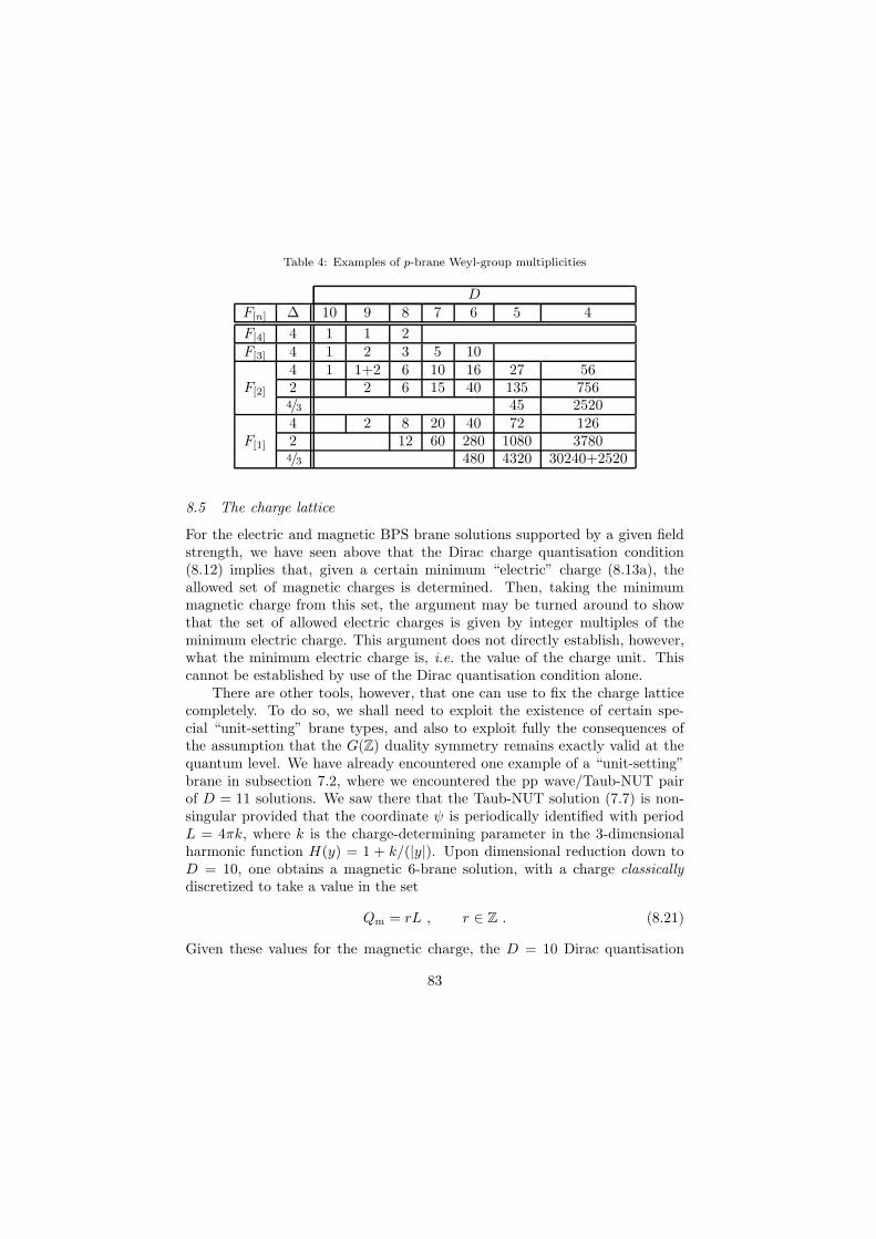
Table 4: Examples of p-brane Weyl-group multiplicities

DF[n] ∆ 10 9 8 7 6 5 4

F[4] 4 1 1 2F[3] 4 1 2 3 5 10

4 1 1+2 6 10 16 27 56F[2] 2 2 6 15 40 135 756

4/3 45 25204 2 8 20 40 72 126

F[1] 2 12 60 280 1080 37804/3 480 4320 30240+2520

8.5 The charge lattice

For the electric and magnetic BPS brane solutions supported by a given fieldstrength, we have seen above that the Dirac charge quantisation condition(8.12) implies that, given a certain minimum “electric” charge (8.13a), theallowed set of magnetic charges is determined. Then, taking the minimummagnetic charge from this set, the argument may be turned around to showthat the set of allowed electric charges is given by integer multiples of theminimum electric charge. This argument does not directly establish, however,what the minimum electric charge is, i.e. the value of the charge unit. Thiscannot be established by use of the Dirac quantisation condition alone.

There are other tools, however, that one can use to fix the charge latticecompletely. To do so, we shall need to exploit the existence of certain spe-cial “unit-setting” brane types, and also to exploit fully the consequences ofthe assumption that the G(Z) duality symmetry remains exactly valid at thequantum level. We have already encountered one example of a “unit-setting”brane in subsection 7.2, where we encountered the pp wave/Taub-NUT pairof D = 11 solutions. We saw there that the Taub-NUT solution (7.7) is non-singular provided that the coordinate ψ is periodically identified with periodL = 4πk, where k is the charge-determining parameter in the 3-dimensionalharmonic function H(y) = 1 + k/(|y|). Upon dimensional reduction down toD = 10, one obtains a magnetic 6-brane solution, with a charge classicallydiscretized to take a value in the set

Qm = rL , r ∈ Z . (8.21)

Given these values for the magnetic charge, the D = 10 Dirac quantisation

83

condition

QeQm = 2πκ210n , n ∈ Z , (8.22)

or, equivalently, as we saw in subsection 7.2, the quantisation of D = 11 ppwave momentum in the compact ψ direction, gives an allowed set of electriccharges

Qe =2πκ210L

n , n ∈ Z . (8.23)

Thus, the requirement that magnetic D = 10 6-branes oxidize up to non-singular Taub-NUT solutions in D = 11 fully determines the 6-brane electricand magnetic charge units and not just the product of them which occurs inthe Dirac quantisation condition

If one assumes that the G(Z) duality symmetries remain strictly unbro-ken at the quantum level, then one may relate the 6-brane charge units tothose of other BPS brane types.t In doing so, one must exploit the fact thatbrane solutions with Poincare worldvolume symmetries may be dimensionallyreduced down to lower dimensions, where the duality groups shown in Table 2grow larger. In a given dimension D, the G(Z) duality symmetries only rotatebetween p-branes of the same worldvolume dimension, supported by the samekind of field strength, as we have seen from our discussion of the Weyl-groupaction on p-branes given in subsection 8.4. Upon reduction down to dimen-sions Dred < D, however, the solutions descending from an original p-branein D dimensions are subject to a larger G(Z) duality symmetry, and this canbe used to rotate a descendant brane into descendants of p′-branes for variousvalues of p′. Dimensional oxidation back up to D dimensions then completesthe link, establishing relations via the duality symmetries between various BPSbrane types which can be supported by different field strengths, including fieldstrengths of different rank.65 This link may be used to establish relations be-tween the charge units for the various p-form charges of differing rank, eventhough the corresponding solutions are Dirac-insensitive to each each other.

Another charge-unit-setting BPS brane species occurs in the D = 10 typeIIB theory. This theory has a well-known difficulty with the formulation of asatisfactory action, although its field equations are perfectly well-defined. Thedifficulty in formulating an action arise from the presence of a self-dual 5-formfield strength, H[5] =

∗H[5]. The corresponding electrically and magneticallycharged BPS solutions are 3-branes, and, owing to the self-duality condition,these solutions are actually dyons, with a charge vector at 45 to the electricaxis. We shall consider the type IIB theory in some more detail in Section9; for now, it will be sufficient for us to note that the dyonic 3-branes of

tFor details of the duality relations between charge units for different p-branes, see Ref.59

84

D = 10 type IIB theory are also a unit-setting brane species.59 The unit-settingproperty arises because of a characteristic property of the Dirac-Schwinger-Zwanziger quantisation condition for dyons in dimensions D = 4r + 2: for

dyons (Q(1)e , Q

(1)m ), (Q

(2)e , Q

(2)m ), this condition is symmetric:59

Q(1)e Q(2)

m +Q(2)e Q(1)

m = 2πκ24r+2n , n ∈ Z , (8.24)

unlike the more familiar antisymmetric DSZ condition that is obtained in di-mensions D = 4r. The symmetric nature of (8.24) means that dyons may beDirac-sensitive to others of their own type,u quite differently from the anti-symmetric cases in D = 4r dimensions. For the 45 dyonic 3-branes, one thusobtains the quantisation condition

|Q[3]| = n√πκIIB , n ∈ Z (8.25)

where κIIB is the gravitational constant for the type IIB theory. Then, usingduality symmetries, one may relate the

√πκIIB charge unit to those of other

supergravity R–R charges.Thus, using duality symmetries together with the pp wave/Taub-NUT and

self-dual 3-brane charge scales, one may determine the charge-lattice units forall BPS brane types.65,59. It is easiest to express the units of the resulting over-all charge lattice by making a specific choice for the compactification periods.If one lets all the compactification periods Li be equal,

Li = LIIB = L = (2πκ211)19 , (8.26)

then the electric and magnetic charge-lattice units for rank-n field strengthsin dimension D are determined to be 59

∆Qe = LD−n−1 , ∆Qm = Ln−1 . (8.27)

9 Local versus active dualities

The proper interpretation of the discretized Cremmer-Julia G(Z) duality sym-metry at the level of supergravity theory is subject to a certain amount ofdebate, but at the level of string theory the situation becomes more clear. Inany dimension D, there is a subgroup of G(Z) that corresponds to T duality,which is a perturbative symmetry holding order-by-order in the string loopexpansion. T duality 66 consists of transformations that invert the radii of a

uThey will be Dirac-sensitive provided one of them is slightly rotated so as to avoid hav-ing any common worldvolume directions with the other, in order to avoid having a Dirac-insensitive configuration as discussed in subsection 8.3.

85

toroidal compactification, under which quantized string oscillator modes andstring winding modes become interchanged. Aside from such a relabeling, how-ever, the overall string spectrum remains unchanged. Hence, T duality needsto be viewed as a local symmetry in string theory, i.e. string configurations oncompact manifolds related by T duality are identified. Depending on whetherone considers (D−3) branes to be an unavoidable component of the spectrum,the same has also been argued to be the case at the level of the supergravityeffective field theory.67 The well-founded basis, in string theory at least, for alocal interpretation of the T duality subgroup of G(Z) has led subsequently tothe hypothesis 62,63 that the full duality group G(Z) should be given a localinterpretation: sets of string solutions and moduli related by G(Z) transforma-tions are to be treated as equivalent descriptions of a single state. This localinterpretation of the G(Z) duality transformations is similar to that adoptedfor general coordinate transformations viewed passively, according to which,e.g., flat space in Cartesian or in Rindler coordinates is viewed as one and thesame solution.

As with general coordinate transformations, however, duality symmetriesmay occur in several different guises that are not always clearly distinguished.As one can see from the charge lattice discussed in subsection 8.5, there is alsoa G(Z) covariance of the set of charge vectors for physically inequivalent BPSbrane solutions. In the discussion of subsection 8.5, we did not consider indetail the action of G(Z) on the moduli, because, as we saw in subsection 8.4,the canonically-defined charges (8.13) are in fact modulus-independent.

Since the dilatonic and axionic scalar moduli determine the coupling con-stants and vacuum θ-angles of the theory, these quantities should be fixedwhen quantizing about a given vacuum state of the theory. This is similar tothe treatment of asymptotically flat spacetime in gravity, where the choice of aparticular asymptotic geometry is necessary in order to establish the “vacuum”with respect to which quantized fluctuations can be considered.

Thus, in considering physically-inequivalent solutions, one should comparesolutions with the same asymptotic values of the scalar fields. When this isdone, one finds that solutions carrying charges (8.13) related by G(Z) transfor-mations generally have differing mass densities. Since the standard Cremmer-Julia duality transformations, such as those of ourD = 8 example in subsection8.1, commute with P 0 time translations and so necessarily preserve mass den-sities, it is clear that the BPS spectrum at fixed scalar moduli cannot forma multiplet under the standard Cremmer-Julia G(Z) duality symmetry. Thisconclusion is in any case unavoidable, given the local interpretation adoptedfor the standard duality transformations as discussed above: once one hasidentified solution/modulus sets under the standard G(Z) duality transforma-

86

tions, one cannot then turn around and use the same G(Z) transformations togenerate inequivalent solutions.

Thus, the question arises: is there any spectrum-generating symmetrylying behind the apparently G(Z) invariant charge lattices of inequivalent so-lutions that we saw in subsection 8.5? At least at the classical level, and forsingle-charge (i.e. ∆ = 4) solutions, the answer 68 turns out to be ‘yes.’ Weshall illustrate the point using type IIB supergravity as an example.v

9.1 The symmetries of type IIB supergravity

Aside from the difficulties arising from the self-duality condition for the 5-form field strength H[5], the equations of motion of the bosonic fields of theIIB theory may be derived from the action

IIIB10 =

∫d10x[eR+ 1

4e tr(∇µM−1 ∇µM)− 112eH

T[3] MH[3]− 1

240eH2[5]

− 12√2ǫij

∗(B[4]∧dA(i)[2]∧dA

(j)[2] )] . (9.1)

The 5-form self-duality condition

H[5] =∗H[5] (9.2)

may be handled in the fashion of Ref.70, being imposed by hand as an extraconstraint on the field equations obtained by varying (9.1). This somewhathybrid procedure will be sufficient for our present purposes.

The matrixM in (9.1) contains two scalar fields: a dilatonic scalar φ whichoccurs nonlinearly through its exponential, and an axionic scalar χ, which mayalso be considered to be a zero-form gauge potential; explicitly, one has

M =

(e−φ + χ2 eφ χ eφ

χ eφ eφ

). (9.3)

The doublet H[3] contains the field strengths of the 2-form gauge potentialsA[2]:

H[3] =

(dA

(1)[2]

dA(2)[2]

). (9.4)

The action (9.1) is invariant under the SL(2,R) transformations

H[3] −→ (ΛT )−1H[3] , M −→ ΛMΛT , (9.5)

vFor a detailed discussion of SL(2,R) duality in type IIB supergravity, see Ref.69

87

where the SL(2,R) parameter matrix is

Λ =

(a bc d

), (9.6)

and the SL(2,R) constraint is ad − bc = 1. If one defines the complex scalarfield τ = χ + i e−φ, then the transformation on M can be rewritten as thefractional linear transformation

τ −→ aτ + b

cτ + d. (9.7)

Note that since H[5] is a singlet under SL(2,R), the self-duality constraint(9.2), which is imposed by hand, also preserves the SL(2,R) symmetry. Sincethis SL(2,R) transformation rotates the doublet A2] of electric 2-form poten-tials amongst themselves, this is an “electric-electric” duality, as opposed tothe “electric-magnetic” duality discussed in the D = 8 example of subsection8.1. Nonetheless, similar issues concerning duality multiplets for a fixed scalarvacuum arise in both cases.

There is one more symmetry of the equations of motion following from theaction (9.1). This is a rather humble symmetry that is not often remarkedupon, but which will play an important role in constructing active SL(2,R)duality transformations for the physically distinct BPS string and 5-brane mul-tiplets of the theory. As for pure source-free Einstein theory, the action (9.1)transforms homogeneously as λ3 under the following scaling transformations:

gµν −→ λ2 gµν , A(i)[2] −→ λ2A

(i)[2] , H[5] −→ λ4H[5] ; (9.8)

note that the power of λ in each field’s transformation is equal to the numberof indices it carries, and, accordingly, the scalars φ and χ are not transformed.Although the transformation (9.8) does not leave the action (9.1) invariant,the λ3 homogeneity of this scaling for all terms in the action is sufficient toproduce a symmetry of the IIB equations of motion. It should be noted thatthe SL(2,R) electric-magnetic duality of theD = 8 example given in subsection8.1 shares with the transformation (9.8) the feature of being a symmetry onlyof the equations of motion, and not of the action.

The SL(2,R) transformations map solutions of (9.1) into other solutions.We shall need to consider in particular the action of these transformations onthe charges carried by solutions. From the equations of motion of the 3-formfield strength H[3] in (9.1),

d ∗(MH[3]) = − 1√2H[5] ∧ΩH[3] , (9.9)

88

where Ω is the SL(2,R)-invariant tensor

Ω =

(0 1−1 0

), (9.10)

one finds that the following two-component quantity is conserved:

Qe =

∫ (∗(MH[3]) +

1

3√2Ω(2B[4] ∧H[3] −H[5] ∧ A[2])

). (9.11)

Under an SL(2,R) transformation, Qe transforms covariantly as a doublet:Qe → ΛQe.

By virtue of the Bianchi identities for the 3-form field strength, one has inaddition a topologically-conserved magnetic charge doublet,

Qm =

∫H[3] , (9.12)

which transforms under SL(2,R) as Qm → (ΛT)−1Qm, i.e. contragrediently toQe. The transformation properties of the electric and magnetic charge doubletsare just such as to ensure that the Dirac quantization condition QT

mQe ∈2πκ2IIBZ is SL(2,R) invariant.

The overall effect of this standard SL(2,R) symmetry on type IIB super-gravity solutions may be expressed in terms of its action on the solutions’charges and on the scalar moduli. This group action may be viewed as anautomorphism of a vector bundle, with the scalar fields’ SL(2,R)/SO(2) targetmanifold as the base space, and the charge vector space as the fiber.

We have seen in our general discussion of charge lattices in subsection8.5 that the continuous classical Cremmer-Julia symmetries G break down todiscretized G(Z) symmetries that map between states on the quantum chargelattice. In the present type IIB case, the classical SL(2,R) symmetry breaksdown to SL(2,Z) at the quantum level. Taking the basis states of the IIBcharge lattice to be

e1 =

(10

)e2 =

(01

), (9.13)

the surviving SL(2,Z) group will be represented by SL(2,R) matrices withintegral entries.

As we have discussed above, the discretized duality symmetries G(Z) aregiven a local interpretation in string theory. In the case of the type IIB theory,this is a hypothesis rather than a demonstrated result, because the SL(2,Z)

89

transformations map between NS–NS and R–R states, and this is a distinctlynon-perturbative transformation. Adopting this hypothesis nonetheless, anorbit of the standard SL(2,Z) transformation reduces to a single point; aftermaking the corresponding identifications, the scalar modulus space becomesthe double coset space SL(2,Z)\SL(2,R)/SO(2).

9.2 Active duality symmetries

Now let us see how duality multiplets of the physically inequivalent BPS statescan occur, even though they will contain states with different mass densities.This latter fact alone tells us that we must include some transformation thatacts on the metric. We shall continue with our exploration of the continu-ous classical SL(2,R) symmetry of the type IIB theory. Finding the survivingquantum-level SL(2,Z) later on will be a straightforward matter of restrict-ing the transformations to a subgroup. The procedure starts with a stan-dard SL(2,R) transformation, which transforms the doublet charges (9.11) ina straightforwardly linear fashion, but which also transforms in an unwantedway the scalar moduli. Subsequent compensating transformations will thenhave the task of eliminating the unwanted transformation of the scalar mod-uli, but without changing the “already final” values of the charges. Let ussuppose that this initial transformation, with parameter Λ, maps the chargevector and complex scalar modulus (Q, τ∞) to new values (Q′, τ ′∞).

After this initial Λ transformation, one wishes to return the complex scalarmodulus τ ′∞ to its original value τ∞, in order to obtain an overall transforma-tion that does not in the end disturb the complex modulus. To do this, noticethat within SL(2,R) there is a subgroup that leaves a doublet charge vectorQ′ invariant up to an overall rescaling. This projective stability group of Q′ isisomorphic to the Borel subgroup of SL(2,R):

Borel =

(a b0 a−1

) ∣∣∣ a, b ∈ R

. (9.14)

This standard representation of the SL(2,R) Borel subgroup clearly leaves thebasis charge vector e1 of Eq. (9.13) invariant up to scaling by a. For a generalcharge vector Q′, there will exist a corresponding projective stability subgroupwhich is isomorphic to (9.14), but obtained by conjugation of (9.14) with anelement of H ∼

= SO(2). The importance of the Borel subgroup for our presentpurposes is that it acts transitively on the G/H = SL(2,R)/SO(2) coset spacein which the scalar fields take their values, so this transformation may beused to return the scalar moduli to the original values they had before the Λtransformation.

90

The next step in the construction is to correct for the unwanted scalingQ′ → aQ′ which occurs as a result of the Borel compensating transformation,by use of a further compensating scaling of the form (9.8), aQ′ → λ2aQ′,in which one picks the rigid parameter λ such that λ2a = 1. This almostcompletes the construction of the active SL(2,R). For the final step, notethat the transformation (9.8) also scales the metric, gµν → λ2gµν = a−1gµν .Since one does not want to alter the asymptotic metric at infinity, one needsto compensate for this scaling by a final general coordinate transformation,xµ → x′µ = a−1/2xµ.

The overall active SL(2,R) duality package constructed in this way trans-forms the charges in a linear fashion, Q→ λQ′, in exactly the same way as thestandard supergravity Cremmer-Julia SL(2,R) duality, but now leaving thecomplex scalar modulus τ∞ unchanged. This is achieved by a net constructionthat acts upon the field variables of the theory in a quite nonlinear fashion.This net transformation may be explicitly written by noting that for SL(2,R)there is an Iwasawa decomposition

Λ = bh , (9.15)

where b ∈ BorelQ′ is an element of the projective stability group of the finalcharge vector Q′ and where h ∈ Hτ∞ is an element of the stability subgroupof τ∞. Clearly, the Borel transformation that is needed in this construction isjust b = (b)−1, leaving thus a transformation h ∈ Hτ∞ which does not changethe complex modulus τ∞. The compensating scaling transformation t of theform (9.8) and the associated general coordinate transformation also leave thescalar moduli unchanged. The net active SL(2,R) transformation thus is justbtΛ = th. Specifically, for τ∞ = χ∞ + ie−φ∞ and a transformation Λ mapping

Qi =

(piqi

)to Qf =

(pfqf

)= ΛQi, the h ∈ Hτ∞ group element is

hfi = V∞

(cos θfi sin θfi− sin θfi cos θfi

)V −1∞ , θfi = θf − θi

tan θi = eφ∞(tan θi − χ∞) , tan θi = pi/qi , (9.16)

where the matrix V∞ is an element of Borel that has the effect of moving thescalar modulus from the point τ = i to the point τ∞:

V∞ = e−φ∞/2

(1 eφ∞χ∞0 eφ∞

). (9.17)

The matrix V∞ appearing here is also the asymptotic limit of a matrix V (φ, χ)that serves to factorize the matrix M given in (9.3), M = V V T. This fac-

91

torization makes plain the transitive action of the Borel subgroup on theSL(2,R)/SO(2) coset space in which the scalar fields take their values. Notethat the matrix M determines both the scalar kinetic terms and also theirinteractions with the various antisymmetric-tensor gauge fields appearing inthe action (9.1).

The scaling-transformation part of the net active SL(2,R) construction issimply expressed as a ratio of mass densities,

tfi =mf

mi, m2

i = QTi M−1

∞ Qi . (9.18)

This expression reflects the fact that the scaling symmetry (9.8) acts on themetric and thus enables the active SL(2,R) transformation to relate solutionsat different mass-density levelsmi,f . Since, by contrast, the mass-density levelsare invariant under the action of the standard SL(2,R), it is clear that the tworealizations of this group are distinctly different. Mapping between differentmass levels, referred to a given scalar vacuum determined by the complexmodulus τ∞, can only be achieved by including the scaling transformation(9.18).

The group composition property of the active SL(2,R) symmetry needs tobe checked in the same fashion as for nonlinear realizations generally, i.e. oneneeds to check that a group operation O(Λ, Q) = th acting on an initial statecharacterized by a charge doublet Q combines with a second group operationaccording to the rule

O(Λ2,Λ1Q)O(Λ1, Q) = O(Λ2Λ1, Q) . (9.19)

One may verify directly that the nonlinear realization given by (9.16, 9.18)does in fact satisfy this composition law, when acting on any of the fields ofthe type IIB theory.

At the quantum level, the Dirac quantization condition restricts the al-lowed states of the theory to a discrete charge lattice, as we have seen. Thestandard SL(2,R) symmetry thus becomes restricted to a discrete SL(2,Z) sub-group in order to respect this charge lattice, and the active SL(2,R) constructedabove likewise becomes restricted to an SL(2,Z) subgroup. This quantum-leveldiscretized group of active transformations is obtained simply by restricting thematrix parameters Λ for a classical active SL(2,R) transformation so as to liein SL(2,Z).

In lower-dimensional spacetime, the supergravity duality groups G shownin Table 2 grow in rank and the structure of the charge orbits becomes progres-sively more and more complicated, but the above story is basically repeatedfor an important class of p-brane solutions. This is the class of single-charge

92

solutions, for which the charges Q fall into highest-weight representations ofG. The duality groups shown in Table 2 are all maximally noncompact, andpossess an Iwasawa decomposition generalizing the SL(2,R) case (9.15):

Λ = bh b ∈ BorelQ , h ∈ Hmoduli , (9.20)

where BorelQ is isomorphic to the Borel subgroup of G. Once again, thissubgroup acts transitively on the coset space G/H in which the scalar fieldstake their values, so this is the correct subgroup to use for a compensatingtransformation to restore the moduli to their original values in a given scalarvacuum. As in the SL(2,R) example of the type IIB theory, one may seethat this group action is transitive by noting that the matrix M (9.3) whichgoverns the scalar kinetic terms and interactions can be parameterized in theform M = V V #, where V is an element of the Borel subgroup. The operation# here depends on the groups G and H in question; in spacetime dimensionsD ≥ 4 we have

V # =

V T, for H orthogonalV †, for H unitaryΩV †, for H a USp group.

(9.21)

(The D = 3 case in which G = E8(+8) and H = SO(16) needs to be treated asa special case.71)

Given the above group-theoretical structure, the construction of active Gsymmetry transformations that preserve the scalar moduli proceeds in strictanalogy with the type IIB SL(2,R) example that we have presented. Thisconstruction depends upon the existence of a projective stability group 68,71

of the charge Q that is isomorphic to the Borel subgroup of G. This is thecase whenever Q transforms according to a highest-weight representation of G.The BPS brane solutions with this property are the single-charge solutions with∆ = 4. As we have seen in Section 7, BPS brane solutions with ∆ = 4/N canbe interpreted as coincident-charge-center cases of intersecting-brane solutionswith N elements, each of which would separately be a ∆ = 4 solution on itsown. The construction of active duality symmetries for such multiple-chargesolutions remains an open problem, for they have a larger class of integrationconstants, representing relative positions and phases of the charge components.Only the asymptotic scalar moduli can be moved transitively by the Borelsubgroup of G and, correspondingly, the representations carried by the chargesin such multi-charge cases are not of highest-weight type.

The active G(Z) duality constructions work straightforwardly enough atthe classical level, but their dependence on symmetries of field equations thatare not symmetries of the corresponding actions gives a reason for caution

93

about their quantum durability. This may be a subject where string theoryneeds to intervene with its famed “miracles.” Some of these miracles can beseen in supergravity-level analyses of the persistence of BPS solutions witharbitrary mass scales, despite the presence of apparently threatening quantumcorrections,68 but a systematic way to understand the remarkable identitiesmaking this possible is not known. Thus, there still remain some areas wherestring theory appears to be more clever than supergravity.

10 Non-compact σ-models, null geodesics, and harmonic maps

A complementary approach 72,73,74 to the analysis of brane solutions in termsof the four D = 11 elemental solutions presented in Section 7 is to makea dimensional reduction until only overall-transverse dimensions remain, andthen to consider the resulting nonlinear σ-model supporting the solution. Insuch a reduction, all of the worldvolume and relative-transverse coordinatesare eliminated, including the time coordinate, which is possible because theBPS solutions are all time independent. The two complementary approachesto the analysis of BPS brane solutions may thus be characterized as oxidationup to the top of Figure 7, or reduction down to the left edge Figure 7, i.e.reduction down to BPS “instantons,” or p = −1 branes, with worldvolumedimension d = 0.

The d = 0 instanton solutions are supported by 1-form field strengths,i.e. the derivatives of axionic scalars, F[1] = dχ. Taken together with thedilatonic scalars accumulated in the process of dimensional reduction, theseform a noncompact nonlinear σ-model with a target manifold G/H ′, where G isthe usual supergravity symmetry group shown in Table 2 for the corresponding(reduced) dimension D but H ′ is a noncompact form of the modulus littlegroup H shown in Table 2. The difference between the groups H ′ and H arisesbecause dimensional reduction on the time coordinate introduces extra minussigns, with respect to the usual spatial-coordinate Kaluza-Klein reduction,in “kinetic” terms for scalars descending from vector fields in the (D + 1)dimensional theory including the time dimension. Scalars descending fromscalars or from the metric in (D + 1) dimensions do not acquire extra minussigns. The change to the little group H ′ is also needed for the transformationof field strengths of higher rank, but these need not be considered for ourdiscussion of the BPS instantons. The relevant groups for the noncompactσ-models in dimensions 9 ≥ D ≥ 3 are given in Table 5. These should becompared to the standard Cremmer-Julia groups given in Table 2.

The sector of dimensionally-reduced supergravity that is relevant for theinstanton solutions consists just of the transverse-space Euclidean-signature

94

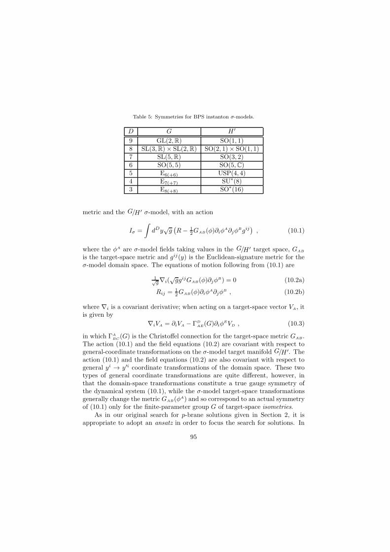
Table 5: Symmetries for BPS instanton σ-models.

D G H ′

9 GL(2,R) SO(1, 1)8 SL(3,R)× SL(2,R) SO(2, 1)× SO(1, 1)7 SL(5,R) SO(3, 2)6 SO(5, 5) SO(5,C)5 E6(+6) USP(4, 4)4 E7(+7) SU∗(8)3 E8(+8) SO∗(16)

metric and the G/H ′ σ-model, with an action

Iσ =

∫dDy

√g(R− 1

2GAB(φ)∂iφA∂jφ

Bgij), (10.1)

where the φA are σ-model fields taking values in the G/H ′ target space, GAB

is the target-space metric and gij(y) is the Euclidean-signature metric for theσ-model domain space. The equations of motion following from (10.1) are

1√g∇i(

√ggijGAB(φ)∂jφ

B) = 0 (10.2a)

Rij =12GAB(φ)∂iφ

A∂jφB , (10.2b)

where ∇i is a covariant derivative; when acting on a target-space vector VA, itis given by

∇iVA = ∂iVA − ΓD

AE(G)∂iφEVD , (10.3)

in which ΓABC

(G) is the Christoffel connection for the target-space metric GAB.The action (10.1) and the field equations (10.2) are covariant with respect togeneral-coordinate transformations on the σ-model target manifold G/H ′. Theaction (10.1) and the field equations (10.2) are also covariant with respect togeneral yi → y′i coordinate transformations of the domain space. These twotypes of general coordinate transformations are quite different, however, inthat the domain-space transformations constitute a true gauge symmetry ofthe dynamical system (10.1), while the σ-model target-space transformationsgenerally change the metric GAB(φ

A) and so correspond to an actual symmetryof (10.1) only for the finite-parameter group G of target-space isometries.

As in our original search for p-brane solutions given in Section 2, it isappropriate to adopt an ansatz in order to focus the search for solutions. In

95

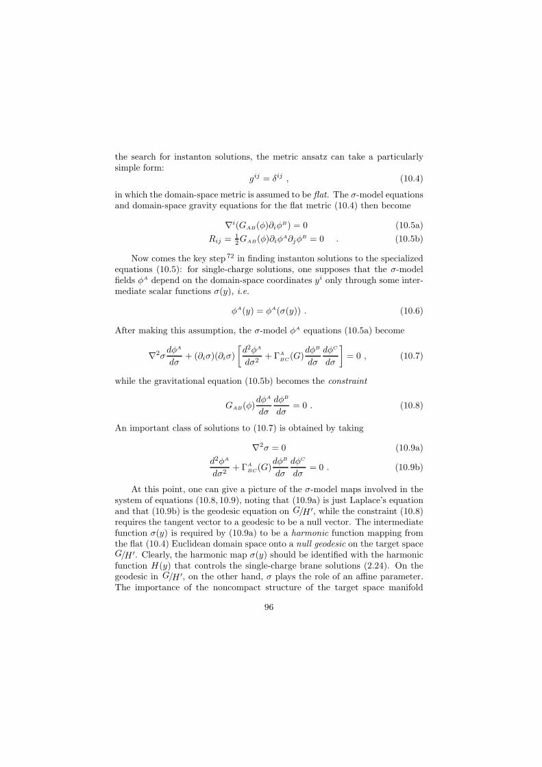
the search for instanton solutions, the metric ansatz can take a particularlysimple form:

gij = δij , (10.4)

in which the domain-space metric is assumed to be flat. The σ-model equationsand domain-space gravity equations for the flat metric (10.4) then become

∇i(GAB(φ)∂iφB) = 0 (10.5a)

Rij =12GAB(φ)∂iφ

A∂jφB = 0 . (10.5b)

Now comes the key step 72 in finding instanton solutions to the specializedequations (10.5): for single-charge solutions, one supposes that the σ-modelfields φA depend on the domain-space coordinates yi only through some inter-mediate scalar functions σ(y), i.e.

φA(y) = φA(σ(y)) . (10.6)

After making this assumption, the σ-model φA equations (10.5a) become

∇2σdφA

dσ+ (∂iσ)(∂iσ)

[d2φA

dσ2+ ΓA

BC(G)

dφB

dσ

dφC

dσ

]= 0 , (10.7)

while the gravitational equation (10.5b) becomes the constraint

GAB(φ)dφA

dσ

dφB

dσ= 0 . (10.8)

An important class of solutions to (10.7) is obtained by taking

∇2σ = 0 (10.9a)

d2φA

dσ2+ ΓA

BC(G)dφB

dσ

dφC

dσ= 0 . (10.9b)

At this point, one can give a picture of the σ-model maps involved in thesystem of equations (10.8, 10.9), noting that (10.9a) is just Laplace’s equationand that (10.9b) is the geodesic equation on G/H ′, while the constraint (10.8)requires the tangent vector to a geodesic to be a null vector. The intermediatefunction σ(y) is required by (10.9a) to be a harmonic function mapping fromthe flat (10.4) Euclidean domain space onto a null geodesic on the target spaceG/H ′. Clearly, the harmonic map σ(y) should be identified with the harmonicfunction H(y) that controls the single-charge brane solutions (2.24). On thegeodesic in G/H ′, on the other hand, σ plays the role of an affine parameter.The importance of the noncompact structure of the target space manifold

96

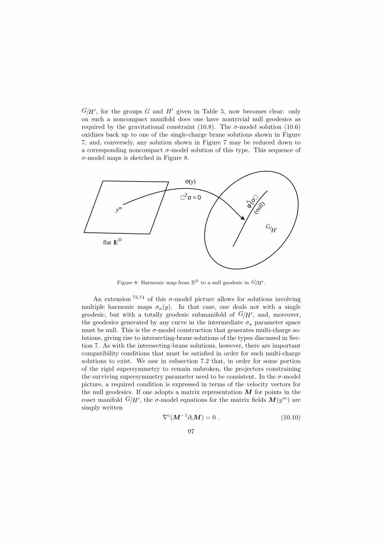
G/H ′, for the groups G and H ′ given in Table 5, now becomes clear: onlyon such a noncompact manifold does one have nontrivial null geodesics asrequired by the gravitational constraint (10.8). The σ-model solution (10.6)oxidizes back up to one of the single-charge brane solutions shown in Figure7, and, conversely, any solution shown in Figure 7 may be reduced down toa corresponding noncompact σ-model solution of this type. This sequence ofσ-model maps is sketched in Figure 8.

ym

flat EI D

σ(y)

∇ σ = 02

φ (σ)

A

GH'/

(nul

l)

Figure 8: Harmonic map from ED to a null geodesic in G/H′.

An extension 73,74 of this σ-model picture allows for solutions involvingmultiple harmonic maps σa(y). In that case, one deals not with a singlegeodesic, but with a totally geodesic submanifold of G/H ′, and, moreover,the geodesics generated by any curve in the intermediate σa parameter spacemust be null. This is the σ-model construction that generates multi-charge so-lutions, giving rise to intersecting-brane solutions of the types discussed in Sec-tion 7. As with the intersecting-brane solutions, however, there are importantcompatibility conditions that must be satisfied in order for such multi-chargesolutions to exist. We saw in subsection 7.2 that, in order for some portionof the rigid supersymmetry to remain unbroken, the projectors constrainingthe surviving supersymmetry parameter need to be consistent. In the σ-modelpicture, a required condition is expressed in terms of the velocity vectors forthe null geodesics. If one adopts a matrix representation M for points in thecoset manifold G/H ′, the σ-model equations for the matrix fields M (ym) aresimply written

∇i(M−1∂iM ) = 0 . (10.10)

97

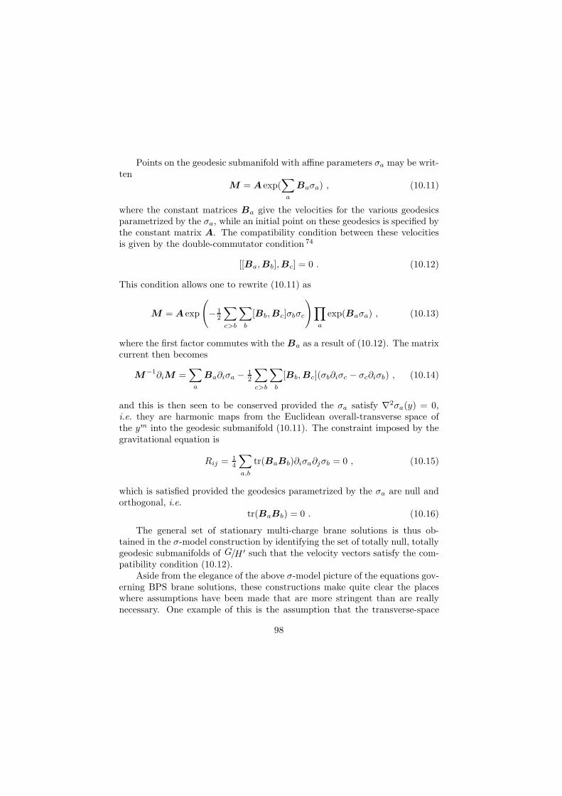
Points on the geodesic submanifold with affine parameters σa may be writ-ten

M = A exp(∑

a

Baσa) , (10.11)

where the constant matrices Ba give the velocities for the various geodesicsparametrized by the σa, while an initial point on these geodesics is specified bythe constant matrix A. The compatibility condition between these velocitiesis given by the double-commutator condition 74

[[Ba,Bb],Bc] = 0 . (10.12)

This condition allows one to rewrite (10.11) as

M = A exp

(− 1

2

∑

c>b

∑

b

[Bb,Bc]σbσc

)∏

a

exp(Baσa) , (10.13)

where the first factor commutes with the Ba as a result of (10.12). The matrixcurrent then becomes

M−1∂iM =

∑

a

Ba∂iσa − 12

∑

c>b

∑

b

[Bb,Bc](σb∂iσc − σc∂iσb) , (10.14)

and this is then seen to be conserved provided the σa satisfy ∇2σa(y) = 0,i.e. they are harmonic maps from the Euclidean overall-transverse space ofthe ym into the geodesic submanifold (10.11). The constraint imposed by thegravitational equation is

Rij =14

∑

a,b

tr(BaBb)∂iσa∂jσb = 0 , (10.15)

which is satisfied provided the geodesics parametrized by the σa are null andorthogonal, i.e.

tr(BaBb) = 0 . (10.16)

The general set of stationary multi-charge brane solutions is thus ob-tained in the σ-model construction by identifying the set of totally null, totallygeodesic submanifolds of G/H ′ such that the velocity vectors satisfy the com-patibility condition (10.12).

Aside from the elegance of the above σ-model picture of the equations gov-erning BPS brane solutions, these constructions make quite clear the placeswhere assumptions have been made that are more stringent than are reallynecessary. One example of this is the assumption that the transverse-space

98

geometry is flat, Eq. (10.4). This is clearly more restrictive than is reallynecessary; one could just as well have a more general Ricci-flat domain-spacegeometry, with a correspondingly covariantized constraint for the null geodesicson the noncompact manifold G/H ′. The use of more general Ricci-flat trans-verse geometries is at the basis of “generalized p-brane” solutions that havebeen considered in Refs.77,78

11 Concluding remarks

In this review, we have discussed principally the structure of classical p-branesolutions to supergravity theories. Some topics that deserve a fuller treatmenthave only been touched upon here. In particular, we have covered only ina cursory fashion the important topic of κ-invariant p-brane worldvolume ac-tions. There are wider classes of worldvolume actions than we have considered,involving excitations other than worldvolume spinors and scalars. For a fullertreatment, the reader is referred to Refs4,7, or to the discussions of κ-symmetricactions for cases involving R–R sector antisymmetric-tensor fields.79

An important extension of this subject is the remarkable duality betweenworldvolume dynamics and bulk dynamics known as AdS/CFT duality.80 Theoriginal and potentially the most physically relevant example of this occurs inthe theory of stacks of N D3 branes in type IIB supergravity. A single D3brane has a worldvolume theory described by D = 4, N = 4 super Maxwelltheory, and example of a worldvolume multiplet involving more than spinorsand scalars. In type IIB string theory, the extra excitations coming from shortstrings linking the leaves of the stack extend the corresponding U(1)N abeliangauge symmetry to a full nonabelian U(N). The AdS/CFT duality expressesthe equivalence between the dynamics of these solitonic excitations on theworldvolume and full type IIB string theory in the spacetime bulk.

Another aspect of the p-brane story, which we have only briefly presentedhere in Section 7, is the large family of intersecting branes. These include78 alsointersections at angles other than 90, and can involve fractions of preservedsupersymmetry other than inverse powers of 2. For a fuller treatment of someof these subjects, the reader is referred to Ref.48,50, and for the implicationsof charge conservation in determining the allowed intersections to Refs. 21

Yet another aspect of this subject that we have not dwelt upon here isthe intrinsically string-theoretic side, in which some of the BPS supergravitysolutions that we have discussed appear as Dirichlet surfaces on which openstrings can end; for this, we refer the reader to Ref.9

Of course, the real fascination of this subject lies in its connection to theemerging picture in string theory/quantum gravity, and in particular to the

99

roles that BPS supergravity solutions play as states stable against the effects ofquantum corrections. In this emerging picture, the duality symmetries that wehave discussed in Section 8 play an essential part, uniting the underlying typeIIA, IIB, E8×E8 and SO(32) heterotic, and also the type I string theories intoone overall theory, which then also has a phase with D = 11 supergravity asits field-theory limit. The usefulness of classical supergravity considerations inprobing the structure of this emerging “M theory” is one of the major surprisesof the subject.

Acknowledgments

The author would like to acknowledge helpful conversations with Marcus Bre-mer, Bernard de Wit, Mike Duff, Francois Englert, Gary Gibbons, Hong Lu,George Papadopoulos, Chris Pope, and Paul Townsend.

References

1. E. Cremmer, B. Julia and J. Scherk, Phys. Lett. B 76, 409 (1978).2. D.N. Page, Phys. Rev. D 28, 2976 (1983).3. J.W. van Holten and A. van Proeyen, “N = 1 Supersymmetry Algebras

in D = 2, D = 3, D = 4 mod-8,” J. Phys. A15, 3763 (1982).4. K.S. Stelle and P.K. Townsend, “Are 2-branes better than 1?” in Proc.

CAP Summer Institute, Edmonton, Alberta, July 1987, KEK libraryaccession number 8801076.

5. P.S. Howe and K.S. Stelle, “The Ultraviolet Properties ofSupersymmetric Field Theories,” Int. J. Mod. Phys. A 4, 1871 (1989).

6. P.K. Townsend, “Three lectures on supersymmetry and extendedobjects,” in Integrable Systems, Quantum Groups and Quantum FieldTheories (23 rd GIFT Seminar on Theoretical Physics, Salamanca,June, 1992), eds L.A. Ibort and M.A. Rodriguez (Kluwer, 1993).

7. M.J. Duff, R.R. Khuri and J.X. Lu, “String solitons,” Physics Reports259, 213 (1995), hep-th/9412184;

8. M.J. Duff, “Supermembranes,” hep-th/9611203.

9. J. Polchinski, “Tasi Lectures on D-branes,” hep-th/9611050.

10. E.S. Fradkin and A.A. Tseytlin, Phys. Lett. B 158, 316 (1985); Nucl.Phys. B 261, 1 (1985).

11. C. Callan, D. Friedan, E. Martinec and M. Perry, Nucl. Phys. B 262,593 (1985).

12. A. Dabholkar, G. Gibbons, J.A. Harvey and F. Ruiz Ruiz,“Superstrings and Solitons,” Nucl. Phys. B 340, 33 (1990).

100

13. H. Lu, C.N. Pope, E. Sezgin and K.S. Stelle, “Stainless Superp-branes,” Nucl. Phys. B 456, 669 (1996), hep-th/9508042.

14. I.C. Campbell and P.C. West, Nucl. Phys. B 243, 112 (1984);F. Giani and M. Pernici, Phys. Rev. D 30, 325 (1984);M. Huq and M.A. Namazie, Class. Quantum Grav. 2, 293 (1985); ibid.2, 597 (1985).

15. M.B. Green and J.H. Schwarz, Phys. Lett. B 122, 143 (1983);J.H. Schwarz and P.C. West, Phys. Lett. B 126, 301 (1983);J.H. Schwarz, Nucl. Phys. B 226, 269 (1983);P.S. Howe and P.C. West, Nucl. Phys. B 238, 181 (1984).

16. C.W. Misner, K.S. Thorne and J.A. Wheeler, Gravitation (W.H.Freeman and Co., San Francisco, 1973), Box 14.5.

17. H. Lu, C.N. Pope, E. Sezgin and K.S. Stelle, “Dilatonic p-branesolitons,” Nucl. Phys. B 371, 46 (1996), hep-th/9511203.

18. M.J. Duff and K.S. Stelle, “Multi-membrane solutions of D = 11Supergravity,” Phys. Lett. B 253, 113 (1991).

19. G.W. Gibbons and P.K. Townsend, Phys. Rev. Lett. 71, 3754 (1993),hep-th/9302049;

M.J. Duff, G.W. Gibbons and P.K. Townsend, Phys. Lett. B 332, 321(1994), hep-th/9405124.

20. E. Bergshoeff, E. Sezgin and P.K. Townsend, Phys. Lett. B 189, 75(1987).

21. E. Witten, “Bound states of strings and p-branes,” Nucl. Phys. B 460,335 (1996), hep-th/9510135;M.R. Douglas, “Branes within branes,” hep-th/9512077;

P.K. Townsend, “Brane Surgery,”in Proc. European Res. Conf. onAdvanced Quantum Field Theory, La Londe-les-Maures, Sept. 1996,hep-th/9609217;

G. Papadopoulos, “Brane surgery with Thom classes,” JHEP 9905 020(1999), hep-th/9905073.

22. M.J. Duff, P.S. Howe, T. Inami and K.S. Stelle, “Superstrings in D = 10from Supermembranes in D = 11,” Phys. Lett. B 191, 70 (1987).

23. H. Lu, C.N. Pope and K.S. Stelle, “Vertical Versus DiagonalDimensional Reduction for p-branes,” Nucl. Phys. B 481, 313 (1996),hep-th/9605082.

24. S.W. Hawking and G.F.R. Ellis, The Large-Scale Structure ofSpace-Time, (Cambridge University Press, 1973).

25. R. Guven, “Black p-brane solutions of D = 11 supergravity theory,”Phys. Lett. B 276, 49 (1992).

26. G.W. Gibbons, G.T. Horowitz and P.K. Townsend, Class. Quantum

101

Grav. 12, 297 (1995), hep-th/9410073.27. G. Horowitz and A. Strominger, Nucl. Phys. B 360, 197 (1991);

M.J. Duff and J.X. Lu, Nucl. Phys. B 416, 301 (1994),hep-th/9306052.

28. M.J. Duff, H. Lu and C.N. Pope, “The Black Branes of M -theory,”Phys. Lett. B 382, 73 (1996), hep-th 9604052.

29. J.A. de Azcarraga, J.P. Gauntlett, J.M. Izquierdo and P.K. Townsend,Phys. Rev. Lett. 63, 2443 (1989).

30. G.W. Gibbons and C.M. Hull, Phys. Lett. B 109, 190 (1982).31. H. Lu and C.N. Pope, p-brane solitons in maximal supergravities, Nucl.

Phys. B 465, 127 (1996), hep-th/9512012.32. H. Lu and C.N. Pope, “An approach to the classification of p-brane

solitons,” hep-th/9601089.

33. P.S. Howe and R.W. Tucker, J. Phys. A 10, L155 (1977).34. I. Bandos, D. Sorokin and and D.V. Volkov, “On the Generalized

Action Principle for Superstrings and Superbranes,” Phys. Lett. B 352,269 (1995), hep-th/9502141;I. Bandos, P. Pasti, D. Sorokin, M. Tonin and D.V. Volkov,“Superstrings and Supermembranes in the Doubly SupersymmetricGeometrical Approach,” Nucl. Phys. B 446, 79 (1995),hep-th/9501113.

35. E. Bergshoeff, E. Sezgin and P.K. Townsend Ann. Phys. 185, 330(1988).

36. A. Achucarro, J.M. Evans, P.K. Townsend and D.L. Wiltshire, Phys.Lett. B 198, 441 (1987).

37. R. Khuri, Nucl. Phys. B 387, 315 (1992), hep-th/9205081;J.P. Gauntlett, J.A. Harvey and J.T. Liu, Nucl. Phys. B 409, 363(1993), hep-th/9211056.

38. B.R. Greene, A. Shapere, C. Vafa and S-T. Yau, Nucl. Phys. B 337, 1(1990);G.W. Gibbons, M.B. Green and M.J. Perry, Phys. Lett. B 370, 37(1996), hep-th/9511080.

39. P.M. Cowdall, H. Lu, C.N. Pope, K.S. Stelle and P.K. Townsend,“Domain Walls in Massive Supergravities,” Nucl. Phys. B 486, 49(1997), hep-th/9608173.

40. J. Scherk and J.H. Schwarz, Phys. Lett. B 82, 60 (1979).41. E. Bergshoeff, M. de Roo, M.B. Green, G. Papadopoulos and P.K.

Townsend, “Duality of Type II 7-branes and 8-branes,” Nucl. Phys. B470, 113 (1996), hep-th/9601150.

42. N. Kaloper, R.R. Khuri and R.C. Myers, “On generalized axion

102

reductions,” Phys. Lett. B 428, 297 (1998), hep-th/9803066.43. H. Lu and C.N. Pope, “Domain walls from M-branes,” Mod. Phys.

Lett. A 12, 1087 (1997), hep-th/9611079;I.V. Lavrinenko, H. Lu and C.N. Pope, “From topology to generalizeddimensional reduction,” Nucl. Phys. B 492, 278 (1997),hep-th/9611134.

44. M. Cvetic, “Extreme domain wall — black hole complementarity inN = 1 supergravity with a general dilaton coupling,” Phys. Lett. B341, 160 (1994).

45. M. Cvetic and H.H. Soleng, “Supergravity domain walls,” PhysicsReports 282, 159 (1997), hep-th/9604090.

46. J. Rahmfeld, Phys. Lett. B 372, 198 (1996), hep-th/9512089;N. Khviengia, Z. Khviengia, H. Lu and C.N. Pope, “IntersectingM-branes and Bound States,” Phys. Lett. B 388, 21 (1996),hep-th/9605077;

M.J. Duff and J. Rahmfeld, “Bound States of Black Holes and Otherp-branes,” Nucl. Phys. B 481, 332 (1996), hep-th/9605085.

47. H.W. Brinkmann, Proc. Nat. Acad. Sci. 9, 1 (1923).48. G. Papadopoulos and P.K. Townsend, “Intersecting M-branes,” Phys.

Lett. B 380, 273 (1996), hep-th/9603087;A. Tseytlin, “Harmonic superpositions of M-branes,” Nucl. Phys. B475, 149 (1996);I.R. Klebanov and A.A. Tseytlin, “Intersecting M-branes asfour-dimensional black holes,” Nucl. Phys. B 475, 179 (1996);K. Berndt, E. Bergshoeff and B. Janssen, “Intersecting D-branes in tendimensions and six dimensions,” Phys. Rev. D 55, 3785 (1997),hep-th/9604168;

J. Gauntlett, D. Kastor and J. Traschen, “Overlapping branes inM-theory,” Nucl. Phys. B 478, 544 (1996).

49. R. Sorkin, Phys. Rev. Lett. 51, 87 (1983);D.J. Gross and M.J. Perry, Nucl. Phys. B 226, 29 (1983).

50. J.P. Gauntlett, “Intersecting Branes,” hep-th/9705011.

51. A.A. Tseytlin, “ ‘No force’ condition and BPS combinations of p-branesin eleven dimensions and ten dimensions,” Nucl. Phys. B 487, 141(1997), hep-th/9609212.

52. K. Shiraishi, Nucl. Phys. B 402, 399 (1993).53. G.W. Gibbons, G. Papadopoulos and K.S. Stelle, “HKT and OKT

geometries on soliton black hole moduli spaces,” Nucl. Phys. B 508,623 (1997), hep-th/9706207.

54. R. Coles and G. Papadopoulos, “The geometry of one-dimensional

103

supersymmetric non-linear sigma models,” Class. Quantum Grav. 7,427 (1990).

55. E. Cremmer and B. Julia, Nucl. Phys. B 159, 141 (1979).56. J.M. Izquierdo, N.D. Lambert, G. Papadopoulos and P.K. Townsend,

“Dyonic Membranes,” Nucl. Phys. B 460, 560 (1996),hep-th/9508177.

57. R. Nepomechie, “Magnetic monopoles from antisymmetric tensor gaugefields,” Phys. Rev. D 31, 1921 (1985).

58. C. Teitelboim, Phys. Lett. B 67, 63, 69 (1986).59. M. Bremer, H. Lu, C.N. Pope and K.S. Stelle, “Dirac quantisation

conditions and Kaluza-Klein reduction,” Nucl. Phys. B 529, 259(1998), hep-th/9710244.

60. S. Deser, A. Gomberoff, M. Henneaux and C. Teitelboim, “Duality,self-duality, sources and charge quantisation in Abelian N-formtheories,” Phys. Lett. B 400, 80 (1997), hep-th/9702184.

61. H. Lu, C.N. Pope and K.S. Stelle, “Weyl Group Invariance and p-braneMultiplets,” Nucl. Phys. B 476, 89 (1996), hep-th/9602140.

62. C.M. Hull and P.K. Townsend, Nucl. Phys. B 438, 109 (1995),hep-th/9410167.

63. E. Witten, “String theory dynamics in various dimensions,” Nucl.Phys. B 443, 85 (1995).

64. M.J. Duff and J. Rahmfeld, “Bound States of Black Holes and Otherp-branes,” Nucl. Phys. B 481, 332 (1996), hep-th/9605085.

65. J.H. Schwarz, “The power of M-theory,” Phys. Lett. B 367, 97 (1996),hep-th/9510086.

66. T.H. Buscher, “A symmetry of the string background field equations,”Phys. Lett. B 194, 69 (1987);A. Giveon, M. Porrati and E. Rabinovici, “Target space duality instring theory,” Physics Reports 244, 77 (1994), hep-th/9401139.

67. A. Sen, “Electric and magnetic duality in string theory,” Nucl. Phys. B404, 109 (1993), hep-th/9207053;“SL(2,Z) duality and magnetically charged strings,” Int. J. Mod.Phys. A 8, 5079 (1993), hep-th/9302038.

68. E. Cremmer, H. Lu, C.N. Pope and K.S. Stelle, “Spectrum-generatingsymmetries for BPS Solitons,” Nucl. Phys. B 520, 132 (1998),hep-th/9707207.

69. J.H. Schwarz, “An SL(2,Z) multiplet of type IIB superstrings,” Phys.Lett. B 360, 13 (1995); Erratum ibid. 364, 252 (1995),hep-th/9508143.

70. E. Bergshoeff, C.M. Hull and T. Ortin, “Duality in the type II

104

superstring effective action,” Nucl. Phys. B 451, 547 (1995),hep-th/9504081.

71. E. Cremmer, B. Julia, H. Lu and C.N. Pope, “Dualisation of dualities,I,” Nucl. Phys. B 523, 73 (1998), hep-th/9710119.

72. G. Neugebaur and D. Kramer, Ann. der Physik (Leipzig) 24, 62 (1969).73. P. Breitenlohner, D. Maison and G. Gibbons, Comm. Math. Phys.

120, 253 (1988).74. G. Clement and D. Gal’tsov, “Stationary BPS solutions to dilaton-axion

gravity,” Phys. Rev. D 54, 6136 (1996), hep-th/9607043;D.V. Gal’tsov and O.A. Rytchkov, “Generating branes viasigma-models,” Phys. Rev. D 58, 122001 (1998), hep-th/9801160.

75. H. Lu and C.N. Pope, “Multi-scalar p-brane solitons,” Int. J. Mod.Phys. A 12, 437 (1997), hep-th/9512153.

76. N. Khviengia, Z. Khviengia, H. Lu and C.N. Pope, “IntersectingM-branes and bound states,” Phys. Lett. B 388, 21 (1996),hep-th/9605077.

77. K. Becker and M. Becker, “M-theory on eight-manifolds,” Nucl. Phys.B 477, 155 (1996), hep-th/9605053.

78. M. Berkooz, M.R. Douglas and R.G. Leigh, “Branes intersecting atangles,” Nucl. Phys. B 480, 265 (1996), hep-th/9606139;J.P. Gauntlett, G.W. Gibbons, G. Papadopoulos and P.K. Townsend,“HyperKahler manifolds and multiply intersecting branes,” Nucl. Phys.B 500, 133 (1997), hep-th/9702202.

79. P.S. Howe and E. Sezgin, “Superbranes,” Phys. Lett. B 390, 133(1997), hep-th/9607227;P.S. Howe and E. Sezgin, “D = 11, p = 5,” Phys. Lett. B 394, 62(1997), hep-th/9611008;M. Cederwall, A. von Gussich, B.E.W. Nilsson and A. Westerberg,“The Dirichlet Super Three Brane in Ten-Dimensional Type IIBSupergravity,” Nucl. Phys. B 490, 163 (1997), hep-th/9610148;M. Aganagic, C. Popescu and J.H. Schwarz, “D-brane actions with localkappa-symmetry,” Phys. Lett. B 393, 311 (1997), hep-th/9610249;M. Cederwall, A. von Gussich, B.E.W. Nilsson, P. Sundell and A.Westerberg, “The dirichlet super p-branes in ten-dimensional Type IIAand IIB supergravity,” Nucl. Phys. B 490, 179 (1997),hep-th/9611159;

E. Bergshoeff and P.K. Townsend, “Super D-branes,” Nucl. Phys. B490, 145 (1997), hep-th/9611173.I. Bandos, D. Sorokin and M. Tonin, “Generalized Action Principle andSuperfield Equations of Motion for d = 10 D-p-branes,” Nucl. Phys. B

105

497, 275 (1997), hep-th/9701127.80. I. Klebanov, “Tasi Lectures: Introduction to the AdS-CFT

correspondence,” hep-th/0009139.

106