Thermoelastic stability of a double-layered spherical shell

International Journal of Non-Linear Mechanics 41 (2006) 1016–1027www.elsevier.com/locate/nlm

Thermoelastic stability of a double-layered spherical shell

M. Batistaa,∗, F. Koselb

aFaculty of Maritime Studies and Transportation, University of Ljubljana, Pot pomorscakov 4, SI-6320 Portoroz, Slovenia, EUbFaculty of Mechanical Engineering, University of Ljubljana, Askerceva 6, SI-1000 Ljubljana, Slovenia, EU

Received 17 October 2006; accepted 21 October 2006

Abstract

In the paper the axi-symmetrical thermoelastic stability of free double-layered spherical shells at uniform temperature is considered.The basic equations are derived from Reissner’s theory of thin shells and assumptions that materials of the layers are linear thermoelastic.The conditions for the buckling of shells are determined. The temperature-deflection diagrams are calculated by using the collocationmethod.� 2006 Elsevier Ltd. All rights reserved.

Keywords: Spherical shell; Thermoelasticity; Stability; Snap-through buckling

1. Introduction

The subject of the present paper has its origins in the old andwell-known problem of the theromoelastic stability of shallowbimetallic shells. This problem was first studied by Panev [1]and Wittrick [2], who independently derived the general equa-tions of the problem, calculated the critical temperature andinitial height for buckling, as well the temperature-deflectiondiagrams from which buckling temperature can be determined.Later Aggarwala and Saibel [3] considered shallow bimetal-lic spherical shells subject to simply supported boundary con-ditions and Liu Ren-Huai [4] considered shallow bimetallicspherical shells with a hole at the apex and also bimetallic trun-cated shallow conical shells. Recently the authors [5] of thispaper provided a study of the thermoelastic stability of bimetal-lic shallow shells of revolution in which Poisson’s ratios werenot equal.

From the review of the available literature the present authorsfound that only the stability of bimetallic shallow sphericalshells was studied. The purpose of this paper is to extend thethermoelastic stability analysis to general thin double-layeredspherical shells and in this way among others obtain some

∗ Corresponding author. Tel.: +386 5 6767219; fax: +386 5 6767130.E-mail address: [email protected] (M. Batista).

0020-7462/$ - see front matter � 2006 Elsevier Ltd. All rights reserved.doi:10.1016/j.ijnonlinmec.2006.10.016

insight as to how good a shallow shell approximation is. Forthe theoretical basis of the treatment the non-linear thin shellsof revolution theory is adopted [6,7].

2. Basic equations

Consider a weightless double-layered spherical shell of ra-dius a and constant thickness h heated up to the uniform tem-perature ϑ above reference stress free state. It is assumed thatthe temperature does not vary through the shell and that noexternal loads are applied on its surface. It is also assumed thatthe materials of the layers are homogeneous and isotropic ther-moelastic and that the strains are linearly distributed across theshell.

2.1. Geometry

In the reference state, the geometry of the reference sur-face of the spherical shell may be represented by cylindri-cal coordinates r, �, z by parametric equations of the form(Fig. 1)

r = a sin �, z = a(1 − cos �), (1)

where � is the meridian angle, which is also the tangent angleof the meridians. If H0 �a is the overall shell height then the

http://www.elsevier.com/locate/nlm

mailto:[email protected]

M. Batista, F. Kosel / International Journal of Non-Linear Mechanics 41 (2006) 1016–1027 1017

Fig. 1. The geometry of the spherical shell.

shell’s outer radius a0 and end angle �0 are given by

a0 = a

√2�0 − �2

0, �0 = arccos(1 − �0),

�0 ≡ H0

a∈ (0, 1], (2)

where �0 is the dimensionless shell height.The geometry of a deformed shell is described by the fol-

lowing differential equations:

dR

ds= (1 + �1) cos � − � sin �,

dZ

ds= (1 + �1) sin � + � cos �,

d�

ds= d�

ds+ �1, (3)

where ds = a d� = dr/ cos �, R and Z are the radial and axialcoordinates of the deformed reference surface, � is the tangentangle of the meridians of the deformed reference surface, �1is the meridional strain, � is the shear strain and �1 is themeridional strain measure. The circumferential strain �2 andthe circumferential strain measure �2 are defined by

�2 = R − r

r, �2 = sin � − sin �

r. (4)

2.2. Equilibrium equations

For weightless shells with no external loads applied on thesurface, the equilibrium equations may be written in the form

d

ds= N2,

dM1

ds= M2 cos � − M1 cos �

r− [(1 + �1)Q − �N1], (5)

where is a stress function, N2 is the circumferential stressresultant per unit of undeformed length, and M1 and M2 arethe meridional and the circumferential bending stress couplesper unit of undeformed length. The meridional and shear stressresultant per unit of undeformed length N1, Q are expressed interms of as

N1 = cos �

r, Q = −

sin �

r. (6)

2.3. Constitutive equations

Let h(1) and h(2) be the constant thickness of the shell layerswhere h = h(1) + h(2), E(1) and E(2) are its Young’s modulus,and (1) and (2) its coefficients of thermal expansion where itis assumed that (1) > (2). For future use, the following ratiosof the listed quantities are introduced:

ch ≡ h(2)

h(1)

, cE ≡ E(2)

E(1)

, c ≡ (2)

(1)

, (7)

where 0 < ch, cE < ∞ and 0 < c < 1.Let Poisson’s ratios of the shell layers be �(1) and �(2). Having

in view that especially for metallic materials Poisson’s ratiosexhibit marginal variations in their values the assumption ismade that they are equal

�(1) = �(2) = �. (8)

As is well known [8] this assumption enables the setting ofthe position of the reference surface in such a way that nobending–stretching coupling exists in constitutive equations andthus the double-layered shells become equivalent to a single-layered shell. As can be shown [4,5,8], for the case of double-layered shells the appropriate position of the reference surfaceof the shell for bending–stretching decoupling is at distance h0from the internal surface, which is given by

h0 = h

2

[1 + chcE(2 + ch)](1 + ch)(1 + chcE)

. (9)

The material responses of the shell are, besides �, governedby the shell extensional stiffness B, the bending stiffness D

and the reduced coefficient of thermal expansion , which aredefined, respectively, as

B ≡ hE

1 − �2 fB(ch, cE), D ≡ h2B

12fD(ch, cE),

≡ f(ch, cE, c), (10)

where

fB(ch, cE) ≡ 2(1 + chcE)

(1 + ch)(1 + cE),

f(ch, cE, c) ≡ 2(1 + chcEc)

(1 + c)(1 + chcE),

fD(ch, cE) ≡ (1 + c3hcE)(1 + chcE) + 3chcE(1 + ch)

2

(1 + ch)2(1 + chcE)2 (11)

and where

E = 12 (E1 + E2), = 1

2 (1 + 2). (12)

The average Young modulus E and average coefficients of ther-mal expansion are introduced in order to ensure that the func-tions (11) remain bounded. It can be shown that the bounds are

0 < fB(ch, cE) < 2, 0 < fD(ch, cE) < 43 ,

0 < f(ch, cE, c) < 2. (13)

1018 M. Batista, F. Kosel / International Journal of Non-Linear Mechanics 41 (2006) 1016–1027

Also in the case ch = cE = 1 one has

fB(1, 1) = fD(1, 1) = f(1, 1, c) = 1 (14)

so (10) simplifies to

B = hE

1 − �2 , D = h2B

12, = . (15)

The constitutive equations may now be written in the form

N1

B= �1 + ��2 − (1 + �)ϑ,

N2

B= �2 + ��1 − (1 + �)ϑ,

Q

B= (1 − �)

2�,

M1

D= �1 + ��2 + 3

2(1 + �)

�

hf h

ϑ,

M2

D= �2 + ��1 + 3

2(1 + �)

�

hf h

ϑ, (16)

where

� ≡ (1) − (2) = 21 − c

1 + c,

fh(ch, cE) ≡ 3

4+ (1 + c3

hcE)(1 + chcE)

4chcE(1 + ch)2 . (17)

It can be shown that fh(ch, cE)�1 where equality holds inthe case ch = cE = 1. Note that if either of the materials isextremely thin or extremely soft relative to the other—i.e., ifch, cE → 0 or ch, cE → ∞—then fh → ∞. In this case thelast terms in the Eqs. (16)4,5 become marginal and so such ashell is temperature insensitive.

2.4. Boundary value problem

Eqs. (3)–(16) represent 14 equations for three geometricalunknowns R, Z, �, five unknown strains �1, �2, �1, �2, �, stressfunction , three stress resultants N1, N2, Q and two stresscouples resultants M1, M2, and thus form the complete sys-tem of equation of the problem. The inputs are temperature ϑand six material parameters �, B, D, , �, and hf h. Now,�1, �2, �1, �2, �, N1, N2, Q and M2 can by means of (4), (6) and(16) be expressed interms of R, �, and M1, which are un-knowns in the remaining system of five differential equations(3) and (5). These equations are to be solved subject to thefollowing boundary conditions: at s = 0 the regular conditionsmust hold

R(0) = 0, Z(0) = 0, �(0) = 0 (18)

and since by assumption the shell is free of load, at the shelledge one must have

(s0) = 0, M1(s0) = 0, (19)

where s0 = a�0.

2.5. Non-dimensionalization

The differential equations (3) and (5) are made dimensionlessby introducing the following dimensionless variables:

R∗ ≡ R

a(1+�)(1+0), Z∗ ≡ Z

a(1+�)(1+0), �∗ ≡a�,

∗ ≡

aB(1 + �)(1 + 0), M∗ ≡ aM

D, ϑ∗ ≡ ϑ

ϑ0, (20)

where on the basis of dimensional analysis the characteristictemperature ϑ0 is chosen to be

ϑ0 ≡ 2

3�

h

afh(ch, cE). (21)

Given this, the differential equations (3) and (5) may be writtenin the form

dR∗d�

= ∗2−(1+�)cos2�

(1−�) sin �−�R∗

cos �

sin �+ (1 + 0ϑ∗)

(1 + 0)cos �,

dZ∗d�

= −1+�

1−�∗

sin � cos �

sin �−�R∗

sin �

sin �+ (1 + 0ϑ∗)

(1+0)sin �,

d�

d�= M1∗ − �

sin �

sin �+ (1 + �)(1 − ϑ∗),

d∗d�

= �∗cos �

sin �+ (1 − �2)

[R∗

sin �− (1 + 0ϑ∗)

(1 + �)(1 + 0)

],

dM∗1

d�= M1∗

(� cos � − cos �)

sin �

+ (1 − �2)

[sin �

sin �− 1 + ϑ∗

]cos �

sin �

+ �2∗[−�R∗

sin �

sin2�+ (1 + 0ϑ∗)

(1 + 0)

sin �

sin �

−1 + �

1 − �∗

sin � cos �

sin2�

]. (22)

The boundary conditions (19) and (18) preserve the form andare

R∗(0) = 0, Z∗(0) = 0, �(0) = 0,

∗(�0) = 0, M1∗(�0) = 0. (23)

The dimensionless parameters 0 and � in (22) are defined by

0 ≡ ϑ0 = (1 + c)

3(1 − c)

h

af(ch, cE, c)fh(ch, cE),

� ≡ a(1 + �)(1 + 0)

√B

D

= a

h(1 + �)(1 + 0)

√12

fD(ch, cE). (24)

From the assumption c < 1 it follows that 0 < 0, � < ∞. Note,however, that the parameter 0 can be interpreted as temperaturedeformation of a free bar with at ϑ0 so that the upper limitof 0 is of the order of elastic deformation that the selected


materials can withstand. This is by assumption also a limit ofthe applicability of the present theory.

The solution of the boundary problem (24) and (23) providesthe unknowns Z∗, R∗, �, ∗ and M1∗ as functions of � andthe five input parameters ϑ∗, �, 0, � and �0. Note that thedimensionless form of the equations reduces the number ofrequired material parameters from six to three. Each solutionthus has for the given � and 0 theoretically infinitely manymaterial realizations; i.e., choices of values of �, ch, cE, c anda/h. However, for selected values of ch, cE , and �, one hasfrom (24) for the given � and 0 the unique solution for a/h

and c,

a

h= �

√fD(ch, cE)

2√

3(1 + �)(1 + 0),

c =320�(1 + chcE)

√fD(ch, cE) − 2

√3(1 + �)(1 + 0)fh(ch, cE)

320�(1 + chcE)

√fD(ch, cE) + 2

√3(1 + �)(1 + 0)chcEfh(ch, cE)

. (25)

Note that since by assumption c > 0 one has from (25) for theselect values for ch, cE , and � the following lower limits:

� >4√

3(1 + �)fh(ch, cE)

3(1 + chcE)√

fD(ch, cE)

(1 + 1

0

),

a

h>

2fh(ch, cE)

3(1 + chcE)

1

0. (26)

It is seen from this that when 0 → 0, �, a/h → ∞. Thus if thematerial of the layers can stand only a small elastic deformationthe shell should be very thin.

3. Simple solutions

3.1. Stress free state

Motivated by the solutions of shallow shells we first look forthe possible solutions of the shell’s stress free states. In this case

∗(�) = M1∗(�) = 0 (27)

and therefore by (5)1, (6) and (16)1,2,3 one has

N1∗(�) = N2∗(�) = Q∗(�) = �(�) = 0, �1 = �2 = 0ϑ∗.

(28)

The introduction of (27) into (22), taking into account boundaryconditions (23)1,2,3, yields

R∗(�) = (1 + 0ϑ∗)(1 + �)(1 + 0)

sin �,

sin � = (1 − ϑ∗) sin �, cos � = cos �,

Z∗(�) = (1 + 0ϑ∗)(1 + �)(1 + 0)

(1 − ϑ∗)(1 − cos �),

�(�) = (1 − ϑ∗)�. (29)

Finally, by means of (29), (3)3, (4)2 and (16)5 one finds

�1∗(�) = �2∗(�) = −ϑ∗, M2∗(�) = 0. (30)

The temperature ϑ∗ at which the shell is stress free is obtainedas follows. From (29)2,3 and the trigonometric identity sin2�+cos2� = 1 one obtains ϑ∗(2 − ϑ∗) = 0, so the two possiblesolutions are ϑ∗ = 0 and ϑ∗ = 2. A similar result is also knownfor stress free shallow shells [2,5]. Now, for the case ϑ∗ = 0the solution (28)2–(30)1 becomes

R∗(�) = sin �

(1 + �)(1 + 0), Z∗(�) = (1 − cos �)

(1 + �)(1 + 0),

�(�) = �,

�1(�) = �2(�) = �1∗(�) = �2∗(�) = 0 (31)

which corresponds to the reference shell geometry. In the caseϑ∗ = 2 the solution (29) is

R∗(�) = (1 + 20)

(1 + �)(1 + 0)sin �,

Z∗(�) = − (1 + 20)

(1 + �)(1 + 0)(1 − cos �), �(�) = −�,

�1(�) = �2(�) = 20, �1∗(�) = �2∗(�) = −2. (32)

This solution corresponds to the geometry of shells that areturned inside out with the shell radius a scaled by the factor1 + 20.

3.2. Flat state

Upon heating, the shells deform in such a way that theybecome flatter. At the critical temperature ϑc∗ at which theybecome flat one has

Z∗(�) = �(�) = 0. (33)

Using this, one finds from (3)2,3, (4)2, (6)2, (16)5, and (22)3,5,

�(�) = Q∗(�) = M2∗(�) = M1∗(�) = 0,

�1∗ = �2∗ = −1, ϑc∗ = 1. (34)

The remaining Eqs. (22)1,4 are

dR∗d�

= ∗sin �

− �R∗

sin �+ 1,

d∗d�

= �∗

sin �+ (1 − �2)

R∗sin �

+ (1 − �) (35)

and the corresponding boundary conditions (23) are

R∗(0) = 0, ∗(�0) = 0. (36)

The linear boundary value problem (35) and (36) has the ana-lytical solution obtained as follows: from (35)1 one can express


∗ in terms of R∗ as

∗ = sin �

(dR∗d�

− 1

)+ �R∗. (37)

The introduction of (37) into (35)2 gives a linear non-homogeneous second order differential equation for R∗,

d

d�

(sin �

dR∗d�

)− R∗

sin �= −(1 − cos �). (38)

This equation has the solution

R∗(�) = C1sin �

1 − cos �+ C2

1 − cos �

sin �

+ cos � − (1 + cos �) ln(1 + cos �)

sin �, (39)

where C1 and C2 are integration constants. Observe that all theterms in (39) are indefinite at �=0 so in order to determine oneof the integration constants from boundary condition (36)1 thefollowing method may be used. The asymptotic expansion ofthe solution at �=0 is R∗(�)=(2C1−2 ln 2+1)�−1+O(�), soto satisfy condition (36)1 one must set C1 = ln 2− 1

2 . Thereforethe final solution of (38) is

R∗(�, C2) = (2C2 − 1)1 − cos �

2 sin �

+ sin �[ln 2 − ln(1 + cos �)]1 − cos �

. (40)

Introducing (40) into (37) gives the expression for ∗ in theform

∗(�, �, C2) = (2C2 − 1)(1 + �)(1 − cos �)

2 sin �− (1 − �)

× (1 + cos �)[ln 2 − ln(1 + cos �)]sin �

. (41)

Note that at � = 0 this function is indeterminate; however, onehas lim�→0∗(�)=0. Introducing (41) into boundary condition(36)2 gives the second integration constant

C2(�, �0)

= 1

2+ (1 − �)(1 + cos �0)[ln 2 − ln(1 + cos �0)]

(1 + �)(1 − cos �0). (42)

This expression is indeterminate for � = 0 and � = . Thecorresponding limit values are lim�→0C2 = (3 − �)/2(1 + �)and lim�→ C2 → 1

2 . Note also that the solutions (40) and (41)are valid for 0��0 � .

To obtain stress resultants N1∗(�) and N2∗(�) expression(41) is introduced into (5)1 and (6)1. The typical distributionof stress resultants are shown in Fig. 2. As is seen, the stressresultant N1∗(�) is negative over the whole shell meridian andmonotonically decreases to zero at the shell’s edge. The stressresultant N2∗(�) is negative in the neighbourhood of � = 0,while near the shell’s edge its values become positive. For asmall �0 the angle at which N2∗(�s) = 0 is approximately

�s ≈ 2�0√12 − �2

0

(43)

Fig. 2. Stress resultants N1∗ (�) and N2∗ (�) versus � in the shell’s flat statefor � = 0.3 and �0 = 0.1.

and as is seen it is independent for �. For �0 < 0.6 the formulagives the angle differing from the exact value by less than 5%.Take the examples for � = 0.3 and �0 = 0.1: the exact result is�s = 0.26139, while (43) gives �s ≈ 0.26264, which is abouta 0.5% relative error. For �0 =0.5 the exact value is �s =0.617and approximated is �s ≈ 0.634, which is about a 3% relativeerror.

Of particular interest are the stress resultants’ extreme values,which are at � = 0 and � = �0. If instead of the end angle �0the dimensionless shell height �0 is used then these values aregiven by

N1∗(0, �0, �) = N2∗(0, �0, �)

= − 1 − �

2

[1 − (2 − �0)[ln 2 − ln(2 − �0)]

�0

],

N2∗(�0, �0, �) = (1 − �)

[2[ln 2 − ln(2 − �0)]

�0− 1

]. (44)

The graphs of (44) are shown in Fig. 3.Once N1∗(�) and N2∗(�) are known one may obtain defor-

mations �1(�) and �2(�) from the constitutive equations (16)1,2.The maximal values of deformations are on the shell’s edgeand are given by

�1(�0, 0) = 0 + �(1 + 0)

[1 − 2

ln 2 − ln(2 − �0)

�0

],

�2(�0, 0) = (1 + 0)2[ln 2 − ln(2 − �0)]

�0− 1. (45)

For a very small �0 one has the expansion �1 =�2 =0 +O(�0).The graphs of (45) are shown in Fig. 4.

3.3. Shallow spherical shells

In order to compare the obtained flat state solution with theshallow spherical shell flat state solution [5] the expression forthe stress function (41) is expanded into the power series. For a


Fig. 3. Stress resultant N2∗ on the shell’s edge (solid lines) and the shell’sapex (dashed lines) as the function of the dimensionless shell height �0 forvarious values of �.

Fig. 4. Meridional strain �1 (dashed lines) and circumferential strain �2 (solidlines) on the shell’s edge at flat state as a function of dimensionless shellheight �0 for � = 0.3 and various values of 0.

small � one has ∗(�)=−((1− �)�20/16)�+ ((1− �)16)�3 +

O(�5). Also, for a small � one has r ≈ a� and a0 ≈ a�0;thus this series can be written in the form

∗(�) = − (1 − �)a30

16a3 �(1 − �2) + O(�5), (46)

where � ≡ r/a0. This result matches the solution for stressfunction given in Ref. [5].

4. Buckling analysis

In this section the conditions for the shell’s loss ofstability—i.e., its buckling—will be determined by analysingits flat state solution subject to small perturbations or, in otherwords, from a linearized system (22) regarding its flat state.

4.1. Linearization

It can be shown that the linearization of the system (22)regarding the flat state solution leads to the second order lineardifferential equation for perturbated value �(�) of the tangentangle of the meridians of the deformed reference surface, whichmay be written in the form

d2�

d�2 + cos �

sin �

d�

d�− (1 + �2�)

�

sin2�= 0, (47)

where

�(�, �0, �) ≡ ∗(�)

(−1 + �

1 − �∗(�, �0, �)

−�R∗(�, �0, �) + sin �

). (48)

The corresponding boundary conditions are, from (19)2 and(18)3,

�(0) = 0,d�

d�(�0) + �

�(�0)

sin �0= 0. (49)

The obtained eigenvalue problem (47) and (49) asks for valuesof � for which a non-zero solution of the problem exists. Theproblem can be solved by various analytical and numericalmethods. Here the power series method will be used.

4.2. Series solution

For obtaining a series solution of the boundary problem (47)and (49) the independent variable � is, by using (1)1, first re-placed by the independent variable r . By introducing dimen-sionless radii

� ≡ r

a, �0 ≡ a0

a(50)

and noting that, from (1), sin � = �, cos � = √1 − �2 and

d/d� = √1 − �2 d/d�, (47) and (49) transform to

�2(1 − �2)d2�

d�2 + �(1 − 2�2)d�

d�− (1 + �2 �)� = 0, (51)

�(0) = 0,

√1 − �2

0d�

d�(�0) + �

�(�0)

�0= 0, (52)

where � ∈ [0, �0]. To solve the stated boundary value problem,series expansion for � is first needed. By inspection of (51) itis found that this expansion has the form

�(�) =∞∑

n=0

Ln�2n+2. (53)

The coefficients Ln of this series are obtained as follows. From(40) and (37) one has

R∗(�) =∞∑

n=0

an�2n+1, ∗(�) =

∞∑n=0

bn�2n+1, (54)


where coefficients of these series are

a0 = 1

4+ C2

2, an =

(−1)n(

1/2n

)+ 2n(2n − 1)an−1

4n(n + 1)

[n = 1, 2, 3, . . .],b0 = (1 + �)a0 − 1,

bn = �an +n∑

k=0

(−1)n−k

(1/2

n − k

)(2k + 1)ak

[n = 1, 2, 3, . . .]. (55)

Substituting (54) into (48) gives the required formula for cal-culation of the coefficients

Ln ≡ bn −n∑

k=0

bn−k

(1 + �

1 − �bk + �ak

). (56)

The solution of (51) which satisfies (52)1 is now sought in theform

�(�) =∞∑

n=0

cn�2n+1, (57)

where cn are unknown coefficients that are to be determined.Introducing (57) and (53) into (51) yields the recurrence rela-tions

c1 = (2 + �L0)

8c0,

cn = 2n(2n − 1)cn−1 + �2∑n−1k=0Ln−k−1ck

4n(n + 1)

[n = 2, 3, . . .]. (58)

By successive application of (58) one can see that the coefficientcn can be represented as a polynomial of � in the form

cn = c0

n∑k=0

Cn,k�k [n = 1, 2, 3, . . .]. (59)

In order to obtain the coefficients Cn,k the above expressionis introduced into (58). Straightforward calculation gives thefollowing recursion relations:

C0,0 = 1,

Cn,0 = (2n − 1)Cn−1,0

2(n + 1), Cn,n = L0Cn−1,n−1

4n(n + 1),

Cn,k = 2n(2n − 1)Cn−1,k + ∑n−1j=k−1Ln−j−1Cj,k−1

4n(n + 1)

[n = 1, 2, . . . ; k = 1, 2, . . . , n − 1]. (60)

Substituting solution (57) into boundary condition (52)2 andtaking (59) into account finally yields the characteristic equa-tion∞∑

n=0

{ ∞∑k=n

Ck,n

[(2k + 1)

√1 − �2

0 + �

]�2k

0

}�2n = 0. (61)

The first positive zero of this transcendental equation gives therequired critical value of parameter �c(�, �0) at which �(�) =0, which means that the shell’s flat state becomes unstable.

4.3. Shallow spherical shells

The obtained results can be compared with the shallow spher-ical shell solution by expansion of (47) and (48) into series of� by making � small. This leads to the following equation:

�2 d2�

d�2 + �d�

d�− (1 + �2�)� + O(�6) = 0,

� = − (1 − �)

16(1 + �)(�4

0�2 − �4) + O(�6). (62)

Again, for a small � one has r ≈ a� and a0 ≈ a�0, so theabove equation is transformed into the Whittaker differentialequation

�2 d2�

d�2 + �d�

d�− (1 − �2�2 + �2�4)� = 0, (63)

where � ≡ r/a0 and where

�2 ≡ (1 − �)

16(1 + �)

(a0

a

)4�2. (64)

The solution of this equation, which is bounded at � = 0, is

�(�) = cM�/4,1/2(��2)/�, (65)

where M�,�(x) is the Whittaker function and c the integrationconstant. Substituting (65) into boundary condition (52)2 yieldsthe characteristic equation

[� − 2(� − 1)]M�/4,1/2(�) + (4 + �)M1+�/4,1/2(�) = 0

(66)

from which the critical �c(�) can be calculated. The obtainedcharacteristic equation is essentially the same as for the shallowspherical shells given in Ref. [5].

4.4. Critical shell height

From (61) one may obtain the critical value �c(�, �0) andthen by (25) one may, for selected material parameters, obtainthe critical ratio (a/h)c. By identity a/h = a/H0 × H0/h onecan also determine the critical shell height, which is given by

(H0/h)c = �0(a/h)c. (67)

However, in order to compare critical shell height values ofspherical shells and shallow spherical shells the following pa-rameter derived from (64) is introduced:

�c(�, �0) ≡ 1

4

√1 − �

1 + ��0(2 − �0)�c(�, �0). (68)

Observe that for spherical shells �c depends on � and �0, whilefor shallow spherical shells—as seen from the characteristicequation (66)—it depends only on �. Once �c is calculated, thecritical ratio (H0/h)c for shells to become unstable at the flat


Table 1Calculated critical values of �c and �c for various values of H0/a and �

H0/a\� �c �c

0.0 0.3 0.5 0.0 0.3 0.5

0.0001 576821.1 85446.8 113184.5 2.884426 3.134883 3.2671910.001 57691.4 8543.0 11316.0 2.882619 3.132850 3.2650070.01 5768.1 852.58 1129.13 2.864578 3.112475 3.2432120.05 575.79 168.98 223.62 2.784861 3.022495 3.1470080.1 114.25 83.526 110.42 2.686283 2.911353 3.0282790.2 56.553 40.785 53.808 2.492727 2.693553 2.7959580.3 27.697 26.527 34.921 2.30404 2.481817 2.5705790.4 18.071 19.388 25.464 2.120311 2.276254 2.3522630.5 13.252 15.095 19.779 1.941582 2.076950 2.1411150.6 10.355 12.223 15.976 1.767142 1.883599 1.9370120.7 8.415 10.154 13.246 1.593453 1.695102 1.7398660.8 7.004 8.610 11.237 1.417713 1.516335 1.557078

state can be calculated from the formula

(H0

h

)c

= 2�c(�, �0)

(2 − �0)

√fD(ch, cE)

3(1 − �2)

− (1 + c)

3(1 − c)�0fh(ch, cE)f(ch, cE, c) (69)

which is obtained by means of (10), (17), (24), and (68). Theformula contains five parameters: �0, �, ch, cE and c and itbecomes a bit simpler for ch = cE = 1,(

H0

h

)c

= 2�c(�, �0)

(2 − �0)√

3(1 − �2)− (1 + c)

3(1 − c)�0. (70)

The shallow shell solution is obtained if �0>1, so the abovebecomes(

H0

h

)c

= �c(�)√3(1 − �2)

+ O(�0)

which matches the result given in Ref. [5].

4.5. Numerical examples

The procedure for solving Eq. (61) for the critical value�c(�, �0) was implemented into a Maple worksheet. All thefloating-point calculations were performed by setting the num-ber of digits at 16. The values of �c(�, �0) were calculated asthe first positive root of the polynomial approximation of (61).The number of the series terms included into the polynomialwas determined by successive calculations of �c where at eachcalculation one more series term was added until the absoluteerror between successive solutions became less than 10−8. Inall the calculations this error was reached by including the first8–12 series terms. Results of the calculation are presented inTables 1 and 2, where Table 1 shows calculated values of the�c and �c as a function of � and �0 and Table 2 provides thecritical values of a/h for �=0.3, ch=cE =1 and various valuesof �0 and c.

Table 2Calculated critical values of a/h for �= 0.3, ch = cE = 1, and various valuesof H0/a and c

H0/a c

0.20 0.4 0.6 0.8

0.0001 18973.6 4212.5 934.1 204.40.001 1896.5 420.4 92.0 17.40.01 188.8 41.2 7.8 –0.05 37.0 7.4 0.3 –0.1 18.0 3.2 – –0.2 8.6 1.1 – –0.3 5.4 0.4 – –

From the values in Table 1 the following regression formulawas established:

�c(�0, �) ≈ 2.88 + 0.76� − 1.844�0 − 0.66��0 (71)

valid for the range �0 ∈ [10−4, 0.8]. The formula gives thevalues of �c with a relative error of less than 3% and for�0 < 0.7 with a relative error less than 1%. The relations showthat �c in the given range �c decreases with increasing �0,which, by (69), approximately means that for very thin andrelatively deep spherical shells the buckling conditions of theflat state are not likely to be reached. This is illustrated moreprecisely in Fig. 5, where the critical �0 is plotted as a functionof a/h for two cases. The function is obtained by combining(25)1, (68) and (71). The absolute upper limit for �0 at whichthe shells still can lose stability is obtained for �=0.5, 0 → 0and fD → 4

3 . For example, as can be seen from the figure,at a/h = 20 the upper limit is �0 = 0.12 while for a/h = 20the upper limit is �0 = 0.025. To further illustrate the role ofparameter 0 the curves 0 = const and �c = const are plottedfor various values of �0 in the plane (a/h, c) for � = 0.3 andch = cE = 1 (Fig. 6). For example, as can be seen from thefigure, if a/h = 40, then if �0 = 0.05, the shell is above thecritical value of � and its flat state is unstable for any 0. Onthe other hand, if �0 = 0.04 the shell’s flat state remains stableif approximately 0 < 0.2 or, equivalently, c < 0.9.


Fig. 5. Critical �0 as a function of a/h. In the shaded region the bucklingcannot occur.

Fig. 6. The curves 0 =const and �c(�0)=const for �=0.3 and ch =cE =1.

In order to compare the values in Table 1 with shallow spher-ical shells, consider an example. For shallow spherical shellswith � = 0.3 one has �c = 3.1351 [5]. Comparing this valuewith the critical values in Table 1 it can be estimated that for�0 �0.0001 the relative error of approximation is about 0.01%,for �0 �0.01 less than 1% and for �0 �0.1 less than 8%.

To compare the critical shell height calculated from shallowshell approximation and exact models, take for example ch =cE = 1 and � = 0.3. For the shallow spherical shells one has inthis case (H0/h)c=1.89746 [5]. For �0=0.001 and c=0.2 theformula (70) gives the value (H0/h)c = 1.8965, which differsfrom the spherical shell value by less than 0.05%, while for�0=0.1 one has (H0/h)c=1.8048; so the discrepancy increasesto 5%.

4.6. Influence of shear strain

A question also arises as to the shear strain influence �c. Inorder to answer this question, one takes �(�)= 0 and as can beshown this only influences the function �(�) in (51), which inthis case has the form

�(�) = ∗(�)[∗(�) − �R∗(�) + sin �]. (72)

The whole procedure of calculation of �c remains the sameexcept that the coefficients of series expansion (53) are nowgiven by

Ln = bn +n∑

k=0

bn−k(bk − �ak) [n = 0, 1, 2, . . .]. (73)

Consider some examples. For �=0.3 and �0=0.001 one obtains�c = 3.13492 which differs from the value in Table 1 by lessthan 0.002%, while for �0 = 0.1 the value is �c = 2.94079,which differs from the value in Table 1 by about 1%. Fromthis one can conclude that the effect of shear strain on �c ismarginal, at least for �0 < 0.1.

5. Shell deflection

To construct a so-called load-deflection diagram, which is,for the present case, a diagram of variation of overall shellheight H∗ ≡ Z∗(�0) with temperature ϑ∗, the boundary value(22) and (23) must be solved. For the integration of the equa-tions the subroutine colnew was used, which implements thecollocation method for solving a non-linear two point bound-ary value problem [9]. Thus, for a given ϑ∗, one may obtainthe shell height H∗ corresponding to that temperature. If theintegration of the equations is performed by successively in-creasing temperature, the required function relation H∗=f (ϑ∗)is obtained. However, since for � > �c the shell’s flat state be-comes unstable above critical temperature ϑ∗c , the multivaluedsolution and turning points of H∗ = f (ϑ∗) are expected. Toovercome difficulties connected with this the original bound-ary value problem is modified in such a way that the inverserelation ϑ∗ = f −1(H∗) is constructed. This is done by addingthe additional equation dϑ∗/d� = 0 to the system (22) as wellas the additional boundary condition Z∗(�0) = H∗ to bound-ary conditions (23). Thus for a given H∗ the solution of theboundary problem gives the correspondent temperature ϑ∗. Toobtain ϑ∗ = f −1(H∗) for the H∗ from its initial value H0 tosome prescribed end value, the boundary value problem is suc-cessively solved each time by lowering the value of H∗ bysome small value. At each but the first calculation the initialapproximation of the solution of the system (22) is taken to bethe previously obtained solution. In three examples which willbe discussed the influence of parameters �, �0 and c will beshown, respectively. For simplicity in all examples it was takenthat ch = cE = 1 and � = 0.3.

In Fig. 7 the deflection diagram for �0 =0.1, and c =0.2 forvarious values of ��c are displayed. The deflection curvesin the figure illustrate the increasing critical temperature ϑc∗


Fig. 7. Variation of shell height with temperature for various values of �.

Fig. 8. The shape of the profile of the reference surface of the shell at initialstate and at critical temperature for � = 1.75�c . The dashed line correspondsto the profile after snap-through. The unit in r and z differs.

for buckling and increasing snap-through distance with the in-crease of �; i.e., with the increase of the shell’s thickness. Itis also seen from the figure that while ϑc∗ increases the criti-cal shell height Hc∗ for buckling decreases. Note that in con-trast to a shallow spherical shell the deflection curves are notasymmetrical regarding the flat state [2]. In Fig. 8 the profileof the shell reference surface at the initial state and the statecorresponding to critical temperature difference are shown for� = 1.75�c. The correspondentdistribution of stress resultantsand stress couples resultants at the critical state are shown inFigs. 9 and 10. In these figures one can observe substantialdeclining of the values of stress resultants and stress coupleresultants after snap-through.

For a second example the critical temperature, critical heightand corresponding snap-through distance upon heating wascalculated for various values of � and �0 with c = 0.2. Thediagrams are shown in Figs. 11–13. As seen from these

Fig. 9. Stress resultants versus r/a0 for the case in Fig. 6. The dashed linecorresponds to the stress resultants after snap-through.

Fig. 10. Stress couples resultants versus r/a0 for the case in Fig. 6. Thedashed line corresponds to the stress couples resultants after snap-through.

figures the shapes of diagrams are, because the variables arenormalized, very similar for different values of �0. The discrep-ancy of the critical temperature, critical height and snappingdistance increases with �/�c. For the critical temperature thedifference between values are small. Thus for �/�c = 2 and�0 = 0.001 the critical temperature is ϑc∗ = 1.733, while for�0 =0.2 it is ϑc∗ =1.743. The relative discrepancy between thevalues is about 0.5%. The difference between critical heightand snapping distance is not small. For example, for �/�c = 2and �0 = 0.001 the snapping distance is �H/H0 = 1.441 andfor �0 = 0.2 it is �H/H0 = 1.616, which is a discrepancy ofabout 10%.

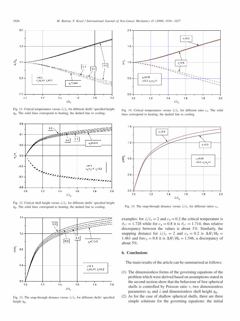
The illustration of the influence of the value of parameterc on critical temperature and the snapping distance at heatingare shown in Figs. 14 and 15 for the case �0 = 0.05. Again itcan be observed that in both figures the curves are similar andthe discrepancies between the values are small. Consider the


Fig. 11. Critical temperatures versus �/�c for different shells’ specified height�0. The solid lines correspond to heating, the dashed line to cooling.

Fig. 12. Critical shell height versus �/�c for different shells’ specified height�0. The solid lines correspond to heating, the dashed line to cooling.

Fig. 13. The snap-through distance versus �/�c for different shells’ specifiedheight �0.

Fig. 14. Critical temperatures versus �/�c for different ratio c. The solidlines correspond to heating, the dashed line to cooling.

Fig. 15. The snap-through distance versus �/�c for different ratios c.

examples: for �/�c = 2 and c = 0.2 the critical temperature isϑc∗ = 1.728 while for c = 0.8 it is ϑc∗ = 1.714; thus relativediscrepancy between the values is about 1%. Similarly, thesnapping distance for �/�c = 2 and c = 0.2 is �H/H0 =1.461 and forc = 0.8 it is �H/H0 = 1.546, a discrepancy ofabout 5%.

6. Conclusions

The main results of the article can be summarized as follows:

(1) The dimensionless forms of the governing equations of theproblem which were derived based on assumptions stated inthe second section show that the behaviour of free sphericalshells is controlled by Poisson ratio �, two dimensionlessparameters 0 and � and dimensionless shell height �0.

(2) As for the case of shallow spherical shells, there are threesimple solutions for the governing equations: the initial


stress free state at ϑ∗ = 0; the flat state at ϑ∗ = 1; and theinside-out state at ϑ∗ = 2. For all these cases closed formsolutions were obtained.

(3) The stability of the shell’s flat state is controlled by pa-rameter �. Its critical value depends only on � and �0. Forcalculation of the critical value �c the explicit form of thecharacteristic equation is given.

(4) For a given a/h there exists the upper �0 for which thebuckling can still occur. The limit is essentially controlledby parameter 0 and the absolute limit is obtained for 0 →0. For example for thin shells one has a/h�20 [10], sothermal buckling is possible for � < 0.12 only.

(5) The parameter �c, which controls the critical shell height,depends on � and unlike the shallow spherical shells alsoon �0. It is found that for �0 �0.05 the relative discrepancyof �c from shallow spherical shells is less than 5%.

(6) It is also found that for � < 0.1 values the influence of shearstrains on �c is marginal.

(7) The collocation method used is found to be very efficientfor constructing deflection diagrams.

There is a restriction in using the results of the above analysisregarding the limit of the elastic deformation of the material. Formetals one has 0 =O(10−3). This, by (26)2, limits a/h > 100(approximately).

References

[1] D.V. Panov, On the stability of a bimetallic membrane on heating,Prikladnaja Matematika i Mehanika [J. Appl. Math. Mech.] 11 (1947)603–610 (in Russian).

[2] W.H. Wittrick, Stability of bimetallic disk, Q. Mech. Appl. Math. 6(1953) 15–31.

[3] B.D. Aggarwala, E. Saibel, Thermal stability of bimetallic shallowspherical shells, Int. J. Non-linear Mech. 5 (1) (1970) 49–62.

[4] R.-H. Liu, Non-linear thermal stability of bimetallic shallow shells ofrevolution, Int. J. Non-linear Mech. 18 (5) (1983) 409–429.

[5] M. Batista, F. Kosel, Thermoelastic stability of bimetallic shallow shellsof revolution, Int. J. Solids Struct. 44 (2) (2007) 447–464.

[6] E. Reissner, On finite axi-symmetrical deformations of thin elastic shellsof revolution, Comput. Mech. 4 (1989) 387–400.

[7] S.S. Antman, Nonlinear Problems of Elasticity, Springer, Berlin, 1995,pp. 343–370.

[8] L. Librescu, Elastostatics and Kinetics of Anisotropic and HeterogeneousShell-Type Structures, Noordhoff International Publications, Leyden, TheNetherlands, 1975, pp. 306–308.

[9] U.M. Ascher, R. Mattheij, R. Russell, Numerical Solution of BoundaryValue Problems for Ordinary Differential Equations, SIAM, Philadelphia,PA, 1995.

[10] E. Ventsel, T. Krauthammer, Thin Plates and Shells, Marcel Dekker,Inc., New York, 2001.

Thermoelastic stability of a double-layered spherical shell

Documents

Transcript of Thermoelastic stability of a double-layered spherical shell