Localisation and weighted inequalities for spherical Fourier means

LOCALISATION AND WEIGHTED INEQUALITIES

FOR SPHERICAL FOURIER MEANS

Anthony Carbery, Fernando Soria and Ana Vargas

Abstract. In this work we establish certain equivalences between the localisation propertieswith respect to spherical Fourier means of the support of a given Borel measure and the L2-rate of decay of the Fourier extension operator associated to it. This, in turn, is intimatelyconnected with the property that the X-ray transform of the measure be uniformly bounded.Geometric properties of sets supporting such a measure are studied.

§1. Introduction.

In this paper we continue with the work initiated in [CS2] and [CS3] concerning thegeometric properties of the sets where the localisation property for the spherical Fouriermeans in Rn holds. Let us start by recalling some basic definitions and notation. For asuitable function f defined on Rn we denote its Fourier transform by f , and for R > 0 wedefine

SRf(x) =∫

|ξ|<R

f(ξ) e2πix·ξ dξ.

One of the most interesting and difficult problems in harmonic analysis is that ofdetermining whether we can recover the values of every function f in L2(Rn) from thepointwise limit of its spherical means SRf . That is, whether or not we have

limR→∞

SRf(x) = f(x) a.e., ∀f ∈ L2(Rn).

The result is known to be true in dimension n = 1; this is the extension to the real line ofthe celebrated theorem of Carleson (see [C], [KT]). The problem however remains openfor n ≥ 2.

On the other hand, Riemann’s localisation principle says that for any f ∈ L1(R) wehave

limR→∞

SRf(x) = 0

1991 Mathematics Subject Classification. 42B10, 42B25.Key words and phrases. Spherical Fourier Means, Localisation Principle, maximal inequalities.The research of this paper has been partially supported by the EU Comission via the network HARP,

and by MEC Grant MTM2004-00678. The first author was partially supported by a Leverhulme StudyAbroad Fellowship, and the second and third authors by Grant MEC MTM2004-00678.

Typeset by AMS-TEX

1

2 ANTHONY CARBERY, FERNANDO SORIA AND ANA VARGAS

at every point x off the support of f . In fact the convergence is uniform on compactsubsets of (supp f)c. In [CS1] the first two authors considered the related question oflocalisation in higher dimensions. They proved the following:

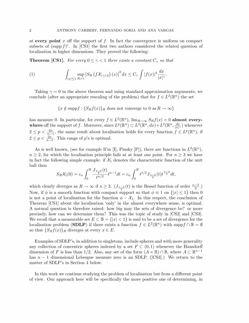
Theorem [CS1]. For every 0 ≤ γ < 1 there exists a constant Cγ so that

(1)∫

|x|≤1

supR>1

∣∣SR

(fX|·|>2

)(x)

∣∣2 dx ≤ Cγ

∫|f(x)|2 dx

|x|γ .

Taking γ = 0 in the above theorem and using standard approximation arguments, weconclude (after an appropriate rescaling of the problem) that for f ∈ L2(Rn) the set

{x /∈ suppf : {SRf(x)}R does not converge to 0 as R →∞}

has measure 0. In particular, for every f ∈ L2(Rn), limR→∞ SRf(x) = 0 almost every-where off the support of f . Moreover, since Lp(Rn) ⊂ L2(Rn, dx)+L2(Rn, dx

|x|γ ) whenever2 ≤ p < 2n

n−γ , the same result about localisation holds for every function f ∈ Lp(Rn), if2 ≤ p < 2n

n−1 . This range of p’s is optimal.

As is well known, (see for example Il’in [I], Pinsky [P]), there are functions in L2(Rn),n ≥ 2, for which the localisation principle fails at at least one point. For n ≥ 3 we havein fact the following simple example: if X1 denotes the characteristic function of the unitball then

SRX1(0) = cn

∫ R

0

Jn−22

(t)

tn/2tn−1dt = cn

∫ R

0

t1/2Jn−22

(t)tn−3

2 dt,

which clearly diverges as R →∞ if n ≥ 3. (Jn−22

(t) is the Bessel function of order n−22 .)

Now, if φ is a smooth function with compact support so that φ ≡ 1 on {|x| ≤ 1} then 0is not a point of localisation for the function φ − X1. In this respect, the conclusion ofTheorem [CS1] about the localisation ‘only’ in the almost everywhere sense, is optimal.A natural question is therefore raised: how big may the sets of divergence be? or moreprecisely, how can we determine them? This was the topic of study in [CS2] and [CS3].We recall that a measurable set E ⊂ B = {|x| < 1} is said to be a set of divergence for thelocalisation problem (SDLP) if there exists a function f ∈ L2(Rn) with suppf ∩ B = ∅so that {SRf(x)}R diverges at every x ∈ E.

Examples of SDLP’s, in addition to singletons, include spheres and with more generalityany collection of concentric spheres indexed by a set F ⊂ (0, 1) whenever the Hausdorffdimension of F is less than 1/2. Also, any set of the form (A× R) ∩ B, where A ⊂ Rn−1

has n − 1 dimensional Lebesgue measure zero is an SDLP. ([CS3].) We return to thematter of SDLP’s in Section 4 below.

In this work we continue studying the problem of localisation but from a different pointof view. Our approach here will be specifically the more positive one of determining, in

LOCALISATION AND WEIGHTED INEQUALITIES FOR SPHERICAL FOURIER MEANS 3

analogy with (1) above, for which positive, finite Borel measures µ supported in the unitball of Rn one has the following inequality

(A)∫

supR>1

∣∣SR

(fX|·|>2

)(x)

∣∣2 dµ(x) ≤ Cµ

∫|f(x)|2 dx, ∀f ∈ L2(Rn),

for a certain constant Cµ < ∞. Whenever this holds, then, for every function f ∈ L2(Rn)with suppf ⊂ {|x| ≥ 2} there exists at least one point x ∈ supp µ (in fact a set of fullµ-measure) for which {SRf(x)}R converges. Hence, supp µ cannot be an SDLP.

One of the things that was observed in [CS3] is that the maximal condition (A) is infact equivalent to a uniform estimate for each of the spherical means; that is,

(B) supR>1

∫ ∣∣SR

(fX|·|>2

)(x)

∣∣2 dµ(x) ≤ Cµ

∫|f(x)|2 dx.

An indication of this equivalence was given using heuristic arguments, via the “folk-calculation” of C. Fefferman. This calculation in turn leads to a direct formulation ofthe problem in terms of the order of decay of the L2-average over the unit sphere of theFourier transform of gdµ, for every g ∈ L2(dµ). In other words, both (A) and (B) hold ifand only if the following holds:

(C)(∫

Sn−1

∣∣∣gdµ(Rω)∣∣∣2

dσ(ω))1/2

≤ C

Rn−1

2

(∫|g|2dµ

)1/2

,

with C independent of g ∈ L2(dµ) and R > 1. In Theorems 1 and 2 below we give formalproofs of all these results.

The dual statement of (C) is the condition that

(C*)(∫ ∣∣∣hdσ(Ry)

∣∣∣2

dµ(y))1/2

≤ C

Rn−1

2

(∫

Sn−1|h|2dσ

)1/2

, ∀h ∈ L2(Sn−1).

This condition was considered independently by Barcelo, Ruiz and Vega in [BRV] inconnection with weighted inequalities for solutions to the Helmholtz equation. We shallcome back to this point later.

Condition (B) can be interpreted as an L2-weighted inequality for each operator SR.This is reminiscent of a problem posed by E.M. Stein (see [St1]) during the famous con-ference on harmonic analysis at Williamstown, in 1978. The proposed problem was todetermine the operator or operators which control the L2-inequalities for the Bochner-Riesz means. To be more precise, if Sδ denotes the (smooth) Fourier multiplier operatorassociated to the annulus {ξ : 1− δ < |ξ| < 1} then the question is to find a pairing whichassociates to a given weight u another weight U so that the following holds

∫|Sδf(x)|2 u(x) dx ≤ C

∫|f(x)|2 U(x) dx.


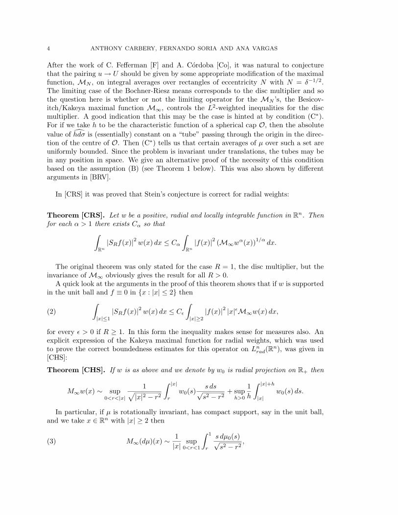
After the work of C. Fefferman [F] and A. Cordoba [Co], it was natural to conjecturethat the pairing u → U should be given by some appropriate modification of the maximalfunction, MN , on integral averages over rectangles of eccentricity N with N = δ−1/2.The limiting case of the Bochner-Riesz means corresponds to the disc multiplier and sothe question here is whether or not the limiting operator for the MN ’s, the Besicov-itch/Kakeya maximal function M∞, controls the L2-weighted inequalities for the discmultiplier. A good indication that this may be the case is hinted at by condition (C∗).For if we take h to be the characteristic function of a spherical cap O, then the absolutevalue of hdσ is (essentially) constant on a “tube” passing through the origin in the direc-tion of the centre of O. Then (C∗) tells us that certain averages of µ over such a set areuniformly bounded. Since the problem is invariant under translations, the tubes may bein any position in space. We give an alternative proof of the necessity of this conditionbased on the assumption (B) (see Theorem 1 below). This was also shown by differentarguments in [BRV].

In [CRS] it was proved that Stein’s conjecture is correct for radial weights:

Theorem [CRS]. Let w be a positive, radial and locally integrable function in Rn. Thenfor each α > 1 there exists Cα so that

∫

Rn

|SRf(x)|2 w(x) dx ≤ Cα

∫

Rn

|f(x)|2 (M∞wα(x))1/αdx.

The original theorem was only stated for the case R = 1, the disc multiplier, but theinvariance of M∞ obviously gives the result for all R > 0.

A quick look at the arguments in the proof of this theorem shows that if w is supportedin the unit ball and f ≡ 0 in {x : |x| ≤ 2} then

(2)∫

|x|≤1

|SRf(x)|2 w(x) dx ≤ Cε

∫

|x|≥2

|f(x)|2 |x|εM∞w(x) dx,

for every ε > 0 if R ≥ 1. In this form the inequality makes sense for measures also. Anexplicit expression of the Kakeya maximal function for radial weights, which was usedto prove the correct boundedness estimates for this operator on Ln

rad(Rn), was given in[CHS]:

Theorem [CHS]. If w is as above and we denote by w0 is radial projection on R+ then

M∞w(x) ∼ sup0<r<|x|

1√|x|2 − r2

∫ |x|

r

w0(s)s ds√s2 − r2

+ suph>0

1h

∫ |x|+h

|x|w0(s) ds.

In particular, if µ is rotationally invariant, has compact support, say in the unit ball,and we take x ∈ Rn with |x| ≥ 2 then

(3) M∞(dµ)(x) ∼ 1|x| sup

0<r<1

∫ 1

r

s dµ0(s)√s2 − r2

,


where µ0 denotes the radial projection of µ (see Theorem 3). Observe that the secondterm in the right hand side of (3), the “sup” term, is just a constant which only dependson µ, call it |||µ0|||. Then, (2) becomes in the case of a rotationally invariant measure µ

(4)∫

|x|≤1

|SRf(x)|2 dµ(x) ≤ Cε|||µ0|||∫

|x|≥2

|f(x)|2 dx

|x|1−ε.

The constant |||µ0||| is easily seen to be equivalent, after a change of variables to polarcoordinates, to the L∞ norm of the averages on tubes that we mentioned above for generalmeasures. So, one of the consequences of (2) is that in the case of rotationally invariantmeasures the maximal estimate (A) follows from, and in fact is equivalent to the finitenessof |||µ0|||. We give all the details in Theorem 3 below.

In [BRV] the authors study conditions on the radial weight V for the inequality∫

Rn

|u(x)|2V (x)dx ≤ CV

∫

Rn

|(∆ + 1)u(x)|2V −1(x)dx

to hold. Their result is that this is true if and only if |||V ||| is finite; this is referred to asthe “radial Mizohata-Takeuchi” condition. In fact one can take CV ∼ |||V |||2. If u satisfiesthe so-called Sommerfeld outgoing radiation condition then u is given by the convolutionof f = (∆+1)u with a kernel which is more singular than that of SR. However, for radialweights the problems are, as we see, equivalent.

The paper is organised as follows. In the next section we give a proof of the equivalencebetween the conditions (A), (B), (C) described in this introduction. Section 3 addressesthe problem for the special case of rotationally invariant measures, for which we havea complete solution. In the last section we analyse the geometry of those measures forwhich the “norm” ||| · ||| is finite and further explore the relation between sets supportingsuch a measure and SDLP’s. We would like to thank Laura Wisewell for a number ofilluminating and very helpful discussions on the material of the last section.

§2. The maximal localisation theorem for general measures.

For a general finite Borel measure µ we want to investigate the connection between thelocalisation property that it inherits, the L2 behaviour of the spherical means SR withrespect to it and the decay of the restriction of its Fourier transform to spheres. To thisend, let us look at the conditions

(B)∥∥SR

(fX|·|≥2

)∥∥L2(dµ)

≤ C ‖f‖2and

(C)∥∥∥gdµ(R·)

∥∥∥L2(Sn−1)

≤ C

Rn−1

2

‖g‖L2(dµ) ,


as well as the two seemingly weaker conditions

(B′)∫

|x|≥2

|(SR+1 − SR) (gdµ)|2 dx ≤ C

∫|g|2 dµ,

and

(C′)∫ R+1

R

∫

Sn−1

∣∣∣gdµ(tω)∣∣∣2

dσ(ω)tn−1dt ≤ C

∫|g|2 dµ.

In all the cases, the constant C is understood to be uniform in R ≥ 1 and independent ofthe functions f, g, . . . considered.

Theorem 1. Let µ be any positive finite Borel measure whose support lies in the unitball of Rn. The four conditions (B), (B′), (C) and (C ′) stated above are equivalent.

Moreover, if we denote by Tε(x, ω), x ∈ Sn, ω ∈ Sn−1 the translation to x and rotationby ω of the infinite tube {(y′, yn) ∈ Rn−1 × R : |y′| < ε}, then the condition

|||µ||| := supε>0,x,ω

1εn−1

∫

Tε(x,ω)

dµ < ∞

is necessary for any of the above to hold.

In what follows, we sometimes refer to ||| · ||| as the “triple norm”.

Proof. Let us begin with the observation that, by duality, condition (B) is equivalent to

(B*)∫

|x|≥2

|SR(gdµ)|2 dx ≤ C

∫|g|2 dµ,

and that Plancherel’s identity shows that (C′) is the same as

(B′′)∫

Rn

|(SR+1 − SR) (gdµ)|2 dx ≤ C

∫|g|2 dµ,

Clearly (B∗) => (B′), so the first part of the theorem will follow from the proof of thechain of implications (B′) => (C′) => (C) => (B∗).

(C) => (B∗). We will prove first the following:


Lemma 1. Let ψ be a function in the Schwartz class with ψ(0) = 1. Then, if we denoteby δ0 the Dirac delta at the point 0 and if BR is the ball centred at the origin with radiusR, we have ∣∣∣

(δ0 − ψ

)∗ XBR(x)

∣∣∣ ≤ 2∫

|y|≥||x|−R|

∣∣∣ψ(y)∣∣∣ dy.

Proof. Set I(x) =(δ0 − ψ

)∗ XBR

(x) =∫|x−y|<R

(δ0 − ψ(y)

)dy and consider the two

cases:Case 1: |x| > R. Then |I(x)| ≤ ∫

|x−y|<R

∣∣∣ψ(y)∣∣∣ dy ≤ ∫

|y|≥|x|−R

∣∣∣ψ(y)∣∣∣ dy.

Case 2: |x| ≤ R. Observe that |I(x)| ≤∣∣∣∫|y|<R−|x|

(δ0 − ψ(y)

)dy

∣∣∣ +∫|y|≥R−|x|

∣∣∣ψ(y)∣∣∣ dy

= I + II.

Now, using the hypothesis ψ(0) =∫

ψ = 1 we obtain

I =

∣∣∣∣∣1−∫

|y|<R−|x|ψ(y)dy

∣∣∣∣∣ =

∣∣∣∣∣∫

|y|≥R−|x|ψ(y)dy

∣∣∣∣∣ ≤ II.

Therefore, |I(x)| ≤ 2II = 2∫|y|≥R−|x|

∣∣∣ψ(y)∣∣∣ dy. Q.E.D.

Now take a smooth function ψ with suppψ ⊂ {|x| ≤ 1} and ψ(0) = 1 and let KR be thekernel of the operator SR (i.e., KR = XBR

). Put KR = ψKR + (1 − ψ)KR = K1R + K2

R.Now, if µ has support in the unit ball then K1

R ∗ (gdµ) ∩ {|x| ≥ 2} = ∅. Therefore, fromthe lemma we get

∫

|x|≥2

|KR ∗ (gdµ)|2 dx ≤∫|(1− ψ)KR ∗ (gdµ)|2 dx

=∫ ∣∣∣

(δ0 − ψ

)∗ XBR

(ξ)gdµ(ξ)∣∣∣2

dξ

≤∫ (

2∫

||ξ|−R|≤|y|

∣∣∣ψ(y)∣∣∣ dy

)2 ∣∣∣gdµ(ξ)∣∣∣2

dξ.

Using Cauchy-Schwarz in the y-integral and writing the integral in ξ in polar coordinateswe obtain from (C)

∫

|x|≥2

|KR ∗ (gdµ)|2 dx ≤ 4||ψ||1∫ ∣∣∣ψ(y)

∣∣∣∫

|t−R|≤|y|tn−1

∫

Sn−1

∣∣∣gdµ(tω)∣∣∣2

dσ(ω) dt dy

≤ C

∫ ∣∣∣ψ(y)∣∣∣ |y|dy

∫|g|2dµ ∼ C ′

∫|g|2dµ.


(C′) => (C). Fix R ≥ 1 and assume that (C′) holds for all functions in L2(dµ). Takeany g in that class and set

A(t) =∫

Sn−1

∣∣∣gdµ(tω)∣∣∣2

dσ(ω).

By hypothesis, there exists at least one t0 ∈ [R, R + 1] so that A(t0) ≤ Ctn−10

∫ |g|2dµ.Observe that

d

dt

(gdµ

)(tω) = 2πi

∫(ω · y) g(y)e2πitω·ydµ(y).

Therefore, ∫

Sn−1

∣∣∣∣d

dt

(gdµ

)(tω)

∣∣∣∣2

dσ(ω) ≤n∑

j=1

|Aj(t)|2 = A(t),

where each Aj is defined as A but with g(y) replaced by yjg(y), if y = (y1, . . . , yn). Since

A(R) = A(t0)−∫ t0

R

A′(t)dt ≤ A(t0) + 2∫ R+1

R

(A(t))1/2 (A(t))1/2dt,

we conclude, using (C′) again, that

Rn−1A(R) ≤ tn−10 A(t0) + 2

(∫ R+1

R

tn−1A(t)dt

∫ R+1

R

tn−1A(t)dt

)1/2

≤ C

∫|g|2dµ.

In the last inequality we have used the support condition on µ.

(B′) => (C′). Fix g ∈ L2(dµ) and R ≥ 1. Define h(x) = (SR+ε − SR) (gdµ)(x). We firstclaim that for a sufficiently small ε > 0 (depending only on the dimension) we have

∫

Rn

|h(x)|2dx ≤ 2∫

|x|≥2

|h(x)|2dx.

This, after rescaling, will do the job, (using (B′) and the equivalence of (B′′) with (C′)).Take a function ψ in the Schwartz class, so that ψ(x) ≡ 1 on {|x| ≤ 2}. Then

(∫

|x|≥2

|h|2)1/2

≥(∫

|h(1− ψ)|2)1/2

≥(∫

|h|2)1/2

−(∫

|hψ|2)1/2

.

We show that∫ |hψ|2 ≤ 1

2

∫ |h|2, and that will prove our claim. Now, we observe thatsupp h ⊂ {ξ : R ≤ |ξ| ≤ R + ε} and that

∫|hψ|2 =

∫|h ∗ ψ|2 ≤

(∫|h|2

)||ψ||1

(sup

x

∫

R≤|x−y|≤R+ε

|ψ(y)|dy

).


Put D(x) = {y : R ≤ |x− y| ≤ R + ε}. Then,

∫

R≤|x−y|≤R+ε

|ψ(y)|dy =∫

D(x)∩{|y|≤1}|ψ(y)|dy +

∑

k≥0

∫

D(x)∩{|y|∼2k}|ψ(y)|dy

≤ CnC ′nε +∑

k≥0

C ′nε 2k(n−1)Cn2−kn = C ′′nε,

where we have used that |ψ(y)| ≤ Cn1

1+|y|n for certain constant Cn. It suffices to takethen ε = 1

2|| bψ||1C′′n.

Finally, we show that if (B) holds then we must have |||µ||| finite. To do that, let usrecall the construction given in Lemma 1 of [CS3]. In fact, we only need the first part ofit:

Lemma 2. Let φ be a smooth bump function supported in {|x| ≤ 1}. Given R >> 1 weconsider the function φR(x) = e2πiRx1φ(x1 − 3, R1/2x′), where x = (x1, x

′) ∈ R × Rn−1.Then |SRφR(x)| ≥ c on the set {|x1| ≤ 1, |x′| ≤ R−1/2}, while for each k ∈ N, there is aconstant Ck so that |SRφR(x)| ≤ Ck{1+R1/2|x′|}−k for all x. Moreover, for each k ∈ N,there is a constant Ck so that |SR′φR(x)| ≤ Ck(R′/R)(n−1)/2 max(R,R′)−k when x ∈ Band R/R′ /∈ [1/2, 2].

With our notation, what the lemma says is that |SRφR(x)| ≥ c on the set Tε(0, e1) ∩{|x| ≤ 1}, where ε = R−1/2, 0 denotes the origin and e1 is just the vector (1, 0, . . . , 0).Therefore, if µ is supported in the unit ball and (B) holds we must have

∫

Tε(0,e1)

dµ ≤ C

∫|φR|2 ∼ C R−

n−12 .

Since we can translate and rotate SRφR as we wish, without changing the size of φR orthe shape of its support, we obtain then

|||µ||| ≤ C.

This finishes the proof of Theorem 1. Q.E.D.

We now prove the equivalence of the above conditions with (A). The proof is similarto the one used to prove (C) => (B∗) but rather more technical. This is why we havedecided to present it separately.


Theorem 2. Let µ be a finite Borel measure µ whose support lies in the unit ball ofRn, n ≥ 2. Then, if µ satisfies condition (C) it satisfies the maximal condition (A) too.In particular, we obtain that the set of conditions (A), (B), (C), as well as (B′) and (C ′),are all equivalent.

Proof. We follow the same line of arguments as in Theorem 2.2 of [CS1]. Take φ a smoothfunction supported in the unit ball so that φ ≡ 1 on {|x| ≤ 1/2}. Define ψ(x) = φ(x

2 )−φ(x)and ψj(x) = ψ( x

2j ) for j = 0, 1, . . . In this way we obtain φ(x) +∑

j≥0 ψj(x) ≡ 1.Now, if f ∈ L2(Rn) with supp f ⊂ {|x| ≥ 2} we have for all |x| ≤ 1

KR ∗ f(x) =∞∑

j=0

k=j+2∑

k=j−2

(ψjKR) ∗ (ψkf) (x).

Writing KjR = (ψjKR), it is clear that it suffices to prove the estimate

(5)∫

supR≥1

∣∣∣KjR ∗ g(x)

∣∣∣2

dµ(x) ≤ C 2−j

∫|g(x)|2dx, ∀g ∈ L2(Rn),

under the assumption

(6)∫

Sn−1

∣∣∣hdµ(rω)∣∣∣2

dω ≤ C

rn−1

∫|h|2dµ, ∀r > 0, ∀h ∈ L2(dµ).

Observe that in (C) we consider only the case r ≥ 1. However (6) is true also for 0 < r < 1always if ||µ|| (the total variation of µ) is finite since

∫

Sn−1

∣∣∣hdµ(rω)∣∣∣2

dω ≤ ||hdµ||2∞ ≤ ||µ||∫|h|2dµ.

We will not require in the rest of the proof the support condition on µ. Using theFundamental Theorem of Calculus we obtain

∣∣∣KjR ∗ g(x)

∣∣∣2

≤∣∣∣Kj

1 ∗ g(x)∣∣∣2

+ 2∫ R

1

∣∣∣∣Kjt ∗ g(x)

d

dtKj

t ∗ g(x)∣∣∣∣ dt.

Hence, using the Cauchy-Schwarz inequality

∫supR≥1

∣∣∣KjR ∗ g(x)

∣∣∣2

dµ(x) ≤∫ ∣∣∣Kj

1 ∗ g(x)∣∣∣2

dµ(x)

+ 2(∫ ∫ ∞

1

∣∣∣Kjt ∗ g(x)

∣∣∣2

dt dµ(x))1/2

(∫ ∫ ∞

1

∣∣∣∣d

dtKj

t ∗ g(x)∣∣∣∣2

dt dµ(x)

)1/2

= I + 2II1 · II2.


We will show that I, II1 ≤ C2−j‖g‖2 while II2 ≤ C‖g‖2. This will prove (5). By duality,these estimates are equivalent, respectively, to

∫

Rn

∣∣∣Kj1 ∗ (hdµ)(x)

∣∣∣2

dx ≤ C 2−j

∫|h|2dµ

∫

Rn

∣∣∣∣∫ ∞

1

Kjt ∗ [f(·, t)dµ](x)dt

∣∣∣∣2

dx ≤ C 2−2j

∫ ∫ ∞

1

|f(x, t)|2dt dµ(x)

∫

Rn

∣∣∣∣∫ ∞

1

(d

dtKj

t

)∗ [f(·, t)dµ](x)dt

∣∣∣∣2

dx ≤ C

∫ ∫ ∞

1

|f(x, t)|2dt dµ(x)

and, by Plancherel’s theorem, to

E1 =∫

Rn

∣∣∣mj1(ξ)hdµ(ξ)

∣∣∣2

dξ ≤ C 2−j

∫|h|2dµ

E2 =∫

Rn

∣∣∣∣∫ ∞

1

mjt (ξ)[f(·, t)dµ] (ξ)dt

∣∣∣∣2

dξ ≤ C 2−2j

∫ ∫ ∞

1

|f(x, t)|2dt dµ(x)

E3 =∫

Rn

∣∣∣∣∫ ∞

1

(d

dtmj

t

)(ξ)[f(·, t)dµ] (ξ)dt

∣∣∣∣2

dξ ≤ C

∫ ∫ ∞

1

|f(x, t)|2dt dµ(x).

Here mjt denotes the Fourier transform of Kj

t , that is, mjt (ξ) = XBt ∗ ψj(ξ). Using the

fact that ψj(0) =∫

ψj = 0 we have, as in Lemma 1 above,

∣∣∣mjt (ξ)

∣∣∣ ≤ 2∫

||ξ|−t|≤2−j |y|

∣∣∣ψ(y)∣∣∣ dy.

In particular, |mjt (ξ)| ≤ C and

∫∞0|mj

t (ξ)| dt ≤ C 2−j . Thus, the first estimate followsfrom

E1 ≤ C 2−j ||hdµ||2∞ ≤ C 2−j ||µ||∫|h|2dµ

since∫Rn |mj

1(ξ)|2dξ ≤ 2−j . For the second we use our hypothesis (6)

E2 ≤∫ (∫ ∞

1

∣∣∣mjt (ξ)

∣∣∣ dt

) ∫ ∞

1

∣∣∣mjt (ξ)

∣∣∣∣∣∣[f(·, t)dµ] (ξ)

∣∣∣2

dt dξ

≤ C 2−j

∫ ∞

1

∫ ∣∣∣ψ(y)∣∣∣∫

|r−t|≤2−j |y|rn−1

∫

Sn−1

∣∣∣[f(·, t)dµ] (rω)∣∣∣2

dω dr dy dt

≤ C 2−2j

∫ ∫ ∞

1

|f(x, t)|2dt dµ(x).

Finally, observe that

d

dt

(mj

t (ξ))

=n

tmj

t (ξ) + 2j

∫

|2jξ−y|<2jt

(y − 2jξ)2jt

· ∇ψ(y) dy.


As in Lemma 1 we obtain here the bound for t ≥ 1∣∣∣∣d

dt

(mj

t (ξ))∣∣∣∣ ≤ C 2j

∫

||ξ|−t|≤2−j |y|

(∣∣∣ψ(y)∣∣∣ +

∣∣∣∇ψ(y)∣∣∣)

dy.

So, the same argument as for E2 gives us E3 ≤ C. Q.E.D.

In the spirit of Stein’s conjecture as discussed in the Introduction, one may ask whetherfiniteness of |||µ||| implies the condition (C) and its equivalents. For the purposes of thispaper we shall label the assertion that this is indeed the case as the triple norm conjecture.In the next section we examine this question in the case of rotationally invariant measuresµ.

§3. The case of rotationally invariant measures.

As we have said in the Introduction, this is the case for which we have the completecharacterisation of condition (C) and its equivalents in terms of the finiteness of the norm||| · |||. (Thus the triple norm conjecture is true in the rotationally invariant case.)

Theorem 3. Consider a finite Borel measure µ which is invariant under rotations andwhose support lies in the unit ball of Rn, n ≥ 2. Let us denote by µ0 its radial projectionon [0,∞), that is

∫

Rn

φdµ =∫ ∞

0

(∫

Sn−1φ(r, θ) dσ(θ)

)rn−1dµ0(r).

Then the following conditions are equivalent:(a) For all f ∈ L2(Rn) with suppf ⊂ {|x| ≥ 2}

∥∥∥∥supR≥1

|SRf(x)|∥∥∥∥

L2(dµ)

≤ C ‖f‖2 .

(b) For all f ∈ L2(Rn) with suppf ⊂ {|x| ≥ 2}

supR≥1

‖SRf‖L2(dµ) ≤ C ‖f‖2 .

(c) For all g, ∥∥∥gdµ(R·)∥∥∥

L2(Sn−1)≤ C

Rn−1

2

‖g‖L2(dµ)

(d) µ satisfies

|||µ||| ∼ supr>0

∫ ∞

r

s12 dµ0(s)

(s− r)12

< ∞.


Obviously, the equivalence between (a), (b) and (c) follows from the results of theprevious section. We will not discuss condition (a) here. However, we do consider (b) and(c) because the arguments that we will use are of a different nature (spherical harmonicsand theory of Bessel functions) and have their own interest. The equivalence between (c)and (d) appears also in [BRV].

Proof. We will prove first that (b) and (c) are equivalent to the condition

(e) supl∈ 1

2NsupR>1

∫ ∞

0

∣∣∣Jl(Rr)∣∣∣2

dµ0(r) < ∞,

where Jl(t) = t1/2Jl(t) and Jl is the Bessel function of order l. We will show later theequivalence between (d) and (e).

We begin with condition (c). Let us fix an orthonormal basis {Yk}k, of sphericalharmonic in L2(Sn−1). Given g ∈ L2(dµ) we consider its expansion with respect tothat basis g ∼ ∑

k gk(·)Yk(·) (the convergence in the L2-sense). Then, the expansion ofgdµ(Rω) is

gdµ(Rω) =1

Rn−1

2

∑

k

(∫ ∞

0

gk(t)Jk′(Rt)tn−1

2 dµ0(t))Yk(ω),

where k′ = n−22 +degree(Yk) (see [SW]). Therefore, the statement in (c) holds if and only

if ∣∣∣∣∫ ∞

0

gk(t)Jk′(Rt)tn−1

2 dµ0(t)∣∣∣∣2

≤ C

∫ ∣∣∣gk(t)tn−1

2

∣∣∣2

dµ0(t),

with constant C independent of R and k. Since we can now assume that gk(t)tn−1

2 is anyarbitrary function in L2(dµ0), the Riesz representation theorem tells us that the aboveholds if and only if ∫ ∞

0

∣∣∣Jl(Rr)∣∣∣2

dµ0(r) ≤ C,

(uniformly in R and l) which is precisely (e).

Let us now see the equivalence between (b) and (e). This is the only place where wewill consider the support condition on the measure µ.

Recall that if f ∼ ∑k fkYk then SRf ∼ ∑

k(TRk′fk)Yk, where

TRl h(r) =

C

rn−1

2

∫ ∞

0

h(s)sn−1

2 RKl(Rr,Rs)ds,

Kl(r, s) =r

r2 − s2Jl(s)J ′l(r) +

s

r2 − s2Jl(r)J ′l(s) = K1

l (r, s) + K2l (r, s)


(here J ′l(t) = t1/2J ′(t)

)

and k′ = n−22 + degree(Yk) as above. (See [W], [CRS].) So, the statement in (b) holds if

and only if

(b′)∫ 1

0

∣∣∣∣∫ ∞

2

h(s)RKl(Rr,Rs)ds

∣∣∣∣2

dµ0(r) ≤ C

∫ ∞

2

|h(s)|2ds,

(with C independent of R > 1 and l). Since |RKl(Rr,Rs)| ≤ Cl1s , we can always assume

that l is large.

The estimates about Bessel functions that we will use are summarised as follows (see[CRS] and [BRV]):

(i) |Jl(t)| ≤ C

[( |l + t||l − t|

)1/4

∧ l1/6

]:= Cτl(t), |J ′l(t)| ≤ C, l ≥ 1, ∀t > 0

(ii) |Jl(t)| ≤ Cl1/2

(l − t), if l/2 ≤ t ≤ l − l1/3.

(C represents an absolute constant.)

Now, we point out that (b′) always holds if we replace Kl with K1l since then the left

hand side is majorised by

C

∫ 1

0

(∫ ∞

2

|h(s)|τl(Rs)s2

ds

)2

dµ0(r) ≤ C||µ0||(∫ ∞

2

|h(s)|2ds

)(∫ ∞

2

|τl(Rs)|2s2

ds

),

and the last integral is bounded uniformly in R. Therefore, (b) follows if and only if (b′)follows with Kl replaced by K2

l , that is, if

∫ 1

0

∣∣∣∣∫ ∞

2

h(s)s

s2 − r2J ′l(Rs)ds

∣∣∣∣2

|J(Rr)|2dµ0(r) ≤ C

∫ ∞

2

|h(s)|2ds,

which is easily seen to be equivalent to (e).

We finally show the equivalence between (d) and (e). That (e) implies (d) follows fromthe additional fact that in (i) one has |Jl(t)| ∼ τl(t) in the region l + l1/3 ≤ t ≤ αl, forsome α > 1.

To prove that (d) implies (e) we define for a fixed R the measure µR0 as

∫ ∞

0

F (s) dµR0 (s) =

∫ ∞

0

F (Rs) dµ0(s).


We make the observation that if (d) holds for µ0 so does for µR0 with the same value,

independent of R. Therefore, in proving (e) we can assume without loss of generality thatR = 1. Let us split the integral as

∫ ∞

0

∣∣∣Jl(t)∣∣∣2

dµ0(t) =

(∫ l/2

0

+∫ l−l1/3

l/2

+∫ l+l1/3

l−l1/3+

∫ ∞

l+l1/3

)∣∣∣Jl(t)∣∣∣2

dµ0(t) =4∑

j=1

Ij .

From estimate (i) we have that I1 ≤ C||µ0|| and

I4 ≤ C

∫ ∞

l+l1/3

( |l + t||l − t|

)1/2

dµ0(t) ≤ C

∫ ∞

l

t12 dµ0(t)(t− l)

12≤ C.

We also get I3 ≤ Cl1/3µ0

([l − l1/3, l + l1/3]

). To estimate this, as well as I2, we observe

that if I = [a, b] then (d) implies

µ0(I) =∫ a+|I|

a

dµ0 ≤( |I|

a

)1/2 ∫ a+|I|

a

(s

s− a

)1/2

dµ0(t) ≤ C

( |I|a

)1/2

.

This shows that I3 ≤ C. Now, the above observation and (ii) gives

I2 ≤ C∑

{k≥0:2k≤l2/3}

∫

(l−t)∼l/2k

l

(l − t)2dµ0(t)

≤ C∑

2k≤l2/3

l

(l/2k)2µ0

([l − l/2k, l]

) ≤ C∑

2k≤l2/3

22k

l

1l1/2

(l

2k

)1/2

∼ C.

Q.E.D.

Recall that the triple norm conjecture may be generated by testing (c) in Theorem 3on g’s which are essentialy characteristic functions of spherical caps of radius R−1/2 andthen letting R tend to ∞. One may be tempted to formulate similar conjectures for eachscale R separately. In [BBC] it has recently been shown that in even in the rotationallyinvariant case, such conjectures fail. One should therefore perhaps exercise caution inone’s belief in the veracity of such conjectures in general.

§4. SDLP’s and geometric measure theory.

Throughout this section the s-dimensional Hausdorff measure on Rn will be denoted byHs, and the Hausdorff dimension of a set E by dimH(E). A tube T is taken to mean theintersection of an infinite tube with the unit ball B. The (n− 1)-dimensional measure ofa cross section of a tube T is denoted by w(T ) and is called (somewhat unconventionally)the width of T . Our main result in this section, Theorem 4, links SDLP’s with the notionof tube-null sets. In the remainder of the section we explore some elementary relationsbetween tube-nullity and other geometric measure theoretic notions.


§4.1 Tube-nullity and SDLP’s.

As mentioned in the Introduction, it was proved in [CS3] that a subset E of B which, foreach ε > 0, can be covered by countably many parallel tubes with total width < ε, isan SDLP. It was also noted in [CS3], without proof, that a countable union of SDLP’s isan SDLP. (The proof is modelled on the classical one for divergence of one-dimensionalFourier series which may be found, for example, in [K], pp. 55-57.) It is therefore naturalto expect that there is a condition similar to the one above, but which is stable undercountable unions, which is sufficient for being an SDLP.

Definition. A subset E of B is tube− null if, for every ε > 0, there exists a countablecollection of tubes {Tj}∞j=1 covering E such that

∑∞j=1 w(Tj) < ε.

Note that this definition is stable under countable unions, that tube-nullity implies (clas-sical) nullity and that if a subset E of B satisfies Hn−1(E) = 0, then E is tube-null.Nevertheless the notion of tube-nullity is not very well understood geometrically. Forexample, it seems not to be known whether there exist tube-null sets containing a unitline segment in each direction. Csornyei has recently shown ([Cs]) that there do existtube-null sets containing, in almost every direction, a unit line segment less a possible setof one-dimensional measure zero. Preiss has subsequently shown ([Pr]) that all H2-nullminimal Besicovitch–Kakeya sets have the property that for each ε > 0, there exists acollection of tubes of total width less than ε, for which, for almost every direction, thepart of the line with that direction not covered by the tubes is of one-dimensional measurezero.

A consequence of Csornyei’s result is that there exist sets A with H1(A) < ∞ but forwhich it is not true that for almost every x ∈ A, almost every line through x meets Ain a finite set. This answers a question in Mattila’s book ([M] Remark 10.11, p.145) inthe negative. However the question remains open for purely unrectifiable sets, where itsinterest is that it would clarify the analysis of the Besicovitch–Federer projection theorem.(Specifically, a positive answer to this question for purely unrectifiable sets would showthat the third alternative in [M], Lemma 18.7, p. 253 was not needed. See also Remark18.10, p. 258 of [M].)

Theorem 4. Let E ⊂ B be tube-null. Then E is an SDLP.

(By [CS1], any SDLP is automatically null.)

Proof of Theorem 4. The proof follows the broad lines of Theorem 5 of [CS3].

We first of all note that it is immaterial whether we use tubes or rectangles in thedefinition of tube-nullity. Let (αm) be a positive sequence tending in a slowly varyingmanner towards∞ and let (γm) be a positive sequence such that

∑∞m=1 αmγ

1/2m converges.

Let now F = {Tj} be a countable family of rectangles with∑∞

j=1 w(Tj) ≤ εγ1, (where ε

is a small dimensional constant) and such that F covers E infinitely often. Now for all Msufficiently large we may assume (at the expense of altering ε by a dimensional constant)that that each Tj has size M−k ×M−k · · · ×M−k × 1 for some k ∈ N (where of course kdepends on the rectangle). Moreover we may assume that if two distinct such rectangles of


the same size have parallel long directions then they are disjoint, and their cross-sectionshave the same orientation (i.e. are translates of each other). Note that there are at mostM2k(n−1) rectangles of size M−k ×M−k · · · ×M−k × 1.

Claim. We may further assume that

(i) w(Tj+1) ≤ w(Tj) for all j, and

(ii) if Tj and Tj+1 are not parallel, then w(Tj) ≥ M (n−1)w(Tj+1).

Proof of Claim. Rename T1 := S11 . Consider now T2. If w(T2) < w(S1), rename T2 as

S12 . If w(T2) > w(S1), or if w(T2) = w(S1), and T2 and S1 are not parallel, decompose

T2 into Mn−1 w(T2)w(S1)

parallel rectangles of smaller size with common width M−(n−1)w(S1).Call these rectangles {Si

2}. Now consider T3. If w(T3) < (the common value of) w(Si2),

rename T3 as S13 . If w(T3) > (the common value of) w(Si

2), or if w(T3) = w(Si2) and T3

is not parallel to the (parallel) rectangles Si2, decompose T3 into parallel rectangles of

smaller size with common width M−(n−1)w(Si2). Call these rectangles {Si

3}.Proceeding inductively, we arrive at Tj+1. We compare it with the parallel congruent

Sij ’s from the previous step. If w(Tj+1) < w(Si

j), rename Tj+1 as S1j+1. If w(Tj+1) >

w(Sij), or if w(Tj+1) = w(Si

j) and Tj+1 is not parallel to the Si2, decompose Tj+1 into

many parallel rectangles of smaller size with common width M−(n−1)w(Sij). Call these

rectangles {Sij+1}.

Finally, we reorder the {Sij} lexicographically (i.e. {S1

1 , S21 , · · · , Si1

1 , S12 , S2

2 , · · · }) andrename this sequence as {W1,W2, · · · }. Then w(Wj+1) ≤ w(Wj) for all j, and if Wj andWj+1 are not parallel, then w(Wj) > w(Wj+1), (and hence w(Wj) ≥ M (n−1)w(Wj+1)).By construction the {Wj} continue to cover E infinitely often, and we have not alteredthe sum of the measures of the rectangles in the collection. Q.E.D.

Let D >> 1 be given. We partition F into subfamilies Fl (1 ≤ l ≤ D(n−1)) withthe property that parallel congruent rectangles in any Fl of any given size R−1/2 × · · · ×R−1/2×1 are DR−1/2 -separated. Let E(l) be the set of those x ∈ E which are in infinitelymany members of Fl; since every x ∈ E is in infinitely many members of F , each x ∈ Ebelongs to some E(l). Since finite unions of SDLP’s are SDLP’s, it suffices to show thateach E(l) is an SDLP. Rename a typical E(l) as E.

Summarising, given D >> 1, we may assume that for all M sufficiently large, E iscovered infinitely often by members of a family F of rectangles which are of size M−k×· · ·×M−k × 1 for various k ∈ N, which satisfies the conclusion of the Claim, for which parallelcongruent rectangles are separated by a factor D times their cross-sectional diameter andfor which

∑T∈F w(T ) ≤ γ1.

Now let T be any rectangle of size R−1/2 × · · · × R−1/2 × 1 (where R = R(T )), anddenote by φT the translation and rotation of the function e2πiRx1φ(x1−3/2, R1/2x′) (fromLemma 2 above) which is adapted to T .

Suppose we have a family G of parallel congruent rectangles of size R−1/2×· · ·×R−1/2×1


such that distinct tubes are separated by DR−1/2. Lemma 2 implies that there is a fixedabsolute constant D0 depending only on the dimension n such that if D ≥ D0, then

(*) |∑

T∈G±SRφT (x)| ≥ C for all x ∈

⋃

T∈GT,

where C is an absolute constant independent of the choice of ±.

For R fixed and F as above, let F∗ be a subfamily of F consisiting of those rectanglesof sizes either larger than ρ−1/2 × · · · × ρ−1/2 × 1 when ρ << R, or smaller than ρ−1/2 ×· · · × ρ−1/2 × 1 when ρ >> R. Taking k > n− 1 in Lemma 2 and using the fact that thenumber of rectangles of size M−l × · · · ×M−l × 1 is at most M2l(n−1) implies that

(**) |∑

T∈F∗±SRφT (x)| ≤ Ck

R(n−1)/2ρ(n−1)/2

(R + ρ)kfor all x ∈ B,

where Ck is an absolute constant independent of ±. In particular, when ρ has the sameorder of magnitude as R, and F∗ consists of rectangles of size different from R−1/2 ×· · · × R−1/2 × 1, we have the estimate |∑T∈F∗ ±SRφT (x)| ≤ c where c << C, by theconclusions of the Claim.

Now let (jm) be a subsequence of N such that∑∞

j=jmw(Tj) ≤ γm. Let Am = {jm, jm+

1, . . . , jm+1 − 1}, Tm = {Tj : j ∈ Am}, and Em =⋃

j∈AmTj . By replacing the sequence

(jm) by one tending more rapidly to infinity, (recall that the w(Tj) are decreasing), wecan arrange it so that no two congruent (hence parallel) rectangles lie in different Tm’s.

Fix m. Observe that there is a choice of ± such that

‖∑

T∈Tm

±φT ‖22 ≤∑

T∈Tm

‖φT ‖22 ≤ C∑

T∈Tm

w(T ) ≤ Cγm.

Set fm =∑

T∈Tm±φT for that choice of ±. Then for each x ∈ Em, there is a Tx such

that x ∈ Tx ∈ Tm, Tx has size R−1/2× · · · ×R−1/2× 1 for some R depending on x and mand, by (*), (**) and the conclusion of the Claim we have |SRfm(x)| ≥ C. (Consider thecontributions arising from rectangles congruent to Tx under (*) and the remainder under(**).) Moreover, if p 6= m, then the members of Tp differ in cross-sectional diameter fromthose of Tm by a multiplicative factor of at least M |p−m|. Hence by (**), for x ∈ B andfor each k > n− 1, if p > m

|SR(fp)(x)| ≤ CkR−(k−n+1)M−(p−m)(n−1)/2

while if p < m,|SR(fp)(x)| ≤ CkR−(k−n+1)M−(m−p)(k−(n−1)/2).

Thus for x ∈ Em, and its associated R, SRfp(x) is negligible for p 6= m.

Set f =∑∞

p=1 αpfp; then f ∈ L2 and supp f ∩ B = ∅. Moreover by the remarkat the end of the previous paragraph, if x ∈ Em, there is an R such that |SRf(x)| ∼αm|SRfm(x)| ≥ Cαm, provided the sequence (αp) does not behave too wildly.


Now if x ∈ E, there is a sequence mk such that x ∈ ⋂∞k=1 Emk

; thus there is a sequenceRmk

(depending on x), such that |SRmkf(x)| ≥ Cαmk

for all k, and solim supR→∞ |SRf(x)| = ∞. Hence SRf(x) diverges on E, and E is therefore an SDLP.

Q.E.D.

One might ask whether the converse is true, i.e. whether being an SDLP impliestube-nullity. At present, all known SDLP’s are also tube-null.

§4.2 Tube-nullity and measure conditions.

There is a strong connection between whether a set E is an SDLP, is tube-null andwhether or not it supports a measure µ with |||µ||| finite. It was asserted without proofin Theorem 9 of [CS3] that a radial set which supports no measure µ with |||µ||| finite isan SDLP; Proposition 6(a) below, in conjunction with Theorem 4 provides evidence forthis assertion, but we have not proved it in general.

Nevertheless, for now we wish to focus on two conditions motivated by this discussionand which are related to tube-nullity. We recall that a tube is the intersection of an infinitetube with the unit ball B. The following discussion is elementary.

Definition. A subset E of B is outer measure tube− null (OM tube-null) if for everyouter measure µ∗ satisfying µ∗(T ) ≤ Cw(T ) for all tubes T , E is µ∗ - null. A subset Eof B is Borel measure tube− null (BM tube-null) if for every positive Borel measureµ satisfying µ(T ) ≤ Cw(T ) for all tubes T , E is µ - null.

Thus a set E is BM tube-null if and only if it supports no positive Borel measure µ with|||µ||| < ∞.

Recall that in the case of s-dimensional Hausdorff measure Hs, the notions Hs-null,null for every outer measure µ∗ satisfying µ∗(B) ≤ Cdiam(B)s and null for every Borelmeasure µ satisfying µ(B) ≤ Cdiam(B)s (B being an arbitrary ball) all coincide. (Thisis a consequence of Frostman’s Lemma.) A weak analogue for tube-nullity is as follows:

Proposition 5. Consider the following conditions on a Borel subset E of B:(a) E is tube-null(b) E is OM tube-null(c) E is BM tube-null(d) E is null (i.e. Hn-null)

Then (a) ⇐⇒ (b) =⇒ (c) =⇒ (d).Moreover if the triple norm conjecture is true, then E an SDLP =⇒ E is BM tube-

null.

Proof.(a) =⇒ (b).Let µ∗ be an outer measure satisfying µ∗(T ) ≤ Cw(T ) for all tubes T . Let ε > 0. CoverE by tubes Tj with

∑w(Tj) < ε; then

µ∗(E) ≤ µ∗(∪Tj) ≤∑

µ∗(Tj) < ε


so that µ∗(E) = 0.

(b) =⇒ (a).Define an outer measure ν∗ by ν∗(A) = infA⊂∪Tj

∑w(Tj). If E is not tube-null, then

ν∗(E) > 0, and, as is easily checked, ν∗(T ) = w(T ) for all tubes T .

(a), (b) =⇒ (c).If E is not BM tube-null, then there exists a Borel measure µ with µ(T ) ≤ Cw(T ) forall tubes T but µ(E) > 0. Hence E is not tube-null (and indeed ν∗ as above provides anouter measure for which E is not null).

(c) =⇒ (d).Take µ to be Lebesgue measure restricted to E: certainly |||µ||| < ∞, and µ(E) = 0, sothat E is null.

Finally, if the triple norm conjecture is true and if E supports a Borel measure µ with|||µ||| < ∞, then by Theorem 2 above, SRf(x) converges to zero µ-almost everywhere onE when f ∈ L2 is supported outside B, and so E is not an SDLP. Q.E.D.

We shall see below in the discussion of the rotationally invariant case that (d) does notimply (c), but we do not know whether (c) implies (a),(b). The problem in trying to showthat (c) implies (a) is that the measurable sets for the outer measure ν∗ may be very fewand far between. In particular, Borel sets E need not be ν∗–measurable as is seen by thesimple example E = [0, 1/2]× [−1/2, 1/2] and A = [−1/2, 1/2]× [0, δ]. While ν∗(A) = δ,both ν∗(E∩A) and ν∗(Ec∩A) are both equal to δ too. Thus E is not ν∗-measurable. It isnot clear whether there are any ν∗–measurable sets for which the set and its complementhave positive measure. Wisewell [Wi] has shown (when n = 2) that if a ν∗-measurableset is Lebesgue measurable, then either it or its complement is Lebesgue-null.

§4.3 The rotationally invariant case.

Consider a set of the form E = E′ × [−1, 1] ∩ B with E′ ⊂ Rn−1. Then the conditionstube-nullity, OM tube-nullity, BM tube-nullity and being an SDLP are all equivalent andare equivalent to Hn nullity of E or to Hn−1 nullity of E′.

More interesting is the rotationally invariant case as discussed in Section 3 above. Inaccordance with the notation there, for a set F ⊂ [1/2, 1] let E = E(F ) = {x : |x| ∈ F}.Once again, the discussion is elementary.

Proposition 6.(a) If F is H1/2-null, then E is tube-null.

(b) E is BM tube-null if and only if F is null for every positive Borel measure µ0 satisfying

(7) supr>0

∫ ∞

r

s12 dµ0(s)

(s− r)12

< ∞.

(c) If E is tube-null then dimH(F ) ≤ 1/2.


(d) E is null if and only if H1(F ) = 0.

Proof.

(a) Let ε > 0. Cover F by intervals I such that∑

I |I|1/2 < ε. Then, for each I, E(I) canbe covered by O(|I|−n+3/2) tubes each of width |I|n−1 because of the curvature of thesphere. So E can be covered by tubes of total width

∑I |I|−n+3/2|I|n−1 =

∑I |I|1/2 < ε.

Thus E is tube-null.

(b) The forward implication is obvious as (7) is the triple norm of the radial extension ofµ0. If E is not BM tube-null, then there is a Borel measure with |||µ||| < ∞ and µ(E) > 0.By averaging µ over rotations, there will be a radial such µ. Thus F is not null for someBorel measure µ0 satisfying (7).

(c) If E is tube-null, it is also BM tube-null by Proposition 5, and thus by (b), F is nullfor every µ0 satisfying (7). Hence F has dimension at most 1/2.

(d) This is obvious by Fubini’s theorem.Q.E.D.

If we take a set F ⊂ [1/2, 1] which is H1-null but of Hausdorff dimension strictly

larger than 1/2, then it will support a measure µ0 with supr>0

∫∞r

s12 dµ0(s)

(s− r)12

< ∞. Thus the

implication (d) =⇒ (c) in Propositon 5 fails.

§4.4 Hausdorff dimension and tube-nullity.

As mentioned in the Introduction, it was proved in [CS3] that sets of Hausdorff dimensionless than n − 1 are SDLP’s. Here we improve this to include sets of σ-finite (n − 1) -dimensional Hausdorff measure, and show that such sets are in fact tube-null.

Proposition 8. Let E ⊂ B a be set of σ-finite (n− 1) - dimensional Hausdorff measure.Then E is tube-null.

Proof. Without loss of generality we may assume that Hn−1(E) < ∞.Note first that by the structure theorem (see [M], p.205), if Hn−1(E) < ∞ then there

is a decomposition of E = E1 ∪E2, where E1 is an (n− 1)-rectifiable set and E2 is purely(n− 1)-unrectifiable.

Also, by [M] Theorem 16.2 on p.222, or by Theorem 18.1 on p.250, there is an (n− 1)–hyperplane V such that Hn−1(PV (E2)) = 0, where PV is the orthogonal projection ontoV. Thus E2 is tube null.

Moreover, by Theorem 15.21, p.214 in [M], there is a countable collection of (n − 1)–dimensional C1 submanifolds, M1, M2, . . . , such that

Hn−1(E1 \∞⋃

i=1

Mi) = 0,

Since Hn−1–null sets are tube-null, it is therefore enough to prove the proposition fora set E which is an (n− 1)-dimensional manifold in Rn.


We can assume that E is the graph of a C1 function φ; thus E = {(x, φ(x)) = Φ(x) :x ∈ U ⊂ Rn−1} where U is bounded and where we may assume that φ and its derivativesare bounded on U . Let ε > 0. By the definition of the derivative of φ and the Littlewoodprinciples, there is an exceptional subset U ′ of U with Hn−1(U ′) < ε such that for x ∈U \U ′, E ∩Br(Φ(x)) is contained in an rε – neighbourhood of the tangent plane at Φ(x)whenever r is sufficiently small. This is uniform in x ∈ U \ U ′.

Now Hn−1(Φ(U ′)) < Cε and thus Φ(U ′) can be covered by tubes of total width lessthan Cε.

For x /∈ U ′, E ∩ Br(Φ(x)) can be covered by tubes of total width Cεrn−1 and soΦ(U \ U ′) can be covered by tubes of total width Cεrn−1 × r−(n−1) = Cε.

So E is tube-null and we are done.Q.E.D.

Since there exist tube-null sets of Hausdorff dimension n (take E′ × [−1, 1] with E′

of dimension n− 1 but Hn−1(E′) = 0), there is no interesting smallness consequence (interms of Hausdorff dimension) of being tube-null. The radial case tells us that for eachs ∈ (n − 1/2, n), every radial set E of positive finite s-dimensional Hausdorff measure isnot tube-null and indeed supports a positive Borel measure µ (which we can take to beHs|E) with |||µ||| < ∞.

Thus

n− 1 ≤ sup{s : dimH(E) ≤ s =⇒ E tube-null} ≤ n− 1/2.

It would be of interest to determine the middle number in this chain of inequalities. It ishoped to address this question in a future work.

REFERENCES

[BRV] J.A. Barcelo, A. Ruiz and L. Vega, Weighted estimates for the Helmholtz equation and someapplications, Jour. Funct. Anal. 150, no.2 (1997), 356-382.

[BBC] J.A. Barcelo, J. Bennett and A. Carbery, A note on localised weighted estimates for the exten-sion operator, preprint (2005).

[CHS] A. Carbery, E. Hernandez and F. Soria, Estimates for the Kakeya maximal operator on radialfunctions in Rn, ICM-90 Satellite Conference Proc. on Harmonic Analysis (1991), 41-50.

[CRS] A. Carbery, E Romera and F. Soria, Radial weights and mixed norm inequalities for the discmultiplier, Jour. Funct. Anal. 109 (1992), 52-75.

[CS1] A. Carbery and F. Soria, Almost everywhere convergence of Fourier integrals for functionsin Sobolev spaces and an L2-localisation principle, Revista Matematica Iberoamericana 4 (2)(1988), 319-337.


[CS2] A. Carbery and F. Soria, Sets of divergence for the localization problem for Fourier integrals,Comptes Rendus Acad. Sci. Paris 325, I (1997), 1283-1286.

[CS3] A. Carbery and F. Soria, Pointwise Fourier Inversion and Localisation in Rn, Jour. FourierAnal. Appl. 3 (1997), 846-858.

[C] L. Carleson, On convergence and growth of partial sums of Fourier series, Acta Math. 116(1966), 135-157.

[Co] A. Cordoba, The Kakeya maximal function and spherical summation multipliers, Amer. J.Math 99 (1977), 1-22.

[Cs] M. Csornyei, Personal communication.

[F] C. Fefferman, A note on spherical summation multipliers, Israel J. Math. 15 (1973), 44-52.

[I] V.A. Il’in, The problem of localisation and convergence of Fourier Series with respect to thefundamental system of functions of the Laplace operator, Russian Math. Surv. 23 (2) (1968),59-116.

[K] Y. Katznelson, An Introduction to Harmonic Analysis (Dover, ed.), 1976.

[KT] C. Kenig and P. Tomas, Maximal operators defined by Fourier multipliers, Studia Math. 68(1980), 79-83.

[M] P. Mattila, Geometry of sets and measures in Euclidean spaces. Fractals and rectifiability (Cam-bridge Studies in Advanced Mathematics, 44. Cambridge University Press, ed.), 1995.

[P] M. Pinsky, Pointwise Fourier inversion in several variables, Notices of A.M.S. 42, 3 (1995),330-334.

[Pr] D. Preiss, Personal communication.

[St1] E. M. Stein, Some problems in Harmonic Analysis, Proc. Symp. Pure Math., Amer. Math. Soc.35 (1) (1979), 3-20.

[St2] E.M. Stein, Harmonic Analysis: Real-variable methods, orthogonality, and oscillatory integrals(Princeton U. Press, ed.), 1993.

[StW] E.M. Stein and G. Weiss, Introduction to Harmonic Analysis on Euclidean Spaces (PrincetonU. Press, ed.), 1971.

[W] G. N. Watson, Theory of Bessel functions (Cambridge U. Press, ed.), 1922.

[Wi] L. Wisewell, Personal communication.

Anthony CarberySchool of MathematicsUniversity of [email protected]


Fernando SoriaDepartment of MathematicsUniversidad Autonoma de [email protected]

Ana VargasDepartment of MathematicsUniversidad Autonoma de [email protected]

Localisation and weighted inequalities for spherical Fourier means

Documents

Transcript of Localisation and weighted inequalities for spherical Fourier means