Expected Number of Maxima in the Envelope of a Spherically ...

of 21

Expected Number of Maxima in the Envelope of a Spherically Invariant Random Process

Ali Abdi and Said Nader-Esfahani

Abstract—In many engineering applications, specially in communication engineering, one

usually encounters a bandpass non-Gaussian random process, with a slowly varying envelope.

Among the available models for non-Gaussian random processes, spherically invariant random

processes (SIRP's) play an important role. These processes are of interest mainly due to the fact

that they allow one to relax the assumption of Gaussianity, while keeping many of its useful

characteristics. In this paper, we have derived a simple and closed-form formula for the expected

number of maxima of a SIRP envelope. Since Gaussian random processes are special cases of

SIRP's, this formula holds for Gaussian random processes as well. In contrast with the available

complicated expression for the expected number of maxima in the envelope of a Gaussian

random process, our simple result holds for an arbitrary power spectrum. The key idea in

deriving this result is the application of the characteristic function, rather than the probability

density function, for calculating the expected level crossing rate of a random process.

Index Terms—Characteristic function, Envelope, Gaussian processes, Level crossing problems,

Maxima of the envelope, Spherically invariant processes.

• This work has been supported in part by Grant No. 612-1-204 of the University of Tehran. • Parts of this work have been presented in IEEE Int. Symp. Inform. Theory, Whistler, B.C., Canada, 1995,

and Ulm, Germany, 1997.

of 21

I. I NTRODUCTION

In many engineering applications, specially in communication engineering, we usually encounter

a bandpass non-Gaussian random process. Such a random process behaves approximately like a single

frequency sine wave, with slowly varying envelope and phase. Although both of the envelope and

phase carry useful information about the original random process, however, the envelope usually

receives more attention. So, it is important to study the statistical properties of the envelope of

bandpass non-Gaussian random processes. In this paper we focus on the expected number of maxima

of the envelope, per unit time. In addition to the communication engineering, this topic is also of

interest of other fields, for example, mechanical and structural engineering [1] [2].

In order to calculate the expected number of maxima of the envelope, per unit time, we have to

consider a model for the underlying bandpass non-Gaussian random process. Among the available

models for non-Gaussian random processes, spherically invariant random processes (SIRP's) play an

important role. These processes are of interest mainly due to the fact that they allow one to relax the

assumption of Gaussianity, while keeping many of its useful characteristics [3]-[6]. Hence, it is not

surprising why SIRP's have found numerous applications, summarized in [7]. In what follows, we

assume that the underlying bandpass non-Gaussian random process is a bandpass SIRP, and focus on

the expected number of the envelope maxima per unit time. As will be discussed later, Gaussian

random processes are special cases of SIRP’s. So, our results are applicable to Gaussian random

processes as well.

According to the characterization theorem for SIRP’s [3] [4], any SIRP can be represented by a

Gaussian random process, multiplied by an independent and positive-valued random variable.

Therefore, the wide sense stationary (WSS), bandpass, zero-mean SIRP X t( ) can be written as:

X t C I t( ) ( )= , (1)

where C is a positive random variable with the probability density function (PDF) p cC ( ), and I t( ) is a

WSS, bandpass zero-mean Gaussian random process, independent of C. Using Rice's representation

[8] [9] [10], I t( ) can be written as:

tftItftItI msmc π−π= 2sin)(2cos)()( , (2)

of 21

where fm is a representative midband frequency, and I tc( ) and I ts( ) are two joint WSS, lowpass, and

zero-mean Gaussian random processes. Writing (2) in polar form yields:

I t R t f t tm( ) ( )cos[ ( )]= +2π Θ , (3)

where R t( ) and Θ( )t are the envelope and phase of I t( ), respectively, defined by:

)()()( 22 tItItR sc += , )()()(tan tItIt cs=Θ . (4)

After replacing I t( ) in (1) with (3), X t( ) can be written as:

X t C R t f t tm( ) ( )cos[ ( )]= +2π Θ , (5)

which shows that C R t( )and Θ( )t are the envelope and phase of X t( ), respectively. Based on this

representation for X t( ) in (5), it becomes evident that the envelopes of X t( ) and I t( ), i.e. C R t( ) and

R t( ), respectively, have the same expected number of maxima per unit time. So, for calculating the

expected number of maxima of the envelope of a bandpass SIRP, we only need to calculate the

expected number of maxima of the corresponding Gaussian process envelope, per unit time. It should

be mentioned that such a shortcut approach for deriving the statistical properties of SIRP's, based on

their characterization in terms of Gaussian random processes, has already been used in [4] (see also

[11]), to determine the expected number of zeros of SIRP's per unit time.

In the early days of statistical communication theory, Rice [8], Davenport and Root (see chap. 8

of [12]), and Middleton (see chap. 9 of [13]) derived basic statistical properties of R t( ). However, due

to the complicated multivariate PDF and characteristic function (CF) of R t( ), only a limited number of

its statistical properties have been explored and still there are numerous unsolved problems regarding

R t( ). One of these unsolved problems is the expected number of maxima of R t( ) per unit time. In this

paper we show that a CF-based approach, instead of the traditional PDF-based method, makes it

possible to derive a simple and closed-form expression for the expected number of maxima of R t( ),

per unit time, assuming an arbitrary power spectrum for )(tI .

The remainder of this paper is organized as follows. In Section II, the Rice’s result for N, the

expected number of maxima of the Gaussian process envelope, per unit time, is presented. His result

has been derived for a power spectrum with even symmetry. Then it is shown in Section III that for an

arbitrary power spectrum, PDF-based level crossing formula results in a double-fold integral for N,

of 21

which should be solved numerically. Section IV presents a novel CF-based level crossing formula, by

which an exact and simple solution is derived for N, assuming an arbitrary-shaped power spectrum.

Section V gives the required result for N~

, the expected number of maxima of the SIRP envelope, per

unit time, assuming an arbitrary power spectrum. Some concluding remarks are given in Section VI.

II. R ICE 'S RESULT FOR THE MAXIMA OF R t( ) WITH A SYMMETRIC SPECTRUM

Rice was the first person who studied the statistical properties of the maxima of R t( ) [8]. In

order to obtain a closed-form formula for N , the expected number of maxima of R t( ) per unit time, he

assumed that w fI ( ) , the one-sided power spectrum of I t( ) defined for 0≥f , has even symmetry

around fm, to simplify the problem. Then he derived the following formula using a PDF-based

approach [8] (the method of derivation is briefly outlined in [14]):

�∞

= γδ

+Γ+Γ

��

��

�

πγ−γ=

0 47

2

45

2

21

0

225

22

)(

)(

)2(

)1(

nnn

n

n

b

bN , (6)

where:

2

3,,)1(

!

))...()(( 2

22

402

0

21

23

21 γ−==γ+−

−=δ �

=

bb

bbbkn

k

kn

k

kn , (7)

and bn is the nth central spectral moment of I t( ), given by:

�∞

−π=0

)()()2( dffwffb In

mn

n . (8)

Note that (6) is valid only for w fI ( ) with even symmetry around mf , which results in b b1 3 0= = .

Equation (6) has been used in pp. 162-163 of [15] for computing the mean distance between the

envelope fadings in a Rayleigh fading channel, while in [16], it has been employed for estimating the

bandwidth of a Gaussian random process with a Gaussian-shaped power spectrum. Some historical

remarks about Rice’s work on the maxima of )(tR can be found in [17] and [18].

In the sequel, we discuss PDF and CF-based methods for calculating N, assuming an arbitrary

shape for w fI ( ) , which indicates that the associated bn ’s are not necessarily zero for odd n. Note that

such a general assumption is not just of theoretical interest, because in many practical cases, such as

wireless propagation channels where the scattering is nonisotropic, the underlying random process has

a nonsymmetric power spectrum [19].

of 21

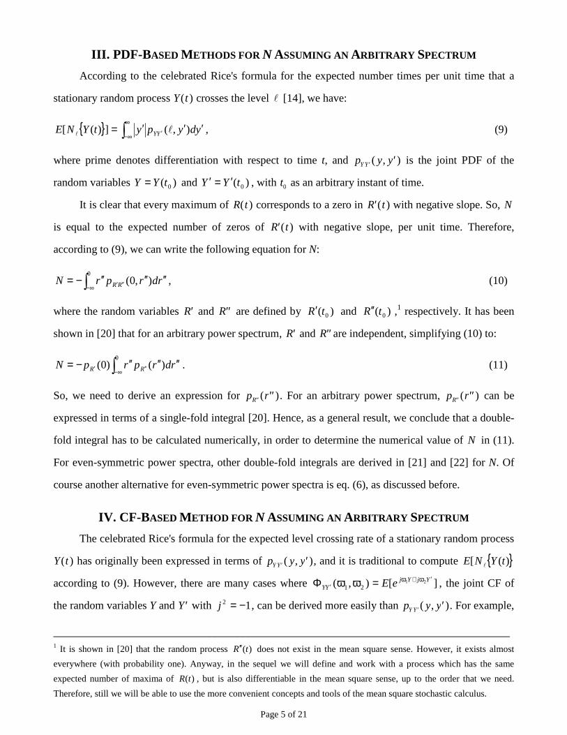
III. PDF-B ASED METHODS FOR N ASSUMING AN ARBITRARY SPECTRUM

According to the celebrated Rice's formula for the expected number times per unit time that a

stationary random process Y t( ) crosses the level � [14], we have:

{ } ydypytYNE YY ′′′= ′

∞

∞−� ),(])([ ��

, (9)

where prime denotes differentiation with respect to time t, and p y yY Y ′ ′( , ) is the joint PDF of the

random variables )( 0tYY = and )( 0tYY ′=′ , with t0 as an arbitrary instant of time.

It is clear that every maximum of R t( ) corresponds to a zero in ′R t( ) with negative slope. So, N

is equal to the expected number of zeros of ′R t( ) with negative slope, per unit time. Therefore,

according to (9), we can write the following equation for N:

� ∞− ′′′ ′′′′′′−=0

),0( rdrprN RR , (10)

where the random variables ′R and ′′R are defined by )( 0tR′ and )( 0tR ′′ ,1 respectively. It has been

shown in [20] that for an arbitrary power spectrum, ′R and ′′R are independent, simplifying (10) to:

� ∞− ′′′ ′′′′′′−=0

)()0( rdrprpN RR . (11)

So, we need to derive an expression for p rR′′ ′′( ). For an arbitrary power spectrum, p rR′′ ′′( ) can be

expressed in terms of a single-fold integral [20]. Hence, as a general result, we conclude that a double-

fold integral has to be calculated numerically, in order to determine the numerical value of N in (11).

For even-symmetric power spectra, other double-fold integrals are derived in [21] and [22] for N. Of

course another alternative for even-symmetric power spectra is eq. (6), as discussed before.

IV. CF-BASED METHOD FOR N ASSUMING AN ARBITRARY SPECTRUM

The celebrated Rice's formula for the expected level crossing rate of a stationary random process

Y t( ) has originally been expressed in terms of p y yY Y ′ ′( , ), and it is traditional to compute { })([ tYNE�

according to (9). However, there are many cases where ][),( 2121

YjYjYY eE ′ω+ω

′ =ωωΦ , the joint CF of

the random variables Y and ′Y with 12 −=j , can be derived more easily than p y yY Y ′ ′( , ). For example,

__________________________________________________________________________________ 1 It is shown in [20] that the random process ( )R t′′ does not exist in the mean square sense. However, it exists almost

everywhere (with probability one). Anyway, in the sequel we will define and work with a process which has the same

expected number of maxima of ( )R t , but is also differentiable in the mean square sense, up to the order that we need.

Therefore, still we will be able to use the more convenient concepts and tools of the mean square stochastic calculus.

of 21

in calculating the fading rate in diversity systems operating over frequency selective fading channels, it

is very straightforward to derive ),( 21 ωωΦ ′YY rather than p y yY Y ′ ′( , ) [26]. So, we need to express (9)

in terms of ΦY Y ′ ( , )ω ω1 2 . Such a formula apparently was first reported in [27] and then rederived,

independently, in [26]:

{ } 1 11 2 1 2 11 2 1 22 2 2

2 2 2

( , ) ( , ) ( )1 1 1[ ( ) ] .

2 2YY YY Yj jd

E N Y t e d d e d dd

∞ ∞ ∞ ∞′ ′− ω − ω

−∞ −∞ −∞ −∞

Φ ω ω Φ ω ω − Φ ω− −= ω ω = ω ωπ ω ω π ω� � � ��

�

(12)

The same results can be obtained using Hsu’s formula for the absolute moments of a random variable,

in terms of the associated CF, given in pp. 19-20 of [28]. This is due to the fact that (9) is essentially a

first-order absolute moment, i.e., { } |[ ( ) ] ( ) ( | )Y Y YE N Y t p y p y dy∞

′−∞′ ′ ′= ��

� � . Note that because of the

presence of 2ω in the denominator of the integrands in (12), both integrals seem to be divergent in

some cases. However, in Appendix A it has been shown that both integrands are bounded at the origin

1 2( , ) (0,0)ω ω = , provided that 2[ ]E Y ′ is finite.

By symmetry, N is equal to the half of the expected number of the extrema of ( )R t per unit time.

In other words, N is equal to the half of the expected number of zeros of ( )R t′ per unit time. Therefore

we rewrite (10) as:

{ }0

1 1(0, ) [ ( ) ]

2 2R RN r p r dr E N R t∞

′ ′′−∞′′ ′′ ′′ ′= =� .

Since R t( ) has a Rayleigh PDF, i.e. ( ) 002 2exp)( bbrrrpR −= for r > 0 and zero otherwise [8], we

have { } 00)(Pr =≤tR . So, we can conclude that ′R t( ) and the auxiliary random process

)()()( tRtRtA ′= have the same number of zeros per unit time, i.e., { } { })()( 00 tANtRN =′ . In this way,

the following useful relationship can be established:

{ }0(1 2) [ ( ) ]N E N A t= . (13)

The utility of the auxiliary random process A t( ), also used in [29], lies on the fact that ΦAA′( , )ω ω1 2 , in

which )( 0tAA = and )( 0tAA ′=′ ,2 with 0t as an arbitrary instant of time, can be calculated more

easily than Φ ′ ′′R R ( , )ω ω1 2 .

__________________________________________________________________________________ 2 Since 2( ) ( ) ( ) ( )A t R t R t R t′ ′ ′′= + , we see that the random process ( )A t′ exists almost everywhere (with probability one), as

( )R t′ and ( )R t′′ exist in the same sense [20]. However, note that 212( ) ( )A t dR t dt= and 2( )R t is shown to be twice

differentiable in the mean square sense [20]. Therefore, ( )A t′ exists in the mean square sense.

of 21

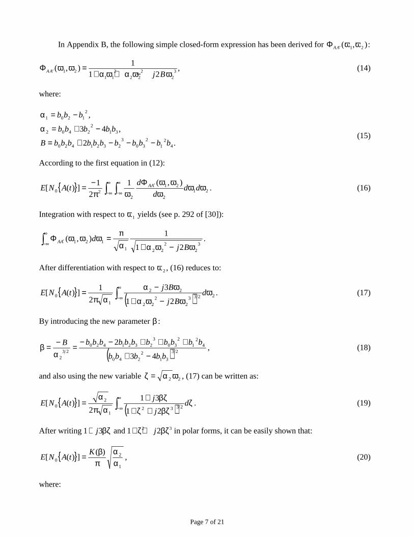
In Appendix B, the following simple closed-form expression has been derived for ΦAA′( , )ω ω1 2 :

ΦAA j B′ =+ + −

( , )ω ωα ω α ω ω1 2

1 12

2 22

23

11 2

, (14)

where:

.2

,43

,

42

12

303

2321420

312

2402

21201

bbbbbbbbbbbB

bbbbb

bbb

−−−+=

−+=α

−=α

(15)

According to the first equation in (12):

{ } 212

21

220

),(1

2

1])([ ωω

ωωωΦ

ωπ−= ′∞

∞−

∞

∞−� � ddd

dtANE AA . (16)

Integration with respect to ω1 yields (see p. 292 of [30]):

32

2221

121

21

1),(

ω−ωα+απ=ωωωΦ�

∞

∞− ′Bj

dAA .

After differentiation with respect to ω2, (16) reduces to:

{ } ( ) 22332

222

22

1

0

21

3

2

1])([ ω

ω−ωα+

ω−ααπ

= �∞

∞−d

Bj

BjtANE . (17)

By introducing the new parameter β :

( ) 23

312

240

42

12

303

232142023

2 43

2

bbbbb

bbbbbbbbbbbB

−+

+++−−=

α−=β , (18)

and also using the new variable 22 ωα=ζ , (17) can be written as:

{ } ( ) ζβζ+ζ+

βζ+απ

α= �

∞

∞−d

j

jtANE

23321

20

21

31

2])([ . (19)

After writing 1 3+ j βζ and 1 22 3+ +ζ βζj in polar forms, it can be easily shown that:

{ }1

20

)(])([

αα

πβ= K

tANE , (20)

where:

of 21

( )( ) ( ) ζ

��

��

��

�

ζ+βζ−βζ

ζβ+ζ+ζ+ζβ+=β �

∞ −− dK0 2

311

436242

2122

1

2tan

2

33tancos

421

91)( . (21)

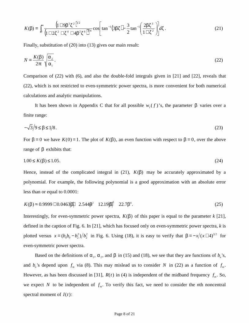
Finally, substitution of (20) into (13) gives our main result:

NK= ( )β

παα2

2

1

. (22)

Comparison of (22) with (6), and also the double-fold integrals given in [21] and [22], reveals that

(22), which is not restricted to even-symmetric power spectra, is more convenient for both numerical

calculations and analytic manipulations.

It has been shown in Appendix C that for all possible w fI ( ) ’s, the parameter β varies over a

finite range:

3 9 1 8− ≤ β ≤ . (23)

For β = 0 we have K( )0 1= . The plot of K ( )β , an even function with respect to β = 0, over the above

range of β exhibits that:

100 105. ( ) .≤ ≤K β . (24)

Hence, instead of the complicated integral in (21), )(βK may be accurately approximated by a

polynomial. For example, the following polynomial is a good approximation with an absolute error

less than or equal to 0.0001:

K ( ) . . . . .β β β β β≈ + + − +0 9999 0 0463 2 544 12 19 22 72 3 4. (25)

Interestingly, for even-symmetric power spectra, K ( )β of this paper is equal to the parameter k [21],

defined in the caption of Fig. 6. In [21], which has focused only on even-symmetric power spectra, k is

plotted versus 2 24 0 2 2( )x b b b b= − in Fig. 6. Using (18), it is easy to verify that 3 2( 4)x xβ = − + for

even-symmetric power spectra.

Based on the definitions of α1, α2, and β in (15) and (18), we see that they are functions of bn 's,

and bn 's depend upon fm via (8). This may mislead us to consider N in (22) as a function of fm.

However, as has been discussed in [31], R t( ) in (4) is independent of the midband frequency fm. So,

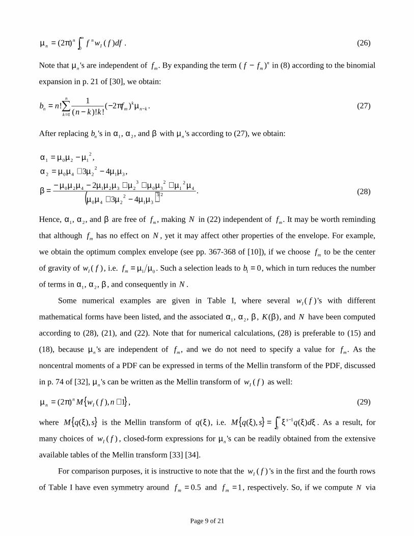
we expect N to be independent of fm. To verify this fact, we need to consider the nth noncentral

spectral moment of I t( ):

of 21

�∞

π=µ0

)()2( dffwf Inn

n . (26)

Note that µn 's are independent of fm. By expanding the term ( )f fmn− in (8) according to the binomial

expansion in p. 21 of [30], we obtain:

b nn k k

fn mk

k

n

n k=−

−=

−�! ( )! !( )

12

0

π µ . (27)

After replacing bn 's in α1, α2, and β with µn 's according to (27), we obtain:

( ) .43

2

,43

,

23

312

240

42

12

303

2321420

312

2402

21201

µµ−µ+µµ

µµ+µµ+µ+µµµ−µµµ−=β

µµ−µ+µµ=α

µ−µµ=α

(28)

Hence, α1, α2, and β are free of fm , making N in (22) independent of fm . It may be worth reminding

that although fm has no effect on N , yet it may affect other properties of the envelope. For example,

we obtain the optimum complex envelope (see pp. 367-368 of [10]), if we choose fm to be the center

of gravity of w fI ( ) , i.e. fm = µ µ1 0 . Such a selection leads to b1 0= , which in turn reduces the number

of terms in α1, α2, β , and consequently in N .

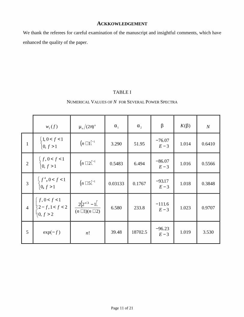
Some numerical examples are given in Table I, where several w fI ( ) 's with different

mathematical forms have been listed, and the associated α1, α2, β , K ( )β , and N have been computed

according to (28), (21), and (22). Note that for numerical calculations, (28) is preferable to (15) and

(18), because µn 's are independent of fm , and we do not need to specify a value for fm . As the

noncentral moments of a PDF can be expressed in terms of the Mellin transform of the PDF, discussed

in p. 74 of [32], µn 's can be written as the Mellin transform of )( fwI as well:

{ }1),()2( +π=µ nfwM In

n , (29)

where { }sqM ),(ξ is the Mellin transform of q( )ξ , i.e. { } ξξξ=ξ �∞ − dqsqM s )(),(0

1 . As a result, for

many choices of )( fwI , closed-form expressions for µn 's can be readily obtained from the extensive

available tables of the Mellin transform [33] [34].

For comparison purposes, it is instructive to note that the )( fwI 's in the first and the fourth rows

of Table I have even symmetry around 5.0=mf and 1=mf , respectively. So, if we compute N via

of 21

the Rice’s result in (6), for the above mf 's, with nb 's calculated according to (27) based on the nµ 's

given in Table I, we obtain the same results for N listed in Table I.

V. EXPECTED NUMBER OF MAXIMA OF THE SIRP ENVELOPE

As mentioned in Section I, the envelopes of the SIRP X t( ) and its associated Gaussian random

process I t( ) in (1), i.e. C R t( ) and R t( ), respectively, have the same expected number of maxima per

unit time. Hence, NN =~, where N

~ is the expected number of maxima for the envelope of X t( ) per

unit time and N is given by (22). In order to express N~

in terms of nb~

's, the central spectral moments

of X t( ), rather than bn 's, we proceed as follows. By definition:

�∞

−π=0

)()()2(~

dffwffb Xn

mn

n . (30)

Since X t( ) is related to I t( ) through (1), we have w f E C w fX I( ) [ ] ( )= 2 , and then nn bCEb ][~ 2= .

Now, rewriting (22) in terms of nb~

's yields the final result:

1

2~

~

2

)~

(~αα

πβ= K

N , (31)

where 1~α , 2

~α , and β~ are the same as α1, α2, and β in (15) and (18), with bn 's replaced by nb~

's.

VI. CONCLUSION

Spherically invariant random processes (which include Gaussian random processes as special

cases) play an important role in modeling non-Gaussian random processes. They allow us to relax the

assumption of Gaussianity, while keeping many of its useful characteristics. In this paper we have

derived a simple, exact, and closed-form expression for the expected number of maxima of a SIRP

envelope, per unit time, assuming an arbitrary-shaped power spectrum for the underlying SIRP. We

have obtained this result using the characteristic function-based level crossing formula, while the

traditional probability density function-based level crossing formula leads to a complicated double-fold

integral, which has to be solved via numerical integration techniques. As an application, the interested

reader may refer to [35], where the formula for the expected number of maxima of the SIRP envelope,

derived in this paper, has been used for estimating the velocity of a mobile vehicle in a Rayleigh fading

channel.

of 21

ACKKOWLEDGEMENT

We thank the referees for careful examination of the manuscript and insightful comments, which have

enhanced the quality of the paper.

TABLE I

NUMERICAL VALUES OF N FOR SEVERAL POWER SPECTRA

)( fwI nn )2( πµ α1 α2 β K ( )β N

1 ��

><<

1,0

10,1

f

f ( ) 11 −+n 3.290 51.95

−−

76 073

.E

1.014 0.6410

2 ��

><<

1,0

10,

f

ff ( ) 12 −+n 0.5483 6.494 −

−86 07

3.

E 1.016 0.5566

3 ��

><<

10

104

f

ff

,

, ( ) 15 −+n 0.03133 0.1767 −

−9317

3.

E 1.018 0.3848

4 ��

��

�

><<−

<<

2,0

21,2

10,

f

ff

ff

( ))2)(1(

122 1

++−+

nn

n

6.580 233.8 −

−1116

3.

E 1.023 0.9707

5 exp( )− f n! 39.48 18702.5 −

−96 23

3.

E 1.019 3.530

of 21

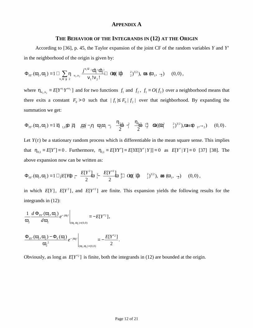
APPENDIX A

THE BEHAVIOR OF THE INTEGRANDS IN (12) AT THE ORIGIN

According to [36], p. 45, the Taylor expansion of the joint CF of the random variables Y and ′Y

in the neighborhood of the origin is given by:

1 2 1 2

1 2

1 2

2 2 3 21 21 2 , 1 2 1 2

2 1 2

( , ) 1 (( ) ), as ( , ) (0,0)! !YY

jO

ν +ν ν ν

′ ν νν +ν ≤

ω ωΦ ω ω = + η + ω + ω ω ω →ν ν� ,

where 1 2

1 2, [ ]E Y Yν νν ν ′η = and for two functions 1f and 2f , 1 2( )f O f= over a neighborhood means that

there exits a constant 0 0F > such that 1 0 2| | | |f F f≤ over that neighborhood. By expanding the

summation we get:

2,0 0,22 2 2 2 3 21 2 1,0 1 0,1 2 1,1 1 2 1 2 1 2 1 2( , ) 1 (( ) ), as ( , ) (0,0)

2 2YY j j O′

η ηΦ ω ω = + η ω + η ω − η ω ω − ω − ω + ω + ω ω ω → .

Let Y t( ) be a stationary random process which is differentiable in the mean square sense. This implies

that 0,1 [ ] 0E Y ′η = = . Furthermore, 1,1 [ ] [ [ | ]] 0E YY E YE Y Y′ ′η = = = as [ | ] 0E Y Y′ = [37] [38]. The

above expansion now can be written as:

2 22 2 2 2 3 2

1 2 1 1 2 1 2 1 2

[ ] [ ]( , ) 1 [ ] (( ) ), as ( , ) (0,0)

2 2YY

E Y E YjE Y O′

′Φ ω ω = + ω − ω − ω + ω + ω ω ω → ,

in which [ ]E Y , 2[ ]E Y , and 2[ ]E Y ′ are finite. This expansion yields the following results for the

integrands in (12):

1

1 2

1 2 2

2 2 ( , ) (0,0)

( , )1[ ]YY jd

e E Yd′ − ω

ω ω =

Φ ω ω ′= −ω ω

� ,

1

1 2

21 2 1

22 ( , ) (0,0)

( , ) ( ) [ ]

2YY Y j E Y

e′ − ω

ω ω =

′Φ ω ω − Φ ω = −ω

� .

Obviously, as long as 2[ ]E Y ′ is finite, both the integrands in (12) are bounded at the origin.

of 21

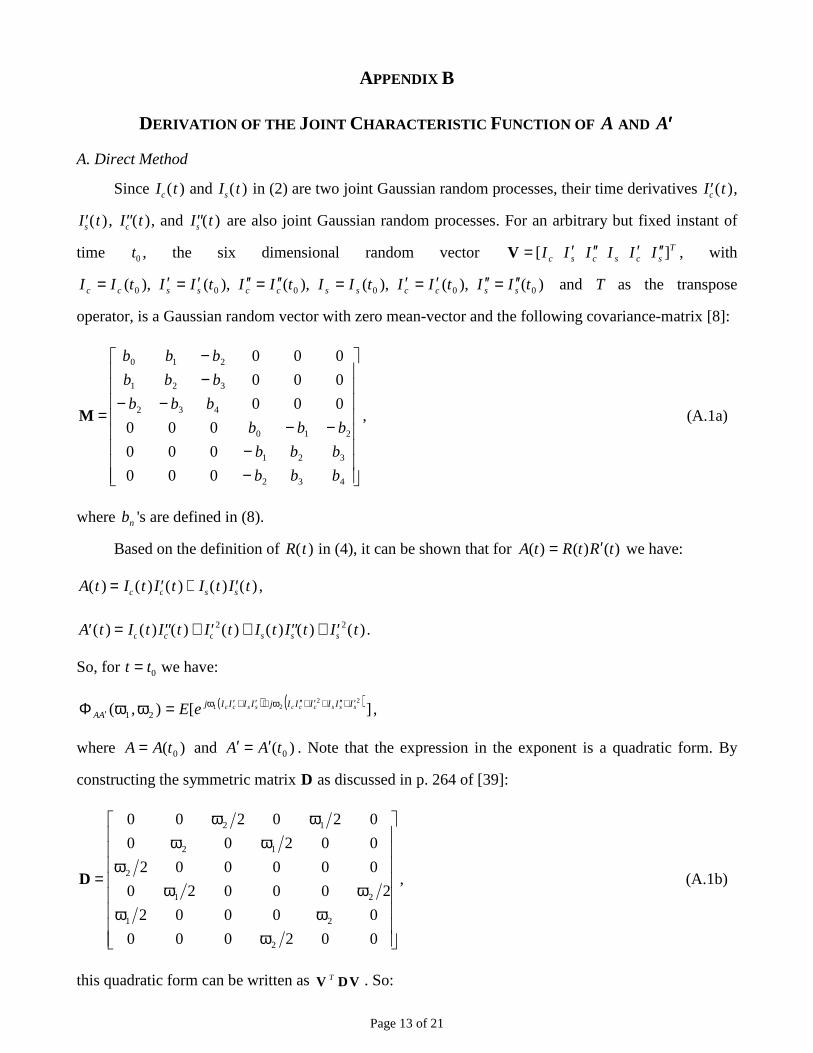
APPENDIX B

DERIVATION OF THE JOINT CHARACTERISTIC FUNCTION OF A AND ′′′′A

A. Direct Method

Since I tc( ) and I ts( ) in (2) are two joint Gaussian random processes, their time derivatives ′I tc( ),

′I ts( ), ′′I tc ( ), and ′′I ts ( ) are also joint Gaussian random processes. For an arbitrary but fixed instant of

time t0 , the six dimensional random vector Tscscsc IIIIII ][ ′′′′′′=V , with

)(),(),(),(),(),( 000000 tIItIItIItIItIItII ssccssccsscc ′′=′′′=′=′′=′′′=′= and T as the transpose

operator, is a Gaussian random vector with zero mean-vector and the following covariance-matrix [8]:

�

��

�

−−

−−−−

−−

=

432

321

210

432

321

210

000

000

000

000

000

000

bbb

bbb

bbb

bbb

bbb

bbb

M , (A.1a)

where nb 's are defined in (8).

Based on the definition of R t( ) in (4), it can be shown that for )()()( tRtRtA ′= we have:

A t I t I t I t I tc c s s( ) ( ) ( ) ( ) ( )= ′ + ′ ,

′ = ′′ + ′ + ′′ + ′A t I t I t I t I t I t I tc c c s s s( ) ( ) ( ) ( ) ( ) ( ) ( )2 2 .

So, for t t= 0 we have:

( ) ( ) ][),(22

2121

ssscccsscc IIIIIIjIIIIjAA eE ′+′′+′+′′ω+′+′ω

′ =ωωΦ ,

where )( 0tAA = and )( 0tAA ′=′ . Note that the expression in the exponent is a quadratic form. By

constructing the symmetric matrix D as discussed in p. 264 of [39]:

�

��

�

ωωω

ωωω

ωωωω

=

002000

00002

200020

000002

00200

020200

2

21

21

2

12

12

D , (A.1b)

this quadratic form can be written as VDV T . So:

of 21

)1(][),( 21 VDVVDV

T

TjAA eE Φ==ωωΦ ′ . (A.2)

It has been shown in p. 152 of [40] that for a k ×1 real Gaussian random vector Z with zero

mean-vector and covariance-matrix ΣΣΣΣ , the CF of the homogeneous quadratic form Z FZT can be

expressed as:

ΦZ FZT

j ii

k

( )ωωλ

=−=

∏ 1

1 21

, (A.3)

where F is the k k× real symmetric matrix of the quadratic form, and λ i 's are the eigenvalues of ΣF,

i.e. the roots of equation det( )ΣF I− =λ 0, with I as the k k× identity matrix. However, as is stated in

[41], (A.3) can be written as:

ΦΣZ FZ I F

T

j( )

det( )ω

ω=

−1

2, (A.4)

which is more appropriate for our purpose. For the case of a complex Gaussian random vector Z and a

complex Hermitian F, the reader may refer to pp. 590-595 of [42].

Based on the above information, ),( 21 ωωΦ ′AA in (A.2) can be written as:

)2det(

1),( 21

DMI jAA −

=ωωΦ ′ .

Using Mathematica software [43] for symbolic operations, it can be shown that:

( )232

222

211 21)2det( ω−ωα+ωα+=− Bjj DMI ,

which in turn results in (14).

B. Indirect Method

Based on the definition of the derivative for a random process Y t( ) we have:

��

��

��

�

τ−

ω+ω=ωωΦ τ

→τ′YY

jYjEYY 210

21 explim),( ,

where )( 0 τ+=τ tYY . Based on the bounded convergence theorem in p. 108 of [44], we can change the

order of lim and E to obtain:

��

��

�

τω

τω

−ωΦ=ωωΦτ→τ′

221

021 ,lim),( YYYY . (A.5)

of 21

So, ΦAA′ ( , )ω ω1 2 can be derived by calculating the limit of ( )τωτω−ωΦτ 221 ,AA , with

)( 0 τ+=τ tAA .

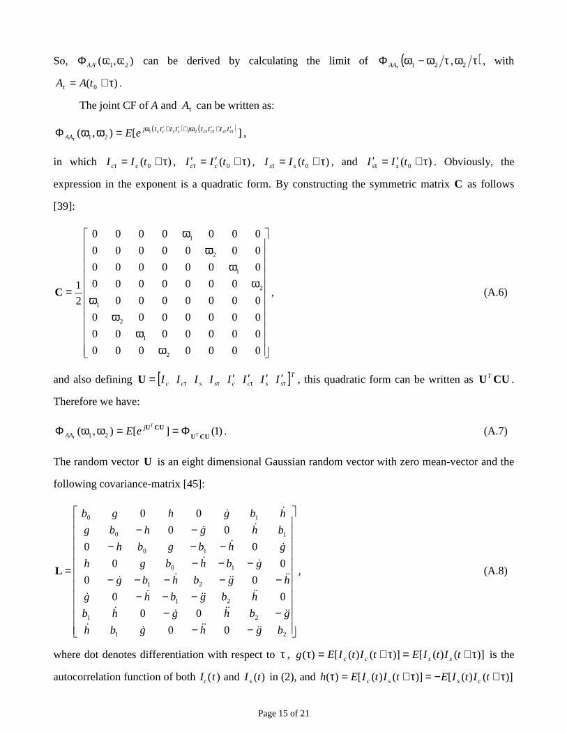
The joint CF of A and τA can be written as:

( ) ( ) ][),( 2121

ττττ

τ

′+′ω+′+′ω=ωωΦ ssccsscc IIIIjIIIIjAA eE ,

in which )( 0 τ+=τ tII cc , )( 0 τ+′=′τ tII cc , )( 0 τ+=τ tII ss , and )( 0 τ+′=′τ tII ss . Obviously, the

expression in the exponent is a quadratic form. By constructing the symmetric matrix C as follows

[39]:

�

��

�

ωω

ωω

ωω

ωω

=

0000000

0000000

0000000

0000000

0000000

0000000

0000000

0000000

2

1

2

1

2

1

2

1

2

1

C , (A.6)

and also defining [ ]Tssccsscc IIIIIIII ττττ ′′′′=U , this quadratic form can be written as UCUT .

Therefore we have:

)1(][),( 21 UCUUCU

T

TjAA eE Φ==ωωΦ

τ. (A.7)

The random vector U is an eight dimensional Gaussian random vector with zero mean-vector and the

following covariance-matrix [45]:

�

��

�

−−−−

−−−−−−−−

−−−−−−

−−

=

21

21

21

21

10

10

10

10

00

00

00

00

00

00

00

00

bghgbh

gbhghb

hbgbhg

hgbhbg

gbhbgh

ghbgbh

bhghbg

hbghgb

��

��

��

��

��

��

��

��

L , (A.8)

where dot denotes differentiation with respect to τ , )]()([)]()([)( τ+=τ+=τ tItIEtItIEg sscc is the

autocorrelation function of both I tc ( ) and )(tI s in (2), and )]()([)]()([)( τ+−=τ+=τ tItIEtItIEh cssc

of 21

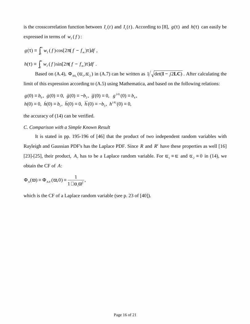
is the crosscorrelation function between I tc ( ) and I ts( ). According to [8], )(τg and )(τh can easily be

expressed in terms of )( fwI :

dffffwg mI ])(2cos[)()(0

τ−π=τ �∞

,

dffffwh mI ])(2sin[)()(0

τ−π=τ �∞

.

Based on (A.4), ΦAAτω ω( , )1 2 in (A.7) can be written as )2det(1 LCI j− . After calculating the

limit of this expression according to (A.5) using Mathematica, and based on the following relations:

,0)0(,)0(,0)0(,)0(,0)0(

,)0(,0)0(,)0(,0)0(,)0()4(

31

4)4(

20

=−====

==−===

hbhhbhh

bggbggbg

��

��

the accuracy of (14) can be verified.

C. Comparison with a Simple Known Result

It is stated in pp. 195-196 of [46] that the product of two independent random variables with

Rayleigh and Gaussian PDF's has the Laplace PDF. Since R and ′R have these properties as well [16]

[23]-[25], their product, A, has to be a Laplace random variable. For ω ω1 = and ω2 0= in (14), we

obtain the CF of A:

Φ ΦA AA( ) ( , )ω ωα ω

= =+′ 0

11 1

2,

which is the CF of a Laplace random variable (see p. 23 of [40]).

of 21

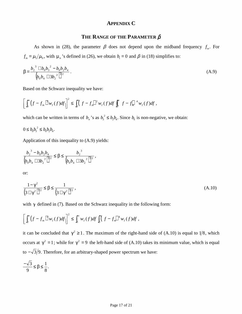
APPENDIX C

THE RANGE OF THE PARAMETER ββββ

As shown in (28), the parameter β does not depend upon the midband frequency fm . For

fm = µ µ1 0 , with nµ ’s defined in (26), we obtain b1 0= and β in (18) simplifies to:

( ) 232240

4202

303

2

3bbb

bbbbbb

+

−+=β . (A.9)

Based on the Schwarz inequality we have:

( ) ( ) ( )��∞∞∞

−−≤�

� � −

0

4

0

22

0

3 )()()( dffwffdffwffdffwff ImImIm ,

which can be written in terms of nb ’s as b b b32

2 4≤ . Since b0 is non-negative, we obtain:

0 0 32

0 2 4≤ ≤b b b b b .

Application of this inequality to (A.9) yields:

( ) ( ) 232240

32

232240

4203

2

33 bbb

b

bbb

bbbb

+≤β≤

+

−,

or:

( ) ( ) 232232

2

3

1

3

1

γ+≤β≤

γ+γ−

, (A.10)

with γ defined in (7). Based on the Schwarz inequality in the following form:

( ) ( )��∞∞∞

−≤�

� � −

0

4

0

2

0

2 )()()( dffwffdffwdffwff ImIIm ,

it can be concluded that 12 ≥γ . The maximum of the right-hand side of (A.10) is equal to 1 8, which

occurs at 12 =γ ; while for 92 =γ the left-hand side of (A.10) takes its minimum value, which is equal

to − 3 9. Therefore, for an arbitrary-shaped power spectrum we have:

− ≤ ≤39

18

β .

of 21

REFERENCES [1] Y. K. Lin, “Random processes,” Appl. Mechanics Rev., vol. 22, pp. 825-831, 1969.

[2] D. E. Newland, An Introduction to Random Vibrations and Spectral Analysis, 2nd ed., New

York: Longman, 1984.

[3] K. Yao, “A representation theorem and its applications to spherically-invariant random

processes,” IEEE Trans. Inform. Theory, vol. 19, pp. 600-608, 1973.

[4] G. L. Wise and N. C. Gallagher, Jr., “On spherically invariant random processes,” IEEE Trans.

Inform. Theory, vol. 24, pp. 118-120, 1978.

[5] K. Chu, “Estimation and decision for linear systems with elliptical random processes,” IEEE

Trans. Automat. Contr., vol. 18, pp. 499-505, 1973.

[6] B. Picinbono, Random Signals and Systems. Englewood Cliffs, NJ: Prentice Hall, 1993.

[7] A. Abdi, H. A. Barger, and M. Kaveh, “Signal modeling in wireless fading channels using

spherically invariant processes,” in Proc. IEEE Int. Conf. Acoust., Speech, Signal Processing,

Istanbul, Turkey, 2000, pp. 2997-3000.

[8] S. O. Rice, “Mathematical analysis of random noise,” reprinted in Selected Papers on Noise and

Stochastic Processes. N. Wax, Ed., New York: Dover, 1954, pp. 133-294.

[9] W. A. Gardner, Introduction to Random Processes with Applications to Signals and Systems, 2nd

ed., Singapore: McGraw-Hill, 1990.

[10] A. Papoulis, Probability, Random Variables, and Stochastic Processes, 3rd ed., Singapore:

McGraw-Hill, 1991.

[11] G. L. Wise, “A comment on 'Zero-crossing rates of functions of Gaussian processes,'" IEEE

Trans. Inform. Theory, vol. 38, p. 213, 1992.

[12] W. B. Davenport, Jr. and W. L. Root, An Introduction to the Theory of Random Signals and

Noise. New York: McGraw-Hill, 1958.

[13] D. Middleton, An Introduction to Statistical Communication Theory. New York: McGraw-Hill,

1960.

[14] I. F. Blake and W. C. Lindsey, “Level-crossing problems for random processes,” IEEE Trans.

Inform. Theory, vol. 19, pp. 295-315, 1973.

[15] M. D. Yacoub, Foundations of Mobile Radio Engineering. Boca Raton, FL: CRC, 1993.

[16] J. Komaili, L. A. Ferrari, and P. V. Sankar, “Estimating the bandwidth of a normal process from

the level crossings of its envelope,” IEEE Trans. Acoust., Speech, Signal Processing, vol. 35, pp.

1481-1483, 1987.

[17] D. Middleton, “S. O. Rice and the theory of random noise: Some personal recollections,” IEEE

Trans. Inform. Theory, vol. 34, pp. 1367-1373, 1988.

[18] A. J. Rainal, “Origin of Rice's formula,” IEEE Trans. Inform. Theory, vol. 34, pp. 1383-1387,

1988.

[19] A. Abdi, J. A. Barger, and M. Kaveh, “A parametric model for the distribution of the angle of

arrival and the associated correlation function and power spectrum at the mobile station,” IEEE

Trans. Vehic. Technol., vol. 51, pp. 425-434, 2002.

of 21

[20] A. Abdi, “On the second derivative of a Gaussian process envelope,” IEEE Trans. Inform.

Theory, vol. 48, pp. 1226-1231, 2002.

[21] N. M. Blachman, “The distributions of local extrema of Gaussian noise and of its envelope,”

IEEE Trans. Inform. Theory, vol. 45, pp. 2115-2121, 1999.

[22] R. Narasimhan and D. C. Cox, “Speed estimation in wireless systems using wavelets,” IEEE

Trans. Commun., vol. 47, pp. 1357-1364, 1999.

[23] D. Middleton, “Spurious signals caused by noise in triggered circuits,” J. Appl. Phys., vol. 19,

pp. 817-830, 1948.

[24] M. R. Leadbetter, “On crossings of levels and curves by a wide class of stochastic processes,”

Ann. Math. Statist., vol. 37, pp. 260-267, 1966.

[25] A. M. Hasofer, “The joint distribution of the envelope of a Gaussian process and its derivative,”

Austral. J. Statist., vol. 15, pp. 215-216, 1973.

[26] A. Abdi and M. Kaveh, “Level crossing rate in terms of the characteristic function: A new

approach for calculating the fading rate in diversity systems,” IEEE Trans. Commun., vol. 50,

pp. 1397-1400, 2002.

[27] T. Vinje, “On the statistical distribution of second-order forces and motion,” Int. Shipbulid.

Prog., vol.30, pp. 58-68, 1983.

[28] V. V. Petrov, Sums of Independent Random Variables. Berlin: Springer, 1975.

[29] S. Nader-Esfahani and A. Abdi, “A new formula for the mean number of the peaks of a normal

process envelope, in Proc. Iranian Conf. Elec. Eng., Tarbiat Modarres University, Tehran, Iran,

1994, vol. 5, pp. 450-456 (in Persian).

[30] I. S. Gradshteyn and I. M. Ryzhik, Table of Integrals, Series, and Products, corrected and

enlarged ed., A. Jeffrey, Ed., New York: Academic, 1980.

[31] J. Dugundji, “Envelopes and pre-envelopes of real waveforms,” IRE Trans. Inform. Theory, vol.

4, pp. 53-57, 1958.

[32] W. C. Giffin, Transform Techniques for Probability Modeling. New York: Academic, 1975.

[33] A. Erdelyi, Ed., Tables of Integral Transforms. vol. 1, New York: McGraw-Hill, 1954.

[34] F. Oberhettinger, Tables of Mellin Transforms. Berlin: Springer, 1974.

[35] A. Abdi and M. Kaveh, “A new velocity estimator for cellular systems based on higher order

crossings,” in Proc. Asilomar Conf. Signals, Systems, Computers, Pacific Grove, CA, 1998, pp.

1423-1427.

[36] R.N. Bhattacharya and R. R. Rao, Normal Approximation and Asymptotic Expansions. New

York: Wiley, 1976.

[37] J. E. Mazo and J. Salz, “A theorem on conditional expectation,” IEEE Trans. Inform. Theory,

vol. 16, pp. 379-381, 1970.

[38] B. L. S. Prakasa Rao, “Characterization of stationary processes differentiable in mean square,”

IEEE Trans. Inform. Theory, vol. 18, pp. 659-661, 1972.

[39] S. Lipschutz, Theory and Problems of Linear Algebra, 2nd ed., Singapore: McGraw-Hill, 1974.

of 21

[40] N. L. Johnson and S. Kotz, Distributions in Statistics: Continuous Univariate Distributions. vol.

2, New York: Wiley, 1970.

[41] G. L. Turin, “The characteristic function of Hermitian quadratic forms in complex normal

variables,” Biometrika, vol. 47, pp. 199-201, 1960.

[42] M. Schwartz, W. R. Bennett, and S. Stein, Communication Systems and Techniques. New York:

McGraw-Hill, 1966.

[43] S. Wolfram, Mathematica: A System for Doing Mathematics by Computer, 2nd ed., Redwood

City, CA: Addison-Wesley, 1991.

[44] B. Fristedt and L. Gray, A Modern Approach to Probability Theory. Boston, MA: Birkhauser,

1997.

[45] S. O. Rice, “Statistical properties of a sine wave plus random noise,” Bell Syst. Tech. J., vol. 27,

pp. 109-157, 1948.

[46] W. B. Davenport, Jr., Probability and Random Processes: An Introduction for Applied Scientists

and Engineers. New York: McGraw-Hill, 1970.

of 21

Ali Abdi

Ali Abdi (S'98, M'01) received the Ph.D. degree in electrical engineering from the University of

Minnesota, Minneapolis, MN, in Summer 2001. He joined the Department of Electrical and Computer

Engineering of New Jersey Institute of Technology (NJIT), Newark, NJ, in Fall 2001, as an Assistant

Professor. His previous research interests have included stochastic processes, wireless

communications, pattern recognition, neural networks, and time series analysis. His current work is

mainly focused on wireless communications, with special emphasis on modeling, estimation, and

efficient simulation of wireless channels, multiantenna systems, and system performance analysis. He

is an Associate Editor for IEEE Transactions on Vehicular Technology.

Expected Number of Maxima in the Envelope of a Spherically ...

Documents

Transcript of Expected Number of Maxima in the Envelope of a Spherically ...