arX

iv:h

ep-t

h/01

1201

9v4

20

Aug

200

2

hep-th/0112019December 2001

Spherically Symmetric Braneworld Solutions with (4)R term inthe Bulk

G. Kofinas1 , E. Papantonopoulos2 , I. Pappa3

1 Department of Physics, Nuclear and Particle Physics Section, University of Athens,Panepistimioupolis GR 157 71, Ilisia, Athens, Greece

2, 3 Physics Department, National Technical University of Athens,Zografou Campus GR 157 80, Athens, Greece

Abstract

An analysis of a spherically symmetric braneworld configuration is performed whenthe intrinsic curvature scalar is included in the bulk action; the vanishing of theelectric part of the Weyl tensor is used as the boundary condition for the embed-ding of the brane in the bulk. All the solutions outside a static localized matterdistribution are found; some of them are of the Schwarzschild-(A)dS4 form. Twomodified Oppenheimer-Volkoff interior solutions are also found; one is matched toa Schwarzschild-(A)dS4 exterior, while the other does not. A non-universal gravita-tional constant arises, depending on the density of the considered object; however,the conventional limits of the Newton’s constant are recovered. An upper boundof the order of TeV for the energy string scale is extracted from the known solarsystem measurements (experiments). On the contrary, in usual brane dynamics,this string scale is calculated to be larger than TeV .

1gkofin@phys.uoa.gr2lpapa@central.ntua.gr3gpappa@central.ntua.gr

1. Introduction

The desire to explore physics beyond the Standard Model has led us to explore

the ideas that spacetime is of a dimension larger than four, and that we are essentially

confined to a four-dimensional hypersurface. String theories provide a framework for

exploring such ideas, but nevertheless we are still far away of having a viable low-energy

realization of these theories. Braneworld models consist relevant world realizations in

which some underlying features are often minimized. Replacing, for example, a whole

field with a constant (solitonic solution) may probably oversimplifies the reality, but at

the same time makes it possible to obtain a more concrete picture, with the hope that any

new behavior appearing will be still present in the more complete theory. Not only at the

cosmological level, but also at a local one - concerning stars, galaxies, clusters of galaxies

- has a brane solution to be consistent with the various astrophysical observations, which

are often more reliable than the cosmological ones.

Attempts for obtaining braneworld solutions are cast into two categories. First, the

bulk space assumes a given geometry, a coordinate system is adopted and the influence on

the brane geometry is somehow extracted. It seems as a disadvantage of this approach that

the bulk is prefixed and also that the brane imbedding obtained is not gauge-invariant

(independent of the coordinate system chosen). Second, do not specify the exact bulk

geometry, adopt a coordinate system adapted to the brane (gauss normal coordinates

or some relevant one) and deduce a brane dynamics, containing imprints from the bulk.

Assumptions on the brane geometry are often sufficient for obtaining an exactly closed

brane dynamics. This approach allows of a dynamically interacting brane with bulk,

though this situation is not necessarily considered. A disadvantage of this method is that

finding a bulk geometry in which the brane consists its boundary may be a very difficult

task. A probable advantage would be the extraction of common braneworld characteristics

holding for a broad class of bulk backgrounds. In both approaches, if the codimension

is one, Israel matching conditions are necessarily used. In the present paper we shall

elaborate on the second approach.

The effective brane equations have been obtained [1] when the effective low-energy

theory in the bulk is higher-dimensional gravity. However, a more fundamental descrip-

tion of the physics that produces the brane could include [2] higher order terms in a

derivative expansion of the effective action, such as a term for the scalar curvature of the

brane, and higher powers of curvature tensors on the brane. A brane action that contains

powers of the brane curvature tensors has also been used in the context of the AdS/CFT

1

correspondence (e.g. [3]) to regularize the action of a bulk AdS space which diverges when

the radius of the AdS space becomes infinite. If the dynamics is governed not only by the

ordinary five-dimensional Einstein-Hilbert action, but also by the four-dimensional Ricci

scalar term induced on the brane, new phenomena appear. In [4, 5] it was observed that

the localized matter fields on the brane (which couple to bulk gravitons) can generate via

quantum loops a localized four-dimensional worldvolume kinetic term for gravitons (see

also [6, 7, 8, 9]). That is to say, four-dimensional gravity is induced from the bulk gravity

to the brane worldvolume by the matter fields confined to the brane. It was also shown

that an observer on the brane will see correct Newtonian gravity at distances shorter than

a certain crossover scale, despite the fact that gravity propagates in extra space which

was assumed there to be flat with infinite extent; at larger distances, the force becomes

higher-dimensional. The first realization of the induced gravity scenario in string the-

ory was presented in [10]. Furthermore, new closed string couplings on Dp-branes for

the bosonic string were found in [11]. These couplings are quadratic in derivatives and

therefore take the form of induced kinetic terms on the brane. For the graviton in partic-

ular these are the induced Einstein-Hilbert term as well as terms quadratic in the second

fundamental tensor. Considering the intrinsic curvature scalar in the bulk action, the

effective brane equations have been obtained in [12]. Results concerning cosmology have

been discussed in [13, 14, 15, 16, 17].

The original Randall-Sundrum models [18], based on a Minkowski brane and a specific

relation between the bulk cosmological constant and the brane tension, have drawn much

attention because they might be realizable in supergravity and superstring compactifica-

tions [19, 20, 21, 22]. However, any Ricci-flat four-dimensional metric can be embedded

(with the common warped embedding) in (A)dS5 (e.g. [23, 24]). This way, a black-string

solution [23, 25, 26, 27] can be easily constructed. Furthermore, it is known that any

four-dimensional Einstein spaces can foliate an (A)dS5 bulk [28, 29, 30, 31, 32, 33]. Thus,

asymptotically non-flat black holes (Schwarzschild-(A)dS4) can be obtained as slices of

the above precise bulks. Almost all treatments on spherically symmetric braneworld so-

lutions, as the previously mentioned, representing, for example, the exterior of a star,

do not take care of the finite extension of the object. Till now, there is no known exact

five-dimensional solution for astrophysical brane black holes. Furthermore, looking for

bulks having some interior star solution as part of their boundaries is even harder. In

[34, 35, 36], some interior and exterior solutions were found, without including the (4)R

term.

In the present paper, we discuss the gravitational field of an uncharged, non-rotating

2

spherically symmetric rigid object when in the dynamics there is a contribution from the

brane intrinsic curvature invariant. In section 2, we find all the possible exterior solutions,

containing one undetermined parameter which is the parameter of the Newtonian term.

Some of these solutions are of the Schwarzschild-(A)dS4 form. In two cases, we can solve

also the interior problem which reduces to a generalization of the Oppenheimer-Volkoff

solution, and thus determine the unknown parameter. This is found different from the

conventional value of a localized spherically symmetric distribution within the frame-

work of four-dimensional general relativity. Hence, a non-universal Newton’s constant,

depending on the density of the object, naturally arises. In section 3, taking care of the

classical experiments of gravity in the solar system, we can set an upper bound for the

five-dimensional Planck mass being of the order of TeV . The revival of the conventional

results is discussed, and also, a comparison with the more standard brane dynamics is

presented. Finally, in section 4 are our conclusions.

2. Four-Dimensional Spherically Symmetric Solutions

We consider a 3-dimensional brane Σ (with normal vector field nA) embedded in

a 5-dimensional spacetime M . Capital Latin letters A, B, ... = 0, 1, ..., 4 will denote full

spacetime, lower Greek µ, ν, ... = 0, 1, ..., 3 run over brane worldvolume, while lower Latin

ones span some 3-dimensional spacelike surfaces foliating the brane, i.e. i, j, ... = 1, ..., 3.

For convenience, we can quite generally, choose a coordinate y such that the hypersurface

y = 0 coincides with the brane. The total action for the system is taken to be:

S =1

2κ25

∫

M

√

−(5)g(

(5)R − 2Λ5

)

d5x +1

2κ24

∫

Σ

√

−(4)g(

(4)R − 2Λ4

)

d4x

+

∫

M

√

−(5)g Lmat5 d5x +

∫

Σ

√

−(4)g Lmat4 d4x. (1)

For clarity, we have separated the cosmological constants Λ5, Λ4 from the rest matter

contents Lmat5 , Lmat

4 of the bulk and the brane respectively. Λ4/κ24 can be interpreted as

the brane tension of the standard Dirac-Nambu-Goto action, or as the sum of a brane

worldvolume cosmological constant and a brane tension. We basically concern on the case

with no fields in the bulk, i.e. (5)TAB = 0.

From the dimensionful constants κ25, κ2

4 the Planck masses M5, M4 are defined as:

κ25 = 8πG(5) = M−3

5 , κ24 = 8πG(4) = M−2

4 , (2)

3

with M5, M4 having dimensions of (length)−1. Then, a distance scale rc is defined as :

rc ≡κ2

5

κ24

=M2

4

M35

. (3)

Varying (1) with respect to the bulk metric gAB, we obtain the equations

(5)GAB = −Λ5gAB + κ25

(

(5)TAB + (loc)TAB δ(y))

, (4)

where

(loc)TAB ≡ − 1

κ24

√

−(4)g

−(5)g

(

(4)GAB − κ24

(4)TAB + Λ4hAB

)

(5)

is the localized energy-momentum tensor of the brane. (5)GAB, (4)GAB denote the Einstein

tensors constructed from the bulk and the brane metrics respectively. Clearly, (4)GAB acts

as an additional source term for the brane through (loc)TAB. The tensor hAB = gAB−nAnB

is the induced metric on the hypersurfaces y = constant, with nA the normal vector on

these.

The way the y-coordinate has been defined, allows us to write, at least in the neigh-

borhood of the brane, the 5-line element in the block diagonal form

ds2(5) = −N2dt2 + gijdxidxj + dy2 , (6)

where N, gij are generally functions of t, xi, y. The distributional character of the brane

matter content makes necessary for the compatibility of the bulk equations (4) the fol-

lowing modified (due to (4)Gµν ) Israel-Darmois-Lanczos-Sen conditions [37, 38, 39, 40]

[Kµν ] = −κ2

5

(

(loc)T µν −

(loc)T

3δµν

)

, (7)

where the bracket means discontinuity of the extrinsic curvature Kµν = ∂ygµν/2 across

y = 0. A Z2 symmetry on reflection around the brane is considered throughout.

One can derive from equations (4), (7) the induced brane gravitational dynamics [12],

which consists of a four-dimensional Einstein gravity, coupled to a well-defined modified

matter content. More explicitly, one gets

(4)Gµν = κ2

4(4)T µ

ν −(

Λ4 +3

2α2

)

δµν + α

(

Lµν +

L

2δµν

)

, (8)

where α ≡ 2/rc, while the quantities Lµν are related to the matter content of the theory

through the equation

LµλLλ

ν − L2

4δµν = T µ

ν − 1

4(3α2 + 2T λ

λ ) δµν , (9)

4

and L ≡ Lµµ. The quantities T µ

ν are given by the expression

T µν =

(

Λ4 −1

2Λ5

)

δµν − κ2

4(4)T µ

ν +

+2

3κ2

5

(

(5)T µν +

(

(5)T yy −

(5)T

4

)

δµν

)

− Eµ

ν , (10)

with (5)T = (5)T AA , (5)T A

B = gAC (5)T CB. Bars over (5)TAB and the electric part E

µ

ν =

CµAνBnAnB of the 5-dimensional Weyl tensor CA

BCD mean that the quantities are evaluated

at y = 0. Eµ

ν carries the influence of non-local gravitational degrees of freedom in the

bulk onto the brane [1] and makes the brane equations (8) not to be, in general, closed.

This means that there are bulk degrees of freedom which cannot be predicted from data

available on the brane. One needs to solve the field equations in the bulk in order to

determine Eµ

ν on the brane. In the present paper, for making (8) closed, we shall set

Eµ

ν = 0 as a boundary condition of the propagation equations in the bulk space. This is

somehow simplified from the viewpoint of geometric complexity, but it is the first step

for investigating the characteristics carried by the brane curvature invariant on the local

brane dynamics we are interested in. Treatments and solutions without this assumption,

in the context of usual brane dynamics, have been given in [26, 41, 42, 43, 34, 35, 36, 44].

Due the block-diagonal form of the metric (6) the solution of the algebraic system (9),

whenever

T ij = τδi

j , (11)

is

L00 = ± 1

2B

(

(7 − 4n+n−)T 00 − (3 − 4n+n−)τ + 3α2

)

, (12)

Lij = SEi

j , (13)

L0i = Li

0 = 0 , (14)

where

S =1

2B

∣

∣T 00 + 3(τ + α2)

∣

∣ , (15)

B =(

− 6(n+ − 1)(n− − 1)T 00 + 2 n+n−(1 − n+n−)τ + 3(3 − 2n+n−)α2

)12, (16)

5

while the matrix Eij is either diag(+1, +1, +1) (with n+ = 3, n− = 0) or diag(+1, +1,−1)

(with n+ = 2, n− = 1).

Inspecting equation (8), we see that the inclusion of the term (4)R has brought a

convenient decomposition of the matter terms. First, standard energy-momentum tensor

enters without having made any choice for the brane tension Λ4 in terms of M4, M5 (in

[45, 1] it has to be Λ4 = 3α2/2). Note that if (4)R is not included in the action, for Λ4 = 0,

ordinary energy-momentum terms cannot arise. Furthermore, in that case, Λ4 has to be

positive in order for κ24 to be positive. Second, the additional matter terms (which rather

appear here as square roots instead of squares of the four-dimensional energy-momentum

tensor) all contain the factor α of energy string scale. Thus, conventional four-dimensional

General Relativity revives on some region of a 4-spacetime, whenever these extra terms

remain suppressed relative to the conventional ones; the specific value of α determines

the region validity of General Relativity.

From now on, we are interested on static (non-cosmological) local braneworld solutions

arising from the action (1). More specifically we consider a spherically symmetric line

element

ds2(4) = −B(r)dt2 + A(r)dr2 + r2(dθ2 + sin2 θdφ2). (17)

The matter content of the 3-universe is a localized spherically symmetric untilted perfect

fluid (e.g. a star) (4)Tµν = (ρ + p)uµuν + pgµν with ρ = p = 0 for r > R, plus the

cosmological constant Λ4. The matter content of the bulk is a cosmological constant Λ5.

These matter contents enter T µν in equation (10) and thus determine Lµ

ν on the right hand

side of our dynamical equations (8). The result is

L00 = ± 1

2B

(

|4Λ4 − 2Λ5 + 3α2| + κ24

(

(7 − 3n+n−)ρ + (n+ + 3n−)p))

, (18)

S =1

2B

∣

∣

∣4Λ4 − 2Λ5 + 3α2 + κ2

4 (ρ − 3p)∣

∣

∣, (19)

B =(

(3 − 4n−)(4Λ4 − 2Λ5 + 3α2) − 4κ24

(

3(n− − 1)ρ + (n+ − 3)p))1/2

, (20)

with the only restriction imposed by the square root appeared in B. Thus, necessarily

4Λ4 − 2Λ5 + 3α2 is non-negative (non-positive) for Eij = δi

j (similarly the other choice of

Eij).

For the metric (17), one evaluates the Ricci tensor (4)Rµν and then constructs the field

equations (8). The combination (4)Rrr/2A + (4)Rθθ/r2 + (4)R00/2B provides the following

6

differential equation for A(r) :

( r

A

)′

= 1 − κ24 ρ(r)r2 −

(

Λ4 +3

2α2

)

r2 +α

2

(

3L00 + (n+ − n−)S

)

r2 , (21)

(′≡ ddr

). Eliminating A ′

Afrom (21) in the (θθ) component of (8), we get an equation for

B ′

B, from which we obtain

(AB)′

AB= Ar

(

κ24 (ρ + p) − α

(

L00 + (2 − n+ + n−)S

))

. (22)

There are various different cases (namely eight) according to the choice of Eij and the

alternative signs in L00, S. However, in the outside region, there are only four different

cases, according to n+, n− and the ± sign in (18); in all these cases, we can integrate

equation (21) in the outside region, obtain the solution A>(r) and from (22) get the

solution B>(r). The result is

1

A>(r)= 1 − γ

r− βr2 , r ≥ R , (23)

B>(r) =1

A>(r)Fn+ , n−(r) , r ≥ R , (24)

with

β =1

3Λ4 +

1

2α2 − α

n+ − n− ± 3

12√

|3 − 4n−|√

|4Λ4 − 2Λ5 + 3α2| , (25)

Fn+ , n−(r) = 1 +(

f(r)αr1

n+−(2+3√

3)n−6√

3 β (3γ−2r1)

√|4Λ4−2Λ5+3α2| − 1

)

δn+∓1 , 4−3n− , (26)

f(r) = (r − r1)( r

A>

)1− 2γr1 g(r)

√

|r1−γ|r1+3γ , (27)

where r1 is the minimum horizon distance and g(r) is equal to∣

∣

∣

r + r1/2 +√

(r1+3γ)/(4βr1)

r + r1/2−√

(r1+3γ)/(4βr1)

∣

∣

∣for

β > 0, or e2 arctan (√

4|β|r1/(r1+3γ) (r + r1/2) ) for β < 0. For β = 0, g(r)√

|r1−γ| / β is replaced

by (r − γ)4γ5/2e2

√γ (r+3γ) (r−γ) . The ±, ∓ signs appearing in (25), (26) correspond to the

± sign of (18). A multiplicative constant of integration for B> has been absorbed to a

redefinition of time and γ is a constant of integration. Note that for β ≤ 0 there is only

one horizon r1 ≤ γ, while for β > 0 (and 27βγ2 < 4 to have well defined horizons) there

are two horizons γ < r1 < 3γ and 1/√

3β < r2 < 1/√

β.

7

Solutions (23), (24) are not yet completely defined unless the parameter γ is deter-

mined, i.e. the interior solution is found. In the case Eij = δi

j , we can find two situations

where equation (21) does not contain p and so, we can integrate it in the interior region

(we give these solutions below, equation (31)).

As it is seen from (24) and (26), all the exterior solutions are either of the form

where A>, B> are inverse to each other, or of the form where the product A>B> is

equal to f(r) to a power appeared in (26). The first class of these solutions is of the

Schwarzschild-(A)dS4 form, while the second is not. For zero β (we can interpret β as

the effective brane cosmological constant) the first class of these solutions reduces to

Schwarzschild-like, while the second does not. Non-Schwarzschild-like exterior solutions

were also obtained in [34, 41, 36, 44], but this fact was rendered to the non-vanishing

Eµ

ν . Such irregular behavior also appears here, due to the intrinsic curvature invariant,

without having involved non-local bulk effects onto the brane. There is one case of our

non-Schwarzschild-(A)dS4 solutions with β > 0, γ/r1 = 2/3, where at large distances –

given that the second horizon is actually at cosmological distances – A>B> is almost one,

i.e. the solution asymptotes the Schwarzschild-dS4.

If we take the covariant derivative (denoted by |) with respect to the induced brane

metric hAB = gAB − nAnB of the equations (7), and make use of the Codacci’s equations,

and of the bulk equations (4), we arrive at the equations (4)TAB|A = −[(5)TCD]nChD

B . When

the matter content of the bulk space is only a cosmological constant, then the common

conservation law of our world is obtained. For the static case we are discussing, this law

is equivalent to the equation

B ′

B= − 2p ′

ρ + p. (28)

Thus, for r ≤ R we get the equation for p(r) :

p ′

ρ + p=

1 − A

2r− Ar

2

(

κ24 p −

(

Λ4 +3

2α2

)

+α

2L0

0 −3

2α(4

3− n+ + n−

)

S)

. (29)

We assume a uniform distribution ρ(r) = ρo = 3M4πR3 for r ≤ R. Then, the immediate

integration of (28) gives:

B<(r) =

(

1 − γR− βR2

)

Fn+ , n−(R)(

1 + 4πR3

3Mp(r)

)2 , r ≤ R , (30)

in which, continuity of B(r) at r = R and the condition p(R) = 0 have been used. The

vanishing of the pressure at the surface, which is certainly physically reasonable, is a

8

consequence of the application of the Israel matching conditions at the stellar surface

[46, 47]. The pressure p(r) in (30) is found from (29).

Now, we proceed, as we said before, with the two cases where we can solve the system

of equations (21), (29). Both have Eij = δi

j. The first case corresponds to the upper sign

of the ± sign in (18), and the quantity inside the absolute value of (19) in the interior

of the star being positive. The second case corresponds to the lower ± sign in (18) and

negative quantity in (19). In these cases, integration of (21) gives

1

A<(r)= 1 −

(

β +γ

R3

)

r2 , r ≤ R , (31)

where the parameters γ and β (from (25)) are given in terms of M, α, Λ5, Λ4 by :

First solution

γ

R3=

κ24M

4πR3+

α

2√

3

√

4Λ4 − 2Λ5 + 3α2 − α

2√

3

√

4Λ4 − 2Λ5 + 3α2 +3κ2

4M

πR3, (32)

β =1

3Λ4 +

1

2α2 − α

2√

3

√

4Λ4 − 2Λ5 + 3α2 (33)

Second solution

γ

R3=

κ24M

4πR3+

α

2√

3

√

4Λ4 − 2Λ5 + 3α2 +3κ2

4M

πR3, (34)

β =1

3Λ4 +

1

2α2 . (35)

The first solution, as it is seen from (26) and (24), is matched to a Schwarzschild-(A)dS4

exterior solution, while the second solution is matched to a non-Schwarzschild-(A)dS4

exterior solution. Note that no additional constant of integration enters the above solu-

tions by requiring that the metric is non-degenerate at r = 0. In the special case with

4Λ4 − 2Λ5 + 3α2 = 0, (34) is matched to an exterior Schwarzschild-(A)dS4.

From (29), p(r) for our two solutions, is found to be

p(r) = −ρo

√

1 −(

β + γR3

)

r2 ⊖√

1 −(

β + γR3

)

R2

√

1 −(

β + γR3

)

r2 ⊖ ω√

1 −(

β + γR3

)

R2

, (36)

where

ω−1 = 1 − 2

κ24 ρo

(

β +γ

R3

)(

1 ∓√

3α√

4Λ4 − 2Λ5 + 3α2 + 4κ24 ρo

)−1

. (37)

9

The symbol ⊖ means −, except from the (rather irregular) case with ω < 0, p > ρo/|ω|,where it becomes +. In the limit α, Λ4 → 0 both solutions for A<(r), B<(r), p(r) reduce

to the known Oppenheimer-Volkoff solution. Also, in the limit α → 0, the exterior

solutions corresponding to (32), (33) and (34), (35) reduce to the Kottler [48, 49] solution

of 4-dimensional General Relativity.

It is of some importance to notice the following. Although three unrelated parameters

α, Λ4, Λ5 (which are rather supposed to be fundamental) enter our problem, the final

exterior solutions contain only two combinations of them, namely the parameters γ, β.

Thus, from exterior experimental data only two constraints on α, Λ4, Λ5 can be extracted.

However, the interior solutions contain, furthermore, the parameter ω, which means that a

third combination of α, Λ4, Λ5 could be obtained from possible astrophysical information.

Thus, α, Λ4, Λ5 can be uniquely determined from local measurements. Of course, as it is

seen from (37), if the parameters α, Λ4, Λ5 are extremely small (as will be seen in the next

section), the influence of the bulk effects onto the interior solution is also small.

It can be seen from (32) that for a given set of parameters α, Λ4, Λ5, the relative

change (γ/2G(4)M) − 1 on the parameter of the Newtonian term is negative and it is an

increasing function of ρo. This deviation from the common situation can be interpreted

as an object-dependent gravitational constant, while M remains unchanged, i.e. γ =

2G(4)(ρo)M , where G(4)(ρo)/G(4) = 1 + 2(

1 + 4Λ4−2Λ5

3 α2

)−1/2 1sρo

(

1 −√1 + sρo

)

and s =

32πG(4)

3 α2

(

1 + 4Λ4−2Λ5

3 α2

)−1. Then, G(4)(ρo) starts from the value G(4)

(

1 −(

1 + 4Λ4−2Λ5

3α2

)−1/2)

when ρo → 0, and asymptotically tends to G(4) for ρo → ∞. In this picture, GN ,

the measured Newton’s constant, is not a universal quantity, but simply corresponds to

G(4)(ρo, everyday), where ρo, everyday is the density of common matter ∼ gr/cm3. There

is a characteristic value of energy, which can be advocated to these densities, namely

αe =√

GNρo, everyday ∼ 10−14cm−1. If 4Λ4 − 2Λ5 ≫ 3α2 (plot 1a in Fig. 1), G(4)(ρo) is

always almost equal to GN ≃ G(4), and no significant deviations from Newton’s constant

universality exist. Otherwise (plot 1b in Fig. 1), significant deviations from GN can arise.

Then, there exist only two situations which do not contradict with the everyday experi-

ence of no deviation from Newton’s constant universality. These are: α ≪ αe or α ≫ αe.

In the first case, GN ≃ G(4) and significant deviations from GN appear at extremely

low densities ρo ≪ α2/GN . In the second case, GN ≃ G(4)

(

1 −(

1 + 4Λ4−2Λ5

3α2

)−1/2)

and

significant deviations appear at extremely dense objects. In the next section, we will set

upper bounds on α, similar to α ≪ αe, from solar system experiments, and thus the

second case is excluded. If this is really the situation, the possibility for the parameters

having 4Λ4 − 2Λ5 < 0, which leads to repulsive gravity on very low density objects, is

10

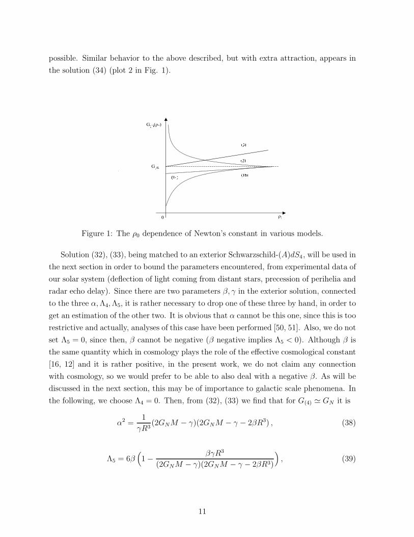
possible. Similar behavior to the above described, but with extra attraction, appears in

the solution (34) (plot 2 in Fig. 1).

*����!��

*���

� !�

��D� ��E�

���

���

Figure 1: The ρ0 dependence of Newton’s constant in various models.

Solution (32), (33), being matched to an exterior Schwarzschild-(A)dS4, will be used in

the next section in order to bound the parameters encountered, from experimental data of

our solar system (deflection of light coming from distant stars, precession of perihelia and

radar echo delay). Since there are two parameters β, γ in the exterior solution, connected

to the three α, Λ4, Λ5, it is rather necessary to drop one of these three by hand, in order to

get an estimation of the other two. It is obvious that α cannot be this one, since this is too

restrictive and actually, analyses of this case have been performed [50, 51]. Also, we do not

set Λ5 = 0, since then, β cannot be negative (β negative implies Λ5 < 0). Although β is

the same quantity which in cosmology plays the role of the effective cosmological constant

[16, 12] and it is rather positive, in the present work, we do not claim any connection

with cosmology, so we would prefer to be able to also deal with a negative β. As will be

discussed in the next section, this may be of importance to galactic scale phenomena. In

the following, we choose Λ4 = 0. Then, from (32), (33) we find that for G(4) ≃ GN it is

α2 =1

γR3(2GNM − γ)(2GNM − γ − 2βR3) , (38)

Λ5 = 6β(

1 − βγR3

(2GNM − γ)(2GNM − γ − 2βR3)

)

, (39)

11

while in the other limiting case

α2 = 2β +2γ2

R3

(

γ − 2GNM − 2γ

βR3GNM

±√

(2GNM − γ)(2GNM − γ +4γ

βR3GNM)

)−1

. (40)

Finally, we note that the non-Schwarzschild-(A)dS4 solution (34), (35) could be also

used for extracting phenomenological bounds on the string parameters from the solar-

system experiments. We have chosen in this paper the simplest solution for this purpose.

However, it is known [52] that the agreement with the solar-system tests of some metric-

based relativistic theory requires on kinematical grounds that AB ≃ 1 to high accuracy

in the vicinity of the sun.

3. Constraints from Classical Tests

A difficulty arising with the calculations of the measurable quantities (integrals)

comes from the fact that the solution (32), (33) is not asymptotically flat, but diverges

at large distances, thus, an expansion in powers of 1/r, performed in the standard PPN

(parametrized post-Newtonian) analysis, does not work here. Hence, one has to make

expansions according to parameters of the problem which are sufficiently small, and for-

tunately, such parameters exist.

The motion of a freely falling material particle or photon in a static isotropic gravita-

tional field (17) is described [53] by the equation

(dφ

dr

)2

=A>

r4

( 1

J2B>− 1

r2− E

J2

)−1

, (41)

where J, E are constants of integration (E > 0 for material particles and E = 0 for

photons). At the points of minimum or maximum distance ro, it is dr/dφ = 0 and thus

J = ro

( 1

B>(ro)− E

)1/2

. (42)

We will analyze the three classical solar scale experiments - deflection of electromag-

netic waves coming from distant stars by the sun, precession of the perihelia of planets,

and time delay of radio waves.

1) Deflection of light. Although the metric is not asymptotically flat, the photon, as

it can be seen from equation (41), has dφ/dr → 0 as r → ∞, and thus, it moves in a

“straight” line of the background geometry in that region. The deviation from this line

12

is measured by the total deflection angle ∆φd = 2|φ(ro) − φ(∞)| − π, where ro is the

minimum distance of the orbit to the sun (when a ray grazes sun ro = R⊙). As it is

expected and will be shown below, |β| has an extremely small value, thus, for β > 0 the

horizon r2 is of cosmological scale and scattering of light can be practically defined even

in this case. The angular momentum J is related to the “impact parameter” b through

the relation J = b(1 − βb2)−1/2. Integrating (41) we arrive at

φ(r) − φ(∞) =

√

r3o

ro − γ

∫ ∞

r

[

r(r − ro)(

r2 + ror −γr2

o

ro − γ

)]−1/2

dr . (43)

For the above expression being well-defined, it has to be ro ≥ 32γ (which is always the case

for common stars such as our sun). Note that the parameter β has disappeared in the

expression (43), i.e. the deflection phenomenon is the same as if it had been occurred in a

Schwarzschild field of parameter γ. Expression (43) leads to an elliptic integral. Since γ

is almost 2GNM⊙ and ro is of the order of R⊙, thus, γro

is of the order of 10−6. Hence, we

can expand the integrand of (43) to first order in this parameter before integration [54].

It is convenient, simultaneously, to set sin u = ro

r, and the result is

∆φd =2γ

ro. (44)

The best measurements on the deflection of light from the sun were obtained using

radio-interferometric methods [55] and found to be (for ro = R⊙) ∆φd = 1.761 ± 0.016

arc sec. Then, from (44),

29.440 × 104 cm < γ < 29.979 × 104 cm , (45)

which is around the conventional value 2GNM⊙ = 29.539 × 104 cm.

2) Precession of perihelia. Here, there are two values r+, r− of maximum and minimum

distance, satisfying equation (42). The two constants of motion J, E are expressed in terms

of r+, r− and are plugged in (41). The expression arising is very complicated, but referring

to [50], [51], we can write the precession per orbit ∆φp = 2|φ(r+) − φ(r−)| − π as

∆φp =3πγ

L+

6πβL3

γ, (46)

where L−1 = (r−1+ + r−1

− )/2 is the semilatus rectum of the orbit. Both [50], [51] agree on

the result (46). Actually, they refer to the Gibbons-Hawking metric, but their methods

are immediately applied in our case. They disagree on the next order terms, which are,

however, negligible compared to the second term of (46), for stars with small Schwarzschild

radius and for slightly eccentric orbits.

13

For Mercury, the uncertainty in the quantity ∆φp− 6πGN M⊙L

is ±10−9 rad/orbit. Then,

taking into account the range (45) of γ received from deflection, we obtain

− 7.908 × 10−43 cm−2 < β < 2.465 × 10−43 cm−2 . (47)

The bounds (45), (47) give from equation (38):

α < 4.379 × 10−16 cm−1 . (48)

Actually, as far as, the upper bound of |β| remains many orders of magnitude smaller

than GN M⊙R⊙

, the above result, as can be seen from (38), is insensitive to the exact value of

β. Furthermore, the fact that α has upper, instead of lower, bound is due to the specific

functional form of the expression (38) in terms of γ. This means that the crossover scale

rc > 4.567×1015 cm, i.e. the lower bound of rc is a few times the diameter of our planetary

system. Thus, the five-dimensional fundamental Planck scale M5 is less than 0.9 TeV .

From equation (40), one can see that for β → 0, α → 0 and then, from (45), (47), an

upper bound of the order 10−22 cm−1 is set for α, which is incompatible with α ≫ αe.

Thus, this case is not acceptable.

From (39), an upper bound for Λ5 can be obtained

Λ5 < 3.804 × 10−43 cm−2 . (49)

Uncertainties in the measurement of the precession of perihelion are known to exist,

due to the rotation of sun; thus, it is better to examine the bounds on β from the radar

echo delay independently.

3) Radar echo delay. The time required for a radar signal to go from a point r to the

closest to the sun point ro of its orbit is

t(r, ro) =

∫ r

ro

(A>

B>

)1/2(

1 − r2o

r2

B>

B>(ro)

)−1/2

dr . (50)

As in the deflection of light, expanding to first order in γR

we obtain

t(r, R) =1

√

|β|arctanh

(

√

|β|√

r2 − R2

1 − βR2

)

+

γ(

ln

√

1 − βR2 r +√

r2 − R2

R√

1 − βr2+

1

2√

1 − βR2

√

r − R

r + R

1 + βrR

1 − βr2

)

. (51)

This expression holds for β > 0, while for β < 0, arctan h(

√

|β|√

r2−R2

1−βR2

)

has to be

replaced by π2− arctan

(

1√|β|

√

1−βR2

r2−R2

)

. Whenever |β|r2 ≪ 1, the above expression takes

14

the form

t(r, R) ≃√

r2 − R2 + γ lnr +

√r2 − R2

R+

γ

2

√

r − R

r + R+

β

3(r2 − R2)3/2 . (52)

We will use this expression to get bounds from the solar radar echo experiments. Notice,

however, that (51) may be applicable to some more general cases.

In [56], the time delay on solar system scales was measured to an accuracy of 0.1 per

cent. A ray that leaves the Earth, grazes the sun, reaches Mars and comes back would have

a time delay of 248±0.25 µs where the 248µs is the exact prediction of the “Shapiro” time

delay and the uncertainty ±0.25µs can be used to constrain β. At superior conjunction,

the radius of the sun to the Earth, re, and to the Mars, rm, are much greater than the

radius of the sun R⊙, and thus, 23β(r3

e + r3m) = ±0.25 µs. This constrains β to the range

|β| < 7.555 × 10−37 cm−2 . (53)

It is interesting to compare the bounds on the various parameters of the brane theory

with an (4)R term, with the bounds on the parameters which are resulting from the brane

dynamics without the (4)R term. In [1], the dynamics on the brane is given, instead of

(8), by the following equation

(4)Gµν =

κ45

6κ24

Λ4(4)T µ

ν − 1

2

(

Λ5 +κ4

5

6κ44

Λ24

)

δµν

− κ45

24

(

6 (4)T µρ

(4)T ρν − 2 (4)T (4)T µ

ν − 3 (4)T ρσ

(4)T σρ δµ

ν + (4)T 2 δµν

)

− Eµ

ν . (54)

For Eµ

ν = 0, following the same steps for solving (54), as before, we arrive to the unique

Schwarzschild-(A)dS4 exterior solution B>(r) = 1A>(r)

, where A>(r) is given by (23). The

parameters of this solution, denoted by the subscripts SMS, are given by

γSMS =κ2

4 Λ4,SMS

6πα2SMS

(

1 +3κ2

4M

8πΛ4,SMSR3

)

M , (55)

βSMS =1

6Λ5,SMS +

Λ24,SMS

9α2SMS

. (56)

It is obvious that the conventional value 2GNM of the Newtonian term can dominate

γSMS only if Λ4,SMS = 3α2SMS/2. This is the same value which revives the common

four-dimensional energy-momentum terms in the general equation (54). This value is

substituted in (55), (56) and then, using the bounds (45), (47) from the classical tests,

15

we can set bounds on αSMS , Λ5,SMS. More specifically, since Λ5,SMS is not contained in

(55), equation (45) is enough for finding

αSMS > 2.425 × 10−13 cm−1 , (57)

which means M5 > 7 TeV . Then, from (56)

Λ5,SMS < −8.818 × 10−26 cm−2 , (58)

and only a bulk of negative curvature is allowed in this approach. The above results are

exact, since now, there are only two unknown parameters αSMS, Λ5,SMS to be determined

from the two γSMS, βSMS. It is seen from equation (55) (plot 3 in Fig. 1) that the point

particle limit of infinite density cannot be obtained (contrary to the plots 1a, 1b, 2 of Fig.

1), since then, G(4) → ∞. Even for different boundary conditions [34] the above limit,

sometimes, is not defined at all.

Finishing, we make the following comment. In our second solution (34), we have

obtained γ > 2GNM . Thus, from (44), the deflection angle ∆φd is larger than the corre-

sponding “Einstein” deflection 4GN Mro

. This situation of increased deflection (compared to

that caused from the luminous matter) has been well observed in galaxies or clusters of

galaxies, and the above solution might serve as a possible way for providing an explana-

tion. In Weyl gravity [57, 58, 54], the above increase is advocated to some parameter like

our β (with the difference of a linear instead of quadratic term), which has to be positive

in order to account for this (see also [52, 59]). But, then, a β > 0 cannot account for the

additional attractive force needed to explain the galactic rotation curves. In our solution,

instead, there is the additional freedom for the parameter β being negative, which can be

used for the galactic rotation curve fittings. Notice also that the Gibbons-Hawking solu-

tion cannot explain this way the extra deflection in galaxies. Alternative gravity theories

may probably not have succeeded their best in illuminating the missing mass problem,

but this does not mean that a new gravity modification must not be tested in the arena of

local phenomena; it is certain that the whole topic deserves a more thorough investigation.

4. Conclusions

In the present paper, we have investigated the influence of the brane curvature invari-

ant included in the bulk action, on the local spherically symmetric braneworld solutions.

The brane dynamics is made closed by assuming the vanishing of the electric part of the

Weyl tensor as a boundary condition for the propagation equations in the bulk space. All

16

the exterior solutions of a compact rigid object have been obtained. Some of them are

of the Schwarzschild-(A)dS4 form. Furthermore, two generalized interior Oppenheimer-

Volkoff solutions have been found, one of which is matched to a Schwarzschild-(A)dS4

exterior, while the other does not. A remarkable consequence is that the bulk space

“sees” the finite region of the body and modifies the parameter of the Newtonian term

in the outside region. No contradiction with the everyday Newton’s constant universality

leads to bounds on the string scale. The known classical solar system tests, which were

used in the past to check the validity of General Relativity, are here used to put precise

bounds on the parameters of our model. More specifically, the crossover scale is found

to be beyond our planetary system diameter, which means that the upper bound for the

energy string scale is of the order of TeV . The limit of the idealized infinite density point

particle is obtained, and significant deviations from the known Newton’s constant might

occur on extremely low density matter distributions. In usual brane dynamics, contrary to

our case, the solar tests impose a lower, instead of upper, bound of the above order on the

string scale. Furthermore, in that case, for obtaining exterior non-Schwarzschild-(A)dS4

solutions, one has to consider non-local bulk effects.

We have followed a braneworld viewpoint for obtaining braneworld solutions, ignoring

the exact bulk space. We have not provided a description of the gravitational field in the

bulk space, but confined our interest to effects that can be measured by brane-observers.

However, our formalism assures the existence of a 5-dimensional Einstein space as the

bulk space. By making assumptions for obtaining a closed brane dynamics, there is

no guarantee that the brane is embeddable in a regular bulk. This is the case for a

Friedmann brane [45], whose symmetries imply that the bulk is Schwarzschild-AdS5 [60,

61]. A Schwarzschild brane can be embedded in a “black string” bulk metric, but this has

singularities [23, 62]. The investigation of bulk backgrounds which reduce to Schwarzschild

(or Schwarzschild-(A)dS4) black holes is in progress.

It is clear that a density-dependent gravitational constant, generally violates, at the

weak field limit, Newton’s third law of equal action-reaction. This, furthermore, means

violation of the conservation of linear momentum and incapability to define precisely the

potential energy for a system of two masses. Since the point particle limit does not meet

any problem in our model, and also the Newtonian limit arises in metric-based theories for

point particles moving along geodesics, we think that the understanding of the motion of

the extended body in General Relativity (or more generally) would shed light to the above

subteties. Beyond these, in our everyday phenomena, where very low density distributions

do not contribute gravitationally, no such difficulties arise. However, such situations may

17

be relevant to early stages of the universe, before or during structure formation.

As a motivation for further speculation, we refer that it would be quite interesting,

even for the formal status of the theory, if the existence of the ρo → ∞ asymptotic behav-

ior of the solutions found here, keeps valid, whenever (4)R term is present. Besides this,

it is known that in cosmology the (4)R term revives the desirable early universe of stan-

dard General Relativity. However, to conclude, as braneworld solutions are continuously

investigated, they have to confront with the accumulated cosmological and astrophysical

observations, if the underlying theories wish to be considered as viable generalizations of

General Relativity.

References

[1] T. Shiromizu, K. Maeda and M. Sasaki, “The Einstein equations on the 3-Brane

World”, Phys. Rev. D62 (2000) 024012, gr-qc/9910076.

[2] R. Sundrum, “Effective field theory for a three-brane universe”, Phys. Rev. D59

(1999) 085009, hep-ph/9805471.

[3] O. Aharony, S.S. Gubser, J. Maldacena, H. Ooguri and Y. Oz, “Large N field theories,

string theory and gravity”, Phys. Rept. 323, 183 (2000), hep-th/9905111.

[4] G. Dvali, G. Gabadadze and M. Porati, “4D Gravity on a Brane in 5D Minkowski

Space”, Phys. Lett. B485 (2000) 208, hep-th/0005016.

[5] G. Dvali and G. Gabadadze, “Gravity on a Brane in Infinite Volume Extra Space”,

Phys. Rev. D63, 065007 (2001), hep-th/0008054.

[6] D.M. Capper, “On quantum corrections to the graviton propagator”, Nuovo Cim.

A25 (1975) 29.

[7] S.L. Adler, “Order R vacuum action functional in scalar free unified theories with

spontaneous scale breaking”, Phys. Rev. Lett. 44 (1980) 1567; “A formula for the

induced gravitational constant”, Phys. Lett. B95 (1980) 241; “Einstein gravity as a

symmetry breaking effect in quantum field theory”, Rev. Mod. Phys. 54 (1982) 729;

Erratum-ibid. 55 (1983) 837.

[8] A. Zee, “Calculating Newton’s gravitational constant in infrared stable Yang-Mills

theories”, Phys. Rev. Lett. 48 (1982) 295.

18

[9] N. N. Khuri, “An upper bound for induced gravitation”, Phys. Rev. Lett. 49 (1982)

513; “The sign of the induced gravitational constant”, Phys. Rev. D26 (1982) 2664.

[10] E. Kiritsis, N. Tetradis and T.N. Tomaras, “Thick branes and 4D gravity”, JHEP

0108 (2001) 012, hep-th/0106050.

[11] S. Corley, D. Lowe and S. Ramgoolam, “Einstein-Hilbert action on the brane for the

bulk graviton”, JHEP 0107 (2001) 030, hep-th/0106067.

[12] G. Kofinas, “General brane cosmology with (4)R term in (A)dS5 or Minkowski bulk”,

JHEP 0108 (2001) 034, hep-th/0108013.

[13] H. Collins and B. Holdom, “Brane cosmologies without Orbifolds”, Phys. Rev. D62

(2000) 105009, hep-ph/0003173.

[14] Y. Shtanov, “On brane-world cosmology”, hep-th/0005193.

[15] S. Nojiri and S.D. Odintsov, “Brane-World Cosmology in higher derivative gravity or

warped compactification in the next-to-leading order of AdS/CFT correspondence”,

JHEP 0007 (2000) 049, hep-th/0006232.

[16] C. Deffayet, “Cosmology on a brane in Minkowski bulk”, Phys. Lett. B502 (2001)

199, hep-th/0010186.

[17] N.J. Kim, H.W. Lee and Y.S. Myung, “Role of the brane curvature scalar in the

brane world cosmology”, Phys. Lett. B504 (2001) 323, hep-th/0101091.

[18] L. Randall, R. Sundrum, “A large mass hierarchy from a small extra dimension”,

Phys. Rev. Lett. 83 (1999) 3370, hep-th/9905221; “An alternative to compactifica-

tion”, Phys. Rev. Lett. 83 (1999) 4690, hep-th/9906064.

[19] P. Horava and E. Witten, “Heterotic and type I string dynamics from eleven dimen-

sions”, Nucl. Phys. B460 (1996) 506, hep-th/9510209.

[20] M. Cvetic and H. Soleng, “Supergravity domain walls”, Phys. Rep. 282 (1997) 159,

hep-th/9604090.

[21] A. Kehagias, “Exponential and power-law hierarchies from supergravity”, Phys. Lett.

B469 (1999) 123, hep-th/9906204.

[22] H. Verlinde, “Holography and compactification”, Nucl. Phys. B580 (2000) 264, hep-

th/9906182.

19

[23] A. Chamblin, S.W. Hawking and H.S. Reall, “Brane-world black holes”, Phys. Rev.

D61 (2000) 065007, hep-th/9909205.

[24] D. Brecher and M.J. Perry, “Ricci-Flat Branes”, Nucl. Phys. B566 (2000) 151, hep-

th/9908018.

[25] R. Emparan, G.T. Horowitz and R.C. Myers, “Exact description of black holes on

branes”, JHEP 0001 (2000) 007, hep-th/9911043.

[26] A. Chamblin, H.S. Reall, H. Shinkai and T. Shiromizu, “Charged brane-world black

holes”, Phys. Rev. D63 (2001) 064015, hep-th/0008177.

[27] A. Chamblin, C. Csaki, J. Erlich and T.J. Hollowood, “Black diamonds at brane

junctions”, Phys. Rev. D62 (2000) 044012, hep-th/0002076.

[28] T. Hirayama and G. Kang, “Stable black strings in Anti-de Sitter space”, Phys. Rev.

D64 (2001) 064010, hep-th/0104213.

[29] A. Karch and L. Randall, “Locally localized gravity”, JHEP 0105 (2001) 008, hep-

th/0011156.

[30] O. Dewolfe, D.Z. Freedman, S.S. Gubser and A. Karch, “Modeling the fifth dimension

with scalars and gravity”, Phys. Rev. D62 (2000) 046008, hep-th/9909134.

[31] H.B. Kim and H.D. Kim, “Inflation and gauge hierarchy in Randall-Sundrum com-

pactification”, Phys. Rev. D61 (2000) 064003, hep-th/9909053.

[32] N. Kaloper, “Bent domain walls as braneworlds”, Phys. Rev. D60 (1999) 123506,

hep-th/9905210.

[33] J. Garriga and M. Sasaki, “Brane-world creation and black holes”, Phys. Rev. D62

(2000) 043523, hep-th/9912118.

[34] C. Germani and R. Maartens, “Stars in the braneworld”, Phys. Rev. D64 (2001)

124010, hep-th/0107011.

[35] T. Wiseman, “Relativistic stars in Randall-Sundrum gravity”, Phys. Rev. D65 (2002)

124007, hep-th/0111057.

[36] N. Deruelle, “Stars on branes: the view from the brane”, gr-qc/0111065.

20

[37] W. Israel, “Singular hypersurfaces and thin shells in general relativity”, Nuovo Ci-

mento 44B [Series 10] (1966) 1; Errata-ibid 48B [Series 10] (1967) 463.

[38] G. Darmois, “Memorial des sciences mathematiques XXV” (1927).

[39] K. Lanczos, “Untersuching uber flachenhafte verteiliung der materie in der Einstein-

schen gravitationstheorie” (1922), unpublished; “Flachenhafte verteiliung der materie

in der Einsteinschen gravitationstheorie”, Ann. Phys. (Leipzig) 74 (1924) 518.

[40] N. Sen, “Uber dei grenzbedingungen des schwerefeldes an unstetig keitsflachen”, Ann.

Phys. (Leipzig) 73 (1924) 365.

[41] N. Dadhich, R. Maartens, P. Papadopoulos and V. Rezania, “Black holes on the

brane”, Phys. Lett. B487 (2000) 1, hep-th/0003061.

[42] R. Maartens, “Cosmological dynamics on the brane”, Phys. Rev. D62 (2000) 084023,

hep-th/0004166; “Geometry and dynamics of the brane-world”, gr-qc/0101059.

[43] N. Dadhich, “Negative energy condition and black holes on the brane”, Phys. Lett.

B492 (2000) 357, hep-th/0009178; P. Singh and N. Dadhich, “Non-conformally flat

bulk spacetime and the 3-brane world”, Phys. Lett. B511 (2001) 291, hep-th/0104174.

[44] R. Casadio, A. Fabbri and L. Mazzacurati, “New black holes in the brane-world?”,

Phys. Rev. D65 (2002) 084040, gr-qc/0111072.

[45] P. Binetruy, C. Deffayet, U. Ellwanger and D. Langlois, “Brane cosmological evo-

lution in a bulk with cosmological constant”, Phys. Lett. B477 (2000) 285, hep-

th/9910219.

[46] J.L. Synge, “Relativity: the General Theory”, North Holland, Amsterdam (1971).

[47] N.O. Santos, Mon. Not. R. Ast. Soc. 216 (1985) 403.

[48] F. Kottler, Ann. Phys. (Leipzig) 56 (1918) 410.

[49] G.W. Gibbons and S.W. Hawking, “Cosmological event horizons, thermodynamics,

and particle creation”, Phys. Rev. D15 (1977) 2738.

[50] E.L. Wright, “Interplanetary measures can not bound the cosmological constant”,

UCLA-ASTRO-ELW-98-01, astro-ph/9805292.

[51] I.P. Neupane, “Planetary perturbation with cosmological constant”, gr-qc/9902039.

21

[52] A. Edery, “The bright side of dark matter”, Phys. Rev. Lett. 83 (1999) 3990, gr-

qc/9905101.

[53] S. Weinberg, “Gravitation and Cosmology”, John Wiley and Sons Inc., 1972.

[54] A. Edery and M.B. Paranjape, “Classical tests for Weyl gravity: deflection of light

and time delay”, Phys. Rev. D58 (1998) 024011, astro-ph/9708233.

[55] E.B. Fomalont and R.A. Sramek, Phys. Rev. Lett. 36 (1976) 1475.

[56] R.D. Reasenberg et all., Ap. J. 234 (1979) L219.

[57] P.D. Mannheim and D. Kazanas, “Exact vacuum solution to conformal Weyl gravity

and galactic rotation curves”, Ap. J. 342 (1989) 635; “Solutions to the Kerr and

Kerr-Newman problems in fourth order conformal Weyl gravity”, Phys. Rev. D44

(1991) 417.

[58] P.D. Mannheim, “Linear potentials and galactic rotation curves - formalism”, astro-

ph/9307004; “Microlensing, Newton-Einstein gravity and conformal gravity”, astro-

ph/9412007; “Attractive and repulsive gravity”, Found. Phys. 30 (2000) 709, gr-

qc/0001011.

[59] J.D. Bekenstein, M. Milgrom and R.H. Sanders, “Comment on the “The bright side

of dark matter””, Phys. Rev. Lett. 85 (2000) 1346, astro-ph/9911518.

[60] S. Mukoyama, T. Shiromizu and K. Maeda, “Global structure of exact cosmological

solutions in the brane world”, Phys. Rev. D62 (2000) 024028, hep-th/9912287.

[61] P. Bowcock, C. Charmousis and R. Gregory, “General brane cosmologies and their

global spacetime structure”, Class. Quant. Grav. 17 (2000) 4745, hep-th/0007177.

[62] R. Gregory, “Black string instabilities in anti-de Sitter space”, Class. Quant. Grav.

17 (2000) L125, hep-th/0004101.

22