PHYSICAL REVIEW A 90, 022114 (2014)

Systems of coupled PT -symmetric oscillators

Carl M. Bender,1,2,* Mariagiovanna Gianfreda,1,3,† and S. P. Klevansky4,5,‡1Department of Physics, Washington University, St. Louis, Missouri 63130, USA

2Department of Mathematical Science, City University London, Northampton Square, London EC1V 0HB, United Kingdom3Institute of Industrial Science, University of Tokyo, Komaba, Meguro, Tokyo 153-8505, Japan

4Institut fur Theoretische Physik, Universitat Heidelberg, Philosophenweg 12, 69120 Heidelberg, Germany5Department of Physics, University of the Witwatersrand, Johannesburg, South Africa

(Received 27 June 2014; published 19 August 2014)

The Hamiltonian for a PT -symmetric chain of coupled oscillators is constructed. It is shown that if theloss-gain parameter γ is uniform for all oscillators, then as the number of oscillators increases, the region ofunbroken PT symmetry disappears entirely. However, if γ is localized in the sense that it decreases for moredistant oscillators, then the unbroken PT -symmetric region persists even as the number of oscillators approachesinfinity. In the continuum limit the oscillator system is described by a PT -symmetric pair of wave equations,and a localized loss-gain impurity leads to a pseudobound state. It is also shown that a planar configuration ofcoupled oscillators can have multiple disconnected regions of unbroken PT symmetry.

DOI: 10.1103/PhysRevA.90.022114 PACS number(s): 11.30.Er, 03.65.−w, 02.30.Mv, 11.10.Lm

I. INTRODUCTION

A previous paper [1] considered a system consisting ofa pair of coupled oscillators, one with loss and the otherwith gain. Such a system is PT symmetric if the loss andgain parameters are equal. The energy of this PT -symmetricsystem is exactly conserved because this system is describedby a time-independent Hamiltonian. In the current paper weexamine the systems that arise when the number of pairs ofcoupled oscillators is extended from 1 to N , where N can bearbitrarily large.

Let us review the case N = 1. A single pair of coupledoscillators, the first with loss and the second with gain, isdescribed by the equations of motion

x + ω2x + μx = −εy, y + ω2y − νy = −εx. (1)

To treat this system at a classical level, we seek solutions to(1) of the form eiλt . The classical frequency λ then satisfiesthe quartic polynomial equation

λ4 − i(μ − ν)λ3 − (2ω2 − μν)λ2

+ iω2(μ − ν)λ − ε2 + ω4 = 0. (2)

This classical system becomes PT symmetric if the lossand gain are balanced; that is, if we set μ = ν = 2γ . In thiscase the frequencies λ are given by

λ2 = ω2 − 2γ 2 ±√

ε2 − 4γ 2ω2 + 4γ 4. (3)

Note that there are four real frequencies when ε is in the range

ε1 = 2γ√

ω2 − γ 2 < ε < ε2 = ω2. (4)

This defines the unbroken PT -symmetric region. In thebroken PT -symmetric region ε < ε1 there are two pairsof complex-conjugate frequencies and in the broken PT -symmetric region ε > ε2 there are two real frequencies andone complex-conjugate pair of frequencies.

*cmb@wustl.edu†Maria.Gianfreda@le.infn.it‡spk@physik.uni-heidelberg.de

When μ �= ν, system (1) cannot be derived from aquadratic time-independent Hamiltonian. To verify this, onecan construct the most general quadratic Hamiltonian forthe four variables p, q, x, and y with arbitrary constantcoefficients. It is then a simple algebraic calculation toshow that there is no choice of coefficients for which oneobtains a Hamiltonian that leads to Eqs. (1). However,when the system is PT symmetric (μ = ν = 2γ ), (1) canbe derived from the two-coupled-oscillator time-independentHamiltonian

H2 = pq + γ (yq − xp) + (ω2 − γ 2)xy + 12ε(x2 + y2). (5)

This Hamiltonian is PT symmetric because under parityreflection P the loss and gain oscillators are interchanged [2],

P: x → −y, y → −x, p → −q, q → −p, (6)

and under time reversal T the signs of the momenta arereversed,

T : x → x, y → y, p → −p, q → −q. (7)

The Hamiltonian H2 is PT symmetric but it is not invariantunder P or T separately [3]. Because the balanced loss-gainsystem is described by a time-independent Hamiltonian, theenergy (that is, the value of H2) is conserved. However, thetotal energy (5) is not the usual sum of the kinetic and potentialenergies (such as p2 + q2 + x2 + y2).

If we set the coupling parameter ε to 0, H2 describes thesystem studied by Bateman [4]. Bateman showed that anequation of motion having a friction term linear in velocitycould be derived from a variational principle. To do thishe introduced a time-reversed companion of the originaldamped harmonic oscillator. This auxiliary oscillator actsas an energy reservoir and can be viewed as a thermalbath. The classical Hamiltonian for the Bateman system wasconstructed by Morse and Feschbach [5] and the correspondingquantum theory was analyzed by many authors, includingBopp [6], Feshbach and Tikochinsky [7], Tikochinsky [8],Dekker [9], Celeghini, Rasetti, and Vitiello [10], Banerjeeand Mukherjee [11], and Chruscinski and Jurkowski [12].

1050-2947/2014/90(2)/022114(11) 022114-1 ©2014 American Physical Society

BENDER, GIANFREDA, AND KLEVANSKY PHYSICAL REVIEW A 90, 022114 (2014)

Only the noninteracting (ε = 0) case was considered in thesereferences.

The noteworthy feature of PT -symmetric systems is thatthey exhibit transitions; the classical system described by H2

exhibits two transitions. The first occurs at ε = ε1. If ε < ε1,the energy flowing into the y resonator cannot transfer fastenough to the x resonator, where energy is flowing out, so thesystem cannot be in equilibrium. However, when ε > ε1, theenergy flowing into the y resonator transfers to the x resonatorand the entire system is in equilibrium. The frequencies ofa classical system in equilibrium are real and the systemexhibits Rabi oscillations (power oscillations between thetwo resonators) in which the two oscillators are 90◦ out ofphase. Complex frequencies indicate exponential growth anddecay and are a signal that the system is not in equilibrium. Asecond transition occurs at ε = ε2; when ε > ε2, the classicalsystem is no longer in equilibrium. This transition is difficultto see in classical experiments because in the strong-couplingregime the loss and gain components would have to be soclose that they would interfere with one another. For example,in the pendulum experiment in Ref. [13] the pendula wouldbe so close that they could no longer swing freely, and inthe optical resonator experiment in Ref. [14] the solid-stateresonators would be damaged. This strong-coupling region isdiscussed for the case of coupled systems without loss andgain in Ref. [15], where it is called the ultrastrong-couplingregime.

In Ref. [1] it is shown that the classical and the quantumsystems described by H2 exhibit transitions at the same twovalues of the coupling parameter ε. When ε < ε1 and whenε > ε2 the quantum energies are complex, but in the unbrokenPT -symmetric region ε1 < ε < ε2 the quantum energies arereal.

This paper is organized as follows. In Sec. II we formulatethe equations of motion for a linear chain of N identicalpairs of PT -symmetric loss-gain oscillators and we constructthe Hamiltonians H2N for such systems. We show that thereare two ways to represent such Hamiltonians: one that wecall a sum representation and another that we call a productrepresentation. In the product representation it is easy to seethat the Hamiltonian is not unique and that this nonuniquenesstakes the form of a gauge invariance. Next, in Sec. IIIwe construct the Hamiltonians for a general PT -symmetricsystem of 2N coupled oscillators in which the couplingparameter ε and the loss-gain parameter γ are allowed tovary from oscillator to oscillator. In addition, we consider asystem of 2N + 1 coupled PT -symmetric oscillators, wherePT symmetry requires that the central oscillator have neitherloss nor gain. We also perform the N → ∞ limit of H2N . Inthis limit the equations of motion of the oscillators becomecoupled linear wave equations with balanced loss and gain.

In Sec. IV we ask whether a PT -symmetric chain of2N coupled oscillators can have an unbroken PT -symmetricregion. We show that as N increases, if γ and ε are thesame for all oscillators, the region of unbroken PT symmetryshrinks and then disappears entirely as N → ∞. However, ifthe loss-gain parameter γ decreases to 0 for distant oscillators,then such systems always have an unbroken PT -symmetricregion for intermediate values of the coupling parameter ε

surrounded by broken PT -symmetric regions for small and

large values of ε. Specifically, for the cases in which γn

decreases like 1/n or 1/n2, where 1 � n � N is the numberof oscillators measured from the center of the system, weshow that an unbroken PT -symmetric region persists in thelimit as N → ∞. If one views loss-gain as the consequenceof an impurity, then a configuration of oscillators for which γ

decreases with increasing distance from the center can be seenas having a localized impurity. Thus, in Sec. V we investigatea special case for the continuum model in which there isa pointlike PT -symmetric impurity localized at the origin.We find that this impurity gives rise to a pseudobound-statesolution. In Sec. VI we consider the simplest case of atwo-dimensional array of coupled oscillators, namely, threeoscillators—one with loss, one with gain, and the third withneither loss nor gain. This system is interesting because itcan exhibit five distinct regions as a function of the couplingconstant, two having unbrokenPT symmetry and three havingbroken PT symmetry. Finally, in Sec. VII we make some briefconcluding remarks.

II. PT -SYMMETRIC SYSTEM OF COUPLEDCLASSICAL OSCILLATORS

In this section we describe the properties of a PT -symmetric one-dimensional chain of 2N coupled oscillatorswith alternating loss and gain. We begin by making thesimplifying assumptions that the natural frequency ω, thecoupling to adjacent oscillators ε, and the loss-gain parameterγ are the same for all oscillators. The classical coordinates arexk(t) (1 � k � 2N ) and the equations of motion are

x1 + ω2x1 + 2γ x1 = −εx2,

x2 + ω2x2 − 2γ x2 = −εx1 − εx3,

x3 + ω2x3 + 2γ x3 = −εx2 − εx4,(8)

x4 + ω2x4 − 2γ x4 = −εx3 − εx5,

. . .

x2N + ω2x2N − 2γ x2N = −εx2N−1.

These equations of motion are PT symmetric, where thedefinitions of P and T are generalized from (6) and (7) to

P: xk → −x2N−k+1, pk → −p2N−k+1 (1 � k � 2N ),

T : xk → xk, pk → −pk (1 � k � 2N ). (9)

The equations of motion (8) imply that there is a conservedquantity. To construct this constant of the motion we multiplythe first equation by x2, the second equation by x1 + x3, thethird equation by x2 + x4, the fourth equation by x3 + x5, andso on. If we add the resulting equations, γ drops out entirelyand we obtain a time-independent quantity, which we canidentify as the energy E2N of the system:

E2N =2N−1∑j=1

(xj xj+1 + ω2xjxj+1)

+ ε

2

(x2

1 + x22N

) + ε

2N−1∑j=2

x2j + ε

2N−2∑j=1

xjxj+2. (10)

022114-2

SYSTEMS OF COUPLED PT -SYMMETRIC . . . PHYSICAL REVIEW A 90, 022114 (2014)

The existence of a conserved quantity suggests that (8) isa Hamiltonian system, and indeed one can find a Hamiltonianfrom which these equations of motion can be derived. Thereare two ways to express the (nonunique) Hamiltonian thatgives rise to (8); we can use what we call a sum or a productrepresentation. We describe these two structures below.

A. Sum representation of the Hamiltonian

In the sum representation H2N consists of four terms.First, there is a pure momentum term of the form

p1p2 + p2p3 + p3p4 + · · · + p2N−1p2N . Second, there is amomentum times a coordinate term proportional to γ :γ (−p1x1 + p2x2 − p3x3 + · · · + p2Nx2N ). Third, there is apotential-energy-like term proportional to ε: 1

2ε(x21 + x2

2 +x2

3 + · · · + x22N ). (It is surprising that this term is proportional

to ε because in the equations of motion ε appears to play therole of a coupling constant; ε does not appear to be a measureof the potential energy, which one associates with a frequencyof oscillation.) Fourth, there is an oscillator coupling termproportional to ω2 − γ 2:

[x1x2 + x3x4 + x5x6 + x7x8+ · · · +x2N−7x2N−6 + x2N−5x2N−4 + x2N−3x2N−2 + x2N−1x2N

− x1x4 − x3x6 − x5x8− · · · −x2N−7x2N−4 − x2N−5x2N−2 − x2N−3x2N

+ x1x6 + x3x8+ · · · +x2N−7x2N−2 + x2N−5x2N

(11)−x1x8− · · · −x2N−7x2N

. . .

(−1)N+1x1x2N ](ω2−γ 2).

Note the interesting structure of this term: The jumps in theproducts in (11) skip 0, 2, 4, 6, . . . and change sign. A compactexpression for H2N is

H2N =2N−1∑j=1

pjpj+1 + ε

2

2N∑j=1

x2j + γ

2N∑j=1

(−1)j xjpj

+ (ω2 − γ 2)N−1∑j=0

(−1)jN−j∑k=1

x2k−1x2j+2k. (12)

To obtain the equations of motion (8) for this Hamiltonianfrom Hamilton’s equations, we take one derivative of H2N withrespect to pk to find xk:

xk = pk+1 + pk−1 + (−1)kγ xk. (13)

We then take a time derivative,

xk − (−1)kγ xk = −∂H2N

∂xk+1− ∂H2N

∂xk−1

= −εxk+1 − εxk−1 + (−1)kγ (pk+1 + pk−1)

+ (ω2 − γ 2)(. . .), (14)

and use the one-derivative equation (13) to recover theequations of motion (8).

B. Product representation of the Hamiltonian

In this representation it is easy to understand the nonunique-ness of the Hamiltonian that gives rise to the equations ofmotion (8). This nonuniqueness is a gauge invariance, whereγ plays the role of an electric charge. Without changing theequations of motion we rewrite the sum representation H2 in(5) so that the momentum terms appear in factored form:

H2 = (p + γy)(q − γ x) + ω2xy + ε(x2 + y2)/2. (15)

Similarly, the sum representation for H4,

H4 = p1p2 + p2p3 + p3p4 + ε(x2

1 + x22 + x2

3 + x24

)/2

+ γ (−x1p1 + x2p2 − x3p3 + x4p4)

+ (ω2 − γ 2)(x1x2 + x3x4 − x1x4), (16)

can be reconfigured in product form as

H4 = [p1 + γ (x2 − x4)](p2 − γ x1) + (p2 − γ x1)(p3 + γ x4)

+ (p3 + γ x4)[p4 − γ (x3 − x1)]

+ω2(x1x2 + x3x4 − x1x4) + ε(x2

1 + x22 + x2

3 + x24

)/2

(17)

without changing the equations of motion. The productrepresentation of H6 has the form

H6 = [p1 + γ (x2 − x4 + x6)](p2 − γ x1) + (p2 − γ x1)

× [p3 + γ (x4 − x6)] + [p3 + γ (x4 − x6)]

× [p4 − γ (x3 − x1)] + [p4 − γ (x3 − x1)]

× (p5 + γ x6) + (p5 + γ x6)[p6 − γ (x5 − x3 + x1]

+ω2(x1y1 + x3x4 + x5x6 − x1x4 − x3x6 + x1x6)

+ ε(x2

1 + x22 + x2

3 + x24 + x2

5 + x26

)/2. (18)

The general structure for the product representation of H2N isnow clear.

The advantage of the product representation is that ifwe consider the Hamiltonian to be quantum mechanical,we can identify a gauge invariance. Each momentum factorin the product representation has the form [p + γ (sumof spatial coordinates)]. This term resembles the structurep − eA in electrodynamics, which suggests that we can makea unitary (canonical) transformation analogous to a gaugetransformation in electrodynamics. By virtue of the Heisen-berg algebra [x,p] = i, it follows that e−iaxpeiax = p + a,where a is a constant. Therefore, if we perform the unitary

022114-3

BENDER, GIANFREDA, AND KLEVANSKY PHYSICAL REVIEW A 90, 022114 (2014)

transformation

e−iamnxmxnH2Neiamnxmxn (19)

on the Hamiltonian, the only terms that will be affected are theproduct terms because they contain the momentum operators.The only changes that will occur are that the momentumoperators pm and pn will be shifted by terms that are linear inthe coordinates xn and xm. There are N (2N − 1) independentgauge transformations that can be performed on H2N , andtherefore we can introduce N (2N − 1) arbitrary constants amn

into H2N . Furthermore, since the transformation is unitary, itleaves the equations of motion invariant [16].

C. Lagrangian

Having found a Hamiltonian for system (8), it is easy toconstruct a Lagrangian:

L2N =N−1∑j=0

(−1)jN−j∑k=1

[γ (x2k−1x2j+2k − x2k−1x2j+2k)

−ω2x2k−1x2j+2k + x2k−1x2j+2k] − ε

2

2N∑j=1

x2j . (20)

III. GENERAL CASE OF NONCONSTANT ε, γ , AND ω

We can construct a Hamiltonian (in the sum representation)for a PT -symmetric system of 2N oscillators even if theparameters ε, γ , and ω vary from oscillator to oscillator:

H2N =N∑

k=1

(−1)kγk(xkpk − x2N+1−kp2N+1−k)

+N−1∑k=1

εk(xkx2N−k + xk+1x2N+1−k)

+ εN

(x2

N + x2N+1

)/2 +

N∑k=1

pkp2N+1−k

+N∑

k=1

(ω2

k − γ 2k

)xkx2N+1−k. (21)

We can also construct a Hamiltonian for 2N + 1 oscillators:

H2N+1 =N∑

k=1

(−1)kγk(xkpk − x2N+2−kp2N+2−k)

+N∑

k=1

εk(xkx2N+1−k + xk+1x2N+2−k)

+ (x2

N+1 + p2N+1

)/2 +

N∑k=1

pkp2N+2−k

+N∑

k=1

(ω2

k − γ 2k

)xkx2N+2−k. (22)

The even Hamiltonian H2N leads to the equations of motion

x1 + ω21x1 + 2γ1x1 = −ε1x2,

x2 + ω22x2 − 2γ2x2 = −ε1x1 − ε2x3,

. . .

xN + ω2NxN − (−1)N2γN xN = −εN−1xN−1−εNxN+1,

xN+1+ω2NxN+1 + (−1)N2γN xN+1 = −εNxN−εN−2xN+2,

. . . (23)

x2N−1 + ω22x2N−1 + 2γ2x2N−1 = −ε1x2N − ε2x2N−2,

x2N + ω21x2N − 2γ1x2N = −ε1x2N−1,

and the odd Hamiltonian H2N+1 gives the equations of motion

x1 + ω21x1 + 2γ1x1 = −ε1x2,

x2 + ω22x2 − 2γ2x2 = −ε1x1 − ε2x3,

. . .

xN+1 + ω2N+1xN+1 = −εN (xN + xN+2) ,

. . . (24)

x2N + ω22x2N + 2γ2x2N = −ε1x2N+1 − ε2x2N−1,

x2N+1 + ω21x2N+1 − 2γ1x2N+1 = −ε1x2N .

A. Continuum limit N → ∞In this subsection we show how to take the limit as the

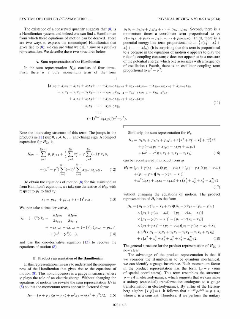
number of oscillators approaches infinity. For simplicity, letus consider two rows of identical particles of mass m. Thesemasses are coupled by springs, as illustrated in Fig. 1.

The top row of particles is subject to damping (friction)forces and the bottom row is subject to undamping forces.Each particle in the top row is coupled by horizontal springs(of force constant per unit length k/�) to the adjacent particlesto the left and right. Thus, the particle at xn is coupled toits neighbors at xn−1 and at xn+1. The neighboring particlesexert a net force on the nth mass of strength k

�(xn+1 − 2xn +

xn−1), where � is the equilibrium spacing. The constant k

is the tension in the horizontal chain of masses. Also, thereare fixed springs above the top row of masses that exert arestoring force per unit length of −μ1ν

21� on each of the x

masses. This force tends to pull the x masses back to their

FIG. 1. (Color online) Infinite PT -symmetric array of identicalparticles coupled by springs. The masses in the top row, whoseposition coordinates are xn(t), experience loss, and the masses inthe bottom row, which are located at yn(t), experience gain.

022114-4

SYSTEMS OF COUPLED PT -SYMMETRIC . . . PHYSICAL REVIEW A 90, 022114 (2014)

equilibrium positions. The parameter μ1 has dimensions ofmass density (mass per unit length) and the parameter ν1 isa frequency having dimensions of 1/time. The force on thenth mass due to these vertical springs is −μ1ν

21�xn. Finally,

the particle at xn in the top row is coupled to the particle atposition yn in the bottom row by a vertical spring of forceper unit length μ2ν

22�. (Here, μ2 is a mass density and ν2 is

a frequency.) The force exerted on the mass at xn due to theparticle at yn is μ2ν

22�(yn − xn). The particles in the top row

lose energy due to friction (drag), where the dissipation per unitlength is given by . Thus, the equation of motion of the nthparticle is

mxn + �xn = k

�(xn+1 − 2xn + xn−1) − μ1ν

21�xn

+μ2ν22� (yn − xn) . (25)

Let m = ρ�, where ρ is the horizontal mass per unit length.We then divide (25) by � and take the limit as � → 0 to getthe continuum wave equation

ρutt + ut = kuxx − μ1ν21u + μ2ν

22 (v − u). (26)

Finally, we divide by ρ and define the quantities c2 ≡ k/ρ,γ ≡ /ρ, ω2 ≡ (μ1ν

21 + μ2ν

22 )/ρ, and ε ≡ −μ2ν

22/ρ. This

leads to the wave equation

utt + 2γ ut + ω2u − c2uxx = −εv. (27)

Similarly, from the equation for the particle at yn we obtainthe wave equation

vtt − 2γ vt + ω2v − c2vxx = −εu. (28)

These equations are the continuous analogs of (8).

In anticipation of the calculation in Sec. V, we rewrite theseequations in a more convenient form by defining S(x,t) ≡u(x,t) + v(x,t) and D(x,t) ≡ u(x,t) − v(x,t). The coupledwave equations satisfied by S and D are

Stt + ω2S − c2Sxx + εS = −2γ (x)Dt,(29)

Dtt + ω2D − c2Dxx − εD = −2γ (x)St ,

where we have now taken the loss-gain parameter γ to dependon x.

IV. EXISTENCE OF AN UNBROKENPT -SYMMETRIC REGION

The question addressed in this section is whether a region ofunbroken PT symmetry persists as the number of oscillatorsN increases. First, we consider the case in which the loss-gain parameter γ is the same for all oscillators and showthat the unbroken region disappears as N increases. Next,we demonstrate numerically that if γ decreases for the moredistant oscillators, a region of unbrokenPT symmetry persistsas N → ∞.

A. Case of constant γ

To find the frequencies of system (8), we seek solutions ofthe form xk = Ake

iλt . The frequencies λ can then be foundby imposing the condition that det [M2N ] = 0 (Cramer’s rule),where M2N is the 2N × 2N tridiagonal matrix

M2N =

⎛⎜⎜⎜⎜⎜⎜⎜⎜⎝

a − ib −ε 0 0 0 0 . . .

−ε a + ib −ε 0 0 0 . . .

0 −ε a − ib −ε 0 0 . . .

0 0 −ε a + ib −ε 0 . . .

0 0 0 −ε a − ib −ε . . .

0 0 0 0 −ε a + ib . . ....

......

......

.... . .

⎞⎟⎟⎟⎟⎟⎟⎟⎟⎠

, (30)

and a and b are given by a = λ2 − ω2 and b = 2λγ .Let PN = det [M2N ] (N = 1,2, . . .) be the polynomial

obtained by computing the determinant of the matrix M2N .The first five of these polynomials areP1 = −ε2 + x,

P2 = ε4 − 3xε2 + x2,

P3 = −ε6 + 6xε4 − 5x2ε2 + x3,

P4 = ε8 − 10xε6 + 15x2ε4 − 7x3ε2 + x4,

P5 = −ε10 + 15xε8 − 35x2ε6 + 28x3ε4 − 9x4ε2 + x5, (31)

where x = a2 + b2 = λ4 + λ2(4γ 2 − 2ω2) + ω4. These poly-nomials satisfy the recursion relation

PN = (x − 2ε2)PN−1 − ε4PN−2 (N � 2), (32)

where we take P0 = 1.

Given these polynomials, we can calculate the frequenciesλ to see what happens to the unbroken PT -symmetric regionas N increases. In Fig. 2 we plot the imaginary part of λ forN = 1, 2, 3, and 4 for fixed ω = 1 and γ = 0.1. It is clear thatas N increases, the size of the unbroken region in the couplingparameter ε shrinks and at N = 4 it disappears entirely.

To study analytically the shrinking of the unbroken regionwith increasing N , we solve the constant-coefficient recursionrelation (32). The exact solution is

PN = √π

N∑k=0

(−1)k4k−N (2N − k)!

(N − k)!k!(N − k + 1/2)xN−kε2k.

(33)

022114-5

BENDER, GIANFREDA, AND KLEVANSKY PHYSICAL REVIEW A 90, 022114 (2014)

FIG. 2. (Color online) Imaginary parts of the frequencies λ for N = 1, 2, 3, and 4 as functions of the coupling constant ε for ω = 1 andγ = 0.1. Frequencies are the zeros of the polynomials PN in (31). Observe that the extent of the unbroken PT -symmetric region (where thefrequencies are all real) decreases as N increases and disappears entirely when N = 4.

Substituting x = −4ε2y and � = √y(y + 1), we express

these polynomials more simply:

PN = ε2N

2�(−1)N [(1 + 2y − 2�)N (� − y)

+ (1 + 2y + 2�)N (� + y)]. (34)

The zeros of PN are the roots of the equation√y + √

y + 1 = (−1)1/(4N+2). Since y = −[(λ2 − ω2)2 +4λ2γ 2]/(4ε2) is negative, we substitute y = −z2. The equationfor z then reads iz + √

1 − z2 = (−1)1/(4N+2), whose solutionsare

z = sin[π (2k + 1)/(4N + 2)] (k = 0,1, . . . ,4N + 1).

(35)

Consequently, the equation for λ becomes 4ε2z2 = (λ2 −ω2)2 + 4λ2γ 2, whose roots are

λ1,2,3,4 = ±√

ω2 − 2γ 2 ± 2√

γ 2(γ 2 − ω2) + ε2z2. (36)

We consider two cases. For N = 1 there are four roots,z = sin θ = ±1, ± 1

2 with e6iθ = −1. These correspond to thesix values θ = {π

6 , π2 , 5π

6 , 7π6 , 3π

2 , 11π6 }. The solutions z = ±1

are spurious because the denominator of (34) contains � =√z2(z2 − 1) and this expression vanishes at z = ±1. Thus, the

only admissible solutions are z = ±1/2. Substituting z2 = 1/4into (36), we obtain the four roots of the polynomial P1 in (31).

For the case N = 2 there are six roots,

z = sin θ = {−1, − (1 +√

5)/4, (1 −√

5)/4,

(√

5 − 1)/4, (1 +√

5)/4,1},with e10iθ = −1. These correspond to the 10 values

θ={

1

10π,

3

10π,

5

10π,

7

10π,

9

10π,

11

10π,

13

10π,

3

2π,

17

10π,

19

10π

}.

The solutions z = ±1 are spurious and there are only fourgenuine roots, z = ±(1 ± √

5)/4, and two values, z2 = (1 ±√5)2/16, to substitute into (36) to get the eight roots of the

polynomial P2 in (31).In general, in the region of unbroken PT symmetry the

roots λ in (36) are all real. Thus,

0 < γ <

√ω2/2 − √

ω4/4 − ε2z2min,

(37)γ√

ω2 − γ 2/√

zmin < ε < ω2/(2zmax),

where zmin = sin[π/(4N + 1)] and zmax = sin[π (2N −1)/(4N + 1)]. Condition (37) identifies the region in theparameter space (γ,ε) where the PT symmetry is unbroken.Note that as N → ∞, zmin → 0 and zmax → 1. Thus, asN → ∞ the only allowed γ is 0 (so that there is no lossand gain), and the range of ε shrinks to 0 � ε < ω2/2.

Let us examine further how the allowed γ decreases as afunction of increasing N . We can see from Fig. 2 that at thelower end of the unbroken region the curves open to the left andat the upper end of this region the curves open to the right. Forfixed N and fixed ε = ω2/(2zmax), if we increase γ , the left-opening curves will eventually touch the right-opening curvesand the unbroken region in ε will disappear. We designate asγcrit the critical value of γ at which the unbroken region in ε

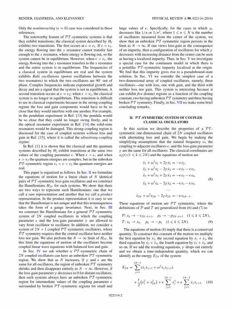
disappears. When we compute γcrit as a function of N and plotin Fig. 3 these values of γcrit versus 1/N , we see clearly thatthe critical value of γ decreases to 0. Thus, if there are toomany oscillators, there cannot be a region of unbroken PTsymmetry in a system with uniform nonzero loss and gain.

The only way for an unbroken region of PT symmetry tosurvive as N → ∞ is for the loss-gain parameter to decreasewith increasingly distant oscillators. Our numerical calcula-tions show that if the loss-gain parameter is γ /(N − n + 1)(where n ranges from 1 to N ), there will be an unbroken region

022114-6

SYSTEMS OF COUPLED PT -SYMMETRIC . . . PHYSICAL REVIEW A 90, 022114 (2014)

FIG. 3. (Color online) Plot of γcrit as a function of 1/N . Thissequence evidently converges to 0 with increasing N . Thus, a systemof coupled oscillators with a uniform loss-gain parameter γ > 0 hasno unbroken PT -symmetric region if N is sufficiently large.

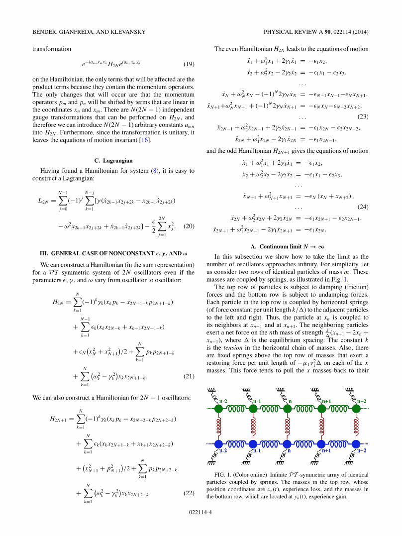
if γ is less than about 0.1 (Fig. 4, left), and if the loss-gainparameter is γ /(N − n + 1)2 (where n ranges from 1 to N ),there will be an unbroken region if γ is less than about 0.2(Fig. 4, right).

V. LOCALIZED IMPURITY IN THE CONTINUUM MODEL

In Sec. IV we have shown that if the effect of loss and gainis localized about the central oscillators and decays for moredistant oscillators, then the unbroken PT -symmetric regioncan survive as N → ∞. This suggests that for the continuummodel developed in Sec. III A it would be interesting toexamine what happens when γ (x) decreases with increasing|x|. The simplest case to study is that for which γ (x) = γ δ(x);that is, the case of a localized pointlike PT -symmetricloss-gain impurity at the origin. Studies of this type have beenperformed for tight-binding models by Joglekar et al. [17,18]and Longhi [19].

Let us assume that the loss-gain parameter is a localizedfunction of x at the origin, γ (x) = γ δ(x), and seek a solutionto (29) with frequency �:

S(x,t) = ei�t s(x), D(x,t) = ei�td(x). (38)

If we assume that a2 = ω2 − �2 + ε > 0 and that −b2 =ω2 − �2 − ε < 0, where a and b are positive, the coupled

wave equations become coupled ordinary differential equa-tions:

c2s ′′(x) − a2s(x) = 2i�γ δ(x)d(x) and

c2d ′′(x) + b2d(x) = 2i�γ δ(x)s(x). (39)

The functions s(x) and d(x) are continuous at x = 0 and theδ function gives rise to a discontinuity in the derivatives of s

and d at x = 0:

2iγ�d(0) = c2[s ′(0+) − s ′(0−)] and

2iγ�s(0) = c2[d ′(0+) − d ′(0−)]. (40)

A simple solution to (39) has the form

s(x) = e−a|x|/c and d(x) = iac

γ�cos

bx

c+ i

γ�

bcsin

b|x|c

.

(41)

This solution is PT symmetric, where P changes the sign ofx and interchanges u and v, which in turn changes the signof d while leaving the sign of s unchanged, and T performscomplex conjugation.

This solution can be viewed as a pseudobound-state solutionin the sense that s(x) decays exponentially as |x| → ∞.However, while d(x) also has a cusp at x = 0, it is notlocalized and oscillates as |x| → ∞. This solution resemblesthat found by Hatano et al. [20,21] and Longhi [19]. It isinteresting that no localized bound-state solution exists ifa2 = ω2 − �2 + ε > 0 and b2 = ω2 − �2 − ε > 0, where a

and b are positive.

VI. THREE PLANAR OSCILLATORS

It appears that for all one-dimensional chains of oscillatorsthere is just one region of unbroken PT symmetry. However,it is possible to have more than one region of unbroken PTsymmetry if the oscillators are coupled in a planar array. Forexample, let us consider three oscillators in a plane, where thefirst (the x oscillator) has loss, the second (the y oscillator)has gain, and the third (the z oscillator) has neither loss norgain. The x and y oscillators are coupled directly and are alsocoupled indirectly through the z oscillator. The Hamiltonianfor this system is

H = ω22

4q2 + ω2

2

2pr + y2 + 2

ω21 − γ 2

ω22

xz − 2ε1

ω22

(xy + yz)

− ε2

ω22

(x2 + z2) + γ (zr − xp). (42)

FIG. 4. (Color online) Analog of Fig. 3: Oscillatory convergence of γcrit when the loss-gain parameter γn decreases like γ /n (left) and likeγ /n2 (right). Evidently, if the loss-gain parameter decays to 0 for more distant oscillators, a region of unbroken PT symmetry can persist asN → ∞.

022114-7

BENDER, GIANFREDA, AND KLEVANSKY PHYSICAL REVIEW A 90, 022114 (2014)

FIG. 5. (Color online) Regions in the space of parameters (ε1 horizontal axis; ε2, vertical axis) for which the PT symmetry is unbroken;that is, the roots of P (λ) in (46) are all real and positive. The frequency ω = 0.8 and the damping parameter has the values γ = 0.02, 0.06,0.10, 0.20, 0.28, 0.34, 0.40, and 0.50. As γ increases, the unbroken PT -symmetric regions in (ε1,ε2) space decrease in size and eventuallydisappear. Unlike the case of linear chains of PT -symmetric coupled oscillators, as ε2 increases from 0 for fixed ε1, there is a range of γ and ω

such that one can observe five regions of broken, unbroken, broken, unbroken, and broken PT symmetry. For example, there are five regionswhen γ = 0.10, ε1 = 0.10, and 0 � ε2 � 0.70.

This Hamiltonian gives the equations of motion

x + ω21x + 2γ x = ε1y + ε2z, y + ω2

2y = ε1(x + z),

z + ω21z − 2γ z = ε1y + ε2x. (43)

This oscillator system can have two regions of unbrokenPT symmetry. Without loss of generality, we choose ω2 = 1and ω1 = ω, so that H in (42) becomes

H = 14q2 + 1

2pr + y2 + 2(ω2 − γ 2)xz − 2ε1(xy + yz)

− ε2(x2 + z2) + γ (zr − xp) (44)

and the system of equations (43) becomes

x + ω2x + 2γ x = ε1y + ε2z, y + y = ε1(x + z),

z + ω2z − 2γ z = ε1y + ε2x. (45)

To find the frequencies of this classical system, we seeksolutions to (45) of the form x(t) = Aeiλt , y(t) = Beiλt ,and z(t) = Ceiλt . We use Cramer’s rule to eliminate thecoefficients A, B, and C and find that the resulting equationfor the frequency λ is

P (λ) = λ6 + λ4(4γ 2 − 2ω2 − 1) + λ2(ω4 + 2ω2 − 2ε21

− ε22 − 4γ 2) + 2ε2

1 (ε2 + ω2) + ε22 − ω4.

With the substitution μ = λ2, this polynomial becomes

p(μ) = μ3 − αμ2 + βμ − σ, (46)

with coefficients α = 1 + 2ω2 − 4γ 2, β = ω4 + 2ω2 − 2ε21 −

ε22 − 4γ 2, and σ = ω4 − 2ε2

1 (ε2 + ω2) − ε22 . Positive real

roots of (46) are obtained by searching for the regions in the pa-rameter space where the minimum μm = (α −

√α2 − 3β)/3

and maximum μp = (α +√

α2 − 3β)/3 are real and positive,

FIG. 6. (Color online) Same as Fig. 5, but with ω = 0.9.

022114-8

SYSTEMS OF COUPLED PT -SYMMETRIC . . . PHYSICAL REVIEW A 90, 022114 (2014)

FIG. 7. (Color online) Same as Fig. 5, but with ω = 1.0.

and p(μm) > 0 and p(μp) < 0. Figures 5, 6, 7, and 8 displaythe regions of unbroken PT symmetry [where the roots ofP (λ) in (46) are all real] for various values of ω, γ , ε1, and ε2.For special ranges of the parameters ω, γ , and ε1 one can getfive distinct regions of broken and unbroken PT symmetryas ε2 increases continuously from 0. (For the case of linearchains of PT -symmetric coupled oscillators one can have, atmost, three regions.) The imaginary parts of the frequenciesλ as functions of ε2 are plotted in Fig. 9. The unbrokenPT -symmetric regions are characterized by the vanishing ofIm λ.

VII. CONCLUDING REMARKS

The purpose of this paper has been to examine physicallyconstructable PT -symmetric systems consisting of manycoupled oscillators. (Similar studies have been done for PT -symmetric arrays of optical waveguides with loss and gain[22,23].) We have implemented PT symmetry by arrangingthe oscillators so that loss and gain are balanced pairwise. We

have examined one-dimensional systems consisting of botheven and odd numbers of oscillators and have also studiedthe limiting behavior as the number of oscillators approachesinfinity. We have shown that the Hamiltonians associated withthese systems can be formulated in two ways: first, as a sumrepresentation and, second, as a product representation. Thelatter representation has a gaugelike coupling structure thatcan be used to demonstrate that the Hamiltonian is not unique.

We have shown that when the oscillators are arranged in aone-dimensional chain, for sufficiently many oscillators therecannot be a region of unbroken PT symmetry (where thefrequencies are all real) unless the loss-gain parameter γ

decays with the distance from the center of the chain. Ournumerical calculations show that if γ decays rapidly enough,then a region of unbroken PT symmetry will always exist,even if the number of oscillators is infinite. We have also shownthat in the continuum limit, a localized gain-loss impurity cangive rise to a pseudobound state.

Our analysis shows that for a one-dimensional chain ofoscillators, as the coupling constant ε increases from 0, onecan find, at most, only three regions: two regions of brokenPT

FIG. 8. (Color online) Same as Fig. 5, but with ω = 1.1.

022114-9

BENDER, GIANFREDA, AND KLEVANSKY PHYSICAL REVIEW A 90, 022114 (2014)

FIG. 9. (Color online) Imaginary parts of the frequencies λ plotted as a function of ε2 for various values of the parameters ω, γ , and ε1.The regions of unbroken PT symmetry occur when the imaginary parts vanish and all frequencies are real.

symmetry surrounding a region of unbroken PT symmetry.However, a two-dimensional array of oscillators can exhibitmore than three regions. For example, a triangle of coupledoscillators can exhibit five regions. Optics experiments arecurrently under way to study such a system [24].

ACKNOWLEDGMENTS

C.M.B. is grateful for the hospitality of the HeidelbergGraduate School of Fundamental Physics. C.M.B. also thanksthe U.S. Department of Energy and M.G. thanks the Fon-dazione Angelo Della Riccia for financial support.

[1] C. M. Bender, M. Gianfreda, S. K. Ozdemir, B. Peng, andL. Yang, Phys. Rev. A 88, 062111 (2013); See also J. Cuevas,P. G. Kevrekidis, A. Saxena, and A. Khare, ibid. 88, 032108(2013).

[2] The minus signs in (6) are optional; they are included so thatthis definition of parity reduces to the conventional one for thecase of one oscillator.

[3] The structure of the Hamiltonian (5) is similar to that ofthe Pais-Uhlenbeck Hamiltonian studied by C. M. Ben-der and P. D. Mannheim, Phys. Rev. Lett. 100, 110402(2008).

[4] H. Bateman, Phys. Rev. 38, 815 (1931).[5] P. M. Morse and H. Feshbach, Methods of Theoretical Physics

(McGraw–Hill, New York, 1953), Vol. I.[6] F. Bopp, Sitz.-Bcr. Bayer. Akad. Wiss. Math.-naturw. KI. 67

(1973).[7] H. Feshbach and Y. Tikochinsky, in A. Festschrift for I. I. Rabi,

N.Y. Acad. Sci. Ser. 2, Vol. 38 (New York Academy of Sciences,New York, 1977), p. 44.

[8] Y. Tikochinsky, J. Math. Phys. 19, 888 (1978).[9] H. Dekker, Phys. Rep. 80, 1 (1981).

[10] E. Celeghini, M. Rasetti, and G. Vitiello, Ann. Phys. (N.Y.) 215,156 (1992).

[11] R. Banerjee and P. Mukherjee, J. Phys. A: Math. Gen. 35, 5591(2002)

[12] D. Chruscinski and J. Jurkowski, Ann. Phys. (N.Y.) 321, 854(2006).

[13] C. M. Bender, B. Berntson, D. Parker, and E. Samuel, Am. J.Phys. 81, 173 (2013).

[14] B. Peng, S. K. Ozdemir, F. Lei, F. Monifi, M. Gianfreda, G. L.Long, S. Fan, F. Nori, C. M. Bender, and L. Yang, Nat. Phys. 10,394 (2014). [This work was reported at the conference Pseudo-Hermitian Hamiltonians in Quantum Physics 12, Istanbul,Turkey, July (2013).]

[15] V. Sudhir, M. G. Genoni, J. Lee, and M. S. Kim, Phys. Rev. A86, 012316 (2012).

[16] There may be an interesting connection with the Calogeromodel, which is also a gauge theory with N degrees of freedom.

022114-10

SYSTEMS OF COUPLED PT -SYMMETRIC . . . PHYSICAL REVIEW A 90, 022114 (2014)

See, for example, A. P. Polychronakos, J. Phys. A: Math. Gen.39, 12793 (2006).

[17] Y. N. Joglekar, D. Scott, M. Babbey, and A. Saxena, Phys. Rev.A 82, 030103 (2010).

[18] N. Szpak and R. Schutzhold, Phys. Rev. A 84, 050101 (2011).[19] S. Longhi, Opt. Lett. 39, 1697 (2014).[20] H. Nakamura, N. Hatano, S. Garmon, and T. Petrosky, Phys.

Rev. Lett. 99, 210404 (2007).

[21] S. Garmon, H. Nakamura, N. Hatano, and T. Petrosky, Phys.Rev. B 80, 115318 (2009).

[22] I. V. Barashenkov, L. Baker, and N. V. Alexeeva, Phys. Rev. A87, 033819 (2013).

[23] S. D. Dmitriev, A. A. Sukhorukov, and Y. S. Kivshar, Opt. Lett.35, 2976 (2010).

[24] C. M. Bender, M. Gianfreda, S. K. Ozdemir, B. Peng, andL. Yang (unpublished).

022114-11