Physica D 182 (2003) 125–149

Widely separated frequencies in coupled oscillators withenergy-preserving quadratic nonlinearity

J.M. Tuwankotta∗Mathematisch Instituut, Utrecht University, PO Box 80.010, 3508 TA Utrecht, The Netherlands

Received 13 June 2002; received in revised form 24 February 2003; accepted 26 March 2003Communicated by C.K.R.T. Jones

Abstract

In this paper we present an analysis of a system of coupled oscillators suggested by atmospheric dynamics. We maketwo assumptions for our system. The first assumption is that the frequencies of the characteristic oscillations are widelyseparated and the second is that the nonlinear part of the vector field preserves the distance to the origin. Using thefirst assumption, we prove that the reduced normal form of our system has an invariant manifold which exists for allvalues of the parameters. This invariant manifold cannot be perturbed away by including higher order terms in the nor-mal form. Using the second assumption, we view the normal form as an energy-preserving three-dimensional systemwhich is linearly perturbed. Restricting ourselves to a small perturbation, the flow of the energy-preserving system isused to study the flow in general. We present a complete study of the flow of the energy-preserving system and its bi-furcations. Using these results, we return to the dissipative system and provide the condition for having a Hopf bifur-cation of one of the two equilibria of the perturbed system. We also numerically follow the periodic solution createdvia the Hopf bifurcation and find a sequence of period-doubling and fold bifurcations, also a torus (or Neimark–Sacker)bifurcation.© 2003 Elsevier Science B.V. All rights reserved.

Keywords:High-order resonances; Singular perturbation; Bifurcation

1. Introduction

High-order resonances in a system of coupled oscillators tend to get less attention rather than the lower-orderones. In fact, as noticed in[10], the tradition in engineering is to neglect the effect of high-order resonances in asystem. However, the results of Broer et al.[1,2], Langford and Zhan[14,15], Nayfeh et al.[16,17], Tuwankottaand Verhulst[21], etc. showed that in the case of widely separated frequencies, which can be seen as an extremetype of high-order resonances, the behavior of the system is different from the expectation.

∗ Present address: Departemen Matematika, FMIPA, Institut Teknologi Bandung, Jl. Ganesha No. 10, Bandung 40132, Jawa Barat, Indonesia.Tel.: +62-22-250-2545; fax:+62-22-250-6450.E-mail addresses:theo@dns.math.itb.ac.id, tuwankotta@math.uu.nl (J.M. Tuwankotta).

0167-2789/03/$ – see front matter © 2003 Elsevier Science B.V. All rights reserved.doi:10.1016/S0167-2789(03)00123-4

126 J.M. Tuwankotta / Physica D 182 (2003) 125–149

Think of a system

x + ω2xx = f(x, x, y, t), y + ω2

yy = g(y, x, y, t),

whereωx andωy are assume to be positive real numbers, andf andg are sufficiently smooth functions. If thereexistsk1, k2 ∈ N such thatk1ωx − k2ωy = 0, we call the situation resonance. Ifk1 andk2 are relatively prime andk1 + k2 < 5 we call thislow-order resonance(or, also calledgenuineor strong resonances).

One of the phenomena of interest in a system of coupled oscillators is the energy exchanges between the oscillators.It is well known that in low-order resonances, this happens rather dramatically compared to higher-order ones. Forsystems with widely separated frequencies, the behavior is different from the usual high-order resonances in thefollowing sense. In[10,16,17], the authors observed a large scale of energy exchanges between the oscillators. Inthe Hamiltonian case, the results in[1,2,21]show that although there is no energy exchange between the oscillators,there are important phase interactions occurring on a relatively short time-scale.

1.1. Motivations

In this paper we study a system of coupled oscillators with widely separated frequencies. This system is comparablewith the systems which are considered in[10,14–17]. However, we are mainly concerned with the internal dynamics,i.e. autonomousframework. Thus, in comparison with[10,16,17], there is no time-dependent forcing term in oursystem. Our goal is to describe the dynamics of the model using normal form theory. This analysis can be consideredas a supplement to[14,15]which are concentrated on the unfolding of the trivial equilibrium and its bifurcation. Ingeneral, the trivial equilibrium has a degeneracy of codimension three. In this paper, we are more concerned withthe existence of a nontrivial equilibrium and its bifurcation.

Another motivation for studying this system comes from the applications in atmospheric research. In[4], a modelfor ultra-low-frequency variability in the atmosphere is studied which represents a novel approach to the longtime behavior (weeks or more) of the atmosphere. In such a study, one usually encounters a system with a largenumber of degrees of freedom, which is a projection of the Navier–Stokes equation to a finite-dimensional space.The projected system in[4] is 10-dimensional and the projection is done using so-calledEmpirical OrthogonalFunctions(see the reference in[4] for an introduction to the EOF-approach). In that projected system, the linearizedsystem around an equilibrium has two (among five) pairs of eigenvalues which areλ1 = −0.00272154± 0.438839andλ5 = 0.00165548± 0.0353438. One can see that Im(λ1)/Im(λ2) = 12.4163. . . , which is clearly not a strongresonance.

A study of the dynamics of the two modes mentioned above is done in[4]. The author found that the flowcollapses into a nontrivial equilibrium. In this paper we consider a wider, physically relevant, range of parametersin the system which allow us to study the bifurcation of the nontrivial equilibrium. The existence of a homoclinic orheteroclinic orbit in a dynamical system often follows by the existence of chaotic dynamics for the nearby parametervalues. This is interesting for application in atmospheric research since it provides an explanation for the occurrenceof very long time-scales in the system. Motivated by this, in this paper we will look for such an orbit.

One of the main differences between the analysis in this paper and in[4] is the bifurcation parameter. In[4]the bifurcation parameter is one ofdetuning. In this paper, the frequencies are fixed. There are two bifurcationparameters which represent the strength of the coupling between the two modes and the strength of self-interactionterm within the slow oscillator.

In fluid dynamics the model usually has a special property, namely the nonlinear part of the vector field (theadvection term) preserves the energy while the linear part makes it dissipative. We assume the same holds in oursystem. We take the simplest representation of the energy, i.e. the distance to the origin, and assume that the flowof the nonlinear part of the vector field preserves the distance to the origin.

J.M. Tuwankotta / Physica D 182 (2003) 125–149 127

1.2. Summary of the results

Let us consider a system of first-order ordinary differential equations inR4 with coordinatez = (z1, z2, z3, z4).

We add the following assumptions to our system:

(A1) The system has an equilibrium:z ∈ R4 such that the linearized vector field aroundz has four simple

eigenvaluesλ1, λ1, λ2, andλ2, whereλ1, λ2 ∈ C. Furthermore, we assume that Im(λ1) is much larger in sizecompared to Im(λ2), Re(λ1) and Re(λ2).

(A2) The nonlinear part of the vector field preserves the energy which is represented by the distance to the origin.

In Section 2, we will re-state these assumptions in a more mathematically precise manner.We use normal form theory to construct an approximation for our system. InTheorem 3.1, we show that the normal

form, truncated up to any finite degree, exhibits an invariant manifold which exists for all values of parameters.This invariant manifold coincides with the linear eigenspace corresponding to the pair of eigenvaluesλ2 andλ2. In[10], the same invariant manifold is found. In this paper, we prove that this invariant manifold exists for a slightlymore general system. Furthermore, it exists in the truncated up to any finite degree of the normal form of thatsystem.

We start with a simpler situation where Re(λ1) = Re(λ2) = 0. In this situation the system preserves theenergy. The phase space of such a system is fibered by the energy manifolds, which are spheres in our case. Byrestricting the flow of the normal form to each of these spheres, we reduce the normal form to a two-dimensionalsystem of differential equations parameterized by the value of the energy, which is the radius of the sphere. Asa consequence, each equilibrium that we find on a particular sphere (which is nondegenerate on that particularsphere) can be continued to some neighboring spheres. This gives us a manifold of equilibria of the normal form forRe(λ1) = Re(λ2) = 0. In fact we have two of such manifolds in our system. This analysis is presented inSections5 and 6.

For small values of Re(λ1) and Re(λ2), the normal form can be considered as an energy-preserving three-dimensional system which is linearly perturbed. Note that the linear perturbation removes the conservation ofenergy from the system. The dynamics consists of slow–fast dynamics. The fast dynamics corresponds to themotion on two-spheres described in the above paragraph. The slow dynamics is the motion from one sphere toanother along the direction of the curves of critical points.

In [7], Fenichel proved the existence of an invariant manifold where the slow dynamics takes place. This slowmanifold is actually a perturbation of the manifold of equilibria which exists for the unperturbed case. The conditionsthat have to be satisfied are that the unperturbed manifold should be normally hyperbolic and compact. Since bothof such curves in our system, fail to satisfy these condition, we cannot conclude that there exists an invariant slowmanifold. For an introduction to geometric singular perturbation, see[12]. For a thorough treatment on the theoryof invariant manifolds, see[11] and also[22]. The dynamics however, is similar apart from the fact that the slowmotion is funneling into a very narrow tube along the curve instead of following a unique manifold.

The linear perturbation is governed by two parameters:µ1 (= Re(λ1)) andµ2 (= Re(λ2)). If µ1µ2 > 0, thesystem becomes simple in the sense that we have only one equilibrium, the trivial one. The flow of the normal formcollapses to the trivial equilibrium either in positive or negative time, which implies the nonexistence of any otherlimit set. In the opposite case:µ1µ2 < 0, the trivial equilibrium is unstable. In general, ifµ1µ2 < 0 we have twocritical points: the trivial one and the nontrivial one. Note that the nontrivial critical point is not branching out ofthe trivial critical point. The reason for this is since we assume a fixed ratio betweenµ1 andµ2.

There are two situations where the nontrivial equilibrium fails to exist. The first situation is when we have nointeraction between the dynamics of(z1, z2) and(z3, z4). The other situation corresponds to a particular instabilitybalance between the modes. For a large part of the parameter space, we prove that the solutions are bounded (see

128 J.M. Tuwankotta / Physica D 182 (2003) 125–149

Section 4). Combining the information of the energy-preserving flow (Section 5) and its bifurcations (Section 6),we can derive a lot of information of the dynamics of the normal form for smallµ1 andµ2.

The nontrivial equilibrium that we mentioned above is a continuation of one of the equilibria of the fast system.Although we have the explicit expression for the location of the nontrivial equilibrium, to derive the stability resultusing linearization is still cumbersome. Using geometric arguments, the stability result and also the bifurcationsof this nontrivial equilibrium can be achieved easily. In[14,15] the bifurcation of the nontrivial equilibrium is notcovered because they are concerned with the unfolding of the trivial equilibrium.

We show in this paper that the only possible bifurcation for the nontrivial equilibrium is Hopf bifurcation. ThisHopf bifurcation can be predicted analytically. This result is presented inSection 8. We also study the bifurcationof the periodic solution which is created via the Hopf bifurcation of the nontrivial equilibrium. However, this isdifficult to do analytically. Using the continuation software AUTO[5], we present the numerical bifurcation analysisof this periodic solution inSection 9. Numerically, we find torus (Neimark–Sacker) bifurcation and a sequence ofperiod-doubling and fold bifurcations.

1.3. The layout

In Section 2the system is introduced. The small parameter in the system is the frequency of one of the oscillatorsand it is calledε. Using averaging we normalize the system and reduce it to a three-dimensional system of differentialequations. The normalized system is analyzed inSection 3. We complete the analysis of the case whereµ1µ2 > 0in this section and assume thatµ1µ2 < 0 in the rest of the paper. InSection 4, we re-scaleµ1 andµ2 using a newsmall parameterε. By doing this we formulate the normal form as a perturbation of an energy-preserving systemin three-dimensional space. There are two continuous sets of equilibria of the energy-preserving part of the systemand they are analyzed inSection 5. In Section 6, we use the fact that the phase space of the energy-preserving partof the system is fibered by invariant half spheres, to project the unperturbed system to a two-dimensional system ofdifferential equations. The stability results derived inSection 5are applied to study the bifurcation in the projectedsystem. InSection 7, we turn on our perturbation parameter:ε = 0. Using geometric arguments, we derive thestability results for the nontrivial equilibrium. Furthermore, inSection 8we use a similar argument to derive thecondition for Hopf bifurcation of the nontrivial equilibrium. The bifurcation of the periodic solution which is createdvia Hopf bifurcation is studied numerically inSection 9.

2. Problem formulation and normalization

Let 0< ε 1 be a small parameter. Consider a system of ordinary differential equations inR4 with coordinates

z = (z1, z2, z3, z4), defined by:

z =(A1 0

0 A2

)z + F (z), (2.1)

whereAj, j = 1,2 are 2× 2 matrices, with eigenvalues:εµ1 ± i, andεµ2 ± iεω, ω, µ1, andµ2 are real numbers.We assume thatµ1 andµ2 are bounded andω is bounded away from zero and infinity. The nonlinear functionF

is a quadratic, homogeneous polynomial inz satisfying:z · F (z) = 0. Thus, the flow of the systemz = F (z) istangent to the sphere:z2

1 + z22 + z2

3 + z24 = R2, whereR is the radius. We view the system(2.1)also as a coupled

oscillators system. It is easy to see that in the caseF (z) = 0, then system(2.1) is equivalent to the system of twooscillators with dissipations.

J.M. Tuwankotta / Physica D 182 (2003) 125–149 129

We re-scale the variables byz → εz. By doing this we formulate the system(2.1)as a perturbation problem, i.e.

z =(A1 0

0 0

)z + εF (z), (2.2)

with

A1 =(

0 1

−1 0

).

Note thatF is no longer homogeneous; it contains linear terms. We normalize(2.2) with respect to the actionsdefined by the flow of theunperturbedvector field of(2.2) (that is for ε = 0). This can be done by applying thetransformation

z1 → r cos(t + ϕ), z2 → −r sin(t + ϕ), z3 → x, z4 → y

to (2.2) and then average the resulting equations of motion with respect tot over 2π. See[18] for details on theaveraging method.

The averaged equations are of the form

ϕ = εG1(r, x, y) + O(ε2), r = εG2(r, x, y) + O(ε2),

x = εG3(r, x, y) + O(ε2), y = εG4(r, x, y) + O(ε2),

whereGj, j = 1, . . . ,4 are at most quadratic. Thus, we can reduce the system to a three-dimensional system ofdifferential equations by dropping the equation forϕ. This reduction is typical for an autonomous system. We note thatby applying the averaging method, we can preserve the energy-preserving nature of the nonlinearity. Furthermore,by rotation we can choose a coordinate system such that the equation forr is of the formr = εG2(r, x) + O(ε2).

We omit the details of the computations and just write down the reduced averaged equations (or normal form)after rescaling time byt → εt, i.e.

r

x

y

=

µ1 0 0

0 µ2 0

0 0 µ2

r

x

y

+

δxr

Ω(x, y)y − δr2

−Ω(x, y)x

, (2.3)

whereΩ(x, y) = ω + αx+ βy, µ1, µ2, α, β, ω, andδ are real numbers. It is important to note that up to this order,the small parameterε is no longer present in the normal form, by time reparameterization.

To facilitate the analysis we introduce some definitions. Let a functionG : R3 → R

3 be defined by

G(ξ) =

δxr

Ω(x, y)y − δr2

−Ω(x, y)x

, (2.4)

whereξ = (r, x, y)T, Ω(x, y) = ω + αx + βy. We also define a functionS : R3 → R by

S(ξ) = r2 + x2 + y2. (2.5)

Note that dS/dt = 0 along the solution ofξ = G(ξ). Lastly, we define

S(R) = ξ |r2 + x2 + y2 = R2, R ≥ 0, (2.6)

which is the level setS(ξ) = R2.

130 J.M. Tuwankotta / Physica D 182 (2003) 125–149

Remark 2.1 (Symmetries in the system). We consider two types of transformations: transformation in the phasespaceΦj : R

3 → R3, j = 1,2 and in the parameter space:Ψ : R

6 → R6. ConsiderΦ1(r, x, y) = (−r, x, y),

which keeps the system(2.3) invariant. This immediately reduces the phase space toD = r ≥ 0|r ∈ R ×R

2. Another symmetry which turns out to be important is a combination betweenΦ2(r, x, y) = (r,−x,−y) andΨ(α, β, δ, ω, µ1, µ2) = (−α,−β,−δ, ω, µ1, µ2). System(2.3) is invariant if we transform the variables usingΦ2

and also the parameters usingΨ . It implies that we can reduce the parameter space by fixing a sign forβ. Wechooseβ < 0. One can also consider a combination involving time-reversal symmetry. We are not going to take thissymmetry into account because this symmetry changes the stability of all invariant structures in the system. Thus,we assume:ω > 0.

3. General invariant structures

System(2.3) has exactly two general invariant structures in the sense that they exist for all values of the pa-rameters. They are the trivial equilibrium(r, x, y) = (0,0,0) and the invariant manifoldr = 0. The linearizedsystem around the trivial equilibrium has eigenvaluesµ1, µ2 ± iω. We have three cases:µ1µ2 > 0,µ1µ2 < 0 orµ1µ2 = 0.

If µ1µ2 > 0, along the solutions of system(2.3), we haveS = µ1r2 +µ2(x

2 +y2) (see(2.5)for the definition ofS) is positive (or negative) semi-definite ifµ1 > 0 (orµ1 < 0, respectively). Thus,S is a globally defined Lyapunovfunction. As a consequence, all solutions collapse into the neighborhood of the trivial equilibrium for positive (ornegative) time, ifµ1 < 0 (orµ1 > 0, respectively). Moreover, there is no other invariant structure apart from thistrivial equilibrium and the invariant manifoldr = 0. This completes the analysis for this case.

Forµ1µ2 < 0 the trivial equilibrium is unstable. In the case whereµ1 > 0, the equilibrium has one-dimensionalunstable manifold and two-dimensional stable manifold. The stable manifold is the invariant manifoldr = 0. Thesituation is reversed in the caseµ1 < 0. The global dynamics in this case is not clear at the moment. We will comeback to this question inSections 7–9.

Forµ1µ2 = 0, we have again three different possibilities:µ1 = 0, orµ2 = 0 orµ1 = µ2 = 0. For the purposeof this paper, we consider only the most degenerate case:µ1 = µ2 = 0. In this case,S = 0 which meansS(R) isinvariant under the flow of(2.3). Thus, the trivial equilibrium is neutrally stable. The phase space of system(2.3)is fibered by invariant sphereS(R) and hence the flow reduces to a two-dimensional flow on these spheres.

The second invariant is the invariant manifoldr = 0. The following theorem gives us the existence of this manifoldin more general circumstances than for(2.3), where it is trivial.

Theorem 3.1 (The existence of an invariant manifold).Consider system(2.1), i.e.

z =(A1 0

0 A2

)z + F (z), (3.1)

with z ∈ R4, F : R

4 → R4 is sufficiently smooth with properties: F (0) = 0 andDzF (0) is a zero matrix. The

eigenvalues ofA1 are: εµ1 ± i while for A2 are: εµ2 ± iεω, whereω,µj ∈ R, j = 1,2 and 0 < ε 1. Letz = F k(z) be a normal form for(3.1), up to an arbitrary finite degree k. The flow of the normal form keeps theplaneM = z|z1 = 0 = z2 invariant.

Proof. Let us transform the coordinate byz → εz. System(3.1) is transformed to

z = diag(A1,0)z + εF (z; ε),

J.M. Tuwankotta / Physica D 182 (2003) 125–149 131

whereF contains also linear term. Consider the algebra of vector fields inR4: X(R4). Note that we can view the

vector fieldX as a mapX : R4 → R

4. The Lie bracket in this algebra is the standard commutator between vectorfields, i.e.

[X1, X2](z) = dX1(z) · X2(z) − dX2(z) · X1(z),

whereX1, X2 ∈ X(R4) andz ∈ R4. Let the unperturbed vector field of(2.2)be denoted byX. It defines a linear

rotation in(z1, z2)-plane. This action keeps all points in the manifoldM = z|z1 = 0 = z2 invariant. We normalizethe vector field corresponding to the systemz = εF (z)with respect to this rotation. The resulting normalized vectorfield truncated to a finite orderk: XF , commutes withX. Thus [X, XF ] = 0. In particular, for everym ∈M

0 = [X, XF ](m) = dX(m) · XF (m) − dXF (m) · X(m) = dX(m) · XF (m).

This impliesXF (m) ∈ ker(dX(m)) =M.

The dynamics in this invariant manifold gives us only a partial information of the flow. In the next section were-write(2.3)as a perturbation of a system with a first integral.

4. The re-scaled system

Recall that ifµ1 = µ2 = 0, system(2.3) has an integral, i.e.S(ξ). Let ε be a small parameter. We re-scale:µ1 = εκ1 andµ2 = −εκ2 with κ1κ2 > 0. System(2.3)becomes

r = δxr + εκ1r, x = Ωy − δr2 − εκ2x, y = −Ωx − εκ2y, (4.1)

whereΩ = ω + αx + βy. We have assumed thatω > 0 andβ < 0.

Lemma 4.1. There exists a bounded domainB in phase space such that all solutions of system(4.1) with δ > 0,κ1 > 0 andκ2 > 0 enter a bounded domainB and remain there forever after.

Proof. Consider a functionF(ξ) = r2 + x2 + y2 − 2η(βx−αy), whereη is a parameter to be determined later. Thelevel set ofF , i.e.F(r, x, y) = c is a sphere, centered at(r, x, y) = (0, ηβ,−ηα) with radius

√c + η2(α2 + β2).

The derivative ofF along a solution of system(4.1) is

LtF = (2εκ1 + 2ηβδ)r2 − εκ2(x2 + y2) − 2η(αx + βy)2 − L(x, y),

whereL(x, y) is a polynomial with degree at most one. Sinceκ1 > 0,κ2 > 0 andδ > 0, we have: 2εκ1 + 2ηβδ < 0if and only if η > −εκ1/(βδ) > 0. This means under the conditions in this Lemma, we can always chooseη in sucha way that the quadratic part ofLtF is negative definite.

Let us fix η so that the quadratic part ofLtF is negative definite. Consider(x, y) ∈ R2 and a real number

c ∈ R. From equationr2 + (x − ηα)2 + (y + ηα) = c + η2(α2 + β2) we can computer which solves theequation, as a function ofx, y, andc: r(x, y; c). Let us defineG : R

2 → R, by assigning to(x, y) the value of(LtF)(r(x, y; c), x, y). One can check thatG(x, y) has a unique maximum and∂G/∂c does not depend onx or y.Thus, we can solve∂G/∂x = 0 and∂G/∂y = 0 for (x, y), and the solution is independent ofc. Let (x, y) be thesolution of∂G/∂x = 0 and∂G/∂y = 0. We can solve the equationG(x, y; c) = 0 for c and let us call the solutionc. We haveG(x, y; c) < 0 for c > c, which implies thatLt(F) < 0 if F(ξ) > c. It follows that every solutionenters the ballB = (r, x, y)|r2 + (x − ηβ)2 + (y + ηα)2 ≤ c + η2(α2 + β2) and remains there forever after.

132 J.M. Tuwankotta / Physica D 182 (2003) 125–149

We cannot apply the same arguments as above ifδ < 0. In Section 7we will derive the conditions for boundedsolutions in this case. Ifδ = 0, then the dynamics ofr is decoupled from the rest. Moreover,r grows exponentiallywith a rate:εκ1. Thus, we conclude that all solutions except for those inr = 0, eventually run off to infinity. Ifκ1 < 0 andκ2 < 0, in the invariant manifoldr = 0 all solutions run off to infinity accept for the origin. Thismotivates us to restrict ourselves to the case whereκ1 > 0 andκ2 > 0. To understand system(4.1), first we studythe case whereε = 0.

5. Two manifolds of equilibria

Recall that we have assumed thatω > 0 andβ < 0 (seeRemark 2.1). Forε = 0, system(4.1)becomes

r = δxr, x = Ωy − δr2, y = −Ωx. (5.1)

At this point we assume thatα = 0, δ = 0,β < 0, andω > 0.

5.1. A manifold of equilibria in the planer = 0

There are two manifolds of equilibria in system(5.1). One of them is the line:Ω = ω + αx+ βy = 0 and it liesin the invariant manifoldr = 0. We parameterize this set byy = y, i.e.

(r, x, y) =(

0,−βy + ω

α, y

), y ∈ (−∞,+∞). (5.2)

The eigenvalues of system(5.1) linearized around(5.2), are

λ1 = 0, λ2 = −δ(βy + ω)

α, λ3 = (α2 + β2)y + βω

α. (5.3)

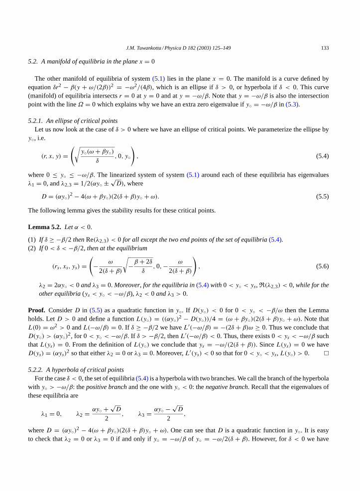
It is clear thatλ1 is the eigenvalue corresponding to the tangential direction to the set(5.2). The behavior of thelinearized system around the equilibria in(5.2)is determined by the eigenvalues(5.3). They are presented inFig. 1.

Remark 5.1. If α = 0 we parameterize the manifold as(r, x, y) = (0, x,−ω/β), x ∈ (−∞,+∞). Each ofthese equilibria withx > 0 has two positive eigenvalues (and one zero) and those withx < 0 have two negativeeigenvalues (and one zero). Atx = 0 we have two extra zero eigenvalues.

Fig. 1. The diagram shows the sign of the eigenvalues(5.3) for α < 0.

J.M. Tuwankotta / Physica D 182 (2003) 125–149 133

5.2. A manifold of equilibria in the planex = 0

The other manifold of equilibria of system(5.1) lies in the planex = 0. The manifold is a curve defined byequationδr2 − β(y + ω/(2β))2 = −ω2/(4β), which is an ellipse ifδ > 0, or hyperbola ifδ < 0. This curve(manifold) of equilibria intersectsr = 0 aty = 0 and aty = −ω/β. Note thaty = −ω/β is also the intersectionpoint with the lineΩ = 0 which explains why we have an extra zero eigenvalue ify = −ω/β in (5.3).

5.2.1. An ellipse of critical pointsLet us now look at the case ofδ > 0 where we have an ellipse of critical points. We parameterize the ellipse by

y, i.e.

(r, x, y) =(√

y(ω + βy)δ

,0, y

), (5.4)

where 0≤ y ≤ −ω/β. The linearized system of system(5.1) around each of these equilibria has eigenvaluesλ1 = 0, andλ2,3 = 1/2(αy ± √

D), where

D = (αy)2 − 4(ω + βy)(2(δ + β)y + ω). (5.5)

The following lemma gives the stability results for these critical points.

Lemma 5.2. Letα < 0.

(1) If δ ≥ −β/2 thenRe(λ2,3) < 0 for all except the two end points of the set of equilibria(5.4).(2) If 0 < δ < −β/2, then at the equilibrium

(rs, xs, ys) =(

− ω

2(δ + β)

√−β + 2δ

δ,0,− ω

2(δ + β)

), (5.6)

λ2 = 2αy < 0 andλ3 = 0. Moreover, for the equilibria in(5.4)with 0 < y < ys,R(λ2,3) < 0, while for theother equilibria(ys < y < −ω/β), λ2 < 0 andλ3 > 0.

Proof. ConsiderD in (5.5) as a quadratic function iny. If D(y) < 0 for 0 < y < −β/ω then the Lemmaholds. LetD > 0 and define a functionL(y) = ((αy)2 − D(y))/4 = (ω + βy)(2(δ + β)y + ω). Note thatL(0) = ω2 > 0 andL(−ω/β) = 0. If δ ≥ −β/2 we haveL′(−ω/β) = −(2δ + β)ω ≥ 0. Thus we conclude thatD(y) > (αy)2, for 0 < y < −ω/β. If δ > −β/2, thenL′(−ω/β) < 0. Thus, there exists 0< ys < −ω/β suchthatL(ys) = 0. From the definition ofL(y) we conclude thatys = −ω/(2(δ + β)). SinceL(ys) = 0 we haveD(ys) = (αys)

2 so that eitherλ2 = 0 orλ3 = 0. Moreover,L′(ys) < 0 so that for 0< y < ys, L(y) > 0.

5.2.2. A hyperbola of critical pointsFor the caseδ < 0, the set of equilibria(5.4)is a hyperbola with two branches. We call the branch of the hyperbola

with y > −ω/β: thepositive branchand the one withy < 0: thenegative branch. Recall that the eigenvalues ofthese equilibria are

λ1 = 0, λ2 = αy + √D

2, λ3 = αy − √

D

2,

whereD = (αy)2 − 4(ω + βy)(2(δ + β)y + ω). One can see thatD is a quadratic function iny. It is easyto check thatλ2 = 0 or λ3 = 0 if and only if y = −ω/β of y = −ω/2(δ + β). However, forδ < 0 we have

134 J.M. Tuwankotta / Physica D 182 (2003) 125–149

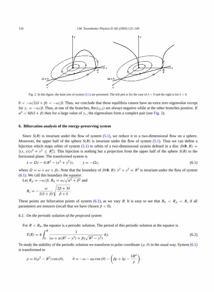
Fig. 2. In this figure, the limit sets of system(5.1)are presented. The left plot is for the case ofδ > 0 and the right is forδ < 0.

0 < −ω/2(δ + β) < −ω/β. Thus, we conclude that these equilibria cannot have an extra zero eigenvalue exceptfor y = −ω/β. Thus, at one of the branches, Re(λ2,3) are always negative while at the other branches positive. Ifα2 < 8β(δ + β) then for a large value ofy, the eigenvalues form a complex pair (seeFig. 2).

6. Bifurcation analysis of the energy-preserving system

SinceS(R) is invariant under the flow of system(5.1), we reduce it to a two-dimensional flow on a sphere.Moreover, the upper half of the sphereS(R) is invariant under the flow of system(5.1). Thus we can define abijection which maps orbits of system(5.1) to orbits of a two-dimensional system defined in a discD(0, R) =(x, y)|x2 + y2 ≤ R2. This bijection is nothing but a projection from the upper half of the sphereS(R) to thehorizontal plane. The transformed system is

x = Ωy − δ(R2 − (x2 + y2)), y = −Ωx, (6.1)

whereΩ = ω + αx + βy. Note that the boundary ofD(0, R): x2 + y2 = R2 is invariant under the flow of system(6.1). We call this boundarythe equator.

LetRp = −ω/β, Rh = ω/√α2 + β2 and

Rs = − ω

2(δ + β)

√2β + 3δ

β + δ.

These points are bifurcation points of system(6.1), as we varyR. It is easy to see thatRh < Rp < Rs if allparameters are nonzero (recall that we have chosenβ < 0).

6.1. On the periodic solution of the projected system

ForR < Rh, the equator is a periodic solution. The period of this periodic solution at the equator is

T(R) = 4∫ R

0

1

(ω + α(R2 − y2) + βy√R2 − y2)

dy. (6.2)

To study the stability of the periodic solution we transform to polar coordinate(ρ, θ) in the usual way. System(6.1)is transformed to

ρ = δ(ρ2 − R2) cos(θ), θ = −ω − αρ cos(θ) −(βρ + δρ − δR2

ρ

).

J.M. Tuwankotta / Physica D 182 (2003) 125–149 135

We then computeρ′ = dρ/dθ = F(ρ, θ), linearized it aroundρ = R, to have a first-order differential equation ofthe formρ′ = A(θ)ρ. Near the periodic solution (i.e.ρ = R), θ(t) is monotonically increasing. Thus,ρ′ = A(θ)ρ

can be approximated byρ′ = Aρ where

A =∫ 2π

0A(θ)dθ = αδ

4π2ω(−1 + p2 +√

1 − p2)

(α2 + β2)3/2(−1 + p2), (6.3)

andp = R√α2 + β2/ω. Thus the periodic solutionx2 + y2 = R2 is unstable ifαδ < 0 and stable ifαδ > 0,

respectively. Ifα = 0, then this periodic solution is the only periodic solution in the projected system(6.1).

Theorem 6.1. If α = 0, system(6.1)has no periodic solution in the interior ofD(0, R).

Proof. Let us fixR < Rp. Then there is a unique equilibrium of system(6.1) in the interior ofD(0, R), namely:(0, y). DefineI = (0, y)|y < y ≤ R andJ = (0, y)| − R ≤ y < y. We writeν(x, y) for the velocity vectorfield corresponds to system(6.1). If Φ(t; (x, y)) is the flow of system(6.1)at timet with initial condition(x, y), wewant to show that

for allP ∈ J, there existstP ∈ (0,∞) such thatΦ(tP ;P) ∈ I.Let J ′ be a maximal subset ofJ with such a property. ClearlyJ ′ = ∅ sinceΦ(T ; (0,−R)) = (0, R) ∈ I, whereT < ∞ is defined in(6.2). Take(0, y) ∈ J ′ arbitrary, writingΦ(t; (0, y)) = (x(t), y(t)), there existst such thatx(t) = 0. If x(t) = 0, we havey(t) = 0, andx(t) = 0 (otherwise the equilibrium is not unique). By the ImplicitFunction Theorem we have: for an open neighborhoodN of (0, y) there existst (in the neighborhood oft) such thatx(t) = 0. Thus,J ′ is open inJ. J ′ is also closed by uniqueness of the equilibrium and the fact that(0,−R) ∈ J ′.Thus, we conclude thatJ ′ = J (from the definition,J is connected).

Let us define a mapX : R2 → R

2 by X(x, y) = (−x, y). ConsiderΓ(t) which is the trajectory(x(t), y(t))= Φ(t;P), 0 ≤ t ≤ s, whereP ∈ J andΦ(s;P) ∈ I. Considert > 0 such thatΓ(t) = (x, y) with x = 0. Wehave

d

dtX(Γ(t))|t=t = X

(d

dtΓ(t)

∣∣∣∣t=t

)= X

(d

dtΦ(t;P)

)= X(ν(x, y))

= −ν(−x, y) + 2αx(x,−y)T = −ν(X(Γ(t)|t=t) + 2αx(x,−y)T.

Thus the vector field of system(6.1) is nowhere tangent toX(Γ ) accept ifα = 0.Finally, consider the domain with boundaryΓ ∪X(Γ ). The flow of system(6.1)is either flowing into the domain,

or flowing out of the domain. We can make the domain as small as we want by choosingP close enough to(0, y)or as big as possible by choosingP close enough to(0,−R). We conclude that there is no other limit cycle in theinterior ofD(0, R).

LetR > Rp. If δ > −β/2, we can use Poincaré’s theorem that the interior of a periodic orbit for a planar vectorfield always contain an equilibrium point, see[19]. He proved this by observing that the index of the vector fieldalong the periodic orbit is equal to one. This was the first application of his invention, in the same paper, of theconcept of the index of a vector field, which was one of the founding ideas of algebraic topology. System(6.1)has no other critical points apart from those in the equator. Thus, the limit cycle could not exists. This idea alsoapplicable in the case 0< δ < −β/2 andR > Rs. If Rp < R < Rs is similar with the caseR < Rp.

Corollary 6.2. If α = 0 all but the critical solution of(6.1) for R < Rh are periodic.

Remark 6.3 (The Bounded-Quadratic-Planar systems). In 1966, Coppel proposed a problem of identifying allpossible phase portrait of the so-called Bounded-Quadratic-Planar systems. A Bounded-Quadratic-Planar system is a

136 J.M. Tuwankotta / Physica D 182 (2003) 125–149

system of two autonomous, ordinary, first-order differential equations with quadratic nonlinearity where all solutionsare bounded. The maximum number of limit cycles that could exists is one of the questions of Coppel. This problemturns out to be very interesting and not as easy as it seems. In fact, the answer to this problem contains the solution tothe 16th Hilbert problem which is unsolved up to now (see[6]). System(6.1)is a Bounded-Quadratic-Planar system.From this point of view,Theorem 6.1is an important result for our systems. This result enables us to compute allpossible phase portraits of system(6.1).

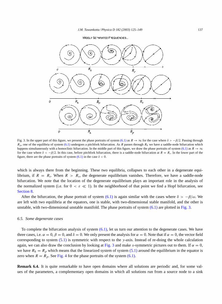
From the previous section, one could guess that there are three situations for system(6.1), i.e. if δ > −β/ω,0 < δ < −ω/2, andδ < 0. ForR close to zero but positive, the phase portrait of system(6.1) is similar in all threesituations. The equator is an unstable periodic solution and there is only one equilibrium of system(6.1). Thereare three possible bifurcations of the equilibria in system(6.1), namely simultaneous saddle-node and homoclinicbifurcation, pitchfork bifurcation and saddle-node bifurcation.

6.2. A simultaneous saddle-node and homoclinic bifurcation

If R passes the valueRh, system(6.1) undergoes a simultaneous saddle-node and homoclinic bifurcation (alsocalled Andronov–Leontovich bifurcation, see[13, pp. 250–252]). If R < Rh the equator is a periodic solution.The period of this periodic solution goes to infinity asR approachesRh from below. Exactly atR = Rh the limitcycle becomes an homoclinic to a degenerate equilibrium (with one zero eigenvalue). This degenerate equilibriumis created via a saddle-node bifurcation. This is clear since after the bifurcation (that is whenR > Rh) we have twoequilibria in the equator and the homoclinic orbit vanishes.

This bifurcation occurs in all three situations of system(6.1). The difference is that, in the case ofδ > 0, the limitcycle at the equator is stable while ifδ < 0 is unstable. This difference has a consequence for the stability type ofthe two equilibria at the equator after the saddle-node bifurcation.

6.3. A pitchfork bifurcation

The second bifurcation which occurs also in all three situation of system(6.1) is a pitchfork bifurcation, whichis natural due to the presence of the symmetryΦ1 : (r, x, y) → (−r, x, y). However, there is a difference betweenthe cases ofδ > −β/ω, 0< δ < −β/ω and the cases ofδ < 0. In the first cases, the equilibrium which is inside thedomain, collapses into the saddle-type equilibrium at the equator whenR = Rp. After the bifurcation (R > Rp)a stable (with two negative eigenvalues) equilibrium is created at the equator. The flow of system(6.1) after thisbifurcation is then simple. We have two equilibria at the equator, one is stable with two-dimensional stable manifoldand one is unstable with two-dimensional unstable manifold. The flow simply moves from one equilibrium to theother. This is the end of the story for the caseδ > −β/ω.

In the second cases (0< δ < −β/ω), a saddle-type equilibrium branches out of the saddle-type equilibrium atthe equator, atR = Rp. The equilibrium at the equator then becomes a stable equilibrium with two-dimensionalstable manifold.

In the third cases (δ < 0), a stable focus branches out of the saddle-type equilibrium at the equator. After thebifurcation, we have four equilibria, two at the equator and two inside the domain. Both of the equilibria at theequator are of the saddle-type. One of the equilibria inside the domain is a stable focus while the other is unstablefocus. There is no other bifurcation in the cases whereδ < 0 (Fig. 3).

6.4. A saddle-node bifurcation

In the cases where 0< δ < −β/ω we have an extra bifurcation, i.e. a saddle-node bifurcation. Recall af-ter a pitchfork bifurcation, inside the domain there is a saddle-type equilibrium. There is also a stable focus

J.M. Tuwankotta / Physica D 182 (2003) 125–149 137

Fig. 3. In the upper part of this figure, we present the phase portraits of system(6.1)asR → ∞ for the case whereδ > −β/2. Passing throughRp, one of the equilibria of system(6.1)undergoes a pitchfork bifurcation. AsR passes throughRh we have a saddle-node bifurcation whichhappens simultaneously with a homoclinic bifurcation. In the middle part of this figure, we draw the phase portraits of system(6.1)asR → ∞for the case whereδ < −β/2. In this case, before pitchfork bifurcation, there is a saddle-node bifurcation atR = Rs. In the lower part of thefigure, there are the phase portraits of system(6.1) in the caseδ < 0.

which is always there from the beginning. These two equilibria, collapses to each other in a degenerate equi-librium, if R = Rs. WhenR > Rs, the degenerate equilibrium vanishes. Therefore, we have a saddle-nodebifurcation. We note that the location of the degenerate equilibrium plays an important role in the analysis ofthe normalized system (i.e. for 0< ε 1). In the neighborhood of that point we find a Hopf bifurcation, seeSection 8.

After the bifurcation, the phase portrait of system(6.1) is again similar with the cases whereδ > −β/ω. Weare left with two equilibria at the equators, one is stable, with two-dimensional stable manifold, and the other isunstable, with two-dimensional unstable manifold. The phase portraits of system(6.1)are plotted inFig. 3.

6.5. Some degenerate cases

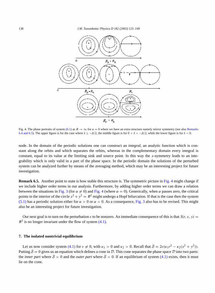
To complete the bifurcation analysis of system(6.1), let us turn our attention to the degenerate cases. We havethree cases, i.e.α = 0,β = 0, andδ = 0. We only present the analysis forα = 0. Note that ifα = 0, the vector fieldcorresponding to system(5.1) is symmetric with respect to they-axis. Instead of re-doing the whole calculationagain, we can also draw the conclusion by looking atFig. 3and makex-symmetric pictures out to them. Ifα = 0,we haveRh = Rp which means that the linearized system of system(5.1)around the equilibrium in the equator iszero whenR = Rp. SeeFig. 4for the phase portraits of the system(6.1).

Remark 6.4. It is quite remarkable to have open domains where all solutions are periodic and, for some val-ues of the parameters, a complementary open domains in which all solutions run from a source node to a sink

138 J.M. Tuwankotta / Physica D 182 (2003) 125–149

Fig. 4. The phase portraits of system(6.1)asR → ∞ for α = 0 where we have an extra structure namely mirror symmetry (see alsoRemarks6.4 and 6.5). The upper figure is for the case whereδ ≥ −β/2, the middle figure is for 0< δ < −β/2, while the lower figure is forδ < 0.

node. In the domain of the periodic solutions one can construct anintegral, an analytic function which is con-stant along the orbits and which separates the orbits, whereas in the complementary domain every integral isconstant, equal to its value at the limiting sink and source point. In this way thex-symmetry leads to an inte-grability which is only valid in a part of the phase space. In the periodic domain the solutions of the perturbedsystem can be analyzed further by means of the averaging method, which may be an interesting project for futureinvestigation.

Remark 6.5. Another point to state is how stable this structure is. The symmetric picture inFig. 4might change ifwe include higher order terms in our analysis. Furthermore, by adding higher order terms we can draw a relationbetween the situations inFig. 3(for α = 0) andFig. 4(whereα = 0). Generically, whenα passes zero, the criticalpoints in the interior of the circlex2 +y2 = R2 might undergo a Hopf bifurcation. If that is the case then the system(5.1)has a periodic solution either forα > 0 orα < 0. As a consequence,Fig. 3also has to be revised. This mightalso be an interesting project for future investigation.

Our next goal is to turn on the perturbationε to be nonzero. An immediate consequence of this is thatS(r, x, y) =R2 is no longer invariant under the flow of system(4.1).

7. The isolated nontrivial equilibrium

Let us now consider system(4.1) for ε = 0, with κ1 > 0 andκ2 > 0. Recall thatS = 2ε(κ1r2 − κ2(x

2 + y2)).PuttingS = 0 gives us an equation which defines a cone inD. This cone separates the phase spaceD into two parts:the inner partwhereS > 0 and theouter partwhereS < 0. If an equilibrium of system(4.1)exists, then it mustlie on the cone.

J.M. Tuwankotta / Physica D 182 (2003) 125–149 139

The location of the nontrivial equilibrium of system(4.1) is

r(ε) =√(ε2(βκ1 − δκ2)2 + (εακ1 − δω)2)κ1κ2

((βκ1 − δκ2)δ)2, x(ε) = −ε

κ1

δ, y(ε) = (εακ1 − δω)κ1

(βκ1 − δκ2)δ. (7.1)

One can immediately see that(7.1)exists if and only if(βκ1 − δκ2)δ = 0.To facilitate the analysis, let us write(7.1) asξ(ε) = (r(ε), x(ε), y(ε)) and correspondingly, the variables

ξ = (r, x, y). In the variableξ the system(4.1) is written asξ = H (ξ ; ε). Let us also name the coneS =κ1r

2 − κ2(x2 + y2) = 0 asC and the manifold of critical points(5.4)asE.

Assuming thatDξH (ξ(0)) has only one eigenvalue with zero real part, by the Center Manifold Theorem, thereexists a coordinate system such that aroundξ(0), system(4.1)can be written as(

ξh

ξc

)=(A(ε)ξh

λ(ε)ξc

)+ higher-order term, (7.2)

whereA(0) has no eigenvalue with zero real part andλ(0) = 0. Let us chooseε1 small enough such that the realpart of the eigenvalues ofA(ε) remain nonzero for 0< ε ≤ ε1.

Let Wε be the invariant manifold of system(7.2) which is tangent toEλ(ε) at ξ(ε), whereEλ(ε) is the lineareigenspace corresponding toλ(ε). We note that the Center Manifold Theorem gives the existence ofWε. Also,W0

is the center manifold ofξ(0), which is, in our case, uniquely defined and tangent toE at ξ(0). SinceE intersectsC at ξ(0) transversally, for small enoughε2 we haveWc(ε) intersectC at ξ(ε) transversally for 0< ε ≤ ε2.

Lastly,E also intersectsS(R) transversally, for|R−‖ξ(0)‖| < c for some positive numberc. This follows fromthe assumption thatDξH (ξ(0)) has only one zero eigenvalue. Thus, there existsε3, small enough, such thatWc(ε)

intersectsS(R) transversally for|R−‖ξ(ε)‖| < c and 0< ε ≤ ε3. Choosingε∗ = minε1, ε2, ε3, we have proventhe following lemma.

Lemma 7.1. Let us assume thatDξH (ξ(0)) has only one zero eigenvalue. There exists0 < ε∗ 1 such that,for ε ∈ (0, ε∗), the system(7.2) has an invariant manifoldWε which is tangent toEλ(ε) at ξ(ε). This invariantmanifold intersects the coneS = 0 transversally atξ(ε). It also intersects the sphereS(R) transversally, for all R,|R − ‖ξ(0)‖| < ε.

From system(7.2), we conclude that the dynamics in the manifoldWε is slow sinceλ(ε) = O(ε) if ε ∈ (0, ε∗).TheLemma 7.1also gives us the stability result for the equilibrium(7.1). If ε ∈ [0, ε∗), then the eigenvalues ofA(ε)remain hyperbolic. Thus, we can use the analysis inSection 4. For the sign ofλ(ε) we have the following lemma.

Lemma 7.2. Consider the system(7.2). For ε ∈ (0, ε∗), we haveλ(ε) > 0 if

(1) δ < 0 andκ2δ > κ1β, or(2) −βκ1/(2κ1 + κ2) < δ < −β/2.

Also forε ∈ (0, ε∗), λ(ε) < 0 if

(1) δ < 0 andκ2δ < κ1β, r(2) δ ≥ −β/2, or 0 < δ < −βκ1/(2κ1 + κ2).

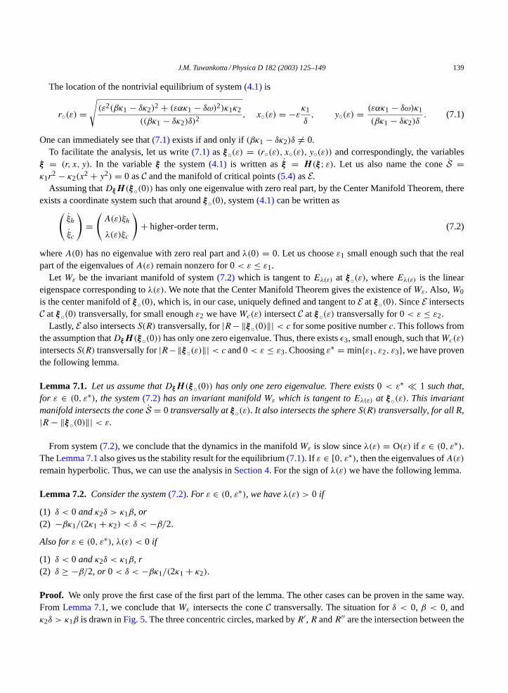
Proof. We only prove the first case of the first part of the lemma. The other cases can be proven in the same way.From Lemma 7.1, we conclude thatWε intersects the coneC transversally. The situation forδ < 0, β < 0, andκ2δ > κ1β is drawn inFig. 5. The three concentric circles, marked byR′,R andR′′ are the intersection between the

140 J.M. Tuwankotta / Physica D 182 (2003) 125–149

Fig. 5. The continuous set of critical pointsE for δ < 0 andβ < 0 is plotted on the figure above. The dashed lines represent the coneC. Itseparates the phase space into two parts, the expanding part (the shadowed area) and the contracting part. There are also three concentric circlesdrawn in this figure. The radius of these circles satisfies:R′ < R < R′′.

sphereS(R′), S(R), andS(R′′)with the planex = 0, respectively. Note that max|R′ −R|, |R′′ −R′|, |R′′ −R| < ε.As ε becomes positive, an open subset ofE which containsξ can be continued withε and form the invariantslow manifoldWε with properties described inLemma 7.1. Thus, we conclude that inside the shadowed area,the dynamics is moving fromS(R) to S(R′′). On the other side, the dynamics is moving fromS(R) to S(R′), i.e.λ(ε) > 0.

In Section 4we left out a question whether the solutions of system(4.1) are bounded in the caseδ < 0. Usingthe same arguments as inLemma 7.1and the proof ofLemma 7.2, for ε small enough we have the following result.

Corollary 7.3. If δ < 0,α < 0 andκ2δ < κ1β then the solution of(4.1) is bounded.

Proof. If δ < 0,E is a hyperbola with two branches: the negative and positive branches. The negative branch is theone that passes through the origin. Forα < 0, the positive branch is attracting. Moreover, the positive branch is inthe interior ofS < 0. This ends the proof.

In the next section we are going to study the behavior near the boundaryκ2/κ1 = (βδ − 2(δ + β))/δ.

8. Hopf bifurcations of the nontrivial equilibrium

The most natural thing to start with in doing the bifurcation analysis is to follow an equilibrium while varying oneof the parameters in system(4.1). However, the analysis in the previous sections shows that we have no possibility ofhaving more than one nontrivial critical point. Thus, we have excluded the saddle-node bifurcation of the nontrivialequilibrium of our system. Let us fix all parameters butδ. We will use this parameter as our continuation parameter.Recall that we have fixedβ < 0,α < 0,ω > 0 andκj > 0, j = 1,2.

Let δ > −βκ1/(2κ1 + κ2) and consider the system(7.2). By Lemma 5.2, considering the chosen value ofparameters:β < 0, α < 0, ω > 0 andκj > 0, j = 1,2, we conclude thatR(λ1,2) < 0, whereλ1,2 are theeigenvalues ofA(0). UsingLemma 7.1, for small enoughε,R(λ1,2(ε)) < 0, whereλ1,2(ε) are the eigenvalues ofA(ε). If δ < −βκ1/(2κ1 + κ2), by Lemma 7.1we haveλ(ε) > 0 and byLemma 5.2, we haveλ3 > 0.

See the left figure ofFig. 6where we have drawn an illustration for this situation. Atδ = −βκ1/(2κ1 + κ2) wehave the situation where system(4.1)nearξ(0) has a two-dimensional center manifoldWε. Locally,W intersect

J.M. Tuwankotta / Physica D 182 (2003) 125–149 141

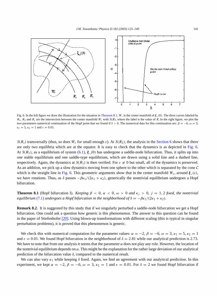
Fig. 6. In the left figure we draw the illustration for the situation inTheorem 8.1.W is the center manifold ofξ(0). The three curves labeled byR1, R2 andRs are the intersection between the center manifoldWε with S(R), where the label is the value ofR. In the right figure, we plot thetwo parameters numerical continuation of the Hopf point that we found ifδ > 0. The numerical data for this continuation are:β = −6,ω = 3,κ1 = 5, κ2 = 1 andε = 0.01.

S(Rs) transversally (thus, so doesWε for small enoughε). At S(R2), the analysis in theSection 6shows that thereare only two equilibria which are at the equator. It is easy to check that the dynamics is as depicted inFig. 6.At S(R1), as a equilibrium of system(6.1), ξ(0) has undergone a saddle-node bifurcation. Thus, it splits up intoone stable equilibrium and one saddle-type equilibrium, which are drawn using a solid line and a dashed line,respectively. Again, the dynamics atS(R1) is then verified. Forε = 0 but small, all of the dynamics is preserved.As an addition, we pick up a slow dynamics moving from one sphere to the other which is separated by the coneCwhich is the straight line inFig. 6. This geometric arguments show that in the center manifoldWε, aroundξ(ε),we have rotations. Thus, asδ passes−βκ1/(2κ1 + κ2), generically the nontrivial equilibrium undergoes a Hopfbifurcation.

Theorem 8.1 (Hopf bifurcation I). Keepingβ < 0, α < 0, ω > 0 and κj > 0, j = 1,2 fixed, the nontrivialequilibrium(7.1)undergoes a Hopf bifurcation in the neighborhood ofδ = −βκ1/(2κ1 + κ2).

Remark 8.2. It is suggested by this study that if we singularly perturbed a saddle-node bifurcation we get a Hopfbifurcation. One could ask a question how generic is this phenomenon. The answer to this question can be foundin the paper of Stiefenhofer[20]. Using blown-up transformations with different scaling (this is typical in singularperturbation problems), it is proved that this phenomenon is generic.

We check this with numerical computation for the parameter values:α = −2, β = −6,ω = 3, κ1 = 5, κ2 = 1andε = 0.01. We found Hopf bifurcation in the neighborhood ofδ = 2.81 while our analytical prediction is 2.73.We have to note that from our analysis it seems that the parameterα does not play any role. However, the location ofthe nontrivial equilibrium depends onα. This might be the explanation for the rather large deviation of our analyticalprediction of the bifurcation valueδ, compared to the numerical result.

We can also varyκ1 while keepingδ fixed. Again, we find an agreement with our analytical prediction. In thisexperiment, we keptα = −2, β = −6, ω = 3, κ2 = 1 andε = 0.01. Forδ = 2 we found Hopf bifurcation if

142 J.M. Tuwankotta / Physica D 182 (2003) 125–149

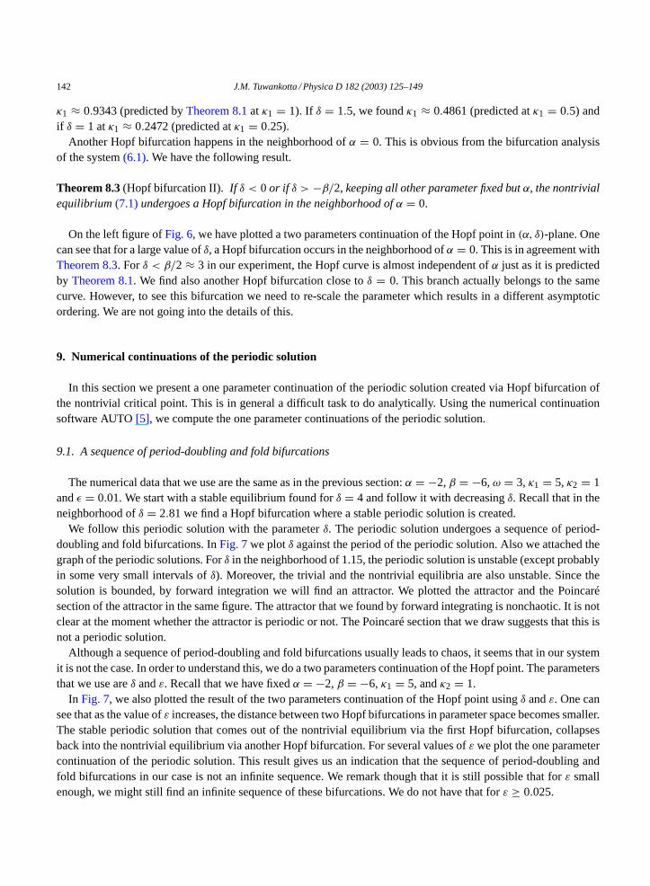
κ1 ≈ 0.9343 (predicted byTheorem 8.1atκ1 = 1). If δ = 1.5, we foundκ1 ≈ 0.4861 (predicted atκ1 = 0.5) andif δ = 1 atκ1 ≈ 0.2472 (predicted atκ1 = 0.25).

Another Hopf bifurcation happens in the neighborhood ofα = 0. This is obvious from the bifurcation analysisof the system(6.1). We have the following result.

Theorem 8.3 (Hopf bifurcation II). If δ < 0 or if δ > −β/2,keeping all other parameter fixed butα, the nontrivialequilibrium(7.1)undergoes a Hopf bifurcation in the neighborhood ofα = 0.

On the left figure ofFig. 6, we have plotted a two parameters continuation of the Hopf point in(α, δ)-plane. Onecan see that for a large value ofδ, a Hopf bifurcation occurs in the neighborhood ofα = 0. This is in agreement withTheorem 8.3. Forδ < β/2 ≈ 3 in our experiment, the Hopf curve is almost independent ofα just as it is predictedby Theorem 8.1. We find also another Hopf bifurcation close toδ = 0. This branch actually belongs to the samecurve. However, to see this bifurcation we need to re-scale the parameter which results in a different asymptoticordering. We are not going into the details of this.

9. Numerical continuations of the periodic solution

In this section we present a one parameter continuation of the periodic solution created via Hopf bifurcation ofthe nontrivial critical point. This is in general a difficult task to do analytically. Using the numerical continuationsoftware AUTO[5], we compute the one parameter continuations of the periodic solution.

9.1. A sequence of period-doubling and fold bifurcations

The numerical data that we use are the same as in the previous section:α = −2,β = −6,ω = 3,κ1 = 5,κ2 = 1andε = 0.01. We start with a stable equilibrium found forδ = 4 and follow it with decreasingδ. Recall that in theneighborhood ofδ = 2.81 we find a Hopf bifurcation where a stable periodic solution is created.

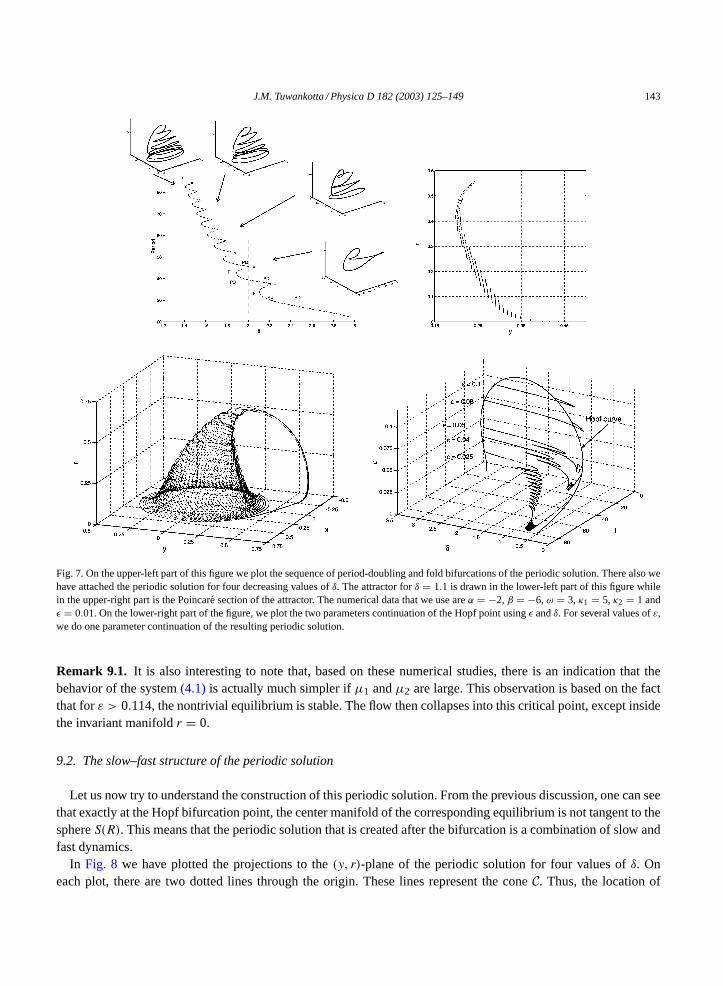
We follow this periodic solution with the parameterδ. The periodic solution undergoes a sequence of period-doubling and fold bifurcations. InFig. 7we plotδ against the period of the periodic solution. Also we attached thegraph of the periodic solutions. Forδ in the neighborhood of 1.15, the periodic solution is unstable (except probablyin some very small intervals ofδ). Moreover, the trivial and the nontrivial equilibria are also unstable. Since thesolution is bounded, by forward integration we will find an attractor. We plotted the attractor and the Poincarésection of the attractor in the same figure. The attractor that we found by forward integrating is nonchaotic. It is notclear at the moment whether the attractor is periodic or not. The Poincaré section that we draw suggests that this isnot a periodic solution.

Although a sequence of period-doubling and fold bifurcations usually leads to chaos, it seems that in our systemit is not the case. In order to understand this, we do a two parameters continuation of the Hopf point. The parametersthat we use areδ andε. Recall that we have fixedα = −2,β = −6, κ1 = 5, andκ2 = 1.

In Fig. 7, we also plotted the result of the two parameters continuation of the Hopf point usingδ andε. One cansee that as the value ofε increases, the distance between two Hopf bifurcations in parameter space becomes smaller.The stable periodic solution that comes out of the nontrivial equilibrium via the first Hopf bifurcation, collapsesback into the nontrivial equilibrium via another Hopf bifurcation. For several values ofε we plot the one parametercontinuation of the periodic solution. This result gives us an indication that the sequence of period-doubling andfold bifurcations in our case is not an infinite sequence. We remark though that it is still possible that forε smallenough, we might still find an infinite sequence of these bifurcations. We do not have that forε ≥ 0.025.

J.M. Tuwankotta / Physica D 182 (2003) 125–149 143

Fig. 7. On the upper-left part of this figure we plot the sequence of period-doubling and fold bifurcations of the periodic solution. There also wehave attached the periodic solution for four decreasing values ofδ. The attractor forδ = 1.1 is drawn in the lower-left part of this figure whilein the upper-right part is the Poincare section of the attractor. The numerical data that we use areα = −2,β = −6,ω = 3, κ1 = 5, κ2 = 1 andε = 0.01. On the lower-right part of the figure, we plot the two parameters continuation of the Hopf point usingε andδ. For several values ofε,we do one parameter continuation of the resulting periodic solution.

Remark 9.1. It is also interesting to note that, based on these numerical studies, there is an indication that thebehavior of the system(4.1) is actually much simpler ifµ1 andµ2 are large. This observation is based on the factthat forε > 0.114, the nontrivial equilibrium is stable. The flow then collapses into this critical point, except insidethe invariant manifoldr = 0.

9.2. The slow–fast structure of the periodic solution

Let us now try to understand the construction of this periodic solution. From the previous discussion, one can seethat exactly at the Hopf bifurcation point, the center manifold of the corresponding equilibrium is not tangent to thesphereS(R). This means that the periodic solution that is created after the bifurcation is a combination of slow andfast dynamics.

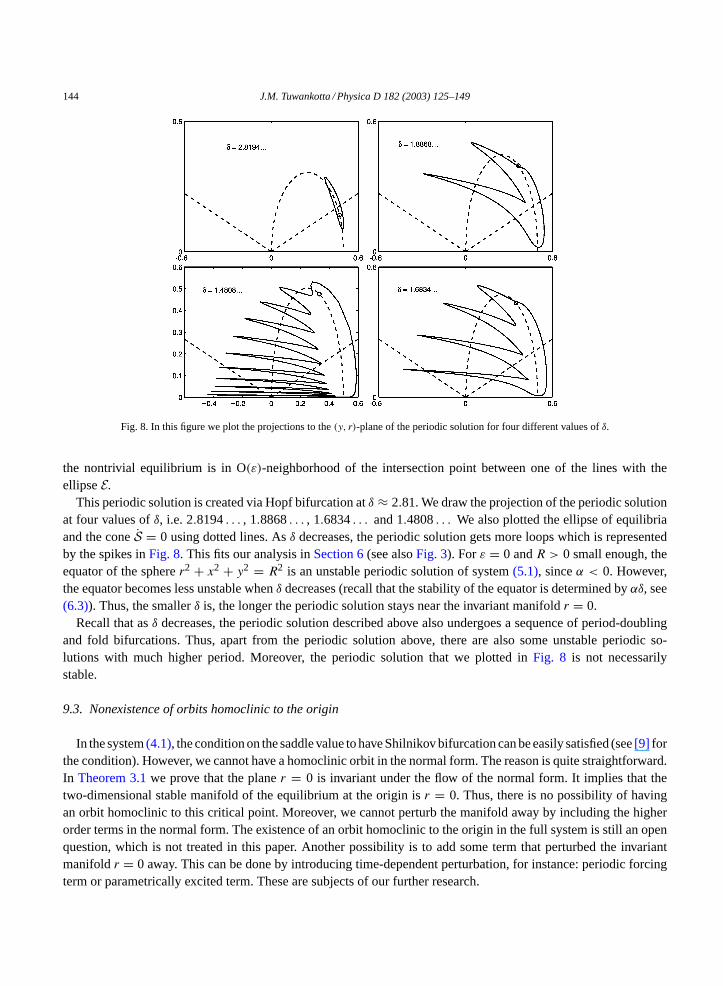
In Fig. 8 we have plotted the projections to the(y, r)-plane of the periodic solution for four values ofδ. Oneach plot, there are two dotted lines through the origin. These lines represent the coneC. Thus, the location of

144 J.M. Tuwankotta / Physica D 182 (2003) 125–149

Fig. 8. In this figure we plot the projections to the(y, r)-plane of the periodic solution for four different values ofδ.

the nontrivial equilibrium is in O(ε)-neighborhood of the intersection point between one of the lines with theellipseE.

This periodic solution is created via Hopf bifurcation atδ ≈ 2.81. We draw the projection of the periodic solutionat four values ofδ, i.e. 2.8194. . . , 1.8868. . . , 1.6834. . . and 1.4808. . . We also plotted the ellipse of equilibriaand the coneS = 0 using dotted lines. Asδ decreases, the periodic solution gets more loops which is representedby the spikes inFig. 8. This fits our analysis inSection 6(see alsoFig. 3). Forε = 0 andR > 0 small enough, theequator of the spherer2 + x2 + y2 = R2 is an unstable periodic solution of system(5.1), sinceα < 0. However,the equator becomes less unstable whenδ decreases (recall that the stability of the equator is determined byαδ, see(6.3)). Thus, the smallerδ is, the longer the periodic solution stays near the invariant manifoldr = 0.

Recall that asδ decreases, the periodic solution described above also undergoes a sequence of period-doublingand fold bifurcations. Thus, apart from the periodic solution above, there are also some unstable periodic so-lutions with much higher period. Moreover, the periodic solution that we plotted inFig. 8 is not necessarilystable.

9.3. Nonexistence of orbits homoclinic to the origin

In the system(4.1), the condition on the saddle value to have Shilnikov bifurcation can be easily satisfied (see[9] forthe condition). However, we cannot have a homoclinic orbit in the normal form. The reason is quite straightforward.In Theorem 3.1we prove that the planer = 0 is invariant under the flow of the normal form. It implies that thetwo-dimensional stable manifold of the equilibrium at the origin isr = 0. Thus, there is no possibility of havingan orbit homoclinic to this critical point. Moreover, we cannot perturb the manifold away by including the higherorder terms in the normal form. The existence of an orbit homoclinic to the origin in the full system is still an openquestion, which is not treated in this paper. Another possibility is to add some term that perturbed the invariantmanifoldr = 0 away. This can be done by introducing time-dependent perturbation, for instance: periodic forcingterm or parametrically excited term. These are subjects of our further research.

J.M. Tuwankotta / Physica D 182 (2003) 125–149 145

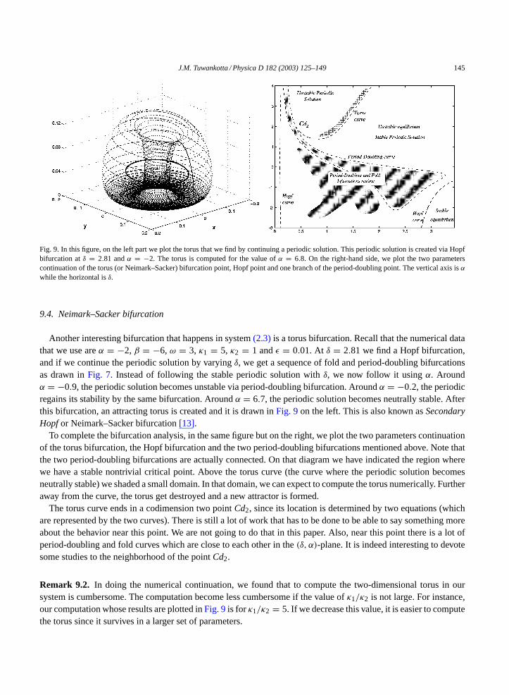
Fig. 9. In this figure, on the left part we plot the torus that we find by continuing a periodic solution. This periodic solution is created via Hopfbifurcation atδ = 2.81 andα = −2. The torus is computed for the value ofα = 6.8. On the right-hand side, we plot the two parameterscontinuation of the torus (or Neimark–Sacker) bifurcation point, Hopf point and one branch of the period-doubling point. The vertical axis isα

while the horizontal isδ.

9.4. Neimark–Sacker bifurcation

Another interesting bifurcation that happens in system(2.3) is a torus bifurcation. Recall that the numerical datathat we use areα = −2, β = −6,ω = 3, κ1 = 5, κ2 = 1 andε = 0.01. At δ = 2.81 we find a Hopf bifurcation,and if we continue the periodic solution by varyingδ, we get a sequence of fold and period-doubling bifurcationsas drawn inFig. 7. Instead of following the stable periodic solution withδ, we now follow it usingα. Aroundα = −0.9, the periodic solution becomes unstable via period-doubling bifurcation. Aroundα = −0.2, the periodicregains its stability by the same bifurcation. Aroundα = 6.7, the periodic solution becomes neutrally stable. Afterthis bifurcation, an attracting torus is created and it is drawn inFig. 9on the left. This is also known asSecondaryHopfor Neimark–Sacker bifurcation[13].

To complete the bifurcation analysis, in the same figure but on the right, we plot the two parameters continuationof the torus bifurcation, the Hopf bifurcation and the two period-doubling bifurcations mentioned above. Note thatthe two period-doubling bifurcations are actually connected. On that diagram we have indicated the region wherewe have a stable nontrivial critical point. Above the torus curve (the curve where the periodic solution becomesneutrally stable) we shaded a small domain. In that domain, we can expect to compute the torus numerically. Furtheraway from the curve, the torus get destroyed and a new attractor is formed.

The torus curve ends in a codimension two pointCd2, since its location is determined by two equations (whichare represented by the two curves). There is still a lot of work that has to be done to be able to say something moreabout the behavior near this point. We are not going to do that in this paper. Also, near this point there is a lot ofperiod-doubling and fold curves which are close to each other in the(δ, α)-plane. It is indeed interesting to devotesome studies to the neighborhood of the pointCd2.

Remark 9.2. In doing the numerical continuation, we found that to compute the two-dimensional torus in oursystem is cumbersome. The computation become less cumbersome if the value ofκ1/κ2 is not large. For instance,our computation whose results are plotted inFig. 9is forκ1/κ2 = 5. If we decrease this value, it is easier to computethe torus since it survives in a larger set of parameters.

146 J.M. Tuwankotta / Physica D 182 (2003) 125–149

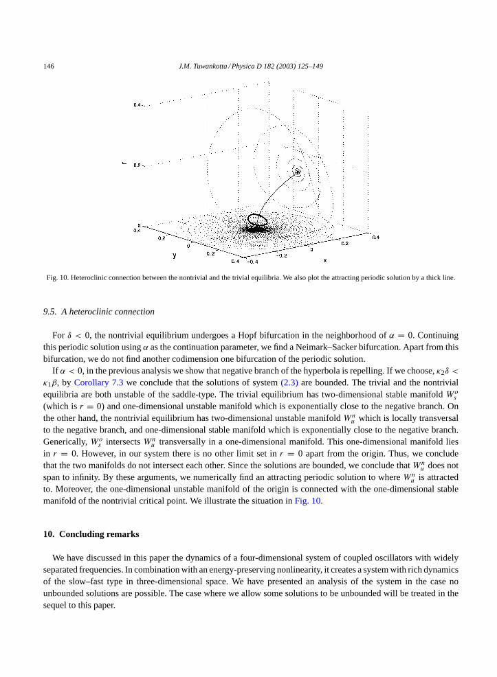
Fig. 10. Heteroclinic connection between the nontrivial and the trivial equilibria. We also plot the attracting periodic solution by a thick line.

9.5. A heteroclinic connection

For δ < 0, the nontrivial equilibrium undergoes a Hopf bifurcation in the neighborhood ofα = 0. Continuingthis periodic solution usingα as the continuation parameter, we find a Neimark–Sacker bifurcation. Apart from thisbifurcation, we do not find another codimension one bifurcation of the periodic solution.

If α < 0, in the previous analysis we show that negative branch of the hyperbola is repelling. If we choose,κ2δ <

κ1β, by Corollary 7.3we conclude that the solutions of system(2.3) are bounded. The trivial and the nontrivialequilibria are both unstable of the saddle-type. The trivial equilibrium has two-dimensional stable manifoldWo

s

(which is r = 0) and one-dimensional unstable manifold which is exponentially close to the negative branch. Onthe other hand, the nontrivial equilibrium has two-dimensional unstable manifoldWn

u which is locally transversalto the negative branch, and one-dimensional stable manifold which is exponentially close to the negative branch.Generically,Wo

s intersectsWnu transversally in a one-dimensional manifold. This one-dimensional manifold lies

in r = 0. However, in our system there is no other limit set inr = 0 apart from the origin. Thus, we concludethat the two manifolds do not intersect each other. Since the solutions are bounded, we conclude thatWn

u does notspan to infinity. By these arguments, we numerically find an attracting periodic solution to whereWn

u is attractedto. Moreover, the one-dimensional unstable manifold of the origin is connected with the one-dimensional stablemanifold of the nontrivial critical point. We illustrate the situation inFig. 10.

10. Concluding remarks

We have discussed in this paper the dynamics of a four-dimensional system of coupled oscillators with widelyseparated frequencies. In combination with an energy-preserving nonlinearity, it creates a system with rich dynamicsof the slow–fast type in three-dimensional space. We have presented an analysis of the system in the case nounbounded solutions are possible. The case where we allow some solutions to be unbounded will be treated in thesequel to this paper.

J.M. Tuwankotta / Physica D 182 (2003) 125–149 147

We have completed the analysis for the energy-preserving part of the normal form. Although in a sense it isvery special, we note that the energy-preserving part can be viewed as a Bounded-Quadratic-Planar system whichhas been extensively studied but in general still contains a lot of open problems. Extending this analysis for smallperturbations, we can get a lot of information of the dissipative normal form.

10.1. On the energy exchanges

Although we leave out the forcing terms, there is energy exchange between the characteristic modes of ournormal form. The main ingredient that we need for this energy exchange isµ1µ2 < 0. Physically, this meansone of the modes should be damped while the other is excited. This, however, is not a restrictive condition sinceif both modes are damped (or excited), clearly one would need an energy source (or an absorber) to have energyexchange.

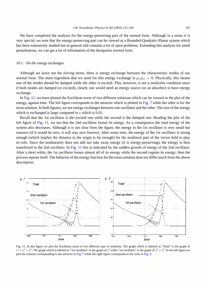
In Fig. 11, we have plotted the Euclidean norm of two different solutions which can be viewed as the plot of theenergy, against time. The left figure corresponds to the attractor which is plotted inFig. 7while the other is for thetorus solution. In both figures, we see energy exchanges between one oscillator and the other. The size of the energywhich is exchanged is large compared toε which is 0.01.

Recall that the 1st oscillator is the excited one while the second is the damped one. Reading the plot of theleft figure of Fig. 11, we see that the 2nd oscillator looses its energy. As a consequence the total energy of thesystem also decreases. Although it is not clear from the figure, the energy in the 1st oscillator is very small butnonzero (if it would be zero, it will stay zero forever). After some time, the energy of the 1st oscillator is strongenough (which implies the distance to the origin is far enough) for the nonlinear part of the vector field to playits role. Since the nonlinearity does not add nor take away energy (it is energy-preserving), the energy is thentransferred to the 2nd oscillator. InFig. 11this is indicated by the sudden growth of energy of the 2nd oscillator.After a short while, the 1st oscillator looses almost all of its energy while the second regains its energy; then theprocess repeats itself. The behavior of the energy function for the torus solution does not differ much from the abovedescription.

Fig. 11. In this figure we plot the Euclidean norm of two different type of solutions. The graph which is labeled as “Total” is the graph ofr2 + x2 + y2. The graph which is labeled as “1st oscillator” is the graph ofr2 while “1st oscillator” is the graph ofx2 + y2. In the left figure weplot the solution corresponding to the attractor inFig. 7while the right figure corresponds to the torus inFig. 9.

148 J.M. Tuwankotta / Physica D 182 (2003) 125–149

10.2. Back to the atmospheric research

It is interesting to translate back the results in this paper to the atmospheric model. The model used in[4] is derivedusing EOFs as its basis functions. Thus, the state variables in this paper are actually the coefficients of these basisfunctions. The basis functions itself can be interpreted as dominant patterns in the atmosphere. An asymptoticallystable nontrivial equilibrium that we find in this paper means an attracting pattern in the atmosphere. This pattern isa (nontrivial) linear combination of the EOF basis functions. A periodic solution would mean a periodic evolutionfrom one pattern to the other and back.

Although in[4] the dynamics of the two modes with wide separation in the frequencies does not show interestingbehavior, in this paper we show that the dynamics of such a systemin generalis rich. One of the conclusions of[4]is that the homoclinic orbit found in the five-modes system might be responsible for the long time-scale behaviorin the system. The analysis in our paper gives an indication that although the homoclinic orbit is not there, a longtime-scale behavior may appear because of the slow–fast structure in the system.

In relation with the results in[8,23] on how to prove that a three-dimensional system of differential equations isnonchaotic, we note that our system is more complex than theirs. The studies in[8,23]are concentrated on nonlinearthree-dimensional systems having only at most five terms. Our normal form contains 11 terms. So far in our analysiswe do not find chaotic behavior. It is evident in our system that we cannot have homoclinic orbits. This excludesthe Shilnikov’s scenario for a route to chaos. Thus, whether our system is chaotic or not is still an open question.It is also interesting to note that torus (or Neimark–Sacker) bifurcation usually is followed by a lot of chaos in thesystem in the presence of homoclinic tangencies (see for instance[3]). This may provide us with a way to findchaotic behavior in our system.

We left out several interesting questions from our analysis. Below we have listed several open questions.The invariant manifoldr = 0 can be perturbed away by perturbing the systems with small periodic forcing term

or a parametrical excitation term. In the absence of this invariant manifold, we might find a homoclinic orbit thatcould lead to a lot of interesting dynamics. The complication is that we have to analyze a four-dimensional normalform.

The behavior (dynamics) of the system near the codimension two point:Cd2 is not analyzed in this paper. Thistype of codimension two point is treated carefully in the book by Kuznetsov[13]. One could for instance follow theperiodic solution around the pointCd2 and compare the result with the cases studied in[13].

The global dynamics in the case of the absence of the nontrivial equilibrium is a very interesting case. This willbe treated in a sequel to this paper.

Acknowledgements

J.M. Tuwankotta wishes to thank KNAW and CICAT TUDelft for financial support. He wishes to thank HansDuistermaat, Ferdinand Verhulst (both from Universiteit Utrecht), Henk Broer (Rijksuniversiteit Groningen) andDaan Crommelin (Universiteit Utrecht and KNMI) for many discussions during this research; also Yuri Kuznetsov,Bob Rink, Thijs Ruijgrok and Lennaert van Veen (all from Universiteit Utrecht) for many comments. He also thanksSanti Goenarso for her support in various ways.

References

[1] H.W. Broer, S.N. Chow, Y. Kim, G. Vegter, A normally elliptic Hamiltonian bifurcation, ZAMP 44 (1993) 389–432.[2] H.W. Broer, S.N. Chow, Y. Kim, G. Vegter, The Hamiltonian double-zero eigenvalue, Fields Inst. Commun. 4 (1995) 1–19.

J.M. Tuwankotta / Physica D 182 (2003) 125–149 149

[3] H.W. Broer, C. Simó, J.C. Tatjer, Towards global models near homoclinic tangencies of dissipative diffeomorphisms, Nonlinearity 11 (3)(1998) 667–770.

[4] D.T. Crommelin, Homoclinic dynamics: a scenario for atmospheric ultralow-frequency variability, J. Atmos. Sci. 59 (9) (2002) 1533–1549.[5] E. Doedel, A. Champneys, T. Fairgrieve, Y. Kuznetsov, B. Sandstede, X.-J. Wang, AUTO97: continuation and bifurcation software for

ordinary differential equations (with HomCont), in: Computer Science, Concordia University, Montreal, Canada, 1986.[6] F. Dumortier, C. Herssens, L. Perko, Local bifurcations and a survey of bounded quadratic systems, J. Differ. Equ. 165 (2) (2000) 430–467.[7] N. Fenichel, Geometric singular perturbation theory for ordinary differential equations, J. Differ. Equ. 31 (1979) 53–98.[8] Z. Fu, J. Heidel, Non-chaotic behaviour in three-dimensional quadratic systems, Nonlinearity 10 (5) (1997) 1289–1303.[9] J. Guckenheimer, P.H. Holmes, Nonlinear oscillations, dynamical systems, and bifurcations of vector fields, in: Applied Mathematical

Science, vol. 42, Springer, Berlin, 1997.[10] G. Haller, Chaos near resonance, in: Applied Mathematical Sciences, vol. 138, Springer, New York, 1999.[11] M.W. Hirsch, C.C. Pugh, M. Shub, Invariant manifolds, in: Lecture Notes in Mathematics, vol. 583, Springer, Berlin, 1977.[12] C.K.R.T. Jones, Geometric singular perturbation theory, in: R. Johnson (Ed.), Dynamical Systems, Montecatibi Terme, Lecture Notes in

Mathematics, vol. 1609, Springer, Berlin, 1994, pp. 44–118.[13] Y.A. Kuznetsov, Elements of applied bifurcation theory, in: Applied Mathematical Sciences, 2nd ed., vol. 112, Springer, New York, 1998.[14] W.F. Langford, K. Zhan, Interactions of Andronov–Hopf and Bogdanov–Takens bifurcations, Fields Inst. Commun. 24 (1999) 365–383.[15] W.F. Langford, K. Zhan, Hopf bifurcations near 0:1 resonance, in: C. Chen, Li (Eds.), Proceedings of the BTNA’98, Springer, New York,

1999, pp. 1–18.[16] S.A. Nayfeh, A.H. Nayfeh, Nonlinear interactions between two widely spaced modes-external excitation, Int. J. Bifurcat. Chaos 3 (1993)

417–427.[17] A.H. Nayfeh, C.-M. Chin, Nonlinear interactions in a parametrically excited system with widely spaced frequencies, Nonlinear Dyn. 7

(1995) 195–216.[18] J.A. Sanders, F. Verhulst, Averaging method on nonlinear dynamical system, in: Applied Mathematical Sciences, vol. 59, Springer, New

York, 1985.[19] H. Poincaré, Mémoire sur les courbes définies par une équation différentielle, J. de Math. 7 (1881) 375–422;

H. Poincaré, Mémoire sur les courbes définies par une équation différentielle, J. de Math. 8 (1882) 251–296.[20] M. Stiefenhofer, Singular perturbation with limit points in the fast dynamics, Z. Angew. Math. Phys. 49 (5) (1998) 730–758.[21] J.M. Tuwankotta, F. Verhulst, Hamiltonian systems with widely separated frequencies, Nonlinearity 16 (2) (2003) 689–706.[22] S. Wiggins, Normally hyperbolic invariant manifolds in dynamical systems, with the assistance of György Haller and Igor Mezic, in:

Applied Mathematical Sciences, vol. 105, Springer, New York, 1994.[23] X.-S. Yang, A technique for determining autonomous 3-ODEs being non-chaotic, Chaos Solitons Fract. 11 (14) (2000) 2313–2318.