Widely-Tunable Optical Parametric Oscillation in χ
159
Widely-Tunable Optical Parametric Oscillation in χ (3) Microresonators Noel Lito Betonio Sayson A thesis submitted in fulfilment of the requirements for the degree of Doctor of Philosophy in Physics The University of Auckland August 2020
-
Upload
khangminh22 -
Category
Documents
-
view
0 -
download
0
Transcript of Widely-Tunable Optical Parametric Oscillation in χ

Widely-Tunable Optical ParametricOscillation in χ (3) Microresonators
Noel Lito Betonio Sayson
A thesis submitted in fulfilment of the requirements for the degree ofDoctor of Philosophy in Physics
The University of AucklandAugust 2020


Abstract
In this thesis, we report a novel approach to enable optical sources with widebandwavelength tunability. By using χ(3) microresonators, we are able to generate twonew narrowband widely detuned optical frequencies via the nonlinear process of opticalparametric oscillation. The wideband tunability is enabled by operating the resonator incondition of normal dispersion, in the presence of higher order dispersion. This allowsus to phasematch unusually large frequency shift parametric oscillation.
We first present an experimental demonstration of widely tunable optical parametricoscillation in silica (SiO2) microspheres. Through comprehensive theoretical analysisand experiments, we are able to demonstrate over 720 nm of discrete tunability usinga low-power, continuous wave C-band pump laser. We find that the maximum tuningrange attainable in this system was limited due to the high attenuation of fused silicaabove 1900 nm.
We then show that magnesium fluoride (MgF2) microresonators can overcome thelimitations experienced by silica-based resonators. We consider several different MgF2
microresonators to experimentally demonstrate over an optical octave of discrete tun-able output from 1083 to 2670 nm. In addition, signatures of mid-infrared sidebands(out to 3860 nm) are also observed in this demonstration. By using the delayed self-heterodyne interferometer method, we find that these generated sidebands share similarspectral linewidths to the pump laser. Moreover, we demonstrate a small amount ofcontinuous tunability of the parametric sidebands by leveraging the resonators intrinsicthermal nonlinearity.
Finally, we investigate the formation of localized frequency combs located aroundthe pump and the two widely detuned sidebands. In this investigation, we present anexperimental demonstration of these clustered frequency combs in microresonators, aswell as proposing a theory that explains their generation. Numerical simulations basedon the Lugiato-Lefever equation are carried out to validate the proposed theory. Fur-thermore, we also look at, in detail, the coherence of the numerically simulated combclusters.
iii


To my Parents, Papa Danny† and Mama Zita
v


Acknowledgements
First and foremost, I would like to express my profound gratitude to my academic su-pervisors, Associate Professor Stuart Murdoch, Associate Professor Stephane Coen,and Dr. Miro Erkintalo, for giving me an opportunity to work in the field of nonlinearoptics and photonics. I truly appreciate the knowledge and skills that you imparted onme. I am and will be forever grateful of the all-out support and guidance throughout thecourse of my Phd studies.
Thank you to Dr. Karen Webb for patiently assisting me in the laboratory worksduring the start of my studies. Also, I thank Dr. Vincent Ng, Toby Bi, and Hoan Phamfor the advices that they shared, and for the support, as well.
I also want to extend my thanks to Dr. Harald Schwefel and Luke Trainor for shar-ing their time and expertise in the fabrication of microresonators, and for the provisionof the microresonators that we used in our experiments.
I also would like to thank my colleagues: Dr. Bruno Garbin, Dr. Yadong Wang,Dr. Dominik Vogt, Dr. Ray Xu, Andrew Su, Max Li, Robert Otupiri, James Loveday,Vivian McPhail, Alexander Uhde Nielsen, Ian Hendry and Logan Baber for their friend-ship, support and encouragement.
I express my sincere thanks to my parents, Mama Zita and Papa Danny†, sevenbrothers and Dr. Jannah Lee Tarranza for their understanding, love, and support duringmy entire stay at UOA.
Most importantly, I would like to thank the Man above us all, for He is the source ofmy strength, and for the constant guidance and wisdom in helping me fulfill this PhDdream.
vii


List of Publications
Journal articles
1. N. L. B. Sayson, K. E. Webb, S. Coen, M. Erkintalo, and S. G. Murdoch, “ Widelytunable optical parametric oscillation in a Kerr microresonator, ” Optics Letters42, 5190-5193 (2017).
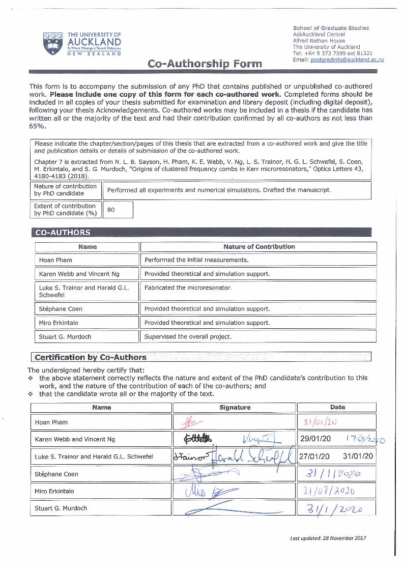
2. N. L. B. Sayson, H. Pham, K. E. Webb, V. Ng, L. S. Trainor, H. G. L. Schwefel, S.Coen, M. Erkintalo, and S. G. Murdoch, “ Origins of clustered frequency combsin Kerr microresonators,” Optics Letters 43, 4180-4183 (2018, editor’s pick).
3. N. L. B. Sayson, T. Bi, H. Pham, V. Ng, L. S. Trainor, H. G. L. Schwefel, S.Coen, M. Erkintalo, and S. G. Murdoch, “ Octave-spanning tunable parametricoscillation in crystalline Kerr microresonators, ” Nature Photonics 13, 701-706(2019).
ix

x
Conference contributions
1. N. L. B. Sayson, K. E. Webb, S. Coen, M. Erkintalo, and S. G. Murdoch, “ Wide-band wavelength tunability of parametric oscillation in silica microsphere res-onators, ” 3rd Australian and New Zealand Conference on Optics and Photonics(ANZCOP, 2017).
2. N. L. B. Sayson, H. Pham, K. E. Webb, L. S. Trainor, H. G. L. Schwefel, S. Coen,M. Erkintalo, and S. G. Murdoch, “ Widely-tunable optical parametric oscillationin MgF2 microresonators, ” Conference on Lasers and Electro-Optics (CLEO,2018).
3. N. L. B. Sayson, H. Pham, T. Bi, V. Ng, L. S. Trainor, H. G. L. Schwefel, S.Coen, M. Erkintalo, and S. G. Murdoch, “ Broad wavelength tunability in mag-nesium fluoride microresonators, ” International Conference on Advanced Func-tional Materials and Nanotechnology (ICAFM, 2018 - Best Oral Presentation).
4. N. L. B. Sayson, H. Pham, T. Bi, V. Ng, L. S. Trainor, H. G. L. Schwefel, S.Coen, M. Erkintalo, and S. G. Murdoch, “ Wideband tunability of Kerr parametricoscillation in an MgF2 microresonator,” Conference on Lasers and Electro-Optics(CLEO, 2019).
5. N. L. B. Sayson, H. Pham, T. Bi, V. Ng, L. S. Trainor, H. G. L. Schwefel, S. Coen,M. Erkintalo, and S. G. Murdoch, “ Mid-infrared optical parametric oscillation incrystalline microresonators, ” International Conference on Advanced FunctionalMaterials and Nanotechnology (ICAFM, 2019).
6. N. L. B. Sayson, H. Pham, T. Bi, V. Ng, L. S. Trainor, H. G. L. Schwefel, S. Coen,M. Erkintalo, and S. G. Murdoch, “ Generation of tunable mid-infrared opticalparametric oscillation in MgF2 microresonators,” The 8th Asia-Pacific OpticalSensors Conference (APOS, 2019).

Contents
Abstract iii
Dedication v
Acknowledgements vii
List of Publications ix
Contents xi
List of Figures xv
List of Tables xxi
Glossary xxiii
Co-Authorship Forms xxv
1 Introduction 1
1.1 Overall Objective of Thesis . . . . . . . . . . . . . . . . . . . . . . . . 3
1.2 Outline of Thesis . . . . . . . . . . . . . . . . . . . . . . . . . . . . . 3
2 Fundamental Concepts 7
2.1 Step - Index Optical Fibers . . . . . . . . . . . . . . . . . . . . . . . . 7
xi

xii Contents
2.2 Chromatic Dispersion . . . . . . . . . . . . . . . . . . . . . . . . . . . 8
2.3 Fiber Nonlinearities . . . . . . . . . . . . . . . . . . . . . . . . . . . . 11
2.3.1 Kerr Effect . . . . . . . . . . . . . . . . . . . . . . . . . . . . 12
2.3.2 Self-Phase and Cross-Phase Modulation . . . . . . . . . . . . . 12
2.3.3 Four-Wave Mixing . . . . . . . . . . . . . . . . . . . . . . . . 13
2.3.4 Stimulated Raman Scattering . . . . . . . . . . . . . . . . . . . 14
2.4 Nonlinear Propagation in Optical Waveguides . . . . . . . . . . . . . . 16
2.5 Modulation Instability . . . . . . . . . . . . . . . . . . . . . . . . . . 17
2.5.1 Linear Stability Analysis . . . . . . . . . . . . . . . . . . . . . 17
2.6 Summary . . . . . . . . . . . . . . . . . . . . . . . . . . . . . . . . . 20
3 Cavity Dynamics 21
3.1 Ring Resonator Cavity . . . . . . . . . . . . . . . . . . . . . . . . . . 21
3.1.1 Linear Cavity Response . . . . . . . . . . . . . . . . . . . . . 22
3.1.2 Nonlinear Cavity Response due to Kerr Effect . . . . . . . . . . 24
3.2 Lugiato-Lefever Equation . . . . . . . . . . . . . . . . . . . . . . . . . 25
3.3 Intracavity Modulation Instability . . . . . . . . . . . . . . . . . . . . 27
3.4 Lugiato-Lefever Simulations of Modulation Instability . . . . . . . . . 29
3.4.1 Stable Modulation Instability . . . . . . . . . . . . . . . . . . . 30
3.4.2 Unstable Modulation Instability . . . . . . . . . . . . . . . . . 31
3.5 Effect of Higher Order Dispersion . . . . . . . . . . . . . . . . . . . . 33
3.6 Summary . . . . . . . . . . . . . . . . . . . . . . . . . . . . . . . . . 36
4 Microresonator Fabrication and Characterization 39
4.1 Optical Microresonators . . . . . . . . . . . . . . . . . . . . . . . . . 39
4.2 Fabrication . . . . . . . . . . . . . . . . . . . . . . . . . . . . . . . . 40

Contents xiii
4.2.1 SiO2 Microspheres . . . . . . . . . . . . . . . . . . . . . . . . 40
4.2.2 MgF2 Microdisk Resonators . . . . . . . . . . . . . . . . . . . 41
4.3 Taper Coupling . . . . . . . . . . . . . . . . . . . . . . . . . . . . . . 43
4.4 Finesse Measurement . . . . . . . . . . . . . . . . . . . . . . . . . . . 45
4.5 Thermal Locking . . . . . . . . . . . . . . . . . . . . . . . . . . . . . 46
4.6 Summary . . . . . . . . . . . . . . . . . . . . . . . . . . . . . . . . . 47
5 Widely Tunable Optical Parametric Oscillation in Silica Microspheres 49
5.1 Theoretical Analysis . . . . . . . . . . . . . . . . . . . . . . . . . . . 50
5.2 Experimental Setup . . . . . . . . . . . . . . . . . . . . . . . . . . . . 55
5.3 Experimental Results and Discussion . . . . . . . . . . . . . . . . . . . 56
5.3.1 Resonance Scan . . . . . . . . . . . . . . . . . . . . . . . . . 56
5.3.2 Widely Tunable Parametric Sidebands . . . . . . . . . . . . . . 56
5.3.3 Stimulated Raman Scattering (SRS) . . . . . . . . . . . . . . . 60
5.4 Summary . . . . . . . . . . . . . . . . . . . . . . . . . . . . . . . . . 61
6 Octave Tunability of Parametric Oscillation in MgF2 Microresonators 63
6.1 Resonator Dispersion . . . . . . . . . . . . . . . . . . . . . . . . . . . 64
6.2 Experimental Setup . . . . . . . . . . . . . . . . . . . . . . . . . . . . 68
6.3 Experimental Results and Discussion . . . . . . . . . . . . . . . . . . . 72
6.3.1 Widely Tunable Parametric Sidebands . . . . . . . . . . . . . 72
6.3.2 Octave Tunability and Signatures of Mid-IR Sidebands . . . . . 77
6.3.3 Conversion Efficiency . . . . . . . . . . . . . . . . . . . . . . 83
6.3.4 Continuous Tunability . . . . . . . . . . . . . . . . . . . . . . 84
6.4 Summary . . . . . . . . . . . . . . . . . . . . . . . . . . . . . . . . . 85

xiv Contents
7 Origins of Clustered Frequency Combs in Kerr Microresonators 87
7.1 Experimental Set-up . . . . . . . . . . . . . . . . . . . . . . . . . . . 88
7.2 Experimental Results . . . . . . . . . . . . . . . . . . . . . . . . . . . 89
7.3 Theoretical Analysis . . . . . . . . . . . . . . . . . . . . . . . . . . . 91
7.4 Coherence of Simulated Comb Clusters . . . . . . . . . . . . . . . . . 95
7.5 Summary . . . . . . . . . . . . . . . . . . . . . . . . . . . . . . . . . 97
8 Conclusion 99
A Conversion Efficiency of Large Frequency Shift Parametric Oscillation inKerr Microresonators 103
A.1 Theoretical model . . . . . . . . . . . . . . . . . . . . . . . . . . . . . 103
A.2 Numerical Simulation Results . . . . . . . . . . . . . . . . . . . . . . 105
A.2.1 Constant Coefficients . . . . . . . . . . . . . . . . . . . . . . . 105
A.2.2 Frequency-Dependent Nonlinear Coefficients . . . . . . . . . . 107
A.2.3 Frequency-Dependent Coupling Coefficients . . . . . . . . . . 108
Bibliography 111

List of Figures
2.1 Schematic view of a step-index. . . . . . . . . . . . . . . . . . . . . . 82.2 Refractive index nL (solid lines) and the group refractive index ng (dashed
lines) for SiO2 and MgF2 (O and E rays). . . . . . . . . . . . . . . . . 102.3 Variation of β2 with wavelength for SiO2 and MgF2 (O and E rays). . . 112.4 Schematic of degenerate four-wave mixing, where two pump photons
ωp are annihilated to create Stokes ωs and anti-Stokes ωa photons. . . . 142.5 Schematic of spontaneous (a) Stokes and (b) anti-Stokes Raman scat-
tering of a pump photon ωp by a vibrational state at frequency Ω. . . . . 152.6 Normalized Raman gain curve of fused SiO2. . . . . . . . . . . . . . . 162.7 MI power gain spectrum as a function of frequency shift for three dif-
ferent powers. The parameters used are γ = 1.5 W−1 km−1, β2 = -18ps2 km−1, and P0 = 2, 4 and 8 W. . . . . . . . . . . . . . . . . . . . . . 19
3.1 Schematic of a ring resonator cavity. θ and ρ are the intensity couplingand transmission coefficients of the coupling, respectively. . . . . . . . 22
3.2 Linear cavity resonances with ρ equals to 0.2 (blue), 0.4 (red), and 0.8(pink). The corresponding F are ∼ 15.7, ∼ 8, and ∼ 4, respectively. . . 23
3.3 The nonlinear resonances of a cavity with ρ = 0.6 and φNL = 0 (blue),π/2 (red), and π (pink). . . . . . . . . . . . . . . . . . . . . . . . . . . 25
3.4 (a) Temporal and (b) spectral LLE evolutions through scanning the nor-malized detuning ∆. . . . . . . . . . . . . . . . . . . . . . . . . . . . . 30
3.5 Spectral evolution of the intracavity field over a million roundtrips for∆ = -4.5. . . . . . . . . . . . . . . . . . . . . . . . . . . . . . . . . . . 31
3.6 Temporal (a) and spectral (b) profiles of a stable modulation instabilitypattern. These profiles were taken from the simulation results in Fig.3.5 at ∆ = -4.5 and after 1 million roundtrips. . . . . . . . . . . . . . . 31
3.7 LLE simulation showing the spectral evolution of the intracavity fieldagainst a million roundtrips for ∆ = 1. . . . . . . . . . . . . . . . . . . 32
3.8 Temporal (a) and spectral (b) profiles of an unstable modulation insta-bility. These profiles were taken from the simulation results in Fig. 3.7at ∆ = 1 after 1 million roundtrips. . . . . . . . . . . . . . . . . . . . . 32
3.9 Modulation instability phase-matching diagram calculated with the pa-rameters: Pin = 100 mW, γ = 1.5 W−1 km−1 for β3 = 0.051 ps3 km−1
and β4 = −2.0 × 10⁻⁴ ps4 km−1 at ZDW = 1550 nm. Dashed lineindicate the ZDW. . . . . . . . . . . . . . . . . . . . . . . . . . . . . . 34
xv

xvi List of Figures
3.10 Modulation instability gain spectra for pump wavelengths 1548 nm (blue),1542 nm (red) and 1535 nm (magenta). Parameters used were Pin = 100mW, γ = 1.5 W−1 km−1 for β3 = 0.051 ps3 km−1 and β4 = −2.0× 10⁻⁴
ps4 km−1 at ZDW = 1550 nm. . . . . . . . . . . . . . . . . . . . . . . 353.11 Parametric gain curve as a function of frequency shift Ω. Calculated
using the parameters: Pin = 100 mW, γ = 1.5 W−1 km−1 for β3 = 0.051ps3 km−1 and β4 = −2.0 × 10⁻⁴ ps4 km−1 at ZDW = 1550 nm. . . . . . 36
4.1 Ericsson FSU 995 Polarization Maintaining fusion splicer. (b) Image ofa 163 µm diameter silica microsphere. The fiber stem is connected onone side of the microsphere. . . . . . . . . . . . . . . . . . . . . . . . 41
4.2 (a) MgF2 crystal blank with a 10 mm diameter and 1 mm thickness (b)The preform disk is epoxied onto the tip of a brass rod. . . . . . . . . . 41
4.3 (a) Front view image of the SPDT set-up. (b) Sketch showing the ori-entation of the diamond cutter to set the desired rake angle. . . . . . . . 42
4.4 Images of the five MgF2 microresonators used in the experiments withmajor radii R as indicated. . . . . . . . . . . . . . . . . . . . . . . . . 43
4.5 Top-view microscope image of (a) 265-µm major radius MgF2 mi-crodisk resonator and (b) 81.5-µm radius SiO2 microsphere togetherwith their tapered fiber. . . . . . . . . . . . . . . . . . . . . . . . . . . 44
4.6 A schematic diagram of a tapered fiber. . . . . . . . . . . . . . . . . . 444.7 Schematic of experimental setup for finesse measurement. TLC: tun-
able laser controller, ECL: external cavity laser, PM: phase modulator,and PD: photodetector. . . . . . . . . . . . . . . . . . . . . . . . . . . 45
4.8 (a) 515-µm major radius MgF2 cavity resonance with 15 MHz symmet-rically detuned sidebands. (b) Resonance curve with Lorentzian fit (redcurve). . . . . . . . . . . . . . . . . . . . . . . . . . . . . . . . . . . . 46
4.9 Mechanism of the microcavity resonance response as the pump-laserwavelength is scanned in the presence of a positive thermal nonlinear-ity. The green-dashed curve represents the cold resonance of the micro-cavity. Scanning the pump laser from short to long wavelengths leadsto thermal broadening of the resonance (red curve) while the resonancebecomes narrower when going to the opposite direction (blue curve). . . 47
5.1 Variation of β2 with wavelength of the fundamental TM mode for silicamicrospheres with three different diameters: 140 µm (blue), 160 µm(red), and 180 µm (magenta). Inset: Corresponding β4 values for thethree different diameters. . . . . . . . . . . . . . . . . . . . . . . . . . 52
5.2 Phase-matching curves for the fundamental TM mode of silica micro-spheres with three different diameters: 140 µm (blue), 160 µm (red),and 180 µm (magenta). These curves are calculated using Eq. 5.2.Dashed lines correspond to the three different ZDWs of the microspheres. 53
5.3 Parametric gain bandwidth for a 160 µm diameter silica microsphere,calculated from Eq. 3.21 using the same parameters as in Fig. 5.2.Dashed line indicates where the MI gain bandwidth is equivalent to asingle FSR. . . . . . . . . . . . . . . . . . . . . . . . . . . . . . . . . 54

List of Figures xvii
5.4 Schematic diagram for the SiO2 microsphere tunability experiment. TLC:tunable laser controller, ECL: external cavity laser, EDFA: erbium dopedfiber amplifier, BPF: band-pass filter, PC: polarization controller, WDM:wavelength-division multiplexer, VOA: variable optical attenuator, PD:photodetector, and OSA: optical spectrum analyzer. . . . . . . . . . . . 55
5.5 Scan of the resonances of a 163 µm diameter SiO2 microsphere cavity.(a) Linear transmission measured directly after the resonator output,where dips (in red trace) indicate the cavity resonances (b) while peaks(in blue trace) correspond to nonlinear signals generated between 1200– 1400 nm. . . . . . . . . . . . . . . . . . . . . . . . . . . . . . . . . 57
5.6 Spectra of widely tunable parametric sidebands in a 163 µm diametersilica microsphere resonator for six different pump wavelengths (fromtop to bottom: 1563.7, 1559.5, 1551.1, 1545.3, 1535.3 and 1527.7 nm).The black arrows point the positions of the individual parametric side-bands and the black dashed line indicates the predicted position of theZDW. . . . . . . . . . . . . . . . . . . . . . . . . . . . . . . . . . . . 58
5.7 Experimentally measured sideband wavelengths as the pump wavelengthis varied from 1569 to 1527 nm (solid circles). Solid curves show thetheoretical phase-matching curve predicted by Eq. 5.2 for a 160 µmdiameter silica microsphere. Dashed line indicates the ZDW. . . . . . . 59
5.8 Experimental spectra of SRS signals in 163 µm diameter silica micro-sphere resonator. . . . . . . . . . . . . . . . . . . . . . . . . . . . . . 60
6.1 Microdisk geometry used in the resonator modelling. Inset: mode dis-tribution for the fundamental TE mode for a microresonator with R =300 µm and r = 130 µm. . . . . . . . . . . . . . . . . . . . . . . . . . 65
6.2 Modelled zero-dispersion wavelength as a function of major radius Rfor a fixed minor radius (r = 130 µm) in MgF2 microresonator. . . . . . 65
6.3 Modelled variation of the group-velocity dispersion (GVD) coefficientβ2 for the two microresonators (R = 200 and 300 µm). Inset: an en-larged view of the β2 values in the C-band wavelength range. . . . . . . 66
6.4 Theoretically predicted phase-matching curve as a function of pumpwavelength for the two microresonators (R = 200 and 300 µm). Blackdashed lines: ZDWs of the two microresonators, shaded region: C-bandpump wavelength range. . . . . . . . . . . . . . . . . . . . . . . . . . 67
6.5 Schematic diagram for the first experimental setup of the MgF2 mi-croresonator tunability experiment. TLC: tunable laser controller, ECL:external cavity laser, EDFA: erbium doped fiber amplifier, PC: polariza-tion controller, BPF: band-pass filter, PM: power meter, WDM: wavelength-division multiplexer, PD: photodetector, VOA: variable optical attenua-tor, and OSA: optical spectrum analyzer. . . . . . . . . . . . . . . . . . 69

xviii List of Figures
6.6 A schematic of the second experimental setup for measuring the spec-tra of the parametric sidebands that goes beyond 2400 nm in MgF2 mi-croresonator. TLC: tunable laser controller, ECL-1 (C-band) and ECL-2 (L-band): external cavity laser, EDFA-1 (C-band) and EDFA-2 (L-band): erbium doped fiber amplifier, PC: polarization controller, BPF:band-pass filter, PM: power meter, GM: gold mirror, FM: fiber mount,IR-BPF: Infrared radiation - bandpass filter, FTIR: Fourier transform in-frared spectrometer, WDM: wavelength-division multiplexer, PD: pho-todetector, VOA: variable optical attenuator, and OSA: optical spectrumanalyzer. Note that the unaltered components have been faded out andsurrounded with dashed red lines in this figure. . . . . . . . . . . . . . 70
6.7 Schematic of the delayed self-heterodyne interferometer used for linewidthmeasurements of the pump laser and the generated parametric side-bands. TBF: tunable bandpass filter, AOM: acousto-optic modulator,PC; polarization controller, SMF: single-mode fiber, PD: photodetec-tor, and RFSA: radio frequency spectrum analyzer. . . . . . . . . . . . 71
6.8 Experimentally measured spectra from the 515 µm major radius MgF2microresonator at five different pump wavelengths (from top to bottom):λ = 1557.3, 1553.2, 1543, 1535.1, 1529.1 nm. The black dashed lineindicates the estimated ZDW of the microresonator. . . . . . . . . . . . 73
6.9 Experimentally measured sideband wavelengths as a function of pumpwavelength, together with the theoretical phase-matching curve for the515 µm major radius MgF2 microresonator. Filled circles: experimen-tal data, solid curves (red and blue): theoretical fit, black dashed line:ZDW, shaded region: C-band pump wavelength range. . . . . . . . . . 74
6.10 Linewidth measurements using an optical DSHI technique for the short-wavelength sideband (SWS), the pump wavelength and the long-wavelengthsideband (LWS). Solid black curves indicate the Gaussian fits to themeasured beat signals. . . . . . . . . . . . . . . . . . . . . . . . . . . 75
6.11 Experimentally measured spectra from the 400 µm major radius MgF2microresonator at five different pump wavelengths (from top to bottom):λ = 1563.8, 1557.8, 1548.19, 1536.2, 1530.6 nm. The black dashed lineindicates the estimated ZDW of the microresonator. . . . . . . . . . . . 76
6.12 Experimentally measured sideband wavelengths as a function of pumpwavelength, together with the theoretical phase-matching curve for the400 µm major radius MgF2 microresonator, calculated with parame-ters β3 = 3.6 ps3 km−1 and β4 = -1.39 × 10⁻⁴ ps4 km−1 at the ZDWof 1595.5 nm. Filled circles: experimental data, solid curves (red andblue): theoretical fit, dashed black line: ZDW, shaded region: C-bandpump wavelength range. . . . . . . . . . . . . . . . . . . . . . . . . . 77
6.13 Experimentally measured spectra from the 265 µm major radius MgF2microresonator at five different pump wavelengths (from top to bottom):λ = 1564, 1553.9, 1546.1, 1543.1, 1541 nm. The black dashed lineindicates the estimated ZDW of the microresonator. . . . . . . . . . . . 79

List of Figures xix
6.14 Experimentally measured sideband wavelengths as a function of pumpwavelength for the two different mode families within the 265 µm ma-jor radius MgF2 microresonator. Filled circles (green and magenta):experimental data, solid curves (red and blue): theoretical fit, dashedblack line: ZDW, shaded region: C-band pump wavelength range. . . . 80
6.15 Sideband wavelengths as a function of pump wavelength for the small-est two MgF2 microresonators with major radii of R = 190 µm and165 µm. Filled circles: measured short-wavelength sidebands (SWSs),open circles: inferred long-wavelength sidebands (LWSs), solid curves(red and blue): theoretical fit. . . . . . . . . . . . . . . . . . . . . . . . 81
6.16 Selected experimentally measured SWSs spectra from the 165 µm ma-jor radius MgF2 microresonator at five different pump wavelengths (fromtop to bottom): λ = 1588.1, 1579.1, 1568.4, 1547.4, 1533.8 nm. TheZDW of this microresonator is at 1750 nm. . . . . . . . . . . . . . . . 82
6.17 Experimentally measured spectrum from one of our MgF2 microres-onators studied in this thesis. . . . . . . . . . . . . . . . . . . . . . . . 83
6.18 Experimental demonstration of 10 GHz continuous tunability in 265µm major radius MgF2 microresonator. Inset: Experimentally mea-sured optical spectrum with a pump wavelength of 1569 nm and twosidebands at wavelengths of 1512 nm and 1630 nm, respectively. . . . . 85
7.1 The experimental setup used for demonstrating clustered frequency combsin 400 µm major radius MgF2 microresonator. TLC: tunable laser con-troller, ECL: external cavity laser, EDFA: erbium doped fiber ampli-fier, PC: polarization controller, BPF: bandpass filter, PM: power me-ter, WDM: wavelength-division multiplexer, PD: photodetector, VOA:variable optical attenuator, OSA: optical spectrum analyzer, and RFSA:radio frequency spectrum analyzer. . . . . . . . . . . . . . . . . . . . . 88
7.2 (a-d) Experimentally measured spectrum of the clustered frequency combsas we increase the pump detuning ∆. The panel on the right-hand sideis the zoom of the spectrum of the long-wavelength sidebands. . . . . . 90
7.3 Experimentally measured RF spectrum, corresponding to the differentspectra presented in Fig. 7.2, respectively. . . . . . . . . . . . . . . . . 91
7.4 Numerically simulated spectra using the generalized LLE at selectedcavity detuning. . . . . . . . . . . . . . . . . . . . . . . . . . . . . . . 92
7.5 β2 values as a function of wavelength. Blue circle: short sideband,magenta circle: pump wavelength, red circle: long sideband. . . . . . . 93
7.6 (a) Numerical simulation of clustered frequency comb formation as thecavity detuning ∆ is scanned. (b) The red horizontal solid line denotesthe MI threshold, while the black solid line represents the peak intra-cavity power of the long-wavelength sideband (red-detuned anomaloussideband). Dotted lines in (a) and (b) denote the detuning at which thelong-wavelength sideband power crosses the MI threshold. . . . . . . . 94

xx List of Figures
7.7 (a) - (d) Numerical simulations of the spectral evolution of the anoma-lous sideband cluster, and (e) - (h) corresponding simulations of thedegree of coherence as a function of delay in units of photon lifetimetph = tR/(2α), carried out at normalized detunings of (a), (e) ∆ = −3,(b), (f) ∆ =−2, (c), (g) ∆ =−1, and (d), (h) ∆ = 2. . . . . . . . . . . . 96
A.1 Numerical simulation of the maximum conversion efficiency to eachsideband as a function of the cavity detuning for a normalized drivingpower of X = 5. . . . . . . . . . . . . . . . . . . . . . . . . . . . . . . 106
A.2 Optical mode profiles of the three waves (pump, SWS and LWS) in the265 µm major radius MgF2 microresonator. . . . . . . . . . . . . . . . 107
A.3 Numerical simulation of the effect of frequency-dependent nonlinearcoefficients on the maximum conversion efficiency for the short-wavelengthsideband(SWS) and long-wavelength sideband (LWS). . . . . . . . . . 108
A.4 Numerical simulation of the effect of frequency-dependent coupling co-efficients on the maximum conversion efficiency. . . . . . . . . . . . . 109

List of Tables
2.1 Summary of Sellmeier coefficients for SiO2 and MgF2 (O and E rays). . 9
6.1 Summary of two distinct mode families that produce large frequencyshift sidebands in 265 µm major radius MgF2 microresonator. . . . . . 78
6.2 Summary of the dispersion characteristics for two smallest microres-onators with R = 190 µm and 165 µm. . . . . . . . . . . . . . . . . . . 81
xxi


Glossary
AOM acousto-optic modulatorASE amplified spontaneous emissionBPF bandpass filterCW continuous waveDSHI delayed self-heterodyne interferometerECL external cavity laserEDFA erbium doped fiber amplifierFSR free spectral rangeFWHM full width at half maximumFWM four wave mixingGHz gigaHertz (109 cycles per second)GVD group velocity dispersionkHz kiloHertz (103 cycles per second)LWSs long-wavelength sidebandsLLE Lugiato-Lefever equationMgF2 magnesium fluorideMI modulation instabilityNLSE nonlinear Schrodinger equationOSA optical spectrum analyzerPC polarization controllerPD photodiodePM phase modulatorQ qualityRFSA radio frequency spectrum analyzerSiO2 fused silica glassSMF single-mode optical fiberSMI stable modulation instabilitySPDT single-point diamond turning
xxiii

xxiv Glossary
SPM self-phase modulationSRS stimulated Raman scatteringSWSs short-wavelength sidebandsTE transverse electricTHz teraHertz (1012 cycles per second)TLC tunable laser controllerTM transverse magneticUMI unstable modulation instabilityVOA variable optical attenuatorWDM wavelength-division multiplexerWGMs whispering-gallery modesXPM cross-phase modulationZDW zero dispersion wavelength

Co-Authorship Forms
xxv


Chapter 1
Introduction
The invention of the laser by Theodore H. Maiman in 1960 [1] is one of the great-est scientific achievements of the 20th century. The ability of these lasers to producehigh intensity coherent light, has seen them utilized for a wide variety of applicationssuch as spectroscopy [2], telecommunications [3], metrology [4] and even in the field ofmedicine [5]. However, there are still many spectral regions in the optical spectrum, par-ticularly in the mid-infrared (mid-IR), that remain difficult to access using conventionallasers. The primary reason for this problem is the restricted availability of suitable gainmaterials at these spectral regions. Fortunately, immediately after the demonstration ofthe first laser, there was already significant research focusing on developing nonlinearoptical techniques to allow the generation of wavelengths not accessible by conven-tional lasers. In 1961, Franken et al. [6] reported the first experimental demonstrationof second harmonic generation in a quartz crystal. Since then, many other nonlinearoptical processes have been experimentally demonstrated [7–10].
Nowadays, optical parametric oscillation in nonlinear crystals is a commonly usednonlinear optical technique to generate coherent light with wide spectral coverage. Thistechnique relies on the nonlinear strength and the phase-matching properties of the op-tical material. The most common type of optical parametric oscillator (OPO) is basedaround nonlinear crystals possessing a χ(2) optical nonlinearity. Here, the pump laserfrequency is converted into two lower frequencies (called the signal and idler waves).These χ(2) OPO’s are capable of producing laser-like signals at virtually any opticalwavelength [11]. They have become a standard laboratory source that can generatewidely-tunable coherent light ranging from the visible to mid-infrared (IR) spectral re-gions. Due to their broad wavelength tunability, OPO’s have made a significant impacton numerous scientific applications such as quantum optics [12], imaging [13], envi-ronmental gas detection [14, 15], and high-resolution spectroscopy [16, 17]. However
1

2 Chapter 1 Introduction
to date, their widespread adoption outside of the laboratory has been impeded by theircomplexity, size, and cost.
Another approach to optical parametric oscillation is to utilize the χ(3) Kerr nonlin-earity in optical fibers to generate large frequency shift optical parametric sidebandsthrough degenerate four-wave mixing (FWM). Such sideband generation in opticalfibers have been demonstrated in both single pass and oscillator configurations [18–21], and leverage a variety of modal [18–20] and dispersive [21–24] phase-matchingschemes. One of the most successful schemes involves pumping in the regime of nor-mal group-velocity dispersion. The phase matching condition in this regime is satisfiedby taking into account the higher-order dispersion terms, allowing for large frequencyshift parametric sidebands. In addition, small changes in the pump wavelength resultin large frequency shifts in the sideband wavelengths, enabling wideband tunability.Utilizing these ideas, fiber optical parametric oscillators with widely tunable outputsidebands have been demonstrated [22–31]. Such devices have been able to demon-strate high conversion efficiency and very impressive sideband tunabilities that rangeup to an octave of optical spectrum [25, 32, 33]. For instance, Wong et al. [25] wereable to experimentally demonstrate over 560 nm wavelength span of parametric side-band tunability by tuning the pump wavelength between 1532 and 1556 nm. Despitethe promising performance from these fiber optical parametric oscillators, they typicallysuffer from a major drawback because of their high intracavity losses, arising from theuse of standard fiber components. Thus, they require costly high-power pump lasers(often pulsed) to achieve parametric oscillation.
In the past two decades, high-Q optical microresonators have been studied exten-sively paving the way for the development of new efficient platforms for nonlinear op-tical sources [34–36] due to their ultra high finesse and small modal volumes [37].These microresonators are capable of producing nonlinear effects at extremely lowdriving powers. Recently, microresonators with third-order Kerr nonlinearities haveattracted particular interest [38–40] with the development of chip-scale coherent opti-cal frequency combs [36, 41–48]. Through Kerr nonlinear processes, these frequencycombs are created in the anomalous group-velocity dispersion (GVD) regime. The dis-covery of these Kerr frequency combs have led to an impressive range of applications inspectroscopy [49–51], telecommunications [52, 53], optical ranging [54, 55], and ultra-precise distance measurements [56].
Aside from the comb formation, microresonators can also produce single pairs ofnew optical frequencies at widely separated frequency shifts from the original pump viaFWM [57–59]. These oscillators are phasematched through exactly the same mecha-nism as the previously developed fiber oscillators. As such, parametric oscillators based

Chapter 1 Introduction 3
on Kerr optical microresonators offer the prospect of overcoming the limitations experi-enced by fiber-based systems. This offers an intriguing opportunity for the developmentof a new type of low power, widely tunable optical source.
The motivation of this thesis is to address the current limitations in the operationof OPOs, since they are one of the few sources of tunable coherent light that can giveaccess to the strong molecular transitions in the mid-IR region. With the current OPOplatforms, suffering from significant disadvantages, their operation remains limited in-side the research laboratory. This thesis aims to develop a new type of widely-tunableparametric oscillator that does not hold any of the disadvantages mentioned above. Thiscan be done by harnessing the unique properties of optical microresonators to enableefficient widely tunable optical parametric oscillation.
1.1 Overall Objective of Thesis
The overall objective of this thesis is to develop a new type of low-cost, low-powerwidely tunable optical source: the χ(3) based microresonator oscillators, capable ofdemonstrating wideband tunability particularly in the near-IR (1 – 2 µm) and the mid-IR (2 – 4 µm) regions of the optical wavelength spectrum. Below are the key objectivesthat we aim to achieve in this thesis.1. Demonstrate, for the first time, the widely tunable parametric oscillation in χ(3) mi-croresonators operated in the near- IR region.2. Extend the operating range of these χ(3) microresonators to mid-IR region anddemonstrate an optical octave of discrete tunability of the parametric sidebands.3. Determine the origins of the associated clustered frequency combs formed from thesesidebands.
1.2 Outline of Thesis
This thesis is divided into eight chapters, including this introduction. The presentationof the topics is organized as follows:
Chapter 2 provides an overview of light propagation in dielectric waveguides, specif-ically in optical fibers. Several general properties such as chromatic dispersion and fibernonlinearities are also described. We then introduce the propagation equation that gov-erns the evolution of light in χ(3) optical waveguides.
Chapter 3 introduces the resonator configuration used to describe the dynamics of

4 Chapter 1 Introduction
optical microresonators. We then discuss the resonance profile of linear and nonlin-ear cavities, followed by the presentation of Lugiato-Lefever equation (LLE) whichdescribes the propagation of light in Kerr resonators. The effects of higher order disper-sion on the intracavity modulation instability are also presented at the later part of thechapter.
Chapter 4 presents the fabrication procedures developed for SiO2 microspheres andMgF2 microresonators. We then describe the polishing and cleaning methods used withthe crystalline MgF2 microresonators, as well as the coupling method of tapered opticalfibers. In addition, we present the experimental setup and procedure used to measurethe finesse of our microresonators. Lastly, we discuss the thermal locking techniquewhich will be used in the following experimental chapters.
Chapter 5 presents our experimental work on the wideband tunability of parametricsidebands in SiO2 microspheres. Theoretical analysis on the generation of large fre-quency shift sidebands is also presented. We then compare the experimentally measuredsideband wavelengths with the theoretically predicted frequency shifts. We discuss thedrawbacks of using SiO2 microspheres as a tunable optical source. Using this systemwe are able to demonstrate discretely tunable parametric oscillation from 1207 nm to1930 nm. This work has been published in Optics Letters Vol. 42, pp. 5190-5193(2017) [60].
Chapter 6 presents a new platform, based on MgF2 microresonators, that can over-come the shortcomings of the silica-based resonators presented in chapter 5. Modellingof the waveguide dispersion allows us to identify the resonator dimensions that are ca-pable of achieving widely tunable parametric oscillation. We describe the experimentalsetups used to achieve parametric oscillation. We then present the demonstration ofover an octave of discretely tunable parametric sideband wavelengths. In addition, weconduct linewidth measurements of the two sidebands and compare them to that of thepump source using the delayed self-heterodyne interferometer method. We also performan experiment that demonstrates the continuous tunability of the parametric sidebands.The output of this work has been published in Nature Photonics Vol. 13, pp. 701-706(2019) [61].
Chapter 7 investigates a recently observed phenomenon in Kerr microresonatorsclosely related to the parametric oscillators we discuss above - clustered frequencycombs. We first present the experimental demonstrations of these clustered frequencycombs. Then we propose a theory that explains these comb formations. We verify thisproposal by performing a series of numerical simulations with the LLE. We also lookat the coherence properties of these numerically simulated clustered frequency combs.This work has appeared in Optics Letters Vol. 43, pp. 4180-4183 (2018) [62].
Finally, chapter 8 presents our conclusions in this thesis, and also discusses some of

Chapter 1 Introduction 5
the potential directions for future research and possible applications of optical paramet-ric oscillation in χ(3) microresonators.


Chapter 2
Fundamental Concepts
This chapter is intended to present the fundamental concepts in the field of nonlinearoptics, particularly in dielectric waveguides such as optical fibers. First we discuss thegeneral properties that are relevant to this work such as chromatic dispersion, the thirdorder χ(3) nonlinearity, and its associated phenomena including four-wave mixing. Wealso discuss the nonlinear scattering phenomenon known as Raman scattering. Finally,we introduce nonlinear Schrodinger equation to describe light propagation in dielectricwaveguides.
2.1 Step - Index Optical Fibers
One of the most common dielectric waveguides is the optical fiber. An optical fiberis a flexible circular dielectric waveguide that can efficiently transmit light. Typicallythese optical fibers are made of fused silica glass (SiO2) [63]. In this thesis, we usedstep-index fibers wrapped with a plastic jacket to provide additional environmental pro-tection. A step-index fiber contains a core that has a higher refractive index ncore sur-rounded by a low refractive index nclad cladding. Fig. 2.1 shows the cross-sectional ge-ometry and the refractive index profile of a step-index fiber with the core and claddingradii of a and b respectively.
There are two parameters that are use to characterize a step-index fiber. First, thenormalized frequency V parameter, which functions to identify the number of guidedspatial modes supported by the fiber and is defined as
V =2πaλ
(n2
core−n2clad)1/2
, (2.1)
7

8 Chapter 2 Fundamental Concepts
where λ is the optical wavelength of light and a is the core radius. A step-index fibersupports only a single spatial mode if the value of V parameter is less than 2.405 [64].Optical fibers that satisfy this condition are called single-mode fibers (SMF). The othercharacteristic parameter for step-index fiber is the core-cladding refractive index differ-ence and is expressed as
∆ =ncore−nclad
ncore. (2.2)
A typical value of the core-cladding index difference for the single mode fibers we usedin this thesis is ∆≈ 0.006.
Jacket
Cladding
Core
ab
Radial distance
Inde
x
b
a
ncore
nclad
n0
Figure 2.1: Schematic view of a step-index fiber [65].
2.2 Chromatic Dispersion
In the field of optics, chromatic dispersion is the phenomenon in which the refractiveindex of a material varies with the frequency of the incident electromagnetic wave [66].In the case when the electromagnetic field propagates in a spatial mode of an opticalfiber, the total chromatic dispersion will be comprised of two distinct components: ma-terial dispersion and waveguide dispersion [67].
Material dispersion originates from the frequency-dependent response of the atom-s/molecules in the dielectric medium to the incident electromagnetic wave. In the eventwhere the incident electromagnetic wave is far from the medium’s resonances, the fre-quency dependence of the refractive index can be approximated by the Sellmeier equa-tion [68]
n2L (ω) = 1+
N
∑k=1
Bkω2k
ω2k−ω2 (2.3)

Chapter 2 Fundamental Concepts 9
SiO2 MgF2 O ray MgF2 E rayB1 0.6961663 0.48755108 0.41344023B2 0.4079426 0.39875031 0.50497499B3 0.8974794 2.3120353 2.4904862
λ 1 (µm) 0.0684043 0.04338408 0.03684262λ 2 (µm) 0.1162414 0.09461442 0.09076162λ 3 (µm) 9.896161 23.793604 23.771995
Table 2.1: Summary of Sellmeier coefficients for SiO2 and MgF2 (O and Erays).
where Bk is the kth resonance strength and ωk is the corresponding kth resonant fre-quency. One thing to note about Eq. 2.3 is that resonant frequency can be expressed asωk = 2πc/λ k and c is the speed of light in vacuum. There are two types of resonator ma-terials used throughout this thesis: magnesium fluoride (MgF2) and fused silica (SiO2).We can approximate the linear refractive indices nL for bulk-fused silica, and the twopolarization axes (Ordinary and Extraordinary rays) of bulk single-crystal MgF2 usingthe coefficients found in Refs. [68, 69] and summarized in Table 2.1. Another piece ofinformation that can be obtained from nL is the group refractive index ng of a materialdefined as
ng (ω) = nL (ω)+ωdnL
dω. (2.4)
It is important to know the ng of a material since this defines the speed at whichpulses propagate in the medium. Using Eq. 2.3, we plot the refractive indices of SiO2
and the two polarization axes of MgF2 as a function of wavelength in Fig. 2.2.Waveguide dispersion comes from the geometry of the waveguide itself. When a
light is confined inside an optical fiber, the guided mode does not entirely propagatesin the core, a portion of it also goes to the cladding. The amount of confinement insidethe core depends with the optical frequency. As a result, the guided mode experiencesan effective refractive index n whose value lies between the refractive indices of thecore and the cladding. This effective index will change with wavelength leading to anadditional waveguide dispersion term.
The total chromatic dispersion can be represented by expanding the mode of propa-gation constant β (ω) in a Taylor series about the central frequency ω0
β (ω) =ω
cn(ω) = ∑
k∈N
β k
k!(ω−ω0)
k
= β 0 +β 1 (ω−ω0)+β 2
2(ω−ω0)
2 +β 3
6(ω−ω0)
3 + . . .
(2.5)

10 Chapter 2 Fundamental Concepts
Figure 2.2: Refractive index nL (solid lines) and the group refractive index ng(dashed lines) for SiO2 and MgF2 (O and E rays).
where the coefficients β k are defined as
β k (ω) =dkβ (ω)
dωk
∣∣∣∣ω=ω0
, for k ∈ N. (2.6)
In this expression, the first and second order derivatives, β1 and β2, represent thereciprocal of the medium’s group velocity and group velocity dispersion (GVD), re-spectively and are given by
β 1 (ω) =dβ (ω)
dω
∣∣∣∣ω=ωL
=1c[n(ω) +ω
dn(ω)
dω] =
ng (ω)
c=
1vg
(2.7)
β 2 (ω) =1c
(2
dn(ω)
ω+ω
d2n(ω)
dω2
)=
ddω
(1vg
). (2.8)
The first order derivative β1 describes the velocity of the envelope of an opticalpulse, while the second order derivative β2 is responsible for pulse’s broadening asit propagates in an optical fiber. In this thesis, we operate primarily in the normal
dispersion regime (β2 > 0) for both SiO2 and MgF2. This is the regime where theshorter wavelength pulses travel slower than the longer wavelength pulses. Whereas inthe anomalous dispersion regime (β2 < 0), the opposite occurs. Fig. 2.3 shows the GVDparameter β2 as a function of wavelength for SiO2 and MgF2 (O and E rays) obtainedusing Eq. 2.8. One notable feature in Fig. 2.3 is the Zero Dispersion Wavelength

Chapter 2 Fundamental Concepts 11
Figure 2.3: Variation of β2 with wavelength for SiO2 and MgF2 (O and E rays).
(ZDW), this is the point where group velocity dispersion of the medium falls to zero.
2.3 Fiber Nonlinearities
Any dielectric material will experience nonlinear effects when a sufficiently intenseelectric field E is applied. This nonlinear response arises from the anharmonic motionof bound electrons under the influence of the applied field. In this case, the total inducedelectric polarization P can be expressed in the form of a Taylor series of the appliedE [70]
P(r, t) = ε0
(χ(1) ·E+χ
(2) : EE+χ(3)... EEE . . .
)
= ε0
∞
∑k=1
χ(k) E(k).
(2.9)
where ε0 is the vacuum permittivity and χk is the kth order susceptibility tensor of rankk + 1. In this work, all light field propgate with the same polarization. This allowsus to use scalar approximation on the fields and tensors. Eq. 2.9 is dominated by thecontribution of the linear susceptibility χ(1) which is responsible for the linear refrac-tive index and loss of the medium. The second order susceptibility χ(2) is responsiblefor three wave mixing phenomena such as second-harmonic generation, sum frequency

12 Chapter 2 Fundamental Concepts
generation and difference frequency generation [70]. However, χ(2) is only non-zero formaterials that are not centrosymmetric. As a result, both SiO2 and MgF2 do not showany appreciable χ(2) nonlinear effects. On the other hand, the third order susceptibilityχ(3) can be observed in both centrosymmetric and non-centrosymmetric materials. Infact, all nonlinear processes observed in this thesis come from the third order suscepti-bility χ(3).
2.3.1 Kerr Effect
Materials that exhibit a χ(3) nonlinearity are responsible for nonlinear phenomena suchas third harmonic generation, four - wave mixing (FWM), and nonlinear refraction [71].To have an efficient nonlinear conversion, third-harmonic generation and FWM pro-cesses must satisfy phase-matching conditions. On the other hand, nonlinear refractiondoes not require any special conditions since it is naturally phase-matched for any lightfield inside a dielectric medium. The physical origin of this phenomenon is the inten-sity dependence of the refractive index, also known as the Kerr effect [72] and can bewritten as
n(ω,E) = nL (ω)+nNL (ω) |E|2 (2.10)
where |E|2 = I is the intensity of the field, nL(ω) is the linear refractive index at fre-quency ω and NL(ω) is the nonlinear refractive index coefficient related to third ordersusceptibility χ(3) by
nL (ω) = Re(√
1+χ(1) (ω)
)(2.11)
nNL (ω) =3
8nL (ω)Re(χ(3)). (2.12)
The strength of confinement and interaction between the fields inside the waveguideis described by nonlinear coefficient
γ (ω) =nNL (ω)ω
cAeff(2.13)
where Aeff is the effective mode area of the waveguide and c is the speed of light [65].
2.3.2 Self-Phase and Cross-Phase Modulation
Self-Phase Modulation (SPM) is one of the well studied nonlinear effects that arise fromnonlinear refraction. This phenomenon refers to the nonlinear phase-shift φNL acquired

Chapter 2 Fundamental Concepts 13
by the pulse as it propagates along an optical fiber and is proportional to its intensity.Mathematically, the time-dependent φNL acquired over a propagation distance L can besimply expressed as
φNL(L,τ) = γL|E(0,τ)|2. (2.14)
Spectral broadening of the pulse spectrum is one of the consequence of SPM. Thishappens when there is an induced time dependent phase change and accompanied by afrequency shift described by δω =−dφ/dt.
Cross-Phase Modulation (XPM) is another optical nonlinear effect that is similar toSPM, except that the nonlinear shift of one optical field E1 is induced by another fieldE2 [73]. In the case where E1 and E2 have different wavelengths and are polarised inthe same axis, the total φNL experienced by the two fields over a propagation distance Lis given by
φNL,1(L,τ) = γL(|E1(0,τ)|2 +2|E2(0,τ)|2
)(2.15a)
φNL,2(L,τ) = γL(|E2(0,τ)|2 +2|E1(0,τ)|2
). (2.15b)
Here we notice the first term on the right-hand side in Eq. 2.15a and Eq. 2.15b corre-sponds to SPM, while the second term on the right-hand side is due to XPM and that itscontribution is twice that of SPM.
2.3.3 Four-Wave Mixing
Parametric four-wave mixing (FWM) is an interaction between four fields that arisesfrom the Kerr nonlinearity. This process occurs when two incident photons with fre-quencies ω1 and ω2 are annihilated to generate two new photons of frequencies, ω3 andω4, such that they obey the condition for energy conservation. This is summarized inthe matching of the photon frequencies [65, 70]
ω1 +ω2 = ω3 +ω4. (2.16)
To have an efficient conversion, it must also satisfy the conservation of momentum.This can be expressed in the phase matching condition
∆k = β (ω1)+β (ω2)−β (ω3)−β (ω4) = 0. (2.17)
In optical waveguides, the most common case is degenerate FWM where both the in-cident photons have a single pump frequency of ω1 = ω2 and create two symmetrical

14 Chapter 2 Fundamental Concepts
Virtual state
Ground state
ωp ωa
ωsωp
Figure 2.4: Schematic of degenerate four-wave mixing, where two pump pho-tons ωp are annihilated to create Stokes ωs and anti-Stokes ωa photons.
sidebands at frequency ω3 and ω4 about the pump. The frequency shift Ω of thesesidebands is defined as
Ω = ω1−ω3 = ω4−ω1, (2.18)
with the assumption that ω4 > ω3. The corresponding phase mismatch condition is thenbecome as
∆k = 2β1−β3−β4. (2.19)
The down-shifted frequency at ω3 and up-shifted frequency at ω4 are often called theStokes and anti-Stokes sidebands respectively. Fig. 2.4 shows a schematic diagram ofdegenerate FWM. In this thesis, degenerate FWM is the nonlinear process that drivesthe large frequency shift parametric oscillation we wish to observe.
2.3.4 Stimulated Raman Scattering
Raman Scattering is an important nonlinear process that can be observed in any molec-ular medium and was first discovered by Sir C.V. Raman and his student K.S. Krishnanin 1928 [74]. In general, Raman scattering is an inelastic scattering of photons from themolecules of the medium. There are two possible Raman processes. The most commonone is the Stokes Raman scattering and this happen during the transition of the moleculefrom the ground state to a vibrational state at frequency Ω. This results in the emissionof photon of a lower frequency ωs = ωp−Ω. The second process is anti-Stokes Ramanscattering, whereby, the molecule transition from vibrational state at frequency Ω to the

Chapter 2 Fundamental Concepts 15
Virtual state
Vibrational state
Ground state
ωsωp ωp ωa
(a) (b)
Ω Ω
Figure 2.5: Schematic of spontaneous (a) Stokes and (b) anti-Stokes Ramanscattering of a pump photon ωp by a vibrational state at frequency Ω.
ground state and emits a photon at a higher frequency ωa = ωp +Ω. These two pro-cesses, Stokes and anti-Stokes Raman scattering, are shown in Fig. 2.5.
In optical waveguides, a strong pump can generate strong down shifted frequencysignals through a stimulated process called Stimulated Raman Scattering (SRS). Theprimary application of SRS is Raman amplification and it has been used as an amplifierin optical communication systems [75]. Including the Raman effect, the full nonlinearresponse of the χ(3) is now in the form of
χ(3)(τ− τ1,τ− τ2,τ− τ3) = χ
(3)h(τ− τ1)δ (τ− τ2)δ (τ− τ3), (2.20)
where h(t) is the nonlinear response function written in the time domain and expressedas
h(τ) = (1− fR)δ (τ)+ fRhR(τ). (2.21)
On the right hand side in Eq. 2.21, the term hR is the temporal Raman response functionand fR corresponds to the fractional contribution of the Raman susceptibility. In silicafibers, measurements have shown that fR ' 0.18 [76, 77]. The Raman gain coefficientof the Stokes Raman scattering process is given by
gR(Ω) = γ fRℑ
[χ(3)R (Ω)
], (2.22)
where χ(3)R is the complex Raman susceptibility and Ω=ωp−ωs. Here, χ
(3)R is obtained
from the Fourier transform of hR(t). Fig. 2.6 shows the normalized Raman gain curve offused SiO2 as a function of the frequency shift [76]. One important feature that we canobserve in Fig. 2.6 is that fused silica has a Raman gain bandwidth up to 40 THz witha maximum peak located around -13 THz below the pump. By contrast, in the case ofMgF2 it has a narrow Raman gain curve with a maximum peak occuring at a frequency

16 Chapter 2 Fundamental Concepts
Figure 2.6: Normalized Raman gain curve of fused SiO2, adapted from [76].
shift around -12.6 THz and a bandwidth of only ≈ 200 GHz [78]. The implicationsof these very different Raman spectra on microresonator parametric oscillation will bediscussed further in Chapter 5.
2.4 Nonlinear Propagation in Optical Waveguides
Prior to this section, we have introduced several nonlinear phenomena that describesthe behaviour of light as it propagates inside an optical waveguide. Also, we have madesome additional assumptions such as single-mode operation, instantaneous optical Kerrnonlinearity and the scalar approximation. Another assumption to consider is that theenvelope of the propagating optical pulse typically varies slowly with respect to theoptical period. This is known as slowly varying envelope approximation. Combiningall these assumptions, we can describe the propagation of a pulse in a χ(3) dispersiveoptical waveguide using the Nonlinear Schrodinger Equation (NLSE) given by [65]
∂E (z,τ)∂ z
=
[−α0
2+ i ∑
k≥2
β k
k!
(i
∂
∂τ
)k
+ iγ|E (z,τ)|2]
E (z,τ) . (2.23)
Here, E (z,τ) is the slowly varying amplitude of the pulse envelope of the intracavityfield and τ = t - β1z is the time in the frame of reference of the pulse. On the right-handside of Eq. 2.23, we also have α0 as the fiber attenuation constant, βk denotes the kth

Chapter 2 Fundamental Concepts 17
order dispersion coefficient given in Eq. 2.6, and γ is the nonlinear coefficient whichis defined in Eq. 2.13. By adding Raman scattering to NLSE, we can also obtain theGeneralized Nonlinear Schrodinger Equation (GNLSE):
∂E (z,τ)∂ z
=
[−α0
2+ i ∑
k≥2
β k
k!
(i
∂
∂τ
)k
+ iγ∫ +∞
−∞
h(τ ′)∣∣E(z,τ− τ
′)∣∣2dτ′]
E (z,τ)
(2.24)where h(τ ′) is the Raman nonlinear response function discussed in the previous section.To solve both Eq. 2.23 and Eq. 2.24, we use a numerical technique known as split-stepFourier method since both of equations take the form of nonlinear partial differentialequations. This method sequentially evaluates the dispersive and the nonlinear termsseparately while computing them in small step sizes [65].
2.5 Modulation Instability
One of the fundamental processes in the theory of nonlinear waves is Modulation insta-
bility (MI) [79]. It refers to the break-up of a homogenous wave and the formation of aperiodic pattern. MI has been observed and extensively studied in many fields such asplasma physics [80], nonlinear optics [81, 82], fluid physics [83] and solid-state physics[84]. In the field of nonlinear optics, MI occurs due to the interplay between the dis-persion and the Kerr effect. The effect of this instability in the frequency domain is togenerate a pair of parametric sidebands (Stokes and anti-Stokes) that are symmetricallydetuned from the pump frequency. In fact, MI can be considered as an equivalent timedomain description of degenerate four-wave mixing process described in Section 2.3.3.
2.5.1 Linear Stability Analysis
We begin our analysis of MI with the NLSE given in Eq. 2.23. Applying the assumptionthat α = 0 (or ignoring the fiber loss) and truncated the dispersion terms to just the 2nd
order, the equation then becomes
∂E∂ z
=−iβ2
2∂ 2
∂τ2 + iγ|E|2E. (2.25)
Assuming that we have a continuous-wave (CW) input, the steady state solution of Eq.2.25 has the form
E(z,τ) =√
P0eiγP0z, (2.26)
18 Chapter 2 Fundamental Concepts
where P0 is its optical power and γP0z is the SPM induced phase shift. To test thestability of Eq. 2.26, we apply a small perturbation to the steady state solution such that
E(z,τ) =[√
P0 +Aa(z)eiΩτ +As(z)e−iΩτ
]eiγP0z. (2.27)
The Ω term represents the frequency detuning from the pump frequency while As andAa are the Stokes and anti-Stokes perturbation amplitudes, respectively. For simplicity,we restrict our analysis by the condition |As|, |Aa|
√P0 and neglecting the higher
order terms in As and Aa. We then substitute Eq. 2.27 back into Eq. 2.25 and linearizewith respect to the small perturbations. This process results to a system of differentialequations
∂As
∂ z=
(β2Ω2
2+ γP0
)iAs + iγP0A∗a , (2.28a)
∂A∗a∂ z
=−(
β2Ω2
2+ γP0
)iA∗a− iγP0As. (2.28b)
The equivalent matrix representation of the above equations is written as
∂
∂ z
(As
A∗a
)=
iβ2Ω2
2 + iγP0 iγP0
−iγP0 −(
iβ2Ω2
2 + iγP0
)(
As
A∗a
). (2.29)
For simplicity, we let K = β2Ω2/(2γP0) and the new matrix form is
∂
∂ z
(As
A∗a
)= iγP0
(K +1 1−1 −(K +1)
)(As
A∗a
). (2.30)
This linearized system has a general solution in terms of the eigenvectors v± of thesystem matrix (
As
A∗a
)= v+eλ+z +v−eλ−z (2.31)
where λ± are the corresponding eigenvalues given by
λ± =±γP0 [−K(K +2)]1/2 . (2.32)
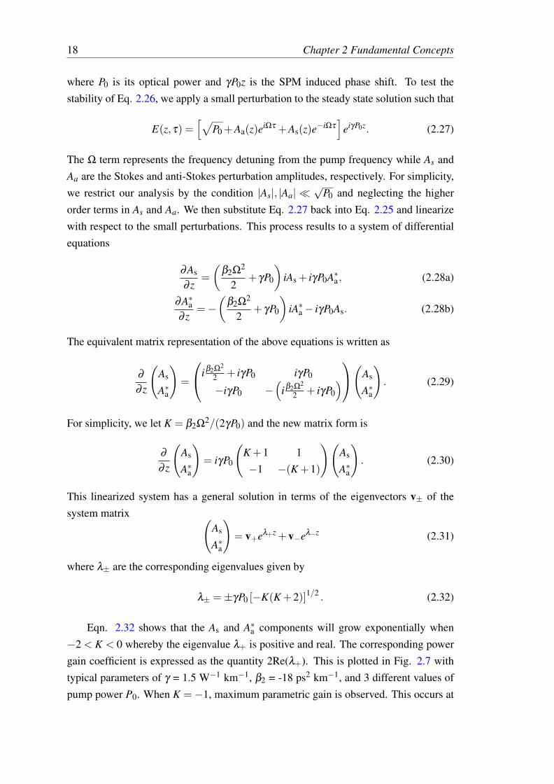
Eqn. 2.32 shows that the As and A∗a components will grow exponentially when−2 < K < 0 whereby the eigenvalue λ+ is positive and real. The corresponding powergain coefficient is expressed as the quantity 2Re(λ+). This is plotted in Fig. 2.7 withtypical parameters of γ = 1.5 W−1 km−1, β2 = -18 ps2 km−1, and 3 different values ofpump power P0. When K =−1, maximum parametric gain is observed. This occurs at

Chapter 2 Fundamental Concepts 19
Figure 2.7: MI power gain spectrum as a function of frequency shift for threedifferent powers. The parameters used are γ = 1.5 W−1 km−1, β2 = -18 ps2
km−1, and P0 = 2, 4 and 8 W.
a frequency detuning ofβ2Ω
2pm +2γP0 = 0, (2.33)
where Ωpm denotes as the phase matched frequency. In this particular case, where 2nd
order of dispersion only is considered, Eq. 2.33 shows that MI will only occur in theanomalous dispersion regime ( β2 < 0 ). It is also possible that MI can exist for a pumplocated in the normal dispersion regime if higher even-orders of dispersion are included[22–33]. A signal will experience a parametric amplification when a pump wave co-propagates if its falls within the MI gain band. Parametric sidebands can arise frombroadband noise even in the absence of an input signal. This is the mechanism that wewill use in this thesis in order to demonstrate the generation of new optical frequencies.The discussion in this section is specifically focused on single-pass MI in an opticalwaveguide. The effects of linear and nonlinear cavity dynamics will be discussed in thefollowing chapter.

20 Chapter 2 Fundamental Concepts
2.6 Summary
We have presented the basic physics of optical waveguides. We also have presented thephenomenon of chromatic dispersion. The origin of fiber nonlinearity and χ(3) nonlin-ear effects such as self-phase modulation, cross-phase modulation, four-wave mixing,and Raman scattering were also presented. The Nonlinear Schrodinger Equation wasintroduced to model the evolution of light in optical fibers. We also presented a studyof its stability by applying a small perturbation to an input continuous wave.

Chapter 3
Cavity Dynamics
The optical microresonators that we consider in this thesis belong to the larger class ofnonlinear ring resonators. In this chapter, we first present the basic ring resonator con-figuration. We then discuss the cavity operation and study the linear cavity resonances.Next, we describe the effect of Kerr nonlinearity on the cavity resonances and introducethe Lugiato-Lefever equation (LLE) to describe the dynamics of light inside a high fi-nesse optical Kerr resonator. We perform numerical simulations of the LLE to look indetail the modulation instability (MI) evolution inside the cavity. Lastly, we investigatethe effect of the higher-order dispersion on the intracavity MI gain.
3.1 Ring Resonator Cavity
In this section, we focus our analysis on understanding the dynamics of optical mi-croresonators by considering a simple dielectric ring resonator cavity and a couplingwaveguide. This analysis is identical to an all-fiber ring resonator model [85]. Forsimplicity, we will deal only with a single spatial mode dielectric cavity. This cavitycan only supports wavelengths that corresponds to mλm = neffL (m = 1, 2, 3,....), whereneff is the effective refractive index, and L is the cavity length. Fig. 3.1 illustrates theschematic of this simple ring cavity. The propagation of light in Fig. 3.1 is describedas follows: pump field Ein enters the ring resonator cavity through the pump evanescentfield produced at the coupler with an intensity coupling coefficient θ . The field strengthcoupled into the cavity is
√θEin. Here, we assume a minimal coupling losses such that
θ +ρ = 1, where θ and ρ are the coupling and transmission coefficients, respectively.As the field circulates around the ring cavity, it accumulates all the linear and nonlin-ear effects that are described in the previous chapter. At each roundtrip inside the ring
21

22 Chapter 3 Cavity Dynamics
Ein Eout
√θEin
√ρE
E
Figure 3.1: Schematic of a ring resonator cavity. θ and ρ are the intensitycoupling and transmission coefficients of the coupling, respectively.
cavity, a portion of the field is lost due to the coupling and the roundtrip loss. Thisintracavity field is then added coherently to the original injected Ein, and the cycle re-peats. This feedback mechanism of the cavity is expressed mathematically as the cavity
boundary condition and is given by [86]
E(m+1)(z = 0,τ) =√
ρE(m)(z = L,τ)eiφ0 +√
θEin(τ), (3.1)
where m is the roundtrip number, L is the roundtrip cavity length, τ is the fast timedefined in Eq. 2.23, and φ0 = β0L = 2πneffL/λ0 is the linear cavity-roundtrip phaseshift accumulated by the intracavity field over a single roundtrip. Eq. 3.1 also relates theintracavity field E(m+1) (0,τ) at the start of the (m + 1)th roundtrip to the field E(m) (L,τ)at the end of the mth roundtrip. To fully understand the dynamics of light as it propagatesalong the cavity, Eq. 3.1 must be used together with the Nonlinear Schrodinger Equationpresented in Eq. 2.23.
3.1.1 Linear Cavity Response
We begin our investigation by first considering the simplest case, a continuous-wave(CW) field propagating inside the cavity with no chromatic dispersion, material loss,or nonlinearity. In this manner, we can study the linear cavity feedback mechanism.The steady-state condition of Eq. 3.1, in this case, is E(m+1)(0,τ) = E(m)(0,τ) and this

Chapter 3 Cavity Dynamics 23
Figure 3.2: Linear cavity resonances with ρ equals to 0.2 (blue), 0.4 (red), and0.8 (pink). The corresponding F are ∼ 15.7, ∼ 8, and ∼ 4, respectively.
yields the well-known Airy function response of a linear ring cavity [66],
E =
√θ Ein
1−√ρ eiφ (3.2)
and can be expressed in power terms
PPin
=θ
(1−√ρ)2 [1+Fsin2(φ0/2)](3.3)
where F = 4√
ρ/(1−√ρ)2. P = |E|2 and Pin = |Ein|2 are the intracavity and inputpowers respectively. Fig. 3.2 shows graphically the linear cavity response calculatedfrom Eq. 3.3 for various ρ values. We can observe that the resonance peaks occur atvalues of φ0 = 2kπ (k = 1, 2, 3, ...) and the corresponding maximum intracavity powerachieved at the resonance peak is Pmax = Pin/θ . The value of this maximum power isoften greater than the incident power since the cavity acts as an energy accumulator.
The spacing between two adjacent resonances in Fig. 3.2 is called the cavity free-
spectral range (FSR = c/neffL). This term is in units of frequency and is commonly usedfor both Fabry-Perot and ring cavities. We define the sharpness of the resonance curvesas the cavity finesse parameter F . This parameter F is a dimensionless number and isexpressed as the ratio of the cavity FSR to the full width at half maximum (FWHM) ∆ν

24 Chapter 3 Cavity Dynamics
of the cavity resonance. From Eq. 3.3, we can obtain the parameter F as
F =FSR∆ν
=π
2 arcsin(
1−√ρ
2 4√ρ
) ≈ π
α(3.4)
where α ≈ (1−ρ)/2 is half of the total cavity losses. This implies that a high valuefinesse indicates a low loss cavity. The photon lifetime tph within the cavity can berelated to F as
tph =tR2α
=F tR2π
, (3.5)
where tR is the cavity roundtrip time. This describes the exponential decay time of aphoton inside the cavity without an external pump. Another parameter that also de-scribes the amount of loss of a cavity is the quality factor or Q-factor defined as
Q = 2πEnergy stored in the resonator
Energy dissapated every roundtrip. (3.6)
The Q-factor can be expressed in terms of F through
Q =2πnLRF
λ0, (3.7)
where R = L/(2π) is the radius of the resonator and λ0 is the pump wavelength.
3.1.2 Nonlinear Cavity Response due to Kerr Effect
We next take into account the nonlinearity of the cavity. As discussed in Chapter 2,an optical field will experience a power-dependent phase shift as it travels along a Kerrwaveguide (this phenomenon is known as self-phase modulation or SPM). Due to this,a SPM term is added to the intensity-dependence of the cavity roundtrip phase shiftφ = φ0 + φNL where φNL = γLP. By applying this change to Eq. 3.3, the nonlinearresonance response then becomes
PPin
=θ
(1−√ρ)2 [1+Fsin2((φ0 +φNL)/2]. (3.8)
The effect of the added SPM term is to shift the position of the resonance, suchthat the resonance changes proportionally to the intracavity power. At the resonancepeaks, an additional nonlinear phase shift of −γLPin/θ is experienced. Fig. 3.3 showsthe cavity nonlinear resonances as a function of phase shift which are calculated fromEq. 3.8. The presence of the Kerr nonlinearity makes the cavity resonances tilted. Wecan also observe that when the maximum phase shift −γLPin/θ exceeds the original

Chapter 3 Cavity Dynamics 25
Figure 3.3: The nonlinear resonances of a cavity with ρ = 0.6 and φNL = 0(blue), π/2 (red), and π (pink).
resonance width, the cavity response function exhibits three distinct solutions. However,only two of these solutions are stable, the upper and lower branches as depicted in Fig.3.3. The intermediate branch can be shown to be inherently unstable. Thus, the systemexhibits only bistability.
3.2 Lugiato-Lefever Equation
To understand more the behaviour of our dielectric cavity, we now take into accountthe contribution of chromatic dispersion. It is possible to reduce the complexity of thissituation by combining Eqs. 2.23 and 3.1 to transform into a single partial differentialequation [85]. To proceed further, there are some assumptions that must be made. Weassume that our cavity is in single mode operation with a high Q-factor/finesse (lowloss cavity, F 1) and that the evolution of the intracavity field is small over a singleroundtrip.
Under these conditions, we can now develop a mean-field equation for the pulsepropagation in the resonator. We start by integrating Eq. 2.23 using the Euler method.

26 Chapter 3 Cavity Dynamics
This gives us the expression for the intracavity field over a single roundtrip.
E(m) (L,τ)≈ E(m) (0,τ)+L(∂E)
∂ z
∣∣∣∣z=0
≈[
1− α0
2L+ iL ∑
k≥2
β k
k!
(i
∂
∂τ
)k
+ iγL∣∣∣E(m) (0,τ)
∣∣∣2]
E(m) (0,τ)(3.9)
From here, we substitute the above equation into the cavity boundary condition pre-sented in Eq. 3.1 and introduce the cavity phase detuning parameter δ0 = 2kπ−φ0 1.This parameter tells us the phase detuning between the pump frequency and the nearestcavity resonance. Taking the first order approximations yields
E(m+1) (0,τ)≈[1−α− iδ0 + iL ∑
k≥2
β k
k!
(i
∂
∂τ
)k
+ iγL∣∣∣E(m) (0,τ)
∣∣∣2]
E(m)+√
θ Ein(3.10)
where α = (α0L+θ)/2 corresponds to all the loss terms per roundtrip. We then definethe term slow time (t) to describe the evolution of the intracavity field between suc-cessive roundtrips such that E(m) (z = 0,τ) = E (t = mtR,τ) where tR is the roundtriptime [85]. As a result, the roundtrip evolution is now expressed in the form of
∂E∂ t≈ E(m+1) (0,τ)−E(m) (0,τ)
tR(3.11)
By applying Eq. 3.11 and Eq. 3.10, we have reached the nonlinear partial differentialequation that describes an externally driven, damped NLSE [86, 87]:
tR∂E (t,τ)
∂ z=
[−α− iδ0 + iL ∑
k≥2
β k
k!
(i
∂
∂τ
)k
+ iγL|E|2]
E +√
θ Ein. (3.12)
This equation is analogous to the Lugiato-Lefever equation (LLE) developed for diffrac-tive nonlinear optical cavities, and that has been used extensively for modelling the dy-namics of fiber-ring resonators [85, 88, 89]. Recently, Eq. 3.12 has also been applied todescribe the dynamics of optical microresonators [86, 90, 91]. In the case of CW inputinto the cavity, the steady-state solutions of the LLE can be solved by setting ∂E/∂ t = 0such that Eq. 3.12 reduces to
(α− iδ0 + iγL|E|2
)E +√
θ Ein = 0. (3.13)

Chapter 3 Cavity Dynamics 27
Taking the modulus squared of this equation leads to the cubic polynomial form
γ2L2P3−2δ0P2 +(α2 +δ
20 )P−θPin = 0, (3.14)
where Pin = |Ein|2 and P = |E|2 are defined as the input power and intracavity power,respectively. It is of note that Eq. 3.14 describes the same bistable cavity response (dueto the effect of Kerr nonlinearity) as discussed in Section 3.1.2.
When taking the effect of Raman scattering into account, we can extend the LLE toyield [92]
tR∂E (t,τ)
∂ z=
[−α− iδ0 + iL ∑
k≥2
β k
k!
(i
∂
∂τ
)k
+ iγL(
h(τ)∗ |E(τ)|2)]
E +√
θ Ein
(3.15)where ∗ represents the convolution and h(τ) is the total nonlinear response functionincluding the Kerr and Raman contributions given in Eq. 2.21. The solutions of LLEcan be solved using the split-step Fourier method, the same numerical technique usedto integrate Eq. 2.23 and Eq. 2.24 from Chapter 2. In the simulation, the size of thetemporal window should be set to tR which makes the spacing of the components in thefrequency domain separated by one FSR.
3.3 Intracavity Modulation Instability
Next we wish to analyze the stability of the LLE including the dispersion to all orders.The method of analysis is the same as we used in the case of single-pass MI discussedin Chapter 2. We begin our analysis by adding a small perturbation into the steady stateintracavity solution Es of a CW pump
E(t,τ) = Es +a+(t)eiΩτ +a−(t)e−iΩτ , (3.16)
where a±(t) are the small perturbations, and Ω is the relative frequency shift from thepump frequency. Then substituting Eq. 3.16 into the Eq. 3.12, and linearizing the

28 Chapter 3 Cavity Dynamics
equation with respect to the small perturbations a±(t), results in two equations
tR∂a+∂ t
=
[−α− iδ0 + iL
(β2Ω2
2− β3Ω3
6+
β4Ω4
24− ...
)+ i2γL|Es|2
]a++ iγLE2
s a∗−
(3.17a)
tR∂a∗−∂ t
=
[−α + iδ0− iL
(β2Ω2
2+
β3Ω3
6+
β4Ω4
24+ ...
)− i2γL|Es|2
]a∗−− iγLE2
s a+
(3.17b)
To simplify the equations above, we introduce the function K′ = −δ0 +Deven(Ω)L+
2γL|Es|2 and define even and odd dispersion operators
Deven(Ω) =∞
∑k≥1
β 2kΩ2k/(2k)! (3.18a)
Dodd(Ω) =∞
∑k≥1
β 2k+1Ω2k+1/(2k+1)! (3.18b)
Eqs. 3.17a and 3.17b then reduce to
tR∂a+∂ t
=[−α + iK′− iDodd(Ω)L
]a++ iγLE2
s a∗− (3.19a)
tR∂a∗−∂ t
=[−α + iK′− iDodd(Ω)L
]a∗−− iγLE2
s a+ (3.19b)
To solve this system of equations, we transform them into a matrix form
tRddt
(a+a∗−
)=
(−α + iK′− iDodd(Ω)L iγLE∗2s
−iγLE∗2s −α− iK′− iDodd(Ω)L
)(a+a∗−
)(3.20)
and find that the eigenvalues are in the form of
λ±(Ω)tR =−(α + iDodd(Ω)L)
±√
4γPL(δ0−Deven(Ω)L)− (δ0−Deven(Ω)L)2−3γ2P2L2(3.21)
where P = |Es|2 denotes as the intracavity power. To obtain parametric amplificationin this system, the components of the eigenvalues λ± must be positive and real. Thesquare root term in Eq. 3.21 determines the condition for parametric oscillation to existand this condition is expressed as
γPL≤ δ0−Deven(Ω)L≤ 3γPL. (3.22)

Chapter 3 Cavity Dynamics 29
From here, we can derive the phase-matching condition that shows the maximum am-plification of the small signal perturbation occurs at the phase-matched frequency ΩPM.
Deven(Ωpm)L+2γPL−δ0 = 0. (3.23)
Typically the above expression is simplified by truncating the even dispersion parameterDeven(Ωpm) to just the 2nd order term, β2. This is valid in standard microresonatorconfigurations where the impact of higher order is negligible.
β2Ω2pmL
2+2γPL−δ0 = 0. (3.24)
A notable feature that can be observed in Eq. 3.24 is the presence of the detuningparameter δ0, which serves as an extra degree of freedom in the cavity system. Asa result, the phase-matching condition is not anymore restricted only to negative β2
values, as was the case for single-pass MI discussed in Chapter 2 [93]. This meansin a Kerr cavity, MI can occur for both anomalous and normal dispersion regime. Wenote that, however, only small frequency shift sidebands are attainable in both cases. Toachieve larger frequency shifts, the inclusion of higher order of dispersions are needed.
3.4 Lugiato-Lefever Simulations of Modulation Insta-bility
The small signal analysis performed in the previous section only describes the initialevolution of the MI signal. To capture the full MI dynamics, we conduct numericalsimulations of the LLE. We begin our simulations by slowly changing the detuningparameter over successive roundtrips. By doing this, we can identify the different op-erating regions of intracavity MI. In these simulations, we consider first MI that occursin the anomalous dispersion where β2 < 0. We set our resonator with the followingparameters typical of the experiments we will present in the following chapter: β2 = -10ps2 km−1, Pin = 90 mW, γ = 2 W−1 km−1, F = 7 · 104, FSR ≈ 68 GHz and α = π/F
= 4.49 x 10⁻⁵. We also use a normalized detuning parameter ∆ = δ0/α that has a scan-ning range from -10 to 10 over the course of 10 million roundtrips. The output temporaland spectral LLE evolutions are shown in Figs. 3.4 (a) and (b), respectively. Thereare 2 distinct dynamics as the detuning changes. The intracavity field initially remainsCW in the region from ∆ = -10 to around ∆ = -5. Above ∆ = -5, we observe a tem-poral modulation which corresponds to an evenly spaced comb frequencies in spectralplot. This initial MI pattern is regular and unchanged from roundtrip to roundtrip and

30 Chapter 3 Cavity Dynamics
-100
(a) (b)
Figure 3.4: (a) Temporal and (b) spectral LLE evolutions through scanning thenormalized detuning ∆.
is called stable modulation instability (SMI). Above ∆ = -2, this SMI transforms intoa chaotic regime known as unstable modulation instability (UMI), where the intracav-ity field changes randomly from roundtrip to roundtrip. In the next two sections willdiscuss SMI and UMI in more detail.
3.4.1 Stable Modulation Instability
Using the same parameters as those in the previous section, we then perform LLE sim-ulations at ∆ = -4.5 over a million roundtrips to observe the characteristics of the fieldin this region (Fig. 3.5). In the time domain, a stable periodic pattern is observed thatis unchanged from roundtrip to roundtrip, as shown in Fig. 3.6 (a). In the frequencydomain, we observe the initial formation of new frequency components at ± 0.9 THz(± 13 FSRs), as depicted in Fig. 3.6 (b). Subsequent FWM between the pump fre-quency and these initial frequency components leads to the creation of additional pairsof sidebands, yielding a stable modulation instability (SMI) comb. This mechanism isoften called as primary comb formation, with a spectrum spaced by multiple FSRs. Inthe literature, SMI combs have shown to be highly coherent [94, 95].

Chapter 3 Cavity Dynamics 31
Figure 3.5: Spectral evolution of the intracavity field over a million roundtripsfor ∆ = -4.5.
(b)(a)
Figure 3.6: Temporal (a) and spectral (b) profiles of a stable modulation insta-bility pattern. These profiles were taken from the simulation results in Fig. 3.5at ∆ = -4.5 and after 1 million roundtrips.
3.4.2 Unstable Modulation Instability
From Fig. 3.4, we can observe that a new regime occurs as ∆ goes to larger values. Ata detuning of ∆ = -2 in the temporal domain, the field transitions from a stable periodicpattern to a highly chaotic pattern known as unstable modulation instability (UMI). Weperform LLE simulations where we set the pump at a fixed detuning ∆ = 1, just abovethe starting point of the UMI regime. The spectral evolution of this LLE simulations ispresented in Fig. 3.7 and we find that the primary comb is filled in with new frequencycomponents resulting in a comb with a single FSR spacing, as shown in Fig. 3.8 (b)

32 Chapter 3 Cavity Dynamics
which plots the spectrum after 1 million roundtrips. The corresponding time domainpicture of this simulation is shown in Fig. 3.8 (a). We note that this temporal patternis unstable and evolves in a chaotic manner from roundtrip to roundtrip. As a result,unstable MI combs suffer from excess intensity and phase noise.
Figure 3.7: LLE simulation showing the spectral evolution of the intracavityfield against a million roundtrips for ∆ = 1.
(b)(a)
Figure 3.8: Temporal (a) and spectral (b) profiles of an unstable modulationinstability. These profiles were taken from the simulation results in Fig. 3.7 at∆ = 1 after 1 million roundtrips.

Chapter 3 Cavity Dynamics 33
3.5 Effect of Higher Order Dispersion
Up to now, our analysis on intracavity MI has considered up to second-order dispersiononly, and this demonstrated only small frequency shift sidebands. Since the primaryaim of this thesis is to able to generate very large frequency sidebands, it is necessaryto include the effects of higher order dispersion on the MI phase-matching condition.Generally, dispersion in materials always possess high order dispersion coefficients. It isjust common practice to truncate the dispersion at the second-order since it is often suf-ficient to fully describe the behavior of the system. However, there are other situationswhere higher order dispersion is influential enough to alter the system’s performance.Specifically, when working near the zero-dispersion wavelength (β2 = 0), higher ordersof dispersion can play an important role in the MI phase-matching condition [22]. Webegin our investigation of this regime by using expression derived in Eq. 3.21, includ-ing dispersion parameters up to fourth-order term. We note that even higher orders ofdispersion can be simply included as well if necessary [22, 24, 96]. Applying the sameanalysis as we conducted in Section 3.3, we can establish an expression for the range offrequencies where parametric oscillation will occur.
γPL≤ δ0−β2Ω2L
2− β4Ω4L
24≤ 3γPL (3.25)
And the phasematched frequency which will experience maximum parametric gain.
2γPL−δ0 +β2Ω2
pmL2
+β4Ω4
pmL24
= 0. (3.26)
We notice in the above expressions that odd-orders of dispersion (such as β3) donot contribute to the phase-matching condition [25, 32]. Thus, MI gain is dependent onthe sign and magnitude of β2 and β4 only. Here we focus our attention in the normaldispersion regime where β2 > 0.
In this regime, the presence of negative β4 can balance the contribution of the pos-itive β2, leading to phase-matched FWM. Depending on the exact values of β2 and β4,this can allow the generation of large frequency shift MI sidebands [22–33]. This is themechanism that we utilize in this thesis to generate widely tunable new optical para-metric sidebands. Fig. 3.9 displays the plot of MI phase-matching curve for a typicalresonator parameters. A 100 mW pump is set to the resonator and the higher dispersionparameters used are β3 = 0.051 ps3 km−1 and β4 = −2.0 × 10⁻⁴ ps4 km−1 evaluated ata zero-dispersion regime (ZDW) of 1550 nm. At any pump wavelength, this allow us to

34 Chapter 3 Cavity Dynamics
Figure 3.9: Modulation instability phase-matching diagram calculated with theparameters: Pin = 100 mW, γ = 1.5 W−1 km−1 for β3 = 0.051 ps3 km−1 andβ4 = −2.0× 10⁻⁴ ps4 km−1 at ZDW = 1550 nm. Dashed line indicate the ZDW.
evaluate the dispersion coefficients of this wavelength as:
β4(ωp) = β4 (3.27a)
β2(ωp) = β3(ωp−ωZDW)+β4(ωp−ωZDW)2. (3.27b)
Eq. 3.27b shows that while β3 does not effect the phasematched frequency (Eq.3.26), it will have an effect on the phasematching curve as it sets the rate of change ofβ2 with frequency. The MI phasematched sideband wavelengths as a function of thepump wavelength are plotted in Fig. 3.9. As can be clearly seen, MI sidebands existin both anomalous and normal dispersion regime as discussed in Section 3.3. At wave-lengths above the ZDW, the pump is located in the anomalous dispersion regime andthe sidebands are located close to the pump. On the other hand at wavelengths belowthe ZDW, the pump experiences normal dispersion, and the parametric sidebands arelocated widely far from the pump. In this regime the sidebands frequency shift is wellapproximated by ΩPM ≈
√−12β2
β4. Tunability of these large frequency shift parametric
sidebands can be easily achieved by making a small changes in the pump wavelength.For example, a 50 nm change in the pump wavelength in Fig. 3.9 is predicted to produce

Chapter 3 Cavity Dynamics 35
Figure 3.10: Modulation instability gain spectra for pump wavelengths 1548nm (blue), 1542 nm (red) and 1535 nm (magenta). Parameters used were Pin =100 mW, γ = 1.5 W−1 km−1 for β3 = 0.051 ps3 km−1 and β4 = −2.0 × 10⁻⁴
ps4 km−1 at ZDW = 1550 nm.
a combined tuning range of 870 nm (from 1180 to 2050 nm) for the two widely detunedparametric sidebands.
From Eq. 3.21, we can plot the gain spectrum of the MI parametric sidebands. Forconvenience, the resonator parameters used in here are the same as used in Fig. 3.9.Fig. 3.10 shows the plot of the MI gain spectrum for three different pump wavelengths:1548, 1542 and 1535 nm. Here we see that as the pump wavelength moves away fromthe ZDW into the normal dispersion regime, the gain bandwidth of the parametric side-bands becomes narrower at the same time as their frequency shifts increases.
To investigate this more, we plot the parametric gain bandwidth in FSR as a func-tion of sideband frequency shift in Fig. 3.11. As can be seen, small sideband frequencyshifts exhibit a large gain bandwidth which will encompass multiple FSRs of the res-onator. This finding suggest that in general it is always possible to observe parametricoscillation at smaller frequency shifts since some cavity modes will always overlapwith the gain spectrum. However, for the typical parameters presented here, at around20 THz, the gain bandwidth starts to decline rapidly and eventually falls below one FSRfor shifts beyond 50 THz. This implies that for very large frequency shifts, there is no

36 Chapter 3 Cavity Dynamics
Figure 3.11: Parametric gain curve as a function of frequency shift Ω. Calcu-lated using the parameters: Pin = 100 mW, γ = 1.5 W−1 km−1 for β3 = 0.051ps3 km−1 and β4 = −2.0 × 10⁻⁴ ps4 km−1 at ZDW = 1550 nm.
longer a guarantee to observe any parametric oscillation, as it is possible no resonatorcavity modes will overlap with the parametric gain curve. We will return to this analysisin more detail in the following chapters.
3.6 Summary
We have presented the basic equations and nonlinear physics present in Kerr microres-onators. We first discussed the dynamics of the linear cavity resonances neglecting thenonlinearity and material absorption. Then, accounting for the effect of the Kerr non-linearity in the cavity, we found that the cavity resonances tilted and exhibits bistability.
We introduced the Lugiato-Lefever equation (LLE) to describe the propagation oflight in Kerr resonators. Through a linear stability analysis, we found that there is anadditional parameter δ0 in the phase-matching condition. We also carried numericalsimulations of the LLE to demonstrates how MI evolution inside the cavity. These sim-ulations revealed two dynamical states as we alter the detuning parameter.

Chapter 3 Cavity Dynamics 37
Finally, influence of the higher order dispersion on the MI gain was investigated. Weincluded dispersion up to fourth order in the LLE simulations, which resulted in largetunable phasematched frequency shifts in the normal dispersion regime.


Chapter 4
Microresonator Fabrication andCharacterization
This chapter first gives a brief historical introduction to whispering gallery modes inoptical microresonators. We then outline the procedures used in fabricating fused silica(SiO2) microspheres and crystalline magnesium fluoride (MgF2) microdisk resonators.We also present the tapered optical fiber method to couple light into our microres-onators. We also introduce a characterization technique to measure the finesse F ofour fabricated microresonators. This key parameter provides a qualitative measure forthe efficiency of the nonlinear processes inside the resonator. Finally, we discuss theexperimental technique that enables the resonance frequency to lock to the pump laser.
4.1 Optical Microresonators
Optical microresonators are tiny dielectric cavities that are only∼ 100 µm to a few mil-limeters in diameter and possess an ultra-high finesse. They can be understood as opticalwaveguides that confines light efficiently in a closed loop. Moreover, these microres-onators support whispering gallery modes (WGMs); waves that can travel around thecircumference via continuous total internal reflection and return to the same position,interfering constructively with themselves after a single roundtrip. The term ”whisper-
ing gallery waves” was first used by Lord Rayleigh in the 19th century to describe theacoustic phenomenon noticed inside the dome of the St. Paul’s Cathedral in London.He explained that this phenomenon occurred due to the sound waves that were contin-uously reflected around the the whispering gallery of the Cathedral [97], allowing thesound produced at one end of the gallery to still be heard at the opposite end.
39

40 Chapter 4 Microresonator Fabrication and Characterization
In 1939, R. D. Richtmyer applied the theory of WGMs to electromagnetic mi-crowaves [98]. However, it was only 30 years ago that the direct measurement ofWGMs in a high-Q factor optical microresonator was reported. This was the work ofBraginsky and his group [99] who developed optical microresonators in 1989 by melt-ing the end tip of fused silica fibers. Since then, many microresonator geometries havebeen demonstrated to support WGMs such as spheres [100], disks [101] and toroids[102]. Many materials have been used for microresonator fabrication; these includeSiO2 [103], magnesium fluoride [104], silicon nitride [105], calcium flouride [106],and lithium niobate [107]. These materials are chosen for their high transparency inthe desired spectral region of operations, as well as their useful nonlinear properties.Microresonators have found applications as laser cavities [108, 109], and in nonlinearoptics [38, 39, 110, 111], molecular sensing [112], and cavity quantum electrodynamics[113–115].
In particular, the ability of a microresonator to confine light over long timescales,allows for very large intracavity powers, making them an ideal candidate for nolinearfrequency conversion [34, 110, 116]. This thesis focuses on degenerate four-wave mix-ing (FWM) in microresonators through the χ(3) Kerr nonlinearity to generate large fre-qeuncy shift parametric sidebands. In the experimental chapters to follow, we will useSiO2 microspheres and MgF2 microdisk resonators to demonstrate optical parametricoscillation in microresonators.
4.2 Fabrication
4.2.1 SiO2 Microspheres
The SiO2 microspheres used in this thesis were fabricated by melting the end face of astandard single mode optical fiber, that has a cladding diameter of 80 µm, in an EricssonFSU 995 Polarization Maintaining fiber fusion splicer. There are few steps to performbefore we place the optical fiber into the fusion splicer. First, the fiber was prepared bystripping-off the coating layer and cleaning the bare optical fiber surface with isopropylalcohol. The bare fiber was then cut using an optical fiber cleaver in order to ensure aflat endface. Finally, the bare fiber was inserted in one arm of the fusion splicer. Weset a prefuse arc current to 12 mA for one second to clean the fiber. To melt the endtip of the fiber, a sequence of fuses are applied; 20 mA for four seconds and followedby 23 mA for three seconds. Due to the surface tension forces, the fiber transforms intoa nearly perfect sphere mounted on a stem [110]. The typical diameters of the spheres

Chapter 4 Microresonator Fabrication and Characterization 41
(a) (b) microsphere
fiber stem
163 μm
Figure 4.1: Ericsson FSU 995 Polarization Maintaining fusion splicer. (b) Im-age of a 163 µm diameter silica microsphere. The fiber stem is connected onone side of the microsphere.
formed by the fusion splicer are about twice the original fiber diameter (160 µm). Thisresult in a resonator with a free-spectral range of FSR ≈ 414 GHz. One can adjust theoutput diameter of the formed sphere by varying the amount of fiber inserted into thefusion splicer. Fig. 4.1 (b.) shows a microscope image of a SiO2 microsphere used inthis thesis that was fabricated using the method mentioned above.
4.2.2 MgF2 Microdisk Resonators
(a) (b)
Figure 4.2: (a) MgF2 crystal blank with a 10 mm diameter and 1 mm thickness(b) The preform disk is epoxied onto the tip of a brass rod.
We used a single-point diamond turning (SPDT) [117] process for fabricating MgF2
microdisk resonators since melting is not anymore suitable, as this will destroy thecrystalline structure of the material. We begin the process with a MgF2 crystal blankwhose diameter and thickness are 10 mm and 1 mm, respectively. An example of this isshown in Fig. 4.2 (a), whereby we can see that this crystal blank is smaller than a NewZealand 20-cent coin. The crystal blanks were then placed on the worktable of a highspeed drill to make the preform. We used a cylindrical brass tube as the drill bit with

42 Chapter 4 Microresonator Fabrication and Characterization
(b)
rake angle
diamond
precursor
(a)
Figure 4.3: (a) Front view image of the SPDT set-up. (b) Sketch showing theorientation of the diamond cutter to set the desired rake angle.
inner diameter set to the desired preform size, typically ∼ 1-4 mm. Before the coringprocess begins, we bathed the top part of the blank with Allied High Tech 30 µm grainsized diamond suspension to be used as an abrasive. We do this every time we resetthe drilling process. To trim the thickness preform down to 0.5 mm, it is glued onto abrass rod with industrial strength epoxy (Araldite Super Strength). The brass rods weused have a base of 13 mm and are tapered towards a tip with a radius of 0.5 mm. Weattached the brass rod onto a rotating air-bearing spindle and trim the thickness of theprecursor using a 30 µm sandpaper. The output of the described process is shown inFig. 4.2 (b).
The cutting process is performed in the SPDT set-up in the laboratory of Prof.Harald G. L. Schwefel at the University of Otago. We first attached the brass rod intothe air bearing spindle and set the rotation speed at 100 rpm. The tip of the diamondcutting tool is mounted onto a programmable stage in such a way that it is centered withthe rotation axis of the rod. The orientation of the diamond cutting tool is carefullyposition with a rake angle of - 300 to - 350, these angles are specific to MgF2 [118] andillustrated in Fig. 4.3. The set-up is computer-controlled and we used a Matlab programto operate the periodic movements of the diamond cutter. We occasionally inspect thesurface of the crystal with a microscope to ensure that the cutting is done properly andboth the desired minor and major radii are achieved.
After the cutting process, the output resonator is usually not perfectly opticallysmooth, hence additional polishing is necessary to achieve an ultra-high finesse. We dothis polishing by hand using Thorlabs lens cleaning tissues soaked with diamond sus-pension (Allied High Tech). We perform this polishing while the resonator is spinningon the air-bearing stage, regularly checking the condition of the resonator through anoptical microscope. The grain size of the diamond suspension to be used depends onthe post-cut surface quality of the resonator. Typically, we started with 1 µm diamond

Chapter 4 Microresonator Fabrication and Characterization 43
(a) 515 μm (b) 400 μm (c) 265 μm
(d) 195 μm (e) 165 μm
Figure 4.4: Images of the five MgF2 microresonators used in the experimentswith major radii R as indicated.
suspension and subsequently change the size in steps of 0.5 µm, 0.25 µm and 0.10µm. The resonator needs to be cleaned thoroughly before going to the next particlesize of diamond suspension. Cleaning of the resonator starts with distilled water forat least 5 minutes, and then pure isopropanol until you see no more residue of the dia-mond grains on the surface. Each polishing step usually takes from 30 minutes to 1.5hours depending on the surface roughness of the resonator. It should be noted that thispolishing process is the crucial step in achieving an ultra-high finesse resonator. Extracare must be observed since over-polishing the resonator will destroy its shape. It mightalso knock off the resonator from the brass rod if too much force is applied during thepolishing and cleaning. That is why it is advisable to regularly inspect the microres-onator under a microscope during these periods. In this thesis, we fabricated five MgF2
microresonators of different diameters, these are shown in Fig. 4.4.
4.3 Taper Coupling
There are many methods for coupling light into microresonator. Examples of whichinclude prisms [99], angle-cleaved fibers [119], gratings [120], and polished half-blockcouplers [121]. In this thesis, we implemented the tapered optical fiber method becauseit offers more efficient and controllable coupling since it does not require any free-spaceoptics [122, 123].
To couple light into the microresonator, it requires that the waist diameter of the

44 Chapter 4 Microresonator Fabrication and Characterization
(b)
SiO2 microsphere
taper(a) taper
MgF2 resonator
Figure 4.5: Top-view microscope image of (a) 265-µm major radius MgF2microdisk resonator and (b) 81.5-µm radius SiO2 microsphere together withtheir tapered fiber.
core
taper waist
cladding
core
cladding
taper transition
Figure 4.6: A schematic diagram of a tapered fiber.
tapered fiber to be of the order of the wavelength of the light being used, or smaller,so that it can produce a large evanescent wave outside the fiber which can overlap withthe evanescent field of a mode of the microresonator. It is also necessary to match theeffective index of the mode in the taper to the effective index of the resonator mode.This is typically done by moving the resonator back and forwards along the taper untilthe taper diameter is correct and efficient coupling is observed. Example images ofthe microresonator coupling arrangement with the tapered fiber are shown in Fig. 4.5.These tapered fibers were fabricated using the flame-brush technique [124, 125] wherea standard single mode optical fiber is simultaneously heated by a hydrogen torch thatmoves back and forth over a certain distance, and pulled apart until the desired profileof the taper waist is achieved. During the fiber pulling process, the output transmissionof the fiber was monitored to ensure that the taper transition region is adiabatic [126].The typical final waist diameter of the tapered fiber is approximately 1 µm and has atleast 97% transmission. Fig. 4.6 shows the different regions of the tapered fiber. Thereare, however, some drawbacks when using the tapered fibers for coupling. First they aremechanically fragile because of their very small taper waist. Additionally, there will bea significant reduction in the transmission if any debris is embedded or lodged in thetaper waist. Thus, extra care must be taken after the tapered fiber has been made. It isalso important to correctly tension the tapered fiber so it can be stably coupled to the

Chapter 4 Microresonator Fabrication and Characterization 45
OscilloscopeTLC
ECLPM
Signal Generator
Taper
Microresonator
PD
Figure 4.7: Schematic of experimental setup for finesse measurement. TLC:tunable laser controller, ECL: external cavity laser, PM: phase modulator, andPD: photodetector.
microresonator.
4.4 Finesse Measurement
After polishing and cleaning the microresonator, a finesse measurement is carried outto determine whether the microresonator is capable of producing optical nonlinear ef-fects. As indicated in Eq. 3.4, both the resonance linewidth and the resonator’s FSR areneeded to determine the finesse of the microresonator.
The experimental setup used for measuring the finesse of a microresonator modeis shown in Fig. 4.7. In here, we used a continuous-wave (CW) laser to perform thefrequency sweep. We operate this scan at low powers, on average ∼ 100 µW or lower,to avoid the contributions of the Kerr and thermal effects on the resonance. We notethat the laser must also have a significantly smaller linewidth than the resonator for themeasurement to be valid. To calibrate the measurement, a phase modulator (PM) drivenby a signal generator is connected after the laser [127]. We set the signal generatorfor 15 MHz sinusoidal modulation. Through this modulation, two sidebands are gener-ated symmetrically frequency-detuned from the pump laser. These frequencies are thenswept over the cavity’s resonance. As a result, a series of resonance dips with 15 MHzsymmetric sidebands are seen on the trace on the oscilloscope. These sidebands arethen used as a reference to convert from scan time (in seconds) to frequency (in Hz).
Fig. 4.8 (a) shows the resonance dip of a mode of the 515-µm major radius MgF2
resonator. Since the trace is quite noisy, we perform a Lorentzian fit on the data anduse the extracted value as the measured linewidth of the resonance. For the case of Fig.4.8 (b), the resonance had a value of ∆ν = 1.33 MHz. The FSR is calculated usingthe dimensions of the resonator and found to be 67 GHz. This gives this mode of the515-µm major radius MgF2 resonator a finesse F ≈ 50,300. Simulations based on theLLE presented in chapter 3, shows that this resonator should be able to observe χ(3)

46 Chapter 4 Microresonator Fabrication and Characterization
(b)(a)
Δυ
Lorentz fit
Figure 4.8: (a) 515-µm major radius MgF2 cavity resonance with 15 MHzsymmetrically detuned sidebands. (b) Resonance curve with Lorentzian fit (redcurve).
parametric oscillation at pump power ∼ 10’s of mW.
4.5 Thermal Locking
Aside from the Kerr effect, thermal effects can also influence the microcavity reso-nances. This is mainly due to the significantly reduced mode volume of the microres-onators making them highly susceptible to thermal heating, resulting in a thermal shiftof the microcavity resonances. The temperature dependence of the refractive index ofthe material means the modes of the microcavity experiences a resonance shift that isproportional to the applied intracavity power [128–130]. Thus, this thermal effect in-duces an optical bistability similar to the Kerr effect discussed in Section 3.1.2. In mostcases, thermal shift is much stronger than the Kerr nonlinearity. The sign of the thermo-optic coefficient ( dn
dT ) of the resonator material indicates the direction of the thermalshift [128]. If the sign is positive then thermal shift goes on same direction as the Kerrnonlinearity. However, it must be noted that the thermal effect is much slower than theKerr nonlinearity which is almost instantaneous.
For the resonator materials used in this thesis: dndT = +12.9 × 10⁻⁶/ oC [131] for
SiO2, while dndT = (+1.7, +2.3) × 10−6/ oC [132] for the O and E axes of MgF2. Both of
these possess a positive thermo-optic coefficient. This tells us that as we scan the pumplaser across the resonance, the microcavity will always experience a resonance shiftleaning towards long wavelengths. When scanning from short to long wavelengths, themicrocavity’s linewidth will be artificially broadened and form a triangular shape shownin Fig. 4.9. On the other hand, if the sweeping starts from the opposite direction (blue

Chapter 4 Microresonator Fabrication and Characterization 47
0
0.2
0.4
0.6
0.8
1
Pow
er (
arb.
unit)
Pump Wavelength (arb. unit)
Figure 4.9: Mechanism of the microcavity resonance response as the pump-laser wavelength is scanned in the presence of a positive thermal nonlinearity.The green-dashed curve represents the cold resonance of the microcavity. Scan-ning the pump laser from short to long wavelengths leads to thermal broadeningof the resonance (red curve) while the resonance becomes narrower when goingto the opposite direction (blue curve).
curve in Fig. 4.9), the microcavity resonance will become narrower. One good conse-quence of this thermal broadening is that the microcavity resonance can be thermallystabilized to the pump frequency when operating at a detuning where the slope of thethermal triangle is positive. In this region, a slight increase of the pump wavelength willresult in an increase in the intracavity power, then the microcavity will heat up and shiftthe resonance towards long wavelengths, thus following the pump laser. Likewise, thisthermal locking also works for small decrease in the pump wavelengths since the intra-cavity power will decrease resulting in a shift of the resonance to shorter wavelengths.In this thesis, we used this thermal locking method to lock the microcavity resonance toour pump laser.
4.6 Summary
The fabrication procedures for SiO2 microspheres and MgF2 microresonators were pre-sented. Taper coupling was introduced as the method of choice to couple light into ourmicroresonators.

48 Chapter 4 Microresonator Fabrication and Characterization
An outline describing the polishing and cleaning routines used were discussed in de-tail. We found this was the crucial step in achieving a high finesse in our crystalline mi-croresonators. The experimental setup for measuring the finesse of our microresonatorswas also presented. We added a phase modulator after the pump laser to generate twosidebands at the output, which served as an absolute calibration scale for measuring thecavity’s resonance linewidth. Lastly, the thermal locking technique was introduced forstabilizing the cavity resonance to the pump laser.

Chapter 5
Widely Tunable Optical ParametricOscillation in Silica Microspheres
1 At the time the research in this chapter was carried out, the generation of large-frequency shift parametric sidebands in Kerr nonlinear optical microresonators had al-ready been demonstrated by several groups [57–60, 133], yet none of these works wereable to demonstrate the full tuning capabilities of these devices. Fixed large frequencyshift parametric sidebands had been observed in both MgF2 microdisks [58] and silicamicrotoroids [59]. These sidebands were phasematched through higher-order dispersion(as described in chapter 3) and detuned from the pump frequency by approximately 40THz [58, 59]. By exploiting phase matching between different spatial modes of theresonator, larger fixed frequency shifts, up to 74.5 THz, had been also observed in aMgF2 microdisk resonator [57]. In addition, Si3N4 planar microresonators had beendemonstrated to produce large frequency shift of parametric sidebands using a novelquasi-phase-matching scheme. These sidebands were symmetrically detuned from thepump source by ∼ 40.2 THz and allowed the demonstration of approximately 1.5 THzof discrete sideband tunability as the pump frequency was tuned by a similar amount,∼ 1.2 THz [133]. However, before the work presented in this chapter, the widebandtunability of parametric sidebands in microresonators had yet to be observed.
In this chapter, we first discuss the theoretical analysis of the large frequency shiftparametric sideband generation in a Kerr resonator. Next, we calculate the dispersion ofa silica microsphere as a function of its radius. We then discuss the experimental setup
1Work presented in this chapter has been published in ”Widely tunable optical parametric oscillationin a Kerr microresonator, ” Optics Letters 42, 5190-5193 (2017).
49

50 Chapter 5 Widely Tunable Optical Parametric Oscillation in Silica Microspheres
used and experimentally show that a silica (SiO2) microsphere resonator with care-fully chosen higher-order dispersion characteristics can support widely-tunable phase-matched parametric oscillation. This allows us to provide the first proof of principledemonstration of a widely tunable Kerr microresonator parametric oscillator.
5.1 Theoretical Analysis
The generation of large frequency shift signal and idler sidebands in a microresonatorKerr parametric oscillator has been demonstrated via phasematching through modalwavevector mismatch [57], higher-order dispersion [58, 59] and quasi-phasematching[133]. In this study, we used the higher-order dispersion technique to phasematch anddemonstrate the wideband tunability of the MgF2 microresonators. The use of higher-order dispersion to phasematch and tune large frequency shift parametric sidebands wasfirst demonstrated in the context of optical fiber in Ref. [20]. Since then, this techniquehas been applied in fiber parametric oscillators to develop both pulsed [25, 26, 29–33]and CW oscillators [134, 135], and was first proposed in an optical microresonator plat-form in Ref. [58].
Our theoretical analysis begins by considering an optical Kerr microresonator drivenby a CW optical pump (frequency ωp) in the presence of higher-order dispersion. Wespecifically focus our attention in the ”scalar” regime where the three waves (pump, sig-nal and idler) all belong to the same mode family. The evolution of the intracavity fieldE(t,τ) in this situation is well described by the mean-field Lugiato-Lefever equation(LLE) with dispersion included to all orders [86] as introduced in chapter 3:
tR∂E(t,τ)
∂ t=
[−α− iδ0 + iL ∑
k≥2
βk
k!
(i
∂
∂τ
)k]
E + iγL|E|2E +√
θEin. (5.1)
We then consider the interaction between a strong CW pump field and two small-amplitude sidebands for the analysis of the generation of degenerate FWM sidebands.The solutions of the intracavity field then takes the form E(t,τ)≈ A0 +a+1exp(−Ωt +
λ t/tR)+a−1exp(Ωt +λ ∗t/tR), where Ω is the frequency detuning, A0 is the CW solu-tion of Eq. 5.1, and a±1 are the amplitudes of the sideband.
Following the same intracavity modulation instability analysis as presented in chap-ter 3, allows us to write the phasematched frequency as:
Deven(Ωpm)L+2γPL−δ0 = 0. (5.2)

Chapter 5 Widely Tunable Optical Parametric Oscillation in Silica Microspheres 51
Typically, we can truncate the Taylor expansion at β4 for shifts that are not toolarge, such that Deven(Ω) = β2Ω2/2+β4Ω4/24 [22–24]. This gives the phasematchingcondition as
β2Ω2L2
+β4Ω4L
24+2γPL−δ0 = 0. (5.3)
In this scenario, generation of large frequency shift parametric sidebands can beachieved when pumping in the normal dispersion regime (β2 > 0), and in the presenceof negative 4th order dispersion (β4 < 0). We note that, rather amazingly, only the evenorders of dispersion play any role in this phasematching expression. The presence ofnegative fourth-order dispersion compensates the positive contribution of the second-order dispersion at large frequency shifts, setting the phasematched frequency as
Ω≈√−12β2
β4. (5.4)
Frequency shifts of the order of 10 - 100 THz can be expected to be achieved for typ-ical dispersion parameters [21–23, 25]. Moreover, the frequency shift at which phase-matching occurs can be controlled by adjusting the value of the dispersion coefficientβ2. This is done by small changes of the pump frequency, resulting in a change to theβ2 coefficient at this new pump wavelength. The new value of β2 for a small shift inpump wavelength (δω) can be written as,
β2(ωp +δω) = β2 +β3δω +β4
2δω
2. (5.5)
This shows that the phasematched sideband frequency shift can thus be tuned by mak-ing small adjustments of the pump wavelength.
We next need to consider the dispersion of the modes of a silica microsphere to en-sure we can obtain the required dispersion profile (β2 > 0, β4 < 0). The total dispersionof the microsphere is set by a combination of the material dispersion of silica, and thewaveguide dispersion of the resonator. The resonance frequencies for the TE (p = 1)and TM (p = -1) modes of a spherical dielectric cavity are well known to be set by thecharacteristic equation [136, 137],
npa
ψ′l (nk0ρ)
ψl(nk0ρ)= np
bχ′l (nbk0ρ)
χl(nbk0ρ). (5.6)
where p is the polarization coefficient, k0 is the resonance wavenumber, l is the an-gular mode number, ρ is the sphere radius, na is the the sphere index, nb is the sur-rounding index, ψl(z) = z jl(z) and χl(z) = znl(z) are the spherical Ricatti-Bessel andRicatti-Neumann functions, where jl(z) and nl(z) are the spherical Bessel and Neumann

52 Chapter 5 Widely Tunable Optical Parametric Oscillation in Silica Microspheres
Figure 5.1: Variation of β2 with wavelength of the fundamental TM mode forsilica microspheres with three different diameters: 140 µm (blue), 160 µm(red), and 180 µm (magenta). Inset: Corresponding β4 values for the threedifferent diameters.
functions, respectively [136, 137]. From this Eq. 5.6, two quantum numbers (azimuthalmode number l and the radial mode number q) can be determined. l determines the num-ber of nodes of the field in the azimuthal direction such that lλ
na= 2πr. q likewise sets the
number of modes in the radial direction. We note that for simplicity, we only considerthe first-order modes (q = 1) with the largest value of k0 for each l. Using Eq. 5.6, andusing the refractive index in silica given by the Sellmeier coefficients of Table 2.1, al-lows us to calculate the effective index of each mode as a function of frequency. We thencalculate β2 =
−naD2cD2
1, where D1 = 2π(νl+1− νl) and D2 = 2π(νl+1 + νl-1− 2νl). This
allows us to estimate the microsphere dispersion characteristics for any mode at anywavelength used in the experiments. Through this, we can evaluate the phase-matchedfrequency shift Ωpm using Eq. 5.2. For simplicity, we consider the fundamental TMmode of the microsphere in the example that follows.
In Fig. 5.1, we plot the variation of β2 and β4 (inset) values with wavelength forthe fundamental TM mode of silica microspheres with diameters 140, 160 and 180 µm.The wavelength position where the contribution of the group velocity dispersion (GVD)vanishes (or β2 = 0) is called zero-dispersion wavelength (ZDW). Wavelengths below

Chapter 5 Widely Tunable Optical Parametric Oscillation in Silica Microspheres 53
Figure 5.2: Phase-matching curves for the fundamental TM mode of silica mi-crospheres with three different diameters: 140 µm (blue), 160 µm (red), and180 µm (magenta). These curves are calculated using Eq. 5.2. Dashed linescorrespond to the three different ZDWs of the microspheres.
the ZDW have β2 > 0 (normal dispersion regime) while wavelengths above the ZDWhave β2 < 0 (anomalous dispersion regime). The inset, on the other hand, shows allcorresponding β4 have negative values (β4 < 0) for all three different diameters.
Fig. 5.1 clearly shows that for a range of pump wavelength in the C-band (1520- 1570 nm) all these spheres possesses the correct dispersion characteristics for largefrequency shift parametric oscillation (β2 > 0, β4 < 0). This is confirmed in Fig. 5.2,showing the plot of the phase-matched parametric wavelengths as a function of pumpwavelength for microspheres with these three diameters. The dashed solid lines showthe ZDW of each sphere. As can be seen in Fig. 5.2, small frequency shift parametricsidebands with little tunability occur when operating above the ZDW. However, pump-ing below the ZDW (normal dispersion regime, β2 > 0), and in the presence of negativefourth-order dispersion (β4 < 0) much larger frequency shift parametric sidebands arepossible. Fig. 5.2 also shows that, as expected in this regime, small changes in pumpwavelength result in very widely tunable parametric sidebands.
In this chapter, we focus our experimental efforts on the 160 µm diameter silica

54 Chapter 5 Widely Tunable Optical Parametric Oscillation in Silica Microspheres
Figure 5.3: Parametric gain bandwidth for a 160 µm diameter silica micro-sphere, calculated from Eq. 3.21 using the same parameters as in Fig. 5.2.Dashed line indicates where the MI gain bandwidth is equivalent to a singleFSR.
microsphere, shown in solid red line in Fig. 5.2. The dashed red line indicates the po-sition of the ZDW of the fundamental TM mode at 1565.6 nm. We see from Fig. 5.2that small changes in pump wavelength result in large frequency shift of the parametricsidebands when operating in normal dispersion regime. For instance, a 60 nm change inpump wavelength from 1500 to 1560 nm results in a pair of phasematched parametricsidebands that tune over an octave of optical frequency (from 1120 to 2270 nm).
Although Eq. 3.21 already provides the position of the phasematched sideband fre-quency, the actual frequency of oscillation still needs to correspond to a resonant modeof the microresonator for parametric oscillation to occur. Generally, it is possible to sat-isfy both these conditions simultaneously since the parametric gain bandwidth is non-zero. Fig. 5.3 shows the parametric gain bandwidth for a 160 µm silica microsphere,calculated using Eq. 3.21. This figure shows that for small sideband detunings theparametric gain bandwidth is large and spans over multiple free-spectral range (FSRs).However, the gain bandwidth considerably decreases at larger detunings. Specifically,for frequency shifts above 30 THz it falls below one FSR. This implies that parametricoscillation may not always be possible in this regime since there is no guarantee that the

Chapter 5 Widely Tunable Optical Parametric Oscillation in Silica Microspheres 55
Oscilloscope
TLCECL
EDFA Isolator
Taper
Microresonator
PD-1
1%
99%
PM
50/50
1500 nm1000 nm 2200 nm1200 nm
PC
OSAVOA
PD-2 WDM
VOA
99/1PC
BPF
Figure 5.4: Schematic diagram for the SiO2 microsphere tunability experi-ment. TLC: tunable laser controller, ECL: external cavity laser, EDFA: er-bium doped fiber amplifier, BPF: band-pass filter, PC: polarization controller,WDM: wavelength-division multiplexer, VOA: variable optical attenuator, PD:photodetector, and OSA: optical spectrum analyzer.
modes of the resonator will overlap with the frequencies that support parametric gain.In such cases, precise dispersion engineering may be needed to achieve such large fre-quency shifts. This technical requirement may set the operational limit for the sidebanddetuning achievable in this system. We also note that the parametric oscillation pre-sented in above discussion only allows for discrete tunability (rather than continuous)since the sidebands and the pump need to be resonant with a mode of the resonator.Thus, the pump frequency cannot be advanced continuously but only in steps of oneFSR.
5.2 Experimental Setup
The experimental setup for observing widely detuned parametric oscillation in SiO2
microsphere resonators is presented in Fig. 5.4. The pump laser is a C-band externalcavity laser (TLB-6728 VelocityTM Widely Tunable Laser, linewidth ∼ 70 kHz) with atuning range from 1520 to 1570 nm. The laser contains a piezoelectric controlled finetuning range of around 0.3 nm. The output of the pump laser is amplified by an erbium-doped fiber amplifier (EDFA). To spectrally filter the unwanted amplified spontaneousemission (ASE) noise produced from the EDFA, we used a free-space tunable band-passfilter (BPF) with a bandwidth of about 3 nm. This provides a clean CW input field thathas an average power of 50 mW. A polarization controller is also positioned before the

56 Chapter 5 Widely Tunable Optical Parametric Oscillation in Silica Microspheres
taper, allowing us to select for the resonator’s TE or TM modes. To monitor the inputpower of the CW signal that goes to the taper, we used a 99/1 coupler so that the 1%branch output is led to a power meter. The pump is coupled to the silica microspherevia an optical taper with a 1 µm diameter waist. We then split the output of the taperusing a 50/50 optical coupler where the first half is directed to an optical spectrumanalyzer (OSA) and the other half passes through a wavelength-division multiplexer(WDM) before detection on a photodiode for data acquisition. The WDM splits light ofdifferent wavelengths; the passband is 1200 to 1400 nm, and the reflection band 1400- 1680 nm. Measuring the output of the passband allows us to easily determine thelocation of all resonator modes that produce large frequency shift sidebands as we scanthe pump laser wavelength over one free spectral range (FSR). Measuring the reflectionband signal allows us to determine the linear resonance profiles of the microsphere.
5.3 Experimental Results and Discussion
5.3.1 Resonance Scan
To identify the candidate nonlinear modes in the SiO2 microsphere resonator, we scanthe laser over one FSR and look at the WDM passband transmission. Measuring thepassband of the WDM at the output of the taper allows us to determine if there are anynonlinear signals between 1200 – 1400 nm. In this chapter, we used 163 µm diameterSiO2 microsphere resonator with an FSR ≈ 401 GHz (or 3.2 nm) and a finesse F ≈5 · 104. Fig. 5.5 (a) shows the linear transmission of this microsphere over a scanof approximately one FSR. The dips in the transmission indicates the many differentspatial cavity modes present in SiO2 microsphere. The corresponding nonlinear signalsare shown in Fig. 5.5 (b). Each peak of the nonlinear signals represent a resonance thatis capable of generating new widely spaced sideband frequencies.
5.3.2 Widely Tunable Parametric Sidebands
We now present our experimental investigations of wideband wavelength tunable para-metric oscillation in a SiO2 microsphere resonator. In Fig. 5.6, we plot the experimen-tally observed optical spectra of widely spaced parametric sidebands observed at theoutput of the resonator for pump wavelengths of (from top to bottom) 1563.7, 1559.5,1551.1, 1545.3, 1535.3 and 1527.7 nm. The black arrows indicate the positions of the

Chapter 5 Widely Tunable Optical Parametric Oscillation in Silica Microspheres 57
(a)
(b)
Figure 5.5: Scan of the resonances of a 163 µm diameter SiO2 microspherecavity. (a) Linear transmission measured directly after the resonator output,where dips (in red trace) indicate the cavity resonances (b) while peaks (in bluetrace) correspond to nonlinear signals generated between 1200 – 1400 nm.
phase-matched sideband wavelengths while the dashed black line represents the pre-dicted ZDW of the microsphere resonator. At each of these pump wavelengths, theexact frequency of the spatial mode that generates the large frequency shift sidebandsis determined using the WDM filter shown in the experimental setup in Fig. 5.4. Finepiezo-tuning is then used to tune the pump into resonance with this mode (from theshort wavelength side) and thermally lock the resonance at a detuning where parametricoscillation is observed.
As can be seen in Fig. 5.6, this SiO2 microsphere clearly demonstrates widebandoscillations. As the pump wavelength is tuned to shorter wavelengths, further from theZDW (deeper into normal dispersion regime), the wavelength detuning of the observedFWM sidebands rapidly increases. The total observed tuning range of the parametricsidebands exceeds 720 nm (indicated by the black arrows), stretching from 1207 to 1930nm. For the two lowest pump wavelengths (1527.7 and 1535.3 nm), the correspondinglong wavelength sideband falls below the noise floor of our OSA. We believe this powerasymmetry is due to the strong material attenuation of fused silica above 1900 nm whichreduces the sideband power levels at these wavelengths. We also observe that there is adecreasing trend of the conversion efficiency from the input pump to output sidebands.A conversion efficiency of ∼ 10−2 can be observed for frequency shifts below 10 THz,and this decreases to ∼ 10−7 for the largest observed shifts.
Another visible feature in Fig. 5.6 is the competing nonlinear effect of stimulatedRaman scattering (SRS), which is responsible for the generation of broadband opticalsignals at a detuning of approximately −13 THz from the pump frequency. The posi-tions of these SRS signals in Fig. 5.6 coincides with the peak gain of SRS in fused silica

58 Chapter 5 Widely Tunable Optical Parametric Oscillation in Silica Microspheres
Figure 5.6: Spectra of widely tunable parametric sidebands in a 163 µm diam-eter silica microsphere resonator for six different pump wavelengths (from topto bottom: 1563.7, 1559.5, 1551.1, 1545.3, 1535.3 and 1527.7 nm). The blackarrows point the positions of the individual parametric sidebands and the blackdashed line indicates the predicted position of the ZDW.

Chapter 5 Widely Tunable Optical Parametric Oscillation in Silica Microspheres 59
Figure 5.7: Experimentally measured sideband wavelengths as the pump wave-length is varied from 1569 to 1527 nm (solid circles). Solid curves show thetheoretical phase-matching curve predicted by Eq. 5.2 for a 160 µm diametersilica microsphere. Dashed line indicates the ZDW.
[110, 138]. We clearly see the presence of these parasitic SRS signals in all our mea-surements. We expect their main effect is to reduce the sideband conversion efficiencyof the FWM process by depleting the pump wave. We note, that in silica microsphereswe are never able observe clean FWM spectra, and Raman scattering signals are alwayspresent. This is one of the drawbacks of this platform.
In Fig. 5.7, we present detailed comparison between our experimental measuredfrequency shifts and theoretical phase-matching predictions. The experimentally mea-sured sideband wavelengths (solid circles) are plotted as a function of pump wavelength.The solid curve superimposed on this graph is the phase-matching curve calculated us-ing Eq. 5.2 for the fundamental TM mode of a 160 µm diameter silica microsphereresonator. The agreement between experimentally measured sideband wavelengths andtheoretically predicted phase-matching curve is extremely good. The close agreementbetween these two curves allows us to conclude that the widely tunable parametric os-cillation observed in Fig. 5.7 does indeed occur when we pump a mode with positiveβ2 and negative β4.

60 Chapter 5 Widely Tunable Optical Parametric Oscillation in Silica Microspheres
(a) (b)
2nd1st 1st
pump pump
2nd
Figure 5.8: Experimental spectra of SRS signals in 163 µm diameter silicamicrosphere resonator.
5.3.3 Stimulated Raman Scattering (SRS)
Aside from the generation of large frequency shift parametric sidebands, we also com-monly observed modes that generated SRS in our experiments since our microsphere ismade of fused silica which has a strong broadband Raman gain that spans several THzaround a central frequency shift of -13 THz. We can access these modes by using thelaser piezo to finely tune into the mode. We tune into the mode from the short wave-length side. Once the first order SRS signal (detuned by approximately - 13 THz fromthe pump) is observed on the OSA, we halt the tuning. The pump laser then remainsat a constant detuning with respect to the cavity resonance through the thermal lockingmechanism discussed in chapter 4. Further increasing the pump detuning can then re-sult in the generation of a second order SRS signal.
The first and second order of SRS emission spectrum from a silica microsphere res-onator is shown in Figs. 5.8 (a). These cascaded SRS signals frequency shifts are ingood agreement to the predicted frequency shift (∼ -13 THz), as discussed in Chapter2. Fig. 5.8 (b) shows the presence of additional FWM processes between pump andthe SRS signals, producing extra sidebands that are separated by the FSR of the micro-sphere.
In fact, the presence of strong SRS is a considerable drawback when trying to ob-serve large frequency shift parametric sidebands, and in practice considerable experi-mental effort needs to be expended to find nonlinear modes in which Raman scatteringdoes not overwhelm the FWM sidebands we wish to observe.

Chapter 5 Widely Tunable Optical Parametric Oscillation in Silica Microspheres 61
5.4 Summary
In this chapter, we presented the first experimental demonstration of wideband tunabil-ity of parametric sidebands in a Kerr nonlinear microresonator. We used a high-Q silicamicrosphere with a carefully selected diameter to ensure the higher-order dispersion ofthe sphere’s fundamental TM mode family allowed large frequency shift phasematchedFWM. By using a CW laser tunable in the C-band and operating in the normal disper-sion regime, we are able to experimentally demonstrate discretely tunable, narrowbandparametric signals with a tuning range between 1638–1930 nm for the long wavelengthsideband, and 1207–1506 nm for the short wavelength sideband. The largest frequencyshift short wavelength sideband measured is +51.9 THz from the pump source. Theupper wavelength limit is set by the strong attenuation of fused silica above 1.9 µm.We observed strong Raman components to the spectra at all pump wavelengths. Theseresults are achieved with only 50 mW of pump power and tuning the pump wavelengthfrom 1569 and 1527 nm, and allowed a total measured tuning range of 720 nm.
We also derived simple theoretical expressions for both the phase-matched sidebandfrequencies and the parametric gain bandwidth of the microsphere. A good agreement isobserved between the experimentally measured sideband wavelengths and theoreticallypredicted frequency shifts obtained from simple phase-matching analysis. This firstdemonstration of wideband tunability clearly displays the potential of χ(3) microres-onators to operate as low-cost and low-power tunable optical sources. The simplicityof their manufacture makes SiO2 microspheres an ideal prototype platform in which togenerate large frequency shift parametric sidebands. However, the strong attenuationof silica above 1.9 µm and its strong broadband Raman gain spectrum prevent us fromdemonstrating the full potential of this new type of widely tunable source. In the nextchapter we investigate the use of crystalline microresonators to lift these restrictions.


Chapter 6
Octave Tunability of ParametricOscillation in MgF2 Microresonators
1 The mid-infrared (IR) spectral region between 2 and 4 µm is of particular interest forsensing applications because it contains many important strong molecular resonances.In this chapter we explore the possibility of reaching this region through the generationof large-frequency shift parametric sidebands using Kerr nonlinear optical microres-onators. To date, our demonstration in Chapter 5 using dispersion engineered fused-silica microspheres has the largest optical tuning range reported. Here, we observedsingle pairs of parametric sidebands that were tunable from 1207 nm to 1930 nm asthe pump wavelength was tuned across about 42 nm around 1550 nm. However, thetuning range observed in our microsphere resonator was limited to wavelengths below1930 nm due to the high attenuation of fused silica at longer wavelengths [65]. Anothersignificant drawback of using fused silica was the presence of the broad Raman gainresulting to the generation of parasitic spectral components through stimulated Ramanscattering. These further decrease the attractiveness of this kind of system. Hence, toovercome these deficiencies, we need to develop a new platform that is capable of re-vealing the full potential of microresonator Kerr parametric oscillators.
A promising type of optical material that might be the solution to the deficienciesencountered in fused silica microspheres are the crystalline fluoride microresonatorssuch as barium fluoride (BaF2) [139], calcium fluoride (CaF2) [38], magnesium fluo-ride (MgF2) [140], and strontium fluoride (SrF2) [141], because they are transparent inmid-IR region [131]. Furthermore, this type of microresonator is typically capable ofachieving high-Q factors on the order of 108 to 109 [38, 139–141].
1Work presented in this chapter has been published in ”Octave-spanning tunable parametric oscillationin crystalline Kerr microresonators, ” Nature Photonics 13, 701-706 (2019).
63

64 Chapter 6 Octave Tunability of Parametric Oscillation in MgF2 Microresonators
In this chapter, we first perform a modelling using commercial finite-element soft-ware (COMSOL Multiphysics) to evaluate the waveguide dispersion of MgF2 microdiskresonators. This allows us to choose resonator dimensions that enable the generation oflarge frequency shift sidebands. We used five crystalline magnesium fluoride (MgF2)microresonators in this chapter, each with a different carefully engineered dispersionprofile to allow us to access different spectral regions. Since MgF2 is optically transpar-ent at wavelengths up to 6000 nm, it addresses the material loss restriction encounteredin fused-silica micropshere resonators [60]. Moreover, these MgF2 crystals have nar-rowband Raman gain spectrum, allowing us to generate pure Kerr FWM signals. Weintroduce the two experimental setups used in our experiments, and present experimen-tal demonstrations of widely tunable optical parametric oscillation in five crystallineMgF2 Kerr microdisk resonators. In addition, we perform linewidth measurements ofthe output sidebands using a delayed self-heterodyne method. Finally, we demonstratelimited continuous tunability of parametric sidebands.
6.1 Resonator Dispersion
The microresonators used in this study are fabricated from magnesium fluoride (MgF2)crystals. MgF2 was selected since it is transparent over the target range of wavelengths(1000 - 4000 nm) and can be fabricated using the well developed single-point turningtechniques [142, 143]. Moreover, MgF2 has a narrowband Raman gain spectrum dueto its crystalline structure [144]. However, the zero-dispersion wavelength (ZDW) ofMgF2 is located around 1300 nm [145]. Since our aim is to drive the resonator with aC-band telecommunication laser (1520 - 1570 nm), additional waveguide dispersion isnecessary to shift the ZDW to longer wavelengths.
We use commercial finite-element software (COMSOL Multiphysics) to model thedispersion characteristics of our microresonators. This will identify the range of mi-croresonator dimensions that satisfy the phase-matching conditions required to producelarge frequency shift sidebands. In this modelling, we only consider the range of mi-croresonator dimensions (minor radius, r ≈ 50 - 250 µm and major radius, R ≈ 100- 500 µm) accessible with our fabrication process. We use COMSOL Multiphysics tocalculate the resonant eigen-frequencies ωm of the fundamental TE mode. From here,this mode propagation constant β (ω) can be obtained using the resonance conditionβ (ωm)L = 2πm. The dispersion coefficients βn can then be determined through a Tay-lor series expansion around a pump frequency ωp.
Fig. 6.1 shows the microdisk resonator geometry with minor and major radii rand R, respectively. From our modelling results, we demonstrate that the ZDW can be

Chapter 6 Octave Tunability of Parametric Oscillation in MgF2 Microresonators 65
R
r
Figure 6.1: Microdisk geometry used in the resonator modelling. Inset: modedistribution for the fundamental TE mode for a microresonator with R = 300µm and r = 130 µm.
Figure 6.2: Modelled zero-dispersion wavelength as a function of major radiusR for a fixed minor radius (r = 130 µm) in MgF2 microresonator.

66 Chapter 6 Octave Tunability of Parametric Oscillation in MgF2 Microresonators
Figure 6.3: Modelled variation of the group-velocity dispersion (GVD) coeffi-cient β2 for the two microresonators (R = 200 and 300 µm). Inset: an enlargedview of the β2 values in the C-band wavelength range.
shifted to longer wavelengths by reducing the microresonator’s major radius. Chang-ing the minor radius of the microresonator, within the limits of our fabrication method(r = 50 - 250 µm), is found to have only a small effect on the resonator dispersion. InFig. 6.2, we plot the ZDW of the fundamental transverse electric (TE) mode of a MgF2
microresonator as a function of its major radius, with the minor radius fixed at r = 130µm. This result shows that it is possible to shift the ZDW to 1550 nm by setting themicroresonator’s major radius to R∼ 360 µm, thus enabling widely tunable parametricoscillation using a C-band pump source.
The variation of the β2 coefficient for two microresonators with major radii 200 µmand 300 µm is shown in Fig. 6.3. Both microresonators have a minor radius set to 130µm. From this figure, two important features can be observed. First, the dispersionsof the two microresonators are normal around 1550 nm. The ZDW’s are 1678 nm and1582 nm, for major radii of 200 µm and 300 µm, respectively. Second, the curvatureof β2 for both microresonators is negative in this region, implying that β4 must also benegative (β4 < 0). Hence, these microresonators fulfil both requirements for achievingphasematched large frequency shift parametric oscillation.
In Fig. 6.4, we evaluate the phase-matched parametric sideband wavelengths forthese two microresonators as a function of pump wavelength predicted by Eq. 5.3. To
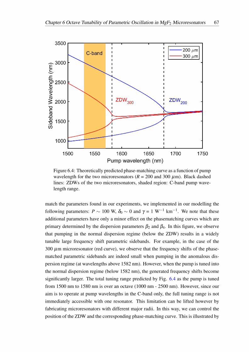
Chapter 6 Octave Tunability of Parametric Oscillation in MgF2 Microresonators 67
Figure 6.4: Theoretically predicted phase-matching curve as a function of pumpwavelength for the two microresonators (R = 200 and 300 µm). Black dashedlines: ZDWs of the two microresonators, shaded region: C-band pump wave-length range.
match the parameters found in our experiments, we implemented in our modelling thefollowing parameters: P ∼ 100 W, δ0 ∼ 0 and γ = 1 W−1 km−1. We note that theseadditional parameters have only a minor effect on the phasematching curves which areprimary determined by the dispersion parameters β2 and β4. In this figure, we observethat pumping in the normal dispersion regime (below the ZDW) results in a widelytunable large frequency shift parametric sidebands. For example, in the case of the300 µm microresonator (red curve), we observe that the frequency shifts of the phase-matched parametric sidebands are indeed small when pumping in the anomalous dis-persion regime (at wavelengths above 1582 nm). However, when the pump is tuned intothe normal dispersion regime (below 1582 nm), the generated frequency shifts becomesignificantly larger. The total tuning range predicted by Fig. 6.4 as the pump is tunedfrom 1500 nm to 1580 nm is over an octave (1000 nm - 2500 nm). However, since ouraim is to operate at pump wavelengths in the C-band only, the full tuning range is notimmediately accessible with one resonator. This limitation can be lifted however byfabricating microresonators with different major radii. In this way, we can control theposition of the ZDW and the corresponding phase-matching curve. This is illustrated by

68 Chapter 6 Octave Tunability of Parametric Oscillation in MgF2 Microresonators
the blue curve of Fig. 6.4, which shows the phasematching curve for a microresonatorwith a major radius of 200 µm. Here, the ZDW of the fundamental TE mode of the mi-croresonator has shifted to 1678 nm, which gives access to the much larger frequencyshifts using the same range of C-band pump wavelengths.
6.2 Experimental Setup
We have fabricated five crystalline MgF2 microdisk resonators with different dimen-sions using the SPDT method discussed in Chapter 4. These microresonators were thenhand-polished with diamond abrasives to achieve a finesse F = 5 ·104, correspondingto a quality- factor Q ranging from 0.5 - 1.5 ·108. The measured major radii of the fivemicroresonators were 515, 400, 265, 190 and 165 µm, while the minor radii were set toabout 1/3 of their corresponding major radius.
We use two experimental setups to demonstrate widely tunable parametric oscilla-tion in MgF2 microresonators. The first setup is intended only for measuring parametricsideband wavelengths between 600 nm and 2400 nm. The schematic of this setup ispresented in Fig. 6.5. The pump laser used to drive the microresonators is a standardC-band external cavity laser (TLB-6728 VelocityTM Widely Tunable Laser, linewidth∼ 70 kHz) with a tunable range from 1520 to 1570 nm, which is amplified by a C-banderbium-doped fiber amplifier (EDFA), and then filtered by a free-space tunable 3 nmband-pass filter to remove the majority of the amplified spontaneous emission (ASE)noise produced from the EDFA. The pump laser is coupled to the microresonator atthe micron diameter waist of silica optical fiber taper. A polarization controller (PC)is placed before the taper to select which of the TE or TM modes will be excited. Tomonitor the input power, a 99/1 coupler is connected so that 1% of the output is directedinto a power meter. This setup provides ∼ 100 mW of pump light. At the exit of thefiber taper, the light output is then split into two. Half the light directed to a wavelength-division multiplexer (WDM) before going to the oscilloscope, whilst the remaining lightis again divided into half and directed to two optical spectrum analyzers (OSAs). Thefirst OSA-1 (Yokogawa AQ6370D) sweeps from 600 nm to 1750 nm while the secondOSA-2 (Yokogawa AQ6375B) sweeps from 1200 nm to 2400 nm. We used the WDMto split the light into wavelengths below 1520 nm and above 1530 nm; the outputs ofthis filter go to two amplified photodetectors (PD). Monitoring the nonlinear channel(λ < 1520 nm) allows us to identify the appropriate microresonator modes that gen-erates large frequency shift sidebands. The other output of the WDM (λ > 1520 nm)allows us to monitor the linear resonances.
Fig. 6.6 shows the schematic of our second experimental set-up. This is used for

Chapter 6 Octave Tunability of Parametric Oscillation in MgF2 Microresonators 69
1%
99%
Microresonator
Taper
PC
VOA
ECLTLC
PM
99/1
PCBPFEDFA Isolator
WDM
PD-1
PD-250/50
VOA
VOA
50/50
1500 nm1000 nm 1500 nm1000 nm 2200 nm1200 nm
OSA-2OSA-1
Oscilloscope
Figure 6.5: Schematic diagram for the first experimental setup of the MgF2microresonator tunability experiment. TLC: tunable laser controller, ECL: ex-ternal cavity laser, EDFA: erbium doped fiber amplifier, PC: polarization con-troller, BPF: band-pass filter, PM: power meter, WDM: wavelength-divisionmultiplexer, PD: photodetector, VOA: variable optical attenuator, and OSA:optical spectrum analyzer.
measuring the optical spectra of parametric sidebands with wavelengths above 2400nm. This setup is adapted from the first experimental setup presented in Fig. 6.5. Theunaltered optical components have been faded out for clarity in Fig. 6.6. Firstly, inaddition to the C-band pump, another laser source (New Focus, Velocity TLB-6730,tunable in the L-band from 1550 nm− 1630 nm) was used together with an L-bandEDFA to provide a larger tuning range. Secondly, we limit the length of silica fiberafter the coupling region to only 5 cm to minimize the strong attenuation of silica glassat wavelengths above 2 µm. The output of the taper is passed to a free-space beamsetup, whereby we used a gold flip mirror (GM) to control which of the two pathwaysthe light will take. The first pathway is coupled back into a single mode fiber (SMF)and split into two branches via a 50/50 coupler. The first branch goes to a WDM and os-cilloscope to allow measurement of the linear and nonlinear signals (as presented in theprevious setup), the second branch goes to OSA-1 to allow the measurement of the shortwavelength sideband’s spectrum. The second free-space pathway goes to the Fourier-transform infrared (FTIR) spectrometer (Bristol Instruments 771), to record the opticalspectra of the sidebands above 2400 nm. Due to the limited (45 dB) dynamic range ofthe FTIR spectrometer, an infrared radiation (IR) bandpass filter with a pass-band of

70 Chapter 6 Octave Tunability of Parametric Oscillation in MgF2 Microresonators
1%
99%
50%
50%1500 nm1000 nm
Microresonator
Taper
PC
VOAPD-1
PD-2
ECL-1TLC
PM
99/1
PCBPFEDFA-1 Isolator
50/50VOA
TLC ECL-2EDFA-2 Isolator
5 cm fiber
Free-space region
WDMOscilloscope
FTIR
Lens
GM
IR-BPF
Flip GM
FM
OSA-1
2500 nm1000 nm
GM
GM
Computer
Figure 6.6: A schematic of the second experimental setup for measuring thespectra of the parametric sidebands that goes beyond 2400 nm in MgF2 mi-croresonator. TLC: tunable laser controller, ECL-1 (C-band) and ECL-2 (L-band): external cavity laser, EDFA-1 (C-band) and EDFA-2 (L-band): er-bium doped fiber amplifier, PC: polarization controller, BPF: band-pass filter,PM: power meter, GM: gold mirror, FM: fiber mount, IR-BPF: Infrared radi-ation - bandpass filter, FTIR: Fourier transform infrared spectrometer, WDM:wavelength-division multiplexer, PD: photodetector, VOA: variable optical at-tenuator, and OSA: optical spectrum analyzer. Note that the unaltered compo-nents have been faded out and surrounded with dashed red lines in this figure.

Chapter 6 Octave Tunability of Parametric Oscillation in MgF2 Microresonators 71
Taper Output
RFSA
PCPCAOM
PDTBF1500 nm1000 nm
30 km SMF
50/5050/50
Figure 6.7: Schematic of the delayed self-heterodyne interferometer used forlinewidth measurements of the pump laser and the generated parametric side-bands. TBF: tunable bandpass filter, AOM: acousto-optic modulator, PC; po-larization controller, SMF: single-mode fiber, PD: photodetector, and RFSA:radio frequency spectrum analyzer.
about 500 nm was placed before the spectrometer, so that the strong pump signal doesnot saturate the FTIR. A selection of filters with center wavelengths between 2000 and4000 nm is available, and chosen to transmit the mid-IR sideband under study. Theoutput spectra are monitored and saved in the computer. We note that FTIR and the twodifferent OSAs were calibrated to equalize their power levels using the 1550 nm lasersignal.
Our procedure for observing parametric sidebands and testing their tunability is asfollows. We first coarsely tune to the desired spectral region of our pump wavelength.We then perform a scan of the laser over one free spectral range (FSR) to look forresonator modes that are capable of generating large frequency shift sidebands. Bymonitoring the signal transmitted by the WDM filter, we can evaluate the generatednonlinear signals. Our laser has a fine piezo scan mode with a 0.3 nm tuning range.This enables us to perform a fine scan over each of these nonlinear resonances. Foreach nonlinear mode we observe in the scan, we set our pump wavelength to withinapproximately 0.1 nm of the start of the signal mode. Using the pump laser’s fine piezo,we slowly bring the pump (starting from the low wavelength side) into the resonancewith the desired mode. The pump-cavity detuning is maintained via the passive ther-mal locking discussed in chapter 4. The goal is to find a nonlinear mode that exhibitswidely shifted parametric sidebands. The optical spectrum is recorded once the modewas found. We then move the pump wavelength to the next FSR, and repeat the exper-imental procedure. In this manner, we can follow the same mode family across the fullwavelength range of the pump.
In addition to spectral measurements, we have the option to perform linewidth mea-surements on the pump laser and the generated parametric sidebands using a delayedself-heterodyne interferometer (DSHI) [146]. Fig. 6.7 presents the principle of opera-tion for the DSHI experimental setup. The microresonator output is first filtered using
72 Chapter 6 Octave Tunability of Parametric Oscillation in MgF2 Microresonators
fiber WDM’s to separate the three fields (pump, and the two sidebands). The signal ofinterest is then split by a 50/50 coupler. The first path contains an acousto-optic mod-ulator (AOM) that shifts the signal by 80 MHz, while the other path passes through 30km of standard single-mode fiber (SMF) so as to decorrelate the two interfering fields.The outputs of the two paths are recombined with a second 50/50 coupler before go-ing into a photodiode (PD). A radio frequency spectrum analyzer is used to measurethe resulting 80 MHz beat note. From here, the spectral linewidth of the input signalcan be estimated from the linewidth of the output RF peak. This RF signal will be theautocorrelation of the original signal lineshape. Assuming that the original signal hasa Gaussian line shape, the measured linewidth in the RF peak has a spectral width
√2
times larger than the original linewidth of the optical signal [146].
6.3 Experimental Results and Discussion
6.3.1 Widely Tunable Parametric Sidebands
We first present our experimental observations of widely tunable parametric sidebandsin the 515 µm major radius MgF2 microresonator using the methods described in Sec-tion 6.2. We note that we have observed several mode families that produce large fre-quency shift parametric sidebands for this microresonator. To showcase the capabilityof our tunability scheme, we present in Fig. 6.8 the experimentally measured spectra ofone of these mode family for five different pump wavelengths in the C-band. For eachof these wavelengths, we continuously tuned the laser into the resonance such that itreaches a detuning where parametric oscillation is observed. Due to the thermal locking,this output spectrum can be maintained for∼ 10’s of minutes in our experiments. FromFig. 6.8, we observed that the parametric frequency shift rapidly increases as the pumpwavelength is decreased by a small amount. This result is expected for phasematchedparametric oscillation in the presence of higher-order dispersion. The largest frequencyshift sidebands that we observed in this microresonator occurs at pump wavelength of1529.1 nm, which generates new parametric frequencies at 1269.2 nm and 1922.8 nm(detuned by ± 40.1 THz from the pump frequency). We also make note that the mea-sured spectra show no evidence of the strong stimulated Raman components observedin the previous widely-tunable experiments conducted in silica microspheres [60]. Thespectra in Fig. 6.8 consist only of a single pair of pure FWM parametric sidebands. Thestrong suppression of stimulated Raman scattering is due to the narrow Raman gainspectrum of crystalline MgF2. As a result, stimulated Raman components typically will

Chapter 6 Octave Tunability of Parametric Oscillation in MgF2 Microresonators 73
Figure 6.8: Experimentally measured spectra from the 515 µm major radiusMgF2 microresonator at five different pump wavelengths (from top to bottom):λ = 1557.3, 1553.2, 1543, 1535.1, 1529.1 nm. The black dashed line indicatesthe estimated ZDW of the microresonator.

74 Chapter 6 Octave Tunability of Parametric Oscillation in MgF2 Microresonators
Figure 6.9: Experimentally measured sideband wavelengths as a function ofpump wavelength, together with the theoretical phase-matching curve for the515 µm major radius MgF2 microresonator. Filled circles: experimental data,solid curves (red and blue): theoretical fit, black dashed line: ZDW, shadedregion: C-band pump wavelength range.
not be resonant with the mode family we are driving.We then repeated the spectral measurements for other pump wavelengths in the
C-band range. Fig. 6.9 shows the full experimentally measured phasematching curvefor the mode family that generated the spectra in Fig. 6.8. For each of the pump wave-length used, we experimentally extract the two parametric sideband wavelengths andplot them as solid circles (red and blue) in Fig. 6.9. As can be seen, by just tuningthe pump wavelength by 32 nm in the C-band, we observe a total tuning range of thesidebands more than 650 nm. Also superimposed on this figure, as solid curves (redand blue), is the theoretical fit to the phasematching condition given by Eq. 5.3 to theseexperimental frequency shifts. This shows a good agreement between the fit and theexperimentally measured frequency shifts. We note that, we can accurately extract theZDW and the higher-order dispersion coefficients of the mode family under study fromthis theoretical fit. For this mode family, the fit yields the following parameters: ZDWat 1558.5 nm (plotted as a black dashed line in Fig. 6.8 and Fig. 6.9), with the disper-sion coefficients (evaluated at the ZDW) of β3 = 0.05 ps3 km−1 and β4 = -2.25 × 10⁻⁴

Chapter 6 Octave Tunability of Parametric Oscillation in MgF2 Microresonators 75
SSB1448 nm
Pump1547 nm
LSB1660 nm
Figure 6.10: Linewidth measurements using an optical DSHI technique forthe short-wavelength sideband (SWS), the pump wavelength and the long-wavelength sideband (LWS). Solid black curves indicate the Gaussian fits tothe measured beat signals.
ps4 km−1.To confirm the narrow linewidths of the generated parametric sidebands, we per-
formed spectral linewidth experiments using a delayed self-heterodyne interferometer(DSHI) [146], as shown in Fig. 6.7. Here, a pump wavelength at 1547 nm gener-ates short and long wavelength sidebands at 1448 nm and 1660 nm, respectively. Thelinewidth measurements of the pump and the two parametric sidebands are presentedin Fig. 6.10. The short and long wavelength sideband linewidths are estimated to beabout 101.7 kHz and 76.9 kHz, respectively. These sideband linewidth values are com-parable to the original pump linewidth of ∼ 70 kHz. This confirms that the parametricsidebands retain the narrow spectral linewidth of the pump, making them perfect forpotential spectroscopic applications.
To increase the sideband frequency shifts accessible using a C-band pump, we re-peat the tunability experiments using the 400 µm major radius MgF2 microresonator.The ∼ 22% decrease of the major radius in the microresonator, resulted in a ∼ 40%increase in the frequency shifts of the parametric sidebands. Fig. 6.11 presents theexperimentally obtained optical spectra with the 400 µm major radius MgF2 microres-onator for five different pump wavelengths in the C-band. For the lowest three pumpwavelengths (1548.19, 1536.2, and 1530.6 nm) in Fig. 6.11, there is a discontinuity ontheir plots at ∼ 1600 nm since we are obliged to use two separate OSAs to producethese composite plots. Fig. 6.12 shows the plot of the experimentally measured side-band wavelengths as a function of the pump wavelength. As can be seen, there is again agood agreement between the experimental data and theoretical phasematching analysis.The largest detuned parametric sidebands were observed at 1159 nm and 2242 nm whenusing a pump wavelength of 1528 nm. This corresponds to ± 62.5 THz frequency shiftfrom the pump frequency. We note that this result has already exceeded the results ob-tained in the SiO2 microspheres since the 400 µm major radius MgF2 microresonator is

76 Chapter 6 Octave Tunability of Parametric Oscillation in MgF2 Microresonators
Figure 6.11: Experimentally measured spectra from the 400 µm major radiusMgF2 microresonator at five different pump wavelengths (from top to bottom):λ = 1563.8, 1557.8, 1548.19, 1536.2, 1530.6 nm. The black dashed line indi-cates the estimated ZDW of the microresonator.

Chapter 6 Octave Tunability of Parametric Oscillation in MgF2 Microresonators 77
Figure 6.12: Experimentally measured sideband wavelengths as a function ofpump wavelength, together with the theoretical phase-matching curve for the400 µm major radius MgF2 microresonator, calculated with parameters β3 =3.6 ps3 km−1 and β4 = -1.39 × 10⁻⁴ ps4 km−1 at the ZDW of 1595.5 nm.Filled circles: experimental data, solid curves (red and blue): theoretical fit,dashed black line: ZDW, shaded region: C-band pump wavelength range.
capable of generating strong sidebands at wavelengths above 1900 nm. Most impressivein here is the fact that the longest wavelength sideband is located at 2242 nm, implyingthat we have reached the start of the mid-infrared (IR) region and observed almost anoctave spanning tunability of two sidebands.
6.3.2 Octave Tunability and Signatures of Mid-IR Sidebands
The experimental findings reported in Figs. 6.9 and 6.12 show that MgF2 microres-onators are capable of generating widely tunable parametric sidebands when drivenwith a C-band pump laser. To achieve even larger frequency shifts, we investigate mi-croresonators with still smaller major radii, allowing for mode families with longerZDWs. To this purpose, we investigated the performance of the three smaller microres-onators with major radius of 265, 190 and 165 µm, respectively. Following the same

78 Chapter 6 Octave Tunability of Parametric Oscillation in MgF2 Microresonators
procedure outlined for the previous two (515 and 400 µm major radii) MgF2 microres-onators, we measured the generated parametric sideband wavelengths for each of thesemicroresonators at a range of pump wavelengths across the C-band. Due to the extremefrequency shifts observed in these miroresonators, fully measuring the output spectrumrequired two different optical spectrum analyzers (OSAs) and a Fourier-transform in-frared spectrometer (FTIR) to perform the measurement. To construct the full spectra ofthe sidebands, we calibrated the OSAs and the FTIR to a single signal at 1550 nm. TheFTIR is used to measure the long-wavelength spectral components above 2400 nm. Tominimize the effect of the very large attenuation of silica glass at longer wavelengths,we only allow a 5 cm length of the silica optical fiber after the coupling region (see Fig.6.6, for a full description of this setup).
ZDW (nm) β3 (ps3 km−1) β4 (ps4 km−1)Green 1637 0.0485 -1.41 × 10⁻⁴
Magenta 1625 0.0410 -1.35 × 10⁻⁴
Table 6.1: Summary of two distinct mode families that produce large frequencyshift sidebands in 265 µm major radius MgF2 microresonator.
We first present our experimental results obtained from 265 µm microresonator.Fig. 6.13 shows the plot of the observed spectra at the microresonator output for pumpwavelengths of 1564, 1553.9, 1546.1, 1543.1, and 1541 nm. This show very large fre-quency shift sidebands with signal measurements up to 2670 nm. We then map out theentire tuning range for C-band pump wavelengths. We note that, in this microresonatorwe identified two distinct nonlinear mode families that produce large frequency shiftparametric sidebands. These experimental results are presented in Fig. 6.14, where weplot the measured phasematched sideband wavelengths against pump wavelength. Forthese measurements, each of the tuning curves is obtained from independent experi-ments. The data are fitted to the theoretical phase-matching curves defined by Eq. 5.3and the fits are plotted as solid curves (red and blue). From these fits, we extract theZDWs and plotted them as black dashed lines. The dispersion characteristics of the twomode families are summarized in Table 6.1. Note that β3 and β4 are evaluated at theZDW. The mode family used in the experimental spectra presented in Fig. 6.13 exhibitsthe widest parametric oscillation in 265 µm microresonator, these are shown as greenfilled circles in Fig. 6.14.
The results reported in Fig. 6.14 are impressive because they show hundreds ofnanometers of parametric sideband tunability. The tuning range observed in this mi-croresonator spans from 1083 nm to 2670 nm (corresponding to an 82.07 THz fre-quency shift from the pump). Combined the three resonators used (515, 400 and 265

Chapter 6 Octave Tunability of Parametric Oscillation in MgF2 Microresonators 79
Figure 6.13: Experimentally measured spectra from the 265 µm major radiusMgF2 microresonator at five different pump wavelengths (from top to bottom):λ = 1564, 1553.9, 1546.1, 1543.1, 1541 nm. The black dashed line indicatesthe estimated ZDW of the microresonator.

80 Chapter 6 Octave Tunability of Parametric Oscillation in MgF2 Microresonators
Figure 6.14: Experimentally measured sideband wavelengths as a function ofpump wavelength for the two different mode families within the 265 µm majorradius MgF2 microresonator. Filled circles (green and magenta): experimen-tal data, solid curves (red and blue): theoretical fit, dashed black line: ZDW,shaded region: C-band pump wavelength range.
µm) allow over an octave of discrete tunability in the output frequency of the two side-bands. In comparison with the reported results in silica microsphere systems [60], wesee no signatures of stimulated Raman scattering or other nonlinear processes in ourmeasured optical spectra. Only a single pair of FWM sidebands are generated duringthe parametric process.
Finally, we present our results for the two smallest microresonators we consider(R = 190 µm and 165 µm). Here, we observed even larger frequency shifts. How-ever, in this case we no longer observe the long-wavelength sidebands (LWSs) on theFTIR. However, we can infer their locations due to the presence of their correspondingshort-wavelength sidebands (SWSs). Fig. 6.15 shows the sideband wavelengths as afunction of pump wavelength for the two smallest (R = 190 µm and 165 µm) MgF2
microresonators. The SWS wavelengths that we measured are already around 1000 nm,with the largest shift sideband located at 957 nm. These measurements imply that thepositions of LWS wavelengths are well above 3000 nm, with the maximum at 3860 nm.This result is very impressive because it represents more than two octave’s in frequency

Chapter 6 Octave Tunability of Parametric Oscillation in MgF2 Microresonators 81
Figure 6.15: Sideband wavelengths as a function of pump wavelength for thesmallest two MgF2 microresonators with major radii of R = 190 µm and 165µm. Filled circles: measured short-wavelength sidebands (SWSs), open cir-cles: inferred long-wavelength sidebands (LWSs), solid curves (red and blue):theoretical fit.
Microresonator (R) ZDW (nm) β3 (ps3 km−1) β4 (ps4 km−1)380 µm 1710 0.0100 -2.70 × 10⁻⁴
330 µm 1750 0.0100 -2.67 × 10⁻⁴
Table 6.2: Summary of the dispersion characteristics for two smallest microres-onators with R = 190 µm and 165 µm.
difference between the two sidebands. Moreover, these LWS wavelengths are alreadylocated in the mid-infrared fingerprint region which contains many important molecularvibrations. Remarkably, we see no significant reduction in conversion efficiency in theoutput SWS wavelengths in these small resonators. This is demonstrated in Fig. 6.16where we plot selected measured SWSs spectra for 165 µm MgF2 microresonator. Notethat we have used an additional L-band laser source here to further expand the tuningcurves. Table 6.2 shows the inferred dispersion characteristics of these two smallestmicroresonators obtained from their phasematching curves.
We speculate that the inability to observe the long wavelength sidebands is due

82 Chapter 6 Octave Tunability of Parametric Oscillation in MgF2 Microresonators
Figure 6.16: Selected experimentally measured SWSs spectra from the 165 µmmajor radius MgF2 microresonator at five different pump wavelengths (fromtop to bottom): λ = 1588.1, 1579.1, 1568.4, 1547.4, 1533.8 nm. The ZDW ofthis microresonator is at 1750 nm.

Chapter 6 Octave Tunability of Parametric Oscillation in MgF2 Microresonators 83
Figure 6.17: Experimentally measured spectrum from one of our MgF2 mi-croresonators studied in this thesis.
to the rapidly increasing absorption in our silica coupling fiber, resulting to inefficientcollection of mid-IR light. An unoptimized outcoupling setup above 3 µm will alsoreduce the observed signal at these wavelengths. We envisage the most promising so-lution to this problem would be to use a prism that is transparent in the mid-IR region,and couple light to the resonators via the evanescent wave at the back face of the prism.Unfortunately, time did not allow us to investigate this potential solution during thisthesis.
6.3.3 Conversion Efficiency
For these microresonators, the observed conversion efficiency of the parametric side-bands ranges from 10−5 to 10−2. Fig. 6.17 shows an example of strong conversionin the experimentally measured spectrum from 515 µm major radius MgF2 microres-onator. As can be seen, the two sideband wavelengths are both ∼ 26 dB below fromthe pump wavelength. Based on numerical and analytical investigations, that we willpresent in Appendix A, we find that it is theoretically possible to achieve conversionefficiencies of approximately 10% to each of the generated parametric sidebands [61].

84 Chapter 6 Octave Tunability of Parametric Oscillation in MgF2 Microresonators
In practice, the best values we are able to obtain experimentally are a factor of 10 be-low this. A crucial parameter in determining the strength of the generated parametricsidebands is the outcoupling efficiency of the resonator at the sideband wavelengths.We suspect this might be the main explanation for the low conversion efficiencies weobserve. Our taper coupling is set to optimize the coupling of the pump at ∼ 1550 nminto the resonator. At sideband wavelengths far from pump wavelength, the couplingcould be significantly reduced. This issue is explored in Appendix A.
6.3.4 Continuous Tunability
So far the wideband tunability demonstrated in our microresonators has been discretesince the parametric sidebands are only generated when the pump is resonant with acavity mode. Thus, the pump wavelength can only be advanced in multiples of an FSR.This limitation can be potentially overcome by shifting the positions of the resonatormodes by applying a mechanical strain on the resonator [147, 148] or by controlling theresonator’s temperature [149, 150]. To confirm this, we utilize the intrinsic thermo-opticnonlinearity of the microresonator [129, 149]. For this demonstration, we use a ±7.2THz frequency shift pair of parametric sidebands in the R = 265 µm microresonator.We scan the laser slowly into resonance. Increasing the pump wavelength, brings thepump further into resonance, and increases the intracavity power. This increases theresonator’s temperature, causing the cavity modes to shift to longer wavelengths. Wefollow this thermally shifted cavity mode by increasing the pump wavelength, and weobserve that the pump can remain resonant with the cavity mode over ∼ 10 GHz, cor-responding to ∼ 5000 cold cavity linewidths. Fig. 6.18 shows the experimental demon-stration of continuous tunability of the two sidebands as the pump frequency is scannedacross this thermal triangle. In this experiment, we separate the pump and the twosidebands using different spectral filters. A high-precision optical wavemeter (BristolInstruments 771B) is used to capture the three wavelengths with an accuracy of 0.75parts per million. We note that we record all the wavelengths by continuously swappingthe input to the wavemeter, as we continuously increase the pump wavelength. Thismeasurement is repeated until the pump wavelength falls out of resonance. Since ourwavemeter can only accommodate one wavelength at a time, there is a ∼15 s delaywhen measuring the wavelengths between the pump and the two sidebands. Becauseof this, we include error bars in Fig. 6.18 to represent the small fluctuations that mightarise during the delay period.
The results plotted in Fig. 6.18 show that we are able to tune the pump wavelengthover ∼ 10 GHz whilst remaining in resonance with the nonlinear mode. Remarkably,

Chapter 6 Octave Tunability of Parametric Oscillation in MgF2 Microresonators 85
Figure 6.18: Experimental demonstration of 10 GHz continuous tunability in265 µm major radius MgF2 microresonator. Inset: Experimentally measuredoptical spectrum with a pump wavelength of 1569 nm and two sidebands atwavelengths of 1512 nm and 1630 nm, respectively.
we see that the two sidebands (whose modes are also thermal tuned by the same amount)likewise track the pump wavelength. As a result we are able to demonstrate ∼ 10 GHzof continuous tunability for both sidebands. We believe that with the addition of exter-nal temperature tuning in even larger tuning ranges could be possible.
6.4 Summary
In this chapter, we first performed a detailed modelling of the dispersion characteristicsof our microresonators using COMSOL Multiphysics. These show that large frequencyshift parametric oscillation should be possible in these resonators. Next, we presentedthe two experimental setups used to measure the widely tunable parametric sidebands.
We demonstrated discrete tunability over an optical octave with our five crystallineMgF2 microresonators. Our experimental results showed good agreement with the the-oretical phase-matching curves. The largest experimentally measured frequency shift

86 Chapter 6 Octave Tunability of Parametric Oscillation in MgF2 Microresonators
was observed in 265 µm major radius microresonator with a pump wavelength of 1541nm, and the generated parametric sidebands located at 1083 nm and 2670 nm (corre-sponding to ∼ 82.07 THz frequency shift). This is an important result because, to thebest of our knowledge, this is the first work that demonstrates a direct observation ofoctave spanning discrete tunability in a Kerr microresonator. Even larger shifts wereachieved in our two smallest resonators (with major radii of 190 and 165 µm). How-ever, here, we did not directly observed the corresponding long sideband wavelengthsin our experiments. Instead, we are forced to infer their positions from the presenceof the associated short sideband wavelengths. The short sideband wavelengths that weobserved were already below 1000 nm (with the shortest sideband at 957 nm), im-plying that their corresponding long sideband wavelengths were above 3000 nm, withthe maximum sideband wavelength at 3860 nm. Additionally, we conducted linewidthmeasurements through the DSHI method on the generated parametric sidebands. Ourresults confirmed that the sideband linewidth values are comparable to the original pumplinewidth. Lastly, we experimentally demonstrated 10 GHz continuous tunability forboth the short and long wavelength sidebands in 265 µm major radius microresonatorthrough thermal tuning.

Chapter 7
Origins of Clustered Frequency Combsin Kerr Microresonators
1 In the previous two chapters, we have demonstrated widely tunable optical parametricoscillation in Kerr nonlinear microresonators, particularly in silica microspheres andcrystalline MgF2 microdisks. Both of these demonstrations were achieved via carefullyengineered dispersion [57–60, 133]. These parametric sidebands arise when the mi-croresonator has a positive (normal) GVD and a negative fourth-order dispersion andcan phasematch a single FWM process [22, 23, 28]. In this scenario, we may presumethat the generated two sidebands would retain the high spectral purity of the pump sincethey are only driven by a single phasematched FWM process. Indeed, it was also shownin chapter 6 that these two sidebands share similar coherence as the pump source. How-ever, a so-called clustered frequency combs have also been demonstrated for certainparameter values in MgF2 microresonators [58]. Such combs form around the pumpfrequency and the widely detuned primary parametric sidebands in strongly driven mi-croresonators. This generation of localized frequency combs could be useful for someapplications. However, there are also other applications that require only a single outputfrequency such as standard spectroscopic measurements. Here, the appearance of theseclusters is unwanted. Thus, it would be useful to understand the underlying dynamicsof the formation of these clustered frequency combs.
In this chapter, we first present the experimental setup used in our experiments.Next, we show the experimental demonstration of the generation of these clustered fre-quency combs in strongly driven Kerr microresonators. We also present the experimen-tally measured radio frequency (RF) intensity noise of the generated clustered frequency
1Work presented in this chapter has been published in ”Origins of Clustered Frequency Combs in KerrMicroresonators, ”Optics Letters 43, 4180-4183 (2018).
87

88 Chapter 7 Origins of Clustered Frequency Combs in Kerr Microresonators
1%
99%
Microresonator
Taper
PC
VOA
ECLTLC
PM
99/1PC
BPFEDFA Isolator
WDM
PD-1
PD-295/5
VOA
VOA
50/50
RFSAOSA
Oscilloscope
1500 nm1400 nm 1700 nm 1500 nm1000 nm
PD-3
Figure 7.1: The experimental setup used for demonstrating clustered frequencycombs in 400 µm major radius MgF2 microresonator. TLC: tunable lasercontroller, ECL: external cavity laser, EDFA: erbium doped fiber amplifier,PC: polarization controller, BPF: bandpass filter, PM: power meter, WDM:wavelength-division multiplexer, PD: photodetector, VOA: variable optical at-tenuator, OSA: optical spectrum analyzer, and RFSA: radio frequency spectrumanalyzer.
combs. We then provide a theoretical explanation for the formation of clustered combs,which coincides with our experimental observations. In addition to this, we examinethe coherence of numerically simulated clustered frequency combs.
7.1 Experimental Set-up
We used a crystalline 400 µm major radius MgF2 microresonator in our experiments.The measured finesse of this microresonator is F = 4.3 ·104 and the free spectral range(FSR) = 87.1 GHz.
Fig. 7.1 shows the experimental setup used to generate clustered frequency combs.It is substantially similar to that presented in Fig. 6.5. The pump laser used to drivethe microresonator is a standard C-band external cavity laser with a chosen pump wave-length at 1547 nm. The output light is amplified with an erbium-doped fiber amplifier(EDFA) and then enters a free-space 3 nm bandpass filter, to remove the unwanted am-plified spontaneous emission (ASE) noise, to produce a 90 mW continuous wave pump.

Chapter 7 Origins of Clustered Frequency Combs in Kerr Microresonators 89
The pump is coupled to the microresonator at the ∼ 1 µm diameter waist of silica op-tical fiber taper. The taper output is then split into two using a 50/50 coupler. Half ofthe output is directed to a wavelength-division multiplexer (WDM) before going to theoscilloscope, while the remaining half is again split using 95/5 coupler. 95% goes toan optical spectrum analyzer (OSA) and the 5% is sent to an amplified 10 GHz pho-todetector and the radio frequency spectrum analyzer (RFSA). We used the WDM tofilter the nonlinear signals between 1200-1400 nm and detected them on an amplifiedphotodiode. Through this filtered channel, we can identify the signals that exhibit largefrequency shift parametric oscillation.
7.2 Experimental Results
In order for us to understand the formation of these clustered combs, we recorded si-multaneously the detuning, optical spectrum of the mode and the corresponding radiofrequency (RF) intensity noise. To do this, we first identify a mode that exhibits stronglarge frequency shift sidebands by scanning the pump wavelength over a single FSR ofthe microresonator. We will slowly tune the detuning into the selected cavity resonanceand observe the various stages of clustered frequency comb formation.
In Fig. 7.2(a), we present the experimentally measured spectra of the clustered fre-quency combs as the pump detuning (∆) progressively increases further into the cavityresonance. At the onset of parametric oscillation, we first observed a single pair ofparametric sidebands located at 1404 nm and 1721 nm respectively, with a pump wave-length of 1546.6 nm (corresponding to a ± 19.7 THz frequency shift). As the pump istuned further into resonance, the appearance of small frequency comb clusters aroundthe pump and two sidebands are observed. The line spacing of these comb clusters isequal to one FSR of the resonator. Further tuning into resonance shows additional fre-quency components have formed around the pump and two sidebands, resulting to anincreased size of these clusters. The structure of these clusters is highlighted in the righthand side of Fig. 7.2, which shows a zoomed in section of the spectra around the longwavelength sideband.
In Fig. 7.3, we show the experimental RF intensity measurements of the clusteredfrequency combs. These measurements correspond to the four different spectra pre-sented in Fig. 7.2, respectively. We observed no excess noise in the RF spectrum whenthere is only a single parametric sideband present, as shown in Fig. 7.3(a). On the otherhand, a substantial increase in the measured low-frequency RF intensity noise occursas the the detuning increases, [Figs. 7.3(b) - 7.3(d)]. This increase in intensity noise

90 Chapter 7 Origins of Clustered Frequency Combs in Kerr Microresonators
Figure 7.2: (a-d) Experimentally measured spectrum of the clustered frequencycombs as we increase the pump detuning ∆. The panel on the right-hand side isthe zoom of the spectrum of the long-wavelength sidebands.

Chapter 7 Origins of Clustered Frequency Combs in Kerr Microresonators 91
Figure 7.3: Experimentally measured RF spectrum, corresponding to the dif-ferent spectra presented in Fig. 7.2, respectively.
is a well known signature of unstable frequency combs [151, 152]. This measurementstrongly suggests the clustered combs we observe in Fig. 7.2 are not stable.
7.3 Theoretical Analysis
To understand the underlying physics of these clustered frequency combs, we resort tonumerical simulations. We first perform numerical simulations of the intracavity dy-namics using the generalized Lugiato-Lefever equation (LLE) [86]. We solve the LLEusing the split-step Fourier method, with the following parameters: γ = 1 W−1km−1,L = 2.5 mm, α = θ = 7.3×10⁻⁵,Pin = 90 mW, and dispersion coefficients up to fourthorder of β2 = 0.486 ps2km−1, β3 = 0.07 ps3km−1, and β4 =−4×10⁴ ps4km−1. Thesedispersion coefficients are calculated at the pump wavelength of 1547 nm. We note thatthese parameters are typical of the MgF2 microresonator used in our experiments, andreproduce the frequency shifts observed in Fig. 7.2. To allow the intracavity field toreach the steady state, we carry out the simulations over 2 · 106 roundtrips at selectedcavity normalized detunings ∆ = δ0/α . The outputs of these numerically simulatedspectra show the formation of clustered frequency combs and are plotted in Fig. 7.4.As can be seen, our numerical simulations show similar behavior to our experimentalresults (see Fig. 7.2). A single pair of large frequency shift sidebands is first generatedat low detunings. Further increasing the detuning leads to the formation of the clustered

92 Chapter 7 Origins of Clustered Frequency Combs in Kerr Microresonators
(a) (b) Δ = -4.3
Δ = -1.1
Δ = -0.6
Δ = 2.4
Figure 7.4: Numerically simulated spectra using the generalized LLE at se-lected cavity detuning.
frequency combs around the pump and the primary sidebands. We note, however, thatthe agreement observed in Fig. 7.4 with our experimental spectra is only qualitative aswe are unable to measure the absolute experimental detunings used.
To gain more insights into the observed clustered frequency combs, we recall andexamine the phase-matching condition (from Eq. 5.3) that allows the generation of theprimary parametric sidebands. By truncating the dispersion to fourth order (i.e., βk = 0for k > 4) and neglecting the second order effects of pump detuning and intracavitypower, we find that to a good approximation the phasematched frequency shift of thetwo sidebands is given by Eq. 5.4,
Ω2pm =
−12β2,p
β4,p(7.1)
where β2,p and β4,p are the second and fourth order dispersion coefficients evaluated atthe pump frequency (ωp).
In the case when β2,p is positive (normal dispersion) and β4,p is negative, gener-ation of large frequency shift parametric sidebands can be achieved. Evaluating thelocal GVD (second-order dispersion coefficient) at the two phase-matched parametric

Chapter 7 Origins of Clustered Frequency Combs in Kerr Microresonators 93
Figure 7.5: β2 values as a function of wavelength. Blue circle: short sideband,magenta circle: pump wavelength, red circle: long sideband.
sidebands located at ω± = ωp±Ωpm to be
β2(ω±) =−5β2,p±β3,p
√−12β2,p
β4,p. (7.2)
Under these conditions, Eq. 7.2 shows that the local β2 value of at least one of thetwo sidebands must have a negative sign. That is, at least one of the sidebands will al-ways propagate in the anomalous dispersion regime. This analysis holds true regardlessof the magnitude or sign of β3,p. We illustrate this point by plotting the local value ofβ2 as a function of wavelength for the parameters used in Fig. 7.4. This is shown in Fig.7.5 and shows that both the pump and the short sideband propagate in the normal dis-persion regime while the long sideband propagates in the anomalous dispersion regime.Due to this, we propose a simple mechanism whereby the two sidebands can evolve intoclustered frequency combs. Initially the only FWM process that is phasematched in theresonator is the direct transfer of energy from the pump to the two sidebands. The shortwavelength sidebands has a local normal dispersion coefficient of 6.1 ps2km−1 and sois inherently stable. The long wavelength sideband however experiences an anomalousdispersion of -10.8 ps2km−1, and so is susceptible to undergo modulation instability ifever its power becomes high enough. Note that the peak gain per roundtrip produced by

94 Chapter 7 Origins of Clustered Frequency Combs in Kerr Microresonators
Normalized detuning ∆F
requ
ency
(T
Hz)
(a)
−6 −4 −2 0 2
−20
−10
0
10
20
−6 −4 −2 0 20
50
100
Normalized detuning ∆
Pea
k po
wer
(W
)
(b)
Rel
. pow
er (
dB)
−60
−40
−20
0
PMI
Figure 7.6: (a) Numerical simulation of clustered frequency comb formation asthe cavity detuning ∆ is scanned. (b) The red horizontal solid line denotes theMI threshold, while the black solid line represents the peak intracavity powerof the long-wavelength sideband (red-detuned anomalous sideband). Dottedlines in (a) and (b) denote the detuning at which the long-wavelength sidebandpower crosses the MI threshold.
this anomalous sideband is given by g = γPL. If the gain of this sideband exceeds theper roundtrip loss (g>α), this particular sideband can act as a pump for a second phase-matched MI process and generate its own small frequency-shift MI sidebands throughstandard anomalous comb formation dynamics. Further non-degenerate FWM betweenthe three primary waves can then transfer the combs to the high-frequency sideband andalso to the pump [151].
To test this theory, we plot in Fig. 7.6 (a) a numerically simulated spectral evolutionas a function of normalized cavity detuning ∆ for the same resonator parameters usedpreviously. At a detuning of approximately ∆ = −4.5, the pump begins to generate asingle pair of large frequency shift sidebands, with a frequency shift of ± 19.7 THzfrom the pump. Additional spectral components start to be generated around the pumpand the two sidebands at approximately ∆ = −2.1, indicating the onset of cluster for-mation. As previously observed in our experiments (see Fig. 7.2), there is an increasein the number of spectral components in the clustered frequency combs as the detuningincreases.

Chapter 7 Origins of Clustered Frequency Combs in Kerr Microresonators 95
Fig. 7.6 (b) shows the corresponding peak intracavity power of the anomalous (lowfrequency) sideband as a function of the normalized cavity detuning (black solid line),as well as the MI threshold power PMI = α/(γL) (red solid line). We find that, the peakpower of the anomalous (red-detuned) sideband crosses this threshold at a detuning ofapproximately ∆≈−2.1. This detuning corresponds exactly to the point at which clus-ter formation is observed to begin in Fig. 7.6 (a). Hence, these results confirm ourproposed theory. We note that we have repeated our numerical simulation analysis fordifferent frequency shifts and observed identical behavior.
7.4 Coherence of Simulated Comb Clusters
We also examine the comb stability of the numerically simulated clustered frequencycombs for a range of detunings. We do this by evaluating the modulus of the complexdegree of first order coherence as a function of wavelength λ [94, 95, 153] for each ofthe selected spectral components:
|g(1)12 (λ , t1− t2)|=|〈E∗(t1,λ )E(t2,λ )〉|
S(λ ), (7.3)
where E(t,λ ) is the Fourier transform of the field at time t, S(λ )= 〈|E(λ )|2〉 is the meanspectrum, and angle brackets denote an ensemble average. This technique was first de-veloped to study the coherence of supercontinuum generation in optical fibers [154],and is equally applicable in our case. To calculate this coherence, we integrate the LLEover 2×10⁶ roundtrips, allowing the simulated frequency comb to reach steady state.We first record one spectrum of the cavity field and calculate E∗(t1,λ ). Another spec-trum is recorded E∗(t2,λ ) after some roundtrips, serving as the coherence delay. Then,we calculate the product of these two fields. The coherence delay in here is definedas a fixed number of cavity roundtrips (|t1− t2| = ntR). We repeat this procedure for1000 different pairs of fields to get the ensemble average and calculate |g(1)12 | using Eq.7.3. Through this coherence calculation, we can characterize the line-by-line spectralcoherence of the simulated clustered frequency combs. We note while we plot only thecoherence of the red-detuned parametric sideband, identical behavior is observed forthe blue detuned sibeband too.
There are four different regimes that we identify in our cluster coherence simula-tions. These regimes are shown in Fig. 7.7. Specifically, Figs. 7.7(a) - 7.7(d) showthe numerically simulated sideband comb clusters at normalized detunings of ∆ = −3,∆ = −2, ∆ = −1, and ∆ = 2, respectively. The corresponding degree of coherence ofthe comb cluster at each detuning is shown in Figs. 7.7(e) - 7.7(h).

96 Chapter 7 Origins of Clustered Frequency Combs in Kerr Microresonators
−22 −20 −180
10
20
30
40(a)
−22 −20 −180
10
20
30
40(e)
−22 −20 −18Frequency (THz)
(b)
−22 −20 −18Frequency (THz)
(f)
−22 −20 −18
(c)
−22 −20 −18
(g)
−22 −20 −18
(d)
−22 −20 −18
(h)
0
0.2
0.4
0.6
0.8
1
Spe
ctru
m (
dB)
−80
−60
−40
−20
0
Coh
eren
cede
lay(t
ph)
Slo
wtim
e(t
ph)
∣ ∣ ∣g(1)
12(∆
t)∣ ∣ ∣
∆ = −3 ∆ = −2 ∆ = −1 ∆ = 2
Figure 7.7: (a) - (d) Numerical simulations of the spectral evolution of theanomalous sideband cluster, and (e) - (h) corresponding simulations of thedegree of coherence as a function of delay in units of photon lifetime tph =tR/(2α), carried out at normalized detunings of (a), (e) ∆=−3, (b), (f) ∆=−2,(c), (g) ∆ =−1, and (d), (h) ∆ = 2.
We observe the formation of a single frequency component at a detuning of ∆=−3,corresponding to the widely spaced parametric sidebands produced by the pump, asshown in Fig. 7.7(a). This single sideband shows high coherence, indicating that itis indeed stable [Fig. 7.7(e)]. Increasing the detuning to ∆ = −2, we observe the in-tracavity spectral profile demonstrates the initial stage of cluster formation, as shownin Fig. 7.7(b). Here, this cluster formation remains stable as it evolves from roundtripto roundtrip. Fig. 7.7(f) shows the corresponding coherence simulation of this clusterformation spectrum and it too exhibits a high degree of coherence across the cluster’sentire spectral bandwidth. However, at a larger detuning of ∆ =−1 [Fig. 7.7(c)] we ob-serve periodic breathing behavior as the spectrum evolves from roundtrip to roundtrip.The coherence properties of this cluster appear similar those of breathing cavity soli-tons [94], showing a recurrence in the coherence, associated with the breathing period,which in this case is ∼ 8 photon lifetimes [Fig. 7.7(g)]. Finally, we reach an unstableclustered comb state at a detuning of ∆ = 2, exhibiting strong chaotic fluctuations in thecluster spectrum [Fig. 7.7(d)]. The large spectral fluctuations of the cluster lead the low

Chapter 7 Origins of Clustered Frequency Combs in Kerr Microresonators 97
degree of coherence in this regime indicating the spectrum is highly incoherent. We seethe degree of coherence rapidly degrades as the coherence delay increases, as can beseen in Fig. 7.7(h). Moreover, based on our numerical simulations over a wide rangeof cavity detunings, we find that this incoherent regime is the most prevalent mode ofcluster operation. This finding could be an explanation regarding our experimental RFintensity noise measurements presented in Fig. 7.3, where clusters formed at higherdetuning always displayed excess noise in the RF spectrum.
We note that the coherence dynamics that we observed here are similar to the stan-dard theory of comb formation in a microresonator driven by an external anomalousdispersion pump source. In both cases an initially coherent primary comb gives way toan incoherent comb as the detuning is increased [151]. The main difference is that inour situation, the pump generating the cluster is the anomalous sideband that is itselfbeing generated internally through another FWM process. Due to this, we expected thatthe system will exhibit a more complex saturation behavior than seen when using anexternal pump. We also observed coherent clustered frequency combs with line spacingof more than a single FSR when using different dispersion parameters. This kind ofcomb behavior is also observable and common in standard comb formation dynamicsin the anomalous dispersion regime [151].
7.5 Summary
In this chapter, we have experimentally demonstrated the formation of clustered fre-quency combs in Kerr nonlinear optical microresonators. We characterized them bymeasuring their low-frequency RF intensity noise. Our observations showed a substan-tial growth in RF intensity noise as the detuning increases, indicating that these clustersare unstable.
We then presented a theory that explains the formation of these clustered frequencycombs. In particular, we showed that at least one of the two generated parametric side-bands must experience anomalous dispersion, and so can act as a pump for its own combformation. This comb structure is then transferred to the other sideband and the pumpvia additional FWM. Numerical simulations of the LLE have shown good agreementwith the experimental results. Moreover, we also performed a line-by-line coherencemeasurement of the numerically simulated comb clusters. This allowed us to identifyseveral coherence regimes for these clustered combs.


Chapter 8
Conclusion
In this thesis, we have theoretically and experimentally investigated widely tunable op-tical parametric oscillation in χ(3) Kerr microresonators. The main findings of each ofthe three experimental chapters are summarized below. Furthermore, we also discussfuture research directions, and possible applications of this study’s findings.
In chapter 5, we have experimentally demonstrated, to the best of our knowledge,the first realization wideband tunability of parametric sibebands in an optical microres-onator. We achieved this demonstration by carefully tailoring the higher-order disper-sion of an optical microsphere, and pumping this microsphere in the normal dispersionregime. In this manner, small changes in pump wavelength would map to large changesin the parametric sideband wavelengths. We were able to demonstrate over 720 nm(from 1207 nm to 1930 nm) of discrete sideband tunability using a low-power, contin-uous wave, C-band pump. However, the range of observation of the upper wavelengthwas limited due to the strong attenuation of fused silica above 1900 nm. We also ob-served the strong presence of Raman components in all of our measured spectra. A goodagreement was found between the theoretically predicted form of the phasematchedsideband frequency shifts and the experimentally measured sideband wavelengths.
In chapter 6, we address the problems encountered by silica microspheres in chapter5. We used high-Q crystalline MgF2 microresonators because they are transparent wellinto the mid-IR (up to 7 µm) [131] and have a narrowband Raman gain spectrum [144],allowing us to observe only a single pair of pure FWM sidebands. We presented fiveMgF2 microresonators with major radii (R) of 515, 400, 265, 190 and 165 µm, while theminor radii (r) was set to approximately 1
3R in each case. Each of these microresonatorshas its own carefully engineered dispersion profile, enabling us to generate sidebandsat different wavelength regions. By using the three different major radii (R = 515,400 and 265 µm) MgF2 microresonators, we have experimentally demonstrated over
99

100 Chapter 8 Conclusion
an octave of tunable parametric sidebands spanning from 1083 nm to 2670 nm, at aninput power of ∼ 100 mW. These experimental results were then compared to the the-oretical phase-matching curves, and a good agreement was found between them. Toour knowledge these are the first direct experimental observations of discrete tunabilityachieved in a microresonator that spans over an optical octave. We then moved on toour smallest resonators (R = 190 and 165 µm) and again measured their phasematch-ing curves. Here, we observed even more impressive experimental demonstrations ofthe tunability of these parametric sidebands. However, to date, we have been unable tomeasure the long-wavelength sidebands (LWSs) in these resonators. We believe this isdue to the use of a silica coupling fiber, that presents high loss, and poor coupling effi-ciency at mid-infrared (IR) wavelengths. Nonetheless, we can infer the positions of thelong wavelength sidebands from the measured shifts of the short-wavelength sidebands(SWSs). In these two resonators (R = 190 and 165 µm), we observed a combined SWSstuning range that spanned from 957 - 1070 nm, as the pump wavelength was scannedacross the L and C-bands (see Fig. 6.15). This implies we must also have generatedmid-IR sidebands that span from 3099 to 3860 nm. In addition, we have performedspectral linewidth measurements of the parametric sidebands using the delayed self-heterodyne interferometric method. The results of these measurements showed that thespectral linewidth of the sidebands are comparable to the original pump laser linewidth.Moreover, we were able to experimentally observe a 10 GHz of continuous tunabilityfor both sidebands in 265 µm microresonator, by using the intrinsic thermal nonlinear-ity of MgF2 resonators.
In chapter 7, we have investigated the formation of localized clustered frequencycombs around the widely spaced parametric sidebands in strongly driven resonators.We characterized these clusters by measuring their low-frequency RF intensity noisefor a range of pump detunings. We found that there was an increase in excess noise inthe RF measurements as the clusters developed. This result indicates that the clusterswe observed experimentally were unstable. We then proposed a simple physical de-scription of the mechanism as to why the two sidebands and the pump developed intolocalized frequency comb structures. In particular, we showed that at least one of thegenerated parametric sidebands, in our case the long wavelength sideband, will alwaysexperience anomalous dispersion. As a result, this sideband can act as a pump for itsown Kerr comb formation. Further four-wave mixing (FWM) processes will then trans-fer this comb to the other sideband and the pump. We validated this proposal throughnumerical simulations of the Lugiato-Lefever equation (LLE). Lastly, we have investi-gated the coherence properties of the numerically simulated frequency comb clusters.Our results showed that as observed experimentally, there was a significant coherencedegradation at larger detuning values.

Chapter 8 Conclusion 101
The works presented in this thesis have provided us with valuable insights into someof the fundamental properties of parametric oscillation in Kerr nonlinear optical mi-croresonators. Despite the promising initial results that we achieved in this thesis, thereis still plenty of work that need to be done to fully understand these topics. Below weoutline some future research directions and possible applications of our work.
The work done on SiO2 microspheres already overcomes the drawbacks of low-finesse fiber-based resonators, yet they still suffer from mid-IR loss and Raman scat-tering. Future directions here could include using other compound glass based micro-sphere resonators [155] such as germanium [156] or chalcogenide [157] that have highnonlinearity and wide optical transmission windows that extends up to mid-IR region.
Crystalline Kerr MgF2 microresonators clearly provided us a highly promising plat-form for demonstrating widely tunable parametric oscillation. Furthermore, this repre-sents a totally-new type of low-cost, low-power, widely-tunable optical source. So far,we have yet to demonstrate a full continuous tunability of parametric sidebands. Whilstwe have shown that it is possible to have 10 GHz of continuous tunability by utilizingthe intrinsic thermal nonlinearirty of MgF2, we believe that this range of continuoustunability can considerably be increased by externally heating the resonator [150] orby applying mechanical stress to the resonator [147, 148]. If the spatial modes of themicroresonator can be continuously shifted across a distance of one free spectral range(FSR), then a full continuous tuning of the parametric sidebands can be achieved. Ex-perimental demonstrations of this full continuous tunability of parametric sidebands inχ(3) microresonators would be a great extension of this work, with immediate applica-tion for high resolution spectroscopy.
The results on our smallest MgF2 resonators (R = 190 and 165 µm) highlights theneed for a new method to out-couple the long wavelength sidebands, particularly atwavelengths beyond 2.6 µm. One promising approach is to use a prism that is transpar-ent in the mid-IR and apply a prism coupling technique in the experiments [158, 159].In this way, the output coupling of light from the microresonator can be optimized.Future work should also concentrate on conducting experiments using MgF2 microres-onators with major radii less than 165 µm. In this way, one can investigate the ultimatelimit of this tuning mechanism. The fact that we do not experimentally observe a sys-tematic reduction in the strength of the parametric sidebands with frequency shift (seeFig. 6.16), suggests that smaller resonators offer the potential to generate even largerfrequency shift parametric sidebands. Due to the ability of these microresonators togenerate a clean and low-noise sidebands at mid-IR wavelengths, they can potentiallybe used for trace-level gas detection systems in the spectroscopically rich mid-IR. Todate, conventional expensive mid-IR sources such as quantum-cascade lasers or bulk
102 Chapter 8 Conclusion
optical parametric oscillators are typically used for these mid-IR measurements. Fur-thermore, with the use of other materials such as silicon or silicon nitride [40, 160–162],these widely tunable microresonator parametric oscillators could be adapted to futureintegrated, on-chip platforms.
Finally, we note that once the experimental work presented in this thesis was pub-lished, several other groups have also reported promising results in this area. Those ina similar observations of widely tunable sidebands in MgF2 resonators [163], as wellas in silicon nitride (Si3N4) and AIN microresonators [164, 165], and the observationof clustered combs in a Si3N4 microresonator [166]. These new works demonstrate theinterest of the community in the development of this new type of widely tunable opticalsource.

Appendix A
Conversion Efficiency of LargeFrequency Shift Parametric Oscillationin Kerr Microresonators
This Appendix discusses a theoretical model that can be used to simulate the optimumattainable conversion efficiencies of the parametric sidebands in Kerr microresonators.
A.1 Theoretical model
In general, the mean-field Lugiato-Lefever equation [86, 87, 91] is used to model thegeneration of new frequency components in a high-finesse Kerr resonator. However, inthis model some of the parameters such as the nonlinear interaction coefficient, intrin-sic resonator losses, and the coupling efficiencies are set to be constant with frequency.These assumptions are not necessary true in the experiments we conduct to generatevery large frequency shift sidebands. Whilst the LLE can be generalized to deal withthese frequency dependent parameters, in the case of large frequency shift parametricoscillation, it is conceptually simple to deal with a truncated three-wave model.
As can be seen in our experimental results in chapter 6, we generate optical para-metric sidebands (with angular frequencies ω1,2) that are far detuned from the pumpfrequency ω0. The frequency shifts, Ω/(2π) = |ω1,2−ω0|/(2π), of these sidebands arein the range from 10 - 100 THz. To estimate the conversion efficiencies possible in here,we adopt a coupled-mode formalism. In this model, we can easily take into account thefrequency-dependence of the nonlinear interaction coefficients, coupling coefficients,and the intrinsic resonator losses [91]. For simplicity, we assume in this model that the
103

104Appendix A Conversion Efficiency of Large Frequency Shift Parametric Oscillation in
Kerr Microresonators
cascaded higher order sidebands at (2Ω,3Ω, ...) will be strongly phase mismatched. Asa result, their amplitudes are low and we can neglect them. This allows us to focusour analysis on a simple three-wave model, consisting the pump frequency (ω0) and theprimary sideband pair frequencies (ω1,2).
To derive our model, we applied the mean-field approximation that is appropriatefor high-finesse resonators [86] to the well known coupled-mode equations used in aKerr nonlinear waveguide [65]. In this way, we obtain the following equations:
tRdA0
dt=− [α0 + iδ0]A0
+ in2ω0
cL[(
f0000|A0|2 +2 f0101|A1|2 +2 f0202|A2|2)
A0 +2 f0012A∗0A1A2]
+√
θ0Ain,
tRdA1
dt=− [α1 + iδ0− iDe(Ω,ω0)L]A1
+ in2ω1
cL[(
f1111|A1|2 +2 f1010|A0|2 +2 f1212|A2|2)
A1 + f1200A20A∗2],
tRdA2
dt=− [α2 + iδ0− iDe(Ω,ω0)L]A2
+ in2ω2
cL[(
f2222|A2|2 +2 f2020|A0|2 +2 f2121|A1|2)
A2 + f2100A20A∗1].
(A.1)
where A0(t) and A1,2(t) are the complex intracavity field amplitudes at ω0 and ω1,2,respectively. tR = 1/FSR is the resonator’s roundtrip time, αn = (αi,nL+ θn)/2 is thehalf the total power loss per roundtrip of the nth wave (θn is the intensity couplingcoefficient and αi,n is the internal resonator loss coefficient), δ0 is the phase detuningbetween the pump laser and the pump mode, n2 is the Kerr nonlinear refractive index,L is the resonator’s circumference, and Ain is the driving field. The function De(Ω,ω0)
corresponds to the even orders of dispersion
Deven(Ω,ωp) = ∑k≥1
β2k
(2k)!Ω
2k, (A.2)
while fi jkl represents the mode overlap integrals
fi jkl =〈F∗i F∗j FkFl〉
[〈|Fi|2〉〈|Fj|2〉〈|Fk|2〉〈|Fl|2〉]1/2 . (A.3)
Here, Fn ≡ F(x,y,ωn) denotes the spatial mode profile of the intracavity field.In order to obtain the normalized form of Eqs. A.1, we introduce the following
variable replacements:t ′ = α0t/tR ∆ = δ0/α0 α ′1,2 = α1,2/α0

Appendix A Conversion Efficiency of Large Frequency Shift Parametric Oscillation inKerr Microresonators 105
X = γ0PinLθ0/α30 κ = LDeven(Ω,ωp)/α0
B0,1,2 = A0,1,2(γ0L/α0)1/2 where γ0 = n2ω0 f0000/c and gi jkl = ωi fi jkl/(ω0 f0000)
Eqs. A.1 then become
dB0
dt=− [1+ i∆]B0
+ i[(
g0000|B0|2 +2g0101|B1|2 +2g0202|B2|2)
B0 +2g0012B∗0B1B2]+√
X ,
dB1
dt=−
[α′1 + i∆− iκ
]B1
+ i[(
g1111|B1|2 +2g1010|B0|2 +2g1212|B2|2)
B1 +g1200B20B∗2],
dB2
dt=−
[α′2 + i∆− iκ
]B2
+ i[(
g2222|B2|2 +2g2020|B0|2 +2g2121|B1|2)
B2 +g2100B20B∗1].
(A.4)
From these Eqs. A.4, we can observe that the parameters α ′1,2 (relative loss coefficients),∆ (normalised detuning ), κ (normalised phase shift), gi jkl (relative nonlinear interactioncoefficients ), and X (normalised driving power ) will all influence the intracavity dy-namics of parametric sidebands. Finally the conversion efficiency from the input pumpto each output parametric sideband can be written as
CE1,2 =θ1,2|A1,2|2
Pin
=θ0θ1,2|B1,2|2
α20 X
,
(A.5)
where Pin = |Ain|2. As can be seen in Eq. A.5, the respective coupling coefficients playsan important role in setting the conversion efficiency of the sidebands.
A.2 Numerical Simulation Results
We next analyze the maximum conversion efficiency to the output sidebands for a rangeof different scenarios.
A.2.1 Constant Coefficients
First we consider the simplest case of a critically coupled pump and small frequencyshift sidebands in which the nonlinear coefficients, out coupling, and internal losses are

106Appendix A Conversion Efficiency of Large Frequency Shift Parametric Oscillation in
Kerr Microresonators
Figure A.1: Numerical simulation of the maximum conversion efficiency toeach sideband as a function of the cavity detuning for a normalized drivingpower of X = 5.
the same for each wave. These conditions can be reduced to the following assumptions:(i) all the fields involve experience the same amount of losses, α ′1,2 = 1(ii) all the nonlinearity coefficients are all identical, gi jkl = 1(iii) the pump is set to be critically coupled, θ0 = Lαi,0
(iv) the coupling coefficients are all identical, θ0 = θ1,2
Under these assumptions, the conversion efficiency function in Eq. A.5 can then besimplified to
CE1,2 =|B1,2|2
X. (A.6)
This depends only on the normalized parameters X and ∆. In our numerical simulations,we set the value of X = 5 and obtain the steady-state solutions of Eqs. A.4 for the entirerange of κ and ∆ over which parametric oscillation occurs. This can be easily donebecause Eqs. A.4 are a simple set of ordinary differential equations that can be readilysolved using MATLAB’s ODE suite of solvers. The output of these simulations is plot-ted in Fig. A.1, where we plot the maximum conversion efficiency (to each sideband) asa function of ∆. As can be seen in this figure, the conversion efficiency to each sidebandreaches a maximum of 12.5 % at a value of ∆≈ 4.5. When we repeat this simulation of

Appendix A Conversion Efficiency of Large Frequency Shift Parametric Oscillation inKerr Microresonators 107
LWS2498.6 nm
Pump1534 nm
SWS1106.7 nm
Max
Min
Figure A.2: Optical mode profiles of the three waves (pump, SWS and LWS)in the 265 µm major radius MgF2 microresonator.
other values of normalized power, we also find the same result. The maximum possibleconversion from input pump to each output sideband is at most 12.5 %.
A.2.2 Frequency-Dependent Nonlinear Coefficients
We next consider the effect of the frequency-dependence of the nonlinear interactioncoefficients on the conversion efficiency. We begin our analysis by performing a numer-ical simulation of the mode profile of the fundamental TM mode in our 265 µm majorradius MgF2 microresonator using the commercial finite-element software (COMSOLMultiphysics). This allows us to determine the spatial mode profiles at the pump andsideband wavelengths used in the experiments. Here, we consider the example of a 1534nm pump mode with sidebands generated at 1106.7 nm and 2498.6 nm. Fig. A.2 showsthe finite element simulations of the optical mode profiles of the three waves (pump andthe two sidebands). As expected we find the long wavelength sideband has a mode fielddiameter roughly twice that of the short wavelength sideband.
From these COMSOL simulations, we obtained the following gi jkl values for theeffective nonlinear strength of each contributing FWM term.
g0000 = 1 g0101 = 1.1561 g0202 = 0.6820 g0012 = 0.8343g1111 = 2.0309 g1010 = 1.6035 g1212 = 0.9659 g1200 = 1.1571g2222 = 0.3472 g2020 = 0.4188 g2121 = 0.4277 g2100 = 0.5123
These gi jkl are then used in Eqs. A.4. Fig. A.3 shows the numerically obtained maxi-mum conversion efficiencies for both sidebands as a function of normalized detuning ∆.We note for this figure that we use again X = 5 and the other assumptions of A.2.1. Aswe can observe, long-wavelength sideband (LWS) has a maximum (power) conversionefficiency of about 7.7 %, whilst the short-wavelength sideband (SWS) has achieved a

108Appendix A Conversion Efficiency of Large Frequency Shift Parametric Oscillation in
Kerr Microresonators
Figure A.3: Numerical simulation of the effect of frequency-dependent nonlin-ear coefficients on the maximum conversion efficiency for the short-wavelengthsideband(SWS) and long-wavelength sideband (LWS).
bit higher of conversion efficiency of about 17.3 %. Here, we have obtained differentconversion efficiencies simply due to the differential photon energy of the two side-bands. If we renormalized to photon number, we again recover the value of 12.5 %maximum conversion from input pump to output sidebands. Again, further simulationsreveal this maximum conversion is independent of X.
A.2.3 Frequency-Dependent Coupling Coefficients
Finally, we investigate the effect of frequency-dependent coupling coefficients on themaximum conversion efficiency. We suspect this could be a major factor in our experi-ments as we experimentally set the taper distance to optimize the coupling of the pumponly. The coupling ratio to each sideband is not a controlled parameter in our experi-ments. In this analysis, we assume the following parameters:(i) the three waves experience the same intrinsic loss, αi,0 = αi,1 = αi,2 = αi
(ii) all the nonlinearity coefficients are all identical, gi jkl = 1(iii) θ2 = kθ0 is the coupling coefficient of the sideband at ω2. k is a positive real

Appendix A Conversion Efficiency of Large Frequency Shift Parametric Oscillation inKerr Microresonators 109
Figure A.4: Numerical simulation of the effect of frequency-dependent cou-pling coefficients on the maximum conversion efficiency.
number.(iv) the pump and the short-wavelength sideband are set to have the same couplingcoefficient, θ1 = θ0
(v) the pump is set to be critically coupled into the microresonator, αi,0 = θ0/L
Fig. A.4 shows the maximum conversion efficiency for both sidebands at a fixednormalized driving power X = 5. When k 1, i.e. the out-coupling of the sidebandat ω2 is small, the conversion efficiency of this sideband drops rapidly, whilst the con-version efficiency of the sideband of ω1 remains constant at 12.5 %. This shows thatthe maximum conversion efficiency of a sideband does indeed depend strongly on anoptimized output coupling. Indeed at k = 5, we see the conversion efficiency to thesideband at ω2 can actually exceed 12.5 %, reaching ∼ 20 %. With too large an outputcoupling (k 1), the roundtrip loss of the parametric oscillation is too large and theprocess stops.

Part of the journey is the end.— Tony Stark, 2019
Bibliography
[1] T. H. Maiman. “Stimulated optical radiation in ruby”. Nature, 187(4736):493–494, 1960.
[2] S. Schilt, L. Thevenaz, and P. Robert. “Wavelength modulation spectroscopy:combined frequency and intensity laser modulation”. Applied Optics, 42(33):6728–6738, 2003.
[3] G. P. Agrawal. Fiber-Optic Communication Systems. (Wiley-Interscience, 2002).
[4] T. Udem, R. Holzwarth, and T. W. Hansch. “Optical frequency metrology”. Na-
ture, 416(6877):233–237, 2002.
[5] J. Spetz. “Physicians and physicists: the interdisciplinary introduction of thelaser to medicine”. Sources of Medical Technology: Universities and Industry,pages 41–53, 1995.
[6] P. A. Franken, A. E. Hill, C. W. Peters, and G. Weinreich. “Generation of opticalharmonics”. Physical Review Letters, 7(4):118, 1961.
[7] P. D. Maker, R. W. Terhune, and C. M. Savage. “Intensity-dependent changes inthe refractive index of liquids”. Physical Review Letters, 12(18):507, 1964.
[8] R. Y. Chiao, C. H. Townes, and B. P. Stoicheff. “Stimulated brillouin scatteringand coherent generation of intense hypersonic waves”. Physical Review Letters,12(21):592, 1964.
[9] J. A. Giordmaine and R. C. Miller. “Tunable coherent parametric oscillation inLiNbO3 at optical frequencies”. Physical Review Letters, 14(24):973, 1965.
[10] S. E. Harris, M. K. Oshman, and R. L. Byer. “Observation of tunable opticalparametric fluorescence”. Physical Review Letters, 18(18):732, 1967.
[11] N. Savage. “Optical parametric oscillators”. Nature Photonics, 4:124–125, 2010.
111

112 Bibliography
[12] A. S. Villar, M. Martinelli, C Fabre, and P. Nussenzveig. “Direct production oftripartite pump-signal-idler entanglement in the above-threshold optical paramet-ric oscillator”. Physical Review Letters, 97:140504, 2006.
[13] G. A. Hill, J. H. Rice, S. R. Meech, D. Q. M. Craig, P. Kuo, K. Vodopyanov, andM. Reading. “Submicrometer infrared surface imaging using a scanning-probemicroscope and an optical parametric oscillator laser”. Optics Letters, 34(4):431–433, Feb 2009.
[14] G. Von Basum, D. Halmer, P. Hering, M. Murtz, S. Schiller, F. Muller, A. Popp,and F. Kuhnemann. “Parts per trillion sensitivity for ethane in air with an opticalparametric oscillator cavity leak-out spectrometer”. Optics Letters, 29(8):797–799, Apr 2004.
[15] J. B. Barria, S. Roux, J.-B. Dherbecourt, M. Raybaut, J.-M. Melkonian, A. Go-dard, and M. Lefebvre. “Microsecond fiber laser pumped, single-frequency op-tical parametric oscillator for trace gas detection”. Optics Letters, 38(13):2165–2167, Jul 2013.
[16] G. M. Gibson, M. H. Dunn, and M. J. Padgett. “Application of a continuouslytunable, cw optical parametric oscillator for high-resolution spectroscopy”. Op-
tics Letters, 23(1):40–42, Jan 1998.
[17] A.K.Y. Ngai, S.T. Persijn, G. von Basum, and F.J.M. Harren. “Automaticallytunable continuous-wave optical parametric oscillator for high-resolution spec-troscopy and sensitive trace-gas detection”. Applied Physics B, 85(2):173–180,Nov 2006.
[18] R. H. Stolen. “Phase-matched-stimulated four-photon mixing in silica-fiberwaveguides”. IEEE Journal of Quantum Electronics, 11:100–103, 1975.
[19] R. H. Stolen, M. A. Bosch, and C. Lin. “Phase matching in birefringent fibers”.Optics Letters, 6(5):213–215, May 1981.
[20] C. Lin and M. A. Bosch. “Large-stokes-shift stimulated four-photon mixing inoptical fibers”. Applied Physics Letters, 38:479–481, 1981.
[21] C. Lin, W. A. Reed, A. D. Pearson, and H.-T. Shang. “Phase matching in theminimum-chromatic-dispersion region of single-mode fibers for stimulated four-photon mixing”. Optics Letters, 6:493–495, 1981.
[22] J. D. Harvey, R. Leonhardt, S. Coen, G. K. L. Wong, J. C. Knight, W. J.Wadsworth, and P. St. J. Russell. “Scalar modulation instability in the normal

Bibliography 113
dispersion regime by use of a photonic crystal fiber”. Optics Letters, 28:2225–2227, Nov 2003.
[23] S. Pitois and G. Millot. “Experimental observation of a new modulational insta-bility spectral window induced by fourth-order dispersion in a normally disper-sion single-mode optical fiber”. Optics Communications, 226:415–422, 2003.
[24] M. E. Marhic, K. K. Y. Wong, and L. G. Kazovsky. “Wide-band tuning of thegain spectra of one-pump fiber optical parametric amplifiers”. IEEE Journal of
Selected Topics in Quantum Electronics, 10(5):1133–1141, 2004.
[25] G. K. L. Wong, S. G. Murdoch, R. Leonhardt, J. D. Harvey, and V. Marie. “Highconversion efficiency widely tunable all fiber optical parametric oscillator”. Op-
tics Express, 15:2947, Nov 2007.
[26] Y. Deng, Q. Lin, F. Lu, G. P. Agrawal, and W. H. Knox. “Broadly tunable fem-tosecond parametric oscillator using a photonic crystal fiber”. Optics Letters, 30(10):1234–1236, May 2005.
[27] J. E. Sharping. “Microstructure fiber based optical parametric oscillators”. Jour-
nal of Lightwave Technology, 26:2184 – 2191, 2008.
[28] F. Bessin, F. Copie, M. Conforti, A. Kudlinski, and A. Mussot. “Modulationinstability in the weak normal dispersion region of passive fiber ring cavities”.Optics Letters, 42(19):3730–3733, Oct 2017.
[29] Y. Zhou, K. K. Y. Cheung, S. Yang, P. C. Chui, and K. K. Y. Wong. “Ultra-widelytunable, narrow linewidth picosecond fiber-optical parametric oscillator”. IEEE
Photonics Technology Letters, 22(23):1756–1758, 2010.
[30] Y. Zhou, K. K. Y. Cheung, S. Yang, P. C. Chui, and K. K. Y. Wong. “Widelytunable picosecond optical parametric oscillator using highly nonlinear fiber”.Optics Letters, 34(7):989–991, 2009.
[31] A. Y. H. Chen, G. K. L. Wong, S. G. Murdoch, R. Leonhardt, J. D. Harvey,J. C. Knight, W. J. Wadsworth, and P. St. J. Russell. “Widely tunable opticalparametric generation in a photonic crystal fiber”. Optics Letters, 30(7):762–764, 2005.
[32] Y. Q. Xu, S. G. Murdoch, R. Leonhardt, and J. D. Harvey. “Widely tunablephotonic crystal fiber fabry–perot optical parametric oscillator”. Optics Letters,33:1351–1353, Jun 2008.

114 Bibliography
[33] J. E. Sharping, M. A. Foster, A. L. Gaeta, J. Lasri, O. Lyngnes, and K. Vogel.“Octave-spanning, high-power microstructure-fiber-based optical parametric os-cillators”. Optics Express, 15:1474–1479, 2007.
[34] K. J. Vahala. “Optical microcavities”. Nature, 424:839–846, 2003.
[35] D. V. Strekalov, C. Marquardt, A. B. Matsko, H. G. L. Schwefel, and G. Leuchs.“Nonlinear and quantum optics with whispering gallery resonators”. Journal of
Optics, 18(12):123002, Nov 2016.
[36] T. J. Kippenberg, R. Holzwarth, and S. A. Diddams. “Microresonator-based op-tical frequency combs”. Science, 332(6029):555–559, 2011.
[37] J. U. Furst, D. V. Strekalov, D. Elser, M. Lassen, U. L. Andersen, C. Mar-quardt, and G. Leuchs. “Naturally phase-matched second-harmonic generationin a whispering-gallery-mode resonator”. Physical Review Letters, 104:153901,Apr 2010.
[38] A. A. Savchenkov, A. B. Matsko, D. Strekalov, M. Mohageg, V. S. Ilchenko,and L. Maleki. “Low threshold optical oscillations in a whispering gallery modeCaF2 resonator”. Physical Review Letters, 93:243905, 2004.
[39] T. J. Kippenberg, S. M. Spillane, and K. J. Vahala. “Kerr-nonlinearity opticalparametric oscillation in an ultrahigh-q toroid microcavity”. Physical Review
Letters, 93:083904, 2004.
[40] D. J. Moss, R. Morandotti, A. L. Gaeta, and M. Lipson. “New cmos-compatibleplatforms based on silicon nitride and hydex for nonlinear optics”. Nature Pho-
tonics, 7(8):597, 2013.
[41] D. T. Spencer, T. Drake, T. C. Briles, J. Stone, L. C. Sinclair, C. Laura, C.Fredrick, Q. Li, D. Westly, B. R. Ilic, A. Bluestone, et al. “An optical-frequencysynthesizer using integrated photonics”. Nature, 557(7703):81, 2018.
[42] T. J. Kippenberg, A. L. Gaeta, M. Lipson, and M. L. Gorodetsky. “DissipativeKerr solitons in optical microresonators”. Science, 361(6402):eaan8083, 2018.
[43] B. Stern, X. Ji, Y. Okawachi, A. L. Gaeta, and M. Lipson. “Battery-operatedintegrated frequency comb generator”. Nature, 562(7727):401, 2018.
[44] P. Del’Haye, A. Schliesser, O. Arcizet, T. Wilken, R. Holzwarth, and T. J.Kippenberg. “Optical frequency comb generation from a monolithic microres-onator”. Nature, 450(7173):1214, 2007.

Bibliography 115
[45] K. E. Webb, J. K. Jang, J. Anthony, S. Coen, M. Erkintalo, and S. G. Murdoch.“Experimental observation of coherent cavity soliton frequency combs in silicamicrospheres”. Optics Letters, 41(20):4613–4616, 2016.
[46] D. C. Cole, E. S. Lamb, P. Del’Haye, S. A. Diddams, and S. B. Papp. “Solitoncrystals in Kerr resonators”. Nature Photonics, 11(10):671, 2017.
[47] A. Pasquazi, M. Peccianti, L. Razzari, D. J. Moss, S. Coen, M. Erkintalo, Y. K.Chembo, T. Hansson, S. Wabnitz, P. Del’Haye, et al. “Micro-combs: A novelgeneration of optical sources”. Physics Reports, 729:1–81, 2018.
[48] X. Xue, F. Leo, Y. Xuan, J. A. Jaramillo-Villegas, P. Wang, D. E. Leaird, M. Erk-intalo, M. Qi, and A. W. Weiner. “Second-harmonic-assisted four-wave mixingin chip-based microresonator frequency comb generation”. Light: Science and
Applications, 6(4):e16253, 2017.
[49] M. Suh, Q. Yang, K. Y. Yang, X. Yi, and K. J. Vahala. “Microresonator solitondual-comb spectroscopy”. Science, 354(6312):600–603, 2016.
[50] M. Yu, Y. Okawachi, A. G. Griffith, N. Picque, M. Lipson, and A. L. Gaeta.“Silicon-chip-based mid-infrared dual-comb spectroscopy”. Nature Communi-
cations, 9(1):1869, 2018.
[51] A. Dutt, C. Joshi, X. Ji, J. Cardenas, Y. Okawachi, K. Luke, A. L. Gaeta, andM. Lipson. “On-chip dual-comb source for spectroscopy”. Science Advances, 4(3):e1701858, 2018.
[52] P. Marin-Palomo, J. N. Kemal, M. Karpov, A. Kordts, J. Pfeifle, M. Pfeiffer,P. Trocha, S. Wolf, V. Brasch, M. H. Anderson, et al. “Microresonator-basedsolitons for massively parallel coherent optical communications”. Nature, 546(7657):274, 2017.
[53] A. Fulop, M. Mazur, A. Lorences-Riesgo, O. B. Helgason, P. Wang, Y. Xuan,D. E. Leaird, M. Qi, P. A. Andrekson, A. M. Weiner, et al. “High-order coher-ent communications using mode-locked dark-pulse Kerr combs from microres-onators”. Nature Communications, 9(1):1598, 2018.
[54] M. Suh and K. J. Vahala. “Soliton microcomb range measurement”. Science,359(6378):884–887, 2018.
[55] P. Trocha, M. Karpov, D. Ganin, M. Pfeiffer, A. Kordts, S. Wolf, J. Krocken-berger, P. Marin-Palomo, C. Weimann, S. Randel, et al. “Ultrafast optical ranging

116 Bibliography
using microresonator soliton frequency combs”. Science, 359(6378):887–891,2018.
[56] I. Coddington, W. C. Swann, L. Nenadovic, and N. R. Newbury. “Rapid andprecise absolute distance measurements at long range”. Nature Photonics, 3(6):351, 2009.
[57] W. Liang, A. A. Savchenkov, Z. Xie, J. F. McMillan, J. Burkhart, V. S. Ilchenko,C. W. Wong, A. B. Matsko, and L. Maleki. “Miniature multioctave light sourcebased on a monolithic microcavity”. Optica, 2:40–47, 2015.
[58] A. B. Matsko, A. A. Savchenkov, S. W. Wei, and L. Maleki. “Clustered frequencycombs”. Optics Express, 41:5102–5105, November 2016.
[59] S. Fujii, T. Kato, R. Suzuki, and T. Tanabe. “Third-harmonic blue light generationfrom Kerr clustered combs and dispersive waves”. Optics Letters, 42:2010–2013,2017.
[60] N. L. B. Sayson, K. E. Webb, S. Coen, M. Erkintalo, and S. G. Murdoch. “Widelytunable optical parametric oscillation in a Kerr microresonator”. Optics Letters,42:5190–5193, 2017.
[61] N. L. B. Sayson, T. Bi, V. Ng, H. Pham, L. S. Trainor, H. GL Schwefel, S.Coen, M. Erkintalo, and S. G. Murdoch. “Octave-spanning tunable parametricoscillation in crystalline Kerr microresonators”. Nature Photonics, 13:701–706,2019.
[62] N. L. B. Sayson, H. Pham, K. E. Webb, V. Ng, L. S. Trainor, H. G. L. Schwefel, S.Coen, M. Erkintalo, and S. G. Murdoch. “Origins of clustered frequency combsin Kerr microresonators”. Optics Letters, 43(17):4180–4183, 2018.
[63] E. Hecht. Optics. (Addison-Wesley, 2002).
[64] D. Gloge. “Dispersion in weakly guiding fibers”. Applied Optics, 10:2442–2445,Nov 1971.
[65] G. P. Agrawal. Nonlinear Fiber Optics. (Academic Press, 2012).
[66] S. J. F. L. Pedrotti, L. M. Pedrotti, and L. S. Pedrotti. Introduction to optics.(Addison-Welsey Publishing Company edition, 2006).
[67] A. Yariv. Photonics:optical electronics in modern communications. New York,(Oxford University Press edition, 2007).

Bibliography 117
[68] B. Tatian. “Fitting refractive-index data with the sellmeier dispersion formula”.Applied Optics, 23(24):4477–4485, Dec 1984.
[69] I. H. Malitson. “Interspecimen comparison of the refractive index of fused silica”.Journal of the Optical Society of America, 55(10):1205–1209, Oct 1965.
[70] R. W. Boyd. Nonlinear optics. Boston, (Academic Press edition, 2008).
[71] Y. R. Shen. The principles of nonlinear optics. N.J., (Wiley-Interscience, Hobo-ken edition, 2003).
[72] J. Kerr LL.D. “Xl. a new relation between electricity and light: Dielectrified me-dia birefringent”. The London, Edinburgh, and Dublin Philosophical Magazine
and Journal of Science, 50:337–348, 1875.
[73] M. N. Islam, L. F. Mollenauer, R. H. Stolen, J. R. Simpson, and H. T. Shang.“Cross-phase modulation in optical fibers”. Optics Letters, 12:625–627, 1987.
[74] C. V. Raman and K. S. Krishman. “A new radiation”. Indian Journal of Physics,2:387–398, Jun 1928.
[75] C. Headley and G. P. Agrawal. Raman amplification in fiber optical communica-
tions systems. Elsevier Inc., (Academic Press edition, 2005).
[76] R. H. Stolen, J. P. Gordon, W. J. Tomlinson, and H. A. Haus. “Raman responsefunction of silica-core fibers”. Journal of the Optical Society of America B, 6:1159–1166, Jun 1989.
[77] A. S. Y. Hsieh, G. K. L. Wong, S. G. Murdoch, S. Coen, F. Vanholsbeeck, R.Leonhardt, and J. D. Harvey. “Combined effect of raman and parametric gain onsingle-pump parametric amplifiers”. Optics Express, 15:8104–8114, Jun 2007.
[78] A. Perakis, E. Sarantopoulou, Y. S. Raptis, and C. Raptis. “Temperature depen-dence of raman scattering and anharmonicity study of MgF2”. Physical Review
B, (59):775–782, Jan 1999.
[79] N. S. Javan. “Negative and positive dust grain effect on the modulation instabilityof an intense laser propagating in a hot magnetoplasma”. Journal of Theoretical
and Applied Physics, 11:235–241, Sep 2017.
[80] A. A. Vedenov, A. V. Gordeev, and L. I. Rudakov. “Oscillations and instabilityof a weakly turbulent plasma”. Plasma Physics, (9):719–735, Jan 1967.

118 Bibliography
[81] A. Hasegawa and W. Brinkman. “Tunable coherent ir and fir sources utilizingmodulational instability”. IEEE Journal of Quantum Electronics, (16):694–697,Jan 1980.
[82] K. Tai, A. Hasegawa, and A. Tomita. “Observation of modulational instability inoptical fibers”. Physical Review Letters, (56):135–138, Jan 1986.
[83] T. B. Benjamin and J. E. Feir. “The disintegration of wave trains on deepwaterpart 1. theory”. Journal of Fluid Mechanics, (27):417, Jan 1967.
[84] R. Lai and A. J. Sievers. “Modulational instability of nonlinear spin waves ineasy-axis antiferromagnetic chains”. Physical Review B, (57):3433–3443, Jan1998.
[85] M. Haelterman, S. Trillo, and S. Wabnitz. “Dissipative modulation instability ina nonlinear dispersive ring cavity”. Optics Communications, 91:401–407, Sep1992.
[86] S. Coen, H. G. Randle, T. Sylvestre, and M. Erkintalo. “Modeling of octave-spanning Kerr frequency combs using a generalized mean-field lugiato-lefevermodel”. Optics Letters, 38:37–39, Sep 2013.
[87] L. Lugiato and R. Lefever. “Spatial dissipative structures in passive optical sys-tems”. Physical Review Letters, 58:2209–2211, Sep 1987.
[88] S. Wabnitz. “Suppression of interactions in a phase-locked soliton optical mem-ory”. Optics Letters, 18:601–603, Sep 1993.
[89] F. Leo, S. Coen, P. Kockaert, S.-P. Gorza, P. Emplit, and M. Haelterman. “Tempo-ral cavity solitons in one-dimensional Kerr media as bits in an all-optical buffer”.Nature Photonics, 4:471–476, Sep 2010.
[90] S. Coen and M. Erkintalo. “Universal scaling laws of Kerr frequency combs”.Optics Letters, 38:1790–1792, Sep 2013.
[91] Y. K. Chembo and C. R. Menyuk. “Spatiotemporal lugiato-lefever formalism forKerr comb generation in whispering-gallery-mode resonators”. Physical Review
A, 87:053852, Sep 2013.
[92] M. Karpov, H. Guo, A. Kordts, V. Brasch, M. H. P. Pfeiffer, M. Zervas, M. Geisel-mann, and T. J. Kippenberg. “Raman self-frequency shift of dissipative Kerrsolitons in an optical microresonator”. Physical Review Letters, 116:103902,Sep 2016.

Bibliography 119
[93] S. Coen. Passive nonlinear optical fiber resonators fundamentals and applica-tions. PhD thesis, Universite Libre de Bruxelles, 1999.
[94] M. Erkintalo and S. Coen. “Coherence properties of Kerr frequency combs”.Optics Letters, 39:283–286, Jan 2014.
[95] K. E. Webb, J. K. Jang, J. Anthony, S. Coen, M. Erkintalo, and S. G. Murdoch.“Measurement of microresonator frequency comb coherence by spectral interfer-ometry”. Optics Letters, 41:277–280, Jan 2016.
[96] S. Pitois and G. Millot. “Experimental observation of a new modulational in-stability spectral window induced by fourth-order dispersion in a normally dis-persive single-mode optical fiber”. Optics Communications, 226:415–422, Jun2003.
[97] L. Rayleigh. “The problem of the whispering gallery”. Scientific Papers, 5:617–620, 1912.
[98] R. D. Richtmyer. “Dielectric resonators”. Journal of Applied Physics, 10:391–398, 1939.
[99] V. B. Braginsky, M. L. Gorodetsky, and V. S. Ilchenko. “Quality-factor andnonlinear properties of optical whispering-gallery modes”. Physics Letters A,137:393–397, May 1989.
[100] G. Gu, L. Chen, H. Fu, K. Che, Z. Cai, and H. Xu. “Uv-curable adhesive micro-sphere whispering gallery mode resonators”. Chinese Optics Letters, 11:101401,2013.
[101] T. J. Kippenberg, S. M. Spillane, D. K. Armani, and K. J. Vahala. “Fabricationand coupling to planar high-q silica disk microcavities”. Applied Physics Letters,83:797–799, 2003.
[102] D. K. Armani, T. J. Kippenberg, S. M. Spillane, and K. J. Vahala. “Ultra-high-qtoroid microcavity on a chip”. Nature, 421:925–928, 2003.
[103] D. W. Vernooy, V. S. Ilchenko, H. Mabuchi, E. W. Streed, and H. J. Kimble.“High-q measurements of fused-silica microspheres in the near infrared”. Optics
Letters, 23:247–249, 1998.
[104] H. Guo, M. Karpov, E. Lucas, A. Kordts, M. H. P. Pfeiffer, V. Brasch, G. Li-hachev, V. E. Lobanov, M. L. Gorodetsky, and T. J. Kippenberg. “Universaldynamics and deterministic switching of dissipative Kerr solitons in optical mi-croresonators”. Nature Physics, 13(1):94, 2017.

120 Bibliography
[105] H. Guo, C. Herkommer, A. Billat, D. Grassani, C. Zhang, M. H. P. Pfeiffer,W. Weng, C.-S. Bres, and T. J. Kippenberg. “Mid-infrared frequency comb viacoherent dispersive wave generation in silicon nitride nanophotonic waveguides”.Nature Photonics, 12:330–335, 2018.
[106] A. A. Savchenkov, A. B. Matsko, V. S. Ilchenko, I. Solomatine, D. Seidel, andL. Maleki. “Tunable optical frequency comb with a crystalline whispering gallerymode resonator”. Nature Photonics, 101:093902, 2008.
[107] R. Wu, J. Zhang, N. Yao, W. Fang, L. Qiao, Z. Chai, J. Lin, and Y. Cheng.“Lithium niobate micro-disk resonators of quality factors above 107”. Optics
Letters, 43:4116–4119, 2018.
[108] B. Min, T. J. Kippenberg, L. Yang, K. J. Vahala, J. Kalkman, and A. Polman. “Er-biumimplanted high-q silica toroidal microcavity laser on a silicon chip”. Physi-
cal Review A, 70:033803, 2004.
[109] J. Kalkman, A. Polman, T. J. Kippenberg, K. J. Vahala, and M. L. Brongersma.“Erbium-implanted silica microsphere laser”. Nuclear Instruments and Methods
in Physics Research B, 242:182–185, 2006.
[110] S. M. Spillane, T. J. Kippenberg, and K. J. Vahala. “Ultralow-threshold ramanlaser using a spherical dielectric microcavity”. Nature, 415:621–623, 2002.
[111] A. A. Savchenkov, A. B. Matsko, D. Strekalov, M. Mohageg, V. S. Ilchenko, andL. Maleki. “Ultralow-threshold microcavity raman laser on a microelectronicchip”. Optics Letters, 29:1224–1226, 2004.
[112] A. M. Armani, R. P. Kulkarni, S. E. Fraser, R. C. Flagan, and K. J. Vahala.“Labelfree, single-molecule detection with optical microcavities”. Science, 317:783–787, 2007.
[113] D. W. Vernooy, A. Furusawa, N. P. Georgiades, V. S. Ilchenko, and H. J. Kimble.“Cavity qed with high-q whispering gallery modes”. Physical Review A, 57:R2293–R2296, 1998.
[114] S. M. Spillane, T. J. Kippenberg, K. J. Vahala, K. W. Goh, E. Wilcut, and H. J.Kimble. “Ultrahigh-q toroidal microresonators for cavity quantum electrody-namics”. Physical Review A, 71:013817, 1998.
[115] T. Aoki, B. Dayan, E. Wilcut, W. P. Bowen, A. S. Parkins, T. J. Kippenberg, K. J.Vahala, and H. J. Kimble. “Observation of strong coupling between one atomand a monolithic microresonator”. Nature, 443:671–674, 2006.

Bibliography 121
[116] B. Min, L. Yang, and K. J. Vahala. “Controlled transition between parametric andraman oscillations in ultrahigh-q silica toroidal microcavities”. Applied Physics
Letters, 87:181109, 2005.
[117] I. S. Grudinin, A. B. Matsko, A. A. Savchenkov, D. Strekalov, V. S. Ilchenko,and L. Maleki. “Ultra high q crystalline microcavities”. Optics Communications,265:33–38, Sept 2006.
[118] F. Sedlmeir. Crystalline whispering gallery mode resonators. PhD thesis, Uni-versity of Erlangen-Nuremberg, 2016.
[119] V. S. Ilchenko, X. S. Yao, and L. Maleki. “Pigtailing the high-q microspherecavity: A simple fiber coupler for optical whispering-gallery modes”. Optics
Letters, 24:723–725, 1999.
[120] D. Farnesi, F. Chiavaioli, G. C. Righini, S. Soria, C. Trono, P. Jorge, and G. NunziConti. “Long period grating-based fiber coupler to whispering gallery mode res-onators”. Optics Letters, 39:6525–6528, 2014.
[121] A. Serpenguzel, G. Griffel, and S. Arnold. “Excitation of resonances of micro-spheres on an optical fiber”. Optics Letters, 20:654–656, 1995.
[122] J. C. Knight, G. Cheung, F. Jacques, and T. A. Birks. “Phase-matched excitationof whispering-gallery-mode resonances by a fiber taper”. Optics Letters, 22:1129–1131, 1997.
[123] M. Cai, O. Painter, and K. J. Vahala. “Observation of critical coupling in a fibertaper to a silica microsphere whispering-gallery mode system”. Physical Review
Letters, 85:74–77, 2000.
[124] F. Bilodeau, K. O. Hill, S. Faucher, and D. C. Johnson. “Low-loss highly over-coupled fused couplers: Fabrication and sensitivity to external pressure”. Journal
of Lightwave Technology, 6:1476–1482, 1988.
[125] T. A. Birks and Y. W. Li. “The shape of fiber tapers”. Journal of Lightwave
Technology, 10:432–438, 1992.
[126] R. Nagai and T. Aoki. “Long period grating-based fiber coupler to whisperinggallery mode resonators”. Optics Express, 22:28427–28436, 2014.
[127] J. Li, H. Lee, K. Y. Yang, and K. J. Vahala. “Sideband spectroscopy and disper-sion measurement in microcavities”. Optics Express, 20:26337–26344, Novem-ber 2012.

122 Bibliography
[128] V. S. Ilchenko and M. L. Gorodetsky. “Thermal nonlinear effects in optical whis-pering gallery microresonators”. Laser Physics, 2:1004–1009, 1992.
[129] T. Carmon, L. Yang, and K. J. Vahala. “Dynamical thermal behavior and thermalself-stability of microcavities”. Optics Express, 12:4742–4750, 2004.
[130] H. Rokhsari, S. M. Spillane, and K. J. Vahala. “Loss characterization in mi-crocavities using the thermal bistability effect”. Applied Physics Letters, 85:3029–3031, 2004.
[131] Crystran. Product Data. https://www.crystran.co.uk/optical-materials/silica-glass-sio2.
[132] Dreamlasers. Optical Crystals. http://www.dreamlasers.com/html/df/cvcvc/a5/s1/.
[133] S.-W. Huang, A. K. Vinod, J. Yang, M. Yu, D.-L. Kwong, and C. W. Wong.“Quasi-phase-matched multispectral Kerr frequency comb”. Optics Letters, 42:2110–2113, 2017.
[134] M. E. Marhic, K. Y. Wong, L. G. Kazovsky, and T. E. Tsai. “Continuous-wavefiber optical parametric oscillator”. Optics letters, 27(16):1439–1441, 2002.
[135] C. J. S. De Matos, J. R. Taylor, and K. P. Hansen. “Continuous-wave, totallyfiber integrated optical parametric oscillator using holey fiber”. Optics Letters,29(9):983–985, 2004.
[136] A. Chiasera, Y. Dumeige, P. Feron, M. Ferrari, Y. Jestin, G. Nunzi Conti,S. Pelli, S. Soria, and G. C. Righini. “Spherical whispering-gallery-mode mi-croresonators”. Laser & Photonics Reviews, 4:457–482, 2010.
[137] N. Riesen, S. Afshar, A. Francois, and T. M. Munro. “Material candidates foroptical frequency comb generation in microspheres”. Optics Express, 23:14784–14795, 2015.
[138] R. H. Stolen, J. P. Gordon, W. J. Tomlinson, and H. A. Haus. “Raman responsefunction of silica-core fibers”. Journal of the Optical Society of America A, 6(6):1159–1166, Jun 1989.
[139] G. Lin, S. Diallo, R. Henriet, M. Jacquot, and Y. K. Chembo. “Barium fluoridewhispering-gallery-mode disk-resonator with one billion quality-factor”. Optics
Letters, 39(20):6009–6012, 2014.

Bibliography 123
[140] C. Lecaplain, C. Javerzac-Galy, M. L. Gorodetsky, and T. J. Kippenberg. “Mid-infrared ultra-high-q resonators based on fluoride crystalline materials”. Nature
Communications, 7:13383, 2016.
[141] R. Henriet, G. Lin, A. Coillet, M. Jacquot, L. Furfaro, L. Larger, and Y. K.Chembo. “Kerr optical frequency comb generation in strontium fluoridewhispering-gallery mode resonators with billion quality factor”. Optics Letters,40(7):1567–1570, 2015.
[142] I. S. Grudinin, K. Mansour, and N. Yu. “Properties of fluoride microresonatorsfor mid-ir applications”. Optics Letters, 41(10):2378–2381, 2016.
[143] F. Sedlmeir, M. Hauer, J. U. Furst, G. Leuchs, and H. GL. Schwefel. “Experimen-tal characterization of an uniaxial angle cut whispering gallery mode resonator”.Optics Express, 21(20):23942–23949, 2013.
[144] S. P. S. Porto, P. A. Fleury, and T. C. Damen. “Raman spectra of TiO2, MgF2,ZnF2, FeF2, and MnF2 ”. Physical Review, 154:522–526, Feb 1967.
[145] G. Lin and Y. K. Chembo. “On the dispersion management of fluoritewhispering-gallery mode resonators for Kerr optical frequency comb generationin the telecom and mid-infrared range”. Optics Express, 23(2):1594–1604, 2015.
[146] T. Okoshi, K. Kikuchi, and A. Nakayama. “Novel method for high resolutionmeasurement of laser output spectrum”. Electronics Letters, 16(16):630–631,1980.
[147] S. B. Papp, P. Del’Haye, and S. A. Diddams. “Mechanical control of a microrod-resonator optical frequency comb”. Physical Review X, 3(3):031003, 2013.
[148] G. Schunk, U. Vogl, D. V. Strekalov, M. Fortsch, F. Sedlmeir, H. GL. Schwefel,M. Gobelt, S. Christiansen, G. Leuchs, and C. Marquardt. “Interfacing transitionsof different alkali atoms and telecom bands using one narrowband photon pairsource”. Optica, 2(9):773–778, 2015.
[149] P. Del’Haye, T. Herr, E. Gavartin, M. L. Gorodetsky, R. Holzwarth, and T. J.Kippenberg. “Octave spanning tunable frequency comb from a microresonator”.Physical Review Letters, 107(6):063901, 2011.
[150] X. Xue, Y. Xuan, C. Wang, P. Wang, Y. Liu, B. Niu, D. E. Leaird, M. Qi, andA. M. Weiner. “Thermal tuning of Kerr frequency combs in silicon nitride mi-croring resonators”. Optics Express, 24(1):687–698, 2016.

124 Bibliography
[151] T. Herr, K. Hartinger, J. Riemensberger, C. Y. Wang, E. Gavartin, R. Holzwarth,M. L. Gorodetsky, and T. J. Kippenberg. “Universal formation dynamics andnoise of Kerr-frequency combs in microresonators”. Nature Photonics, 6(7):480,2012.
[152] S. B. Papp and S. A. Diddams. “Spectral and temporal characterization of afused-quartz-microresonator optical frequency comb”. Physical Review A, 84(5):053833, 2011.
[153] V. Torres-Company, D. Castello-Lurbe, and E. Silvestre. “Comparative analysisof spectral coherence in microresonator frequency combs”. Optics Express, 22(4):4678–4691, 2014.
[154] J. M. Dudley, G. Genty, and S. Coen. “Supercontinuum generation in photoniccrystal fiber”. Reviews of Modern Physics, 78:1135, 2006.
[155] J. Yu, E. Lewis, G. Farrell, and P. Wang. “Compound glass microsphere resonatordevices”. Micromachines, 9(7):356, 2018.
[156] P. Wang, T. Lee, M. Ding, A. Dhar, T. Hawkins, P. Foy, Y. Semenova, Q. Wu, J.Sahu, G. Farrell, J. Ballato and G. Brambilla. “Germanium microsphere high-qresonator”. Optics Letters, 37(4):728–730, 2012.
[157] D. H. Broaddus, M. A. Foster, I. H. Agha, J. T. Robinson, M. Lipson, and A. L.Gaeta. “Silicon-waveguide-coupled high-q chalcogenide microspheres”. Optics
Express, 17(8):5998–6003, 2009.
[158] G. Liu, V. S. Ilchenko, T. Su, y. C. Ling, S. Feng, K. Shang, Y. Zhang, W. Liang,A. A. Savchenkov, A. B. Matsko, L. Maleki, and S. J. B. Yoo. “Low-loss prism-waveguide optical coupling for ultrahigh-q low-index monolithic resonators”.Optica, 5(2):219–226, 2018.
[159] M. L. Gorodetsky, and V. S. Ilchenko. “Optical microsphere resonators: optimalcoupling to high-q whispering-gallery modes”. Journal of the Optical Society of
America B, 16(1):147–154, 1999.
[160] A. G. Griffith, R. KW. Lau, J. Cardenas, Y. Okawachi, A. Mohanty, R. Fain, Y.H. D. Lee, M. Yu, C. T. Phare, C. B. Poitras, et al. “Silicon-chip mid-infraredfrequency comb generation”. Nature Communications, 6:6299, 2015.
[161] C. Joshi, J. K. Jang, K. Luke, X. Ji, S. A. Miller, A. Klenner, Y. Okawachi, M.Lipson, and A. L. Gaeta. “Thermally controlled comb generation and solitonmodelocking in microresonators”. Optics Letters, 41(11):2565–2568, 2016.

Bibliography 125
[162] V. Brasch, M. Geiselmann, T. Herr, G. Lihachev, M. HP. Pfeiffer, M. L. Gorodet-sky, and T. J. Kippenberg. “Photonic chip–based optical frequency comb usingsoliton cherenkov radiation”. Science, 351(6271):357–360, 2016.
[163] S. Fujii, S. Tanaka, M. Fuchida, H. Amano, Y. Hayama, R. Suzuki, Y. Kakinuma,and T. Tanabe. “Octave-wide phase-matched four-wave mixing in dispersion-engineered crystalline microresonators”. Optics Letters, 44(12):3146–3149,2019.
[164] X. Lu, G. Moille, A. Singh, Q. Li, D. A. Westly, A. Rao, S. P. Yu, T. C. Briles,S. B. Papp, and K. Srinivasan. “Milliwatt-threshold visible–telecom optical para-metric oscillation using silicon nanophotonics”. Optica, 6(12):1535–1541, 2019.
[165] Y. Tang, Z. Gong, X. Liu, and H. X. Tang. “Widely-separated optical kerr para-metric oscillation in aln microrings”. Optics Letters, 2020.
[166] J. Yang, S. W. Huang, Z. Xie, M. Yu, D. L. Kwong, and C. W. Wong. “Coherentsatellites in multispectral regenerative frequency microcombs”. Communications
Physics, 3(1):1–9, 2020.