Box dimension, oscillation and smoothness in function spaces

Box dimension, oscillation and smoothness in function spacesAbel Carvalho

Departamento de Matematica of Universidade de Aveiro, 3810-193 Aveiro, PortugalEmail: [email protected]

Abstract. The aim of this paper is twofold. First we relate upper and lower box dimensionswith oscillation spaces, and we develop embeddings or inclusions between oscillation spacesand Besov spaces. Secondly, given a point in the ( 1

p , s)-plane we determine maximal andminimal values for the upper box dimension (also the maximal value for lower box dimension)for the graphs of continuous real functions with a compact support, represented by this point.

Key words. Smoothness — Besov spaces — oscillation spaces — box dimension

2000 Mathematics Subject Classification. 46E35, 28A80.

1 Introduction

The filling of the gaps between spaces, giving origin to the concept of smoothness forany real s, was an important step in the systematization of the function spaces. Inparticular, since the Sixties of the last century there are many papers about Besovspaces Bs

p,q(Rn) and Triebel-Lizorkin spaces F s

p,q(Rn). The diversification of techniques

to measure smoothness, motivated by theoretical and practical reasons, has been es-sential in this view of unification.

Let n ∈ N. In what follows we are looking for functions f : Rn → R continuous and

with a compact support, denoting this condition by (CCS). We define graph of f by

Γ(f) = (x, f(x)) : x ∈ Kf = [−kf , kf ]n,

where kf ∈ N is chosen such that supp f ⊂ Kf . We want to relate three different formsof measuring smoothness of continuous real functions with a compact support:

B Frequency structure, concerning the Besov spaces Bsp,p(R

n) that contain f or not,B Box dimension, that deals with the minimum number of cubes needed to cover Γ(f),B Oscillations, the sum of differences between local maximums and minimums of f .

Let 0 < p ≤ ∞, 0 < q ≤ ∞ and s ∈ R. The frequency structure of the functionsf is characterized by the Besov spaces Bs


p,q(Rn)

(0 0, and Holder spaces Cs(Rn) = Bs

∞,∞(Rn) if 0 < s 6=integer.

———————————————————Research partially supported by Gabinete de Relacoes Internacionais da Ciencia e do Ensino

Superior and Deutscher Akademischer Austauschdienst (Convenio GRICES-DAAD) and by

the Junior Research Team ‘Fractal Analysis’ of the University in Jena.

Also partially supported by Unidade de Investigacao Matematica e Aplicacoes of Universi-

dade de Aveiro through Programa Operacional ‘Ciencia, Tecnologia, Inovacao’ (POCTI) of

the Fundacao para a Ciencia e a Tecnologia (FCT), cofinanced by the European Community

fund (FEDER).

1

Consider now 0 0, and suppose that f verify the condition (CCS).Then by definition, f belongs to the set Bs∗

p (Rn) if and only if for all ε > 0 we have

f ∈ Bs−εp,p (Rn) and f 6∈ Bs+ε

p,p (Rn).

We use a graphical representation in the ( 1p, s)-plane, interpreted in the s∗ sense, i.e.,

point (1p, s) symbolizes all functions that belong to Bs∗

p (Rn). Given f 6∈ C∞(Rn) sat-

isfying (CCS), we define sf (t) such that f ∈ Bsf (t)∗p (Rn), where t = 1

p≥ 0. Then, the

graph of sf (t) describes (see [12], p. 414) a continuous, concave and non-decreasingcurve with left hand derivative s′f−(t) ≤ n for t > 0, as represented in Figure 1.

1/p

s

Figure 1: Tipical curve sf (t) fort ≥ 0, where f 6∈ C∞(Rn) is afunction satisfying (CCS).

The definition of Bs∗p (Rn) will be empty if s < 0, since follows by elementary calcula-

tions that if f satisfies the condition (CCS) then f ∈ B−εp,p(R

n),∀ε > 0. But we restrictourselves to s > 0, thus having by the following Theorem 1.1 a non-empty definition.

Theorem 1.1. ([13], pp. 202, Corollary 9 with elementary adaptations)

Let s > 0 and fs as in [13], p. 202. Then fs ∈ Bs∗p (Rn) for 0 0, we have the equalitiesF s∗

p (Rn) = Bs∗p (Rn) if 0 < p < ∞, Hs∗

p (Rn) = Bs∗p (Rn) if 1 < p < ∞, and Cs∗(Rn) =

C s∗(Rn) = Bs∗∞(Rn), giving us a good reason to restrict the attention to Besov spaces.

x

f(x)

1

Figure 2: Graph of fwith a covering by smalldyadic squares.

Let us introduce some concepts about fractal geometry, which we want to relate withthe function spaces. Suppose f satisfying the condition (CCS) and let N(ν, f) be theminimum number of dyadic cubes of length side 2−ν in R

n+1 required to cover Γ(f)(see Figure 2 for the case n = 1). Then we define the upper box dimension by

dimBΓ(f) = limν→∞log2 N(ν,f)

ν.

2

The lower box dimension is defined in a similar way but with the lower limit. Theoscillations of the graph of a function play an important role in determination of thebox dimension. If I is a dyadic cube of R

n we define the oscillation of f over I byoscI(f) = supIf−infIf . Given a real number α, the oscillation space V α(Rn) containsall real continuous functions with supν≥0 2ν(α−n)

∑

|I|=2−νn oscI(f) <∞.

The main aim of this paper is to calculate the maximal and minimal dimensions Dims

p

and dims

p for 0 0. We define the maximal dimension by

Dims

p = supf∈Bs∗p (Rn) dimBΓ(f),

and the minimal dimension is similarly defined by dims

p = inff∈Bs∗p (Rn) dimBΓ(f).

Theorem 1.2. Let s > 0 and let f : R → R be continuous and with a compact support.Suppose that f ∈ Bs∗

1 (R). Then we have dimBΓ(f) ≥ 2 − min(1, s).

The above Theorem provides a lower bound for the minimal dimension if n = 1, p = 1and s > 0. In [2], p. 220 we find an analogous result but, as we will see, both Theorem1.2 and the counterpart in [2], p. 220 cannot be improved by an estimate from above.

The structure of the paper is the following. In the Section 2 we introduce the Besovspaces and the class s∗. In Section 3 we define upper and lower box dimensions andin Section 4 we give a definition of oscillations spaces and a characterization of thisspaces in terms of box dimension. In Section 5 we give the most remarkable results.In particular, we state there the main theorem of the paper, with the exact values ofthe maximal and minimal dimensions. Proofs are shifted to Section 6.

I would like to thank Professor Antonio Caetano for the English corrections and clari-fication of my ideas, graphics, and suggestions for the research paper topic. I speciallywould like to thank him to make my trip to Jena possible where I had the opportu-nity to meet Professor Hans Triebel, and to be exposed to a creative and academicenvironment. In addition, I would to extend my thanks to Professor Triebel for hisvaluable suggestions concerning selection of the main results, notations and layout ofthe paper. I truly enjoyed discussing the preliminary versions of the paper with Pro-fessor Caetano, and the many discussions that followed based on a good personal andprofessional relationship, as well as the excellent work environment. His advices greatlycontributed for the final quality of this paper. A special thank to Paolo Vettori andRicardo Pereira for their precious contribution in the creation of the figures includedin this paper.

2 Besov spaces and class s∗

Let us start by recalling in a shortened way the definition of the Besov-Triebel-Lizorkinspaces. Afterwards we introduce the concept of class s∗, the class of the real continuousfunctions with an integrability p and an “exact” smoothness s.

Definition 2.1. (a) Let x = (x1, .., xn) ∈ Rn. Then |x| =

√∑n

i=1 x2i .

(b) Let ξ = (ξ1, .., ξn) ∈ Rn. Then ξx =

∑ni=1 ξixi.

3

(c) Let α = (α1, .., αn) ∈ (N0)n. Then Dα is the classic derivative operator.

(d) We define the sets C∞(Rn) = ϕ : Rn → C: Dαϕ is continuous for all α ∈ (N0)

nand C∞

0 (Rn) = ϕ ∈ C∞(Rn): ϕ has a compact support .

Definition 2.2. Let the class of the Schwartz functions be defined by

S(Rn) = ψ ∈ C∞(Rn) with pr,s(ψ) = supRn sup|α|≤s |x|

r|Dαψ(x)| <∞,∀r, s ∈ N0.

The topology of S(Rn) is defined by this family of semi-norms pr,s with r, s ∈ N0.

We define also S ′(Rn), the dual of S(Rn) equipped with the weak topology or with thestrong topology.

Definition 2.3. We define ([9], p. 13) F : S(Rn) → S(Rn), the Fourier transform onS(Rn), by (Fψ)(ξ) = 1

(2π)n2

∫

Rn ψ(x)e−iξxdx,∀ξ ∈ Rn, where e is the Neper’s number.

We extend consistently the Fourier transform to F : S ′(Rn) → S ′(Rn) by defining< FT, ψ > = < T, Fψ >,∀ψ ∈ S(Rn).

Definition 2.4. Let 0 < p ≤ ∞. Then we define the Lebesgue spaces

Lp(Rn) = f : R

n → C measurable with ‖f‖Lp(Rn) =(∫

Rn |f(t)|pdt)1/p

<∞.

(Standard modification for p = ∞.)

Definition 2.5. Let F be the Fourier transform on S(Rn) and ∗ be the convolutionoperator in S ′(Rn).

Let ϕ ∈ S(Rn) with supp(Fϕ) ⊂ ξ ∈ Rn : 1/2 ≤ |ξ| ≤ 2 and (Fϕ)(ξ)+(Fϕ)(2−1ξ) =

1 if 1 ≤ |ξ| ≤ 2. For all j ∈ N we define ϕj(x) = 2jnϕ(2jx),∀x ∈ Rn.

Let ϕ0 ∈ S(Rn) with supp(Fϕ0) ⊂ ξ ∈ Rn : |ξ| ≤ 2 and (Fϕ0)(ξ) + (Fϕ)(2−1ξ) = 1

if |ξ| ≤ 2.

|ξ|

Fϕ0(ξ) Fϕ1(ξ) Fϕ2(ξ) Fϕ3(ξ)

2 4 8

1

Figure 3: The sequence (Fϕj)j∈N0 is a smooth resolution of the unity in frequency,since we have

∑

j≥0(Fϕj)(ξ) = 1,∀ξ ∈ Rn.

Consider now 0 < p ≤ ∞, 0 < q ≤ ∞ and s ∈ R.

We define the Besov spaces

Bsp,q(R

n) = f ∈ S ′(Rn) with ‖f‖Bsp,q(Rn) =

(

∑

j≥0

(

2js‖ϕj ∗ f‖Lp(Rn)

)q)1/q

<∞.

(Standard modification if q = ∞.)

We define also the Triebel-Lizorkin spaces F sp,q(R

n) (0 < p < ∞) with the quasi-norm

4

‖f‖F sp,q(Rn), in an analogous way by commuting the order of integration and summation.

Remark:By [9], p. 46 the Besov spaces Bs


p,q(Rn) are inde-

pendent (equivalent quasi-norms) of ϕ and ϕ0.

We are interested only in functions satisfying the condition (CCS), i.e., real continuousfunctions with a compact support in R

n. By Theorem 1.1, we have the guarantee thatthe following definition of the class Bs∗

p (Rn) —or shortly s∗, the class of the functionswith an integrability p and an “exact” smoothness s— is non-empty, since that weconsider s > 0.

Definition 2.6. Consider 0 0, and suppose that f verify thecondition (CCS). Then by definition, f belongs to the set Bs∗

p (Rn) if and only if for allε > 0 we have

f ∈ Bs−εp,p (Rn) and f 6∈ Bs+ε

p,p (Rn).

We define also the sets Bs−p (Rn) = f with (CCS) such that f ∈ Bs−ε

p,p (Rn),∀ε > 0and

Bs+p (Rn) = f with (CCS) such that f 6∈ Bs+ε

p,p (Rn),∀ε > 0.

Remark:Of course, we have the equality Bs∗

p (Rn) = Bs−p (Rn) ∩Bs+

p (Rn).

3 Box dimension

Next we define upper and lower box dimensions —for more details see [3]— as well themaximal and minimal dimensions.

Definition 3.1. Let ν ∈ N0. A dyadic n-cube I, with volume |I| = 2−νn, is a subsetof R

n of the form I = 2−ν([0, 1]n + k), where ν ∈ N0 and k ∈ Zn. (see Figure 4 for the

case n = 2.)

x1

x2

1

Figure 4: Representation ofdyadic squares in the plane R

2.

Definition 3.2. (a) Let f be a function satisfying the condition (CCS) and let N(ν, f)be the minimum number of dyadic (n + 1)-cubes, with volume |I| = 2−ν(n+1), requiredto cover Γ(f) according to Section 1 (see Figure 2 for the case n = 1). Then we define(see [3], pp. 38 and 41 with elementary adaptations) the upper box dimension

dimBΓ(f) = limν→∞log2N(ν, f)

ν,

5

and the lower box dimension dimBΓ(f) = limν→∞log2 N(ν,f)

ν. If these two limits are

equal we define the box dimension dimB Γ(f) as the common value of them.

Remark:We can assume Kf = [0, 1]n —see Section 1— getting 2νn ≤ N(ν, f) ≤ 2νn2ν2(sup |f |+1) and therefore the inequalities n ≤ dimBΓ(f) ≤ dimBΓ(f) ≤ n + 1. Concerningproperties about box dimension, see e.g. [3].

Definition 3.3. Let 0 0. The classes Bs−p (Rn), Bs+

p (Rn) andBs∗

p (Rn) were introduced in Definition 2.6. Then we can define the maximal dimension

Dims

p = supf∈Bs−

p (Rn)

dimBΓ(f),

and the minimal dimension

dims

p = inff∈Bs+

p (Rn)dimBΓ(f).

Remark:We have dim

s

p ≤ Dims

p for 0 0, because fs ∈ Bs∗p (Rn) = Bs−

p (Rn) ∩Bs+

p (Rn) with fs as in Theorem 1.1. Furthermore, as we will see these definitions ofmaximal and minimal dimension coincide with the ones given in the introduction.

4 Oscillation spaces

Here we define oscillation spaces and give a characterization of them in terms of upperand lower box dimensions. Later these spaces will be related with Besov spaces.

Definition 4.1. Let ν ∈ N0 and f : Rn → R be a continuous function. Then

(a) oscA(f) = supAf − infAf , if A is a compact of Rn (see Figure 5).

(b) Osc(ν, f) =∑

|I|=2−νn oscI(f), where the sum is taken over all dyadic n-cubes I asin Definition 3.1.

x0.5

f(x)

infI f

supIf

1

Figure 5: The oscillation of fover I = [0, 0.5] is oscI(f) =supI f − infI f .

Definition 4.2. Let α ∈ R. We define the oscillation spaces

6

V α(Rn) = f : Rn → R continuous with ‖f‖V α(Rn) <∞,

where‖f‖V α(Rn) = sup

ν≥02ν(α−n)Osc(ν, f).

Consider α > 0. Analogous to the Definition 2.6, a function f verifying (CCS) belongsto the set V α∗(Rn) if and only if for all ε > 0 we have

f ∈ V α−ε(Rn) and f 6∈ V α+ε(Rn).

We define also the sets V α−(Rn) = f with (CCS) such that f ∈ V α−ε(Rn),∀ε > 0and

V α+(Rn) = f with (CCS) such that f 6∈ V α+ε(Rn),∀ε > 0.

Remark:(a) Let α ∈ R. Then ‖.‖V α(Rn) is a semi-norm in the space V α(Rn).

(b) Let α ≥ 0 and f ∈ Cα(Rn) satisfying (CCS). Then f ∈ V α(Rn).

(c) Of course, we have the equality V α∗(Rn) = V α−(Rn) ∩ V α+(Rn).

Definition 4.3. Let 0 < p ≤ ∞, s ∈ R and α ∈ R. Then, we define the setsBs

p,∞(Rn) = f ∈ S ′(Rn) with ‖f‖Bsp,∞(Rn) = limj→∞2js‖ϕj ∗ f‖Lp(Rn) < ∞ and

V α(Rn) = f : Rn → R continuous with ‖f‖V α(Rn) = limν→∞2ν(α−n)Osc(ν, f) <∞.

In an analogous way as in Definition 4.2, if α > 0 we define the sets V α∗(Rn), V α−(Rn)and V α+(Rn), and similarly the sets Bs∗

p (Rn), Bs−p (Rn) and Bs+

p (Rn) if s > 0.

Theorem 4.1. Let f be a function satisfying the condition (CCS). Then we have theequivalences

dimBΓ(f) ≤ n+ 1 − γ ⇐⇒ f ∈ V γ−(Rn), if 0 < γ ≤ 1,and

dimBΓ(f) ≥ n+ 1 − γ ⇐⇒ f ∈ V γ+(Rn), if 0 ≤ γ < 1.

Theorem 4.2. Let f be a function satisfying the condition (CCS), and η : Rn → R

such that η ∈ C1(Rn). Then we have

dimBΓ(ηf) ≤ dimBΓ(f).

Remark 4.3. With the same arguments we can prove that Lemma 6.1, and thereforeTheorems 4.1 and 4.2, are also true for the lower counterparts dimB and V —seeDefinitions 3.2 and 4.3.

5 Main results

All unimportant positive constants are denoted by c. When in the same expression theyare distinguished by c, c′, c′′, ... Sometimes these constants have an index, for examplecm is a constant that depends on m. Furthermore, [] represents the integer part of anon-negative number. In this Section we develop the main results, namely embeddings

7

and inclusions between the oscillation spaces V α(Rn) and the Besov spaces Bsp,q(R

n). Inpapers [4] and [5] we find very fine embeddings that relate oscillation spaces and Besovspaces, nevertheless those results are somewhat complementary to the ones we needhere. We state also here the main theorem of the paper, that gives the exact valuesfor the maximal and minimal upper box dimensions. Maximal lower box dimension isalso given. For more details concerning results and proofs, including counterexamplesfor situations to which the results cannot be extended, see [1].

Theorem 5.1. Let 0 np.

Let f ∈ Bγ−p (Rn). Then we have (see Figure 6)

dimBΓ(f) ≤ n+ 1 − min(1, γ).

In [8], p. 21 we find a result similar to the Corollary 5.2. For a comparison between [8],p. 21 and the above Corollary see [9], pp. 189 and 192 —also Lemma 6.5 concerning thecase 0 < p < 1. In [10], p. 120 we find work concerning the case p = ∞. With a proofsimilar to the one of the Theorem 5.1, we get also the embedding Bn

1,1(Rn) → V 1(Rn).

1/n

1

Dims

p

s = n/p

≤ n + 1 − s

n

1/p

s

1

Figure 6: The Corollary 5.2gives Dim

s

p ≤ n+1−min(1, s)for 0 n

p.

Theorem 5.3. Let 0 γ.Suppose that f ∈ V γ′ max(1,p)(Rn) has a compact support.Then we have

f ∈ Bγp,∞(Rn).

8

Corollary 5.4. Let 0 < p <∞ and 0 ≤ γ < 1max(1,p)

.

Let f ∈ Bγ+p (Rn). Then by Theorems 5.3 and 4.1 we have (see Figure 7)

dimBΓ(f) ≥ n+ 1 − γmax(1, p).

Remark 5.5. (a) With the same proof we can show that the Theorem 5.3 is true alsofor V and B in place of the standard counterparts. Hence by Remark 4.3, we have thatthe Corollary 5.4 is valid also for the lower counterparts B and dimB .

(b) With a similar proof to the one of the Theorem 5.3, we get the embedding (V γ ∩L1)(R

n) → Bγ1,∞(Rn) for γ ∈ R, where ‖ ‖(V γ∩L1)(Rn) = ‖ ‖V γ(Rn) + ‖ ‖L1(Rn).

1

1

dims

p

s = 1/p

s = 1

≥ n + 1 − sp

≥ n + 1 − s

1/p

s

1

Figure 7: The Corollary 5.4gives dim

s

p ≥ n+1−smax(1, p)for 0 < p < ∞ and 0 < s <

1max(1,p)

.

As we can see, the Corollary 5.4 generalizes the Theorem 1.2 given in Section 1. Nextwe will construct extreme functions with the objective of reaching the maximal andminimal dimensions. In Definition 5.1 we construct a function Θ0 that materialize themaximal dimension for 0 < p <∞ and 0 < s ≤ n

p, given in Theorem 5.6. In Definition

5.2 we have a more refined function in order to get the Theorem 5.8, which strengthensthe Theorem 5.6.

Definition 5.1. Let ψ : Rn → R with ψ ∈ S(Rn), ψ(0, .., 0) 6= 0 and supp(Fψ) ⊂ ξ ∈

Rn : 1 − a ≤ |ξ| ≤ 1 + a for a > 0 sufficiently small.

Let j0 ∈ N sufficiently large.

(I) For n = 1:For each j ∈ N \ 1, 2 let Θj : R → R with

Θj = ψ

(

2j+j0

(

−1

ln j

))

.

Let Θ : R → R with Θ =∑

j≥3 Θj. (Pointwise convergence and also convergence inS ′(R) with the weak topology to the same function.)

9

Let φ : R → R with φ ∈ C∞0 (R) and with φ(x) = x,∀x ∈ [0, 1].

Let Θ0 : R → R with Θ0 = φΘ.

(II) For n ∈ N \ 1:For each j ∈ N \ 1, 2 and for l ∈ 1, .., j2(n−1) let Θj,l : R

n → R with

Θj,l = ψ(

2j+j0( −m(j, l)))

,

and with m(j, l) =(

1ln j,

s2,l

j2 , ..,sn,l

j2

)

, where the j2(n−1) different values of l correspond

to the different values of (s2,l, .., sn,l) ∈ 1, .., j2n−1.

Let Θ : Rn → R with Θ =

∑

j≥3

∑j2(n−1)

l=1 Θj,l. (Pointwise convergence and also conver-gence in S ′(Rn) with the weak topology to the same function.)

Let φ : Rn → R with φ ∈ C∞

0 (Rn) and with φ(x) = φ(x1, .., xn) = x1,∀x ∈ [0, 1]n.

Let Θ0 : Rn → R with Θ0 = φΘ.

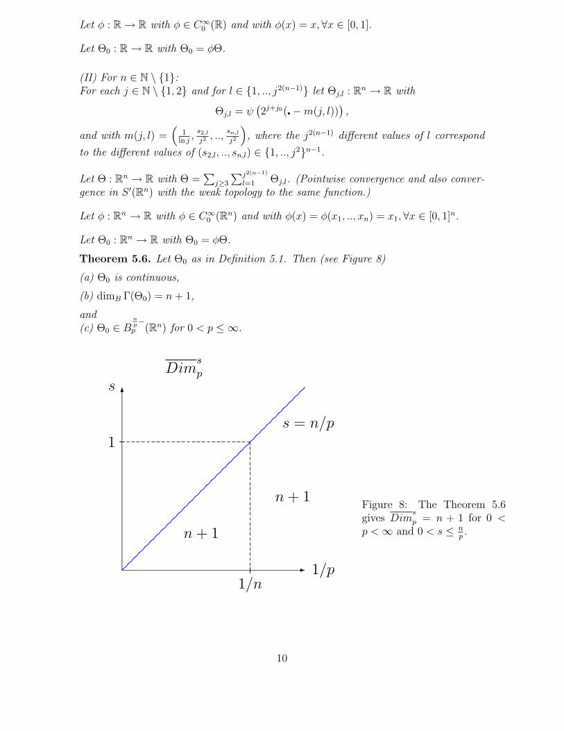
Theorem 5.6. Let Θ0 as in Definition 5.1. Then (see Figure 8)

(a) Θ0 is continuous,

(b) dimB Γ(Θ0) = n+ 1,

and(c) Θ0 ∈ B

np−

p (Rn) for 0 < p ≤ ∞.

1/n

1

Dims

p

s = n/p

n + 1

n + 1

1/p

s

1

Figure 8: The Theorem 5.6gives Dim

s

p = n + 1 for 0 <p <∞ and 0 < s ≤ n

p.

10

As mentioned in the Introduction, the Theorem 1.2 cannot be improved with the in-equality ≤. In the same way, only the part ≥ of the claimed Th. 4.2 of [2], p. 220is true. This follows by the Theorem 5.6 (or Theorem 5.8). The failure of part ≤ ofthis claim in [2], p. 220 comes from the false inequality (4.3) of [2], p. 219, whichoriginates the false inequality (4.1) of [2], p. 219. We can see in Remark 5.7 that (4.1)‖f‖V γ(R) ≤ c‖f‖Bγ

1,1(R) with 0 < γ < 1 of [2], p. 219 is false, even with the restriction of

f to the real functions of the C∞0 (R). Kamont and Wolnik in [6] constructed another

counterexample for this claim of [2], p. 220.

Remark 5.7. Let ϕ be as in Definition 2.5, and with supp(Fϕ) ⊂ ξ ∈ Rn : 1

2(1+a) ≤

|ξ| ≤ 2(1 − a) and (Fϕ)(ξ) = 1 if 1 − a ≤ |ξ| ≤ 1 + a, for some a > 0.

Let ψ : Rn → R with ψ ∈ S(Rn) \ 0 and supp(Fψ) ⊂ ξ ∈ R : 1 − a ≤ |ξ| ≤ 1 + a.

Furthermore, let φ : Rn → R with φ ∈ C∞

0 (Rn) and suppose that (φψ)(0, .., 0) 6= 0.

For each j ∈ N let ψj = ψ(2j) and φj = φψj.

Then for α ∈ R we have ‖φj‖V α(Rn) ≥ ‖φj‖L∞(Rn) ≥ c > 0.

Nevertheless, from the property F (Φ∗Ψ) = (2π)n2 (FΦ)(FΨ) in S ′(Rn) we have ϕj∗ψj =

(2π)n2ψj and then for 0 < p ≤ ∞, 0 < q ≤ ∞ and s ∈ R we have ‖ψj‖Bs

p,q(Rn) =

c2j(s−np). Hence by the Lemma 6.6 we have

‖φj‖Bsp,q(Rn) ≤ c2j(s−n

p).

Definition 5.2. Let ψ : Rn → R with ψ ∈ S(Rn) \ 0 and supp(Fψ) ⊂ ξ ∈ R

n :1 − a ≤ |ξ| ≤ 1 + a for a > 0 sufficiently small.

Let 0 < λ ≤ 1. For each j ∈ N \ 1, 2 let k(j) = [2j(1−λ)].

(I) For n = 1:For each j ∈ N\1, 2 and for k ∈ 1, .., k(j) let m(j, k) = 1

ln j−k2−j and Θj,k : R → R

withΘj,k = ψ

(

2j( −m(j, k)))

.

Let Θ : R → R with Θ =∑

j≥3

∑k(j)k=1 Θj,k. (Pointwise convergence and also convergence

in S ′(R) with the weak topology to the same function.)

Let φ : R → R with φ ∈ C∞0 (R) and with φ(x) = x,∀x ∈ [0, 1].

Let Θ0 : R → R with Θ0 = φΘ.

(II) For n ∈ N \ 1:

Let 0 ≤ h ≤ n−1. For each j ∈ N\1, 2 let d(j) =[

2j n−1−hn−1

]

. (Modification d(j) = j2

if h = n− 1.)

For each j ∈ N \ 1, 2, for k ∈ 1, .., k(j) and for l ∈ 1, .., d(j)n−1 let m(j, k, l) =( 1

ln j− k2−j,

s2,l

d(j), ..,

sn,l

d(j)), where for each fixed (j, k) the d(j)n−1 different values of l

correspond to the different values of (s2,l, .., sn,l) ∈ 1, .., d(j)n−1.

11

Let also Θj,k,l : R → R with

Θj,k,l = ψ(

2j( −m(j, k, l)))

.

Let Θ : Rn → R with Θ =

∑

j≥3

∑k(j)k=1

∑d(j)n−1

l=1 Θj,k,l. (Pointwise convergence and alsoconvergence in S ′(Rn) with the weak topology to the same function.)


0 (Rn) and with φ(x) = φ(x1, .., xn) = x1,∀x ∈ [0, 1]n.

Let Θ0 : Rn → R with Θ0 = φΘ.

Theorem 5.8. Let 0 ≤ h ≤ n− 1, 0 < λ ≤ 1 and Θ0 as in Definition 5.2. Then

(a) Θ0 is continuous,

(b) dimB Γ(Θ0) = n+ 1,

and

(c) Θ0 ∈ Bh+λ

p∗

p (Rn) for 0 < p ≤ ∞.

The Theorem 5.8 strengthens the Theorem 5.6. In fact, if in Definition 5.2 we addi-tionally impose ψ(0, .., 0) 6= 0, replace ψ by ψ(2j0) with j0 ∈ N large, take h = n− 1,λ = 1 and simplify 1

ln j− 2−j by 1

ln j, then we get the same Θ and Θ0 of the Definition

5.1.

In the following Definition 5.3, the function Λ0 materializes the minimal dimension for1 ≤ p < ∞ and 0 < s ≤ 1

p, given in Theorem 5.9. We can realize that the representa-

tion in wavelets, or even in quarks in the context of [11], is an excellent alternative toDefinitions 5.1, 5.2 and 5.3 in order to construct extremal functions. Such approach isgiven in [5], dealing with a multi-fractal analysis in wavelet expansions.

Definition 5.3. Let ψ : Rn → R with ψ ∈ S(Rn) \ 0 and supp(Fψ) ⊂ ξ ∈ R

n :1 − a ≤ |ξ| ≤ 1 + a for a > 0 sufficiently small.

Let 0 < λ ≤ 1. For each j ∈ N let k(j) = [(1 − 2−λ)2j(1−λ)].

In what follows, for λ = 1 we modify k(j) = 1 and replace 2−jλ − k2−j by 0 and 1j

by1j2 .

(I) For n = 1:For each j ∈ N and for k ∈ 1, .., k(j) let m(j, k) = 2−jλ − k2−j and Λj,k : R → R

with

Λj,k =1

jψ

(

2j( −m(j, k)))

.

Let Λ : R → R with Λ =∑

j≥1

∑k(j)k=1 Λj,k. (Pointwise convergence and also convergence

in S ′(R) with the weak topology to the same function.)

Let φ : R → R with φ ∈ C∞0 (R) and with φ(x) = 1,∀x ∈ [0, 1].

Let Λ0 : R → R with Λ0 = φΛ.

(II) For n ∈ N \ 1:

12

For each j ∈ N, for k ∈ 1, .., k(j) and for l ∈ 1, .., 2j(n−1) let m(j, k, l) =(

2−jλ − k2−j,s2,l

2j , ..,sn,l

2j

)

, where for each fixed (j, k) the 2j(n−1) different values of lcorrespond to the different values of (s2,l, .., sn,l) ∈ 1, .., 2jn−1.Let also Λj,k,l : R → R with

Λj,k,l =1

jψ

(

2j( −m(j, k, l)))

.

Let Λ : Rn → R with Λ =

∑

j≥1

∑k(j)k=1

∑2j(n−1)

l=1 Λj,k,l. (Pointwise convergence and alsoconvergence in S ′(Rn) with the weak topology to the same function.)


0 (Rn) and with φ(x) = 1,∀x ∈ [0, 1]n.

Let Λ0 : Rn → R with Λ0 = φΛ.

Theorem 5.9. Let 0 < λ ≤ 1 and Λ0 as in Definition 5.3. Then

(a) Λ0 is continuous,

(b) dimB Γ(Λ0) = n+ 1 − λ,

and

(c) Λ0 ∈ Bλp∗

p (Rn) for 0 < p ≤ ∞.

At this moment we are in a position to summarize the obtained results, in terms ofmaximal and minimal dimensions. The following Theorem is the main theorem of thispaper and makes exactly this.

Theorem 5.10. (Main Theorem)Let 0 0. Then we have (see Figures 9, 10 and 11)

(a) Dims

p = n+ 1 if 0 < s ≤ np,

(b) Dims

p = n+ 1 − min(1, s) if s > np,

and

(c) dims

p = n+ 1 − smax(1, p) if 0 < s ≤ 1max(1,p)

,

(d) dims

p = n if s ≥ 1max(1,p)

.

Proof. In Theorem 5.6 we proved (a). The argument in [13], p. 202-203 proves Theorem1.1 and also the relation fs ∈ Bs∗

p (Rn) for 0 0. Hence, by Corollary 5.2with n

γ+1 in place of p, and by Remark 5.5-(a) with 1 in place of p we have the equality

dimB Γ(fs) = n + 1 − min(1, s) for s > 0. Hence we have dims

p ≤ n + 1 − min(1, s) ≤

Dims

p for 0 0. By Corollary 5.2 we have also (b). It remains us toprove (c) and (d).

(i) Let 0 < p < ∞. By Corollary 5.4 and remark of Definition 3.2 we have dims

p ≥n + 1 − smax(1, p) for 0 < s ≤ 1

max(1,p). On the other hand the Theorem 5.9 gives

dims

p ≤ n+ 1 − sp for 0 < s ≤ 1p. Hence we have (c).

(ii) Let s > 1p, and let Λ0 as in Definition 5.3 if we take λ = 1 and multiply Λj,k and

13

Λj,k,l by the factor 2j( 1p−s). Then, of course Λ0 is continuous, and by the same proof

of Theorem 5.9-(c) we obtain Λ0 ∈ Bs∗p (Rn). By calculations like in the estimation of

∑′′′∗j in part (ii3) of the proof of Theorem 5.9-(b) we obtain dimB Γ(Λ0) = n. Hence

we have (d).

Remark 5.11. (a) As we can see in arguments in the proof of Theorem 5.10, thesupremum Dim

s

p is a maximum and the infimum dims

p is a minimum.

(b) If for taking the supremum and the infimum in Definition 3.3 we suppose f ∈Bs∗

p (Rn), then we have the same results of the Theorem 5.10 for Dims

p and dims

p, in-cluding part (a) of present remark. In fact, as we can see in the proof of Theorem, weneed only replace the Theorem 5.6 by the more general Theorem 5.8.

(c) We define Dimsp if for taking the supremum in Definition 3.3 we replace dimB

by dimB. As can be seen in the proof of Theorem 5.10, we have Dimsp = Dim

s

p for0 0. We have also the counterpart for parts (a) and (b) of presentremark.

(d) Although not proved in this paper, if in Definition 3.3 we relax the continuity in asubset of R

n of upper box dimension n−1 (for example a hyperplane), then we have thesame results of the Theorem 5.10 for Dim

s

p and dims

p, including the remaining previousparts of the present remark.

1/n

1

Dims

p

s = n/p

n + 1

n + 1

n + 1 − s

n

1/p

s

Figure 9: The Theorem 5.10gives the exact values ofDim

s

p for 0 0.

14

1

1

dims

p

s = 1/p

s = 1

n + 1 − sp

n + 1 − s

n

n n

1/p

s

Figure 10: The Theorem5.10 gives the exact valuesof dim

s

p for 0 0.

We also present an alternative graphical representation, to facilitate the interpretation.

np

1max(1,p)

1

dim(graphf)

0

n+1

n

s

Figure 11: Case np< 1.

The solid line representsDim

s

p and the dashed

line represents dims

p. Forthe case n

p> 1 the solid

line is simpler.

6 Proofs

Many of the proofs are outlined in order to save space and to focus in the main ideas.For details about results and proofs see [1]. In this reference we find also counterex-amples for situations to which we cannot extend the results presented here.

Definition 6.1. Let ν ∈ N0 and f be a continuous function. Then we define ϕ(ν, f) =Osc(ν,f)

2ν(n−1) and ϕ+(ν, f) = maxϕ(ν, f), 1.

15

Lemma 6.1. Let f be a function satisfying the condition (CCS). Then we have dimBΓ(f) =

n + limν→∞log2 ϕ+(ν,f)

ν. If ϕ is greater or equal to 1 for infinite many values of ν then

dimBΓ(f) = 1 + limν→∞log2 Osc(ν,f)

ν. (respectively ≥ for the general case.)

Proof of Lemma 6.1

We can assume Kf = [0, 1]n —see Section 1. Let N(ν, I, f) be the minimum numberof dyadic (n+1)-cubes required to cover the graph of f |I , where I ⊂ [0, 1]n is a n-cubewith volume |I| = 2−νn, as in Definition 3.1. Then we have 2−ν(N(ν, I, f) − 2) <oscI(f) ≤ 2−νN(ν, I, f).

By summing over all I ⊂ [0, 1]n we get 2−νN(ν, f)−2ν(n−1)2 < Osc(ν, f) ≤ 2−νN(ν, f),and by multiplying by 2−ν(n−1) we obtain 2−νnN(ν, f)−2 < ϕ(ν, f) ≤ 2−νnN(ν, f). Ofcourse we have also N(ν, f) ≥ 2νn, and therefore 2νnϕ+(ν, f) ≤ N(ν, f) < 2νn(ϕ(ν, f)+2). Hence we obtain

n+ log2 ϕ+(ν,f)ν

≤ log2 N(ν,f)ν

< n+ log2(ϕ(ν,f)+2)ν

≤ n+ log2(2ϕ+(ν,f))ν

.

Proof of Theorem 4.1

We prove two of the four implications, since the other two follow immediately.

(i) We use the inequality of Lemma 6.1. Let 0 < γ ≤ 1 and dimBΓ(f) ≤ n+ 1 − γ.

For every ε > 0, ∃νε ∈ N0 such that log2 Osc(ν,f)ν

≤ n− γ + ε,∀ν ≥ νε.So Osc(ν, f) ≤ 2ν(n−γ+ε),∀ν ≥ νε and then we have f ∈ V γ−ε(Rn).Hence

f ∈ V γ−(Rn).

(ii) We use the second equality of Lemma 6.1. Let 0 ≤ γ < 1 and dimBΓ(f) ≥ n+1−γ.

Then ∃(kν)ν∈N ⊂ N with limν→∞ kν = ∞ such that limν→∞log2 Osc(kν ,f)

kν≥ n− γ.

For every ε > 0, ∃νε ∈ N0 such that log2 Osc(kν ,f)kν

≥ n− γ − ε,∀ν ≥ νε.

So Osc(kν , f) ≥ 2kν(n−γ−ε),∀ν ≥ νε and then we have f 6∈ V γ+2ε(Rn).Hence

f ∈ V γ+(Rn).

Lemma 6.2. Let A be a compact subset of Rn and f, g : A→ R two continuous func-

tions. Hence we have oscA(fg) ≤ supA |f |oscA(g) + supA |g|oscA(f).


For all I as in Definition 3.1, the Lemma 6.2 gives oscI(ηf) ≤ c oscI(f)+sup |f |oscI(η).Let 0 < α ≤ 1. By summing over all I, multiplying by 2ν(α−n) and taking the supre-mum over all ν ∈ N0 we have ‖ηf‖V α(Rn) ≤ c‖f‖V α(Rn) + c′ sup |f | ≤ (c+ c′)‖f‖V α(Rn).Then the first equivalence of Theorem 4.1 gives the desired inequality.

Lemma 6.3. ([9], p. 19) For any h > 0 and k = (k1, .., kn) ∈ Zn, define Qh

k = x =(x1, .., xn) ∈ R

n with hkj ≤ xj < h(kj + 1) for j = 1, .., n. Let Ω ⊂ Rn be a compact

set and 0 < p ≤ ∞. Then, there exist three positive numbers h0, c1 and c2 such that

c1(∑

k∈Zn |ϕ(xk)|p) 1

p ≤ h−np ‖ϕ‖Lp(Rn) ≤ c2

(∑

k∈Zn |ϕ(xk)|p) 1

p

hold for all sets (xk)k∈Zn with xk ∈ Qhk, all h with 0 < h < h0, and all ϕ ∈ SΩ(Rn).

(Modification if p = ∞).

16

Lemma 6.4. ([9], p. 22) Let Ω ⊂ Rn be a compact set. Let 0 < p ≤ q ≤ ∞ and

α ∈ (N0)n a multi-index. Then there exists a positive constant c such that for all

f ∈ LΩp (Rn) we have

‖Dαf‖Lp(Rn) ≤ c‖f‖Lp(Rn).

Lemma 6.5. ([9], p. 129) Let 0 < p0 ≤ p1 ≤ ∞, 0 < q ≤ ∞ and −∞ < s1 ≤ s0 <∞.If s0 −

np0

= s1 −np1

then we have the embedding

Bs0p0,q(R

n) → Bs1p1,q(R

n).

Lemma 6.6. ([9], p. 195) Let ϕ ∈ C∞0 (Rn). Let 0 < p0 ≤ p1 ≤ ∞, 0 < q ≤ ∞

and s ∈ R. Then f 7→ ϕf yields a continuous linear mapping from Bsp1,q(R

n) intoBs

p0,q(Rn).

Definition 6.2. If G ⊂ Rn is a bounded set we define SG(Rn) = ψ ∈ S(Rn) with

supp(Fψ) ⊂ G and LGp (Rn) = f ∈ Lp(R

n) with supp(Ff) ⊂ G for 0 < p ≤ ∞.

Lemma 6.7. Let 0 < p <∞ and consider G,A ⊂ Rn be non-empty bounded sets, with

G open. Then SG(Rn) is dense in LGp (Rn) with the norm ‖ ‖Lp(Rn) + supA | |.

Proof of Lemma 6.7

Consider f ∈ LGp (Rn). Let ζ ∈ S(Rn) with ζ(0) = 1, |ζ(x)| ≤ 1,∀x ∈ R

n and withsupp(Fζ) compact. It is easy to find such a ζ, because a translation of ζ and a multi-plication by a scalar k ∈ C \ 0 preserves supp(Fζ).

For all k ∈ N let ψk(x) = f(x)ζ(x/k),∀x ∈ Rn. Then by the Paley-Wiener-Schwartz

theorems ([9], p. 13) we have ψk ∈ S(Rn),∀k ∈ N. Because G is open, for k sufficientlylarge we have ψk ∈ SG(Rn). Let ε > 0 and Mε > 0 with

∫

|t|≥Mε|f(t)|pdt ≤ 1

2( ε

2)p.

Let kε ∈ N with |ζ(x/k) − 1|p ≤ εp/21+

|t|≤Mε

|f(t)|pdtfor all x ∈ R

n with |x| ≤ Mε or

x ∈ A, and for all k ≥ kε. We observe that by the Paley-Wiener-Schwartz theorem([9], p. 13) we have f bounded on A. Hence supA |ψk − f | ≤ ε supA |f |,∀k ≥ kε and‖ψk − f‖Lp(Rn) ≤ ε.

Lemma 6.8. Let I be a n-cube as in Definition 3.1 and ϕj as in Definition 2.5 for allj ∈ N0. Let f : R

n → R be a continuous function with f ∈ S ′(Rn). Then we have

(2π)n2 oscI(f) ≤

∑

j≥0

oscIRe(ϕj ∗ f).

Proof of Lemma 6.8

We make only a layout of the proof. For all k ∈ N let fk =∑k

j=0 ϕj ∗ f , hk =∑k

j=0 supI Re(ϕj ∗ f) and h′k =∑k

j=0 infI Re(ϕj ∗ f).

Let ε > 0. Then, by the convergence limk→∞ fk = (2π)n2 f with the weak topology in

S ′(Rn), we deduce that ∃kε ∈ N such that we have (2π)n2 supI f ≤ hk + ε,∀k ≥ kε. By

this formula and the counterpart (2π)n2 infI f ≥ h′k − ε,∀k ≥ k′ε for some k′ε ∈ N, we

have the desired inequality.

17

By [9], p. 131 we have f continuous. Let 0 < p ≤ 1. Then γ ≥ 1 and by the Lemma6.5 we have also ‖f‖

Bγ+n−n

p1,1 (Rn)

≤ c‖f‖Bγp,1(Rn). Because γ + n− n

p≥ n

1we can assume

1 ≤ p <∞.

(i) Let j ∈ N0 and ν ∈ N0. Let Gj = ξ ∈ Rn : |ξ| < 2j+2 and ψj ∈ SGj(Rn). Let

|I| = 2−νn, I as in Definition 3.1.

Let∑′ and

∑′j be the sums over the cubes I restricted to the cube [−m,m]n and[−m2j,m2j]n, respectively.

(i1) Let ν ≤ j. We haveoscI(Reψj) ≤ 2 sup

I|ψj|.

Let j0 ∈ N0. By Holder’s inequality and because ν ≤ j we have

′∑

|I|=2−νn

supI

|ψj| ≤ (2ν2m)n p−1p

′∑

|I|=2−νn

supI

|ψj|p

1p

≤ cm2νn p−1p

′j∑

|I|=2−j0n

supI

∣

∣ψj(2−j

)∣

∣

p

1p

.

Taking j0 sufficiently large then by the Lemma 6.3 the factor ()1p can be estimated

from above by

c2j0n

p ‖ψj(2−j

)‖Lp(Rn) = c′2j np ‖ψj‖Lp(Rn).

Because ν ≤ j and γ ≥ np

we have

νγ + (j − ν)n

p≤ jγ.

Then we have2ν(γ−n)

∑′|I|=2−νn oscI(Reψj) ≤ cm2jγ‖ψj‖Lp(Rn).

(i2) Let ν ≥ j. We have by the mean value Theorem

oscI(Reψj) ≤ 2−ν

n∑

i=1

supI

∣

∣

∣

∣

∂

∂xi

Reψj

∣

∣

∣

∣

.

Let i ∈ 1, .., n. By Holder’s inequality we have

′∑

|I|=2−νn

supI

∣

∣

∣

∣

∂

∂xi

Reψj

∣

∣

∣

∣

≤ (2ν2m)n p−1p

′∑

|I|=2−νn

supI

∣

∣

∣

∣

∂

∂xi

ψj

∣

∣

∣

∣

p

1p

.

Let ν0 ∈ N0. Because ν ≥ j the last sum can be estimated from above by∑′j

|I|=2−(ν+ν0−j)n supI

∣

∣

∣( ∂∂xiψj)(2

−j)∣

∣

∣

p

.

Taking ν0 sufficiently large then by the Lemma 6.3 the factor ()1p can be estimated

from above by

c2(ν+ν0−j) np

∥

∥

∥

∥

(

∂

∂xi

ψj

)

(2−j)

∥

∥

∥

∥

Lp(Rn)

.

18

By the Lemma 6.4 this last norm can be estimated from above by

c‖2jψj(2−j

)‖Lp(Rn) = c2j2j np ‖ψj‖Lp(Rn).

Because ν ≥ j we have

νmin(1, γ) − ν + j ≤ jmin(1, γ).

Then we obtain2ν(min(1,γ)−n)

∑′|I|=2−νn oscI(Reψj) ≤ cm2j min(1,γ)‖ψj‖Lp(Rn).

(ii) Let ν ∈ N0, j ∈ N0 and ϕj as in Definition 2.5.

We have ϕj ∗ f ∈ LGjp (Rn). Therefore, by (i) and Lemma 6.7 we have

2ν(min(1,γ)−n)

′∑

|I|=2−νn

oscIRe(ϕj ∗ f) ≤ cm2jγ‖ϕj ∗ f‖Lp(Rn).

(iii) Let ν ∈ N0. By Lemma 6.8 we have

2ν(min(1,γ)−n)

′∑

|I|=2−νn

oscIf ≤ cm‖f‖Bγp,1(Rn).

Of course, we may replace in the obtained inequality∑′ by

∑

. Then by taking thesupν≥0 on the left hand side we have the desired inequality.

Proof of Corollary 5.2

We have f ∈⋂

np≤σ<γ B

σp,1(R

n) and by Theorem 5.1 we have f ∈ V min(1,γ)−(Rn)

in case 0 0 and x ∈ Rn. Then we define Bρx = t ∈ R

n : |t− x| ≤ ρ,the closed ball centered in x and with radius ρ.

Definition 6.4. Let f : Rn → R be a measurable and bounded function with a compact

support. Let 0 < ε < 1, j ∈ N and ϕj as in Definition 2.5.

(i) We define

(ϕj ∗ ∗f)(x) =

∫

|t|≤2−j+[jε]

ϕj(t)f(x− t)dt,∀x ∈ Rn.

(ii)

(ii1) We define (∏n

i=1[ai, ai + 2−j])#

=∏n

i=1[ai − 2−j+[jε], ai + 2−j + 2−j+[jε]], whereai ∈ R,∀i = 1, .., n.

(ii2) Let |I| = 2−jn, I be as in Definition 3.1. We define fI(x) = f(x)− 1|I#|

∫

I# f(t)dt,∀x ∈

19

Rn.

(ii3) Let |I| = 2−jn, I be as in Definition 3.1, and Io be the interior of I. We definealmost everywhere

(ϕj ∗ ∗ ∗ f)(x) =

∫

|t|≤2−j+[jε]

ϕj(t)fI(x− t)dt,∀x ∈ Io.

Remark:(a) We have

∫

I# fI(t)dt = 0.

(b) For j ∈ N we have ϕj ∗ ∗f continuous and ϕj ∗ ∗ ∗ f continuous almost everywhere.

Lemma 6.9. Let f : Rn → R be a measurable and bounded function with a compact

support. Let 0 < p ≤ ∞, 0 < q ≤ ∞ and s ∈ R. Let j0 ∈ N and 0 < ε < 1. Then wehave the equivalences

f ∈ Bsp,q(R

n) ⇐⇒∑

j≥j0

(

2js‖ϕj ∗ ∗f‖Lp(Rn)

)q<∞ ⇐⇒

∑

j≥j0

(

2js‖ϕj ∗ ∗ ∗ f‖Lp(Rn)

)q<∞.


Proof of Lemma 6.9

Let R,L > 0 such that supp f ⊂ BR(0, .., 0) and sup |f | ≤ L. Let ϕ and ϕj as inDefinition 2.5 for all j ∈ N0. By the Paley-Wiener-Schwartz theorems ([9], p. 13) wehave ϕj ∗ f ∈ S(Rn),∀j ∈ N0 and then ‖ϕj ∗ f‖Lp(Rn) <∞,∀j ∈ N0.

Consider k > 0. Then we have |x|k|ϕ(x)| ≤ ck,∀x ∈ Rn. Let j ∈ N sufficiently large.

(i) Let x ∈ Rn. We have (ϕj ∗ ∗f)(x) = 0 for |x| ≥ R+ 1

2and (ϕj ∗ ∗ ∗ f)(x) = 0 for

|x| ≥ R + 2.

(ii) For all x ∈ Rn with |x| ≥ R + 1 we have |(ϕj ∗ f)(x)| ≤ ck,R,L2j(n−k)|x|−k.

(iii) Let k ≥ n+1 and x ∈ Rn. Then we have |(ϕj ∗ ∗f)(x) − (ϕj ∗ f)(x)| ≤ ck,L2j ε

2(n−k).

(iv) Let k ≥ n+ 1 and x ∈ Rn. Then we have

|(ϕj ∗ ∗ ∗ f)(x) − (ϕj ∗ ∗f)(x)| ≤∣

∣

∣

∫

|t|≤2−j+[jε] Lϕj(t)dt∣

∣

∣ = L∣

∣

∣

∫

|t|≥2−j+[jε] ϕj(t)dt∣

∣

∣ ≤

≤ L∫

|t|≥2−j+[jε] |ϕj(t)|dt ≤ L∫

|t|≥2−j+j ε2|ϕj(t)|dt ≤ L

∫

|t|≥2j ε2|ϕ(t)|dt ≤ ckL

∫

|t|≥2j ε2|t|−kdt =

= ck,L2j ε2(n−k)

∫

|t|≥1|t|−kdt ≤ c′k,L2j ε

2(n−k).

(v) Then by (i)-(iv), if we take k ≥ n+ 1 sufficiently large we have the desired equiva-lences.


Of course f is bounded and measurable, and then f ∈ S ′(Rn). Let R,L > 0 such thatsupp f ⊂ BR(0, .., 0) and sup |f | ≤ L. Let 0 < ε < 1. We make use of the Lemma 6.9.

(i) Let 0 < p ≤ 1 and j ∈ N.

20

By Holder’s inequality we have

∫

|x|≤R+1

|(ϕj ∗ ∗f)(x)|pdx ≤

(∫

|x|≤R+1

(|(ϕj ∗ ∗f)(x)|p)1p

)p (∫

|x|≤R+1

11

1−p

)1−p

.

Then we obtain‖ϕj ∗ ∗f‖Lp(Rn) ≤ cR‖ϕj ∗ ∗f‖L1(Rn).

Hence we may assume 1 ≤ p <∞.

(ii) Let 1 ≤ p <∞ and j ∈ N sufficiently large. Let |I| = 2−jn, I as in Definition 3.1.Then for x ∈ I we have

|(ϕj ∗ ∗ ∗ f)(x)| ≤

∫

|t|≤2−j+[jε]

|ϕj(t)fI(x− t)|dt ≤ c2jn2(−j+[jε])n supI#

|fI | ≤ c2jεn supI#

|fI |.

Therefore we obtainsup

I|ϕj ∗ ∗ ∗ f | ≤ c2jεn sup

I#

|fI |.

By the remark (a) of Definition 6.4 we have supI# fI infI# fI ≤ 0, and thereforesupI# |fI | ≤ supI# fI − infI# fI . The right hand side of last inequality can be esti-mated from above by

∑

I′ oscI′(fI) =∑

I′ oscI′(f), where the last two sums are takenover all (1 + 2[jε]2)n n-cubes I ′ ⊂ I#, |I ′| = 2−jn, I ′ as in Definition 3.1.

Hence

‖ϕj ∗ ∗ ∗ f‖Lp(Rn) ≤(

∑

|I|=2−jn |I| supI |ϕj ∗ ∗ ∗ f |p) 1

p

≤

≤ c2−j np

(

∑

|I|=2−jn (2jεn∑

I′ oscI′(f))p) 1

p

≤

≤ c2jεn2−j np

(

∑

|I|=2−jn(1 + 2[jε]2)np∑

I′(oscI′(f))p) 1

p

.

This value can be estimated from above by

c2j2εn2−j np

(

∑

|I|=2−jn

∑

I′(oscI′(f))p) 1

p

≤ cL2j2εn2−j np

(

∑

|I|=2−jn

∑

I′ oscI′(f)) 1

p

≤

≤ cL2j2εn2−j np

(

(1 + 2[jε]2)nOsc(j, f))

1p ≤ c′L2j2εn2j εn

p 2−j npOsc(j, f)

1p .

Because f ∈ V γ′p this value can be estimated from above by

cL2j3εn2−j np (c2j(n−γ′p))

1p = c′L2j3εn2−jγ′

.

Then by taking ε > 0 sufficiently small we get

2jγ‖ϕj ∗ ∗ ∗ f‖Lp(Rn] ≤ cL.

Lemma 6.10. Let r > 1. Then by the mean value Theorem, for some c ∈ (r, r + 1)

we have∣

∣

∣

1ln(r+1)

− 1ln r

∣

∣

∣= 1

c ln2 c≥ 1

(r+1) ln2(r+1). Hence for m ∈ N with m ≥ 2 we obtain

∑mj=2

1

2j| 1ln(m+1)

− 1ln j |

≤∑

j≥21

2j| 1ln(j+1)

− 1ln j |

≤∑

j≥2(j+1) ln2(j+1)

2j <∞.

21

We will restrict us to the case n = 1. For n ∈ N \ 1 the proof is analogous, althoughwith more fastidious calculus. In corresponding parts (i) and (ii) we use essentially thefact that the case n = 1 remains valid if we replace Θ by Θ(, x2, .., xn), for all (somein ii-case) fixed points (x2, .., xn) ∈ R

n−1.

(i) We prove that Θ is bounded on R and continuous on R \ 0:We have |xψ(x)| ≤ c,∀x ∈ R.

(i1) Let x ≤ 0 and j1 ∈ N \ 1, 2.

Then∑

j≥j1|Θj(x)| =

∑

j≥j1

∣

∣

∣ψ

(

2j+j0

(

x− 1ln j

))∣

∣

∣≤

∑

j≥j1c

2j+j0|x− 1ln j |

≤∑

j≥j1c′2−j ln j.

Hence∑

j≥j1Θj is bounded on (−∞, 0] and converges uniformly on (−∞, 0].

In particular Θ is continuous on (−∞, 0).

(i2) Let j1 ∈ N \ 1, 2.Let x ≥ 1

ln j1.

Then∑

j≥j1+1 |Θj(x)| =∑

j≥j1+1

∣

∣

∣ψ

(

2j+j0

(

x− 1ln j

))∣

∣

∣≤

∑

j≥j1+1c

2j+j0|x− 1ln j |

≤ cj1∑

j≥j1+1 2−j.

Hence∑

j≥3 Θj converges uniformly on[

1ln j1

,∞)

.

In particular Θ is continuous on (0,∞).

(i3) Let x > 0.Let j(x) = minj ∈ N \ 1, 2 with x ≥ 1

ln j.

We have∑

j≥3 |Θj(x)| ≤ 2 sup |ψ| +∑j(x)−2

j=3 |Θj(x)| +∑

j≥j(x)+1 |Θj(x)| ≤

≤ 2 sup |ψ| +∑j(x)−2

j=3c

2j+j0| 1ln(j(x)−1)

− 1ln j |

+∑

j≥j(x)+1c

2j+j0| 1ln j(x)

− 1ln j |

.

The second sum on the right hand side can be estimated from above by 2−j(x)

1ln j(x)

− 1ln(j(x)+1)

∑

j≥1c

2j+j0,

and the factor before the sum tends to 0 when x→ 0+.

On the other hand by the Lemma 6.10 we have∑j(x)−2

j=31

2j| 1ln(j(x)−1)

− 1ln j |

≤ c <∞.

Hence we have∑

j≥3 |Θj(x)| ≤ 2 sup |ψ| + c2−j0 ,∀x > 0.

Therefore Θ is bounded on (0,∞).

(ii) We may assume ψ(0) = 18. For the general case, in what follows we need only tochange some constants by the factor ψ(0)/18 6= 0.

Let j1 ∈ N \ 1, 2 and j0 sufficiently large.

We have Θ(

1ln j1

)

= Θj1

(

1ln j1

)

+∑

j≥3∧j 6=j1Θj

(

1ln j1

)

≥ ψ(0)−∑

j≥3∧j 6=j1

∣

∣

∣Θj

(

1ln j1

)∣

∣

∣.

By calculations like (i3) the last sum can be evaluated from above by c2−j0 ≤ 1. Then

Θ(

1ln j1

)

≥ 17.

Also by calculations like in (i3) we have Θ

(

1ln j1

+ 1ln(j1+1)

2

)

≤ c2−j0 ≤ 1.

22

Therefore

supx,y∈ 1

ln(j1+1), 1ln j1

|Θ0(x) − Θ0(y)| ≥17

ln j1−

1

ln j1=

24

ln j1.

Let 0 < ε < 1.

For every ν ∈ N0 let k(ν) = [2ν(1−ε)]. Then k(ν) ≥ 122ν(1−ε),∀ν ∈ N0.

Let ν0 ∈ N0 such that 2e−2νε

2ν(1−2ε) ≤ 1,∀ν ≥ ν0.

Then∣

∣

∣

(

1ln t

)′∣

∣

∣1 ≤ 1

22−ν if 1

ln t≤ k(ν)2−ν with t ≥ 3 and ν ≥ ν0.

Here ()′ represents the derivative operator.

Let ν1 ≥ ν0 with k(ν1)2−ν1 ≤ 1

ln 3. If ν ≥ ν1 then for every k ∈ 1, .., k(ν) there exists

jν,k ∈ N \ 1, 2 such that

1

ln jν,k

,1

ln(jν,k + 1)

⊂[

(k − 1)2−ν , k2−ν]

.

Hence

osc[(k−1)2−ν ,k2−ν ](Θ0) ≥24

ln jν,k

≥ 24(k − 1)2−ν ,∀k ∈ 1, .., k(ν),∀ν ≥ ν1.

Let I as in Definition 3.1. We have

Osc(ν,Θ0) ≥

k(ν)∑

k=1

24(k − 1)2−ν ,∀ν ≥ ν1.

Then Osc(ν,Θ0) ≥ 24 (k(ν)−1)k(ν)2

2−ν ,∀ν ≥ ν1.

For ν ≥ ν2 with ν2 ≥ ν1 sufficiently large we have

Osc(ν,Θ0) ≥ 22(k(ν))22−ν ≥ 2ν(1−2ε).

Hence if we take 0 < 2ε < 1 and use the lower counterpart of the second equality ofthe Lemma 6.1 (see Remark 4.3) then we have dimBΓ(Θ0) ≥ 2 − 2ε. Hence we obtaindimB Γ(Θ0) = 2.

(iii) Here we choose a > 0. Let ϕ be as in Definition 2.5, and with supp(Fϕ) ⊂ ξ ∈R

n : 12(1 + a) ≤ |ξ| ≤ 2(1− a) and (Fϕ)(ξ) = 1 if 1− a ≤ |ξ| ≤ 1 + a, for some a > 0.

Let s < 1p

and 0 < q ≤ ∞. In the next first equality we make use of the continuity (see

[7], p. 18) of the convolution operator in S ′(R).We have

∑

j≥0

(

2js‖ϕj ∗ Θ‖Lp(R)

)q= (2π)

n2

∑

j≥3

(

2(j+j0)s‖Θj‖Lp(R)

)q=

= (2π)n2

∑

j≥3

(

2(j+j0)s2−(j+j0)1p‖ψ‖Lp(R)

)q

= c∑

j≥3 2(j+j0)(s− 1p)q < ∞. (Standard

modification if p, q = ∞.)

Hence we have Θ ∈ Bsp,q(R). By the Lemma 6.6 we have also Θ0 ∈ Bs

p,q(R).


23

The proof is similar to the one of the Theorem 5.6, although more complicated. Wemake a layout for the part (c). We need modification if h = n−1 in the case n ∈ N\1.

We choose a > 0. Let ϕ be as in Definition 2.5, and with supp(Fϕ) ⊂ ξ ∈ Rn :

12(1 + 2a) ≤ |ξ| ≤ 2(1− 2a) and (Fϕ)(ξ) = 1 if 1− 2a ≤ |ξ| ≤ 1 + 2a, for some a > 0.

(i) For n = 1, 0 < q ≤ ∞ and s ∈ R we have the equivalence

Θ ∈ Bsp,q(R) ⇐⇒

∑

j≥3

(

2js∥

∥

∥φ

∑k(j)k=1 Θj,k

∥

∥

∥

Lp(R)

)q

<∞.


On the other hand we have (each ≈j is valid if j is sufficiently large)∥

∥

∥φ

∑k(j)k=1 Θj,k

∥

∥

∥

Lp(R)≈j

(

1(ln j)pk(j)2

−j) 1

p

≈j1

ln j2−j λ

p .

(ii) For n ∈ N \ 1, 0 < q ≤ ∞ and s ∈ R and we have the equivalence

Θ ∈ Bsp,q(R

n) ⇐⇒∑

j≥3

(

2js∥

∥

∥φ

∑k(j)k=1

∑d(j)n−1

l=1 Θj,k,l

∥

∥

∥

Lp(Rn)

)q

<∞.


On the other hand we have (if j is sufficiently large)∥

∥

∥φ∑k(j)

k=1

∑d(j)n−1

l=1 Θj,k,l

∥

∥

∥

Lp(Rn)≈j

(

1(ln j)pk(j)d(j)

n−12−jn) 1

p

≈j1

ln j2−j h+λ

p .


We will restrict us to the case n = 1. For n ∈ N \ 1 the proof is analogous, al-though with calculations slightly more complicated. In corresponding parts (i) and(ii) we use essentially the fact that the case n = 1 remains valid if we replace Λ byΛ(, x2, .., xn), for fixed (x2, .., xn) ∈ R

n−1. For the convenience of the presentation weassume 0 < λ < 1, however the case λ = 1 can be dealt easily. Moreover, the proof ofparts (a) and (c) are similar to the corresponding ones in the proof of Theorem 5.8.

We observe that 2−(j+1)λ ≤ 2−jλ − k2−j ≤ 2−jλ − 2−j,∀k = 1, .., k(j), for all j ∈ N. Wemake use of the estimation |x|m|ψ(x)| ≤ cm for all m ∈ N0.

(i) We have uniform convergence of the series Λ =∑

j≥1

∑k(j)k=1 Λj,k in all R. Then Λ is

bounded and continuous.

(i1) In fact, with the same techniques used in part (i1) of the proof of Theorem 5.6,

we can show the uniform convergence of∑

j≥1

∑k(j)k=1 |Λj,k| on (−∞, 0].

(i2) Also, with the same techniques used in parts (i2) and (i3) of the proof of Theorem

5.6, we can show the uniform convergence of∑

j≥1

∑k(j)k=1 |Λj,k| on (0,∞).

(ii) Let us prove the part (b) for n = 1 and 0 < λ < 1. Let j ∈ N, ρ ≥ 0 andCρ = t ∈ R : |t| ≥ ρ. We define

∑ρj as a general sum over all intervals I ∩ Cρ with

I as in Definition 3.1 and |I| = 2−j. Then, for r ∈ N0 and ρ ≥ 0, there is a positiveconstant cr independent of j and ρ such that

24

ρr

ρ∑

j

osc(ψ) ≤ cr. (1)

Here we consider 00 = 1. In order to prove (1), we notice that the sum of the left handside can be estimated from above by ρr

∑ρj sup |ψ′|2−j ≤ 2−j

∑

|I|=2−j supI |trψ′(t)| ≤

2−j∑

τ≥1 gr(τ2−j), where gr(t) = crtr

1+tr+2 ,∀t ≥ 0. Let mr ∈ N such that gr is de-

creasing on [mr,∞). Then ρr∑ρ

j osc(ψ) ≤ 2−j∑2jmr

τ=1 sup gr + 2−j∑

τ>2jmrgr(τ2

−j) ≤

cr +∫ ∞

mrgr(t)dt = c′r, which proves (1).

We define Cρ,u,v = t ∈ R : |t − m(u, v)| ≥ ρ and Sρ,u,vj,u,v =

∑ρ,u,vj osc(Λu,v),∀u ∈

N,∀v ∈ 1, .., k(u), where the sum∑ρ,u,v

j is taken over all intervals I ∩ Cρ,u,v with I

as in Definition 3.1 and |I| = 2−j. Then by formula (1) there is a positive constant cr

independent of j, ρ, u and v such that

(2uρ)rSρ,u,vj,u,v ≤ cr. (2)

Let Sj,u,v =∑

|I|=2−j oscI(Λu,v),∀u ∈ N,∀v ∈ 1, .., k(u). Of course we have

∑

|I|=2−j

oscI(Λ) ≤∑

u≥1

k(u)∑

v=1

Sj,u,v. (3)

Let∑′

j,∑′′

j and∑′′′

j be general sums over all intervals I∩C with I as in Definition 3.1

and |I| = 2−j, where C represents the set (−∞, 0], [0, 2−jλ] and [2−jλ,∞), respectively.

(ii1) By formula (2) and calculations like in (i1) for x ≤ 0, but with S|x−m(u,v)|,u,vj,u,v in

place of |Λu,v(x)|, we have the inequality∑

u≥1

∑k(u)v=1 S

′j,u,v ≤ c, where by definition

S ′j,u,v is obtained from Sj,u,v by replacing

∑

|I|=2−j by∑′

j. Therefore, by the obvious

counterpart of formula (3) for∑′

j, we have the estimation∑′

j osc(Λ) ≤ c.

(ii2) Because Λ is bounded, we have the estimation∑′′

j osc(Λ) ≤ c2j(1−λ).

(ii3) Also as counterpart of formula (3) we have the inequality∑′′′

j osc(Λ) ≤∑

u≥1

∑k(u)v=1 S

′′′j,u,v,

where by definition S ′′′j,u,v is obtained from Sj,u,v by replacing

∑

|I|=2−j by∑′′′

j .

We denote by∑′′′∗

j or∑′′′∗∗

j the right hand side of the this inequality, if we make therestriction 1 ≤ u ≤ j or u > j, respectively. Then, by formula (2) and calculations like

in (i2) for x ≥ 2−jλ, but with S|x−m(u,v)|,u,vj,u,v in place of |Λu,v(x)|, we have the estimation

∑′′′∗∗j ≤ c.

On the other hand, as a particular case of formula (1) with 0 in place of ρ and r, wehave

∑

|I|=2−j oscI(ψ) ≤ c, where c is independent of j. Then we have the inequality∑′′′∗

j ≤∑j

u=1 k(u)c ≤ c′2j(1−λ), and therefore the estimation∑′′′

j osc(Λ) ≤ c2j(1−λ).

(ii4) Hence by (ii1), (ii2) and (ii3) we obtain Osc(ν,Λ) ≤ c2j(1−λ). Then Λ ∈ V λ(R)and by the proof of Theorem 4.2 we have also Λ0 ∈ V λ(R), so Theorem 4.1 givesdimBΓ(Λ0) ≤ 2 − λ.

(ii5) Finally, with the same argument given for the proof of part (c) we have also

25

Λ0 ∈ Bλp∗

p (Rn) for 0 < p ≤ ∞. Hence Remark 5.5-(a) with 1 in place of p givesdimBΓ(Λ0) ≥ 2 − λ. Therefore we have dimB Γ(Λ0) = 2 − λ.

References

[1] Carvalho, A. (2004). “Box dimension and smoothness in function spaces”,preprint.

[2] Deliu, A. and Jawerth, B. (1992). “Geometrical dimension versus smoothness”.Constr. Approx. 8, 211-222.

[3] Falconer, K. (1990). Fractal Geometry, John Wiley, Chichester.

[4] Jaffard, S. (1998). “Oscillation spaces: Properties and applications to fractal andmultifractal functions”. J. Math. Phys. 39, 4129-4141.

[5] Jaffard, S. (2001). “Wavelet expansions, function spaces and multifractal analy-sis”. Math. Phys. Chem. 33, 127-144.

[6] Kamont, A. and Wolnik, B. (1999). “Wavelet expansions and fractal dimension”.Constr. Approx. 15, 97-108.

[7] Khoan, V. (1972), Distributions, Analyse de Fourier, Operateurs aux Derivees Partielles,tome 2, Librairie Vuibert, Paris.

[8] Solomyak, M. (1996). “Piecewise-polynomial approximation of functions fromSobolev spaces, revisited”. M University. Discourses Math. Appl. 3, 7-27.

[9] Triebel, H. (1983). Theory of Function Spaces, Birkhauser, Basel.

[10] Triebel, H. (1997). Fractals and Spectra, Birkhauser, Basel.

[11] Triebel, H. (2001). The structure of functions, Birkhauser, Basel.

[12] Triebel, H. (2003). “Fractal characteristics of measures; an approach via functionspaces”. Journ. Fourier Anal. Appl. 9, 411-430.

[13] Triebel, H. (2004). “A note on wavelet bases in function spaces”. Orlicz CentenaryVol. Banach Center Publ. 64, 193-205.

26

Box dimension, oscillation and smoothness in function spaces

Documents

Transcript of Box dimension, oscillation and smoothness in function spaces