PA

Mpre

pri

nt.

Collectio

n:

Card

ernos

de

Mate

matica

-Ser

iede

Inve

stig

aca

oC

M06/I-

3In

stit

utio

n:

Univ

ersi

tyofA

veiro

(subm

itted

January

2,2006)

http://pam.pisharp.org/handle/2052/114

Local growth envelopes of Triebel-Lizorkin spaces of

generalized smoothness

Antonio M. Caetano∗

andHans-Gerd Leopold∗∗

2nd January 2006

Abstract

The concept of local growth envelope (ELGA, u) of the quasi-normedfunction space A is applied to the Triebel-Lizorkin spaces of general-ized smoothness F σ,N

p,q (Rn). In order to achieve this, a standardizationresult for these and corresponding Besov spaces is derived.

Keywords: function space, generalized smoothness, growth envelope2000 Mathematics Subject Classification: 46E35

Acknowledgement. This research was partially supported by a projectunder the agreement GRICES/DAAD. Also partially supported by Unidadede Investigacao Matematica e Aplicacoes of Universidade de Aveiro throughPrograma Operacional “Ciencia, Tecnologia, Inovacao” (POCTI) of theFundacao para a Ciencia e a Tecnologia (FCT), co-financed by the EuropeanCommunity fund FEDER.

1 Introduction

In recent years there has been a lot of work on the determination of thelocal growth envelopes of function spaces of the Besov and Triebel-Lizorkintype (see [17, 27, 5, 4, 2, 3]). These results can be seen as refinements ofthe famous Sobolev embedding theorem, being related also with the populartopic of searching for sharp embeddings between classes of function spaces(see, for example, [12, 13, 23, 15, 11, 14, 16]). In any case, local growth

∗Departamento de Matematica, Universidade de Aveiro, 3810-193 Aveiro, Portugal,acaetano@mat.ua.pt∗∗Mathematisches Institut, Friedrich-Schiller Universitat Jena, D-07737 Jena, Germany

leopold@minet.uni-jena.de

1

http://pam.pisharp.org/handle/2052/114

envelopes identify the greatest possible growth which functions from somegiven space can stand locally, so they are useful in distinguishing betweenspaces and have even been used (together with the related concept of conti-nuity envelope) in the proof of the necessity of conditions giving continuousembeddings between spaces.

As the scale of spaces of Besov and Triebel-Lizorkin type comprises nowa-days generalized versions, in various directions, which are proving useful inother areas of mathematics (see, for example, [8, 7, 24]), the question nat-urally arises about how the corresponding growth envelopes look like. Forone of such generalizations, in the direction of the so-called spaces of gen-eralized smoothness, there is now, after the work [10], and its forerunner[9], a common framework for several approaches to generalized smoothnessscattered in the literature (see the mentioned work for references, and alsobelow for additional remarks). Also, the techniques developed in [10] (andin [9]), namely atomic representations, made a broad class of such spaces tobecome suitable for the investigation of the corresponding growth envelopes.

Accordingly, and by improving techniques used in the determinationof the local growth envelopes of spaces which partially generalize in thedirection of generalized smoothness, it was finally possible in [3] to solvethe problem (apart some borderline cases) for Besov spaces of generalizedsmoothness in the broad sense of [9] and whenever atomic decompositionsare available. Relying on the idea used in previous partial works, Triebel-Lizorkin spaces should then be dealt with on the basis of a comparisonwith Besov spaces. However, at the time the work [9] was written, such acomparison for such general spaces was not available.

In the present work we start by developing a so-called standardizationprocedure, which will allow the determination of tight embeddings betweenBesov and Triebel-Lizorkin spaces of generalized smoothness and open theway to the determination (again, apart borderline cases) of the local growthenvelopes for the latter spaces, which we do next.

This standardization procedure might have independent interest, andthis and the related spaces of generalized smoothness have even a bit ofhistory which we would like to briefly recall to finish this introduction:

Function spaces of generalised smoothness were introduced and investi-gated, independently, by M.L. Goldman and G.A. Kalyabin in the middleof the seventies of the last century with the help of differences and generalweight functions and on the basis of expansions in series of entire func-tions, respectively. In both cases the defined function spaces Bσ,N

p,q (Rn) andF σ,N

p,q (Rn) are subspaces of Lp(Rn). For these spaces a standardization wasproved in [18] — see also [20]. In it, the weight sequence β = (2j)j∈N0

was fixed and a suitable sequence (Mj)j∈N0 was defined with the help of(Nk)k∈N0 , (σk)k∈N0 and (2j)j∈N0 such that Bσ,N

p,q = Bβ,Mp,q , and analogously

for F -spaces. This gave a standard weight sequence (2j)j∈N0 and a general

2

http://pam.pisharp.org/handle/2052/114

sequence (Mj)j∈N0 , and is restricted to function spaces which are subspacesof Lp(Rn) and the Banach space case.

But a more powerful tool would be a standardization which fixed thesequence M by M = (2j)j∈N0 , because for this standard dyadic resolution ofthe Rn a lot of results are meanwhile available. Under a natural restrictionto the sequence (Nk)k∈N0 which excludes the exponential growth of thissequence, such a result seems in some sense straightforward. But it is also abit technical to prove, and we found no reference of it in the literature, noteven in the Banach space case. For this reason, the first thing we prove inthis paper is actually such a standardization theorem.

In [2] a connection between admissible sequences and special functionswas considered. We define here also a class of suitable functions, corre-sponding to admissible sequences, and describe the standardization resultwith the help of these functions, too.

2 Notations and conventions

Definition 2.1 By an admissible sequence we will always mean a sequenceγ = (γk)k∈N0 of positive numbers such that there are two positive constantsκ0 and κ1 with

κ0 γk ≤ γk+1 ≤ κ1γk for any k ∈ N0. (1)

We call κ0 and κ1 equivalence constants associated with γ.

We shall need the following notation with respect to an admissible se-quence

γk

:= infj≥0

γj+k

γjand γk := sup

j≥0

γj+k

γj, k ∈ N0. (2)

Note that, in particular, γ1

and γ1 are the best constants κ0 and κ1 in(1), respectively.

In [2] the upper and lower Boyd indices of the given sequence were in-troduced, respectively, by

αγ := limk→∞

log2 γk

kand βγ := lim

k→∞log2 γ

k

k.

Assumption 2.2 We will denote N = (Nk)k∈N0 a sequence of real positivenumbers such that there exist two numbers 1 < λ0 ≤ λ1 with

λ0 Nk ≤ Nk+1 ≤ λ1Nk for any k ∈ N0. (3)

3

http://pam.pisharp.org/handle/2052/114

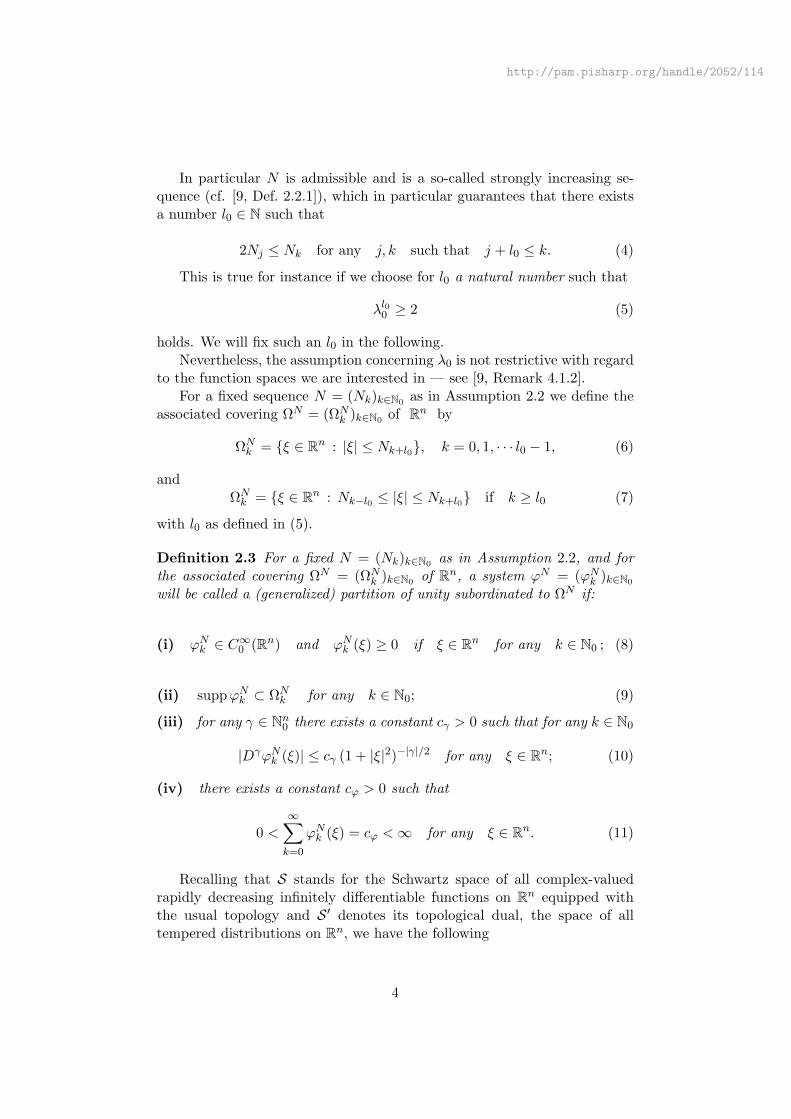
In particular N is admissible and is a so-called strongly increasing se-quence (cf. [9, Def. 2.2.1]), which in particular guarantees that there existsa number l0 ∈ N such that

2Nj ≤ Nk for any j, k such that j + l0 ≤ k. (4)

This is true for instance if we choose for l0 a natural number such that

λl00 ≥ 2 (5)

holds. We will fix such an l0 in the following.Nevertheless, the assumption concerning λ0 is not restrictive with regard

to the function spaces we are interested in — see [9, Remark 4.1.2].For a fixed sequence N = (Nk)k∈N0 as in Assumption 2.2 we define the

associated covering ΩN = (ΩNk )k∈N0 of Rn by

ΩNk = ξ ∈ Rn : |ξ| ≤ Nk+l0, k = 0, 1, · · · l0 − 1, (6)

andΩN

k = ξ ∈ Rn : Nk−l0 ≤ |ξ| ≤ Nk+l0 if k ≥ l0 (7)

with l0 as defined in (5).

Definition 2.3 For a fixed N = (Nk)k∈N0 as in Assumption 2.2, and forthe associated covering ΩN = (ΩN

k )k∈N0 of Rn, a system ϕN = (ϕNk )k∈N0

will be called a (generalized) partition of unity subordinated to ΩN if:

(i) ϕNk ∈ C∞

0 (Rn) and ϕNk (ξ) ≥ 0 if ξ ∈ Rn for any k ∈ N0 ; (8)

(ii) suppϕNk ⊂ ΩN

k for any k ∈ N0; (9)

(iii) for any γ ∈ Nn0 there exists a constant cγ > 0 such that for any k ∈ N0

|DγϕNk (ξ)| ≤ cγ (1 + |ξ|2)−|γ|/2 for any ξ ∈ Rn; (10)

(iv) there exists a constant cϕ > 0 such that

0 <

∞∑

k=0

ϕNk (ξ) = cϕ < ∞ for any ξ ∈ Rn. (11)

Recalling that S stands for the Schwartz space of all complex-valuedrapidly decreasing infinitely differentiable functions on Rn equipped withthe usual topology and S ′ denotes its topological dual, the space of alltempered distributions on Rn, we have the following

4

http://pam.pisharp.org/handle/2052/114

Definition 2.4 Let (σk)k∈N0 be an admissible sequence. Let (Nk)k∈N0 bean admissible sequence satisfying Assumption 2.2 and let ϕN be a system offunctions as in Definition 2.3. Let 0 < p < ∞ and 0 < q ≤ ∞.

The Triebel-Lizorkin space F σ,Np,q of generalized smoothness is defined as

f ∈ S ′ : ‖f |F σ,N

p,q ‖ :=∥∥∥( ∞∑

k=0

σqk |F−1 (ϕN

k Ff)(·)|q)1/q

|Lp(Rn)∥∥∥ < ∞

.

(usual modification when q = ∞) where F and F−1 stand respectively forthe Fourier transformation and its inverse.

Note that if 0 < p ≤ ∞ and 0 < q ≤ ∞ then the Besov space of general-ized smoothness Bσ,N

p,q is defined in an analogous way, by interchanging theroles of the quasi-norms in Lp(Rn) and in `q.

Note also that if Nk = 2k and σ = (2ks)k∈N0 with s real, then the spacesF σ,N

p,q coincide with the usual Triebel-Lizorkin spaces F sp,q on Rn, and the

spaces Bσ,Np,q coincide with the usual Besov spaces Bs

p,q on Rn. We shalluse the simpler notation F s

p,q and Bsp,q in the more classical situation just

mentioned. Even for general admissible σ, when Nk = 2k we shall writesimply F σ

p,q and Bσp,q instead of F σ,N

p,q and Bσ,Np,q , respectively.

We use the equivalence “∼” in

ak ∼ bk or ϕ(x) ∼ ψ(x)

always to mean that there are two positive numbers c1 and c2 such that

c1 ak ≤ bk ≤ c2 ak or c1 ϕ(x) ≤ ψ(x) ≤ c2 ϕ(x)

for all admitted values of the discrete variable k or the continuous variablex, where (ak)k, (bk)k are non-negative sequences and ϕ, ψ are non-negativefunctions.

Definition 2.5 We say that the function ϕ : [1,∞) → (0,∞) belongs to Vif ϕ is measurable and satisfies

0 < ϕ(t) := infs∈[1,∞)

ϕ(ts)ϕ(s)

for all t ∈ [1,∞)

andϕ(t) := sup

s∈[1,∞)

ϕ(ts)ϕ(s)

< ∞ for all t ∈ [1,∞) ,

where we also assume that ϕ and ϕ are measurable functions.

5

http://pam.pisharp.org/handle/2052/114

Remark 2.6 Conditions of the above type have been used at several places,e.g. in connection with real interpolation with a function parameter or inthe theory of function spaces with generalized smoothness. However, therelated functions ϕ are usually defined either on R or on (0,∞). The abovedefinition was given first in connection with weighted Besov spaces in [21]— see also there for details and further references.

We can give Def. 2.4 of the space F σ,Np,q and the corresponding one for

Bσ,Np,q just by starting considering appropriate functions Σ and N in V (note

the abuse of notation in the case of N) and defining the sequences σ andN by σk = Σ(2k) and Nk = N(2k). A similar, though mixed, approach wasfollowed in [22, 6]: there on the side of N a sequence was considered — eventhe particular one (2k)k — and only on the side of the smoothness a functionwas considered, and in a slightly different class defined on (0,∞). On theother hand, with appropriate assumptions on the functions Σ and N involved— namely, that Σ, N ∈ V, N is strictly increasing and λ0N(t) ≤ N(2t), forsome λ0 > 1 —, the scales of spaces thus defined are the same as the onesdefined with the help of sequences, and, as it was shown in [2] in a similarcontext, one can even choose functions and sequences in such a way thatthe so-called Boyd indices of both coincide. For this dual way of definingfunction spaces, we refer also to [1].

As to the relation between functions Σ and N and sequences σ and Ndefining the same spaces, with the help of [21, Lem. 1] we can even statethe following:

• For each admissible sequence σ = (σk)k∈N0 there exists a correspondingfunction Σ ∈ V, that is, a function such that Σ(t) ∼ σk for all t ∈[2k, 2k+1). For example we can define

Σ(t) = σk + (2−kt− 1)(σk+1 − σk) for t ∈ [2k, 2k+1) .

• Vice versa, for each function Σ ∈ V the sequence σ with σk := Σ(2k)is an admissible sequence with κ0 = Σ(2) and κ1 = Σ(2) to which Σcorresponds.

• If in addition an admissible sequence (Nk)k∈N0 fulfils Assumption 2.2,then there exists a corresponding function N ∈ V, strictly increasingand with λ0N(t) ≤ N(2t) for all t ≥ 1.

• And again, vice versa. If N ∈ V is a function with the propertydescribed above, then the sequence Nk := N(2k) is admissible, fulfilsAssumption 2.2 and N corresponds to it.

In what follows, all unimportant positive constants will be denoted byc, occasionally with additional subscripts within the same formula.

6

http://pam.pisharp.org/handle/2052/114

3 A standardization result

The following Fourier-multiplier theorem — [26, Theorem 1.6.3] — will bethe main tool in the proof of the standardization theorem in the case of theF -spaces.

Proposition 3.1 Let 0 < p < ∞, 0 < q ≤ ∞. Let (Ωj)j∈N0 be a sequenceof compact subsets of Rn and dj > 0 be the diameter of Ωj.

If t > n/2 + n/ min (p, q), then there exists a constant c > 0 such that

‖(F−1(MjFfj))j∈N0 |Lp(lq)‖ ≤ c supj∈N0

‖Mj(dj · ) |Ht2‖ ‖(fj)j∈N0 |Lp(lq)‖

holds for all systems (fj)j∈N0 ∈ Lp(lq) with suppFfj ⊂ Ωj for all j, and allsequences (Mj)j∈N0 ⊂ Ht

2.

In the B-case we need a scalar version of Proposition 3.1, including nowp = ∞, see [26, 1.5.2, Remark 3].

Proposition 3.2 Let 0 < p ≤ ∞ and let Ωd = x ∈ Rn : |x| ≤ d withd > 0.

If t > n/min (p, 1)−n/2, then there exists a constant c > 0, independentof d, such that

‖F−1(MFf) |Lp‖ ≤ c ‖M(d · ) |Ht2‖ ‖f |Lp‖

holds for all f ∈ Lp with suppFf ⊂ Ωd and all M ∈ Ht2.

Furthermore, an easy computation shows that for k ≥ l0 and integersM , we have

‖ϕNk (Nk+3l0 · ) |WM

2 ‖ ≤ c (Nk+3l0 N−1k−l0

)M ≤ cλ4l0M1 (12)

where the right-hand side is uniformly bounded with respect to k if (Nk)k∈N0

satisfy Assumption 2.2.For k = 0, · · · , l0 − 1

‖ϕNk (N4l0 · ) |WM

2 ‖ ≤ cNM4l0 (13)

is obvious.

Theorem 3.3 Let N := (Nk)k∈N0 satisfy Assumption 2.2 and σ := (σk)k∈N0

be an admissible sequence with equivalence constants κ0 and κ1. Define

βj := σk(j), with k(j) := mink ∈ N0 : 2j−1 ≤ Nk+l0,

if j ≥ 1 and with l0 defined in (5), and define β0 := σk(1) .

7

http://pam.pisharp.org/handle/2052/114

Then we have that

µ0βj ≤ βj+1 ≤ µ1βj , j ∈ N0,

with µ0 = min1, κl00 , µ1 = max1, κl0

1 .Let, further, 0 < p, q ≤ ∞ (with p 6= ∞ in the F -case). Then

F σ,Np,q = F β

p,q

andBσ,N

p,q = Bβp,q,

where β := (βj)j∈N0.

Proof. Step 1. We start with some preliminary observations. For simplicitywe assume without loss of generality that N0 = 1. Otherwise we would haveto consider large enough values for j and k in what follows.

Let Ω = (Ωj)j∈N0 be the standard dyadic covering of Rn, associated withthe sequence (2j)j∈N0 , i.e.

Ω0 = ξ ∈ Rn : |ξ| ≤ 2,and

Ωj = ξ ∈ Rn : 2j−1 ≤ |ξ| ≤ 2j+1 if j ≥ 1 .

Specify k0 ≥ l0. Then ΩNk0∩ Ωj can be non-empty only if we have

12Nk0−l0 ≤ 2j ≤ 2Nk0+l0 .

LetJ (k0) = j ∈ N0 : Nk0−l0 ≤ 2j+1 ≤ 22Nk0+l0 . (14)

The set J (k0) is always non-empty — let ξ be an element of ΩNk0

, then thereexist at least one j′ with ξ ∈ Ωj′ . But then holds Nk0−l0 ≤ |ξ| ≤ 2j′+1 and2j′−1 ≤ |ξ| ≤ Nk0+l0 .

We will denote by j∗(k0) the smallest element of J (k0). Then it iseasy to see, that ΩN

k0has a non-empty intersection with at most the sets

Ωj∗(k0) , . . . ,Ωj∗(k0)+L where

L = [2l0 log2 λ1] + 2 (15)

is independent of k0.Moreover we have

j∗(k0) < j∗(k0 + 4l0 + 1) . (16)

And vice versa, if we specify j0 ≥ 1 then ΩNk ∩ Ωj0 can be non-empty

only if we have

2j0−1 ≤ Nk+l0 and Nk−l0 ≤ 2j0+1 .

8

http://pam.pisharp.org/handle/2052/114

Let now

K(j0) = k ∈ N0 : 2j0−1 ≤ Nk+l0 and Nk−l0 ≤ 2j0+1 . (17)

The set K(j0) is again always non-empty and we denote by k∗(j0) the small-est element of it.

k∗(j0) coincides with k(j0) from the theorem — k(j0) ≤ k∗(j0) is obviousand the opposite inequality follows by the monotonicity of the sequence(Nk)k∈N0 and l0 ≥ 1. We have Nk(j0)−l0 ≤ Nk(j0)−1+l0 < 2j0−1 < 2j0+1, thatmeans k(j0) belongs to K(j0).

Again it is easy to see, that Ωj0 has a non-empty intersection with atmost the sets ΩN

k∗(j0) , . . . , ΩNk∗(j0)+4l0

and we have

k∗(j0) ≤ k∗(j0 + 1) ≤ k∗(j0) + l0 but k∗(j0) < k∗(j0 + L + 1) (18)

with L from (15).

Step 2. Let σ := (σk)k∈N0 be an admissible sequence with equivalence con-stants κ0 and κ1 and define βj = σk∗(j). Then there exist positive constants,independent of j ≥ 1 and k such that

min (1, κ4l00 ) ≤ σk

βj=

σk

σk∗(j)≤ max (1, κ4l0

1 ) for all k ∈ K(j) . (19)

The cardinality of K(j) is not larger than 4l0 + 1 and so (19) follows imme-diately. In case of κ0 < 1 we have to choose the minimum on the left-handside, and if κ1 < 1 we have to choose the maximum on the right-hand side.

The estimation of the counterpart — there exist positive constants c0

and c1 , independent of j and k ≥ l0, such that

c0 ≤ βj

σk=

σk∗(j)

σk≤ c1 for all j ∈ J (k) (20)

holds — is more delicate.First notice that (16) gives

j∗(k) + l ≤ j∗(k + (4l0 + 1)l) , l ∈ N0.

By the construction in step 1 we have also

k − 4l0 ≤ k∗(j∗(k)) ≤ k

at least for k > 2l0; otherwise j∗(k) might be zero, but we can temporarilyextend the definition of K(j0) in (17) to j0 = 0 and see that this remainstrue for all k ≥ l0.

Both together gives for l = 0, · · · , L

k − 4l0 ≤ k∗(j∗(k) + l) ≤ k∗(j∗(k + (4l0 + 1)l) ≤ k + (4l0 + 1)L . (21)

9

http://pam.pisharp.org/handle/2052/114

Now we can determine c0 and c1 from (20) by

c0 = min (1, κ−4l01 , κ

(4l0+1)L0 ) and c1 = max (1, κ−4l0

0 , κ(4l0+1)L1 ) .

Moreover, similar to (19), we obtain by (18) that (βj)j∈N0 is an admis-sible sequence and

min (1, κl00 ) ≤ βj+1

βj≤ max (1, κl0

1 ) for all j ∈ N0 . (22)

Step 3. Denote by (ϕj)j∈N0 a function system, related to the dyadicdecomposition (Ωj)j∈N0 and let cϕ = 1 for this system.

Then we have

F−1(ϕNk Ff) =

∞∑

j=0

F−1(ϕjϕNk Ff) =

∑

j∈J (k)

F−1(ϕjϕNk Ff) .

We put in Proposition 3.1Mk = ϕN

k

andfk = σk

∑

j∈J (k)

F−1(ϕjFf) if k ≥ l0,

fk = σk

( j∗(l0)−1∑

j=0

+∑

j∈J (l0)

)F−1(ϕjFf) if k = 0, · · · , l0 − 1 .

Then of courseF−1(MkFfk) = σkF−1(ϕN

k Ff) ,

and

suppFfk ⊂⋃

j∈J (k)

suppϕj ⊂ ξ : |ξ| ≤ Nk+3l0 if k ≥ l0,

suppFfk ⊂ ξ : |ξ| ≤ N4l0 if k = 0, · · · , l0 − 1 .

Now proposition 3.1 and (12), (13) give

‖(σkF−1(ϕNk Ff))k∈N0 |Lp(lq)‖ ≤ c ‖(fk)k∈N0 |Lp(lq)‖. (23)

For the rest of the proof, assume, for simplicity, that q 6= ∞; otherwiseusual changes have to be made in what follows.

Let k ≥ l0; then (the cardinality of J (k) is not larger than L + 1)

σqk

∣∣∣∣∑

j∈J (k)

F−1(ϕjFf)(·)∣∣∣∣q

≤ cqq,L

(max

j∈J (k)

σk

βj

)q ∑

j∈J (k)

βqj

∣∣∣∣F−1(ϕjFf)(·)∣∣∣∣q

.

10

http://pam.pisharp.org/handle/2052/114

We take c0 from (20) and get

∞∑

k=l0

σqk

∣∣∣∣∑

j∈J (k)

F−1(ϕjFf)(·)∣∣∣∣q

≤ cqq,Lc−q

0

∞∑

k=l0

∑

j∈J (k)

βqj

∣∣F−1(ϕjFf)(·)∣∣q .

But because of (16) each ϕj can occur in the double sum not more than(L + 1)(4l0 + 1) times.

A similar estimate can be given for the first l0 summands and each ϕj

with 0 ≤ j ≤ j∗(l0) + L can occur only l0 times. The counterpart to (20)is obvious because of the limited number of βj , 0 ≤ j ≤ j∗(l0) + L andσk , 0 ≤ k ≤ l0− 1 which are involved. Together with the key estimate (23)this gives

||f |F σ,Np,q || ≤ c||f |F β

p,q|| .

We obtain the opposite inequality by changing the roles of ϕNk and ϕj .

Step 4. In the case of B-spaces we use the scalar multiplier theorem.Again we have

F−1(ϕNk Ff) = F−1(ϕN

k

∑

j∈J (k)

ϕjFf) .

Now we use Proposition 3.2 with M = ϕNk and the role of f over there being

played now by ∑

j∈J (k)

F−1(ϕjFf) if k ≥ l0.

Similar to step 3 we get

‖F−1(ϕNk Ff) |Lp‖ ≤ c

∥∥∥∑

j∈J (k)

F−1(ϕjFf) |Lp

∥∥∥

with a constant c > 0 and independent of k. Again, by the considerationsof step 1 and step 2, we obtain

∞∑

k=l0

σqk‖F−1(ϕN

k Ff) |Lp‖q ≤ c∗qp,Lc−q0 c

∞∑

j=0

βqj ‖F−1(ϕjFf) |Lp‖q.

Together with a similar estimate of the first l0 summands this gives

||f |Bσ,Np,q || ≤ c||f |Bβ

p,q|| .

Again we obtain the opposite inequality by changing the roles of ϕNk and

ϕj .¤

11

http://pam.pisharp.org/handle/2052/114

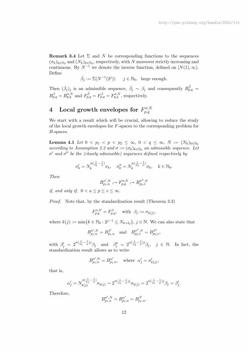
Remark 3.4 Let Σ and N be corresponding functions to the sequences(σk)k∈N0 and (Nk)k∈N0 , respectively, with N moreover strictly increasing andcontinuous. By N−1 we denote the inverse function, defined on [N(1),∞).Define

βj := Σ(N−1(2j)) j ∈ N0, large enough.

Then (βj)j is an admissible sequence, βj ∼ βj and consequently Bβp,q =

Bβp,q = Bσ,N

p,q and F βp,q = F β

p,q = F σ,Np,q , respectively.

4 Local growth envelopes for F σ,Np,q

We start with a result which will be crucial, allowing to reduce the studyof the local growth envelopes for F -spaces to the corresponding problem forB-spaces.

Lemma 4.1 Let 0 < p1 < p < p2 ≤ ∞, 0 < q ≤ ∞, N := (Nk)k∈N0

according to Assumption 2.2 and σ := (σk)k∈N0 an admissible sequence. Letσ′ and σ′′ be the (clearly admissible) sequences defined respectively by

σ′k = Nn( 1

p1− 1

p)

k σk, σ′′k = Nn( 1

p2− 1

p)

k σk, k ∈ N0.

ThenBσ′,N

p1,u → F σ,Np,q → Bσ′′,N

p2,v

if, and only if, 0 < u ≤ p ≤ v ≤ ∞.

Proof. Note that, by the standardization result (Theorem 3.3)

F σ,Np,q = F β

p,q, with βj := σk(j),

where k(j) := mink ∈ N0 : 2j−1 ≤ Nk+l0, j ∈ N. We can also state that

Bσ′,Np1,u = Bβ′

p1,u and Bσ′′,Np2,v = Bβ′′

p2,v,

with β′j = 2n( 1p1− 1

p)j

βj and β′′j = 2n( 1p2− 1

p)j

βj , j ∈ N. In fact, thestandardization result allows us to write

Bσ′,Np1,u = Bα′

p1,u, where α′j = σ′k(j),

that is,

α′j = Nn( 1

p1− 1

p)

k(j) σk(j) ∼ 2n( 1p1− 1

p)j

σk(j) = 2n( 1p1− 1

p)j

βj = β′j .

Therefore,Bσ′,N

p1,u = Bα′p1,u = Bβ′

p1,u.

12

http://pam.pisharp.org/handle/2052/114

The proof of Bσ′′,Np2,v = Bβ′′

p2,v is similar.So, our lemma will be proved if we can show that

Bβ′p1,u → F β

p,q → Bβ′′p2,v

holds if, and only if, 0 < u ≤ p ≤ v ≤ ∞.However, this follows immediately from [2, Prop. 4.7], due to the fact

that β is also an admissible sequence (cf. statement of Theorem 3.3). ¤The definition of the local growth envelope function requires that we

are dealing with regular distributions. Therefore it is reasonable to get firstsome idea about the spaces of Triebel-Lizorkin type for which it makes senseto estimate such function. The following result goes in that direction.

Proposition 4.2 Let 0 < p < ∞, 0 < q ≤ ∞. Let σ and N be as in thepreceding lemma. If

(σ−1

k N δk )k∈N0 ∈ `p′ , for some δ > 0, if 1 ≤ p < ∞

(σ−1k N

n( 1p−1)

k )k∈N0 ∈ `∞, if 0 < p < 1 ,(24)

thenF σ,N

p,q ⊂ Lloc1 .

Proof. We take advantage of the preceding lemma (for u = p = v) in orderto state that

F σ,Np,q → Bσ′′,N

p2,p ,

for any p2 > p. So, we just have to prove that, for some suitable such p2,Bσ′′,N

p2,p is in Lloc1 :

From [3, Rem. 3.20], this will be the case if (σ′′k−1N

n( 1p2−1)+

k )k∈N0 ∈ `p′ .When 0 < p < 1, this follows from (24) by choosing 1 ≥ p2 > p; when1 ≤ p < ∞, again it follows from (24), now by choosing p2 > p such that1p − 1

p2≤ δ. ¤

Remark 4.3 The hypothesis (24) will not be enough for what we want toprove later, so we would like to remark that the condition

(σ−1l N

n( 1p−1)++δ

l )l∈N0 ∈ `min1,p, for some δ > 0, (25)

also implies that F σ,Np,q ⊂ Lloc

1 . Actually, (25) implies (24), as follows easilyfrom the facts σ−1

l ≤ σ−10 σ−1

l , Nl ≤ N0N l, l ∈ N0, and min1, p ≤ p′.

Just to get a feeling of how much of the cases where F σ,Np,q ⊂ Lloc

1 weare ignoring when assuming (24) or (25), let us compare with the classicalsituation: when Nk = 2k, σk = 2ks, s ∈ R, k ∈ N0, (24) is equivalent to

s > 0, if 1 ≤ p < ∞s ≥ n(1

p − 1)+, if 0 < p < 1 , (26)

13

http://pam.pisharp.org/handle/2052/114

while (25) is equivalent to

s > n(1

p− 1

)+. (27)

In this classical setting, both (26) and (27) are “pretty close” to optimal, asit is well-known that for s < n(1

p − 1)+ one never has F σ,Np,q ⊂ Lloc

1 .We also would like to point out that, as artificial as the role of δ may

seem, something stronger than the condition (σ−1k )k∈N0 ∈ `∞ must in general

be assumed in order to have F σ,N1,q ⊂ Lloc

1 : in the classical setting, [25, Theor.3.3.2(i)] tells us that F s

1,q is in Lloc1 if, and only if,

s ≥ 0, when 0 < q ≤ 2s > 0, when 2 < q ≤ ∞ ;

note that the condition (2−ks)k∈N0 ∈ `∞ is not strong enough to yield thesecond case above (that is, when 2 < q ≤ ∞).

The estimation of the growth envelope function is of interest only whenthere are unbounded functions around. So it makes sense to obtain be-forehand some information about the spaces of Triebel-Lizorkin type whichpossess unbounded functions. The next proposition and the following re-mark go in that direction.

Proposition 4.4 Let 0 < p < ∞, 0 < q ≤ ∞, N := (Nk)k∈N0 according toAssumption 2.2 and σ := (σk)k∈N0 an admissible sequence. Then

(σ−1k N

np

k )k∈N0 ∈ `p′ if, and only if, F σ,Np,q → C,

where C is the space of (complex-valued) bounded and uniformly continuousfunctions (on Rn) endowed with the sup-norm.

Proof. We rely again on Lemma 4.1 and on a result for B-spaces corre-sponding to the assertion to be proved now.

(i) Assume that (σ−1k N

np

k )k∈N0 ∈ `p′ . Then also (σ′′k−1N

np2k )k∈N0 ∈ `p′ , for

any p2 with p < p2 ≤ ∞, and therefore F σ,Np,q → Bσ′′,N

p2,p → C, see [3, Corol.3.10].

(ii) Assume now that F σ,Np,q → C. Since Bσ′,N

p1,p → F σ,Np,q , for any 0 < p1 <

p, then Bσ′,Np1,p → C for all such p1. By [3, Corol. 4.9], we can then state

that (σ−1k N

np

k )k∈N0 = (σ′k−1N

np1k )k∈N0 ∈ `p′ . ¤

Remark 4.5 (i) Such type of results was proved first by Kalyabin [19] withthe restrictions 1 < p, q < ∞.

(ii) It’s easy to see that we can write L∞ instead of C in the propositionabove.

14

http://pam.pisharp.org/handle/2052/114

We recall now the main result for B-spaces which we want to “translate”for F -spaces here, concerning the behaviour of the local growth envelopefunction

ELG|Bσ,Np,q (t) := supf∗(t) : ‖f |Bσ,N

p,q ‖ ≤ 1 (28)

near 0, where f∗ stands for the decreasing rearrangement of f . In particu-lar, the hypotheses guarantee that, for the parameters involved, (28) makessense.

Proposition 4.6 ([3, Theor. 4.10]) Let 0 < p, q ≤ ∞, N := (Nk)k∈N0

according to Assumption 2.2 and σ := (σk)k∈N0 an admissible sequence.Assume further that

(σ−1

l )l∈N0 ∈ `minq,1 if p > 1

(σ−1l N

n( 1p−1)+δ

l )l∈N0 ∈ `minq,1, for some δ > 0, if 0 < p ≤ 1 ,

and(σ−1

k Nnp

k )k∈N0 /∈ `q′ .

Let Λ be any admissible function such that Λ(z) ∼ σk, z ∈ [Nk, Nk+1],k ∈ N0, with equivalence constants independent of k, and let Φu be definedin (0, N−n

J0] by

Φu(t) :=(∫ 1

t1/n

y−n

puΛ(y−1)−u dy

y

)1/uif 0 < u < ∞, (29)

andΦu(t) := sup

t1/n≤y≤1

y−n

p Λ(y−1)−1 if u = ∞, (30)

where J0 ∈ N is chosen such that NJ0 > 1.Then there exists ε ∈ (0, 1) such that

ELG|Bσ,Np,q (t) ∼ Φq′(t), t ∈ (0, ε], (31)

and, considering the range 0 < v ≤ ∞, we have that

( ∫ ε

0

( f∗(t)Φq′(t)

)vµq′(dt)

)1/v≤ c ‖f |Bσ,N

p,q ‖ (32)

(with the understanding

supt∈(0,ε]

f∗(t)Φq′(t)

≤ c ‖f |Bσ,Np,q ‖ (33)

when v = ∞) holds for some ε ∈ (0, 1), c > 0 and all f ∈ Bσ,Np,q if, and

only if, q ≤ v ≤ ∞. In (32), µq′ means the Borel measure associated with− log2 Φq′ in (0, ε].

15

http://pam.pisharp.org/handle/2052/114

We recall the meaning of admissible function, used in the precedingassertion:

Definition 4.7 A function Λ : (0,∞) → (0,∞) is called admissible if it iscontinuous and if for any b > 0 satisfies

Λ(bz) ∼ Λ(z) for any z > 0

(where the equivalence constants may depend on b)

Remark 4.8 There is at least one admissible function related with thesequences σ and N as required in Proposition 4.6. This follows from [3,Example 2.3].

Lemma 4.9 Let Λ be an admissible function. Let n ∈ N and 0 < p1, p, p2 ≤∞. Then Λ′ and Λ′′ given by

Λ′(z) = zn( 1

p1− 1

p)Λ(z), z ∈ (0,∞), (34)

Λ′′(z) = zn( 1

p2− 1

p)Λ(z), z ∈ (0,∞), (35)

are both admissible. If moreover,

Λ(z) ∼ σk, z ∈ [Nk, Nk+1], k ∈ N0,

with equivalence constants independent of k, for given admissible sequencesσ and N , then also

Λ′(z) ∼ σ′k, z ∈ [Nk, Nk+1], k ∈ N0,

Λ′′(z) ∼ σ′′k , z ∈ [Nk, Nk+1], k ∈ N0,

in both cases with equivalence constants independent of k, where σ′ and σ′′

are related to σ as in Lemma 4.1.

The proof is straightforward.

Remark 4.10 Recall now the definition (29) and (30) of Φu, which, inparticular, depend on the p and Λ given. If we use, instead, p1 and Λ′, thenwe would write Φ′u instead of Φu, and similarly if we use p2 and Λ′′, in whichcase we would write Φ′′u. Note, however, that

Φ′u = Φu = Φ′′u,

as can easily be seen.

16

http://pam.pisharp.org/handle/2052/114

As a consequence, though we would define µ′u and µ′′u as the Borel mea-sures respectively associated with − log2 Φ′u and − log2 Φ′′u in (0, ε], we seethat, in fact,

µ′u = µu = µ′′u.

We recall that the Borel measure µu is the only measure defined onthe Borel sets (of (0, ε]) such that µu([a, b]) = − log2 Φu(b) + log2 Φu(a) =log2

Φu(a)Φu(b) , ∀[a, b] ⊂ (0, ε].

We are now ready to prove our main result for F -spaces, concerning thebehaviour of the local growth envelope function

ELG|F σ,Np,q (t) := supf∗(t) : ‖f |F σ,N

p,q ‖ ≤ 1 (36)

near 0, where — we recall — f∗ stands for the decreasing rearrangementof f . We can, in particular, see that the hypotheses we are going to takeguarantee — due to Remark 4.3 — that (36) makes sense. We note alsothat the condition

(σ−1k N

np

k )k∈N0 /∈ `p′ (37)

will be assumed because — due to Proposition 4.4 — otherwise (36) isbounded, and therefore the outcome has no interest.

Theorem 4.11 Let 0 < p < ∞, 0 < q ≤ ∞, N := (Nk)k∈N0 according toAssumption 2.2 and σ := (σk)k∈N0 an admissible sequence. Assume furtherthat (25) and (37) hold true. Let Λ be any admissible function such thatΛ(z) ∼ σk, z ∈ [Nk, Nk+1], k ∈ N0, with equivalence constants independentof k, and let Φu be defined by (29) and (30) in (0, N−n

J0], where J0 ∈ N is

chosen such that NJ0 > 1.Then there exists ε ∈ (0, 1) such that

ELG|F σ,Np,q (t) ∼ Φp′(t), t ∈ (0, ε], (38)

and, considering the range 0 < v ≤ ∞, we have that

( ∫ ε

0

( f∗(t)Φp′(t)

)vµp′(dt)

)1/v≤ c ‖f |F σ,N

p,q ‖ (39)

(with the understanding

supt∈(0,ε]

f∗(t)Φp′(t)

≤ c ‖f |F σ,Np,q ‖ (40)

when v = ∞) holds for some ε ∈ (0, 1), c > 0 and all f ∈ F σ,Np,q if, and

only if, p ≤ v ≤ ∞. As before, in (39) µp′ stands for the Borel measureassociated with − log2 Φp′ in (0, ε].

17

http://pam.pisharp.org/handle/2052/114

Proof. We take advantage of Lemma 4.1. In particular, in what follows weadhere to the notation σ′ and σ′′ as considered there.

Step 1. Note that the hypothesis (37) guarantee that

(σ′′k−1

Nnp2k )k∈N0 /∈ `p′ , (41)

for any p2 with p < p2 ≤ ∞, and that the hypothesis (25) guarantees that

(σ′′l−1)l∈N0 ∈ `1 if p ≥ 1

(σ′′l−1N

n( 1p2−1)+δ

l )l∈N0 ∈ `p, for some δ > 0, if 0 < p < 1 ,(42)

for any p2 ∈ (p,∞] close enough to p.Since (41) is clear, we just prove (42):Start by observing that

σ′′l ≥ σlNn( 1

p2− 1

p)

l , l ∈ N0.

Take p ≥ 1. Then∑∞

l=0 σ′′l−1 ≤ ∑∞

l=0 σl−1N

n( 1p− 1

p2)

l < ∞, if p2 > p ischosen such that n(1

p − 1p2

) ≤ δ, with δ given in (25).Take now 0 < p < 1. Then

∞∑

l=0

(σ′′l−1

Nn( 1

p2−1)+δ

l

)p ≤∞∑

l=0

(σl−1N

n( 1p−1)+δ

l

)p< ∞,

using the same δ as in (25).Note that from (42) it also follows that, for p ≥ 1, we can choose p2 > p

close enough to p such that we have both

(σ′′l−1)l∈N0 ∈ `minp,1 and p2 > 1,

while for 0 < p < 1 we can choose p2 > p close enough to p such that wehave both

(σ′′l−1

Nn( 1

p2−1)+δ

l )l∈N0 ∈ `minp,1 and 0 < p2 ≤ 1.

Using this, (41), Lemma 4.9 and Remark 4.10, from Proposition 4.6 weimmediately get that there exists ε ∈ (0, 1), c > 0 such that

ELG|Bσ′′,Np2,p (t) ≤ c Φp′(t), t ∈ (0, ε], (43)

and also that for any v ∈ [p,∞] there is ε ∈ (0, 1), c > 0 such that

(∫ ε

0

( f∗(t)Φp′(t)

)vµp′(dt)

)1/v≤ c ‖f |Bσ′′,N

p2,p ‖ (44)

(modification if v = ∞) for all f ∈ Bσ′′,Np2,p .

18

http://pam.pisharp.org/handle/2052/114

Using the embedding F σ,Np,q → Bσ′′,N

p2,p given by Lemma 4.1, it is easilyseen that (43) and (44) also hold true with F σ,N

p,q instead of Bσ′′,Np2,p

Step 2. Instead of Proposition 4.6, we will use now more precise partialresults contained in [3].

Recall that, by Remark 4.3, the hypothesis (25) guarantees that F σ,Np,q ⊂

Lloc1 . Thus, using Lemma 4.1, we can also assert that Bσ′,N

p1,p ⊂ Lloc1 , for

any 0 < p1 < p, and therefore [3, Prop. 4.8] assures us that there existsε ∈ (0, 1), c > 0 such that

ELG|Bσ′,Np1,p (t) ≥ c Φ′p′(t), t ∈ (0, ε].

Hence Lemmas 4.1, 4.9 and Remark 4.10 allow us to write also

ELG|F σ,Np,q (t) ≥ c Φp′(t), t ∈ (0, ε],

for some ε ∈ (0, 1), c > 0.To see that (39) cannot hold for 0 < v < p, assume, on the contrary,

that, for such v, there existed ε ∈ (0, 1), c > 0 such that

( ∫ ε

0

( f∗(t)Φp′(t)

)vµp′(dt)

)1/v≤ c ‖f |F σ,N

p,q ‖

for all f ∈ F σ,Np,q . Then, using Lemmas 4.1, 4.9 and Remark 4.10, there

would also exist ε ∈ (0, 1), c > 0 such that

(∫ ε

0

( f∗(t)Φ′p′(t)

)vµ′p′(dt)

)1/v≤ c ‖f |Bσ′,N

p1,p ‖. (45)

for all f ∈ Bσ′,Np1,p . But since, as we have already seen above, Bσ′,N

p1,p ⊂ Lloc1 and

(37) trivially implies that (σ′k−1N

np1k )k∈N0 /∈ `p′ , then this would contradict

[3, Rem. 4.11] ((45) can only hold for v ≥ p). ¤

Remark 4.12 1. It is possible to choose ε independent of v in (39). Infact, the ε taken for v = p can also be taken for all v ≥ p — see [27, Prop.12.2(i)].

2. As noted in [3, Rem. 4.15], when 1 < p < ∞, the measure µp′(dt) in(39) can be replaced by

dt

Φp′(t)p′ tp′ Λ(t−1/n)p′ .

In the particular case when Nk = 2k and σk = 2ksΨ(2−k), k ∈ N0, withn(1

p − 1)+ < s < np and Ψ a “log-type” function (cf. also comments after

this remark) — the so-called subcritical case in the setting of [4] — when,again, 1 < p < ∞, µp′(dt) can be further simplified to dt

t — cf. [4, Rem.

19

http://pam.pisharp.org/handle/2052/114

4.8]. Actually, in that subcritical case, and independently of the value of p,Φp′(t) itself can be simplified to t

sn− 1

p Ψ(t)−1.For other cases where simpler expressions, both for Φp′ and for µp′ , can

be taken instead of our general ones, see the work of Bricchi and Moura [2].

We would like to point out that Theorem 4.11 covers and extends theresults previously obtained by Caetano and Moura [5], [4], which alreadycovered the general statements of Haroske [17] and Triebel [27], as far asgrowth envelopes for Triebel-Lizorkin-type spaces are concerned. To seethis, one just has to note that the spaces considered in [4, Cor. 4.5] areincluded in our main theorem. It is, in fact, an easy exercise to show thatthe spaces F σ,N

p,q considered there, namely with Nk = 2k and σk = 2ksΨ(2−k),k ∈ N0, where n(1

p − 1)+ < s ≤ np and Ψ a so-called admissible function

(in the context of that paper) satisfying (Ψ(2−k)−1)k∈N0 /∈ `p′ when s = np ,

are such that (σk)k∈N0 and (Nk)k∈N0 are admissible (in our sense), with thelatter satisfying also Assumption 2.2 and, moreover, (25) and (37) hold.

Our Theorem 4.11 also covers and extends Theorem 6.3(ii) of [2]: it isagain an easy exercise to see that the spaces F σ,N

p,q considered there, namelywith Nk = 2k, k ∈ N0, and σ an admissible sequence satisfying n(1

p −1)+ < liml→∞

log2 σll ≤ liml→∞

log2 σl

l < np , verify all the requirements of our

Theorem 4.11.

We finish with a corollary of Theorem 4.11 which gives more preciseinformation about the sharpness of our results. This is similar to whathappens with Besov-type spaces. A proof can be obtained with the help of[27, Prop. 12.2].

Corollary 4.13 Consider the same hypothesis of Theorem 4.11 and 0 <ε ≤ N−n

J0. Let κ be a positive monotonically decreasing function on (0, ε]

and let 0 < u ≤ ∞. Then

( ∫ ε

0

(κ(t)

f∗(t)Φp′(t)

)uµp′(dt)

)1/u≤ c ‖f |F σ,N

p,q ‖,

for some c > 0 and all f ∈ F σ,Np,q if, and only if, κ is bounded and p ≤ u ≤ ∞,

with the modification

supt∈(0,ε]

κ(t)f∗(t)Φp′(t)

≤ c ‖f |F σ,Np,q ‖ (46)

if u = ∞. Moreover, if κ is an arbitrary non-negative function on (0, ε],then (46) above holds if, and only if, κ is bounded.

20

http://pam.pisharp.org/handle/2052/114

References

[1] A. Almeida. Wavelet bases in generalized Besov spaces. J. Math. Anal.Appl., 304(1):198–211, 2005.

[2] M. Bricchi and S. D. Moura. Complements on growth envelopes ofspaces with generalized smoothness in the sub-critical case. Z. Anal.Anwend., 22(2):383–398, 2003.

[3] A. M. Caetano and W. Farkas. Local growth envelopes of Besov spacesof generalized smoothness. Z. Anal. Anwendungen, (to appear).

[4] A. M. Caetano and S. D. Moura. Local growth envelopes of spaces ofgeneralized smoothness: the critical case. Math. Ineq. & Appl., 7:573–606, 2004.

[5] A. M. Caetano and S. D. Moura. Local growth envelopes of spaces ofgeneralized smoothness: the sub-critical case. Math. Nachr., 273(1):43–57, 2004.

[6] F. Cobos and D. Fernandez. Hardy-Sobolev spaces and Besov spaceswith a function parameter. In Lecture Notes in Math., volume 1302,pages 158–170. Springer, 1988.

[7] L. Diening and M. Ruzicka. Calderon-Zygmund operators on general-ized Lebesgue spaces Lp(·) and problems related to fluid dynamics. J.Reine Angew. Math., 563:197–220, 2003.

[8] W. Farkas and N. Jacob. Sobolev spaces on non-smooth domainsand Dirichlet forms related to subordinate reflecting diffusions. Math.Nachr., 224:75–104, 2001.

[9] W. Farkas and H.-G. Leopold. Characterisations of function spaces ofgeneralised smoothness. preprint Math/Inf/23/01, Univ. Jena, Ger-many, 2001.

[10] W. Farkas and H.-G. Leopold. Characterisations of function spaces ofgeneralised smoothness. Ann. Mat. Pura Appl., 185(1):1–62, 2006.

[11] A. Gogatishvili, J. S. Neves, and B. Opic. Optimality of embeddingsof Bessel-potential-type spaces into Lorentz-Karamata spaces. Proc.Royal Soc. Edinburgh, 134 A, to appear, 2004.

[12] M. L. Gol’dman. On imbedding generalized Nikol’skij-Besov spaces inLorentz spaces. Trudy Mat. Inst. Steklov, 172:128–139, 1985. (Russian)[English translation: Proc. Steklov Inst. Math. 172, 143-154 (1987)].

21

http://pam.pisharp.org/handle/2052/114

[13] M. L. Gol’dman. On imbedding constructive and structural Lipschitzspaces in symmetric spaces. Trudy Mat. Inst. Steklov, 173:90–112, 1986.(Russian) [English translation: Proc. Steklov Inst. Math. 4 (1987), 93-118].

[14] M. L. Gol’dman and F. Enrikes. Description of the rearrangement-invariant hull of an anisotropic Calderon space. Tr. Mat. Inst. Steklova,248:94–105, 2005. (Russian) Issled. po Teor. Funkts. i Differ. Uravn.

[15] M. L. Gol’dman and R. Kerman. On optimal embedding of Calderonspaces and generalized Besov spaces. Tr. Mat. Inst. Steklova, 243:161–193, 2003. (Russian) [English translation: Proc. Steklov Inst. Math.243, 154-184 (2003)].

[16] P. Gurka and B. Opic. Sharp embeddings of Besov spaces with loga-rithmic smoothness. Rev. Mat. Complutense, 18:81–110, 2005.

[17] D. D. Haroske. Envelopes in function spaces - a first approach. preprintMath/Inf/16/01, Univ. Jena, Germany, 2001.

[18] G. A. Kalyabin. Imbedding theorems for generalized Besov and Liou-ville spaces. Dokl. Akad. Nauk SSSR, 232:1245–1248, 1977. (Russian)[English translation: Sov. Math., Dokl. 18, 227-231 (1977)].

[19] G. A. Kalyabin. Criteria of the multiplication property and the em-bedding in C of spaces of Besov-Lizorkin-Triebel type. Mat. Zametki,30:517–526, 1981. (Russian).

[20] G. A. Kalyabin and P. I. Lizorkin. Spaces of generalized smoothness.Math. Nachr., 133:7–32, 1987.

[21] T. Kuhn, H.-G. Leopold, W. Sickel, and L. Skrzypczak. Entropy num-bers of embeddings of weighted Besov spaces II. Proc. Edinburgh Math.Society (to appear).

[22] C. Merucci. Applications of interpolation with a function parameter toLorentz, Sobolev and Besov spaces. In Lecture Notes in Math., volume1070, pages 183–201. Springer, 1984.

[23] B. Opic and W. Trebels. Sharp embeddings of Bessel potential spaceswith logarithmic smoothness. Math. Proc. Camb. Phil. Soc., 134:347–384, 2003.

[24] H.-J. Schmeisser and W. Sickel. Spaces of functions of mixed smooth-ness and approximation from hyperbolic crosses. J. Approximation The-ory, 128:115–150, 2004.

22

http://pam.pisharp.org/handle/2052/114

[25] W. Sickel and H. Triebel. Holder inequalitites and sharp embeddings infunction spaces of Bs

pq and F spq type. Z. Anal. Anwendungen, 14(1):105–

140, 1995.

[26] H. Triebel. Theory of Function Spaces. Birkhauser, Basel, 1983.

[27] H. Triebel. The Structure of Functions. Birkhauser, Basel, 2001.

23