arX

iv:g

r-qc

/940

5010

v1 4

May

199

4

Exotic Smoothness and Physics

Carl H. Brans

Physics DepartmentLoyola University

New Orleans, LA 70118e-mail:BRANS @ MUSIC.LOYNO.EDU

March 29, 1994

Abstract

The essential role played by differentiable structures in physics is reviewed in light of recent

mathematical discoveries that topologically trivial space-time models, especially the simplest one,

R4, possess a rich multiplicity of such structures, no two of which are diffeomorphic to each other

and thus to the standard one. This means that physics has available to it a new panoply of structures

available for space-time models. These can be thought of as source of new global, but not properly

topological, features. This paper reviews some background differential topology together with a

discussion of the role which a differentiable structure necessarily plays in the statement of any

physical theory, recalling that diffeomorphisms are at the heart of the principle of general relativity.

Some of the history of the discovery of exotic, i.e., non-standard, differentiable structures is reviewed.

Some new results suggesting the spatial localization of such exotic structures are described and

speculations are made on the possible opportunities that such structures present for the further

development of physical theories.

To be published in Journal of Mathematical Physics.

1 Introduction

Almost all modern physical theories are stated in terms of fields over a smooth manifold, typicallyinvolving differential equations for these fields. Obviously the mechanism underlying the notion ofdifferentiation in a space-time model is indispensable for physics. However, the essentially local natureof differentiation has led us to assume that the mathematics underlying calculus as applied to physicsis trivial and unique. In a certain sense this is true: all smooth manifolds of the same dimension arelocally differentiably equivalent, and thus physically indistinguishable in the local sense. However, onlyfairly recently have we learned that this need not be true in the global sense. Mathematicians havediscovered that certain common, even topologically trivial, manifolds may not be globally smoothlyequivalent (diffeomorphic) even though they are globally topologically equivalent (homeomorphic). Thisis a strikingly counter-intuitive result which presents new, non-topological, global possibilities for space-time models. The fact that the dimension four plays a central role in this story only enhances thespeculation that these results may be of some physical significance.

Briefly, until some twelve years ago it was known that any smooth manifold that was topologicallyequivalent to Rn for n 6= 4 must necessarily be differentiably equivalent to it. It is probably safe to saymost workers expected that the outstanding case of n = 4 would be resolved the same way when sufficienttechnology was developed for the proof. Thus, it was quite a shock when the work of Freedman[1] andDonaldson[2] showed that there are an infinity of differentiable structures on topological R4, no twoof which are equivalent, i.e., diffeomorphic, to each other. The surprising feature of this result is thefact that while each of these manifolds is locally smoothly equivalent to any other, this local equivalencecannot be continued to a global one, even though the manifold model, R4, is clearly topologically trivial.Among this infinity of smooth manifolds homeomorphic to R4 is the standard one, with smoothnessinherited simply from the smooth product structure R1 × R1 × R1 × R1. This standard one we denoteby the same symbol as we have used for the topological model, R4. The other smooth manifolds arecalled variously “fake,” “non-standard,” or “exotic.” The last is the term used in this paper and sucha manifold is denoted by R4

Θ.

The fact that R4

Θ’s arise only in the physically significant case of dimension four makes the result

even more intriguing to physicists. Unfortunately, however, these proofs have been more existential thanconstructive in the sense of a practical coordinate patch presentation. This lack makes progress in thefield difficult. For example, no global expression can be obtained for any non-scalar field, such as themetric. However, certain existence, and non-existence, results can be obtained and some of these willbe reviewed in this paper.

The intent of this paper is to provide a review of the mathematical technology necessary to graspthe significance of some of these results and to point out their possible implications for physics. In doingso, we draw extensively on two earlier papers, [3],[4]. We begin with a review of some basic differentialtopology and discuss its relevance to the expression of physical theories. In particular, we recall thenotions of topological and smooth manifolds and the important difference between them. This differenceis often overlooked and the smoothness structure is simply assumed to be some “standard” one naturallyassociated with the topological structure. Along the way, the concept of a differentiable structure willbe defined, involving first the notion of an atlas and then the equivalence class under diffeomorphisms.The distinction between “different” and “non-diffeomorphic” differentiable structures is so importantthat it will be exemplified in terms of simple real models and then a toy model in which an explicit“exotic” complex structure is explored as an alternative to the standard one for two-dimensional vacuumMaxwell’s equations.

Next, a brief review of the discovery of exotic smoothness structures will be given, starting with theexplicit case of Milnor seven-spheres. After this, the somewhat tortuous path leading to the discovery ofR4

Θ’s is reviewed. This story is much more involved and calls upon a much wider variety of mathematical

fields than that of the Milnor spheres. Finally, the development of tools enabling the definition of acandidate for “spatially localized” exotic structures will be described and discussed. We close with someconjectures and speculations.

1

2 Manifolds: Topological and Smooth

Our primitive construct for modelling space-time was for a long time the standard Euclidean manifold,R4, a special case of the standard manifold, Rn. This latter is defined as the set of points, p, each ofwhich can be identified with an n-tuple of real numbers, {pα}. The topology is induced by the usualproduct topology of the real line. What is important for our discussion is that this standard modelimplicitly imparts to each space-time point an identifiable, objective, existence, independent of anychoice of coordinatization. In fact, this topological notion is prior to the existence of any coordinates1.A thorough understanding of this fact is absolutely necessary to follow the intricacies involved with thedefinition of differentiable structures. Historically, of course, Einstein and others simply identified the list{pα} as a list of some physical coordinates thereby choosing what we will call the standard differentiablestructure. By choosing this standard R4, we limit physics to the trivial Euclidean topology, eliminatingthe rich and potentially very useful set of physical possibilities inherent in non-trivial topologies. Also,and more importantly for the purposes of this paper, this choice also precludes investigation of themyriad possibilities opened up by the recent discoveries in differential topology. Consequently, we nowproceed to review some of the basic tools of this field.

First, recall the notion of a topological manifold. A topological space, M , is a topological manifoldif it is locally homeomorphic to Rn. Thus, M must be covered by a family of open sets, {Ua}, each ofwhich is homeomorphic to Rn. Such a family is called a (topological) atlas, A = {Ua, x

ia}, where the

xia are the local Rn homeomorphisms. Each (Ua, xi

a) in the atlas thus serves as topological coordinatepatch, or chart, locally identifying points with ordered sets of n real numbers in a topological manner.Unlike the case of smooth manifolds defined below, note that no further assumptions need be madeconcerning the transition functions between two overlapping patches. They will necessarily be localhomeomorphisms in standard Rn. Also note that all manifolds used in this paper are assumed to beHausdorff.

To this point, no notion of differentiation has been introduced. Thus, if M is a topological manifoldwith elements (points) p, and f is a real-valued map, f : M → R, there is not yet any structureavailable to do calculus with f . Of course, the existence of the local charts identifying points, p, withn-tuples, xi

a, of real numbers would seem to provide a clue. For example, we can re-express f locally asfa : xa(Ua) → R given by

fa(xi) = f(p), where xi = xia(p). (1)

We can then proceed to do calculus on the invariantly defined f in terms of the well-known, standard,real variable calculus applied to its coordinate patch form, fa. Using this representation, f will besmooth, or differentiable in the C∞ sense if and only if fa is C∞ in the standard real variable sense.However, to be useful, this definition should be independent of the local chart, {Ua, x

ia} used in its

definition. The condition for this consistency is contained in the definition of a smooth atlas of charts.Given a topological manifold, M , a topological atlas A = {Ua, x

ia} covering M is said to be a smooth

atlas if for every pair for which W = Ua ∩ Ub is not empty, the local homeomorphism of Rn defined byxa ·x

−1

b is smooth in the standard sense in Rn. This forms the basis for differential topology and seemsto contain the minimal structure needed to do physics expressed in differential equations.

Clearly any given M could conceivably support many different smooth atlases. Two such, say Aand A′, are said to be compatible if their union is also a smooth atlas. This leads naturally to a set-theoretic type of ordering and the notion of a maximal atlas. Using this we now define a central notionin differential topology. A differentiable structure, D(M), is a maximal smooth atlas on M , and definesM as a smooth, or differentiable, manifold. Clearly any atlas in a maximal one defines the differentiablestructure, so the maximalization procedure is often not explicitly carried out. It turns out that mosttopological manifolds can support more than one D, so there are many smooth manifolds over anygiven topological one. A natural question to ask, and certainly an important one for physics, is whether

1 This “objective reality” assigned to points in space-time models is, of course, strongly reminiscent of the old pre-

relativity ether models. However, we are not concerned with such questions here. Many people have raised this issue.

Some thoughts on it are contained in my article, “Roles of Space-Time Models,” p27, in Quantum Theory and Gravitation,

ed. A.R. Marlow, Academic Press, 1980.

2

or not two different smooth manifolds with the same topology are really equivalent in an appropriatedifferentiable sense.

This question is answered in terms of the notion of a diffeomorphism. First, a map, f : M → M ′ ofone smooth manifold into another is said to be differentiable if it is smooth in the standard Rn sense whenexpressed in the local smooth charts. f is a diffeomorphism if it is a differentiable homeomorphism. Fromthe viewpoint of differential topology two smooth manifolds are equivalent if they are diffeomorphic.The same is true for physics, since a diffeomorphism is the mathematical embodiment of the notionof a global re-coordinatization of the manifold. Thus, the principle of general relativity demands thatthe physics of two different, but diffeomorphic, manifolds be regarded as identical. However, is thedifferentiable structure determined by the topology? That is,

Fundamental Question:Can two homeomorphic manifolds support truly different, i.e., non-diffeomorphic,differentiable structures?

If so, these manifolds describe space-time models which while identical both in the global topologicaland local smooth senses are not physically equivalent.

3 Simple Examples and a Metaphor

This question opens the door to new possibilities, other than topological, for global structures and theireffects to occur in physical space-time models. However, the difference between different differentiablestructures, and non-diffeomorphic ones, is a somewhat elusive concept, so in this section some simpleexamples will be considered. Also, a toy model involving the more easily managed complex structureson the plane will be explored. This allows us to look explicitly at the distinction between differentcomplex structures and those which produce manifolds which are not biholomorphic to each other.

First, consider the problem of establishing a differentiable structure on the simple topological man-ifold, R1. Recall the distinctive notation to identify the “objectively existing” points of this space,R1 = {p} where, in this case each point, p, is simply one real number, p. A natural maximal atlasand thus a differentiable structure, D, is generated simply by the one global chart with coordinate,x(p) = p. This is the standard differentiable structure for R1. In this differentiable structure, a functionof p is smooth if and only if it is a smooth function of p in the usual sense. However, there are manyother possible differentiable structures. For example, one such is generated by the same global chart,but with coordinate y(p) = p

1

3 . Clearly this leads to a different differentiable structure, say D, since

the combination y · x−1 : p → p1

3 , which is not smooth. So, the topological manifold, R1 has a leasttwo different differentiable structures on it, D and D. However, it is easy to show that these differentstructures would not lead to different physics (or smooth mathematics for that matter) since they areactually diffeomorphic. This result can be explicitly demonstrated by defining the homeomorphism,f , of R1 onto itself by f(p) = p3. This is a diffeomorphism since its expression in the two charts is

y · f · x−1 : p → (p3)1

3 = p is clearly smooth. Thus, D and D, while being different differentiable struc-tures, are in fact diffeomorphic. Actually, it is well known and fairly easy to prove that R1 can supportonly one differentiable structure up to diffeomorphisms. Thus, no new global physics on one-dimensionalmodels can be encountered without changing the topology itself. At first glance, the idea that f(p) = p3

should be a diffeomorphism may be somewhat troubling. However, the issue is that the original numbersp do not of themselves define a basis for differentiation, unless an explicit assumption is made. Thisassumption is that the D is the differentiable structure to be used. However, there is nothing any morenatural to this assumption than there is to the assumption that our space-time geometry should be flat.

From this simple example it is quite tempting to conjecture that while topologically trivial spacessuch as Rn can support an infinity of different differentiable structures, none of these will lead to any newphysics since each will be diffeomorphic to the standard one. If this were true, then there would likelybe no new physics from differential topology since all global structures would have to be relegated to thetopology. As discussed in the introduction this is in fact the case for all n 6= 4. However, the surprisingdiscovery that this conjecture is not true precisely for the physically significant dimension n = 4, meansthat potential new global physical tools are available, apart from topological ones. Unfortunately, the

3

absence of any effective coordinate patch presentation of any exotic smoothness makes the physicalexploration difficult. However, we do have access to a manageable model which can serve illustrate therelationships that are important, but difficult to make explicit, in the smooth case. This is provided bythe notion of complex structures and related holomorphisms. The problem of complex structures on R2

is relatively easy, compared to that of the differentiable structures on R4 , so we can explicitly explorethe relationship between the mathematical structure and its physical implications.

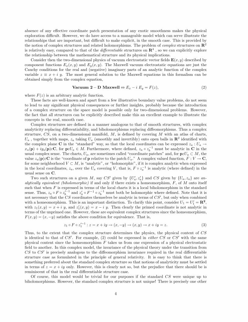
Consider then the two-dimensional physics of vacuum electrostatic vector fields E(x, y) described bycomponent functions Ex(x, y) and Ey(x, y). The Maxwell vacuum electrostatic equations are just theCauchy conditions for the real and (negative) imaginary parts of an analytic function of the complexvariable z ≡ x + i y. The most general solution to the Maxwell equations in this formalism can beobtained simply from the complex equation,

Vacuum 2− D Maxwell ⇔ Ex − i Ey = F (z), (2)

where F (z) is an arbitrary analytic function.These facts are well-known and apart from a few illustrative boundary value problems, do not seem

to lead to any significant physical consequences or further insights, probably because the introductionof a complex structure on the space model is possible only for two-dimensional problems. However,the fact that all structures can be explicitly described make this an excellent example to illustrate theconcepts in the real, smooth case.

Complex structures are defined in a manner analogous to that of smooth structures, with complexanalyticity replacing differentiability, and biholomorphisms replacing diffeomorphisms. Thus a complexstructure, CS, on a two-dimensional manifold, M , is defined by covering M with an atlas of charts,Ua , together with maps, za taking Ua (smoothly and invertibly) onto open balls in R2 identified withthe complex plane C in the “standard” way, so that the local coordinates can be expressed za : Ua →xa(p) + iya(p)εC, for pεUa ∈ M. Furthermore, where defined, za ◦ z−1

b must be analytic in C in theusual complex sense. The charts, Ua, are sometimes called “coordinate patches” and, for pεUa ⊂ M , thevalue za(p)εC is the “coordinate of p relative to the patch Ua.” A complex valued function, F : V → C,for some neighborhood V ⊂ M , is “analytic”, or “holomorphic”, if it is complex analytic when expressedin the local coordinates, za, over the Ua covering V , that is, F ◦ z−1

a is analytic (where defined) in theusual sense on C.

Two such structures on a given M , say CS′ given by {U ′

a, z′

a} and CS given by {Ua, za} are an-alytically equivalent (biholomorphic) if and only if there exists a homeomorphism, F , of M onto itselfsuch that when F is expressed in terms of the local charts it is a local biholomorphism in the standardsense. Thus, za ◦ F ◦ z′−1

b and z′a ◦ F−1 ◦ z−1

b must both be holomorphic where defined. Note that it isnot necessary that the CS coordinates themselves be analytic in terms of CS′, but only when combinedwith a homeomorphism. This is an important distinction. To clarify this point, consider U1 = U ′

1 = R2,with z1(x, y) = x + i y, and z′1(x, y) = x − i y. Then clearly the primed coordinate is not analytic interms of the unprimed one. However, these are equivalent complex structures since the homeomorphism,F (x, y) = (x,−y) satisfies the above condition for equivalence. That is,

z1 ◦ F ◦ z′−1

1: z = x + iy → (x,−y) → (x, y) → x + iy = z. (3)

Thus, to the extent that the complex structure determines the physics, the physical content of CSis identical to that of CS′. For example, (2) could be expressed in either CS or CS′ with the samephysical content since the homeomorphism F takes us from one expression of a physical electrostaticfield to another. In this complex model, the invariance of the physical theory under the transition fromCS to CS′ is precisely analogous to the diffeomorphism invariance required in the real differentiablestructure case as formulated in the principle of general relativity. It is easy to think that there issomething preferred about the standard complex structure so that notions of analyticity must be settledin terms of z = x + iy only. However, this is clearly not so, but the prejudice that there should be isreminiscent of that in the real differentiable structure case.

Of course, this model would be trivial for our purposes if the standard CS were unique up tobiholomorphisms. However, the standard complex structure is not unique! There is precisely one other

4

inequivalent one, that is, one not related by a biholomorphism. One presentation of this second structure,CS1, can be defined by

(x, y) → z1 =e−1/r

r(x + i y)εC. (4)

The key point here is that |z1| is bounded. It is now easy to show that CS0 is not equivalent to CS1. Infact, if it were then there would exist a function, F(x, y) = (Fx(x, y), Fy(x, y)), of the plane onto itself

such that e−1/F

F (Fx(x, y) + i Fy(x, y)) would be a global analytic function of x + i y in the usual sense.Clearly however this cannot be since this function is non-constant, but bounded on the entire plane,violating a well known property of global analytic functions for the standard CS0.

Now we can state the physical implications of the choice of structure, complex in this case: If thephysical theory is expressed by the statement that the x and y components of the electrostatic vacuumtwo-dimensional field are real and (negative) imaginary parts of a function analytic relative to the chosencomplex structure, then CS0 and CS1 lead to different fields, with physically measurable differencessince non-constant electrostatic fields in the CS0 case cannot be bounded, whereas they are in the CS1

case. In other words, to the extent that (2) is the statement of a physical theory, then in principle,experiment could distinguish CS0 from CS1. However, experiment cannot distinguish CS0 from CS′

described earlier, since these are biholomorphic.Of course, this discussion is intended to be illustrative rather than of any likely physical significance

itself. The description of electrostatic field theory in terms of analyticity requirements is certainly notthe basis of a general physical theory. In fact, it could be argued that changing the complex structureresults in a changed metric and that the correct theory should include this metric. However, thismodel does illustrate explicitly the difference between merely different and inequivalent structures, non-biholomorphic in this case, non-diffeomorphic in our smooth case. For this complex model, CS1 playsthe role of an exotic differentiable structure in the real case. While CS1 was easily displayed we donot have yet have this luxury for a R4

Θ. However, we now proceed to review the path to these strange

structures.

4 Some History of Exotic Differentiable Structures

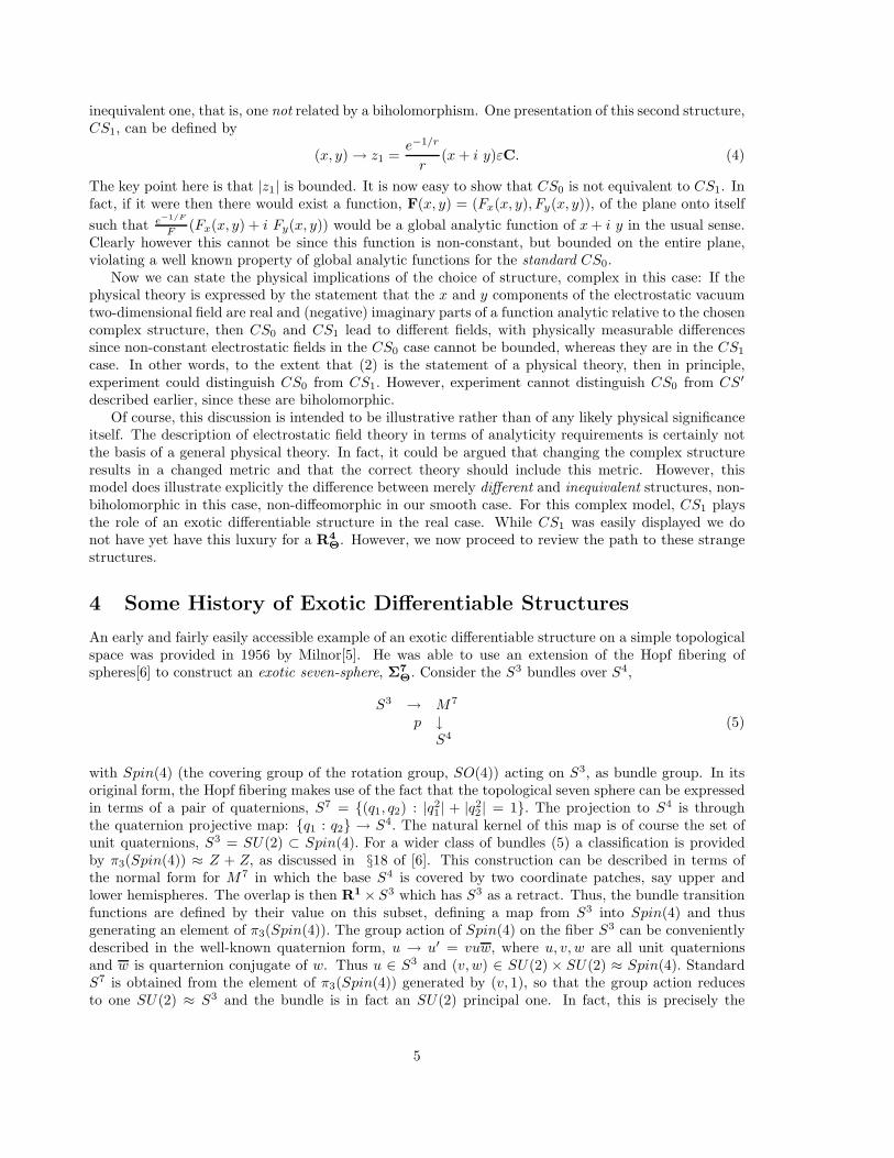
An early and fairly easily accessible example of an exotic differentiable structure on a simple topologicalspace was provided in 1956 by Milnor[5]. He was able to use an extension of the Hopf fibering ofspheres[6] to construct an exotic seven-sphere, Σ7

Θ. Consider the S3 bundles over S4,

S3 → M7

p ↓S4

(5)

with Spin(4) (the covering group of the rotation group, SO(4)) acting on S3, as bundle group. In itsoriginal form, the Hopf fibering makes use of the fact that the topological seven sphere can be expressedin terms of a pair of quaternions, S7 = {(q1, q2) : |q2

1 | + |q22 | = 1}. The projection to S4 is through

the quaternion projective map: {q1 : q2} → S4. The natural kernel of this map is of course the set ofunit quaternions, S3 = SU(2) ⊂ Spin(4). For a wider class of bundles (5) a classification is providedby π3(Spin(4)) ≈ Z + Z, as discussed in §18 of [6]. This construction can be described in terms ofthe normal form for M7 in which the base S4 is covered by two coordinate patches, say upper andlower hemispheres. The overlap is then R1 × S3 which has S3 as a retract. Thus, the bundle transitionfunctions are defined by their value on this subset, defining a map from S3 into Spin(4) and thusgenerating an element of π3(Spin(4)). The group action of Spin(4) on the fiber S3 can be convenientlydescribed in the well-known quaternion form, u → u′ = vuw, where u, v, w are all unit quaternionsand w is quarternion conjugate of w. Thus u ∈ S3 and (v, w) ∈ SU(2) × SU(2) ≈ Spin(4). StandardS7 is obtained from the element of π3(Spin(4)) generated by (v, 1), so that the group action reducesto one SU(2) ≈ S3 and the bundle is in fact an SU(2) principal one. In fact, this is precisely the

5

principle SU(2) Yang-Mills bundle over compactified space-time, S4. For more details on classifyingsphere bundles, see [6], §20 and, from the physics viewpoint, [7].

Milnor’s breakthrough in 1956 involved his proving that M7 for the transition function map, anelement of π3(Spin(4)), given by

u → (uh, uj) ∈ Spin(4), (6)

with h + j = 1 and h − j = k, and k2 ≡/ 1 mod 7, is in fact exotic, i.e., homeomorphic to S7, but notdiffeomorphic to it. Clearly, the constructive part is fairly easy, but the proof of the exotic nature ofthe resulting sphere is more involved, drawing from several important results in differential topologyincluding the Thom bordism result, cohomology theory, Pontrjagin classes, etc. Later, Kervaire andMilnor[8] and others[9] expanded on these results, leading to a good understanding of the class of exoticspheres in dimensions seven and greater.

For the purposes of this paper, the importance of Milnor’s discovery is that it provides an explicitexample of a topologically simple space, S7, for which the topology does not determine the smoothness.Furthermore, its construction is explicit and easily understood. From the physics viewpoint, its mostimportant application may be in terms of some “exotic Yang-Mills” models as discussed below.

Unfortunately, the path to R4

Θis much less easy to describe than are the Milnor spheres. The

techniques required span a variety of mathematical disciplines and the following survey is necessarilybrief. The reader is referred to mathematical reviews for more details[10].

The first step involves a topological tool important in classifications of four manifolds. The intersec-tion form of a compact oriented manifold without boundary, is obtained by the Poincare duality pairingof homology classes in Hn−k and Hk can be simply represented in dimension n = 4 = 2+2 by a symmet-ric square matrix of determinant ±1. This form basically reflects the way in which pairs of oriented two-dimensional closed surfaces fill out the full (oriented) four-space at their intersection points. Physicistsare perhaps more familiar with deRham cohomology involving exterior forms for which this intersectionpairing is the volume integral of the exterior product of a pair of closed two-forms representing theindividual cohomology classes, which again makes sense only in dimension four. Unfortunately, deR-ham cohomology necessarily involves real coefficients and is thus too coarse for our applications, whichneed integral homology theory. At any rate, this integral intersection form, ω, plays a central role inclassifying compact four manifolds. Whitehead used it to prove that one-connected closed 4-manifoldsare determined up to homotopy type by the isomorphism class of ω. Later, Freedman[1] proved thatω together with the Kirby-Siebenmann invariant classifies simply-connected closed 4-manifolds up tohomeomorphism. For our purposes, the important result was that there exists a topological four man-ifold, |E8|, having intersection form ω = E8, the Cartan matrix for the exceptional lie algebra of thesame name.

As it stands, Freedman’s work is in the topological category, and does not address smoothnessquestions. The theorem of Rohlin[11] states that the signature of a closed connected oriented smooth4-manifold must be divisible by 16, so that |E8| cannot exist as a smooth manifold since its signature is8. Next, Donaldson’s theorem[2] provides the crucial (for our purposes) generalization of this result toestablish that |E8 ⊕E8| cannot be endowed with any smooth structure, even though its signature is 16.The work of Donaldson is based on the moduli space of solutions to the SU(2) Yang-Mills equations ona four-manifold, which first occur in physics literature.

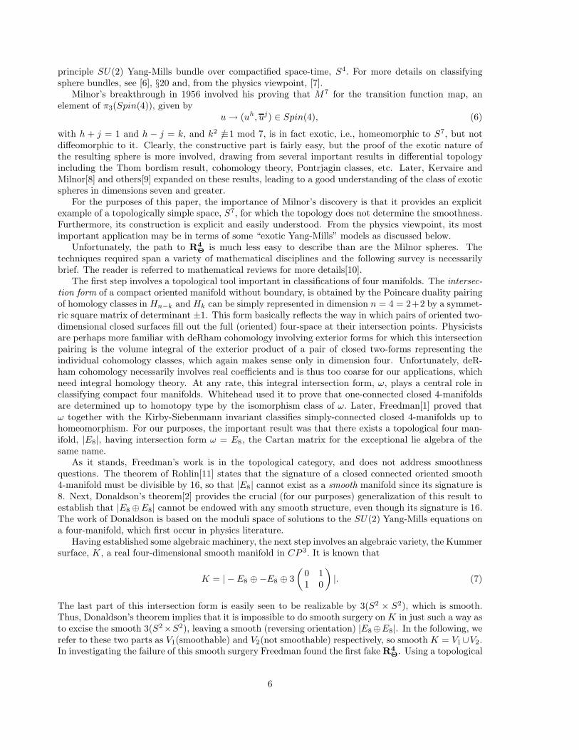
Having established some algebraic machinery, the next step involves an algebraic variety, the Kummersurface, K, a real four-dimensional smooth manifold in CP 3. It is known that

K = | − E8 ⊕−E8 ⊕ 3

(

0 11 0

)

|. (7)

The last part of this intersection form is easily seen to be realizable by 3(S2 × S2), which is smooth.Thus, Donaldson’s theorem implies that it is impossible to do smooth surgery on K in just such a way asto excise the smooth 3(S2×S2), leaving a smooth (reversing orientation) |E8⊕E8|. In the following, werefer to these two parts as V1(smoothable) and V2(not smoothable) respectively, so smooth K = V1∪V2.In investigating the failure of this smooth surgery Freedman found the first fake R4

Θ. Using a topological

6

S3 to separate V1 from V2, Donaldson’s result showed that this S3 cannot be smoothly embedded, sinceotherwise V2 would have a smooth structure. However, by further surgery, it is found that this dividingS3 is also topologically embedded in a topological R4 and actually includes a compact set in its interior.Thus we have

Existence of exotic R4

Θ: This topological R4 contains a compact set which cannot

be contained in any smoothly embedded S3. This surprising result then implies that thismanifold is indeed an R4

Θsince in any diffeomorphic image of R4 every compact set is

included in the interior of a smooth sphere.

5 Some Properties of R4Θ’s

After this basic existence theorem, many developments have occurred, some of which are summarized inthe book by Kirby[12]. Unfortunately, none of the uncountable infinity of R4

Θ’s has been presented in

explicit atlas of charts form, so most of the properties can only be described indirectly, through existenceor non-existence type of theorems. In this paper we restrict the discussion to those topics of possiblephysical applications.

The defining feature of the original R4

Θas discussed above can be summarized in coordinate form

as follows: R4

Θis the topological product R1 × R1 × R1 × R1. Thus, it can be described topologically

as the set R4

Θ= {pα}, α = 1...4. However, these coordinates cannot be globally smooth, since otherwise

the product would be smooth and the manifold diffeomorphic to standard R4. Or, in terms of theproperty used in the discovery, if {pα} were globally smooth, since every compact set is contained insome |p|2 ≡

∑

(pα)2 = R2 for sufficiently large R, then every compact set would be contained in somesmoothly embedded S3, contrary to the existence statement above. In fact, this absence of “sufficientlylarge” smooth three-spheres is a strange and defining characteristic of R4

Θ’s. It shows, among other

things that the exoticness necessarily extends to infinity. Nevertheless, the possibility of confining theexoticness to a time-like tube is shown in Theorem 2 below.

Even though the global topological coordinates cannot be globally smooth, it can be shown that insome diffeomorphic copy they can be made smooth locally. Thus

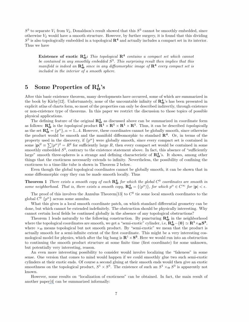
Theorem 1 There exists a smooth copy of each R4

Θfor which the global C0 coordinates are smooth in

some neighborhood. That is, there exists a smooth copy, R4

Θ= {(pα)}, for which pα ∈ C∞ for |p| < ǫ.

The proof of this involves the Annulus Theorem[13] to C0 tie some local smooth coordinates to theglobal C0 {pα} across some annulus.

What this gives is a local smooth coordinate patch, on which standard differential geometry can bedone, but which cannot be extended indefinitely. The obstruction should be physically interesting. Whycannot certain local fields be continued globally in the absence of any topological obstructions?

Theorem 1 leads naturally to the following construction. By puncturing R4

Θin the neighborhood

where the topological coordinates are smooth, we get a “semi-exotic” cylinder, i.e, R4

Θ−{0} ≃ R1×ΘS3,

where ×Θ means topological but not smooth product. By “semi-exotic” we mean that the product isactually smooth for a semi-infinite extent of the first coordinate. This might be a very interesting cos-mological model for physics, which after the big bang is R1×S3. Here we would run into an obstructionto continuing the smooth product structure at some finite time (first coordinate) for some unknown,but potentially very interesting, reason.

An even more interesting possibility to consider would involve localizing the “fakeness” in somesense. One version that comes to mind would happen if we could smoothly glue two such semi-exoticcylinders at their exotic ends. Of course a second gluing at their smooth ends would then give an exoticsmoothness on the topological product, S1 × S3. The existence of such an S1 ×Θ S3 is apparently notknown.

However, some results on “localization of exoticness” can be obtained. In fact, the main result ofanother paper[4] can be summarized informally:

7

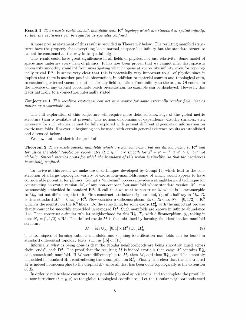
Result 1 There exists exotic smooth manifolds with R4 topology which are standard at spatial infinity,so that the exoticness can be regarded as spatially confined.

A more precise statement of this result is provided in Theorem 2 below. The resulting manifold struc-tures have the property that everything looks normal at space-like infinity but the standard structurecannot be continued all the way in to spatial origin.

This result could have great significance in all fields of physics, not just relativity. Some model ofspace-time underlies every field of physics. It has now been proven that we cannot infer that space isnecessarily smoothly standard from investigating what happens at space- like infinity, even for topolog-ically trivial R4. It seems very clear that this is potentially very important to all of physics since itimplies that there is another possible obstruction, in addition to material sources and topological ones,to continuing external vacuum solutions for any field equations from infinity to the origin. Of course, inthe absence of any explicit coordinate patch presentation, no example can be displayed. However, thisleads naturally to a conjecture, informally stated:

Conjecture 1 This localized exoticness can act as a source for some externally regular field, just asmatter or a wormhole can.

The full exploration of this conjecture will require more detailed knowledge of the global metricstructure than is available at present. The notions of domains of dependence, Cauchy surfaces, etc.,necessary for such studies cannot be fully explored with present differential geometric information onexotic manifolds. However, a beginning can be made with certain general existence results as establishedand discussed below.

We now state and sketch the proof of

Theorem 2 There exists smooth manifolds which are homeomorphic but not diffeomorphic to R4 andfor which the global topological coordinates (t, x, y, z) are smooth for x2 + y2 + z2 ≥ ǫ2 > 0, but notglobally. Smooth metrics exists for which the boundary of this region is timelike, so that the exoticnessis spatially confined.

To arrive at this result we make use of techniques developed by Gompf[14] which lead to the con-struction of a large topological variety of exotic four-manifolds, some of which would appear to haveconsiderable potential for physics. Gompf’s “end-sum” process provides a straightforward technique forconstructing an exotic version, M , of any non-compact four-manifold whose standard version, M0, canbe smoothly embedded in standard R4. Recall that we want to construct M which is homeomorphicto M0, but not diffeomorphic to it. First construct a tubular neighborhood, T0, of a half ray in M0. T0

is thus standard R4 = [0,∞) × R3. Now consider a diffeomorphism, φ0 of T0 onto N0 = [0, 1/2) × R3

which is the identity on the R3 fibers. Do the same thing for some exotic R4

Θwith the important proviso

that it cannot be smoothly embedded in standard R4. Such manifolds are known in infinite abundance[14]. Then construct a similar tubular neighborhood for this R4

Θ, T1, with diffeomorphism, φ1, taking it

onto N1 = [1, 1/2)×R3. The desired exotic M is then obtained by forming the identification manifoldstructure

M = M0 ∪φ0([0, 1] × R3) ∪φ1

R4

Θ(8)

The techniques of forming tubular manifolds and defining identification manifolds can be found instandard differential topology texts, such as [15] or [16].

Informally, what is being done is that the tubular neighborhoods are being smoothly glued acrosstheir “ends”, each R3. The proof that the resulting M is indeed exotic is then easy: M contains R4

Θ

as a smooth sub-manifold. If M were diffeomorphic to M0 then M , and thus R4

Θ, could be smoothly

embedded in standard R4, contradicting the assumption on R4

Θ. Finally, it is clear that the constructed

M is indeed homeomorphic to the original M0 since all that has been done topologically is the extensionof T0.

In order to relate these constructions to possible physical applications, and to complete the proof, letus now introduce (t, x, y, z) as the global topological coordinates. Let the tubular neighborhoods used

8

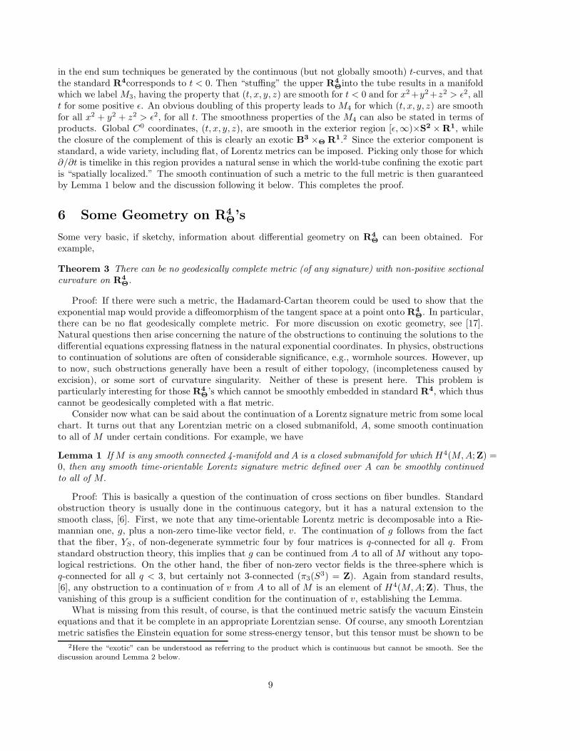
in the end sum techniques be generated by the continuous (but not globally smooth) t-curves, and thatthe standard R4corresponds to t < 0. Then “stuffing” the upper R4

Θinto the tube results in a manifold

which we label M3, having the property that (t, x, y, z) are smooth for t < 0 and for x2 +y2+z2 > ǫ2, allt for some positive ǫ. An obvious doubling of this property leads to M4 for which (t, x, y, z) are smoothfor all x2 + y2 + z2 > ǫ2, for all t. The smoothness properties of the M4 can also be stated in terms ofproducts. Global C0 coordinates, (t, x, y, z), are smooth in the exterior region [ǫ,∞)×S2 × R1, whilethe closure of the complement of this is clearly an exotic B3 ×Θ R1.2 Since the exterior component isstandard, a wide variety, including flat, of Lorentz metrics can be imposed. Picking only those for which∂/∂t is timelike in this region provides a natural sense in which the world-tube confining the exotic partis “spatially localized.” The smooth continuation of such a metric to the full metric is then guaranteedby Lemma 1 below and the discussion following it below. This completes the proof.

6 Some Geometry on R4Θ’s

Some very basic, if sketchy, information about differential geometry on R4

Θcan been obtained. For

example,

Theorem 3 There can be no geodesically complete metric (of any signature) with non-positive sectionalcurvature on R4

Θ.

Proof: If there were such a metric, the Hadamard-Cartan theorem could be used to show that theexponential map would provide a diffeomorphism of the tangent space at a point onto R4

Θ. In particular,

there can be no flat geodesically complete metric. For more discussion on exotic geometry, see [17].Natural questions then arise concerning the nature of the obstructions to continuing the solutions to thedifferential equations expressing flatness in the natural exponential coordinates. In physics, obstructionsto continuation of solutions are often of considerable significance, e.g., wormhole sources. However, upto now, such obstructions generally have been a result of either topology, (incompleteness caused byexcision), or some sort of curvature singularity. Neither of these is present here. This problem isparticularly interesting for those R4

Θ’s which cannot be smoothly embedded in standard R4, which thus

cannot be geodesically completed with a flat metric.Consider now what can be said about the continuation of a Lorentz signature metric from some local

chart. It turns out that any Lorentzian metric on a closed submanifold, A, some smooth continuationto all of M under certain conditions. For example, we have

Lemma 1 If M is any smooth connected 4-manifold and A is a closed submanifold for which H4(M, A;Z) =0, then any smooth time-orientable Lorentz signature metric defined over A can be smoothly continuedto all of M.

Proof: This is basically a question of the continuation of cross sections on fiber bundles. Standardobstruction theory is usually done in the continuous category, but it has a natural extension to thesmooth class, [6]. First, we note that any time-orientable Lorentz metric is decomposable into a Rie-mannian one, g, plus a non-zero time-like vector field, v. The continuation of g follows from the factthat the fiber, YS , of non-degenerate symmetric four by four matrices is q-connected for all q. Fromstandard obstruction theory, this implies that g can be continued from A to all of M without any topo-logical restrictions. On the other hand, the fiber of non-zero vector fields is the three-sphere which isq-connected for all q < 3, but certainly not 3-connected (π3(S

3) = Z). Again from standard results,[6], any obstruction to a continuation of v from A to all of M is an element of H4(M, A;Z). Thus, thevanishing of this group is a sufficient condition for the continuation of v, establishing the Lemma.

What is missing from this result, of course, is that the continued metric satisfy the vacuum Einsteinequations and that it be complete in an appropriate Lorentzian sense. Of course, any smooth Lorentzianmetric satisfies the Einstein equation for some stress-energy tensor, but this tensor must be shown to be

2Here the “exotic” can be understood as referring to the product which is continuous but cannot be smooth. See the

discussion around Lemma 2 below.

9

physically acceptable. Unfortunately, these issues cannot be resolved without more explicit informationon the global exotic structure than is presently available. However, we can be more specific about theconditions under which some smooth Lorentzian metric can be globally continued on an exotic manifoldfrom some local coordinate presentation.

In the applications in this paper, M is non-compact, so H4(M ;Z) = 0. Using the exact cohomologysequence generated by the inclusion A → M, we can develop[4] several easily satisfied sufficient conditionson A to meet the conditions of Lemma 1. One easy one is to require H3(A;Z) = 0. Another would beto establish that the map, H3(M ;Z) → H3(A;Z) is an epimorphism. For example, if A is simply aclosed miniature version of R2 × S2 itself, i.e., A = D2 × S2, then H3(A;Z) = 0 so the continuation ofa smooth Lorentzian metric is ensured. The spaces R2 ×Θ S2, each have the topology of the Kruskalpresentation of the Schwarzschild metric. Using the standard Kruskal notation {(u, v, ω); u2−v2 < 1, ω ∈S2} constitute global topological coordinates. From Theorem 1, these can be smooth over the closure ofsome open set, say A, homeomorphic D2 × S2, but (u, v) cannot be continued as smooth functions overthe entire range: u2−v2 < 1. Over A then we can solve the vacuum Einstein equations as usual to get theKruskal form. From Lemma 1, some smooth metric can be continued from this over the entire manifold.However, whatever it is, it cannot be the standard Kruskal one. The obstruction to continuation ofthe metric occurs not for any reasons associated with the development of singularities in the coordinateexpression of the metric, or for any topological reasons, but simply because the coordinates, (u, v, ω),cannot be continued smoothly beyond some proper subset, A, of the full manifold. This establishes

Theorem 4 On some smooth manifolds which are topologically R2 × S2, the standard Kruskal metriccannot be smoothly continued over the full range, u2 − v2 < 1.

An interesting variation occurs when A contains a trapped surface, so a singularity will inevitablydevelop from well-known theorems. However, if A does not contain a trapped surface what will happenis not known.

Another way to study this metric is in terms of the original Schwarzschild (r, t) coordinates forM4. For this model the coordinates (t, r, ω) are smooth for all of the closed sub-manifold A defined byr ≥ ǫ > 2M but cannot be continued as smooth over the entire M or over any diffeomorphic (physicallyequivalent) copy. In this case A is topologically [ǫ,∞) × S2 × R1, so again H3(A;Z) = 0 and theconditions of lemma 1 are met. Hence there is some smooth continuation of any exterior Lorentzianmetric in A, in particular, the Schwarzschild metric, over the full R4

Θ. Whatever this metric is, it cannot

be Schwarzschild since the manifolds are not diffeomorphic. An interesting feature of this model is thatthe manifold is “asymptotically” standard in spite of the well known fact that exotic manifolds are badlybehaved “at infinity”. However, we note that this model is asymptotically standard only as r → ∞, butcertainly not as t → ∞.

These models are clearly highly suggestive for investigation of alternative continuation of exteriorsolutions into the tube near r = 0. We often first discover an exterior, vacuum solution, and look tocontinue it back to some source. This is a standard problem. In the stationary case, we typically havea local, exterior solution to an elliptic problem, and try to continue it into the origin but find we can’tas a vacuum solution unless we have a topology change (e.g., a wormhole), or unless we add a mattersource, changing the equation. Now, we are led to consider a third alternative, can exotic smoothnessserve as a source for some exterior metric?

Of course, the discussion of stationary solutions involves the idea of time foliations, which cannotexist globally for these exotic manifolds, at least not into standard factors. In fact,

Lemma 2 R4

Θcannot be written as a smooth product, R1 ×smooth R3. Similarly R2 ×Θ S2 cannot be

written as R1 ×smooth (R1 × S2).

Clearly, if either factor decomposition were smooth, the original manifold would be standard, since thefactors are necessarily standard from known lower dimensional results, establishing the lemma. It is notnow possible to establish the more general result for which the second factor is simply some smooththree manifold without restriction.

10

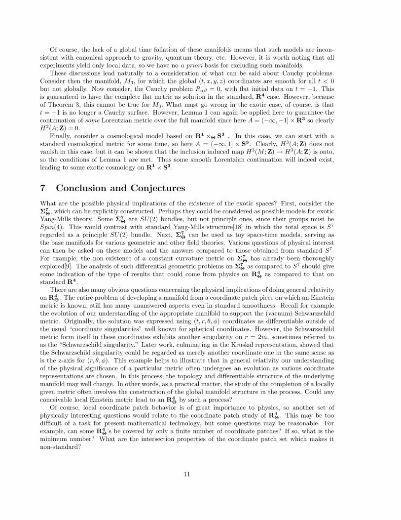
Of course, the lack of a global time foliation of these manifolds means that such models are incon-sistent with canonical approach to gravity, quantum theory, etc. However, it is worth noting that allexperiments yield only local data, so we have no a priori basis for excluding such manifolds.

These discussions lead naturally to a consideration of what can be said about Cauchy problems.Consider then the manifold, M3, for which the global (t, x, y, z) coordinates are smooth for all t < 0but not globally. Now consider, the Cauchy problem Rαβ = 0, with flat initial data on t = −1. Thisis guaranteed to have the complete flat metric as solution in the standard, R4 case. However, becauseof Theorem 3, this cannot be true for M3. What must go wrong in the exotic case, of course, is thatt = −1 is no longer a Cauchy surface. However, Lemma 1 can again be applied here to guarantee thecontinuation of some Lorentzian metric over the full manifold since here A = (−∞,−1]×R3 so clearlyH3(A;Z) = 0.

Finally, consider a cosmological model based on R1 ×Θ S3 . In this case, we can start with astandard cosmological metric for some time, so here A = (−∞, 1] × S3. Clearly, H3(A;Z) does notvanish in this case, but it can be shown that the inclusion induced map H3(M ;Z) → H3(A;Z) is onto,so the conditions of Lemma 1 are met. Thus some smooth Lorentzian continuation will indeed exist,leading to some exotic cosmology on R1 × S3.

7 Conclusion and Conjectures

What are the possible physical implications of the existence of the exotic spaces? First, consider theΣ7

Θ, which can be explicitly constructed. Perhaps they could be considered as possible models for exotic

Yang-Mills theory. Some Σ7

Θare SU(2) bundles, but not principle ones, since their groups must be

Spin(4). This would contrast with standard Yang-Mills structure[18] in which the total space is S7

regarded as a principle SU(2) bundle. Next, Σ7

Θcan be used as toy space-time models, serving as

the base manifolds for various geometric and other field theories. Various questions of physical interestcan then be asked on these models and the answers compared to those obtained from standard S7.For example, the non-existence of a constant curvature metric on Σ7

Θhas already been thoroughly

explored[9]. The analysis of such differential geometric problems on Σ7

Θas compared to S7 should give

some indication of the type of results that could come from physics on R4

Θas compared to that on

standard R4.There are also many obvious questions concerning the physical implications of doing general relativity

on R4

Θ. The entire problem of developing a manifold from a coordinate patch piece on which an Einstein

metric is known, still has many unanswered aspects even in standard smoothness. Recall for examplethe evolution of our understanding of the appropriate manifold to support the (vacuum) Schwarzschildmetric. Originally, the solution was expressed using (t, r, θ, φ) coordinates as differentiable outside ofthe usual “coordinate singularities” well known for spherical coordinates. However, the Schwarzschildmetric form itself in these coordinates exhibits another singularity on r = 2m, sometimes referred toas the “Schwarzschild singularity.” Later work, culminating in the Kruskal representation, showed thatthe Schwarzschild singularity could be regarded as merely another coordinate one in the same sense asis the z-axis for (r, θ, φ). This example helps to illustrate that in general relativity our understandingof the physical significance of a particular metric often undergoes an evolution as various coordinaterepresentations are chosen. In this process, the topology and differentiable structure of the underlyingmanifold may well change. In other words, as a practical matter, the study of the completion of a locallygiven metric often involves the construction of the global manifold structure in the process. Could anyconceivable local Einstein metric lead to an R4

Θby such a process?

Of course, local coordinate patch behavior is of great importance to physics, so another set ofphysically interesting questions would relate to the coordinate patch study of R4

Θ. This may be too

difficult of a task for present mathematical technology, but some questions may be reasonable. Forexample, can some R4

Θ’s be covered by only a finite number of coordinate patches? If so, what is the

minimum number? What are the intersection properties of the coordinate patch set which makes itnon-standard?

11

A directly physical set of questions to be considered would stem from attempts to embed knownsolutions to the Einstein equations in R4

Θ, then asking what sort of obstruction intervenes to prevent

their indefinite, complete, continuation, in this space. Examples of non-topological obstructions tothe continuation of a wide class of Einstein metrics was discussed in Section 6. What is the physicalsignificance of these obstructions?

Finally, it is indeed true that the existence of R4

Θ’s does not in any way change the local physics

of general relativity or any other field theory. However, it has long been known that global questionscan have profound effects on a physical theory. Until recently, physicists have thought of global mattersalmost exclusively as being of purely topological significance, whereas we now know that at least inthe physically important case of R4, there are very exciting global questions related to differentiabilitystructures, the way in which local physics is patched together smoothly to make it global. Certainly, theR4

Θ’s are essentially just “other” manifolds. However, there are an infinity of them which have never

been remotely considered in the physical context of classical space-time physics on Einstein’s originalmodel, R4. It would be surprising indeed if none of these had any conceivable physical significance.

I am very grateful to Duane Randall and Robert Gompf for their invaluable assistance in this work.

12

References

[1] M. Freedman, J. Diff. Geom., 17, 357(1982).

[2] S. K. Donaldson, J. Diff. Geom., 18,269 (1983).

[3] Carl H. Brans and Duane Randall, Gen. Rel. Grav., 25, 205 (1993).

[4] Carl H. Brans, “Localized Exotic Smoothness,” Preprint gr-qc 9404003 to appear in Journal ofClassical and Quantum Gravity

[5] John W. Milnor, Ann. Math. 64, 399 (1956), Amer. J. Math. 81, 962 (1959).

[6] See, for example, The Topology of Fiber Bundles, by Norman Steenrod, Princeton(1951).

[7] This process is described in various books discussing gauge theories and physics. See, for example,Differential Geometry for Physicists, by Andrzej Trautman, Bibliopolis (Naples, 1984).

[8] M. Kervaire, J. Milnor, Ann. Math. 77. 504 (1963).

[9] Detlef Gromoll and Wolfgang Meyer, Ann. Math 100, 401 (1974). A. Rigas, Bull. Soc. Math. France112, 69 (1984).

[10] Reviews of these topics can be found in Instantons and Four- Manifolds, by Daniel S. Freedand Karen K. Uhlenbeck, Springer-Verlag (1984), and Selected Applications of Geometry to Low-Dimensional Topology, by Michael H. Freedman and Feng Luo, American Mathematical Society(1989).

[11] V. A. Rohlin, Dok. Akad. Nauk, USSR, 84, 221 (1952).

[12] Robion C. Kirby The Topology of 4-Manifolds, Springer-Verlag Lecture Notes in Mathematics, 1374

(1989).

[13] Robert D. Edwards, Contemporary Mathematics, 35, 211 (1984).

[14] Robert E. Gompf, J. Diff. Geom., 21, 283 (1985).

[15] Th. Brocker and K. Janisch, Introduction to Differential Topology, Cambridge University Press(1987).

[16] Morris W. Hirsch, Differential Topology, Springer-Verlag (1988).

[17] For more details on the relationship between geodesic structure and smoothness see Bruce L. Rein-hart, Ann. Global Anal. Geom. 9,67(1991).

[18] Kengo Yamagishi, Physics Letters, 134B, 47 (1984).

13