“diss”2002/10/18page 1

Rainer Reichle

Exotic Species of HydrogenExperimental and Theoretical Studies of the Negative Ion and

the Triatomic Molecule of Hydrogen

“diss”2002/10/18page 2

Dekan:Leiter der Arbeit:Referent:Korreferent:Tag der Verkundigungdes Prufungsergebnisses:

Prof. Dr. Rolf SchneiderProf. Dr. Hanspeter HelmProf. Dr. Hanspeter HelmProf. Dr. Hartmut Ropke

2.10.2002

“diss”2002/10/18page 1

Exotic Species of Hydrogen

INAUGURAL-DISSERTATION

zur Erlangung des Doktorgrades derFakultat fur Mathematik und Physik der

Albert-Ludwigs-Universitat Freiburg i.Br.

vorgelegt von

Rainer Reichle

aus Sigmaringen

im August 2002

“diss”2002/10/18page 2

Rainer ReichleDepartment of Optical and Molecular Physics

Albert-Ludwig-University of FreiburgHermann-Herder-Str.379104 Freiburg/Germanyphone: (+49) 761 203 7636fax: (+49) 761 203 5955E-Mail: Rainer.Reichle@physik.uni-freiburg.de

NIPNegative Ion Project

“diss”2002/10/18page I

I

Rainer Reichle

Exotic Species of Hydrogen

PACS:Part I 33.80.-b, 33.80.Eh, 33.80.RvPart II 32.80.Gc, 32.80.Rm

This research was supported by the Deutsche Forschungsgemeinschaft SFB 276.Part I within TP C13 and Part II under TP C14.

This document is electronically available from the Freiburg Document Server under theURL: http://www.freidok.uni-freiburg.de/freidok

E-Mail: Rainer.Reichle@physik.uni-freiburg.de

Click on colored items for getting linked.

c©2002 All rights reserved.

“diss”2002/10/18page II

II

“diss”2002/10/18page III

III

Publications in Refereed Journals

In inverse chronological order

R. Reichle, H. Helm, I. Yu. KiyanDetailed comparison of theory and experiment of strong-field pho-todetachment of negative hydrogento be published in Phys. Rev. A, (2002)

R. Reichle, I. Yu. Kiyan, H. HelmTwo-slit interference in strong-field photodetachment of H−

accepted for publication in Journal of Modern Optics, (2002)

Helm H., Galster U., Mistrık I., Muller U., Reichle R.Coupling of Bound States to Continuum States in Neutral TriatomicHydrogen Dissociative Recombination: Theory, Experiment and Applications, ed:S. Guberman, (2002)

R. Reichle, H. Helm, I. KiyanPhotodetachment of H− in a strong infrared laser fieldPhys. Rev. Lett. 87, 243001 (2001)

I. Mistrık, R. Reichle, H. Helm, and U. MullerPredissociation of H3 Rydberg statesPhys. Rev. A 63, 042711 (2001)

I. Mistrık, R. Reichle, U. Muller, H. Helm, M. Jungen, and J. A. StephensAb initio analysis of autoionization of H3 molecules using multichannelquantum defect theory and new quantum defect surfacesPhys. Rev. A 61, 033410 (2000)

R. Reichle, I. Mistrık, U. Muller, and H. HelmRotational Channel Interactions of Vibrationally Excited np-RydbergStates of the Triatomic Hydrogen MoleculePhys. Rev. A 60, 3929 (1999)

“diss”2002/10/18page IV

IV

U. Muller, R. Reichle, I. Mistrık, J. A. Stephens, M. Jungen, and H. HelmPhotoionization of the triatomic hydrogen molecule18th International Symposium on Molecular Beams, Ameland, The Netherlands,Book of abstracts p.162, May 30-June 4, (1999)

U. Muller, R. Reichle, I. Mistrık, J. A. Stephens, M. Jungen, and H. HelmPhotoionization of the triatomic hydrogen moleculeDissociative Recombination: Theory, Experiment and Applications IV, ed: M.Larsson, J.B.A. Mitchell, I.F. Schneider, World Scientific 1999, p.55

From previous work

U. Muller, M. Braun, R. Reichle, and R. F. SalzgeberVibrational frequencies of the 2p2A′′2 and 3d2E′′ states of the tri-atomic deuterium moleculeJ. Chem. Phys. 108, 4478 (1998)

U. Muller, U. Majer, R. Reichle, and M. BraunSpectroscopy of high n Rydberg States of the Triatomic DeuteriumMolecule D3

J. Chem. Phys. 106, 7958 (1997)

“diss”2002/10/18page V

Contents

Publications in Refereed Journals III

List of Figures IX

List of Tables XIII

1 Significance of Atomic and Molecular Hydrogen 3

I Triatomic Hydrogen - The Herzberg Molecule 7

2 Introduction to Part I 9

3 Quantum Mechanical Treatment of H3 11

3.1 Categorization of Electronic Energies . . . . . . . . . . . . . . . . . . . . . 11

3.2 Geometry and Normal Coordinates . . . . . . . . . . . . . . . . . . . . . . 14

3.3 The Molecular Hamiltonian . . . . . . . . . . . . . . . . . . . . . . . . . . 20

3.3.1 The Kinetic Energy Term . . . . . . . . . . . . . . . . . . . . . . . 20

3.3.2 The Exact Hamilton Operator for H3 . . . . . . . . . . . . . . . . 25

3.4 Non-degenerate Electronic States . . . . . . . . . . . . . . . . . . . . . . . 27

3.4.1 Born-Oppenheimer Approximation . . . . . . . . . . . . . . . . . . 28

3.4.2 Ab initio Born-Oppenheimer Potential Energy Surfaces . . . . . . 30

3.4.3 Final Form of the Rovibrational Schrodinger Equation . . . . . . . 36

3.4.4 Sequential Contact Transformation . . . . . . . . . . . . . . . . . . 38

3.5 Degenerate Electronic States . . . . . . . . . . . . . . . . . . . . . . . . . 43

3.5.1 Vibronic Effects in H3: Anharmonic Jahn-Teller Coupling . . . . . 46

3.5.2 Rotational Levels in Degenerate Electronic States & VibrationalQuenching . . . . . . . . . . . . . . . . . . . . . . . . . . . . . . . . 57

4 Principles of Symmetry - Group Theoretical Aspects 59

4.1 Basic Definitions of Groups & their Relations . . . . . . . . . . . . . . . . 60

V

“diss”2002/10/18page VI

VI Contents

4.1.1 CNP Group and Successive Applications of Permutations . . . . . 60

4.1.2 CNPI Group . . . . . . . . . . . . . . . . . . . . . . . . . . . . . . 61

4.1.3 The Point Group, Rotation & Nuclear Spin Permutation Group . . 61

4.1.4 The MS Group of H3 & its Representation by Subgroups . . . . . 62

4.2 Classification of Rovibronic States . . . . . . . . . . . . . . . . . . . . . . 63

4.2.1 Nuclear Spin Statistics . . . . . . . . . . . . . . . . . . . . . . . . . 65

4.2.2 Total Wavefunctions obeying Fermion Exchange Symmetry . . . . 68

4.3 Selection Rules in Electric Dipole Transitions . . . . . . . . . . . . . . . . 69

4.4 Metastability . . . . . . . . . . . . . . . . . . . . . . . . . . . . . . . . . . 71

5 Electronically Highly Excited States 73

5.1 Rydberg Molecules & H3 . . . . . . . . . . . . . . . . . . . . . . . . . . . . 74

5.1.1 `-Uncoupling & Rotational Frame Transformation . . . . . . . . . 75

5.1.2 Nomenclature of Molecular Energy Levels . . . . . . . . . . . . . . 77

5.2 Experimental . . . . . . . . . . . . . . . . . . . . . . . . . . . . . . . . . . 77

5.2.1 Two-step photoionization scheme . . . . . . . . . . . . . . . . . . . 78

5.2.2 Experimental Results . . . . . . . . . . . . . . . . . . . . . . . . . 81

5.3 Fano’s Access to MQDT . . . . . . . . . . . . . . . . . . . . . . . . . . . . 83

5.3.1 Single Channel Quantum Defect Theory . . . . . . . . . . . . . . . 85

5.3.2 Multichannel Quantum Defect Theory . . . . . . . . . . . . . . . . 87

5.3.3 Two-Channel Quantum Defect Theory . . . . . . . . . . . . . . . . 88

5.4 Two-Channel analysis . . . . . . . . . . . . . . . . . . . . . . . . . . . . . 90

5.4.1 Rydberg series with N = 0 and N = 2 . . . . . . . . . . . . . . . 90

Discrete Spectrum . . . . . . . . . . . . . . . . . . . . . . . . . . . 90

Beutler-Fano Spectrum . . . . . . . . . . . . . . . . . . . . . . . . 92

Modelling of the Spectrum below the H+3 1, 00 Threshold . . . . . 95

5.4.2 Rydberg series with N = 1 . . . . . . . . . . . . . . . . . . . . . . 97

5.4.3 Continuum . . . . . . . . . . . . . . . . . . . . . . . . . . . . . . . 100

5.5 Stephens-Greene Approach of MQDT . . . . . . . . . . . . . . . . . . . . 101

5.5.1 Alternative Description of MQDT . . . . . . . . . . . . . . . . . . 101

5.5.2 Vibrational & Multi-State Vibronic Coupling . . . . . . . . . . . . 102

5.6 Relevancy to Astrophysics & Astrochemistry . . . . . . . . . . . . . . . . 105

5.7 Rydberg Series excited from 3p 2E′ . . . . . . . . . . . . . . . . . . . . . . 107

II The Negative Ion of Hydrogen 113

6 Introduction to Part II 115

6.1 Current Status . . . . . . . . . . . . . . . . . . . . . . . . . . . . . . . . . 116

7 The Binding Potential of Negative Hydrogen: the Temkin-Model 121

7.1 Preliminary Remarks . . . . . . . . . . . . . . . . . . . . . . . . . . . . . . 121

7.2 Static Distortions of the Hydrogen Ground State Wavefunction . . . . . . 122

7.3 Dynamical Stability and Binding of H− . . . . . . . . . . . . . . . . . . . 123

7.4 Zero-Range Approximation & Asymptotic Behaviour . . . . . . . . . . . . 126

“diss”2002/10/18page VII

Contents VII

8 Mapping Continuous Wavefunctions 1278.1 Experimental . . . . . . . . . . . . . . . . . . . . . . . . . . . . . . . . . . 128

8.1.1 The Imaging Spectrometer . . . . . . . . . . . . . . . . . . . . . . 1288.1.2 The CPA Laser System . . . . . . . . . . . . . . . . . . . . . . . . 130

8.2 Imaging in a Beam, Distortions and their Elimination . . . . . . . . . . . 131

8.2.1 The Classical Equations of Motion . . . . . . . . . . . . . . . . . . 1318.2.2 The Quantum Mechanical Picture . . . . . . . . . . . . . . . . . . 132

Geometrical Shape and Temporal Evolution of a Free ContinuousWave . . . . . . . . . . . . . . . . . . . . . . . . . . . . . 132

8.2.3 Limitations in the Quality of Projected-Wave Images . . . . . . . . 1378.2.4 Removal of the Effect of Volume Averaging . . . . . . . . . . . . . 138

9 Nonlinear Interactions and Image Processing 1419.1 Experimental Images in a Strong-field Regime . . . . . . . . . . . . . . . . 1429.2 Back-projection . . . . . . . . . . . . . . . . . . . . . . . . . . . . . . . . . 143

9.2.1 The 1D Problem: One-dimensional tomography . . . . . . . . . . . 144Exact Inversions . . . . . . . . . . . . . . . . . . . . . . . . . . . . 145

The Abel-Fourier-Hankel Ring of Transforms . . . . . . . . . . . . 145Back-projection in Photoelectron Imaging . . . . . . . . . . . . . . 146Direct Iterative Scheme: Onion Peeling . . . . . . . . . . . . . . . 146

9.2.2 The 2D Problem . . . . . . . . . . . . . . . . . . . . . . . . . . . . 147Back-Projection by Iterative Forward-Projection . . . . . . . . . . 147Full 2D Inversion by Regularization . . . . . . . . . . . . . . . . . 149

9.3 Energy Calibration . . . . . . . . . . . . . . . . . . . . . . . . . . . . . . . 1509.4 Elimination of Effects of the Apparatus Function . . . . . . . . . . . . . . 151

10 Theoretical Approach to Strong-Field Detachment 15310.1 The Keldysh-Faisal-Reiss Approach . . . . . . . . . . . . . . . . . . . . . . 15310.2 Saturation, Focal-Volume Averaging, and Ponderomotive Shifts . . . . . . 155

10.3 Spatial Effects in the Focal Area: Short Pulse vs Long Pulse Regime . . . 15710.4 Comparison of Experiment and Theory . . . . . . . . . . . . . . . . . . . 157

11 Physical Interpretations & Discussion 15911.1 Discussion . . . . . . . . . . . . . . . . . . . . . . . . . . . . . . . . . . . . 159

11.1.1 The Lowest-Order Channel and the Threshold effect . . . . . . . . 160

11.1.2 Comparison of Higher Order Channels and Ambiguity in Partial-Wave Analysis . . . . . . . . . . . . . . . . . . . . . . . . . . . . . 165

11.1.3 Quantum Interferences . . . . . . . . . . . . . . . . . . . . . . . . . 16711.2 A Simple Picture of Quantum Path Interferences in Negative Ions . . . . 168

12 Conclusion and Perspectives 173

A Expansion of the µαβ tensor for H3 177

B Implications & Relations of the Discussed Coordinate Sets 179

B.1 Relations between Coefficients for the two Representations of the PotentialEnergy . . . . . . . . . . . . . . . . . . . . . . . . . . . . . . . . . . . . . . 179

B.2 Exact Expressions between Bond Length and Normal Coordinates . . . . 180

“diss”2002/10/18page VIII

VIII Contents

C Discussion of the Fit Quality 181

D Contact Transformation Approach 183

E Properties of the Individual Groups 185E.1 Elements of the D3h Point Group . . . . . . . . . . . . . . . . . . . . . . . 185E.2 Direct Products of Irreducible Representations of D3h . . . . . . . . . . . 185E.3 Character Table of the D3h(M) Group . . . . . . . . . . . . . . . . . . . 186E.4 Multiplication Table of the CNP Group S3 . . . . . . . . . . . . . . . . . 186

F Rovibronic Symmetries in Hund’s case (ab) Notation 187F.1 ns-States & H+

3 . . . . . . . . . . . . . . . . . . . . . . . . . . . . . . . . . 187F.1.1 ns 2A′1 . . . . . . . . . . . . . . . . . . . . . . . . . . . . . . . . . . 187

F.2 np-States . . . . . . . . . . . . . . . . . . . . . . . . . . . . . . . . . . . . 188F.2.1 np 2A′′2 . . . . . . . . . . . . . . . . . . . . . . . . . . . . . . . . . . 188F.2.2 np 2E′ . . . . . . . . . . . . . . . . . . . . . . . . . . . . . . . . . . 189

F.3 nd-States . . . . . . . . . . . . . . . . . . . . . . . . . . . . . . . . . . . . 189F.3.1 nd 2A′1 . . . . . . . . . . . . . . . . . . . . . . . . . . . . . . . . . . 189F.3.2 nd 2E′′ . . . . . . . . . . . . . . . . . . . . . . . . . . . . . . . . . . 190F.3.3 nd 2E′ . . . . . . . . . . . . . . . . . . . . . . . . . . . . . . . . . . 191

G Polarization Dependence of the Photoabsorption Line Strength 193

H Integrals for an Approximate Radial Equation of H− 195

I Laser Beam Diagnostics 197I.1 Determination of the Pulse Length and Center Wavelength . . . . . . . . 197I.2 Focal Geometry and Interaction Volume . . . . . . . . . . . . . . . . . . . 197

J Ambiguity in the Determination of Partial-Wave Amplitudes 199

Bibliography 201

“diss”2002/10/18page IX

List of Figures

3.1 Correlations of the energy spectrum of H3 to the dissociation thresholdson a total energy scale. . . . . . . . . . . . . . . . . . . . . . . . . . . . . . 12

3.2 Definition of internal coordinates and Eliashevich vectors. . . . . . . . . . 15

3.3 Geometrical interpretation of normal modes. . . . . . . . . . . . . . . . . 18

3.4 Illustration of implications of different molecule fixed coordinate systems. 22

3.5 Derivation of the kinetic energy operator. . . . . . . . . . . . . . . . . . . 26

3.6 Contour plots of the H+3 -CRJK potential energy surface. . . . . . . . . . . 37

3.7 Comparison of the potential energy surfaces H+3 -CRJK, 3s 2A′1 and 2p 2A′′2

on a total energy scale. . . . . . . . . . . . . . . . . . . . . . . . . . . . . . 37

3.8 Illustration of the basic assumption for the Jahn-Teller effect in a X3

molecule. . . . . . . . . . . . . . . . . . . . . . . . . . . . . . . . . . . . . 46

3.9 Surface and contour plot of the degenerate electronic state 3p 2E′ . . . . . 52

3.10 Cuts through the fitted potential energy surface of 3p 2E′ along the coor-dinate axes Q2a, Q2b. . . . . . . . . . . . . . . . . . . . . . . . . . . . . . . 53

3.11 Effects of vibronic coupling . . . . . . . . . . . . . . . . . . . . . . . . . . 56

4.1 Symmetry classification scheme of the rovibronic wavefunction. . . . . . . 65

4.2 Graphical representations of symmetry operations. . . . . . . . . . . . . . 66

4.3 Graphical representations of symmetry operations involving inversion E∗. . 67

5.1 Different coupling cases for strong electronic correlation and weak elec-tronic correlation with the core motion. . . . . . . . . . . . . . . . . . . . 76

5.2 Schematic of the Freiburg neutral beam photoionization spectrometer. . 78

5.3 Energy level scheme of the vibrationally symmetric-stretch excited H3

np-Rydberg series accessible via the H3 3s 2A′1 (N = 1, G = 0)1, 00intermediate state. . . . . . . . . . . . . . . . . . . . . . . . . . . . . . . . 79

5.4 Photoionization spectra of H3 via the 3s 2A′1(N = 1, G = 0)1, 00 inter-mediate state. . . . . . . . . . . . . . . . . . . . . . . . . . . . . . . . . . 82

5.5 Experimental determination of the final state total angular momentum Nby changing the orientation of the laser polarization directions. . . . . . . 84

5.6 Illustration of principles of quantum defect theory. . . . . . . . . . . . . . 85

IX

“diss”2002/10/18page X

X List of Figures

5.7 Two-channel quantum defect analysis of the discrete lines with N = 0 andN = 2 final state angular momentum. . . . . . . . . . . . . . . . . . . . . 91

5.8 Lu-Fano plot of the discrete lines with N = 2. . . . . . . . . . . . . . . . . 92

5.9 Photoionization Spectrum of symmetric-stretch excited H3 1, 00 p-Rydbergstates in the Beutler-Fano region between the (N+ = 1, G+ = 0) and(N+ = 3, G+ = 0) thresholds. . . . . . . . . . . . . . . . . . . . . . . . . . 94

5.10 Comparison between simulated and measured spectra below the (1, 0)1, 00threshold. . . . . . . . . . . . . . . . . . . . . . . . . . . . . . . . . . . . . 96

5.11 Close-up spectrum of the N = 2 lines in the region below the (1, 0)1, 00threshold. . . . . . . . . . . . . . . . . . . . . . . . . . . . . . . . . . . . . 97

5.12 Two-channel quantum defect analysis of the discrete lines with final stateangular momentum N = 1. . . . . . . . . . . . . . . . . . . . . . . . . . . 98

5.13 Theoretical result of vibrational and vibronic treatment in MQDT (lowerpanel) and comparison with experimental spectrum (upper panel). . . . . 104

5.14 Scheme of the potential energy curves for H+3 and H3 as a function of the

Jacobi coordinate R in a two body-breakup with fixed r. . . . . . . . . . . 107

5.15 Two-photon ionization spectra via two resonant intermediates coveringthe same range of final states. . . . . . . . . . . . . . . . . . . . . . . . . . 108

5.16 Two-step ionization spectra via the intermediate state 3p 2E′(N = 1, G =0)1, 1±1 and 3p 2E′(N = 1, G = 1)0, 20. . . . . . . . . . . . . . . . . . 111

7.1 Probability |Φ0 + Φpol|2 of the inner electron for various distances of thefixed outer electron. . . . . . . . . . . . . . . . . . . . . . . . . . . . . . . 124

7.2 Radial dependence of the effective potential terms for the outer electron. . 125

8.1 Schematical view of the fast negative ion beam imaging spectrometer. . . 128

8.2 Principle of photoelectron imaging and typical operation conditions ap-plied in the experiments. . . . . . . . . . . . . . . . . . . . . . . . . . . . . 129

8.3 The CLARK CPA 1000 system. . . . . . . . . . . . . . . . . . . . . . . . . 131

8.4 Illustration of the projection process of a continuous wave carrying a puref -wave angular distribution onto a 2D detector. . . . . . . . . . . . . . . . 135

8.5 Definition of ideal imaging conditions. . . . . . . . . . . . . . . . . . . . . 136

8.6 Raw Images of single-photon detachment of H− at 800 nm. . . . . . . . . 139

9.1 Raw image of negative Hydrogen in a laser field of 1.7× 1013W/cm2. . . . 143

9.2 Projection of a circularly symmetric distribution F (r) onto a single di-mension. . . . . . . . . . . . . . . . . . . . . . . . . . . . . . . . . . . . . . 144

9.3 Principle of onion peeling on a finite-sized grid. . . . . . . . . . . . . . . . 147

9.4 Illustration of a two-dimensional, quasi-fitting back-projection method. . . 148

9.5 Energy calibration. . . . . . . . . . . . . . . . . . . . . . . . . . . . . . . . 150

9.6 Experimental photodetachment rate as a function of the continuum energyand emission angle of the photodetached electron. . . . . . . . . . . . . . 152

10.1 Experimental and theoretical differential photodetachment rates. . . . . . 158

11.1 Experimental and theoretical angular distributions for the two-photonchannel. . . . . . . . . . . . . . . . . . . . . . . . . . . . . . . . . . . . . . 161

11.2 Squared moduli of partial wave amplitudes for the two-photon channel. . 163

“diss”2002/10/18page XI

List of Figures XI

11.3 Experimental phase difference between elastic scattering phases of s- andd-wave scattering. . . . . . . . . . . . . . . . . . . . . . . . . . . . . . . . . 164

11.4 Angular distributions of the higher order channels n = 3− 6. . . . . . . . 16611.5 Schematical picture displaying conditions for zero electron yield. . . . . . 16911.6 Close-up of the spectral region in Figure 10.1 near the threshold. . . . . . 17011.7 Double slit analogy of the quantum interference effect. . . . . . . . . . . . 171

12.1 Illustration of ”Photoelectron Tomography” . . . . . . . . . . . . . . . . . 176

I.1 Laser beam diagnostics. . . . . . . . . . . . . . . . . . . . . . . . . . . . . 198

“diss”2002/10/18page XII

XII List of Figures

“diss”2002/10/18page XIII

List of Tables

1.1 Historical importance of hydrogen systems in the development of our mod-ern understanding of structure and matter. . . . . . . . . . . . . . . . . . 5

3.1 Composition of ab initio electronic angular momenta for states with differ-ent principal quantum numbers and electronic species Γe in a triangularequilibrium configuration. . . . . . . . . . . . . . . . . . . . . . . . . . . . 13

3.2 Elements of the inertia tensor I0αβ in dependence of normal coordinates. . 19

3.3 Matrix elements omitted in the Born-Oppenheimer approximation. . . . 303.4 Ab initio energies of 2p 2A′′2 and 3s 2A′1. . . . . . . . . . . . . . . . . . . . 323.5 First eleventh coefficients of polynomial fits of potential energy surfaces

using the exponential Dunham parametrization. . . . . . . . . . . . . . . . 353.6 Expansion terms of the rovibrational Hamiltonian. . . . . . . . . . . . . . 393.7 Molecular Quantities of H+

3 derived by the Sequential Contact Transfor-mation method. . . . . . . . . . . . . . . . . . . . . . . . . . . . . . . . . . 44

3.8 Molecular Quantities of the states 2p 2A′′2 and 3s 2A′1 derived by theSequential Contact Transformation method. . . . . . . . . . . . . . . . . . 45

3.9 Relationship to the expansion coefficients from Ref. [PSK68]. . . . . . . . 503.10 Ab initio energies of 3p 2E′. . . . . . . . . . . . . . . . . . . . . . . . . . 513.11 Jahn-Teller matrix elements for the degenerate 3p 2E′ state. . . . . . . . 513.12 Solution of the first order Jahn-Teller coupling . . . . . . . . . . . . . . . 55

4.1 Relationships between elements of the MS group and its subgroup ele-ments . . . . . . . . . . . . . . . . . . . . . . . . . . . . . . . . . . . . . . 63

5.1 Rovibronic symmetries of the states relevant for two-step photoionizationof H3 via the 3s 2A′1 (1, 0)1, 00 intermediate state. . . . . . . . . . . . . 80

5.2 Quantum defects, frame transformation angle and ionization limits for thesymmetric stretch excited np-Rydberg series of H3. . . . . . . . . . . . . . 93

5.3 Possible H+3 core states for the perturber of the np-Rydberg series with

N = 1 in the energy range 13000-13160 cm−1 above the 3s 2A′1 (1, 0)1, 00intermediate state. . . . . . . . . . . . . . . . . . . . . . . . . . . . . . . . 99

5.4 Observed Rydberg series via the 3p 2E′ state . . . . . . . . . . . . . . . . 109

XIII

“diss”2002/10/18page XIV

XIV List of Tables

11.1 Beta parameters for the channels n = 2− 4. . . . . . . . . . . . . . . . . . 16511.2 Field strengths and energies where destructive interference occurs for the

two- and three-photon channel. . . . . . . . . . . . . . . . . . . . . . . . . 168

A.1 Partial derivatives of the inertia tensor. . . . . . . . . . . . . . . . . . . . 177

“diss”2002/10/18page 1

1

...Ich entwarf ein Sonnenspektrum und ließ dabei die Sonnen-strahlen, bevor sie auf den Spalt fielen, durch eine kraftigeKochsalzflamme treten. War das Sonnenlicht hinreichendgedampft, so erschienen an Stelle der beiden dunklen LinienD zwei helle Linien; uberstieg die Intensitat jenes aber einegewisse Grenze, so zeigten sich die beiden dunklen Linien Din viel großerer Deutlichkeit, als ohne die Anwesenheit derKochsalzflamme.

...(Zitat aus einer Arbeit Kirchhoffs 1859 1)

If you understand hydrogen, you understand all that can be understood.

V. Weisskopf 2

1Kirchhoff gilt als der Begrunder der Spektralanalyse und als einer der ersten Spektroskopiker. SeineUntersuchungen fuhrten zu einer ersten chemischen Analyse der Sonne (Ref. b,c). Es gelang ihm auchdie Erklarung der fehlenden Linien: Tief im Innern der Sonne wird durch einen gluhenden festen Kernzunachst ein kontinuierliches Spektrum erzeugt; die Gase in der außeren Schicht der Sonne absorbierenaus ihm diejenigen Linien, die die Gase auch emittieren konnen (dunkle Linien) [Hen97]. Zitat stammtaus Ref. a S.663. Quellen:

a Kirchhoff Gustav Robert [1859], Uber die Fraunhofer’schen Linien Monatsberichte der kgl.Akademie der Wissenschaften zu Berlin 1859, S.662-665

b Kirchhoff Gustav Robert [1861], Untersuchungen uber das Sonnenspektrum und die Spectrender chemischen Elemente, Abhandlungen der kgl. Akademie der Wissenschaften 1861, S.63-95 undTafeln I-III.

c Kirchhoff Gustav Robert [1863], Zur Geschichte der Spectral-Analyse und der Analyse derSonnenatmosphare. Annalen der Physik (2) 118/1863, S.94-111.

2Quelle:G. Herzberg zitiert V. Weisskopf, aus Ref. [Her67].

“diss”2002/10/18page 2

2

“diss”2002/10/18page 3

CHAPTER 1

Significance of Atomic and Molecular Hydrogen

The English chemist and physicist Henry Cavendish was the first to recognize Hy-drogen gas as a distinct substance. In 1766 he published Three papers, containingExperiments on factitious air1 that dealt with investigations of properties of what hecalled inflammable air. From his careful studies he had clear evidence for a new element,that others had already produced before him. A few years later, the French chemistAntoine-Laurent Lavoisier disproved the old phlogiston theory2 and realized thatevery combustion or corrosion process is accompanied with a loss of air3. This lost partof air he called Oxygen, the Greek word for acid-former. Through these experiments,he discovered that the inflammable air of Cavendish combined with Oxygen produceswater. Therefore, he also named Cavendish’s air Hydrogen, from the Greek words hydroand genes that have the meaning water and formation, respectively. His early investi-gations lead to the foundations of modern chemistry. He is considered as the Father ofModern Chemistry and as a reformer of the chemical nomenclature.

The history of Hydrogen in physics began with the discovery of the Fraunhofer lines inthe sun’s spectrum in 1817 by J. Fraunhofer. Nevertheless, it took 50 years until theSwedish spectroscopist A. J. Angstrom realized that these lines are due to Hydrogen.In 1885, J.J. Balmer derived from Angstrom’s data the empirical Balmer formula thatwas one of main impetus and indicator on the way of understanding the quantum nature.Its theoretical explanation culminated in the atomic model of N. Bohr in 1913 that ini-tiated the development of quantum mechanics and thus our current understanding ofmatter. Today it is known that Hydrogen is the most abundant element in the universe.It is estimated to make up more than 90 percent of all the atoms of the universe4. Hy-drogen was recently detected in the atmosphere of Mars, it was found on Jupiter and

1Philosophical Transactions, Volume LVI for the year 1766, pp.141-184 (London: L. Davis and C.Reymers, printers to the Royal Society, 1767.)

2A theory of combustion that assumes the existence of a hypothetical substance ’the phlogiston’ thatresults in any combustion of matter.

3in Sur la combustion en general (1777) and Considerations Generales sur la Nature des Acides (1778).4Approximately three quarters of the entire mass of the universe.

3

“diss”2002/10/18page 4

4 Chapter 1. Significance of Atomic and Molecular Hydrogen

Saturn, in the Supernova 1987A etc. Hydrogen is thought of being ubiquitous in theinterstellar space. The chemistry of H+

3 is considered as the cornerstone of interstellarchemistry. H+

3 initiates proton transfer reactions that are responsible for the existence ofmany larger molecules in interstellar space. Its dissociative recombination (DR) controlsthe electron density in astrochemistry [MFN+83, Mit90, DSB+95]. Hydrogen occurs inthe outer layers of the sun where it curtails the solar emission spectrum in the IR rangeand is therefore responsible for the major deviation of the continuous spectrum of thesun from a black body. Moreover, Hydrogen is the most likely candidate to occur inthe core of the earth and is supposed to be responsible for the density deficit inferredfrom seismic observations. Besides the implications it has on astrophysics, Hydrogen isvery important for the life sciences, biochemistry and biology. Hydrogen bonds play akey role in the structure and function of biological molecules. Fundamentally importantchemical bonds as the base pairing in the double helix of DNA are based on Hydrogenbonds. Such Hydrogen bonds are also responsible for the anomalies of water, e.g. theykeep water liquid over a wide range of temperatures due to the attraction between in-dividual water molecules. Hydrogen is also of great interest in the current fundamentalresearch in physics. In 1978 it was thought of being the only element for which Bose-Einstein Condensation (BEC) could ever be observed and a group at the MIT initiatedthe quest to an experimental observation of BEC. The condition for BEC, i.e. that themean distance of atoms in a gas is approximately the atomic de-Broglie wavelength, wasthought of being most easily achieved by the low atomic mass of Hydrogen correspondingto long de-Broglie wavelengths. The other remarkable property of spin-polarized atomicHydrogen is that it is completely inert and molecule formation can therefore not hin-der the formation of a condensate. This lead to the opinion that Hydrogen is the bestcandidate for verifying the predictions of Satyendra Bose and Albert Einstein.Eventually, it took twenty years to achieve BEC in Hydrogen in 1998. Other elementsallowed to produce the first BEC in 1995 due to the invention of more efficient coolingtechniques. The current research on atomic Hydrogen (and hydrogenic ions5) also hasa great potential for future frequency standards. Its study aims to relate natural quan-tum frequency standards directly to the fundamental constants. The Hydrogen atom is”simple enough” that calculations can approach the most precise measurements.

By the name Hydrogen we generally mean the experimentally traceable species H+,H, H−, H+

2 , H2, H+3 , H3, and H+

5 and clusters of it, where H+5 is to some extent

a combination of H+3 and H2. The species H2− and H−2 have not been found yet

experimentally but are predicted to have stable configurations in certain electromagneticfield environments. Table 1.1 summarizes some implications that Hydrogen systems hadon the development and current status of atomic and molecular physics. In this thesis weconcentrate on the ”exotic” species of Hydrogen, viz. the negative ion of Hydrogen H−,and the triatomic Hydrogen molecule H3. By ”exotic” we mean that the species do notnaturally occur in our environment. The other species H+

2 , H2 and H+3 are relatively

stable systems with binding energies of a few electron volts. The negative ion of HydrogenH− does not survive for a long time since collisional detachment cross sections are hugeand it photodetaches at even infrared wavelengths. It can only occur in high abundancein plasmas of high electron density. The triatomic Hydrogen molecule is exotic anywayfor a molecule because it is an excimer molecule, i.e. it has a repulsive ground state.

5Atomic ions with a single electron and a nuclear charge Z > 1, He+, Li2+, . . .

“diss”2002/10/18page 5

5

HydrogenSpecies

Implications on Physics discovered by

H Balmer/Rydberg Series, J.J. Balmer 1885, J.R. Rydberg 1889Bohr’s theory, N. Bohr 1913Structure of the Hydrogen atom,Exemplary for Quantum Mechanics,Discovery of Heavy Hydrogen, H.C. Urey 1932Fine Structure caused by Relativity, A. Sommerfeld 1916Discovery of the Spin, G. E. Uhlenbeck, S. Goudsmit 1925 (later

P.A.M. Dirac 1928)Lamb Shift, W.E. Lamb, R.C. Retherford 1947Development of QED, Bethe, Schwinger, Feynman, TomonagaProof of QED: Anomalous value of themagnetic moment of the electron,

J.E. Nafe, E.B. Nelson, I.I. Rabi 1948, P.Kusch, H.M. Foley 1948

Hyperfine structure,Discovery in Interstellar Media, Determi-nation of Rotational Speed of our Galaxy.

H.C. van de Hulst 1945, H.I. Ewen & E.M.Purcell 1951, C.A. Muller & J.H. Oort1951

H− Prediction of Existence of H−, H.A. Bethe, E.A. Hylleras 1929Composition of the Sun, R. Wildt 1939Opacity of the Solar Spectrum, S. Chandrasekhar 1943-1958Prototype for Atomic Three-body System.

H+2 Simplest Molecule, Prototype for charge

transfer reaction in dissociation.H2 Quantum Theory of Chemical Binding, W. Heitler, F. London 1927

First Evidence for Proton Spin (W. Heisen-berg, F. Hund 1927),

T. Hori 1927

Quadrupole Transitions (Enabled Detec-tion on Jupiter),

G. Herzberg 1938

Rotational Fine Structure, Spin andStatistics of Proton, Deuteron and Triton,and Molecular Spin Statistics, QuadrupoleMoment of the Deuteron (in D2), GeneralAspects nowadays common in MolecularSpectroscopy,Multi-Channel Quantum Defect Theory(MQDT) for non-adiabatic rovibronic in-terchannel couplings (Autoionization).

U. Fano 1970, C. Jungen 1984

H+3 Simplest Polyatomic Molecule, Dynami-

cal Richness, Astrophysical Significance,Chemical Key Reaction in Dissociative Re-combination, Quantal and Classical Be-haviour at the Dissociation Limit.

H3 Experimental Discovery & ImportantStudies of visible and infrared Bands,

G. Herzberg & J.K.G. Watson 1979-1982

Ground State Dynamics is the SimplestChemical Reaction H + H2 → H2 + H,Prototype for Intramolecular Dynamicsand InteractionsExotic Properties: Excimer molecule; asingle rotational state preparable (only onemetastable state); except ground state allstates are Rydberg-like states.H3-beam techniques & Laser Spectroscopy H. Helm et al./W. Ketterle et al.MQDT for Polyatomics including ChannelCouplings by the Jahn-Teller effect

J.A. Stephens, C.H. Greene 1993

...

Hydrogenin General

Most abundant Element, Evolution and Nature of the Universe, Emis-sion of light from the Sun, Occurrence in Hot Stars, Planetary Nebulae& Atmospheres , Interstellar Medium

Table 1.1: Historical importance of hydrogen systems in the development of our modernunderstanding of structure and matter ([Her67] and Ref. given herein).

“diss”2002/10/18page 6

6 Chapter 1. Significance of Atomic and Molecular Hydrogen

It is the only experimentally studied polyatomic variant of this kind. It is due to thisproperty that all states of H3 decay within a period shorter than a microsecond. As aconsequence, negative Hydrogen ions and neutral triatomic Hydrogen are not as easy tohandle in experiments as are other Hydrogen species. In practice, they first have to beprepared for a measurement and the experiment has to be performed sufficiently fast orunder proper isolation.

Our knowledge about both systems is associated with two physicists that concen-trated a big part of their scientific work on those and both received the Nobel Prize fortheir work, S. Chandrasekhar and G. Herzberg.

The high abundance of Hydrogen and electrons in the atmosphere of the Sun leadR. Wildt in 1939 to the conclusion about a high concentration of negative Hydrogenions in the outer layers. S. Chandrasekhar recognized the importance of H− for theopacity of solar atmospheres. He showed that H− dominates the continuous absorptionof these layers in the infrared to visible range. He pointed out that this extraordinary roleis mainly attributed to the quite different shapes of cross sections for photodetachmentand photoionization. Chandrasekhar received the Nobel Prize in 1983 for ”his theoreticalstudies of the physical processes of importance to the structure and evolution of thestars”.

Quite late in the history of molecular physics, the triatomic Hydrogen molecule wasdiscovered by G. Herzberg. This molecule is of fundamental interest since it offersproperties that are prototypical for all polyatomic molecules. Its electronic structure isthe simplest possible for a triatomic neutral molecule and its non-linear geometry impliesthat all inner degrees of freedom are fully developed; in particular it owns all rotationaldegrees of freedom as do all heavier molecules. It is only a three-electron system andit allows ab initio calculations of high accuracy, e.g. the chemical reaction H + H2 →H2 + H on the repulsive ground state surface is the most accurate known today fromab initio principles [KW95, SSRW+95, BnAH+98]. Next to its repulsive ground state,there are other extreme molecular features, e.g. the Rydberg-like character of practicallyall excited electronic states and the large molecular constants, viz. huge vibrational androtational energies, strong anharmonicity due to the light masses. Thus, it is an idealsystem for studying non-adiabatic effects, competition processes of predissociation andpreionization, rotational, vibrational and vibronic channel couplings.

From a theoretical point of view both systems represent quantum mechanical three-body problems, either in electronical or in nuclear dynamics. Therefore, similar theoret-ical concepts are invoked for their treatment. The doubly excited states of H− and thedissociation dynamics of H3 are best treated with hyperspherical coordinate approachesthat explicitly account for strong correlation phenomena inherent in the atom and in themolecule. Negative Hydrogen and triatomic Hydrogen represent beautiful examples forinterdisciplinary studies. They show how atomic and molecular physics contributes toastronomy, and combine therefore the interests of physicists, chemists and astronomers.

The manuscript is divided into two parts associated with the two hydrogen speciesand at the beginning of each part a more specific introduction is provided.

“diss”2002/10/18page 7

Part I

Triatomic Hydrogen -The Herzberg Molecule

7

“diss”2002/10/18page 8

“diss”2002/10/18page 9

CHAPTER 2

Introduction to Part I

Gerhard Herzberg (* 1904 †1999) was in many ways one of the great pioneers inthe field of Molecular Physics and Spectroscopy. Several books and publications arededicated in honor to him. His work inspired many scientists, physicists and chemistsequally. Among the books he published, his three volumes on Molecular Spectraand Molecular Structure became soon the standard for the serious student in thisfield. In 1971 Herzberg was awarded as a physicist the Nobel Prize in Chemistry ”for hiscontributions to the knowledge of electronic structure and geometry of molecules, partic-ularly free radicals”.

Besides other molecules, triatomic Hydrogen played a particular role for Herzberg.In 1927, in the early history of molecular physics, he was one of the first who proposedthe existence of H3 in observations in hydrogen discharges [Her27]. But at this stage nomethods for a clear identification were available. Its importance in molecular physics asthe simplest nonlinear triatomic molecule was without any doubt. Therefore, it appearedoften as a hypothetical example in text books demonstrating the essentials of theoreticalapproaches, and even in his books one can find it, written long before its existence wasknown. It took quite a long time (Devienne 1968, [Dev68]) until an experiment couldbe performed which indicated the existence of quasi-stable states of H3. For a detailedinvestigation, however, experimental and theoretical methods were not available at thistime. It seems like a twist of fate that Herzberg and his coworkers found a most efficientapproach for its study.

Searching for the closely related H+3 molecule, he and his collaborators observed

rotationally resolved spectra in the visible region. The rotational constants involved wereconsistent with those of H+

3 , but could not be associated with an electronic transitionof H+

3 . By adding a loosely bound electron to H+3 , this discrepancy could be removed.

The detailed analysis brought unambiguously evidence, that these transitions originatefrom neutral triatomic Hydrogen. Especially for the discovery of H3 ([DH80, HW80,HLSW81, HHW82]) he won in 1985 the prestigious Earle K. Plyler Prize of the

9

“diss”2002/10/18page 10

10 Chapter 2. Introduction to Part I

American Physical Society 1.Limitations in their experimental approach (emission spectroscopy in a liquid nitro-

gen cooled gas discharge) arose from the restricted population of excited states. Thisfact prevented an investigation of highly excited states. Nevertheless their work on thissystem is the most fundamental and it stimulated many experiments and theoreticalconsiderations on H3 in chemistry and physics. Later developments, e.g. isolation ofsingle H3 molecules in the gas phase free of collisional and field effects, separation fromother hydrogen species, and production of vibrationally cold molecules, etc. . . . , couldcircumvent also the experimental restrictions in their pioneering work, and allowed anobservation of highly excited Rydberg states [Hel86]. Also technical developments, liketunable lasers with small bandwidth and background free single event detectors sup-ported the precision in which such experiments can now be performed. Even for simplemolecules like the one considered here, in the era of super computers, the experimentalaccuracy today is still orders of magnitudes better than the theoretical one. Experimen-tal results are therefore often a hint for the direction in which theoretical approachesneed to be developed and extended.

In particular, the understanding of the triatomic hydrogen molecule must be consid-ered as one of the best for any poly-atomic (n ≥ 3) in molecular physics, both from anexperimental and theoretical point of view. One aim of the present work is to demon-strate the fruitful interplay of experimental and theoretical approaches that accompaniedinvestigations on H3.

The experimental part concentrates on a discussion of the spectrum of H3 at highelectronic excitation. Nevertheless, the influence of the low lying states is not separablefrom this problem. Since there are new quantum chemical calculations available, severalmolecular parameters of such close coupled states could be re-fitted. An introductioninto those states is therefore desirable.

This first part is based on three chapters. Chapter 3 discusses energetically low Ry-dberg states in terms of the quantum mechanical Hamiltonian. Rovibrational spectra innon-degenerate and degenerate electronic states are related to the properties and shape oftheir potential energy surfaces. Chapter 4 gives a brief introduction into group theoreti-cal concepts and their relation to the symmetry of the quantum mechanical Hamiltonian.Their application to H3 provides important physical insight into the symmetry of rovi-bronic wavefunctions, optical selection rules, etc.. The main emphasis of the discussionof the triatomic hydrogen molecule is on Chapter 5. An experimental method is out-lined which is used to record spectra of highly excited electronic states. This approachcombines laser spectroscopic methods and neutral beam techniques. Theoretical descrip-tions based on Multichannel Quantum Defect Theory (MQDT) are used to explain andsimulate the experimental spectra. At the end we relate the present work to currentastrophysical and astrochemical issues. A comprehensive appendix supplements the textby more explicit details.

1On the occasion of his 90th birthday he was asked in an interview for the most satisfying of hisdiscoveries. He answered: ”H3 would definitely be one of my favorites because it was quite unexpected.We were actually looking for positively charged H+

3 at the time but found neutral H3 instead”.

“diss”2002/10/18page 11

CHAPTER 3

Quantum Mechanical Treatment of H3

A comprehensive description of the structure and symmetries of molec-ular levels of the triatomic hydrogen molecule is presented. The aim isto explain the discrete structure of molecular levels and to point out theessential mechanisms and couplings in low-lying electronic states froma theoretical point of view. Ab initio electronic structure calculationsallow to predict rovibronic spectra.

Contents

3.1 Categorization of Electronic Energies . . . . . . . . . . . . . . 11

3.2 Geometry and Normal Coordinates . . . . . . . . . . . . . . . 14

3.3 The Molecular Hamiltonian . . . . . . . . . . . . . . . . . . . . 20

3.3.1 The Kinetic Energy Term . . . . . . . . . . . . . . . . . . . . . 20

3.3.2 The Exact Hamilton Operator for H3 . . . . . . . . . . . . . . 25

3.4 Non-degenerate Electronic States . . . . . . . . . . . . . . . . . 27

3.4.1 Born-Oppenheimer Approximation . . . . . . . . . . . . . . . . 28

3.4.2 Ab initio Born-Oppenheimer Potential Energy Surfaces . . . . 30

3.4.3 Final Form of the Rovibrational Schrodinger Equation . . . . . 36

3.4.4 Sequential Contact Transformation . . . . . . . . . . . . . . . . 38

3.5 Degenerate Electronic States . . . . . . . . . . . . . . . . . . . 43

3.5.1 Vibronic Effects in H3: Anharmonic Jahn-Teller Coupling . . . 46

3.5.2 Rotational Levels in Degenerate Electronic States & VibrationalQuenching . . . . . . . . . . . . . . . . . . . . . . . . . . . . . . 57

3.1 Categorization of Electronic Energies

For a coarse survey of the electronic spectrum we can estimate the location of the elec-tronic energy levels of H3 by considering different breakup limits. By doing this we

11

“diss”2002/10/18page 12

12 Chapter 3. Quantum Mechanical Treatment of H3

-50

-45

-40

-35

-30

-25

Tot

alE

ner

gy/

eV

2pE′

4sA′

1, 4dE′′

3dE′, E′′, A′

13sA′

1

3pE′, A′′

2

2pA′′

22sA′

1

H+ + 2 H(1s) + e−

H + H + H

n = 3

n = 4

H+ + H2(X1Σ+

g ) + e−

H(n = 2) + H2(X1Σ+

g )

H(n = 1) + H2(X1Σ+

g )

Li2s

2p

3s

4s4p

3p

H+3 + e−

D3h symmetry

Figure 3.1: Correlations of the energy spectrum of H3 to the dissociation thresholds ona total energy scale. The high similarity of the depicted spectrum of the Li atom to thetriatomic hydrogen levels is due to the validity of the united atom approximation, i.e. inthe limit of bond lengths zero.

may assume different limiting cases for the geometrical configuration of the nuclei andelectrons to extrapolate their energetic differences. This naturally corresponds to adissociation or ionization process. Conversely, we can start from the point of a fullyfragmented system of three electrons and three protons infinitely far apart, and buildup the molecule step by step. The two approaches are summarized in Figure 3.1. Atfirst, we assign the threshold for the continuum state of the totally fractionated systemto an absolute energy of zero. Then, by building up two hydrogen atoms the uppermostlevel in Figure 3.1 lies at −27.2114eV in total energy, twice the binding energy of aground state hydrogen atom. Similarly, by combining each electron with one protonwe arrive at the three-body breakup limit, denoted as H +H +H at −40.8eV . Usingthe binding energy of diatomic Hydrogen H2 ( 4.4772eV from [Gay68]), we describe twomore thresholds; the absolute energies of the threshold H+ +H2(X

1Σ+g ) + e− and the

two-body breakup limit H(n = 1) + H2(X1Σ+

g ). In general, finite series of analogousthresholds exist corresponding to each possible rovibrational excitation of H2, and aninfinite series of electronic excitations of H2, which for the sake of simplicity are notdepicted here. Another infinite series of thresholds, we should consider, is attached tothe two-body breakup limit, where now the electron of the hydrogen atom is promoted

“diss”2002/10/18page 13

3.1. Categorization of Electronic Energies 13

Table 3.1: Composition of ab initio electronicangular momenta for states with different prin-cipal quantum numbers and electronic species Γe

in a triangular equilibrium configuration. Exceptfor the pE ′ states, these numbers are quite insen-sitive for different conformations ([Jun98]).

n` Γe s p

2p A′′2 0.00 1.003s A′1 1.00 0.003p E′ 0.01 0.993p A′′2 0.00 1.003p A′′2 0.00 1.00

to successively higher Rydberg states H(n`) +H2(X1Σ+

g ). To relate these levels to the

lowest ionization limit of H3, we use the dissociation energy of H+3 , known from the re-

action D0(H+3 → H+ +H2) ≈ 4.376eV (calculated from values in [CH88] and ionization

potential of [KMW89]), to define the limit H+3 +e. With the aid of the United Atom

approximation (UA), we are finally able to gain an estimate for the electronic energylevels of H3. Contrary to the above discussion of separated particles, this limit shrinksthe distances between all nuclei to zero. Hence, the electronic energy levels for H3 areapproximated by the electronic levels of the ’isotopic’ lithium atom. To what extentthis is a good approximation depends on how the electrons are shared between the nu-clei or how strongly molecular orbitals are localized. Experimental evidence comes fromthe Rydberg-like character of electronic levels which prevails down to very low principalquantum numbers (n = 2, 3). The validity of this assumption is also justified by abinitio calculations. Quantum chemical calculations predict for most of the electronicstates near-integer electronic angular momenta, even at low principal quantum numbers([Jun98]). Since a non-integral angular momentum indicates that the wavefunction isnot a pure spherical harmonic or is de-localized from the center of mass, this findingcan also be considered as proof of the united atom character of most of the levels ofH3. For example, an angular momentum analysis of the quantum chemical ab initiowavefunction (according to the method of Kaufmann and Baumeister [KB89]) results in’effective angular momenta’ given in Table 3.1.

To give the reader a more quantitative impression we compare in Figure 3.1 accurateexperimental values with the extrapolated values of the lithium atom. Obviously, theagreement is satisfying. The remaining shifts and splittings of extrapolated degeneratestates can be attributed to the non-spherical parent ion.

The correlation of electronic levels in an adiabatic deformation of the geometry ofthe nuclei can also be seen in Figure 3.1. These relationships result from symmetryarguments1. It is noteworthy that the level that correlates with the two lowest thresh-olds H(n = 1) + H2(X

1Σ+g ) and H +H +H is the repulsive ground state 2p 2E′. All

other electronic levels correlate with thresholds lying already above the lowest ionizationthreshold. Consequently, all Rydberg states, except the ground state, are at the equilib-rium geometry of H+

3 stable bound states and can dissociate only via the 2p 2E′ state.Therefore, their predissociation is governed by the energetic separation from the groundstate and their rovibronic and radiative coupling to this state. Predissociation is mostprobable for the 2s 2A′1 state. A molecule with an unstable ground state and stable ex-cited states is called an excimer . Triatomic Hydrogen is one of the very limited numberof such examples, and the only known polyatomic among them ([Her81], [Wat89]).

1 For a discussion of this correlations the reader is referred to Ref. [HLSW81] and to Ref. [Her66],p.288

“diss”2002/10/18page 14

14 Chapter 3. Quantum Mechanical Treatment of H3

The degree of agreement between the atomic levels of lithium and the levels of H3

verifies the small influence which the valence electron contributes to the binding of theparent ion core, H+

3 . A later Section will deal specifically with these small couplingsbetween the parent ion and the Rydberg electron. Despite their smallness they governall the non-radiative dynamics of the H3 Excimer states.

3.2 Geometry and Normal Coordinates

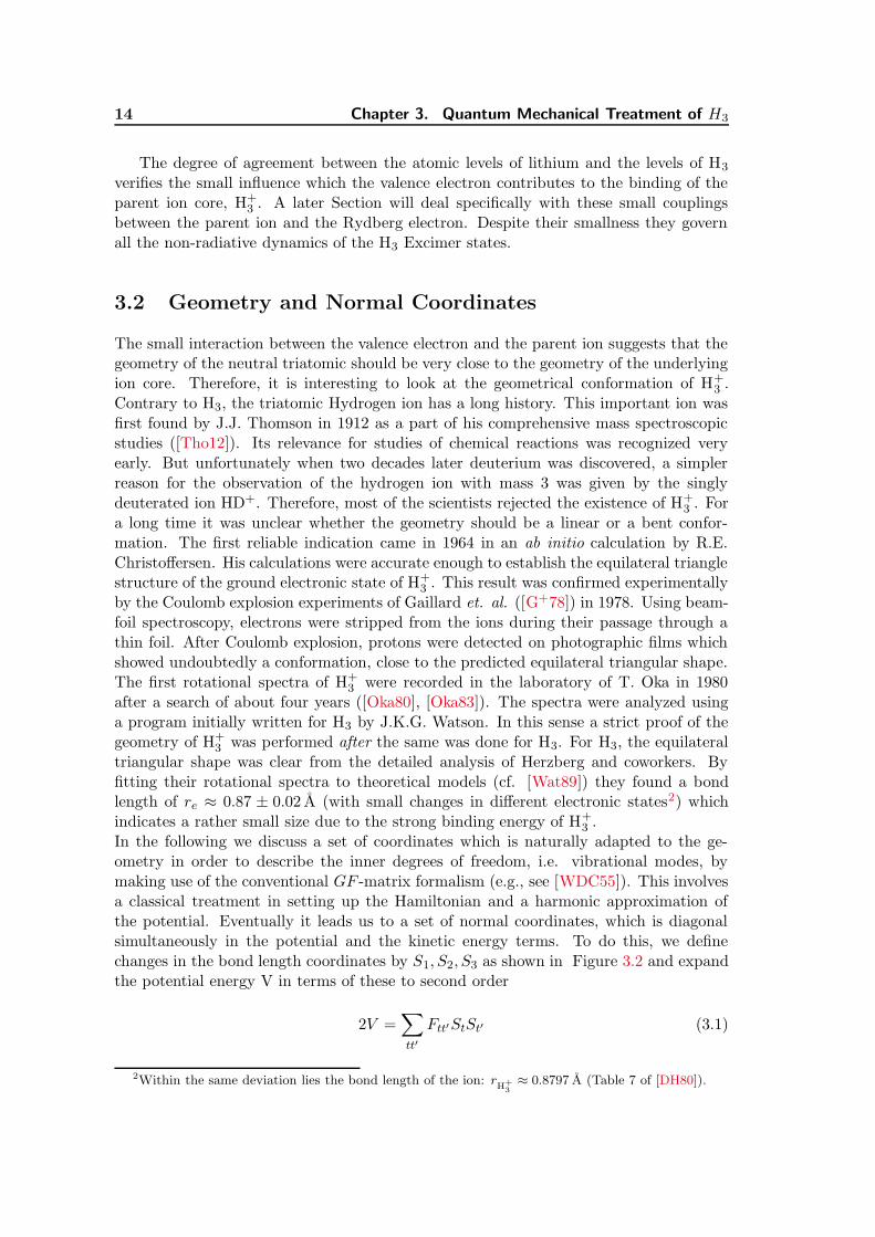
The small interaction between the valence electron and the parent ion suggests that thegeometry of the neutral triatomic should be very close to the geometry of the underlyingion core. Therefore, it is interesting to look at the geometrical conformation of H+

3 .Contrary to H3, the triatomic Hydrogen ion has a long history. This important ion wasfirst found by J.J. Thomson in 1912 as a part of his comprehensive mass spectroscopicstudies ([Tho12]). Its relevance for studies of chemical reactions was recognized veryearly. But unfortunately when two decades later deuterium was discovered, a simplerreason for the observation of the hydrogen ion with mass 3 was given by the singlydeuterated ion HD+. Therefore, most of the scientists rejected the existence of H+

3 . Fora long time it was unclear whether the geometry should be a linear or a bent confor-mation. The first reliable indication came in 1964 in an ab initio calculation by R.E.Christoffersen. His calculations were accurate enough to establish the equilateral trianglestructure of the ground electronic state of H+

3 . This result was confirmed experimentallyby the Coulomb explosion experiments of Gaillard et. al. ([G+78]) in 1978. Using beam-foil spectroscopy, electrons were stripped from the ions during their passage through athin foil. After Coulomb explosion, protons were detected on photographic films whichshowed undoubtedly a conformation, close to the predicted equilateral triangular shape.The first rotational spectra of H+

3 were recorded in the laboratory of T. Oka in 1980after a search of about four years ([Oka80], [Oka83]). The spectra were analyzed usinga program initially written for H3 by J.K.G. Watson. In this sense a strict proof of thegeometry of H+

3 was performed after the same was done for H3. For H3, the equilateraltriangular shape was clear from the detailed analysis of Herzberg and coworkers. Byfitting their rotational spectra to theoretical models (cf. [Wat89]) they found a bondlength of re ≈ 0.87 ± 0.02 A (with small changes in different electronic states2) whichindicates a rather small size due to the strong binding energy of H+

3 .In the following we discuss a set of coordinates which is naturally adapted to the ge-ometry in order to describe the inner degrees of freedom, i.e. vibrational modes, bymaking use of the conventional GF -matrix formalism (e.g., see [WDC55]). This involvesa classical treatment in setting up the Hamiltonian and a harmonic approximation ofthe potential. Eventually it leads us to a set of normal coordinates, which is diagonalsimultaneously in the potential and the kinetic energy terms. To do this, we definechanges in the bond length coordinates by S1, S2, S3 as shown in Figure 3.2 and expandthe potential energy V in terms of these to second order

2V =∑

tt′

Ftt′StSt′ (3.1)

2Within the same deviation lies the bond length of the ion: rH+

3

≈ 0.8797 A (Table 7 of [DH80]).

“diss”2002/10/18page 15

3.2. Geometry and Normal Coordinates 15

S3

~s31

1

2 3

S2

S1

~s21

~s13

~s23~s32

~s12

x1

y1

S1 S2 S3

~s11 = 0 ~s21 =(

b−a

)~s31 =

(ba

)

~s12 =(

0−2a

)~s22 = 0 ~s32 =

(−b−a

)

~s13 =(

02a

)~s23 =

(−ba

)~s33 = 0

a = 1/2 b =√

3/2

~ρj =(∆xj

∆yj

)

Figure 3.2: Definition of internal coordinates and Eliashevich vectors ([Eli40]). Thenuclei are labeled 1, 2 and 3. For the sake of simplicity we only show the cartesiancoordinate system ~ρ1. The systems ~ρ2, ~ρ3 have the same orientation, but are located atthe nuclei 2 and 3.

Due to the symmetry, we only consider lengths rather than angles between the bonds.

The first order term vanishes because of the equilibrium conditions(

∂V∂Si

)∣∣∣Si=0

= 0.

The expansion coefficients Ftt′ are generalized force constants associated with the bondlength coordinates. The appearance of off-diagonal terms indicates that the bond lengthcoordinates S1, S2, S3 are not independent in general. In a next step, we define thekinetic energy in the same internal coordinates. It is convenient to introduce here aset of vectors, first introduced by Eliashevich ([Eli40]), because it allows a descriptionindependent of a specification of a coordinate system. Their definition is illustrated inFigure 3.2. For a triatomic, there are only six non-zero vectors, since the internal motionis restricted to a plane, and there are three bonds. Once we have introduced cartesianreference systems ~ρj =

(∆xj

∆yj

)at each nuclei j = 1, 2, 3, we can define these vectors as

follows:Let us assume that all atoms except atom j are in their equilibrium position and atom jis displaced by some vector ~ρj . Then the vector ~stj points in the direction in which theinternal coordinate St experiences its biggest stretching. It is readily clear that for bondlength coordinates this displacement is always parallel or antiparallel to the directionof the bond. If we define all of these vectors in this way for the equilateral triangleconformation and normalize them to unit length, we arrive at the vectors shown in theright half of Figure 3.2. By this definition, we can now exactly define the internalcoordinates as

St =

3∑

j=1

~stj · ~ρj t = 1, 2, 3 (3.2)

It should be mentioned that this is only approximate for a description of vibrations,since when the displacement for one atom is projected onto the Eliashevich vectorsit is assumed that the other nuclei remain at their equilibrium positions. For largeconformations, however, this is no more appropriate. When we apply this formalism onlyto small vibrational amplitudes it is a good approximation3. The expression Eq.(3.2)

3Exact relations are given in Appendix B.2. In literature, however, the linear variant is most oftenused.

“diss”2002/10/18page 16

16 Chapter 3. Quantum Mechanical Treatment of H3

relates the bond lengths to the cartesian coordinates. It is useful to write it in matrixlanguage. We assume that all ~ρj ’s are grouped into a single mass normalized vector

~q = (~ρ1~ρ2~ρ3)√m, and similarly for ~S = (S1S2S3). Thus, we can write Eq.(3.2) simply

as ~S = D~q, where now the matrix D contains the values of the Eliashevich vectors andan additional mass dependent factor

√m. In this notation the kinetic energy T in terms

of qi or pt = ∂T/∂qt is

2T =∑

t

q2t =∑

t

p2t (3.3)

where the dot implies the derivative with respect to time. By Pi = ∂T/∂Si, we definethe momenta conjugated to Si. Using the rules for partial differentiation it follows that

pt =∂T

∂qt=∑

j

∂T

∂Sj

∂Sj

∂qt≡∑

j

PtDtj (3.4)

The last factor of these terms may be interpreted as elements off the matrix D, due tothe identity ∂St/∂qj = ∂St/∂qj ≡ Dtj . This can now be used to express the kineticenergy in terms of momenta

2T =∑

t,t′,t′′

Pt(D)tt′(DT )t′t′′Pt′′ ≡

∑

t,t′

Gtt′PtPt′ (3.5)

where we defined the matrix G by G = DDT . A closer inspection of G shows that it issolely defined by the Eliashevich vectors

Gtt′ =1

m

3∑

j=1

~stj · ~st′j (3.6)

Now we can easily see that these equations do not depend on the choice of the coordinatesystem we used, because only scalar products are involved in these expressions. Moreover,it is clear that for their derivation any coordinate system could have been used. FromEq.(3.5) it immediately follows from the second Hamilton equation St = ∂T/∂Pt that

~S = G~P (3.7)

From Eq.(3.6), G is obviously symmetric and can always be inverted if det(G) 6= 0, such

that ~P = (G−1) ~S. Replacing Pt in Eq.(3.5) gives

2T =∑

tt′

(G−1)tt′ StSt′ (3.8)

The explicit forms of G andG−1 have a rather simple appearance due to the high intrinsicsymmetry

(G)tt′ = 1/m

2 1/2 1/21/2 2 1/21/2 1/2 2

, (G−1)tt′ = m

5/9 −1/9 −1/9−1/9 5/9 −1/9−1/9 −1/9 5/9

(3.9)

The Hamiltonian is now

2H =∑

tt′

Gtt′PtPt′ +∑

tt′

Ftt′StSt′ (3.10)

“diss”2002/10/18page 17

3.2. Geometry and Normal Coordinates 17

From Eq.(3.10) we see that the equations of motion remain coupled as long as crossterms in the Hamiltonian appear. To disentangle these off-diagonal terms, we seek alinear transformation L to a new set of coordinates Q, i.e. ~S = L ~Q, such that the kineticenergy and the potential term are diagonal in the new coordinates. These are then callednormal coordinates. After substitution the two parts of the transformed Hamiltonian are

2V = QT LT F LQ LT F L = Λ (3.11)

2T = QT LT G−1 L Q LT G−1 L = E (3.12)

Therefore the conditions for L are, first, making LT F L = Λ diagonal and second,transforming LT G−1 L to the unit matrix E. Neglecting at first the normalization, thetwo conditions can be combined into one. If the second LT = L−1G is substituted intothe first then the eigenvalue equation

GF L = ΛL (3.13)

remains to be solved. The diagonal elements of Λ now contain the new force constantswith respect to the normal coordinates. It is simple to solve these equations and wemerely quote the results

Lmm′ = 1/√mp

1 1 0

1 −1/2 −√

3/2

1 −1/2√

3/2

, Λmm′ = (k/mp)

3 0 00 3/2 00 0 3/2

(3.14)

Here we chose the potential diagonal in the bond length coordinates, and due to identicalbonds all those elements are equal to the same force constants k. The mass mp corre-sponds to the proton mass. The eigenvectors of Eq.(3.13) are identical with the columnsin the matrix L and they represent the vibrational modes4. The eigenvalues on the di-

agonal of Λ represent vibrational frequencies according to ωm = Λ1/2mm for a harmonic

oscillator. Pure geometrical results are that the second and third vibrational modes, Q2a

and Q2b respectively, are degenerate and the frequency ratio ω1/ω2(ab) is for infinitesimal

amplitudes exactly√

2. For an interpretation of the normal coordinates, we can find an-other matrix l that relates normal coordinates directly to cartesian coordinates, ~q = l ~Q.Its elements will be of importance later in the study of coriolis interactions. From therelations ~S = D~q = L ~Q, DDT = G and Eq.(3.10) it can be shown (cf. [PA82], p.40),that l obeys the matrix equation l = DTFΛ−1 . If we split the cartesian vector ~q againinto separate vectors for each nucleus i, and label the elements of l belonging to nucleusi by its index (i = 1, 2, 3) we get

l1 α,k =1√3

(1 −1 00 0 1

)

l2 α,k =1√3

(−1

212 −

√3

2

−√

32 −

√3

2 −12

)qi,α =

∑

k

li,αkQk (3.15)

l3 α,k =1√3

(−1

212

√3

2√3

2

√3

2 −12

)

4The normalization from the second equation was taken into account.

“diss”2002/10/18page 18

18 Chapter 3. Quantum Mechanical Treatment of H3

Q1 Q2a Q2b Q2a + iQ2b

1

xy

2 3

Figure 3.3: Geometrical interpretation of normal modes. The normalized directions ofdisplacements for all nuclei is given by the matrix l. Because only internal coordinatesare included, the center of mass must remain stationary and the total angular momentumbe zero. Thus, a collective translation or rotation of all nuclei is not allowed for. On theright an equivalent description of nuclear motion is given by a pseudo-rotation, see text.

Herein, α takes the values x and y, and k refers to the normal coordinate Qk. Therefore,l reflects the displacement of each nucleus in the vibrational mode k. This is illustratedin Figure 3.3 which gives a geometrical interpretation of the normal coordinates.

A superposition of the two degenerate modes with a fixed relative phase of π/2 resultsin the temporal behaviour of nuclear motion shown on the right of Figure 3.3. This isequivalent to considering Q2a, Q2b as a cartesian basis and to form the polar coordinaterepresentation

Q2r = Q2

2a +Q22b ϕ = arctan(Q2b/Q2a) (3.16)

from it, where Qr and ϕ describe the radial and angular motions, respectively. Anequivalent complex variant is given in terms of ladder operators, the annihilation Q2−and creation operator Q2+, with the properties

Q± = 1/2 (Q2a ± iQ2b) = Qr exp(±iϕ) (3.17)

Qr = Q+Q− = Q−Q+

The polar representation is a very useful and more physical description, because thispseudo-rotation is associated with an angular momentum, which is called vibrational an-gular momentum. As will be shown later, it is responsible for various internal couplingsand influences rotational spectra. Especially, if vibronic (≡ vibrational & electronic) cou-plings are present, this vibrational angular momentum becomes ’enhanced’ (cf. Section3.5.2) and it is associated with a change of the phase of the electronic wavefunction byπ (≡geometrical phase) when ϕ is varied from = 0..2π.

Often normal coordinates are expressed in terms of bond length coordinates as well.By taking the inverse of L, we have from ~Q = L−1 ~S an alternative interpretation

Q1 =(mp

3

)1/2 1√3(S1 + S2 + S3)

Q2a =

(2mp

3

)1/2 1√6(2S1 − S2 − S3) (3.18)

Q2b =

(2mp

3

)1/2 1√2(S3 − S2)

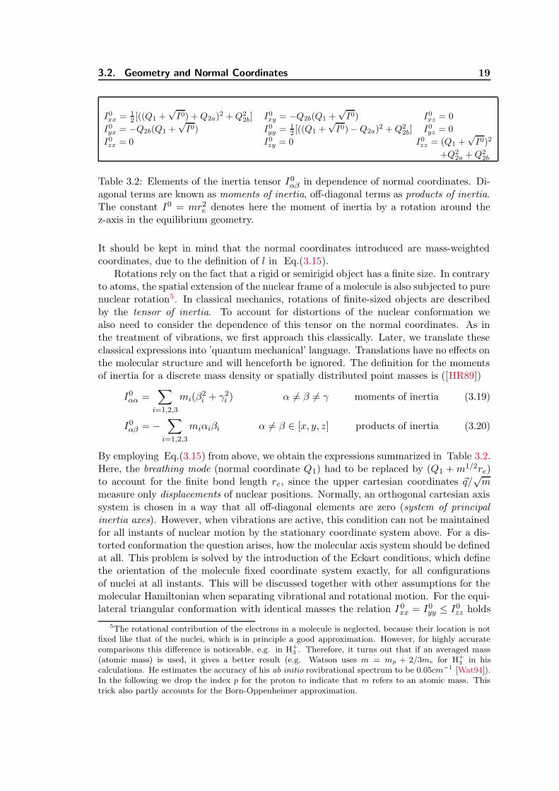
“diss”2002/10/18page 19

3.2. Geometry and Normal Coordinates 19

I0xx = 1

2[((Q1 +

√I0) +Q2a)2 +Q2

2b] I0xy = −Q2b(Q1 +

√I0) I0

xz = 0

I0yx = −Q2b(Q1 +

√I0) I0

yy = 1

2[((Q1 +

√I0)−Q2a)2 +Q2

2b] I0yz = 0

I0zx = 0 I0

zy = 0 I0zz = (Q1 +

√I0)2

+Q22a +Q2

2b

Table 3.2: Elements of the inertia tensor I0αβ in dependence of normal coordinates. Di-

agonal terms are known as moments of inertia, off-diagonal terms as products of inertia.The constant I0 = mr2

e denotes here the moment of inertia by a rotation around thez-axis in the equilibrium geometry.

It should be kept in mind that the normal coordinates introduced are mass-weightedcoordinates, due to the definition of l in Eq.(3.15).

Rotations rely on the fact that a rigid or semirigid object has a finite size. In contraryto atoms, the spatial extension of the nuclear frame of a molecule is also subjected to purenuclear rotation5. In classical mechanics, rotations of finite-sized objects are describedby the tensor of inertia. To account for distortions of the nuclear conformation wealso need to consider the dependence of this tensor on the normal coordinates. As inthe treatment of vibrations, we first approach this classically. Later, we translate theseclassical expressions into ’quantum mechanical’ language. Translations have no effects onthe molecular structure and will henceforth be ignored. The definition for the momentsof inertia for a discrete mass density or spatially distributed point masses is ([HR89])

I0αα =

∑

i=1,2,3

mi(β2i + γ2

i ) α 6= β 6= γ moments of inertia (3.19)

I0αβ = −

∑

i=1,2,3

miαiβi α 6= β ∈ [x, y, z] products of inertia (3.20)

By employing Eq.(3.15) from above, we obtain the expressions summarized in Table 3.2.Here, the breathing mode (normal coordinate Q1) had to be replaced by (Q1 +m1/2re)to account for the finite bond length re, since the upper cartesian coordinates ~q/

√m

measure only displacements of nuclear positions. Normally, an orthogonal cartesian axissystem is chosen in a way that all off-diagonal elements are zero (system of principalinertia axes). However, when vibrations are active, this condition can not be maintainedfor all instants of nuclear motion by the stationary coordinate system above. For a dis-torted conformation the question arises, how the molecular axis system should be definedat all. This problem is solved by the introduction of the Eckart conditions, which definethe orientation of the molecule fixed coordinate system exactly, for all configurationsof nuclei at all instants. This will be discussed together with other assumptions for themolecular Hamiltonian when separating vibrational and rotational motion. For the equi-lateral triangular conformation with identical masses the relation I 0

xx = I0yy ≤ I0

zz holds

5The rotational contribution of the electrons in a molecule is neglected, because their location is notfixed like that of the nuclei, which is in principle a good approximation. However, for highly accuratecomparisons this difference is noticeable, e.g. in H+

3 . Therefore, it turns out that if an averaged mass(atomic mass) is used, it gives a better result (e.g. Watson uses m = mp + 2/3me for H+

3 in hiscalculations. He estimates the accuracy of his ab initio rovibrational spectrum to be 0.05cm−1 [Wat94]).In the following we drop the index p for the proton to indicate that m refers to an atomic mass. Thistrick also partly accounts for the Born-Oppenheimer approximation.

“diss”2002/10/18page 20

20 Chapter 3. Quantum Mechanical Treatment of H3

for the equilibrium moments of inertia. Such a structure is called an oblate symmetrictop rotor.

3.3 The Molecular Hamiltonian

The full molecular Hamiltonian in cartesian coordinates (without spin) is readily ob-tained by writing down the kinetic energies as a sum over all particles and their mutual,electrostatic pair interactions in operator form. In this form, however, it is impossible toextract the intrinsic, stationary and dynamical behaviour. Especially for light moleculeswith large internal dynamics a direct numerical integration of the Schrodinger equation isdifficult. Also a quantitative understanding is difficult to obtain from such calculations.Therefore, one needs to find appropriate approximations to transform the Hamiltonianinto a form that can be interpreted, although this form will appear as much more com-plex. Since most of the dynamics is rotational, it turns out that expressing the kineticenergy in terms of angular momenta is best suited. It is surprising that an exact kineticenergy operator of this type can be found for all molecules in a very general manner.The treatment of the potential needs further approximations to separate electronic andnuclear motion depending on the degeneracy of the electronic state. There are excellentpublications on the derivation of the exact Hamiltonian. In our discussion, we ratherwant to point on the essential assumptions and problems occurring by its derivation, andrefer to the original papers. The basic work was done by Wilson and Howard ([WH36],[WDC55] Chapt. 11), who found the classical Hamiltonian for a molecule taking intoaccount the full semirigid properties of molecules; Eliashevich [Eli38], and Darling &Dennison [DD40] found its correct quantum mechanical form, and eventually Watson[Wat68] simplified it to a great extent, while retaining generality. Another derivationcan be found in the textbook of Papousek and Aliev [PA82] on which the present workis based on. A more supplementary presentation to the above is given in Ref. [BJ98].

3.3.1 The Kinetic Energy Term

A description of translation and rotation requires an introduction of two coordinatesystems. One which is fixed in space with a fixed orientation, which we call laboratorysystem, and a second one, the molecule fixed system, which is attached to the molecule insome way, and which moves and rotates relative to the first. Because isolated moleculesin the gas phase behave independent of their translational motion, we do not consider anytranslation and fix the origins of the two systems at the point of the center of mass of thenuclei. Besides translation and vibration, rotation is an independent degree of freedom.Therefore, a certain set of nuclear coordinates related to a well defined coordinate systemmust possess information about the rotational content of a given conformation. E.g. thecoordinates of a rigid molecule with respect to the laboratory fixed system contain theirrotation in their Eulerian angles, defined through the transformation from the laboratorysystem to the molecule fixed system. Here the latter is fixed to an arbitrary chosenorientation of the molecule. We denote in the following the laboratory fixed coordinatesfor nucleus i with triples (ξi, ηi, ζi) and the analogue in the molecule fixed system by(xi, yi, zi). However, when vibrations are allowed, it is not obvious how this moleculefixed system should be attached to the set of nuclear coordinates. It turns out thatthis difficulty is related to the problem of separation of vibration and rotation, since the

“diss”2002/10/18page 21

3.3. The Molecular Hamiltonian 21

choice of the molecule fixed system can mix the rotational and the vibrational part ofthe motion. Therefore it seems reasonable, to find a molecule fixed system such that therotational content of the nuclei relative to this system is zero. Then all rotation residesin the transformation from the laboratory system to the molecular fixed system and thusin the Eulerian angles. Explicitly, this condition is equivalent to the requirement thatin the molecule fixed system the total angular momentum of the nuclei exactly vanishes,i.e.

J nucl. = m∑

i=1,2,3

ri × ri ≡ 0 where ri = (xi, yi, zi) (3.21)

Unfortunately, a complete separation of rotation and vibration turns out to be impossiblefor a semirigid molecule, implying that the three equations above are still not sufficientto define the Eulerian angles (cf. Ref. [BJ98] and original works [Eck35], [Say39]).This problem arises, because both the positions and momenta are involved in these ex-pressions. However, to achieve a high degree of separability of rotation and vibrationwith minimal approximation, a slight modification of Eq.(3.21) provides an approximatesolution to this problem. By assuming that vibrational amplitudes are small, the instan-taneous positions of nuclei, ri, can be replaced by their equilibrium values req

i . Then, bydemanding ∑

i=1,2,3

reqi × ri = 0 (3.22)

the time derivative of Eqs.(3.22) (∼ J nucl.), must also be zero, and thus, J nucl. can onlytake very small values within this approximation. Eqs.(3.22) is called the second Eckartcondition. It represents the best approach for an approximate separation of rotation andvibration. However, other approaches are possible. A more intuitive way would be tochoose the molecule fixed axis system for a given conformation according to the momentsand products of inertia. One could fix the molecular system at each instant along thedirection of the three principal axes of inertia, since the latter are always unambiguouslydefined. It can be shown, however, that this method mixes much more rotational motioninto vibrational motion, resulting in larger coupling terms. This is illustrated in Figure3.4. For three randomly chosen conformations, the molecule fixed coordinate systemwas attached according to the Eckart conditions (solid line), and to the principle inertiaaxes system (dashed line). For clarity only the x-axis is shown. In order to define thevibrational displacement, a rotated equilibrium configuration is also given. Apparently,a small displacement from equilibrium affects the inertia axis system much more thanthe Eckart axes. The Eckart axes attempt to follow the vibrational motion, therebyreducing the rotational contributions caused by vibrational displacements.

Quantitatively, we determined the rotation angle ε relative to the laboratory system(as defined in Figure 3.4) in D3h symmetry for both cases discussed above. The rotationangle6 corresponds to an Eulerian angle and is defined by the transformation from thelaboratory system to the molecule fixed system. The angle is defined by

tan ε =(ξ2 − ξ3)∓

√3(η2 + η3)

(η3 − η2)∓√

3(ξ2 + ξ3)(3.23)

The upper signs refer to the Eckart axis system and the lower signs to the principalinertia axis system. The angles depend on the laboratory coordinates, (ξi, ηi, ζi), of nuclei

6 ε is defined positive for a clockwise rotation about the z-axis in Figure 3.4.

“diss”2002/10/18page 22

22 Chapter 3. Quantum Mechanical Treatment of H3

11

1

22

2 3

33

x

xx

xx

x

η

ξ

y

ε

x

Figure 3.4: The deformed triangles (1, 2, 3) are randomly chosen conformations, whereonly the center of mass was kept fixed. Molecule fixed coordinate systems were attachedto the center of mass according to the Eckart condition (solid) and to the principle inertiaaxis system (dashed). Only the respective x-axes are shown for clarity. It is obvious thatthe inertia axis (dashed) system deviates much more from the instantaneous conforma-tion. By comparing the parallelism of lines connecting atoms in distorted conformationsto those in the attached systems in equilibrium, it is seen how the Eckart system triesto follow the distortional motion thereby minimizing the inherent rotation.

i = 2, 3, whereby the third (i = 1) is always defined by the center of mass condition.The remaining, non-negligible effect due to the approximation in Eq.(3.22) appears asCoriolis interaction term, spoiling a complete separation of rotational and vibrationalmotions.

The classical expression for the kinetic energy term is now obtained in a straightfor-ward way, as discussed for example in Ref.([PA82] Chap. 2 and 4). We restrict ourselvesto an outline of the procedure. Starting from the kinetic energy in laboratory fixed,cartesian coordinates, a first transformation into a molecule fixed system is performedby using the Eulerian angles (θ, φ, χ) . The angles (θ, φ) describe the orientation of themolecular plane. The third angle ε ≡ χ fixes the orientation of the molecule withinthe plane. By applying the center of mass conditions, i.e.

∑smsrs = 0, and there-

fore also,∑

smsrs = 0 (s refers to electrons and nuclei), the translational motion isremoved and will not be considered further. In this transformation the time derivativesof the coordinates in the kinetic energy term convert into derivatives of Eulerian angles.These can be expressed in a total angular velocity vector ~ω, defined in the molecule fixedframe. Its components define the direction of the rotation axis and the total angularvelocity. At this point it becomes obvious how the Eckart conditions simplify the overallrotation-vibration interaction term. By replacing the absolute coordinates according tori = req

i + ∆ri, this term can be decomposed in a sum of two

2m~ω ·∑

i=nucl.

(ri × ri) = 2m~ω ·∑

i

(reqi × ri) + 2m~ω ·

∑

i

(∆ri ×∆ri) (3.24)

The first term on the right hand side vanishes due to the second Eckart condition, but

“diss”2002/10/18page 23

3.3. The Molecular Hamiltonian 23

the second one does not. It forms the non-removable part of separation of rotation andvibration and corresponds to a Coriolis interaction caused by the remaining rotationalpart of the nuclear motion (vibrational angular momentum). This term is in generalsmall for slight displacements from the equilibrium configuration. In the following wewill see, that this term can only be nonzero if degenerate vibrational modes are excited.The second term of Eq.(3.24) can be expressed by the relations of Eq.(3.15) in the form

2∑

α

ωα

∑

k,l

ζαklQkQl where ζα

kl =∑

i

(liβ,kliγ,l − liγ,kliβ,l) α 6= β 6= γ (3.25)

Here, the sum of l-matrix elements can be combined in a set of parameters, called Coriolisinteraction parameters ζα

kl, describing the Coriolis force for the vibrating nuclei in therotating frame. For the triangular symmetry discussed here, these Coriolis parameterstake a very simple form

ζαkl = 0 for α 6= z, ζα

kl = −ζαlk ≡ −1 for (k = 2a, l = 2b, α = z) (3.26)

which is easily proven utilizing Eq.(3.15) and their definition. All other coefficientsinvolving a symmetric stretch vibration also vanish. Therefore, Coriolis effects on energyare not influenced by a symmetric stretch excitation.

The kinetic energy still depends on the time derivatives of both, coordinates andangles. By considering coordinates and their momenta (rather than time derivatives)as independent, one can express the kinetic energy in a Hamiltonian representation.Hereby, the dependence on nuclear velocities Qk and electron velocities rjα is easilyeliminated by substituting them as functions of the associated momenta. The classicalterm also contains terms involving angular velocities ωα of the type I ′αβωαωβ. Theangular velocities can be expressed as linear combinations of components (Nα−πα−Πα)whereNα is the total angular momentum, πα the vibrational angular momentum, and Πα

the electronic angular momentum components, all defined in the molecule fixed system.Finally, the classical term for the kinetic energy results in

2T =∑

α,β

µα,β(Nα − πα −Πα)(Nβ − πβ −Πβ) +∑

k=1,2,3

P 2k +m−1

e

∑

α;j=1,2,3

p2jα

(3.27)

where

Total Nα(≡ ∂T/∂ωα) =∑

β

I ′αβωβ + πα + Πα α = x, y, z (3.28)

V ibrational πα =∑

k,l

ζαklQkPl Pk(≡ ∂T/∂Qk) = Qk +

∑

α,l

ωαζαlkQl (3.29)

Electronic Πα =∑

j=1,2,3

(rjβpjγ − rjγpjβ) (3.30)

I ′αα = I0αα −

∑

k,l,m

ζαk,mζ

αm,lQkQl, I ′αβ = I0

αβ −∑

k,l,m

ζαk,mζ

βm,lQkQl (3.31)

The first term of Eq.(3.27) must be interpreted in the following way. The total angularmomentum N is a constant of motion and contains the sum of all angular momenta.

“diss”2002/10/18page 24

24 Chapter 3. Quantum Mechanical Treatment of H3

It defines a vector and is constant in the laboratory system and in the molecule at-tached system. The inner molecular properties, i.e. the nuclear and electronic motion,are best described in the molecule fixed system and referred to this system. By ex-pressing N in the molecular frame, the difference occurring in Eq.(3.27) then accountsfor changes in the nuclear rotation induced by vibrational-rotational (semi-rigidity) andelectronic-rotational interactions. Thus, the first term contains an effective nuclear angu-lar momentum accounting for perturbations. From Eq.(3.28), we see how the coefficientsµα,β of the first term are defined. Replacing ωα in terms of (Nα − πα − Πα) requiresknowledge of the inverse of the inertia tensor I ′αβ . Since one tensor already occurs in theterms I ′αβωαωβ, and two inverse tensors are introduced by the replacement of ωα, one

inverse of the inertia tensor remains to form the coefficient µα,β = (I ′αβ)−1. It shouldbe mentioned, however, that these coefficients have a rather complex dependence on thenuclear conformation, as we show in Appendix A. The effect of the approximate sep-aration of rotation and vibration is reflected in Eq.(3.29). As a result, the vibrationalmomenta also have some rotational contributions. A similar feature in the rotationalpart appears in the inertia tensor in Eq.(3.31).

The translation into a quantum mechanical energy operator causes additional prob-lems. The general way in the use of the correspondence rule, i.e. by replacing classicalmomenta by their quantum mechanical counterpart, is restricted to application in carte-sian coordinates. This is a direct consequence of the unity weighting factor in the in-finitesimal volume element for cartesian coordinates and the appearance of only constantcoefficients (mass factors) in the kinetic energy term.

Therefore, two problems occur in finding a quantum description. First, how to applythe correspondence rule for generalized coordinates with a non unity weighting factor inthe volume element? Secondly, the usage of generalized coordinates implies coefficientsin the kinetic energy term which are functions of the coordinates. Because there issome freedom of ordering the factors in the classical expressions before applying thecorrespondence rule, a certain ambiguity results. Both problems can be overcome forthe coordinates used here.

The ordering problem was solved in a general context by Podolsky ([Pod28]) in1928, known as Podolsky’s trick, who found a certain scheme of ordering the factorswhen generalized coordinates are used. The correspondence rule is then applied to thissequence in order to find the correct kinetic energy operator. To deal with the secondproblem, when there is no unity weighting factor in the volume element, a rewriting7 ofthe quantum mechanical Hamiltonian results in a criterion which must be fulfilled forthe coordinate set in order to yield correct results. The derivation of this condition andthe proof that this holds for the above case is given in Ref. [WDC55]. Applying theseresults, the hermitian kinetic energy operator becomes

T =1

2µ1/4

∑

α,β

(Nα−πα− Πα)µα,β µ−1/2(Nβ −πβ − Πβ)µ1/4 (3.32)

+1

2µ1/4

∑

k=1,2,3

Pk µ−1/2 Pk µ

1/4 +1

2m−1

e

∑

α;j=1,2,3

p2jα

7Introducing a factor one by s1/2/s1/2, where s is the weighting factor in the volume element, andrearranging the order leaves the classical expression unchanged, but modifies its quantum mechanicalcounterpart.

“diss”2002/10/18page 25

3.3. The Molecular Hamiltonian 25

with the operator definitions 8

Total Op. Nα linear combinations of pθ = −ih∂/∂θ, pφ = −ih∂/∂φ, pχ = −ih∂/∂χV ibrational Op. πα = −ih

∑

k,l

ζαklQk∂/∂Ql, Pk = −ih∂/∂Qk, (3.33)

Electronic Op. pjα = −ih∂/∂rjα, Πα = −ih∑

j=1,2,3

(rjβ∂/∂rjγ − rjγ∂/∂rjβ)

Here, and in the following we denote operators in typewriter font. The operator µ isdefined as the determinant of the matrix µαβ. At this place it should be mentioned that Ndoes not obey the conventional commutator relations for angular momenta components,as singled out by a few authors. In literature there exists some controversy regardingthis problem ([Wat68], [VV51]).

Watson ([Wat68]) has found a simpler form of the above kinetic energy operatorwithout loss of its generality. In a lengthy, but straightforward calculation based uponcommutator relations and sum rules, he has shown that the first and second term ofEq.(3.32) can be arranged to a much simpler form. He has also shown that the orderof factors in the first term is immaterial despite of their operator character. The overalleffect is an additional term U, depending only on the normal coordinates Q, and actingas a mass dependent contribution to the potential. The pure nuclear part is then givenby neglecting the last term of Eq.(3.32)

TN =1

2

∑

αβ

(Nα−πα)µαβ(Nβ −πβ) +1

2

∑

k=1,2,3

P2k (3.34)

+1

2

∑

αβ

µαβ Πα Πβ −∑

αβ

µαβ Πα(Nβ −πβ) + U where U = −1

8h2∑

α

µαα

Additionally, the product term was expanded, which causes no problems because Πα com-mutes with µαβ . Finally we summarize the above described procedure for the derivationof the kinetic energy operator in Figure 3.5.

3.3.2 The Exact Hamilton Operator for H3

To complete the Hamiltonian an adequate potential energy function must be introduced.The total classical potential function is written as a sum of two terms

V = Vr,Q(r,Q) + VQ(Q) (3.35)

with abbreviations r = (rjα) j=1,2,3α=x,y,z

electronic coord. (3.36)

Q = (Qk)k=1,2,3 nuclear coord.

The first part of the potential energy, Vr,Q(r,Q), represents electron-electron and electron-atomic nucleus interactions and therefore depends on both types of coordinates. Thesecond term, VQ(Q), is the potential energy of mutual nuclear pair interaction. It is solely

8An exact definition for Nα is given in Ref. [PA82], Eq.(4.3.5).

“diss”2002/10/18page 26

26 Chapter 3. Quantum Mechanical Treatment of H3

Classical expression in cartesian, laboratory fixed coordinates& velocities

Second Eckart Condition

Introduction of Normal Coordinates: GF -Matrix Formalism

Separation of Rotation & Vibration & Translation by

Center of Mass (CM) Condition

Classical Expression in Molecule fixed CoordinatesNormal Coordinates, Eulerian Angles & Angular Velocities

Qk by Pk, rjα by pjα

ωβ by a linear combination of (Nα − πα − Πα)

Rewrite solely in momenta, cf. Eq.(3.27); substitute

as defined in Eqs.(3.28)-(3.30)

Classical Hamiltonian Form

Exact QM Kinetic Energy Operator

Simplified Exact QM Kinetic Energy Operator

Watson’s Simplificationbased upon commutator relations

cf. Eq.(3.34)

Translate into QM Operator form (cf. Eq.(3.32))

by using Podolsky’s trickRewriting of QM Hamiltonian → Criterion for CoordinatesFind Operator Representations Nα, πα, Πα

Figure 3.5: Derivation of the kinetic energy operator.

a function of the normal coordinates. Since we deal with the spatial quantum mechanicalrepresentation, the operator form V is readily given by substituting the coordinates (r,Q)by its operators (r, Q)

V = Vr,Q(r, Q) + VQ(Q) (3.37)

Electrostatic pair interactions are more naturally expressed in cartesian coordinates bythe distance vectors of the pair. Generally, the implementation of the specified coordi-nates into the potentials is done in quantum chemical considerations for the derivationof the potential energy surfaces (PES) within the Born-Oppenheimer approximation.To achieve experimental accuracy, such calculations need to be performed numerically.Thus, a representation of the PES is given by points on a finite-sized grid. Local parts ofsuch point surfaces can later be fitted to functional expansions in order to get a functionaldependence.

“diss”2002/10/18page 27

3.4. Non-degenerate Electronic States 27

Combining the kinetic energy operator T = TN + TE with the simplifications fromEq.(3.34) and the potential energy operator of Eq.(3.37), we arrive at the exact Hamilto-nian describing the full internal dynamics of the molecule H3 (TE stands for the electronicpart, last term in Eq.(3.32)).

Hevr = T+ Vr,Q(r, Q) + VQ(Q) (3.38)

where µαβ = (I ′αβ)−1 is calculated from I ′αα = I0αα − δαz Q

2r and I ′αβ = I0

αβ for α 6= β

(I0αα, I

0αβ are taken from Table 3.2)

and πα = δαz(Q2b P2a− Q2a P2b)

The explicit forms of πα, I′αβ are easily derived from Eqs.(3.26), (3.29) and (3.31). δ

is the Kronecker symbol. An inspection of these equations shows that the vibrationalmomentum operator π always points along the z-axis, perpendicular to the molecularplane. Due to this orientation, the Coriolis interaction for an X3 molecule is very simple.In a later application of perturbation theory µαβ will be expanded in normal coordinates.This expansion does not have to be determined directly, since there exists a trick to findthis expansion in terms of first derivatives of Iαβ (see Appendix A).

Eq.(3.38) is still exact, only the center of mass is kept fixed at the origin of thelaboratory system which was achieved by an exact transformation. However, it is im-possible to solve the stationary Schrodinger equation with the Hamiltonian in this form.At this stage, several approximations have to be introduced. The choice of approxima-tion depends on the particular electronic state under consideration. In the following,we consider two cases of electronic states, electronically degenerate and non-degeneratestates, which require different ways of approximations. Because the degeneracy providesadditional complications, we begin with the non-degenerate case.

3.4 Non-degenerate Electronic States

The spatial distribution of the nuclear charges imposes a certain symmetry to the elec-tronic motion in the molecule. Depending on the strength of coupling between electronsand the nuclear frame, electrons are more or less tightly bound to the nuclear frame.For the present discussion of electronic states of low excitation, or so-called close-coupledstates, we assume that the electronic motion is strongly bound to the nuclear frame, pro-ceeds on a time scale much faster than the motion of the frame, and therefore follows itsrotational motion. In this case, electrons feel a spatial orientation or to say it in quantummechanical language, they feel a quantization axis. This axis can be arbitrarily chosen,but it is most convenient to choose it along the molecule fixed z-axis, perpendicular tothe molecular plane. Compared to the atomic case this loss of symmetry in a moleculeresults in a violation of the conservation of the total electronic angular momentum. How-ever, its projection along the quantization axis is still a conserved quantity. Symmetryarguments lead to the conclusion that this projection quantum number defines the kindof degeneracy of the underlying electronic state (cf. to Chapter 4). If the total electronicangular momentum is non-zero then there are always a few projections which are equiv-alent and therefore have the same energy. In the symmetry of point group D3h thereis only one pair of electronic states allowed with the same energy. Thus, only two-fold

“diss”2002/10/18page 28

28 Chapter 3. Quantum Mechanical Treatment of H3

degenerate species can appear. For an integer angular momentum the projection zerois always possible with respect to the quantization axis. If we denote the electronicprojection quantum number with λ (eigenvalue of Πz/h ), then the states, with λ = 0correspond to the non-degenerate states.

In Section 5.1.1 we stress a zeroth order model in which we describe the angulardependence of the electronic wavefunction by a simple spherical harmonic wave. Thisis done in order to find sets of good quantum numbers for different limiting cases ofclose-coupled states or very loosely bound states.

3.4.1 Born-Oppenheimer Approximation

As was the case for separation of rotation and vibration, an exact separation of theelectronic part from the nuclear motion can not be done. The approximation frequentlyemployed for non-degenerate states is the Born-Oppenheimer Approximation (BO). Thismethod relies on the adiabatic nature of the electronic motion with respect to the nuclearmotion. The applicability is a result of the much lighter mass of electrons compared tothe nuclei and the fact, that forces on nuclei and electrons are of the same order ofmagnitude. Consequently, electrons move much faster than nuclei. The ratio of theirvelocities is estimated9 to be of the order ∼ κ−3, where κ = (me/mp)

1/4 ∼ 110 is the

Born-Oppenheimer parameter. Hence, electrons see the nuclei as motionless centers offorces defining the electronic state. Due to the slow motion of the nuclei, electronicmotion can often adiabatically adjust to it. The picture is that during the time it takesfor a nucleus to make a significant displacement, electrons carry out a large number oforbits. Thus, nuclei move only in a potential averaged over many periods of the electronicmotion. The BO approximation consists of neglecting several terms of lower order inthe BO parameter κ. Here we precisely define which terms are left, because the nameBO Approximation is often used in various approaches which may differ in the level ofapproximation (cmp. [AM77]).

First, we formally divide the Hamiltonian of Eq.(3.38) with the simplification forthe kinetic energy operator, Eq.(3.34), into an electronic part He and a nuclear part H′

Hevr = He + H′ with He =1

2m−1

e

∑

α;j=1,2,3

p2jα + Vr,Q(r, Q) (3.39)

H′ = (TN of Eq.(3.34)) + VQ(Q)

We define state vectors for the total and the ’electronic’ Schrodinger equations by

Hevr Ψevr(r,Q, ·) = EevrΨevr(r,Q, ·) and (3.40)

He Ψ(e)n (r,Q) = E(e)

n (Q)Ψ(e)n (r,Q) (3.41)

The dot here indicates the dependence on Eulerian angles. The definition of the complete

set of electronic basis function (Ψ(e)n (r,Q), n = 1 . . .∞) in the electronic space motivates

the following ansatz for the total Schrodinger equation

Ψevr(r,Q, ·) =∑

n

Ψ(vr)n (Q, ·) Ψ(e)

n (r,Q) (3.42)

9see [AW76] and references therein.

“diss”2002/10/18page 29

3.4. Non-degenerate Electronic States 29

where the vibration-rotation wavefunctions Ψ(vr)n (Q, ·) must be considered as expansion

coefficients. Inserting Eq.(3.42) into the total Schrodinger equation Eq.(3.40), multi-

plying from the left by Ψ(e)j (r,Q)∗ and integrating over the electronic variables, yields a

system of equations for the expansion coefficients[E

(e)j (Q)−Eevr

]Ψ

(vr)j (Q, ·) +

∑

n

〈Ψ(e)j (r,Q) | H′ | Ψ(e)

n (r,Q)〉rΨ(vr)n (Q, ·) = 0, (3.43)

j = 1, 2, . . .

where Eq.(3.41) was used to replace He by E(e)n (Q). The pure electronic Schrodinger

equation, Eq.(3.41), gives solutions for static nuclei without consideration of the kinetic

energy associated with nuclear motion. Its solution E(e)n (Q) has a parametric dependence

on normal coordinates. It is used together with the electrostatic energy of the nuclei

VQ(Q), to obtain the n-th Potential Energy Surface PESn(Q) := E(e)n (Q) + VQ(Q)

associated with the n-th electronic eigenvalue. The coupling matrix elements deducedfrom the general expansion Eq.(3.42) mix these ’static-nuclei’ electronic wavefunctionsby taking into account the nuclear dynamics. The BO approximation is composed oftwo levels of approximation

1. Electronic Coupling Terms:In the absence of nearby electronic states, the effect of off-diagonal terms is smalland the off-diagonal terms are simply set to zero. Thereby, the system of coupleddifferential equations breaks up into a set of independent equations. Consequently,each electronic PES is unambiguously related to a set of vibrational-rotationalwavefunctions and Eq.(3.42) simplifies to

Ψevr(r,Q, ·)n = Ψ(vr)n (Q, ·)Ψ(e)

n (r,Q) (3.44)

In the case of degeneracy this approximation is inappropriate and off-diagonalterms between the different degenerated wavefunctions are not negligible. To aboutthe same order of approximation, Eq.(3.44) has to be replaced by a linear combi-nation containing all degenerated and close lying electronic states, see Eq.(3.67)in Section 3.5.1.

2. Omission of Rovibronic Matrix Elements:Since πα, Pα in H′ operate on both factors of the product in Eq.(3.42), the productrule for differentiation can be used to expand the matrix elements of Eq.(3.43)into a sum. If off-diagonal terms are neglected the resulting Schrodinger equationis

[12

∑

αβ

(Nα−πα)µαβ(Nβ −πβ) +1

2

∑

k=1,2,3

P2k−

1

8h2∑

α

µαα +PESj(Q)

+( terms incl. matrix elements

from Table 3.3 with j = n.

)]Ψ

(vr)j (Q, ·) = Ej

evrΨ(vr)j (Q, ·) (3.45)

Table 3.3 contains matrix elements which allow a coupling of rovibrational statesof two arbitrary electronic states, causing the breakdown of the BO approximation.By omitting off-diagonal terms as in the first step above, only couplings within the

“diss”2002/10/18page 30

30 Chapter 3. Quantum Mechanical Treatment of H3

+〈Ψ(e)j | (πα πβ Ψ

(e)n )〉r +〈Ψ(e)

j | Πα Πβ | Ψ(e)n 〉r +〈Ψ(e)

j | (P2k Ψ

(e)n )〉r

−〈Ψ(e)j | (πβ Ψ

(e)n )〉r(Nα−πα) −〈Ψ(e)

j | Πα | Ψ(e)n 〉r(Nβ −πβ) +〈Ψ(e)

j | (Pk Ψ(e)n )〉r Pk

+〈Ψ(e)j | Πα(πβ Ψ

(e)n )〉r

Table 3.3: Matrix elements omitted in the Born-Oppenheimer approximation. The op-erator inside the matrix element acts only within parentheses, and operators on the right

on Ψ(vr)n (Q, ·) in Eq.(3.43).

same electronic state are retained. Neglecting all terms with j 6= n from Table3.3 is a second major approximation of the BO approach. A detailed analysiswhich is based on symmetry arguments selects which rovibronic states can mixby the various terms in Eq.(3.45) [BJ98]. A large number of terms in Table 3.3vanish for H3, since ( Appendix A) µxz = µzx = µyz = µzy = 0 (pre-factors ofterms in parentheses in Eq.(3.45)). In addition it is πx = πy = 0. On the otherhand, any non-zero matrix elements are expected to be big due to the light nuclearmasses. If parts of the diagonal matrix elements from Table 3.3 are retained, theapproximation is usually referred to as the Born-Huang Approximation.

Eq.(3.41) and Eq.(3.45) with the operator definitions in Eq.(3.39) and Table 3.3form the electronic and the rovibrational Schrodinger equation in the adiabatic Born-Oppenheimer approximation, respectively. Quantitative, semiclassical arguments forthe validity of this approximation can be found in Ref. [Mes90]. According to theseestimates, the effects of the breakdown of the BO approximation in energy are usuallysmall for isolated electronic states, and of the order ∼ κ2εrot ∼ 0.01εrot, where εrot is atypical rotational energy. Finally, the term U varies only little in Q and is fairly constant.The accuracy of our ab initio data is much less precise than U and we shall neglecthenceforth the term U.

3.4.2 Ab initio Born-Oppenheimer Potential Energy Surfaces and their

Analytical Representation

Since the beginning of molecular physics and chemistry on the basis of wave mechanics,there have been substantial theoretical efforts to solve the electronic Schrodinger equationEq.(3.40) for H3. Mainly two aspects have been pursued up to now. Most of the workconcentrated on the study of the unstable ground state potential energy surface. As thesimplest chemical reaction, the hydrogen atom-molecule scattering H + H2 → H3

∗ →H2 + H, has been of great interest as prototypical reaction for all atom-diatom reactionsA + BC → AB + C. Here H3 plays the role of an intermediate collision complex. Inthis context, we should mention, that the above reaction is considered to be the bestunderstood chemical reaction from a theoretical point of view, since the underlying PESsare the most accurately known in a neutral polyatomic. Due to the complexity andaccuracy desired, mostly numerical methods have been invoked for its determination.The second aspect addresses the interest in stable excited states which are embeddedin the continuum of the ground state surface. Current interest also focuses on diabaticeffects, which describe the mutual coupling of potential energy surfaces albeit it is ona very crude level of understanding at this time. The main interest in diabatic effects

“diss”2002/10/18page 31

3.4. Non-degenerate Electronic States 31

lies in understanding the processes of predissociation and in quantifying the influence ofJahn-Teller induced interactions. Only very recently, work has been performed on excitedpotential energy surfaces. Shortly after the discovery of stable excited states by Herzberget al. in 1979, quantum chemical calculations were presented by Jungen [Jun79], Martin[Mar79] and by King and Morokuma [KM79], in order to assist in the identification ofspectroscopically determined band structures. More comprehensive investigations werelater performed by Nager and Jungen [NJ82] in 1982, and more recently by Petsalakiset al. [PTW88] and Peng et al. ([PKW90], [PKK95]). Still today theoretical datafor excited states are sparse. However, new quantum defect surfaces were needed forthe Multichannel Quantum Defect Theory analysis described later in this thesis. Thus,new PES were determined in a collaboration with M. Jungen [Jun98], which in partare published in [MRMH00]. We will discuss here the PES of the electronic states2p 2A′′2 , 3s

2A′1 and the ground state PES of H+3 A

′1. In the discussion of degenerate

states we will elaborate on the 3p 2E′ state. The united atom limit orbitals nl are closeapproximations to the true electronic orbitals of H3. Therefore, this notation is adoptedto denote electronic states of H3. The symmetry labels Γe = A′′2 , A

′1 and other qualitative

properties of the PESs and their electronic wavefunctions will be discussed in Chapter4.

Here, we discuss the technical part of finding an analytical representation of poten-tial energy surfaces, that forms the heart of a discussion on rovibrational levels. Tables(3.4(a), 3.4(b)) list the eigenenergies for the states under discussion for different geome-tries in the three dimensional configuration space. To find the eigenenergies E e

n(Q) inEq.(3.41) and thus together with VQ(Q) points of the PESs, the configuration space ofthe nuclei is discretized and the electronic Schrodinger equation is solved on a prede-fined grid. Then, the eigenenergies depend parametrically on the configuration, e.g. theset of normal coordinates or bond length coordinates, building the Born-Oppenheimerpotential energy surface. Based on earlier experience the grid was chosen identical to anearly PES of H+

3 of Dykstra and Swope [DS79]. The data of Tables (3.4(a), 3.4(b)) aregiven in atomic units and their accuracy is estimated to be of the order of ∼ 5 ·10−5a.u..The first of these calculations [NJ82] used a restricted Hartree-Fock for H+

3 combinedwith a frozen core calculation, i.e. frozen orbitals and nuclei of H+

3 , to find the bindingenergies for the outer electron. Innershell correlation and relaxation of the core are thusneglected. More advanced methods, like Multi-Reference CEPA (Coupled Electron PairApproximation), PNO (Pseudo Natural Orbital), were applied later for a numerical de-termination. Explicit details are described in Refs. [NJ82], [MRMH00] and referencestherein. Other excited state calculations involve CI (Configuration Interaction) meth-ods in order to gain a more global view in configuration space ([PTW88], [PKW90],[PKK95]). The eigenenergies of ground state H+

3 are taken from the highly accurate cal-culations of Cencek, Rychlewski, Jaquet and Kutzelnigg ([CRJK98], [JCKR98b]), whichachieved an accuracy of sub-µ a.u. (microhartree). Adiabatic and relativistic correctionsare fully included in these calculations on H+

3 . We do not list those energies here, becauseall 69 points are given in the cited publications. In the following we refer to this PESof H+

3 as the CRJK-PES. An analytical representation of such a surface is desirable,because methods for defining molecular constants exist which are based on the existenceof smooth functional dependence. If such energies only need to be known locally inconfiguration space, a fit to a Taylor expansion in internal coordinates is frequently suffi-cient. However, convergence properties of such polynomial functions are poor, resulting

“diss”2002/10/18page 32

32 Chapter 3. Quantum Mechanical Treatment of H3

No. R1 R2 R3 Energy in a.u.1.640 1.640 1.640 equilibrium

1 1.6504 1.6504 1.6504 -1.477782 1.1370 1.1370 1.1370 -1.368253 1.2766 1.2766 1.2766 -1.430094 1.4136 1.4136 1.4136 -1.461985 1.5492 1.5492 1.5492 -1.475536 1.6440 1.6440 1.6440 -1.477807 1.6508 1.6508 1.6508 -1.477788 1.6560 1.6560 1.6560 -1.477769 1.8193 1.8193 1.8193 -1.4716410 2.0936 2.0936 2.0936 -1.4464711 2.2349 2.2349 2.2349 -1.4297012 2.1700 1.4616 1.4616 -1.4503613 1.9968 1.5074 1.5074 -1.4635614 1.9102 1.5371 1.5371 -1.4692115 1.8236 1.5710 1.5710 -1.4737116 1.7370 1.6088 1.6088 -1.4767017 1.6954 1.6954 1.5638 -1.4765518 1.7435 1.7435 1.4772 -1.4725819 1.7945 1.7945 1.3906 -1.4653320 1.8481 1.8481 1.3040 -1.4541421 1.9625 1.9625 1.1308 -1.4161022 1.7329 1.6531 1.5693 -1.4764023 1.7185 1.6773 1.5593 -1.4763424 1.7890 1.7091 1.4687 -1.4717325 1.9286 1.5859 1.4758 -1.4672726 1.8521 1.7588 1.3744 -1.4631827 2.0016 1.6542 1.3629 -1.4571728 2.0611 1.9197 1.0965 -1.40454

(a) Electronic state 2p 2A′′

2 .

No. R1 R2 R3 Energy in a.u.1.646 1.646 1.646 equilibrium

1 1.6504 1.6504 1.6504 -1.4009062 1.1370 1.1370 1.1370 -1.2941533 1.2766 1.2766 1.2766 -1.3550024 1.4136 1.4136 1.4136 -1.3860955 1.5492 1.5492 1.5492 -1.3990276 1.6440 1.6440 1.6440 -1.4009497 1.6508 1.6508 1.6508 -1.4009268 1.6560 1.6560 1.6560 -1.4008809 1.8193 1.8193 1.8193 -1.39437910 2.0936 2.0936 2.0936 -1.36819411 2.4063 1.4310 1.4310 -1.35630612 2.4018 1.5298 1.3328 -1.35317813 2.3886 1.6277 1.2373 -1.34382614 2.3665 1.7232 1.1471 -1.32838215 2.3358 1.8153 1.0651 -1.30742716 2.2173 1.4524 1.4524 -1.37019617 2.2109 1.5509 1.3573 -1.36764018 2.1917 1.6493 1.2695 -1.36037319 2.1600 1.7451 1.1936 -1.34968020 2.1163 1.8358 1.1344 -1.33797821 2.0611 1.9197 1.0965 -1.32869222 1.9952 1.9952 1.0835 -1.32513123 2.0216 1.5752 1.4255 -1.38355524 2.0016 1.6542 1.3629 -1.38060125 1.9687 1.7312 1.3142 -1.37683426 1.9239 1.8034 1.2831 -1.37369027 1.9286 1.5859 1.4758 -1.39057728 1.9128 1.6451 1.4308 -1.38934829 1.8871 1.7035 1.3962 -1.38780730 1.8521 1.7588 1.3744 -1.38654431 1.8336 1.6119 1.5227 -1.39599132 1.8165 1.6612 1.4897 -1.39548233 1.7890 1.7091 1.4687 -1.39497034 1.7418 1.6285 1.5850 -1.39963035 1.7329 1.6531 1.5693 -1.39956736 1.7185 1.6773 1.5593 -1.39950437 2.3432 1.4354 1.4354 -1.36067338 2.1700 1.4616 1.4616 -1.37387839 1.9968 1.5074 1.5074 -1.38689940 1.9102 1.5371 1.5371 -1.39246841 1.8236 1.5710 1.5710 -1.39691142 1.7370 1.6088 1.6088 -1.39985443 1.9625 1.9625 1.1308 -1.34006244 1.8481 1.8481 1.3040 -1.37761945 1.7945 1.7945 1.3906 -1.38865846 1.7435 1.7435 1.4772 -1.39580447 1.6954 1.6954 1.5638 -1.399718

(b) Electronic state 3s 2A′

1.

Table 3.4: Ab initio energies. All in atomic units; from [Jun98].

“diss”2002/10/18page 33

3.4. Non-degenerate Electronic States 33

in large fitting errors. This explains why a direct fit to normal coordinates is seldomlyfound in literature and different expansion coordinates have been invoked in order toimprove the convergence behaviour, e.g. Dunham, Simons-Parr-Finlan (SPF), Ogilvieetc. expansions [SNF92]. They all have a quantum mechanical basis. In application toH+

3 in D3h symmetry, it turned out that an exponential variant of the Dunham variableyields best properties [MBB86]. Earlier approaches on fitting H+

3 PES, however, usedalso expansions in SPF variables [BNFDH85]. An exponential Dunham-type expansionvariable Ri is given in Eq.(3.46).

Ri =1

β

1− exp

[−β(Ri

re− 1

)]

Sa = (R1 +R2 +R3)/√

3 (3.46)

Sx = (2 R1− R2− R3)/√

6 = Se cos(Φ)

Sy = (R2− R3)/√

2 = Se sin(Φ)

The functional representation of these variables has its origin in accurately describingdiatomic bonds by Morse potentials curves. Morse potentials are essentially given by thesquare of the part in curly braces in Eq.(3.46). Symmetry adapted versions, similar tothose found for normal coordinates are also defined in Eq.(3.46). Specifying the intrinsicsymmetry in advance considerably reduces the number of fitting parameters. The pairSe,Φ defines the polar representation of Sx, Sy similar to the case of normal coordinates(Qr, ϕ). The dimensionless Ri coordinates are pure displacement coordinates, but dependon the absolute size of the bond length coordinate Ri. β is a numerical factor used tooptimize the convergence behaviour. From earlier publications [MBB86] it follows, thatan optimum is found for β = 1.3, and we will take this value throughout. The equilibriumbond length re was introduced in Section 3.2. We use a fitting program based on onegiven by Searles et al. [SNF92] which we modified to include a proper and completeerror treatment. This supports fitting in all mentioned expansion variables, but not thespecial parametrization of the symmetry adapted variables from Eq.(3.46). To keep allpossibilities open we decided to perform the fit in exponential Dunham-type variablesfor the three bond length displacements Ri and to relate these fitting parameters laterto ’symmetry-adapted’ fitting parameters. Thus, we need to define both sets of fittingcoefficients explicitly,

PESj =∑

n,m,k

VnmkSnaS

2m+3ke cos(3kΦ) n+ 2m+ 3k ≤ N (3.47)

PESj = f0 +∑

i

fi Ri +1

2

∑

i,j

fij Ri Rj +1

6

∑

i,j,k

fijk Ri Rj Rk +1

24

∑

i,j,k,l

fijkl Ri Rj Rk Rl + . . .

(3.48)

Algebraic manipulation leads to linear relationships between these two expansion types,which are given in Appendix B.1. In Eq.(3.47)N determines the order of the fit, defininga constraint to the indices n,m, k by the inequality. The second type of expansionresults in many equivalent fitting coefficients. Those equivalent terms are summarized inAppendix B.1. The program employs a least squares fitting technique by using a singularvalue decomposition (SVD). Of course, a high order in the fit is desirable to represent the

“diss”2002/10/18page 34

34 Chapter 3. Quantum Mechanical Treatment of H3

real surface as close as possible, but it is well known that a too high order in polynomialfits introduces artificial oscillations. Therefore, a polynomial fit with a lower χ2 achievedby a higher order is not necessarily always the better fit. Furthermore, a huge set ofbasis function of high order can emphasize high order coefficients too much due to a lackof uniqueness. This always depends strongly on the underlying problem and on the fitfunction itself. The SVD has the great advantage that higher orders are dampened byuncovering near linear dependencies of the used basis functions. The approach we use,finds linear dependencies and eliminates higher order parts when a certain criterion tothe magnitude of singular values is fulfilled. It can be shown that by such an eliminationthe χ2 is not appreciably enhanced, but the fit becomes stabilized [SNF92] and gains inreliability. More details to the quality of the fit and a discussion of errors is presentedin Appendix C. Table 3.5 summarizes the results.

In column one and two, we compare the tenth-order fit of Jaquet et al. [JCKR98b]to our sixth order fit. From the high level of agreement in the fitting parameters, weconclude that the convergence is fast, and that a fit terminated at the sixth order ac-curately represents coefficients of the fourth-order independent of the maximum orderconsidered in the fit. The error introduced here, is for most of the constants lower thana percent and thus negligible. As a further check we re-fitted the H+

3 surfaces of Dykstraand Swope (DYSW, [DS79]) and Meyer, Botschwina, Burton (MBB, [MBB86]). All ofthese fits produce very similar fitting constants and agree very well with original works.Additionally, their standard deviations are reproduced by our results. In the second halfof Table 3.5 we present the results from fits to the states 2p 2A′′2 , 3s 2A′1 of neutraltriatomic Hydrogen. Surprisingly, these fits produce lower standard deviations from theχ2 test than the ones for H+

3 , despite the order of the polynomial is only 5 and the dataare certainly less accurate. The two surfaces are very similar, however, higher orderterms are different from those of H+

3 . Beside different binding energies, included in V000,the most significant differences occur in coefficients that belong to terms involving Se.

In the limit of small displacements from equilibrium the Morse-type symmetry adapteddeformation coordinates (MSADC) Sa, Sx, Sx, Se, and Φ, can be related to normal coor-dinates by

Sa ∼1

re

√3

mQ1 Sx ∼

1

re

√3

2mQ2a Sy ∼ −

1

re

√3

2mQ2b (3.49)

Se ∼1

re

√3

2mQr Φ ∼ −ϕ for |Ri − re| re/β (3.50)

In the proximity of the equilibrium positions these coordinates are equal to length nor-malized normal coordinates and related to the bond length coordinates Si=1,2,3 throughthe relations Eq.(3.18). Since the normal coordinates Q2a, Q2b are degenerate, this im-plies the high similarity of the potential as functions of Sx and Sy in the inner part, asseen in Figure 3.6. From Figure 3.7 it is obvious that all fitted potential energy surfacesare quite ’parallel’, i.e. have almost equal shape, and differ mainly by their location onabsolute scale. To make small differences visible, however, we show on the right side inFigure 3.7 the difference between the CRJK-surface and the two H3-surfaces, 3s 2A′1 and2p 2A′′2 . Deviations are generally small and different for the two states. An explanation

“diss”2002/10/18page 35

3.4. Non-degenerate Electronic States 35

Table 3.5: First eleventh coefficients of polynomial fits of potential energy surfaces usingthe exponential Dunham parametrization in units of µHartree = 0.219cm−1.

Order N 6 10 6 6Coefficient n 2m 3k CRJK-PES by CRJK MBB-PESc DYSW-PES

[JCKR98b]

V000 0 0 0 -1343847.9( 1.1) -1343835.52 -1343100d -1342785d

V100 1 0 0 10.8( 3.1) -148.78 127.81 -157.9( 7.2)

V200 2 0 0 204328.2( 11.0) 204462.24 204411.40 205492.3( 17.5)

V010 0 2 0 265771.8( 30.4) 266605.36 265516.14 266470.4( 67.7)

V300 3 0 0 -49198.9(107.4) -49173.24 -49751.35 -48919.3( 264.7)

V110 1 2 0 -241995.6( 0.8) -240060.32 -243227.04 -238158.3( 1.3)

V001 0 0 3 -6895.4( 11.2) -5975.66 -7326.57 -6696.4( 24.5)

V400 4 0 0 25498.6(130.3) 25642.43 25485.93 25568.3( 129.1)

V210 2 2 0 140657.9( 0.1) 136853.63 139628.31 127093.7( 9.1)

V101 1 0 3 49838.8( 40.2) 46329.34 49593.78 46707.3( 7.3)

V020 0 4 0 88170.6( 11.4) 92622.65 87393.66 90039.4( 5.4)

No. of points. 69 69 69 64No. of Coeff.a 23 67 23 23Condition No. 12186 12186 146407

χ′2 33.58 cm−1 33.71 cm−1 2.41 cm−1

SDev.b 4.95 cm−1 0.05 cm−1 4.97 cm−1 0.4 cm−1

Order N 5 5Coefficient n 2m 3k 2p 2A′′

2 3s 2A′

1

V000 0 0 0 -1477800d -1400949d

V100 1 0 0 -24.0( 8.5) 6180.8( 9.1)

V200 2 0 0 211784.3( 19.2) 206405.1( 30.1)

V010 0 2 0 278585.3( 69.8) 275682.6( 88.0)

V300 3 0 0 -46833.9( 550.8) -43344.2(1353.0)

V110 1 2 0 -189667.2( 1.3) -166967.1( 4.6)

V001 0 0 3 -622.6( 29.7) 225.1( 45.2)

V400 4 0 0 28461.8( 536.1) 43076.9( 775.6)

V210 2 2 0 238469.0( 10.7) 188419.4( 8.8)

V101 1 0 3 104598.9( 178.8) 68680.9( 589.6)

V020 0 4 0 50227.7( 155.3) 43323.3( 472.4)

No. of points. 53 47No. of Coeff.a 16 16Condition No. 286414 6237588

χ′2 6.61 cm−1 14.51 cm−1

SDev.b 1.09 cm−1 2.61 cm−1

Standard deviations for the parameters are enclosed in parentheses.a If full D3h symmetry is considered, the number of coefficients NC rises with the order of the polynomialN as N, NC = 2 → 4, 3 → 7, 4 → 11, 5 → 16, 6 → 23, 7 → 31, 8 → 41, 9 → 53, 10 → 67.b Standard deviation derived from χ′2 by assuming equal and Gaussian errors for all points.See Appendix C.c Errors for MBB are identical to the errors of CRJK-PES.d Standard deviation from fit smaller than specified accuracy of data.

“diss”2002/10/18page 36

36 Chapter 3. Quantum Mechanical Treatment of H3

is that the 3s-electron has higher probability in the inner region than the 2p electron,and therefore reacts more sensitive to symmetric distortions of the equilibrium geometry.On the other hand, the 2p electron is more strongly influenced by asymmetric or bendingvibrations. An advantage of such non-linear coordinates is that all breakup-limits can beincluded in a plot and dissociation energies can be visualized. To locate these extremegeometry points we marked two trajectories corresponding to two-body decay and linearsymmetric three-body decay for H+

3 in Figure 3.6. The endpoints represented by thesymbol belong to infinite reaction coordinates. An indication in which range the fitis reliable is given by a consideration of the dissociation energies reproduced by the fit.This corresponds to an extrapolation because all fitted points are within the blue areain Figure 3.6. The two-body dissociation has C2v symmetry, i.e. one atom moves per-pendicular to the bond of the diatom (the quantity R in Jacobi coordinates) where thediatom distance was held fixed to the equilibrium value of diatomic Hydrogen at ∼ 1.4a0.The two-body decay correlates with the two limits H+ +H2 and H+H+

2 lying at 4.376eV ([CH88]) and 6.060 eV above the H+

3 equilibrium energy, respectively. The secondlimit is estimated from the reaction path H+

3 → H+ +H2 → H+ +2H → H+2 +H to be

(4.376 + 4.477 − 2.79310)eV = 6.060eV = 48880cm−1 above the H+3 equilibrium energy.

Our fit gives for this limit 49535cm−1 and thus a difference of only 655cm−1 ∼ 81meV .It is surprising that the extrapolation is valid over such a big range. Especially in thetwo-body breakup-limit one expects some deviation, because the two channels have asharp avoided crossing at a diatomic distance of 2.5a0. For the three-body decay thesituation is of similar accuracy. The sum (4.376 + 4.477)eV = 8.853eV = 71404cm−1

differs from the fit value 71709cm−1 only by approximately 300cm−1. It was found thatinclusion of higher order terms make the agreement worse. Other authors have usedlarger basis sets but do not find such good agreement [JCKR98b]. For the two-body de-cay, Sy was used as reaction coordinate. Here, the difference by using Sx instead becomesnoticeable. If Sx is used, a deviation of a few thousand wavenumbers from experimentalvalues is found, as estimated from the right to the left panel in Figure 3.6.

3.4.3 Final Form of the Rovibrational Schrodinger Equation

The non-linear Dunham-type variables and their symmetrized coordinates (MSADC)introduced above for improving the fitting convergence of potential energy surfaces, arenot suited for a discussion of rovibrational levels. Most treatments on rovibrationalstructures are based on the approximate normal coordinates discussed at the beginningof this chapter. They are still exact in the sense of a complete set of expansion variables.Only for large amplitude motions they fail in a correct interpretation of vibrationalmotions. Thus, an accurate representation of the PES in terms of normal coordinatesQ1, Q2a, Q2b must be found. By inserting the exact relations from Appendix B.2 intoEq.(3.47) by utilizing Eq.(3.46), we expand the potential surfaces in a Taylor series upto the fourth order in normal coordinates

PESj =1

2

∑

i

λiQ2i +

1

6

∑

i,j,k

KijkQiQjQk +1

24

∑

i,j,k,l

KijklQiQjQkQl (3.51)

in order to define λi,Kijk,Kijkl. Here, the quadratic term is diagonal due to the definitionof normal coordinates. The offset term V000 is neglected because rovibrational levels are

10The dissociation energy of H+2 is 0.102634 a.u. [Sch76]

“diss”2002/10/18page 37

3.4. Non-degenerate Electronic States 37

−1.5 −1.0 −0.5 0.0 0.5 1.0 Sx (dimensionless)

−1.5

−1.0

−0.5

0.0

0.5

1.0

1.5S

a (d

imen

sion

less

)

3.70×10 5

3.30×10 5

2.90×10 5

2.50×10 5

2.10×10 51.70×10 5

1.70×10 52.

10×1

05

2.90

×10

53.

30×1

05

2.50

×10

5

2.10×10 5

1.50×10 5

1.50×105

1.30×10 5

1.30

×10

5

1.10×10 5

1.10×10 59.00×104

9.00×104

7.00×104

7.00×104

5.00×10 4

3.00×10 4

−1.0 −0.5 0.0 0.5 1.0 1.5Sy (dimensionless)

3.30×10 5

2.90×10 5

2.50×10 5

2.10×10 51.70×10 5

1.70

×10

5

2.50

×10

5 2.90

×10

5

3.30

×10

5

2.10

×10

5

1.50

×10

5

1.50×105

1.30

×10

5

1.30×105

1.10×10 5

1.10×10 5

9.00

×10

4

9.00

×10

4 7.00×10 4

7.00×10 4

5.00×104

3.00×10 4

Figure 3.6: H+3 -CRJK. Equipotential lines are labeled in cm−1. The inner contour lines

are in steps of 2000cm−1 (except the outermost of the blue, which is at 22500cm−1).The blue range contains all points that were taken into account in the fit. The straightand the bent trajectory (red curves) on the right correspond to paths of atom-diatomseparation and symmetric separation of linear H+

3 , respectively. In the first case thedistance of the diatom is kept fixed at the hydrogen molecule distance at 1.4a0. Themarked endpoints indicate infinite distances. For the three-body separation the nucleimerge at Sa = −3.56 to a single nucleus (united atom). The crossing point reflects thetunnel barrier through the linear configuration for a fixed distance of 1.4a0 of the diatom.Comparing the left (Φ = 0) and right (Φ = π/2) panel shows the independency on Φ inthe inner part.

−0.6 −0.2 0.2 0.6

Sx (dimensionless)−0.6−0.4

−0.2−0.0

0.20.4

0.6

Sa (a.u.)

−1.50

−1.45

−1.40

−1.35

−1.30

−1.25

−1.20

−1.15

Ene

rgy

(a.u

.)

−0.6−0.4−0.2−0.00.2 0.4 0.6Sx (dimensionless)

−0.6−0.4

−0.2

−0.0

0.2

0.40.6

Sa

(dim

ensi

onle

ss)

180014001000

600

200 0

−400−600

−1000

−1400

−1800

−1800

−200

600

−0.6−0.4−0.2−0.00.2 0.4 0.6Sx (dimensionless)

−0.6−0.4

−0.2

−0.0

0.2

0.40.6

Sa

(dim

ensi

onle

ss)

−600

−600

−600

−140

0

−180

0

−100

0 −1000

−1400−1800

−400

−200

CRJK

3s

2p

CR

JK−

3sC

RJK

−2p

(a)

(b)

(c)

Figure 3.7: Comparison of discussed potential energy surfaces. (a): PESs on a totalenergy scale. The influence of the third electron is primarily to lower the PES by thebinding energy. It does not significantly distort its shape. (b) and (c) are the differenceplots CRJK-3s 2A′1 and CRJK-2p 2A′′2, respectively. They were mutually shifted, so thattheir minima correspond to a difference zero. Contour lines are in cm−1.

“diss”2002/10/18page 38

38 Chapter 3. Quantum Mechanical Treatment of H3

usually given with respect to the potential minimum. Note that it is necessary to takehere the exact relations from Appendix B.2 to find a proper definition for the forceconstants. However, rovibrational spectra are discussed merely in units of cm−1. By

employing the transformations Qk = γ−1/2k qk, Pk = hγ

1/2k pk with γk = (hcωk/h

2) =

λ1/2k /h 11 to dimensionless normal coordinates and momenta qk, pk, respectively, and

dividing the rovibrational Hamilton operator from Eq.(3.45) with Eq.(3.51) by hc, onegets

H′ = (h2/2hc)∑

αβ

(Nα−πα)µαβ(Nβ −πβ) (3.52)

+1

2

∑

i

ωi(q2i + p2

k) +1

6

∑

i,j,k

kijk qi qj qk +1

24

∑

i,j,k,l

kijkl qi qj qk ql

Thus, harmonic frequencies ωi and anharmonic force constants kijk, kijkl are in cm−1,and all operators dimensionless except µαβ. The rotational operators are dimensionless

due to the additional factor h2. Numerical values for the force constants derived bythis method for the CRJK surface are given in the upper section of Table 3.7. Theyare compared with values based on the less accurate DYSW-surface [CAGL86]. A corre-sponding table for the two electronic states of H3 is given by Table 3.8. Error bars for theforce constants cannot be given due to the numerical evaluation of partial derivatives byexpanding in normal coordinates. Eq.(3.52) is the final rovibrational Hamiltonian, ade-quate for a discussion based on the commonly used Contact Transformation in molecularspectroscopy.

3.4.4 Sequential Contact Transformation

For semirigid molecules, i.e. systems that have their full dynamics constrained to anarea belonging to only one equilibrium configuration and excitations as low as that tun-neling over rotational or vibrational barriers can be neglected, perturbative treatmentsof vibrational-rotational interactions have been the most promising approaches and wereused since the beginning of spectroscopic work. In all other cases variational approachesare superior. The latter build a rather new approach, in which energies are more accu-rately determined but only on a numerical basis thus preventing an intuitive access tounderstanding the underlying physics. Especially, if the first type of molecules is underconsideration, the method of contact transformations is a most convenient procedurein order to obtain higher order correction terms for perturbation formulae. An advan-tage is that this approach does not require large sums like other perturbation theories.Furthermore, a perturbative approach is useful, because by fitting formulae to experi-mental values a relationship to a model is obtained that provides direct insight into thestrength of internal couplings and its dynamics that is often specific for a certain (typeof) molecule.

Briefly, the approach successively applies unitary transformations to the Hamilto-nian to convert it into an effective Hamiltonian which has a block-diagonal form andeach block belongs to defined values of the vibrational quantum numbers ν1, ν2. The

11The normalization factors γ−1/2, γ1/2h correspond to the classical amplitudes of Qk and Pk in thezero-point vibration according to hcωk/2 = λQ

(0)2k /2 = P

(0)2k /2 (ωk in cm−1).

“diss”2002/10/18page 39

3.4. Non-degenerate Electronic States 39

Order/ωvib

H20 =1/2 ω1(q21 + p2

1) + 1/2 ω2(q2+ q2−+ p2+ p2−) κ0 r2

H30 =1/6 k111 q31 +1/2 k122 q1 q2+ q2−+1/12 k222(q

32+ + q3

2−) κ1 r3

H40 =1/24 k1111 q41 +1/4 k1122 q

21 q2+ q2−+1/12 k1222 q1(q

32+ + q3

2−)

+ 1/24 k2222(q2+ q2−)2 + 1/2 Be π2z κ2 r4

H21 =−Be πz Nz κ2 r2 N

H31 =C1ω1 q1 πz Nz κ3 r3 N

H41 =− 3/4Be (C1ω1 q1)2 πz Nz κ4 r4 N

H02 =Be(N2−1/2 N2

z) κ2 N2

H12 =− C1ω1 q1(N2−1/2 N2

z)− 1/2 C2ω2(q2+ N2+ +q2− N

2−) κ3 r N2

H22 =3/4Be (C1ω1 q1)2(N2−1/2 N2

z) + (C2ω2)2 q2+ q2−(N2− N2

z)

+ C1ω1 q1C2ω2(q2+ N2+ +q2− N

2−) κ4 r2 N2

H32 =− 1/4B2e 2(C1ω1 q1)

3(N2−1/2 N2z) + 6C1ω1(C2ω2)

2 q1 q2+ q2−(N2− N2z)

+ C2ω2

[3(C1ω1 q1)

2 + (C2ω2)2 q2+ q2−

](q2+ N2

+ +q2− N2−) κ5 r3 N2

S12 =C1 p1(N2−1/2 N2

z) + 1/2 C2(p2+ N2+ + p2− N

2−) other Smn are given in Ref. [Wat84].

Table 3.6: Expansion terms of the rovibrational Hamiltonian. The second box containsthe transformation function S12 used in the described example. r stands for a generalvibrational operator.

usage of effective Hamiltonians implies an uncoupling from other vibrational states. Ingeneral, the remaining blocks are still off-diagonal in l2 and K and must subsequentlybe diagonalized by other methods. For the present case, however, for low vibrationalexcitation in ν2 it is possible to achieve the remaining diagonalization in an ad hoc way,although the complexity of perturbative formulae with higher degenerate mode excitationrises rapidly. The explicit transformations are based on the evaluation of commutatorrelationships. The general method is reviewed in Ref. [AW85]. Introductions are givenin the textbooks [PA82] and [BJ98]. Since there is some degree of freedom in choosingthe transformation, Aliev and Watson [AW76] found a simpler and more direct way forits computation than the traditional approach. Their idea was confirmed and in a moregeneral context also proposed by Niroomand-Rad and Parker [NRP79], [NRP81] andequals to a more iterative scheme of application of contact transformations. The specialcase of an X3 molecule was treated in detail by Watson [Wat84] in view of its applicationto highly excited H+

3 . We use his results for the determination of rotational-vibrationalmolecular constants from the fitted potential energy surfaces for H3 and H+

3 .

In order to apply the sequential contact transformation, the general rotational-vibrational

“diss”2002/10/18page 40

40 Chapter 3. Quantum Mechanical Treatment of H3

Hamiltonian H′ must first be expanded in terms of its vibrational and rotational oper-ators (qk, pk) and Nα, respectively. This is done by inserting the expansions of the µαβ

tensor from Eq.(A.3) into the Hamiltonian Eq.(3.52) and expanding all products in thekinetic energy. All the resulting terms can be sorted according to the rotational opera-tors (N2−1/2 N2

z), (N2− N2z), π

2z, πz Nz and the combined operator (q2+ N2

+ + q2− N2−). The

rotational ladder operators are defined by N± = (Nx±i Ny). Compared to Ref. [Wat84]our representation has an additional minus sign in πz, which is due to our definition ofπz

12. If we adopt the notation of Watson Ci = 2(Be/ωi)3/2, i = 1, 2, where Be and ωi

are the equilibrium rotation constant and harmonic frequencies, respectively, then theexpanded Hamiltonian can be arranged in a scheme like

H′ = H20 + H30 + H40 + · · · Vibrational Terms

H21 + H31 + H41 + · · · Coriolis Terms (3.53)

H02 + H12 + H22 + · · · Rotational Terms

The subscripts of the terms Hmn are m, the order of vibrational operators (sum ofexponents of qk and pk) and n, the order of rotational operators Nα. The resultingterms are summarized in Table 3.6 up to fourth order in vibrational operators. Allof them can be classified into pure vibrational, pure rotational or Coriolis interactioncontributions. The importance of these different parts of the Hamiltonian for the energyis reflected by their order in the Born-Oppenheimer expansion parameter κ and givenin the right column of Table 3.6. Here, r stands for a general vibrational operator.E.g. as lowest order terms in κ, H20 and H02 represent the harmonic oscillator and therigid rotor Hamiltonian, respectively, which are often used in zeroth-order models as acrude approximation. In general, the terms Hmn can be classified by their order in theparameter κ = (me/mp) according to Hmn ∼ κm+2n−2 rm Nn ωvib as shown in [AW85].

In contrary to other perturbation approaches, this method does not start by a changeto a new basis set, instead the Hamilton operator is transformed by a sequence of unitarytransformations UN in the iterative scheme

H(N+1) = UN+1 H(N) U

†N+1 = ei Smn H(N) e−i Smn (3.54)

= H(N) +i[Smn, H(N)]− 1/2 [Smn, [Smn, H

(N)]]− i/6 [Smn, [Smn, [Smn, H(N)]]]

+ 1/24 [Smn, [Smn, [Smn, [Smn, H(N)]]]] + . . .

The transformation operators Smn must be chosen hermitian to guarantee the unitarityof U and the hermiteticy of H. In the last equation the exponential operator functionshave been expanded. The resulting terms on the right hand side can be expressed bycommutators [A,B] = AB − BA. Due to the unitarity U U† = 1, transformations ofthis type do not affect the spectrum of Hamiltonians since U H U†(UΨ) = U U†E(UΨ) =E(UΨ). However, wavefunctions transform according to Ψ → UΨ. The iteration startswith H(0) = H′ and is continued to diagonalize H(0) step by step. The iteration is truncatedat the point where further terms only contribute negligible corrections. The final operatorH(N) is the effective Hamiltonian. It is denoted by H and it is purely diagonal in ν1, ν2and N. The transformation functions for the N-th step are defined by the equations

H(N+1)mn = H(N)

mn +i[Smn, H20] (3.55)

12The additional minus sign is caused by a different coordinate system.

“diss”2002/10/18page 41

3.4. Non-degenerate Electronic States 41

Here, H(N)mn is the (mn)-term resulting from the previous N transformations. The untrans-

formed Hamiltonian only contains terms with rotational operators up to second order.It is immediately clear that addition of commutators like in Eq.(3.54) allows to increasethis order. In applications of this approach often H20 is used solely in Eq.(3.55) aszeroth order Hamiltonian neglecting H02 in contrary to other zeroth-order ro-vibrationaltreatments. This avoids rotational energies in the denominators of the Smn functionsand allows to perform the calculation easily to high orders. The degree of freedom liesin the choice of the sequence of the transformation operators Smn. If the sequence

S12, S13, S14, · · ·S21, S22, S23, · · ·S30, S31, S32, · · ·S40, S41, S42, · · · (3.56)

......

...

is chosen, as proposed by [AW76], i.e. the transformation functions are taken in increas-ing order in n to a maximum value before going to the next m (called the (m + εn)-ordering scheme), the calculation simplifies appreciably. This scheme corresponds tor ∼ 1, N ∼ κ−2+ε and aims to represent high rotational excitation N <

∼100 in low vibra-tional states νi ∼ 1 with least error. The transformation functions S(·) contain no sumsof transformation functions that mix different indices (mn) as is the case in the tradi-tional approach. To outline the procedure we restrict to an example. The full derivationis quite elaborate. Other terms not considered here are explicitly given in Ref. [Wat84].To illustrate the procedure we derive the lowest order terms (up to second order in N)representing rotational energies and their dependence on the vibrational state. Accord-ing to Eq.(3.56) we first have to determine the transformation function S12 by employingEq.(3.55)

H(1)12 =H12 +i[S12, H20] → i H12 = [S12, H20] (3.57)

From Table 3.6 we see that H12 has only linear terms in vibrational operators and thusit has only off-diagonal terms in the harmonic oscillator basis. Since S12 is supposed to

remove off-diagonal terms of H12, the transformed term H(1)12 must vanish. Therefore, the

relation on the right in Eq.(3.57) is valid. Using the explicit expressions for H12, H20

the transformation function S12 is determined from this equation. It is easy to showthat the expression in the last row of Table 3.6 fulfills the definition of Eq.(3.57). Thedesired rotational terms of second order in Nα are given by the sum of the effective partsH02 and H22. In order to find these transformed parts, equation Eq.(3.54) must be em-ployed. From this equation it is seen that in the full sequence of the five transformationsassociated with S12, S13, S14, S22, S30 only the commutator [S12, H30] produces identical(mn)-indices for H22. The term H02 remains unaffected by the successive transformations

H02 = H02 H22 = H22 +i[S12, H30] (3.58)

This commutator is of pure vibrational type because H30 does not contain any rotationaloperator. The sums of indices of operators S12 and H30 is (4, 2), and lowered by the

“diss”2002/10/18page 42

42 Chapter 3. Quantum Mechanical Treatment of H3

commutator in the vibrational degree by 2 to again yield (2, 2). The commutator iseasily evaluated by using the H30 term from Table 3.6 to give

i[S12, H30] =

C1k111

2q2

1 +C1k122

2(q2+ q2−)

(N2−1/2 N2

z) +C2k222

4(q2

2− N2+ + q2

2+ N2−)

+C2k122

2q1(q2+ N2

+ + q2− N2−) (3.59)

The sum of the effective parts in second order can now be written in the rearranged form

H02 + H22 = Bv(N2− N2

z) + Cv N2z +1/8 q2(q2

2+ + p22+) N2

−+(q22−+ p2

2−) N2+) (3.60)

where the definition of Bv, Cv and q2 is now the one from Appendix D. If the operatorsq2

1, (q2+ q2−) are substituted by their respective quantum numbers (ν1 +1/2 ), (ν2 +1), wefinally get the vibrational dependence of the lowest order rotational constants indicatedby the subscript v. It is obvious that these dependencies are influenced by anharmoniccontributions of the potential. The last term with q2 vanishes for all states with zerodegenerate mode excitation, ν2 = 0. This can be seen as follows. The quantum numberl2 is associated with the vibrational angular momentum πz. From a discussion of the 2Dharmonic oscillator Hamiltonian on which the definition of πz is based, it can be shown[BJ98] that l2 must obey the constraint

l2 = −ν2,−ν2 + 2, . . . , ν2 − 2, ν2 (3.61)

Thus, for the states with ν2 = 0 it necessarily holds that l2 = 0. However, the last terminvolving q2 has only zero matrix elements between states with the same l2, because theoperators q2

2+ and q22− both change l2 by 2. As an example of the complete results and

for a definition of the remainder of the molecular constants calculated and presentedin the following tables, we give the perturbation formula for the rotational levels ina vibrational state without degenerate mode excitation ν1, ν

l22 = ν1, 0

0 of a non-degenerate electronic state

Tvr(ν1, ν2 = 0, N,G = K, s) = T00 + (ω1 + x11 + x12)ν1 + x11ν21

+BvN(N + 1) + (Cv −Bv)K2 −DNN

v N2(N + 1)2 −DNKv N(N + 1)K2 −DKK

v K4

+HNNNe N3(N + 1)3 +HNNK

e N2(N + 1)2K2 +HNKKe N(N + 1)K4 +HKKK

e K6

+ sδK3h3(N + 3)!/(N − 3)!

with

T00 =1

2ω1 + ω2 +

1

4x11 +

1

2x12 + x22 as zero-point energy.

(3.62)

Here and in the following, the quantum numbers N and K represent the total angularmomentum and its projection onto the molecule fixed z axis, respectively. Complete setsof quantum numbers are discussed in Section 5.1.1. The quantities introduced as cou-pling constants in Eq.(3.62) are defined in Appendix D as functions of the equilibriumgeometry and anharmonic force constants. Higher vibrational excitations in particu-lar for degenerate vibrational modes lead to rather complicated expressions; Watson[Wat84] also gives an explicit expression for singly degenerate mode excited vibrational

“diss”2002/10/18page 43

3.5. Degenerate Electronic States 43

states ν1, νl22 = ν1, 1

±1. For these states, the Coriolis coupling does not vanish.Within this framework, the Coriolis coupling is given in the effective Hamiltonian by thesum H21 + H41 = −2(Cζ2a)ν2 πz Nz. This term eliminates K as a good quantum num-ber. Instead of K, the quantum number G = l2 −K can be used that remains good byinclusion of this term. This quantum number was generalized to G = λ + l2 − K forelectronic degenerate states by Hougen. We will discuss this in more detail in Chapter4. We evaluate all molecular constants in using the formulae given in Appendix D asfunctions of the equilibrium geometry and force constants which we determined from thepotential energy surfaces in a previous paragraph. Finally we are able to find the rovi-brational energy levels. For H+

3 most of these quantities were determined experimentallyin a series of experiments ([MMM+87], [WFM+84]). This allows a comparison to the abinitio values of our results based on the CRJK-surface (see Table 3.7).

The comparison for H+3 shows excellent agreement. For neutral triatomic Hydro-

gen, the experimental data are rather sparse. Data available are from Refs. ([DH80],[HLSW81], [HHW82]). In Table 3.8 we compare these results with our calculated values.Here, however, some discrepancies exist, which are not understood on the basis of theperturbation formulae Eq.(3.62). The similarity of the potentials of the two neutralstates with the ionic ground state suggests that the parameters of H3 are closer to thoseof H+

3 as they appear from the experiments. On the other side, in the determination ofthe experimental values some simplifications needed to be introduced (planarity relationCv = 1/2 Bv) in the fitting of the molecular parameters, which are not strictly valid.An additional reason could be a close lying electronic state, e.g. the 3p 2E′ for 3s 2A′1,that could mix rotational levels and distort the regular rotational level structure. Al-though both states show the same tendency in theory and experiment the origin of thesediscrepancies remains unclear. Finally, it should be also noted that Hn molecules arethe worst cases for the convergence of perturbation formulae due to the large nucleardynamics imposed by the light masses.

3.5 Degenerate Electronic States

In this context electronically degenerate means that in the solution of the electronicSchrodinger equation at least two different potential energy surfaces have the same energyvalue for a particular conformation. Often, this conformation owns a higher symmetryand the degeneracy is said to be induced by symmetry. States of this type are morecomplicated to treat than non-degenerate states because the proximity of two or moreelectronic states leads to strong mutual coupling terms between them; in the treatment ofnon-degenerate states these off-diagonal terms were simply neglected, cf. item 1 on page29. In general, electronic degeneracy has also strong consequences for all other kinds ofmotion inherent in the dynamics of a molecule. If additionally the symmetry imposes adegenerate vibrational mode, like for X3 molecules, the electronic and vibrational motionbecome strongly coupled too, and a common treatment is necessary. This situation iscalled a ε×E Jahn-Teller coupling, which we will discuss in the following.

Very recent theoretical developments [KGE01] for H3 show that the Jahn-Teller effectis very important in dissociation processes, in particular for the case of DissociativeRecombination (DR) of H+

3 with slow electrons. It has been suggested that this effectis the key to understand the enigma for the destruction mechanism of H+

3 in interstellar

“diss”2002/10/18page 44

44 Chapter 3. Quantum Mechanical Treatment of H3

This work (& CRJK PES) Dykstra-Swope PESd

re 1.6493a

w1 3436.18 3447.29b

w2 2771.11 2774.63b

k111 −2000.31 −2019.06c

k122 −1380.33 −1344.38k222 −1236.31 −1237.86

k1111 1144.55 1142.40k1122 702.03 595.12k1222 855.00 831.78k2222 337.63 321.60

x11 −49.76 −51.78x12 −164.98 −180.66x22 −84.02 −82.37g22 73.70 75.18T00 4310.25 4363.44h

ν1 3171.67 3178.29h

ν2 2510.26 2521.41h

Extracted Rotational Quantitiese Experimentg

Be 43.883f

αB1 1.206 1.051αB2 −0.093 −0.601B0 43.373 43.571Ce 21.942f

αC1 0.603 0.573αC2 0.996 1.061C0 20.644 20.622

(Cζ)(1) 0.602

(Cζ)(2) 1.723(Cζ2a)ν2 −18.192 −18.543

q2 −4.927 −5.340ηN2 −11.67 · 10−2 −9.41 · 10−2

ηK2 10.24 · 10−2 7.51 · 10−2

D(e)NNv 3.63 · 10−2

D(1)NNv −0.20 · 10−2

D(2)NNv 0.50 · 10−2

D(0)NNv 4.04 · 10−2 4.23 · 10−2

D(e)NKv −5.83 · 10−2

D(1)NKv 0.36 · 10−2

D(2)NKv −1.47 · 10−2

D(0)NKv −7.12 · 10−2 −7.74 · 10−2

D(e)KKv 2.56 · 10−2

D(1)KKv −0.17 · 10−2

D(2)KKv 0.94 · 10−2

D(0)KKv 3.41 · 10−2 4.00 · 10−2

qN2 1.515 · 10−2 2.044 · 10−2

qK2 −2.426 · 10−2 −1.289 · 10−2

β2 −0.256 · 10−2 −0.270 · 10−2

ηNN2 2.89 · 10−4

ηNK2 −7.36 · 10−4

ηKK2 4.51 · 10−4

HNNNe 0.51 · 10−4

HNNKe −1.87 · 10−4

HNKKe 2.26 · 10−4

HKKKe −0.89 · 10−4

h3 −6.52 · 10−6 −7.68 · 10−6

Rotational Defects as defined in Appendix D.X1 0.038 · 10−2

X2 0.160 · 10−2

X3 0.102 · 10−2

X4 −1.321 · 10−2

X5 0.714 · 10−2

X6 0.403 · 10−2

X7 1.112 · 10−2

Y1 0.060 · 10−4

Y2 −0.879 · 10−4

Y3 0.062 · 10−2

Y4 0.013 · 10−2

Table 3.7:Molecular Quantities of H+

3(from formulae in Appendix Dand [Wat84]), and comparisonwith other ab initio and mea-sured values.———————————–All quantities in cm−1. Errorsare not given due to the numer-ical determination of the forceconstants. Labels (e), (1), (2),(0) refer to rotational constantsin equilibrium, i.e. neglectingany vibrational contribution,correction from symmetric anddegenerate vibrational modes,and in vibrational ground state,respectively.a determined from the fitted PES.b frequencies in harmonic approx-imation, from [CAGL86].c this and the following force con-stants are from Ref. [CAGL86].Note that these authors use adifferent definition, involvinginteger factors.d The Dykstra-Swope PES isgiven in ([DS79], [DGG+78]).e Their definition is given by theformulae in this paragraph.f calculated from the equilibriumbond length re.g Experimental values whereavailable, from ([MMM+87],[WFM+84]).h Most accurate known values,from [JCKR98b].

“diss”2002/10/18page 45

3.5. Degenerate Electronic States 45

2p 2A′′2 3s 2A′1

re 1.6400a 1.6460a

w1 3512.05 3443.36w2 2869.18 2827.12

k111 −2006.96 −1961.72k122 −1229.20 −1243.27k222 −1235.71 −1209.90

k1111 1145.40 1242.00k1122 587.53 628.94k1222 785.74 753.42k2222 274.66 265.56

x11 −47.88 −38.80x12 −133.97 −128.47x22 −75.94 −76.91g22 78.01 75.50T00 4470.30 4397.95ν1 3282.32 3255.38b 3237.30 3212.31b

ν2 2652.37 2618.34b 2607.64 2588.92b

Extracted Rotational Quantities Experimentc Experimentc

Be 44.441d 44.12αB1 1.170 1.149αB2 −0.315 −.262B0 44.172 44.53 44.806 44.158Ce 22.221d 22.059

αC1 0.585 .575αC2 0.875 .902C0 21.053 22.26 20.870 22.93

(Cζ)(1) .585 .575

(Cζ)(2) 1.562 1.575(Cζ2a)ν2 −18.805 −18.622

q2 −4.764 −4.717ηN2 −11.37 · 10−2 −11.49 · 10−2

ηK2 9.95 · 10−2 10.04 · 10−2

D(e)NNv 3.56 · 10−2 3.60 · 10−2

D(1)NNv −0.12 · 10−2 −0.16 · 10−2

D(2)NNv 0.46 · 10−2 0.46 · 10−2

D(0)NNv 3.96 · 10−2 5.39 · 10−2 3.98 · 10−2 6.75 · 10−2

D(e)NKv −5.69 · 10−2 −5.75 · 10−2

D(1)NKv 0.20 · 10−2 0.26 · 10−2

D(2)NKv −1.34 · 10−2 −1.36 · 10−2

D(0)NKv −6.93 · 10−2 −9.09 · 10−2 −6.98 · 10−2 −11.0 · 10−2

D(e)KKv 2.49 · 10−2 2.51 · 10−2

D(1)KKv −0.09 · 10−2 −0.12 · 10−2

D(2)KKv 0.86 · 10−2 0.87 · 10−2

D(0)KKv 3.30 · 10−2 4.12 · 10−2 3.33 · 10−2 10.88 · 10−2

qN2 1.477 · 10−2 1.447 · 10−2

qK2 −2.282 · 10−2 −2.275 · 10−2

β2 −0.202 · 10−2 −0.21 · 10−2

ηNN2 3.87 · 10−4 3.76 · 10−4

ηNK2 −9.09 · 10−4 −8.91 · 10−4

ηKK2 5.27 · 10−4 5.20 · 10−4

HNNNe 0.52 · 10−4 0.53 · 10−4

HNNKe −1.84 · 10−4 −1.88 · 10−4

HNKKe 2.19 · 10−4 2.23 · 10−4

HKKKe −0.85 · 10−4 −0.87 · 10−4

h3 −5.90 · 10−6 −5.98 · 10−6

Table 3.8: Molecular Quantities of H3 identical to those of Table 3.7.———————————–All quantities in cm−1. A definition of the labels (e), (1), (2), (0) is given in Table 3.7.a From spectroscopical observations of Herzberg, Watson et al. [Wat89].b From Refs. ([Rei97], [LHH89]).c Experimental values where available, from ([DH80], [HLSW81], [HHW82]).d calculated from the equilibrium bond length re.

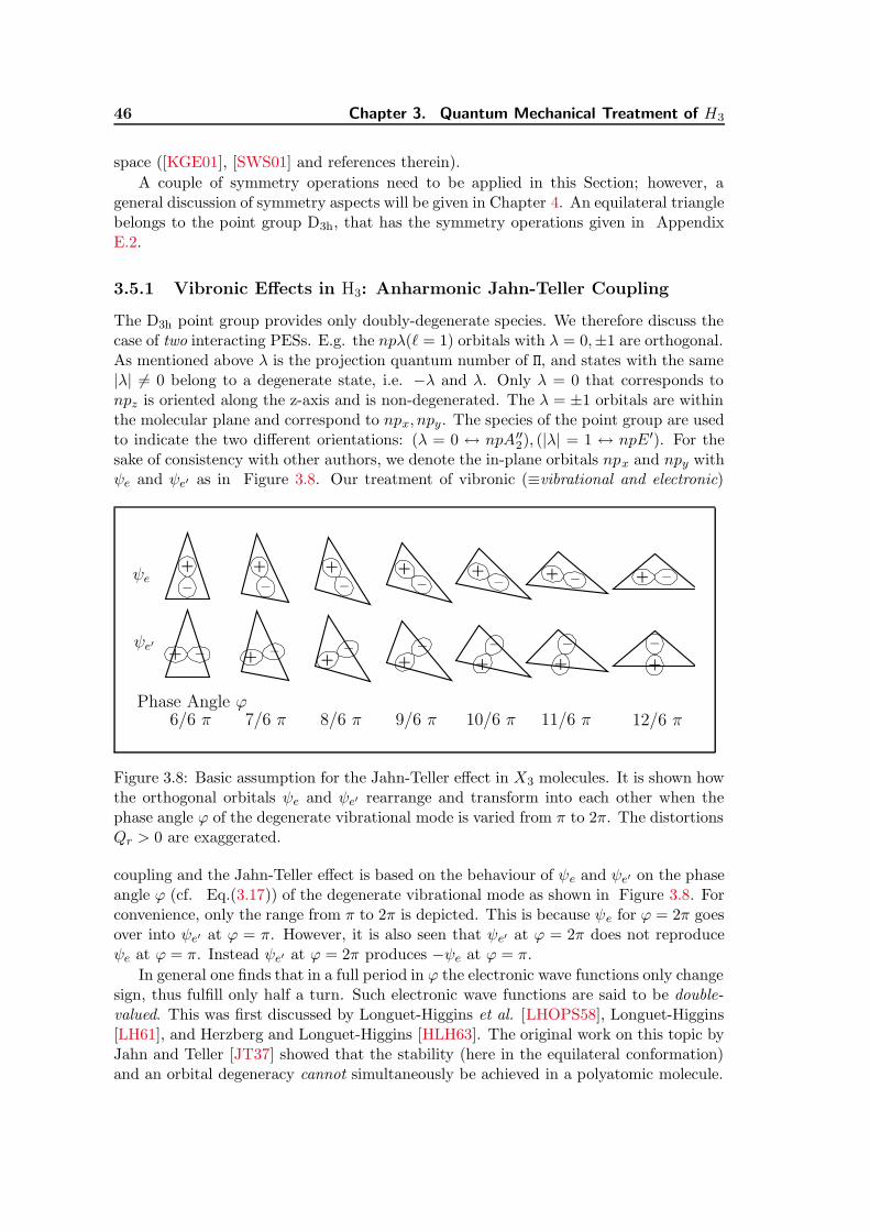
“diss”2002/10/18page 46

46 Chapter 3. Quantum Mechanical Treatment of H3

space ([KGE01], [SWS01] and references therein).

A couple of symmetry operations need to be applied in this Section; however, ageneral discussion of symmetry aspects will be given in Chapter 4. An equilateral trianglebelongs to the point group D3h, that has the symmetry operations given in AppendixE.2.

3.5.1 Vibronic Effects in H3: Anharmonic Jahn-Teller Coupling

The D3h point group provides only doubly-degenerate species. We therefore discuss thecase of two interacting PESs. E.g. the npλ(` = 1) orbitals with λ = 0,±1 are orthogonal.As mentioned above λ is the projection quantum number of Π, and states with the same|λ| 6= 0 belong to a degenerate state, i.e. −λ and λ. Only λ = 0 that corresponds tonpz is oriented along the z-axis and is non-degenerated. The λ = ±1 orbitals are withinthe molecular plane and correspond to npx, npy. The species of the point group are usedto indicate the two different orientations: (λ = 0 ↔ npA′′2), (|λ| = 1 ↔ npE ′). For thesake of consistency with other authors, we denote the in-plane orbitals npx and npy withψe and ψe′ as in Figure 3.8. Our treatment of vibronic (≡vibrational and electronic)

+ + + + +

++++++

+

+

+

– – – – –

––––––

–

–

–

6/6 π 7/6 π 8/6 π 9/6 π 10/6 π 11/6 π 12/6 π

ψe

ψe′

Phase Angle ϕ

Figure 3.8: Basic assumption for the Jahn-Teller effect in X3 molecules. It is shown howthe orthogonal orbitals ψe and ψe′ rearrange and transform into each other when thephase angle ϕ of the degenerate vibrational mode is varied from π to 2π. The distortionsQr > 0 are exaggerated.

coupling and the Jahn-Teller effect is based on the behaviour of ψe and ψe′ on the phaseangle ϕ (cf. Eq.(3.17)) of the degenerate vibrational mode as shown in Figure 3.8. Forconvenience, only the range from π to 2π is depicted. This is because ψe for ϕ = 2π goesover into ψe′ at ϕ = π. However, it is also seen that ψe′ at ϕ = 2π does not reproduceψe at ϕ = π. Instead ψe′ at ϕ = 2π produces −ψe at ϕ = π.

In general one finds that in a full period in ϕ the electronic wave functions only changesign, thus fulfill only half a turn. Such electronic wave functions are said to be double-valued. This was first discussed by Longuet-Higgins et al. [LHOPS58], Longuet-Higgins[LH61], and Herzberg and Longuet-Higgins [HLH63]. The original work on this topic byJahn and Teller [JT37] showed that the stability (here in the equilateral conformation)and an orbital degeneracy cannot simultaneously be achieved in a polyatomic molecule.

“diss”2002/10/18page 47

3.5. Degenerate Electronic States 47

The additional phase π can be viewed as a manifestation of the geometric phase (Berryphase, [Ana92], [Ber98]) that is accumulated in the electronic wave functions in a fullcycle in ϕ. Generally, this phase is proportional to a contour integral around a singu-larity in the topology of a molecular potential energy surface [XBV00]. More generaldiscussions on this subject are given in Refs. [TTM85], [Mea83], [MT79], [VX00] and inparticular for the ground state of H3 in Refs. [Yar96], [Yu97]. Time development studiesand wave packet dynamics in such situations are discussed in [MK98], [RRC89], [VY97].

The implications of Figure 3.8 can quantitatively be summarized by the equations(ψe[ϕ]ψe′ [ϕ]

)=

(sin ϕ/2 − cos ϕ/2cos ϕ/2 sin ϕ/2

)(ψe0

ψe′0

)(3.63)

which immediately lead to

πz ψe = − h2iψe′ πz ψe′ =

h

2iψe (3.64)

by applying the operator on ψe, ψe′ and using πz = − hi

∂∂ϕ . The latter identity re-

sults from the explicit expression for πz in Eq.(3.38) and the definitions of (Qr, ϕ) inEq.(3.17). Eqs.(3.64) represent the key for the following treatment of the Jahn-Tellereffect. Successive application of πz on ψe or ψe′ leads to π2

z = h2/4 that already indicatesthe occurrence of half-integer angular momenta.

In order to exploit the above discussion in a quantitative approach, an approximationsimilar to the one used for the non-degenerate case is required. However, we must accountfor the mutual couplings between the degenerate states. The electronic and nuclearmotion must now be treated simultaneously, since the additional couplings discussed inthe following imply a strong correlation between them. This is achieved by reorderingthe Hamiltonian in Eq.(3.39) and introducing a vibronic Hamilton operator Hev

Hev =1

2m−1

e

∑

α;j=1,2,3

p2jα + VrQ + VQ +

1

2

∑

k=1,2,3

P2k (3.65)

≡ He +pure nuclear parts

≡ H +1

2

∑

k=1,2,3

P2k

The definitions are as in the non-degenerate case and H is introduced to abbreviate termsin what follows. Rotational parts are neglected here. They will be briefly considered ina later paragraph. A general solution of the resulting Schrodinger equation can again berepresented by as ansatz of the type of Eq.(3.42). If we adopt a similar simplificationlike for the non-degenerate case in item 1 on page 29, where far lying electronic stateswere neglected, we shrink the general solution Eq.(3.42) to a sum consisting of two partsassociated with the two degenerate electronic states

Ψ = Ψ(r,Q) = χn(Q)ψe(r,Q) + χn′(Q)ψe′(r,Q) (3.66)

The vibrational prefactors are again considered as Q-depending expansion coefficients.They are related to the two degenerate vibrational modes. The electronic wavefunc-tions ψe, ψe′ are solutions of the electronic Schrodinger equation, solved with a para-metrical dependence on nuclear coordinates by Eq.(3.41) and Q-depending eigenval-

ues E(e)e (Q), E

(e)e′ (Q). For D3h symmetries at Qr = 0 the degeneracy condition is:

“diss”2002/10/18page 48

48 Chapter 3. Quantum Mechanical Treatment of H3

E(e)e = E

(e)e′ . The full PESs we denote by We,e′(Q) := E

(e)e,e′(Q) + VQ(Q). Since phase

dependencies are crucial here, two different vibrational expansion factors χn and χn′

are needed. The application of symmetry principles simplifies the following discussion.Therefore, the complex representation

Ψ = Ψ(r,Q) = χ+(Q)ψ+(r,Q) + χ−(Q)ψ−(r,Q) (3.67)

is more appropriate than Eq.(3.66). In this complex representation, ψ+ and ψ− arelinear combinations of ψe and ψe′ with the properties

1C3ψ+ = ωψ+1C3ψ− = ω∗ψ− (3.68)

where the operator 1C3 rotates by 2π/3 (see Chapter 4). Its eigenvalues are expressedby the complex phase factor ω = e−i2π/3 ; the star indicates the complex conjugate.Furthermore, we assume that this change of basis does not alter the orthonormalityproperties of the functions ψe, ψe′ in electronic space and suppose the unitarity of thetransformation to ψ±. Consequently, the following orthonormality condition holds

∫ψ∗a(r,Q)ψb(r,Q)dr = δab ∀ Q, with a, b ∈ (+,−) (3.69)

These requirements restrict the new basis functions to be of the type

ψfa = eif(Q)(ψe + iaψe′)/

√2 with a ∈ (+,−) (3.70)

The function f(Q) generally depends on all normal coordinates and represents an addi-tional degree of freedom because of the linearity of the Schrodinger equation. We nowcontinue as in the non-degenerate case and evaluate the Schrodinger equation Hev Ψ = εΨwith Eq.(3.65) by multiplying from the left by either ψ+ or ψ−. After integrating overelectronic variables, using the orthonormal properties of Eq.(3.69) and the product rulefor the operators Pk, we arrive at a coupled system of equations for the vibrational factorsχ+, χ−

〈ψ+ | H | ψ+〉r + 1/2∑

k

〈ψ+ | P2

k | ψ+〉r+ 〈ψ+ | Pk | ψ+〉r Pk + P2

k

− ε

〈ψ+ | H | ψ−〉r + 1/2∑

k

〈ψ+ | P2

k | ψ−〉r+ 〈ψ+ | Pk | ψ−〉r Pk

〈ψ− | H | ψ+〉r + 1/2∑

k

〈ψ− | P2

k | ψ+〉r+ 〈ψ− | Pk | ψ+〉r Pk

〈ψ− | H | ψ−〉r + 1/2

∑k

〈ψ− | P2

k | ψ−〉r+ 〈ψ− | Pk | ψ−〉r Pk + P2

k

− ε

(χ+

χ−

)= 0

(3.71)

Here, we made the convention that operators inside matrix elements work only on func-tions below the integral but not outside. For an evaluation of the involved matrix ele-ments a few approximations can be introduced. If we only consider the local behaviourin the vicinity of the conical intersection, i.e. at the point with D3h symmetry, we canapproximate the sums in Eq.(3.71) by using

P2a = cosϕ PQr+

sinϕ

Qrπz

∼Qr→0

sinϕ

Qrπz

P2b = sinϕ PQr−cosϕ

Qrπz

∼Qr→0

− cosϕ

Qrπz (3.72)

∑

k

P2k = P2

1 +h

i QrPQr

+ P2Qr

+1

Q2r

π2z

∼Qr→0

1

Q2r

π2z

“diss”2002/10/18page 49

3.5. Degenerate Electronic States 49

due to the different types of singularities of individual terms. This approximation enablesus to consider only the effects of πz on ψ±. Moreover, it suggests that the phase factorsonly depend on the vibrational phase angle f(Q) = f(ϕ). Particularly convenient forX3 molecules is the choice of the function as f(ϕ) = iαϕ/2, α = 0,±1,±2, . . . to achievea double-valuedness of eif(ϕ), since we want to demand the new basis functions single-valued. The effect of πz on ψ± is

πz

√2ψ(α)

a = [πz eiαϕ/2 ](ψe + iaψe′) + eiα

ϕ/2 ([πz ψe] + ia[πz ψe′ ]) (3.73)

By employing Eqs.(3.64) we obtain the relations

πz ψ(α)a = h/2 (a− α)ψ(α)

a (3.74)

π2z ψ

(α)a = h2/4 (a− α)2ψ(α)

a

Thus, within our approximation all matrix elements of nuclear momentum operatorsvanish if we choose α = a = ±1 for the phase function f(ϕ). The matrix Schrodingerequation Eq.(3.71) simplifies to∑

k P2k /2 0

0∑

k P2k /2

+

〈ψ+ | H | ψ+〉r 〈ψ+ | H | ψ−〉r

〈ψ− | H | ψ+〉r 〈ψ− | H | ψ−〉r

(χ+

χ−

)= ε

(χ+

χ−

)(3.75)

The new basis is called the diabatic representation13 . It is explicitly related to theadiabatic representation (ψe, ψe′) by a unitary transformation matrix S according toEqs.(3.70) (

ψ+

ψ−

)=

1√2

(eiϕ/2 ieiϕ/2

e−iϕ/2 −ie−iϕ/2

)(ψe

ψe′

)≡ S

(ψe

ψe′

)(3.76)

From a comparison of Eq.(3.66) and Eq.(3.67) with the definition of S, the relationshipbetween the nuclear expansion coefficients is apparent

(χ+

χ−

)= S

(χn

χn′

)(3.77)

The second term in brackets of Eq.(3.75) belongs to a generalized potential surface oftwo coupled Born-Oppenheimer surfaces. This is seen by inserting Eq.(3.76) into thematrix elements and using the electronic Schodinger equation Eq.(3.41). The result is

Vdiabat =1

2

(We +We′ (We −We′)e−iϕ

(We −We′ )eiϕ We +We′

)(3.78)

When the two surfaces coincide the coupling vanishes. The matrix elements of thepotential in Eq.(3.75) can be approximated in the proximity of the conical intersectionby a Taylor expansion up to the third order. Instead of Qr and ϕ, it is easier to use theequivalent variables Q+, Q−, defined in Eq.(3.17), for this expansion

〈ψa | H(Q) | ψb〉r =

W0 +∑

ν=+,−WνQv +

1

2

∑

ν,µ=+,−Wν,µQνQµ +

1

6

∑

ν,µ,λ=+,−Wν,µ,λQνQµQλ + . . . (3.79)

13In general, if a global behaviour is of interest and the approximation Eq.(3.72) is not considered,f(Q) cannot always be chosen to make these matrix elements disappear and necessarily a non-removablepart remains. This is demonstrated in detail in [Yar96] where effects of the non-removable part areevaluated numerically for the ground state potential surface of H3.

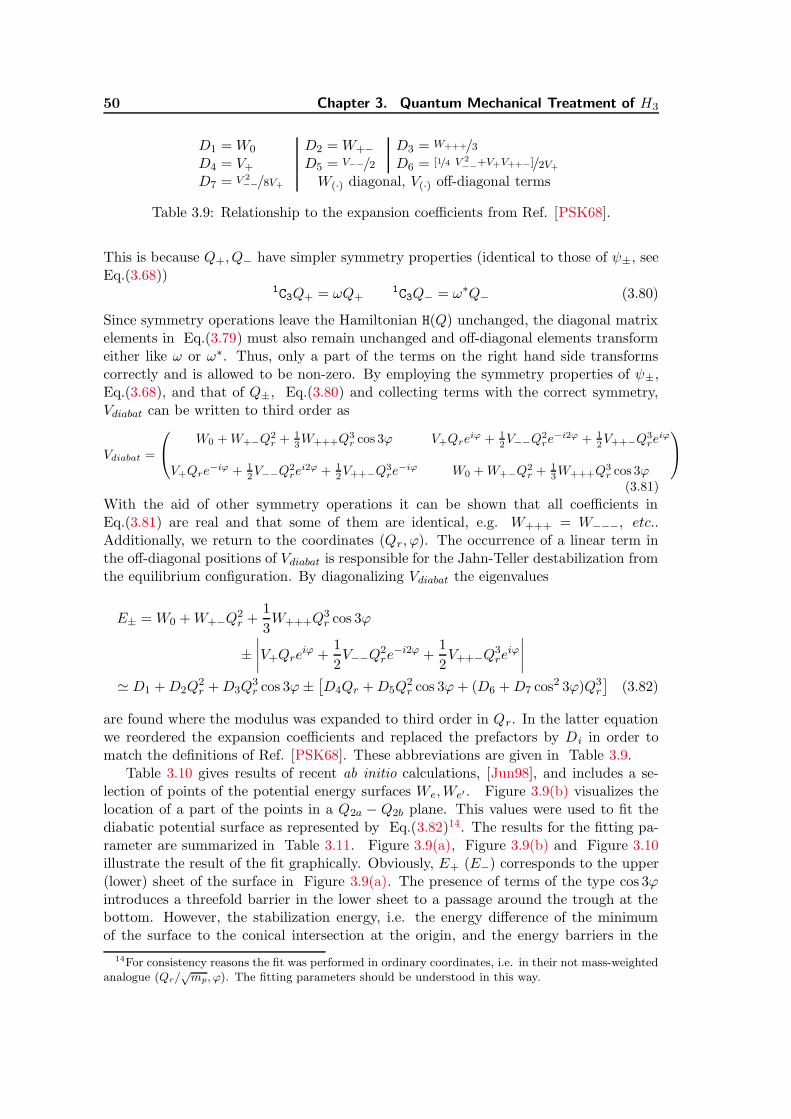
“diss”2002/10/18page 50

50 Chapter 3. Quantum Mechanical Treatment of H3

D1 = W0 D2 = W+− D3 = W+++/3D4 = V+ D5 = V−−/2 D6 = [1/4 V 2

−−+V+V++−]/2V+

D7 = V 2−−/8V+ W(·) diagonal, V(·) off-diagonal terms

Table 3.9: Relationship to the expansion coefficients from Ref. [PSK68].

This is because Q+, Q− have simpler symmetry properties (identical to those of ψ±, seeEq.(3.68))

1C3Q+ = ωQ+1C3Q− = ω∗Q− (3.80)

Since symmetry operations leave the Hamiltonian H(Q) unchanged, the diagonal matrixelements in Eq.(3.79) must also remain unchanged and off-diagonal elements transformeither like ω or ω∗. Thus, only a part of the terms on the right hand side transformscorrectly and is allowed to be non-zero. By employing the symmetry properties of ψ±,Eq.(3.68), and that of Q±, Eq.(3.80) and collecting terms with the correct symmetry,Vdiabat can be written to third order as

Vdiabat =

W0 +W+−Q2r + 1

3W+++Q

3r cos 3ϕ V+Qre

iϕ + 1

2V−−Q

2re

−i2ϕ + 1

2V++−Q

3re

iϕ

V+Qre−iϕ + 1

2V−−Q

2re

i2ϕ + 1

2V++−Q

3re

−iϕ W0 +W+−Q2r + 1

3W+++Q

3r cos 3ϕ

(3.81)

With the aid of other symmetry operations it can be shown that all coefficients inEq.(3.81) are real and that some of them are identical, e.g. W+++ = W−−−, etc..Additionally, we return to the coordinates (Qr, ϕ). The occurrence of a linear term inthe off-diagonal positions of Vdiabat is responsible for the Jahn-Teller destabilization fromthe equilibrium configuration. By diagonalizing Vdiabat the eigenvalues

E± = W0 +W+−Q2r +

1

3W+++Q

3r cos 3ϕ

±∣∣∣∣V+Qre

iϕ +1

2V−−Q

2re−i2ϕ +

1

2V++−Q

3re

iϕ

∣∣∣∣

' D1 +D2Q2r +D3Q

3r cos 3ϕ±

[D4Qr +D5Q

2r cos 3ϕ+ (D6 +D7 cos2 3ϕ)Q3

r

](3.82)

are found where the modulus was expanded to third order in Qr. In the latter equationwe reordered the expansion coefficients and replaced the prefactors by Di in order tomatch the definitions of Ref. [PSK68]. These abbreviations are given in Table 3.9.

Table 3.10 gives results of recent ab initio calculations, [Jun98], and includes a se-lection of points of the potential energy surfaces We,We′ . Figure 3.9(b) visualizes thelocation of a part of the points in a Q2a − Q2b plane. This values were used to fit thediabatic potential surface as represented by Eq.(3.82)14. The results for the fitting pa-rameter are summarized in Table 3.11. Figure 3.9(a), Figure 3.9(b) and Figure 3.10illustrate the result of the fit graphically. Obviously, E+ (E−) corresponds to the upper(lower) sheet of the surface in Figure 3.9(a). The presence of terms of the type cos 3ϕintroduces a threefold barrier in the lower sheet to a passage around the trough at thebottom. However, the stabilization energy, i.e. the energy difference of the minimumof the surface to the conical intersection at the origin, and the energy barriers in the

14For consistency reasons the fit was performed in ordinary coordinates, i.e. in their not mass-weightedanalogue (Qr/

√mp, ϕ). The fitting parameters should be understood in this way.

“diss”2002/10/18page 51

3.5. Degenerate Electronic States 51

No. Q2a/√

mp Q2b/√

mp Qr/√

mp ϕ Ab initio Energy Fit Weight1 0.00000 0.00000 0.00000 90.0 -1.41694 -1.41695 32 0.08184 -0.04723 0.09449 -30.0 -1.41425 -1.41421 13 0.06682 -0.06680 0.09449 -45.0 -1.41416 -1.41416 14 0.08663 0.00000 0.08663 0.0 -1.41469 -1.41459 25 0.04331 -0.07502 0.08662 -60.0 -1.41448 -1.41449 26 0.17318 0.00000 0.17318 0.0 -1.41055 -1.41026 27 0.25980 -0.44999 0.51960 -60.0 -1.34810 -1.34342 28 0.12991 -0.22501 0.25982 -60.0 -1.40065 -1.40016 29 0.18967 -0.21066 0.28346 -48.0 -1.39822 -1.39753 110 0.13359 -0.13362 0.18895 -45.0 -1.40814 -1.40803 111 0.17319 -0.29998 0.34639 -60.0 -1.38824 -1.38678 212 0.08661 -0.15001 0.17322 -60.0 -1.40918 -1.40914 213 0.36442 -0.43429 0.56694 -50.0 -1.33616 -1.33033 114 0.34525 -0.15372 0.37793 -24.0 -1.39144 -1.38953 115 0.51959 0.00000 0.51959 0.0 -1.38315 -1.37849 216 0.34644 0.00000 0.34644 0.0 -1.39780 -1.39680 217 0.25976 0.00000 0.25976 0.0 -1.40503 -1.40424 218 0.27730 -0.05896 0.28349 -12.0 -1.40279 -1.40187 1

Table 3.10: Ab initio energies of 3p 2E′. All quantities in atomic units; from [Jun98].

trough are both small compared to vibrational frequencies. Furthermore, the barrier of11.38 cm−1 is small compared to the stabilization energy of −82.99 cm−1. Therefore,even in the vibrational ground state a rotation in the trough cannot be hindered by thebarrier due to the large zero point energy of a few thousand wavenumbers. The systemis said to be dynamically Jahn-Teller active. It is therefore always a good approximation

This work King & Morokuma [KM79]

D1 -1.41695D2 0.15055 0.1597D3 -0.13371 -0.1102D4 0.01449 0.01687D5 0.00453 -0.0045a

D7 0.00585 0.0055b

D8c 0.03284

Stabilization energy EJT −82.99 cm−1

Barrier 11.38 cm−1

Table 3.11: Jahn-Teller distortion parameters for the degenerate 3p 2E′ state. The fitwas performed in not mass-weighted normal coordinates (Qr/

√mp, ϕ).

———————————–All quantities in atomic units.a The different sign can not be explained. Any other coordinate system does not change the sign of D3;this is in contradiction with Ref. [KM79]b Strictly, this number corresponds to the sum D6 + D7.c This parameter belongs to a fourth order term Q4

r that was included and greatly improved the fit.

to neglect terms responsible for this small barriers and consider the main effect as asmall shift from equilibrium at Qr = 0.

If we perform calculations analogous to Eq.(3.71) but in the adiabatic basis set

“diss”2002/10/18page 52

52 Chapter 3. Quantum Mechanical Treatment of H3

0.001

0.0015

0.002

0.0025

0.003Energy

–0.1

–0.05

0.05

0.1

Q2a

–0.1–0.05

0.050.1

Q2b

(a) Potential Energy Surfaces of the degenerate 3p 2E′ state in a Taylor expansion up to thirdorder. All numbers in atomic units. The energy of the conical intersection point is set to zero.

−0.30 −0.20 −0.10 −0.00 0.10 0.20 0.30Q2a (bohr)

−0.30

−0.20

−0.10

−0.00

0.10

0.20

0.30

Q2b

(bo

hr)

15001300

1100

1100

1100

1100

1300

1500

1300

1300

900

900

900

900

900

700

700

700

700

700

500

500

500

500

400

400

400

400

300

300

300

300200

200

100

100

30

30

−70

−70

(b) Contour plot of the lower sheet E−. The triangles indicate a part of the ab initio pointsused in the fit. Due to permutational symmetry only a sixth of the total configuration space,(Qr, ϕ = 0..60), must be considered. The inner contour rings are (−84,−82 . . . − 70) −black, (−60,−50 . . . 30) − bluecm−1, others are labeled.

Figure 3.9:

“diss”2002/10/18page 53

3.5. Degenerate Electronic States 53

−0.4 −0.2 0.0 0.2 0.4Q2a (bohr)

10

100

1000

10000E

nerg

y / c

m−

1

−0.4 −0.2 0.0 0.2 0.4Q2b (bohr)

10

100

1000

10000

Figure 3.10: Cuts through the fitted potential energy surface of 3p 2E′ along the coor-dinate axes Q2a, Q2b. Triangles show the distribution of the ab initio points; solid linescorrespond to the fit. The conical intersection point was shifted to +100cm−1 due tothe logarithmic representation.

ψe, ψe′ , we get instead

Vadiab =

(We + h2/(8Q2

r) −ih(2Q2r)

−1 πz

ih(2Q2r)

−1 πz We′ + h2/(8Q2r)

)(3.83)

Although, the potential energy surfaces vary with ϕ and Qr, we can assume the loworder terms to be only weakly phase dependent. The justification of this follows fromthe above discussion. As a result, the following commutator is approximately zero

[Vadiab,

(πz 00 πz

)]' 0 (3.84)

Then, we can choose in an equation similar to Eq.(3.75) the vibrational prefactors tobe simultaneous eigenfunctions of πz

πz χn,n′ = jhχn,n′ (3.85)

Now, an important conclusion results from the properties of ψe,e′ . The total wavefunctionΨ, if assumed real, is a physical object, that must be single-valued, i.e. a rotation in ϕover 2π must reproduce the wavefunction of the same sign. However, since the electronicpart is double-valued the vibrational prefactors must also be double-valued. Thus, itfollows directly from Eq.(3.85) that j must be half-odd. Applying πz on χ± as definedin Eq.(3.77), and using Eq.(3.85) we find the eigenvalues of χ+, χ− as

πz χ+ = (j − 1/2 )hχ+ πz χ− = (j + 1/2 )hχ− (3.86)

“diss”2002/10/18page 54

54 Chapter 3. Quantum Mechanical Treatment of H3

that have now integer eigenvalues, implying χ± to be single-valued, as are the associatedelectronic parts. We can abbreviate the eigenvalues by l2 := j−λ/2 . To this accuracy thediabatic potential surface is approximated by a parabola of revolution centered about avertical line that does not pass the conical intersection. This represents the degree ofapproximation for the discussion of the rotational level structure in the next paragraphthat provides insight into the influence of the half-integer angular momenta.

If we neglect in Eq.(3.81) angular dependent terms of order higher than Q2r, the

Schrodinger equation Eq.(3.75) can be solved by expanding the vibrational prefactorsin 2D harmonic oscillator wavefunctions ην2,l2(Qr, ϕ). For a fixed l2 = j−λ/2 the inverseof relation Eq.(3.61) allows only the values ν2 = |l2|, |l2|+2, |l2|+4, . . . for the number ofexcited quanta. Thus, not every harmonic function can contribute to χ±, but only eachsecond. The following expansion is valid for positive values of j (analogous equationsexist for negative j)

χ+,j =

nmax∑

n=0

a2n+1η(j−1/2 +2n),j− 12

= a1ηj−1/2 ,j− 12

+ a3ηj+3/2 ,j− 12

+ . . .

χ−,j =

nmax∑

n=0

a2n+2η(j+1/2 +2n),j+ 12

= a2ηj+1/2 ,j+ 12

+ a4ηj+5/2 ,j+ 12

+ . . . (3.87)

This model is often [TTM85], [LHOPS58], [LH61] used only up to second order in Qr

which is sufficient accurate for heavier molecules. We additionally account for anhar-monicity by incorporating the term Q4

r , which is important here as seen from the fittingof the potential energy surface. In combining ansatz Eq.(3.87) with the HamiltonianEq.(3.75), using the approximation of Eq.(3.81) by skipping all angular dependent termsexcept Qre

iϕ, and by invoking matrix elements of harmonic oscillator wavefunctions[Bel70] directly to the linear system of equations for a fixed j, we obtain

j + 1/2 − ε+Da(j+1/2 )(j+3/2 ) (2j + 1)D 2(j+1/2 )(j+3/2 )Da 0 . . .

(2j + 1)Dj + 3/2 − ε

+Da(j+5/2 )(j+15/2 )

√2D 6(j+5/2 )(j+7/2 )Da . . .

2(j+1/2 )(j+3/2 )Da

√2D

j + 5/2 − ε+Da[2+(j+5/2 )(j+23/2 )] (2j + 3)D . . .

0 6(j+5/2 )(j+7/2 )Da (2j + 3)Dj + 7/2 − ε

+Da[6+(j+9/2)(j+35/2)]. . .

......

...... ·

a1

a2

a3

a4

...

= 0

(3.88)

The quantity D is a dimensionless parameter first introduced by Moffitt and Thorson[MT58]. It is equal to the ratio of the Jahn-Teller stabilization energy EJT to the zeropoint energy of the unperturbed vibrational quantum ωe. Terms involving the parameterDa ≡ D8/ω

3em

2p = 0.0046 result from the quartic term for 3p 2E′ and contribute to the

main diagonal as well as to the diagonals shifted by two from the central. For anapproximate solution of the infinite linear system we abort the series after the sixthterms in Eq.(3.87). Its size has only a minor effect on the the lower eigenvalues and-vectors. From the parabola D1 + D2Q

2r/mp − D4Qr/

√mp, that corresponds to one

branch of a section through the surface, it follows that EJT = Dωe = −D24/4D2 =

“diss”2002/10/18page 55

3.5. Degenerate Electronic States 55

Table 3.12: Solution of the first order Jahn-Teller coupling in the harmonic approxima-tion. For explicit evaluation of the coefficients, the experimental value D = 0.0301 waschosen.

Expansion coefficientsb for positive j

Eigenvaluesa in j = 1/2 j = 3/2increasing order → 0.9415 1.9966 2.9507 1.8887 3.0454 3.9063

a1 0.9723 -0.2316 -0.0309 0.9516 -0.3036 -0.0476a3 0.0282 0.2447 -0.9199 0.0365 0.2603 -0.8986a2 -0.2319 -0.9406 -0.2454 -0.3052 -0.9148 -0.2615a4 -0.0032 -0.0424 0.3042 -0.0050 -0.0566 0.3491

Eigenvaluesa in j = 5/2 j = 7/2increasing order → 2.8403 4.0891 4.8659 3.7953 5.1286 5.8292

a1 0.9353 -0.3481 -0.0639 0.9220 -0.3786 -0.0811a3 0.0414 0.2789 -0.8790 0.0447 0.3007 -0.8600a2 -0.3515 -0.8921 -0.2804 -0.3846 -0.8709 -0.3025a4 -0.0064 -0.0716 0.3803 -0.0077 -0.0882 0.4030

Moffitt-Thorson parameter, Change in BondStabilization Energy & Jahn-Teller Distortion D = EJT/ωe EJT /cm

−1 Length ∆S1/bohrThis work 0.0272 76.5 0.048Experimental value [HLSW81] 0.0301 87.0 0.051King & Morokuma [KM79] 0.0338 97.8 0.054a Eigenvalues in units of the zero point energy ωe.b Amplitudes are normalized, i.e. the sum of their squares is one.

−3.487 · 10−4a.u. = −76.5 cm−1 is the stabilization energy. A similar considerationyields for the Jahn-Teller distortion, i.e. the distance of the minimum in the troughfrom the conical intersection, (Qr/

√mp) = D4/2D2 = 0.048 bohr ≡ ∆S1. The latter

equation gives the relation to a corresponding change in the bond length S1 in the Q2a

mode as defined in Figure 3.2 and as it is obvious from Eq.(3.18). From the constantD2 the harmonic frequency ωe is estimated to 2811 cm−1 and thus we have D = 0.0272.Values from experiment and ab initio calculations are given in Table 3.12 for comparison.Since we have simply neglected higher orders the stabilization energy and the Moffitt-Thorson parameter are too small estimated by the fit. We have solved the linearsystem of equations in a pure harmonic approximation (Da = 0) and also by accountingfor quartic anharmonicity. For D we use 0.0301 from experimental data which seems tobe the most reliable value. A energy level diagram is shown in Figure 3.11 comparingthe two approximations. The results for the eigenvalues and amplitudes for the lowestvibronic levels in the harmonic approximation are included in Table 3.12. Only slightdeviations from integer multiples of harmonic energy levels are obtained in the harmonicapproximation due to the small size of the coupling constant D. States with a + or −belong essentially to χ+, χ− and are lowered, lifted by vibronic interaction, respectively.Contributions in the expansion of the vibrational factors χ± are on the order of a fewpercent, as seen in the squares of amplitudes of higher harmonic oscillator functions.Strictly speaking, in such a situation a level has to be specified by the quantum numbers(ν2, j); for the weak coupling prevailing here, however, a notation using l2 is equally

“diss”2002/10/18page 56

56 Chapter 3. Quantum Mechanical Treatment of H3

l =422l =2 l =3 22l =0 2l =1 l =422l =2 l =3 22l =0 2l =1

+

+

+

=V

ibra

tion

al E

nerg

y / ω

eν

+ 1

2

+

+

+

−

−

−

+

+

+

−

− +

++

+

j=1/2 j=3/2 j=5/2 j=7/2j=1/2 j=3/2 j=5/2 j=7/2

−

−

+

+

−

− +

−

+

+

−

−

−

0

1

2

3

4

5

6

Harmonic Approximation Anharmonic Approximation

Figure 3.11: Effects of vibronic coupling. The solution of the linear system of Eq.(3.88)for positive j values is illustrated. The coupling induces only small line shifts. Dashedlines separate the different j regions. Levels within a column interact by first order Jahn-Teller coupling. Left: harmonic approximation; Right: including anharmonic quarticterm.

unambiguous. Since j remains a good quantum number in this coupling scheme, onlylevels with the same j can mix, i.e. only levels within the same columns of Figure 3.11separated by dashed lines. The anharmonic terms on the diagonal rapidly increase withthe vibrational quantum number and stretch the energy spectrum on the right in Figure3.11. From the fit it is evident that the parameter D8 has a large error bar. By inspectionof Figure 3.11 it seems that the result overestimates anharmonic effects. The effect ofa second order Jahn-Teller interaction V−−Q2

− mixes levels with j differing by multiplesof 3, e.g. the levels j = −3/2 and j = 3/2 etc. [CLH61] and eventually removes j as agood quantum number.

Unfortunately, a direct comparison to experimentally determined levels from ourlaboratory is difficult because the zero potential energy (more precisely the content ofthe symmetric stretch vibration) and the symmetric stretch frequency of the 3p 2E′

state are unknown. Moreover, it is difficult to estimate rotational term values from theexperimental energy positions since the 3p 2E′ state is intermediate between Hund’scase (ab) and Hund’s case (d) (cf. Section 5.1.1) and vibronic effects on rotational levelsare large. Further problems can arise for the lowest excited vibronic levels of 3p 2E′

since they fall into the region of the 3d-complex and might be additionally perturbed byelectronic coupling (item 1 on page 29). For the two rovibronic levels at 18521.4cm−1 and18138.7cm−1 of the electronic state 3p 2E′ employed in Chapter 5, however, a tentativeassignment is possible. The two levels are N = 1 levels with rovibronic symmetry A ′2

“diss”2002/10/18page 57

3.5. Degenerate Electronic States 57

and E′, respectively. In Ref. [LHH89] the ortho level 18521.4cm−1 is proposed to be3p 2E′(N = 1, G = 0)1, 1±1. Using the same arguments (Model I & II of Ref. [LHH89])we assign the para level 18138.7cm−1 to 3p 2E′(N = 1, G = 2)0, 20.

3.5.2 Rotational Levels in Degenerate Electronic States & Vibrational

Quenching

As a consequence of the coupling of electronic and nuclear motion in a degenerate elec-tronic state their associated angular momenta couple to a vibronic angular momentumΠev

z = Πz +πz. One major effect of vibronic interactions on rotational levels [Wat89] isdescribed by replacing the pure vibrational angular momentum by the vibronic angularmomentum in the z-axis Coriolis term

HCor = −2C(Πz +πz) Nz (3.89)

If only the first term in either expansion of Eq.(3.87) is taken in Eq.(3.67), the diagonalmatrix elements of HCor in the vibronic basis are

〈Ψj| Πz +πz |Ψj〉 =sign(j)[(a2

1 − a22)ζe + a2

2ζ2b2a

]≡ sign(j)ζJT

0

(3.90)

with definitions λζe = 〈ψ±| Πz |ψ±〉l2ζ2b2a = 〈χν2l2 |πz |χν2l2〉

The parameter ζ2b2a was already defined in Eq.(3.26) and is equal to one. Similarlythe parameter ζe is one15 if the orbital is a pure npE ′. Thus, it follows from Eq.(3.90)that the effect of vibronic coupling is to quench the electronic angular momentum by afactor (a2

1 − a22) and partially enhance the vibrational angular momentum by a2

2 in thevibrational ground state. These factors were determined experimentally by Herzberg etal. [HLSW81]. Since the coefficients ai depend only on D these factors are consistentwith ab initio values from this work. The contribution to the rotational energy is thus

ECor = −sign(j)2CζJT0 K (3.91)

Another important effect of vibronic coupling on the rotational spectra is caused byoff-diagonal contributions to the main rotational energy operator. As discussed in Ref.[Wat89] this leads to a Λ − doubling effect with large coupling constants and a stronginfluence on the rotational spectra. All these effects were extensively discussed in litera-ture in the detailed analysis of Refs. [DH80], [HW80], [HLSW81], [HHW82] and [Wat89],and the interested reader is referred to it.

15The experimental value of Ref. [HLSW81] is ζe = 0.963.

“diss”2002/10/18page 58

58 Chapter 3. Quantum Mechanical Treatment of H3

“diss”2002/10/18page 59

CHAPTER 4

Principles of Symmetry - Group Theoretical Aspects

Symmetry aspects of the total wavefunction of H3 are discussed in orderto classify symmetries of rovibronic levels. On the basis of symmetryand by using group theoretical theorems, selection rules for optical or ra-diationless transitions can easily be derived. Moreover, symmetry argu-ments allow to explain the experimentally observed metastability of therotational levels 2p 2A′′2(N = 0, G = 0)ν1, ν

l22 and the non-existence

of certain rovibronic levels due to their statistical weight of zero. Theyalso supply a motivation for the introduction of the convenient quantumnumber G, first introduced by Hougen.

Contents

4.1 Basic Definitions of Groups & their Relations . . . . . . . . . 60

4.1.1 CNP Group and Successive Applications of Permutations . . . 60

4.1.2 CNPI Group . . . . . . . . . . . . . . . . . . . . . . . . . . . . 61

4.1.3 The Point Group, Rotation & Nuclear Spin Permutation Group 61

4.1.4 The MS Group of H3 & its Representation by Subgroups . . . 62

4.2 Classification of Rovibronic States . . . . . . . . . . . . . . . . 63

4.2.1 Nuclear Spin Statistics . . . . . . . . . . . . . . . . . . . . . . . 65

4.2.2 Total Wavefunctions obeying Fermion Exchange Symmetry . . 68

4.3 Selection Rules in Electric Dipole Transitions . . . . . . . . . 69

4.4 Metastability . . . . . . . . . . . . . . . . . . . . . . . . . . . . . 71

Symmetry based principles belong to the most fundamental concepts in natural sci-ences. These principles always give strict and exact statements. However, they are notsuited to predict numerical results, rather they deliver a qualitative understanding. Themost general way for a discussion on rovibronic (≡ rotational & vibrational & electronic)symmetries relies on the definition of the CNPI (Complete Nuclear Permutation & In-version) group. In the literature often only a subgroup of the CNPI group, the Point

59

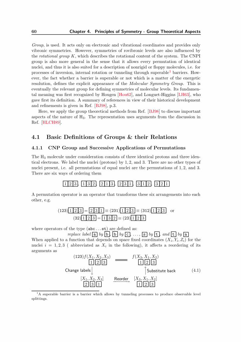
“diss”2002/10/18page 60

60 Chapter 4. Principles of Symmetry - Group Theoretical Aspects

Group, is used. It acts only on electronic and vibrational coordinates and provides onlyvibronic symmetries. However, symmetries of rovibronic levels are also influenced bythe rotational group K, which describes the rotational content of the system. The CNPIgroup is also more general in the sense that it allows every permutation of identicalnuclei, and thus it is also suited for a description of nonrigid or floppy molecules, i.e. forprocesses of inversion, internal rotation or tunneling through superable1 barriers. How-ever, the fact whether a barrier is superable or not which is a matter of the energeticresolution, defines the explicit appearance of the Molecular Symmetry Group. This iseventually the relevant group for defining symmetries of molecular levels. Its fundamen-tal meaning was first recognized by Hougen [Hou62], and Longuet-Higgins [LH63], whogave first its definition. A summary of references in view of their historical developmentand refinements is given in Ref. [BJ98], p.3.

Here, we apply the group theoretical methods from Ref. [BJ98] to discuss importantaspects of the nature of H3. The representation uses arguments from the discussion inRef. [HLCH89].

4.1 Basic Definitions of Groups & their Relations

4.1.1 CNP Group and Successive Applications of Permutations

The H3 molecule under consideration consists of three identical protons and three iden-tical electrons. We label the nuclei (protons) by 1, 2, and 3. There are no other types ofnuclei present, i.e. all permutations of equal nuclei are the permutations of 1, 2, and 3.There are six ways of ordering them

1 2 3 , 1 3 2 , 2 1 3 , 2 3 1 , 3 1 2 , 3 2 1

A permutation operator is an operator that transforms these six arrangements into eachother, e.g.

(123) 1 2 3 = 2 3 1 ≡ (231) 1 2 3 ≡ (312) 1 2 3 or

(32) 1 2 3 = 1 3 2 ≡ (23) 1 2 3

where operators of the type (abc . . . st) are defined as:replace label a by b , b by c , . . . , s by t , and t by a

When applied to a function that depends on space fixed coordinates (Xi, Yi, Zi) for thenuclei i = 1, 2, 3 ( abbreviated as Xi in the following), it affects a reordering of itsarguments as

(123)f(X1, X2, X3)

1 2 3

f(X3, X1, X2)

1 2 3

Change labelsy

xSubstitute back

[X1, X2, X3]

2 3 1Reorder−−−−−−→ [X3, X1, X2]

1 2 3

(4.1)

1A superable barrier is a barrier which allows by tunneling processes to produce observable levelsplittings.

“diss”2002/10/18page 61

4.1. Basic Definitions of Groups & their Relations 61

Products of permutation operators, i.e. successive application of these operators canalways be expressed by a single permutation operator. This is the property of thecompleteness of a group. Some examples are

(23)(123) = (12), (123)(132) = E or E(132)−1 = (123)

A complete set of permutation operators for the interesting case is, e.g.E, (12), (23), (13), (123), (132)

This set builds the CNP (Complete Nuclear Permutation) Group for H3 and is denotedS3. E is the neutral element of the group and it is obvious that for each element aninverse exists. A complete multiplication table of the members of this group is given inAppendix E.4.

4.1.2 CNPI Group

Parity is a property of a molecule that illustrates its behaviour against a transition froma clockwise to an anti-clockwise labeling. For an arbitrary wavefunction parity is definedas exchanging all spatial coordinates of nuclei and electrons by their negatives

E∗f(X1, X2, . . . X6) := f(−X1,−X2, . . . −X6) ≡ mf(X1, X2, . . . X6)

It is clear from E∗ (E∗f(X1, X2, . . . X6)) = m2f(X1, X2, . . . X6) that the eigenvalue m cantake only the values ±1. That is the function can either be symmetric or antisymmetricagainst E∗, i.e. can have positive or negative parity. The smallest possible group con-taining E∗ is the Inversion Group E = E, E∗. The direct product of the CNP and theInversion Group is called the CNPI (Complete Nuclear Permutation Inversion) Group

CNPI = S3 ⊗ E = E, (12), (23), (13), (123), (132) ⊗ E, E∗ =

E, (12), (23), (13), (123), (132), E∗, (12)∗, (23)∗, (13)∗, (123)∗, (132)∗

where operators with stars are the combined operators including inversion, e.g. (12)∗ =(12)E∗ ≡ E∗(12), etc.. This group contains all possible permutations of H3 with andwithout inversion. Its order (number of elements) is twelve, twice the order of CNP.

4.1.3 The Point Group, Rotation & Nuclear Spin Permutation Group

The Point Group The point group is the most frequently discussed group. It actsonly on electronic and nuclear spatial coordinates. Its elements are derived in treatinga molecule as a rigid solid of finite size exhibiting some intrinsic symmetry. Thesesymmetry operations are reflection planes, rotation axes, etc. that leave the molecule inan equivalent indistinguishable configuration. The point group of H3 is the group D3h.It is given by

D3h = E; C3, C23 ; C2a, C2b, C2c; σxy; S3, S

−13 ; σva, σvb, σvc

The elements of the D3h group are described in Appendix E.1.

“diss”2002/10/18page 62

62 Chapter 4. Principles of Symmetry - Group Theoretical Aspects

The Rotation Group The rotation group K(mol) is the group of rotations aboutan axis that passes through the center of mass of the molecule and is attached to themolecule fixed coordinate system. Its elements are denoted either as Rβ

z or Rπα. If the

subscript is z its effect is to rotate the frame by an angle of β around the z axis. On theother hand, Rπ

α rotates around an axis in the molecular plane about an angle of π. Thesubscript gives the orientation of the rotation axis with respect to the x-axis.

The NSP Group The NSP (Nuclear Spin Permutation) Group is analogous to theCNP group and permutes labels. NSP operators act only on nuclear spin coordinatesbut not on nuclear spatial coordinates. Its elements are denoted by

NSP = ρ0, ρ12, ρ23, ρ13, ρ123, ρ132

4.1.4 The MS Group of H3 & its Representation by Subgroups

The CNPI group is designed to include elements that produce identical and indistin-guishable configurations of nuclei and electrons. The conclusion is that the Hamiltonianhas to be invariant against application of the CNPI elements, since the energy is notaltered among all its transpositions of nuclei and electrons. Thus, the invariance of theHamiltonian must hold, i.e. [O, Hevr] ≡ 0 if O ∈ CNPI = S3 ⊗ E .

The CNPI group can be very large and frequently not all elements are needed fromthe CNPI group due to the existence of insuperable barriers. In general therefore, only apart of the full CNPI is necessary for an adequate description. The group obtained fromthe CNPI by deleting all such unfeasible elements is called the Molecular Symmetry Group(MS). However, for H3 there is no structural degeneracy as for ammonia, i.e. more thanone equivalent potential minimum, since a tunneling through the linear configuration ofH3 can equally be achieved by a rotation. Thus, for H3 the MS group is identical to theCNPI. However, since some elements can be expressed by combinations of others thereis a certain redundancy. Related elements are therefore combined in classes2. The MSgroup is thus abbreviated to

D3h(M) = E, (123), (23), E∗, (123)∗, (23)∗

Since the MS group is isomorphic to the D3h point group, it is denoted as D3h(M) whereM distinguishes it from the latter. According to general group theoretical theorems,it can be mapped onto a set of irreducible representations whose character tables stillcharacterize their full symmetry information; Appendix E.3 contains the correspondingcharacter table of the MS group.

The CNPI group is defined in cartesian coordinates. However, as pointed out in theparagraphs above, a description in normal coordinates, angular momenta, etc. is moreappropriate. For the same reason, a decomposition of the MS group into their subgroupsassociated with these coordinates, allows an identification of rotational, vibrational, elec-tronic symmetries. It holds that [BJ98]

D3h(M) ⊂ D3h⊗K(mol)⊗NSP O =1O 2O 3O,

2The number of elements in a class is specified in the second row of Appendix E.3 and needs to betaken into account if its order is concerned.

“diss”2002/10/18page 63

4.2. Classification of Rovibronic States 63

Table 4.1: Relationships between the MS group elements and their subgroup elements.The following identities hold (C2a σxy) ≡ σva, (C2b σxy) ≡ σvb, (C2c σxy) ≡ σvc, (C3 σxy) ≡S3, (C2

3 σxy) ≡ S−13 .

E = ER0 ρ0 (123) = C3R2π/3z ρ123 (132) = C2

3R4π/3z ρ132

(12) = C2aRπ−π/3 ρ12 (23) = C2bRπ

0 ρ23 (13) = C2cRππ/3 ρ23

E∗ = σxyRπz ρ0 (123)∗ = (C3 σxy)R−π/3

z ρ132 (132)∗ = (C23 σxy)Rπ/3

z ρ132

(12)∗ = σvaRππ/6 ρ23 (23)∗ = σvbRπ

π/2 ρ23 (13)∗ = σvcRπ−π/6 ρ23

i.e. each MS group element O can be expressed by a product 1O 2O 3O, where 1O ∈ D3h isan operator that acts solely on vibronic coordinates, 2O ∈ K(mol) on Euler angles, and3O ∈ NSP on nuclear spins. The explicit mechanism of some selected elements of theMS group on the H3 system is graphically demonstrated in the Figure 4.2 and Figure4.3. A random configuration is chosen which represents the starting point. The nucleiare labeled arbitrarily with numbers. Also, a random orientation of the nuclear spinsand an instantaneous position of the outer electron is chosen. For all states consideredexperimentally to date two electrons build a A′1(1s)

2 molecular orbital that is totallysymmetric and only the outer electron defines the electronic symmetry of neutral H3.Since this electron can roam above and below the molecular plane the signs + and − areintroduced. A positive (negative) sign indicates its location above (below) the molecularplane. The orientation of the right-handed coordinate system is chosen such that thex axis always points to nucleus 1 and the y axis to nucleus 3. The orientation mustbe readjusted after a point group operation was performed. This graphically provesthe equalities indicated in the centre of the figures. Other operations can be calculatedfrom these by application of product rules, e.g. (23)∗ = (23)E∗. A representation of allelements of the MS group is given in Table 4.1. They demonstrate the effect of a MSoperation, for example, on the nuclear spins or Euler angles. A remarkable property ofthe relations in Table 4.1 is that they relate symmetries defined in a laboratory systemto symmetries which are intrinsically molecular properties.

4.2 Classification of Rovibronic States

From the invariance of the Hamiltonian to all MS group operations, the symmetries ofindividual levels can now be worked out. For doing this it is sufficient to consider onlythe lowest order terms of the Hamiltonian in Table 3.6 that provide already the numberand the structure of energy levels. These terms do however not explicit carry informationabout degeneracy or splittings due to higher order terms. The lowest order rovibronicwavefunction we want to introduce is given by

Ψevr ' Ψν2`Nl2λK ≡ ην2,l2(Qr, ϕ) Y`λ(r) DN

KM (θ, φ, χ) (4.2)

“diss”2002/10/18page 64

64 Chapter 4. Principles of Symmetry - Group Theoretical Aspects

Only this parts can contribute to the rovibronic symmetry of levels. Eq.(4.2) is com-posed of a 2d harmonic oscillator wavefunction associated with the coordinates (Qr, ϕ),i.e. the solution of the Hamiltonian H20, without the symmetric stretch wavefunction,because Q1 is always totally symmetric and therefore does not play any role for thesymmetry; second, a spherical harmonic function Y`λ(r) that is an idealized solutionwithin the united atom approximation for the angular part of the electronic wavefunc-tion, i.e. an eigenfunction of the electronic angular momentum operator Π2 as definedin Eq.(3.30) with eigenvalue `(` + 1)h2 and its projection Πz ↔ λh on the moleculefixed z axis; third, a rigid rotor model with symmetric-top rotational wavefunctions|N,M,K〉 =

√(2N + 1)/8π2 DN

KM(θ, φ, χ), that correspond to solutions of H02; thesefunctions are defined by quantum numbers for the total angular momentum N , and itsprojections K and M onto the z axis and onto a space fixed axis Z, respectively. Theradial part of the electron wavefunction does not have to be considered.

The Hamiltonian is not explicitly nuclear spin dependent, however, nuclear spinsimpose a symmetry on the total wavefunction. With total wavefunctions we mean herethe product of Ψevr and a nuclear spin wavefunction Φnuc.spin neglecting electron spin.The nuclear spin part is first neglected and considered in the next paragraph. Theeffects of MS group operations E, (123), (23) and E∗ on the rovibronic wavefunction mustbe considered. The identity E yields by definition always the identical wavefunction andis thus totally symmetric. The effect of the operator (123) is

(123)Ψν2`Nl2λK =

(C3 ην2,l2(Qr, ϕ) Y`λ(r)

)(R2π/3

z DNKM(θ, φ, χ)

)ρ123

= e−i2π/3 (l2+λ−K)Ψν2`Nl2λK ρ123 (4.3)

The last equality results from a thorough analysis of the involved functions. For examplefor the effects on the symmetric top wavefunction it generally holds

Rβz DN

KM(θ, φ, χ) = eiβK DNKM(θ, φ, χ)

RπαDN

KM(θ, φ, χ) = (−1)Ne−2iKαDNKM(θ, φ, χ)

Detailed transformation properties of these zero order functions can be found in varioustextbooks, e.g. [BJ98] or in Ref. [Hou62]. From their mathematical properties, it followsfor the other MS operations

(23)Ψν2`Nl2λK =

(C2b ην2,l2 Y`λ

)(Rπ

0 DNKM

)ρ23 = (−1)l2+`+N Ψν2`N

−l2,−λ,−K ρ23 (4.4)

E∗Ψν2`Nl2λK =

(σxy ην2,l2 Y`λ

)(Rπ

z DNKM

)ρ0 = (−1)ν2+`+G Ψν2`N

l2λK ρ0 (4.5)

where a new quantum number G = l2 +λ−K was introduced. As seen earlier in treatingnon-degenerate electronic states, G turns out to be a convenient quantity for definingsymmetry. A generalization to degenerate electronic states is now obvious. It describesthe mechanical rotation around the z axis of the nuclear frame apart from vibrational andelectronic contributions. Other transformation rules are obtained by their multiplicationrelations. For example, the symmetry of the operator (132) ≡ (123)2 is obtained by thesquare of (123) as e−4πiG/3ρ132, and so on.

Since the MS group has the irreducible representations of the Table in Appendix E.3,a classification of the rovibronic levels is now apparent. According to that scheme the

“diss”2002/10/18page 65

4.2. Classification of Rovibronic States 65

evenA′

1

Fermion PairExchange

Linear Combinationsof Eq.(4.6)

even

E′′

oddA′′

1

even

A′′2

odd

even

odd

Rovibronic LevelsL λ; ν2 l2N, G, K G mod 3 = 0

EG mod 3 6= 0

A

Pair Exchange

(123)

exp(−2πiG/3)

Double Fermion

E′

even

A′′1/2

odd

ν2 + L + G

E∗

Parity

l2 =λ=K =0

l2 6= 0 orλ 6= 0 orK 6= 0

(23)

A1

A1/2

A2

oddA′

2

A′1/2

l2 + L + N

η = ±1

Figure 4.1: Symmetry classification scheme of the rovibronic wavefunction.

operator (123) decides if a level belongs to a non-degenerate representation, this is thecase when e−2πiG/3 ≡ 1 or G = 0 mod 3. In a degenerate representation G 6= 0 mod 3.The operator (23) is only defined for non-degenerate representations and it follows fromEq.(4.4) by its application that (−1)l2+`+N is strictly only an eigenvalue if l2 = λ = K =0 vanish; the subscript 1 or 2 of the representation is then defined by (−1)`+N , and ifsymmetric labeled by 1, if antisymmetric by 2. If at least one of the values l2, λ, or K isnonzero, the linear combinations (η = ±1)

ΨLC =[Ψν2`N

l2λK + η(−1)N+GΨν2`N−l2,−λ,−K

]/√

2 (4.6)

can be constructed. They have the transformation property (23)ΨLC = η(−1)l2+`+GΨLC ,which allows the subscripts 1 and 2 simultaneously, because the sign of η is arbitrary.A distinction between the above cases is thus inevitable. Nevertheless, unique circum-stances are given for the inversion E∗ that defines the parity of the level, denoted as asuperscript; a single prime in the case of positive parity, and a double prime if there isa negative parity. This classification scheme is shown in Figure 4.1.

4.2.1 Nuclear Spin Statistics

For a nuclear spin iX = 1/2 of a single nucleus, there are (2iX + 1)3 = 8 possible basicfunctions for the total nuclear spin wavefunction, e.g. ααα, ααβ, αβα, . . ., where α andβ are the spin up | 1/2 ; +1/2 〉 and spin down | 1/2 ;−1/2 〉 functions, respectively. Thesecombinations build a reducible representation Γnuc.spin =

⊕i aiΓi consisting of a sum of

irreducible representations. An isomorphic matrix representation D[Oi] of this basis set

“diss”2002/10/18page 66

66 Chapter 4. Principles of Symmetry - Group Theoretical Aspects

(-z) y

x

1

2

3

+

y

x

(-z)y

x

(+z)

y

x

(+z)

ρ23

+

(23)

C2x

1

3

2

1+

1-

2

3 3

2

(23) = C2b Rπ0 ρ23

Rπ0

(a) Symmetry Operation (23)

(-z)

y x

(-z)

y x

(123)

ρ123

+

R2π/3z

C3(123) = C3 R2π/3

z ρ123

2

3

1

3

2

1

+

1

2

3+

(-z) y

x

1

2

3

+

(-z) y

x

(b) Symmetry Operation (123)

Figure 4.2: Graphical representations of symmetry operations.

“diss”2002/10/18page 67

4.2. Classification of Rovibronic States 67

1

2

3

+

(-z) y

x

1

2

3(-z) y

x

-

y

x

-

3

2

1

-

(-z)

y

x

-

3

2

1

-

(-z)E∗

ρ0

Rπz

E∗ = σxy Rπz ρ0

σxy

(a) Symmetry Operation E∗

(-z) y

x

1

2 3

-(-z)

y

x

(-z)

y

x

(132)∗

(132)∗ = (C23σxy) Rπ/3z ρ132

--

3

2

11

2

3

+

(-z) y

x

2

3-

1

S−13 = C23σxy

Rπ/3z

ρ132

(b) Symmetry Operation (132)∗

Figure 4.3: Graphical representations of symmetry operations involving inversion E∗.

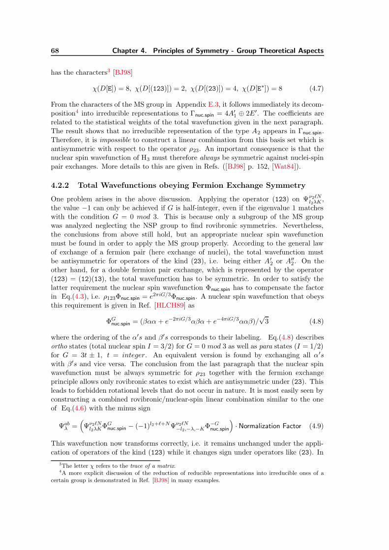
“diss”2002/10/18page 68

68 Chapter 4. Principles of Symmetry - Group Theoretical Aspects

has the characters3 [BJ98]

χ(D[E]) = 8, χ(D[(123)]) = 2, χ(D[(23)]) = 4, χ(D[E∗]) = 8 (4.7)

From the characters of the MS group in Appendix E.3, it follows immediately its decom-position4 into irreducible representations to Γnuc.spin = 4A′1 ⊕ 2E′. The coefficients arerelated to the statistical weights of the total wavefunction given in the next paragraph.The result shows that no irreducible representation of the type A2 appears in Γnuc.spin.Therefore, it is impossible to construct a linear combination from this basis set which isantisymmetric with respect to the operator ρ23. An important consequence is that thenuclear spin wavefunction of H3 must therefore always be symmetric against nuclei-spinpair exchanges. More details to this are given in Refs. ([BJ98] p. 152, [Wat84]).

4.2.2 Total Wavefunctions obeying Fermion Exchange Symmetry

One problem arises in the above discussion. Applying the operator (123) on Ψν2`Nl2λK ,

the value −1 can only be achieved if G is half-integer, even if the eigenvalue 1 matcheswith the condition G = 0 mod 3. This is because only a subgroup of the MS groupwas analyzed neglecting the NSP group to find rovibronic symmetries. Nevertheless,the conclusions from above still hold, but an appropriate nuclear spin wavefunctionmust be found in order to apply the MS group properly. According to the general lawof exchange of a fermion pair (here exchange of nuclei), the total wavefunction mustbe antisymmetric for operators of the kind (23), i.e. being either A′2 or A′′2. On theother hand, for a double fermion pair exchange, which is represented by the operator(123) = (12)(13), the total wavefunction has to be symmetric. In order to satisfy thelatter requirement the nuclear spin wavefunction Φnuc.spin has to compensate the factorin Eq.(4.3), i.e. ρ123Φnuc.spin = e2πiG/3Φnuc.spin. A nuclear spin wavefunction that obeysthis requirement is given in Ref. [HLCH89] as

ΦGnuc.spin = (βαα + e−2πiG/3αβα+ e−4πiG/3ααβ)/

√3 (4.8)

where the ordering of the α′s and β′s corresponds to their labeling. Eq.(4.8) describesortho states (total nuclear spin I = 3/2) for G = 0 mod 3 as well as para states (I = 1/2)for G = 3t ± 1, t = integer. An equivalent version is found by exchanging all α′swith β′s and vice versa. The conclusion from the last paragraph that the nuclear spinwavefunction must be always symmetric for ρ23 together with the fermion exchangeprinciple allows only rovibronic states to exist which are antisymmetric under (23). Thisleads to forbidden rotational levels that do not occur in nature. It is most easily seen byconstructing a combined rovibronic/nuclear-spin linear combination similar to the oneof Eq.(4.6) with the minus sign

Ψabλ =

(Ψν2`N

l2λKΦGnuc.spin − (−1)l2+`+NΨν2`N

−l2,−λ,−KΦ−Gnuc.spin

)· Normalization Factor (4.9)

This wavefunction now transforms correctly, i.e. it remains unchanged under the appli-cation of operators of the kind (123) while it changes sign under operators like (23). In

3The letter χ refers to the trace of a matrix.4A more explicit discussion of the reduction of reducible representations into irreducible ones of a

certain group is demonstrated in Ref. [BJ98] in many examples.

“diss”2002/10/18page 69

4.3. Selection Rules in Electric Dipole Transitions 69

the case of l2 = λ=K = 0 the wavefunction becomes zero for the forbidden rotationallevels which belong to even values of l2 +`+N ; in all other cases, i.e. if at least oneof the values l2, λ, or K is nonzero, the forbidden rotational levels correspond to linearcombinations with a plus sign in Eq.(4.9) instead (η = +1 in Eq.(4.6)). This can alsobe seen from the following argument.

To form correct basis wavefunctions only those rovibronic wavefunctions with sym-metry Γrovibronic can be combined with nuclear spin wavefunctions of symmetry Γnuc.spin

if their direct product contains A′2 or A′′2,

Γtotal = A′2 or A′′2 ⊂ Γrovibronic ⊗ Γnuc.spin (4.10)

The full result of this equation is Γrovibronic = 0A′1 ⊕ 4A′2 ⊕ 2E′ ⊕ 0A′′1 ⊕ 4A′′2 ⊕ 2E′′. It iseasily determined by the methods described in Ref. [BJ98] on page 159, Eq.(8.28). Thenumbers 0, 4, 2 correspond to the statistical weights of the rovibronic levels with symme-tries A1, A2, and E, respectively, independent of their parity. These factors often arisein experimental spectra as relative intensities (intensity alternations) and are importantin identification and assignment of experimental spectra. However, the most importantconclusion is that the statistical weight for levels with A1 symmetry is zero implyingthat these levels are forbidden and do not occur in nature.

A full analysis of the symmetries of rovibronic levels for the most important electronicspecies and for vibrational excitations ν2 = 0, 1 is tabulated in Appendix F includingtheir statistical weights. Symmetries of higher rotationally excited levels can easily beinferred from these patterns. They are very useful in analyzing allowed optical transitionsand metastability, that are issues of the next Sections.

4.3 Selection Rules in Electric Dipole Transitions

The line strength of an electric dipole transition from an initial state Ψi to a final stateΨf for an isolated molecule is determined by the size of the quantity

S(f ← i) =∑

deg.

∑

A=X,Y,Z

|〈Ψi|µA|Ψf 〉|2 (4.11)

The sums have to be taken over possible degeneracies of the initial and final states andover the spaced fixed components of the polarization direction of the incident radiation.The operator µA in the matrix element is the molecular dipole moment operator givenby

µA ≡∑

j

ejAj A = X,Y,Z j = electrons and nuclei (4.12)

where the sum j runs over all electrons and nuclei; ej is the charge of the j-th particle.For allowed transitions, S(f ← i) must have at least one non-negligible term on theright hand side. The application of the vanishing integral rule [BJ98] can now be usedto single out which transitions are not a priori forbidden by symmetry arguments. Sincethe integrals in the matrix elements run over the whole coordinate space it is essentialthat the integrand has a part which transforms totally symmetric; if not the integral iszero. Since the integrand generates the representation Γif = Γ(Ψ∗i )⊗ ΓµA

⊗ Γ(Ψf ), i.e.the direct products of the representations of the initial and final states and the dipole

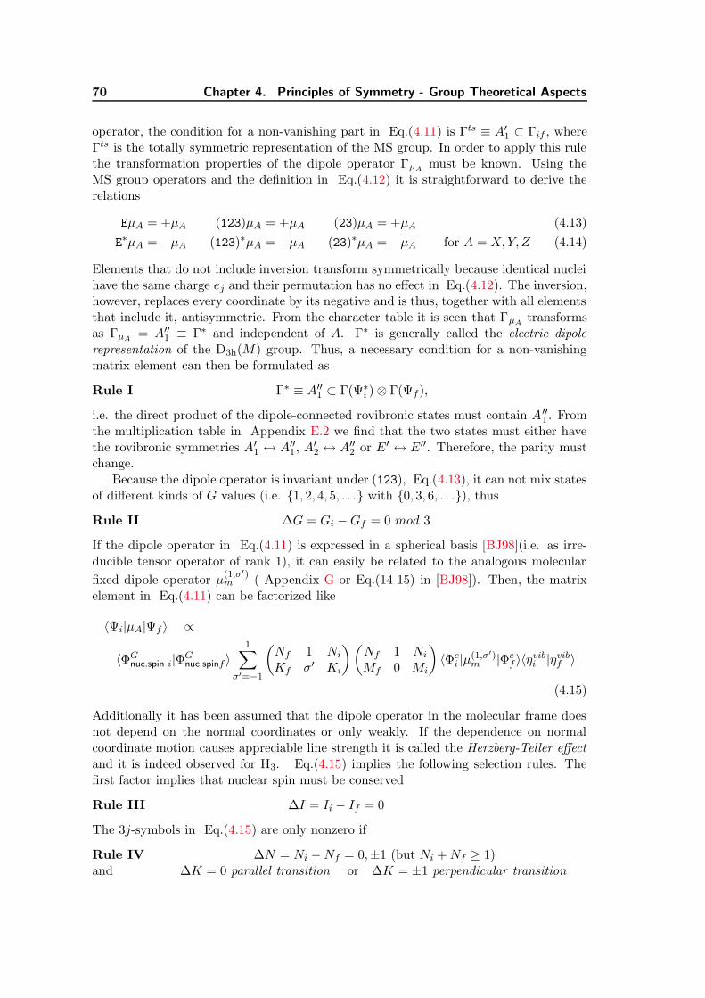
“diss”2002/10/18page 70

70 Chapter 4. Principles of Symmetry - Group Theoretical Aspects

operator, the condition for a non-vanishing part in Eq.(4.11) is Γts ≡ A′1 ⊂ Γif , whereΓts is the totally symmetric representation of the MS group. In order to apply this rulethe transformation properties of the dipole operator ΓµA

must be known. Using theMS group operators and the definition in Eq.(4.12) it is straightforward to derive therelations

EµA = +µA (123)µA = +µA (23)µA = +µA (4.13)

E∗µA = −µA (123)∗µA = −µA (23)∗µA = −µA for A = X,Y,Z (4.14)

Elements that do not include inversion transform symmetrically because identical nucleihave the same charge ej and their permutation has no effect in Eq.(4.12). The inversion,however, replaces every coordinate by its negative and is thus, together with all elementsthat include it, antisymmetric. From the character table it is seen that ΓµA

transformsas ΓµA

= A′′1 ≡ Γ∗ and independent of A. Γ∗ is generally called the electric dipolerepresentation of the D3h(M) group. Thus, a necessary condition for a non-vanishingmatrix element can then be formulated as

Rule I Γ∗ ≡ A′′1 ⊂ Γ(Ψ∗i )⊗ Γ(Ψf ),

i.e. the direct product of the dipole-connected rovibronic states must contain A ′′1 . Fromthe multiplication table in Appendix E.2 we find that the two states must either havethe rovibronic symmetries A′1 ↔ A′′1, A

′2 ↔ A′′2 or E′ ↔ E′′. Therefore, the parity must

change.Because the dipole operator is invariant under (123), Eq.(4.13), it can not mix states

of different kinds of G values (i.e. 1, 2, 4, 5, . . . with 0, 3, 6, . . .), thus

Rule II ∆G = Gi −Gf = 0 mod 3

If the dipole operator in Eq.(4.11) is expressed in a spherical basis [BJ98](i.e. as irre-ducible tensor operator of rank 1), it can easily be related to the analogous molecular

fixed dipole operator µ(1,σ′)m ( Appendix G or Eq.(14-15) in [BJ98]). Then, the matrix

element in Eq.(4.11) can be factorized like

〈Ψi|µA|Ψf 〉 ∝

〈ΦGnuc.spin i|ΦG

nuc.spinf 〉1∑

σ′=−1

(Nf 1 Ni

Kf σ′ Ki

)(Nf 1 Ni

Mf 0 Mi

)〈Φe

i |µ(1,σ′)m |Φe

f 〉〈ηvibi |ηvib

f 〉

(4.15)

Additionally it has been assumed that the dipole operator in the molecular frame doesnot depend on the normal coordinates or only weakly. If the dependence on normalcoordinate motion causes appreciable line strength it is called the Herzberg-Teller effectand it is indeed observed for H3. Eq.(4.15) implies the following selection rules. Thefirst factor implies that nuclear spin must be conserved

Rule III ∆I = Ii − If = 0

The 3j-symbols in Eq.(4.15) are only nonzero if

Rule IV ∆N = Ni −Nf = 0,±1 (but Ni +Nf ≥ 1)and ∆K = 0 parallel transition or ∆K = ±1 perpendicular transition

“diss”2002/10/18page 71

4.4. Metastability 71

Transitions with ∆K = 0 correspond to dipole moments along the z axis, and transitionswith ∆K = ±1 to dipole moments within the x − y plane. The words ’parallel’ and

’perpendicular’ are thus oriented with respect to the z axis. The factor 〈Φei |µ

(1,σ′)m |Φe

f 〉in Eq.(4.15) is the pure electronic dipole moment. The square of the last factor inEq.(4.15) is the Frank-Condon Overlap factor. As stated above, this separation is nota fair approximation because also transitions between non-degenerate and degenerateelectronic states are observed and allowed by symmetry if they only entail excitation ofa degenerate vibrational mode. Therefore this last separation can not be strict and itsimplications should be understood as propensity rules.

4.4 Metastability

The repulsive ground state 2p 2E′ embeds all rovibronic states of excited electronic statesin its continuum. For a radiationless interaction to be allowed between this continuumand a discrete level of an excited electronic state, the initial and final state must havethe same symmetry Γrve ⊂ (Γcontinuum). Here, (Γcontinuum) denotes the set of sym-metries occurring in the continuum. Furthermore, the total angular momentum N isstill a conserved quantum number even in the situation when the electronic state is notbound. The interaction of a rovibronic state with this continuum induces a radiation-less transition which is assumed to conserve the total angular momentum of the system,that means ∆N = 0 (Kronig Rule, [Her66] Eq. (IV,13) p. 459). Two cases must bedistinguished to single out the set of continuum symmetries (Γcontinuum). If Ncont = 0 itfollows Kcont = 0 and with ` = 1, λ = ±1 for the ground state it holds that ν2 + `+ Ghas to be even. Thus all levels in the continuum with N = 0 must have positive parity.All other levels with N > 0 in the continuum can have even and odd K and thus bothparities. Therefore, only rovibronic levels with N = 0 and negative parity are not linkedto the continuum of the ground state and possible candidates for metastability. Thenegative parity implies that ν2 + ` + G must be odd and from Eq.(3.61) it is obviousthat `+λ is odd. The lowest candidates are then the rotationless states 2p 2A′′2, 3d 2E′′

with arbitrary vibrational excitation. Since the 2p 2A′′2 state is also radiatively stableagainst decay into the ground state it is the most likely candidate to be metastable. Aradiative transition to 2s 2A′1 is energetically allowed. Owing to its long wavelength alifetime of 90µs is predicted from ab initio calculations ([AW76] and references therein).

“diss”2002/10/18page 72

72 Chapter 4. Principles of Symmetry - Group Theoretical Aspects

“diss”2002/10/18page 73

CHAPTER 5

Electronically Highly Excited States

In this chapter we investigate highly excited electronic states of H3. In thefirst part rovibrational channel couplings of the np-Rydberg series convergingto vibrationally excited core states of the lowest symmetric-stretch mode arediscussed. Laser spectroscopic methods are applied on H3 molecules in a fastneutral beam. An MQDT (Multichannel Quantum Defect Theory) analysisis performed to explain line positions and intensities, quantum defects andcoupling strengths for the series with angular momenta N = 1 and N = 2.In addition to the strong rotational coupling among p-Rydberg series, firstevidence is found for rotationally induced coupling between electronic p- andd-states in H3. In order to describe the structured continuum more sophis-ticated methods are needed. The MQDT approach of Stephens & Greenethat accounts for multi-state vibronic couplings, rotational and vibrationalchannel couplings is outlined. Its results are compared with the experiment.Especially vibronic interactions seem to be important in the dissociative re-combination process of H+

3 with slow electrons. This process appears to bethe key mechanism of H+

3 destruction in interstellar media.The last part of this chapter describes an experimental study of the influenceof vibronic couplings on the degenerate mode excited s- and d-series via thedynamically Jahn-Teller active 3p 2E′ initial state.

Contents

5.1 Rydberg Molecules & H3 . . . . . . . . . . . . . . . . . . . . . . 74

5.1.1 `-Uncoupling & Rotational Frame Transformation . . . . . . . 75

5.1.2 Nomenclature of Molecular Energy Levels . . . . . . . . . . . . 77

5.2 Experimental . . . . . . . . . . . . . . . . . . . . . . . . . . . . . 77

5.2.1 Two-step photoionization scheme . . . . . . . . . . . . . . . . . 78

5.2.2 Experimental Results . . . . . . . . . . . . . . . . . . . . . . . 81

5.3 Fano’s Access to MQDT . . . . . . . . . . . . . . . . . . . . . . 83

73

“diss”2002/10/18page 74

74 Chapter 5. Electronically Highly Excited States

5.3.1 Single Channel Quantum Defect Theory . . . . . . . . . . . . . 85

5.3.2 Multichannel Quantum Defect Theory . . . . . . . . . . . . . . 87

5.3.3 Two-Channel Quantum Defect Theory . . . . . . . . . . . . . . 88

5.4 Two-Channel analysis . . . . . . . . . . . . . . . . . . . . . . . . 90

5.4.1 Rydberg series with N = 0 and N = 2 . . . . . . . . . . . . . 90

Discrete Spectrum . . . . . . . . . . . . . . . . . . . . . . . . . 90

Beutler-Fano Spectrum . . . . . . . . . . . . . . . . . . . . . . 92

Modelling of the Spectrum below the H+3 1, 00 Threshold . . . 95

5.4.2 Rydberg series with N = 1 . . . . . . . . . . . . . . . . . . . . 97

5.4.3 Continuum . . . . . . . . . . . . . . . . . . . . . . . . . . . . . 100

5.5 Stephens-Greene Approach of MQDT . . . . . . . . . . . . . . 101

5.5.1 Alternative Description of MQDT . . . . . . . . . . . . . . . . 101

5.5.2 Vibrational & Multi-State Vibronic Coupling . . . . . . . . . . 102

5.6 Relevancy to Astrophysics & Astrochemistry . . . . . . . . . 105

5.7 Rydberg Series excited from 3p 2E′ . . . . . . . . . . . . . . . . 107

5.1 Rydberg Molecules & H3

Highly excited states of atoms together with the old quantum theory played an importantrole in early interpretations in atomic spectroscopy. The Swedish physicist J.R. Rydberg(1854-1919) first established their common properties and their similarity to excitedstates of the hydrogen atom. The reason for the high similarity in all atoms lies inthe Coulomb potential experienced by an electron far from the ionic core. Since theouter turning point or the expectation value of r grows fast in a Rydberg state, viz.〈r〉n = a0n

2/Z, with its principal quantum number n, electrons feel mostly everywherein the configuration space a Coulombic region if n is large enough. Consequently, inthe limit n → ∞ the spectra approach the spectrum of the hydrogen atom where thelatter results from a pure Coulombic potential. Today, Rydberg states are of interestfor many reasons. A fundamental issue is the validity of semiclassical methods whichadequately describe Rydberg wavepacket dynamics connecting classical and quantummechanics. Rydberg states are situated at the border of discrete to continuum spectraand exaggerate many properties, e.g. their dimension can assume macroscopic lengthscales, or their long orbiting times allow direct insight into time-resolved dynamics byexperimental methods, etc.. The structure of molecular Rydberg states is much richerthan that of atoms since nuclear vibration and rotation influence the electronic motion.Phenomena as autoionization, predissociation, dissociative recombination, etc. are ofwide interest since they control a variety of chemical reactions in stellar and interstellarmedia and in laboratory plasmas. A recent review on molecular Rydberg states edited byChild et al. [Chi96] summarizes the present state of knowledge. Besides interpretationsof the experimental data of this work we outline the current status of the theory of H3

at the end of this chapter.According to Herzberg [Her87] a Rydberg molecule1 needs to obey two conditions

which are both well fulfilled for H3

1Strictly, this definition implies that even the first excited electronic state of a Rydberg molecule hasalready Rydberg character.

“diss”2002/10/18page 75

5.1. Rydberg Molecules & H3 75

• The corresponding ion has to be stable.

• The neutral ground state has to be bound only weakly or has to be entirely repulsiveso that the first excited state lies far from it. This guarantees that there are nocouplings between the lowest valence state and the excited Rydberg state whicheasily can lead to strong predissociation or mixings.

For molecules additional interesting effects arise due to the existence of a multitude ofRydberg series, e.g. `-Uncoupling effects, Multi-State Vibronic Problems or RovibrationalChannel Interactions. All these partial aspects can be incorporated into the generalformalism of MQDT (Multi Quantum Defect Theory) approaches ([SG95]) which areknown to successfully describe all detailed features of spectra of highly excited diatomics.We demonstrate in the following that MQDT approaches are not restricted to diatomicsystems and equally applicable to polyatomic molecules.

First observations of Rydberg states of H3 with high principal quantum numbers weremade by Helm [Hel86, Hel88] and subsequently by Ketterle et al. [FKW89, KFW89]. Ina series of papers, different aspects of H3 were studied in photoionization experimentscovering the s- and d-series with different core excitations. The corresponding ioniza-tion limits and quantum defects were measured. Depletion spectroscopy was applied toexplore the nature of low-lying Rydberg states and to determine their vibrational fre-quencies [LH89]. Photodissociation of H3 Rydberg states was studied using time- andposition-sensitive detectors [CH88]. Since the p- and f -series are inaccessible in one-photon excitation from the metastable 2p 2A′′2 (N = K = 0) state, two-step excitationexperiments followed [LBH90, BLH91]. Not unexpected interactions between the ion coreand the valence electron were found to be stronger in the p-series than in the f -series.This can be understood from the fact that a low angular momentum electron penetratesdeeper into the ion core and therefore, the short range interaction is much stronger.The analysis of the p-series for total angular momentum N = 2 was performed withtwo-channel quantum defect theory with reasonably good agreement. Deviations in theintensity profile of Rydberg series were attributed to vibrational interactions [BLH91].

A full MQDT calculation using rovibrational frame transformation and ab-initioquantum defect surfaces [NJ82] was subsequently performed by Stephens and Greene[SG94, SG95] in a model including 40 rovibronic channels. Good agreement with thespectrum measured by Bordas and Helm [BLH91] in the vicinity of the lowest ionizationthreshold was achieved in the discrete as well as in the Beutler Fano region. In addition,this model was able to assign a number of vibrationally autoionizing levels in the opencontinuum as well as interlopers in the Beutler Fano region. A most striking result oftheir study [SG95] was the finding that the Jahn-Teller effect plays an essential role inthe autoionization process of H3 .

5.1.1 `-Uncoupling & Rotational Frame Transformation

So far, and in particular in deriving the low order total wavefunction of Eq.(4.9), itwas assumed that the electronic motion is strongly coupled to the nuclear frame bydemanding that the projection λ of the electronic angular momentum is a good quantumnumber. This limit of strongly bound electron motion is called a Hund’s case (a) or (b)model (since spin is disregarded). The total wavefunction in Eq.(4.9) represents thislimit (label ab). The left part of Figure 5.1 illustrates the case graphically. The total

“diss”2002/10/18page 76

76 Chapter 5. Electronically Highly Excited States

λΠ

K

N

z axis

Hund’s case (ab)

Z axis

Π

Hund’s case (d)

M

mN+

N

Figure 5.1: Different coupling cases for strong electronic correlation and weak electroniccorrelation with the core motion.

and electronic angular momentum, N and Π, have well defined projections K and λonto the molecule fixed z axis. Instead of K, we write alternatively K+ ≡ K − λ, asubtraction of well defined quantum numbers. We denote this close-coupling limit bythe set of quantum numbers α = (`, λ,K+, N,M) that are constants of motion. Wehave to expect that the strong binding case is loosened for larger values of n; for n→∞this phenomenon is called `-Uncoupling and another limiting case can be constructed:an analogous wavefunction to Eq.(4.9) can be found for H+

3 by neglecting the electronic

part. We denote this function by Θν2N+

l2K+M. Assuming that the total angular momentum

consists of the sum N = N+ + Π, a wavefunction for zero electronic coupling follows byangular momentum coupling theory from

ΨdN+ = γν2l2`N+K+

NM =∑

m

Y`m(lab)Θν2N+

l2K+M〈`m;N+M −m|`N+ NM〉, (5.1)

where 〈·; ·|·〉 is a Clebsch-Gordan coupling coefficient. Here, all quantities refer to thelaboratory fixed system (X,Y,Z). The electronic motion is completely uncoupled fromthe core rotation. In this transition from the close-coupling basis to the new basis, λ isreplaced by N+ so that the uncoupled states are characterized by i = (`,N+,K+, N,M).The basis set of Eq.(5.1) is often called the ionization basis and it is graphically shownon the right in Figure 5.1 as Hund’s case (d). Pan and Lu have shown that the uni-tary Rotational Frame Transformation Matrix U iα relates these two basis sets [PL88]according to

Ψabλ =

∑

N+

〈λ|N+ K+〉(Nf `)ΨdN+ Ψd

N+ =∑

λ

〈N+ K+|λ〉(Nf `)Ψabλ (5.2)

U iα ≡〈N+ K+|λ〉(Nf `) =

(1 + δλ0δK+0

1 + δK+0

)1/2 (2N+ + 1

2N + 1

)1/2

〈Nf λ+K+|`λ,N+K+〉

This result follows by a straightforward manipulation ([Rei97] p.39) of Eq.(4.9) andEq.(5.1), by using Eq.(5.4) below and some identities of the DN

KM representation given

“diss”2002/10/18page 77

5.2. Experimental 77

in Ref. [Zar88]. From Eq.(5.2) it is seen that in an intermediate coupling case the sumcouples either states with different core rotations N+ or different electronic projectionsλ. Only for ` = 0, i.e. s-states, it holds that N+ = N and a unique relationship existsbetween case (ab) and case (d).

For the special case of a p-Rydberg series with ` = 1 and N = 2, the transformationmatrix U iα is given by:

U iα =

( √2/5

√3/5

−√

3/5√

2/5

)=

(cos θ sin θ− sin θ cos θ

)(5.3)

The two degenerate contributions λ = ±1 are combined in one column or row. Equiva-lently, the frame transformation matrix can be expressed by a rotation matrix with theframe transformation angle θ = arccos(

√2/5). In Section 5.3 this matrix is used to

extend the formulation of quantum defect theory (QDT) to the multichannel problem(MQDT) where several coupled ionization channels are open.

5.1.2 Nomenclature of Molecular Energy Levels

In the following the notation of energy levels is in Hund’s case (ab) (cf. Section 5.1.1).The full pattern is

n` 2Γe (N,G)ν1, νl22

• n principal quantum number

• ` electronic angular momentum

• Γe electronic species/symmetry

• N total angular momentum

• G = |l2 + λ−K|Hougen’s quantum number

• ν1, ν2 and l2 vibrational quantumnumbers and vibrational angularmomentum, respectively.

All quantum numbers with a superscript + refer to the analogous quantities of the ion.

5.2 Experimental

The measurements were done with the Freiburg neutral beam photoionization spectrom-eter that was constructed within the diploma theses of U. Majer [Maj96] and R. Reichle[Rei97]. It is only briefly discussed here. A sketch of the apparatus is shown in Figure5.2. Triatomic hydrogen ions are produced in a hollow cathode glow discharge (I) inHydrogen. The ions are extracted by an electric field (ACC), accelerated to an energy of3.6 keV, focused by an einzel-lens (EL) and mass selected by a Wien Filter (WF). TheH+

3 current is about 100 nA after mass selection. The current ratios of H+3 -, H+

2 -, andH+ are typically 10:1:1. The electrodes of the discharge tube are cooled by liquid nitro-gen which significantly increases the population in the H+

3 rovibrational ground state.The H+

3 beam is partially neutralized (10-30 %) by near-resonant charge transfer (CT)in cesium. After the charge-transfer cell, the residual ions are removed from the neutralbeam by an electric field (ID), which also serves to quench by field-ionization the smallabundance of high principal quantum number Rydberg states formed by charge transfer.Neutral products of dissociative charge transfer are intercepted by an aperture (A) of1mm diameter located 35 cm downstream of the charge transfer cell. H3 molecules in the

“diss”2002/10/18page 78

78 Chapter 5. Electronically Highly Excited States

-

-

+

+

I ACC EL WF CT ID A

MCP

IR 1m QF

5 x10 mbar-6

5 x10 mbar-8

< 5 x10 mbar-9

Figure 5.2: Schematic of the Freiburg neutral beam photoionization spectrometer.Legend:I: hollow cathode discharge ion source, ACC: ion beam extraction and acceleration stage,EL: einzel lens, WF: Wien filter, CT: charge transfer cell, ID: ion deflector, A: aperture,IR: laser-interaction region, QF: electric quadrupole ion deflector, MCP: microchannelplate detector

metastable state 2p 2A′′2 (N = K = 0) which survive the travel from the charge-transfercell to the aperture are excited by counter-propagating laser beams in the 1 m long in-teraction region (IR). H+

3 ions created in the interaction region by photo-excitation ofautoionizing H3 states are energy-selected by a quadrupole field (QF) and deflected to amultichannel plate detector (MCP) which is operated in pulse-counting mode. A gateddual-counter (200 MHz) is used to accumulate the signals produced by the laser pulsesand background events. These data are then transferred to a laboratory computer andstored for further treatment. Two dye lasers pumped by an excimer laser are operatedin the visible spectral range and sent counter-propagating to the neutral beam. An op-tical delay line is adjusted for both pulses to overlap in time in the interaction region.The dye lasers are programmed and scanned under control of the laboratory computer.The calibration of the laser wavelength scale is carried out by optogalvanic spectroscopyin argon or neon. For calibration in the far-red spectral range, a rubidium absorptioncell is employed. Corrections for the Doppler shift seen by the molecules due to theirtranslation and for the change of wavelength due to the refractive index under labora-tory conditions are taken into account. The accuracy of the wavelength calibration is0.15 cm−1. The bandwidth of each laser is 0.20 cm−1. Typically recording times for aspectrum are in the order of 50 hours.

5.2.1 Two-step photoionization scheme

The two-step laser-excitation scheme applied in our experiment is shown in Figure 5.3.The wavelength of one of the lasers is fixed to excite the vibrationally non-diagonaltransition from the metastable 2p 2A′′2 state to the symmetric-stretch excited 3s 2A′1state of H3. At high laser intensity 1+1 photon REMPI2 via this state [LHH89] is used

2Resonance Enhanced Multi Photon Ionization.

“diss”2002/10/18page 79

5.2. Experimental 79

2pA’’(N=G=0)0,02

0A’’2

A’2

A’’2A’2

3sA’(N=1,G=0)1,01

0

N =1+

N =3+

npA’’2

npA’’ & npE’2

npE’

N=0 N=1 N=2

H 3H 3

+

rovibronicsymmetry

rovibronicsymmetry

(G =0)1,0+ 0

⊗Γ∗

⊗Γ∗

Figure 5.3: Energy level scheme of the vibrationally symmetric-stretch excited H3 np-Rydberg series accessible via the H3 3s 2A′1 (N = 1, G = 0)1, 00 intermediate state.The H3 Rydberg-states with total angular momenta N = 0, 1, 2 populated in the two-step laser-excitation experiment are shown along with their rovibronic and electronicsymmetry species. The angular momenta and symmetry labels of the underlying H+

3

core levels are also shown.

to select the wavelength setting of the first laser. Keeping the first laser at low intensity(≤ 200µJ) the second laser is tuned to excite p-type Rydberg states converging to thelowest ortho rotational levels of symmetric-stretch excited H+

3 . The states involved inthis excitation scheme and their symmetries are discussed in the following.

The electronic states in Hund’s case (ab) can equally be characterized by the elec-tronic symmetry Γe. For p-states with ` = 1, the electronic symmetries are A′′2 and E′

for λ = 0 and λ = 1, respectively. The vibrationless 2p 2A′′2 (0, 0)0, 00 metastable stateof H3 which serves as the initial state in our two-step laser-excitation experiments, is anortho level (G = 0). The quantum numbers G of all levels accessible by laser-excitationof the metastable level must be integer multiples of 3 (G = 3t with t = 0, 1, 2 . . . , RuleII).

As discussed by Lembo et al. [LHH89], a Hund’s case (d) model is more convenientfor the description of high principal quantum number Rydberg states. The angular part

“diss”2002/10/18page 80

80 Chapter 5. Electronically Highly Excited States

Table 5.1: Rovibronic symmetries of the states relevant for two-step photoionization ofH3 via the 3s 2A′1 (1, 0)1, 00 intermediate state.

H+3 corea Energyb ΓH+

3

Threshold c Rydberg electron d N G final state Γf

(1, 0)0, 00 86.935 A′2 9655.04 `=0 (ns),A′

1 1 0 A′2

(2, 3)0, 11 2613.874 A′2 12181.98 `=1 (np),A′′

1 1,2 3 A′′2

(3, 3)0, 11 2876.520 A′2 12444.63 ” 2 3 ”

(1, 0)1, 00 3262.997 A′2 12831.10 ” 0,1,2 0 ”

(3, 0)1, 00 3682.472 A′2 13250.58 ” 2 0 ”

a quantum numbers: (N+, G+)ν1, νl22 .

b core energies in cm−1 from Ref. [CRJK98, JCKR98b, JCKR98a], relative to the minimum ofthe H+

3 potential energy surface.c ionization threshold in cm−1 above the 3s 2A′

1 (1, 0)0, 00 state. The values are calculatedusing the energy values 29562.14 cm−1 for the H+

3 (1, 0)0, 00 threshold [KFW89, KMW89]above 2p 2A′′

2 (0, 0)0, 00 , and 19907.1 cm−1 for the 3s 2A′1 (1, 0)1, 00 level [LHH89] above

2p 2A′′2 (0, 0)0, 00 metastable state.

d Angular momentum ` and symmetry label Γ` of the Rydberg electron in Hund’s case (d) basis.

of the Rydberg electron wave function in the molecular frame Y`λ(r) is expressed in aspace fixed frame by

Y`m(r′) =∑

λ

D(`)∗λm (R′ ← R) · Y`λ(r) (5.4)

where primed coordinates refer to the laboratory and unprimed ones to the molecule-fixedcoordinate system (Ref. [SG95] Eq. (18)). An inspection of the wave function Y`m(r′)shows that the symmetry of the Hund’s case (d) Rydberg electron in the D3h group is A′1for ` even and A′′1 for ` odd. From the discussion in Section 4.3 it is clear that only stateswith A′′2 ⊗ A′′1 = A′2 symmetry can be excited in single-photon transitions with 2p 2A′′2(0, 0)0, 00 as initial state. In the first excitation step, we prepare the 3s 2A′1 (1, 0)1, 00state in a vibrationally non-diagonal transition (see Figure 5.3). This intermediate statecan be viewed as an s-Rydberg electron attached to a vibrationally symmetric-stretchexcited H+

3 (1, 0)1, 00 ion core. The A′2 overall symmetry label of this state results froma direct product of the A′1 electronic symmetry of the s-electron with the A′2 rovibronicsymmetry of the H+

3 core 1s2(1, 0)1, 00. The rovibronic symmetry of the final statesaccessible in the second excitation step is A′2 ⊗ A′′1 = A′′2. From this N = 1, G = 0intermediate state, final states with total angular momentum N = 0, 1, 2 are accessiblein one-photon transitions (Rule IV). Additionally, the quantum number G must be zeroor an integer multiple of 3. For p-type final states having electronic angular momentum` = 1 and A′′1 electronic symmetry in the laboratory frame, the ion core symmetry has tobe ΓH+

3= A′2. On the other hand for s- and d-Rydberg electrons (Γ`=0,2 = A′1), ion cores

with symmetry ΓH+3

= A′′2 are required. The accessible final states constructed in the

Hund’s case (d) frame by attaching p-Rydberg electrons to H+3 core states are listed in

Table 5.1. The possible core states are (N+=1, 3, G+ = 0) if no ν2-vibration is excitedand (N+ = 2, 3, G+ = 3) for excitation of one quantum of bending mode.

The energies of the H+3 levels listed in Table 5.1 are the results of highly accurate ab-

initio calculations by R. Jaquet et al. [CRJK98, JCKR98b, JCKR98a]. The ionizationthresholds listed in Table 5.1 are determined using the value of 29562.14 cm−1 for thefirst ionization limit of the 2p 2A′′2 (0, 0)0, 00 state to the H+

3 (1, 0)0, 00 core measured

“diss”2002/10/18page 81

5.2. Experimental 81

by Ketterle et al. [KMW89], and the value of 19907.1 cm−1 for the 2p 2A′′2 → 3s 2A′1(1, 0)1, 00 excitation frequency measured by Lembo et al. [LHH89].

In Figure 5.3, the final states of the p-series with symmetric-stretch vibrationalexcitation are shown in a schematic level scheme. The electronic symmetries in theHund’s case (ab) limit are A′′2 and E′ for N = 0 and N = 1, respectively. For theN = 2 series converging to each, (N+=1, G+ = 0) and (N+=3, G+ = 0), A′′2 as well asE′ electronic symmetries are allowed enabling strong rotational coupling between theseseries.

5.2.2 Experimental Results

In Figure 5.4, the two-step photoionization spectrum of H3 via the 3s 2A′1 (1, 0)1, 00intermediate state is shown. The measurement covers the energy range between 12490cm−1 and 14200 cm−1 relative to the intermediate state. The final state energy fallsinto the range from 351-564 meV above the lowest ionization threshold, encompassingthe first symmetric stretch excited level of H+

3 at 394 meV. The power of the laser pulseexciting the 2p 2A′′2 → 3s 2A′1 transition was attenuated to minimize the backgroundfrom resonance-enhanced multi-photon ionization (1+1 REMPI). The energies of thelowest ortho levels (N+ = 1, G+ = 0) and (N+ = 3, G+ = 0) of H+

3 with one quantumof symmetric stretch excitation 1, 00 are indicated by arrows in Figure 5.4. Thespectrum displays three distinct regions. Below the (N+ = 1,G+ = 0) limit, discrete linesdominate. These transitions appear in the spectrum due to autoionization to the lowestvibrational level of the ion. In the so-called Beutler-Fano region between the (N+ =1,G+ = 0) and (N+ = 3,G+ = 0) limits, we find a regularly structured continuum. Abovethe (N+ = 3,G+ = 0) limit, an almost structureless continuum is observed with strongresonances superimposed. Their asymmetric line profiles (Fano-profiles [Fan61]) are dueto mixing of H3 states having higher vibrational excitation with the open continua.Although the spectra shown in Figure 5.4 are corrected for the dark count rate of thedetector, a small, continuous background is found in the quasi-discrete part below thefirst vibrationally excited threshold. This background is due to direct ionization into theunderlying continua built on vibrationless or degenerate mode excited H+

3 cores, 0, 00and 0, 11, and extends into the Beutler-Fano region and the pure continuum. Forall final states in the energy region covered in Figure 5.4, vibrational autoionizationis an open ionization mechanism which leads to slightly asymmetric line shapes of theresonances.

The quasi-discrete part and the Beutler-Fano region of the spectrum can be under-stood from the level scheme in Figure 5.3. The respective state energies are listed inTable 5.1. Four p-Rydberg series with total angular momenta N = 0, 1 and 2 can beformed from (N+ = 1, G+ = 0) and (N+ = 3, G+ = 0) H+

3 cores. The two serieswith N = 2 are coupled by pure rotational interaction. This coupling is the origin ofthe modulation of the ion yield in the Beutler-Fano region as well as perturbations ofthe line positions and intensity modulations in the quasi-discrete part of the spectrum.Within the subset of states converging to (N+ = 1, G+ = 0), the series with N = 0 andN = 1 are expected to be unperturbed.

The final state angular momentum is further restricted by the relative orientationof the polarization vectors of the two excitation lasers. As shown in Appendix G, forparallel orientation of the polarization of the two lasers, only N = 0 and N = 2 can be

“dis

s”20

02/1

0/18

pag

e82

82

Chapte

r5.

Ele

ctro

nic

ally

Hig

hly

Exc

ited

Sta

tes

−1

0

400

0

200

400

0

400

800

200

N =1+

N =3+

Energy / cm

13200 13400 13600 13800 14000 14200

12900 13000 1320013100

12500 12600 1280012700

Ion

Sign

al (

Cou

nts

/ 100

Las

er S

hots

)

(a)

(b)

(c)

Figure 5.4: Photoioniza-tion spectra of H3 via the3s 2A′1(N = 1, G = 0)1, 00intermediate state.The measurements coverthe 12490 cm−1 to 14200cm−1 energy region above the3s 2A′1 (N = 1, G = 0)1, 00state. The ionization lim-its (N+ = 1, G+ = 0)and (N+ = 3, G+ = 0) ofsymmetric-stretch excitedH+

3 1, 00 are indicated byarrows. The spectrum is sep-arated into the quasi-discretepart (a), the Beutler-Fanoregion (b), and the purecontinuum (c). The insets inthe lower part of the figureshow the resonances in thecontinuum in the energyregions 13470-13520 cm−1

and 13830-13855 cm−1 ,respectively.

“diss”2002/10/18page 83

5.3. Fano’s Access to MQDT 83

excited, for perpendicular orientation only N = 1 and N = 2 states. The line strengthsfor different total angular momenta in the final state depend on the angle θ between thetwo polarizations as

S(2)Nf=0 ∝ cos2 θ

S(2)Nf=1 ∝ sin2 θ (5.5)

S(2)Nf=2 ∝

(cos2 θ +

3

4sin2 θ

).

This dependence allows to determine the final state angular momenta of every individualdiscrete line. Measurements in the 12750 cm−1 to 12780 cm−1 region of the discretespectrum with parallel and perpendicular orientation of the electric vectors of the laserfields are shown as spectra (a) and (b) in Figure 5.5. Lines appearing in the spectrawith parallel ( Figure 5.5(a)) as well as with perpendicular ( Figure 5.5(b)) relativepolarization must have N = 2 final state angular momentum. Lines appearing only inthe measurement with parallel polarization ( Figure 5.5(a)) belong to Rydberg serieswith N = 0, those appearing only in the measurement with perpendicular polarization( Figure 5.5(b)) have N = 1.

A third measurement was carried out at an angle of 30 between the polarizationvectors of the two photons. The resulting spectrum (c) in Figure 5.5 is an incoherentsuperposition of the parallel and perpendicular spectra and contains lines with N = 0,N = 1, and N = 2. We determined the excitation frequencies of the discrete linesby fitting gaussian functions to the measured spectra. The two series with N = 2 arestrongly mixed. Their transition frequencies can not be fitted by a simple Rydbergformula. A two-channel quantum defect theory was used to evaluate the data as wediscuss in the following.

5.3 Fano’s Access to MQDT

In order to simulate the observed spectra, we follow the formalism of Fano [Fan70, Fan77].The H3 molecule is viewed as an H+

3 core with an additional valence electron attachedto it. The two inner electrons fill the (1sa′1) molecular orbital forming a closed shell.For large distances of the valence electron, the electric field of the nuclei is shielded tothat of a single positive elementary charge. Only at very small distances, the motionof the valence electron is influenced by the structure and the properties of the ion core.This leads to an `-uncoupling effect which was described in Section 5.1.1. The close-coupling (or eigenchannel) basis is appropriate for small distances of the electron fromthe core and for low principal quantum numbers n. With increasing distance, the motionof the valence electron separates from the core motion (Hund’s case (d) limit), and thequantum number N+ of the core angular momentum is a good quantum number. Inthis ionization basis, the total energy E of the system can be written as the sum of therovibronic energy Iion of the H+

3 core and the energy W of the Rydberg electron:

E = Iion +W W = −Rν2

(5.6)

Herein R = 109717.405 cm−1 represents the Rydberg constant for H3 calculated usingthe reduced mass of the H+

3 + e− system. The eigenvalue spectrum of E is determined

“dis

s”20

02/1

0/18

pag

e84

84

Chapte

r5.

Ele

ctro

nic

ally

Hig

hly

Exc

ited

Sta

tes

0

1200

1800

600

0

200

400

0

300

600

(a) parallel

(b) perpendicular

(c) 30 degree relative

12750 12755 12760 12765 12770 12775 12780

Energy / cm

Ion

Sign

al (

Cou

nts/

100

Las

er S

hots

)

−1

Figure 5.5: Experimental de-termination of the final statetotal angular momentum Nby changing the orientationof the laser polarization direc-tions.The two-step photoionizationspectrum of H3 in the 12750-12780 cm−1 energy regionabove the 3s 2A′1 (N =1, G = 0)1, 00 intermediatestate is shown. The electricvectors of the two laser fieldswere oriented parallel in spec-trum (a) and perpendicular inspectrum (b) with respect toeach other. Spectrum (c) wasrecorded with a 30 relativeorientation of the laser polar-ization vectors. Spectrum (a)contains lines with onlyN = 0and N = 2. Spectrum (b)contains only lines withN = 1and N = 2. Spectrum (c) cor-responds to an incoherent su-perposition of spectra (a) and(b).

“diss”2002/10/18page 85

5.3. Fano’s Access to MQDT 85

HydrogenicWavefunction

V(r)

∞r

V (r) = −2r

r0

BC II

Short RangeInteraction

ρ(W, r)

BC I

δ = −πµ

Figure 5.6: Illustration of principles of quantum defect theory. The dotted curve refersto a pure Coulomb potential and the solid to an actual, non-hydrogenic potential V (r).BC I and II represent the necessary boundary condition at r0 and at ∞.

by the effective quantum number ν = n − µ which is written as an integer n and thenearly energy-independent quantum defect µ.

5.3.1 Single Channel Quantum Defect Theory

In a system consisting of a spherically symmetric ion core and a single valence electron,e.g. an alkali atom, the potential V (r) depends only on the distance r of the valenceelectron from the centre of the core as shown in Figure 5.6. The wave function separatesinto an angular and a radial part. The radial Schrodinger equation is given by

h2

2µ

∂2ρ(W, r)

∂r2+

(W − V (r)− h2`(`+ 1)

2µr2

)ρ(W, r) = 0 (5.7)

with the total energy W , and the angular momentum ` of the valence electron. Thesolution ρ(W, r) = rR(W, r) is the product of the distance r with the radial wave functionR(W, r). The second order differential equation has two independent solutions for eachpotential.

For a pure Coulomb potential [Sea83], these solutions are the regular and irregu-lar Coulomb functions f(ν, `, r) and g(ν, `, r) with the parameter ν =

√−R/W . The

Coulomb functions are known analytically. They oscillate in the classically allowed re-gion of the potential with a phase shift of 90 with respect to each other [Gal94]. Theasymptotic behavior of the Coulomb functions for r→ 0 is

limr→0 f(r) ∼ r`+1 regularlimr→0 g(r) ∼ r−` irregular

(5.8)

“diss”2002/10/18page 86

86 Chapter 5. Electronically Highly Excited States

independent of W, and in the limit r →∞f(r) → u(ν, `, r) sinπν − v(ν, `, r) cos πνg(r) → −u(ν, `, r) cos πν − v(ν, `, r) sin πν

(5.9)

for W < 0. For large r, the functions u(ν, `, r) and v(ν, `, r) are exponentially increasingand decreasing, respectively.

For W < 0, the general solutions ρ(W, r) of the radial Schrodinger equation Eq.(5.7)are linear combinations of f(ν, `, r) and g(ν, `, r). The solutions which are physicallymeaningful have to remain finite at the origin (r → 0) and to vanish sufficiently fast atlarge distances r →∞. For bound states (W < 0), these requirements lead to a discretespectrum of eigenvalues W . For the pure Coulomb potential, only the regular Coulombfunction f(r) remains finite at the origin. The additional condition

sinπν = 0 (5.10)

has to be fulfilled to cancel the exponentially increasing part (function u(ν, `, r)) at larger in Eq.(5.9). As a consequence, the values of the parameter ν are integers n and theenergy spectrum is discrete with W = −R/n2. For W > 0, the asymptotic solutions forr →∞ are outgoing waves having oscillatory character [Sea83].

The potential V (r) contains the attraction by the nuclei as well as the repulsion bythe inner-shell electrons. In the following, we assume that the potential V (r) outside ofa sphere with radius r0 can be approximated to high accuracy by a Coulomb potential,Figure 5.6. Of course, this approximation is increasingly accurate for large values of r0,however, due to the length scaling ∝ n2 it is already applicable for even low Rydbergstates. Within the sphere (short-range interaction zone), the shielding of the nuclearcharge by the inner shell electrons is incomplete, and the attraction is stronger than thatof a single charge. The wave functions ρ(W, r) for V (r) outside of the interaction zonediffer from those of the pure Coulomb potential only by a nearly energy-independentphase shift πµ and can be constructed by a linear superposition of regular and irregularCoulomb functions:

ρ(W, `, r) = f(ν, `, r) cos πµ− g(ν, `, r) sin πµ (5.11)

The value of µ is chosen to join ρ(W, r) smoothly to the exact solutions inside the short-range zone at the boundary r = r0 (BC I). According to Eq.(5.9) and Eq.(5.11), theasymptotic form of ρ(W, `, r) is

limr→∞

ρ(W, `, r) ∼ u(ν, `, r)(sin πν cos πµ+ cosπν sinπµ)

−v(ν, `, r)(cos πν cos πµ+ sinπν sinπµ) (5.12)

for large r. For stationary states (W < 0), the physically meaningful wave functionshave to decrease sufficiently fast in the limit of large r (BC II). This condition can ingeneral only be fulfilled if the coefficient of the exponentially increasing function u(ν, `, r)vanishes

sin(π(ν + µ)) = 0 (5.13)

The argument ν+µ = n has to assume integer values n yielding non-integer value of theeffective quantum number ν and energy eigenvalues W = −R/(n− µ)2. The phase shift−πµ at r = r0 is given by the quantum defect. It can be determined either empiricallyfrom experimental data or by ab-initio calculations.

“diss”2002/10/18page 87

5.3. Fano’s Access to MQDT 87

5.3.2 Multichannel Quantum Defect Theory

The properties of a molecular core (rotation,vibration) may lead to the existence ofN ionization channels with individual ionization limits Ii. The solutions of the radialSchrodinger equation Eq.(5.7) for a total energyW are linear combinations of the regularand irregular Coulomb functions f(νi, `, r) and g(νi, `, r) with the effective quantumnumbers νi defined by

W ≡ I1 −R

ν21

= . . . = IN −R

ν2N

(5.14)

We can construct the ionization-basis wave functions Ψi

Ψi =1

rχi [f(νi, `, r) cos(πνi) + g(νi, `, r) sin(πνi)] i = 1, . . . , N (5.15)

for each ionization threshold Ii. The functions χi contain the angular- and spin-dependentparts of the wave functions. The wave functions Eq.(5.15) automatically fulfill theboundary condition at large distance r. As discussed in Section 5.3.1, the boundaryconditions at r = r0 select the physically meaningful solutions. If the ionization chan-nels are not interacting, an individual quantum defect is associated with each ionizationchannel. In general, the quantum numbers classifying the core states (ionization ba-sis) are inappropriate at small r, as discussed in Section 5.1.1. To apply the boundaryconditions, we have to switch to the eigenchannel basis. We construct eigenchannel wave-functions using the transformation matrix U iα of Section 5.1.1 and radial functions ofthe type Eq.(5.11)

Ψα =1

r

∑

i

U iα χi [f(νi, `, r) cos(πµα)− g(νi, `, r) sin(πµα)] (5.16)

The sum runs over all ionization channels i coupled by the transformation matrix U iα.The wave functions Eq.(5.16) allow us to introduce independent quantum defects µα

for each element of the eigenchannel basis. These quantum defects can be determinedempirically or by ab-initio methods. In general, the wave functions Ψ are neither diagonalin the eigenchannel nor in the ionization basis and can be expanded in terms of thefunctions Ψi or Ψα with coefficients Ai and Bα respectively

Ψ =∑

i

AiΨi =∑

α

BαΨα (5.17)

which allows a mixing of all channels within a basis set. To fulfill the boundary conditionat r →∞, we could proceed in the same way as in the single channel case and demandthe coefficients of the exponentially increasing functions u(νi, `, r) to be zero. However,in view of a later extension we deduce the MQDT equations in a slight more generalfashion. Comparing the coefficients of the functions f(νi, `, r) and g(νi, `, r) in Eq.(5.17)and rewriting the two relations as a complex one it follows

Ai =∑

α

Bα U iα eiπ(νi+µα) (5.18)

“diss”2002/10/18page 88

88 Chapter 5. Electronically Highly Excited States

Choosing Ai and Bα being real3 it leads to the systems of equations

Ai =∑

α

U iα cosπ(νi + µα)Bα (5.19)

0 =∑

α

U iα sinπ(νi + µα)Bα (5.20)

Eq.(5.20) gives an implicit dependence of all effective quantum numbers νi and a mixingof all channels of the ionization basis. Non-trivial solutions of the system of linearequations Eq.(5.20) exist only if

det (U iα sinπ(νi + µα)) = 0 (5.21)

Using equation Eq.(5.21) together with the N-1 relations between the νi established bythe Rydberg equations Eq.(5.14), the unknown νi can be determined exactly. Theydefine the total energy W of the stationary states. Since equation Eq.(5.21) containsa periodic function, these equations yield a complete spectrum of energies W . Knowingνi, the amplitudes Bα can be determined by solving Eq.(5.20), and a complete set ofwave functions for the stationary states can be constructed.

The model described above holds for the case of N closed channels, i.e. the totalenergy W is always below the lowest ionization limit. If the energy is increased beyondan ionization limit, the respective channel is said to open. In this case, an interactionbetween continuous and discrete states takes place which leads to regular structures inthe continuous spectrum. If several channels are open, continuum-continuum interactionsmay occur. The theoretical formalism for this case is analogous. For an open channel,the effective quantum number is replaced by a phase shift [Fan70] which is implicitlydefined by Eq.(5.21) as a function of the energy W . The absorption intensities arecalculated from the transition moments in the eigenchannel basis and the amplitudes ofthe wave functions.

5.3.3 Two-Channel Quantum Defect Theory

The photoionization spectrum with final state angular momentum N = 2 is dominatedby the rotational interaction between p-Rydberg series built on the (1, 0)1, 00 and(3, 0)1, 00 cores, respectively (see Figure 5.3). This interaction is apparent from thepronounced Beutler-Fano profiles in the region between the two thresholds ( Figure5.4b) and the corresponding intensity modulation in the region below the N+ = 1threshold ( Figure 5.4a). It is highly instructive to first analyze the complex spectrum inFigure 5.4 in the restricted two-channel quantum defect model. This approach permitsa direct comparison of the experimentally determined parameters with the theoreticalframe transformation angle and ab-initio quantum defect functions.

In the case of only two ionization channels with ionization limits I1 and I2, the frametransformation matrix U iα in Eq.(5.3) can be used, and Eq.(5.21) simplifies to

tanπ[−ν1(W )− µ]− c1 +c2

c1 − tanπ[ν2(W ) + µ]= 0 (5.22)

3An accurate analysis shows that this includes the requirement that the coefficient of the exponentialrising function is zero.

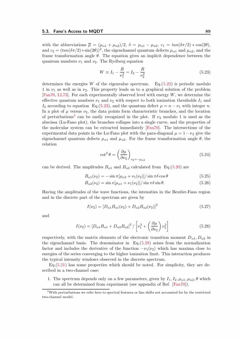
“diss”2002/10/18page 89

5.3. Fano’s Access to MQDT 89

with the abbreviations µ = (µα1 + µα2)/2, δ = µα1 − µα2, c1 = tan(δπ/2) ∗ cos(2θ),and c2 = (tan(δπ/2) ∗ sin(2θ))2, the eigenchannel quantum defects µα1 and µα2, and theframe transformation angle θ. The equation gives an implicit dependence between thequantum numbers ν1 and ν2. The Rydberg equation

W ≡ I1 −R

ν21

= I2 −R

ν22

(5.23)

determines the energies W of the eigenvalue spectrum. Eq.(5.22) is periodic modulo1 in ν1 as well as in ν2. This property leads us to a graphical solution of the problem[Fan70, LL73]. For each experimentally observed level with energy W , we determine theeffective quantum numbers ν1 and ν2 with respect to both ionization thresholds I1 andI2 according to equation Eq.(5.23), and the quantum defect µ = n− ν1 with integer n.In a plot of µ versus ν2, the data points form characteristic branches, and the locationof perturbations4 can be easily recognized in the plot. If ν2 modulo 1 is used as theabscissa (Lu-Fano plot), the branches collapse into a single curve, and the properties ofthe molecular system can be extracted immediately [Fan70]. The intersections of theexperimental data points in the Lu-Fano plot with the para-diagonal µ = 1− ν2 give theeigenchannel quantum defects µα1 and µα2. For the frame transformation angle θ, therelation

cot2 θ =

(∂µ

∂ν2

)

ν2=−µα2

(5.24)

can be derived. The amplitudes Bα1 and Bα2 calculated from Eq.(5.20) are

Bα1(ν2) = − sinπ[µα2 + ν1(ν2)]/ sin πδ cos θ (5.25)

Bα2(ν2) = sinπ[µα1 + ν1(ν2)]/ sin πδ sin θ. (5.26)

Having the amplitudes of the wave functions, the intensities in the Beutler-Fano regionand in the discrete part of the spectrum are given by

I(ν2) = [Dα1Bα1(ν2) +Dα2Bα2(ν2)]2 (5.27)

and

I(ν2) = [Dα1Bα1 +Dα2Bα2]2 /

[ν31 +

(∂µ

∂ν2

)ν32

](5.28)

respectively, with the matrix elements of the electronic transition moment Dα1, Dα2 inthe eigenchannel basis. The denominator in Eq.(5.28) arises from the normalizationfactor and includes the derivative of the function −ν1(ν2) which has maxima close toenergies of the series converging to the higher ionization limit. This interaction producesthe typical intensity windows observed in the discrete spectrum.

Eq.(5.21) has some properties which should be noted. For simplicity, they are de-scribed in a two-channel case:

1. The spectrum depends only on a few parameters, given by I1, I2, µα1, µα2, θ whichcan all be determined from experiment (see appendix of Ref. [Fan70]).

4With perturbations we refer here to spectral features or line shifts not accounted for by the restrictedtwo-channel model.

“diss”2002/10/18page 90

90 Chapter 5. Electronically Highly Excited States

2. Solving Eq.(5.21) in the limit of µα1 → µα2, the spectrum converges to that of theunperturbed µα2-series. The physical meaning of this is that the colliding electronsees an isotropic core which cannot cause any mixing.

3. In the limit θ → 0, the frame transformation matrix U iα becomes a unit matrix.The eigenchannel basis converges to the ionization channel basis. As a result,the equation system breaks up into N single channel problems having individualquantum defects. The coupling strength is monotonically increasing with the valueof θ. For θ = π/2 the U iα matrix has only off diagonal elements meaning that bothseries appear unperturbed but interchanged their quantum defects.

5.4 Two-Channel analysis

As discussed in Section 5.2.1 and shown in Figure 5.3, the electronic symmetries ofpure p-states in Hund’s case (ab) are A′′2 and E′. Neglecting perturbations from differentvibrational channels other than 1, 00, two eigenchannel quantum defects µA′′

2, µE′ have

to be specified for solving Eq.(5.21). In this approximation, the N = 0 and N = 1 serieshave pure electronic symmetries A′′2 andE′, respectively, and should appear unperturbed.For N = 2, both electronic symmetries are allowed leading to rotational interaction. Inthe following, we apply a two-channel model to fit the discrete lines of the N = 2 series.

5.4.1 Rydberg series with N = 0 and N = 2

Discrete Spectrum

For the discrete lines with final state angular momentum N = 0 and N = 2 (see Section5.2.2), we calculated the effective quantum numbers ν1 and ν3 with respect to the ion-ization limits (N+ = 1, G+ = 0) and (N+ = 3, G+ = 0) of symmetric stretch excited H+

3

listed in Table 5.1. (The subscripts 1 and 3 refer to the quantum numbers N+ = 1, 3of the ionization thresholds). In Figure 5.7, the quantum defect µ = (n− ν1) is plottedversus the effective quantum number ν3. For orientation, the relation between ν1 and ν3

established by the Rydberg equation Eq.(5.23) is shown as a set of thin vertical lines inFigure 5.7. The data points of the p-Rydberg series with angular momentum N = 0 showa constant quantum defect µ with two minor irregularities. The line positions for theN = 0 series can be fitted by a simple Rydberg formula. We find an ionization thresh-old of 12831.10±0.01 cm−1 in excellent agreement with the (N+ = 1, G+ = 0)1, 00threshold listed in Table 5.1 and a quantum defect of 0.0602±0.001. In contrast to this,the lines of the series with N = 2 follow monotonically increasing branches. Three per-turbers belonging to the N+ = 3 threshold are clearly recognized in the spectral rangeinvestigated. In Figure 5.8, the state energies with N = 2 are shown in a (µ = n− ν1)versus (ν3 modulo 1) plot (Lu-Fano plot). Now, the three different branches seen inFigure 5.7 collapse forming two monotonically increasing curves. The thick solid linesrepresent the implicit relation between ν1 and ν3 of Eq.(5.22). The optimum fit to theexperimental points is achieved for the values µA′′

2= 0.0599, µE′ = 0.397 of the eigen-

channel quantum defects and a frame angle of θ = 0.880. The results are listed in Table5.2. The frame transformation angle θ agrees extremely well with the theoretical valueθ = arccos(

√2/5) ≈ 0.8861 derived in the beginning of Section 5.1.1. The quantum

“diss”2002/10/18page 91

5.4. Two-Channel analysis 91

!!""##$$%%&& ''(()*++,,--. /012334455667788 99::;;<<==>> ??

?@@@AABCCDDEEEEFFFFGGH I JKLLLLMMNO PPQ

QRSTTUVVWWXXXX

XXYYYYYYZZZZ[[

\\\\]]]] ^^^___

`abbcddeeffgg

hhhhiiiijjjjkkkklllmmnnnoooppqq

rrrsss ttttuuuuvvvvwwww xxyyzz||~~

¡¡ ¢¢£¤¤¥¦¦§§¨¨©ªªªª««

¬¬­­®¯°°±±

²²³³ ´´´´µµµµ

0.0

0.2

0.4

0.6

3ν

1µ=

νn−

¶·

¸¹

º» ¼¼½½ ¾¿

ÀÀÁÁ

ÂÂÃ ÄÄÅÅ ÆÇ

ÈÈÉ

ÊËÌÍ ÎÏ

ÐÑ ÒÒÓÓÔÔÕÖ× ØÙ

ÚÛ

ÜÜÝÝÞß àá âã

äå æç èé êëìí

îï

ðñòó ôõöö÷ øù úû üý

þÿ

!" #$ %& '( )*+,--.. /0112 34556778899::

;<==============================

>>>>>>>>>>>>>>>>>>>>>>>>>>>>>>

????????????????????????????????????????????????????????????

@@@@@@@@@@@@@@@@@@@@@@@@@@@@@@n=25 30 35 40

N=2N=0

62

0.8

0.0

0.2

0.4

0.6

13.0 13.5 14.0 14.5 15.0 15.5

Figure 5.7: Two-channel quantum defect analysis of the discrete lines with N = 0 andN = 2 final state angular momentum. The quantum defect µ = n− ν1 with respect tothe (N+ = 1, G+ = 0) threshold is plotted versus the effective quantum number ν3 withrespect to the (N+ = 3, G+ = 0) threshold of symmetric-stretch excited H+

3 1, 00. Theionization limits listed in Table 5.1 are used. The data points for N = 0 and N = 2are displayed by squares and circles, respectively. Lines connecting the data points aredrawn to guide the eye. The dependence between µ and ν3 established by the Rydbergequation Eq.(5.23) is shown as a set of lines labeled by the integer values of the principalquantum number n.

defects µA′′

2, µE′ of vibrationally excited H3 are slightly higher than the corresponding

values for vibrationless H3 measured by Bordas et. al. [BLH91]. The theoretical quan-tum defects listed in Table 5.2 were calculated recently by M. Jungen [Jun98] using thePseudo Natural Orbitals method (PNO) already used in Section 3.4.2.

Considering the high accuracy of the experimental and theoretical data, the agree-ment between the experimental values for symmetric-stretch excited H3 and the theoret-ical values for equilibrium geometry is not satisfying at first. The discrepancies cannotbe attributed to the weak dependence of the quantum defects on the principal quantumnumber n. However the ab-initio quantum defects depend sensitively on the nuclear con-figuration. For a comparison between theory and experiment, we therefore calculated theeigenchannel quantum defects µv,Γ by integrating [BLCB89, SG94, SG95, GS97] over theab-initio quantum defect surface µΓ(Q) 5 [Jun98] weighted by vibrational wavefunctions

5 The tangent function is used below the integral because this refers to a more significant physicalquantity (cf. Section 5.5).

“diss”2002/10/18page 92

92 Chapter 5. Electronically Highly Excited States

mod 1ν3

!!"##$$ %&

'())*++,--. /0 1234556677899:;<==>>??@@

AB

CD

EEFFGH

IIJKKLL

MMNNOOPQR

SS

0.0

0.2

0.4

0.6

0.8

1.0

0.0 0.2 0.4 0.6 0.8 1.0

µ

Figure 5.8: Lu-Fano plot of the discrete lines with N = 2. The effective quantum defectµ is plotted as a function of the effective quantum number ν3 modulo 1. The solidline represents the implicit relation between µ and ν3 established by the two-channelquantum defect equation Eq.(5.22). The eigenchannel quantum defects µA′′

2, µE′ and

the frame transformation angle θ were varied for optimum fit to the data points whilekeeping the thresholds I1 and I3 fixed. The fit parameters are listed in Table 5.2.

according to

tan πµv,Γ =

∫ ∞

−∞d3Q χ+

v (Q) tan[πµΓ(Q)] χ+v (Q) (5.29)

For the calculation of the np µA′′

2, we used the vibrational wave function χ+

1,00(Q) of

symmetric stretch excited H+3 and integrated over the three normal coordinates. To

avoid complications by Jahn-Teller splitting, integration was restricted to the symmetricstretch normal coordinate to calculate the np µE′ eigenchannel quantum defect. Theseab-initio expectation values for the eigenchannel quantum defects are listed in the lastcolumn of Table 5.2. They agree extremely well with the experimental data.

Beutler-Fano Spectrum

The photoionization spectrum in the region between the (N+ = 1, G+ = 0) and (N+ =3, G+ = 0) ionization limits recorded with parallel polarization vectors of the lasers isshown in Figure 5.9. The regular modulations in the continuum are characteristic forthe presence of an open and a closed channel. The channel mixing between N = 2 Ry-dberg states converging to the N+ = 1 and N+ = 3 thresholds already observed in the

“diss”2002/10/18page 93

5.4. Two-Channel analysis 93

Table 5.2: Quantum defects, frame transformation angle and ionization limits for thesymmetric stretch excited np-Rydberg series of H3.

experimental 1, 00 a 0, 00 b theoreticalN = 0 N = 1 N = 2 at equilibriumc χ+

1,00 weighted e

np µA′′

20.0602 0.0599 0.05 n=4: 0.0701 n=4: 0.0619

n=5: 0.0700np µE′ 0.389 0.397 0.39 n=4: 0.3869 n=4: 0.3976

n=5: 0.3819nd µE′ 0.067

n=3: 0.049 d

θ (N = 2) 0.880 arccos(√

2/5) = 0.8861θ (N = 1) 0.181

IN+=1 = 12831.10 cm−1

IN+=3 = 13250.58 cm−1

IN+=3 − IN+=1 = 419.48 cm−1 IN+=3 − IN+=1 = 419.475 cm−1 f

a this work. We estimate the uncertainties of the quantum defects to be ±0.001.b analogous values for the vibrationless np-series measured by Bordas et.al. [BLH91].c ab-initio quantum defects of np-states in H3 equilibrium configuration [Jun98].d quantum defect of the H3 3d E′ (1, 3)0, 00 state (cf. footnote 6).e weighted over the ab-initio quantum defect surface using the vibrational wave function ofsymmetric-stretch excited H+

3 1, 00.f ab-initio data of Ref. [CRJK98, JCKR98b, JCKR98a].

discrete spectrum extends into the Beutler-Fano region. The process can be viewed as arotational autoionization process of the N = 2 series from a bound state of the N+ = 3series into the continuum of the N+ = 1 series. The dip widths represent the lifetimes ofthe discrete states which are of the order of some hundred fs. The two-channel model isapplied by replacing −πν1 by a continuous phase shift τ and solving Eq.(5.22) analyti-cally as a function τ(ν3) using the eigenchannel quantum defects already determined. Wecalculated the amplitudes from Eq.(5.25) and Eq.(5.26) and the photoion intensity fromEq.(5.27). Optimum agreement between the calculated photoion intensity and the mea-sured curve was achieved for a ratio of the transition moments DA′′

2/DE′ = 1.41 with an

estimated uncertainty of ±0.3. The theoretical spectrum is shown as curve (a) in Figure5.9. The absorption intensity oscillates between zero (shifted to intensity 0.036 in Fig-ure 5.9) and a constant maximum intensity. The two-channel theory reproduces all theperiodic structures in the measured spectrum (b). In the experiment the autoionizationspectrum of the N = 2 states is superimposed on the continua of the symmetric-stretch-exited N = 0 series and on the underlying vibrationless and degenerate-mode excitedopen ionization channels. Therefore, the minima of the experimental curve do not reachthe zero-level of the intensity scale. The marked deviation of the experimental spectranear 13040 cm−1 is attributed to an instability of the laser power.

The ratio of the transition moments DA′′

2/DE′ = 1.41 used to fit the experimental

data is appreciably larger than the ratio DA′′

2/DE′ = (

√4/45/

√2/15) ≈ 0.82 used by

Bordas et al. [BLH91] to model the Beutler-Fano region of vibrationless H3 . Bordaset al. [BLH91] calculated the ratio of the transition moments from angular momentumconsiderations in the united atom approximation assuming the pure electronic transitionmoment Tel to be independent of the electronic symmetry. This assumption is inappro-

“diss”2002/10/18page 94

94 Chapter 5. Electronically Highly Excited States

0.00

0.01

0.02

0.03

0.04

0.05

Energy / cm −112800 13000 13100 1320012900

(b)

(a)

Inte

nsity

(ar

bitr

ary

unit)

Figure 5.9: Photoionization Spectrum of symmetric-stretch excited H3 1, 00 p-Rydbergstates in the Beutler-Fano region between the (N+ = 1, G+ = 0) and (N+ = 3, G+ = 0)thresholds. For a comparison between theoretical (a) and the experimental (b), spec-tra in the energy region 12790-13210 cm−1 above the 3s 2A′1 (N = 1, G = 0)1, 00intermediate state are shown. The experimental spectrum was measured with parallelorientation of the laser polarization vectors. The theoretical curve is shifted vertically by0.036 for clarity of presentation. Strong resonances from vibrational interloper states aremarked by ×. Additional weaker resonances marked by become more clearly visibleon an enlarged intensity scale.

priate. We find that the larger ratio of the transition moments DA′′

2/DE′ = 1.41 found

here appreciably improves the agreement between measurement and calculation in theBeutler-Fano region shown in Ref. [BLH91]. In order to explore this subject further wecalculated the electronic eigenchannel transition moments from the 3s 2A′1 state to the15pα (α = A′′2 , E

′) states by numerically integrating the dipole transition formula

T(el)3sA′

1→15pα=

∫ ∞

0dr ρνf 15pα(r) · r · ρνi 3sA′

1(r) α = A′′2 , E

′ (5.30)

using the solutions of the radial Schrodinger equation

ρν ` Γ = fν `(r) cos(πµΓ)− gν `(r) sin(πµΓ) (5.31)

For the 3s 2A′1 state, we use ` = 0, µ3sA′

1= 0.067, and ν = 3 − µ3sA′

1= 2.933. For the

15pα states, we have ` = 1 and the effective quantum numbers ν = 15− µα determinedfrom the eigenchannel quantum defects µα listed in Table 5.2. The r-integration was

“diss”2002/10/18page 95

5.4. Two-Channel analysis 95

carried out in the region between 0.5 and 40 bohr. We find a ratio of

DA′′

2

DE′

≡√

4/45 T(el)3sA′

1→15pA′′

2√2/15 T

(el)3sA′

1→15pE′

= 1.14 (5.32)

between these transition moments. The value calculated here falls outside the stateduncertainty of the fitted value. Therefore, we calculated geometry-dependent dipoletransition moments T (el)(Q) from the ab-initio quantum defect surface [Jun98]. Weweighted the expanded function T (el)(Q) with the vibrational wave function by an ex-pression similar to formula Eq.(5.29). The weighting changes the amplitude ratio by onepercent compared to the ratio in equilibrium configuration and cannot be responsible forthe disagreement with the experiment.

Several resonance features appear in the spectral region shown in Figure 5.9 whichare not part of the two-channel modulation of the ionization spectrum. Four narrowresonances appear at excitation energies of 12838, 12901, 12957, and 13152cm−1 markedby × in Figure 5.9. Closer inspection of the spectrum on enlarged intensity scalesreveals at least five additional resonances marked by in Figure 5.9. The features at12957cm−1 and 13152cm−1 are found to have a double-peak structure. All resonances areof similar widths but show quite different intensities. They are attributed to interlopersfrom higher excited vibrational levels of the H+

3 core with N = 0 or N = 2. Vibrationalautoionization is treated in more detail in Section 5.5.

Modelling of the Spectrum below the H+3 1, 00 Threshold

In order to test the quality of the two-channel model parameters determined above,we also simulated the ionization spectrum below threshold. The intensity of the quasi-discrete lines was calculated using Eq.(5.25) and Eq.(5.28). We combined the fittedeigenchannel quantum defects listed in Table 5.2 with the ratio of the transition mo-ments DA′′

2/DE′ = 1.41 which we assumed to be energy-independent. In Figure 5.10,

the theoretically calculated spectrum (a) is compared with the measured discrete spec-trum (b) in the 12695cm−1 to 12840cm−1 range. The experimental spectrum (a) wasmeasured with parallel polarization of the lasers. Therefore, the lines of the N = 0series were included in the calculation. The theoretical stick spectrum was convolutedwith a gaussian function of 0.2cm−1 width (FWHM) to take into account the finite laserbandwidth. In comparing the calculated with the measured spectrum, the intensity scaleis the only free parameter. The agreement between measured and calculated spectra inFigure 5.10 is extremely good. From the 40 fitted lines, 36 lines are within a deviationof 0.15cm−1 and all of them agree to better than 0.4cm−1 . This agreement is excel-lent considering the 0.15cm−1 uncertainty of the laser excitation energy. Figure 5.11demonstrates the effect of the coupling between the two N = 2 channels. The calculatedand the experimental spectrum are shown in the 12710cm−1 to 12760cm−1 range. Thedashed lines at the top of Figure 5.11 show the propagation of the spectral line positionsfrom the unperturbed series to the real physical case, when the frame transformationangle is varied from θ = 0 to θ = arccos

√2/5. This graphic demonstration of channel

interaction provides a rough idea of the mutual shift among energy levels. For θ = 0the n3 = 15 Rydberg member is nearly degenerate with the n1 = 34 state. Increasing θ,which is equivalent to increasing the channel interaction, the two states repel each other

“dis

s”20

02/1

0/18

pag

e96

96

Chapte

r5.

Ele

ctro

nic

ally

Hig

hly

Exc

ited

Sta

tes

(a)

(b)

(arb

itrar

y un

its)

−0.4−0.3−0.2−0.1

0.00.10.20.30.40.5

12700 12720 12740 12760 12780 12800 12820 12840−1Energy / cm

Exp

erim

ent

The

ory

Figure 5.10: Comparison between simulated and measured spectra below the (1, 0)1, 00 threshold. The simulated spectrum of thenp-Rydberg series with total angular momenta N = 0 and N = 2 is shown in the 12695-12840 cm−1 energy range as curve (a). Theionization thresholds, eigenchannel quantum defects, the frame angle, and the transition moment ratio listed in Table 5.2 were used.The theoretically calculated stick spectrum was convoluted with a gaussian of 0.2 cm−1 width FWHM. The experimental spectrummeasured with the laser polarizations oriented parallel with respect to each other is shown as curve (b). A negative scaling factor wasapplied to the measured spectrum for clarity of presentation.

“diss”2002/10/18page 97

5.4. Two-Channel analysis 97

N+=3, n=

N+=1, n=31

−0.3

−0.2

−0.1

0.0

0.1

0.2

0.3

0.4

0.5

Energy / cm−1

(a)

(b)

(c)

32 34 35 36 37 38 3933

15 θ=0

0.886rad

Exp

erim

ent

The

ory

(arb

itrar

y un

its)

12710 12720 12730 12740 12750 12760

Figure 5.11: Close-up spectrum of the N = 2 lines in the region below the (1, 0)1, 00threshold. The calculated (b) and the measured (c) spectra of the np-Rydberg series withN = 0 and N = 2 are shown in the 12710cm−1 to 12760cm−1 range. The low-intensityseries belongs to N = 0. The dashed lines (a) show the propagation of the spectrallines with N = 2 when turning on the coupling strength from the uncoupled case θ = 0(top) to the theoretical value θ = arccos

√2/5 (bottom). An interloper from a higher

vibrationally excited channel marked by leads to a significant shift of the N = 2 linemarked by ×.

and this interaction propagates to neighbouring n1 states. While n1 = 31 is significantlypushed towards lower energy as θ increases, the state n1 = 39 remains practically con-stant in energy. This is due to the next higher member of the N+ = 3 series, n3 = 16.At the location of n1 = 39 the interactions due to n3 = 15 and n3 = 16 nearly cancel intheir effect on the level position of n1 = 39.

An additional feature appears in the measured spectrum in Figure 5.11 marked by. This line cannot be attributed to the symmetric-stretch excited 1, 00 p-series andis due to an interloper from a vibrationally highly excited core state. We note that thisisolated perturber leads to a significant shift of the N = 2 line marked by × in Figure5.11.

5.4.2 Rydberg series with N = 1

Unexpectedly we discovered that the energies of the discrete lines with final state angularmomentum N = 1 cannot be fitted by a simple Rydberg formula. Three perturbations

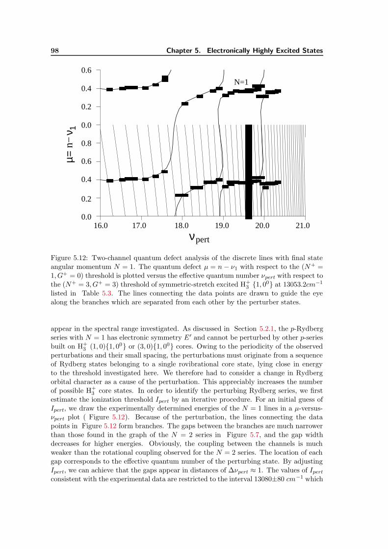
“diss”2002/10/18page 98

98 Chapter 5. Electronically Highly Excited States

!" #$ %& '( )* +,--.. /0112334 56 78 9:;;<<

==>??@@

AAB CD EF GHIIJJ KL MNOOPP QQRRST UUV

WXYZ[[\\]]^^__``

aaaaaaaaaaaaaaaaaaaaaaaaaaaaa

bbbbbbbbbbbbbbbbbbbbbbbbbbbbb

1µ=

νn−

νpert

19.0 20.0 21.018.017.016.0

N=1

0.4

0.0

0.2

0.6

0.8

0.0

0.2

0.4

0.6

Figure 5.12: Two-channel quantum defect analysis of the discrete lines with final stateangular momentum N = 1. The quantum defect µ = n− ν1 with respect to the (N+ =1, G+ = 0) threshold is plotted versus the effective quantum number νpert with respect tothe (N+ = 3, G+ = 3) threshold of symmetric-stretch excited H+

3 1, 00 at 13053.2cm−1

listed in Table 5.3. The lines connecting the data points are drawn to guide the eyealong the branches which are separated from each other by the perturber states.

appear in the spectral range investigated. As discussed in Section 5.2.1, the p-Rydbergseries with N = 1 has electronic symmetry E ′ and cannot be perturbed by other p-seriesbuilt on H+

3 (1, 0)1, 00 or (3, 0)1, 00 cores. Owing to the periodicity of the observedperturbations and their small spacing, the perturbations must originate from a sequenceof Rydberg states belonging to a single rovibrational core state, lying close in energyto the threshold investigated here. We therefore had to consider a change in Rydbergorbital character as a cause of the perturbation. This appreciably increases the numberof possible H+

3 core states. In order to identify the perturbing Rydberg series, we firstestimate the ionization threshold Ipert by an iterative procedure. For an initial guess ofIpert, we draw the experimentally determined energies of the N = 1 lines in a µ-versus-νpert plot ( Figure 5.12). Because of the perturbation, the lines connecting the datapoints in Figure 5.12 form branches. The gaps between the branches are much narrowerthan those found in the graph of the N = 2 series in Figure 5.7, and the gap widthdecreases for higher energies. Obviously, the coupling between the channels is muchweaker than the rotational coupling observed for the N = 2 series. The location of eachgap corresponds to the effective quantum number of the perturbing state. By adjustingIpert, we can achieve that the gaps appear in distances of ∆νpert ≈ 1. The values of Ipert

consistent with the experimental data are restricted to the interval 13080±80 cm−1 which

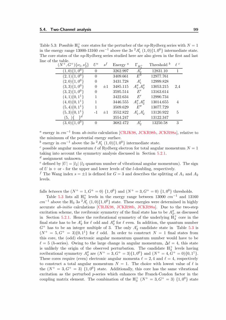
“diss”2002/10/18page 99

5.4. Two-Channel analysis 99

Table 5.3: Possible H+3 core states for the perturber of the np-Rydberg series with N = 1

in the energy range 13000-13160 cm−1 above the 3s 2A′1 (1, 0)1, 00 intermediate state.The core states of the np-Rydberg series studied here are also given in the first and lastline of the table.

(N+, G+)ν1, νl2 U e sf Energy a ΓH+

3Threshold b ` c

(1, 0)1, 00 0 3262.997 A′2 12831.10 1

(2, 1)1, 00 0 3409.661 E ′′ 12977.761(2, 0)1, 00 0 3431.728 A′1 12999.828(3, 3)1, 00 0 ±1 3485.115 A′′1 ,A

′′2 13053.215 2,4

(3, 2)1, 00 0 3595.514 E ′ 13163.614(4, 1)0, 11 1 3422.634 E ′ 12990.734(4, 0)0, 11 1 3446.555 A′′1 ,A

′′2 13014.655 4

(5, 4)0, 11 1 3509.629 E ′′ 13077.729(5, 3)0, 11 -1 ±1 3552.822 A′1,A

′2 13120.922 5

(5, ) d 3554.247 13122.347

(3, 0)1, 00 0 3682.472 A′2 13250.58 3

a energy in cm−1 from ab-initio calculation [CRJK98, JCKR98b, JCKR98a], relative tothe minimum of the potential energy surface.b energy in cm−1 above the 3s 2A′1 (1, 0)1, 00 intermediate state.c possible angular momentum ` of Rydberg electron for total angular momentum N = 1taking into account the symmetry analysis discussed in Section 5.2.1.d assignment unknown.e defined by |U | = |l2| (l2 quantum number of vibrational angular momentum). The signof U is + or - for the upper and lower levels of the l-doubling, respectively.f The Wang index s = ±1 is defined for G = 3 and describes the splitting of A1 and A2

levels.

falls between the (N+ = 1, G+ = 0) 1, 00 and (N+ = 3, G+ = 0) 1, 00 thresholds.

Table 5.3 lists all H+3 levels in the energy range between 13000 cm−1 and 13160

cm−1 above the H3 3s 2A′1 (1, 0)1, 00 state. These energies were determined in highlyaccurate ab-initio calculations [CRJK98, JCKR98b, JCKR98a]. Due to the two-stepexcitation scheme, the rovibronic symmetry of the final state has to be A′′2 , as discussedin Section 5.2.1. Hence the rovibrational symmetry of the underlying H+

3 core in thefinal state has to be A′2 for ` odd and A′′2 for ` even. In addition, the quantum numberG+ has to be an integer multiple of 3. The only A′2 candidate state in Table 5.3 is(N+ = 5, G+ = 3)0, 11 for ` odd. In order to construct N = 1 final states fromthis core, the (odd) electronic angular momentum quantum number would have to be` = 5 (h-series). Owing to the large change in angular momentum, ∆` = 4, this stateis unlikely the origin of the observed perturbation. The candidate H+

3 levels havingrovibrational symmetry A′′2 are (N+ = 3, G+ = 3)1, 00 and (N+ = 4, G+ = 0)0, 11.These cores require (even) electronic angular momenta ` = 2, 4 and ` = 4, respectivelyto construct a total angular momentum N = 1. The choice with lowest value of ` isthe (N+ = 3, G+ = 3) 1, 00 state. Additionally, this core has the same vibrationalexcitation as the perturbed p-series which enhances the Franck-Condon factor in thecoupling matrix element. The combination of the H+

3 (N+ = 3, G+ = 3) 1, 00 state

“diss”2002/10/18page 100

100 Chapter 5. Electronically Highly Excited States

with a d-electron (` = 2) leads to the nd (1, 3)1, 00-series of H3 . In the Hund’scase (ab) frame, this series has a projection λ = 2 of the electronic angular momentum` = 2 onto the top axis and, therefore, E ′ electronic symmetry identical to the electronicsymmetry of the perturbed N = 1 series.

In the µ-versus-νpert plot Figure 5.12, the ionization limit 13053.2 cm−1 of the(N+ = 3, G+ = 3)1, 00 core listed in Table 5.3 was used. We fitted the experimentaldata of the N = 1 series by a two-channel QDT model according to Eq.(5.22) witha threshold fixed to Ipert = 13053.2 cm−1 and the eigenchannel quantum defects andthe frame transformation angle as free parameters. Optimum fit was achieved with thevalues µnpE′ = 0.389, µndE′ = 0.067, and θ = 0.181. The value of µnpE′ agrees wellwith that found in the analysis of the N = 2 series. Our fitted value µndE′ = 0.067applies to the (n = 18 . . . 20) d states of the (N+ = 3, G+ = 3) 1, 00 core and isreasonably close to the quantum defect of the 3d E ′ (1, 3)0, 00 state µ = 0.049 whichhas a (N+ = 3, G+ = 3) 0, 00 core 6.

Due to the change in electronic angular momentum, the frame transformation anglecannot be calculated analytically as is the case in pure rotational coupling. The channelcoupling between the np-series with a (N+ = 1, G+ = 0) core and the nd-series with a(N+ = 3, G+ = 3) core is quite surprising, and has to our knowledge never previouslybeen reported. In terms of a collision picture, the core angular momentum N+ as wellas it’s projection on the molecular top axis K+ are changed back and forth between(N+ = 1,K+ = 0) and (N+ = 3,K+ = 3) by the impact of the valence electron whichswitches between p- and d-character. The enormous mass difference of the ion core andthe outer electron lets this process be only a small perturbation.

5.4.3 Continuum

In our two-channel model, the pure continuum starting above the (N+ = 3, G+ = 0)limit at 13250.58 cm−1 should appear as a structureless ionization continuum. Themeasured spectrum in the 13250 cm−1 to 14200 cm−1 region is shown as curve (c) inFigure 5.4. During the comparatively long duration of the data acquisition (∼ 60 hours),it is a challenge to guarantee stable operating conditions of the apparatus. The dropin the overall signal level around 13800 cm−1 may be due to an instability of the ionbeam alignment. Apart from this, we observe an almost structureless continuum withonly isolated resonances superimposed. The resonances are produced by interloper statesfrom higher vibrationally excited H+

3 ion cores. Some resonances appear as broad featureswith peak widths of more than 7 cm−1 FWHM. Others are narrow lines and the peakstructure becomes visible on expanded energy scales shown in the two insets in Figure5.4c). A few resonances show strongly asymmetric, Fano-type line profiles [Fan61] withnegative as well as positive values of the shape-defining profile index q. The appearanceof these resonances shows no regular pattern and an assignment is beyond the scope ofa two-channel model.

6 The 3d E′ (1, 3)0, 00 state has a pure (N+ = 3, G+ = 3) 0, 00 core and an energy of 17196.38cm−1 above the 2p 2A′′

2 (0, 0)0, 00 state [HHW82]. Using the first ionization threshold of the H3 2p 2A′′

2

(0, 0)0, 00 state (29562.14 cm−1) [KMW89], and the energies of the H+3 states (N+ = 1, G+ = 0) 0, 00

(86.935 cm−1) and (N+ = 3, G+ = 3) 0, 00 (315.35 cm−1) [CRJK98, JCKR98b, JCKR98a], we findthe quantum defect of the H3 3d E′ (1, 3)0, 00 state to be µ = 0.0484.

“diss”2002/10/18page 101

5.5. Stephens-Greene Approach of MQDT 101

5.5 Stephens-Greene Approach of MQDT

To describe the features in the continuum more sophisticated approaches are required[MRMH00] and we will give a brief survey of it. For inclusion of vibrational autoion-ization and vibronic coupling mechanisms as employed in the approach of Stephens &Greene [SG95] another representation of the MQDT is more suited. This representationreveals MQDT as a collision-like process.

5.5.1 Alternative Description of MQDT

The MQDT equations in Eq.(5.20) are formulated in a body-fixed frame. In order to findthe analogue of Eq.(5.20) in a laboratory frame we multiply Eq.(5.18) by U iα′ e−iπνi ,use the orthogonality δαα′ =

∑i U iα U iα′ and require again that the amplitudes Ai and

Bα are real. Taking only the imaginary part we obtain∑

i

U iα sinπ(νi + µα)Ai = 0 (5.33)

It is obvious that these MQDT equations in the ionization basis lead to the same deter-minantal equation Eq.(5.21) as does the body fixed ones. Upon expanding the trigono-metric terms in Eq.(5.33) the equations can be cast into the form

0 =cos πµα

∑

i

U iα

(tanπνi + tanπµα

)cos πνiAi (5.34)

If the amplitudes are redefined and Eq.(5.34) is multiplied from the left by U i′α andsummed over α an equivalent form to the MQDT equations Eq.(5.20) is obtained

0 =∑

i

(Ki′i + δi′i tanπνi) ai Ki′i ≡∑

α

U i′α tan πµα (U)Tαi (5.35)

ai ≡ cos πνiAi

Here, we defined the reaction matrix Ki′i in the laboratory system. The linear system isequivalent to the MQDT equations although the number of equations has changed7. Inorder to interpret the reaction matrix let us now consider the eigenchannel wavefunctionsin this representation. If we rearrange Eq.(5.16) in the same manner as in Eq.(5.34)and introduce a sum by 1 =

∑i′ δii′ then we have

Ψα =1

r

∑

i

U iα χi

fi cos πµα − gi sinπµα

(5.36)

=cos πµα

r

∑

ii′

U i′α χi fi δii′ −∑

i

U iα tan πµα gi

Employing the definition of the Ki′i matrix in the form U iα tanπµα =∑

i′ Kii′ U i′α

Eq.(5.35), the eigenchannel wavefunction is

Ψα = cos πµα

∑

i′

U i′α ·1

r

∑

i

χi

fi(r) δii′ − gi(r) Kii′

(5.37)

7 The reason is that in this formulation the boundary conditions (BCs in Figure 5.6) have not yet beenapplied and the dimension of Ki′i is just N ×N with N as the number of channels under consideration.The number of boundary conditions, however, depends on the number of open channels, i.e. on theenergy, and provides additional constraints to Eq.(5.35). A more detailed discussion is given in [GJ84].

“diss”2002/10/18page 102

102 Chapter 5. Electronically Highly Excited States

By comparing this expression with Eq.(5.16) and Eq.(5.15) we find a relationshipbetween an ionization channel i′ and the reaction matrix with an incident radial wave i

Ψi′ =1

r

∑

i

χi

fi(r) δii′ − gi(r) Kii′

(5.38)

The term cos πµα is neglected since it can be incorporated into a normalization factor.Eq.(5.38) now provides a link to a collision picture. An incident wave i is scattered bythe short-range interaction partially into channel i′. After scattering the admixture ofthe irregular part is determined by the size of the matrix element Kii′ that comprisesthe net effect of the scattering information. It is important to note that the problem isformulated here in a laboratory fixed system (indices i and i′). Therefore, MQDT canbe considered as a continuation of scattering theory to negative energies. Eq.(5.35) andEq.(5.38) are appropriate descriptions to incorporate vibrational and vibronic channelcouplings.

5.5.2 Vibrational & Multi-State Vibronic Coupling

In the rotational frame transformation Eq.(5.2) the Clebsch-Gordan coefficient repre-sents a projection of the rotational properties in the ionization basis (N+) onto those ofthe eigenchannel basis (λ). Vibrational interactions characterize the ionization channelsby the additional property of the vibrational quantum numbers of the core. In anal-ogy, the vibrational part of a generalized frame transformation can be understood as aprojection of the core state in the ionization basis (ν+

1 ν+2 ) onto a state described in the

close-coupled basis. The latter is identified as an instantaneous configuration of the nu-clei, i.e. (Q). Thus, the vibrational part of a generalized frame transformation consists ofthe projection 〈ν+

1 ν+2 |Q〉 = χ+(Q), i.e. a vibrational wavefunction of the H+

3 core. Then,the total frame transformation is given as the product of a rotational and vibrationalpart U iα = 〈i|α〉 = 〈N+K+|λ〉〈ν+

1 ν+2 |Q〉 and the channels are extended to α = (λ,Q)

and i = (N+, ν+). The definition of Ki′i in Eq.(5.35) represents a similarity transforma-tion with U iα as the transforming matrix. Thus, the matrix Kb

α′α ≡ tan[πµλ(Q)]δα′α inEq.(5.35) is identified as the analogous matrix to Ki′i in a body-fixed frame. Expandingonly the rotational part of the ionization channels in the eigenchannel basis for K i′i, theeffect on the body-frame Kb matrix by inclusion of vibrational interactions is a weightingover the vibrational wavefunction of the core [SG95].

Ki′i ≡ 〈i′|K|i〉 =∑

λ′λ

〈N+′K+′|λ′〉 〈ν+′| Kλ′λ(Q)|ν+〉Q 〈λ|N+K+〉 (5.39)

From a scattering point of view that is generally beyond the Born-Oppenheimer approx-imation it is obvious that the incident electron will find the nuclei at different instantsof position of their vibrational motion.

All MQD approaches rely on the weak dependence of the quantum defects or thereaction matrix on energy. However, as seen here their dependence on the configurationof the nuclei may be strong in the case of strong vibrational channel mixing. This pointsto a way how vibrational interactions have to be treated in MQDT and which input isrequired. As mentioned in Section 3.4.2, we determined new ab initio surfaces and usedthem as input in the formalism of Stephens & Greene. Thus, the Q-depending body-frame reaction matrix derives its dependence on the configuration from the quantum

“diss”2002/10/18page 103

5.5. Stephens-Greene Approach of MQDT 103

defect surfaces as in Eq.(5.40) (See entry Kb11(Q), the different appearance of other

diagonal entries is explained in the following).

Kbα′α(Q) =

tan[µA′′

2(Q)] 0 0

0 δQ2r V+Qr exp(iϕ)

0 V+Qr exp(−iϕ) δQ2r

(5.40)

A Feshbach projector formalism of a model Hamiltonian (Domcke et al. [SD88]) allows toderive the MQDT equations from a very general point of view. In spite of being more ab-stract it delivers a more complete picture and reveals how vibronic multi-state couplingsenter the formalism. A great advantage of this formalism is that it is a Hamiltonian rep-resentation. This allows to identify additional entries for the body frame reaction matrixwhich may play a role in various types of couplings. Especially for vibronic interaction,Staib & Domcke [SD90, SDS90] have demonstrated that the scattering between the twodegenerate npE ′ orbitals λ = ±1 from Section 3.5.1 can be included for in MQDT in thesubblock of the λ = ±1 entries of the reaction matrix Eq.(5.40). If the off-diagonal con-tributions are identified with off-diagonal terms from the Longuet-Higgins Jahn-TellerHamiltonian Eq.(3.81) then scattering between degenerate np states is accounted for.If an approximation to second order is employed for Eq.(3.81) the parameters are givenby the linear Jahn-Teller coupling constant V+ (denoted as λ in Ref. [SG95]) and afrequency shift parameter δ. The latter is introduced empirically to account for thechange of the vibrational frequency ωe in different Rydberg states. These parametershave been fitted by us [MRMH00] to the ab initio data of Ref. [Jun98]. The quantumdefect terms in the diagonal positions for λ = ±1 analogous to the one in Kb

11(Q) areassumed to be approximately constant and are not present in the diagonal elements inthe subblock. This is allowed since a phase-renormalized base pair of Coulomb functions[SG95] is used. As seen from Eq.(5.35) U may be interpreted as the matrix that di-agonalizes K. Thus, the procedure is to calculate from the generalized reaction matrixthe full rovibronic frame transformation and then use it to solve the MQDT equationsEq.(5.20). For the No open channels (No = N − Nc) the quantum defect is replacedby an eigenchannel phase shift. The energy-dependent amplitudes Bαρ, ρ = 1, . . . , No (ρlabels the No independent solutions) obtained by the solution are used to calculate thetotal differential oscillator strength according to

dfν+Γ+N+K+←νiΓiNiKi

dE= 2ω

∑

Nf

No∑

ρ=1

[N∑

α=1

d(Nf )α Bαρ

]2

(5.41)

This quantity is proportional to the ion yield registrated by the experiments in Section

5.2.2. The calculation of the transition moments d(Nf )α needs a thorough analysis of

the various angular parts and is explicitly performed in Ref. [SG95]. The full energydependence is contained in the amplitudes Bαρ. If the energetically lowest channel isclosed the expression Eq.(5.41) must be normalized differently, i.e. to the density ofstates. This normalization constant is energy-dependent and accounts for the windowresonances in the quasi-discrete region as in Eq.(5.28). The number of included channelswas chosen to be N = 40 whereas the thresholds energies to calculate the quantum defectsurfaces from the PESs are taken from Ref. [JCKR98b]. In Figure 5.13 we show theenergy region above N+ = 1, v+

1 = 1. Vibrational interlopers from series with vibrational

“dis

s”20

02/1

0/18

pag

e10

4

104

Chapte

r5.

Ele

ctro

nic

ally

Hig

hly

Exc

ited

Sta

tes

Osc

illat

or S

tren

gth

/ eV

−1

Energy above 3sA1’(1,0)1,00 / cm−1

Nf=0 + Nf=2

C12

13000 13200 13400 13600 13800 14000 14200

13400 13600 13800 14000 14200

0.1

0.0

0.2

0.3

0.40

100

200

300

400

500

600

1320013000

B1 B4B5 B8

B9

B10

B12

C1 C3C4

C5

C6

C7

C8

C10

C13C15

C16C17

C17

C16

C15C13

C12

C7

C8

C5

C6C4C3

B12

B10

B8B5

B4

B1

Ion

Sign

al (

Cou

nts/

100

Shot

s)

Figure 5.13: Theoretical result of vibrational and vibronic treatment in MQDT (lower panel) and comparison with experimentalspectrum (upper panel).

“diss”2002/10/18page 105

5.6. Relevancy to Astrophysics & Astrochemistry 105

excited ion core states fall into the Beutler-Fano region as well as in the quasi-continuumabove. The comparison shows a good agreement with the experimental spectrum. Theinclusion of vibronic effects in MQDT turns out to be important. Despite the weak JTeffect of the npE ′ series these vibronic couplings are responsible for the strongest featuresin the spectrum. Quantitative assignments were made which are given in Table VI ofRef. [MRMH00]. The width of the features or equivalently their lifetime in vibrationalautoionization constitutes a direct measure of the gradient of the quantum defect surfacealong a specific normal coordinate. This was first shown for the diatomic case of H2 byHerzberg & Jungen [HJ72]. A more generalized discussion was recently given by Jungen& Pratt [JP97].

5.6 Relevancy to Astrophysics & Astrochemistry

In the 1930s and 1940s the predominance of Hydrogen in interstellar space was estab-lished. The interstellar matter in dense clouds is mainly dominated by molecular Hy-drogen. Due to its low temperatures and low density the formation of other moleculesin interstellar clouds is constrained to two-body reactions with low activation energies.While gas-phase reactions are responsible for production of most of the molecules ininterstellar space, the formation of molecular Hydrogen is believed to occur on surfacesof small dust grains [Her00]. Since photons inherent in these clouds are limited in energyto < 13.6eV and thus do not exceed the ionization potential of H2 (15.4eV ), molecularionization occurs dominantly via external cosmic ray flux. This flux consists essentiallyof protons and determines the abundance of the molecular ion H+

2 . In a next step, thepredominant reaction path for H+

3 occurs via the ion-molecule reaction

H2 +H+2 → H+

3 +H (5.42)

which is highly efficient due to its high exothermicity (1.7eV ), large cross section (ca.100 A2)

and lack of an activation barrier [Oka00]. This reaction is known to prevail in most hy-drogen plasmas. H+

3 was observed in molecular clouds in the interstellar medium, in theauroral regions of Jupiter, and in the ionospheres of Uranus and Saturn and plays animportant role for astrochemistry. Miller et al. [MTLD92] report also on the observationof H+

3 in the Supernova 1987A.The number density of H+

3 provides a sensitive tool for measuring the cosmic rayionizing flux [Dal94] whose uncertainty ranges currently over two orders of magnitude.The detection of H+

3 absorption allowed a rough determination of the column densityof H+

3 providing the most direct evidence of the cosmic-ray driven ion-neutral reactionscheme of Herbst & Klemperer [HK73] for the chemistry of molecular clouds. Theimportance of H+

3 is derived from the chemistry at various interstellar locations whereit acts as a major agent responsible for formation of larger molecules via the proton hopreaction

H+3 +X→ HX+ + H2 (5.43)

A strong competing process to the above reactions Eq.(5.42) and Eq.(5.43) definingthe H+

3 number density is given by the dissociative recombination (DR) with electrons

H+3 +e− →H +H2 (ν,J) (25%) (5.44)

H +H+H (75%)

“diss”2002/10/18page 106

106 Chapter 5. Electronically Highly Excited States

Since electron densities are relatively high in dense molecular clouds, DR is the dominantdestruction process for H+

3 . In certain areas of the parameter set of a chemical modelthe two competing destructive reactions Eq.(5.43) and Eq.(5.44) may exhibit a certainchaotical bistability whose steady-state solutions are rather dissimilar [FR00]. Usually,excited neutral fragments produced by reaction Eq.(5.44) are responsible for chains ofchemical reactions that would not occur in the case of ground-state reactants. Thisexplains the importance of Eq.(5.44) as a key reaction in astrochemical environments.While the rates of reaction Eq.(5.42) and Eq.(5.43) are sufficiently well understood, theDR rate of Eq.(5.44) has a long and controversial history which is not yet resolved andprevents accurate determinations of the abundance of H+

3 in interstellar media to date.The involved inconsistencies are twofold. Different experimental approaches deviate upto four orders of magnitude in the rate constant of dissociative recombination. Secondly,large discrepancies of these persist with theories already for many years indicating thateven the major mechanism for H+

3 destruction with slow electrons is not yet identifieddespite of the great effort that has been started for its understanding.

The necessity to discuss DR in terms of the neutral complex H+3 +e− gives a link to

the present work. Figure 5.14 shows schematically potential curves along the two-bodyreaction coordinate. From ab initio calculations it is known that the ionic potential sur-face is intersected by several neutral potential surfaces but at energies more than 1eVabove the H+

3 ground vibrational state. The high-energy region (II) has been success-fully described by a two-dimensional wave-packet approach including curve-crossings offour doubly-excited dissociative states and is well understood [OSSW00] (arrow on theright). However, for electronic recombination below the H(n = 2) + H2 limit, i.e. in theenergetic region (I), the previous mechanism is forbidden. Nevertheless in this region theexperimental cross section rises by almost three orders of magnitude when decreasingthe electron energy from 0.5eV to 0.5meV . Here, the only doorway to dissociation isvia the repulsive ground state of H3 which lies energetically far from the ionic potential.The direct process to DR mediated by non-adiabatic coupling between the ionizationand the 2p 2E′ continuum was shown to be orders of magnitude too weak to explain theexperimental data [OSSW00].

An indirect mechanism corresponding to the capture into Rydberg states with subse-quent predissociation was suggested to contribute significantly to the cross section. Thiscapture is identical to the time inverse process of autoionization and well described byMQDT as demonstrated above. These states decay along the same pathways as beingphoto-excited by the experimental methods described in this Chapter. Therefore, byphotoexcitation valuable information for the lifetimes of these states is gained reflectingthe importance of indirect processes leading to DR. Non-adiabatic couplings betweenthe ionization continuum and the Rydberg states of closed channels are accounted forby MQDT in the first step in DR. It has also been shown that the inclusion of disso-ciative channels in MQDT models is possible [Giu80]. However, calculations have beenperformed so far only on diatomics and complete formulations for polyatomics with morevibrational degrees of freedom are still missing. Nevertheless, the question for an ade-quate explanation of the key mechanism still remains open. While latest experiments[JPS+01] tend to very large dissociation recombination rates (α = 1.0 · 10−7cm−3s−1)at a temperature8 of 300K the best theoretical approach is still one order of magni-

8The temperature dependence of the recombination rate was experimentally found to scale as

“diss”2002/10/18page 107

5.7. Rydberg Series excited from 3p 2E′ 107

-45

-40

-35

-30

r=1.65a.u. R

H + H + H

H(n = 2) + H2(X1Σ+

g )

H−(1S) + H+2 (2Σ+

g )Total Energy / eV

H(n = 1) + H2(X1Σ+

g )

I

II

R ∞

Entrance

H+3 + e−

MQDT

Channel2D Wavepacket

Approach

Figure 5.14: Scheme of the potential energy curves for H+3 and H3 as a function of the

Jacobi coordinate R in a two body-breakup with fixed r.

tude lower (α = 1.2 · 10−8cm−3s−1). This latter value is from the recent approach ofKokoouline, Greene & Esry [KGE01] and is based on a MQDT model. The inclusionof the Jahn-Teller effect allows these authors to treat the problem again as a curvecrossing of potential surfaces which strongly enhance the DR rate. Further refinementof this approach might clarify the enigma. Currently, this approach appears to be themost promising [SWS01]. However, a full understanding of this important reaction stillrequires some more effort and as it seems now basically from the theoretical side.

5.7 Rydberg Series excited from 3p 2E ′

In order to further investigate the influence of vibronic couplings we interchanged theelectronic properties of the initial and final states by choosing different vibronic levelsof the 3p 2E′ as intermediate in a two-photon excitation scheme as shown in Figure5.15. Excitation into 3p 2E′ from the metastable state is allowed by a change in the con-current excitation of degenerate mode vibrations (as a consequence of Herzberg-Tellercoupling [BJ98]). The choice of the vibrational state in the intermediate implies a certainpreference of the vibrational excitation of the ion core in the ionization channel |ν+〉.Vibrational induced channel couplings should appear differently for higher vibrationallyexcited ion cores. Additionally, propensity rules exist that favour vibrational autoion-ization in continua with ∆ν = −1 [JP97]. However, a major drawback of this scheme isthat channel couplings of the s- and d-Rydberg series are generally quite small; s-states

(T [K]/300K)−0.65 [SMD+94]. The temperatures of dark interstellar clouds are approximately 10−15K.

“diss”2002/10/18page 108

108 Chapter 5. Electronically Highly Excited States

2pA

3pE3pE

’

’’

’(N=G=0)0,0

(N=1,G=0)1,1 (N=1,G=2)0,2

2

0

+1

0

H3

H 3

+

1,1

0,2

0,0

1

2

0

4000

4500

5000

5500

6000

0

(2 ,0 )

(1 ,0 )

(2 ,3 )

(1 ,3 )

++

cm-1

-

(N ,G ) nd ns

Figure 5.15: Two-photon ionization spectra via two resonant intermediates covering thesame range of final states.

“diss”2002/10/18page 109

5.7. Rydberg Series excited from 3p 2E′ 109

Table 5.4: Observed Rydberg series via the 3p 2E′ state. Explanations are given in thetext.

Core state Observed Range Threshold Elim Quantum Defect

Orbital ` (N+, G+) ν1, νl22 n Exp. Theory Experiment

nd(A′1, E′, E′′) (1, 3) 0, 22 14 − 61 4995.0 4994.49 0.026 ± 0.011

nd(A′1, E′, E′′) (2, 3) 0, 22 12 − 75 5181.3 5180.79 0.0199 ± 0.006

nd(A′1, E′, E′′) (1, 0) 1, 11 10 − 51 5644.9 5644.40 0.0239 ± 0.005

nd(A′1, E′, E′′) (2, 0) 1, 11 9− 67 5835.7 5834.94 0.0217 ± 0.005

nsA′1 (2, 0) 1, 11 9− 67 5835.8 5834.94 0.0526 ± 0.003

reflect a more homogeneous electron distribution and do not support asymmetric distor-tions, while d-states do not penetrate the ion core sufficiently deep. This follows from anestimation by the semiclassical `-scaling of the quantum defect µ ∝ α/(`+ 1/2 )5 [JR77]relying on a pure polarization of the core.

We recorded spectra over a wide range using a stepwise excitation as shown in Figure5.15 via the states 3p 2E′(N = 1, G = 0)1, 1±1 and 3p 2E′(N = 1, G = 1)0, 20. Fora proper comparison we scanned the same final state energy region. The two spectra arecompared in Figure 5.16.

The analysis shows for both spectra an identical composition of s and d Rydberg seriesconverging to vibrationally excited H+

3 cores. The only exceptions are a few vibrationalinterloper states which appear quite irregularly distributed and are difficult to assign.Five Rydberg series over large ranges of the principal quantum number were found inthese spectra and fitted to the Rydberg formula. Due to the reasons discussed abovethey appear all quite regular. Their quantum defects and series limits are listed in Table5.4. There seems to be a systematic offset of ∼ 0.5cm−1 in the series limits; nevertheless,their identification is unambiguous. As a result of the strong `-dependence of a quantumdefect the electronic angular momenta are easily identified by their absolute size. Theidentification of the core is based on an assignment of the fitted series limit to the ab initiothresholds of Refs. [JCKR98b][JCKR98a]. We checked our assignment for consistencyemploying symmetry based arguments of Section 4.3. The notable broad features markedwith red dots in the lower trace of Figure 5.16 have a simple explanation and belongto experimental artefacts. For excitation via the state 3p 2E′(N = 1, G = 1)0, 20 thesecond laser can become resonant with some low Rydberg states. Due to its strength,ions are produced via 1 + 1 REMPI.

Surprisingly, the relative intensities of the series are approximately reproduced inboth spectra via the two intermediate states. According to Figure 3.11 the two inter-mediate states are coupled by vibronic effects. However on the basis of the small mixingcoefficients of ∼ 5% ( Table 3.12) the high similarity of the two spectra is not explained.Thus, we conclude that our studies do not support the expected propensity law ∆ν = −1for vibrational autoionization. However the smallness of the interchannel coupling is inaccord with our expectations. This is further manifested by the small coupling of thend(2, 0)1, 11 as seen from the behaviour of the intensity progression emphasized inthe enlarged portion in the inset of Figure 5.16. A fast rise and a steep cut-off of the

“diss”2002/10/18page 110

110 Chapter 5. Electronically Highly Excited States

intensity progression in the vicinity of a perturber reveals a small coupling constant asderived from the relations Eq.(5.24) and Eq.(5.28) of a two-channel model.

“diss”

2002/10/18page

111

5.7

.Ryd

berg

Serie

sexcite

dfro

m3p

2E′

111

4450 4500 4550 4600 4650 4700 4750 4800 4850 4900 4950 50004400−+

1−+

1vi

a 3p

E’

1,1

vi

a 3p

E’

0,2

vi

a 3p

E’

1,1

vi

a 3p

E’

0,2

(N ,G )=(1,3)+ +

(N ,G

)=

(2,0

)+

+

+3

−1Energy in cm relative to Zero Point Energy of H

5000 5050 5100 5150 5200 5250 5300 5350 5400 5450 5500 5550 5600 5650 5700 5750 5800 5850

(N ,G )=(2,3)+ + (N ,G )=(1,0)

+ +

Ion

Sign

als

(arb

. uni

ts) 0

0

Figure 5.16: Two-step ionization spectra via the intermediate state 3p 2E′(N = 1, G = 0)1, 1±1 and 3p 2E′(N = 1, G = 1)0, 20.The sticks correspond to two parameter fits to a Rydberg formula.

“diss”2002/10/18page 112

112 Chapter 5. Electronically Highly Excited States

“diss”2002/10/18page 113

Part II

The Negative Ion of Hydrogen

113

“diss”2002/10/18page 114

“diss”2002/10/18page 115

CHAPTER 6

Introduction to Part II

The negative hydrogen ion can be considered as the simplest, non-trivial problem inatomic physics. This property tells already much about its controversial character. Ithas been studied since the early days of quantum mechanics and continues to pose chal-lenges to our understanding. Together with atomic Helium it is the simplest atom forwhich no exact mathematical solutions exists. Both of these two similar atoms are three-body systems and belong to the two-electron isoelectronic sequence H−, He, Li+, . . ..They differ by their nuclear constituents distinguished by spin, mass and charge. Whilethe nuclear spin and mass affect the electronic spectrum only on sub-meV energy scales,the nuclear charge represents the critical parameter here. It determines their large-scaleelectronic structure and their density of states. While for atomic Helium the binding ofboth electrons is Coulombic and easily understood, the outer electron in negative Hydro-gen relies on a dynamical potential. This peculiarity requires explicit electron-electroncorrelations already in the ground state. Negative Hydrogen is therefore already in itssingle bound state a prototypical system for electron correlation phenomena. A preciseunderstanding of electronic correlation is desired since it occurs in the structures of morecomplex atomic and molecular systems. As long as not extreme double excitations in thevicinity of the two-electron detachment threshold are considered, the electronic struc-ture of the negative hydrogen ion is widely understood today. Ground state electrondynamics occurs on time scales of one atomic unit of time (1 a.u. ∼ 2 · 1017s) and is ingeneral not directly accessible by experimental methods today. Dynamical informationon H− can however be obtained by exposing it to a precisely known time-dependentperturbation like a short electromagnetic light pulse. Especially, when a strong laserpulse of the order of the internal atomic field drives the electronic motion in an atom,a big amount of dynamical information can be retrieved from experiments. In the limitF →∞, where F is the electrical field strength of the laser pulse, the system turns into aclassical problem when the binding potential can be totally neglected. Such strong fieldsare easily produced today by femtosecond laser systems. Another intriguing aspect isthat laser fields of this strength always induce nonlinear light-matter interactions. Thisis a challenge for theory because conventional perturbational approaches are no more

115

“diss”2002/10/18page 116

116 Chapter 6. Introduction to Part II

suitable in this regime. Many experiments have been performed on neutral atoms instrong fields so far, although for theoretical treatments negative ions are the simpler sys-tem. Due to the absence of resonant intermediate states, complex mechanisms such asresonantly enhanced ionization do not play a role in multiphoton detachment processesof negative ions. However, experimental investigations of negative ions in intense laserfields to date are limited [BCDG91, DMH91, SBBH91]. In experiments, negative ionsfirst have to be produced in sufficient amounts and must be properly separated from theirneutral counterpart. This makes them more difficult to handle in an experiment. An-other advantage for theory and especially for Keldysh-like approaches comes from theirinner atomic potential that is to a very good approximation modeled by a zero-rangepotential. This simplifies the spatial integration in the evaluation of the main matrixelement and a pure analytical description becomes possible [GK97]. In unraveling theinherent ionization mechanisms this approximation turns out to be very practicable andmakes possible expansions of the matrix element in complex trajectories in the formalismof path-integrals. The processes involved reveal many peculiarities ranging from pureclassical characteristics to full quantum mechanical features. The dynamics of the activeelectron is thus related to quantum trajectories that lead to interpretations of the spectrain terms of semiclassical dynamics. It was recently pointed out that strong-field ioniza-tion of a single electron represents one of the very rare cases in which only a small numberof such paths contribute to the observed features [SCD+01, KBK00]. These quantumpaths are found to overlap spatially under certain conditions and exhibit interferencephenomena.

In the second part of this thesis experimental and theoretical studies of nonlinearlight-matter interactions and the dynamics of the fundamental negative ion of Hydrogenare investigated. Interpretations of these processes in terms of semiclassical argumentsare attempted.

6.1 Current Status

The study of atomic systems in strong laser fields received much attention over the pastyears. The rapid progress in the development of high power short pulse lasers opened upa new area in non-linear interactions between light and matter. Today, light intensitiesexceeding 1020 W/cm2 can be produced. This is much more than typical atomic fieldstrengths. Such interactions must be totally reconsidered in theory and new approacheshave to be found. A multitude of new effects was found theoretically and experimentallythat are already observable at much more moderate fields [DA95, JDK00]. The interestin these effects is manifold and ranges from fundamental aspects to pure technical ap-plications. Phenomena, such as above threshold ionization (ATI), tunnel ionization, andhigh harmonic generation (HHG) were observed and characterized [DK94]. Most often asingle active electron (SAE) is responsible for the complex dynamics in these processes.Other phenomena occurring in a strong laser field, as the process of multiple ionizationand atomic stabilization, have also been studied experimentally and theoretically butstill await a complete understanding. The technical importance of non-linear processesderives from the HHG that might be exploited in the near future for the production ofcoherent light sources at photon energies in the XUV region [CRW+97, SBS+97]. Vari-ous theoretical approaches were developed to describe and understand them theoretically.

“diss”2002/10/18page 117

6.1. Current Status 117

Among these methods are direct numerical integration [LKGP+01], Keldysh-Faisal-Reiss(KFR) approaches [GK97, LKKB97], and a quasistationary quasienergy state (QQES)approach [BFMS01]. A more explicit summary of theoretical methods especially of thoseapplied to the negative hydrogen ion is listed in Ref. [GK97].

The KFR theory was developed to describe ionization from an atomic system witha short range potential. Thus, this approach is particularly appropriate for the descrip-tion of photodetachment. However since most of the strong field experiments to datewere performed on neutral atoms, where the long range Coulomb potential needs to betaken into account, a comprehensive experimental verification of the KFR theory is stillmissing so far. A general experimental problem for these studies lies in the weak bindingenergies of negative ions. Those lightly bound electrons are easily ionized by alreadysmall electrical field strengths and only a small part of the ions survive up to the timethe laser intensity reaches its maximum. In our approach this difficulty is overcomeby employing short laser pulses in combination with long wavelengths in the IR range.Gribakin and Kuchiev [GK97] have formulated a Keldysh-like approximation that is validfrom the multiphoton detachment to the tunneling regime. A new effect was proposedthat explains the unusual dependence of the angular distribution in the vicinity of thedetachment threshold in terms of a quantum interference effect. Similar quantum pathinterferences have been already observed and explained in neutral atoms by Paulus et al.These authors demonstrated experimentally that the high-order ATI region exhibits aplateau followed by a cutoff similar as in the case of HHG. This plateau was described asbeing due to a rescattering of the electrons with the atomic core [LKKB97]. According tothis mechanism, the ejected photoelectron is driven back to the core under the action ofthe external oscillating field and undergoes elastic scattering before it finally drifts awayfrom the atomic nucleus. In this context, Keldysh-like approaches have been helpful inthe interpretation of the complex interplay between the involved quasi-classical electrontrajectories [KMB00, KBK00]. Direct electrons, i.e. electrons that leave the atomiccore without rescattering, are known to be restricted to kinetic energies less than 2UP ,where UP is the ponderomotive energy. In this energy region a weak manifestation of aquantum interference of electron trajectories could so far be observed only for ellipticallypolarized light [PZW+98] and it was thought of being unobservable for linearly polarizedlight. In the experiments of Paulus et al. the addition of a new physical parameter, viz.the ellipticity, was the key point for the observation of the quantum path interference.This is because elliptically polarized light influences ATI spectra more drastically thanlinearly polarized light [PZW+98, PGD+00]. In the plateau region, which extends upto approximately 10 UP , the quantum path interference has also been observed betweendirect and rescattered electrons in the region of the onset of the plateau [PGD+00]. Thepeculiarity of the quantum path interference effect observed by Paulus et al. relies there-fore on the rescattering model and appears as much more complex to the one observedhere.

We show that quantum path interferences between exclusively direct electrons canequally be observed by exposing negative ions to a strong linearly polarized laser fieldthat are not subjected to any complex rescattering mechanism. In particular, this effectdominates the angular distributions (ADs) at low kinetic energies in a drastic manner,preventing under certain circumstances any electron emission along the laser polarizationaxis. Similar predictions have recently been made by Borca et al. [BFMS01]. Thedominance of this interference effect in our spectra must be inferred from its relation

“diss”2002/10/18page 118

118 Chapter 6. Introduction to Part II

to the detachment threshold. As obvious from the theory, the information of quantumpath interferences is gained by the study of the angular distributions in a single n-photondetachment channel close to the threshold. The type of interference effect consideredhere might be equally interpreted by the fundamental different threshold law in the caseof photodetachment which governs the process at low photoelectron energies. This workreports on the first experimental observation of a quantum path interference effect in anegative ion.

Due to its simplicity and prototype character the negative hydrogen ion has beenalready the subject of many theoretical and experimental investigations1. The experi-mental observation of excess photon detachment (EPD) processes in H−, the analogousprocess to ATI for negative ions, was shown to be difficult due to the small binding en-ergy and the large required photon intensities [ZGB+97, GZB+99]. Zhao et al. found aweak signature of the first non-resonant excess photon channel in their electron spectra.Generally, the difficulty lies in the finite rise time of a short laser pulse that depletesthe major part of the H− bound state population already at intensities orders of mag-nitude below the peak intensity. This fact demands a large signal-to-noise ratio in theexperiment.

Recently, Wang and Elliott have shown that the study of ADs of multiphoton ion-ization allows a direct experimental determination of differences of the elastic scatteringphase shifts associated with the binding potential. Their experiment was performed ontwo-photon ionization of Rb employing elliptically polarized light [WE00a, WE00b] andthey used an imaging technique similar to the one described herein. They called theirapproach complete because the sign of the phase difference could also be determined. Ina similar way, our data allow us to determine complex partial wave amplitudes of finalcontinuum states apart from a common absolute phase. It is well known that the phasesof the partial amplitudes in a multiphoton transition correspond to the elastic scatteringphases [SL88]. In our approach we extract these quantities from the measured partialamplitudes and instead of tuning the wavelength, we derive their energy dependence bymapping the ADs as a function of the ponderomotive energy which is proportional tothe laser intensity.

Our experiment is based on a fast beam of negative ions and a photoelectron imag-ing technique. High statistics is guaranteed since it corresponds to a 4π solid angledetection scheme. The combination of a fast beam and an imaging technique introducescomplications associated with image distortions and interaction volume averaging. Wedemonstrate that these complications are all circumvented by the special design of ourimaging spectrometer that operates in a so-called velocity mapping regime. This lattertechnique was initially designed for photoion imaging [EP97]. In our detailed analysiswe present energy resolved angular distributions of photoelectrons for the strong fieldphotodetachment of the negative hydrogen ion. The measured electron spectrum revealsfour excess photon detachment channels. A comparison of our experimental data withpredictions based on the Keldysh theory shows that this theoretical approach is able toaccount for all observed features of the rich experimental spectrum. The predicted quan-tum interference effect is observed in the region of low electron kinetic energies, wherethe process is dominated by the lowest two-photon detachment channel. A comprehen-

1For a more general and comprehensive survey of various aspects of the negative hydrogen ion see therecent review paper Ref. [Rau96] and references therein.

“diss”2002/10/18page 119

6.1. Current Status 119

sive analysis of the angular distributions is presented for all excess photon detachmentchannels. The elastic scattering phase shifts of the partial continuum waves determinedfor the lowest order channel are in a good agreement with accurate effective range calcu-lations. The extraction of partial wave amplitudes from the experimental data is shownto underlie a certain ambiguity that can not be bypassed for quantitative results. TheWigner threshold law of photodetachment is examined experimentally in the strong fieldregime and its role in the observed quantum interferences is discussed.

The outline is as follows. In Chapter 7 we review some structural particularitiesof the negative hydrogen ion and prepare some approximations used in the followingtheoretical treatment. Chapter 8 introduces our experimental setup, and provides detailsof the operating conditions of our experiment. We discuss various distortion mechanismsthat arise by kinematical effects in the imaging process in fast beams. We also show thatour design avoids all major sources of image distortions. We briefly sketch the methodsof numerical back-projection of electron density distribution, deconvolution routines andenergy calibration in Chapter 9. The next Chapter 10 deals with a short introduction intothe adiabatic theory of Gribakin and Kuchiev. It also describes further aspects necessaryfor a complete theoretical account. Quantitative comparisons and interpretations of theexperimental and theoretical data are given in Chapter 11. The discussion encompassessemiclassical arguments for the quantum path interference and its relationship to thenearby threshold. A simple picture is worked out that relies on the analogy to a double-slit configuration. This picture appears as alternative description and is fully consistentwith a quantum path picture. Our main concern is to test a Keldysh-like approach overa wide range in the phase space of the continuum state of the active electron.

“diss”2002/10/18page 120

120 Chapter 6. Introduction to Part II

“diss”2002/10/18page 121

CHAPTER 7

The Binding Potential of Negative Hydrogen:

The Temkin-model without Anti-symmetrization

We discuss some approximate solutions to the exact Hamiltonian of H−

according to the model of Temkin et al. [Tem59, TL61]. This allowsto explore the nature of the binding from an ab initio point of view.The model is perturbational and reveals an approximate radial equationfor the additional electron. Its effective potential contains two termswhich are identified as a Hartree term and a dipole polarization termdescribing an average charge distribution of the residual hydrogen atomand its distortion, respectively.

Contents

7.1 Preliminary Remarks . . . . . . . . . . . . . . . . . . . . . . . . 121

7.2 Static Distortions of the Hydrogen Ground State Wavefunc-tion . . . . . . . . . . . . . . . . . . . . . . . . . . . . . . . . . . . 122

7.3 Dynamical Stability and Binding of H− . . . . . . . . . . . . . 123

7.4 Zero-Range Approximation & Asymptotic Behaviour . . . . 126

7.1 Preliminary Remarks

The existence of the negative hydrogen ion and its discrete spectrum was for a longtime controversial and unknown. Today, an exact mathematical proof exists that theinner-atomic potential of H− provides a discrete spectrum consisting of a single boundstate [Hil77]. For the isoelectronic He atom the binding of both electrons is strong andreadily explained by Coulombic attraction. While a simple Hartree self-consistent fieldtreatment provided a rather precise value for its binding energy, the same approachfailed completely for the negative Hydrogen, i.e. even the existence of H− could not beproposed at that time. It took until 1929, when Bethe could unambiguously prove by

121

“diss”2002/10/18page 122

122 Chapter 7. The Binding Potential of Negative Hydrogen: the Temkin-Model

employing a Hylleraas trial wavefunction that H− is a bound system. Later in 1944,Chandrasekhar [Cha44] used a simple trial wavefunction of the kind

Ψ = exp(−αr1 − βr2) + exp(−αr2 − βr1) (7.1)

that gave more insight into the electronic structure as Bethe’s ansatz did. The variationprinciple in combination with his trial wavefunctions establishes a minimum for theenergy functional if α = 1.03925a−1

0 and β = 0.28309a−10 . These rather distinct numerical

values indicate a strong radial correlation between the two electrons and provide a hint toa totally different binding character than in He. The respective energy eigenvalue is E =−0.51330a.u. implying a binding energy of ∼ −360meV for the second electron whichunderestimates the real value by approximately a factor of 2. A significant improvementis found if terms of the kind cr12 are included in the trial wave function with c asan additional adjustable parameter showing the importance of electronic correlations.The numbers a, b from above also show that the inner electron is pushed closer to thenucleus (α > 1) by the second electron which roams far away from the nucleus at anapproximate distance of 1/β ∼ 3− 4a0. This small shift of the charge is responsible forthe binding energy of a negative ion. A closer inspection of the Schrodinger equationshows that a dynamical polarization force is the underlying mechanism for the existenceof the binding. Consequently, the radial electron-electron correlations are important forthe dynamical stability of the ion and enable a shallow minimum in energy. As outlinedin this Section, a potential based on a dynamical dipole polarization decays as r−4 withthe electronic distance r and is therefore of a very short-ranged nature. Generally, sucha potential can support only a limited number of bound states, typically a few states∼ 1− 4. Expressions analogous to the Rydberg formula are known in the semiclassicallimit for this potential [KBHP98]. In order to understand the electronic structure ofH− from an ab initio point of view we start from the Hamiltonian of H− where thekinetic energy term −∆1/2 of the ”outer electron” is included in the dynamical regimeand neglected in the static regime, respectively.

7.2 Static Distortions of the Hydrogen Ground State Wave-

function

We first consider a stationary picture where the second electron is spatially fixed and theground state wavefunction of neutral Hydrogen is distorted by the additional elementarycharge. We denote the Hamiltonian of the neutral hydrogen atom by

H0 = −∆2

2− 1

r2(7.2)

and its electron (”the inner electron”) here and in the following by the index 2. Ifanother electron at position r1 (”the outer electron”) approaches the hydrogen atom twomore Coulombic interactions arise as shown in Figure 7.1e) by the arrows r2 − r1 andr1. If these additional interactions are treated as a perturbation V we find the staticHamiltonian Hstat as

Hstat = H0 +V, V(r1, r2) = − 1

r1+

1

|r1 − r2|(7.3)

“diss”2002/10/18page 123

7.3. Dynamical Stability and Binding of H− 123

The effect of the perturbation is to distort the hydrogen ground state wavefunction. Ifwe assume distinguishable electrons, i.e. neglect exchange and anti-symmetrization, wecan write the total wavefunction as a product state as

Ψ(r1, r2) =u(r1)

r1

[Φ0(r2) + Φpol(r1, r2)

]u(r1) = ul(r1)Yl0(Ω) (7.4)

The special choice for u(r1) means that we do not admit strong angular correlations(see below). Within perturbation theory the additional term V induces a small additivecontribution Φpol to the ground state wavefunction of Hydrogen Φ0. The wavefunctionul(r1) associated with the outer electron is defined by the full Hamiltonian discussed inthe next paragraph. The ground state (n = 1, l = 0,m = 0) wavefunction of HydrogenΦ0(r2) = 2e−r2Y00(Ω2) satisfies the Hamiltonian Eq.(7.2) with an eigenvalue E(2) =1/2 a.u. Temkin et al. have derived an approximate differential equation for Φpol andgave an approximate solution valid for the constraint r2 < r1 and large r1

Φpol(r1, r2) ∼r1→∞r1>r2

∞∑

l=1

u1s→l(r2)/r2

rl+11

Pl(cos θ2)

(4π)1/2u1s→l(r2) = 2e−r2

(rl+22

l + 1+rl+12

l

)

(7.5)

≈ −ε(r1, r2)r21

u1s→p(r2)

r2

P1(cos θ12)

(4π)1/2

Here the step function ε(r1, r2) is defined by ε = 1 for r1 > r2 and zero for r1 ≤ r2. Theangular dependence is solely given by the angle θ12 between the two spatial vectors r1, r2,Figure 7.1e). The expansion in Eq.(7.5) refers to a multipole expansion where the dipoleterm is dominant over higher orders and sufficiently accurate for the discussion here. Toillustrate the effect of the distortion we plot the probability of the inner electron as afunction of the distance of the perturbing charge in Figure 7.1. The subfigures a)-d)clearly show the strong repulsive nature of the interaction between the two electrons.

7.3 Dynamical Stability and Binding of H−

In order to understand the existence and type of the binding of the negative hydrogen ionwe have to include the kinetic energy term for the outer electron. The exact Hamiltonianof H− is then given by

H = −∆1

2+H0 +V (7.6)

The solution to this Hamiltonian, i.e. the total wavefunction, is defined by the variationalprinciple. We can find a defining equation for the wavefunction ul(r1) independent ofother product functions if we apply this principle in a slightly modified form, i.e. weintegrate only over those variables that are not part of the unknown product functionassociated with the outer electron

δ

∫Ψ∗(H−E)ΨdΩ1dΩ2r

22dr2 = 0. (7.7)

From the static model of the last paragraph we can substitute the approximate productwavefunctions of the known part from Eq.(7.4) into Ψ. Within first order corrections

“diss”2002/10/18page 124

124 Chapter 7. The Binding Potential of Negative Hydrogen: the Temkin-Model

−1 0 a.u.1 2 3 4

−1 −0.5 0 0.5 1 1.5a.u. −1 0 0.5 1 1.5 2a.u.

−0.5

−0.8

−0.4

0

0.4

0.8

−1 −0.5 0 0.5 1a.u.

a.u.

d)

−0.8

−0.4

0

0.4

0.8

a.u.

θ12

r1

r2r2 r1−

a) b)

e)

c)

Figure 7.1: Contour plots of the probability |Φ0 + Φpol|2 of the ”inner electron” r2 as afunction of the fixed position r1 of the outer electron in first order perturbation theory.The position of the nucleus is chosen at the origin. a)-d) Distorted hydrogen ground stateprobability in the presence of a fixed point charge e− for the distances r1 = 1, 1.5, 2, 4a.u.,respectively. e) Definition of the angle θ12 and radial vectors of the electrons constrainedto r2 < r1.

it is sufficient to consider the distorted wavefunction only for Ψ in the energy functionalEq.(7.7) and use the zero order approximation for the conjugated part Ψ∗. Then Eq.(7.7)reads ∫ [

u(r1)

r1Φ0(r2)

]∗(H−E)Ψ(r1, r2)dΩ1dΩ2r

22dr2 = 0 (7.8)

To a good approximation we can substitute from Eq.(7.5) only the dipole term into Ψas the leading term in the multipole expansion for large r1. If in addition we employ theexact relationship

1

|r1 − r2|=∞∑

l=0

rl<

rl+1>

Pl(cos θ2) r< < r>; r<, r> ∈ (r1, r2) (7.9)

and use the integrals given in Appendix H, Eq.(7.8) is found to be equivalent to thedifferential equation

[− ∂2

∂r21+l(l + 1)

r21− 2e−2r1

(1 +

1

r1

)− α(r1)

r41

]ul(r1) = 2E(1)ul(r1) (7.10)

α(r1) =9

2− 2

3e−2r1

(r51 +

9

2r41 + 9r3

1 +27

2r21 +

27

2r1 +

27

4

)E = E(1) +E(2)

for the unknown part ul(r1). Obviously, Eq.(7.10) defines an effective binding po-tential for the outer electron of H−. This potential consists of the two terms V eff ≡

“diss”2002/10/18page 125

7.3. Dynamical Stability and Binding of H− 125

1r /a.u.10 15 205

−0.5

−0.4

−0.3

−0.2

−0.1

Ene

rgy

/ a.u

.

Figure 7.2: Radial dependence of the effective potential terms for the outer electron.Solid line: polarization term Vpol, dashed-dotted: Hartree term VHartree, dashed line: at-tractive Coulomb potential VCoul.

VHartree +Vpol = −e−2r1(1 + 1r1

) − α(r1)/2r41 . Their interpretations are given in the

following.

VHartree This term refers to a Hartree term describing the mean field of the static hydro-gen atom that the outer electron experiences at a distance r1 from the nucleus.Since it results solely from the zero order product wavefunctions it does notinclude any electron correlation.

Vpol This part of the potential results from the first order correction Φpol to thezero order wavefunction. It describes a dynamical polarization potential ofthe hydrogen charge distribution for the outer electron and can be explainedclassically. An electrical field E induces an electrical dipole moment p in a po-larizable atom according to the relation p = αE. The strength of this couplingis described by the polarizability α of the atom. If this field is produced by anelectron at a distance r it holds that E = −er/r3. The induced dipole exertsa force on the electron at a distance r given by F = [p − 3r(r · p)/r2]/r3. Anelectron approaching from infinity to a distance r1 releases the classical energyVclass(r) = −α/2r4 (Ref. [Fri98]). This term is identical to the operator formfound in Eq.(7.10). Since the angular dependence drops out, the polarizationhas to follow the position of the perturbing elementary charge. Thus, if bothelectrons move at approximately the same radial mean value (as it is for double-excited states) a preferred configuration in the dynamics of H− occurs in whichthe two electrons move diametral with respect to the nucleus. However, theChandrasekhar ansatz suggests r1 ∼ 3− 4 and thus according to Figure 7.1d),a rather small angular correlation in the ground state.

Both parts of the potential are attractive and contribute to the binding energy. We plotthem in Figure 7.2 for a comparison with the Coulomb potential of the neutral hydrogenatom. It is seen that both potentials decay much faster than the Coulomb potential and

“diss”2002/10/18page 126

126 Chapter 7. The Binding Potential of Negative Hydrogen: the Temkin-Model

are very short-ranged. In particular, it shows that the Hartree term VHartree is muchsmaller than the polarization term so that it can be neglected in general. The slowlyvarying function α(r1) in Eq.(7.10) converges for r1 → ∞ to the polarizability of thehydrogen atom α0 = α(∞) = 9/2 a.u. If the last two approximations are made, i.e. ifthe effective potential is taken as V eff ∼ α0/2r

4, the radial equation derived for ul(r1)can be transformed to the Mathieu equation which has an analytical solution [Hol73].

7.4 Zero-Range Approximation & Asymptotic Behaviour

Due to its short-range character the effective potential V eff can to a good approximationbe modeled by a potential of zero extension VZRP. For an outer electron with s-characterthe three-dimensional Schrodinger equation in a zero-range potential (ZRP) is given inatomic units by [DO88]

(−∆1

2+ VZRP

)Φ0 = E0Φ0 Veff ∼ VZRP =

2π

κδ(r1)

∂

∂r1r1 (7.11)

κ is related here to the binding energy E0 ≡ E(1) according to −κ2/2 = E0. The zerorange potential VZRP acts with the electron only in the manner that its radial functionis constrained to the boundary condition at the origin. The special form in Eq.(7.11) ischosen in order to properly ensure this condition. A zero range potential supports onlya single bound level and is thus appropriate for a description of H−. The correspondingwavefunction to Eq.(7.11) is

Φ0(r1) ≡u(r1)

r1=√

2κ1

(4π)1/2

e−κr1

r1(7.12)

The prefactor represents the amplitude, AZRP =√

2κ of the wavefunction and satisfiesnormalization to unity. The most accurate value for the quantity κ = 0.23544 a.u. or thebinding energy E0 = −0.75421eV for H− is known from the experiment [AHH99]. Thus,within the zero-range approximation the amplitude is AZRP ∼ 0.6862. Eq.(7.12) revealsthe correct large-r asymptotic behaviour, however, the normalization constant dependsalso on the behaviour in the inner range of the atomic structure. A more precise valuefor the normalization constant and thus for the amplitude in the asymptotic range canbe inferred from fitting Eq.(7.12) to accurate Hartree-Fock calculations [RS85]. Thesecalculations result in a slightly higher value AHF = 0.75, because for the real potentialthe wavefunction Φ0 can not be singular and must tend to zero at the origin.

For negative ions the asymptotic behaviour in Eq.(7.12) is valid over almost the entirerange in the configuration space of the outer electron and represents a rather precisedescription of the ionic wavefunction. The simple expression of Eq.(7.12) thus indicatesthe advantages that negative ions have in comparison to neutral atoms when treating theinteraction with strong laser fields. Particularly, an evaluation of matrix elements withΦ0 as initial state can be most often performed analytically [BLM90, GK97]. Anotherconsequence of the short-range potential is that extensive summations in multiphotontransitions are avoided due to the absence of intermediate states. These facts have beentwo of the main motivations for the studies described in this thesis. In the Keldysh-Faisal-Reiss approach outlined in Chapter 10, expression Eq.(7.12) is used as initialstate for the evaluation of a multiphoton transition matrix element.

“diss”2002/10/18page 127

CHAPTER 8

Mapping Continuous Wavefunctions in a Momentum

Representation

An introduction to the experimental technique of photoelectron imag-ing in a fast atomic beam is given. Our Electron Imaging Spectrometer(EIS) is a useful tool for the study of low-order multiphoton processeswhere volume averaging is completely eliminated by a beam techniquein combination with a velocity mapping regime. The image distortionintroduced by the translation of the target ion and the finite projectionquality are minimized by suitable projection conditions. An energy reso-lution of ∼ 30meV is achieved representing the typical order of accuracyin photoelectron spectroscopy. The 4π detection scheme allows the accu-mulation of energy-resolved angular distribution of photoelectrons withhigh statistics. Raw photoelectron images obtained for negative hydro-gen ions exposed to a short infrared laser pulse of 2.15 µm wavelengthand 250 fs duration are presented here. The evaluation and interpreta-tion of these data is subject of the following chapters.

Contents

8.1 Experimental . . . . . . . . . . . . . . . . . . . . . . . . . . . . . 128

8.1.1 The Imaging Spectrometer . . . . . . . . . . . . . . . . . . . . 128

8.1.2 The CPA Laser System . . . . . . . . . . . . . . . . . . . . . . 130

8.2 Imaging in a Beam, Distortions and their Elimination . . . . 131

8.2.1 The Classical Equations of Motion . . . . . . . . . . . . . . . . 131

8.2.2 The Quantum Mechanical Picture . . . . . . . . . . . . . . . . 132

Geometrical Shape and Temporal Evolution of a Free Continu-ous Wave . . . . . . . . . . . . . . . . . . . . . . . . . 132

8.2.3 Limitations in the Quality of Projected-Wave Images . . . . . . 137

8.2.4 Removal of the Effect of Volume Averaging . . . . . . . . . . . 138

127

“diss”2002/10/18page 128

128 Chapter 8. Mapping Continuous Wavefunctions

Beam−Monitoring

Focused Laser + Ion Beam

SpectrometerPhotoelectron−

AccelerationIon Source

Wien−Filter

BeamDeflection Einzel Lenses 2 & 3

+ Einzel Lens 1

QuadrupoleDeflector

DifferentialApertures

Figure 8.1: Schematical view of the fast negative ion beam imaging spectrometer. Detailsare given in the text.

8.1 Experimental

8.1.1 The Imaging Spectrometer

Figure 8.1 gives a schematic view of our fast beam imaging spectrometer. A fast beam ofnegative hydrogen ions is formed in a hollow cathode discharge ion source, and shaped byan einzel lens 1. The einzel lens 1 collimates the 3keV beam for optimal passage throughthe Wien-Filter. The settings of the Wien-Filter also prohibit the passage of electronsco-propagating in the beam into subsequent vacuum chambers. The einzel lenses 2 and 3serve as an electrostatic telescope to control the collimation and convergence propertiesof the beam in the interaction chamber. The H− flux corresponds to a current of 100nAand arrives at the center of the photoelectron spectrometer with a beam waist of 400µm.The 90 degree beam bend in the quadrupole deflector removes neutral hydrogen atomsfrom the beam. These are produced by collisional detachment with residual gas atoms inthe first two vacuum sections where a higher residual pressure prevails. The three vacuumsections are differentially pumped to maintain a residual pressure of 5×10−10mbar in thethird section during operation. Intense laser pulses of an energy of 56µJ , a pulse lengthof 250fs and a wavelength of 2.15µm cross the ion beam under 90 degrees and interactwith atomic particles at a repetition rate of 1kHz. We use a standard Ti:Sapphire lasersystem with a regenerative amplifier and an optical parametric amplifier (OPA) describedin more detail in Section 8.1.2. The outgoing pulses are linearly polarized along theion beam propagation axis and focused at the center of the ion beam. The heart of oursetup is an imaging spectrometer that was first introduced by Helm et al. [HBD+93].

The original tool employs a focused laser beam acting on background gas atoms. Intheir approach multiphoton ionization restricts the interaction volume to spatial areaswith only highest field intensity in a point-like source of electrons because only high-nphoton processes (n ≥ 4) can exceed the ionization treshold. In the method presented

“diss”2002/10/18page 129

8.1. Experimental 129

Typical OperatingConditions

µmµm

µm

13 W/cm 2

Wavelength 2150 Laser Focus Size 50Ion Beam: ca 100 nA

108 Electrons / 3 hours

Laser Peak Intensity 1.7 10

focused to 400

.

Detection Field Strength 83 V/cm

Figure 8.2: Principle of photoelectron imaging and typical operation conditions appliedin the experiments.

“diss”2002/10/18page 130

130 Chapter 8. Mapping Continuous Wavefunctions

here by utilizing a focused ion and laser beam, the prevalence of low order processescauses a small image convolution over the ion beam waist. In Section 8.2.4 we showhow this problem is eliminated by the application of a velocity-mapping method. Theprinciple of such a spectrometer is shown in Figure 8.2. Electrons produced in theinteraction volume by laser irradiation of atoms, ejected in a solid angle of 4π are mappedonto a 2D position sensitive detector. The projection is achieved by homogeneous orweakly inhomogeneous electrical fields of 80 V/cm2 in the inner spectrometer region.The detector consists of a Chevron stack of 2 inch diameter high-quality Multi-ChannelPlates (MCPs) and a phosphor screen coated by a transparent, conducting gold layer.The amplified signal of an electron impact is drawn onto the phosphor screen by apotential of 2keV to enhance in phosphorescence yield. This finite-sized light spotsare accumulated and integrated by a 12bit charge-coupled-device (CCD) camera andthe data are taken by a frame grabber. The total electron yield is 107 − 108 spatiallyresolved electrons per hour acquisition time. Conventional photoelectron spectroscopyusually requires higher repetition laser systems in order to achieve similar statistics.

The suppression of a large residual background from electrons formed in collisionalevents with background gas and apertures is gained by pulsing the ion beam with 10µson and 990µs off during every laser shot period. This background is the major sourceof statistical uncertainty and must be kept as low as possible. The last vertical pair ofsteering plates is adjusted in a way that the small deflection of negative ions towards thedetector by the projection field is compensated for. This provides a horizontal beam overthe interaction length. This is important for properly mapping the momentum vectors ofelectrons. In the case of a slightly non-parallel beam with respect to the detector surfacean asymmetry of the photoelectron image results. Background measurements are takenwithout laser beam and are subsequently subtracted from the raw images to define thesmall inhomogeneous background. The latter is a result of scattered laboratory lightand small amounts of collisional events. In this way single event conditions are achievedproviding about ∼ 5 events per laser shot. By keeping the total yield low, distortionsby space charge effects are eliminated. Electronic noise from reading out of the CCDcamera is found to be much lower than single event responses of our detector. We givea more detailed account of the imaging process in Section 8.2, and characterize theaberration inherent in this kind of imaging in Section 8.2.3. Additionally, we point outthe essential parameters which define the quality of an image in this Section.

8.1.2 The CPA Laser System

For our experiments we employed the laser setup shown schematically in Figure 8.3(a).The commercial system (CLARK CPA 1000) relies on a chirped pulse amplification(CPA) technique. Short pulses of a duration of approximately 100fs and a center wave-length of ∼ 800nm are generated in a Ti:Sapphire oscillator stage by a passive mode-locking technique based upon the optical Kerr effect in the active medium. Pulses ata repetition rate of ∼ 80MHz enter the regenerative amplifier section equipped witha second Ti:Sapphire crystal. The bandwidth of such a short pulse amplifier must besufficiently large in order to retain the pulse duration of the Fourier-limited pulses. Gen-erally, the high fluence in these amplifiers leads to intensities that are above the damagethreshold of the amplifier components. In order to achieve highest intensities the pulsesare therefore first stretched by a factor of ∼ 1000 in time in a stretcher. The outgoing

“diss”2002/10/18page 131

8.2. Imaging in a Beam, Distortions and their Elimination 131

PulseCompressor

Auto−correlator

Regenerative Amplifier

PulseStretcher Oscillator

Ti:sapphire

Argon Ion

Nd:YAG

Amplifier

Optical Parametrical

(a) Scheme of the laser system used for the generation of theintense, infrared laser pulses.

Center Wavelength 2.15µmPulse Energy 56µJRepetition Rate 1 kHzPulse Length FWHM 250 fs

(b) Output specifications of the usedlaser system.

Figure 8.3: The CLARK CPA 1000 system.

pulses leave the stretcher with a precisely defined chirp, i.e. the frequency varies duringthe pulse in a predefined way. Thus, high peak intensities in the amplifier are avoided.These long pulses can be safely amplified by a factor of 105. A final re-compression unit( prism compressor) reduces the pulse duration to its initial length. Electro-optical com-ponents are used in the regenerative amplifier to select only the most intense pulses thathave passed several times through the amplifying medium. This selection reduces thepulse repetition to 1kHz. The final section of our setup consists of an optical parametricalamplifier (OPA) that down-converts the photon energy to a wavelength 2.15µm. Theprinciple of this component is based on optical parametrical conversion where a photonof a certain energy is split into a pair of photons, the signal and the idler photon thatare emitted with perpendicular linear polarization vectors. Their emission angles andenergies are defined by energy and momentum conservation together with the orientationof the optical axis of a BBO crystal. The output specifications are summarized in Table8.3(b).

8.2 Imaging in a Beam, Distortions and their Elimination

The probability of a free electron in the projection field moves along classical trajectories,and the process of projection can be equally described in classical or quantum mechanicalterms 1.

8.2.1 The Classical Equations of Motion

The mapping of an ionized electron with a fixed electron momentum vector in a homo-geneous electrical field is identical to the simple classical problem of an inclined throw

1According to Ehrenfest’s theorem the mean value of the position is defined by the mean value of theforce med

2〈x〉/dt2 = 〈K(x)〉 = −〈∇V (x)〉. Generally, if all second derivatives of Ki(x) vanish then itholds that 〈K(x)〉 ≡ K(〈x〉) and the mean values 〈x〉, 〈p〉 obey Newton’s equations. For the case of ahomogeneous electrical field this condition is trivially fulfilled because the force K = −eE eY is constantin space.

“diss”2002/10/18page 132

132 Chapter 8. Mapping Continuous Wavefunctions

under the influence of the gravitational field. If we choose the field direction along thenegative Y -axis and additionally assume a translation of the electron source along theZ-direction, then the equations of motion for this problem and their solution are givenby

vZ

X

θΦ

Y meX(t) = 0 → X(t) = v0X t

meY (t) = −e E → Y (t) =e|E|2me

t2 + v0Y t

meZ(t) = 0 → Z(t) = (v0Z + vtrans)t (8.1)

The vector v = (v0X , v0Y , v0Z) represents here the initial velocity at time t = 0 in the restframe of the electron source. If we now place a detector in the XZ-plane at a distanceY = L all electrons are accelerated towards the detector after an individual flight timetTOF . Expressing this time by the flight distance L using the second equation, the impactposition on the detector is given by

X(tTOF ) =2L

ρ

v0X

v0

(√sin2 φ sin2 θ + ρ− sinφ sin θ

)

Y (tTOF ) = L (8.2)

Z(tTOF ) =2L

ρ

v0Z + vtrans

v0

(√sin2 φ sin2 θ + ρ− sinφ sin θ

)

where we have introduced the parameter ρ = e|E|L/Epn representing the ratio of theelectro-static energy gained by the electron in the projection field E to the initial energyin the continuum Epn (see following Section). Additionally, the initial velocity vectoris expressed by its absolute value v0 and two angles (θ, φ) referring to the meridianand azimuthal orientation, respectively (see coordinate system left to the equations ofmotion Eq.(8.2)). It is found that by inverting Eq.(8.2) always two different initialejection direction lead to the same position on the detector.

8.2.2 The Quantum Mechanical Picture

For a discussion of imaging properties of such continuous waves it turns out that thequantum mechanical representation is a useful description. Therefore, we want to stressthe geometrical properties of the freely propagating wave first.

Geometrical Shape and Temporal Evolution of a Free Continuous Wave

The laser prepares a continuous wave associated with the outgoing electron in a n-photonprocess with a drift energy2 of

Epn = p2n/2 = nω +E0 − F 2/4ω2 (8.3)

This energy corresponds to the drift momentum pn. E0 represents here the bindingenergy −0.75421eV of the negative hydrogen ion, and the last term of Eq.(8.3) refers to

2The validity of this equation is discussed in Section 10.3.

“diss”2002/10/18page 133

8.2. Imaging in a Beam, Distortions and their Elimination 133

the ponderomotive energy of a free electron in a laser field (Chapter 10). ω and F arethe frequency and the electric field strength of the incident laser pulse, respectively. Fora short-range potential the outgoing wave in the ionization continuum of an atom hasthe asymptotic form for r →∞

ψ−p =1

p1/2

∞∑

l=0

+l∑

m=−l

ile−iδlRp l(r)Ylm(r)Y ∗lm(p) with

Rp l(r) −→r→∞

(2

πp

)1/2 sin (pr − lπ/2 + δl)

r(8.4)

where the total information of the potential is included in the phase shifts δl. Thisexpression obeys the correct boundary conditions in a photoionization process, i.e. itcorresponds to a superposition of an outgoing plane wave for the released electron andseveral incoming spherical waves [Sta82]. Therefore, Eq.(8.4) contains all angular mo-menta and the individual terms in Eq.(8.4) are interpreted as follows

Rp l(r)Ylm(r) single electron wavefunction with angular properties (l,m),

Y ∗lm(p) probability amplitude that the electron is ejected along the direction p,

ile−iδlp−1/2 ensures correct boundary conditions of the radial wavefunction and nor-malization [Sta82].

Upon projection of Eq.(8.4) on 〈ψi|eZ · r as it is done in the calculation of a bound-free transition rate, the final composition of different angular momentum states (l,m)is selected. In particular for linear polarization and an isotropic initial state the linearpolarization axis defines a quantization axis and prohibits the occurrence of m 6= 0 in thefinal state. According to Eq.(8.4) the outgoing momentum direction p is thus referencedto the laser polarization axis. We write the outgoing part of Eq.(8.4) in generalized formas

ψoutp (r, t) ∝ exp i(pr −Ep(t− t0))/h

rfp(θ, φ) (8.5)

where we have introduced the time-dependence and allowed for a more general angulardistribution represented by fp(θ, φ). The index p also allows for a smooth energy de-pendence. We form a set of Gaussian wave-packets consisting of several outgoing partslabeled by n

ψcont(r, t) =∑

n

an

∫dp

2πhψout

p (r, t)ϕn(p) ϕn(p) = A exp−(p− pn)2/(∆p)2 (8.6)

where we have specified their widths by ∆pn. The sum has to be introduced as aconsequence of non-linear interactions and refers to the various n-photon channels whichhave an amplitude given by an. Combining Eq.(8.5) and Eq.(8.6), and assuming ∆pn

small, i.e. we can approximate fp(θ, φ) ∼ fpn(θ, φ), we find for the probability

|ψcont(r, t)|2 =∑

n

|an|2 |fpn(θ, φ)|2/r2 g(r − pn(t− t0)) with

g(y) =∆pn√

2π(1 + Γ2)e−y2(∆pn)2/2(1+Γ2) −→

∆pn→∞δ(y)

and Γ2 = (t− t0)2(∆pn)4/4 (8.7)

“diss”2002/10/18page 134

134 Chapter 8. Mapping Continuous Wavefunctions

As the function g has a sharp maximum the full 3D probability function of the finalcontinuous wave can be thought of as a set of expanding concentric spheres. Their radiiare defined by the expectation values 〈r(t)〉n ≡ pn · (t − t0). Each sphere is labeled byn and corresponds to an n-photon process. The amplitudes an describe the amount ofpopulation created in the n-th channel by photodetachment. The function g(y) also hasa certain width due to the uncertainty principle and the temporal spread of the wave-packet. As indicated in Eq.(8.7) the geometry of the continuous wave tends to a sphericalsurface if it is composed of a broad momentum distribution. The uncertainty in the radiiis given by the standard deviation ∆rn(t) =

√〈(r − 〈r〉n)2〉n =

√(1 + Γ2)/∆pn. In

order to see how much this temporal evolution affects the accuracy of the measurementprocess we estimate the parameters appropriate for our case. The uncertainty in themomentum of the continuous wave produced by photodetachment is defined by thefinite bandwidth of the Fourier-limited laser pulse. This bandwidth is for a sech2-shapeat least ∆ωFWHM ≥ 1.978/τFWHM ∼ 5meV for a pulse duration of τFWHM = 250fs, orin terms of the wavelength |∆λ| = (λ2/2πc)∆ωFWHM = 19.4nm. This corresponds to anuncertainty of ∆p = ∆E/

√2E = 1.1 · 10−3 a.u. for the momentum at E = 400meV. For

a flight distance of L = 85mm and a projection field of |E| ∼ 83 V/cm the time of flightis tTOF ∼ 11ns = 4.46 · 108 a.u. For an electron with 400meV energy this predicts animage size of 8.1mm in diameter and a radial spread of 13µm. Thus the image is wellresolvable by our detection scheme whereas the radial spread is below the experimentalresolution of 100µm.

The function fpn(θ, φ) which we assume to be normalized to the spherical area carriesthe total angular information of the n-photon process associated with the n-th sphere.For dipole transitions it does not explicitly depend on the azimuthal angle φ. Thus, wehave fpn ≡ fpn(θ) where θ corresponds to the angle between the electron momentum andthe laser polarization axis. The radial symmetry of fpn is an important requirement in theimaging approach. It implies that the loss of a dimension by the projection is withoutloss of information provided adequate projection geometries are used. An extensiveexploitation of this fact is done by several back-projection algorithms in reconstructingthe full 3D distribution from the detector distributions. We consider such methods inmore detail in Chapter 9 and extract the angular distributions fpn from the experimentaldata in Chapter 11. Figure 8.4 shows a simulation of the temporal evolution of theprobability distribution of a pure f -wave before and after its projection on the screen.

Full solutions of the Schrodinger equation including a linear potential (i.e. an ap-proximate gravitational potential) are also known ([BDDV99] and references therein).However, as soon as we choose the polarization vector parallel to the detector planeand perpendicular to the field direction, the angular and radial variables are no longerseparable. A recent experiment [BDDV99] has demonstrated that for very low electronenergies above the threshold these continuous wave solutions in a linear electrical fieldcan be brought to interfere with itself. This occurs if the forward and backward emit-ted probability with respect to the detector direction, is separated only by a distanceof the order of the de-Broglie wavelength at the time when the backward emitted partreaches it turning point. Semiclassical methods have been used for determining the phasedifference between this trajectories theoretically [BBD01].

“diss”

2002/10/18page

135

8.2

.Im

agin

gin

aB

eam

,D

istortio

ns

and

their

Elim

inatio

n135

Figure 8.4: Illustration of the projection process of a continuous wave carrying a pure f -wave angular distribution onto a 2D detector.

“diss”2002/10/18page 136

136 Chapter 8. Mapping Continuous Wavefunctions

Z/LZ/L

Z/L

Z/L

Z/L

Z/L

X/L

X/L

X/L

X/L

X/L

X/L

ρ=1000

ρ=10

ρ=1

Z

Y

Z

Y

0

4

−4

−2

2

−0.5

0.0

0.5

−0.05

0.00

0.05

0

4

−4

−2

2

−0.5

0.0

0.5

−0.05

0.00

0.05

a)

b) c)

Ideal Conditions

Additional TranslationParabolic Trajectories

Det

ecto

r

Laser

Ion Beam, X

Z

Laser−Polarization

Field Strength

−4 −2 0 2 4

−0.5 0.0 0.5

−0.05 0.00 0.05

−2 0 2 4

−0.5 0.0 0.5

−0.05 0.00 0.05

YFigure 8.5: a) Definition ofideal imaging conditions. Theleft part shows schematically asection through the sphere andthe resulting distribution func-tion for a constant area den-sity if ideal imaging conditionsprevail (parallel projection). b)Distortions by parabolic trajec-tories, and c) additional arisingeffects by the translation of thenegative ion target if the mod-uli of translational momentumand drift momentum are iden-tical.The X − Z plots show howthe parallels of latitude of thesphere become mapped underdifferent imaging conditions asa function of the imaging pa-rameter ρ. The quality ofour measurement correspondsto ρ = 1000 in c) allowing inprinciple for a 1D evaluationtreatment. For low ρ values therings are spread over two di-mensions. Calculations base onclassical trajectory solutions ina homogeneous field.

“diss”2002/10/18page 137

8.2. Imaging in a Beam, Distortions and their Elimination 137

8.2.3 Limitations in the Quality of Projected-Wave Images

For the projection processes in the setup described in Section 8.1.1 several sources ofdistortions of the photoelectron images arise. Not all of them can be generally avoidedand their influence depends on the experimental parameters. We have summarized thedefinition of ideal imaging together with the two kinematical distortion mechanisms inFigure 8.5. An ideal imaging would take place if the spheres of the continuous wavebecome mapped in a parallel projection as indicated on the left in Figure 8.5a) bythe two guiding parallel lines. In this case each parallel of latitude is projected ontoa single line on the plane detector surface (right of Figure 8.5a)). This situation canonly approximately be achieved. In reality every parallel of latitude is spread over twodimension and appears as a quasi-elliptical contour on the detector. This lateral spreadprovides a measure for the quality of a projection process. Also shown on the left is adetector distribution resulting from mapping a sphere with a constant surface density(s-wave). From geometrical considerations it is clear that surface elements with normalvectors parallel to the detector (surface elements located at the largest meridian parallelto the detector) result in a circular singularity on a plane detector with infinite resolution.One of the problems in the imaging process is that a projection itself is completed onlyin a finite time interval ∆tproj, i.e. the time the sphere is in touch with the detectorplane. More explicitly, in real experiments the spheres still expand during the time∆tproj. While the front part of the sphere is being mapped, the back part still expands.This effect is classically analogous to the parabolic nature of the electron trajectoriesand thus the mapping conditions can equally be analyzed by classical considerations.We can define the projection time by the expectation value of the diameter of the largestsphere divided by the mean velocity of the center of the sphere ∆tproj = 2v0tTOF/vTOF .Here, tTOF refers to the time of flight of the center of the sphere and v0 = pnmax/me. Inorder to minimize the expansion during the projection the ratio

∆tproj/tTOF = 2v0/vTOF ≡ 2/√ρ ≈ 0 (8.8)

must be chosen close to zero, or equivalently ρ must be chosen very large. We will useρ as parameter representing the quality of an imaging process; it was already defined inthe context of classical trajectories in Section 8.2.1. Projected distributions of variousqualities are displayed in Figure 8.5b). It is intuitively clear that the sharp featuresfrom the singularity are smeared out by this effect. The parallels of latitude are nowdistributed over the two detector dimensions, where the ones at medium to large latitudeare more severely affected. This is because their velocity components parallel to thedetector plane are larger, implying locally an even smaller value of ρ.

Even more drastically are the distortions when the translational motion of a fastbeam is considered. Then, the sphere experiences a shift over the detector surface in thedirection of the translation during the projection. These circumstances are schematicallyillustrated in Figure 8.5c) for the case of identical moduli of the continuum momentumin the rest frame of the moving ions and the translational momentum of the electron. Inthis special case the exactly backwards emitted electrons have zero kinetic energy andare mapped onto a single point on the detector whereas forward emitted electrons haveadditional poor imaging conditions due to the motion of the ions’ rest frame comparedto Figure 8.5b). A similar condition as Eq.(8.8) then holds for the quality of images of

“diss”2002/10/18page 138

138 Chapter 8. Mapping Continuous Wavefunctions

electrons from moving targets. We can quantify the two effects by

Caused by

Inherent Lateral Spread(∆R)2

4L2=

2

ρ2(1 +

vtrans

v0)2

Expansion during projection& translational motion

Left-right AsymmetryZ(last)− Z(first)

4L=

1

ρ

vtrans

v0Translational motion

Here, ∆R corresponds to the lateral spread of the parallel of latitude with θ = 45 degree;Z(last) and Z(first) to the z-positions of the last and the first point of the sphere thatare projected. Thus, the quality is essentially defined by the parameters ρ and vtrans

and the right hand sides should therefore be chosen as small as possible. According toEq.(8.8), both criteria can be satisfied by choosing the ratio of the two time scales smallenough in the experiment.

However, the constraint in Eq.(8.8) also influences the size of the image on thedetector. The quantity

√ρ/4 is also identical to the ratio L/2R of the flight distance L

to the diameter of the image on the detector 2R. Therefore, it is possible to achieve for apredefined quality ρ an appropriate size 2R by choosing the flight distance L long enough.Since ρ is proportional to E L the electric field strength E must be adequately chosen. Thephysical meaning of condition Eq.(8.8) together with the requirement of the appropriatesize of an image is then to project the probability function infinitely hard while havingthe detector at infinite distance. In our experiment, we achieve for the ratio of the twotime scales in Eq.(8.8) a value of ≈ 1/8 corresponding to ρ = 1000. Figs. 8.6a) and8.6b) represent two examples of images taken either with a moderate projection quality(ρ = 30) and a flight distance L = 16mm, or by employing a hard projection with a fivetimes longer flight distance L. Figure 8.6a) shows both kinematical distortional effectsdiscussed above; a broadening of the outer rim and an left-right-asymmetry resultingfrom the finite projection time ∆tproj and the translation of the target, respectively.

8.2.4 Removal of the Effect of Volume Averaging

It is obvious that the image in Figure 8.6a) has a non-circular shape and is elongatedalong the horizontal axis. This is caused by the finite-sized interaction volume thatextends along the direction of the laser propagation axis over the ion beam width of400µm and blurs the image. The Rayleigh length of our laser focus is ≈ 2mm andappreciably larger than the ion beam width ( Appendix I). The two dimensions of theinteraction volume perpendicular to the laser propagation are defined by the laser focuswaist of 50µm. Since the minimal position sensitivity of our detector is by a factorof 2 larger than this focus waist, these two dimensions do not contribute to volumeaveraging. In order to avoid the residual averaging over the spatial extent of the ionbeam we employed a velocity mapping regime. This technique was already successfullyapplied in photoion/photoelectron imaging of neutral atoms and molecules [EP97]. Themain idea is to make the deflection field slightly inhomogeneous over the interactionvolume such that the deflection field operates as an electrostatic immersion lens. Forour setup we have chosen the field as depicted in Figure 8.6c). It shows a set ofequipotential surfaces together with an electron trajectory simulation. The trajectoriesof two arbitrarily placed electrons starting at different lateral positions while having the

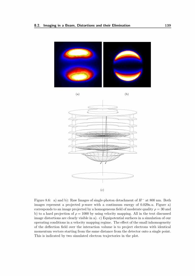
“diss”2002/10/18page 139

8.2. Imaging in a Beam, Distortions and their Elimination 139

(a) (b)

(c)

Figure 8.6: a) and b): Raw Images of single-photon detachment of H− at 800 nm. Bothimages represent a projected p-wave with a continuum energy of 0.029a.u. Figure a)corresponds to an image projected by a homogeneous field of moderate quality ρ = 30 andb) to a hard projection of ρ = 1000 by using velocity mapping. All in the text discussedimage distortions are clearly visible in a). c) Equipotential surfaces in a simulation of ouroperating conditions in a velocity mapping regime. The effect of the small inhomogeneityof the deflection field over the interaction volume is to project electrons with identicalmomentum vectors starting from the same distance from the detector onto a single point.This is indicated by two simulated electron trajectories in the plot.

“diss”2002/10/18page 140

140 Chapter 8. Mapping Continuous Wavefunctions

same velocity vector merge at the same point on the detector. Velocity mapping wasapplied in the experimental image of Figure 8.6b). The image now appears circular.Quantitatively, the images taken under these operating conditions were found to have aradius constant within deviations of less than half a percent over a full turn in the polarangle.

“diss”2002/10/18page 141

CHAPTER 9

Nonlinear Interactions and Image Processing

The experimental approach of the last chapter is applied to the strongfield regime and images of continuous waves formed in photodetach-ment of the negative hydrogen ion are given. Quantitative informa-tion from the raw images is extracted by employing a combination ofback-projection algorithms. This allows a reconstruction of the full 3Dprobability function of the emitted wave. In a further step the data aredeconvolved by a regularization method in order to remove the effectof the finite apparatus function of the spectrometer. Finally, an energycalibration is performed to retrieve the energetic information containedin the spatial images.

Contents

9.1 Experimental Images in a Strong-field Regime . . . . . . . . . 142

9.2 Back-projection . . . . . . . . . . . . . . . . . . . . . . . . . . . 143

9.2.1 The 1D Problem: One-dimensional tomography . . . . . . . . . 144

Exact Inversions . . . . . . . . . . . . . . . . . . . . . . . . . . 145

The Abel-Fourier-Hankel Ring of Transforms . . . . . . . . . . 145

Back-projection in Photoelectron Imaging . . . . . . . . . . . . 146

Direct Iterative Scheme: Onion Peeling . . . . . . . . . . . . . 146

9.2.2 The 2D Problem . . . . . . . . . . . . . . . . . . . . . . . . . . 147

Back-Projection by Iterative Forward-Projection . . . . . . . . 147

Full 2D Inversion by Regularization . . . . . . . . . . . . . . . 149

9.3 Energy Calibration . . . . . . . . . . . . . . . . . . . . . . . . . 150

9.4 Elimination of Effects of the Apparatus Function . . . . . . . 151

141

“diss”2002/10/18page 142

142 Chapter 9. Nonlinear Interactions and Image Processing

9.1 Experimental Images in a Strong-field Regime

The main difficulty in photodetachment experiments in a strong laser field is the depletionof negative ions by a low order detachment process at the leading front of the laserpulse, where the intensity is already sufficient to drive the detachment step. The firstobservation of excess photon detachment (EPD), the analog to ATI, was reported for theF−, Cl−, and Au− negative ions [BCDG91, DMH91, DSB+92, SBBH91], which have arelatively high binding energy of the outer electron. The lowest order detachment processrequired absorption of two or more photons in these experiments. It is not surprisingthat EPD photoelectron spectra were more prominent in these earlier experiments thanin later experiments on H− [SZS+95, ZGB+97], where only the first EPD channel wasobserved in the presence of the prevailing one-photon detachment process. Despite therather high peak laser intensity in the latter observations, the EPD signal was verylow because of saturation of the one-photon process. One should also mention a recentexperiment [PAB99] where photodetachment of H− was studied at the threshold ofthe one-photon process. Here the two-photon channel was observed due to the factthat in negative ions, according to the Wigner threshold law [Wig48], the probability ofphotodetachment tends to zero at threshold, thus, effectively suppressing the one-photonchannel. Higher EPD channels were not observed in this experiment due to saturationof the two-photon process. Reducing the interaction time of negative ions with thelaser beam and increasing the order of the lowest channel is a solution to overcomethe depletion problem. In the present experiment we investigate angle resolved energydistributions of photoelectrons produced by photodetachment of H− in a laser pulse of250fs duration and 2.15µm wavelength. The infrared wavelength requires absorption ofat least two photons in order to overcome the binding energy of 0.75421 eV of H−. Underthese conditions, we observe a photoelectron spectrum which reveals four prominent EPDchannels.

Figure 9.1 shows an image taken under the optimized imaging conditions discussedin Chapter 8. A polarizing cube ensures linear polarization oriented parallel with respectto the detector surface. The laser is focused with a 15cm focal lens to the center of thenegative hydrogen ion beam yielding a peak intensity of 1.7×1013W/cm2. The acquisitiontime was about 3 hours corresponding to ca. 108 accumulated electrons. To avoid longterm drifts of the ion current we recorded the image together with its background imagein a sequence of images, having the laser off and on for the same periods of time. Thesum of background files was subtracted from the sum of signal files. As seen from Figure9.1 a very smooth and highly structured image results. The rings correspond to differentn-photon channels according to the proportionality 〈r〉n ∝ pn. The modulation of theelectron yield at constant radii, i.e. for fixed energies, as a function of the polar angleresembles the energy dependent angular distributions. Nodes indicate the dominance ofsome specific angular momenta. A quantitative analysis of the differential detachmentrates requires the application of numerical routines and is performed here in three steps.First, the process of the projection of the continuous electronic wavefunction must beinverted by a back-projection. In a second step, we correct the data for our apparatusfunction inherent in our detector. Finally, we have to calibrate our momentum scale.

“diss”2002/10/18page 143

9.2. Back-projection 143

050

100150

200

X (pixel)

050100150200

Z (pixel)

1000

2000

3000

CC

D S

igna

l (ar

b. u

.)

Figure 9.1: Raw image of negative Hydrogen in a laser field of 1.7 × 1013W/cm2. Theimage corresponds to ≈ 108 electrons.

9.2 Back-projection

A basic assumption of photoelectron imaging spectrometry, and thus one of the keypoints of the present experiment, is the possibility of an exact reconstruction from theplane detector distribution to the initial three-dimensional distribution function. Thisreconstruction or inversion procedure of a plane distribution most often depends onlyon the geometrical properties of the projection and is called the ”back-projection” pro-cess. In general, projecting always implies a reduction of at least one dimension andthus averaging and loss of information. Nevertheless, in cases where some symmetry ofthe original distribution is known, the full initial distribution can be recovered from theprojected one. This is the case when the initial distribution has cylindrical symmetryaround an axis parallel to the detector. As we show below this important informationof the initial distribution cancels exactly the information loss in the projection process.In the imaging processes described in this thesis a cylindrical symmetry of the electronyield is assured to a high degree of accuracy due to the radial symmetry of an opticaldipole transition in a linearly polarized laser field. Problems involving line-of-sight mea-surements of cylindrically formed objects are commonly known in physics and occur inmany other research fields, such as radio astronomy, flame and plasma diagnostics etc..In practice, all these problems are described by Abel’s integral equation and most tech-niques of back-projection are concerned with its inversion. A large number of inversionmethods have been developed in the last decades. Most of the known techniques are ap-plicable in photoelectron imaging only in the case of ideal imaging conditions, where the2D back-projection problem decays into a set of one-dimensional, independent inversionproblems (see Section 8.2). Apparently, there is in some cases the need of having moresophisticated routines that allow a more general imaging setup, especially for inhomoge-neous field configurations or high initial energy values. The majority of methods is basedon numerical treatments and the traditional inversion routines accumulate numerical er-rors at localized parts of the spectra where significant physical information is then lost.

“diss”2002/10/18page 144

144 Chapter 9. Nonlinear Interactions and Image Processing

In the following we give a brief outline of the most important back-projection methodsthat are appropriate for application in photoelectron imaging. We outline the two moresophisticated 2D inversion methods, and describe the procedure of back-projection thatwe have applied in our experiment.

9.2.1 The 1D Problem: One-dimensional tomography

From Figure 8.5 it is obvious that the problem of reconstructing the full 3D distributionis much simplified for the ideal imaging conditions discussed in Section 8.2.3. Underthese conditions, i.e. when each parallel of latitude is ”separately” projected onto thescreen, the back-projection can be carried out by recovering a set of 2D distributionsfrom associated 1D distributions on the detector surface. This simplifying property turnsout to be very helpful in practice even if back-projecting algorithms exist that can treatmore dimensions.

Let us assume a radial distribution in a plane

rmax

g(x)

x

X

yL

F(r)

r

Y

0

Figure 9.2: Projection of a circularlysymmetric distribution F (r) onto a sin-gle dimension along x. The measureddistribution is represented by g(x).

given by F (r) that is projected onto a singledimension x as depicted in Figure 9.2. Inthis process the radial density is redistributedinto a linear distribution g(x). We take F (r)zero for r > rmax and normalize it to unity inthe plane of definition. The projection alongthe negative y coordinate takes the two-dimensional distribution F (r) over into a one-dimensional distribution function g(x) accord-ing to

g(x) = 2

∫ ymax

0F (√x2 + y2)dy

= 2

∫ rmax

x

F (r)r√r2 − x2

dr (9.1)

The factor 2 arises from the fact that the in-tegration accounts only for the hemisphere ori-entated towards the detector. In the second equation we performed a substitution andexpressed y and dy by r for constant x according to the relation r2 = x2 +y2. The latterrelation is easily found in Figure 9.2 by geometrical means. The second equation inEq.(9.1) has the form of Abel’s integral equation and relates the measured distributiong(x) to the unknown distribution F (r). Extracting the axially symmetric distributionfunction F (r) from the line-of-sight projection g(x) is therefore equivalent to an inversionof Abel’s integral transform. This might be also considered as the one-dimensional vari-ant of the general projection-slice theorem that forms the base of computer tomography.

“diss”2002/10/18page 145

9.2. Back-projection 145

Exact Inversions

Surprisingly, Eq.(9.1) has an exact solution for a general function g(x) whose firstderivative exists1. This solution is unique and has the form

F (r) = − 1

π

∫ rmax

r

g′(x)√x2 − r2

dx (9.2)

Any inversion method based on this exact solution is impracticable in application toexperimental data because the derivative in the integrand tends to amplify the randomerrors in the experimental data appreciably2 [DB82]. To overcome the necessity of dif-ferentiating experimental data M. Deutsch and I. Beniaminy [DB82] have developed in1982 a derivative-free inversion formula

F (r) = − 1

π

g(rmax)− g(r)√

r2max − r2+

∫ rmax

r

g(x) − g(r)(x2 − r2)3/2

xdx

(9.3)

Singular integrands of the kind as in Eq.(9.3) are treatable in numerical integration byavailable standard routines. They demonstrated that the amplification of the randomerrors is suppressed by one order of magnitude compared to a direct computation usingEq.(9.2). Obviously, the simplification of Eq.(9.3) for the back-projection in photoelec-tron imaging has not been appreciated yet and most often iterative inversion schemeshave been invoked.

The Abel-Fourier-Hankel Ring of Transforms

The Abel transformation can be reformulated in terms of a one-dimensional Fourier anda Hankel transform. If an even function F (r) is subsequently transformed by an Abel,Fourier and Hankel transformation according to

2π

∫ ∞

0dq J0(2πξq)q

∫ ∞

−∞dx ei2πqx

∫ ∞

xdr 2rF (r)(r2 − x2)−1/2 = F (ξ) (9.4)

Hankel Fourier Abel

the original function F (ξ) is exactly returned. Hence, the series of this three trans-forms builds a transformation ring. Similarly as the Fourier transformation, the Hankeltransform is self-reciprocal. This remarkable relationship can therefore be used to in-vert Abel’s integral transform by first taking the Fourier transform of the projecteddistribution g(x), and subsequently applying the zeroth order Hankel transform. Thistechnique was first applied in the context of radio-astronomic imaging by R. Bracewellin 1956 [Bra56]. One advantage is that Fast Fourier Transform (FFT) algorithms canbe exploited in its evaluation that greatly reduce the computation time for the inversionprocess.

1This solution can be easily found after transformation to the modified Abel transform and employingthe convolution theorem [Bra00]. For a rigorous mathematical derivation and for a proof of uniquenesssee the mathematical book [B09].

2A reason for this is that Eq.(9.1) belongs mathematically to the class of the so-called ill-posedproblems [WMH+99].

“diss”2002/10/18page 146

146 Chapter 9. Nonlinear Interactions and Image Processing

Back-projection in Photoelectron Imaging

In the process of photoelectron imaging an infinite number of circular distributions as inFigure 9.2 is simultaneously mapped. Only in the case of an exact parallel projectionthese parallels of latitude are not mixed by the projection on the detector. As discussedin Section 8.2 all circles that correspond to the same energy are arranged on a sphere.The radii of these circles are given by r⊥ = X|φ=0 = 2L

√ε sin θ where we have used

ε ≡ 1/ρ instead of ρ. The solution of the classical equations in Eq.(8.1) simplify in thelimit ε→ 0 to

Xε→0−→ 2L cos φ sin θ

√ε Z

ε→0−→ 2L cos θ√ε. (9.5)

If we substitute r⊥ into Eq.(9.1) and rewrite the 3D distribution employing the normal-ization3 2F (r⊥)r⊥dr⊥dφ ≡ f(ε, θ)d(cos θ)dφdε we find

dgZ(X) =

∫ εmax

εmin

dεf(ε, θ)

4L2ε sin θ

√1−

(X

2L sin θ√

ε

)2dZ with θ = arccos

(Z

2L√ε

)

(9.6)The experimental resolution is given by the finite-sized pixels of the CCD array. Theirintensities on the detector are related to the differential rate f(ε, θ) by

gij =

∫ Xi+∆/2

Xi−∆/2

∫ Zj+∆/2

Zj−∆/2dXdZ dgZ(X)/dZ (9.7)

The pixels are assumed to have a square shape of length ∆ and their positions are refer-enced by the indices i and j. Often the pixel size is so small that to a good approximationthe function f(ε, θ) can be taken as constant over the pixel extension and representedby its value at the center values Xi, Zj . Thus, only the kernel function K(X,Z, ε), thatis defined as the integrand apart from f(ε, θ), has to be integrated over X and Z. Thekernel function becomes discretized by this averaging.

Direct Iterative Scheme: Onion Peeling

A commonly used method to invert the equations in Eq.(9.6) is an approach called”Onion Peeling” that is based on an iterative scheme. Consider the symmetric randomdistribution dgZ(X)/dZ on the top left in Figure 9.3 for a fixed θj, or equivalentlyZj . In a first step the discretized kernel K(Xi, Zj , εmax) is scaled to the height of theoutermost pixel(s), top of the right column in Eq.(9.6). This is possible because thesingularity in the denominator is removed on the detector grid for a finite resolution∆. Thus, the scaling factor divided by the energy spacing ∆ε describes the value off(ε = εmax, θj) since no other energy can contribute to dgZ(X)/dZ at its outermost pixel[BPHH96]. In the next step, the scaled kernel function is subtracted from the projecteddistribution at all inner pixel positions. This yields a new function dgZ(X)/dZ thatcontains the information of f(εmax−∆ε, θj) in its outermost energy εmax−∆ε and so on.By this iterative way, the distribution function f(ε, θj) can be found. If this procedureis repeated for all discrete values of θj according to Eq.(9.5) the total 3D distributionf(ε, θ) is recovered from the image gij .

3The normalization for f(ε, θ) was taken in accordance with Ref. [WMH+99], Eq.(4).

“diss”2002/10/18page 147

9.2. Back-projection 147

0

Iter

atio

nSte

pito

i+1

X

dg (X)/dZZ

ε

Scaled kernel functions

Discretized Kernel K(Xi, Zj, εmax)

f(ε, θj)

Figure 9.3: Principle of onion peeling on a finite-sized grid. See text.

9.2.2 The 2D Problem

All known one-dimensional back-projection routines have the additional drawback thatthey accumulate numerical errors in the central line of the unfold images, i.e. at thepositions θj ∼ 0 or π. Moreover, the above method is restricted to ideal imaging con-ditions, i.e. it is valid only in the limit of slow electrons ε → 0. These two reasonshave basically lead to the development of 2D algorithms for the back-projection process[Vra01, WMH+99].

Back-Projection by Iterative Forward-Projection a Quasi-Fitting Method

For all back-projected images presented in this thesis we have used the approach ofVrakking [Vra01] that is illustrated in Figure 9.4. This approach is based on the close re-lationship between the initial 3D angular and velocity distribution P (v) ≡ P1(v)P2(v, θ)and the measured 2D angular and radial distribution Q(R,α) = Q1(R)Q2(R,α). Theradial and angular parts of the 2D and the 3D distributions are defined in Figure 9.4a).The algorithm relies on a quasi-fitting procedure where a first guess is made of the 3Dradial and angular distribution in the back-projected domain due to the high similarity to

“diss”2002/10/18page 148

148 Chapter 9. Nonlinear Interactions and Image Processing

Backprojected byFourier-Hankel Transform

P1,i(v) = P1,i−1(v)− c1 [Q1,i−1(R)−Q1,exp(R)] /2πR

P2,i(v, θ) = P2,i−1(v, θ)− c2 [Q2,i−1(R, α)−Q2,exp(R, α)]

Stop if Average Error

has no more decreasedbetween Qi ↔ Qexp

in the last step.

P2(v, θ)

P1(v)

a) Definition

b) Initialization ( +Normalization)

i=0 A) P1,i=0(v) = Q1,exp(R)/2πR

B) P1,i=0(v)

P2,i=0(v, θ) = Q2,exp(R, α = θ)

c) Iteration

Q1,exp(R)αR

Pi=0(v, θ)

Q2,exp(R,α)

P2,i=0(v, θ)

RenormalizationForward-Projection

2D3D

Perform Correction

Numerical

i→ i+ 1

Take Pi−1(v, θ) = P1,i−1(v)P2,i−1(v, θ) as solution.

Q2,i(R, α)

Q1,i(R)

i > 1

Figure 9.4: Illustration of a two-dimensional, quasi-fitting back-projection method.

the projected distribution. This defines the starting point of the iteration process, Fig-ure 9.4b)A. An alternative is to setup the initialization by means of a 1D back-projectionmethod as described above, Figure 9.4b)B. In a second step, Figure 9.4c), the initialdistribution is numerically ”forward-projected”. Such a forward-projection simulatesthe projection process under the same conditions as the experiment by computing thedetector distribution Qi(R,α) from a given 3D distribution Pi−1(v, θ) according to theclassical model from above. The resulting detector distribution Qi(R,α) is then com-pared to the experimental image Qexp(R,α). The difference of the two 2D distributionsobtained this way is used to setup a correction in the back-projected domain of a fixedsize separately for the angular and radial distribution, c1 and c2, respectively. Thus forevery point in the angular or radial distribution the correction is individual. In the nextcycle the corrected distributions are again forward-projected and subsequently comparedto the experimental image. This procedure repeats and a χ2-test is used to decide on the

“diss”2002/10/18page 149

9.2. Back-projection 149

truncation of the iteration. Finally, if the two detector distribution nearly coincide, theassociated 3D distribution is regarded as the best back-projected physical solution. Abig advantage of this method is that numerical errors are contracted to the unessentialcenter of the image that carries generally no physical information. Additionally, theapproach can even handle images which have involved asymmetries thus allowing forhigh flexibility. However, the iterative convergence in treating our images we found tobe slow. The computational effort greatly benefits from symmetric experimental imageswhen full use of the fourfold symmetry can be made. This reduces running times inback-projecting appreciably and allows also for considering finer iteration steps. In thisway a 3D differential distribution P is found as a function of the radius (or a scaledmomentum) and the polar angle θ. With the aid of a precise momentum calibrationoutlined in Section 9.3 the radial scale is easily turned into an energy or momentumscale.

Full 2D Inversion by Regularization

The general relationship between the differential rate and the pixel intensities valid forany value of ε was derived by Winterhalter et al. Since there are two equivalent directions(θ+, θ−) for the emission of an electron that can hit the same point on the detector, thekernel function K decays into two components K+,K− and the general relationshipassumes the form

gij ≈∫ εmax

εmin

dε K+(Xi, Zj , ε)f(ε, θ+) +K−(Xi, Zj , ε)f(ε, θ−) (9.8)

An expansion of f(ε, θ) into various basis sets turns the integral equation over into amatrix equation for every pixel. The ill-conditioned nature of this matrix is explicitlydemonstrated by these authors employing a singular value decomposition. For a finitevalue of εmax some singular values are exactly zero. This property results in an extremesensitivity to statistical uncertainties of the experimental data. A Tikhonov regulariza-tion is employed that determines an estimate for the differential rate f(ε, θ) from thenoisy data by minimizing the functional

V (λ) =∑

ij

1

σ2ij

(gexpij − gij

)2+ λ||Lf ||2 (9.9)

with respect to the unknown function f(ε, θ) for a constant value of λ. The second termin Eq.(9.9) is a regularization term that constrains the function to some predefined prop-erties, as e.g. the smoothness. Thus, an input information for f(ε, θ) may be suppliedby the operator L and the regularization parameter λ. Often, the identity or the secondderivative is used for the operator L. The regularization parameter λ, which acts as aweighting factor between the two terms, can be chosen manually or by Self-Consistent(SC) methods ([WMH+99] and references therein). This approach currently representsthe most general back-projection algorithm available in photoelectron imaging. However,the computational effort is significantly larger than in the previously outlined methodsand the application in the moment is limited to small image dimensions. For more detailsof this approach the reader is referred to the original publication Ref. [WMH+99]. Aregularization approach in one dimension also turns out to be useful for a deconvolutionof the experimental spectra in Section 9.4.

“diss”2002/10/18page 150

150 Chapter 9. Nonlinear Interactions and Image Processing

9.3 Energy Calibration

(a) Digitally summed image consisting of ex-perimental images at three different wave-lengths. The image was back-projected bythe methods outlined in the preceding Sec-tions. The residual radial width representsthe apparatus function.

Pixel

Ene

rgy

/ eV

2

0.0

0.5

1.0

1.5

2.0

2.5

0 2000 4000 6000 8000 10000

(b) Linearity of the energy scale. The high ac-curacy in the linearity of the mapping is illus-trated. The slope corresponds to the energycalibration coefficient.

Figure 9.5: Energy calibration.

In order to perform a proper energy calibration we recorded images for differentwavelengths by single photon detachment of H−. For this calibration, we performedthree separate measurements at the laser wavelengths: 795.5, 590.1, and 397.8 nm. Thecorresponding kinetic energies of photoelectrons span the broad range from 0.804 to2.363 eV. The intensities were kept low in order to avoid broadening and shifting dueto ponderomotive effects. The centering and addition of individual images at the threewavelengths necessary for a precise calibration, is best done by a mirroring techniquethat relies on the symmetry of the images. This enabled us to determine the center ofan image to within a quarter of the width of a pixel in both dimensions. The digitallysummed image is back-projected using the techniques described in the last Section,Figure 9.5a). The three known wavelengths and the zero momentum point are usedto calibrate the momentum axis. We found an exact linear relation between the radiiand the momenta with a calibration coefficient of 0.976(3) × 106mem/(s pixel) with astandard deviation as given in the round brackets, see Figure 9.5b). The inherent radialprofile in this back-projected calibration image defines the apparatus function of ourdetector. Space charge effects in the projecting area are not significant due to the lownumber of electrons detached per laser pulse. The finite resolution is defined by twoeffects occurring in the detector by the impact of single electrons. The amplified signalat the rear side of the MCPs is of the order of 106 electrons distributed over a spot of a

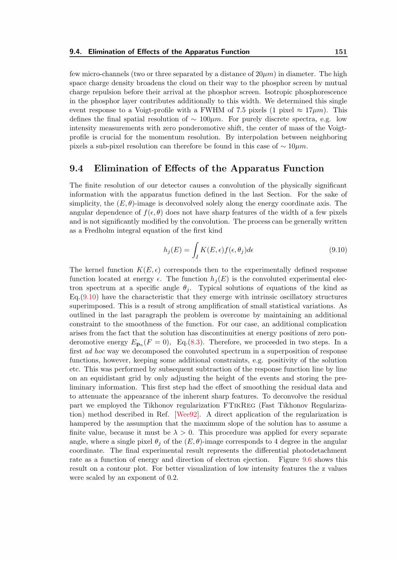
“diss”2002/10/18page 151

9.4. Elimination of Effects of the Apparatus Function 151

few micro-channels (two or three separated by a distance of 20µm) in diameter. The highspace charge density broadens the cloud on their way to the phosphor screen by mutualcharge repulsion before their arrival at the phosphor screen. Isotropic phosphorescencein the phosphor layer contributes additionally to this width. We determined this singleevent response to a Voigt-profile with a FWHM of 7.5 pixels (1 pixel ≈ 17µm). Thisdefines the final spatial resolution of ∼ 100µm. For purely discrete spectra, e.g. lowintensity measurements with zero ponderomotive shift, the center of mass of the Voigt-profile is crucial for the momentum resolution. By interpolation between neighboringpixels a sub-pixel resolution can therefore be found in this case of ∼ 10µm.

9.4 Elimination of Effects of the Apparatus Function

The finite resolution of our detector causes a convolution of the physically significantinformation with the apparatus function defined in the last Section. For the sake ofsimplicity, the (E, θ)-image is deconvolved solely along the energy coordinate axis. Theangular dependence of f(ε, θ) does not have sharp features of the width of a few pixelsand is not significantly modified by the convolution. The process can be generally writtenas a Fredholm integral equation of the first kind

hj(E) =

∫

IK(E, ε)f(ε, θj)dε (9.10)

The kernel function K(E, ε) corresponds then to the experimentally defined responsefunction located at energy ε. The function hj(E) is the convoluted experimental elec-tron spectrum at a specific angle θj. Typical solutions of equations of the kind asEq.(9.10) have the characteristic that they emerge with intrinsic oscillatory structuressuperimposed. This is a result of strong amplification of small statistical variations. Asoutlined in the last paragraph the problem is overcome by maintaining an additionalconstraint to the smoothness of the function. For our case, an additional complicationarises from the fact that the solution has discontinuities at energy positions of zero pon-deromotive energy Epn(F = 0), Eq.(8.3). Therefore, we proceeded in two steps. In afirst ad hoc way we decomposed the convoluted spectrum in a superposition of responsefunctions, however, keeping some additional constraints, e.g. positivity of the solutionetc. This was performed by subsequent subtraction of the response function line by lineon an equidistant grid by only adjusting the height of the events and storing the pre-liminary information. This first step had the effect of smoothing the residual data andto attenuate the appearance of the inherent sharp features. To deconvolve the residualpart we employed the Tikhonov regularization FTikReg (Fast Tikhonov Regulariza-tion) method described in Ref. [Wee92]. A direct application of the regularization ishampered by the assumption that the maximum slope of the solution has to assume afinite value, because it must be λ > 0. This procedure was applied for every separateangle, where a single pixel θj of the (E, θ)-image corresponds to 4 degree in the angularcoordinate. The final experimental result represents the differential photodetachmentrate as a function of energy and direction of electron ejection. Figure 9.6 shows thisresult on a contour plot. For better visualization of low intensity features the z valueswere scaled by an exponent of 0.2.

“diss”2002/10/18page 152

152 Chapter 9. Nonlinear Interactions and Image Processing

Electron energy [eV]

Em

issi

on a

ngle

(de

gree

) 360

270

180

90

00 0.5 1.0 2.0 2.5

n=4n=3n=2 n=5 n=6

1.5

3000

1000

240

30

1

0

Figure 9.6: Experimental photodetachment rate as a function of the continuum energyand emission angle of the photodetached electron.

“diss”2002/10/18page 153

CHAPTER 10

Theoretical Approach to Strong-Field Detachment

We outline the recent KFR-approach of Gribakin and Kuchiev that isused in the following discussion and interpretation of our experimentaldata. With the help of this theory we simulate our experiment includingsaturation, ponderomotive and residual volume averaging effects. Thisallows us to perform a quantitative comparison between theory and ex-periment. We prove that in the short-pulse regime of our experimentspatial intensity variations in the focal area have no major influence onthe energy spectra.

Contents

10.1 The Keldysh-Faisal-Reiss Approach . . . . . . . . . . . . . . . 153

10.2 Saturation, Focal-Volume Averaging, and PonderomotiveShifts . . . . . . . . . . . . . . . . . . . . . . . . . . . . . . . . . . 155

10.3 Spatial Effects in the Focal Area: Short Pulse vs Long PulseRegime . . . . . . . . . . . . . . . . . . . . . . . . . . . . . . . . . 157

10.4 Comparison of Experiment and Theory . . . . . . . . . . . . . 157

10.1 The Keldysh-Faisal-Reiss Approach

The adiabatic approach of Gribakin and Kuchiev [GK97] is quite similar to the originalwork by Keldysh [Kel64] and Perelomov et al. [PPT66]. These so-called KFR-approaches[Kel64, Fai73, Rei80] are characterized by some strict assumptions. However, the mainadvantage of these methods is their high flexibility and analyticity. This enables oneto easily interpret and explore the general behaviour of the solutions. Owing to theshort range potential which binds the electron in negative ions, Keldysh-Faisal-Reisstheories are appropriate to describe the observed energy and angular distributions froma multiphoton regime γ 1 to a tunneling regime γ 1. The quantity γ representshere the famous Keldysh- or adiabaticity parameter that is introduced later in the text.

153

“diss”2002/10/18page 154

154 Chapter 10. Theoretical Approach to Strong-Field Detachment

The theory of Gribakin and Kuchiev [GK97] follows this original approach but is notlimited to small electron momenta as are earlier approaches. The n-photon transitionamplitude is calculated as

Anp =

1

T

∫ T

0dt 〈Ψp(r, t)|V (t)|Ψ0(r, t)〉 , (10.1)

where the matrix element is averaged over the laser-cycle period T . The wave functionΨ0(r, t) = e−iE0t Φ0(r) describes the unperturbed ground state of the negative ion withthe binding energy E0 = −κ2/2. Its time-independent part Φ0 was introduced in Chapter7. The final state is described by the Volkov function

Ψp(r, t) = exp

[i(p + kt) · r−

i

2

∫ t

(p + kt′)2dt′]

(10.2)

which represents the wave function of a free electron in the laser field. This approachreceived the name strong field approximation since only one of the two fields, either theatomic core field or the laser field is considered to be strong and is taken into accountexplicitly in the description of the initial or final state, respectively.

Due to the energy conservation rule the energy of the released electron is given by(in atomic units)

E(n) = E0 + nω (10.3)

This energy is also given as the sum of a drift term and the ponderomotive energy,Up = F 2/(4ω2), a term describing the quiver motion of the electron in the laser fieldF(t) = F0 cosωt :

E(n) = p2/2 +F 2

4ω2. (10.4)

Under conditions of a short laser pulse (see Section 10.3) the electron energy at aremote detector is equal to the drift energy E = p2/2. In the presence of the field, themomentum of the released electron at time t is given by p + kt, where the momentumgained from the electric field of the laser is given by

kt =

∫ t

F(t′) dt′ . (10.5)

With the Volkov wave function Eq.(10.2), the integrand of Eq.(10.1) contains therapidly oscillating exponential term [GK97]

exp [iS(ωt)] = exp

[i

2

∫ t

(p + kt′)2dt′ − iE0t

]. (10.6)

Thus, the transition amplitude in Eq.(10.1) can be evaluated by employing a saddlepoint approximation. Note that t describes the time during the laser pulse while t ′ is thetime the electron has spent in the continuum state, measured from the time of emissionfrom the bound state. The saddle points are given by the condition of stationary actiondS(ωt)/dt = 0 which yields the relation

(p + kt)2 + κ2 = 0 . (10.7)

“diss”2002/10/18page 155

10.2. Saturation, Focal-Volume Averaging, and Ponderomotive Shifts 155

Using expression Eq.(10.5) the solution of(p +

F0

ωsinωtµ

)2

+ κ2 = 0 (10.8)

defines two pairs of complex values of the time tµ when the transition from the boundstate to the Volkov state may occur. The real part of tµ denotes the real time of oc-currence, the inverse of the magnitude of the imaginary part of tµ is a measure of theprobability of the electron emission process. Obviously the maximum probability occursnear the maximum of the electric field. In this case the two saddle-point pairs merge toa single pair and an electron of zero kinetic energy emerges. The main matrix elementEq.(10.1) describing a n-photon transition for a negative ion with isotropic initial state(ν = l = m = 0) is finally reduced to

Anp =

∑

µ=1,2

(cµ + isµ)n√2π(−iS′′µ)

exp[−icµ(ξ + zsµ)] (10.9)

The abbreviated terms of this equation are

cµ = ±√

1− s2µ (10.10)

sµ = (−ξ ± i√

8z(n− z)− ξ2)/4z

S′′µ = cµ(ξ + 4zsµ)

where the quantity S ′′µ represents the second derivative of the classical action. The +and − sign correspond to the saddle points µ = 1, 2. The parameters ξ = eFp cos θ/ω2

and z = e2F 2/4ω3 describe the angular dependence and the ponderomotive energy inunits of the photon frequency, respectively. F is the electrical field strength of the laserand θ the ejection angle of the electron with respect to the laser polarization. For laterconsiderations we introduce here the Keldysh parameter defined by γ = ωκ/F .

As pointed out by Salieres et al. [SCD+01] (and references therein), an amplitudeas in Eq.(10.9) represents the familiar form occurring in path integral formalisms ofquantum theory. This circumstance enables the interpretation in terms of complex tra-jectories whose real part is identical to the classical path and whose imaginary part isa measure for the weight for a possible path in the amplitude An

p. The simultaneousexistence of two equivalent saddle points is responsible for the occurrence of interfer-ence phenomena between the two associated quantum trajectories. From the amplitudeEq.(10.9) the differential rate for the n-th channel dwn/dΩ is calculated in a straight-forward manner [GK97]. In the next Section we make use of these rates to extract thedifferential rate that describes our experiment. The total rate involving n photons isgiven by the integral over the solid angle

wn(ω, I) = 2π

∫ π

0

dwn

dΩ(ω, θ) sin θdθ (10.11)

10.2 Saturation, Focal-Volume Averaging, and Inclusion of

Ponderomotive Shifts

For a direct comparison with the experimental spectrum of Figure 10.1 several mech-anisms defined by the experiment need to be taken into account. We approximate the

“diss”2002/10/18page 156

156 Chapter 10. Theoretical Approach to Strong-Field Detachment

temporal and spatial intensity profile (cf. Appendix I) of our laser pulse by

I(ρ, t) = IPeak e−(ρ/σρ)2sech2((t− t0)/σt) (10.12)

This defines the pulse length by σt and the focus waist by σρ. It is not necessary toconsider an intensity dependence along the laser propagation axis because the Rayleighlength of the focus is about five times longer than the width of the ion beam (or in-teraction volume). The experimental parameters were extracted from a thorough laserpulse diagnostics described in Appendix I: σt corresponds to a FWHM ≡ 2 ln(1 +√

2)σt = 250fs. The focal waist associated with σρ is well described by a Gaussianshape with an experimentally determined FWHM of 50µm. From these values and fromthe measured pulse energy Epulse = 56µJ the peak intensity was calculated by usingIPeak = 0.85Epulse/(2πσtσ

2ρ) to 1.7 × 1013W/cm2 where we also included the window

transmission of 0.85. Characteristic values for the ion beam are given in the experimen-tal Section. Saturation effects in the interaction volume are taken into account by theset of rate equations

g(ω, ρ, t) = exp

−∑

n

∫ t

−∞dt wn(ω, I(ρ, t))

(10.13)

pn(ω, θ, ρ, t) =dwn

dΩ(ω, θ, I(ρ, t)) · g(ω, ρ, t) (10.14)

The time dependent differential rates pn(·) of Eq.(10.14) of all final channels n areassumed to be proportional to the ground state population g(·) in Eq.(10.13). Thedepletion of the ground state population at time t is defined by the sum of the totalrates wn(ω, I(ρ, t)) of all final channels integrated over the time interval [−∞, t]. Thetotal and differential rates in Eqs.(10.13) and (10.14) are computed by relating the fieldstrength F in Eqs.(10.9)-(10.10) to the laser intensity I in Eq.(10.12) using I ≡ F 2.

At high intensities ponderomotive effects do play an important role. The temporaldependence of I affects the electron spectrum by shifting and broadening of the EPDpeaks. Both effects are consequences of the ponderomotive energy shift and electrondynamics. According to Eq.(8.3) the electron drift energy is reduced when the laserintensity rises. The shift of the maximum of a EPD peak is then defined by the compe-tition between the channels according to the rate equations Eqs.(10.13) and (10.14). Athigh energies the residual population for a specific channel is transferred preferentiallyto higher channels and the rate for this channel decreases again. This also defines theponderomotive width of an EPD peak and its asymmetric line shape. In the followingSection we show that our experiment is in a short-pulse regime and that Eq.(8.3) exactlydefines the electron energy in the continuum at all instants of time. The complete resultis then given by the superposition of the n-th channel differential rates as

dΓ

dΩ(E, θ) ∝

∑

n

∫ ∞

0dρ ρ

∫dt pn(ω, θ, ρ, t)δ(nω −E − I(ρ, t)

4 ω2+E0) (10.15)

where the δ-function accounts for the ponderomotive shift at time t. This differentialrate is compared in Figure 10.1 with the experimentally measured rate. In the simula-tion we recognized that the sensitivity to the temporal shape of the laser beam is crucialin reproducing the correct widths of the EPD peaks. We noticed that this is particu-larly important at intensities several orders of magnitude below the peak intensity. We

“diss”2002/10/18page 157

10.3. Spatial Effects in the Focal Area: Short Pulse vs Long Pulse Regime 157

achieved best agreement with a temporal envelope as a sech2 dependence, consistentwith the measured autocorrelation trace.

10.3 Spatial Effects in the Focal Area: Short Pulse vs Long

Pulse Regime

The spatial variation of intensities in a laser focus gives rise to a ponderomotive forceF = −∇Up on the electron where Up ≡ I(x, y, z)/4ω2. This corresponds to a conversionof the electron quiver energy into translation energy, when the electron leaves the areaof the laser focus. For a short laser pulse this energy transfer can not be completedif the pulse duration is shorter than the escape time to exit from the laser beam. Inthe opposite limit, i.e. for a infinite pulse duration, the total quiver energy can betransferred completely into translation energy and adds 1 Up to the drift energy. Uponinspection of the drift energy in Eq.(8.3) the influence of the AC level shift is exactlycanceled in this regime, i.e. the last term in Eq.(8.3) vanishes by this effect. Hence, theelectron energy spectrum appears as totally unaffected by ponderomotive effects. Forthe case under discussion here a classical estimate establishes whether partial conversionof ponderomotive into drift energy has to be considered in our case. The temporalbehaviour of the envelope of the electrical field of a laser pulse can be approximatedby an exponential pulse shape exp(−γ|t|). This has the advantage that the transferredenergy from the quiver motion to translational energy can be given in analytical form[SDH94]

EGain = Up(1−[√π exp(β2)erfc(β)

]) (10.16)

with β = σρ/(2σtvn=2). The latter ratio uses the value β ∼ 265 for the parame-ters discussed in Section 10.2, viz the pulse length σt = 12511 a.u., the focal radiusσρ = 1.14 · 106 a.u., Up = 7.33eV and the nascent velocity vn=2 = 0.171 a.u., wherethe latter corresponds to 400meV continuum energy of the electron. Inserting β intoEq.(10.16) yields EGain ∼ 50µeV which is much below our experimental resolution.Thus, ponderomotive acceleration in the focal area does not influence our electron en-ergy spectra in any significant way and the validity of Eq.(8.3) is established.

10.4 Comparison of Experiment and Theory

The result of Eq.(10.15) is shown in Figure 10.1 together with the experimental result.The latter is repeated from Figure 9.6 for easier comparison. The color scaling isidentical in both images and the normalization of the two spectra was taken accordingto the volumina below their surfaces. The overall comparison shows a good agreementand all features are present in both spectra. The ponderomotive shift of the peaksincreases with the order of the EPD channel. This shift however is much smaller thanthe value 7.33eV, which corresponds to the peak intensity measured in the laser focus.Thus, most of the detachment events occur at a small fraction of the peak intensity.The theoretical curve reproduces the heights and energy positions of peaks well, thoughthe experimental peaks are slightly narrower and lower for higher EPD channels. In thefollowing Chapter 11 we give a quantitative account for the comparison shown here.

“diss”2002/10/18page 158

158 Chapter 10. Theoretical Approach to Strong-Field Detachment

Electron energy [eV]0 0.5 1.0 2.0 2.51.5

n=4n=3n=2 n=5 n=6

270

180

90

0

360

270

180

90

0/360

3000

240

30

1

0

1000

Em

issi

on a

ngle

(de

gree

)T

heor

yE

xper

imen

t

Figure 10.1: Differential rates as extracted from the experiment (upper panel, identicalto Figure 9.6) and from the Keldysh-approach (lower panel). Note that the out ofplane scale was taken to an exponent of 0.2 for visualizing also tiny features of thespectrum. Hence, the only slightly broader peaks in the simulated spectra comparedto the experimental peaks appear exaggerated. The normalization of the two spectra isdone by adjusting their volumes below the surfaces. Scale numbers of the contours arearbitrarily chosen units.

“diss”2002/10/18page 159

CHAPTER 11

Physical Interpretations & Discussion

We present a comprehensive analysis of the energetically resolved angu-lar distributions of the four observed excess photon detachment (EPD)channels. A quantitative comparison between theory and experimentis made in terms of partial wave amplitudes and phases. We showthat both spectra exhibit the quantum interference effect that causescounter-intuitive angular patterns in photodetachment. The relation ofthis effect to the Wigner-threshold law of photodetachment is discussed.The good agreement between experiment and theory suggests that theWigner-law also holds in a strong AC-field regime. We outline problemsthat arise in the determination of partial wave amplitudes and point outthe existence of a certain physical domain of the generally used asym-metry parameters (or β parameters).

Contents

11.1 Discussion . . . . . . . . . . . . . . . . . . . . . . . . . . . . . . . 159

11.1.1 The Lowest-Order Channel and the Threshold effect . . . . . . 160

11.1.2 Comparison of Higher Order Channels and Ambiguity in Partial-Wave Analysis . . . . . . . . . . . . . . . . . . . . . . . . . . . 165

11.1.3 Quantum Interferences . . . . . . . . . . . . . . . . . . . . . . . 167

11.2 A Simple Picture of Quantum Path Interferences in Nega-tive Ions . . . . . . . . . . . . . . . . . . . . . . . . . . . . . . . . 168

11.1 Discussion

The final result of our theoretical and experimental analysis is summarized in Figure10.1. Due to the large difference between the first and the second ionization potential ofH− (∼ 0.75 eV and ∼ 13.61 eV, respectively), it is obvious that the detected electronsstem solely from single photoionization processes of H− and not from further ionization

159

“diss”2002/10/18page 160

160 Chapter 11. Physical Interpretations & Discussion

of neutral Hydrogen or double photoionization. At the wavelength used here the latterprocess would require 25 photons to overcome the total ionization potential of −14.36eV .From both spectra in Figure 10.1 the ponderomotive level shift is visible as a shift ofthe population towards lower energy. It is apparent that this shift increases for higherchannels. The unshifted positions Epn(F = 0), n = 2−6 are indicated at the top by thearrows. This shift shows that higher channels become only effectively populated at higherintensities where large ponderomotive shifts prevail. Since the different photon channelsare energetically well separated we can analyze each photon channel individually. Thetwo-photon channel extends to zero electron energy and we discuss it in a separateparagraph.

11.1.1 The Lowest-Order Channel and the Threshold effect

Figure 11.1 shows the experimental ADs of the lowest order channel from Figure 10.1as polar plots at energies between the threshold and the unperturbed two-photon limitat Ep2(F = 0) = 399.1meV . We employed a standard Levenberg-Marquard algorithmto perform a non-linear fit to the functional expression

dΓn

dΩ= |fpn(θ)|2 with fpn(θ) =

Lmax∑

L=0

f(n)L YL0(θ, φ) (11.1)

dΓn/dΩ represents the differential rates of the n-th channel in Figure 10.1. This func-tional form corresponds to a partial wave decomposition with the complex amplitudes

f(n)L . A natural choice for the total phase in the sum of Eq.(11.1) is to choose the phase

for the highest contributing partial wave zero, i.e. we choose f(n)Lmax

real, because thephases in a short-range potential rapidly tend to zero for higher L. The parity of thefinal state implies that either only odd or even partial waves contribute to the sum inEq.(11.1). Thus, there remain Lmax or Lmax + 1 fitting parameters for a given maximalpartial wave with angular momentum Lmax for odd or even final state parity, respectively.In order to explore effects of stimulated reemission processes from the three photon intothe two photon channel we chose Lmax = 4 corresponding to an inclusion of g-waves inthe lowest order channel. A simple consideration by selection rules would allow only s-and d-wave angular momentum states for a pure two-photon channel. The theoreticalspectrum is analyzed in the same way as the experimental one. The outer solid line inthe right column of Figure 11.1 corresponds to the result of the experimental fit and thedots to the measured pixel values. The inner dotted line defines the analogous fit to theresult of the KFR-approach. For better visual convenience it is adjusted to 0.8 of the sizeof the experimental maximum. Generally, we find a good agreement between theory andexperiment. For the two-photon channel the ADs undergo strong modification closer tothe threshold. These modifications are associated with an increase of the intensity ofthe laser pulse or according to the energy conservation Eq.(8.3) with a decrease in thecontinuum energy of the electron.

However, these drastic changes result not unexpectedly if the Wigner-law is assumedto hold. E. Wigner has presented in 1948 [Wig48] a general law for the energy depen-dence of partial cross sections in elastic scattering processes1 in the vicinity of thresholds.

1Its application is also justified in the case of photoionization. The incoming photon is viewed just

“diss”2002/10/18page 161

11.1. Discussion 161

Figure 11.1: Experimental andtheoretical angular distributionsfor the two-photon channel. Thelaser polarization is oriented ver-tically in the graph. The depen-dence of the ADs on the laser in-tensity is shown from the top tothe bottom with increasing fieldstrength F . The left columncontains 3D angular distributionsobtained from the experimentaldata where we have assumed thecylindrical symmetry implied bythe dipole transition. The rightcolumn depicts the experimentaldata together with a fit (dots andouter solid line, respectively). Theinner dotted line represents theab initio ADs from Figure 10.1(lower spectrum). The radial scaleof the theoretical curve with re-spect to the maximum of the ex-perimental fit was shrunk by a fac-tor 0.8 for visual convenience. Thecorresponding electron energy Eabove the detachment threshold isalso given on the right for eachAD.

F ~ 0.0022 a.u.E ~ 325 meV

F ~ 0.0035 a.u.E ~ 217 meV

F ~ 0.0029 a.u.E ~ 271 meV

F ~ 0.0040 a.u.E ~ 163 meV

F ~ 0.0044 a.u.E ~ 108 meV

F ~ 0.0042 a.u.E ~ 136 meV

“diss”2002/10/18page 162

162 Chapter 11. Physical Interpretations & Discussion

According to this law, a partial cross section scales as σL ∝ |fL|2 ∝ εL+1/2 where L isassociated with the angular momentum of the outgoing partial wave. Thus, partial waveamplitudes behave according to the Wigner-law quite different as functions of energy

f(2)L ∝ εL/2+1/4 in the proximity of the threshold. Close to the threshold the s-wave

clearly dominates and an isotropic distribution is to be expected. We can see thatthis tendency is indeed observed in the experiment. For the intensities associated withF = 0.0040a.u., F = 0.0042a.u. and F = 0.0044a.u. just below F = 0.0051a.u. at whichthe two-photon channel closes, the ADs assume slowly an isotropic s-wave distribution.ADs from data at energies closer to the threshold have already decreased appreciably inelectron yield and are not presented here. Their estimated statistical and/or systemati-cal errors introduced by the back-projecting and deconvolution are of the same order asthe signal. The isotropic electron yield is reproduced and better seen in the theoreticalspectrum in the lower part of Figure 10.1 which exactly follows the behaviour of theexperimental data in the vicinity of the threshold. More quantitatively, we present inFigure 11.2 the squared moduli of the normalized partial wave amplitudes for the exper-imental and the theoretical data. This partial wave analysis provides information about

the energy dependence of the partial wave composition. Since f(2)4 is very small in the

experimental as well as in the theoretical curve, this analysis establishes that reemissionprocesses from higher channels by stimulated emission pumping is not effective enoughto be observable. The main error in the fit is of systematic nature and a result of theuncertainty in the background. From this uncertainty the error bars in Figure 11.2 wereestimated. An additional problem arises through systematical errors in the data process-ing. The disagreement with the theoretical data at the right end of the displayed curvesis attributed to a failure of the deconvolution process at the infinite slopes. Nevertheless,we find quantitative agreement in the low energy part of the two-photon channel. From

the fit we can also extract the relative phase of the amplitudes f(2)0 and f

(2)2 . This phase

difference is identified as δ0−δ2 where δ0 and δ2 are the elastic scattering phases of s- andd-wave electron scattering on neutral Hydrogen [SL88]. In general these quantities definethe asymptotical final state wavefunction in a photodetachment process, cf. Eq.(8.4).The values extracted from our data are only defined modulo π and the sign is not definedby the experiment in the case of linear polarization. This leads to an ambiguity thatwe describe in the next Section. We show the data in Figure 11.3 together with resultsfrom an effective range theory (ERT) approach [OO60], given by

p cot δ0p→0= −γ +

1

2ρ(γ2 + p2) +O[(γ2 + p2)2] (11.2)

The parameters in Eq.(11.2) are taken from Ref. [OO60] and precisely known for singlets-wave scattering. For the sake of completeness, we also plot the d scattering phase basedon the polarization force (α0 = 4.5a.u., see Section 7.3) [LC93] of the hydrogen coreaccording to Eq.(11.3)

tan δLp→0=

πα0

(2L+ 3)(2L + 1)(2L − 1)p2 +O[p3] (11.3)

Its determination is however much below the accuracy of our experiment. Again, wefind the experiment in good agreement with these theoretical approach, whereas the

to lift the electron into the continuum where the subsequent potential interaction defines the outgoingstate as in elastic scattering.

“diss”2002/10/18page 163

11.1. Discussion 163

0 50 100 150 200 250 300 350 4000.0

0.2

0.4

0.6

0.8

1.0

Electron energy [meV]

L=0 L=2

L=0L=2

L=4

L=4

2l

Part

ial P

roba

bilit

y |f

|

0.0

0.2

0.4

0.6

0.8

1.0

Figure 11.2: Squared moduli of partial wave amplitudes for the two-photon channel. Theprobabilities of the three considered partial waves with angular momenta L = 0, 2, 4 arenormalized to unity. a) and b) refer to an analysis of the experimental and theoreticalspectra in Figure 10.1, respectively.

phase extracted from a similar fit to the KFR-approach is in complete disagreement.This should not surprise because the KFR-approach uses a very simple initial statewavefunction associated with a zero-range potential that does not carry any energydependent phase characterizing the real potential. The slightly smaller slope in theexperimental curve might be an error introduced by the residual broadening that is stillretained from the apparatus function.

Due to the good agreement in Figure 11.1, we expect the Wigner-law also to hold ina strong-field regime. It is intriguing to pursue this aspect further in the analytical KFR-approach. Upon expansion of the general result from the matrix element in Eq.(10.9)in the vicinity of the detachment threshold, Gribakin and Kuchiev have presented asimplified formula for low momenta (Eq.(42) of Ref.[GK97]) valid in the range p2 κ2 = 2|E0|. For the case considered here it is given by

dwn

dΩ∝ p exp

[(− sinh−1 γ +

γ cos2 θ√γ2 + 1

)p2

ω

]1 + (−1)n cos

(2κp cos θ

√γ2 + 1

ωγ

)

(11.4)

This formula is an odd function in the momentum p implying, that written as a powerseries in p, only odd powers in the momentum exist. On the other hand, using theWigner law in the form fL ∝ pL+1/2 it is obvious that all terms in the differential rate inEq.(11.1) assume only odd powers in p, viz. fLf

∗L′ ∝ pL+L′+1, because L+ L′ is always

even for a definite parity. Thus, the KFR approach is consistent with the Wigner-law.Furthermore, it is clear that for even parity in the final state the ADs from the KFR-approach reduce close to threshold to a constant, i.e. to an isotropic distribution. In

“diss”2002/10/18page 164

164 Chapter 11. Physical Interpretations & Discussion

0 50 100 150 200 250 300 350 400Electron energy [meV]

0

1

2

3

4

Phas

e di

ffer

ence

x 100

δ0

δ2

(δ0−

δ 2)m

od

/R

adia

n π

Figure 11.3: Experimental phase difference between elastic scattering phases of s- andd-wave scattering. Error bars are estimated as in Figure 11.2. The upper and lowersolid line represent theoretical results from the ERT formula Eq.(11.2) of Ref.[OO60]for singlett s-wave scattering δ0, and for d-wave scattering from formula Eq.(11.3),respectively. The dashed line depicts the numerical data taken from Ref.[LC93]. For thescattering phase δ2 the two theoretical approaches exactly coincide in this energy range.

analyzing the expression in Eq.(11.4) it is found that all expansion coefficients containthe term (1 + (−1)n) that switches between even and odd parity final states. Especiallythe lowest expansion term proportional to p is switched on for even parity and off forodd parity. In the latter case the lowest order becomes proportional to p3 in accordancewith the Wigner law. Thus, our measurements in combination with the KFR approachsuggest that there is no modification of the Wigner-law to expect up to intensities of thetwo-channel closure intensity of 9.2× 1011W/cm2.

We also mention that for strong static electrical fields such modifications of theWigner-law have been theoretically described [FMS01]. The dramatic change in the an-gular distributions was recently also identified as a threshold phenomena by calculationsof Borca et al. [BFMS01]. They used a three-dimensional, zero-range potential anddiscussed the general case of elliptically polarized light. Fortunately, the left columnof their Figure 3 is nearly comparable to our Figure 11.1. Their angular distributionsare plotted for ω = 0.8 in units of the binding energy, where we have ω = 0.76. Theunusual behaviour of a complete destructive interference along the laser polarizationobserved here experimentally is thus confirmed by their approach. These authors alsocalculate data of the three-photon channel, which we find in qualitative agreement withthe Keldysh-approach used here. Preferential detachment along directions of θ ∼ π/4with respect to the laser polarization are expected. A similar behaviour is seen in thetheoretical spectrum in Figure 10.1 at energies just above the two-photon limit. In ourapproach however the maximum yield in contrary to Ref. [BFMS01] appears at θ ∼ π/3.Since in this energetic area our experimental data is not reliable due to the failure of

“diss”2002/10/18page 165

11.1. Discussion 165

proper deconvolution, we do not observe this feature experimentally.

11.1.2 Comparison of Higher Order Channels and Ambiguity in Partial-

Wave Analysis

A direct comparison of our theoretical and experimental analysis of the higher-orderchannels is presented in Figure 11.4. The variations of the ADs with energy in theobservable range are small and we show the three- to six-photon channels only at thespecific energies 813(n = 3), 1382(n = 4), 1897(n = 5), 2466(n = 6) meV where the EPDpeaks assume their maxima. Due to the increase in the photon number the maximumallowed angular momenta become larger for higher channels as well as the expectationvalue of the angular momentum. This explains the decreasing width of maxima of theelectron yield along the laser polarization for increasing n. This is a general tendency ofboth the experimental and the theoretical data. The ADs and in particular the widthof the maxima are very precisely reproduced by the KFR approach. In the intermediaterange smaller discrepancies are found. Noticeable is that the systematic disagreementappears strongest for the odd photon channels.

In fitting the angular distributions we found that a certain ambiguity arises in thedetermination of the partial amplitudes. This follows from the mathematical structureand introduces a 2Lmax/2 degeneracy to the solution. Experimental results cannot be usedto distinguish between these equivalent sets of complex partial amplitudes and furthersupport from theory is required to identify the correct solution. This ambiguity is ofthe same type as the ambiguity that arises in nucleon-nucleon scattering of zero spinparticles [BA85]. As we show here, this does not only concern the sign of the phases andcombinations thereof but also the moduli of partial wave amplitudes are affected. Thus,the solution resulting from a fit is only one of 2Lmax/2 possibilities and care must be takenin its interpretation. Further consequences are found for the set of beta parameters whichare most often given as simple fit parameter in an expansion in Legendre polynomials.We show in Appendix J the origin of this ambiguity and how all other solutions areeasily generated if one is known. It will also become obvious which additional constraintsto the set of beta parameters must be considered in fitting angular distributions.

In order to circumvent the numerical representation of all solutions we summarizethe results in Table 11.1 in the form of correct sets of beta-parameters for the two-,three- and four-photon channel.

Table 11.1: Beta parameters for the channels n = 2 − 4. These sets were obtained byexplicitly accounting for the constraint discussed in Appendix J.

Order of photon process Energy in Beta parametersn meV β0 β2 β4 β6 β8

2 108 1.00 -1.22 0.13 0.11 0.01325 1.00 -0.17 1.67 0.04 0.00

3 813 1.00 2.51 2.44 2.12 - 1

4 1382 1.00 3.39 3.67 2.62 0.73

1 For final states of odd parity we included in the fit only p- and f -waves and their relative phase.

“diss”2002/10/18page 166

166 Chapter 11. Physical Interpretations & Discussion

0.0

0.4

0.8

1.2

1.6

2.0

n=3

0.00

0.10

0.20

0.30

0.40

0.50

0.60

n=4

0.00

0.04

0.08

0.12

0.16

n=5

0 30 60 90 120 150 180

0.000

0.010

0.020

0.030

0.040

n=6

elec

tron

yie

ld (

a.u.

)

emission angle / degree

1897 meV

2466 meV

813 meV

1382 meV

Figure 11.4: ADs of the chan-nels n = 3 − 6. The effect of in-tensity variations on the ADs ismuch weaker than for the two-photon channel. The subfiguresin this graph represent angulardistributions close to the max-ima of the EPD-peaks at ener-gies 813(n = 3), 1382(n = 4),1897(n = 5), 2466(n = 6) meV.The y-axes are scaled to eachother for best overlap.

“diss”2002/10/18page 167

11.1. Discussion 167

11.1.3 Quantum Interferences

As mentioned above the two saddle points can be associated with two complex quantumtrajectories. Such trajectories are candidates that may destructively interfere and thusreduce the detachment yield for any specific spatial direction. We want to suggest anotherphysical picture that naturally develops from the KFR-approach used. This turns outto be equally useful and is fully consistent with the mentioned one, however, its originhas a rather stationary nature. In the simplified expression Eq.(11.4) the existence oftwo equivalent electron trajectories is expressed by the existence of the cos-term in thelast factor surrounded by curly braces. We can analyze from this last term under whichconditions a complete destructive interference might be supported. Since this expressionis only valid for p2/2 |E0| we may only expect to see interference effects for the lowerphoton channels. The last factor exactly vanishes along the polarization axis (θ = 0) if

p =ω

2κ

γ√1 + γ2

×ck with ck =

(2k + 1)π for even parity

2kπ for odd parity k = 0, 1, . . .(11.5)

Herein, the parity refers to the parity of the final state which is exactly defined by thenumber of photons involved in the multiphoton transition. The values of the index k,are defined by the electrical field strength as follows from Eq.(11.5)

F = ω

√(2nω + 3E0)±

√(2nω +E0)2 − ω2c2k/2 (11.6)

as a real quantity. Thus, for n = 2 we find only k = 0, and for n = 3 only k = 1 aspossible values. The corresponding energies are then given by

Epn =

((2nω +E0)∓

√(2nω +E0)2 − ω2c2k/2

)/4 (11.7)

where the upper(lower) sign in Eq.(11.6) corresponds to the upper(lower) sign in Eq.(11.7).Table 11.2 contains the energies and field strengths where total destructive interference

should occur for the photon channels n = 2 and n = 3 for H− and for the wavelengthω = 0.0212a.u. used in our experiment. In order to find a more intuitive picture we canmodify Eq.(11.5) further. The amplitudes along the laser polarization of the quiveringmotion of the electron are given by [GK97]

r(tµ) = ±κω

√1 + γ2

γ(11.8)

at the two saddle points, µ = 1, 2, respectively. If we combine Eqs.(11.5) and (11.8), andexpress the momentum p by the de-Broglie wavelength 2π/λ of a free particle, we findthe condition for the ”slit separation” d as

d ≡ |r(t1) − r(t2)| = 2r(t1) =

(k+1/2)λ for even parity

kλ for odd parity k = 0, 1, . . .(11.9)

This means whenever the distance d becomes an odd- or even-integer multiple of λ/2destructive interference occurs for even parity or odd parity in the final state, respectively.

“diss”2002/10/18page 168

168 Chapter 11. Physical Interpretations & Discussion

Table 11.2: Field strengths and energies where destructive interference occurs for thetwo- and three-photon channel (n = 2, 3) and the given experimental conditions. Theroots for the expanded expression are given in the left columns and minima of the fullexpression in the right columns, respectively. The field strength Fn and the energy Epn

are given in atomic units. The latter is also given in meV . The third column containsthe threshold energies for the two channels for vanishing ponderomotive shift.

channel index Threshold Fn Epn

from Eq.(11.6) FE2: Eq.(10.9) from Eq.(11.7) FE2: Eq.(10.9)n k (meV ) (a.u.) (a.u.) (a.u.) (meV ) (a.u.) (meV )

2 0 399.1 0.00390 0.00423 0.00621 168.9 0.00470 127.83 1 975.8 0.00584 0.00646 0.01687 458.9 0.01266 344.5

0.00232 ×1 0.03285 894.0 ×1 ×1

1 Corresponding minimum no more supported by the full expression, because p2 ≈ κ2.2 FE Full Expression, determined numerically.

Figure 11.5 shows this condition schematically for the two different types of final states.This figure suggests a physical mechanism where the detachment might be thought ofoccurring primarily at the outer turning points of the quiver motion where the electricalfield is maximal. As already suggested by Gribakin et al. these two points may bethought of two equivalent emitter sources for the detachment of electrons in analogy toa double-slit configuration. Such a simple picture easily explains the observed unusualangular distributions by the interference of two spatially distinct and coherent electronsources (cf. next Section). From the predicted energy positions for interference in Table11.2 only the n = 2 is observable in our data. The n = 3 interference just falls onto themuch stronger two-photon yield. The strong manifestation of the interference effect forn = 2 was already demonstrated in Section 11.1.1 and in Figure 11.1 in the plot for thefield strength F = 0.0042a.u. This value is close to the predicted value F = 0.00390a.u.from Table 11.2.

11.2 A Simple Picture of Quantum Path Interferences in

Negative Ions: Analogy to a Double-Slit

Figure 11.5 motivates a simple model that explains intuitively the origin of the observedinterference effect in terms of a two slit interference. To illustrate the accuracy of thepredictions of the KFR theory with the experimental data in this energy region weshow a close-up of both spectra in Figure 11.6. It is interesting to further explore thesignificance of equation Eq.(11.4) for our understanding of strong-field photodetachment.Even closer to the threshold, viz. p2/2 ω/2 ≈ 288meV , the exponential prefactor ofEq.(11.4) becomes nearly one and its angular dependence drops out. Note that the totalangular dependence then arises solely by the cos-term in the curly braces of Eq.(11.4).The unusual behaviour of the differential cross section in this energy region is thereforedue to the existence of this term. It is most interesting that the reduced equation, i.e.Eq.(11.4) apart from the prefactor, is formally equivalent to an equation which describesthe interference of two waves of wavevector k emitted from two isotropic point sources

“diss”2002/10/18page 169

11.2. A Simple Picture of Quantum Path Interferences in Negative Ions 169

even parity odd parity

+

−

−

+

+

−

−

+

Quiveringmotion

d

Zeroelectron yield

p−waves−wave

2 kk 1 0 10

Figure 11.5: Schematical picture displaying graphically the conditions Eq.(11.9) for zeroelectron yield along the laser polarization axis derived from the KFR-approach in thelimit for small momenta p2 κ2. Shown are the dominating angular momentum wavess and p in the vicinity of the threshold for even and odd parity, respectively.

at a separation d. According to Figure 11.7 we can introduce their geometrical phasedifference Γ by means of the distance d and the emission angle θ of the two outgoingplane waves by

Γ ≡ kd = kd cos θ =2pκ

ω

√1 + γ2

γcos θ (11.10)

Here, we take the distance d as twice the quiver amplitude from the KFR-approach,Eq.(11.8) and Eq.(11.9). Then, we can calculate an intensity by

I(θ) = |eikr ± eikr+Γ(θ)|2 ≡ 1± cos Γ(θ) (11.11)

This exactly reproduces the reduced equation of Eq.(11.4). Due to the proportionalityto the differential cross section, this reduced expression can be also interpreted as thesquared modulus of the final wavefunction. This wavefunction has a defined parity whichcan be chosen in the reduced expression by the relative phase of the two emitted waves,cf. Figure 11.5. Thus, the factor (−1)n accounts for the correct parity of the final state.The energy dependence of this effect implies the following interpretation. Near zerokinetic energy the de-Broglie wavelength λ of the detached electron is much larger thanthe slit separation d. Hence emission from the two point sources produces a homogeneousfar field distribution when n is even. This is in agreement with the Wigner threshold lawwhich predicts the s-wave contribution to prevail in the limit of low electron energy. Notethat in the case of n odd the two interference terms in Eq.(11.4) are of nearly the samesize and add with opposite sign. As a consequence Eq.(11.4) predicts that in this caseemission perpendicular to the slit dimension vanishes in the far field, leaving a p-wavedistribution oriented along the direction of the laser polarization. This prediction is alsoconsistent with the Wigner threshold law for the limit of zero kinetic energy. As the

“diss”2002/10/18page 170

170 Chapter 11. Physical Interpretations & Discussion

00 55 1010 1515 2020

energy/ (27.1 meV)energy/ (27.1 meV)

005050

100100ejection angle [deg]

00

11

22

33

44

Theory

Phot

odet

achm

ent s

igna

l(a

rbitr

ary

units

)

Experiment

Figure 11.6: Close-up of the spectral region in Figure 10.1 near the threshold.

electron energy increases, the situation will occur when the de-Broglie wavelength of thecontinuum electron becomes of the order of the slit separation. In this case interferencephenomena as discussed in the last paragraph occur. Obviously, if the interference isdestructive along the direction of the slit (the laser polarization), the interference mustbe constructive under a direction close to the perpendicular one, and vice versa. Thus,also a simple explanation of the phenomena discussed at the end of Section 11.1.1 (inRef. [BFMS01] only qualitatively) is provided, where the maximum of the detachmentyield is expected to be under θ ∼ π/3 degrees for n = 3. Here, the geometric phase Γcorresponds to half of the wavelength λ/2 for the direction of constructive interferenceand the slit separation d to λ for zero yield along the slit. The angle for maximumemission is then θ = arccos(λ/2/λ ) = π/3. We want to emphasize that such phenomenaare much easier explained by the two-slit analogy rather than by the interplay of quantumpath trajectories of the more formal approach [SCD+01]. Under the conditions where thede-Broglie wavelength is much smaller than the slit separation predicted from Eq.(11.8)and Eq.(11.9), the reduced model now predicts that emission occurs again along the laserpolarization as normally expected. Apart from the expected failure at high continuumelectron energies, the reduced equation Eq.(11.4) reproduces rather well the generalfeatures of the angular distribution for low continuum energies.

An interesting question arises at which location the electron tunnels in the processof photodetachment. An answer could be given by an explicit calculation of the Wigner-function for an electron bound in a short-range potential in the presence of a strong laserfield. This is a task that remains to be done in the future.

“diss”2002/10/18page 171

11.2. A Simple Picture of Quantum Path Interferences in Negative Ions 171

d

Γθ

I(θ)

Figure 11.7: Double slit analogy of the quantum interference effect.

“diss”2002/10/18page 172

172 Chapter 11. Physical Interpretations & Discussion

“diss”2002/10/18page 173

CHAPTER 12

Conclusion and Perspectives

This thesis deals with detailed, experimental and theoretical studies on the triatomichydrogen molecule and the negative ion of Hydrogen. Both systems are known to havea rather instable character and do not naturally occur in our environment. Their com-mon behaviour is characterized by strong internal coupling and correlation phenomenaimposed by the extreme properties of atomic Hydrogen, e.g. its small nuclear mass, itshigh polarizability, etc.. The strength of these couplings challenges current theoreticalapproaches and makes these systems to outstanding examples for our understanding inatomic and molecular physics. High abundances of the studied species are only found inplasmas, stellar or interstellar media. Nevertheless, their astrophysical importance andtheir significance as exemplary cases in fundamental research justify the great interestthat is devoted to them in physics and other related scientific disciplines.

In Part I a comprehensive account for the internal structure and dynamics of elec-tronic states of the simplest, neutral polyatomic molecule was given. New highly accuratequantum chemical calculations of low electronic states of triatomic Hydrogen were de-termined in a collaboration with Prof. M. Jungen (Basel, Switzerland). This enabledsimultaneously an ab initio description of the various couplings occurring in the close-coupled states of triatomic Hydrogen as well as for the short-range interaction thatdominates the dynamics of Rydberg levels with low electronic angular momentum.

In the first case, the internal couplings and rovibrational spectra of the metastable2p 2A′′2 state, and the 3s 2A′1 state were explored by the high-order perturbation theoryapproach of J.K.G. Watson. In this method, all coupling constants are expressible bygeneralized force constants of the potential energy surface and depend sensitively onits shape. Employing this theory to the determined potential energy surfaces a goodquantitative agreement with the experimental results of Herzberg was found. In a similarmanner the degenerate electronic state 3p 2E′ was explored on the basis of the fittedpotential energy surface. This provided insight into the dynamical Jahn-Teller effectcorrelating nuclear and electronic motion in a highly symmetric molecule that exhibitselectronic degeneracy. In this analysis, a quantitative agreement was found for the Jahn-Teller stabilization energy and the geometry of the distorted equilibrium configuration.

173

“diss”2002/10/18page 174

174 Chapter 12. Conclusion and Perspectives

A direct comparison of the determined vibronic states is impossible due to the lack ofexperimental data.

Group theoretical aspects were reviewed and applied to the triatomic hydrogenmolecule. A comprehensive discussion was performed to find symmetries of rovibronicand total wavefunctions of triatomic Hydrogen. Their application to molecular spec-troscopy is a powerful method which establishes many important aspects on the be-haviour of transitions, like selection or propensity rules, metastability etc.

The highly excited spectrum was explored experimentally and theoretically. Laserspectroscopic investigations using a neutral beam photoionization spectrometer wereused to record photoionization spectra for the process

H3 3sA′1(N′ = 1,K ′ = 0, 1, 00) + hν2 → H+

3 + e− (12.1)

over a wide range of energies between 340 and 500 meV above the lowest ionizationthreshold. Multichannel Quantum Defect Theory (MQDT) was applied to describe thespectra theoretically. This theory reveals detailed information on the internal dynam-ics of the correlated motion of the parent ion H+

3 and the Rydberg electron. Such anapproach goes beyond the Born-Oppenheimer approximation and is a complementarydescription to the latter. It corresponds to a collision-like picture between the parention and the incoming Rydberg electron. In such an intramolecular collision process theelectron undergoes a collision with the parent ion during the short-range interactionwhere it can exchange energy and angular momentum. In a first step of the analysis, atwo-channel QDT model was fitted to the experimental data that enabled a direct de-termination of eigenchannel quantum defects, interchannel coupling strengths, and tran-sition moments in the quasi-discrete and Beutler-Fano region. The Rydberg series withtotal angular momentum N = 2 were found to be dominated in this region by rotationalchannel interactions. Thus, their couplings originate mainly due to the `-Uncoupling ofthe electron from the ionic core if the electron is promoted to higher Rydberg states.The MQDT formalism of Stephens and Greene designed especially for the triatomic hy-drogen molecule is the only known approach that can treat rovibrational and vibronicinterchannel couplings simultaneously. Together with the newly determined quantum de-fect surfaces we applied their approach to predict with high precision the photoionizationcross section of laser-excited triatomic hydrogen from ab initio principles. Their MQDTapproach is able to account for most of the observed resonances and perturbations whichappear in the photoexcitation and photoionization spectrum of vibrationally excited H3.The associated continua show strong vibrational autoinizing interloper resonances andJahn-Teller enhanced interactions. While most of the features are accurately describedby the MQDT theory some features appear due to other effects. For a full theoreticalaccount dissociative channels and channels with different electronic angular momentawould have to be incorporated to allow for predissociation and `-mixing effects. Bycomparing the experimental and calculated spectra we demonstrated the applicability ofMQDT methods to treat Rydberg spectra of small polyatomic molecules. MQDT provesto be an extremely useful tool to assign and understand the nature of resonances andperturbations appearing in the Rydberg spectra. As recently found, this processes seemto be very important for the dissociative recombination process of triatomic hydrogenions with electrons as a key process for interstellar chemistry.

In Part II of this thesis we have investigated photodetachment processes in strong

“diss”2002/10/18page 175

175

laser-field regimes of the fundamentally important negative ion of Hydrogen. The combi-nation of a negative ion with a strong laser field is best suited for the study of strong-fieldeffects because the so-called ”strong field approximation” (or Keldysh-Faisal-Reiss ap-proach) is assumed to describe the process of photodetachment to high accuracy. Thisapproximation received its name from the assumption that only one of the two fields, i.e.either the atomic core field or the laser field, is considered to be strong and is taken intoaccount in the description of the initial or final state, respectively. Strictly, this approxi-mation is therefore only valid for negative ions due to its short-ranged binding potential.Often it is however also applied to neutral atoms where its applicability is in question.This originates from the fact that most of the experiments have been done on neutralatoms because those experiments are much easier to perform. Only a limited numberof experiments on negative ions has been done under strong-field conditions and a com-prehensive verification of these KFR-approaches is missing so far. The importance ofthis approximation derives from the circumstances that it permits a description of theseprocesses by a fully analytical theory. This helps much in unraveling the complex ion-ization mechanisms by semiclassical arguments since the results are interpretable withinthe Feynman path integral formalism.

The experiment employed a new kind of photoelectron imaging spectrometer in com-bination with an atomic beam that was setup in the course of this thesis. This techniqueallowed to record energy-resolved angular distributions by photoelectron imaging whileavoiding simultaneously major inherent distortion mechanisms. A summary on the cur-rently used back-projection algorithms applicable for photoelectron imaging was given,together with procedures for the determination of the energy-dependent differential pho-todetachment rate. We reported on the first observation of a series of excess photondetachment channels in non-linear laser-matter interactions in negative Hydrogen. Athorough analysis of the angular distributions of these channels was presented in termsof partial wave amplitudes and phases. The associated problems in their extraction fromexperimental data involving a certain ambiguity and the existence of a physical domainof the asymmetry parameters were pointed out and discussed.

The KFR approach of Gribakin and Kuchiev was used to simulate the experimentby explicitly accounting for volume-averaging, saturation and ponderomotive effects as aresult of the spatial and temporal properties of our laser pulses. This enabled an ab ini-tio determination of the differential photodetachment rate and thus a direct comparisonwith our experiment over a wide range of continuum energies. Our experimental verifi-cation of the KFR theory showed that it describes well the process of photodetachment.Particularly, all features of the rich experimental spectrum are reproduced by this the-ory. The KFR method predicts a quantum interference effect that was observed as anunusual angular distributions in the experiment. Compared to the weak manifestationof the quantum interferences in atoms known so far, our spectra are dominated by thiseffect. The interference arises due to the spatial overlap of two outgoing electron tra-jectories under certain experimental conditions. The conditions when such interferencephenomena occur were derived from the KFR theory and interpreted. It was found thatthe associated oscillatory behaviour of the angular distributions is most pronounced nearthe threshold, where photodetachment is determined by the Wigner threshold law. TheWigner law is a specific feature of a short-range potential, which makes a fundamentaldifference between photodetachment and photoionization. It was shown here that theKFR approach contains the Wigner law and is therefore fully consistent with it. Our

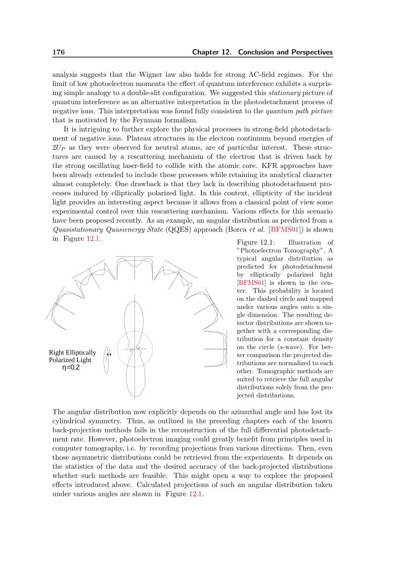
“diss”2002/10/18page 176

176 Chapter 12. Conclusion and Perspectives

analysis suggests that the Wigner law also holds for strong AC-field regimes. For thelimit of low photoelectron momenta the effect of quantum interference exhibits a surpris-ing simple analogy to a double-slit configuration. We suggested this stationary picture ofquantum interference as an alternative interpretation in the photodetachment process ofnegative ions. This interpretation was found fully consistent to the quantum path picturethat is motivated by the Feynman formalism.

It is intriguing to further explore the physical processes in strong-field photodetach-ment of negative ions. Plateau structures in the electron continuum beyond energies of2UP as they were observed for neutral atoms, are of particular interest. These struc-tures are caused by a rescattering mechanism of the electron that is driven back bythe strong oscillating laser-field to collide with the atomic core. KFR approaches havebeen already extended to include these processes while retaining its analytical characteralmost completely. One drawback is that they lack in describing photodetachment pro-cesses induced by elliptically polarized light. In this context, ellipticity of the incidentlight provides an interesting aspect because it allows from a classical point of view someexperimental control over this rescattering mechanism. Various effects for this scenariohave been proposed recently. As an example, an angular distribution as predicted from aQuasistationary Quasienergy State (QQES) approach (Borca et al. [BFMS01]) is shownin Figure 12.1.

Polarized Lightη=0.2

Right Elliptically

Figure 12.1: Illustration of”Photoelectron Tomography”. Atypical angular distribution aspredicted for photodetachmentby elliptically polarized light[BFMS01] is shown in the cen-ter. This probability is locatedon the dashed circle and mappedunder various angles onto a sin-gle dimension. The resulting de-tector distributions are shown to-gether with a corresponding dis-tribution for a constant densityon the circle (s-wave). For bet-ter comparison the projected dis-tributions are normalized to eachother. Tomographic methods aresuited to retrieve the full angulardistributions solely from the pro-jected distributions.

The angular distribution now explicitly depends on the azimuthal angle and has lost itscylindrical symmetry. Thus, as outlined in the preceding chapters each of the knownback-projection methods fails in the reconstruction of the full differential photodetach-ment rate. However, photoelectron imaging could greatly benefit from principles used incomputer tomography, i.e. by recording projections from various directions. Then, eventhose asymmetric distributions could be retrieved from the experiments. It depends onthe statistics of the data and the desired accuracy of the back-projected distributionswhether such methods are feasible. This might open a way to explore the proposedeffects introduced above. Calculated projections of such an angular distribution takenunder various angles are shown in Figure 12.1.

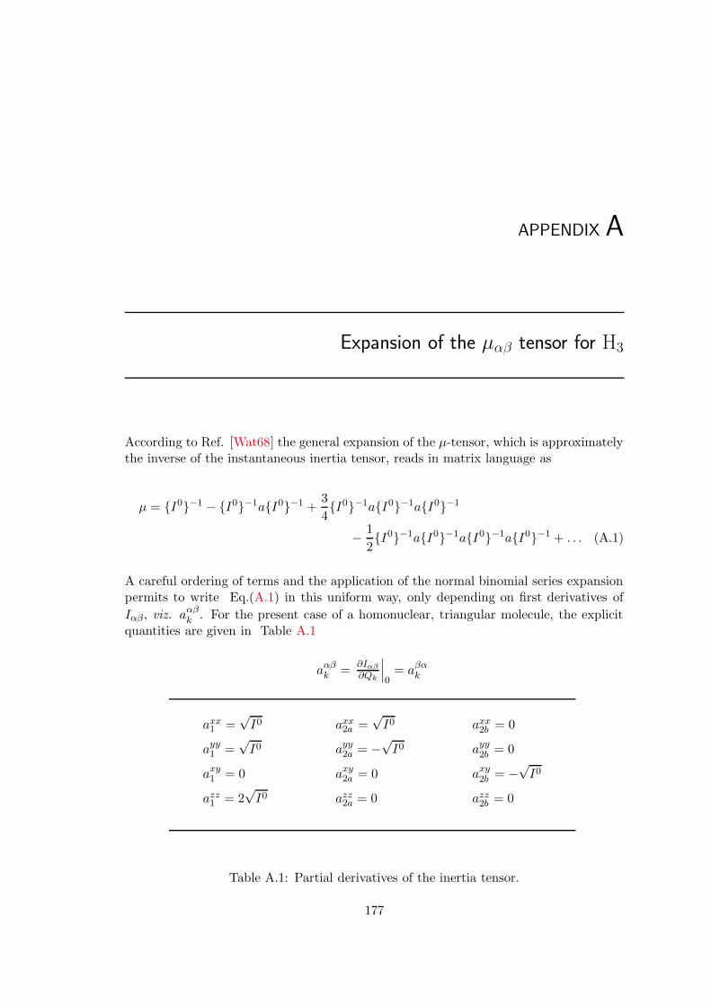
“diss”2002/10/18page 177

APPENDIX A

Expansion of the µαβ tensor for H3

According to Ref. [Wat68] the general expansion of the µ-tensor, which is approximatelythe inverse of the instantaneous inertia tensor, reads in matrix language as

µ = I0−1 − I0−1aI0−1 +3

4I0−1aI0−1aI0−1

− 1

2I0−1aI0−1aI0−1aI0−1 + . . . (A.1)

A careful ordering of terms and the application of the normal binomial series expansionpermits to write Eq.(A.1) in this uniform way, only depending on first derivatives of

Iαβ, viz. aαβk . For the present case of a homonuclear, triangular molecule, the explicit

quantities are given in Table A.1

aαβk =

∂Iαβ

∂Qk

∣∣∣0

= aβαk

axx1 =

√I0 axx

2a =√I0 axx

2b = 0

ayy1 =

√I0 ayy

2a = −√I0 ayy

2b = 0

axy1 = 0 axy

2a = 0 axy2b = −

√I0

azz1 = 2

√I0 azz

2a = 0 azz2b = 0

Table A.1: Partial derivatives of the inertia tensor.

177

“diss”2002/10/18page 178

178 Appendix A. Expansion of the µαβ tensor for H3

I0[Q = 0]−1 =

2 0 00 2 00 0 1

/I0, a =

∑

k

akQk =

Q1 +Q2a −Q2b 0−Q2b Q1 −Q2a 0

0 0 2Q1

√I0

(A.2)Explicitly we arrive at the following expansions up to third order,

µxx =2

I0

[1− 2

(Q1 +Q2a)√I0

+ 3(Q1 +Q2a)

2 +Q22b

I0− 4

(Q1 +Q2a)3 + 3Q1Q

22b +Q2aQ

22b

(I0)3/2+ . . .

]

µyy =2

I0

[1− 2

(Q1 −Q2a)√I0

+ 3(Q1 −Q2a)

2 +Q22b

I0− 4

(Q1 −Q2a)3 + 3Q1Q

22b −Q2aQ

22b

(I0)3/2+ . . .

]

µxy = µyx =4Q2b

(I0)3/2

[1− 3Q1√

I0+

2

I0(3Q2

1 +Q22a +Q2

2b) + . . .

]

µzz =1

I0

[1− 2Q1√

I0+

3Q21

I0− 4Q3

1

(I0)3/2+ . . .

](A.3)

Note that for X3 molecules it holds that µxz = µzx = µyz = µzy = 0, πx = πy = 0.

“diss”2002/10/18page 179

APPENDIX B

Implications & Relations of the Discussed Coordinate Sets

B.1 Relations between Coefficients for the two Represen-

tations of the Potential Energy

Equivalent expansion coefficients

Second Order

f11 = f22 = f33

f12 = f13 = f23 +permutations

Third Order

f111 = f222 = f333

f112 = f113 = f221 = f223 = f331 = f332

+permutations

Fourth Order

f1111 = f2222 = f3333

f1112 = f1113 = f2221 = f2223 = f3331 = f3332

+permutations

f1122 = f1133 = f2233 +permutations

f1231 = f1232 = f1233 +permutations

V000 = f0

V100 =√

3fi

V200 =f11

2+ f12

V300 =f111 + 6f112 + 2f123

6√

3

V400 =f1111 + 8f1112 + 6f1122 + 12f1123

72

V010 =f11 − f12

2

V110 =f111 − f123

2√

3

V210 =f1111 + 2f1112 − 3f1123

12

V001 =f111 − 3f112 + 2f123

6√

6

V101 =f1111 − f1112 − 3f1122 + 3f1123

18√

2

V020 =f1111 − 4f1112 + 3f1122

48

179

“diss”2002/10/18page 180

180 Appendix B. Implications & Relations of the Discussed Coordinate Sets

B.2 Exact Expressions between Bond Length and Normal

Coordinates

By employing Eq.(3.15), that relate cartesian displacement coordinates to normal coor-dinates, a straightforward calculation gives

R21 =

(re +

1√m

(Q1 +Q2a)

)2

+1

mQ2

2b

R22 =

(re +

1√m

(Q1 −

Q2a

2−√

3

2Q2b

))2

+1

m

(√3

2Q2a −

Q2b

2

)2

R23 =

(re +

1√m

(Q1 −

Q2a

2+

√3

2Q2b

))2

+1

m

(√3

2Q2a +

Q2b

2

)2

For small amplitudes of normal coordinates an expansion up to the linear term is equiv-alent with the result in Eqs.(3.18) of approximate displacement coordinates S1, S2, S3

derived using the Eliashevich vectors. These equations can also unambiguously invertedanalytically, see e.g. [Wat94], resulting in complicated expressions.

“diss”2002/10/18page 181

APPENDIX C

Discussion of the Fit Quality

In general, a least squares problem can be written in the form [FMM77]

A · x = b with aij = Φj(ti), Φj(t) basis functions (C.1)

b ab initio points, and

x set of fit parameters

If the inverse of A exists, the solution is simply x = (A−1)b. However, this requires thatA is a square matrix and often this is not the case because in a typical problem moredata values than fit parameters are involved. Thus, a search for a vector x is performed,so that Ax approaches b best. Then, A is a N ×M matrix with N number of datapoints, M number of fit parameters and N ≥ M . In a singular value decomposition(SVD), A can be written as the product A = UWVT, where U, W and V are N ×M ,diagonal-N × N and N × N matrices, respectively. It can be shown [Hon90] that theoptimum vector x is given by

xα =M∑

γ

1

wγVαγ

N∑

i

Uiγbi, α = 1 . . . M (C.2)

wγ , γ = 1 . . .M are called the singular values of A. From this form, it is obvious that fora low singular value wγ the result can become extremely sensitive to small uncertaintiesin b and it can greatly distort the optimum solution. The great advantage of a SVD-leastsquare fit is that it makes these deficiencies visible. If the matrix A is near singular, thenthe singular values extend over a huge range of magnitudes of orders, indicating thatthe problem is ’ill-conditioned’. A number of methods exists to remove this sensitivity.The simplest of these is to set singular values to zero below a certain boundary τ . Thiscorresponds to an elimination of the associated basis function and thus, according toEq.(C.2), to a diminution of the sensitivity. However, a criterion has to be specified,when a basis function needs to be removed. This must be formulated on the accuracyof the involved data or, e.g. on the numerical precision of the data type used. In our

181

“diss”2002/10/18page 182

182 Appendix C. Discussion of the Fit Quality

approach the minimum singular value tolerance τ is defined as the product of the relativeerror of the data, 10−5 as mentioned above, and the largest singular value wmax.

For near-singular cases a condition number κ can be defined, as the ratio of thelargest to the smallest singular value wmax/wmin. This number can be considered as anerror magnification number. This interpretation results from the exact relation ([LH74],Eq.(9.21))

‖dx‖‖x‖ ≤ κ

‖db‖‖b‖ (C.3)

where ‖ · ‖ indicates the Euclidean length. Here, no error from A is assumed. Thus,errors dx caused by the uncertainties of the data db, are ruled by the condition numberκ. Therefore, κ should be as small as possible. Skipping basis functions with singularvalues lower than τ , wγ ≤ τ , has only a minor effect on the total χ2 [SNF92]. Hereby,κ = wmax/wmin goes over into κ = wmax/τ = 105, which is a typical value compared toour fits in Table 3.5.

Moreover, the SVD method also allows a specification of errors resulting from thescattering of the data points [PFTV92],[Hon90] according to

σ2(xα) =M∑

γ

(Vαγ

wγ

)2

(C.4)

This was implemented into the program. Standard deviations for each fit parameterwere determined and are given in parentheses in Table 3.5.

In order to specify the quality of the fit by a χ2-test an uncertainty for each datapoint is required. Since the quantum chemical calculations do not provide the standarddeviation for each data point, we proceeded in the opposite way and checked the resultafterwards whether it is in accordance with our assumptions. If we assume a Gaussiandistribution of errors, equal for all data points, an estimate for the standard deviation isobtained from χ′2 with a weight of one by [Hon90]

σ =

√χ′2

N −M χ′2 =N∑

m

(V [m]− VFit[R1, R2, R3m]

)2(C.5)

Here, N corresponds to the number of data points and M to the number of parameters.The given standard deviations in Table 3.5 are of the order 2 cm−1 ∼ 0.9 · 10−5hartree.Thus, the result of the fit is consistent with our assumptions of a relative error of ∼ 10−5.

“diss”2002/10/18page 183

APPENDIX D

Contact Transformation Approach to Rovibrational Levels of

X3 Molecules

Applying the Sequential Contact Transformation perturbation theory, Watson ([Wat84])derived high order correction terms for a general X3 molecule depending on anharmonic-ity constants. The simplicity of Coriolis interactions for this type of molecule allows itto take into account also higher orders. A summary is given here of the terms appliedin Section 3.4.4 to determine molecular quantities. These formulae were used to obtainthe values in Table 3.7 and Table 3.8.

x11 =k1111

16− 5k2

111

48ω21

x12 =k1122

4− k111k122

4ω1− k2

122ω2

2(4ω22 − ω2

1)

x22 =k2222

16− k2

122(8ω22 − 3ω2

1)

16ω1(4ω22 − ω2

1)− 5k2

222

48ω2

g22 =Be

2− k2222

48− k2

122ω1

16(4ω22 − ω2

1)+

7k2222

48ω2

(Cζ2a)v = −1

2

Be + k111C1

2+

3B2e

ω1 (ν1 +1

2) + k122C1

2− k2

222Be

6ω22 (ν2 + 1)

Bv = Be + k111C1

2+

3B2e

ω1 (ν1 +1

2) + k122C1

2+

3B2e

ω2 (ν2 + 1)

Cv =Be

2+ k111C1

4+

3B2e

2ω1 (ν1 +1

2) + k122C1

4 (ν2 + 1)

q2 = k222C2

ηN2 = −C2

1ω1 − 2C22ω2

ηK2 =

C21ω1

2+ 2C2

2ω2

Molecular Quantities in Non-degenerate States

183

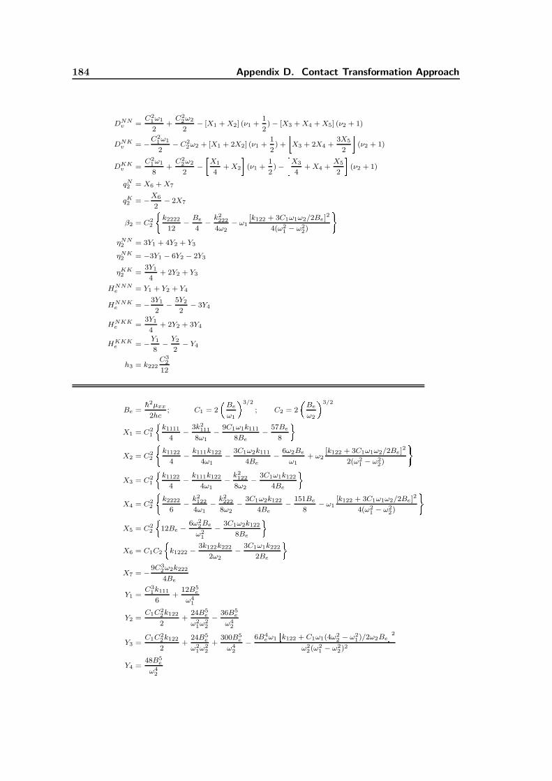
“diss”2002/10/18page 184

184 Appendix D. Contact Transformation Approach

DNNv =

C21ω1

2+

C22ω2

2− [X1 + X2] (ν1 +

1

2)− [X3 + X4 + X5] (ν2 + 1)

DNKv = −C2

1ω1

2− C2

2ω2 + [X1 + 2X2] (ν1 +1

2) + X3 + 2X4 +

3X5

2 (ν2 + 1)

DKKv =

C21ω1

8+

C22ω2

2− X1

4+ X2 (ν1 +

1

2)− X3

4+ X4 +

X5

2 (ν2 + 1)

qN2 = X6 + X7

qK2 = −X6

2− 2X7

β2 = C22 k2222

12− Be

4− k2

222

4ω2− ω1

[k122 + 3C1ω1ω2/2Be]2

4(ω21 − ω2

2) ηNN2 = 3Y1 + 4Y2 + Y3

ηNK2 = −3Y1 − 6Y2 − 2Y3

ηKK2 =

3Y1

4+ 2Y2 + Y3

HNNNe = Y1 + Y2 + Y4

HNNKe = −3Y1

2− 5Y2

2− 3Y4

HNKKe =

3Y1

4+ 2Y2 + 3Y4

HKKKe = −Y1

8− Y2

2− Y4

h3 = k222C3

2

12

Be =h2µxx

2hc; C1 = 2 Be

ω1 3/2

; C2 = 2 Be

ω2 3/2

X1 = C21

k1111

4− 3k2

111

8ω1− 9C1ω1k111

8Be− 57Be

8

X2 = C22 k1122

4− k111k122

4ω1− 3C1ω2k111

4Be− 6ω2Be

ω1+ ω2

[k122 + 3C1ω1ω2/2Be]2

2(ω21 − ω2

2) X3 = C2

1

k1122

4− k111k122

4ω1− k2

122

8ω2− 3C1ω1k122

4Be

X4 = C22 k2222

6− k2

122

4ω1− k2

222

8ω2− 3C1ω2k122

4Be− 151Be

8− ω1

[k122 + 3C1ω1ω2/2Be]2

4(ω21 − ω2

2) X5 = C2

2

12Be −

6ω22Be

ω21

− 3C1ω2k122

8Be

X6 = C1C2

k1222 −

3k122k222

2ω2− 3C1ω1k222

2Be

X7 = −9C32ω2k222

4Be

Y1 =C3

1k111

6+

12B5e

ω41

Y2 =C1C2

2k122

2+

24B5e

ω21ω2

2

− 36B5e

ω42

Y3 =C1C2

2k122

2+

24B5e

ω21ω2

2

+300B5

e

ω42

−6B4

eω1 k122 + C1ω1(4ω22 − ω2

1)/2ω2Be 2

ω22(ω2

1 − ω22)2

Y4 =48B5

e

ω42

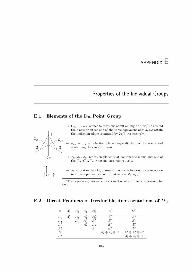
“diss”2002/10/18page 185

APPENDIX E

Properties of the Individual Groups

E.1 Elements of the D3h Point Group

(-z) y

x

C2c

C2b

C2a

1

2 3

→ Cn, n = 2, 3 refer to rotations about an angle of -2π/n a aroundthe z-axis or either one of the three equivalent axes a, b, c withinthe molecular plane separated by 2π/3, respectively.

→ σxy ≡ σh a reflection plane perpendicular to the z-axis andcontaining the center of mass.

→ σva, σvb, σvc reflection planes that contain the z-axis and one ofthe C2a, C2b, C2c rotation axes, respectively.

→ S3 a rotation by -2π/3 around the z-axis followed by a reflectionin a plane perpendicular to that axis ≡ C3 σxy.

aThe negative sign arises because a rotation of the frame is a passive rota-tion.

E.2 Direct Products of Irreducible Representations of D3h

⊗ A′1 A′

2 A′′1 A′′

2 E′ E′′

A′1 A′

1 A′2 A′′

1 A′′2 E′ E′′

A′2 A′

1 A′′2 A′′

1 E′ E′′

A′′1 A′

1 A′2 E′′ E′

A′′2 A′

1 E′′ E′

E′ A′1 ⊕A′

2 ⊕E′ A′′1 ⊕A′′

2 ⊕E′′

E′′ A′1 ⊕A′

2 ⊕E′

185

“diss”2002/10/18page 186

186 Appendix E. Properties of the Individual Groups

E.3 Character Table of the D3h(M) Group

E (123) (23) E∗ (123)∗ (23)∗

D3h(M) : 1 2 3 1 2 3

D3h : E 2C3 3C2 σh 2S3 3σv

Equiv. Rot.: R0 R2π/3z Rπ

0 Rπz R−π/3

z Rππ/2

A′1 : 1 1 1 1 1 1 : αzz , αxx + αyy

A′′1 : 1 1 1 −1 −1 −1 : Γ∗

A′2 : 1 1 −1 1 1 −1 : Nz

A′′2 : 1 1 −1 −1 −1 1 : Tz

E′ : 2 −1 0 2 −1 0 : (Tx, Ty), (αxx − αyy), αxy

E′′ : 2 −1 0 −2 1 0 : (Nx, Ny), αxz, αyz

E.4 Multiplication Table of the CNP Group S3

E (12) (23) (13) (123) (132)

E : E (12) (23) (13) (123) (132)

(12) : (12) (E) (123) (132) (23) (13)

(23) : (23) (132) (E) (123) (13) (12)

(13) : (13) (123) (132) (E) (12) (23)

(123) : (123) (13) (12) (23) (132) (E)

(132) : (132) (23) (13) (12) (E) (123)

“diss”2002/10/18page 187

APPENDIX F

Rovibronic Symmetries of ns 2A′1, np2(A′′2, E

′) and

nd 2(A′1, E′′, E ′) states for N ≤ 3

Here we present results of the symmetry analysis in Chapter 4. Each rotational line has a

symmetry label defined by the quantum numbers N , G and ν2 in Hund’s case (ab) notation.

Statistical weights are indicated by the number on the right of the levels. Dashed lines are

solutions of the rovibronic Schrodinger equation but do not occur in nature, i.e. in the total

wavefunction, due to the fermion exchange principle.

F.1 ns-States: ` = λ = 0 & H+3

F.1.1 λ = 0

ns 2A′1(ν1, 0, N,K)/H+3 A′1(ν1, 0, N

+, K+)

4 2 24- - - - 0

N/N+ = 3 A′2 E ′′ E ′ A′′1/2

- - - - 0 2 2N/N+ = 2 A′1 E ′′ E ′

4 2N/N+ = 1 A′2 E ′′

- - - - 0N/N+ = 0 A′1

|G | / |G+ | 0 1 2 3K/K+ 0 1 2 3

187

“diss”2002/10/18page 188

188 Appendix F. Rovibronic Symmetries in Hund’s case (ab) Notation

ns 2A′1(ν1, 1, N,K)/H+3 A′1(ν1, 1, N

+, K+)

24- - - - 0 2 2

4- - - - 0 2 2N/N+ = 3 E ′ A′′1/2 E ′′ E ′ A′1/2 E ′′ E ′′

24- - - - 0 2 2

4- - - - 0N/N+ = 2 E ′ A′′1/2 E ′′ E ′ A′1/2

24- - - - 0 2

N/N+ = 1 E ′ A′′1/2 E ′′

2N/N+ = 0 E ′

|G | / |G+ | 1 0 2 1 3 2 4K/K+ 0 1 2 3

F.2 np-States: ` = 1, λ = 0,±1

F.2.1 λ = 0

np 2A′′2(ν1, 0, N,K)

- - - - 0 2 24- - - - 0

N = 3 A′′1 E ′ E ′′ A′1/2

4 2 2N = 2 A′′2 E ′ E ′′

- - - - 0 2N = 1 A′′1 E ′

4N = 0 A′′2

|G | 0 1 2 3K 0 1 2 3

np 2A′′2(ν1, 1, N,K)

24- - - - 0 2 2

4- - - - 0 2 2N = 3 E ′′ A′1/2 E ′ E ′′ A′′1/2 E ′ E ′

24- - - - 0 2 2

4- - - - 0N = 2 E ′′ A′1/2 E ′ E ′′ A′′1/2

24- - - - 0 2

N = 1 E ′′ A′1/2 E ′

2N = 0 E ′′

|G | 1 0 2 1 3 2 4K 0 1 2 3

“diss”2002/10/18page 189

F.3. nd-States 189

F.2.2 λ = ±1

np 2E ′(ν1, 0, N,K)

24- - - - 0 2 2

4- - - - 0 2 2N = 3 E ′ A′′1/2 E ′′ E ′ A′1/2 E ′′ E ′′

24- - - - 0 2 2

4- - - - 0N = 2 E ′ A′′1/2 E ′′ E ′ A′1/2

24- - - - 0 2

N = 1 E ′ A′′1/2 E ′′

2N = 0 E ′

|G | 1 0 2 1 3 2 4K 0 1 2 3

np 2E ′(ν1, 1, N,K)

4- - - - 0 2 24- - - - 0

4- - - - 0 2 2 24- - - - 0 2

N = 3 A′1/2 E ′ E ′′ A′′1/2 A′1/2 E ′ E ′ E ′′ A′′1/2 E ′′

4- - - - 0 2 24- - - - 0

4- - - - 0 2 2N = 2 A′1/2 E ′ E ′′ A′′1/2 A′1/2 E ′ E ′

4- - - - 0 2 24- - - - 0

N = 1 A′1/2 E ′ E ′′ A′′1/2

4- - - - 0 2N = 0 A′1/2 E ′

|G | 0 2 1 3 0 2 4 1 3 5K 0 1 2 3

F.3 nd-States: ` = 2, λ = 0,±1,±2

F.3.1 λ = 0nd 2A′1(ν1, 0, N,K)

4 2 24- - - - 0

N = 3 A′2 E ′′ E ′ A′′1/2

- - - - 0 2 2N = 2 A′1 E ′′ E ′

4 2N = 1 A′2 E ′′

- - - - 0N = 0 A′1

|G | 0 1 2 3K 0 1 2 3

“diss”2002/10/18page 190

190 Appendix F. Rovibronic Symmetries in Hund’s case (ab) Notation

nd 2A′1(ν1, 1, N,K)

24- - - - 0 2 2

4- - - - 0 2 2N = 3 E ′ A′′1/2 E ′′ E ′ A′1/2 E ′′ E ′′

24- - - - 0 2 2

4- - - - 0N = 2 E ′ A′′1/2 E ′′ E ′ A′1/2

24- - - - 0 2

N = 1 E ′ A′′1/2 E ′′

2N = 0 E ′

|G | 1 0 2 1 3 2 4K 0 1 2 3

F.3.2 λ = ±1

nd 2E ′′(ν1, 0, N,K)

24- - - - 0 2 2

4- - - - 0 2 2N = 3 E ′′ A′1/2 E ′ E ′′ A′′1/2 E ′ E ′

24- - - - 0 2 2

4- - - - 0N = 2 E ′′ A′1/2 E ′ E ′′ A′′1/2

24- - - - 0 2

N = 1 E ′′ A′1/2 E ′

2N = 0 E ′′

|G | 1 0 2 1 3 2 4K 0 1 2 3

nd 2E ′′(ν1, 1, N,K)

4- - - - 0 2 24- - - - 0

4- - - - 0 2 2 24- - - - 0 2

N = 3 A′′1/2 E ′′ E ′ A′1/2 A′′1/2 E ′′ E ′′ E ′ A′1/2 E ′

4- - - - 0 2 24- - - - 0

4- - - - 0 2 2N = 2 A′′1/2 E ′′ E ′ A′1/2 A′′1/2 E ′′ E ′′

4- - - - 0 2 24- - - - 0

N = 1 A′′1/2 E ′′ E ′ A′1/2

4- - - - 0 2N = 0 A′′1/2 E ′′

|G | 0 2 1 3 0 2 4 1 3 5K 0 1 2 3

“diss”2002/10/18page 191

F.3. nd-States 191

F.3.3 λ = ±2

nd 2E ′(ν1, 0, N,K)

2 24- - - - 0

4- - - - 0 2 2 2N = 3 E ′ E ′′ A′′1/2 A′1/2 E ′ E ′′ E ′′

2 24- - - - 0

4- - - - 0 2N = 2 E ′ E ′′ A′′1/2 A′1/2 E ′

2 24- - - - 0

N = 1 E ′ E ′′ A′′1/2

2N = 0 E ′

|G | 2 1 3 0 4 1 5K 0 1 2 3

nd 2E ′(ν1, 1, N,K)

2 4- - - - 04- - - - 0 2 2 2 4- - - - 0 2 4- - - - 0 2 2 4- - - - 0

N = 3 E′ A′1/2

A′′1/2

E′′ E′′ E′ A′1/2

E′ A′′1/2

E′′ E′′ A′′1/2

24- - - - 0

4- - - - 0 2 2 24- - - - 0 2

N = 2 E′ A′1/2

A′′1/2

E′′ E′′ E′ A′1/2

E′

2 4- - - - 04- - - - 0 2 2

N = 1 E′ A′1/2

A′′1/2

E′′ E′′

24- - - - 0

N = 0 E′ A′1/2

|G | 1 3 0 2 4 1 3 5 0 2 4 6K 0 1 2 3

“diss”2002/10/18page 192

192 Appendix F. Rovibronic Symmetries in Hund’s case (ab) Notation

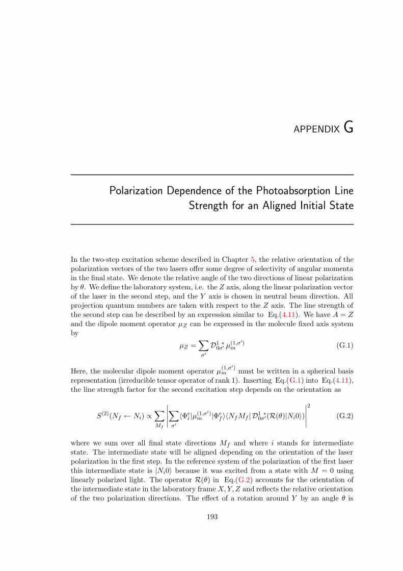
“diss”2002/10/18page 193

APPENDIX G

Polarization Dependence of the Photoabsorption Line

Strength for an Aligned Initial State

In the two-step excitation scheme described in Chapter 5, the relative orientation of thepolarization vectors of the two lasers offer some degree of selectivity of angular momentain the final state. We denote the relative angle of the two directions of linear polarizationby θ. We define the laboratory system, i.e. the Z axis, along the linear polarization vectorof the laser in the second step, and the Y axis is chosen in neutral beam direction. Allprojection quantum numbers are taken with respect to the Z axis. The line strength ofthe second step can be described by an expression similar to Eq.(4.11). We have A = Zand the dipole moment operator µZ can be expressed in the molecule fixed axis systemby

µZ =∑

σ′

D1 ∗0σ′ µ(1,σ′)

m (G.1)

Here, the molecular dipole moment operator µ(1,σ′)m must be written in a spherical basis

representation (irreducible tensor operator of rank 1). Inserting Eq.(G.1) into Eq.(4.11),the line strength factor for the second excitation step depends on the orientation as

S(2)(Nf ← Ni) ∝∑

Mf

∣∣∣∣∣∑

σ′

〈Φei |µ(1,σ′)

m |Φef 〉〈NfMf | D1 ∗

0σ′(R(θ)|Ni0〉)∣∣∣∣∣

2

(G.2)

where we sum over all final state directions Mf and where i stands for intermediatestate. The intermediate state will be aligned depending on the orientation of the laserpolarization in the first step. In the reference system of the polarization of the first laserthis intermediate state is |Ni0〉 because it was excited from a state with M = 0 usinglinearly polarized light. The operator R(θ) in Eq.(G.2) accounts for the orientation ofthe intermediate state in the laboratory frameX,Y,Z and reflects the relative orientationof the two polarization directions. The effect of a rotation around Y by an angle θ is

193

“diss”2002/10/18page 194

194 Appendix G. Polarization Dependence of the Photoabsorption Line Strength

([Zar88] Eq.(3.52))

R(θ)|Ni0〉 =∑

m

dNim0(θ)|Nim〉 (G.3)

By inserting this relation in Eq.(G.2) and employing the identities Eqs. (3.125), (3.118)of Ref. [Zar88] the sum over σ′ cancels since σ′ = Kf − Ki, and a straightforwardmanipulation leads to

S(2)(Nf ← Ni) ∝∑

m

∣∣∣dNim0(θ)〈Nfm; 10|Nim〉

∣∣∣2

(G.4)

In our experiment the intermediate state must always have Ni = 1 since the first exci-tation step starts from the metastable state with N = 0. The explicit dependence ofthe line strength on θ is easily found by using the tabulated values from Ref. [Zar88]for the Clebsch-Gordan coefficients and rotation matrices for the total angular momentaallowed in the final state Nf = 0, 1, 2. The result is

S(2)[θ]Nf=0 = S(2)[ 0o]0 · cos2 θ

S(2)[θ]Nf=1 = S(2)[90o]1 · sin2 θ (G.5)

S(2)[θ]Nf=2 = S(2)[ 0o]2 ·(

cos2 θ +3

4sin2 θ

)

Thus, for parallel polarizations θ = 0o only N = 0 and 2 are excited, and for perpen-dicular orientation θ = 90o only N = 1 and N = 2. This allows to identify the totalangular momentum Nf for each individual state by its behaviour on different ’relativepolarizations’.

“diss”2002/10/18page 195

APPENDIX H

Integrals for an Approximate Radial Equation of H−

In the application of the variational principle in Chapter 7 some integrals have to beevaluated. Since we have chosen the wavefunctions of the hydrogen atom as zero orderapproximation the occurring matrix elements can easily be computed. We cite here allintegrals that are nonzero.

−E∫Y ∗l0(Ω1)Φ

0(r2)∗Ψ(r1, r2)dΩ1dΩ2r22dr2 = −Eul(r1)

r1∫Y ∗l0(Ω1)Φ

0(r2)∗(−∆2

2− 1

r2

)Ψ(r1, r2)dΩ1dΩ2r

22dr2 = E(2)ul(r1)

r1

−∫Y ∗l0(Ω1)Φ

0(r2)∗∆1

2Ψ(r1, r2)dΩ1dΩ2r

22dr2 =

1

2r1

(− ∂2

∂r21+l(l + 1)

r21

)ul(r1)

∫Y ∗l0(Ω1)Φ

0(r2)∗(− 1

r1+

1

r12

)Ψ(r1, r2)dΩ1dΩ2r

22dr2 =

[−e−2r1

(1

r1+ 1

)− α(r1)

2r41

]ul(r1)

r1

195

“diss”2002/10/18page 196

196 Appendix H. Integrals for an Approximate Radial Equation of H−

“diss”2002/10/18page 197

APPENDIX I

Laser Beam Diagnostics

I.1 Determination of the Pulse Length and Center Wave-

length

For measuring the pulse length we used an autocorrelator based on a Michelson inter-ferometer in combination with a BBO crystal and some absorption filters. A single laserpulse is split into two pulses with equal intensity. Both pulses are again spatially over-lapped in a BBO crystal to produce high harmonic frequencies. The path length of oneof the two arms is varied to produce an optical correlation by shifting the optical delay τ .Lower orders were properly filtered after the BBO to provide only the fourth-harmonicfield that falls into the visible wavelength range. Assuming gaussian envelopes for thepulses, the fourth order autocorrelation signal is fitted to the expression

Autocorr4th(τ) ∝∫ ∞

−∞dt(|E1e

−(t−t0)2/σ2t + E2e

−((t−t0)−τ)2/σ2t |2)4

(I.1)

as a function of the optical delay time τ . In this fit, the amplitudes E1,E2, the absolutescale t0, and the pulse duration σt are taken as adjustable parameters. This procedurefinally defines the pulse duration as FWHM = 2

√ln 2σt = 250fs. In a similar arrange-

ment, we directed the output of the fourth harmonic into a commercial wavelength meterCOHERENT WaveMate. In this way the center wavelength is determined to 2150nm withan accuracy of ∼ 5nm.

I.2 Focal Geometry and Interaction Volume

The shape of the focal area was recorded by measuring the integral energy as a functionof the lateral position of a razor blade scanning perpendicular over the beam axis. Theintegral intensity of the partially blocked beam assumes for a radial profile of Gaussian

197

“diss”2002/10/18page 198

198 Appendix I. Laser Beam Diagnostics

shape an error function

Integral Intensity ∝ 1

2(1 + erf ((z − z0)/σρ)) (I.2)

For the IR-region we have used a sensitive Indium Arsenide (InAs) photodiode to inte-grate the transmitted intensity. Figure I.1a) illustrates the integral intensity as a func-tion of the lateral position z for a fixed distance from the lens x. In a two-parametricalnonlinear fit we adjusted the parameters z0 and σρ. The excellent agreement in FigureI.1a) between the fit function and the measured data shows that the focus can be well re-produced by a radial Gaussian shape. The above step was repeated for a set of distancesx to find the position of highest intensity at the waist of the focused beam. In FigureI.1b) this widths are plotted versus the position parallel to the laser propagation. Thus,

0 50 100 150 200Position perpendicular to laser propagation axis (Z-position in Figure 8.5a))/µm

a)

0.00

0.10

0.20

0.30

0.40

0.50

Inte

gral

Inte

nsity

22 24 26 28 30 32 34 36

b)

Position along beam laser propagation axis (X-position in Figure 8.5a))/ mm

0

20

40

60

80

100

Rayleigh Length ∼ 2mm

FWHM/2

=√

ln2σ

ρ

Figure I.1: a) Integral intensity versus perpendicular blocking position z at a fixeddistance from the lens x. b) Radial widths (in µm) of the laser focus at various distancesfrom the lens in the vicinity of the focus.

we have determined the minimum waist of the laser focus to 50µm, and the Rayleighrange of ∼ 2mm for the conditions employed in the experiments. From this geometricalquantities the peak intensity in the laser focus is found to be 1.7 × 1013 W/cm2 (cf.Section 10.2).

“diss”2002/10/18page 199

APPENDIX J

Ambiguity in the Determination of Partial-Wave Amplitudes

and Physical Domain of Beta Parameters

It is well known that in general an electron angular distribution (AD) after multiphotondetachment from an isotropic initial state by linearly polarized light has the form

N2Lmax∑

L≥0 even

βLPL(cos θ) ≡ N2Lmax∑

L≥0 even

αL cosL θ (J.1)

The overall normalization is fixed by adjusting N so that β0 = 1. The second equationgives an equivalent functional form representing a polynomial of order 2Lmax in thevariable x = cos θ. The coefficients αL and the set of beta parameters βL obey a linearrelationship. The polynomial has another equivalent representation in terms of productsas follows from a mathematical theorem

Eq.(J.1) ≡ αLmax

2Lmax∏

i=1

(x− zi) (J.2)

where the zi are the complex roots of the polynomial and related to the above coefficientsin a non-trivial way. If however the roots are known the sets α(·) and β(·) are easilycomputed by factorizing the expression. A quite simple conclusion is now that, sinceall beta parameters are real the conjugated roots z∗i are also roots of the polynomial.Or more specific: if a zi is not real, i.e. its imaginary part is nonzero =(zi) 6= 0, ithas a coupled partner z∗i that is also a root. Such roots necessarily emerge in pairs. Itmight be the case that =(zj) = 0, then it holds that z∗j = zj is also a root, but it doesnot necessarily be a twofold root. It is easy to see that for the possibility to exist todecompose the general form as in Eq.(11.1) into a product of partial wave amplitudes

fpn(θ)fpn(θ)∗ = αLmax

Lmax∏

i=1

(x− zi)Lmax∏

i=1

(x− z∗i ) (J.3)

199

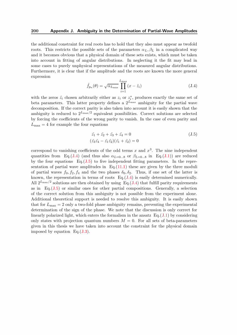
“diss”2002/10/18page 200

200 Appendix J. Ambiguity in the Determination of Partial-Wave Amplitudes

the additional constraint for real roots has to hold that they also must appear as twofoldroots. This restricts the possible sets of the parameters αL, βL in a complicated wayand it becomes obvious that a physical domain of these sets exists, which must be takeninto account in fitting of angular distributions. In neglecting it the fit may lead insome cases to purely unphysical representations of the measured angular distributions.Furthermore, it is clear that if the amplitude and the roots are known the more generalexpression

fpn(θ) =√αLmax

Lmax∏

i=1

(x− zi) (J.4)

with the zeros zi chosen arbitrarily either as zi or z∗i , produces exactly the same set ofbeta parameters. This latter property defines a 2Lmax ambiguity for the partial wavedecomposition. If the correct parity is also taken into account it is easily shown that theambiguity is reduced to 2Lmax/2 equivalent possibilities. Correct solutions are selectedby forcing the coefficients of the wrong parity to vanish. In the case of even parity andLmax = 4 for example the four equations

z1 + z2 + z3 + z4 = 0 (J.5)

(z3z4 − z1z2)(z1 + z2) = 0

correspond to vanishing coefficients of the odd terms x and x3. The nine independentquantities from Eq.(J.4) (and thus also αL=0...8 or βL=0...8 in Eq.(J.1)) are reducedby the four equations Eq.(J.5) to five independent fitting parameters. In the repre-sentation of partial wave amplitudes in Eq.(11.1) these are given by the three moduliof partial waves f0, f2, f4 and the two phases δ0, δ2. Thus, if one set of the latter isknown, the representation in terms of roots Eq.(J.4) is easily determined numerically.All 2Lmax/2 solutions are then obtained by using Eq.(J.4) that fulfill parity requirementsas in Eq.(J.5) or similar ones for other partial compositions. Generally, a selectionof the correct solution from this ambiguity is not possible from the experiment alone.Additional theoretical support is needed to resolve this ambiguity. It is easily shownthat for Lmax = 2 only a two-fold phase ambiguity remains, preventing the experimentaldetermination of the sign of the phase. We note that the discussion is only correct forlinearly polarized light, which enters the formalism in the ansatz Eq.(J.1) by consideringonly states with projection quantum numbers M = 0. For all sets of beta-parametersgiven in this thesis we have taken into account the constraint for the physical domainimposed by equation Eq.(J.3).

“diss”2002/10/18page 201

Bibliography

[AHH99] Andersen, T. ; Haugen, H. K. ; Hotop, H.Binding energies in atomic negative ions: III. J. Phys. Chem. Ref. Data 28 (1999), 1511126

[AM77] Azumi, Tohru ; Matsuzaki, KazuoWhat does the term ”vibronic coupling” mean ? Photochemistry and Photobiology 25(1977), 315 28

[Ana92] Anandan, JeevaThe geometric phase. Nature 360 (1992), 307 47

[AW76] Aliev, M.R. ; Watson, J. K. G.Calculated Sextic Centrifugal Distortion Constants of Polyatomic Molecules. J. Mol. Spec-trosc. 61 (1976), 29 28, 39, 41, 71

[AW85] Aliev, M.R. ; Watson, J. K. G.Higher-Order Effects in the Vibration-Rotation Spectra of Semirigid Molecules. MolecularSpectroscopy: Modern Research Vol. III. K. Narahari Rao (Ed.), Academic Press, New York,1985 39, 40

[B09] Bocher, M.Introduction to Integral Equations. Vol. 10. Cambridge Math. Tracts, 1909 145

[BA85] Basrak, Z. ; Auger, F.A straightforward model-independent determination of the complete scattering matrix forreactions involving zero-spin particles. Nucl. Phys. A441 (1985), 150 165

[BBD01] Blondel, C. ; Berge, S. ; Delsart, C.Physical and unphysical phases of uniformly accelerated particles. Am. J. Phys. 69 (2001),810 134

[BCDG91] Blondel, C. ; Crance, M. ; Delsart, C. ; Giraud, A.Excess-photon absorption in a negative ion. J. Phys. B 24 (1991), 3575 116, 142

[BDDV99] Blondel, C. ; Delsart, C. ; Dulieu, F. ; Valli, C.Photodetachment microscopy of O−. Eur. Phys. J. D 5 (1999), 207 134

[Bel70] Bell, SMatrix elements in harmonic oscillator representation: I and II. J. Phys. B 3 (1970),735–750 54

[Ber98] Berry, MichaelThe Geometric Phase. Scientific American December (1998), 26 47

[BFMS01] Borca, Bogdan ; Frolov, M. V. ; Manakov, N. L. ; Starace, Anthony F.Threshold Effects on Angular Distributions for Multiphoton Detachment by Intense Ellip-tically Polarized Light. Phys. Rev. Lett. 87 (2001), 133001 117, 164, 170, 176

201

“diss”2002/10/18page 202

202 Bibliography

[BJ98] Bunker, P.R. ; Jensen, P.Molecular Symmetry and Spectroscopy, 2nd ed.. NRC Research Press, Ottawa, Ontario,Canada 747p., 1998 20, 21, 30, 39, 42, 60, 62, 64, 68, 69, 70, 107

[BLCB89] Bordas, C. ; Labastie, P. ; Chevaleyre, J. ; Broyer, M.MQDT Analysis of Rovibrational Interactions and Autoionization in Na2 Rydberg States.Chem. Phys. 129 (1989), 21 91

[BLH91] Bordas, M.C. ; Lembo, L.J. ; Helm, H.Spectroscopy and multichannel quantum-defect theory analysis of the np Rydberg series ofH3. Phys. Rev. A 44 (1991), 1817 75, 91, 93, 94

[BLM90] Becker, W. ; Long, S. ; McIver, J. K.Short-Range potential model for multiphoton detachment of the H− ion. Phys. Rev. A 42(1990), 4416 126

[BnAH+98] Banares, L. ; Aoiz, F.J. ; Herrero, V.J. ; D’Mello, M.J. ; Niederjohann, B. ;Seekamp-Rahn, K. ; Wrede, E. ; Schnieder, L.Experimental and quantum mechanical study of the H + D2 reaction near 0.5eV : Theassessment of the H3 potential energy surface. J. Chem. Phys. 108 (1998), 6160 6

[BNFDH85] Burton, P. G. ; Nagy-Felsobuki, E. von ; Doherty, G. ; Hamilton, M.The vibration spectrum of H+

3 . A PNO-CI ab initio potential energy surface and its analyt-ical representation. Molecular Phys. 55 (1985), 527 33

[BPHH96] Bordas, C. ; Paulig, F. ; Helm, H. ; Huestis, D.L.Photoelectron imaging spectrometry: Principle and inversion method. Rev. Sci. Instrum.67 (1996), 2257 146

[Bra56] Bracewell, R.N.Strip integration in radio astronomy & Two-dimensional aerial smoothing in radio astron-omy. Austr. J. Phys. 9 (1956), 198–217 & 297–314 145

[Bra00] Bracewell, R.N.The Fourier Transform and Its Applications. McGraw-Hill, New York, 2000 145

[CAGL86] Carney, G. D. ; Adler-Golden, S. M. ; Lesseski, D. C.A comparison of force fields and calculation methods for vibration intervals of isotopic H+

3

molecules. J. Chem. Phys. 84 (1986), 3921 38, 44

[CH88] Cosby, P. C. ; Helm, H.Photodissociation of Triatomic Hydrogen. Phys. Rev. Lett. 61 (1988), 298 13, 36, 75

[Cha44] Chandrasekhar, S.Some Remarks on the Negative Hydrogen Ion and its Absorption Coefficient. Astrophys. J.100 (1944), 176 122

[Chi96] Child, M.S.Molecular Rydberg States. Phil. Trans. R. Soc. Lond. A 355 (1996), 1475–1711 74

[CLH61] Child, M.S. ; Longuet-Higgins, H.C.III. The Rotational and Vibrational Spectra of Symmetric-Top Molecules in ElectronicallyDegenerate States. Phil. Trans. R. Soc. A 254 (1961), 259 56

[CRJK98] Cencek, W. ; Rychlewski, J. ; Jaquet, R. ; Kutzelnigg, W.Sub-microhartree accuracy potential energy surface for H+

3 including adiabatic and rela-tivistic effects. I. Calculation of the potential points. J. Chem. Phys. 108 (1998), 2831 31,80, 93, 99, 100

[CRW+97] Chang, Z. ; Rundquist, A. ; Wang, H. ; Murnane, M. M. ; Kapteyn, H. C.Generation of Coherent Soft X Rays at 2.7 nm using High Harmonics. Phys. Rev. Lett. 79(1997), 2967 116

[DA95] DiMauro, L. F. ; Agostini, P.Ionization Dynamics in Strong Laser Fields. Adv. At. Mol. Opt. Phys. 35 (1995), 79 116

[Dal94] Dalgarno, A.Terrestrial and Extraterrestrial H+

3 . Adv. At. Mol. Opt. Phys. 32 (1994), 57 105

“diss”2002/10/18page 203

Bibliography 203

[DB82] Deutsch, Moshe ; Beniaminy, IsraelDerivative-free inversion of Abel’s integral equation. Appl. Phys. Lett. 41 (1982), 27 145

[DD40] Darling, B.T. ; Dennison, D.M.The Water Vapour Molecule. Phys. Rev. 57 (1940), 128 20

[Dev68] Devienne, F. M.C.R. Acad. Sci. Paris B 267 (1968), 1279 9

[DGG+78] Dykstra, C. E. ; Gaylord, A. S. ; Gwinn, W. D. ; Swope, W. C. ; Schaefer, H. F.The uncoupled symmetric stretch frequency of H+

3 . J. Chem. Phys. 68 (1978), 3951 44

[DH80] Dabrowski, I. ; Herzberg, G.The electronic emission spectrum of triatomic hydrogen. I. Parallel bands of H3 and D3 near5600 and 6025 A. Can. J. Phys. 58 (1980), 1238 9, 14, 43, 45, 57

[DK94] Delone, N.B. ; Krainov, V.P.Multiphoton Processes in Atoms. Springer-Verlag, Berlin, 1994 116

[DMH91] Davidson, M.D. ; Muller, H.G. ; Heuvell, H.B. van L. v. d.Experimental observation of excess-photon detachment of negative ions. Phys. Rev. Lett.67 (1991), 1712 116, 142

[DO88] Demkov, Y. N. ; Ostrovskii, V. N.Zero-Range Potentials and Their Application in Atomic Physics. Plenum Press, New York,1988 126

[DS79] Dykstra, C. E. ; Swope, W. C.The H+

3 potential surface. J. Chem. Phys. 70 (1979), 1 31, 34, 44

[DSB+92] Davidson, M.D. ; Schumacher, D.W. ; Bucksbaum, P.H. ; Muller, H.G. ;Heuvell, H.B. van L. v. d.Longer wavelengths require lower intensity in multiphoton detachment of negative ions.Phys. Rev. Lett. 69 (1992), 3459 142

[DSB+95] Datz, S. ; Sundstrom, G. ; Biedermann, Ch. ; Brostrom, L. ; Danared, H. ;Mannervik, S. ; Mowat, J.R. ; Larsson, M.Branching Processes in the Dissociative Recombination of H+

3 . Phys. Rev. Lett. 74 (1995),896 4

[Eck35] Eckart, C.Some Studies Concerning Rotating Axes and Polyatomic Molecules. Phys. Rev. 47 (1935),552 21

[Eli38] Eliashevich, M.A.Trudy Gosudarstvenogo opticheskogo instituta (SSSR) 106 (1938), 12 20

[Eli40] Eliashevich, M.Compt. rend. acad. sci. U.R.S.S. 28 (1940), 605 15

[EP97] Eppink, Andre T. J. B. ; Parker, David H.Velocity map imaging of ions and electrons using electrostatic lenses: Application in photo-electron and photofragment ion imaging. Rev. Sci. Instrum. 68 (1997), 3477 118, 138

[Fai73] Faisal, F.H.M.Multiple absorption of laser photons by atoms. J. Phys. B 6 (1973), L89 153

[Fan61] Fano, U.Effects of Configuration Interaction on Intensities and Phase Shifts. Phys. Rev. 124 (1961),1866 81, 100

[Fan70] Fano, U.Quantum Defect Theory of l Uncoupling in H2 as an Example of Channel InteractionTreatment. Phys. Rev. A 2 (1970), 353 83, 88, 89

[Fan77] Fano, U.Erratum: Quantum Defect Theory of l Uncoupling in H2 as an Example of Channel Inter-action Treatment [ Phys. Rev. A 2 (1970), 353 ]. Phys. Rev. A 15 (1977), 817 83

“diss”2002/10/18page 204

204 Bibliography

[FKW89] Figger, H. ; Ketterle, W. ; Walther, H.Spectroscopy of triatomic hydrogen. I. Bands near 5600, 5800 and 6025 A. Z. Phys. D 13(1989), 129 75

[FMM77] Forsythe, G. ; Malcolm, M.A. ; Moler, G.B.Computer Methods for Mathematical Computations. Prentice Hall, New York, 1977 181

[FMS01] Frolov, M. V. ; Manakov, N. L. ; Starace, A. F.Dynamic hyperpolarizability and two-photon detachment in the presence of a strong staticelectric field: Application to H−. Phys. Rev. A 64 (2001), 023417 164

[FR00] Forets, Guillaume Pineau d. ; Roueff, EvelyneH+

3 recombination and bistability in the interstellar medium. Phil. Trans. Roy. Soc. Lond.A 358 (2000), 2549 106

[Fri98] Friedrich, H.Theoretical Atomic Physics. 2nd ed. Springer-Verlag Berlin Heidelberg New York, 1998 125

[G+78] Gaillard, M.J. et alExperimental determination of the structure of H+

3 . Phys. Rev. A 17 (1978), 1797 14

[Gal94] Gallagher, T.F.Rydberg Atoms. Cambridge Univ. Press, 1994 85

[Gay68] Gaydon, A.D.Dissociation Energies. 11 New Fetter Lane, E.C. 4, London : Chapman and Hall LTD, 196812

[Giu80] Giusti, A.A multichannel quantum defect approach to dissociative recombination. J. Phys. B 13(1980), 3867 106

[GJ84] Greene, Chr. ; Jungen, Ch.Molecular Applications of Quantum Defect Theory. Adv. At. Mol. Phys. Vol. 21. p.51, 1984101

[GK97] Gribakin, G.F. ; Kuchiev, M.Yu.Multiphoton detachment of electrons from negative ions. Phys. Rev. A 55 (1997), 3760116, 117, 126, 153, 154, 155, 163, 167

[GS97] Greene, Chris H. ; Stephens, J. A.Rydberg states of triatomic hydrogen. Phil. Trans. R. Soc. Lond. A 355 (1997), 1609 91

[GZB+99] Gulley, M. S. ; Zhao, Xin M. ; Bryant, H. C. ; Strauss, Charlie E. M. ; Funk, D. J.; Stintz, A. ; Rislove, D. C. ; Kyrala, G. A. ; Ingalls, W. B. ; Miller, W. A.Nonresonant excess photon detachment of negative hydrogens ions. Phys. Rev. A 60 (1999),4753 118

[HBD+93] Helm, H. ; Bjerre, N. ; Dyer, M. J. ; Huestis, D. L. ; Saeed, M.Images of photoelectrons formed in intense laser fields. Phys. Rev. Lett. 70 (1993), 3221128

[Hel86] Helm, H.Observation of High-n Rydberg Series (7 < n < 40) of the H3 Molecule. Phys. Rev. Lett.56 (1986), 42 10, 75

[Hel88] Helm, H.Measurement of the ionization potential of triatomic hydrogen. Phys. Rev. A 38 (1988),3425 75

[Hen97] Hentschel, KlausGustav Robert Kirchhoff (1824-1887) & Robert Wilhelm Bunsen (1811-1899). Meyenn,Karl von (Ed.): Die grossen Physiker Vol. I. C.H. Beck, 1997 1

[Her27] Herzberg, G.Ann. Phys. (Leipzig) 84 (1927), 565 9

[Her66] Herzberg, G.Molecular spectra and molecular structure III . Van Nostrand Reinhold, New York, 1966(Electronic spectra and electronic structure of polyatomic molecules) 13, 71

“diss”2002/10/18page 205

Bibliography 205

[Her67] Herzberg, G.The Spectra of Hydrogen and Their Role in the Development of Our Understanding of theStructure of Matter and of the Universe. Trans. Roy. Soc. Can. Vol. V Ser. IV (1967),3 1, 5

[Her81] Herzberg, G.Rydberg Spectra of Triatomic Hydrogen and of the Ammonium Radical. Young, D.A.(Ed.): Faraday Discussions of the Chemical Society, No.71, High Resolution Spectroscopy ,1981 13

[Her87] Herzberg, G.Rydberg Molecules. Ann. Rev. Phys. Chem. 38 (1987), 27 74

[Her00] Herbst, E.The astrochemistry of H+

3 . Phil. Trans. Roy. Soc. Lond. A 358 (2000), 2523 105

[HHW82] Herzberg, G. ; Hougen, J.T. ; Watson, J.K.G.The electronic emission spectrum of triatomic hydrogen. IV. Visible bands near 5800 A andinfrared bands near 3950 cm-1. Can. J. Phys. 60 (1982), 1261 9, 43, 45, 57, 100

[Hil77] Hill, R. N.Proof that the H− Ion has only one Bound State. Phys. Rev. Lett. 38 (1977), 643 121

[HJ72] Herzberg, G. ; Jungen, Chr.Rydberg Series and Ionization Potential of the H2 Molecule. J. Mol. Spectrosc. 41 (1972),425 105

[HK73] Herbst, E. ; Klemperer, W.The formation and depletion of molecules in dense interstellar clouds. Astrophys. J. 185(1973), 505 105

[HLCH89] Helm, H. ; Lembo, L.J. ; Cosby, P.C. ; Huestis, D.L.Photoionization and Dissociation of the Triatomic Hydrogen Molecule. Fundamentals ofLaser Interaction II . edited by F. Ehlotzky (Springer Verlag, Berlin), 1989, 264 60, 68

[HLH63] Herzberg, G.H. ; Longuet-Higgins, H.C.Intersection of potential energy surfaces in polyatomic molecules. Disc. Faraday Soc. 35(1963), 77 46

[HLSW81] Herzberg, G. ; Lev, H. ; Sloan, J.J. ; Watson, J.K.G.The electronic emission spectrum of triatomic hydrogen. III. Infrared perpendicular bandsnear 3600 cm-1. Can. J. Phys. 59 (1981), 428 9, 13, 43, 45, 55, 57

[Hol73] Holzwarth, N. A. W.Mathieu function solutions to the radial Schrodinger equation for the −f 2/r4 interaction.J. Math. Phys. 14 (1973), 191 126

[Hon90] Honerkamp, JosefStochastische Dynamische Systeme:Konzepte, numerische Methoden, Datenanalysen. VCHWeinheim, 1990 181, 182

[Hou62] Hougen, Jon T.Classification of Rotational Energy Levels for Symmetric-Top Molecules. J. Chem. Phys.37 (1962), 1433 60, 64

[HR89] Honerkamp, J. ; Romer, H.Klassische Theoretische Physik, 2nd edition. Springer-Verlag Berlin Heidelberg New York,1989 19

[HW80] Herzberg, G. ; Watson, J.K.G.The electronic emission spectrum of triatomic hydrogen. II. The perpendicular bands near7100 A. Can. J. Phys. 58 (1980), 1250 9, 57

[JCKR98a] Jaquet, R. ; Cencek, W. ; Kutzelnigg, W. ; Rychlewski, J. private communication.1998 80, 93, 99, 100, 109

[JCKR98b] Jaquet, R. ; Cencek, W. ; Kutzelnigg, W. ; Rychlewski, J.Sub-microhartree accuracy potential energy surface for H+

3 including adiabatic and rela-tivistic effects. II. Rovibrational analysis for H+

3 and D+3 . J. Chem. Phys. 108 (1998), 2837

31, 34, 35, 36, 44, 80, 93, 99, 100, 103, 109

“diss”2002/10/18page 206

206 Bibliography

[JDK00] Joachain, C. J. ; Dorr, M. ; Kylstra, N.High-Intensity Laser-Atom Physics. Adv. At. Mol. Opt. Phys. 42 (2000), 225 116

[JP97] Jungen, Chr. ; Pratt, S.T.Vibrational autoionization in polyatomic molecules. J. Chem. Phys. 106 (1997), 9529 105,107

[JPS+01] Jensen, M.J. ; Pedersen, H.B. ; Safvan, C.P. ; Seiersen, K. ; Urbain, X. ; An-dersen, L.H.Dissociative recombination and excitation of H+

3 . Phys. Rev. A 63 (2001), 052701 106

[JR77] Jaffe, Charles ; Reinhardt, William P.Semiclassical theory of quantum defects: Alkali Rydberg states. J. Chem. Phys. 66 (1977),1285 109

[JT37] Jahn, H.A. ; Teller, E.Stability of Polyatomic Molecules in Degenerate Electronic States. Proc. Roy. Soc. A 161(1937), 220 46

[Jun79] Jungen, M.Rydberg states of H3. Chem. Phys. 71 (1979), 3540 31

[Jun98] Jungen, M. private communication. 1998 13, 31, 32, 50, 51, 91, 93, 95, 103

[KB89] Kaufmann, K. ; Baumeister, W.Single-centre expansion of Gaussian basis functions and the angular decomposition of theiroverlap integrals. J. Phys. B 22 (1989), 1 13

[KBHP98] Kiyan, I. Y. ; Berzinsh, U. ; Hanstorp, D. ; Pegg, D. J.Series of Doubly Excited Quartet States of He−. Phys. Rev. Lett. 81 (1998), 2874 122

[KBK00] Kopold, R. ; Becker, W. ; Kleber, M.Quantum path analysis of high-order above-threshold ionization. Optics Communications179 (2000), 39 116, 117

[Kel64] Keldysh, L.V.Ionization in the Field of a Strong Electromagnetic Wave. Zh. Eksp. Teor. Fiz. [Sov. Phys.JETP] 47 [20] (1964), 1945 [1307] 153

[KFW89] Ketterle, W. ; Figger, H. ; Walther, H.Spectroscopy of triatomic hydrogen. II. Bands near 4500 and 7100 A. Z. Phys. D 13 (1989),139 75, 80

[KGE01] Kokoouline, V. ; Greene, C. H. ; Esry, B.D.Mechanism for the destruction of H+

3 ions by electron impact. Nature 412 (2001), 891 43,46, 107

[KM79] King, H. F. ; Morokuma, K.Theory of the Rydberg spectrum of triatomic hydrogen. J. Chem. Phys. 71 (1979), 321331, 51, 55

[KMB00] Kopold, R. ; Milosevic, D.B. ; Becker, W.Rescattering Processes for Elliptical Polarization: A Quantum Trajectory Analysis. Phys.Rev. Lett. 84 (2000), 3831 117

[KMW89] Ketterle, W. ; Messmer, H.-P. ; Walther, H.The ν1 Vibration of H+

3 and Autoionizing Rydberg States of H3. Europhys. Lett. 8 (1989),333 13, 80, 81, 100

[KW95] Kuppermann, A. ; Wu, Y.-S. M.The quantitative prediction and lifetime of a pronounced reactive scattering resonance.Chem. Phys. Lett. 241 (1995), 229 6

[LBH90] Lembo, L.J. ; Bordas, M.C. ; Helm, H.f-electron Rydberg series of triatomic hydrogen. Phys. Rev. A 42 (1990), 6660 75

[LC93] Laughlin, Cecil ; Chu, Shih-IMultiphoton detachment of H−. Phys. Rev. A 48 (1993), 4654 162, 164

“diss”2002/10/18page 207

Bibliography 207

[LH61] Longuet-Higgins, H.C.Some recent developments in the theory of molecular energy levels. Adv. Spectrosc. 2 (1961),429 46, 54

[LH63] Longuet-Higgins, H.C.The symmetry groups of non-rigid molecules. Mol. Phys. 6 (1963), 445 60

[LH74] Lawson, C.L. ; Hanson, R.J.Solving Least Squares Problems. Prentice Hall, Inc., Englewood Cliffs, N.J., 1974 182

[LH89] Lembo, L.J. ; Helm, H.Observation of low-lying Rydberg States of the Triatomic Hydrogen Molecule. Chem. Phys.Lett. 163 (1989), 425 75

[LHH89] Lembo, L.J. ; Helm, H. ; Huestis, D.L.Measurement of vibrational frequencies of the H3 molecule using two-step photoionization.J. Chem. Phys. 90 (1989), 5299 45, 57, 78, 79, 80, 81

[LHOPS58] Longuet-Higgins, H.C. ; Opik, U. ; Pryce, M.H.L. ; Sack, R.A.Studies of the Jahn-Teller effect: II The dynamical problem. Proc. Roy. Soc. A 244 (1958),1 46, 54

[LKGP+01] Lagmago Kamta, G. ; Grosges, T. ; Piraux, B. ; Hasbani, R. ; Cormier, E. ;Bachau, H.Ionization of H− by a strong ultrashort laser pulse. J. Phys. B 34 (2001), 857 117

[LKKB97] Lohr, A. ; Kleber, M. ; Kopold, R. ; Becker, W.Above-threshold ionization in the tunneling regime. Phys. Rev. A 55 (1997), R4003 117

[LL73] Lee, C.-M. ; Lu, K.T.Spectroscopy and Collision Theory. II. The Ar Absorption Spectrum. Phys. Rev. A 8(1973), 1241 89

[Maj96] Majer, U.Aufbau einer Laser-Molekularstrahl-Apparatur und spektroskopische Untersuchungendreiatomiger Wassertstoff-Molekule, Albert-Ludwigs-Universitat Freiburg i. Br., Diplomar-beit, 1996 77

[Mar79] Martin, R. L.Rydberg states of H3. J. Chem. Phys. 71 (1979), 3541 31

[MBB86] Meyer, W. ; Botschwina, P. ; Burton, P.Ab initio calculation of near-eqilibrium potential and multipole moment surfaces and vi-brational frequencies of H+

3 and its isotopomers. J. Chem. Phys. 84 (1986), 891 33,34

[Mea83] Mead, C. A.Electronic Hamiltonian, wave functions, and energies, and derivative coupling between Born-Oppenheimer states in the vicinity of a conical intersection. J. Chem. Phys. 78 (1983), 80747

[Mes90] Messiah, AlbertQuantenmechanik 2, 3. Auflage. D-Berlin 30 : Walter de Gruyter, Berlin New York, 199030

[MFN+83] Mitchell, J.B.A. ; Forand, J.L. ; Ng, C.T. ; Levac, D.P. ; Mitchell, R.E. ; Mul,P.M. ; Claeys, W. ; Sen, A. ; McGowan, J. W.Measurement of the Branching Ratio for the Dissociative Recombination of H+

3 +e−. Phys.Rev. Lett. 51 (1983), 885 4

[Mit90] Mitchell, J.B.A.The Dissociative Recombination of Molecular Ions. Phys. Reports 186 (1990), 215 4

[MK98] Mahapatra, Susanta ; Koppel, HorstSpectra and time-dependent dynamics of H3 near the conical intersection in the (2p)1E′

ground electronic manifold. J. Chem. Phys. 109 (1998), 1721 47

“diss”2002/10/18page 208

208 Bibliography

[MMM+87] Majewski, W. A. ; Marshall, M. D. ; McKellar, A. R. W. ; Johns, J. W. C. ;Watson, J.K.G.The infrared spectrum of the ν2 fundamental band of the H+

3 molecular ion. J. Mol. Spec-trosc. 122 (1987), 341 43, 44

[MRMH00] Mistrik, I. ; Reichle, R. ; Muller, U. ; Helm, H.Ab initio analysis of autoionization of H3 molecules using multichannel quantum-defecttheory and new quantum defect surfaces. Phys. Rev. A 61 (2000), 033410 31, 101, 103,105

[MT58] Moffitt, W. ; Thorson, W.Calcul des Fonctions d’Onde Moleculaire, p.141 . edited by R. Daudel; Centre National dela Recherche Scientifique, Paris, 1958 54

[MT79] Mead, C. A. ; Truhlar, Donald G.On the determination of Born-Oppenheimer nuclear motion wave functions including com-plications due to conical intersections and identical nuclei. J. Chem. Phys. 70 (1979), 228447

[MTLD92] Miller, S. ; Tennyson, J. ; Lepp, S. ; Dalgarno, A.Identification of features due to H+

3 in the infrared spectrum of supernovae SN1987A. Nature355 (1992), 420 105

[NJ82] Nager, Chr. ; Jungen, M.Potential surfaces for the Rydberg states of H3. Chem. Phys. 70 (1982), 189 31, 75

[NRP79] Niroomand-Rad, A. ; Parker, P. M.A Modified Vibration-Rotation Contact Transformation Technique. J. Mol. Spectrosc. 75(1979), 454 39

[NRP81] Niroomand-Rad, A. ; Parker, P. M.Sequential Contact Transformation Formulation of Asymmetric-Rotor Vibration-RotationHamiltonian. J. Mol. Spectrosc. 85 (1981), 40 39

[Oka80] Oka, TakeshiObservation of the Infrared Spectrum of H+

3 . Phys. Rev. Lett. 45 (1980), 531 14

[Oka83] Oka, T.in Molecular Ions: Spectroscopy, Structure and Chemistry. Miller, T.A. (Ed.) ; Bondy-bey;, V.E. (Ed.): Molecular Energies and Structure; North-Holland Publishing Company ,1983, 73 14

[Oka00] Oka, T.Introductory Remarks. Phil. Trans. Roy. Soc. Lond. A 358 (2000), 2363 105

[OO60] Ohmura, T. ; Ohmura, H.Electron-Hydrogen Scattering at Low Energies. Phys. Rev. 118 (1960), 154 162, 164

[OSSW00] Orel, A. E. ; Schneider, I.F. ; Suzor-Weiner, A.Dissociative recombination of H+

3 : progress in theory. Phil. Trans. Roy. Soc. Lond. A 358(2000), 2445 106

[PA82] Papousek, D. ; Aliev, M.R.Molecular Vibrational-Rotational Spectra. Academia, Prague, 1982 17, 20, 22, 25, 39

[PAB99] Præstegaard, L. ; Andersen, T. ; Balling, P.Two-photon detachment of H− in the vicinity of the one-photon detachment threshold.Phys. Rev. A 59 (1999), R3154 142

[PFTV92] Press, W. H. ; Flannery, B. P. ; Teukolsky, S. A. ; Vetterling, W. T.Numerical Recipes in C . Second Edition. Cambridge University Press, 1992 182

[PGD+00] Paulus, G.G. ; Grasbon, F. ; Dreischuh, A. ; Walther, H. ; Kopold, R. ; Becker,W.Above-Threshold Ionization by an Elliptically Polarized Field: Interplay between ElectronicQuantum Trajectories. Phys. Rev. Lett. 84 (2000), 3791 117

[PKK95] Peng, Z. ; Kristyan, S. ; Kuppermann, A.Excited electronic potential-energy surfaces and transition moments for the H3 system.Phys. Rev. A 52 (1995), 1005 31

“diss”2002/10/18page 209

Bibliography 209

[PKW90] Peng, Z. ; Kuppermann, A. ; Wright, J. S.Excited electronic potential energy surfaces and transition moments for the H3 system.Chem. Phys. Lett. 175 (1990), 242 31

[PL88] Pan, Shao-hua ; Lu, K.T.Triatomic molecular H3 frame transformation theory of the l-uncoupling effect. Phys. Rev.A 37 (1988), 299 76

[Pod28] Podolsky, B.Quantum-Mechanically Correct Form of Hamiltonian Function for Conservative Systems.Phys. Rev. 32 (1928), 812 24

[PPT66] Perelomov, A. M. ; Popov, V. S. ; Terent’ev, M. V.Ionization of Atoms in an Alternating Electric Field. Zh. Eksp. Teor. Fiz. [Sov. Phys. JETP]50 [23] (1966), 1393 [924] 153

[PSK68] Porter, R. N. ; Stevens, R. M. ; Karplus, M.Symmetric H3: A Semiempirical and Ab Initio Study of a Simple Jahn-Teller System. J.Chem. Phys. 49 (1968), 5163 XIII, 50

[PTW88] Petsalakis, I. D. ; Theodorakopoulos, G. ; Wright, J. S.Theoretical calculations on electronic transitions for H3, including Rydberg and transitionstate spectra. J. Chem. Phys. 89 (1988), 6850 31

[PZW+98] Paulus, G. G. ; Zacher, F. ; Walther, H. ; Lohr, A. ; Becker, W. ; Kleber, M.Above-Threshold Ionization by an Elliptically Polarized Field: Quantum Tunneling Inter-ferences and Classical Dodging. Phys. Rev. Lett. 80 (1998), 484 117

[Rau96] Rau, A. R. P.The Negative Ion of Hydrogen. J. Astrophys. Astr. 17 (1996), 113 118

[Rei80] Reiss, H.R.Effect of an intense electromagnetic field on a weakly bound system. Phys. Rev. A 22(1980), 1786 153

[Rei97] Reichle, R.Identifizierung hochangeregter Zustande von H3 und D3 mit Zweiphotonenanregung , Albert-Ludwigs-Universitat Freiburg i. Br., Diplomarbeit, 1997 45, 76, 77

[RRC89] Romero-Rochin, Victor ; Cina, Jeffrey A.Time development of geometric phases in the Longuet-Higgins model. J. Chem. Phys. 91(1989), 6103 47

[RS85] Radzig, A. A. ; Smirnov, B.M.Reference Data on Atoms, Molecules, and Ions. Springer-Verlag Heidelberg New YorkTokyo, 1985 126

[Say39] Sayvetz, A.The Kinetic Energy of Polyatomic Molecules. J. Chem. Phys. 7 (1939), 383 21

[SBBH91] Stapelfeldt, H. ; Balling, P. ; Brink, C. ; Haugen, H.K.Excess-photon detachment in the negative gold ion. Phys. Rev. Lett. 67 (1991), 1731 116,142

[SBS+97] Spielmann, Ch. ; Burnett, H ; Sartania, R ; Koppitsch, R ; Schnurer, M ; Kan,C ; Lenzner, M ; Wobrauschek, P ; Krausz, FGeneration of coherent X-rays in the water window using 5-femtosecond laser pulses. Science278 (1997), 661 116

[SCD+01] Salieres, P. ; Carre, B. ; Deroff, L. L. ; Grasbon, F. ; Paulus, G. G. ; Walther,H. ; Kopold, R. ; Becker, W. ; Milosevic, D. B. ; Sanpera, A. ; Lewenstein, M.Feynman’s Path-Integral Approach for Intense-Laser-Atom Interactions. Science 292(2001), 902 116, 155, 170

[Sch76] Schutte, C.J.H.The Theory of Molecular Spectroscopy . Vol. I. The Quantum Mechanics and Group Theoryof Vibrating and Rotating Molecules. North-Holland Publishing Company / AmericanElsevier, 1976 36

“diss”2002/10/18page 210

210 Bibliography

[SD88] Sobolewski, A.L. ; Domcke, W.Resonances in molecular photoionization. III. Multichannel extension and application topolyatomic molecules. J. Chem. Phys. 88 (1988), 5571 103

[SD90] Staib, A. ; Domcke, W.Analysis of the Jahn-Teller effect in the np 2E′ Rydberg series of H3 and D3. Z. Phys. D16 (1990), 275 103

[SDH94] Saeed, M. ; Dyer, M.J. ; Helm, H.Spatial anisotropy of the velocity of electrons emitted from a short-pulse laser focus. Phys.Rev. A 49 (1994), 1491 157

[SDS90] Staib, A. ; Domcke, W. ; Sobolewski, A.L.Jahn-Teller effect in Rydberg series: a multi-state vibronic coupling problem. Z. Phys. D16 (1990), 49 103

[Sea83] Seaton, M.J.Quantum defect theory. Rep. Prog. Phys. 46 (1983), 167 85, 86

[SG94] Stephens, J.A. ; Greene, Chris H.Quantum Defect Description of H3 Rydberg State Dynamics. Phys. Rev. Lett. 72 (1994),1624 75, 91

[SG95] Stephens, J.A. ; Greene, Chris H.Rydberg state dynamics of rotating, vibrating H3 and the Jahn-Teller effect. J. Chem. Phys.102 (1995), 1579 75, 80, 91, 101, 102, 103

[SL88] Smith, S. J. ; Leuchs, G.Angular Correlation in Multiphoton Ionization of Atoms. Adv. At. Mol. Opt. Phys. 24(1988), 157 118, 162

[SMD+94] Sundstrom, G. ; Mowat, J. R. ; Danared, H. ; Datz, S. ; Brostrom, L. ; Filevich,A. ; Kallberg, A. ; Mannervik, S. ; Rensfelt, K. G. ; Sigray, P. ; Ugglas, M. af; Larsson, M.Destruction rate of H+

3 by low-energy electrons measured in a storage-ring experiment.Science 263 (1994), 785 107

[SNF92] Searles, D. J. ; Nagy-Felsobuki, E. I.A fitting program for potential energy surfaces of bent triatomic molecules. Comput. Phys.Commun. 67 (1992), 527 33, 34, 182

[SSRW+95] Schnieder, L. ; Seekamp-Rahn, J. ; Wrede, E. ; Welge, K.H. ; Aoiz, F.J. ;Banares, L. ; D’Mello, M.J. ; Herrero, V.J. ; Rabanos, V.S. ; Wyatt, R.E.Experimental Studies and Theoretical Predictions for the H + D2 → HD + D Reaction.Science 269 (1995), 207 6

[Sta82] Starace, A. F.Theory of Atomic Photoionization. Handbuch der Physik 31 (1982), 1 133

[SWS01] Suzor-Weiner, A. ; Schneider, I.F.Mystery of an interstellar ion. Nature 412 (2001), 871 46, 107

[SZS+95] Stintz, A. ; Zhao, X.M. ; Strauss, C.E.M. ; Ingalls, W.B. ; Kyrala, G.A. ; Funk,D.J. ; Bryant, H.C.Resonant Two-Photon Detachment through the Lowest Singlet D State in H−. Phys. Rev.Lett. 75 (1995), 2924 142

[Tem59] Temkin, A.A Note on the Scattering of Electrons from Atomic Hydrogen. Phys. Rev. 116 (1959), 358121

[Tho12] Thomson, J.J.Philosophical Magazine 24 (1912), 209 14

[TL61] Temkin, A. ; Lamkin, J. C.Application of the Method of Polarized Orbitals to the Scattering of Electrons from Hydro-gen. Phys. Rev. 121 (1961), 788 121

“diss”2002/10/18page 211

Bibliography 211

[TTM85] Thompson, Todd C. ; Truhlar, Donald G. ; Mead, C. A.On the form of the adiabatic and diabatic representation and the validity of the adiabaticapproximation for X3 Jahn-Teller systems. J. Chem. Phys. 82 (1985), 2392 47, 54

[Vra01] Vrakking, Marc J. J.An iterative procedure for the inversion of two-dimensional ion/photoelectron imaging ex-periments. Rev. Sci. Instrum. 72 (2001), 4084 147

[VV51] Van Vleck, J.H.The Coupling of Angular Momentum Vectors in Molecules. Rev. Mod. Phys. 23 (1951), 21325

[VX00] Varandas, A.J.C. ; Xu, Z.R.On the behaviour of single-surface nuclear wavefunctions in the vicinity of the conical in-tersection for an X3 system. Chem. Phys. Lett. 316 (2000), 248 47

[VY97] Varandas, A.J.C. ; Yu, H.G.Geometric phase effects on transition-state resonances and bound vibrational states of H3

via a time-dependent wavepacket method. J. Chem. Soc., Faraday Trans. 93 (1997), 81947

[Wat68] Watson, J.K.G.Simplification of the molecular vibration-rotation hamiltonian. Molecular Phys. 15 (1968),479 20, 25, 177

[Wat84] Watson, J.K.G.Higher-Order Vibration-Rotation Energies of the X3 Molecule. J. Mol. Spectrosc. 103(1984), 350 39, 40, 41, 42, 44, 68, 183

[Wat89] Watson, James K. G.Chap. 4 Hydride Excimers. From atoms to polymers: isoelectronic analogies Vol. 11. editedby Joel F. Liebman, Arthur Greenberg; VCH Publishers, 1989 13, 14, 45, 57

[Wat94] Watson, J.K.G.Vibration-rotation calculations for H+

3 using a Morse-based discrete variable representation.Can. J. Phys. 72 (1994), 238 19, 180

[WDC55] Wilson, E. B. ; Decius, J.C. ; Cross, Paul C.Molecular Vibrations. McGraw-Hill Book Company (New York, Toronto, London), 195514, 20, 24

[WE00a] Wang, Z. ; Elliott, D. S.Complete measurements of two-photon ionization of atomic rubidium using elliptically po-larized light. Phys. Rev. A 62 (2000), 053404 118

[WE00b] Wang, Z. ; Elliott, D. S.Determination of Cross Sections and Continuum Phases of Rubidium through CompleteMeasurements of Atomic Multiphoton Ionization. Phys. Rev. Lett 84 (2000), 3795 118

[Wee92] Weese, JurgenA reliable and fast method for the solution of Fredholm integral equations of the first kindbased on Tikhonov regularization. Comp. Phys. Commun. 69 (1992), 99 151

[WFM+84] Watson, J.K.G. ; Foster, S. C. ; McKellar, A. R. W. ; Bernath, P. ; Amano, T.The infrared spectrum of the ν2 fundamental band of the H+

3 molecular ion. Can. J. Phys.62 (1984), 1875 43, 44

[WH36] Wilson, E. B. J. ; Howard, J.B.The Vibration-Rotation Energy Levels of Polyatomic Molecules. J. Chem. Phys. 4 (1936),260 20

[Wig48] Wigner, E.P.On the behavior of Cross Sections Near Thresholds. Phys. Rev. 73 (1948), 1002 142, 160

[WMH+99] Winterhalter, J. ; Maier, D. ; Honerkamp, J. ; Schyja, V. ; Helm, H.Imaging of charged atomic reaction products: inversion by a two-dimensional regularizationmethod. J. Chem. Phys. 110 (1999), 11187 145, 146, 147, 149

“diss”2002/10/18page 212

212 Bibliography

[XBV00] Xu, ZongRong ; Baer, Michael ; Varandas, A.J.C.On phase factors and geometric phases in isotopes of H3: A line integral study. J. Chem.Phys. 112 (2000), 2746 47

[Yar96] Yarkony, David R.On the consequences of nonremovable derivative couplings. I. The geometric phase andquasidiabatic states: A numerical study. J. Chem. Phys. 105 (1996), 10456 47, 49

[Yu97] Yu, Hua-GenAn efficient grid calculation of vibrational states for H3

∗ with geometric phases in hyper-spehrical coordinates. Chem. Phys. Lett. 281 (1997), 312 47

[Zar88] Zare, Richard N.Angular Momentum: Understanding Spatial Aspects in Chemistry and Physics. A Wiley-Interscience Publication: John Wiley & Sons, 1988 77, 194

[ZGB+97] Zhao, X.M. ; Gulley, M.S. ; Bryant, H.C. ; Strauss, C.E.M. ; Funk, D.J. ; Stintz,A. ; Rislove, D.C. ; Kyrala, G.A. ; Ingalls, W.B. ; Miller, W.A.Nonresonant Excess Photon Detachment of Negative Hydrogen Ions. Phys. Rev. Lett. 78(1997), 1656 118, 142

“diss”2002/10/18page 213

213

Acknowledgments

This project would not have been possible within the period of a PhD thesis withoutthe help of many supporting hands. At this place I wish to thank all who contributedto this work in some way.

Many thanks to the scientific head of our group, Prof. Dr. Hanspeter Helmwho is eventually responsible for the work presented here. I had the chance to enjoyhis group during my diploma and my PhD thesis. During this fruitful time I learned toappreciate the way he lead a group on a high scientific level despite of a wide varietyof research topics. It was never difficult to interest him to see my own work in a newlight and to become aware of the physical importance inherent in it. A most importantingredient is his ability to instill self confidence in my work and for giving a ’kick’ at theright moment in order not to waste time for impossible ideas. His meticulous correctionsand his comments are greatly appreciated.

Thanks to PD Dr. Ulrich Muller who supervised me in the H3 project andduring my diploma time. His talent and his endeavour allowed him to keep runningthree laboratories at the same time and to have still an open ear for everything. I willnever forget many enthusiastic discussions on physics when we often completely losttrack of time. Also, I learned from him the important small things that simplify thedaily work in a laboratory. I believe that his departure to ZEISS was a big loss for ourgroup and I wish him all the best for his future.

I also thank my colleague Dr. Igor Kiyan. He came up with the excellent idea tostudy H− in a strong laser field and to combine it with imaging techniques. Here, I hadthe chance to learn a lot from an expert in the field of negative ions. Igor told me what’precision’ can mean. Even his unconventional biorythm for working and sleeping couldnot bring us out of ’phase’.

Thanks to Dipl. Ing. Ulrich Person, our engineer, who is specialist for vacuumtechnology. His excellent technical knowledge was important for the construction of theapparatus. He also maintained all kinds of technical devices, and he has been always agood advisor in computer problems. He soon became a close friend to me at the instituteand eventually as my neighbour. It is due to his social activities that our group grewtogether over the years.

Thanks to our laser technician Achim Holzer who has been of invaluable help inassisting laser operation and adjustment. He impressed me with his stories about flyingand parachuting, but I will probably never be courageous enough to try myself.

Thanks to Isabella Siegel. She has to stand attacks of more than twenty peopleof our group that all have serious problems which need to be solved in seconds. Not aneasy job.

I am grateful to my colleague Dr. Ivan Mistrık for his help during many experi-ments on H3.

We are indebted to Prof. Dr. M. Jungen (Univ. Basel) for performing ab-initiocalculations of the quantum defects for the states of H3 relevant for our work.

“diss”2002/10/18page 214

214

I am grateful for discussions with Dr. J. A. Stephens (IAEA, Wien and JILA, BoulderCO), for providing us with his MQDT code and for many instructions.

I wish to thank my Swedish friends, in particular Prof. Dr. Dag Hanstorp whoarranged a scholarship for me at the Chalmers University of Technology. He made mystay in Goeteborg as nice as possible and a unique event. I greatly enjoyed the dayat his nice Swedish country house where Germany played the final soccer game againstTennessee/USA lead by David Pegg after Russia and Sweden had dropped out.

I would like to thank Prof. Dr. R. Jaquet (Univ. Siegen) for fruitful discussionsand for making available to us the results of his ab-initio calculations of the rovibrationallevels of H+

3 .

We are indebted to Dr. M. J. J. Vrakking (FOM, Institute for Atomic andMolecular Physics, Amsterdam) for supplying us with his Fortran code used for thenumerical back-projection.

And finally, thanksto all Members of our Group whom I could enjoy during my time (chronolog-

ically): The PhD brothers Volker Schyja, Steffen Wolf, Carsten Winnewisser, ChristophSchellhammer, Marcus Braun, Alexander Hielscher, Rudiger Jaensch, some early diplomastudents Uwe Majer, Tobias Lang, Ralph Schmittgens, Mark Schittenhelm, Andreas Blum,Stefan Krieg, Stephan Sprengel, Alf Zugenmaier, Ewald Schlotterer, Thomas Eckert, MarcoBeckert, Andreas Gurtler, our former secretary Christine Seiler, the ATT (atomic traptrio) Mark Kemman, Michael Erhard, Stefan Nussmann, recent members Ulrich Galster,Toni Ottl, Thorsten Harter, Patrick Kaminski, Markus Walther, our secretary Fuffi (MarionFurtwangler-Fritz), my PhD sister Stefie Walz, Peter Uhd Mahlzeit Jepsen, Michael Schall,Bernd Witzel, Wolfgang Kamke, Eric Meisl, our polish guests Paulina Plochocka and Wo-jciech Lewoczko, and the new generation Ajay Tripathi, Frank Rutz, Rolf Wiehle, BerndFischer, Holger Munz, Dmitry Turchinovich, Ulf Geyer, Matthias Moll, Christian Eisele, andMatthias Hoffmann. Last but not least to all people of our machine shop and electronicshop for their effort, support, and advice in all practical problems.

To my close friends during my time in Freiburg, especially Frank & Brigitte Kas-subek, Tobias & Anja Roths, Sibylle Huber, Joachim Hainz, the Jo(o)sts: Ste-fan Joost & Hartmut Jost, and Silvia Binder & Stefan Kermer.

To my good friend Hans Moser. I appreciate his support during my study and hisadvice on many personal concerns and for enlighting discussions on philosophical issues.

To my parents Maria-Luise & Reinhold Reichle.

To my girlfriend Carmen Hafner, for her constant support and understanding of myjob.

This research was supported by the Deutsche Forschungsgemeinschaft SFB 276. Part Iwithin TP C13 and Part II under TP C14. I greatly acknowledge the SFB for the financialsupport and the chance for attending many national and international conferences.

“diss”2002/10/18page 215

215

“diss”2002/10/18page 216

216

This thesis concentrates on experimental and theoretical investi-gations of the triatomic hydrogen molecule H and the negative ion 3

-of Hydrogen H . These "exotic" systems of Hydrogen are known to have a rather instable character due to their strong internal coupling and correlation phenomena.Their astrophysical signifi-cance and their role as exemplary cases in fundamental research justify the great interest that is devoted to them in many scienti-fic disciplines.

In Part I a full account of the structure and dynamics of the simplest, neutral polyatomic molecule is given. While for close-coupled states the electronic motion follows the vibrational and rotational nuclear motion adiabatically implying the validity of the Born-Oppenheimer approach, this principle is strictly violated for higher electronically excited states. This latter energy domain is better interpreted by a collision-like picture between the parent ion and the incoming Rydberg electron, enabling exchange of ener-gy and angular momentum between these two kinematical motions during the short-range interaction. We apply the most advanced approach known today for such processes to predict spectra on an ab initio basis and for a comparison with our experimental data.

In Part II of this thesis, we investigate photodetachment proces-ses of the negative Hydrogen ion in strong laser-field regimes. A Keldysh-Faisal-Reiss theory allows semiclassical interpretations of complex ionization mechanisms in strong laser-fields due to its conformity with the Feynman path integral formalism. We employ a new kind of photoelectron imaging that maps continuous wave-functions generated from a fast atomic beam in the focal area of an intense laser onto a 2D detector. The recorded image permits a full reconstruction of the wavefunction by means of numerical inversion of the projection. A series of excess photon detachment channels by non-linear laser-matter interactions and a quantum path interference effect in negative Hydrogen is observed for the first time.