Smoothness Prior Approach to Explore the

Mean Structure in Large Time Series Data

Genshiro Kitagawa, Tomoyuki Higuchi, and Fumiyo N. Kondo

The Institute of Statistical Mathematics,4-6-7 Minami-Azabu, Minato-ku, Tokyo 106-8569 Japan

{kitagawa, higuchi, kondo}@ism.ac.jphttp://www.ism.ac.jp/

Abstract. This article is addressed to the problem of modeling and ex-ploring time series with mean value structure of large scale time seriesdata and time-space data. A smoothness priors modeling approach [11]is taken and applied to POS and GPS data. In this approach, the ob-served series are decomposed into several components each of which areexpressed by smoothness priors models. In the analysis of POS and GPSdata, various useful information were extracted by this decomposition,and result in some discoveries in these areas.

1 Introduction

In statistical information processing, introduction of the information criterionAIC [1] facilitated to compare statistical models freely and changed the conven-tional paradigm of statistical research which consisted of estimation and sta-tistical test. It reveals the importance of proper statistical modeling, and theuse of parametric models become very popular since then [12]. AIC criterionsuggests that if the available data are short, we have to use simpler model toobtain reliable information from that data. However, by the progress of variousmeasuring devices, it becomes possible to use a huge amount of data in variousfields of sciences and societies. In this situation, a more important problem isto extract useful information from a huge amount of data, but it is difficult toachieve by a simple parametric model. Namely, in this situation, modeling withsmall number of parameters is sometimes insufficient and a more flexible toolfor extracting useful information from data is necessary.

In an analysis of input-output relationship of econometric time series, Shiller[15] introduced the notion of “smoothness priors”, and considered constrainedleast squares problem. A similar concept has already appeared in [17] addressinga problem of the estimation of a smooth trend. The trade-off parameters weredetermined subjectively until Akaike [2,3] proposed the method of choosing thepriors (trade-off parameters), or hyperparameters in a Bayesian framework, bymaximizing the likelihood of a Bayes model [14]. The calculation of the likeli-hood of the model requires intensive computation, of which burden Gersch andKitagawa [6] eased by employing a state space representation of the model andrecursive algorithm of Kalman filtering [9].

S. Arikawa, K. Furukawa (Eds.): DS’99, LNAI 1721, pp. 230–241, 1999.c© Springer-Verlag Berlin Heidelberg 1999

Smoothness Prior Approach to Explore the Mean Structure 231

In this paper, we will present applications of this smoothness priors approachfor exploring large scale time series data or space-time data. Specifically, weconsider the POS (Point of Sales scanner) data and GPS (Global PositioningSystem) data, because an automatic transaction of these data is one of themost attractive and potential targets in statistical science. By the analyses ofthese data, it will be shown that by removing trend and seasonal componentsby a proper smoothness prior modeling, useful information such as competitiverelation (for POS data) and local fluctuation associated with an atmosphericcondition (for GPS) are discovered.

2 Smoothness Prior Modeling

2.1 Flexible (Semi-parametric) Modeling

A smoothing approach attributed to [17], is as follows: Let

yn = fn + εn, n = 1, ..., N (1)

denote observations, where fn is an unknown smooth function, and εn is an inde-pendently identically distributed (i.i.d.) normal random variable with zero meanand unknown variance σ2. The problem is to estimate fn, n = 1, ..., N from theobservations, yn, n = 1, ..., N , in a statistically sensible way. Here the numberof parameters to be estimated is equal to the number of observations. Ordinaryleast squares or maximum likelihood methods yield meaningless results. Whit-taker [17] suggested that the solution fn, n = 1, ..., N balances a tradeoff betweeninfidelity to the data and infidelity to a kth-order difference equation constraint.Namely, for fixed values of λ2 and k, the solution satisfies

minf

[N∑

n=1

(yn − fn)2 + λ2N∑

n=1

(∆kfn)2]

. (2)

The first term in the brackets in (2) is the infidelity-to-the-data measure, the sec-ond is the infidelity-to-the-constraint measure, and λ2 is the smoothness tradeoffparameter. Whittaker left the choice of λ2 to the investigator.

2.2 Automatic Parameter Determination via BayesianInterpretation

A smoothness priors solution [2] explicitly solves the problem posed by Whit-taker [17]. A version of the solution is as follows: Multiply (2) by −1/(2σ2) andexponentiate it. Then the solution that minimizes (2) achieves the maximizationof

I(f) = exp

{− 1

2σ2

N∑n=1

(yn − fn)2}

exp

{− λ2

2σ2

N∑n=1

(∆kfn)2}

. (3)

232 Genshiro Kitagawa, Tomoyuki Higuchi, and Fumiyo N. Kondo

Under the assumption of normality, (3) yields a Bayesian interpretation

π(f |y, λ2, σ2, k) ∝ p(y|σ2, f)π(f |λ2, σ2, k), (4)

where π(f |λ2, σ2, k) is the prior distribution of f and p(y|σ2, f) the data distri-bution, conditional on σ2 and f , and π(f |y, λ2, σ2, k) the posterior of f . Akaike[2] obtained the marginal likelihood for λ2 and k by integrating (3) with respectto f . This facilitates an automatic determination of the tradeoff parameters inconstrained least squares which has been treated subjectively for many yearsand eventually led to the frequent use of Bayesian method in statistical and in-formation science communities. Several interesting applications of this methodcan be seen in [4].

2.3 Time Series Interpretation and State Space Modeling

Consider a problem of fitting polynomial of order k − 1 defined by

yn = tn + εn, tn = a0 + a1n + · · ·+ ak−1nk−1, (5)

where εn ∼ N(0, σ2). It is easy to see that this polynomial is the solution to thedifference equation

∆ktn = 0, (6)

with appropriately defined initial conditions. This suggests that by modifyingthe above difference equation so that it allows for a small deviation from theequation, namely by assuming ∆ktn ≈ 0, it might be possible to obtain a moreflexible regression curve than the usual polynomials. A possible formal expressionis the stochastic difference equation model

∆ktn = vn, (7)

where vn ∼ N(0, τ2) is an i.i.d. Gaussian white noise sequence. For small noisevariance τ2, it reasonably expresses our expectation that the noise is mostlyvery “small” and with a small probability it may take a relatively “large” value.Actually, the solution to the model is, at least locally, very close to a k − 1thorder polynomial. However, globally a significant difference arises and it canexpress a very flexible function. For k = 1, it is locally constant and becomes awell-known random walk model, tn = tn−1 + vn. For k = 2, the model becomestn = 2tn−1 − tn−2 + vn and the solution is a locally linear function.

The models (5) together with (7) can be expressed in a special form of thestate space model

xn = Fxn−1 + Gvn (system model)yn = Hxn + wn (observation model), (8)

where vn ∼ N(0, τ2), wn ∼ N(0, σ2) and xn = (tn, ..., tn−k+1)′ is a k-dimensionalstate vector, F , G and H are k × k, k × 1 and 1× k matrices, respectively. Forexample, for k = 2, they are given by

Smoothness Prior Approach to Explore the Mean Structure 233

xn =[

tntn−1

], F =

[2 −11 0

], G =

[10

], H = [1, 0]. (9)

One of the merit of using this state space representation is that we canuse computationally efficient Kalman filter for state estimation. Since the statevector contains unknown trend component, by estimating the state vector xn,the trend is automatically estimated. Also unknown parameters of the model,such as the variances σ2 and τ2 can be estimated by the maximum likelihoodmethod. In general, the likelihood of the time series model is given by

L(θ) =N∏

n=1

p(yn|Yn−1, θ), (10)

where Yn−1 = {y1, . . . , yn−1} and each component p(yn|Yn−1, θ) can be obtainedas byproduct of the Kalman filter [9]. It is interesting to note that the tradeoffparameter λ2 in the penalized least squares method (2) can be interpreted as theratio of system noise variance to the observation noise variance, or the signal-to-noise ratio.

The individual terms in (10) are given by, in general multivariate case,

p(yn|Yn−1, θ) =1

(√

2π)k

∣∣Wn|n−1

∣∣− 12 exp

{−1

2ε′n|n−1W

−1n|n−1εn|n−1

}, (11)

where εn|n−1 = yn − yn|n−1 is one-step-ahead prediction error of time seriesand yn|n−1 and Vn|n−1 are the mean and the variance covariance matrix of theobservation yn, respectively, and are defined by

yn|n−1 = Hnxn|n−1 (12)

Wn|n−1 = HnVn|n−1H′n + σ2. (13)

Here xn|n−1 and Vn|n−1 are the mean and the variance covariance matrix of thestate vector given the observations Yn−1 and can be obtained by the Kalmanfilter [9].

2.4 Modeling of Space-Time Data

Let Zin, (n = 1, . . . , N ; i = 1, . . . , I) be scaler observation at a discrete time of n

for a station (site) i. Along the line mentioned above, we consider the followingmodel to decompose Zi

n into trend, T in, and irregular component, Di

n, namely,

Zin = T i

n + Din, Di

n ∼ N(0, σ2,i). (14)

A direct approach to realize the Bayesian space-time model is given by consid-ering the following system model for each n

T in = 2 T i

n−1 − T in−2 + Ei

n, Ein ∼ N(0, τ2,i) for ∀ i, (15)

T in − T j

n = V in, V i

n ∼ N(0, (φ(∆ij))2s2

)for ∀ (i, j), (16)

234 Genshiro Kitagawa, Tomoyuki Higuchi, and Fumiyo N. Kondo

where ∆ij is some measure of a distance between station i and j, and φ isusually assumed as a linear function truncated at ∆th which is set to be themean of distance between the neighboring points. Although this approach isdesirable from the statistical viewpoint, its numerical realization on computer isimpractical due to large memory required for a large number of I ≈ 1, 000 thatwe usually deal with. For a case with lower dimensional model like I ≤ 100, asimple approach to deal with Tn = [T 1

n , T 2n , . . . , T I

n | T 1n−1, T

2n−1, . . . , T

In−1]

′ as astate vector can be implemented on a computer with large memory [10].

A simple way to mitigate this computational difficulty in the direct Bayesianapproach for a case with I ≈ 1, 000 is to assume that each time series Zi =[Zi

1, Zi2, . . . , Z

iN ]′ is mutually independent vector. This assumption allows the

smoothness priors approach mentioned earlier to be employed. Then we use thesystem model given by (15) only. The maximum likelihood estimates for σ2,i andτ2,i are denoted by σ̂2,i and τ̂2,i, respectively. The Kalman filter and smootherwith σ̂2,i and τ̂2,i yield the estimates for the trend component, T̂ i

n. The estimatedirregular components D̂i

n = Zin − T̂ i

n is called the residual hereafter. A vector ofthe residual components for a station i is denoted by Di and a median of T̂ i

n, foreach n, by Tn. Similarly, their percentile points corresponding to ±σ and ±2σintervals of T̂ i

n versus n are denoted by T±1n and T±2

n , respectively.The next step for exploring the mean structure of the space-time data is

to examine the spatial correlation of the residual components in terms of acorrelation coefficient Cij between Di and Dj . For a fixed station i, a spatialdistribution of Cij as a function of a distance measure ∆ij has to be examinedvisually. In fact, a large number of Cij hampers such kind of visual examination.Therefore, a plot of Cij versus ∆ij guides us to further improvements on themean structure of the space-time data. Obviously, when there appears manypoints with high correlation in the small value of ∆, taking the spatial correlationinto account would improve an initial estimate on the mean structure of thespace-time data, T̂ i

n. Such kind of improvements can be realized by consideringthe following smoothness prior model for a spatial data

T̂ in = µi

n + U in, U i

n ∼ N(0, r2) for ∀ iµi

n − µjn = V i

n, V in ∼ N(0, (φ(∆ij))2s2) for ∀ (i, j)

(17)

where µin is an improved trend component. The iterative procedure mentioned

above is practical for improving the estimates of the mean structure of the space-time data set [8].

3 Applications

3.1 Seasonal Adjustment, Earth Tide, and Groundwater

The smoothness priors method has been applied to many real world problems[4,11]. The most of the economic time series contains trend and almost periodiccomponents which make it difficult to capture the essential change of economic

Smoothness Prior Approach to Explore the Mean Structure 235

activities. Therefore in economic data analysis, removal of these effects is impor-tant and it is realized by the decomposition

yn = tn + sn + wn, (18)

where tn, sn and wn are trend, seasonal and irregular components. A practicalsolution to this decomposition was given by the use of smoothness priors forboth tn and sn [6].

Similar decomposition methods are developed for the analysis of earth tidedata and groundwater data, where the time series is decomposed as

yn = tn + pn + en + rn + wn, (19)

where pn, en and rn are the barometric air pressure effect, the earth tide effectand the precipitation effect, respectively [4]. By the decomposition of 10 yearsgroundwater data with this model, the effects of earthquakes are clearly detected,and various knowledges on the relation between occurrence of earthquakes andthe groundwater level are obtained [12].

3.2 Analysis of POS Data

Analysis of Point-of-Sales (POS) scanner data is an important research areas of“data mining” and discovery science, which may provide store managers withuseful information to control price or stock levels of goods. The effect measure-ments responding to price changes and semi-automatic sales forecasts of eachbrand may be useful in order to pursue price promotions efficiently and reducethe risk of “dead-stock” or “out-of-stock”.

POS data set is consisted of a huge number of items and the analyses so far aremostly concentrated on the detection of mutual relation between items. In thissubsection, we will show that, by the smoothness prior modeling of multivariatetime series which takes into account of various components such as long termbaseline sales trend, day-of-the-week effect and competitive effects, it is possibleto discover the effect of temporary price-cut and competitive relation betweenseveral items.

Assume that yn = [y(1)n , . . . , y

(`)n ]′ denotes ` dimensional time series of sales

of a certain product category, and pn = [p(1)n , . . . , p

(`)n ]′ the covariate expressing

the price of each brand. The generic model we consider here for the analysis ofPOS data is given by

yn = tn + dn + xn + wn, (20)

where tn, dn, xn and wn are the baseline sales trend, day-of-the-week effect,sales promotion effect and observation noise. Each component of the baselinesales trend, t

(j)n , is assumed to follow the first order trend model

t(j)n = t(j)n−1 + u(j)

n . (21)

236 Genshiro Kitagawa, Tomoyuki Higuchi, and Fumiyo N. Kondo

The day-of-the week effect, d(j)n , can be considered as a special form of seasonal

component with period length 7 and is assumed to follow

d(j)n = −(d(j)

n−1 + · · ·+ d(j)n−6) + v(j)

n . (22)

The price promotion effect is assumed to be expressed by a linear function ofnonlinear transformation of the price (price function)

xn = Bnf(pn). (23)

In the analysis that follows, we assume that the price function is given by

f(pn)(j) = exp {−γ(n− n0)} IA

(∆p(j)

n − c(j)n

)(24)

where ∆p(j)n denotes the temporary price-cut from its regular (precisely the max-

imum) price, γ, a parameter, n0 a starting point of price-cut, c(j)n a condition

that a price-cut is effective to cause sales increases, and IA( ) an indicator func-tion. In actual modeling, this price promotion effect is further decomposed intoxn = gn + zn, where gn is the category expansion effect and corresponds to thecontribution to the increase of total sales. On the other hand, zn is the brandswitch effect which is the increase of the sales of a brand obtained at the ex-pense of the decrease of other brands and does not contribute to the increase ofcategory total.

This model can be conveniently expressed in linear state space model and thusthe numerically efficient Kalman filter can be used for state estimation, namelyfor the decomposition into components, and parameter estimation. Within var-ious possible candidate models, the best model was found by the AIC criterion.

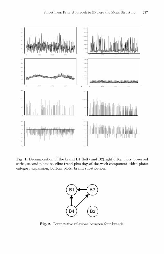
The presented model was applied to scanner data sets of daily milk category,for the period of 1994/2/28 – 1996/3/3 (N=735). Five variate series consisted oftop four brands and the others total were analyzed. Only two brands B1 and B2are shown on top of Fig. 1. The second plots show the estimated baseline trendcomponents plus the estimated day-of-the-week effects. Only about 20% of thevariation of the original series is explained by this day of the week effect. However,for other stores where the prices of brands did not change so significantly, theday-of-the-week effect contribute much more than this present case.

The Fig. 2 shows the detected competitive relation between four major brandsobtained via identified model. It can be seen that B3 is independent of otherbrand’s price promotion. Price-cut of B4 (B2) increases sales of B4(B2), butreduces those of B1 and B2 (B1). Price-cut of B1 increases sales of B1 and doesnot affect the sales of other brands. The third plots of Fig. 1 show the estimatedcategory expansion effect. The price-cuts of B1 and B2 contribute the expansionof category total. On the other hand, the bottom plots show the estimatedbrand switch components. The brand switch components of B1 and B2 are quitedifferent. The plot for B1 indicates that the price-cut of B1 slightly contributesto the expansion of its own sales. But B1 is vulnerable to the price-cut of B2and B4. On the other hand, the price-cut of B2 considerably contributes to theincrease of the own sales and B2 is slightly affected by the price-cut of B4.

Smoothness Prior Approach to Explore the Mean Structure 237

0 200 400 600

0

100

200

300

400

500

600

0 200 400 600

0

100

200

300

400

500

600

0 200 400 600

0

100

200

300

400

500

600

0 200 400 600

0

100

200

300

400

500

600

0

50

100

150

0

50

100

150

-200

-150

-100

-50

0

50

100

-150

-100

-50

0

50

100

150

Fig. 1. Decomposition of the brand B1 (left) and B2(right). Top plots: observedseries, second plots: baseline trend plus day-of-the-week component, third plots:category expansion, bottom plots; brand substitution.

B1

B4 B3

B2

Fig. 2. Competitive relations between four brands.

238 Genshiro Kitagawa, Tomoyuki Higuchi, and Fumiyo N. Kondo

3.3 Analysis of GPS Data

The GPS (Global Positioning System) is one of most interesting and impor-tant data set which allows us to investigate a global change in environmentprecisely. Its high precision information on positions of permanent stations canbe supplied by signal processing of microwave signal from GPS satellite. Sev-eral physical quantities of media existing between the GPS satellite and groundstations affect phase information of microwave signals and result in propaga-tion delays. Therefore, a careful treatment of propagation delays is required toextract reliable information as to measurements of the positions.

Dominant sources to bring about propagation delays are (1) ionosphere originand (2) troposphere origin, such as atmospheric pressure and atmospheric watervapor [16]. The propagation delay generated by the atmospheric water vapor,called the wet delay, is most difficult to evaluate among these factors. A goodestimation on the propagation delay can be given to the ionosphere origin andatmospheric pressure origin sources, by utilizing other physical quantities mea-sured simultaneously. As a result, the wet delay turns out to appear as “noisesource” in the processing of the GPS data and has to be subtracted prior todiagnosing the GPS data in terms of information on positions.

In Japan, considerable efforts to establish a nationwide GPS array has beenkept making by the Geographical Survey Institute of Japan (GSI) [7]. TheJapanese GPS array is characterized by its high spatial resolution; the arrayis composed of nearly one thousand stations separated typically by 15-30 kmfrom one another [16]. Then, a proper processing of the GPS data set takingthe wet delay effect into account allows us to estimate a high-frequent spatialpattern of the atmospheric water vapor, in particular, precipitable water vapor(PWV) which plays an important role in forecasting a weather map. Actually,an approach to extract information concerning the PWV from the GPS datadraws much attention in a field of the meteorology and now is referred to as theGPS meteorology [5,16].

Our objective in this study is also aimed at finding rules to give a quantitativedescription for the relationship between the fluctuations observed in the GPSdata and the PWV, and making it possible to give a PWV map with high spatialresolution. We begin with an analysis of the daily GPS array data provided bythe GSI. Let Ui

n be the nth day starting from January 1st, 1996 at the station(site) i:

Uin = [X i

n, Y in, Zi

n]′ (i = 1, . . . , I; n = N is, . . . , N

ie) (25)

where X , Y , and Z correspond to the north-south, east-west, and up-downcomponents, respectively. N i

s and N ie represent the starting and last date of the

GPS data available to us now. I is the number of stations.Our preparatory analysis shows that the fluctuations associated with the

PWV are most clearly seen in the up-down component, Zin, among the three

components. Then, in this study, we focus on the up-down component Zin. Unfor-

tunately, the original GPS array data contains the outliers as well as the missingobservations. These unsatisfactory cases can be easily treated by a smoothnesspriors approach with the state space model, presented in Sect. 2.3, which provides

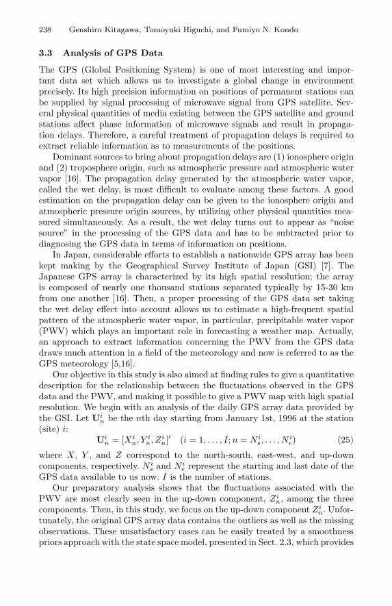
Smoothness Prior Approach to Explore the Mean Structure 239

us with the reasonable interpolated data (see [4] in detail). The interpolation al-lows us to determine Tn, T±1

n , and T±2n systematically. In Fig. 3 we show Tn,

T±1n , and T±2

n obtained by applying the smoothness priors approach to Zin. A

seasonal pattern, which is expected to be associated with the PWV, is clearlyseen in this figure. In addition, a relatively significant amplitude of the seasonalvariation is found to be larger than the typical amplitude of the residuals, whichcan be approximated by a mean of the standard deviation of Di. Therefore, it isapparent that an extraction of precise information on the position from the GPSarray requires an elimination of an effect of the PWV from the GPS data. Apower spectrum analysis is performed on the Tn component and find no eminentpeak except for a yearly cycle in a frequency domain. A detail investigation isbeing made on this figure to discover with what factors is associated from theviewpoint of a climatology.

Trend for UD-comp.

0 200 400 600 800

-30

-20

-10

010

2030

1996 1997 1998

Fig. 3. The median, ±1σ, and ±2σ percentile points of the estimated trend ofthe up-down component versus n, Tn, T±1

n , and T±2n

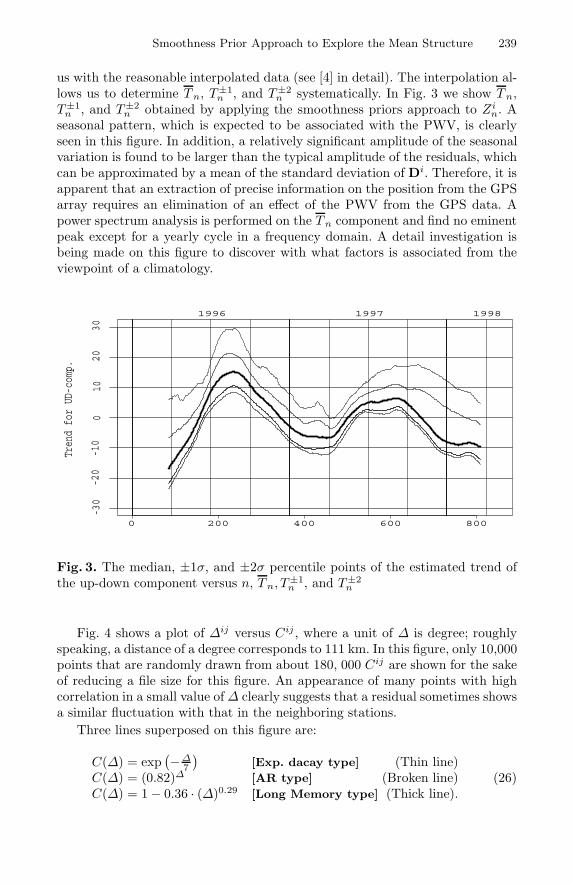
Fig. 4 shows a plot of ∆ij versus Cij , where a unit of ∆ is degree; roughlyspeaking, a distance of a degree corresponds to 111 km. In this figure, only 10,000points that are randomly drawn from about 180, 000 Cij are shown for the sakeof reducing a file size for this figure. An appearance of many points with highcorrelation in a small value of ∆ clearly suggests that a residual sometimes showsa similar fluctuation with that in the neighboring stations.

Three lines superposed on this figure are:

C(∆) = exp(−∆

7

)[Exp. dacay type] (Thin line)

C(∆) = (0.82)∆ [AR type] (Broken line)C(∆) = 1− 0.36 · (∆)0.29 [Long Memory type] (Thick line).

(26)

240 Genshiro Kitagawa, Tomoyuki Higuchi, and Fumiyo N. Kondo

The horizontal line indicates a value of 1/e. Each curve represents a correlationfunction induced from a model denoted in bold face. The thin and thick lines aredrawn so as to resemble an envelope of the upper bound and +2σ percentile asa function of ∆ in a range of ∆ ≤ 10. A good agreement of the thick line to +2σenvelope would implies that a long-memory-type spatial correlation (H ∼ 0.15)[13] happens to be observed for an atmospheric spatial pattern. An examinationof the weather map for these cases is interesting, but the detailed discussion willbe left to other places.

.

.. ...

.

.

.

.

.

.

...

.

.. ..

.

.

....

...

.

....

.

....

.

.

..

..

.

..

.

..

...

.

.

.

.

.

. .

.

..

.

.

.

.

..

.

.

.

...

.

.

. .

..

. .

.

..

.

.

..

.

..

..

..

.

.

.

.

.

.

..

. ..

.

.

.

...

..

.

.

..

. .

.. .

.

.

.

.

.

. ..

..

.

.

. ...

..

.

.....

.

. .

.

.

.

..

.

.

.

.

.

.

. .. .

....

.

..

.

.

.

.

..

. .

.

. ...

.

.

.

.

.

..

...

..

..

.

.

.

.

....

.

.

..

.

...

.

...

.

.

.

...

.. ...

.

.

..

... .

...

.

.

...

.

.

.

...

...

..

. .

.

.

.. .....

..

..

.

... .

.

.

.

.

.

.

.

.

.

.

.

.

...

.

.

.

.

. ....

.

..

.

.

.

.

.

.

.

.

.

.

..

..

.

.

.

.

...

....

...

. .

.

.

.

.

..

...

.

..

.

..

...

. ..

..

..

. .

.. .

.

.

.

...

..

. .

.

.

..

....

.

..

.

.

..

...

.

.

.

.

.

.

...

.

.. ..

.

.

..

. ...

..

..

. .. .

..

.

.

.

..

.

.

.

.

. .

.

.

.

...

.

.

.

..

.

..

..

.

.

...

...

.

.

. .

..

.

.

.

..

.. .

.

.

.

..

..

..

.

.

..

.

.

.

.

.

.

.

.

.

.

.

.

.

...

. .. .

.

.

.

.

.

.

.

..

.

..

.

.

.

.. .

.

.

.

..

.

.. ..

.

.

.

.

. .. .

.

... .

.

.

.

..

.

.

.

.

.

.

.

.

.

..

.

.

.

.

.. ..

..

..

.

.

.

..

.

.

.

.

.

..

. ..

.. .

..

..

.. .

.

.

.. .

.

.

. .

.

..

..

.

.

.

. .

.

.

..

.

.

..

..

.

.

..

.

.

...

.

.

.

..

.

.

. .. .

.. .

.

...

.

.

.

.

.

....

.

...

..

.

..

.

.

.

.

.

..

.

..

..

..

.

..

..

....

.

.

.

.

..

.

.

.. .

..

.

.

.... ..

.

.

.

..

.

.

.

.

..

.

. .

.

.

..

.

.

.

.

. .

.

.

.

.

.

. .. ..

.

.

.

.....

..

.

.

.

.

.

. ...

..

. ..

.

.

.

.. .

..

.... .

.

.

.

.

.

.

..

.

.

.

.

.

..

..

..

.

.. .

.

..

..

.

..

.

.

.

.

.

.

..

. ..

. .

.

..

.

..... ..

.

.

..

. ..

..

.

..

.

.

.

.

.

..

.

.

..

.

..

. .

.

..

..

...

...

.

..

.

.

.

..

.

.

.

.

.

.

. ..

..

..

. ..

.

..

.

.. .

.

..

.

.

.

.

.

.

.

.

.

.

..

.

.

.

.

..

.

...

.....

.

.

.

.

....

..

..

.

..

.

.. ..

..

. .... .

..

. .

.

.

.

.

.

.

.

.

.

.

.

.

.

.

..

.

.

.

.

.

.

..

..

.

.

.

.

.

.

..

.

. .

..

.

..

.

.

.

.

..

.

.

.

. .

.

.

. .

.

.

.

..

..

.

.

.

.

.

..

.

.

.

.

.

..

.

.

. .

..

...

..

..

.

...

.

.

. ..

.

.

.

.

.

.

. ..

. . .. ...

..

.

.. .

.

....

..

.

.

.

.

.

..

..

.

.. .

. .

.

....

..

.

..

.

.

.

...

. .. ..

.

..

...

.

..

. ...

.

...

.

.

.

.

.

.

.

.

.

.. .

.

..

.

.

.

..

.. .

.

..

....

..

.

.

.

..

.. .

.

.

..

.. .

....

..

. .. .. .

.

.

..

.

.

.

..

..

.

.

.

.

.

.

.

.

.

.

.

.. .

.

.

...

..

.

.

.

...

.

.. ..

.

..

.

..

....

...

.

. ..

.

.

..

.

.

.

.

.

..

.

.

.

..

.

...

.

.

. .. .

..

..

.

..

.

..

..

.

.

..

..

...

..

. . .

.

.

.

..

...

.

.

.

..

..

.

.

.

.

.

.

.

.

...

.

.

...

.

.

...

.

.

.....

..

.

.

.

..

.

.

..

.

.

. .. .

.. .. .

. . .

.

..

.

.

.

.

..

...

..

.

.

.

. .

..

.

.

. .

..

.

.

.

.

.. .

...

.

.

.

.

.

.

..

.

.

.

.

.

..

.....

.. ..

... .

.

.

.

.

.

.

.

.

.

.

...

.

.

.

.

.

.

. .

.

.

..

..

..

.

..

..

...

.

.

...

.

.

.

.

.

. . .

.

.

..

.

.. .

.

.

...

.

.

.

.

.

.

..

..

..

. ..

..

. .

.

..

.

.

. ..

...

..

.

.

.

..

.

.

.

.

.

..

.

. .

.. .

..

. . ..

...

.. .

.

..

. ..

...

. .

.

...

..

..

. .

.

.

..

..

..

..

.

.

.

... .

..

.

..

.

.

.

..

.

.

.

.

. .

.

..

.

.

.

. .

.

.

.

.

.

.

.

.

. .

.

..

..

.

. . .

. .

. ..

...

..

.

...

.

.. ..

.

..

.

.

.

. ..

..

.

. .

.

. .

.

..

.

. .

..

.

.

.

..

.

..

.

..

..

...

.

..

.

.

.

.

.

..

.

..

.

..

...

.

.. ..

.

..

...

.

.

.. .

.

..

...

.

.

..

.

.

.

.

.

..

.

.

..

.

.

.

.

.

..

.

.

...

.

..

. .

.

.

.

..

. . .

.

..

.

..

..

..

.

..

. .

. .

..

.

.

..

.

.

.

..

.

.

.

.

.

.

.

..

.

.

.

.

..

.

.

.

...

.

.

.

.

.

.

.

.

.

...

.

.

..

. .

...

..

. .. .

. ..

..

.

. .

.

.

.

.

.

.

.

..

..

.

..

..

.

. . . ..

..

....

.

.

.

.

.

.

.

.

..

..

..

.

.

..

..

.

.

.

...

.

.

.

.

.

.

.

.

.

..

.

.

.

.

.

...

.

.

... .

..

.

.

.

.

.....

. ..

.

..

.

..

.

..

.

.. .

. ..

..

.

.

..

.

..

. .

..

.

.

..

.

.

.

.

.

.

..

.

..

.

.

.

. .

.

.

.

.

....

.

..

.

..

.

.

.

..

.

.

.

.. .

.. ...

.

.

.

.

..

. ..

..

.

.

.

.

.

.

.

.

.

.

.

.

.

.

.

.

. .

. .

..

.

...

.

....

.

..

.

.

.

. .

.

..

.

.

.. .

.

...

.

...

.

.

. .

.. .

.

..

.

.

..

.

.

.

.

.

.

.

..

.

.

..

..

.

..

..

..

. .

.

.

.

.

.

. .

.

.

... .. .

.

.

...

..

.

.

..

.

...

.

.

..

.

.

. .. .

.

.

...

..

..

.

.

.

.

...

.

.

..

.

.

.

..

.

..

..

.

..

.

.

.

. ..

.

..

. .

.

...

.

.

.

. .

.

.

..

.

.

.

.

..

.

.

.

.

.

.

. ..

.

.

...

.....

.

..

.

.

.. ..

.

...

..

.

. ..

.

.

..

.

.

..

...

. .

.

.

.

.

..

.

.

..

.

....

... . .

.

.

.....

..

.

.

.

.

.

..

.. .

. ..

.

...

..

. ..

..

. ..

..

.

.

.

.

..

..

.

.

.

.

.

.

.

.

..

.

.

.

.

..

.

.

.

...

..

..

.

.

.

.

. ..

..

..

.. .

.. ..

.

..

.. ..

. .

.

.

..

.

.

.

.

.

.

.

..

.

.

..

.

.

.

..

.

.

.

.

......

.

.

..

.

.

. ..

.

.

..

..

...

.

.

..

. .

. ..

..

.. ..

.

.

.

.

.

.

.

.

..

.

.

...

.

. ..

. .

.

.

...

.

..

.

..

.

.

.

..

..

..

.

.

. ..

.

.

.

..

...

.

.

...

.

.

.

..

..

..

.

. ..

..

..

...

.. .

..

.. .

.

.

..

.

.

..

.

.

.

..

...

. . ..

. ...

..

.

.

.

.

. .

.

.

.

.

..

..

.

.

.

.

..

.

..

...

. .

...

..

..

.

.

..

.

.

..

.

. .

.

.

.

.

...

.. ..

.

.

. . .

... .

..

.

.

.

.

.

.

..

.

...

.

.

.

.

.

.

.

. .

..

.

.

...

....

.

.

..

.

.

.

.

.

. .

.

.

.. .

..

.

..

.

.

..

.. .

.. .

.

...

..

.

.

.

..

.

..

.

.

..

.

.. .

.

..

...

.. .

..

.

..

.

..

.

...

..

.

..

..

..

..

..

. .

.

..

.

.

.

.

.

..

..

..

.

..

.

.. .. . .

.

.

..

.

.

..

.

.

.

.

..

.

.

.

.. .

.

...

.

.

.

..

.

.

. .

.

.

..

.

. ..

.

..

.

..

.

.

..

.

.

..

...

. .

.. ..

...

.

...

...

.

.

.

..

..

.

.

.

..

..

.

.

.

..

.. . .. .

..

. .

.

..

.

.

..

.

.

.

.

..

.

.

..

..

.

.

.

...

.

...

..

.

.

.

.

..

. ..

.

.

.

.

. ...

. .

.

...

..

.

.

.

..

...

.

.

.

.

.

..

.

.

.

..

.

.

.

.. .

.

..

..

... .

.

.

.

..

..

.

.

.

..

..

..

. .

..

.. .

..

.

..

.

. .

.

.

....

...

.

.

.

..

.

...

..

.

.

....

....

.

..

.

.

.

.

.

.

.

..

.

.

.. . .

.

..

. .

. ..

. .

.. .

.

...

.

.

.

.

.

.

.

.

..

... . .

. .

.

.

.

..

.

..

. .

..

.

.

..

.

...

.

.

.. ..

.. .

.

...

.

...

..

..

.

..

.

.

..

.

. ..

.

.

... ..

..

.

.

.

...

.

.

. ..

.

.

. .

.

.

.

. ..

..

.

..

..

.

.

.

.

.

..

.

..

. .

.

.

.. ..

.

...

..

...

..

.

. .

. .

.

.

.

.

..

.

..

.

.

.

.

.

..

.. .

...

. .. .

...

.

. .

...

.

.

..

.

....

..

....

.

.

...

...

.

.

..

..

.

.

..

.

.

..

.

..

.

.

.

.

.

.

.

.

.

.

..

...

..

.

..

.. ...

.

.

.

.

.

.

. ..

.

.

.

.

...

.

.

.

.

... .

.

..

..

.....

.

.

.. .

..

.

..

.. .

.

. ..

.

.

. .

.

...

..

.

.

. ..

.

.

.

.

.

.

.

.

..

...

..

.

.

.

.

..

.

.

...

.

.

.

..

.

...

.

..

.

.

.

.

...

.

.

.

..

..

.

.

..

.

..

.

... .

.

.

.

.

.

.

..

..

.

.

. .

. .

. ...

...

.

.

.

.

.

.

.

.

.

..

.

.

.

.

.

.

. ..

..

.

.

.

.

.

.... .

.

..

..

..

..

.

.

.

.

.

.

.

.

..

..

.

..

...

.

..

.

.

.

.

.

.

.

.

.

.

.

.

.

. ...

.. . .

...

..

.

..

.

. .

.

..

..

.

.

..

.

.

..

.

.

.

..

..

. .

.

....

..

....

. .

.

. ...

.

.

. . .

..

..

.

..

.. ... .

. .

.

.

.

.... . .

..

.

.

.

.

.

..

.

.

.

.

.

...

.

.

.

.

....

.

.

..

.

.

.

..

.

.

.

.. ..

..

.

..

.

.

.

.

..

.

.

.

...

...

.

.

.

.

....

.. . . .

.

.

..

..

.

.

..

...

.

..

.

.

..

.. .. .

....

..

.

...

.

..

.

..

.

...

.

.

.

.

.

..

..

.

.

..

.

.

.

.

.

.

...

....

..

...

...

.

.

..

.

.. .

...

.

.

. .

.

..

..

.

.

.

.

.

.

...

.

.

...

..

.

..

.

.

..

.

.

.

....

.

..

.

.

.

.

.

.

. ...

..

.. ..

.

..

.

.. .

... .

..

.

.

.

...

.

.

.

... .

.

..

.

..

. .

..

.

..

...

...

..

.

.

.

..

... .

.

... .

.

..

.

..

.

..

..

...

.

.

.

. ..

.

..

.

.

.

.

..

..

.

.

..

. ..

..

..

..

..

.

.

.

....

.

.

...

. ..

.

..

..

.

. .. .

. . .

.

.

.

.

..

..

.

.

.

..

.

..

.

.

...

. .

.

.

...

...

.

.

.

.

.

.

.

..

.

..

.

. ...

......

. .

.

.. .

.

.. . .

.

.

.

.

.

.

.

. ..

.

..

.

.

.

.

.

..

.

. ...

.

...

.

.

.

.

.

.

.

...

.. .

..

. . .

.

.

.

. ... .

.

..

.. .

.

.

.

.

.

.

.

. ..

.

....

... .

. ...

....

.

.

..

.

.

.

..

..

.

....

.. .

.

.

..

.

. ..

..

..

.

.

.

..

..

.

. .

.

.

.

.

.

.

..

.

.

... .

.

..

.

.

..

.

..

..

.

.

.

..

.

. ..

.

. ..

. ..

..

... ..

.

.

.

..

. .

...

.

.

. ..

.

.

..

..

.

.

.

..

.

.

..

...

..

.

..

.

.

. ..

..

..

.

...

. ..

.

.

...

..

.

.

..

.

.

..

.

.

..

.

..

.

.

..

... .

. .

..

.

.

....

.

.

.

..

.

.

...

..

..

.

.

. ...

..

.

. ...

.

.

..

.

.

.

.

....

..

....

...

..

.

...

..

.

...

.

.. ..

.

..

.

..

.. ...

.

.. ..

..

.

..

..

.

. ..

.

.

..

..

..

..

.

. ..

..

...

..

.

.

.

. ..

..

.

..

.

..

.

.

.

..

.

... . .

.

.....

.

..

...

.

..

..

..

.

. .

.

.

.

.

.

.

.

.

..

.

..

. .

..

.

. ...

.

.....

.

.

.

..

.

.. .

.

.

.. .

..

.. .. .

..

..

...

.

.

.

..

.

.

... ..

.

..

..

.

.. .

.

.

.. ..

.

... ..

.

..

.

..

.

.

...

.

. . ....

.. .

.

.

..

.

.. .

.

.

..

.

.

.

.

.

.

..

..

.

.

.

..

..

. .

..

..

..

..

.

.

..

.

..

.. ..

.

.

. .

..

.

.

.

.

. .

.

..

.

.

.. .

.

.

.

..

.

.

..

.

.

.

.

.

.

..

.

. .

..

.

.

.

..

..

. ..

.

.

.

.

.

..

.

.

. .

..

.

.

.

..

.. .. .

..

..

.

.

.

.

.

.

.

.

.

.

.

.

.

.

.

.

..

. .. .

. .

.

..

...

..

..

..

.

..

.

.

.

...

. .

...

.

.

.. . ..

.. ..

..

.

.

..

..

.

.

.

..

.

.

.

..

..

.

.

. .

.

....

.

..

..

.

.

. .

...

.

. .

.

..

..

. .

.

..

..

.

...

..

..

.

..

..

.

.

..

.

.

.

...

.

..

..

.

.

.

....

..

.

.

.

..

.

..

.

..

.. .

..

.. ..

. ..

.. ..

.

.

...

.

....

.

.

.

. ..

.

....

..

..

. .

.

.

..

..

..

...

.

.

.

..

...

.

.

.. . .

.

.

.

.

.

..

.

.

..

.. . .

.

...

.

..

.

.

..

.

..

.. ..

..

.

.

.

.. ...

. ...

.

. ..

...

..

.. .

... .. .. .

..

..

.

.

. .

.

.

..

.

.

..

.

.

..

..

.

..

.

.

.

.

..

..

.

..

..

.

.

.

.

.

.

..

.

.

.... .

..

...

.

.. ..

.. .

.

.

.

..

...

..

.

.

.

.

..

..

.

.

.

..

...

.

.......

.

.

.

.

.

.

.

.

.

. .

.

.

.

.

. .

..

. ..

...

....

..

.

..

..

.

.

..

.

.

.

..

.

.

. ..

.. .

....

.

..

. .

.

.

..

.

.

...

..

... .

...

...

..

. ..

.

.

. .

.

...

.

.

.

.

.

..

.

..

.

..

..

.

.

.

.

...

.

...

.

.

.

.

.

.

...

.

.

..

.

.

.

...

.

.

.

. .. .

.

.

...

. .

..

.

.

.

.

.

..

.

.

.

.

..

.

.

..

. .

.

..

..

...

..

.

.

.

.

..

.

.

.

.

.

..

.

.

.

.. .

. .. .

.

.

..

.

.

..

.

.

.

.

.

.

.

..

.

.

...

... .

.

....

....

.

..

.

.

.

..

.

.

.

..

..

.. ..

.

. .. .

.. ..

..

..

.

.

..

..

.

...

.

.

.

.

..

.

.

.

... .

..

...

....

.

.

.

....

..

..

..

..

...

..

.

.

.

.

.

.

.

. .

.

..

.

..

.

.

.

.

.

.

.

..

.

.

..

.. .

.

....

...

.

.

..

.

.

...

.

.

..

.

.

.

...

.

. .

. .

..

.

...

. .

.

..

.

.

..

.

.

.

.

.

....

.

..

.. .

..

..

..

.. .

.

.

.

.

..

.

..

.

.

..

.

..

.

..

.

. ....

....

.

.

.

...

.

.

.

..

..

..

.

...

.

..

.

.

.

..

...

...

.

.

.

.

.

...

...

..

. .

.

..

..

. .. ..

. .. .

.

.

..

..

..

.

.

..

.

.

.

..

.

.

.

.

..

..

...

..

.

.

.

..

.

..

.

.

.... .

.. ...

.

..

..

.

..

..

.

.

.

...

.

.

.

.

.

..

.

..

..

.

. .

..

.

..

.

..

....

..

.

.

..

.

.

..

.

... .

..

.. .. ...

.. .

..

.

.

.

.

..

.

.

.

.

..

.

..

..

.

.

.

.. .

.

. ...

..

. .

.

.

.

.

.

. ...

.

.

. . . . .

. ..

.

.

..

.

..

.

...

.

...

.

.

.

.

.

.

.

.

.

.

..

.

..

.

.

.

.

..

..

..

.

.

.

.

..

.

.. .

..

..

.

.

.

. ...

.

.

..

.

..

.

.

..

..

. .

.

.

.

.

.

..

.

.

..

.

.

.

. . .. .

.

.

.

..

..

.

.

...

.

.

.

.

.

..

.

. ..

.

..

.

. .. .

.. .

.

..

.

.

.

.

.

.

.

.

.

.

.

..

.

.

..

.. .. .

. .

.

..

....

.

..

.

.

.

...

.

.

..

...

. ...

..

.

... .

...

..

.

.

.

.

..

.

.

.

.

.

.

..

.

.

.

.

.

.

..

.

....

.

..

.

.

.

.

.

.

..

.

.

...

..

.

.

..

...

. .. ... .

.. .

.

.

...

.

.

...

.

.

.

...

.

. .

.

.

.

.

......

.

.

...

.

.

..

.

.

..

..

.

...

.

...

..

.

. ..

.

. .

.

...

.

.

.

..

.

.

.

....

. .

. .

.

.

...

..

..

..

..

.

.

..

.

.

.

.

.

.

.

.

.

...

...

..

.

.

..

..

..

.

...

.

.

.

..

..

..

.

..

.

.

..

.

.

.

..

..

...

..

.

.

.

.

....

..

.

.

. ..

..

..

..

..

.

. ...

.

. ..

..

.

.

.

..

.

.

.

..

..

.. .

.

.

.

.

.

.

...

.

.

.

..

.

.

.

.

..

.

..

..

..

..

... ..

.

. . ..

.

.

..

....

.

..

..

.

..

..

..

.

.

..

..

..

....

..

.

..

.

.

.

.

.

.

.

.

.

.

. ...

. .

.

.

. .

.. ..

.

. .

.

.

.

.

.

..

.

..

.

..

.

.

.

.

.

..

.

.

. ...

..

..

.

.

.

.

.

. .....

.. .

. ....

..

..

.

..

.

.

. ..

.

..

....

..

.

.

.

..

..

..

..

..

..

..

...

..

.

.

.

.

.

.

...

.

.

.

.

.

.

..

.

.

.

.

.. .

.

.

.

.

.

..

. ...

.

..

..

..

..

....

.. .

.

.

.

..

..

.

.

.

.

..

.

.

.

.

.

.

.

.

.

.

..

..

.

.

.

.

..

..

..

.

. .

...

....

..

..

.

.

.

..

.

.. ..

.

..

...

.

.

.

.

.

.

.

.

..

..

.

..

.

...

..

. . ..

...

.

.

..

.

. .

.

..

.

.

.

..

..

.

.

...

.

.. .. . .

...

.

..

. ..

.

.

.

...

.

.

.

.

. . ..

.

. .

..

.. .

.

.

.

.

...

.

.

.

...

.

.

.

..

.

.

..

.

..

. ...

.

..

..

..

..

.

...

.

.....

.

.

.

..

. . ..

.

.

.

.. .

.

..

.

. .

..

.

..

..

.

.

..

.

...

.

.

. . .. .

..

....

.

.

...

.

.

.

..

...

. .

.

. .

..

...

.

..

.

...

..

. .

..

.

.

.

.

.. .

.

.

.

.

.

.

.

.

.

.. .

.

. ...

. .

..

..

.

.

.. .

.. .

.

. ....

. .

.

.

.

.

.

... .

..

..

..

.

... ..

.

..

.

.

.

.

..

.

. ..

.

..

..

. ..

..

.

. ....

.

..

. ...

..

.

..

.

..

....

.

..

..

...

..

.

.

. . .

.

..

...

.. .

. ..

...

. . . ..

.

.

..

.

..

..

.. .

..

.

.

.

.

.

..

.

.. ..

.

.. .

..

. .

. ..

.

.

.

.

.

.

.

.

.

..

.

.

.

.

...

.

..

..

.

.

.

..

..

.

...

.

...

.

.

.. .. .

..

..

. ..

.

.

.

.. .

.. .

.

..

.

..

.

.

.

.

.

..

.

.

.

.

.. . .

.

..

..

. ..

. .. .

..

...

.

..

...

.

.. ...

.

..

.

..

...

..

.

.

.

.

.

.

.

.

.

.

.

.

.

.

.

..

. ..

..

.

.

..

.

..

.

.

.

.

.

.

.

. . .

. .

....

..

.

..

. .

.

.

.

. .

..

..

.

.

.

.

.

.

.

..

.

..

.

...

. .

. .. .

.

. ..

.

.

.

.

...

.

.. ..

.

..

.

..

..

.

.

..

..

.

..

.

..

.

. . .

.

.

.

.

..

. .

. . . .

.

.

. . .

..

.

..

..

.

.. .

. .

.. .. .

.

.

.

.

.

. .

.

...

.

..

. ..

.

. ..

..

.

.

...

.

.

.

.

.

.

..

.

.

.

.

.

.

..

. .

...

..

.

...

. ..

.

....

.

..

.

.

.. .

.

. ...

.

.

...

..

.

....

.

.

.

.

.

.

..

..

.

.

...

.

.

.

. . .

..

.. .

.

.

.

. .

..

.

.

.

.

...

..

. .

.

..

.

....

..

.

..

.

.

.

..

.

.

.

.

.

..

.

..

.

..

.

.

..

.

.

. .

. . .

..

.

.

.

...

.

...

.

.

. ...

.

.

.. .

.

.. ...

..

..

. .

.

. .

.

..

.

..

.

.

.

...

. . .

.. .

..

.

..

.

. . .. .

.

...

..

.

..

... .

...

. .

. ..

..

.

.

. ...

..

.

..

.

.

.

. .

..

.. .

. . ..

.

. ..

.

....

.

.

.

... .

..

.

.

.

.

.

. ..

.

.

..

. ..

..

.

.....

.. .

.

.

. .

.

.

..

. ..

.

.

.

.

.

.

.

..

.

.

..

. .. .

.

....

..

.

.

.

..

.. . ..

.

.

... .

.. .

.

..

.

.

.

.

.

.

.

.

..

.

.

.

.

... . .

..

..

... .

.. .

..

...

...

...

..

. .. .

.. .

.

.. .

.

. ...

.

..

.

.

.

.

.

..

.

..

..

.

.

..

..

.

..

...

.

.

.

.

.

.

.

.

.. .

.. ..

.

.. .

..

.. .

..

.

.. . ..

.

.

.

.

.

..

.

.

.

.. . .

....

..

..

..

.. ..

.

. ...

. .... .

.

. .

..

..

. .

.

.

..

.

.

.

.

.

.

..

.

. . .

.

.

.

.

.

.

. .

..

. .

.

...

..

..

.

.

.

.

.

..

.

. ... .. .

.

.

.

.

.

. .

.

.

...

.

.

..

.

.

. .. .

.

.

.. .

.

.

.

. .

.

.. . .

.

.

. .

...

..

.

..

.

.

..

.. . ..

.....

.

.. .

.

..

.

.. ..

.

.

.

.

..

.

.

.

.. .

.

.

.

..

.

.

.

..

.

.....

.

.

..

. .

. .

.

. .. .

.

.

. ..

...

.

.

.....

.

....

.

.

.

. . .

. .

.

...

.

..

.

.

. .

.

. .

.

.

.

..

.. .

.

.

.

.

.

.

. ..

.

.. .

.

... .

. ..

.

..

..

.

.

...

. .

.

....

..

..

..

.

.

.

.

..

.

.

..

.

...

.

..

.

..

.

..

.. .

.

.

.

.

. ..

. .

..

..

.. ... .

.

.

.. ... .

..

.

.

. . ..

.

.

.

..

..

..

.

. ..

.

.

.

..

.

..

.

.

.

..

. .

.

.. ..

.

...

.

.

. .

.

. ..

.

..

. .

...

.

..

..

. .

.

..

.

.

.

.

..

.

.

.

. .

.

.

..

.

.

. ..

.

. . . ..

..

.

..

..

.

...

..

.

. .. ..

..

.

.

.. .

.

. .

.

. ..

..

.

.

..

.

..

.

.

.

..

..

.

.

.

.

.

..

.

.

. ..

.

.. .

. .....

.

.

. ..

..

.

..

..

..

.

.. ..

..

.

.

...

.

.

..

.

.

.

. ..... .

.. .

..

... .

.

.

.

.

.

.

.

.. ...

.. ...

..

.

..

. .

. .. . .

.

..

.

..

..

.

.

.

.. .

. ....

.

.

.

.

.

. .

.

. .

.

.

.. .

...

... .

.

.

. ..

..

. ....

. .

.

.

. . ..

.

.

.

.

..

.

.

.

.

.

. .

.

.

..

.

.....

..

.

.

..

.

.

.

.. .

..

.

.

.

..

.

.

..

.

.. ..

..

.

. .

.

.

.

.

..

.

..

.

..

.

.

.

.

.

.

.

.

.

.

....

..

. .

..

.

.

..

.

..

.

....

..

..

.

...

.. .. .

.

..

.

.

. . .

.

.

.. . .

.

..

.

.

.

.

. .. .

..

....

.

.. ..

.

.

.

.

..

.

.

. .

.

.

.

..

.

. .

.

..

.

.

..

.

.

..

...

. .

.

.. . .

.

.

..

.

.

.

.

.

. .

..

.. ....

.

..

. .. ..

.. .

.. .

.. .

..

...

. ..

.

.

...

..

.. . ..

..

.. .

.

.

.

.

.

.

.

.

. .

.

.

. .

.

...

....

. .

.

..

.

.

.

.

.

.. .

.

.

..

.

..

... .

.

...

..

..

..

.

.

. ..

.

..

.

..

.

.

. ..

. .

...

.

..

.

.

.

. .

.

...

...

.

..

.

..

. . ..... .. .

...

.

..

.

...

..

. ..

..

.

.

. ..

.

..

.

. ...

.

.

...

.

..

.

.

. ..

..

. .

..

.

.

.

. .

..

.

.

... .

.

.

.

...

.. . .

.

.

. .

..

.

.

.

..

. .

.

..

...

.

.

.

..

.

..

... .

.

.

..

...

. .....

... .

.

..

.

..

..

. ..

.

...

.

.

..

.

.

.

.

.

.

. .

.

..

.

...

. ..

.

..

.

.

.

.

..

.

.

.

.

..

..

.

..

..

..

.

.

...

.

..

.

.. ..

. .

..

.

.

.

.

. ... .

.

.

...

.......

..

.

.

.. .

. ..

... .

.

..

..

.

.. ..

.... .

..

. .. .

.

....

.

..

.

.

. .

.

. .

.

.

.

.

...

. ...

..

.

.

...

..

... .

..

.

.

.. .

...

.

... .

.

.. .

..

.

.

.

. .

..

.

.

..

..

. ..

.

.

..

.

.

.

..

.... .

.

..

. ..

. ..

.

.

.

..

. .. .

... .

.

..

. .

.. .

.

. ..

. . .

.

..

.

.

.

.

.

. ..

.

.

.

..

.

.

....

. ..

..

.

..

.

.

.

.

.

...

..

.

.

..

.. ..

..

.

.

.

.

..

.

..

..

.

.

..

.

.

.

.

.

.

.

..

..

.

.

..

.

..

. . .

..

..

..

.

..

...

.

. .

.

.

.

.

.

. .

.. . .

..

.

.. .

..

..

.

.

..

.

.

.

.

..

.

.

..

.

.

.

.

.

.

..

..

.

..

..

.

.

.

. .

...

.. .

. ..

.. . .

.

..

.

..

..

. .

.

. .. .

...

.

.

.

.

.

.

.

..

...

..

.

..

....

. .

.. .

.

.

.. .

..

.

.

..

... .

. ...

.

.

.

. ..

.

..

.

...

..

.

..

.

. .

.

.

..

...

..

..

.

..

.

..

.

.

.

.. .

... .

..

. .. .

.

. .

.

.

.. .

..

.

..

.

..

.

...

..

..

.

.

.

. .

..

.

.

.

..

.

.

. ...

.

..

.

.

.

. .

.

.. .

.

.

....

...

.

.

... . .

.. ...

...

.

...

..

.

..

.

..

. .

. ...

...

.

.

.

.

..

..

..

.

...

... .

.

. . .

..

. .

.. .

..

.

...

..

.

.

.

.

..

.

.

..

.

.

...

..

.

..

..

.

..

..

.

..

...

..

..

.

. ..

.

.

.

..

. . ..

.

.

..

..

.

..

.

. . .

.

. ...

.

.

.

.

. ..

.. . .

.

..

..

...

..

.

.

.

.

. .

. ..

..

..

..

.

.

...

..

.

.. ... .

....

..

.

..

.

..

.

.

.

.. .

..

..

..

....

.

..

.

.

.

.

. . .

.

. ..

..

... .

.

.

..

..

..

..

.

..

.

..

..

.

.

.

.. .

.

.

..

.

.

.

.

..

.

.

..

.

.

.

.

.

.

.

..

..

. ..

. ..

. .

.. ... .

..

..

...

..

.

.

.. ....

. ..

.

..

.

..

..

.

. .

..

..

..

...

.

.

.

.

.

...

. ... .

.

...

.

.

.

.

..

..

.

.

.

...

..

Separation [deg.]

C.C.

0 5 10 15 20

-0.20.0

0.20.4

0.60.8

1.0

Fig. 4. Plots of ∆ij versus Cij .

4 Conclusion

The key to the success of the statistical procedure is the appropriateness of themodel used in the analysis. The smoothness priors facilitates to develop vari-ous types of models based on prior information on the subject and the data. Inthis paper, we applied the smoothness priors method for the modeling of largescale time series and space-time data with mean value structure and competi-tive relations between variables. In the analysis of POS data, the time series isdecomposed into several components and various knowledges to make a strat-egy concerning price promotion and risk control of dead-stock are obtained.The useful information for making a conjecture on the relationship between thepropagation delay and PWV is successfully extracted based on the detailed in-vestigation on the trend and residual components.

Smoothness Prior Approach to Explore the Mean Structure 241

Acknowledgments. The GPS array data were provided by the GeographicalSurvey Institute of Japan (GSI). One of the authors (T.H.) thanks to Dr. S.Miyazaki (GSI) for his help to understand the original data structure.

References

1. Akaike, H.: A new look at the statistical model identification, IEEE Transactionson Automatic Control, AC-19, 716–723 (1974)

2. Akaike, H.: Likelihood and the Bayes procedure (with discussion), in BayesianStatistics, edited by J.M. Bernardo, M.H. De Groot, D.V. Lindley and A.F.M.Smith, University press, Valencia, Spain, 143–166 (1980)

3. Akaike, H.: Seasonal adjustment by a Bayesian modeling, J. Time Series Analysis,1, 1–13 (1980)

4. Akaike, H., and Kitagawa, G.: The Practice of Time Series Analysis, Springer-VerlagNew York (1999)

5. Bevis, M., Businger, S., Herring, T. A., Rocken, C., Anthes, R. A., and Ware, R. H.:Remote sensing of atmospheric water vapor using the Global Positioning System,J. Geophysical Research, 97, 15,787–15,801 (1992)

6. Gersch, W., and Kitagawa, G.: The prediction of time series with trends and sea-sonalities, Journal of Business & Economic Statistics, 1, No. 3, 253–264 (1983)

7. Heki, K., Miyazaki, S., and Tsuji, H.: Silent fault slip following an interplate thrustearthquake at the Japan trench, Nature, 386, 595–598 (1997)

8. Higuchi, T.: A method to separate the spin synchronized signals using a Bayesianapproach (in Japanese with English Abstract), Proceedings of the Institute of Sta-tistical Mathematics, 41, 115–130 (1993)

9. Kalman, R.E.: A new approach to linear filtering and prediction problems, Trans.Amer. Soc. Mech. Eng., J. Basic Engineering, 82, 35–45 (1960)

10. Kashiwagi, N.: On the use of the Kalman filter for spatial smoothing, Annals ofthe Institute of Statistical Mathematics, 45, 21–34 (1993)

11. Kitagawa, G. and Gersch, W.: Smoothness Priors Analysis of Time Series, LectureNotes in Statistics, No. 116, Springer-Verlag, New York (1996)

12. Kitagawa, G. and Higuchi, T.: Automatic Transaction of Signal via Statistical Mod-eling, The proceedings of The First International Conference on Discovery Science,Springer-Verlag Lecture Notes in Artificial Intelligence Series, 375–386 (1998)

13. Mandelbrot, B.: Fractals: Form, Chance and Dimension, Freeman, San Francisco(1977)

14. Rissanen, J.: Modeling by shortest data description, Automatica, Vol. 14, 465–471(1978)

15. Shiller, R.: A distributed lag estimator derived from smoothness priors, Economet-rica, 41, 775–778 (1973)

16. Tsuda, T., Heki, K., Miyazaki, S., Aonashi, K., Hirahara, K., Nakamura, H., To-bita, M., Kimata, F., Tabei, T., Matsushima, T., Kimura, F., Satomura, M., Kato,T., and Naito, I.: GPS meteorology project of Japan — Exploring frontiers ofgeodesy—, Earth Planets Space, 50, No.10, i–v (1998)

17. Whittaker, E.T: On a new method of graduation, Proc. Edinborough Math. Assoc.,78, 81–89 (1923).