ICMA Centre • The University of Reading Whiteknights • PO Box 242 • Reading RG6 6BA • UK Tel: +44 (0)1183 788239 • Fax: +44 (0)1189 314741 Web: www.icmacentre.rdg.ac.uk Director: Professor John Board, Chair in Finance The ICMA Centre is supported by the International Capital Market Association

Generalized Beta-Generated Distributions

Carol AlexanderICMA Centre, Henley Business School at Reading, UK

Gauss M. CordeiroDepartamento de Estatística, Universidade Federal de Pernambuco, Brazil.

Edwin M. M. OrtegaDepartamento de Ciências Exatas, Universidade de São Paulo, Brazil.

José María SarabiaDepartment of Economics, University of Cantabria, Spain

February 5, 2011

ICMA Centre Discussion Papers in Finance DP2011-05Replacing DP2010-09

Copyright © 2011 Alexander et al. All rights reserved.

Generalized Beta-Generated Distributions

Carol Alexander,a Gauss M. Cordeiro,b Edwin M. M. Ortegac and Jose Marıa Sarabiad

First Version: 27 July 2010

This Version: 27 January 2011

Abstract

This article introduces generalized beta-generated (GBG) distributions. Sub-models includeall classical beta-generated, Kumaraswamy-generated and exponentiated distributions. Theyare maximum entropy distributions under three intuitive conditions, which show that theclassical beta generator skewness parameters only control tail entropy and an additionalshape parameter is needed to add entropy to the centre of the parent distribution. Thisparameter controls skewness without necessarily differentiating tail weights. The GBG classalso have tractable properties: we present various expansions for moments, generating func-tion, quantiles, deviations and reliability. The model parameters are estimated by maximumlikelihood and the usefulness of the new class is illustrated by means of some real data sets.

Key Words: Beta, Distribution, Entropy, Estimation, Exponentiated, Gamma, Generalized,Generated, Gumbel, Inverse Guassian, Kumaraswamy, Kurtosis, Laplace, McDonald, Minimax,MLE, MGF, Reliability, Skewness, Weibull.

JEL Codes: C16, G1

a ICMA Centre, Henley Business School at Reading, UK. e-mail:c.alexander@icmacentre.ac.ukb Departamento de Estatıstica, Universidade Federal de Pernambuco, Brazil.e-mail:gausscordeiro@uol.com.brc Departamento de Ciencias Exatas, Universidade de Sao Paulo, Brazil. e-mail:edwin@esalq.usp.brd Department of Economics, University of Cantabria, Spain. e-mail:jose.srabia@unican.es

Many thanks to Prof. M.C. Jones of the Open Univerisity, UK, for very insightful comments on the first

draft of this paper. Also, Jose Marıa Sarabia acknowledges support from the Ministerio de Educacion of

Spain (PR2009-0200, Programa Nacional de Movilidad de Recursos Humanos, and SEJ2007-65818) and

would like to thank the ICMA Centre for its hospitality.

1

1 Introduction

The statistics literature is filled with hundreds of continuous univariate distributions: see John-son et al. (1994, 1995). Recent developments focus on new techniques for building meaningfuldistributions, including the two-piece approach introduced by Hansen (1994), the perturbationapproach of Azzalini and Capitanio (2003), and the generator approach pioneered by Eugene etal. (2002) and Jones (2004). Many subsequent articles apply these techniques to induce a skewinto well-known symmetric distributions such as the Student t: see Aas and Haff (2006) for areview. Using the two-piece approach with a view to finance applications Zhu and Galbraith(2010) argue that, in addition to Student t parameters, three shape parameters are required:one parameter to control asymmetry in the centre of a distribution and two parameters to con-trol the left and right tail behavior. This paper addresses similar issues to Zhu and Galbraith(2010) but takes a different approach. We introduce a class of generalized beta generated (GBG)distributions that have three shape parameters in the generator. By considering quantile-basedmeasures of skewness and kurtosis and by decomposing the entropy, we demonstrate that twoparameters control skewness and kurtosis through altering only the tail entropy and one controlsskewness and kurtosis through adding entropy to the centre of the parent distribution as well.

The first distribution of the beta-generated (BG) class was the beta normal distributionintroduced by Eugene et al. (2002). Denote the standard normal cdf and pdf by Φ(.) and ϕ(.),respectively, and let X = Φ−1(U) with U ∼ B(a, b).1 Then X has a beta normal distributionBN (a, b, 0, 1) with density function

fBN (x; a, b, 0, 1) = B(a, b)−1 ϕ(x) [Φ(x)]a−1 [1− Φ(x)]b−1, −∞ < x <∞. (1)

Location and scale parameters are redundant in the generator since if X ∼ BN (a, b, 0, 1) thenY = σX + µ ∼ BN (a, b, µ, σ) has the non-standard beta-normal distribution with N(µ, σ2)parent. The parameters a and b control skewness through the relative tail weights. The betanormal density is symmetric if a = b, it has negative skewness when a < b and positive skewnesswhen a > b. When a = b > 1 the beta-normal distribution has positive excess kurtosis and whena = b < 1 it has negative excess kurtosis, as demonstrated by Eugene al. (2002). However, bothskewness and kurtosis are very limited and the only way to gain even a modest degree of excesskurtosis is to skew the distribution as far as possible.2

Changing the parent distribution so that it is no longer normal offers more flexibility. Re-placing Φ in (1) by any other parent distribution F yields the general class of BG distributionsdiscussed by Jones (2004). These encompass many other types of distributions, including skewedt and log F . BG distributions may be characterized by their pdf

fBG(x) = B(a, b)−1 f(x)F (x)a−1 [1− F (x)]b−1, x ∈ I, (2)

where F (x) and f(x) are the cdf and pdf of the parent. Jones (2004) concentrates on caseswhere F is symmetric about zero with no free parameters other than location and scale andwhere I is the whole real line.

BG distributions have been studied by Nadarajah and Kotz (2004, 2005), Akinsete et al.(2008), Zografos and Balakrishnan (2009) and Barreto-Souza et al. (2010). Jones and Larsen

1The classical beta distribution B(a, b) may be characterized by its density function:

fB(u; a, b) = B(a, b)−1ua−1(1− u)b−1, 0 ≤ u ≤ 1,

where B(a, b) = Γ(a)Γ(b)/Γ(a+ b) denotes the beta function, Γ(·) the gamma function, and the two parametersa and b are such that a, b > 0. Although it has only two parameters, the beta density accommodates a verywide variety of shapes including (for a = b = 1) the standard uniform distribution U [0, 1]. The beta density issymmetric iff a = b, is unimodal when a, b > 1 and “U” shaped when a, b < 1. It has positive skew when a < band negative skew when a > b.

2Eugene al. (2002) tabulate the mean, variance, skewness and kurtosis of BN (a, b, 0, 1) for some particularvalues of a and b between 0.05 and 100. The skewness always lies in the interval (−1, 1) and the largest kurtosisvalue found is 4.1825, for a = 100 and b = 0.1 and vice versa.

2

(2004) and Arnold et al. (2006) introduce the multivariate BG class. Some practical applicationshave been considered: e.g. Jones and Larsen (2004) fit skewed t and log F to temperature data;Akinsete et al. (2008) fit the beta-Pareto distribution to flood data; and Razzaghi (2009) appliesthe beta-normal distribution to dose-response modeling. However, the classical beta generatorhas only two parameters, so it can add only a limited structure to the parent distribution.For many choices of parent the computations of quantiles and moments of BG distribution canbecome rather complex. Also, when a = b (so the skewness is zero if F is symmetric) the betagenerator typically induces mesokurtosis, in that the BG distribution has a lower kurtosis thanthe parent.3

Jones (2009) advocates the Kumaraswamy (1980) distribution, commonly termed the “mi-nimax” distribution, as a generator. It has tractable properties especially for simulation, as itsquantile function takes a simple form. However, Kumaraswamy-generated (KwG) distributionsstill introduce only two extra shape parameters, whereas three may be required to control bothtail weights and the distribution of weight in the centre. Therefore, we propose the use of a moreflexible generator distribution: the generalized beta distribution of the first kind. It has one moreshape parameter than the classical beta or Kumaraswamy distribution, and we shall demonstratethat this parameter gives additional control over both skewness and kurtosis. Special cases ofgeneralized beta-generated (GBG) distributions include BG and KwG distributions and theclass of exponentiated distributions.

The rest of the paper is organized as follows: Section 2 describes the cdf, pdf and hazardfunctions of the GBG distribution. Section 3 investigates the role of the generator parametersand relates this to the skewness and the decomposition of the GBG entropy. In Section 4, wepresent some special models. A variety of theoretical properties are considered in Section 5.Estimation by maximum likelihood is described in Section 6. Section 7 provides an empiricalapplication. Finally, some conclusions are noted in Section 8.

2 The GBG Distribution

The generalized beta distribution of the first kind (or, beta type I) was introduced by McDonald(1984). It may be characterized by its density function

fGB(u; a, b, c) = cB(a, b)−1 uac−1 (1− uc)b−1, 0 < u < 1. (3)

with a > 0, b > 0 and c > 0. Two important special cases are the classical beta distribution(c = 1), and the Kumaraswamy distribution (a = 1).

Given a parent distribution F (x; τ ), x ∈ I with parameter vector τ and density f(x; τ ), theGBG distribution may be characterized by its density function:

fGBG(x; τ , a, b, c) = cB(a, b)−1 f(x; τ )F (x; τ )ac−1 [1− F (x; τ )c]b−1, x ∈ I. (4)

Now, a, b and c are shape parameters to those in τ . If X is a random variable with pdf (4), wewrite X ∼ GBG(F ; τa, b, c). Two important special sub-models are the BG distribution (c = 1)proposed by Jones (2004), and the Kumaraswamy generated (KwG) distribution (a = 1) recentlyproposed by Cordeiro and de Castro (2011). Of course, the beta type I density function itselfarises immediately if F (x; τ ) is taken to be the uniform cumulative function.

GBG distributions admit a straightforward translation of location and scale. If Y = µ+σXthen Y has density function

fGBG(y; τ , a, b, c, µ, σ) = τ(a, b, c, σ) f(σ−1(y − µ))F (σ−1(y − µ))ac−1[1− F (σ−1(y − µ))c

]b−1,

3For example, using a Student t parent and a = b > 1 we find that the kurtosis converges rapidly to 3 as aand b increase, and for a = b < 1 the kurtosis is infinite.

3

where τ(a, b, c, σ) = c σ−1B(a, b)−1. Assuming the mean µ and standard deviation σ of X existand are finite, then Y has mean µ+ σ µ and standard deviation σ σ. Hence, it is redundant touse scale or location parameters in the generator itself, only shape parameters are needed.

The random variable X admits the simple stochastic representation

X = F−1(U1/c), U ∼ B(a, b). (5)

Using the transformation (5), the cdf of (4) may be written:

FGBG(x; τ , a, b, c) = I(F (x; τ )c; a, b) = B (a, b)−1∫ F (x;τ )c

0ωa−1(1− ω)b−1dω, (6)

where I(x; a, b) denotes the incomplete beta ratio function. The GBG hazard rate function (hrf)reduces to

h(x; τ , a, b, c) =c f(x; τ )F (x; τ )ac−1 {1− F (x; τ )c}b−1

B (a, b) {1− IF (x;τ )c (a, b)}. (7)

It follows immediately from (4) that the GBG with parent cdf F is a standard BG distributionwith exponentiated parent cdf F c. This simple transformation facilitates the computation ofmany of its properties. From now on, for an arbitrary parent F , we write X ∼ ExpcF if X hascdf and pdf given by

Gc(x) = F (x; τ )c and gc(x) = cf(x; τ )F (x; τ )c−1,

respectively. The properties of exponentiated distributions have been studied by many authorsin recent years, see Mudholkar et al. (1995) for exponentiated Weibull, Gupta et al. (1998) forexponentiated Pareto, Gupta and Kundu (2001) for exponentiated exponential, and Nadarajahand Gupta (2007) for exponentiated gamma distribution.

The transformation ExpcF is called the Lehmann type I distribution. There is a dual trans-formation defined by Expc(1 − F ) refereed to as the Lehmann type II distribution. The cdf ofthe last transformation corresponds to Hc(x) = [1 − F (x; τ )]c. Clearly, the double construc-tion beta-ExpcF yields the GBG distribution. Thus, in addition to the classical BG and KwGdistributions and the parent distribution F itself, the GBG distribution encompasses the ExpF(for b = 1) and Exp(1 − F ) (for a = c = 1) distributions. The classes of distributions that areincluded as special sub-models of the GBG distribution are displayed in Figure 1.

We end this section by stating some useful expansions for the GBG cdf and pdf and, forbrevity of notation, from henceforth we shall drop the explicit reference to the parent parametersτ , unless otherwise stated. First note that when b is an integer (6) may be written:

FGBG(x; a, b, c) =b−1∑r=0

(a+ b− 1

r

)F (x)c(a+b−r−1)[1− F (x)c]r.

Alternatively, if a is an integer:

FGBG(x; a, b, c) = 1−a−1∑r=0

(a+ b− r

r

)F (x)cr[1− F (x)c]a+b−r−1.

Other expansions for (4) and (6) may be derived using properties of exponentiated distributions.Expanding the binomial in (4) yields:

fGBG(x; a, b, c) = cB(a, b+ 1)−1 f(x)∞∑i=0

(−1)i(b

i

)F (x)c (a+i)−1. (8)

4

KwG

F

Exp(1- F) ExpF

BG

GBG

b=1

c=1

b=1a=1

a=c=1b=1

c=1

a=1

KwG

F

Exp(1- F) ExpF

BG

GBG

b=1

c=1

b=1a=1

a=c=1b=1

c=1

a=1

Figure 1: Relationships of the GBG sub-models

Hence, the GBG is a mixture of exponentiated-F distributions. Its density may be written:

fGBG(x; a, b, c) =∞∑i=0

wi ga (i+c)(x), (9)

and its distributions is

FGBG(x; a, b, c) =∞∑i=0

wiGa (i+c)(x), (10)

where ga (i+c)(x) and Ga (i+c)(x) denote the pdf and cdf of Expa (i+c)F and

wi =(−1)i

(bi

)(a+ i)B(a, b+ 1)

. (11)

Using the mixture representation (9), some of the GBG properties may be obtained from thecorresponding properties of exponentiated distributions.

Finally, we remark that the cdf (6) may also be expressed in terms of the hypergeometricfunction as

FGBG(x; a, b, c) =c F (x)a

aB(a, b)2F1 (F (x)

a; a, 1− b, a+ 1) ,

where

2F1(x; a, b, c) =Γ(c)

Γ(a)Γ(b)

∞∑j=0

Γ(a+ j)Γ(b+ j)

Γ(c+ j)

xj

j!.

Thus, the GBG properties could, in principle, be obtained from well-established properties ofthe hypergeometric function. See, for example, Gradshteyn and Ryzhik (2000, Section 9.1).

5

3 Entropy and Higher Moments

In this section we interpret the effect of each parameter a, b and c by examining the skewnessand kurtosis of the generated distribution and the decomposition of the GBG Shannon entropy.

3.1 Skewness and Kurtosis

To illustrate the effect of the shape parameters a, b and c on skewness and kurtosis we considermeasures based on quantiles. The shortcomings of the classical kurtosis measure are well-known. There are many heavy-tailed distributions for which this measure is infinite, so itbecomes uninformative precisely when it needs to be. Indeed, our motivation to use quantile-based measures stemmed from the non-existance of classical kurtosis for many of the GBGdistributions we studied.

The Bowley’s skewness (see Kenney and Keeping, 1962) is based on quartiles:

B =Q(3/4)− 2Q(1/2) +Q(1/4)

Q(3/4)−Q(1/4)

and the Moors’ kurtosis (see Moors, 1998) is based on octiles:

M =Q(7/8)−Q(5/8)−Q(3/8) +Q(1/8)

Q(6/8)−Q(2/8),

where Q(·) represents the quantile function. These measures are less sensitive to outliers andthey exist even for distributions without moments. For the standard normal distribution, thesemeasures are 0 (Bowley) and 1.2331 (Moors). For the classical Student t distribution with10 degrees of freedom, these measures are 0 (Bowley) and 1.27705 (Moors). For the classicalStudent t distribution with 5 degrees of freedom, they are zero (Bowley) and 1.32688 (Moors).

0 5 10 15 20

-0.05

0.00

0.05

0 5 10 15 201.220

1.225

1.230

1.235

1.240

1.245a=b=0.5

a=b=0.5

a=b=1

a=b=1

a=b=10 a=b=10

a=b=50 a=b=50

Figure 2: The Bowley skewness (left) and Moors kurtosis (right) coefficients for the GBN dis-tribution as a function of c, for a = b = 0.5, 1, 10 and 50.

Figures 2, 3 and 4 depict the Bowley and Moors measures for the GB-normal distribution andfor the GB-Student distribution with 10 and 5 degrees of freedom, respectively. These are easilyderived from the GBG quantile function, which is presented in Section 5.2. Since our primarypurpose is to investigate the effect that c has on skewness and kurtosis, we have representedthese measures as a function of c assuming that the other two shape parameters a and b areequal and take the values 0.5, 1, 10 and 50. For all three distributions the Bowley skewnesscoefficient is zero for c = 1, negative for c < 1 and positive for c > 1. Whilst the three skewnessplots are similar, they have different vertical and horizontal scales, and it is clear that whenc = 1 the degree of skewness that can be induced by the generator increases with the kurtosisof the parent, and decreases with the value of a and b.

A different picture emerges on consideration of the Moors kurtosis, which may be fairlylimited for GBG distributions. With a normal parent, the right hand graph in Figure 2 shows

6

0 2 4 6 8 10

-0.10

-0.05

0.00

0.05

0.10

0.15

0 2 4 6 8 10

1.25

1.30

1.35

1.40a=b=0.5

a=b=0.5

a=b=1

a=b=1

a=b=10

a=b=10

a=b=50

a=b=50

Figure 3: The Bowley skewness (left) and Moors kurtosis (right) coefficients for the GBG Studentt distribution with 10 degrees of freedom as a function of c, for a = b = 0.5, 1, 10 and 50.

0 2 4 6 8 10

-0.1

0.0

0.1

0.2

0 2 4 6 8 10

1.3

1.4

1.5

1.6

1.7

a=b=0.5

a=b=0.5a=b=1

a=b=1

a=b=10

a=b=10

a=b=50

a=b=50

Figure 4: The Bowley skewness (left) and Moors kurtosis (right) coefficients for the GBG Studentt distribution with 5 degrees of freedom as a function of c, for a = b = 0.5, 1, 10 and 50.

that the Moors coefficient is increasing in c, for all values of a and b, and effect is largest fora = b = 1. It is equal to the parent kurtosis for c = 1, less than the parent kurtosis for c < 1and greater for c > 1. However, as c increases the Moors kurtosis converges to a limit only alittle greater than 1.2331, i.e. the normal Moors kurtosis. Therefore we conclude that whenthe parent is normal the additional parameter c acts primarily as another skewness parameterrather than a kurtosos parameter.

Figures 3 and 4 depict (on the right) the Moors kurtosis of GBG distributions with Studentt parents. Here the Moors measure can become large and positive, but only for small values of c.Initially, as c increases from small values the measure decreases sharply presenting a minimumaround c = 2. When a = b < 1 the Moors kurtosis is always greater for the GBG Studentt distribution than for the classical Student t distributions. However, very high kurtosis canonly be captured using a very low value for c. When a = b >> 1 the Moors measures for thegenerated distribution are lower than they are for the parent, except when c takes extremelysmall values.

3.2 Entropy

The Shannon (1948) entropy H(g) = −Eg[log g(x)] = −∫g(x) log g(x)dx of a pdf g(x) (hence-

forth called simply entropy) is a measure of the uncertainty in a probability distribution and itsnegative is a measure of information.4 Because the generalized beta is a classical BG distributionwith parent G(x) = xc, we may write (3) as:

fGB(x; a, b, c) = B(a, b)−1g(x)[G(x)]a−1[1−G(x)]b−1, (12)

4Ebrahimi et al. (1999) show that there is no universal relationship between variance and entropy and wheretheir orderings differ entropy is the superior measure of information.

7

where G(x) = xc, 0 < x < 1 and g(x) = G′(x). Hence,

−EGB[log fGB(x)] = logB(a, b)− EfGB [log g(x)]

−(a− 1)EfGB [logG(x)]− (b− 1)EfGB [log(1−G(x))],

−EGB[logG(x)] = ζ(a, b),

−EGB[log(1−G(x))] = ζ(b, a),

EGB[log g(x)] =

∫ 1

0(log c+ (c− 1) log x)fGB(x)dx

= log c− c−1(c− 1)ζ(a, b),

where ζ(a, b) = ψ(a + b) − ψ(a) and ψ(·) represents the digamma function. Thus, the entropyof a BG distribution is:

−EGB[log fGB(x)] = logB(a, b)− log c+ c−1(c− 1)ζ(a, b)

+(a− 1)ζ(a, b) + (b− 1)ζ(b, a). (13)

Setting a, b and c in (13) equal to certain values gives the entropy of sub-model distributions.5

Appendix A proves that the GBG density (4) with parent distribution F statisfies

−EGBG [logF (X)c] = ζ(a, b), (15)

−EGBG [1− logF (X)c] = ζ(b, a), (16)

EGBG [log f(X)]− EU [log f(F−1(U1/c))] = c−1(c− 1)ζ(a, b), (17)

where f(x) = F ′(x) and U ∼ B(a, b). Furthermore, the GBG has the maximum entropy of alldistributions satisfying the information constraints (15) – (17) and its entropy is:

−EGBG [log fGBG(x)] = logB(a, b)− log c+ c−1(c− 1)ζ(a, b)

+(a− 1)ζ(a, b) + (b− 1)ζ(b, a)− EU [log f(F−1(U1/c))]. (18)

Thus, the GBG entropy is the sum of the entropy of the generalized beta generator (13),which is independent of the parent, and another term −EU [log f(F

−1(U1/c))] that is relatedto the entropy of the parent. Furthermore, the constraints (15) and (16) reflect informationonly about the generalized beta generator. Note that (13) takes its maximum value of zerowhen a = b = c = 1; otherwise, the structure in the generator adds information to the GBGdistribution. From

EGBG [logF (X)c] = EBG [logG(x)] = EB[logU ],

EGBG [logF (X)] = EBG [log(1−G(x))] = EB[log(1− U)],

it follows that (15) is related to the information in the left tail and (16) is related to the infor-mation in the right tail, and this information is the same when a = b. Clearly, the parametersa and b influence skewness only though taking different values, i.e. having differential weightsin the two tails. By contrast, the additional parameter c influences skewness though (17) byadding entropy to the centre of the distribution.

To illustrate the concepts introduced above, consider two samples of daily returns on the S&P500 index. Sample 1 (January 2004 - December 2006) and Sample 2 (January 2007 to December2009) are chosen to represent two very different market regimes: in the first sample markets wererelatively stable with a low volatility; the second sample encompasses the credit crunch and the

5For instance, for c = 1 we obtain the entropy of the classical beta distribution (Nadarajah and Zografos,2003) and for a = 1 we obtain the Kumaraswamy entropy:

−EKw[log fKw(x)] = − log(c b) + c−1(c− 1)ζ(1, b) + (b− 1)ζ(b, 1). (14)

which follows on noting that B(1, b) = b−1.

8

banking crisis, when market risk factors were extremely volatile. These observations are verifiedby the sample statistics shown in the upper section of table 1. Our purpose here is to comparea, b and c and hence also the entropy decomposition (18) for the two samples. However, the sizeof the GBG parameters depends on the mean and variance, which are quite different in thesetwo samples. So we estimate the GBG parameters on standardized samples Z = (X − µ)/σ,where µ and σ are the mean and standard deviation of each sample. The parameters a, b and c,estimated using the method outlined in Section 6, are reported in the middle section of table 1.6

The bottom section of the table reports the lower and upper tail components of the generalizedbeta entropy, i.e. ζ(a, b) and ζ(b, a) in (15) and 16), and the term − log c+ c−1(c− 1)ζ(a, b) in(18) which is zero for the classical beta generated distribution but which more generally controlsthe information in the centre of a GBG distribution.

Table 1: S&P 500 daily returns: descriptive statistics,GBN parameter estimates and entropy decomposition.

Sample 1 Sample 2Jan 2004 - Dec 2006 Jan 2007 - Dec 2009

Mean 0.00034 −0.00014Std. Dev. 0.00659 0.01885Skewness 0.00259 0.05921Kurtosis 3.25954 9.35811

a 0.33261 0.44417

b 1.00898 1.05067c 3.02177 2.32358

ζ(a, b) 3.01637 2.30010

ζ(b, a) 0.43951 0.52847

− log c+ c−1(c− 1)ζ(a, b) 0.91232 0.46710

Since both samples have positive skewness, a < b in both cases. The lower tail entropy ζ(a, b)is greater in sample 1 and the upper tail entropy ζ(b, a) is greater in sample 2. Thus, sample1, where markets were stable and trending, has less uncertainty (i.e. more information) aboutpositive returns than sample 2; but sample 2, which is during the banking crisis, has moreinformation than sample 1 does about negative returns. Finally, considering the estimates ofthe parameter c which determines the entropy in the centre of the GBN distribution, it is greaterfor sample 1 than it is for sample 2. Moreover, the last row of the table indicates that there isgreater entropy (i.e. less information) in the centre of sample 1 than there is in sample 2.

4 Special GBG Distributions

This section introduces some of the many distributions which can arise as special sub-modelswithin the GBG class of distributions.

4.1 Generalized Beta Normal

Taking F to be the standard normal distribution, the GBG density function (4) becomes

fGBΦ(x; a, b, c) = cB(a, b)−1 ϕ(x)Φ(x)ac−1 [1− Φ(x)c]b−1, −∞ < x <∞. (19)

6Note that afterwards, if required, we could translate the GBN (a, b, c; 0, 1) distribution to GBN (a, b, c; µ, σ2)using X = Zσ + µ.

9

When a, b and c are integers, the moments of (19) can be obtained in terms of the Lauricellafunctions of type A (Exton, 1978) using the methodology proposed by Nadarajah (2008).

If we set c = 1 in (19), we obtain the standard beta normal distribution proposed by Eugeneet al. (2002). More generally, the generalized beta normal (GBN) density function is obtainedfrom (4) by taking F (·) and f(·) to be the cdf and pdf of the normal N(µ, σ2) distribution, sothat

fGBN (x; a, b, c) =c

B(a, b)σϕ(σ−1(x− µ)

) {Φ(σ−1(x− µ)

)}ac−1 {1− Φ

(σ−1(x− µ)

)c}b−1,

where x ∈ R, µ ∈ R is a location parameter, σ > 0 is a scale parameter. The GBN distributionwith µ = 0, σ = 1, b = 1 and ac = 2 coincides with the skew normal distribution withshape parameter equal to one (Azzalini, 1985). Plots of the GBN density function for selectedparameter values are given in Figure 5.

−4 −2 0 2 4

0.0

0.2

0.4

0.6

0.8

x

f(x)

a=0.3; b=1; c=1a=1; b=1; c=1a=5; b=1; c=1a=15; b=1; c=1a=30; b=1; c=1

−2 0 2 4

0.0

0.1

0.2

0.3

0.4

0.5

0.6

x

f(x)

a=1; b=0.3; c=1a=1; b=0.7; c=1a=1; b=2; c=1a=1; b=3; c=1a=1; b=5; c=1

−20 −15 −10 −5 0 5

0.0

00

.01

0.0

20

.03

0.0

40

.05

x

f(x)

a=0.01; b=0.02; c=0.5a=0.01; b=0.03; c=0.5a=0.01; b=0.05; c=0.5a=0.01; b=0.07; c=0.5a=0.01; b=0.09; c=0.5

Figure 5: The GBN density function for selected parameter values and µ = 0 and σ = 1.

4.2 Generalized Beta Log-normal

Taking F to be a standard log-normal distribution with distribution function F (x) = Φ(log x)we characterize the generalized beta log-normal (GBlogN) distribution by its density

fGBlnN (x; a, b, c) =cϕ(log x)Φ(log x)ac−1[1− Φ(log x)c]b−1

xB(a, b), 0 < x <∞. (20)

Again, when a, b and c are integers, the moments of (20) can be expressed as a finite sum of theLauricella functions of type A.

4.3 Generalized Beta Skewed-t

Taking F to be a scaled Student-t distribution on 2 degrees of freedom with scale factor√λ/2

and distribution

F (x) =1

2

(1 +

x√λ+ x2

), −∞ < x <∞,

where λ = a + b, we obtain the class of generalized beta skewed-t (GB-St) density functionsdefined on −∞ < x <∞ as follows:

fGB−St(x; a, b, c) =λc

2acB(a, b)

1

(λ+ x2)3/2

(1 +

x√λ+ x2

)ac−1 [1− 1

2c

(1 +

x√λ+ x2

)c]b−1

,

10

Two special cases deserve our attention:

• When c = 1 and a = b, we obtain a Student-t distribution with 2p degrees of freedom.

• When c = 1, we obtain the skewed t(a, b) distribution proposed by Jones and Faddy (2003).

4.4 Generalized Beta Laplace

Taking F to be a scaled Laplace distribution, having distribution function

F (x) =

{12 exp(x/λ), x < 0,

1− 12 exp(−x/λ), x > 0,

where λ > 0, the generalized beta Laplace distribution is a new class of skewed Laplace distri-butions.

4.5 Generalized Beta Weibull

Taking F to be a Weibull distribution with scale parameter λ > 0 and shape parameter γ > 0given by F (x) = 1− exp{−(λx)γ}, we obtain the generalized beta Weibull (GBW) distribution.Its cdf (for x > 0) can be expressed as

fGBW(x) =c γ λγ

B (a, b)xγ−1 exp{−(λx)γ} {1− exp[−(λx)γ ]}ac−1 {1− [1− exp{−(λx)γ}]c}b−1 .(21)

We study the mathematical properties of this distribution more closely than those abovebecause it extends many distributions previously considered in the literature. Of course, theWeibull distribution (with parameters λ and γ) is a sub-model for a = b = c = 1 and other sub-models include: the beta Weibull (BW) (Lee et al., 2007) and Kumaraswamy Weibull (KwW)(Cordeiro et al., 2010) distributions for c = 1 and a = 1, respectively; the exponentiated Weibull(EW) (Mudholkar et al., 1995; Mudholkar et al., 1996; Nassar and Eissa, 2003; Nadarajah andGupta, 2005; and Choudhury, 2005) and exponentiated exponential (EE) (Gupta and Kundu,2001) distributions for b = c = 1 and b = c = λ = 1, respectively; and the beta exponential(BE) (Nadarajah and Kotz, 2006) distribution for b = c = γ = 1.

The cdf and hazard rate function corresponding to (21) are

FGBW(x) = I ({1− exp[−(λx)γ ]}c; a, b) = 1

B (a, b)

∫ {1−exp[−(λx)γ ]}c

0ωa−1(1− ω)b−1dω

and

hGBW(x) =c γ λγ xγ−1 exp{−(λx)γ} {1− exp[−(λx)γ ]}ac−1 {1− [1− exp{−(λx)γ}]c}b−1

B (a, b){1− I ({1− exp[−(λx)γ ]}c; a, b)

} , (22)

respectively. Some possible shapes for (21) and (22) for selected parameter values, includingthose of some well-known distributions, are illustrated in Figures 6 and 7, respectively. Acharacteristic of the GBW distribution is that its hazard rate function can be bathtub shaped,monotonically increasing or decreasing and upside-down bathtub depending basically on theparameter values.

4.6 Generalized Beta Gumbel

Taking F to be the Gumbel distribution with location parameter µ > 0 and scale parameterσ > 0, having pdf and cdf

f(x) =1

σexp

{x− µ

σ− exp

(x− µ

σ

)}, x > 0,

11

(a) (b) (c)

0.0 0.5 1.0 1.5 2.0

0.0

0.5

1.0

1.5

2.0

2.5

x

f(x)

GBW(1,1,1,1.5,1)

GBW(0.05,1.5,0.05,3,0.5)

GBW(3,2.5,0.25,0.65,2)

GBW(1,1,1,3,0.6)

GBW(6,1.5,4,1,3)

0.0 0.5 1.0 1.5 2.0

0.0

0.5

1.0

1.5

2.0

2.5

x

f(x)

GBW(1,1,1,1.5,1)

GBW(0.05,1.5,0.05,3,0.5)

GBW(3,2.5,0.25,0.65,2)

GBW(1,1,1,3,0.6)

GBW(6,1.5,4,1,3)

GBW(0.3,0.06,7.0,8.0,0.75)

GBW(0.5,0.1,8.0,9.0,1.5)

GBW(0.7,0.1,10.0,9.0,0.8)

0.0 0.2 0.4 0.6 0.8 1.0

01

23

45

x

f(x)

BWKwWBEEWEEGRWeibullexponential

Figure 6: The GBW density function: (a) and (b) for selected parameter values; (c) for somesub-models.

0 1 2 3 4 5

01

23

45

x

h(x)

GBW(1,1,1,0.5,1)

GBW(1,1,1,1,2)

GBW(1,1,1,1.5,1)

GBW(0.05,1.5,0.05,3,0.5)

GBW(3,2.5,0.25,0.65,2)

Figure 7: The GBW hazard rate function for selected parameter values.

and

F (x) = 1− exp

{− exp

(−x− µ

σ

)},

we obtain the Generalized Beta Gumbel (GBGu) distribution. Plots of the GBGu densityfunction, obtained by putting the above expressions into (4) for selected parameter values, aregiven in Figure 8.

4.7 Generalized Beta Inverse Gaussian

Adopting the parametrization in Stasinopoulos and Rigby (2007), the pdf and cdf of the inverseGaussian (IG) distribution are

f(x) =1√

2πσ2x3exp

{− 1

2µ2σ2x(x− µ)2

}, x, µ, σ > 0

12

(a) (b) (c)

−3 −2 −1 0 1 2

0.0

0.2

0.4

0.6

0.8

1.0

x

f(x)

b=0.5; c=3.0 b=1.0; c=2.5 b=1.5; c=2.0 b=2.0; c=1.5 b=2.5; c=1.0

−3 −2 −1 0 1 2

0.0

0.1

0.2

0.3

0.4

0.5

0.6

0.7

x

f(x)

a=0.5; b=1.0; c=3.0a=1.0; b=1.5; c=2.5a=1.5; b=2.0; c=2.0a=2.0; b=2.5; c=1.5a=2.5; b=3.0; c=1.0

−4 −2 0 2 4

0.0

0.2

0.4

0.6

0.8

x

f(x)

a=0.5; c=3.0; µ=−2a=1.0; c=2.5; µ=−1a=1.5; c=2.0; µ=0a=2.0; c=1.5; µ=1a=2.5; c=1.0; µ=2

Figure 8: The GBGu density function for selected parameter values: (a) a = 1.5, µ = 0 andσ = 1; (b) µ = 0 and σ = 1; (c) b = 1.5 and σ = 1.

and

F (x) = Φ

(1√σ2x

(x

µ− 1

))+ exp

(2

µσ2

)Φ

(− 1√

σ2x

(x

µ+ 1

)).

Putting these expressions into (4) yields the Generalized Beta Inverse Gaussian (GBIG) densityfunction.

4.8 Generalized Beta Gamma

Let F be the gamma distribution with cdf

F (x) = γ1(α, βx) = γ(α, βx)/Γ(α)

for x > 0, α, β > 0, where Γ(·) is the gamma function and

γ(α, z) =

∫ z

0tα−1 e−tdt

is the incomplete gamma function. With this parent we obtain the generalized beta gamma(GBGa) distribution, with pdf

fGBGa(x) =c βα

B(a, b+ 1)Γ(α)xα−1e−βx γ1(α, βx)

ac−1 {1− γ1(α, βx)c}b , x, β, α, a, b, c > 0.

Figure 9 illustrates some possible shapes of the GBGa density function.

5 Theoretical Properties

This section derives the moments and moment generating function (mgf), the quantile function,deviations and reliability of the GBG class of distributions.

13

(a) (b) (c)

0 1 2 3 4 5

0.0

0.2

0.4

0.6

0.8

1.0

x

f(x)

a=4.5; b=0.5; α=0.5 a=3.5; b=1.5; α=1.5 a=2.5; b=2.5; α=2.5 a=1.5; b=3.5; α=3.0 a=0.5; b=4.5; α=3.5

0 5 10 15 20

0.0

00.0

50.1

00.1

50.2

00.2

5

x

f(x)

a=4.5; c=1.0; α=1.0 a=3.5; c=2.0; α=1.5 a=2.5; c=3.0; α=2.5 a=1.5; c=4.0; α=3.5 a=0.5; c=5.0; α=4.5

0.0 0.2 0.4 0.6 0.8 1.0

01

23

4

x

f(x)

b=3.5; c=4.5; β=5.5 b=2.5; c=3.5; β=4.5 b=1.5; c=2.5; β=3.5 b=2.5; c=1.5; β=2.0 b=3.5; c=0.5; β=1.5

Figure 9: The GBGa density function for selected parameter values: (a) c = 2.5 and β = 1.5;(b) b = 0.5 and β = 0.5; (c) a = 1.5 and α = 1.5.

5.1 Moments and Generating Function

We derive several representations for the sth moment µ′s := E(Xs) and mgfM(t) := E[exp(tX)]of X ∼ GBG(F ; a, b, c). Note that other kinds of moments related to the L-moments of Hosking(1990) may also be obtained in closed form, but we confine ourselves here to µ′s for reasons ofspace.

By definition, when X ∼ GBG(F ; a, b, c), µ′s = E{[F−1(U1/c)]s}, where U ∼ B(a, b). Then,we obtain

µ′s = cB(a, b)−1

∫ 1

0[F−1(x)]s xac−1(1− xc)b−1dx. (23)

Our first representation is an approximation to µ′s obtained upon expanding F−1(x) in (23)using a Taylor series around the point E(XF ) = µF :

µ′s ≈s∑

k=0

(s

k

)[F−1(µF )]

s−k [F−1(1)(µF )]k

k∑i=0

(−1)i(k

i

)µiF

B(a+ k−ic , b)

B(a, b),

where F−1(1)(x) = ddxF

−1(x) = [f(F−1(x))]−1.An alternative series expansion for µ′s is given in terms of τ(s, r) = E{Y sF (Y )r}, where Y

follows the parent distribution F , for s, r = 0, 1, . . . When both a and c are integers, it followsimmediately from (8) that

µ′s = cB(a, b+ 1)−1∞∑i=0

(−1)i(b

i

)τ(s, a (i+ c)− 1).

Otherwise, if at least one of these parameters is a real non-integer, we can use the followingexpansion for F (x)α for real non-integer α:

F (x)α =∞∑k=0

tk(α)F (x)k, (24)

where

tk(α) =

∞∑j=k

(−1)k+j

(α

j

)(j

k

).

14

Substituting this in (8) yields:

µ′s =∞∑k=0

vk τ(s, k), (25)

where

vk = cB(a, b+ 1)−1∞∑i=0

∞∑j=k

(−1)k+i+j

(a (i+ c)− 1

j

)(j

k

)(b

i

). (26)

A third representation for µ′s is also derived from (8) as

E(Xs) = B(a, b+ 1)−1c∞∑i=0

(−1)i(b

i

)τ(s, c (i+ a)− 1), (27)

where, setting QF (u) = F−1(u):

τ(s, r) =

∫ ∞

−∞xs F (x)r f(x)dx =

∫ 1

0QF (u)

s urdu. (28)

Similarly, the mgf of X may be written:

M(t) = B(a, b+ 1)−1c

∞∑i=0

(−1)i(b

i

)ρ(t, a (i+ c)− 1), (29)

where

ρ(t, r) =

∫ ∞

−∞exp(tx)F (x)r f(x)dx =

∫ 1

0exp{tQF (u)}urdu. (30)

If b is an integer, the index i in (29) stops at b− 1. An application of these expansions to threespecific GBG distributions is given in Appendix B.

A fourth representation for µ′s can be obtained from (9) as

µ′s =

∞∑k=0

wk E(Y sk ), Yk ∼ Expc(k+a)F (31)

Similarly, equation (9) yields an alternative expression for the mgf of a GBG distribution:

M(t) =

∞∑k=0

wkMk(t),

where Mk(t) is the mgf of Yk. Again, if b is an integer, the index k in the previous sum stops atb − 1. This way, GBG moments and generating functions may be inferred from moments andgenerating functions of exponentiated F distributions, such as those derived by Nadarajah andKotz (2006). For example:

(i) If Y has the cdf F (x) = (1 − e−x)α of the exponentiated unit exponential with parameterα > 0, its mgf is MY (t) = Γ(α + 1)Γ(1− t)/Γ(α − t+ 1) for −1 < t < 1. Then the mgf of theGB-exponential with unit parameter reduces to

M(t) =

∞∑i=0

wiΓ(a (i+ c) + 1) Γ(1− t)

Γ(a (i+ c)− t+ 1), −1 < t < 1.

(ii) For the GBW distribution introduced in Section 4.5, Y has the Exp-Weibull(a) distributionwhose moments are known:

E(Y s) =a

λsΓ

(s

γ+ 1

) ∞∑i=0

(1− a)i

i! (i+ 1)(s+γ)/γ,

15

where (a)i = a (a+1) . . . (a+ i−1) denotes the ascending factorial (also called the Pochhammerfunction). From the last expression and (31), the sth moment of the GBW distribution reducesto

µ′s = λ−sΓ

(s

γ+ 1

) ∞∑k,i=0

wk c (k + a) [1− c(k + a)i]

i! (i+ 1)(s+γ)/γ.

(iii) For the GBGu distribution introduced in Section 4.6, where F (x) = 1−exp{− exp

(−x−µ

σ

)},

the moments of Y having the exponentiated-Gumbel(a) can be obtained from Nadarajah andKotz (2006) as

E(Y s) = a

s∑i=0

(s

i

)µs−i (−σ)i

(∂

∂p

)i [a−p Γ(p)

]∣∣∣∣p=1

.

From the last equation and (31), the sth moment of the GBGu distribution becomes

µ′s = c

∞∑k=0

wk (k + a)

s∑i=0

(s

i

)µs−i (−c σ)i

(∂

∂p

)i [(k + a)−p Γ(p)

]∣∣∣∣p=1

.

Finally, we mention that another alternative for the mgf of X is evidently

M(t) =

∞∑s=0

µ′ss!ts,

where µ′s is calculated (for both a and c integers and for at least one of the parameters realnon-integers) from any of the moment expressions derived above.

5.2 Quantile Function

The GBG quantile function is obtained by inverting the parent cdf F . We have

QGBG(u; a, b, c) = F−1([Qβ(a,b)(u)

]1/c), (32)

where Qβ(a,b)(u) = I−1(u; a, b) is the ordinary beta quantile function. It is possible to obtainsome expansions for the beta quantile function with positive parameters a and b. One of themcan be found in wolfram website7 as

z = Qβ(a,b)(u) = a1v + a2v2 + a3v

3 + a4v4 +O(v5/a),

where v = [aB(a, b)u]1/a for a > 0 and a0 = 0, a1 = 1, a2 = (b− 1)/(a+ 1),

a3 =(b− 1)[a2 + (3b− 1)a+ 5b− 4]

2(a+ 1)2(a+ 2),

a4 = (b− 1)[a4 + (6b− 1)a3 + (b+ 2)(8b− 5)a2 + (33b2 − 30b+ 4)a

+ b(31b− 47) + 18]/[3(a+ 1)3(a+ 2)(a+ 3)], . . .

The coefficients a′is for i ≥ 2 can be derived from a cubic recursion of the form

ai =1

[i2 + (a− 2)i− (a− 1)]

{(1− δi,2)

i−1∑r=2

ar ai+1−r

[r(1− a)(i− r)

− r(r − 1)]+

i−1∑r=1

i−r∑s=1

ar as ai+1−r−s

[r(r − a) + s(a+ b− 2)

× (i+ 1− r − s)]},

7http://functions.wolfram.com/06.23.06.0004.01

16

where δi,2 = 1 if i = 2 and δi,2 = 0 if i = 2. In the last equation, we note that the quadraticterm only contributes for i ≥ 3.

5.3 Deviations and Reliability

When X ∼ GBG(a, b, c) the mean deviation and the deviation about the median are defined by

δ1(X) =

∫ ∞

−∞

∣∣x− µ′1∣∣ fGBG(x)dx and δ2(X) =

∫ ∞

−∞|x−M | fGBG(x)dx,

respectively, where µ′1 is the mean of X and M is its median calculated by evaluating (32) atu = 0.5. Thus, δ1(X) and δ2(X) are determined by

δ1(X) = 2µ′1 FGBG(µ′1)− 2I(µ′1) and δ2(X) = µ′1 − 2I(M), (33)

where I(d) =∫ d−∞ x fGBG(x)dx. From (4) and using the binomial expansion, we obtain

I(d) =c

B(a, b)

∫ d

−∞f(x)F ac−1(x) {1− F c(x)}b−1 dx

=c

B(a, b)

∞∑k=0

(−1)k(b− 1

k

) ∫ d

0x g(x)F c (k+a)−1(x)dx

and then by integrating by parts

I(d) =

∞∑k=0

mk(a, b)[z F c (k+a)(z)−Hk(z)

], (34)

where mk(a, b) =(−1)k (b−1

k )(k+a)B(a,b) and

Hk(d) =

∫ d

0F c (k+a)(x)dx. (35)

So, the mean deviations in (33) can be computed from (34) and (35). Some examples are givenin Appendix B. Equations (34) and (35) are also useful to obtain Bonferroni and Lorenz curves,which have applications in fields like economics, reliability, demography, insurance and medicine.For X ∼ GBG(a, b, c), they are defined, respectively, by

B(p) =I(q)

p µ′1and L(p) =

I(q)

µ′1,

where q = F−1(p) is computed (for given probability p) from the quantile function (32).Finally, we derive an expression for the reliability R = Pr(X2 < X1) when X1 and X2 are

independent random variables with positive support and each follows a GBG distribution withthe same parent, having pdf f(x). Let fi(x) and Fi(x) denote the pdf and cdf of Xi so that

R =

∫ ∞

0f1(x)F2(x)dx.

Now, if the generator parameters are (ai, bi, ci), for i = 1, 2 then (8) and (10) yield:

f1(x) = c1B(a1, b1 + 1)−1 f(x)

∞∑i=0

(−1)i(b1i

)F1(x)

c1(a1+i)−1

F2(x) = B(a2, b2 + 1)−1∞∑j=0

(−1)j(b2j

)(a2 + j)−1 F2(x)

a2(c2+j)

17

Hence, after some calculations,

R =

∞∑i,j=0

c1 c2(b1i

) (b2j

)a2 (c2 + i) [a1(c1 + i) + a2(c2 + j)]B(a1, b1 + 1)B(a2, b2 + 1)

.

Reliability has many applications especially in engineering concepts.

6 Estimation

Here we derive the maximum likelihood estimates (MLEs) of the parameters of the GBG family.Let x1, . . . , xn be a random sample of size n on X ∼ GBG(a, b, c, τ ), where τ is a p × 1 vectorof unknown parameters in the parent distribution F (x; τ ). The log-likelihood function for θ =(a, b, c, τ ) may be written:

l(θ) = n log(c)− n log[B(a, b)] +

n∑i=1

log[f(xi; τ )] + (ac− 1)

n∑i=1

log[F (xi; τ )]

+(b− 1)n∑

i=1

log[1− F c(xi; τ )]. (36)

This may be maximized either directly, e.g. using SAS (Proc NLMixed) or Ox (sub-routineMaxBFGS)(see, Doornik, 2007) or by solving the nonlinear likelihood equations obtained bydifferentiating (36).

Initial estimates of parameters a and b may be inferred from estimates of c and τ . To seewhy, note that X ∼ GBG(F ; τa, b, c) implies F (X; τ ) ∼ GB(a, b, c). Then, knowing the momentsof a generalized beta distribution, we have

E[F (X)s] =B(a+ s

c , b)

B(a, b), (37)

E{[1− F (X)c]r} =B(a, b+ r)

B(a, b), (38)

E{F (X)s[1− F (X)c]r} =B(a+ s

c , b+ r)

B(a, b). (39)

Now considering (37) with s = c and (39) with s = c and r = 1 we have:

E[F (X)c] =a

a+ b,

E{F (X)c[1− F (X)c]} =ab

(a+ b)(a+ b+ 1).

Solving the last two equations for a and b yields

a =uv

u(1− u)− v, and b =

v(1− u)

u(1− u)− v, (40)

where u = E[F (X)c] and v = E{F (X)c[1− F (X)c]}.

18

The components of the score vector U(θ) are given by

Ua(θ) = −n[ψ(a)− ψ(a+ b)

]+ c

n∑i=1

log[F (xi; τ )],

Ub(θ) = −n[ψ(b)− ψ(a+ b)

]+

n∑i=1

log[1− F c(xi; τ )],

Uc(θ) =n

c+

n∑i=1

log[f(xi; τ )]− (b− 1)

n∑i=1

F c(xi; τ ) log[F (xi; τ )]

[1− F c(xi; τ )],

Uτ (θ) =

n∑i=1

f(xi)τf(xi; τ )

+ (ac− 1)

n∑i=1

F (xi)τF (xi; τ )

+ (b− 1)

n∑i=1

cF c−1(xi; τ )F (xi)τ[1− F c(xi; τ )]

,

where ψ(.) is the digamma function, f(xi)τ = ∂f(xi; τ )/∂τ and F (xi)τ = ∂F (xi; τ )/∂τ arep× 1 vectors.

For interval estimation and hypothesis tests on the model parameters, we require the observedinformation matrix. The (p+3)× (p+3) unit observed information matrix J = J(θ) is given inAppendix C. Under conditions that are fulfilled for parameters in the interior of the parameterspace but not on the boundary,

√n(θ − θ) is asymptotically normal: Np+3(0, I(θ)

−1), where

I(θ) is the expected information matrix. We can substitute I(θ) by J(θ), i.e., the observedinformation matrix evaluated at θ. The multivariate normal Np+3(0, J(θ)

−1) distribution canbe used to construct approximate confidence intervals for the individual parameters and for thehazard rate and survival functions.

We can compute the maximum values of the unrestricted and restricted log-likelihoods toconstruct the likelihood ratio (LR) statistics for testing some sub-models of the GBG distribu-tion. For example, we may use the LR statistic to check if the fit using a GBG sub-model isstatistically superior to a fit using the BG distribution for a given data set. In any case, hypo-thesis tests of the type H0 : θ = θ0 versus H : θ = θ0, can be performed using LR statistics. Forexample, a comparison of the GBG and the BG distributions is equivalent to testing H0 : c = 1versus H1 : c = 1. The LR statistic reduces to

w = 2 {ℓ(a, b, c, λ, γ)− ℓ(a, b, 1, λ, γ)}, (41)

where a, b, c, λ, and γ are the MLEs under H and a, b, λ and γ are the estimates under H0.

7 Empirical Applications

In this section we use several real data sets to compare the fits of a GBG distribution withthose of three sub-models, i.e., the BG, KwG and the parent distribution itself. In each caseparameters are estimated via the MLE method described in Section 6 using the subroutineNLMixed in SAS. First we describe the data sets. Then we report the the MLEs (and the cor-responding standard errors in parentheses) of the parameters and the values of the AIC (AkaikeInformation Criterion), CAIC (Consistent Akaike Information Criterion) and BIC (BayesianInformation Criterion) statistics. The lower the value of these criteria, the better the fit. Notethat over-parameterization is penalized in these criteria, so that the additional parameter in theGBG distribution does not necessarily lead to a lower value of the AIC, BIC or CAIC. Next weperform the LR tests described in Section 6, for a formal test of the need for a third skewnessparameter. Finally, we plot histograms of each data set to provide a visual comparison of thefitted density functions.

(i) Voltage dataThis data set was previously studied by Meeker and Escobar (1998, page 383). These data

19

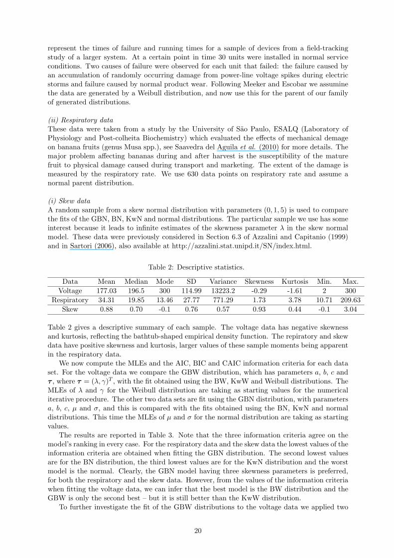
represent the times of failure and running times for a sample of devices from a field-trackingstudy of a larger system. At a certain point in time 30 units were installed in normal serviceconditions. Two causes of failure were observed for each unit that failed: the failure caused byan accumulation of randomly occurring damage from power-line voltage spikes during electricstorms and failure caused by normal product wear. Following Meeker and Escobar we assuminethe data are generated by a Weibull distribution, and now use this for the parent of our familyof generated distributions.

(ii) Respiratory dataThese data were taken from a study by the University of Sao Paulo, ESALQ (Laboratory ofPhysiology and Post-colheita Biochemistry) which evaluated the effects of mechanical demageon banana fruits (genus Musa spp.), see Saavedra del Aguila et al. (2010) for more details. Themajor problem affecting bananas during and after harvest is the susceptibility of the maturefruit to physical damage caused during transport and marketing. The extent of the damage ismeasured by the respiratory rate. We use 630 data points on respiratory rate and assume anormal parent distribution.

(i) Skew dataA random sample from a skew normal distribution with parameters (0, 1, 5) is used to comparethe fits of the GBN, BN, KwN and normal distributions. The particular sample we use has someinterest because it leads to infinite estimates of the skewness parameter λ in the skew normalmodel. These data were previously considered in Section 6.3 of Azzalini and Capitanio (1999)and in Sartori (2006), also available at http://azzalini.stat.unipd.it/SN/index.html.

Table 2: Descriptive statistics.

Data Mean Median Mode SD Variance Skewness Kurtosis Min. Max.

Voltage 177.03 196.5 300 114.99 13223.2 -0.29 -1.61 2 300

Respiratory 34.31 19.85 13.46 27.77 771.29 1.73 3.78 10.71 209.63

Skew 0.88 0.70 -0.1 0.76 0.57 0.93 0.44 -0.1 3.04

Table 2 gives a descriptive summary of each sample. The voltage data has negative skewnessand kurtosis, reflecting the bathtub-shaped empirical density function. The repiratory and skewdata have positive skewness and kurtosis, larger values of these sample moments being apparentin the respiratory data.

We now compute the MLEs and the AIC, BIC and CAIC information criteria for each dataset. For the voltage data we compare the GBW distribution, which has parameters a, b, c andτ , where τ = (λ, γ)T , with the fit obtained using the BW, KwW and Weibull distributions. TheMLEs of λ and γ for the Weibull distribution are taking as starting values for the numericaliterative procedure. The other two data sets are fit using the GBN distribution, with parametersa, b, c, µ and σ, and this is compared with the fits obtained using the BN, KwN and normaldistributions. This time the MLEs of µ and σ for the normal distribution are taking as startingvalues.

The results are reported in Table 3. Note that the three information criteria agree on themodel’s ranking in every case. For the respiratory data and the skew data the lowest values of theinformation criteria are obtained when fitting the GBN distribution. The second lowest valuesare for the BN distribution, the third lowest values are for the KwN distribution and the worstmodel is the normal. Clearly, the GBN model having three skewness parameters is preferred,for both the respiratory and the skew data. However, from the values of the information criteriawhen fitting the voltage data, we can infer that the best model is the BW distribution and theGBW is only the second best – but it is still better than the KwW distribution.

To further investigate the fit of the GBW distributions to the voltage data we applied two

20

Table 3: MLEs and information criteria.

Voltage a b c λ γ AIC BIC CAIC

GBW 0.0727 0.0625 1.0613 0.0050 7.9634 349.9 356.9 352.4(0.0168) (0.0137) (0.0521) (0.00006) (0.2336)

BW 0.0879 0.0987 1 0.0047 7.8425 348.3 353.9 349.9(0.0261) (0.0707) - (0.0004) (0.2461)

KwW 1 0.2269 0.0484 0.0043 7.7495 352.7 358.3 354.3- (0.0966) (0.0236) (0.0003) (0.2387)

Weibull 1 1 1 0.0053 1.2650 372.6 375.4 373.1- - - (0.00079) (0.2044)

Respiratory a b c µ σ AIC CAIC BIC

GBN 274.67 0.4191 38.4879 -153.36 44.0310 5631.1 5631.2 5653.3(3.7263) (0.0340) (10.0676) (8.4972) (1.8586)

BN 16.5062 0.4651 1 -37.4796 29.9743 5757.3 5757.4 5775.1(0.7466) (0.0339) - (1.8586) (0.7919)

KwN 1 0.4242 4.9486 -15.6954 27.3319 5826.8 5826.9 5844.6- (0.0279) (0.5375) (2.5505) (0.7148)

Normal 1 1 1 34.3166 27.7500 5979.3 5979.4 5988.2- - - (1.1056) (0.7818)

Skew a b c µ σ AIC CAIC BIC

GBN 0.0889 0.1186 15.9969 0.2813 0.3366 109.2 110.6 118.8(0.0351) (0.0246) (7.1536) (0.0045) (0.0022)

BN 2.9920 0.1405 1 -0.4438 0.4244 112.2 113.1 119.9(1.0429) (0.0223) - (0.1614) (0.0216)

KwN 1 0.1508 1.9342 -0.1948 0.4001 113.0 113.9 120.7- (0.0243) (0.8905) (0.1657) (0.0212)

Normal 1 1 1 0.8849 0.7489 117.0 117.2 120.8- - - (0.1059) (0.0749)

Table 4: LR tests.

Voltage Hypotheses Statistic w p-value

GBW vs BW H0 : c = 1 vs H1 : H0 is false 0.40 0.5271GBW vs KwW H0 : a = 1 vs H1 : H0 is false 4.80 0.0285GBW vs Weibull H0 : a = b = c = 1 vs H1 : H0 is false 28.70 <0.0001

Respiratory Hypotheses Statistic w p-value

GBN vs BN H0 : c = 1 vs H1 : H0 is false 128.2 <0.00001GBN vs KwN H0 : a = 1 vs H1 : H0 is false 197.7 <0.00001

GBN vs Normal H0 : a = b = c = 1 vs H1 : H0 is false 354.2 <0.00001

Skew Hypotheses Statistic w p-value

GBN vs BN H0 : c = 1 vs H1 : H0 is false 5.0 0.0253GBN vs KwN H0 : a = 1 vs H1 : H0 is false 5.8 0.0160

GBN vs Normal H0 : a = b = c = 1 vs H1 : H0 is false 13.8 0.0032

formal goodness-of-fit criteria, i.e. the Cramer-von Mises (W ∗) and Anderson-Darling (A∗)statistics.8 The smaller the values ofW ∗ and A∗, the better the fit to the sample data. We obtainW ∗ = 0.1892 and A∗ = 0.8572 for the GBW distribution, W ∗ = 0.1901 and A∗ = 0.8492 for the

8These are described in detail in Chen and Balakrishnan (1995).

21

BW distribution,W ∗ = 0.2328 and A∗ = 1.1043 for the KwW distribution andW ∗ = 0.3853 andA∗ = 1.8206 for the Weibull distribution. Thus, according to the Cramer-von Mises statistic,the GBW distribution yields the best fit, but the Anderson-Darling test suggests that the BWgives the best fit.

A formal test of the need for the third skewness parameter in GBG distributions is based onthe LR statistics described in Section 6. Applying these to our three data sets, the results areshown in Table 4. For the voltage data the additional parameter of the GBW distribution maynot, in fact, be necessary because the LR test results provide no indications against the BWmodel when compared with the GBW model. However, for the respiratory and skew data wereject the null hypotheses of all three LR tests in favor of the GBN distribution. The rejectionis extremely highly significant for the respiratory data, and highly or very highly significant forthe skew data. This gives clear evidence of the potential need for three skewness parameterswhen modelling real data.

(a) (b)

x

f(x)

0 50 100 150 200 250 300

0.00

00.

002

0.00

40.

006

0.00

80.

010

GBWBWKwWWeibull

0 50 100 150 200 250 300

0.0

0.2

0.4

0.6

0.8

1.0

x

S(x

)Kaplan−MeierGBWBWKwWWeibull

Figure 10: (a) Estimated densities of the GBW, BW, KwW and Weibull models for voltagedata. (b) Estimated survival functions and the empirical survival for voltage data.

More information is provided by a visual comparison of the histogram of the data with thefitted density functions. In Figure 10, we plot the empirical and estimated density and survivalfunctions of the GBW and BW, KwW and Weibull distributions. In each case, both the GBWand BW distributions provide reasonable fits, but it is clear that the GBW distribution providesa more adequate fit to the histogram of the data and better captures its extreme bathtub shape.The plots of the fitted GBN, BN, KwN and normal densities are given in Figure 11 for therespiratory data and Figure 12 for the skew data. In both cases the new distribution appears toprovide a closer fit to the histogram than the other three sub-models.

22

x

f(x)

0 50 100 150 200

0.000

0.005

0.010

0.015

0.020

0.025

GBNBNKwNNormal

Figure 11: Fitted GBN, BN, KwN and normal densities for the respiratory rate data.

x

f(x)

−1 0 1 2 3

0.00.2

0.40.6

0.8

GBNBNKwNNormal

Figure 12: Fitted GBN, BN, KwN and normal densities for the skew data.

23

8 Conclusions

We propose a new class of generalized beta-generated (GBG) distributions which includes allclassical beta-generated, Kumaraswamy-generated and exponentiated distributions. The GBGclass extends several common distributions such as normal, log-normal, Laplace, Weibull, gammaand Gumbel distributions. Indeed, for any parent distribution F we can define the correspondinggeneralized beta F distribution. The mathematical properties of GBG distributions, such asmoments, quantile and generating functions are tractable. The role of the generator parametersis investigated and related to the skewness of the GBG distribution and the decomposition ofits entropy. We discuss maximum likelihood estimation and inference on the parameters basedon likelihood ratio statistics for testing nested models. Several applications to real data showthe usefulness of the GBG class. We hope this generalization proves useful for applied statisticalresearch.

Appendix A: GBG Entropy

The conditions (15) and (16) follow immediately from the first two conditions in Lemma 1 ofZografos and Balakrishnan (2009), on noting that the GBG density is a standard beta densitywith parent G(x) = xc. The third condition may be written:

EBG [log g(X)] = EU [log g(G−1(U))], U ∼ B(a, b), (42)

where g(x) = G′(x) = c F (x)c−1 f(x). Now G−1(U) = F−1(U1/c) and

log g(X) = log c+ (c− 1) logF (X) + log f(X),

and since

EB[logU ] = B(a, b)−1

∫ 1

0ua−1 (1− up)b−1 log(u)du = −ζ(a, b),

we have

EB[log g(G−1(U))] = log c+ (c− 1)EB[logU

1/c] + EB[log f(F−1(U1/c))],

= log(c)− c−1(c− 1)ζ(a, b) + EB[log f(F−1(U1/c))]. (43)

By Lemma 1 of Zografos and Balakrishnan (2009), EBG [logF (X)] = −ζ(a, b). Hence (42) be-comes:

(c− 1)ζ(a, b)− EGBG [log f(X)] = c−1(c− 1)ζ(a, b)− EB[log f(F−1(U1/c))]. (44)

which may be rewritten as (17). The entropy (18) follows from (43), and corollary 1 andproposition 1 of Zografos and Balakrishnan (2009).

24

Appendix

B:ExpressionsforM

oments,M

GF

and

Mean-D

eviationsofSomeGBG

Distributions

Theparentdistributionis

given

inthefirstrow

ofTab

le8,thesecondrow

applies

equations(27)

and(28)to

calculate

themom

ents,thethirdrow

uses(29)

and(30)

tofindthegeneratingfunctionandthelast

row

applies

equations(34)–(35)

toob

tain

anexpansionforthemeandeviation

s.The

coeffi

cientswian

dv k

aredefined

in(11)an

d(26)respectively.

Distribution

GB-expon

ential

GB-Pareto

GB-standardlogistic

Parent

1−

exp(−λx),λ>

01−

(1+x)−

ν,ν>

0[1+

exp(−x)]−1

E(X

s)

s!λs∑ ∞ k

,j=0v k

(−1)s

+j( c(k+

a)−

1j

) (j+1)

−(s+1)

∑ ∞ k,j=0v k

(−1)s

+j( s j) B( c

(k+a),1−

j ν

) ∑∞ k=0v k

( ∂ ∂t

) s B(t+c(k

+a),1−t)

∣ ∣ ∣ ∣ t=0

M(t)

B(a,b

+1)−

1c∑ ∞ i=

0(−

1)i( b i) B(a

(i+c),1

−λt)

exp(−t)∑ ∞ i,

r=0B(a

(i+c),1

−rν

−1)w

itr

r!

∑ ∞ i=0wiB(t+a(i+c),1

−t)

Hk(z)

Γ(c

(k+a)+

1)

λ

∑ ∞ j=0

(−1)j

{1−ex

p(−

jλz)}

Γ(c

(k+a)+

1−j)(j+1)!

∑ ∞ j=0

∑ j r=0

(−1)j(c

(k+a)

j)(

j r)

(1−rν)

z1−rν

∑ ∞ j=0(−

1)j

Γ(c

(k+a)+

j){1

−ex

p(−

jz)}

Γ(k)(j+1)!

Table

5:Moments,generatingfunctionsanddeviationsofsomespecificGBG

distributions

25

Appendix C: Information Matrix

The elements of the observed information matrix J(θ) for the parameters (a, b, c, τ ) are

Jaa = −n[ψ′(a)− ψ′(a+ b)], Jab = nψ′(a+ b), Jac =n∑

i=1

log[F (xi; τ )],

Jaτ = c

n∑i=1

F (xi)τF (xi, τ )

, Jbb = −n[ψ′(b)− ψ′(a+ b)], Jbc = −n∑

i=1

F c(xi; τ ) log[F (xi; τ )]

[1− F c(xi; τ )],

Jbτ = −n∑

i=1

cF c−1(xi; τ )F (xi)τ[1− F c(xi; τ )]

, Jcc = − n

c2− (b− 1)

∑ F c(xi, τ ) log2[F (xi; τ )]

[1− F c(xi; τ )]2,

Jcτ =

n∑i=1

f(xi)τf(xi; τ )

− (b− 1)

n∑i=1

F c−1(xi; τ )F (xi)τ[1− F c(xi; τ )]2

{[c log[F (xi; τ )] + 1

][1− F c(xi; τ )

]+cF c(xi; τ ) log[F (xi; τ )]

},

Jττ =

n∑i=1

f(xi)ττ f(xi; τ )− [f(xi)τ ]2

f2(xi; τ )+ (ac− 1)

n∑i=1

F (xi)ττF (xi; τ )− [F (xi)τ ]2

F 2(xi; τ )+

(b− 1)n∑

i=1

cF c−1(xi; τ )

[1− F c(xi; τ )]2

{[(c− 1)F−1(xi; τ )[F (xi)τ ]

2 + F (xi)ττ]

×[1− F c(xi; τ )

]+ cF c−1(xi; τ )[F (xi)τ ]

2},

where ψ′(.) is the derivative of the digamma function, f(xi)τ = ∂f(xi; τ )/∂τ , F (xi)τ =∂F (xi; τ )/∂τ , f(xi)ττ = ∂2f(xi; τ )/∂ττ

T and F (xi)ττ = ∂2F (xi; τ )/∂ττT .

References

[1] Aas, K. and Haff, I.H. (2006). The generalized hyperbolic skew Student’s t-distribution.Journal of Financial Econometrics, 4, 275-309.

[2] Akinsete, A., Famoye, F. and Lee, C. (2008). The beta-Pareto distribution. Statistics, 42,547-563.

[3] Arnold, B.C., Castillo, E. and Sarabia, J.M. (2006). Families of multivariate distributionsinvolving the Rosenblatt construction. Journal of the American Statistical Association, 101,1652-1662.

[4] Azzalini, A. and Capitanio, A. (2003). Distributions generated by perturbation of symmetrywith emphasis on a multivariate skew t distribution. Journal of the Royal Statistical SocietyB, 65, 367-389.

[5] Barreto-Souza, W., Santos, A.H.S. and Cordeiro, G.M. (2010). The beta generalized expo-nential distribution. Journal of Statistical Computation and Simulation, 80, 159-172.

[6] Chen, G. and Balakrishnan, N. (1995). A general purpose approximate goodness-of-fit test.Journal of Quality Technology, 27, 154–161.

26

[7] Choudhury, A. (2005). A simple derivation of moments of the exponentiated Weibull dis-tribution. Metrika, 62, 17-22

[8] Cordeiro, G.M. and de Castro, M. (2011). A new family of generalized distributions. Journalof Statistical Computation and Simulation. DOI: 10.1080/0094965YY.

[9] Cordeiro, G.M., Ortega, E.M.M. and Nadarajah, S. (2010). The Kumaraswamy Weibulldistribution with application to failure data. Journal of the Franklin Institute, 347, 1399–1429.

[10] Doornik, J.A. (2007). An Object-Oriented Matrix Language Ox 5. Timberlake ConsultantsPress: London.

[11] Eugene, N., Lee, C. and Famoye, F. (2002). Beta-normal distribution and its applications.Communications in Statistics – Theory and Methods, 31, 497-512.

[12] Exton, H. (1978). Handbook of Hypergeometric Integrals: Theory, Applications, Tables,Computer Programs. Halsted Press, New York.

[13] Gradshteyn, I.S. and Ryzhik, I.M. (2000). Table of Integrals, Series, and Products, sixthedition. Academic Press, San Diego.

[14] Gupta, R.C., Gupta, R. D. and Gupta, P.L. (1998). Modeling failure time data by Lehmanalternatives. Communications in Statistics—Theory and Methods, 27, 887-904.

[15] Gupta, R.D. and Kundu, D. (2001). Exponentiated exponential family: an alternative togamma and Weibull distributions. Biometrical Journal, 43, 117-130.

[16] Hansen, B.E. (1994). Autoregressive conditional density estimation. International EconomicReview, 35, 705-730.

[17] Hosking, J.R.M. (1990). L-moments: analysis and estimation of distributions using linearcombinations of order statistics. Journal Royal Statistical Society B, 52, 105-124.

[18] Johnson, N.L., Kotz, S. and Balakrishnan, N. (1994). Continuous Univariate DistributionsI. Wiley, New York.

[19] Johnson, N.L., Kotz, S. and Balakrishnan, N. (1995). Continuous Univariate DistributionsII. Wiley, New York.

[20] Jones, M.C. and Faddy, M.J. (2003).A skew extension of the t distribution, with applica-tions. Journal Royal Statistical Society Serie B, 65, 159-174.

[21] Jones, M.C. (2004). Families of distributions arising from distributions of order statistics.Test, 13, 1-43.

[22] Jones, M.C. and Larsen, P.V. (2004). Multivariate distributions with support above thediagonal. Biometrika, 91, 975-986.

[23] Jones, M.C. (2009). Kumaraswamy’s distribution: A beta-type distribution with sometractability advantages. Statistical Methodology, 6, 70-81.

[24] Kenney, J.F. and Keeping, E.S. (1962). Mathematics of statistics, pp. 101-102, Part 1, 3rded. Princeton, NJ.

[25] Kumaraswamy, P. (1980). A generalized probability density function for double-boundedrandom processes. Journal of Hydrology, 46, 79-88.

27

[26] Lee, C., Famoye, F. and Olumolade, O. (2007). Beta-Weibull Distribution: Some Propertiesand Applications to Censored Data. Journal of Modern Applied Statistical Methods, 6, 173-186.

[27] Meeker, W.Q. and Escobar, L.A. (1998). Statistical Methods for Reliability Data. JohnWiley, New York.

[28] McDonald, J.B. (1984). Some generalized functions for the size distribution of income.Econometrica, 52, 647-663.

[29] Moors, J.J.A. (1998). A quantile alternative for kurtosis. Journal of the Royal StatisticalSociety Ser. D., The Statistician, 37, 25-32.

[30] Mudholkar, G.S., Srivastava, D.K. and Friemer, M. (1995). The exponentiated Weibullfamily: A reanalysis of the bus-motor-failure data. Technometrics, 37, 436-445.

[31] Mudholkar, G.S., Srivastava, D.K. and Kollia, G.D. (1996). A generalization of the Weibulldistribution with application to the analysis of survival data. Journal of American StatisticalAssociation, 91, 1575-1583.

[32] Nadarajah, S. (2008). Explicit expressions for moments of order statistics. Statistics andProbability Letters, 78, 196–205.

[33] Nadarajah S. and Zografos, K. (2003). Formulas for Renyi information and related measuresfor univariate distributions. Information Sciences, 155, 199-138.

[34] Nadarajah, S. and Kotz, S. (2004). The beta Gumbel distribution. Math. Probab. Eng., 10,323-332.

[35] Nadarajah, S. and Kotz, S. (2005). The beta exponential distribution. Reliability Engineer-ing and System Safety, 91, 689-697.

[36] Nadarajah, S. and Gupta, A.K. (2005). On the moments of the exponentiated Weibulldistribution. Communication in Statistics - Theory and Methods, 35, 253-256.

[37] Nadarajah, S. and Kotz, S. (2006). The beta exponential distribution. Reliability Engineer-ing and System Safety, 91, 689-697.

[38] Nadarajah, S. and Gupta, A.K. (2007). The exponentiated gamma distribution with appli-cation to drought data. Calcutta Statistical Association Bulletin, 59, 29-54.

[39] Nassar, M.M. and Eissa, F.H. (2003). On the exponentiated Weibull distribution. Commu-nication in Statistics - Theory and Methods, 32, 1317-1336.

[40] Razzaghi, M. (2009). Beta-normal distribution in dose-response modeling and risk assess-ment for quantitative responses. Environmental and Ecological Science, 16, 21-36.

[41] Saavedra del Aguila, J., Heiffig-del Aguila, L. S., Sasaki, F. F., Tsumanuma, G. M., On-garelli, M. G., Spoto, M. H. F., Jacomino, A. P., Ortega, E. M. M. and Kluge, R. A.(2010). Postharvest modifications of mechanically injured bananas. Revista Iberoamericanade Tecnologia Postcosecha, 10, 73–85.

[42] Sartori, N. (2006).Bias prevention of maximum likelihood estimates for scalar skew normaland skew t distributions. Journal of Statistical Planning and Inference, 136, 4259-4275.

[43] Shannon, C.E. (1948). The mathematical theory of communication, Bell System TechnicalJournal July-Oct. Reprinted in: C.E. Shannon and W. Weaver, The Mathematical Theoryof Communication. Illinois University Press, Urbana.

28

[44] Stasinopoulos, D.M. and Rigby, R.A. (2007). Generalized additive models for location scaleand shape (GAMLSS) in R. Journal of Statistical Software, 23, 1-46.

[45] Zhu, D. and Galbraith, J.W. (2010). A generalized asymmetric Student-t distribution withapplication to financial econometrics. Journal of Econometrics, 157, 297-305.

[46] Zografos, K. and Balakrishnan, N. (2009). On families of beta- and generalized gamma-generated distributions and associated inference. Statistical Methodology, 6, 344-362.

29