Brazilian Journal of Probability and Statistics2012, Vol. 26, No. 1, 88–112DOI: 10.1214/10-BJPS124© Brazilian Statistical Association, 2012

The beta power distribution

Gauss Moutinho Cordeiro and Rejane dos Santos BritoUniversidade Federal Rural de Pernambuco

Abstract. The power distribution is defined as the inverse of the Pareto dis-tribution. We study in full detail a distribution so-called the beta power dis-tribution. We obtain analytical forms for its probability density and hazardrate functions. Explicit expressions are derived for the moments, probabilityweighted moments, moment generating function, mean deviations, Bonfer-roni and Lorenz curves, moments of order statistics, entropy and reliability.We estimate the parameters by maximum likelihood. The practicability of themodel is illustrated in two applications to real data.

1 Introduction

We study the so-called beta power (BP) distribution. Although we can only referto the book by Balakrishnan and Nevzorov (2003, Chapter 14, pp. 127–132) aboutthe power distribution, we believe that this distribution can have wider applicationsthan the power distribution. Boyce et al. (1999) related the power distribution toenvironmental policy and stress and public health and Van Dorp and Kotz (2002)presented applications in financial engineering domain. Keeping these applicationsin mind, we take them as a basis to the power distribution and also to the BPdistribution.

The BP distribution stems from the following idea: Eugene et al. (2002) definedthe beta G distribution from a quite arbitrary cumulative distribution function (cdf)G(x) by

F(x) = IG(x)(a, b), (1.1)

where a > 0 and b > 0 are two extra parameters, Iy(a, b) = By(a, b)/B(a, b) isthe incomplete beta function ratio, By(a, b) = ∫ y

0 ωa−1(1 − ω)b−1 dω is the in-complete beta function and B(a, b) is the complete beta function. The unknownpositive parameters a and b are shape parameters which introduce skewness andvary tail weights.

The class of distributions (1.1) has raised increased attention in recent yearsafter the work by Jones (2004).

Eugene et al. (2002), Nadarajah and Gupta (2004), Nadarajah and Kotz (2004)and Nadarajah and Kotz (2005) defined the beta normal, beta Fréchet, beta Gumbel

Key words and phrases. Beta power distribution, Bonferroni curve, maximum likelihood estima-tion, moments, order statistic, reliability

Received December 2009; revised May 2010.

88

The beta power distribution 89

and beta exponential distributions by taking G(x) to be the cdf of the normal,Fréchet, Gumbel and exponential distributions, respectively. Another distributionthat happens to belong to (1.1) is the log-F (or beta logistic) distribution, which isknown for over 20 years (Brown et al., 2002), even if it did not originate directlyfrom equation (1.1). Sepanski and Kong (2007) compared the performance of somegeneralized beta distributions, such as the beta normal, skewed Student t , log-F,beta exponential and beta Weibull distributions, to the widely used generalizedbeta distributions of the first and second types in terms of some measures of fit.Recently, Barreto-Souza et al. (2010) proposed the beta generalized exponentialdistribution motivated by the wide use of the exponential distribution in practice,and also for the fact that the generalization provides more flexibility to analyzemore complex situations.

In this article, we provide a comprehensive mathematical treatment of the BPdistribution. We begin with the probability density function (pdf) and cdf of thepower distribution given by

gα,β(x) = αβαxα−1, 0 < x <1

β, (1.2)

and

Gα,β(x) = (βx)α, (1.3)

respectively, where α > 0 is a shape parameter and β > 0 is a scale parameter. Forα = 1, we obtain as a special case the uniform distribution defined on the interval(0,1/β), say X ∼ U(0,1/β). For β = 1, we have gα,1(x) = αxα−1 and Gα,1(x) =xα as defined by Balakrishnan and Nevzorov (2003). The power distribution isrelated to the Pareto distribution using an inverse transformation (Akinsete et al.,2008). Some other distributions can be obtained from the Pareto distribution usingsome well-known transformations such as the exponential, logistic and chi-squareddistributions.

Using (1.1) and replacing G(x) by the cdf of the power distribution (1.3), theBP cumulative function can be written as

F(x) = I(βx)α (a, b) = B(a, b)−1∫ (βx)α

0wa−1(1 − w)b−1 dw (1.4)

for 0 < x < 1/β . Here, a > 0, b > 0 and α > 0 are shape parameters and β > 0 isa scale parameter. For any values of a and b, we can express (1.4) in terms of thewell-known hypergeometric function given by

F(x) = (βx)αa

aB(a, b)2F1

(a,1 − b, a + 1; (βx)α

).

In general, the cdf F(x) defined from a baseline cdf G(x) in (1.1) could followthe properties of the hypergeometric function which are well established in theliterature; see, for example, Section 9.1 of Gradshteyn and Ryzhik (2000).

90 G. M. Cordeiro and R. S. Brito

The density function corresponding to (1.1) is given by

f (x) = g(x)

B(a, b)G(x)a−1[1 − G(x)]b−1, (1.5)

where g(x) = dG(x)/dx is the baseline density function. The pdf f (x) will bemost tractable when the functions G(x) and g(x) have simple analytic expressionssuch as the power distribution. Except for some special choices for G(x) in (1.1),equation (1.5) could be very difficult to deal with in generality.

The hazard rate function defined by h(x) = f (x)/[1 − F(x)] is an importantquantity characterizing lifetime phenomena. Correspondingly, the pdf and hazardrate function of the BP distribution are

f (x) = αβ(βx)αa−1[1 − (βx)α]b−1

B(a, b), 0 < x <

1

β(1.6)

and

h(x) = αβ(βx)αa−1[1 − (βx)α]b−1

B(a, b)[1 − I(βx)α (a, b)] , (1.7)

respectively. Equation (1.6) is not new. McDonald and Richards (1987) defined itas the generalized beta distribution of the second kind. However, they do not studyits mathematical properties which we do in this article.

We denote a random variable X having density function (1.6) by X ∼BP(a, b,α,β). Simulation of the BP distribution is very easy: if V is a randomvariable having a beta distribution with parameters a and b, then the random vari-able X = β−1V 1/α follows the BP(a, b,α,β) distribution.

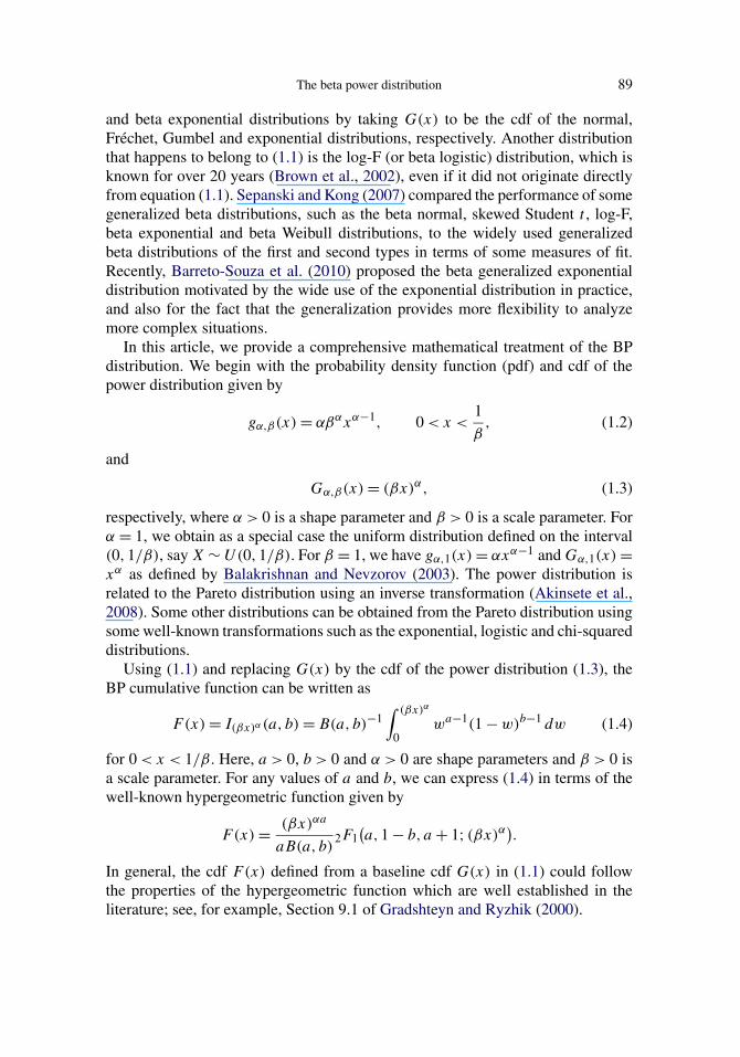
Figures 1 and 2 illustrate some possible shapes of the density function (1.6) andhazard rate function (1.7), respectively, for selected parameter values, includingthe power distribution. It is evident that the BP distribution is much more flexiblethan the power distribution. Figure 2 shows that the BP hazard function can bebathtub shaped, monotonically increasing or decreasing and upside-down bathtubdepending basically on the values of the parameters.

The rest of the paper is organized as follows. In Section 2, we give expan-sions for the pdf and cdf of the BP distribution depending on whether the param-eter b is real noninteger and integer. Section 3 provides the moments and a smallstudy on the variation of the skewness and kurtosis measures. Probability weightedmoments (PWMs) are determined in Section 4. The moment generating function(mgf) and the quantile function are obtained in Section 5. Mean deviations andBonferroni and Lorenz curves are derived in Section 6. We show, in Section 7, thatthe density function of the BP order statistics can be expressed as a mixture ofpower density functions. The moments of order statistics are also derived in thissection for b real noninteger and integer. Sections 8 and 9 are devoted to the en-tropy and reliability, respectively. In Section 10, we discuss maximum likelihoodestimation of the model parameters. Section 11 provides two applications to realdata sets. Some conclusions are addressed in Section 12.

The beta power distribution 91

Figure 1 BP(a, b,1,1) density function for selected parameter values.

Figure 2 BP(a, b,1,1) hazard function for selected parameter values.

2 Expansion for the density function

Here, we give a simple expansion for the BP density function. We consider thebinomial expansion

(1 − z)b−1 =∞∑i=0

(−1)i�(b)

�(b − i)i! zi, (2.1)

92 G. M. Cordeiro and R. S. Brito

valid for |z | < 1 and b > 0 real noninteger.Application of (2.1) to equation (1.4) if b is real noninteger gives

F(x) = �(a + b)

�(a)

∞∑i=0

(−1)i(βx)α(a+i)

�(b − i)i!(a + i). (2.2)

Correspondingly, the BP density function can be written as

f (x) = �(a + b)

�(a)

∞∑i=0

(−1)i

�(b − i)i!(a + i)gα(a+i),β(x), (2.3)

where gα(a+i),β(x) is the power density with shape parameter α(a + i) and scaleparameter β . The BP density function (1.6) is easily computed using any statisticalsoftware. However, it is clear from (2.3) that it can be expressed as an infinite (orfinite) mixture of power densities with increasing shape parameters α(a + i) and acommon scale parameter β . This result is important to provide some mathematicalproperties of the BP distribution (ordinary, central, factorial and inverse moments,mgf, etc.) directly from those of the power distributions. For b integer, the sumsin (2.2) and (2.3) stop at b − 1. These two expansions are the main results of thissection.

3 Moments

If X has a BP density (1.6), its r th moment about zero becomes

μ′r = E(Xr) = αβαa

B(a, b)

∫ 1/β

0xr+αa−1[1 − (βx)α]b−1 dx. (3.1)

Using the binomial expansion (2.1), (3.1) can be rewritten as

μ′r = �(a + b)

�(a)

∞∑j=0

(−1)jJ (j, r)

�(b − j)j ! ,

where J (j, r) denotes the integral

J (j, r) =∫ 1/β

0αxr−1G(x)a+j dx = α{βr [r + α(a + j)]}−1.

Equation (3.1) can be expressed as

μ′r = α�(a + b)

βr�(a)

∞∑j=0

(−1)j {�(b − j)[r + α(a + j)]j !}−1.

Hence, a closed-form expression for the moments of X is given by

μ′r = B(a + r/α, b)

βrB(a, b). (3.2)

The beta power distribution 93

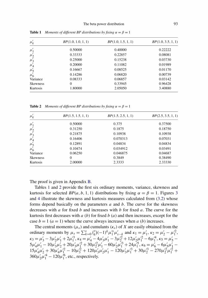
Table 1 Moments of different BP distributions by fixing α = β = 1

μ′k BP(1.0,1.0,1,1) BP(1.0,1.5,1,1) BP(1.0,3.5,1,1)

μ′1 0.50000 0.40000 0.22222

μ′2 0.33333 0.22857 0.08081

μ′3 0.25000 0.15238 0.03730

μ′4 0.20000 0.11082 0.01989

μ′5 0.16667 0.08525 0.01170

μ′6 0.14286 0.06820 0.00739

Variance 0.08333 0.06857 0.03142Skewness 0 0.33945 0.96428Kurtosis 1.80000 2.05050 3.40880

Table 2 Moments of different BP distributions by fixing α = β = 1

μ′k BP(1.5,1.5,1,1) BP(1.5,2.5,1,1) BP(2.5,3.5,1,1)

μ′1 0.50000 0.375 0.37500

μ′2 0.31250 0.1875 0.18750

μ′3 0.21875 0.10938 0.10938

μ′4 0.16406 0.070313 0.07031

μ′5 0.12891 0.04834 0.04834

μ′6 0.10474 0.034912 0.03491

Variance 0.06250 0.046875 0.04687Skewness 0 0.3849 0.38490Kurtosis 2.00000 2.3333 2.33330

The proof is given in Appendix B.Tables 1 and 2 provide the first six ordinary moments, variance, skewness and

kurtosis for selected BP(a, b,1,1) distributions by fixing α = β = 1. Figures 3and 4 illustrate the skewness and kurtosis measures calculated from (3.2) whoseforms depend basically on the parameters a and b. The curve for the skewnessdecreases with a for fixed b and increases with b for fixed a. The curve for thekurtosis first decreases with a (b) for fixed b (a) and then increases, except for thecase b = 1 (a = 1) where the curve always increases when a (b) increases.

The central moments (μs) and cumulants (κs) of X are easily obtained from theordinary moments by μs = ∑s

k=0(sk

)(−1)kμ′s

1 μ′s−k and κ1 = μ′

1, κ2 = μ′2 − μ′2

1 ,κ3 = μ′

3 − 3μ′2μ

′1 + 2μ′3

1 , κ4 = μ′4 − 4μ′

3μ′1 − 3μ′2

2 + 12μ′2μ

′21 − 6μ′4

1 , κ5 = μ′5 −

5μ′4μ

′1 − 10μ′

3μ′2 + 20μ′

3μ′21 + 30μ′2

2 μ′1 − 60μ′

2μ′31 + 24μ′5

1 , κ6 = μ′6 − 6μ′

5μ′1 −

15μ′4μ

′2 + 30μ′

4μ′21 − 10μ′2

3 + 120μ′3μ

′2μ

′1 − 120μ′

3μ′31 + 30μ′3

2 − 270μ′22 μ′2

1 +360μ′

2μ′41 − 120μ′6

1 , etc., respectively.

94 G. M. Cordeiro and R. S. Brito

Figure 3 Skewness and kurtosis of the BP(a, b,1,1) distribution for selected values of b as afunction of parameter a.

The r th descending factorial moment of X is

μ′(r) = E

[X(r)] = E[X(X − 1) × · · · × (X − r + 1)] =

r∑k=0

s(r, k)μ′k,

where s(r, k) is the Stirling number of the first kind that can be defined by s(r, k) =(k!)−1[ dk

dxk x(r)]x=0. They count the number of ways to permute a list of r items

into k cycles. Thus, the factorial moments of X are

μ′(r) =

r∑k=0

s(r, k)B(a + k/α, b)

βkB(a, b).

The beta power distribution 95

Figure 4 Skewness and kurtosis of the BP(a, b,1,1) distribution for selected values of a as afunction of parameter b.

4 Probability weighted moments

PWMs are expectations of certain functions defined for any random variable whosemean exists and were first fomulated by Greenwood et al. (1979) primarily as anaid to estimate the parameters of the Wakeby distribution. However, the use ofthe PWMs covers: the summarization and description of theoretical probabilitydistributions and observed data samples, nonparametric estimation of the under-lying distribution of an observed sample, estimation of parameters and quantilesof probability distributions and hypothesis tests for probability distributions. ThePWM method can generally be used in estimating parameters of a distributionwhose inverse form cannot be given explicitly. For several distributions, such as

96 G. M. Cordeiro and R. S. Brito

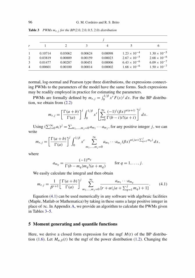
Table 3 PWMs mr,j for the BP(2.0,2.0,0.5,2.0) distribution

j

r 1 2 3 4 5 6

1 0.10714 0.03062 0.00624 0.00098 1.23 × 10−4 1.30 × 10−5

2 0.03819 0.00889 0.00159 0.00023 2.67 × 10−5 2.68 × 10−6

3 0.01477 0.00287 0.00451 0.00006 6.43 × 10−6 6.09 × 10−7

4 0.00601 0.00100 0.00014 0.00002 1.68 × 10−6 1.50 × 10−7

normal, log-normal and Pearson type three distributions, the expressions connect-ing PWMs to the parameters of the model have the same forms. Such expressionsmay be readily employed in practice for estimating the parameters.

PWMs are formally defined by mr,j = ∫ 1/β0 xrF (x)j dx. For the BP distribu-

tion, we obtain from (2.2)

mr,j =[�(a + b)

�(a)

]j ∫ 1/β

0xr

[ ∞∑i=0

(−1)i(βx)α(a+i)

�(b − i)i!(a + i)

]j

dx.

Using (∑∞

i=0 ai)j = ∑

m1,...,mj=0 am1 · · ·amj, for any positive integer j , we can

write

mr,j =[�(a + b)

�(a)

]j ∫ 1/β

0xr

∞∑m1,...,mj=0

am1 · · ·amj(βx)

α(ja+∑jq=1 mq)

dx,

where

amq = (−1)mq

�(b − mq)mq !(a + mq)for q = 1, . . . , j.

We easily calculate the integral and then obtain

mr,j = 1

βr+1

[�(a + b)

�(a)

]j ∞∑m1,...,mj=0

am1 · · ·amq

[r + α(ja + ∑jq=1 mq) + 1] . (4.1)

Equation (4.1) can be used numerically in any software with algebraic facilities(Maple, Matlab or Mathematica) by taking in these sums a large positive integer inplace of ∞. In Appendix A, we provide an algorithm to calculate the PWMs givenin Tables 3–5.

5 Moment generating and quantile functions

Here, we derive a closed form expression for the mgf M(t) of the BP distribu-tion (1.6). Let Mα,β(t) be the mgf of the power distribution (1.2). Changing the

The beta power distribution 97

Table 4 PWMs mr,j for the BP(1.0,2.0,1.0,1.0) distribution

j

r 1 2 3 4 5 6

1 0.41667 0.11111 0.02080 0.00296 0.00339 3.24 × 10−5

2 0.30000 0.06612 0.01097 0.00144 0.00015 1.42 × 10−5

3 0.23333 0.04340 0.00640 0.00077 7.80 × 10−5 6.76 × 10−6

4 0.19048 0.03049 0.00403 0.00045 4.21 × 10−5 3.46 × 10−6

Table 5 PWMs mr,j for the BP(2.5,3.5,1.0,1.0) distribution

j

r 1 2 3 4 5 6

1 0.39583 0.08507 0.01184 0.00121 0.97 × 10−4 6.41 × 10−6

2 0.29427 0.05610 0.00735 0.00072 0.57 × 10−4 3.69 × 10−6

3 0.23210 0.03917 0.00480 0.00045 0.34 × 10−4 2.19 × 10−6

4 0.19069 0.02860 0.00326 0.00029 0.22 × 10−4 1.34 × 10−6

variable u = tx yields

Mα,β(−t) = α

(β

t

)α

γ (α, t/β),

where γ (α, z) = ∫ z0 uα−1e−u du is the incomplete gamma function defined for any

complex z. The mgf of the power distribution comes (for any t) as

Mα,β(t) = α

(β

−t

)α

γ (α,−t/β).

The above equation was also checked using Mathematica. Combining (2.3) andthe last equation, we obtain

M(t) = α�(a + b)

�(a)

∞∑i=0

(−1)i

�(b − i)i!(

β

−t

)α(a+i)

γ(α(a + i),−t/β

). (5.1)

The characteristic function of the BP distribution is

M(it) = α�(a + b)

�(a)

∞∑j=0

(−1)j

�(b − j)j !(

β

−it

)α(a+j)

γ(α(a + j),−it/β

).

It is possible to obtain some expansions for the inverse of the beta incompletefunction ratio I−1

z (a, b). One of them can be found in wolfram website.1 From this

1http://functions.wolfram.com/06.23.06.0004.01.

98 G. M. Cordeiro and R. S. Brito

expansion, we can express the BP quantile function F−1(x) = I−1(βx)α (a, b) as

F−1(x) = w + b − 1

a + 1w2 + (b − 1)(a2 + 3ba − a + 5b − 4)

2(a + 1)2(a + 2)w3

+ (((b − 1)[a4 + (6b − 1)a3 + (b + 2)(8b − 5)a2

+ (33b2 − 30b + 4)a + b(31b − 47) + 18]) (5.2)

/3(a + 1)3(a + 2)(a + 3))w4

+ O((βx)5α/a),

where w = [aB(a, b)(βx)α]1/a for a > 0.

Equations (5.1) and (5.2) are the main result of this section.

6 Mean deviations

The amount of scatter in a population is evidently measured to some extent bythe totality of deviations from the mean and median. If X has the BP distribu-tion, we can derive the mean deviations about the mean μ′

1 = E(X) and about themedian M from

δ1 =∫ 1/β

0|x − μ′

1|f (x) dx and δ2 =∫ 1/β

0|x − M|f (x) dx,

respectively. The median is the solution of the equation I(βM)α(a, b) = 1/2. Thesemeasures can be calculated using the following relationships

δ1 = 2[μ′

1F(μ′1) −

∫ μ′1

0xf (x) dx

]and δ2 = μ′

1 − 2∫ M

0xf (x) dx. (6.1)

The integrals in (6.1) are easily obtained by the density expansion (2.3). We obtain

J (s) =∫ s

0xf (x) dx = s

α�(a + b)

�(a)

∞∑i=0

(−1)i

�(b − i)i!(βs)α(a+i)

[α(a + i) + 1] . (6.2)

Equation (6.2) can be used to determine Bonferroni and Lorenz curves whichhave applications not only in economics to study income and poverty, but also inother fields like reliability, demography, insurance and medicine. They are definedby

B(p) = J (q)

pμ′1

and L(p) = J (q)

μ′1

, (6.3)

respectively, where q = F−1(p) can be calculated by (5.2) for given p.

The beta power distribution 99

7 Order statistics

The density of the ith order statistic Xi:n, fi:n(x) say, in a random sample of size n

from the BP distribution is obtained from the well-known formula

fi:n(x) = f (x)

B(i, n − i + 1)F (x)i−1[1 − F(x)]n−i ,

for i = 1, . . . , n. Using formulae (1.4) and (1.6) we can express fi:n(x) in terms ofthe incomplete beta function ratio

fi:n(x) = αβ(βx)αa−1[1 − (βx)α]b−1

B(a, b)B(i, n − i + 1)I(βx)α (a, b)i−1I1−(βx)α (a, b)n−i .

The moments of the order statistics could in principle be determined from themoments of the BP distribution by expressing the density of the order statistics interms of linear combination of BP densities. However, this method is much moredifficult to be developed here. Alternatively, the moments of the BP order statisticscan be derived from a result due to Barakat and Abdelkander (2004), applied to theindependent and identically distributed case. Then, the kth moment of Xi:n can bewritten as

E(Xki:n) = k

n∑j=n−i+1

j∑l=0

(−1)j−n+i+l−1(

j − 1n − i

)(n

j

)(j

l

)[�(a + b)

�(a)

]l

×∞∑

m1,...,ml=0

am1 · · ·aml(7.1)

×{β

k+α∑l

q=1(a+mq)

[k + α

l∑q=1

(a + mq)

]}−1

.

The proof is given in Appendix C. The sums in (7.1) extend over all l-tuples(m1, . . . ,ml) of nonnegative integers and are easily implementable in softwaresuch as Matlab, Mathematica and Maple. The moments in Tables 6–9 are producedby a Mathematica script given in Appendix D.

Table 6 Moments of the order statistics E(Xki:n) for BP(2.5,3.5,1.0,1.0) and n = 10

i

k 1 3 5 7 10

1 −0.60400 −0.33360 0.96739 0.99993 1.000002 −0.64119 0.41267 1.96333 1.99992 2.000003 −0.48620 1.48566 2.96768 2.99994 3.000004 −0.18850 2.64677 3.97367 3.99995 4.00000

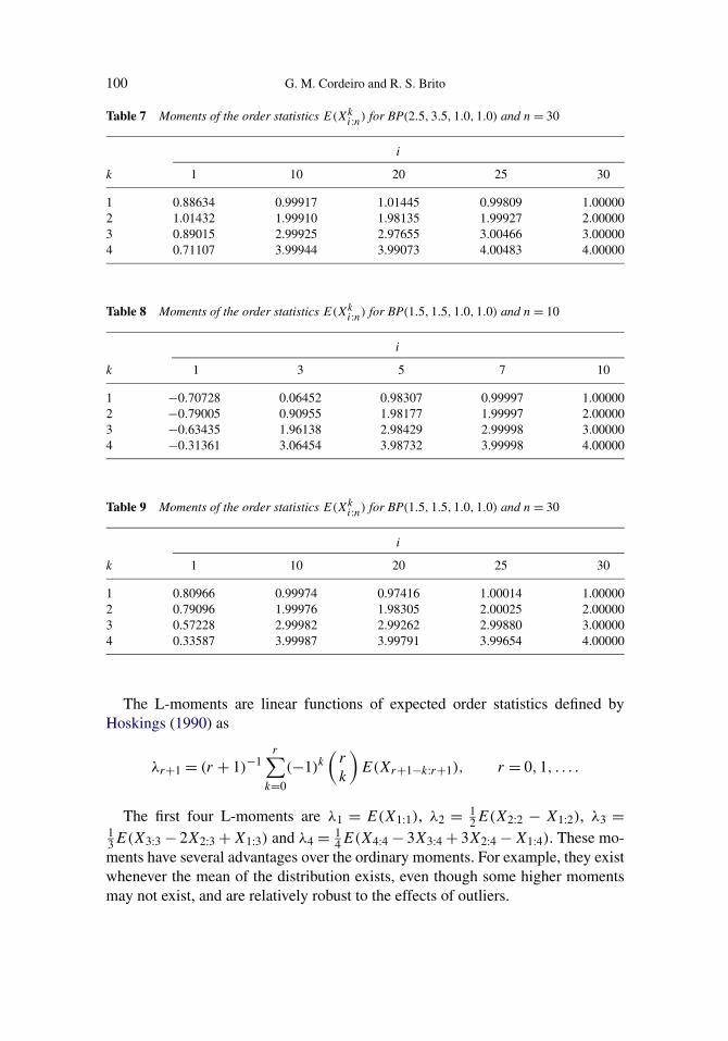
100 G. M. Cordeiro and R. S. Brito

Table 7 Moments of the order statistics E(Xki:n) for BP(2.5,3.5,1.0,1.0) and n = 30

i

k 1 10 20 25 30

1 0.88634 0.99917 1.01445 0.99809 1.000002 1.01432 1.99910 1.98135 1.99927 2.000003 0.89015 2.99925 2.97655 3.00466 3.000004 0.71107 3.99944 3.99073 4.00483 4.00000

Table 8 Moments of the order statistics E(Xki:n) for BP(1.5,1.5,1.0,1.0) and n = 10

i

k 1 3 5 7 10

1 −0.70728 0.06452 0.98307 0.99997 1.000002 −0.79005 0.90955 1.98177 1.99997 2.000003 −0.63435 1.96138 2.98429 2.99998 3.000004 −0.31361 3.06454 3.98732 3.99998 4.00000

Table 9 Moments of the order statistics E(Xki:n) for BP(1.5,1.5,1.0,1.0) and n = 30

i

k 1 10 20 25 30

1 0.80966 0.99974 0.97416 1.00014 1.000002 0.79096 1.99976 1.98305 2.00025 2.000003 0.57228 2.99982 2.99262 2.99880 3.000004 0.33587 3.99987 3.99791 3.99654 4.00000

The L-moments are linear functions of expected order statistics defined byHoskings (1990) as

λr+1 = (r + 1)−1r∑

k=0

(−1)k(

r

k

)E(Xr+1−k:r+1), r = 0,1, . . . .

The first four L-moments are λ1 = E(X1:1), λ2 = 12E(X2:2 − X1:2), λ3 =

13E(X3:3 − 2X2:3 + X1:3) and λ4 = 1

4E(X4:4 − 3X3:4 + 3X2:4 − X1:4). These mo-ments have several advantages over the ordinary moments. For example, they existwhenever the mean of the distribution exists, even though some higher momentsmay not exist, and are relatively robust to the effects of outliers.

The beta power distribution 101

Equation (7.1) applied to the means (k = 1) of the order statistics give theL-moments of the BP distribution. They can also be determined in terms of thePWMs from (4.1) as

λr+1 =r∑

k=0

(−1)r−k

(r

k

)(r + k

k

)m1,k, r = 0,1, . . . .

In particular, λ1 = m1,0, λ2 = 2m1,1 − m1,0, λ3 = 6m1,2 − 6m1,1 + m1,0, λ4 =20m1,3 − 30m1,2 + 12m1,1 − m1,0.

8 Entropy

The entropy of a random variable X with density function f (x) is a measure ofvariation of the uncertainty. One of the popular entropy measure is the Rényi en-tropy given by

JR(γ ) = 1

1 − γlog

[∫f γ (x) dx

], γ > 0, γ �= 1. (8.1)

The expansion of the BP density (2.3) yields

JR(γ ) = 1

1 − γlog

{[α

�(a + b)

�(a)

]γ ∫ 1/β

0

[ ∞∑i=0

(−1)iβα(a+i)xα(a+i)−1

�(b − i)i!]γ

dx

}.

In order to obtain an expansion for G(x)γ for γ > 0 real noninteger, we canwrite

G(x)γ = [1 − {1 − G(x)}]γ =∞∑

j=0

(γ

j

)(−1)j {1 − G(x)}j

and then

G(x)γ =∞∑

j=0

j∑r=0

(−1)j+r

(γ

j

)(j

r

)G(x)r .

We can substitute∑∞

j=0∑j

r=0 for∑∞

r=0∑∞

j=r to obtain

G(x)γ =∞∑

r=0

∞∑j=r

(−1)j+r

(γ

j

)(j

r

)G(x)r

and then

G(x)γ =∞∑

r=0

sr(γ )G(x)r , (8.2)

102 G. M. Cordeiro and R. S. Brito

where the coefficients sr(γ ) are given by

sr(γ ) =∞∑

j=r

(−1)r+j

(γ

j

)(j

r

). (8.3)

For the BP distribution, we have

F(x) =∞∑i=0

(−1)iβα(a+i)xα(a+i)−1

�(b − i)i! .

Thus, from equations (8.2) and (8.3), we obtain

JR(γ ) = γ

1 − γ[log(α) + δ(a + b) − δ(a)]

+ 1

1 − γlog

{∫ 1/β

0

∞∑r=0

sr(γ )

[ ∞∑i=0

(−1)iβα(a+i)xα(a+i)−1

�(b − i)i!]r

dx

},

where δ(·) = log{�(·)}. Hence,

JR(γ ) = γ

1 − γ[log(α) + δ(a + b) − δ(a)]

+ 1

1 − γlog

[∫ 1/β

0

∞∑r=0

sr(γ )

×r∑

m1,...,mq=0

am1 · · ·amq βα(ra+∑r

q=1 mq)

× xα(ra+∑r

q=1 mq)−rdx

],

where

amq = (−1)mq

�(b − mq)mq ! , q = 1, . . . , r.

Then,

JR(γ ) = γ

1 − γ[log(α) + δ(a + b) − δ(a)]

+ 1

1 − γlog

[ ∞∑r=0

sr(γ )

r∑[m1,...,mq ]=0

am1 · · ·amq βα(ra+∑r

q=1 mq)

×∫ 1/β

0x

α(ra+∑rq=1 mq)−r

dx

].

The beta power distribution 103

By calculating the integral, we have

JR(γ ) = γ

1 − γ[log(α) + δ(a + b) − δ(a)]

+ 1

1 − γlog

{ ∞∑r=0

sr(γ )

×r∑

m1,...,mq=0

(am1 · · ·amq β

α(ra+∑rq=1 mq))

×(β

α(ra+∑rq=1 mq)−r+1

×[α

(ra +

r∑q=1

mq

)− r + 1

])−1}.

Finally, the entropy of the BP distribution reduces to

JR(γ ) = γ

1 − γ[log(α) + δ(a + b) − δ(a)]

+ 1

1 − γlog

{ ∞∑r=0

βr−1sr(γ )

r∑m1,...,mq=0

am1 · · ·amq

[α(ra + ∑rq=1 mq) − r + 1]

}.

9 Reliability

In the area of stress-strength models there has been a large amount of work asregards estimation of the reliability R = Pr(X2 < X1) when X1 and X2 are inde-pendent random variables belonging to the same univariate family of distributions.The algebraic form for R has been worked out for the majority of the well-knownstandard distributions. Here, we derive the reliability R when X1 and X2 are inde-pendent and have the same BP distribution. The definition of the reliability is

R =∫ 1/β

0f (x)F (x) dx. (9.1)

Using the expansions (2.2) and (2.3) in (9.1), we have

R =∫ 1/β

0

[�(a + b)

�(a)

]2

×∞∑i=0

∞∑j=0

{(−1)i+j [α(a + i)β(βx)α(a+i)−1](βx)α(a+j)

�(b − i)�(b − j)i!j !(a + i)(a + j)

}dx.

104 G. M. Cordeiro and R. S. Brito

Interchanging the integral and the sums and calculating the integral, we obtain

R =[�(a + b)

�(a)

]2 ∞∑i=0

∞∑j=0

[(−1)i+j

�(b − i)�(b − j)i!j !(a + j)(2a + i + j)

].

The reliability of the power distribution is 1/2.

10 Estimation

We consider that X has the BP distribution and let θ = (a, b,α,β)T be the vec-tor of parameters. The log-likelihood = (θ) for a random sample x1, . . . , xn

from (1.6) reduces to

= n log(αβ) − n logB(a, b)

+ (αa − 1)

n∑i=1

log(βxi) + (b − 1)

n∑i=1

log[1 − (βxi)α].

The components of the score vector U = U(θ) = (∂/∂a, ∂/∂b, ∂/∂α, ∂/∂β)T

for n observations are

∂

∂a= −nψ(a) + nψ(a + b) + α

n∑i=1

log(βxi),

∂

∂b= −nψ(b) + nψ(a + b) +

n∑i=1

log[1 − (βxi)α],

∂

∂α= n

α+ a

n∑i=1

log(βxi) − (b − 1)

n∑i=1

(βxi)α log(βxi)

1 − (βxi)α,

∂

∂β= α

β

[na − (b − 1)

n∑i=1

(βxi)α

1 − (βxi)α

],

where ψ(p) = ∂ log{�(p)}/∂p is the digamma function. We can obtain the maxi-mum likelihood estimate (MLE) of θ by setting the components of the score vectorto zero and solving the nonlinear equations simultaneously. The MLE θ of θ canbe calculated by the Newton–Raphson method. Since the support of the BP dis-tribution depends on the parameter β , the normal distribution could not be a goodapproximation for the asymptotic distribution of

√n(θr −θr) in moderate samples.

However, we can construct a confidence interval with significance level γ for eachparameter θr given by

ACI(θr ,100(1 − γ )%

) = (θr − zγ/2

√j θr ,θr , θr + zγ/2

√j θr ,θr

),

The beta power distribution 105

under the assumption that the normal approximation holds. Here, j θr ,θr is the r thdiagonal element of the estimated inverse observed information matrix for r =1, . . . ,4 and zγ/2 is the quantile 1 − γ /2 of the standard normal distribution.

The likelihood ratio (LR) statistic is useful for testing goodness of fit of theBP distribution and for comparing this distribution with some of its special sub-models. If we consider the partition θ = (θT

1 , θT2 )T , tests of hypotheses of the type

H0 : θ1 = θ(0)1 versus HA : θ1 �= θ

(0)1 can be performed via LR statistics. The LR

statistic for testing the null hypothesis H0 is w = 2{(θ) − (θ)}, where θ and θare the MLEs of θ under HA and H0, respectively. Under the null hypothesis, w

could be approximated by the χ2q distribution, where q is the dimension of the

vector θ1 of interest. The approximation could be poor in moderate samples. TheLR test rejects H0 if w > ξγ , where ξγ denotes the upper 100γ % point of the χ2

q

distribution. For example, we can check if the fit of the BP distribution is statisti-cally “superior” to a fit using the power distribution for a given dataset by testingH0 :a = b = 1 versus HA :H0 is not true.

11 Applications

In this section, we analyze two real datasets in order to illustrate the good perfor-mance of the BP distribution.

First dataset

The BP distribution is fitted to a dataset obtained from measurements on petroleumrock samples. The data consist of 48 rock samples from a petroleum reservoir. Thedataset corresponds to twelve core samples from petroleum reservoirs that weresampled by four cross-sections. Each core sample was measured for permeabilityand each cross-section has the following variables: the total area of pores, the totalperimeter of pores and shape. We analyze the shape perimeter by squared (area)variable. Table 10 gives the dataset.

The Newton–Raphson procedure to calculate the MLEs is performed by takingthe initial values a = 55.0, b = 98.0, α = 0.4 and β = 0.2 leading to the following

Table 10 Shape perimeter by squared (area) from measurements on petroleum rock samples

0.0903296 0.2036540 0.2043140 0.2808870 0.1976530 0.32864100.1486220 0.1623940 0.2627270 0.1794550 0.3266350 0.23008100.1833120 0.1509440 0.2000710 0.1918020 0.1541920 0.46412500.1170630 0.1481410 0.1448100 0.1330830 0.2760160 0.42047700.1224170 0.2285950 0.1138520 0.2252140 0.1769690 0.20074400.1670450 0.2316230 0.2910290 0.3412730 0.4387120 0.26265100.1896510 0.1725670 0.2400770 0.3116460 0.1635860 0.18245300.1641270 0.1534810 0.1618650 0.2760160 0.2538320 0.2004470

106 G. M. Cordeiro and R. S. Brito

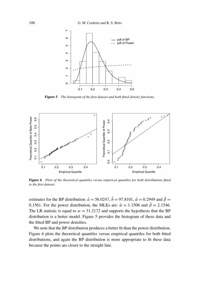
Figure 5 The histogram of the first dataset and both fitted density functions.

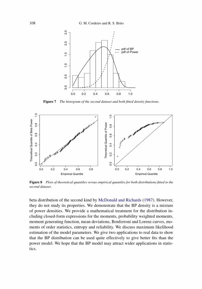
Figure 6 Plots of the theoretical quantiles versus empirical quantiles for both distributions fittedto the first dataset.

estimates for the BP distribution: a = 56.0247, b = 97.8101, α = 0.2949 and β =0.1561. For the power distribution, the MLEs are: α = 1.1506 and β = 2.1546.The LR statistic is equal to w = 31.2172 and supports the hypothesis that the BPdistribution is a better model. Figure 5 provides the histogram of these data andthe fitted BP and power densities.

We note that the BP distribution produces a better fit than the power distribution.Figure 6 plots the theoretical quantiles versus empirical quantiles for both fitteddistributions, and again the BP distribution is more appropriate to fit these databecause the points are closer to the straight line.

The beta power distribution 107

Table 11 Proportion of total milk production

0.4365 0.4260 0.5140 0.6907 0.7471 0.2605 0.61960.8781 0.4990 0.6058 0.6891 0.5770 0.5394 0.14790.2356 0.6012 0.1525 0.5483 0.6927 0.7261 0.33230.0671 0.2361 0.4800 0.5707 0.7131 0.5853 0.67680.5350 0.4151 0.6789 0.4576 0.3259 0.2303 0.76870.4371 0.3383 0.6114 0.3480 0.4564 0.7804 0.34060.4823 0.5912 0.5744 0.5481 0.1131 0.7290 0.01680.5529 0.4530 0.3891 0.4752 0.3134 0.3175 0.11670.6750 0.5113 0.5447 0.4143 0.5627 0.5150 0.07760.3945 0.4553 0.4470 0.5285 0.5232 0.6465 0.06500.8492 0.8147 0.3627 0.3906 0.4438 0.4612 0.31880.2160 0.6707 0.6220 0.5629 0.4675 0.6844 –0.3413 0.4332 0.0854 0.3821 0.4694 0.3635 –0.4111 0.5349 0.3751 0.1546 0.4517 0.2681 –0.4049 0.5553 0.5878 0.4741 0.3598 0.7629 –0.5941 0.6174 0.6860 0.0609 0.6488 0.2747 –

Second dataset

The BP distribution is now fitted to the data about the total milk production in thefirst birth of 107 cows from SINDI race. These cows are property of the Carnaúbafarm which belongs to the Agropecuária Manoel Dantas Ltda (AMDA), locatedin Taperoá City, Paraíba (Brazil).

The original data is not in the interval (0,1), and it was necessary to makea transformation given by xi = [yi − min(yi)]/[max(yi) − min(yi)], for i =1, . . . ,107. These data are presented in Table 11 and the values of yi are givenin Table 3.1 of Brito (2009, p. 46).

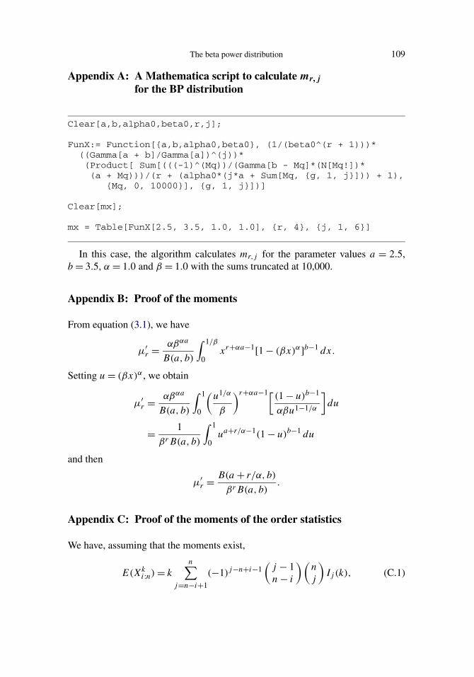
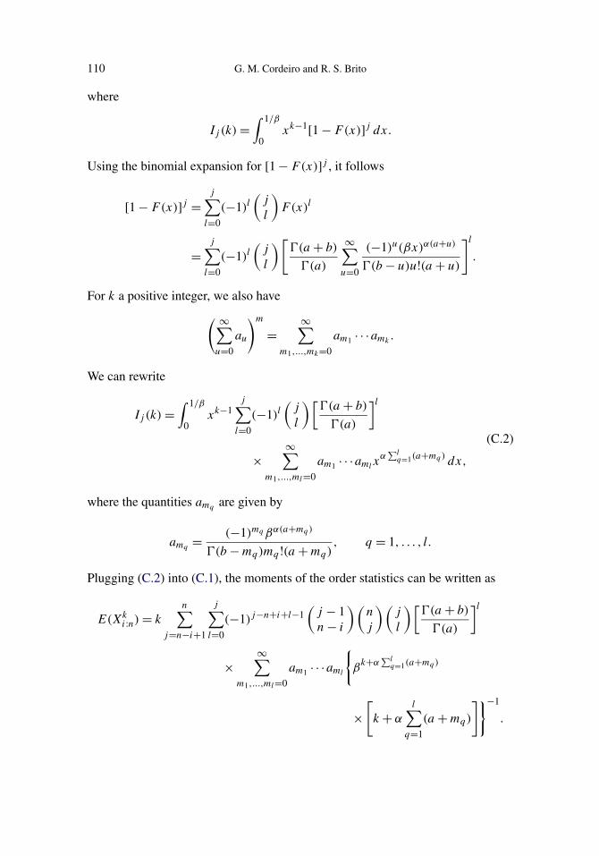
The initial values for the iterative algorithm are: a = 0.5, b = 42.0, α = 4.0 andβ = 0.8. The MLEs of the parameters of the BP distribution are: a = 0.2704,b = 42.0228, α = 6.6402 and β = 0.7756. For the power distribution, the es-timates of the parameters are: α = 5.0027 and β = 1.1364. The LR statisticw = 333.615 indicates that the BP distribution is a better model than the powerdistribution. Figure 7 gives the histogram of the second dataset and the plots ofboth fitted densities. It is possible to verify the good performance of the BP dis-tribution. The plots of the theoretical quantiles versus empirical quantiles given inFigure 8 suggest that the BP distribution is very suitable for these data.

12 Conclusion

We study the mathematical properties of the beta power (BP) distribution whichextends the power distribution defined by Balakrishnan and Nevzorov (2003). TheBP distribution is not new since it was defined as the name of the generalized

108 G. M. Cordeiro and R. S. Brito

Figure 7 The histogram of the second dataset and both fitted density functions.

Figure 8 Plots of theoretical quantiles versus empirical quantiles for both distributions fitted to thesecond dataset.

beta distribution of the second kind by McDonald and Richards (1987). However,they do not study its properties. We demonstrate that the BP density is a mixtureof power densities. We provide a mathematical treatment for the distribution in-cluding closed-form expressions for the moments, probability weighted moments,moment generating function, mean deviations, Bonferroni and Lorenz curves, mo-ments of order statistics, entropy and reliability. We discuss maximum likelihoodestimation of the model parameters. We give two applications to real data to showthat the BP distribution can be used quite effectively to give better fits than thepower model. We hope that the BP model may attract wider applications in statis-tics.

The beta power distribution 109

Appendix A: A Mathematica script to calculate mr,j

for the BP distribution

Clear[a,b,alpha0,beta0,r,j];

FunX:= Function[{a,b,alpha0,beta0}, (1/(beta0^(r + 1)))*((Gamma[a + b]/Gamma[a])^(j))*(Product[ Sum[(((-1)^(Mq))/(Gamma[b - Mq]*(N[Mq!])*(a + Mq)))/(r + (alpha0*(j*a + Sum[Mq, {g, 1, j}])) + 1),

{Mq, 0, 10000}], {g, 1, j}])]

Clear[mx];

mx = Table[FunX[2.5, 3.5, 1.0, 1.0], {r, 4}, {j, 1, 6}]

In this case, the algorithm calculates mr,j for the parameter values a = 2.5,b = 3.5, α = 1.0 and β = 1.0 with the sums truncated at 10,000.

Appendix B: Proof of the moments

From equation (3.1), we have

μ′r = αβαa

B(a, b)

∫ 1/β

0xr+αa−1[1 − (βx)α]b−1 dx.

Setting u = (βx)α , we obtain

μ′r = αβαa

B(a, b)

∫ 1

0

(u1/α

β

)r+αa−1[(1 − u)b−1

αβu1−1/α

]du

= 1

βrB(a, b)

∫ 1

0ua+r/α−1(1 − u)b−1 du

and then

μ′r = B(a + r/α, b)

βrB(a, b).

Appendix C: Proof of the moments of the order statistics

We have, assuming that the moments exist,

E(Xki:n) = k

n∑j=n−i+1

(−1)j−n+i−1(

j − 1n − i

)(n

j

)Ij (k), (C.1)

110 G. M. Cordeiro and R. S. Brito

where

Ij (k) =∫ 1/β

0xk−1[1 − F(x)]j dx.

Using the binomial expansion for [1 − F(x)]j , it follows

[1 − F(x)]j =j∑

l=0

(−1)l(

j

l

)F(x)l

=j∑

l=0

(−1)l(

j

l

)[�(a + b)

�(a)

∞∑u=0

(−1)u(βx)α(a+u)

�(b − u)u!(a + u)

]l

.

For k a positive integer, we also have( ∞∑u=0

au

)m

=∞∑

m1,...,mk=0

am1 · · ·amk.

We can rewrite

Ij (k) =∫ 1/β

0xk−1

j∑l=0

(−1)l(

j

l

)[�(a + b)

�(a)

]l

(C.2)

×∞∑

m1,...,ml=0

am1 · · ·amlx

α∑l

q=1(a+mq)dx,

where the quantities amq are given by

amq = (−1)mq βα(a+mq)

�(b − mq)mq !(a + mq), q = 1, . . . , l.

Plugging (C.2) into (C.1), the moments of the order statistics can be written as

E(Xki:n) = k

n∑j=n−i+1

j∑l=0

(−1)j−n+i+l−1(

j − 1n − i

)(n

j

)(j

l

)[�(a + b)

�(a)

]l

×∞∑

m1,...,ml=0

am1 · · ·aml

{β

k+α∑l

q=1(a+mq)

×[k + α

l∑q=1

(a + mq)

]}−1

.

The beta power distribution 111

Appendix D: A Mathematica script to calculate the moments of theorder statistics for the BP distribution

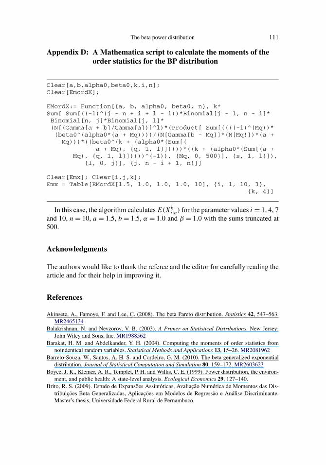
Clear[a,b,alpha0,beta0,k,i,n];Clear[EmordX];

EMordX:= Function[{a, b, alpha0, beta0, n}, k*Sum[ Sum[((-1)^(j - n + i + l - 1))*Binomial[j - 1, n - i]*Binomial[n, j]*Binomial[j, l]*(N[(Gamma[a + b]/Gamma[a])]^l)*(Product[ Sum[((((-1)^(Mq))*(beta0^(alpha0*(a + Mq))))/(N[Gamma[b - Mq]]*(N[Mq!])*(a +

Mq)))*((beta0^(k + (alpha0*(Sum[(a + Mq), {q, 1, l}]))))*((k + (alpha0*(Sum[(a +

Mq), {q, 1, l}]))))^(-1)), {Mq, 0, 500}], {s, 1, l}]),{l, 0, j}], {j, n - i + 1, n}]]

Clear[Emx]; Clear[i,j,k];Emx = Table[EMordX[1.5, 1.0, 1.0, 1.0, 10], {i, 1, 10, 3},

{k, 4}]

In this case, the algorithm calculates E(Xki:n) for the parameter values i = 1,4,7

and 10, n = 10, a = 1.5, b = 1.5, α = 1.0 and β = 1.0 with the sums truncated at500.

Acknowledgments

The authors would like to thank the referee and the editor for carefully reading thearticle and for their help in improving it.

References

Akinsete, A., Famoye, F. and Lee, C. (2008). The beta Pareto distribution. Statistics 42, 547–563.MR2465134

Balakrishnan, N. and Nevzorov, V. B. (2003). A Primer on Statistical Distributions. New Jersey:John Wiley and Sons, Inc. MR1988562

Barakat, H. M. and Abdelkander, Y. H. (2004). Computing the moments of order statistics fromnoindentical random variables. Statistical Methods and Applications 13, 15–26. MR2081962

Barreto-Souza, W., Santos, A. H. S. and Cordeiro, G. M. (2010). The beta generalized exponentialdistribution. Journal of Statistical Computation and Simulation 80, 159–172. MR2603623

Boyce, J. K., Klemer, A. R., Templet, P. H. and Willis, C. E. (1999). Power distribution, the environ-ment, and public health: A state-level analysis. Ecological Economics 29, 127–140.

Brito, R. S. (2009). Estudo de Expansões Assintóticas, Avaliação Numérica de Momentos das Dis-tribuições Beta Generalizadas, Aplicações em Modelos de Regressão e Análise Discriminante.Master’s thesis, Universidade Federal Rural de Pernambuco.

112 G. M. Cordeiro and R. S. Brito

Brown, B. W., Spears, F. M. and Levy, L. B. (2002). The log F: A distribution for all seasons.Computational Statistics 17, 47–58. MR1895873

Eugene, N., Lee, C. and Famoye, F. (2002). Beta-normal distribution and its applications. Communi-cations in Statistics—Theory and Methods 31, 175–195. MR1902307

Gradshteyn, I. S. and Ryzhik, I. M. (2000). Table of Integrals, Series, and Products. San Diego:Academic Press. MR1773820

Greenwood, J. A., Landwehr, J. M., Matalas, N. C. and Wallis, J. R. (1979). Probability weightedmoments: Definitions and relation to parameters of several distributions expressable in inverseform. Water Resources Research 15, 1049–1054.

Hoskings, J. R. M. (1990). L-moments: analysis and estimation of distribution using linear combina-tions of order statistics. Journal of the Royal Statistical Society B 52, 105–124. MR1049304

Jones, N. (2004). Families of distributions arising from distributions of order statistics. Test 13, 1–43.MR2065642

Nadarajah, S. and Gupta, A. K. (2004). The beta Fréchet distribution. Far East Journal of TheoreticalStatistics 14, 15–24. MR2108090

Nadarajah, S. and Kotz, S. (2004). The beta Gumbel distribution. Mathematical Problems in Engi-neering 10, 323–332. MR2109721

Nadarajah, S. and Kotz, S. (2005). The beta exponential distribution. Reliability Engineering andSystem Safety 91, 689–697.

McDonald, J. B. and Richards, D. O. (1987). Some generalized models with application to reliability.Journal of Statistical Planning and Inference 16, 365–376. MR0912632

Sepanski, J. H. and Kong, L. (2007). A family of generalized beta distributions for income. Availableat http://arxiv.org/PS_cache/arxiv/pdf/0710/0710.4614v1.pdf.

Van Dorp, J. R. and Kotz, S. (2002). The standard two-sided power distribution and its prop-erties: With applications in financial engineering. American Statistical Association 56, 90–99.MR1945867

Departamento de Estatística e InformáticaUniversidade Federal Rural de Pernambuco52171-900, Recife, PEBrazilE-mail: gausscordeiro@uol.com.br

janesbrito@gmail.com