
Optimal Power Flow for Active Distribution Networks
186
Optimal Power Flow for Active Distribution Networks Advanced Formulations, Practical Considerations and Laboratory Demonstration by Michael Z. Liu ORCID ID: 0000-0002-9609-4544 A thesis submitted to The University of Melbourne for the degree of Doctor of Philosophy October 2020 Department of Electrical and Electronic Engineering Melbourne School of Engineering This thesis is submitted for the partial fulfilment of this degree.
-
Upload
khangminh22 -
Category
Documents
-
view
0 -
download
0
Transcript of Optimal Power Flow for Active Distribution Networks
Optimal Power Flow for
Active Distribution Networks Advanced Formulations, Practical Considerations
and Laboratory Demonstration
by
Michael Z. Liu
ORCID ID: 0000-0002-9609-4544
A thesis submitted to The University of Melbourne for the degree of
Doctor of Philosophy
October 2020
Department of Electrical and Electronic Engineering
Melbourne School of Engineering
This thesis is submitted for the partial fulfilment of this degree.

Copyright © Michael Z. Liu
All rights reserved. No part of this thesis may be reproduced in any form
without written permission from the author.
I
ABSTRACT
The rapid growth of renewable distributed generation (DG) has introduced
unconventional challenges for distribution companies (e.g., dealing with voltage rise).
To enable future DG growth, a promising alternative (to the otherwise capital-intensive
and time-consuming network reinforcements) is the real-time orchestration of DG and
existing network assets using advanced schemes. In this context, the operational usage
of Optimal Power Flow (OPF)—an optimisation-based technique traditionally found
in transmission network applications, albeit using simplified formulations—as a
decision-making engine has gained tremendous interest in recent literature.
Nonetheless, before such schemes can be readily integrated in the control room of
distribution networks, there are several practical challenges that must be addressed.
Firstly, the operational usage of OPF requires a fast and scalable formulation that
can handle the size (thousands of nodes) and complexity (phase unbalances, discrete
devices) of typical distribution networks. Furthermore, since the differences in device-
specific characteristics in the sub-minute scale (delays, ramp rates and deadbands) may
lead to coordination issues when multiple devices are being controlled simultaneously,
additional adaptations are necessary to ensure OPF-based setpoints can be
implemented in real-world applications. Finally, while active power curtailment is
inevitable at times, since such actions has a direct impact on the return on investment
for DG owners, the implications from different fairness objectives (e.g., removing
disparity in renewable energy harvesting or financial benefits) as well as the trade-offs
between fairness (reducing disparity) and efficiency (aggregated performance) need to
be first understood.
In this PhD project, the following research is carried out to address the
aforementioned challenges:
• A linearised, three-phase AC OPF is developed to cater for multi-voltage level
distribution feeders and integer variables. Its performance is demonstrated
using a realistic MV-LV residential feeder (from the primary substation down
to individual connection points of 4,626 single-phase consumers) with over
4,900 nodes.
II
• The necessary adaptations in existing device controllers and the OPF
formulation are proposed, allowing network participants and assets to be
successfully controlled using OPF-based schemes in an operational setting
with minute-scale control actions. Particularly, the importance of the proposed
adaptations in preventing short-term voltage spikes are demonstrated using a
rural distribution feeder with multiple actively managed on-load tap changers
and wind farms.
• The implications and trade-offs from different fairness considerations are
investigated using several OPF-based schemes, each considering a unique and
contrasting fairness objective. The findings highlight the multi-facet nature of
curtailment fairness and the importance of identifying the most appropriate
objective for a given application. Furthermore, it can help
operators/policymakers to make informed decisions when a portfolio of DG is
to be managed.
• A hardware-in-the-loop demonstration platform is built using commercially
available software and hardware at the Smart Grid Lab of The University of
Melbourne. This implementation extends beyond static plots and tables by
introducing a rich and interactive user interface, and thus enabling a more
realistic and engaging way of showcasing advanced schemes to industry.

III
DECLARATION
This is to certify that
1. the thesis comprises only of my original work towards the degree of Doctor of
Philosophy except where indicated in the preface,
2. due acknowledgement has been made in the text to all other material used, and
3. the thesis is less than 100,000 words in length, exclusive of tables, maps
bibliographies and appendices.
________________________
Michael Z. Liu, October 2020

IV
This page is intentionally left blank.
V
PREFACE
Parts of this thesis have been carried out in collaboration with Dr Andreas T.
Procopiou (The University of Melbourne), Dr Kyriacos Petrou (The University of
Melbourne), Dr Luis Gutierrez-Lagos (The University of Manchester), Prof Steven H.
Low (California Institute of Technology). The list below identifies the publications
that correspond to each chapter, as well as the contributions of each collaborator.
Chapter 2
1. L. Gutierrez-Lagos, M. Z. Liu, and L. F. Ochoa, "Implementable Three-Phase OPF Formulations for MV-LV Distribution Networks: MILP and MIQCP," in Proc. 2019 2019 IEEE PES Innovative Smart Grid Technologies Conference - Latin America (ISGT Latin America), pp. 1-6.
It should be noted that publication (1) is a comparison paper between two OPF
formulations that are developed independently. The first formulation is developed by
me which is also presented in Chapter 2 of this thesis. The second formulation is
developed by Dr Luis Gutierrez-Lagos. Dr Luis Gutierrez-Lagos also provided the
necessary network data to perform the benchmarks.
Chapter 3
2. M. Z. Liu, L. F. Ochoa, S. H. Low, “On the Implementation of OPF-Based Set-Points for Active Distribution Networks”, IEEE Transactions on Smart Grids, in Review.
Prof Steven H. Low provided support in reviewing publication (2).
Chapter 4
3. M. Z. Liu, A. T. Procopiou, K. Petrou, L. F. Ochoa, T. Langstaff, J. Harding and J. Theunissen, “On the Fairness of PV Curtailment Schemes in Residential Distribution Networks”, IEEE Transactions on Smart Grids, Accepted March 2020.
Dr Andreas T. Procopiou and Dr Kyriacos Petrou provided support in developing
the household-centric metrics, which is a part of the overall methodology developed
by me to analyse and assess the fairness implications of different PV curtailment
schemes (e.g., identifying the different perspectives of fairness as well as the trade-
offs between fairness and efficiency). Particularly, these metrics are used to quantify
the impact of PV curtailment on individual households. The analysis in terms of

VI
fairness, which is the core contribution of publication (3) and Chapter 4 of this thesis,
is built on top of these metrics and focuses on the differences among all households.
Dr Andreas T. Procopiou and Dr Kyriacos Petrou also provided support in
developing the network model used in the case study.
As per regulation of The University of Melbourne, it is hereby declared that I,
Michael Z. Liu, have contributed to the majority (at least 51%) of the content found in
publication (3) and Chapter 4 of this thesis.

VII
“Genius is one percent inspiration and ninety-nine percent perspiration.”
– Thomas Edison

VIII
This page is intentionally left blank.

IX
DEDICATION
To Xingfu and Liqun,
my loving parents.
Thank you for raising me into the person I am today.
敬爱的父亲,母亲:谢谢你们一直以来
无私的付出和牺牲,无条件的鼓励与支持。

X
This page is intentionally left blank.

XI
ACKNOWLEDGEMENTS
First and foremost, I would like to express the sincerest gratitude to my supervisor
Prof. Luis F. Ochoa—a respected mentor, an amazing boss, and a caring friend. Thank
you for the support and guidance over the past years. You have been a constant source
of inspiration to me, not only as researcher, but also as an engineer and as a leader.
Special thanks to my fellow colleagues at Team Nando: Kyriacos, William, Dillon,
Andreas, Luis, Yolanda and Arthur. It has been a pleasure working with everyone,
sharing crazy-yet-brilliant ideas over often-extendedly-long team meetings and still-
educated conversations after oneway-too-many beers at team BBQs. I would also like
to thank my friends and colleagues, at The University of Melbourne and beyond, your
friendship has made this journey even more worthwhile. Looking forward to sharing
a beer and some laughter with you again, sometime, somewhere.
Finally, I would like to thank my beloved partner Yan. Thank you for your
accompany, support and understanding during this important chapter of my life. Just
like the saying “the little things in life matter more than anything else”, coming home
every day to a gentle smile and a warm hug has always helped me to get through the
toughest and most stressful moments.

XII
This page is intentionally left blank.
XIII
TABLE OF CONTENTS
1 INTRODUCTION .................................................................................................. 1
1.1 The Emergence of Active Distribution Networks ......................................... 1
1.1.1 Passive Distribution Networks ................................................................. 1
1.1.2 The Rise of Distributed Generation .......................................................... 4
1.1.3 Impacts of Renewable DG ........................................................................ 4
1.1.4 Towards Active Distribution Networks .................................................... 6
1.1.5 Advanced Schemes for Active Distribution Networks ............................ 8
1.2 Challenges ...................................................................................................... 8
1.2.1 Scalability and Speed of OPF Formulations ............................................ 8
1.2.2 Real-World Implementation of OPF-Based Setpoints ............................. 9
1.2.3 Ensuring Fairness in Curtailment Schemes .............................................. 9
1.2.4 Realistic Demonstration of OPF-Based Schemes .................................. 10
1.3 Research Questions ...................................................................................... 10
1.4 Objectives .................................................................................................... 11
1.4.1 A Scalable and Fast OPF Formulation ................................................... 11
1.4.2 Necessary Adaptations ........................................................................... 11
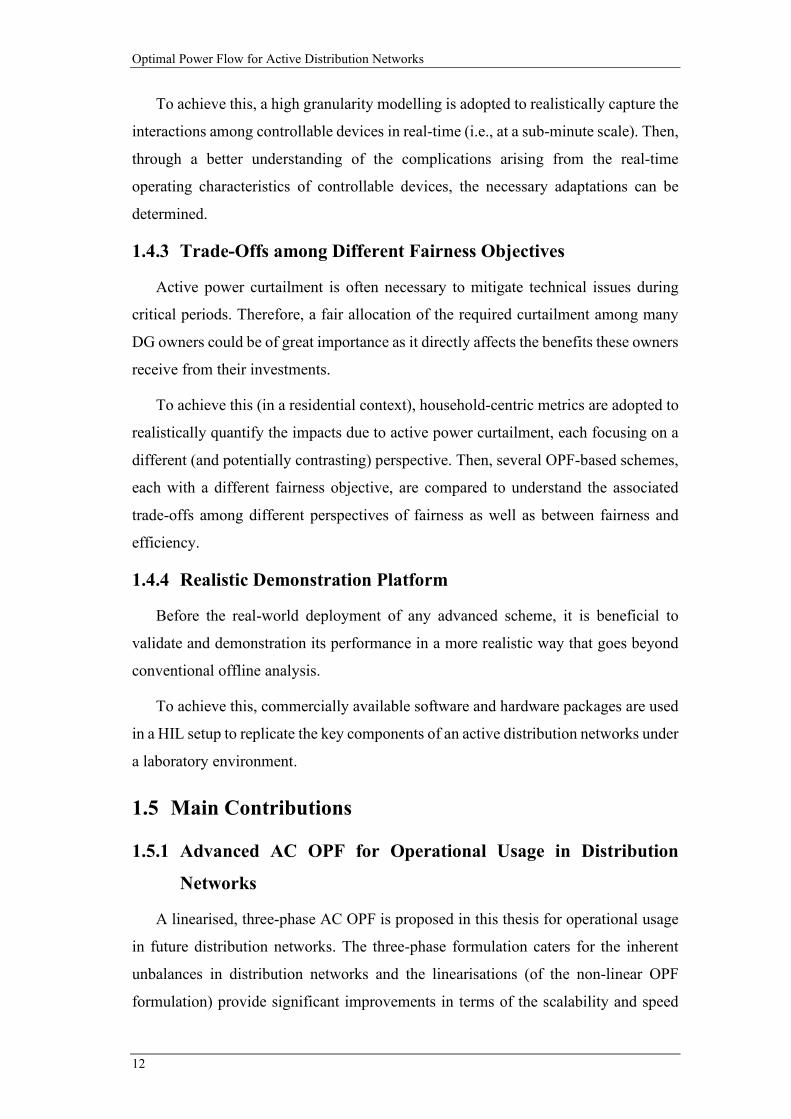
1.4.3 Trade-Offs among Different Fairness Objectives .................................. 12
1.4.4 Realistic Demonstration Platform .......................................................... 12
1.5 Main Contributions ...................................................................................... 12
1.5.1 Advanced AC OPF for Operational Usage in Distribution Networks ... 12
1.5.2 Necessary Adaptations to Implement OPF-Based Setpoints .................. 13
1.5.3 Different Fairness Objectives of Curtailment Schemes ......................... 14
1.5.4 A Hardware-in-the-Loop Demonstration Platform ................................ 14
1.6 Publications .................................................................................................. 15
1.6.1 Journal Papers ......................................................................................... 15
1.6.2 Conference Papers .................................................................................. 15
XIV
1.6.3 Technical Reports .................................................................................. 15
1.6.4 Magazine Articles .................................................................................. 16
1.7 Thesis Outline .............................................................................................. 16
2 A FAST AND SCALABLE THREE-PHASE OPF FOR DISTRIBUTION NETWORKS . 19
2.1 Introduction .................................................................................................. 19
2.2 Literature Review ......................................................................................... 20
2.2.1 Categories of Mathematical Optimisation Problems ............................. 20
2.2.2 Variations of AC Power Flow Equations .............................................. 22
2.2.3 Three-Phase OPF Formulations ............................................................. 26
2.2.4 Summary of Research Gaps ................................................................... 28
2.3 Linearised Three-Phase OPF ........................................................................ 28
2.3.1 Households ............................................................................................. 29
2.3.2 Distribution Lines .................................................................................. 30
2.3.3 Delta-Wye Transformers ....................................................................... 35
2.3.4 Nodal Constraints .................................................................................. 41
2.3.5 Power Balance ....................................................................................... 41
2.3.6 Objective Function ................................................................................. 42
2.3.7 Summary of the OPF Formulation......................................................... 42
2.3.8 Solution Process ..................................................................................... 43
2.4 Case Study .................................................................................................... 44
2.4.1 Co-Simulation Platform ......................................................................... 44
2.4.2 Assessment Methodology and Metrics .................................................. 44
2.4.3 PV-Rich Distribution Network .............................................................. 45
2.4.4 Investigated Cases .................................................................................. 46
2.4.5 Simulation Results ................................................................................. 47
2.4.6 OPF Solution Time ................................................................................ 52
2.5 Error in Linearised OPF Formulation .......................................................... 52
XV
2.5.1 Error in Linearised Three-Phase Line Model ......................................... 52
2.5.2 Error in Linearised Delta-Wye Transformer Model ............................... 58
2.6 Summary ...................................................................................................... 61
3 IMPLEMENTING OPF-BASED SETPOINTS: CHALLENGES AND SOLUTIONS ........ 63
3.1 Introduction .................................................................................................. 63
3.2 Literature Review ........................................................................................ 63
3.3 Necessary Adaptations ................................................................................. 66
3.3.1 Decision-Making Process with Control Cycles ...................................... 66
3.3.2 Understanding Operating Characteristics ............................................... 67
3.3.3 Challenges of Implementing OPF-Based Setpoints ............................... 69
3.3.4 Adaptations in Device Controllers ......................................................... 71
3.3.5 Adaptations in OPF Formulations .......................................................... 73
3.4 Case Study ................................................................................................... 75
3.4.1 EHV1 Network ....................................................................................... 75
3.4.2 Modelling Considerations ...................................................................... 77
3.4.3 Cases Investigated .................................................................................. 79
3.4.4 Results .................................................................................................... 80
3.4.5 Sensitivity Analysis of Scaling Factors .................................................. 91
3.4.6 Remarks on Solution Speed .................................................................... 93
3.5 Summary ...................................................................................................... 94
4 FAIRNESS OF ACTIVE POWER CURTAILMENT SCHEMES: A RESIDENTIAL
CONTEXT ..................................................................................................................... 95
4.1 Introduction .................................................................................................. 95
4.2 Literature Review ........................................................................................ 96
4.2.1 Fairness in PV Curtailment Schemes ..................................................... 96
4.2.2 Different Perspectives of Fairness .......................................................... 97
4.2.3 Fairness vs. Efficiency .......................................................................... 100
4.2.4 Fairness Metrics .................................................................................... 104
XVI
4.3 OPF-Based PV Curtailment Schemes ........................................................ 106
4.3.1 OPF-Generation ................................................................................... 106
4.3.2 OPF-Export .......................................................................................... 107
4.3.3 OPF-Financial ...................................................................................... 107
4.3.4 OPF-Alpha-Fairness ............................................................................ 108
4.4 Case Study: Different Perspectives of Fairness ......................................... 108
4.4.1 PV-Rich Distribution Network ............................................................ 108
4.4.2 Simulation Setup .................................................................................. 109
4.4.3 Results .................................................................................................. 110
4.4.4 Remarks on Solution Speed ................................................................. 120
4.5 Case Study: Fairness-Efficiency Trade-Offs ............................................. 121
4.5.1 Scenarios Investigated ......................................................................... 121
4.5.2 Results .................................................................................................. 122
4.6 Summary .................................................................................................... 126
5 A HARDWARE-IN-THE-LOOP DEMONSTRATION PLATFORM .......................... 127
5.1 Introduction ................................................................................................ 127
5.2 Literature Review ....................................................................................... 128
5.3 Architecture ................................................................................................ 129
5.3.1 Distribution Network ........................................................................... 130
5.3.2 Communication Infrastructure ............................................................. 130
5.3.3 Control Room ...................................................................................... 130
5.4 Implementation of a HIL Demonstration Platform .................................... 130
5.4.1 Real-Time Simulator ............................................................................ 131
5.4.2 Communication Infrastructure ............................................................. 132
5.4.3 Advanced Network Management System ............................................ 132
5.4.4 Data Visualisation ................................................................................ 133
5.5 Live Demonstration .................................................................................... 135
5.6 Summary .................................................................................................... 137
XVII
6 CONCLUSION ................................................................................................. 139
6.1 Research Gaps and Contributions .............................................................. 139
6.1.1 Advanced OPF Formulation ................................................................. 140
6.1.2 Practical Considerations: Real-World Implementation of OPF-Based
Setpoints ........................................................................................................... 141
6.1.3 Practical Considerations: Fairness of Curtailment Schemes ................ 142
6.1.4 Laboratory Demonstration .................................................................... 143
6.2 Key Findings .............................................................................................. 144
6.2.1 Linearised Three-Phase OPF Formulation ........................................... 144
6.2.2 OPF-Based Schemes in an Operational Environment .......................... 144
6.2.3 Fairness of Curtailment Schemes in Residential Feeders ..................... 145
6.3 Future Works ............................................................................................. 146
6.3.1 Distributed Algorithms for OPF ........................................................... 146
6.3.2 More Accurate Forecast vs. Shorter Control Cycles ............................ 146
6.3.3 Multi-Period Optimisation .................................................................... 147
6.3.4 More Scalable Formulation of OPF-Alpha-Fairness ............................ 147
6.3.5 Fairness Implications when Additional Sources of Flexibility are
Considered ........................................................................................................ 147
REFERENCES .............................................................................................................. 149

XVIII
This page is intentionally left blank.

XIX
LIST OF TABLES
Table 2-1. AC power flow equations used in existing OPF literature. ...................... 28
Table 2-2. Summary of the proposed linearised OPF. .............................................. 43
Table 2-3. Summary simulation setup for C1-C8...................................................... 47
Table 2-4. Summary of results for C1-C8. ................................................................ 48
Table 2-5. Reference values for the unknown variables. .......................................... 53
Table 3-1. Objective function. ................................................................................... 78
Table 3-2. Summary of cases. ................................................................................... 79
Table 3-3. Conventional AVR settings. .................................................................... 79
Table 3-4. Selected network-level metrics. ............................................................... 81
Table 3-5. Sensitivity matrix (energy harvested). ..................................................... 92
Table 3-6. Sensitivity matrix (tap changes). .............................................................. 92
Table 3-7. Sensitivity matrix (reactive power). ......................................................... 92
Table 4-1. Aggregated energy statistics. ................................................................. 112
Table 4-2. Household data. ...................................................................................... 113
Table 4-3. Jain’s Fairness Index for household-centric metrics. ............................. 117
Table 4-4. Modified Gini Coefficient for household-centric metrics. ..................... 117
Table 4-5. Summary of cases. ................................................................................. 121
Table 4-6. Aggregated energy statistics for different 𝜶𝜶 values. .............................. 123
Table 4-7. Jain’s Fairness Index and modified Gini Coefficient for different 𝜶𝜶 values.
.................................................................................................................................. 124
Table 4-8. Marginal change as 𝜶𝜶 increases. ............................................................ 125

XX
This page is intentionally left blank.
XXI
LIST OF FIGURES
Figure 1-1. Unidirectional power flows in a passive distribution network. ................ 2
Figure 1-2. Technical issues from excessive reverse power flows. ............................. 5
Figure 1-3. Managed bidirectional power flows in an active distribution network. ... 7
Figure 2-1. Illustration of convexity. ......................................................................... 21
Figure 2-2. A single-phase distribution line. ............................................................. 23
Figure 2-3. Visualisation of the piecewise linearisation technique. .......................... 35
Figure 2-4. A delta-wye transformer. ........................................................................ 36
Figure 2-5. Voltage phasors for balanced and unbalanced scenarios. ....................... 39
Figure 2-6. Data flow of the co-simulation platform. ............................................... 44
Figure 2-7. Topology of the 22kV feeder. ................................................................. 45
Figure 2-8. Boxplot of nodal voltages and asset utilisations for C1-C8.................... 49
Figure 2-9. Boxplot of APE (in %) for nodal voltages and asset utilisations for C1-
C8. .............................................................................................................................. 51
Figure 2-10. Test LV feeder. ..................................................................................... 53
Figure 2-11. Impact of inaccuracies in estimated power terms on the linearised line
model. ......................................................................................................................... 55
Figure 2-12. Impact of inaccuracies in estimated voltage terms on the linearised line
model .......................................................................................................................... 56
Figure 2-13. Approximation error of the linearised thermal model. ......................... 57
Figure 2-14. Test LV feeder with a delta-wye transformer. ...................................... 58
Figure 2-15. Impact of load unbalances on the linearised delta-wye transformer model.
.................................................................................................................................... 60
Figure 3-1. Decision-making process using control cycles. ...................................... 66
Figure 3-2. OLTC-fitted transformer with AVR. ...................................................... 68
Figure 3-3. Principles of AVR operation. ................................................................. 68
Figure 3-4. Timing diagrams of control events: a) uncoordinated scenario, b)
coordinated scenario. .................................................................................................. 70
XXII
Figure 3-5. Different ramping behaviours. ............................................................... 73
Figure 3-6. EHV1 network. ...................................................................................... 76
Figure 3-7. Demand and generation profiles. ........................................................... 77
Figure 3-8. Time-series voltage profiles. .................................................................. 81
Figure 3-9. Time-series utilisation profiles for lines and transformers. ................... 82
Figure 3-10. Uncoordinated execution of set-points (Case 2). ................................. 83
Figure 3-11. Coordinated execution of setpoints (Case 3). ...................................... 85
Figure 3-12. Uncoordinated execution of setpoints (Case 1). .................................. 85
Figure 3-13. Impacts of not including operational constraints in the OPF formulation
(Case 2). ..................................................................................................................... 87
Figure 3-14. Adequate consideration of operational constraints in the OPF
formulation (Case 3). ................................................................................................. 88
Figure 3-15. Number of tap changes per OLTC. ...................................................... 89
Figure 3-16. Wind power and demand at node 1115. ............................................... 90
Figure 3-17. Inadequate behaviour due to deadbands and voltage drifts in OLTCs
(Case 2). ..................................................................................................................... 90
Figure 3-18. Improvements in OLTC behaviour from the proposed direct control
method (Case 3). ........................................................................................................ 90
Figure 4-1. Household with positive net demand. .................................................... 98
Figure 4-2. A simple LV feeder. ............................................................................. 100
Figure 4-3. Illustration of the solutions to (a) maximum throughput, (b) proportional
fairness and (c) max-min fairness. ........................................................................... 101
Figure 4-4. Fairness-efficiency spectrum. .............................................................. 103
Figure 4-5. Demand and generation profiles. ......................................................... 109
Figure 4-6. Modified Volt-Watt curve. ................................................................... 110
Figure 4-7. Time-series voltage profiles for all 4,626 households. ........................ 111
Figure 4-8. Time-series plots for two households: towards the head of a feeder (A)
and towards the end of a feeder (B). ........................................................................ 115
XXIII
Figure 4-9. Time-series plots for two representative households: with high demand
(C) and with low demand (D). .................................................................................. 115
Figure 4-10. Time-series scattered plot of household-centric metrics. ................... 117
Figure 4-11. Illustration of quartiles. ....................................................................... 119
Figure 4-12. Boxplots of average PHI, EEI and NBI for all households shown in four
quartiles. ................................................................................................................... 119
Figure 4-13. Illustration of the differences in average EEIs due to non-defined
instances. .................................................................................................................. 120
Figure 4-14. Time-series voltage profiles for all 4,626 households. ....................... 123
Figure 4-15. Average network voltages for different for different 𝜶𝜶 values. .......... 123
Figure 4-16. Boxplots of average PHI for different 𝜶𝜶 values. ................................ 124
Figure 5-1. Architecture of the HIL demonstration platform. ................................. 129
Figure 5-2. Implementation of a HIL demonstration platform. ............................... 131
Figure 5-3. Data flows in the proposed setup. ......................................................... 133
Figure 5-4. Screenshot of dashboard one. ............................................................... 134
Figure 5-5. Main design elements of dashboard one. .............................................. 134
Figure 5-6. Screenshot of dashboard two. ............................................................... 135
Figure 5-7. A live demonstration of an OPF-based scheme for active distribution
networks. .................................................................................................................. 136

XXIV
This page is intentionally left blank.

XXV
ABBREVIATIONS
AC Alternating Current
AVR Automatic Voltage Regulator
DC Direct Current
DG Distributed Generation
DMS Distribution Management System
EEI Energy Export Index
GC Genie Coefficient
HIL Hardware-in-the-Loop
JFI Jain’s Fairness Index
LP Linear Program
LV Low Voltage
MILP Mixed-Integer Linear Program
MV Medium Voltage
NBI Net Benefit Index
NLP Non-linear Program
OLTC On-Load Tap Changer
OPF Optimal Power Flow
PHI PV Harvesting Index
POC Point of Connection
PV Photovoltaic
QCP Quadratically-Constrained Program
RTS Real-Time Simulator
SCADA Supervisory Control and Data Acquisition
SDP Semi-Definite Program
SOCP Second-Order Cone Program
XXVI
NOMENCLATURE
Sets
𝐻𝐻 Households
𝐺𝐺 Households with PV systems
𝑁𝑁 Buses/nodes
Φ Phases (electrical)
𝐿𝐿 Lines
𝑇𝑇 Transformers
𝑆𝑆 Sources
Parameters
𝑷𝑷𝑫𝑫, 𝑸𝑸𝑫𝑫 Household active and reactive power demand
𝑷𝑷𝑷𝑷𝑷𝑷 Maximum available PV power
𝑷𝑷�𝐺𝐺 PV inverter capacity
𝑷𝑷−, 𝑷𝑷+ Upper and lower voltage limits of a bus/node
𝑹𝑹, 𝑿𝑿 Physical impedance of a line
𝑹𝑹′, 𝑿𝑿′ Equivalent impedance of a line
𝑷𝑷��⃑ Approximated complex voltage phasor
𝑰𝑰+ Ampacity of a line
𝝉𝝉 Tap ratio of an on-load tap changer
𝝆𝝆, 𝚫𝚫�, 𝚲𝚲 Approximation constants to model the thermal capacity
Variables
𝑃𝑃𝐺𝐺 , 𝑄𝑄𝐺𝐺 PV inverter output, active and reactive
𝑃𝑃𝐶𝐶𝐶𝐶𝐶𝐶𝐶𝐶𝐶𝐶𝐶𝐶𝐶𝐶 PV curtailed active power
𝑃𝑃𝑁𝑁𝑁𝑁, 𝑄𝑄𝑁𝑁𝑁𝑁 Household net demand, active and reactive
𝑣𝑣 Squared line-to-neutral voltage of a bus/node
𝑃𝑃, 𝑄𝑄 Active and reactive power flow into an element
𝜅𝜅1 … 𝜅𝜅5 Auxiliary variables
𝑃𝑃+ , 𝑃𝑃− , 𝑄𝑄+ , 𝑄𝑄− ,
Δ𝑃𝑃, Δ𝑄𝑄, 𝜆𝜆
Approximation variables to model the thermal capacity
𝑘𝑘 Status of a tap position (binary) in OLTC-fitted transformer

XXVII
This page is intentionally left blank.

XXVIII
This page is intentionally left blank.
Chapter 1: Introduction
1
1 INTRODUCTION
Tackling climate change has become a global focus in recent decades. Particularly,
in the electricity sector, there has been tremendous support for renewable energy as an
alternative to fossil fuel. In fact, as of 2018, at least 162 countries have adopted a
national target for power generation from renewables [1]. With notable names such as
Germany and Denmark leading the charge—80% and 100% by 2050, respectively—
this collective effort has resulted in a more than tripling of the total renewable
generation capacity in less than two decades (from 754 GW in 2000 to over 2356 GW
in 2018) [2].
Undoubtedly, renewable generation has a crucial role in decarbonising the
electricity sector. However, integrating large volumes of renewable generation into the
existing power system is a rather challenging task. This is especially true considering
that renewable generation (e.g., from rooftop PV systems) are increasingly being
connected to the distribution network—the part of a power system that is typically
associated with the last-mile delivery of power to consumers, not necessarily designed
for bidirectional power flows as a result of local generation. Consequently, this rapid
transformation of the electricity generation mix necessitates a paradigm shift in the
way distribution networks are managed: moving from passive distribution networks
(with conservative design principles to cope with the worst-case scenarios) towards
active distribution networks (where network issues are tackled at the operational stage
through real-time monitoring and control).
1.1 The Emergence of Active Distribution Networks
1.1.1 Passive Distribution Networks
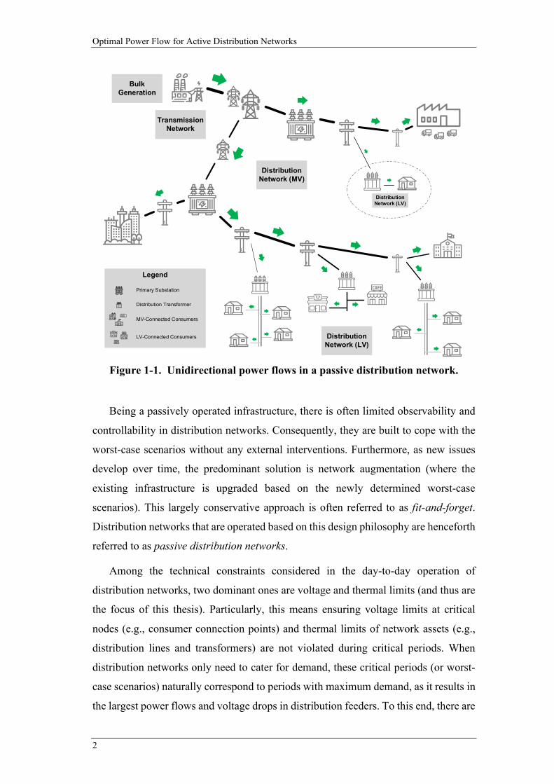
In traditional power systems, distribution networks are predominantly operated as
passive circuits with the assumption of unidirectional power flows. The typical
structure is shown in Figure 1-1 where power is received in bulk from the transmission
network and distributed to individual consumers (e.g., houses, businesses, factories,
etc.) through a radially connected system of poles and wires (commonly referred to as
feeders).
Optimal Power Flow for Active Distribution Networks
2
Being a passively operated infrastructure, there is often limited observability and
controllability in distribution networks. Consequently, they are built to cope with the
worst-case scenarios without any external interventions. Furthermore, as new issues
develop over time, the predominant solution is network augmentation (where the
existing infrastructure is upgraded based on the newly determined worst-case
scenarios). This largely conservative approach is often referred to as fit-and-forget.
Distribution networks that are operated based on this design philosophy are henceforth
referred to as passive distribution networks.
Among the technical constraints considered in the day-to-day operation of
distribution networks, two dominant ones are voltage and thermal limits (and thus are
the focus of this thesis). Particularly, this means ensuring voltage limits at critical
nodes (e.g., consumer connection points) and thermal limits of network assets (e.g.,
distribution lines and transformers) are not violated during critical periods. When
distribution networks only need to cater for demand, these critical periods (or worst-
case scenarios) naturally correspond to periods with maximum demand, as it results in
the largest power flows and voltage drops in distribution feeders. To this end, there are
Legend
Bulk Generation
Transmission Network
Distribution Network (MV)
Distribution Network (LV)
Primary Substation
Distribution Transformer
MV-Connected Consumers
LV-Connected Consumers
Distribution Network (LV)
Figure 1-1. Unidirectional power flows in a passive distribution network.
Chapter 1: Introduction
3
several well-established ways of managing voltage and thermal issues in passive
distribution networks.
From a thermal perspective, the existing assets (e.g., lines and transformers) are
designed according to the expected peak demand, and thus prevents being thermally
overloaded. In terms of voltage management, apart from sizing the conductor
appropriately to minimise ohmic losses (and thus voltage drops), there are a few other
mechanisms in place. For instance, primary substations are equipped with on-load tap
changers (OLTCs), autonomous devices that adjusts the transformation ratio of the
corresponding transformer (and thus the voltage) according to the variations in demand
throughout a day. Furthermore, distribution transformers are often configured to
provide a voltage boost, albeit being fixed, to compensate for voltage drops in LV
feeders. Lastly, capacitor banks and voltage regulators can also be installed along a
feeder for voltage regulation purposes.
Finally, it is worth noting that there are two distinct voltage levels in a distribution
network: medium voltage (MV) and low voltage (LV) [3], also shown in Figure 1-1.
Although the specific voltages used may vary around the world, the design principles
are largely the same.
MV feeders start from primary substations and extend throughout the serviced area.
Since each primary substation can service a large geographical area (e.g., across
multiple suburbs), transporting electricity at the MV level has obvious technical
benefits (i.e., lower losses). Typical voltages used in MV networks can range from
several kV to tens of kV; for instance, the most common voltages are 6.6, 11 and 22 kV
in Australia. Large consumers such as high-rise buildings and factories are also
connected directly to MV feeders for increased power capacity (e.g., peak demands
over hundreds of kVA).
In contrast, LV feeders are created for groups of small consumers (e.g., residential
properties along a street) and interfaced to the MV feeders through distribution
transformers. Around the world, the (line-to-line) voltages used in LV networks
largely fall within two categories: around 400 V (e.g., China and across Europe) and
200 V (e.g., Japan, the US and across South America). In Australia, the nominal
voltage is 400 V (line-to-line) for three-phase connections and 230 V (line-to-neutral)
for single-phase connections. Depending on the population density, each LV feeder
Optimal Power Flow for Active Distribution Networks
4
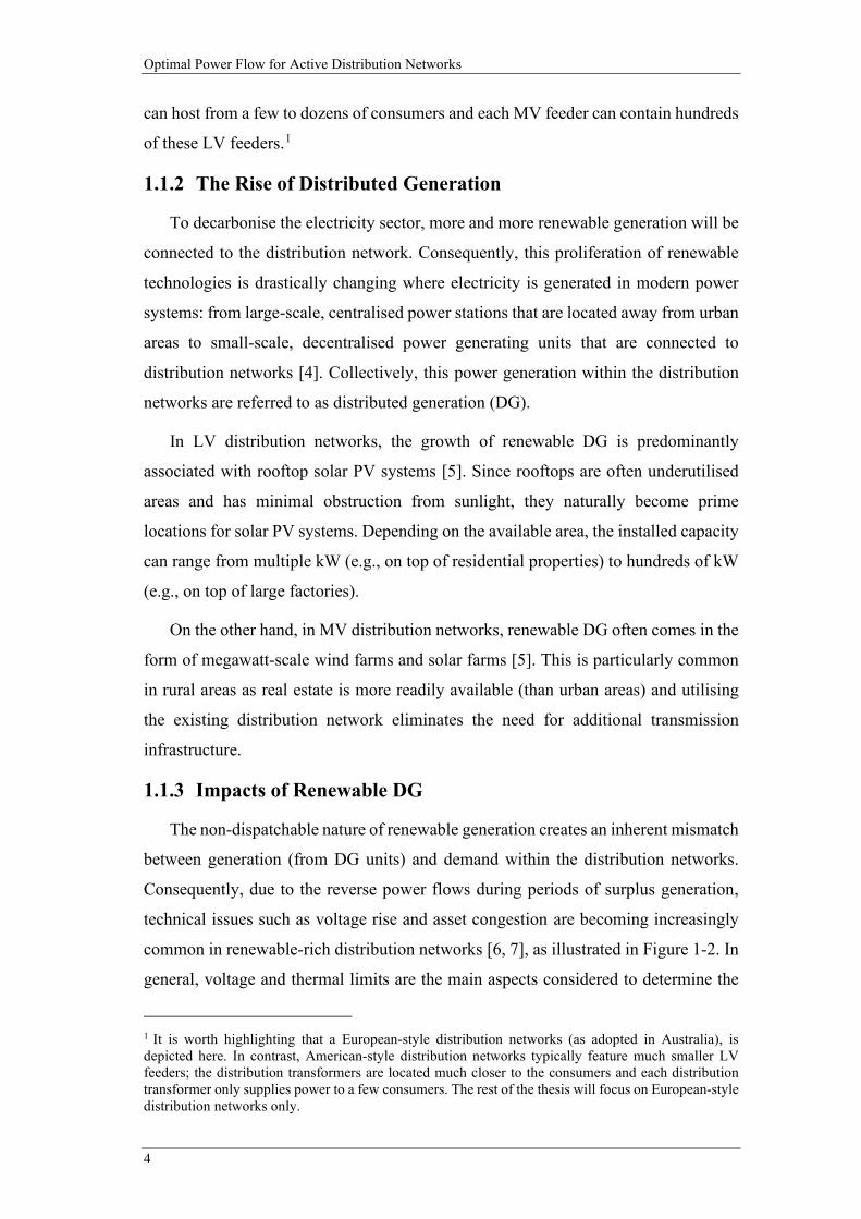
can host from a few to dozens of consumers and each MV feeder can contain hundreds
of these LV feeders.1
1.1.2 The Rise of Distributed Generation
To decarbonise the electricity sector, more and more renewable generation will be
connected to the distribution network. Consequently, this proliferation of renewable
technologies is drastically changing where electricity is generated in modern power
systems: from large-scale, centralised power stations that are located away from urban
areas to small-scale, decentralised power generating units that are connected to
distribution networks [4]. Collectively, this power generation within the distribution
networks are referred to as distributed generation (DG).
In LV distribution networks, the growth of renewable DG is predominantly
associated with rooftop solar PV systems [5]. Since rooftops are often underutilised
areas and has minimal obstruction from sunlight, they naturally become prime
locations for solar PV systems. Depending on the available area, the installed capacity
can range from multiple kW (e.g., on top of residential properties) to hundreds of kW
(e.g., on top of large factories).
On the other hand, in MV distribution networks, renewable DG often comes in the
form of megawatt-scale wind farms and solar farms [5]. This is particularly common
in rural areas as real estate is more readily available (than urban areas) and utilising
the existing distribution network eliminates the need for additional transmission
infrastructure.
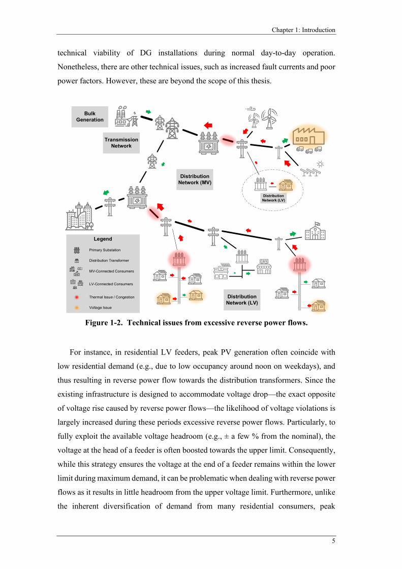
1.1.3 Impacts of Renewable DG
The non-dispatchable nature of renewable generation creates an inherent mismatch
between generation (from DG units) and demand within the distribution networks.
Consequently, due to the reverse power flows during periods of surplus generation,
technical issues such as voltage rise and asset congestion are becoming increasingly
common in renewable-rich distribution networks [6, 7], as illustrated in Figure 1-2. In
general, voltage and thermal limits are the main aspects considered to determine the
1 It is worth highlighting that a European-style distribution networks (as adopted in Australia), is depicted here. In contrast, American-style distribution networks typically feature much smaller LV feeders; the distribution transformers are located much closer to the consumers and each distribution transformer only supplies power to a few consumers. The rest of the thesis will focus on European-style distribution networks only.
Chapter 1: Introduction
5
technical viability of DG installations during normal day-to-day operation.
Nonetheless, there are other technical issues, such as increased fault currents and poor
power factors. However, these are beyond the scope of this thesis.
For instance, in residential LV feeders, peak PV generation often coincide with
low residential demand (e.g., due to low occupancy around noon on weekdays), and
thus resulting in reverse power flow towards the distribution transformers. Since the
existing infrastructure is designed to accommodate voltage drop—the exact opposite
of voltage rise caused by reverse power flows—the likelihood of voltage violations is
largely increased during these periods excessive reverse power flows. Particularly, to
fully exploit the available voltage headroom (e.g., ± a few % from the nominal), the
voltage at the head of a feeder is often boosted towards the upper limit. Consequently,
while this strategy ensures the voltage at the end of a feeder remains within the lower
limit during maximum demand, it can be problematic when dealing with reverse power
flows as it results in little headroom from the upper voltage limit. Furthermore, unlike
the inherent diversification of demand from many residential consumers, peak
Legend
Bulk Generation
Transmission Network
Distribution Network (MV)
Distribution Network (LV)
Distribution Network (LV)
Primary Substation
Distribution Transformer
MV-Connected Consumers
LV-Connected Consumers
Thermal Issue / Congestion
Voltage Issue
Figure 1-2. Technical issues from excessive reverse power flows.
Optimal Power Flow for Active Distribution Networks
6
generation from rooftop PV systems is largely correlated in any given region (e.g., a
residential suburb or across an area of a few squared kilometres). As a result, there is
an increased risk of asset congestion in not only the LV feeders, but also the upstream
MV feeder.
The underlying causes of technical issues in MV distribution networks largely
follow the same principles as in LV networks: a mismatch between peak generation
and peak demand. Furthermore, due to longer distances of rural MV feeders (which is
where most renewable generation is being connected to at the MV level), the
corresponding infrastructure is substantially weaker than their urban counterparts (e.g.,
more susceptible to voltage issues due to the higher impedances, and thus higher
magnitude of voltage rise for the same volume of reverse power flows). Consequently,
this significant amplifies the risk of technical issues from excessive reverse power
flows.
1.1.4 Towards Active Distribution Networks
The rapid uptake of DG in recent decades has changed the role of modern
distribution networks at a fundamental level; it is no longer just the last mile delivery
of power to consumers. As a result, the passive way of tackling voltage and thermal
issues at the planning stage through network augmentation may no longer be effective;
due to the bidirectional power flows in a modern distribution network, issues from two
extreme scenarios—maximum generation and minimum demand as well as maximum
demand and minimum generation—must be dealt with simultaneously. To this end,
the concept of active distribution networks, where network issues are solved at the
operational stage through the real-time monitoring and control of network assets and
participants, is becoming an increasingly attractive option. Particularly, by leveraging
the various sources of flexibility in real-time, network operators can fully exploit the
capability of existing infrastructure, and thus defer (or eliminate) the need of costly
network augmentation.
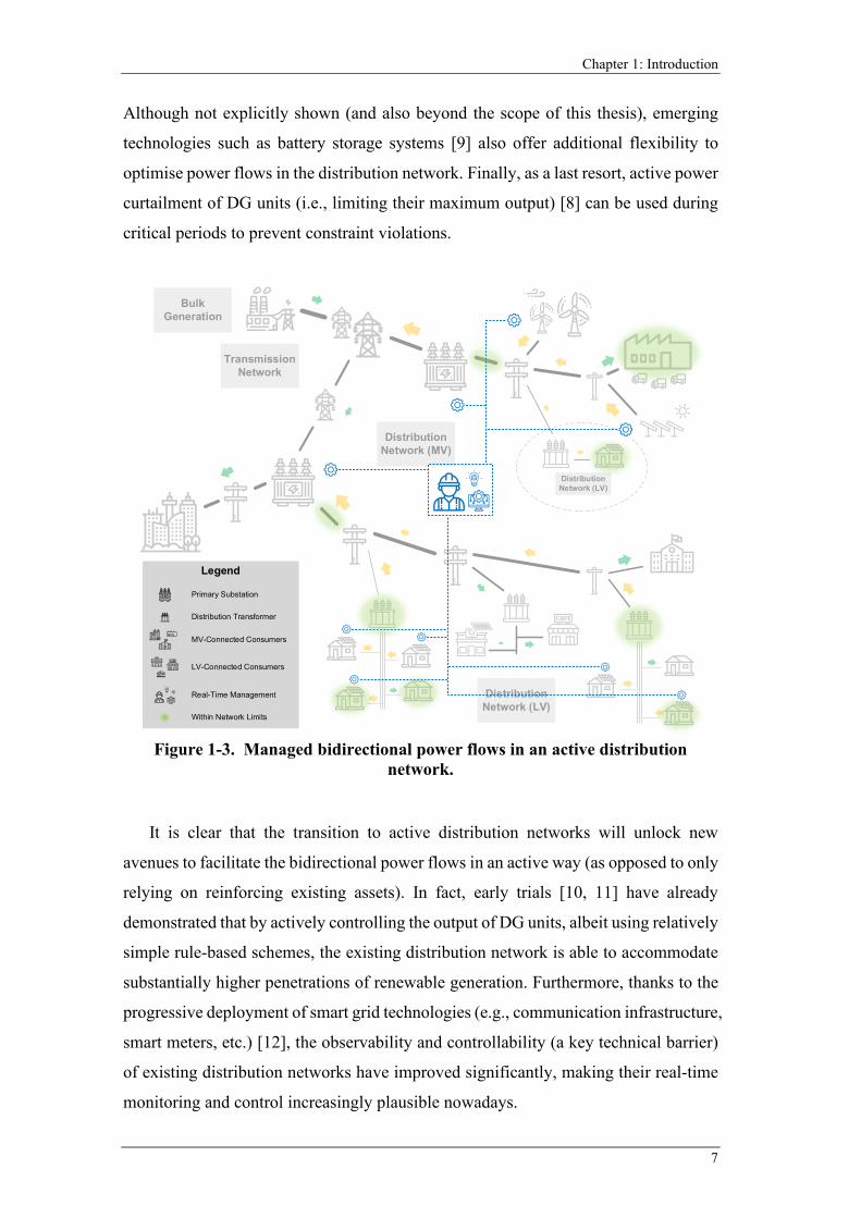
An example of an active distribution network is shown in Figure 1-3 where a
centralised control scheme in adopted to manage network assets and participants in
real-time, and thus mitigates potential technical issues from the bidirectional power
flows. As depicted here, the coordination of OLTC-fitted transformers and the reactive
power capability of inverter-based DG units can help to tackle voltage issues [8].
Chapter 1: Introduction
7
Although not explicitly shown (and also beyond the scope of this thesis), emerging
technologies such as battery storage systems [9] also offer additional flexibility to
optimise power flows in the distribution network. Finally, as a last resort, active power
curtailment of DG units (i.e., limiting their maximum output) [8] can be used during
critical periods to prevent constraint violations.
It is clear that the transition to active distribution networks will unlock new
avenues to facilitate the bidirectional power flows in an active way (as opposed to only
relying on reinforcing existing assets). In fact, early trials [10, 11] have already
demonstrated that by actively controlling the output of DG units, albeit using relatively
simple rule-based schemes, the existing distribution network is able to accommodate
substantially higher penetrations of renewable generation. Furthermore, thanks to the
progressive deployment of smart grid technologies (e.g., communication infrastructure,
smart meters, etc.) [12], the observability and controllability (a key technical barrier)
of existing distribution networks have improved significantly, making their real-time
monitoring and control increasingly plausible nowadays.
Bulk Generation
Transmission Network
Distribution Network (MV)
Distribution Network (LV)
Distribution Network (LV)
Legend
Primary Substation
Distribution Transformer
MV-Connected Consumers
LV-Connected Consumers
Real-Time Management
Within Network Limits
Figure 1-3. Managed bidirectional power flows in an active distribution
network.
Optimal Power Flow for Active Distribution Networks
8
1.1.5 Advanced Schemes for Active Distribution Networks
Given the size (e.g., large number of assets and participants across multiple voltage
levels) and complexity (e.g., phase unbalances, discrete devices) of distribution
networks, developing adequate control schemes using rule-based approaches (as
commonly adopted by industry) can be prohibitively cumbersome. Considering that
more and more sources of flexibility are becoming available, this is especially true as
many variables (e.g., the settings of controllable devices) and constraints (e.g., network
limits) must be considered simultaneously by the network operator. Therefore, to fully
utilise these various sources of flexibility, advanced approaches that can cater for these
challenges associated with realistic distribution networks is necessary.
To this end, AC Optimal Power Flow (OPF), a technique that combines
optimisation with an electrical model of the distribution network, has emerged as a
promising alternative for more advanced schemes [13]. Particularly, by formulating
the decision-making process as a mathematical optimisation problem, an OPF-based
approach enables a more systematic way of determining the most appropriate setpoints
for controllable devices in an active distribution network while also respecting the
corresponding constraints. Nonetheless, there are several technical challenges that
must be overcome before OPF-based schemes are readily adopted in the control rooms
of future distribution networks. These challenges are discussed in the following section.
1.2 Challenges
1.2.1 Scalability and Speed of OPF Formulations
The classical AC OPF formulation is non-convex [14] due to the non-linearity of
AC power flow equations. In general, this type of optimisation problems is known to
suffer scalability and speed issues (i.e., solvable fast enough to be practically relevant)
as a) there are generally no effective way of finding the global optimum [15] and b) a
local optimum can be very sub-optimal (i.e., substantially worse in performance
compared with the global optimum) [16]. Consequently, this becomes a major
challenge for the operational usage of OPF-based approaches due to the associated
constraints on solution time (i.e., within minutes).
Furthermore, this issue is exacerbated by the need of modelling discrete devices
found in typical distribution networks (e.g., OLTCs and capacitor banks) where integer
Chapter 1: Introduction
9
programming is required. Particularly, due to the combinatorial nature of solving a
mixed-integer program, it often requires an exhaustive search (i.e., going through all
possible combinations) to find the optimal solution [17]. Consequently, the non-
convex nature of classical OPF formulations is expected to make this an extremely
time-consuming process.
1.2.2 Real-World Implementation of OPF-Based Setpoints
Since there are different types of controllable devices in a distribution network,
such as legacy devices (e.g., OLTCs and capacitor banks) and inverter-interfaced
devices (e.g., modern wind farms and PV systems), their operating characteristics (e.g.,
delays, ramp rates and deadbands) can vary significantly. Consequently, this
introduces several practical challenges when OPF-based setpoints are to be
implemented in real-world applications. For instance, due to the design for
autonomous operation, there is usually a relatively long delay (e.g., around a minute)
[18] associated with conventional OLTC controllers. As a result, this introduces
coordination issues with inverter-interfaced devices that can typically respond to new
setpoints within seconds [19]. Therefore, since the execution of setpoints do not
happen instantaneously, this and similar sub-minute scale interactions among multiple
controllable devices (due to the differences in their operating characteristics) may lead
to undesirable behaviours not envisaged by the OPF-based scheme, such as temporary
constraint violations and unnecessary control actions.
1.2.3 Ensuring Fairness in Curtailment Schemes
Although the definition of fairness—ensuring equality or removing disparity—is
relatively simple to understand, assessing fairness in the context of distribution
networks is a more challenging task. Firstly, it requires defining an appropriate metric
to quantify the benefits for DG owners, which is not necessarily straightforward given
that there are many perspectives that can be used to quantify the impact due to active
power curtailment (e.g., PV harvesting and monetary benefits) [20]. Furthermore, it
also requires an adequate understanding (and assessment) of the trade-offs between
fairness (i.e., equally for everyone) and efficiency (i.e., aggregated performance) [21],
a topic that is rarely investigated in distribution network studies.
Optimal Power Flow for Active Distribution Networks
10
1.2.4 Realistic Demonstration of OPF-Based Schemes
Traditionally, distribution network studies are done offline using PC-based
software. While this is indispensable from a research and development perspective, it
often lacks the ability to from a demonstration perspective as it is difficult to fully
capture the physical interactions among the various components in an active
distribution network (e.g., network-connected devices, communication infrastructure,
SCADA system, advanced control schemes, etc.). Therefore, as more and more
advanced concepts are being developed for future distribution networks, it is also
increasingly important to demonstrate these concepts to industry through more
realistic means, such as using hardware-in-the-loop (HIL) techniques [22].
Nonetheless, developing such a HIL demonstration platform is not a trivial task, as it
involves specialised software and hardware from different domains that extend beyond
conventional tools used in typical power system studies.
1.3 Research Questions
The decarbonisation of the electricity sector will inevitably introduce a large
volume of renewable DG. Consequently, there is a need for more advanced schemes
to manage the bidirectional power flows in renewable-rich distribution networks.
Therefore, acknowledging the potential benefits of the OPF technique and the
associated challenges of its real-world application, this thesis aims to demonstrate the
technical feasibility of integrating OPF-based schemes in the control rooms of future
distribution networks. Particularly, this thesis aims to answer the following key
research questions:
• What modifications (or adaptations) are needed to conventional AC OPF
formulations so as to handle the size and complexity of realistic distribution
networks in an operational environment?
• What considerations are required to ensure OPF-based setpoints are adequately
implemented in practice (i.e., the real world)?
• What considerations are required to ensure adequate fairness is incorporated in
OPF-based curtailment schemes?
• How to demonstrate advanced schemes for future distribution networks to the
industry in a realistic and engaging way?
Chapter 1: Introduction
11
1.4 Objectives
To answer the aforementioned questions, the following four main objectives have
been identified (and briefly discussed in the remainder of this section):
• Developing a scalable and fast OPF formulation.
• Identifying the necessary adaptations in existing device controllers and OPF
formulation.
• Understanding different aspects of fairness and quantify the trade-offs from
different fairness objectives.
• Developing a realistic and engaging demonstration platform to showcase
advanced schemes to industry.
1.4.1 A Scalable and Fast OPF Formulation
A crucial step to enable the operational usage of OPF is to develop an adequate
formulation that can be implemented by industry. Particularly, the formulation needs
to cater for the size and complexity of a realistic distribution network, such as being
able to handle as several thousand nodes across multiple voltage levels and multiple
discrete devices. Furthermore, the solution time must be sufficiently small for
operational usage where control decisions are needed within minutes.
To achieve this, a linearisation approach is adopted to convexity the classical OPF
formulation, and thus significantly improves it scalability and speed when dealing with
large and complex distribution network models. Furthermore, thanks to the operational
usage of the proposed formulation, real-time measurements of the network can be
exploited as linearisation points of the proposed formulation, and thus used as warm-
start conditions to improve the accuracy of the linearised formulation.
1.4.2 Necessary Adaptations
Apart from being able to calculate setpoints using the OPF technique, how these
setpoints are being implemented by controllable devices is equally important.
Particularly, in addition for the calculated setpoints to the satisfying the power flow
constraints, adequate considerations related to the device control is necessary to ensure
the expected outcome is achieved in practice; particularly when multiple devices (with
vastly different operating characteristics) are being controlled at the same time.
Optimal Power Flow for Active Distribution Networks
12
To achieve this, a high granularity modelling is adopted to realistically capture the
interactions among controllable devices in real-time (i.e., at a sub-minute scale). Then,
through a better understanding of the complications arising from the real-time
operating characteristics of controllable devices, the necessary adaptations can be
determined.
1.4.3 Trade-Offs among Different Fairness Objectives
Active power curtailment is often necessary to mitigate technical issues during
critical periods. Therefore, a fair allocation of the required curtailment among many
DG owners could be of great importance as it directly affects the benefits these owners
receive from their investments.
To achieve this (in a residential context), household-centric metrics are adopted to
realistically quantify the impacts due to active power curtailment, each focusing on a
different (and potentially contrasting) perspective. Then, several OPF-based schemes,
each with a different fairness objective, are compared to understand the associated
trade-offs among different perspectives of fairness as well as between fairness and
efficiency.
1.4.4 Realistic Demonstration Platform
Before the real-world deployment of any advanced scheme, it is beneficial to
validate and demonstration its performance in a more realistic way that goes beyond
conventional offline analysis.
To achieve this, commercially available software and hardware packages are used
in a HIL setup to replicate the key components of an active distribution networks under
a laboratory environment.
1.5 Main Contributions
1.5.1 Advanced AC OPF for Operational Usage in Distribution
Networks
A linearised, three-phase AC OPF is proposed in this thesis for operational usage
in future distribution networks. The three-phase formulation caters for the inherent
unbalances in distribution networks and the linearisations (of the non-linear OPF
formulation) provide significant improvements in terms of the scalability and speed
Chapter 1: Introduction
13
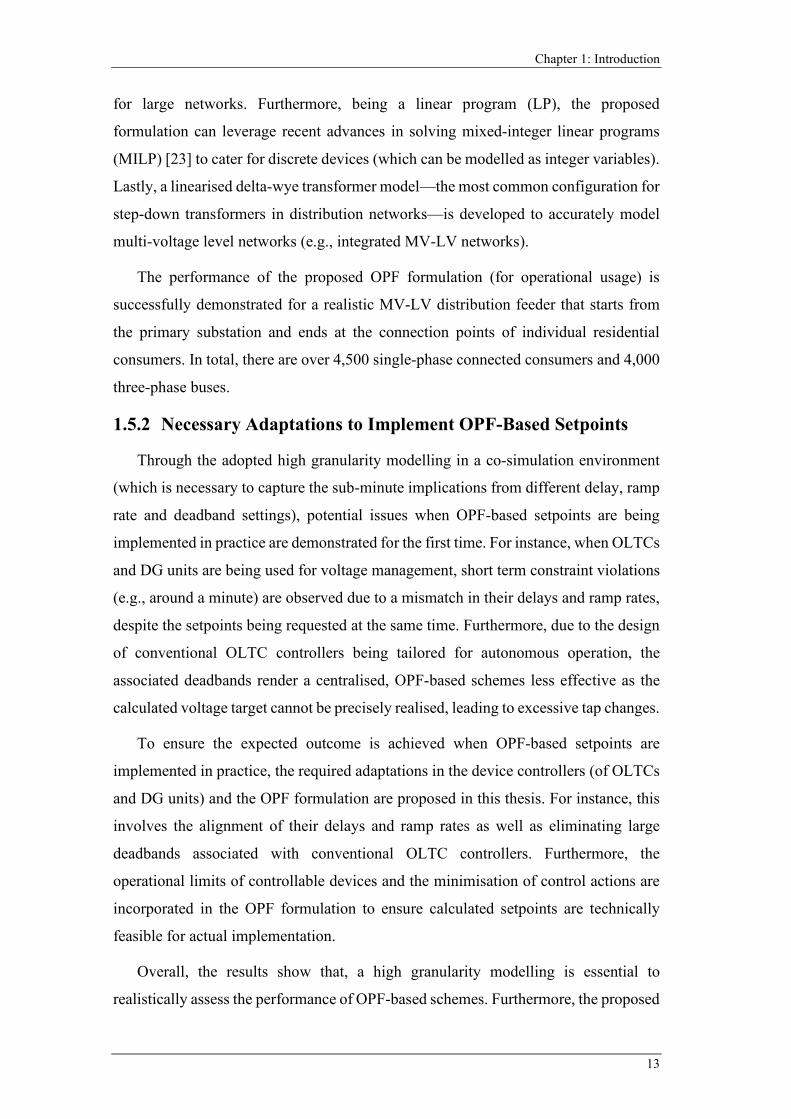
for large networks. Furthermore, being a linear program (LP), the proposed
formulation can leverage recent advances in solving mixed-integer linear programs
(MILP) [23] to cater for discrete devices (which can be modelled as integer variables).
Lastly, a linearised delta-wye transformer model—the most common configuration for
step-down transformers in distribution networks—is developed to accurately model
multi-voltage level networks (e.g., integrated MV-LV networks).
The performance of the proposed OPF formulation (for operational usage) is
successfully demonstrated for a realistic MV-LV distribution feeder that starts from
the primary substation and ends at the connection points of individual residential
consumers. In total, there are over 4,500 single-phase connected consumers and 4,000
three-phase buses.
1.5.2 Necessary Adaptations to Implement OPF-Based Setpoints
Through the adopted high granularity modelling in a co-simulation environment
(which is necessary to capture the sub-minute implications from different delay, ramp
rate and deadband settings), potential issues when OPF-based setpoints are being
implemented in practice are demonstrated for the first time. For instance, when OLTCs
and DG units are being used for voltage management, short term constraint violations
(e.g., around a minute) are observed due to a mismatch in their delays and ramp rates,
despite the setpoints being requested at the same time. Furthermore, due to the design
of conventional OLTC controllers being tailored for autonomous operation, the
associated deadbands render a centralised, OPF-based schemes less effective as the
calculated voltage target cannot be precisely realised, leading to excessive tap changes.
To ensure the expected outcome is achieved when OPF-based setpoints are
implemented in practice, the required adaptations in the device controllers (of OLTCs
and DG units) and the OPF formulation are proposed in this thesis. For instance, this
involves the alignment of their delays and ramp rates as well as eliminating large
deadbands associated with conventional OLTC controllers. Furthermore, the
operational limits of controllable devices and the minimisation of control actions are
incorporated in the OPF formulation to ensure calculated setpoints are technically
feasible for actual implementation.
Overall, the results show that, a high granularity modelling is essential to
realistically assess the performance of OPF-based schemes. Furthermore, the proposed
Optimal Power Flow for Active Distribution Networks
14
adaptations are extremely crucial to ensure adequate coordination when multiple
controllable devices are being centrally managed using OPF-based (or similar)
schemes. Conversely, inadequate considerations can result in undesirable outcomes,
such as network constraints violations and accelerated device wear-and-tear.
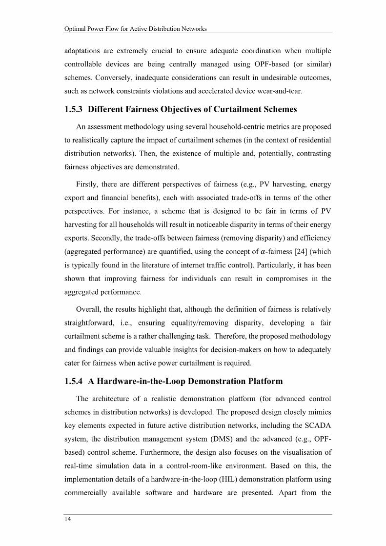
1.5.3 Different Fairness Objectives of Curtailment Schemes
An assessment methodology using several household-centric metrics are proposed
to realistically capture the impact of curtailment schemes (in the context of residential
distribution networks). Then, the existence of multiple and, potentially, contrasting
fairness objectives are demonstrated.
Firstly, there are different perspectives of fairness (e.g., PV harvesting, energy
export and financial benefits), each with associated trade-offs in terms of the other
perspectives. For instance, a scheme that is designed to be fair in terms of PV
harvesting for all households will result in noticeable disparity in terms of their energy
exports. Secondly, the trade-offs between fairness (removing disparity) and efficiency
(aggregated performance) are quantified, using the concept of 𝛼𝛼-fairness [24] (which
is typically found in the literature of internet traffic control). Particularly, it has been
shown that improving fairness for individuals can result in compromises in the
aggregated performance.
Overall, the results highlight that, although the definition of fairness is relatively
straightforward, i.e., ensuring equality/removing disparity, developing a fair
curtailment scheme is a rather challenging task. Therefore, the proposed methodology
and findings can provide valuable insights for decision-makers on how to adequately
cater for fairness when active power curtailment is required.
1.5.4 A Hardware-in-the-Loop Demonstration Platform
The architecture of a realistic demonstration platform (for advanced control
schemes in distribution networks) is developed. The proposed design closely mimics
key elements expected in future active distribution networks, including the SCADA
system, the distribution management system (DMS) and the advanced (e.g., OPF-
based) control scheme. Furthermore, the design also focuses on the visualisation of
real-time simulation data in a control-room-like environment. Based on this, the
implementation details of a hardware-in-the-loop (HIL) demonstration platform using
commercially available software and hardware are presented. Apart from the
Chapter 1: Introduction
15
validation aspect (which is typically associated with HIL simulations), the proposed
platform enables a more realistic and engaging experience when showcasing advanced
schemes to industry.
1.6 Publications
The following publications have been produced as part of the research carried out
for (or related) to this thesis.
1.6.1 Journal Papers
• M. Z. Liu, A. T. Procopiou, K. Petrou, L. F. Ochoa, T. Langstaff, J. Harding and J. Theunissen, “On the Fairness of PV Curtailment Schemes in Residential Distribution Networks”, IEEE Transactions on Smart Grids, vol. 11, no. 5, pp. 4502-4512, 2020.
DOI link: https://www.doi.org/10.1109/TSG.2020.2983771
• M. Z. Liu, L. F. Ochoa, S. H. Low, “On the Implementation of OPF-Based Set-Points for Active Distribution Networks”, IEEE Transactions on Smart Grids, in Review (R2).
1.6.2 Conference Papers
• M. Z. Liu and L. F. Ochoa, "Hardware-In-the-Loop Demonstration of Advanced Control Schemes for Active Distribution Networks," in Proc. 2019 IEEE PES Innovative Smart Grid Technologies Conference - Latin America (ISGT Latin America), pp. 1-6.
DOI link: https://www.doi.org/10.1109/ISGT-LA.2019.8895493
• L. Gutierrez-Lagos, M. Z. Liu, and L. F. Ochoa, "Implementable Three-Phase OPF Formulations for MV-LV Distribution Networks: MILP and MIQCP," in Proc. 2019 IEEE PES Innovative Smart Grid Technologies Conference - Latin America (ISGT Latin America), pp. 1-6.
DOI link: https://www.doi.org/10.1109/ISGT-LA.2019.8895008
1.6.3 Technical Reports
The following technical report was produced for the consultancy project “Smart
Grid Test and Evaluation” funded by QinetiQ Australia.
• M. Z. Liu, L. F. Ochoa, Deliverable 1 "Testing Facilities Report", prepared for QinetiQ Australia, 2018
Optimal Power Flow for Active Distribution Networks
16
1.6.4 Magazine Articles
• Dubey, A. Bose, M. Liu, and L. N. Ochoa, "Paving the Way for Advanced Distribution Management Systems Applications: Making the Most of Models and Data," IEEE Power and Energy Magazine, vol. 18, no. 1, pp. 63-75, 2020.
DOI link: https://www.doi.org/10.1109/MPE.2019.2949442
1.7 Thesis Outline
A summary for each of the remaining chapters is presented below.
Chapter 2 - A Fast and Scalable Three-Phase OPF for Distribution Networks
presents the linearised, three-phase AC OPF formulation that is used as the basis for
all subsequent chapters. The proposed formulation is based on the branch flow model
[25] and utilises squared voltages and power injections terms as state variables to
model the power flow equations. It is adapted from the single-phase formulation in
[26] and the process is documented in this chapter, including the extension to a three-
phase models, the introduction of a linearised model for delta-wye transformers (to
cater for the modelling of multi-voltage level distribution feeders) and the usage of
integer variables (to cater for the discrete devices in distribution networks).
Chapter 3 - Implementing OPF-Based Setpoints: Challenges and Solutions
investigates the necessary adaptations in device controllers and the OPF formulation
when OPF-based setpoints are to be implemented in practice. This chapter focuses on
the active management of OLTCs and DG units (e.g., wind farms) in rural distribution
network. Due to the diverse operating characteristics of different types of controllable
devices (e.g., OLTCs and inverter-interfaced DG units), an alignment process of their
delays and ramp rates as well as the modifications to remove large deadbands are
identified. Then, the benefits of the proposed changes are demonstrated using a rural,
UK-style distribution network considering the active management of wind farms and
OLTCs. Particularly, it has been shown that, inadequate considerations from a device
control perspective may lead to temporary voltage violations and excessive control
actions. On the other hand, the proposed adaptations allow OPF-based setpoints to be
successfully implemented (i.e., achieving the outcome as intended by the OPF) in an
operational environment.
Chapter 4 - Fairness of Active Power Curtailment Schemes: A Residential
Context investigates how to adequately cater for fairness when active power
Chapter 1: Introduction
17
curtailment is required in a residential context. This first requires defining several
household-centric metrics that are related to how performance/impact can be
quantified for residential prosumers (consumers with PV systems). To this end, three
metrics in the perspective of energy harvesting (of PV systems), energy export (of
households) and financial benefit (from the PV investment) are considered.
Furthermore, the concept of 𝛼𝛼 -fairness is adopted to model the relative priority
between fairness and efficiency. Based on these, several OPF-based schemes that
incorporate different fairness objectives are proposed. Finally, the implications from
different fairness objectives are demonstrated using a PV-rich MV-LV residential
feeder with over 4,500 households. The results highlight that, fairness can be achieved
from multiple perspectives, each with their associated trade-offs. Furthermore, the
marginal improvement in terms of fairness can result in substantial compromises in
terms of the aggregated performance.
Chapter 5 - A Hardware-in-the-Loop Demonstration Platform first introduces
the proposed architecture of a realistic demonstration platform for advanced schemes
in future distribution networks. Then, a specific implementation at the Smart Grid Lab
of The University of Melbourne using a real-time simulator as well as commercially
available software and hardware packages is presented. Lastly, this platform is used to
create a live demonstration of the advanced control scheme (to actively manage a
renewable-rich distribution network) presented in Chapter 3.
Chapter 6 - Conclusion summarises the key findings of this thesis and highlights
the potential future works.

Optimal Power Flow for Active Distribution Networks
18
This page is intentionally left blank.
2 A FAST AND SCALABLE THREE-PHASE OPF
FOR DISTRIBUTION NETWORKS
2.1 Introduction
Optimal power flow (OPF) is a mathematical optimisation problem that seeks to
find the set of optimal control actions (e.g., output of generators) according to a given
objective (e.g., minimise costs) while satisfying the corresponding constraints (e.g.,
the physics of power flows, operational limits, etc.). Since its first introduction by
Carpentier in 1962 [27], OPF has played a significant role as an operation tool for
modern transmission networks.
The classical formulation of an AC OPF can be very be difficult to solve due to
the non-convex (and non-linear) nature of AC power flow equations—the most
accurate form to capture the underlying physics. Therefore, its operational usage in
transmission networks is largely based on a simplified version of a full AC OPF, i.e.,
a DC OPF [28, 29], which only captures the active power and excludes the losses.
Furthermore, a single-phase DC OPF is usually sufficient due to the balanced nature
of power flows at the transmission level. One such example is in Australia, where an
DC OPF-based engine is used by the Australian Energy Market Operator (AEMO) to
dispatch scheduled generators in real-time, once every five minutes [28]. Similar
examples can also be found around the world, such as the US [30, 31] and across
Europe [32].
In recent decades, driven by the rapid growth of distributed generation (DG), as
well as the emergence of other distributed energy resources, there has been a
significant interest in the application of OPF in distribution networks. Particularly, by
combining mathematical optimisation with the electrical model of a distribution
network, an OPF can become a powerful decision-making engine to manage (i.e.,
determine the most appropriate setpoints) the various sources of flexibility in an active
distribution network (e.g., OLTCs, output of DG units, etc.).
However, due to the size and complexity of distribution networks, the operational
usage of OPF is significantly more challenging than transmission networks. Firstly,
the number of elements (e.g., buses, lines, etc.) in a distribution network can be several

Optimal Power Flow for Active Distribution Networks
20
orders of magnitude larger than a transmission network. Furthermore, due to the higher
resistance/reactive (i.e., R/X) ratio in distribution networks, both the active and
reactive power must be modelled, and thus requiring the full AC OPF formulation.
This is exacerbated by the inherent topological and load unbalances in distribution
networks, resulting in the need of modelling all three phases and their mutual effects
on each other. Lastly, to accurately represent discrete devices1 in distribution networks
(e.g., OLTCs and capacitor banks), integer variables are needed, and thus introducing
extra difficulty in solving the AC OPF problem within limited time frames.
Given the various challenges discussed above, a crucial step to enable the
operational usage of OPF is to develop a scalable (i.e., tractable) and fast (i.e.,
sufficiently fast solution time) formulation that can cater for the size and complexity
of distribution networks. To this end, a linearised, three-phase OPF is proposed and
analysed in this chapter.
2.2 Literature Review
This section first presents an overview of the different categories of mathematical
optimisation problems. This is followed by a summary of the variations of power flow
equations used in existing OPF formulations. Lastly, existing work on three-phase
OPF and the research gaps are presented.
2.2.1 Categories of Mathematical Optimisation Problems
All mathematical optimisation problems can be expressed in the generic form
shown in (2.1). It contains an objective function 𝑓𝑓0(𝑥𝑥) , the set of variables 𝑥𝑥 =
{𝑥𝑥1, … , 𝑥𝑥𝑛𝑛} and the set of constraints {𝑓𝑓1, … ,𝑓𝑓𝑚𝑚}.
minimise 𝑓𝑓0(𝑥𝑥) subject to 𝑓𝑓𝐶𝐶(𝑥𝑥) ≤ 0, 𝑖𝑖 = 1,2, … ,𝑚𝑚 (2.1)
Depending on the types of functions used (e.g., linear, quadratic, cubic,
trigonometric, logarithmic, etc.), the relative difficulty2 of optimisation problems can
1 The setpoints for these devices only take discrete values, e.g., {1, 2, 3}, as opposed to any value within a range, e.g., [0, 3]. Hence, they are referred to as discrete devices. 2 In this thesis, the term ‘difficulty’ refers to whether the solution time of an OPF problem is adequate for operational usage (e.g., when decisions are needed within minutes).
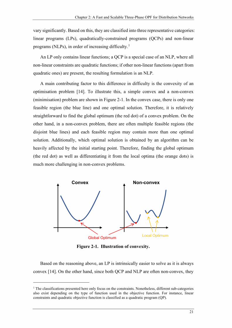
Chapter 2: A Fast and Scalable Three-Phase OPF for Distribution Networks
21
vary significantly. Based on this, they are classified into three representative categories:
linear programs (LPs), quadratically-constrained programs (QCPs) and non-linear
programs (NLPs), in order of increasing difficulty.1
An LP only contains linear functions; a QCP is a special case of an NLP, where all
non-linear constraints are quadratic functions; if other non-linear functions (apart from
quadratic ones) are present, the resulting formulation is an NLP.
A main contributing factor to this difference in difficulty is the convexity of an
optimisation problem [14]. To illustrate this, a simple convex and a non-convex
(minimisation) problem are shown in Figure 2-1. In the convex case, there is only one
feasible region (the blue line) and one optimal solution. Therefore, it is relatively
straightforward to find the global optimum (the red dot) of a convex problem. On the
other hand, in a non-convex problem, there are often multiple feasible regions (the
disjoint blue lines) and each feasible region may contain more than one optimal
solution. Additionally, which optimal solution is obtained by an algorithm can be
heavily affected by the initial starting point. Therefore, finding the global optimum
(the red dot) as well as differentiating it from the local optima (the orange dots) is
much more challenging in non-convex problems.
Based on the reasoning above, an LP is intrinsically easier to solve as it is always
convex [14]. On the other hand, since both QCP and NLP are often non-convex, they
1 The classifications presented here only focus on the constraints. Nonetheless, different sub-categories also exist depending on the type of function used in the objective function. For instance, linear constraints and quadratic objective function is classified as a quadratic program (QP).
Figure 2-1. Illustration of convexity.
Convex Non-convex
Global Optimum Local Optimum
Optimal Power Flow for Active Distribution Networks
22
are generally considered as harder problems than an LP due to various numerical
difficulties of finding an optimal solution (global or local) [33]. While quadratic
constraints are technically non-linear, the special category of QCP exists due to the
various established techniques of convexifying a QCP, such as through semi-definite
program (SDP) relaxation and second-order cone program (SOCP) relaxation [14]. In
contrast, there are generally no effective methods for solving NLP, and thus NLPs are
often regarded as the most difficult category of optimisation problems.
It is also worth noting that, the above discussions only represent a general rule of
thumb for comparable problems. For instance, an LP with over thousands of
constraints is likely to be more difficult than an NLP with only one constraint.
Lastly, LPs also have an added benefit when dealing with integer variables (e.g.,
when modelling discrete devices). Thanks to the simplex algorithm—an algorithm that
is only applicable to LPs—the non-integral solutions found at the parent node during
the branching stage of solving a mixed-integer linear program (MILP) can be utilised
as warm start values (also known as providing an advanced basis) in the subsequent
child nodes [34], resulting in significant speed boosts. Furthermore, combined with the
recent advances in solving MILP by commercial solvers [23], this makes linearised
formulations of OPF even more preferable when dealing with discrete variables.
2.2.2 Variations of AC Power Flow Equations
A core component of any AC OPF formulation (henceforth referred to as OPF) is
the power flow equations that model the underlying physics. In general, there are four
main variations used by existing OPF literature, ranging from non-linear functions to
quadratic functions. Consequently, the difficulty of the corresponding OPF
formulation can vary as discussed earlier in Section 2.2.1 (i.e., LP → QCP → NLP, in
increasing order of difficulty). These four variations are introduced in this sub-section.
For simplicity, a single-phase line is used here to illustrate the key differences among
these variations.
For a line 𝑙𝑙 as shown in Figure 2-2, the purpose of power flow equations is to model
the relationships between the complex voltage phasors (e.g., 𝑉𝑉�⃗ 𝐶𝐶𝑥𝑥 and 𝑉𝑉�⃗ 𝐶𝐶𝑦𝑦 ) and the
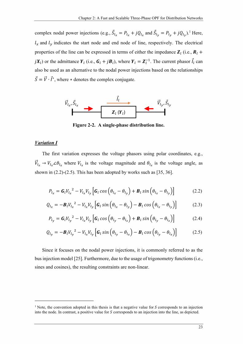
Chapter 2: A Fast and Scalable Three-Phase OPF for Distribution Networks
23
complex nodal power injections (e.g., 𝑆𝑆𝐶𝐶𝑥𝑥 = 𝑃𝑃𝐶𝐶𝑥𝑥 + 𝑗𝑗𝑄𝑄𝐶𝐶𝑥𝑥 and 𝑆𝑆𝐶𝐶𝑦𝑦 = 𝑃𝑃𝐶𝐶𝑦𝑦 + 𝑗𝑗𝑄𝑄𝐶𝐶𝑦𝑦).1 Here,
𝑙𝑙𝑥𝑥 and 𝑙𝑙𝑦𝑦 indicates the start node and end node of line, respectively. The electrical
properties of the line can be expressed in terms of either the impedance 𝒁𝒁𝐶𝐶 (i.e., 𝑹𝑹𝐶𝐶 +
𝑗𝑗𝑿𝑿𝐶𝐶) or the admittance 𝒀𝒀𝐶𝐶 (i.e., 𝑮𝑮𝐶𝐶 + 𝑗𝑗𝑩𝑩𝐶𝐶), where 𝒀𝒀𝐶𝐶 = 𝒁𝒁𝐶𝐶−1. The current phasor 𝐼𝐼𝐶𝐶 can
also be used as an alternative to the nodal power injections based on the relationships
𝑆𝑆 = 𝑉𝑉�⃗ ∙ 𝐼𝐼∗, where ∗ denotes the complex conjugate.
Variation I
The first variation expresses the voltage phasors using polar coordinates, e.g.,
𝑉𝑉�⃗ 𝐶𝐶𝑥𝑥 → 𝑉𝑉𝐶𝐶𝑥𝑥∠𝜃𝜃𝐶𝐶𝑥𝑥 where 𝑉𝑉𝐶𝐶𝑥𝑥 is the voltage magnitude and 𝜃𝜃𝐶𝐶𝑥𝑥 is the voltage angle, as
shown in (2.2)-(2.5). This has been adopted by works such as [35, 36].
𝑃𝑃𝐶𝐶𝑥𝑥 = 𝑮𝑮𝐶𝐶𝑉𝑉𝐶𝐶𝑥𝑥2 − 𝑉𝑉𝐶𝐶𝑥𝑥𝑉𝑉𝐶𝐶𝑦𝑦 �𝑮𝑮𝐶𝐶 𝑐𝑐𝑐𝑐𝑐𝑐 �𝜃𝜃𝐶𝐶𝑥𝑥 − 𝜃𝜃𝐶𝐶𝑦𝑦� + 𝑩𝑩𝐶𝐶 𝑐𝑐𝑖𝑖𝑠𝑠 �𝜃𝜃𝐶𝐶𝑥𝑥 − 𝜃𝜃𝐶𝐶𝑦𝑦�� (2.2)
𝑄𝑄𝐶𝐶𝑥𝑥 = −𝑩𝑩𝐶𝐶𝑉𝑉𝐶𝐶𝑥𝑥2 − 𝑉𝑉𝐶𝐶𝑥𝑥𝑉𝑉𝐶𝐶𝑦𝑦 �𝑮𝑮𝐶𝐶 𝑐𝑐𝑖𝑖𝑠𝑠 �𝜃𝜃𝐶𝐶𝑥𝑥 − 𝜃𝜃𝐶𝐶𝑦𝑦� − 𝑩𝑩𝐶𝐶 𝑐𝑐𝑐𝑐𝑐𝑐 �𝜃𝜃𝐶𝐶𝑥𝑥 − 𝜃𝜃𝐶𝐶𝑦𝑦�� (2.3)
𝑃𝑃𝐶𝐶𝑦𝑦 = 𝑮𝑮𝐶𝐶𝑉𝑉𝐶𝐶𝑦𝑦2 − 𝑉𝑉𝐶𝐶𝑥𝑥𝑉𝑉𝐶𝐶𝑦𝑦 �𝑮𝑮𝐶𝐶 𝑐𝑐𝑐𝑐𝑐𝑐 �𝜃𝜃𝐶𝐶𝑦𝑦 − 𝜃𝜃𝐶𝐶𝑥𝑥� + 𝑩𝑩𝐶𝐶 𝑐𝑐𝑖𝑖𝑠𝑠 �𝜃𝜃𝐶𝐶𝑦𝑦 − 𝜃𝜃𝐶𝐶𝑥𝑥�� (2.4)
𝑄𝑄𝐶𝐶𝑦𝑦 = −𝑩𝑩𝐶𝐶𝑉𝑉𝐶𝐶𝑦𝑦2 − 𝑉𝑉𝐶𝐶𝑥𝑥𝑉𝑉𝐶𝐶𝑦𝑦 �𝑮𝑮𝐶𝐶 𝑐𝑐𝑖𝑖𝑠𝑠 �𝜃𝜃𝐶𝐶𝑦𝑦 − 𝜃𝜃𝐶𝐶𝑥𝑥� − 𝑩𝑩𝐶𝐶 𝑐𝑐𝑐𝑐𝑐𝑐 �𝜃𝜃𝐶𝐶𝑦𝑦 − 𝜃𝜃𝐶𝐶𝑥𝑥�� (2.5)
Since it focuses on the nodal power injections, it is commonly referred to as the
bus injection model [25]. Furthermore, due to the usage of trigonometry functions (i.e.,
sines and cosines), the resulting constraints are non-linear.
1 Note, the convention adopted in this thesis is that a negative value for 𝑆𝑆 corresponds to an injection into the node. In contrast, a positive value for 𝑆𝑆 corresponds to an injection into the line, as depicted.
Figure 2-2. A single-phase distribution line.
𝑉𝑉𝐶𝐶𝑥𝑥 , 𝑆𝑆𝐶𝐶𝑥𝑥 𝑉𝑉𝐶𝐶𝑦𝑦 , 𝑆𝑆𝐶𝐶𝑦𝑦𝒁𝒁𝐶𝐶 (𝒀𝒀𝐶𝐶)
𝐼𝐼𝐶𝐶
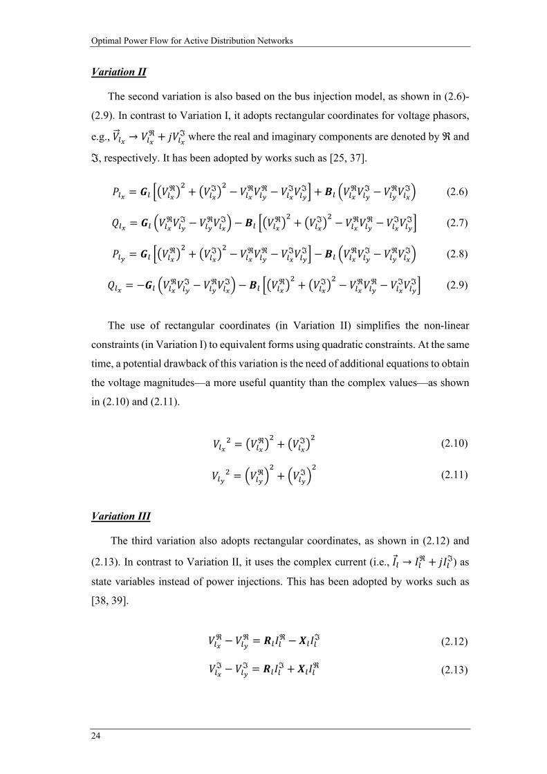
Optimal Power Flow for Active Distribution Networks
24
Variation II
The second variation is also based on the bus injection model, as shown in (2.6)-
(2.9). In contrast to Variation I, it adopts rectangular coordinates for voltage phasors,
e.g., 𝑉𝑉�⃗ 𝐶𝐶𝑥𝑥 → 𝑉𝑉𝐶𝐶𝑥𝑥ℜ + 𝑗𝑗𝑉𝑉𝐶𝐶𝑥𝑥
ℑ where the real and imaginary components are denoted by ℜ and
ℑ, respectively. It has been adopted by works such as [25, 37].
𝑃𝑃𝐶𝐶𝑥𝑥 = 𝑮𝑮𝐶𝐶 ��𝑉𝑉𝐶𝐶𝑥𝑥ℜ�
2+ �𝑉𝑉𝐶𝐶𝑥𝑥
ℑ�2− 𝑉𝑉𝐶𝐶𝑥𝑥
ℜ𝑉𝑉𝐶𝐶𝑦𝑦ℜ − 𝑉𝑉𝐶𝐶𝑥𝑥
ℑ𝑉𝑉𝐶𝐶𝑦𝑦ℑ� + 𝑩𝑩𝐶𝐶 �𝑉𝑉𝐶𝐶𝑥𝑥
ℜ𝑉𝑉𝐶𝐶𝑦𝑦ℑ − 𝑉𝑉𝐶𝐶𝑦𝑦
ℜ𝑉𝑉𝐶𝐶𝑥𝑥ℑ� (2.6)
𝑄𝑄𝐶𝐶𝑥𝑥 = 𝑮𝑮𝐶𝐶 �𝑉𝑉𝐶𝐶𝑥𝑥ℜ𝑉𝑉𝐶𝐶𝑦𝑦
ℑ − 𝑉𝑉𝐶𝐶𝑦𝑦ℜ𝑉𝑉𝐶𝐶𝑥𝑥
ℑ� − 𝑩𝑩𝐶𝐶 ��𝑉𝑉𝐶𝐶𝑥𝑥ℜ�
2+ �𝑉𝑉𝐶𝐶𝑥𝑥
ℑ�2− 𝑉𝑉𝐶𝐶𝑥𝑥
ℜ𝑉𝑉𝐶𝐶𝑦𝑦ℜ − 𝑉𝑉𝐶𝐶𝑥𝑥
ℑ𝑉𝑉𝐶𝐶𝑦𝑦ℑ� (2.7)
𝑃𝑃𝐶𝐶𝑦𝑦 = 𝑮𝑮𝐶𝐶 ��𝑉𝑉𝐶𝐶𝑥𝑥ℜ�
2+ �𝑉𝑉𝐶𝐶𝑥𝑥
ℑ�2− 𝑉𝑉𝐶𝐶𝑥𝑥
ℜ𝑉𝑉𝐶𝐶𝑦𝑦ℜ − 𝑉𝑉𝐶𝐶𝑥𝑥
ℑ𝑉𝑉𝐶𝐶𝑦𝑦ℑ� − 𝑩𝑩𝐶𝐶 �𝑉𝑉𝐶𝐶𝑥𝑥
ℜ𝑉𝑉𝐶𝐶𝑦𝑦ℑ − 𝑉𝑉𝐶𝐶𝑦𝑦
ℜ𝑉𝑉𝐶𝐶𝑥𝑥ℑ� (2.8)
𝑄𝑄𝐶𝐶𝑥𝑥 = −𝑮𝑮𝐶𝐶 �𝑉𝑉𝐶𝐶𝑥𝑥ℜ𝑉𝑉𝐶𝐶𝑦𝑦
ℑ − 𝑉𝑉𝐶𝐶𝑦𝑦ℜ𝑉𝑉𝐶𝐶𝑥𝑥
ℑ� − 𝑩𝑩𝐶𝐶 ��𝑉𝑉𝐶𝐶𝑥𝑥ℜ�
2+ �𝑉𝑉𝐶𝐶𝑥𝑥
ℑ�2− 𝑉𝑉𝐶𝐶𝑥𝑥
ℜ𝑉𝑉𝐶𝐶𝑦𝑦ℜ − 𝑉𝑉𝐶𝐶𝑥𝑥
ℑ𝑉𝑉𝐶𝐶𝑦𝑦ℑ� (2.9)
The use of rectangular coordinates (in Variation II) simplifies the non-linear
constraints (in Variation I) to equivalent forms using quadratic constraints. At the same
time, a potential drawback of this variation is the need of additional equations to obtain
the voltage magnitudes—a more useful quantity than the complex values—as shown
in (2.10) and (2.11).
𝑉𝑉𝐶𝐶𝑥𝑥2 = �𝑉𝑉𝐶𝐶𝑥𝑥
ℜ�2
+ �𝑉𝑉𝐶𝐶𝑥𝑥ℑ�
2 (2.10)
𝑉𝑉𝐶𝐶𝑦𝑦2 = �𝑉𝑉𝐶𝐶𝑦𝑦
ℜ�2
+ �𝑉𝑉𝐶𝐶𝑦𝑦ℑ�
2 (2.11)
Variation III
The third variation also adopts rectangular coordinates, as shown in (2.12) and
(2.13). In contrast to Variation II, it uses the complex current (i.e., 𝐼𝐼𝐶𝐶 → 𝐼𝐼𝐶𝐶ℜ + 𝑗𝑗𝐼𝐼𝐶𝐶ℑ) as
state variables instead of power injections. This has been adopted by works such as
[38, 39].
𝑉𝑉𝐶𝐶𝑥𝑥ℜ − 𝑉𝑉𝐶𝐶𝑦𝑦
ℜ = 𝑹𝑹𝐶𝐶𝐼𝐼𝐶𝐶ℜ − 𝑿𝑿𝐶𝐶𝐼𝐼𝐶𝐶ℑ (2.12)
𝑉𝑉𝐶𝐶𝑥𝑥ℑ − 𝑉𝑉𝐶𝐶𝑦𝑦
ℑ = 𝑹𝑹𝐶𝐶𝐼𝐼𝐶𝐶ℑ + 𝑿𝑿𝐶𝐶𝐼𝐼𝐶𝐶ℜ (2.13)
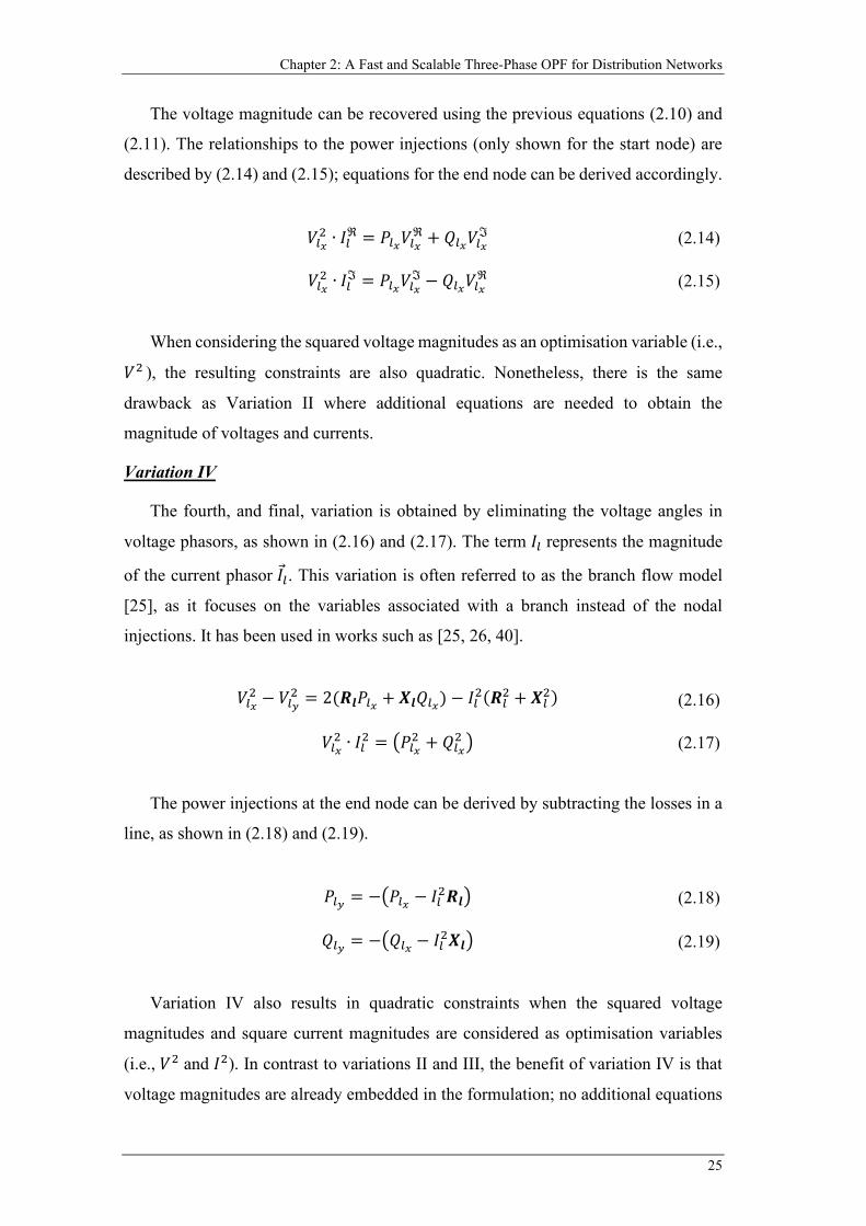
Chapter 2: A Fast and Scalable Three-Phase OPF for Distribution Networks
25
The voltage magnitude can be recovered using the previous equations (2.10) and
(2.11). The relationships to the power injections (only shown for the start node) are
described by (2.14) and (2.15); equations for the end node can be derived accordingly.
𝑉𝑉𝐶𝐶𝑥𝑥2 ∙ 𝐼𝐼𝐶𝐶ℜ = 𝑃𝑃𝐶𝐶𝑥𝑥𝑉𝑉𝐶𝐶𝑥𝑥
ℜ + 𝑄𝑄𝐶𝐶𝑥𝑥𝑉𝑉𝐶𝐶𝑥𝑥ℑ (2.14)
𝑉𝑉𝐶𝐶𝑥𝑥2 ∙ 𝐼𝐼𝐶𝐶ℑ = 𝑃𝑃𝐶𝐶𝑥𝑥𝑉𝑉𝐶𝐶𝑥𝑥
ℑ − 𝑄𝑄𝐶𝐶𝑥𝑥𝑉𝑉𝐶𝐶𝑥𝑥ℜ (2.15)
When considering the squared voltage magnitudes as an optimisation variable (i.e.,
𝑉𝑉2 ), the resulting constraints are also quadratic. Nonetheless, there is the same
drawback as Variation II where additional equations are needed to obtain the
magnitude of voltages and currents.
Variation IV
The fourth, and final, variation is obtained by eliminating the voltage angles in
voltage phasors, as shown in (2.16) and (2.17). The term 𝐼𝐼𝐶𝐶 represents the magnitude
of the current phasor 𝐼𝐼𝐶𝐶. This variation is often referred to as the branch flow model
[25], as it focuses on the variables associated with a branch instead of the nodal
injections. It has been used in works such as [25, 26, 40].
𝑉𝑉𝐶𝐶𝑥𝑥2 − 𝑉𝑉𝐶𝐶𝑦𝑦
2 = 2(𝑹𝑹𝒍𝒍𝑃𝑃𝐶𝐶𝑥𝑥 + 𝑿𝑿𝒍𝒍𝑄𝑄𝐶𝐶𝑥𝑥) − 𝐼𝐼𝐶𝐶2(𝑹𝑹𝐶𝐶2 + 𝑿𝑿𝐶𝐶2) (2.16)
𝑉𝑉𝐶𝐶𝑥𝑥2 ∙ 𝐼𝐼𝐶𝐶2 = �𝑃𝑃𝐶𝐶𝑥𝑥
2 + 𝑄𝑄𝐶𝐶𝑥𝑥2 � (2.17)
The power injections at the end node can be derived by subtracting the losses in a
line, as shown in (2.18) and (2.19).
𝑃𝑃𝐶𝐶𝑦𝑦 = −�𝑃𝑃𝐶𝐶𝑥𝑥 − 𝐼𝐼𝐶𝐶2𝑹𝑹𝒍𝒍� (2.18)
𝑄𝑄𝐶𝐶𝑦𝑦 = −�𝑄𝑄𝐶𝐶𝑥𝑥 − 𝐼𝐼𝐶𝐶2𝑿𝑿𝒍𝒍� (2.19)
Variation IV also results in quadratic constraints when the squared voltage
magnitudes and square current magnitudes are considered as optimisation variables
(i.e., 𝑉𝑉2 and 𝐼𝐼2). In contrast to variations II and III, the benefit of variation IV is that
voltage magnitudes are already embedded in the formulation; no additional equations
Optimal Power Flow for Active Distribution Networks
26
are needed. However, since information on voltage angles is eliminated from the
formulation, a potential drawback is that it cannot cater for meshed sections.
Nonetheless, this is unlikely to be a significant issue since distribution feeders are
mostly operated radially.
2.2.3 Three-Phase OPF Formulations
Many early works on OPF formulations have focused on single-phase models (e.g.,
[25, 26, 35-40]). However, since distribution networks are inherently unbalanced, the
applicability of these single-phase formulations is very limited as the interactions
among phases due to any topological and load unbalances cannot be captured.
Particularly, this involves not only modelling each phase individually but also
considering the mutual impedances among phases. Therefore, the rest of this chapter
will focus on three-phase OPF formulations only.
In the context of distribution networks, the main challenges of using OPF in an
operational environment is its scalability (tractability) and speed. For instance, when
dealing with a model that contains thousands of nodes—a rather common size for
realistic distribution feeders—a non-linear formulation is unlikely to be solved in a
short amount of time (e.g., within minutes), if it is even technically feasible. Therefore,
several approaches have been proposed in the existing literature to address these
challenges.
The first approach is developing advanced algorithms to solve the non-convex OPF
formulation. For instance, a convex iteration algorithm is proposed in [41], where the
non-convex OPF problem is approximated as a sequence of convex problems; the
solution to the non-convex problem can be recovered once the iterative algorithm
converges. The use of advanced primal-dual interior point methods, a well-known
iterative algorithm that guides the search for an optimal solution within a feasible
region, have been investigated by [42-44]. Sequential quadratic programming with
multiple starting point is investigated in [45] where the non-linear problem is solved
iteratively by creating and solving a quadratic subproblem in each iteration. However,
there is a common drawback associated with these algorithms: it is often difficult to
guarantee their convergence. Furthermore, this is expected to worsen as the size and
complexity of the OPF problem grows. Lastly, how to cater for discrete devices (e.g.,
OLTCs) is largely un-investigated by these and similar works.
Chapter 2: A Fast and Scalable Three-Phase OPF for Distribution Networks
27
The second approach is through relaxation techniques, after which, convex OPF
formulations are obtained. For instance, the use of SDP relaxation and SOCP
relaxation for the non-convex quadratic constraints have been proposed in [46, 47] and
[48], respectively. However, since the feasible region is extended by the relaxation
process, exactness (i.e., when the optimal solution of a relaxed problem is also the
optimal solution to the original non-relaxed problem) is only guaranteed under special
conditions, and thus significantly limiting its applicability in more general applications.
Particularly, existing derivations on exactness conditions are largely based on an
objective function that aims to minimise the total network losses (or generation cost).
Therefore, from the perspective of maximising renewable energy harvesting, a highly
relevant objective function in the context of renewable-rich distribution networks [8,
36], the sufficient conditions are largely invalidated. This is due to the fact that, the
process of maximising renewable energy harvesting will inherently increase the
network losses (which is the exact opposite as considered in aforementioned works)
due to higher volumes of reverse power flows.
The third, and final, approach involves approximations to simplify the non-convex
constraints in an OPF formulation, typically to achieve a fully linear formulation. To
this end, linear approximations of the non-linear power flow equations have been
proposed in [49, 50] (for Variation I), [51, 52] (for Variation III) and [53, 54] (for
Variation IV). The linearisation point is typically based on the last known state of the
network (e.g., recent SCADA measurements). In an operational environment, this is
expected to be sufficiently accurate as the state of the network will not change
dramatically from consecutive OPF runs. Nonetheless, existing literature on three-
phase OPF has largely focused on linearised models for distribution lines; modelling
of OLTC-fitted delta-wye transformers—the most common type in distribution
networks—has not been adequately investigated (apart from [49] where the delta-wye
transformers are considered without modelling the OLTC).
For completeness, the classification of the aforementioned literature based on the
four variations presented in Section 2.2.2 is summarised in Table 2-1.
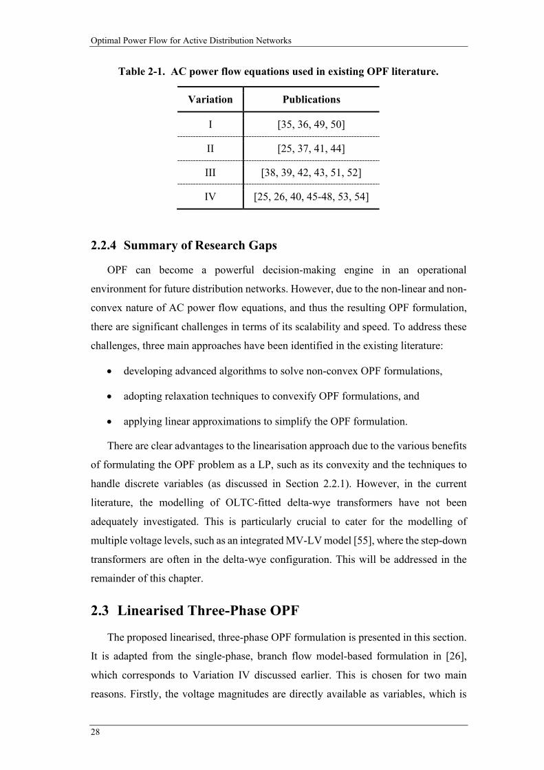
Optimal Power Flow for Active Distribution Networks
28
2.2.4 Summary of Research Gaps
OPF can become a powerful decision-making engine in an operational
environment for future distribution networks. However, due to the non-linear and non-
convex nature of AC power flow equations, and thus the resulting OPF formulation,
there are significant challenges in terms of its scalability and speed. To address these
challenges, three main approaches have been identified in the existing literature:
• developing advanced algorithms to solve non-convex OPF formulations,
• adopting relaxation techniques to convexify OPF formulations, and
• applying linear approximations to simplify the OPF formulation.
There are clear advantages to the linearisation approach due to the various benefits
of formulating the OPF problem as a LP, such as its convexity and the techniques to
handle discrete variables (as discussed in Section 2.2.1). However, in the current
literature, the modelling of OLTC-fitted delta-wye transformers have not been
adequately investigated. This is particularly crucial to cater for the modelling of
multiple voltage levels, such as an integrated MV-LV model [55], where the step-down
transformers are often in the delta-wye configuration. This will be addressed in the
remainder of this chapter.
2.3 Linearised Three-Phase OPF
The proposed linearised, three-phase OPF formulation is presented in this section.
It is adapted from the single-phase, branch flow model-based formulation in [26],
which corresponds to Variation IV discussed earlier. This is chosen for two main
reasons. Firstly, the voltage magnitudes are directly available as variables, which is
Table 2-1. AC power flow equations used in existing OPF literature.
Variation Publications
I [35, 36, 49, 50]
II [25, 37, 41, 44]
III [38, 39, 42, 43, 51, 52]
IV [25, 26, 40, 45-48, 53, 54]
Chapter 2: A Fast and Scalable Three-Phase OPF for Distribution Networks
29
beneficial for voltage management schemes since no extra equations (such as those
found in variations I and III) are needed. Furthermore, the quadratic terms in Variation
IV correspond to the line losses, which typically small compared with the
corresponding power flows. Consequently, it offers accuracy advantages when
applying linear approximations (as discussed later).
For benchmark purposes, an objective function is required to create an OPF
problem. Unlike typical OPF formulations for transmission networks that carry an
economic emphasis (e.g., minimisation of generation cost), the application of OPF in
distribution networks is often more technical [35, 36, 56]. Therefore, the maximisation
of energy harvesting from rooftop PV systems (i.e., maximising PV generation) in a
PV-rich residential distribution network is considered. Furthermore, to better
demonstrate the scalability and speed of the proposed formulation, an integrated MV-
LV feeder that fully models the interconnections from the primary station (in the MV
network) down to the connection point of individual residential consumers (in the LV
network) is considered (also discussed later).
Parameters (i.e., constants) are highlighted as bolded symbols (e.g., 𝑪𝑪). Per unit
(p.u.) values are used where appropriate. A nomenclature for the key terms is provided
at the start of this thesis (Page XXVI).
2.3.1 Households
For a given household ℎ ∈ 𝐻𝐻, its location (i.e., the node) and the phase connection
are denoted by 𝛽𝛽ℎ ∈ 𝑁𝑁 and 𝜑𝜑ℎ ∈ Φ = {𝐴𝐴,𝐵𝐵,𝐶𝐶} , respectively. All households are
assumed to have a single-phase connection, which is the most common type in
Australia (and most countries around the world); nonetheless, other connections types
can also be modelled if necessary.
The demand of each household is represented by 𝑷𝑷ℎ𝑁𝑁 (for active power) and 𝑸𝑸ℎ𝑁𝑁
(for reactive power). These are assumed to be uncontrollable (i.e., they are constants
in the OPF).
Power generation for households with PV systems (i.e., ℎ ∈ 𝐺𝐺 ⊂ 𝐻𝐻) is represented
by 𝑃𝑃ℎ𝐺𝐺 . This is assumed to be controllable (i.e., it is a variable in the OPF). Furthermore,
the total generation is limited by the maximum power available from the PV panels
𝑷𝑷ℎ𝑃𝑃𝑃𝑃 (which is determined by the irradiance) and the inverter capacity 𝑷𝑷�ℎ𝐺𝐺, as well as
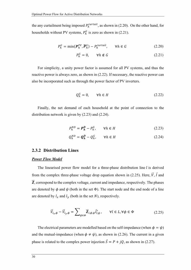
Optimal Power Flow for Active Distribution Networks
30
the any curtailment being imposed 𝑃𝑃ℎ𝑐𝑐𝐶𝐶𝐶𝐶𝐶𝐶𝐶𝐶𝐶𝐶𝐶𝐶, as shown in (2.20). On the other hand, for
households without PV systems, 𝑃𝑃ℎ𝐺𝐺 is zero as shown in (2.21).
𝑃𝑃ℎ𝐺𝐺 = min(𝑷𝑷ℎ𝑃𝑃𝑃𝑃,𝑷𝑷�ℎ𝐺𝐺) − 𝑃𝑃ℎ𝑐𝑐𝐶𝐶𝐶𝐶𝐶𝐶𝐶𝐶𝐶𝐶𝐶𝐶, ∀ℎ ∈ 𝐺𝐺 (2.20)
𝑃𝑃ℎ𝐺𝐺 = 0, ∀ℎ ∉ 𝐺𝐺 (2.21)
For simplicity, a unity power factor is assumed for all PV systems, and thus the
reactive power is always zero, as shown in (2.22). If necessary, the reactive power can
also be incorporated such as through the power factor of PV inverters.
𝑄𝑄ℎ𝐺𝐺 = 0, ∀ℎ ∈ 𝐻𝐻 (2.22)
Finally, the net demand of each household at the point of connection to the
distribution network is given by (2.23) and (2.24).
𝑃𝑃ℎ𝑁𝑁𝑁𝑁 = 𝑷𝑷𝒉𝒉𝑫𝑫 − 𝑃𝑃ℎ𝐺𝐺 , ∀ℎ ∈ 𝐻𝐻 (2.23)
𝑄𝑄ℎ𝑁𝑁𝑁𝑁 = 𝑸𝑸𝒉𝒉𝑫𝑫 − 𝑄𝑄ℎ𝐺𝐺 , ∀ℎ ∈ 𝐻𝐻 (2.24)
2.3.2 Distribution Lines
Power Flow Model
The linearised power flow model for a three-phase distribution line 𝑙𝑙 is derived
from the complex three-phase voltage drop equation shown in (2.25). Here, 𝑉𝑉�⃑ , 𝐼𝐼 and
𝒁𝒁��⃑ , correspond to the complex voltage, current and impedance, respectively. The phases
are denoted by 𝜙𝜙 and 𝜓𝜓 (both in the set Φ). The start node and the end node of a line
are denoted by 𝑙𝑙𝑥𝑥 and 𝑙𝑙𝑦𝑦 (both in the set 𝑁𝑁), respectively.
𝑉𝑉�⃑ 𝐶𝐶𝑥𝑥,𝜙𝜙 − 𝑉𝑉�⃑ 𝐶𝐶𝑦𝑦,𝜙𝜙 = � 𝒁𝒁��⃑ 𝐶𝐶,𝜙𝜙,𝜓𝜓𝐼𝐼𝐶𝐶,𝜓𝜓∗𝜓𝜓∈𝛷𝛷
, ∀𝑙𝑙 ∈ 𝐿𝐿,∀𝜙𝜙 ∈ Φ (2.25)
The electrical parameters are modelled based on the self-impedance (when 𝜙𝜙 = 𝜓𝜓)
and the mutual-impedance (when 𝜙𝜙 ≠ 𝜓𝜓), as shown in (2.26). The current in a given
phase is related to the complex power injection 𝑆𝑆 = 𝑃𝑃 + 𝑗𝑗𝑄𝑄, as shown in (2.27).
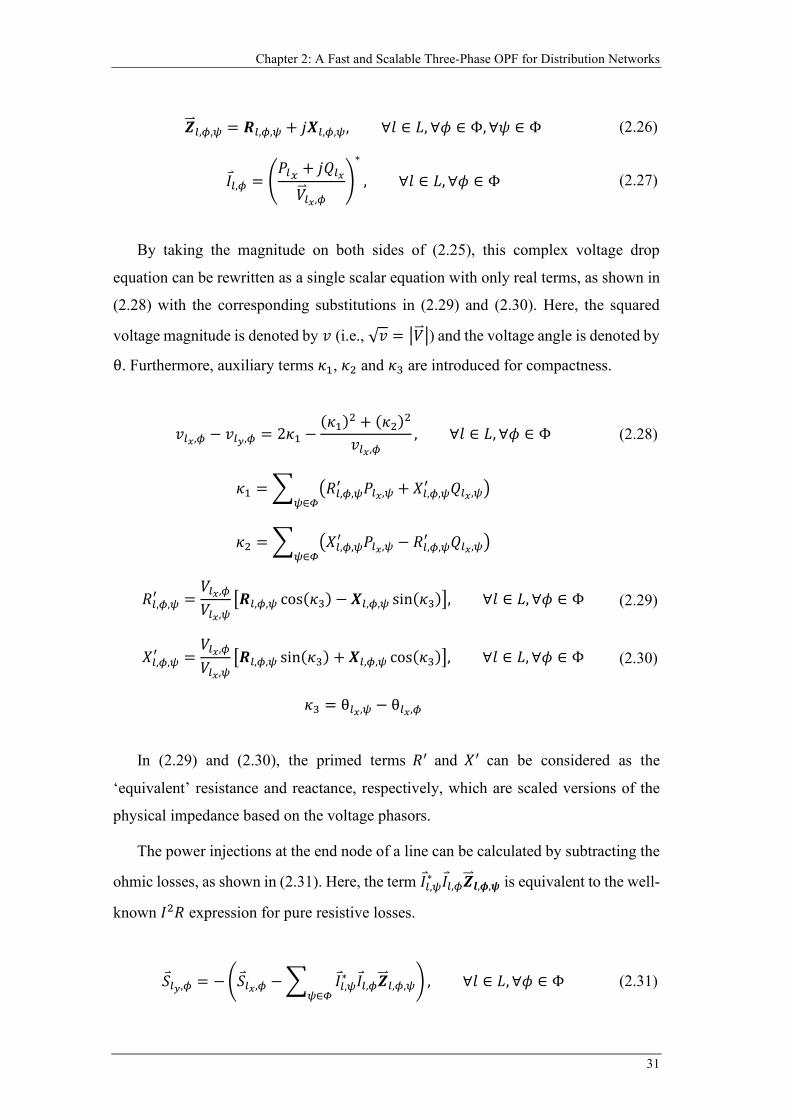
Chapter 2: A Fast and Scalable Three-Phase OPF for Distribution Networks
31
𝒁𝒁��⃑ 𝐶𝐶,𝜙𝜙,𝜓𝜓 = 𝑹𝑹𝐶𝐶,𝜙𝜙,𝜓𝜓 + 𝑗𝑗𝑿𝑿𝐶𝐶,𝜙𝜙,𝜓𝜓, ∀𝑙𝑙 ∈ 𝐿𝐿,∀𝜙𝜙 ∈ Φ,∀𝜓𝜓 ∈ Φ (2.26)
𝐼𝐼𝐶𝐶,𝜙𝜙 = �𝑃𝑃𝐶𝐶𝑥𝑥 + 𝑗𝑗𝑄𝑄𝐶𝐶𝑥𝑥𝑉𝑉�⃑ 𝐶𝐶𝑥𝑥,𝜙𝜙
�∗
, ∀𝑙𝑙 ∈ 𝐿𝐿,∀𝜙𝜙 ∈ Φ (2.27)
By taking the magnitude on both sides of (2.25), this complex voltage drop
equation can be rewritten as a single scalar equation with only real terms, as shown in
(2.28) with the corresponding substitutions in (2.29) and (2.30). Here, the squared
voltage magnitude is denoted by 𝑣𝑣 (i.e., √𝑣𝑣 = �𝑉𝑉�⃑ �) and the voltage angle is denoted by
θ. Furthermore, auxiliary terms 𝜅𝜅1, 𝜅𝜅2 and 𝜅𝜅3 are introduced for compactness.
𝑣𝑣𝐶𝐶𝑥𝑥,𝜙𝜙 − 𝑣𝑣𝐶𝐶𝑦𝑦,𝜙𝜙 = 2𝜅𝜅1 −(𝜅𝜅1)2 + (𝜅𝜅2)2
𝑣𝑣𝐶𝐶𝑥𝑥,𝜙𝜙, ∀𝑙𝑙 ∈ 𝐿𝐿,∀𝜙𝜙 ∈ Φ (2.28)
𝜅𝜅1 = � �𝑅𝑅𝐶𝐶,𝜙𝜙,𝜓𝜓′ 𝑃𝑃𝐶𝐶𝑥𝑥,𝜓𝜓 + 𝑋𝑋𝐶𝐶,𝜙𝜙,𝜓𝜓
′ 𝑄𝑄𝐶𝐶𝑥𝑥,𝜓𝜓�𝜓𝜓∈𝛷𝛷
𝜅𝜅2 = � �𝑋𝑋𝐶𝐶,𝜙𝜙,𝜓𝜓′ 𝑃𝑃𝐶𝐶𝑥𝑥,𝜓𝜓 − 𝑅𝑅𝐶𝐶,𝜙𝜙,𝜓𝜓
′ 𝑄𝑄𝐶𝐶𝑥𝑥,𝜓𝜓�𝜓𝜓∈𝛷𝛷
𝑅𝑅𝐶𝐶,𝜙𝜙,𝜓𝜓′ =
𝑉𝑉𝐶𝐶𝑥𝑥,𝜙𝜙
𝑉𝑉𝐶𝐶𝑥𝑥,𝜓𝜓�𝑹𝑹𝐶𝐶,𝜙𝜙,𝜓𝜓 cos(𝜅𝜅3) − 𝑿𝑿𝐶𝐶,𝜙𝜙,𝜓𝜓 sin(𝜅𝜅3)�, ∀𝑙𝑙 ∈ 𝐿𝐿,∀𝜙𝜙 ∈ Φ (2.29)
𝑋𝑋𝐶𝐶,𝜙𝜙,𝜓𝜓′ =
𝑉𝑉𝐶𝐶𝑥𝑥,𝜙𝜙
𝑉𝑉𝐶𝐶𝑥𝑥,𝜓𝜓�𝑹𝑹𝐶𝐶,𝜙𝜙,𝜓𝜓 sin(𝜅𝜅3) + 𝑿𝑿𝐶𝐶,𝜙𝜙,𝜓𝜓 cos(𝜅𝜅3)�, ∀𝑙𝑙 ∈ 𝐿𝐿,∀𝜙𝜙 ∈ Φ (2.30)
𝜅𝜅3 = θ𝐶𝐶𝑥𝑥,𝜓𝜓 − θ𝐶𝐶𝑥𝑥,𝜙𝜙
In (2.29) and (2.30), the primed terms 𝑅𝑅′ and 𝑋𝑋′ can be considered as the
‘equivalent’ resistance and reactance, respectively, which are scaled versions of the
physical impedance based on the voltage phasors.
The power injections at the end node of a line can be calculated by subtracting the
ohmic losses, as shown in (2.31). Here, the term 𝐼𝐼𝐶𝐶,𝜓𝜓∗ 𝐼𝐼𝐶𝐶,𝜙𝜙𝒁𝒁��⃑ 𝒍𝒍,𝝓𝝓,𝝍𝝍 is equivalent to the well-
known 𝐼𝐼2𝑅𝑅 expression for pure resistive losses.
𝑆𝑆𝐶𝐶𝑦𝑦,𝜙𝜙 = −�𝑆𝑆𝐶𝐶𝑥𝑥,𝜙𝜙 −� 𝐼𝐼𝐶𝐶,𝜓𝜓∗ 𝐼𝐼𝐶𝐶,𝜙𝜙𝒁𝒁��⃑ 𝐶𝐶,𝜙𝜙,𝜓𝜓𝜓𝜓∈𝛷𝛷
� , ∀𝑙𝑙 ∈ 𝐿𝐿,∀𝜙𝜙 ∈ Φ (2.31)
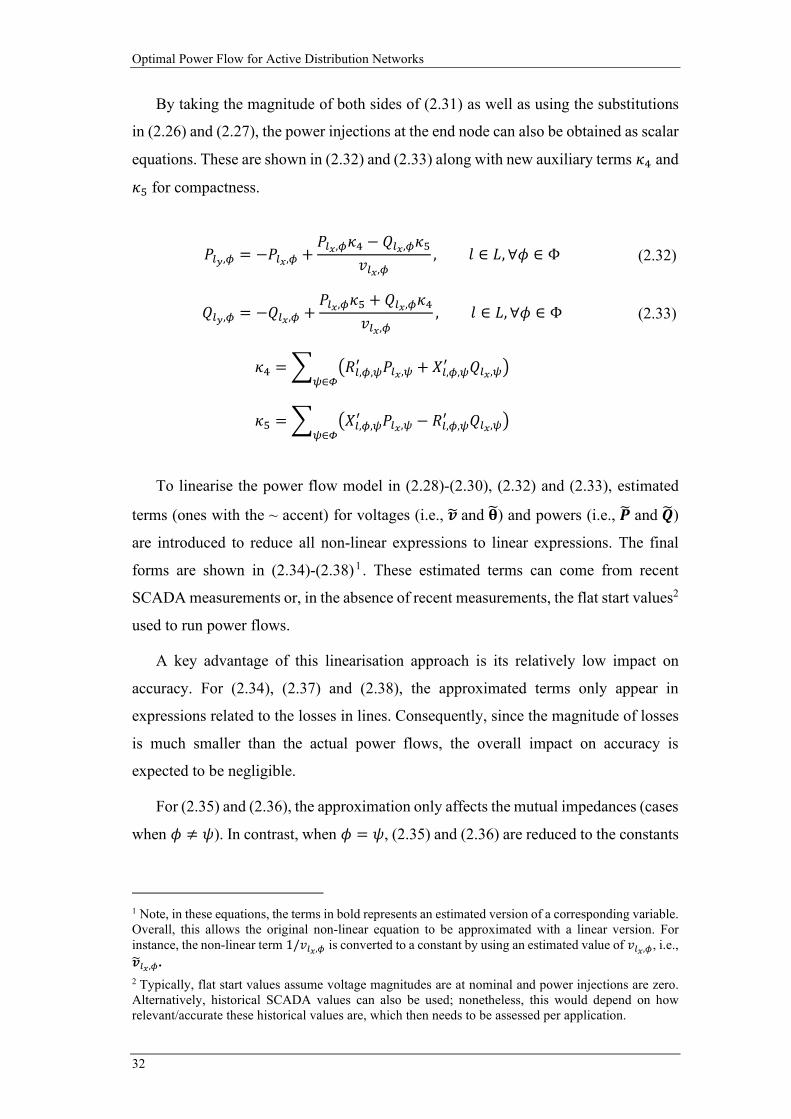
Optimal Power Flow for Active Distribution Networks
32
By taking the magnitude of both sides of (2.31) as well as using the substitutions
in (2.26) and (2.27), the power injections at the end node can also be obtained as scalar
equations. These are shown in (2.32) and (2.33) along with new auxiliary terms 𝜅𝜅4 and
𝜅𝜅5 for compactness.
𝑃𝑃𝐶𝐶𝑦𝑦,𝜙𝜙 = −𝑃𝑃𝐶𝐶𝑥𝑥,𝜙𝜙 +𝑃𝑃𝐶𝐶𝑥𝑥,𝜙𝜙𝜅𝜅4 − 𝑄𝑄𝐶𝐶𝑥𝑥,𝜙𝜙𝜅𝜅5
𝑣𝑣𝐶𝐶𝑥𝑥,𝜙𝜙, 𝑙𝑙 ∈ 𝐿𝐿,∀𝜙𝜙 ∈ Φ (2.32)
𝑄𝑄𝐶𝐶𝑦𝑦,𝜙𝜙 = −𝑄𝑄𝐶𝐶𝑥𝑥,𝜙𝜙 +𝑃𝑃𝐶𝐶𝑥𝑥,𝜙𝜙𝜅𝜅5 + 𝑄𝑄𝐶𝐶𝑥𝑥,𝜙𝜙𝜅𝜅4
𝑣𝑣𝐶𝐶𝑥𝑥,𝜙𝜙, 𝑙𝑙 ∈ 𝐿𝐿,∀𝜙𝜙 ∈ Φ (2.33)
𝜅𝜅4 = � �𝑅𝑅𝐶𝐶,𝜙𝜙,𝜓𝜓′ 𝑃𝑃𝐶𝐶𝑥𝑥,𝜓𝜓 + 𝑋𝑋𝐶𝐶,𝜙𝜙,𝜓𝜓
′ 𝑄𝑄𝐶𝐶𝑥𝑥,𝜓𝜓�𝜓𝜓∈𝛷𝛷
𝜅𝜅5 = � �𝑋𝑋𝐶𝐶,𝜙𝜙,𝜓𝜓′ 𝑃𝑃𝐶𝐶𝑥𝑥,𝜓𝜓 − 𝑅𝑅𝐶𝐶,𝜙𝜙,𝜓𝜓
′ 𝑄𝑄𝐶𝐶𝑥𝑥,𝜓𝜓�𝜓𝜓∈𝛷𝛷
To linearise the power flow model in (2.28)-(2.30), (2.32) and (2.33), estimated
terms (ones with the ~ accent) for voltages (i.e., 𝒗𝒗� and 𝛉𝛉�) and powers (i.e., 𝑷𝑷� and 𝑸𝑸�)
are introduced to reduce all non-linear expressions to linear expressions. The final
forms are shown in (2.34)-(2.38)1 . These estimated terms can come from recent
SCADA measurements or, in the absence of recent measurements, the flat start values2
used to run power flows.
A key advantage of this linearisation approach is its relatively low impact on
accuracy. For (2.34), (2.37) and (2.38), the approximated terms only appear in
expressions related to the losses in lines. Consequently, since the magnitude of losses
is much smaller than the actual power flows, the overall impact on accuracy is
expected to be negligible.
For (2.35) and (2.36), the approximation only affects the mutual impedances (cases
when 𝜙𝜙 ≠ 𝜓𝜓). In contrast, when 𝜙𝜙 = 𝜓𝜓, (2.35) and (2.36) are reduced to the constants
1 Note, in these equations, the terms in bold represents an estimated version of a corresponding variable. Overall, this allows the original non-linear equation to be approximated with a linear version. For instance, the non-linear term 1/𝑣𝑣𝐶𝐶𝑥𝑥,𝜙𝜙 is converted to a constant by using an estimated value of 𝑣𝑣𝐶𝐶𝑥𝑥,𝜙𝜙, i.e., 𝒗𝒗�𝐶𝐶𝑥𝑥,𝜙𝜙. 2 Typically, flat start values assume voltage magnitudes are at nominal and power injections are zero. Alternatively, historical SCADA values can also be used; nonetheless, this would depend on how relevant/accurate these historical values are, which then needs to be assessed per application.
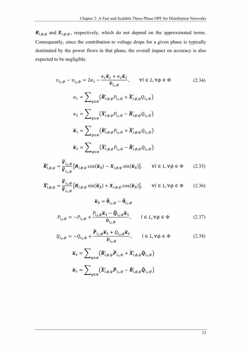
Chapter 2: A Fast and Scalable Three-Phase OPF for Distribution Networks
33
𝑹𝑹𝐶𝐶,𝜙𝜙,𝜓𝜓 and 𝑿𝑿𝐶𝐶,𝜙𝜙,𝜓𝜓 , respectively, which do not depend on the approximated terms.
Consequently, since the contribution to voltage drops for a given phase is typically
dominated by the power flows in that phase, the overall impact on accuracy is also
expected to be negligible.
𝑣𝑣𝐶𝐶𝑥𝑥,𝜙𝜙 − 𝑣𝑣𝐶𝐶𝑦𝑦,𝜙𝜙 = 2𝜅𝜅1 −𝜅𝜅1𝜿𝜿�1 + 𝜅𝜅2𝜿𝜿�2
𝒗𝒗�𝐶𝐶𝑥𝑥,𝜙𝜙, ∀𝑙𝑙 ∈ 𝐿𝐿,∀𝜙𝜙 ∈ Φ (2.34)
𝜅𝜅1 = � �𝑹𝑹�𝐶𝐶,𝜙𝜙,𝜓𝜓′ 𝑃𝑃𝐶𝐶𝑥𝑥,𝜓𝜓 + 𝑿𝑿�𝐶𝐶,𝜙𝜙,𝜓𝜓
′ 𝑄𝑄𝐶𝐶𝑥𝑥,𝜓𝜓�𝜓𝜓∈𝛷𝛷
𝜅𝜅2 = � �𝑿𝑿�𝐶𝐶,𝜙𝜙,𝜓𝜓′ 𝑃𝑃𝐶𝐶𝑥𝑥,𝜓𝜓 − 𝑹𝑹�𝐶𝐶,𝜙𝜙,𝜓𝜓
′ 𝑄𝑄𝐶𝐶𝑥𝑥,𝜓𝜓�𝜓𝜓∈𝛷𝛷
𝜿𝜿�1 = � �𝑹𝑹�𝐶𝐶,𝜙𝜙,𝜓𝜓′ 𝑃𝑃𝐶𝐶𝑥𝑥,𝜓𝜓 + 𝑿𝑿�𝐶𝐶,𝜙𝜙,𝜓𝜓
′ 𝑄𝑄𝐶𝐶𝑥𝑥,𝜓𝜓�𝜓𝜓∈𝛷𝛷
𝜿𝜿�2 = � �𝑿𝑿�𝐶𝐶,𝜙𝜙,𝜓𝜓′ 𝑃𝑃𝐶𝐶𝑥𝑥,𝜓𝜓 − 𝑹𝑹�𝐶𝐶,𝜙𝜙,𝜓𝜓
′ 𝑄𝑄𝐶𝐶𝑥𝑥,𝜓𝜓�𝜓𝜓∈𝛷𝛷
𝑹𝑹�𝐶𝐶,𝜙𝜙,𝜓𝜓′ =
𝑷𝑷�𝐶𝐶𝑥𝑥,𝜙𝜙
𝑷𝑷�𝐶𝐶𝑥𝑥,𝜓𝜓�𝑹𝑹𝐶𝐶,𝜙𝜙,𝜓𝜓 cos(𝜿𝜿�𝟑𝟑) − 𝑿𝑿𝐶𝐶,𝜙𝜙,𝜓𝜓 sin(𝜿𝜿�𝟑𝟑)�, ∀𝑙𝑙 ∈ 𝐿𝐿,∀𝜙𝜙 ∈ Φ (2.35)
𝑿𝑿�𝐶𝐶,𝜙𝜙,𝜓𝜓′ =
𝑷𝑷�𝐶𝐶𝑥𝑥,𝜙𝜙
𝑷𝑷�𝐶𝐶𝑥𝑥,𝜓𝜓�𝑹𝑹𝐶𝐶,𝜙𝜙,𝜓𝜓 sin(𝜿𝜿�𝟑𝟑) + 𝑿𝑿𝐶𝐶,𝜙𝜙,𝜓𝜓 cos(𝜿𝜿�𝟑𝟑)�, ∀𝑙𝑙 ∈ 𝐿𝐿,∀𝜙𝜙 ∈ Φ (2.36)
𝜿𝜿�𝟑𝟑 = 𝛉𝛉�𝐶𝐶𝑥𝑥,𝜓𝜓 − 𝛉𝛉�𝐶𝐶𝑥𝑥,𝜙𝜙
𝑃𝑃𝐶𝐶𝑦𝑦,𝜙𝜙 = −𝑃𝑃𝐶𝐶𝑥𝑥,𝜙𝜙 +𝑃𝑃𝐶𝐶𝑥𝑥,𝜙𝜙𝜿𝜿�4 − 𝑸𝑸�𝐶𝐶𝑥𝑥,𝜙𝜙𝜿𝜿�5
𝒗𝒗�𝐶𝐶𝑥𝑥,𝜙𝜙, 𝑙𝑙 ∈ 𝐿𝐿,∀𝜙𝜙 ∈ Φ (2.37)
𝑄𝑄𝐶𝐶𝑦𝑦,𝜙𝜙 = −𝑄𝑄𝐶𝐶𝑥𝑥,𝜙𝜙 +𝑷𝑷�𝐶𝐶𝑥𝑥,𝜙𝜙𝜿𝜿�5 + 𝑄𝑄𝐶𝐶𝑥𝑥,𝜙𝜙𝜿𝜿�4
𝒗𝒗�𝐶𝐶𝑥𝑥,𝜙𝜙, 𝑙𝑙 ∈ 𝐿𝐿,∀𝜙𝜙 ∈ Φ (2.38)
𝜿𝜿�4 = � �𝑹𝑹�𝐶𝐶,𝜙𝜙,𝜓𝜓′ 𝑷𝑷�𝐶𝐶𝑥𝑥,𝜓𝜓 + 𝑿𝑿�𝐶𝐶,𝜙𝜙,𝜓𝜓
′ 𝑸𝑸�𝐶𝐶𝑥𝑥,𝜓𝜓�𝜓𝜓∈𝛷𝛷
𝜿𝜿�5 = � �𝑿𝑿�𝐶𝐶,𝜙𝜙,𝜓𝜓′ 𝑷𝑷�𝐶𝐶𝑥𝑥,𝜓𝜓 − 𝑹𝑹�𝐶𝐶,𝜙𝜙,𝜓𝜓
′ 𝑸𝑸�𝐶𝐶𝑥𝑥,𝜓𝜓�𝜓𝜓∈𝛷𝛷
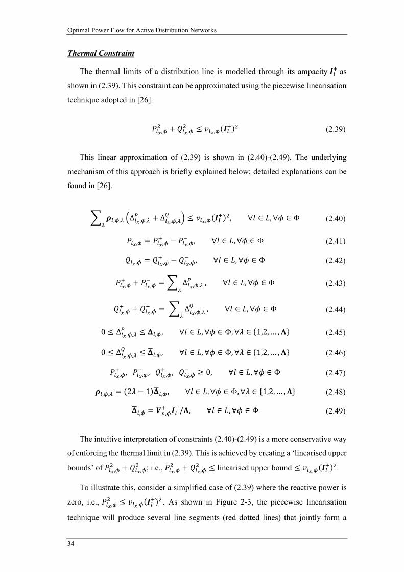
Optimal Power Flow for Active Distribution Networks
34
Thermal Constraint
The thermal limits of a distribution line is modelled through its ampacity 𝑰𝑰𝐶𝐶+ as
shown in (2.39). This constraint can be approximated using the piecewise linearisation
technique adopted in [26].
𝑃𝑃𝐶𝐶𝑥𝑥,𝜙𝜙2 + 𝑄𝑄𝐶𝐶𝑥𝑥,𝜙𝜙
2 ≤ 𝑣𝑣𝐶𝐶𝑥𝑥,𝜙𝜙(𝑰𝑰𝐶𝐶+)2 (2.39)
This linear approximation of (2.39) is shown in (2.40)-(2.49). The underlying
mechanism of this approach is briefly explained below; detailed explanations can be
found in [26].
� 𝝆𝝆𝐶𝐶,𝜙𝜙,𝜆𝜆 �Δ𝐶𝐶𝑥𝑥,𝜙𝜙,𝜆𝜆𝑃𝑃 + Δ𝐶𝐶𝑥𝑥,𝜙𝜙,𝜆𝜆
𝑄𝑄 �𝜆𝜆
≤ 𝑣𝑣𝐶𝐶𝑥𝑥,𝜙𝜙(𝑰𝑰𝒍𝒍+)2, ∀𝑙𝑙 ∈ 𝐿𝐿,∀𝜙𝜙 ∈ Φ (2.40)
𝑃𝑃𝐶𝐶𝑥𝑥,𝜙𝜙 = 𝑃𝑃𝐶𝐶𝑥𝑥,𝜙𝜙+ − 𝑃𝑃𝐶𝐶𝑥𝑥,𝜙𝜙
− , ∀𝑙𝑙 ∈ 𝐿𝐿,∀𝜙𝜙 ∈ Φ (2.41)
𝑄𝑄𝐶𝐶𝑥𝑥,𝜙𝜙 = 𝑄𝑄𝐶𝐶𝑥𝑥,𝜙𝜙+ − 𝑄𝑄𝐶𝐶𝑥𝑥,𝜙𝜙
− , ∀𝑙𝑙 ∈ 𝐿𝐿,∀𝜙𝜙 ∈ Φ (2.42)
𝑃𝑃𝐶𝐶𝑥𝑥,𝜙𝜙+ + 𝑃𝑃𝐶𝐶𝑥𝑥,𝜙𝜙
− = � Δ𝐶𝐶𝑥𝑥,𝜙𝜙,𝜆𝜆𝑃𝑃
𝜆𝜆, ∀𝑙𝑙 ∈ 𝐿𝐿,∀𝜙𝜙 ∈ Φ (2.43)
𝑄𝑄𝐶𝐶𝑥𝑥,𝜙𝜙+ + 𝑄𝑄𝐶𝐶𝑥𝑥,𝜙𝜙
− = � Δ𝐶𝐶𝑥𝑥,𝜙𝜙,𝜆𝜆𝑄𝑄
𝜆𝜆, ∀𝑙𝑙 ∈ 𝐿𝐿,∀𝜙𝜙 ∈ Φ (2.44)
0 ≤ Δ𝐶𝐶𝑥𝑥,𝜙𝜙,𝜆𝜆𝑃𝑃 ≤ 𝚫𝚫�𝐶𝐶,𝜙𝜙, ∀𝑙𝑙 ∈ 𝐿𝐿,∀𝜙𝜙 ∈ Φ,∀𝜆𝜆 ∈ {1,2, … ,𝚲𝚲} (2.45)
0 ≤ Δ𝐶𝐶𝑥𝑥,𝜙𝜙,𝜆𝜆𝑄𝑄 ≤ 𝚫𝚫�𝐶𝐶,𝜙𝜙, ∀𝑙𝑙 ∈ 𝐿𝐿,∀𝜙𝜙 ∈ Φ,∀𝜆𝜆 ∈ {1,2, … ,𝚲𝚲} (2.46)
𝑃𝑃𝐶𝐶𝑥𝑥,𝜙𝜙+ , 𝑃𝑃𝐶𝐶𝑥𝑥,𝜙𝜙
− , 𝑄𝑄𝐶𝐶𝑥𝑥,𝜙𝜙+ , 𝑄𝑄𝐶𝐶𝑥𝑥,𝜙𝜙
− ≥ 0, ∀𝑙𝑙 ∈ 𝐿𝐿,∀𝜙𝜙 ∈ Φ (2.47)
𝝆𝝆𝐶𝐶,𝜙𝜙,𝜆𝜆 = (2𝜆𝜆 − 1)𝚫𝚫�𝐶𝐶,𝜙𝜙, ∀𝑙𝑙 ∈ 𝐿𝐿,∀𝜙𝜙 ∈ Φ,∀𝜆𝜆 ∈ {1,2, … ,𝚲𝚲} (2.48)
𝚫𝚫�𝐶𝐶,𝜙𝜙 = 𝑷𝑷𝑛𝑛,𝜙𝜙+ 𝑰𝑰𝐶𝐶+/𝚲𝚲, ∀𝑙𝑙 ∈ 𝐿𝐿,∀𝜙𝜙 ∈ Φ (2.49)
The intuitive interpretation of constraints (2.40)-(2.49) is a more conservative way
of enforcing the thermal limit in (2.39). This is achieved by creating a ‘linearised upper
bounds’ of 𝑃𝑃𝐶𝐶𝑥𝑥,𝜙𝜙2 + 𝑄𝑄𝐶𝐶𝑥𝑥,𝜙𝜙
2 ; i.e., 𝑃𝑃𝐶𝐶𝑥𝑥,𝜙𝜙2 + 𝑄𝑄𝐶𝐶𝑥𝑥,𝜙𝜙
2 ≤ linearised upper bound ≤ 𝑣𝑣𝐶𝐶𝑥𝑥,𝜙𝜙(𝑰𝑰𝐶𝐶+)2.
To illustrate this, consider a simplified case of (2.39) where the reactive power is
zero, i.e., 𝑃𝑃𝐶𝐶𝑥𝑥,𝜙𝜙2 ≤ 𝑣𝑣𝐶𝐶𝑥𝑥,𝜙𝜙(𝑰𝑰𝐶𝐶+)2 . As shown in Figure 2-3, the piecewise linearisation
technique will produce several line segments (red dotted lines) that jointly form a
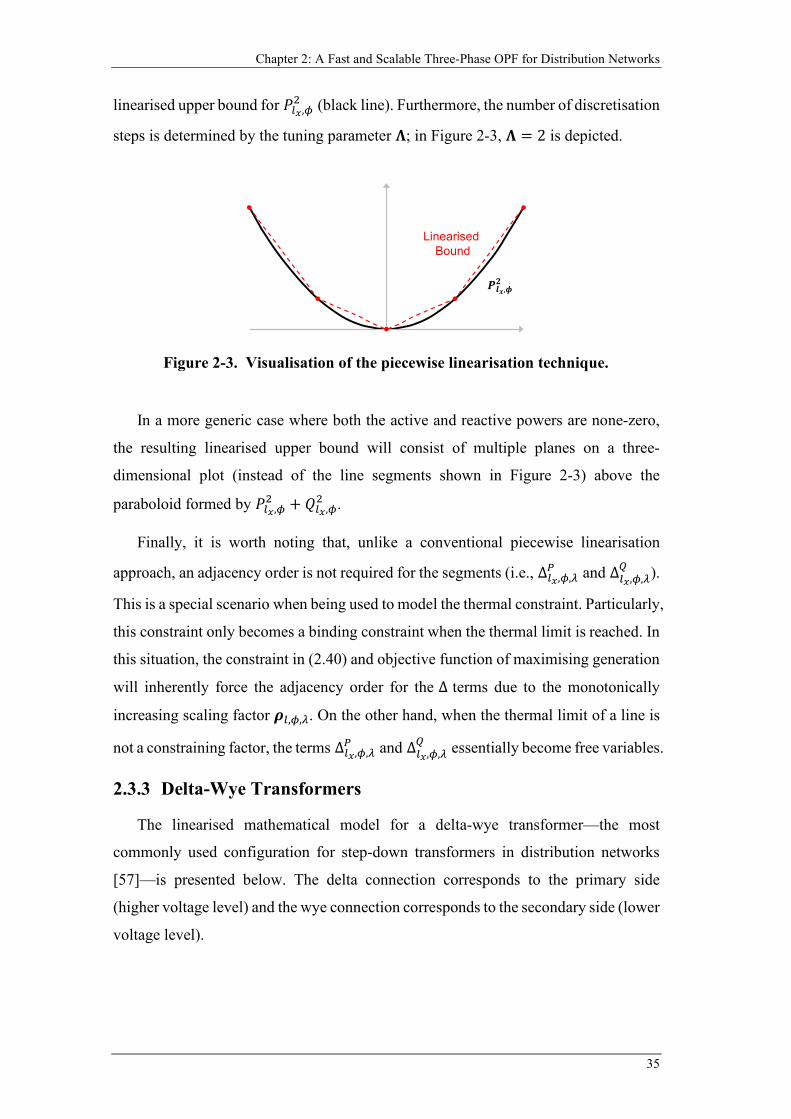
Chapter 2: A Fast and Scalable Three-Phase OPF for Distribution Networks
35
linearised upper bound for 𝑃𝑃𝐶𝐶𝑥𝑥,𝜙𝜙2 (black line). Furthermore, the number of discretisation
steps is determined by the tuning parameter 𝚲𝚲; in Figure 2-3, 𝚲𝚲 = 2 is depicted.
In a more generic case where both the active and reactive powers are none-zero,
the resulting linearised upper bound will consist of multiple planes on a three-
dimensional plot (instead of the line segments shown in Figure 2-3) above the
paraboloid formed by 𝑃𝑃𝐶𝐶𝑥𝑥,𝜙𝜙2 + 𝑄𝑄𝐶𝐶𝑥𝑥,𝜙𝜙
2 .
Finally, it is worth noting that, unlike a conventional piecewise linearisation
approach, an adjacency order is not required for the segments (i.e., Δ𝐶𝐶𝑥𝑥,𝜙𝜙,𝜆𝜆𝑃𝑃 and Δ𝐶𝐶𝑥𝑥,𝜙𝜙,𝜆𝜆
𝑄𝑄 ).
This is a special scenario when being used to model the thermal constraint. Particularly,
this constraint only becomes a binding constraint when the thermal limit is reached. In
this situation, the constraint in (2.40) and objective function of maximising generation
will inherently force the adjacency order for the Δ terms due to the monotonically
increasing scaling factor 𝝆𝝆𝐶𝐶,𝜙𝜙,𝜆𝜆. On the other hand, when the thermal limit of a line is
not a constraining factor, the terms Δ𝐶𝐶𝑥𝑥,𝜙𝜙,𝜆𝜆𝑃𝑃 and Δ𝐶𝐶𝑥𝑥,𝜙𝜙,𝜆𝜆
𝑄𝑄 essentially become free variables.
2.3.3 Delta-Wye Transformers
The linearised mathematical model for a delta-wye transformer—the most
commonly used configuration for step-down transformers in distribution networks
[57]—is presented below. The delta connection corresponds to the primary side
(higher voltage level) and the wye connection corresponds to the secondary side (lower
voltage level).
Figure 2-3. Visualisation of the piecewise linearisation technique.
-1 -0.5 0 0.5 1
𝑷𝑷𝒍𝒍𝒙𝒙,𝝓𝝓𝟐𝟐
Linearised Bound
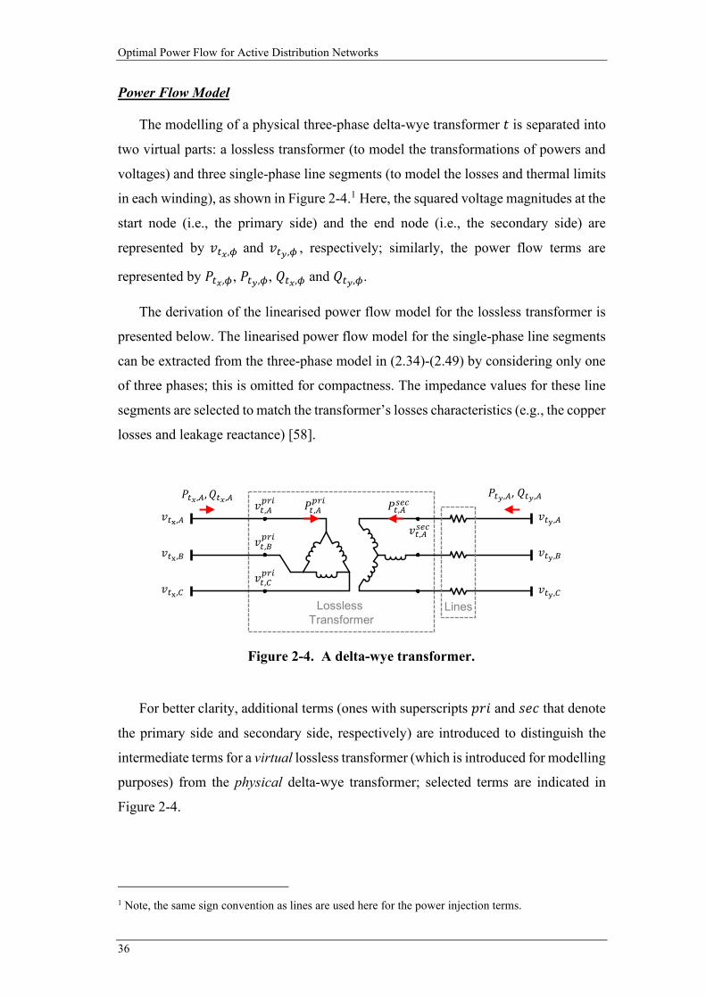
Optimal Power Flow for Active Distribution Networks
36
Power Flow Model
The modelling of a physical three-phase delta-wye transformer 𝑡𝑡 is separated into
two virtual parts: a lossless transformer (to model the transformations of powers and
voltages) and three single-phase line segments (to model the losses and thermal limits
in each winding), as shown in Figure 2-4.1 Here, the squared voltage magnitudes at the
start node (i.e., the primary side) and the end node (i.e., the secondary side) are
represented by 𝑣𝑣𝐶𝐶𝑥𝑥,𝜙𝜙 and 𝑣𝑣𝐶𝐶𝑦𝑦,𝜙𝜙 , respectively; similarly, the power flow terms are
represented by 𝑃𝑃𝐶𝐶𝑥𝑥,𝜙𝜙, 𝑃𝑃𝐶𝐶𝑦𝑦,𝜙𝜙, 𝑄𝑄𝐶𝐶𝑥𝑥,𝜙𝜙 and 𝑄𝑄𝐶𝐶𝑦𝑦,𝜙𝜙.
The derivation of the linearised power flow model for the lossless transformer is
presented below. The linearised power flow model for the single-phase line segments
can be extracted from the three-phase model in (2.34)-(2.49) by considering only one
of three phases; this is omitted for compactness. The impedance values for these line
segments are selected to match the transformer’s losses characteristics (e.g., the copper
losses and leakage reactance) [58].
For better clarity, additional terms (ones with superscripts 𝑝𝑝𝑝𝑝𝑖𝑖 and 𝑐𝑐𝑠𝑠𝑐𝑐 that denote
the primary side and secondary side, respectively) are introduced to distinguish the
intermediate terms for a virtual lossless transformer (which is introduced for modelling
purposes) from the physical delta-wye transformer; selected terms are indicated in
Figure 2-4.
1 Note, the same sign convention as lines are used here for the power injection terms.
Figure 2-4. A delta-wye transformer.
𝑣𝑣𝐶𝐶,𝐴𝐴𝑠𝑠𝑠𝑠𝑐𝑐
𝑃𝑃𝐶𝐶,𝐴𝐴𝑝𝑝𝐶𝐶𝐶𝐶 𝑃𝑃𝐶𝐶,𝐴𝐴
𝑠𝑠𝑠𝑠𝑐𝑐𝑣𝑣𝐶𝐶,𝐴𝐴𝑝𝑝𝐶𝐶𝐶𝐶
𝑣𝑣𝐶𝐶y,𝐴𝐴
Lossless Transformer
Lines
𝑣𝑣𝐶𝐶,𝐵𝐵𝑝𝑝𝐶𝐶𝐶𝐶
𝑣𝑣𝐶𝐶,𝐶𝐶𝑝𝑝𝐶𝐶𝐶𝐶
𝑣𝑣𝐶𝐶y,𝐵𝐵
𝑣𝑣𝐶𝐶y,𝐶𝐶
𝑣𝑣𝐶𝐶x,𝐴𝐴
𝑣𝑣𝐶𝐶x,𝐵𝐵
𝑣𝑣𝐶𝐶x,𝐶𝐶
𝑃𝑃𝐶𝐶𝑦𝑦,𝐴𝐴, 𝑄𝑄𝐶𝐶𝑦𝑦,𝐴𝐴𝑃𝑃𝐶𝐶𝑥𝑥,𝐴𝐴,𝑄𝑄𝐶𝐶𝑥𝑥,𝐴𝐴
Chapter 2: A Fast and Scalable Three-Phase OPF for Distribution Networks
37
The linearised power equations for the lossless transformer is derived based on the
phasor model proposed in [59]; an example is illustrated through (2.50)-(2.54).
Due to the phase-to-phase connection on the primary side of a delta-wye
transformer, a (phase-to-neutral) power on phase A at the secondary terminal (i.e.,
𝑆𝑆𝐶𝐶,𝐴𝐴𝑠𝑠𝑠𝑠𝑐𝑐 = 𝑃𝑃𝐶𝐶,𝐴𝐴
𝑠𝑠𝑠𝑠𝑐𝑐 + 𝑗𝑗𝑄𝑄𝐶𝐶,𝐴𝐴𝑠𝑠𝑠𝑠𝑐𝑐) will result in a (phase-to-phase) current between phases A and
C on the primary side, as shown in (2.50).
�𝐼𝐼𝐶𝐶,𝐴𝐴→𝐶𝐶𝑝𝑝𝐶𝐶𝐶𝐶 �
∗=
−𝑆𝑆𝐶𝐶,𝐴𝐴𝑠𝑠𝑠𝑠𝑐𝑐
𝑉𝑉�⃑𝐶𝐶,𝐴𝐴𝑝𝑝𝐶𝐶𝐶𝐶 − 𝑉𝑉�⃑𝐶𝐶,𝐶𝐶
𝑝𝑝𝐶𝐶𝐶𝐶 , ∀𝑡𝑡 ∈ 𝑇𝑇 (2.50)
Using (2.50) and the complex power formula 𝑆𝑆 = 𝑉𝑉�⃑ ∙ 𝐼𝐼∗, the corresponding power
injections at phase A of the primary side can be calculated by (2.51).
𝑆𝑆𝐶𝐶,𝐴𝐴𝑝𝑝𝐶𝐶𝐶𝐶 =
𝑉𝑉�⃑𝐶𝐶,𝐴𝐴𝑝𝑝𝐶𝐶𝐶𝐶
𝑉𝑉�⃑𝐶𝐶,𝐴𝐴𝑝𝑝𝐶𝐶𝐶𝐶 − 𝑉𝑉�⃑𝐶𝐶,𝐶𝐶
𝑝𝑝𝐶𝐶𝐶𝐶 𝑆𝑆𝐶𝐶,𝐴𝐴𝑠𝑠𝑠𝑠𝑐𝑐 , ∀𝑡𝑡 ∈ 𝑇𝑇 (2.51)
To linearise (2.51), the following conditions for relatively balanced three-phase
voltages are assumed: �𝑉𝑉�⃑𝐶𝐶,𝐴𝐴𝑝𝑝𝐶𝐶𝐶𝐶� ≈ �𝑉𝑉�⃑𝐶𝐶,𝐶𝐶
𝑝𝑝𝐶𝐶𝐶𝐶� and ∠𝑉𝑉�⃑𝐶𝐶,𝐶𝐶𝑝𝑝𝐶𝐶𝐶𝐶 − ∠𝑉𝑉�⃑𝐶𝐶,𝐴𝐴
𝑝𝑝𝐶𝐶𝐶𝐶 ≈ 120°. For MV networks,
where these transformers are usually being connected to, this assumption is generally
valid due to the diversity of power flows at an aggregated level.
Based on the above, the approximated form of (2.51) is shown in (2.52). Also, by
separating the real and imaginary parts of (2.52), the linear equations in (2.53) and
(2.54) are obtained. It is worth noting that, pure active power on the secondary side of
a delta-wye transformer actually results in both active and reactive powers on the
primary side.
𝑆𝑆𝐶𝐶,𝐴𝐴𝑝𝑝𝐶𝐶𝐶𝐶 = �
12− 𝑗𝑗
12√3
� 𝑆𝑆𝐶𝐶,𝐴𝐴𝑠𝑠𝑠𝑠𝑐𝑐 , ∀𝑡𝑡 ∈ 𝑇𝑇 (2.52)
𝑃𝑃𝐶𝐶,𝐴𝐴𝑝𝑝𝐶𝐶𝐶𝐶 =
12𝑃𝑃𝐶𝐶,𝐴𝐴𝑠𝑠𝑠𝑠𝑐𝑐 +
12√3
𝑄𝑄𝐶𝐶,𝐴𝐴𝑠𝑠𝑠𝑠𝑐𝑐, ∀𝑡𝑡 ∈ 𝑇𝑇 (2.53)
𝑄𝑄𝐶𝐶,𝐴𝐴𝑝𝑝𝐶𝐶𝐶𝐶 =
12𝑄𝑄𝐶𝐶,𝐴𝐴𝑠𝑠𝑠𝑠𝑐𝑐 +
12√3
𝑃𝑃𝐶𝐶,𝐴𝐴𝑠𝑠𝑠𝑠𝑐𝑐 , ∀𝑡𝑡 ∈ 𝑇𝑇 (2.54)
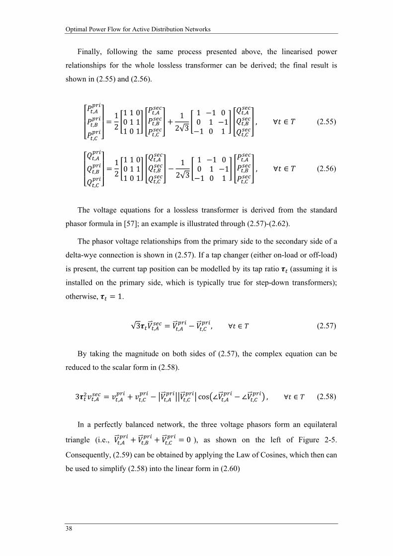
Optimal Power Flow for Active Distribution Networks
38
Finally, following the same process presented above, the linearised power
relationships for the whole lossless transformer can be derived; the final result is
shown in (2.55) and (2.56).
⎣⎢⎢⎡𝑃𝑃𝐶𝐶,𝐴𝐴
𝑝𝑝𝐶𝐶𝐶𝐶
𝑃𝑃𝐶𝐶,𝐵𝐵𝑝𝑝𝐶𝐶𝐶𝐶
𝑃𝑃𝐶𝐶,𝐶𝐶𝑝𝑝𝐶𝐶𝐶𝐶⎦⎥⎥⎤
=12�1 1 00 1 11 0 1
� �𝑃𝑃𝐶𝐶,𝐴𝐴𝑠𝑠𝑠𝑠𝑐𝑐
𝑃𝑃𝐶𝐶,𝐵𝐵𝑠𝑠𝑠𝑠𝑐𝑐
𝑃𝑃𝐶𝐶,𝐶𝐶𝑠𝑠𝑠𝑠𝑐𝑐� +
12√3
�1 −1 00 1 −1−1 0 1
� �𝑄𝑄𝐶𝐶,𝐴𝐴𝑠𝑠𝑠𝑠𝑐𝑐
𝑄𝑄𝐶𝐶,𝐵𝐵𝑠𝑠𝑠𝑠𝑐𝑐
𝑄𝑄𝐶𝐶,𝐶𝐶𝑠𝑠𝑠𝑠𝑐𝑐� , ∀𝑡𝑡 ∈ 𝑇𝑇 (2.55)
⎣⎢⎢⎡𝑄𝑄𝐶𝐶,𝐴𝐴
𝑝𝑝𝐶𝐶𝐶𝐶
𝑄𝑄𝐶𝐶,𝐵𝐵𝑝𝑝𝐶𝐶𝐶𝐶
𝑄𝑄𝐶𝐶,𝐶𝐶𝑝𝑝𝐶𝐶𝐶𝐶⎦⎥⎥⎤
=12�1 1 00 1 11 0 1
� �𝑄𝑄𝐶𝐶,𝐴𝐴𝑠𝑠𝑠𝑠𝑐𝑐
𝑄𝑄𝐶𝐶,𝐵𝐵𝑠𝑠𝑠𝑠𝑐𝑐
𝑄𝑄𝐶𝐶,𝐶𝐶𝑠𝑠𝑠𝑠𝑐𝑐� −
12√3
�1 −1 00 1 −1−1 0 1
� �𝑃𝑃𝐶𝐶,𝐴𝐴𝑠𝑠𝑠𝑠𝑐𝑐
𝑃𝑃𝐶𝐶,𝐵𝐵𝑠𝑠𝑠𝑠𝑐𝑐
𝑃𝑃𝐶𝐶,𝐶𝐶𝑠𝑠𝑠𝑠𝑐𝑐� , ∀𝑡𝑡 ∈ 𝑇𝑇 (2.56)
The voltage equations for a lossless transformer is derived from the standard
phasor formula in [57]; an example is illustrated through (2.57)-(2.62).
The phasor voltage relationships from the primary side to the secondary side of a
delta-wye connection is shown in (2.57). If a tap changer (either on-load or off-load)
is present, the current tap position can be modelled by its tap ratio 𝝉𝝉𝐶𝐶 (assuming it is
installed on the primary side, which is typically true for step-down transformers);
otherwise, 𝝉𝝉𝐶𝐶 = 1.
√3𝝉𝝉𝐶𝐶𝑉𝑉�⃑ 𝐶𝐶,𝐴𝐴𝑠𝑠𝑠𝑠𝑐𝑐 = 𝑉𝑉�⃑𝐶𝐶,𝐴𝐴
𝑝𝑝𝐶𝐶𝐶𝐶 − 𝑉𝑉�⃑𝐶𝐶,𝐶𝐶𝑝𝑝𝐶𝐶𝐶𝐶, ∀𝑡𝑡 ∈ 𝑇𝑇 (2.57)
By taking the magnitude on both sides of (2.57), the complex equation can be
reduced to the scalar form in (2.58).
3𝝉𝝉𝐶𝐶2𝑣𝑣𝐶𝐶,𝐴𝐴𝑠𝑠𝑠𝑠𝑐𝑐 = 𝑣𝑣𝐶𝐶,𝐴𝐴
𝑝𝑝𝐶𝐶𝐶𝐶 + 𝑣𝑣𝐶𝐶,𝐶𝐶𝑝𝑝𝐶𝐶𝐶𝐶 − �𝑉𝑉�⃑𝐶𝐶,𝐴𝐴
𝑝𝑝𝐶𝐶𝐶𝐶��𝑉𝑉�⃑𝐶𝐶,𝐶𝐶𝑝𝑝𝐶𝐶𝐶𝐶� cos�∠𝑉𝑉�⃑𝐶𝐶,𝐴𝐴
𝑝𝑝𝐶𝐶𝐶𝐶 − ∠𝑉𝑉�⃑𝐶𝐶,𝐶𝐶𝑝𝑝𝐶𝐶𝐶𝐶� , ∀𝑡𝑡 ∈ 𝑇𝑇 (2.58)
In a perfectly balanced network, the three voltage phasors form an equilateral
triangle (i.e., 𝑉𝑉�⃑𝐶𝐶,𝐴𝐴𝑝𝑝𝐶𝐶𝐶𝐶 + 𝑉𝑉�⃑𝐶𝐶,𝐵𝐵
𝑝𝑝𝐶𝐶𝐶𝐶 + 𝑉𝑉�⃑𝐶𝐶,𝐶𝐶𝑝𝑝𝐶𝐶𝐶𝐶 = 0 ), as shown on the left of Figure 2-5.
Consequently, (2.59) can be obtained by applying the Law of Cosines, which then can
be used to simplify (2.58) into the linear form in (2.60)

Chapter 2: A Fast and Scalable Three-Phase OPF for Distribution Networks
39
�𝑉𝑉�⃑𝐶𝐶,𝐵𝐵𝑝𝑝𝐶𝐶𝐶𝐶�
2= �𝑉𝑉�⃑𝐶𝐶,𝐴𝐴
𝑝𝑝𝐶𝐶𝐶𝐶�2
+ �𝑉𝑉�⃑𝐶𝐶,𝐶𝐶𝑝𝑝𝐶𝐶𝐶𝐶�
2− 2�𝑉𝑉�⃑𝐶𝐶,𝐴𝐴
𝑝𝑝𝐶𝐶𝐶𝐶��𝑉𝑉�⃑𝐶𝐶,𝐶𝐶𝑝𝑝𝐶𝐶𝐶𝐶� cos�∠𝑉𝑉�⃑𝐶𝐶,𝐴𝐴
𝑝𝑝𝐶𝐶𝐶𝐶 − ∠𝑉𝑉�⃑𝐶𝐶,𝐶𝐶𝑝𝑝𝐶𝐶𝐶𝐶� , ∀𝑡𝑡 ∈ 𝑇𝑇 (2.59)
3𝝉𝝉𝐶𝐶2𝑣𝑣𝐶𝐶,𝐴𝐴𝑠𝑠𝑠𝑠𝑐𝑐 = 2𝑣𝑣𝐶𝐶,𝐴𝐴
𝑝𝑝𝐶𝐶𝐶𝐶 + 2𝑣𝑣𝐶𝐶,𝐶𝐶𝑝𝑝𝐶𝐶𝐶𝐶 − 𝑣𝑣𝐶𝐶,𝐵𝐵
𝑝𝑝𝐶𝐶𝐶𝐶, ∀𝑡𝑡 ∈ 𝑇𝑇 (2.60)
While (2.59) is no longer true in an unbalanced network, a similar condition still
holds when a small offset phasor 𝑉𝑉�⃑𝐶𝐶,𝑂𝑂𝑝𝑝𝐶𝐶𝐶𝐶 is introduced to obtain 𝑣𝑣𝐶𝐶,𝐵𝐵′
𝑝𝑝𝐶𝐶𝐶𝐶 , as shown on the
right of Figure 2-5; the offset vector is exaggerated on the diagram for better clarity.
Based on this, (2.60) can be adapted to (2.61) to account for the voltage unbalances.
3𝝉𝝉𝐶𝐶2𝑣𝑣𝐶𝐶,𝐴𝐴𝑠𝑠𝑠𝑠𝑐𝑐 = 2𝑣𝑣𝐶𝐶,𝐴𝐴
𝑝𝑝𝐶𝐶𝐶𝐶 + 2𝑣𝑣𝐶𝐶,𝐶𝐶𝑝𝑝𝐶𝐶𝐶𝐶 − 𝑣𝑣𝐶𝐶,𝐵𝐵′
𝑝𝑝𝐶𝐶𝐶𝐶 , ∀𝑡𝑡 ∈ 𝑇𝑇 (2.61)
Combining (2.61) with the relationship 𝑉𝑉�⃑ 𝐶𝐶,𝐵𝐵′𝑝𝑝𝐶𝐶𝐶𝐶 = 𝑉𝑉�⃑𝐶𝐶,𝐴𝐴
𝑝𝑝𝐶𝐶𝐶𝐶 + 𝑉𝑉�⃑𝐶𝐶,𝐵𝐵𝑝𝑝𝐶𝐶𝐶𝐶 = 𝑉𝑉�⃑𝐶𝐶,𝐵𝐵
𝑝𝑝𝐶𝐶𝐶𝐶 + 𝑉𝑉�⃑𝐶𝐶,𝑂𝑂𝑝𝑝𝐶𝐶𝐶𝐶 , an
linear approximation of (2.61) with the physical squared voltage magnitudes (i.e., 𝑣𝑣𝐶𝐶,𝐴𝐴𝑝𝑝𝐶𝐶𝐶𝐶,
𝑣𝑣𝐶𝐶,𝐵𝐵𝑝𝑝𝐶𝐶𝐶𝐶 and 𝑣𝑣𝐶𝐶,𝐶𝐶
𝑝𝑝𝐶𝐶𝐶𝐶 ) can be obtained, as shown in (2.62). Here, the offset expression
�𝑷𝑷��⃑�𝐶𝐶,𝐴𝐴𝑝𝑝𝐶𝐶𝐶𝐶 + 𝑷𝑷��⃑�𝐶𝐶,𝐶𝐶
𝑝𝑝𝐶𝐶𝐶𝐶�2− �𝑷𝑷��⃑�𝐶𝐶,𝐵𝐵
𝑝𝑝𝐶𝐶𝐶𝐶�2
can be calculated based on the available data for the
corresponding transformer to account for the unbalances among phases.
3𝝉𝝉𝐶𝐶2𝑣𝑣𝐶𝐶,𝐴𝐴𝑠𝑠𝑠𝑠𝑐𝑐 = 2𝑣𝑣𝐶𝐶,𝐴𝐴
𝑝𝑝𝐶𝐶𝐶𝐶 + 2𝑣𝑣𝐶𝐶,𝐶𝐶𝑝𝑝𝐶𝐶𝐶𝐶 − 𝑣𝑣𝐶𝐶,𝐵𝐵
𝑝𝑝𝐶𝐶𝐶𝐶 − ��𝑷𝑷��⃑�𝐶𝐶,𝐴𝐴𝑝𝑝𝐶𝐶𝐶𝐶 + 𝑷𝑷��⃑�𝐶𝐶,𝐶𝐶
𝑝𝑝𝐶𝐶𝐶𝐶�2− �𝑷𝑷��⃑�𝐶𝐶,𝐵𝐵
𝑝𝑝𝐶𝐶𝐶𝐶�2� , ∀𝑡𝑡 ∈ 𝑇𝑇 (2.62)
Finally, following the same process presented above, the linearised voltage
relationships for the whole lossless transformer can be derived; the final result is
shown in (2.63).
Figure 2-5. Voltage phasors for balanced and unbalanced scenarios.
𝑉𝑉𝐶𝐶,𝐴𝐴𝑝𝑝𝐶𝐶𝐶𝐶 𝑉𝑉𝐶𝐶,𝐵𝐵
𝑝𝑝𝐶𝐶𝐶𝐶
𝑉𝑉𝐶𝐶,𝐶𝐶𝑝𝑝𝐶𝐶𝐶𝐶
𝑉𝑉𝐶𝐶,𝐴𝐴𝑝𝑝𝐶𝐶𝐶𝐶
𝑉𝑉𝐶𝐶,𝐵𝐵𝑝𝑝𝐶𝐶𝐶𝐶
𝑉𝑉𝐶𝐶,𝐶𝐶𝑝𝑝𝐶𝐶𝐶𝐶
𝑉𝑉𝐶𝐶,𝑂𝑂 𝑝𝑝𝐶𝐶𝐶𝐶
𝑉𝑉𝐶𝐶,𝐵𝐵′𝑝𝑝𝐶𝐶𝐶𝐶
Balanced Unbalanced
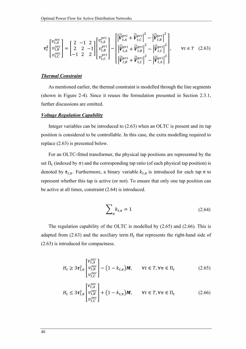
Optimal Power Flow for Active Distribution Networks
40
𝝉𝝉𝐶𝐶𝟐𝟐 �𝑣𝑣𝐶𝐶,𝐴𝐴𝑠𝑠𝑠𝑠𝑐𝑐 𝑣𝑣𝐶𝐶,𝐵𝐵𝑠𝑠𝑠𝑠𝑐𝑐
𝑣𝑣𝐶𝐶,𝐶𝐶𝑠𝑠𝑠𝑠𝑐𝑐
� = �2 −1 22 2 −1−1 2 2
�
⎣⎢⎢⎡𝑣𝑣𝐶𝐶,𝐴𝐴
𝑝𝑝𝐶𝐶𝐶𝐶
𝑣𝑣𝐶𝐶,𝐵𝐵𝑝𝑝𝐶𝐶𝐶𝐶
𝑣𝑣𝐶𝐶,𝐶𝐶𝑝𝑝𝐶𝐶𝐶𝐶
⎦⎥⎥⎤−
⎣⎢⎢⎢⎢⎡�𝑷𝑷��⃑�𝐶𝐶,𝐴𝐴
𝑝𝑝𝐶𝐶𝐶𝐶 + 𝑷𝑷��⃑�𝐶𝐶,𝐶𝐶𝑝𝑝𝐶𝐶𝐶𝐶�
2− �𝑷𝑷��⃑�𝐶𝐶,𝐵𝐵
𝑝𝑝𝐶𝐶𝐶𝐶�2
�𝑷𝑷��⃑�𝐶𝐶,𝐴𝐴𝑝𝑝𝐶𝐶𝐶𝐶 + 𝑷𝑷��⃑�𝐶𝐶,𝐵𝐵
𝑝𝑝𝐶𝐶𝐶𝐶�2− �𝑷𝑷��⃑�𝐶𝐶,𝐶𝐶
𝑝𝑝𝐶𝐶𝐶𝐶�2
�𝑷𝑷��⃑�𝐶𝐶,𝐵𝐵𝑝𝑝𝐶𝐶𝐶𝐶 + 𝑷𝑷��⃑�𝐶𝐶,𝐶𝐶
𝑝𝑝𝐶𝐶𝐶𝐶�2− �𝑷𝑷��⃑�𝐶𝐶,𝐴𝐴
𝑝𝑝𝐶𝐶𝐶𝐶�2
⎦⎥⎥⎥⎥⎤
, ∀𝑡𝑡 ∈ 𝑇𝑇 (2.63)
Thermal Constraint
As mentioned earlier, the thermal constraint is modelled through the line segments
(shown in Figure 2-4). Since it reuses the formulation presented in Section 2.3.1,
further discussions are omitted.
Voltage Regulation Capability
Integer variables can be introduced to (2.63) when an OLTC is present and its tap
position is considered to be controllable. In this case, the extra modelling required to
replace (2.63) is presented below.
For an OLTC-fitted transformer, the physical tap positions are represented by the
set Πt (indexed by 𝜋𝜋) and the corresponding tap ratio (of each physical tap position) is
denoted by 𝝉𝝉𝐶𝐶,𝜋𝜋. Furthermore, a binary variable 𝑘𝑘𝐶𝐶,𝜋𝜋 is introduced for each tap 𝜋𝜋 to
represent whether this tap is active (or not). To ensure that only one tap position can
be active at all times, constraint (2.64) is introduced.
� 𝑘𝑘𝐶𝐶,𝜋𝜋𝜋𝜋
= 1 (2.64)
The regulation capability of the OLTC is modelled by (2.65) and (2.66). This is
adapted from (2.63) and the auxiliary term 𝐻𝐻𝐶𝐶 that represents the right-hand side of
(2.63) is introduced for compactness.
𝐻𝐻𝐶𝐶 ≥ 3𝝉𝝉𝐶𝐶,𝜋𝜋2 �
𝑣𝑣𝐶𝐶,𝐴𝐴𝑠𝑠𝑠𝑠𝑐𝑐 𝑣𝑣𝐶𝐶,𝐵𝐵𝑠𝑠𝑠𝑠𝑐𝑐
𝑣𝑣𝐶𝐶,𝐶𝐶𝑠𝑠𝑠𝑠𝑐𝑐
� − �1 − 𝑘𝑘𝐶𝐶,𝜋𝜋�𝑴𝑴, ∀𝑡𝑡 ∈ 𝑇𝑇,∀𝜋𝜋 ∈ Π𝐶𝐶 (2.65)
𝐻𝐻𝐶𝐶 ≤ 3𝝉𝝉𝐶𝐶,𝜋𝜋2 �
𝑣𝑣𝐶𝐶,𝐴𝐴𝑠𝑠𝑠𝑠𝑐𝑐 𝑣𝑣𝐶𝐶,𝐵𝐵𝑠𝑠𝑠𝑠𝑐𝑐
𝑣𝑣𝐶𝐶,𝐶𝐶𝑠𝑠𝑠𝑠𝑐𝑐
� + �1 − 𝑘𝑘𝐶𝐶,𝜋𝜋�𝑴𝑴, ∀𝑡𝑡 ∈ 𝑇𝑇,∀𝜋𝜋 ∈ Π𝐶𝐶 (2.66)
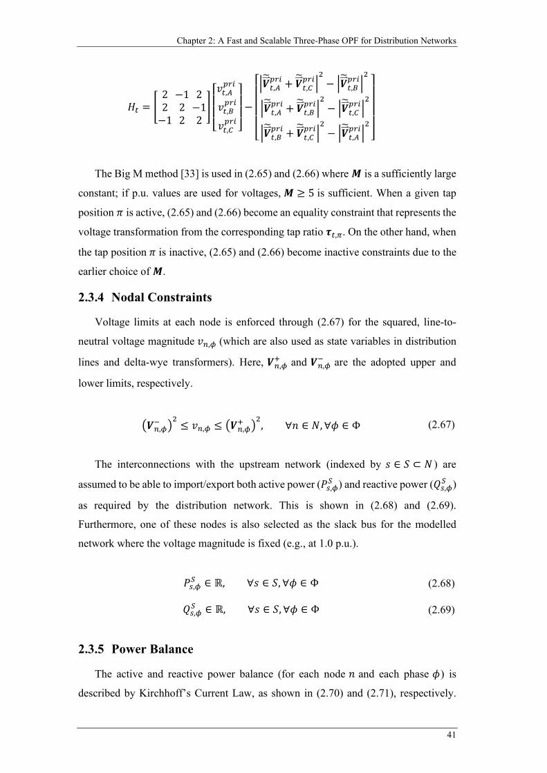
Chapter 2: A Fast and Scalable Three-Phase OPF for Distribution Networks
41
𝐻𝐻𝐶𝐶 = �2 −1 22 2 −1−1 2 2
�
⎣⎢⎢⎡𝑣𝑣𝐶𝐶,𝐴𝐴
𝑝𝑝𝐶𝐶𝐶𝐶
𝑣𝑣𝐶𝐶,𝐵𝐵𝑝𝑝𝐶𝐶𝐶𝐶
𝑣𝑣𝐶𝐶,𝐶𝐶𝑝𝑝𝐶𝐶𝐶𝐶
⎦⎥⎥⎤−
⎣⎢⎢⎢⎢⎡�𝑷𝑷��⃑�𝐶𝐶,𝐴𝐴
𝑝𝑝𝐶𝐶𝐶𝐶 + 𝑷𝑷��⃑�𝐶𝐶,𝐶𝐶𝑝𝑝𝐶𝐶𝐶𝐶�
2− �𝑷𝑷��⃑�𝐶𝐶,𝐵𝐵
𝑝𝑝𝐶𝐶𝐶𝐶�2
�𝑷𝑷��⃑�𝐶𝐶,𝐴𝐴𝑝𝑝𝐶𝐶𝐶𝐶 + 𝑷𝑷��⃑�𝐶𝐶,𝐵𝐵
𝑝𝑝𝐶𝐶𝐶𝐶�2− �𝑷𝑷��⃑�𝐶𝐶,𝐶𝐶
𝑝𝑝𝐶𝐶𝐶𝐶�2
�𝑷𝑷��⃑�𝐶𝐶,𝐵𝐵𝑝𝑝𝐶𝐶𝐶𝐶 + 𝑷𝑷��⃑�𝐶𝐶,𝐶𝐶
𝑝𝑝𝐶𝐶𝐶𝐶�2− �𝑷𝑷��⃑�𝐶𝐶,𝐴𝐴
𝑝𝑝𝐶𝐶𝐶𝐶�2
⎦⎥⎥⎥⎥⎤
The Big M method [33] is used in (2.65) and (2.66) where 𝑴𝑴 is a sufficiently large
constant; if p.u. values are used for voltages, 𝑴𝑴 ≥ 5 is sufficient. When a given tap
position 𝜋𝜋 is active, (2.65) and (2.66) become an equality constraint that represents the
voltage transformation from the corresponding tap ratio 𝝉𝝉𝐶𝐶,𝜋𝜋. On the other hand, when
the tap position 𝜋𝜋 is inactive, (2.65) and (2.66) become inactive constraints due to the
earlier choice of 𝑴𝑴.
2.3.4 Nodal Constraints
Voltage limits at each node is enforced through (2.67) for the squared, line-to-
neutral voltage magnitude 𝑣𝑣𝑛𝑛,𝜙𝜙 (which are also used as state variables in distribution
lines and delta-wye transformers). Here, 𝑷𝑷𝑛𝑛,𝜙𝜙+ and 𝑷𝑷𝑛𝑛,𝜙𝜙
− are the adopted upper and
lower limits, respectively.
�𝑷𝑷𝑛𝑛,𝜙𝜙− �
2≤ 𝑣𝑣𝑛𝑛,𝜙𝜙 ≤ �𝑷𝑷𝑛𝑛,𝜙𝜙
+ �2
, ∀𝑠𝑠 ∈ 𝑁𝑁,∀𝜙𝜙 ∈ Φ (2.67)
The interconnections with the upstream network (indexed by 𝑐𝑐 ∈ 𝑆𝑆 ⊂ 𝑁𝑁 ) are
assumed to be able to import/export both active power (𝑃𝑃𝑠𝑠,𝜙𝜙𝑆𝑆 ) and reactive power (𝑄𝑄𝑠𝑠,𝜙𝜙
𝑆𝑆 )
as required by the distribution network. This is shown in (2.68) and (2.69).
Furthermore, one of these nodes is also selected as the slack bus for the modelled
network where the voltage magnitude is fixed (e.g., at 1.0 p.u.).
𝑃𝑃𝑠𝑠,𝜙𝜙𝑆𝑆 ∈ ℝ, ∀𝑐𝑐 ∈ 𝑆𝑆,∀𝜙𝜙 ∈ Φ (2.68)
𝑄𝑄𝑠𝑠,𝜙𝜙𝑆𝑆 ∈ ℝ, ∀𝑐𝑐 ∈ 𝑆𝑆,∀𝜙𝜙 ∈ Φ (2.69)
2.3.5 Power Balance
The active and reactive power balance (for each node 𝑠𝑠 and each phase 𝜙𝜙) is
described by Kirchhoff’s Current Law, as shown in (2.70) and (2.71), respectively.
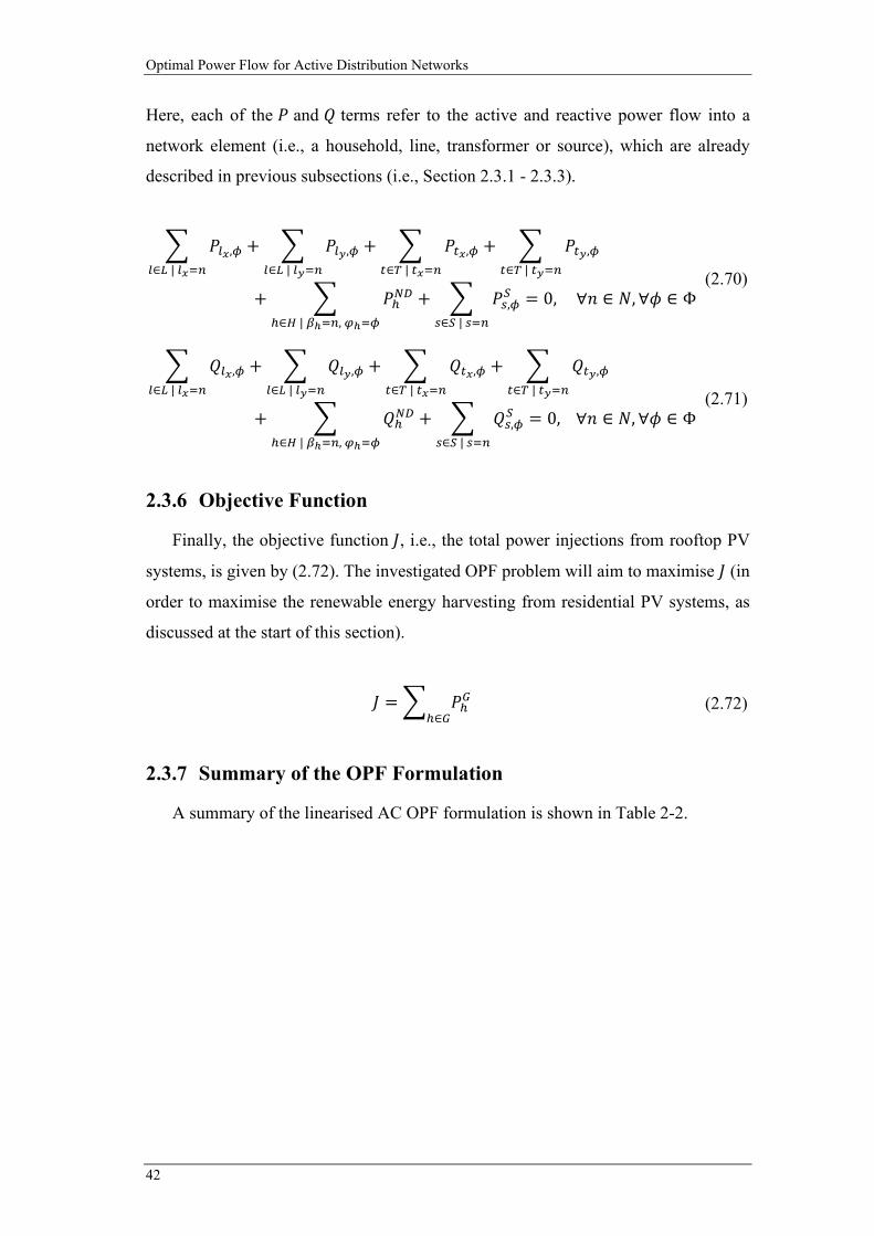
Optimal Power Flow for Active Distribution Networks
42
Here, each of the 𝑃𝑃 and 𝑄𝑄 terms refer to the active and reactive power flow into a
network element (i.e., a household, line, transformer or source), which are already
described in previous subsections (i.e., Section 2.3.1 - 2.3.3).
� 𝑃𝑃𝐶𝐶𝑥𝑥,𝜙𝜙𝐶𝐶∈𝐿𝐿 | 𝐶𝐶𝑥𝑥=𝑛𝑛
+ � 𝑃𝑃𝐶𝐶𝑦𝑦,𝜙𝜙𝐶𝐶∈𝐿𝐿 | 𝐶𝐶𝑦𝑦=𝑛𝑛
+ � 𝑃𝑃𝐶𝐶𝑥𝑥,𝜙𝜙𝐶𝐶∈𝑇𝑇 | 𝐶𝐶𝑥𝑥=𝑛𝑛
+ � 𝑃𝑃𝐶𝐶𝑦𝑦,𝜙𝜙𝐶𝐶∈𝑇𝑇 | 𝐶𝐶𝑦𝑦=𝑛𝑛
+ � 𝑃𝑃ℎ𝑁𝑁𝑁𝑁
ℎ∈𝐻𝐻 | 𝛽𝛽ℎ=𝑛𝑛, 𝜑𝜑ℎ=𝜙𝜙
+ � 𝑃𝑃𝑠𝑠,𝜙𝜙𝑆𝑆
𝑠𝑠∈𝑆𝑆 | 𝑠𝑠=𝑛𝑛
= 0, ∀𝑠𝑠 ∈ 𝑁𝑁,∀𝜙𝜙 ∈ Φ (2.70)
� 𝑄𝑄𝐶𝐶𝑥𝑥,𝜙𝜙𝐶𝐶∈𝐿𝐿 | 𝐶𝐶𝑥𝑥=𝑛𝑛
+ � 𝑄𝑄𝐶𝐶𝑦𝑦,𝜙𝜙𝐶𝐶∈𝐿𝐿 | 𝐶𝐶𝑦𝑦=𝑛𝑛
+ � 𝑄𝑄𝐶𝐶𝑥𝑥,𝜙𝜙𝐶𝐶∈𝑇𝑇 | 𝐶𝐶𝑥𝑥=𝑛𝑛
+ � 𝑄𝑄𝐶𝐶𝑦𝑦,𝜙𝜙𝐶𝐶∈𝑇𝑇 | 𝐶𝐶𝑦𝑦=𝑛𝑛
+ � 𝑄𝑄ℎ𝑁𝑁𝑁𝑁
ℎ∈𝐻𝐻 | 𝛽𝛽ℎ=𝑛𝑛, 𝜑𝜑ℎ=𝜙𝜙
+ � 𝑄𝑄𝑠𝑠,𝜙𝜙𝑆𝑆
𝑠𝑠∈𝑆𝑆 | 𝑠𝑠=𝑛𝑛
= 0, ∀𝑠𝑠 ∈ 𝑁𝑁,∀𝜙𝜙 ∈ Φ (2.71)
2.3.6 Objective Function
Finally, the objective function 𝐽𝐽, i.e., the total power injections from rooftop PV
systems, is given by (2.72). The investigated OPF problem will aim to maximise 𝐽𝐽 (in
order to maximise the renewable energy harvesting from residential PV systems, as
discussed at the start of this section).
𝐽𝐽 = � 𝑃𝑃ℎ𝐺𝐺ℎ∈𝐺𝐺
(2.72)
2.3.7 Summary of the OPF Formulation
A summary of the linearised AC OPF formulation is shown in Table 2-2.
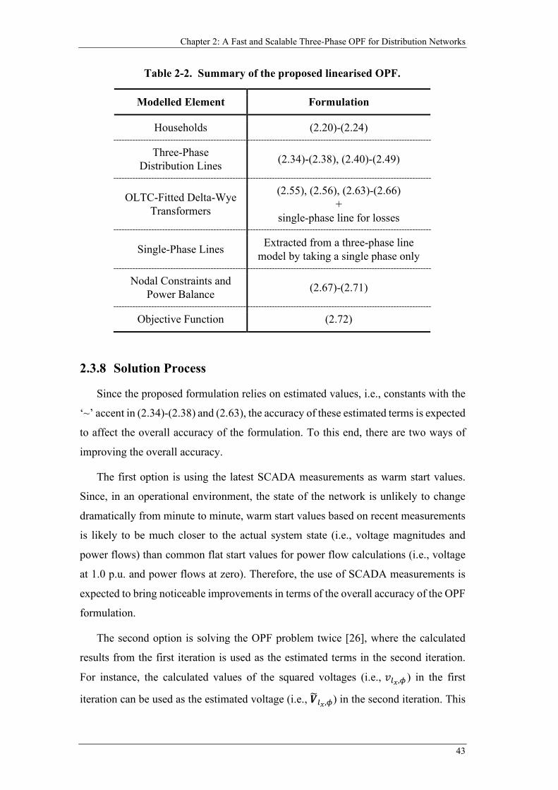
Chapter 2: A Fast and Scalable Three-Phase OPF for Distribution Networks
43
2.3.8 Solution Process
Since the proposed formulation relies on estimated values, i.e., constants with the
‘~’ accent in (2.34)-(2.38) and (2.63), the accuracy of these estimated terms is expected
to affect the overall accuracy of the formulation. To this end, there are two ways of
improving the overall accuracy.
The first option is using the latest SCADA measurements as warm start values.
Since, in an operational environment, the state of the network is unlikely to change
dramatically from minute to minute, warm start values based on recent measurements
is likely to be much closer to the actual system state (i.e., voltage magnitudes and
power flows) than common flat start values for power flow calculations (i.e., voltage
at 1.0 p.u. and power flows at zero). Therefore, the use of SCADA measurements is
expected to bring noticeable improvements in terms of the overall accuracy of the OPF
formulation.
The second option is solving the OPF problem twice [26], where the calculated
results from the first iteration is used as the estimated terms in the second iteration.
For instance, the calculated values of the squared voltages (i.e., 𝑣𝑣𝐶𝐶𝑥𝑥,𝜙𝜙 ) in the first
iteration can be used as the estimated voltage (i.e., 𝑷𝑷�𝐶𝐶𝑥𝑥,𝜙𝜙) in the second iteration. This
Table 2-2. Summary of the proposed linearised OPF.
Modelled Element Formulation
Households (2.20)-(2.24)
Three-Phase Distribution Lines (2.34)-(2.38), (2.40)-(2.49)
OLTC-Fitted Delta-Wye Transformers
(2.55), (2.56), (2.63)-(2.66) +
single-phase line for losses
Single-Phase Lines Extracted from a three-phase line model by taking a single phase only
Nodal Constraints and Power Balance (2.67)-(2.71)
Objective Function (2.72)
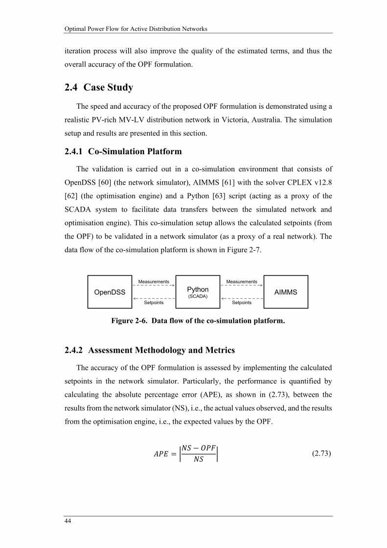
Optimal Power Flow for Active Distribution Networks
44
iteration process will also improve the quality of the estimated terms, and thus the
overall accuracy of the OPF formulation.
2.4 Case Study
The speed and accuracy of the proposed OPF formulation is demonstrated using a
realistic PV-rich MV-LV distribution network in Victoria, Australia. The simulation
setup and results are presented in this section.
2.4.1 Co-Simulation Platform
The validation is carried out in a co-simulation environment that consists of
OpenDSS [60] (the network simulator), AIMMS [61] with the solver CPLEX v12.8
[62] (the optimisation engine) and a Python [63] script (acting as a proxy of the
SCADA system to facilitate data transfers between the simulated network and
optimisation engine). This co-simulation setup allows the calculated setpoints (from
the OPF) to be validated in a network simulator (as a proxy of a real network). The
data flow of the co-simulation platform is shown in Figure 2-7.
2.4.2 Assessment Methodology and Metrics
The accuracy of the OPF formulation is assessed by implementing the calculated
setpoints in the network simulator. Particularly, the performance is quantified by
calculating the absolute percentage error (APE), as shown in (2.73), between the
results from the network simulator (NS), i.e., the actual values observed, and the results
from the optimisation engine, i.e., the expected values by the OPF.
𝐴𝐴𝑃𝑃𝐴𝐴 = �𝑁𝑁𝑆𝑆 − 𝑂𝑂𝑃𝑃𝑂𝑂
𝑁𝑁𝑆𝑆� (2.73)
Figure 2-6. Data flow of the co-simulation platform.
Measurements Measurements
SetpointsSetpoints
OpenDSS Python(SCADA)
AIMMS
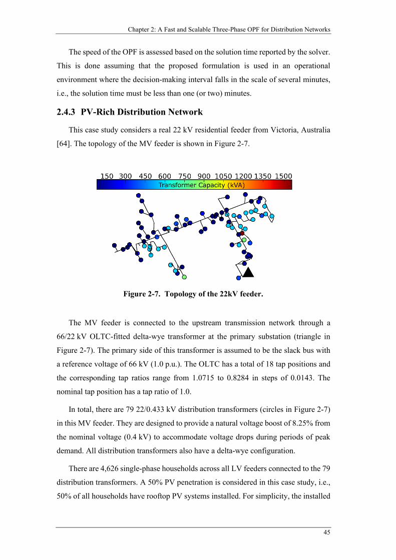
Chapter 2: A Fast and Scalable Three-Phase OPF for Distribution Networks
45
The speed of the OPF is assessed based on the solution time reported by the solver.
This is done assuming that the proposed formulation is used in an operational
environment where the decision-making interval falls in the scale of several minutes,
i.e., the solution time must be less than one (or two) minutes.
2.4.3 PV-Rich Distribution Network
This case study considers a real 22 kV residential feeder from Victoria, Australia
[64]. The topology of the MV feeder is shown in Figure 2-7.
The MV feeder is connected to the upstream transmission network through a
66/22 kV OLTC-fitted delta-wye transformer at the primary substation (triangle in
Figure 2-7). The primary side of this transformer is assumed to be the slack bus with
a reference voltage of 66 kV (1.0 p.u.). The OLTC has a total of 18 tap positions and
the corresponding tap ratios range from 1.0715 to 0.8284 in steps of 0.0143. The
nominal tap position has a tap ratio of 1.0.
In total, there are 79 22/0.433 kV distribution transformers (circles in Figure 2-7)
in this MV feeder. They are designed to provide a natural voltage boost of 8.25% from
the nominal voltage (0.4 kV) to accommodate voltage drops during periods of peak
demand. All distribution transformers also have a delta-wye configuration.
There are 4,626 single-phase households across all LV feeders connected to the 79
distribution transformers. A 50% PV penetration is considered in this case study, i.e.,
50% of all households have rooftop PV systems installed. For simplicity, the installed
Figure 2-7. Topology of the 22kV feeder.

Optimal Power Flow for Active Distribution Networks
46
capacity of each household is assumed be 5 kW. A large pool of anonymized smart
meter data (at 30-min time resolution) is used as the demand profile for each household.
Nonetheless, only two snapshots are considered in this analysis, as discussed in the
following sub-section.
2.4.4 Investigated Cases
In addition to quantifying the accuracy and speed of the proposed formulation (as
discussed in Section 2.4.2), the potential improvements from warm start values and
second OPF iteration (as discussed in Section 2.3.8) are also investigated.
To this end, two different snapshots (i.e., time instances) on a weekday are
considered for this case study. The first instance is noon, where there is sufficient
sunlight such that all rooftop PV systems can generate at their maximum rated capacity.
Due to the coincidence of high PV generation and low residential demand, curtailment
is expected during this period. The second instance is late afternoon where, due to the
lower irradiance, PV systems can only generate at 20% of their rated capacity. In
contrast to noon, much lower curtailment (if any) is expected as a result of the
simultaneous reduction in PV generation and increase in demand (e.g., from people
returning home after work). For both snapshots, three potential tap positions are
considered: nominal (0), one up (+1) to boost voltage and one down (-1) to lower
voltage.
Based on the above, there are a total of eight cases considered in this analysis; a
summary of the setup in each case is shown in Table 2-3.
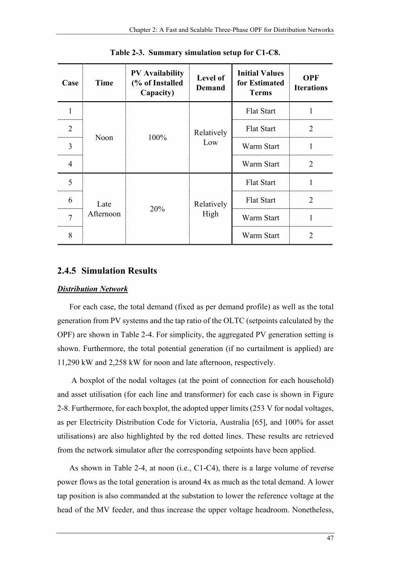
Chapter 2: A Fast and Scalable Three-Phase OPF for Distribution Networks
47
2.4.5 Simulation Results
Distribution Network
For each case, the total demand (fixed as per demand profile) as well as the total
generation from PV systems and the tap ratio of the OLTC (setpoints calculated by the
OPF) are shown in Table 2-4. For simplicity, the aggregated PV generation setting is
shown. Furthermore, the total potential generation (if no curtailment is applied) are
11,290 kW and 2,258 kW for noon and late afternoon, respectively.
A boxplot of the nodal voltages (at the point of connection for each household)
and asset utilisation (for each line and transformer) for each case is shown in Figure
2-8. Furthermore, for each boxplot, the adopted upper limits (253 V for nodal voltages,
as per Electricity Distribution Code for Victoria, Australia [65], and 100% for asset
utilisations) are also highlighted by the red dotted lines. These results are retrieved
from the network simulator after the corresponding setpoints have been applied.
As shown in Table 2-4, at noon (i.e., C1-C4), there is a large volume of reverse
power flows as the total generation is around 4x as much as the total demand. A lower
tap position is also commanded at the substation to lower the reference voltage at the
head of the MV feeder, and thus increase the upper voltage headroom. Nonetheless,
Table 2-3. Summary simulation setup for C1-C8.
Case Time PV Availability (% of Installed
Capacity)
Level of Demand
Initial Values for Estimated
Terms
OPF Iterations
1
Noon 100% Relatively Low
Flat Start 1
2 Flat Start 2
3 Warm Start 1
4 Warm Start 2
5
Late Afternoon 20% Relatively
High
Flat Start 1
6 Flat Start 2
7 Warm Start 1
8 Warm Start 2
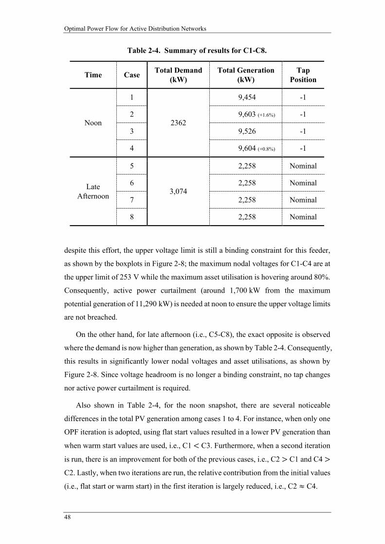
Optimal Power Flow for Active Distribution Networks
48
despite this effort, the upper voltage limit is still a binding constraint for this feeder,
as shown by the boxplots in Figure 2-8; the maximum nodal voltages for C1-C4 are at
the upper limit of 253 V while the maximum asset utilisation is hovering around 80%.
Consequently, active power curtailment (around 1,700 kW from the maximum
potential generation of 11,290 kW) is needed at noon to ensure the upper voltage limits
are not breached.
On the other hand, for late afternoon (i.e., C5-C8), the exact opposite is observed
where the demand is now higher than generation, as shown by Table 2-4. Consequently,
this results in significantly lower nodal voltages and asset utilisations, as shown by
Figure 2-8. Since voltage headroom is no longer a binding constraint, no tap changes
nor active power curtailment is required.
Also shown in Table 2-4, for the noon snapshot, there are several noticeable
differences in the total PV generation among cases 1 to 4. For instance, when only one
OPF iteration is adopted, using flat start values resulted in a lower PV generation than
when warm start values are used, i.e., C1 < C3. Furthermore, when a second iteration
is run, there is an improvement for both of the previous cases, i.e., C2 > C1 and C4 >
C2. Lastly, when two iterations are run, the relative contribution from the initial values
(i.e., flat start or warm start) in the first iteration is largely reduced, i.e., C2 ≈ C4.
Table 2-4. Summary of results for C1-C8.
Time Case Total Demand (kW)
Total Generation (kW)
Tap Position
Noon
1
2362
9,454 -1
2 9,603 (+1.6%) -1
3 9,526 -1
4 9,604 (+0.8%) -1
Late Afternoon
5
3,074
2,258 Nominal
6 2,258 Nominal
7 2,258 Nominal
8 2,258 Nominal
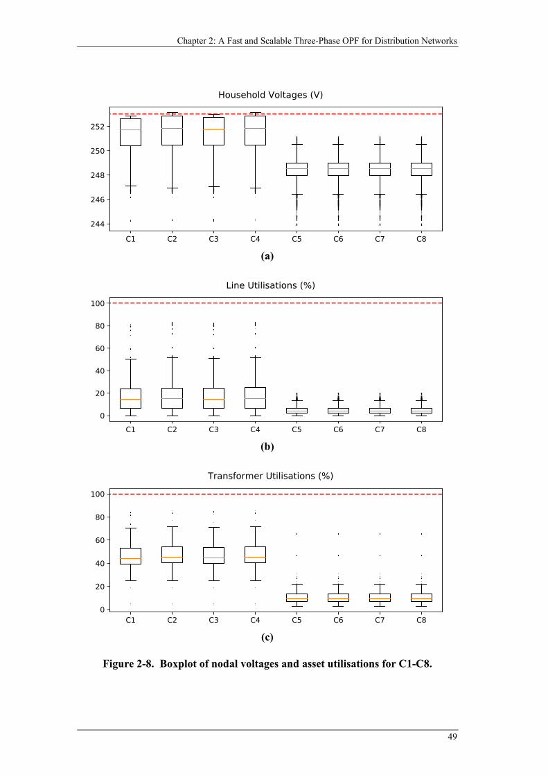
Chapter 2: A Fast and Scalable Three-Phase OPF for Distribution Networks
49
(a)
(b)
(c)
Figure 2-8. Boxplot of nodal voltages and asset utilisations for C1-C8.
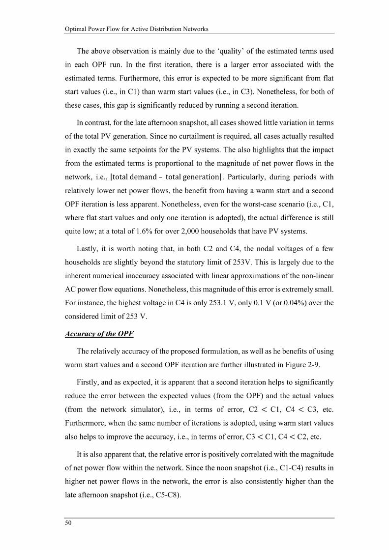
Optimal Power Flow for Active Distribution Networks
50
The above observation is mainly due to the ‘quality’ of the estimated terms used
in each OPF run. In the first iteration, there is a larger error associated with the
estimated terms. Furthermore, this error is expected to be more significant from flat
start values (i.e., in C1) than warm start values (i.e., in C3). Nonetheless, for both of
these cases, this gap is significantly reduced by running a second iteration.
In contrast, for the late afternoon snapshot, all cases showed little variation in terms
of the total PV generation. Since no curtailment is required, all cases actually resulted
in exactly the same setpoints for the PV systems. The also highlights that the impact
from the estimated terms is proportional to the magnitude of net power flows in the
network, i.e., |total demand – total generation|. Particularly, during periods with
relatively lower net power flows, the benefit from having a warm start and a second
OPF iteration is less apparent. Nonetheless, even for the worst-case scenario (i.e., C1,
where flat start values and only one iteration is adopted), the actual difference is still
quite low; at a total of 1.6% for over 2,000 households that have PV systems.
Lastly, it is worth noting that, in both C2 and C4, the nodal voltages of a few
households are slightly beyond the statutory limit of 253V. This is largely due to the
inherent numerical inaccuracy associated with linear approximations of the non-linear
AC power flow equations. Nonetheless, this magnitude of this error is extremely small.
For instance, the highest voltage in C4 is only 253.1 V, only 0.1 V (or 0.04%) over the
considered limit of 253 V.
Accuracy of the OPF
The relatively accuracy of the proposed formulation, as well as he benefits of using
warm start values and a second OPF iteration are further illustrated in Figure 2-9.
Firstly, and as expected, it is apparent that a second iteration helps to significantly
reduce the error between the expected values (from the OPF) and the actual values
(from the network simulator), i.e., in terms of error, C2 < C1, C4 < C3, etc.
Furthermore, when the same number of iterations is adopted, using warm start values
also helps to improve the accuracy, i.e., in terms of error, C3 < C1, C4 < C2, etc.
It is also apparent that, the relative error is positively correlated with the magnitude
of net power flow within the network. Since the noon snapshot (i.e., C1-C4) results in
higher net power flows in the network, the error is also consistently higher than the
late afternoon snapshot (i.e., C5-C8).
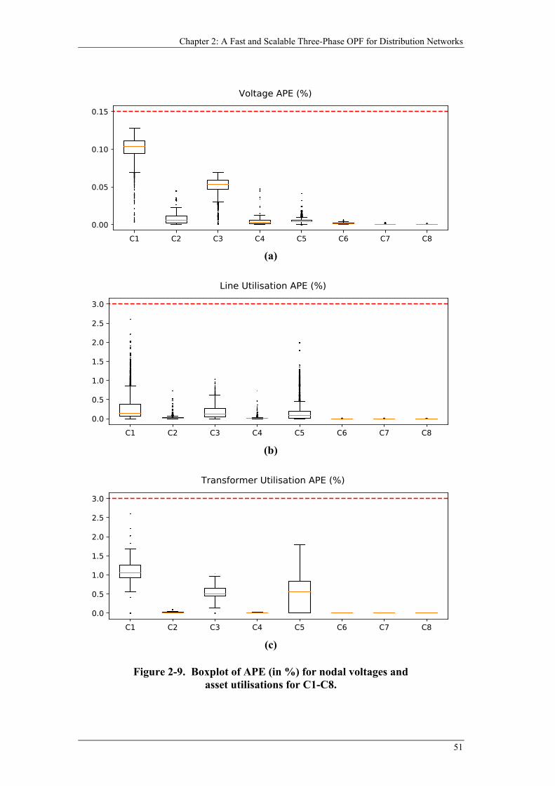
Chapter 2: A Fast and Scalable Three-Phase OPF for Distribution Networks
51
(a)
(b)
(c)
Figure 2-9. Boxplot of APE (in %) for nodal voltages and
asset utilisations for C1-C8.

Optimal Power Flow for Active Distribution Networks
52
Finally, despite noticeable accuracy improvements from using warm start values
and a second OPF iteration, the accuracy of the worst-case (i.e., C1 where only flat
start values and one OPF iteration is adopted) is still fairly small: below 0.15% for
nodal voltages and 3% for asset utilisation. Therefore, although two iterations are
desirable from an accuracy perspective, it will incur extra computation time as the
same OPF problem must be solved twice.
2.4.6 OPF Solution Time
The simulation PC used has an i7 processor with 32GB of RAM. The computation
time of the first iteration is around 25 seconds. For cases 2, 4, 6 and 8, the second
iteration around 15 seconds, which is consistently faster than the first iteration.
2.5 Error in Linearised OPF Formulation
For completeness, and also to complement the findings in Section 2.4.5, an
additional analysis of the error associated with the linearised three-phase line model
(presented in Section 2.3.2) and delta-wye transformer model (presented in Section
2.3.3) are investigated in this subsection.
2.5.1 Error in Linearised Three-Phase Line Model
Power Flow Model
As discussed in Section 2.3.2, the accuracy of the linearised power flow model for
three-phase lines depend on the accuracy of estimated voltage and power terms, i.e.,
the terms with the ~ accent in (2.28)-(2.30). Therefore, the following analysis aims to
explore the impact of different inaccuracies in these estimated terms on the overall
power flow model. Furthermore, the potential improvement from a second OPF
iteration (as discussed in Section 2.3.8) is also investigated.
The test network (an LV feeder) for this analysis is shown in Figure 2-10. It is
modelled based the MV-LV network presented in Section 2.4.3. The head of this LV
feeder is assumed to be the slack bus and its voltage is set to 433 V line-to-line (i.e.,
250 V line-to-neutral). The total impedance is shown in Figure 2-10, which is based
on an 800m long LV feeder (a typical length for the investigated network).
Furthermore, to exaggerate the voltage drop in this LV feeder, all single-phase loads
are lumped at the end of the feeder, also shown in Figure 2-10. It is worth noting that,
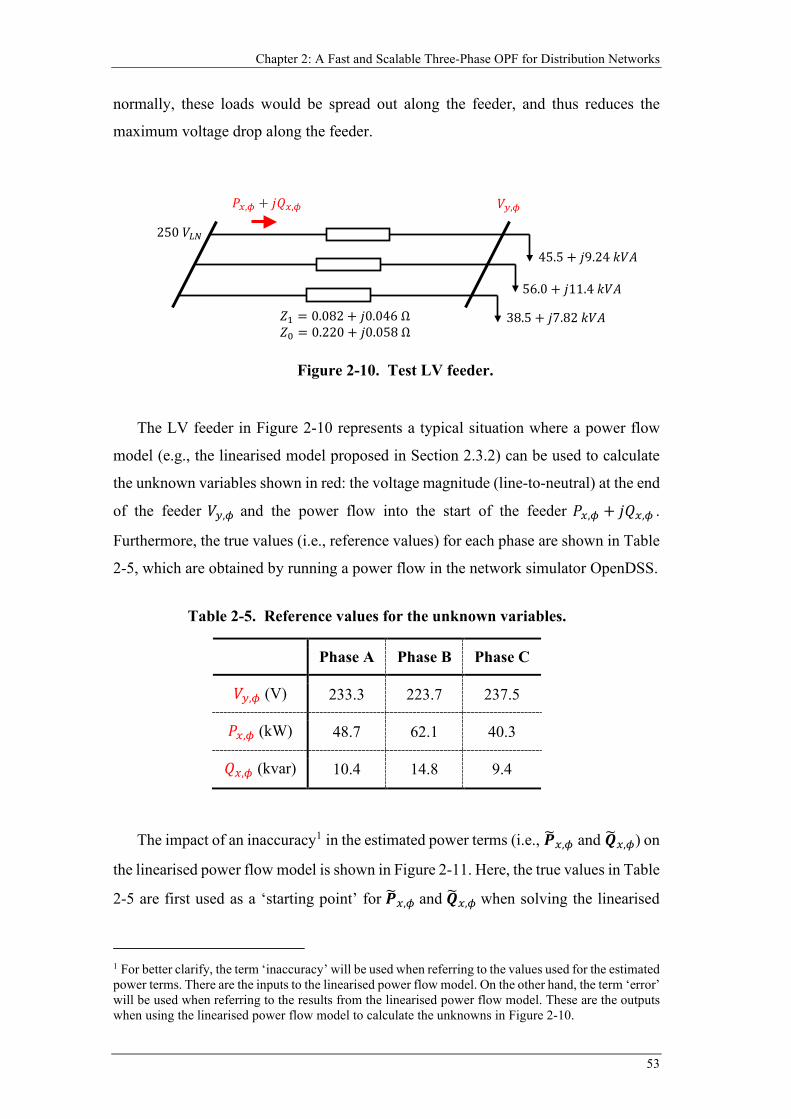
Chapter 2: A Fast and Scalable Three-Phase OPF for Distribution Networks
53
normally, these loads would be spread out along the feeder, and thus reduces the
maximum voltage drop along the feeder.
The LV feeder in Figure 2-10 represents a typical situation where a power flow
model (e.g., the linearised model proposed in Section 2.3.2) can be used to calculate
the unknown variables shown in red: the voltage magnitude (line-to-neutral) at the end
of the feeder 𝑉𝑉𝑦𝑦,𝜙𝜙 and the power flow into the start of the feeder 𝑃𝑃𝑥𝑥,𝜙𝜙 + 𝑗𝑗𝑄𝑄𝑥𝑥,𝜙𝜙 .
Furthermore, the true values (i.e., reference values) for each phase are shown in Table
2-5, which are obtained by running a power flow in the network simulator OpenDSS.
The impact of an inaccuracy1 in the estimated power terms (i.e., 𝑷𝑷�𝑥𝑥,𝜙𝜙 and 𝑸𝑸�𝑥𝑥,𝜙𝜙) on
the linearised power flow model is shown in Figure 2-11. Here, the true values in Table
2-5 are first used as a ‘starting point’ for 𝑷𝑷�𝑥𝑥,𝜙𝜙 and 𝑸𝑸�𝑥𝑥,𝜙𝜙 when solving the linearised
1 For better clarify, the term ‘inaccuracy’ will be used when referring to the values used for the estimated power terms. There are the inputs to the linearised power flow model. On the other hand, the term ‘error’ will be used when referring to the results from the linearised power flow model. These are the outputs when using the linearised power flow model to calculate the unknowns in Figure 2-10.
Figure 2-10. Test LV feeder.
𝑉𝑉𝑦𝑦,𝜙𝜙𝑃𝑃𝑥𝑥,𝜙𝜙 + 𝑗𝑗𝑄𝑄𝑥𝑥,𝜙𝜙
250 𝑉𝑉𝐿𝐿𝑁𝑁
38.5 + 𝑗𝑗7.82 𝑘𝑘𝑉𝑉𝐴𝐴
56.0 + 𝑗𝑗11.4 𝑘𝑘𝑉𝑉𝐴𝐴
45.5 + 𝑗𝑗9.24 𝑘𝑘𝑉𝑉𝐴𝐴
𝑍1 = 0.082 + 𝑗𝑗0.046 Ω𝑍0 = 0.220 + 𝑗𝑗0.058 Ω
Table 2-5. Reference values for the unknown variables.
Phase A Phase B Phase C
𝑉𝑉𝑦𝑦,𝜙𝜙 (V) 233.3 223.7 237.5
𝑃𝑃𝑥𝑥,𝜙𝜙 (kW) 48.7 62.1 40.3
𝑄𝑄𝑥𝑥,𝜙𝜙 (kvar) 10.4 14.8 9.4
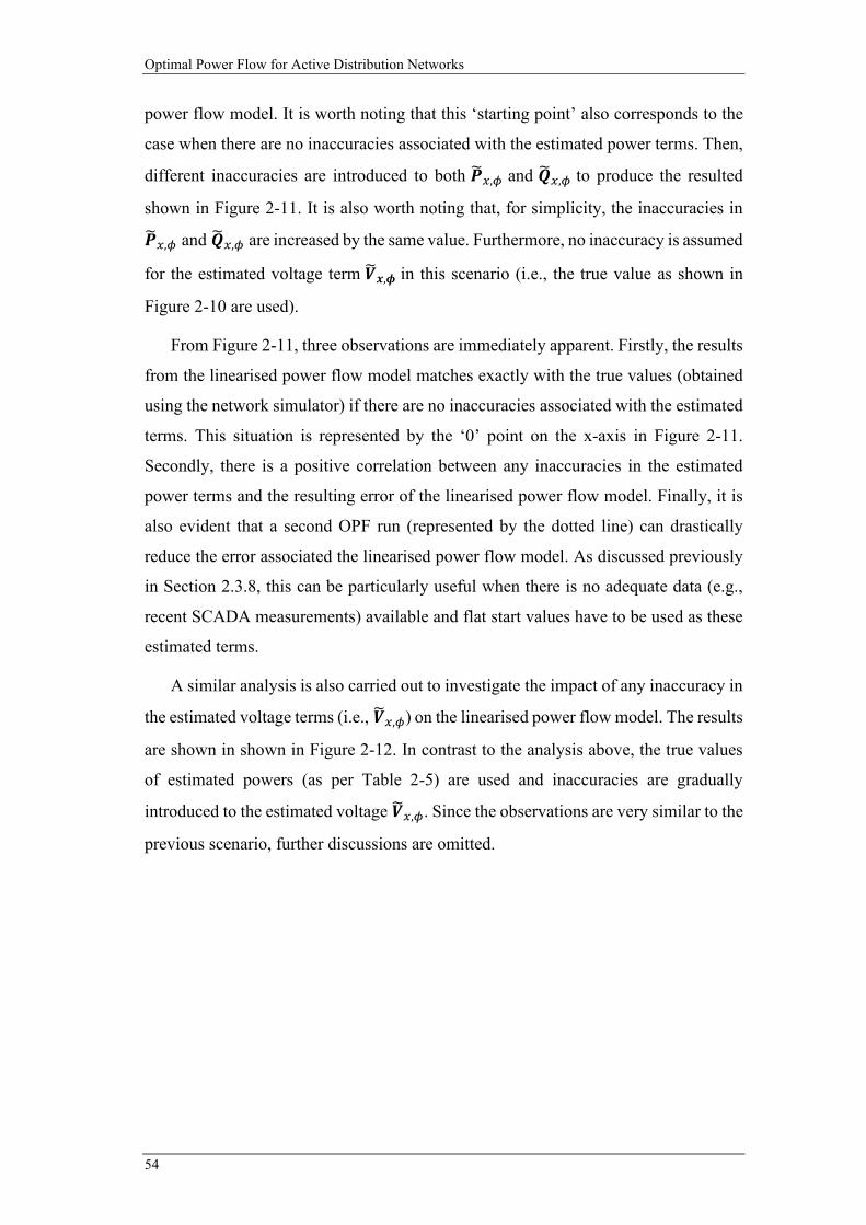
Optimal Power Flow for Active Distribution Networks
54
power flow model. It is worth noting that this ‘starting point’ also corresponds to the
case when there are no inaccuracies associated with the estimated power terms. Then,
different inaccuracies are introduced to both 𝑷𝑷�𝑥𝑥,𝜙𝜙 and 𝑸𝑸�𝑥𝑥,𝜙𝜙 to produce the resulted
shown in Figure 2-11. It is also worth noting that, for simplicity, the inaccuracies in
𝑷𝑷�𝑥𝑥,𝜙𝜙 and 𝑸𝑸�𝑥𝑥,𝜙𝜙 are increased by the same value. Furthermore, no inaccuracy is assumed
for the estimated voltage term 𝑷𝑷�𝒙𝒙,𝝓𝝓 in this scenario (i.e., the true value as shown in
Figure 2-10 are used).
From Figure 2-11, three observations are immediately apparent. Firstly, the results
from the linearised power flow model matches exactly with the true values (obtained
using the network simulator) if there are no inaccuracies associated with the estimated
terms. This situation is represented by the ‘0’ point on the x-axis in Figure 2-11.
Secondly, there is a positive correlation between any inaccuracies in the estimated
power terms and the resulting error of the linearised power flow model. Finally, it is
also evident that a second OPF run (represented by the dotted line) can drastically
reduce the error associated the linearised power flow model. As discussed previously
in Section 2.3.8, this can be particularly useful when there is no adequate data (e.g.,
recent SCADA measurements) available and flat start values have to be used as these
estimated terms.
A similar analysis is also carried out to investigate the impact of any inaccuracy in
the estimated voltage terms (i.e., 𝑷𝑷�𝑥𝑥,𝜙𝜙) on the linearised power flow model. The results
are shown in shown in Figure 2-12. In contrast to the analysis above, the true values
of estimated powers (as per Table 2-5) are used and inaccuracies are gradually
introduced to the estimated voltage 𝑷𝑷�𝑥𝑥,𝜙𝜙. Since the observations are very similar to the
previous scenario, further discussions are omitted.
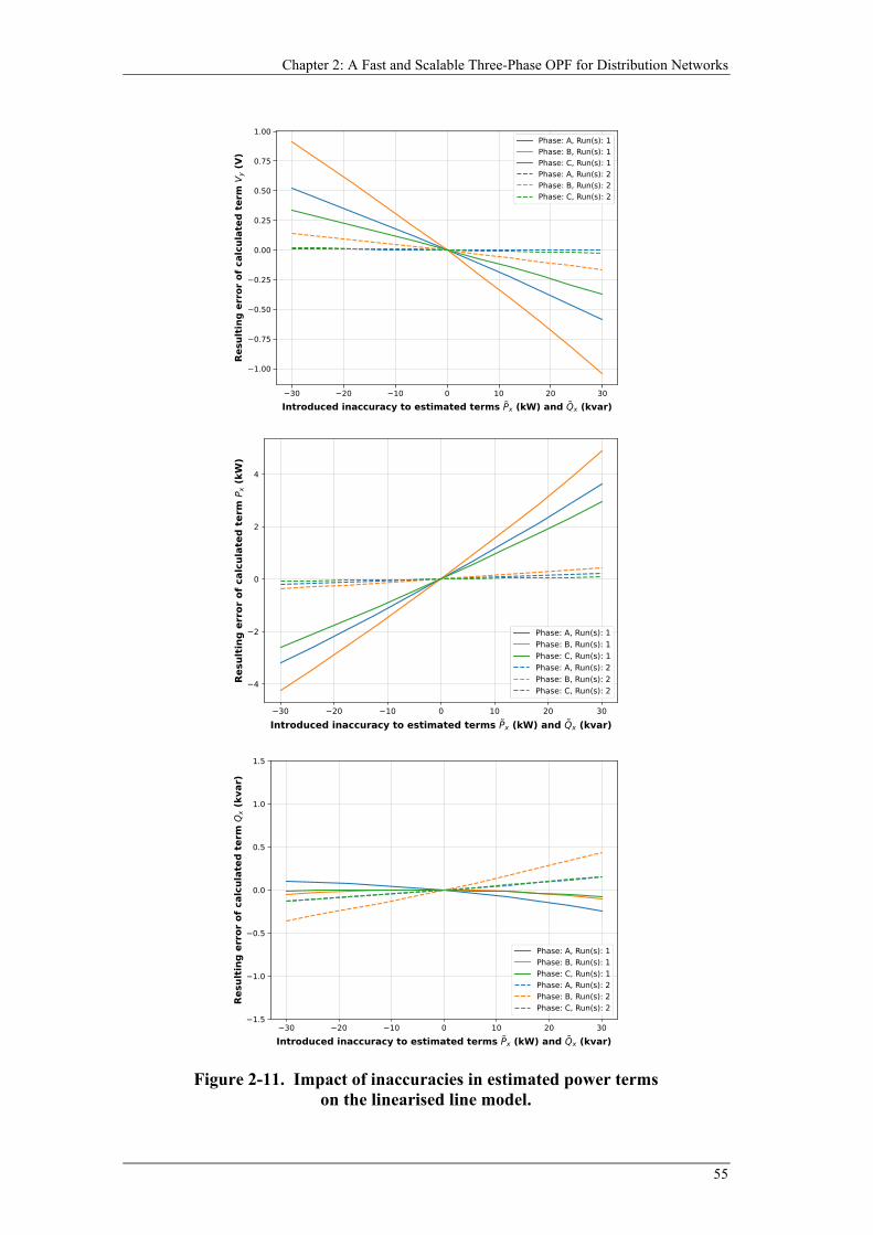
Chapter 2: A Fast and Scalable Three-Phase OPF for Distribution Networks
55
Figure 2-11. Impact of inaccuracies in estimated power terms on the linearised line model.
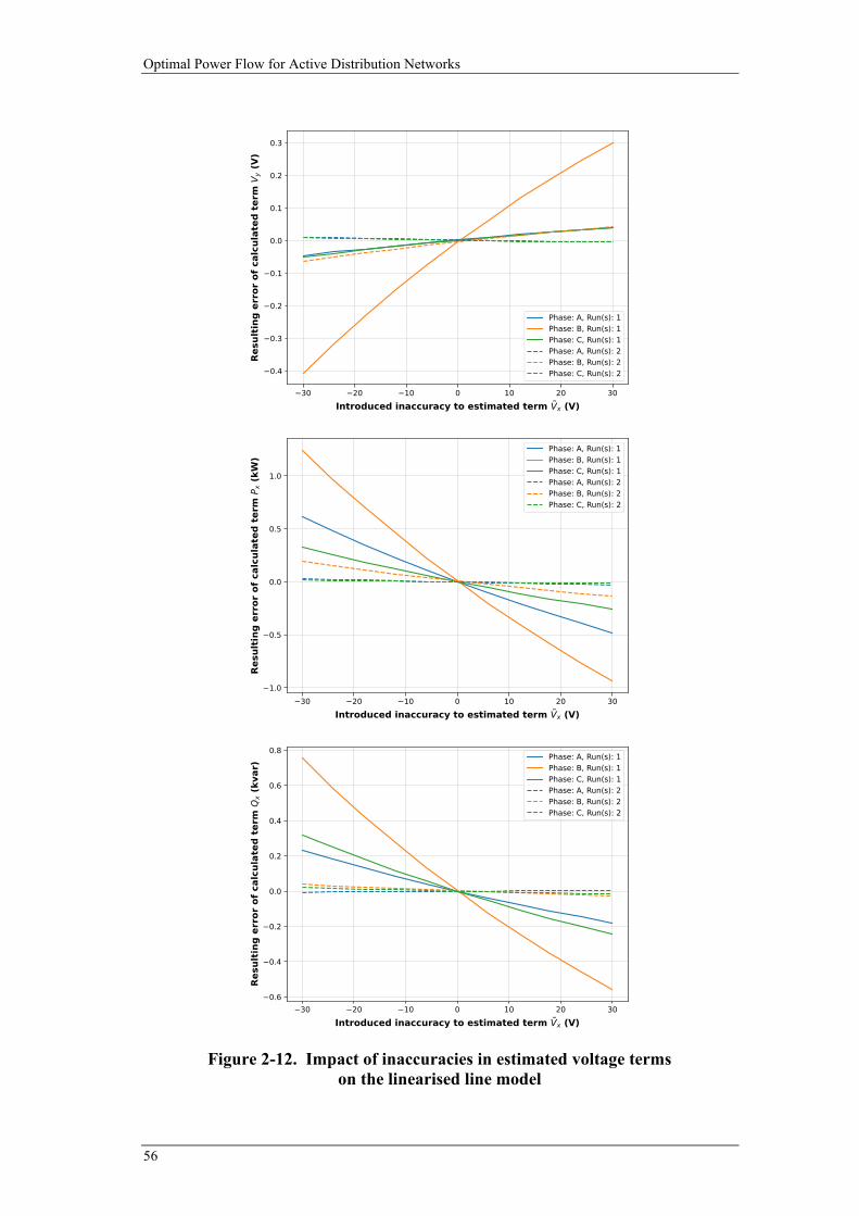
Optimal Power Flow for Active Distribution Networks
56
Figure 2-12. Impact of inaccuracies in estimated voltage terms on the linearised line model
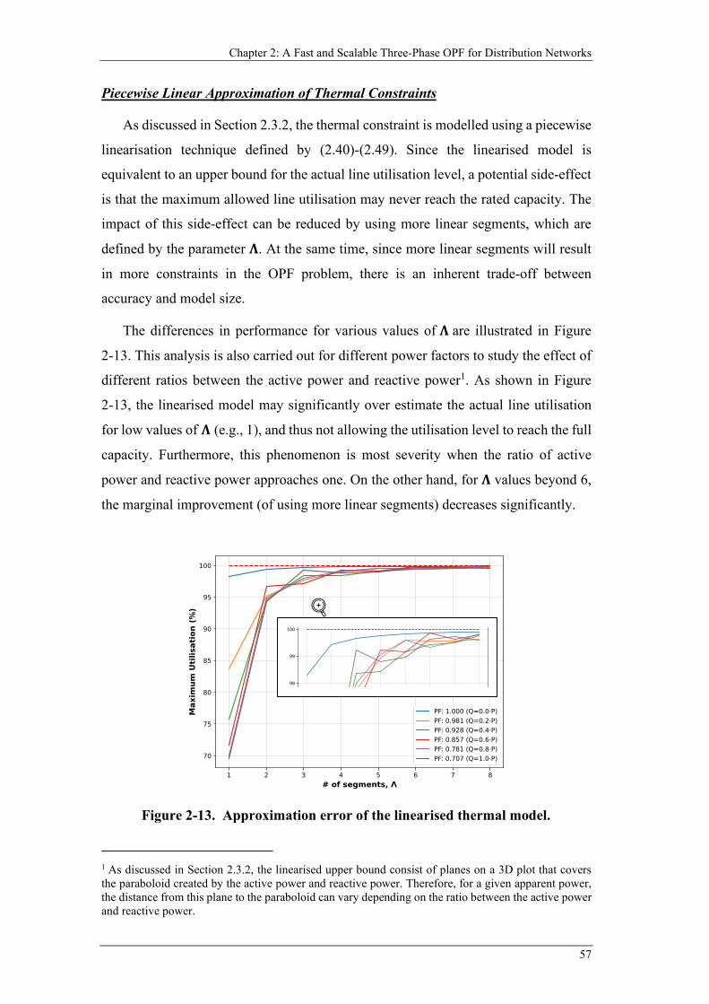
Chapter 2: A Fast and Scalable Three-Phase OPF for Distribution Networks
57
Piecewise Linear Approximation of Thermal Constraints
As discussed in Section 2.3.2, the thermal constraint is modelled using a piecewise
linearisation technique defined by (2.40)-(2.49). Since the linearised model is
equivalent to an upper bound for the actual line utilisation level, a potential side-effect
is that the maximum allowed line utilisation may never reach the rated capacity. The
impact of this side-effect can be reduced by using more linear segments, which are
defined by the parameter 𝚲𝚲. At the same time, since more linear segments will result
in more constraints in the OPF problem, there is an inherent trade-off between
accuracy and model size.
The differences in performance for various values of 𝚲𝚲 are illustrated in Figure
2-13. This analysis is also carried out for different power factors to study the effect of
different ratios between the active power and reactive power1. As shown in Figure
2-13, the linearised model may significantly over estimate the actual line utilisation
for low values of 𝚲𝚲 (e.g., 1), and thus not allowing the utilisation level to reach the full
capacity. Furthermore, this phenomenon is most severity when the ratio of active
power and reactive power approaches one. On the other hand, for 𝚲𝚲 values beyond 6,
the marginal improvement (of using more linear segments) decreases significantly.
1 As discussed in Section 2.3.2, the linearised upper bound consist of planes on a 3D plot that covers the paraboloid created by the active power and reactive power. Therefore, for a given apparent power, the distance from this plane to the paraboloid can vary depending on the ratio between the active power and reactive power.
Figure 2-13. Approximation error of the linearised thermal model.
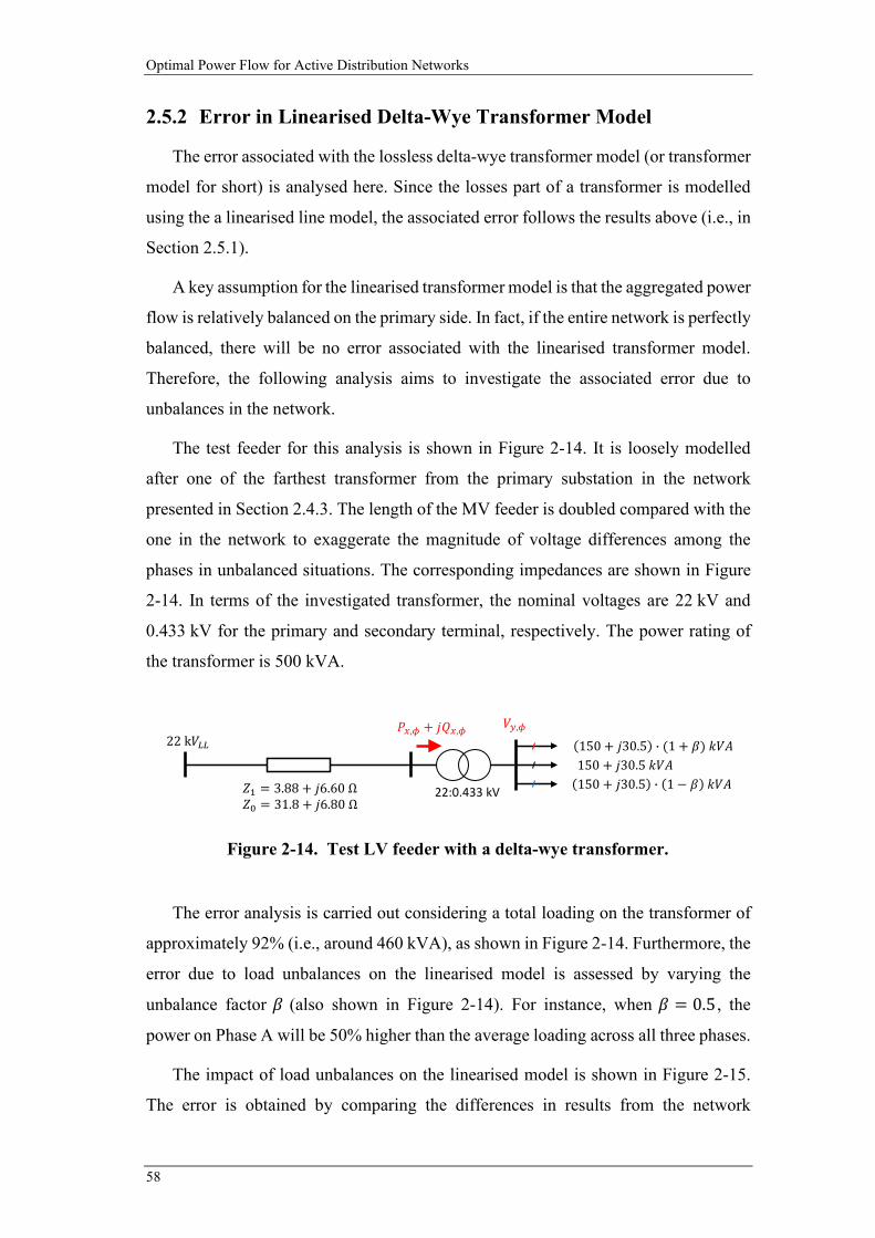
Optimal Power Flow for Active Distribution Networks
58
2.5.2 Error in Linearised Delta-Wye Transformer Model
The error associated with the lossless delta-wye transformer model (or transformer
model for short) is analysed here. Since the losses part of a transformer is modelled
using the a linearised line model, the associated error follows the results above (i.e., in
Section 2.5.1).
A key assumption for the linearised transformer model is that the aggregated power
flow is relatively balanced on the primary side. In fact, if the entire network is perfectly
balanced, there will be no error associated with the linearised transformer model.
Therefore, the following analysis aims to investigate the associated error due to
unbalances in the network.
The test feeder for this analysis is shown in Figure 2-14. It is loosely modelled
after one of the farthest transformer from the primary substation in the network
presented in Section 2.4.3. The length of the MV feeder is doubled compared with the
one in the network to exaggerate the magnitude of voltage differences among the
phases in unbalanced situations. The corresponding impedances are shown in Figure
2-14. In terms of the investigated transformer, the nominal voltages are 22 kV and
0.433 kV for the primary and secondary terminal, respectively. The power rating of
the transformer is 500 kVA.
The error analysis is carried out considering a total loading on the transformer of
approximately 92% (i.e., around 460 kVA), as shown in Figure 2-14. Furthermore, the
error due to load unbalances on the linearised model is assessed by varying the
unbalance factor 𝛽𝛽 (also shown in Figure 2-14). For instance, when 𝛽𝛽 = 0.5 , the
power on Phase A will be 50% higher than the average loading across all three phases.
The impact of load unbalances on the linearised model is shown in Figure 2-15.
The error is obtained by comparing the differences in results from the network
Figure 2-14. Test LV feeder with a delta-wye transformer.
𝑉𝑉𝑦𝑦,𝜙𝜙𝑃𝑃𝑥𝑥,𝜙𝜙 + 𝑗𝑗𝑄𝑄𝑥𝑥,𝜙𝜙22 k𝑉𝑉𝐿𝐿𝐿𝐿
150 + 𝑗𝑗30.5 𝑘𝑘𝑉𝑉𝐴𝐴
𝑍1 = 3.88 + 𝑗𝑗6.60 Ω𝑍0 = 31.8 + 𝑗𝑗6.80 Ω
150 + 𝑗𝑗30.5 � (1 + 𝛽𝛽) 𝑘𝑘𝑉𝑉𝐴𝐴
150 + 𝑗𝑗30.5 � 1− 𝛽𝛽 𝑘𝑘𝑉𝑉𝐴𝐴22:0.433 kV

Chapter 2: A Fast and Scalable Three-Phase OPF for Distribution Networks
59
simulator OpenDSS and the linearised transformer model. As shown in Figure 2-15, it
is evident that the error increases as the load unbalances increases. Nonetheless, even
at an unbalanced factor of 0.6, the error introduced is negligible compared with the
actual power flows in the network. For instance, the maximum error in 𝑃𝑃𝑥𝑥,𝜙𝜙 is only
around 2.5 kW, which is just over 1.5% compared with the average power flow of
150 kW.
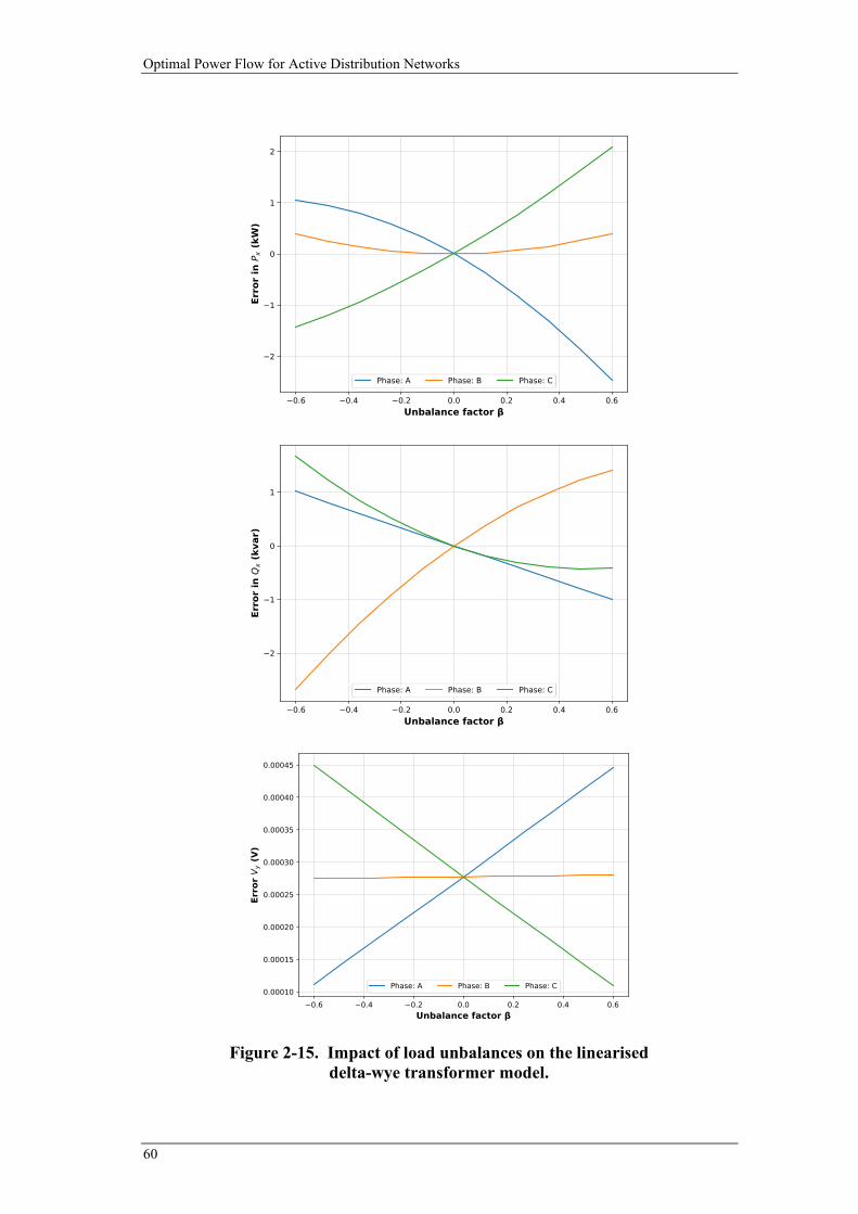
Optimal Power Flow for Active Distribution Networks
60
Figure 2-15. Impact of load unbalances on the linearised delta-wye transformer model.
Chapter 2: A Fast and Scalable Three-Phase OPF for Distribution Networks
61
2.6 Summary
Driven by the rapid growth of DG in recent decades, there has been significant
interests in the real-world application of OPF-based control schemes in distribution
networks. However, due to the non-linear and non-convex nature of classical AC OPF
formulations, there are significant scalability (tractability) and speed challenges of
using OPF in an operational environment.
To this end, a linearised, three-phase AC OPF is proposed in this chapter. The
linearised formulation significantly improves its scalability when dealing with large-
scale distribution networks. Furthermore, thanks to the maturity of mixed-integer
linear programming techniques, it offers an effective way of handling discrete devices
in distribution networks, such as OLTCs. Lastly, a linearised model for delta-wye
transformers is proposed, allowing the realistic modelling of distribution networks
across multiple voltage levels (where the interface is commonly a delta-wye
transformer), such as integrated MV-LV feeders.
The accuracy and speed of the proposed OPF formulation is validated using a
realistic residential MV-LV feeder in Australia that consists of over 4,600 households.
Overall, the proposed linearised, three-phase AC OPF formulation is found to be
sufficiently accurate for determining the optimal setpoints for controllable devices
such as OLTCs and PV systems. Particularly, it achieved an error of less than 1% for
both voltage magnitudes and power flows when validated in a network simulator.
Furthermore, the computation time is found to be within a minute, making its
operational usage technically feasible for similar sized networks.

Optimal Power Flow for Active Distribution Networks
62
This page is intentionally left blank.
3 IMPLEMENTING OPF-BASED SETPOINTS:
CHALLENGES AND SOLUTIONS
3.1 Introduction
The rapid uptake of DG is driving a paradigm shift in future distribution networks
where network assets and participants are managed in real-time so as to facilitate the
bidirectional power flows and ensure network integrity. In this context, and as
demonstrated in Chapter 2, OPF allows network operators to determine the most
appropriate setpoints according to their objective (e.g., maximisation of renewable
energy harvesting) while catering for the distribution network constraints (e.g., steady-
state voltage and thermal limits).
At the same time, apart from being able to calculate these setpoints, the physical
implementation of these setpoints is another crucial aspect that requires careful
considerations in a real-world application of OPF-based schemes. For instance, since
the execution of these setpoints do not happen instantaneously, sub-minute scale
interactions among multiple devices with different delays and ramp rates may lead to
undesirable outcomes that are typically not (or difficult to be) captured by the OPF
problem. Therefore, when multiple devices are being controlled at the same time,
potential differences in their operating characteristics (e.g., delays, ramp rates,
deadbands, etc.) must be catered for so as to ensure OPF-based setpoints can be
adequately implemented in reality.
In this context, the necessary adaptations within existing device controllers as well
as the OPF formulation will be investigated in this chapter, focusing on the adequate
management of MW-scale DG in distribution networks.
3.2 Literature Review
Recognising that OPF can play a crucial role in the day-to-day operation of future
distribution network, there has been significant efforts in the existing literature that
investigates how OPF can be used to orchestrate the various sources of flexibility from
network-connected assets and participants (collectively referred to as controllable
devices), and thus facilitate high penetrations of renewable generation. For instance,
Optimal Power Flow for Active Distribution Networks
64
an OPF-based congestion management scheme is proposed in [66] to minimise the
active power curtailment (of DG units) while ensuring thermal limits are not breached.
The extension to cater for voltage issues are proposed in [8, 67, 68] through the
coordinated control of both the reactive power (of DG units) and existing OLTCs.
Other avenues such as battery storage systems (e.g., [69, 70]), flexible demand (e.g.,
[71]) and network reconfiguration (e.g., [72]) are also proposed to further maximise
the harvesting of renewable energy.
The integration of OPF with other techniques has also been a key focus so as to
cater for the inherent variability of demand and renewable generation. For instance,
chance-constrained OPF (e.g., [35]) is proposed to cater for the uncertainty in wind
power. Particularly, it ensures that the probability of satisfying the OPF constraints is
above a certain threshold for multiple wind generation scenarios. In contrast to this
probabilistic approach, the application of robust optimisation (e.g., [73]) is proposed
where the corresponding constraints for multiple scenarios are satisfied simultaneously,
and thus being robust to these scenarios. Lastly, similar to the non-probabilistic
approach of robust optimisation, the application of information gap decision theory
(e.g., [74]) is also studied to cater for severe uncertainty in demand.
Among these and similar studies, time-series simulations are predominantly used
in order to capture the continuous changes in demand and generation. However, this
is usually done using relatively large time-steps that range from multiple minutes to
hours. Although this is sufficient from an energy perspective (to demonstrate the
underlying concept), it is not adequate to assess the performance of OPF-based
schemes in an operational environment. Particularly, large time-steps cannot capture
the real-time behaviours of controllable devices and the interactions among them,
which typically happen in the sub-minute scale [75, 76]. Therefore, in addition to
capturing the power flows, the real-time and inter-temporal characteristics of devices
(e.g., delays, ramp rates and deadbands) as well as their effects from a control
perspective (e.g., volume of control actions and impacts on the network) must also be
accounted for.
Understanding this, the authors in [36] adopted a 5s time-step to realistically
capture the sequences of control events in an operational environment, from the
calculation of setpoints by using an OPF to the final realisation of these setpoints by
the controllable devices in a network simulator. Then, using this setup, the
Chapter 3: Implementing OPF-Based Setpoints: Challenges and Solutions
65
performance of an OPF-based scheme that produces new setpoints for DG units and
OLTCs every five minutes is evaluated. It has been shown that, although the OPF
solution may satisfy the considered constraints, voltage violations may still occur in
real-time due to the deadbands (an operating characteristic that is typically not
modelled in the OPF) of conventional OLTC controllers. Furthermore, it has been
highlighted that, given the available headroom in a distribution network, there are often
multiple feasible control actions. Consequently, an inadequately designed OPF may
produce discontinuous setpoints from consecutive OPF runs, and thus results in
unnecessary control actions and accelerated wear-and-tear. The proposed solution to
mitigate these issues is by operating away from the statutory limit. While this approach
helps to reduce the impact associated with the deadbands, it does not fully address the
drawbacks associated with conventional OLTC controllers. Furthermore, potential
coordination issues when OLTCs and DG units are being controlled at the same time
were not considered.
This coordination between OLTCs and DG units have been discussed in [77],
where an OPF-based voltage management scheme is proposed. Particularly, a
sequential process is proposed for coordination purposes: reactive power setpoints for
DG units are executed first, then followed by the setpoints for OLTCs. However,
scenarios where the setpoints of these devices are executed at the same time were not
considered. Consequently, potential issues due to the simultaneous actions of OLTCs
and DG units still need to be investigated and tackled.
To this end, the main challenges associated with ensuring OPF-based setpoints can
be adequately implemented in a real-world application are outlined below and further
discussed/addressed in the remainder of this chapter:
• Temporal coordination issues among multiple devices with different delays
and ramp rates
• Deadbands in device controllers (e.g., OLTCs) preventing the precise
enactment of the requested setpoints
• Multiple sets of feasible control actions resulting from the flexibility of several
controllable devices
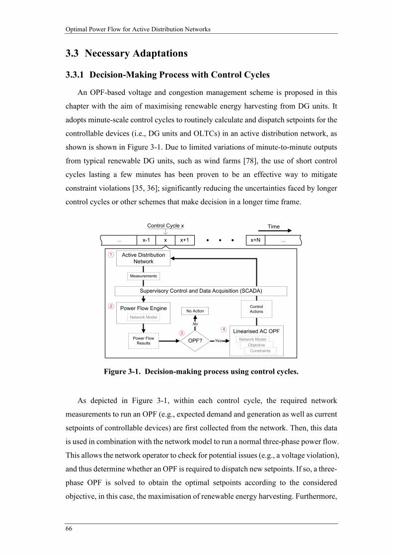
Optimal Power Flow for Active Distribution Networks
66
3.3 Necessary Adaptations
3.3.1 Decision-Making Process with Control Cycles
An OPF-based voltage and congestion management scheme is proposed in this
chapter with the aim of maximising renewable energy harvesting from DG units. It
adopts minute-scale control cycles to routinely calculate and dispatch setpoints for the
controllable devices (i.e., DG units and OLTCs) in an active distribution network, as
shown is shown in Figure 3-1. Due to limited variations of minute-to-minute outputs
from typical renewable DG units, such as wind farms [78], the use of short control
cycles lasting a few minutes has been proven to be an effective way to mitigate
constraint violations [35, 36]; significantly reducing the uncertainties faced by longer
control cycles or other schemes that make decision in a longer time frame.
As depicted in Figure 3-1, within each control cycle, the required network
measurements to run an OPF (e.g., expected demand and generation as well as current
setpoints of controllable devices) are first collected from the network. Then, this data
is used in combination with the network model to run a normal three-phase power flow.
This allows the network operator to check for potential issues (e.g., a voltage violation),
and thus determine whether an OPF is required to dispatch new setpoints. If so, a three-
phase OPF is solved to obtain the optimal setpoints according to the considered
objective, in this case, the maximisation of renewable energy harvesting. Furthermore,
Figure 3-1. Decision-making process using control cycles.
...
Control Actions
Supervisory Control and Data Acquisition (SCADA)
x+Nx-1 x x+1 ...
Control Cycle x
Active Distribution Network
Power Flow EngineNetwork Model
Linearised AC OPFNetwork Model
ObjectiveConstraints
Power Flow Results Yes
No
OPF?
No Action
1
2
34
Time
Measurements
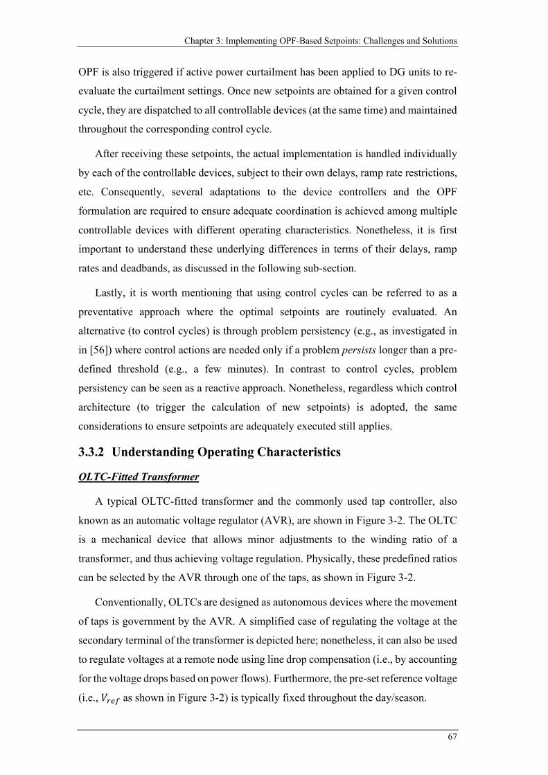
Chapter 3: Implementing OPF-Based Setpoints: Challenges and Solutions
67
OPF is also triggered if active power curtailment has been applied to DG units to re-
evaluate the curtailment settings. Once new setpoints are obtained for a given control
cycle, they are dispatched to all controllable devices (at the same time) and maintained
throughout the corresponding control cycle.
After receiving these setpoints, the actual implementation is handled individually
by each of the controllable devices, subject to their own delays, ramp rate restrictions,
etc. Consequently, several adaptations to the device controllers and the OPF
formulation are required to ensure adequate coordination is achieved among multiple
controllable devices with different operating characteristics. Nonetheless, it is first
important to understand these underlying differences in terms of their delays, ramp
rates and deadbands, as discussed in the following sub-section.
Lastly, it is worth mentioning that using control cycles can be referred to as a
preventative approach where the optimal setpoints are routinely evaluated. An
alternative (to control cycles) is through problem persistency (e.g., as investigated in
in [56]) where control actions are needed only if a problem persists longer than a pre-
defined threshold (e.g., a few minutes). In contrast to control cycles, problem
persistency can be seen as a reactive approach. Nonetheless, regardless which control
architecture (to trigger the calculation of new setpoints) is adopted, the same
considerations to ensure setpoints are adequately executed still applies.
3.3.2 Understanding Operating Characteristics
OLTC-Fitted Transformer
A typical OLTC-fitted transformer and the commonly used tap controller, also
known as an automatic voltage regulator (AVR), are shown in Figure 3-2. The OLTC
is a mechanical device that allows minor adjustments to the winding ratio of a
transformer, and thus achieving voltage regulation. Physically, these predefined ratios
can be selected by the AVR through one of the taps, as shown in Figure 3-2.
Conventionally, OLTCs are designed as autonomous devices where the movement
of taps is government by the AVR. A simplified case of regulating the voltage at the
secondary terminal of the transformer is depicted here; nonetheless, it can also be used
to regulate voltages at a remote node using line drop compensation (i.e., by accounting
for the voltage drops based on power flows). Furthermore, the pre-set reference voltage
(i.e., 𝑉𝑉𝐶𝐶𝑠𝑠𝑟𝑟 as shown in Figure 3-2) is typically fixed throughout the day/season.
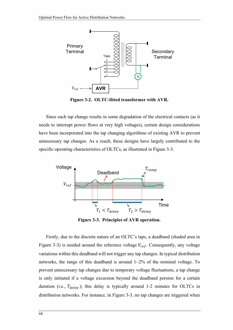
Optimal Power Flow for Active Distribution Networks
68
Since each tap change results in some degradation of the electrical contacts (as it
needs to interrupt power flows at very high voltages), certain design considerations
have been incorporated into the tap changing algorithms of existing AVR to prevent
unnecessary tap changes. As a result, these designs have largely contributed to the
specific operating characteristics of OLTCs, as illustrated in Figure 3-3.
Firstly, due to the discrete nature of an OLTC’s taps, a deadband (shaded area in
Figure 3-3) is needed around the reference voltage 𝑉𝑉𝐶𝐶𝑠𝑠𝑟𝑟. Consequently, any voltage
variations within this deadband will not trigger any tap changes. In typical distribution
networks, the range of this deadband is around 1~2% of the nominal voltage. To
prevent unnecessary tap changes due to temporary voltage fluctuations, a tap change
is only initiated if a voltage excursion beyond the deadband persists for a certain
duration (i.e., 𝑇𝑇𝑑𝑑𝑠𝑠𝐶𝐶𝐶𝐶𝑦𝑦 ); this delay is typically around 1-2 minutes for OLTCs in
distribution networks. For instance, in Figure 3-3, no tap changes are triggered when
Figure 3-2. OLTC-fitted transformer with AVR.
Secondary Terminal
1
2345
AVR
Primary Terminal
V
Taps
𝑉𝑉𝐶𝐶𝑠𝑠𝑟𝑟
Figure 3-3. Principles of AVR operation.
Deadband
𝑉𝑉𝐶𝐶𝑠𝑠𝑟𝑟
𝑇𝑇𝐶𝐶𝐶𝐶𝑚𝑚𝑝𝑝
𝑇𝑇1 < 𝑇𝑇𝑑𝑑𝑠𝑠𝐶𝐶𝐶𝐶𝑦𝑦 𝑇𝑇2 > 𝑇𝑇𝑑𝑑𝑠𝑠𝐶𝐶𝐶𝐶𝑦𝑦
Voltage
Time
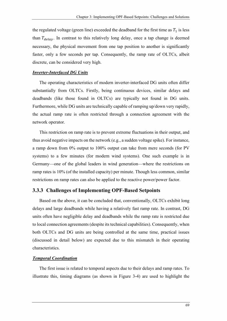
Chapter 3: Implementing OPF-Based Setpoints: Challenges and Solutions
69
the regulated voltage (green line) exceeded the deadband for the first time as 𝑇𝑇1 is less
than 𝑇𝑇𝑑𝑑𝑠𝑠𝐶𝐶𝐶𝐶𝑦𝑦 . In contrast to this relatively long delay, once a tap change is deemed
necessary, the physical movement from one tap position to another is significantly
faster, only a few seconds per tap. Consequently, the ramp rate of OLTCs, albeit
discrete, can be considered very high.
Inverter-Interfaced DG Units
The operating characteristics of modern inverter-interfaced DG units often differ
substantially from OLTCs. Firstly, being continuous devices, similar delays and
deadbands (like those found in OLTCs) are typically not found in DG units.
Furthermore, while DG units are technically capable of ramping up/down very rapidly,
the actual ramp rate is often restricted through a connection agreement with the
network operator.
This restriction on ramp rate is to prevent extreme fluctuations in their output, and
thus avoid negative impacts on the network (e.g., a sudden voltage spike). For instance,
a ramp down from 0% output to 100% output can take from mere seconds (for PV
systems) to a few minutes (for modern wind systems). One such example is in
Germany—one of the global leaders in wind generation—where the restrictions on
ramp rates is 10% (of the installed capacity) per minute. Though less common, similar
restrictions on ramp rates can also be applied to the reactive power/power factor.
3.3.3 Challenges of Implementing OPF-Based Setpoints
Based on the above, it can be concluded that, conventionally, OLTCs exhibit long
delays and large deadbands while having a relatively fast ramp rate. In contrast, DG
units often have negligible delay and deadbands while the ramp rate is restricted due
to local connection agreements (despite its technical capabilities). Consequently, when
both OLTCs and DG units are being controlled at the same time, practical issues
(discussed in detail below) are expected due to this mismatch in their operating
characteristics.
Temporal Coordination
The first issue is related to temporal aspects due to their delays and ramp rates. To
illustrate this, timing diagrams (as shown in Figure 3-4) are used to highlight the
Optimal Power Flow for Active Distribution Networks
70
various events during a control cycle for two key scenarios: uncoordinated and
coordinated.
In Figure 3-4, the start and end of a control cycle are denoted by 𝟎𝟎 and 𝑻𝑻CC ,
respectively. The time required for network operators to calculate and dispatch new
setpoints (i.e., collect network measurements, check constraint violations, solve the
OPF and dispatch to controllable devices, as depicted in Figure 3-1) is collectively
represented by Δ𝑇𝑇OPF. The remaining Δ terms are used to represent the execution times,
i.e., the time required for a setpoint to be fully reached after accounting for the
associated delays and ramp rates. Here, the execution times of a DG unit’s active
power setpoint (Δ𝑇𝑇𝑁𝑁𝐺𝐺𝑃𝑃 ) and power factor setpoint (Δ𝑇𝑇𝑁𝑁𝐺𝐺𝑃𝑃𝑃𝑃, as a proxy of the reactive
power) as well as the OLTC’s tap setpoint (Δ𝑇𝑇𝑂𝑂𝐿𝐿𝑇𝑇𝐶𝐶) are shown. Within each of the
execution times, the components associated with the delay (shaded region) and ramp
rate (solid region) are also highlighted.
As illustrated by Figure 3-4-a, the uncoordinated scenario occurs when there is a
significant misalignment of their execution times. Despite all setpoints are being
dispatched at the same time (i.e., after Δ𝑇𝑇OPF), the full execution of each of these can
(a)
(b)
Figure 3-4. Timing diagrams of control events: a) uncoordinated
scenario, b) coordinated scenario.
ControlEvents
Control Cycle
Δ𝑇𝑇𝑂𝑂𝑃𝑃𝑃𝑃
Δ𝑇𝑇𝑂𝑂𝐿𝐿𝑇𝑇𝐶𝐶Δ𝑇𝑇𝑁𝑁𝐺𝐺𝑃𝑃
Δ𝑇𝑇𝑁𝑁𝐺𝐺𝑃𝑃𝑃𝑃
𝑡𝑡
𝑻𝑻∗
𝟎𝟎 𝑻𝑻𝑪𝑪𝑪𝑪
ControlEvents
Control Cycle
Δ𝑇𝑇𝑂𝑂𝑃𝑃𝑃𝑃
Δ𝑇𝑇𝑂𝑂𝐿𝐿𝑇𝑇𝐶𝐶Δ𝑇𝑇𝑁𝑁𝐺𝐺𝑃𝑃
Δ𝑇𝑇𝑁𝑁𝐺𝐺𝑃𝑃𝑃𝑃
𝑡𝑡
𝑻𝑻∗
𝟎𝟎 𝑻𝑻𝑪𝑪𝑪𝑪
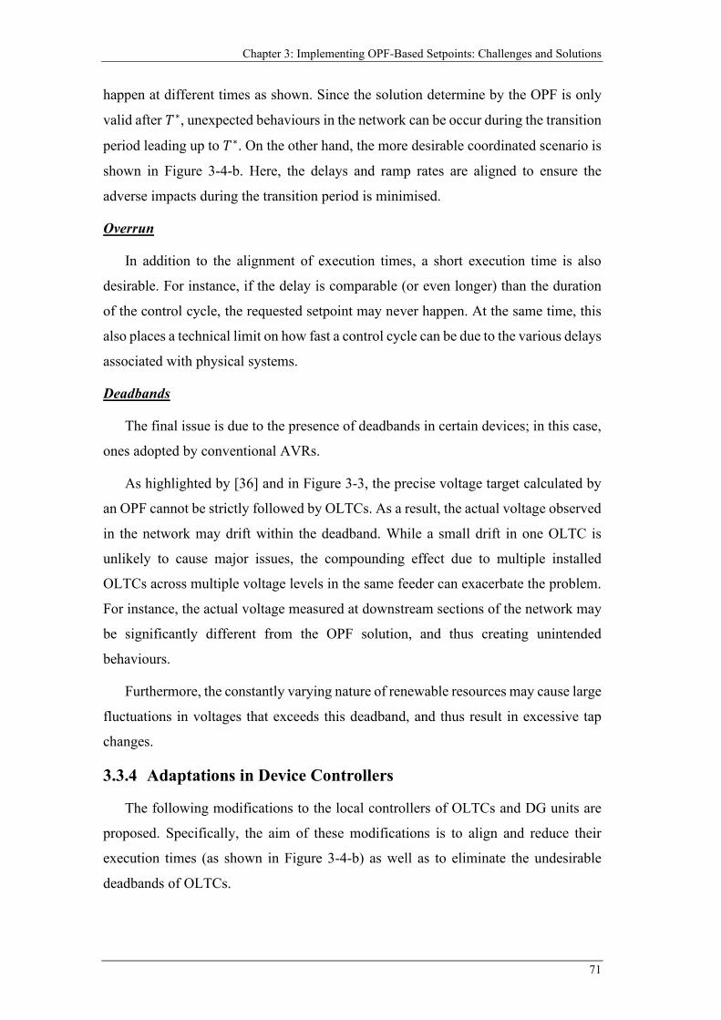
Chapter 3: Implementing OPF-Based Setpoints: Challenges and Solutions
71
happen at different times as shown. Since the solution determine by the OPF is only
valid after 𝑇𝑇∗, unexpected behaviours in the network can be occur during the transition
period leading up to 𝑇𝑇∗. On the other hand, the more desirable coordinated scenario is
shown in Figure 3-4-b. Here, the delays and ramp rates are aligned to ensure the
adverse impacts during the transition period is minimised.
Overrun
In addition to the alignment of execution times, a short execution time is also
desirable. For instance, if the delay is comparable (or even longer) than the duration
of the control cycle, the requested setpoint may never happen. At the same time, this
also places a technical limit on how fast a control cycle can be due to the various delays
associated with physical systems.
Deadbands
The final issue is due to the presence of deadbands in certain devices; in this case,
ones adopted by conventional AVRs.
As highlighted by [36] and in Figure 3-3, the precise voltage target calculated by
an OPF cannot be strictly followed by OLTCs. As a result, the actual voltage observed
in the network may drift within the deadband. While a small drift in one OLTC is
unlikely to cause major issues, the compounding effect due to multiple installed
OLTCs across multiple voltage levels in the same feeder can exacerbate the problem.
For instance, the actual voltage measured at downstream sections of the network may
be significantly different from the OPF solution, and thus creating unintended
behaviours.
Furthermore, the constantly varying nature of renewable resources may cause large
fluctuations in voltages that exceeds this deadband, and thus result in excessive tap
changes.
3.3.4 Adaptations in Device Controllers
The following modifications to the local controllers of OLTCs and DG units are
proposed. Specifically, the aim of these modifications is to align and reduce their
execution times (as shown in Figure 3-4-b) as well as to eliminate the undesirable
deadbands of OLTCs.
Optimal Power Flow for Active Distribution Networks
72
OLTCs
The existing design of AVR is largely contributed by the autonomous design for
passive operations. As a result, the associated delays and deadbands are, fundamentally,
less compatible with OPF-based schemes where network devices are actively managed.
Therefore, this work proposes the direct control of each OLTC’s tap position,
bypassing the mechanism that takes a voltage target as an input.
Through this approach, the undesirable initial delay is completely eliminated,
allowing the OLTC to respond swiftly after receiving the required tap position.
Furthermore, requesting a precise tap position helps to eliminate the inherent voltage
drifts associated with a deadband.
At the same time, this means the precise tap position must also be considered as a
variable in the OPF formulation; this can be catered for using integer variables as
discussed in Chapter 2.
DG Units
For DG units, the main issue is associated with slow ramp rates as a result of local
restrictions. Nonetheless, since the ramp rate is often specified in terms of the
maximum change per minute, e.g., 1 MW per minute, how this is achieved in the sub-
minute scale can be exploited to ensure better coordination with OLTCs.
Two different ramping behaviours are illustrated in Figure 3-5. The most
commonly adopted behaviour in literature is a linear ramp (solid line in Figure 3-5)
between the original setpoint 𝑃𝑃0 and the new setpoint 𝑃𝑃∗ . However, a potential
drawback of this approach is the relatively long execution time (as indicated by Δ𝑃𝑃𝑁𝑁𝐺𝐺𝑃𝑃,2).
Instead, the propose ramping behaviour has a faster initial ramp (dashed line in Figure
3-5) to achieve the desired execution time (as indicated by Δ𝑃𝑃𝑁𝑁𝐺𝐺𝑃𝑃,1).
At the same time, this requires the OPF to consider both the connection agreement
and the full ramping capability of the DG unit so as to ensure the calculated setpoint
𝑃𝑃∗ is technically feasible.
Lastly, no ramp rate restrictions for the reactive power of DG units is assumed.
Nonetheless, the aforementioned approach can also be applied if needed.
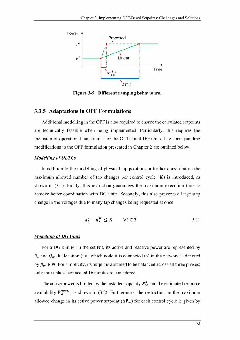
Chapter 3: Implementing OPF-Based Setpoints: Challenges and Solutions
73
3.3.5 Adaptations in OPF Formulations
Additional modelling in the OPF is also required to ensure the calculated setpoints
are technically feasible when being implemented. Particularly, this requires the
inclusion of operational constraints for the OLTC and DG units. The corresponding
modifications to the OPF formulation presented in Chapter 2 are outlined below.
Modelling of OLTCs
In addition to the modelling of physical tap positions, a further constraint on the
maximum allowed number of tap changes per control cycle (𝑲𝑲) is introduced, as
shown in (3.1). Firstly, this restriction guarantees the maximum execution time to
achieve better coordination with DG units. Secondly, this also prevents a large step
change in the voltages due to many tap changes being requested at once.
�𝜋𝜋𝐶𝐶∗ − 𝝅𝝅𝒕𝒕𝟎𝟎� ≤ 𝑲𝑲, ∀𝑡𝑡 ∈ 𝑇𝑇 (3.1)
Modelling of DG Units
For a DG unit 𝑤𝑤 (in the set 𝑊𝑊), its active and reactive power are represented by
𝑃𝑃𝑤𝑤 and 𝑄𝑄𝑤𝑤. Its location (i.e., which node it is connected to) in the network is denoted
by 𝛽𝛽𝑤𝑤 ∈ 𝑁𝑁. For simplicity, its output is assumed to be balanced across all three phases;
only three-phase connected DG units are considered.
The active power is limited by the installed capacity 𝑷𝑷𝑤𝑤+ and the estimated resource
availability 𝑷𝑷𝑤𝑤𝐶𝐶𝑎𝑎𝐶𝐶𝐶𝐶𝐶𝐶, as shown in (3.2). Furthermore, the restriction on the maximum
allowed change in its active power setpoint (Δ𝐏𝐏w) for each control cycle is given by
Figure 3-5. Different ramping behaviours.
𝑃𝑃∗
Power
Time
𝑃𝑃0
Δ𝑇𝑇𝑁𝑁𝐺𝐺𝑃𝑃,1
Proposed
Linear
Δ𝑇𝑇𝑁𝑁𝐺𝐺𝑃𝑃,2
Optimal Power Flow for Active Distribution Networks
74
(3.3) where 𝑷𝑷𝑤𝑤0 is the setpoint in the previous control cycle. The correspond value for
Δ𝐏𝐏w must satisfying the ramping requirement as discussed in Section 3.3.4.
𝑃𝑃𝑤𝑤 ≤ 𝑷𝑷𝑤𝑤𝐶𝐶𝑎𝑎𝐶𝐶𝐶𝐶𝐶𝐶 ≤ 𝑷𝑷𝑤𝑤+ , ∀𝑤𝑤 ∈ 𝑊𝑊 (3.2)
|𝑃𝑃𝑤𝑤 − 𝑷𝑷𝑤𝑤0 | ≤ Δ𝐏𝐏w, ∀𝑤𝑤 ∈ 𝑊𝑊 (3.3)
The control of reactive power is assumed to be based on the power factor. While
the power factor (i.e., 𝑃𝑃𝑂𝑂𝑤𝑤) is not explicitly modelled as a variable, it can be extracted
from 𝑃𝑃𝑤𝑤 and 𝑄𝑄𝑤𝑤 using (3.4). Furthermore, the physical capability is enforced through
(3.5) where 𝑷𝑷𝑷𝑷𝑤𝑤+ is the maximum feasible power factor.
𝑃𝑃𝑂𝑂𝑤𝑤 = tan−1 �𝑄𝑄𝑤𝑤𝑃𝑃𝑤𝑤� , ∀𝑤𝑤 ∈ 𝑊𝑊 (3.4)
|𝑄𝑄𝑤𝑤| ≤ 𝑃𝑃𝑤𝑤 𝑡𝑡𝑡𝑡𝑠𝑠(cos−1 𝑷𝑷𝑷𝑷𝑤𝑤+) , ∀𝑤𝑤 ∈ 𝑊𝑊 (3.5)
Nodal Power Balance
Due to the addition of DG units, the nodal power balance in (2.70) and (2.71) are
updated accordingly, as shown in (3.8) and (3.9), respectively.
� 𝑃𝑃𝐶𝐶𝑥𝑥,𝜙𝜙𝐶𝐶∈𝐿𝐿 | 𝐶𝐶𝑥𝑥=𝑛𝑛
+ � 𝑃𝑃𝐶𝐶𝑦𝑦,𝜙𝜙𝐶𝐶∈𝐿𝐿 | 𝐶𝐶𝑦𝑦=𝑛𝑛
+ � 𝑃𝑃𝐶𝐶𝑥𝑥,𝜙𝜙𝐶𝐶∈𝑇𝑇 | 𝐶𝐶𝑥𝑥=𝑛𝑛
+ � 𝑃𝑃𝐶𝐶𝑦𝑦,𝜙𝜙𝐶𝐶∈𝑇𝑇 | 𝐶𝐶𝑦𝑦=𝑛𝑛
+ �13𝑃𝑃𝑤𝑤
𝑤𝑤∈𝑊𝑊 | 𝛽𝛽𝑤𝑤=𝑛𝑛
+ � 𝑃𝑃ℎ𝑁𝑁𝑁𝑁
ℎ∈𝐻𝐻 | 𝛽𝛽ℎ=𝑛𝑛, 𝜑𝜑ℎ=𝜙𝜙
+ � 𝑃𝑃𝑠𝑠,𝜙𝜙𝑆𝑆
𝑠𝑠∈𝑆𝑆 | 𝑠𝑠=𝑛𝑛
= 0,
∀𝑠𝑠 ∈ 𝑁𝑁,∀𝜙𝜙 ∈ Φ
(3.6)
� 𝑄𝑄𝐶𝐶𝑥𝑥,𝜙𝜙𝐶𝐶∈𝐿𝐿 | 𝐶𝐶𝑥𝑥=𝑛𝑛
+ � 𝑄𝑄𝐶𝐶𝑦𝑦,𝜙𝜙𝐶𝐶∈𝐿𝐿 | 𝐶𝐶𝑦𝑦=𝑛𝑛
+ � 𝑄𝑄𝐶𝐶𝑥𝑥,𝜙𝜙𝐶𝐶∈𝑇𝑇 | 𝐶𝐶𝑥𝑥=𝑛𝑛
+ � 𝑄𝑄𝐶𝐶𝑦𝑦,𝜙𝜙𝐶𝐶∈𝑇𝑇 | 𝐶𝐶𝑦𝑦=𝑛𝑛
+ �13𝑄𝑄𝑤𝑤
𝑤𝑤∈𝑊𝑊 | 𝛽𝛽𝑤𝑤=𝑛𝑛
+ � 𝑄𝑄ℎ𝑁𝑁𝑁𝑁
ℎ∈𝐻𝐻 | 𝛽𝛽ℎ=𝑛𝑛, 𝜑𝜑ℎ=𝜙𝜙
+ � 𝑄𝑄𝑠𝑠,𝜙𝜙𝑆𝑆
𝑠𝑠∈𝑆𝑆 | 𝑠𝑠=𝑛𝑛
= 0
∀𝑠𝑠 ∈ 𝑁𝑁,∀𝜙𝜙 ∈ Φ
(3.7)
Optimisation Objective
Due to the various sources of flexibility as well as the available headroom in
distribution networks, there are often multiple control actions that can achieve the
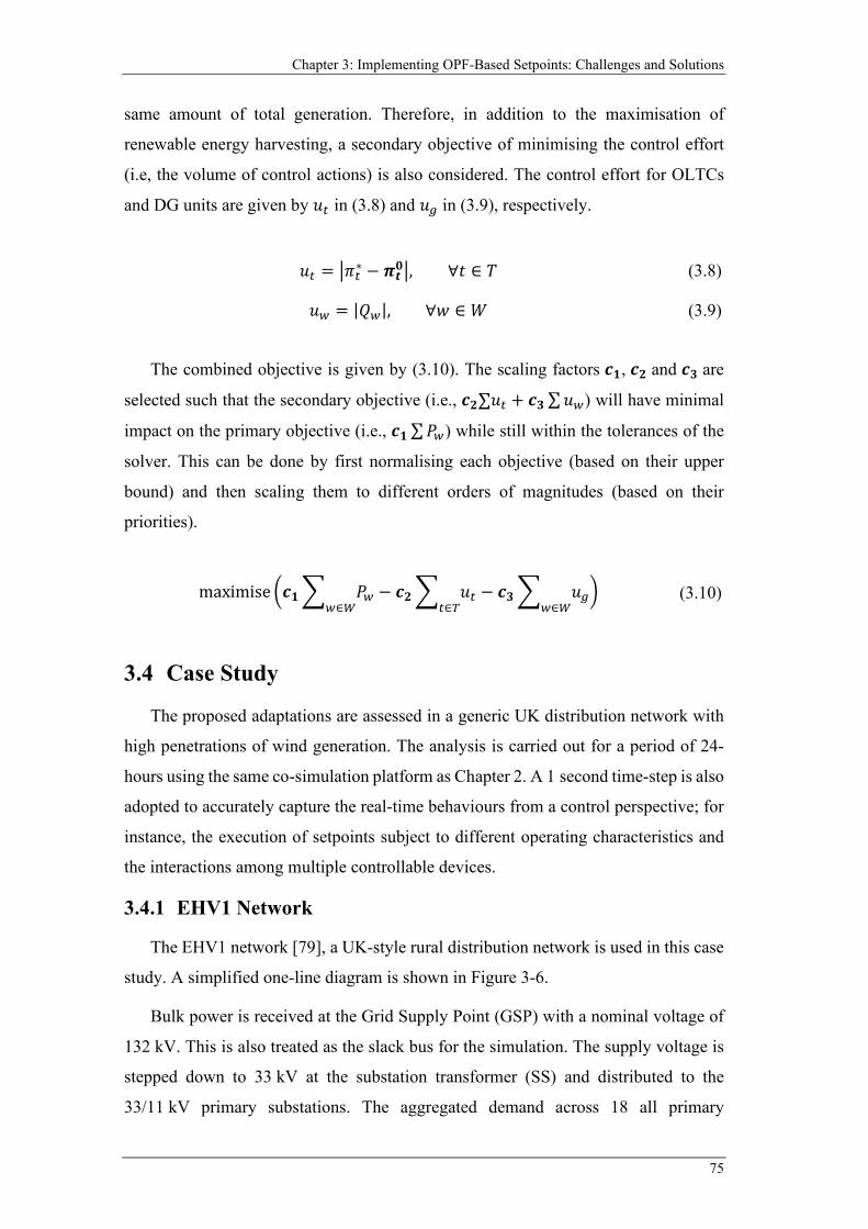
Chapter 3: Implementing OPF-Based Setpoints: Challenges and Solutions
75
same amount of total generation. Therefore, in addition to the maximisation of
renewable energy harvesting, a secondary objective of minimising the control effort
(i.e, the volume of control actions) is also considered. The control effort for OLTCs
and DG units are given by 𝑢𝑢𝐶𝐶 in (3.8) and 𝑢𝑢𝑔𝑔 in (3.9), respectively.
𝑢𝑢𝐶𝐶 = �𝜋𝜋𝐶𝐶∗ − 𝝅𝝅𝒕𝒕𝟎𝟎�, ∀𝑡𝑡 ∈ 𝑇𝑇 (3.8)
𝑢𝑢𝑤𝑤 = |𝑄𝑄𝑤𝑤|, ∀𝑤𝑤 ∈ 𝑊𝑊 (3.9)
The combined objective is given by (3.10). The scaling factors 𝒄𝒄𝟏𝟏, 𝒄𝒄𝟐𝟐 and 𝒄𝒄𝟑𝟑 are
selected such that the secondary objective (i.e., 𝒄𝒄𝟐𝟐∑𝑢𝑢𝐶𝐶 + 𝒄𝒄𝟑𝟑 ∑𝑢𝑢𝑤𝑤) will have minimal
impact on the primary objective (i.e., 𝒄𝒄𝟏𝟏 ∑𝑃𝑃𝑤𝑤) while still within the tolerances of the
solver. This can be done by first normalising each objective (based on their upper
bound) and then scaling them to different orders of magnitudes (based on their
priorities).
maximise �𝒄𝒄𝟏𝟏� 𝑃𝑃𝑤𝑤𝑤𝑤∈𝑊𝑊
− 𝒄𝒄𝟐𝟐� 𝑢𝑢𝐶𝐶𝐶𝐶∈𝑇𝑇
− 𝒄𝒄𝟑𝟑� 𝑢𝑢𝑔𝑔𝑤𝑤∈𝑊𝑊
� (3.10)
3.4 Case Study
The proposed adaptations are assessed in a generic UK distribution network with
high penetrations of wind generation. The analysis is carried out for a period of 24-
hours using the same co-simulation platform as Chapter 2. A 1 second time-step is also
adopted to accurately capture the real-time behaviours from a control perspective; for
instance, the execution of setpoints subject to different operating characteristics and
the interactions among multiple controllable devices.
3.4.1 EHV1 Network
The EHV1 network [79], a UK-style rural distribution network is used in this case
study. A simplified one-line diagram is shown in Figure 3-6.
Bulk power is received at the Grid Supply Point (GSP) with a nominal voltage of
132 kV. This is also treated as the slack bus for the simulation. The supply voltage is
stepped down to 33 kV at the substation transformer (SS) and distributed to the
33/11 kV primary substations. The aggregated demand across 18 all primary
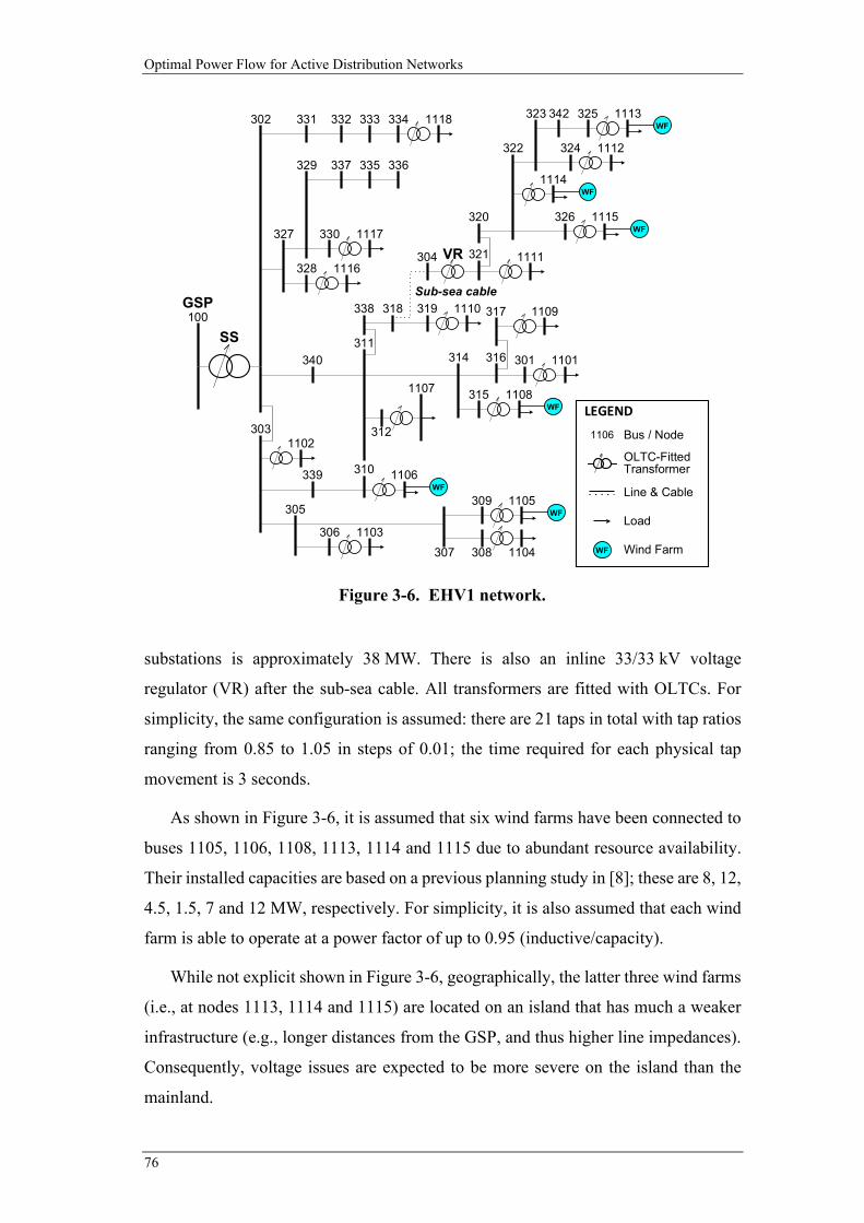
Optimal Power Flow for Active Distribution Networks
76
substations is approximately 38 MW. There is also an inline 33/33 kV voltage
regulator (VR) after the sub-sea cable. All transformers are fitted with OLTCs. For
simplicity, the same configuration is assumed: there are 21 taps in total with tap ratios
ranging from 0.85 to 1.05 in steps of 0.01; the time required for each physical tap
movement is 3 seconds.
As shown in Figure 3-6, it is assumed that six wind farms have been connected to
buses 1105, 1106, 1108, 1113, 1114 and 1115 due to abundant resource availability.
Their installed capacities are based on a previous planning study in [8]; these are 8, 12,
4.5, 1.5, 7 and 12 MW, respectively. For simplicity, it is also assumed that each wind
farm is able to operate at a power factor of up to 0.95 (inductive/capacity).
While not explicit shown in Figure 3-6, geographically, the latter three wind farms
(i.e., at nodes 1113, 1114 and 1115) are located on an island that has much a weaker
infrastructure (e.g., longer distances from the GSP, and thus higher line impedances).
Consequently, voltage issues are expected to be more severe on the island than the
mainland.
Figure 3-6. EHV1 network.
100
302 331 332 333 334 1118
329 337 336335
330 1117327
328 1116
311
338 318
304
320
1114
326 1115
1112324
323 342 325 1113
322
321 1111
1109317
316314 301 1101
11083151107
312
310339
1102303
340
305
306 1103
309 1105
1106
1104308
319 1110GSP
VR
SS
Sub-sea cable
WF
WF
WF
WF
307
WF
WF LEGEND1106 Bus / Node
Line & Cable
OLTC-Fitted Transformer
Load
WF Wind Farm
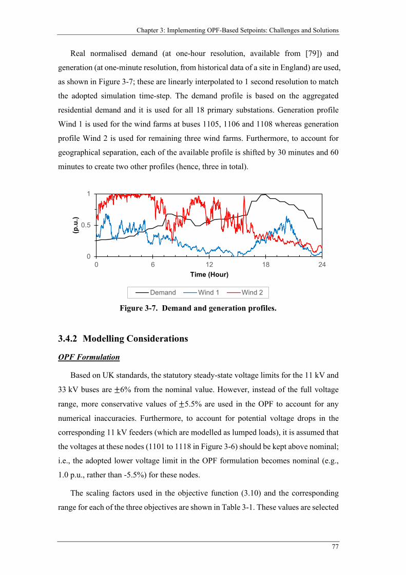
Chapter 3: Implementing OPF-Based Setpoints: Challenges and Solutions
77
Real normalised demand (at one-hour resolution, available from [79]) and
generation (at one-minute resolution, from historical data of a site in England) are used,
as shown in Figure 3-7; these are linearly interpolated to 1 second resolution to match
the adopted simulation time-step. The demand profile is based on the aggregated
residential demand and it is used for all 18 primary substations. Generation profile
Wind 1 is used for the wind farms at buses 1105, 1106 and 1108 whereas generation
profile Wind 2 is used for remaining three wind farms. Furthermore, to account for
geographical separation, each of the available profile is shifted by 30 minutes and 60
minutes to create two other profiles (hence, three in total).
3.4.2 Modelling Considerations
OPF Formulation
Based on UK standards, the statutory steady-state voltage limits for the 11 kV and
33 kV buses are ±6% from the nominal value. However, instead of the full voltage
range, more conservative values of ±5.5% are used in the OPF to account for any
numerical inaccuracies. Furthermore, to account for potential voltage drops in the
corresponding 11 kV feeders (which are modelled as lumped loads), it is assumed that
the voltages at these nodes (1101 to 1118 in Figure 3-6) should be kept above nominal;
i.e., the adopted lower voltage limit in the OPF formulation becomes nominal (e.g.,
1.0 p.u., rather than -5.5%) for these nodes.
The scaling factors used in the objective function (3.10) and the corresponding
range for each of the three objectives are shown in Table 3-1. These values are selected
Figure 3-7. Demand and generation profiles.
0
0.5
1
0 6 12 18 24
(p.u
.)
Time (Hour)
Demand Wind 1 Wind 2
Optimal Power Flow for Active Distribution Networks
78
to prioritise renewable energy harvesting (over control actions). Furthermore, using
reactive power is more preferable than triggering tap changes.
Control Cycles
A two-minute control cycle is considered for the case study. Furthermore, the
concept of persistent forecast is adopted in each control cycle. Therefore, when new
setpoints are calculated, the estimated demand and wind resource availability will be
based on the corresponding averages over the previous minute.
Practical Considerations
During each control cycle, the time required to compute new setpoints (i.e., Δ𝑇𝑇OPF
in Figure 3-4) is assumed to be 10 seconds. The desired execution time is also assumed
to be within 10 seconds; this will be used as a basis to align the execution times of
OLTCs and wind farms, as discussed below.
For all wind farms, the proposed ramping behaviour in Figure 3-5 is adopted for
both the active power and power factor. Therefore, after receiving a new setpoint, the
active power/power factor is linearity ramped to the setpoint in 10 seconds. This is
also in line with the capability of typical wind turbine controllers [19]. The ramp rate
restriction per local connection agreements is assumed to be 10% of the installed
capacity/minute. Therefore, the adopted value for Δ𝐏𝐏w in (3.3) is set to 0.1𝑷𝑷𝑤𝑤+ .
Table 3-1. Objective function.
Objective Function Scaling Factor (𝒄𝒄𝒊𝒊) Range
𝒄𝒄1� 𝑃𝑃𝑤𝑤𝑤𝑤∈𝑊𝑊
𝒄𝒄1 = �� 𝑷𝑷𝑤𝑤𝐶𝐶𝑎𝑎𝐶𝐶𝐶𝐶𝐶𝐶𝑤𝑤∈𝑊𝑊
�−1
[0, 1]
𝒄𝒄2� 𝑢𝑢𝐶𝐶𝐶𝐶∈𝑇𝑇
𝒄𝒄2 = �10� 3𝐶𝐶∈𝑇𝑇
�−1
[0, 0.1]
𝒄𝒄3� 𝑢𝑢𝑔𝑔𝑤𝑤∈𝑊𝑊
𝒄𝒄3 = �100� 𝑷𝑷𝑤𝑤𝐶𝐶𝑎𝑎𝐶𝐶𝐶𝐶𝐶𝐶 𝑡𝑡𝑡𝑡𝑠𝑠(cos−1 𝑷𝑷𝑤𝑤+)𝑤𝑤∈𝑊𝑊
�−1
[0, 0.01]
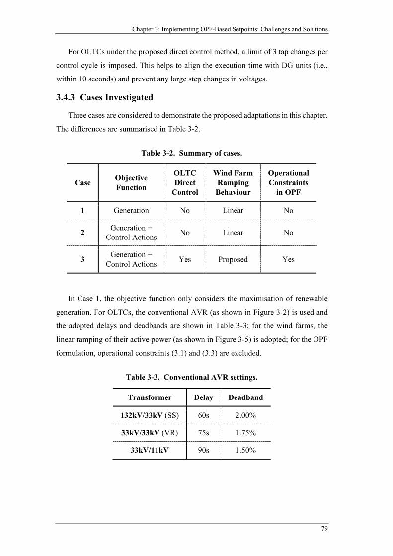
Chapter 3: Implementing OPF-Based Setpoints: Challenges and Solutions
79
For OLTCs under the proposed direct control method, a limit of 3 tap changes per
control cycle is imposed. This helps to align the execution time with DG units (i.e.,
within 10 seconds) and prevent any large step changes in voltages.
3.4.3 Cases Investigated
Three cases are considered to demonstrate the proposed adaptations in this chapter.
The differences are summarised in Table 3-2.
In Case 1, the objective function only considers the maximisation of renewable
generation. For OLTCs, the conventional AVR (as shown in Figure 3-2) is used and
the adopted delays and deadbands are shown in Table 3-3; for the wind farms, the
linear ramping of their active power (as shown in Figure 3-5) is adopted; for the OPF
formulation, operational constraints (3.1) and (3.3) are excluded.
Table 3-3. Conventional AVR settings.
Transformer Delay Deadband
132kV/33kV (SS) 60s 2.00%
33kV/33kV (VR) 75s 1.75%
33kV/11kV 90s 1.50%
Table 3-2. Summary of cases.
Case Objective Function
OLTC Direct
Control
Wind Farm Ramping Behaviour
Operational Constraints
in OPF
1 Generation No Linear No
2 Generation + Control Actions No Linear No
3 Generation + Control Actions Yes Proposed Yes
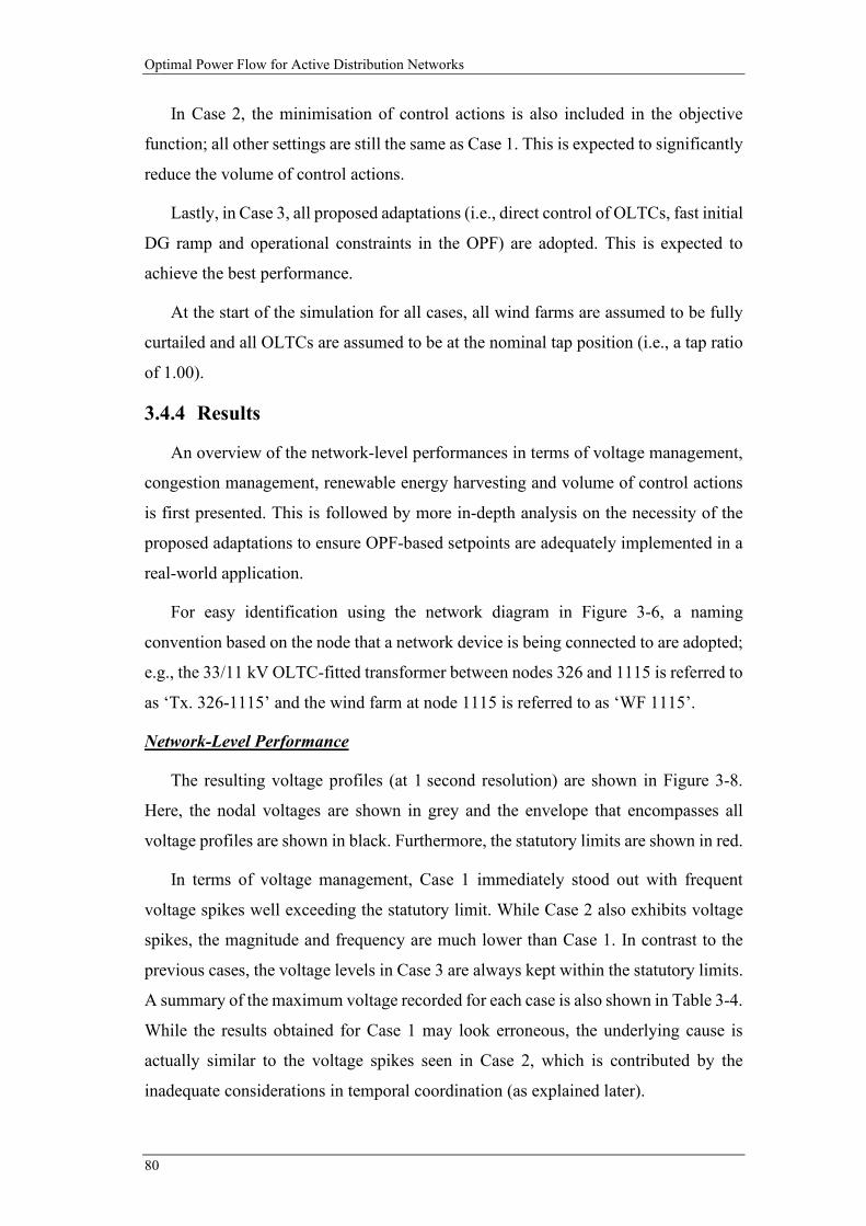
Optimal Power Flow for Active Distribution Networks
80
In Case 2, the minimisation of control actions is also included in the objective
function; all other settings are still the same as Case 1. This is expected to significantly
reduce the volume of control actions.
Lastly, in Case 3, all proposed adaptations (i.e., direct control of OLTCs, fast initial
DG ramp and operational constraints in the OPF) are adopted. This is expected to
achieve the best performance.
At the start of the simulation for all cases, all wind farms are assumed to be fully
curtailed and all OLTCs are assumed to be at the nominal tap position (i.e., a tap ratio
of 1.00).
3.4.4 Results
An overview of the network-level performances in terms of voltage management,
congestion management, renewable energy harvesting and volume of control actions
is first presented. This is followed by more in-depth analysis on the necessity of the
proposed adaptations to ensure OPF-based setpoints are adequately implemented in a
real-world application.
For easy identification using the network diagram in Figure 3-6, a naming
convention based on the node that a network device is being connected to are adopted;
e.g., the 33/11 kV OLTC-fitted transformer between nodes 326 and 1115 is referred to
as ‘Tx. 326-1115’ and the wind farm at node 1115 is referred to as ‘WF 1115’.
Network-Level Performance
The resulting voltage profiles (at 1 second resolution) are shown in Figure 3-8.
Here, the nodal voltages are shown in grey and the envelope that encompasses all
voltage profiles are shown in black. Furthermore, the statutory limits are shown in red.
In terms of voltage management, Case 1 immediately stood out with frequent
voltage spikes well exceeding the statutory limit. While Case 2 also exhibits voltage
spikes, the magnitude and frequency are much lower than Case 1. In contrast to the
previous cases, the voltage levels in Case 3 are always kept within the statutory limits.
A summary of the maximum voltage recorded for each case is also shown in Table 3-4.
While the results obtained for Case 1 may look erroneous, the underlying cause is
actually similar to the voltage spikes seen in Case 2, which is contributed by the
inadequate considerations in temporal coordination (as explained later).
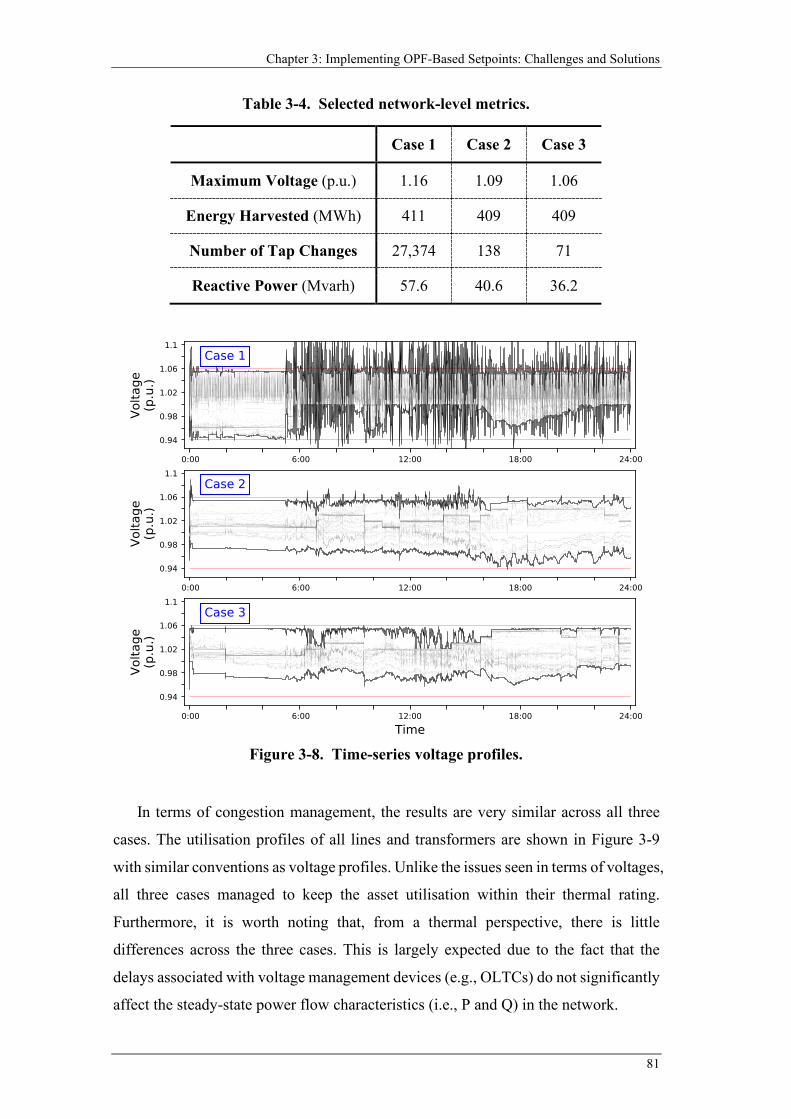
Chapter 3: Implementing OPF-Based Setpoints: Challenges and Solutions
81
In terms of congestion management, the results are very similar across all three
cases. The utilisation profiles of all lines and transformers are shown in Figure 3-9
with similar conventions as voltage profiles. Unlike the issues seen in terms of voltages,
all three cases managed to keep the asset utilisation within their thermal rating.
Furthermore, it is worth noting that, from a thermal perspective, there is little
differences across the three cases. This is largely expected due to the fact that the
delays associated with voltage management devices (e.g., OLTCs) do not significantly
affect the steady-state power flow characteristics (i.e., P and Q) in the network.
Table 3-4. Selected network-level metrics.
Case 1 Case 2 Case 3
Maximum Voltage (p.u.) 1.16 1.09 1.06
Energy Harvested (MWh) 411 409 409
Number of Tap Changes 27,374 138 71
Reactive Power (Mvarh) 57.6 40.6 36.2
Figure 3-8. Time-series voltage profiles.
Optimal Power Flow for Active Distribution Networks
82
In terms of renewable energy harvesting, there are also little variations across the
three cases (within 1% from each other), as shown in Table 3-4. On the other hand, the
volume of control actions (measured by the number of tap changes and reactive power
absorbed by the wind farms) showed significant discrepancies among the three cases.
Particularly, the results for Case 1 is very unrealistic (over 27,000 tap changes) due
to the poor design of the OPF formulation where excessive control actions are not
being penalised. At the same time, despite incorporating the minimisation of control
actions in Case 2, it is not as effective as Case 3; there are almost twice as many tap
changes and 12% more reactive power absorbed. Overall, these findings further
reinforce the need to assess the performance of a control scheme both in terms of the
power flows and the control aspect. Detailed discussions in a control perspective are
presented next.
Temporal Coordination
As discussed earlier, the root cause of the behaviour in Case 1 is very similar to
Case 2. Therefore, a comparison between Case 2 and Case 3 are first presented below.
Figure 3-9. Time-series utilisation profiles for lines and transformers.
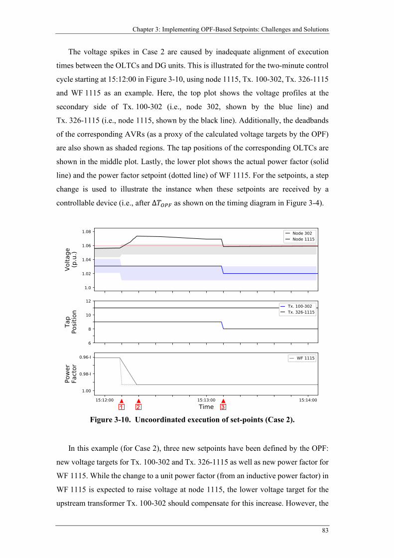
Chapter 3: Implementing OPF-Based Setpoints: Challenges and Solutions
83
The voltage spikes in Case 2 are caused by inadequate alignment of execution
times between the OLTCs and DG units. This is illustrated for the two-minute control
cycle starting at 15:12:00 in Figure 3-10, using node 1115, Tx. 100-302, Tx. 326-1115
and WF 1115 as an example. Here, the top plot shows the voltage profiles at the
secondary side of Tx. 100-302 (i.e., node 302, shown by the blue line) and
Tx. 326-1115 (i.e., node 1115, shown by the black line). Additionally, the deadbands
of the corresponding AVRs (as a proxy of the calculated voltage targets by the OPF)
are also shown as shaded regions. The tap positions of the corresponding OLTCs are
shown in the middle plot. Lastly, the lower plot shows the actual power factor (solid
line) and the power factor setpoint (dotted line) of WF 1115. For the setpoints, a step
change is used to illustrate the instance when these setpoints are received by a
controllable device (i.e., after Δ𝑇𝑇𝑂𝑂𝑃𝑃𝑃𝑃 as shown on the timing diagram in Figure 3-4).
In this example (for Case 2), three new setpoints have been defined by the OPF:
new voltage targets for Tx. 100-302 and Tx. 326-1115 as well as new power factor for
WF 1115. While the change to a unit power factor (from an inductive power factor) in
WF 1115 is expected to raise voltage at node 1115, the lower voltage target for the
upstream transformer Tx. 100-302 should compensate for this increase. However, the
Figure 3-10. Uncoordinated execution of set-points (Case 2).
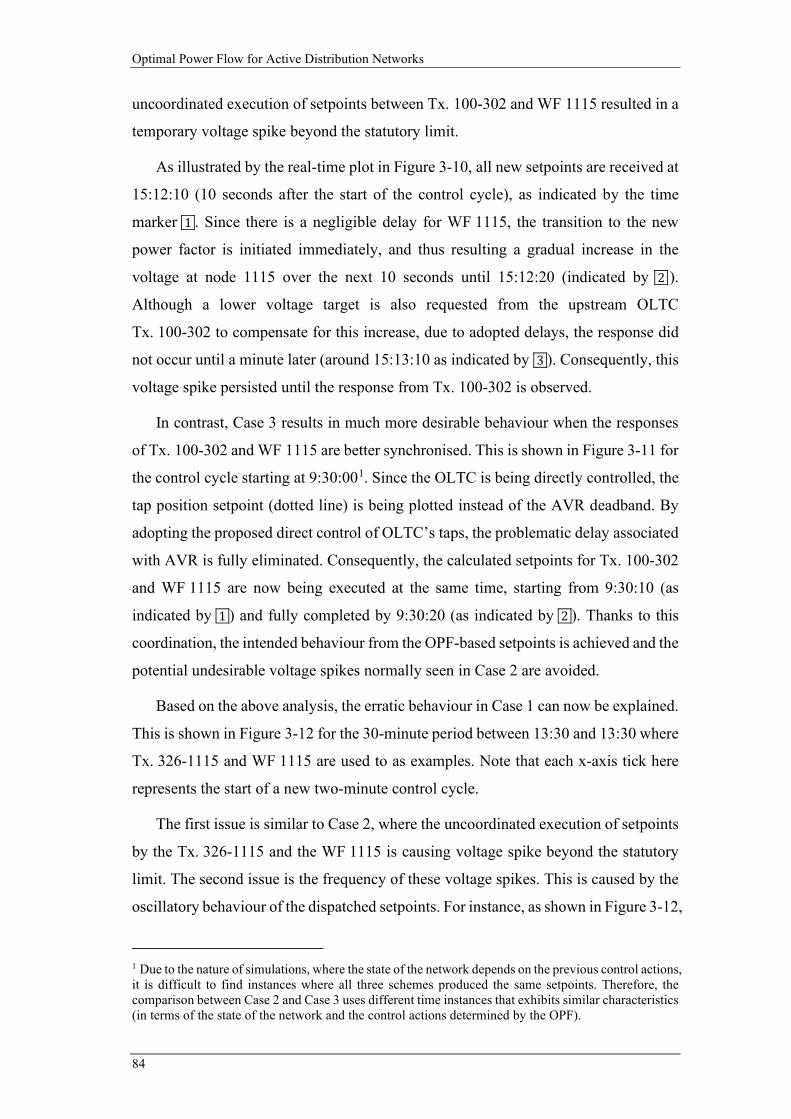
Optimal Power Flow for Active Distribution Networks
84
uncoordinated execution of setpoints between Tx. 100-302 and WF 1115 resulted in a
temporary voltage spike beyond the statutory limit.
As illustrated by the real-time plot in Figure 3-10, all new setpoints are received at
15:12:10 (10 seconds after the start of the control cycle), as indicated by the time
marker 1 . Since there is a negligible delay for WF 1115, the transition to the new
power factor is initiated immediately, and thus resulting a gradual increase in the
voltage at node 1115 over the next 10 seconds until 15:12:20 (indicated by 2 ).
Although a lower voltage target is also requested from the upstream OLTC
Tx. 100-302 to compensate for this increase, due to adopted delays, the response did
not occur until a minute later (around 15:13:10 as indicated by 3 ). Consequently, this
voltage spike persisted until the response from Tx. 100-302 is observed.
In contrast, Case 3 results in much more desirable behaviour when the responses
of Tx. 100-302 and WF 1115 are better synchronised. This is shown in Figure 3-11 for
the control cycle starting at 9:30:001. Since the OLTC is being directly controlled, the
tap position setpoint (dotted line) is being plotted instead of the AVR deadband. By
adopting the proposed direct control of OLTC’s taps, the problematic delay associated
with AVR is fully eliminated. Consequently, the calculated setpoints for Tx. 100-302
and WF 1115 are now being executed at the same time, starting from 9:30:10 (as
indicated by 1 ) and fully completed by 9:30:20 (as indicated by 2 ). Thanks to this
coordination, the intended behaviour from the OPF-based setpoints is achieved and the
potential undesirable voltage spikes normally seen in Case 2 are avoided.
Based on the above analysis, the erratic behaviour in Case 1 can now be explained.
This is shown in Figure 3-12 for the 30-minute period between 13:30 and 13:30 where
Tx. 326-1115 and WF 1115 are used to as examples. Note that each x-axis tick here
represents the start of a new two-minute control cycle.
The first issue is similar to Case 2, where the uncoordinated execution of setpoints
by the Tx. 326-1115 and the WF 1115 is causing voltage spike beyond the statutory
limit. The second issue is the frequency of these voltage spikes. This is caused by the
oscillatory behaviour of the dispatched setpoints. For instance, as shown in Figure 3-12,
1 Due to the nature of simulations, where the state of the network depends on the previous control actions, it is difficult to find instances where all three schemes produced the same setpoints. Therefore, the comparison between Case 2 and Case 3 uses different time instances that exhibits similar characteristics (in terms of the state of the network and the control actions determined by the OPF).
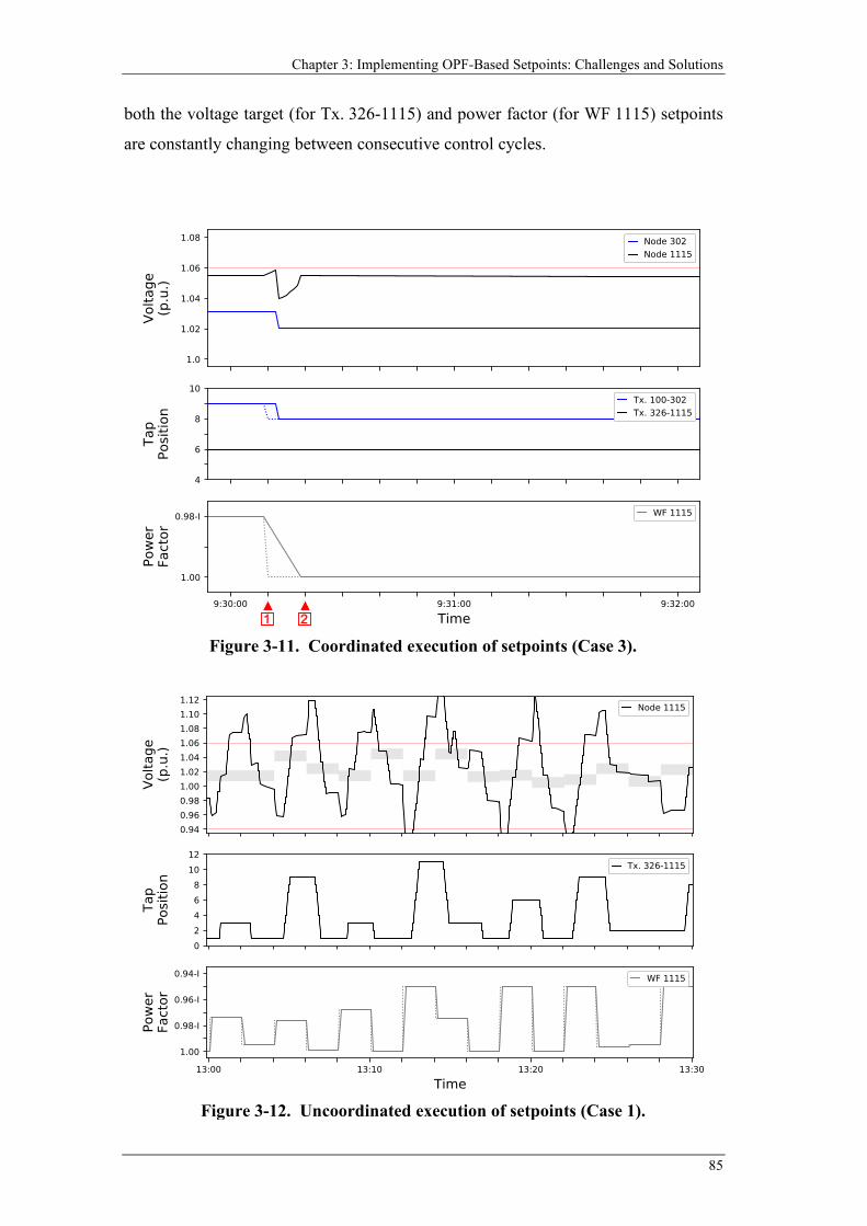
Chapter 3: Implementing OPF-Based Setpoints: Challenges and Solutions
85
both the voltage target (for Tx. 326-1115) and power factor (for WF 1115) setpoints
are constantly changing between consecutive control cycles.
Figure 3-11. Coordinated execution of setpoints (Case 3).
Figure 3-12. Uncoordinated execution of setpoints (Case 1).
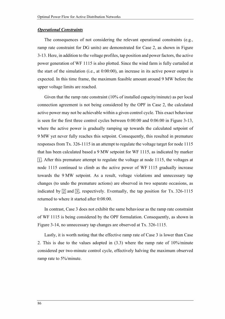
Optimal Power Flow for Active Distribution Networks
86
Operational Constraints
The consequences of not considering the relevant operational constraints (e.g.,
ramp rate constraint for DG units) are demonstrated for Case 2, as shown in Figure
3-13. Here, in addition to the voltage profiles, tap position and power factors, the active
power generation of WF 1115 is also plotted. Since the wind farm is fully curtailed at
the start of the simulation (i.e., at 0:00:00), an increase in its active power output is
expected. In this time frame, the maximum feasible amount around 9 MW before the
upper voltage limits are reached.
Given that the ramp rate constraint (10% of installed capacity/minute) as per local
connection agreement is not being considered by the OPF in Case 2, the calculated
active power may not be achievable within a given control cycle. This exact behaviour
is seen for the first three control cycles between 0:00:00 and 0:06:00 in Figure 3-13,
where the active power is gradually ramping up towards the calculated setpoint of
9 MW yet never fully reaches this setpoint. Consequently, this resulted in premature
responses from Tx. 326-1115 in an attempt to regulate the voltage target for node 1115
that has been calculated based a 9 MW setpoint for WF 1115, as indicated by marker
1 . After this premature attempt to regulate the voltage at node 1115, the voltages at
node 1115 continued to climb as the active power of WF 1115 gradually increase
towards the 9 MW setpoint. As a result, voltage violations and unnecessary tap
changes (to undo the premature actions) are observed in two separate occasions, as
indicated by 2 and 3 , respectively. Eventually, the tap position for Tx. 326-1115
returned to where it started after 0:08:00.
In contrast, Case 3 does not exhibit the same behaviour as the ramp rate constraint
of WF 1115 is being considered by the OPF formulation. Consequently, as shown in
Figure 3-14, no unnecessary tap changes are observed at Tx. 326-1115.
Lastly, it is worth noting that the effective ramp rate of Case 3 is lower than Case
2. This is due to the values adopted in (3.3) where the ramp rate of 10%/minute
considered per two-minute control cycle, effectively halving the maximum observed
ramp rate to 5%/minute.
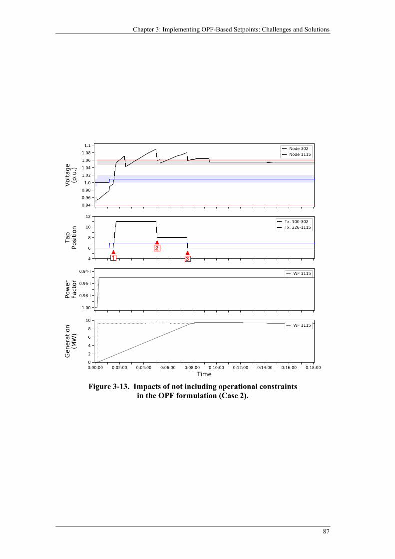
Chapter 3: Implementing OPF-Based Setpoints: Challenges and Solutions
87
Figure 3-13. Impacts of not including operational constraints
in the OPF formulation (Case 2).
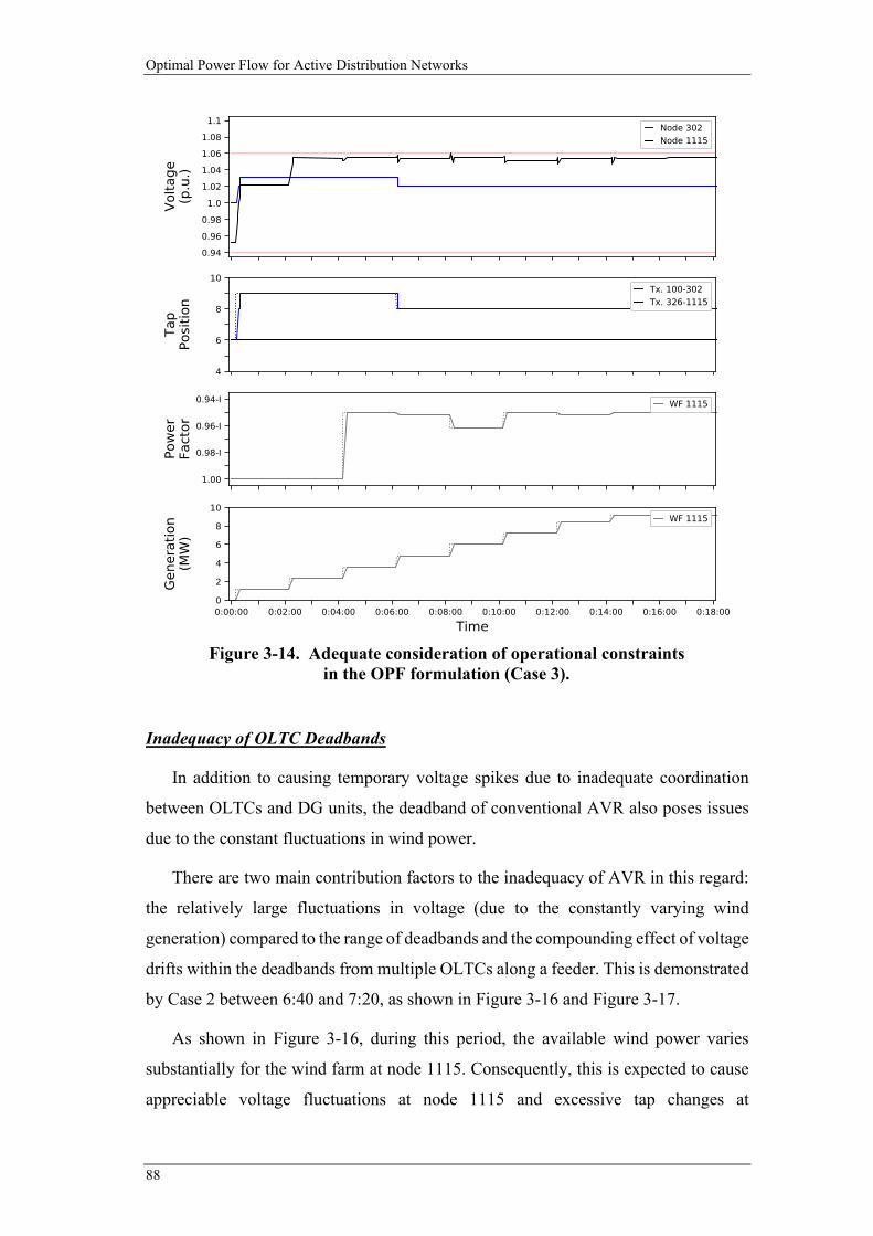
Optimal Power Flow for Active Distribution Networks
88
Inadequacy of OLTC Deadbands
In addition to causing temporary voltage spikes due to inadequate coordination
between OLTCs and DG units, the deadband of conventional AVR also poses issues
due to the constant fluctuations in wind power.
There are two main contribution factors to the inadequacy of AVR in this regard:
the relatively large fluctuations in voltage (due to the constantly varying wind
generation) compared to the range of deadbands and the compounding effect of voltage
drifts within the deadbands from multiple OLTCs along a feeder. This is demonstrated
by Case 2 between 6:40 and 7:20, as shown in Figure 3-16 and Figure 3-17.
As shown in Figure 3-16, during this period, the available wind power varies
substantially for the wind farm at node 1115. Consequently, this is expected to cause
appreciable voltage fluctuations at node 1115 and excessive tap changes at
Figure 3-14. Adequate consideration of operational constraints
in the OPF formulation (Case 3).
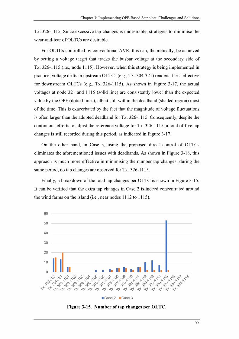
Chapter 3: Implementing OPF-Based Setpoints: Challenges and Solutions
89
Tx. 326-1115. Since excessive tap changes is undesirable, strategies to minimise the
wear-and-tear of OLTCs are desirable.
For OLTCs controlled by conventional AVR, this can, theoretically, be achieved
by setting a voltage target that tracks the busbar voltage at the secondary side of
Tx. 326-1115 (i.e., node 1115). However, when this strategy is being implemented in
practice, voltage drifts in upstream OLTCs (e.g., Tx. 304-321) renders it less effective
for downstream OLTCs (e.g., Tx. 326-1115). As shown in Figure 3-17, the actual
voltages at node 321 and 1115 (solid line) are consistently lower than the expected
value by the OPF (dotted lines), albeit still within the deadband (shaded region) most
of the time. This is exacerbated by the fact that the magnitude of voltage fluctuations
is often larger than the adopted deadband for Tx. 326-1115. Consequently, despite the
continuous efforts to adjust the reference voltage for Tx. 326-1115, a total of five tap
changes is still recorded during this period, as indicated in Figure 3-17.
On the other hand, in Case 3, using the proposed direct control of OLTCs
eliminates the aforementioned issues with deadbands. As shown in Figure 3-18, this
approach is much more effective in minimising the number tap changes; during the
same period, no tap changes are observed for Tx. 326-1115.
Finally, a breakdown of the total tap changes per OLTC is shown in Figure 3-15.
It can be verified that the extra tap changes in Case 2 is indeed concentrated around
the wind farms on the island (i.e., near nodes 1112 to 1115).
Figure 3-15. Number of tap changes per OLTC.
0
10
20
30
40
50
60
Case 2 Case 3
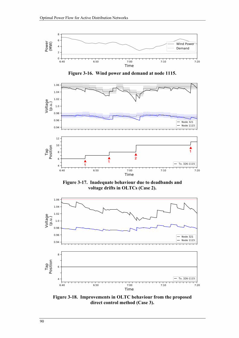
Optimal Power Flow for Active Distribution Networks
90
Figure 3-16. Wind power and demand at node 1115.
Figure 3-17. Inadequate behaviour due to deadbands and
voltage drifts in OLTCs (Case 2).
Figure 3-18. Improvements in OLTC behaviour from the proposed
direct control method (Case 3).
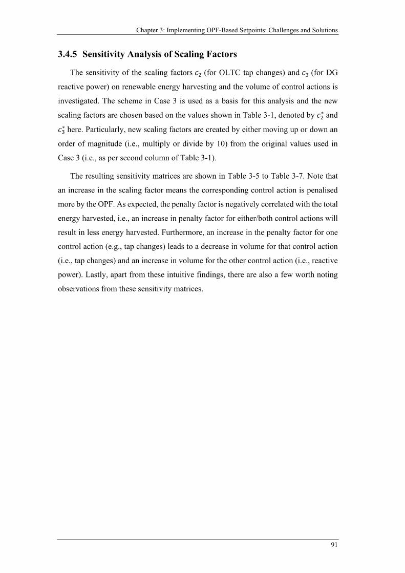
Chapter 3: Implementing OPF-Based Setpoints: Challenges and Solutions
91
3.4.5 Sensitivity Analysis of Scaling Factors
The sensitivity of the scaling factors 𝑐𝑐2 (for OLTC tap changes) and 𝑐𝑐3 (for DG
reactive power) on renewable energy harvesting and the volume of control actions is
investigated. The scheme in Case 3 is used as a basis for this analysis and the new
scaling factors are chosen based on the values shown in Table 3-1, denoted by 𝑐𝑐2∗ and
𝑐𝑐3∗ here. Particularly, new scaling factors are created by either moving up or down an
order of magnitude (i.e., multiply or divide by 10) from the original values used in
Case 3 (i.e., as per second column of Table 3-1).
The resulting sensitivity matrices are shown in Table 3-5 to Table 3-7. Note that
an increase in the scaling factor means the corresponding control action is penalised
more by the OPF. As expected, the penalty factor is negatively correlated with the total
energy harvested, i.e., an increase in penalty factor for either/both control actions will
result in less energy harvested. Furthermore, an increase in the penalty factor for one
control action (e.g., tap changes) leads to a decrease in volume for that control action
(i.e., tap changes) and an increase in volume for the other control action (i.e., reactive
power). Lastly, apart from these intuitive findings, there are also a few worth noting
observations from these sensitivity matrices.
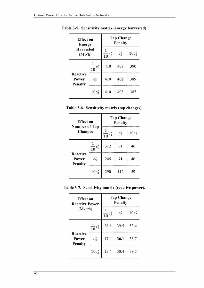
Optimal Power Flow for Active Distribution Networks
92
Table 3-5. Sensitivity matrix (energy harvested).
Effect on Energy
Harvested (MWh)
Tap Change Penalty
110
𝑐𝑐2∗ 𝑐𝑐2∗ 10𝑐𝑐2∗
Reactive Power Penalty
110
𝑐𝑐3∗ 410 408 390
𝑐𝑐3∗ 410 408 389
10𝑐𝑐3∗ 410 408 387
Table 3-6. Sensitivity matrix (tap changes).
Effect on Number of Tap
Changes
Tap Change Penalty
110
𝑐𝑐2∗ 𝑐𝑐2∗ 10𝑐𝑐2∗
Reactive Power Penalty
110
𝑐𝑐3∗ 312 61 46
𝑐𝑐3∗ 245 71 46
10𝑐𝑐3∗ 290 112 59
Table 3-7. Sensitivity matrix (reactive power).
Effect on Reactive Power
(Mvarh)
Tap Change Penalty
110
𝑐𝑐2∗ 𝑐𝑐2∗ 10𝑐𝑐2∗
Reactive Power Penalty
110
𝑐𝑐3∗ 28.6 39.5 53.4
𝑐𝑐3∗ 17.4 36.1 53.7
10𝑐𝑐3∗ 15.4 30.4 39.5

Chapter 3: Implementing OPF-Based Setpoints: Challenges and Solutions
93
As shown in Table 3-5, while a decrease in the penalty factor only produced minor
improvements of the total energy harvested (up to +0.5%), an increase in the penalty
factor for tap changes (i.e., column 10𝑐𝑐2∗) has a much more significant impact on the
total energy harvest (around -4.5%).
As shown in Table 3-6, a very low penalty factor for tap changes is potentially
undesirable as it leads to a substantial spike in the number of tap changes. Furthermore,
since tap changes is often less preferred than reactive power due to the associated wear-
and-tear, it is also desirable to ensure the penalty factor for tap changes is higher than
that for the reactive power.
3.4.6 Remarks on Solution Speed
Overall, the resulting OPF formulation has approximately 3,750 constraints and
5,900 variables (including 140 binary variables.).
The simulation PC has an i7 processor and 32GB of RAM. The OPF problem in
Case 3 (which is formulated as a MILP) requires an average computation time of
0.46 second by CPLEX v12.8. Furthermore, the maximum recorded time is 1.2 second.
Optimal Power Flow for Active Distribution Networks
94
3.5 Summary
The adequate implementation of OPF-based setpoints requires practical
considerations on the real-time operating characteristics and behaviours (e.g., delays,
ramp rates and deadbands) of the devices being controlled. Particularly, due to the
diversity in their temporal characteristics (i.e., delays and ramp rates), coordination
challenges may arise when multiple devices are being controlled at the same time.
Furthermore, existing controller designs (e.g., the AVR for an OLTC) may be geared
towards autonomous and passive operation, which creates compatibility issues with an
OPF-based scheme where the network is being centrally managed in real-time. As a
result, in addition to the modelling of steady-state power flows (e.g., voltages, currents,
etc.), these control aspects must also be captured to realistically assess the performance
of an OPF-based control scheme.
In this chapter, necessary adaptations in the device controllers and the OPF
formulation are proposed to ensure the calculated setpoints from the OPF problem are
properly realised in an operational environment. From a device perspective, the direct
control of OLTCs’ taps and a new active power ramping method for DG units are
proposed to align their delays and ramp rates. Furthermore, the proposed OLTC
control eliminates the undesirable deadbands associated with conventional AVR. In
terms of the OPF formulation, operational constraints (to ensure the calculated
setpoints are technically feasible) and a secondary objective (to minimise control
actions) are proposed.
The necessity of the proposed adaptations is demonstrated in a realistic co-
simulation environment with high granularity (1 second time-step) to capture the
control aspects that happens in the sub-minute scale. The results show that, when OPF-
based setpoints are being implemented in practice, the proposed adaptations are
extremely crucial in ensuring the expected behaviour as well as preventing temporary
constraint violations and unnecessary control actions.
4 FAIRNESS OF ACTIVE POWER CURTAILMENT
SCHEMES: A RESIDENTIAL CONTEXT
4.1 Introduction
Over the recent decade, residential PV systems have seen an unprecedented growth
[80]. At the same time, excessive reverse power flows are also creating significant
operational challenges for network operators to cope with issues such as voltage rise
and congestion. This is particularly evident in residential feeders due to the high
coincidence of peak PV generation and low residential demand (e.g., around noon on
weekdays when occupancy declines). As a result, active power curtailment is often
necessary to maintain network integrity. To date, two curtailment schemes are
commonly adopted by network operators around the world to reduce the volume of
reverse power flows in PV-rich residential networks: through the Volt-Watt
functionality found in modern PV inverters [81, 82] or through a fixed limit on the
households’ power exports (either in kW [83] or as a percentage of the installed PV
capacity [84, 85]).
While PV curtailment has been shown as an effective solution to mitigate network
issues [86] (since it eliminates the cause of these issues), ensuring adequate fairness1
among the affected households can be a rather challenging task. For instance, since
typical distribution networks are operated radially, households farther away from
substations are expected to experience higher voltages during periods of high reverse
power flows [64]. Consequently, a Volt-Watt scheme inherently introduces locational
penalisation that mostly affects households at remote locations (i.e., these households
will typically see higher volumes of curtailment). Furthermore, since the impacts on
households (from PV curtailment) can be quantified in different, and potentially
conflicting, perspectives (e.g., PV harvesting, electricity bills, etc.), whether a scheme
can be considered as fair or not is not necessarily a straightforward process. Therefore,
1 In this context, fairness is defined as the quality of a PV curtailment scheme to treat households equally; in other words, unfairness arises if one household receives more curtailment than others.
Optimal Power Flow for Active Distribution Networks
96
the most appropriate perspective needs to be determined first before even attempting
to improve the fairness aspect of curtailment schemes.
As the volume of curtailment directly affects households’ return on investment for
their PV systems, appropriate measurements are desirable to ensure curtailment is
applied effectively and fairly. Therefore, the implications from different perspectives
on fairness are first investigated in this chapter so as to better understand how to
adequately cater for fairness when active power curtailment is necessary. Following
this, the trade-offs between fairness (i.e., eliminating disparity) and efficiency (i.e.,
improving aggregated performance) is also assessed.
4.2 Literature Review
4.2.1 Fairness in PV Curtailment Schemes
As mentioned earlier, for a Volt-Watt-based approach, the voltage at each house’s
point of connection (POC) is used to determine the volume of curtailment (for that
household); e.g., higher voltage results in more curtailment. While this is a readily
implementable solution to mitigate technical issues (e.g., voltage rise), the underlying
mechanism is inherently unfair. Particularly, due to the radial nature of most
distribution feeders, houses located farther away from the substation/head of feeder
are expected to experience higher voltages during periods of high reverse power flows.
As a result, a Volt-Watt scheme naturally penalises these households, and thus can be
considered as unfair.
On the other hand, while the second strategy of adopting a fixed limit for all
households can be argued as a fairer approach (as the same limit is given to everyone),
it is often overly prohibitive. For instance, such strategies are often implemented as a
region-wide policy based on the worst-case scenarios (i.e., maximum generation and
minimum demand) and relatively high PV penetrations. Consequently, households in
areas with low PV penetration and/or strong network infrastructure can still be
unnecessarily penalised.
Therefore, it is clear that the existing schemes adopted by industry has significant
drawbacks that may hinder the future adoption of residential PV systems. To address
this, several different approaches have been proposed in the existing literature to apply
curtailment in a more effective and fairer way.
Chapter 4: Fairness of Active Power Curtailment Schemes: A Residential Context
97
For instance, a model-free approach is proposed in [87] to tackle voltage issues by
coordinating PV curtailment through distress signals. Particularly, when over-voltage
occurs, a distress signal is broadcasted to other PV systems to initiate the active power
curtailment process. Then, a time-based algorithm where, after receiving the signal,
each household will curtail at the same rate until the distress signal disappears (i.e.,
after sufficient curtailment is achieved to restore the voltage levels). Since each
household is curtailing at the same rate, curtailment is naturally shared among them in
a fair way. Another model-free approach is proposed in [88] where the network state
between two time instances (one before voltage issues are detected and one after) are
used to linearly interpolate the required volume of curtailment that eliminates voltage
issues. Once the total volume of curtailment is computed, fairness is achieved by
equally distributing curtailment among all PV systems.
A hybrid scheme that consists of both central and local control of PV systems is
proposed in [89] to improve the unfairness of Volt-Watt schemes. Particularly, a
centralised optimisation problem is solved every 15 minutes to determine individual
Volt-Watt settings for all PV systems such that that similar volume of PV curtailment
is achieved while mitigating network issues.
Lastly, fully centralised approaches using OPF are considered in [90, 91] to
determine (and dispatch) fair curtailment settings throughout the day. In [90], this is
achieved by adding a constraint to the OPF formulation that ensures the amount of
curtailment is the same for each PV system. On the other hand, in [91], a penalty factor
is introduced to the objective function to minimise the variances of curtailment among
multiple PV systems.
Despite these various efforts in the existing literature to tackle fairness in PV
curtailment schemes, two key aspects related to fairness are still yet to be adequately
investigated: the different perspectives of fairness (in a residential context) and how
fairness is interpreted when also considering the trade-offs with efficiency. These two
aspects are further explained in the following sub-sections.
4.2.2 Different Perspectives of Fairness
While the mechanisms of applying PV curtailment largely differ in the
aforementioned works, they all share the same perspective when treating fairness:
fairness is considered and assessed only based on the impacts at the PV system (i.e.,
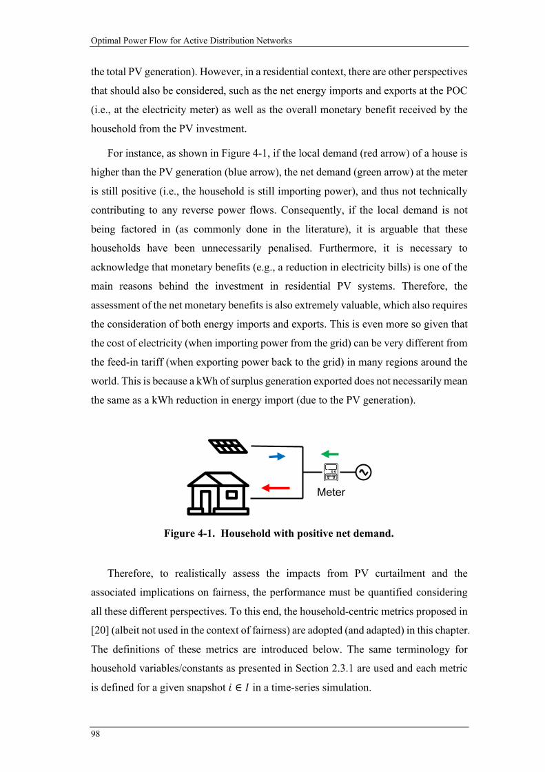
Optimal Power Flow for Active Distribution Networks
98
the total PV generation). However, in a residential context, there are other perspectives
that should also be considered, such as the net energy imports and exports at the POC
(i.e., at the electricity meter) as well as the overall monetary benefit received by the
household from the PV investment.
For instance, as shown in Figure 4-1, if the local demand (red arrow) of a house is
higher than the PV generation (blue arrow), the net demand (green arrow) at the meter
is still positive (i.e., the household is still importing power), and thus not technically
contributing to any reverse power flows. Consequently, if the local demand is not
being factored in (as commonly done in the literature), it is arguable that these
households have been unnecessarily penalised. Furthermore, it is necessary to
acknowledge that monetary benefits (e.g., a reduction in electricity bills) is one of the
main reasons behind the investment in residential PV systems. Therefore, the
assessment of the net monetary benefits is also extremely valuable, which also requires
the consideration of both energy imports and exports. This is even more so given that
the cost of electricity (when importing power from the grid) can be very different from
the feed-in tariff (when exporting power back to the grid) in many regions around the
world. This is because a kWh of surplus generation exported does not necessarily mean
the same as a kWh reduction in energy import (due to the PV generation).
Therefore, to realistically assess the impacts from PV curtailment and the
associated implications on fairness, the performance must be quantified considering
all these different perspectives. To this end, the household-centric metrics proposed in
[20] (albeit not used in the context of fairness) are adopted (and adapted) in this chapter.
The definitions of these metrics are introduced below. The same terminology for
household variables/constants as presented in Section 2.3.1 are used and each metric
is defined for a given snapshot 𝑖𝑖 ∈ 𝐼𝐼 in a time-series simulation.
Figure 4-1. Household with positive net demand.
Meter
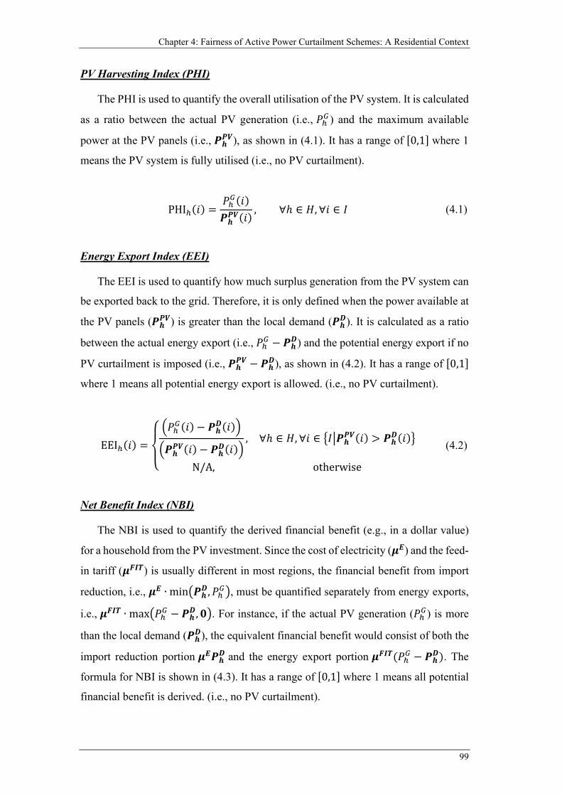
Chapter 4: Fairness of Active Power Curtailment Schemes: A Residential Context
99
PV Harvesting Index (PHI)
The PHI is used to quantify the overall utilisation of the PV system. It is calculated
as a ratio between the actual PV generation (i.e., 𝑃𝑃ℎ𝐺𝐺 ) and the maximum available
power at the PV panels (i.e., 𝑷𝑷𝒉𝒉𝑷𝑷𝑷𝑷), as shown in (4.1). It has a range of [0,1] where 1
means the PV system is fully utilised (i.e., no PV curtailment).
PHIℎ(𝑖𝑖) =𝑃𝑃ℎ𝐺𝐺(𝑖𝑖)𝑷𝑷𝒉𝒉𝑷𝑷𝑷𝑷(𝑖𝑖)
, ∀ℎ ∈ 𝐻𝐻,∀𝑖𝑖 ∈ 𝐼𝐼 (4.1)
Energy Export Index (EEI)
The EEI is used to quantify how much surplus generation from the PV system can
be exported back to the grid. Therefore, it is only defined when the power available at
the PV panels (𝑷𝑷𝒉𝒉𝑷𝑷𝑷𝑷) is greater than the local demand (𝑷𝑷𝒉𝒉𝑫𝑫). It is calculated as a ratio
between the actual energy export (i.e., 𝑃𝑃ℎ𝐺𝐺 − 𝑷𝑷𝒉𝒉𝑫𝑫) and the potential energy export if no
PV curtailment is imposed (i.e., 𝑷𝑷𝒉𝒉𝑷𝑷𝑷𝑷 − 𝑷𝑷𝒉𝒉𝑫𝑫), as shown in (4.2). It has a range of [0,1]
where 1 means all potential energy export is allowed. (i.e., no PV curtailment).
EEIℎ(𝑖𝑖) =
⎩⎨
⎧ �𝑃𝑃ℎ𝐺𝐺(𝑖𝑖) − 𝑷𝑷𝒉𝒉𝑫𝑫(𝑖𝑖)�
�𝑷𝑷𝒉𝒉𝑷𝑷𝑷𝑷(𝑖𝑖) − 𝑷𝑷𝒉𝒉𝑫𝑫(𝑖𝑖)�, ∀ℎ ∈ 𝐻𝐻,∀𝑖𝑖 ∈ �𝐼𝐼�𝑷𝑷𝒉𝒉𝑷𝑷𝑷𝑷(𝑖𝑖) > 𝑷𝑷𝒉𝒉𝑫𝑫(𝑖𝑖)�
N/A, otherwise
(4.2)
Net Benefit Index (NBI)
The NBI is used to quantify the derived financial benefit (e.g., in a dollar value)
for a household from the PV investment. Since the cost of electricity (𝝁𝝁𝑬𝑬) and the feed-
in tariff (𝝁𝝁𝑷𝑷𝑰𝑰𝑻𝑻) is usually different in most regions, the financial benefit from import
reduction, i.e., 𝝁𝝁𝑬𝑬 ∙ min�𝑷𝑷𝒉𝒉𝑫𝑫,𝑃𝑃ℎ𝐺𝐺�, must be quantified separately from energy exports,
i.e., 𝝁𝝁𝑷𝑷𝑰𝑰𝑻𝑻 ∙ max�𝑃𝑃ℎ𝐺𝐺 − 𝑷𝑷𝒉𝒉𝑫𝑫,𝟎𝟎�. For instance, if the actual PV generation (𝑃𝑃ℎ𝐺𝐺) is more
than the local demand (𝑷𝑷𝒉𝒉𝑫𝑫), the equivalent financial benefit would consist of both the
import reduction portion 𝝁𝝁𝑬𝑬𝑷𝑷𝒉𝒉𝑫𝑫 and the energy export portion 𝝁𝝁𝑷𝑷𝑰𝑰𝑻𝑻(𝑃𝑃ℎ𝐺𝐺 − 𝑷𝑷𝒉𝒉𝑫𝑫). The
formula for NBI is shown in (4.3). It has a range of [0,1] where 1 means all potential
financial benefit is derived. (i.e., no PV curtailment).
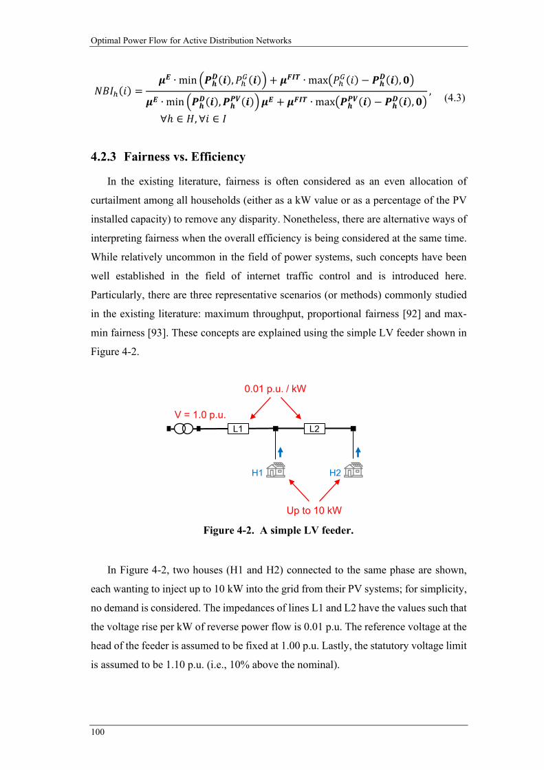
Optimal Power Flow for Active Distribution Networks
100
𝑁𝑁𝐵𝐵𝐼𝐼ℎ(𝑖𝑖) =𝝁𝝁𝑬𝑬 ∙ min �𝑷𝑷𝒉𝒉𝑫𝑫(𝒊𝒊),𝑃𝑃ℎ𝐺𝐺(𝒊𝒊)� + 𝝁𝝁𝑷𝑷𝑰𝑰𝑻𝑻 ∙ max�𝑃𝑃ℎ𝐺𝐺(𝑖𝑖) − 𝑷𝑷𝒉𝒉𝑫𝑫(𝒊𝒊),𝟎𝟎�
𝝁𝝁𝑬𝑬 ∙ min �𝑷𝑷𝒉𝒉𝑫𝑫(𝒊𝒊),𝑷𝑷𝒉𝒉𝑷𝑷𝑷𝑷(𝒊𝒊)�𝝁𝝁𝑬𝑬 + 𝝁𝝁𝑷𝑷𝑰𝑰𝑻𝑻 ∙ max�𝑷𝑷𝒉𝒉𝑷𝑷𝑷𝑷(𝒊𝒊) − 𝑷𝑷𝒉𝒉𝑫𝑫(𝒊𝒊),𝟎𝟎�,
∀ℎ ∈ 𝐻𝐻,∀𝑖𝑖 ∈ 𝐼𝐼
(4.3)
4.2.3 Fairness vs. Efficiency
In the existing literature, fairness is often considered as an even allocation of
curtailment among all households (either as a kW value or as a percentage of the PV
installed capacity) to remove any disparity. Nonetheless, there are alternative ways of
interpreting fairness when the overall efficiency is being considered at the same time.
While relatively uncommon in the field of power systems, such concepts have been
well established in the field of internet traffic control and is introduced here.
Particularly, there are three representative scenarios (or methods) commonly studied
in the existing literature: maximum throughput, proportional fairness [92] and max-
min fairness [93]. These concepts are explained using the simple LV feeder shown in
Figure 4-2.
In Figure 4-2, two houses (H1 and H2) connected to the same phase are shown,
each wanting to inject up to 10 kW into the grid from their PV systems; for simplicity,
no demand is considered. The impedances of lines L1 and L2 have the values such that
the voltage rise per kW of reverse power flow is 0.01 p.u. The reference voltage at the
head of the feeder is assumed to be fixed at 1.00 p.u. Lastly, the statutory voltage limit
is assumed to be 1.10 p.u. (i.e., 10% above the nominal).
Figure 4-2. A simple LV feeder.
V = 1.0 p.u.
H1
L1 L2
H2
0.01 p.u. / kW
Up to 10 kW

Chapter 4: Fairness of Active Power Curtailment Schemes: A Residential Context
101
Based on this setup, it can be immediately verified that, if both houses are to inject
10 kW into the grid, the voltage at H1 and H2 would rise to 1.20 p.u. and 1.30 p.u.,
well above the statutory limit of 1.10 p.u. Consequently, without other means of
mitigating voltage rise, active power curtailment is inevitable. At the same time,
depending on how fairness is considered, the curtailment seen in each house can vary
significantly. To this end, the three unique solutions for maximum throughput,
proportional fairness and max-min fairness are shown in Figure 4-3.
As the name suggests, maximum throughput refers to the scenario when the
aggregated generation is maximised. In this example, this is achieved by allowing H1
to inject at 10 kW while H2 is fully curtailed, as shown in Figure 4-3-a. Since H2 is
farther away from the head of the feeder (i.e., has higher impedance), it is more
(a)
(b)
(c)
Figure 4-3. Illustration of the solutions to (a) maximum throughput, (b) proportional fairness and (c) max-min fairness.
1.0 p.u. 1.1 p.u. 1.1 p.u.
10 kW 0 kW
H1
L1 L2
H2
1.0 p.u. 1.075 p.u. 1.1 p.u.
5.0 kW 2.5 kW
H1
L1 L2
H2
1.0 p.u. 1.067 1.1 p.u.
3.3 kW 3.3 kW
H1
L1 L2
H2
Optimal Power Flow for Active Distribution Networks
102
susceptible to voltage rise than H1. Particularly, if only H2 is to inject power, only
5 kW can be accommodated before the upper voltage limit is reached at H2. Therefore,
in terms of being efficient, H1 is preferred. At the same time, the unfairness of this
allocation method is extremely obvious as there is a huge disparity between the volume
of curtailment H1 (i.e., 0%) and H2 (i.e., 100%) received.
The solution to the max-min fairness method (i.e., Figure 4-3-c) is the same as how
fairness is interpreted in most of the aforementioned literature on PV curtailment
schemes, where the volume of curtailment is equally shared between H1 and H2. It is
also worth highlighting that this is a special case of the max-min fairness when dealing
with voltage issues. This is because every household with a PV system in a feeder will
contribute to voltage rise to a certain degree. In a more generic sense, max-min fairness
attempts to minimise the curtailment for the least fortunate household (H2 in this case).
Lastly, the solution for the proportional fairness method is shown in Figure 4-3-b.
While, at a first glance, this solution does not resemble a fair allocation of curtailment,
as there is still a disparity in how much curtailment is applied for H1 (5 kW, or 50%
curtailment) and H2 (7.5 kW, or 75% curtailment). Nonetheless, it is fair if the relative
impact on each other is also factored in. To illustrate this, consider a small deviation
from this solution where the curtailment of H2 is reduced by 1% (i.e., H2 will inject at
2.6 kW instead of 2.5 kW). In this new scenario, to still satisfy the voltage constraints,
a further 2% curtailment from H1 (i.e., H1 will inject at 4.8 kW instead of 5.0 kW) is
needed. Therefore, based on the relative impact on each other, this method can be
argued as fair. In a more generic sense, the proportional fairness method will find a
solution such that any marginal gain in one household will result in more marginal
losses in all other households combined.
From an optimisation perspective, the aforementioned three scenarios (i.e.,
maximum throughput, proportional fairness and max-min fairness) can be
encompassed by a more generic concept known as 𝛼𝛼-fairness [24]. Mathematically, it
can be formulated through the objective function in (4.4) where 𝑃𝑃ℎ𝐶𝐶𝑛𝑛𝑖𝑖 is the individual
household injections used in the previous examples. Then, through different 𝛼𝛼 values,
the solution to the maximisation problem in (4.5) with the corresponding network
constraints (not shown) can result in different allocation methods (including the three
considered in this sub-section).
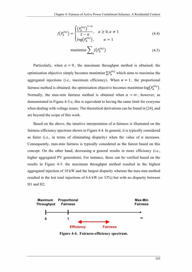
Chapter 4: Fairness of Active Power Curtailment Schemes: A Residential Context
103
𝐽𝐽�𝑃𝑃ℎ𝐶𝐶𝑛𝑛𝑖𝑖� = �
�𝑃𝑃ℎ𝐶𝐶𝑛𝑛𝑖𝑖�
1−𝛼𝛼
1 − 𝛼𝛼, 𝛼𝛼 ≥ 0,𝛼𝛼 ≠ 1
log�𝑃𝑃ℎ𝐶𝐶𝑛𝑛𝑖𝑖� , 𝛼𝛼 = 1
(4.4)
maximise� 𝐽𝐽�𝑃𝑃ℎ𝐶𝐶𝑛𝑛𝑖𝑖�
ℎ (4.5)
Particularly, when 𝛼𝛼 = 0 , the maximum throughput method is obtained; the
optimisation objective simply becomes maximise∑𝑃𝑃ℎ𝐶𝐶𝑛𝑛𝑖𝑖 which aims to maximise the
aggregated injections (i.e., maximum efficiency). When 𝛼𝛼 = 1 , the proportional
fairness method is obtained; the optimisation objective becomes maximise log�𝑃𝑃ℎ𝐶𝐶𝑛𝑛𝑖𝑖�.
Normally, the max-min fairness method is obtained when 𝛼𝛼 → ∞ ; however, as
demonstrated in Figure 4-3-c, this is equivalent to having the same limit for everyone
when dealing with voltage issues. The theoretical derivations can be found in [24], and
are beyond the scope of this work.
Based on the above, the intuitive interpretation of 𝛼𝛼-fairness is illustrated on the
fairness-efficiency spectrum shown in Figure 4-4. In general, it is typically considered
as fairer (i.e., in terms of eliminating disparity) when the value of 𝛼𝛼 increases.
Consequently, max-min fairness is typically considered as the fairest based on this
concept. On the other hand, decreasing 𝛼𝛼 general results in more efficiency (i.e.,
higher aggregated PV generation). For instance, these can be verified based on the
results in Figure 4-3: the maximum throughput method resulted in the highest
aggregated injection of 10 kW and the largest disparity whereas the max-min method
resulted in the lest total injections of 6.6 kW (or 33%) but with no disparity between
H1 and H2.
Figure 4-4. Fairness-efficiency spectrum.
Maximum Throughput
0 1 ∞
ProportionalFairness
Max-MinFairness
Efficiency Fairness
Optimal Power Flow for Active Distribution Networks
104
4.2.4 Fairness Metrics
Qualitatively, fairness is relatively easy to grasp as it is often immediately apparent
that a scheme is fair (when all households are injecting the same amount) or not fair
(when there is a disparity among households). However, this binary way of classifying
schemes does not allow a quantitative comparison of how much one scheme is unfair
compared to another as any scheme that resulting in an uneven allocation is classified
as unfair. Therefore, several fairness metrics have been proposed in the existing
literature to allow more meaningful comparisons. In general, these metrics are largely
based on the relative spread (i.e., disparity) of the benefits (e.g., power injections to
the grid) among multiple households. For illustration purposes, the benefit each
household ℎ receives will be denoted by 𝑏𝑏ℎ.
The simplest form of a fairness metric is based on the maximum benefit (i.e.,
maxℎ{𝑏𝑏ℎ} ) and minimum benefit (i.e., minℎ{𝑏𝑏ℎ} ). This can be done either as a
difference, as shown in (4.6), or as a ratio, as shown in (4.7). While this gives a general
sense of fairness based on the extremes (households with the maximum benefit and
minimum benefit), it does not factor in all other households in between. Therefore, it
is often inadequate for a large number of households.
Max-Min Difference = maxℎ{𝑏𝑏ℎ} − minℎ{𝑏𝑏ℎ} (4.6)
Max-Min Ratio =minℎ{𝑏𝑏ℎ}maxℎ{𝑏𝑏ℎ} (4.7)
The variance can also be used to quantify fairness, as it considers the relative
spread of all benefits from the mean value; the formula is shown in (4.8) where |𝐻𝐻| is
the cardinality of the set 𝐻𝐻 and 𝑏𝑏� is the mean of all 𝑏𝑏ℎ values. A scaled version of the
variance based on the mean can also be used, which is commonly referred to as the
coefficient of variation (COV), as shown in (4.9). However, a potential drawback of
both the variance and COV is its unboundedness, i.e., they are in range of [0,∞), and
thus becomes difficult for comparison purposes.
Variance = �𝑏𝑏ℎ − 𝑏𝑏�
|𝐻𝐻|ℎ∈𝐻𝐻 (4.8)
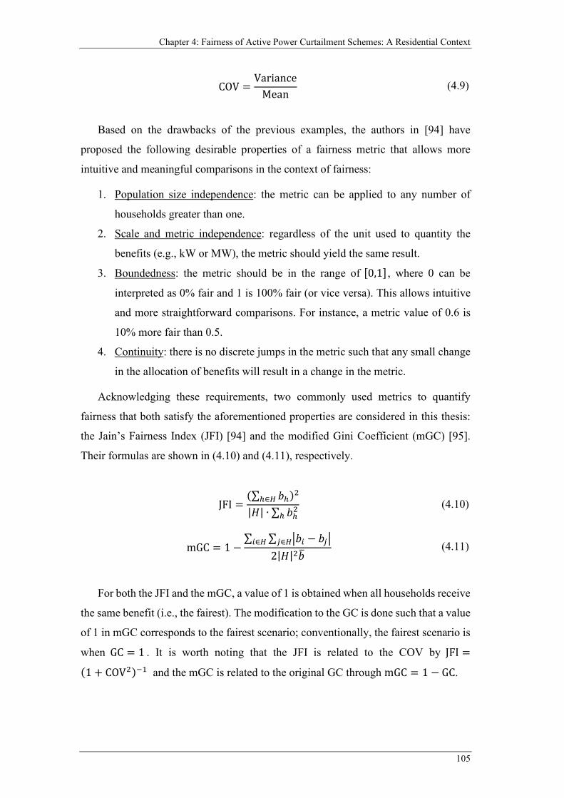
Chapter 4: Fairness of Active Power Curtailment Schemes: A Residential Context
105
COV =Variance
Mean (4.9)
Based on the drawbacks of the previous examples, the authors in [94] have
proposed the following desirable properties of a fairness metric that allows more
intuitive and meaningful comparisons in the context of fairness:
1. Population size independence: the metric can be applied to any number of
households greater than one.
2. Scale and metric independence: regardless of the unit used to quantity the
benefits (e.g., kW or MW), the metric should yield the same result.
3. Boundedness: the metric should be in the range of [0,1] , where 0 can be
interpreted as 0% fair and 1 is 100% fair (or vice versa). This allows intuitive
and more straightforward comparisons. For instance, a metric value of 0.6 is
10% more fair than 0.5.
4. Continuity: there is no discrete jumps in the metric such that any small change
in the allocation of benefits will result in a change in the metric.
Acknowledging these requirements, two commonly used metrics to quantify
fairness that both satisfy the aforementioned properties are considered in this thesis:
the Jain’s Fairness Index (JFI) [94] and the modified Gini Coefficient (mGC) [95].
Their formulas are shown in (4.10) and (4.11), respectively.
JFI =(∑ 𝑏𝑏ℎℎ∈𝐻𝐻 )2
|𝐻𝐻| ∙ ∑ 𝑏𝑏ℎ2ℎ (4.10)
mGC = 1 −∑ ∑ �𝑏𝑏𝐶𝐶 − 𝑏𝑏𝑖𝑖�𝑖𝑖∈𝐻𝐻𝐶𝐶∈𝐻𝐻
2|𝐻𝐻|2𝑏𝑏� (4.11)
For both the JFI and the mGC, a value of 1 is obtained when all households receive
the same benefit (i.e., the fairest). The modification to the GC is done such that a value
of 1 in mGC corresponds to the fairest scenario; conventionally, the fairest scenario is
when GC = 1 . It is worth noting that the JFI is related to the COV by JFI =
(1 + COV2)−1 and the mGC is related to the original GC through mGC = 1 − GC.
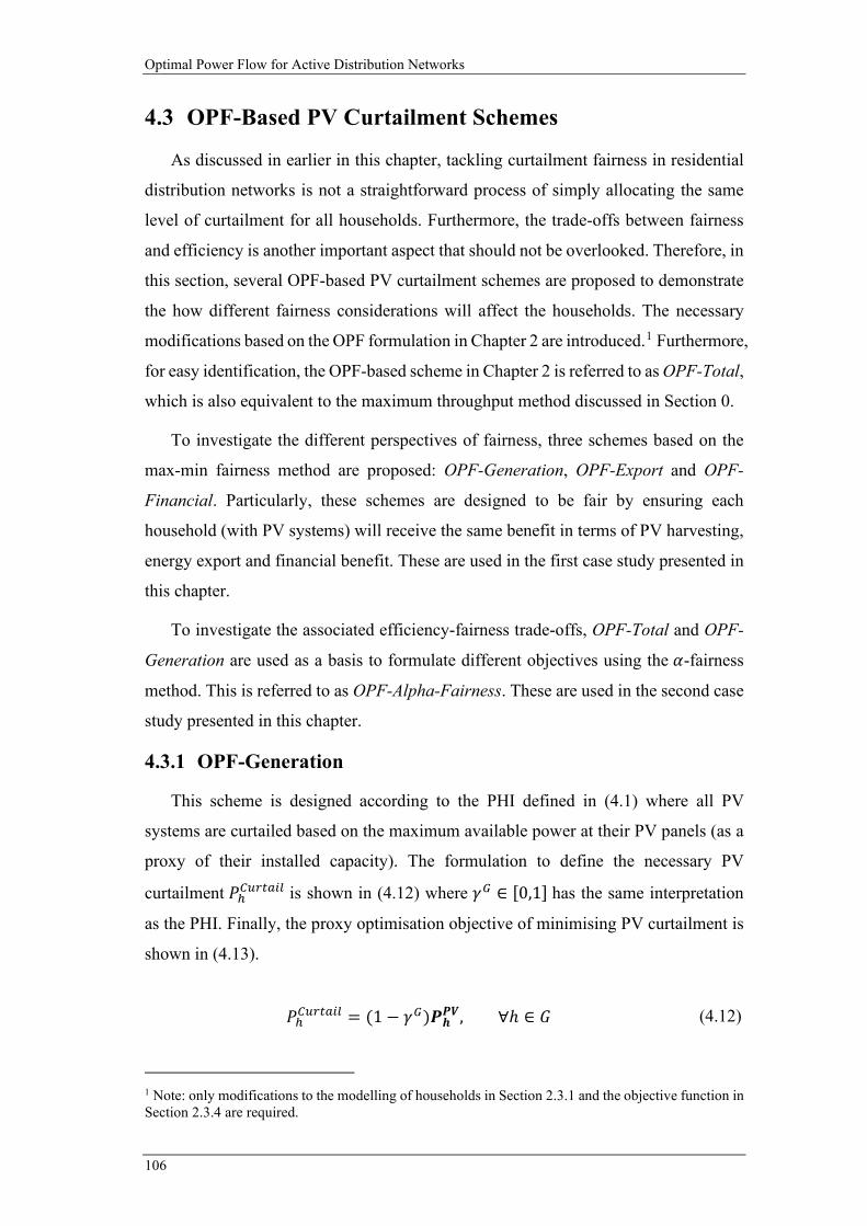
Optimal Power Flow for Active Distribution Networks
106
4.3 OPF-Based PV Curtailment Schemes
As discussed in earlier in this chapter, tackling curtailment fairness in residential
distribution networks is not a straightforward process of simply allocating the same
level of curtailment for all households. Furthermore, the trade-offs between fairness
and efficiency is another important aspect that should not be overlooked. Therefore, in
this section, several OPF-based PV curtailment schemes are proposed to demonstrate
the how different fairness considerations will affect the households. The necessary
modifications based on the OPF formulation in Chapter 2 are introduced.1 Furthermore,
for easy identification, the OPF-based scheme in Chapter 2 is referred to as OPF-Total,
which is also equivalent to the maximum throughput method discussed in Section 0.
To investigate the different perspectives of fairness, three schemes based on the
max-min fairness method are proposed: OPF-Generation, OPF-Export and OPF-
Financial. Particularly, these schemes are designed to be fair by ensuring each
household (with PV systems) will receive the same benefit in terms of PV harvesting,
energy export and financial benefit. These are used in the first case study presented in
this chapter.
To investigate the associated efficiency-fairness trade-offs, OPF-Total and OPF-
Generation are used as a basis to formulate different objectives using the 𝛼𝛼-fairness
method. This is referred to as OPF-Alpha-Fairness. These are used in the second case
study presented in this chapter.
4.3.1 OPF-Generation
This scheme is designed according to the PHI defined in (4.1) where all PV
systems are curtailed based on the maximum available power at their PV panels (as a
proxy of their installed capacity). The formulation to define the necessary PV
curtailment 𝑃𝑃ℎ𝐶𝐶𝐶𝐶𝐶𝐶𝐶𝐶𝐶𝐶𝐶𝐶𝐶𝐶 is shown in (4.12) where 𝛾𝛾𝐺𝐺 ∈ [0,1] has the same interpretation
as the PHI. Finally, the proxy optimisation objective of minimising PV curtailment is
shown in (4.13).
𝑃𝑃ℎ𝐶𝐶𝐶𝐶𝐶𝐶𝐶𝐶𝐶𝐶𝐶𝐶𝐶𝐶 = (1 − 𝛾𝛾𝐺𝐺)𝑷𝑷𝒉𝒉𝑷𝑷𝑷𝑷, ∀ℎ ∈ 𝐺𝐺 (4.12)
1 Note: only modifications to the modelling of households in Section 2.3.1 and the objective function in Section 2.3.4 are required.
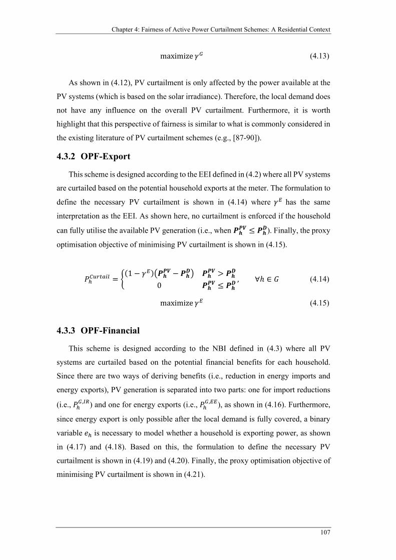
Chapter 4: Fairness of Active Power Curtailment Schemes: A Residential Context
107
maximize 𝛾𝛾𝐺𝐺 (4.13)
As shown in (4.12), PV curtailment is only affected by the power available at the
PV systems (which is based on the solar irradiance). Therefore, the local demand does
not have any influence on the overall PV curtailment. Furthermore, it is worth
highlight that this perspective of fairness is similar to what is commonly considered in
the existing literature of PV curtailment schemes (e.g., [87-90]).
4.3.2 OPF-Export
This scheme is designed according to the EEI defined in (4.2) where all PV systems
are curtailed based on the potential household exports at the meter. The formulation to
define the necessary PV curtailment is shown in (4.14) where 𝛾𝛾𝐸𝐸 has the same
interpretation as the EEI. As shown here, no curtailment is enforced if the household
can fully utilise the available PV generation (i.e., when 𝑷𝑷𝒉𝒉𝑷𝑷𝑷𝑷 ≤ 𝑷𝑷𝒉𝒉𝑫𝑫). Finally, the proxy
optimisation objective of minimising PV curtailment is shown in (4.15).
𝑃𝑃ℎ𝐶𝐶𝐶𝐶𝐶𝐶𝐶𝐶𝐶𝐶𝐶𝐶𝐶𝐶 = �(1 − 𝛾𝛾𝐸𝐸)�𝑷𝑷𝒉𝒉𝑷𝑷𝑷𝑷 − 𝑷𝑷𝒉𝒉𝑫𝑫� 𝑷𝑷𝒉𝒉𝑷𝑷𝑷𝑷 > 𝑷𝑷𝒉𝒉𝑫𝑫
0 𝑷𝑷𝒉𝒉𝑷𝑷𝑷𝑷 ≤ 𝑷𝑷𝒉𝒉𝑫𝑫, ∀ℎ ∈ 𝐺𝐺 (4.14)
maximize 𝛾𝛾𝐸𝐸 (4.15)
4.3.3 OPF-Financial
This scheme is designed according to the NBI defined in (4.3) where all PV
systems are curtailed based on the potential financial benefits for each household.
Since there are two ways of deriving benefits (i.e., reduction in energy imports and
energy exports), PV generation is separated into two parts: one for import reductions
(i.e., 𝑃𝑃ℎ𝐺𝐺,𝐼𝐼𝐼𝐼) and one for energy exports (i.e., 𝑃𝑃ℎ
𝐺𝐺,𝐸𝐸𝐸𝐸), as shown in (4.16). Furthermore,
since energy export is only possible after the local demand is fully covered, a binary
variable 𝑠𝑠ℎ is necessary to model whether a household is exporting power, as shown
in (4.17) and (4.18). Based on this, the formulation to define the necessary PV
curtailment is shown in (4.19) and (4.20). Finally, the proxy optimisation objective of
minimising PV curtailment is shown in (4.21).
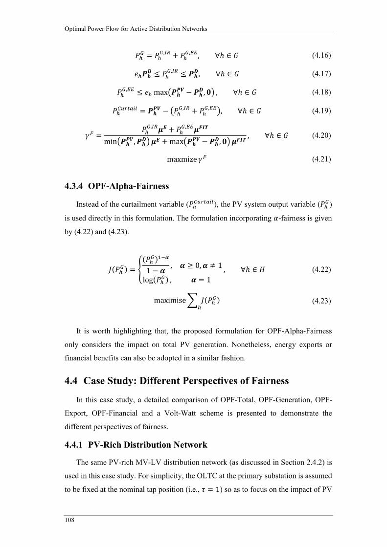
Optimal Power Flow for Active Distribution Networks
108
𝑃𝑃ℎ𝐺𝐺 = 𝑃𝑃ℎ𝐺𝐺,𝐼𝐼𝐼𝐼 + 𝑃𝑃ℎ
𝐺𝐺,𝐸𝐸𝐸𝐸 , ∀ℎ ∈ 𝐺𝐺 (4.16)
𝑠𝑠ℎ𝑷𝑷𝒉𝒉𝑫𝑫 ≤ 𝑃𝑃ℎ𝐺𝐺,𝐼𝐼𝐼𝐼 ≤ 𝑷𝑷𝒉𝒉𝑫𝑫, ∀ℎ ∈ 𝐺𝐺 (4.17)
𝑃𝑃ℎ𝐺𝐺,𝐸𝐸𝐸𝐸 ≤ 𝑠𝑠ℎ max�𝑷𝑷𝒉𝒉𝑷𝑷𝑷𝑷 − 𝑷𝑷𝒉𝒉𝑫𝑫,𝟎𝟎� , ∀ℎ ∈ 𝐺𝐺 (4.18)
𝑃𝑃ℎ𝐶𝐶𝐶𝐶𝐶𝐶𝐶𝐶𝐶𝐶𝐶𝐶𝐶𝐶 = 𝑷𝑷𝒉𝒉𝑷𝑷𝑷𝑷 − �𝑃𝑃ℎ𝐺𝐺,𝐼𝐼𝐼𝐼 + 𝑃𝑃ℎ
𝐺𝐺,𝐸𝐸𝐸𝐸�, ∀ℎ ∈ 𝐺𝐺 (4.19)
𝛾𝛾𝑃𝑃 =𝑃𝑃ℎ𝐺𝐺,𝐼𝐼𝐼𝐼𝝁𝝁𝑬𝑬 + 𝑃𝑃ℎ
𝐺𝐺,𝐸𝐸𝐸𝐸𝝁𝝁𝑷𝑷𝑰𝑰𝑻𝑻
min�𝑷𝑷𝒉𝒉𝑷𝑷𝑷𝑷,𝑷𝑷𝒉𝒉𝑫𝑫�𝝁𝝁𝑬𝑬 + max�𝑷𝑷𝒉𝒉𝑷𝑷𝑷𝑷 − 𝑷𝑷𝒉𝒉𝑫𝑫,𝟎𝟎�𝝁𝝁𝑷𝑷𝑰𝑰𝑻𝑻, ∀ℎ ∈ 𝐺𝐺 (4.20)
maxmize 𝛾𝛾𝑃𝑃 (4.21)
4.3.4 OPF-Alpha-Fairness
Instead of the curtailment variable (𝑃𝑃ℎ𝐶𝐶𝐶𝐶𝐶𝐶𝐶𝐶𝐶𝐶𝐶𝐶𝐶𝐶), the PV system output variable (𝑃𝑃ℎ𝐺𝐺)
is used directly in this formulation. The formulation incorporating 𝛼𝛼-fairness is given
by (4.22) and (4.23).
𝐽𝐽(𝑃𝑃ℎ𝐺𝐺) = �(𝑃𝑃ℎ𝐺𝐺)1−𝜶𝜶
1 − 𝜶𝜶, 𝜶𝜶 ≥ 0,𝜶𝜶 ≠ 1
log(𝑃𝑃ℎ𝐺𝐺) , 𝜶𝜶 = 1, ∀ℎ ∈ 𝐻𝐻 (4.22)
maximise� 𝐽𝐽(𝑃𝑃ℎ𝐺𝐺)ℎ
(4.23)
It is worth highlighting that, the proposed formulation for OPF-Alpha-Fairness
only considers the impact on total PV generation. Nonetheless, energy exports or
financial benefits can also be adopted in a similar fashion.
4.4 Case Study: Different Perspectives of Fairness
In this case study, a detailed comparison of OPF-Total, OPF-Generation, OPF-
Export, OPF-Financial and a Volt-Watt scheme is presented to demonstrate the
different perspectives of fairness.
4.4.1 PV-Rich Distribution Network
The same PV-rich MV-LV distribution network (as discussed in Section 2.4.2) is
used in this case study. For simplicity, the OLTC at the primary substation is assumed
to be fixed at the nominal tap position (i.e., 𝜏𝜏 = 1) so as to focus on the impact of PV
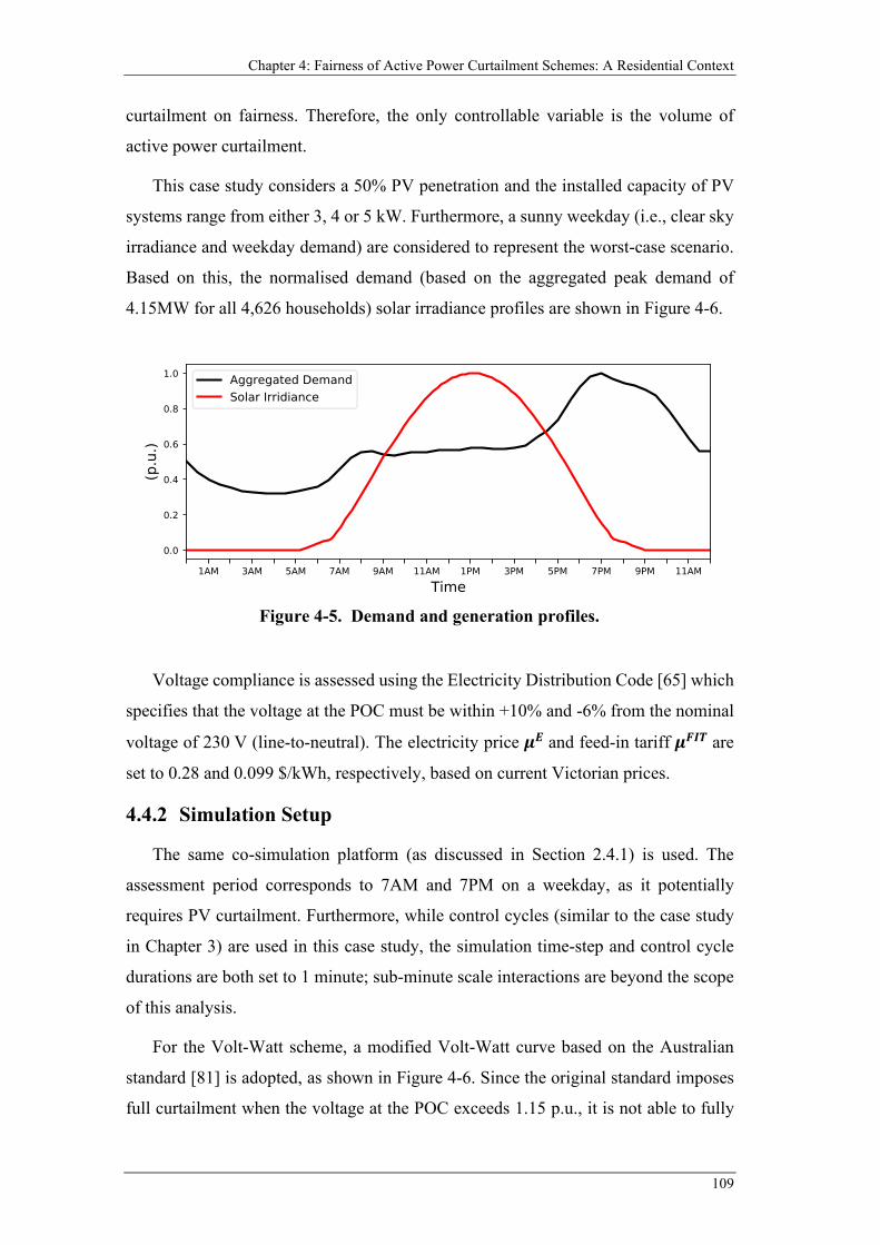
Chapter 4: Fairness of Active Power Curtailment Schemes: A Residential Context
109
curtailment on fairness. Therefore, the only controllable variable is the volume of
active power curtailment.
This case study considers a 50% PV penetration and the installed capacity of PV
systems range from either 3, 4 or 5 kW. Furthermore, a sunny weekday (i.e., clear sky
irradiance and weekday demand) are considered to represent the worst-case scenario.
Based on this, the normalised demand (based on the aggregated peak demand of
4.15MW for all 4,626 households) solar irradiance profiles are shown in Figure 4-6.
Voltage compliance is assessed using the Electricity Distribution Code [65] which
specifies that the voltage at the POC must be within +10% and -6% from the nominal
voltage of 230 V (line-to-neutral). The electricity price 𝝁𝝁𝑬𝑬 and feed-in tariff 𝝁𝝁𝑷𝑷𝑰𝑰𝑻𝑻 are
set to 0.28 and 0.099 $/kWh, respectively, based on current Victorian prices.
4.4.2 Simulation Setup
The same co-simulation platform (as discussed in Section 2.4.1) is used. The
assessment period corresponds to 7AM and 7PM on a weekday, as it potentially
requires PV curtailment. Furthermore, while control cycles (similar to the case study
in Chapter 3) are used in this case study, the simulation time-step and control cycle
durations are both set to 1 minute; sub-minute scale interactions are beyond the scope
of this analysis.
For the Volt-Watt scheme, a modified Volt-Watt curve based on the Australian
standard [81] is adopted, as shown in Figure 4-6. Since the original standard imposes
full curtailment when the voltage at the POC exceeds 1.15 p.u., it is not able to fully
Figure 4-5. Demand and generation profiles.
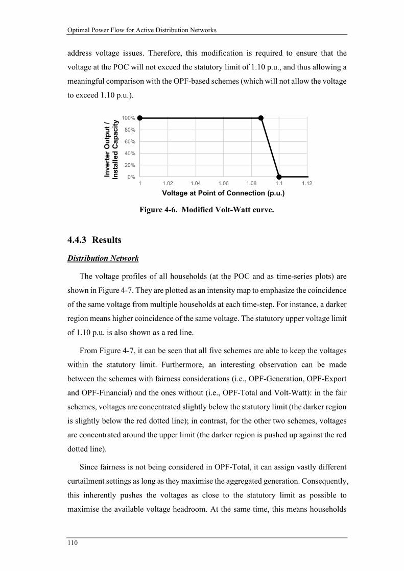
Optimal Power Flow for Active Distribution Networks
110
address voltage issues. Therefore, this modification is required to ensure that the
voltage at the POC will not exceed the statutory limit of 1.10 p.u., and thus allowing a
meaningful comparison with the OPF-based schemes (which will not allow the voltage
to exceed 1.10 p.u.).
4.4.3 Results
Distribution Network
The voltage profiles of all households (at the POC and as time-series plots) are
shown in Figure 4-7. They are plotted as an intensity map to emphasize the coincidence
of the same voltage from multiple households at each time-step. For instance, a darker
region means higher coincidence of the same voltage. The statutory upper voltage limit
of 1.10 p.u. is also shown as a red line.
From Figure 4-7, it can be seen that all five schemes are able to keep the voltages
within the statutory limit. Furthermore, an interesting observation can be made
between the schemes with fairness considerations (i.e., OPF-Generation, OPF-Export
and OPF-Financial) and the ones without (i.e., OPF-Total and Volt-Watt): in the fair
schemes, voltages are concentrated slightly below the statutory limit (the darker region
is slightly below the red dotted line); in contrast, for the other two schemes, voltages
are concentrated around the upper limit (the darker region is pushed up against the red
dotted line).
Since fairness is not being considered in OPF-Total, it can assign vastly different
curtailment settings as long as they maximise the aggregated generation. Consequently,
this inherently pushes the voltages as close to the statutory limit as possible to
maximise the available voltage headroom. At the same time, this means households
Figure 4-6. Modified Volt-Watt curve.
0%
20%
40%
60%
80%
100%
1 1.02 1.04 1.06 1.08 1.1 1.12
Voltage at Point of Connection (p.u.)
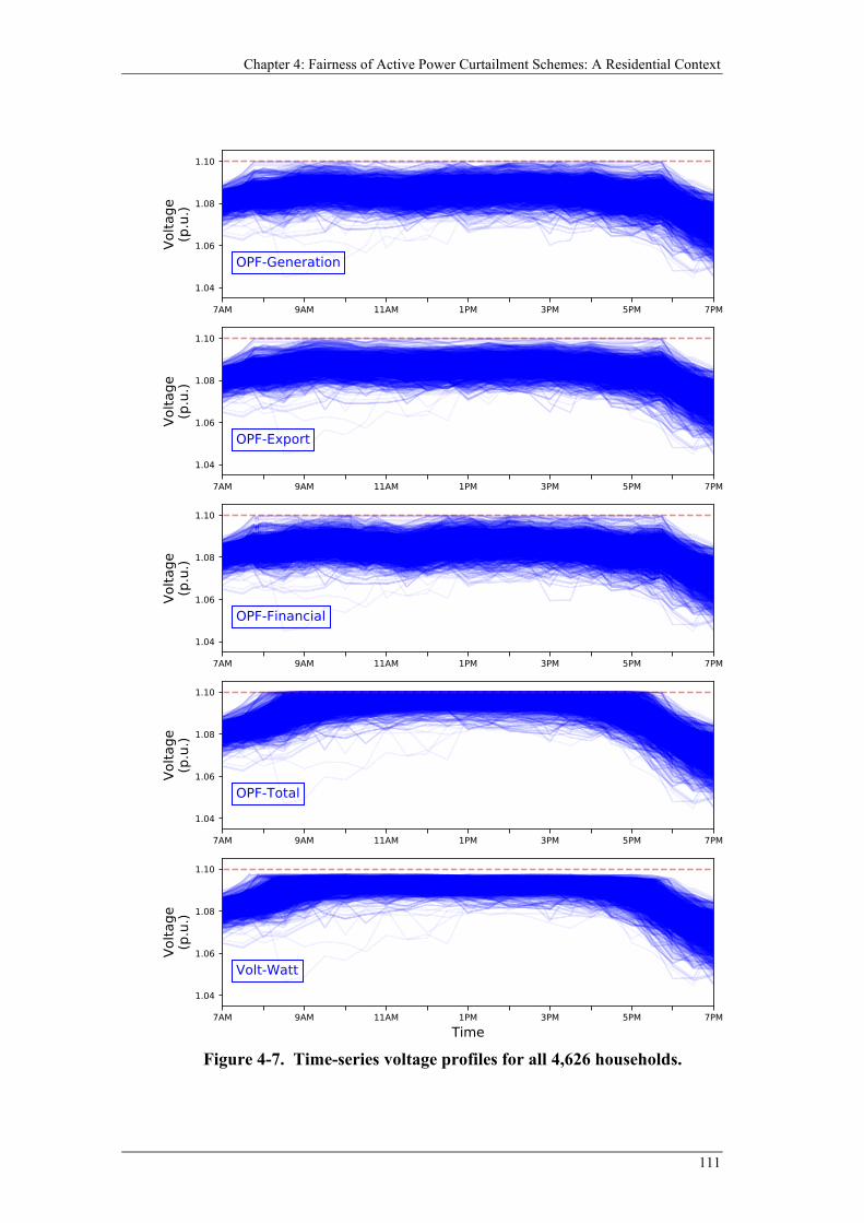
Chapter 4: Fairness of Active Power Curtailment Schemes: A Residential Context
111
Figure 4-7. Time-series voltage profiles for all 4,626 households.
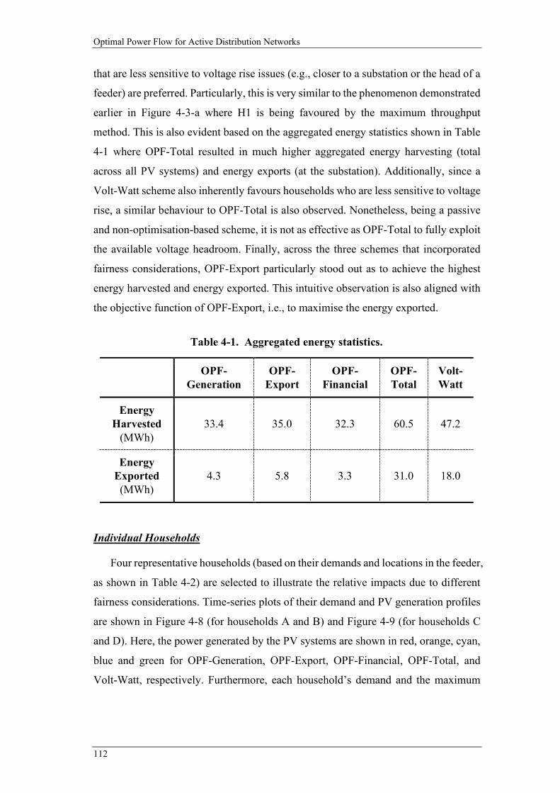
Optimal Power Flow for Active Distribution Networks
112
that are less sensitive to voltage rise issues (e.g., closer to a substation or the head of a
feeder) are preferred. Particularly, this is very similar to the phenomenon demonstrated
earlier in Figure 4-3-a where H1 is being favoured by the maximum throughput
method. This is also evident based on the aggregated energy statistics shown in Table
4-1 where OPF-Total resulted in much higher aggregated energy harvesting (total
across all PV systems) and energy exports (at the substation). Additionally, since a
Volt-Watt scheme also inherently favours households who are less sensitive to voltage
rise, a similar behaviour to OPF-Total is also observed. Nonetheless, being a passive
and non-optimisation-based scheme, it is not as effective as OPF-Total to fully exploit
the available voltage headroom. Finally, across the three schemes that incorporated
fairness considerations, OPF-Export particularly stood out as to achieve the highest
energy harvested and energy exported. This intuitive observation is also aligned with
the objective function of OPF-Export, i.e., to maximise the energy exported.
Individual Households
Four representative households (based on their demands and locations in the feeder,
as shown in Table 4-2) are selected to illustrate the relative impacts due to different
fairness considerations. Time-series plots of their demand and PV generation profiles
are shown in Figure 4-8 (for households A and B) and Figure 4-9 (for households C
and D). Here, the power generated by the PV systems are shown in red, orange, cyan,
blue and green for OPF-Generation, OPF-Export, OPF-Financial, OPF-Total, and
Volt-Watt, respectively. Furthermore, each household’s demand and the maximum
Table 4-1. Aggregated energy statistics.
OPF- Generation
OPF- Export
OPF- Financial
OPF- Total
Volt- Watt
Energy Harvested
(MWh) 33.4 35.0 32.3 60.5 47.2
Energy Exported (MWh)
4.3 5.8 3.3 31.0 18.0
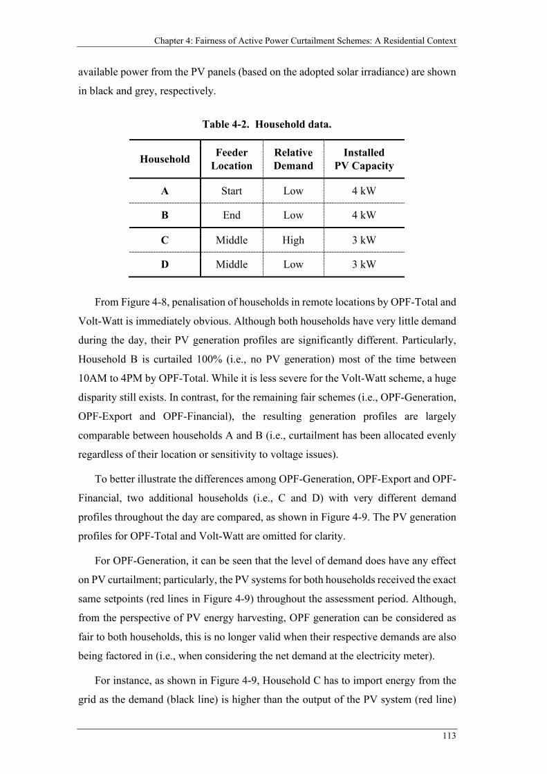
Chapter 4: Fairness of Active Power Curtailment Schemes: A Residential Context
113
available power from the PV panels (based on the adopted solar irradiance) are shown
in black and grey, respectively.
From Figure 4-8, penalisation of households in remote locations by OPF-Total and
Volt-Watt is immediately obvious. Although both households have very little demand
during the day, their PV generation profiles are significantly different. Particularly,
Household B is curtailed 100% (i.e., no PV generation) most of the time between
10AM to 4PM by OPF-Total. While it is less severe for the Volt-Watt scheme, a huge
disparity still exists. In contrast, for the remaining fair schemes (i.e., OPF-Generation,
OPF-Export and OPF-Financial), the resulting generation profiles are largely
comparable between households A and B (i.e., curtailment has been allocated evenly
regardless of their location or sensitivity to voltage issues).
To better illustrate the differences among OPF-Generation, OPF-Export and OPF-
Financial, two additional households (i.e., C and D) with very different demand
profiles throughout the day are compared, as shown in Figure 4-9. The PV generation
profiles for OPF-Total and Volt-Watt are omitted for clarity.
For OPF-Generation, it can be seen that the level of demand does have any effect
on PV curtailment; particularly, the PV systems for both households received the exact
same setpoints (red lines in Figure 4-9) throughout the assessment period. Although,
from the perspective of PV energy harvesting, OPF generation can be considered as
fair to both households, this is no longer valid when their respective demands are also
being factored in (i.e., when considering the net demand at the electricity meter).
For instance, as shown in Figure 4-9, Household C has to import energy from the
grid as the demand (black line) is higher than the output of the PV system (red line)
Table 4-2. Household data.
Household Feeder Location
Relative Demand
Installed PV Capacity
A Start Low 4 kW
B End Low 4 kW
C Middle High 3 kW
D Middle Low 3 kW
Optimal Power Flow for Active Distribution Networks
114
between 9AM and 4PM, even though this demand can be fully covered by the PV
system (grey line). In contrast, with OPF-Export, Household C is able to better utilise
its PV system to cover the local demand between 9AM and 4PM; not only achieving
zero energy import, but also some energy export (when the orange line is above the
black line in Figure 4-9). Although not immediately apparent, it can be verified that,
during periods when energy export is possible (i.e., grey line is above the black line),
both households are allowed to export the same proportion (i.e., distance between the
orange line and black line) with respective to their total potential energy export (i.e.,
distance between grey line and black line). Therefore, from an energy export
perspective, OPF-Export can be considered as fair.
While the PV generation profiles for OPF-Generation and OPF-Export showed
distinct characteristics for households C and D, the results for OPF-Financial is quite
the opposite. This is mainly due to the fact that curtailment is applied not only based
on their demand and generation, but also the and generation of other households as
well as the adopted cost of electricity and feed-in tariff. Nonetheless, the results can
still be analysed using the metric to quantify financial benefits (i.e., the NBI).
Particularly, households C and D both received the same average NBI1 of 0.547 for
the assessment period, and thus OPF-Financial can be considered as fair from the
perspective of financial benefits.
1 Firstly, calculated for each time-step. Then, averaged throughout the assessment period.
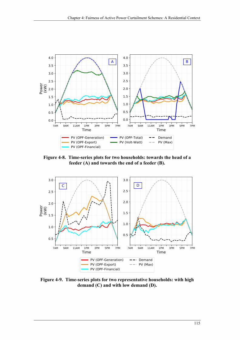
Chapter 4: Fairness of Active Power Curtailment Schemes: A Residential Context
115
Figure 4-8. Time-series plots for two households: towards the head of a feeder (A) and towards the end of a feeder (B).
Figure 4-9. Time-series plots for two representative households: with high demand (C) and with low demand (D).
Optimal Power Flow for Active Distribution Networks
116
Fairness Assessment
To extend the previous analysis (on the different perspectives of fairness) for all
households in the network, the proposed household-centric metrics (i.e., PHI, EEI and
NBI, as discussed in Section 4.2.4) are evaluated for each household and at each
simulation time-step; these are shown as scatted plots in Figure 4-10. The key feature
of this figure is the spread at each timestep, which is an indicator for the disparity
among households. For instance, if all the points overlap, it means no disparity (i.e.,
absolute equality for all households). It is also worth noting that, for the EEI plots, a
‘N/A’ is used to indicate the instances when EEI is not applicable to a household, i.e.,
time-steps with no surplus PV generation.
From these household-centric metrics, the JFI and mGC are also evaluated per
time-step to quantitatively compare the fairness of the investigated schemes. The
average values of JFI and mGC throughout the assessment period are shown in
Table 4-3 and Table 4-4, respectively. As discussed previously, a value of 1 means all
households received the same benefit (i.e., absolute equity). Furthermore, the highest
values (i.e., the fairest scheme) in terms of the four perspectives (i.e., PV harvesting,
import reduction, energy export and financial benefit) are highlighted in bold.
Based on the results, it is apparent that, from the perspective of PV harvesting,
OPF-Generation is the fairest scheme. As shown in Figure 4-10, the setpoints
calculated by OPF-Generation ensures that the PHI for all households is exactly the
same in every time-step. Consequently, both the JFI and mGC evaluated for the PHI
are also 1, indicating that there is no disparity among all households in terms of PV
harvesting. In contrast, the PHI for each time-step can vary significantly for the other
four schemes (as shown in Figure 4-10), and thus resulting in lower JFI and mGC (as
shown in Table 4-3 and Table 4-4, respectively). Therefore, it can be argued that, from
the perspective of PV harvesting, the remaining four schemes are less effective in
removing the disparity among households, and thus not as fair as OPF-Generation.
Similar observations (to OPF-Generation) can also be made for OPF-Export and OPF-
Financial: they are the most effective in removing disparity in terms of energy export
and financial benefit, respectively, while also having the associated trade-offs in terms
of the other metrics. Lastly, it is worth noting that the correlation between JFI and
mGC are very high. At the same time, the mGC tends to place a heavier emphasis on
disparity as the mGC is consistently lower than JFI for the same scenario.
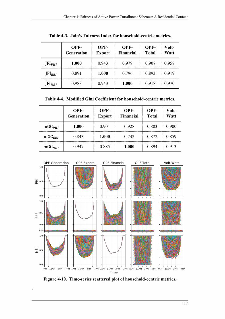
Chapter 4: Fairness of Active Power Curtailment Schemes: A Residential Context
117
.
Table 4-3. Jain’s Fairness Index for household-centric metrics.
OPF- Generation
OPF- Export
OPF- Financial
OPF- Total
Volt- Watt
JFI𝑷𝑷𝑷𝑷𝑰𝑰 1.000 0.943 0.979 0.907 0.958
JFI𝑬𝑬𝑬𝑬𝑰𝑰 0.891 1.000 0.796 0.893 0.919
JFI𝑵𝑵𝑩𝑩𝑰𝑰 0.988 0.943 1.000 0.918 0.970
Table 4-4. Modified Gini Coefficient for household-centric metrics.
OPF- Generation
OPF- Export
OPF- Financial
OPF- Total
Volt- Watt
mGC𝑷𝑷𝑷𝑷𝑰𝑰 1.000 0.901 0.928 0.883 0.900
mGC𝑬𝑬𝑬𝑬𝑰𝑰 0.843 1.000 0.742 0.872 0.859
mGC𝑵𝑵𝑩𝑩𝑰𝑰 0.947 0.885 1.000 0.894 0.913
Figure 4-10. Time-series scattered plot of household-centric metrics.
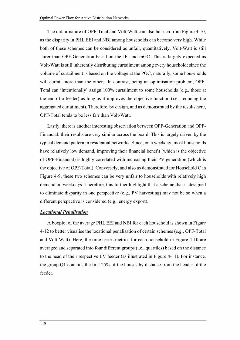
Optimal Power Flow for Active Distribution Networks
118
The unfair nature of OPF-Total and Volt-Watt can also be seen from Figure 4-10,
as the disparity in PHI, EEI and NBI among households can become very high. While
both of these schemes can be considered as unfair, quantitatively, Volt-Watt is still
fairer than OPF-Generation based on the JFI and mGC. This is largely expected as
Volt-Watt is still inherently distributing curtailment among every household; since the
volume of curtailment is based on the voltage at the POC, naturally, some households
will curtail more than the others. In contrast, being an optimisation problem, OPF-
Total can ‘intentionally’ assign 100% curtailment to some households (e.g., those at
the end of a feeder) as long as it improves the objective function (i.e., reducing the
aggregated curtailment). Therefore, by design, and as demonstrated by the results here,
OPF-Total tends to be less fair than Volt-Watt.
Lastly, there is another interesting observation between OPF-Generation and OPF-
Financial: their results are very similar across the board. This is largely driven by the
typical demand pattern in residential networks. Since, on a weekday, most households
have relatively low demand, improving their financial benefit (which is the objective
of OPF-Financial) is highly correlated with increasing their PV generation (which is
the objective of OPF-Total). Conversely, and also as demonstrated for Household C in
Figure 4-9, these two schemes can be very unfair to households with relatively high
demand on weekdays. Therefore, this further highlight that a scheme that is designed
to eliminate disparity in one perspective (e.g., PV harvesting) may not be so when a
different perspective is considered (e.g., energy export).
Locational Penalisation
A boxplot of the average PHI, EEI and NBI for each household is shown in Figure
4-12 to better visualise the locational penalisation of certain schemes (e.g., OPF-Total
and Volt-Watt). Here, the time-series metrics for each household in Figure 4-10 are
averaged and separated into four different groups (i.e., quartiles) based on the distance
to the head of their respective LV feeder (as illustrated in Figure 4-11). For instance,
the group Q1 contains the first 25% of the houses by distance from the header of the
feeder.
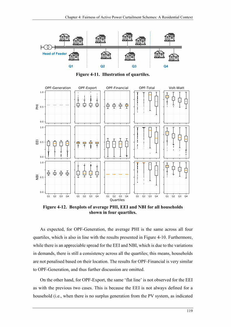
Chapter 4: Fairness of Active Power Curtailment Schemes: A Residential Context
119
As expected, for OPF-Generation, the average PHI is the same across all four
quartiles, which is also in line with the results presented in Figure 4-10. Furthermore,
while there is an appreciable spread for the EEI and NBI, which is due to the variations
in demands, there is still a consistency across all the quartiles; this means, households
are not penalised based on their location. The results for OPF-Financial is very similar
to OPF-Generation, and thus further discussion are omitted.
On the other hand, for OPF-Export, the same ‘flat line’ is not observed for the EEI
as with the previous two cases. This is because the EEI is not always defined for a
household (i.e., when there is no surplus generation from the PV system, as indicated
Figure 4-11. Illustration of quartiles.
Figure 4-12. Boxplots of average PHI, EEI and NBI for all households
shown in four quartiles.
Q1 Q2 Q3 Q4
Head of Feeder
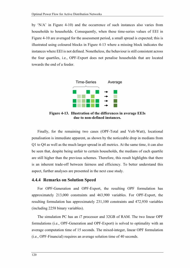
Optimal Power Flow for Active Distribution Networks
120
by ‘N/A’ in Figure 4-10) and the occurrence of such instances also varies from
households to households. Consequently, when these time-series values of EEI in
Figure 4-10 are averaged for the assessment period, a small spread is expected; this is
illustrated using coloured blocks in Figure 4-13 where a missing block indicates the
instances where EEI is not defined. Nonetheless, the behaviour is still consistent across
the four quartiles, i.e., OPF-Export does not penalise households that are located
towards the end of a feeder.
Finally, for the remaining two cases (OPF-Total and Volt-Watt), locational
penalisation is immediate apparent, as shown by the noticeable drop in medians from
Q1 to Q4 as well as the much larger spread in all metrics. At the same time, it can also
be seen that, despite being unfair to certain households, the medians of each quartile
are still higher than the previous schemes. Therefore, this result highlights that there
is an inherent trade-off between fairness and efficiency. To better understand this
aspect, further analyses are presented in the next case study.
4.4.4 Remarks on Solution Speed
For OPF-Generation and OPF-Export, the resulting OPF formulation has
approximately 213,000 constraints and 463,900 variables. For OPF-Export, the
resulting formulation has approximately 231,100 constraints and 472,930 variables
(including 2258 binary variables).
The simulation PC has an i7 processor and 32GB of RAM. The two linear OPF
formulations (i.e., OPF-Generation and OPF-Export) is solved to optimality with an
average computation time of 15 seconds. The mixed-integer, linear OPF formulation
(i.e., OPF-Financial) requires an average solution time of 40 seconds.
Figure 4-13. Illustration of the differences in average EEIs
due to non-defined instances.
Time-Series Average
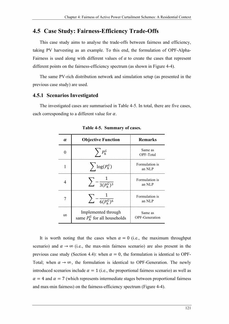
Chapter 4: Fairness of Active Power Curtailment Schemes: A Residential Context
121
4.5 Case Study: Fairness-Efficiency Trade-Offs
This case study aims to analyse the trade-offs between fairness and efficiency,
taking PV harvesting as an example. To this end, the formulation of OPF-Alpha-
Fairness is used along with different values of 𝛼𝛼 to create the cases that represent
different points on the fairness-efficiency spectrum (as shown in Figure 4-4).
The same PV-rich distribution network and simulation setup (as presented in the
previous case study) are used.
4.5.1 Scenarios Investigated
The investigated cases are summarised in Table 4-5. In total, there are five cases,
each corresponding to a different value for 𝛼𝛼.
It is worth noting that the cases when 𝛼𝛼 = 0 (i.e., the maximum throughput
scenario) and 𝛼𝛼 → ∞ (i.e., the max-min fairness scenario) are also present in the
previous case study (Section 4.4): when 𝛼𝛼 = 0, the formulation is identical to OPF-
Total; when 𝛼𝛼 → ∞ , the formulation is identical to OPF-Generation. The newly
introduced scenarios include 𝛼𝛼 = 1 (i.e., the proportional fairness scenario) as well as
𝛼𝛼 = 4 and 𝛼𝛼 = 7 (which represents intermediate stages between proportional fairness
and max-min fairness) on the fairness-efficiency spectrum (Figure 4-4).
Table 4-5. Summary of cases.
𝜶𝜶 Objective Function Remarks
0 �𝑃𝑃ℎ𝐺𝐺 Same as OPF-Total
1 � log(𝑃𝑃ℎ𝐺𝐺) Formulation is an NLP
4 �−1
3(𝑃𝑃ℎ𝐺𝐺)3 Formulation is
an NLP
7 �−1
6(𝑃𝑃ℎ𝐺𝐺)6 Formulation is
an NLP
∞ Implemented through same 𝑃𝑃ℎ𝐺𝐺 for all households
Same as OPF-Generation
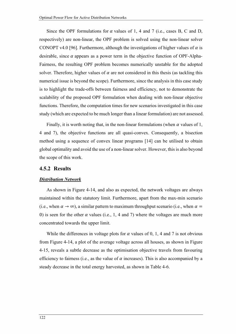
Optimal Power Flow for Active Distribution Networks
122
Since the OPF formulations for 𝛼𝛼 values of 1, 4 and 7 (i.e., cases B, C and D,
respectively) are non-linear, the OPF problem is solved using the non-linear solver
CONOPT v4.0 [96]. Furthermore, although the investigations of higher values of 𝛼𝛼 is
desirable, since 𝛼𝛼 appears as a power term in the objective function of OPF-Alpha-
Fairness, the resulting OPF problem becomes numerically unstable for the adopted
solver. Therefore, higher values of 𝛼𝛼 are not considered in this thesis (as tackling this
numerical issue is beyond the scope). Furthermore, since the analysis in this case study
is to highlight the trade-offs between fairness and efficiency, not to demonstrate the
scalability of the proposed OPF formulation when dealing with non-linear objective
functions. Therefore, the computation times for new scenarios investigated in this case
study (which are expected to be much longer than a linear formulation) are not assessed.
Finally, it is worth noting that, in the non-linear formulations (when 𝛼𝛼 values of 1,
4 and 7), the objective functions are all quasi-convex. Consequently, a bisection
method using a sequence of convex linear programs [14] can be utilised to obtain
global optimality and avoid the use of a non-linear solver. However, this is also beyond
the scope of this work.
4.5.2 Results
Distribution Network
As shown in Figure 4-14, and also as expected, the network voltages are always
maintained within the statutory limit. Furthermore, apart from the max-min scenario
(i.e., when 𝛼𝛼 → ∞), a similar pattern to maximum throughput scenario (i.e., when 𝛼𝛼 =
0) is seen for the other 𝛼𝛼 values (i.e., 1, 4 and 7) where the voltages are much more
concentrated towards the upper limit.
While the differences in voltage plots for 𝛼𝛼 values of 0, 1, 4 and 7 is not obvious
from Figure 4-14, a plot of the average voltage across all houses, as shown in Figure
4-15, reveals a subtle decrease as the optimisation objective travels from favouring
efficiency to fairness (i.e., as the value of 𝛼𝛼 increases). This is also accompanied by a
steady decrease in the total energy harvested, as shown in Table 4-6.
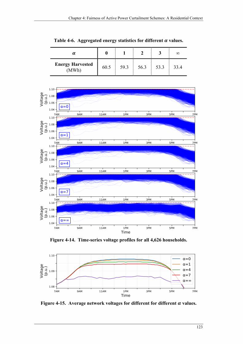
Chapter 4: Fairness of Active Power Curtailment Schemes: A Residential Context
123
Table 4-6. Aggregated energy statistics for different 𝜶𝜶 values.
𝜶𝜶 0 1 2 3 ∞
Energy Harvested (MWh) 60.5 59.3 56.3 53.3 33.4
Figure 4-14. Time-series voltage profiles for all 4,626 households.
Figure 4-15. Average network voltages for different for different 𝜶𝜶 values.
Optimal Power Flow for Active Distribution Networks
124
Fairness Assessment
A boxplot of the average PHI for all households (adopting the same four quartiles
as before) is shown in Figure 4-16. Here, there are two distinct features as the value of
𝛼𝛼 increases (i.e., becoming increasingly fair based on the fairness-efficiency spectrum).
Firstly, as indicated by the red shaded region, the relative spread between the medians
steadily decreases, which means, the scheme is becoming increasingly fair by reducing
the disparity in curtailment. Secondly, as indicated by the red line, the minimum PHI
(which corresponds to the most heavily penalised household) steadily increases, which
means, the least fortunate household is increasingly being protected as fairness
improves. This gradual increase in fairness is also reflected through the two adopted
fairness metrics (i.e., JFI and mGC), as shown in Table 4-7, where the JFI and mGC
continuous to improve as 𝛼𝛼 increases.
Finally, it is worth acknowledging that, for the scenario considered here, the
marginal improvement in fairness may result in appreciable impact on the overall
efficiency (i.e., total energy harvest), as shown in Table 4-8. This is especially so after
the proportional fairness case (i.e., for 𝛼𝛼 > 1). For instance, while an increase of 𝛼𝛼
Table 4-7. Jain’s Fairness Index and modified Gini Coefficient for different 𝜶𝜶 values.
𝜶𝜶 0 1 4 7 ∞
JFI 0.907 0.951 0.960 0.962 1.000
mGC 0.883 0.904 0.909 0.910 1.000
Figure 4-16. Boxplots of average PHI for different 𝜶𝜶 values.
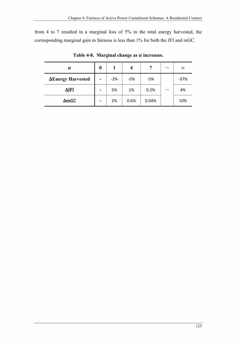
Chapter 4: Fairness of Active Power Curtailment Schemes: A Residential Context
125
from 4 to 7 resulted in a marginal loss of 5% in the total energy harvested, the
corresponding marginal gain in fairness is less than 1% for both the JFI and mGC.
Table 4-8. Marginal change as 𝜶𝜶 increases.
𝜶𝜶 0 1 4 7 ∙∙∙ ∞
𝚫𝚫Energy Harvested - -2% -5% -5%
∙∙∙
-37%
𝚫𝚫JFI - 5% 1% 0.2% 4%
𝚫𝚫mGC - 2% 0.6% 0.04% 10%

Optimal Power Flow for Active Distribution Networks
126
4.6 Summary
While active power curtailment is a simple yet effective solution to mitigate the
issues associated with excessive reverse power flows, applying it in a fair and effective
way is not necessarily a straightforward process in a residential context, as
demonstrated in this chapter.
The first challenge is due to the many, and potentially conflicting, perspectives that
can be used to quantify the impact on households, such as PV harvesting, energy
exports and financial benefits. As demonstrated in this chapter, a curtailment scheme
that is designed to be fair in one of these perspectives may not be so in others.
The second challenge is due to the trade-offs between achieving absolute fairness
(where there is no disparity among households for a given perspective) and its impact
on overall efficiency (e.g., aggregated PV harvesting). Since there is an inherent trade-
off between fairness and efficiency, this may justify the need for alternative avenues
to address the resulting disparities, such as through compensation schemes.
Overall, the results highlight that, since fairness is a multi-facet problem, an
ultimate fair scheme may not exist. Consequently, there is always the need for
decision-makers to determine the most appropriate objectives and compromises that
best aligns with their respective policies. To this end, the methodology presented in
this chapter can help to compare different schemes so as to allow more informed
decisions.
5 A HARDWARE-IN-THE-LOOP
DEMONSTRATION PLATFORM
5.1 Introduction
Distribution networks studies are typically carried out offline, using PC-based
power flow analysis packages; a few notable names include OpenDSS [60],
MATPOWER [97] and PSS®SINCAL [98]. Furthermore, to cater for advanced
schemes, co-simulation setups are often adopted, such as the one introduced in
Section 2.4.1 that uses a Python script and AIMMS, as these power flow analysis
packages are typically not built with such functionality.
Although these offline approaches are indispensable to the research and
development of new concepts, there are limitations from a validation and
demonstration perspective. Firstly, they are based on software models, and thus it is
difficult to realistically capture all the intricacies of physical systems. For instance, in
the context of active distribution networks, using scripts/code is not possible to
realistically model the physical interactions between the control room (and the
associated infrastructure such as SCADA, distribution management system, advanced
schemes, etc.) and the devices in a distribution network (e.g., DG units, OLTCs, etc.).
Furthermore, it often lacks the flexibility (or capability) for live demonstration
purposes, which require the real-time visualisation of simulation data rather than
creating tables and plots after the simulation has finished. Therefore, in addition to the
development of adequate schemes for future distribution networks, new approaches to
facilitate the real-time validation and demonstration of these schemes are also
desirable. Particularly, this helps to boost industry’s confidence in adopting these
advanced approaches in real networks.
To this end, this can be accomplished through an online approach using a real-time
simulator (RTS). An RTS is specialised hardware that not only can carry out network
simulations in real-time 1 but also features extensive interfaces to facilitate the
1 Real-time simulation is achieved when, given an adopted simulation time-step (e.g., around microseconds for electromagnetic transient simulations in power systems), the computation time is guaranteed to be less than the adopted time-step.
Optimal Power Flow for Active Distribution Networks
128
interactions of physical systems/hardware with the simulated network; notable
examples of an RTS include the RTDS Simulator [99] and the Opal-RT Simulator
[100]. Therefore, leveraging these capabilities of an RTS, the development of a
realistic hardware-in-the-loop (HIL) demonstration platform for advanced schemes in
future distribution networks is presented in this chapter.
5.2 Literature Review
In general, HIL-based studies can be classified in two categories: controller HIL
and power HIL. Their main differences lie in the physical hardware being tested and
the interfaces required to the simulated network (in the RTS). For a controller HIL
simulation, it only involves low voltage data communications (e.g., through an
Ethernet connection or analogue signals) to the RTS; all power system components
(e.g., lines, transformers and DG units) are modelled in the RTS. One such example is
[101] that investigates the usage of demand-response signals to manage voltages in
active distribution networks. In the proposed setup, the proposed network controller
that is responsible for calculating the required demand-response signals is
implemented on a PC and interacts with the simulated network (in an RTS) via both
Ethernet and low-voltage analogue signals. Similar setups can also be found in [102]
(for a Volt-VAR optimisation), [103] (for state estimation in low-voltage networks)
and [104] (for adaptive protection schemes). In contrast, a power HIL simulation also
involves real power devices to be interfaced with the RTS; this can range from a few
kWs (e.g., a rooftop PV system in [105] and a residential battery system in [106]) to
hundreds of kWs (e.g., a wind generator in [107]). To facilitate this, power amplifiers
(also known as grid simulators) are required to replicate the responses of the simulated
network such that the real power devices can be operated and tested as if they are
physically connected to the simulated networks.
There are also novel approaches to extend the capability of a conventional HIL
setup. For instance, a key limitation of an RTS is the size of the network that can be
modelled; due to the finite computing power and the rigid restriction on computation
time to guarantee real-time simulation, there is an inherent limit on the size of the
network that can be modelled by an RTS. To tackle this, a hybrid setup that consists
of both offline software and an RTS is developed in [108] to model larger distribution
networks that are technically not feasible for an RTS.
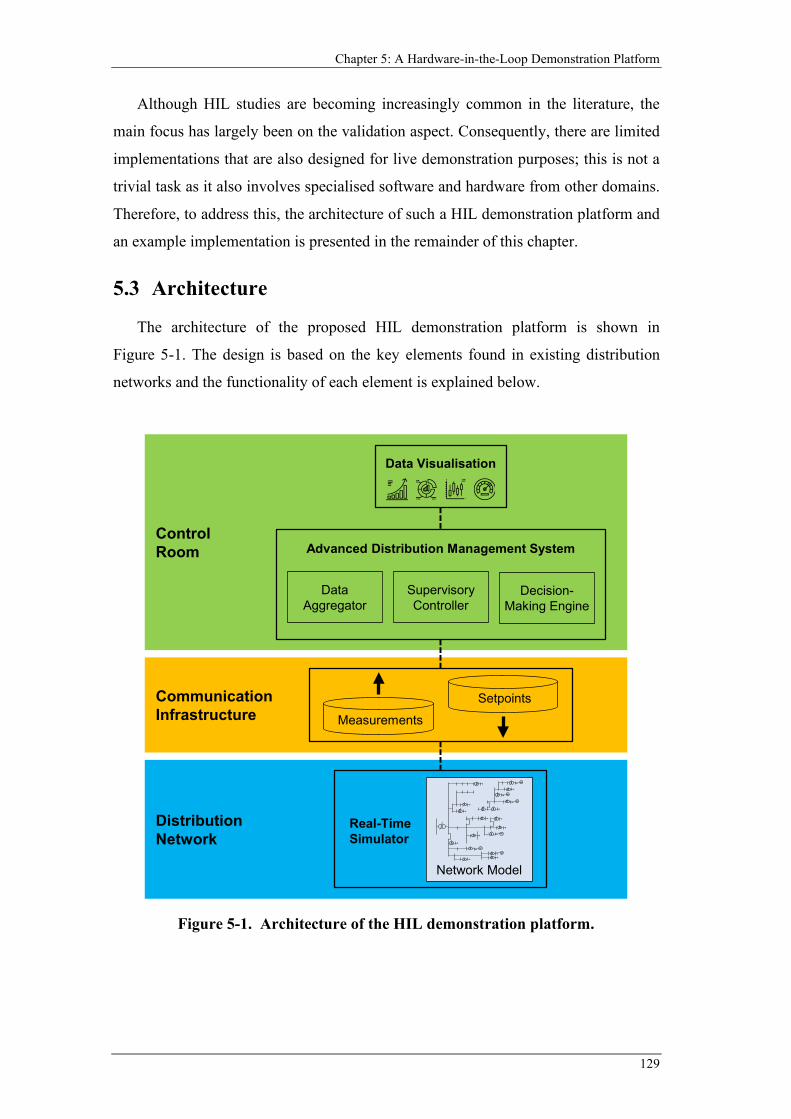
Chapter 5: A Hardware-in-the-Loop Demonstration Platform
129
Although HIL studies are becoming increasingly common in the literature, the
main focus has largely been on the validation aspect. Consequently, there are limited
implementations that are also designed for live demonstration purposes; this is not a
trivial task as it also involves specialised software and hardware from other domains.
Therefore, to address this, the architecture of such a HIL demonstration platform and
an example implementation is presented in the remainder of this chapter.
5.3 Architecture
The architecture of the proposed HIL demonstration platform is shown in
Figure 5-1. The design is based on the key elements found in existing distribution
networks and the functionality of each element is explained below.
Figure 5-1. Architecture of the HIL demonstration platform.
Distribution Network
Control Room
Data Visualisation
Communication Infrastructure
Advanced Distribution Management System
DataAggregator
SupervisoryController
Decision-Making Engine
SetpointsMeasurements
Real-Time Simulator
WF
WF
WF
WF
WF
WF
Network Model
Optimal Power Flow for Active Distribution Networks
130
5.3.1 Distribution Network
A controller HIL setup is considered where the distribution network is modelled in
the RTS. This includes the power system elements (e.g., lines, transformers, loads and
DG units as well as the associated device controllers) that utilise the available model
of an RTS and the communication elements that utilise the hardware interfaces of the
RTS (e.g., DNP3 [109] over Ethernet).
5.3.2 Communication Infrastructure
Physical communication infrastructure (based on the hardware capability of the
RTS) is used to facilitate data transfers between the RTS and the control room. This
includes the necessary network measurements (RTS → control room) for the advanced
scheme and the setpoints (control room → RTS) determined by the advance scheme.
5.3.3 Control Room
Inside the control room, an advanced distribution management system (ADMS)
that contains a data aggregator, a supervisory controller and an advanced decision-
making engine is created. The data aggregator is responsible for handling the
communication with the distribution network; this is necessary for compatibility
reasons as several different protocols can be used in typical distribution networks. The
supervisory controller is responsible for overseeing the real-time operation of the
distribution network, such as identifying constraint violations. The supervisory
controller is also responsible for accessing the decision-making engine (if required) to
determine new setpoints for the controllable devices in the distribution network; this
can be done in regular intervals or when constraint violation is detected.
In addition to the ADMS, a rich data visualisation interface is also created inside
the control room. This is typically achieved through an interactive user interface
displayed on multiple large monitors.
5.4 Implementation of a HIL Demonstration Platform
Based on the proposed architecture, the implementation details of a HIL
demonstration platform (shown in Figure 5-2) at the Smart Grid Lab of The University
of Melbourne [110] is presented in this section. This is combined with the network
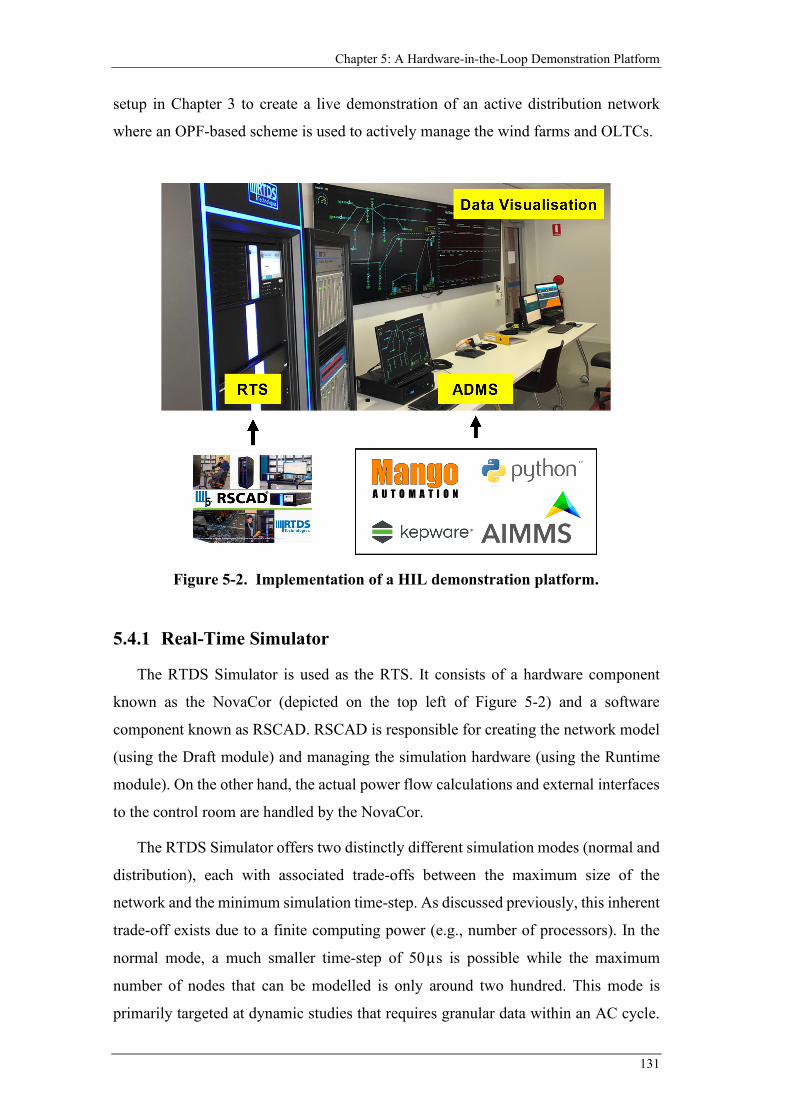
Chapter 5: A Hardware-in-the-Loop Demonstration Platform
131
setup in Chapter 3 to create a live demonstration of an active distribution network
where an OPF-based scheme is used to actively manage the wind farms and OLTCs.
5.4.1 Real-Time Simulator
The RTDS Simulator is used as the RTS. It consists of a hardware component
known as the NovaCor (depicted on the top left of Figure 5-2) and a software
component known as RSCAD. RSCAD is responsible for creating the network model
(using the Draft module) and managing the simulation hardware (using the Runtime
module). On the other hand, the actual power flow calculations and external interfaces
to the control room are handled by the NovaCor.
The RTDS Simulator offers two distinctly different simulation modes (normal and
distribution), each with associated trade-offs between the maximum size of the
network and the minimum simulation time-step. As discussed previously, this inherent
trade-off exists due to a finite computing power (e.g., number of processors). In the
normal mode, a much smaller time-step of 50μs is possible while the maximum
number of nodes that can be modelled is only around two hundred. This mode is
primarily targeted at dynamic studies that requires granular data within an AC cycle.
Figure 5-2. Implementation of a HIL demonstration platform.
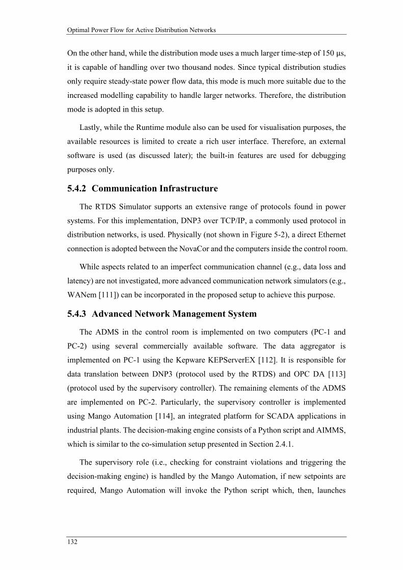
Optimal Power Flow for Active Distribution Networks
132
On the other hand, while the distribution mode uses a much larger time-step of 150 μs,
it is capable of handling over two thousand nodes. Since typical distribution studies
only require steady-state power flow data, this mode is much more suitable due to the
increased modelling capability to handle larger networks. Therefore, the distribution
mode is adopted in this setup.
Lastly, while the Runtime module also can be used for visualisation purposes, the
available resources is limited to create a rich user interface. Therefore, an external
software is used (as discussed later); the built-in features are used for debugging
purposes only.
5.4.2 Communication Infrastructure
The RTDS Simulator supports an extensive range of protocols found in power
systems. For this implementation, DNP3 over TCP/IP, a commonly used protocol in
distribution networks, is used. Physically (not shown in Figure 5-2), a direct Ethernet
connection is adopted between the NovaCor and the computers inside the control room.
While aspects related to an imperfect communication channel (e.g., data loss and
latency) are not investigated, more advanced communication network simulators (e.g.,
WANem [111]) can be incorporated in the proposed setup to achieve this purpose.
5.4.3 Advanced Network Management System
The ADMS in the control room is implemented on two computers (PC-1 and
PC-2) using several commercially available software. The data aggregator is
implemented on PC-1 using the Kepware KEPServerEX [112]. It is responsible for
data translation between DNP3 (protocol used by the RTDS) and OPC DA [113]
(protocol used by the supervisory controller). The remaining elements of the ADMS
are implemented on PC-2. Particularly, the supervisory controller is implemented
using Mango Automation [114], an integrated platform for SCADA applications in
industrial plants. The decision-making engine consists of a Python script and AIMMS,
which is similar to the co-simulation setup presented in Section 2.4.1.
The supervisory role (i.e., checking for constraint violations and triggering the
decision-making engine) is handled by the Mango Automation, if new setpoints are
required, Mango Automation will invoke the Python script which, then, launches
Chapter 5: A Hardware-in-the-Loop Demonstration Platform
133
AIMMS to calculate the new setpoints. For this implementation, the same control
cycle-based approach (discussed in Section 3.3.1) is adopted.
An overview of data flows in the proposed setup is highlighted in Figure 5-3.
5.4.4 Data Visualisation
The built-in dashboard designer of Mango Automation is used to create custom,
HTML-based dashboards for data visualisation. Particularly, two dashboards are
created, one for each of the wall-mounted TVs shown in Figure 5-2.
Dashboard one, shown in Figure 5-4, features the network diagram in a map-like
format to highlight the instantaneous power flows within the network. The main
features include nodal voltages, asset utilisation, demand, OLTC tap positions and
wind farm controls, as shown in Figure 5-5. The base design of the dashboard is draw
as a static image in the scalable vector graphics (SVG) format. Then, live operational
data are used to animate the base design using CSS functions (commonly known as
CSS Animations), e.g., changing the nodal voltages and animating flashing signals.
Dashboard two, shown in Figure 5-6, offers the ability to plot (selectable) network
measurements over time, such as the nodal voltages and output of wind farms. This is
achieved using the built-in graphing features of Mango Automation.
Figure 5-3. Data flows in the proposed setup.
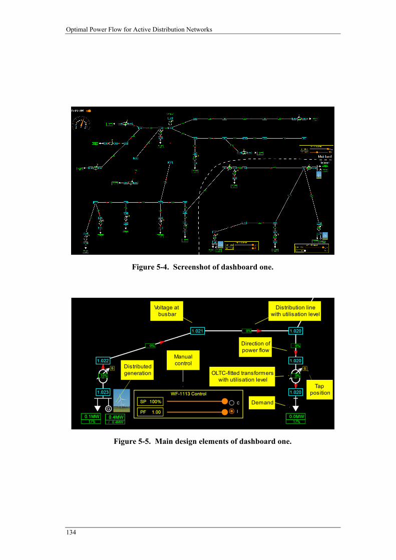
Optimal Power Flow for Active Distribution Networks
134
Figure 5-4. Screenshot of dashboard one.
Figure 5-5. Main design elements of dashboard one.
Distribution line with utilisation level
OLTC-fitted transformers with utilisation level
Voltage at busbar
Direction of power flow
Distributed generation
Demand
Tapposition
Manualcontrol
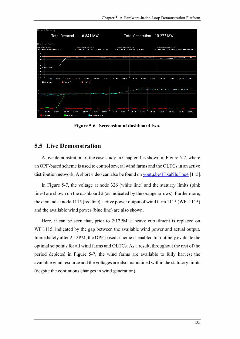
Chapter 5: A Hardware-in-the-Loop Demonstration Platform
135
5.5 Live Demonstration
A live demonstration of the case study in Chapter 3 is shown in Figure 5-7, where
an OPF-based scheme is used to control several wind farms and the OLTCs in an active
distribution network. A short video can also be found on youtu.be/1TxaNIqTno4 [115].
In Figure 5-7, the voltage at node 326 (white line) and the statuary limits (pink
lines) are shown on the dashboard 2 (as indicated by the orange arrows). Furthermore,
the demand at node 1115 (red line), active power output of wind farm 1115 (WF. 1115)
and the available wind power (blue line) are also shown.
Here, it can be seen that, prior to 2:12PM, a heavy curtailment is replaced on
WF 1115, indicated by the gap between the available wind power and actual output.
Immediately after 2:12PM, the OPF-based scheme is enabled to routinely evaluate the
optimal setpoints for all wind farms and OLTCs. As a result, throughout the rest of the
period depicted in Figure 5-7, the wind farms are available to fully harvest the
available wind resource and the voltages are also maintained within the statutory limits
(despite the continuous changes in wind generation).
Figure 5-6. Screenshot of dashboard two.
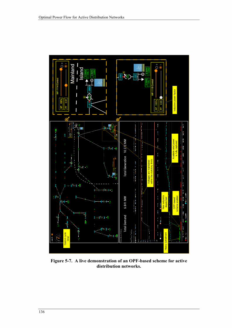
Optimal Power Flow for Active Distribution Networks
136
Figure 5-7. A live demonstration of an OPF-based scheme for active distribution networks.
Volta
ges
are
main
taine
d wi
thin
the
stat
utor
y lim
its
Avail
able
wind
pow
er
is fu
lly c
aptu
red
OPF
-bas
ed
sche
me
enab
led
New
setp
oints
dis
patc
hed
2
3
Heav
y cu
rtailm
ent
1
4
5
Indu
ctive
pow
er fa
ctor
Cont
rol c
ycle
timer
Chapter 5: A Hardware-in-the-Loop Demonstration Platform
137
5.6 Summary
Traditionally, distribution networks studies are carried out offline, using PC-based
software. Although indispensable, there are several limitations from a validation and
demonstration perspective as the it is difficult to capture all the intricacies of physical
systems using software models. Furthermore, while the validation aspect has been
examined in the existing literature through the usage of HIL simulation, the
demonstration aspect is less frequently discussed.
To this end, the architecture of a HIL platform (with a particular focus on the
demonstration and data visualisation) is proposed. Based on this, a specific
implementation using the RTDS Simulator and several commercially available
software at the Smart Grid Lab of The University of Melbourne is presented. The
implemented HIL platform is then used to demonstrate the active control of wind farms
and OLTCs using an OPF-based scheme.
A highlight of such HIL setups is the ability to showcase (in a control room-like
environment) that advanced concepts for future distribution networks, and thus helping
to prove that these advanced concepts are getting closer and closer to real-world
implementation.

Optimal Power Flow for Active Distribution Networks
138
This page is intentionally left blank.
6 CONCLUSION
In this chapter, a summary of the research gaps and contributions is first presented.
Then, the key findings of this thesis are outlined. Finally, potential improvements and
extensions based on the concepts explored in this thesis are introduced.
6.1 Research Gaps and Contributions
Driven by the increasing environmental awareness and financial incentives,
renewable DG, from MW-scale wind farms in rural areas to kW-scale PV systems on
city’s rooftops, has seen a tremendous growth over the last decade. At the same time,
this sudden influx of power generation within the distribution network—the part of a
power system that is typically associated with the last-mile delivery of power to
consumers, not necessarily facilitating the bidirectional power flows as a result of local
generation—has introduced significant operational challenges for distribution
companies. Particularly, technical issues such as voltage rise and asset congestion are
becoming increasingly common in renewable-rich distribution networks.
In this context, the concept of active distribution networks, where network issues
are solved at the operational stage through the real-time monitoring and control of
network assets and participants, is becoming an increasingly attractive alternative to
the otherwise capital-intensive and time-consuming network augmentation. For
instance, existing OLTCs and the reactive power capability of DG units can be
simultaneously exploited to alleviate voltage issues. As a last resort, active power
curtailment can also provide temporary relief from voltage and thermal violations by
reducing the volume of reverse power flows during constrained periods.
However, as more and more sources of flexibility are becoming available to
network operators, existing rule-based approaches (commonly adopted by industry)
are also becoming prohibitively cumbersome due to the fact that many variables (e.g.,
setpoints for each of the controllable devices) and constraints (e.g., voltage limits at
multiple nodes) must be to be considered at the same time. To this end, AC OPF—a
mathematical optimisation problem that seeks the optimal setpoints while satisfying
the network constraints—has shown great potential (albeit mostly in academia) as the
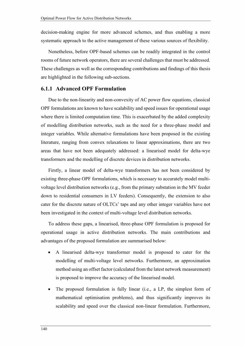
Optimal Power Flow for Active Distribution Networks
140
decision-making engine for more advanced schemes, and thus enabling a more
systematic approach to the active management of these various sources of flexibility.
Nonetheless, before OPF-based schemes can be readily integrated in the control
rooms of future network operators, there are several challenges that must be addressed.
These challenges as well as the corresponding contributions and findings of this thesis
are highlighted in the following sub-sections.
6.1.1 Advanced OPF Formulation
Due to the non-linearity and non-convexity of AC power flow equations, classical
OPF formulations are known to have scalability and speed issues for operational usage
where there is limited computation time. This is exacerbated by the added complexity
of modelling distribution networks, such as the need for a three-phase model and
integer variables. While alternative formulations have been proposed in the existing
literature, ranging from convex relaxations to linear approximations, there are two
areas that have not been adequately addressed: a linearised model for delta-wye
transformers and the modelling of discrete devices in distribution networks.
Firstly, a linear model of delta-wye transformers has not been considered by
existing three-phase OPF formulations, which is necessary to accurately model multi-
voltage level distribution networks (e.g., from the primary substation in the MV feeder
down to residential consumers in LV feeders). Consequently, the extension to also
cater for the discrete nature of OLTCs’ taps and any other integer variables have not
been investigated in the context of multi-voltage level distribution networks.
To address these gaps, a linearised, three-phase OPF formulation is proposed for
operational usage in active distribution networks. The main contributions and
advantages of the proposed formulation are summarised below:
• A linearised delta-wye transformer model is proposed to cater for the
modelling of multi-voltage level networks. Furthermore, an approximation
method using an offset factor (calculated from the latest network measurement)
is proposed to improve the accuracy of the linearised model.
• The proposed formulation is fully linear (i.e., a LP, the simplest form of
mathematical optimisation problems), and thus significantly improves its
scalability and speed over the classical non-linear formulation. Furthermore,
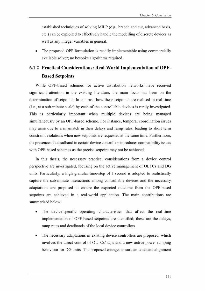
Chapter 6: Conclusion
141
established techniques of solving MILP (e.g., branch and cut, advanced basis,
etc.) can be exploited to effectively handle the modelling of discrete devices as
well as any integer variables in general.
• The proposed OPF formulation is readily implementable using commercially
available solver; no bespoke algorithms required.
6.1.2 Practical Considerations: Real-World Implementation of OPF-
Based Setpoints
While OPF-based schemes for active distribution networks have received
significant attention in the existing literature, the main focus has been on the
determination of setpoints. In contrast, how these setpoints are realised in real-time
(i.e., at a sub-minute scale) by each of the controllable devices is rarely investigated.
This is particularly important when multiple devices are being managed
simultaneously by an OPF-based scheme. For instance, temporal coordination issues
may arise due to a mismatch in their delays and ramp rates, leading to short term
constraint violations when new setpoints are requested at the same time. Furthermore,
the presence of a deadband in certain device controllers introduces compatibility issues
with OPF-based schemes as the precise setpoint may not be achieved.
In this thesis, the necessary practical considerations from a device control
perspective are investigated, focusing on the active management of OLTCs and DG
units. Particularly, a high granular time-step of 1 second is adopted to realistically
capture the sub-minute interactions among controllable devices and the necessary
adaptations are proposed to ensure the expected outcome from the OPF-based
setpoints are achieved in a real-world application. The main contributions are
summarised below:
• The device-specific operating characteristics that affect the real-time
implementation of OPF-based setpoints are identified; these are the delays,
ramp rates and deadbands of the local device controllers.
• The necessary adaptations in existing device controllers are proposed, which
involves the direct control of OLTCs’ taps and a new active power ramping
behaviour for DG units. The proposed changes ensure an adequate alignment
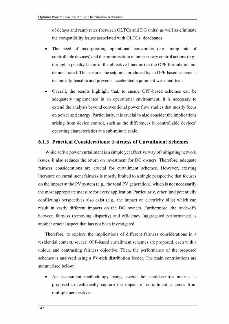
Optimal Power Flow for Active Distribution Networks
142
of delays and ramp rates (between OLTCs and DG units) as well as eliminate
the compatibility issues associated with OLTCs’ deadbands.
• The need of incorporating operational constraints (e.g., ramp rate of
controllable devices) and the minimisation of unnecessary control actions (e.g.,
through a penalty factor in the objective function) in the OPF formulation are
demonstrated. This ensures the setpoints produced by an OPF-based scheme is
technically feasible and prevents accelerated equipment wear-and-tear.
• Overall, the results highlight that, to ensure OPF-based schemes can be
adequately implemented in an operational environment, it is necessary to
extend the analysis beyond conventional power flow studies that mostly focus
on power and energy. Particularly, it is crucial to also consider the implications
arising from device control, such as the differences in controllable devices’
operating characteristics at a sub-minute scale.
6.1.3 Practical Considerations: Fairness of Curtailment Schemes
While active power curtailment is a simple yet effective way of mitigating network
issues, it also reduces the return on investment for DG owners. Therefore, adequate
fairness considerations are crucial for curtailment schemes. However, existing
literature on curtailment fairness is mostly limited to a single perspective that focuses
on the impact at the PV system (e.g., the total PV generation), which is not necessarily
the most appropriate measure for every application. Particularly, other (and potentially
conflicting) perspectives also exist (e.g., the impact on electricity bills) which can
result in vastly different impacts on the DG owners. Furthermore, the trade-offs
between fairness (removing disparity) and efficiency (aggregated performance) is
another crucial aspect that has not been investigated.
Therefore, to explore the implications of different fairness considerations in a
residential context, several OPF-based curtailment schemes are proposed, each with a
unique and contrasting fairness objective. Then, the performance of the proposed
schemes is analysed using a PV-rich distribution feeder. The main contributions are
summarised below:
• An assessment methodology using several household-centric metrics is
proposed to realistically capture the impact of curtailment schemes from
multiple perspectives.
Chapter 6: Conclusion
143
• The different perspectives of fairness (e.g., PV harvesting, energy export and
financial benefits) are identified and the associated trade-offs for different
fairness objectives are quantified. For instance, a scheme that is designed to be
fair in terms of PV harvesting for all households will result in noticeable
disparity in terms of their energy exports.
• For the first time in the context of distribution networks, the concept of alpha-
fairness (commonly used in internet traffic management) is applied as a way to
quantify the relative trade-offs between fairness and efficiency.
• Overall, the results highlight the need of adequate fairness considerations (by
network operators, policymakers, etc.) that best align with the corresponding
objective when active power curtailment is used.
6.1.4 Laboratory Demonstration
While PC-based software is typically used in distribution network studies, it is
often difficult to capture the physical interactions among different systems in an actual
distribution network using software models. To this end, HIL simulations has been
widely used in the existing literature for validation purposes of advanced schemes as
it allows physical hardware to tested. However, there are limited implementations in
the existing literature of HIL setups that also focuses on the demonstration aspect,
which can be extremely useful as an initial step to showcase advanced schemes to
industry (before their eventual trials). Instead, the results are often analysed post
simulation using static plots and tables, which is similar to how it is traditionally done
using PC-based software.
To address this, the architecture of a HIL demonstration platform is proposed, with
a particularly focus on the visualisation of live data. Based on this, a specific
implementation is created at the Smart Grid Lab of The University of Melbourne to
demonstrate OPF-based schemes for active distribution networks. The main
contributions and advantages of the proposed setups are summarised below:
• The process of building a realistic HIL demonstration platform (for advanced
schemes in active distribution networks) from various commercially available
software and hardware packages is documented.
Optimal Power Flow for Active Distribution Networks
144
• The proposed setup extends beyond static plots and tables by introducing a rich
and interactive user interface, and thus enabling a more realistic experience for
demonstration purposes.
6.2 Key Findings
6.2.1 Linearised Three-Phase OPF Formulation
The scalability and speed of the proposed OPF formulation is evaluated using a
realistic MV-LV feeder in Victoria, Australia, which starts from the primary substation
and ends at the connection points of individual residential consumers. In total, the
modelled feeder consists of 4,947 three-phase nodes and 4,626 single-phase connected
residential consumers. The main findings are:
• The proposed linearised OPF is highly accurate in terms of the calculated
voltages and power flows (when compared with the actual values from a
network simulator after the calculated setpoints are implemented) even if flat
start values are used for the estimated terms in the linearised formulation.
• The accuracy of the linearised formulation can be improved through warm start
values (e.g., using recent network measurements) as well as running a second
iteration of the OPF (where the results from the first OPF run is used in the
second iteration). Furthermore, while the latter is found to give the largest
improvement, it also requires the OPF problem to be solved twice (i.e., it
compromises on the solution speed).
• The solution time is sufficiently fast (within a minute for one iteration) even
when integer variables are introduced (e.g., 3 binary variables to model the
OLTC’s taps, as investigated in Chapter 2, and over 2,000 binary variables to
model the export status of households, as investigated in Chapter 4).
6.2.2 OPF-Based Schemes in an Operational Environment
The operational usage of OPF-based schemes is demonstrated using a UK-style
rural distribution feeder with 21 OLTCs and 6 wind farms. The main findings are:
• Due to the mismatch between the delays and ramp rates of existing device
controllers (of OLTCs and wind farms), temporary issues can arise when OPF-
based setpoints are implemented in practice. In contrast, once their delays and
Chapter 6: Conclusion
145
ramp rates are aligned through the propose adaptations, the desirable behaviour
can be achieved.
• The presence of deadbands (e.g., within existing controllers for OLTCs)
introduces compatibility issues with OPF-based schemes as the requested
setpoint cannot be precisely realised, leading to excessive number of control
actions. In contrast, the direct control of OLTCs’ taps (as proposed) is found
to be much more effective as the tap position calculated by the OPF can be
precisely implemented in practice.
• Due to the various sources of flexibility within distribution networks,
inadequate design of a control scheme (i.e., not penalising unnecessary control
actions) may result in an oscillatory behaviour among multiple sets of feasible
control actions, and thus accelerated equipment wear-and-tear. Therefore, the
operational usage of OPF-based schemes must ensure the unnecessary control
actions are penalised (e.g., through a penalty factor in the objective function).
• High granularity modelling is essential to realistically capture the
aforementioned complications that arise from the different operating
characteristics of controllable devices in the sub-minute scale.
6.2.3 Fairness of Curtailment Schemes in Residential Feeders
The implications and trade-offs from different fairness considerations are
investigated using several OPF-based schemes, each considering a unique and
contrasting fairness objective. The main findings are:
• Since the impact from curtailment can be quantified in multiple ways, e.g.,
based on PV harvesting, energy export or financial benefits, there are also
multiple perspectives of fairness. Furthermore, improving fairness in one
particular perspective may lead to a decrease in fairness for the other
perspectives.
• There is an inherent trade-off between fairness (i.e., equality) and efficiency
(i.e., aggregated performance). Particularly, when voltage is the limiting factor
in radial distribution feeders, the marginal gain in fairness may require
substantial compromises in terms of the overall efficiency.
Optimal Power Flow for Active Distribution Networks
146
• While the definition of fairness is relatively simple, i.e., ensuring equality,
incorporating fairness in curtailment schemes is not necessarily a
straightforward process due to the multi-facet nature of fairness in the context
of distribution networks. Therefore, before attempting to improve fairness, it is
necessary to first define the most appropriate fairness objective for a given
application.
6.3 Future Works
6.3.1 Distributed Algorithms for OPF
In this thesis, the OPF formulation is solved as single problem. While the solution
time has been adequate for the investigated networks, alternative approaches that can
further improve the solution time is also desirable to cater for larger/more complex
network models. One such approach is through a distributed algorithm that breaks
down the single OPF problem into multiple smaller sub-problems that can be solved
in parallel. Particularly, an interesting aspect of a distributed approach is the
improvement in solution time when many integer variables are considered (e.g., when
many OLTCs are being modelled, the formulation for OPF-Export in Chapter 4 or
OPF formulations that involves batteries where binary variables are often needed to
model the charging/discharging state [20]). Due to the combinatory nature of mixed-
integer programming where an exhaust search is often required to find the optimal
solution, the process of breaking down the main problem into multiple sub-problems
is expected to bring significant benefits. For instance, a single OPF with 2𝑥𝑥 binary
variables will result in 22𝑥𝑥 different combinations; in contrast, two sub-problems each
with 𝑥𝑥 binary variables (still 2𝑥𝑥 in total) only consists of 2𝑥𝑥 combinations (for each
sub-problem), which is an exponential reduction from 22𝑥𝑥. Therefore, the significant
reduction in complexity from a mixed-integer programming perspective can outweigh
the extra complexity associated with distributed algorithms.
6.3.2 More Accurate Forecast vs. Shorter Control Cycles
In Chapter 3, persistent forecast is adopted for simplicity where the resource
availability (for wind farms) and the demand is expected to remain the same when new
setpoints are calculated. Therefore, the extent of improvements from more accurate
forecast is worth exploring. Furthermore, the potential benefits of using short control

Chapter 6: Conclusion
147
cycles (as opposed to more accurate forecast, but with longer control cycles) should
be explored. Particularly, given that, the level of uncertainty in forecasts is expected
to reduce as the duration of each control cycle shortens, the benefits from more
accurate forecast algorithm is also likely to reduce.
6.3.3 Multi-Period Optimisation
The proposed scheme only considered a single snapshot (i.e., the upcoming control
cycle) when decisions are made. An extension of this work is to quantify the potential
benefits from performing a multi-period optimisation, such as using the receding-
horizon technique, where multiple snapshots in the future are modelled. This can be
particularly beneficial in reducing the number of unnecessary control cycles.
Nonetheless, it also has the drawbacks of longer computation time.
6.3.4 More Scalable Formulation of OPF-Alpha-Fairness
While the concept of alpha-fairness is successfully used (in an offline analysis) to
quantify the trade-offs between fairness and efficiency, due to the nonlinear nature of
the corresponding objective functions, the resulting formulation (i.e., OPF-Alpha-
Fairness in Chapter 4) is not necessarily practical in an operational environment. For
instance, a single snapshot can require as long as ten minutes to solve. Therefore,
alternative formulations are desirable to improve the solution speed, and thus enabling
the operational usage of OPF-Alpha-Fairness.
6.3.5 Fairness Implications when Additional Sources of Flexibility
are Considered
In Chapter 4, only active power curtailment is considered. Therefore, it is worth
extending the analysis to incorporate other sources of flexibility, such as the reactive
power of PV inverters and the OLTC commonly found at primary substations.
Naturally, the OLTC is expected to bring benefits for all households in a PV-rich
distribution network where voltage rise is the issue. However, due to the apparent
power limits of PV inverters, using the reactive power is expected to bring additional
complications depending on whether active power or reactive power is prioritised.

Optimal Power Flow for Active Distribution Networks
148
This page is intentionally left blank.
REFERENCES
[1] REN21, "Renewables 2019: Global status report," REN21 Secretariat, 2019. [2] International Renewable Energy Agency. [Online]. Available:
http://www.irena.org/ [3] E. Lakervi and E. J. Holmes, Electricity distribution network design: IET, 1995. [4] G. Pepermans, J. Driesen, D. Haeseldonckx, R. Belmans, and W. D’haeseleer,
"Distributed generation: definition, benefits and issues," Energy policy, vol. 33, no. 6, pp. 787-798, 2005.
[5] Distributed Energy Generation Market Size, Global Industry Report 2025. [Online]. Available: https://www.grandviewresearch.com/
[6] R. A. Walling, R. Saint, R. C. Dugan, J. Burke, and L. A. Kojovic, "Summary of Distributed Resources Impact on Power Delivery Systems," IEEE Transactions on Power Delivery, vol. 23, no. 3, pp. 1636-1644, Jun. 2008.
[7] A. Navarro-Espinosa and L. F. Ochoa, "Probabilistic Impact Assessment of Low Carbon Technologies in LV Distribution Systems," IEEE Trans. Power Syst., vol. 31, no. 3, pp. 2192-2203, 2016.
[8] L. F. Ochoa, C. J. Dent, and G. P. Harrison, "Distribution Network Capacity Assessment: Variable DG and Active Networks," IEEE Trans. Power Syst., vol. 25, no. 1, pp. 87-95, Nov. 2010.
[9] B. P. Roberts and C. Sandberg, "The Role of Energy Storage in Development of Smart Grids," Proceedings of the IEEE, vol. 99, no. 6, pp. 1139-1144, 2011.
[10] C. Foote, R. Johnston, F. Watson, R. Currie, D. Macleman, and A. Urquhart, "Second generation active network management on Orkney," in Proc. 2013 22nd International Conference and Exhibition on Electricity Distribution (CIRED 2013), pp. 1-4.
[11] S. Georgiopoulos, E. Cerqueira, R. Johnston, R. Currie, and C. Marantes, "Flexible plug and play low carbon networks: An open and scalable active network management solution for a faster and cheaper distributed generation connection," in Proc. 2013 22nd International Conference and Exhibition on Electricity Distribution (CIRED 2013), pp. 1-4.
[12] F. Tariq and L. S. Dooley, "Smart Grid Communication and Networking Technologies: Recent Developments and Future Challenges," in Smart Grids: Opportunities, Developments, and Trends, A. B. M. S. Ali, Ed. London: Springer London, 2013, pp. 199-213.
[13] S. Frank, I. Steponavice, and S. Rebennack, "Optimal power flow: a bibliographic survey I," Energy Systems, vol. 3, no. 3, pp. 221-258, 2012/09/01 2012.
[14] S. Boyd, S. P. Boyd, and L. Vandenberghe, Convex optimization: Cambridge university press, 2004.
[15] J. Chinneck, "Chapter 16: Introduction to Nonlinear Programming," Practical Optimization: a Gentle Introduction, pp. 1-13.
Optimal Power Flow for Active Distribution Networks
150
[16] W. A. Bukhsh, A. Grothey, K. I. M. McKinnon, and P. A. Trodden, "Local Solutions of the Optimal Power Flow Problem," IEEE Transactions on Power Systems, vol. 28, no. 4, pp. 4780-4788, 2013.
[17] L. A. Wolsey and G. L. Nemhauser, Integer and combinatorial optimization, vol. 55: John Wiley & Sons, 1999.
[18] C. A. Smith, S. C. Potts, and M. A. Redfern, "Optimised and pre-emptive strategies for on-load tap changing transformer control relays," in Proc. 2004 2004 Eighth IEE International Conference on Developments in Power System Protection, vol. 2, pp. 526-529 Vol.2.
[19] K. Clark, N. W. Miller, and J. J. Sanchez-Gasca, "Modeling of GE Wind Turbine-Generators for Grid Studies," GE Energy, Schenectady, NY, Apr. 16, 2010.
[20] T. R. Ricciardi, K. Petrou, J. F. Franco, and L. F. Ochoa, "Defining Customer Export Limits in PV-Rich Low Voltage Networks," IEEE Trans. Power Syst., vol. 34, no. 1, pp. 87-97, 2019.
[21] M. Zukerman, L. Tan, H. Wang, and I. Ouveysi, "Efficiency-fairness tradeoff in telecommunications networks," IEEE Communications Letters, vol. 9, no. 7, pp. 643-645, 2005.
[22] M. Steurer, F. Bogdan, W. Ren, M. Sloderbeck, and S. Woodruff, "Controller and Power Hardware-In-Loop Methods for Accelerating Renewable Energy Integration," in Proc. 2007 2007 IEEE Power Engineering Society General Meeting, pp. 1-4.
[23] R. M. Lima and I. E. Grossmann, "Computational advances in solving mixed integer linear programming problems," 2011.
[24] J. Mo and J. Walrand, "Fair end-to-end window-based congestion control," IEEE/ACM Transactions on Networking, vol. 8, no. 5, pp. 556-567, 2000.
[25] S. H. Low, "Convex Relaxation of Optimal Power Flow—Part I: Formulations and Equivalence," IEEE Transactions on Control of Network Systems, vol. 1, no. 1, pp. 15-27, 2014.
[26] J. F. Franco, L. F. Ochoa, and R. Romero, "AC OPF for Smart Distribution Networks: An Efficient and Robust Quadratic Approach," IEEE Trans. Smart Grid, vol. 9, no. 5, pp. 4613-4623, 2018.
[27] J. Carpentier, "Contribution to the economic dispatch problem," Bulletin de la Societe Francoise des Electriciens, vol. 3, no. 8, pp. 431-447, 1962.
[28] Activation of Distributed Energy Resources in the Energy Market. [Online]. Available: https://aemo.com.au/
[29] B. Stott, J. Jardim, and O. Alsac, "DC Power Flow Revisited," IEEE Transactions on Power Systems, vol. 24, no. 3, pp. 1290-1300, 2009.
[30] Market Optimization Details. [Online]. Available: https://www.caiso.com/ [31] A. L. Ott, "Experience with PJM market operation, system design, and
implementation," IEEE Transactions on Power Systems, vol. 18, no. 2, pp. 528-534, 2003.
[32] EUPHEMIA Public Description. [Online]. Available: https://www.nordpoolgroup.com/
References
151
[33] S. P. Bradley, A. C. Hax, and T. L. Magnanti, "Applied mathematical programming," 1977.
[34] User's Manual for CPLEX. [Online]. Available: https://www.ibm.com/analytics/cplex-optimizer
[35] S. W. Alnaser and L. F. Ochoa, "Advanced Network Management Systems: A Risk-Based AC OPF Approach," IEEE Trans. Power Syst., vol. 30, no. 1, pp. 409-418, May 2015.
[36] J. G. Robertson, G. P. Harrison, and A. R. Wallace, "OPF Techniques for Real-Time Active Management of Distribution Networks," IEEE Trans. Power Syst., vol. 32, no. 5, pp. 3529-3537, 2017.
[37] Y. Wei, Y. Juan, D. C. Yu, and K. Bhattarai, "A new optimal reactive power flow model in rectangular form and its solution by predictor corrector primal dual interior point method," IEEE Transactions on Power Systems, vol. 21, no. 1, pp. 61-67, 2006.
[38] Y. Tao and A. P. S. Meliopoulos, "Optimal power flow via quadratic power flow," in Proc. 2011 2011 IEEE/PES Power Systems Conference and Exposition, pp. 1-8.
[39] Q. Y. Jiang, H. Chiang, C. X. Guo, and Y. J. Cao, "Power-current hybrid rectangular formulation for interior-point optimal power flow," IET Generation, Transmission & Distribution, vol. 3, no. 8, pp. 748-756, 2009.
[40] M. Farivar and S. H. Low, "Branch Flow Model: Relaxations and Convexification—Part I," IEEE Trans. Power Syst., vol. 28, no. 3, pp. 2554-2564, 2013.
[41] W. Wang and N. Yu, "Chordal Conversion Based Convex Iteration Algorithm for Three-Phase Optimal Power Flow Problems," IEEE Transactions on Power Systems, vol. 33, no. 2, pp. 1603-1613, 2018.
[42] F. Meng, B. Chowdhury, and M. Chamanamcha, "Three-Phase Optimal Power Flow for Market-Based Control and Optimization of Distributed Generations," IEEE Transactions on Smart Grid, vol. 9, no. 4, pp. 3691-3700, 2018.
[43] L. R. Araujo, D. R. R. Penido, S. Carneiro, and J. L. R. Pereira, "A Three-Phase Optimal Power-Flow Algorithm to Mitigate Voltage Unbalance," IEEE Transactions on Power Delivery, vol. 28, no. 4, pp. 2394-2402, 2013.
[44] Q. Nguyen, H. V. Padullaparti, K. Lao, S. Santoso, X. Ke, and N. Samaan, "Exact Optimal Power Dispatch in Unbalanced Distribution Systems With High PV Penetration," IEEE Trans. Power Syst., vol. 34, no. 1, pp. 718-728, 2019.
[45] X. Su, M. A. S. Masoum, and P. J. Wolfs, "Optimal PV Inverter Reactive Power Control and Real Power Curtailment to Improve Performance of Unbalanced Four-Wire LV Distribution Networks," IEEE Trans. Sustain. Energy, vol. 5, no. 3, pp. 967-977, 2014.
[46] M. Bazrafshan, N. Gatsis, and H. Zhu, "Optimal Power Flow With Step-Voltage Regulators in Multi-Phase Distribution Networks," IEEE Transactions on Power Systems, vol. 34, no. 6, pp. 4228-4239, 2019.
[47] P. Li, H. Ji, C. Wang, J. Zhao, G. Song, F. Ding, and J. Wu, "Optimal Operation of Soft Open Points in Active Distribution Networks Under Three-Phase Unbalanced Conditions," IEEE Transactions on Smart Grid, vol. 10, no. 1, pp. 380-391, 2019.
Optimal Power Flow for Active Distribution Networks
152
[48] N. Nazir, P. Racherla, and M. Almassalkhi, "Optimal multi-period dispatch of distributed energy resources in unbalanced distribution feeders," IEEE Transactions on Power Systems, pp. 1-1, 2020.
[49] Y. Ju, C. Chen, L. Wu, and H. Liu, "General Three-Phase Linear Power Flow for Active Distribution Networks With Good Adaptability Under a Polar Coordinate System," IEEE Access, vol. 6, pp. 34043-34050, 2018.
[50] Y. Wang, N. Zhang, H. Li, J. Yang, and C. Kang, "Linear three-phase power flow for unbalanced active distribution networks with PV nodes," CSEE Journal of Power and Energy Systems, vol. 3, no. 3, pp. 321-324, 2017.
[51] J. F. Franco, M. J. Rider, and R. Romero, "A Mixed-Integer Linear Programming Model for the Electric Vehicle Charging Coordination Problem in Unbalanced Electrical Distribution Systems," IEEE Transactions on Smart Grid, vol. 6, no. 5, pp. 2200-2210, 2015.
[52] H. Ahmadi, J. R. Martı´, and A. v. Meier, "A Linear Power Flow Formulation for Three-Phase Distribution Systems," IEEE Transactions on Power Systems, vol. 31, no. 6, pp. 5012-5021, 2016.
[53] P. P. Vergara, J. C. López, M. J. Rider, and L. C. P. d. Silva, "Optimal Operation of Unbalanced Three-Phase Islanded Droop-Based Microgrids," IEEE Transactions on Smart Grid, vol. 10, no. 1, pp. 928-940, 2019.
[54] B. A. Robbins and A. D. Domínguez-García, "Optimal Reactive Power Dispatch for Voltage Regulation in Unbalanced Distribution Systems," IEEE Transactions on Power Systems, vol. 31, no. 4, pp. 2903-2913, 2016.
[55] A. Ballanti and L. F. Ochoa, "On the integrated PV hosting capacity of MV and LV distribution networks," in Proc. 2015 2015 IEEE PES Innovative Smart Grid Technologies Latin America (ISGT LATAM), pp. 366-370.
[56] L. Gutierrez-Lagos and L. F. Ochoa, "OPF-Based CVR Operation in PV-Rich MV–LV Distribution Networks," IEEE Transactions on Power Systems, vol. 34, no. 4, pp. 2778-2789, 2019.
[57] W. H. Kersting, Distribution System Modeling and Analysis, Fourth edition. ed: CRC Press, 2017.
[58] W. H. Kersting, Distribution system modeling and analysis. Boca Raton, FL, USA: CRC press, 2012.
[59] C. Tsai-Hsiang and C. Yung-Liang, "Integrated models of distribution transformers and their loads for three-phase power flow analyses," IEEE Trans. Power Del., vol. 11, no. 1, pp. 507-513, 1996.
[60] R. C. Dugan and T. E. McDermott, "An open source platform for collaborating on smart grid research," in Proc. 2011 IEEE Power and Energy Society General Meeting, pp. 1-7.
[61] AIMMS. [Online]. Available: https://www.aimms.com/ [62] CPLEX. [Online]. Available: https://www.ibm.com/analytics/cplex-optimizer [63] Python. [Online]. Available: https://www.python.org [64] A. T. Procopiou, K. Petrou, L. F. Ochoa, T. Langstaff, and J. Theunissen,
"Adaptive Decentralized Control of Residential Storage in PV-Rich MV–LV Networks," IEEE Trans. Power Syst., vol. 34, no. 3, pp. 2378-2389, 2019.
[65] Electricity Distribution Code, C/15/19688, 2015
References
153
[66] M. J. Dolan, E. M. Davidson, I. Kockar, G. W. Ault, and S. D. J. McArthur, "Distribution Power Flow Management Utilizing an Online Optimal Power Flow Technique," IEEE Trans. Power Syst., vol. 27, no. 2, pp. 790-799, Jan. 2012.
[67] M. J. Dolan, E. M. Davidson, I. Kockar, G. W. Ault, and S. D. J. McArthur, "Reducing Distributed Generator Curtailment Through Active Power Flow Management," IEEE Transactions on Smart Grid, vol. 5, no. 1, pp. 149-157, 2014.
[68] Y. Xu, Z. Y. Dong, R. Zhang, and D. J. Hill, "Multi-Timescale Coordinated Voltage/Var Control of High Renewable-Penetrated Distribution Systems," IEEE Trans. Power Syst., vol. 32, no. 6, pp. 4398-4408, 2017.
[69] S. Gill, I. Kockar, and G. W. Ault, "Dynamic Optimal Power Flow for Active Distribution Networks," IEEE Trans. Power Syst., vol. 29, no. 1, pp. 121-131, Sept. 2014.
[70] A. Gabash and P. Li, "Active-Reactive Optimal Power Flow in Distribution Networks With Embedded Generation and Battery Storage," IEEE Trans. Power Syst., vol. 27, no. 4, pp. 2026-2035, 2012.
[71] A. Mosaddegh, C. A. Cañizares, and K. Bhattacharya, "Optimal Demand Response for Distribution Feeders With Existing Smart Loads," IEEE Trans. Smart Grid, vol. 9, no. 5, pp. 5291-5300, 2018.
[72] Y. Liu, J. Li, and L. Wu, "Coordinated Optimal Network Reconfiguration and Voltage Regulator/DER Control for Unbalanced Distribution Systems," IEEE Transactions on Smart Grid, vol. 10, no. 3, pp. 2912-2922, 2019.
[73] T. Soares, R. J. Bessa, P. Pinson, and H. Morais, "Active Distribution Grid Management Based on Robust AC Optimal Power Flow," IEEE Trans. Smart Grid, vol. 9, no. 6, pp. 6229-6241, 2018.
[74] A. O’Connell, A. Soroudi, and A. Keane, "Distribution Network Operation Under Uncertainty Using Information Gap Decision Theory," IEEE Trans. Smart Grid, vol. 9, no. 3, pp. 1848-1858, 2018.
[75] M. J. Reno, J. Deboever, and B. Mather, "Motivation and requirements for quasi-static time series (QSTS) for distribution system analysis," in Proc. 2017 IEEE Power & Energy Society General Meeting, pp. 1-5.
[76] IEEE Guide for Conducting Distribution Impact Studies for Distributed Resource Interconnection, IEEE P1547.7, 2013
[77] M. A. Azzouz, M. F. Shaaban, and E. F. El-Saadany, "Real-Time Optimal Voltage Regulation for Distribution Networks Incorporating High Penetration of PEVs," IEEE Trans. Power Syst., vol. 30, no. 6, pp. 3234-3245, 2015.
[78] Y. Wan, "Analysis of Wind Power Ramping Behavior in ERCOT," National Renewable Energy Laboratory, Golden, CO, Mar., 2011.
[79] United Kingdom Generic Distribution System. [Online]. Available: https://github.com/sedg/ukgds
[80] "Global Market Outlook For Solar Power / 2019 - 2023," SolarPower Europe, Brussels, Belgium, 2019.
[81] Grid connection of energy systems via inverters, AS/NZS 4777.2:2015, 2015
Optimal Power Flow for Active Distribution Networks
154
[82] IEEE Standard for Interconnection and Interoperability of Distributed Energy Resources with Associated Electric Power Systems Interfaces, IEEE 1547-2018, 2018
[83] "Export limits for Embedded Generators up to 200 kVA connected at Low Voltage," AusNet Services, Victoria, Australia, 2017.
[84] "German Renewable Energy Act," German Federal Ministry for Ecnomic Affairs and Energy, Berlin, Germany, 2014.
[85] "Decision and order no. 33258," Hawaii Public Utilities Commission, Honolulu, HI, USA, 2015.
[86] B. Bletterie, S. Kadam, R. Bolgaryn, and A. Zegers, "Voltage Control with PV Inverters in Low Voltage Networks—In Depth Analysis of Different Concepts and Parameterization Criteria," IEEE Trans. Power Syst., vol. 32, no. 1, pp. 177-185, 2017.
[87] F. Olivier, P. Aristidou, D. Ernst, and T. V. Cutsem, "Active Management of Low-Voltage Networks for Mitigating Overvoltages Due to Photovoltaic Units," IEEE Trans. Smart Grid, vol. 7, no. 2, pp. 926-936, 2016.
[88] S. Alyami, Y. Wang, C. Wang, J. Zhao, and B. Zhao, "Adaptive Real Power Capping Method for Fair Overvoltage Regulation of Distribution Networks With High Penetration of PV Systems," IEEE Trans. Smart Grid, vol. 5, no. 6, pp. 2729-2738, 2014.
[89] S. Weckx, C. Gonzalez, and J. Driesen, "Combined Central and Local Active and Reactive Power Control of PV Inverters," IEEE Trans. Sustain. Energy, vol. 5, no. 3, pp. 776-784, 2014.
[90] J. Zhao, A. Golbazi, C. Wang, Y. Wang, X. Lijian, and L. Jiping, "Optimal and fair real power capping method for voltage regulation in distribution networks with high PV penetration," in Proc. 2015 2015 IEEE Power & Energy Society General Meeting, pp. 1-5.
[91] P. Lusis, L. L. H. Andrew, S. Chakraborty, A. Liebman, and G. Tack, "Reducing the Unfairness of Coordinated Inverter Dispatch in PV-Rich Distribution Networks," in Proc. 2019 2019 IEEE Milan PowerTech, pp. 1-6.
[92] F. Kelly, "Charging and rate control for elastic traffic," European transactions on Telecommunications, vol. 8, no. 1, pp. 33-37, 1997.
[93] A. Charny, D. D. Clark, and R. Jain, "Congestion control with explicit rate indication," in Proc. 1995 Proceedings IEEE International Conference on Communications ICC '95, vol. 3, pp. 1954-1963 vol.3.
[94] R. K. Jain, D.-M. W. Chiu, and W. R. Hawe, "A quantitative measure of fairness and discrimination," Eastern Research Laboratory, Digital Equipment Corporation, Hudson, MA, 1984.
[95] C. Gini, "Concentration and dependency ratios," Rivista di politica economica, vol. 87, pp. 769-792, 1997.
[96] CONOPT. [Online]. Available: http://www.conopt.com/ [97] MATPOWER. [Online]. Available: http://www.pserc.cornell.edu/matpower/ [98] PSS(R)SINCAL. [Online]. Available: https://new.siemens.com/au/en.html [99] RTDS. [Online]. Available: https://www.rtds.com/ [100] Opal-RT. [Online]. Available: https://www.opal-rt.com/
References
155
[101] K. Christakou, M. Pignati, R. Rudnik, S. Sarri, J. L. Boudec, and M. Paolone, "Hardware-in-the-Loop validation of the Grid Explicit Congestion Notification mechanism for primary voltage control in Active Distribution Networks," in Proc. 2016 2016 Power Systems Computation Conference (PSCC), pp. 1-7.
[102] M. Manbachi, A. Sadu, H. Farhangi, A. Monti, A. Palizban, F. Ponci, and S. Arzanpour, "Real-Time Co-Simulation Platform for Smart Grid Volt-VAR Optimization Using IEC 61850," IEEE Transactions on Industrial Informatics, vol. 12, no. 4, pp. 1392-1402, 2016.
[103] A. Mutanen, S. Repo, P. Järventausta, A. Löf, and D. D. Giustina, "Testing low voltage network state estimation in RTDS environment," in Proc. 2013 IEEE PES ISGT Europe 2013, pp. 1-5.
[104] A. Nelson, S. Chakraborty, W. Dexin, P. Singh, C. Qiang, Y. Liuqing, and S. Suryanarayanan, "Cyber-physical test platform for microgrids: Combining hardware, hardware-in-the-loop, and network-simulator-in-the-loop," in Proc. 2016 2016 IEEE Power and Energy Society General Meeting (PESGM), pp. 1-5.
[105] S. Chakraborty, A. Nelson, and A. Hoke, "Power hardware-in-the-loop testing of multiple photovoltaic inverters' volt-var control with real-time grid model," in Proc. 2016 2016 IEEE Power & Energy Society Innovative Smart Grid Technologies Conference (ISGT), pp. 1-5.
[106] M. Maniatopoulos, D. Lagos, P. Kotsampopoulos, and N. Hatziargyriou, "Combined control and power hardware in-the-loop simulation for testing smart grid control algorithms," IET Generation, Transmission & Distribution, vol. 11, no. 12, pp. 3009-3018, 2017.
[107] C. Breaden, P. Medley, F. Watson, R. Currie, C. Abbey, and I. Mendoza, "Power hardware-in-the-loop testing of a smart distribution system," in Proc. 2017 2017 IEEE Power & Energy Society General Meeting, pp. 1-5.
[108] B. Palmintier, B. Lundstrom, S. Chakraborty, T. Williams, K. Schneider, and D. Chassin, "A Power Hardware-in-the-Loop Platform With Remote Distribution Circuit Cosimulation," IEEE Transactions on Industrial Electronics, vol. 62, no. 4, pp. 2236-2245, 2015.
[109] DNP3. [Online]. Available: https://www.dnp.org/ [110] Smart Grid Lab - University of Melbourne. [Online]. Available:
https://electrical.eng.unimelb.edu.au/power-energy/smart-grid/ [111] WANem - The Wide Area Network Emulator. [Online]. Available:
http://wanem.sourceforge.net/ [112] Kepware. [Online]. Available: https://www.kepware.com/ [113] OPC Foundation. [Online]. Available: https://opcfoundation.org/ [114] Mango Automation. [Online]. Available: https://infiniteautomation.com/mango-
overview/ [115] Using OPF for Smart Grids. [Online]. Available: https://youtu.be/1TxaNIqTno4

Minerva Access is the Institutional Repository of The University of Melbourne
Author/s:Liu, Michael Ziguang
Title:Optimal Power Flow for Active Distribution Networks: Advanced Formulations, PracticalConsiderations and Laboratory Demonstration
Date:2020
Persistent Link:http://hdl.handle.net/11343/247821
Terms and Conditions:Terms and Conditions: Copyright in works deposited in Minerva Access is retained by thecopyright owner. The work may not be altered without permission from the copyright owner.Readers may only download, print and save electronic copies of whole works for their ownpersonal non-commercial use. Any use that exceeds these limits requires permission fromthe copyright owner. Attribution is essential when quoting or paraphrasing from these works.