Proper Orthogonal Decomposition for Flow Calculations and Optimal Control in a Horizontal CVD...

Proper Orthogonal Decomposition forFlow Calculationsand Optimal Control in a HorizontalCVD Reactor �Hung V. Ly 1 and Hien T. Tran 2Center for Research in Scienti�c Computation-Box 8205North Carolina State UniversityRaleigh, NC 27695-8205USAMarch 23, 1998AbstractProper orthogonal decomposition (which is also known as the KarhunenLo�eve decomposition) is a reduction method that is used to obtain lowdimensional dynamic models of distributed parameter systems. Roughlyspeaking, proper orthogonal decomposition (POD) is an optimal tech-nique of �nding a basis which spans an ensemble of data, collected froman experiment or a numerical simulation of a dynamical system, in thesense that when these basis functions are used in a Galerkin procedurewill yield a �nite dimensional system with the smallest possible degreesof freedom. Thus the technique is well suited to treat optimal controland parameter estimation of distributed parameter systems. In this pa-per, the method is applied to analyze the complex ow phenomenon ina horizontal chemical vapor deposition (CVD) reactor. In particular, weshow that POD can be used to e�ciently approximate solutions to thecompressible viscous ows coupled with the energy and the species equa-tions. In addition, we also examined the feasibility and e�ciency of PODmethod in the optimal control of the source vapors to obtain the mostuniform deposition pro�le at the maximum growth rate. Finally, issuesconcerning the implementation of the method and numerical calculationsare discussed.AMS Subject Classi�cation: 76N10, 65K10, 49J20 & 35C10�This research was supported in part by the DOD-MURI grant F49620-95-1-0447 throughthe Center for Intelligent Design and Manufacturing in Electronics and Materials.1Email: [email protected]: [email protected].

Use of the POD method in CVD reactor 21 IntroductionChemical vapor deposition (CVD) processes use a chemical reaction in the gasphase above the surface of the �lm to deposit desired materials onto a susceptor.CVD is a key element in a wide variety of industrial applications, ranging fromthe fabrication of microelectronic circuits, solar cells, and optical devices to thedeposition of wear resistant coatings onto high performance machine tools. Ina typical CVD reactor, a mixture of reactants and carrier gas is forced to owacross a heated susceptor. The temperature �eld from the heated susceptorinduces gas phase reactions to produce activated species which then di�use tothe surface reaction layer and decompose to produce a thin �lm.The deposited �lms, whose thicknesses range from a few nanometers to afew microns, must be produced with controllable properties such as purity, com-position, thickness, microstructure, and surface morphology (see e.g., Jensen etal. (1991)). The tolerance limits on the properties of the �lms vary with theapplication. Currently, however, the required properties of the majority ofindustrially important thin �lms that are produced by CVD have become in-creasingly di�cult to achieve. For example, some most important applicationswhich pertain to infrared laser sources require micron thick �lms. This man-dates epitaxial deposition at rates higher than those which can be achieved atlow densities. The associated density gradients (due to large temperature gra-dients between the inlet and the susceptor) in a gravitational �eld will inducenatural convection ows. Convection, in turn, in uences the growth processesin two di�erent ways, only one of which is bene�cial. Convection increases mix-ing and the overall transport and, thus, the growth rate, which is desirable. Onthe other hand, it can also a�ect the morphology of the solid adversely. Thelatter phenomenon is due, in part, to the increased residential time resultingfrom the slow di�usional exchange of the reactant species between the main ow stream and laminar recirculation cells. Thus, for both the design of CVDreactors (including determining optimal operative conditions such as input owrates) and the improvement of device properties, a qualitative and/or quan-titative understanding of the transport processes in CVD reactors is of greatimportance.In the past two decades steady progress has been made in the modelingof the transport processes in CVD reactors. For example, Mo�at and Jensen(1986), (1988) used a fully parabolic ow approximation in axial direction fora three-dimensional (3D) horizontal reactor. Gokoglu et al. (1989) studied thedeposition of Si with a more detailed 3D ow treatment in a similar reactorgeometry. In Ouazzani et al. (1988), (1990), various 2D and 3D models of ahorizontal chemical vapor deposition reactor were investigated and the resultswere compared with experimental data. Studies also have been carried out toinvestigate crystal growth under reduced gravity conditions (see e.g., Ouazzaniet al. (1988) and Scroggs et al. (1995)). One potential advantage of such con-ditions is that, under low gravity environment, buoyancy-driven convection isreduced (Ostrach (1982)). For an in-depth review of the work in these areas seethe articles by Jensen (1989), Fotiadis (1990), and Jensen et al. (1991). Becauseof the complexity in CVD reactor models (represented by systems of nonlinear

Use of the POD method in CVD reactor 3partial di�erential equations), the majority of the models are solved numeri-cally by either �nite-di�erence (Coltrin et al. (1984)), �nite-volume (Ouazzaniet al. (1990)), or �nite-element methods (Jensen et al. (1991)). On the otherhand, analytical investigations have used similarity transformations (Pollardand Newman (1980)) or separation of variable techniques (Fujii et al. (1972)).These approaches are restricted to one-dimensional, linear, and constant coe�-cient equations. Consequently, these models neglect some of the more importantnonlinear e�ects in CVD processes such as buoyancy, temperature dependent ow parameters, and nonlinear coupling between the thermal, ow, and species�elds. An asymptotic analysis of a CVD system which included temperaturedependent coe�cients, nonlinear coupling of transport processes and Soret dif-fusion e�ects was given by Young et al. (1992).In addition to the above parameter studies (e�ects of operating conditions,reactor geometry, and heat transfer characteristics on ow patterns and growthrate uniformity), a more rigorous approach to the optimal design and controlhas also been investigated. In Ito, et al. (1994), a shape optimization prob-lem with respect to the geometry of the reactor and a boundary temperaturecontrol problem were formulated. The material and shape derivatives of solu-tions to the Boussinesq approximation were derived. Optimality conditions anda numerical optimization method based on the augmented Lagrangian methodwere developed for boundary control of Boussinesq ow. Numerical calculationsin Ito et al. (1995) indicated the e�ectiveness of temperature control througha portion of the boundary for improving the vertical transport of ow in thecavity.Numerical simulation has been shown to be an e�ective tool for the un-derstanding and improvement of CVD processes. Of particular interest to thepresent investigation is the development of a framework to extend these simu-lation capabilities into the realm of optimal design and optimal control of CVDreactors. For the optimal control of CVD processes, we begin by de�ning a set ofprocess parameters which control the system (e.g., ow rates, species concentra-tion), and cost and constraint functions which quantify the desirable quantitiesof the response (e.g., growth rate and uniform uxes of reactants at the suscep-tor). We then perform the simulation of the system process, and subsequentlyevaluate the cost and the constraint functions. These data are then suppliedto some numerical optimization routine which modi�es the process parametersto reduce the cost functional value and to satisfy the constraints (Banks, etal. (1997)). The complex uid dynamics in CVD processes are described bya system of nonlinear partial di�erential equations representing the continuity,momentum, energy, species and equation of state. Therefore, numerical sim-ulations of such systems using �nite element, �nite volume, �nite di�erence,or spectral methods will lead, in general, to a very large system of ordinarydi�erential equations rendering it inapplicable in real time estimation and con-trol. One approach to overcome these di�culties is to perform model-predictivecontrol of these distributed parameter systems. Although this method has themerit of small degrees of freedom, they do not represent the physical model, butrather an empirical model that is based on input and output of a given system

Use of the POD method in CVD reactor 4and may become unstable as the operating condition of the system changes.For an e�cient real-time control of CVD reactors where continuous computa-tions must be performed, not only the degrees of freedom of the dynamic modelmust be small but the dynamic model must also be robust. In this work, wedemonstrate the feasibility and e�ciency of the proper orthogonal decompo-sition technique (or the Karhunen-Lo�eve procedure) in ow calculations andthe optimal control of CVD processes. The proper orthogonal decomposition(POD) is a reduction method that has been shown to be an e�ective tool forthe analysis of complex systems such as turbulence ows, shear ows, patternrecognition, and weather prediction (see e.g., Berkooz, et al. (1993) and thereferences therein). In general, the discretization of nonlinear partial di�eren-tial equations using �nite element, �nite volume, or �nite di�erent methodsinvolves basis functions that have little to do with the di�erential equation.For example, piecewise polynomials are used in the �nite element method, gridfunctions are used in the �nite di�erence method, and Legendre or Chebyshevpolynomials are used in some spectral methods. POD, on the other hand, usesbasis functions that span a data set, collected from an experiment or numericalsimulation of a dynamical system, in a certain \optimal" fashion. Because PODbasis elements are optimal in the sense that they are the extractions of char-acteristic features of the data set, only a small number of POD basis functionsare needed to describe the solution.The organization of this paper is as follow. We describe in x2 a horizontalCVD reactor and its mathematical description. The POD technique and itsmathematical properties are presented in x3. In x4 we discuss issues concerningthe implementation and numerical calculations using POD in the context ofsimulating the ow dynamics in the CVD process. Finally, in x5 the methodis applied to solve an optimal control problem to achieve �lm uniformity andmaximum growth rate.2 Formulation of the ProblemThe particular geometry of the organo-metallic chemical vapor deposition (OM-CVD) reactor under consideration here features horizontal ow of the processgases and source vapor/carrier gas mixtures into an expansion section leadinginto a rectangular channel that contains the substrate (see Figure 1). The sub-strate wafer is mounted on a rotating induction heated SiC coated graphite sus-ceptor. The exhaust gases are vented through a vertical exhaust tube. Loadingand unloading of substrate wafers is accomplished through a load-lock chamberbeneath the radio frequency (rf) section of the reactor that can be evacuated bya turbomolecular pump. After purging with ultra-pure nitrogen, sample trans-fer can be executed using a magnetic transfer rod. Gas is purging through thegap between the susceptor and the reactor's base to avoid ow of gas mixturesto the mechanical workings behind the susceptor. The quartz glass reactor isconnected at the inlet to a source vapor/process gas ow control and switchingpanel that directs individual streams of source vapor saturated carrier gas ei-ther to a vent line or to the reactor. Thus, pulsed operation separating plugs of

Use of the POD method in CVD reactor 5Figure 1: Schematic representation of a horizontal, quartz reactor in a steelcon�nement shellsource vapor saturated carrier gas by plugs of high purity carrier gas, ow ratemodulated ow or continuous ow can be implemented for all source vaporswithout change in reactor pressure or total ow. Two optical windows at theBrewster angle of the substrate are attached to the sides of the reactor. Theyallow for the real-time process monitoring utilizing p-polarized re ectance spec-troscopy (PRS) (see e.g., Bachmann, et al (1998) and the references therein).This OMCVD reactor has been built in the laboratory of Prof. Klaus Bachmannat North Carolina State University and is now undergoing initial testing.To demonstrate that the POD method can be implemented to approximatetransport processes e�ciently in the CVD reactor, we will restrict our study toa two-dimensional horizontal reactor as shown in Figure 2 (this can be thoughtof as a vertical \slice" of the actual 3-D reactor tube). Our study involving thefull 3-dimensional geometry will be presented in subsequent papers. We willconsider the deposition of GaN using pulsed trimethyl-gallium (TMGa) andammonia (NH3) as source vapors and nitrogen as carrier gas (see Figure 3).The function F (t) in Figure 3 represents the pulses of reactive gases enteringthe reactor. In particular, at �rst only carrier gas ows through the reactor.After the ow reaches steady state, a pulse of reactant (e.g., TMGa) diluted withcarrier gas enters the reactor. After the pulse, the reactor is then ushed withcarrier gas. This process is then repeated for another reactant. Furthermore,the following assumptions are made for the mathematical formulation of this

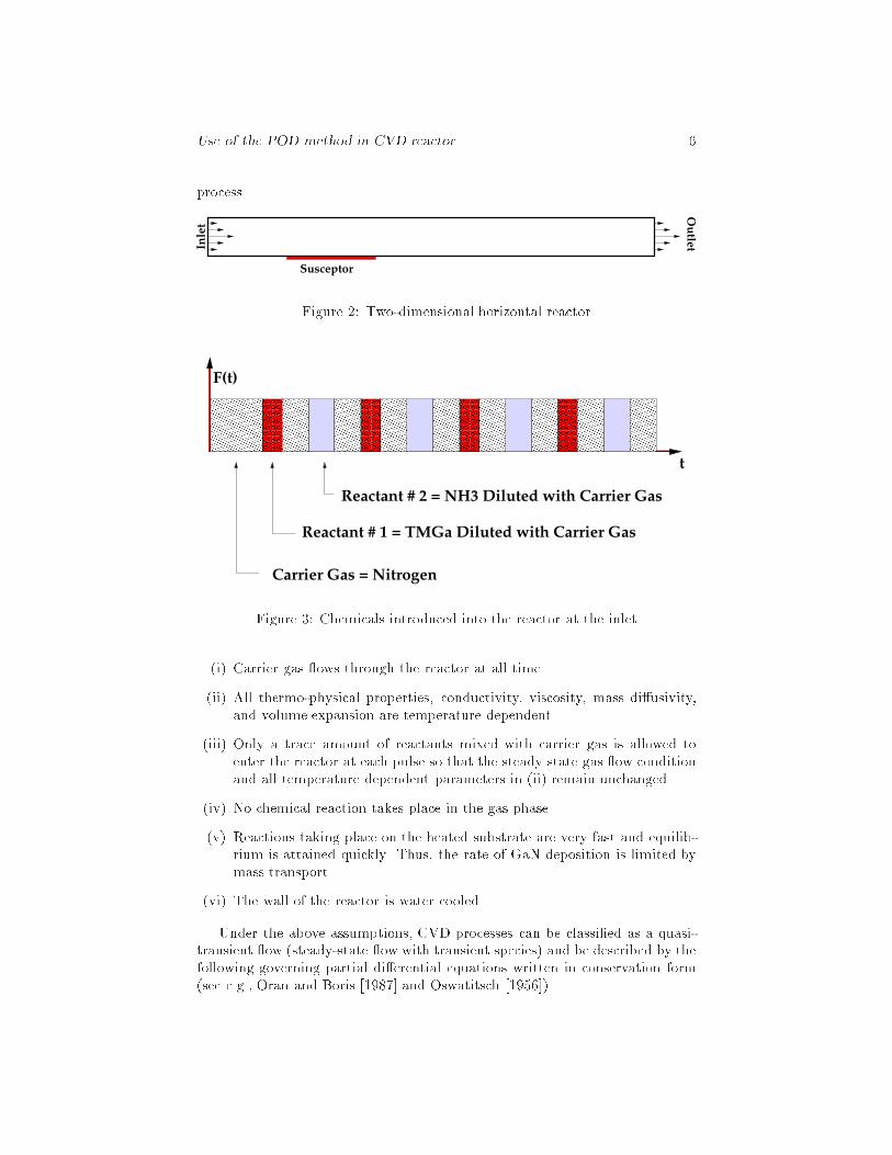
Use of the POD method in CVD reactor 6process.In

let

Ou

tlet

SusceptorFigure 2: Two-dimensional horizontal reactor��

��

��

��

��

��

��

��

��

��

��

��

��

��

��

��

��

��

��

��

��

��

��

��

��

��

t

F(t)

Reactant # 1 = TMGa Diluted with Carrier Gas

Reactant # 2 = NH3 Diluted with Carrier Gas

Carrier Gas = NitrogenFigure 3: Chemicals introduced into the reactor at the inlet(i) Carrier gas ows through the reactor at all time.(ii) All thermo-physical properties, conductivity, viscosity, mass di�usivity,and volume expansion are temperature dependent.(iii) Only a trace amount of reactants mixed with carrier gas is allowed toenter the reactor at each pulse so that the steady state gas ow conditionand all temperature dependent parameters in (ii) remain unchanged.(iv) No chemical reaction takes place in the gas phase.(v) Reactions taking place on the heated substrate are very fast and equilib-rium is attained quickly. Thus, the rate of GaN deposition is limited bymass transport.(vi) The wall of the reactor is water cooled.Under the above assumptions, CVD processes can be classi�ed as a quasi-transient ow (steady-state ow with transient species) and be described by thefollowing governing partial di�erential equations written in conservation form(see e.g., Oran and Boris [1987] and Oswatitsch [1956]).

Use of the POD method in CVD reactor 7Mass conservation equation: r � (�~u) = 0; (2.1)where � is the density of the carrier gas and ~u = (u1; u2) is the velocity vector.Momentum conservation equation:�~u � r~u = �rP +r � � + (� � �0)g~j; (2.2)where the viscous stress tensor � has the form� = [�T (r~u+ (r~u)T )] + (�� 23�T )(r � ~u) � I:Here we treat the gas mixture as a Newtonian uid and P is the pressure,�T is the carrier gas viscosity, � is the bulk viscosity which can be neglectedfor dense gases or liquids, g is the gravitational force, and �0 is the referencedensity. The (� � �0)g~j term accounts for the natural convection e�ect causedby the gravitational force.Energy conservation equation:cp�~u � rT = r � (�TrT ); (2.3)where T is the temperature, and cp is the heat capacity and �T is thermalconductivity of the carrier gas.Mass conservation of species:@c@t + ~u � rc = 1�r � (�DTrc); (2.4)where c is the mass fraction of TMGa and DT is the di�usion coe�cient ofTMGa in the carrier gas. Here, without loss of generality, only the transportof TMGa is modeled.Expansion of the gas as it approaches the heated susceptor plays a major rolein the ow behavior and it is accounted for by using the following Boussinesqapproximation for the density as a function of the temperature:� = �0[1� �T (T � T0)]; (2.5)where �T is the volume expansion and T0 is a reference temperature.The boundary conditions for the above set of equations (2.2)-(2.5) are sum-marized in Figure 4, where the parabolic pro�le for the velocity �eld at the inletis described by u1(t) = Umax4h2 y(H � y) and u2(t) = 0;with Umax = 0:25 m/s and H = 0:535 inch is the height of the reactor. Theinitial condition for the species equation is zero throughout the domain of therectangular reactor.

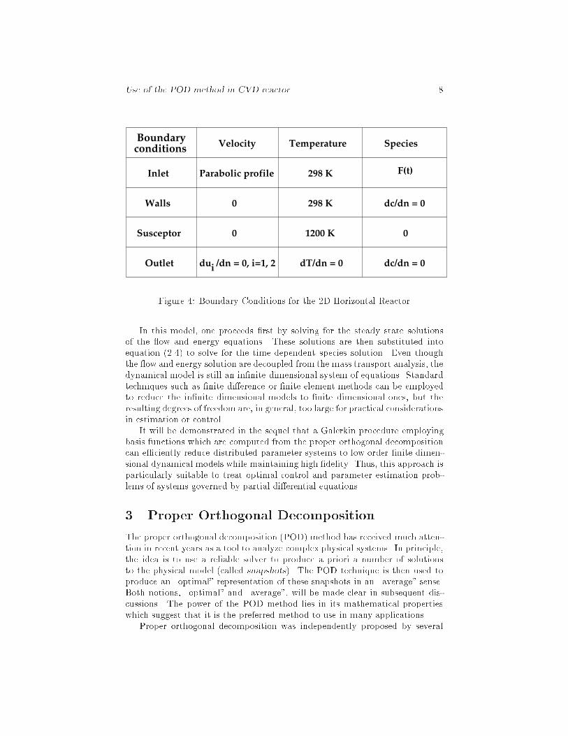
Use of the POD method in CVD reactor 8Inlet

Velocity Temperature Species

Parabolic profile 298 K F(t)

dc/dn = 0298 K0Walls

Susceptor 0 0

Outlet dT/dn = 0 dc/dn = 0

1200 K

Boundaryconditions

idu /dn = 0, i=1, 2Figure 4: Boundary Conditions for the 2D Horizontal ReactorIn this model, one proceeds �rst by solving for the steady state solutionsof the ow and energy equations. These solutions are then substituted intoequation (2.4) to solve for the time dependent species solution. Even thoughthe ow and energy solution are decoupled from the mass transport analysis, thedynamical model is still an in�nite dimensional system of equations. Standardtechniques such as �nite di�erence or �nite element methods can be employedto reduce the in�nite dimensional models to �nite dimensional ones, but theresulting degrees of freedom are, in general, too large for practical considerationsin estimation or control.It will be demonstrated in the sequel that a Galerkin procedure employingbasis functions which are computed from the proper orthogonal decompositioncan e�ciently reduce distributed parameter systems to low order �nite dimen-sional dynamical models while maintaining high �delity. Thus, this approach isparticularly suitable to treat optimal control and parameter estimation prob-lems of systems governed by partial di�erential equations.3 Proper Orthogonal DecompositionThe proper orthogonal decomposition (POD) method has received much atten-tion in recent years as a tool to analyze complex physical systems. In principle,the idea is to use a reliable solver to produce a priori a number of solutionsto the physical model (called snapshots). The POD technique is then used toproduce an \optimal" representation of these snapshots in an \average" sense.Both notions, \optimal" and \average", will be made clear in subsequent dis-cussions. The power of the POD method lies in its mathematical propertieswhich suggest that it is the preferred method to use in many applications.Proper orthogonal decomposition was independently proposed by several

Use of the POD method in CVD reactor 9scientists including Karhunen (1946), Lo�eve (1945), Pougachev (1953), andObukhov (1954) (for recent surveys in this area see the works of Lumley (1970)and Berkooz (1992)). Some mathematical theories of POD can be found inrecent articles by Aubry, Lian and Titi (1993) and Graham and Kevrekidis(1996). The POD technique has been applied to numerous applications. Onesuch important application was the attraction of spatial organized motions in uid ows. Theodorsen (1952) and later Townsend (1956) observed and in-dicated that there are large-scale organized motions embedded in turbulentshear ows. Lumley (1967), Aubry, Holmes, Lumley and Stone (1988), Sirovich(1991), Berkooz, Holmes and Lumley (1993), Berkooz, Holmes, Lumley andMattingly (1997) have adapted the POD technique to study turbulent ows.Other applications of POD include channel ows by Moin and Moser (1989),Ball, Sirovich and Keefe (1991), square-duct ows by Reichert, Hatay, Biringerand Husser (1994), and shear ows by Rajaee, Karlson and Sirovich (1993),Kirby, Boris and Sirovich (1990). Other scientists have also applied the PODtechnique to uid related problems. For instance, it has been applied to theBurgers' equation by Chambers, Adrian, Moin, Stewart and Sung (1988), theGinzburg-Landau equation and the B�enard convection by Sirovich (1989). Lyand Tran (1998) have used POD to simulate and solve an optimal control prob-lem for Rayleigh-B�enard convection. Other interesting non- uid applications ofPOD techniques are the characterization of human faces by Kirby and Sirovich(1990) and image recognition by Hilai and Rubinstein (1994).As will be seen in the following section, one reason that POD is an attractivemethod is that it is a linear procedure. Its mathematical theory is based onthe spectral theory of compact, self-adjoint operators. However, it should benoted that POD makes no assumption on the linearity of the problem to whichit is applied and this is an extremely positive feature of this approach to modelreduction.3.1 Mathematical Aspects of PODLet fUi(x) : 1 � i � N ;x 2 g denote the set of N observations (also calledsnapshots) of some physical processes over a domain . In the context of CVDprocess, these observations could be experimental measurements or numericalsolutions of velocity �elds, temperatures, species etc. taken at di�erent phys-ical parameters (Reynolds number, input ow rates etc.) or time steps. ThePOD technique is designed to extract from this set of observations a coherentstructure, which has the largest mean square projection on the observations.In other words, we look for a function �, or the so-called POD basis element,that most resembles fUi(x)gNi=1 in the sense that it maximizes1N NXi=1 j(Ui;�)j2; (3.1)subject to (�;�) = k�k2 = 1;

Use of the POD method in CVD reactor 10where (�; �) and k � k denote the usual L2 inner product and L2-norm over ,respectively. We choose a special class of trial functions for � to be of the form:� = NXi=1 aiUi; (3.2)where the coe�cients ai are to be determined so that � given by the expression(3.2) provides a maximum for (3.1). To this end, let us de�neK(x; x0) := 1N NXi=1Ui(x)Ui(x0) and R� := ZK(x; x0)�(x0)dx0;where R : L2()! L2().Then straightforward calculations reveal that(R�;�) = ZR�(x)�(x)dx= Z ZK(x; x0)�(x0)dx0�(x)dx= 1N NXi=1 Z ZUi(x)Ui(x0)�(x0)dx0�(x)dx= 1N NXi=1 j(Ui;�)j2:Furthermore, it follows that(R�;) = (�;R) for any �; 2 L2:Thus R is a nonnegative symmetric operator on L2(). Consequently, the prob-lem of maximizing the expression (3.1) amounts to �nding the largest eigenvalueto the eigenvalue problemR� = �� subject to k�k = 1; (3.3)or ZK(x; x0)�(x0)dx0 = �� with k�k = 1: (3.4)Substituting expression (3.2) and the de�nition of K into equation (3.4), weobtain NXi=1[ NXk=1( 1N ZUi(x0)Uk(x0)dx0)ak]Ui(x) = NXi=1 �aiUi(x):This can be rewritten as the eigenvalue problemCV = �V;

Use of the POD method in CVD reactor 11where Cik = 1N ZUi(x)Uk(x)dx and V = 26664 a1a2...aN 37775 : (3.5)Since C is a nonnegative Hermitian matrix, it has a complete set of orthogonaleigenvectors V1 = 26664 a11a12...a1N 37775 ;V2 = 26664 a21a22...a2N 37775 ; : : : ;VN = 26664 aN1aN2...aNN 37775with the corresponding eigenvalues �1 � �2 � � � � � �N � 0. Thus, the solutionto the optimization problem for (3.1) is given by�1 = NXi=1 a1iUi;where a1i are the elements of the eigenvector V1 corresponding to the largesteigenvalue �1. The remaining POD basis elements, �i, i = 2; : : : ; N , are ob-tained by using the elements of other eigenvectors, Vi, i = 2; : : : ; N . Moreoverusing the orthogonality of fVk : 1 � k � Ng and the imposed condition:Vk �Vk0 = NXi=1 aki ak0i = 8<: 1N�k0 k = k00 k 6= k0;we obtain (�k;�k0) = Z�k(x)�k0(x)dx= Z NXi=1 akiUi(x) NXj=1 ak0j Uj(x)dx= NXi=1 akiN NXj=1( 1N ZUi(x)Uj(x)dx)ak0j= NXi=1 akiN NXj=1Cijak0j= NVk �CVk0= NVk � �k0Vk0= N�k0Vk �Vk0= � 1 k = k00 k 6= k0:

Use of the POD method in CVD reactor 12Thus, the POD basis f�1;�2; : : : ;�Ng forms an orthonormal set.Remarks. An alternative approach for �nding the solution to maximizationof (3.1) is by using the so-called Rayleigh-Ritz method for �nding eigenvalues(see Kanwal (1997) p. 176). Since(R�;�) = (R[ NXi=1 aiUi]; NXk=1akUk) = NXi=1 NXk=1Rikaiak;and k�k2 = (�;�) = NXi=1 NXk=1NCikaiak;where Rik = (RUi;Uk) = (Ui;RUk) and Cik = 1N (Ui;Uk) = 1N (Uk;Ui) asabove in (3.5), the problem of maximizing (3.1) can be transformed into anextremal problem in multi-variable calculus with fa1; a2; : : : ; aNg as variables.Recalling the method of Lagrange multipliers, we de�neG(a1; : : : ; aN ) := NXi=1 NXk=1Rikaiak � �NCikaiak;where � is the Lagrange multiplier. Equating @G=@ai to 0 (a necessary condi-tion for optimality) we �ndNXk=1(Rik � �NCik)ak = 0 for i = 1; : : : ; N: (3.6)Equation (3.6) has a nontrivial solution if and only if the determinant of(R��NC) = 0. This determinant, when expanded, yields an N th degree poly-nomial in � which can be shown to haveN nonnegative real roots, but not neces-sarily distinct (these can be ordered in descending order as �1 � �2 � � � � � �N )(Kanwal (1997)). Moreover by multiplying equation (3.6) by ai and summingover i = 1; : : : ; N , we obtain � = (R�;�). It can be shown that solution pair(�i; V i) where Vi = (ai1; : : : ; aiN ), is the eigenvalue and eigenvector of the ma-trix C. One then uses the de�nition of � in (3.2) to obtain f�1;�2; : : : ;�Ngand uses the fact that the matrix C = [Cij] is Hermitian to justify the or-thonormality of f�kg's as in previous argument.3.2 Optimality of the POD BasisSuppose that we have a signal v(x; t) with v 2 L2(; [0; T ]) and an approxi-mation of vN of v with respect to an arbitrary orthonormal basis i(x), i =1; 2; : : : ; N : vN (x; t) = NXi=1 ai(t) i(x):

Use of the POD method in CVD reactor 13If the i(x) have been nondimensionalized, then the coe�cients ai carry thedimension of the quantity vN . If vN (x; t) denotes the velocity and < � > denotesthe time average operator, then the average kinetic energy per unit mass is givenby < Z vN (x; t)vN�(x; t) dx >=< NXi=1 ai(t)a�i (t) > :Consequently, the expression < aia�i > represents the average kinetic energy inthe ith-mode. The following lemma establishes the notion of optimality of thePOD method.Lemma 3.1 Let f�1;�2; : : : ;�Ng denote the orthonormal set of POD basiselements and (�1; �2; : : : ; �N ) denote the corresponding set of eigenvalues. IfvN (x; t) = NXi=1 bi(t)�i(x)denotes the approximation to v with respect to this basis, then the followinghold:(a) < bi(t)b�j (t) >= �ij�i (that is, the POD coe�cients are uncorrelated).(b) For every N ,NXi=1 < bi(t)b�i (t) >= NXi=1 �i � NXi=1 < ai(t)a�i (t) > :The proof of this lemma is straight forward from the optimality of the eigen-values and can be found in Berkooz, Holmes, and Lumley (1993). This lemmaestablishes that among all linear combinations, the POD is the most e�cient,in the sense that, for a given number of modes, N , the projection on the sub-space used for approximation will contain the most kinetic energy possible inan average sense.3.3 Model Reduction Features of POD ApproximationsTo this point we have not discussed any model reduction features associatedwith using POD basis elements in approximation schemes. In the construc-tion described above, the number N may be large, 100 � 1000 or even more,depending on the complexity of the dynamics represented in the \snapshots"Ui. In general, one should take N su�ciently large so that the snapshots Uicontain all salient features of the dynamics being investigated. Thus, the PODbasis functions �i, used with the original dynamics in a nonlinear Galerkinprocedure, o�ers the possibilities of achieving a high �delity model, albeit withperhaps a large dimension N .To achieve model reduction, one chooses M � N and carries out a nonlin-ear Galerkin procedure with the set of elements f�1;�2; : : : ;�Mg. The crucial

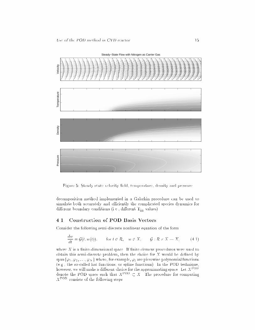
Use of the POD method in CVD reactor 14question is how to choose M . As we indicated in the previous section, PMi=1 �irepresents the average kinetic energy contained in the �rst M modes and henceto capture most of the energy of the system contained in the N POD ele-ments, it su�ces to choose M so that PMi=1 �i � PNi=1 �i. Indeed, the ratioPMi=1 �i=PNi=1 �i yields the percentage of the total kinetic energy in the NPOD elements that is contained in the �rst M POD elements. Since the asso-ciated POD eigenvalues are ordered �1 � �2 � � � � � �N , one can reasonablyexpect to achieve a high percentage of the total kinetic energy in a reducedmodel of order M with M su�ciently smaller than N . For the CVD examplesdetailed below, the POD system was constructed for N = 200 and a reducedorder model with M = 10 yielded a ratio of :999, resulting in a truly signi�-cant computational savings over the �nite element model (2,400 quadrilateralelements) of dimension 14,801 used to generate the 200 snapshots.4 Application of POD for the Simulation of CVDProcessesWe return to the CVD example of x2 to apply the POD techniques. Underassumption (iii) of x2, that is only a trace amount of TMGa mixed with carriergas is used, the steady state ow and energy solutions can be decoupled fromthe mass transport equation. Therefore, we �rst solve equations (2.1)-(2.3)and (2.5) for the steady state solutions of velocity �eld, temperature, densityand pressure. These solutions, depicted graphically in Figure 5, are computedusing a commercial uid dynamics package called FIDAP version 7.6 whichemploys the �nite element method. In our simulations we used 2,400 (9-nodalquadratic) quadrilateral elements. Here and in all subsequent plots, highernumerical values are represented by darker shaded region.Once the ow has reached steady state condition in the reactor, we introduceTMGa into the reactor from the inlet. As mentioned earlier, the term F (t)used in the boundary condition for the species at the inlet, c(~x; t)jinlet = F (t),describes the incoming pulses of TMGa. Using the steady state velocity anddensity solutions (for the terms ~u and �) and the steady state temperaturesolution (to compute temperature dependent mass di�usivity DT ) in equation(2.4), we simulated the species equation for zero initial condition and variousboundary conditions F (t) using FIDAP. Figure 6 displays TMGa pro�les atdi�erent time steps from 0.05 to 0.75 seconds corresponding to the boundarycondition c(~x; t)jinlet = F (t) = 1; for all t > 0. We note that, depending on theduration of TMGa introduced at the inlet, di�erent TMGa pro�les will result inthe reactor. In particular, for the following boundary condition (see also Figure8): c(~x; t)jinlet = � F (t) = 1 0 < t � Tin;0 Tin < t � Tin+Tout:Figure 7 depicts two di�erent reactant pro�les at di�erent time steps from 0.05second to Tout = 0:4 second corresponding to Tin = 0:3 second and Tin =0:75 second. In the sequel, we will demonstrate that the proper orthogonal

Use of the POD method in CVD reactor 15V

eloc

itySteady−State Flow with Nitrogen as Carrier Gas

Tem

pera

ture

Den

sity

Pre

ssur

e Figure 5: Steady state velocity �eld, temperature, density and pressuredecomposition method implemented in a Galerkin procedure can be used tosimulate both accurately and e�ciently the complicated species dynamics fordi�erent boundary conditions (i.e., di�erent Tin values).4.1 Construction of POD Basis VectorsConsider the following semi-discrete nonlinear equation of the formdwdt = G(t; w(t)); for t 2 R; w 2 X; G : R�X ! X; (4.1)where X is a �nite-dimensional space. If �nite element procedures were used toobtain this semi-discrete problem, then the choice for X would be de�ned byspanf'1; '2; : : : ; 'Ng where, for example, 'i are piecewise polynomial functions(e.g., the so-called hat functions, or spline functions). In the POD technique,however, we will make a di�erent choice for the approximating space. Let XPODdenote the POD space such that XPOD � X. The procedure for computingXPOD consists of the following steps.

Use of the POD method in CVD reactor 160.

1 s

0.15

s0.

2 s

0.25

s0.

3 s

0.35

s0.

4 s

0.45

s0.

5 s

0.55

s0.

6 s

0.65

s0.

7 s

0.75

s0.

05 s

Species Introduced into Reactor

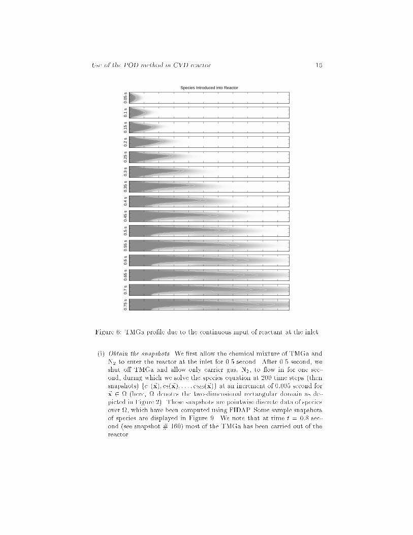
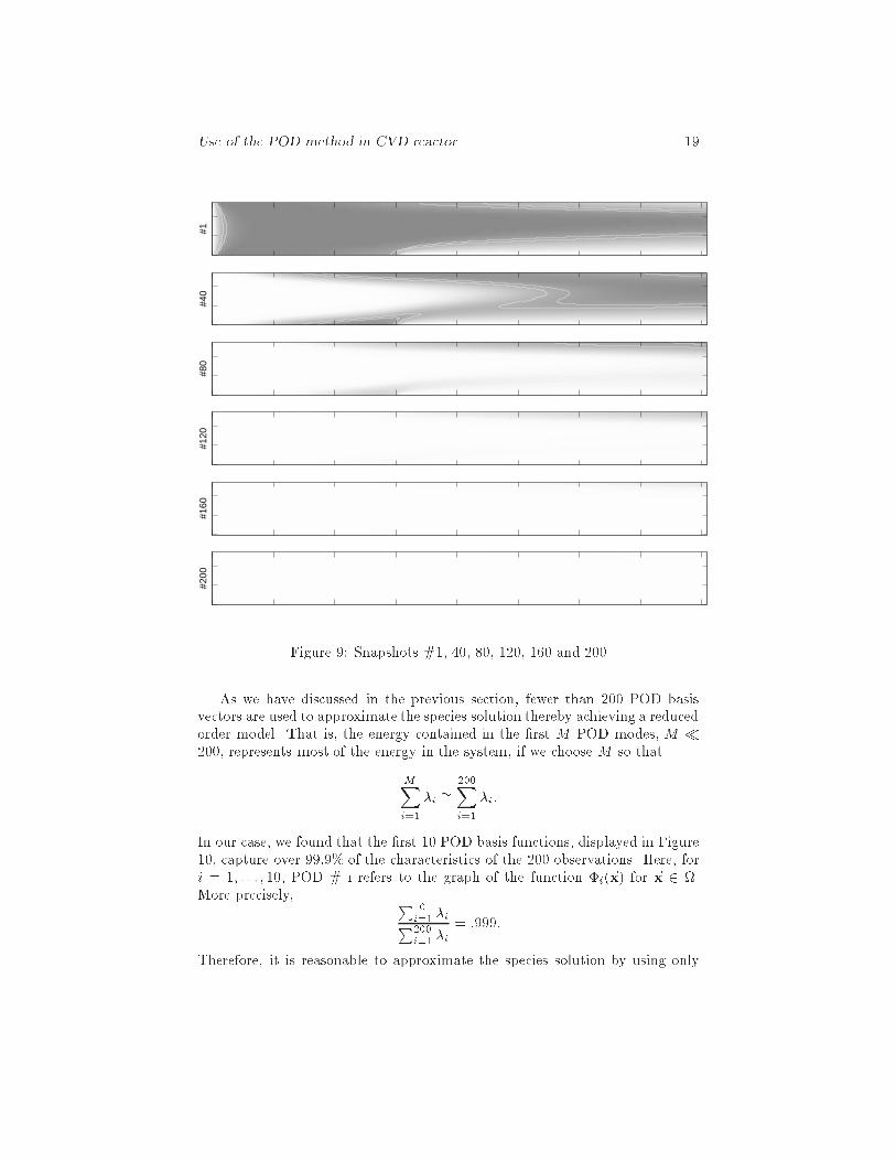
Figure 6: TMGa pro�le due to the continuous input of reactant at the inlet(i) Obtain the snapshots. We �rst allow the chemical mixture of TMGa andN2 to enter the reactor at the inlet for 0.5 second. After 0.5 second, weshut o� TMGa and allow only carrier gas, N2, to ow in for one sec-ond, during which we solve the species equation at 200 time steps (thensnapshots) fc1(~x); c2(~x); : : : ; c200(~x)g at an increment of 0:005 second for~x 2 (here, denotes the two-dimensional rectangular domain as de-picted in Figure 2). These snapshots are pointwise discrete data of speciesover , which have been computed using FIDAP. Some sample snapshotsof species are displayed in Figure 9. We note that at time t = 0:8 sec-ond (see snapshot # 160) most of the TMGa has been carried out of thereactor.


1 s

0.1

s

0.15

s

0.15

s

0.2

s

0.2

s

0.25

s

0.25

s

0.3

s

0.3

s

0.35

s

0.35

s

0.4

s

0.4

s

0.05

s

After Species in for 0.300 sec

0.05

s


Figure 7: TMGa pro�les corresponding to Tin equals to .3 second (left) and0.75 second (right)(ii) Compute the covariant matrix C. The matrix elements of C are given byCik = 1200 Z ci(~x)ck(~x)dx;for i; k = 1; 2; : : : ; 200.(iii) Solve the eigenvalue problem CV = �V. We recall that since C is anonnegative, Hermitian matrix, it has a complete set of orthogonal eigen-vectors V1 = 26664 a11a12...a1200 37775 ;V2 = 26664 a21a22...a2200 37775 ; : : : ;V200 = 26664 a2001a2002...a200200 37775with the corresponding eigenvalues arranged in ascending order as �1 ��2 � � � � � �200 � 0.

Use of the POD method in CVD reactor 18��

��

��

tT_outT_in

F(t)

Carrier Gas

Reactant

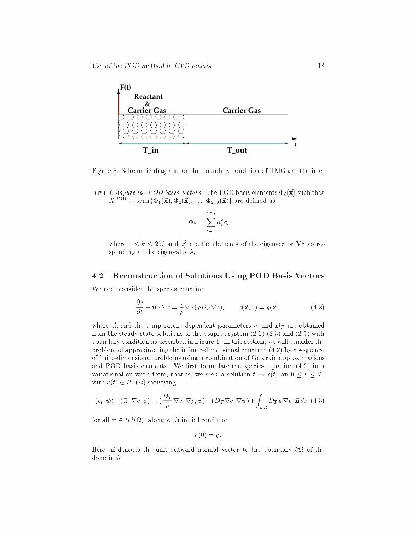
Carrier Gas & Figure 8: Schematic diagram for the boundary condition of TMGa at the inlet(iv) Compute the POD basis vectors. The POD basis elements �i(~x) such thatXPOD = spanf�1(~x);�2(~x); : : : ;�200(~x)g are de�ned as�k = 200Xi=1 aki ci;where 1 � k � 200 and aki are the elements of the eigenvector Vk corre-sponding to the eigenvalue �k.4.2 Reconstruction of Solutions Using POD Basis VectorsWe next consider the species equation@c@t + ~u � rc = 1�r � (�DTrc); c(~x; 0) = g(~x); (4.2)where ~u, and the temperature dependent parameters �, and DT are obtainedfrom the steady state solutions of the coupled system (2.1)-(2.3) and (2.5) withboundary condition as described in Figure 4. In this section, we will consider theproblem of approximating the in�nite-dimensional equation (4.2) by a sequenceof �nite-dimensional problems using a combination of Galerkin approximationsand POD basis elements. We �rst formulate the species equation (4.2) in avariational or weak form; that is, we seek a solution t ! c(t) on 0 � t � T ,with c(t) 2 H1() satisfying(ct; )+(~u �rc; ) = (DT� rc �r�; )� (DTrc;r )+Z@DT rc �~nds (4.3)for all 2 H1(), along with initial conditionc(0) = g:Here, ~n denotes the unit outward normal vector to the boundary @ of thedomain .

Use of the POD method in CVD reactor 19#4

0#8

0#1

20#1

60#2

00#1

Figure 9: Snapshots #1, 40, 80, 120, 160 and 200As we have discussed in the previous section, fewer than 200 POD basisvectors are used to approximate the species solution thereby achieving a reducedorder model. That is, the energy contained in the �rst M POD modes, M �200, represents most of the energy in the system, if we choose M so thatMXi=1 �i �= 200Xi=1 �i:In our case, we found that the �rst 10 POD basis functions, displayed in Figure10, capture over 99:9% of the characteristics of the 200 observations. Here, fori = 1; : : : ; 10, POD # i refers to the graph of the function �i(~x) for ~x 2 .More precisely, P10i=1 �iP200i=1 �i = :999:Therefore, it is reasonable to approximate the species solution by using only

Use of the POD method in CVD reactor 20the �rst 10 POD basis vectors, wherein we obtain a solution of the formcPOD(~x; t) = 10Xi=1 �i(t)�i(~x): (4.4)P

OD

# 1

PO

D #

2

PO

D #

3

PO

D #

4

PO

D #

5

PO

D #

6

PO

D #

7

PO

D #

8

PO

D #

9

PO

D #

10Figure 10: The �rst 10 POD elementsUsing the form of c(~x; t) in (4.4) and the orthonormality of the f�ig's, weapply a Galerkin procedure to equation (4.2) to obtain a system of 10 ordinarydi�erential equations for the coe�cients �jd�jdt = Nj(�1; �2; : : : ; �10)�j(0) = (c(~x; Tin);�j); (4.5)for 1 � j � 10, whereNj = 10Xi=1 "(1�r � (�DTr�i);�j) � 10Xi=1(~u � r�i;�j)#�i(t)= � 10Xi=1[(DTr�i;r�j) + (DT� r�i � r�;�j)� (~u � r�i;�j)]�i(t):

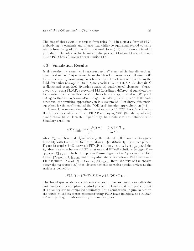
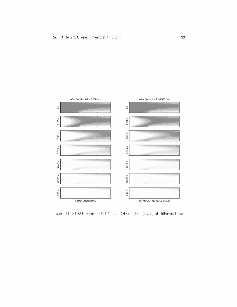
Use of the POD method in CVD reactor 21The �rst of these equalities results from using (4.4) in a strong form of (4.2),multiplying by elements and integrating, while the equivalent second equalityresults from using (4.4) directly in the weak form (4.3) in the usual Galerkinprocedure. The solutions to the initial value problem (4.5) yield the coe�cientsof the POD basis function approximation (4.4).4.3 Simulation ResultsIn this section, we examine the accuracy and e�ciency of the low-dimensionaldynamical model (4.5) obtained from the Galerkin procedure employing PODbasis functions by comparing its solution with the solution obtained from the uid dynamics package FIDAP. More speci�cally, in FIDAP the domain is discretized using 2400 (9-nodal quadratic) quadrilateral elements. Conse-quently, by using FIDAP, a system of 14,801 ordinary di�erential equations hasto be solved for the coe�cients of the basis function approximation. We pointout again that in our formulation using a Galerkin procedure with POD basisfunctions, the resulting approximation is a system of 10 ordinary di�erentialequations for the coe�cients of the POD basis function approximation (4.4).Figure 11 compares the reduced solution using 10 POD basis functions tothe full solution obtained from FIDAP employing 2400 (9-nodal quadratic)quadrilateral �nite elements. Speci�cally, both solutions are obtained withboundary conditionc(~x; t)jinlet = � F (t) = 1 0 < t � Tin;0 Tin < t;where Tin = 0:5 second. Qualitatively, the reduced POD basis results agreesfavorably with the full FIDAP calculations. Quantitatively, the upper plot inFigure 12 graphs the L2 norms of FIDAP solutions, kcFIDAP(�; t)kL2(), and theL2 absolute errors between POD solutions and FIDAP solutions kcPOD(�; t)�cFIDAP(�; t)kL2(). The bottom plot in Figure 12 graphs the L2 norms of FIDAP uxes, kFFIDAP(�; t)kL2(), and the L2 absolute errors between POD uxes andFIDAP uxes kFPOD(�; t) � FFIDAP(�; t)kL2(s) Here, the ux of the speciesabove the susceptor (s) that dictates the rate at which species arrives at thesurface is de�ned byF(~x; t) := (DTrc(~x; t) + �c(~x; t)~u) � ~nj~x2s :The ux of species above the susceptor is used in the next section to de�ne thecost functional in an optimal control problem. Therefore, it is important thatthis quantity can be computed accurately. For a comparison, Figure 13 depictsthe uxes at the susceptor computed using POD basis functions and FIDAPsoftware package. Both results agree remarkably well.


105

s

0.10

5 s

0.21

s

0.21

s

0.31

5 s

0.31

5 s

0.42

s

0.42

s

0.52

5 s

0.52

5 s

0 s


0 s


0.63

s

FIDAP SOLUTIONS

0.63

s

10−MODE POD SOLUTIONSFigure 11: FIDAP Solution (left) and POD solution (right) at di�erent times

Use of the POD method in CVD reactor 230.1 0.2 0.3 0.4 0.5 0.6

0

0.005

0.01

0.015

0.02

0.025

time (sec)

L^2−

norm

s S

peci

es (

o) a

nd E

rror

(*)

After Species in for 0.500 sec in the Reactor

0.1 0.2 0.3 0.4 0.5 0.60

0.5

1

1.5

2x 10

−7

time (sec)

L^2−

norm

s F

lux

(o)

and

Err

or (

*)

After Species in for 0.500 sec at the Susceptor

Figure 12: Top: the L2-norm of FIDAP solution (o), kcFIDAP(�; t)k, and theL2-norm error (*), kcPOD(�; t)� cFIDAP(�; t)k. Bottom: the L2-norm of FIDAP ux (o), kFFIDAP(�; t)k, and the L2-norm of the ux error (*), kFPOD(�; t) �FFIDAP(�; t)k

Use of the POD method in CVD reactor 240

0.5

10.

18 s

ec

0

0.5

1

0.27

sec

0

0.5

1

0.36

sec

0

0.5

1

0.45

sec

0

0.5

1

0.54

sec

0

0.5

1

0.09

sec

FIDAP FLUX (dotted) −vs− POD FLUX (dashed) at the Susceptor * 1.0e−06

0

0.5

1

0.63

sec

After Species in for 0.500 secFigure 13: Fluxes of species at the susceptor using FIDAP (.) and POD basisfunctions (-) at di�erent timesWe recall that POD basis functions were computed from the snapshots cor-responding to the boundary condition (4.3) with Tin = 0:5 second. To be usefulin developing both open loop and feedback control strategies, we would like forthese same reduced number of POD elements to yield good approximationsunder other ow input conditions. That is, we would like to demonstrate thatusing exactly these 10 POD modes, we are able to construct POD solutionsfor di�erent durations of species introduced into the reactor. Particularly, wesolved the same system (4.5) with initial conditions �j(0) = (c(~x; Tin);�) forTin = 0:3 second and Tin = 0:75 second. Figure 14 depicts the L2-norms of thesolution errors and L2-norms of the ux errors above the susceptor using PODbasis functions and FIDAP for Tin = 0:30 second and Tin = 0:75 second.

Use of the POD method in CVD reactor 250.1 0.2 0.3 0.4 0.5 0.6

0

0.005

0.01

0.015

0.02

time (sec)

L^2−

norm

s S

peci

es (

o) a

nd E

rror

(*)


0.1 0.2 0.3 0.4 0.5 0.60

0.005

0.01

0.015

0.02

0.025

time (sec)

L^2−

norm

s S

peci

es (

o) a

nd E

rror

(*)


0.1 0.2 0.3 0.4 0.5 0.60

0.5

1

1.5

2x 10

−7

time (sec)

L^2−

norm

s F

lux

(o)

and

Err

or (

*)

At the Susceptor

0.1 0.2 0.3 0.4 0.5 0.60

0.5

1

1.5

2x 10

−7

time (sec)

L^2−

norm

s F

lux

(o)

and

Err

or (

*)

At the Susceptor

Figure 14: (left columm, Tin = 0:3 second, right columm, Tin = 0:75 sec-ond): Top, the L2-norm of FIDAP solution (o), kcFIDAP(�; t)k, and the solutionerror (*), kcPOD(�; t)� cFIDAP(�; t)k; Bottom, the L2-norm of FIDAP ux (o),kFFIDAP(�; t)k, and the L2-norm of the ux error (*), kFPOD(�; t)�FFIDAP(�; t)k5 An Optimal Control ProblemIn this section we demonstrate the use of reduced POD models in an open loopoptimal control problem. While this example involves only one control variable,it does illustrate e�ectively the potential of POD methods in control problems.In the case of GaN heteroepitaxy �lm growth employing pulsed trimethyl-gallium (TMGa) and ammonia (NH3) as source vapors, depending on the delaybetween the TMGa and NH3 source vapor pulses, carry-over of TMGa frag-ments from one precursor pulse cycle to the next may occur. This, in turn,establishes a surface reaction layer (SRL), consisting of mixture of reactantsand products of the chemical reactions that drive the epitaxial growth process.The thickness and composition of the SRL depends on the relative heights andwidths, i.e. Tin, of the employed TMGa and NH3 source vapor pulses and theirrepetition rate. More speci�cally, if Tin is small, then the ux above the sus-ceptor is uniform. Yet this will take a long time to grow a �lm which makes

Use of the POD method in CVD reactor 26it inviable in industrial applications. On the other hand, by allowing massivechemical input at the inlet (i.e., Tin is large) we will speed up the growingprocess; but the ux above the susceptor may not be uniform. Therefore itis desirable to perform an optimization procedure to determine the most de-sirable Tin to achieve both �lm uniformity and fastest possible growth rate.Mathematically, we would like to �nd the optimal Tin so that the ux uctu-ation, @@xF , is small while at the same time we maximize the ux, F , to thesubstrate. Consequently, one way to formulate a quantitative representation ofthese con icting desires is to seek T �in so that the cost functionalCost = I + �J ; � = 15:0� 1012 ; (5.1)is minimized, where I = Z Tin+Tout0 Zs j @@xFj2dxdt;and J = Z Tin+Tout0 Zs jFj2dxdt:Here, Tout denotes the time delay between the source vapor pulses and, based onexperimental results, we take Tout � 0:600 second. The above cost functional(5.1) is minimized subject to the system (2.2)-(2.5) along with their boundaryconditions. The constant � in (5.1) is scaled to make I and 1J proportioned. Italso bears the trade-o� value which represents on one's desires to balance �lmuniformity and faster growth rate.Given a value of Tin the system of equations (2.2)-(2.5) is solved for thespecies solution which is then substituted into the formula (4.3) for the ux,F . Hence, the above optimization problem is an unconstrained minimizationproblem involving one parameter, Tin. We carried out computations for such acontrol example. For these, we chose the DUVMGS subroutine in the FortranIMSL library [1989] which is designed to minimize a nonsmooth function withdouble-precision accuracy. The subroutine DUVMGS uses the so-called goldensection method to search for its minimal point. Other choices of minimizationtechniques are possible. We found that with the value of � given in (5.1), theoptimal width of the pulses, T �in, is 0.395 second. The time-dependent uxesabove the susceptor for the optimal T �in are compared in Figure 15 with non-optimal uxes computed using Tin = 0:300 second and Tin = 0:650 second. Wenote that Tin must be at least .300 second which is the fastest on-o� switch inthe ow control panel. The ux above the susceptor for Tin = 0:300 second isuniform, i.e., the curve is at, however, the growth rate is small. On the otherhand, for Tin = 0:650 second, the growth rate speeds up, but non-uniformityof �lm growth results. The optimal solution lies between the above two non-optimal curves. This solution which corresponds to the optimal duration of thesource vapor pulses achieves both �lm uniformity and fastest possible growthrate.

Use of the POD method in CVD reactor 270

0.5

10.

05 s

ec

0

0.5

1

0.09

5 se

c

0

0.5

1

0.14

sec

0

0.5

1

0.18

5 se

c

0

0.5

1

0.23

sec

0

0.5

1

0.00

5 se

c

Flux above the Susceptor *1.0e06

0

0.5

1

T_in = 0.300 s (−.), T*_in = 0.395 s (solid), T_in = 0.650 s (−−)

0.27

5 se

cFigure 15: Comparing the optimal ux solution with two non-optimal uxsolutionsAcknowledgment.The authors is grateful to Dr. Grace M. Kepler for helping us to set-upFIDAP7.6 for obtaining the snapshots and to Drs. K.J. Bachman, H.T. Banks,C. Hoepfner and J.S. Scroggs for many helpful discussions.References[1] N. Aubry, P. Holmes, J.L. Lumley, and E. Stone, \The dynamics of coher-ent structures in the wall region of a turbulent boundary layer," Journal ofFluid Mechanics, 192 (1988) p. 115-173.

Use of the POD method in CVD reactor 28[2] N. Aubry, W.Y. Lian, and E.S. Titi, \Preserving symmetries in the properorthogonal decomposition," SIAM J. Sci. Comput., 14, No. 2 (1993) p.483-505.[3] K.J. Bachmann, N. Sukidi, C. Hopfner, C. Harris, N. Dietz, H.T. Tran, S.Beeler, K. Ito, and H.T. Banks \Real-time monitoring of steady-state pulsedchemical beam epitaxy by p-polarized re ectance," J. of Crystal Growth,183 (1998) p. 323-337.[4] K.S. Ball, L. Sirovich, and L.R. Keefe \Dynamical eigenfunction decom-position of turbulent channel ow," International Journal for NumericalMethods in Fluids, 12 (1991) p. 585-604.[5] H.T. Banks, K. Ito, J.S. Scroggs, H.T. Tran, N. Dietz, and K.J. Bachmann,\Modeling and control of advanced chemical vapor deposition processes,"in \Mathematics of Microstructure Evolution," (eds.: L.Q. Chen, et al),SIAM/TMS Publications, (1996) p. 327-344.[6] G. Berkooz, \Observations on the proper orthogonal decomposition,"in \ Studies in Turbulence," (eds.: T.B. Gatski, S. Sarkar, and C.G.Speziale), Springer-Verlag, New York (1992) p. 229-247.[7] G. Berkooz, P. Holmes, and J.L. Lumley, \The Proper orthogonal decom-position in the analysis of turbulent ows," Annual Review of Fluids Me-chanics, 25 (1993) N5:539-575.[8] G. Berkooz, P. Holmes J.L. Lumley, and J.C. Mattingly, \Low-dimensionalmodels of coherent structures in turbulence," Physics Reports-Review Sec-tion of Physics Letters, 287 (1997) N4:338-384.[9] D.H. Chambers, R.J. Adrian, P. Moin, D.S. Stewart, and H.J. Sung,\Karhunen-Lo�eve expansion of Burgers' model of turbulence," Phys. Flu-ids, 31 (1988) p. 2573-2582.[10] M.E. Coltrin, R.J. Kee, and J.A. Miller, \A mathematical model of Siliconchemical vapor deposition," J. Electrochem. Soc., 133 (1986) p. 1206-1213.[11] D.I. Fotiadis, \Two- and three-dimensional �nite element simulations ofreacting ows in chemical vapor deposition of compound semiconductors,"PhD thesis,, Univ. Minn., Minneapolis, (1990).[12] E. Fujii, H. Nakamura, K. Haruna, and Y. Koga, \A quantitative calcula-tion of the growth rate of epitaxial silicon from SiCl4 in a barrel reactor,"J. Electrochem. Soc., 119 (1972) p. 1106-1113.[13] S.A. Gokoglu, M. Kuczmarski, P. Tsui, and A. Chait, \Convection andchemistry e�ects in CVD - A 3-D analysis for silicon deposition," Journalde Physique, 50 (1989) N5-17.[14] M. Graham and I.G. Kevrekidis, \Alternative approaches to the Karhunen-Lo�eve decomposition for model reduction and data analysis," ComputersChem. Engineering, 20 (1996) N5:495-506.

Use of the POD method in CVD reactor 29[15] R. Hilai and J. Rubinstein, \Recognition of rotated images by invariantKarhunen-Lo�eve expansion," Journal of the Optical Society of AmericaA-Optics Image Science and Vision, 11 (1994) N5:1610-1618.[16] K.Ito, J.S. Scroggs, and H.T. Tran, \Mathematical Issues in Optimal De-sign of a Vapor Transport Reactor", in IMA Volumes in Mathematics andIts Applications, 68, Flow Control (Max D. Gunzburger, ed.), (1994) p.197-218.[17] K.Ito, J.S. Scroggs, and H.T. Tran, \Optimal Control of Thermally Cou-pled Navier-Stokes Equation", in Optimal Design and Control, Max D.Gunzburger et al. , eds.), (1995) p. 199-214.[18] K.F. Jensen, \Chemical vapor deposition,", inMicroelectronics Processing:Chemical Engineering Aspects, D.W. Hess and K.F. Jensen, eds., (1989)p. 199-263.[19] K.F. Jensen, E.O. Einset, and D.I. Fotiadis, \Flow phenomena in chemicalvapor deposition of thin �lms," Annu. Rev. Fluid Mech., 23 (1991) p. 197-232.[20] R.P. Kanwal, \Linear Integral Equations: Theory & Technique",Birkh�auser, Boston (1997).[21] K. Karhunen, \Zur spektral theorie stochasticher prozesse," Ann. Acad.Sci. Fennicae, Ser. A1 Math Phys., 37 (1946).[22] M. Kirby and L. Sirovich, \Application of the Karhunen-Lo�eve procedurefor the characterization of human faces," IEEE Transactions on PatternAnalysis and Machine Intelligence, 12 (1990) N1:103-108.[23] M. Kirby, J.P. Boris, and L. Sirovich, \A proper orthogonal decompositionof a simulated supersonic shear layer," International Journal for NumericalMethods in Fluids, 10 (1990) p. 411-428.[24] M. Lo�eve, \Functions aleatoire de second ordre", \Compte Rend. Acad.Sci. (Paris)", (1945) p. 220.[25] J.L. Lumley, \The structure of inhomogeneous turbulent ows," in \Atmo-spheric turbulence and radio wave propagation", A.M. Yaglom and V.I.Tatarski, eds.: Moscow: Nauka (1967) p. 166-178.[26] J.L. Lumley, \ Stochastic Tools in Turbulence," Academic Press, New York(1970).[27] H.V. Ly and H.T. Tran, \Applications of proper orthogonal decompositionin simulations and optimal control of the Rayleigh-B�enard Convection,"1998, to be submitted.[28] H.K. Mo�at and K.F. Jensen, \Complex ow phenomena in MOCVD re-actors," Journal of Crystal Growth, 77 (1986) p. 108-119.

Use of the POD method in CVD reactor 30[29] H.K. Mo�at and K.F. Jensen, \Three-dimensional ow e�ects in SiliconCVD in horizontal reactors," J. Electrochem. Soc., 135 (1988) p. 459-471.[30] P. Moin and R.D. Moser, \Characteristic-eddy decomposition of turbulencein a channel," Journal Fluids Mechanics, 200 (1989) p. 417-509.[31] A.M. Obukhov, \Statistical description of continuous �elds", T. Geophys.Int. Akad. Nauk. USSR, 24 (1954), p. 3-42.[32] S. Ostrach, \Low-gravity uid ows," Ann. Rev. Fluid Mech., 14 (1982)p. 313-345.[33] K. Oswatitsch, \Gas Dynamics," Academic Press, New York (1956).[34] J. Ouazzani, Kuan-Cheng Chiu, and F. Rosenberger, \On the 2D modelingof horizontal CVD reactors and its limitations," Journal of Crystal Growth,91 (1988) p. 497-508.[35] J. Ouazzani and F. Rosenberger, \Three-dimensional modeling of horizon-tal chemical vapor deposition I. MOCVD at atmospheric pressure," Journalof Crystal Growth, 100 (1990) p. 545-576.[36] R. Pollard and J. Newman, \Silicon deposition on a rotating disk," J.Electrochem. Soc.," 127 (1980) p. 744-752.[37] V.S. Pougachev, \General theory of the correlations of random functions,"Izv. Akad. Naul. USSR, Ser. Mat., 17 (1953) p. 1401-2.[38] M. Rajaee, S.K.F. Karlson, and L. Sirovich, \Low-dimensional descrip-tion of free-shear- ow coherent structures and their dynamical behavior,"Journal of Fluid Mechanics, 258 (1994) p. 1-29.[39] R.S. Reichert, F.F. Hatay, S.Biringer, and A. Husser, \Proper orthogonaldecomposition applied to turbulent ows in a square duct," Phys. FluidsMechanics, 6 (1994) N9:3086-3092.[40] M.A. Saad, \Compressible Fluid Flow," Prentice-Hall, New Jersey (1985).[41] L. Sirovich, \Chaotic dynamics of coherent structures," Physica D, 37(1989) p. 126-145.[42] L. Sirovich, \Analysis of turbulent ows by means of the empirical eigen-functions," Fluid Dynamics Research, 8 (1991) p. 85-100.[43] J.S. Scroggs, H.T. Banks, K. Ito, S. Ravindran, H.T. Tran, K.J. Bachmann,H. Castleberry, and N. Dietz, \High pressure vapor transport of ZnGeP2:II, three-dimensional simulation of gasdynamics under microgravity con-ditions," in \Proceedings of the 1995 TMS Annual Meeting,", Las Vegas,Nevada, (1995).[44] T. Theodorsen, \Mechanism of Turbulence," in \Proc. 2nd MidwesternConf. on Fluid Mechanics," Ohio State University, Columbus, OH (1952).

Use of the POD method in CVD reactor 31[45] A.A. Townsend, \The Structure of Turbulent Shear Flow," UniversityPress, Cambridge, (1956).[46] G.W. Young, S.I Hariharan, and R. Carnahan, \Flow e�ects in a verticalCVD reactor," SIAM J. Appl. Math., 52, No. 6, (1992) p. 1509-1532.

Proper Orthogonal Decomposition for Flow Calculations and Optimal Control in a Horizontal CVD...

Documents

Transcript of Proper Orthogonal Decomposition for Flow Calculations and Optimal Control in a Horizontal CVD...