Preplanning And Scheduling Of Road Construction By Using PPM
Upload
independentCategory
view
0download
0
Performance of Orthogonal and Non-Orthogonal TH-PPM for Multi-User UWB
Communication Systems
by
Behzad Bahr-Hosseini
B.Sc., University of Arak, Iran, 2003
A Thesis Submitted in Partial Fulfillment of the
Requirements for the Degree of
MASTER OF APPLIED SCIENCE
in the Department of Electrical and Computer Engineering
c⃝ Behzad Bahr-Hosseini, 2009
University of Victoria
All rights reserved. This dissertation may not be reproduced in whole or in part, by
photocopying
or other means, without the permission of the author.

ii
Performance of Orthogonal and Non-Orthogonal TH-PPM for Multi-User UWB
Communication Systems
by
Behzad Bahr-Hosseini
B.Sc., University of Arak, Iran, 2003
Supervisory Committee
Dr. T. Aaron Gulliver, Co-Supervisor
(Dept. of Electrical and Computer Engineering)
Dr. Wei Li, Co-Supervisor
(Dept. of Electrical and Computer Engineering)
Dr. Abolfazl Ghassemi, Departmental Member
(Dept. of Electrical and Computer Engineering)

iii
Supervisory Committee
Dr. T. Aaron Gulliver, Co-Supervisor
(Dept. of Electrical and Computer Engineering)
Dr. Wei Li, Co-Supervisor
(Dept. of Electrical and Computer Engineering)
Dr. Abolfazl Ghassemi, Departmental Member
(Dept. of Electrical and Computer Engineering)
ABSTRACT
The performance of orthogonal pulse position modulation (PPM) and non-orthogonal
pulse position modulation (NPPM) is studied and compared with different ultra wide-
band (UWB) channel models. Time hopping (TH) is used to decrease the effect of
interference in multi access environments. Rake receiver is studied as an ideal UWB
receiver for multiuser environments. It is shown that an ideal rake (I-Rake) receiver
has the best performance among all rake receivers, followed by 5 finger selective rake
(5S-Rake), 5 finger partial rake (5P-Rake), 2 finger selective rake (2S-Rake), and 2
finger partial rake (2P-Rake). With a large number of users, NPPM can achieve a
better bit error rate (BER) performance than PPM. It is also shown that PPM and
NPPM in a triple Saleh-Valenzuela (TSV) channel has performance similar to that
in a Saleh-Valenzuela (SV) channel.
iv
Contents
Supervisory Committee ii
Abstract iii
Table of Contents iv
List of Tables vi
List of Figures vii
List of Abbreviations x
List of Symbols xii
Acknowledgements xv
Dedication xvi
1 Introduction 1
1.1 UWB History and FCC Regulations . . . . . . . . . . . . . . . . . . . 1
1.2 UWB Concept . . . . . . . . . . . . . . . . . . . . . . . . . . . . . . . 5
1.3 UWB Advantages . . . . . . . . . . . . . . . . . . . . . . . . . . . . . 5
1.4 UWB Challenges . . . . . . . . . . . . . . . . . . . . . . . . . . . . . 6
1.5 60 GHz MM-Wave Communications . . . . . . . . . . . . . . . . . . . 6
1.6 UWB Pulse Modulation Schemes . . . . . . . . . . . . . . . . . . . . 8
1.7 UWB Applications . . . . . . . . . . . . . . . . . . . . . . . . . . . . 12
1.8 Thesis Summary and Outline . . . . . . . . . . . . . . . . . . . . . . 12
2 UWB System Model 14
2.1 TH-PPM UWB Model . . . . . . . . . . . . . . . . . . . . . . . . . . 14
2.2 UWB Channel Models . . . . . . . . . . . . . . . . . . . . . . . . . . 17

v
2.2.1 The Saleh-Valenzuela Model . . . . . . . . . . . . . . . . . . . 19
2.2.2 The Triple S-V Model . . . . . . . . . . . . . . . . . . . . . . 26
2.3 Summary . . . . . . . . . . . . . . . . . . . . . . . . . . . . . . . . . 34
3 UWB Receiver Model 38
3.1 Optimum Receiver . . . . . . . . . . . . . . . . . . . . . . . . . . . . 38
3.2 Rake Receiver . . . . . . . . . . . . . . . . . . . . . . . . . . . . . . . 42
3.3 High Gain Directional Antenna . . . . . . . . . . . . . . . . . . . . . 46
4 Simulation Results 51
4.1 AWGN Channel . . . . . . . . . . . . . . . . . . . . . . . . . . . . . . 51
4.2 SV Channel . . . . . . . . . . . . . . . . . . . . . . . . . . . . . . . . 57
4.3 TSV Channel . . . . . . . . . . . . . . . . . . . . . . . . . . . . . . . 65
5 Conclusions and Future Work 70
5.1 Conclusions . . . . . . . . . . . . . . . . . . . . . . . . . . . . . . . . 70
5.2 Future Work . . . . . . . . . . . . . . . . . . . . . . . . . . . . . . . . 71
Bibliography 72

vi
List of Tables
Table 1.1 FCC Spectral Masks for UWB Applications. . . . . . . . . . . . 2
Table 1.2 UWB advantages and disadvantages compared to narrow band
communications. . . . . . . . . . . . . . . . . . . . . . . . . . . 8
Table 1.3 60 GHz UWB advantages and disadvantages compared to lower
frequency UWB. . . . . . . . . . . . . . . . . . . . . . . . . . . 8
vii
List of Figures
Figure 1.1 FCC spectral mask for indoor UWB communications. . . . . . 3
Figure 1.2 FCC spectral mask for outdoor UWB communications. . . . . . 4
Figure 1.3 Available global frequency bands around 60 GHz. . . . . . . . . 7
Figure 1.4 On-off keying modulation. . . . . . . . . . . . . . . . . . . . . . 9
Figure 1.5 Antipodal PAM modulation. . . . . . . . . . . . . . . . . . . . 10
Figure 1.6 PPM modulation. . . . . . . . . . . . . . . . . . . . . . . . . . 11
Figure 2.1 TH-PPM transmitter block diagram for UWB system . . . . . 15
Figure 2.2 A TH-PPM signal with frame time Tf = 3 nsec, chip time Tc = 1
nsec, pulse duration Tp = 0.5 nsec, and PPM shift ϵ = 0.5 nsec. 16
Figure 2.3 A typical second derivative Gaussian pulse waveform . . . . . . 17
Figure 2.4 Ray and cluster instantaneous power for a typical SV channel. . 20
Figure 2.5 Instantaneous power per cluster for a typical SV channel. . . . 21
Figure 2.6 Average power per cluster for a typical SV channel. . . . . . . . 22
Figure 2.7 The SV channel impulse response with ray arrival rate λ, cluster
arrival rate Λ, ray power decay factor γ, and cluster power decay
factor Γ. . . . . . . . . . . . . . . . . . . . . . . . . . . . . . . . 22
Figure 2.8 Power delay profile for UWB channel model CM1. . . . . . . . 24
Figure 2.9 Power delay profile for UWB channel model CM4. . . . . . . . 25
Figure 2.10Discrete time impulse response for UWB channel model CM1. . 26
Figure 2.11Discrete time impulse response for UWB channel model CM4. . 27
Figure 2.12A typical TSV channel model realization. . . . . . . . . . . . . 28
Figure 2.13The two path channel model. . . . . . . . . . . . . . . . . . . . 29
Figure 2.14A 3D realization of a typical TSV channel impulse response with
respect to ToA, AoA and amplitude. . . . . . . . . . . . . . . . 30
Figure 2.15A typical power delay profile for the TSV channel. . . . . . . . 31
Figure 2.16Average power delay profile for a typical TSV channel. . . . . . 32
Figure 2.17The channel excess delay. . . . . . . . . . . . . . . . . . . . . . 33
viii
Figure 2.18TSV Channel model RMS delay spread. . . . . . . . . . . . . . 34
Figure 2.19The continuous channel impulse response for 100 realizations of
the mm-wave UWB channel. . . . . . . . . . . . . . . . . . . . 35
Figure 2.20Image and real demonstaration of impulse response realization . 36
Figure 3.1 Optimum receiver block diagram. . . . . . . . . . . . . . . . . . 41
Figure 3.2 Rake receiver block diagram. . . . . . . . . . . . . . . . . . . . 43
Figure 3.3 I-Rake receiver for a UWB system. . . . . . . . . . . . . . . . . 43
Figure 3.4 5P-Rake receiver for a UWB system. . . . . . . . . . . . . . . . 44
Figure 3.5 5S-Rake receiver for a UWB system. . . . . . . . . . . . . . . . 45
Figure 3.6 2P-Rake receiver for a UWB system. . . . . . . . . . . . . . . . 46
Figure 3.7 2S-Rake receiver for a UWB system. . . . . . . . . . . . . . . . 47
Figure 3.8 Transmitter antenna model. . . . . . . . . . . . . . . . . . . . . 49
Figure 3.9 Receiver antenna model. . . . . . . . . . . . . . . . . . . . . . . 50
Figure 4.1 The BER performance of orthogonal and non-orthogonal TH-
PPM with no interferer in AWGN Channel. . . . . . . . . . . . 52
Figure 4.2 The BER performance of orthogonal and non-orthogonal TH-
PPM with 3 interferers in AWGN Channel. . . . . . . . . . . . 53
Figure 4.3 The BER performance of orthogonal and non-orthogonal TH-
PPM with 5 interferers in AWGN Channel. . . . . . . . . . . . 54
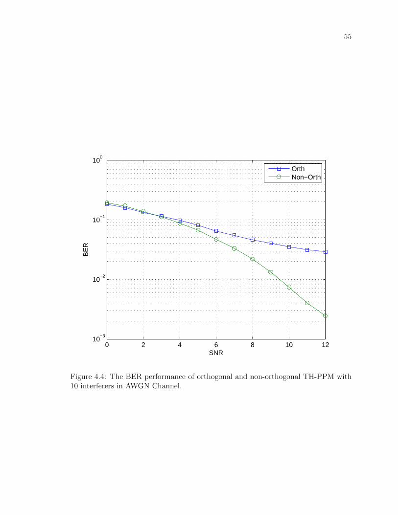
Figure 4.4 The BER performance of orthogonal and non-orthogonal TH-
PPM with 10 interferers in AWGN Channel. . . . . . . . . . . . 55
Figure 4.5 The BER performance of orthogonal and non-orthogonal TH-
PPM with 15 interferers in AWGN Channel. . . . . . . . . . . . 56
Figure 4.6 The BER Performance of TH-PPM with different rake receivers
in UWB-CM1 channel . . . . . . . . . . . . . . . . . . . . . . . 58
Figure 4.7 The BER Performance of TH-PPM with different rake receivers
in UWB-CM4 channel . . . . . . . . . . . . . . . . . . . . . . . 59
Figure 4.8 The BER performance of orthogonal and non-orthogonal TH-
PPM with no interferer in SV Channel. . . . . . . . . . . . . . 60
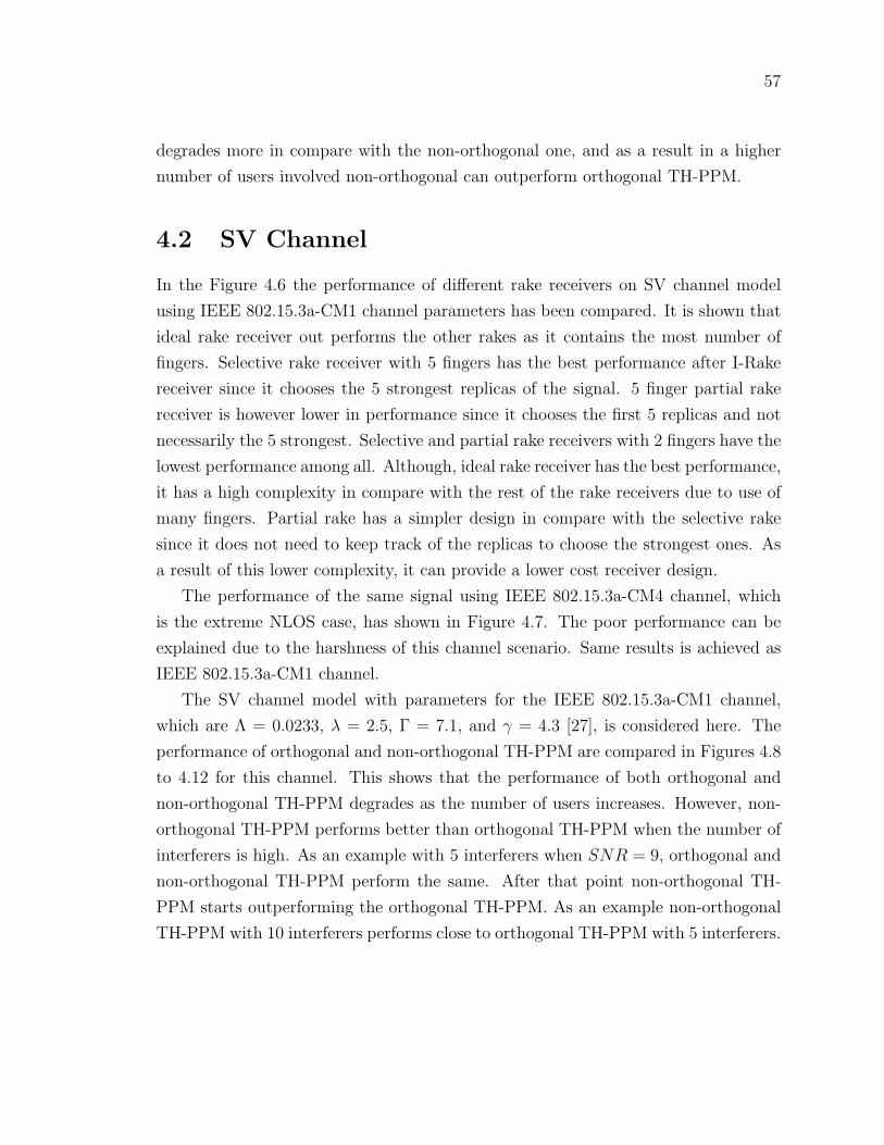
Figure 4.9 The BER performance of orthogonal and non-orthogonal TH-
PPM with 3 interferers in SV Channel. . . . . . . . . . . . . . . 61
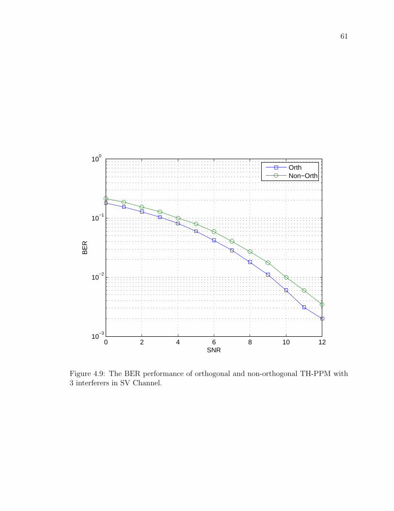
Figure 4.10The BER performance of orthogonal and non-orthogonal TH-
PPM with 5 interferers in SV Channel. . . . . . . . . . . . . . . 62

ix
Figure 4.11The BER performance of orthogonal and non-orthogonal TH-
PPM with 10 interferers in SV Channel. . . . . . . . . . . . . . 63
Figure 4.12The BER performance of orthogonal and non-orthogonal TH-
PPM with 15 interferers in SV Channel. . . . . . . . . . . . . . 64
Figure 4.13The BER performance of orthogonal and non-orthogonal TH-
PPM with no interferer in TSV Channel. . . . . . . . . . . . . 65
Figure 4.14The BER performance of orthogonal and non-orthogonal TH-
PPM with 3 interferers in TSV Channel. . . . . . . . . . . . . . 66
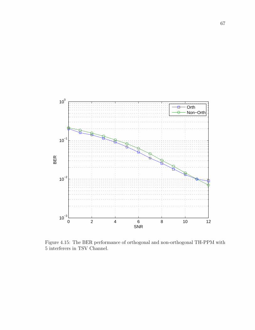
Figure 4.15The BER performance of orthogonal and non-orthogonal TH-
PPM with 5 interferers in TSV Channel. . . . . . . . . . . . . . 67
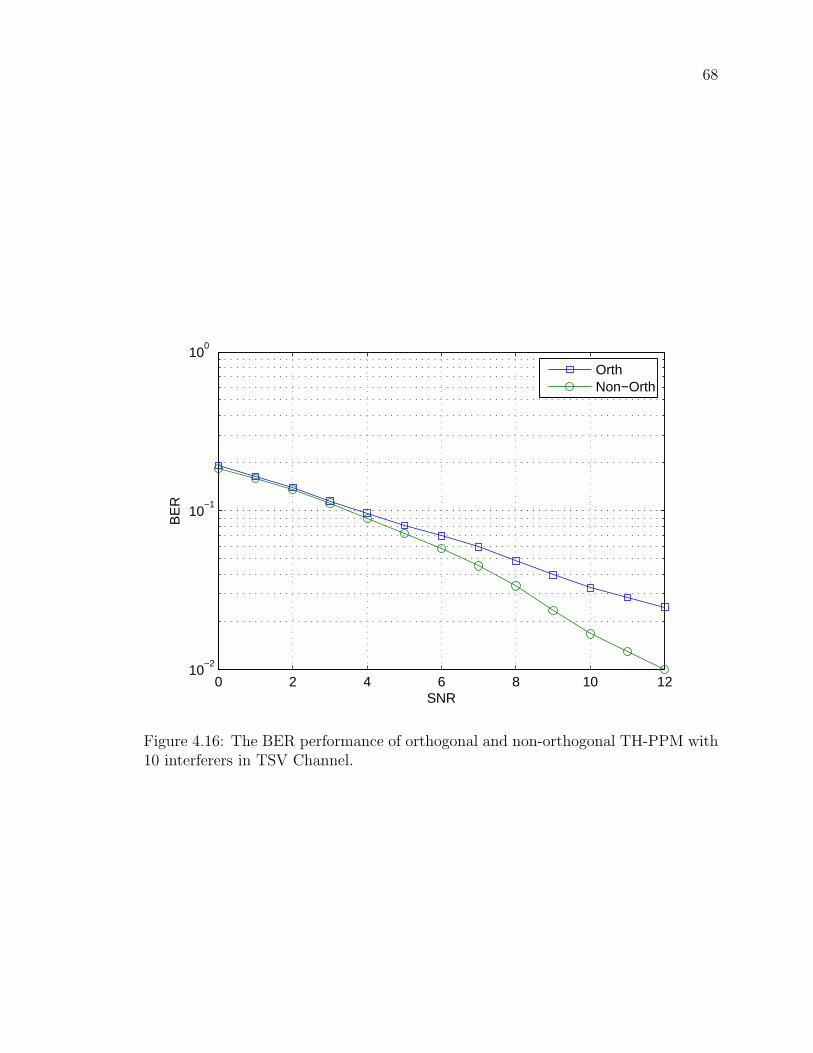
Figure 4.16The BER performance of orthogonal and non-orthogonal TH-
PPM with 10 interferers in TSV Channel. . . . . . . . . . . . . 68
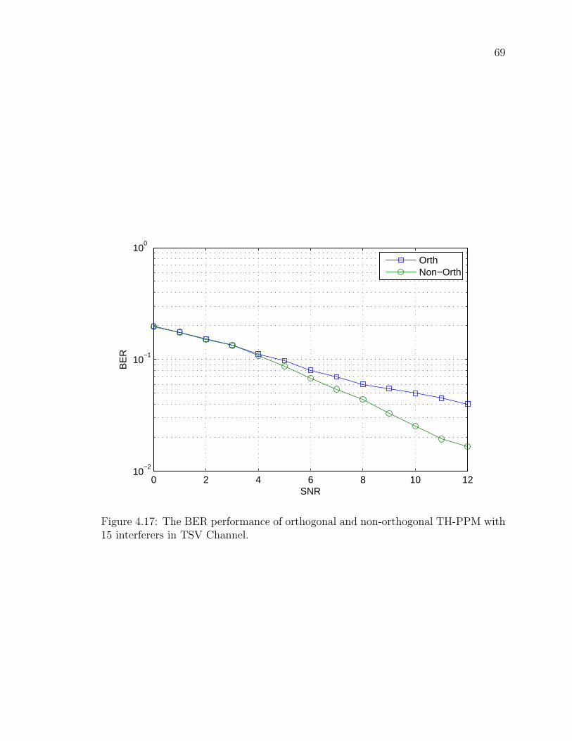
Figure 4.17The BER performance of orthogonal and non-orthogonal TH-
PPM with 15 interferers in TSV Channel. . . . . . . . . . . . . 69

x
List of Abbreviations
2P-Rake 2-finger Partial Rake
2S-Rake 2-finger Selective Rake
5P-Rake 5-finger Partial Rake
5S-Rake 5-finger Selective Rake
Ant Antenna
AoA Angle of Arrival
AWGN Additive White Gaussian Noise
BER Bit Error Rate
CDMA Code Division Multiple Access
CIR Channel Impulse Response
DoD Department of Defense
DS Direct Sequence
DVD Digital Video Disc
EIRP Equivalent Isotropically Radiated Power
FCC Federal Communications Commission
Gbps Gigabits per Second
GHz Gigahertz
GPS Global Positioning System
I-Rake Ideal Rake
Int Interferer
IR Impulse Response
IEEE Institute of Electrical and Electronics Engineers
ISI Inter Symbol Interference
LOS Line of Sight
Mbps Megabits per Second
MHz Megahertz
ML Maximum Likelihood
MM-Wave Millimeter Wave
MRC Maximum Ratio Combining
NLOS Non Line of Sight
xi
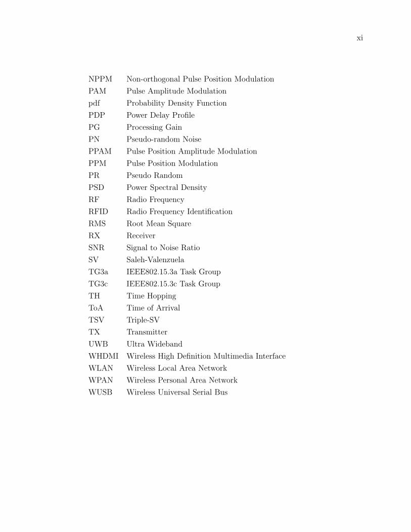
NPPM Non-orthogonal Pulse Position Modulation
PAM Pulse Amplitude Modulation
pdf Probability Density Function
PDP Power Delay Profile
PG Processing Gain
PN Pseudo-random Noise
PPAM Pulse Position Amplitude Modulation
PPM Pulse Position Modulation
PR Pseudo Random
PSD Power Spectral Density
RF Radio Frequency
RFID Radio Frequency Identification
RMS Root Mean Square
RX Receiver
SNR Signal to Noise Ratio
SV Saleh-Valenzuela
TG3a IEEE802.15.3a Task Group
TG3c IEEE802.15.3c Task Group
TH Time Hopping
ToA Time of Arrival
TSV Triple-SV
TX Transmitter
UWB Ultra Wideband
WHDMI Wireless High Definition Multimedia Interface
WLAN Wireless Local Area Network
WPAN Wireless Personal Area Network
WUSB Wireless Universal Serial Bus

xii
List of Symbols
aq Data Symbol
A Shadowing Path Loss
bi Input Bits
B Channel Bandwidth
Bf Fractional Bandwidth
c Speed of Light
C Channel Capacity
Ci Random Code
d Distance
d1 Direct Path
d2 Reflected Path
D Distance Between Transmit and Receive Antennas
f Frequency
fc Center Frequency
fH Higher Frequency
fL Lower Frequency
G Gain
Gt Transmitter Antenna Gain
Gt1 Transmitter Gain for Direct Path
Gt2 Transmitter Gain for Reflected Path
Gr Receiver Antenna Gain
Gr1 Receiver Gain for Direct Path
Gr2 Receiver Gain for Reflected Path
GTX Maximum Transmitter Antenna Gain
h1 Transmit Antenna Height
h2 Receive Antenna Height
h(t) Channel Impulse Response
I(t) Interference

xiii
ji(t) Basis Function
j(t− τ) Cross Correlator Basis Function
J Number of Different Waveforms
K Constant
LI All Multipath Components
LP Partial Multipath Components
LS Selective Multipath Components
m Ray Number
M Total Number of Rays
n Cluster Number
n(t) Noise
N Total Number of Clusters
Ns Number of Pulses Per Bit
Pnm Uniform Random Variable with value from ±1
Pr Received Signal Power
p(t) Pulse
Pt Transmitted Signal Power
PB Bit Error Probability
PNoise Noise Power
PTX Maximum Transmitter Antenna Power
q Bit Number
Q Total Number of Bits
r(t) Received Signal
Rb Bit Rate
sj(t) Waveform
sji Correlator Function
s(t) Transmitted Signal
sOOK OOK Signal
sPAM PAM Signal
sPPM PPM Signal
S Signal Power
t Time
T Pulse Repetition
Tc Chip Duration
Tf Frame Time
Tn First Ray Arrival Time
Tp Pulse Duration
U Total Number of Users

xiv
√W Signal Amplitude
√WRX Received Signal Amplitude
√WTX Transmitted Signal Amplitude√W (u) Amplitude of the uth User
Z Decision Variable
Zn Decision Variable for Noise
ZI Decision Variable for Interference
ZRX Decision Variable for Received Signal
α Channel Gain
αnm Multipath Gain Coefficient of the m-th Ray in the n-th Cluster
βnm Lognormal Fading Term
χ Antenna Beam Width
δ() Dirac Delta Function
ϵ PPM Shift
γ Ray Power Decay
Γ Cluster Power Decay
Γ0 Reflection Coefficient
λ Ray Arrival Rate
λf Wavelength of Center Frequency
Λ Cluster Arrival Rate
µD Average Distance Distribution
µnm Mean
ρ(ϵ) Autocorrelation Function
σ2 Variance
σϕ Ray Angle Spread
τ Channel Delay
τn,(m−1) Delay of the (m− 1)-th Ray in the n-th Cluster
Ω0 Average Power of the First Ray of the First Cluster
Ψn AoA of the n-th cluster
ψnm AoA of the m-th ray in the n-th cluster
ζn Channel Gain Fluctuations on each Cluster
ζnm Channel Gain Fluctuations on each Ray within a Cluster
xv
ACKNOWLEDGEMENTS
This thesis could not have been accomplished without the assistance of many people
whose contributions I gratefully acknowledge.
Foremost, I would like to express my sincere gratitude toward my graduate advisor
Professor T. Aaron Gulliver for his continuous support, excellent academic advice and
his input since the beginning of the study. I deeply appreciate his visionary supervision
and constructive suggestions in numerous ways during the course of this thesis.
I would like to thank my co-supervisor Dr. Wei Li for giving his insightful advice
which shaped my unformed ideas to start the thesis.
I want to express my gratitude to Dr. Abolfazl Ghassemi for his guidance throughout
my thesis. Without the degree of support that I got from him, this thesis could not
have been successfully completed.
I would like to thank my many student colleagues in our Telecommunications lab for
providing a stimulating and fun environment in which to learn and grow, specially
my good friend Carlos Quiroz Perez for all the support, entertainment, and caring he
provided.
I wish to thank my family who always supported me by their unwavering love and
encouragement. My sisters Bahareh, Kathy and Mercedeh, and my aunt Mitra.
I wish to thank my family in Victoria for providing a loving environment for me. My
uncle, Abie, aunty, Nahid, cousins, Tahara and Ian, and Farid. I have been lucky to
have them.
Lastly, and most importantly, I wish to thank my parents, Azar and Mohammad.
They raised me, supported me, taught me, and loved me. To them I dedicate this
thesis.

xvi
DEDICATION
This thesis is dedicated to my parents for their love, endless support
and encouragement.

Chapter 1
Introduction
In recent years demand for faster, less expensive and more secure wireless communi-
cations has increased remarkably. The entrance of new technologies to the wireless
world has made the radio frequency spectrum over crowded, which results in higher
prices for spectrum licensing and lower availability of spectrum. Ultra wideband
(UWB) [1], [2] is one solution to the spectrum concerns. UWB devices work under
the noise floor and therefore can coexist with the other technologies with very little
interference [3]. The noise like nature of UWB signals results from the allocation
of a significantly large bandwidth for this technology. Therefore, UWB is capable of
offering very large data rates, in the order of gigabits per second (Gbps), which makes
this technology very attractive.
Another reason that makes UWB attractive in the wireless market is that a vast
number of applications can use UWB. The trade-off between data rate and distance
is the reason for the diversity of applications. UWB can transfer information with
a very high data rate, but over a short range, or with a lower data rate but over a
longer range. This can be done by using more pulses per bit, which lowers the data
rate but allows for a longer transmission distance [4].
1.1 UWB History and FCC Regulations
The first use of impulse radio goes back to 1901 when Guglielmo Marconi used Morse
code to transfer information. He used a spark gap radio transmitter to send data over
the Atlantic Ocean. About sixty years later, the US military started using impulse ra-
dio because it is an extremely secure transmission technique. For almost thirty years,
2
from the 1960’s to 1990 research was almost exclusively done by the US Department
of Defence (DoD). In the recent years, due to advances in fast semiconductors impulse
radio has made its way into commercial applications under the new name of UWB. In
February 2002, federal communications commission (FCC) [5] allowed for unlicensed
commercial use of UWB for high data rate short range wireless data communications
[3].
Based on the FCC definition, UWB signals must have bandwidth of at least
500MHz or a fractional bandwidth of at least 0.20. The fractional bandwidth is
defined as [5]
Bf =B
fc× 100 =
(fH − fL)
(fH + fL)/2× 100 (1.1)
where B and fc are the total UWB bandwidth and center frequency, respectively, and
fH and fL are the higher and the lower frequencies at -10 dB.
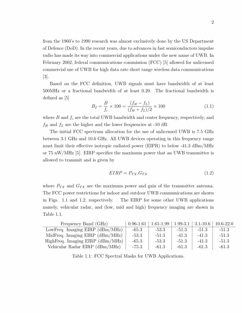
The initial FCC spectrum allocation for the use of unlicensed UWB is 7.5 GHz
between 3.1 GHz and 10.6 GHz. All UWB devices operating in this frequency range
must limit their effective isotropic radiated power (EIPR) to below -41.3 dBm/MHz
or 75 nW/MHz [5]. EIRP specifies the maximum power that an UWB transmitter is
allowed to transmit and is given by
EIRP = PTX .GTX (1.2)
where PTX and GTX are the maximum power and gain of the transmitter antenna.
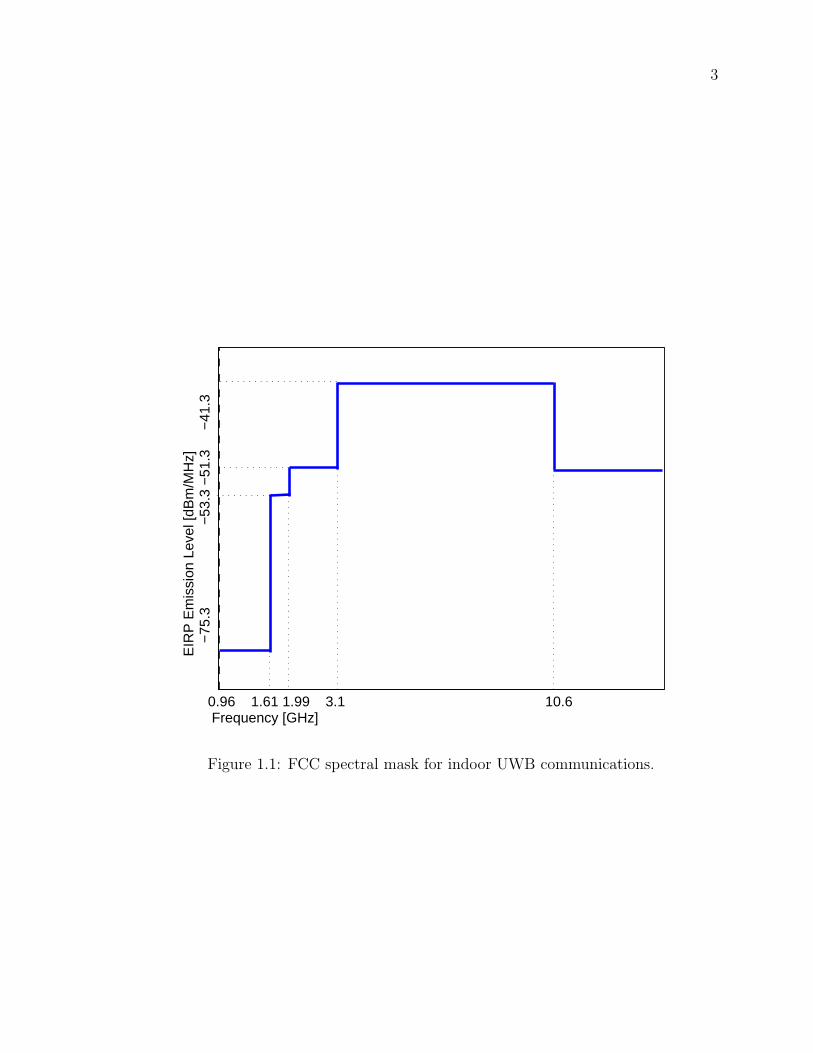
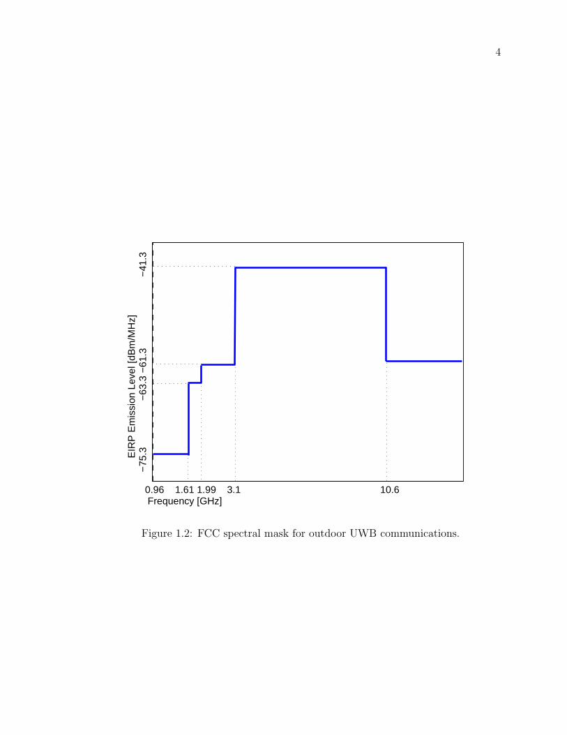
The FCC power restrictions for indoor and outdoor UWB communications are shown
in Figs. 1.1 and 1.2, respectively. The EIRP for some other UWB applications
namely, vehicular radar, and (low, mid and high) frequency imaging are shown in
Table 1.1.
Frequency Band (GHz) 0.96-1.61 1.61-1.99 1.99-3.1 3.1-10.6 10.6-22.0LowFreq. Imaging EIRP (dBm/MHz) -65.3 -53.3 -51.3 -51.3 -51.3MidFreq. Imaging EIRP (dBm/MHz) -53.3 -51.3 -41.3 -41.3 -51.3HighFreq. Imaging EIRP (dBm/MHz) -65.3 -53.3 -51.3 -41.3 -51.3Vehicular Radar EIRP (dBm/MHz) -75.3 -61.3 -61.3 -61.3 -61.3
Table 1.1: FCC Spectral Masks for UWB Applications.
3
0.96 1.61 1.99 3.1 10.6 Frequency [GHz]
EIR
P E
mis
sion
Lev
el [d
Bm
/MH
z]
−
75.3
−
53.3
−51
.3
−41
.3
Figure 1.1: FCC spectral mask for indoor UWB communications.
4
0.96 1.61 1.99 3.1 10.6 Frequency [GHz]
EIR
P E
mis
sion
Lev
el [d
Bm
/MH
z]
−
75.3
−
63.3
−61
.3
−
41.3
Figure 1.2: FCC spectral mask for outdoor UWB communications.
5
1.2 UWB Concept
Ultra wideband communications spreads the total signal power across a very wide
band of frequencies up to 7.5 GHz within the region 3.1 GHz to 10.6 GHz. This wide
band can be obtained using very short duration pulses, resulting in a signal with a
very low power spectral density (PSD). This reduces the interference to narrowband
users that use the same spectrum, while yielding a low probability of detection and
excellent multipath immunity. The low probability of interference comes from the fact
that the very low PSD appears as noise to other systems because the UWB signal is
below their noise floors. UWB also has a very low duty cycle which results in a very
low average transmission power. The duty cycle is the actual time duration of the
pulse over the time when a pulse can be transmitted [3].
1.3 UWB Advantages
UWB has several advantages over narrow band systems. The first advantage is the
low complexity of this system. This is due to the carrierless nature of UWB signal
which eliminates several radio frequency (RF) components from the circuit, such as
local oscillators and complex delay and phase tracking loops [4]. The unlicensed
bandwidth eliminates expensive licensing fees and bandwidth costs. UWB can share
the spectrum with other systems because signal can be generated which are below the
noise floor of other users [4]. This also decreases the probability of detection which
results a higher security for UWB systems.
As mentioned previously, due to the low pulse duty cycle, UWB has a low average
transmission power. This low power translates into the longer battery life for UWB
devices which can be an important advantage.
A high data rate is another advantage of UWB, but this can be achieved only for
short range communications. The high data rate is a result of the large bandwidth
and thus large channel capacity as given by Shannon’s theorem [6]
C = B log2
(1 +
S
Pnoise
)(1.3)
where C, B, S and Pnoise are the channel capacity, channel bandwidth, total signal
power and total noise power, respectively. Since UWB has a very large bandwidth,
the channel capacity which defines the maximum bit rate, is very large.

6
UWB systems have greater resistance to jamming compared with narrow band
systems. The reason is that these systems have a high processing gain (PG) [3],
which is given by PG = RFBandwidthDataBandwidth
. The processing gain can be interpreted as
frequency diversity, which provides resistance to jamming.
Finally, UWB has a better performance in multipath channels with multiple users
compared with narrow band systems. The very short duration of transmitted pulses
is the reason for this, as the nanosecond duration pulses are unlikely to overlap [3].
1.4 UWB Challenges
Some of the challenges exist for UWB communication are, UWB pulse distortion,
complicated synchronization between the receiver and the transmitter and compli-
cated channel estimation.
According to the Friis formula
Pr = Pt ·Gt ·Gr(c/(4πdf))2. (1.4)
Pr, Pt, Gt and Gr are the received and transmitted signal powers and the transmitter
and receiver antenna gains, respectively; c, d and f are the speed of light, transmitter
and receiver distance and the signal frequency. It can be seen in the equation that
with increase of frequency, the received signal power decreases. Due to the very wide
range of UWB frequencies the received power changes constantly and as a result the
pulse shape gets distorted [3].
The other challenge is the synchronization of high frequency UWB transmitter
and receiver. Due to the very short duration of UWB pulses, the sampling and
synchronization is more complicated than narrow band. To overcome this, very fast
analog to digital converters are required [3].
Moreover, because of the wide frequency band of UWB and the reduced signal
energy, channel estimation would also be a complicated task [3].
1.5 60 GHz MM-Wave Communications
While having all the advantages the lower frequency UWB band has over narrow
band systems, this frequency band, although approved by the FCC, is not available
in all countries. Therefore, the entire 7.5 GHz of bandwidth cannot be used globally
7
[7]. In addition, the capacity in this band is insufficient for some applications such
as coaxial cable replacement in the home [7]. Finally, even though lower frequency
UWB signals are below the noise floor and this reduces the interference to the other
systems, some interference still occurs, i.e., the UWB signal introduces additional
noise to other systems.
The frequency range of 57 GHz to 64 GHz, the 60 GHz millimeter-wave (mm-
wave) [8] band, is another frequency range that has been made available for UWB
communications. This frequency range is a promising solution for all the aforemen-
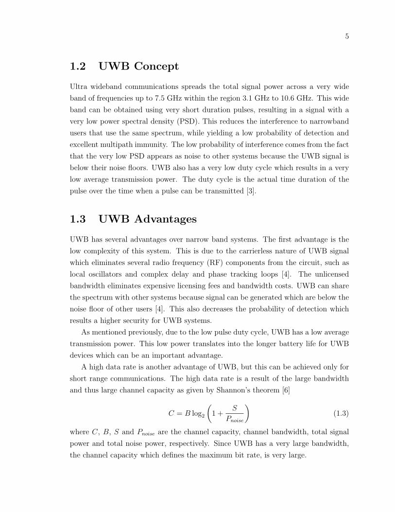
tioned problems. 3.5 to 7 GHz of bandwidth is available worldwide over the 60 GHz
frequency band, as summarized in Fig. 1.3 [9]. Due to the high frequency and large
bandwidth, 60 GHz mm-wave can support data rates up to 2-3 Gbps [8]. Also mm-
wave signals do not interfere with other systems as much since fewer systems operate
at these higher frequencies. This higher frequency band operation can be seen to
provide higher security for mm-wave systems.
Figure 1.3: Available global frequency bands around 60 GHz.
A higher frequency band means greater path loss for the transmitted signal. Fur-
thermore, in this frequency range, atmospheric phenomena such as oxygen (O2) ab-
sorption exists. Oxygen absorption is absorption of electromagnetic energy by oxygen
molecules. The resulting severe attenuation of mm-wave signals can be overcome by
using multiple directional antennas. Other advantages of this approach are higher
spatial reuse, higher security and less interference to other users [8]. Challenges with
this channel inlcude increased transceivers phase noise and limited gain amplifiers [7].
8
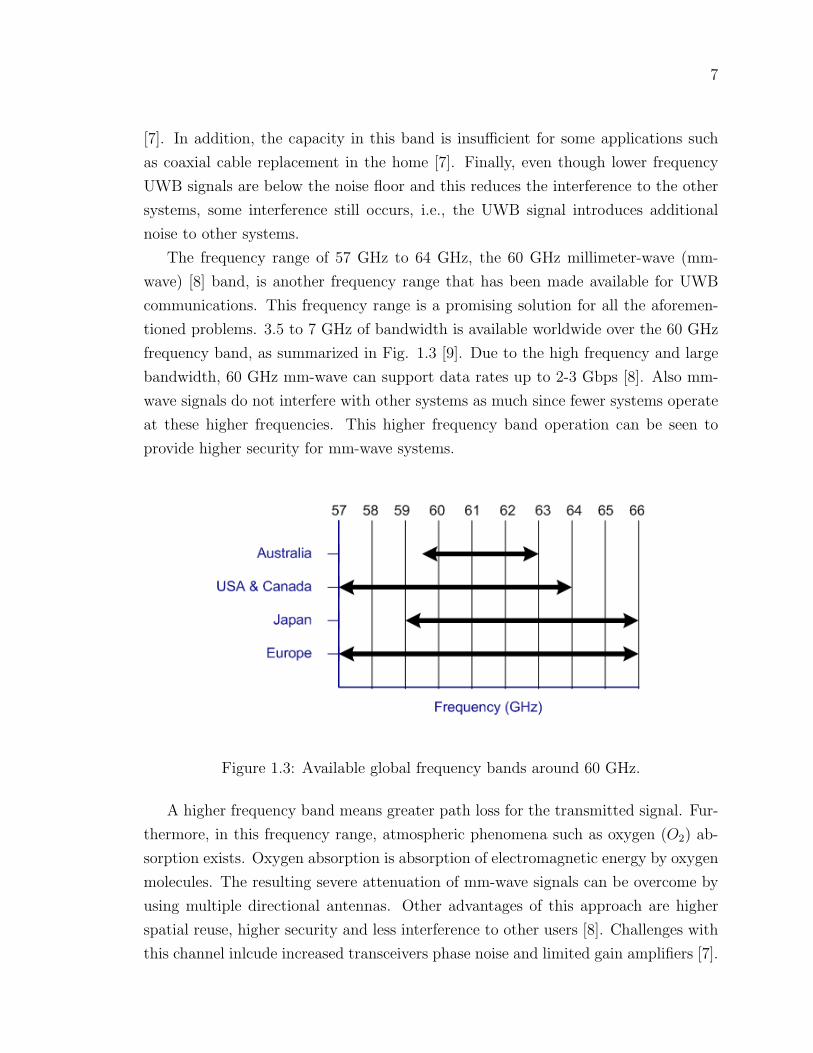
The advantages and disadvantages of lower UWB band and mm-wave UWB sys-
tems are shown in Tables 1.2 and 1.3.
UWB Benefits UWB ChallengesLow complexity Pulse shape distortionLow interference complicated synchronization
Coexistance with narrow band complicated channel estimationHigh security
Low power and long battery lifeHigh date rateNo licence fee
Resistance to jammingBetter performance in multipath environments
Table 1.2: UWB advantages and disadvantages compared to narrow band communi-cations.
60 GHz mm-wave UWB Benefits 60 GHz mm-wave UWB ChallengesFrequency band available globaly Greater pathlossHigh capacity (cable replacement) Oxygen absorption
Less interference Transceiver phase noiseHigher security Limited gain amplifiers
High spatial reuse
Table 1.3: 60 GHz UWB advantages and disadvantages compared to lower frequencyUWB.
1.6 UWB Pulse Modulation Schemes
High data rate impulse radio UWB provides short range communications with very
low transmitted power, and can be implemented simply. It uses a pulse or a sequence
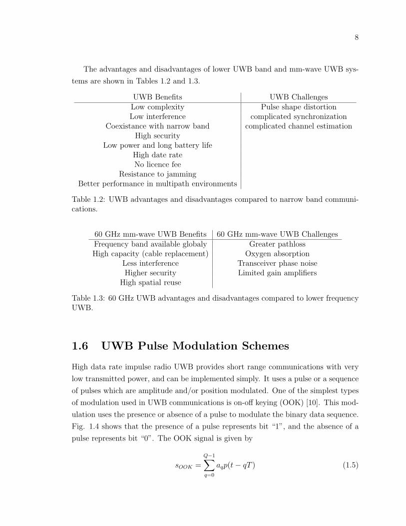
of pulses which are amplitude and/or position modulated. One of the simplest types
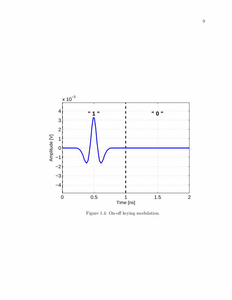
of modulation used in UWB communications is on-off keying (OOK) [10]. This mod-
ulation uses the presence or absence of a pulse to modulate the binary data sequence.
Fig. 1.4 shows that the presence of a pulse represents bit “1”, and the absence of a
pulse represents bit “0”. The OOK signal is given by
sOOK =
Q−1∑q=0
aqp(t− qT ) (1.5)
9
0 0.5 1 1.5 2
−4
−3
−2
−1
0
1
2
3
4
x 10−3
Time [ns]
Am
plitu
de [V
]
" 1 " " 0 "
Figure 1.4: On-off keying modulation.
10
where Q, T , p(t), and aq are total number of bits, pulse repetition, pulse, and data
symbol given by
aq =
0 represents bit “0′′
1 represents bit “1′′.
During off times there is no transmission, and as a result undesired signals may be
detected as a transmitted signal. This can cause poor performance in multiple access
environments.
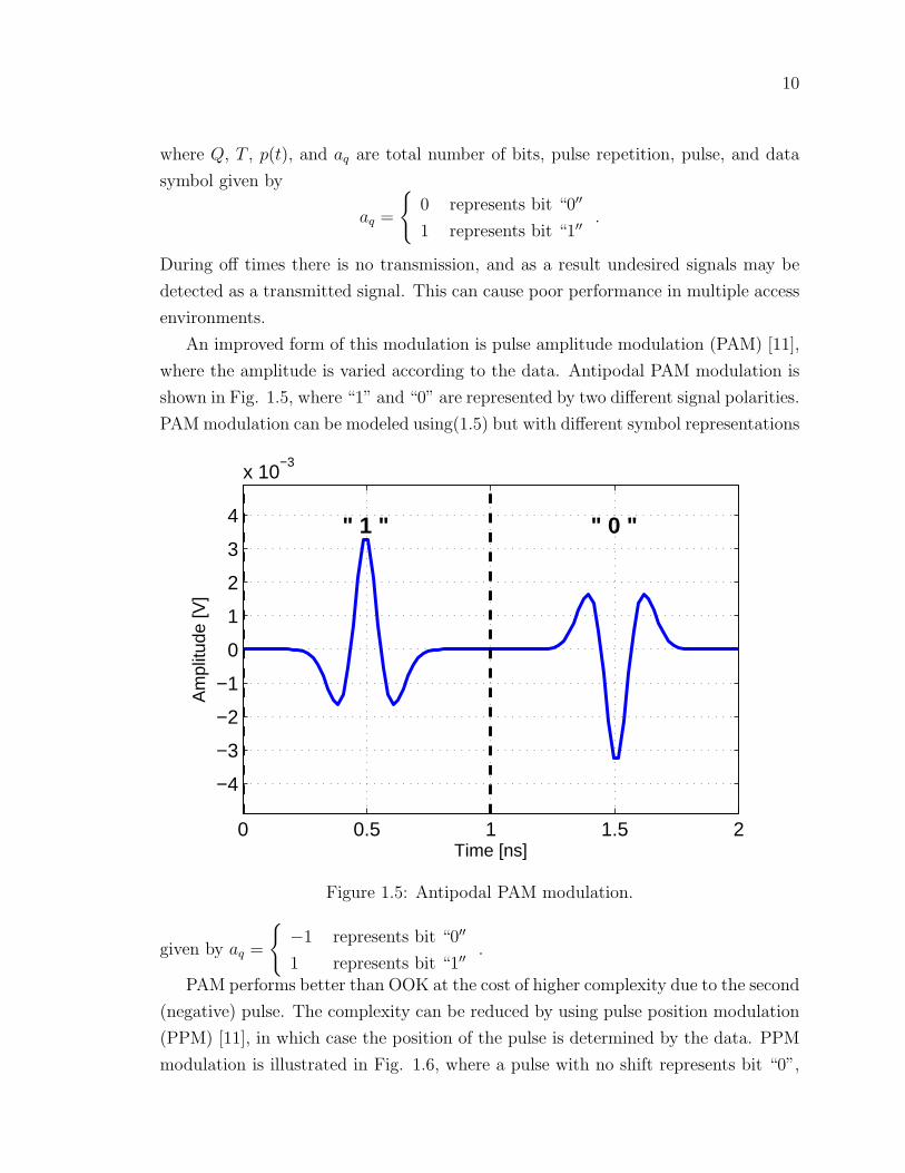
An improved form of this modulation is pulse amplitude modulation (PAM) [11],
where the amplitude is varied according to the data. Antipodal PAM modulation is
shown in Fig. 1.5, where “1” and “0” are represented by two different signal polarities.
PAM modulation can be modeled using(1.5) but with different symbol representations
0 0.5 1 1.5 2
−4
−3
−2
−1
0
1
2
3
4
x 10−3
Time [ns]
Am
plitu
de [V
]
" 1 " " 0 "
Figure 1.5: Antipodal PAM modulation.
given by aq =
−1 represents bit “0′′
1 represents bit “1′′.
PAM performs better than OOK at the cost of higher complexity due to the second
(negative) pulse. The complexity can be reduced by using pulse position modulation
(PPM) [11], in which case the position of the pulse is determined by the data. PPM
modulation is illustrated in Fig. 1.6, where a pulse with no shift represents bit “0”,
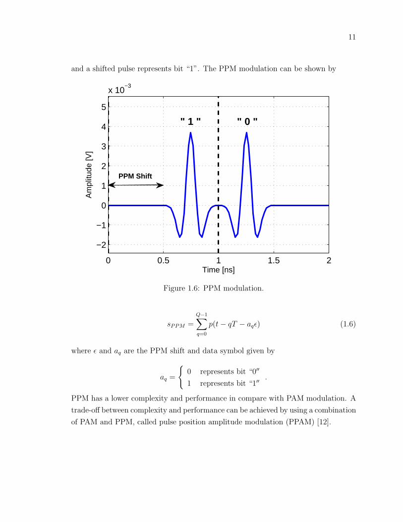
11
and a shifted pulse represents bit “1”. The PPM modulation can be shown by
0 0.5 1 1.5 2
−2
−1
0
1
2
3
4
5
x 10−3
Time [ns]
Am
plitu
de [V
]
" 0 "" 1 "
PPM Shift
Figure 1.6: PPM modulation.
sPPM =
Q−1∑q=0
p(t− qT − aqϵ) (1.6)
where ϵ and aq are the PPM shift and data symbol given by
aq =
0 represents bit “0′′
1 represents bit “1′′.
PPM has a lower complexity and performance in compare with PAM modulation. A
trade-off between complexity and performance can be achieved by using a combination
of PAM and PPM, called pulse position amplitude modulation (PPAM) [12].

12
1.7 UWB Applications
UWB can be used in numerous applications. These applications can be categorized
in two main groups, high data rate and low data rate. Typically, the closer the
transmitter and the receiver are, the higher the achievable data rate. Both high data
rate short range and low data rate long range communication systems are widely
employed in industry. Some of the main applications are high data rate wireless local
area network (WLAN), wireless personal area network (WPAN), wireless universal
serial bus (WUSB), radio frequency identification (RFID), and home entertainment
systems. Wall through imaging, vehicular applications, medical monitoring, rescue
localization, and object positioning are some of lower date rate UWB applications
[3].
Some of the potential applications for 60 GHz mm-wave communications are mo-
bile broadband, high speed fixed wireless access, high speed WLANs, coaxial cable
replacement for fast WPANs, wireless high definition multimedia interface (WHDMI)
such as high definition television (HDTV), wireless digital video disc (DVD) player
and cable box communications [7]. Application which required higher capacity such
as coaxial cable replacement need at least 2Gb/s of data rate. Such capacity is
achievable using 60 GHz mm-wave communications [13].
1.8 Thesis Summary and Outline
In this thesis, UWB is studied, concepts and history are discussed, and the advantages
of UWB over narrow band are described. It is shown that UWB can provide a better
data rate while having a lower probability of interference. Advantages and disadvan-
tages of higher frequency UWB communications, 60 GHz mm-wave, in compare with
the lower frequency UWB are discussed.
Different pulse modulations for UWB system have introduced. It is discussed why
PPM is considered in this thesis as the chosen modulation technique. The rest of this
thesis is organized as follow. In Chapter 2, time hopping (TH) technique is intro-
duced. It is employed to the PPM modulation, TH-PPM, to reduce the interference
in multiple access environments. Orthogonality and non-orthogonality of pulses are
then discussed and compared. More over, TH-PPM is defined over additive white
Gaussian noise (AWGN), Saleh-Valenzuela (SV) and Triple-SV (TSV) channel mod-
els. Each of these models discussed separately in details. In Chapter 3, different

13
types of rake receivers are introduced and compared. It is shown that ideal rake
(I-Rake) receiver has the best performance among all rake receivers, followed by 5
finger selective rake (5S-Rake), 5 finger partial rake (5P-Rake), 2 finger selective rake
(2S-Rake), and 2 finger partial rake (2P-Rake). High gain directional antennas are
then introduced for 60 GHz mm-wave UWB. In Chapter 4, the bit error rate (BER)
performance of TH-PPM over AWGN, SV and TSV channels is evaluated. Moreover,
the performance of orthogonal and non-orthogonal TH-PPM with different numbers
of users are compared. Performance results show that non-orthogonal TH-PPM can
perform better than orthogonal TH-PPM when the number of users is large. It is
shown that orthogonal and non-orthogonal TH-PPM modulation in a TSV channel
performs close to TH-PPM modulation in a SV channel. Finally Chapter 5 concludes
the thesis.

14
Chapter 2
UWB System Model
2.1 TH-PPM UWB Model
TH-PPM modulation uses the position of the pulses to modulate the binary data
sequence. Time hopping is applied to this modulation for multi access environments.
Time hopping code is a pseudo-random (PN) code that is unique for each user. In
TH-PPM, the time frame is divided into several smaller time slots called chips. Each
data bit is presented by one or more pulses where then each pulse, using TH code, is
located randomly in a specific chip.
To transmit data in this system, the bit stream is first repetition encoded to
obtain Ns pulses per bit. Time hopping is then applied to the output of the encoder,
bi, giving
CiTc + ϵb⌊i/Ns⌋
where Ci, Tc and ϵ are the random code, chip duration, and PPM shift (applied to
the pulse to differentiate between bits 0 and 1), respectively. We assume that ϵ < Tc,
ϵ ≥ Tp, and CiTc + ϵ < Tf where Tp and Tf are the pulse duration and frame time.
The output of TH encoder is then modulated using PPM modulator which is given
by
iTf + CiTc + ϵb⌊i/Ns⌋.
At this stage the position of unit pulses are set and ready to enter the pulse shaper
filter to generate the pulse shaped TH-PPM signal. In Figure 2.1 the block diagram
for TH-PPM is shown. The pulse shape of the TH-PPM signal must satisfy the FCC’s
spectral mask requirements. Sine, Gaussian (first and second derivative), and rectan-

15
Figure 2.1: TH-PPM transmitter block diagram for UWB system

16
gular pulse shapes have been employed for this purpose [14]. The second derivative of
the Gaussian pulse is used here since it satisfies the FCC spectral mask requirements
and has been widely employed in UWB system designs [15]. The transmitted signal
is then given by
s(t) =√W∑i
p(t− iTf − CiTc − ϵb⌊i/Ns⌋) (2.1)
where√W is the signal amplitude. Fig. 2.2 illustrates a typical TH-PPM signal
with Tf = 3 nsec, Tc = 1 nsec, Tp = 0.5 nsec, and a PPM shift of ϵ = 0.5 nsec. The
0 3 6 9 12 15 18 21 24 27 30
−2
0
2
4
6
8
x 10−3
Time [nsec]
Am
plitu
de [V
]
Figure 2.2: A TH-PPM signal with frame time Tf = 3 nsec, chip time Tc = 1 nsec,pulse duration Tp = 0.5 nsec, and PPM shift ϵ = 0.5 nsec.
Gaussian pulse can be expressed as [16]
p(t) = ±√2
αe
−2πt2
α2 (2.2)
where α2 is the pulse shape factor equal to 4πσ2 (with variance σ2). Hence, the
second derivative is
p2(t) =
[1− 4π
t2
α2
]e−
2πt2
α2 . (2.3)

17
Fig. 2.3 shows a typical second derivative Gaussian pulse waveform.
0 5 10 15 20 25−4
−2
0
2
4
6
8
10x 10
−3
Number of Samples
Am
plitu
de
Figure 2.3: A typical second derivative Gaussian pulse waveform
For TH-PPM the pulse p(t) is assumed to has non-zero values only in the interval
of [0, Tp]. The transmitted signal is a series of pulses given by [17]
pm(t) =
p(t+mϵ) mϵ ≤ t ≤ mϵ+ Tp
0 mϵ > t > mϵ+ Tp(2.4)
where ϵ < Tp for non-orthogonal TH-PPM, ϵ ≥ Tp for orthogonal TH-PPM, and m
is an integer.
2.2 UWB Channel Models
A channel can be modelled by calculating the physical processes that affect the trans-
mitted signal. As the transmitted signal goes through the channel, it gets distorted
18
by multipath fading and Gaussian noise. Because transmission can be in a multiuser
environment, the effect of multiuser interference must also be considered.The received
signal is given by
r(t) = s(t) ∗ h(t) + I(t) + n(t) (2.5)
where h(t) is the channel impulse response (CIR) which is convolved with the trans-
mitted signal s(t), and I(t) and n(t) are the interference from other users and additive
white Gaussian noise, respectively.
The impulse response of the channel is
h(t) = αδ(t− τ) (2.6)
where δ(), α and τ are the Dirac delta function, channel gain and delay, respectively.
Using (2.5) and (2.6), the received signal is
r(t) = αs(t− τ) + I(t) + n(t). (2.7)
The transmitted signal using TH-PPM modulation (2.1) can be expressed as
s(t) =√WTX
∑i
p(t− iTf − CiTc − ϵb⌊i/Ns⌋) (2.8)
where√WTX is the transmitted signal amplitude. From (2.7) and (2.8), the received
signal is then
r(t) =√WRX
∑i
p(t− iTf − CiTc − ϵb⌊i/Ns⌋ − τ) + I(t) + n(t) (2.9)
where the received signal amplitude is given by,√WRX = α
√WTX .
I(t) represents the interference from other users and is given by
I(t) =U−1∑u=1
√W (u)
∑i
p(t− iTf − C(u)i Tc − ϵb
(u)⌊i/N
(u)s
⌋ − τ (u)) (2.10)
where√W (u) is the amplitude of the uth user signal. The received signal using (2.9)
19
and (2.10) is then
r(t) =√WRX
∑i
p(t− iTf − CiTc − ϵb⌊i/Ns⌋ − τ) +U−1∑u=1
√W (u)
∑i
p(t− iTf (2.11)
−C(u)i Tc − ϵb
(u)⌊i/N
(u)s
⌋ − τ (u)) + n(t)
2.2.1 The Saleh-Valenzuela Model
The Saleh-Valenzuela (SV) model [18] is an UWB channel model which assumes the
multipath components (rays) arrive at the receiver in groups called clusters [19]. The
rays are delayed and attenuated replicas of the transmitted signal, and each cluster
consists of several rays. Each cluster and each ray within a cluster has independent
fading. The average power for the clusters and rays decays gradually. Both decay
factors follow a Poisson distribution. This is illustrated in Fig. 2.4, which shows
the instantaneous powers for the clusters and rays. Typically, the later the rays and
clusters arrive, the lower the power of the rays and clusters. In this figure there are
14 clusters, and each contains 140 rays, which makes a total of 1960 rays.
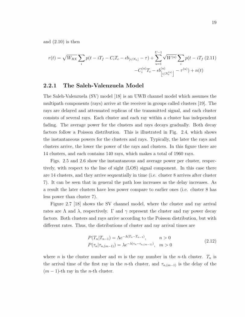
Figs. 2.5 and 2.6 show the instantaneous and average power per cluster, respec-
tively, with respect to the line of sight (LOS) signal component. In this case there
are 14 clusters, and they arrive sequentially in time (i.e. cluster 8 arrives after cluster
7). It can be seen that in general the path loss increases as the delay increases. As
a result the later clusters have less power compare to earlier ones (i.e. cluster 8 has
less power than cluster 7).
Figure 2.7 [18] shows the SV channel model, where the cluster and ray arrival
rates are Λ and λ, respectively. Γ and γ represent the cluster and ray power decay
factors. Both clusters and rays arrive according to the Poisson distribution, but with
different rates. Thus, the distributions of cluster and ray arrival times are
P (Tn|Tn−1) = Λe−Λ(Tn−Tn−1), n > 0
P (τn|τn,(m−1)) = λe−λ(τn−τn,(m−1)), m > 0(2.12)
where n is the cluster number and m is the ray number in the n-th cluster. Tn is
the arrival time of the first ray in the n-th cluster, and τn,(m−1) is the delay of the
(m− 1)-th ray in the n-th cluster.

20
0 500 1000 1500 2000−60
−55
−50
−45
−40
−35
−30
−25
−20
−15
−10
Rays/Clusters
dB
Figure 2.4: Ray and cluster instantaneous power for a typical SV channel.
21
1 2 3 4 5 6 7 8 9 10 11 12 13 14−60
−50
−40
−30
−20
−10
0
10
Number of Channels
dB
Figure 2.5: Instantaneous power per cluster for a typical SV channel.

22
1 2 3 4 5 6 7 8 9 10 11 12 13 14−50
−40
−30
−20
−10
0
10
Number of Channels
dB
Figure 2.6: Average power per cluster for a typical SV channel.
Figure 2.7: The SV channel impulse response with ray arrival rate λ, cluster arrivalrate Λ, ray power decay factor γ, and cluster power decay factor Γ.

23
The channel impulse response for this model is
h(t) = A
N∑n=1
M∑m=1
αnmδ(t− Tn − τnm) (2.13)
where A is the path loss due to shadowing and is modeled as a log-normal random
variable. M and N are the number of rays and clusters, respectively. αnm is the
multipath gain coefficient of the m-th ray in the n-th cluster defined as
αnm = Pnmβnm (2.14)
where Pnm is a uniform random variable with value from ±1 which defines the random
pulse inversion that happens because of reflections. βnm is the lognormal fading term
which can be modelled as
βnm = 10χnm/20 (2.15)
χnm = µnm + ζn + ζnm (2.16)
where ζn and ζnm are zero-mean Gaussian random variables with variances σ2ξ and
σ2ζ , respectively. They define the channel gain fluctuations for the clusters and rays.
µnm = K − TnΓ
− τnmγ
(2.17)
where K is a constant, and Γ and γ are the cluster and ray power decays. Using
(2.5), (2.8) and (2.13) the received signal is
r(t) =√WRX
∑i
N∑n=1
M∑m=1
αnmp(t− iTf − CiTc − ϵb⌊i/Ns⌋ − Tn − τnm)(2.18)
+U−1∑u=1
√W (u)
∑i
N∑n=1
M∑m=1
αnmp(t− iTf − C(u)i Tc − ϵb
(u)⌊i/N
(u)s
⌋ − Tn − τ (u)) + n(t)
where√WRX = A
√WTX .
The power delay profile (PDP) of the UWB channel (using IEEE 802.15.3a-CM1
channel parameters) is shown in Fig. 2.8. The PDP is a graphical view of signal
intensity as a function of time delay with respect to the arrival of the first signal,
which is assumed to have zero delay. It is calculated as the expected value of the

24
magnitude squared channel impulse response, and is given by [20]
PDP = E[|h(τ)|2]. (2.19)
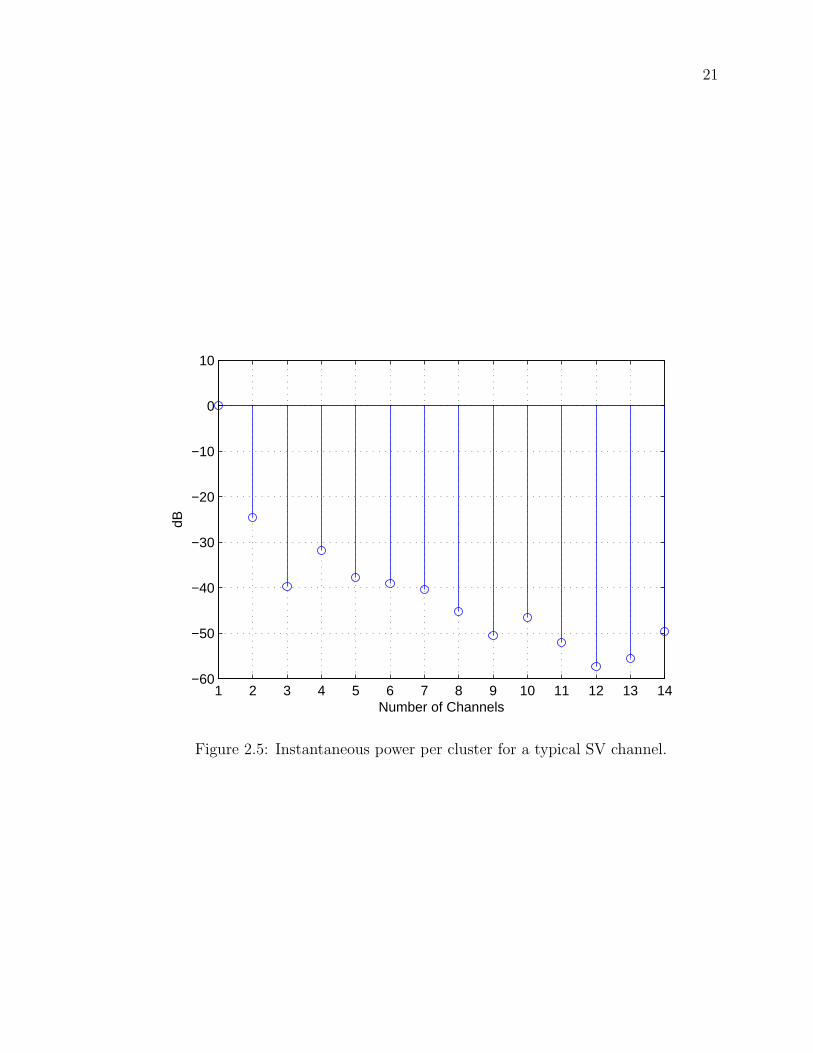
Fig. 2.9 shows the PDP of the UWB channel using IEEE 802.15.3a-CM4 parameters.
0 0.5 1 1.5 2 2.5
x 10−7
0
1000
2000
3000
4000
5000
6000
7000
8000
9000
10000
Time [s]
Pow
er [V
2 ]
Figure 2.8: Power delay profile for UWB channel model CM1.
More arrivals occur at the receiver for channel CM4, as the fading is the more severe
in non-line-of-sight (NLOS). Due to the longer duration of the CM4 channel impulse
response, the time separation between pulses must be carefully chosen to avoid inter-
symbol interference (ISI).
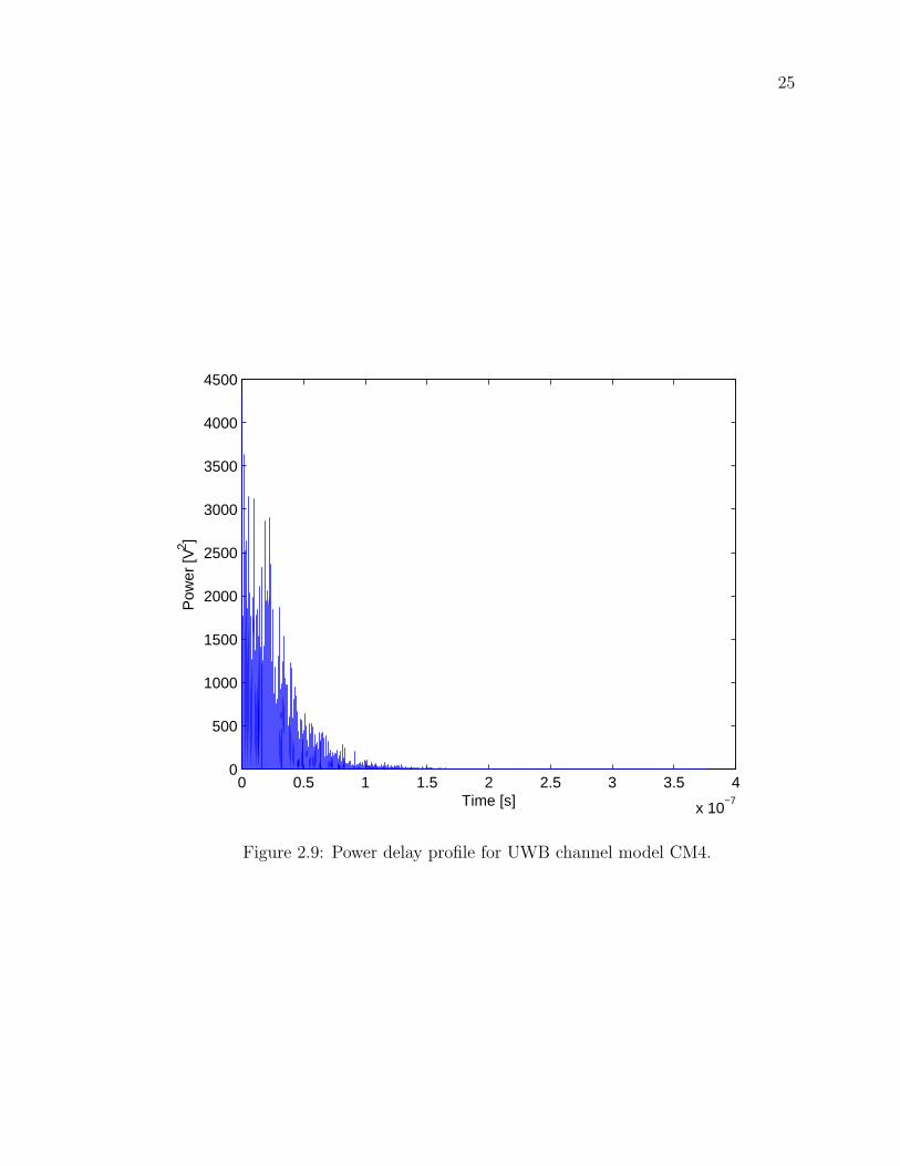
A discrete time channel impulse response is employed for multipath environments
so that performance can be practically evaluated. In this model, the time dimension
is divided into small time intervals called bins. Each bin can contain one or more
multipath components. Figs. 2.10 and 2.11 show the corresponding discrete time
impulse responses for channels CM1 and CM4. Since CM4 represents an extreme
25
0 0.5 1 1.5 2 2.5 3 3.5 4
x 10−7
0
500
1000
1500
2000
2500
3000
3500
4000
4500
Time [s]
Pow
er [V
2 ]
Figure 2.9: Power delay profile for UWB channel model CM4.
26
NLOS channel, the discrete CIR has more multipath components compare to channel
CM1.
0 0.2 0.4 0.6 0.8 1
x 10−7
−1.5
−1
−0.5
0
0.5
1x 10
−3
Time
Am
plitu
de G
ain
Figure 2.10: Discrete time impulse response for UWB channel model CM1.
2.2.2 The Triple S-V Model
The triple-SV (TSV) model [21] is a combination of the SV model [18] and the two
path model [22]. It was developed and found by Shoji, Sawada, Saleh and Valenzuela.
This channel model is considered appropriate for the 60 GHz mm-wave UWB channel.
The SV model discussed previously does not consider the angle of arrival (AoA).
However, antenna directivity has a significant impact on the signal to noise ratio
for high frequencies such as with mm-wave signals. Hence the TSV channel model
considers the AoA. In this case, the channel impulse response for the SV channel
model is defined as
h(t) =N∑n=1
M∑m=1
αnmδ(t− Tn − τnm)δ(ϕ−Ψn − ψnm) (2.20)

27
0 0.5 1 1.5 2 2.5 3
x 10−7
−12
−10
−8
−6
−4
−2
0
2
4
6
8x 10
−4
Time
Am
plitu
de G
ain
Figure 2.11: Discrete time impulse response for UWB channel model CM4.

28
where Ψn is the AoA of the n-th cluster and ψnm is the AoA of the m-th ray. ψnm is
assumed to have a Laplacian distribution
p(ψnm) =1√2σϕ
e−√2ψnm/σϕ . (2.21)
σϕ is the angle spread of the rays, and αnm is the m-th ray n-th cluster gain and can
be presented as
|αnm|2 = Ω0e−TnΓ e
−τnmγ
√Gr(0,Ψn + ψnm) (2.22)
where Gr is the receiver antenna gain, and ∠αnm is a uniform random variable dis-
tributed over [0, 2π). The parameters Γ,Λ, γ, λ, σ1(σζ), σ2(σξ) are the same as in
Figure 2.12: A typical TSV channel model realization.
Section 3.1. The remaining parameters are σϕ and Ω0, which are the angle spread
of the rays with Laplace distribution, and the average power of the first ray of the
first cluster, respectively. Fig. 2.12 [23] represents a typical TSV channel model
realization where βLOS is the line of sight (LOS) component.
The second component of the TSV model is based on a two-path model and is
given by
β =µDD
∣∣∣∣Gt1Gr1 +Gt2Gr2Γ0exp
[j2π
λf
2h1h2D
]∣∣∣∣ (2.23)
where D is the distance between the transmit and receive antennas, and h1, h2 are the

29
antenna heights. λf , Γ0, and µD are the wavelength of center frequency, the reflection
coefficient, and the average distance distribution. Gt1 and Gr1 are the transmitter and
receiver gains for the direct path d1, and Gt2 and Gr2 are the transmitter and receiver
gains for the reflected path d2. The value of β is very sensitive to small antenna
movements, even on order of a few millimeters. The two path model is illustrated in
Fig. 2.13 [22].
Figure 2.13: The two path channel model.
Combining (2.20) and (2.23), the TSV channel model is
h(t) = βδ(t) +N∑n=1
M∑m=1
αnmδ(t− Tn − τnm)δ(ϕ−Ψn − ψnm) (2.24)
where βδ(t) represents the LOS component and the remaining terms represent the
SV model component.
The average power of the channel can be represented as a function of the angle of
arrival, which is called the power azimuth profile. Based on the power azimuth profile,
the distribution of the cluster mean AoA can be described by a uniform distribution
over [0, 2π], i.e.,
p(Θn|Θn−1) =1
2π, (n > 0). (2.25)
Fig. 2.14 shows a 3D realization of the clusters with respect to power, angle of
arrival and time of arrival. It can be seen that the later the clusters and rays arrive,
the lower the power is. This figure also shows that the clusters arrive with different
angles.
The main TSV channel model parameters which determine the performance are
power decay profile (PDP), mean excess delay and root mean square (RMS) delay
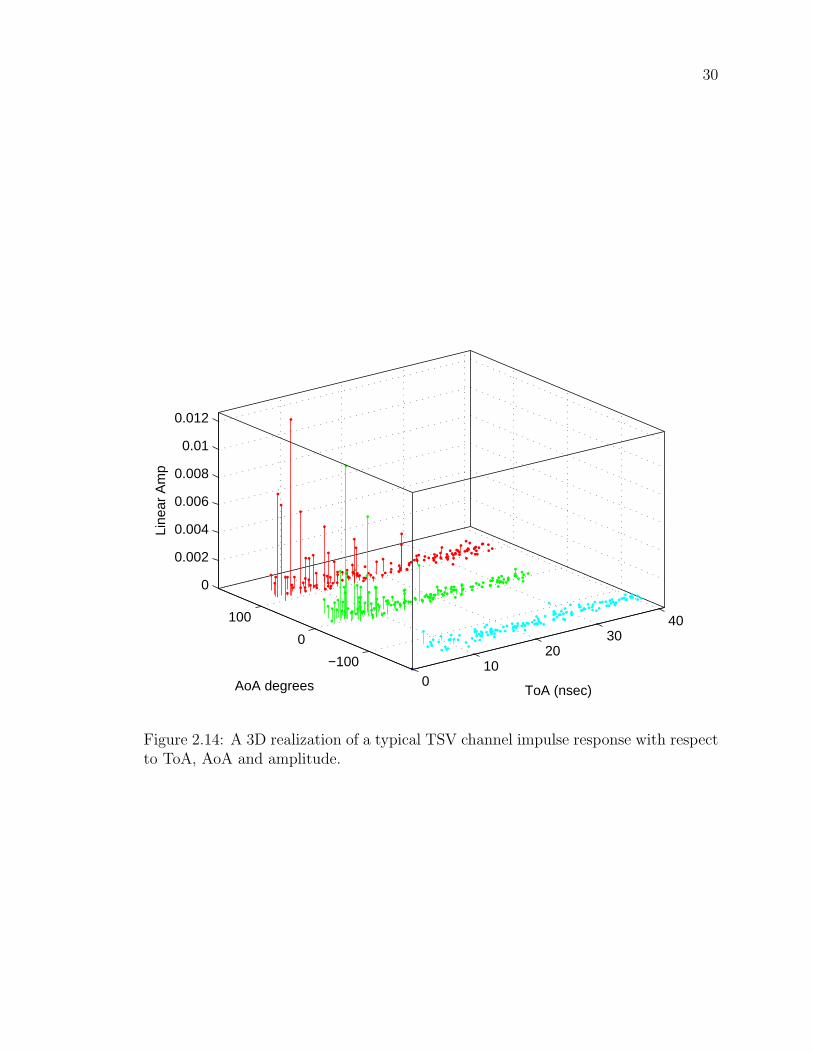
30
010
2030
40
−100
0
100
0
0.002
0.004
0.006
0.008
0.01
0.012
ToA (nsec)AoA degrees
Line
ar A
mp
Figure 2.14: A 3D realization of a typical TSV channel impulse response with respectto ToA, AoA and amplitude.

31
spread. A typical PDP for the TSV channel is shown in Fig. 2.15. The LOS compo-
nent is located at the zero position with power of -81.9842 dB. The average PDP for
this channel model is shown in Fig. 2.16.
0 50 100 150
−140
−130
−120
−110
−100
−90
−80
Time of Arrival (ns)
Rel
ativ
e P
ower
[dB
m]
Figure 2.15: A typical power delay profile for the TSV channel.
The mean excess delay is the weighted average or the first moment of the power
delay profile, and is given by [20]
τ =
∑k a
2kτk∑
k a2k
=
∑k P (τk)τk∑k P (τk)
. (2.26)
In Figure 2.17 the mean excess delay of TSV channel is illustrated. For this figure,
the standard deviation of the log normal variable for cluster fading is 6.6300 nsec.
The RMS delay spread is the square root of the second central moment of the
PDP and is given by [20]
στ =
√τ 2 − (τ)2 (2.27)
where
τ 2 =
∑k a
2kτ
2k∑
k a2k
=
∑k P (τk)τ
2k∑
k P (τk). (2.28)

32
0 20 40 60 80 100
−140
−130
−120
−110
−100
−90
−80
Time of Arrival (ns)
Ave
rage
Pow
er [d
B]
Figure 2.16: Average power delay profile for a typical TSV channel.

33
0 20 40 60 80 1003
4
5
6
7
8
9
10
11
12
13x 10
−9
Number of Channel Realizations
Exc
ess
Del
ay (
sec)
Figure 2.17: The channel excess delay.

34
The RMS delay spread is a measure of the effective duration of the channel and is
shown in Figure 2.18. In this figure, the standard deviation of the log normal variable
for ray fading is equal to 9.8300 nsec.
0 20 40 60 80 1000.6
0.7
0.8
0.9
1
1.1
1.2
1.3
1.4x 10
−8
Number of Channel Realizations
RM
S D
elay
(se
c)
Figure 2.18: TSV Channel model RMS delay spread.
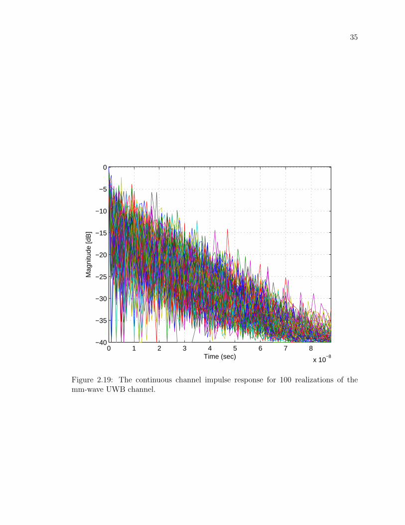
Since channel impulse response is random, in the simulation more than one real-
ization is required to make the results more realistic. 100 realizations is used here in
this thesis and in Figure 2.19 the continuous impulse response for these 100 realiza-
tions is shown. In Figure 2.20, the real and imaginary parts of the channel impulse
response realizations are given.
2.3 Summary
In this chapter, TH-PPM model and a recommended pulse shape for UWB are intro-
duced, and orthogonality and non-orthogonality of these pulses are discussed accord-
ingly.
35
0 1 2 3 4 5 6 7 8
x 10−8
−40
−35
−30
−25
−20
−15
−10
−5
0
Time (sec)
Mag
nitu
de [d
B]
Figure 2.19: The continuous channel impulse response for 100 realizations of themm-wave UWB channel.

36
0 1 2 3 4 5 6 7 8 9
x 10−8
−1
−0.5
0
0.5
1Real Impulse Response
0 1 2 3 4 5 6 7 8 9
x 10−8
−1
−0.5
0
0.5
1Imag Impulse Response
sec
Figure 2.20: Image and real demonstaration of impulse response realization

37
In the channel model section, channel impulse response is defined and the trans-
mitted and received signals are modeled. Two UWB channels namely SV and TSV are
introduced for lower frequency UWB and 60 GHz mm-wave UWB communications.
It is discussed in SV channel that the delayed and attenuated replicas of transmitted
signal, rays, arrive in groups of clusters. It is shown that the average power of rays
and clusters decays gradually which are following the Poisson distribution but with
different rates. The impulse response and the power delay profile of two different
scenarios of this model is shown and compared.
TSV channel model is considered for mm-wave UWB communications, which is
a combination of SV and two-path channel models. In this model, angle of arrival is
added to the SV channel since antenna directivity is an important factor in higher
frequency communications such as mm-wave UWB. The main channel parameters
such as power decay profile, mean excess, and root mean square delay are defined
and shown in this chapter.
38
Chapter 3
UWB Receiver Model
3.1 Optimum Receiver
One of the main challenges in wireless communications is to design a receiver which
can provide an accurate estimate of the transmitted signal with good performance in
noise, fading, and interference. Good performance must be achieved with reasonable
system complexity, such as with the optimum pulse detection receiver in [16].
From (2.7), the received signal in an AWGN fading channel is r(t) = αs(t− τ) +
I(t) + n(t). With M-ary TH-PPM, s(t) consists of J different waveforms sj(t). Each
of these waveforms can be generated by a basis function which is given by [24]
sj(t) =J−1∑i=0
sjiji(t). (3.1)
As a result sji can be calculated as
sji =
∫ T
0
sj(t)ji(t)dt. (3.2)
The basis functions for 2-ary TH-PPM are given by
ji(t) = p0(t− iTf − CiTc − ϵb⌊i/Ns⌋) (3.3)
where b⌊i/Ns⌋ can be either 0 or 1.
The received signal r(t) goes through a correlator system which consist of J cross
correlators, so the received signal is multiplied by j0(t − τ) to jJ−1(t − τ). The

39
mathematical operation of cross correlator is to integrate the received signal with a
replica of the transmitted signal over the interval of one symbol [6]. For 2-ary TH-
PPM, to detect bits 0 and 1, the correlator consists of two cross correlators. One
multiplies the received signal by j0(t− τ), and the other by j1(t− τ). Using (3.3), we
have j0(t− τ) = p0(t− iTf − CiTc − τ)
j1(t− τ) = p0(t− iTf − CiTc − ϵ− τ). (3.4)
However, for 2-ary TH-PPM, the receiver can be implemented with only one cross
correlator, which results in lower complexity [24]. The single cross correlator is a
combination of the two cross correlators in (3.4), using j(t) = j0(t)− j1(t). Based on
this, the basis function in the new cross corelator is given by
j(t− τ) = p0(t− iTf − CiTc − τ)− p0(t− iTf − CiTc − ϵ− τ). (3.5)
The received signal (2.7) is multiplied by j(t − τ), and the result is input to the
integrator. The output of the cross correlation function is the decision variable, Z.
Z =
∫ NsTf+τ
τ
r(t)j(t− τ)dt. (3.6)
The correlator is in charge of converting the received signal into a set of decision
variables [24]. Using (2.7), (3.5) and (3.6) we have
Z =
∫ NsTf+τ
τ
[αs(t−τ)+I(t)+n(t)].[p0(t−iTf−CiTc−τ)−p0(t−iTf−CiTc−ϵ−τ)]dt.
(3.7)
To simplify the calculations, the decision variable components are calculated sepa-
rately.
Z = ZRX + ZI + Zn (3.8)
where ZRX , ZI and Zn are decision variable for αs(t − τ), interference and noise
respectively, and can be calculated as
ZRX =
∫ NsTf+τ
τ
sRX(t).[p0(t− iTf −CiTc − τ)− p0(t− iTf −CiTc − ϵ− τ)]dt (3.9)
ZI =
∫ NsTf+τ
τ
I(t).[p0(t− iTf − CiTc − τ)− p0(t− iTf − CiTc − ϵ− τ)]dt (3.10)

40
and
Zn =
∫ NsTf+τ
τ
n(t).[p0(t− iTf − CiTc − τ)− p0(t− iTf − CiTc − ϵ− τ)]dt. (3.11)
Using (2.9) and (3.9) we get
ZRX =
∫ NsTf+τ
τ
[√WRX
∑i
p(t− iTf − CiTc − ϵb⌊i/Ns⌋ − τ)] (3.12)
·[p0(t− iTf − CiTc − τ)− p0(t− iTf − CiTc − ϵ− τ)]dt
ZRX =√WRX
∫ NsTf+τ
τ
[∑i
p(t− iTf − CiTc − ϵb⌊i/Ns⌋ − τ) · p0(t− iTf − CiTc − τ)(3.13)
−∑i
p(t− iTf − CiTc − ϵb⌊i/Ns⌋ − τ) · p0(t− iTf − CiTc − ϵ− τ)]dt
ZRX = Ns
√WRX
∫ Tf
0
[p(t− ϵb) · p0(t)− p(t− ϵb) · p0(t− ϵ)]dt. (3.14)
In the case that bit 0 is transmitted
ZRX = Ns
√WRX
∫ Tf0
[p(t) · p0(t)− p(t) · p0(t− ϵ)]dt
ZRX = Ns
√WRX(1− ρ(ϵ))
and for bit 1
ZRX = Ns
√WRX
∫ Tf0
[p(t− ϵ) · p0(t)− p(t− ϵ) · p0(t− ϵ)]dt
ZRX = Ns
√WRX(ρ(ϵ)− 1) = −Ns
√WRX(1− ρ(ϵ))
where ρ(ϵ) is the auto-correlation function and is equal to
ρ(ϵ) =
∫ Tf
0
[p0(t) · p0(t− ϵ)]dt. (3.15)
Using (2.10), the decision variable for the interference, ZI , is a zero mean random

41
variable equal to [24]
σ2I =
Ns
Tsσ2X
∑Uu=1W
(u)
where σ2X is a constant and depends on both the pulse shape and the PPM shift [24].
Noise is a random variable with uniform double-sided power spectral density (PSD)
of N0
2. PSD characterizes the power distribution of a signal in frequency domain [6].
The noise decision variable Zn, has zero mean and variance
σ2n = NsN0(1− ρ(ϵ)).
Variance determines the randomness of a random variable [6].
Based on the decision variable Z, the detector decides which waveform signal was
transmitted. The output of the optimum detector using (3.8) and (3.14) is given by
Z =
Ns
√WRX(1− ρ(ϵ)) + ZI + Zn bit“0′′
−Ns
√WRX(1− ρ(ϵ)) + ZI + Zn bit“1′′
(3.16)
which shows that if Z > 0, the optimum detector esitmate is bit “0”, and if Z < 0,
bit “1” is estimated. A block diagram of the optimum receiver is shown in Fig. 3.1.
Figure 3.1: Optimum receiver block diagram.
The bit error probability of the system can be calculated as [6]
PB =1
2P (Z|bit(0)) + 1
2P (Z|bit(1))
where P (Z|bit(0)) and P (Z|bit(1)) are the probability density function (pdf) of likeli-

42
hood transfered values of “0” and “1”. However, due to the equal a priori probabilities
PB = P (Z|bit(0)) = P (Ns
√WRX(1− ρ(ϵ)) + Zi + Zn < 0)
The average bit error probability is given by [24]
PB =1
2erfc
√√√√√1
2
(NsWRX
N0
(1− ρ(ϵ))
)−1
+
((1− ρ(ϵ))2
Rbσ2X
∑Uu=1
W (U)
WRX
)−1−1
(3.17)
where Rb denotes the user bit rate.
3.2 Rake Receiver
To obtain acceptable performance, the optimum receiver should employ additional
correlators for use in the SV channel. These are used for the different replicas of the
transmitted waveform. Such an approach is called a rake receiver [24]. Rake receivers
combine the replicas which are chosen using several different fingers.
The correlators in the receiver are delayed appropriately to provide the best signal
estimate. Space diversity or antenna diversity is used to provide diversity in the sys-
tem by using multiple receiving antennas. Several space diversity reception methods
exist which can be used with rake receivers. Maximum ratio combining (MRC) is a
commonly used technique and is the one utilized here. MRC weights the branches
according to their signal to noise power ratios and then sums them together [20]. A
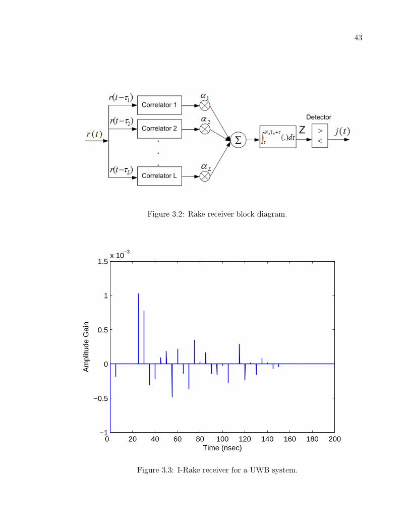
block diagram of a typical rake receiver is shown in Fig. 3.2 [20].
Three different types of rake receiver are considered here. The ideal rake (I-Rake)
receiver detects all LI multipath components of the same signal, so LI is the number
of fingers in the receiver. The I-Rake receiver is illustrated in Figure 3.3. The partial
rake (P-Rake) receiver detects the first LP components that arrive at the receiver.
Figure 3.4 shows a P-Rake receiver with 5 fingers. A selective rake (S-Rake) receiver
is shown in Figure 3.5. The name comes from the fact that in this method, receiver
selects the LS best components among the LI received components and combines them
together. Figure 3.5 shows an S-Rake receiver with 5 fingers. Since the selective rake
receiver has to keep track of all the replicas in order to choose the best ones, it has a
higher complexity than the partial rake. The receiver complexity can be reduced by
43
Figure 3.2: Rake receiver block diagram.
0 20 40 60 80 100 120 140 160 180 200−1
−0.5
0
0.5
1
1.5x 10
−3
Time (nsec)
Am
plitu
de G
ain
Figure 3.3: I-Rake receiver for a UWB system.

44
0 10 20 30 40 50−1.5
−1
−0.5
0
0.5
1
1.5x 10
−3
Time (nsec)
Am
plitu
de G
ain
Figure 3.4: 5P-Rake receiver for a UWB system.

45
0 10 20 30 40 50−1.5
−1
−0.5
0
0.5
1
1.5x 10
−3
Time (nsec)
Am
plitu
de G
ain
Figure 3.5: 5S-Rake receiver for a UWB system.
46
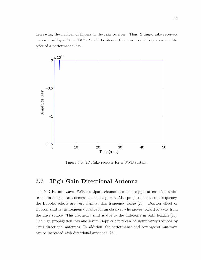
decreasing the number of fingers in the rake receiver. Thus, 2 finger rake receivers
are given in Figs. 3.6 and 3.7. As will be shown, this lower complexity comes at the
price of a performance loss.
0 10 20 30 40 50−1.5
−1
−0.5
0x 10
−3
Time (nsec)
Am
plitu
de G
ain
Figure 3.6: 2P-Rake receiver for a UWB system.
3.3 High Gain Directional Antenna
The 60 GHz mm-wave UWB multipath channel has high oxygen attenuation which
results in a significant decrease in signal power. Also proportional to the frequency,
the Doppler effects are very high at this frequency range [25]. Doppler effect or
Doppler shift is the frequency change for an observer who moves toward or away from
the wave source. This frequency shift is due to the difference in path lengths [20].
The high propagation loss and severe Doppler effect can be significantly reduced by
using directional antennas. In addition, the performance and coverage of mm-wave
can be increased with directional antennas [25].

47
0 10 20 30 40 50−1.5
−1
−0.5
0
0.5
1
1.5x 10
−3
Time (nsec)
Am
plitu
de G
ain
Figure 3.7: 2S-Rake receiver for a UWB system.

48
Directional antennas radiate the power in one direction and have higher gain than
omni-directional antennas because of this narrow antenna pattern or high antenna
directivity. This can improve the performance by increasing the SNR and compensate
the high path loss [9]. However, problems occur in transmission with directional
antennas when the LOS path is blocked by a moving object such as a human body.
This problem can be overcome by using multiple antennas [26]. Fortunately, at higher
frequencies, such as 60 GHz, the radio frequency (RF) components including antennas
are smaller in size, which permits the use of multiple antennas [26]. The possible
solutions using multiple antennas are beam steering, adaptive antenna array, antenna
switching and phase array antennas [9].
Reference antenna model with average sidelobes is employed here in the simula-
tions for the TSV channel. This is a simple mathematical model based on measured
data [23]. The antenna gain for the TSV channel 2.22 based on the reference model
is
Gr(0,Ψn + ψnm) = GD(0,Ψn + ψnm) (3.18)
where
D(0,Ψn + ψnm) = 1
for omni-directional antennas, and
D(0,Ψn + ψnm) = exp(−χ(Ψn + ψnm)2)
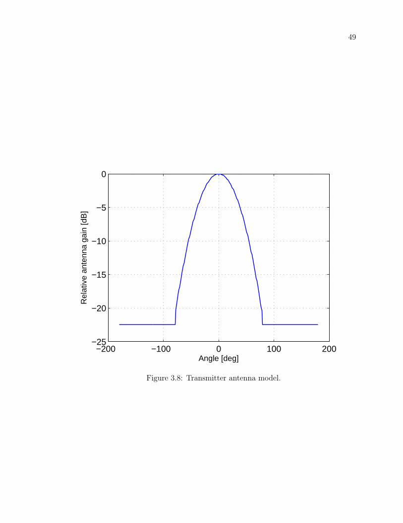
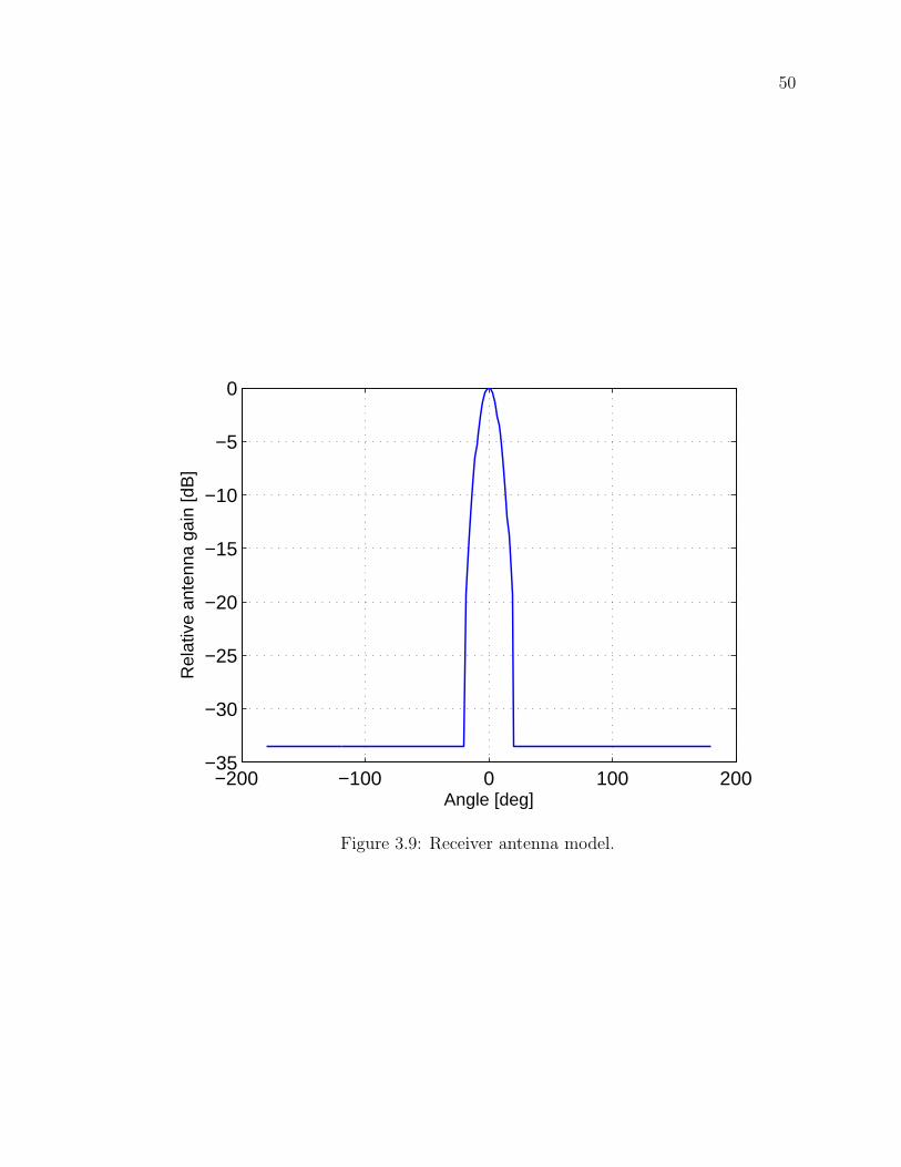
for directional antennas. χ represents the beam width of the antenna.
Figs. 3.8 and 3.9 show the relative antenna gain versus the angle for the transmit-
ter and receiver. In this example, the transmitter angle is 60 degrees and the receiver
angle is 15 degrees.
49
−200 −100 0 100 200−25
−20
−15
−10
−5
0
Angle [deg]
Rel
ativ
e an
tenn
a ga
in [d
B]
Figure 3.8: Transmitter antenna model.
50
−200 −100 0 100 200−35
−30
−25
−20
−15
−10
−5
0
Angle [deg]
Rel
ativ
e an
tenn
a ga
in [d
B]
Figure 3.9: Receiver antenna model.

51
Chapter 4
Simulation Results
In this chapter, the bit error rate (BER) performance of orthogonal and non-orthogonal
TH-PPM using the UWB channel models described in Chapter 2 is evaluated. The
number of users U considered is in the range 1 ≤ U ≤ 16, so the number of interferers
is between 0 and 15. In addition the performance of TH-PPM over SV and TSV
channels with different types of rake receiver has been compared in here.
The simulations and calculations are entirely done in Matlab. The pulse duration
used in this simulation is Tp = 0.5nsec, the PPM time shift is ϵ = 0.5nsec and the
chip time is Tc = 1nsec.
4.1 AWGN Channel
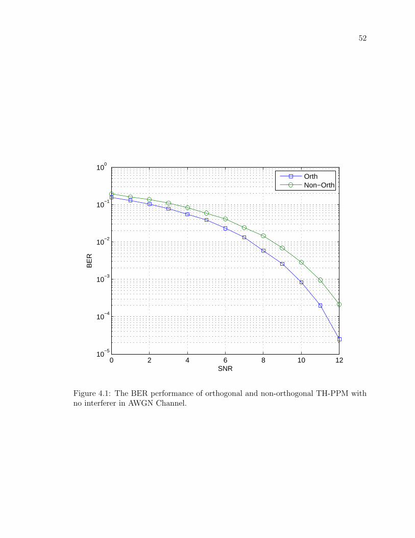
Figures 4.1 to 4.5 compare the performance of orthogonal and non-orthogonal TH-
PPM over an AWGN channel with different numbers of interferers. With no inter-
ferers at BER = 10−3, orthogonal TH-PPM outperforms non-orthogonal TH-PPM
by approximately 1 dB. When the number of interferers increases to 3, orthogonal
TH-PPM performs better than non-orthogonal TH-PPM up to SNR = 11 dB. For
high SNRs (between 8 dB to 12 dB) with 5 interferers, non-orthogonal TH-PPM has
better BER performance, and the improvement increases as the number of interferers
increases. For example, with 15 interferers and SNR = 12 dB, non-orthogonal TH-
PPM has BER = 4 × 10⁻³ dB, while orthogonal TH-PPM has BER = 4 × 10⁻² for
the same SNR. This shows when the number of users increases in the system, non-
orthogonal PPM can achieve a better performance than the orthogonal TH-PPM.
This is because by adding more interference to the users signal, orthogonal TH-PPM
52
0 2 4 6 8 10 1210
−5
10−4
10−3
10−2
10−1
100
SNR
BE
R
OrthNon−Orth
Figure 4.1: The BER performance of orthogonal and non-orthogonal TH-PPM withno interferer in AWGN Channel.

53
0 2 4 6 8 10 1210
−4
10−3
10−2
10−1
100
SNR
BE
R
OrthNon−Orth
Figure 4.2: The BER performance of orthogonal and non-orthogonal TH-PPM with3 interferers in AWGN Channel.

54
0 2 4 6 8 10 1210
−3
10−2
10−1
100
SNR
BE
R
OrthNon−Orth
Figure 4.3: The BER performance of orthogonal and non-orthogonal TH-PPM with5 interferers in AWGN Channel.
55
0 2 4 6 8 10 1210
−3
10−2
10−1
100
SNR
BE
R
OrthNon−Orth
Figure 4.4: The BER performance of orthogonal and non-orthogonal TH-PPM with10 interferers in AWGN Channel.

56
0 2 4 6 8 10 1210
−3
10−2
10−1
100
SNR
BE
R
OrthNon−Orth
Figure 4.5: The BER performance of orthogonal and non-orthogonal TH-PPM with15 interferers in AWGN Channel.
57
degrades more in compare with the non-orthogonal one, and as a result in a higher
number of users involved non-orthogonal can outperform orthogonal TH-PPM.
4.2 SV Channel
In the Figure 4.6 the performance of different rake receivers on SV channel model
using IEEE 802.15.3a-CM1 channel parameters has been compared. It is shown that
ideal rake receiver out performs the other rakes as it contains the most number of
fingers. Selective rake receiver with 5 fingers has the best performance after I-Rake
receiver since it chooses the 5 strongest replicas of the signal. 5 finger partial rake
receiver is however lower in performance since it chooses the first 5 replicas and not
necessarily the 5 strongest. Selective and partial rake receivers with 2 fingers have the
lowest performance among all. Although, ideal rake receiver has the best performance,
it has a high complexity in compare with the rest of the rake receivers due to use of
many fingers. Partial rake has a simpler design in compare with the selective rake
since it does not need to keep track of the replicas to choose the strongest ones. As
a result of this lower complexity, it can provide a lower cost receiver design.
The performance of the same signal using IEEE 802.15.3a-CM4 channel, which
is the extreme NLOS case, has shown in Figure 4.7. The poor performance can be
explained due to the harshness of this channel scenario. Same results is achieved as
IEEE 802.15.3a-CM1 channel.
The SV channel model with parameters for the IEEE 802.15.3a-CM1 channel,
which are Λ = 0.0233, λ = 2.5, Γ = 7.1, and γ = 4.3 [27], is considered here. The
performance of orthogonal and non-orthogonal TH-PPM are compared in Figures 4.8
to 4.12 for this channel. This shows that the performance of both orthogonal and
non-orthogonal TH-PPM degrades as the number of users increases. However, non-
orthogonal TH-PPM performs better than orthogonal TH-PPM when the number of
interferers is high. As an example with 5 interferers when SNR = 9, orthogonal and
non-orthogonal TH-PPM perform the same. After that point non-orthogonal TH-
PPM starts outperforming the orthogonal TH-PPM. As an example non-orthogonal
TH-PPM with 10 interferers performs close to orthogonal TH-PPM with 5 interferers.

58
0 2 4 6 8 10 1210
−3
10−2
10−1
100
SNR
BE
R
I−Rake5S−Rake5P−Rake2S−Rake2P−Rake
Figure 4.6: The BER Performance of TH-PPM with different rake receivers in UWB-CM1 channel

59
0 2 4 6 8 10 1210
−3
10−2
10−1
100
SNR
BE
R
I−Rake5S−Rake5P−Rake2S−Rake2P−Rake
Figure 4.7: The BER Performance of TH-PPM with different rake receivers in UWB-CM4 channel

60
0 2 4 6 8 10 1210
−3
10−2
10−1
100
SNR
BE
R
OrthNon−Orth
Figure 4.8: The BER performance of orthogonal and non-orthogonal TH-PPM withno interferer in SV Channel.
61
0 2 4 6 8 10 1210
−3
10−2
10−1
100
SNR
BE
R
OrthNon−Orth
Figure 4.9: The BER performance of orthogonal and non-orthogonal TH-PPM with3 interferers in SV Channel.
62
0 2 4 6 8 10 1210
−3
10−2
10−1
100
SNR
BE
R
OrthNon−Orth
Figure 4.10: The BER performance of orthogonal and non-orthogonal TH-PPM with5 interferers in SV Channel.

63
0 2 4 6 8 10 1210
−3
10−2
10−1
100
SNR
BE
R
OrthNon−Orth
Figure 4.11: The BER performance of orthogonal and non-orthogonal TH-PPM with10 interferers in SV Channel.

64
0 2 4 6 8 10 1210
−2
10−1
100
SNR
BE
R
OrthNon−Orth
Figure 4.12: The BER performance of orthogonal and non-orthogonal TH-PPM with15 interferers in SV Channel.

65
4.3 TSV Channel
For the TSV channel model, the IEEE 802.15.3c-CM1.1 channel with Λ = 0.191,
λ = 1.22, Γ = 4.46, and γ = 6.25 [23], is considered. Directional antennas have been
used with angles of 360 and 15 degrees for the transmitter and receiver, respectively.
Figures 4.13 to 4.17 show the performance of orthogonal and non-orthogonal TH-
PPM with different numbers of interferers. As with the previous channels, an increase
in the number of users increases the BER with both modulation techniques. Same
as SV channel in here also non-orthogonal TH-PPM has better performance than
orthogonal TH-PPM when the number of users is large.
Comparing Figures 4.13 to 4.17 to the ones in SV channel, the performance with
both orthogonal and non-orthogonal TH-PPM in the TSV channel model is close
to that with the SV channel model. Even though TSV channel model has a severe
attenuation and higher path loss than the lower frequency band channels [8], TH-PPM
modulation can achieve similar performance in both channel models. This shows the
robustness of TH-PPM modulation scheme in UWB channels.
0 2 4 6 8 10 1210
−3
10−2
10−1
100
SNR
BE
R
OrthNon−Orth
Figure 4.13: The BER performance of orthogonal and non-orthogonal TH-PPM withno interferer in TSV Channel.

66
0 2 4 6 8 10 1210
−3
10−2
10−1
100
SNR
BE
R
OrthNon−Orth
Figure 4.14: The BER performance of orthogonal and non-orthogonal TH-PPM with3 interferers in TSV Channel.
67
0 2 4 6 8 10 1210
−3
10−2
10−1
100
SNR
BE
R
OrthNon−Orth
Figure 4.15: The BER performance of orthogonal and non-orthogonal TH-PPM with5 interferers in TSV Channel.
68
0 2 4 6 8 10 1210
−2
10−1
100
SNR
BE
R
OrthNon−Orth
Figure 4.16: The BER performance of orthogonal and non-orthogonal TH-PPM with10 interferers in TSV Channel.
69
0 2 4 6 8 10 1210
−2
10−1
100
SNR
BE
R
OrthNon−Orth
Figure 4.17: The BER performance of orthogonal and non-orthogonal TH-PPM with15 interferers in TSV Channel.

70
Chapter 5
Conclusions and Future Work
5.1 Conclusions
Ultra wideband (UWB) is a promising way of communications which provides a very
fast and secure connection between transmitter and receiver. Systems required high
bandwidth, low power consumption and shared frequency spectrum resources can
take advantage of this technology. In multipath environments UWB can provide
secure and low interference connections. Because of the tradeoff between data rate
and distance, UWB can be applied to several different wireless applications.
Different types of modulations can be used for UWB such as on-off keying (OOK),
pulse amplitude modulation (PAM), pulse position modulation (PPM) and pulse
position amplitude modulation (PPAM). PPM was chosen for this thesis and time
hopping (TH) was applied to reduce the interference in multiple access environments.
Higher frequency UWB, 60 GHz mm-wave, was introduced as lower frequency UWB
is not globally available and because mm-wave UWB can support applications which
require a higher data rate.
The bit error rate (BER) performance of orthogonal and non-orthogonal time
hopping pulse position modulation (TH-PPM) has been evaluated for ultra wideband
(UWB) communication systems. Two channel models, Saleh-Valenzuela (SV) and
triple-SV (TSV) were considered with various numbers of users. The SV channel is a
typical channel model used for the 3.1 - 10.6 GHz UWB band, while the TSV channel
corresponds to the 60 GHz millimeter wave (mm-wave) UWB band.
It was shown that the number of users has a significant impact on the performance
of both orthogonal and non-orthogonal TH-PPM. However, non-orthogonal TH-PPM

71
provides better performance when the number of users is large. The performance of
orthogonal and non-orthogonal TH-PPM modulation in the TSV channel is similar
to that in the SV channel. This shows that TH-PPM modulation is a good candidate
for UWB communications since it can provide good performance even in multipath
fading, which shows the robustness of this modulation scheme. In addition, the
performance of different rake receivers has been compared for the SV channel model.
While the ideal rake has the best performance, it is not practical to have a rake
receiver with this many fingers due to the high complexity of the receiver. It was
shown that a selective rake receiver with 5 fingers outperforms the other receivers
that were considered. A partial rake receiver, on the other hand, has a simpler design
in comparison with selective rake since it does not have to keep track of the signal
replicas to choose the strongest ones. As a result, it can provide a lower cost receiver
at the expense of reduced performance. Directional antennas were considered for TSV
channel model. The directivity helps mm-wave UWB systems combat the Doppler
effects caused by moving objects.
5.2 Future Work
In this thesis TH-PPM modulation using both orthogonal and non-orthogonal pulses
was introduced. The performance was evaluated for AWGN, SV and TSV models.
It was shown that non-orthogonal TH-PPM has better performance than orthogonal
TH-PPM when the number of users is large. The results are the same for all the
channels considered.
As PPM is the only modulation employed in this thesis, this work can be ex-
tended to other modulation schemes such as PAM and PPAM with a variety of pulse
shapes. Sine, first and second derivative Gaussian, and rectangular pulse shapes can
be employed since they all satisfy the FCC’s spectral mask requirements. The second
derivative of the Gaussian pulse was used in this thesis.
Different channel models can also be considered. The SV and TSV models are the
two most commonly used channels have been approved by IEEE. However, many other
channel models have been proposed for UWB and mm-wave UWB communications.
Within the SV and TSV channel models, several scenarios exist which can be used
depending on the environment. These scenarios include residential, office, desktop,
and kiosk environments with LOS and NLOS signal paths. A residential scenario was
used here. Thus these other scenarios would be useful to investigate in the future.
72
Bibliography
[1] R. A. Scholtz, “Multiple access with time-hopping impulse modulation,” Proc.
IEEE Military Commun. Conf., pp. 11–14, Oct 1993.
[2] M. Z. Win and R. A. Scholtz, “Impulse radio: How it works,” IEEE Commun.
Lett., vol. 2, pp. 36–38, Feb 1998.
[3] F. Nekoogar, Ultra-wideband Communications: Fundamentals and Applications.
Prentice Hall, 2005.
[4] I. Oppermann, M. Hamalainen, and J. Iinatti, UWB Theory and Applications.
Wiley, 2004.
[5] Federal Communications Commission, “Revision of Part 15 of the Commission’s
rules regarding ultra-wideband transmission systems,” FCC 02-48, Apr 2002.
[6] B. Sklar, Digital Communications: Fundamentals and Applications. Prentice
Hall, 2nd ed., 2001.
[7] R. C. Daniels and R. W. Heath, “60 GHz wireless communication: Emerging
requirements and design recommendations,” IEEE Vehic. Tech. Magazine, vol. 2,
pp. 41–50, Sept 2007.
[8] C. Park and T. S. Rappaport, “Short-range wireless communications for next-
generation networks: UWB, 60 GHz millimeter-wave WPAN, and ZigBee,” IEEE
Trans. Wireless Commun., vol. 14, pp. 70–78, Aug 2007.
[9] N. Guo, R. C. Qiu, S. S. Mo, and K. Takahashi, “60 GHz millimeter-wave radio:
Principle, technology, and new results,” EURASIP J. on Wireless Commun. and
Networking, p. 8, Sept 2006.

73
[10] K. A. Hamidi and X. Gu, “On the validity of the Gaussian approximation for
performance analysis of TH-CDMA/OOK impulse radio networks,” Proc. IEEE
Vehic. Tech. Conf., pp. 2211–2215, Apr 2003.
[11] Z. Bai and K. Kwak, “Analysis of multiuser DS-PAM and TH-PPM UWB sys-
tems in data and image transmission,” Proc. IEEE Int. Conf. on Wireless Com-
mun., Networking and Mobile Computing, pp. 324–327, Sept 2005.
[12] H. Zhang, W. Li, and T. A. Gulliver, “Pulse position amplitude modulation
for time-hopping multiple-access UWB communications,” Proc. IEEE Wireless
Commun. and Networking Conf., pp. 895–900, Mar 2004.
[13] Y. P. Zhang, M. Sun, K. M. Chua, L. L. Wai, D. Liu, and B. P. Gaucher,
“Antenna-in-package in LTCC for 60 GHz radio,” Proc. Int. Workshop on An-
tenna Technology: Small and Smart Antennas Metamaterials and Applications,
pp. 279–282, Mar 2007.
[14] X. Chen and S. Kiaei, “Monocycle shapes for ultra wideband system,” Proc.
IEEE Int. Symp. on Circuits and Systems, pp. 597–600, May 2002.
[15] H. Xie, X. Wang, A. Wang, B. Qin, H. Chen, Y. Zhou, and B. Zhao, “A
varying pulse width second order derivative gaussian pulse generator for UWB
transceivers in CMOS,” Proc. IEEE Int. Symp. on Circuits and Systems,
pp. 2794–2797, May 2007.
[16] M. D. Benedetto and B. R. Vojcic, “Ultra wide band wireless communications:
A tutorial,” J. Commun. and Networks, vol. 5, pp. 290–302, Dec 2003.
[17] H. Zhang, W. Li, and T. A. Gulliver, “Performance analysis of non-orthogonal
pulse position modulation for time-hopping UWB transmission,” Proc. IEEE
Commun. Networks and Services Research Conf., pp. 287–293, May 2007.
[18] A. A. M. Saleh and R. A. Valenzuela, “A statistical model for indoor multipath
propagation,” IEEE J. Select. Areas Commun., vol. 5, pp. 128–137, Feb 1987.
[19] G. L. Turin, F. D. Clapp, T. L. Johnston, S. B. Fine, and D. Lavry, “A statistical
model of urban multipath propagation,” IEEE Trans. Vehic. Tech., vol. 21, no. 1,
pp. 1–9, 1972.

74
[20] T. S. Rappaport, Wireless Communications: Principles and Practice. Prentice
Hall, 2nd ed., 2001.
[21] H. Sawada, Y. Shoji, and C. S. Choi, “Proposal of novel statistic channel model
for millimeter waveWPAN,” Proc. Asia-Pacific Microwave Conf., pp. 1855–1858,
Dec 2006.
[22] S. Promwong, J. Takada, P. Supanakoon, and P. Tangtisanon, “Theoretical
ground reflection model for UWB communication systems,” Proc. Int. Sym.
Commun. and Information Tech., pp. 1208–1212, Oct 2004.
[23] http://ieee802.org/15/pub/TG3c.html
[24] M. Benedetto and G. Giancola, Understanding Ultra Wide Band Radio Funda-
mentals. Prentice Hall, 2004.
[25] H. Yang, P. F. M. Smulders, and M. H. A. J. Herben, “Channel characteristics
and transmission performance for various channel configurations at 60 GHz,”
EURASIP J. on Wireless Commun. and Networking, p. 15, Mar 2007.
[26] S. K. Yong and C.-C. Chong, “An overview of multi gigabit wireless through mil-
limeter wave technology: Potentials and technical challenges,” EURASIP Jour-
nal on Wireless Commun. and Networking, p. 8, Sept 2006.
[27] http://ieee802.org/15/pub/TG3a.html
Copyright © 2022 FDOKUMEN