
DISCRETE ORTHOGONAL MOMENTS BASED ... - IIT Guwahati
246
HAND POSTURE RECOGNITION USING DISCRETE ORTHOGONAL MOMENTS S. Padam Priyal
-
Upload
khangminh22 -
Category
Documents
-
view
2 -
download
0
Transcript of DISCRETE ORTHOGONAL MOMENTS BASED ... - IIT Guwahati

HAND POSTURE RECOGNITION USING DISCRETE ORTHOGONAL MOMENT S
S. Padam Priyal

TH-1228_06610210

HAND POSTURE RECOGNITION USING
DISCRETE ORTHOGONAL MOMENTS
A
Thesis submitted
for the award of the degree of
DOCTOR OF PHILOSOPHY
By
S. PADAM PRIYAL
DEPARTMENT OF ELECTRONICS AND ELECTRICAL ENGINEERING
INDIAN INSTITUTE OF TECHNOLOGY GUWAHATI
GUWAHATI - 781 039, ASSAM, INDIA
APRIL 2014
TH-1228_06610210

TH-1228_06610210

!"#$%&'()*$%+ !$%& ,-%./
01"2$30.4564%.
- 78-9/5: (400)
Learning is excellence of wealth that none destroy;
To man nought else affords reality of joy.
- Thirukkural (400)
This thesis is dedicated to
My Teacher, Prof.Bora;
My Husband, Shyam;
and
My Friends and Family.
TH-1228_06610210

TH-1228_06610210

Certificate
This is to certify that the thesis entitled “HAND POSTURE RECOGNITION USING DISCRETE OR-
THOGONAL MOMENTS ”, submitted byS. Padam Priyal(06610210), a research scholar in theDepartment
of Electronics and Electrical Engineering, Indian Institute of Technology Guwahati, for the award of the degree
of Doctor of Philosophy, is a record of an original research work carried out by her under my supervision and
guidance. The thesis has fulfilled all requirements as per the regulations of the institute and in my opinion has
reached the standard needed for submission. The results embodied in this thesis have not been submitted to any
other University or Institute for the award of any degree or diploma.
Dated: Dr. Prabin Kumar Bora
Guwahati. Professor
Dept. of Electronics and Electrical Engineering
Indian Institute of Technology Guwahati
Guwahati - 781 039, Assam, India.
TH-1228_06610210

TH-1228_06610210

Acknowledgements
The successful completion of this thesis is benefited from the contributions and the support of many individuals,
to whom I feel indebted. At the outset, I would like to expressmy heartfelt gratitude to my thesis supervisor,
Prof. Prabin Kumar Borafor his support and encouragement. He has trained me in research and imparted
discipline for being a good academician and person. I would particularly like to thank him for the patience he
has shown in carefully correcting my manuscripts.
I am very thankful to my doctoral committee members,Prof. S. Dandapat, Prof. Chitralekha Mahanta
andProf. S.R.M. Prasannafor their moral support, thorough evaluations and suggestions that improved my
research work. I am very much indebted toProf. S.R.M. Prasannafor providing me the additional computing
resources to complete my research work.
I owe my deepest gratitude toDr. J.S. Sahambi, who had been on my doctoral committee for a brief period
and has given valuable advices for improving my skills as a researcher. I would like to extend my gratitude to
Prof. Anil Mahantafor his kindness and motivation to stay focussed in work.
I am also thankful to the Head of the Department and the other faculty members for their kind help in
carrying out this work. I express my gratitude to all the members of the research and technical staff of the
Department for their timely help. My special thanks go toMr. Sanjib Dasfor providing excellent computing
facilities and helping me with various resources that were useful for the research work.
I have been very fortunate to have a great group of friends in IITG. They have immensely contributed
to my research work, by spending their time with me and helping me in database collection. Without their
support, this research would have been incomplete. I would like to convey my special thanks to my friends
Mr. T. KannanandMs. Babita Jajodiafor being there for me at all the times. I could not have completed this
manuscript without their supports. My heartfelt thanks to my friendsMrs. Sumitra Shukla, Dr. S. R. Nirmala
andDr. Amrita Gangulyfor the love and the care they have been showing to me, ever since I joined IITG. I
would like to express my sincere thanks toMr. Ramesh Kumar Mishrafor his kindness.
I would like to express my heartfelt gratitude toMs. V. Kohilafor being a great friend. I gratefully acknowl-
edge my friends like brothers,Mr. V. Satheesh Kumar, Mr. S. ArunandMr. R. Vinoth Kumarfor their constant
support and unconditional help. My heartfelt thanks toMs. D. J. SheebaandMs. N. Sharmilafor the great
companionship that they both have shared with me. All my other friends have also helped me in several ways
and so, I would like to say a big thank you to all of them for their friendship and support.
TH-1228_06610210

My sincere thanks goes to the following friends, who during their stay in IITG have been a great support to
me and took part in my database collection.
Dr. Amrita Ganguly, Assam engineering college, Guwahati.
Dr. S.R. Nirmala, Guwahati university, Guwahati.
Dr. Rupaban Subadar, North-eastern hill university, Shillong.
Dr. C. Shyam Anand, Samsung research and development institute, Delhi.
Dr. D. Senthil Kumar, GE global research, Bengaluru.
Dr. S. S. Karthikeyan, Indian institute of information technology, Kancheepuram.
Dr. Sarada Prasad Dakua, Quatar foundation, Doha.
Dr. Himanshu Katiyar, BBD university, Lucknow.
Dr. K.C.Narasimhamurthy, Siddaganga institute of technology, Tumkur.
Dr. D. Govind, Amrita vishwa vidyapeetham, Coimbatore.
Mrs. Sowmya Athreya, Central research lab-BEL, Bengaluru.
Ms. Anushree Neogi, Cambridge institute of technology, Ranchi.
Mr. S. Hemanth Kumar, IISC, Bengaluru.
Ms. V. Kohila, National institute of technology, Warangal.
Ms. Sumithra Das, National institute of technology, Warangal.
Ms. R. Vinnarasi, Sharda university, Noida.
Ms. Ellanti Saranya, NetApp, Inc. , Bengaluru.
Ms. Anusha, IIT Hyderabad.
Mrs. Sumitra Shukla, IIT Guwahati.
Mrs. G. Aruna, IIT Guwahati.
Mr. CH. Nagesh, IIT Guwahati.
Mr. Kuntal Deka, IIT Guwahati.
Mr. T. Kannan, IIT Guwahati.
Ms. Nabanita Adhikary, IIT Guwahati.
Ms. Bhavana.
Ms. Anupa Majumdar.
Ms. Poornima.
Ms. Durga.
My deepest gratitude goes to my husbandDr. C. Shyam Anandand my parentsDr. S. Soundararajanand
Mrs. S. Brinda Devifor their continuous love and support throughout my studies. I would like to convey my
sincere thanks to my father-in-lawMr. A. Chandranand my mother-in-lawMrs. C. Suseelafor the opportunity
they have given me to pursue my interest in research. The unlimited sacrifices of my family are the reasons
where I am and what I have accomplished so far.
My deepest and heartfelt thanks to my Godfather in my uncleMr. S. Chandrasekaran, who molded me into
x
TH-1228_06610210

the person I am today. I take this opportunity to thank him forall the love, care and the support he is giving to
me ever since my childhood. Without him, I could have never pursued this career.
Finally, I thank the great God for guiding my life through these wonderful people. I pray to Him to watch
over them every day and night and give them all, a blissful life.
S. Padam Priyal
xi
TH-1228_06610210

TH-1228_06610210

Abstract
Hand posture recognition involves interpretation of hand shapes by a computer. To find an ap-
propriate shape descriptor for uniquely characterising this, has been a major issue in hand posture
recognition. This thesis develops a novel hand posture recognition technique based on discrete
orthogonal moments (DOMs). These moments are derived from the approximation of the image
by the two-dimensional discrete orthogonal polynomials (DOPs).
The theory of the DOPs is studied and the Krawtchouk and the discrete Tchebichef moments are
considered for shape representation. The experiments conducted on the MPEG-7 (CE Shape-1,
Part-B) shape database confirm that these moments are robustto shape deformations and hence
they form potential descriptors for recognising the hand postures.
The proposed DOM based hand posture recognition technique takes the hand image as the input.
A rule based technique depending on the anthropometric dimensions of the hand is developed to
segment the hand from the forearm. An adaptive rotation normalisation procedure based on the
abducted fingers and the major axes of the hand is proposed. The normalised hand shapes are rep-
resented using the Krawtchouk and the discrete Tchebichef moments. The technique is analysed
for robustness against scale, user and view-angle variations on a hand posture database containing
4, 230 samples of 10 gesture signs. The experiments on the classification of hand postures suggest
that the DOMs are robust to user and view-angle variations. The performance of the DOMs is
analysed in comparison with the other shape descriptors like the geometric moments, the Zernike
moments, the Fourier descriptors, the Gabor wavelets and the principal component analysis (PCA).
Comparative studies show that the DOMs are superior to the Gabor wavelets, the Fourier descrip-
tors, the geometric moments and the Zernike moments. The DOMbased classification offer high
accuracies and is comparable to the PCA based classification. Particularly, the discrete Tchebichef
moments show marginally better performance than the Krawtchouk moments.
The proposed DOM based recognition technique is applied forthe recognition of 32 single-hand
postures of Bharatanatyam known as the Asamyuta hastas. Theperformances of the Krawtchouk
TH-1228_06610210

and the discrete Tchebichef moments are compared with that of the PCA technique. The experi-
ments are performed on a hand posture database containing 8, 064 samples of 32 Asamyuta hastas.
The results show that the discrete Tchebichef moments offerbetter classification performance than
the Krawtchouk moments and the PCA. The proposed system aimstowards promoting hand pos-
tures as data cues to automatically annotate and retrieve Bharatanatyam dance videos.
TH-1228_06610210

Contents
List of Figures xxi
List of Tables xxxiii
List of Acronyms xxxvii
List of Symbols xxxix
1 Introduction 1
1.1 Hand gestures in CBA systems . . . . . . . . . . . . . . . . . . . . . . . .. . . . . . . . . . 3
1.1.1 Hand gesture taxonomy . . . . . . . . . . . . . . . . . . . . . . . . . . .. . . . . . 3
1.1.2 Applicability in CBA . . . . . . . . . . . . . . . . . . . . . . . . . . . .. . . . . . . 4
1.1.2.1 Application as user interface data . . . . . . . . . . . . . .. . . . . . . . . 4
1.1.2.2 Application as a data cue . . . . . . . . . . . . . . . . . . . . . . .. . . . 5
1.1.3 Significance of hand postures in CBA . . . . . . . . . . . . . . . .. . . . . . . . . . 6
1.2 Structure and the movements of the hand . . . . . . . . . . . . . . .. . . . . . . . . . . . . . 6
1.3 Hand posture based user interfaces . . . . . . . . . . . . . . . . . .. . . . . . . . . . . . . . 8
1.3.1 Sensor based interfaces . . . . . . . . . . . . . . . . . . . . . . . . .. . . . . . . . . 8
1.3.2 Vision based interfaces . . . . . . . . . . . . . . . . . . . . . . . . .. . . . . . . . . 11
1.3.3 Merits of vision based interfaces over sensor based interfaces . . . . . . . . . . . . . . 12
1.4 Vision based hand posture recognition: the informationprocessing step . . . . . . . . . . . . 13
1.4.1 Hand localization . . . . . . . . . . . . . . . . . . . . . . . . . . . . . .. . . . . . . 14
1.4.2 Hand posture modelling . . . . . . . . . . . . . . . . . . . . . . . . . .. . . . . . . 15
1.4.3 Feature extraction . . . . . . . . . . . . . . . . . . . . . . . . . . . . .. . . . . . . . 16
1.4.4 Classification . . . . . . . . . . . . . . . . . . . . . . . . . . . . . . . . .. . . . . . 17
1.5 Issues in vision based hand posture recognition . . . . . . .. . . . . . . . . . . . . . . . . . 17
1.5.1 Segmentation errors . . . . . . . . . . . . . . . . . . . . . . . . . . . .. . . . . . . 17
xv
TH-1228_06610210

Contents
1.5.2 Geometrical distortions . . . . . . . . . . . . . . . . . . . . . . . .. . . . . . . . . . 19
1.5.2.1 Geometrical transformations . . . . . . . . . . . . . . . . . .. . . . . . . 19
1.5.2.2 Variations in the hand posture parameter . . . . . . . . .. . . . . . . . . . 19
1.5.2.3 Variations due to the angle of view . . . . . . . . . . . . . . .. . . . . . . 21
1.6 Motivation for the present work . . . . . . . . . . . . . . . . . . . . .. . . . . . . . . . . . 22
1.7 Contributions of the thesis . . . . . . . . . . . . . . . . . . . . . . . .. . . . . . . . . . . . 23
1.8 Organization of the thesis . . . . . . . . . . . . . . . . . . . . . . . . .. . . . . . . . . . . . 24
2 A Review on Feature Extraction in Hand Posture Recognition 25
2.1 Introduction . . . . . . . . . . . . . . . . . . . . . . . . . . . . . . . . . . . .. . . . . . . . 26
2.2 Silhouette image based methods . . . . . . . . . . . . . . . . . . . . .. . . . . . . . . . . . 26
2.2.1 Geometric features . . . . . . . . . . . . . . . . . . . . . . . . . . . . .. . . . . . . 27
2.2.2 Curvature scale space . . . . . . . . . . . . . . . . . . . . . . . . . . .. . . . . . . . 29
2.2.3 Modified Hausdorff distance based matching . . . . . . . . .. . . . . . . . . . . . . 31
2.2.4 Fourier descriptors . . . . . . . . . . . . . . . . . . . . . . . . . . . .. . . . . . . . 31
2.2.5 Moments and moment invariants . . . . . . . . . . . . . . . . . . . .. . . . . . . . . 32
2.2.6 Multi-fusion features . . . . . . . . . . . . . . . . . . . . . . . . . .. . . . . . . . . 35
2.3 Gray-level image based methods . . . . . . . . . . . . . . . . . . . . .. . . . . . . . . . . . 36
2.3.1 Edge-based Features . . . . . . . . . . . . . . . . . . . . . . . . . . . .. . . . . . . 37
2.3.1.1 Orientation histograms . . . . . . . . . . . . . . . . . . . . . . .. . . . . 37
2.3.1.2 Hough transform . . . . . . . . . . . . . . . . . . . . . . . . . . . . . .. . 38
2.3.2 Image transform features . . . . . . . . . . . . . . . . . . . . . . . .. . . . . . . . . 38
2.3.2.1 DCT features . . . . . . . . . . . . . . . . . . . . . . . . . . . . . . . . .38
2.3.2.2 PCA and LDA based features . . . . . . . . . . . . . . . . . . . . . .. . . 39
2.3.2.3 Wavelet transform based descriptors . . . . . . . . . . . .. . . . . . . . . 42
2.3.3 Elastic Graph matching . . . . . . . . . . . . . . . . . . . . . . . . . .. . . . . . . . 44
2.3.4 Local spatial pattern analysis . . . . . . . . . . . . . . . . . . .. . . . . . . . . . . . 44
2.3.4.1 Local binary patterns . . . . . . . . . . . . . . . . . . . . . . . . .. . . . 45
2.3.4.2 Modified census transform . . . . . . . . . . . . . . . . . . . . . .. . . . 45
2.3.4.3 Haar-like features . . . . . . . . . . . . . . . . . . . . . . . . . . .. . . . 46
2.3.4.4 Scale invariant feature transform . . . . . . . . . . . . . .. . . . . . . . . 47
xvi
TH-1228_06610210
Contents
2.3.5 Local linear embedding . . . . . . . . . . . . . . . . . . . . . . . . . .. . . . . . . . 48
2.4 Summary and conclusion . . . . . . . . . . . . . . . . . . . . . . . . . . . .. . . . . . . . . 49
3 A Study on the Characteristics of Discrete Orthogonal Moments for Shape Representation 53
3.1 Introduction . . . . . . . . . . . . . . . . . . . . . . . . . . . . . . . . . . . .. . . . . . . . 54
3.2 Theory of discrete orthogonal polynomials . . . . . . . . . . .. . . . . . . . . . . . . . . . . 56
3.3 Formulation of the Krawtchouk polynomials . . . . . . . . . . .. . . . . . . . . . . . . . . . 59
3.3.1 Rodrigues formula . . . . . . . . . . . . . . . . . . . . . . . . . . . . . .. . . . . . 60
3.3.2 Recurrence relation . . . . . . . . . . . . . . . . . . . . . . . . . . . .. . . . . . . . 60
3.3.3 Hypergeometric representation . . . . . . . . . . . . . . . . . .. . . . . . . . . . . . 61
3.3.4 Derivation of∥
∥
∥ψn
∥
∥
∥
2
w. . . . . . . . . . . . . . . . . . . . . . . . . . . . . . . . . . . . 62
3.3.5 Weighted Krawtchouk polynomials (WKPs) . . . . . . . . . . .. . . . . . . . . . . . 63
3.4 Formulation of discrete Tchebichef polynomials (DTPs). . . . . . . . . . . . . . . . . . . . 64
3.4.1 Rodrigues formula . . . . . . . . . . . . . . . . . . . . . . . . . . . . . .. . . . . . 65
3.4.2 Recurrence relation . . . . . . . . . . . . . . . . . . . . . . . . . . . .. . . . . . . . 65
3.4.3 Hypergeometric representation . . . . . . . . . . . . . . . . . .. . . . . . . . . . . . 65
3.4.4 Derivation of‖Tn‖2w . . . . . . . . . . . . . . . . . . . . . . . . . . . . . . . . . . . . 66
3.5 Least squares approximation of functions by DOPs . . . . . .. . . . . . . . . . . . . . . . . 66
3.5.1 Image representation using two-dimensional DOPs . . .. . . . . . . . . . . . . . . . 67
3.6 Spatial domain behaviour of the DOPs . . . . . . . . . . . . . . . . .. . . . . . . . . . . . . 68
3.7 Frequency domain behaviour of the DOPs . . . . . . . . . . . . . . .. . . . . . . . . . . . . 71
3.7.1 Quantitative analysis . . . . . . . . . . . . . . . . . . . . . . . . . .. . . . . . . . . 73
3.7.2 Short-time Fourier transform (STFT) analysis . . . . . .. . . . . . . . . . . . . . . . 73
3.8 Shape approximation using DOPs . . . . . . . . . . . . . . . . . . . . .. . . . . . . . . . . 75
3.8.1 Metrics for reconstruction accuracy . . . . . . . . . . . . . .. . . . . . . . . . . . . 76
3.8.2 Experiments on shape representation . . . . . . . . . . . . . .. . . . . . . . . . . . . 77
3.8.2.1 Characterizing shapes using curvature properties. . . . . . . . . . . . . . . 77
3.8.2.2 Spatial scale of the shapes . . . . . . . . . . . . . . . . . . . . .. . . . . . 81
3.8.2.3 Variation in shapes versus reconstruction accuracy . . . . . . . . . . . . . . 82
3.8.2.4 Noise versus reconstruction accuracy . . . . . . . . . . .. . . . . . . . . . 91
3.8.3 Experiments on shape classification . . . . . . . . . . . . . . .. . . . . . . . . . . . 97
xvii
TH-1228_06610210

Contents
3.9 Summary . . . . . . . . . . . . . . . . . . . . . . . . . . . . . . . . . . . . . . . . .. . . . 104
3.10 Appendix : Proof for the QMF property of WKP basis . . . . . .. . . . . . . . . . . . . . . 105
4 Robust Hand Posture Recognition Using Geometry-based Normalisation and DOM based ShapeDescription 107
4.1 Introduction . . . . . . . . . . . . . . . . . . . . . . . . . . . . . . . . . . . .. . . . . . . . 108
4.2 Hand posture acquisition and database development . . . .. . . . . . . . . . . . . . . . . . . 110
4.2.1 Determination of camera position . . . . . . . . . . . . . . . . .. . . . . . . . . . . 111
4.2.2 Determination of view-angle . . . . . . . . . . . . . . . . . . . . .. . . . . . . . . . 112
4.2.3 System setup . . . . . . . . . . . . . . . . . . . . . . . . . . . . . . . . . . .. . . . 112
4.2.4 Development of Hand posture database . . . . . . . . . . . . . .. . . . . . . . . . . 114
4.3 System Implementation . . . . . . . . . . . . . . . . . . . . . . . . . . . .. . . . . . . . . . 114
4.3.1 Hand detection and segmentation . . . . . . . . . . . . . . . . . .. . . . . . . . . . 114
4.3.2 Normalization techniques . . . . . . . . . . . . . . . . . . . . . . .. . . . . . . . . 116
4.3.2.1 Proposed method for rule based hand extraction . . . .. . . . . . . . . . . 116
4.3.2.1.1 Anthropometry based palm detection . . . . . . . . . . .. . . . . 118
4.3.2.2 Proposed approach to orientation correction . . . . .. . . . . . . . . . . . 122
4.3.2.3 Normalization of scale and spatial translation . . .. . . . . . . . . . . . . . 124
4.3.3 Feature Extraction . . . . . . . . . . . . . . . . . . . . . . . . . . . . .. . . . . . . 124
4.3.3.1 Extraction of moment shape descriptors . . . . . . . . . .. . . . . . . . . 125
4.3.3.2 Extraction of non-moment shape descriptors . . . . . .. . . . . . . . . . . 126
4.3.4 Classification . . . . . . . . . . . . . . . . . . . . . . . . . . . . . . . . .. . . . . . 128
4.4 Experimental Studies and Results . . . . . . . . . . . . . . . . . . .. . . . . . . . . . . . . 128
4.4.1 Quantitative analysis of hand posture variations . . .. . . . . . . . . . . . . . . . . . 129
4.4.2 Experiments on hand posture classification . . . . . . . . .. . . . . . . . . . . . . . 132
4.4.2.1 Verification of user independence . . . . . . . . . . . . . . .. . . . . . . . 133
4.4.2.2 Verification of view invariance . . . . . . . . . . . . . . . . .. . . . . . . 140
4.4.2.3 Improving view invariant recognition . . . . . . . . . . .. . . . . . . . . . 143
4.5 Summary . . . . . . . . . . . . . . . . . . . . . . . . . . . . . . . . . . . . . . . . .. . . . 146
5 DOM based Recognition of Asamyuta Hastas 147
5.1 Introduction . . . . . . . . . . . . . . . . . . . . . . . . . . . . . . . . . . . .. . . . . . . . 148
5.2 Bharatanatyam and its gestures . . . . . . . . . . . . . . . . . . . . .. . . . . . . . . . . . . 150
xviii
TH-1228_06610210

Contents
5.2.1 Asamyuta hastas - the single-hand postures . . . . . . . . .. . . . . . . . . . . . . . 151
5.3 Hand posture acquisition and database development . . . .. . . . . . . . . . . . . . . . . . . 152
5.3.1 Determination of camera position . . . . . . . . . . . . . . . . .. . . . . . . . . . . 152
5.3.2 Determination of view-angle . . . . . . . . . . . . . . . . . . . . .. . . . . . . . . . 154
5.3.3 System setup . . . . . . . . . . . . . . . . . . . . . . . . . . . . . . . . . . .. . . . 156
5.4 Development of Asamyuta hasta database . . . . . . . . . . . . . .. . . . . . . . . . . . . . 156
5.5 System implementation . . . . . . . . . . . . . . . . . . . . . . . . . . . .. . . . . . . . . . 158
5.5.1 Hand segmentation . . . . . . . . . . . . . . . . . . . . . . . . . . . . . .. . . . . . 159
5.5.2 Orientation normalisation . . . . . . . . . . . . . . . . . . . . . .. . . . . . . . . . 160
5.5.3 Normalisation for scale and translation changes . . . .. . . . . . . . . . . . . . . . . 162
5.5.4 Extraction of DOM features . . . . . . . . . . . . . . . . . . . . . . .. . . . . . . . 162
5.5.4.1 Comparison with other descriptors . . . . . . . . . . . . . .. . . . . . . . 162
5.5.5 Classification . . . . . . . . . . . . . . . . . . . . . . . . . . . . . . . . .. . . . . . 163
5.6 Experimental studies and results . . . . . . . . . . . . . . . . . . .. . . . . . . . . . . . . . 164
5.6.1 Quantitative analysis on hand posture variations . . .. . . . . . . . . . . . . . . . . . 164
5.6.2 Experiments on posture classification . . . . . . . . . . . . .. . . . . . . . . . . . . 171
5.6.2.1 Verification of user invariance . . . . . . . . . . . . . . . . .. . . . . . . . 172
5.6.2.2 Verification of view invariance . . . . . . . . . . . . . . . . .. . . . . . . 176
5.6.2.3 Improving view invariant classification . . . . . . . . .. . . . . . . . . . . 182
5.7 Summary . . . . . . . . . . . . . . . . . . . . . . . . . . . . . . . . . . . . . . . . .. . . . 183
6 Conclusions and Future Work 185
6.1 Concluding remarks . . . . . . . . . . . . . . . . . . . . . . . . . . . . . . .. . . . . . . . . 186
6.2 Suggestions for future research . . . . . . . . . . . . . . . . . . . .. . . . . . . . . . . . . . 190
References 193
List of Publications 205
xix
TH-1228_06610210

Contents
xx
TH-1228_06610210

List of Figures
1.1 Illustration of anatomy of the human hand explaining thebone segments and the joints of the
hand. Image courtesy www.ossurwebshop.co.uk . . . . . . . . . . .. . . . . . . . . . . . . . 7
1.2 Illustration of anatomical movements with respect to (a) thumb and (b) four fingers of the hand. 7
1.3 Examples of hand postures to illustrate the variations in the hand shape relative to the anatomi-
cal movements of the hand joints. Image courtesy wikimedia.org/wiki/File:ABC pict.png . . 9
1.4 Sensor based glove interfaces. (a) Dataglove. Image courtesy www.dipity.com; (b) CyberGlove
II; (c) Example of hand gesture animation using CyberGlove II. Copyright c©2011 CyberGlove
Systems LLC All rights reserved; (d) 5DT data glove. Image courtesy www.5dt.com; (e) Hu-
manglove. Image courtesy Humanware (www.hmw.it) and (f) Pinch glove. Image courtesy
Fakespace Labs (www.fakespacelabs.com). . . . . . . . . . . . . . .. . . . . . . . . . . . . 10
1.5 Illustration of the monocular vision based interface unit for CBA systems. . . . . . . . . . . . 11
1.6 General block diagram representation of a hand posture recognition unit for CBA systems. . . 14
1.7 Illustration of different hand posture models. (a) 3D textured volumetric model; (b) 3D wire-
frame volumetric model; (c) 3D skeletal model; (d) Binary silhouette and (e) Contour. Image
courtesy Wikipedia [1]. . . . . . . . . . . . . . . . . . . . . . . . . . . . . . .. . . . . . . . 15
1.8 Illustration of variations in the details of the hand posture image with respect to illumination
changes. (a) Poor illumination - dark image; (b) Normal (average) illumination - average con-
trast and (c) High illumination - high contrast. . . . . . . . . . .. . . . . . . . . . . . . . . . 18
1.9 Histograms of (a) the dark image; (b) the average contrast image and (c) the high contrast image
shown in Figure 1.8. . . . . . . . . . . . . . . . . . . . . . . . . . . . . . . . . . .. . . . . 18
1.10 Examples of hand posture images taken in varying background: (a) hand posture acquired in a
uniform background and (b) hand posture images acquired in complex backgrounds. The hand
posture images are taken from the Jochen Triesch static handposture database [2]. . . . . . . . 18
xxi
TH-1228_06610210

List of Figures
1.11 Illustration of hand posture parameters using the handskeleton. The joint angles represent the
hand posture parameters. . . . . . . . . . . . . . . . . . . . . . . . . . . . . .. . . . . . . . 20
1.12 Illustration of (a) finger abduction; (b) MP joint rangeof motion, flexion-extension and (c)
Palmar abduction and adduction of the thumb at the MP joint. The negative angle in (b) refers
to the extension movement. . . . . . . . . . . . . . . . . . . . . . . . . . . . .. . . . . . . . 20
1.13 Examples of a hand posture taken at various angles of view. The figure illustrates the structural
deviations or deviations in the appearance of the hand posture. Similarly, occlusion of certain
parts of the hand can be observed at each angle of view. The hand posture images are taken
from the Massey hand posture database for the American sign language [3]. . . . . . . . . . . 21
2.1 Illustration of smoothing of the shape boundary and the evolution of the inflection points at
different scales(σ). (a)σ = 3.5; (b)σ = 8.2 and (c)σ = 14.6. The concave segments at each
scale are enumerated. The number of concavities decreases with the increase in the scale. (d)
The CSS image constructed from the locations of the inflection points at various scales. . . . 30
2.2 (a) 1D Zernike radial polynomialsRnm(ρ) and (b) 2D complex Zernike polynomialsVnm(ρ, θ)
(real part). . . . . . . . . . . . . . . . . . . . . . . . . . . . . . . . . . . . . . . . .. . . . . 34
2.3 Plots of the real part of the Gabor wavelet kernelsGϑ,θ obtained at 4 scales(P = 4) and 8
orientations(Q = 8). The parameters are chosen asσ = π, ωmax =π2 and∆ f =
√2 [4]. . . . . 43
2.4 Haar-like rectangular kernels used for feature extraction. The rectangular kernels are capable
of extracting (a) Edge features; (b) Line features and (c) Center-surround features. . . . . . . . 46
3.1 Plots of the WKPs for different values ofp and ordern. The plots illustrate the translation of
Kn (x) with respect to the value ofp. For p = 0.5± ∆p, the polynomial is shifted by a factor of
±N∆p. The value ofN = 60. . . . . . . . . . . . . . . . . . . . . . . . . . . . . . . . . . . . 69
3.2 Basis images of 2D WKPs for different values ofp1 andp2. The parametersp1 andp2 control
the polynomial position in the vertical (x− axis) and the horizontal direction (y− axis) respec-
tively. From the illustration, it can also be observed that the spatial support of the polynomial
increase in thex− direction as the value ofn increases. Similarly, the support increases in the
y− direction as the value ofm increases. . . . . . . . . . . . . . . . . . . . . . . . . . . . . . 69
3.3 (a) Plots of the 1D WKPs of higher ordern and (b) Basis images of the 2D WKPs for higher
values of(n+m). The parametersn = mandN = 100. . . . . . . . . . . . . . . . . . . . . . 70
xxii
TH-1228_06610210

List of Figures
3.4 (a) Plots of the 1D normalised DTPs and (b) Basis images ofthe 2D normalised DTPs of
different orders. The order(n+m) of the 2D normalised DTPs is chosen such thatn = m. The
value ofN = 100. . . . . . . . . . . . . . . . . . . . . . . . . . . . . . . . . . . . . . . . . . 70
3.5 Plots of the ESD of the 1D WKPs for (N + 1) = 8, p = 0.5 andn = 0, 1, · · · , 7. ωBW =
|ω2 − ω1|. The figure illustrates the QMF property of the WKPs with respect to the frequency
ω = π2. The frequency characteristics implies that the polynomials act as band-pass functions.
The WKPs exhibit sidelobes at the lower as well as the higher frequencies. Forn < N+12 the
sidelobes at lower frequencies have higher energy. On the contrary, forn > N+12 the sidelobes
present at the higher frequencies exhibit higher energy. . .. . . . . . . . . . . . . . . . . . . 72
3.6 Plots of the ESD of the 1D normalised DTPs for (N + 1) = 8, p = 0.5 andn = 0, 1, · · · , 7.
ωBW = |ω2 − ω1|. The frequency characteristics implies that these polynomials act as band-pass
functions. It is also observed that the DTPs contain sidelobes at higher frequencies. The energy
of the sidelobes is more in the middle-order polynomials. Itcan be observed that the sidelobe
energy of the DTPs is higher than that of the WKPs. The DTPs do not exhibit quadrature
symmetry. . . . . . . . . . . . . . . . . . . . . . . . . . . . . . . . . . . . . . . . . . .. . . 72
3.7 Plots of the 1D WKPs and corresponding ESD obtained usingSTFT as functions ofx. The
plots are obtained for (N + 1) = 60 andp = 0.5. The illustration shows that for ordern < N+12 ,
the low-frequency ESD of the polynomial increases for the values of x close tox = 0 and
x = N. Forn > N+12 , the high-frequency ESD with respect to these values gradually increases.
The length of the sliding windowξ (.) is chosen as 30 and the number of frequency points is 128. 74
3.8 Plots of the 1D normalised DTPs and corresponding ESD obtained using STFT as a function
of x. The plots are obtained for (N + 1) = 60. The illustration shows that for any given ordern,
the high-frequency ESD increases for the values ofx close tox = 0 andx = N. The length of
the sliding windowξ (.) is chosen as 30 and the number of frequency points is 128. . . . .. . 74
3.9 Illustration of finding the concave segments of a shape from the curvature function derived from
the corresponding shape boundary. (a) Geometric shape usedfor illustration; (b) The curvature
function derived from the boundary of the geometric shape and (c) Representing the inflection
points and the concave segments on the shape boundary. The zero-crossings correspond to the
inflection points. Similarly, the negative maxima correspond to the concave points. . . . . . . 78
xxiii
TH-1228_06610210

List of Figures
3.10 CSS representation of star-shaped polygons composed of 16 concave segments of varying
depth. The polygon shape in (a) consists of shallow concave segments and (c) consists of
deeper concave segments. The figure illustrates the variation in the height of the arch-shaped
contours in the CSS map with respect to the variation in the depth of the concavities. . . . . . 80
3.11 CSS representation of four different geometric shapeswith varying number of concave seg-
ments and width. The figure illustrates the variation in the base width of the arch-shaped con-
tours relative to the variation in the width of the concavities. Also, the number of arch-shape
contours is proportional to the number of concavities. The shape of character ‘T’ has compar-
atively less number of concave segments and the concavitiesare more wide. The cross-shaped
polygon has concave segments of similar width and depth. Conversely, the fork-shaped polygon
is composed of concave segments of different widths and depth. . . . . . . . . . . . . . . . . 80
3.12 Illustration of reconstruction accuracy with respectto the star-shaped polygon consisting of
shallow concavities. The illustration shows that the WKP based approximation is better for
lower scales of the shape. For approximating shapes at lowerscales, the DTPs require higher
orders. At large scales the DTPs offer better reconstruction accuracy. However, as the order in-
creases both the moments exhibits similar performance. In the case of lower order Krawtchouk
moments, only a local region of the original shape that lie within the spatial support of the cor-
responding polynomials is efficiently reconstructed. Hence, the reconstruction accuracy evalu-
ated in terms of the SSIM and MHD of the lower order Krawtchoukmoments is comparatively
less for scales 60× 60 and 80× 80. . . . . . . . . . . . . . . . . . . . . . . . . . . . . . . . . 83
3.13 Illustration of reconstruction accuracy with respectto the star-shaped polygon with moderately
deep concavities. The results in terms of the SSIM and MHD indicates that the accuracy of the
WKPs is comparatively higher than the DTPs in approximatingshapes at different scales. The
concavities are more accurately reconstructed by the Krawtchouk moments and the Tchebichef
moments result in smoothened reconstruction of the sharp concave segments. . . . . . . . . . 84
3.14 Illustration of DOM based approximation of a star-shaped polygon consisting of deep concave
segments. The illustration shows that the performance of the Krawtchouk moments at all the
orders is consistently superior to the discrete Tchebichefmoments in approximating the shapes
at all three different scales. . . . . . . . . . . . . . . . . . . . . . . . . .. . . . . . . . . . . 85
xxiv
TH-1228_06610210

List of Figures
3.15 Illustration of reconstruction accuracy for varying orders of DOP based approximations of the
shape of character ‘T’. The shape is composed of two wide-deep concave segments. The values
of the SSIM index and the MHD show that the WKP based approximations give high recon-
struction accuracy at scale 40× 40. At scale 60× 60, the performance of both the moments are
very close in terms of SSIM index and MHD. The DTP based approximation results in exces-
sive smoothing. For scale 80× 80, the DTP based approximation shows better performance.
For scale 40× 40, the accuracy of DTPs at lower orders is reduced due to excessive smoothing
and for scale 80× 80, the performance of WKPs at lower orders is affected due tothe compact
spatial support of the polynomials. . . . . . . . . . . . . . . . . . . . .. . . . . . . . . . . . 86
3.16 Illustration of reconstruction accuracy with respectto the cross-shaped polygon. The shape is
composed of four concave segments of same width and depth. The SSIM index and the MHD
show that the WKP based approximations give high reconstruction accuracy for scales 40× 40
and 60× 60. The shapes reconstructed from DTP based approximation are over-smoothened.
At higher scale 80× 80, the spatial support of the lower order WKPs is not sufficiently large
and hence, the reconstruction error is more at these orders.. . . . . . . . . . . . . . . . . . . 88
3.17 Illustration of reconstruction accuracy with respectto a fork-shaped polygon. The shape is
a high spatial frequency structure consisting of five concave segments of different width and
depth. The accuracy in reconstruction evaluated in terms ofthe SSIM index and the MHD show
that the Krawtchouk moments based approximation is comparatively high for scales 40× 40
and 60× 60. It is observed that the shapes reconstructed from Tchebichef moments are more
smoothened and the high spatial frequency regions are not properly reconstructed at lower
orders. At a higher scale of 80× 80, the accuracy of the WKP based approximation is poor due
to the limited spatial support of the polynomial basis. . . . .. . . . . . . . . . . . . . . . . . 89
xxv
TH-1228_06610210

List of Figures
3.18 Illustration of the reconstruction accuracy of the DOMs with respect to a beetle shape that
is degraded by binary noise of levelpn. For different values ofpn, the shapes reconstructed
from the Krawtchouk moments are more accurate than those reconstructed from the discrete
Tchebichef moments. The high spatial frequency regions in the beetle shape are efficiently
recovered by the Krawtchouk moments. For high noise levels,the significant noise pixels in
the foreground region are not sufficiently denoised in WKP based approximation. The discrete
Tchebichef moments results in over-smoothening of the structural features and a few noise
pixels are retained in the background region of the reconstructed shape. The values of the SSIM
index and the MHD suggest that the Krawtchouk moments perform better than the discrete
Tchebichef moments at lower noise levels. As the noise levelincreases, the number of noise
pixels retained in DOP based approximation increases. . . . .. . . . . . . . . . . . . . . . . 92
3.19 Illustration of the noise sensitivity of the DOMs with respect to a bird shape. The order of the
moments is chosen as(n+m) = 60. The shapes reconstructed from the Krawtchouk moments
based approximation exhibit comparatively higher perceptual similarity to the original shape.
The values of the SSIM index and the MHD suggest that forpn ≤ 0.35, the Krawtchouk
moments are more robust to noise than the discrete Tchebichef moments and result in high
reconstruction efficiency. Aspn increases, both the moments result in poor denoising efficiency.
The discrete Tchebichef moments exhibit sensitivity to noise along the image border and the
Krawtchouk moments are sensitive to noise around the centrethe image. . . . . . . . . . . . 93
3.20 Illustration of the denoising efficiency of the DOMs with respect to the square shape. The
shape reconstructed from the Krawtchouk and the discrete Tchebichef moments exhibits similar
perceptual quality with respect to the original shape. Hence, the corresponding SSIM values
are almost similar for lowerpn. With the increase inpn, the number of noise pixels are more in
the background region for discrete Tchebichef moments based approximation and noise occurs
in the foreground region for Krawtchouk moments based approximation. The values of the
SSIM index and the MHD indicate that the performance of the WKP based approximation is
comparatively poor for higher noise levels. . . . . . . . . . . . . .. . . . . . . . . . . . . . 94
xxvi
TH-1228_06610210
List of Figures
3.21 Illustration of the robustness of the DOMs to noise withrespect to varying orders of DOPs
based approximation of the beetle shape. With the increase in order, most of the noise pixels
are recovered in reconstruction. Particularly, the Krawtchouk moments exhibit more sensitivity
towards noise in the foreground region. As the order increases, the discrete Tchebichef mo-
ments result in better reconstruction of the high spatial frequency structures in the beetle shape.
Simultaneously, the reconstruction quality gets degradeddue to the recovery of more noise
pixels in the background region. The SSIM index and the MHD suggest that the Krawtchouk
moments exhibit better performance than the discrete Tchebichef moments in most of the or-
ders. . . . . . . . . . . . . . . . . . . . . . . . . . . . . . . . . . . . . . . . . . . . . . .. 95
3.22 Illustration of noise sensitivity of the different orders of DOM based reconstruction of the bird
shape. With the increase in the order, the moments exhibit more sensitivity to noise. The higher
order discrete Tchebichef moments offer better reconstruction of the high spatial frequency
structures in the bird shape. However, the reconstruction quality is affected due to the recovery
of more noise pixels in the background region. The shapes reconstructed from the Krawtchouk
moments exhibit noise in the foreground as well as the background region. The performance in
terms of the SSIM index and the MHD indicates that the Krawtchouk moments are better than
the discrete Tchebichef moments upto certain orders. . . . . .. . . . . . . . . . . . . . . . . 96
3.23 Illustration of noise sensitivity of DOM based approximation of the square shape at various
orders. The values of SSIM index and MHD indicate that up to (n + m) = 50, the discrete
Tchebichef moments exhibit better performance than the Krawtchouk moments. . . . . . . . 96
3.24 Illustration of undistorted training sample per shapeclass constituting the reference dataset. . . 98
3.25 Examples of test samples contained in each shape class.The figure illustrates the shape defec-
tion in the test samples that are caused due to boundary distortion and segmentation errors. . . 98
3.26 Plot of the Pratt’s FOM values of the test samples with respect to the reference dataset. The
measure indicates the deviation in the edge characteristics of the test sample in each class from
the corresponding sample in the training set. The illustration signifies the intraclass distance
between the test and the reference shapes. . . . . . . . . . . . . . . .. . . . . . . . . . . . . 99
xxvii
TH-1228_06610210

List of Figures
3.27 Illustration comparing the intraclass and the interclass distances between the samples in the
database. The distance is measured in terms of the similarity in the spatial distribution of
pixels. Hence, the correlation is used as the metric. The values of the correlation signify the
similarity between the shapes. . . . . . . . . . . . . . . . . . . . . . . . .. . . . . . . . . . 99
3.28 Comparison of the consolidated classification resultsobtained with respect to each class. The
results are obtained for 1 training sample per shape class and 18 testing samples per shape
class. The overall classification rate obtained for discrete Tchebichef moments as features is
87.11%. The overall classification rate for Krawtchouk momentsas features is 86.58%. The
overall classification rate for MHD matching is 86%. . . . . . . .. . . . . . . . . . . . . . . 102
3.29 Results from the experiment on shape classification using 1 training sample per shape class.
Examples of the testing samples exhibiting higher misclassification with respect to both the
Krawtchouk and the discrete Tchebichef moments as features. It is observed that most of the
mismatches have occurred between the shape classes with less interclass distances. The spatial
similarity between the misclassified test sample and the corresponding match in the reference
set can be obtained from the respective plots in Figure 3.27.. . . . . . . . . . . . . . . . . . . 102
3.30 Comparison of the comprehensive scores of the classification results obtained with respect to
each class. The results are obtained for 2 training samples per shape class and 18 testing sam-
ples per shape class. The overall classification rate obtained for discrete Tchebichef moments
as features is 94.17%. The overall classification rate for Krawtchouk momentsas features is
94.44%. The overall classification rate for MHD matching is 94.16%. The number of classes
misclassified is comparatively higher in MHD matching. . . . .. . . . . . . . . . . . . . . . 102
4.1 Illustration of a tabletop user interface setup using a top-mounted camera for natural human-
computer interaction through hand postures. . . . . . . . . . . . .. . . . . . . . . . . . . . . 109
4.2 Illustration of different camera positions with respect to the object of focus in a 3D cartesian
space. . . . . . . . . . . . . . . . . . . . . . . . . . . . . . . . . . . . . . . . . . . . . .. . 111
4.3 A schematic representation of the experimental setup employed for acquiring the hand posture
images. . . . . . . . . . . . . . . . . . . . . . . . . . . . . . . . . . . . . . . . . . . . .. . 112
xxviii
TH-1228_06610210

List of Figures
4.4 Illustrations of (a) the estimation of camera position and the view angle using a 3D cartesian
coordinate system. The object is assumed to lie on thex− y plane and the camera is mounted
along thez axis. Ch denotes the distance between the camera and the table surface and is
experimentally chosen as 30cm. The view angle (Cθ) is measured with respect to thex − y
plane. (b) the view angle variation between the camera and the object of focus. . . . . . . . . 113
4.5 Posture signs in database. . . . . . . . . . . . . . . . . . . . . . . . . .. . . . . . . . . . . . 113
4.6 Schematic representation of the proposed hand posture recognition technique. . . . . . . . . . 115
4.7 Results of hand segmentation using skin colour detection. . . . . . . . . . . . . . . . . . . . . 116
4.8 Illustration of the disk-shaped structuring element used for morphological closing. The radius
of the element is 3. . . . . . . . . . . . . . . . . . . . . . . . . . . . . . . . . . . .. . . . . 116
4.9 Pictorial representation of the regions composing the binary imagef . Rdenotes the hand region
andRdenotes the background region. . . . . . . . . . . . . . . . . . . . . . . . .. . . . . . 117
4.10 (a) Hand geometry and (b) Histogram of the experimentalvalues of palm length (Lpalm) to palm
width (Wpalm) ratio calculated for 140 image samples taken from 23 persons. . . . . . . . . . 119
4.11 Illustration of the rule based region detection and separation of the hand from the acquired
posture imagef . The intensity of the background pixels is assigned a 0 and the object pixels
are assigned the maximum intensity value 1. . . . . . . . . . . . . . .. . . . . . . . . . . . . 121
4.12 Description for finger tip detection using the peaks in the distance curve.- - - - - denotes ˆγ. . . 124
4.13 Illustration of reconstruction of the hand posture shape for different orders of orthogonal mo-
ments. (a) Original hand posture shape; (b) Shape reconstructed from orthogonal moments.
Comparative plot of (c) SSIM index vs number of moments and (d) MHD vs number of moments.126
4.14 Illustration of shape reconstruction with respect to varying number of eigen components (a)
Original shape; (b) Shapes reconstructed from the PCA projections for different number of
eigenvalues and (c) the results of binarisation of the reconstructed shapes in (b). The threshold
for binarisation is uniformly chosen as 120. Comparative plots of (d) SSIM index vs number
of eigenvalues and (e) MHD vs number of eigenvalues, computed between the shape in (a) and
the reconstructed binary shapes in (c). . . . . . . . . . . . . . . . . .. . . . . . . . . . . . . 128
xxix
TH-1228_06610210

List of Figures
4.15 Intraclass distance measured in terms of Pratt’s FOM for samples in (a) Dataset 1 and (b)
Dataset 2. The reference set is taken from Dataset 1. There are 690 testing samples with 69
samples\ posture sign in each of the dataset and 230 samples in the reference set with 23
samples\ posture sign. . . . . . . . . . . . . . . . . . . . . . . . . . . . . . . . . . . . . . . 130
4.16 Illustration of variability in the intraclass FOM values with respect to samples in each posture
class. . . . . . . . . . . . . . . . . . . . . . . . . . . . . . . . . . . . . . . . . . . . . .. . . 130
4.17 Illustration comparing the intraclass and the interclass variability of the samples in (a) Dataset
1 and (b) Dataset 2 based on the correlation measure. The correlation values exhibits the region
based similarity between the samples. . . . . . . . . . . . . . . . . . .. . . . . . . . . . . . 131
4.18 Illustration of the classes of the hand posture shapes that form the subsets of other posture class
in the context of finger configuration. . . . . . . . . . . . . . . . . . . .. . . . . . . . . . . . 132
4.19 Examples of the hand postures taken from Dataset 1 to form the training set. . . . . . . . . . . 133
4.20 Plots of the posture wise classification results for (a)23 users; (b) 15 users; (c) 7 users and (d)
1 user in the training set. . . . . . . . . . . . . . . . . . . . . . . . . . . . . .. . . . . . . . 135
4.21 Examples of results from DOM based classification. The illustration is presented to show that
the DOM depend on the similarity between the spatial distribution of the pixels within the
posture regions. The spatial correspondence between the postures is analyzed based on the
shape boundary. It can be observed that the maximum number ofboundary pixels from the test
sample coincide more with the obtained match rather than theactual match. . . . . . . . . . . 138
4.22 Results from the experiment on user invariance. Examples of the testing samples that are mis-
classified in DOMs based method. The correspondence of the test posture can be observed to
be high with respect to the mismatched posture rather than the trained postures within the same
class. . . . . . . . . . . . . . . . . . . . . . . . . . . . . . . . . . . . . . . . . . . . . .. . . 138
4.23 Illustration of separation between the hand posture classes in PCA projection space. . . . . . . 139
4.24 Samples of the test postures from Dataset 2 that has less recognition accuracy with respect to all the methods.. . 141
4.25 Plots of consolidated values of posture wise classification results for samples in Dataset 2 with
respect to (a) Training set-I and (b) Training set-II. The plots illustrate the improvement in the
classification results with respect to the extended training set, Training set-II. . . . . . . . . . 145
5.1 Illustration of different Asamyuta hastas. The indexing as (a) and (b) represents the variations
in postures as adapted by different dancers. Images are taken from: [5] and [6]. . . . . . . . . 153
xxx
TH-1228_06610210

List of Figures
5.2 Schematic representation of the (a) camera at normal-angle position with respect to the dancer
and (b) different types of body positions the dancer exhibitwhile performing on the stage. The
illustration in (a), also shows the spatial arrangement between the dancer and the audience. . . 154
5.3 (a) Illustration of camera alignment with respect to thehand; (b) A schematic representation of
the setup created for database development. The angleθ1 = 90− θ andθ2 = 90+ θ. . . . . . . 156
5.4 Illustration of Asamyuta hastas acquired for the database. The figure illustrates the variation
in the usage of some of the hastas, namely, the Padmakosam, the Kangulam and the Kataka-
mukham 2. These variations are also included in the database. The number indicates the posture
index. . . . . . . . . . . . . . . . . . . . . . . . . . . . . . . . . . . . . . . . . . . . . .. . 157
5.5 Schematic representation of the proposed hand posture recognition system. . . . . . . . . . . 159
5.6 Illustration of hand posture segmentation through thresholding the in-phase colour component. 159
5.7 Examples to illustrate the effect of orientation correction using the posture geometry based
approach. The illustration shows that the orientation normalisation leads to unstable results and
it is due to the variation in the shape of the posture caused byself-occlusion of fingers and
different view-angles. . . . . . . . . . . . . . . . . . . . . . . . . . . . . . .. . . . . . . . . 161
5.8 Illustration of shape reconstruction from PCA projection on different number of eigen compo-
nents (a) Original hasta shape; (b) Reconstruction of (a) from the PCA projections for different
values ofl; (c) Binarisation of the images in (b) to obtain the reconstructed shapes. The thresh-
old for binarisation is uniformly chosen as 120. Comparative plot of (c) SSIM index vs number
of eigenvalues and (d) MHD vs number of eigenvalues computedbetween the image in (a) and
the reconstructed shapes in (c). . . . . . . . . . . . . . . . . . . . . . . .. . . . . . . . . . . 163
5.9 Illustration of samples of hand posture images and the corresponding shapes in the Asamyuta
hasta database. The illustration shows the variations in the hand postures when acquired at
different view-angles. . . . . . . . . . . . . . . . . . . . . . . . . . . . . . .. . . . . . . . . 165
5.10 Plots illustrating the intraclass variability of the hand posture shapes in the hastas of (a) Right
view dataset; (b) Front view dataset and (c) Left view dataset. The intraclass FOMs are mea-
sured with reference to the samples taken from Front view. . .. . . . . . . . . . . . . . . . . 166
5.11 Plots illustrating the postures with high intraclass variations and intraclass similarities using the
(a) mean and the (b) standard deviation of the intraclass FOMvalues respectively. The plots
are obtained for the posture classes in the Right view, the Front view and the Left view datasets. 167
xxxi
TH-1228_06610210

List of Figures
5.12 Illustration of a few examples of hand posture images from the Front view dataset, exhibiting
more intraclass variations. The shape of a hand posture varies due to structural changes caused
by variations in the gesturing style of the gesturers. . . . . .. . . . . . . . . . . . . . . . . . 168
5.13 Illustration comparing the intraclass and the interclass correlations between the hand posture
samples. The reference samples for comparison are taken from the Front view dataset. The
plots show the correlation values computed with respect to reference postures from class 1 to
class 18. . . . . . . . . . . . . . . . . . . . . . . . . . . . . . . . . . . . . . . . . . . .. . . 169
5.14 Illustration comparing the intraclass and the interclass correlations between the hand posture
samples. The reference samples for comparison are taken from the Front view dataset. The
plots show the correlation values computed with respect to reference postures from class 19 to
class 32. . . . . . . . . . . . . . . . . . . . . . . . . . . . . . . . . . . . . . . . . . . .. . . 170
5.15 Illustration comparing the posture wise classification results obtained for the Right view, Front
view and the Left view datasets. The classification accuracies obtained for (a) Krawtchouk
moments based features; (b) discrete Tchebichef moments based features and (c) PCA based
hand posture description. . . . . . . . . . . . . . . . . . . . . . . . . . . . .. . . . . . . . . 173
5.16 Examples of the hand posture classes in the Front view dataset of the Asamyuta hasta database
exhibiting higher misclassification rate. . . . . . . . . . . . . . .. . . . . . . . . . . . . . . 174
5.17 Examples of the hand posture classes in the Right view dataset of the Asamyuta hasta database
exhibiting higher misclassification rate. . . . . . . . . . . . . . .. . . . . . . . . . . . . . . 177
5.18 Examples of the hand posture classes in the Left view dataset of the Asamyuta hasta database
exhibiting higher misclassification rate. . . . . . . . . . . . . . .. . . . . . . . . . . . . . . 178
5.19 Illustration comparing the posture wise classification results obtained for the Right view, Front
view and the Left view datasets with respect to the extended training set. The classification ac-
curacies obtained for (a) Krawtchouk moments based features (b) discrete Tchebichef moments
based features and (c) PCA based hand posture description. .. . . . . . . . . . . . . . . . . . 183
6.1 Block diagram representation of the model for the content-based (a) annotation system and (b)
retrieval system for Bharatanatyam dance videos. . . . . . . . .. . . . . . . . . . . . . . . . 192
xxxii
TH-1228_06610210

List of Tables
1.1 Details of anatomical movements associated with the joints between the bone segments of the
hand. . . . . . . . . . . . . . . . . . . . . . . . . . . . . . . . . . . . . . . . . . . . . . .. . 8
1.2 Maximum range of motion parameters defining the movements with respect to the thumb and
the finger joints [7]. . . . . . . . . . . . . . . . . . . . . . . . . . . . . . . . . .. . . . . . . 21
3.1 Frequency domain characteristics of WKPs and the normalised DTPs for various ordern. The
length of the sequenceN + 1 = 8. . . . . . . . . . . . . . . . . . . . . . . . . . . . . . . . . 73
3.2 Types of concavities based on the width and the depth of the concave segments. . . . . . . . . 78
4.1 Comparison of classification results obtained for varying number of users in the training set.
The number of testing samples in Dataset 1 is 2030. (% of CC- Percentage of correct classifi-
cation ) . . . . . . . . . . . . . . . . . . . . . . . . . . . . . . . . . . . . . . . . . . . .. . 134
4.2 Confusion matrix corresponding to the results in Table 4.1 for Krawtchouk moment features
with respect to varying number of users in the training set and 203 testing samples\gesture. . . 136
4.3 Comprehensive scores of the classification results in Table 4.1 for discrete Tchebichef moments
based features with respect to different number of users in the training set and 203 testing
samples\gesture. . . . . . . . . . . . . . . . . . . . . . . . . . . . . . . . . . . . . . . . . . 136
4.4 Confusion matrix corresponding to the results in Table 4.1 for geometric moments based fea-
tures with respect to different number of users in the training set and 203 testing samples\gesture.136
4.5 Confusion matrix corresponding to the results in Table 4.1 for Zernike moment features under
varying number of users in the training set and 203 testing samples\gesture. . . . . . . . . . . 136
4.6 Confusion matrix corresponding to the results in Table 4.1 for FD based representation with
respect to varying number of users in the training set and 203testing samples\gesture. . . . . 137
4.7 Confusion matrix corresponding to the results in Table 4.1 for Gabor wavelets based features
under varying number of users in the training set and 203 testing samples\gesture. . . . . . . . 137
xxxiii
TH-1228_06610210

List of Tables
4.8 Confusion matrix corresponding to the results in Table 4.1 for PCA based description with
different number of users in the training set and 203 testingsamples\gesture. . . . . . . . . . 137
4.9 Experimental validation of view invariance. Comparison of classification results obtained for
Training set-I and II. The training set includes hand postures collected from 23 users. The
number of testing samples in Dataset 1 and Dataset 2 is 2, 030 and 1, 570 respectively. (% CC-
percentage of correct classification. ) . . . . . . . . . . . . . . . . .. . . . . . . . . . . . . . 141
4.10 Confusion Matrix for the classification results given in Table 4.9 for Training set-I with 23
training samples\gesture sign and 360 testing samples\gesture sign. Detailed scores for . . . . 142
4.11 Confusion Matrix for the classification results given in Table 4.9 for Training set-II with 23
training samples\gesture sign and 360 testing samples\gesture sign. Detailed scores for . . . . 144
5.1 Consolidated classification results of DOM based features in comparison to the PCA method.
The values are sorted with respect to the Right view, Front view and the Left view datasets. The
training set contained 1, 152 samples of 32 hand postures taken from the Front view dataset.
Considering rotation invariance, there are 41, 472 samples generated by rotating the 1, 152 sam-
ples in the training set. The number of testing samples in each dataset is 1, 536 and hence, the
total number of testing samples is 4, 608. (% CC- Percentage of correct classification. ) . . . . 172
5.2 Confusion matrix corresponding to the results in Table 5.1 for Krawtchouk moments based
description of testing samples in the Front view dataset. The total number of testing samples
per posture is 48 with a total of 1, 536 testing samples. . . . . . . . . . . . . . . . . . . . . . 175
5.3 Confusion matrix corresponding to the results in Table 5.1 for discrete Tchebichef moments
based description of testing samples in the Front view dataset. The total number of testing
samples per posture is 48 with a total of 1, 536 testing samples. . . . . . . . . . . . . . . . . . 175
5.4 Confusion matrix corresponding to the results in Table 5.1 for PCA based description of testing
samples in the Front view dataset. The total number of testing samples per posture is 48 with a
total of 1, 536 testing samples. . . . . . . . . . . . . . . . . . . . . . . . . . . . . . . . . .. 176
5.5 Confusion matrix corresponding to the results in Table 5.1 for Krawtchouk moments based
description of testing samples in the Right view dataset. The total number of testing samples
per posture is 48 with a total of 1, 536 testing samples. . . . . . . . . . . . . . . . . . . . . . 179
xxxiv
TH-1228_06610210

List of Tables
5.6 Confusion matrix corresponding to the results in Table 5.1 for discrete Tchebichef moments
based description of testing samples in the Right view dataset. The total number of testing
samples per posture is 48 with a total of 1, 536 testing samples. . . . . . . . . . . . . . . . . . 179
5.7 Confusion matrix corresponding to the results in Table 5.1 for PCA based description of testing
samples in the Right view dataset. The total number of testing samples per posture is 48 with a
total of 1, 536 testing samples. . . . . . . . . . . . . . . . . . . . . . . . . . . . . . . . . .. 180
5.8 Confusion matrix corresponding to the results in Table 5.1 for Krawtchouk moments based
description of testing samples in the Left view dataset. Thetotal number of testing samples per
posture is 48 with a total of 1, 536 testing samples. . . . . . . . . . . . . . . . . . . . . . . . 180
5.9 Confusion matrix corresponding to the results in Table 5.1 for discrete Tchebichef moments
based description of testing samples in the Left view dataset. The total number of testing
samples per posture is 48 with a total of 1, 536 testing samples. . . . . . . . . . . . . . . . . . 181
5.10 Confusion matrix corresponding to the results in Table5.1 for PCA based description of testing
samples in the Left view dataset. The total number of testingsamples per posture is 48 with a
total of 1, 536 testing samples. . . . . . . . . . . . . . . . . . . . . . . . . . . . . . . . . .. 181
5.11 Consolidated values of the classification results comparing the DOM based descriptors with the
PCA. The training set contained 3, 456 samples of 32 hand postures taken from the all the three
datasets. For rotation invariance, the each training samples is rotated between 0 to 350 in
steps of 10. The total number of testing samples is 4, 608 with 1, 536 samples per dataset.
(% CC- Percentage of correct classification. ) . . . . . . . . . . . .. . . . . . . . . . . . . . 182
xxxv
TH-1228_06610210

List of Tables
xxxvi
TH-1228_06610210

List of Acronyms
1D One Dimensional
2D Two Dimensional
3D Three Dimensional
1/4L One-quarter Left
1/4R One-quarter Right
3/4L Three-quarter Left
3/4R Three-quarter Right
CBA Computer Based Automation
CSS Curvature Scale Space
DCT Discrete Cosine Transform
DFT Discrete Fourier Transform
DIP Distal interphalangeal
DOG Difference-of-Gaussian
DOP Discrete Orthogonal Polynomials
DOM Discrete Orthogonal Moments
DTP Discrete Tchebichef Polynomials
ESD Energy Spectral Density
FB Full Back
FD Fourier Descriptor
FF Full Front
FOM Figure-of-Merit
FOV Field-of-View
xxxvii
TH-1228_06610210

List of Acronyms
HCI Human-Computer Interaction
HMM Hidden Markov Models
IP Interphalangeal
LBP Local Binary Patterns
LDA Linear Discriminant Analysis
LLE Local Linear Embedding
MCT Modified Census Transform
MHD Modified Hausdorff Distance
MP Metacarpophalangeal
PCA Principal Component Analysis
PIP Proximal Interphalangeal
PL Profile Left
PR Profile Right
PZM Pseudo-Zernike Moment
QMF Quadrature Mirror Filters
SIFT Scale Invariant Feature Transform
SSIM Structural Similarity
STFT Short-time Fourier Transform
TMC Trapeziometacarpal
WKP Weighted Krawtchouk Polynomial
ZM Zernike Moment
xxxviii
TH-1228_06610210

List of Symbols
(a)k Pochhammer symbol
B Shape boundary
Cθ Angle of view
ek kth eigenvector
rFs (a1 · · · ar ; b1 · · · bs; z) Hypergeometric function
f (x, y) Binary shape image
F(ω) Fourier transform of f(t)
Gnm Geometric moments of order (n+m)
Gϑ,θ Gabor wavelets of scaleϑ and orientationθ
G (x, t) Generating function
Kn (x; p) 1D Krawtchouk polynomial basis of ordern
Kn (x; p) 1D Weighted Krawtchouk polynomial basis of ordern
Kn (ω) Discrete Fourier transform ofKn (x; p)
λk kth eigenvalue
Mn 1D Discrete orthogonal moments of ordern
Mnm 2D Discrete orthogonal moments of order (n+m)
ωp Peak frequency
ωBW Bandwidth
ψn (x) Discrete orthogonal polynomials of ordern
Ψn (ω) Discrete Fourier transform ofψn (x)
Ψn (r, ω) Short-time Fourier transform ofψn (x)
xxxix
TH-1228_06610210

List of Symbols
p Shifting parameter
pn Noise level
Qnm 2D Krawtchouk moments of order (n+m)
σ scale parameter
Tn (x) 1D discrete Tchebichef polynomial basis of ordern
T n (ω) Discrete Fourier transform ofTn (x)
Vnm 2D discrete Tchebichef moments of order (n+m)
Wpca PCA projection matrix
Wlda LDA projection matrix
w (x) Weight function
ξ (l) Hanning window function
Znm Zernike moment of ordern and repetitionm
xl
TH-1228_06610210

1Introduction
Contents1.1 Hand gestures in CBA systems . . . . . . . . . . . . . . . . . . . . . . . .. . . . . . . . . 3
1.2 Structure and the movements of the hand . . . . . . . . . . . . . . .. . . . . . . . . . . . 6
1.3 Hand posture based user interfaces . . . . . . . . . . . . . . . . . .. . . . . . . . . . . . 8
1.4 Vision based hand posture recognition: the informationprocessing step . . . . . . . . . . 13
1.5 Issues in vision based hand posture recognition . . . . . . .. . . . . . . . . . . . . . . . . 17
1.6 Motivation for the present work . . . . . . . . . . . . . . . . . . . . .. . . . . . . . . . . 22
1.7 Contributions of the thesis . . . . . . . . . . . . . . . . . . . . . . . .. . . . . . . . . . . 23
1.8 Organization of the thesis . . . . . . . . . . . . . . . . . . . . . . . . .. . . . . . . . . . . 24
1
TH-1228_06610210
1. Introduction
Computer based automation (CBA) systems can be defined as thecomputing systems for automatic data
analysis and process control via computers. The CBA system is basically an information processing system
in which the characteristics of the input data and the man-machine interface for providing the input data are
important factors along with the techniques for data processing. Thus, a CBA system can be considered to
comprise of two functional units. They are: (a) theuser interfaceand (b) theinformation processing unit.
The user interface acts as the channel for interaction between the humans and the computer. Thus, as a
functional unit, the user interface provides the means for
Input, allowing the users to pass the data and the instructions to the computer in order to execute the desired
process.
Output, allowing the computer to present to the user the outcome of the executed process.
This activity of communication between the human and the computer is generally stated as the human-computer
interaction (HCI). The main objective in the design of a userinterface is to provide an efficient interaction unit
that correlates with the user’s knowledge, skills and the capabilities. The widely employed input interfaces for
HCI in CBA systems are the keyboard and the mouse. The other input interfaces for voice and video inputs are
the microphone and the camera respectively. The processed output data can be of any form such as the textual
data, image, video and audio. Accordingly, the commonly used output interfaces are a monitor, a printer and
the speakers.
The information processing unit is the software unit that comprises of programs, algorithms and instructions
related to automatic data processing.
The advancements in data representation techniques allow complex data such as the text, image, video and
sound to be digitally represented. This enables the information processing unit of a computer to handle and
process the complex data types. From the past few decades, more research is oriented towards developing
computational algorithms for processing the image and the sound data. In this context, several image, video
and sound processing algorithms are successfully developed for exploiting the information underlying the raw
data. The success of these information processing algorithms encourages advanced user interfaces that are
capable of providing image, video or sound inputs to CBA systems. Hence, the goal of HCI is intended towards
developing interactive user interfaces that emulate the ‘natural’ way of interaction among humans.
The futuristic technologies in CBA systems attempt to incorporate communication modalities like speech,
hand writing and hand gestures with HCI. Among these, the gesture based user interfaces offer several ad-
vantages in CBA systems for supervision and control. Further, the inclusion of computer technology in the
2
TH-1228_06610210

1.1 Hand gestures in CBA systems
fields like cognitive linguistics and sign language communication has increased the role of hand gestures as an
element for user interface.
1.1 Hand gestures in CBA systems
Gestures are a means of non-verbal interaction among peoplethrough modes like facial expressions, hand
poses and bodily movements specific to the hand, the head, theshoulder and the leg. Among these, the most
participating and meaningful elements while gesturing arethe hands and the facial expressions.The hand ges-
tures comprise of specific postures and movements that are relative or non-relative to the semantic of the spoken
language. For this reason, it is possible to have a structured gesture language based on hand gestures that can
act as a substitute for the spoken language. On the other hand, the facial expression can only emphasise the
underlying emotions in a sentence and it cannot be a stand-alone structured language. Therefore, it is under-
stood that in a structured gesture language the level of semantic content conveyed through the hand gestures
is more significant than the other gesturing entities. Hence, hand gesture based user interfaces are considered
as an interesting alternative to achieve natural interaction between the humans and the computer. This section
explains the types of gestures and their applicability in CBA system.
1.1.1 Hand gesture taxonomy
From the study of literature on the role of gestures in communication [8–12], the hand gestures can be
broadly classified into three categories based on the context of their occurrence:
(i) The gestures that accompany speechare spontaneous and unintentional gestures that may or may not
relate to the semantic content of the speech. The gestures that accompany speech are usually hand
movements. The taxonomy of the gestures belonging to this class includes [8]
• Iconic gesturesthat are used as referential symbols to illustrate the concrete features relative to the
semantics of speech.
• Metaphoric gesturesare those used to illustrate abstract contents in effect towards imagining the
nonexisting aspects of the speech.
• Deictic gesturesare known as the pointing gestures. They involve pointing through fingers to
illustrate thewhereand thewhoaspects that occur within the context of the speech.
• Beat gesturesare unintentional hand movements that occur along with the rhythmical pulsation of
speech. The beat gestures are not correlated to the semanticof the speech and are used to draw the
3
TH-1228_06610210

1. Introduction
attention of the listeners.
(ii) The gestures that substitute speechare communicative gestures and they are independent of the spoken
language. These gestures combine to frame an autonomous gesture system that assumes a language like
form structured at the syntactic, morphological and the phonological levels. The system of gestures with
this kind of linguistic structure is known as thesign language[8]. The sign language comprises of several
units of meaningful hand poses and hand movements. The otherclass under the communicative gestures
is the class ofemblems.Unlike the sign language, the emblems do not have a linguistic structure and are
mere hand poses with specific meanings [8]. They can occur independent of the speech and the gestures
under this class have standard meanings that clearly substitute for a spoken word. The emblems are
otherwise known as thehand posturesor static hand gestures[11,12].
(iii) Pantomime is a combination of meaningful hand poses and hand movementsthat may or may not ac-
company speech [12]. The gestures in pantomime are consciously communicative and stand-alone as a
substitute for the spoken word even if accompanied with speech. However, the pantomime does not have
a formal linguistic structure as the sign language [10].
1.1.2 Applicability in CBA
The choice on the type of gestures to be employed for the HCI ina CBA system depends on the application
domain. Based on these applications they may serve as user interface data for HCI or as data cue for analyzing
image or video sequences containing gestures. These applications are outlined below.
1.1.2.1 Application as user interface data
In the context of user interface, the gestures are employed to replace the mouse and the keyboard. The
gestures made by a person are captured using sensing devicesthat are interfaced to the computer. The input
gesture acquired using the sensors/camera is then interpreted by the information processing unit in order to
execute a specific task associated with the input. Accordingto Nielsen et al. [11], the functions of the hand
gestures as a user interface language are summarised as follows.
(i) The gestures are used to issuecommands for executing system functions that occur within the context of
the application. For example, the system commands such as the cut, copy, paste, delete and refresh can
be executed with the use of gestures. Typically, hand postures can be used for the command function, so
that the appearance of each hand pose can be specified to relate to a particular system command [13].
4
TH-1228_06610210

1.1 Hand gestures in CBA systems
(ii) The deictic gestures are commonly used as an alternative to the mouse. In the HCI, these gestures are
used aspointers to select an object or to specify the spatial location of an object in application domains
including the desktop computer [13] and virtual reality systems [14,15].
(iii) The other important function of gestures as a user interface ismanipulation. The gestures for manipu-
lation are related to functions such as editing an object andmoving an object to a specific location. The
useful gesture types for manipulation are the iconic and thedeictic gestures [11].
(iv) The gesture as the interactive element for thecontrol function enables supervising and manipulating a
process from distance. The gestures used for the control process can use any of the gesture types [11].
The application domains of such gestures are the robotic systems, avatar animation, interactive gaming
and assistive systems.
(v) The gestures act as thecommunication language in automatic sign translation systems. The automatic
sign translation systems are higher end applications in which the sign language performed by a person is
interpreted by the computer and converted to other communication modes like speech and text [16,17].
Except for the communicate function, the choice of the gesture type for the command, point, manipulate and
control operations is subjective. For example, a sequence of hand postures can be used to execute the point and
the manipulate operations instead of the hand movements.
1.1.2.2 Application as a data cue
Because of the advancements in computer and internet technology, a large number of data are stored,
shared and accessed by the users world wide. Likewise, thereare several samples of images and videos related
to gestures such as the sign-language and the pantomime sequences that are digitally stored and shared across
the web.
With the enormous volume of data available for access, the major concern that needs to be addressed is the
effective retrieval of the desired data. The current techniques for data retrieval rely on keyword indexing and
textual annotations. The procedure is performed manually and hence, it is subjective and prone to errors. There-
fore, automation systems for annotation and retrieval of data based on the information processing techniques
have evolved.
The CBA systems for annotation and retrieval of images and/or videos containing a particular gesture
requirecuesthat are relative to the content to be processed. The data cues here will be the samples of the hand
gesture that are acquireda priori through the input interface.
5
TH-1228_06610210

1. Introduction
1.1.3 Significance of hand postures in CBA
From the details on the gestures, it can be inferred that the gesture types beneficial for HCI are the iconic
gestures, deictic gestures and the hand postures. The characteristics of hand gestures that are of principal
importance in CBA are the hand movements and the hand postures. The choice of the gesture type depends on
the demand of the application. Thus, the HCI in a CBA system can involve hand movements or hand postures
or a combination of both.
The hand postures are relatively more meaningful and their usefulness can be conveniently extended to
all the functional requirements in CBA. The applicability of hand movements is convenient only as the user
interface component and it is very difficult to analyse meaningful gesture events such as those in the sign-
language by using the hand movements as a data cue. On the other hand, a sequence of relative hand postures
can be used effectively as data cues for analyzing the gesture events and may be useful in annotation and
retrieval systems for large digital gesture libraries.
The steps involved in processing the hand movements are complex due to the spatio-temporal variations
such as the speed and the duration of the gesture event. Also,in real time applications, tracking the hand
movements are relatively difficult when compared to detecting the hand postures. Despite these difficulties,
the role of hand movements in HCI cannot be ignored in sophisticated applications such as avatar animation,
automatic sign translation systems and interactive gaming. For applications like assistive systems, robotics,
annotation and retrieval systems, the hand postures can effectively satisfy the requirement as a user interface
component and a data cue.
1.2 Structure and the movements of the hand
The user interface unit in a gesture based CBA system refers to the data acquisition device through which
the hand posture input is provided to the computer. Therefore, the gesture interface device should be designed
in such a way that the variations in the hand structure are properly defined to the information processing unit.
The structure of the human hand is primarily attributed to the bones comprising the hand and the element
responsible for the varied hand postures is the anatomical position of the bone segments of the fingers. The
anatomy of the hand shown in Figure 1.1 illustrates the hand joints and the bone segments that constitute the
hand structure [18]. From the figure, it can be observed that each of the five fingers has three joints. The
joints corresponding to the thumb are theinterphalangeal joint(IP), themetacarpophalangeal(MP) and the
trapeziometacarpal(TMC) joints. The joints of the other four fingers are thedistal interphalangeal(DIP),
6
TH-1228_06610210

1.2 Structure and the movements of the hand
Index finger
Middle fingerRing finger
Little fingerDistal phalanx
Bone segments
Distal interphalangeal joints (DIP)
Proximal interphalangeal joints (PIP) Thumb
gMiddle phalanx
Proximal phalanx
Metacarpophalangeal joints (MP)
Interphalangeal joint (IP) Metacarpal
Wrist
Palm
CarpalsTrapeziometacarpal joint (TMC)
Figure 1.1: Illustration of anatomy of the human hand explaining the bone segments and the joints of the hand. Imagecourtesy www.ossurwebshop.co.uk
Thumb flexion Thumb extensionThumb adduction Thumb abduction Thumb flexion Thumb extensionThumb adduction Thumb abduction
(a)
Adduction
Abduction
Flexion Extension
(b)
Figure 1.2: Illustration of anatomical movements with respect to (a) thumb and (b) four fingers of the hand.
theproximal interphalangeal(PIP) and themetacarpophalangeal(MP) joints. The various hand movements
because of which the position of the bone segments vary are known as theflexion, extension, adductionand
abduction. These hand movements are defined as follows [7,18,19].
(i) Flexion is a bending movement in which the relative angleof a joint between two adjacent bone segments
decreases. This involves moving the bone segments towards the palm.
(ii) Extension is a straightening movement in which the relative angle between the two adjacent bone seg-
ments increases as a joint returns to the zero or reference position. The extension motion permits the
fingers to move away from the palm.
(iii) Adduction is the movement of a finger towards the medianplane of the hand.
(iv) Abduction is the movement of a finger away from the medianplane of the hand.
7
TH-1228_06610210

1. Introduction
Table 1.1: Details of anatomical movements associated with the jointsbetween the bone segments of the hand.
DIP PIP IP MP TMC
Thumb - -Flex, Flex, Extend Flex, Extend
Extend Adduct, Abduct Adduct, Abduct
Index fingerFlex, Flex,
-Flex, Extend
-Extend Extend Adduct, Abduct
Middle fingerFlex, Flex,
-Flex, Extend
-Extend Extend Adduct, Abduct
Ring fingerFlex, Flex,
-Flex, Extend
-Extend Extend Adduct, Abduct
Little fingerFlex, Flex,
-Flex, Extend
-Extend Extend Adduct, Abduct
Figure 1.2(a) and 1.2(b) illustrate the anatomical movements with respect to the thumb and the other four
fingers respectively. It can be noticed that the adduction and the abduction movements of the thumb occur at
90 with respect to the palm [19]. The degree of movement varies from joint to joint and the movement of
the bone segments are relatively dependent. The details of the movements associated with the joints between
the adjacent bone segments are given in Table 1.1. A few examples of hand postures obtained through varied
motion of the hand joints are shown in Figure 1.3.
1.3 Hand posture based user interfaces
From the discussion on the anatomical movements of the hand joints, it is evident that the appearance of a
hand shape is based on the angles made by the finger joints. Thus, the cues acquired by the gesture interface
device for HCI can be direct measurement of the parameters defining the anatomical motion or they can be
visual cues such as the colour, texture, disparity and geometry [20]. The gesture based user interface for HCI
is broadly classified as
1. Sensor based interface
2. Vision based interface
A brief outline of these gesture interfaces, their advantages and limitations are discussed as follows.
1.3.1 Sensor based interfaces
The sensor based interfaces are electronic devices that employ sensors to provide information about the
motion, the orientation and the position of the fingers to thecomputer. The key element in a sensor based
interface is the hand glove to which the flex sensors, the abduction sensors and the palm-arch sensors are
8
TH-1228_06610210

1.3 Hand posture based user interfaces
Adduction of fin
gers
and Flexion of PIP, MP
Adduction
of Thumb
Flexion of DIP, PIP
Extension of MP
Thumb – Flexion
of IP, MP
Index finger – Extension of MP
Flexion of PIP, DIP
Flexion of all
the joints
Adduction - Extension
Thumb – Flexion
of MP, TMC
Abduction - Extension
Thumb –
Extension
Abduction - Extension
Adduction - Flexion
Thumb – Flexion
of MP, TMC
Figure 1.3: Examples of hand postures to illustrate the variations in the hand shape relative to the anatomical movementsof the hand joints. Image courtesy wikimedia.org/wiki/File:ABC pict.png
attached [21]. The flex sensors are placed at the finger jointsto measure the angular information at the finger
joints. The abduction sensors are placed between the adjacent fingers for measuring the abduction angle.
The palm-arch sensors measure the bending of the palm. Alongwith these, additional sensors such as the
magnetic or acoustic sensors are used to measure the relative orientation and the position of the hand in the
three dimensional (3D) space [22, 23]. The angular and the positional information measured by the sensors
is then passed to the computer through a wired or wireless connection. Such sensor based hand gloves are
generally known as the instrumented gloves or the data gloves.
The sensor measurements relative to a hand posture are the cues provided to the information analysis unit.
Depending on the application, the information analysis unit either directly interprets the hand posture or it maps
to an animated hand such that it mirrors the shape of the user’s hand posture. There are different types of data
gloves that are designed specific to an application. Detailed surveys on the types of data gloves developed so
far and their relative applications are given in [22], [24] and [25]. The design of a data glove varies based on
the sensor technology, the number of sensors and the sensor precision [22]. The types of sensors used in the
instrumented gloves include the accelerometer, conductive pads, Hall effect sensors, capacitive bend sensors,
piezo-sensitive sensors, resistive ink sensors and the fiber optic sensors.
The Sayre glove is the first instrumented glove developed by Thomas DeFanti and Daniel Sandin in 1977.
9
TH-1228_06610210
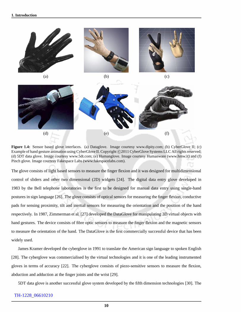
1. Introduction
(a) (b) (c)
(d) (e) (f)
Figure 1.4: Sensor based glove interfaces. (a) Dataglove. Image courtesy www.dipity.com; (b) CyberGlove II; (c)Example of hand gesture animation using CyberGlove II. Copyright c©2011 CyberGlove Systems LLC All rights reserved;(d) 5DT data glove. Image courtesy www.5dt.com; (e) Humanglove. Image courtesy Humanware (www.hmw.it) and (f)Pinch glove. Image courtesy Fakespace Labs (www.fakespacelabs.com).
The glove consists of light based sensors to measure the finger flexion and it was designed for multidimensional
control of sliders and other two dimensional (2D) widgets [24]. The digital data entry glove developed in
1983 by the Bell telephone laboratories is the first to be designed for manual data entry using single-hand
postures in sign language [26]. The glove consists of optical sensors for measuring the finger flexion, conductive
pads for sensing proximity, tilt and inertial sensors for measuring the orientation and the position of the hand
respectively. In 1987, Zimmerman et al. [27] developed the DataGlove for manipulating 3D virtual objects with
hand gestures. The device consists of fibre optic sensors to measure the finger flexion and the magnetic sensors
to measure the orientation of the hand. The DataGlove is the first commercially successful device that has been
widely used.
James Kramer developed the cyberglove in 1991 to translate the American sign language to spoken English
[28]. The cyberglove was commercialised by the virtual technologies and it is one of the leading instrumented
gloves in terms of accuracy [22]. The cyberglove consists ofpiezo-sensitive sensors to measure the flexion,
abduction and adduction at the finger joints and the wrist [29].
5DT data glove is another successful glove system developedby the fifth dimension technologies [30]. The
10
TH-1228_06610210

1.3 Hand posture based user interfaces
User Camera
Computer
Hand gestureHand gesture
Figure 1.5: Illustration of the monocular vision based interface unit for CBA systems.
5DT data gloves consist of fiber optic sensors for measuring the joint movements of the hand [31]. Similarly,
the other commercially available glove systems are the Humanglove [32] and the pinch glove [33]. The Hu-
manglove consists of Hall effect sensors to measure the joint movements [34] and the pinch glove consists of
two or more electrical contacts placed at specific parts of the hands. When a hand posture is made, the electrical
contacts meet to complete a conductive path [34].
These sensor based glove interfaces facilitate accurate interpretation or mapping of the hand postures and
hence, they find wide applications in sign-to-speech/text translation systems [35, 36], animation [37–39] and
virtual reality [40–42].
1.3.2 Vision based interfaces
The vision based interfaces for CBA involve acquisition of hand postures using one or more cameras that
are connected to the computer [43]. The vision based system using single camera is referred as the monocular
vision system and that with multiple camera is referred as the multi-vision system. The schematic diagram of a
monocular vision based interface setup for CBA systems is shown in Figure 1.5.
Unlike the sensor based interface, a computer vision methoddoes not permit direct measurement of the hand
posture parameters and hence, the images of the hand postures are the only cues provided to the information
analysis unit. The information analysis unit employs imageprocessing techniques for modelling and estimating
the hand postures from the acquired hand posture image. The key factor in vision based interface is to ensure
sufficient visibility such that the hand posture and the parameters pertaining to it are properly defined to the
computer [44]. Accordingly, the camera’s angle of view withrespect to the user’s hand should be chosen in such
11
TH-1228_06610210

1. Introduction
a way that there is no self-occlusion between the fingers and the shape of the hand is accurately captured [44]. In
real time, the choice of the angle of view varies with respectto every hand posture. Thus, in order to accurately
recover the hand posture, the vision based interface shouldeither employ one moving camera or multiple still
cameras for capturing the posture images at different angles of view. However, the choice of one moving
camera is not a feasible solution in most of the practical applications of CBA. Hence, multiple cameras are
placed at different angles of view to accurately capture thehand posture [45]. Bebis et al. [46], have employed
one moving camera and multiple still cameras for HCI in virtual environments.
The multi-vision system offers the advantages of the accurate reconstruction of hand posture and the elim-
ination of occlusion [44]. As a result the multi-vision systems are successful in higher-end applications like
robotics, virtual reality, 3D object manipulation and animation. Despite these advantages, the multi-vision
based interface is resource-intensive and requires computationally complex algorithms for hand pose estima-
tion [44, 47]. Due to the difficulties associated with the multi-vision systems, the monocular vision based
interfaces are widely employed.
In a monocular vision based system, the hand postures are acquired using one camera and the visual fea-
tures extracted through image processing techniques are used for the interpretation of hand postures. Several
researchers have already shown that the hand posture image acquired at one angle of view is accurate and
effective for HCI. Further, the development of estimation methods [48] for 3D reconstruction from a 2D im-
age encourages the use of monocular vision based interface in high-end applications. Accordingly, several
estimation methods are being proposed for reconstructing 3D hand postures from the corresponding 2D im-
ages [49–54]. The reduced computational complexity and theavailability of image processing algorithms for
accurate modelling and interpretation of 2D images make the monocular vision based interface more suitable
for real time CBA systems.
1.3.3 Merits of vision based interfaces over sensor based interfaces
The choice of the type of interface depends on the requirements of the CBA system such as accuracy,
the size of the gesture vocabulary, ease while interaction and adaptability. In this context, the sensor based
interfaces facilitate precise estimation of posture parameters and modelling/interpretation of hand postures [47].
As a result, the sensor based interfaces are capable of accurately interpreting a large class of gesture vocabulary
that includes hand postures with minor differences.
Despite the advantages, the sensor based glove interfaces are obtrusive and they hinder the naturalness of
the user interacting with the computer. They are not user adaptive and it requires to calibrate the device with
12
TH-1228_06610210

1.4 Vision based hand posture recognition: the informationprocessing step
respect to each user [22, 47]. Other drawbacks associated with them are the expensiveness and the limited
portability [44]. Further, they cannot be used for generating data cues required in other CBA applications such
as the content-based annotation and retrieval of images/videos containing the hand postures.
The vision based interfaces are non-intrusive and they facilitate natural HCI. They are robust to user vari-
ations and do not involve calibration in order to adapt to thevarying users [44, 47]. The other advantages of
vision based interfaces include cost effectiveness and thescope beyond HCI that includes generating data cues
for content-based annotation and retrieval of images/videos containing the hand postures. The major limitation
of the vision based interfaces is that the accuracy of the system is compromised due to the occlusion errors and
the structural variations with the angle of view of the camera. As a result, the vision based interfaces facilitate
only partial estimation of the hand posture and so the size ofthe gesture vocabulary that can be accurately inter-
preted is also restricted [47]. However, the advancements in pattern recognition algorithms favor effective and
accurate interpretation of hand postures from the partial estimation [47]. Therefore, the vision based interface
is considered as one of the potential elements for HCI in CBA systems.
1.4 Vision based hand posture recognition: the informationprocessing step
The procedures involved in interpreting the acquired hand posture constitute the information processing unit
of the CBA system. The key idea in automatically recognizingthe hand posture is to search for similar hand
postures that are already stored as templates. Accordingly, the development of the hand posture recognition
unit is divided into two major phases. They are the training and the testing phases.
Training is the process of deriving decision functions based on the samples of the hand posture that are
acquireda priori to constitute the training data. The decision rule requiredfor the classification of hand postures
is formulated through the extraction of significant properties of each hand posture image contained in the
training set. Based on the properties, the postures are associated with different classes through a decision
function. The mode of training can besupervisedor unsupervised.
In supervised training, for a given a set ofP number of training samplesX = x1, x2, . . . , xP, the corre-
sponding class labelsY = y1, y2, . . . , yP will be priorly available. Hence, the supervised training involves
deriving or learning a decision function that relatesX to Y. In the case of unsupervised learning, the class labels
are not known and only the training samplesX = x1, x2, . . . , xP are used for learning. Unsupervised learn-
ing involves analyzing the underlying structure ofX and grouping the data into clusters based on the analysis.
Supervised training is employed in pattern recognition application.
13
TH-1228_06610210

1. Introduction
Information analysisInformation acquisition
Hand localizationHand posture
modelling
Feature
extractionRecognition
Input gesture
image
Information analysisInformation acquisitionDecision making
Output: Matched gesture
Figure 1.6: General block diagram representation of a hand posture recognition unit for CBA systems.
Testing refers to verifying the performance of the recognition unitin accurately classifying the test patterns
based on the decision function derived while training. The correct classification (CC) accuracy of the hand
posture recognition unit is defined as
CC =Total number of correctly classified test patterns
Total number of test patterns(1.1)
The information processing unit for recognizing the hand postures employs image processing algorithms
to analyse the hand postures and derive the decision functions. The procedure for analysis includes hand
localization and hand modelling. The decision function is derived through feature extraction and the decision
label associated with a sample is obtained through classification. The general block diagram representation
of the procedures involved in hand posture recognition is shown in Figure 1.6. The procedures are explained
briefly as follows.
1.4.1 Hand localization
The primary aspect in developing a vision based CBA system isto ensure that the hand posture and its
relative parameters are properly emphasised to aid information analysis. The common method employed to
highlight the posture parameters in vision based interfaceis through the use of optical markers and the coloured
gloves. Traditional methods use retro-reflective markers or light emitting diodes (LEDs) placed at various finger
joints in order to track the posture parameters [24,55]. However, the use of such optical markers is obtrusive [55]
and finding the correspondence between the markers and the relative joints is a major problem [56]. Hence,
colour-coded gloves are used as an effective alternative [44, 55, 56]. The colour-coded glove is made of fabric
and designed to consist of different colours for every jointand the bone segment of the hand. These colours are
used as cues to detect the segments of the hand and the hand posture parameters.
Even though the colour-coded gloves are simple and effective as a vision based interface, ideally it is
not desirable for the gesturer to rely on the colour-coded gloves in practical applications. Hence, glove-free
and markerless vision based interfaces in which the hand region is extracted from the image are employed.
The commonly employed technique reported in the literaturefor hand extraction in a vision based interface
14
TH-1228_06610210

1.4 Vision based hand posture recognition: the informationprocessing step
(a) (b) (c) (d) (e)
Figure 1.7: Illustration of different hand posture models. (a) 3D textured volumetric model; (b) 3D wireframe volumetricmodel; (c) 3D skeletal model; (d) Binary silhouette and (e) Contour. Image courtesy Wikipedia [1].
is through skin colour detection [47]. Some of the methods for hand detection use background subtraction
techniques [57, 58], object contours [59] or a combination of the colour and the edge characteristics for hand
localization [60].
1.4.2 Hand posture modelling
The detected hand posture can be considered as the configuration of the hand in the 3D space. Hence,
the description of the hand posture through information analysis involves the characterization of their spatial
properties. The approaches to spatial modelling of the handpostures are themodel based approachand the
appearance based approach[47,61].
The model based approach to spatial modelling of the hand involves synthesizing 3D hand models to anal-
yse the hand posture. The important parameters of the model based approach are the angles made by the hand
joints and the palm position [61]. The 3D hand models are mainly classified into thevolumetricand theskeletal
models. The volumetric models describe either the 3D visualappearance or the 3D geometric appearance of
the human hand. The geometric appearance in volumetric modelling is achieved through the use of generalised
cylinders and superquadrics which encompass cylinders, spheres, ellipsoids and hyper-rectangles. The skele-
tal models are constructed using simple geometric structures such as the rectangular segments and lines. The
illustrations of these different hand posture models are inFigure 1.7.
Unlike the model-based approach, the appearance based approaches are based on the projection of the 3D
object into a 2D plane. Therefore, the appearance based models are the 2D images of the hand postures. This
implies that the 2D appearance based modelling does not recover the entire hand posture and it results in loss
of information in comparison to 3D modelling methods. However, the computational cost in fully recovering
the 3D hand posture state is very high for real-time recognition and slight variations in the model parameters
greatly affect the system performance. By contrast, processing the 2D appearance based models offers low
15
TH-1228_06610210

1. Introduction
computational cost and high accuracy for a modest gesture vocabulary [62]. Thus, the 2D models are well
pertinent for real time processing in CBA systems.
1.4.3 Feature extraction
The general approach to deriving the decision function is through analyzing the unique set of visual features
that accurately represent the hand postures. The procedureof deriving the features that describe the given object
is known as feature extraction and it is one of the most crucial steps that directly influence the performance
efficiency of the hand posture based CBA systems. The features employed for describing the hand posture vary
depending on the type of hand posture models. In the case of 3Dhand models, the direct parameters defining
the hand postures such as the joint angles, the palm position, the height and the width of the fingers can be
accurately estimated and they form the feature set representing the hand postures [61].
In the appearance based models, the 2D images of the hand postures are used as the templates. The feature
describing the hand posture images can be derived either from the spatial domain or the transform domain
representation of the binary hand shapes or the gray-level hand images. In the spatial domain representation, the
features are directly derived by analyzing the pixel valuesconstituting the hand posture image. The transform
domain representation is the projection of the image from spatial domain on another domain in such a way that
the distinct characteristics of the image are emphasised. Some of the image properties that are characterised
by the extracted features are the spatial distribution of the intensity values, the magnitude and the orientation
properties of the image gradients or the edges and the shape.These feature descriptors are derived either from
the gray-level images or the binary silhouette images of thehand posture. Some of the other visual features
derived from the appearance based models include the geometric features such as the number of extended
fingers, their spatial positions and the inclination angles. Among these features, the shape is an important visual
feature and it has been successfully used for representing the hand postures. The computational requirements
in shape based object analysis is less when compared to processing the gray-level and the colour images.
A large number of features based on the above image properties are reported in the area of hand posture
recognition. The efficiency of the extracted features for object recognition is generally evaluated based on the
compactness in representation, robustness to spatial transformations, sensitivity to noise, accuracy in classifica-
tion and the complexity of computation [63]. In this context, the moments are transform domain representations
that are known to be efficient for shape representation [64].Accordingly, some of the robust moments based
features reported for hand posture recognition are the geometric moments [65] and the continuous orthogonal
Zernike moments [66,67]. The moment based features are simple, robust and offer compact representations. A
16
TH-1228_06610210

1.5 Issues in vision based hand posture recognition
detailed review on the feature descriptors used for hand posture recognition is presented in Chapter 2.
1.4.4 Classification
Classification is the process of assigning the class label toa given hand posture input. The class label
is chosen through classifying the test hand posture as one ofthe classes of hand postures that constitute the
training set. The classification is performed by analyzing the similarity between the features of the test hand
posture and each of the hand posture in the training set. Someof the classification methods employed in
pattern recognition are the minimum distance classifiers, probability based classifiers, discriminant functions
and neural networks [60].
1.5 Issues in vision based hand posture recognition
The efficiency of the hand posture recognition unit depends on the accurate representation of hand postures.
The features used for representation must be capable of uniquely describing the hand postures such that the
recognition system is robust to variations that affect its performance efficiency. The important factors that
affect the performance efficiency of the vision based hand posture recognition system are (a) the segmentation
errors and (b) the geometrical distortions.
1.5.1 Segmentation errors
The accurate representation of a hand posture based on its features relies on the proper segmentation of
the hand posture from the acquired image. Image segmentation is an ill-posed problem that relies on the depth
cues, the colour cues and the geometric properties of the object to be segmented. The depth cues can be
obtained only in multi-vision systems and the monocular vision systems have to rely only on the colour and the
geometrical properties of the hand region. As mentioned in Section 1.4.1, the commonly employed method for
hand localization is the skin colour detection.
The proper segmentation of hand postures based on the skin colour is affected by the illumination changes
because of the non-uniform illumination of the hand region.Improper illumination also affects the dynamic
range of the image intensity values contained within the hand region. As a result, it is difficult to choose
an adaptive threshold for proper segmentation of hand postures under illumination changes. This leads to
segmentation errors. Figure 1.8 presents hand posture captured under three different illumination conditions.
The corresponding plots of the image histograms shown in Figure 1.9 illustrate the distribution of the intensity
values with respect to the hand posture region. Figure 1.8(a) is an example of the hand posture image captured
17
TH-1228_06610210

1. Introduction
(a) (b) (c)
Figure 1.8: Illustration of variations in the details of the hand posture image with respect to illumination changes. (a)Poor illumination - dark image; (b) Normal (average) illumination - average contrast and (c) High illumination - highcontrast.
0 50 100 150 200 2500
200
400
600
Intensity values (I.V.)
Pro
bab
ilit
y o
f I.
V.
(a)
0 50 100 150 200 2500
200
400
600
Intensity values (I.V.)
Pro
bab
ilit
y o
f I.
V.
(b)
0 50 100 150 200 2500
200
400
600
Intensity values (I.V.)P
ro
bab
ilit
y o
f I.
V.
(c)
Figure 1.9: Histograms of (a) the dark image; (b) the average contrast image and (c) the high contrast image shown inFigure 1.8.
(a) (b)
Figure 1.10: Examples of hand posture images taken in varying background: (a) hand posture acquired in a uniformbackground and (b) hand posture images acquired in complex backgrounds. The hand posture images are taken from theJochen Triesch static hand posture database [2].
under poor illumination with the corresponding histogram shown in Figure 1.9(a). The hand posture captured
under normal illumination and the corresponding plot of image histogram are shown in Figure 1.8(b) and Figure
1.9(b) respectively. Similarly, Figure 1.8(c) is an example of the hand posture image captured under relatively
high illumination and the corresponding plot of histogram is shown in Figure 1.9(c). Under poor illumination,
the dynamic range of the intensity values is low and hence, the resultant image is dark and has a poor contrast.
In the case of normal illumination, the dynamic range of the intensity values has increased and distribution of
the intensity values within the range is almost uniform. Hence, the resultant image is relatively bright and has
18
TH-1228_06610210

1.5 Issues in vision based hand posture recognition
good contrast. Similarly, under high illumination the dynamic range of the intensity values is relatively more
and the resultant image has higher contrast than the poor andthe normal illumination images.
Additionally, segmentation errors also occur while segmenting the hand postures from a complex or clut-
tered background that contains several other objects with almost similar colour or geometrical characteristics
as the hand region. The proper segmentation of hand posturesis also affected if the colour of the user’s clothing
coincides the skin colour. Some examples of the hand posturecaptured under different backgrounds are shown
in Figure 1.10.
1.5.2 Geometrical distortions
The other major issue involved in accurate recognition of the hand postures is the geometrical distortions
that occur due to geometrical transformations, variationsin the hand posture parameters and variations due to
changes in the angle of view.
1.5.2.1 Geometrical transformations
The geometrical transformations affecting the performance of the recognition unit includes thescale, the
rotational and thetranslationalchanges induced during gesture acquisition as described below.
• The scale represents the spatial resolution of the acquiredhand posture. The resolution will differ with
respect to the variations in the hand geometry of the users and the distance between the gesturer and the
camera.
• Rotation changes refer to the variation in the orientation of the hand posture that occurs either when the
user rotates the hand while gesturing or when the camera is rotated along its plane within the field-of-view
(FOV).
• Translational changes represent the variation in the spatial location of the hand posture that occurs due to
the user’s movement of the hand.
1.5.2.2 Variations in the hand posture parameter
As explained in Section 1.2, the parameters that characterise the hand shape are the angles caused by the
flexion/extension and the abduction/adduction movements of the finger joints. Among these, the flexion and
the adduction movements are positive joint excursions and the extension and the abduction movements are
negative joint excursions. The joint angle between two adjacent bone segments is measured by considering one
19
TH-1228_06610210

1. Introduction
Little finger
Carpals Metacarpophalangeal joints (MP)
DIP
PIP
MP
Proximal interphalangeal joints (PIP)
Distal interphalangeal joints (DIP)
Interphalangeal joints (IP)
Middle finger
Ring finger
Thumb
Index finger
Middle finger
IP
(a)
Figure 1.11: Illustration of hand posture parameters using the hand skeleton. The joint angles represent the hand postureparameters.
20 20
(a)
[ 30 , 35 ]MP ! " # " #
0M P ! #
90MP ! #
(b)
0
70
0
(c)
Figure 1.12: Illustration of (a) finger abduction; (b) MP joint range of motion, flexion-extension and (c) Palmar abductionand adduction of the thumb at the MP joint. The negative anglein (b) refers to the extension movement.
of the bone segments at close distance to the carpals as the reference axis. The procedure for measuring the
hand posture parameters at the finger joints is illustrated using a hand skeleton in Figure 1.11(a). Similarly,
a few examples illustrating the angular positions of the bone segments with respect to the abduction and the
flexion movements of the metacarpal joints (MP) are shown in Figure 1.12. The maximum value of the motion
parameters with respect to each finger joints are given in Table 1.2.
Based on these movement parameters, the hand postures can beconsidered assimple posturesandcomplex
postures. With simple postures, every individual finger is either extended or flexed to the maximum range.
Complex postures are those in which the fingers can be bent at any angle within the maximum range of motion
in order to constitute a hand posture. In the case of complex postures, the joint angles defining a hand posture
are only approximations that lie within a defined range of angular values. The structural variations with respect
to a hand posture occur due to the changes in the flexibility ofthe user’s hand joints within the defined range.
Similarly, the hand posture parameters vary due to the variations in the hand geometry. An experimental
study on the effects of the hand length and the flexibility of the joint angles in [68] states that the joint flexibility
20
TH-1228_06610210

1.5 Issues in vision based hand posture recognition
(a)
(b)
Figure 1.13: Examples of a hand posture taken at various angles of view. The figure illustrates the structural deviationsor deviations in the appearance of the hand posture. Similarly, occlusion of certain parts of the hand can be observed ateach angle of view. The hand posture images are taken from theMassey hand posture database for the American signlanguage [3].
Table 1.2: Maximum range of motion parameters defining the movements with respect to the thumb and the fingerjoints [7].
Extension Flexion Abduction Adduction
FingersθMP θPIP θDIP θMP θPIP θDIP 20 0
[−30,−35] 0 −20 90 [100,120] [80,90]
ThumbθMP θIP θMP θIP 70 00 −20 50 90
of the fingers increase with the increase in the hand length. Therefore, the variations in the flexibility of the
user’s hand and the hand geometry result in the deviation of hand posture parameters due to which there is
diversity in the appearance of a hand posture.
1.5.2.3 Variations due to the angle of view
In the field of imaging, the angle of view is known as the view-angle. The viewpoint refers to the position
of the camera with respect to the object of focus [69]. The optimal choice of the viewing angle or the viewpoint
is determined by the amount of perspective distortion. Perspective distortion is a phenomenon in which, the
part of the object present at a larger distance from the camera appears to be smaller than the closer part of the
same object and vice versa [69, 70]. As a result, the perceived shape of the object is distorted / altered. The
distortion is caused if the focal plane is not parallel to theobjects surface and/or not in level with the centre of
the object.It means that the camera is not at equidistance from all the parts of the object [70]. The variations in
the viewpoint result in structural deviations and self-occlusion of the fingers. A few examples illustrating the
21
TH-1228_06610210

1. Introduction
structural variations and the occlusion errors in a hand posture due to variations in the view-angle are shown in
Figure 1.13.
1.6 Motivation for the present work
Vision based hand posture recognition is one of the important research areas spawning advanced HCI
techniques for intelligent interaction in CBA systems. Theefficiency of these systems depends on the accuracy
of the features used for describing the input hand postures.For improved performance, the features defining
the hand postures should be robust to geometrical distortions caused by the similarity transformations, user
and the view-angle variations. Among these, the geometrical transformations can be easily addressed through
proper normalization techniques. Unlike geometrical transformations, it is very difficult to model and develop
techniques for normalizing user and view-angle variations.
Only very few works in hand posture recognition have concentrated in developing user and view invariant
recognition techniques. The comparative evaluation of theexisting feature descriptors and their robustness
to user and view-angle variations are not yet explored. Hence, this research is motivated towards identifying
features that are robust to user and view-angle changes. Accordingly, the goal is to develop a robust monocular
vision based hand posture recognition system that is capable of handling simple and complex hand postures.
Recently, the discrete orthogonal moments are introduced as efficient approximations for image analysis.
These discrete orthogonal moments were shown to be efficientin terms of compact representation, robustness
to noise and accurate reconstruction [71–73]. However, they are yet to be explored for shape description and
classification. In this research work, two discrete orthogonal moments , namely theKrawtchoukand thediscrete
Tchebichefmoments are proposed as features for shape representation.Based on the validation in representing
the general shapes, a vision based hand posture recognitionsystem using the discrete orthogonal moments as
feature descriptors is proposed.
The thesis also aims at assessing the user and the view invariant characteristics of the proposed and other
existing descriptors. Accordingly, the geometric moments, the Zernike moments, the Fourier descriptors, the
Gabor wavelets and the principal component analysis (PCA) based descriptors will be evaluated.
The proposed discrete orthogonal moment based hand posturerecognition system and the various feature
descriptors are to be tested on two different classes of handpostures that are intended to find the applicability
in different CBA systems. The first class of postures consists of 10 simple single-hand postures formed by
extension/flexion and abduction/adduction of fingers to themaximum range. These simple hand postures can
22
TH-1228_06610210

1.7 Contributions of the thesis
be used to command, control and manipulate operations in HCI. The second class of gestures consists of
32 complex single-hand postures taken from Bharatanatyam,a pantomimic dance form in India [74, 75]. The
recognition technique for recognizing the hand postures inBharatanatyam is aimed at developing content-based
dance annotation and retrieval systems for Bharatanatyam.
1.7 Contributions of the thesis
The contributions of this research work are as follows.
(i) Discrete orthogonal moments, namely the Krawtchouk moments and the discrete Tchebichef moments
are introduced as features for shape representation. The accuracy of the discrete orthogonal moments
in representing the shapes from the MPEG 7 shape database is experimentally studied. The study is
considered as validation towards using the discrete orthogonal moments as features for hand posture
recognition.
(ii) A monocular vision based hand posture recognition system that is robust to geometrical transformations,
user and view-angle variations is developed based on the discrete orthogonal moments.
(iii) For comparative evaluation, the user and the view-angle invariance characteristics of the proposed method
and the state-of-the art methods like the Fourier descriptors, the geometric moments, the Zernike mo-
ments, the Gabor wavelets and the PCA descriptors are studied in detail.
(iv) In this research work, two different hand posture databases are developed. The first database consists of
4, 230 samples of 10 simple hand postures acquired at varied scales, orientations and view-angles. The
database is collected from 23 users. The gesture recognition technique developed on this database may
find applicability in hand posture based HCI to perform command, control and manipulation functions in
CBA systems.
The second database consists of 8, 064 samples of 32 complex single-hand postures in Bharatanatyam,
known as theAsamyuta hastas. The images are acquired by varying the scale and view-angle. The
database is collected from 6 female subjects. The hand posture recognition technique developed on
this database aims towards promoting hand postures as data cues to automatically annotate and retrieve
Bharatanatyam dance videos.
23
TH-1228_06610210

1. Introduction
1.8 Organization of the thesis
The rest of this thesis is organised as follows.
Chapter 2 presents a review on the feature descriptors used for hand posture recognition. The chapter con-
cludes with an insight into the applicability of discrete orthogonal moment based descriptors for hand posture
analysis.
Chapter 3 presents the theory of discrete orthogonal moments and the formulation of Krawtchouk and
Tchebichef moments. The chapter includes experimental studies on the spatial- and the spectral-domain prop-
erties of the Krawtchouk and the discrete Tchebichef polynomials. The efficiency of the discrete orthogonal
moments in shape representation and shape classification isstudied using the MPEG 7 shape database. The
experimental study presented in this chapter validates thediscrete orthogonal moments as efficient shape de-
scriptors.
Chapter 4 elaborates the proposed discrete orthogonal moment based hand posture recognition technique
that is robust to similarity transformations and user and view-angle variations. The system deals with the silhou-
ette model of the simple hand postures that are intended for application in HCI. In this chapter, anthropometry
based normalization techniques for the removal of the forearm and orientation correction are proposed. The
chapter includes details about the database development and the analysis on structural variations in a hand pos-
ture with respect to user variations and view-angle changes. The experiments on hand posture classification
validate the efficiency of the discrete orthogonal moments in comparison to the other considered methods.
Chapter 5 explains the hand posture recognition technique developed for recognizing the single-hand pos-
tures in Bharatanatyam known as theAsamyuta hastas. The chapter explains the development of the Asamyuta
hastas database and the system implementation procedure. The representation methods for analyzing the com-
plex hand postures in Bharatanatyam are chosen based on the experimental results in Chapter 4. Accordingly,
the Krawtchouk moments and the discrete Tchebichef momentsand the PCA descriptors are considered. The
experiments validate that the Tchebichef and the Krawtchouk moments are efficient features for representing
these complex hand postures.
Chapter 6 concludes this thesis with suggestions for the application of the proposed discrete orthogonal
moment based hand posture recognition technique for the automatic annotation of the Bharatanatyam video
and content-based retrieval Bharatanatyam video from a database.
24
TH-1228_06610210

2A Review on Feature Extraction in Hand
Posture Recognition
Contents2.1 Introduction . . . . . . . . . . . . . . . . . . . . . . . . . . . . . . . . . . . .. . . . . . . 26
2.2 Silhouette image based methods . . . . . . . . . . . . . . . . . . . . .. . . . . . . . . . . 26
2.3 Gray-level image based methods . . . . . . . . . . . . . . . . . . . . .. . . . . . . . . . . 36
2.4 Summary and conclusion . . . . . . . . . . . . . . . . . . . . . . . . . . . .. . . . . . . . 49
25
TH-1228_06610210

2. A Review on Feature Extraction in Hand Posture Recognition
In this chapter we present the existing state-of-art methods in hand posture recognition. The methods are
categorised based on the features derived from the hand posture images for description. The advantages and
the limitations of the existing methods in terms of the computational complexity, robustness to similarity trans-
formations, user and view-angle invariance, classification rate and the supported size of the posture vocabulary
are reviewed.
2.1 Introduction
The recognition of an object in an image requires the extraction of some features that uniquely characterise
the object. These features are called the descriptors for the object and represented in a form suitable for the
classifier used for mapping the object into a known class. Thedescriptor may be derived from the geometric
shape in the form of the binary silhouette image that is obtained by the segmentation of the original image.
Alternatively, the descriptor may be derived from the variation of intensity in the gray-level image containing
the object.
There are large number of descriptors derived from the silhouette image and the gray level image to rep-
resent the hand posture. We classify these methods into two category they are: (a) the silhouette image based
methods and (b) the gray-level image based methods. The important descriptors belonging to both the cate-
gories are described below.
2.2 Silhouette image based methods
The silhouette image based methods derive features that represent the hand posture by its shape. The pro-
cedure for recognizing the shape of a given object requires to derive parameters that uniquely characterise the
shape [76]. The efficiency of a method used for representing the shapes is evaluated in terms of retrieval ac-
curacy, compactness of representation, hierarchy of coarse to fine representations, computational complexity,
robustness to geometrical transformations and robustnessto shape defections [77]. The geometrical transfor-
mations include rotation, scaling, translation and affine variations of a given shape. The shape defections are
structural distortions caused by noise, boundary distortions and the segmentation errors that occur while bi-
narisation [63]. The retrieval efficiency represents the ability of the shape descriptor to effectively recognise
similar shapes inspite of the above mentioned geometrical transformations and the shape defections. The sil-
houette image based methods generally derive the importantfeatures by using either the shape boundary or the
interior points of the shape along with the boundary [63]. Hence, the silhouette based shape features can be
26
TH-1228_06610210

2.2 Silhouette image based methods
classified intocontour featuresandregion features. The contour features exploit only the pixels that form the
shape boundary and the region features take in to consideration all the pixels constituting the shape region or
the entire silhouette image. The details of several contour-based features and region-based features used for
hand posture analysis are discussed below.
2.2.1 Geometric features
The geometric features of the hand posture are the simple shape descriptors that can be derived both from
the shape boundary and the shape region. The geometric features for defining the entire shape are derived by
extracting the morphological characteristics of the fingerand the palm regions of the hand. Accordingly, the
location, the position and the inclination angles of the fingers are among the geometric features employed for
representing the hand posture.
In [78], a hand posture recognition technique using the boundary profile of the hand postures as features
was proposed. LetB define the boundary of the hand posture and(xc, yc) be its centroid of the hand posture
region. Then, for(x, y) ∈ B, the boundary profile (BP) describing the hand posture is computed as
BP(x, y) =√
(x− xc)2+ (y− yc)
2 (2.1)
The number of peaks in the boundary profile represents the number of extended fingers with the peaks
corresponding to the finger tips. The positions of the peaks of the BP denotes the positions of the fingers with
respect to the centroid of the hand posture. The BP was used toclassify a database consisting of 6 distinct
static hand gestures. The classification was performed withthe minimum distance classifier and the average
recognition rate obtained was 95%.
Jag et al. [79] proposed a view-point invariant hand posturerecognition technique combining the silhouette
model and 3D-hand posture model for recognition. The methodderived the centroidal profile from the boundary
of the hand posture. Given the shape boundary, the centroidal profile is obtained by mapping the boundary
points into a polar(r, θ) representation. The radiusr describes the distance between the shape centroid and the
boundary points. Theθ value describes the inclination angle of the extended fingers. The system was tested
on a dataset containing 5 distinct hand postures that were captured at 15 different viewing directions. Their
technique achieved a classification rate of 90.8%.
The above methods based on the shape boundary are sensitive to noise, rotation variations and there may be
two different hand postures with almost similar boundaries. Also, the locations of the peaks vary according to
the user’s hand geometry and hence, it is not possible to handle gestures with various finger flexions. In order
27
TH-1228_06610210

2. A Review on Feature Extraction in Hand Posture Recognition
to overcome this, different region based techniques for detecting the number of extended fingers, their positions
and the relative length of the fingers are employed in [80–84]. In [80], a circle that intersects all the abducted
fingers was drawn with respect to the centroid of the hand posture. The diameter of the circle was fixed as 0.7 of
the farthest distance from the centroid. The number of extended fingers was estimated by counting the number
of background-to-foreground transitions and used as the feature. The technique was tested on a small gesture
library consisting of 5 distinct hand postures and was shownto be invariant to the similarity transformations.
Yin and Xie [82] employed a similar technique for finding the number of extended fingers. However, the circle
that intersects the abducted fingers was obtained iteratively. The other features used in this technique include
the positions of the fingers with respect to the circle. The method was tested on a database consisting of 8
gesture signs.
The skeleton of the hand posture image was used in [81] for extracting the geometric features such as the
position, the orientation and the number of extended fingers. These features were employed for classifying the
basic hand shapes in the Japanese sign language. Stergiopoulou and Papamarkos [83] proposed a graph based
searching method for deriving the morphological features of the palm and the finger regions of the hand posture.
The shape of a given hand posture was approximated using the Self-Growing and Self-Organised Neural Gas
(SGONG) network. The morphological features of the hand such as the number of the extended fingers, palm
centre, slope of the hand, inclination angles of the extended fingers relative to the hand slope were derived
from the SGONG approximation of the hand posture. A probabilistic classifier that is based on the choice of
the most probable finger combination of a set of feasible gestures was used for recognition. The system was
tested on a dataset of 180 images of 31 hand postures. The system achieved a maximum classification rate of
90% and is invariant to similarity transformations. However, the system is computationally complex and very
sensitive to the errors in extracting the geometric features. In [84], the concave and the convex points in the
boundary profile of the hand posture were used for partitioning the finger and the palm regions. Based on these
points, the extended fingers were identified and the length and the width of the detected fingers were employed
as features for classifying the hand postures. The geometric measures of each finger were determined based on
the anthropometric measurements. The system achieved a classification rate of 91.4% in classifying 12 hand
postures from the Arabic sign language.
Flasinski and Myslinski [85] have used boundary-based graph models and a parsing method for the recog-
nition of hand postures in the Polish sign language. In general, the model graph of a given hand posture is
obtained by deriving the polygonal approximation of its contour. the nodes of the graph are the vertices of the
28
TH-1228_06610210

2.2 Silhouette image based methods
polygon and are labeled with the vertex angles. The nodes areconnected by directed lines known as the edges.
The orientations of the edges with respect to a reference node are used for labeling the edges. The obtained
graph is called theindexed edge-unambiguous graph(IE-graph) and the vertex angles and the edge orientations
are the feature descriptors. In [85], a set of IE-graphs representing the hand postures was treated as a formal
language generated with the ETPL(k) (Embedding transformation preserved production orderedk-left nodes
unambiguous) graph grammar. The graph grammar was used for classifying 48 hand posture signs in the Polish
sign language. It was shown that the system is robust to moderate changes in the view-angle and variations in
the user hand anatomy. However, the system is sensitive evento small variations in the geometry of the hand
posture induced due to user variations. Further experiments are required to verify the robustness of the system
to perspective distortions induced by the view-angle changes.
Dias et al [86] developed a system known as theOpen Gestures Recognition Engine(O.G.R.E) for recogniz-
ing the hand postures in the Portuguese Sign Language. The histogram of the distances and the angle between
the contour edges were used to derive a contour signature known as the pair-wise geometrical histogram. The
classification was performed by comparing the pair-wise geometrical histograms representing the gestures.
The above discussed geometric features are simple shape descriptors and usually can discriminate only
hand postures with large differences. Further, these simple shape descriptors cannot handle hand postures that
are deformed due to segmentation errors and self-occlusion.
2.2.2 Curvature scale space
The curvature scale space (CSS) representation of the hand posture is a boundary based shape description
method. In this technique, the evolution of the zero-crossing points with respect to the multi-scale represen-
tations of the shape boundary is used as the features for handposture recognition [87]. Consider the shape
boundaryB, which is assumed to be a planar curve. Then, the curvature functionκ (u) is computed as
κ (u) =x (u) y (u) − x (u) y (u)(
x (u)2+ y (u)2
)3/2(2.2)
whereu is the length parameter. ConvolvingB with a 1D Gaussian kernelg (u, σ) of standard deviationσ
results in the smoothed curveBσ. The smoothed boundary points are given by
X (u, σ) = x (u) ∗ g (u, σ)
Y (u, σ) = y (u) ∗ g (u, σ)(2.3)
where∗ denotes the convolution operation.
29
TH-1228_06610210

2. A Review on Feature Extraction in Hand Posture Recognition
13
4 25
(a)
3
45
2
(b)
4 5
3
(c)
0 50 100 150 200 2500
5
10
15
20
u
σ
5
1
2
3 4
(d)
Figure 2.1: Illustration of smoothing of the shape boundary and the evolution of the inflection points at different scales(σ). (a)σ = 3.5; (b)σ = 8.2 and (c)σ = 14.6. The concave segments at each scale are enumerated. The number ofconcavities decreases with the increase in the scale. (d) The CSS image constructed from the locations of the inflectionpoints at various scales.
Accordingly, the curvatureκ (u, σ) at a scaleσ is computed as
κ (u, σ) =X (u, σ) Y (u, σ) − X (u, σ) Y (u, σ)
(
X (u, σ)2+ Y (u, σ)2
)3/2(2.4)
The CSS descriptors represent the location of the inflectionpoints on the curve at different scales and are
extracted as the CSS image. The CSS imageICS S(u, σ) is defined as
ICS S(u, σ) = (u, σ) |κ (u, σ) = 0 (2.5)
An example illustrating the evolution of the concave segments in the hand posture boundary for different values
of σ and the corresponding CSS image are shown in Figure 2.1. The shape boundary is convolved with the
smoothing kernel iteratively until there are no inflection points on the smoothened boundary. The scale of
the smoothing kernel increases with the number of iterations. The peaks in the CSS image correspond to the
concavities in the hand posture contour and the height of thepeaks depends on the depth and the size of the
concave segments. In general, the CSS image is used as the feature descriptor and the classification is performed
using nearest neighbor classifier.
Kopf et al [88] employed CSS descriptors for classifying a class of 3 simple hand postures. They proposed
a modified CSS approach in which the convex segments of the shapes were also represented in the CSS image.
Chang et al [89,90] proposed a feature alignment approach for making the CSS image invariant to translation,
scale and rotation changes. The feature alignment involvedcircularly shifting the coordinate peaks of the CSS
image with respect to the coordinate containing the largestpeak. The proposed approach was tested on a hand
posture database consisting of 600 images of 6 hand postures. It was shown that the performance of the aligned
CSS descriptors is better than that of the Zernike and the pseudo-Zernike moment invariants representing the
hand posture. The major drawback of the CSS image based approach is that the locations of the peaks are
30
TH-1228_06610210
2.2 Silhouette image based methods
highly unstable making it difficult to adapt to user variances and perspective distortions induced by view-angle
changes. The number of peaks representing the number of concave or convex segments are stable features and
hence, CSS image might be useful only for classifying distinct hand signs. Also, two different shapes with the
same sets of concavities will have the same CSS representations resulting in misclassification.
2.2.3 Modified Hausdorff distance based matching
The modified Hausdorff distance (MHD) based matching is a contour-based shape matching technique
introduced by Dubuisson and Jain in [91]. The method employsthe nearest point search strategy for com-
puting the similarity between two shapes. The MHD is used forhand posture recognition in [92] and [93].
Let A =
α1, α2, · · · , αNA
andB =
β1, β2, · · · , βNB
be the two point sets to be compared, whereNA andNB
represent the cardinality of the setA andB respectively.
Sanchez-Nielsen et al [92] used theL1 norm and computed the bidirectional partial Hausdorff distance as
H = maxh (A,B) , h (B,A) (2.6)
whereh (A,B) is the directed distance between the point setsA andB and it is defined as
h (A,B) = iKthα∈A ‖α − β‖1 , (2.7)
iKthα∈A represents theKth ranked distance such thatK/NA = i %. The distance measureH was used to classify
a set of 26 static hand postures and the experiments show thatthe system achieved an average classification
accuracy of 90%. The MHD based shape matching is a widely employed technique robust to outlier points and
similarity transformations. However, the MHD technique isa point-wise correspondence based method and
hence, it exhibits high computational complexity.
2.2.4 Fourier descriptors
Fourier descriptors are boundary based representations that are robust to noise and invariant to translation,
scale and rotation changes. Given a shape boundaryB of sizeL and the points(x, y) ∈ B, the Fourier descriptors
are obtained through the Fourier transform on a complex vector derived from the coordinates(x, y). For u =
0, 1, · · · , L − 1, the complex co-ordinates characterizing the shape boundary are obtained as
f (u) = (x (u) − xc) + i (y (u) − yc) (2.8)
31
TH-1228_06610210

2. A Review on Feature Extraction in Hand Posture Recognition
where(xc, yc) is the centroid of the shape. Forω = 2πkL , k = 0, 1, · · · , L − 1, the Fourier transform of (2.8) is
given by
F (ω) =L−1∑
u=0
f (u) exp(− jωu) (2.9)
The magnitude of|F (ω)| is known as the Fourier descriptor and it is invariant to rotation and translation
changes. In order to achieve scale-invariance, the spectrum is normalised as
∣
∣
∣F (ω)∣
∣
∣ =|F (ω)||F (0)| (2.10)
Chen et al [57] developed a system based on the Fourier descriptors and the hidden-Markov model (HMM)
for classifying gestures in the Taiwanese sign language. The Fourier descriptors were used as features for
representing the hand postures contained in the gesture sign. The Fourier descriptors along with the other
temporal features were used to build the HMM model for gesture classification. In [94], the Fourier descriptors
were used as features for user-adaptive hand posture classification. The Fourier descriptors were used to classify
a database of 1600 samples of 9 hand postures. Similarly, Yang et al [95] developed a command system
using hand posture as the user-interface element. The system employed the Fourier descriptors as features for
classifying 4 hand posture signs that are used for specifying the commands in human-computer interaction.
Bourennane and Fossati [96] have shown that the Fourier descriptors are efficient over region-based features
like moments. They performed experiments on two different hand posture databases and the results confirm
Fourier descriptors as efficient features for scale and rotation invariant hand posture classification.
The works on Fourier descriptor based hand posture recognition have considered only a few distinct hand
postures and the performance of the Fourier descriptors in the case of more gesture classes, view-angle varia-
tions and user-independence needs to be evaluated.
2.2.5 Moments and moment invariants
Moments are region based descriptors in which all the pixelswithin a shape region are taken into account
to obtain the shape representation [63, 97]. The moments extract statistical description of the pixels in the
shape region [63]. The moment functions allow to derive moment invariants that are robust to geometrical
transformations and less sensitive to shape defections [98].
Moments can be defined as the projection of a given function onto the polynomials that form the basis
set [99]. The polynomials can be orthogonal or non-orthogonal. Accordingly, the moments are categorised
as non-orthogonal moments and orthogonal moments [99]. Thesimple and the widely used non-orthogonal
32
TH-1228_06610210

2.2 Silhouette image based methods
moments in hand posture description are the geometric moment invariants.
Consider f (x, y) to represent a binary image of size(N + 1) × (M + 1) such thatx ∈ 0, 1, · · · ,N and
y ∈ 0, 1, · · · ,M. The functionf (x, y) takes the unity value inside the shape region and otherwise it takes the
zero value. The geometric moments of order(n+m) representing the image is defined as
Gnm =
N∑
x=0
M∑
y=0
xnym f (x, y), n,m= 0, 1, 2, · · · (2.11)
Using non-linear combinations of the lower order geometricmoments, Hu [100] derived a set of moment
invariants called asgeometric moment invariantsthat are invariant under image scaling, translation and rotation.
Previous works on shape classification [63] have shown that the geometric moment invariants are not sufficient
for describing arbitrarily distorted contour-based shapes and perspectively transformed shapes. Hence, the
geometric moment invariants are used along with other geometric properties for representing hand postures.
Chalechale et al [65] used geometric moment invariants and geometric properties (area, perimeter, major
axis length, minor axis length and eccentricity) as features for representing 25 hand posture signs. The classi-
fication was based on Bayesian rule assuming Gaussian distribution for the extracted features. The descriptors
were used to classify a database consisting of 2080 hand posture samples and achieved a classification accu-
racy of 98%. Similarly, in [101], the geometric moment invariants were combined with features like normalised
length of the contour and directional gradients for representing hand postures. The classification was performed
using weighted nearest neighbor-based classification scheme. The technique was tested on a database consist-
ing of 700 samples of 3 hand postures acquired under various lighting conditions. Out of 700 samples 200
samples were used for testing and the technique achieved an average performance of 95%. Tofighi et al [102]
derived geometric moment invariants from the shape boundary of the hand postures as feature descriptors.
Along with the geometric moments, the convex points on the hand posture were also employed to form the
feature vector. The classification was performed using the minimum distance classifier. The efficiency of the
geometric moment was tested on a database of 500 samples of 10gesture classes and their results reported an
average classification rate of 90%.
The studies suggest that the geometric moment invariants are suitable for describing simple shapes and not
sufficient to accurately describe large number of shapes. The basis functions of the geometric moments are cor-
related implying that these moment features are redundant [98]. Teague [103] suggested image representation
through orthogonal moments that are derived from the orthogonal polynomials. The Zernike moments (ZMs)
and the pseudo-Zernike moments (PZMs) are among the efficient orthogonal moments used for hand posture
33
TH-1228_06610210

2. A Review on Feature Extraction in Hand Posture Recognition
0 0.2 0.4 0.6 0.8 1−1.5
−1
−0.5
0
0.5
1
1.5
ρ − Radius
Rnm − Radial polynomial
0 0.5 1−1
0
1
R00
R11
R20
R22
R31
R33
R40
(a)
n=6, m=0
n=6, m=2
n=6, m=4
n=12, m=0
n=12, m=2
n=12, m=4
(b)
Figure 2.2: (a) 1D Zernike radial polynomialsRnm(ρ) and (b) 2D complex Zernike polynomialsVnm(ρ, θ) (real part).
representation. The ZMs and the PZMs are rotation invariantdescriptors that are derived using the complex
Zernike polynomials and pseudo-Zernike polynomials respectively as basis functions.
The ZMs and PZMs are defined on the polar coordinates(ρ, θ), such that 0≤ ρ ≤ 1 and 0≤ θ ≤ 2π. The
complex Zernike polynomialVnm(ρ, θ) of ordern ≥ 0 andrepetition mis defined as [99]
Vnm(ρ, θ) = Rnm(ρ) exp(− jmθ) (2.12)
For even values ofn− |m| and|m| ≤ n, Rnm(ρ) is the real-valued radial polynomial given by
Rnm(ρ) =(n−|m|)/2∑
s=0
(−1)s(n− s)!ρn−2s
s!((n+ |m|)/2− s)!((n− |m|)/2− s)!
The plots of the radial polynomialsRnm(ρ) for different ordersn and repetitionmare given in Figure 2.2(a). The
2D complex Zernike polynomialsVnm(ρ, θ) obtained for different values ofn andmare shown in Figure 2.2(b).
From the plots, we can infer that the Zernike polynomials have wider supports. Therefore, the Zernike moments
characterise the global shape features.
The complex Zernike polynomials satisfy the orthogonalityproperty,
2π∫
0
1∫
0
V∗nm(ρ, θ) Vlk (ρ, θ) ρdρdθ =π
n+ 1δ [n− l] δ [m− k]
34
TH-1228_06610210

2.2 Silhouette image based methods
whereδ [.] is the Kronecker delta function. The Zernike momentZnm of ordern and repetitionm is given by
Znm =n+ 1π
2π∫
0
1∫
0
V∗nm(ρ, θ) f (ρ, θ) ρ dρdθ (2.13)
where|m| ≤ n andn− |m| is even.
The integration in (2.13) needs to be computed numerically.The magnitude|Znm| is invariant to rotation
and hence, used for rotation invariant gesture representation [66,67].
The pseudo-Zernike basis polynomials exhibit properties similar to those of Zernike basis polynomials.
The pseudo-Zernike basis polynomials differ only in terms of the radial polynomials. The radial basis of the
pseudo-Zernike polynomials are real-valued functions anddefined as
Rnm(ρ) =(n−|m|)∑
s=0
(−1)s(2n+ 1− s)!ρn−2s
s!(n− |m| − s)!(n+ |m| + 1− s)!
Chang et al [66] used the ZMs and the PZMs as combined featuresfor hand posture classification. The ex-
periments were performed on a database consisting of 600 hand postures of 6 gesture signs collected from
10 subjects. The ZMs and PZMs features representing the handpostures were classified using the nearest
neighborhood classification technique and achieved a classification rate of 97.3%.
Gu and Su [67] have shown that the ZMs as efficient descriptorsfor view and user invariant representation of
the hand postures. A hierarchial classifier based on the multivariate decision tree was employed for classifying
the hand posture features. The database used for the experiment consisted of 3850 samples of 11 gesture signs.
The images were acquired from 5 subjects and at 7 different viewing directions with the frontal view-angle
varying between−60 to 60. The results have shown that the ZMs are robust to large variations in the viewing
angle and the user’s hand shape.
2.2.6 Multi-fusion features
A few works in hand posture recognition have combined various contour and region based descriptors to
derive multiple features for representing hand postures. In [104], the geometrical features like the location of
the fingertips, convex and concave points of the fingers, areaand the principal axes were combined with the
geometric moments to form a feature vector for classification. Kelly et al [105] have derived features from the
binary silhouette and the one dimensional boundary profile to represent the hand postures. The binary silhouette
was represented using the geometric moments. The size functions were derived from the boundary profile to
describe the hand shape. The dimensionality of the size functions was reduced using the principal component
35
TH-1228_06610210

2. A Review on Feature Extraction in Hand Posture Recognition
analysis. The reduced size functions are known as theeigen space size functions. The geometric moments and
the eigen space size functions were combined to achieve userindependent gesture recognition. In [106], the
eigen features are extracted from the contour of the hand posture and is combined with the mean shape of the
hand posture samples for finding the exact match.
Feng et al [107] have proposed a two-step feature extractionprocedure in which the first and the second
steps are known as the coarse location phase (CLP) and the refined location phase (RLP) respectively. In the
CLP phase, the hand posture features like the convex and the concave points of the hand and the intersection of
knuckle on different fingers were used for coarse representation. In the RLP phase, the features were derived
from the multi-scale space representation of the hand postures. The multi-scale space representation charac-
terises the blob, ridge, corner and edge features of the handposture at different scales. The integration of these
features were used for classifying 26 hand posture signs.
Yun et al [108] combined the geometric moment invariants andthe colour cues derived from the hand
posture regions to form a feature vector for the descriptionof hand postures. These features were classified
using the Euclidean distance based matching technique. Themethod was tested on a database consisting of
1000 samples of 10 hand posture signs acquired at different backgrounds. Using these multiple features, a
classification accuracy of 91% was achieved.
2.3 Gray-level image based methods
The gray-level image based approaches use image features derived using the gray-level or the intensity val-
ues of the acquired hand posture image. The gray-level imagebased methods are also known as the appearance
based approaches [109]. The hand postures are modeled basedon these appearance features and used as prede-
fined templates for classifying the test hand postures. These features characterise the image parameters such as
the intensity distribution around a neighborhood and the edge characteristics of the hand postures. Similar to
the silhouette image based methods, the efficiency of the gray-level image based methods is also evaluated in
terms of retrieval efficiency, computational complexity and robustness to geometric and perspective distortions.
In addition to these, the gray-level image based methods must also be robust to illumination variations that
occur while acquisition. The various gray-level image based approaches used for hand posture analysis are
discussed as follows.
36
TH-1228_06610210

2.3 Gray-level image based methods
2.3.1 Edge-based Features
The shape and the appearance of an object in an image can be represented by the local distribution of
magnitudes and the orientations of the gradient image. A fewdescriptors for the hand posture are based on the
edge maps. They are discussed as follows.
2.3.1.1 Orientation histograms
Orientation histograms are edge based features that are derived from the edge map or the gradient map of
the hand posture image. The orientation histogram represents summarised information on the orientations of
the edges or the gradients constituting the hand posture image. The orientation histogram can be computed as
a global feature or as a local feature.
Freeman [110] derived the orientation histogram from the intensity values of the hand posture image. The
gradients were computed using two-tap derivative filters along thex and they directions. IfIx and Iy are the
outputs of thex and they derivative operators, then the gradient direction is derived as tan−1( Iy
Ix
)
. The proba-
bility distribution of the gradient orientation gives the orientation histogram of the hand posture. The feature
vectors were formed by the orientation histograms and classified using the nearest neighborhood classification.
The experiments performed on a dataset of 10 different hand postures show that the orientation histograms are
robust to illumination variations.
The orientation histograms computed from the local gradients were used as features and classified through
Euclidean distance matching in [111]. Zhou et al [112] and Sha et al [113] derived the orientation histograms
from the local gradient directions computed by dividing theimage into over-lapping blocks of uniform size. The
accumulated orientation histogram is known as thehistogram of oriented gradients. Zhou et al [112] classified
the histogram features using thek −meansclustering algorithm. In [113], the classification was performed by
calculating the similarity between the histograms in termsof the Bhattacharyya coefficient.
Above studies on the orientation histogram features for hand posture description have shown that they are
invariant to translation, scale and illumination changes.However, they are sensitive to rotation variations and a
hand posture acquired at two different orientations yieldsdifferent orientation histograms. Further, it is possible
that two different hand postures exhibit similar orientation histograms and hence, it requires that the gesture
vocabulary should have only gestures with distinct orientation characteristics. The studies in [110] show that
the orientation histogram is sensitive to the perspective distortions.
37
TH-1228_06610210

2. A Review on Feature Extraction in Hand Posture Recognition
2.3.1.2 Hough transform
One of the simplest method for pattern analysis is the Hough transform that extracts and describes para-
metrically the important structural features such as the lines, circles and ellipses. Munib et al [114] developed
a system based on the Hough transform and the neural networksfor the recognition of hand postures in Amer-
ican sign language. The desired hand region was segmented from the background and the edge maps of the
hand postures were derived using the Canny edge operator. The Hough features derived from the edge maps
form the feature vector representing the hand posture. The feature vectors corresponding to each hand posture
was classified using the feed-forward back propagation neural network. The dataset used for the experiment
consisted of 330 samples of 20 hand posture signs. The hand postures were collected from 15 users at var-
ious scales and orientations. The scale invariance was achieved by fixing the scale of the hand posture to a
predefined value through image interpolation. In order to achieve rotation invariance, the system was trained
with samples taken at several orientations. The developed system achieved an average classification rate of
92%. Altun and Albayrak [115] employed the generalised Hough transform for classifying 29 classes of hand
postures in the Turkish sign language. Instead of the edge maps, the interest regions were derived using the
scale invariant feature transform (SIFT). Using the Hough transform, the system attained a classification rate of
93%. The main drawbacks of the Hough transform are its substantial computational and storage requirements
that become acute when the object orientation and the scale have to be considered.
2.3.2 Image transform features
The image transforms map the image to the frequency domain orspatio-frequency domain. Common linear
transformations used for image representation include thediscrete Fourier transform (DFT), discrete Cosine
transform (DCT), principal component analysis (PCA), linear discriminant analysis (LDA) and the wavelet
transforms. Among these, the wavelet transforms are multi-resolution, spatio-frequency representations that
extract the localised spatio-frequency features for imagedescription.
2.3.2.1 DCT features
AL-Rousan et al [116] developed a system for user-independent representation of 30 gesture signs in the
Arabic sign language. The gesture signs in their experiments are composed of hand shapes and hand move-
ments. The hand shapes were represented using the DCT features. The DCT features were combined with the
hidden Markov modelling (HMMs) for classifying the gesturesigns. The database consisted of 7860 samples
collected from 18 users. The system achieved an overall highclassification rate of 94.2%. The DCT features are
38
TH-1228_06610210

2.3 Gray-level image based methods
only frequency localised and hence, the loss of spatial localization may limit the applicability of these features
to large gesture classes.
2.3.2.2 PCA and LDA based features
The PCA and the LDA are important multivariate data analysismethods used in pattern recognition. The
LDA is also known as the Fisher’s discriminant analysis method. The PCA finds a set of the most represen-
tative projection vectors such that the projected samples retain most information about original samples. The
dimensionality of the projected samples is less than the dimensionality of the original samples yielding compact
representations.
Consider a set ofI images f1, f2, · · · , fI each of dimension(N + 1) × (M + 1). Assume that there areP
classes withQ number of samples belonging to each class, such thatI = PQ. The 2D images are represented
as 1-dimensional vectors by concatenating the rows. Therefore, we getI vectors of sizel = (N + 1) (M + 1)
represented as f1, f2, · · · , fI . The steps in PCA are as follows.
Step 1: Compute the mean centered image vectorsf i by
f i = fi −1I
I∑
i=1
fi (2.14)
Step 2: Find the eigen vectors and the eigen values of the covariance matrix
R=1I
I∑
i=1
f i fTi (2.15)
The eigenvectorse1, e2, · · · , ek corresponding to thek largest eigenvaluesλ1, λ2, · · · , λk of R form a trans-
formation matrix
Wpca = [e1 e2 e3 . . . ek], (2.16)
for k << l. The matrixWpca forms the orthonormal basis that projects eachl− dimensional vectorfi in the
original space to ank− dimensional vectorgi defined as
gi =WTpcafi (2.17)
Thek largest eigenvaluesλ1, λ2, · · · , λk are known as the principal components and the correspondingeigen-
vectorse1, e2, · · · , ek are known as the eigenimages. The subspace spanned by the eigenvectors is known as
the eigenspace. Each eigenimage forms the feature descriptor for image classification. The classification is
performed by finding a match that minimises the Euclidean distance between the input image projected in to
39
TH-1228_06610210

2. A Review on Feature Extraction in Hand Posture Recognition
the eigenspace and an image class represented in the eigenspace.
Unlike the PCA, the LDA uses the class information and finds a set of vectors that maximise the between-
class scatter while minimizing the within-class scatter ofthe original samples. In the LDA technique, the
projection vector is selected in such a way that the ratio of the between-class scatter and the within-class scatter
is maximised.
Consider a set ofI image vectors f1, f2, · · · , fI with I = PQ. For notational convenience, let us label the
image vectors in terms of the image class and rewrite f1, · · · , fI as
f11, · · · , f1Q, · · · , fP1, · · · , fPQ
. The steps involved in the LDA are summarised as follows.
Step 1: Forp ∈ 1, 2, · · · ,P andq ∈ 1, 2, · · · ,Q , compute the mean image vectors for each image class by
f pmean=
1Q
Q∑
q=1
fpq (2.18)
Compute the global mean image vectorfmeanthrough
fmean=1P
P∑
p=1
f pmean (2.19)
Step 2: Compute the between-class scatter matrix(Sb) and the within-class scatter matrix(Sw) as
Sb =
P∑
p=1
pr (p)(
f pmean− fmean
) (
f pmean− fmean
)T(2.20)
Sw =
P∑
p=1
pr (p)Q
∑
q=1
(
fpq− f pmean
) (
fpq− f pmean
)T(2.21)
respectively.pr (p) denotes the probability of the image classp.
Step 3: Compute the transformation matrixWlda such that it maximises the class separability with regard toa
chosen separability criterion. One of the most widely used discriminant criteria is given by
Wlda = argmaxW
∣
∣
∣WTSbW∣
∣
∣
∣
∣
∣WTSwW∣
∣
∣
(2.22)
If Sw is non-singular,Wlda is formed by thek eigenvectorse1, e2, · · · , ek of the matrix(Sw)−1 Sb correspond-
ing to thek largest eigenvalues
λ1, λ2, · · · , λk
. However, ifSw is singular,Wlda is computed by first projecting
the images in to a lower dimensional space through PCA so thatSw is non-singular. Then, the standard defi-
nition in (2.21) is applied to the reduced data set. Accordingly, the transformation matrix is defined as [117]
WTlda =WT
f ldWTpca (2.23)
40
TH-1228_06610210

2.3 Gray-level image based methods
where
Wf ld = argmaxW
∣
∣
∣WTWTpcaSbWpcaW
∣
∣
∣
∣
∣
∣WTWTpcaSwWpcaW
∣
∣
∣
(2.24)
The projected image vectorsgpq are obtained using the following linear transformation.
gpq =WTlda fpq (2.25)
In the case of LDA, the upper bound onk is P − 1, whereP is the number of classes. The classification is
performed by computing the minimum distance between the projected image vectors.
The efficiency PCA and the LDA methods is widely studied in thefield of face recognition. The comparative
studies show that the PCA and the LDA features are robust under varying view-angle, illumination changes and
other variations [118,119].
A few works on hand posture recognition based on the PCA have been reported in [120–123]. The gray-
values of the segmented hand posture regions constitute thedesired input for PCA based classification. Birk
et al [121] combined PCA based description with the Bayes classifier for classifying 25 hand signs in the
American sign language. The segmented gray-level images were normalised for geometric transformations
during the preprocessing stage. The database used for the experiment consisted of 2500 samples of 25 hand
postures. The results demonstrated an over-all recognition rate of 99% on a test database containing 1500
images. Dardas and Petriu [123] developed a robust hand posture classification system using the PCA features
derived from hand posture images with different scales, orientations and illumination variations. The features
were used to classify 4000 samples of 4 gesture signs acquired at various scales, orientations and illumination
conditions. The system achieved an average recognition rate of 93%.
The LDA based features were employed for hand posture analysis in [124–127]. The performance of the
PCA and the LDA features in hand posture classification is studied in detail in [124, 125]. The hand postures
were segmented from the background and the intensity maps inthe posture segment are used as the input. The
gesture signs used in their experiment were dynamic gestures in which the hand posture changes with time.
The system was trained with 504 samples of 28 gesture signs acquired at varying illumination. Similarly, the
test dataset consisted of 540 samples of 28 gesture signs. The performance of the LDA features were shown to
be superior to the PCA based classification method. Deng and Tsui [127] investigated the performance of the
LDA features in classifying 100 hand gesture signs taken from the American sign language. The dimensionality
of the dataset was initially reduced through the PCA and the discriminant features were derived from the
41
TH-1228_06610210
2. A Review on Feature Extraction in Hand Posture Recognition
reduced dataset as defined in (2.25). They combined the LDA features with the HMM classifier and achieved
a classification accuracy of 93.5%. In [126], LDA was employed to classify the hand posture signs in the
Japanese sign language. The LDA features representing the hand postures were classified through theK-means
clustering method. The system achieved an average recognition accuracy of 98% on the samples of 41 hand
posture signs taken from 4 subjects.
From the above studies we can infer that the PCA and the LDA techniques provide potential features for
classifying large classes of hand postures and results in dimensionality reduction offering efficient compact
representations and better discriminations. However, more research is required to examine the performance of
these multivariate data analysis methods in the presence ofview-angle distortions and user-variations.
2.3.2.3 Wavelet transform based descriptors
The wavelet transforms using the Gabor basis functions offer spatio-frequency representations that over-
come the limitations of the frequency localised features. The Gabor wavelets are multi-scale and multi-
orientation representations that allow to derive the imagefeatures at different scales and orientations. Gabor
wavelets are derived by sinusoidally modulating Gaussian functions of different scales and orientations. LetP
be the maximum number of scales andQ be the maximum number of orientations such thatp ∈ 0, 1, · · · ,P− 1
andq ∈ 0, 1, · · · ,Q− 1. The Gabor waveletsGϑ,θ are defined as [4]
Gϑ,θ (x, y) =U2ϑ
σ2exp
−U2ϑ
2σ2
(
x2+ y2
)
[
exp(iUϑ (xcosθ + ysinθ)) − exp
(
−σ2
2
)]
(2.26)
where the radialUϑ and the orientationθ are given by
Uϑ =ωmax
(∆ f )ϑand θ =
πqQ
respectively. In the above,ωmax is the centre frequency of the highest band and∆ f is the spacing factor between
the kernels in the frequency domain. Figure 2.3 shows the plot of real part of the Gabor kernels forP = 4 and
Q = 8.
Amin and Yan [128] used Gabor wavelet transforms as feature descriptors for the classification of hand
posture signs in the American sign language. The desired hand region was segmented from the background and
normalised for scale, translation and orientation changes. The intensity values of the segmented hand posture
region was normalised for illumination variations. The normalised hand posture image was convolved with
Gabor kernels of 5 different scales and 8 different orientations. Thus, the obtained 40 filter responses form the
feature vector for each hand posture image. The dimensionality of the feature vector was reduced using the
42
TH-1228_06610210

2.3 Gray-level image based methods
θ =0 θ =45 θ =90 θ =135 θ =180 θ =225 θ =270 θ =315
(a)
θ =0 θ =45 θ =90 θ =135 θ =180 θ =225 θ =270 θ =315
(b)
θ =0 θ =45 θ =90 θ =135 θ =180 θ =225 θ =270 θ =315
(c)
θ =0 θ =45 θ =90 θ =135 θ =180 θ =225 θ =270 θ =315
(d)
Figure 2.3: Plots of the real part of the Gabor wavelet kernelsGϑ,θ obtained at 4 scales(P = 4) and 8 orientations(Q = 8).The parameters are chosen asσ = π, ωmax =
π2 and∆ f =
√2 [4].
PCA method. The reduced feature set was classified using the fuzzy C-means classifier. The experiment was
performed on a database consists of 3432 images of 26 hand posture signs performed by 11 persons. Among
these 572 images were used for testing and the method achieved an average classification rate of 93.23%.
In [129], a similar technique combining the Gabor-PCA features with neural network based classifier was
employed for the recognition of hand posture signs in the Ethiopian sign language.
Huang et al [130] derived the Gabor-PCA features from the binary silhouette of the hand postures and
used support vector machines for the classification stage. The rotation variations of the hand postures were
normalised based on the Gabor wavelet responses. The orientation at which the Gabor wavelet response exhibits
maximum energy was shown to be the orientation of the hand posture. Using the estimated angle values, the
orientation of the hand postures were aligned to a fixed degree. The Gabor feature vectors were then derived
from the rotation normalised images and the dimensionalityof the feature vector was reduced using PCA.
The gesture dataset used in the experiment consisted of 1320samples of 11 gestures performed by 10 people.
Among these, 660 samples were used for testing and the recognition rate achieved was 96.1%.
The wavelet features derived using the Haar bases were used for recognizing the hand postures in the Persian
sign language [131]. The Haar wavelet transform was appliedon the segmented gray-level images containing
the hand posture and the higher-scale transform coefficients were used as the feature descriptors. The extracted
features were used to train a multi-layered perceptron neural network. The technique was implemented and
tested on a data set of 640 samples of 32 hand postures among which 224 samples were used for testing. The
experimental results show that the technique offers an average classification accuracy of 94.06%.
From the above studies, we infer that the wavelet transformsare successfully employed for classifying large
number of posture classes. However, the performance of the wavelet features in representing the hand shapes
that are distorted due to view-angle variations and user dependencies is yet to be explored.
43
TH-1228_06610210
2. A Review on Feature Extraction in Hand Posture Recognition
2.3.3 Elastic Graph matching
Elastic graph matching is an image matching problem in whichthe images are represented by the graph
structures. Given a model image, a regular or an irregular grid is superimposed and the image features computed
at the intersections of the grid lines used as the feature descriptors [132]. During the classification phase, an
isomorphic grid is superimposed on the test image, and then deformed in order to have the best matching
between the features computed at the sample grid points of the model image.
Triesch et al [2,133] employed elastic graph matching to develop a system for user-independent classifica-
tion of hand postures against a complex background. The system does not require a separate segmentation stage
and is robust to various background conditions. The structural information of the hand postures was represented
by a graph composed of irregular grid. The grid intersections are the graph nodes and the lines connecting the
grids constitute the edges. The edges were labeled with a distance vector and the nodes were labeled with
local image descriptions derived from the Gabor wavelet responses of the hand posture. The Gabor wavelet
responses were obtained at three different scales and eightorientations. Thus, there were 24 feature descriptors
representing each node and they were used for classifying the hand postures.
The developed system was tested on a dataset consisting of 10hand postures performed by 24 persons
against different types of backgrounds. The system reached86.2% correct classification for 239 test samples of
10 postures. The experimental results showed that the elastic graph matching technique is robust to background
changes and is user-independent. The major drawbacks of thesystem are the high computational complexity
and the sensitivity to geometric distortions induced due toview-angle variation. Further, the nodes in the model
graph are required to be constructed manually.
2.3.4 Local spatial pattern analysis
Local spatial pattern analysis involves analyzing the local structural properties at each pixel of the image.
The local spatial patterns derived encode the structural information like the oriented edges and the curvature
points within a local region of the image. The local structural information are accumulated as feature descriptors
for classification. Some of the local spatial pattern analysis methods employed in hand posture classification
include local binary patterns, modified Census transform and Haar-like feature descriptors and scale invariant
feature transforms (SIFTs).
44
TH-1228_06610210

2.3 Gray-level image based methods
2.3.4.1 Local binary patterns
Local binary patterns (LBP) are illumination invariant descriptors that characterise the local spatial patterns
at each pixel of the image. The descriptors are derived from the gray-values of the pixels and they involve
labelling each pixel value in terms of the radiometric distance between the pixels in the neighbourhood. Given
a pixel f (x, y), let g(k), k = 1, 2, · · · ,m2 − 1 denote the intensity values of the pixels in am×m neighborhood
of f (x, y), excluding (x, y). Then, the LBP descriptor is derived as follows
LBP(x, y) =m2−1∑
k=1
T (g (k) − f (x, y))2k−1 (2.27)
whereT (.) is the thresholding operator given by
T (c) =
1 c > threshold
0 other wise(2.28)
Ding et al [134] employed the LBP descriptors for representing a class of 12 hand postures. The threshold was
chosen based on the minimum and the maximum difference values of g(k). The experiment was performed
on a database consisting of 600 samples and the Adaboost classifier [135] was employed for classifying the
LBP descriptors. It was shown that the LBP descriptors are robust to scale changes and non-linear illumination
conditions.
2.3.4.2 Modified census transform
Similar to the local binary pattern, the modified census transform (MCT) is also local spatial pattern de-
scriptor proposed in [136] for face recognition. The MCT is similar to the LBP descriptor except that in MCT
the pixel differences are computed with respect to the mean intensity value within the considered neighborhood.
Accordingly, the MCT is defined as
MCT (x, y)m2−1= ⊗T
k=1
(
g(k) − f (x, y))
(2.29)
where f (x, y) is the mean intensity of the pixel at(x, y) computed with respect to its neighborhood and⊗
denotes the concatenation operation. The thresholding operatorT (.) is given by
T (c) =
1 c > f (x, y)
0 other wise(2.30)
45
TH-1228_06610210

2. A Review on Feature Extraction in Hand Posture Recognition
(a) (b) (c)
Figure 2.4: Haar-like rectangular kernels used for feature extraction. The rectangular kernels are capable of extracting(a) Edge features; (b) Line features and (c) Center-surround features.
The MCT value corresponding to each pixel is a binary string of(
m2 − 1)
bits. The MCT values are used
as the local feature descriptors and classified through the Adaboost classification scheme. Just et al [137]
computed the MCT features for classifying hand postures against a complex background. The efficiency of the
technique was verified on the Jochen Triesch database reported in [133]. Similar to the elastic graph matching
method, the MCT technique does not require segmentation andis capable of recognizing the hand postures
under illumination variations and different background conditions. The major drawback of the method is its
sensitivity to the scale, translation and the rotation variations. The technique depends on the choice of the
neighborhood window size and hence, more experiments are required in order to evaluate the influence of the
neighborhood size.
2.3.4.3 Haar-like features
The Haar-like feature descriptors combined with the Adaboost classification scheme were proposed by Vi-
ola and Jones for real-time face detection [138]. The Haar-like features are robust to noise and illumination
variations. The kernels used for computing the Haar-like features are shown in Figure 2.4. The features can
be derived by convolving the image with these kernels. Sincethe convolution with several kernels is computa-
tionally demanding, the concept ofintegral imagewas introduced in [138] for computing the kernel responses.
Using the technique in [138], several works have been done for illumination invariant hand posture classifica-
tion [139–141].
Wachs et al [139] used the Haar-like features for fuzzy c-means clustering based classification of three
distinct hand posture signs. Chen et al [140] and Tran et al [141] employed Haar-like features and the Adaboost
classifier for recognizing a class of 4 hand posture signs. In[140], the experiments were performed on a
database of 450 samples for each posture that were acquired at different scales. Among these, 100 samples
were used for testing and an average classification accuracyof 97% was achieved. In [141], the hand region
was obtained through skin colour detection and the Haar-like features were derived with respect to the detected
hand region. The database used in their experiments was composed of an average of 1000 samples per hand
posture acquired at varying illumination. The experimentsin [140, 141] involved studying the efficiency of
46
TH-1228_06610210

2.3 Gray-level image based methods
the Haar-like features in classifying hand postures against varying background and illumination changes. The
Haar-like features are found to be sensitive to rotation variations.
The above techniques based on the local spatial pattern analysis are shown to be efficient for illumination
changes and robust to complex backgrounds. Particularly, the LBP and the MCT methods do not require
a separate segmentation stage and hence are effective for real-time hand posture recognition based systems.
Despite its robustness, the training phase is very demanding and it requires large number of training samples
including the samples of the background images in order to reduce the false classification rate. The performance
of these techniques also depends on the efficiency of the classifier and hence it requires to combine more
complex classifiers in a cascaded structure for achieving high recognition rate.
2.3.4.4 Scale invariant feature transform
The scale invariant feature transform (SIFT) is an efficientimage descriptor developed by Lowe [142]. The
SIFT is robust under translation, scaling, rotation and intensity variations. The basic idea in SIFT is to describe
the local image features in terms of key points that are invariant to geometrical transformations. The scale-
invariant key features are identified using the multi-scalerepresentation of the image derived by convolving the
image with Gaussian functions of different variances.
Given an imagef (x, y) and the Gaussian functiong (x, y, σ) of standard deviationσ, the corresponding
scale space imagesFσ (x, y) for multi-scale representation are derived as
Fσ (x, y) = g (x, y, σ) ∗ f (x, y) (2.31)
where
g (x, y, σ) =1
2πσ2exp
−(
x2+ y2
)
2σ2
(2.32)
and∗ is the convolution operation. At each up scale, the standarddeviationσ is varied by a constant multiplica-
tive factork. The key points for feature description are detected from the extrema points in the multi-scale rep-
resentation. The extrema points are obtained by computing the difference-of-Gaussian (DOG) imagesDσ (x, y)
given by [143]
Dσ (x, y) = Fkσ (x, y) − Fσ (x, y) (2.33)
47
TH-1228_06610210

2. A Review on Feature Extraction in Hand Posture Recognition
Using (2.31),Dσ (x, y) can be rewritten as
Dσ (x, y) = (g (x, y, kσ) − g (x, y, σ)) ∗ f (x, y) (2.34)
Accordingly, the difference between the scale-space images at a scalei can be written as
Diσ (x, y) =
(
g(
x, y, ki+1σ)
− g(
x, y, kiσ))
∗ f (x, y) (2.35)
The local maxima and the minima points in the difference image Diσ (x, y) are determined by comparing
the magnitude of the pixels inDiσ (x, y) with respect to its 8-neighbors in the current scalei and 9-neighbors
in the adjacent scalesi − 1, i + 1. The unstable extrema points are identified and eliminated using the ratio of
principal of curvature s along the scales. The resultants are the keypoints used for image description. The SIFT
descriptors are obtained from the local gradient magnitudeand orientation characteristics of the image pixels
that lie around the neighborhood of the detected keypoints.
The SIFT features were classified using the Adaboost classifier for view-angle independent hand posture
recognition in [144]. The experiments demonstrated the performance of the SIFT feature in recognizing three
hand posture classes and the average classification rate obtained was 95.6%. The results have shown that the
SIFT features are robust to background noise issues, rotation changes and achieve satisfactory multi-view hand
detection.
Though the SIFT features are very robust, the main drawbacksare that the computational complexity of
the algorithm increases rapidly with the number of keypoints and the dimensionality of the SIFT descriptors is
high.
2.3.5 Local linear embedding
Local linear embedding (LLE) is a non-linear multivariate data analysis method. LLE maps the high dimen-
sional data to a low dimensional space that preserves the relationship between the local neighborhood pixels.
The LLE algorithm consists of three different steps. The first step selects a number of nearest neighbors of each
data pixel based on the Euclidean distance. The second step computes the the optimal reconstruction weights
for each pixel within the neighborhood. The optimal weightsare obtained from the covariance matrix computed
within the considered neighborhood. The third step performs the embedding by preserving the local geometry
represented by the reconstruction weights. The embedded matrix is constructed from the largest eigenvectors
of the reconstruction weights.
Teng et al [62] and Ge et al [145] developed hand posture recognition systems based on LLE. The hand
48
TH-1228_06610210
2.4 Summary and conclusion
posture regions were segmented from the background and normalised for scale changes. The LLE features were
derived from the normalised gray-level images of the hand posture. In [62], the experiments were performed
on a dataset consisting of 4125 images of 30 hand postures in the Chinese sign language. Among these, 2475
samples were used for training and 1650 samples for testing.The results obtained show an average classification
accuracy of 92.2%. Ge et al [145] combined LLE features with probabilistic neural networks for classifying
280 samples of 14 hand postures. The system was trained with 1120 samples and high recognition rate of 93.2%
was achieved. Despite the recognition rate, the LLE technique is scale and rotation variant. It is also sensitive
to structural variations in the hand posture images that occur due to boundary distortions. The efficiency of
LLE is controlled by the number of neighbors of each data point and involves several computations.
2.4 Summary and conclusion
In this chapter, existing hand posture representation techniques have been reviewed. The feature extraction
methods are broadly classified in to two classes: silhouetteimage based methods and gray-level image based
methods. The silhouette image based methods can be further divided as boundary based and region based
techniques. The gray-level image based methods use the edgemaps or the intensity values for feature extraction.
The silhouette image based methods are simple, robust and fast to compute. Hence, they are preferred in
real-time systems for hand posture classification. The contour based features of the hand posture silhouettes
are compact representations and they can be easily made robust to scale, translation and orientation changes.
Among the contour based techniques, the Fourier descriptors are robust to similarity transformations and shape
distortions. Basically, the important primitives characterised by the contour based features are the number of
extended fingers. In practical applications, this primitives may not sufficiently represent a large posture class.
Hence, the contour based features have shown high classification accuracy only in handling hand postures with
distinct shape boundaries. The CSS images are efficient boundary representations in which the multi-scale evo-
lution of the contour can be used for classifying large posture classes. But, the limitation is due to the sensitivity
of the CSS technique even to small variations in the shape boundary. The number of concave points detected at
each scale is not stable and hence, it is difficult to achieve view and user independent representations of large
posture classes. The above limitations can be overcome by using region based features. Region based features
are more robust than contour features as they use the entire shape information for representation. However, the
region based features are not necessarily more complex thancontour based methods. The Zernike moments are
the promising region based features that are successfully employed for view and user invariant hand posture
49
TH-1228_06610210

2. A Review on Feature Extraction in Hand Posture Recognition
classification. The implementation of the Zernike moments are simple and they provide compact representation
of the images. The moments are in general robust to noise and can cope well with shape defections.
Compared with the silhouette image based approaches, the gray-level image based methods are too complex
to implement and some methods like Haar-like features, Gabor wavelet transform and SIFT are over-complete
representations. Hence, these methods require feature selection techniques and more efficient matching al-
gorithms for accurate retrieval. Also, since the methods are based on the intensity values, it is required that
they are invariant to illumination changes. The gray-levelimage based methods mostly characterise the shape
information in terms of primitives such as the orientation of the edge structures and the radiometric similarity
between the pixels within a neighborhood. Therefore, thesemethods are extremely useful in dealing with large
posture classes. Another important advantage is that the gray-level image based methods are comparatively
more robust in partial matching. From the review, it can be inferred that the some of the gray-level image
based methods are robust to the background conditions and hence, the system based on those methods does not
require a segmentation stage. Though this can be seen an important advantage over the silhouette image based
systems, the overload appears in the training stage. In order to achieve robustness against background changes,
the system also requires to be trained with several samples of background images. Such methods require com-
plex algorithms to achieve invariance to geometrical transformations. The multivariate data analysis methods
that include the PCA and the LDA are efficient techniques and can handle large variations between the hand
postures. Compared with other gray-level image based approaches, the PCA and the LDA features are compact
representations and also offer accurate retrieval efficiency.
In summary, gray-level image based methods are useful in classifying large posture classes and they are
useful in locating the hand postures in an image or sub-imagematching. The silhouette image based methods
ignore the internal contours and hence, their applicability is limited to a moderate posture library. However,
applications that use hand postures as user-interface entities and data cues can be efficiently realised with sil-
houette image based approaches. Hence, the choice between the silhouette and the gray-level image based
methods is clearly limited to the demand of the application.Therefore, deriving features from the silhouettes
are advantageous in terms of the computational requirements, compact representation and robust retrieval effi-
ciency. It should also be noted that some of the techniques like the Gabor wavelet transform and the PCA that
are discussed under gray-level image based approaches can also be used for deriving features from the silhou-
ette image. In terms of the compact representation and robustness to shape distortions, the review shows that
the Fourier descriptors, the Zernike moments and the PCA andthe LDA are the best choices. The Fourier de-
50
TH-1228_06610210

2.4 Summary and conclusion
scriptors have offered good retrieval efficiency in classifying samples belonging to a small posture class. Some
of the works in shape retrieval show the Fourier descriptorsto be efficient for classifying large shape classes.
Hence, it is required to study the efficiency of the Fourier descriptors in representing large hand posture classes.
The performance of the Zernike moments has been tested and they are shown to be robust for view-angle and
user invariant hand posture representations. Though, the efficiency of the PCA in view and user invariant clas-
sification is yet to be studied, the success of these techniques in the field of face recognition promises them to
be robust to view-and user variations. Similarly, the Gaborwavelets also offer high classification accuracy. But
the Gabor wavelets are over-complete representations and hence, the dimensionality of the feature vectors is
more than the dimensionality of the original image.
We infer that the Zernike moments, the Gabor wavelets and thePCA based techniques as efficient methods
in terms of retrieval efficiency. Despite these advantages,these techniques also have certain limitations. The
Zernike moments are derived from the continuous orthogonalpolynomials. For computation, the Zernike
moments have to be approximated in the discrete domain and the discretization error increases for higher
orders. As a result, the choice of the order of the Zernike moments for accurate representation is limited
due to the numerical errors at higher orders. Though the PCA method offer best compact representations,
the complexity involved in computing the covariance valuesand the computation of eigen vectors is high and
increases with the increase in the size of the database.
Recently the discrete orthogonal moments like the discreteTchebichef moments and the Krawtchouk mo-
ments were introduced for image analysis [71,72]. It is shown that these moments are compact representations
and provide higher approximation accuracy than the existing moment based representations. The discrete or-
thogonal moments are derived from the discrete orthogonal polynomials defined in the image coordinate space.
Hence, the computation of the discrete orthogonal moments does not involve any numerical approximation
and they offer higher representation accuracy with the increase in the order. A few works in image retrieval
show that they are potential features for pattern classification [71, 72, 146]. Our subsequent research works
concentrate on applying the discrete orthogonal moments for hand posture classification.
51
TH-1228_06610210

2. A Review on Feature Extraction in Hand Posture Recognition
52
TH-1228_06610210

3A Study on the Characteristics of Discrete
Orthogonal Moments for ShapeRepresentation
Contents3.1 Introduction . . . . . . . . . . . . . . . . . . . . . . . . . . . . . . . . . . . .. . . . . . . 54
3.2 Theory of discrete orthogonal polynomials . . . . . . . . . . .. . . . . . . . . . . . . . . 56
3.3 Formulation of the Krawtchouk polynomials . . . . . . . . . . . . . . . . . . . . . . . . . 59
3.4 Formulation of discrete Tchebichef polynomials (DTPs). . . . . . . . . . . . . . . . . . . 64
3.5 Least squares approximation of functions by DOPs . . . . . .. . . . . . . . . . . . . . . 66
3.6 Spatial domain behaviour of the DOPs . . . . . . . . . . . . . . . . .. . . . . . . . . . . . 68
3.7 Frequency domain behaviour of the DOPs . . . . . . . . . . . . . . .. . . . . . . . . . . 71
3.8 Shape approximation using DOPs . . . . . . . . . . . . . . . . . . . . .. . . . . . . . . . 75
3.9 Summary . . . . . . . . . . . . . . . . . . . . . . . . . . . . . . . . . . . . . . . . .. . . . 104
3.10 Appendix : Proof for the QMF property of WKP basis . . . . . . . . . . . . . . . . . . . . 105
53
TH-1228_06610210
3. A Study on the Characteristics of Discrete Orthogonal Moments for Shape Representation
Discrete orthogonal moments derived from discrete orthogonal polynomials are efficient tools for image
analysis. This chapter empirically studies the characteristics of two discrete orthogonal moments, namely the
Krawtchouk and the discrete Tchebichef moments for representing shapes. The analysis is performed in terms
of the shape reconstruction and shape classification accuracies. The study includes exploring the band-pass filter
like characteristics of the discrete orthogonal moments. Particularly, the Krawtchouk polynomials are shown
as quadrature mirror functions exhibiting a wavelet like property. Based on these studies, the applicability of
the discrete orthogonal moments to hand posture recognition is validated.
3.1 Introduction
Image understanding through digital image processing is anelementary step in developing computer vi-
sion based techniques for applications like content-basedimage retrieval, character recognition and gesture
recognition. Image understanding involves recognizing objects that constitute the image content [76]. It can
be considered as an object recognition problem that relies on the visual features such as the colour, the texture
and the shape of the objects. Among these features, the shapeis an important visual feature and it has been
successfully used as a cue in various applications that involve object recognition [63].
The shape of an object is a binary image representing the extent of the object and it can be thought as
the silhouette of the object [76]. The procedure for recognizing the shape of a given object requires to derive
parameters that uniquely characterise the object’s shape.This step is known as the feature extraction or shape
description and the features are known as the shape descriptors [76].
The methods for representing and describing the shapes are broadly classified into thecontour basedand
the region basedmethods [63]. Moment-based shape description is one of the popular region based methods
and widely used for object recognition [63, 97]. The major advantage of the moment based representation is
the compactness due to which the amount of data needed for storage and/or analysis is reduced. The mo-
ments explored widely in object recognition are the geometric moments. However, the geometric moments
are nonorthogonal and so image reconstruction from the geometric moments is an intricate task. Teague [103]
suggested image representation through orthogonal moments that are derived from the orthogonal polynomials.
Teague [103] introduced two classes of orthogonal moments,namely, the Legendre moments derived from
the Legendre polynomials and the Zernike moments derived from the Zernike polynomials as features for
image analysis. These polynomials are continuous functions that form a complete orthogonal basis set on the
unit circle. The feature representation capability of the Zernike moments is shown to be superior to those of the
54
TH-1228_06610210

3.1 Introduction
geometric and the Legendre moments [147]. Also, the Zernikemoments are less sensitive to noise and rotation
invariant [99, 147]. Therefore, the Zernike moments are extensively used in object classification [77], optical
character recognition [148], face recognition [149] and hand gesture recognition [66].
Despite their advantages, the reconstruction error of the Zernike moments increases due to the numerical
instability that arises with the approximation of the continuous Zernike polynomials in the discrete domain
[99]. This led to the evolution of discrete orthogonal moments (DOMs) for image analysis. The discrete
orthogonal moments derived from the discrete orthogonal polynomials (DOPs) are advantageous in the absence
of discretization errors and for the high reconstruction accuracy. The DOPs are defined in the image domain
itself and hence, do not require coordinate transformationas in the case of Legendre and Zernike polynomials.
Some of the DOPs explored for image analysis are the discreteTchebichef polynomials [71], Krawtchouk
polynomials [72], Hahn polynomials [150,151] and the Racahpolynomials [152]. The moments derived using
the Krawtchouk polynomials act as local descriptors such that the moments of a particular order emphasise
only the features within a certain region of the image [72, 153]. Conversely, the discrete Tchebichef moments
are global descriptors in which the features are extracted from the image as a whole. Yap et al [151] have
shown that the discrete Hahn polynomials are the generalization of the discrete Tchebichef and the Krawtchouk
polynomials. Zhu et al [152], in their study on image analysis using the Racah moments have shown that the
reconstruction accuracy of the Racah moments depends on theproper choice of parameters and exhibits almost
similar characteristics as the Krawtchouk moments. It is also shown that the Krawtchouk moments are more
robust to noise than the discrete Tchebichef and the Racah moments.
From the previous works, we can infer that the Krawtchouk andthe discrete Tchebichef moments are
unique with diverse properties in terms of global and local feature descriptions. The invariants of the discrete
Tchebichef and the Krawtchouk moments that are robust to rotation, scale and translation changes have been
derived in [71] and [72]. However, the efficiency of those Krawtchouk and the discrete Tchebichef moment
invariants is yet to be well explored. Similarly, a few studies have concentrated on analyzing the energy com-
paction ability of the DOPs [153]. The characteristics of these DOPs in representing the binary shapes and their
responses to the structural variations need to be explored.
This chapter empirically analyses the accuracy of the Krawtchouk moments and the discrete Tchebichef
moments in representing binary shapes with different structural variations. It presents the formulations, the
spatial and the frequency domain properties of the Krawtchouk and the discrete Tchebichef polynomials. The
behaviour of these DOPs in shape approximation is explainedin terms of their frequency domain character-
55
TH-1228_06610210

3. A Study on the Characteristics of Discrete Orthogonal Moments for Shape Representation
istics. It is experimentally shown that the Krawtchouk polynomials and the discrete Tchebichef polynomials
of different orders act as band-pass functions. Experiments are performed to analyse the relation between the
structural characteristics of the shape and the accuracy ofthe DOP based approximations. The experiments
also include a study on the reconstruction accuracy of the orthogonal moments in the presence of noise.
3.2 Theory of discrete orthogonal polynomials
This section outlines the theory of discrete orthogonal polynomials. The details are available in [154–158].
The analysis here is based on the excellent text in [158].
Consider a set of non-negative numbersw (x) |x ∈ Z , where Z is the set of integers. Letψ andφ be real
functions defined on Z with the corresponding inner product
〈ψ, φ〉 =∞∑
x=−∞ψ (x) φ (x) w (x) (3.1)
The functionsψ(x) andφ(x) are called orthogonal with respect to the weightw(x) if
〈ψ, φ〉 =
0 ; ψ , φ
‖ψ‖2w ; ψ = φ(3.2)
where,‖ψ‖w =(
∞∑
x=−∞ψ2 (x) w (x)
)1/2
is the norm induced by the inner product. The weightw (x) is normalised
such that∞∑
x=−∞w (x) = 1. The set of all such functions on Z with the inner product defined as in (3.1) constitutes
the L2w subspace. In particular cases,w (x) may be nonzero only forx ∈ Z≥0 = 0, 1, · · · or for x ∈ ZN+1 =
0, 1, · · ·N. In the later case,L2w is of dimensionN + 1.
Under the condition
∞∑
x=0
x2nw (x) < ∞, (3.3)
we can get a set of degreen polynomials
ψn (x) ∈ L2w
such that forn,m ∈ Z≥0, ψn (x) andψm (x) satisfy the
orthogonality relation in (3.2). These polynomialsψn (x), n ∈ Z≥0 are called discrete orthogonal polynomials
(DOPs). The DOPψn (x) of degreen is given by
ψn (x) = κn,0xn+ κn,1xn−1
+ · · · + κn,n−1x+ κn,n (3.4)
whereκn,i s are appropriate real constants.
56
TH-1228_06610210

3.2 Theory of discrete orthogonal polynomials
The DOPs constitute an orthogonal basis set ofL2w and under the condition,
∞∑
x=0
e2c|x|w (x) < ∞, (3.5)
for c > 0, this basis set is complete [158]. Thus, any functionf (x) ∈ L2w can be expressed as
f (x) =∑
n≤∞〈 f (x) , ψn (x)〉ψn (x) (3.6)
Just like the continuous orthogonal polynomials, the DOPs are widely studied and applied. Some important
properties of the DOPs are listed below.
Property 1: DOPs satisfy a second-order linear difference equation.
Consider the second-order difference equation
P1 (x) [∆∇u (x)] + Q (x)∇u (x) + R u(x) = 0, (3.7)
where∇u (x) = u (x)−u (x− 1) is the backward difference and∆u (x) = u (x+ 1)−u (x) is the forward difference
operations,P1(x), Q(x) andu(x) are real functions defined forx ∈ Z≥0 andR is a constant. Using the finite
difference expansions, the difference equation (3.7) can be rewritten as
P1 (x)∆u (x) − P2 (x)∇u (x) + R u(x) = 0, (3.8)
whereP2(x) = Q(x) − P1(x).
The DOPs satisfy the second-order difference equations in (3.7) and (3.8). In the operator notation (3.8)
can be written as
Υu (x) = 0 (3.9)
whereΥ = P1∆ − P2∇ + R is a linear operator. The DOPs form the eigen functions of theoperatorΥ if
(i) Υ is symmetric with respect to the weightw(x).
(ii) P1 (x) andP2 (x) are polynomials of at most degree 2.
(iii) R is a constant which is assumed to be zero.
Given the real functionsψ (x) andφ (x), the symmetry ofΥ implies that
〈Υψ, φ〉 − 〈ψ,Υφ〉 = 0 (3.10)
57
TH-1228_06610210

3. A Study on the Characteristics of Discrete Orthogonal Moments for Shape Representation
From (3.10), we can derive
P2 (x) w (x) = P1 (x− 1) w (x− 1) (3.11)
(3.11) implies that forΥ to be symmetric, the weightw(x) should be a recursive function of the form
w (x) =P1 (x− 1)
P2 (x)w (x− 1) (3.12)
Because of the above conditions, the eigenfunctions of (3.8) are the polynomialsψn (x) which are orthogonal
with respect tow (x). The eigen value equation corresponding to (3.9) can be written as
P1 (x) ∆ψn (x) − P2 (x) ∇ψn (x) + λnψn (x) = 0 (3.13)
where
λn = n∆ (P2 (x) − P1 (x)) +n−1∑
j=1
∆P1 (x) − ∆P1 (x+ j) (3.14)
By solving (3.13), the general form for thenth degree DOP is obtained as
ψn (x) =n
∑
k=0
(−1)n−k
n
k
n−k−1∏
j=0
P1 (x+ j)k−1∏
j=0
P2 (x− j) (3.15)
Property 2: DOPs can be expressed using the generalised Rodrigues formula.
The discrete Rodrigues formula associated with the DOP solution in (3.15) can be derived as
ψn (x) = Bnw (x)−1∇n
w (x)n−1∏
k=0
P1 (x+ k)
(3.16)
whereBn is a normalizing constant.
Property 3: DOPs satisfy a three term recurrence relation.
The three-term recurrence associated with the DOPS can be derived as
xψn (x) = αnψn+1 (x) + βnψn (x) + γnψn−1 (x) (3.17)
whereαn, βn andγn are the constants. Using (3.4), the constants in the recurrence relation are computed as
αn =κn,0
κn+1,0; βn =
κn,1
κn,0−κn+1,1
κn+1,0; γn =
κn−1,0
κn,0
〈ψn, ψn〉〈ψn−1, ψn−1〉
Property 4: The DOP can be represented in terms of the hypergeometric series.
58
TH-1228_06610210

3.3 Formulation of the Krawtchouk polynomials
Any series∑
kCk is known as thehypergeometric series[156] if C0 = 1 and
Ck+1
Ck=
(k+ a1) (k+ a2) · · · (k+ ar )(k+ 1) (k+ b1) (k+ b2) · · · (k+ bs)
z (3.18)
where, the function defined by
r Fs (a1 · · · ar ; b1 · · · bs; z) =n
∑
k=0
(a1)k · · · (ar )k
(b1)k · · · (bs)k
zk
k!(3.19)
is called the hypergeometric function [156,157].
In (3.19),(a)k denotes thePochhammer symbolgiven as
(a)k = a (a+ 1) · · · (a+ k− 1) =Γ (a+ k)Γ (a)
, (3.20)
r ands are the constants denoting the number of terms in the numerator and the denominator respectively and
zmay be a constant or variable.
The classical DOPs, namely, the Charlier, the Meixner, the Krawtchouk and the Tchebichef-Hahn polyno-
mials are the only DOPs that occur as eigenfunctions ofΥu (x) with respect to the choices ofP1(x) andP2(x).
The discrete Tchebichef polynomials are the special case ofTchebichef-Hahn polynomials. The formulation of
the Krawtchouk and the discrete Tchebichef polynomials of afixed degree are presented below. Through out
this thesis, the degree of the polynomial is synonymously mentioned as the order of the polynomial.
3.3 Formulation of the Krawtchouk polynomials
The Krawtchouk polynomials are defined over a finite setZN = 0, 1, · · · ,N. Suppose in (3.8),
P1 (x) = p (N − x) and P2 (x) = qx
with p, q > 0 andp+ q = 1. Then, from (3.12)
w(x) =pxN (N − 1) (N − 2) ... (N − x+ 1)
qxx!w (0) . (3.21)
We can write, (N − x+ 1)x =N!
(N − x)!
Therefore,
w (x) =pxN!
qxx! (N − x)!w (0) (3.22)
59
TH-1228_06610210

3. A Study on the Characteristics of Discrete Orthogonal Moments for Shape Representation
By assumingw (0) = qN, w (x) is given by
w (x) =
N
x
pxqN−x (3.23)
Note thatw (x) is the binomial probability mass function and the polynomials associated with it are the Krawtchouk
polynomials. SubstitutingP1 (x) andP2 (x) in (3.14) and (3.15), we getλn = n and
ψn (x) =n
∑
k=0
(−1)n−k
n
k
n−k−1∏
j=0
p (N − x− j)k−1∏
j=0
q (x− j) (3.24)
=
n∑
k=0
(−1)n−k
n
k
pn−kqk
(N − x) (N − x− 1) · · · (N − x− n+ k+ 1)
x (x− 1) · · · (x− k+ 1)
ψn (x) can be simplified as
ψn (x) = n!n
∑
k=0
(−1)n−k pn−kqk
N − x
n− k
x
k
(3.25)
The standard form of the Krawtchouk polynomials defined after normalization is given by [158]
ψn (x) =(−1)n
n!pnψn (x) =
n∑
k=0
N − x
n− k
x
k
(
−qp
)k
(3.26)
3.3.1 Rodrigues formula
Using (3.16), the discrete Rodrigues formula associated with the Krawtchouk polynomialsψn (x) can be
derived as
ψn (x) = qN
N
n
w (x)−1∇n
N − n
x
(
pq
)x
(3.27)
Clearly,ψ0 (x) = 1,ψ1 (x) = N − xp−1 and so on.
3.3.2 Recurrence relation
From the series expansion, the three-term recurrence relation for computing the Krawtchouk polynomials
of ordern > 1 is obtained as [72,157,158]
p (n+ 1)ψn+1 (x) = (pN+ n− 2pn− x)ψn (x) + (1− p) (N − n+ 1)ψn−1 (x) . (3.28)
60
TH-1228_06610210

3.3 Formulation of the Krawtchouk polynomials
It is easy to verify that the Krawtchouk polynomials exhibitsymmetry with respect to the parametersn and
x [72,157]. The symmetry properties of the Krawtchouk polynomials are stated below.
(i) For p = 0.5, the symmetry alongx-axis is given by
ψn (x) = (−1)nψn (N − x) (3.29)
(ii) For p = 0.5, the symmetry alongn-axis is expressed as
ψn (x) = (−1)xψN−n (x) (3.30)
(iii) For any p, the diagonal symmetry with respect ton = x is defined as
ψn (x) = ψx (n) (3.31)
By using the symmetry property, the Krawtchouk polynomialscan be efficiently computed for largeN.
3.3.3 Hypergeometric representation
The Krawtchouk polynomial in (3.26) can be written as
ψn (x) =
N − x
n
n∑
k=0
x
k
n!(n− k)! (N − x− n+ 1) · · · (N − x− n+ k)
(
−qp
)k
(3.32)
By defining,
Ck =
x
k
n!(n− k)! (N − x− n+ 1) · · · (N − x− n+ k)
(
−qp
)k
(3.33)
the ratio in (3.18) is obtained as
Ck+1
Ck=
(k− n) (k− x)(k+ N − x− n+ 1) (k+ 1)
(
−qp
)
(3.34)
Thus, the hypergeometric representation of the Krawtchoukpolynomials is given by
ψn (x) =
N − x
n
2F1
(
−n,−x; N − x− n+ 1;p− 1
p
)
(3.35)
Using the hypergeometric identity [159],
2F1 (−n, b; c; z) =(c− b)n
(c)n2F1 (−n, b; b+ 1− n− c; 1− z) ,
61
TH-1228_06610210

3. A Study on the Characteristics of Discrete Orthogonal Moments for Shape Representation
(3.35) can be further simplified as
ψn (x) =
N
n
2F1
(
−n,−x;−N;1p
)
(3.36)
An alternative form of the normalised Krawtchouk polynomials as defined in [72,157] is
Kn (x; p) =
N
n
−1
ψn (x) (3.37)
= 2F1
(
−n,−x;−N;1p
)
(3.38)
3.3.4 Derivation of∥
∥
∥ψn
∥
∥
∥
2
w
The squared norm∥
∥
∥ψn
∥
∥
∥
2
wof the Krawtchouk polynomials is derived using the method ofgenerating function
G (x, t) that is defined as
G (x, t) =∞∑
n=0
ψn (x) tn (3.39)
The definition in (3.39) implies thatψn (x) appears as the coefficient oftn. By substitutingψn (x) in (3.39), we
have
G (x, t) =∞∑
k=0
x
k
(
−qp
)k
tk∞∑
n−k=0
N − x
n− k
tn−k (3.40)
Using the binomial theorem, the generating function for theKrawtchouk polynomials in (3.40) can be simplified
as [155,160]
G (x, t) =
(
1− qp
t
)x
(1+ t)N−x (3.41)
Based on (3.41), we determine the inner product
〈Gt,Gr〉w =N
∑
x=0
N
x
pxqN−xψn (x)tnψn (x) rn (3.42)
=
N∑
x=0
N
x
pxqN−x(
1− qp
t
)x
(1+ t)N−x(
1− qp
r
)x
(1+ r)N−x
=
(
1+qp
rt
)N
(3.43)
62
TH-1228_06610210

3.3 Formulation of the Krawtchouk polynomials
Thus
〈Gt,Gr〉w =N
∑
k=0
N
k
(
qp
tr
)k
(3.44)
In (3.44), it is clear that∥
∥
∥ψn
∥
∥
∥
2
wappears as the coefficient oftnrn. Therefore,
∥
∥
∥ψn
∥
∥
∥
2
w=
N
n
(
qp
)n
(3.45)
From (3.37), the squared norm of the normalised Krawtchouk polynomials can be easily derived as
‖Kn‖2w =
N
n
−1(
qp
)n
(3.46)
Substitutingq = 1− p and N!(N−n)! = (−N)n (−1)n, the squared norm can be rewritten as
‖Kn‖2w =(−1)n n!(−N)n
(
1− pp
)n
(3.47)
The Krawtchouk polynomial basis can be made orthonormal by dividing the polynomial by its norm‖Kn‖w [72].
Thus, the orthonormal Krawtchouk polynomial can be defined as
Kn (x; p) =Kn (x; p)‖Kn‖w
(3.48)
3.3.5 Weighted Krawtchouk polynomials (WKPs)
From the definition of the orthonormal Krawtchouk polynomials in (3.48), it can be seen that the range
of the polynomial values increases by a factor ofNn/2 (n!)−1/2 with respect to the ordern. For large values
of N, the order of magnitude of the polynomial values exceeds 5 [72]. Hence, in order to ensure numerical
stability, Yap et al [72] introduced a set of WKPs that are obtained through multiplyingKn (x; p) with a scaling
factor. The scaling factor is simply the square root of the binomial weight function. Therefore, the set of WKPs
Kn (x; p; N)
is defined by [72]
Kn (x; p) = Kn (x; p)
√
w (x; p)
‖Kn‖w(3.49)
63
TH-1228_06610210

3. A Study on the Characteristics of Discrete Orthogonal Moments for Shape Representation
ReplacingKn (x; p) in (3.28) withKn (x; p), the recurrence relation for the WKPs can be derived as
p (N − n) Kn+1 (x) =
√
(1− p) (n+ 1)p (N − n)
(pN+ n− 2pn− x) Kn (x)
+
√
(1− p)2 n (n+ 1)
p2 (N − n) (N − n+ 1)n (1− p) Kn−1 (x) (3.50)
3.4 Formulation of discrete Tchebichef polynomials (DTPs)
For x ∈ ZN, let the real valued functions in (3.8) be assumed as [158]
P1 (x) = (N − x) (x+ 1) ; P2 (x) = x (N − x+ 1)
Using (3.12), the weight function for the DTPs can be derivedas
w (x) = 1.w (x− 1) (3.51)
= (1)x w (0)
By assumingw (0) = 1, the weight function associated with the DTPs is given byw (x) = 1N+1.
SubstitutingP1 (x) andP2 (x) in (3.14) givesλn = n (n+ 1). Similarly, by substitutingP1 (x) andP2 (x) in
(3.15), the DTP of ordern can be derived as
ψn (x) =n
∑
k=0
(−1)n−k
n
k
n−k−1∏
j=0
(x+ 1+ j) (N − x− j)k−1∏
j=0
(x− j) (N − x+ 1+ j) (3.52)
=
n∑
k=0
(−1)n−k
n
k
(x+ 1) · · · (x+ n− k) (N − x) · · · (N − x− n+ k + 1)
x (x− 1) · · · (x− k+ 1) (N − x+ 1) · · · (N − x+ k)
The above equation can be simplified as
ψn (x) =n
∑
k=0
(−1)n−k
n
k
(x+ n− k)! (N − x+ k)!(x− k)! (N − x− n+ k)!
(3.53)
The simple form of DTPs is obtained by normalizing by the factor n! and is given as [158]
Tn (x) =1n!
n∑
k=0
(−1)n−k
n
k
(x+ n− k)! (N − x+ k)!(x− k)! (N − x− n+ k)!
(3.54)
64
TH-1228_06610210

3.4 Formulation of discrete Tchebichef polynomials (DTPs)
3.4.1 Rodrigues formula
Using (3.16), the discrete Rodrigues formula for the DTPs isderived as
Tn (x) = ∇n
x
n
N − x+ n
n
(3.55)
Clearly,T0 (x) = 1, T1 (x) = 2x− N and so on.
3.4.2 Recurrence relation
For n > 1, the three term recurrence relation for the discrete Tchebichef polynomial can be derived as
[71,154]
(n+ 1) Tn+1 (x) = (2n+ 1) (2x− N) Tn (x) − n(
(N + 1)2 − n2)
Tn−1 (x) , (3.56)
From (3.54), it is easy to show that the DTPs are symmetric with respect tox as given by
(−1)n Tn (x) = Tn (N − x) (3.57)
3.4.3 Hypergeometric representation
Expanding the terms in the series in (3.54) gives
ψn (x) =(−1)n (N − x)! (x+ n)!
n!x! (N − x− n)!
n∑
k=0
(−1)k
n
k
x (x− 1) · · · (x− k+ 1) (x+ n− 1) · · · (x+ n− k)
(N − x+ 1) · · · (N − x+ k)
(N − x− n+ 1) · · · (N − x− n+ k)(3.58)
Assuming,
Ck = (−1)k
n
k
x (x− 1) · · · (x− k+ 1) (x+ n− 1) · · · (x+ n− k) (N − x+ 1) · · · (N − x+ k)(N − x− n+ 1) · · · (N − x− n+ k)
in (3.18), we get
Ck+1
Ck=
(k− n) (k− x) (N − x+ k+ 1)(k+ 1) (k− x− n) (N − x− n+ k+ 1)
Therefore,
Tn (x) =(−1)n (N − x− n+ 1)n (x+ 1)n
n! 3F2 (−n,−x,N − x+ 1;−x− n,N − x− n+ 1; 1) (3.59)
65
TH-1228_06610210

3. A Study on the Characteristics of Discrete Orthogonal Moments for Shape Representation
Using the hypergeometric identity [159],
3F2 (−n, a, b; d, e; 1) =(d − a)n (e− a)n
(d)n (e)n3F2 (−n, a, a+ b− n− d − e+ 1;a− n− d + 1, a− n− e+ 1; 1)
Tn (x) in (3.59) can be simplified as
Tn (x) = (−N)n 3F2 (−n,−x, 1+ n; 1,−N; 1) (3.60)
Tn (x) in (3.60) defines the standard form of the DTPs [71,154].
3.4.4 Derivation of‖Tn‖2w
The squared norm‖Tn‖2w can be derived using the Rodrigues type formula given in (3.55). Suppose
V (x) =
x
n
x− N − 1
n
=1
(n!)2x (x− 1) · · · (x− n+ 1) (x− N − 1) · · · (x− N − n) . (3.61)
Accordingly, (3.56) can be written asTn (x)=∇nV (x). The squared norm‖Tn‖2w is computed as
‖Tn‖2w =1
N + 1
∑
x
Tn (x) Tn (x) =1
N + 1
∑
x
Tn (x)∆nV (x) (3.62)
Using the analog of integration by parts, the solution for (3.62) as derived in [161] is given by
‖Tn‖2w =(N + 1)
(
(N + 1)2 − 1) (
(N + 1)2 − 22)
· · ·(
(N + 1)2 − n2)
2n+ 1(3.63)
The orthonormal discrete Tchebichef polynomial basisTn (x) is obtained by normalization as
Tn (x) =Tn (x)‖Tn‖w
(3.64)
3.5 Least squares approximation of functions by DOPs
A function f (x) defined forx ∈ 0, 1, · · · ,N can be approximated in terms of the orthogonal polynomials
defined through (3.15) and the approximation is given by
f (x) n
∑
u=0
Muψu (x) w (x) (3.65)
whereMu is the coefficient of the polynomialψu (x) andn ≤ N is the highest order of the polynomials.
66
TH-1228_06610210
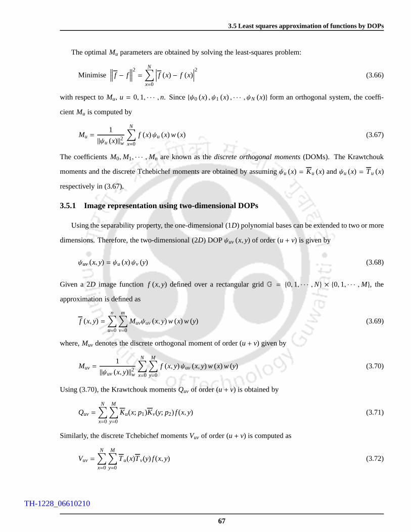
3.5 Least squares approximation of functions by DOPs
The optimalMu parameters are obtained by solving the least-squares problem:
Minimise∥
∥
∥
∥
f − f∥
∥
∥
∥
2=
N∑
x=0
∣
∣
∣
∣
f (x) − f (x)∣
∣
∣
∣
2(3.66)
with respect toMu, u = 0, 1, · · · , n. Sinceψ0 (x) , ψ1 (x) , · · · , ψN (x) form an orthogonal system, the coeffi-
cient Mu is computed by
Mu =1
‖ψu (x)‖2w
N∑
x=0
f (x)ψu (x) w (x) (3.67)
The coefficientsM0,M1, · · · ,Mn are known as thediscrete orthogonal moments(DOMs). The Krawtchouk
moments and the discrete Tchebichef moments are obtained byassumingψu (x) = Ku (x) andψu (x) = Tu (x)
respectively in (3.67).
3.5.1 Image representation using two-dimensional DOPs
Using the separability property, the one-dimensional(1D) polynomial bases can be extended to two or more
dimensions. Therefore, the two-dimensional (2D) DOPψuv (x, y) of order(u+ v) is given by
ψuv (x, y) = ψu (x)ψv (y) (3.68)
Given a 2D image function f (x, y) defined over a rectangular gridG = 0, 1, · · · ,N × 0, 1, · · · ,M, the
approximation is defined as
f (x, y) =n
∑
u=0
m∑
v=0
Muvψuv (x, y) w (x) w (y) (3.69)
where,Muv denotes the discrete orthogonal moment of order(u+ v) given by
Muv =1
‖ψuv (x, y)‖2w
N∑
x=0
M∑
y=0
f (x, y)ψuv (x, y) w (x) w (y) (3.70)
Using (3.70), the Krawtchouk momentsQuv of order(u+ v) is obtained by
Quv =
N∑
x=0
M∑
y=0
Ku(x; p1)Kv(y; p2) f (x, y) (3.71)
Similarly, the discrete Tchebichef momentsVuv of order (u+ v) is computed as
Vuv =
N∑
x=0
M∑
y=0
Tu(x)Tv(y) f (x, y) (3.72)
67
TH-1228_06610210
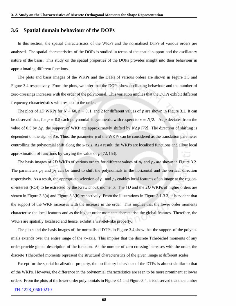
3. A Study on the Characteristics of Discrete Orthogonal Moments for Shape Representation
3.6 Spatial domain behaviour of the DOPs
In this section, the spatial characteristics of the WKPs andthe normalised DTPs of various orders are
analysed. The spatial characteristics of the DOPs is studied in terms of the spatial support and the oscillatory
nature of the basis. This study on the spatial properties of the DOPs provides insight into their behaviour in
approximating different functions.
The plots and basis images of the WKPs and the DTPs of various orders are shown in Figure 3.3 and
Figure 3.4 respectively. From the plots, we infer that the DOPs show oscillating behaviour and the number of
zero-crossings increases with the order of the polynomial.This variation implies that the DOPs exhibit different
frequency characteristics with respect to the order.
The plots of 1D WKPs forN = 60,n = 0, 1, and 2 for different values ofp are shown in Figure 3.1. It can
be observed that, forp = 0.5 each polynomial is symmetric with respect tox = N/2. As p deviates from the
value of 0.5 by∆p, the support of WKP are approximately shifted byN∆p [72]. The direction of shifting is
dependent on the sign of∆p. Thus, the parameterp of the WKPs can be considered as the translation parameter
controlling the polynomial shift along thex-axis. As a result, the WKPs are localised functions and allow local
approximation of functions by varying the value ofp [72,153].
The basis images of 2D WKPs of various orders for different values ofp1 andp2 are shown in Figure 3.2.
The parametersp1 and p2 can be tuned to shift the polynomials in the horizontal and the vertical direction
respectively. As a result, the appropriate selection ofp1 andp2 enables local features of an image at the region-
of-interest (ROI) to be extracted by the Krawtchouk moments. The 1D and the 2D WKPs of higher orders are
shown in Figure 3.3(a) and Figure 3.3(b) respectively. Fromthe illustrations in Figure 3.1-3.3, it is evident that
the support of the WKP increases with the increase in the order. This implies that the lower order moments
characterise the local features and as the higher order moments characterise the global features. Therefore, the
WKPs are spatially localised and hence, exhibit a wavelet-like property.
The plots and the basis images of the normalised DTPs in Figure 3.4 show that the support of the polyno-
mials extends over the entire range of thex−axis. This implies that the discrete Tchebichef moments of any
order provide global description of the function. As the number of zero crossing increases with the order, the
discrete Tchebichef moments represent the structural characteristics of the given image at different scales.
Except for the spatial localization property, the oscillatory behaviour of the DTPs is almost similar to that
of the WKPs. However, the difference in the polynomial characteristics are seen to be more prominent at lower
orders. From the plots of the lower order polynomials in Figure 3.1 and Figure 3.4, it is observed that the number
68
TH-1228_06610210

3.6 Spatial domain behaviour of the DOPs
0 10 20 30 40 50 600
0.1
0.2
0.3
x
K0(x
;p)
p = 0.25, n = 0
0 10 20 30 40 50 60
−0.2
0
0.2
p = 0.25, n = 1
x
K1(x
;p)
0 10 20 30 40 50 60
−0.2
−0.1
0
0.1
0.2
p = 0.25, n = 2
x
K2(x
;p)
0 10 20 30 40 50 600
0.1
0.2
0.3
p = 0.5, n = 0
x
K0(x
;p)
0 10 20 30 40 50 60
−0.2
0
0.2
p = 0.5, n = 1
x
K1(x
;p)
0 10 20 30 40 50 60
−0.2
−0.1
0
0.1
0.2
p = 0.5, n = 2
x
K2(x
;p)
0 10 20 30 40 50 600
0.1
0.2
0.3
p = 0.75, n = 0
x
K0(x
;p)
0 10 20 30 40 50 60
−0.2
0
0.2
p = 0.75, n = 1
x
K1(x
;p)
0 10 20 30 40 50 60
−0.2
−0.1
0
0.1
0.2
p = 0.75, n = 2
xK
2(x
;p)
Np
+N∆p
−N∆p
Figure 3.1: Plots of the WKPs for different values ofp and ordern. The plots illustrate the translation ofKn (x) withrespect to the value ofp. For p = 0.5± ∆p, the polynomial is shifted by a factor of±N∆p. The value ofN = 60.
p1 = 0.25, p2 = 0.25n = 2,m= 0 n = 2,m= 1 n = 2,m= 2 n = 0,m= 5 n = 1,m= 5 n = 2,m= 5
p1 = 0.5, p2 = 0.5n = 2,m= 0 n = 2,m= 1 n = 2,m= 2 n = 0,m= 5 n = 1,m= 5 n = 2,m= 5
p1 = 0.75, p2 = 0.75n = 2,m= 0 n = 2,m= 1 n = 2,m= 2 n = 0,m= 5 n = 1,m= 5 n = 2,m= 5
Figure 3.2: Basis images of 2D WKPs for different values ofp1 andp2. The parametersp1 andp2 control the polynomialposition in the vertical (x− axis) and the horizontal direction (y− axis) respectively. From the illustration, it can also beobserved that the spatial support of the polynomial increase in thex− direction as the value ofn increases. Similarly, thesupport increases in they− direction as the value ofm increases.
69
TH-1228_06610210
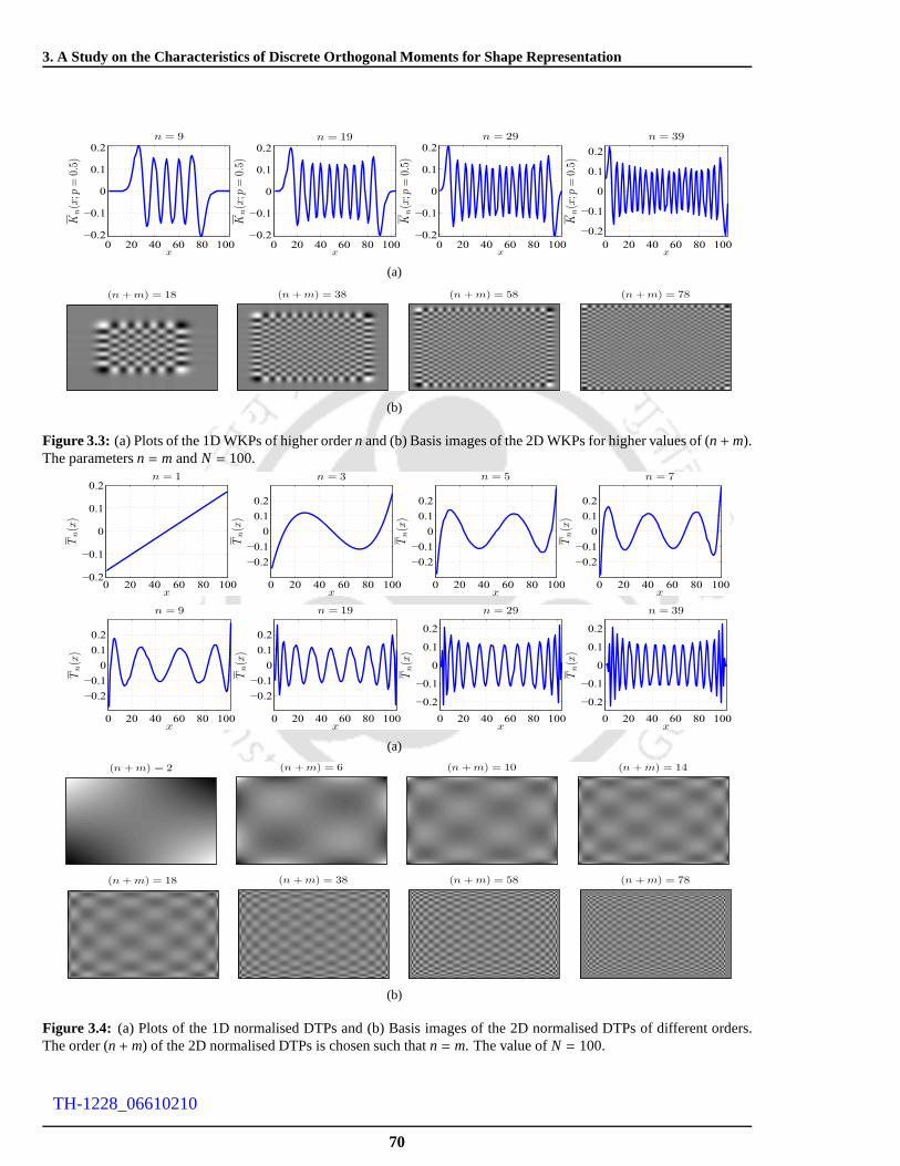
3. A Study on the Characteristics of Discrete Orthogonal Moments for Shape Representation
0 20 40 60 80 100−0.2
−0.1
0
0.1
0.2n = 9
x
Kn(x
;p=
0.5)
0 20 40 60 80 100−0.2
−0.1
0
0.1
0.2n = 19
x
Kn(x
;p=
0.5)
0 20 40 60 80 100−0.2
−0.1
0
0.1
0.2n = 29
x
Kn(x
;p=
0.5)
0 20 40 60 80 100
−0.2
−0.1
0
0.1
0.2
n = 39
x
Kn(x
;p=
0.5)
(a)
(n + m) = 18 (n + m) = 38 (n + m) = 58 (n + m) = 78
(b)
Figure 3.3: (a) Plots of the 1D WKPs of higher ordern and (b) Basis images of the 2D WKPs for higher values of(n+m).The parametersn = m andN = 100.
0 20 40 60 80 100−0.2
−0.1
0
0.1
0.2n = 1
x
Tn(x
)
0 20 40 60 80 100
−0.2
−0.1
0
0.1
0.2
n = 3
x
Tn(x
)
0 20 40 60 80 100
−0.2
−0.1
0
0.1
0.2
n = 5
x
Tn(x
)
0 20 40 60 80 100
−0.2
−0.1
0
0.1
0.2
n = 7
x
Tn(x
)
0 20 40 60 80 100
−0.2
−0.1
0
0.1
0.2
n = 9
x
Tn(x
)
0 20 40 60 80 100
−0.2
−0.1
0
0.1
0.2
n = 19
x
Tn(x
)
0 20 40 60 80 100
−0.2
−0.1
0
0.1
0.2
n = 29
x
Tn(x
)
0 20 40 60 80 100
−0.2
−0.1
0
0.1
0.2
n = 39
x
Tn(x
)
(a)
(n + m) = 2 (n + m) = 6 (n + m) = 10 (n + m) = 14
(n + m) = 18 (n + m) = 38 (n + m) = 58 (n + m) = 78
(b)
Figure 3.4: (a) Plots of the 1D normalised DTPs and (b) Basis images of the2D normalised DTPs of different orders.The order(n+m) of the 2D normalised DTPs is chosen such thatn = m. The value ofN = 100.
70
TH-1228_06610210

3.7 Frequency domain behaviour of the DOPs
of zero crossing at a given order is comparatively higher in WKPs. It is further observed that the densities of
zero crossings slightly vary along its support. This variation in the oscillatory nature is comparatively more
noticeable in the normalised DTPs.
This study on the spatial behaviour of the DOPs suggests thatthe WKPs and the normalised DTPs are
band-pass functions and the moments of different orders approximate different frequency bands of the function
being approximated. The variation in the frequency characteristics of the DOPs can be studied in detail through
their frequency domain representations.
3.7 Frequency domain behaviour of the DOPs
In this section, we empirically analyse the frequency domain characteristics of the WKPs and the nor-
malised DTPs. The frequency domain representation of annthorder DOP is obtained by computing the discrete
Fourier transform (DFT) of the polynomial functionψn (x). The DFT of the polynomial functionψn (x) is given
by [162]
Ψn (ω) =N
∑
x=0
ψn (x) exp(− jωx) (3.73)
where,ω = 2πkN+1, k = 0, 1, · · · ,N. Theenergy spectral density(ESD) of the functionψn (x) is given by|Ψn (ω)|2.
It gives the contribution of the frequency component atω to the total energy.
The Fourier transformsKn (ω) andT n (ω) are obtained by substitutingψn (x) = Kn (x) andψn (x) = Tn (x)
respectively in (3.73).
The plot of the ESD∣
∣
∣
∣
Kn (ω)∣
∣
∣
∣
2of the WKPs obtained forp = 0.5 is shown in Figure 3.5. From the
plots we can infer that the Krawtchouk polynomials act as band-pass functions and exhibit quadrature mirror
symmetry with respect to the ordern. The quadrature mirror property of the WKPs can also be verified by
solving the frequency domain representation obtained through (3.73). Accordingly, by substituting (3.73) it is
straightforward to show
∣
∣
∣
∣
∣
Kn
((
ω − π2
))
∣
∣
∣
∣
∣
=
∣
∣
∣
∣
∣
KN−n
((
ω +π
2
))
∣
∣
∣
∣
∣
(3.74)
The condition in (3.74) ensures that the WKPs of ordersn and N − n exhibit quadrature mirror symmetry
with respect to the quadrature frequencyω = π2. The proof for (3.74) is given in the Appendix 3.10. Using the
quadrature mirror property of the WKPs, Akansu et al [163] derived a class of orthonormal binomial quadrature
mirror filters (QMF) for multiresolution signal decomposition. The binomial QMFs are shown to be identical to
71
TH-1228_06610210

3. A Study on the Characteristics of Discrete Orthogonal Moments for Shape Representation
0.1 0.3 0.5 0.7 0.9 10
2
4
6
ω (×πrad/sample)
∣ ∣
Kn
(ω)∣ ∣
2
n = 0
0.1 0.3 0.5 0.7 0.9 10
2
4
ω (×πrad/sample)
∣ ∣
Kn
(ω)∣ ∣
2
n = 1
0.1 0.3 0.5 0.7 0.9 10
2
4
ω (×πrad/sample)
∣ ∣
Kn
(ω)∣ ∣
2
n = 2
0.1 0.3 0.5 0.7 0.9 10
2
4
ω (×πrad/sample)
∣ ∣
Kn
(ω)∣ ∣
2
n = 3
0.1 0.3 0.5 0.7 0.9 10
2
4
ω (×πrad/sample)
∣ ∣
Kn
(ω)∣ ∣
2
n = 4
0.1 0.3 0.5 0.7 0.9 10
2
4
ω (×πrad/sample)
∣ ∣
Kn
(ω)∣ ∣
2
n = 5
0.1 0.3 0.5 0.7 0.9 10
2
4
ω (×πrad/sample)
∣ ∣
Kn
(ω)∣ ∣
2
n = 6
0.1 0.3 0.5 0.7 0.9 10
2
4
6
ω (×πrad/sample)
∣ ∣
Kn
(ω)∣ ∣
2
n = 7
ω1 = ωp
ω2 ω1 ω2 ω1
ω1
ωBWωp,
ω2 = ωp
ω1ω1 ω2 ω2
ω2ω1 ω2
ω2ω1
Figure 3.5: Plots of the ESD of the 1D WKPs for (N+1) = 8, p = 0.5 andn = 0, 1, · · · , 7. ωBW = |ω2 − ω1|. The figureillustrates the QMF property of the WKPs with respect to the frequencyω = π
2. The frequency characteristics implies thatthe polynomials act as band-pass functions. The WKPs exhibit sidelobes at the lower as well as the higher frequencies.For n < N+1
2 the sidelobes at lower frequencies have higher energy. On the contrary, forn > N+12 the sidelobes present at
the higher frequencies exhibit higher energy.
0.1 0.3 0.5 0.7 0.9 10
2
4
6
8
ω (×πrad/sample)
∣ ∣
Tn
(ω)∣ ∣
2
n = 0
0.1 0.3 0.5 0.7 0.9 10
2
4
ω (×πrad/sample)
∣ ∣
Tn
(ω)∣ ∣
2
n = 1
0.1 0.3 0.5 0.7 0.9 10
2
4
ω (×πrad/sample)
∣ ∣
Tn
(ω)∣ ∣
2
n = 2
0.1 0.3 0.5 0.7 0.9 10
2
4
ω (×πrad/sample)
∣ ∣
Tn
(ω)∣ ∣
2
n = 3
0.1 0.3 0.5 0.7 0.9 10
1
2
3
ω (×πrad/sample)
∣ ∣
Tn
(ω)∣ ∣
2
n = 4
0.1 0.3 0.5 0.7 0.9 10
1
2
3
ω (×πrad/sample)
∣ ∣
Tn
(ω)∣ ∣
2
n = 5
0.1 0.3 0.5 0.7 0.9 10
2
4
ω (×πrad/sample)
∣ ∣
Tn
(ω)∣ ∣
2
n = 6
0.1 0.3 0.5 0.7 0.9 10
2
4
ω (×πrad/sample)
∣ ∣
Tn
(ω)∣ ∣
2
n = 7
ωBW
ω1 = ωp
ω2
ω1 ω2 ω2ω1 ω1 ω2
ω1
ω2 = ωp
ω1ω2ω2ω1
ω2
ωp,
ω1
Figure 3.6: Plots of the ESD of the 1D normalised DTPs for (N+ 1) = 8, p = 0.5 andn = 0, 1, · · · , 7. ωBW = |ω2 − ω1|.The frequency characteristics implies that these polynomials act as band-pass functions. It is also observed that the DTPscontain sidelobes at higher frequencies. The energy of the sidelobes is more in the middle-order polynomials. It can beobserved that the sidelobe energy of the DTPs is higher than that of the WKPs. The DTPs do not exhibit quadraturesymmetry.
72
TH-1228_06610210

3.7 Frequency domain behaviour of the DOPs
Table 3.1: Frequency domain characteristics of WKPs and the normalised DTPs for various ordern. The length of the sequenceN + 1 = 8.
Ordern
WKPs normalised DTPs
Peak frequency Bandwidth Peak frequency Bandwidth
ωp (×πrad/ sec) ωBW (×πrad/ sec) ωp (×πrad/ sec) ωBW (×πrad/ sec)
0 0.016 0.0952 0.016 0.0635
1 0.206 0.159 0.175 0.127
2 0.333 0.159 0.286 0.143
3 0.444 0.143 0.381 0.159
4 0.571 0.143 0.492 0.159
5 0.683 0.159 0.619 0.175
6 0.810 0.159 0.762 0.191
7 1 0.0952 1 0.127
the Daubechies wavelet filters and binomial QMF based signaldecomposition exhibit higher energy compaction
than the discrete cosine transform.
The plots of∣
∣
∣
∣
T n (ω)∣
∣
∣
∣
2for different values ofn are shown in Figure 3.6. From these plots, it is evident
that normalised DTPs show the behaviour of the band-pass functions. However,∣
∣
∣
∣
T n (ω)∣
∣
∣
∣
2does not exhibit the
property of quadrature mirror symmetry.
3.7.1 Quantitative analysis
Similar to the spectral analysis of moments in [164], the frequency domain characteristics of the DOPs are
analysed in terms of the peak frequencies and the bandwidths.
Thepeak frequencyωp is the frequency at which energy of the function is the highest. ThebandwidthωBW
is computed as the difference between the frequencies for which the energy value is 0.707 times of the highest
energy.
The values ofωp and the correspondingωBW for different orders of 8-point WKP and DCP sequences
are given in Table. 3.1. From the table, it is inferred that the peak frequencies of the normalised DTPs are
comparatively smaller than that of the WKPs of the same order. Further, it is also observed that the bandwidth
of the normalised DTPs increases with the order. At higher orders, the normalised DTPs behave as wide-band
band-pass functions and the WKPs are relatively narrow-band functions.
3.7.2 Short-time Fourier transform (STFT) analysis
The plots of the WKPs and the DTPs in the spatial domain, as in Figure 3.3 and Figure 3.4 respectively,
show slightly varying densities of zero-crossings along the support. This suggests the variation of oscillatory
nature of the polynomials alongx. The frequency variation of the polynomial functions with respect tox is
73
TH-1228_06610210

3. A Study on the Characteristics of Discrete Orthogonal Moments for Shape Representation
10 20 30 40 50 60
−0.1
0
0.1
0.2
Kn(x
)
WKP of n = 10
x
x
ω(×
πrad/sam
ple)
Short-time ESD of n = 10
0 20 40 60
0.2
0.4
0.6
0.8
10 20 30 40 50 60
−0.1
0
0.1
0.2
Kn(x
)
WKP of n = 20
x
x
ω(×
πrad/sam
ple)
Short-time ESD for n = 20
0 20 40 60
0.2
0.4
0.6
0.8
10 20 30 40 50 60
−0.2
0
0.2
x
Kn(x
)
WKP of n = 30
x
ω(×
πrad/sam
ple)
Short-time ESD for n = 30
0 20 40 60
0.2
0.4
0.6
0.8
x
ω(×
πrad/sam
ple)
Short-time ESD for n = 40
0 20 40 60
0.2
0.4
0.6
0.8
10 20 30 40 50 60
−0.2
−0.1
0
0.1
0.2
Kn(x
)
WKP of n = 40
x
Figure 3.7: Plots of the 1D WKPs and corresponding ESD obtained using STFT as functions ofx. The plots are obtainedfor (N + 1) = 60 andp = 0.5. The illustration shows that for ordern < N+1
2 , the low-frequency ESD of the polynomialincreases for the values ofx close tox = 0 andx = N. Forn > N+1
2 , the high-frequency ESD with respect to these valuesgradually increases. The length of the sliding windowξ (.) is chosen as 30 and the number of frequency points is 128.
10 20 30 40 50 60
−0.2
−0.1
0
0.1
0.2
Tn(x
)
DTP of n = 10
x
x
ω(×
πrad/sam
ple)
Short-time ESD of n = 10
0 20 40 60
0.2
0.4
0.6
0.8
10 20 30 40 50 60−0.2
−0.1
0
0.1
0.2
Tn(x
)
DTP of n = 20
x
x
ω(×
πrad/sam
ple)
Short-time ESD for n = 20
0 20 40 60
0.2
0.4
0.6
0.8
10 20 30 40 50 60
−0.2
−0.1
0
0.1
0.2
x
Tn(x
)
DTP of n = 30
x
ω(×
πrad/sam
ple)
Short-time ESD for n = 30
0 20 40 60
0.2
0.4
0.6
0.8
x
ω(×
πrad/sam
ple)
Short-time ESD for n = 40
0 20 40 60
0.2
0.4
0.6
0.8
10 20 30 40 50 60
−0.2
−0.1
0
0.1
0.2
Tn(x
)
DTP of n = 40
x
Figure 3.8: Plots of the 1D normalised DTPs and corresponding ESD obtained using STFT as a function ofx. The plotsare obtained for (N + 1) = 60. The illustration shows that for any given ordern, the high-frequency ESD increases for thevalues ofx close tox = 0 andx = N. The length of the sliding windowξ (.) is chosen as 30 and the number of frequencypoints is 128.
74
TH-1228_06610210

3.8 Shape approximation using DOPs
studied from the time-frequency representation of the DOPs. The time-frequency representation is obtained by
computing theshort-time fourier transform(STFT) of the DOPs. The procedure for deriving the STFT involves
multiplying the polynomial with a window function of compact support and then compute the DFT for each
windowed portion of the polynomial [165]. Accordingly, theexpression for STFT can be written as
Ψn (r, ω) =N
∑
x=0
ψn (x) ξ (x− r) exp(− jωx) (3.75)
where,ξ (.) denotes the window function. The Hanning window is used for experimentation and the coefficients
of anL− point symmetric Hanning window are computed from the following equation.
ξ (l) = 0.5
(
1− cos
(
2πlL − 1
))
, 0 ≤ l ≤ L − 1 (3.76)
The ESD of the STFT response corresponding to the WKP and the normalised DTP bases of different orders
are shown in Figure 3.7 and Figure 3.8 respectively.
The time-frequency images in Figure 3.7 show that the low-frequency ESD of the WKPs up to ordern <
0.5(N + 1) increases as the value ofx deviates fromx = N/2 and approaches the values 0 andN. As the order
becomesn > 0.5(N + 1), the high-frequency ESD increases for the values close tox = 0 andx = N. Contrary
to the WKPs, the STFT response of the DTPs in Figure 3.8 exhibits stronger high frequency response as the
value ofx deviates fromN/2 approaching towardsx = 0 andx = N.
From this frequency characteristics of the DOPs, it clear that the WKPs exhibit better band-pass behaviour
than the DTPs and the energy of the frequency components varies with the derivation from the middle of the
support of the polynomials.
3.8 Shape approximation using DOPs
The studies on the spatial and the frequency domain behaviour of the WKPs and DTPs have shown that
these DOPs are band-pass functions and they exhibit varied characteristics in terms of the spatial localization
and band-pass characteristics. Therefore, these DOPs can be considered as efficient tools for approximating
different shapes. The shape features that are acquired by the Krawtchouk and the discrete Tchebichef moments
will significantly vary due to the varying spatial and the frequency domain characteristics. This section presents
the empirical studies performed to comparatively analyse the performance of the Krawtchouk and the discrete
Tchebichef moments based approximations for shape representation and shape classification. The objective of
this experimentation is to study the efficiency of these DOPsin accurately representing shapes with different
75
TH-1228_06610210

3. A Study on the Characteristics of Discrete Orthogonal Moments for Shape Representation
structural characteristics and defections induced by noise.
The shapes required for the experiments are taken from the MPEG-7 (CE Shape-1, Part-B) database. The
dataset used in the experimentation consists of 20 different shape classes containing 20 samples in each class.
Two sets of experiments were performed. The first set studiesthe efficiency of the WKPs and DTPs in shape
representation. The results include accuracy in approximating different shapes and sensitivity to noise. The
second set of the experiments validates the discrete orthogonal moments as features for shape classification.
3.8.1 Metrics for reconstruction accuracy
The reconstruction accuracy of the DOMs is evaluated using the structural similarity index and the modified
Hausdorff distance as defined below:
The Structural similarity (SSIM) index [166] is a region based similarity measure. The SSIM index
between the shapesf and f is computed locally by dividing the image intoL blocks of uniform size 11× 11.
For l ∈ 1, 2, · · · , L, the SSIM between thelth blocks of f and f is evaluated as
S S IM(
f , f)
l=
(
2µ fµ f + c1
) (
2σ f f + c2
)
(
µ2f + µ
2f+ c1
) (
σ2f + σ
2f+ c2
) (3.77)
whereµ f andµ f denote the mean intensities,σ2f andσ2
fdenote the variances andσ f f denotes the covariance.
The constantsc1 andc2 are included to avoid unstable results when (µ2f + µ
2f) and (σ2
f + σ2f) are very close to
zero. We chosec1 = 0.01 andc2 = 0.03 [166]. The SSIM index betweenf and f S S IM(
f , f)
is given by
S S IM(
f , f)
=1L
L∑
l=1
S S IM(
f , f)
l(3.78)
The value of SSIM index lies in [−1, 1] and a larger value means high similarity between the compared shapes.
Themodified Hausdorff distance (MHD) [91] is employed to measure the similarity based on the shape
boundary. LetA =
α1, α2, · · · , αNA
andB =
β1, β2, · · · , βNB
be the two point sets representing the boundaries
in the shapesf and f respectively andNA and NB represent the corresponding cardinalities. The directed
distance between the point setsA andB is defined as
D (A,B) =1
NA
∑
α∈Aminβ∈B
(‖α − β‖) (3.79)
where,‖.‖ denotes the Euclidean norm. Based on the directed distancesD (A,B) and D (B,A), the MHD is
computed as [91]
MHD = max(D (A,B) ,D (B,A)) (3.80)
76
TH-1228_06610210

3.8 Shape approximation using DOPs
The similarity between the compared shapesf and f is high, if the corresponding MHD is small.
Given the binary shapef (x, y), its approximationf (x, y) is obtained using the Krawtchouk and the dis-
crete Tchebichef moments defined through (3.71) and (3.72) respectively. The approximated shape is binarised
through thresholding. In these experiments, the thresholdfor binarisation is chosen as 0.5. The reconstruction
accuracy of the DOMs is quantitatively compared by using thevalues of the SSIM index and the MHD. The
performance of the orthogonal moments is analysed by varying the order of the moments used for approxima-
tion.
3.8.2 Experiments on shape representation
In this experiment, we analyse the efficiency of the DOP approximations of different orders in representing
the structural variations in shapes under different spatial scales. The structural variation in the shapes are studied
using the curvature variations in the boundary contour. Accordingly, the shapes used for the experiments are
chosen based on their curvature properties. The differencein the structural characteristics of the shapes are
compared based on the number of concave segments and their geometrical properties. The properties of the
concavities on the shape boundary are represented through the curvature scale space (CSS) representation. This
section explains the distinct variation in the structural characteristics of shapes using the CSS and details the
experimental analysis performed to study the accuracy of DOMs in representing different shapes.
3.8.2.1 Characterizing shapes using curvature properties
The curvature properties of the shape boundary are among theimportant perceptual features describing the
shape. The curvature can be defined as the rate of change of slope along the shape boundary and it can be
expressed in terms of the first and the second order derivatives.
Let f denote a binary shape andB be the corresponding shape boundary. Assume,B(u)=(x (u) , y (u)) as
a continuous vector valued function defined by the position vectors(x(u), y(u)). Given the boundary points
(x, y) ∈ B of lengthL, the curvature function is computed as [87]
κ (u) =x (u) y (u) − x (u) y (u)(
x (u)2+ y (u)2
)3/2(3.81)
whereu is a real value such that 0≤ u ≤ (L − 1). For the discrete case, the derivatives ofx and y are
approximated by the corresponding finite differences.
The zero-crossings of the curvature function are theinflection pointson the shape boundary. The local
absolute maximum in the curvature corresponds to a generic corner in the shape [167]. If the maximum value
77
TH-1228_06610210

3. A Study on the Characteristics of Discrete Orthogonal Moments for Shape Representation
0 50 100 150 200 250−1
−0.75
−0.5
−0.25
1
0.25
0.5
0.75
1
Boundary points - u
Cur
vatu
re-κ
(u)
− Zero−crossings
− Negative maxima
− Concave points
− Inflection points
Concave segments
Concavesegment
Concavesegment
Figure 3.9: Illustration of finding the concave segments of a shape from the curvature function derived from the corre-sponding shape boundary. (a) Geometric shape used for illustration; (b) The curvature function derived from the boundaryof the geometric shape and (c) Representing the inflection points and the concave segments on the shape boundary. Thezero-crossings correspond to the inflection points. Similarly, the negative maxima correspond to the concave points.
Table 3.2: Types of concavities based on the width and the depth of the concave segments.
Width Depth Type of concavitySmall Small Narrow - Shallow concavitySmall High Narrow - Deep concavityHigh Small Wide - Shallow concavityHigh High Wide - Deep concavity
is positive, the corner is considered as the convex point andif the maximum is negative, the corner is considered
as the concave point. The boundary section between the inflection points that contain the convex point is the
convex segmentand the section constituting the concave point comprises theconcave segment.
Since, the shape boundary is a closed curve, the concave segments provide comparatively more detailed
information and they constitute the transition between different parts of the shape. An example illustrating
the inflection points and the concave segments of a geometricshape along with the corresponding curvature
function is shown in Figure 3.9.
The structural variations in shape can be characterised by the variations in the width and the depth of the
concave segments. The width of a concave segment can be computed as the length of the line connecting the
corresponding two inflection points. The depth of the concave segment is the distance between the concave
point and the line connecting the corresponding inflection points. Based on the width and the depth values, the
concavities can be divided in to four types as listed in Table3.2.
The characteristics of the concavities present in the shapecan be represented using the curvature scale
space (CSS) representation. The CSS representation is a mapof the location of the zero-crossings in the
curvature functionκ (u) obtained over successive smoothing of the shape boundary [87]. ConvolvingB with a
1D Gaussian kernelg (u, σ) of standard deviationσ results in the smoothed curveBσ = (X,Y). The smoothed
78
TH-1228_06610210

3.8 Shape approximation using DOPs
boundary points are given by
X (u, σ) = x (u) ∗ g (u, σ)
Y (u, σ) = y (u) ∗ g (u, σ)(3.82)
Accordingly, the curvature onBσ is computed as
κ (u, σ) =X (u, σ) Y (u, σ) − X (u, σ) Y (u, σ)
(
X (u, σ)2+ Y (u, σ)2
)3/2(3.83)
The CSS descriptors that represent the location of the inflection points on the curve are extracted for varying
values ofσ and are used to obtain the CSS image that is defined as
ICS S(u, σ) = (u, σ) |κ (u, σ) = 0 (3.84)
The CSS map consists of several arch-shaped contours, each related to the concave segments of the shape
boundary. The height and the base width of the arch-shaped contours reflect the depth and the width of the
concavities respectively [168, 169]. The height of the CSS contours is larger for wide-shallow, wide-deep and
narrow-deep concavities.
A few examples of the shapes used in this experiment and the corresponding CSS representations are
shown in Figure 3.10 and Figure 3.11. The CSS representations of three star-shaped polygons consisting of 16
concave segments of almost same width and varying depth are illustrated in Figure 3.10. It can be observed
that the number of arch-shaped contours in the CSS map is equal to the number of concave segments in the
shape boundary. The shape in Figure 3.10(a) consists of shallow concave segments in comparison to the shapes
illustrated in Figure 3.10(b) and 3.10(c). The star-shapedpolygon in Figure 3.10(c) exhibits deeper concave
segments and hence, the height of the arch-shaped contours in the corresponding CSS map is comparatively
higher. By comparing the CSS maps in Figure 3.10, it can easily inferred that the height of the contours in the
CSS map increases with the depth of the concave segments.
Figure 3.11 illustrates the CSS representation of three different shapes composed of different number of
concave segments of different width. The shape of the character ‘T’ in Figure 3.11(a) consists of two wide-
deep concave segments and hence, the corresponding CSS map exhibits two arch-shaped contours representing
the concavities. Similarly, the CSS representations of a cross-shaped and the fork-shaped polygons in Fig-
ure 3.11(b) and Figure 3.11(c) respectively reflect the number of concavities in the shape boundary. The cross-
shaped polygon is composed of concave segments of almost same width and depth. Hence, the arch-shaped
contours in the corresponding CSS map are of approximately same height and base width. The fork-shaped
79
TH-1228_06610210
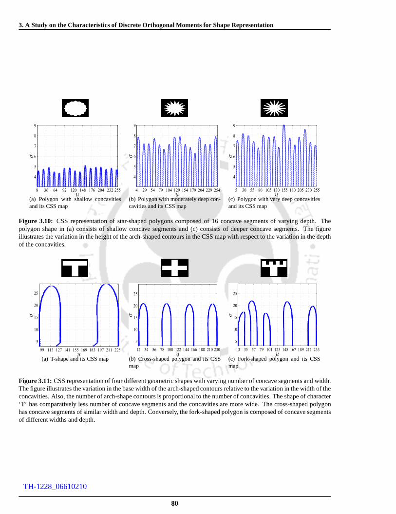
3. A Study on the Characteristics of Discrete Orthogonal Moments for Shape Representation
8 36 64 92 120 148 176 204 232 255
4
5
6
7
8
9
u
σ
(a) Polygon with shallow concavitiesand its CSS map
4 29 54 79 104 129 154 179 204 229 254
4
5
6
7
8
9
u
σ
(b) Polygon with moderately deep con-cavities and its CSS map
5 30 55 80 105 130 155 180 205 230 255
4
5
6
7
8
9
u
σ
(c) Polygon with very deep concavitiesand its CSS map
Figure 3.10: CSS representation of star-shaped polygons composed of 16 concave segments of varying depth. Thepolygon shape in (a) consists of shallow concave segments and (c) consists of deeper concave segments. The figureillustrates the variation in the height of the arch-shaped contours in the CSS map with respect to the variation in the depthof the concavities.
99 113 127 141 155 169 183 197 211 225
5
10
15
20
25
u
σ
(a) T-shape and its CSS map
12 34 56 78 100 122 144 166 188 210 230
5
10
15
20
25
u
σ
(b) Cross-shaped polygon and its CSSmap
13 35 57 79 101 123 145 167 189 211 233
5
10
15
20
25
u
σ
(c) Fork-shaped polygon and its CSSmap
Figure 3.11:CSS representation of four different geometric shapes withvarying number of concave segments and width.The figure illustrates the variation in the base width of the arch-shaped contours relative to the variation in the width of theconcavities. Also, the number of arch-shape contours is proportional to the number of concavities. The shape of character‘T’ has comparatively less number of concave segments and the concavities are more wide. The cross-shaped polygonhas concave segments of similar width and depth. Conversely, the fork-shaped polygon is composed of concave segmentsof different widths and depth.
80
TH-1228_06610210

3.8 Shape approximation using DOPs
polygon consists of five deep concave segments. Based on the base width of the arch-shaped contours in the
CSS map, it can be easily verified that the fork-shaped polygon is composed of two wide concavities and three
comparatively narrow concavities. The base width of the CSScontours in Figure 3.11(b) and Figure 3.11(c) is
less than that of the CSS contours illustrated in Figure 3.11(a). This implies that the T-shape is composed of
comparatively wide concavities. By comparing the base widths of the arch-shaped contours in the CSS maps
shown in Figure 3.10 and Figure 3.11, it can be inferred that the shapes presented in Figure 3.10 are composed
of comparatively narrow concave segments.
Using the above curvature properties of the shape boundaries, it is also possible to infer the various spatial
frequency structures of the shapes. It can be easily verifiedthat the shapes composed of many number of deep
concave segments consists of large number of transitions between the background and the object regions. Such
shapes can be considered as complex shapes with higher spatial frequency regions and hence, exhibit large
structural details. The shapes composed of shallow segments such as the star-shaped polygon in Figure 3.10(a)
consist of less number of transitions between the background and the object regions. Hence, such shapes are
composed of low spatial frequency regions with less structural details. On the other hand, the shapes presented
in Figure 3.11 consist of less number of concave segments than the star-shaped polygon in Figure 3.10(a).
However, the concave segments of the shapes presented in Figure 3.11 are comparatively deeper exhibiting
high spatial frequency regions. From this discussion on thecurvature properties, it is understood that the
complexity of the shapes in terms of the structural details increases with the number of concavities and the
depth of the concavities.
3.8.2.2 Spatial scale of the shapes
Another important factor considered in this experiment is the spatial scale of the foreground region contain-
ing the shape with respect to the enclosed background region. Generally, in shape based object representation
methods, the objects to be recognised are segmented from a scene and hence, the size of the object may vary de-
pending upon the spatial resolution of the scene. Since the scenes are unconstrained, the size of the segmented
object that constitutes the foreground region is unpredictable. As the DOPs are computed over the entire shape
grid, the representation accuracy of the DOPs may vary with the spatial scale of the foreground object.
The images containing the shapes are binarised such that thepixels belonging to the object region are
assigned the intensity value ‘1’ and the pixels constituting the background are assigned the intensity value
‘0’.The size of the image grid is fixed at 90× 90. The scale of the object’s shape is varied as 40× 40, 60× 60
and 80× 80. The parametersp1 andp2 of the WKPs are chosen as 0.5 so that the emphasis of the polynomial
81
TH-1228_06610210

3. A Study on the Characteristics of Discrete Orthogonal Moments for Shape Representation
is with respect to the centroid of the shape.
3.8.2.3 Variation in shapes versus reconstruction accuracy
The experiments are performed on the shapes presented in Figure 3.10 and Figure 3.11 and the results
obtained are presented in the illustrations given through Figure 3.12 - Figure 3.17. The efficiency of the DOMs
in accurately approximating different shapes is tested anddiscussed in terms of variation in the spatial scale of
the shape and different structural characteristics.
From the results shown in Figure 3.12 - Figure 3.17, we can observe that the performance of the Krawtchouk
moments in terms of the SSIM index and the MHD is consistentlyhigher at all the orders while approximating
shapes of lower scale 40×40. As the scale increases to 60×60 and 80×80, it is noticed that the reconstruction
accuracy of the WKPs decreases for lower order approximations. This occurs due to the variation in the spatial
support of the WKPs with respect to its order. As mentioned earlier, the lower order WKPs have smaller spatial
supports and the support increases only with the order. In the case of shapes with lower scale values, most
of the shape region lies within the spatial support of the WKPs yielding higher reconstruction accuracy at the
lower order itself. As the scale of the shape increases, the entire shape region is not sufficiently spanned by the
lower order WKPs. Hence, under this condition, the order of the WKPs has to be high for better reconstruction
accuracy.
Converse to the performance of WKPs, it can be observed that the lower order DTPs offer poor reconstruc-
tion accuracy while approximating shapes of lower scale. Itis known that the spatial support of the DTP extends
over the entire range of the image grid offering a global support. The lower order DTPs exhibit less peak fre-
quencies and hence, while approximating shapes they more orless behave like averaging functions resulting
in excessive smoothing. As the order increases, the high frequency response of the DTP increases providing
effective reconstruction of the high spatial frequency structures of the shape. While approximating shapes of
lower scales, the background region is more dominating thanthe shape region and hence the averaging effect
on the shapes is more than in the case of shapes with higher scales.
The results of DOM based approximation of the star-shaped polygons with varying depth of concavities
are shown in Figure 3.12, Figure 3.13 and Figure 3.14. These results illustrate the efficiency of the DOMs in
approximating the concave segments that constitute the structure of the shape. From the corresponding plots
of the SSIM index and the MHD values obtained for various orders of the DOM based approximation, it is
observed that the performance of the DOMs significantly varies at the lower orders.
The star-shaped polygon in Figure 3.12 consists of shallow concave segments and the shape is composed
82
TH-1228_06610210
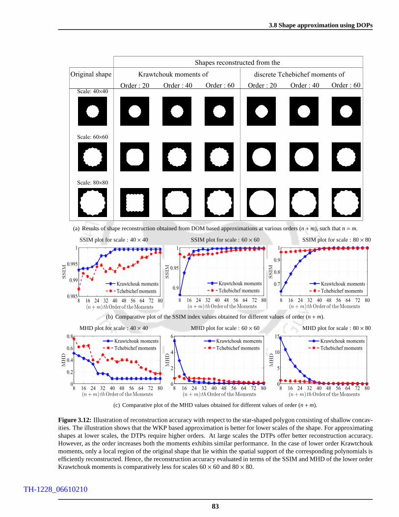
3.8 Shape approximation using DOPs
Scale: 40×40
Scale: 60×60
Scale: 80×80
Krawtchouk moments of discrete Tchebichef moments of
Order : 20 Order : 40 Order : 60 Order : 60Order : 40Order : 20
Shapes reconstructed from the
Original shape
(a) Results of shape reconstruction obtained from DOM basedapproximations at various orders (n+m), such thatn = m.
SSIM plot for scale : 40× 40 SSIM plot for scale : 60× 60 SSIM plot for scale : 80× 80
8 16 24 32 40 48 56 64 72 800.985
0.99
0.995
1
(n + m) thOrder of theMoments
SSIM
Krawtchouk moments
Tchebichef moments
8 16 24 32 40 48 56 64 72 80
0.9
0.95
1
(n + m) thOrder of theMoments
SSIM
Krawtchouk moments
Tchebichef moments
8 16 24 32 40 48 56 64 72 80
0.7
0.8
0.9
1
(n + m) thOrder of theMoments
SSIM
Krawtchouk moments
Tchebichef moments
(b) Comparative plot of the SSIM index values obtained for different values of order (n+m).
MHD plot for scale : 40× 40 MHD plot for scale : 60× 60 MHD plot for scale : 80× 80
8 16 24 32 40 48 56 64 72 800
0.2
0.4
0.6
0.8
(n + m) thOrder of theMoments
MH
D
Krawtchouk moments
Tchebichef moments
8 16 24 32 40 48 56 64 72 800
2
4
6
(n + m) thOrder of theMoments
MH
D
Krawtchouk moments
Tchebichef moments
8 16 24 32 40 48 56 64 72 800
5
10
15
(n + m) thOrder of theMoments
MH
D
Krawtchouk moments
Tchebichef moments
(c) Comparative plot of the MHD values obtained for different values of order (n+m).
Figure 3.12: Illustration of reconstruction accuracy with respect to the star-shaped polygon consisting of shallow concav-ities. The illustration shows that the WKP based approximation is better for lower scales of the shape. For approximatingshapes at lower scales, the DTPs require higher orders. At large scales the DTPs offer better reconstruction accuracy.However, as the order increases both the moments exhibits similar performance. In the case of lower order Krawtchoukmoments, only a local region of the original shape that lie within the spatial support of the corresponding polynomials isefficiently reconstructed. Hence, the reconstruction accuracy evaluated in terms of the SSIM and MHD of the lower orderKrawtchouk moments is comparatively less for scales 60× 60 and 80× 80.
83
TH-1228_06610210

3. A Study on the Characteristics of Discrete Orthogonal Moments for Shape Representation
Scale: 40×40
Scale: 60×60
Scale: 80×80
Krawtchouk moments of discrete Tchebichef moments of
Order : 20 Order : 40 Order : 60 Order : 60Order : 40Order : 20
Shapes reconstructed from the
Original shape
(a) Results of shape reconstruction obtained from DOM basedapproximations at various orders (n+m), such thatn = m.
SSIM plot for scale : 40× 40 SSIM plot for scale : 60× 60 SSIM plot for scale : 80× 80
8 16 24 32 40 48 56 64 72 800.95
0.96
0.97
0.98
0.99
(n + m) thOrder of theMoments
SSIM
Krawtchouk moments
Tchebichef moments
8 16 24 32 40 48 56 64 72 800.9
0.95
1
(n + m) thOrder of theMoments
SSIM
Krawtchouk moments
Tchebichef moments
8 16 24 32 40 48 56 64 72 800.8
0.85
0.9
0.95
1
(n + m) thOrder of theMoments
SSIM
Krawtchouk moments
Tchebichef moments
(b) Comparative plot of the SSIM index values obtained for different values of order (n+m).
MHD plot for scale : 40× 40 MHD plot for scale : 60× 60 MHD plot for scale : 80× 80
8 16 24 32 40 48 56 64 72 800
1
2
3
(n + m) thOrder of theMoments
MH
D
Krawtchouk moments
Tchebichef moments
8 16 24 32 40 48 56 64 72 800
1
2
3
4
(n + m) thOrder of theMoments
MH
D
Krawtchouk moments
Tchebichef moments
8 16 24 32 40 48 56 64 72 800
2
4
6
8
(n + m) thOrder of theMoments
MH
D
Krawtchouk moments
Tchebichef moments
(c) Comparative plot of the MHD values obtained for different values of order (n+m).
Figure 3.13: Illustration of reconstruction accuracy with respect to the star-shaped polygon with moderately deep concav-ities. The results in terms of the SSIM and MHD indicates thatthe accuracy of the WKPs is comparatively higher than theDTPs in approximating shapes at different scales. The concavities are more accurately reconstructed by the Krawtchoukmoments and the Tchebichef moments result in smoothened reconstruction of the sharp concave segments.
84
TH-1228_06610210

3.8 Shape approximation using DOPs
Scale: 40×40
Scale: 60×60
Scale: 80×80
Krawtchouk moments of discrete Tchebichef moments of
Order : 20 Order : 40 Order : 60 Order : 60Order : 40Order : 20
Shapes reconstructed from the
Original shape
(a) Results of shape reconstruction obtained from DOM basedapproximations at various orders (n+m), such thatn = m.
SSIM plot for scale : 40× 40 SSIM plot for scale : 60× 60 SSIM plot for scale : 80× 80
8 16 24 32 40 48 56 64 72 800.94
0.96
0.98
1
(n + m) thOrder of theMoments
SSIM
Krawtchouk moments
Tchebichef moments
8 16 24 32 40 48 56 64 72 800.85
0.9
0.95
1
(n + m) thOrder of theMoments
SSIM
Krawtchouk moments
Tchebichef moments
8 16 24 32 40 48 56 64 72 80
0.8
0.9
1
(n + m) thOrder of theMoments
SSIM
Krawtchouk moments
Tchebichef moments
(b) Comparative plot of the SSIM index values obtained for different values of order (n+m).
MHD plot for scale : 40× 40 MHD plot for scale : 60× 60 MHD plot for scale : 80× 80
8 16 24 32 40 48 56 64 72 800
1
2
3
4
(n + m) thOrder of theMoments
MH
D
Krawtchouk moments
Tchebichef moments
8 16 24 32 40 48 56 64 72 800
2
4
6
(n + m) thOrder of theMoments
MH
D
Krawtchouk moments
Tchebichef moments
8 16 24 32 40 48 56 64 72 800
2
4
6
8
(n + m) thOrder of theMoments
MH
D
Krawtchouk moments
Tchebichef moments
(c) Comparative plot of the MHD values obtained for different values of order (n+m).
Figure 3.14: Illustration of DOM based approximation of a star-shaped polygon consisting of deep concave segments.The illustration shows that the performance of the Krawtchouk moments at all the orders is consistently superior to thediscrete Tchebichef moments in approximating the shapes atall three different scales.
85
TH-1228_06610210
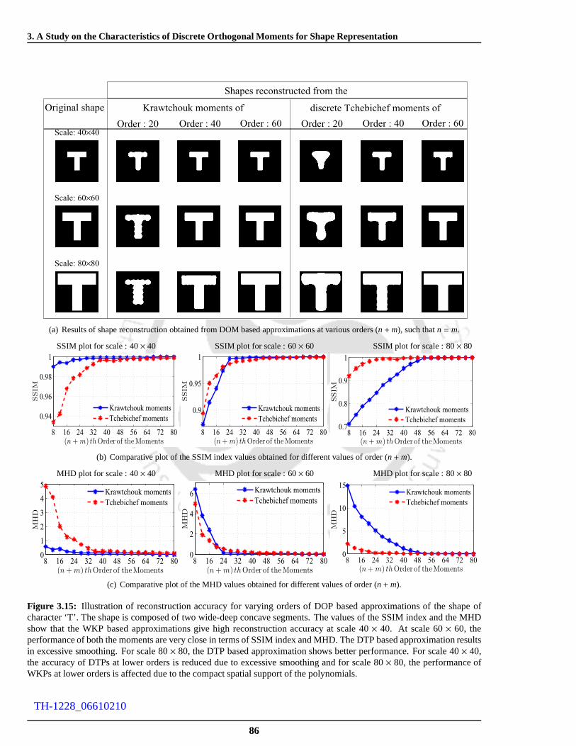
3. A Study on the Characteristics of Discrete Orthogonal Moments for Shape Representation
Scale: 40×40
Scale: 60×60
Scale: 80×80
Krawtchouk moments of discrete Tchebichef moments of
Order : 20 Order : 40 Order : 60 Order : 60Order : 40Order : 20
Shapes reconstructed from the
Original shape
(a) Results of shape reconstruction obtained from DOM basedapproximations at various orders (n+m), such thatn = m.
SSIM plot for scale : 40× 40 SSIM plot for scale : 60× 60 SSIM plot for scale : 80× 80
8 16 24 32 40 48 56 64 72 80
0.94
0.96
0.98
1
(n + m) thOrder of theMoments
SSIM
Krawtchouk moments
Tchebichef moments
8 16 24 32 40 48 56 64 72 80
0.9
0.95
1
(n + m) thOrder of theMoments
SSIM
Krawtchouk moments
Tchebichef moments
8 16 24 32 40 48 56 64 72 800.7
0.8
0.9
1
(n + m) thOrder of theMoments
SSIM
Krawtchouk moments
Tchebichef moments
(b) Comparative plot of the SSIM index values obtained for different values of order (n+m).
MHD plot for scale : 40× 40 MHD plot for scale : 60× 60 MHD plot for scale : 80× 80
8 16 24 32 40 48 56 64 72 800
1
2
3
4
5
(n + m) thOrder of theMoments
MH
D
Krawtchouk moments
Tchebichef moments
8 16 24 32 40 48 56 64 72 800
2
4
6
(n + m) thOrder of theMoments
MH
D
Krawtchouk moments
Tchebichef moments
8 16 24 32 40 48 56 64 72 800
5
10
15
(n + m) thOrder of theMoments
MH
D
Krawtchouk moments
Tchebichef moments
(c) Comparative plot of the MHD values obtained for different values of order (n+m).
Figure 3.15: Illustration of reconstruction accuracy for varying orders of DOP based approximations of the shape ofcharacter ‘T’. The shape is composed of two wide-deep concave segments. The values of the SSIM index and the MHDshow that the WKP based approximations give high reconstruction accuracy at scale 40× 40. At scale 60× 60, theperformance of both the moments are very close in terms of SSIM index and MHD. The DTP based approximation resultsin excessive smoothing. For scale 80× 80, the DTP based approximation shows better performance. For scale 40× 40,the accuracy of DTPs at lower orders is reduced due to excessive smoothing and for scale 80× 80, the performance ofWKPs at lower orders is affected due to the compact spatial support of the polynomials.
86
TH-1228_06610210

3.8 Shape approximation using DOPs
of a low spatial frequency region. The plots of the SSIM indexand the MHD obtained between DOM based
approximation and the original shape are shown in Figure 3.12(b) and Figure 3.12(c) respectively. From the
values obtained, we infer that the WKP based reconstructionyields higher representation accuracy for the scales
of 40× 40 and 60× 60. From the corresponding reconstructed shapes shown in Figure 3.12(a), it is evident
that the shallow concavities are accurately reconstructedin the Krawtchouk moments based approximation. We
observe that the DTPs require higher orders to accurately approximate the shallow concave segments. Since the
shape is composed of a low spatial frequency region, the lower order DTP based approximations at higher scale
80× 80 is comparatively superior. Though, the performance of lower order WKPs is limited due to compact
support, it should be noted that the concavities are better represented in the WKP based approximation of the
shapes at various scales.
The star-shaped polygons presented in Figure 3.13 and Figure 3.14 are composed of deep concave segments
exhibiting high spatial frequency regions. Particularly,the polygon in Figure 3.14 exhibits comparatively more
structural variations. The reconstructed shapes shown in Figure 3.13(a) and Figure 3.14(a) show that the WKP
based approximation results in perceptually more similar reconstruction than the DTPs based approximation.
The plots of the SSIM index and the MHD values also confirm the efficiency of the WKPs. By comparing
the results obtained for the three different star-shaped polygons, we can infer that the DTPs are not efficient
in accurately representing the sharp transitions such as the concave segments of the shapes. The efficiency of
the DTPs decreases if the shape consists of more high spatialfrequency regions. On the other hand, even the
lower order Krawtchouk moments are more efficient in representing the high spatial frequency regions in the
star-shaped polygons discussed above.
Similar evaluations are performed on the geometric shapes shown in Figure 3.11. Accordingly, the evalua-
tions reflect the behaviour of the DOMs in representing shapes composed of deep concave segments of various
widths. Figure 3.15 illustrates the efficiency of the DOMs inrepresenting the shape of character T. The T-shape
consists of only two deep concave segments with less number of transitions between the background and the
foreground. However, the T-shape is composed of two regionsof different spatial supports and in comparison
to the cross-shaped and fork-shaped polygons, the T-shape exhibits less structural variations. From the recon-
structed shapes shown in Figure 3.15(a), it is evident that at lower order approximations the WKPs result in
better approximation of the sharp structural details. The plots of the SSIM index and the MHD show that at
lower scales, the performance of the Krawtchouk moments is significantly better than the DTP based approxi-
mations. As the scale increases to 60×60, the efficiency of the DOPs in terms of the SSIM index and theMHD
87
TH-1228_06610210

3. A Study on the Characteristics of Discrete Orthogonal Moments for Shape Representation
Scale: 40×40
Scale: 60×60
Scale: 80×80
Krawtchouk moments of discrete Tchebichef moments of
Order : 20 Order : 40 Order : 60 Order : 60Order : 40Order : 20
Shapes reconstructed from the
Original shape
(a) Results of shape reconstruction obtained from DOM basedapproximations at various orders (n+m), such thatn = m.
SSIM plot for scale : 40× 40 SSIM plot for scale : 60× 60 SSIM plot for scale : 80× 80
8 16 24 32 40 48 56 64 72 800.94
0.96
0.98
1
(n + m) thOrder of theMoments
SSIM
Krawtchouk moments
Tchebichef moments
8 16 24 32 40 48 56 64 72 80
0.9
0.95
1
(n + m) thOrder of theMoments
SSIM
Krawtchouk moments
Tchebichef moments
8 16 24 32 40 48 56 64 72 80
0.8
0.85
0.9
0.95
1
(n + m) thOrder of theMoments
SSIM
Krawtchouk moments
Tchebichef moments
(b) Comparative plot of the SSIM index values obtained for different values of order (n+m).
MHD plot for scale : 40× 40 MHD plot for scale : 60× 60 MHD plot for scale : 80× 80
8 16 24 32 40 48 56 64 72 800
1
2
3
4
(n + m) thOrder of theMoments
MH
D
Krawtchouk moments
Tchebichef moments
8 16 24 32 40 48 56 64 72 800
2
4
6
(n + m) thOrder of theMoments
MH
D
Krawtchouk moments
Tchebichef moments
8 16 24 32 40 48 56 64 72 800
5
10
(n + m) thOrder of theMoments
MH
D
Krawtchouk moments
Tchebichef moments
(c) Comparative plot of the MHD values obtained for different values of order (n+m).
Figure 3.16: Illustration of reconstruction accuracy with respect to the cross-shaped polygon. The shape is composed offour concave segments of same width and depth. The SSIM indexand the MHD show that the WKP based approximationsgive high reconstruction accuracy for scales 40×40 and 60×60. The shapes reconstructed from DTP based approximationare over-smoothened. At higher scale 80× 80, the spatial support of the lower order WKPs is not sufficiently large andhence, the reconstruction error is more at these orders.
88
TH-1228_06610210

3.8 Shape approximation using DOPs
Scale: 40×40
Scale: 60×60
Scale: 80×80
Krawtchouk moments of discrete Tchebichef moments of
Order : 20 Order : 40 Order : 60 Order : 60Order : 40Order : 20
Shapes reconstructed from the
Original shape
(a) Results of shape reconstruction obtained from DOM basedapproximations at various orders (n+m), such thatn = m.
SSIM plot for scale : 40× 40 SSIM plot for scale : 60× 60 SSIM plot for scale : 80× 80
8 16 24 32 40 48 56 64 72 800.94
0.96
0.98
1
(n + m) thOrder of theMoments
SSIM
Krawtchouk moments
Tchebichef moments
8 16 24 32 40 48 56 64 72 80
0.9
0.95
1
(n + m) thOrder of theMoments
SSIM
Krawtchouk moments
Tchebichef moments
8 16 24 32 40 48 56 64 72 800.8
0.85
0.9
0.95
1
(n + m) thOrder of theMoments
SSIM
Krawtchouk moments
Tchebichef moments
(b) Comparative plot of the SSIM index values obtained for different values of order (n+m).
MHD plot for scale : 40× 40 MHD plot for scale : 60× 60 MHD plot for scale : 80× 80
8 16 24 32 40 48 56 64 72 800
2
4
6
8
(n + m) thOrder of theMoments
MH
D
Krawtchouk moments
Tchebichef moments
8 16 24 32 40 48 56 64 72 800
2
4
6
8
(n + m) thOrder of theMoments
MH
D
Krawtchouk moments
Tchebichef moments
8 16 24 32 40 48 56 64 72 800
5
10
(n + m) thOrder of theMoments
MH
D
Krawtchouk moments
Tchebichef moments
(c) Comparative plot of the MHD values obtained for different values of order (n+m).
Figure 3.17: Illustration of reconstruction accuracy with respect to a fork-shaped polygon. The shape is a high spatialfrequency structure consisting of five concave segments of different width and depth. The accuracy in reconstructionevaluated in terms of the SSIM index and the MHD show that the Krawtchouk moments based approximation is compar-atively high for scales 40× 40 and 60× 60. It is observed that the shapes reconstructed from Tchebichef moments aremore smoothened and the high spatial frequency regions are not properly reconstructed at lower orders. At a higher scaleof 80× 80, the accuracy of the WKP based approximation is poor due tothe limited spatial support of the polynomialbasis.
89
TH-1228_06610210

3. A Study on the Characteristics of Discrete Orthogonal Moments for Shape Representation
are very close even at lower orders.
The cross-shaped polygon illustrated in Figure 3.16 consists of more concave segments and exhibits more
structural details than the T-shape. In comparison to the behaviour of DTPs in approximating the T-shape, we
can observe that its performance is decreased in approximating the cross-shaped polygon. This can be clearly
inferred by comparing the plots in Figure 3.15(b) and Figure3.16(b). The DTPs require comparatively higher
orders for approximating the cross-shaped polygon. Similarly, by comparing the plots in Figure 3.15(c) and
Figure 3.16(c), we can infer that the order of the DTPs required for approximating shapes of scale 80× 80
depends on the complexity of the shape i.e., the structural details. It can observed that the order of the DTPs
required for accurately representing the cross-shaped polygon at scale 80×80 is more than that required for the
T-shape.
Similar variations in the performance of the DOPs can be observed from the results obtained for the ap-
proximation of fork-shaped polygons of various scales. Thefork-shaped polygon consists of more concave
segments than the T-shape and the cross-shaped polygons. For scales 40× 40 and 60× 60, the WKP based ap-
proximation recovers the spatial structures of the fork-shaped polygon, whereas the DTPs result in excessively
smoothened reconstruction. At a higher scale of 80× 80, the concavities are recovered well by the Krawtchouk
moments but their performance is limited due to their compact spatial support at lower orders. From the values
of SSIM index and the MHD in shown Figure 3.17(c), it is clear that the order of DTPs required for accurate
reconstruction has increased in comparison to the T-shape and the cross-shaped polygons.
From the above analysis, we infer that the performance of theDOPs depends on the scale of the shape
and the structural characteristics. Accordingly, the characteristics of the WKPs and the DTPs in representing
different shapes can be summarised as follows.
(i) The Krawtchouk moments are efficient when the shape region is sufficiently spanned by the corresponding
WKPs. The WKPs have compact supports at lower orders and behave as spatially localised functions.
Further, as explained in Section 3.7, the peak frequencies ‘ωp’ of the lower order WKPs is higher than the
peak frequencies of the DTPs. Therefore, the lower order Krawtchouk moments are comparatively more
efficient in approximating regions with high spatial frequencies and smaller spatial supports.
(ii) The DTPs have wider support and for any order the supportis equal to the size of the image. This
implies that the Tchebichef moments are global functions. Hence, the DTPs are better than the WKPs in
approximating shapes composed of wide regions of low spatial frequencies such as the shapes composed
of convex segments and shallow concavities. For complex shapes composed of several high frequency
90
TH-1228_06610210

3.8 Shape approximation using DOPs
structures, the DTPs result in excessive smoothing.
(iii) In terms of the data compaction, we can infer that for approximating shapes at lower scales, the WKPs
require less order than the DTPs. As the scale increases, theWKPs require higher orders than the DTPs.
However, it should be noted that the optimal choice of the order of DTPs in approximating shapes at higher
scales is greatly influenced by the structural characteristics of the shape. When the shape is composed
of high spatial frequency structures, the WKPs are superiorto the DTPs even if the scale of the shape is
high.
Thus, we can infer that the WKPs offer better data compactionat lower scales and at these scales, the
performance of the WKPs is consistently superior irrespective of the structural characteristics of the shapes.
At higher scales, the WKPs offer better data compaction in the case of shapes with high spatial frequencies.
Conversely, at higher scales, the data compaction capability of the DTPs is high for shapes with less structural
variations.
3.8.2.4 Noise versus reconstruction accuracy
During the binarisation of an image, segmentation errors such as isolated pixels within a uniform region
occur due to the presence of the acquisition noise in the gray-scale image and improper threshold selection.
These pixels appear as extraneous foreground pixels in the background and extraneous background pixels in
the foreground. This results in a noisy binary shape and the resulting binary noise is known as thesalt and
pepper noise. Therefore, noise removal is an essential task in shape representation.
The noise pixels in an image are randomly distributed and they exhibit higher spatial frequencies than
the image structures. The study on the spectral characteristics of the WKPs and the DTPs suggests that the
polynomials up to certain order may behave like smoothing functions and result in noise removal. The shapes
reconstructed from the corresponding moment based approximations can be expected to be denoised.
The objective of this set of experiments is to study the performance of the DOPs in accurately reconstructing
shapes that are degraded by different levels of noise. The noisy shapefnoisy is obtained by allowing a fixed
percentage of randomly selected pixel values to be altered to zero or one with equal probabilities. In this
experiment, the robustness of the DOPs is verified by the varying the noise levelpn between 0.05 to 0.6.
Based on the results in Section 3.8.2.3, the size of the shapeis fixed at 60× 60 and the image grid size is
fixed at 90× 90. The order of the WKPs and the DTPs is chosen as(n+m) = 60. The parametersp1 andp2 of
the WKPs are fixed at 0.5. The reconstruction accuracy of the DOMs is evaluated in terms of the SSIM index
91
TH-1228_06610210

3. A Study on the Characteristics of Discrete Orthogonal Moments for Shape Representation
Original shape
(a)
pn = 0.05 pn = 0.2 pn = 0.35 pn = 0.5
(b) Noisy samples of the original shape in Figure 3.18(a).
Reconstructed shapes from Krawtchouk moments
Reconstructed shapes from discrete Tchebichef moments
(c) Results of shapes reconstructed from the DOM based ap-proximations of the noisy samples illustrated in Figure 3.18(b).The order of the moments is chosen as(n+m) = 60.
0.1 0.2 0.3 0.4 0.5 0.60.85
0.9
0.95
1
Noise level (pn)
SSIM
Krawtchouk moments
Tchebichef moments
(d) Plot of the SSIM index values obtained for theshapes reconstructed with respect to varyingpn.
0.1 0.2 0.3 0.4 0.5 0.60
0.03
0.06
0.09
Noise level (pn)
MH
D
Krawtchouk moments
Tchebichef moments
(e) Plot of the MHD values obtained for differentvalues of noise levels (pn).
Figure 3.18: Illustration of the reconstruction accuracy of the DOMs with respect to a beetle shape that is degradedby binary noise of levelpn. For different values ofpn, the shapes reconstructed from the Krawtchouk moments aremore accurate than those reconstructed from the discrete Tchebichef moments. The high spatial frequency regions in thebeetle shape are efficiently recovered by the Krawtchouk moments. For high noise levels, the significant noise pixelsin the foreground region are not sufficiently denoised in WKPbased approximation. The discrete Tchebichef momentsresults in over-smoothening of the structural features anda few noise pixels are retained in the background region of thereconstructed shape. The values of the SSIM index and the MHDsuggest that the Krawtchouk moments perform betterthan the discrete Tchebichef moments at lower noise levels.As the noise level increases, the number of noise pixelsretained in DOP based approximation increases.
and the MHD. Different sets of shapes with various curvatureproperties are used and the results are discussed
as below.
The illustrations in Figure 3.18 demonstrate the noise sensitivity of the DOMs in the case of the beetle
shape shown in Figure 3.18(a). The samples of beetle shape corrupted by noise of different levels are shown
in Figure 3.18(b). The shapes reconstructed from the Krawtchouk and the discrete Tchebichef moments based
approximation of the noisy shapes are given in Figure 3.18(c). From the results, it is observed that the shape
reconstructed from the Krawtchouk moments is perceptuallycloser to the original shape in comparison to the
discrete Tchebichef moment based approximations. The highspatial frequency structures in the beetle shape
are properly recovered by the Krawtchouk moments. The reconstruction accuracy of the DOMs in terms of the
SSIM index and the MHD is shown in Figure 3.18(d) and Figure 3.18(e). For low noise levels, the Krawtchouk
92
TH-1228_06610210
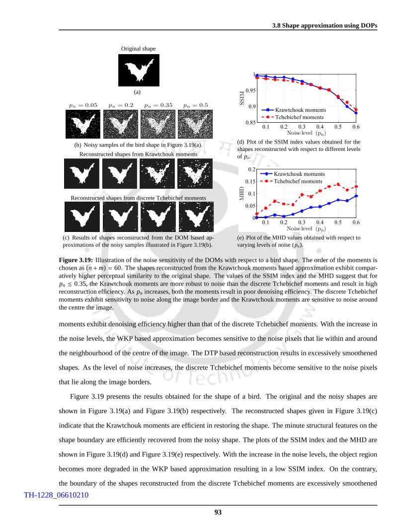
3.8 Shape approximation using DOPs
Original shape
(a)
pn = 0.05 pn = 0.2 pn = 0.35 pn = 0.5
(b) Noisy samples of the bird shape in Figure 3.19(a).
Reconstructed shapes from Krawtchouk moments
Reconstructed shapes from discrete Tchebichef moments
(c) Results of shapes reconstructed from the DOM based ap-proximations of the noisy samples illustrated in Figure 3.19(b).
0.1 0.2 0.3 0.4 0.5 0.60.85
0.9
0.95
1
Noise level (pn)
SSIM
Krawtchouk moments
Tchebichef moments
(d) Plot of the SSIM index values obtained for theshapes reconstructed with respect to different levelsof pn.
0.1 0.2 0.3 0.4 0.5 0.60
0.05
0.1
0.15
0.2
Noise level (pn)
MH
D
Krawtchouk moments
Tchebichef moments
(e) Plot of the MHD values obtained with respect tovarying levels of noise (pn).
Figure 3.19: Illustration of the noise sensitivity of the DOMs with respect to a bird shape. The order of the moments ischosen as(n+m) = 60. The shapes reconstructed from the Krawtchouk moments based approximation exhibit compar-atively higher perceptual similarity to the original shape. The values of the SSIM index and the MHD suggest that forpn ≤ 0.35, the Krawtchouk moments are more robust to noise than the discrete Tchebichef moments and result in highreconstruction efficiency. Aspn increases, both the moments result in poor denoising efficiency. The discrete Tchebichefmoments exhibit sensitivity to noise along the image borderand the Krawtchouk moments are sensitive to noise aroundthe centre the image.
moments exhibit denoising efficiency higher than that of thediscrete Tchebichef moments. With the increase in
the noise levels, the WKP based approximation becomes sensitive to the noise pixels that lie within and around
the neighbourhood of the centre of the image. The DTP based reconstruction results in excessively smoothened
shapes. As the level of noise increases, the discrete Tchebichef moments become sensitive to the noise pixels
that lie along the image borders.
Figure 3.19 presents the results obtained for the shape of a bird. The original and the noisy shapes are
shown in Figure 3.19(a) and Figure 3.19(b) respectively. The reconstructed shapes given in Figure 3.19(c)
indicate that the Krawtchouk moments are efficient in restoring the shape. The minute structural features on the
shape boundary are efficiently recovered from the noisy shape. The plots of the SSIM index and the MHD are
shown in Figure 3.19(d) and Figure 3.19(e) respectively. With the increase in the noise levels, the object region
becomes more degraded in the WKP based approximation resulting in a low SSIM index. On the contrary,
the boundary of the shapes reconstructed from the discrete Tchebichef moments are excessively smoothened
93
TH-1228_06610210

3. A Study on the Characteristics of Discrete Orthogonal Moments for Shape Representation
Original shape
(a)
pn = 0.05 pn = 0.2 pn = 0.35 pn = 0.5
(b) Noisy samples of the original shape in Figure 3.20(a).
Reconstructed shapes from Krawtchouk moments
Reconstructed shapes from discrete Tchebichef moments
(c) Shapes reconstructed from the DOM based approximationsof the noisy samples illustrated in Figure 3.20(b). The order ofthe moments are chosen as(n+m) = 60.
0.1 0.2 0.3 0.4 0.5 0.60.85
0.9
0.95
1
Noise level (pn)
SSIM
Krawtchouk moments
Tchebichef moments
(d) Plot of the SSIM index values obtained with re-spect to different levels of noise (pn).
0.1 0.2 0.3 0.4 0.5 0.60
0.03
0.06
0.09
Noise level (pn)
MH
D
Krawtchouk moments
Tchebichef moments
(e) Plot of the MHD values obtained for differentvalues ofpn.
Figure 3.20: Illustration of the denoising efficiency of the DOMs with respect to the square shape. The shape recon-structed from the Krawtchouk and the discrete Tchebichef moments exhibits similar perceptual quality with respect tothe original shape. Hence, the corresponding SSIM values are almost similar for lowerpn. With the increase inpn, thenumber of noise pixels are more in the background region for discrete Tchebichef moments based approximation andnoise occurs in the foreground region for Krawtchouk moments based approximation. The values of the SSIM index andthe MHD indicate that the performance of the WKP based approximation is comparatively poor for higher noise levels.
resulting in lower MHD values. As the noise level increases,the noise pixels present in the background region
and along the image borders are retained in DTP based approximation.
The experimental results obtained for the square shape is presented in Figure 3.20. The original shape
and the noisy samples simulated for varying levels of noise are shown in Figure 3.20(a) and Figure 3.20(b)
respectively. The shapes reconstructed from the Krawtchouk and the discrete Tchebichef moments are shown in
Figure 3.20(c). The plots of the SSIM index and the MHD are given in Figure 3.20(d) and 3.20(e) respectively.
From the results, it is evident that the performances of the WKP based and the DTP based reconstructions are
similar at lower noise levels. As the noise level increases,the degradations in the WKP based reconstruction is
more in the DTP based reconstruction.
From the above results on noise sensitivity, it is evident that the performance of the DOPs is significantly
better for pn ≤ 0.3. It is inferred that the WKPs are efficient in discriminating the high spatial frequency
structures of the shape from the noise pixels. As a result, the reconstruction accuracy is comparatively higher for
94
TH-1228_06610210

3.8 Shape approximation using DOPs
(pn = 0.4)
(a) Noisy shape
Reconstructed shapes from Krawtchouk moments of
Order: 20 Order: 40 Order: 60 Order: 80
Reconstructed shapes from discrete Tchebichef moments of
Order: 20 Order: 40 Order: 60 Order: 80
(b) Shapes reconstructed from the DOM based approxima-tion of the noisy sample in Figure 3.21(a).
20 30 40 50 60 70 800.9
0.95
1
(n + m) thOrder of theMoments
SSIM
Krawtchouk moments
Tchebichef moments
(c) Plot of the SSIM index values versus the orderof the moments.
20 30 40 50 60 70 800
0.05
0.1
(n + m) thOrder of theMoments
MH
D
Krawtchouk moments
Tchebichef moments
(d) Plot of the MHD values versus the order of themoments.
Figure 3.21: Illustration of the robustness of the DOMs to noise with respect to varying orders of DOPs based approxima-tion of the beetle shape. With the increase in order, most of the noise pixels are recovered in reconstruction. Particularly,the Krawtchouk moments exhibit more sensitivity towards noise in the foreground region. As the order increases, thediscrete Tchebichef moments result in better reconstruction of the high spatial frequency structures in the beetle shape.Simultaneously, the reconstruction quality gets degradeddue to the recovery of more noise pixels in the background re-gion. The SSIM index and the MHD suggest that the Krawtchouk moments exhibit better performance than the discreteTchebichef moments in most of the orders.
the WKP based approximation. At these noise levels, the DTP based approximation results in over-smoothening
of shapes.
It is observed that the robustness of the DOPs decreases at higher noise levels and they exhibit varied
behaviour. For 0≤ x ≤ N, the STFT plots in Figure 3.7 and Figure 3.8 have shown that the frequency response
of the DOPs varies as the value ofx deviate fromx = N/2. The WKPs exhibit higher frequency response at the
data points aroundx = N/2 and the frequency response decreases as the value ofx gets close to 0 andN. As
a result, the WKPs are more sensitive to the high spatial frequency structures that lie around the centre of the
image. Unlike the WKPs, the DTPs exhibit lower frequency response at the data points aroundx = N/2 and the
frequency response increases as the value ofx gets close to 0 andN. Therefore, the DTPs are more sensitive to
the high spatial frequency components lying along the imageborders.
Considering that the DOMs are computed with respect to the centre of the shape, it can be inferred that
the robustness of the WKPs to significant noise pixels aroundthe centre of the image decreases at higher noise
levels. On the other hand, the DTPs result in smoothening of the pixels around the centre of the image and are
more sensitive to the noise pixels in the background region that lie along the image borders.
95
TH-1228_06610210

3. A Study on the Characteristics of Discrete Orthogonal Moments for Shape Representation
(pn = 0.2)
(a) Noisy shape
Reconstructed shapes from Krawtchouk moments of
Order: 20 Order: 40 Order: 60 Order: 80
Reconstructed shapes from discrete Tchebichef moments of
Order: 20 Order: 40 Order: 60 Order: 80
(b) Results of the shapes reconstructed from DOMs of vari-ous orders.
20 30 40 50 60 70 800.96
0.98
1
1.02
(n + m) thOrder of theMoments
SSIM
Krawtchouk moments
Tchebichef moments
(c) Plot of the SSIM index values versus order of themoments.
20 30 40 50 60 70 800
0.05
0.1
(n + m) thOrder of theMomentsM
HD
Krawtchouk moments
Tchebichef moments
(d) Plot of the MHD values versus order of the mo-ments.
Figure 3.22: Illustration of noise sensitivity of the different orders of DOM based reconstruction of the bird shape. Withthe increase in the order, the moments exhibit more sensitivity to noise. The higher order discrete Tchebichef momentsoffer better reconstruction of the high spatial frequency structures in the bird shape. However, the reconstruction quality isaffected due to the recovery of more noise pixels in the background region. The shapes reconstructed from the Krawtchoukmoments exhibit noise in the foreground as well as the background region. The performance in terms of the SSIM indexand the MHD indicates that the Krawtchouk moments are betterthan the discrete Tchebichef moments upto certain orders.
(pn = 0.3)
(a) Noisy shape
Reconstructed shapes from Krawtchouk moments of
Order: 20 Order: 40 Order: 60 Order: 80
Reconstructed shapes from discrete Tchebichef moments of
Order: 20 Order: 40 Order: 60 Order: 80
(b) Results of shape reconstruction from the higher orderDOMs computed from the noisy shape in Figure 3.23(a).
20 30 40 50 60 70 800.85
0.9
0.95
1
(n + m) thOrder of theMoments
SSIM
Krawtchouk moments
Tchebichef moments
(c) Plot of the SSIM index values versus order of themoments.
20 30 40 50 60 70 800
0.05
0.1
(n + m) thOrder of theMoments
MH
D
Krawtchouk moments
Tchebichef moments
(d) Plot of the MHD values versus order of the mo-ments.
Figure 3.23: Illustration of noise sensitivity of DOM based approximation of the square shape at various orders. The val-ues of SSIM index and MHD indicate that up to (n+m) = 50, the discrete Tchebichef moments exhibit better performancethan the Krawtchouk moments.
96
TH-1228_06610210

3.8 Shape approximation using DOPs
Similar experiments were performed in order to evaluate thenoise sensitivity of the DOMs at different
orders of approximation. Hence, the performance of the DOMsin recovering the shape from a noisy sample
is tested by varying the order of the approximation. The experimental results obtained for the beetle, bird and
the square shapes corrupted by different noise levels are presented in Figure 3.21, Figure 3.22 and Figure 3.23
respectively.
From the results, it is clear that at higher orders, the polynomials tend to behave like all-pass functions.
Therefore, as the order increases the number of noise pixelsin the recovered shapes also increases. The plots of
the SSIM index and MHD in Figure 3.21, Figure 3.22 and Figure 3.23 show an increase in the reconstruction
error with the increase in the order of the moments.
In Figure 3.21 and Figure 3.22, it is noticed that the structural degradation in the shapes reconstructed from
the Krawtchouk moments is less than in the shapes reconstructed from the discrete Tchebichef moments. It
is also observed that for higher order DTPs, the high spatialfrequency structures of the shape are efficiently
reconstructed. Despite this improvement, the performanceof the discrete Tchebichef moments is marked by
the large number of noise pixels left in the background region of the reconstructed shape. The denoising results
obtained for the square shape are shown in Figure 3.23. From the plots of the SSIM index and the MHD, it
is observed that the reconstruction error for the WKP based approximation is high at the lower orders. As the
order increases, the performance of the Krawtchouk momentsand the discrete Tchebichef moments becomes
almost similar.
By consolidating the results in Figure 3.21, Figure 3.22 andFigure 3.23, it is observed that the recon-
struction error for the WKP based approximation reaches itsminimum approximately for(n+m) = 50. At this
order, the spatial structures constituting the shape are effectively recovered and hence, they do not require higher
order approximations. The DTPs require higher orders for recovering the high spatial frequency structures of
the shapes. Even as the order increases, the noise sensitivity of the discrete Tchebichef moments increases, thus
degrading the quality of the reconstructed shape.
3.8.3 Experiments on shape classification
The purpose of this study is to demonstrate the capability ofthe DOMs as features for shape classification.
The experiment is conducted on a dataset collected from the MPEG-7 (CE Shape-1, Part-B) database. The
dataset consists of 400 samples of 20 different shape classes with 20 samples per shape class. Out of these, 40
samples are used for training and 360 samples are used for testing. Of the 40 training samples, 20 samples are
undistorted shapes and the remaining 20 samples are distorted shapes.
97
TH-1228_06610210

3. A Study on the Characteristics of Discrete Orthogonal Moments for Shape Representation
Shape−1 Shape−2 Shape−3 Shape−4 Shape−5 Shape−6 Shape−7 Shape−8 Shape−9 Shape−10
Shape−11 Shape−12 Shape−13 Shape−14 Shape−15 Shape−16 Shape−17 Shape−18 Shape−19 Shape−20
Figure 3.24: Illustration of undistorted training sample per shape class constituting the reference dataset.
Class 1 Class 2 Class 3
Class 4 Class 5 Class 6
Class 7 Class 8 Class 9
Class 10 Class 11 Class 12
Class 13 Class 14 Class 15
Class 16 Class 17 Class 18
Class 19 Class 20
Figure 3.25:Examples of test samples contained in each shape class. The figure illustrates the shape defection in the testsamples that are caused due to boundary distortion and segmentation errors.
Two sets of experiments are performed on shape classification. The first experiment is performed by using
the 20 undistorted shapes for forming training set. Therefore, we have 1 training sample and 18 testing sam-
ples for each shape class. In the second experiment, the sizeof the training set is increased by including the
remaining 20 samples of the undistorted shapes in the training set. Thus, the extended training set consists of 2
training samples per shape class.
The training samples used in the first experiment for shape classes are shown in Figure 3.24. The shape
classes in the training set are labeled as Shape 1, Shape 2, Shape 3,· · · , Shape 20. A few examples of the
test samples for different shape classes are given in Figure3.25. The shape classes belonging to the test data
are labeled as Class 1, Class 2,· · · , Class 20. It can be observed that the test dataset consists of shapes that
98
TH-1228_06610210
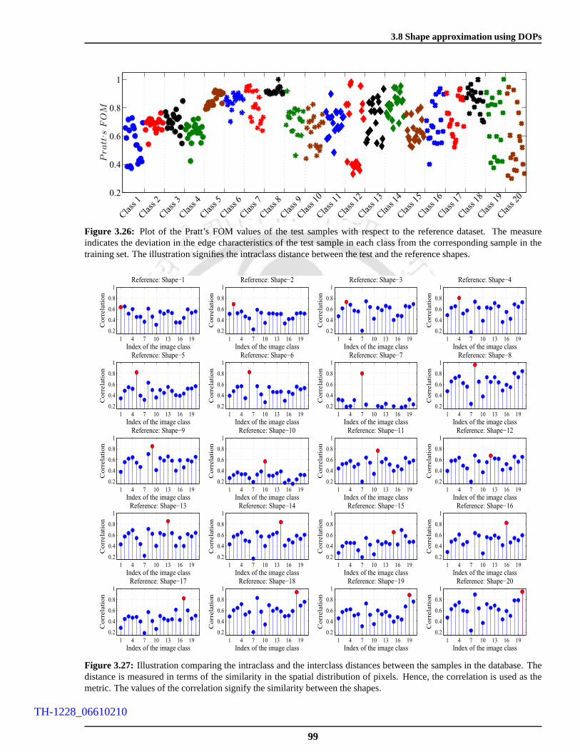
3.8 Shape approximation using DOPs
0.2
0.4
0.6
0.8
1
Pratt, s
FO
M
Cla
ss 1
Cla
ss 2
Cla
ss 3
Cla
ss 4
Cla
ss 5
Cla
ss 6
Cla
ss 7
Cla
ss 8
Cla
ss 9
Cla
ss 1
0
Cla
ss 1
1
Cla
ss 1
2
Cla
ss 1
3
Cla
ss 1
4
Cla
ss 1
5
Cla
ss 1
6
Cla
ss 1
7
Cla
ss 1
8
Cla
ss 1
9
Cla
ss 2
0
Figure 3.26: Plot of the Pratt’s FOM values of the test samples with respect to the reference dataset. The measureindicates the deviation in the edge characteristics of the test sample in each class from the corresponding sample in thetraining set. The illustration signifies the intraclass distance between the test and the reference shapes.
1 4 7 10 13 16 19
0.2
0.4
0.6
0.8
1
Index of the image class
Corr
ela
tion
Reference: Shape−1
1 4 7 10 13 16 19
0.2
0.4
0.6
0.8
1
Index of the image class
Corr
ela
tion
Reference: Shape−2
1 4 7 10 13 16 19
0.2
0.4
0.6
0.8
1
Index of the image class
Corr
ela
tion
Reference: Shape−3
1 4 7 10 13 16 19
0.2
0.4
0.6
0.8
1
Index of the image class
Corr
ela
tion
Reference: Shape−4
1 4 7 10 13 16 19
0.2
0.4
0.6
0.8
1
Index of the image class
Corr
ela
tion
Reference: Shape−5
1 4 7 10 13 16 19
0.2
0.4
0.6
0.8
1
Index of the image class
Corr
ela
tion
Reference: Shape−6
1 4 7 10 13 16 19
0.2
0.4
0.6
0.8
1
Index of the image class
Corr
ela
tion
Reference: Shape−7
1 4 7 10 13 16 19
0.2
0.4
0.6
0.8
1
Index of the image classC
orr
ela
tion
Reference: Shape−8
1 4 7 10 13 16 19
0.2
0.4
0.6
0.8
1
Index of the image class
Corr
ela
tion
Reference: Shape−9
1 4 7 10 13 16 19
0.2
0.4
0.6
0.8
1
Index of the image class
Corr
ela
tion
Reference: Shape−10
1 4 7 10 13 16 19
0.2
0.4
0.6
0.8
1
Index of the image class
Corr
ela
tion
Reference: Shape−11
1 4 7 10 13 16 19
0.2
0.4
0.6
0.8
1
Index of the image class
Corr
ela
tion
Reference: Shape−12
1 4 7 10 13 16 19
0.2
0.4
0.6
0.8
1
Index of the image class
Corr
ela
tion
Reference: Shape−13
1 4 7 10 13 16 19
0.2
0.4
0.6
0.8
1
Index of the image class
Corr
ela
tion
Reference: Shape−14
1 4 7 10 13 16 19
0.2
0.4
0.6
0.8
1
Index of the image class
Corr
ela
tion
Reference: Shape−15
1 4 7 10 13 16 19
0.2
0.4
0.6
0.8
1
Index of the image class
Corr
ela
tion
Reference: Shape−16
1 4 7 10 13 16 19
0.2
0.4
0.6
0.8
1
Index of the image class
Corr
ela
tion
Reference: Shape−17
1 4 7 10 13 16 19
0.2
0.4
0.6
0.8
1
Index of the image class
Corr
ela
tion
Reference: Shape−18
1 4 7 10 13 16 19
0.2
0.4
0.6
0.8
1
Index of the image class
Corr
ela
tion
Reference: Shape−19
1 4 7 10 13 16 19
0.2
0.4
0.6
0.8
1
Index of the image class
Corr
ela
tion
Reference: Shape−20
Figure 3.27: Illustration comparing the intraclass and the interclass distances between the samples in the database. Thedistance is measured in terms of the similarity in the spatial distribution of pixels. Hence, the correlation is used as themetric. The values of the correlation signify the similarity between the shapes.
99
TH-1228_06610210

3. A Study on the Characteristics of Discrete Orthogonal Moments for Shape Representation
are severely distorted due to shape defections such as segmentation errors and boundary distortion. It is quite
evident that the shapes of the objects belonging to a class are perceptually similar but exhibit large differences
in terms of structural features. Therefore, the intraclassdistance between the samples is measured using the
Pratt’s figure-of-merit (FOM). The FOM is computed as [170,171]
Pratt′s FOM=1
maxNs,Nv
Ns∑
j=1
11+ αDE ( j)
(3.85)
where,Nv andNsdenote the number of edge pixels in the reference shape and the test shape respectively,α is
the scaling constant andDE( j) is the distance from thejth edge pixel of the reference shape to the corresponding
edge pixel in the test shape. In our experiments,α is chosen as 1/9 in accordance with [171].
The plot illustrating the Pratt’s FOM value obtained for each sample in the test dataset is given in Fig-
ure 3.26. The plot shows that most of the test samples belonging to class 5, 6, 7, 8 and 18 exhibit similar
edge characteristics with respect to the corresponding reference shape. In the case of samples belonging to
other classes, the FOM value implies that the difference in terms of the edge characteristics is significant. The
difference occurs due to shape defections as mentioned earlier.
Similarly, the intraclass and interclass distances between the samples belonging to different classes are
measured in terms of the correlation coefficient. The correlation coefficient between the testftest and the
referencefre f shapes is computed as
N∑
x=0
M∑
y=0
(
ftest(x, y) − µ ftest
) (
fre f (x, y) − µ fre f
)
√
N∑
x=0
M∑
y=0
(
ftest(x, y) − µ ftest
)2 N∑
x=0
M∑
y=0
(
fre f (x, y) − µ fre f
)2
(3.86)
µ ftest andµ fre f denotes the mean of the test and the reference shapes respectively. For ease, we refer the corre-
lation coefficient as the correlation.
The plots of average correlation values obtained for each shape class with respect to a reference shape are
shown in Figure 3.27. From the values of the correlation, we infer that some of the shape classes exhibit high
interclass similarity along with the intraclass similarity. For example, the correlation values obtained for the
Shape 1 reference class exhibits a high similarity with the test samples in its own group Class 1 and other group
Class 2. Similarly, the test samples in Class 12, Class 13 andClass 14 exhibit high similarity to the reference
class Shape 12. The test samples in Class 17 has high structural similarity with the reference class Shape 15.
Therefore, the evaluation of the database in terms of the correlation implies that some of the shape shapes
considered in the experiment are perceptually different but exhibit an intricate correlation in terms of the spatial
100
TH-1228_06610210
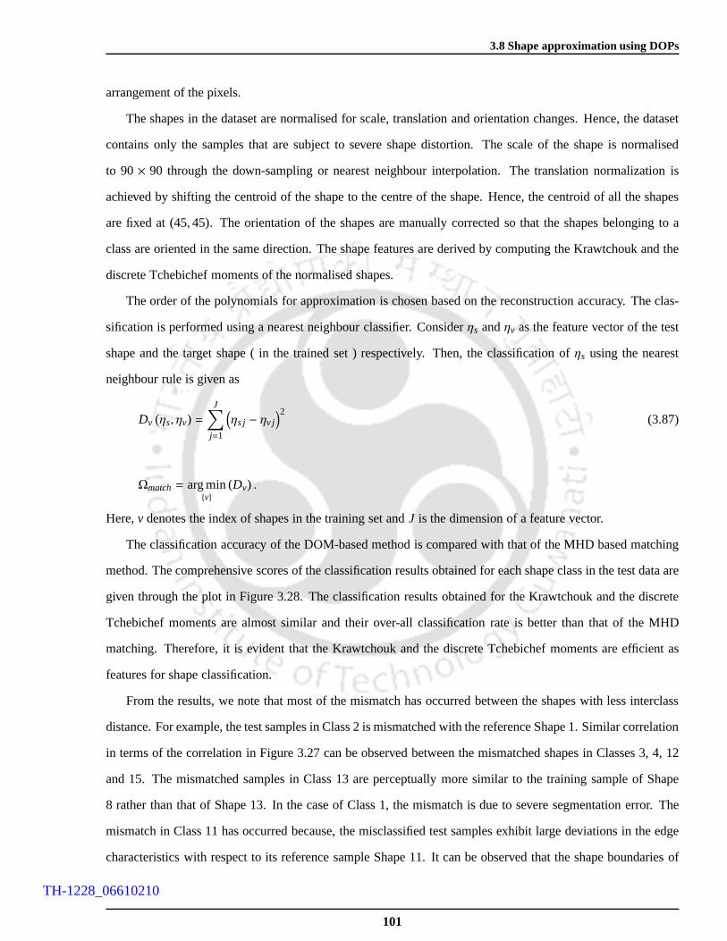
3.8 Shape approximation using DOPs
arrangement of the pixels.
The shapes in the dataset are normalised for scale, translation and orientation changes. Hence, the dataset
contains only the samples that are subject to severe shape distortion. The scale of the shape is normalised
to 90× 90 through the down-sampling or nearest neighbour interpolation. The translation normalization is
achieved by shifting the centroid of the shape to the centre of the shape. Hence, the centroid of all the shapes
are fixed at(45, 45). The orientation of the shapes are manually corrected so that the shapes belonging to a
class are oriented in the same direction. The shape featuresare derived by computing the Krawtchouk and the
discrete Tchebichef moments of the normalised shapes.
The order of the polynomials for approximation is chosen based on the reconstruction accuracy. The clas-
sification is performed using a nearest neighbour classifier. Considerηs andηv as the feature vector of the test
shape and the target shape ( in the trained set ) respectively. Then, the classification ofηs using the nearest
neighbour rule is given as
Dv (ηs, ηv) =J
∑
j=1
(
ηs j − ηv j
)2(3.87)
Ωmatch= arg minv
(Dv) .
Here,v denotes the index of shapes in the training set andJ is the dimension of a feature vector.
The classification accuracy of the DOM-based method is compared with that of the MHD based matching
method. The comprehensive scores of the classification results obtained for each shape class in the test data are
given through the plot in Figure 3.28. The classification results obtained for the Krawtchouk and the discrete
Tchebichef moments are almost similar and their over-all classification rate is better than that of the MHD
matching. Therefore, it is evident that the Krawtchouk and the discrete Tchebichef moments are efficient as
features for shape classification.
From the results, we note that most of the mismatch has occurred between the shapes with less interclass
distance. For example, the test samples in Class 2 is mismatched with the reference Shape 1. Similar correlation
in terms of the correlation in Figure 3.27 can be observed between the mismatched shapes in Classes 3, 4, 12
and 15. The mismatched samples in Class 13 are perceptually more similar to the training sample of Shape
8 rather than that of Shape 13. In the case of Class 1, the mismatch is due to severe segmentation error. The
mismatch in Class 11 has occurred because, the misclassifiedtest samples exhibit large deviations in the edge
characteristics with respect to its reference sample Shape11. It can be observed that the shape boundaries of
101
TH-1228_06610210

3. A Study on the Characteristics of Discrete Orthogonal Moments for Shape Representation
1 2 3 4 5 6 7 8 9 10 11 12 13 14 15 16 17 18 19 20
40
60
80
100C
lass
ific
ati
on r
ate
(%
)
Index denoting the image class
Krawtchouk moments
Tchebichef moments
MHD
Figure 3.28: Comparison of the consolidated classification results obtained with respect to each class. The results areobtained for 1 training sample per shape class and 18 testingsamples per shape class. The overall classification rateobtained for discrete Tchebichef moments as features is 87.11%. The overall classification rate for Krawtchouk momentsas features is 86.58%. The overall classification rate for MHD matching is 86%.
Testing samples:
Class 1 Class 2 Class 3 Class 4
Misclassified as:
Shape 7 Shape 1 Shape 13 Shape 14 Shape 8
Testing samples:
Class 11 Class 12 Class 13 Class 15
Misclassified as:
Shape 8 Shape 14 Shape 8 Shape 17
Figure 3.29: Results from the experiment on shape classification using 1 training sample per shape class. Examples ofthe testing samples exhibiting higher misclassification with respect to both the Krawtchouk and the discrete Tchebichefmoments as features. It is observed that most of the mismatches have occurred between the shape classes with lessinterclass distances. The spatial similarity between the misclassified test sample and the corresponding match in thereference set can be obtained from the respective plots in Figure 3.27.
1 2 3 4 5 6 7 8 9 10 11 12 13 14 15 16 17 18 19 2040
60
80
100
Cla
ssif
icati
on r
ate
(%
)
Index denoting the image class
Krawtchouk moments
Tchebichef moments
MHD
Figure 3.30: Comparison of the comprehensive scores of the classification results obtained with respect to each class.The results are obtained for 2 training samples per shape class and 18 testing samples per shape class. The overallclassification rate obtained for discrete Tchebichef moments as features is 94.17%. The overall classification rate forKrawtchouk moments as features is 94.44%. The overall classification rate for MHD matching is 94.16%. The numberof classes misclassified is comparatively higher in MHD matching.
102
TH-1228_06610210

3.8 Shape approximation using DOPs
the misclassified test samples in Class 11 and the reference Shape 8 are almost similar. Hence, the test samples
of Class 11 shown in Figure 3.27 can be perceived as the distorted forms of Shape 8.
Despite these misclassifications, it has to be noted that theDOMs exhibit higher classification accuracy
for several other test samples that are subject to severe structural distortions. For example, the test samples
of Classes 18, 19 and 20 as shown in Figure 3.25 exhibit variations due to segmentation errors. However, the
shapes belonging to these classes have higher classification accuracies. The structural variations in these shape
classes can be verified from the plot of Pratt’s FOM values in Figure 3.26. Similarly, the test samples in Classes
7, 9, 10, 16 and 17 illustrated in Figure 3.25 exhibit significant deviations in the structural characteristics and
the corresponding values of intraclass distance can be known from Figure 3.26. The test samples belonging to
these classes are accurately classified.
Based on the above discussion, it can be inferred that the DOMs exhibit robustness to deviations in the
structural characteristics and to some extent they are insensitive to segmentation errors. Hence, we can expect to
increase the classification accuracies of some of the shape classes by increasing the number of training samples.
In order to improve the classification results, the experiment on shape classification is repeated by taking an
extended training set with 2 training samples per shape class, out of which 1 training sample per shape class has
structural distortion. The evaluation is performed on the 360 testing samples used in the previous experiment
on classification.
The consolidated plot of the classification results obtained for each shape class with respect to the ex-
tended training set is given in Figure 3.30. As expected, thetest samples in Classes 1, 4, 11, 12 and 13 show
higher classification accuracies. However, there is no significant improvement in the classification accuracies
of Classes 2, 3 and 15. Similar to the previous classificationresults, the test samples of Class 2 is misclassified
as Shape 1. The test samples of Class 3 is misclassified as Shape 13 and Class 15 as Shape 17. These results
imply that the performance of the DOMs in shape classification depends mainly on the spatial distribution of
the pixels. Under such cases, the number of training samplesmay be increased in order to improve the clas-
sification accuracy. The performance of MHD based classification has also improved with the increase of the
training set. However, the number of shape classes misclassified in MHD based matching is higher than that in
the DOM based matching.
The experiments for evaluating the capability of the DOMs asfeatures for shape classification confirm the
Krawtchouk and the discrete Tchebichef moments as robust features for efficient classification of shapes under
shape defections such as segmentation errors and boundary deviations.
103
TH-1228_06610210
3. A Study on the Characteristics of Discrete Orthogonal Moments for Shape Representation
3.9 Summary
This chapter has presented studies on the characteristics of the WKPs and the DTPs in representing shapes.
It is shown that for any given order, the WKPs and the DTPs behave like band-pass functions. Accordingly, the
polynomials exhibits varied characteristics in representing different shapes.
The first empirical study is on the accuracy of the Krawtchoukand the discrete Tchebichef moments in
shape representation. The efficiency of the DOMs is studied with respect to the changes in the shape scale
and different structural characteristics. It has been shown that the performance of these moments significantly
differs for lower order approximations. The discrete Tchebichef moments are superior to the Krawtchouk
moments in accurately representing shapes with low structural variations. On the contrary, the Krawtchouk
moments offer representation accuracy higher than that of the discrete Tchebichef moments in approximating
shapes containing high spatial frequency structures. Particularly, the discrete Tchebichef moments require
higher orders to efficiently reconstruct high spatial frequency structures of the shapes. From this analysis on
the shape representation accuracy, it is inferred that the WKPs offer comparatively more data compaction in
representing shapes at lower scales. At higher scales, the data compaction of WKPs is more for shapes with
more structural variations. The data compaction capability of DTPs is significant only for low spatial frequency
shapes at higher scale.
Similar experiments on the noise sensitivity have shown that for low levels of noise, the Krawtchouk mo-
ments are comparatively more robust to noise and capable of efficiently recovering the shape from the noisy
shape. The discrete Tchebichef moments result in excessively smoothened reconstruction of shapes. As the
noise level increases, the robustness of the WKPs and the DTPs to noise decreases resulting in poor denoising
efficiency.
The second empirical study is on the applicability of the Krawtchouk and the discrete Tchebichef moments
as features in shape classification. The experiment is performed on 400 samples of 20 shape classes taken
from the MPEG-7 (CE Shape 1, Part-B) database. The study confirms that the Krawtchouk and the discrete
Tchebichef moments are potential features for shape classification and are robust to shape defections caused by
segmentation errors and structural deviations.
The empirical studies and the results obtained on shape analysis suggests the DOMs as potential feature
descriptors for representing the different shapes. This implies that the DOMs can be employed as a silhouette
based feature descriptor for classifying the hand posturesbased on their silhouette.
104
TH-1228_06610210

3.10 Appendix : Proof for the QMF property of WKP basis
3.10 Appendix : Proof for the QMF property of WKP basis
Let us write the weighted Krawtchouk polynomial in (3.49) as
Kn (x; p) =1
√
w (x; p)√
ρ (n; p)w (x; p) Kn (x; p) (3.88)
The objective is to find the frequency domain representationof the termw (x; p) Kn (x; p) in the above equation.
Let us assumeψn (x) = w (x; p) Kn (x; p) andz = e(
jωN+1
)
in (3.73). Accordingly, we get the Z-transform of
ψn (x) as
ψn (ω) =N
∑
x=0
w (x; p) Kn (x; p) z−x (3.89)
The Rodrigues type formula associated with the Krawtchouk polynomial w (x; p) Kn (x; p) can be written
as
N
x
(
pq
)x
Kn (x; p) = ∆n
N − n
x
(
pq
)x
(3.90)
Therefore,
ψn (z) =N
∑
x=0
∆n
N − n
x
(
pq
z−1)x
(3.91)
Using the properties of Z-transform, we can obtain the solution
ψn (z) =
(
1− pq
z−1)n (
1+pq
z−1)N−n
(3.92)
From (3.92), we can infer
ψn (z) = ψN−n (−z) (3.93)
Substitutingz= ejω in the above equation gives
ψn
(
ejω)
= ψN−n
(
ej(ω+π))
(3.94)
On substitutingω = ω − π2 in (3.94), we obtain [172]
∣
∣
∣
∣
ψn
(
ej(ω− π2))
∣
∣
∣
∣
=
∣
∣
∣
∣
ψN−n
(
ej(ω+ π2))
∣
∣
∣
∣
(3.95)
Therefore, the quadrature mirror property of∣
∣
∣
∣
ψn
(
ej(ω))
∣
∣
∣
∣
and∣
∣
∣
∣
ψN−n
(
ej(ω))
∣
∣
∣
∣
aboutω = π2 is proved.
105
TH-1228_06610210

3. A Study on the Characteristics of Discrete Orthogonal Moments for Shape Representation
106
TH-1228_06610210

4Robust Hand Posture Recognition Using
Geometry-based Normalisation and DOMbased Shape Description
Contents4.1 Introduction . . . . . . . . . . . . . . . . . . . . . . . . . . . . . . . . . . . .. . . . . . . 108
4.2 Hand posture acquisition and database development . . . .. . . . . . . . . . . . . . . . . 110
4.3 System Implementation . . . . . . . . . . . . . . . . . . . . . . . . . . . .. . . . . . . . . 114
4.4 Experimental Studies and Results . . . . . . . . . . . . . . . . . . .. . . . . . . . . . . . 128
4.5 Summary . . . . . . . . . . . . . . . . . . . . . . . . . . . . . . . . . . . . . . . . .. . . . 146
107
TH-1228_06610210

4. Robust Hand Posture Recognition Using Geometry-based Normalisation and DOM based Shape Description
The empirical study in Chapter 3 has shown the DOMs as efficient descriptors for representing shapes of
different structural complexity and the analysis of the experiments on the MPEG-7 shape database suggests the
DOMs as potential features for shape classification. This encourages to employ the DOMs as features for shape
based hand posture description and classification.
The objective of this work is to propose a hand posture recognition technique based on the DOMs and
experimentally validate the efficiency of DOMs as hand shapedescriptors. This work also presents a rule-
based method for automatically extracting the hand from theforearm region. The technique developed in this
work provides a framework for hand posture based interactive tabletop applications. This chapter presents the
proposed method and the experimental studies that comparatively validates the DOMs as hand posture features.
4.1 Introduction
Vision based interactive tabletops are surface computing systems that create a virtual environment for users
based on hand posture interactions. They perform the operations of the conventional devices that include the
mouse and the keyboard.
These tabletops are typically constructed using a single desktop computer linked to a projector and a camera.
The projector is rear or front-mounted to display the content on the surface of the table. The camera is used
to capture the hand postures performed on the tabletop surface. The acquired images are processed by the
hand posture recognition system in order to detect the hand posture and interpret the underlying information.
The retrieved information is passed to the computer as inputcommands for interaction. The position of the
camera and the projector units vary depending upon the type of application. Similarly, the projection and the
acquisition surfaces are either different or coupled together depending on the ease of the application. The
schematic representation of a typical vision based tabletop interface system using a front-projected display is
shown in Figure 4.1.
The hand posture recognition system developed in this work is aimed to find applicability in vision based
tabletop interactions and hence, the experimental setup employed is designed to be in accord with the config-
uration of hand posture based tabletop interfaces. The proposed system is a monocular vision based system
using shape based methodologies for interpreting the hand postures. The acquired hand posture images are
modeled using the binary silhouettes. The hand posture recognition system developed in this work addresses
the three major issues in hand shape interpretation. They are:
• segmentation of the forearm and extraction of hand region.
108
TH-1228_06610210

4.1 Introduction
Projector
Camera
Table-top
Gesturer
Figure 4.1: Illustration of a tabletop user interface setup using a top-mounted camera for natural human-computer inter-action through hand postures.
• orientation normalization of the hand postures.
• accurate recognition of postures in the presence of view-angle and the user variations.
The identification of the hand region involves separating the hand from the forearm. The lack of posture
information in the forearm makes it redundant and its presence increases the data size. In most of the previous
works, the forearm region is excluded by either making the gesturers to wear full arm clothing or by limiting
the forearm region into the scene while acquisition. However, such restrictions are not suitable in real-time
applications. The orientation of the acquired posture changes due to the angle made by the gesturer with
respect to the camera and vice-versa.
This research work proposes novel methods based on the anthropometric measures to automatically identify
the hand and its constituent regions. The geometry of the posture is characterized in terms of the abducted
fingers. This posture geometry is used to normalize for the orientation changes. These proposed normalization
techniques are robust to similarity and perspective distortions. The main contributions reported in this chapter
are:
(i) A rule based technique using the anthropometric measures of the hand is devised to identify the forearm
and the hand regions.
(ii) A rotation normalization method based on the protruded\abducted fingers and the longest axis of the
hand is devised.
(iii) A static hand posture database consisting of 10 posture classes and 4, 230 samples is constructed.
(iv) DOMS are introduced as user and view-invariant hand posture descriptors. In comparison to DOMs,
some of the state-of-the art shape descriptors, namely the Fourier descriptors, the geometric moments,
109
TH-1228_06610210

4. Robust Hand Posture Recognition Using Geometry-based Normalisation and DOM based Shape Description
the Zernike moments, the Gabor wavelets and the PCA descriptors are also studied for user and view
invariant hand posture recognition.
The proposed posture recognition framework is explained bydividing the system development into three sec-
tions, namely,
1. Hand posture acquisition and database development
2. System implementation
3. Experimental studies and results
The posture acquisition and the database development section explains the experimental setup used for acquir-
ing the hand postures and the construction of the hand posture database required for the experimental studies.
The section also includes a quantitative analysis on the variations in the shape of the hand postures in order val-
idate the database for usability in the experimental studies on user and view independent hand posture descrip-
tion. The section on system implementation presents the procedures and the techniques involved in realising the
hand posture recognition system. The section on experimental studies and the results discusses the experiments
performed to comparatively evaluate the efficiency of the proposed system with respect to the DOMs and the
other shape features. The results of user invariant and viewinvariant recognition are independently presented.
4.2 Hand posture acquisition and database development
The acquisition of hand posture images is the first step towards implementing a hand posture recognition
system. The experimental setup employed for posture acquisition consists of a monocular camera that is in-
terfaced to a computer. The two important factors to be considered while setting up the camera for posture
acquisition are the
(i) Position of the camera
(ii) View-angle of the camera
The position of the camera specifies the camera’s location with respect to the object of focus. The view-
angle specifies the angle between the camera and the object offocus. Choosing the optimal position and the
view-angle of the camera is an important task in image acquisition.
110
TH-1228_06610210

4.2 Hand posture acquisition and database development
Camera
Object of
focus
y
z
x x
(a) Low-angle position
Object of
focus
Camera
y y
z
x
(b) High-angle position
Object of
focus
Camera y
z
x
(c) Normal-angle position
Figure 4.2: Illustration of different camera positions with respect tothe object of focus in a 3D cartesian space.
4.2.1 Determination of camera position
The position of the camera with respect to the object of focusinfluences the object details that are being
efficiently captured by the camera. The three types of cameralocations generally used while image acquisition
are the [173].
• Low-angle position
• High-angle position
• Normal-angle position
In the low-angle position, the camera is placed below the object such that the camera lens has to be titled
upwards for focussing. Thehigh-angle positionoccurs when the camera is placed above the object and the
camera is lens is titled downwards for focussing the object.Thenormal-angle positionhas the camera at the
same height from the ground as the object of focus. The normalangle position is also known as the eye-level
position. Figure 4.2 illustrates the variation in the camera position with respect to the object of focus in a 3D
cartesian coordinate system.
The position of the camera for image acquisition must be chosen such that the desired object region is
completely within the focus of the camera. In realtime, the optimal position of the camera for acquiring the
hand posture depends on the application. In applications like table-top interaction, the postures are performed
on the surface of the table [95, 101, 104, 174]. Hence, the camera has to be mounted in the high-angle position
such that the entire posture space lie within the focus of thecamera. In such systems, the dorsal surface of the
hand is focussed by the camera. In the case of table-top interfaces using the glass table tops for interaction,
the camera is mounted at low-angle position such that the palmar surface is focussed while acquiring the hand
111
TH-1228_06610210

4. Robust Hand Posture Recognition Using Geometry-based Normalisation and DOM based Shape Description
Light source
Incident rays
Lens
Camera
Object of focus
Principal axis
Figure 4.3: A schematic representation of the experimental setup employed for acquiring the hand posture images.
postures [175]. In some of the posture based interface systems [2,94,133], the camera is placed at the normal-
angle position focussing the palmar surface of the hand posture.
4.2.2 Determination of view-angle
As mentioned in Section 1.5.2.3 of Chapter 1, the view-anglerefers to the angle made by the camera with
respect to the object of focus [69]. The optimal choice of viewing angle is determined by the amount of
perspective distortion. Perspective distortion is caused if the focal plane is not parallel to the object’s surface
and/or not in level with the center of the object. Hence, the optimum view-angle is assumed to be the angle for
which the camera is parallel to the object of focus i.e., the image plane must be parallel to the object plane.
4.2.3 System setup
The setup for image acquisition consists of a tabletop and a RGB Frontech e-cam mounted on an adjustable
stand with an view of the tabletop. The postures are performed on the surface of the table such that the dorsal
side of the hand posture is captured by the camera. The camerahas a resolution of 1280×960 and is connected
to an Intel core-II duo 2GB RAM processor. The schematic representation of the acquisition setup is shown in
Figure 4.3.
The table surface constitutes the object plane and the length × width of the tabletop used for the setup is
83 cm× 96 cm. The distance between the table surface and the camera (Ch) is experimentally chosen such that
the object plane is entirely focussed by the camera. Accordingly, the e-cam is placed at a height ofCh = 30cm
from the table surface.
In the context of our experiment, we define the viewing angle (Cθ) as the angle made by the camera with
the longest axis or the principal axis of the hand. Hence, theviewpoint is assumed to be optimum if the
camera is placed parallel to the surface of the hand. For our experimental setup, the optimum viewing angle is
112
TH-1228_06610210

4.2 Hand posture acquisition and database development
y
z
x
Ch
C
Width = 96 cm
Camera
Principal axis
of hand
(a)
y
x
z
45o
90o
135o
225o
315o
Viewing angle
(b)
Figure 4.4: Illustrations of (a) the estimation of camera position and the view angle using a 3D cartesian coordinatesystem. The object is assumed to lie on thex−y plane and the camera is mounted along thezaxis.Ch denotes the distancebetween the camera and the table surface and is experimentally chosen as 30cm. The view angle (Cθ) is measured withrespect to thex− y plane. (b) the view angle variation between the camera and the object of focus.
0 1 2 3 4
5 6 7 8 9
Figure 4.5: Posture signs in database.
determined to be 90. Figure 4.4(a) illustrates the estimation of camera position and the view angle with respect
to the principal axis of the hand using a 3D cartesian coordinate system. Thex − y plane is the object plane
constituting the hand posture. The variations in the viewpoint of the camera with respect to the hand region are
illustrated through Figure 4.4(b).
In our experiment, the segmentation overload is simplified by capturing the images under uniform back-
ground. However, the foreground is cluttered with other objects and the hand is ensured as the largest skin color
object within the FOV. Except for the size, there were no restrictions imposed on the color and texture of the
irrelevant cluttered objects. Also, the FOV was sufficiently large enabling the users to perform postures more
naturally without interfering their gesturing styles.
113
TH-1228_06610210

4. Robust Hand Posture Recognition Using Geometry-based Normalisation and DOM based Shape Description
4.2.4 Development of Hand posture database
The hand posture images required for the experiment are collected from several users at different view
angles. The hand posture database is developed in order to evaluate the robustness of several hand posture
features for user and view invariant hand posture recognition.
The hand posture database is constructed out in two phases. In the first phase, the hand posture data are
acquired at an optimum view angle ofCθ = 90. During the second phase, the hand postures images are
captured at different view angles. The database consists ofa total of 4, 230 postures collected from 23 users.
The data contains 10 posture signs with 423 samples for each user. The posture signs taken for evaluation are
shown in Figure 4.5. The images are collected under three different scales, seven orientations and the view
angles at 45, 90, 135, 225 and 315.
The scale variations are achieved by varying the optical zoom of the camera during each session of image
acquisition. The orientation change is achieved by orbiting the camera around the object of focus. However, the
view angle is maintained at 90. In the second phase of data collection, changing the viewpoint automatically
causes the change in the orientation of acquired image.
4.3 System Implementation
The proposed hand posture recognition system is developed by broadly dividing the procedure into three
phases. They are: (1) hand detection and segmentation, (2) normalization and (3) feature extraction and classi-
fication. A description of these tasks are presented below. Figure 4.6 shows a schematic representation of the
proposed posture recognition system.
4.3.1 Hand detection and segmentation
This phase detects and segments the hand data from the captured image. The hand regions are detected
using the skin color pixels. The background is restricted such that the hand is the largest object with respect to
the skin color.
Teng et al [62] have given a simple and effective method to detect skin color pixels by combining the
features obtained from the YCbCr and the YIQ color spaces. The hue valueHθ is estimated from the Cb-Cr
chromatic components by
Hθ = tan−1(CrCb
)
(4.1)
114
TH-1228_06610210

4.3 System Implementation
Input: Acquired hand
posture
Hand detection and
segmentationsegmentation
Rule based extraction of
Normalization
Rule based extraction of
hand and
forearm region
Orientation
correction
Forearm
removal
Correcting for scale
and spatial translation
Computation of
DOM descriptors
Classification phase
Nearest neighborhood
classificationStorage of features
Training phase
Output: Matched hand
posture
Figure 4.6: Schematic representation of the proposed hand posture recognition technique.
The in-phase color componentCphaseis calculated from theRGBcomponents as
Cphase = 0.596R− 0.274G − 0.322B (4.2)
Their experiments conclude about the ranges ofHθ and the in-phase color componentCphase for Asian and
European skin tones. The pixels are grouped as skin color pixels if 105 ≤ Hθ ≤ 150 and 30≤ Cphase≤ 100.
Figure 4.7(b) illustrates the skin color detection using this method for the hand posture images shown in
Figure 4.7(a). The detection results in a binary image whichmay also contain other objects not belonging to
the hand. Since, the hand is assumed to be the largest skin color object, the other components are filtered by
comparing the area of the detected binary objects. The resultant is subjected tomorphological closingoperation
with a disk-shaped structuring element in order to obtain a well defined segmented posture image.
For a binary imagef (x, y) defined on a discrete gridG = 0, 1, · · ·N × 0, 1, · · ·M and the structuring
elementsl , the morphological closing operation denoted byf • sl is defined as
f • sl = ( f ⊕ sl) ⊖ sl (4.3)
f ⊕sl and f ⊖sl denotesdilation anderosionoperations respectively [176]. The disk-shaped structuring element
used for morphological closing operation is shown in Figure4.8.
115
TH-1228_06610210

4. Robust Hand Posture Recognition Using Geometry-based Normalisation and DOM based Shape Description
Example 1
Example 2
(a) Acquired images (b) Skin color regions (c) Segmented
hand images
Figure 4.7: Results of hand segmentation using skin colour de-tection.
0 0 0 1 0 0 0
0 1 1 1 1 1 0
0 1 1 1 1 1 00 1 1 1 1 1 0
1 1 1 1 1 1 1
0 1 1 1 1 1 0
0 1 1 1 1 1 0
Origin
0 1 1 1 1 1 0
0 0 0 1 0 0 0
Figure 4.8: Illustration of the disk-shaped struc-turing element used for morphological closing.The radius of the element is 3.
4.3.2 Normalization techniques
This is an essential phase in which the segmented image is normalized for any geometrical variations in
order to obtain the desired hand posture. The important factors to be compensated in this step are
(i) the presence of forearm region.
(ii) the orientation of the object.
The recognition efficiency can be improved through proper normalization of the hand posture image. Hence,
a robust normalization method based on the posture geometryis proposed for extracting the hand region and
correcting the orientation.
4.3.2.1 Proposed method for rule based hand extraction
Consider a binary imagef defined over a gridB of size (N + 1)× (M + 1). B is composed of two comple-
mentary regionsRandR representing the hand (object) and the background respectively. Thus,
R=
(x, y)∣
∣
∣
∣
∣
(x, y) ∈ B and f (x, y) = 1
(4.4)
and the complementary regionR is given by
R= B\R (4.5)
116
TH-1228_06610210

4.3 System Implementation
R
Finger region
Circle enclosingmaximum neighbourhood region.
Wrist crease.
Forearm region
Binary image
R
Estimated palm centroid
Object pixels within the circle:Palm region
(xc, yc)
f
Rfingers
Rpalm
Rforearm
Figure 4.9: Pictorial representation of the regions composing the binary image f . R denotes the hand region andRdenotes the background region.
The boundaryδR of the hand region is defined by the set of pixels inR that are adjacent to at least one pixel in
the regionR. It is represented as
δR=
(x, y)∣
∣
∣
∣
∣
(x, y) ∈ R and (x, y) is adjacent to a pixel inR
(4.6)
The hand region R can be partitioned in to three subregions. They are (a)Rf ingers (fingers), (b)Rpalm (palm)
and (c)Rf orearm (forearm). Hence
R= Rf ingers∪Rpalm∪ Rf orearm (4.7)
such that
Rf ingers∩ Rpalm = ∅
Rf ingers∩ Rf orearm= ∅
Rpalm∩ Rf orearm= ∅.
(4.8)
Figure 4.9 illustrates these elementary regions comprising the hand object R. Based on the anatomy, the palm
and the forearm can be considered as continuous smooth regions.The forearm extends outside the palm and its
width is less than that of the palm region. Conversely, the region containing the fingers is discontinuous under
abduction. Also, the width of a finger is much smaller than that of the palm and the forearm. Therefore, the
geometrical variations in thewidth and thecontinuity of these subregions in the hand image are used as cues
for detection.
(a) Computation of width
The variation in the width along the longest axis of the hand image is calculated from the distance map
obtained using the Euclidean distance transform (EDT). TheEDT gives the minimum distance of an object
117
TH-1228_06610210

4. Robust Hand Posture Recognition Using Geometry-based Normalisation and DOM based Shape Description
pixel to any pixel on the boundary setδR. The Euclidean distance between a boundary pixel (xb, yb) ∈ δR
and an object pixel (x, y) ∈ R is defined as
d(xb,yb),(x,y) =
√
(x− xb)2+ (y− yb)2 (4.9)
The value of the EDT,D(x,y) for the object pixel (x, y) is computed as
D(x,y) = min(xb,yb)∈δR
d(xb,yb),(x,y) (4.10)
The values ofD(x,y) at different (x, y) are used to detect the subregions ofR.
The straightforward implementation of EDT defined through (4.9) and (4.10) is computationally expen-
sive. Therefore, the conventional approach to fast EDT based on the Voronoi decomposition of the image
proposed in [177] is employed. A study on the several other algorithms proposed for reducing the compu-
tational complexity of EDT is discussed in [178].
(b) Verification of region continuity
The continuity of the subregions after detection is verifiedthrough connected component labelling pre-
ceded by morphological erosion. The erosion operation witha small structuring element is performed to
disconnect the weakly connected object pixels. The structuring element considered is a disk operator with
radius 3. The resultant is verified to be a continuous region if there is only one connected component. If
there is more than one connected component, the detected region is verified as discontinuous.
The geometrical measurements along the finger region vary with the users and they get altered due to
geometric distortions. However, the measures across the palm and the forearm can be generalized and their
ratios are robust to geometric distortions.The palm is an intactly acquired part that connects the fingers and
the forearm.SinceRpalm lies as an interface betweenRf ingers andRf orearm, the separation of palm facilitates the
straightforward detection of the other two regions. Hence,the anthropometry of palm is utilized for detecting
the regions in the hand image.
4.3.2.1.1 Anthropometry based palm detection The parameters of the hand considered for palm detection
are the hand length, palm length and the palm width as illustrated in Figure 4.10(a). The anthropometric studies
in [179–181] present the statistics of the above mentioned hand parameters. From these studies, we infer that
the minimum value of the ratio of palm length (Lpalm) to palm width (Wpalm) is approximately 1.322 and its
maximum value is 1.43. Similar observations were made from our photometric experiments. Figure 4.10(b)
118
TH-1228_06610210

4.3 System Implementation
Han
d l
eng
th
Fo
rear
m r
egio
n
Palm width
Minimumforearm width
Pal
m l
eng
th
Lpalm
Wpalm
(a)
1.32 1.35 1.37 1.39 1.41 1.43 1.455
10
15
20
25
30
Values of
Nu
mb
er
of
occu
ren
ces
Lpalm
:Wpalm
(b)
Figure 4.10: (a) Hand geometry and (b) Histogram of the experimental values of palm length (Lpalm) to palm width(Wpalm) ratio calculated for 140 image samples taken from 23 persons.
gives the histogram of theLpalm
Wpalmvalues obtained through our experimentation. This ratio will be utilized to
approximate the palm region as an ellipse. Considering all the variations of this ratio, we take
Lpalm = 1.5×Wpalm (4.11)
Based on the geometry, we approximate the palm regionRpalm as an elliptical region with
Major axis length= 1.5×minor axis length (4.12)
Assumingapalm as the semi-major axis length andbpalm as the semi-minor axis length, we can write
apalm =Lpalm
2(4.13)
bpalm =Wpalm
2(4.14)
Therefore,
apalm = 1.5× bpalm (4.15)
From (4.15), it can be inferred that all the pixels constituting Rpalm will lie within the ellipse of semi-major
axis lengthapalm. Therefore, the palm centre and the value ofapalm have to be estimated for detecting the palm
region.
a) Computing the palm centreGiven that the boundary ofRpalm is an ellipse, its centre is known to have the
maximum distance to the nearest boundary. Therefore, the centre ofRpalm is computed using the EDT in (4.10).
The pixels (x, y) with EDT valuesD(x,y) greater than a thresholdζ are the points belonging to the neighborhood
119
TH-1228_06610210
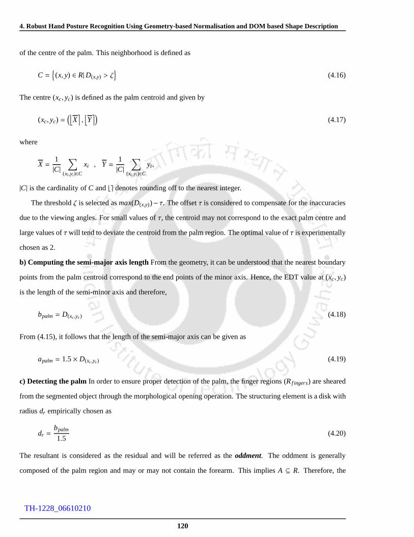
4. Robust Hand Posture Recognition Using Geometry-based Normalisation and DOM based Shape Description
of the centre of the palm. This neighborhood is defined as
C =
(x, y) ∈ R|D(x,y) > ζ
(4.16)
The centre (xc, yc) is defined as the palm centroid and given by
(xc, yc) =(⌊
X⌉
,⌊
Y⌉)
(4.17)
where
X =1|C|
∑
(xi ,yi )∈Cxi , Y =
1|C|
∑
(xi ,yi )∈Cyi ,
|C| is the cardinality ofC and⌊⌉ denotes rounding off to the nearest integer.
The thresholdζ is selected asmax(D(x,y))− τ. The offsetτ is considered to compensate for the inaccuracies
due to the viewing angles. For small values ofτ, the centroid may not correspond to the exact palm centre and
large values ofτwill tend to deviate the centroid from the palm region. The optimal value ofτ is experimentally
chosen as 2.
b) Computing the semi-major axis lengthFrom the geometry, it can be understood that the nearest boundary
points from the palm centroid correspond to the end points ofthe minor axis. Hence, the EDT value at (xc, yc)
is the length of the semi-minor axis and therefore,
bpalm = D(xc,yc) (4.18)
From (4.15), it follows that the length of the semi-major axis can be given as
apalm = 1.5× D(xc,yc) (4.19)
c) Detecting the palmIn order to ensure proper detection of the palm, the finger regions (Rf ingers) are sheared
from the segmented object through the morphological opening operation. The structuring element is a disk with
radiusdr empirically chosen as
dr =bpalm
1.5(4.20)
The resultant is considered as the residual and will be referred as theoddment. The oddment is generally
composed of the palm region and may or may not contain the forearm. This impliesA ⊆ R. Therefore, the
120
TH-1228_06610210

4.3 System Implementation
Input
Segmented image ‘f’
Separation of forearm
from ‘f’
Oddment ‘A’
Detected palm ˆ fingers forearmR = R R
Morphologicalopening palm from ‘R’
Abstraction of
Region containing pixels with
!"
x,yD T
Forearm detection
Output: Hand
Computed
Distance
transformation
(xc ,yc) and bpalm
Figure 4.11: Illustration of the rule based region detection and separation of the hand from the acquired posture imagef .The intensity of the background pixels is assigned a 0 and theobject pixels are assigned the maximum intensity value 1.
oddmentA can be defined as
A = Rpalm∪ Rf orearm
For R with no forearm region,Rf orearm = ∅ and A = Rpalm. Rpalm is a part ofA that is approximated as an
elliptic region. Thus,
Rpalm =
(xo, yo)
∣
∣
∣
∣
∣
∣
∣
∣
∣
∣
∣
(xo, yo) ∈ A and(
xo − xc
apalm
)2
+
(
yo − yc
bpalm
)2
6 1
(4.21)
d) Detection of forearm The forearm is detected through the abstraction of the palm regionRpalm from the
posture imageR. The abstraction separates the forearm and the finger regions, such thatR is modified as
R= R\Rpalm = Rf ingers∪ Rf orearm (4.22)
As in the case of palm detection, the finger region is removed from R through the morphological opening
operation. The structuring element is a disk with its radiuscalculated from (4.20). The resultant is a forearm
region and has the following characteristics:
(i) The resultantRf orearm⊆ A and the region enclosingRf orearm is continuous.
(ii) The width of the wrist crease is considered as the minimum width of the forearm region. From the
anthropometric measures in [180], the minimum value of the ratio of the palm width to wrist breadth is
obtained as 1.29 and the maximum value is computed as 1.55. Using this statistics, the empirical value
121
TH-1228_06610210

4. Robust Hand Posture Recognition Using Geometry-based Normalisation and DOM based Shape Description
for the width of the forearm should satisfy the relation
Wf orearm>2bpalm
1.29(4.23)
e) Identifying the finger region Having detected the palm and the forearm, the remaining section of the hand
imageRwill contain the finger region if it satisfies the following conditions,
• Rf ingers* A.
• The region enclosingRf ingers is marked by irregular boundary, if more than one finger is abducted.
• The width of a finger (maximum EDT value in this section) is much less than that of the palm and the
forearm. Experimentally,
Wf inger ≤bpalm
2(4.24)
A procedural illustration of the proposed rule-based method for detecting the hand region from the input image
is shown in Figure 4.11. After detecting the hand region, thepixels belonging to the forearmRf orearm are
assigned with zero values, thus includingRf orearm in the background.
4.3.2.2 Proposed approach to orientation correction
The orientation of the hand can be assumed to imply the orientation of the hand posture. In a hand posture
based system, the information is conveyed through the fingerconfigurations. Since the human hand is highly
flexible, it is natural that the orientation of the oddment might not be the orientation of the fingers. Hence, the
major axis of the hand posture is not sufficient to estimate the angular deviation that is caused by the fingers.
Therefore, in order to align a posture class uniformly, the orientation with respect to the abducted fingers is uti-
lized. If the number of abducted fingers is less than 2, the orientation correction is achieved using the oddment.
a) Orientation correction using finger configuration The normalization of rotation changes based on the fin-
ger configuration is achieved by detecting the tip of the abducted fingers. For this purpose, the boundary points
(xb, yb) are ordered as a contiguous chain of coordinates using the 8-connectivity. Any one of the boundary
pixels that is not enclosed within the region containing fingers is used as the starting point and the ordering is
performed in the clockwise direction.
Suppose,z is the length of the boundary measured in the number of pixels. A distance curveg(z) is
generated by computing the Euclidean distances between thepalm centroid (xc, yc) and the boundary pixel
(xb, yb) at zusing (4.9).
122
TH-1228_06610210

4.3 System Implementation
The curveg is smoothed using cubic-spline smoothing [182]. The resultant is a smooth curve consisting of
peaks that correspond to the finger tips of the hand posture. These peaks are detected by computing the first
and the second order derivatives ofg using the finite difference approximations. Thus,g (z) is considered to be
a peak if
∣
∣
∣g′ (z)∣
∣
∣ < ξ and g′′ (z) < 0 (4.25)
whereξ is the user defined minimum permissible difference. The finite difference approximations,
g′ (z) ≃ g (z+ 1) − g (z− 1)2
(4.26)
and
g′′ (z) ≃ g (z+ 1) + g (z− 1) − 2g (z)4
(4.27)
are used to implement (4.25). In some cases, a few peaks may correspond to the palm region. These points are
easily eliminated by verifying their presence in the oddment A. The 2D coordinate positions of the detected
peaks are utilized to find a representative peak for each abducted finger. The distance curve corresponding to a
posture and the detected finger tips are shown in Figure 4.12.
Let L be the total number of detected peaks andγi , i = 1, . . . , L define the position vectors of the detected
points with respect to(xc, yc), indexed from left to right. These vectorsγis are referred as thefinger vectorsand
the central finger vector ˆγ is computed from
γ =
γ L+12
i f L is oddγ L
2+γ L
2+1
2 otherwise(4.28)
The postures are assumed to be perfectly aligned if the vector γ is at 90 with respect to the horizontal axis of
the image. Otherwise, the segmented hand posture image is tobe rotated by 90 − ∠γ.
b) Orientation correction using the oddment The geometry of the oddmentA is utilized to correct the
orientation of the hand postures with only one abducted finger and the postures like thefist. The shape of the
oddment can be well approximated by an ellipse and hence, theorientation of its major axis with respect to the
horizontal axis of the image gives the approximate rotationangle of the hand posture.
123
TH-1228_06610210
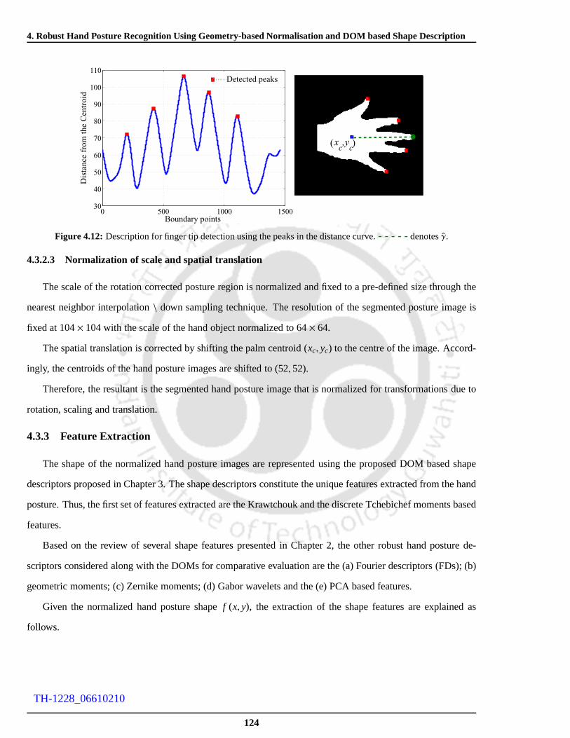
4. Robust Hand Posture Recognition Using Geometry-based Normalisation and DOM based Shape Description
0 500 1000 150030
40
50
60
70
80
90
100
110
Boundary points
Dis
tan
ce f
rom
th
e C
entr
oid
Detected peaks
(xc,yc)
Figure 4.12: Description for finger tip detection using the peaks in the distance curve.- - - - - denotes ˆγ.
4.3.2.3 Normalization of scale and spatial translation
The scale of the rotation corrected posture region is normalized and fixed to a pre-defined size through the
nearest neighbor interpolation\ down sampling technique. The resolution of the segmented posture image is
fixed at 104× 104 with the scale of the hand object normalized to 64× 64.
The spatial translation is corrected by shifting the palm centroid (xc, yc) to the centre of the image. Accord-
ingly, the centroids of the hand posture images are shifted to (52, 52).
Therefore, the resultant is the segmented hand posture image that is normalized for transformations due to
rotation, scaling and translation.
4.3.3 Feature Extraction
The shape of the normalized hand posture images are represented using the proposed DOM based shape
descriptors proposed in Chapter 3. The shape descriptors constitute the unique features extracted from the hand
posture. Thus, the first set of features extracted are the Krawtchouk and the discrete Tchebichef moments based
features.
Based on the review of several shape features presented in Chapter 2, the other robust hand posture de-
scriptors considered along with the DOMs for comparative evaluation are the (a) Fourier descriptors (FDs); (b)
geometric moments; (c) Zernike moments; (d) Gabor waveletsand the (e) PCA based features.
Given the normalized hand posture shapef (x, y), the extraction of the shape features are explained as
follows.
124
TH-1228_06610210

4.3 System Implementation
4.3.3.1 Extraction of moment shape descriptors
The moment based shape descriptors that include the geometric, the Zernike, the Krawtchouk and the
discrete Tchebichef moments are region based descriptors.Proper choice of the order of the moments is an
important factor in deriving the moment features. The orderof the orthogonal moments are chosen based on
the reconstruction accuracy.
a) Extracting the proposed DOM based shape descriptorsThe DOPs namely the WKPs and the DTPs
required for approximating the functionf (x, y) are derived from (3.50) and (3.64) respectively. The corre-
sponding Krawtchouk and the discrete Tchebichef moment features are computed using (3.71) and (3.72) re-
spectively. For the Krawtchouk and the discrete Tchebichefmoments computed up to order(n+m), the number
of moment features obtained are(n+ 1) (m+ 1).
b) Extracting the geometric and the Zernike moment descriptors The non-orthogonal geometric moments
of order (n +m) representingf (x, y) are derived using (2.11). The order of the geometric momentsis chosen
experimentally as 14 (n = 7 andm= 7).
The continuous orthogonal Zernike moment features are computed using the formulation given through
(2.12) and (2.13). In the case of Zernike moments, the repetition m is chosen to take only positive integer
values. For order up ton andm≥ 0, the number of Zernike moment features obtained can be easily verified to
be(
n2 + 1
)2if n is evenand (n+1)(n+3)
4 if n is odd.
An example illustrating the reconstruction accuracy of theZernike, the Krawtchouk and the discrete Tchebichef
moments for various choice of number of moment features is shown in Figure 4.13. The images reconstructed
from the moments based approximations at various order are shown in Figure 4.13(b). The reconstruction error
computed in terms of the SSIM index and the MHD values are shown in Figure 4.13(c) and 4.13(d) respec-
tively. From the plots, we infer that for the given order, theKrawtchouk moments exhibit comparatively higher
reconstruction accuracy. The results in Figure 4.13(b) show that the images reconstructed using the Zernike
moments are comparatively not well defined. It is noted that the concavities are better defined in Krawtchouk
based approximation and the rate of convergence towards theoptimal value is faster in the case of Krawtchouk
moments. For higher orders, the Zernike moments become numerically unstable resulting in higher reconstruc-
tion errors. However, at lower orders, the performance of the Zernike moments is almost close to that of the
discrete Tchebichef moments. As the order increases, the performance of the discrete Tchebichef moments is
close to that of the Krawtchouk moments.
Based on the analysis on reconstruction error, the ordern of the Zernike moments is chosen as 29. Be-
125
TH-1228_06610210

4. Robust Hand Posture Recognition Using Geometry-based Normalisation and DOM based Shape Description
Original shape
(a)
Zernike discrete TchebichefKrawtchouk
Order: 10
Order: 20
Order: 30
Order: 40
Shapes reconstructed using
(b)
9 25 81 169 289 625 1681
0.6
0.7
0.8
0.9
Number of moments
SS
IM
(c) ∗X-axis and Y-axis are in log-scale.
9 25 81 169 289 625 1681
0.3
1.22
3.32
9
24.5
Number of moments
MH
D
(d) ∗X-axis is in log-scale.
Zernike moments
Krawtchouk moments
discrete Tchebichef moments
Figure 4.13: Illustration of reconstruction of the hand posture shape for different orders of orthogonal moments. (a)Original hand posture shape; (b) Shape reconstructed from orthogonal moments. Comparative plot of (c) SSIM index vsnumber of moments and (d) MHD vs number of moments.
yond this order, there is only marginal improvement in the reconstruction accuracy. Also, it is known that
the computational complexity of the Zernike moments increases with the order. Therefore, as a trade-off be-
tween the computational time and the reconstruction accuracy, the order is chosen asn = 29. The optimal
choice of the order(n+m) for the Krawtchouk and the discrete Tchebichef moments are chosen as 80 such that
n = 40 andm= 40. At this order, we observed that both the moments exhibit similar performance with higher
reconstruction accuracy.
4.3.3.2 Extraction of non-moment shape descriptors
a) Extracting FDs The FDs representing the hand postures are derived from the boundary of the hand
posture images. The number of boundary points representingthe shape boundary are normalized to a fixed
value. The points on the shape boundary for efficiently representing the hand postures are chosen at uniform
intervals and the number of boundary points is experimentally chosen as 255. For these points(x, y) ∈ B, the
FDs are computed using (2.9) and (2.10).
b) Deriving Gabor wavelet featuresThe Gabor wavelet features are derived from the normalized hand posture
126
TH-1228_06610210

4.3 System Implementation
images using the formulation given in (2.26). The number of scales and the orientations are experimentally
chosen as 8 and 10 respectively. As per the experimental studies in [4], the optimal value of width of the
Gaussian function is chosen asσ = π and the center frequency is chosen asωmax =π2.
c) Computing PCA featuresSimilar to the moments based approach, the PCA based method is a region based
shape descriptor. The PCA based shape features are computedthrough the steps explained in Section 2.3.2.2.
The PCA features are estimated using the definitions in (2.14) to (2.16) and the projected images are computed
using (2.17).
The number of eigen components required for computing the transformation matrix is experimentally cho-
sen based on the reconstruction accuracy. Given the eigen values λ1, λ2, · · · , λk , the eigen values to be
retained is computed from the ratio [183],
χeigen=
l∑
i=1λi
k∑
i=1λi
; l < k (4.29)
The number of eigenvaluesl for which the ratioχeigen is atleast 0.95 are chosen to form the projection matrix.
This ratio implies that 95% of the variance present in the data are retained by the firstl number of eigenvalues
that are arranged in decreasing order.
Based on (4.29), the number of eigen components representing 99% of the data variance is obtained as 130.
Therefore, the eigenvectors corresponding to the first 130 eigenvalues can be used to form the transformation
matrixWpca. However, the experiments on reconstruction accuracy withrespect to the varyingl have shown that
the number of eigen components required for accurately reconstructing the image from the PCA projections is
only 30. An example, illustrating the shape reconstructionaccuracy of the PCA projections for varying choice
of number of eigen components is shown in Figure 4.14. The reconstruction accuracy is computed using the
SSIM index and the MHD value. The results show that forl = 30, the reconstruction accuracy in terms of the
SSIM index is around 0.99 and the MHD value is around 0.3. Beyondl = 30, the improvement is not very
significant and hence, it suggests that the eigenvectors corresponding to the first 30 eigenvalues are sufficient
for forming the transformation matrix. Forl = 30, the ratioχeigen is 0.78 implying that 78% of the data variance
are represented by the first 30 eigenvalues.
127
TH-1228_06610210

4. Robust Hand Posture Recognition Using Geometry-based Normalisation and DOM based Shape Description
Original shape
(a)
l = 110l = 70l = 30l = 10l = 8
(b)
(c)
4 30 50 70 90 110 1300.98
0.99
1
Number of eigen components (l)
SSIM
(d)
4 30 50 70 90 110 1300
1
2
Number of eigen components (l)M
HD
(e)
Figure 4.14: Illustration of shape reconstruction with respect to varying number of eigen components (a) Original shape;(b) Shapes reconstructed from the PCA projections for different number of eigenvalues and (c) the results of binarisationof the reconstructed shapes in (b). The threshold for binarisation is uniformly chosen as 120. Comparative plots of (d)SSIM index vs number of eigenvalues and (e) MHD vs number of eigenvalues, computed between the shape in (a) andthe reconstructed binary shapes in (c).
4.3.4 Classification
Considerzs andzt as the feature vectors of the test and the target shapes ( in the reference set ) respectively.
Then, the classification ofzs is done using the minimum distance classifier defined as
dt (zs, zt) =T
∑
j=1
(zs j − zt j )2 (4.30)
Match= arg mint
(dt)
wheret is the index of signs in the reference set andT is the dimension of the feature vectors.
4.4 Experimental Studies and Results
The performance of the proposed DOM descriptors in comparison with the other shape descriptors dis-
cussed above is verified through two different experiments on hand posture shapes. The first experiment stud-
ies the user independence characteristics of the shape descriptors. The second experiment is for verifying the
robustness of the shape features in view invariant hand posture representation.
128
TH-1228_06610210

4.4 Experimental Studies and Results
Of the 4, 230 hand posture images corresponding to 10 posture classes, 2, 260 are collected during the first
phase at a view angle of 90 and the remaining 1, 970 are collected during the second phase by varying the view
angles. We refer the dataset taken at 90 asDataset 1and the remaining data asDataset 2. The 10 postures
classes in the database are labeled from 0 to 9.
The Dataset 1 consists of postures that vary due to similarity transformations of rotation and scaling. Dataset
2 consists of postures that are taken at different view angles and scales. Due to the viewing angles, the postures
undergo perspective distortions and the view angle variation also imposes orientation changes. Thus, the pos-
tures in Dataset 2 accounts for both perspective (view angle) and similarity (orientation and scale) distortions.
Also, the postures in Dataset 1 are collected cautiously such that there is no self-occlusion between the fingers.
But, while collecting the samples in Dataset 2 the precautions were not taken to control self-occlusion which
might occur due to either the user’s flexibility or the view angle variation. Therefore, it can be expected that
the hand posture shapes in the Dataset 2 are more distorted than those in Dataset 1. The variations in the hand
posture shapes caused due to user and viewpoint changes are quantitatively analyzed using the Pratt’s FOM and
the correlation coefficient.
4.4.1 Quantitative analysis of hand posture variations
The structural variations between the hand posture images of each class are verified from the intraclass
and the interclass distances among the hand posture images.The intraclass and the interclass distances are
computed using the Pratt’s FOM and the correlation coefficient. The samples required for this analysis are
randomly chosen from Dataset 1 and Dataset 2. The reference set required for computing the distances are
taken from Dataset 1 and there are 23 samples per hand postureclass comprising of data collected from 23
users. Similarly, the query set is formed by collecting 69 samples per posture class from each of Dataset 1 and
Dataset 2.
Figure 4.15 illustrates the intraclass distances computedin terms of the Pratt’s FOM. By comparing the plots
in Figure 4.15(a) and Figure 4.15(b), we can infer that most of the samples in Dataset 1 exhibits comparatively
higher values of FOM. Further, it is also evident that the range of variation in the FOM values corresponding to
the samples from Dataset 2 is more than that of the samples from Dataset 1. The standard deviation plot of the
intraclass FOMs shown in Figure 4.16 shows the variability in the values of Pratt’s FOM with respect to each
class . By comparing the standard deviation values obtainedfor each class, it is observed that the intraclass
distance is comparatively less only for the samples from posture classes 6, 7 and 9.
The plots illustrating the comparison between the intraclass and the interclass distances for hand posture
129
TH-1228_06610210

4. Robust Hand Posture Recognition Using Geometry-based Normalisation and DOM based Shape Description
0 1 2 3 4 5 6 7 8 90.5
0.6
0.7
0.8
0.9
Index of the Posture Class
Pra
tt’s
FO
M
(a)
0 1 2 3 4 5 6 7 8 90.4
0.5
0.6
0.7
0.8
0.9
Index of the Posture Class
Pra
tt’s
FO
M
(b)
Figure 4.15: Intraclass distance measured in terms of Pratt’s FOM for samples in (a) Dataset 1 and (b) Dataset 2. Thereference set is taken from Dataset 1. There are 690 testing samples with 69 samples\ posture sign in each of the datasetand 230 samples in the reference set with 23 samples\ posture sign.
0 1 2 3 4 5 6 7 8 90.02
0.04
0.06
0.08
Index of the Posture Class
Sta
nd
ard
dev
iati
on
of
intr
acla
ss P
ratt
’s F
OM
Dataset 1
Dataset 2
(a)
Figure 4.16: Illustration of variability in the intraclass FOM values with respect to samples in each posture class.
images in Dataset 1 and Dataset 2 are shown in Figure 4.17. Theplots are generated by computing the average
of the correlation values obtained with respect to the samples in each posture class. From the distance values,
it is evident that the intraclass samples exhibit higher similarity than the interclass samples. This implies that
the posture signs comprising the database are structurallydistinct shapes.
As we examine the correlation values in Figure 4.17 obtainedfor Dataset 1 and Dataset 2, it is observed
that the correlation values with respect to the interclass samples are over 0.55. Further, the maximum difference
between the intraclass and the interclass correlation values is approximately around 25%. Despite the structural
distinctiveness, these values indicate that the samples corresponding to any class exhibit approximately 50%
structural similarity with respect to the samples in every other class. Therefore, it is clear that the hand posture
shapes of different classes consist of overlapping regions.
It is known that the hand is composed of the palm and the finger regions. Of these, the fingers move at
different degrees in order to constitute different hand postures. The palm region is a static region and the hand
130
TH-1228_06610210
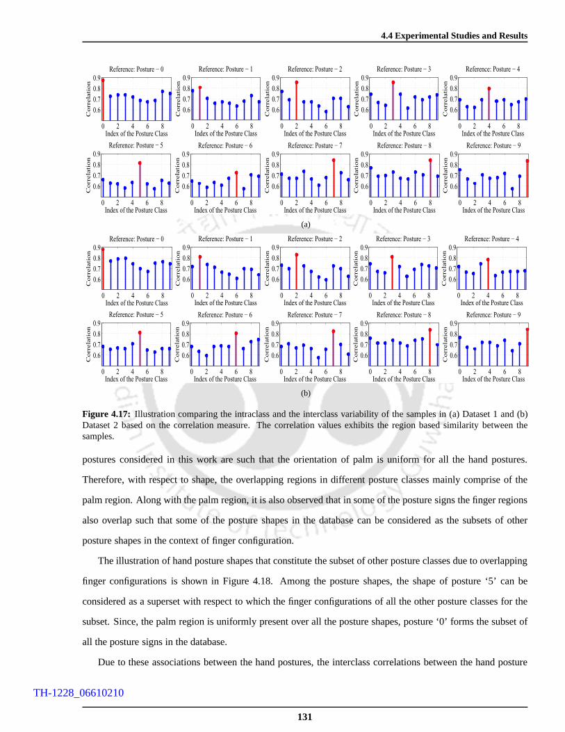
4.4 Experimental Studies and Results
0 2 4 6 8
0.6
0.7
0.8
0.9
Index of the Posture Class
Corr
ela
tion
Reference: Posture − 0
0 2 4 6 8
0.6
0.7
0.8
0.9
Index of the Posture Class
Corr
ela
tion
Reference: Posture − 1
0 2 4 6 8
0.6
0.7
0.8
0.9
Index of the Posture Class
Corr
ela
tion
Reference: Posture − 2
0 2 4 6 8
0.6
0.7
0.8
0.9
Index of the Posture Class
Corr
ela
tion
Reference: Posture − 3
0 2 4 6 8
0.6
0.7
0.8
0.9
Index of the Posture Class
Corr
ela
tion
Reference: Posture − 4
0 2 4 6 8
0.6
0.7
0.8
0.9
Index of the Posture Class
Corr
ela
tion
Reference: Posture − 5
0 2 4 6 8
0.6
0.7
0.8
0.9
Index of the Posture Class
Corr
ela
tion
Reference: Posture − 6
0 2 4 6 8
0.6
0.7
0.8
0.9
Index of the Posture Class
Corr
ela
tion
Reference: Posture − 7
0 2 4 6 8
0.6
0.7
0.8
0.9
Index of the Posture Class
Corr
ela
tion
Reference: Posture − 8
0 2 4 6 8
0.6
0.7
0.8
0.9
Index of the Posture Class
Corr
ela
tion
Reference: Posture − 9
(a)
0 2 4 6 8
0.6
0.7
0.8
0.9
Index of the Posture Class
Co
rrela
tion
Reference: Posture − 0
0 2 4 6 8
0.6
0.7
0.8
0.9
Index of the Posture Class
Co
rrela
tion
Reference: Posture − 1
0 2 4 6 8
0.6
0.7
0.8
0.9
Index of the Posture Class
Co
rrela
tion
Reference: Posture − 2
0 2 4 6 8
0.6
0.7
0.8
0.9
Index of the Posture Class
Co
rrela
tion
Reference: Posture − 3
0 2 4 6 8
0.6
0.7
0.8
0.9
Index of the Posture Class
Co
rrela
tion
Reference: Posture − 4
0 2 4 6 8
0.6
0.7
0.8
0.9
Index of the Posture Class
Co
rrela
tio
n
Reference: Posture − 5
0 2 4 6 8
0.6
0.7
0.8
0.9
Index of the Posture Class
Co
rrela
tio
n
Reference: Posture − 6
0 2 4 6 8
0.6
0.7
0.8
0.9
Index of the Posture Class
Co
rrela
tio
n
Reference: Posture − 7
0 2 4 6 8
0.6
0.7
0.8
0.9
Index of the Posture Class
Co
rrela
tio
n
Reference: Posture − 8
0 2 4 6 8
0.6
0.7
0.8
0.9
Index of the Posture Class
Co
rrela
tio
n
Reference: Posture − 9
(b)
Figure 4.17: Illustration comparing the intraclass and the interclass variability of the samples in (a) Dataset 1 and (b)Dataset 2 based on the correlation measure. The correlationvalues exhibits the region based similarity between thesamples.
postures considered in this work are such that the orientation of palm is uniform for all the hand postures.
Therefore, with respect to shape, the overlapping regions in different posture classes mainly comprise of the
palm region. Along with the palm region, it is also observed that in some of the posture signs the finger regions
also overlap such that some of the posture shapes in the database can be considered as the subsets of other
posture shapes in the context of finger configuration.
The illustration of hand posture shapes that constitute thesubset of other posture classes due to overlapping
finger configurations is shown in Figure 4.18. Among the posture shapes, the shape of posture ‘5’ can be
considered as a superset with respect to which the finger configurations of all the other posture classes for the
subset. Since, the palm region is uniformly present over allthe posture shapes, posture ‘0’ forms the subset of
all the posture signs in the database.
Due to these associations between the hand postures, the interclass correlations between the hand posture
131
TH-1228_06610210

4. Robust Hand Posture Recognition Using Geometry-based Normalisation and DOM based Shape Description
54
7
23
1 800
9
66
Figure 4.18: Illustration of the classes of the hand posture shapes that form the subsets of other posture class in thecontext of finger configuration.
shapes illustrated through Figure 4.17 are high. On comparing the correlation values obtained for Dataset 1 and
Dataset 2, it is clear that the intraclass correlation and the difference between the intraclass and the interclass
correlation values decreases for the samples in Dataset 2. Further, due to viewpoint changes the interclass
correlation between the posture classes that form the set and the postures contained in the corresponding subsets
is observed to increase.
The above analysis on the hand posture variations in terms ofthe intraclass and the interclass distances
suggests that the database is composed of hand posture images with more structural deviations indicating the
effects of user variations and the viewpoint changes. Therefore, the above analysis validates the applicability
of the developed hand posture database for experiments on user and view invariant hand posture classification.
4.4.2 Experiments on hand posture classification
In this study, two sets of experiments are performed to analyze the efficiency of the proposed DOM based
hand posture recognition technique. The first experiment studies the user independent characteristics of the
DOM features. The second experiment concentrates on studying the view invariant classification accuracy of
the DOM features. The performance of the DOM features in boththe experiments is verified in comparison with
the hand posture descriptors obtained using other state-of-the art features discussed in Section 4.3.3. The details
of the experiment and the results obtained for user independent and view invariant hand posture classification
are discussed as follows.
132
TH-1228_06610210
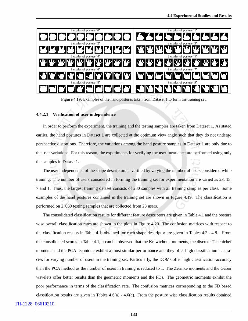
4.4 Experimental Studies and Results
Samples of posture ‘0’ Samples of posture ‘1’
Samples of posture ‘2’ Samples of posture ‘3’
Samples of posture ‘4’ Samples of posture ‘5’
Samples of posture ‘6’ Samples of posture ‘7’
Samples of posture ‘8’ Samples of posture ‘9’
Figure 4.19:Examples of the hand postures taken from Dataset 1 to form thetraining set.
4.4.2.1 Verification of user independence
In order to perform the experiment, the training and the testing samples are taken from Dataset 1. As stated
earlier, the hand postures in Dataset 1 are collected at the optimum view angle such that they do not undergo
perspective distortions. Therefore, the variations amongthe hand posture samples in Dataset 1 are only due to
the user variations. For this reason, the experiments for verifying the user-invariance are performed using only
the samples in Dataset1.
The user independence of the shape descriptors is verified byvarying the number of users considered while
training. The number of users considered in forming the training set for experimentation are varied as 23, 15,
7 and 1. Thus, the largest training dataset consists of 230 samples with 23 training samples per class. Some
examples of the hand postures contained in the training set are shown in Figure 4.19. The classification is
performed on 2, 030 testing samples that are collected from 23 users.
The consolidated classification results for different feature descriptors are given in Table 4.1 and the posture
wise overall classification rates are shown in the plots in Figure 4.20. The confusion matrices with respect to
the classification results in Table 4.1, obtained for each shape descriptor are given in Tables 4.2 - 4.8. From
the consolidated scores in Table 4.1, it can be observed thatthe Krawtchouk moments, the discrete Tchebichef
moments and the PCA technique exhibit almost similar performance and they offer high classification accura-
cies for varying number of users in the training set. Particularly, the DOMs offer high classification accuracy
than the PCA method as the number of users in training is reduced to 1. The Zernike moments and the Gabor
wavelets offer better results than the geometric moments and the FDs. The geometric moments exhibit the
poor performance in terms of the classification rate. The confusion matrices corresponding to the FD based
classification results are given in Tables 4.6(a) - 4.6(c). From the posture wise classification results obtained
133
TH-1228_06610210

4. Robust Hand Posture Recognition Using Geometry-based Normalisation and DOM based Shape Description
Table 4.1: Comparison of classification results obtained for varying number of users in the training set. The number of testing samplesin Dataset 1 is 2030. (% of CC- Percentage of correct classification )
CLASSIFICATION RESULTS FOR THE TESTING SAMPLES FROM DATASE T 1 BASED ON
No. of No. of discrete
users in the Training Krawtchouk Tchebichef Geometric Zernike Gabor
Training samples per moments moments moments moments FDs wavelets PCA
set gesture
% of CC % of CC % of CC % of CC % of CC % of CC % of CC
23 23 95.22 95.47 82.07 91.87 88.08 92.81 95.37
15 15 94.98 95.12 78.47 90.44 86.01 91.23 94.83
7 7 91.97 92.25 72.66 86.11 82.71 87.24 92.27
1 1 82.12 82.27 59.16 68.13 65.52 73.65 78.87
for varying number of users during training, it can be observed that the misclassifications in FD based repre-
sentation have occurred for samples with almost similar boundary profiles. The posture classes 1, 2, 8 and 9
exhibit higher misclassifications as the number of users in the training set vary. Similarly, posture 6 is mostly
mismatched with posture 7 and the misclassification increases for decreasing number of users while training.
Apart from these, the samples belonging to other posture classes exhibit almost similar classification rates for
varying number of users.
In the case of geometric moments, the rate of misclassification increases considerably as the number of users
in the training set decreases. Further, the decline in the classification accuracies indicates that the geometric
moments provide the least user independence. The posture-wise classification results of the geometric moments
obtained for varying number of users in the training set are tabulated in Tables 4.4(a) - 4.4(c). From these results,
it is observed that most of the mismatches have occurred among the postures that are geometrically close. For
example, posture 3 is mostly misclassified as posture 2, posture 1 is misidentified as posture 7, posture 2 is
recognized as either posture 1 or posture 3 and posture 7 is matched as posture 2. It is also observed that in the
case of geometric moments there is poor perceptual correspondence between the mismatched postures. This is
because the geometric moments are global features and they only represent the statistical attributes of a shape.
The Zernike moments offer better classification rate than the geometric moments even as the number of
users considered for training decreases. From the comprehensive scores of the classification results given in
Tables 4.5(a) - 4.5(c), it is understood that the accuracy ofZernike moments is mainly reduced due to the
confusion among the postures 1, 8 and 9. Since the Zernike polynomials are defined in the polar domain, the
magnitude of the Zernike moments for shapes with almost similar boundary profile will also be approximately
same. Hence, similar to the FDs, the misclassification in thecase of Zernike moments occurred between the
postures that have almost similar boundary profiles. From the samples shown in Figure 4.19, it can be noted
that the postures 1, 8 and 9 have almost same boundary profilesand hence, are frequently mismatched.
134
TH-1228_06610210

4.4 Experimental Studies and Results
0 1 2 3 4 5 6 7 8 920
40
60
80
100
Index of the Posture Class
% C
C
Krawtchouk
discrete Tchebichef
FDs
Geometric
Zernike
Gabor wavelets
PCA
(a)
0 1 2 3 4 5 6 7 8 920
40
60
80
100
Index of the Posture Class
% C
C
Krawtchouk
discrete Tchebichef
FDs
Geometric
Zernike
Gabor wavelets
PCA
(b)
0 1 2 3 4 5 6 7 8 920
40
60
80
100
Index of the Posture Class
% C
C
Krawtchouk
discrete Tchebichef
FDs
Geometric
Zernike
Gabor wavelets
PCA
(c)
0 1 2 3 4 5 6 7 8 920
40
60
80
100
Index of the Posture Class
% C
C
Krawtchouk
discrete Tchebichef
FDs
Geometric
Zernike
Gabor wavelets
PCA
(d)
Figure 4.20: Plots of the posture wise classification results for (a) 23 users; (b) 15 users; (c) 7 users and (d) 1 user in thetraining set.
135
TH-1228_06610210

4. Robust Hand Posture Recognition Using Geometry-based Normalisation and DOM based Shape Description
Table 4.2: Confusion matrix corresponding to the results in Table 4.1 for Krawtchouk moment features with respect to varying numberof users in the training set and 203 testing samples\gesture.
(a) 23 training samples\gesture.
@@I/PO/P
1 2 3 4 5 6 7 8 9
0 200 1 21 188 152 2 198 33 1 201 14 2 2 198 15 201 26 3 174 25 17 1 1 1 195 58 4 3 2 1 3 1909 3 6 6 188
(b) 15 training samples\gesture.
@@I/PO/P
0 1 2 3 4 5 6 7 8 9
0 199 1 31 191 122 2033 2 199 1 14 2 2 198 15 201 26 5 174 23 17 2 1 3 191 68 7 2 4 1 3 1869 5 5 7 186
(c) 7 training samples\gesture.
@@I/PO/P
0 1 2 3 4 5 6 7 8 9
0 197 1 51 192 112 4 1993 1 192 1 1 7 14 2 198 2 15 201 26 8 154 417 1 3 1 197 18 4 5 4 1 1 1889 1 4 3 23 23 149
(d) 1 training samples\gesture.
@@I/PO/P
0 1 2 3 4 5 6 7 8 9
0 198 4 11 1 191 1 1 7 1 12 2 43 1583 194 1 1 6 14 5 2 4 189 2 15 200 36 18 91 81 11 27 2 42 3 1568 12 3 15 1 1 12 2 1579 5 2 21 12 30 133
Table 4.3: Comprehensive scores of the classification results in Table4.1 for discrete Tchebichef moments based features with respectto different number of users in the training set and 203 testing samples\gesture.
(a) 23 training samples\gesture.
@@I/PO/P
0 1 2 3 4 5 6 7 8 9
0 200 1 21 189 142 1 199 33 202 14 2 2 1995 201 26 3 176 23 17 1 1 1 194 68 3 3 2 1 3 1919 3 8 5 187
(b) 15 training samples\gesture.
@@I/PO/P
0 1 2 3 4 5 6 7 8 9
0 199 1 31 191 122 2033 2 200 14 2 1 199 15 201 26 6 174 22 17 2 1 3 190 78 4 2 4 1 3 1899 4 1 6 7 185
(c) 7 training samples\gesture.
@@I/PO/P
0 1 2 3 4 5 6 7 8 9
0 197 1 51 192 112 4 1993 1 193 1 1 6 14 2 199 1 15 201 26 9 155 397 1 3 1 197 18 4 4 4 1 1 1899 1 3 3 26 22 148
(d) 1 training samples\gesture.
@@I/PO/P
0 1 2 3 4 5 6 7 8 9
0 197 5 11 1 191 1 1 7 1 12 2 43 1583 196 1 1 4 14 5 2 3 190 2 15 202 16 29 90 71 12 17 2 42 3 1568 9 3 15 1 2 12 2 1599 5 2 23 1 12 29 131
Table 4.4: Confusion matrix corresponding to the results in Table 4.1 for geometric moments based features with respect to differentnumber of users in the training set and 203 testing samples\gesture.
(a) 23 training samples\gesture.
@@I/PO/P
0 1 2 3 4 5 6 7 8 9
0 175 1 8 1 1 8 91 184 192 18 163 13 4 2 1 1 13 4 1 53 126 12 1 64 1 1 12 18 160 5 2 3 15 13 179 7 46 1 1 10 5 156 27 37 1 17 2 3 3 172 58 9 3 3 5 13 2 1 1679 1 4 2 12 184
(b) 15 training samples\gesture.
@@I/PO/P
0 1 2 3 4 5 6 7 8 9
0 171 5 1 12 3 1 7 31 185 1 172 18 157 19 6 1 1 13 5 1 65 108 19 54 1 1 15 15 158 5 3 2 35 22 165 13 36 5 16 6 150 23 1 27 1 10 2 3 5 175 78 11 2 4 2 22 3 1 1589 3 2 1 8 2 25 162
(c) 7 training samples\gesture.
@@I/PO/P
0 1 2 3 4 5 6 7 8 9
0 168 4 1 14 4 1 8 31 177 1 252 26 135 29 8 2 1 23 19 54 100 20 1 1 84 1 2 2 19 159 5 10 2 35 2 22 155 21 36 1 2 30 1 129 38 1 17 1 15 2 4 4 171 68 13 4 3 2 34 4 1439 2 2 2 9 4 5 41 138
(d) 1 training samples\gesture.
@@I/PO/P
0 1 2 3 4 5 6 7 8 9
0 167 33 1 21 152 2 9 5 4 26 52 111 49 34 2 73 16 6 20 110 12 1 3 354 1 26 8 119 13 1 16 195 36 162 1 46 45 18 88 48 1 37 14 65 12 3 1 104 2 28 15 2 24 16 10 1 129 69 1 1 11 16 3 47 3 121
Table 4.5: Confusion matrix corresponding to the results in Table 4.1 for Zernike moment features under varying number of users inthe training set and 203 testing samples\gesture.
(a) 23 training samples\gesture.
@@I/PO/P
0 1 2 3 4 5 6 7 8 9
0 177 4 18 41 180 5 3 152 4 194 53 1 198 3 14 1 200 1 15 199 46 182 17 1 37 3 199 18 18 2 161 229 8 1 19 175
(b) 15 training samples\gesture.
@@I/PO/P
0 1 2 3 4 5 6 7 8 9
0 175 6 17 51 174 4 6 192 4 193 63 1 198 3 14 2 197 2 25 197 66 181 17 1 47 2 3 1 195 28 17 2 160 249 17 1 4 15 166
(c) 7 training samples\gesture.
@@I/PO/P
0 1 2 3 4 5 6 7 8 9
0 161 12 16 141 168 3 14 3 152 5 184 143 198 3 1 14 1 200 25 1 196 66 176 26 17 2 3 197 18 32 1 12 144 149 17 5 25 32 124
(d) 1 training samples\gesture.
@@I/PO/P
0 1 2 3 4 5 6 7 8 9
0 153 12 381 135 4 36 282 7 86 20 1 893 195 6 24 9 1945 5 193 56 1 1 69 130 1 17 24 1 151 1 268 25 3 5 3 16 105 469 30 9 48 14 102
136
TH-1228_06610210

4.4 Experimental Studies and Results
Table 4.6: Confusion matrix corresponding to the results in Table 4.1 for FD based representation with respect to varying number ofusers in the training set and 203 testing samples\gesture.
(a) 23 training samples\gesture.
@@I/PO/P
0 1 2 3 4 5 6 7 8 9
0 195 2 61 155 41 72 2 2013 1 198 2 1 14 2 201 0005 5 1986 3 184 14 1 17 2 1 4 189 2 58 20 1 168 149 41 63 99
(b) 15 training samples\gesture.
@@I/PO/P
0 1 2 3 4 5 6 7 8 9
0 193 4 61 144 47 122 2 2013 1 198 2 1 14 2 201 0005 5 1986 6 177 19 17 2 4 185 3 98 21 2 166 149 47 73 83
(c) 7 training samples\gesture.
@@I/PO/P
0 1 2 3 4 5 6 7 8 9
0 191 121 153 1 36 132 200 1 1 13 198 2 1 24 2 2015 10 193 0006 4 151 487 5 1 188 5 48 37 5 143 189 62 80 61
(d) 1 training samples\gesture.
@@I/PO/P
0 1 2 3 4 5 6 7 8 9
0 200 31 179 13 1 4 62 158 6 393 199 1 34 4 194 5 0005 25 176 26 14 61 126 27 47 4 68 22 628 89 50 31 339 80 48 11 64
Table 4.7: Confusion matrix corresponding to the results in Table 4.1 for Gabor wavelets based features under varying number of usersin the training set and 203 testing samples\gesture.
(a) 23 training samples\gesture.
@@I/PO/P
0 1 2 3 4 5 6 7 8 9
0 172 7 5 191 2 177 2 11 112 193 3 73 187 1 10 2 34 1 198 1 35 197 66 1 3 1 190 87 1 1 3 1 196 18 8 5 4 185 19 4 1 1 8 189
(b) 15 training samples\gesture.
@@I/PO/P
0 1 2 3 4 5 6 7 8 9
0 165 10 6 221 2 177 2 11 112 193 3 73 189 1 9 2 24 1 198 2 25 195 86 7 4 1 184 6 17 1 1 3 1 196 18 10 9 4 179 19 6 1 14 6 176
(c) 7 training samples\gesture.
@@I/PO/P
0 1 2 3 4 5 6 7 8 9
0 163 14 7 191 9 173 1 5 5 102 1 187 5 103 16 172 1 7 5 24 1 200 25 197 66 11 10 1 169 9 37 1 1 15 1 184 18 15 13 9 165 19 5 3 26 8 161
(d) 1 training samples\gesture.
@@I/PO/P
0 1 2 3 4 5 6 7 8 9
0 149 36 2 2 141 42 142 4 2 1 122 3 188 1 4 73 1 10 176 13 1 24 3 159 1 19 215 197 66 29 1 11 19 79 63 17 1 52 33 1 1168 1 46 1 18 135 29 4 36 9 154
Table 4.8: Confusion matrix corresponding to the results in Table 4.1 for PCA based description with different number of users in thetraining set and 203 testing samples\gesture.
(a) 23 training samples\gesture.
@@I/PO/P
0 1 2 3 4 5 6 7 8 9
0 196 3 1 31 188 14 12 1 2023 2 200 14 4 1995 194 3 66 1 177 24 17 4 1 193 58 2 3 1 1 2 1949 4 1 1 2 2 193
(b) 15 training samples\gesture.
@@I/PO/P
0 1 2 3 4 5 6 7 8 9
0 195 4 1 31 186 2 14 12 1 2023 2 200 14 4 1 197 15 193 4 66 1 179 22 17 5 1 3 186 88 3 2 1 1 1 1959 4 2 2 3 192
(c) 7 training samples\gesture.
@@I/PO/P
0 1 2 3 4 5 6 7 8 9
0 193 5 4 11 186 2 152 4 1993 3 2 184 3 8 34 4 197 25 193 5 56 3 152 47 17 3 2 2 195 18 2 1 7 2 1 1909 3 7 9 184
(d) 1 training samples\gesture.
@@I/PO/P
0 1 2 3 4 5 6 7 8 9
0 189 10 3 11 1 184 10 7 12 2 62 1393 1 2 1 181 1 14 34 4 10 1 165 235 4 173 20 2 46 29 65 87 20 27 2 5 52 2 1428 3 10 4 13 1 1729 3 1 1 6 1 191
In the case of Krawtchouk moments, the mismatch has occurredbetween the postures with coinciding re-
gions. As per the results in Tables 4.2(a) - 4.2(c), the postures 1, 6 and 9 exhibit higher misclassifications.
Further, it is observed that the posture classes 6 and 9 show significant improvement in the classification ac-
curacy as the number of users in the training set increases. It can be noticed that posture classes 1 and 6 are
frequently mismatched with posture class 7 and posture class 9 is mismatched with posture classes 6 and 7.
Similar observations can be made from the results obtained for discrete Tchebichef moment based features.
From the confusion matrices given in Tables 4.3(a) - 4.3(c),it is clear that the misclassifications in the case of
discrete Tchebichef moment features are similar to the Krawtchouk moments.
The misclassifications in DOM based representations occur when the hand posture images consist of over-
lapping regions. With respect to the shape, some posture signs in the dataset can be considered as the subsets
of other signs in the context of spatial distribution of their pixels. To show that, in DOMs based representation
137
TH-1228_06610210

4. Robust Hand Posture Recognition Using Geometry-based Normalisation and DOM based Shape Description
Test posture Obtained match Actual match in Test posture Obtained match Actual match inposture ‘1’ posture ‘7’ Training set of posture ‘1’ posture ‘9’ posture ‘7’ Training set of posture ‘9’
Comparison between the spatial distribution of boundary points Comparison between the spatial distribution of boundary points
20 30 40 50 60 70 80
10
20
30
40
50
60
70
80
20 30 40 50 60 70 80
10
20
30
40
50
60
70
8020 30 40 50 60 70 80
20
30
40
50
60
70
80
20 30 40 50 60 70 80
20
30
40
50
60
70
80
Test data
Obtained match
Actual match
Test data
Obtained match
Actual match
Figure 4.21:Examples of results from DOM based classification. The illustration is presented to show that the DOM de-pend on the similarity between the spatial distribution of the pixels within the posture regions. The spatial correspondencebetween the postures is analyzed based on the shape boundary. It can be observed that the maximum number of boundarypixels from the test sample coincide more with the obtained match rather than the actual match.
Trained postures Tested postures Mismatched as
posture ‘1’ posture ‘1’posture
‘7’ ‘7’ ‘7’ ‘7’ ‘7’ ‘7’ ‘7’ ‘7’ ‘7’
posture ‘6’ posture ‘6’posture
‘7’ ‘4’ ‘7’ ‘7’ ‘7’ ‘7’ ‘7’ ‘7’ ‘7’
posture ‘9’ posture ‘9’posture
‘7’ ‘7’ ‘0’ ‘6’ ‘7’ ‘7’ ‘6’ ‘6’ ‘0’
Figure 4.22: Results from the experiment on user invariance. Examples ofthe testing samples that are misclassified inDOMs based method. The correspondence of the test posture can be observed to be high with respect to the mismatchedposture rather than the trained postures within the same class.
the confusion has occurred between the postures with almostsame spatial distribution of the pixels, a simple
analysis is performed by comparing the spatial distribution of the boundary pixels. If the boundary pixels ex-
hibit higher correspondence, so will be the regions within the boundaries will exhibit similar correspondence.
Figure 4.21 illustrates a few examples from the misclassifications in posture classes 1 and 9. It can be veri-
fied that the spatial distribution of the pixels in the test postures coincides highly with the matches obtained
through Krawtchouk moments based classification. Some examples of these misclassifications along with the
corresponding training postures are shown in Figure 4.22.
The comprehensive scores of the classification results obtained for Gabor wavelet based hand posture de-
scription are given in Table 4.7(a) and Table 4.7(c). It is seen that more misclassification occurs due to the
138
TH-1228_06610210

4.4 Experimental Studies and Results
−4000 −2000 0 2000 4000
−4000
−3000
−2000
−1000
0
1000
2000
3000
PCA 1
PC
A 2
Projection vectors for the training set
−2000 0 2000 4000−4000
−3000
−2000
−1000
0
1000
2000
3000
PCA 1
PC
A 2
Projection vectors for samples from the testing set
Class 0
Class 1
Class 2
Class 3
Class 4
Class 5
Class 6
Class 7
Class 8
Class 9
Figure 4.23: Illustration of separation between the hand posture classes in PCA projection space.
posture classes 0, 1, 3, 6, 8 and 9. The mismatch in Gabor wavelets based description occurs between the sam-
ples with similar edge magnitudes and the orientations. Forexample, the posture class 9 is mostly mismatched
with posture class 6. In Section 4.4.1, it has been shown thatthe posture sign 9 can be considered as a subset
of posture sign 6. The coinciding thumb finger region in both these posture classes have same orientation and
hence, these postures are matched. From Table 4.1, it can be observed that the rate of misclassification in Gabor
wavelets based classification drastically increases when the number of users in training is decreased to 7. As
we examine the confusion matrix in Table 4.7(c), it is evident that the misclassification has increased for all the
posture classes.
The confusion matrices for the PCA based classification results are given in Tables 4.8(a) - 4.8(c). By com-
paring the posture wise classification results, it can be understood that the performance of the PCA technique
is consistent with the varying number of users in training. More misclassification has occurred in the posture
classes 1 and 6. In the case of PCA projections, the between-class separation is not considered and hence,
the projections corresponding to different image classes largely overlap. The plot illustrating the projection
on the first two PCA components is shown in Figure 4.23. The misclassification occurs when the projection
corresponding to the test sample fall within the overlapping region.
The observations from the experimental results on user invariance can be summarized as follows.
1] The Krawtchouk and the discrete Tchebichef moments offerhigh classification accuracies. Even as the num-
ber of users decreases during training, the classification scores are almost similar. This shows that the DOMS
are user invariant features. Particularly, the discrete Tchebichef moments offer slightly better performance in
comparison to Krawtchouk moments.
2] The geometric moments offer low classification accuracies and the misclassifications increases for decreas-
ing number of users. This implies that the geometric momentsare sensitive to user variations and they exhibit
139
TH-1228_06610210

4. Robust Hand Posture Recognition Using Geometry-based Normalisation and DOM based Shape Description
poor user invariance.
3] The FDs and the Zernike moments fail in efficiently discriminating hand posture shapes with almost similar
boundary profile. The FDs are derived from the frequency description of 1D boundary profile and hence, the
information on spatial localization is lost. In the case of Zernike moments, the information about spatial local-
ization in preserved in the polar domain representation. However, even small boundary deviations in the spatial
domain may cause large shifts in the polar domain due to whichmisclassifications occur between samples with
similar boundary profiles.
From the plot of the intraclass distance based on Pratt’s FOMas shown in Figure 4.15, it can be noted that
the boundary distortion between the intraclass samples is comparatively more for posture classes 1, 6, 8 and
9. As a result, the misclassifications in FDs and Zernike moments are mainly due to postures 1, 6, 8 and 9.
Except for these postures, the FDs and the Zernike moments exhibit consistently high classification accuracies
for other posture classes. Hence, the FDs and the Zernike moments are robust to user variations in classifying
hand postures with distinct boundary profile.
4] The Gabor wavelets offer better classification accuracy when the number of users in the training is more.
As the number of users decreases to 7, the performance of the Gabor wavelets decreases by almost 4%. This
implies that the Gabor wavelets based description requireslarge number of training samples for achieving user
independence.
5] From the results obtained for the PCA, we infer that the performance efficiency of the PCA is similar to
that of the Krawtchouk features and PCA offers high classification accuracy exhibiting more robustness to user
variations. However, as the number of user is reduced to 1, the performance of PCA is significantly less than
the DOMs.
4.4.2.2 Verification of view invariance
The view angle variations during hand posture acquisition lead to perspective distortions and may some-
times cause self-occlusion. The self-occlusion can also bedue to the poor flexibility of the postures. The study
on view invariance verifies the robustness of the methods towards the effects of viewpoint changes.
In order to study the view invariance property of the considered methods, the initial experiment is performed
by considering the training set taken from Dataset 1. We refer the training samples from Dataset 1 asTraining
set-I. The testing set consists of 3, 600 samples that include 2, 030 samples from Dataset 1 and 1, 570 samples
from Dataset 2. The classification results obtained using the Training set-I are tabulated in Table 4.9. The
comprehensive posture-wise classification scores are given in Table 4.10(a) - 4.10(g).
140
TH-1228_06610210

4.4 Experimental Studies and Results
Table 4.9: Experimental validation of view invariance. Comparison ofclassification results obtained for Training set-I and II. Thetraining set includes hand postures collected from 23 users. The number of testing samples in Dataset 1 and Dataset 2 is 2,030 and1,570 respectively. (% CC- percentage of correct classification. )
Training set-I Training set-II
Methods % CC forDataset 1
% CC forDataset 2
Overall% CC
% CC forDataset 1
% CC forDataset 2
Overall% CC
Krawtchouk moments 95.22 87.90 92.03 97.93 95.73 96.97
discrete Tchebichef moments 95.47 88.79 92.55 97.83 96.24 97.14
Geometric moments 82.07 71.4 77.42 87.39 80.57 84.42
Zernike moments 90.89 75.48 84.17 94.83 90.32 92.86
FDs 88.08 70.57 80.44 90.15 85.99 88.33
Gabor wavelets 92.81 73.12 84.22 95.52 88.47 92.44
PCA 95.37 88.79 91.38 97.93 96.24 97.19
Examples of posture ‘0’ Examples of posture ‘1’ Examples of posture ‘2’
Examples of posture ‘3’ Examples of posture ‘4’ Examples of posture ‘5’
Examples of posture ‘6’ Examples of posture ‘7’ Examples of posture ‘8’
Examples of posture ‘9’
Figure 4.24: Samples of the test postures from Dataset 2 that has less recognition accuracy with respect to all the methods.
From the results in Table 4.9, it is evident that among the considered methods, the Krawtchouk moments,
the discrete Tchebichef moments and the PCA technique offerbetter classification accuracy. The performance
efficiency of other methods that includes FDs, Zernike moments and Gabor wavelets mainly degrades for
samples from Dataset 2. This implies that the DOMs and the PCAbased descriptors exhibit more robustness
to view angle variations. It should be noted that the discrete Tchebichef moments
By comparing the classification results given in the Tables 4.9, it is observed that the number of misclas-
sifications is notably more for almost all the postures in Dataset 2. It is known that the perspective distortion
affects the boundary profile and the geometric attributes ofa shape. Hence, the FDs and the geometric mo-
ments are insufficient for recognizing the postures under view angle variations. From the detailed scores in
Tables 4.10(e), we infer that the number of classes misclassified in FD based technique is more than in the
case of user independence and it is difficult to establish theperceptual correspondence between the mismatched
samples.
From the comprehensive scores for the geometric moments based features given in Table 4.10(c), it is un-
derstood that performance of the geometric moments becomesunstable for structural distortions due to view
141
TH-1228_06610210

4. Robust Hand Posture Recognition Using Geometry-based Normalisation and DOM based Shape Description
Table 4.10: Confusion Matrix for the classification results given in Table 4.9 for Training set-I with 23 training samples\gesture signand 360 testing samples\gesture sign. Detailed scores for
(a) Krawtchouk moments based features
@@I/P
O/P0 1 2 3 4 5 6 7 8 9
0 355 3 0 0 0 0 0 0 2 01 0 323 1 0 0 0 0 34 0 22 6 17 334 0 0 0 0 3 0 03 18 1 10 317 1 1 0 0 2 104 12 0 0 7 331 3 0 3 3 15 1 0 0 0 0 337 4 0 3 156 0 0 0 0 4 0 304 39 9 47 0 1 2 0 0 0 2 346 9 08 13 5 0 0 6 0 1 5 329 19 6 0 0 0 0 0 8 9 0 337
(b) discrete Tchebichef moment based features
@@I/P
O/P0 1 2 3 4 5 6 7 8 9
0 355 3 0 0 0 0 0 0 2 01 0 324 1 0 0 0 0 32 0 32 5 16 336 0 0 0 0 3 0 03 16 1 10 320 1 1 0 0 1 104 9 0 0 8 335 2 0 3 2 15 1 0 0 0 0 341 4 0 2 126 0 0 0 0 4 0 310 36 6 47 0 1 2 0 0 0 1 346 10 08 12 5 0 0 6 0 1 5 330 19 6 0 0 0 1 0 10 8 0 335
(c) Geometric moments based features
@@I/P
O/P0 1 2 3 4 5 6 7 8 9
0 306 3 1 14 1 0 0 1 17 171 1 309 0 0 0 4 0 45 0 12 0 39 277 22 10 2 0 1 2 73 24 3 90 203 21 0 0 1 2 164 6 2 23 35 272 10 2 0 6 45 0 0 0 1 39 274 25 0 1 206 0 2 0 5 37 6 259 39 4 87 0 10 38 13 3 0 7 276 11 28 21 4 7 7 28 0 4 1 285 39 1 0 1 13 1 0 2 16 0 326
(d) Zernike moments based features
@@I/P
O/P0 1 2 3 4 5 6 7 8 9
0 320 9 0 0 0 0 0 0 25 61 0 293 0 0 0 0 0 9 18 402 0 41 303 0 0 0 0 0 0 163 5 1 7 317 16 0 0 2 0 124 0 1 0 6 334 1 3 0 2 135 0 3 0 0 2 332 11 0 0 126 0 26 0 0 0 0 283 35 5 117 0 3 17 0 0 0 0 327 6 78 2 43 0 0 0 0 0 4 277 349 0 25 0 0 0 0 0 1 43 291
(e) FD based representation
@@I/P
O/P0 1 2 3 4 5 6 7 8 9
0 350 2 0 0 0 0 0 0 8 01 0 265 0 0 0 0 0 0 83 122 0 11 341 0 0 0 0 1 6 13 4 2 13 297 17 0 2 4 1 204 1 5 0 9 338 0 0 0 0 75 1 3 1 0 34 320 0 0 0 16 0 36 0 0 0 0 286 20 6 127 0 4 27 0 0 0 6 285 12 268 0 58 0 0 0 0 0 1 277 249 3 103 0 0 0 0 1 1 115 137
(f) Gabor wavelets based descriptors
@@I/P
O/P0 1 2 3 4 5 6 7 8 9
0 310 10 0 0 0 0 1 0 8 311 12 298 0 0 0 0 0 9 19 222 7 6 285 0 0 0 1 33 28 03 3 0 7 255 3 0 2 51 21 184 1 0 0 3 314 1 3 19 18 15 4 0 0 0 2 315 30 0 0 96 19 23 0 0 1 0 281 25 11 07 1 3 6 3 0 0 4 334 2 78 21 9 0 0 0 0 0 11 316 39 23 4 0 0 0 0 1 8 0 324
(g) PCA based description
@@I/P
O/P0 1 2 3 4 5 6 7 8 9
0 352 4 0 0 0 0 0 1 3 01 1 319 1 0 0 0 0 35 0 42 7 16 337 0 0 0 0 0 0 03 26 1 8 310 2 0 0 0 7 64 16 0 0 9 334 1 0 0 0 05 2 0 0 0 0 319 19 0 0 206 0 0 0 0 1 0 303 48 5 37 1 11 3 0 0 0 0 334 10 18 8 4 0 0 3 0 1 3 341 09 7 3 1 4 0 0 0 4 0 341
142
TH-1228_06610210
4.4 Experimental Studies and Results
angle variation. Similarly, the Zernike moments are sensitive to boundary distortions and as a result the per-
formance of the Zernike moments is low for the posture samples from Dataset 2. From the detailed scores in
Table 4.10(d), it is observed that the maximum misclassification in Zernike moments based method is again
due to the confusion among the postures 1, 8, and 9. Similarly, posture 7 is confused with posture 2 and posture
6 is misclassified as posture 7. Unlike FDs and the geometric moments, the Zernike moments exhibit some
correspondence between the mismatched samples.
The detailed scores of the classification results of Gabor wavelet based description is given in Table 4.10(f).
From the table, it is evident that samples in most of the posture classes show misclassification. The perspective
distortion caused by the view angle variations affects the orientation of contours and it can be observed that
most of the mismatched samples are from the posture classes 0, 1, 7, 8 and 9.
The Krawtchouk and the discrete Tchebichef moments have higher recognition rates for the testing samples
from Dataset 1 and 2. Particularly, in the case of Dataset 2, the improvement is almost by 11% forTraining
set-Iand it indicates that the DOMs are robust to the view angle variations. The PCA based description method
exhibits similar performance as the DOMs. From the detailedscores in Tables 4.10(a), 4.10(b) and 4.10(g), it
is observed that the misclassifications in the case of DOMs and the PCA occur with respect to similar samples.
Accordingly, the maximum misclassification has occurred for posture classes 1 and 6. The samples in both of
these posture classes are mismatched with posture 7.
From Table 4.9 it should be noted that the classification accuracy is better for the testing samples from
Dataset 1. The samples of some of the postures from Dataset 2 with higher misclassification rates are shown
in Figure 4.24. It can be understood that the recognition efficiency is reduced mainly due to the self-occlusion
between the fingers and the boundary deviations. This is because theTraining set-I is constructed using the
samples taken from Dataset 1. This indicates that the performance for Dataset 2 can be improved if the training
set also includes samples taken at varied view angles.
4.4.2.3 Improving view invariant recognition
In order to improve the view invariant classification rate, the experiments are repeated by including the
postures taken at different view angles in the training set.The extended training set consists of 630 posture
samples that are collected from 23 users. Among those, 230 samples are taken from Dataset 1 and 400 samples
from Dataset 2. We refer the extended training set asTraining set-II. The classification results are obtained
for 3600 samples that contain 2030 samples from Dataset 1 and1570 samples from Dataset 2. The results are
consolidated in Table 4.9. As expected, the improvement in recognition accuracies for Dataset 2 is higher for
143
TH-1228_06610210

4. Robust Hand Posture Recognition Using Geometry-based Normalisation and DOM based Shape Description
Table 4.11:Confusion Matrix for the classification results given in Table 4.9 for Training set-II with 23 training samples\gesture signand 360 testing samples\gesture sign. Detailed scores for
(a) Krawtchouk moments based features
@@I/P
O/P0 1 2 3 4 5 6 7 8 9
0 355 2 0 0 0 0 0 0 0 31 0 354 0 0 0 0 0 2 0 42 0 0 357 0 0 0 0 3 0 03 5 0 2 346 0 0 0 1 0 64 0 0 0 8 345 4 0 1 2 05 1 0 0 0 0 358 0 0 0 16 0 0 0 0 0 0 327 21 6 67 0 3 1 0 0 0 5 350 1 08 4 2 0 0 3 0 7 2 342 09 2 1 0 0 0 0 0 0 0 357
(b) discrete Tchebichef moments based features
@@I/P
O/P0 1 2 3 4 5 6 7 8 9
0 354 2 0 0 0 0 0 0 1 31 0 353 0 0 0 0 0 3 0 42 0 0 357 0 0 0 0 3 0 03 5 0 2 347 0 0 0 1 0 54 0 0 0 8 347 3 0 1 1 05 1 0 0 0 0 359 0 0 0 06 0 0 0 0 0 0 330 21 4 57 0 3 1 0 0 0 4 351 1 08 3 2 0 0 2 1 7 3 342 09 2 1 0 0 0 0 0 0 0 357
(c) Geometric moments based features
@@I/P
O/P0 1 2 3 4 5 6 7 8 9
0 323 5 2 12 5 0 0 0 6 71 0 328 4 2 3 1 1 19 1 12 0 19 305 24 6 1 0 4 1 03 14 1 60 246 27 0 1 1 2 84 1 2 11 62 264 11 2 2 4 15 0 0 1 2 14 330 4 0 0 96 0 0 0 4 9 6 286 42 8 57 0 13 10 7 0 0 5 322 2 18 4 3 0 13 20 0 3 5 310 29 1 3 0 12 2 5 8 4 0 325
(d) Zernike moments based features
@@I/P
O/P0 1 2 3 4 5 6 7 8 9
0 341 1 0 0 0 0 0 0 4 141 0 331 0 0 0 0 1 0 13 152 0 0 353 0 0 0 0 7 0 03 0 0 2 350 1 0 1 0 0 64 0 0 0 4 351 4 0 0 0 15 0 0 0 0 1 359 0 0 0 06 0 3 0 0 0 0 342 9 6 07 0 1 4 0 0 0 6 349 0 08 1 36 0 0 0 0 7 3 289 249 1 12 0 0 0 0 1 0 25 321
(e) FD based representation
@@I/P
O/P0 1 2 3 4 5 6 7 8 9
0 351 1 0 0 0 0 0 0 3 51 1 265 0 0 0 0 1 1 53 392 0 0 342 6 0 0 0 9 3 03 0 0 9 341 2 0 2 1 1 44 0 0 3 9 346 1 1 0 0 05 0 0 0 0 2 358 0 0 0 06 0 5 0 0 0 0 317 32 3 37 0 1 8 0 0 0 14 325 8 48 0 47 1 0 0 0 3 6 278 259 4 66 0 0 0 0 0 0 33 257
(f) Gabor wavelets based descriptors
@@I/P
O/P0 1 2 3 4 5 6 7 8 9
0 322 3 0 0 0 0 0 0 4 311 6 327 0 0 0 0 0 1 9 172 3 0 342 1 0 0 0 8 6 03 1 0 12 325 3 0 1 9 2 74 0 0 4 19 331 0 1 4 1 05 0 0 0 0 1 358 1 0 0 06 5 4 0 0 0 0 338 9 2 27 0 0 3 3 0 0 10 339 0 58 17 18 1 0 0 0 8 4 311 19 15 1 0 1 0 0 3 3 2 335
(g) PCA based description
@@I/P
O/P0 1 2 3 4 5 6 7 8 9
0 353 4 0 0 1 0 0 0 1 11 0 352 1 0 0 1 0 2 0 42 0 0 360 0 0 0 0 0 0 03 4 1 3 344 1 0 0 1 1 54 0 0 0 8 352 0 0 0 0 05 0 0 0 0 1 358 0 0 0 16 0 0 0 0 0 1 334 21 2 27 0 5 0 0 0 0 10 344 1 08 1 1 0 0 6 0 2 3 347 09 2 1 0 2 0 0 0 0 0 355
144
TH-1228_06610210

4.4 Experimental Studies and Results
0 1 2 3 4 5 6 7 8 920
40
60
80
100
Index of the Posture Class
% C
C
Krawtchouk
discrete Tchebichef
FDs
Geometric
Zernike
Gabor wavelets
PCA
(a)
0 1 2 3 4 5 6 7 8 920
40
60
80
100
Index of the Posture Class
% C
C
Krawtchouk
discrete Tchebichef
FDs
Geometric
Zernike
Gabor wavelets
PCA
(b)
Figure 4.25:Plots of consolidated values of posture wise classificationresults for samples in Dataset 2 with respect to (a)Training set-I and (b) Training set-II. The plots illustrate the improvement in the classification results with respectto theextended training set, Training set-II.
Training set-II. The performances of the DOMs and the PCA based features are consistently superior to that of
the other considered methods for both the training sets.
The comprehensive scores for the results obtained usingTraining set-II is given in Table 4.11. It is evident
that including more samples from different view points to the training set has improved the distinctness of the
postures. The results in Table 4.11(e) show that the FDs exhibit good classification accuracy for most of the
posture classes. Similar to the user independence case, themisclassifications have occurred between samples
with similar boundary profiles. From the results for geometric moments in Table 4.11(c), it is observed that
more misclassifications have occurred for postures 2, 3, 4 and 6. In the case of Zernike moments, the results in
Table 4.11(d) show that postures 6, 8 and 9 have less classification rates. Similarly, the detailed scores for the
Gabor wavelets in Table 4.11(f) show good correspondence between the mismatched classes. The posture class
3 is mismatched with 2 and posture class 4 is mismatched with 3. Also, more misclassifications have occurred
between posture classes 0 and 9.
The plots in Figure 4.25 illustrate the posture wise classification accuracies obtained for Dataset 2 with
respect to the Training set-I and Training set-II. By comparing the plots in Figure 4.25a and 4.25b, it can be
inferred that the classification accuracies of the different feature descriptors increase and show significant im-
provement for classification using Training set-II. The performances of the Krawtchouk moments, the discrete
145
TH-1228_06610210

4. Robust Hand Posture Recognition Using Geometry-based Normalisation and DOM based Shape Description
Tchebichef moments and the PCA technique are consistently superior and they are more robust features for
view invariant posture classification.
4.5 Summary
This chapter has presented a hand posture recognition technique using geometry based normalizations and
DOM based features for classifying the simple single-hand postures. The proposed technique is robust to simi-
larity transformations and projective variations. A rule based normalization method utilizing the anthropometry
of hand is formulated for separating the hand region from theforearm. The method also identifies the finger
and the palm regions of the hand. An adaptive rotation normalization procedure based on the abducted fingers
and the major axes of the hand is proposed. The 2D DOMs are used to represent the hand posture shape. The
classification is performed using a minimum distance classifier. The experiments are aimed towards analyzing
the accuracy of the DOMs as descriptors in user and view invariant hand posture classification.
The experiments are conducted on a large database consisting of 10 posture classes and 4, 230 hand posture
samples. The analysis on the intraclass and the interclass similarities of the hand posture shapes in the database
is quantified using Pratt’s FOM and correlation coefficient.The analysis has shown that the database exhibits
more structural deviations in the hand posture shape that are caused due to user and view-angle variations.
A detailed study on the DOM based classification is conductedin comparison with the geometric moments,
the Zernike moments, the Fourier descriptors, the Gabor wavelets and the PCA based methods. The results
show that the DOMs are robust features for achieving user independent and view invariant recognition of hand
postures. It is also observed that the discrete Tchebichef moments offer marginally better performance than the
Krawtchouk moments.
146
TH-1228_06610210
5DOM based Recognition of Asamyuta Hastas
Contents5.1 Introduction . . . . . . . . . . . . . . . . . . . . . . . . . . . . . . . . . . . .. . . . . . . 148
5.2 Bharatanatyam and its gestures . . . . . . . . . . . . . . . . . . . . .. . . . . . . . . . . 150
5.3 Hand posture acquisition and database development . . . .. . . . . . . . . . . . . . . . . 152
5.4 Development of Asamyuta hasta database . . . . . . . . . . . . . .. . . . . . . . . . . . . 156
5.5 System implementation . . . . . . . . . . . . . . . . . . . . . . . . . . . .. . . . . . . . . 158
5.6 Experimental studies and results . . . . . . . . . . . . . . . . . . .. . . . . . . . . . . . . 164
5.7 Summary . . . . . . . . . . . . . . . . . . . . . . . . . . . . . . . . . . . . . . . . .. . . . 183
147
TH-1228_06610210

5. DOM based Recognition of Asamyuta Hastas
This research work is motivated towards developing CBA systems like content-based annotation and re-
trieval of Bharatanatyam dance videos. As a first step, the DOM based hand posture recognition technique
developed in Chapter 4 is applied for robust recognition of the Asamyuta hastas in Bharatanatyam. This chap-
ter presents in detail the development of the Asamyuta hastadatabase, the system implementation strategies
and the experimental studies on the automatic recognition of hand postures constituting the Asamyuta hastas in
Bharatanatyam.
5.1 Introduction
Dance is a remarkable art form that involves body movements and facial expressions to portray human
emotions insync with the music. The intelligence level in a dance form can be either high so as to depict the
vocal information or subtle as just movements in accord withthe rhythm. The artistic features in the dance
genre offer insight into the ethnicity, geography, dress, and the religious nature of a particular populace [184].
With the effort to conserve and pass on the culture, the dancestyles are documented using the notation systems.
These notation systems are symbolic representations of movement that are used for individual interpretation
and learning [185]. The widely employed dance notation system is the Labanotation [185–187].
The first instance of technology in dance is the use of computers to compose and edit the dance notation
scores. Eventually, the developments in the computer and the imaging technologies have facilitated CBA
systems in dance. These systems include dance partner robots [188], interactive dance games [189], automated
dance training and evaluation systems [190,191], dance synthesis [192], and dancing avatar animation [193].
A few works [194–199] have concentrated in developing computer vision based markerless motion-capture
methods for dance technology. Some of the dance forms for which vision based gesture representation algo-
rithms are explored include the modern or free style dance [190,194,197,200,201], ballet [198,202,203], ball-
room dance [188] and Japanese traditional dances [204–206]. Other applications of computer vision techniques
for dance includes retrieval systems [207,208] and dance video annotations [209–211]. However, only very few
works have concentrated on developing intelligent algorithms for Indian classical dances like Bharatanatyam.
Mamania et al. [195], have used some basic movements in Bharatanatyam for their work on developing mark-
erless motion-capture method from monocular videos. In [212], Bharatanatyam is considered for developing
concept based video annotation. The technique relied on specific body movements, body postures and mu-
sic for annotation. Recently, vision based techniques for recognising the hand postures in Bharatanatyam are
developed. In [213], edge orientation histograms were employed as features for representing the single-hand
148
TH-1228_06610210

5.1 Introduction
postures in Bharatanatyam. Their work is aimed at facilitating E-learning tools for Bharatanatyam. Similar
technique was used in [214] for recognising the two-hand postures in Bharatanatyam. Their work combined
the edge orientation histogram features and the skeleton based matching technique for classifying the hand
postures.
From the literature, it is evident that the CBA systems are yet to be adopted to different classical dance
genres around the world. Particularly, the Indian classical dance forms are yet to advance even to the level
of automated notation systems. The Indian classical dance,Bharatanatyam is an intricate dance form that
comprises of hand postures, facial expressions and different movements with respect to each part of the body.
Hence, developing CBA systems for Bharatanatyam is a challenge.
The integral meaning of a Bharatanatyam dance performance is conveyed through the hand postures. Un-
like the simple hand postures that involve basic movements like abduction/adduction and extension/flexion of
fingers, the hand postures in Bharatanatyam involve complexmovements in which the configuration at every
finger joint varies resulting in variegated hand postures. Therefore, for successful realisation of a vision based
CBA system for Bharatanatyam, it is crucial to develop imageprocessing techniques for efficient description
and classification of the hand postures in Bharatanatyam. Itis also essential that the technique must be robust
to the user and the view-angle variations.
In a Bharatanatyam dance video, the frames containing the hand postures will be considered as the key
frames. The key frames and the order in which these frames occur within the shots can be used to characterise
a video segment. Eventually, the descriptions of the shots will represent the entire video. Thus, it can be under-
stood that the primary factor in developing a vision-based CBA system for Bharatanatyam is the recognition of
the hand postures in the key frames. Some of the major issues in developing the vision-based CBA system for
recognizing the hand postures in a Bharatanatyam dance video are:
(i) Segmentation of the hand from the dance video.
(ii) Variations in the scale, the orientation and the spatial position of the hand postures.
(iii) Structural variations due to variabilities in the hand geometry and the gesturing style of the dancers.
(iv) Structural distortions due to varying view-angles that occur while capturing the dance video.
This research is focussed towards developing techniques that are robust to variations in the shape of the hand
posture caused by user and viewpoint changes.
149
TH-1228_06610210

5. DOM based Recognition of Asamyuta Hastas
In Chapter 4, a DOM based hand posture recognition techniqueis proposed for the description of simple
hand postures. The experimental studies have confirmed DOMsas robust and efficient descriptors for user
and view invariant representation of simple hand postures formed by simple finger configurations. This work
aims at employing DOMs for the description of hand postures in Bharatanatyam and experimentally verify the
robustness of DOMs in uniquely representing these complex hand postures.
The rest of the chapter is divided into four broad sections. The first section gives an brief introduction to
Bharatanatyam, emphasizing the role of hand postures in representing the content of a Bharatanatyam dance.
The second section explains the posture acquisition and thedatabase development procedures. The system
implementation strategies and the experimental studies are presented in the third and the fourth sections respec-
tively.
5.2 Bharatanatyam and its gestures
In the world of dance, the Indian classical dance forms are unique for their intricate styles through the com-
bination of facial expressions, body poses and the hand gestures. The classical dances of India are Bharatanatyam,
Kathak, Kathakali, Kuchipudi, Manipuri, Mohiniyattam, Odissi and Sattriya [215]. These dances derived their
form and meaning from the books of arts, theNatyashastraand theAbhinayadarphana[216]. Bharatanatyam
is one of the ancient and most widely practised dance forms inIndia. It is believed to be created by Bharata, the
saint author of Natyashastra. The dancers consider the practice of Bharatanatyam to be the high form ofyoga
and as a way of spiritual elevation that goes beyond mere entertainment [215].
Bharatanatyam is composed of three basic units known as thehastas, theadavusand thebhedas[6]. Each
of these units stipulates the movements with respect to a particular part of the body and is described as follows:
(i) Hastas: The hastas refer to hand postures and are descriptively defined in [217] as “the fingers in
Bharatanatyam speak an eloquent language of their own. Theystretch, fold, raise, lower, close, open,
separate and join to create variegated hand patterns known as the hastas or mudras”. The hand postures
in Bharatanatyam are used to denote a lot of emotions, nouns,verbs , adverbs and adjectives [218].
(ii) Adavus: The word “adavu” means “basic step”. It denotes the combination of position of the legs,
standing posture, walking movement and hand postures insync with the rhythm.
(iii) Bhedas: In the context of dance, the word “bheda” refers to movement.This specifies the neck move-
ments, eye movements and the head movements. These Bhedas form the integral part of Bharatanatyam
and are used to improve the quality of expression.
150
TH-1228_06610210

5.2 Bharatanatyam and its gestures
Clearly, these basic units can be considered as the gesturing entities. Among these three entities, hastas or
the hand postures are the most essential features that depict or communicate the essence of vocals. The hastas
are considered as individual words that combine appropriately to form a sentence, thus, forming the dance
phonemics [219]. The hastas are basically divided into two groups. They are (i) Asamyuta hastas (single-hand
postures) and (ii) Samyuta hastas (two-hand postures). The Samyuta hastas can be perceived as postures formed
by the combination of two Asamyuta hastas in such a way to portray different meanings. Therefore, sufficient
information about the different hand symbols in Bharatanatyam can be derived from the Asamyuta hastas.
In general, a Bharatanatyam dance comprises of three aspects, namely, theNritta, the Nritya and the
Natya [220, 221]. The Nritta of Bharatanatyam is an abstract styleof dance in which the body movements
and the postures are performed rhythmically and they do not convey any meaning. The Nritya aspect of
Bharatanatyam is an interpretative dance style accompanied by the music and song. The mood of the music
and the information in the song are conveyed through facial expressions, hand postures and body movements.
The Natya corresponds to the drama representation and it is acomposite form that encompasses, the Nritta and
the Nritya. Natya is accompanied by entities including music, song and speech. The postures and the body
movements in Natya represent the meaning of the song and the speech accompanying the dance. Particularly,
the hastas are the real language of the Nritya and the Natya conveying literal word meanings and they can be
used as cues for the description of an entire dance performance.
The hand postures in the form of hastas occur in all the three aspects of a Bharatanatyam dance and there-
fore, they can be considered as the key elements in developing CBA systems for Bharatanatyam.
5.2.1 Asamyuta hastas - the single-hand postures
The Asamyuta hastas are the single-hand postures in Bharatanatyam in which the fingers are bent at different
angles to form patterns leading to visually distinct hand postures. The occurrence of Asamyuta hastas in Nritta
does not convey any meaning and they are used to accentuate the beauty of the dance. In Nritya, the hastas
are used as narrative elements to indicate different characters, objects and emotions associated with the story
narrated through the dance.
According to Natyashastra and the Abhinayadarphana, thereare 28 Asamyuta hastas [216] of which 27 has-
tas are static signs and one corresponds to a dynamic hand gesture, namely, thesamdamshawhich is composed
of a sequence of two hand postures belonging to Asamyuta hastas. The contemporary form of Bharatanatyam
defines 32 Asamyuta hastas by including four other hastas from theAngika Abhinaya. In Natyashastra, Angika
Abhinaya is a detailed study on the possible gestures, postures and movements of every part of the body. The
151
TH-1228_06610210

5. DOM based Recognition of Asamyuta Hastas
study states the use of total body to express certain meaning[6].
Excluding the samdamsha hand gesture, the other 31 Asamyutahastas used in Bharatanatyam are illustrated
in Figure 5.1. The slight variations in practising these hastas are also included in the illustration. For example,
in Figure 5.1, the Bhramaram posture in 22(b) is the variation of the original posture in 22(a) and it is used in
the Samyuta hastas to convey a different meaning. The meaning of the hastas and some of the representations
emoted through them are given in [6,222,223].
From the illustration of the Asamyuta hastas, it can be observed that each Asamyuta hasta is formed by
obeying certain rules associated with the spatial localisation of the fingers and bending angles at the finger
joints. However, the values of the joint angles are not precisely defined and to certain extent, variations in the
joint angles depending on the convenience of the dancer and the dancer’s hand geometry are allowed. These
variations will neither be perceivable nor large in such a way to alter the appearance of the posture. Unlike the
simple hand postures that are formed by either complete extension/flexion or abduction/adduction of fingers,
the Asamyuta hastas are formed by bending the fingers at intermediate angles and varying the spatial position
of each finger. Since, the hand postures are formed by complexfinger configurations, the Asamyuta hastas in
Bharatanatyam are considered as complex hand postures.
5.3 Hand posture acquisition and database development
The images of the Asamyuta hastas are captured using a monocular camera that is interfaced to a computer.
As explained in Section 4.2, the position and the view-angleof the camera are important factors to be considered
while acquisition. The choice of the optimal camera position and the view-angle to capture the hand postures
in Bharatanatyam is discussed as follows.
5.3.1 Determination of camera position
The optimal position of the camera for acquiring the Asamyuta hastas is chosen based on the spatial ar-
rangement between the dancer and the audience in a Bharatanatyam recital. In a Bharatanatyam recital, the
audience is positioned in front of the stage in such a way thatthey do not surround the performance space and
so, are able to gain a frontal view of the dancers body at all times [224]. Therefore, while recording the dance
video, the camera must be placed at a position to capture the frontal view of the dancer and the dancer must
be completely within the focus of the camera. The camera position with respect to the dancer in a 3D space is
illustrated using the 3D cartesian coordinate system as shown in Figure 5.2(a). The dancer is the object of focus
and the frontal view of the dancer is its projection onto they−zplane. Thus, in order to acquire the frontal view
152
TH-1228_06610210

5.3 Hand posture acquisition and database development
1. Pathakam 2. Tirupathakam 3. Ardhapathakam 4. Kartarimukham 5. Mayuram 6. Ardhachandran
7. Aralam 8. Shukathundam 9. Mushti 10. Shikaram 11. Kapitham
(a) (b)
12. Katakamukham 13. Suchi 14. Chandrakala 15. Padmakosam
(a) (b)
16. Sarpasirisham 17. Mrigashirisham 18. Simhamukham 19. Kangulam 20. Alapadmam 21. Chaturam
22. Bhramaram 23. Hamsasyam 24. Hamsapakshakam 25. Mukulam 26.Tamarachuda
(a) (b)
27. Trisoolam 28. Ardhasuchi 29. Vyagraha 30. Palli 31. Kataka
(a) (b)
Figure 5.1: Illustration of different Asamyuta hastas. The indexing as(a) and (b) represents the variations in postures asadapted by different dancers. Images are taken from: [5] and[6].
153
TH-1228_06610210

5. DOM based Recognition of Asamyuta Hastas
z
Dancer
(Obj f f )
y
(Object of focus)
Camera
x
y
(a)
FF
FB
PR PL
1/4 L1/4 R
3/4 L3/4 R
x
y
z
FF
(b)
Figure 5.2: Schematic representation of the (a) camera at normal-angleposition with respect to the dancer and (b)different types of body positions the dancer exhibit while performing on the stage. The illustration in (a), also shows thespatial arrangement between the dancer and the audience.
of the dancer, the camera must be placed at the normal-angle position, in which the camera and the object of
focus are at the same height from the ground. The image acquired at the normal-angle position is also known
as theeye-level shot.
5.3.2 Determination of view-angle
For illustration in Figure 5.2(a), the view-angle refers tothe angle made by the camera with respect to the
y− zplane. Therefore, at the normal-angle position, the structural variations occur due to the movement of the
dancer along thex − y plane. As the dancer moves, the camera should pan such that itstays intact with the
object of focus. Pivoting the camera horizontally from leftto right or right to left is known as thepanning.
The movement along thex direction causes variation in the distance between the camera and the dancer,
resulting in the variation in the scale of the acquired object. The movement along thex axis does not cause
view-angle changes. The angle of view between the camera andthe dancer varies, when the dancer moves and
the camera pans along the horizontal direction. As the dancer moves, he/she exhibits different body positions
on stage that influences the range up to which the camera can bepanned.
Like in any theatrical performance, the body position of thedancer on stage can be categorised into eight
types [225]. They are
Full front (FF) : The position in which the dancer faces the audience.
154
TH-1228_06610210

5.3 Hand posture acquisition and database development
Profile left (PL) : The dancer turns 90 to left, such that the right profile is towards the audience.
Profile right (PR) : The dancer turns 90 to right, so that the left profile is towards the audience.
One-quarter left (1/4L) : The dancer is in a position halfway between the FF and the PL position.
One-quarter right ( 1/4R): The dancer is in a position halfway between the FF and the PR position.
Full back (FB): The dancer’s back is towards the audience.
Three-quarter left (3/4L) : The dancer is in a position halfway between the FB and the PL position.
Three-quarter right ( 3/4R): The dancer is in a position halfway between the FB and the PR position.
The illustration of body positions on a stage using the 3D Euclidean coordinate system is shown in Fig-
ure 5.2(b). As mentioned earlier, in Bharatanatyam the communication with the audience is mainly through
facial expressions and hand postures. Hence, it requires that the dancer’s face and the body must be open to the
audience in order to gain better visibility. Therefore, during the Nritya aspect of a Bharatanatyam recital, the
frequently occurring body positions on stage are the FF, PL,PR, 1/4L and 1/4R. The FB and the three-quarter
positions (3/4L, 3/4R) mainly occur during the Nritta aspect. If the hand postures are used as significant el-
ements in the FB and three-quarter positions, the postures are formed by stretching the hands away from the
body in such a way that they are visible to the audience. This ensures that the projection of the hand postures
onto they− z plane occur at all the body positions and hence, camera panning can be limited only along they
direction.
While acquiring the video of a Bharatanatyam recital, the reference spatial position of the camera can be
fixed as the position at which the optical axis intersects thecentre of the object of focus. At this position, the
image plane is parallel to the object plane and the angle of view corresponds to the optimum view-angle. The
image acquired at optimum view-angle corresponds to the front view of the object of focus. Panning the camera
along they direction, results in oblique view-angles for which the right or the left side view of the object of
focus is acquired.
When the camera pans from the reference position to the right, the acquired image corresponds to the right
side view of the object. Similarly, as the camera pans towards the left, the resultant image corresponds to the
left side view of the object. Since the camera is at normal-angle position and not tilted upwards or downwards,
the perspective distortion is minimised for camera panning[226]. As the view-angle varies along the horizontal
direction, the structural variation in the acquired imagesoccurs due to the variation in the side view profile of
the object and the self-occlusion between the fingers at oblique angle of views.
155
TH-1228_06610210

5. DOM based Recognition of Asamyuta Hastas
x’
y
z
Camera
C
(a)
θ2 θ1
Front view Left view Right view
Cd
x
y
z
(b)
Figure 5.3: (a) Illustration of camera alignment with respect to the hand; (b) A schematic representation of the setupcreated for database development. The angleθ1 = 90− θ andθ2 = 90+ θ.
5.3.3 System setup
The postures in the database are captured using a RGB Frontech e-cam under varying light conditions. The
camera has a resolution of 1280×960 and is connected to a Intel core-II duo 2GB RAM processor.The images
are collected in a black background and the subjects are madeto wear a black suit. Therefore, hand is ensured
as the only skin colour object contained within the FOV.
The subjects perform the hastas by holding the hand in front of their body. Thus the dancer is in the FF
position with respect to the audience. The camera is mountedon a tripod in such a way that the optical axis of
the camera passes through the centre of the object plane as illustrated in Figure 5.3(a). In this experiment, the
viewing angle (Cθ) is measured as the angle made by the camera with respect to they− zplane. The viewpoint
is assumed to be optimum if the camera is placed parallel to the hand making the posture. They − z plane
comprises of the object plane and the optimal view-angle is determined to beCθ = 90. The camera is kept at a
distanceCd from the gesturer. The distanceCd is chosen such that the entire hand posture lies within the FOV.
The schematic representation of the studio set up employed for acquiring the hastas is given in Figure 5.3(b).
5.4 Development of Asamyuta hasta database
The database is collected from 6 female subjects. Among these, 3 subjects are well trained in Bharatanatyam
and the remaining received training on the hastas in order toparticipate in database development. The hand
postures are made with the right hand and the hand is extendedoutwards and placed approximately at the chest
level.
156
TH-1228_06610210

5.4 Development of Asamyuta hasta database
Pathakam Tirupathakam Ardhapathakam Kartarimukham Mayuram
‘1’ ‘2’ ‘3’ ‘4’ ‘5’
Ardhachandran Aralam Shukathundam Mushti Shikaram
‘6’ ‘7’ ‘8’ ‘9’ ‘10’
Kapitham Katakamukham 1 Suchi Chandrakala Padmakosam
‘11’ ‘12’ ‘13’ ‘14’ ‘15’ ‘16’
Sarpasirisham Mrigasirisham Simhamukham Kangulam Alapadmam
‘17’ ‘18’ ‘19’ ‘20’ ‘21’ ‘22’
Chaturam Bhramaram Hamsasyam Hamsapakshakam Mukulam
‘23’ ‘24’ ‘25’ ‘26’ ‘27’
Tamarachuda Trisoolam Katakamukham 2 Vyaghra
‘28’ ‘29’ ‘30’ ‘31’ ‘32’
Figure 5.4: Illustration of Asamyuta hastas acquired for the database.The figure illustrates the variation in the usage ofsome of the hastas, namely, the Padmakosam, the Kangulam andthe Katakamukham 2. These variations are also includedin the database. The number indicates the posture index.
157
TH-1228_06610210

5. DOM based Recognition of Asamyuta Hastas
Among the hand postures shown in Figure 5.1, 29 Asamyuta hastas that occur in the contemporary form of
Bharatanatyam are chosen for constructing the database. The usage of each hand posture changes according to
the context of dance and it continues to evolve with the progress in Bharatanatyam. By including the variations
in the usage of some of the hastas, this database includes 32 hand postures under the group of Asamyuta hasta.
The hand postures are collected by varying the view-angleCθ. The Asamyuta hastas are sensitive to view-
angles and they adopt different shape profiles with the change in the angle of view. The other major issue that
accompanies view-angle is the self-occlusion between the fingers. The degree of occlusion completely depends
on the angle of view. To take these distortions into account,the images are acquired at 3 viewing directions:
the front view, theright viewand theleft viewas illustrated in Figure 5.3.
The front view of the hand posture is obtained at the optimal angle of viewCθ = 90. The right and the
left views of the hand postures are obtained by panning the camera to the right and the left respectively of the
object of focus. Therefore, the right and the left views respectively are the directions in which the optical axis
of the camera is at angle 90 − θ and 90 + θ with respect to the object plane. The angleθ is chosen such that
there is no severe occlusion among the fingers and is fixed at 30 by trial and error.
The postures are collected by allocating 14 sessions for each subject. In 7 sessions, the data were collected
by fixing the distanceCd approximately to 1meter. For the other 7 sessions, the distance between the ges-
turer and the camera is fixed approximately asCd = 0.6meter. The images are acquired under uncontrolled
illumination conditions.
At a session, 96 hand postures (32 postures per view) corresponding to the 3 viewing directions are acquired.
Therefore, the database consists of 8, 064 images of 32 Asamyuta hastas with 252 samples for each hasta. The
images in the database are 24 bit colour images with the maximum spatial resolution of 1280× 960 and are
saved as JPEG files.
Figure 5.4 illustrates samples of hastas acquired for the Asamyuta hasta database. As shown in this figure,
the 32 hand posture classes in the Asamyuta hasta database are labelled from 1 to 32.
5.5 System implementation
The block diagram representation of the hand posture recognition technique proposed for classifying the
postures in the Asamyuta hasta database is shown in Figure 5.5. The procedure is broadly divided into four
phases. They are: (1) hand segmentation, (2) normalisationof scale and translation changes, (3) feature extrac-
tion and (4) classification. A description of these tasks arepresented below.
158
TH-1228_06610210

5.5 System implementation
Input: Acquired handInput: Acquired hand
posture
Hand segmentation
Normalization for scale Extraction of DOMSt f f t
Training phase
and spatial translation
O
descriptorsStorage of features
Classification phase
Nearest neighborhood
classification
Output: Matched hand
posture
Figure 5.5: Schematic representation of the proposed hand posture recognition system.
Original image In−phase component Skin color regions
Removal of small regionsSegmented posture image
(a) (c)
(e) (d)
(b)
Figure 5.6: Illustration of hand posture segmentation through thresholding the in-phase colour component.
5.5.1 Hand segmentation
The hand postures were acquired in uniform, uncluttered background and hence, the face and the hand are
the only contrasting objects present in the acquired image.Therefore, the segmentation is achieved simply by
thresholding the image at a particular intensity level. Since the illumination conditions are uncontrolled, it is
difficult to determine a global threshold based on theRGBvalues. Therefore, the skin colour detection method
based on the hue and the in-phase colour component, as explained in Section 4.3.1 can be used for segmenting
the hand postures. In this experiment, the background is uncluttered and hence, it is not necessary to employ
the hue component. The threshold can be derived by using onlythe in-phase colour component defined in (4.2).
The threshold is experimentally chosen as 10 and the pixels are grouped as skin colour pixels ifCphase≥ 10.
159
TH-1228_06610210

5. DOM based Recognition of Asamyuta Hastas
The in-phase colour component of an acquired hand posture image in Figure 5.6a is shown in Figure 5.6b
and Figure 5.6(c) illustrates the result of skin colour detection through thresholding the in-phase colour compo-
nent. The detection results in a binary image which may also contain other regions not belonging to the hand.
The unwanted regions are mostly pixels belonging to the faceand the neck part of the gesturer.
Among the detected regions, the hand and the face regions have large areas and hence, the other small
regions are removed by comparing the area of the detected regions. The hand and the face regions are differ-
entiated based on their spatial localisations. The postures are performed by extending the hand outwards at the
chest level or lower than the face level. Therefore, in the acquired image, the hand is spatially separated from
the face and the desired hand region is easily segmented by comparing the spatial coordinates of the detected
regions. Figure 5.6 illustrates the segmentation of the desired hand posture from the acquired image. The
segmented image is the binary silhouette of the hasta, as shown in Figure 5.6(e).
5.5.2 Orientation normalisation
In Bharatanatyam, the orientations of the hand postures vary widely depending on the context of their
occurrences. In order to achieve rotation invariant classification, the hand postures belonging to each class
must be aligned such that the orientation of the postures remain uniform. A method based on the geometry
of the hand postures is proposed in Section 4.3.2.2, for orientation alignment of the simple hand postures.
The method is based on the abducted fingers that comprise the geometry of the posture and is experimentally
verified to be efficient for uniquely aligning the simple handpostures of each class.
The results suggest that the orientation of the binary silhouettes of the hand postures in the Asamyuta
hasta database can be normalised using the geometry based orientation correction method explained in Section
4.3.2.2. The illustration in Figure 5.7 presents a few examples of the result of orientation alignment based on
the geometry of the segmented hand postures. It is observed that the approach leads to unstable results and the
segmented hand postures are not aligned uniformly when there are structural deviations due to the user and the
view-angle changes.
Unlike the simple hand postures employed in Chapter 4, the orientation of the palm surface in the hand
postures of Asamyuta hasta database varies for each postureclass and in some posture classes like posture 15,
the palm region does not constitute the frontal plane of the hand posture. As a result, the centre of the palm
cannot be accurately estimated from the segmented hand posture and it is difficult to separate the palm and
the finger regions. Additionally, the user and the view-angle variations result in self-occlusion of the fingers
leading to variations in the shape of the hand posture. This leads to errors in orientation normalisation.
160
TH-1228_06610210
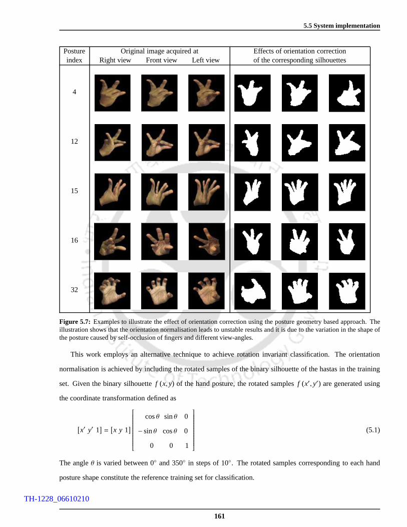
5.5 System implementation
Posture Original image acquired at Effects of orientation correctionindex Right view Front view Left view of the corresponding silhouettes
4
12
15
16
32
Figure 5.7: Examples to illustrate the effect of orientation correction using the posture geometry based approach. Theillustration shows that the orientation normalisation leads to unstable results and it is due to the variation in the shape ofthe posture caused by self-occlusion of fingers and different view-angles.
This work employs an alternative technique to achieve rotation invariant classification. The orientation
normalisation is achieved by including the rotated samplesof the binary silhouette of the hastas in the training
set. Given the binary silhouettef (x, y) of the hand posture, the rotated samplesf (x′, y′) are generated using
the coordinate transformation defined as
[
x′ y′ 1]
=[
x y 1]
cosθ sinθ 0
− sinθ cosθ 0
0 0 1
(5.1)
The angleθ is varied between 0 and 350 in steps of 10. The rotated samples corresponding to each hand
posture shape constitute the reference training set for classification.
161
TH-1228_06610210

5. DOM based Recognition of Asamyuta Hastas
5.5.3 Normalisation for scale and translation changes
The resolutions of the rotated hand posture silhouettes arenormalised to 104× 104 through the nearest
neighbourhood interpolation\ down sampling technique. The scale of the silhouette is normalised to 64× 64.
The spatial translation is normalised by shifting the centroid of the silhouette to the centre (52, 52) of the image.
5.5.4 Extraction of DOM features
The DOM based descriptors are derived as features for representing the shape of the hand postures in the
Asamyuta hasta database. The parameter to be determined is the order of the DOMs required for representing
the hand postures. Experiments have been already performedin Chapter 3 and Chapter 4 to study the optimal
choice of the order of DOMs for representing different shapes. The results in Chapter 3 and Chapter 4 suggest
that at higher orders the DOMs give accurate reconstruction. Accordingly, for representing the shape of the
hand posture of scale 64× 64, the order of the DOMs is chosen as 80 (n = 40 andm= 40). At this order, it is
shown in Chapter 3 and 4 that both Krawtchouk and discrete Tchebichef moments exhibit similar performance
with high reconstruction accuracy.
5.5.4.1 Comparison with other descriptors
The results in Chapter 4 have demonstrated the DOMs and the PCA based features as comparatively effi-
cient shape descriptors for user and view invariant classification of the simple hand postures. Therefore, based
on the experimental studies presented in Section 4.4.2, theother feature descriptor used for comparatively val-
idating the efficiency of the DOMs is the PCA based method. Thenumber of eigen features for computing the
transformation matrixWpca, is chosen based on the reconstruction accuracy.
Using (4.29), it is determined that 90% of the data variance corresponding to each sample in the database
is represented by the firstl = 180 eigen components. The number of eigen components for which the shapes
are efficiently represented is determined by verifying the reconstruction accuracies for different values ofl.
The reconstruction accuracy is computed using the SSIM index and the MHD value. From the experiments
performed on the normalized silhouettes of the hand postures in the Asamyuta hasta database, the value of
l for which the reconstruction accuracy is sufficiently high is determined as 100. The experiments on the
reconstruction accuracy with respect to different values of l for a hasta shape is illustrated in Figure 5.8. The
results show that forl > 90, the shapes are efficiently reconstructed and the accuracy in terms of the SSIM
index and the MHD value are significantly high. The transformation matrixWpca is formed using the eigen
vectors corresponding to the firstl = 100 eigen values. Therefore, if there areI number of training samples, the
162
TH-1228_06610210

5.5 System implementation
(a) Origi-nal shape
l = 180l = 120l = 60l = 30l = 10
(b) Reconstruction from PCA projections
(c) Reconstructed shapes obtained through binarisation
4 30 60 90 120 150 1800.4
0.6
0.8
1
Number of eigen components (l)
SSIM
(d)
4 30 60 90 120 150 1800
2
4
6
Number of eigen components (l)
MH
D
(e)
Figure 5.8: Illustration of shape reconstruction from PCA projection on different number of eigen components (a) Origi-nal hasta shape; (b) Reconstruction of (a) from the PCA projections for different values ofl; (c) Binarisation of the imagesin (b) to obtain the reconstructed shapes. The threshold forbinarisation is uniformly chosen as 120. Comparative plot of(c) SSIM index vs number of eigenvalues and (d) MHD vs number of eigenvalues computed between the image in (a) andthe reconstructed shapes in (c).
total number of feature vectors obtained after projection into eigen space is 100× I . For the selected number of
eigen values, the ratioχeigen in (4.29) is 0.85.
5.5.5 Classification
Let zs be the feature vector of the test image of unknown orientation andzθt the feature vector of the target
image of orientationθ contained in the reference set. The classification ofzs is done using the minimum
distance classifier defined in (4.30). Considering the training samples at different orientations, the distance can
be calculated as
dθt (zs, zt) =T
∑
j=1
(zs j − zθt j )2 (5.2)
Match= argmint,θ
(
dθt)
163
TH-1228_06610210

5. DOM based Recognition of Asamyuta Hastas
5.6 Experimental studies and results
The experiments presented in this section verify the efficiency of the proposed DOM based hand posture
recognition technique in classifying the hand posture shapes in the Asamyuta hasta database. The robustness of
the DOM descriptors to the user and the view-angle distortions in the hand posture shapes is investigated. The
classification accuracy of the DOM descriptors is compared with that of the PCA based description.
The 8, 064 hand posture images in the Asamyuta hasta database is divided into three equal datasets based
on the angle of view employed for posture acquisition. Accordingly, the three datasets are referred as theRight
view, theFront viewand theLeft view. Each of these datasets consists of 2, 688 samples of the 32 hand postures,
thereby containing 84 samples per hand posture.
The hand posture shapes in all the 3 datasets exhibit user variations and orientation and scale changes. The
hand postures in Front view are acquired at the optimum view-angleCθ = 90 and hence, these samples are
not subject to distortions that occur at oblique angles of view. The Right view and the Left view datasets are
composed of hand posture images acquired atCθ = 60 andCθ = 120 respectively. Therefore, the images
in the Right view and the Left view datasets exhibit shape variations caused by self-occlusion of fingers and
variations in the perceived hand posture shapes due to different view-angles. Examples of the hand postures
in the Asamyuta hasta database obtained at three different view-angles and the corresponding binary shapes
are illustrated in Figure 5.9. From this figure, the structural difference between the hand posture shapes of
each class contained in the three datasets can be observed. These variations in the hand posture shapes are
quantitatively analysed to corroborate the robustness of the DOM descriptors in classifying hand postures under
several structural variations.
5.6.1 Quantitative analysis on hand posture variations
The structural variations in the hand posture shapes are represented by computing the intraclass and the
interclass distances between the shapes in each dataset. The intraclass distance in terms of the boundary simi-
larity is measured using the Pratt’s FOM. The interclass andthe intraclass distances based on region similarity
between the samples are measured using the correlation coefficient. The reference samples for computing these
measures are taken from the Front view dataset.
The plots of the Pratt’s FOM values obtained for the hand posture shapes in the Right view, the Front view
and the Left view datasets are given in Figure 5.10. The intraclass FOM values obtained for the Front view
dataset as shown in Figure 5.10(b), represent the structural changes in the hand posture shapes that occur due
164
TH-1228_06610210

5.6 Experimental studies and results
Posture 1 Posture 2 Posture 3
Posture 4 Posture 5 Posture 6
Posture 7 Posture 8 Posture 9
Posture 10 Posture 11 Posture 12
Posture 13 Posture 14 Posture 15
Posture 16 Posture 17 Posture 18
Posture 19 Posture 20 Posture 21
Posture 22 Posture 23 Posture 24
Posture 25 Posture 26 Posture 27
Posture 28 Posture 29 Posture 30
Posture 31 Posture 32
Figure 5.9: Illustration of samples of hand posture images and the corresponding shapes in the Asamyuta hasta database.The illustration shows the variations in the hand postures when acquired at different view-angles.
165
TH-1228_06610210

5. DOM based Recognition of Asamyuta Hastas
for Right view dataset for Front view dataset
1 2 3 4 5 6 7 8 9 10111213141516171819202122232425262728293031320.4
0.6
0.8
1
Index of the Posture Class
Pra
tt’s
FO
M
(a)
1 2 3 4 5 6 7 8 9 10111213141516171819202122232425262728293031320.4
0.6
0.8
1
Index of the Posture Class
Pra
tt’s
FO
M
(b)
for Left view dataset
1 2 3 4 5 6 7 8 9 10111213141516171819202122232425262728293031320.4
0.6
0.8
1
Index of the Posture Class
Pra
tt’s
FO
M
(c)
Figure 5.10: Plots illustrating the intraclass variability of the hand posture shapes in the hastas of (a) Right view dataset;(b) Front view dataset and (c) Left view dataset. The intraclass FOMs are measured with reference to the samples takenfrom Front view.
to user variations in the gesturing style. The user variations in the gesturing style correspond to the changes in
the silhouette of the hand posture due to small variations inthe angular displacements at the finger joints and
the self-occlusions caused by it.
The intraclass FOMs corresponding to the Front view datasetrepresent the user variations and the FOM
values corresponding to the Right view and the Left view datasets include both the user and the view-angle vari-
ations. From the values of the intraclass FOMs, it can be inferred that the hand posture shapes in the Asamyuta
hasta database exhibit at least 20% deviation in the structural characteristics. The plots of intraclass FOMs of
the samples in the the Right view and the Left view datasets are given in Figure 5.10(a) and Figure 5.10(c)
respectively. The values in Figure 5.10(a) signify the similarities between the Right view and the Front view
samples. Similarly, Figure 5.10(c) represents the similarities between the hand posture shapes in the Left view
and the Front view datasets.
The plot comparing the posture wise mean of the intraclass FOM values obtained for the three datasets is
shown in Figure 5.11(a). From the plot, it is evident that thehand posture shapes in the Right view and the
Left view samples exhibit lower intraclass similarities with the reference samples in Front view. The decrease
in the intraclass FOM values quantifies the structural changes that occur at different view-angles. Employing
166
TH-1228_06610210

5.6 Experimental studies and results
2 4 6 8 10 12 14 16 18 20 22 24 26 28 30 320.6
0.65
0.7
0.75
0.8
0.85
0.9
Index of the Posture Class
Mean
of
Intr
acla
ss P
ratt
’s F
OM
Right view Front view Left view
(a)
2 4 6 8 10 12 14 16 18 20 22 24 26 28 30 320.02
0.04
0.06
0.08
0.1
Index of the Posture Class
Sta
ndard
devia
tion o
fIn
tracla
ss P
ratt
’s F
OM
Right view Front view Left view
(b)
Figure 5.11: Plots illustrating the postures with high intraclass variations and intraclass similarities using the (a) meanand the (b) standard deviation of the intraclass FOM values respectively. The plots are obtained for the posture classesinthe Right view, the Front view and the Left view datasets.
different view-angles in the horizontal direction acquires the variation in the side profile of the hand postures.
For different view-angles along the horizontal direction,the variations in the side profile of the hand postures
are acquired. These variations may cause notable changes inthe silhouette of the hand postures. Therefore, the
intraclass FOMs of the Right view and the Left view samples are less in comparison to the Front view samples.
Particularly, Figure 5.11(a) shows that the Right view samples exhibit less FOM values than the Left view
samples. For the given experimental setup, it should be noted that the view-angles for which the structural
variations are more is based on the hand used for performing the postures. The posture classes in the Right
view dataset with less intraclass FOM values are the postures 5, 16, 26 and 31. The variations in the shapes of
these postures with respect to the view-angles can be inferred from the examples illustrated in Figure 5.9.
As we observe the FOM values in the plots shown in Figure 5.10,it is evident that the variations in the
range of the FOM values obtained for the Right view and the Left view datasets are less than that of the Front
view dataset. This suggests that the effect of user variations on the hand posture shape is comparatively less,
when the hand postures are acquired from the right and the left views. However, these variations may cause
significant changes in the hand posture shape when acquired from the front view. Further, it is also known that
the perspective distortion due to the view-angle changes gets minimised when the camera is placed at a normal-
angle position [226]. Due to these factors, the variation inthe intraclass FOM values are comparatively less
for the Right view and the Left view datasets. This can also beconfirmed by analyzing the standard deviations
of the intraclass FOM values for each dataset. The plots comparing the standard deviation of the posture wise
FOM values in the datasets are given in Figure 5.11(b). It is evident that the variability in the intraclass samples
is comparatively more for the Front view dataset. Examples of the hand posture shapes in the Front view dataset
167
TH-1228_06610210

5. DOM based Recognition of Asamyuta Hastas
Posture 5 Posture 13 Posture 15Original image Original image Original image
Binary shape Binary shape Binary shape
Posture 16 Posture 20 Posture 23Original image Original image Original image
Binary shape Binary shape Binary shape
Posture 25 Posture 26 Posture 30Original image Original image Original image
Binary shape Binary shape Binary shape
Figure 5.12: Illustration of a few examples of hand posture images from the Front view dataset, exhibiting more intraclassvariations. The shape of a hand posture varies due to structural changes caused by variations in the gesturing style of thegesturers.
with more variations in the intraclass FOM values are shown in Figure 5.12.
The region based similarities between the interclass samples in comparison to the intraclass similarities are
measured using the correlation coefficient. The plots of theinterclass correlation values computed with respect
to each posture class in the datasets are shown in Figure 5.13and Figure 5.14. The plots comparatively illustrate
the interclass correlation values obtained with respect toeach dataset. It shows that the hand posture shapes in
all the datasets exhibit approximately similar interclasscorrelation characteristics.
As we examine the plots, the minimum difference between the intraclass and the interclass correlation
values can be observed to be approximately around 10%. Similarly, the maximum difference between the
intraclass and the interclass correlation values is approximately 50%. This implies that the Asamyuta hasta
database is composed of different hand posture shapes with distinct as well as overlapping regions.
168
TH-1228_06610210

5.6 Experimental studies and results
1 3 5 7 9 11 13 15 17 19 21 23 25 27 29 310
0.2
0.4
0.6
0.8
1
Index of the Posture Class
Co
rrela
tio
n
Reference: Posture− 1
1 3 5 7 9 11 13 15 17 19 21 23 25 27 29 310
0.2
0.4
0.6
0.8
1
Index of the Posture Class
Corr
ela
tion
Reference: Posture− 2
1 3 5 7 9 11 13 15 17 19 21 23 25 27 29 310
0.2
0.4
0.6
0.8
1
Index of the Posture Class
Co
rrela
tio
n
Reference: Posture− 3
1 3 5 7 9 11 13 15 17 19 21 23 25 27 29 310
0.2
0.4
0.6
0.8
1
Index of the Posture Class
Co
rrela
tio
n
Reference: Posture− 4
1 3 5 7 9 11 13 15 17 19 21 23 25 27 29 310
0.2
0.4
0.6
0.8
Index of the Posture Class
Corr
ela
tion
Reference: Posture− 5
1 3 5 7 9 11 13 15 17 19 21 23 25 27 29 310
0.2
0.4
0.6
0.8
1
Index of the Posture Class
Co
rrela
tio
n
Reference: Posture− 6
1 3 5 7 9 11 13 15 17 19 21 23 25 27 29 310
0.2
0.4
0.6
0.8
1
Index of the Posture Class
Co
rrela
tio
n
Reference: Posture− 7
1 3 5 7 9 11 13 15 17 19 21 23 25 27 29 310
0.2
0.4
0.6
0.8
1
Index of the Posture Class
Corr
ela
tion
Reference: Posture− 8
1 3 5 7 9 11 13 15 17 19 21 23 25 27 29 310
0.2
0.4
0.6
0.8
1
Index of the Posture Class
Corr
ela
tion
Reference: Posture− 9
1 3 5 7 9 11 13 15 17 19 21 23 25 27 29 310
0.2
0.4
0.6
0.8
1
Index of the Posture Class
Co
rrela
tio
n
Reference: Posture− 10
1 3 5 7 9 11 13 15 17 19 21 23 25 27 29 310
0.2
0.4
0.6
0.8
1
Index of the Posture Class
Co
rrela
tio
n
Reference: Posture− 11
1 3 5 7 9 11 13 15 17 19 21 23 25 27 29 310
0.2
0.4
0.6
0.8
1
Index of the Posture Class
Co
rrela
tio
n
Reference: Posture− 12
1 3 5 7 9 11 13 15 17 19 21 23 25 27 29 310
0.2
0.4
0.6
0.8
1
Index of the Posture Class
Co
rrela
tio
n
Reference: Posture− 13
1 3 5 7 9 11 13 15 17 19 21 23 25 27 29 310
0.2
0.4
0.6
0.8
1
Index of the Posture Class
Co
rrela
tio
n
Reference: Posture− 14
1 3 5 7 9 11 13 15 17 19 21 23 25 27 29 310
0.2
0.4
0.6
0.8
Index of the Posture Class
Corr
ela
tion
Reference: Posture− 15
1 3 5 7 9 11 13 15 17 19 21 23 25 27 29 310
0.2
0.4
0.6
0.8
Index of the Posture Class
Co
rrela
tio
n
Reference: Posture− 16
1 3 5 7 9 11 13 15 17 19 21 23 25 27 29 310
0.2
0.4
0.6
0.8
1
Index of the Posture Class
Co
rrela
tio
n
Reference: Posture− 17
1 3 5 7 9 11 13 15 17 19 21 23 25 27 29 310
0.2
0.4
0.6
0.8
1
Index of the Posture Class
Corr
ela
tion
Reference: Posture− 18
- Right view• - Front view,• - Left view
Figure 5.13: Illustration comparing the intraclass and the interclass correlations between the hand posture samples. Thereference samples for comparison are taken from the Front view dataset. The plots show the correlation values computedwith respect to reference postures from class 1 to class 18.
169
TH-1228_06610210

5. DOM based Recognition of Asamyuta Hastas
1 3 5 7 9 11 13 15 17 19 21 23 25 27 29 310
0.2
0.4
0.6
0.8
1
Index of the Posture Class
Co
rrela
tio
n
Reference: Posture− 19
1 3 5 7 9 11 13 15 17 19 21 23 25 27 29 310
0.2
0.4
0.6
0.8
Index of the Posture Class
Corr
ela
tion
Reference: Posture− 20
1 3 5 7 9 11 13 15 17 19 21 23 25 27 29 310
0.2
0.4
0.6
0.8
1
Index of the Posture Class
Corr
ela
tion
Reference: Posture− 21
1 3 5 7 9 11 13 15 17 19 21 23 25 27 29 310
0.2
0.4
0.6
0.8
Index of the Posture Class
Corr
ela
tion
Reference: Posture− 22
1 3 5 7 9 11 13 15 17 19 21 23 25 27 29 310
0.2
0.4
0.6
0.8
1
Index of the Posture Class
Co
rrela
tio
n
Reference: Posture− 23
1 3 5 7 9 11 13 15 17 19 21 23 25 27 29 310
0.2
0.4
0.6
0.8
1
Index of the Posture Class
Corr
ela
tion
Reference: Posture− 24
1 3 5 7 9 11 13 15 17 19 21 23 25 27 29 310
0.2
0.4
0.6
0.8
Index of the Posture Class
Corr
ela
tion
Reference: Posture− 25
1 3 5 7 9 11 13 15 17 19 21 23 25 27 29 310
0.2
0.4
0.6
0.8
1
Index of the Posture Class
Corr
ela
tion
Reference: Posture− 26
1 3 5 7 9 11 13 15 17 19 21 23 25 27 29 310
0.2
0.4
0.6
0.8
1
Index of the Posture Class
Corr
ela
tion
Reference: Posture− 27
1 3 5 7 9 11 13 15 17 19 21 23 25 27 29 310
0.2
0.4
0.6
0.8
1
Index of the Posture Class
Co
rrela
tio
n
Reference: Posture− 28
1 3 5 7 9 11 13 15 17 19 21 23 25 27 29 310
0.2
0.4
0.6
0.8
1
Index of the Posture Class
Co
rrela
tio
n
Reference: Posture− 29
1 3 5 7 9 11 13 15 17 19 21 23 25 27 29 310
0.2
0.4
0.6
0.8
1
Index of the Posture Class
Co
rrela
tio
n
Reference: Posture− 30
1 3 5 7 9 11 13 15 17 19 21 23 25 27 29 310
0.2
0.4
0.6
0.8
1
Index of the Posture Class
Corr
ela
tion
Reference: Posture− 31
1 3 5 7 9 11 13 15 17 19 21 23 25 27 29 310
0.2
0.4
0.6
0.8
Index of the Posture Class
Corr
ela
tion
Reference: Posture− 32
- Right view• - Front view,• - Left view
Figure 5.14: Illustration comparing the intraclass and the interclass correlations between the hand posture samples. Thereference samples for comparison are taken from the Front view dataset. The plots show the correlation values computedwith respect to reference postures from class 19 to class 32.
170
TH-1228_06610210

5.6 Experimental studies and results
From the plots obtained with respect to different referenceposture classes, as shown in Figure 5.13 and
Figure 5.14, we can infer that the posture classes 6, 14, 18, 22, 23, 27 and 28 exhibit high intraclass correlation
values in comparison to the respective interclass correlations. The minimum difference between the intraclass
correlation and the interclass correlation values corresponding to these posture classes is over 21%. Therefore,
they constitute the comparatively distinct hand posture shapes in the Asamyuta hasta database. The examples
of the hand posture shapes belonging to these classes are shown in Figure 5.9.
The hand posture classes with interclass correlations as high as the intraclass correlation values are the
samples belonging to classes 1, 2, 3, 5, 7, 8, 13, 15, 17 and 21.The minimum difference between the intraclass
and the interclass correlation values for these posture classes is less than 12%. Among these, the interclass
correlation is high between the posture shapes in the classes 1, 2, 3, 5, 7 and 8. This implies that these hand
postures exhibit almost similar structural characteristics with more overlapping regions. Few examples of the
shapes of these posture classes are illustrated in Figure 5.9.
From the mean of intraclass FOM values shown in Figure 5.11(a), it is known that the posture classes 5,
16, 24, 26 and 31 in the Right view dataset show less intraclass similarity with respect to the samples in the
Front view dataset. This suggests that these hand posture classes may exhibit high interclass correlations when
acquired from the right view direction. This can be verified from the plots in Figure 5.13 and Figure 5.14 that
illustrate the correlation values obtained for the samplesin the Right view dataset with respect to the reference
posture classes 5, 16, 24, 26 and 31.
The analysis on the structural variations in the hand posture shapes in terms of the intraclass and the inter-
class distances confirms that the Asamyuta hasta database consists of hand posture images with more structural
deviations indicating the effects of user variations and the view-angle changes. Therefore, the above analysis
validates the applicability of the developed Asamyuta hasta database for experiments on user and view invariant
hand posture classification.
5.6.2 Experiments on posture classification
The efficiency of the proposed DOM based descriptors for userand view invariant classification of the hand
posture shapes in the Asamyuta hasta database are empirically studied in this section. The performance of the
DOM descriptors is verified in comparison with the PCA based description method discussed in Section 5.5.4.
The details of the experiment and the results obtained for user independent and view invariant recognition of
the postures in the Asamyuta hasta database are discussed asfollows.
In this work, the Asamyuta hasta database is developed by collecting the hand postures from 6 users and
171
TH-1228_06610210
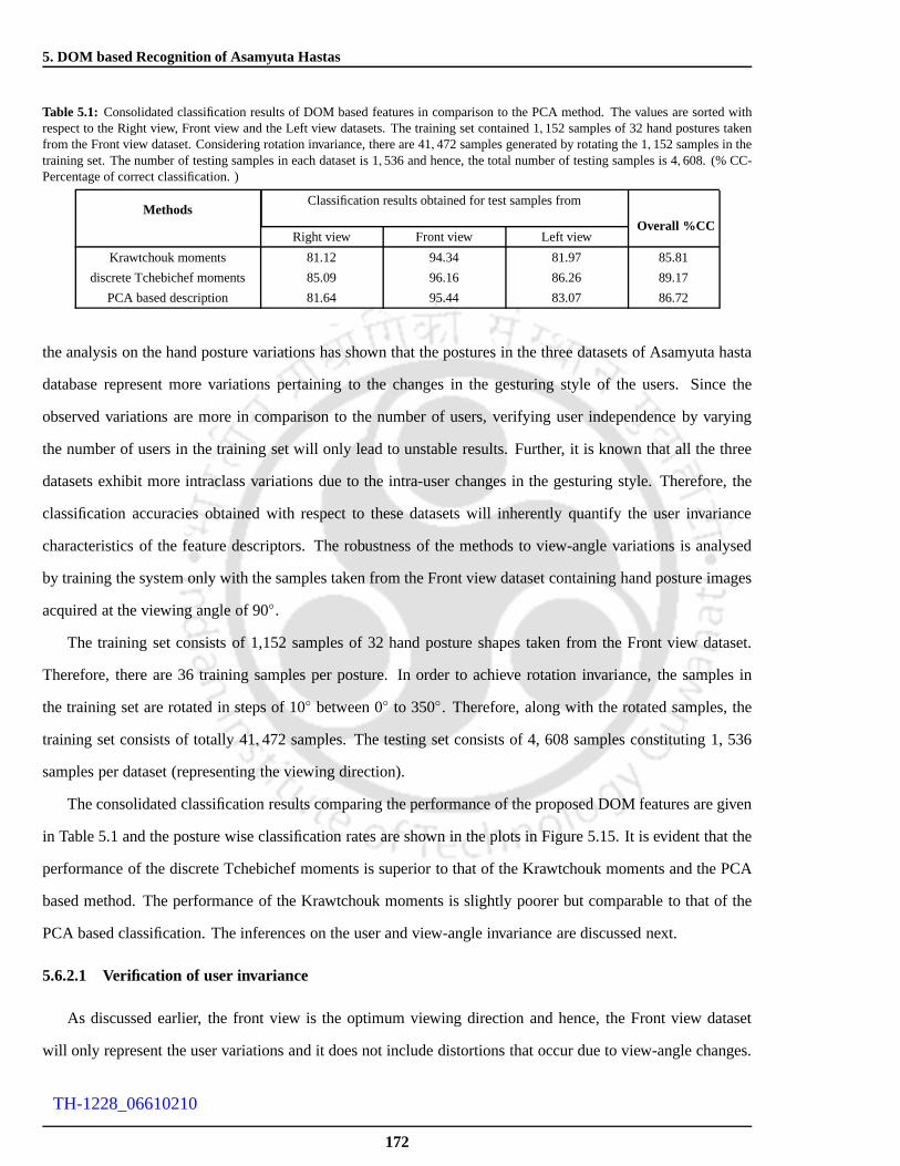
5. DOM based Recognition of Asamyuta Hastas
Table 5.1: Consolidated classification results of DOM based features in comparison to the PCA method. The values are sorted withrespect to the Right view, Front view and the Left view datasets. The training set contained 1,152 samples of 32 hand postures takenfrom the Front view dataset. Considering rotation invariance, there are 41, 472 samples generated by rotating the 1, 152 samples in thetraining set. The number of testing samples in each dataset is 1,536 and hence, the total number of testing samples is 4, 608. (% CC-Percentage of correct classification. )
MethodsClassification results obtained for test samples from
Overall %CCRight view Front view Left view
Krawtchouk moments 81.12 94.34 81.97 85.81
discrete Tchebichef moments 85.09 96.16 86.26 89.17
PCA based description 81.64 95.44 83.07 86.72
the analysis on the hand posture variations has shown that the postures in the three datasets of Asamyuta hasta
database represent more variations pertaining to the changes in the gesturing style of the users. Since the
observed variations are more in comparison to the number of users, verifying user independence by varying
the number of users in the training set will only lead to unstable results. Further, it is known that all the three
datasets exhibit more intraclass variations due to the intra-user changes in the gesturing style. Therefore, the
classification accuracies obtained with respect to these datasets will inherently quantify the user invariance
characteristics of the feature descriptors. The robustness of the methods to view-angle variations is analysed
by training the system only with the samples taken from the Front view dataset containing hand posture images
acquired at the viewing angle of 90.
The training set consists of 1,152 samples of 32 hand postureshapes taken from the Front view dataset.
Therefore, there are 36 training samples per posture. In order to achieve rotation invariance, the samples in
the training set are rotated in steps of 10 between 0 to 350. Therefore, along with the rotated samples, the
training set consists of totally 41, 472 samples. The testing set consists of 4, 608 samples constituting 1, 536
samples per dataset (representing the viewing direction).
The consolidated classification results comparing the performance of the proposed DOM features are given
in Table 5.1 and the posture wise classification rates are shown in the plots in Figure 5.15. It is evident that the
performance of the discrete Tchebichef moments is superiorto that of the Krawtchouk moments and the PCA
based method. The performance of the Krawtchouk moments is slightly poorer but comparable to that of the
PCA based classification. The inferences on the user and view-angle invariance are discussed next.
5.6.2.1 Verification of user invariance
As discussed earlier, the front view is the optimum viewing direction and hence, the Front view dataset
will only represent the user variations and it does not include distortions that occur due to view-angle changes.
172
TH-1228_06610210

5.6 Experimental studies and results
2 4 6 8 10 12 14 16 18 20 22 24 26 28 30 3218
38
58
78
98
Index of the Posture Class
%C
C
Right view Front view Left view
(a) Krawtchouk moments based features
2 4 6 8 10 12 14 16 18 20 22 24 26 28 30 3218
38
58
78
98
Index of the Posture Class
%C
C
Right view Front view Left view
(b) discrete Tchebichef moments based features
2 4 6 8 10 12 14 16 18 20 22 24 26 28 30 3218
38
58
78
98
Index of the Posture Class
%C
C
Right view Front view Left view
(c) PCA based description
Figure 5.15: Illustration comparing the posture wise classification results obtained for the Right view, Front view andthe Left view datasets. The classification accuracies obtained for (a) Krawtchouk moments based features; (b) discreteTchebichef moments based features and (c) PCA based hand posture description.
Therefore, the user invariance efficiency of the descriptors can be studied by analyzing the classification results
obtained on the Front view dataset.
The results in Table 5.1 show that the discrete Tchebichef moments offer around 3% increase in the clas-
sification accuracy and hence, it implies that the discrete Tchebichef moments exhibit better user invariance
characteristics. The response of the DOM descriptors with respect to each posture class can be inferred from
the plots in Figure 5.15(a) and Figure 5.15(b). From the plotof the posture wise classification values corre-
sponding to the Front view dataset, it is evident that most ofthe posture classes are correctly classified and only
the posture classes 5, 9, 15, 21 and 25 attain classification accuracies less than 85%. The samples of these pos-
ture classes that are misclassified in DOM based descriptionare illustrated in Figure 5.16. From the illustration
it is evident that the misclassification has occurred when the shapes of the postures change due to self-occlusion
between the fingers which takes place as the effect of user variations. The change in the posture shape is in such
a way that it matches with the shape of a different posture class leading to classification errors. The overlap
173
TH-1228_06610210

5. DOM based Recognition of Asamyuta Hastas
Test samples of Misclassified as PosturesPosture-5 2 2 19 19
Test samples of Misclassified as samples inPosture-15 Posture 30
Test samples of Misclassified as samples inPosture-9 Posture 17
Test samples of Misclassified as PosturesPosture-21 5 5 5 11
Test samples of Misclassified as PosturesPosture-25 4 4 12 12
Figure 5.16: Examples of the hand posture classes in the Front view dataset of the Asamyuta hasta database exhibitinghigher misclassification rate.
between the regions of the two hand posture shapes also occurs as the orientations of the hand posture vary.
As a result, two different hand posture classes exhibiting overlapping regions at different orientations are also
mismatched. For example, as shown in Figure 5.16, the samples of posture 15 are mismatched with the samples
in posture 30. The mismatch has occurred for a particular orientation of the samples in posture 30. The study
on intraclass variations in Section 5.6.1 has shown that thehand posture shapes in the Asamyuta hasta database
exhibit at least 20% structural deviation and shapes belonging to classes 13, 18, 20, 23 and 26 have shown
utmost 40% intraclass variations. Despite of high intraclass variations, the classification accuracies for these
classes are higher than 90%. Further, the analysis on interclass correlation in Section 5.6.1 has shown that, ex-
cept the posture classes 6, 14, 18, 22, 23, 27 and 28, all the other posture classes exhibit interclass correlations
comparably high as the intraclass correlations. For example, the posture classes 1, 2, 3, 7 and 8 show interclass
correlations almost similar to the intraclass correlationvalue. As we examine the classification results in Fig-
ure 5.15(a) and Figure 5.15(b), it can be known that these posture classes offer classification accuracies around
98%. These observations on the misclassified samples and theanalysis on the classification accuracies with
respect to intraclass variations confirm that the DOM based descriptors are efficient as user invariant features.
The posture wise classification results of the Front view dataset obtained with respect to the PCA based
description is shown in Figure 5.15(c). From the results, itis observed that the PCA based classification results
174
TH-1228_06610210

5.6 Experimental studies and results
Table 5.2: Confusion matrix corresponding to the results in Table 5.1 for Krawtchouk moments based description of testing samplesin the Front view dataset. The total number of testing samples per posture is 48 with a total of 1,536 testing samples.
@@I/P
O/P1 2 3 4 5 6 7 8 9 10 11 12 13 14 15 16 17 18 19 20 21 22 23 24 25 26 27 28 29 3031 32
1 482 42 63 484 485 1 2 40 1 1 36 487 488 1 479 41 710 4811 4812 47 113 1 2 4514 4815 1 1 41 1 416 2 43 1 217 2 4618 4819 47 120 1 45 1 121 3 6 38 122 1 44 323 1 1 2 4424 1 3 43 125 6 3 38 126 4827 4828 1 4729 1 1 45 130 1 1 1 1 4431 1 4732 1 47
Table 5.3: Confusion matrix corresponding to the results in Table 5.1 for discrete Tchebichef moments based description of testingsamples in the Front view dataset. The total number of testing samples per posture is 48 with a total of 1, 536 testing samples.
@@I/P
O/P1 2 3 4 5 6 7 8 9 10 11 12 13 14 15 16 17 18 19 20 21 22 23 24 25 26 27 28 29 3031 32
1 482 47 13 1 474 485 2 43 1 26 487 488 1 479 43 510 4811 4812 4813 1 2 4514 4815 1 1 43 316 1 44 2 117 1 4718 4819 47 120 1 44 1 1 121 3 4 1 1 3922 1 46 123 1 2 4524 1 2 4525 3 2 4326 4827 4828 4829 1 4730 1 1 45 131 1 4732 1 47
175
TH-1228_06610210
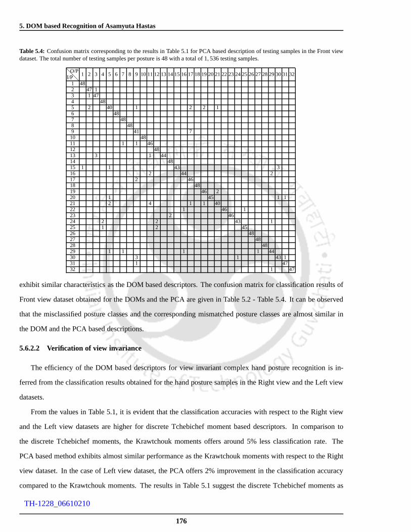
5. DOM based Recognition of Asamyuta Hastas
Table 5.4: Confusion matrix corresponding to the results in Table 5.1 for PCA based description of testing samples in the Front viewdataset. The total number of testing samples per posture is 48 with a total of 1, 536 testing samples.
@@I/P
O/P1 2 3 4 5 6 7 8 9 10 11 12 13 14 15 16 17 18 19 20 21 22 23 24 25 26 27 28 29 3031 32
1 482 47 13 1 474 485 2 40 1 2 2 16 487 488 489 41 710 4811 1 1 4612 4813 3 1 4414 4815 1 1 43 316 2 44 217 2 4618 4819 46 220 1 45 1 121 2 4 1 1 4022 1 46 123 2 4624 2 2 43 125 1 2 4526 4827 4828 4829 1 1 1 1 4430 3 1 43 131 1 4732 1 47
exhibit similar characteristics as the DOM based descriptors. The confusion matrix for classification results of
Front view dataset obtained for the DOMs and the PCA are givenin Table 5.2 - Table 5.4. It can be observed
that the misclassified posture classes and the corresponding mismatched posture classes are almost similar in
the DOM and the PCA based descriptions.
5.6.2.2 Verification of view invariance
The efficiency of the DOM based descriptors for view invariant complex hand posture recognition is in-
ferred from the classification results obtained for the handposture samples in the Right view and the Left view
datasets.
From the values in Table 5.1, it is evident that the classification accuracies with respect to the Right view
and the Left view datasets are higher for discrete Tchebichef moment based descriptors. In comparison to
the discrete Tchebichef moments, the Krawtchouk moments offers around 5% less classification rate. The
PCA based method exhibits almost similar performance as theKrawtchouk moments with respect to the Right
view dataset. In the case of Left view dataset, the PCA offers2% improvement in the classification accuracy
compared to the Krawtchouk moments. The results in Table 5.1suggest the discrete Tchebichef moments as
176
TH-1228_06610210

5.6 Experimental studies and results
Test samples of Misclassified as PosturesPosture-4 12 12 21 32
Test samples of Misclassified as samples inPosture-11 Posture- 1
Test samples of Misclassified as PosturesPosture-16 4 6 14 32
Test samples of Misclassified as PosturesPosture-21 11 11 14 14
Test samples of Misclassified as PosturesPosture-25 4 4 12 12
Test samples of Misclassified as samples inPosture-5 Posture-2
Test samples of Misclassified as PosturesPosture-13 8 8 23 23
Test samples of Misclassified as PosturesPosture-19 8 8 21 21
Test samples of Misclassified as samples inPosture-24 Posture-12
Test samples of Misclassified as PosturesPosture-31 11 11 13 13
Figure 5.17: Examples of the hand posture classes in the Right view dataset of the Asamyuta hasta database exhibitinghigher misclassification rate.
better feature descriptors for view invariant hand postureclassification.
The posture wise classification results for the Right view and the Left view datasets using the DOM based
descriptors are shown in Figure 5.15(a) and Figure 5.15(b) respectively. These plots show that almost 38%
of the posture classes exhibit classification accuracies less than 80%. Of these, some of the posture classes
achieved the lowest classification rate of 30%. The posture classes in the Right view dataset with less clas-
sification rates are postures 5, 11 and 16. Similarly, the posture classes in the Left view dataset offering less
classification accuracy are the postures 9, 16, 21 and 30.
Figure 5.17 and Figure 5.18 present an illustration of the mismatched posture samples in the Right view
and the Left view datasets respectively. The illustrationsshow that the mismatch occurs between the hand
posture samples whose shapes contain more overlapping regions. The variation in shapes is mainly due to the
177
TH-1228_06610210

5. DOM based Recognition of Asamyuta Hastas
Test samples of Misclassified as PosturesPosture-5 17 19 21 21
Test samples of Misclassified as samples inPosture-13 Posture-11
Test samples of Misclassified as PosturesPosture-21 5 5 19 30
Test samples of Misclassified as samples inPosture-9 Posture-17
Test samples of Misclassified as samples inPosture-16 Posture-29
Test samples of Misclassified as samples inPosture-30 Posture-10
Test samples of Misclassified as PosturesPosture-32 17 17 17 27
Figure 5.18: Examples of the hand posture classes in the Left view datasetof the Asamyuta hasta database exhibitinghigher misclassification rate.
self-occlusion of fingers and the variation in the side profiles of the hand postures. It should also be observed
that the high correspondence between the mismatched posture classes occurs also due to orientation changes.
From Figure 5.11(a), it can be inferred that the samples in the Right view and the Left view datasets with more
misclassification rates correspond to the posture classes with less intraclass FOM values.
From the plot in Figure 5.15(c), the posture wise classification results obtained for the PCA method on to
the Right view and the Left view datasets can be verified. It can be inferred that the posture wise classification
response of PCA is almost similar to that of the Krawtchouk moments.
The detailed scores of the classification results obtained with respect to the Right view dataset are given in
Table 5.5-Table 5.7 and the results corresponding to the Left view dataset are given in Table 5.8-Table 5.10.
By analyzing the detailed scores of the posture wise classification results, it is observed that the mismatch has
occurred between the classes that exhibit more interclass correlations.
178
TH-1228_06610210

5.6 Experimental studies and results
Table 5.5: Confusion matrix corresponding to the results in Table 5.1 for Krawtchouk moments based description of testing samplesin the Right view dataset. The total number of testing samples per posture is 48 with a total of 1,536 testing samples.
@@I/P
O/P1 2 3 4 5 6 7 8 9 10 11 12 13 14 15 16 17 18 19 20 21 22 23 24 25 26 27 28 29 3031 32
1 482 41 5 01 13 1 474 37 4 75 1 19 3 09 2 3 1 6 46 487 43 3 1 18 489 35 1310 4811 11 1 33 312 4 43 113 3 1 5 29 1 1 7 114 4815 01 40 1 1 2 1 1 116 4 6 4 14 2 2 3 2 3 2 1 517 3 4518 4819 2 01 8 2 2 27 620 2 01 1 43 121 1 1 01 2 1 1 40 122 1 2 1 1 41 1 123 2 1 7 3824 1 1 6 1 1 2 34 1 125 9 6 1 3226 1 46 127 4828 1 1 4629 1 3 3 39 230 1 02 3 1 3 2 35 131 1 1 9 3 3432 4 2 1 1 1 39
Table 5.6: Confusion matrix corresponding to the results in Table 5.1 for discrete Tchebichef moments based description of testingsamples in the Right view dataset. The total number of testing samples per posture is 48 with a total of 1, 536 testing samples.
@@I/P
O/P1 2 3 4 5 6 7 8 9 10 11 12 13 14 15 16 17 18 19 20 21 22 23 24 25 26 27 28 29 3031 32
1 482 47 13 484 35 7 65 20 1 11 2 1 7 5 16 487 45 1 1 18 489 39 910 4811 10 2 30 612 3 44 113 6 4 2 32 2 214 4815 1 1 43 2 116 5 2 2 3 21 4 1 6 1 2 117 3 4518 4819 2 1 6 1 33 520 1 46 121 1 1 1 2 1 1 1 4022 1 4723 1 6 40 124 1 1 6 1 38 125 6 3 3926 1 46 127 4828 1 4729 1 1 3 1 40 230 3 2 1 4 1 1 35 131 1 1 7 1 3832 1 3 1 1 42
179
TH-1228_06610210

5. DOM based Recognition of Asamyuta Hastas
Table 5.7: Confusion matrix corresponding to the results in Table 5.1 for PCA based description of testing samples in the Right viewdataset. The total number of testing samples per posture is 48 with a total of 1, 536 testing samples.
@@I/P
O/P1 2 3 4 5 6 7 8 9 10 11 12 13 14 15 16 17 18 19 20 21 22 23 24 25 26 27 28 29 3031 32
1 45 32 47 013 484 34 6 85 19 08 1 9 5 1 56 487 45 1 1 18 489 37 1110 4811 12 2 5 26 2 112 3 44 113 7 8 29 414 4815 1 1 01 38 2 1 2 216 6 0 1 3 1 12 4 5 2 8 1 3 217 5 42 118 4819 3 1 3 32 8 120 1 44 1 221 1 1 1 2 1 1 1 38 222 2 1 1 1 1 38 2 223 1 5 4224 1 3 1 4 1 3825 7 3 3826 1 4727 4828 1 4729 1 3 1 1 2 38 230 2 1 10 5 1 1 27 131 1 1 6 1 3932 3 1 1 43
Table 5.8: Confusion matrix corresponding to the results in Table 5.1 for Krawtchouk moments based description of testing samplesin the Left view dataset. The total number of testing samplesper posture is 48 with a total of 1,536 testing samples.
@@I/P
O/P1 2 3 4 5 6 7 8 9 10 11 12 13 14 15 16 17 18 19 20 21 22 23 24 25 26 27 28 29 3031 32
1 482 1 42 53 2 44 24 485 1 34 2 5 3 2 16 47 17 47 18 47 19 21 25 210 4811 1 1 3 42 112 44 1 313 1 3 12 31 114 45 1 215 1 1 2 35 1 1 2 1 2 216 3 2 1 19 2 2 14 517 1 45 218 4819 1 1 1 1 42 220 1 1 8 1 1 31 1 1 321 11 1 4 1 1 8 15 722 3 3 1 39 223 1 46 124 2 4625 1 1 4626 3 1 41 327 1 3 3 4128 1 4729 1 2 1 2 4230 2 1 1 18 2 1 4 1931 2 1 3 2 1 1 3 3532 6 1 1 5 1 34
180
TH-1228_06610210

5.6 Experimental studies and results
Table 5.9: Confusion matrix corresponding to the results in Table 5.1 for discrete Tchebichef moments based description of testingsamples in the Left view dataset. The total number of testingsamples per posture is 48 with a total of 1,536 testing samples.
@@I/P
O/P1 2 3 4 5 6 7 8 9 10 11 12 13 14 15 16 17 18 19 20 21 22 23 24 25 26 27 28 29 3031 32
1 482 2 45 13 45 2 14 485 42 3 1 1 16 487 47 18 489 24 22 210 4811 1 1 3 4312 46 1 113 1 1 11 34 114 4815 1 1 39 1 1 2 316 1 1 1 20 1 1 14 917 1 45 218 4819 1 1 44 1 120 2 10 4 30 1 121 8 2 1 6 25 622 3 43 1 123 47 124 4825 1 4726 3 41 427 4 3 4128 1 4729 1 1 4630 1 1 17 4 2 2331 2 1 1 1 4 3932 3 1 1 4 1 38
Table 5.10: Confusion matrix corresponding to the results in Table 5.1 for PCA based description of testing samples in the Left viewdataset. The total number of testing samples per posture is 48 with a total of 1, 536 testing samples.
@@I/P
O/P1 2 3 4 5 6 7 8 9 10 11 12 13 14 15 16 17 18 19 20 21 22 23 24 25 26 27 28 29 3031 32
1 482 3 44 13 45 2 14 485 35 5 6 1 16 487 42 4 1 18 47 19 24 21 310 4811 1 6 4112 46 1 113 1 1 2 10 3414 47 115 2 1 1 1 29 1 2 2 1 5 1 216 2 22 2 2 1 11 817 4 42 218 4819 1 43 3 120 2 1 5 3 30 1 4 221 8 2 5 5 20 822 3 1 42 223 47 124 1 4725 1 1 4626 4 40 427 1 4 4328 1 2 4529 1 3 1 4330 2 16 3 2 1 2431 3 4 2 1 1 1 3 3332 5 3 1 3 1 35
181
TH-1228_06610210

5. DOM based Recognition of Asamyuta Hastas
Table 5.11: Consolidated values of the classification results comparing the DOM based descriptors with the PCA. The training setcontained 3,456 samples of 32 hand postures taken from the all the three datasets. For rotation invariance, the each training samplesisrotated between 0 to 350 in steps of 10. The total number of testing samples is 4,608 with 1,536 samples per dataset.(% CC- Percentage of correct classification. )
MethodsClassification results obtained for test samples from
Overall % CCRight view Front view Left view
Krawtchouk moments 96.16 96.09 94.01 95.42
discrete Tchebichef moments 97.27 97.53 96.48 97.09
PCA based description 96.61 96.35 94.92 95.96
5.6.2.3 Improving view invariant classification
The study on the view-angle invariance has shown that the training set consisting of samples taken only
from the Front view dataset are not sufficient to conceal the structural variations in the hand postures that occur
due to view-angle changes. Though, the performance offeredby the DOM based descriptors, particularly,
the discrete Tchebichef moments are comparatively better,the efficiency of these descriptors can be further
improved by adding hand posture samples taken from the rightand the left viewing directions to the training
set. Accordingly, the experiment for view invariance is repeated by increasing the number of samples in the
training set.
The size of the training set is increased by adding 1, 152 samples from each of the Right view and the Left
view dataset to the training set. Therefore, the extended training set consists of 3, 456 samples of 32 hand
posture shapes in the Asamyuta hasta database. As in the previous studies, the number of testing samples used
for the experiment is 4, 608. In order to achieve rotation invariant recognition, the samples in the training set
are rotated in steps of 10 between 0 to 350.
The classification results obtained with respect to the extended training set are given in Table 5.11 and the
posture wise classification accuracies are shown in the plots in Figure 5.19. Clearly, the performance of the
feature descriptors with respect to the Right view and the Left view dataset has increased. The efficiency of the
Krawtchouk moments has improved by approximately 14% and they exhibit similar performance as the PCA
based method.
The posture wise classification results obtained for the extended training set are shown in Figure 5.19. From
the plots obtained for the DOM descriptors, as shown in Figure 5.19(a) and Figure 5.19(b), we can infer that
the samples with classification accuracies less than 80% belong to the posture classes 5 and 9. Among these,
posture 9 exhibits classification accuracy over 80% in discrete Tchebichef moments based description. Similar
to the results in Figure 5.16, Figure 5.17 and Figure 5.18, weobserved that the the samples of posture 5 are
182
TH-1228_06610210

5.7 Summary
2 4 6 8 10 12 14 16 18 20 22 24 26 28 30 3270
80
90
100
Index of the Posture Class
%C
C
Right view Front view Left view
(a) Krawtchouk moments based features
2 4 6 8 10 12 14 16 18 20 22 24 26 28 30 3270
80
90
100
Index of the Posture Class
%C
C
Right view Front view Left view
(b) discrete Tchebichef moments based features
2 4 6 8 10 12 14 16 18 20 22 24 26 28 30 3270
80
90
100
Index of the Posture Class
%C
C
Right view Front view Left view
(c) PCA based hand posture description
Figure 5.19: Illustration comparing the posture wise classification results obtained for the Right view, Front view andthe Left view datasets with respect to the extended trainingset. The classification accuracies obtained for (a) Krawtchoukmoments based features (b) discrete Tchebichef moments based features and (c) PCA based hand posture description.
mostly misclassified with postures 2 and 21. The samples of posture 9 are mostly misclassified as posture 17.
In some cases, the shapes of these mismatched posture classes are not visually distinguishable and they exhibit
more overlapping regions.
From the results obtained in this experiment, it is evident that the DOMs are robust features for view
invariant hand posture recognition. The discrete Tchebichef moments offer comparatively higher classification
accuracies exhibiting better view invariance characteristics.
5.7 Summary
This work has presented a novel DOM based hand posture recognition technique for representation and
description of Asamyuta hastas in Bharatanatyam. The proposed technique is robust to similarity transforma-
tions, user variations and view-angle changes along the horizontal direction. A database, namely, the Asamyuta
hasta database, consisting of 8, 064 samples of the 32 hand postures in Bharatanatyam is developed for con-
183
TH-1228_06610210

5. DOM based Recognition of Asamyuta Hastas
ducting the experiments. The database is collected from 6 users and it contains samples acquired at 3 viewing
directions- the Right view, the Front view and the Left view.
The hand region is segmented through skin colour detection and the DOMs are used to represent the
segmented binary hand postures. The classification is performed using a minimum distance classifier. The
experiments are aimed towards analyzing the accuracy of theDOMs as features in user and view invariant
classification of the hand postures in the Asamyuta hasta database.
The structural variations in the hand posture shapes in Asamyuta hasta database are studied by computing
the intraclass and interclass distances in terms of the Pratt’s FOM and the correlation coefficient. A detailed
study on the DOM based classification is conducted in comparison with the PCA based descriptor. Based on
the results, the performance of the DOMs are comparable to the PCA based method. Especially the discrete
Tchebichef moments offer better performance than the PCA method.
184
TH-1228_06610210

6Conclusions and Future Work
Contents6.1 Concluding remarks . . . . . . . . . . . . . . . . . . . . . . . . . . . . . . .. . . . . . . . 186
6.2 Suggestions for future research . . . . . . . . . . . . . . . . . . . .. . . . . . . . . . . . . 190
185
TH-1228_06610210

6. Conclusions and Future Work
This chapter summarizes the conclusions derived from the main contributions of this thesis. Also, it pro-
vides a direction into few areas that may be explored for further research.
6.1 Concluding remarks
The objective of this research has been to explore the two DOMs, namely the Krawtchouk and the discrete
Tchebichef moments as shape descriptors for hand posture recognition. The proposed DOM based hand posture
recognition technique is intended to find applicability in hand posture based HCI for tabletop interfaces and data
cues for automatic annotation and retrieval of Bharatanatyam dance videos. In this context, we have tested the
efficiency of the proposed DOM based shape descriptors in representing two different classes of hand postures.
They are the simple hand postures that are suitable for HCI and the complex hand postures in Bharatanatyam,
known as the Asamyuta hastas.
This thesis studied the characteristics of the Krawtchouk and the discrete Tchebichef polynomials and
empirically inferred that the Krawtchouk and the discrete Tchebichef moments are efficient descriptors in rep-
resenting shape under structural deformations. The DOMs are employed for robustly representing the hand
posture shapes in the presence of structural distortions caused by the user and the view-angle variations. The
conclusions of the work reported in this dissertation are presented chapter wise.
(i) In the Introduction , we presented the scope of hand gestures in CBA systems and stated the significance
of hand postures as user interface data in HCI and as data cuesfor content-based image/video analysis.
Based on the angular positions of the finger joints, the hand postures are categorised as simple and
complex hand postures. The advantages of the monocular vision based approaches to hand posture
recognition in CBA systems are discussed. The general outline of vision based hand posture recognition
techniques and the major issues to be addressed by the methodare elaborated. It is shown that the
variations in the hand posture parameters (angular position of the finger joints) and the view-angle while
image acquisition are the major issues that cause structural distortions in the hand posture image that is to
be used as input for the hand posture recognition technique.Based on the general outline, the problems
to be explored were defined.
(ii) A review on the feature descriptors used for representing the hand postures in vision-based hand posture
recognition was presented inChapter 2. From this chapter,it is understood that the shape based methods
for hand posture representation are computationally less demanding and they offer good classification
accuracies. Some of the important shape based descriptors identified are, the geometric moments, the
186
TH-1228_06610210
6.1 Concluding remarks
Zernike moments, the Fourier descriptors, the Gabor wavelets and the PCA. In comparison to some of
these methods, the DOMs have the prospects to be efficient in terms of accurate representation in image
analysis. Unlike the Zernike class of moments, DOMs do not involve numerical approximations. Unlike
the PCA, the basis functions do not vary for different images. As a result, the computations involved
in deriving the DOM features are less than that of the PCA method. This suggested the applicability of
DOMs for shape description.
(iii) The DOMs are derived from the DOPs. Particularly, the Krawtchouk and the discrete Tchebichef mo-
ments are derived from the WKPs and the DTPs respectively. The formulations of these DOPs and their
characteristics were presented inChapter 3. It is shown that for any given order, the WKPs and the DTPs
behave like band-pass functions and hence, they exhibit varied characteristics in representing different
shapes.
The chapter studied the efficiency of the Krawtchouk and the discrete Tchebichef moments in shape
representation in the presence of different shape defections. It established that at lower scales, the
Krawtchouk moments are superior to the discrete Tchebichefmoments in accurately representing the
shapes. With the increase in scale, the performance of thesemoments varies at lower orders according
to the structural characteristics of the shapes. At the lower orders, the discrete Tchebichef moments are
superior to the Krawtchouk moments in accurately representing shapes with low structural variations.
On the contrary, the Krawtchouk moments offer representation accuracy higher than that of the discrete
Tchebichef moments in approximating shapes containing high spatial frequency structures. Particularly,
the discrete Tchebichef moments require higher orders to efficiently reconstruct high spatial frequency
structures of the shapes. The study on the shape representation accuracy has shown that the WKPs offer
comparatively more data compaction in representing shapesat lower scales. At higher scales, the data
compaction of WKPs is more for shapes with more structural variations. The data compaction capability
of DTPs is found to be significant only for low spatial frequency shapes at higher scales. Similar exper-
iments were performed to verify the robustness of the DOMs inshape representation in the presence of
noise. The experiments suggested that both the moments are robust up to 35% noise level.
The second empirical study verified the applicability of theKrawtchouk and the discrete Tchebichef
moments as shape descriptors for classification. The experiment was performed on 400 samples of
20 shape classes taken from the MPEG-7 (CE Shape 1, Part-B) database. The database consisted of
samples subject to various structural distortions. The study suggested the Krawtchouk and the discrete
187
TH-1228_06610210

6. Conclusions and Future Work
Tchebichef moments as potential features for robust shape classification against shape defections caused
by segmentation errors and structural deviations.
The empirical studies and the results obtained in this chapter have shown that the DOMs are potential
feature descriptors for representing different shapes. Therefore, it is concluded that the DOMs can be
employed as feature descriptors for classifying the hand postures based on their shapes.
(iv) Chapter 4 presented the proposed hand posture recognition techniqueusing geometry based normaliza-
tions and DOM based features for classifying the simple single-hand postures. The hand postures are
formed by the flexion/extension and abduction/adduction movements of fingers to their maximum range.
The hand postures and the experimental setup employed in this work are chosen to suit the framework of
tabletop interfaces. In this chapter, two major issues of the separation of the forearm and the orientation
alignment of the hand postures are investigated. The methods based on the anthropometric dimensions
of the hand and the geometry of the hand postures are proposedto address these issues.
The experiments are conducted on a large database consisting of 10 posture classes and 4, 230 hand pos-
ture samples acquired at varying view-angles and orientations. The hand postures images are collected
from 23 users. For the experimental setup used in this work, the images are acquired from the high-angle
position. Hence, varying the view-angles while acquisition, resulted in more perspective distortions and
the effect like self-occlusion of fingers is minimised. The structural variations in the hand posture sam-
ples of each class are analyzed using the Pratt’s FOM and the correlation coefficient. The analysis has
shown that the database exhibits more structural deviations in the hand posture shapes that are caused
due to user and view-angle variations. The comparison of theinterclass and intraclass correlations of
the hand posture shapes has shown that the database constitutes of visually distinct hand posture shapes.
However, the hand posture shapes of different classes consist of overlapping regions such that some of the
hand posture classes form a subset of the other hand posture classes. A detailed study on the DOM based
classification is conducted in comparison with the geometric moments, the Zernike moments, the Fourier
descriptors, the Gabor wavelets and the PCA based methods. The user invariance is verified by varying
the number of users considered for forming the training dataset. The view invariance is verified by ex-
amining the classification accuracies obtained for the handposture samples that are acquired at different
view-angles. The results established that the DOMs are comparatively robust features for achieving user
independent and view invariant recognition of simple hand postures. The classification accuracies of
the DOMs are comparable to the PCA method. In some cases, the discrete Tchebichef moments offer
188
TH-1228_06610210

6.1 Concluding remarks
marginally better performance than the Krawtchouk momentsand the PCA. The experimental results ob-
tained in this work suggest that the proposed hand posture recognition technique using geometry based
normalizations and DOM based features is robust to the similarity transformations (scale, translation and
orientation changes), the user variations and the projective distortions caused by the view-angle changes.
(v) A novel DOM based hand posture recognition technique forrepresentation and description of Asamyuta
hastas in Bharatanatyam was proposed inChapter 5. The Asamyuta hastas are complex hand postures
in which the angular positions of each finger joint are variedto form a hand posture. The hand posture
images for the database are acquired at normal-angle position and the hand postures are performed by
extending the hand outwards, in front of the body. Therefore, for this setup the view-angle is changed
along the horizontal direction in such a way that the front profile and the right and the left profiles of the
hand postures are acquired. The developed Asamyuta hasta database consists of 8, 064 samples of the 32
hand postures in Bharatanatyam. The database is collected from 6 users and it contains samples acquired
at 3 viewing directions- the Right view, the Front view and the Left view. In this setup, the view-angle
changes result in minimised perspective distortions and the structural variations are mainly due to the
self-occlusion of fingers and the variations in the right andthe left side profiles of the hand postures. The
structural variations in the hand posture shapes in Asamyuta hasta database are studied by computing the
intraclass and interclass distances in terms of the Pratt’sFOM and the correlation coefficient. The samples
in the Asamyuta hasta database have shown comparatively less intraclass variations for the samples in
the Right view and the Left view dataset. Also, samples of some of the hand posture classes have shown
high interclass correlations. Unlike the hand posture database in Chapter 4, the Asamyuta hasta database
consists of both structurally distinct as well as overlapping hand posture samples. The variations in the
side profiles and the self-occlusion of fingers have resultedin structural distortions such that the hand
posture shapes are structurally overlapping in nature.
The analysis on intraclass variations has shown that the samples exhibit at least 20% structural deviations.
The deviations are the result of intra-user as well as the inter-user variabilities. It is obvious that the
inter-user variability will be comparatively more due to the variations in the hand geometry. Hence,
establishing user invariance by varying the number of usersin the training set will only lead to more
misclassifications. However, the user invariance with respect to the intra-user variations in the gesturing
style can be easily verified. Therefore, the user invarianceefficiency of the DOMs is inferred from the
classification results obtained for the samples in the Frontview dataset. The view invariance is studied
189
TH-1228_06610210

6. Conclusions and Future Work
from the results obtained for the Right view and the Left viewdatasets. The discrete Tchebichef moments
offered higher performance efficiency than the Krawtchouk moments and the PCA. The classification
accuracies of the Krawtchouk moments are comparable to thatof the PCA method.
The results in Chapter 4 and Chapter 5 have shown that, of the two DOMs considered, the discrete Tchebichef
moments are better than the Krawtchouk moments in classifying the hand posture shapes. Particularly, for the
hand posture shapes in the Asamyuta hasta database, the performance of the Krawtchouk moments is signifi-
cantly poorer than that of the discrete Tchebichef moments.The possible reason for the reduced efficiency of
Krawtchouk moments, may be the localised support of the lower order WKPs, due to which the lower order
Krawtchouk moments cannot represent the variations in the entire hand posture shape. Therefore, if the struc-
tural variations in the regions of different shape classes that lie within the localised supports of the lower order
WKPs are less, it may lead to more misclassifications. Considering that the lower order WKPs are capable
of accurately representing the shapes of low spatial scales, we can expect to achieve better performance by
either reducing the scale of the shape or by increasing the size of the image grid on which the shape is defined.
Practically, these approaches may not be advantageous, because, reducing the scale of the shape through down
sampling may result in losing the structural features and increasing the size of the image grid will unnecessarily
increase the computational load.
Our study shows the discrete Tchebichef moment based shape descriptor proves to be a suitable alternative
for hand posture recognition.
6.2 Suggestions for future research
The research of the thesis points to some interesting extensions.
(i) The WKPs offer some interesting properties such as varying the spatial support of the polynomials by
controlling parametersp1 andp2 and localization at the lower orders. These properties can be explored to
derive the local description of shapes, such that the local variations in the structural characteristics of the
shapes of different classes are efficiently represented forimproving the shape classification accuracies.
This may be useful in hand posture classification, because the hand posture shapes consists of more
overlapping regions due to which the misclassifications occur.
(ii) The other DOMs, namely the discrete Hahn moments and thediscrete Racah moments may be explored
for shape description.
190
TH-1228_06610210

6.2 Suggestions for future research
(iii) Further work may also concentrate on verifying the inter-user variabilities in performing the Asamyuta
hastas. An improved Asamyuta hasta database can be developed by collecting the hastas from more num-
ber of persons. The inter-user variabilities can be analysed and the efficiency of the DOMs in classifying
the hastas can be verified by varying the number of persons included in the training.
(iv) The proposed hand posture recognition technique for Asamyuta hastas can be extended for classifying the
Samyuta hastas, the two-hand postures in Bharatanatyam.
(v) The proposed DOM based hand posture recognition technique can be extended to develop content-based
annotation and retrieval systems for Bharatanatyam dance videos. The block diagram representations of
the models for the content-based annotation and the retrieval systems are illustrated in Figure 6.1.
191
TH-1228_06610210

6. Conclusions and Future Work
Classification
Key frame detection using object based
inter-frame difference
DOMs based
representation
Posture-based
knowledge base
(Metadata)
Dance
annotation
ASAMYUTA HASTA
database
MODELLING PHASE
ANNOTATION PHASE
Input dance video
Hand posture segmentation and
normalisation
(a)
Classification
Detection, segmentation and
normalisation of hand postures
ASAMYUTA HASTA
database
Extracting DOM features
Content
representation
Database of indexed
dance video
Dance video
Classification
Detection, segmentation and
normalisation of hand postures
Extracting DOM features
Query video
Retrieval of
dance videos
Archival : DEVELOPMENT OF DANCE VIDEO DATABASE
Content
representation
(b)
Figure 6.1: Block diagram representation of the model for the content-based (a) annotation system and (b) retrievalsystem for Bharatanatyam dance videos.
192
TH-1228_06610210

References
[1] [Online]. Available: http://en.wikipedia.org/wiki/Gesturerecognition
[2] J. Triesch and C. von der Malsburg, “Robust classification of hand postures against complex backgrounds,” inProc. of the2nd International conference on automatic face and gesture recognition. IEEE Computer societypress, October 1996, pp. 170–175.
[3] A. Barczak, N. Reyes, M. Abastillas, A. Piccio, and T. Susnjak, “A new 2D static hand gesture colour image datasetfor ASL gestures,”Research letters in the information and mathematical sciences, vol. 15, pp. 12–20, 2011.
[4] M. Lades, J. C. Vorbruggen, J. Buhmann, J. Lange, C. v.d.Malsburg, R. P. Wurtz, and W. Konen, “Distortioninvariant object recognition in the dynamic link architecture,” IEEE Trans. on Computers, vol. 42, no. 3, pp. 300–311, March 1993.
[5] [Online]. Available: http://www.gauri-dance.narod.ru/Hastas.pdf
[6] Anjali Nandan. [Online]. Available: http://onlinebharatanatyam.com/
[7] D. C. Schoen,Adult orthopaedic nursing. Philadelphia: Lippincott, 2000.
[8] S. Goldin-Meadow, “The role of gesture in communicationand thinking,”Trends in cognitive sciences, vol. 3,no. 11, pp. 419–429, November 1999.
[9] D. McNeill, Ed., Language and Gesture, ser. Language, culture and cognition ; 2. Cambridge university press,2000.
[10] K. Emmorey,Language, cognition, and the brain: Insights From sign language research. Lawrence ErlbaumAssociates Inc., 2002.
[11] M. Nielsen, T. B. Moeslund, M. Storring, and E. Granum,HCI beyond the GUI:Design for haptic, speech, olfactoryand other nontraditional interfaces. Morgan Kauffman, Elsevier, 2008, ch. Gesture Interfaces,pp. 75–106.
[12] R.-D. Vatavu, “Interfaces that should feel right: Natural interaction with multimedia information,” inRecent ad-vances in multimedia signal processing and communications, M. Grgic, K. Delac, and M. Ghanbari, Eds. Springer-Berlin Heidelberg, 2009, vol. 231, pp. 145–170.
[13] A. A. Argyros and M. I. Lourakis, “Vision-based interpretation of hand gestures for remote control of a computermouse,” inComputer Vision in Human-Computer Interaction, ser. Lecture notes in computer science, vol. 3979.Springer-Verlag, 2006, pp. 40–51.
[14] R. A. Bolt, “Put-that-there: Voice and gesture at the graphics interface,”ACM Siggraph Computer Graphics,vol. 14, no. 3, pp. 262–270, July 1980.
[15] T. B. Moeslund, M. Strring, and E. Granum, “Pointing andcommand gestures for augmented reality,” inPro-ceedings of International Workshop on Visual Observation of Deictic Gestures (Pointing 2004), Cambridge, U.K,August 2004.
[16] D. Stein, P. Dreuw, H. Ney, S. Morrissey, and A. Way, “Hand in Hand: Automatic sign language to Englishtranslation,” in 11th Conference on theoretical and methodological issues in machine translation, Skvde, Sweden,September 2007, pp. 214–220.
[17] P. Dreuw, D. Stein, and H. Ney, “Enhancing a sign language translation system with vision-based features,” inGesture-Based Human-Computer Interaction and Simulation, ser. Lecture Notes in Computer Science, vol. 5085.Springer-Verlag, 2009, pp. 108–113.
193
TH-1228_06610210

REFERENCES
[18] I. Singh,Text book of anatomy with colour atlas. Jaypee Brothers Medical Publishers (P) Limited, 2008.
[19] G. A. Malanga and S. Nadler,Musculoskeletal Physical Examination: An Evidence-BasedApproach. ElsevierHealth Sciences, 2006.
[20] P. Cavanagh, “Reconstructing the third dimension: Interactions between color, texture, motion, binocular disparity,and shape,”Computer vision, Graphics and Image processing, vol. 37, pp. 171–195, 1987.
[21] F. Parvini, D. McLeod, C. Shahabi, B. Navai, B. Zali, andS. Ghandeharizadeh, “An approach to glove-basedgesture recognition,” in 13th International conference on human-computer interaction.Part II: Novel interactionmethods and techniques. Springer-Verlag, 2009, pp. 236–245.
[22] L. Dipietro, A. M. Sabatini, and P. Dario, “A survey of glove-based systems and their applications,”IEEE trans. onsystems, man and cybernatics - Part C: Applications and reviews, vol. 38, no. 4, pp. 461–482, July 2008.
[23] G. D. Kessler, L. F. Hodges, and N. Walker, “Evaluation of the CyberGlove as a whole-hand input device,”ACMtrans. on computer-human interaction, vol. 2, no. 4, pp. 263–283, December 1995.
[24] D. J. Sturman and D. Zeltzer, “A survey of glove-based input,” IEEE computer graphics and applications, vol. 14,no. 1, pp. 30–39, January 1994.
[25] M. Bhuiyan and R. Picking, “Gesture-controlled user interfaces, what have we done and whats next?” inProc. of5th collaborative reserach symposium on security, E-learning, internet and networking. University of Plymoth,Darmstadt, Germany, November 2009, pp. 59–69.
[26] G. J. Grimes, “Digital data entry glove interface device,” U.S. Patent 4 414 537, November 8, 1983. [Online].Available: http://www.google.com/patents/US4414537
[27] T. G. Zimmerman, J. Lanier, C. Blanchard, S. Bryson, andY. Harvill, “A hand gesture interface device,” inPro-ceedings of the SIGCHI/GI conference on Human factors in computing systems and graphics interface. ACM,1987, pp. 189–192.
[28] J. P. Kramer, P. Lindener, and W. R. George, “The talkingglove an expressive and receptive verbal communicationaid for the deaf, deaf-blind, and non-vocal,” U.S. Patent 5 047 952, September 10, 1991. [Online]. Available:http://www.freepatentsonline.com/5047952.html
[29] [Online]. Available: http://www.cyberglovesystems.com/sites/default/files/CyberGloveIIBrochure2009.pdf
[30] [Online]. Available: http://www.5dt.com
[31] [Online]. Available: www.5dt.com/downloads/dataglove/old/5DTDataGlove5Manual.pdf
[32] [Online]. Available: http://www.hmw.it
[33] [Online]. Available: http://www.fakespacelabs.com
[34] L. Dipietro, A. M. Sabatini, and P. Dario, “Evaluation of an instrumented glove for hand-movement acquisition,”Journal of Rehabilitation Research and Development, vol. 40, no. 2, pp. 179–190, 2003.
[35] S. S. Fels and G. E. Hinton, “Glove-Talk II - a neural-network interface which maps gestures to parallel formantspeech synthesizer controls,”IEEE trans. on neural networks, vol. 9, no. 1, pp. 205–212, January 1998.
[36] J. L. Hernandez-Rebollar, N. Kyriakopoulos, and R. W. Lindeman, “A new instrumented approach for translatingAmerican sign language into sound and text,” inProc. of the 6th IEEE International conference on automaticfaceand gesture recognition. IEEE, May 2004, pp. 547–552.
[37] Y. Kitamura, T. Higashi, T. Iida, and F. Kishino, “Interactive computer animation of hand gestures using statusestimation with multiple regression analysis,”Computer Graphics Forum, vol. 20, no. 3, pp. 251–259, September2001.
[38] J. Steffen, J. Maycock, and H. Ritter, “Robust dataglove mapping for recording human hand postures,”in Intelligent Robotics and Applications, ser. Lecture Notes in Computer Science, S. Jeschke, H. Liu,and D. Schilberg, Eds. Springer Berlin / Heidelberg, 2011, vol. 7102, pp. 34–45. [Online]. Available:http://dx.doi.org/10.1007/978-3-642-25489-54
[39] H. Du, W. Xiong, and Z. Wang, “Modeling and interaction of virtual hand based on Virtools,” inInternationalconference on multimedia technology (ICMT). IEEE, July 2011, pp. 416–419.
194
TH-1228_06610210

REFERENCES
[40] T. P. Bednarz, C. Caris, J. Thompson, C. Wesner, and M. Dunn, “Human-computer interaction experiments -Immersive virtual reality applications for the mining industry,” in 24th IEEE International conference on advancedinformation networking and applications. IEEE, April 2010, pp. 1323–1327.
[41] N. I. N. Ismail and M. Oshita, “Motion selection and motion parameter control using data gloves,” inIEEE Inter-national Games Innovation Conference (IGIC). IEEE, 2011, pp. 113–114.
[42] H. Teleb and G. Chang, “Data glove integration with 3D virtual environments,” in2012 International conferenceon systems and informatics (ICSAI). IEEE, May 2012, pp. 107–112.
[43] M. Porta, “Vision-based user interfaces: methods and applications,” International Journal of Human-ComputerStudies, Elsevier, vol. 57, no. 1, pp. 27–73, July 2002.
[44] J. J. L. Jr., “A survey of hand posture and gesture recognition techniques and technology,” Brown University,Providence, RI,USA, Tech. Rep., 1999.
[45] E. Ueda, Y. Matsumoto, M. Imai, and T. Ogasawara, “A hand-pose estimation for vision-based human interfaces,”IEEE trans. on industrial electronics, vol. 50, no. 4, pp. 676–684, August 2003.
[46] G. Bebis, F. Harris, A. Erol, B. Yi, J. Martinez, J. Hernandez-Usabiaga, and S. Fritzinger, “Development of anationally competitive program in computer vision technologies for effective human-computer interaction in virtualenvironments,” BioVIS Lab. in BioVIS Technology Center of NASA Ames Research Center, Tech. Rep., 2002.
[47] A. Erol, G. Bebis, M. Nicolescu, R. D. Boyle, and X. Twombly, “Vision-based hand pose estimation: A review,”Computer Vision and Image Understanding, Elsevier, vol. 108, no. 1-2, pp. 52–73, January 2007.
[48] R. Hartley and A. Zisserman,Multiple View Geometry in Computer Vision. Cambridge university press, 2003.
[49] H. Y. Guan, C. S. Chua, and Y. K. Ho, “Hand posture estimation from 2D monocular image,” inProc. of secondInternational conference on 3-D digital Imaging and modeling. IEEE, 1999, pp. 424–429.
[50] N. Shimada, K. Kimura, and Y. Shirai, “Real-time 3D handposture estimation based on 2D appearance retrievalusing monocular camera,” inProc. of IEEE ICCV Workshop on Recognition, Analysis, and Tracking of Faces andGestures in Real-Time Systems. IEEE, 2001.
[51] C.-S. Chua, H. Guan, and Y.-K. Ho, “Model-based 3D hand posture estimation from a single 2D image,”Imageand vision computing, Elsevier, vol. 20, pp. 191–202, 2002.
[52] A. Thayananthan, “Template-based pose estimation andtracking of 3D hand motion,” Ph.D. dissertation, Universityof Cambridge, 2005.
[53] M. de La Gorce, D. J. Fleet, and N. Paragios, “Model-based 3D hand pose estimation from monocular video,”IEEE trans. on pattern analysis and machine intelligence, vol. 33, no. 9, pp. 1793–1805, September 2011.
[54] M. Vaezi and M. A. Nekouie, “3D human hand posture reconstruction using a single 2D image,”Internationaljournal of human computer interaction, vol. 1, no. 4, pp. 83–94, 2011.
[55] R. Y. Wang and J. Popovic, “Real-time hand-tracking with a color glove,”ACM trans. on Graphics, vol. 28, no. 3,Article No.63, pp. 63:1–63:8, August 2009.
[56] B. Dorner, “Chasing the colour glove: Visual hand tracking,” Master’s thesis, Simon Fraser University, June 1994.
[57] F.-S. Chen, C.-M. Fu, and C.-L. Huang, “Hand gesture recognition using a real-time tracking method and hiddenMarkov models,”Image and Vision Computing, vol. 21, no. 8, pp. 745–758, August 2003.
[58] A. Ogihara, H. Matsumoto, and A. Shiozaki, “Hand regionextraction by background subtraction with renewablebackground for hand gesture recognition,” inInternational symposium on intelligent signal processingand com-munications. IEEE, December 2006, pp. 227–230.
[59] J. christophe Terrillon, A. Pilpr, Y. Niwa, and K. Yamamoto, “Robust face detection and Japanese sign languagehand posture recognition for human-computer interaction,” in 5 th International conference on vision interface,2002.
[60] S. C. Ong and S. Ranganath, “Automatic sign language analysis: A survey and the future beyond lexical meaning,”IEEE trans. on pattern analysis and machine intelligence, vol. 27, no. 6, pp. 873–891, June 2005.
195
TH-1228_06610210
REFERENCES
[61] V. I. Pavlovic, R. Sharma, and T. S. Huang, “Visual interpretation of hand gestures for human-computer interaction:A Review,” IEEE trans. on pattern analysis and machine intelligence, vol. 19, no. 7, pp. 677–695, July 1997.
[62] X. Teng, B. Wu, W. Yu, and C. Liu, “A Hand Gesture Recognition based on Local Linear Embedding,”Journal ofVisual Languages and Computing, vol. 16, pp. 442–454, April 2005.
[63] D. Zhang and G. Lu, “Review of shape representation and description techniques,”Pattern Recognition, vol. 37,no. 1, pp. 1–19, 2004.
[64] J.-L. Coatrieux, “Moment-based approaches in imaging. Part 2: Invariance,”IEEE engineering in medicine andbiology magazine, vol. 27, no. 1, pp. 81–83, 2008.
[65] A. Chalechale, F.Safaei, G.Naghdy, and P.Premaratne,“Hand posture analysis for visual based human machineinterface,” inProc. of the APRS Workshop on Digital image Computing, B. C. Lovell and A. J. Maeder, Eds.Brisbane, Australia: The Australian Pattern Recognition Society, February 2005, pp. 91–96.
[66] C.-C. Chang, J. J. Chen, W.-K. Tai, and C.-C. Han, “New approach for static gesture recognition,”Journal ofInformation Science and Engineering, vol. 22, pp. 1047–1057, January 2006.
[67] L. Gu and J. Su, “Natural hand posture classification based on Zernike moments and hierarchial classifier,” inProc.of the International Conference on Robotics and Automaton. CA, USA: IEEE, May 2008, pp. 3088–3093.
[68] B. Buchholz, “A kinematic model of the human hand to evaluate its prehensile capabilities,”Journal of Biome-chanics, vol. 25, no. 2, pp. 149–162, 1992.
[69] F. Hunter and P. Fuqua,Light Science and Magic: An Introduction to Photographic Lighting, 2nd ed. Elsevier,1997.
[70] K. Milburn, Digital Photography Expert Techniques. O’Reilly Media, March 2004.
[71] R. Mukundan, S. H. Ong, and P. A. Lee, “Image analysis by Tchebichef moments,”IEEE Trans. on Image Pro-cessing, vol. 10, no. 9, pp. 1357–1364, September 2001.
[72] P. T. Yap, R. Paramesran, and S. H. Ong, “Image analysis by Krawtchouk moments,”IEEE Trans. on ImageProcessing, vol. 12, no. 11, pp. 1367–1376, November 2003.
[73] B. Bayraktar, T. Bernas, J. Robinson, and B. Rajwa, “A numerical recipe for accurate image reconstruction fromdiscrete orthogonal moments,”Pattern Recognition, vol. 40, no. 2, pp. 659–669, February 2007.
[74] A. Sinha,Let’s know Dances of India. Star publications Pvt Ltd., 2006.
[75] C. A. Jones and J. D. Ryan,Encyclopedia of Hinduism, J. G. Melton, Ed. Infobase publications, 2007.
[76] S. Loncaric, “A survey of shape analysis techniques,”Pattern Recognition, vol. 31, no. 8, pp. 983–1001, 1998.
[77] H.-K. Kim and J.-D. Kim, “Region-based shape descriptor invariant to rotation, scale and translation,”SignalProcessing: Image Communication, vol. 16, no. 12, pp. 87–93, 2000.
[78] J. Lee, Y. Lee, E. Lee, and S. Hong, “Hand region extraction and gesture recognition from video stream withcomplex background through entropy analysis,” inProc. of the 26th Annual International Conference of the IEEEEMBS. San Francisco, CA, USA: IEEE, September 2004, pp. 1513–1516.
[79] H. Jag, J.-H. Do, J. Jung, K.-H. Park, and Z. Z. Bien, “View-invariant hand-posture recognition method for Soft-Remocon system,” inProc. of 2004 IEEE/RSJ lnternatlonal Conference on Intelligent Robots and Systems. Sendal,Japan: IEEE, September 2004, pp. 295–300.
[80] A. Malima, E.Ozgur, and M. Cetin, “A fast algorithm for vision-based hand gesture recognition for robot control,”in 14th IEEE Conference on Signal Processing and Communications Applications. Turkey: IEEE, April 2006,pp. 1–4.
[81] K. Fujimura and X. Liu, “Sign recognition using depth image streams,” inProc. of the 7th International Conferenceon Automatic Face and Gesture Recognition. Southampton, United Kingdom: IEEE, April 2006, pp. 381–386.
[82] X. Yin and M. Xie, “Finger identification and hand posture recognition for human−robot interaction,”Image andVision Computing, vol. 25, no. 8, pp. 1291–1300, August 2007.
196
TH-1228_06610210

REFERENCES
[83] E. Stergiopoulou and N. Papamarkos, “Hand gesture recognition using a neural network shape fitting technique,”Engineering Applications of Artificial Intelligence, vol. 22, no. 8, pp. 1141–1158, December 2009.
[84] D. Dahmani and S. Larabi, “User independent system of hand postures recognition using part-based shape rep-resentation,” in7th International Conference on Signal-Image Technology and Internet-Based Systems. Dijon,France: IEEE, November-December 2011, pp. 366–373.
[85] M. Flasinski and S. Myslinski, “On the use of graph parsing for recognition of isolated hand postures of Polish signlanguage,”Pattern Recognition, vol. 43, no. 6, pp. 2249–2264, June 2010.
[86] J. M. S. Dias, P. Nande, N. Barata, and A. Correia, “O.G.R.E.-Open Gesture Recognition Engine, A platform forgesture based communication and interaction,”Lecture Notes in Artificial Intelligence, Springer-Verlag, vol. 3881,pp. 129–132, March 2006.
[87] F. Mokhtarian and A. Mackworth, “A theory of multiscale, curvature-based shape representation for planar curves,”IEEE Trans. on Pattern Analysis and Machine Intelligence, vol. 4, no. 8, pp. 789–805, August 1992.
[88] S. Kopf, T. Haenselmann, and W. Effelsberg, “Shape-based posture and gesture recognition in videos,” inProc. ofIS&T/SPIE Electronic Imaging, vol. 5682, San Jose, CA, USA, 2005, pp. 114–124.
[89] C.-C. Chang, “Adaptive multiple sets of CSS features for hand posture recognition,”Neurocomputing, vol. 69, no.16-18, pp. 2017–2025, October 2006.
[90] C.-C. Chang, C.-Y. Liu, and W.-K. Tai, “Feature alignment approach for hand posture recognition based on curva-ture scale space,”Neurocomputing, vol. 71, p. 1947 1953, 2008.
[91] M. pierre Dubuisson and A. K. Jain, “A modified Hausdorffdistance for object matching,” inProceedings of the12th IAPR International Conference on Pattern Recognition, Conference A: Computer Vision and Image Process-ing, vol. 1. IEEE, October 1994, pp. 566–568.
[92] E. Sanchez-Nielsen, L. Anton-Canalis, and M. Hernandez-Tejera, “Hand gesture recognition for human-machineinteraction,”Jounal of WSCG, vol. 12, no. 1-3, 2003.
[93] V.S.Rao and C.Mahanta, “Gesture based robot control,”in 4th International Conference on Intelligent Sensing andInformation Processing. Bangalore, India: IEEE, December 2006, pp. 145–148.
[94] A. Licsar and T. Sziranyi, “User-adaptive hand gesture recognition system with interactive training,”Image andVision Computing, vol. 23, no. 12, pp. 1102–1114, November 2005.
[95] J. Yang, J. Xu, M. Li, D. Zhang, and C. Wang, “A real-time command system based on hand gesture recognition,” in7th International Conference on Natural Computation, vol. 3. Shangai, China: IEEE, July 2011, pp. 1588–1592.
[96] S. Bourennane and C. Fossati, “Comparison of shape descriptors for hand posture recognition in video,”Signal,Image and Video Processing, Springer-Verlag, vol. 6, no. 1, pp. 147–157, March 2012.
[97] R. J. Prokop and A. P. Reeves, “A survey of moment-based techniques for unoccluded object representation andrecognition,”CVGIP: Graphical Models and Image Processing, vol. 54, no. 5, pp. 438–460, 1992.
[98] J. Flusser, T. Suk, and B. Zitov,Moments and Moment Invariants in Pattern Recognition. Wiley, 2009.
[99] R.Mukundan and K.R.Ramakrishnan,Moment Functions in Image Analysis: Theory and Applications. WorldScientific Publishing Co.Pte.Ltd., 1998.
[100] M.-K. Hu, “Visual pattern recognition by moment invariants,”IRE Trans. on Information Theory, vol. 8, no. 2, pp.179–187, February 1962.
[101] P. Ziaie, T. Muller, and A. Knoll, “A novel approach to hand-gesture recognition in a human-robot dialog system,”in First International Workshop on Image Processing Theory, Tools and Applications. Sousse, Tunisia: IEEE,November 2008, pp. 1–8.
[102] G. Tofighi, S. Monadjemi, and N. Ghasem-Aghaee, “Rapidhand posture recognition using adaptive histogramtemplate of skin and hand edge contour,” in6th Iranian Machine Vision and Image Processing. Isfahan, Iran:IEEE, October 2010, pp. 1–5.
[103] M.R.Teague, “Image analysis via the general theory ofmoments,”Journal of Optic Society of America, vol. 70, pp.920–930, August 1962.
197
TH-1228_06610210

REFERENCES
[104] R.G.O’Hagan, A.Zelinsky, and S.Rougeaux, “Visual gesture interfaces for virtual environments,”Interacting withComputers, vol. 14, no. 3, pp. 231–250, April 2002.
[105] D. Kelly, J. McDonald, and C. Markham, “A person independent system for recognition of hand postures used insign language,”Pattern Recognition Letters, vol. 31, no. 11, pp. 1359–1368, August 2010.
[106] N. Liu and B. C. Lovell, “Hand gesture extraction by active shape models,” inProc. of the Digital Image Computingon Techniques and Applications. Washington, DC, USA: IEEE, December 2005, p. 10.
[107] Z. Feng, B. Yang, Y. Chen, Y. Zheng, T. Xu, Y. Li, T. Xu, and D. Zhu, “Features extraction from hand images basedon new detection operators,”Pattern Recognition, vol. 44, no. 5, pp. 1089–1105, May 2011.
[108] L. Yun, Z. Lifeng, and Z. Shujun, “A hand gesture recognition method based on multi-feature fusion and templatematching,”Procedia Engineering, vol. 29, pp. 1678–1684, 2012.
[109] P. M. Roth and M. Winter, “Survey of appearance-based methods for object recognition,” Inst. for ComputerGraphics and Vision, Graw University of Technology, Austria, Technical Report ICG-TR-01/08, January 2008.
[110] William.T.Freeman and M. Roth, “Orientation histogram for hand gesture recognition,” inProc. of the 1st Interna-tional Workshop on Automatic Face and Gesture Recognition. IEEE, June 1995, pp. 296–301.
[111] B. Ionescu, D. Coquin, P. Lambert, and V. Buzuloiu, “Dynamic hand gesture recognition using the skeleton of thehand,”EURASIP Journal on Applied Signal Processing, vol. 13, p. 21012109, December 2005.
[112] H. Zhou, D. J. Lin, and T. S. Huang, “Static hand gesturerecognition based on local orientation histogram featuredistribution model,” inProc.of the IEEE Conference on Computer Vision and Pattern Recognition Workshops,vol. 10. IEEE, June 2004, p. 161.
[113] L. Sha, G. Wang, A. Yao, X. Lin, and X. Chai, “Hand posture recognition in video using multiple cues,” inIEEEInternational Conference on Multimedia and Expo. New York, USA: IEEE, June-July 2009, pp. 886–889.
[114] Q. Munib, M. Habeeb, B. Takruri, and H. A. Al-Malik, “American sign language (ASL) recognition based onHough transform and neural networks,”Expert Systems with Applications, vol. 32, no. 1, pp. 24–37, January 2007.
[115] O. Altun and S. Albayrak, “Turkish fingerspelling recognition system using generalized hough transform, interestregions, and local descriptors,”Pattern Recognition Letters, vol. 32, no. 13, pp. 1626–1632, October 2011.
[116] M. AL-Rousan, K. Assaleh, and A. Talaa, “Video-based signer-independent Arabic sign language recognition usinghidden markov models,”Applied Soft Computing, vol. 9, no. 3, pp. 990–999, June 2009.
[117] P. N. Belhumeur, J. P. Hespanha, and D. J. Kriegman, “Eigenfaces vs. Fisherfaces: Recognition using class specificlinear projection,”IEEE Trans. on Pattern Analysis and Machine Intelligence, vol. 19, no. 7, pp. 711–720, July1997.
[118] A. M. Martinez and A. C. Kak, “PCA versus LDA,”IEEE Trans. on Pattern Analysis and Machine Intelligence,vol. 23, no. 2, pp. 228–233, February 2001.
[119] K. Delac, M. Grgic, and S. Grgic, “Independent comparative study of PCA, ICA, and LDA on the FERET dataset,” International Journal of Imaging Systems and Technology, Wiley, vol. 15, no. 5, pp. 252–260, 2005.
[120] J. Martin and J. L. Crowley, “An appearance-based approach to gesture recognition,”Lecture Notes in ComputerScience, Springer-Verlag, vol. 1311, pp. 340–347, 1997.
[121] H. Birk, T. B. Moeslund, and C. B. Madsen, “Real-time recognition of hand alphabet gestures using principalcomponent analysis,” inThe 10th Scandinavian Conference on Image Analysis, Lappeenranta,Finland, June 1997.
[122] S. Malassiotis and M. Strintzis, “Real-time hand posture recognition using range data,”Image and Vision Comput-ing, vol. 26, no. 7, p. 10271037, July 2008.
[123] N. H. Dardas and E. M. Petriu, “Hand gesture detection and recognition using principal component analysis,” inIEEE International conference on computational intelligence for measurement systems and applications (CIMSA).IEEE, September 2011, pp. 1–6.
[124] Y. Cui, D. L. Swets, and J. J. Weng, “Learning-based hand sign recognition using SHOSLF-M,” inInternationalWorkshop on Automatic Face and Gesture Recognition, Zurich, 1995, pp. 631–636.
198
TH-1228_06610210
REFERENCES
[125] Y. Cui and J. Weng, “Appearance- based hand sign recognition from intensity image sequences,”Computer Visionand Image Understanding, vol. 78, no. 2, pp. 157–176, May 2000.
[126] K. YASUMOTO, J. MIZUNO, and T. KURITA, “Improvement ofgeneralization ability of kernel-based Fisher dis-criminant analysis for recognition of Japanese sign language hand postures, ”Yubi-Moji”, using K-means method,”in IAPR Workshop on Machine Vision Applications, Nara, Japan, December 2002, pp. 269–272.
[127] J. Deng and H. Tsui, “A PCA/MDA scheme for hand posture recognition,” inProc. of the 5th IEEE InternationalConference on Automatic Face and Gesture Recognition. IEEE, May 2002, pp. 294–299.
[128] M. Amin and H. Yan, “Sign language finger alphabet recognition from Gabor-PCA representation of hand ges-tures,” inProc. of the International Conference on Machine Learning and Cybernatics, vol. 4. IEEE, August2007, pp. 2218–2223.
[129] Y. F. Admasu and K. Raimond, “Ethiopian sign language recognition using artificial neural network,” in10thInternational Conference on Intelligent Systems Design and Applications. Cairo, Egypt: IEEE, November 2010,pp. 995–1000.
[130] D.-Y. Huang, W.-C. Hu, and S.-H. Chang, “Gabor filter-based hand pose angle estimation for hand gesture recog-nition under varying illumination,”Expert Systems with Applications, vol. 38, no. 5, pp. 6031–6042, May 2011.
[131] A. Karami, B. Zanj, and A. K. Sarkaleh, “Persian sign language (PSL) recognition using wavelet transform andneural networks,”Expert Systems with Applications, vol. 38, no. 3, pp. 2661–2667, March 2011.
[132] D. Conte, P. Foggia, C. Sansone, and M. Vento, “Thirty years of graph matching in pattern recognition,”Interna-tional Journal of Pattern Recognition and Artificial Intelligence, vol. 18, no. 3, pp. 265–298, 2004.
[133] J. Triesch and C. von der Malsburg, “A system for personindependent hand posture recognition against com-plex backgrounds,”IEEE Trans. on Pattern Analysis and Machine Intelligence, vol. 23, no. 12, pp. 1449–1453,December 2001.
[134] Y. Ding, H. Pang, X. Wu, and J. Lan, “Recognition of handgestures using improved local binary pattern,” inInternational Conference on Multimedia Technology (ICMT). China: IEEE, July 2011, pp. 3171–3174.
[135] Y. Freund and R. E. Schapire, “A decision-theoretic generalization of on-line learning and an application to boost-ing,” Journal of System and Computer Sciences, vol. 55, pp. 119–139, 1997.
[136] B. Froba and A. Ernst, “Face detection with the modified Census transform,” inSixth IEEE International Confer-ence on Automatic Face and Gesture Recognition. Seoul, Korea: IEEE, May 2004, pp. 91–96.
[137] A. Just, Y. Rodriguez, and S. Marcel, “Hand posture classification and recognition using the modified Census trans-form,” in Proc. of the 7th International Conference on Automatic Faceand Gesture Recognition. Southampton,United Kingdom: IEEE, April 2006, pp. 351–356.
[138] P. Viola and M. J. Jones, “Robust real-time face detection,” International Journal of Computer Vision, vol. 57,no. 2, pp. 137–154, 2004.
[139] J. Wachs, H. Stern, Y. Edan, M. Gillam, C. Feied, M. Smith, and J. Handler, “A real - time hand gesture systembased on evolutionary search,” inVision. Society of Manufacturing Engineers, October 2006, vol. 22, no. 3.
[140] Q. Chen, N. D. Georganas, and E. M. Petriu, “Hand gesture recognition using Haar-like features and a stochasticcontext-free grammar,”IEEE Trans. on Instrumentation and Measurement, vol. 57, no. 8, p. 15621571, August2008.
[141] T.-T.-H. Tran and T.-T.-M. Nguyen, “Invariant lighting hand posture classification,” inIEEE International Confer-ence on Progress in Informatics and Computing, vol. 2. Shanghai, China: IEEE, December 2010, pp. 827–831.
[142] D. G. Lowe, “Object recognition from local scale-invariant features,” inProc. of the Seventh IEEE InternationalConference on Computer Vision, vol. 2. Corfu, Greece: IEEE, September 1999, pp. 1150–1157.
[143] ——, “Distinctive image features from scale-invariant keypoint,”International Journal of Computer Vision, vol. 60,no. 2, pp. 91–110, 2004.
[144] C.-C. Wang and K.-C. Wang,Hand Posture Recognition Using Adaboost with SIFT for HumanRobot Interaction,ser. Lecture notes in control and information sciences, S. Lee, I. H. Suh, and M. S. Kim, Eds. Springer-Verlag,2008, vol. 370.
199
TH-1228_06610210

REFERENCES
[145] S.S.Ge, Y.Yang, and T.H.Lee, “Hand gesture recognition and tracking based on distributed locally linear embed-ding,” Journal of Image and Vision Computing, vol. 26, no. 12, pp. 1607–1620, December 2008.
[146] P. Xiang, C. Qihua, and L. Zhi, “Content-based 3D retreival by Krawtchouk moments,”Lecture Notes in ComputerScience, Springer-Verlag, vol. 4142, pp. 217–224, September 2006.
[147] C.-H. Teh, “On image analysis by the methods of moments,” IEEE Trans. on Pattern Analysis and Machine Intel-ligence, vol. 10, no. 4, pp. 496 – 513, 1988.
[148] C. Kan and M. D. Srinath, “Invariant character recognition with Zernike and orthogonal Fourier-mellin moments,”Pattern Recognition, vol. 35, no. 1, pp. 143–154, 2002.
[149] A. Ono, “Face recognition with Zernike moments,”Systems and Computers in Japan, vol. 34, no. 10, p. 2635,2003.
[150] J. Zhou, H. Shu, H. Zhu, C. Toumoulin, and L. Luo, “Imageanalysis by discrete orthogonal Hahn moments,”in Image Analysis and Recognition, ser. Lecture Notes in Computer Science, M. Kamel and A. Campilho, Eds.Springer Berlin Heidelberg, 2005, vol. 3656, pp. 524–531.
[151] P.-T. Yap, R. Paramesran, and S.-H. Ong, “Image analysis using Hahn moments,”IEEE Trans. on Pattern Analysisand Machine Intelligence, vol. 29, no. 11, pp. 2057–2062, 2007.
[152] H. Zhu, H. Shu, J. Liang, L. Luo, and J.-L. Coatrieux, “Image analysis by discrete orthogonal Racah moments,”Signal Processing, vol. 87, no. 4, p. 687708, 2007.
[153] H. Zhu, M. Liu, H. Shu, H. Zhang, and L. Luo, “General form for obtaining discrete orthogonal moments,”IETImage Processing, vol. 4, no. 5, pp. 335–352, 2010.
[154] Harry Bateman,Higher Transcendental Functions. McGraw-Hill book company, Inc, 1953, vol. II.
[155] G. Szego,Orthogonal Polynomials, 4th ed. American Mathematical Society Colloquium Publications, 1975, vol.XXIII.
[156] W. Koepf,Hypergeometric Summation -An Algorithmic Approach to Summation and Special Function Identities.Braunschweig, Germany: Vieweg, 1998.
[157] R. Koekoek, P. A. Lesky, and R. F. Swarttouw,Hypergeometric Orthogonal Polynomials and Their q-Analogues,ser. Springer monographs in mathematics. Springer, 2010.
[158] R. Beals and R. Wong,Special Functions : A Graduate Text, ser. Cambridge Studies In Advanced Mathematics,B. Bollobas, W. Fulton, A. Katok, F. Kirwan, P. Sarnak, B. Simon, and B. Totaro, Eds. Cambridge UniversityPress, 2010.
[159] G. E. Andrews, R. Askey, and R. Roy,Special Functions, ser. Encyclopedia Of Mathematics And Its Applications,G.-C. Rota, Ed. Cambridge University Press, 1999, vol. 71.
[160] R. Koekoek and R. Swarttouw, “The Askey-scheme of hypergeometric orthogonal polynomials and its q-analogue,”Technische Universiteit Delft Faculty of Technical Mathematics and Informatics Report 98-17, Delft, Netherlands,Tech. Rep., 1998.
[161] P. Tchebychef,Oeuvres de P.L. Tchebychef. Imprimerie De L’Acadmie Impriale Des Sciences, 1899, vol.1, ch.Sur l’interpolation, pp. 541–560.
[162] R. C. Gonzalez and R. E. Woods,Digital Image Processing, 2nd ed. Upper Saddle River, New Jersey: PrenticeHall, 2002.
[163] A. N. Akansu, R. A. Haddad, and H. Caglar, “The binomialQMF-wavelet transform for multiresolution signaldecomposition,”IEEE Trans. on Signal Processing, vol. 41, no. 1, pp. 13–19, 1993.
[164] J. Shen, W. Shen, and D. Shen, “On geometric and orthogonal moments,”International Journal of Pattern Recog-nition and Artificial Intelligence, vol. 14, no. 7, pp. 875–894, November 2000.
[165] M. M. Goodwin,Springer Handbook of Speech Processing. Springer, 2007, ch. The STFT, Sinusoidal Modelsand Speech Modification, pp. 229–258.
[166] Z. Wang, A. C. Bovik, H. R. Sheikh, and E. P. Simoncelli,“Image quality assessment: From error visibility tostructural similarity,”IEEE Trans. on Image Processing, vol. 13, no. 4, pp. 600–612, 2004.
200
TH-1228_06610210

REFERENCES
[167] S. Rueda, J. K. Udupa, and L. Bai, “A comparison of localand global scale approaches in characterizing shapes,”in Proc. of SPIE Medical imaging 2009: Image processing, J. P. W. Pluim and B. M. Dawant, Eds., vol. 7259, no.725951, Orlando, FL., U.S.A., February 2009.
[168] S. Abbasi, F. Mokhtarian, and J. Kittler, “Enhancing CSS-based shape retrieval for objects with shallow concavi-ties,” Image and Vision Computing, vol. 18, no. 3, pp. 199–211, February 2000.
[169] S. Richter, G. Kuehne, and O. Schuster, “Contour-based classification of video objects,” inProc. of SPIE, Storageand Retreival of Media Databases 2001, M. M. Yeung, C.-S. Li, and R. W. Lienhart, Eds., vol. 4315, 2001, pp.608–618.
[170] I. E. Abdou and W. K. Pratt, “Quantitative design and evaluation of enhancement/thresholding edge detectors,”Proceedings of the IEEE, vol. 67, no. 5, pp. 753–763, May 1979.
[171] W. K. Pratt,Digital Image Processing: PIKS Scientific Inside. Wiley, 2007.
[172] Y. Sheng,Transforms and Applications Handbook. CRC Press, Taylor & Francis Group, 2010, ch. WaveletTransform, pp. 10.1–10.53.
[173] G. H. Anderson,Video Editing and Post Production: A professional guide. Knowledge industry publications,Inc., 1984.
[174] P. Song, S. Winkler, S. Gilani, and Z. Zhou, “Vision-based projected tabletop interface for finger interactions,”in Human-Computer Interaction, ser. Lecture Notes in Computer Science, M. Lew, N. Sebe, T. S. Huang,and E. M. Bakker, Eds. Springer-Berlin Heidelberg, 2007, vol. 4796, pp. 49–58. [Online]. Available:http://dx.doi.org/10.1007/978-3-540-75773-36
[175] M. Miura and S. Kunifuji, “A tabletop interface using controllable transparency glass for collaborative card-basedcreative activity,” inKnowledge-Based Intelligent Information and EngineeringSystems, ser. Lecture Notes inComputer Science, I. Lovrek, R. J.Howlett, and L. C.Jain, Eds. Springer-Berlin Heidelberg, 2008, vol. 5178, pp.855–862. [Online]. Available: http://dx.doi.org/10.1007/978-3-540-85565-1106
[176] P. Maragos and M. A. Butt,Mathematical Morphology. IOS Press, Amsterdam, 2000, ch. Curve Evolution,Differential Morphology and Distance Transforms Applied to Multiscale and Eikonal Problems, pp. 91–129.
[177] H. Breu, J. Gil, D. Kirkpatrick, and M. Werman, “LinearTime Euclidean Distance Transform Algorithms,”IEEETrans. on Pattern Analysis and Machine Intelligence, vol. 17, no. 5, pp. 529–533, May 1995.
[178] R. Fabbri, L. da F. Costa, J. C. Torelli, and O. M. Bruno,“2D Euclidean Distance Transform Algorithms: AComparative Survey,”ACM Computing Surveys, vol. 40, no. 1, February 2008.
[179] S. Pheasant,Bodyspace: Anthropometry, Ergonomics and the Design of work. Taylor and Francis Routledge,1996.
[180] A. Nag, P. Nag, and H. Desai, “Hand Anthropometry of Indian Women,”The Indian journal of medical research,vol. 117, pp. 260–269, June 2003.
[181] T. Kanchan and P. Rastogi, “Sex Determination from Hand Dimensions of North and South Indians,”Journal ofForensic Sciences, vol. 54, no. 3, pp. 546–550, May 2009.
[182] C. de Boor,A Practical Guide to Splines, revised edition ed., J.E.Marsden and L.Sirovich, Eds. Springer-Verlag,2001.
[183] D. L. Swets and J. J. Weng, “Using discriminant eigenfeatures for image retrieval,”IEEE Trans. on Pattern Analysisand Machine Intelligence, vol. 18, no. 8, pp. 831–836, August 1996.
[184] Janet W. Descutner,World of dance: Asian dance, 2nd ed., Elizabeth A. Hanley, Ed. Chelsea house, 2010.
[185] N. Ebenreuter, “Dance movement: A focus on the technology,” IEEE trans. on Computer Graphics and Applica-tions, vol. 25, no. 6, pp. 80–83, November 2005.
[186] T. Calvert, L. Wilke, R. Ryman, and I. Fox, “Applications of computers to dance,”IEEE trans. on ComputerGraphics and Applications, vol. 25, no. 2, pp. 6–12, March 2005.
[187] K. Kojima, K. Hachimura, and M. Nakamura, “LabanEditor : Graphical editor for dance notation,” inProc. of theIEEE Int. workshop on robot and human interactive communication. IEEE, September 2002, pp. 59–64.
201
TH-1228_06610210
REFERENCES
[188] T. Takeda, Y. Hirata, and K. Kosuge, “Dance step estimation method based on HMM for dance partner robot,”IEEE trans. on Industrial Electronics, vol. 54, no. 2, pp. 699–706, April 2007.
[189] B. Stang, M. A. Osterholt, E. Hoftun, J. Kirksaeter, and H. C. Bjorne,The book of games, B. Stang, Ed. gameX-plore N.A.Inc, 2007, vol. 2.
[190] J. C. Chan, H. Leung, J. K. Tang, and T. Komura, “A virtual reality dance training system using motion capturetechnology,”IEEE Trans. on Learning Technologies, vol. 4, no. 2, pp. 187–195, April 2011.
[191] K. Hachimura, K. Takashina, and M. Yoshimura, “Analysis and evaluation of dancing movement based on LMA,”in Proc. of the IEEE Int. workshop on robot and human interactive communication, August 2005, pp. 294–299.
[192] T. Shiratori and K. Ikeuchi, “Synthesis of dance performance based on analyses of human motion and music,”IPSJtrans. on Computer Vision and Image Media, vol. 1, no. 1, pp. 34–47, June 2008.
[193] F. Ofli, E. Erzin, Y. Yemez, A. M. Tekalp, Cigdem ErogluErdem, A. T. Erdem, T. Abaci, and M. K.Ozkan,“Unsupervised dance figure analysis from video for dancing avatar animation,” inProc. of the Int. conf. on imageprocessing. IEEE, 2008, pp. 1484–1487.
[194] Y. Iwadate, M. Inoue, R. Suzuki, N. Hikawa, M. Makino, and Y. Kanemoto, “MIC Interactive dance system: Anemotional interaction system,” inProc. of 4th Int. conf. on knowledge-based intelligent engineering systems andallied technologies, vol. 1, August 2000, pp. 95–98.
[195] V. Mamania, A. Shaji, and S. Chandran, “Markerless motion capture from monocular videos,” inIndian conf. oncomputer vision, graphics and image processing, 2004, pp. 126–132.
[196] F. Guo and G. Qian, “Dance posture recognition using wide-baseline orthogonal stereo cameras,” in7th Int. conf.on automatic face and gesture recognition. IEEE, April 2006, pp. 481–486.
[197] B. Peng, G. Qian, and S. Rajko, “View-invariant full-body gesture recognition via multilinear analysis of voxeldata,” inProc.of ACM/IEEE Int. conf. on distributed smart cameras, August 2009, pp. 1–8.
[198] A. Soga, R. Boulic, and D. Thalmann, “Motion planning and animation variety using dance motion clips,” inInt.conf. on cyberworlds, October 2010, pp. 421 – 424.
[199] “Organic Motion powers research into the science of dance,” June 2011. [Online]. Available:http://www.organicmotion.com/news/press/pr2011m06d14
[200] L. Deng, H. Leung, N. Gu, and Y. Yang, “Recognizing dance motions with segmental SVD,” in20th Int. conf. onpattern recognition, August 2010, pp. 1537–1540.
[201] A. Soga, B. Umino, and M. Hirayama, “Automatic composition for contemporary dance using 3D motion clips:Experiment on dance training and system evaluation,” inInt.conf. on cyberworlds, September 2009, pp. 171–176.
[202] L. W. Campbell and A. E. Bobick, “Recognition of human body motion using phase space constraints,” inProc. ofthe 5th Int. conference on computer vision, June 1995, pp. 624 – 630.
[203] A. SOGAT, M. ENDO, and T. YASUDA, “Motion description and composing system for classic ballet animationon the web,” inProc. of 10th IEEE Int. workshop on robot and human interactive communication, 2001, pp. 134 –139.
[204] M. Yoshimura, K. Kojimal, K. Hachimura, Y. Marumo, andA. Kuromiya, “Quantification and recognition ofbasic motion okuri in Japanese traditional dance,” in13th IEEE Int. workshop on robot and human interactivecommunication. IEEE, September 2004, pp. 205–210.
[205] M. Sakata, M. Marumo, and K. Hachimura, “An analysis ofmotion features of different characters in Nihon-Buyo dance using motion capture,” inProc. of the 17th IEEE Int. symposium on robot and human interactivecommunication, August 2008, pp. 273–278.
[206] B. orn Rennhak, T. Shiratori, S. Kudoh, P. Vinayavekhin, and K. Ikeuchi, “Detecting dance motion structure usingbody components and turning motions,” inIEEE/RSJ Int. conf. on intelligent robots and systems, October 2010,pp. 2264 – 2269.
[207] W. Choensawat, W. Choi, and K. Hachimura, “A quick filtering for similarity queries in motion capture databases,”in 10th Pacific Rim Conference on Multimedia: Advances in multimedia information processing. Springer-Verlag,2009, pp. 404–415.
202
TH-1228_06610210
REFERENCES
[208] R. Kannan, F. Andres, and C. Guetl, “DanVideo: an MPEG-7 authoring and retrieval system for dance videos,”Multimedia Tools and Applications, Springer, vol. 46, no. 2-3, pp. 545–572, 2009.
[209] A. Salway and K. Ahmad, “Multimedia systems and semiotics: Collateral texts for video annotation,” inIEEColloquium digest on multimedia databases and MPEG-7, January 1999.
[210] B. Ramadoss and K. Rajkumar, “Modeling and annotatingthe expressive semantics of dance videos,”Int. Journalon Information Technologies and Knowledge, vol. 1, pp. 137–146, 2007.
[211] D. Cabral, U. Carvalho, J. a. Silva, J. a. Valente, C. Fernandes, and N. Correia, “Multimodal video annotation forcontemporary dance creation,” in2011 Annual conf. extended abstracts on human factors in computing systems.ACM, 2011, pp. 2293–2298.
[212] A. Mallik and S. Chaudhury, “Using concept recognition to annotate a video collection,” inProc. of the 3rd Int.conf. on pattern recognition and machine intelligence, LNCS, vol. 5909. Springer-Verlag, 2009, pp. 507–512.
[213] D. Hariharan, T. Acharya, and S. Mitra, “Recognizing hand gestures of a dancer,” inPattern recognition andmachine intelligence, LNCS, vol. 6744. Springer-Verlag, 2011, pp. 186–192.
[214] P. K. Srimani and S. Kavitha, “Recognizing Samyuktha hand gestures of Bharatanatyam using skeleton matchingand gradient orientation,”International Journal of Current Research, vol. 5, no. 6, pp. 1457–1462, June 2013.
[215] Shovana Narayan,The sterling book of :Indian classical dances. New Dawn press group, 2007.
[216] Manomohan Ghosh,Nandikesvara’s Abhinayadarpanam: A manual of gesture and posture used in hindu danceand drama, 2nd ed. Firma K. L. Mukhopadhyay, 1957.
[217] P. V. Subramaniam,Bharatanatyam. Samkaleen Prakashan, New Delhi, 1980.
[218] [Online]. Available: http://onlinebharathanatyamacademy.wordpress.com/
[219] S. Bhagyalekshmy,Music and Bharathanatyam. Sundeep Prakashan, Delhi, 1991.
[220] V. P. Dhananjayan,A Dancer on Dance. Bharata Kalanjali, 1984.
[221] S. Sehgal,Encyclopedia of Hinduism, 1st ed. Sarup and Sons, New Delhi, 1999, vol. 2.
[222] Ragini Devi,Dance dialects of India, 2nd ed. Motilal Banaridass, 1990.
[223] Anjana Rajan, “Learn the Lingo,” The Hindu [Delhi],Friday Review, July’09 - January’10 2009-2010.
[224] R. Puri, “Bharatanatyam performed: A typical recital,” Visual Anthropology, vol. 17, pp. 45–68, 2004.
[225] J. Deer and R. D. Vera,Acting in Musical Theatre: A Comprehensive Course. Taylor and Francis, 2008.
[226] B. Andersson and J. L. Geyen,The DSLR Filmmaker’s Handbook: Real-World Production Techniques. JohnWiley and Sons, Inc., 2012.
203
TH-1228_06610210

REFERENCES
204
TH-1228_06610210

List of Publications
List of Publications
Journal Publications
1. S. Padam Priyal and P.K. Bora, “A Robust Static Hand Gesture Recognition System using Geometry
based Normalizations and Krawtchouk Moments”, ,Pattern Recognition (Elsevier), vol. 46, no. 8, pp.
2202–2219, 2013.
Conference Publications
1. S. Padam Priyal and P.K. Bora, “A Study on Static Hand Gesture Recognition using Moments”, in Proc.
of IEEE International Conference on Signal Processing and Communication (SPCOM), IISC- Bangalore
, pp. 1–5, July 2010.
2. S. Padam Priyal and P.K. Bora, “Database of Asamyuta Hastas: a step towards intelligent system for
Bharatanatyam”, Proc. of Centenary Conference-EE, IISC- Bangalore , pp.15–17, December 2011.
205
TH-1228_06610210

List of Publications
206
TH-1228_06610210