Estimation by Fitting Generalized Moments
36
ESTIMATION BY FITTING GENERALIZED MOMENTS JOHANNES LEITNER AND GRIGORY TEMNOV Abstract. We propose a new estimation method by minimizing a centralized and nor- malized distance based on generalized (exponential) moments. An asymptotic sensitivity analysis shows that the proposed estimator belongs to the class of minimal contrast estima- tors. The approach can be used for model selection problems. As an example, we apply the estimator to generalized Pareto distributed operational risk data. Keywords: Higher order minimum contrast estimator, goodness-of-fit, operational risk, generalized Pareto distribution. MSC: 62F10, 62F12, 62-07. 1. Introduction In this paper, we consider a generalized moments goodness-of-fit type of approach. As a special case, we propose to work with generalized (exponential) moments in addition to using standard (higher order) moments, leading to a goodness-of-fit criterion of the Laplace transform based on fitting points on a grid as well as fitting (higher order) derivatives at zero. The main idea is simple: Instead of estimating a parameter by minimizing a distance measure, we argue that one should rather estimate by minimizing the p-value of the observed distance, since a smaller distance does not necessarily mean a better p-value. The latter being typically Date : April 12, 2015. Johannes Leitner: Research Unit for Financial and Actuarial Mathematics, Institute for Mathem. Eco- nomics, Vienna University of Technology, Wiedner Hauptstraße 8-10/105-1, A–1040 Vienna, Austria. Grigory Temnov: School of Mathematical Sciences, University College Cork. Aras na Laoi, UCC Main Campus, Cork, Co. Cork, Ireland. Emails: [email protected], [email protected] . Corresponding author is G.Temnov (phone: +353-0861659315). This work was financially supported by the Christian Doppler Research Association (CDG). The authors gratefully acknowledge a fruitful collaboration and continued support by Bank Austria through CDG. 1
-
Upload
independent -
Category
Documents
-
view
1 -
download
0
Transcript of Estimation by Fitting Generalized Moments
ESTIMATION BY FITTING GENERALIZED MOMENTS
JOHANNES LEITNER AND GRIGORY TEMNOV
Abstract. We propose a new estimation method by minimizing a centralized and nor-
malized distance based on generalized (exponential) moments. An asymptotic sensitivity
analysis shows that the proposed estimator belongs to the class of minimal contrast estima-
tors. The approach can be used for model selection problems. As an example, we apply the
estimator to generalized Pareto distributed operational risk data.
Keywords: Higher order minimum contrast estimator, goodness-of-fit, operational risk,
generalized Pareto distribution.
MSC: 62F10, 62F12, 62-07.
1. Introduction
In this paper, we consider a generalized moments goodness-of-fit type of approach. As
a special case, we propose to work with generalized (exponential) moments in addition to
using standard (higher order) moments, leading to a goodness-of-fit criterion of the Laplace
transform based on fitting points on a grid as well as fitting (higher order) derivatives at zero.
The main idea is simple: Instead of estimating a parameter by minimizing a distance measure,
we argue that one should rather estimate by minimizing the p-value of the observed distance,
since a smaller distance does not necessarily mean a better p-value. The latter being typically
Date: April 12, 2015.
Johannes Leitner: Research Unit for Financial and Actuarial Mathematics, Institute for Mathem. Eco-
nomics, Vienna University of Technology, Wiedner Hauptstraße 8-10/105-1, A–1040 Vienna, Austria.
Grigory Temnov: School of Mathematical Sciences, University College Cork. Aras na Laoi, UCC Main
Campus, Cork, Co. Cork, Ireland.
Emails: [email protected], [email protected] .
Corresponding author is G.Temnov (phone: +353-0861659315).
This work was financially supported by the Christian Doppler Research Association (CDG). The authors
gratefully acknowledge a fruitful collaboration and continued support by Bank Austria through CDG.
1
2 JOHANNES LEITNER AND GRIGORY TEMNOV
computationally too expensive, we propose to minimize a centralized and normalized distance
based on generalized (exponential) moments.
The present paper has several objectives and consists of two parts that, to some extend,
can be read independently. In the theoretical part we argue that the use of MLE and classical
moment fit estimators is not satisfactorily justified for small sample sizes and we propose a
new type of estimator that also turns out to be asymptotically efficient. In our opinion it is not
enough to demonstrate asymptotic efficiency of an estimator. Notoriously too small sample
sizes force us to check performance of almost any estimator for realistic sample sizes case-by-
case (general results seem out of reach). In the applied part of the paper we show how to
use our approach in the case of generalized Pareto distributions and demonstrate its superior
performance for small sample sizes compared to MLE and classical moment fit estimators. As
performance measures we look at bias, variance and quantiles of estimators. Given a model,
our approach can be used for parametric estimation. Given a nested sequence of models, our
approach also contains a discrimination feature allowing, in addition to parametric estimation,
selection of the most parsimonious model that can not be rejected at a given confidence level.
We start by discussing the connection of Maximal Entropy, Maximum Likelihood Estima-
tion principles and various information criteria in Section 2. Our line of argument leads to a
generalized moment goodness-of-fit approach, which is considered in Section 3. In Section 4 a
sensitivity analysis provides a bound on the asymptotic precision of the proposed estimator,
which turns out to be a minimum contrast estimator.
It is beyond the scope of the present paper to study a nested sequence of models or to apply
the approach in a high dimensional setting and carry out a full statistical analysis in these
situations. However, as an example and proof of concept, in Subsection 5.2 we apply our
approach to heavy-tailed (Generalized Pareto distributed) data from operational risk. The
topic of model selection is discussed in Subsection 5.3.
ESTIMATION BY FITTING GENERALIZED MOMENTS 3
2. Maximal Entropy and Maximum Likelihood Estimation
Before proposing our generalized moment fit estimation approach in Section 3, let us start
by providing some motivation by looking at some popular alternative estimation methods.
One intensely studied estimation approach is the principle of maximum entropy (MAX-
ENT), going back to work by Jaynes (1957) (or even Boltzmann and Gibbs) in statistical
physics. See also Jaynes (2003) and e.g. Kapur and Kesavan (1992) and Kapur (1994) for
applications. Despite its wide applicability, MAXENT is still controversial. See e.g. Jaynes
(1979), Jaynes (1981), Jaynes (1982), Grendar and Grendar (2001) and Uffink (1995) for
discussions of MAXENT. Furthermore, in some cases it is known that there does not exist
a density in exponential form satisfying the desired moment constraints, see e.g. Wragg and
Dowson (1970), making it impossible to apply MAXENT.
It is a key assumption of MAXENT that (generalized) moments of the unknown distribution
are already known and the idea is to maximize entropy under these moment constraints. This
can realistically be assumed for many statistical mechanics models (as well as the validity
of asymptotic approximations if the number of particles is large enough), where e.g. the
temperature can be observed by an (arbitrarily often repeatable) experiment. In contrast,
for non-Bayesian statistical problems, where there is typically only one set of observed data
available, the moments are not known ! It is tempting to use observed empirical (generalized)
means for the constraints instead, so that one can apply MAXENT. However, it is not clear
why one should restrict the model class from which to choose the to be estimated model to
just those models that have theoretical generalized means equal to the observed empirical
ones (which are necessarily subject to statistical fluctuations). See also Uffink (1996) for the
problem of choosing constraints for MAXENT.
On the other hand it is also well known, that using empirical means as constraints for MAX-
ENT corresponds to maximum likelihood estimation (MLE) w.r.t. a certain parameterization,
see e.g. Good (1963), Theorem 4 or Campbell (1970).
If one accepts the MLE principle, as a next step one has to decide on a parameterization
(or equivalently which (generalized) empirical moments to use as constraints for MAXENT).
4 JOHANNES LEITNER AND GRIGORY TEMNOV
Given a nested sequence of parameterizations, the maximum likelihood value will necessarily
not decrease as the number of parameters increases and typically, introducing more parame-
ters will strictly increase likelihood. If for a finite probability space the generalized moments
eventually form a complete orthogonal system, then the distribution estimated by MLE or
MAXENT will just equal the empirical distribution. It has been observed by Akaike (1973),
that the log-likelihood for an observed sample provides an estimator for the entropy. Unfor-
tunately this estimator is biased, and increasing the number of parameters increases the bias
(see bellow).
The problem is that there seems not to be a natural way to choose the number of parameters
or the approximation order. This is similar as for Fourier approximation approaches, where
it is known that the order of approximation must not be chosen too high, see Crain (1973)
and Kronmal and Tarter (1968).
In the next subsection we are going to consider the MAXENT and MLE approach for
exponential families in more detail.
2.1. Exponential Families. Let P be a Borel probability measure on Rn, n ≥ 1, and let
G = (Gj)1≤j≤m : Rn → Rm,m ≥ 1, be a measurable function. Assume that the set A of
all α ∈ Rm, such that exp(−α ·G) is integrable w.r.t. P , has a non-empty interior (α ·G :=∑m
j=1 αjGj). (Clearly A is always convex and contains the origin, but 0 ∈ ∂A is not excluded.)
In order to exclude trivial cases, assume also that α ·G is P -a.s. constant iff α = 0 (otherwise
we could reduce the number of dimensions after a change of coordinate system).
For α ∈ A define a Borel probability measure Pα on Rn by
(1)dPα
dP= exp
(− Z(α)− α ·G),
where Z(α) := log( ∫
exp(−α · G)dP)
is a normalizing constant. Denote the expectation
operator w.r.t. Pα by Eα[·], so that E[·] = E0[·], and similarly for the (co-)variance.
Denote by Lα := LαG the Laplace transform of G w.r.t. Pα and set L := LG := L0
G. We
have 1 = E[
dPαdP
]= exp
( − Z(α))E[exp(−α · G)] = exp
( − Z(α))L(α), i.e. the normalizing
function Z equals log(L) on A. Furthermore, note that for α, γ ∈ Rm with α, α + γ ∈ A we
ESTIMATION BY FITTING GENERALIZED MOMENTS 5
have
Lα(γ) = Eα
[exp(−γ ·G)
]= E
[exp
(− Z(α)− (α + γ) ·G)]
= exp(− Z(α)
)L0(α + γ) =L0(α + γ)L0(α)
.
For all α ∈ A, we have
(2) ∇Z(α) = −∫
G exp(−α ·G)dP∫exp(−α ·G)dP
= −∫
G exp(− Z(α)− α ·G)
dP = −Eα[G],
and
IZ(α) :=(
∂2Z
∂αj ∂αk(α)
)
1≤j,k≤m
=(∫
GjGk exp(− Z(α)− α ·G)
dP − ∂Z
∂αj(α)
∂Z
∂αk(α)
)
1≤j,k≤m
=(Covα[Gj , Gk]
)1≤j,k≤m
,
implying Z to be a convex function since the covariation matrix of G is always positive
semi-definite. Note also that IZ(α) equals the Fisher information matrix of Pα.
Let ω = (ωi)1≤i≤N be an i.i.d. sample drawn under the law Pα for some α ∈ A. Define
G = (Gj)1≤j≤m :=(N−1
∑Ni=1 Gj(ωi)
)1≤j≤m
, i.e. G describes the empirical generalized
moments corresponding to G.
Assume now that there exists a (unique) maximum likelihood estimator (MLE) α ∈ A for
ω. Denoting the log-likelihood function by
(3) LL(α) := LL(α, ω) := N−1 log
(N∏
i=1
dPα
dP(ωi)
)= −Z(α)− α · G,
this is equivalent to the existence of a (unique) α ∈ A (A open) with
(4) −∇Z(α) = G,
i.e. α ∈ A is a MLE for ω iff empirical generalized moments equal implied theoretical ones:
(5) Eα[G] =∫
G dPα = G.

6 JOHANNES LEITNER AND GRIGORY TEMNOV
On the other hand we find for the relative entropy of Pα w.r.t. P
(6) H(Pα|P ) :=∫
dPα
dPlog
(dPα
dP
)dP =
∫ (− Z(α)− α ·G)dPα = −Z(α)− α · Eα[G].
Clearly, maximizing H(Pα|P ) under the (generalized) moment constraints Eα[G] = G leads
to the same estimator(s) α as the MLE approach.
However, having estimated α by MAXENT or MLE, the theoretical covariance matrix of
G is given by IZ(α) and it is not guaranteed that IZ(α) equals approximately the empirical
covariance matrix calculated from ω. Since under regularity conditions (e.g. Carleman’s
condition) a distribution is uniquely characterized by its moments, one could naively think
that the more moments of two distributions coincide, the more similar the distributions
are, and in this logic it is tempting to extend the model by including moment constraints
on G = (GiGj)1≤i≤j≤m and apply MAXENT to (G, G). Provided that solutions exist to
the minimal relative entropy problems, this procedure can be repeated as often as desired.
Unfortunately it is not guaranteed that this will always lead to improved estimators. First
of all, there is no guarantee that the higher moments of G not yet included in G are fitted
well. For example, in the case of contingency tables the distribution is determined by a
finite number of moments, thus fitting enough moments, eventually the moment fit estimator
corresponds to the empirical distribution. While this might not be too bad an estimator for
small (well-filled) tables (if the independence hypothesis has to be rejected) for multivariate
non-binary tables the possibly exorbitantly large number of cells results even for quite large
sample sizes into an extremely sparsely filled observed frequency table. In this situation some
kind of smoothing of the empirical distribution (putting some probability mass on empty cells
in the neighborhood of filled ones) becomes necessary.
A second reason being as follows: If ω is an i.i.d. sample drawn under the law Pα (for α
known), then H(α) := −Z(α) − α · G is an unbiased estimator for H(Pα|P ) (which is even
known to possess good asymptotic properties). However, since we have estimated α from G,
H(α) is not anymore guaranteed to be unbiased, and even worse, the bias is for special cases
known to increase in the model dimension m ! (It then becomes necessary provide a method
for choosing the model dimension). Adjusting for this bias and maximizing the bias-corrected
ESTIMATION BY FITTING GENERALIZED MOMENTS 7
estimated entropy led to the introduction of several information criteria (IC). To mention
just a few, see Akaike (1973) for the famous AIC, Schwarz (1978) for BIC, Hurvich and Tsai
(1989) and Hurvich et al. (1990) for the corrected AIC, and Konishi and Kitagawa (1996)
for generalized ICs. Asymptotic formulas for the entropy estimation bias have also been
derived for finite probability spaces by Basharin (1959) (see also Clough (1964)). Konishi
and Kitagawa (1996) derive general expressions for the bias (under technical conditions)
for continuous distributions. The intuition provided in Smith (1987) might be helpful to
understanding the AIC. See also Claeskens and Hjort (2008).
The serious drawback of IC approaches is, that the derived biases vary strongly, depending
on which assumptions have been made for the underlying distribution in the model class.
Only for some cases the ICs can be justified in certain asymptotic Bayesian settings, see
e.g. Schwarz (1978) and Akaike (1978). In any case, the above IC-methods (as well as the
MLE approach) seem only to be justified in an asymptotical sense and/or under quite strong
additional assumptions.
The question remains, what to do in a high-dimensional setting for a medium sample size,
i.e. not asymptotically large relative to the dimension of the model.
In fact there is a third interpretation for the MAXENT/MLE approach, which leads to our
Laplace transform fitting approach: Estimating α under the generalized moment constraints
Eα[G] = G means that the Laplace transform LαG, of G w.r.t. Pα approximates the empirical
Laplace transform LG(γ) := N−1∑N
i=1 exp(− γ ·G(ωi)
)near γ = 0, since ∇LG(0) = −G =
−Eα[G] = ∇LαG(0). In this light, it makes sense to give up perfect first order fit of the
Laplace transform at the origin and to try instead to estimate α by approximating LG with
LαG using a generalized moment goodness-of-fit approach. In particular, if the tail behavior
of the estimated distribution are of concern (like e.g. in many risk management application)
one might ask if an estimator that does not enforce perfect fit of the mean of G, but tries
to minimize some goodness-of-fit criterion for the Laplace transform, might lead to improved
(w.r.t. to some performance measure, e.g. bias, variance, quantiles, etc., see Pfanzagl (1994))
results.

8 JOHANNES LEITNER AND GRIGORY TEMNOV
A naive approach to this method could be to minimize a (weighted) sum (or integral) over
the square of the (relative) differences of theoretical and empirical Laplace transform. For
more sophisticated approaches, leading to good asymptotic properties of the estimators, see
e.g. Hansen (1982) or Knight and Satchell (1997). Being interested in the non-asymptotic
case, the problem here is, that the distribution of the quantity we use in order to measure
the goodness of fit will in general depend on the (yet to be estimated) parameter α, render-
ing comparison of the deviation for different values of α difficult. Ideally, one would like to
compare the p-values of deviations for different α. This approach can be justified as follows:
Given the observations G, in fact we have also observed all (mixed) polynomials (and func-
tions) in the components of G. This allows to construct an increasing nested sequence of
models by including ever higher moments. (Here we face a problem of choice regarding the
polynomials used and the order in which new polynomials are added). We can expect that
the most parsimonious models are not capable of explaining the observed data at reasonable
confidence levels, allowing to reject them. Proceeding in our nested sequence to models with
more parameters, eventually we will reach a rich enough model class which can not be rejected
anymore. For this model class parametric estimation is done via minimizing the p-value of the
deviation. Parameter choices with high p-values will again be rejected. Those parameters,
that have the lowest p-value in this model class are the ones that are hardest to reject if
the rejection level is lowered, leaving us eventually with the parameters corresponding to the
minimal p-value (if unique). Furthermore, if the p-value increases steeply around its abso-
lute minimum, the area of not rejected parameters will be small, letting us hope for a high
accuracy of the resulting estimator. Note that model size selection, parametric estimation
and back-testing are then carried out in one go ! Admittedly our arguments are heuristic,
however, they are not based on asymptotic arguments (even so it turns out that the estimator
is asymptotically efficient).
For MLE it could happen that the MLE estimator has to be rejected if back-tested by
considering the p-value of the observed likelihood, even so there might exist another parameter
choice (with sub-optimal likelihood) but lower p-value of the observed likelihood not allowing
ESTIMATION BY FITTING GENERALIZED MOMENTS 9
rejection anymore. Comparing likelihoods (or deviations) for different parameter choices
means in a sense comparing apples with pears ! Without knowing at which sample size the
asymptotic justifications for MLE or standards moment fit estimators start being valid, we
do not understand the meaning of these estimators.
However, optimization of a p-value that has to be calculated by a Monte-Carlo-simulation
(if the distribution is not explicitly known, as it is typically the case) is computationally
extremely expensive.
In the following, we are going to consider a deviation measure Xα, that is comparable for
different values of α, in the sense, that Xα has vanishing expectation and variance 1 w.r.t. Pα
for all α ∈ A.
3. Generalized Moment Fit
Let Ω := (Ω,F , P ) be a probability space and let A ⊆ Rm, 1 ≤ m < ∞, be a set,
containing the origin, and uniquely parameterizing a family of probability measures on Fsuch that Pα ∼ P for all α ∈ A and P0 = P . Denote the expectation operator w.r.t. Pα
by Eα and similar for the (co)-variances. For simplicity of notation, we do not explicitly
distinguish between Pα on Ω and corresponding probability measure on the N -fold product
space ΩN , N ≥ 1.
Set [K] := 1, · · · ,K for 1 ≤ K < ∞. For a random variable g on Ω, g on ΩN is defined
as g(ω) := N−1∑
i∈[N ] g(ωi) for all (i.i.d. sequences) ω = (ωi)i∈[N ] ∈ ΩN .
Let g = (gk)k∈[K] be a sequence of random variables on Ω, square integrable w.r.t. Pα for
all α ∈ A and set µα := (µαk )k∈[K] :=
(Eα[gk]
)k∈[K]
. For sake of simplicity we assume the
components of g to be linearly independent (as elements of L2(P )).
Given an i.i.d. sample ω = (ωi)i∈[N ] ∈ ΩN , drawn under the law of Pα0 for some unknown
α0 ∈ A, a naive way to estimate α0 could be to minimize the weighted sum Dα(ω) :=∑
k∈[K] wk (gk(ω)− µαk )2 and use an optimal α as an estimator for α0.
There are several problems with this approach:
10 JOHANNES LEITNER AND GRIGORY TEMNOV
(1) In case that we can achieve a perfect fit, i.e. if there exists an α ∈ A such that
gk(ω) = µαk for all k ∈ [K], then the p-value of Dα(ω) = 0 w.r.t. Pα vanishes, a
typically extremely unlikely outcome, rather indicating serious over-fitting than a
good fit. Only in an asymptotic sense this choice seems to be justified. For small
sample sizes it is not clear why α ∈ A with perfect fit should be a good estimator,
especially if the model size is not known, since arbitrarily many moments can be fitted
with enough parameters.
(2) In case that we can not achieve a perfect fit, it is not clear how to compare Dα(ω) for
different α ∈ A, since the p-value of Dα(ω) w.r.t. Pα might be higher than the p-value
of Dα(ω) w.r.t. Pα even so Dα(ω) < Dα(ω) holds.
(3) How should one choose the weights ? Is there a good way to do this ?
To sum up, except for the asymptotic case we find the line of reasoning leading to standard
moment fit approaches (or MLE) difficult to follow. If on top of the parametric estimation
problem a model (size) selection problem has to be handled, both approaches are not satis-
factory. Artificially splitting up model selection, parametric estimation and back testing into
three separate parts is rather hiding the true difficulty of statistical reasoning. Expect for
the cases where there is no model selection problem (e.g. because there are strong arguments
for a certain model class derived from laws of physics) we always have at least to face a vari-
able selection problem. In particular, for econometric applications based on high dimensional
(balance sheet) data, variable and model selection is essential.
We are going to propose a way how to deal with these problems at least to some extend.
More general, we consider the following quadratic goodness-of-fit measure Dα for α ∈ A
(7) Dα := ‖g − µα‖2Γ := (g − µα)tΓ(g − µα),
where Γ is a symmetric positive definite matrix so that Dα ≥ 0 holds for all α ∈ A on ΩN ,
and Dα = 0 iff P0-a.s. g = µα. (It is possible to let Γ depend on α as well, however, in order
to keep formulas simple Γ is chosen constant here. For example, Γ could be chosen in such a
way, that w.r.t. Pα the asymptotic distribution of Dα does not depend on α ∈ A.)
ESTIMATION BY FITTING GENERALIZED MOMENTS 11
By including (appropriately transformed and scaled) higher order moments in g, which
are dominated by the extreme observations, we can hope that this approach even works for
extreme value distributions.
We also assume throughout the paper, that Dα is not deterministic and square integrable,
i.e. Varα[Dα] > 0 for all α ∈ A.
In order to make Dα better comparable for different α ∈ A we propose to base estimation
on minimization of the centralized and normalized statistic
(8) Xα :=Dα − Eα [Dα]√
Varα[Dα].
For α ∈ A denote by Fα the cdf of Xα w.r.t. Pα and define its pseudo-inverse by F←α (u) :=
inft ∈ R|Fα(t) ≥ u for u ∈ (0, 1). Note that Eα[Xα] = 0 and Varα[Xα] = 1 for all α ∈ A
and in this sense comparing Xα for different values of α ∈ A means now at least comparing
different types of apples.
We still have the problem, that Xα(ω) and its corresponding p-value w.r.t. Pα are not
guaranteed to be in a co-monotone relationship, however, the situation has at least not got
worse since we now have the following general result, which is an immediate consequence of
Chebyshev’s inequality:
Lemma 3.1. Let Xα, α ∈ A, be a family of random variables such that for all α ∈ A, Xα
has vanishing expectation and variance equal to 1 w.r.t. Pα. For all p ∈ (0, 1) the upper
p-quantiles of Xα w.r.t. Pα, α ∈ A, are then uniformly bounded from above by√
p−1. I.e. for
all α ∈ A and p ∈ (0, 1) we have F←α (1− p) ≤
√p−1.
Proof. The assertion clearly holds for F←α (1−p) ≤ 0. Assume F←
α (1−p) > 0. By definition of
F←α we have Fα
(F←
α (1−p)−ε)
< 1−p for all ε > 0, or equivalently p < 1−Fα
(F←
α (1−p)−ε)
=
Pα
(Xα > F←
α (1 − p) − ε)
for all ε > 0. Hence by Chebyshev’s inequality p ≤ Pα
(Xα ≥
F←α (1− p)
) ≤ Pα
(|Xα| ≥ F←α (1− p)
) ≤ (F←
α (1− p))−2, since Xα has vanishing expectation
and variance 1 w.r.t. Pα. ¤
Remark 3.1. Similarly, the one-sided version of Chebyshev’s inequality gives the stronger
bound F←α (1− p) ≤
√p−1 − 1.
12 JOHANNES LEITNER AND GRIGORY TEMNOV
The situation has in fact improved, since now, if we are willing to accept an estimator
α only if the p-value of Xα(ω) w.r.t. Pα is smaller or equal than, say p0 = 0.04, then we
can exclude all α ∈ A with Xα(ω) >√
p−10 = 5 from our search. (Parameters α ∈ A with
Xα(ω) < −√
p−10 indicate over-fitting and it is in this case recommended to use a more
parsimonious model class. For real world data, we expect the true mechanism by which the
observed data were generated to be more complicated than our model, and that our aim is
only to find parameters for a parsimonious model that can not be rejected on a reasonable
confidence level. Similarly as over-dispersion is more often observed than under-dispersion,
we therefore do not expect over-fitting to occur easily.)
This fact does not help us with the numerical minimization itself, which we still have
to do using a gradient search or by an exhaustive grid search algorithm, it rather helps us
with the problem of variable selection or with determining the maximal order with which
(mixed) moments of variables should be included in the model, see Subsection 5.3. The set
α ∈ A|Xα(ω) ≤√
p−10 can also be interpreted as a confidence region at level p0. However,
since this region is derived from Chebyshev’s inequality without using any further properties of
the distribution of g we do not expect this region to be a particularly small confidence region,
it is well possible that using specific properties of the distribution class under consideration
much better confidence regions could be found. Note that it can also happen, that the p-value
corresponding to an α ∈ A with Xα(ω) <√
p−10 is still a lot worse than p0. Therefore, we are
rather interested in the point estimator minimizing Xα and its asymptotic properties. Note,
however, that as for MLE and classical moment fit estimation, we can not escape the problem
of local minima.
4. Sensitivity
In this section we are going to study the precision of the estimator given by the optimal
α ∈ A minimizing Xα. In order to do this we calculate the (perturbed) expectations and
variances of Dα.
ESTIMATION BY FITTING GENERALIZED MOMENTS 13
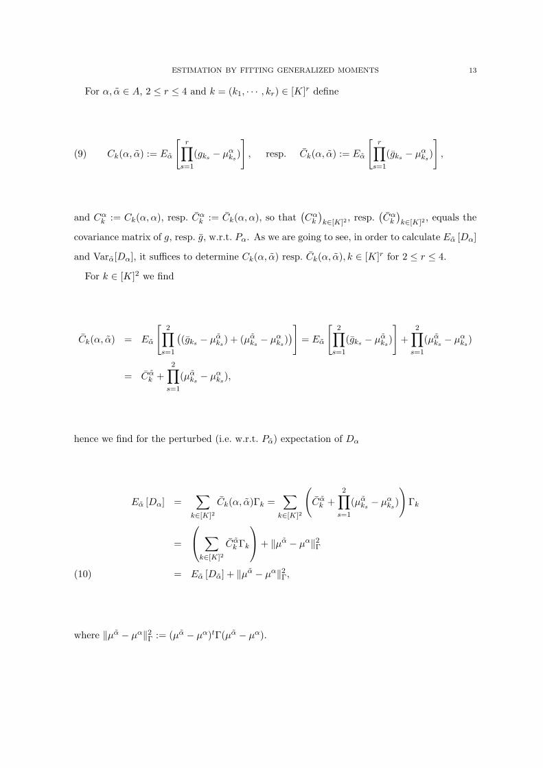
For α, α ∈ A, 2 ≤ r ≤ 4 and k = (k1, · · · , kr) ∈ [K]r define
(9) Ck(α, α) := Eα
[r∏
s=1
(gks − µαks
)
], resp. Ck(α, α) := Eα
[r∏
s=1
(gks − µαks
)
],
and Cαk := Ck(α, α), resp. Cα
k := Ck(α, α), so that(Cα
k
)k∈[K]2
, resp.(Cα
k
)k∈[K]2
, equals the
covariance matrix of g, resp. g, w.r.t. Pα. As we are going to see, in order to calculate Eα [Dα]
and Varα[Dα], it suffices to determine Ck(α, α) resp. Ck(α, α), k ∈ [K]r for 2 ≤ r ≤ 4.
For k ∈ [K]2 we find
Ck(α, α) = Eα
[2∏
s=1
((gks − µα
ks) + (µα
ks− µα
ks))]
= Eα
[2∏
s=1
(gks − µαks
)
]+
2∏
s=1
(µαks− µα
ks)
= Cαk +
2∏
s=1
(µαks− µα
ks),
hence we find for the perturbed (i.e. w.r.t. Pα) expectation of Dα
Eα [Dα] =∑
k∈[K]2
Ck(α, α)Γk =∑
k∈[K]2
(Cα
k +2∏
s=1
(µαks− µα
ks)
)Γk
=
∑
k∈[K]2
Cαk Γk
+ ‖µα − µα‖2
Γ
= Eα [Dα] + ‖µα − µα‖2Γ,(10)
where ‖µα − µα‖2Γ := (µα − µα)tΓ(µα − µα).
14 JOHANNES LEITNER AND GRIGORY TEMNOV
In order to calculate the perturbed variance of Dα w.r.t. Pα, we start by calculating Ck(α, α)
for k ∈ [K]4:
Ck(α, α) = Eα
[4∏
s=1
(gks − µαks
)
]= Eα
[4∏
s=1
((gks − µα
ks) + (µα
ks− µα
ks))]
= Cαk +
4∏
s=1
(µαks− µα
ks) +
(µαk4− µα
k4)Cα
(k1,k2,k3) + (µαk3− µα
k3)Cα
(k1,k2,k4) +
(µαk2− µα
k2)Cα
(k1,k3,k4) + (µαk1− µα
k1)Cα
(k2,k3,k4) +
(µαk3− µα
k3)(µα
k4− µα
k4)Cα
(k1,k2) + (µαk2− µα
k2)(µα
k4− µα
k4)Cα
(k1,k3) +
(µαk1− µα
k1)(µα
k4− µα
k4)Cα
(k2,k3) + (µαk2− µα
k2)(µα
k3− µα
k3)Cα
(k1,k4) +
(µαk1− µα
k1)(µα
k3− µα
k3)Cα
(k2,k4) + (µαk1− µα
k1)(µα
k2− µα
k2)Cα
(k3,k4),
thus,
Ck(α, α)− C(k1,k2)(α, α)C(k3,k4)(α, α)
= Cαk − Cα
(k1,k2)Cα(k3,k4) +
(µαk4− µα
k4)Cα
(k1,k2,k3) + (µαk3− µα
k3)Cα
(k1,k2,k4) +
(µαk2− µα
k2)Cα
(k1,k3,k4) + (µαk1− µα
k1)Cα
(k2,k3,k4) +
(µαk2− µα
k2)(µα
k4− µα
k4)Cα
(k1,k3) + (µαk1− µα
k1)(µα
k4− µα
k4)Cα
(k2,k3) +
(µαk2− µα
k2)(µα
k3− µα
k3)Cα
(k1,k4) + (µαk1− µα
k1)(µα
k3− µα
k3)Cα
(k2,k4).
ESTIMATION BY FITTING GENERALIZED MOMENTS 15
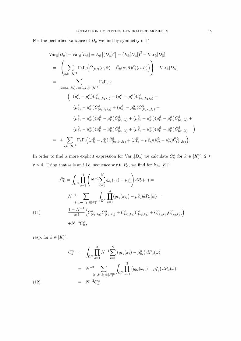
For the perturbed variance of Dα we find by symmetry of Γ
Varα[Dα]−Varα[Dα] = Eα
[(Dα)2
]− (Eα[Dα]
)2 −Varα[Dα]
=
∑
k,l∈[K]2
ΓkΓl
(C(k,l)(α, α)− Ck(α, α)Cl(α, α)
)−Varα[Dα]
=∑
k=(k1,k2),l=(l1,l2)∈[K]2
ΓkΓl ×
((µα
l2 − µαl2)C
α(k1,k2,l1) + (µα
l1 − µαl1)C
α(k1,k2,l2) +
(µαk2− µα
k2)Cα
(k1,l1,l2) + (µαk1− µα
k1)Cα
(k2,l1,l2) +
(µαk2− µα
k2)(µα
l2 − µαl2)C
α(k1,l1) + (µα
k1− µα
k1)(µα
l2 − µαl2)C
α(k2,l1) +
(µαk2− µα
k2)(µα
l1 − µαl1)C
α(k1,l2) + (µα
k1− µα
k1)(µα
l1 − µαl1)C
α(k2,l2)
)
= 4∑
k,l∈[K]2
ΓkΓl
((µα
l2 − µαl2)C
α(k1,k2,l1) + (µα
k2− µα
k2)(µα
l2 − µαl2)C
α(k1,l1)
).
In order to find a more explicit expression for Varα[Dα] we calculate Cαk for k ∈ [K]r, 2 ≤
r ≤ 4. Using that ω is an i.i.d. sequence w.r.t. Pα, we find for k ∈ [K]4
Cαk =
∫
ΩN
4∏
s=1
(N−1
N∑
i=1
gks(ωi)− µαks
)dPα(ω) =
N−4∑
(i1,··· ,i4)∈[N ]4
∫
ΩN
4∏
s=1
(gks(ωis)− µαks
)dPα(ω) =
1−N−1
N2
(Cα
(k1,k2)Cα(k3,k4) + Cα
(k1,k3)Cα(k2,k4) + Cα
(k1,k4)Cα(k2,k3)
)(11)
+N−3Cαk ,
resp. for k ∈ [K]3
Cαk =
∫
ΩN
3∏
s=1
N−1N∑
i=1
(gks(ωi)− µα
ks
)dPα(ω)
= N−3∑
(i1,i2,i3)∈[N ]3
∫
ΩN
3∏
s=1
(gks(ωis)− µα
ks
)dPα(ω)
= N−2Cαk ,(12)
16 JOHANNES LEITNER AND GRIGORY TEMNOV
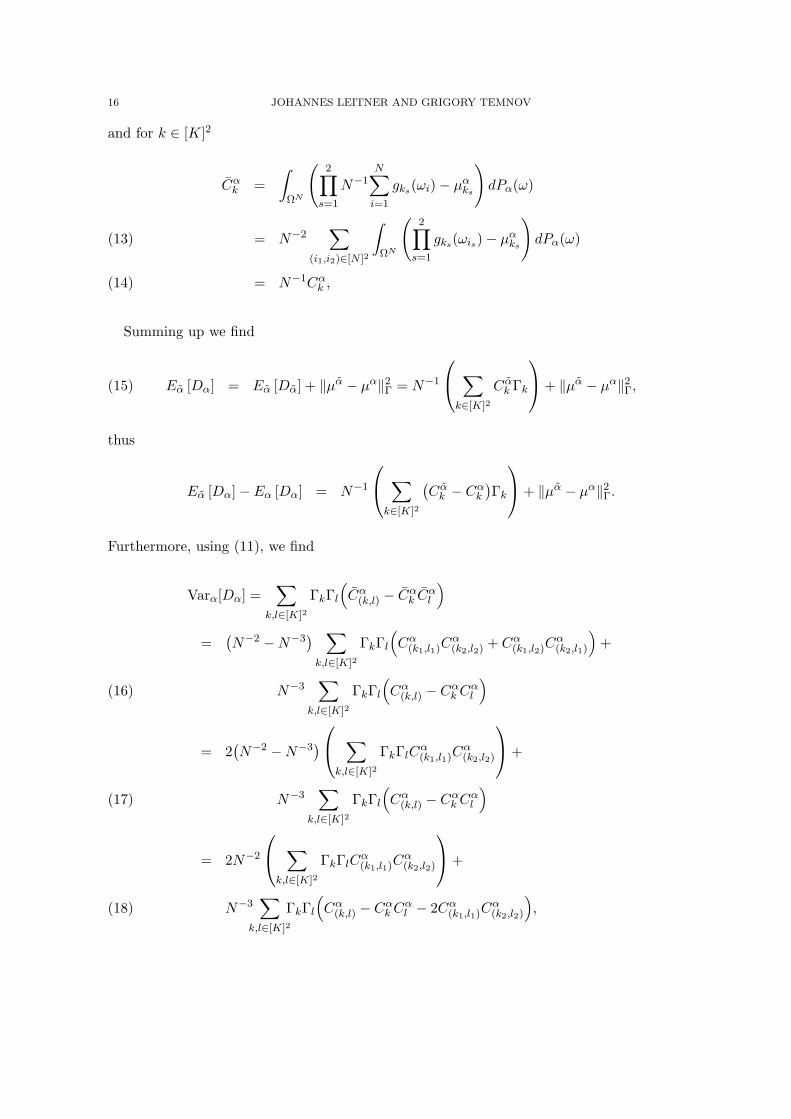
and for k ∈ [K]2
Cαk =
∫
ΩN
(2∏
s=1
N−1N∑
i=1
gks(ωi)− µαks
)dPα(ω)
= N−2∑
(i1,i2)∈[N ]2
∫
ΩN
(2∏
s=1
gks(ωis)− µαks
)dPα(ω)(13)
= N−1Cαk ,(14)
Summing up we find
Eα [Dα] = Eα [Dα] + ‖µα − µα‖2Γ = N−1
∑
k∈[K]2
Cαk Γk
+ ‖µα − µα‖2
Γ,(15)
thus
Eα [Dα]− Eα [Dα] = N−1
∑
k∈[K]2
(Cα
k − Cαk
)Γk
+ ‖µα − µα‖2
Γ.
Furthermore, using (11), we find
Varα[Dα] =∑
k,l∈[K]2
ΓkΓl
(Cα
(k,l) − Cαk Cα
l
)
=(N−2 −N−3
) ∑
k,l∈[K]2
ΓkΓl
(Cα
(k1,l1)Cα(k2,l2) + Cα
(k1,l2)Cα(k2,l1)
)+
N−3∑
k,l∈[K]2
ΓkΓl
(Cα
(k,l) − Cαk Cα
l
)(16)
= 2(N−2 −N−3
) ∑
k,l∈[K]2
ΓkΓlCα(k1,l1)C
α(k2,l2)
+
N−3∑
k,l∈[K]2
ΓkΓl
(Cα
(k,l) − Cαk Cα
l
)(17)
= 2N−2
∑
k,l∈[K]2
ΓkΓlCα(k1,l1)C
α(k2,l2)
+
N−3∑
k,l∈[K]2
ΓkΓl
(Cα
(k,l) − Cαk Cα
l − 2Cα(k1,l1)C
α(k2,l2)
),(18)
ESTIMATION BY FITTING GENERALIZED MOMENTS 17
and
Varα[Dα]−Varα[Dα]
= 4N−2∑
k,l∈[K]2
ΓkΓl
((µα
l2 − µαl2)C
α(k1,k2,l1) + N(µα
k2− µα
k2)(µα
l2 − µαl2)C
α(k1,l1)
),
so that
Varα[Dα]Varα[Dα]
=Varα[Dα]Varα[Dα]
(1 +
Varα[Dα]−Varα[Dα]Varα[Dα]
)
=(
1 +Varα[Dα]−Varα[Dα]
Varα[Dα]
)(1 +
Varα[Dα]−Varα[Dα]Varα[Dα]
).
It is important to note that therefore Varα[Dα]Varα[Dα] = 1+O(
√N−1) if ‖α−α‖ is of order O(
√N−1).
Note also, that setting x := x(α, α, N) := Eα[Xα], we find
x =Eα [Dα]− Eα [Dα]√
Varα[Dα]
=N‖µα − µα‖2
Γ +∑
k∈[K]2(Cα
k − Cαk
)Γk√
2∑
k,l∈[K]2 ΓkΓl Cα(k1,l1)C
α(k2,l2)
+ O(√
N−1).(19)
Proposition 4.1. For x < x we have
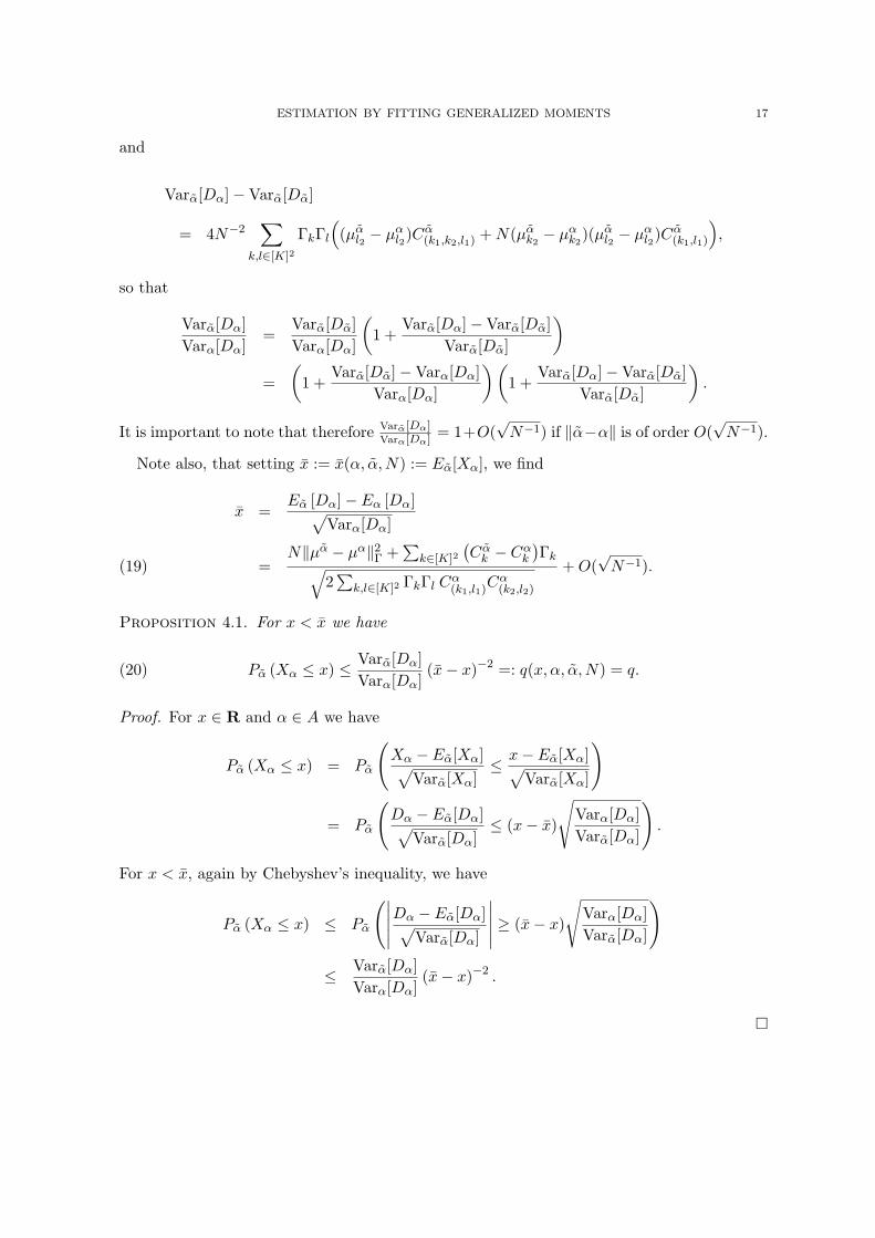
(20) Pα (Xα ≤ x) ≤ Varα[Dα]Varα[Dα]
(x− x)−2 =: q(x, α, α, N) = q.
Proof. For x ∈ R and α ∈ A we have
Pα (Xα ≤ x) = Pα
(Xα − Eα[Xα]√
Varα[Xα]≤ x− Eα[Xα]√
Varα[Xα]
)
= Pα
(Dα − Eα[Dα]√
Varα[Dα]≤ (x− x)
√Varα[Dα]Varα[Dα]
).
For x < x, again by Chebyshev’s inequality, we have
Pα (Xα ≤ x) ≤ Pα
(∣∣∣∣∣Dα −Eα[Dα]√
Varα[Dα]
∣∣∣∣∣ ≥ (x− x)
√Varα[Dα]Varα[Dα]
)
≤ Varα[Dα]Varα[Dα]
(x− x)−2 .
¤
18 JOHANNES LEITNER AND GRIGORY TEMNOV
Note that Proposition 4.1 implies that for all α, α0 ∈ A with ‖µα0 − µα‖Γ > 0 and for
any fixed x ∈ R, we have limN→∞ Pα0 (Xα ≤ x) = 0 since in this case (see equation (19)),
x(α, α0, N) →∞ as N →∞. Hence Xα diverges to +∞ in law w.r.t. Pα0 for all α ∈ A such
that ‖µα0 − µα‖Γ > 0. Intuitively speaking this means (for large enough sample size) that
Xα increases steeply around α, resulting into a small area of non-rejectable parameter choices
α ∈ A and indicating a high precision of our estimator α.
Note that for all α0 ∈ A, Xα0 converges by the multivariate central limit theorem in law
w.r.t. Pα0 to a finite valued (centralized and normalized χ2-type of) probability distribution.
Assuming for α, α0 ∈ A, ‖µα0−µα‖Γ = 0 iff α = α0, this means that estimation by minimizing
Xα is in fact a minimum contrast estimation with the contrast function g(·, α0) := K1A\α0
defined on A for any K > 0, since lim infN→∞(Xα − Xα0) ≥ g(α, α0) w.r.t. Pα0 for all
α, α0 ∈ A. See e.g. Guyon (1995) or Anh et al. (2007) for minimum contrast estimators.
However, due to Chebyshev’s inequality we can in addition reject models at a given confidence
level depending on the minimal Xα.
The extreme type of contrast function leads us to expect that the discriminative power
of our estimator will be strong for sufficiently large N . Intuitively speaking, Proposition 4.1
allows us to asymptotically determine the precision of the estimator given as the optimal
α ∈ A minimizing Xα. Consider the following situation:
Let Uα ⊆ A be a neighborhood of α such that on Uα the first order approximation µα =
µα +∇µα · (α− α) is valid up to a precision of order O(N−1). We then have ‖µα − µα‖2Γ =
‖α− α‖Γα + O(N−2) for Γα := (∇µα)tΓ∇µα. Assume that Γα is again strictly positive with
smallest eigenvalue λ > 0. It follows on Uα that N‖µα − µα‖2Γ ≥ Nλ‖α− α‖2 + O(N−1) and
if ‖α− α‖ is of magnitude
(21) d :=
√a + 1
λ
(Varα[Dα]
p0
) 14 √
N−1,
for a > 0, we find approximately x ≥ (a + 1)√
p−10 + O(
√N−1).
If Xα := Xα(ω) ≤√
p−10 is minimal at α ∈ A, then for large enough N the probability
q of observing Xα ≤ Xα if the true law was in fact Pα for a α ∈ A such that ‖α − α‖ is of
ESTIMATION BY FITTING GENERALIZED MOMENTS 19
magnitude d, is approximately bounded by
q(Xα, α, α, N) =Varα[Dα]Varα[Dα]
(x− Xα
)−2= (x− Xα)−2 + O(
√N−1)
≤(
(a + 1)√
p−10 −
√p−10
)−2
+ O(√
N−1)
= p0a−2 + O(
√N−1).
Conversely, if for fixed a > 0 a precision of d is desired for the estimation of the optimal α, a
worst case sample length N can be approximately calculated from equation (21).
In order to estimate the optimal α ∈ A, we suggest to start by minimizing Dα over A. In
a second step, Xα can then be minimized by a gradient search algorithm. Alternatively, for
large N , we approximately have
(22) Xα =Dα√
Varα[Dα]=
NDα√2
∑k,l∈[K]2 ΓkΓlC
α(k1,l1)C
α(k2,l2)
,
and the right side of the last expression can be minimized.
If the optimal α is expected to be near some α0 ∈ A, then Γ can be chosen such that Γα0
equals the identity matrix, so that the minimal eigenvalue λ will be approximately 1 too.
There are many possible choices for the generalized moments g. E.g. one could include all
moments of G up to some order, leading to an improved fit of the Laplace transform near
the origin. Alternatively (or in addition) one can as well include exponential moments of the
type exp(−γ ·G) in g for γ ∈ Rm \ 0. For computational efficiency it is crucial, that all the
corresponding generalized moments µα are known or can be computed for all α ∈ A. E.g. if
LG is known, then exponential moments can be calculated since LαG = LG(α+·)
LG(α) .
In a non-parametric approach one could choose the components of g to be orthogonal at
α0 ∈ A, e.g. by orthogonalizing a general g or by choosing orthogonal polynomials as the
components of g.
5. Applications
In this section we apply our approach to two statistical problems.
20 JOHANNES LEITNER AND GRIGORY TEMNOV
5.1. Fitting one-dimensional data. In order to illustrate the proposed method, we apply
the generalized moment fit to simulated artificial data having realistic parameters related to
the practice of (operational) risk management.
Our main aims are to compare the generalized moments fit with the maximum likelihood
estimator in application to various data sets and to show that the use of these two methods
simultaneously can increase the confidence in the resulting fit and make the modelling more
reliable.
Recall the common setting: one has a sample ω = (ωi)i∈[N ] ∈ ΩN , drawn under the law
of Pα0 and wishes to estimate the parameters’ vector α0. Assume that we deal with the
one-dimensional case and our sample is a sequence of i.i.d. random variables X1, . . . , XN ,
sampled from a distribution Fα for some α ∈ A.
Recall the quadratic goodness-of-fit measure Dα defined by (7) and take the matrix Γ
simply as a unit matrix, such that the expression Dα reduces to the sum:
(23) Dα :=K∑
k=1
Dαk :=
K∑
k=1
(gk − µαk )2 .
Minimizing Dα would correspond to the ”naive way” of the estimation of α. Instead, we
minimize the centralized and normalized statistics Xα, defined as in (8).
In order to use the expressions for Eα[Dα] and Varα[Dα] obtained in Section 4, let us first
rewrite definitions of Ck(α, α) and Ck(α, α) given by (9), which become simpler in our case:
(24) Cαk,k = Eα
[(gk − µα
k )2], resp. Cα
k,k = Eα
[(gk − µα
k )2],
Thus for k = 1, . . . ,K,
(25) Cαk,k = Eα
[(N−1gk − µα
k
)2]
= N−1Varα[gk] = N−1Cαk,k
and so the expression for numerator in (8) reduces to
(26) Eα[Dα] = N−1K∑
k=1
Varα[gk],
which is a special case of (15).
ESTIMATION BY FITTING GENERALIZED MOMENTS 21
Consider now a simple choice of the moment gk for the fitting. Particularly, let us base the
estimation of the parameters’ vector α on the Laplace transform of the distribution Fα taken
on a chosen grid within some fixed interval. That is, µαk :=
∫exp(−τkx)dFα(x)
= Eα[exp(−τkX1)] = Eα[gk] and gk := N−1N∑
i=1exp(−τkXi), where τk = τ0 + (k − 1) ·
T/(K − 1),
k = 1, . . . ,K. The parameters τk ≥ 0 and T > 0 define the interval on the support of the
Laplace transform which the estimation is performed on.
Remark 5.1. Though in our setting it is the uniform grid on the interval [τ0; τ0 + T ] that
is chosen for the estimation, the further argument could be easily changed for the case of the
more complex structure of the grid.
In the following argument, we denote for sake of simplicity µ[τk] ≡ µαk . Note that µ[τl+τk] =
Eα[exp(−(τl + τk)X1)].
Recall (26), denote Dαk := Varα[gk] = µ[2τk] − µ2
[τk] and note that in the specified case the
statistics Xα can be written as
(27) Xα :=
∑k
[Dαk −Eα [Dα
k ]]√
Varα[Dα]=
∑k
[N
(gk − µ[τk]
)2 −Varα(gk)]
N√
Varα[Dα].
The calculation of the quantity Varα[Dα] forming the denominator of (27) in this cases
reduces to the computation of the double sum containing the cross-products as well as the
squares of the quantities Dαk :
Varα[Dα] =K∑
k=1
K∑
l=1
Cov (Dαk , Dα
l )
=K∑
k=1
K∑
l=1
Eα
[(gk − µ[τk]
)2 (gl − µ[τl]
)2]−Eα[Dα
k ]Eα[Dαl ]
The latter expression can be simplified significantly. Recall formula (17). Considering a
special choice of the matrix Γ simply as a unit matrix, and check that in our case it reduces
22 JOHANNES LEITNER AND GRIGORY TEMNOV
to
Varα[Dα] = 2N−2
∑
k,l=1,··· ,KCovα(gk, gl)
+ N−3
∑
k,l=1,··· ,KEα
[(gk − µ[τk]
)2 (gl − µ[τl]
)2]
−2 [Covα(gk, gl)]2 −Varα(gk)Varα(gl)
)
= 2N−2∑
k,l=1,··· ,K
(µ[τk+τl] − µ[τl]µ[τk]
)2 +
N−3∑
k,l=1,··· ,K
(µ[2(τk+τl)] − 2(µ[(τk+τl)])
2 − µ[2τk]µ[2τl] + 2µ[2τl](µτk)2
+ 2µ[2τk](µ[τl])2 − 2µ[τl+2τk]µ[τl] − 2µ[τk+2τl]µ[τk] + 8µ[τk+τl]µ[τk]µ[τl] − 6µ2
[τk]µ2[τl]
).(28)
5.2. Estimation of the Generalized Pareto Distribution. Let us turn now to the im-
plementation of this method for the case when the c.d.f. Fα belongs to a specified family
of distribution functions. As we were interested in applications for risk management the so
called Extreme Value Theory should be referred to.
The Extreme Value Theory (EVT) originates from the works of Fisher and Tippett who
investigated limiting distributions of maxima and minima of a random sample. The funda-
mental theorem of EVT states that the limit distribution of (properly shifted and normalized)
maxima of a random population can be represented as a family of distributions having the
form
H(x) = exp−
[1 + ξ
(x
σ
)]−1/ξ
where 1 + ξ(x
σ
)> 0
which is associated with Generalized Extreme Value (GEV).
Using a straightforward argument, one can pass from GEV to Generalized Pareto distribu-
tion as a limit distribution for the scaled exceedances over a sufficiently high threshold:
(29) G(x) =
1− [1 + ξ
(xσ
)]−1/ξ, ξ 6= 0, σ > 0
1− exp(1− x/σ),
where the exponential distribution appears as the degenerate case for ξ = 0. When the shape
parameter ξ > 1, the first moment does not exist.
GPD is widely used in applications, including actuarial practice, where rare and severe
events appear naturally, thus the tails of distributions are of a particular interest, and fitting
ESTIMATION BY FITTING GENERALIZED MOMENTS 23
the data that exceeds high threshold is an appropriate methodology. For GPD estimation
approaches see e.g. Castillo and Hadi (1997), Chouklakian and Stephens (2001) and Luceno
(2006).
The common methodology used for fitting the GPD in most practical applications is Max-
imum likelihood estimation. To estimate the shape parameter ξ critical for heavy tails, such
methods as Hill estimator are often used. Dealing with actuarial data one is usually restricted
to limited databases embracing several years or even only months of historical losses. Thus the
reliability of the common estimation methods may become questionable. A thorough discus-
sion of the statistical estimation using MLE, Hill estimation and other techniques regarding
coarse actuarial data can be found in Embrechts et al. (1997).
We are going to work with a subclass of GPD in slightly different parametrization than
(29), e.g. with c.d.f. and p.d.f. respectively
(30) Fa, σ(x) = 1−(1 +
x
aσ
)−a, fa, σ(x) =
1σ
(1 +
x
aσ
)−a−1, a, σ > 0 x > 0.
Working with logarithmically transformed losses simplifies the setup, as the exponential dis-
tribution comes into play:
(31) Fa, σ(x) = 1− exp(−a(ln(x + aσ)− ln[aσ])).
Note that, nevertheless, GPD does not belong to exponential families of distributions, as after
introducing the notation y := ln(x+aσ) we still have the parameters a and σ included in the
new argument.
Remark 5.2. We remark on the range for the shape parameter. In the original definition
of GPD, the range of values for the shape parameter ξ can be naturally divided into ξ < 0,
ξ = 0 and ξ > 0, such that ξ > 0 can be considered as a heavy-tailed case and ξ < 0
corresponds to (in general) lighter tails than the exponential distribution. In our application,
we were particularly interested in the heavy tailed region of parameters. That is why we restrict
ourselves to the range ξ > 0; moreover, the re-parametrization a = 1/ξ allows to concentrate
on the heavy tailed side of the shape parameter, corresponding to small a. We exclude the
case a = 0 (as well as σ = 0) as a border for the possible parameter’s range, as these cases
24 JOHANNES LEITNER AND GRIGORY TEMNOV
are not reasonable in applications. At the same time, the case ξ = 0 corresponding to a →∞can be formally included in our model.
However, one may use this notation to obtain the values connected with the statistics Xα.
Specifically, we have the following expressions for the first and second exponential moments,
as well as for the variance:
µ[τk] =a([aσ]−τk)
a + τk, µ[2τk] =
a([aσ]−2τk)a + 2τk
, Varα[gk] =a([aσ]−2τk)τ2
k
(a + 2τk)(a + τk)2.
Expressions for the mixed moments are also easy to write down. Using (27) and (28), the sta-
tistics Xα can be calculated, and the task of its minimization can be solved for this particular
case.
Then the minimization for the moment fit can be made by a regular grid search algorithm.
Certainly, it is just the simplest version of the optimization scheme, eligible for the one-
dimensional case. In higher dimensions, searching the minimum within the grid should be
replaced by a suitable gradient search algorithm or other relevant minimization techniques.
In our application, minimization of the statistics Xα in question was performed using a
numerical SPlus procedure based on a quasi-Newton method using the double dogleg step
with the BFGS secant update to the Hessian. In order to apply the maximization procedure,
one needs to choose the domain of the parameters’ search. In the present algorithm, we
used the method based on p-values estimation outlined in the discussion part of Section 3.
Specifically, we select the preliminary (wider) domain and estimate the range of p–values
associated with the statistics Xα using Chebyshev equality as formulated in Lemma 4.1 and
exclude the values with Xα >√
p−10 (where p0 is pre-chosen) from the consideration. We
select p0 such that√
p−10 = 5.
Anticipating the application results, we indicate the plot of the statistics −Xα for a pseudo-
random sample simulated from GPD on Figure 1. We note that the statistics as the function
of the parameters is (visually) convex it a certain region and that the range of parameters
whose p−values exclude them from the vicinity the minimum is not hard to select (although
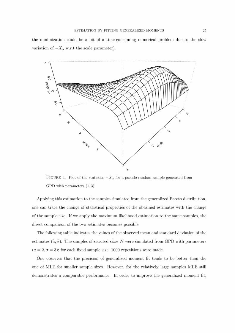
ESTIMATION BY FITTING GENERALIZED MOMENTS 25
the minimization could be a bit of a time-consuming numerical problem due to the slow
variation of −Xα w.r.t the scale parameter).
1
2
3
4
5
scale
1
2
3
4
shape
-0.5
00.
51
-X_a
lpha
Figure 1. Plot of the statistics −Xα for a pseudo-random sample generated from
GPD with parameters (1, 3)
Applying this estimation to the samples simulated from the generalized Pareto distribution,
one can trace the change of statistical properties of the obtained estimates with the change
of the sample size. If we apply the maximum likelihood estimation to the same samples, the
direct comparison of the two estimates becomes possible.
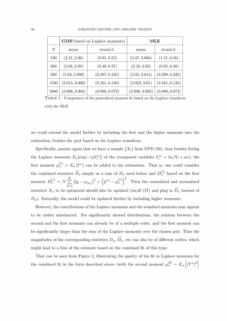
The following table indicates the values of the observed mean and standard deviation of the
estimates (a, σ). The samples of selected sizes N were simulated from GPD with parameters
(a = 2, σ = 3); for each fixed sample size, 1000 repetitions were made.
One observes that the precision of generalized moment fit tends to be better than the
one of MLE for smaller sample sizes. However, for the relatively large samples MLE still
demonstrates a comparable performance. In order to improve the generalized moment fit,
26 JOHANNES LEITNER AND GRIGORY TEMNOV
GMF(based on Laplace moments) MLE
N mean stand.d. mean stand.d.
100 (2.21, 2.96) (0.91, 0.52) (2.47, 3.068) (1.51, 0.56)
200 (2.08, 2.98) (0.49, 0.37) (2.16, 3.03) (0.65, 0.38)
500 (2.02, 2.999) (0.287, 0.235) (2.05, 3.014) (0.298, 0.235)
1500 (2.015, 3.006) (0.161, 0.136) (2.023, 3.01) (0.161, 0.135)
5000 (2.006, 3.004) (0.086, 0.072) (2.006, 3.002) (0.086, 0.072)
Table 1. Comparison of the generalized moment fit based on the Laplace transform
with the MLE.
we could extend the model further by including the first and the higher moments into the
estimation, besides the part based on the Laplace transform.
Specifically, assume again that we have a sample Xi from GPD (30), then besides fitting
the Laplace moments Eα[exp(−τkYα1 )] of the transposed variables Y α
i = ln (Xi + aσ), the
first moment µ(1)α = Eα [Y α] can be added to the estimation. That is, one could consider
the combined statistics Dα simply as a sum of Dα used before and D(1)α based on the first
moment D(1)α = N
K∑k=1
(gk − µ[τk]
)2 +(g(1) − µ
(1)α
)2. Then the centralized and normalized
statistics Xα to be optimized should also be updated (recall (27) and plug in Dα instead of
Dα). Naturally, the model could be updated further by including higher moments.
However, the contributions of the Laplace moments and the standard moments may appear
to be rather unbalanced. For significantly skewed distributions, the relation between the
second and the first moments can already be of a multiple order, and the first moment can
be significantly larger than the sum of the Laplace moments over the chosen grid. Thus the
magnitudes of the corresponding statistics Dα, Dα, etc can also be of different orders, which
might lead to a bias of the estimate based on the combined fit of this type.
That can be seen from Figure 2, illustrating the quality of the fit in Laplace moments for
the combined fit in the form described above (with the second moment µ(2)α = Eα
[(Y α)2
]
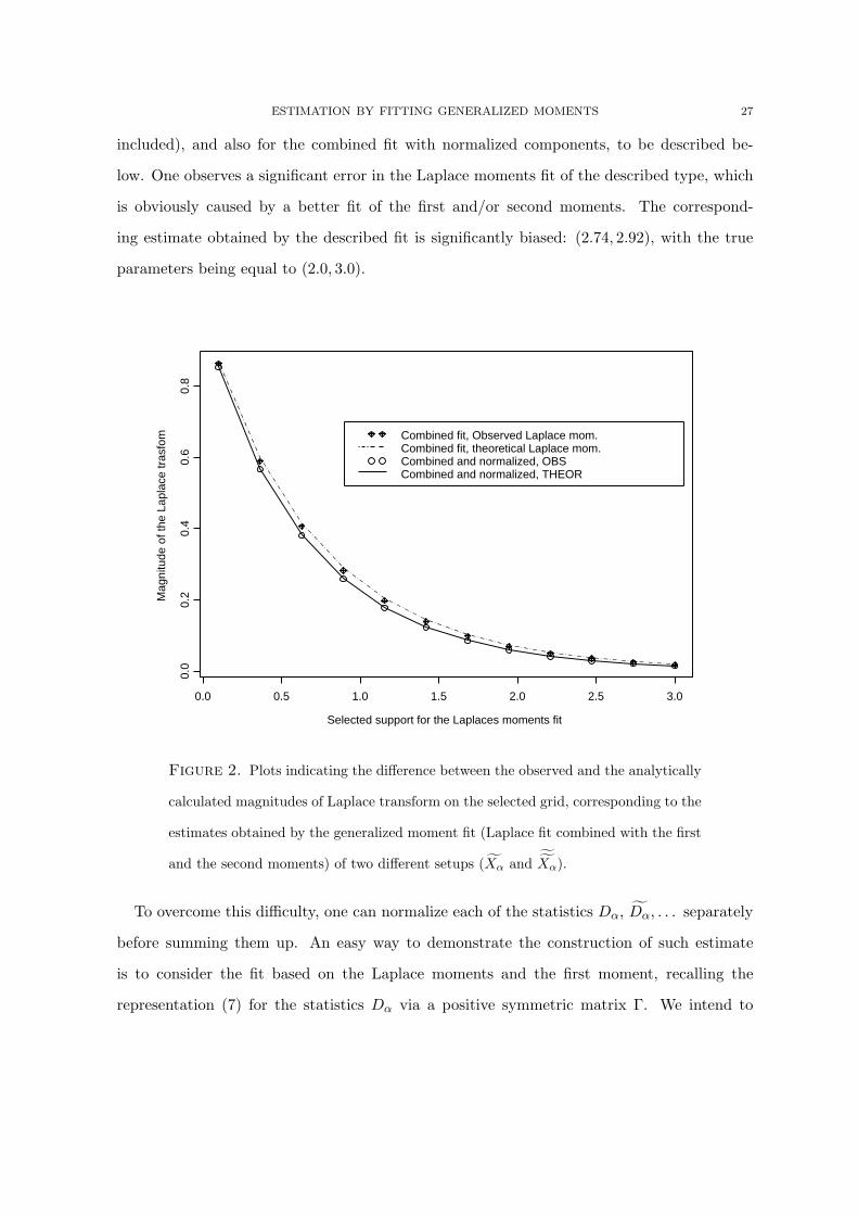
ESTIMATION BY FITTING GENERALIZED MOMENTS 27
included), and also for the combined fit with normalized components, to be described be-
low. One observes a significant error in the Laplace moments fit of the described type, which
is obviously caused by a better fit of the first and/or second moments. The correspond-
ing estimate obtained by the described fit is significantly biased: (2.74, 2.92), with the true
parameters being equal to (2.0, 3.0).
Selected support for the Laplaces moments fit
Mag
nitu
de o
f the
Lap
lace
tras
fom
0.0 0.5 1.0 1.5 2.0 2.5 3.0
0.0
0.2
0.4
0.6
0.8
Combined fit, Observed Laplace mom.Combined fit, theoretical Laplace mom.Combined and normalized, OBSCombined and normalized, THEOR
Figure 2. Plots indicating the difference between the observed and the analytically
calculated magnitudes of Laplace transform on the selected grid, corresponding to the
estimates obtained by the generalized moment fit (Laplace fit combined with the first
and the second moments) of two different setups (Xα and ˜Xα).
To overcome this difficulty, one can normalize each of the statistics Dα, Dα, . . . separately
before summing them up. An easy way to demonstrate the construction of such estimate
is to consider the fit based on the Laplace moments and the first moment, recalling the
representation (7) for the statistics Dα via a positive symmetric matrix Γ. We intend to
28 JOHANNES LEITNER AND GRIGORY TEMNOV
construct a new statistics ˜Dα based on the normalized Dα and normalized D
(1)α . Note that
the arguments of Section 4 allow to make Γ depend on α. We assumed Γ to be the unit matrix
previously in this section; let it now be a diagonal matrix with first k diagonal elements taking
values of 1/√
Var[Dαk ] correspondingly and the (k + 1)th diagonal element taking the value
of 1/
√Var[D(1)
α ]. Then one can use formula (7) to obtain ˜Dα, and the statistics ˜
Xα can then
be calculated.
It is also possible to construct ˜Dα in a simpler way, based on the variance of the summed
statistic Dα. That is, the first k diagonal elements would then take the same value of
1/√
Var[Dα]. Numerical modelling shows that this particular construction of the combined
moment fit leads to quite satisfactory results. It is illustrated by Figure 2 (see the part of the
plot concerning the combined and normalized fit). The corresponding estimate obtained by
the described fit with normalized components is (2.04, 2.98) (with the true parameters equal
to (2.0, 3.0)).
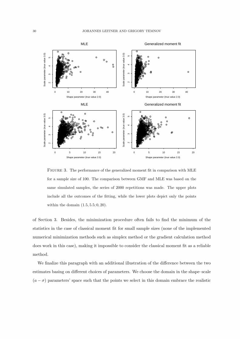
The performance of the fit is also illustrated by the series of numerical examples, summa-
rized in Table 2.
Thus, the generalized moment fit of the specified form proves to be as least as efficient
as MLE also for large sample sizes up 104. At the same time, for smaller sample sizes, the
moment fit is significantly better. That can be also seen for the graphical illustration: Figure
3 depicts the comparison between the generalized moment fit and the MLE.
We complete the numerical example for simulated data by a brief comparison with the
classical moment fit, i.e. the one that does not include the centralization and normalization
of the optimized statistics.
The method of moments is used in many applications of statistics, including the analysis
of heavy tailed data, see e.g. Panjer (2006). If theoretical moments have simple analytical
representations, the method can be reduced to solving the system of equations with respect to
the distribution parameters. In other cases, numerical optimization is needed. In our setting
for Laplace moments, the classical way of fitting would correspond to the minimization of the
statistics Dα, without passing to the centralized and normalized statistics Xα.
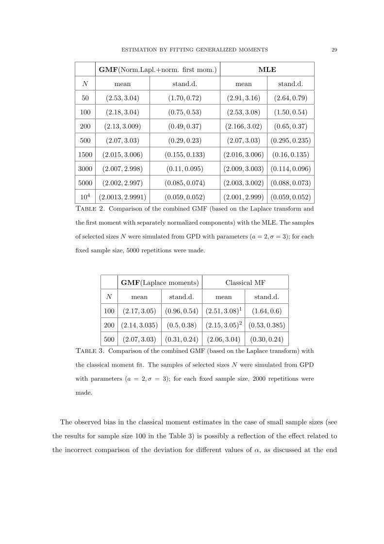
ESTIMATION BY FITTING GENERALIZED MOMENTS 29
GMF(Norm.Lapl.+norm. first mom.) MLE
N mean stand.d. mean stand.d.
50 (2.53, 3.04) (1.70, 0.72) (2.91, 3.16) (2.64, 0.79)
100 (2.18, 3.04) (0.75, 0.53) (2.53, 3.08) (1.50, 0.54)
200 (2.13, 3.009) (0.49, 0.37) (2.166, 3.02) (0.65, 0.37)
500 (2.07, 3.03) (0.29, 0.23) (2.07, 3.03) (0.295, 0.235)
1500 (2.015, 3.006) (0.155, 0.133) (2.016, 3.006) (0.16, 0.135)
3000 (2.007, 2.998) (0.11, 0.095) (2.009, 3.003) (0.114, 0.096)
5000 (2.002, 2.997) (0.085, 0.074) (2.003, 3.002) (0.088, 0.073)
104 (2.0013, 2.9991) (0.059, 0.052) (2.001, 2.999) (0.059, 0.052)
Table 2. Comparison of the combined GMF (based on the Laplace transform and
the first moment with separately normalized components) with the MLE. The samples
of selected sizes N were simulated from GPD with parameters (a = 2, σ = 3); for each
fixed sample size, 5000 repetitions were made.
GMF(Laplace moments) Classical MF
N mean stand.d. mean stand.d.
100 (2.17, 3.05) (0.96, 0.54) (2.51, 3.08)1 (1.64, 0.6)
200 (2.14, 3.035) (0.5, 0.38) (2.15, 3.05)2 (0.53, 0.385)
500 (2.07, 3.03) (0.31, 0.24) (2.06, 3.04) (0.30, 0.24)
Table 3. Comparison of the combined GMF (based on the Laplace transform) with
the classical moment fit. The samples of selected sizes N were simulated from GPD
with parameters (a = 2, σ = 3); for each fixed sample size, 2000 repetitions were
made.
The observed bias in the classical moment estimates in the case of small sample sizes (see
the results for sample size 100 in the Table 3) is possibly a reflection of the effect related to
the incorrect comparison of the deviation for different values of α, as discussed at the end
30 JOHANNES LEITNER AND GRIGORY TEMNOV
MLE
Shape parameter (true value 2.0)
Sca
le p
aram
eter
(tr
ue v
alue
3.0
)
0 10 20 30 40
23
45
Generalized moment fit
Shape parameter (true value 2.0)
Sca
le p
aram
eter
(tr
ue v
alue
3.0
)
0 10 20 30 40
23
45
MLE
Shape parameter (true value 2.0)
Sca
le p
aram
eter
(tr
ue v
alue
3.0
)
0 5 10 15 20
23
45
Generalized moment fit
Shape parameter (true value 2.0)
Sca
le p
aram
eter
(tr
ue v
alue
3.0
)
0 5 10 15 20
23
45
Figure 3. The performance of the generalized moment fit in comparison with MLE
for a sample size of 100. The comparison between GMF and MLE was based on the
same simulated samples, the series of 2000 repetitions was made. The upper plots
include all the outcomes of the fitting, while the lower plots depict only the points
within the domain (1.5, 5.5; 0, 20).
of Section 3. Besides, the minimization procedure often fails to find the minimum of the
statistics in the case of classical moment fit for small sample sizes (none of the implemented
numerical minimization methods such as simplex method or the gradient calculation method
does work in this case), making it impossible to consider the classical moment fit as a reliable
method.
We finalize this paragraph with an additional illustration of the difference between the two
estimates basing on different choices of parameters. We choose the domain in the shape–scale
(a− σ) parameters’ space such that the points we select in this domain embrace the realistic
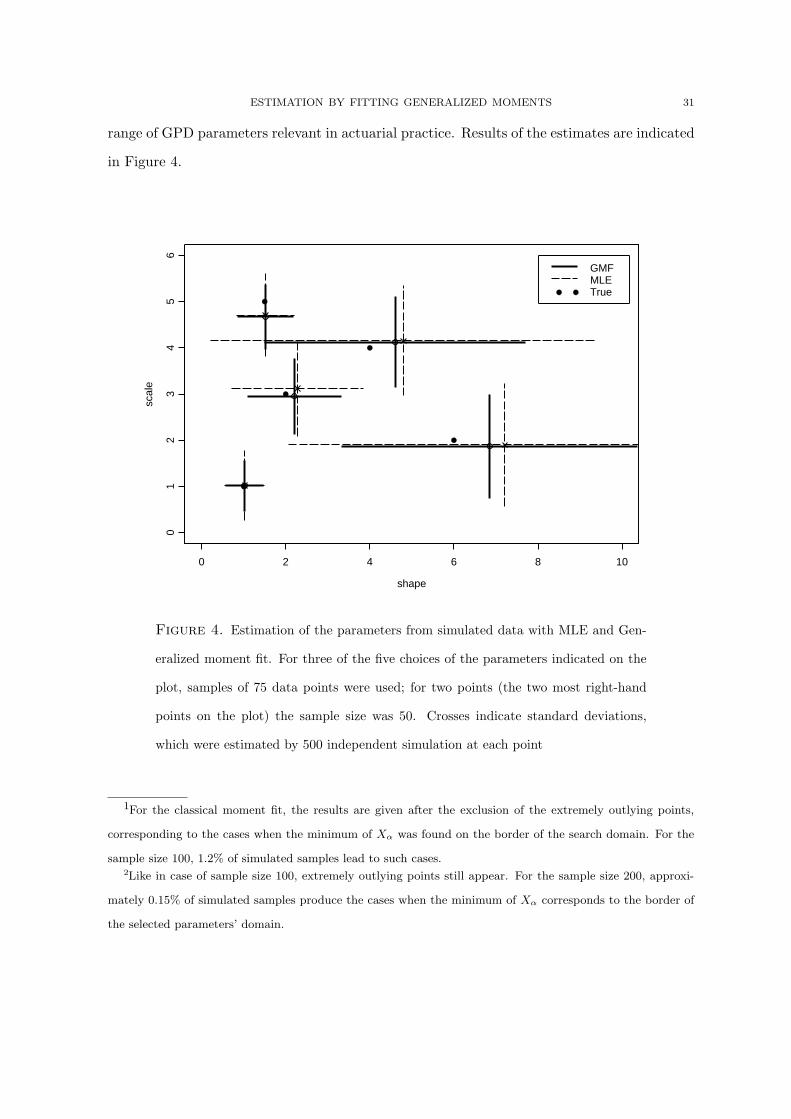
ESTIMATION BY FITTING GENERALIZED MOMENTS 31
range of GPD parameters relevant in actuarial practice. Results of the estimates are indicated
in Figure 4.
shape
scal
e
0 2 4 6 8 10
01
23
45
6
GMFMLETrue
Figure 4. Estimation of the parameters from simulated data with MLE and Gen-
eralized moment fit. For three of the five choices of the parameters indicated on the
plot, samples of 75 data points were used; for two points (the two most right-hand
points on the plot) the sample size was 50. Crosses indicate standard deviations,
which were estimated by 500 independent simulation at each point
1For the classical moment fit, the results are given after the exclusion of the extremely outlying points,
corresponding to the cases when the minimum of Xα was found on the border of the search domain. For the
sample size 100, 1.2% of simulated samples lead to such cases.2Like in case of sample size 100, extremely outlying points still appear. For the sample size 200, approxi-
mately 0.15% of simulated samples produce the cases when the minimum of Xα corresponds to the border of
the selected parameters’ domain.
32 JOHANNES LEITNER AND GRIGORY TEMNOV
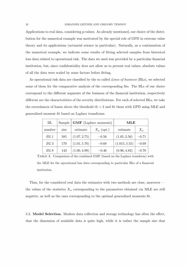
Applications to real data, considering p-values. As already mentioned, our choice of the distri-
bution for the numerical example was motivated by the special role of GPD in extreme value
theory and its applications (actuarial science in particular). Naturally, as a continuation of
the numerical example, we indicate some results of fitting selected samples from historical
loss data related to operational risk. The data we used was provided by a particular financial
institution, but, since confidentiality does not allow us to present real values, absolute values
of all the data were scaled by some factors before fitting.
As operational risk data are classified by the so called Lines of business (BLs), we selected
some of them for the comparative analysis of the corresponding fits. The BLs of our choice
correspond to the different segments of the business of the financial institution, respectively
different are the characteristics of the severity distributions. For each of selected BLs, we take
the exceedances of losses above the threshold th = 2 and fit them with GPD using MLE and
generalized moment fit based on Laplace transforms.
BL Sample GMF (Laplace moments) MLE
number size estimate Xα (opt.) estimate Xα
BL 1 585 (1.07, 2.75) −0.56 (1.05, 2.56) −0.71
BL 3 170 (1.01, 5.76) −0.68 (1.015, 5.55) −0.69
BL 8 143 (1.00, 4.99) −0.46 (0.96, 4.82) −0.70
Table 4. Comparison of the combined GMF (based on the Laplace transform) with
the MLE for the operational loss data corresponding to particular BLs of a financial
institution.
Thus, for the considered real data the estimates with two methods are close, moreover —
the values of the statistics Xα corresponding to the parameters obtained via MLE are still
negative, as well as the ones corresponding to the optimal generalized moments fit.
5.3. Model Selection. Modern data collection and storage technology has often the effect,
that the dimension of available data is quite high, while it is rather the sample size that
ESTIMATION BY FITTING GENERALIZED MOMENTS 33
remains limited. E.g. balance sheets contain a lot of relevant information about a company,
while the number of companies for which balance sheet data are available is often quite small
compared to the number of variables provided. On one hand, we have to cope with high-
dimensional data, while on the other hand, we can not expect to have large enough samples in
order that asymptotic (optimality, efficiency, consistency) properties of standard estimators
can be justified to approximately hold. One way to overcome this problem, are variable
selection methods that allow to reduce the dimension of the data, such that relative to the
reduced variable set, the sample size becomes large enough in order to justify the use of a
particular estimator.
Let us describe how to model selection can be done. Assume that we have a (eventually
constant) nested sequence 0 = A0 ⊆ A1 ⊆ · · · ⊆ ⋃i≥0 Ai = A, describing increasingly
complex models for the true law P of the observed sample ω ∈ ΩN . If our task is to find
the smallest model class i ≥ 0 such that there exists an α ∈ Ai, with corresponding p-value
w.r.t. Pα of observing Xα less than some given confidence level p0 := t−10 ∈ (0, 1), and if
infα∈Aj Xα > t0 holds for j ≥ 0, then we have at least to choose i > j. On the other hand,
infα∈Aj Xα < −t0 for some j ≥ 0 indicates over-fitting for small p. (Of course, if X0 < −t0 we
are in trouble (and something might be wrong with the data)). But typically, for real world
data, we expect Xα > 0 for α ∈ Ai for small i ≥ 0 and only if the full model A allows to
approximate the empirical law of the observed sample (e.g. if g consists of a complete system
of polynomials, orthogonal w.r.t. P ), then infα∈Aj Xα will always eventually become negative
as j increases.
The rationale of a goodness-of-fit estimation is to determine for a j ≥ 0, α ∈ Aj such that
infα∈Aj Fα
(Xα
)= Fα
(Xα
)holds, i.e. to find the α ∈ Aj which minimizes the p-value of Xα
w.r.t. Pα, and to find the smallest j such that this p-value becomes acceptable. As already
mentioned, doing this is typically computationally too expensive and we propose to minimize
Xα over Aj instead. We can not expect α ∈ Aj with Xα = infα∈Aj Xα to equal α exactly.
(This is actually similar as for maximum likelihood estimation). However, Proposition 4.1
tells us, that for large enough N , it becomes increasingly unlikely that α is far away from α.
34 JOHANNES LEITNER AND GRIGORY TEMNOV
Furthermore, for Xα ≤ t0, there is no guarantee that the p-value of Xα w.r.t. Pα is acceptable,
we only know that it is not acceptable for Xα > t0. (The calculation of the p-value of Xα
w.r.t. Pα can be done by importance sampling Monte-Carlo techniques, using the weight dPαdP ,
provided sampling under the measure P can be done efficiently.) In any case, α can serve as a
starting point for a (e.g. stochastic) search for the optimal α in the region α ∈ Aj | Xα ≤ t0.
6. Conclusion and outlook
In the present paper, we approached the classical problem of point estimation (and jointly
model selection). We present a new insight on this problem by considering a special type of
optimizing statistics based on generalized moments. We have shown that the introduction
of the centralized and normalized statistics into the procedure of the moment fit allows to
achieve useful asymptotic properties of the resulting estimate.
Application of the proposed method to statistical data shows that its properties are par-
ticularly useful when dealing with relatively small sample sizes. Numerical examples based
on the generalized Pareto distribution show that the generalized moment fit outperforms
maximum likelihood estimation, considering both the estimation precision and stability.
Further steps in the investigation of the considered method will include applications with
high dimensional data, e.g. data related to multivariate financial processes. Our numerical
results indicate that the generalized moment fit can be particularly useful in application to
heavy tailed data, which can also be a motivation for future research.
References
Akaike, H. (1973): Information Theory and an Extension of the Maximum Likelihood Principle. In: Petrov, B.N. and F. Csaki,
(Eds.), 2nd International Symposium on Information Theory, pp. 267–281, reprinted in: Kotz and Johnson (1992),
pp. 610–624.
Akaike, H. (1978): A Bayesian Analysis of the Minimum AIC Procedure. Ann. Inst. Statist. Math. Tokyo 30A, 9–14.
Anh, V.V., N.N. Leonenko and L.M. Sakhno (2007): Minimum contrast estimation of random processes based on information
of second and third orders. Journal of statistical planning and inference 137, 1302–1331.
Basharin, G.P. (1959): On a Statistical Estimate for the Entropy of a Sequence of Independent Random Variables. Theory of
Probability and its Applications 4, 333–336. Translated from: Teoriya Veroyatnostei iee Primeneniya 4, p. 361, 1959.
Campbell, L.L. (1970): Equivalence of Gauss’s Principle and Minimum Discrimination Information Estimation of Probabilities.
The Annals of Mathematical Statistics 41(3), 1011–1015.
ESTIMATION BY FITTING GENERALIZED MOMENTS 35
Castillo, E. and A.S. Hadi (1997): Fitting the Generalized Pareto Distribution to Data. Journal of the American Statistical
Association 92(440), 1609–1620.
Chouklakian. V. and M.A. Stephens (2001): Goodness-of-fit tests for the Generalized Pareto Distribution. Technometrics 43(4),
478–484.
Claeskens, G. and N.L. Hjort (2008): Model Selection and Model Averaging. Cambridge Series in Statistical and Probabilistic
Mathematics, Vol. 26. Cambridge: University Press.
Clough, D.J. (1964): Application of the Principle of Maximizing Entropy in the formulation of Hypotheses. Canadian
Operational Research Society (CORS) Journal 2(2), 53–70.
Crain, B.R. (1973): A Note on Density Estimation Using Orthogonal Expansions. Journal of the American Statistical
Association 68, 964–965.
Cramer, H. (1946): Mathematical Methods of Statistics. Princeton: University Press.
deLeeuw, J. (1992): Introduction to Akaike (1973) Information Theory and an Extension of the Maximum Likelihood Principle.
In: Kotz and Johnson (1992), pp. 600–609.
Embrechts, P., C. Kluppelberg and T. Mikosch (1997): Modelling extremal events. Applications of Mathematics, Volume 33.
Berlin: Springer.
Good, I.J. (1963): Maximum Entropy for Hypothesis Formulation, especially for multidimensional contingency tables. Annals
of Mathematical Statistics 34(3), 911–934.
Grendar, M. (jr.) and M. Grendar (2001): Maximum Entropy: Clearing up Mysteries. New York: Marcel Dekker.
Guyon, X. (1995): Random fields on a network. Berlin: Springer.
Hansen, L.P. (1982): Large sample properties of generalized method of moments estimators. Econometrica 50(4), 1029–1054.
Hurvich, C.M. and C.-L. Tsai (1989): Regression and time series model selction in small samples. Biometrika 76(2), 297–307.
Hurvich, C.M., R. Shumway and C.-L. Tsai (1990): Improved estimators of Kullback-Leibler information for autoregressive
model selction in small samples. Biometrika 77(4), 709–719.
Jaynes, E.T. (1957): Information Theory and Statistical Mechanics. The Physical Review 106(4), 620–630.
Jaynes, E.T. (1979): Where do we stand on Maximum Entropy ? In: Levine, R.D. and M. Tribus (Eds.), The Maximum
Entropy Formalism, pp. 210–314, (reprinted in Jaynes (1981)). Cambridge: MIT Press.
Jaynes, E.T. (1981): Papers on Probability, Statistics and Statistical Physics. Rosenkrantz, R. (Ed.), Dordrecht: Reidel.
Jaynes, E.T. (1982): On the Rationale of Maximum-Entropy Methods. Proceedings of the IEEE 70(9), 939–952.
Jaynes, E.T. (2003): Probability Theory: The Logic of Science. Cambridge: University Press.
Johnson, N.L. and N. Balakrishnan (1997): Advances in the theory and practice of statistics: a volume in honor of Samuel
Kotz. Wiley series in probability and statistics. New York: Wiley.
Kapur, J.N. and H.K. Kesavan (1992): Entropy Optimization Principles with Applications. San Diego: Academic Press.
Kapur, J.N. (1994): Measures of Information and their Applications. New York: Wiley.
Knight, J.L. and S.E. Satchell (1997): The cumulant generating function estimation method. Econometric Theory 13, 170–184.
Konishi, S. and G. Kitagawa (1996): Generalised information criteria in model selection. Biometrika 83(4), 875–890.
Kotz, S. and N.L. Johnson, (Eds.) (1992): Breakthroughs in Statistics, Vol. I. New York: Springer.
Kronmal, R. and M. Tarter (1968): The Estimation of Probability Densities and Cumulatives by Fourier Series Methods.
Journal of the American Statistical Association 63, 925–952.
Kullback, S. (1968): Information Theory and Statistics. New York: Dover Publications.
Luceno, A. (2006): Fitting the generalized Pareto distribution to data using maximum goodness-of-fit estimators. Computa-
tional Statistics & Data Analysis 51, 904–917.
Panjer, H.H. (2006): Operational Risk – Modeling Analytics. Hoboken, New Jersey: Wiley.
Pfanzagl, J. (1994): Parametric Statistical Theory. Berlin: de Gruyter.
Schwarz, G. (1978): Estimating the Dimension of a Model. The Annals of Statistics 6(2), 461–464.
Smith, P.L. (1987): On Akaike’s Model-Fit Criterion. IEEE Transactions on Automatic Control AC-32(12), 1100–1101.

36 JOHANNES LEITNER AND GRIGORY TEMNOV
Uffink, J. (1995): Can the maximum entropy principle be explained as a consistency requirement ? Studies in History and
Philosophy of Modern Physics 26B(3), 223–261.
Uffink, J. (1996): The Constraint Rule of the Maximum Entropy Principle Studies in History and Philosophy of Modern
Physics 27B(1), 47–79.
Wragg, A. and D.C. Dowson (1970): Fitting Continuous Probability Density Functions over [0,∞) using Information Theory
Ideas. IEEE Transactions on Information Theory IT-16, 226–230.