Generalized Hardy spaces

Acta Mathematica Sinica, English Series

Sep., 2010, Vol. 26, No. 9, pp. 1673–1692

Published online: August 15, 2010

DOI: 10.1007/s10114-010-8647-9

Http://www.ActaMath.com

Acta Mathematica Sinica, English Series© Springer-Verlag Berlin Heidelberg & The Editorial Office of AMS 2010

Generalized Hardy Spaces

Alexandre ALMEIDA Antonio M. CAETANODepartamento de Matematica, Universidade de Aveiro, 3810–193 Aveiro, Portugal

E-mail : [email protected] [email protected]

Abstract Hardy spaces with generalized parameter are introduced following the maximal character-

ization approach. As particular cases, they include the classical Hp spaces and the Hardy–Lorentz

spaces Hp,q. Real interpolation results with function parameter are obtained. Based on them, the

behavior of some classical operators is studied in this generalized setting.

Keywords Generalized Hardy spaces, maximal functions, Poisson kernel, interpolation with function

parameter, Riesz potentials, singular integrals

MR(2000) Subject Classification 42B30, 42B25, 46M35, 31B15, 42B20

1 Introduction

The n-dimensional theory of Hardy spaces has started with Stein and Weiss [1] based on theproperties of harmonic functions. Later, Fefferman and Stein [2] have characterized these spacesthrough maximal functions. This maximal characterization was crucial for the development ofthe real variable theory of Hardy spaces. Close to this, we also refer to the papers [3, 4] whereatomic decomposition tools were first developed within the framework of these spaces. Wemention [5, Chapter 3] and [6] for a nice exposition on real Hp spaces and further references.

Meanwhile, several generalizations of the original Hp spaces have been considered, such asHardy spaces on weighted Lp spaces (see [7]), Hardy spaces Hp,q modeled on classical Lorentzspaces Lp,q (see [8, 9]) or Hardy spaces defined on spaces of homogeneous type (see [10, 11]).Following the maximal function approach, we study Hardy spacesHq(φ) modeled on generalizedLorentz spaces Λq(φ). They include the classical Hp spaces and the just mentioned Hardy–Lorentz spaces Hp,q as particular cases. Maximal characterizations in terms of the Poissonkernel are also given.

We also study interpolation properties by the real method with function parameter. Ourresults generalize the interpolation statements proved in [8] for the Hardy–Lorentz spaces. Asan application, we show the connection between Hq(φ) and the space Λq(φ). This extends, inparticular, the classical result asserting that Hp = Lp for p > 1.

With the help of interpolation tools, we prove the continuity of the Fourier transform ofthe functions from Hq(φ) and give a control for its growth. We also prove the boundednessof some classical convolution operators acting in Hq(φ) spaces, namely we establish a Hardy–Littlewood–Sobolev type theorem for the Riesz fractional integration and prove the boundednessof singular integral operators.

Received December 22, 2008, accepted September 24, 2009

Supported by the Research Unit Matematica e Aplicacoes (UIMA) of University of Aveiro, Portugal

1674 Almeida A. and Caetano A. M.

The paper is structured as follows. After some necessary preliminaries, in Section 3 weintroduce the spaces Hq(φ) and prove the consistency of the definition given via maximalfunctions. A characterization in terms of Poisson integrals is also obtained. Section 4 is mainlydevoted to the study of real interpolation properties using function parameters. In Section 5 wegeneralize to the spaces Hq(φ) some classical results on the behavior of the Fourier transform,Riesz potentials and singular integrals on Hp spaces.

2 Preliminaries

Basic notation We shall consider basic notation as follows. By |E| we denote the (Lebesgue)measure of a measurable subset E of the Euclidean space R

n (n ∈ N). The measure of the unitball will be simply denoted by ωn, where we write B(x, r) for the open ball centered at x ∈ R

n

with radius r > 0. By Rn+1+ we denote the space R

n+1+ = {(x, t) : x ∈ R

n, t > 0}.In general, we deal with function spaces defined on the whole R

n, so that we shall omit theRn in their notation for simplicity. Hence, for 0 < p ≤ ∞, Lp denotes the classical Lebesgue

space quasi-normed by

‖f |Lp‖ :=( ∫

Rn

|f(x)|p dx)1/p

,

with the usual modification when p = ∞.By C∞ we denote the collection of all infinitely differentiable functions (in R

n). S standsfor the Schwartz class consisting of all functions in C∞ which are rapidly decreasing and S ′, itstopological dual, is the space of all tempered distributions. We write f for the Fourier transformof f ∈ S. The Fourier transform is considered in S ′ in the standard way.

The symbol “↪→” means continuous embedding between two quasi-normed spaces. Theequivalence f(x) ∼ g(x) (f, g non-negative functions) means that there are constants c1, c2 > 0such that c1f(x) ≤ g(x) ≤ c2f(x) for all the admitted values of x. The symbol “∼” is alsoused to denote equivalence of quasi-norms. By C, or c (possibly with subscripts), we denotegeneric positive constants, which may have different values even in the same line. Although theexact values of the constants are usually irrelevant for our purposes, sometimes we emphasizetheir dependence on certain parameters (e.g. C(p) means that C depends on p, etc.). Furthernotation will be properly introduced whenever needed.

2.1 Function Parameters

Definition 2.1 A function φ : (0,∞) → (0,∞) belongs to the class B if it is continuous,φ(1) = 1 and

φ(t) := sups>0

φ(st)φ(s)

<∞, t > 0.

For φ ∈ B, the function φ is submultiplicative, and the Boyd lower and upper indices arewell defined by

βφ = limt→0

log φ(t)log t

and αφ = limt→+∞

log φ(t)log t

,

respectively, with −∞ < βφ ≤ αφ <∞. Examples of functions belonging to B are

φa,b(t) = ta(1 + | log t|)b, a, b ∈ R.

Generalized Hardy Spaces 1675

In this case, φa,b(t) = ta(1 + | log t|)|b| and βφa,b= αφa,b

= a.

The main connection between φ ∈ B and φ is made with the estimates

φ(u)φ(1/t)

≤ φ(ut) ≤ φ(u)φ(t), u, t > 0. (2.1)

With the help of (2.1), we may express some properties of φ ∈ B through the Boyd indices ofφ. For instance,

βφ > 0 if and only if∫ 1

0

φ(t)dt

t<∞ (2.2)

andαφ < 0 if and only if

∫ ∞

1

φ(t)dt

t<∞. (2.3)

Furthermore, if βφ > 0 (resp. αφ < 0), then φ is equivalent to some increasing (resp. decreasing)function ψ ∈ B. These (and other) properties of class B may be found in [12, 13].

2.2 Generalized Lorentz Spaces

For 0 < q < ∞ and φ ∈ B, the generalized Lorentz space Λq(φ) is defined as the collection ofall measurable functions f on R

n such that

‖f |Λq(φ)‖ :=(∫ ∞

0

[f∗(t)φ(t)]qdt

t

)1/q

<∞, (2.4)

where f∗ stands for the usual decreasing rearrangement of f (see [14] for details). One can showthat (2.4) defines a quasi-norm and that Λq(φ) is a quasi-Banach space. Clearly, Λq(φ) = Λq(ψ)if φ(t) ∼ ψ(t).

If φ(t) = t1/p (1 + | log t|)b, with 0 < p < ∞ and b ∈ R, then Λq(φ) = Lp,q(logL)b are theLorentz–Zygmund spaces studied in [15]. They are classical Lorentz spaces Lp,q if b = 0, whichin turn are the usual Lebesgue spaces Lp when q = p.

Generalized Lorentz spaces were considered in [13, 16, 17] and [12], for example. Theyare a particular case of weighted Lorentz spaces with the weight constructed from class B. Asystematic study on general weighted Lorentz spaces can be found in [18], including furtherreferences.

The spaces Λq(φ) have the lattice property, that is, for measurable functions f, g in Rn there

holds|f | ≤ |g| a.e. =⇒ ‖f |Λq(φ)‖ ≤ ‖g |Λq(φ)‖ . (2.5)

We note that Λq(φ) has an absolutely continuous “norm” (see [14, pp. 13–16], for details) ifβφ > 0. To see this, taking into account Theorem 2.3.4 in [18], it suffices to show that φ(t)qt−1

is not integrable in (0,∞). Since φq is equivalent to some increasing function g ∈ B (becauseβφq = qβφ > 0), then ∫ ∞

0

φ(t)qdt

t≥ c

∫ ∞

1

g(t)dt

t≥ c g(1)

∫ ∞

1

dt

t= ∞.

The absolute continuity of the “norm” is important, because it allows us to make use of thedominated convergence argument in this generalized setting, namely for any f ∈ Λq(φ), withβφ > 0, the following holds (see [18, Proposition 2.3.3]): for measurable functions fk, k ∈ N,

|fk| ≤ |f | and limk→∞

fk = 0 a.e. =⇒ limk→∞

‖fk |Λq(φ)‖ = 0. (2.6)


From general properties in [18], one can see also that Λq(φ) is a reflexive space if 1 < q <∞and 0 < βφ ≤ αφ < 1, being the dual space given by

(Λq(φ))′ = Λq′(ψ), with ψ(t) =

t

φ(t),

1q

+1q′

= 1.

Finally, we notice that the Hardy–Littlewood maximal operator M, defined by

(Mf)(x) := supr>0

1|B(x, r)|

∫B(x,r)

|f(y)| dy (2.7)

is bounded in Λq(φ) if 0 < q <∞ and 0 < βφ ≤ αφ < 1 (see [13, 16, 18]).

3 Hardy Spaces Modeled on Spaces Λq(φ)

3.1 Definition

In the sequel, ϕ denotes a Schwartz function and ϕt(x) := t−nϕ(x/t), x ∈ Rn, t > 0. If f

is a tempered distribution then the convolution ϕ ∗ f is a well-defined infinitely differentiablefunction. Hence the following maximal functions, well-known in the theory of Hardy spaces,make sense:

(Rϕf)(x) = supt>0

|(ϕt ∗ f)(x)| (3.1)

(radial maximal function),

(Nϕf)(x) = sup(y,t)∈Γ(x)

|(ϕt ∗ f)(y)| (3.2)

(non-tangential maximal function),

(T μϕ f)(x) = sup

y∈Rn, t>0|(ϕt ∗ f)(y)|

[t

|x− y| + t

]μ, μ > 0 (3.3)

(tangential maximal function), where in (3.2) Γ(x) denotes a cone in Rn+1+ with vertex at

x ∈ Rn, more precisely, Γ(x) := {(y, t) ∈ R

n+1+ : |x− y| < t}.

We shall also consider “grand maximal functions” which are based on a collection of semi-norms on S, instead of a single approximation of identity as in the previous functions. Givenψ ∈ S, we put

|||ψ|||m := supu∈Rn

|α|≤m

(1 + |u|)m+n |Dαψ(u)| , m ∈ N0.

The grand maximal function Gmf is defined by

(Gmf)(x) = sup|||ψ|||m≤1

(Nψf)(x) = sup|||ψ|||m≤1

sup(y,t)∈Γ(x)

|(ψt ∗ f)(y)| , m ∈ N0. (3.4)

In what follows we assume that our ϕ ∈ S satisfies∫

Rn ϕ(x) dx = 1 (so that also ϕt ∈ Swith

∫Rn ϕt(x) dx = 1).

Definition 3.1 Let 0 < q < ∞ and φ ∈ B with βφ > 0. The space Hq(φ) is the collection ofall f ∈ S ′ such that Rϕf ∈ Λq(φ), equipped with the quasi-norm

‖f |Hq(φ)‖ϕ := ‖Rϕf |Λq(φ)‖ . (3.5)


The fact that (3.5) is a quasi-norm follows immediately from the properties of spaces Λq(φ)and the sublinearity of Rϕ.

Examples If φ(t) = t1/p(1 + | log t|)b, 0 < p < ∞, b ∈ R, we would obtain Hardy–Lorentz–Zygmund spaces, which could be denoted by Hp,q(logL)b, following the analogy with theLorentz–Zygmund spaces. If b = 0 then Hq(φ) = Hp,q are the so-called Hardy–Lorentz spaces,introduced in [8] and recently studied in [9], which in turn are the classical (real) Hardy spacesHp when q = p.

A fundamental result of Fefferman and Stein asserts that the definition of Hq does notdepend on the particular choice of ϕ, in the sense that different choices of ϕ lead to equivalentquasi-norms. To make Definition 3.1 consistent, we need to guarantee a corresponding resultin the generalized setting. We will see that this is the case (and the reason for imposing therestriction βφ > 0 in Definition 3.1).

The following statement extends the maximal characterization of Hardy spaces of Feffermanand Stein [2] to our generalized case.

Theorem 3.2 Let φ ∈ B with βφ > 0 and 0 < q < ∞. For a tempered distribution f , thefollowing conditions are equivalent :

(i) Rϕf ∈ Λq(φ) for some ϕ ∈ S with∫

Rn ϕ(x) dx = 1.(ii) There is a natural number m0 = m0(n, φ) such that Gmf ∈ Λq(φ), for every m ≥ m0.(iii) Nηf ∈ Λq(φ) for some η ∈ S with

∫Rn η(x) dx = 1.

Moreover,

‖Rϕf |Λq(φ)‖ ∼ ‖Gmf |Λq(φ)‖ ∼ ‖Nηf |Λq(φ)‖

for any f ∈ S ′.

Remark 3.3 The assertions (ii) ⇒ (i) and (ii) ⇒ (iii) are in fact valid for all ϕ, η ∈ S underthe assumptions above. To see this, observe that, for any ψ ∈ S and m ∈ N, one has

Rψf(x) ≤ Nψf(x) ≤ K Gmf(x), x ∈ Rn, (3.6)

with K ≥ |||ψ|||m, in view of the definitions (3.1), (3.2), (3.4) themselves.

Theorem 3.2 and Remark 3.3 show that the definition of Hq(φ) is, in fact, independent ofthe choice of ϕ (with the properties above).

Corollary 3.4 Let ϕ, η ∈ S with∫

Rn ϕ(x) dx =∫

Rn η(x) dx = 1. Under the same hypothesisof Theorem 3.2, we have

‖f |Hq(φ)‖ϕ ∼ ‖f |Hq(φ)‖η (3.7)

for any f ∈ Hq(φ).

In view of (3.7), we may omit the “ϕ” on the left-hand side of (3.5) and write only‖f |Hq(φ)‖ to denote the quasi-norm of f .

3.2 Proof of Theorem 3.2

The proof of Theorem 3.2 follows the main steps of the original approach developed in [2].However, it is structured in a slightly different way, close to the arrangement given in [6].

Everywhere in this section we assume f ∈ S ′.


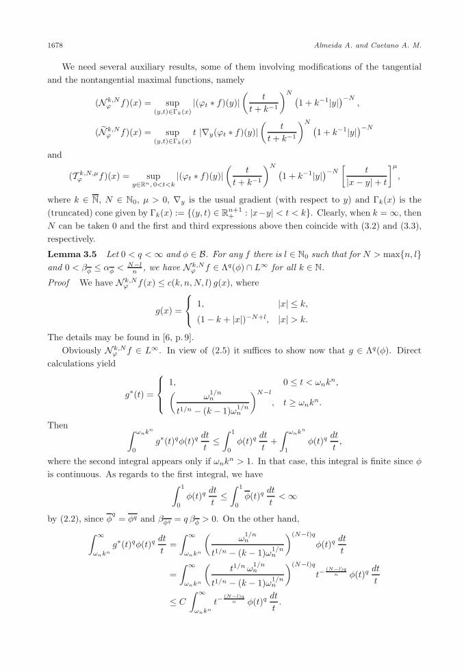
We need several auxiliary results, some of them involving modifications of the tangentialand the nontangential maximal functions, namely

(N k,Nϕ f)(x) = sup

(y,t)∈Γk(x)

|(ϕt ∗ f)(y)|(

t

t+ k−1

)N (1 + k−1|y|

)−N,

(N k,Nϕ f)(x) = sup

(y,t)∈Γk(x)

t |∇y(ϕt ∗ f)(y)|(

t

t+ k−1

)N (1 + k−1|y|

)−N

and

(T k,N,μϕ f)(x) = sup

y∈Rn, 0<t<k|(ϕt ∗ f)(y)|

(t

t+ k−1

)N (1 + k−1|y|

)−N [t

|x− y| + t

]μ,

where k ∈ N, N ∈ N0, μ > 0, ∇y is the usual gradient (with respect to y) and Γk(x) is the(truncated) cone given by Γk(x) := {(y, t) ∈ R

n+1+ : |x−y| < t < k}. Clearly, when k = ∞, then

N can be taken 0 and the first and third expressions above then coincide with (3.2) and (3.3),respectively.

Lemma 3.5 Let 0 < q <∞ and φ ∈ B. For any f there is l ∈ N0 such that for N > max{n, l}and 0 < βφ ≤ αφ <

N−ln , we have N k,N

ϕ f ∈ Λq(φ) ∩ L∞ for all k ∈ N.

Proof We have N k,Nϕ f(x) ≤ c(k, n,N, l) g(x), where

g(x) =

⎧⎨⎩

1, |x| ≤ k,

(1 − k + |x|)−N+l, |x| > k.

The details may be found in [6, p. 9].Obviously N k,N

ϕ f ∈ L∞. In view of (2.5) it suffices to show now that g ∈ Λq(φ). Directcalculations yield

g∗(t) =

⎧⎪⎨⎪⎩

1, 0 ≤ t < ωnkn,(

ω1/nn

t1/n − (k − 1)ω1/nn

)N−l, t ≥ ωnk

n.

Then ∫ ωnkn

0

g∗(t)qφ(t)qdt

t≤

∫ 1

0

φ(t)qdt

t+

∫ ωnkn

1

φ(t)qdt

t,

where the second integral appears only if ωnkn > 1. In that case, this integral is finite since φis continuous. As regards to the first integral, we have∫ 1

0

φ(t)qdt

t≤

∫ 1

0

φ(t)qdt

t<∞

by (2.2), since φq

= φq and βφq = q βφ > 0. On the other hand,∫ ∞

ωnkn

g∗(t)qφ(t)qdt

t=

∫ ∞

ωnkn

(ω

1/nn

t1/n − (k − 1)ω1/nn

)(N−l)qφ(t)q

dt

t

=∫ ∞

ωnkn

(t1/n ω

1/nn

t1/n − (k − 1)ω1/nn

)(N−l)qt−

(N−l)qn φ(t)q

dt

t

≤ C

∫ ∞

ωnkn

t−(N−l)q

n φ(t)qdt

t.


If ωnkn < 1 we split the integral into∫ ∞ωnkn · · · =

∫ 1

ωnkn · · ·+∫ ∞1

· · · . Clearly the first integral is

finite. Moreover, since t−(N−l)q

n φ(t)q = t−(N−l)q

n φ(t)q and αt−

(N−l)qn φ(t)q

= − (N−l)qn + q αφ < 0,

then the second integral is also finite in view of estimate∫ ∞

1

t−(N−l)q

n φ(t)qdt

t≤

∫ ∞

1

t−(N−l)q

n φ(t)qdt

t

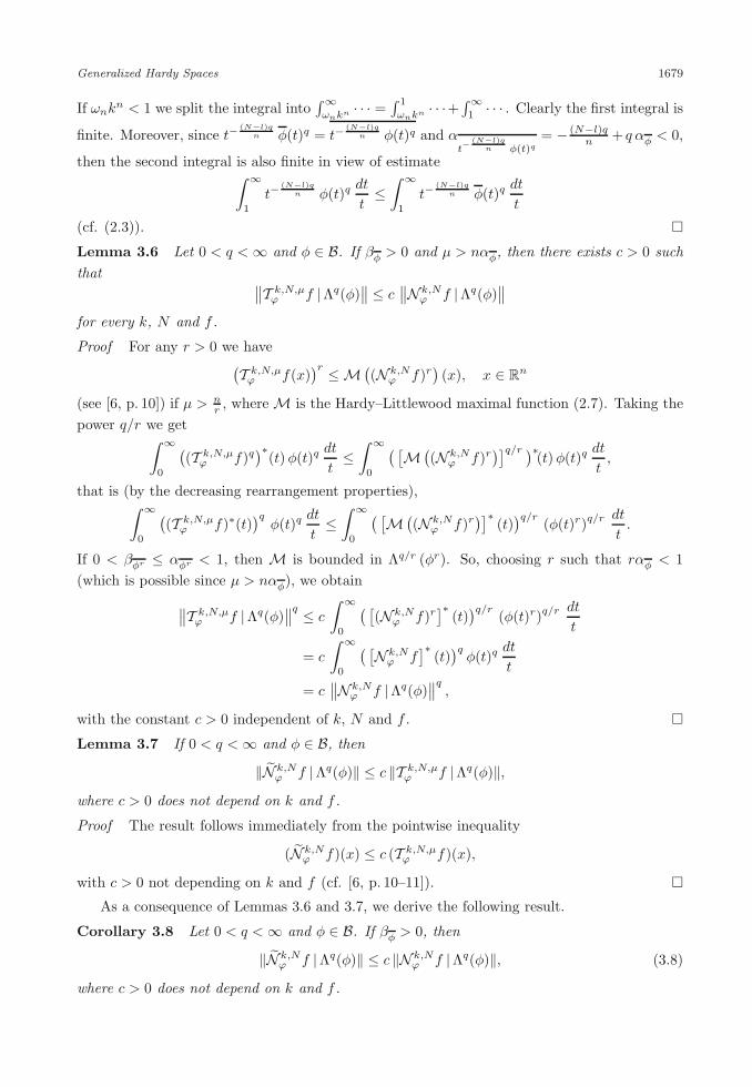
(cf. (2.3)). �Lemma 3.6 Let 0 < q <∞ and φ ∈ B. If βφ > 0 and μ > nαφ, then there exists c > 0 suchthat ∥∥T k,N,μ

ϕ f |Λq(φ)∥∥ ≤ c

∥∥N k,Nϕ f |Λq(φ)

∥∥for every k, N and f .

Proof For any r > 0 we have(T k,N,μϕ f(x)

)r ≤ M((N k,N

ϕ f)r)(x), x ∈ R

n

(see [6, p. 10]) if μ > nr , where M is the Hardy–Littlewood maximal function (2.7). Taking the

power q/r we get∫ ∞

0

((T k,N,μϕ f)q

)∗(t)φ(t)q

dt

t≤

∫ ∞

0

( [M

((N k,N

ϕ f)r)]q/r )∗(t)φ(t)q

dt

t,

that is (by the decreasing rearrangement properties),∫ ∞

0

((T k,N,μϕ f)∗(t)

)qφ(t)q

dt

t≤

∫ ∞

0

( [M

((N k,N

ϕ f)r)]∗

(t))q/r (φ(t)r)q/r

dt

t.

If 0 < βφr ≤ αφr < 1, then M is bounded in Λq/r (φr). So, choosing r such that rαφ < 1(which is possible since μ > nαφ), we obtain

∥∥T k,N,μϕ f |Λq(φ)

∥∥q ≤ c

∫ ∞

0

( [(N k,N

ϕ f)r]∗

(t))q/r (φ(t)r)q/r

dt

t

= c

∫ ∞

0

( [N k,Nϕ f

]∗(t)

)qφ(t)q

dt

t

= c∥∥N k,N

ϕ f |Λq(φ)∥∥q ,

with the constant c > 0 independent of k, N and f . �Lemma 3.7 If 0 < q <∞ and φ ∈ B, then

‖N k,Nϕ f |Λq(φ)‖ ≤ c ‖T k,N,μ

ϕ f |Λq(φ)‖,

where c > 0 does not depend on k and f .

Proof The result follows immediately from the pointwise inequality

(N k,Nϕ f)(x) ≤ c (T k,N,μ

ϕ f)(x),

with c > 0 not depending on k and f (cf. [6, p. 10–11]). �As a consequence of Lemmas 3.6 and 3.7, we derive the following result.

Corollary 3.8 Let 0 < q <∞ and φ ∈ B. If βφ > 0, then

‖N k,Nϕ f |Λq(φ)‖ ≤ c ‖N k,N

ϕ f |Λq(φ)‖, (3.8)

where c > 0 does not depend on k and f .


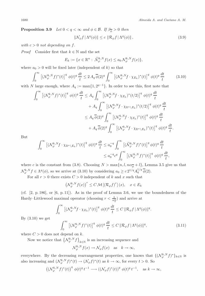
Proposition 3.9 Let 0 < q <∞ and φ ∈ B. If βφ > 0 then

‖Nϕf |Λq(φ)‖ ≤ c ‖Rϕf |Λq(φ)‖ , (3.9)

with c > 0 not depending on f .

Proof Consider first that k ∈ N and the set

Ek := {x ∈ Rn : N k,N

ϕ f(x) ≤ a0 N k,Nϕ f(x)},

where a0 > 0 will be fixed later (independent of k) so that∫ ∞

0

[(N k,N

ϕ f)∗(t)]qφ(t)q

dt

t≤ 2Aq φ(2)q

∫ ∞

0

[(N k,N

ϕ f · χEk)∗(t)

]qφ(t)q

dt

t(3.10)

with N large enough, where Aq := max{1, 2q−1}. In order to see this, first note that∫ ∞

0

[(N k,N

ϕ f)∗(t)]qφ(t)q

dt

t≤ Aq

∫ ∞

0

[(N k,N

ϕ f · χEk)∗(t/2)

]qφ(t)q

dt

t

+Aq

∫ ∞

0

[(N k,N

ϕ f · χRn\Ek)∗(t/2)

]qφ(t)q

dt

t

≤ Aq φ(2)q∫ ∞

0

[(N k,N

ϕ f · χEk)∗(t)

]qφ(t)q

dt

t

+Aq φ(2)q∫ ∞

0

[(N k,N

ϕ f · χRn\Ek)∗(t)

]qφ(t)q

dt

t.

But ∫ ∞

0

[(N k,N

ϕ f · χRn\Ek)∗(t)

]qφ(t)q

dt

t≤ a−q0

∫ ∞

0

[(N k,N

ϕ f)∗(t)]qφ(t)q

dt

t

≤ a−q0 cq∫ ∞

0

[(N k,N

ϕ f)∗(t)]qφ(t)q

dt

t,

where c is the constant from (3.8). Choosing N > max{n, l, nαφ + l}, Lemma 3.5 give us that

N k,Nϕ f ∈ Λq(φ), so we arrive at (3.10) by considering a0 ≥ c 21/qA

1/qq φ(2).

For all r > 0 there exists C > 0 independent of k and x such that(N k,Nϕ f(x)

)r ≤ CM [(Rϕf)r] (x), x ∈ Ek

(cf. [2, p. 186], or [6, p. 11]). As in the proof of Lemma 3.6, we use the boundedness of theHardy–Littlewood maximal operator (choosing r < 1

αφ) and arrive at

∫ ∞

0

[(N k,N

ϕ f · χEk)∗(t)

]qφ(t)q

dt

t≤ C ‖Rϕf |Λq(φ)‖q.

By (3.10) we get ∫ ∞

0

[(N k,N

ϕ f)∗(t)]qφ(t)q

dt

t≤ C ‖Rϕf |Λq(φ)‖q, (3.11)

where C > 0 does not depend on k.Now we notice that

{N k,Nϕ f

}k∈N

is an increasing sequence and

N k,Nϕ f(x) → Nϕf(x) as k → ∞,

everywhere. By the decreasing rearrangement properties, one knows that {(N k,Nϕ f)∗}k∈N is

also increasing and (N k,Nϕ f)∗(t) → (Nϕf)∗(t) as k → ∞, for every t > 0. So(

(N k,Nϕ f)∗(t)

)qφ(t)q t−1 −→ ((Nϕf)∗(t))q φ(t)q t−1, as k → ∞,


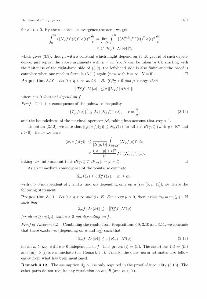
for all t > 0. By the monotone convergence theorem, we get∫ ∞

0

((Nϕf)∗(t))q φ(t)qdt

t= lim

k→∞

∫ ∞

0

((N k,N

ϕ f)∗(t))qφ(t)q

dt

t

≤ C ‖Rϕf |Λq(φ)‖q,

which gives (3.9), though with a constant which might depend on f . To get rid of such depen-dence, just repeat the above arguments with k = ∞ (so, N can be taken by 0): starting withthe finiteness of the right-hand side of (3.9), the left-hand side is also finite and the proof iscomplete when one reaches formula (3.11) again (now with k = ∞, N = 0). �Proposition 3.10 Let 0 < q <∞ and φ ∈ B. If βφ > 0 and μ > nαφ, then∥∥T μ

ϕ f |Λq(φ)∥∥ ≤ c ‖Nϕf |Λq(φ)‖ ,

where c > 0 does not depend on f .

Proof This is a consequence of the pointwise inequality(T μϕ f(x)

)r ≤ M [(Nϕf)r] (x), r =n

μ, (3.12)

and the boundedness of the maximal operator M, taking into account that rαφ < 1.To obtain (3.12), we note that |(ϕt ∗ f)(y)| ≤ Nϕf(z) for all z ∈ B(y, t) (with y ∈ R

n andt > 0). Hence we have

|(ϕt ∗ f)(y)|r ≤ 1|B(y, t)|

∫B(y,t)

(Nϕf(z))r dz

≤ (|x− y| + t)n

tnM [(Nϕf)r] (x),

taking also into account that B(y, t) ⊂ B(x, |x− y| + t). �As an immediate consequence of the pointwise estimate

Gmf(x) ≤ c T μϕ f(x), m ≥ m0,

with c > 0 independent of f and x, and m0 depending only on μ (see [6, p. 15]), we derive thefollowing statement.

Proposition 3.11 Let 0 < q <∞ and φ ∈ B. For every μ > 0, there exists m0 = m0(μ) ∈ N

such that‖Gmf |Λq(φ)‖ ≤ c

∥∥T μϕ f |Λq(φ)

∥∥for all m ≥ m0(μ), with c > 0 not depending on f .

Proof of Theorem 3.2 Combining the results from Propositions 3.9, 3.10 and 3.11, we concludethat there exists m0 (depending on n and αφ) such that

‖Gmf |Λq(φ)‖ ≤ c ‖Rϕf |Λq(φ)‖ (3.13)

for all m ≥ m0, with c > 0 independent of f . This proves (i) ⇒ (ii). The assertions (ii) ⇒ (iii)and (iii) ⇒ (i) are immediate (cf. Remark 3.3). Finally, the quasi-norm estimates also followeasily from what has been mentioned.

Remark 3.12 The assumption βφ > 0 is only required in the proof of inequality (3.13). Theother parts do not require any restriction on φ ∈ B (and m ∈ N).


3.3 Characterization through the Poisson Kernel

Hardy spaces are classically connected with the theory of harmonic functions through theapproximations of identity Pt(·) := t−nP (·/t), t > 0, involving the Poisson kernel

P (x) :=cn

(1 + |x|2)n+12

, Pt(x) := t−nP (x/t) =cn t

(t2 + |x|2)n+12

, t > 0,

where

cn = π−n+12 Γ

(n+ 1

2

). (3.14)

With this normalizing constant, one has∫

Rn P (x) dx = 1 (see [19, 20] for further details).It is known that the maximal characterization of the usual Hp spaces in terms of the radial

and the non-tangential functions can be done with the kernel P in place of the original functionϕ ∈ S, provided that convolution is appropriately defined. In fact, since the Poisson kernel is“only” integrable, the usual convolution Pt ∗ f may be meaningless for a tempered distributionf . A way of overcoming this difficulty is to restrict ourselves to a convenient subset of S ′. Asin [5], we shall say that f ∈ S ′ is bounded if ψ ∗ f ∈ L∞ for every ψ ∈ S. For such f theconvolution Pt ∗ f is well defined in the distributional sense as

〈Pt ∗ f, ψ〉 := 〈ψ ∗ f, Pt〉 =∫

Rn

(ψ ∗ f)(x) Pt(x) dx, ψ ∈ S,

where we use the notation g(y) := g(−y). This coincides with the usual definition when f isan integrable function.

For a bounded distribution f , we may then define maximal-type functions as in Subsec-tion 3.1 with P in place of ϕ. Let RP f and NP f be the corresponding versions of (3.1)and (3.2), respectively.

Theorem 3.13 Let 0 < q < ∞ and φ ∈ B with βφ > 0. Then, for f ∈ S ′, the followingassertions are equivalent :

(I) f ∈ Hq(φ).(II) f is a bounded distribution and NP f ∈ Λq(φ).

Moreover, we have

‖f |Hq(φ)‖ ∼ ‖NP f |Λq(φ)‖

for all bounded distributions f .

Proof Suppose first that f ∈ Hq(φ). By Theorem 3.2 one knows that Gmf ∈ Λq(φ) for somelarge m ∈ N.

For any ψ ∈ S, it follows immediately from (3.2) that

|(ψ ∗ f)(x)| ≤ Nψf(y) for all y ∈ B(x, 1).

Therefore, by (3.6), we have

|(ψ ∗ f)(x)|q ≤ c [(Gmf)∗(t)]q, t ∈ (0, ωn),

so that

|(ψ ∗ f)(x)|q∫ ωn

0

φ(t)qdt

t≤ c

∫ ωn

0

[(Gmf)∗(t)]q φ(t)qdt

t. (3.15)


Since βφq = qβφ > 0, then∫ 1

0φ(t)q dtt ≤

∫ 1

0φ(t)q dtt <∞. Hence, from (3.15), we get

|(ψ ∗ f)(x)|q ≤ cA−1q,φ ‖Gmf |Λq(φ)‖q ,

where0 < Aq,φ :=

∫ ωn

0

φ(t)qdt

t<∞. (3.16)

So, by Theorem 3.2, we have proved that

‖ψ ∗ f |L∞‖ ≤ C ‖f |Hq(φ)‖ ,

which means that f is a bounded distribution, since ψ is arbitrary.To prove that (I) implies (II), it is now enough to show that

‖NP f |Λq(φ)‖ ≤ c ‖f |Hq(φ)‖ . (3.17)

But this is a consequence of Theorem 3.2 and the pointwise estimate

NP f(x) ≤ cGmf(x), (3.18)

where c > 0 is independent of f and x. A proof of (3.18) can be found in [5, p. 98], or [6,pp. 15–16].

Let us prove now that (II) implies (I). Suppose that the distribution f is bounded andNP f ∈ Λq(φ). An analysis of the proof given in [5, p. 99], or [6, pp. 7–8], shows that there existsϕ ∈ S with

∫Rn ϕ(x) dx = 1, such that

Rϕf(x) ≤ RP f(x). (3.19)

Since RP f(x) ≤ NP f(x), then f ∈ Hq(φ) and

‖f |Hq(φ)‖ ≤ ‖NP f |Λq(φ)‖ .

This and (3.17) also prove the statement about the equivalence of quasi-norms. �Remark 3.14 The result given in Theorem 3.13 remains true if we replace the non-tangentialfunction NP f by its radial version RP f . In fact, from (3.19) and the obvious estimate RP f(x) ≤NP f(x), we get the equivalence

‖f |Hq(φ)‖ ∼ ‖RP f |Λq(φ)‖

from Theorems 3.2 and 3.13.

Note that Theorem 3.13 gives a characterization of the generalized Hardy spaces in termsof Poisson integrals. In particular, this provides another characterization for the spaces Hp,q ,0 < p, q < ∞, introduced in [8]. From this theorem, we also recover some classical results wellknown in the theory of the usual Hp spaces.

3.4 A Denseness Result for Spaces Hq(φ)

If f is a bounded distribution then (x, t) �→ (Pt∗f)(x) is harmonic in Rn+1+ and Pt∗f ∈ L∞∩C∞

for all t > 0 (cf. [5]). From Theorem 3.13 we know that this is the case when f ∈ Hq(φ) withβφ > 0. Under these assumptions we can even say more about the behavior of Pt∗f as t→ +∞and as t→ 0+. The existence of lim

t→0+(Pt ∗f)(x) for almost all x ∈ R

n follows from a Calderon’s

result on the existence of non-tangential limits of harmonic functions which are bounded in some


truncated cone (see [19, Chapter 7] or [20, Chapter 2]). Note that NP f ∈ Λq(φ) if f ∈ Hq(φ)(by Theorem 3.13), thus

sup(y,t)∈Γ(x)

|(Pt ∗ f)(y)| <∞ a.e. x ∈ Rn.

Lemma 3.15 Let 0 < q <∞ and φ ∈ B with βφ > 0. For f ∈ Hq(φ), we have

limt→∞(Pt ∗ f)(x) = 0

for every x ∈ Rn.

Proof Since

|(Pt ∗ f)(x)| ≤ NP f(y), y ∈ B(x, t), t > 0,

we have

|(Pt ∗ f)(x)|q∫ ωnt

n

0

φ(s)qds

s≤

∫ ωntn

0

[(NP f)∗(s)]q φ(s)qds

s≤ ‖NP f |Λq(φ)‖q . (3.20)

For t > 1, we may split the integral on the left-hand side and we get

∞ >

∫ ωntn

0

φ(s)qds

s= Aq,φ +

∫ ωntn

ωn

φ(s)qds

s, (3.21)

where Aq,φ is the constant from (3.16).Let us take 0 < ε < qβφ. Then we have β

φ(s)qs−ε = qβφ − ε > 0, so that φ(s)qs−ε ∼ g(s)for some increasing function g ∈ B (see Subsection 2.1). Hence

∫ ωntn

ωn

φ(s)qds

s∼

∫ ωntn

ωn

g(s) sε−1 ds

≥ g(ωn)∫ ωnt

n

ωn

sε−1 ds

= c (tnε − 1) > 0 (3.22)

with c > 0 independent of t. Using (3.21) and (3.22) in (3.20), by Theorem 3.13 we arrive atthe estimate

|(Pt ∗ f)(x)| ≤ C (Aq,φ + c (tnε − 1))−1/q ‖f |Hq(φ)‖ , t > 1,

from which we get the result. �The assertion in Lemma 3.15 was already known for the classical Hp spaces. A proof of this,

using a p-mean inequality for harmonic functions, can be found, for example, in [6, Chapter 2,Proposition 3.4].

With the help of Lemma 3.15 and the existence of limit at t = 0 discussed at the beginningof this section, we may derive the following statement:

Lemma 3.16 Let 0 < q <∞ and f ∈ Hq(φ) with βφ > 0. Then the function t �→ (Pt ∗ f)(x)is uniformly continuous on (0,∞) for almost all x ∈ R

n.

A useful property of the Poisson kernel which will be used below is the semigroup structure.

Proposition 3.17 If 0 < q <∞ and βφ > 0, then L∞ ∩ C∞ ∩Hq(φ) is dense in Hq(φ).


Proof Let f ∈ Hq(φ). Define fk(x) := (P 1k∗ f)(x), k ∈ N. Then fk ∈ L∞ ∩ C∞. Moreover,

since RP fk(x) ≤ RP f(x) then we also have fk ∈ Hq(φ) for all k, by Theorem 3.13 andRemark 3.14. It remains to show that ‖f − fk |Hq(φ)‖ → 0 as k → ∞, which is equivalent to

‖RP (f − fk) |Λq(φ)‖ −→ 0 as k → ∞. (3.23)

We have

Pt ∗ (f − fk)(x) = Pt ∗ f(x) − Pt+ 1k∗ f(x).

Using the uniform continuity of t �→ (Pt ∗ f)(x) for a.e. x (cf. Lemma 3.16), it turns out that

supt>0

|Pt ∗ (f − fk)(x)| −→ 0 as k → ∞,

for almost all x ∈ Rn. On the other hand,

RP (f − fk)(x) ≤ 2NP f(x).

Therefore, we get (3.23) by using the hypothesis NP f ∈ Λq(φ) and the dominated convergenceargument in these spaces (cf. (2.6)). �

4 Interpolation with Function Parameter

4.1 Preliminaries

Real interpolation with function parameter is appropriate to study interpolation properties ofspaces Hq(φ), since we may take the interpolation parameter from the same class B.

We recall that, for 0 < p ≤ ∞ and γ ∈ B (with 0 < βγ ≤ αγ < 1), the interpolation space(A0, A1)γ,p, formed from compatible quasi-normed spaces A0, A1, is the space of all a ∈ A0+A1

such that the quasi-norm

‖a | (A0, A1)γ,p‖ :=(∫ ∞

0

[γ(t)−1K(t, a)

]p dtt

)1/p

(usual modification if p = ∞) is finite, where

K(t, a) = K(t, a;A0, A1) = infa0+a1=a

a0∈A0,a1∈A1

(‖a0|A0‖ + t ‖a1|A1‖) , t > 0

is the well-known PeetreK-functional. The space (A0, A1)γ,p is continuously embedded betweenA0 ∩ A1 and A0 + A1. As usual, if γ(t) = tθ then we simply write (A0, A1)θ,p to denotethe corresponding interpolation space. We refer to [13, 21] for further information on realinterpolation.

The next statement will be useful only in Section 5, but we formulate it here for convenience.

Lemma 4.1 Let (A0, A1) and (B0, B1) be two compatible couples of quasi-normed spaces.Suppose that T : A0 + A1 → B0 + B1 is a linear operator whose restriction to each Ai isbounded into Bi, i = 0, 1. If 0 < p ≤ ∞, γ ∈ B, 0 < βγ ≤ αγ < 1 and Ci ≥ ‖T‖Ai→Bi

arepositive constants, then

‖Ta | (B0, B1)γ,p‖ ≤ C0 γ(C1/C0) ‖a | (A0, A1)γ,p‖ (4.1)

for every a ∈ (A0, A1)γ,p.


Inequality (4.1) can be derived from the estimate

K(t, Ta;B0, B1) ≤ C0K (C1t/C0, a;A0, A1) , a ∈ A0 +A1, t > 0,

using appropriately the left-hand side of (2.1) in the estimation of the quasi-norm.

4.2 Interpolation of Hq(φ) Spaces

Before describing the interpolation spaces between generalized Hardy spaces, we consider thefollowing lemma on the decomposition of a function into its “good” and “bad” parts. Its proofis similar to that given in [8] for the case f ∈ S.

Lemma 4.2 Let f ∈ L∞ ∩ C∞, 0 < p ≤ 1, m ∈ N0, δ > 0 and Ωδ = {x ∈ Rn : Gmf(x) > δ}.

There are tempered distributions gδ and bδ such that f = gδ + bδ and

‖gδ |L∞‖ ≤ c1 δ, ‖bδ |Hp‖p ≤ c2

∫Ωδ

[Gmf(x)]p dx,

with c1, c2 > 0 independent of δ and f .

With the help of Lemma 4.2 we are now able to give the first interpolation result.

Theorem 4.3 Let 0 < p0 < q <∞ and γ ∈ B with 0 < βγ ≤ αγ < 1. Then we have

(Hp0 , L∞)γ,q = Hq(φp0), (4.2)

where φp0(t) := t1/p0

γ(t1/p0) .

Proof We make the proof with the extra assumption p0 ≤ 1. After Theorem 4.9 we will seehow to get rid of this restriction. First we note that φp0 ∈ B with

φp0(t) = t1/p0 γ(t−1/p0) and βφp0=

1p0

− 1p0αγ > 0. (4.3)

The embedding

(Hp0 , L∞)γ,q ↪→ Hq(φp0)

is easily obtained from the interpolation formula (Lp0 , L∞)γ,q = Λq(φp0) (see Theorem 3 in [13]),observing that Rϕ is a sublinear operator which is bounded from Hp0 into Lp0 and from L∞

into itself.For the converse embedding, it suffices to prove it for functions f belonging to Hq(φp0) ∩

L∞ ∩ C∞. In fact, since βφp0> 0, this set is dense in Hq(φp0) by Proposition 3.17.

Let t > 0 be arbitrary and m ≥ m0(p0). By Lemma 4.2 there are tempered distributions gtand bt such that gt + bt = f with

‖gt |L∞‖ ≤ c1 (Gmf)∗(tp0) and ‖bt |Hp0‖p0 ≤ c2

∫Ωt

(Gmf(x))p0dx, (4.4)

where Ωt := {x ∈ Rn : Gmf(x) > (Gmf)∗(tp0)}. In the case (Gmf)∗(tp0) = 0, which is not

covered by Lemma 4.2, we may choose the trivial decomposition gt = 0 and bt = f .Since K(t, f ;Hp0 , L∞) ≤ ‖bt |Hp0‖ + t ‖gt |L∞‖, it suffices to estimate appropriately the

quantities ∫ ∞

0

[γ(t)−1‖bt |Hp0‖

]q dtt

and∫ ∞

0

[t γ(t)−1‖gt |L∞‖

]q dtt. (4.5)


For the first one, we have( ∫ ∞

0

[γ(t)−1‖bt |Hp0‖]q dtt

)1/q

≤ c

( ∫ ∞

0

[γ(t)−1

(∫ tp0

0

[(Gmf)∗(s)]p0ds)1/p0]q dt

t

)1/q

≤ c

{∫ 1

0

( ∫ ∞

0

[γ(u1/p0)−1u1

p0− 1

q (Gmf)∗(uσ)]qdu)p0/q

dσ

}1/p0

(4.6)

≤ c

{∫ 1

0

( ∫ ∞

0

[γ(τ1/p0σ−1/p0)−1

(τ

σ

) 1p0

− 1q

(Gmf)∗(τ )]qσ−1 dτ

)p0/qdσ

}1/p0

≤ c ‖Gmf |Λq(φp0)‖, (4.7)

where in (4.6) we have used Minkowski inequality with q/p0 > 1, and in (4.7) we took intoaccount (2.1) and that

∫ 1

0γ(v)p0 dvv <∞ since βγp0 = p0 βγ > 0.

As regards to the second quantity in (4.5), the first estimate in (4.4) and a convenientchange of variables give∫ ∞

0

[t γ(t)−1‖gt |L∞‖

]q dtt

≤ c ‖Gmf |Λq(φp0)‖q.

Therefore, we get

‖f | (Hp0 , L∞)γ,q‖ ≤ c ‖Gmf |Λq(φp0)‖ ∼ ‖f |Hq(φp0)‖,

the last equivalence being valid for large values of m since βφp0> 0 (cf. Theorem 3.2). �

Remark 4.4 Theorem 4.3 above generalizes the main theorem in [8] (cf. Theorem 1) givenfor Hardy–Lorentz spaces. In fact, in the case of the power parameter γ(t) = tθ, 0 < θ < 1, wehave φp0(t) = t

1−θp0 , so that formula (4.2) yields

(Hp0 , L∞)θ,q = Hq(t1/p) = Hp,q ,1p

=1 − θ

p0.

Remark 4.5 The proof given above follows essentially the arguments used in the classicalcase. However, it is worth noticing, in contrast to [8], that we did not use Hardy’s inequalitiesto get (4.7).

Using reiteration arguments, from (4.2) we derive the following statement.

Theorem 4.6 Let 0 < q0, q1, q < ∞, φ0, φ1, γ ∈ B and ψ = φ0/φ1. If βφi> 0 (i = 0, 1),

0 < βγ ≤ αγ < 1 and βψ > 0 or αψ < 0, then

(Hq0(φ0), Hq1(φ1))γ,q = Hq(φ), (4.8)

where φ(t) = φ0(t)γ(ψ(t)) .

Proof The proof is similar to the second part of the proof of Theorem 3 in [13]. Nevertheless,we give here the main steps for completeness. If βψ > 0, then φ ∈ B and βφ > 0. Choosing

0 < r < min{1, q0, q1, q, α−1

φ0, α−1

φ1, α−1

φ

},

by Theorem 4.3 we have

Hqi(φi) = (Hr, L∞)γi,qi, γi(t) =

t

φi(tr), i = 0, 1.


Now we get the result by reiteration (see, for instance, Theorem 2 in [13]) and by applyingTheorem 4.3 once more.

The case αψ < 0 can be proved by interchanging the order of the interpolation couple andusing the previous case. Indeed, we have

(Hq0(φ0), Hq1(φ1))γ,q = (Hq1(φ1), Hq0(φ0))γ,q , γ(t) = tγ(1/t).

Moreover, β1/ψ = −αψ > 0 and φ1(t)γ(1/ψ(t)) = φ1(t)ψ(t)

γ(ψ(t)) = φ(t). �As a particular case of (4.8) (with φi(t) = t1/pi and γ(t) = tθ), one gets the interpolation

formula obtained in [8] for Hardy–Lorentz spaces: for 0 < θ < 1, 0 < q0, q1, q < ∞, 0 < p0 �=p1 <∞,

(Hp0,q0 , Hp1,q1)θ,q = Hp,q ,1p

=1 − θ

p0+

θ

p1.

Of course, this also covers the interpolation result for classical Hardy spaces, namely if qi = pi

(i = 0, 1), p0 �= p1, and q = p, 1p = 1−θ

p0+ θ

p1, one gets

(Hp0 , Hp1)θ,p = Hp. (4.9)

Remark 4.7 The behavior of the interpolation constants involved in (4.9) was investigatedin [22] when 0 < p0, p1 ≤ 1. For a fixed r > 0, with r < min{p0, p1}, it was shown that

‖f |Hp‖ ≤ c0(p0, p1) ‖f | (Hp0 , Hp1)θ,p‖

and

‖f | (Hp0 , Hp1)θ,p‖ ≤ c1(p0, p1) [θ(1 − θ)]−1/r ‖f |Hp‖ ,

where ci(p0, p1), i = 0, 1, are positive constants depending on p0 and p1 only. In particular, theinterpolation constants “blow up” when θ tends to the extremal values. However, if we keepaway from those values, then we may have absolute estimates for those constants.

As an immediate consequence of Theorem 4.6, we can see that the generalized Hardy spacesHq(φ) (with βφ > 0) may be written as interpolation spaces between classical Hardy spaces.

Corollary 4.8 Let 0 < q < ∞ and φ ∈ B with βφ > 0. If p0, p1 satisfy 0 < 1p1< βφ ≤ αφ <

1p0<∞, then

Hq(φ) = (Hp0 , Hp1)η,q, with η(t) =t

p1p1−p0

φ(t

p0p1p1−p0

) . (4.10)

Concerning the function η from (4.10), with the choice of p0, p1 as above, simple calculationsshow that 0 < βη ≤ αη < 1.

4.3 Connection between Hq(φ) and Λq(φ)

As is known, the classical Hardy spaces Hp = Hp(t1/p) coincide with the usual Lebesgue spacesLp when 1 < p < ∞. Using Corollary 4.8, we can establish a corresponding result in ourgeneralized context.

Theorem 4.9 If 0 < q < ∞, φ ∈ B with 0 < βφ ≤ αφ < 1, then Hq(φ) = Λq(φ) (equivalentquasi-norms).


Proof Take p0, p1 such that 0 < 1p1< βφ ≤ αφ <

1p0< 1. In particular, we have 1 < p0, p1 <

∞, so that Hpi = Lpi , i = 0, 1. Combining this with Corollary 4.8 and the corresponding resultfor Lorentz spaces (cf. [13, Thoerem 3]), we get

Hq(φ) = (Hp0 , Hp1)η,q = (Lp0 , Lp1)η,q = Λq(φ),

where η is the function from (4.10). �Remark 4.10 We can now complete the proof of Theorem 4.3: if p0 > 1, then the previousTheorem allows us to write formula (4.2) as (Lp0 , L∞)γ,q = Λq(φp0), which is already knownto be true (cf. [13, Remark 2]).

Theorem 4.9 shows, in particular, that Hp,q = Lp,q when 1 < p <∞, 0 < q <∞.

5 Classical Operators on Spaces Hq(φ)

We are now interested in investigating the behavior of some classical operators on generalizedHardy spaces.

The Fourier transform If 0 < p ≤ 1 and f ∈ Hp then the Fourier transform f is continuouson R

n and

|f(ξ)| ≤ cp |ξ|n( 1p−1) ‖f |Hp‖ (5.1)

with cp > 0 independent of ξ ∈ Rn and f . This result was proved in [23] (see also [6, Chapter 3],

or [5, p. 128], for details).For general Hq(φ) spaces we have the following result.

Theorem 5.1 Let 0 < q <∞ and φ ∈ B. If f ∈ Hq(φ) and βφ > 1, then f is continuous onRn. Moreover,

|f(ξ)| ≤ c |ξ|−n φ(|ξ|n) ‖f |Hq(φ)‖ (5.2)

(with the interpretation |ξ|−n φ(|ξ|n) = 0 when ξ = 0), with c > 0 not depending on ξ ∈ Rn and

f ∈ Hq(φ).

Proof For fixed ξ ∈ Rn consider the linear operator T : Hp0 + Hp1 → C + C defined by

Tf := f(ξ), where 0 < p0, p1 < 1 are chosen so that 1p1

< βφ ≤ αφ < 1p0

(C is the set ofcomplex numbers). T is well defined and since Hq(φ) ↪→ Hp0 +Hp1 (by Corollary 4.8), we candecompose f ∈ Hq(φ) as f = f0 + f1 with fi ∈ Hpi , i = 0, 1. Clearly, f is continuous becauseeach fi is continuous.

By (5.1), for each i = 0, 1, the restriction of T to Hpi is bounded into C and

‖T‖Hpi→C ≤ cpi|ξ|n( 1

pi−1)

, (5.3)

with cpi> 0 independent of ξ. If ξ = 0 then f(ξ) = 0, so that (5.2) should be properly

interpreted in this case, namely assuming φ(|ξ|n)|ξ|n = 0. This is a natural convention since

limt→0+φ(t)t = 0 in view of the condition βφ > 1.

Let now ξ �= 0. We have (Hp0 , Hp1)η,q = Hq(φ) and (C,C)η,q = C, where η is the functiongiven in (4.10), so that the restriction of T toHq(φ) is bounded into C. Moreover, an applicationof (4.1), with Ci := cpi

|ξ|n( 1pi

−1), i = 0, 1 (cpibeing the constants from (5.3)), yields

|f(ξ)| ≤ cp0 |ξ|n( 1

p0−1) η

(cp1 c

−1p0 |ξ|n( 1

p1− 1

p0)) ‖f |Hq(φ)‖ .


Now we arrive at (5.2) by simple calculations involving the submultiplicativity and the expres-sion of η itself (similar to (4.3)). �Remark 5.2 Note that, for 0 < p < 1, the classical inequality (5.1) can be recovered from (5.2)by taking φ(t) = φ(t) = t1/p and q = p.

In the sequel we will consider some convolution operators. We shall make use of the followingcriterion for the boundedness of linear operators acting on Hq(φ) spaces, which can be derivedfrom Theorem 4.6 and Corollary 4.8.

Theorem 5.3 Let 0 < p0 < p1 < ∞, 0 < q0 �= q1 < ∞ and κ := 1/q0−1/q11/p0−1/p1

. Suppose thatT is a linear operator from Hp0 + Hp1 into Hq0 + Hq1 which is bounded from Hpi into Hqi ,i = 0, 1. Then T is also bounded from Hq(φ) into Hq(t

1q0

−κ 1p0 φ(tκ)) for every 0 < q < ∞ and

φ ∈ B such that 1p1< βφ ≤ αφ <

1p0

.

Remark 5.4 A version of Theorem 5.3 for generalized Lorentz spaces can be found in [13,Theorem 5].

Riesz potential operators The Riesz potential of a locally integrable function f is definedby

Iλf(x) =1

d(α, n)

∫Rn

f(y)|x− y|n−λ dy, 0 < λ < n, (5.4)

where d(α, n) is an appropriate normalizing constant. The Hardy–Littlewood–Sobolev theoremon the Lp → Lq boundedness of Iλ, with 1 < p < n

λ , 1q = 1

p − λn , is known to be valid for

Hp spaces as well (see [23, 24]). Nevertheless, for f ∈ Hp, 0 < p ≤ 1, the Riesz potentialIλf needs to be properly interpreted. Note that the Fourier transform of (5.4), in the sense ofdistributions, is given by

Iλf(ξ) = |ξ|−λ f(ξ).

This provides a way for dealing with this operator on Hardy spaces.The following statement may be seen as a generalized version of the Hardy–Littlewood–

Sobolev theorem on fractional integrals, since it extends several classical results.

Theorem 5.5 Let 0 < λ < n, 0 < q < ∞ and φ ∈ B. If βφ >λn , then Iλ is bounded from

Hq(φ) into Hq(η), whereη(t) = t−

λn φ(t). (5.5)

Proof Choose p0 < p1 such that λn < 1

p1< βφ ≤ αφ <

1p0

. Taking 1qi

:= 1pi

− λn , i = 0, 1,

then we may define Iλ as a linear operator mapping Hp0 + Hp1 into Hq0 + Hq1 , which actsboundedly from Hpi into Hqi . By Theorem 5.3, we conclude that Iλ is also bounded fromHq(φ) into Hq(η), where η(t) = t

1q0

−κ 1p0 φ(tκ). Since κ = 1/q0−1/q1

1/p0−1/p1= 1, we get (5.5), and the

proof is completed. �Corollary 5.6 Under the assumptions of Theorem 5.5, if we assume, additionally, αφ < 1+ λ

n ,then Iλ is bounded from Hq(φ) into Λq(η), where η is the function defined in (5.5).

Proof The proof is an immediate consequence of Theorems 5.5 and 4.9, noting that βη =βφ − λ

n > 0 and αη = αφ − λn < 1. �

Remark 5.7 With the additional assumption αφ < 1, we have Hq(φ) = Λq(φ), so that Theo-rem 5.5 gives the boundedness of Iλ from Λq(φ) into Λq(η). This is precisely the result obtained


by Merucci [13] on the boundedness of Iλ on generalized Lorentz spaces. In particular, thisextends the Hardy–Littlewood–Sobolev type theorem for classical Lorentz spaces Lp,q (cf. [25]).

Singular integral operators Classical Hardy spaces Hp are closely connected with singularintegrals since they can be characterized in terms of Riesz transforms (cf. [5, Chapter III]) Rj ,j = 1, 2, . . . , n, which are defined by

Rjf = f ∗Kj , where Kj =cn xj|x|n+1

, with Kj = −i ξj|ξ| ,

where cn is the constant from (3.14). In the one-dimensional case, R1 = H is the Hilberttransform. We refer to [19, 26] for further details.

We consider now more general singular integral operators realized in the principal valuesense,

Tf(x) = p.v. (f ∗K)(x) := limε→0+

∫|x−y|>ε

K(x− y)f(y) dy,

where the kernel K satisfies the cancellation condition∫R1<|x|<R2

K(x) dx = 0, 0 < R1 < R2 <∞. (5.6)

and the operator T is assumed to be bounded in L2. It is known that if K satisfies, in addition,the integral assumption ∫

|x|≥2|y||K(x− y) −K(x)| dx ≤ C, y �= 0, (5.7)

then T is bounded in Lp if 1 < p < ∞ (see [19] for details). The behavior of T on Hp spaces,0 < p ≤ 1, is also known, namely if the kernel K satisfies the smoothness condition

|K(x− y) −K(x)| ≤ c|y|δ

|x|n+δ, |x| ≥ 2|y|, (5.8)

for some 0 < δ ≤ 1, then T is bounded in Hp for nn+δ < p ≤ 1 (see [27] and [5, 6] for further

details).We extend these results to our generalized spaces as follows.

Theorem 5.8 Let 0 < q < ∞ and φ ∈ B such that 1 < βφ ≤ αφ < 1 + δn , for some fixed

0 < δ ≤ 1. If K satisfies (5.6) and (5.8), then the operator T , given by Tf = p.v. (f ∗K), isbounded in Hq(φ).

Proof The idea is similar to that used in the proof of Theorem 5.5. We choose p0, p1 suchthat 1 < 1

p1< βφ ≤ αφ <

1p0< 1 + δ

n . Then nn+δ < p0 < p1 < 1, thus T can be defined in

the usual way in the sum Hp0 +Hp1 so that it is bounded from each Hpi into itself (i = 0, 1).Therefore, we get the result from Theorem 5.3. �

References[1] Stein, E. M., Weiss, G.: On the theory of harmonic functions of several variables, I, The theory of Hp

spaces. Acta Math., 103, 25–62 (1960)

[2] Fefferman, C., Stein, E. M.: Hp spaces of several variables. Acta Math., 129, 137–193 (1972)

[3] Coifman, R. R.: A real variable characterization of Hp. Studia Math., 51, 269–274 (1974)

[4] Latter, R.: A decomposition of Hp(Rn) in terms of atoms. Studia Math., 62, 93–101 (1978)


[5] Stein, E. M.: Harmonic Analysis: Real-Variable Methods, Orthogonality and Oscillatory Integrals, Prince-

ton University Press, Princeton, 1993

[6] Lu, S.: Four lectures on real Hp spaces, World Scientific, Singapore, 1995

[7] Garcıa-Cuerva, J.: Weighted Hp spaces. Dissertationes Math., 162, 1–63 (1979)

[8] Fefferman, C., Riviere, N. M., Sagher, Y.: Interpolation between Hp-spaces: the real method. Trans. Amer.

Math. Soc. 191, 75–81 (1974)

[9] Abu-Shammala, W., Torchinsky, A.: The Hardy–Lorentz spaces Hp,q(Rn). Studia Math., 182, 283–294

(2007)

[10] Coifman, R. R., Weiss, G.: Extensions of Hardy spaces and their use in analysis. Bull. Amer. Math. Soc.,

83, 569–645 (1977)

[11] Nakai, E.: A generalization of Hardy spaces Hp by using atoms. Acta Mathematica Sinica, English Series,

24(8), 1243–1268 (2008)

[12] Boyd, D. W.: The Hilbert transform on rearrangement-invariant spaces. Canad. J. Math., 19, 599–616

(1967)

[13] Merucci, C.: Applications of interpolation with a function parameter to Lorentz, Sobolev and Besov spaces,

Lecture Notes in Math. 1070, Springer, Berlin, 1984, 183–201

[14] Bennett, C., Sharpley, R.: Interpolation of Operators, Academic Press, Boston, 1988

[15] Bennet, C., Rudnick, K.: On Lorentz–Zygmund spaces. Dissertationes Math., 175, 67 pp. (1980)

[16] Merucci, C.: Interpolation reelle avec parametre fonctionnel des espaces Lp,q . C. R. Acad. Sci. Paris Ser.

I Math., 294, 653–656 (1982)

[17] Merucci, C.: Interpolation reelle avec fonction parametre: reiteration et applications aux espaces Λp(ϕ).

C. R. Acad. Sci. Paris Ser. I Math., 295, 427–430 (1982)

[18] Carro, M. J., Raposo, J. A., Soria, J.: Recent Developments in the Theory of Lorentz Spaces and Weighted

Inequalities, Mem. Amer. Math. Soc., Vol. 187, Providence, RI, 2007

[19] Stein, E. M.: Singular Integrals and Differentiablity Properties of Functions, Princeton University Press,

Princeton, 1970

[20] Stein, E. M., Weiss, G.: Introduction to Fourier Analysis on Euclidean Spaces, Princeton University Press,

Princeton, 1971

[21] Bergh, J, Lofstrom, J.: Interpolation Spaces, An introduction, Springer-Verlag, Berlin, 1976

[22] Almeida, A.: Real Interpolation of Hardy Spaces (in Portuguese), MSc Thesis, University of Aveiro, 2000

[23] Taibleson, M. H., Weiss, G.: The molecular characterization of certain Hardy spaces. Asterisque, 77, 67–149

(1980)

[24] Krantz, S. G.: Fractional integration on Hardy spaces. Studia Math., 73, 87–94 (1982)

[25] O’Neil, R. O.: Convolution operators and L(p, q) spaces. Duke Math. J., 30, 129–142 (1963)

[26] Duoandikoetxea, J.: Fourier Analysis, AMS, Providence, RI, 2001

[27] Alvarez, J., Milman, M.: Hp continuity properties of Calderon–Zygmund-type operators. J. Math. Anal.

Appl., 118, 65–79 (1986)

Generalized Hardy spaces

Documents

Transcript of Generalized Hardy spaces