CE 601: Numerical Methods

Lecture 27

Multi-Point Methods

Course Coordinator:Dr. Suresh A. Kartha,Associate Professor,

Department of Civil Engineering,IIT Guwahati.

• Multi Point Methods:

• The Euler’s methods and Runge-Kuttamethods that were discussed till now for solving IV-ODEs were single step (or single point) methods.

• In the time scale, only the information of was considered for obtaining

ny

1ny

• If the information of more than one previous instant is used, then the method is called a multi-point method.

• Principle of Multi-Point methods:

• We can approximately represent the above equation as

( , )dy

f t ydt

( , ( )) ( )dy f t y t dt F t dt

( )dy F t dt

• at different instants is approximated by Newton’s backward difference polynomials.

• So, for the discrete time domain, we have

( )F t

( )kdy P t dt

1 1

1 1

( )n n

n q n q

y t

k

y t

dy P t dt

• If is obtained with base point time , the resulting expression will be explicit multi-step equation.

• If is obtained with base point time , then the resulting expression will be implicit multi-step equation.

( )kP t nt

( )kP t1nt

• If , we have

• This integration (1) is called Adams’ finite-difference equations.

• Explicit ones are called Adams-Bashforth FDEs.

• Implicit ones are called Adams-Moulton FDEs.

1q1 1

( ) (1)n n

n n

y t

k

y t

dy P t dt y

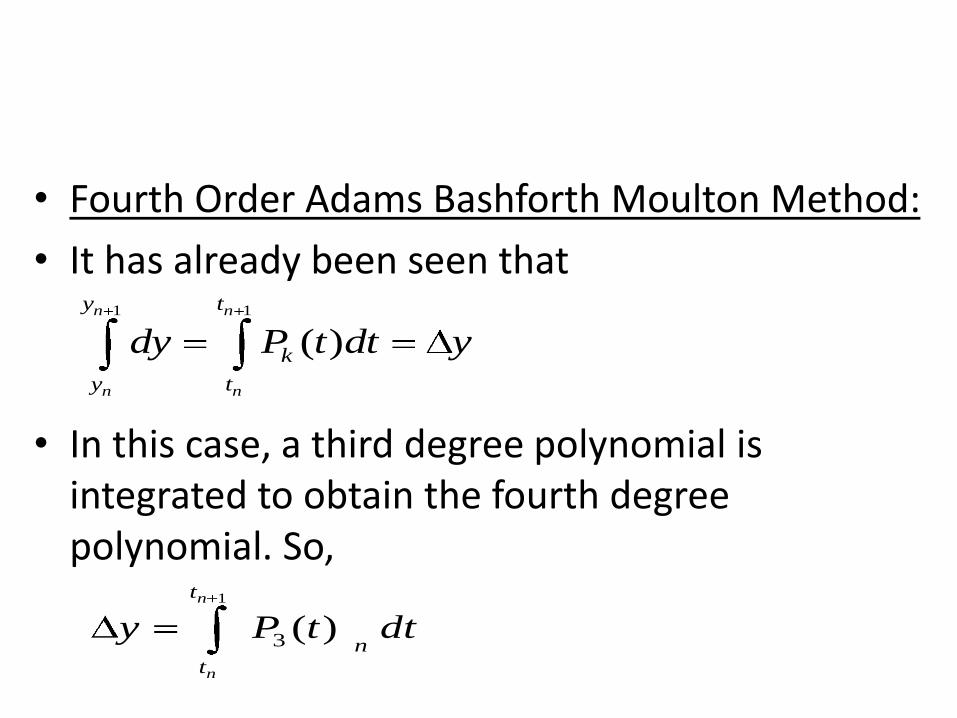
• Fourth Order Adams Bashforth Moulton Method:

• It has already been seen that

• In this case, a third degree polynomial is integrated to obtain the fourth degree polynomial. So,

1 1

( )n n

n n

y t

k

y t

dy P t dt y

1

3 ( )n

n

t

nt

y P t dt

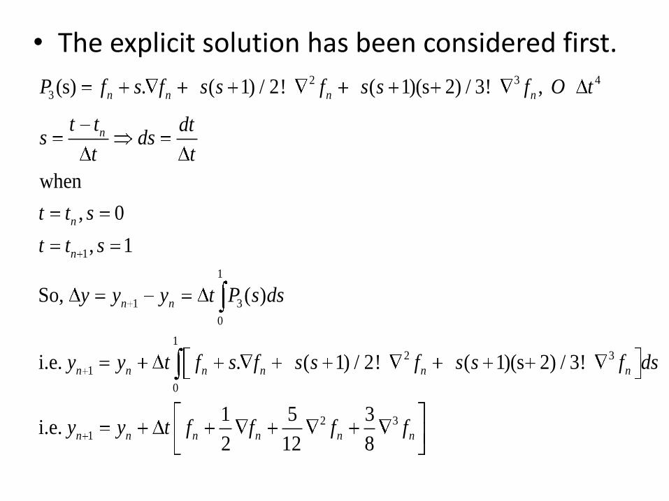
• The explicit solution has been considered first.2 3 4

3

1

1

1 3

0

1

2 3

1

0

1

(s) . ( 1) / 2! ( 1)(s 2) / 3! ,

when

, 0

, 1

So, ( )

i.e. . ( 1) / 2! ( 1)(s 2) / 3!

i.e.

n n n n

n

n

n

n n

n n n n n n

n n

P f s f s s f s s f O t

t t dts ds

t t

t t s

t t s

y y y t P s ds

y y t f s f s s f s s f ds

y y t f 2 31 5 3

2 12 8n n n nf f f

• Backward difference table is as follows:2 3

3 3

n n

t f f f f

t f

2 3

2 2 1 2 3

1 2

2.

n n

n n n n n

n n

f f

t f f f f

f f 1 2 3

1 1 1 2

1

3. 3.

2.

n n n n

n n n n n

n n

f f f f

t f f f f

f f 1 1 2

1 1

1

1

3. 3.

2.

n n n n

n n n n n

n n

n

f f f f

t f f f f

f f

t 1 nf

• So, substituting all the relevant values in the equation, we have

Or,

This is called Adams-Bashforth fourth order

explicit FDE.

1 1 1 2 1 2 3

1 5 32. 3. 3.

2 12 8n n n n n n n n n n n ny y t f f f f f f f f f f

1 1 2 355 59 37 924

n n n n n n

ty y f f f f

• Similarly, in case we integrate using implicit approach,

• This is the fourth order Adams-Moulton implicit FDE.

• As it is observed difficulty in evaluating ‘f’ in implicit condition, so Adams-Moulton FDE can be simplified by predictor-corrector approach (known as 4th order Adams-Bashforth-Moulton predictor corrector

method):

1 0

3 1

1

1 1 1 2

( ) ( ) error

9 19 5 924

n

n

t

nt

n n n n n n

y P t dt P s ds

ty y f f f f

1 1 2 3

1 1 1 2

55 59 37 924

9 19 5 924

P

n n n n n n

C P

n n n n n n

ty y f f f f

ty y f f f f

• To solve IV-ODE’s having Non-Linear DerivativeFunctions

• For the IV-ODE

it has been seen that explicit and implicit

methods can be employed. However, when

is non-linear in , then employing the

implicit methods become quite tedious and

difficult.

0 0( , ); ( )dy

f t y y t ydt

( , )f t y y

• Let us consider the Euler implicit method

• Here, is non-linear. So, in the time scale

is unknown in

Let us write it as

1 1 1. ,n n n ny y t f t y

1 1,n nf t y

1 1. ,n n ny t f t y 1ny

1( )nG y

• Hence, we will need to solve the equation

• We need to find out the value of using iterative procedures. Let us define

• Newton Raphson method suggests that

1 1( ) 0n ny G y

1ny

1 1 1( ) ( )n n nF y y G y

( )

1( 1) ( )

1 1 ( )

1'

k

nk k

n n k

n

F yy y

F y

• Modified Newton Raphson method suggests that

• Here, is calculated only once.

( )

1( 1) ( )

1 1'

k

nk k

n n

F yy y

F

'F

• Example: Solve

using Euler’s implicit method and apply

Newton Raphson method.

• Solution:

4 4 12

0; 250 , 2500 , 4 10a a

dTT T T K T K

dt

1 1

12 4 4

2

where

4 10 250

n n n n

tT T f f

f T

• Using , we have

• Initial guess is taken as

2.0t s

12 4 4 4 4

1 0 1

12 4

1 1 1

12 4

1 1 1

11 3

1 1

2.04.0 10 2500 250 250

2

2343.78 4 10

2343.78 4 10

' 1 1.6 10

T T T

T T G T

F T T T

F T T

(0)

1 2500T

(0)

1(1) (0)

1 1 (0)

1'

F TT T

F T

• Eventually, after several iterations, we arrive at the answer as .

(1)

1

(1)

1(2) (1)

1 1 (1)

1

(2)

1

(3)

1

(4)

1

(5)

1

312.47002500 2083.373

0.7500

'

185.0492083.373 2299.725

0.8553

67.8282299.725 2215.508

0.8054

31.8992215.508 2254.127

0.826

13.6162254.127 223

0.8167

T

F TT T

F T

T

T

T

T 7.454

1 2242.605T K