Fast Optimal Mass Transport for Dynamic Active Contour Trackingon the GPU

Gallagher Pryor, Tauseef ur Rehman, Shawn Lankton, Patricio A. Vela and Allen Tannenbaum

Abstract— In computational vision, visual tracking remainsone of the most challenging problems due to noise, clutter,occlusion, and dynamic scenes. No one technique has yet tosolve this problem completely, but those that employ control-theoretic filtering techniques have proven to be quite successful.In this work, we extend one such technique by Niethammeret al. in which implicitly represented dynamically evolvingcontours are filtered using a geometric observer framework.The effectiveness of the observer hangs upon the solution of twomajor problems: (1) the calculation of accurate curve velocitiesand (2) the determination of diffeomorphic correspondencemaps between curves for geometric interpolation. We proposethe use of novel image registration techniques such as imagewarping and optimal mass transport for the solution of theseproblems which increase the performance of the frameworkand reduce algorithmic complexity. One major drawback tothe original scheme, as it relies on PDE solutions, is itscomputational burden restricting it from real time use. Weshow that the framework can, in fact, run in real time byimplementing our additions to the framework on the graphicsprocessing unit (GPU) and show better execution times for thesealgorithms than reported in recent literature.

I. INTRODUCTION

In computational vision, visual tracking is the act ofconsistently locating a desired feature in each image of aninput sequence. Visual tracking is a critical step in numerousmachine vision applications such as surveillance, driverassistance, human-computer interactions, etc. However, it isa challenging problem due to noise, clutter, occlusion, anddynamic scenes. Numerous approaches and techniques existfor the solution of the tracking problem and some of the mostsuccessful employ control-theoretic filtering techniques.

In this paper we build on one such control-theoretictracking framework by Niethammer et al. [1] who proposeda deterministic observer framework for visual tracking basedon non-parametric implicit (level-set) curve descriptions.This work is novel in that it provides a general frameworkfor the filtering of implicit curves along with any amountof additional state associated with those curves without theneed for parameterizations which are complex to implementin practice have their own particular drawbacks.

The above referenced work involves a continuous-discrete observer with continuous-time system dynamicsand discrete-time measurements. The proposed framework

This work was supported in part by grants from NSF, AFOSR, ARO,MURI, MRI-HEL, and NIH

Tauseef ur Rehman, Patricio Vela, Shawn Lankton, Allen Tan-nenbaum are with the School of Electrical and Computer Engi-neering, Georgia Institute of Technology, Atlanta, GA 30332-0250,tauseef,slankton,tannenba@ece.gatech.edu.

Gallagher Pryor is with College of Computing, Georgia Institute ofTechnology donovang@cc.gatech.edu

is general in nature and multiple simulation models can beincorporated. Measurements can be performed through staticsegmentation techniques and optical flow computations.

Unfortunately, discrete-time measurements lead to theproblem of geometric curve interpolation and the filtering ofquantities propagated along with implicitly represented esti-mated curves. Interpolation and filtering are intimately linkedto the correspondence problem between curves. In [1], thisis done using a Laplace equation approach, establishing aone-to-one correspondence between measured and estimatedcurves to determine unique ”distances” between points andto exchange information between them for dynamic filtering.The distance measurements allow for a geometric interpo-lation between measured and estimated curves, facilitatinggeometric, intuitively tunable gains for position filtering.

In our work, we use the Monge-Kantorovich formula-tion of the optimal mass transport (OMT) problem for thepurpose of establishing the diffeomorphic correspondencemaps between the estimated and measured curves insteadof the Laplace equation approach which requires complexdomain decompositions in order compute the correct map.The OMT method, on the other hand, is an elegant solutionto the correspondence problem and is applied globally on theimplicit representations of the curve. Although in the L2 caseOMT is an NP-hard problem we benefit from a fast and near-realtime, multi-resolution and multigrid implementation ofthe OMT algorithm on the GPU [2], [3]. Another significantcontribution is the use of a registration warp as a velocitymeasurement instead of the classical Horn & Schunck [4]optical flow used by Niethammer et al. [1]. This warp is alsoa 2D velocity field over every point in the image like itspredecessor but has accurate magnitudes making advectionunnecessary in the framework and velocity measurementsaccurate.

The paper is organized in the following sections. Section IIbriefly reviews curve evolution equations and the generalobserver structure as proposed in [1]. Section III briefly de-scribes the areas of contribution of this work. In Sections IVto VII we describe our proposed velocity measurementbased upon image warping, our proposed error correctionscheme based upon optimal mass transport, and the GPUimplementation of the framework. Results are presented inSection VIII. Conclusions are given and future work isdiscussed in Section IX.

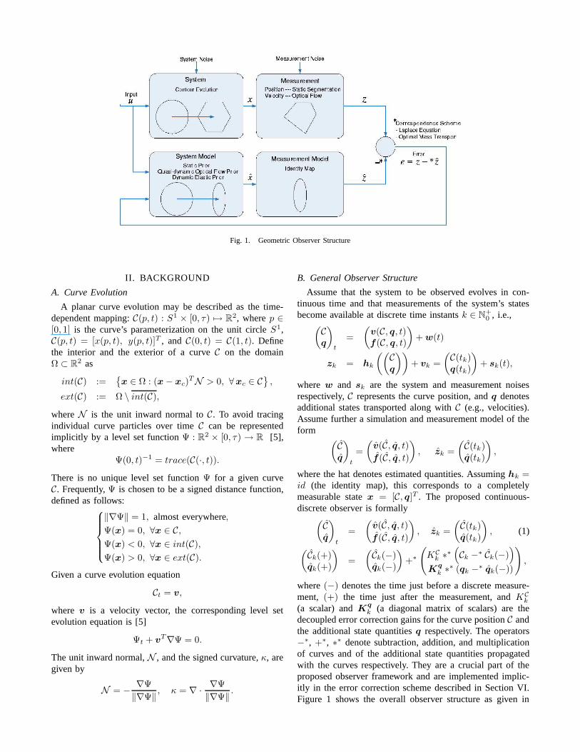
Fig. 1. Geometric Observer Structure

II. BACKGROUND

A. Curve Evolution

A planar curve evolution may be described as the time-dependent mapping: C(p, t) : S1 × [0, τ) 7→ R

2, where p ∈[0, 1] is the curve’s parameterization on the unit circle S1,C(p, t) = [x(p, t), y(p, t)]T , and C(0, t) = C(1, t). Definethe interior and the exterior of a curve C on the domainΩ ⊂ R

2 as

int(C) :=

x ∈ Ω : (x − xc)TN > 0, ∀xc ∈ C

,

ext(C) := Ω \ int(C),

where N is the unit inward normal to C. To avoid tracingindividual curve particles over time C can be representedimplicitly by a level set function Ψ : R

2 × [0, τ) → R [5],where

Ψ(0, t)−1 = trace(C(·, t)).

There is no unique level set function Ψ for a given curveC. Frequently, Ψ is chosen to be a signed distance function,defined as follows:

‖∇Ψ‖ = 1, almost everywhere,

Ψ(x) = 0, ∀x ∈ C,

Ψ(x) < 0, ∀x ∈ int(C),

Ψ(x) > 0, ∀x ∈ ext(C).

Given a curve evolution equation

Ct = v,

where v is a velocity vector, the corresponding level setevolution equation is [5]

Ψt + vT∇Ψ = 0.

The unit inward normal, N , and the signed curvature, κ, aregiven by

N = −∇Ψ

‖∇Ψ‖, κ = ∇ ·

∇Ψ

‖∇Ψ‖.

B. General Observer Structure

Assume that the system to be observed evolves in con-tinuous time and that measurements of the system’s statesbecome available at discrete time instants k ∈ N

+0 , i.e.,

(

Cq

)

t

=

(

v(C, q, t)f(C, q, t)

)

+ w(t)

zk = hk

((

Cq

))

+ vk =

(

C(tk)q(tk)

)

+ sk(t),

where w and sk are the system and measurement noisesrespectively, C represents the curve position, and q denotesadditional states transported along with C (e.g., velocities).Assume further a simulation and measurement model of theform

(

Cq

)

t

=

(

v(C, q, t)

f(C, q, t)

)

, zk =

(

C(tk)q(tk)

)

,

where the hat denotes estimated quantities. Assuming hk =id (the identity map), this corresponds to a completelymeasurable state x = [C, q]T . The proposed continuous-discrete observer is formally

(

Cq

)

t

=

(

v(C, q, t)

f(C, q, t)

)

, zk =

(

C(tk)q(tk)

)

, (1)

(

Ck(+)qk(+)

)

=

(

Ck(−)qk(−)

)

+∗

(

KCk ∗∗

(

Ck −∗ Ck(−))

Kq

k ∗∗ (qk −∗ qk(−))

)

,

where (−) denotes the time just before a discrete measure-ment, (+) the time just after the measurement, and KC

k

(a scalar) and Kq

k (a diagonal matrix of scalars) are thedecoupled error correction gains for the curve position C andthe additional state quantities q respectively. The operators−∗, +∗, ∗∗ denote subtraction, addition, and multiplicationof curves and of the additional state quantities propagatedwith the curves respectively. They are a crucial part of theproposed observer framework and are implemented implic-itly in the error correction scheme described in Section VI.Figure 1 shows the overall observer structure as given in

Equation (1) and model assumptions associated with eachcomponent of the observer.

III. CONTRIBUTIONS

We extend the geometric observer framework of Nietham-mer et al. [1] (given above) with image registration tech-niques such as optimal mass transport in place of the previousmethods utilized for curve correspondence and velocity com-putation. These modifications lead to more accurate trackingperformance and overall algorithmic simplification as well asreal time implementations on GPU hardware. Specifically,the improvements can be divided into three areas and aredescribed below:

A. Registration Warp Velocity Measurement

In the original model, classical optical flow (which ingeneral gives incorrect velocity magnitudes) is utilized bothas a motion prior and to measure curve velocity. We proposean image warp based on a brightness constancy assumptionas a motion prior and curve velocity measurement. Thisleads to accurate estimation of velocity field magnitudes andorientations, thereby increasing performance and removingthe need for advection of state during prediction.

B. Optimal Mass Transport Error Correction Scheme

In the original model, a non-trivial procedure was neededto carry out filtering of both curve and velocity informationinvolving complex domain decomposition, the solution of thelaplacian, and advections. We solve this problem globallyusing optimal mass transport as a registration techniquebetween curves. This results in a mapping between curves,removing the need for advection to transport informationfor error correction. It also alleviates any need for complexdomain decomposition and leads to more accurate trackingperformance.

C. Computational Efficiency.

We leverage the full multigrid PDE solution scheme onthe graphics processing unit (GPU; now available on mostconsumer computers) to solve the PDEs employed in thegeometric observer framework resulting in computationtimes that outperform implementations documented inthe recent literature. This shows that the framework iscapable of functioning as a real time vision system and thatsome PDE methods that were previously impractical forreal time use are now reasonable to consider in such systems.

In what follows, we describe how the aforementionedcontributions are integrated into the observer framework.

IV. MEASUREMENTS

A. Velocity Measurements

Previously in [1], optical flow was used as the velocitymeasurement v corresponding to the curve velocity statewithin the geometric observer. In this strategy, a classicalHorn & Schunck optical flow [4] is calculated, whichestimates the 2D velocities of all image points from frame

to frame which are then used as the measurement of curvevelocity. However, optical flow is in general inaccurate withrespect to flow magnitude and Horn & Schunck optical flowcan be inaccurate in terms of flow direction. While bothof these facts can lead to poor performance, the formerleads to the necessity of advection to transport informationfor curve prediction; without correct magnitudes informationmust be transported in a particular direction until it reachesits destination.

As a solution to these problems, we propose the use ofa registration warp as a motion prior. Like optical flow, thiswarp is a velocity field over every point in the image domain,but has more accurate magnitudes which are suitable fordirectly mapping one image to another, making advectionunnecessary and velocity measurements accurate.

Given two frames of imagery I1 and I2, solving for theregistration warp u : R

2 7→ R2 entails minimization of the

following energy:

L(I) =

∫∫

(

I1(x + v(x)) − I2(x))2

dx

In other words, we wish to find a u that transforms I1 so asto match I2 as closely as possible in terms of squared error.

Such a quadratic minimization can be sufficiently dealtwith via the Gauss-Newton method. Leaving derivationsaside, the resulting algorithm for computing v is as follows:

1) Set v = 0.2) Calculate Horn & Schunck optical flow by minimizing

the following with respect to v,∫∫

(

I1(x+v)−I2(x)+〈∆I1, v〉)2

+λ||∆v||2dx,

where λ is a constant determining the required smooth-ness of the resulting field.

3) Set v = v + ρv, where ρ is the predefined time stepfor the Gauss-Newton method.

4) If not yet converged, go to (2).

Previously, such minimization would be considered im-practical for tracking due to the computational cost involvedwith step (2). However, this is not the case when computedusing a full multigrid scheme on a small, parallel computingarchitecture such as the graphical processing unit which isnow available in most consumer computers (see SectionVII for details on the GPU implementation of the warpingalgorithm).

B. Curve Position Measurement

Static measurements of curve position provide informationabout the actual system and allow the model state to convergeto the true system states. Motion models used in visualtracking cannot possibly be rich enough to capture the vari-ability seen in deformable objects in natural video sequences.Therefore, it is important that the observer estimate besupplemented with measurements so the observer can adaptto real-life changes in the system.

The estimate model is a function of the curve positionand dynamics as it evolves through time. The measurement

of the actual system, however, is independent of the model.Therefore, the static curve measurements can be obtainedusing any segmentation technique with no modification tothe observer. Most segmentation methods are either based onlocal image information from an edge detector, or statisticsof regions of image data defined by the curve. Additionally,shape priors can be learned and included in the segmentationalgorithm to improve accuracy if detailed shape informationis available a priori.

We create our static measurements in a two step process.First, background subtraction is used as a pre-processing stepto help separate the target from background clutter. Second,the resulting image is segmented to isolate the target.

In order to obtain a smooth curve C that representsthis segmentation, we employ the active contour techniqueproposed by Chan and Vese [6]. This method attemptsminimize the variance over the region inside the curve C,Cinside and outside the curve, Coutside. This is accomplishedby minimizing the following energy with respect to C whereu and v represent the mean image intensity over Cinside andCoutside respectively:

∫

Cinside

(I − u)2dA +

∫

Coutside

(I − v)2dA + µ

∫

C(s)ds

This energy is at a minimum when the interior and exteriorare modeled best by u and v. The Chan-Vese segmentationtechnique is advantageous in that it is robust to noise sinceimage data is integrated over large regions, it’s global use ofimage information makes it robust to different initializations,and its simplicity allows for real time implementation.

V. MOTION PRIORS

In [1], three major motion priors were defined: A staticmotion prior,

Ct = 0,

a quasi-dynamic optical flow prior,

Ct = (vOF · N )N ,

and a dynamic elastic prior,

µCtt =

(

1

2µ‖Ct‖

2 + a

)

κN − (∇ · N )N −1

2µ(‖Ct‖

2)sT .

For our work, we utilize the latter, as it correctly models thedynamics of the estimated curve C .

VI. ERROR CORRECTION

The observer framework proposed in this paper requiresa methodology to associate an estimated curve state to ameasured curve state. This amounts to establishing corre-spondences between points on the measured and the esti-mated curves. The correspondence map between measuredand estimated curves should be diffeomorphic.

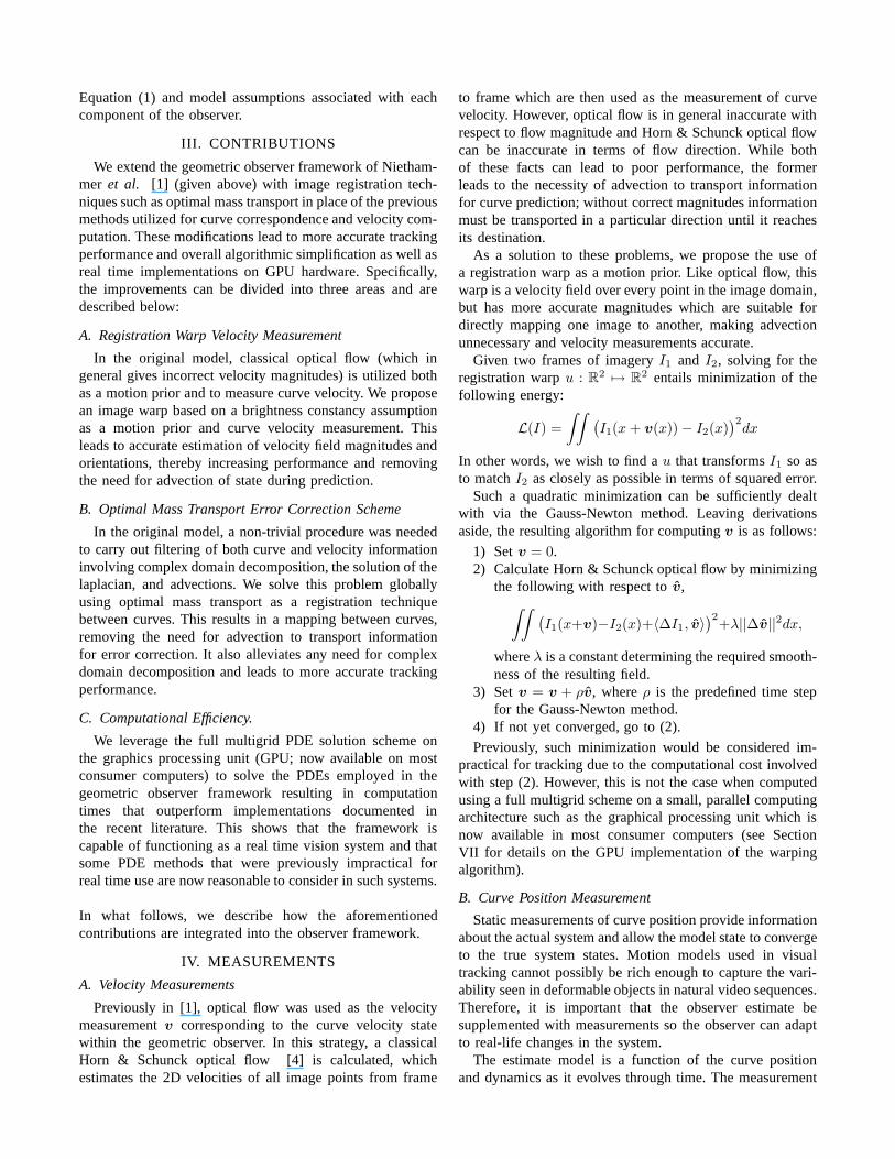
Fig. 2. Optimal Mass Transport Algorithm

A. The Optimal Mass Transport Problem

Motivated by our earlier work [2], [3] one-to-one corre-spondences between curves can be established using the Op-timal Mass Transport technique. The optimal mass transportproblem was first formulated by a French engineer GasperMonge in 1781, and was given a modern formulation inthe work of Kantorovich [7] and, therefore, is now knownas the Monge-Kantorovich problem. The original problemconcerned finding the optimal way to move a pile of soil fromone site to another in the sense of minimal transportationcost. Hence, the Kantorovich-Wasserstein distance is alsocommonly referred to as the Earth Mover’s Distance (EMD).

1) Formulation of the Problem: We will briefly pro-vide an introduction to modern formulation of the Monge-Kantorovich problem. We assume we are given, a priori, twosub-domains Ω0 and Ω1 of Rd with smooth boundaries, anda pair of positive density functions, µ0 and µ1 defined onΩ0 and Ω1 respectively. We assume that,

∫

Ω0

µ0 =

∫

Ω1

µ1 (2)

This ensures that we have same total mass in both thedomains. We now consider diffeomorphisms u from Ω0 toΩ1 which map one density to other in the sense that,

µ0 = |Du|µ1 u (3)

which we call the mass preservation (MP) property, and writeu ∈ MP . Equation (3) is called the Jacobian equation. Here,|Du| denotes the determinant of the Jacobian map Du, anddenotes composition of functions. It basically implies that if

a small region in Ω0 is mapped to a larger region in Ω1,then there must be a corresponding decrease in density inorder for the mass to be preserved. There may be many suchmappings, and we want to pick an optimal one in some sense.Accordingly, we define the squared L2 Monge-Kantorovichdistance as following:

d22(µ0, µ1) = infu∈MP

∫

‖ u(x) − x ‖2 µ0(x)dx (4)

The optimal MP map is a map which minimizes this integralwhile satisfying the constraint given by Equation (3). TheMonge-Kantorovich functional, Equation (4), is seen to placea penalty on the distance the map u moves each bit ofmaterial, weighted by the material’s mass. A fundamentaltheoretical result [8], [9], is that there is a unique optimalu ∈ MP transporting µ0 to µ1, and that u is characterizedas the gradient of a convex function ω, i.e., u = ∇ω. Thistheory translates into a practical advantage, since it meansthat there are no non-global minima to stall our solutionprocess.

2) Computing the Transport Map: We will describe hereonly the algorithm for finding the optimal mapping u. Thedetails of this method can be found in [10]. The basic ideafor finding the optimal warping function is first to find aninitial MP mapping u0 and update it iteratively to decreasean energy functional. When the pseudo time t goes to ∞, theoptimal u will be found, which is u. Basically there are twosteps. The first step in this algorithm is to find an initial masspreserving mapping. This can be done for general domainsusing the method of Moser [11] or the algorithm proposedin [10]. The later method can simply be interpreted as thesolution of a one-dimensional Monge-Kantorovich problemin the x-direction followed by the solution of a family of one-dimensional Monge-Kantorovich problems in y-direction.The second step is to adjust the initial mapping found aboveiteratively using gradient descent in order to minimize thefunctional defined in Equation (4), while constraining u

so that it continues to satisfy Equation (3). This processiteratively removes the curl from the initial mapping u and,thereby, finds the polar factorization of u. For details onthis technique, please refer to [10]. The overall algorithm issummarized graphically in Figure 2.

B. Curve Interpolation

Optimal mass transport can be employed to find correspon-dences between curves in the following way. Let a curve C

be represented as a binary mask as follows:

Cbinary(x) =

1, x ∈ Cinside

0, otherwise(5)

Given two curves, C1 and C2, a correspondence map can becalculated between these curves by finding a mass-preservingmapping (via the algorithm described above) between theirimplicit representations C1

binary and C2binary.

The resulting mapping u∗ provides a one-to-one corre-spondence from the implicit represention C1

binary to C2binary.

However, for the purposes of filtering, an intermediate

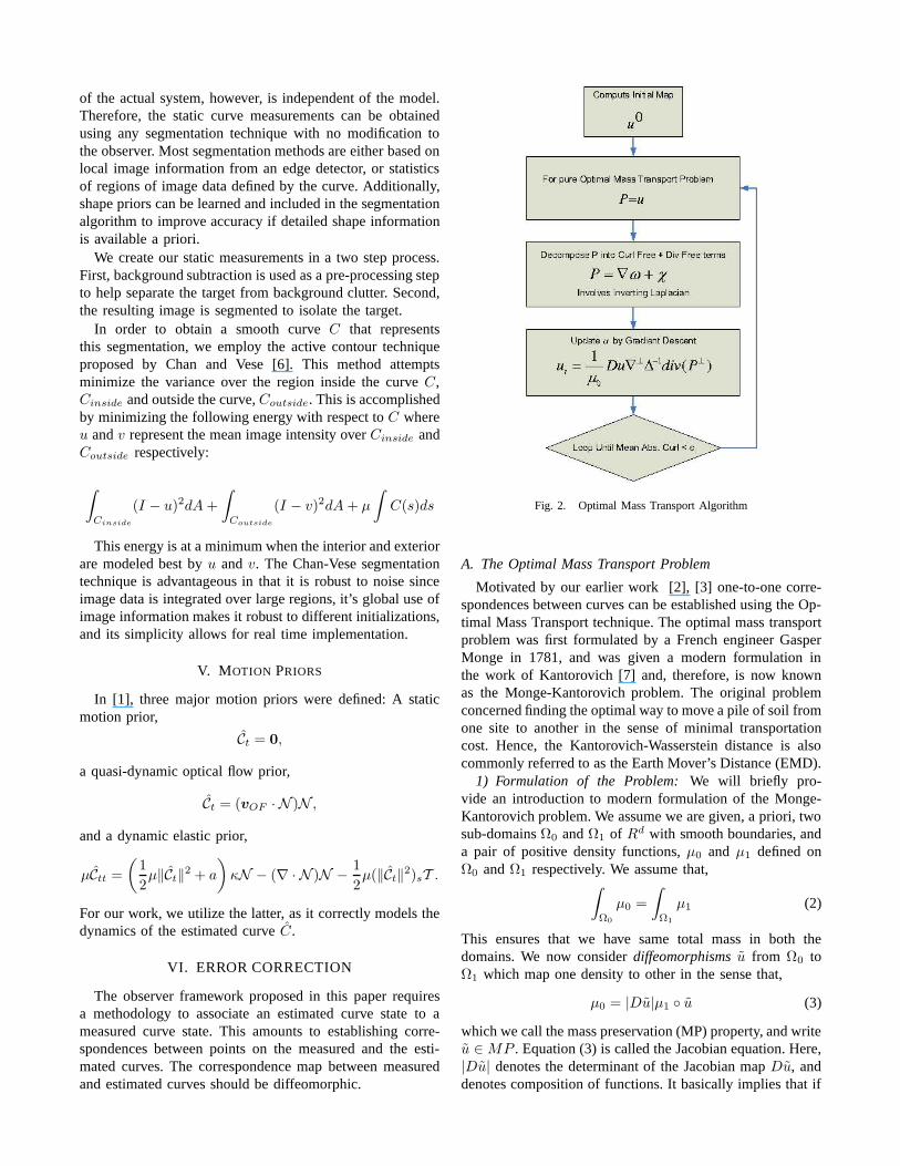
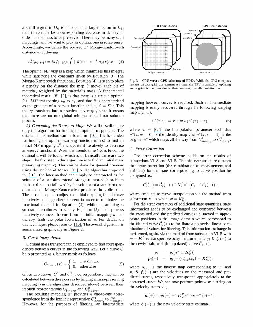
Fig. 3. CPU versus GPU solutions of PDEs. While the CPU computesupdates on data grids one element at a time, the GPU is capable of updatingentire grids in one pass due to their massively parallel architecture.

mapping between curves is required. Such an intermediatemapping is easily recovered through the following warpingmap u(x, w),

u∗(x, w) = x + w ∗ (u∗(x) − x), (6)

where w ∈ [0, 1] the interpolation parameter such thatu∗(x, w = 0) is the identity map and u∗(x, w = 1) is theoriginal u∗ which maps all the way from C1

binary to C2binary.

C. Error Correction

The error correction scheme builds on the results ofsubsections VI-A and VI-B. The observer structure dictatesthat error correction (the combination of measurement andestimate) for the state corresponding to curve position becomputed as:

Ck(+) = Ck(−) +∗ KCk ∗∗

(

Ck −∗ Ck(−))

,

which amounts to curve interpolation via the method fromsubsection VI-B where w = KC

k .For the error correction of additional state quantities, state

information needs to be exchanged and compared betweenthe measured and the predicted curves i.e. moved to appro-priate positions in the image domain which correspond tothe filtered curve Ck(+) to facilitate a pointwise linear com-bination of values for filtering. This information exchange isperformed, again, via the method from subsection VI-B withw = KC

k to transport velocity measurements qi & qi(−) tothe newly estimated (interpolated) curve Ck(+),

pi = qi(u∗(x, KC

k ))

pi(−) = qi(−)(u∗inv(x, 1 − KC

k )),

where u∗inv is the inverse map corresponding to u∗ and

pi & pi(−) are the velocities on the measured and pre-dicted curves, respectively, transported appropriately to thecorrected curve. We can now perform pointwise filtering onthe velocity states via,

qi(+) = pi(−) +∗ Kq

k ∗∗ (pi −∗ pi(−)) ,

where qi(+) is the new velocity state estimate.

VII. GPU IMPLEMENTATION

In this paper, the basic building blocks of all the givenalgorithms (optical flow for image warping, optimal masstransport, and active contour evolution) are the solutions ofPDEs. Typically, such problems are computationally inten-sive and prohibitive for real time tracking implementations.However, in the past few years, it has been shown thatgraphical processing units (GPUs), which are now standardin most consumer computers and are normally applied tographics processing for gaming, are particularly suited forseveral types of parallelizable problems including the solu-tion of PDEs [12], [13]. In our work, we implemented allPDE solvers on the GPU utilizing the full multigrid method,making two algorithms practical for tracking which werenot practical before: optical flow for image warping andoptimal mass transport. In this section, we give details on theGPU, our implementation, and the computational advantagesachieved.

The GPU can be considered a massively parallel copro-cessor and dedicated memory interfacing to the CPU overa standard bus. Modern GPUs are comprised of up to 128symmetric processing units running up to speeds of 1.35Ghz.Their advantage over the CPU in this sense is that while theCPU can execute only one or two threads of computation ata time, the GPU can execute over two orders of magnitudemore. From a PDE perspective, while the CPU computesupdates on data grids one element at a time, the GPUcomputes updates on entire grids at a time (Figure 3).

Both the optical flow and optimal mass transport algo-rithms were implemented on the GPU using a full multigridsolver. In this method, a fine-to-coarse hierarchy of equationsystems with excellent error reduction properties [3] iscreated and the PDEs are solved using classical iterativemethods at different resolution grids. The principle gridoperations are grid interpolation, relaxation, and restrictionand unlike the CPU, the GPU computes each update in onerender pass, increasing speed dramatically.

On a modest Dual Xeon 1.6Ghz machine with an nVidiaGeForce 8800 GX GPU (3DMark score of 7200) opticalflow speeds of 153 FPS were achieved on imagery of size1282. This is in contrast to the optical flow framerate of97 FPS achieved on specialized FPGA hardware recentlyreported in [14] on comparably sized imagery. Note that theformer implementation will run on most modern consumerlevel PC’s without modification.

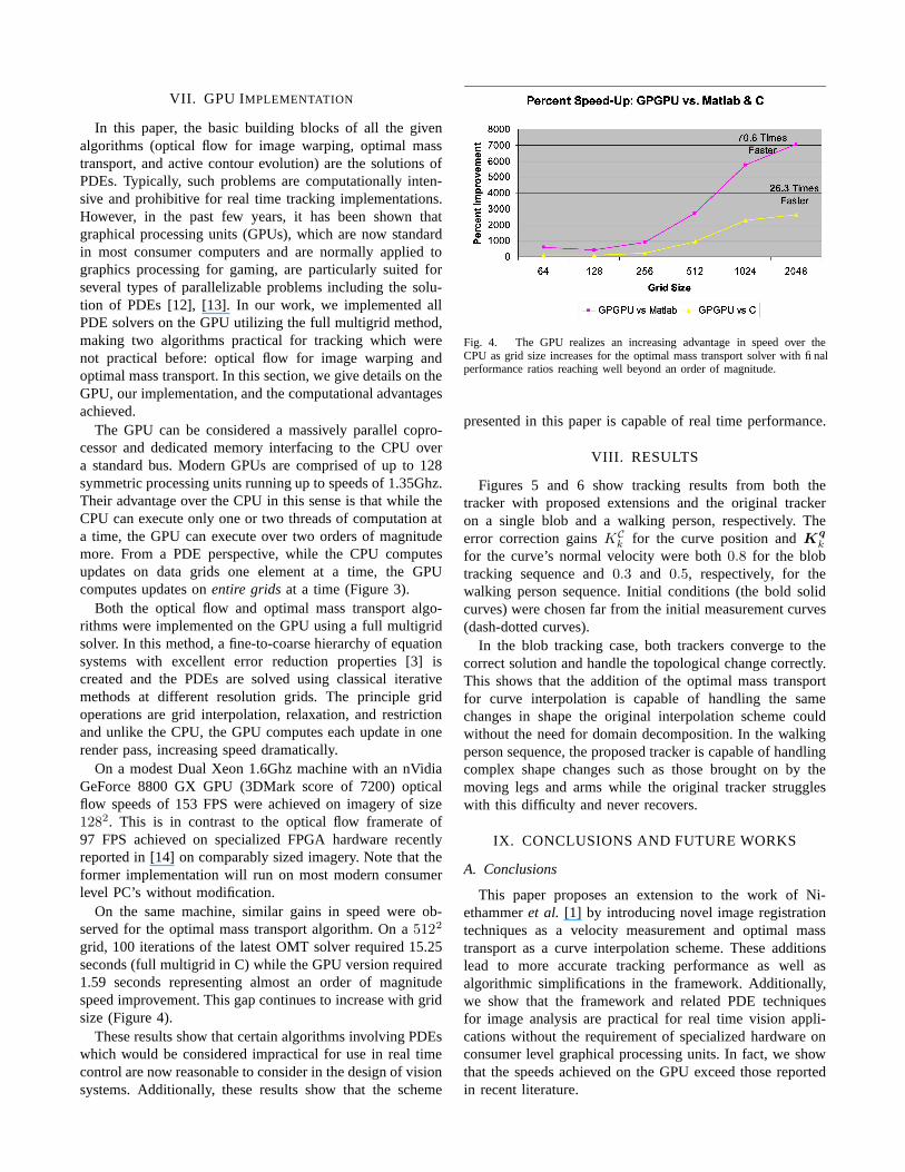
On the same machine, similar gains in speed were ob-served for the optimal mass transport algorithm. On a 5122

grid, 100 iterations of the latest OMT solver required 15.25seconds (full multigrid in C) while the GPU version required1.59 seconds representing almost an order of magnitudespeed improvement. This gap continues to increase with gridsize (Figure 4).

These results show that certain algorithms involving PDEswhich would be considered impractical for use in real timecontrol are now reasonable to consider in the design of visionsystems. Additionally, these results show that the scheme

Fig. 4. The GPU realizes an increasing advantage in speed over theCPU as grid size increases for the optimal mass transport solver with finalperformance ratios reaching well beyond an order of magnitude.

presented in this paper is capable of real time performance.

VIII. RESULTS

Figures 5 and 6 show tracking results from both thetracker with proposed extensions and the original trackeron a single blob and a walking person, respectively. Theerror correction gains KC

k for the curve position and Kq

k

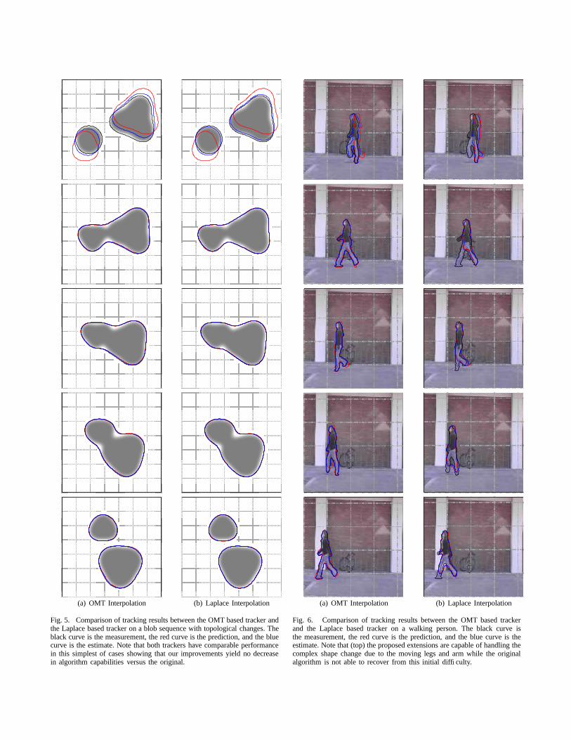
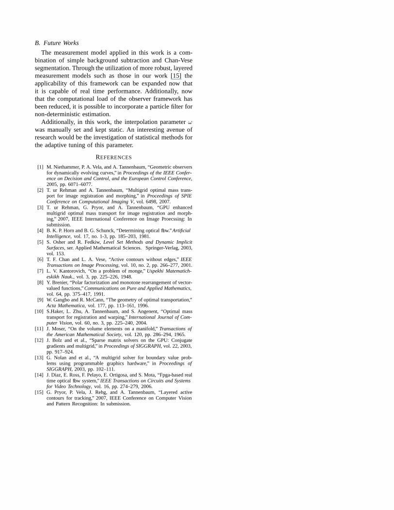
for the curve’s normal velocity were both 0.8 for the blobtracking sequence and 0.3 and 0.5, respectively, for thewalking person sequence. Initial conditions (the bold solidcurves) were chosen far from the initial measurement curves(dash-dotted curves).

In the blob tracking case, both trackers converge to thecorrect solution and handle the topological change correctly.This shows that the addition of the optimal mass transportfor curve interpolation is capable of handling the samechanges in shape the original interpolation scheme couldwithout the need for domain decomposition. In the walkingperson sequence, the proposed tracker is capable of handlingcomplex shape changes such as those brought on by themoving legs and arms while the original tracker struggleswith this difficulty and never recovers.

IX. CONCLUSIONS AND FUTURE WORKS

A. Conclusions

This paper proposes an extension to the work of Ni-ethammer et al. [1] by introducing novel image registrationtechniques as a velocity measurement and optimal masstransport as a curve interpolation scheme. These additionslead to more accurate tracking performance as well asalgorithmic simplifications in the framework. Additionally,we show that the framework and related PDE techniquesfor image analysis are practical for real time vision appli-cations without the requirement of specialized hardware onconsumer level graphical processing units. In fact, we showthat the speeds achieved on the GPU exceed those reportedin recent literature.

(a) OMT Interpolation (b) Laplace Interpolation

Fig. 5. Comparison of tracking results between the OMT based tracker andthe Laplace based tracker on a blob sequence with topological changes. Theblack curve is the measurement, the red curve is the prediction, and the bluecurve is the estimate. Note that both trackers have comparable performancein this simplest of cases showing that our improvements yield no decreasein algorithm capabilities versus the original.

(a) OMT Interpolation (b) Laplace Interpolation

Fig. 6. Comparison of tracking results between the OMT based trackerand the Laplace based tracker on a walking person. The black curve isthe measurement, the red curve is the prediction, and the blue curve is theestimate. Note that (top) the proposed extensions are capable of handling thecomplex shape change due to the moving legs and arm while the originalalgorithm is not able to recover from this initial difficulty.

B. Future Works

The measurement model applied in this work is a com-bination of simple background subtraction and Chan-Vesesegmentation. Through the utilization of more robust, layeredmeasurement models such as those in our work [15] theapplicability of this framework can be expanded now thatit is capable of real time performance. Additionally, nowthat the computational load of the observer framework hasbeen reduced, it is possible to incorporate a particle filter fornon-deterministic estimation.

Additionally, in this work, the interpolation parameter ω

was manually set and kept static. An interesting avenue ofresearch would be the investigation of statistical methods forthe adaptive tuning of this parameter.

REFERENCES

[1] M. Niethammer, P. A. Vela, and A. Tannenbaum, “Geometric observersfor dynamically evolving curves,” in Proceedings of the IEEE Confer-ence on Decision and Control, and the European Control Conference,2005, pp. 6071–6077.

[2] T. ur Rehman and A. Tannenbaum, “Multigrid optimal mass trans-port for image registration and morphing,” in Proceedings of SPIEConference on Computational Imaging V, vol. 6498, 2007.

[3] T. ur Rehman, G. Pryor, and A. Tannenbaum, “GPU enhancedmultigrid optimal mass transport for image registration and morph-ing,” 2007, IEEE International Conference on Image Proecssing: Insubmission.

[4] B. K. P. Horn and B. G. Schunck, “Determining optical flow.” ArtificialIntelligence, vol. 17, no. 1-3, pp. 185–203, 1981.

[5] S. Osher and R. Fedkiw, Level Set Methods and Dynamic ImplicitSurfaces, ser. Applied Mathematical Sciences. Springer-Verlag, 2003,vol. 153.

[6] T. F. Chan and L. A. Vese, “Active contours without edges,” IEEETransactions on Image Processing, vol. 10, no. 2, pp. 266–277, 2001.

[7] L. V. Kantorovich, “On a problem of monge,” Uspekhi Matematich-eskikh Nauk., vol. 3, pp. 225–226, 1948.

[8] Y. Brenier, “Polar factorization and monotone rearrangement of vector-valued functions,” Communications on Pure and Applied Mathematics,vol. 64, pp. 375–417, 1991.

[9] W. Gangbo and R. McCann, “The geometry of optimal transportation,”Acta Mathematica, vol. 177, pp. 113–161, 1996.

[10] S.Haker, L. Zhu, A. Tannenbaum, and S. Angenent, “Optimal masstransport for registration and warping,” International Journal of Com-puter Vision, vol. 60, no. 3, pp. 225–240, 2004.

[11] J. Moser, “On the volume elements on a manifold,” Transactions ofthe American Mathematical Society, vol. 120, pp. 286–294, 1965.

[12] J. Bolz and et al., “Sparse matrix solvers on the GPU: Conjugategradients and multigrid,” in Proceedings of SIGGRAPH, vol. 22, 2003,pp. 917–924.

[13] G. Nolan and et al., “A multigrid solver for boundary value prob-lems using programmable graphics hardware,” in Proceedings ofSIGGRAPH, 2003, pp. 102–111.

[14] J. Diaz, E. Ross, F. Pelayo, E. Ortigosa, and S. Mota, “Fpga-based realtime optical flow system,” IEEE Transactions on Circuits and Systemsfor Video Technology, vol. 16, pp. 274–279, 2006.

[15] G. Pryor, P. Vela, J. Rehg, and A. Tannenbaum, “Layered activecontours for tracking,” 2007, IEEE Conference on Computer Visionand Pattern Recognition: In submission.