Efficient irregular wavefront propagation algorithms on hybrid CPU–GPU machines
Upload
khangminh22Category
view
5download
0
University of West Bohemia in PilsenDepartment of Computer Science and EngineeringUniverzitní 8306 14 PilsenCzech Republic
Ivo Hanák
State of the Art and Concept of PhD ThesisThe GPU and Graphic Algorithms
Distribution: public
Technical Report No. DCSE/TR-2005-05April, 2005

The GPU and Graphic Algorithms
Ivo Hanák
AbstractIn the begging, graphic hardware was utilized only to convert binaryinformation to display device. Through its evolution, it gainedcapabilities and last improvement enhanced it so far that it can beconsidered as a next processing unit. Thus, this document concernswith graphic hardware, its applications and proposed improvements.It is an overview with selected samples that shall introduce thereader to the area of research a application of graphic hardware.
This work was supported by Microsoft Research Ltd. projectFPG-PLT-511568, MSM 23500005 „Záměry“, Ati Technologies Inc.,and project 3DTV: Integrated Three-Dimensional Television, NoE.Copies of this report are available onhttp://www.kiv.zcu.cz/publicationsor by surface mail on request sent to the following address:
University of West BohemiaDepartment of Computer Science and EngineeringUniverzitni 8306 14 PilsenCzech Republic
Copyright © 2005 University of West Bohemia, Czech Republic
Technical Report No. DSCE/TR-2005-05April 2005

Acknowledgments
I would like also to thank colleagues at University of West Bohemia, Faculty of AppliedSciences, Department of Informatics for giving me interesting ideas and for consultations on thetopic, as well. Finally, I would like to thank Ati for providing us with hardware that was used inexperiments.

Table of Contents
1 Introduction ............................................................................................................................... 1
2 Hardware Architectures ........................................................................................................... 32.1 Classical Pipeline ................................................................................................................ 3
2.1.1 Vertex Pipeline ............................................................................................................ 32.1.2 Pixel Pipeline ............................................................................................................... 5
2.2 Programmable Classical Pipeline ........................................................................................ 62.2.1 Common Attributes ..................................................................................................... 72.2.2 Vertex Shader ............................................................................................................ 112.2.3 Pixel Shader ............................................................................................................... 13
2.3 Modified Classical Pipeline .............................................................................................. 172.3.1 General Modifications ............................................................................................... 172.3.2 Vertex Pipeline Modifications ................................................................................... 182.3.3 Pixel Pipeline Modifications ..................................................................................... 23
3 GPU Languages and Programming ...................................................................................... 273.1 Graphical Purposes ............................................................................................................ 27
3.1.1 Direct3D: HLSL ........................................................................................................ 283.1.2 Cg .............................................................................................................................. 313.1.3 OpenGL: GLSL ......................................................................................................... 323.1.4 Sh ............................................................................................................................... 34
3.2 General Purposes ............................................................................................................... 353.2.1 Brook for GPU .......................................................................................................... 36
3.3 Language Enhancements ................................................................................................... 383.3.1 Large Code Division .................................................................................................. 38
4 GPU/Hardware Aided Approaches ....................................................................................... 414.1 Local Illumination ............................................................................................................. 41
4.1.1 Shading and Materials ............................................................................................... 414.1.2 Shadows ..................................................................................................................... 45
4.2 Global Illumination ........................................................................................................... 504.2.1 Ray tracing ................................................................................................................. 504.2.2 Radiosity .................................................................................................................... 53
4.3 Data Visualization ............................................................................................................. 564.3.1 Surface Representation .............................................................................................. 564.3.2 Volume Representation ............................................................................................. 584.3.3 Scattered Data and Point Representations ................................................................. 694.3.4 Other Representations ............................................................................................... 72
v

Table of Contents
4.4 Others ................................................................................................................................ 734.4.1 Computer Vision and Image Processing ................................................................... 734.4.2 Computational Geometry .......................................................................................... 754.4.3 Mathematics .............................................................................................................. 78
5 Conclusion ............................................................................................................................... 85
6 Future Work ............................................................................................................................ 87
References ................................................................................................................................... 91
Appendix A: GPU Registers ..................................................................................................... 97
Appendix B: GPU Limitations .................................................................................................. 99
vi

1 Introduction
Computer graphics is an area of computer science aimed mostly on image synthesis, i.e. itspurpose is to generate artificial images based on scene description. This is true, even thoughtsome branches of computer graphics performs computation to produce either differentrepresentation of scene or modified scene with requested attributes. However, at the end, thegenerated data are utilized in process of image synthesis to find a balance between visual realismand computational costs.
In its beginning, the computer graphics was able to provide only simple, low-resolution andusually line based images on displays of various hardware principles. In these day thecomputational costs were quite high in comparison to visual quality of resulting images. Thus,algorithms has to be invented that improves overall performance. Nevertheless, that was notenough because as the computational power of computers was increasing so was increasing theresolution of displays and the complexity of displayed scenes.The importing thing in computer graphics image synthesis is that the display hardware structureallows or even requires an image to be composed of N-dimensional array of image element, i.e.pixels. The constant N depends on display construction and in the case of common 2D colordisplay, the N is equal to three. The task of image synthesis is then a question of value estimationfor every pixel in the image, i.e. every pixel has to be processed in order to construct the resultingimage.There are many approaches that in the end lead to a value of the pixel. Some of these approachesprovide convincing image others provide just crude approximation of the scene. Most of theseapproaches consist of large number of rather simple steps that are repeated during imageconstruction many times. And thats a point where hardware enters the scene.
The hardware was there from the beginning of the computers. Without the hardware there wouldbe no software because software is just an attempt to generalize it and therefore both simplifyand speedup the process of new solution creation. Still, it is true that software solution is muchslower than its hardware equivalent. In some cases, solved problem leads to large number ofsimilar simple steps whose computation consumes significant amount of central processor unit(CPU) time. In such case a hardware performance overweights benefits of software solution.In the field of computer graphics there exist many experimental and rather specialized pieces ofhardware whose only purpose is to improve overall running time of several algorithms. Inmajority of cases these were rather experimental platforms and thus many of these solution wereabandoned due to their ineffectiveness in comparison of computer science advances, some of thefound its way to an industrial utilization.
In the industrial area, hardware dedicated to aid image synthesis helps computer aided design(CAD) to visualize models described by its surface with high detail. Such hardware is able toperform a task that is both significant in process of image synthesis and rather time consuming,
1
1 Introduction
i.e. the task of rendered primitive decomposing to elements such as pixels including a simpleport-processing. This decreases the load on the CPU and thus allows visualization of large scenesat interactive framerates. This is rather satisfying for CAD purposes.However, it was not enough for game industry. Thanks to the fact that this dedicated hardwarebecame available for the home users, the games began to utilize it in order to provide higherrealism and/or more complicated environments. It was the game industry that later on supplied astimuli for enhancement of graphic hardware.
In first generations the hardware was able to perform triangle rasterization including texturemapping, occlusion solution, and other pixel post-processing tasks. The solution was hard-wiredwith a possibility for limited customization and/or programmability. Thanks to its limitations, thehardware was able to outperform general CPUs and that was a point were attempts were made toutilize such graphic hardware for little bit different purposes than the image synthesis.Later on, the rest of the scene processing became a part of hardware allowing a game developersto move almost complete visualization load out of the CPU and thus gain more time for otheraspects of the game. However, still there were tasks concerning scene visualization that had to becomputed on the CPU as well as visual effects that were hard to cope on that hardware.
Therefore, a possibility of pipeline customization by application was added to the list of graphichardware capabilities. The next logical step was then to allow a user to gain almost completecontrol over particular components of the pipeline by execution of customizable programs thatreplace the hardwired solution.The original purpose for many of these enhancement was to provide an environment for specialeffects that would improve both quality and realism of the resulting image in real-time but notdecrease performance significantly at the same time. Thanks to that the graphic hardware camefrom state of dedicated single purpose hardware to state of processing unit able to performspecialized but fast numerical operation. Thus, the graphics processing unit (GPU) could beconsidered as a hi-performance special purpose processing unit running in parallel to the CPU.
This document concerns the graphic hardware and its capabilities including examples of possiblehardware-aided solutions. It is mostly aimed on the GPU because this platform is widelyavailable and therefore its application may be utilized by wide public. The document consists oftwo major parts: the state of the art in the graphic hardware computing and future work in a fieldof the graphic hardware. The author assumes a reader has at least a basic knowledge ofC language syntax and computer graphic principle basics.
2

2 Hardware Architectures
This chapter contains introduction into hardware itself. It divides hardware by its availability forhome user. It also describes capabilities and important aspects of these hardware if relevant forcontents of this work.
2.1 Classical PipelineAt the begging of graphic hardware evolution there was a need to perform image synthesis with ahigh performance. The process was based on displaying of triangles on raster displays. This wassimple enough to be implemented straightforwardly in the hardware. The resulting hardware wasenhanced by additional capability during its evolution until it contained complete pipelinerequired for rasterization of a scene described by surface in a form of triangles. The pipeline that is description of data flow in current common widely available hardware willbe called as classical pipeline because it is the only one pipeline that survived its evolution andfound its place in both industrial and home use. Also, majority of approaches described in thiswork utilizes it directly and/or derives from it, hence the denotation. The implemented pipelinecan be divided into two major blocks: the vertex pipeline and the pixel pipeline [DX05].
2.1.1 Vertex PipelineThe vertex pipeline prepares a geometry for rasterization (see Figure 2.1). The input of thispipeline consists of data provided by a user. In majority of cases those are rendering primitives ortheir modification such as strips and fans that may be used in order to decrease the overallstorage requirements and bus traffic. In a special case the input may consist of high-ordersurfaces.
vertex data
indices High-orderPrimitive
Tessellation
TransformLighting
PrimitiveAssembly
PerspectiveDivide
CullingClipping
ViewportScaling
PixelPipeline
a obligatoryparts a non-vertex
pipeline partsa optionalparts
Figure 2.1: Vertex pipeline scheme.
3

2 Hardware Architectures
The first step of the vertex pipeline is a tessellation of high-order primitives. This step isoptional1 and if present, it is preformed only when either a high-order primitive is passed or thetessellation functionality is enabled. The output of the tessellation step are triangles whosenumber is usually larger than a number of incoming ones. The benefit of the approach is todecrease of both data storage and data transfer because all operations are performed on chip.Currently, there are two possible high-order primitives:
• RT-Patches2 that provide hardware support for high-order primitives. The functionality isaccessible through a special set of functions and allows the user to utilize Bézier, B-spline,and Catmull-Rom patches. The tessellation does not take any quality measurement intoaccount and utilizes user provided maximum depth of division. The depth controls dividing ofthe patch into a set of triangles. For more details, refer to [Mor99, DX05].
• N-Patches or PN Triangles3 that perform a conversion from a triangle with normals atvertices to a triangular Bézier surface according to an interpolation rules. After the conversionthe user supplied maximum depth is used to divide the patch back into triangles.
This functionality is rather transparent for a user because it is performed automatically, ifenabled. N-patches provide surface smoothing and together with displacement maps (seebelow) they allow displaying of models of various level of detail (LOD) without additionalstructures and/or storage requirement. For more details, refer to [Vla01, DX05].
As the next, transformation and lighting computation takes place. The goal of this step is toprepare vertices for clipping by a viewing frustum. This is done by transforming of vertices into aunit clip space with camera at origin of the space oriented along the z-axis4. The lighting is alocal illumination system that utilizes the Phong lighting model [Wat99, Pho75] in order tocompute lighting for every vertex.
Afterwards, primitives are assembled. This step is required because the input data my not beconfigured as a list of vertices that forms a desired primitive. Based on performance issues theuser is able to pass a list of primitives where a next subsequent primitive utilizes an informationfor the previous one thus saving the space for storing. Besides that, there are indexed primitiveswhere the user passes an array of vertices and an array of indices that point to the vertex arrayand thus form the desired primitive.The primitive assembling step utilized a buffer that hold processed vertices before theirembedding to a given primitive. Surely, this buffer is a rather limited in its size and therefore thepipeline may throw some processed vertices if an input stream exhibits inappropriate order. Thismay cause a performance drop down.
Afterwards, perspective divide, culling, and clipping takes a place. Perspective dividetransforms vertices from P3 a projective extension of E3 space back to the E3 space. Culling thenremoves triangles that are facing away from the viewer, if enabled. It assumes that trianglesfacing away from user and on reversed side of closed solid object and thus their rasterizationwould have not impact on the resulting image.
The clipping on the other hand clips all elements and/or its parts that are outside the viewingfrustum, i.e. unit clipping space/cube. If a primitive is partially inside the cube, the mechanism
1 Currently only Ati-based GPUs has this capability widely supported.2 RT-patches were implemented first by nVidia.3 N-patches were implemented first by Ati4 For the OpenGL, the camera is oriented towards negative z-axis. For the Direct3D, the camera is oriented
towards positive z-axis, i.e. it is left-haded system.
4
2.1 Classical Pipeline
computes clipped coordinates. For a triangle this can lead to a hexagon that is divided back to alist of triangles because the rasterizer is able to process triangles only.Actual algorithm utilized for clipping is hardware provider dependent and is part of an internalnon-public structure of the hardware. From capabilities and runtime requirements it seems thatthe clipping algorithm could be a Sutherland-Hodgman or its modification [Wat99, Ska04].
Together with the clipping another term could be mentioned: a guard-band clipping [Die99].This feature is not very important in current hardware and it is rather part of pixel pipeline.Nevertheless it has impact on the vertex pipeline construction and thus it is mentioned here.Guard band clipping is aimed on decreasing of the computational load on a vertex pipeline bymoving it towards the high-performance rasterized in the pixel pipeline.
The idea is based on a fact that there a lot of rather small triangles that are incident with edges ofthe unit clip space. Such triangles can be lead to a rasterizer, which automatically discards out-of-screen pixels. It is sure that rasterizer works only on specified limited area5 and therefore it mayhappen that given triangle is even outside the enlarged workspace of the rasterizer. Such trianglehas to be clipped before the rasterization.Nevertheless, thanks to the guard-band clipping a lot of triangles does not need to be clipped atall before entering the rasterizer. This enhancement has significant impact for older hardwaregraphic hardware mostly that lacks implementation of the vertex pipeline. In such case, theguard-band clipping utilization decreases load on the CPU.
The last step performed on the vertex pipeline is the window-viewport transformation thatconverts projected triangles from unit screen to an actual screen size. The output of this step isthe output of the vertex pipeline and it is directly processed by the rasterizer.
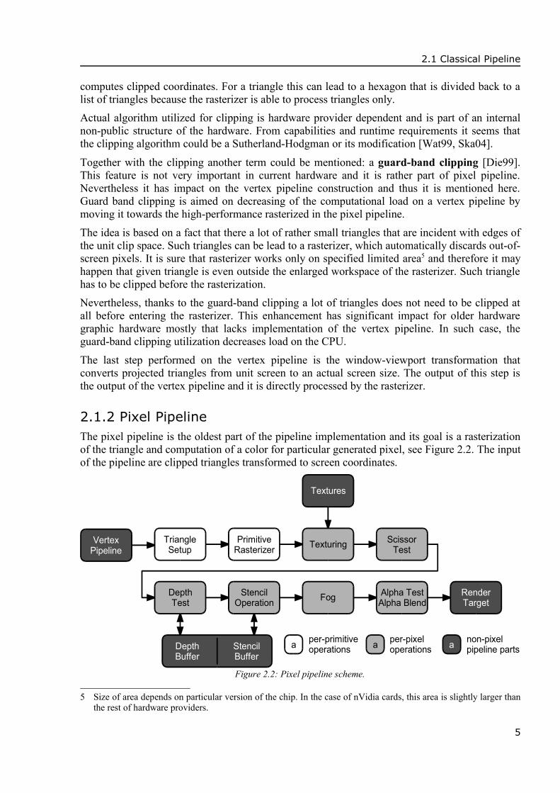
2.1.2 Pixel PipelineThe pixel pipeline is the oldest part of the pipeline implementation and its goal is a rasterizationof the triangle and computation of a color for particular generated pixel, see Figure 2.2. The inputof the pipeline are clipped triangles transformed to screen coordinates.
TexturingPrimitiveRasterizer
ScissorTest
a per-primitiveoperations a non-pixel
pipeline partsa per-pixeloperations
VertexPipeline
TriangleSetup
DepthTest
StencilOperation Fog Alpha Test
Alpha BlendRenderTarget
DepthBuffer
StencilBuffer
Textures
Figure 2.2: Pixel pipeline scheme.
5 Size of area depends on particular version of the chip. In the case of nVidia cards, this area is slightly larger thanthe rest of hardware providers.
5

2 Hardware Architectures
The major part of the pixel pipeline consist of the rasterizer that decomposes given triangle topixels6 together with proper perspective correct [Cat80, Wat99] interpolation of a vertexassociated information, i.e. texture coordinates, color, depth information, fog, etc. The rasterizerutilizes a scan-line conversion algorithm with triangle prepares in the triangle setup phase. For ahardware implementation, there are two possible mechanisms that both lead to rasterized triangleas described in [Mit00]:
• Algorithm based on linear interpolation that first forms vertical slopes from the triangle duringthe triangle setup and then utilizes these slopes to create a set of horizontal pixel segments.Each such segment is iterated in order to generate individual pixels.
• Algorithm based on edge function handles the triangles as a set of linear edge functions thatare utilized to check whether given pixel is inside the triangle thus being processed or whetheris outside the triangle thus being omitted. The approach can be improved by utilizing arectangular array of pixels denoted as pixelstamp: processing of each pixelstamp may run inparallel.
Then, a texture mapping is performed for each generated pixel. The common structure that isused for texture mapping is a cascade-like connection of texture units that utilizes texturecoordinates associated with the pixel. The number of texture units is strictly hardware dependent;in a majority of cases the number is 2—3. This number is satisfying for the most of applicationsuch as games because it allows mapping of a surface texture and a light map in a single pass.The output of this step is a pixel with associated color, fog, and depth information.
Later on, a post-processing is performed on the pixel. This post-processing allows a significantamount of customization and thus enables the user to create several interesting visual effects. Thepixel is tested against scissors rectangle, a depth buffer, and a stencil buffer [Kil99] that is in themost of cases a part of the depth buffer. During the stencil test, the pixel is compared against thedepth buffer and the results of both depth and stencil test determines fate of the pixel7.
Last post-processing operation involves application of a fog based on a fog value associated withthe pixel. Afterwards, an alpha-blending is performed according to the pipeline setup and a pixelassociated alpha value. This includes a simple alpha test that may discard pixel with too lowalpha in order to render an image with only a minimal number of visual artifacts utilizing depthbuffer only. Then, the result is written to the current render target, also denoted as color buffer.
2.2 Programmable Classical PipelineThe programmable pipeline is a next evolution step in commodity graphic hardwaredevelopment. The basic idea for such enhancement was to allow an application to performcustomizable texture mapping in order to improve visual quality of synthesized image withoutsignificant impact on the performance.
At the first, enhancement were made in vertex pipeline by allowing a simple program to beexecuted for modification of vertex blending and/or texture coordinate generation. This waspossible because the vertex pipeline has lower requirements on a throughput in a comparison tothe pixel one.
6 In some literature the value in this stage is called a fragment rather than a pixel because of the the contains moreadditional information besides its color.
7 The pixel may be either passed through or discarded. The corresponding value in the stencil buffer may beupdated as well.
6
2.2 Programmable Classical Pipeline
As the next, the pixel pipeline was enhanced by allowing an application to customize textureblending. This modification significantly enlarged the range of possible effect for real-timesynthesized graphics and it was known as a register combiner [Kil04]. This was the last stepbefore a programmability of both pixel and vertex pipeline became a reality [Lin01].
Surely, not all parts of the pipeline are programmable. However, the hard-wired parts usuallyprovides functionality that is common for all image synthesis tasks and thus its programmabilitywould not mean almost any benefit besides the increase in both computation time and cost due toprogrammability.The major idea behind the graphic hardware development in this area is to keep it as simple aspossible in order to gain maximum performance. Therefore, the pipeline still retains its pipelinecharacteristics thus resulting to several limitation for programmable blocks in comparison to theCPU. However, thanks to these limitation the pipeline may apply massive parallelization in bothnumber of pipelines and number of operands processed by a single instruction and thus itoutperforms comparable CPU.
Currently, the pipeline contains two programmable blocks: the vertex shader and the pixelshader. In some environments such as OpenGL the pixel shader is usually called a fragmentshader. This difference is based on a fact that while the pixel shader output is a pixel color, theinput is a pixel with additional information, i.e. a fragment of a rasterized surface. In such case,term pixel shader denotes a post-pixel production [3DL04]. However, for sake of this workuniformity, the therm pixel shader origination from Direct3D [DX05] is used.
2.2.1 Common AttributesAs it was mentioned in previous paragraph, the pipeline has two programmable blocks. Eventhought these blocks are situated at different places in the pipeline and provide different output atthe same time, both follow similar rules and have similar capabilities and limitations as well.
The most important fact that every user should be aware of is the locality of both shaders.Neither the pixel shader nor the vertex shader are aware of processed element context during itsprocessing. This means that the user is not able to access neighborhood in both geometrical andimage meaning because the shader has no information about it.On the other hand, this restriction allows simple parallelization of element processing thanks tothe lack of synchronization for read/write request that may appear from within the shader code.Similar to the rule already mentioned, the shader is unable to alter the context of the element, e.g.the user is not allowed to convert triangle to points or to modify position of vertex within thetriangle.
The next important attribute of the shader is its execution: shader is executed upon dataavailability. The user is not able to execute the shader separately without any supplied data. Thislimitation is based on a fact that shaders are part of hard-wired pipeline and therefore thecapability of execution independently on pipeline would disturb its structures and complicate itshardware implementation.
Similar to that, the next important restriction in shader programming is that the shader is notcapable to generate any additional elements. It is sure that the shader is capable of generatingnew data upon given one but those data has to be associated with currently processed element.The capability of new element generation would lead to a complication and therefore aperformance drop down for the whole pipeline.
7

2 Hardware Architectures
In previous paragraphs, the execution management and input/output capabilities were mentioned.However, still there is a one important area that has restriction applied as well: the memorymanagement. The important is, the shader has no memory management at all. It is not capable toaccess memory of the graphic adapter directly and random manner.The only area available to the shader code for random read/write access is a shader local memorythat is limited in its size. The size of the memory has no dependence on memory available on thegraphic board because it is implemented as a set of read/write on-chip registers and this is verysmall and very fast at the same time.
Memory substituting registers as freely accessible to the shader code but their values areundefined once the shader finishes processing particular element, i.e. the memory is intendedonly for a temporary storage. This means that all computations in shaders are stateless and theonly way of obtaining of computed results is through the output of the pipeline, i.e. the rendertarget and/or depth buffer.
Besides limitation for computation and memory management, available data types are alsoimportant feature of the shader. The native type supported by a majority of GPUs is a 32-bitfloating-point single [IEE85], i.e. float in C-language syntax. However, there exist otherfloating-point formats that were mostly added due to either performance or construction reasons:half-precision floating-point and fixed-point data type.
The half-precision floating-point data type is usually denoted as a half. Its length is 16 bits andwas added due to performance reasons in order to sacrifice accuracy and gain performance at thesame time. It is recommended for a shader code to use this data type whenever the accuracy isnot crucial such as color computation intended for displaying.On the other hand, the fixed-point data type was added due to construction reasons. It is usuallydenoted as fixed and its length is usually 12 bits. It is the only numerical data type available onfirst generation of graphic hardware with shader model of version less than 2.0. This is becauseolder hardware utilize faster but less accurate fixed-point point arithmetic. It has an appropriateaccuracy for image synthesis purposes and is much faster in comparison to the floating-pointarithmetic8.However, according the nature of fixed-point computations, the accuracy is very restricted andthe range of values is strictly given. Thus, all mathematic operations on the hardware with shadermodel less than 2.0 including fixed data type are saturated to a range ⟨−1 ;1 ⟩ . This makes theolder hardware almost useless for general purpose computing but it is sufficient for basic imagesynthesis computations such as Phong shading.
Integers of 32-bit length are also supported but in a majority of cases it is replaced by the floatinternally. Besides numerical data type, the GPU is able to handle a boolean type that is used forflow control in a form of if-branching, both static that depends on values supplied by theapplication and dynamic that depends on values computed in the shader code.
The last available data type are samplers. These are intended for obtaining a color sample from atexture and their behavior is determined by the pipeline settings. Currently, there are fouravailable types of samplers that differs by the texture type they are sampling from: 1D, 2D, 3D9,rectangle10, and cube-map.
8 Try to compare implementation of floating-point and fixed-point division of two numbers.9 3D Texture is basically a volume texture.10 Rectangle texture is 2D texture with a side not equal to 2k , k∈ℕ . On some hardware, rectangle texture may
have limited set of possible filters for obtaining a sample.
8
2.2 Programmable Classical Pipeline
Value sampled from a texture is always a four-component vector of floating-point number nomatter what is the actual data type of a texture element, i.e. texel. Texels with color componentsof integer data types are converted to a range of ⟨0 ;1 ⟩ . Floating-point textures are sampledwithout any value modification and/or saturation.Thanks to fact that in mathematics for computer graphics the most used one computationalelements are vectors, the GPU is able to operate with an up to four-component vectors instead ofplain scalars. The important attribute of the modification is a capability to convert betweenvectors of the same type but various lengths.
From the code point of view, the vector is handled similar to a structure, i.e. individual elementsare accessed via point operator. There are three sets of names for element: xyzw, rgba, andstpq. Event thought it is not allowed to mix sets used for and while accessing a single particularregister, they do not distinguish in functionality. The reason for their existence is an attempt toimprove readability of the code mostly when done in the assembly language, see Chapter 3.The next important capability concerning numerical data types is a possibility to perform userspecified vector component rearrangement. This basically allows the user to select particularelements of a vector to be used either as source or target for an operation, e.g. consider four-component vector v than code v.zx denotes a two-component vector that has first component ofvalue vz and second value of vx. When used for a argument of a function, this operation is called aswizzling and when used for specification of target vector element it is called a masking.
Similar to that, vector per-component negation is supported, too. All mentioned operation withregisters are performed naturally without any requirements for special instruction. Therefore, thismodification allows a shader to perform several computation with both color and position in P3
the projective 3D space without additional computational and/or shader instruction requirements.Besides that, each register has access restriction applied. These restriction divides all availableregisters into three groups. Actual numbers of registers depends on particular shader model andshader type. For details, refer to Appendix A. Groups are:
• Read-only registers. These are registers that are considered as an input to the shader. First ofall, there are input from a pipeline. The number of these registers as well as their semanticsdepends on particular shader and is described in next sections.
Next, there are numerical and boolean constants: a special relatively large set of registerscontaining values set up by the user of the shader, i.e. the application. They are often used fortransferring of object and/or scene information such as transformations, light settings,material, animation information, etc. to the shader code.Similar to numerical constants, there are special constant registers for samplers. The exceptionfrom registers mentioned above is a loop control register that is read-only as well butaccessible only inside of the loop and contain number of already performed loop repeats.
• Write-only register group that contains registers intended to hold output values that are usedas input for the rest of the pipeline. Similar to the rest of registers, their numbers as well assemantics is shader type and version dependent. These registers are either floating-pointvector of four component or floating-point scalar.The important attribute of these output registers is the fact, that some of them are obligatory.The obligatory registers have to be set prior to shader code exit. The optional ones does notrequire it and contains predefined value: usually zero or vector of zeros, if not set.
9
2 Hardware Architectures
• Read/write registers supply the local memory for a shader during element processing. As itwas already mentioned, such memory is strictly temporary, hence the temporary registers.Their count is low and they are usually of float data type. For exact data, refer to Appendix A.Besides numerical temporary registers, there are special purpose registers: predicate registerthat is utilized in dynamic if-branching and address register that is used for relativeaddressing of constant register, i.e. allows implementation of application supplied arrays.
The program that controls behavior of the shader has also several limitations. First of all, itslength is strictly limited. In some cases the length of the program is divided by type of operation.Actual minimal numbers of instruction per shader depends on a particular shader model and arelisted in a table within the Appendix B.
The next important restriction applied to a program is a limited flow control that is mostlyunderstood as a branching capability. For a lower shader model, the branching is not available atall but it is possible to bypass it by simply computing both branches and then selectingappropriate result. This inability to perform float control simplifies hardware construction andtherefore improves the overall performance of the shader [Lin01].GPUs of newer shader models have a certain capability to perform either static or dynamicbranching. The static branching is a situation when a condition is a boolean value supplied bythe application in a form of constant, the dynamic branching utilizes predicate register whosevalue is computed during shader execution.
The looping is also supported and a loop exposes its control variable for read-only access as itwas mentioned. The looping is static because maximum number of repeats has to be stored into aconstant register. Nevertheless, when dynamic flow control is available the loop execution maybe interrupted according to a condition. Maximum number of loop repeats is limited to 255.
Besides that, the next possibility for flow control are a subroutine calls. In the case of olderhardware, this is not supported and a code of a subroutine have to be copied instead if asubroutine call is required. If this feature is available, the user may call a subroutine eitherstatically or dynamically, i.e. it may give a condition that has to be fulfilled in order to performthe call.
Maximum nesting depth for subroutine calling is strictly limited and thus recursion is notavailable for the shader code. Nesting level for branching and looping is restricted as well. In thecase of static branching, some shader models may apply restriction to a number of suchinstruction to appear in the code but they allow almost limitless nesting of these instruction at thesame time. Nesting depth depends on shader model version and a type of the shader. For details,see Appendix B.
Operations preformed by GPU show behavior similar to Simple Instruction Multiple Data(SIMD) system in a majority of cases . They allow to process whole four-component register atonce. This is one of fundamentals of the GPU computational power, i.e. parallelization oninstruction level.
It is true that the overall performance of an instruction depends on a performed operation but thisdifference in performance when using a single scalar or when using four-element vector does notexcess the coefficient of four, i.e. the instruction execution time when using a vector shall be lessthan four times the same but using a scalar.
Accuracy of mathematical operations utilizing floating-point value type depends on particularhardware but for shader model 3.0 and newer, the accuracy is 128 bits per register, i.e. 32 bits persingle floating-point register component. For a shader model 2.0, the accuracy may be reduced to
10

2.2 Programmable Classical Pipeline
96 bits11 per register but this reduced accuracy should have almost any visible impact on resultingsynthetic image. Lower shader models does not have support for floating-point operations at alland therefore their accuracy is limited by 12-bit fixed-point data type.The GPU supports wide range of operations in a form of instruction. For completeness of thissection a brief overview of instruction groups is provided. Supported instructions are:
• Mathematical operations. This group includes instruction of adding, multiplying of vectorsper element, dot product that allows implementation of other important operation such asmatrix multiplications, cross product, linear interpolation, rounding functions, reciprocal ofscalar, reciprocal square root, logarithmic functions, and sin/cos.
• Flow control instruction group that contains if-branching, looping and subroutine calling,both static and dynamic.
• Texture sampling support including projective mapping and cube-map sampling.
• Geometry operations that include vector normalization, lighting computation support thatshall simplify the task of disabling propagation of specular lighting if element normal hasreversed direction than direction of light.
2.2.2 Vertex ShaderVertex Shader is the first programmable block in pipeline data flow. It resides at a verybeginning of the pipeline just after the tessellator. Its purpose is to process vertices and preparethem for clipping and primitive assembling. Based on its functionality, it replaces thetransformation and lighting block of the vertex pipeline and whenever a vertex shader is used ithas to perform all tasks done by replaced blocks.
2.2.2.1 Input
The input of the vertex shader consist of three parts:
• Input from the pipeline that consist of tessellator processed data. In a majority of cases theseare geometrical data passed by the user to the pipeline. Data consist of up to 16 four-component vector a 32-bit floating-point per each component. Each vector has its owndesignated semantics, i.e. it is mapped right to a particular vertex component. None of thesevectors is mandatory, but based on a fact that execution is driven by a data availability at leastone of them contains valid value.
• Constants that are set by an application in order to modify computation performed. In a caseof the vertex shader they usually consist of transformation matrices and possible light settingseven thought in a majority cases, lighting is performed on per-pixel basis rather than on per-vertex bases as it is common for the hard-wired pipeline. Number of constants varies andbesides four-component floating-point vectors, vectors of boolean type are allowed in order toperform static flow control.
• Vertex textures are the largest source of data for vertex shader and are in a majority of casesutilized for displacement mapping and for utilizing of data computed in a pixel shader duringprevious pass. This is rather important because it allows utilization of pipeline output in orderto modify processed geometry without expensive downloading computed data back to the
11 96 bit accuracy is mostly true for graphic hardware by Ati.
11

2 Hardware Architectures
CPU. Such benefit may be crucial for computation of various particle system includingfluid/gas simulation.
The vertex shader is usually a place for application of the displacement maps [Coo84, Dog00].These are textures that contain modification of a vertex position according to vertex texturecoordinates. The modification benefits from a possibility to parametrize the surface by utilizing atexture coordinates. Based on that, let P u , v be a vertex of base surface, D u , v a samplefrom the displacement map and N u , v a normalized normal of base surface then new positionP new u , v is defined as:
P new u , v =P u , v D u , v N u , v (1)
Vertex normal may remain unmodified even thought they are possibly incorrect for modifiedvertex because it is replaced by a value from a normal map during per-pixel lighting, seeSection 4.1. The technique of displacement mapping is utilized whenever a silhouettemodification is required.
This mechanism can be utilized together with the high-order primitives such as N-Patches inorder to compute and display models with appropriate LOD on the fly. This does not save onlythe rendering but also storage and transport requirements because the application supplies sameamount for primitives and their division into larger set of triangle is done completely on-chip.Currently, only shader model 3.0 and newer supports vertex textures, older shader models are notcapable of utilizing this input source and have to bypass it by utilizing the CPU for performingvertex data manipulations. The supported format for vertex textures is usually either a 32-bitfloating-point four-component vector or 32-bit floating-point scalar per texel.
Nevertheless, in some cases vertex textures can be bypassed by a proposed extensions of theOpenGL 2.0 denoted as a pixel buffer object. From the view of this extensions all buffer objectsin the video memory are basically the same and thus it is possible to utilize them as the rendertarget, i.e. this allows to render directly to the vertex buffer and utilize such data as the geometryin the next pass of the algorithm.
2.2.2.2 Output
The output of the vertex shader is based on the pipeline requirements for vertices that has to beclipped and utilized during primitive rasterization in pixel part of the pipeline. The output itselfconsist of up to 12 four-component floating-point vectors. Each vector has its own semanticassigned in order to distinguish meaning of the vertex shader output. With a single exception, alloutput values are optional, i.e. setting of them is not required. The possible output of vertexshader are:
• Vertex coordinate that is the only obligatory value that has to be set up as a result of everyvertex shader execution because its value is used for clipping purposes. The coordinate has tobe transformed into a unit clip space and is passed out of vertex shader in homogeneouscoordinates.
• Diffuse and specular color that contains colors computed during vertex lighting. Thesevalues are interpolated over the surface of rasterized primitive in perspective-correct mannerand thus it is possible to estimate their appropriate value for every pixel. Interpolation isperformed per element. Its meaning is mostly bound to non-programmable pixel pipeline inwhich they are utilized to modify the output of texture mapping. If the pixel shader is used,the meaning is user dependent but there may be a risk of saturated arithmetic on an olderhardware.
12

2.2 Programmable Classical Pipeline
• Texture coordinates that are utilized for transporting of texture coordinated to the pixelpipeline in order to perform texture mapping. There are up to 8 of texture coordinates thatmay hold almost any value possible. Similar to colors, texture coordinates are interpolatedduring rasterization. They are mostly used for transporting a user defined values to the pixelpipeline in order to compute several per-pixel operations, such as Phong shading where onetexture coordinate contains estimation of a surface normal for given pixel.
• Fog and pixel size that are the only scalars and they are utilized by the pixel pipeline duringeither primitive rasterization or pixel post-processing that are both hard-wired.
2.2.2.3 Program and Operations
Operation in the vertex shader are exhibits SIMD behavior with only few exceptions and thepalette of possible operation is larger than in the case of the pixel shader. The vertex shader alsodoes not have limitation of saturated arithmetic and provides better support in a field of flowcontrol abilities, e.g. even for shader model 2.0, static flow control in vertex shader is supported.As it was mentioned in previous section, the vertex shader has no information concerningcontext of processed vertex. Whenever such information is required, the application has to pass itas a part of vertex data or in a vertex texture, if available. Also, the vertex shader is not able togenerate additional geometry on its own. Fer example, refer to Subsection 4.3.2.5.
The typical use for vertex shader lies in a field of scene preparation, such as a simpletransformation and per-vertex lighting. Besides that and already mentioned displacementmapping based LOD, it is possible to utilize it in a field of animation based either on simplemorphing between two key meshes or on particular mathematical function, automatic texturecoordinate generation, skinning of meshes, etc.At general, the utilization of vertex shader is a field of low data throughput computation becausethe vertex shader is not assumed for processing of large number of elements. This assumption isbased on a fact that the number of vertices in scene is significantly lower in comparison tonumber of generated pixels and it allows much richer functionality and higher accuracy forcomputations in comparison to the pixel shader.
2.2.3 Pixel ShaderThe next programmable block in the pipeline is the pixel shader. It allows modification on a levelof individual pixels generated during primitives rasterization. In the pipeline flow described bythe Figure 2.2 it replaces texture mapping and replaces completely its functionality. It is intendedto perform more sophisticated texture mapping but thanks to its capabilities it allows severaleffects that make hard-wired implementation of several pixel-based techniques obsolete.
2.2.3.1 Input
The input of the pixel shader consists of pipeline provided information that is basically an outputof the vertex shader, samplers, and constants. Constants are similar four-component vectors as itwere described in previous sections. Opposite to the vertex shader, the pixel shader constants arelimited in their numbers almost to a quarter of the vertex shader count and therefore theapplication is not able to pass complicated structures to the pixel shader.As it was mentioned in previous section, the output of the vertex shader consists among othersfrom vectors of texture coordinates and color information for a processed vertex. These vectorsare interpolated in perspective correct manner over the surface in order to provide appropriate
13
2 Hardware Architectures
value for each of generated surface element. Currently, there are 8 up to 10 of such floating-pointfour-component vectors.Besides the interpolated output values from the vertex shader, in the shader model 3.0 the pixelshader has a possibility to obtain other pixel-associated information that was produced by thepipeline: the face register and the position register. Both of these registers are enhancement thatallows to access some context information for particular manner. In detail:
• Face register contains a scalar boolean value denoting that a processed pixel was generatedby rasterization of either front-facing or back-facing triangle. Even thought this value is ofboolean nature, the register is declared as a floating-point register: the sign of the valuereplaces the boolean. The register is accessible only by dynamic flow instructions.
• Position register is a two-component floating-point register that contains exact position ofprocessed pixel in screen coordinates. Opposite to the face register, the lack of the positionregister for lower shader models may be bypassed by utilizing a single texture coordinate forposition of particular vertex with aid of texture coordinate interpolation during therasterization.
Texture is the second most important input source for the pixel shader because it allows anaccess to rather large set of data stored in on-board memory. Values stored in a texture are readby the sampler whose settings including actual texture are influenced by settings of the pipeline.The sample performs sampling according to a sampling filter/mode and a texture coordinate.
Sampling filter depends on the pipeline settings and may be one of these:
• Nearest-neighbor (also point sampling) that is used mostly for floating-point textures andnon-graphical computation because it allows the shader to retrieve a value that is notcorrupted by its neighbors. When sampling, coordinates are rounded down to the nearestlower position on the texel boundary, see below.
• Linear that is the most used for high-performance texture mapping and it is widely supportedin current hardware. This sampling mode is not supported for full 32-bit floating-pointtextures but it may be supported for textures of lower accuracy per component, i.e. half. Thismode may be denoted as a bilinear because it utilizes two consecutive linear interpolations.
• Anisotropic that provides excellent visual results for surfaces that are almost perpendicular toplane of the viewer because the texture is sampled many times according to settings and thusit reduces aliasing issues. This sampling mode is the slowest approach and is intended mostlyfor texture mapping of textures that contains thin lines or well-defined sharp edges, e.g. text.Similar to previous sampler mode, this mode is not capable to operate on full 32-bit floating-point texture.
• Mip-mapping [Wil83] that provides reasonable quality with much less computational affordand requirements. The basic idea is to obtain a value from an image of appropriate resolutionin order to avoid aliasing problem. This significantly improves the image quality incomparison to both point and linear sampling mostly for texture down-sampling and has onlya little additional performance costs in comparison to the anisotropic sampling.Similar to the previous sampling, this mode is intended for texture mapping purposes ratherthan for general processing. However, it applicable to full 32-bit floating-point textures andallows the shader to access individual resolution levels independently. Besides that thehardware is also capable to perform automatic generation of lower mip-map levels even forfloating-point textures thus making this feature useful for averaging of large arrays.
14
2.2 Programmable Classical Pipeline
Texture coordinate utilized for addressing of the texture is a floating-point vector with anumber of components depending on given texture type. Each of the components is utilized onlyin a range of ⟨0 ;1 ⟩ ; out-of-range values are handled according to settings of the sampler, i.e.the sampler may either clamp values to boundaries of the region or take only the fraction part ofthe pipeline for addressing or provide an application defined value, if overlap is detected.
In contrary to pixels in the render target, texture coordinate points to a boundary of the texelrather than its center. This may be little bit confusing when exact texel-to-pixel mapping isrequired. In such case a texture address has to be offset by a half of a texel size. This approachmay also solve problems with inaccurate floating-point arithmetic when performing non-graphiccomputation with a floating texture even for point-sampling.Sampler always reads a four-component floating-point vector from a texture no matter how maycomponent were exactly available in a texture. In a case, a texture with 8 or lower bits per texelis utilized the values are stretched into a range for ⟨0 ;1 ⟩ in order to unify the computation onthe hardware with saturated arithmetics.
2.2.3.2 Output
Output from a shader is basically a color in a form of a RGBA quadruplet that is used as a sourcefor pixel post-processing such as alpha blending. If the render target has depth of 8 bits or less,the only valid values for components of output color are values in range of ⟨0 ;1 ⟩ because it hasto be mapped to given bit depth. In order to achieve this goal, the output is saturated to this rangefor render targets with bit depth of 8 or less.
The floating-point render target has no limitation in its values but it usually have only partialpost-processing. For 32-bit floating-point data type an alpha-blending is not supported at all. For16-bit half the alpha-blending is available only for defined formats of render target, i.e. it has toconsist of either single or four-components vectors. Besides that, floating-point render targetdoes not support complete write masks, i.e. the application is not able to block writing forindividual color channel, only complete write block is available.
Some of the hardware has a capability to utilize a facility called multiple render target. Thisdoes not mean anything else then a possibility to output to more then one render target in a singlepixel shader execution. The pixel shader is able to store up to four colors in a single executionthat may save computation time, e.g. a color map and normal map of the scene and both of thesemaps are then utilized for advanced illumination techniques [CFX03]. This surely reducesnumber of generated pixels and rendering calls and thus it reduces the whole computation time.The drawback of using multiple render targets is the lack of hardware accelerated anti-aliasing,possible restriction in pixel post-processing, and restrictions in data formats of render targets. Allrender targets have to have same width, height, and bit depth as sum of bit depths of all colorcomponents, i.e. it is possible to utilize different format but they all have to fill up area of thesame size12. For more details, refer to [NVG04].
Besides a color, the shader is able to modify depth information associated with a pixel andprovide it as an output. This allows depth displacement of a pixel that be useful for a higher LODwhen an object or its part is reduced to a 2D image, i.e. billboard [Szi04]. Nevertheless,modification of depth information significantly reduces computational speed because thehardware is capable of optimization by pre-estimation of the depth test before the shaderexecution.
12 It is possible to mix R32F and A8R8B8G8 because in both of them a pixel requires space of 32 bits.
15

2 Hardware Architectures
Such optimization is based on a assumption that pixel, which fails the depth test, is occluded byanother one and therefore does not need to be computed in pixel shader at all. Based on that,modification of the depth information in the shader forces the hardware drop precomputed valuesand execute the pixel shader.This may seem to be a limitation but it allows simple, yet powerful optimization whenever ascene contains object with complicated and therefore computation time extensive materials. Insuch case, the scene may build its complete depth information by rendering of a geometrywithout color evaluation and then use this information in pre-estimation of the depth in order tostrip all occluded pixed that has to be computed otherwise. This is basically a slight modificationof technique called a deferred shading [Las95].
2.2.3.3 Program and Operations
Program of the pixel shader is more limited in comparison to the vertex shader. Usually, while aparticular version of the vertex shader has capability of dynamic flow control, the pixel shadereither lacks such capability completely or has certain limitation in nesting depth. Also, there is agreat reduction in program length for the shader model lower then extension of version 2.013.Regardless of the version, the pixel shader is capable of a simple dynamic control flow by apossibility to discard current pixel.
For shader model 2.0 or lower the total number of available instructions is divided into twogroups: arithmetic and texture instruction, i.e. instructions that utilizes samplers in order toobtain a sample from a texture. This limits maximum number of reading from all samplers in asingle shader execution.Otherwise, the number of texture accesses for a single texture is not limited but multiplesampling of a single texture may reduce the performance due to possible texture cache miss andtexture memory latency [Hak97]. The worst possible scenario is a situation when a pixel shaderis accessing the texture in random manner. In such case, the cache miss is quite high and thus theperformance is reduced. The drop-down may be decreased by utilizing multiple samplers forobtaining samples from the same texture.
Similar to that, a dependent texture lookups may be a cause for performance drop-downbecause the hardware has to wait until the shader has evaluated texture coordinates. Thissituation occurs whenever a sample from a texture is used as a source for coordinate computationof another sample.
Arithmetic accuracy depends in particular shader model. For shader model 3.0 and newer theaccuracy is full 32-bit floating-point, for a lower versions of the shader model, the accuracy maybe limited, e.g. the hardware can utilize 24-bit accuracy instead of 32-bits14. Nevertheless thislimitation has almost no influence on quality of synthesized image because at the end the color isquantized to 8-bit depth per component for display. However, it may cause difficulties fromgeneral processing on the GPU.
For versions of the shader model lower then version 2.0, the arithmetic my not be even limited inaccuracy it may be saturated to range of ⟨−1 ;1 ⟩ . This is typical for hardware that utilizesfixed-point arithmetic instead of floating-point one due to performance reasons and due to thefact that many of computations for enhanced texture mapping are performable in this rangewithout almost any impact on output visual quality.
13 Also called a version 2.x, where 2.0a is an extension by nVidia and 2.0b is an extension by Ati.14 24-bit accuracy is typical for shader model 2.0 and Ati-based hardware.
16
2.2 Programmable Classical Pipeline
Similar to the vertex shader, the pixel shader is unable to access or modify context of generatedpixel during computation. In the case of access, the application has two possibilities: either it canprovide such information on its own or it can benefit from enhancement of shader model 3.0, ifavailable. The first possibility utilizes texture coordinates in order to deliver appropriate data tothe pixel shader but it requires additional code and data in vertex shader because some of theinformation is not accessible even in the vertex shader due to locality.The pixel shader is the last programmable block but not the last customizable. It was intended toperform more sophisticated texture mapping and therefore optimized for high throughput.Thanks to enhancement in both program length and flow control in newer shader model versions,the pixel shader became a programmable block intended to perform various per-pixel operations.Based on its high throughput and a possibility to influence every pixel on the render target thepixel shader is utilized as a computation kernel for general computation running on the GPU.
2.3 Modified Classical PipelineProgrammable extension of classical pipeline allows implementation of many effects andapproaches that either improve the visual quality or increase the performance. Nevertheless, stillthere are some issues caused by limitations that has to be solved on the CPU thus decreasing theperformance of particular solution.Therefore, there have always been attempts for enhancing the classical pipeline for being able toeither process other primitives then a triangle or to provide a new capability. This is an area thathas been researched for a longer time then utilization of the GPU for general processing. That iswhy a large amount of paper for this area exist.
Rather then a complete list of solutions this section contains selected examples of possibilitiesthat may have or already had improved the functionality of programmable classical pipeline.Each example is based on a particular paper and provides a brief description of both problem andits solution proposes in the paper.
2.3.1 General Modifications
2.3.1.1 Multiple GPU: SLI
In order to speedup the rendering, multiple GPUs may also be utilized and with an aid from ahardware device it is possible to make the whole system invisible to the user by solving all issueson both driver and hardware level. An example of such hardware-bases connection is ScalableLink Interface (SLI) bridge utilized by NVIDIA [NVG04, NVT05], which is basically a hardwarebridge between two independent GPUs that allows both their synchronization and data sharing.The goal of this solution is to improve the performance by parallelization of multiple GPUs withonly a limited set of restrictions. Currently, the system utilizes two GPUs thus allowing atheoretical speedup of almost two. Nevertheless, in practice the speedup of 1.9 for ideal scene(see below) is expected due to synchronization and data sharing issues. The maximum memorycapacity is denoted by minimum of available memory from both connected GPUs, i.e. the linkdoes not create distributed memory system due to requirement of same data for both GPUs.
17

2 Hardware Architectures
In order to allow the synchronization, one GPU is denoted as a master adapter during systemsetup. The master adapter is responsible for rendering control and assembling of the outputimage, if required. The system then is able to run in three modes:
• Alternate frame rendering (AFR) mode that threats each GPU as a stand-alone. Every frameis rendered completely on one GPU at once. The speedup achieved in this mode is based oncapability of frame buffering available in some graphical interface. The frame bufferingallows with a certain limitations of available operations to buffer few successive frame inorder to allow the GPU to run independently on the CPU.
The speedup achievable by the (AFR) is almost double for ideal scenes, i.e. scenes that do notshares temporary data among successive frames and do not forces hard GPU-CPUsynchronization, i.e. flushing of the pipeline during back-buffer locking. In order to limit datasharing the application should perform all render to texture operations in a single frame ratherthan sharing data among frames. Also, it should perform a clear operation for all rendertargets indicating that no pixels are reused from previous frame.
• Split frame rendering (SFR) mode that simply divides the screen to two parts: the upper andthe lower part. Each GPU render its own part almost independently and at the end of the framethe master adapter assemblers both parts into a single image digitally. The benefit of suchdivision is the simplified sorting then in a case of other approaches.In order to improve the performance, the system has an ability to balance the computationload between GPUs by moving the division line up and down. Nevertheless, the overallperformance of this mode is little bit lower in comparison to previous mode due to higher datasharing ration. This mode is assumed for applications that do not utilize frame buffering orlimits significantly maximum number of frames for buffering.
• compatibility mode that is the last mode. In this mode, the SLI abilities are not utilizes at all:only a single GPU is active. This mode is intended for applications bounded by the CPU andit does not provide any speedup.
The mechanism of SLI is simple and power-full solution that aims on utilizing a brute force inorder to improve the performance. Thanks to that, it is applicable for wide range of solutions thatrequires high-speed rendering of scenes with large amount of generated pixels, i.e. games atmost.
2.3.2 Vertex Pipeline Modifications
2.3.2.1 Advanced Displacement Mapping
Vertex pipeline performs primitive preparation in order to allow its proper rasterization. Suchprimitive is a plain triangle that is stored in and/or transported to GPU accessible memory. Thesize of such memory is limited and it is usually only a fraction of average main memory size. Amajority of the video memory capacity is consumed by textures and other elements utilized in thepixel pipeline whose reduction would lead to decrease of synthesized image visual quality.Therefore, the application has to save by reducing another kind of data: the geometry.In games as an example of high-performance application, geometry of object is rather simple inorder to save both storage requirement and bandwidth of the bus when transporting data from theCPU to the GPU. It is also true that this reduction decreases a number of generated pixels in thepixel pipeline thus saves a computation time. Nevertheless, high reduction has negative effect on
18
2.3 Modified Classical Pipeline
visual quality and in order to prevent degradation of the image an application usually utilizesgeometry of various LOD thus increasing the storage requirements.A possible solution for a conflict of both quality and performance is to compute geometry ofappropriate LOD utilizing only a little additional information directly in graphical pipelineautomatically. Such solution would then use only crude geometry with low number of primitivesthus saving storage requirements and improving visual quality at the same time. Such solution iscalled a displacement mapping and was already described in Subsection 2.2.2.
One of solutions already available in the hardware is a mechanism of N-patches [Vla01]mentioned in the Section 2.1. It is completely transparent to the user and allows to round thegeometry through tessellating of triangular Bézier surface defined by supplied triangular mesh.With a capability of the shader model 3.0 to access a vertex texture a geometry of custom LODgeneration is possible.
Nevertheless, tessellation performed by N-patch is uniform. The surface is tessellated accordingto user supplied request and thus it completely ignores complexity of displacement map, i.e. fartoo many triangles may be generated for almost planar portions while corrugated parts ofdisplacement map suffer from aliasing issues. Also, the tessellation is not view-dependent.Much more sophisticated is a solution proposed by [Dog00] that aims on eliminationsupersampling and undersampling issues by adaptivity of a tessellation level. It utilizes recursivedivision of edges by inserting midpoints according to several tests. Thanks to the fact that newpoints are midpoints estimation of their position and associated attributes is matter of averagingwhose hardware implementation requires only addition and binary shift for division by two.
Normal of displaced vertex is either computer from displacement map directly or extracted fromprecomputed normal map that the preferred approach. The displacement map then may containboth normals and displacement values thus forming a four component (ARGB) texture whosefloating-point version is already accessible in shader model 3.0 even from the vertex pipeline.The division of edges is an important feature of this approach because it prevents cracks betweenadjacent triangles, which may have appear if a global criteria of adaptivity would have been used.Also, thanks to the locality of the test the overall implementation could be very simple because itignores the context of the triangle. Nevertheless, the drawback is that test for division of edges isgenerally performed multiple times for the same edge thus introducing additional costs.
Let P1' and P 2
' be displaced vertices that defines examined edge. In order to estimate suitabilityof the division, the algorithm executes four tests:
• surface normal variance test that compares new normal to normals of vertices P1' and P 2
' .The comparison utilizes a threshold value provided by the application thus allowingcustomization of LOD generation. This test is sensitive to even small perturbation of the newsurface and therefore it decreases the aliasing issue. Nevertheless, it may miss changes inheight.
• local area average height test that detect changes in height by comparing a difference insummary of heights for an area around newly created vertex and areas around vertices P1
' andP 2
' to a threshold value provided by the application. This test is sensitive to changes in heightbut insensitive to perturbation of the surface thus being capable of handling situating wherethe surface normal variance test fails and vice-versa.
19
2 Hardware Architectures
In order to speedup the process of the estimation, the algorithm utilizes a summed area table(SAT) that is a basically a table based bivariate scalar function defined as:
SAT x , y =∑ j=0j≤ y ∑i=0
i≤x D i , j , (2)
where D i , j is a displacement height mentioned in Subsection 2.2.2. The SAT then allowsa computation of given area just by utilizing additions and subtractions thus simplifies thehardware implementation. It is assumed that SAT computation is invisible to the application.
• view dependent resampling test that is restricts the division of the edge according to its sizein the screen space. The test utilizes vertices P 1
' and P 2' transformed into screen coordinates
and estimates its distance that is compared to threshold value provided by the application. Dueto the performance reasons, the test utilizes Manhattan metrics, i.e. d=∣x1 −x2 ∣∣y1 − y2 ∣ .If this test fails no vertex is inserted.
• refinement limit test that limits the level of recursive division by a resolution of displacementmap. This test stops the recursion by comparing texture coordinates of original vertices andnew vertex. Comparison utilizes integers as coordinates resized to a texture resolution ratherthan comparing original floating-point coordinates. If this test fails no vertex is inserted,i.e. the algorithm refuses to extrapolate displacement values.
After tests are performed for each edge of the triangle, the algorithm divides the triangle intosmaller fractions and passes these smaller versions for newer division. If no division appears, thealgorithm releases a triangle for next part of the pipeline.Hardware implementation of the algorithm is an enhancement of classical vertex pipeline and itdoes restricts a its functionality. The implementation follows a flow graph in the Figure 2.5 thatutilizes following blocks:
• triangle extractor that obtains a triangle from either a triangle queue or input of the pipeline.
• new vertex calculation, which estimates position of new vertex including associatedattributes by averaging ends of the edge.
• vertex displacer that displaces vertices according to displacement map. All vertices aredisplaced only once, i.e. usually only new midpoints are displaced.
• transformation stage that is simply performs all computations required in order to transformvertex to screen space, i.e. it performs clipping and projective/viewport transformation. Theback-face culling cannot be performed in this stage because the back-facing triangle in low-resmodel may contain front-facing triangle due to displacement mapping.
• tessellation tester that runs tests mentioned above and decides whether the triangle is goingto be divided or not.
• tessellator that divides triangle according to results of both tessellation tester and vertexdisplacer.
• triangle queue that is a buffer for triangles generated by tessellator that may be utilized foranother recursive division.
20

2.3 Modified Classical Pipeline
TriangleExtractor
New VertexCalculation
VertexDisplacer Transform Tessellation
Tester
Tessellator
TriangleQueue
Figure 2.3: Modified graphic pipeline for adaptive displacement mapping. This flow-graph basically replaces bothHigh-order Primitive Tessellation and Transform&Lighting as shown in Figure 2.1.
The solution utilizes as many parts of original common vertex pipeline as possible and it alsoutilizes only simple operation such as addition, subtraction, and binary shifts. The flow graph inFigure 2.5 also does not disturb pipeline behavior of the vertex pipeline. The possible drawbackof this solution may be the division of transformation and lighting operations into two bothseparate and distant blocks while the GPU performs both these operations in a single vertexshader.However, this drawback may be eliminated by dividing the vertex shader code into part thathandles transformation only and the rest. The division may be performed automatically in driverby eliminated unused instructions from the shader code. This makes the mechanism completelyinvisible to the application while the shader pipeline still retains it programmability.
2.3.2.2 Clipping in Homogeneous Coordinates
Clipping is an internal part of the vertex pipeline. It process output of primitive competition partand its output is passed to triangle setup for rasterization. Due to both performance and the factthat it is natural part of image synthesis process, it is hard-wired. It seems that this solution shalloffer the best performance possible but with increasing number of primitives per scene even thispart may be the bottleneck.According to observations [Ska04], algorithm utilized by current hardware is probably a versionof Sutherland-Hodgman. This algorithm works in non-projective space thus requiring ahomogeneous divide before the clipping is performed. Also, during the computation divisionmay be required. The advantage is a possibility to utilize similar group of operation for all foursides just by switching coordinates. Nevertheless it still requires wide range of operation to beimplemented in that group.
Solution proposed in [Ska04] may a possible approach for this problem even thought thissolution utilizes P2 space, i.e. projective enhancement of 2D space. It performs a clipping againstrectangle. It benefits from features of projective enhancement: let consider p1 =[ x1 , y1 , w1] andp2 =[ x2 , y2 , w2] be two points in P2. Let a l=[a ,b , c ] by a line defined as:
axbycw=0, w≠0 . (3)
For such case, a line l defined as crossproduct:l= p1 × p2 . (4)
Besides that the proposed solution benefits from a principle of duality. In a P2 space a point maya considered as a line in its duality. Therefore a line l that is defined by two point p1 and p2 isbasically a result of intersection of lines p1 and p2 as it is defined in the Equation (4).In order to estimate the side, which is intersected by the line, the algorithm utilizes a series of testbenefiting from a line definition in the Equation (3) that basically divides a plane into two halves.By substitution of clipping rectangle corner points in the equation a vector of boolean flags is
21

2 Hardware Architectures
created according to the left side of the Equation (3), i.e. the flag is true if the left side is less orequal to zero.Then by utilizing a table to all possible situation, an intersected border is determined.Afterwards, the algorithm performs line intersection based on features of P2 space mentionedabove. The algorithm is visualized in the Figure 2.4.
The important feature of this algorithm is a possibility of parallelization of border forintersection. Also, the algorithm utilizes only table lookups and crossproducts and comparisonsare done against zero thus according to [IEE85] this operation is reduced to a single bit test.Operations are performed in projective space thus removing a requirement for homogeneousdivide and improving the accuracy thanks to lack of division.All features mentioned above simplify hardware implementation of the algorithm thus probablyimproving the performance. The only drawback of the algorithm is the fact that is it strictlybound to 2D space and its projective enhancement: the 3D extension is currently in research.
l ← xA × xB
c ← [0, 0, 0, 0]for each k in {1, 2, 3, 4}:
if l • xk ≥ 0:ck ← 1
else:ck ← 0
if c ≠ [0, 0, 0, 0] and c ≠ [1, 1, 1, 1]:eA ← tableA[c] eB ← tableB[c]xA ← l × eA xB ← l × eB
Figure 2.4: Clipping algorithm of line defined by points xA and xB. Line is clipped by rectangle [x1, x2, x3,x4].Algorithm utilizes an edge table tableA and tableB. For details, refer to [Ska04].
2.3.2.3 Visibility Solving in Vertex Pipeline
The fill rate is the major bottleneck in current graphic hardware mostly experienced in gameapplication. It is caused by a fact that while the large number of pixels are processed but only asmall fraction stays visible due to occlusion. Even thought this bottleneck is caused by the pixelpipeline, its reduction may be achieved before the geometry leaves the vertex pipeline, as it isproposed in [Ail03].Surely, major performance improvements may by achieved by simply presorting renderedelements according to their depths. However, application such as games usually tends to sortrendered object in order to minimize state changes, rather than the visibility because frequentstate change is an expensive.
In order to decrease the fill rate, a delayed occlusion test is introduced. This test decrease thefill-rate by performing an occlusion test on per-triangles basis. Incoming triangle is tested againstalready known occlusion information and if it is still visible then it is used to update theocclusion of the scene and stored into a delay stream for later testing. When a flush request isdetected, processing of triangles stored in delay stream starts. In this processing a triangle istested once more against collected occlusion information in order to decide its visibility. Visibletriangles are then passed to the pixel pipeline.Besides geometry information, the delay stream contains render state changes so the pipeline isable to render scene appropriately. Storing vertices into a stream may include a simple
22
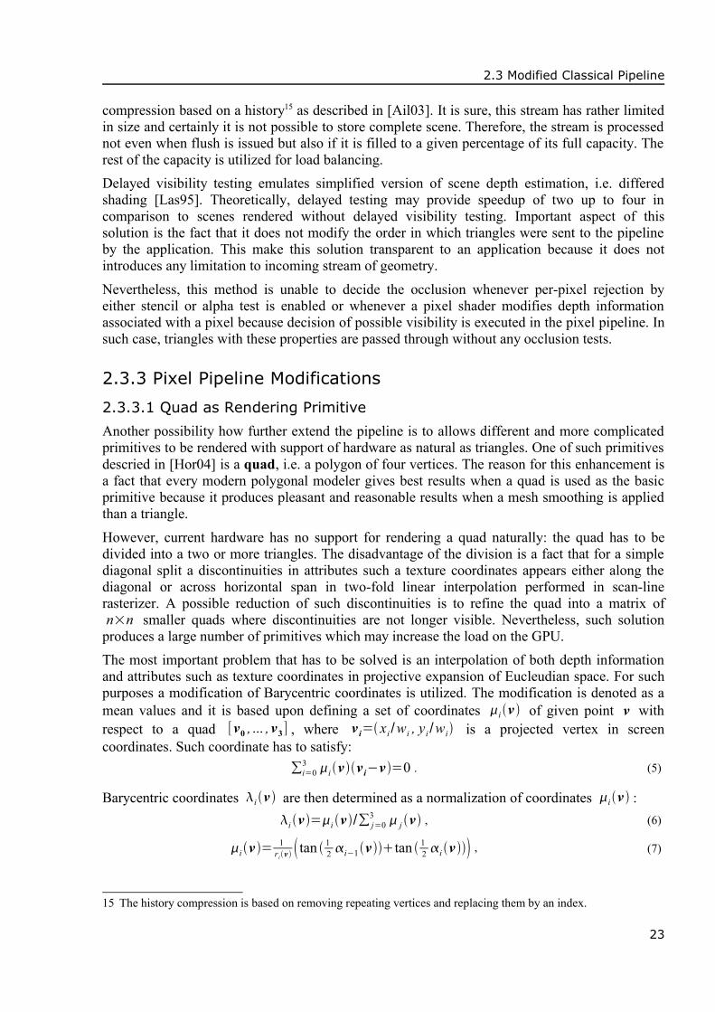
2.3 Modified Classical Pipeline
compression based on a history15 as described in [Ail03]. It is sure, this stream has rather limitedin size and certainly it is not possible to store complete scene. Therefore, the stream is processednot even when flush is issued but also if it is filled to a given percentage of its full capacity. Therest of the capacity is utilized for load balancing.Delayed visibility testing emulates simplified version of scene depth estimation, i.e. differedshading [Las95]. Theoretically, delayed testing may provide speedup of two up to four incomparison to scenes rendered without delayed visibility testing. Important aspect of thissolution is the fact that it does not modify the order in which triangles were sent to the pipelineby the application. This make this solution transparent to an application because it does notintroduces any limitation to incoming stream of geometry.
Nevertheless, this method is unable to decide the occlusion whenever per-pixel rejection byeither stencil or alpha test is enabled or whenever a pixel shader modifies depth informationassociated with a pixel because decision of possible visibility is executed in the pixel pipeline. Insuch case, triangles with these properties are passed through without any occlusion tests.
2.3.3 Pixel Pipeline Modifications
2.3.3.1 Quad as Rendering Primitive
Another possibility how further extend the pipeline is to allows different and more complicatedprimitives to be rendered with support of hardware as natural as triangles. One of such primitivesdescried in [Hor04] is a quad, i.e. a polygon of four vertices. The reason for this enhancement isa fact that every modern polygonal modeler gives best results when a quad is used as the basicprimitive because it produces pleasant and reasonable results when a mesh smoothing is appliedthan a triangle.
However, current hardware has no support for rendering a quad naturally: the quad has to bedivided into a two or more triangles. The disadvantage of the division is a fact that for a simplediagonal split a discontinuities in attributes such a texture coordinates appears either along thediagonal or across horizontal span in two-fold linear interpolation performed in scan-linerasterizer. A possible reduction of such discontinuities is to refine the quad into a matrix ofn×n smaller quads where discontinuities are not longer visible. Nevertheless, such solution
produces a large number of primitives which may increase the load on the GPU.The most important problem that has to be solved is an interpolation of both depth informationand attributes such as texture coordinates in projective expansion of Eucleudian space. For suchpurposes a modification of Barycentric coordinates is utilized. The modification is denoted as amean values and it is based upon defining a set of coordinates i v of given point v withrespect to a quad [v0 , ... ,v3] , where v i= xi /wi , yi /wi is a projected vertex in screencoordinates. Such coordinate has to satisfy:
∑i=03 i v v i−v =0 . (5)
Barycentric coordinates i v are then determined as a normalization of coordinates iv :i v =i v /∑ j=0
3 j v , (6)
i v =1
r i v tan 1 2 i−1v tan 1
2 i v , (7)
15 The history compression is based on removing repeating vertices and replacing them by an index.
23

2 Hardware Architectures
where i v is a signed angle at point v in triangle [v , v i , v i1] and r i v =∣v−v i∣ , i.e. adistance between v and i-th vertex. The important characteristics of i v is that they has hasidentical signs when the point is inside the quad even if the quad is self-intersecting.In order to be able to compute attribute for each point of projected quad, the algorithm utilizes avariable ' i v to compute exact location in projective space. Basically, it is simple perspectiveenhancement of Barycentric coordinates. Appropriate attributes are computed by analogy to ' i v . However, it is possible to interpolate attribute ai /wi and divide it by interpolated 1 /wi
value. Projection enhancement of Barycentric coordinated is defined as:
' i v=i v
wi/∑
j=0
3 j v w j
=i v
wi/∑
j=0
3 j v w j
. (8)
The proposed implementation utilizes a scan-line renderer and benefits from a knowledge ofmaximum number of spans per a single line, which is one for triangles and two for quads. Thissimplifies organization of structures required for list of active edges. Besides that theimplementation may also benefit from a fact that Equation (7) can be expressed with help offollowing:
tan 1 2i=
r i r i1−siT⋅si1
∣s i×s i1∣, (9)
where si=v i−v . This allows computation of coordinate i v from projected point v in screencoordinates. Based on a fact that dot product is linear and both cross product and r i
2 arequadratical, the implementation may utilize incremental modification from the pixel to the pixelaccording to a initial values generated in quad setup phase, similar to triangle.
The benefit of this solution is based on modification of rasterizer only, the rest of the pipelineremains the same. Even though the pure hardware solution is not available yet, results weregenerated utilizing the hybrid GPU solution aided by the CPU for geometry setup. The hybridsolution benefits from a possibility to determine whether the projected point is inside or outsideof rendered quad. For more details and exact description of algorithm used, refer to [Hor04].
2.3.3.2 Displaced Pixels
Besides introducing a new rendering primitive that surely improves the visual quality of therendering with only a minimal performance effect an expectable extension to the pixel pipeline isto enhance output of the pixel shader towards a context modification, i.e. modification ofposition. Currently, shader model allows depth modifications but more effects may be achievedwhen a depth would be enhanced by position modification as it is proposed in [Die04].If implemented, this modification allows implementation of algorithms based on accumulation ofvalues in multiple accumulators according to a definition such as histogram computation or othersolution from image analysis area. These kind of algorithms are currently implementable ongraphic hardware with only high number of passes thus reducing the performance even under theCPU level.
Another area which may benefit from relocatable pixels are particle systems. This enhancementwould allow a particle system to be both simulated and even rendered in a single pass withoutadditional computation and storage costs by utilizing a multiple render targets. Currently, thanksto vertex textures introduced in shader model 3.0, particle systems do not require GPU→CPUdata traffic and may be rendered in two-pass algorithm.
24

2.3 Modified Classical Pipeline
Similar to particle systems this pixel processing enhancement would allow an effective directrendering of curves by simply applying an appropriate definition of the curve. Also, it is assumedthat this extension would allow an effective rendering of a fur with fur parameters stored intextures and based information the pixel may be reallocated to a proper position. Thanks to that,a effecting the LOD could be achieved just by increasing a number of rasterized pixels whenevera furry surface gets closer to the camera.Nevertheless, the extension proposed in [Die04] does not offer a solution for severalimplementation issues. It is clearly visible that such implementation would require both colorand depth buffer with random access, which may reduce the reflectivity of memory writeoperation even if caching based on coherency of changes is enabled.
Also a requirement of additional clipping operation after the pixel has been reallocated in orderto avoid invalid memory access reduces the performance even thought such clipping is similar toa guard-band mechanism described in previous sections. However, this is not the major problemof the implementation.The major difficulty of the implementation is disturbance of pipeline structures that is afundamental for current GPUs. There are synchronization issues in the pixel post-processingwhere a coherence in operations such as an alpha-blending or a stencil/depth-test is required. In acurrent graphic hardware the synchronization is probably solved on a primitive level thusallowing pixel pipeline to run almost unsynchronized, which surely improves the overallthroughput of the pixel pipeline.
2.3.3.3 Order-independent Alpha Blending
Another possibility for improvement if the pixel pipeline is to solve the problem of an alpha-blending × depth buffer, i.e. to provide order-independent alpha-blending. Whenever an alphablended surfaces occur in a scene the application has to handle them separately because thedepth-buffer visibility does not consider the transparency and thus it handles transparent pixels asthey were a solid.The solution proposed by [Ail03] utilizes a FIFO stream in order to store geometry of trianglesand coordinates of their unprocessed pixel. For optimization reasons, pixels are groups into 8×8pixel block that each has a mask of unprocessed pixels. The solution requires a division of pixelshader program into a alpha-modifying part and color/depth-modifying part. This can beperformed automatically and therefore invisible to the application as a part of a device driver.
Every time a triangle with enabled order-independent transparency arrives, it is rasterized, andalpha-modifying shader code is applied. Obtained data are then stored into the stream for laterprocessing as it is described by the Figure 2.3 below.
mark hidden pixels as processedwhile stream.Count > 0:
remove processed triangles from streamclear depth bufferwalk the stream and find highest depth value for each pixelwalk the stream:
if depth value is equal to found one:process pixelblend pixel with outputmark pixel as processed
Figure 2.5: Order-independent alpha blending pixel processing algorithm.
25

2 Hardware Architectures
2.3.3.4 Simple and Effective Anti-aliasing
Another performance issue in the pixel shader pipeline is a question of proper anti-aliasing.Currently, the hardware may perform either full screen anti-aliasing that is rather expensive oranti-aliasing of edges. In latter case, the anti-aliasing is performed even on edges that are not partof the silhouette. In majority of cases these are the only ones where the alias is visible at mostand therefore their proper estimation may save a computational power as proposed in [Ail03].The solution utilizes a simple set of flags for each triangle and its edges. This set indicateswhether is it a inner edge or discontinuity edge. When a triangle arrives, a lookup into a edgehash table is made: if edge is found then the record is remove from a hash table and newlyincoming edge is marked as closing one. Otherwise, a new record is inserted into the table andthe edge is marked as opening one.
During the rasterization, each pixel has a counter assigned. This counter increments whenever anopening edge crosses it and decreased in the case of closing edge. At the end, if the counter iszero then this pixel is not an issue for anti-aliasing because it is either inner pixel or resides ashared edge. For the rest of pixels a supersampling is applied. This approach shall reduce numberof anti-aliased edges to 3—20 % of the total number but it increases memory bandwidth at thesame time.
26

3 GPU Languages and Programming
The GPU provides great amount of functionality accessible by the application in order to eithercompute general purpose solutions or build visual effects. Nevertheless, until now GPUlimitations and capabilities were only described in previous chapters, there was no comment onan actual programming language and/or tool. Therefore, in this chapter an overview of selectedavailable languages is presented.
For each language, its features are described in order to familiarize the reader with languages thatare utilized by solutions described in this document. Only major features are mentioned, fordetails, please refer to particular language specification. Languages are divided according to anintention of their utilization even thought this intention may not force the utilization for suchpurposes.
3.1 Graphical PurposesLanguages intended for graphical purposes are the most widespread languages for the GPUprograming on common graphic hardware. At their beginnings they were intended for enhancingof a visual output during image synthesis, i.e. allowing to program a part of the pipeline.Therefore they have same attributes as the GPU itself.
In a majority of cases their construction is based on shaders that are utilized for various off-linerendering system, such as RenderMan shading language [Han90]. Opposite of this system, theimportant feature is a division of shader code into two parts: the vertex and the pixel shader codefor the sake of the performance. Such division accommodates better to the underlaying structureof the GPU that is basically a pipeline with two processors.According to [Mar03] this feature becomes an important when branching comes to play. In thecase where the compiler does the division between underlaying processing units, the resultingcode may be far too ineffective due to branching in cooperation with inappropriate mixing ofinstructions for the first and the second processing unit. On the other hand, the division made bythe application forces the developer to optimize the code with the division in mind thus resultingto a code of higher performance. Also, it keeps the programming model simply enough.
Languages for graphical purposes may be divided into two groups according to their complexity:
• low-level languages, i.e. basically assemblers. These languages are primary languages for theGPU and they were utilized since the beginning of modern GPUs. They exhibit SIMDbehavior in their instruction as it was described in the Section 2.2 and they are unable tobypass even minor limitations of the GPU. Currently, they are not utilized for both graphicaland general computing on GPUs due to complexity of codes written with them. Therefore,assemblers for the GPU are not described further in this section at all.
27

3 GPU Languages and Programming
• high-level languages that are utilized instead of assembler languages in a majority ofcurrently available solutions. In the most cases they are based on C-language with certainrestriction of its capabilities based on features of the GPU. They also allow handling of fewminor yet annoying limitations such as lacks flow control and non-SIMD behaviorautomatically by the compiler thus simplifying the process of implementation. Currently, thereare many of these languages and those mentioned below are utilized at the most.
3.1.1 Direct3D: HLSLHigh Level Shading Language is a GPU language introduced in a version 9.0 of DirectX [DX05].It shares both syntax and semantics with the Cg language [Mar03] thus making it compatible onthe source code level. In a limited manner the HLSL may be considered as a subset of the Cgeven thought this it mentioned in neither the HLSL documentation nor the Cg specification.
In its fundamentals, the HLSL is based on syntax of C language with a few features from C++such as boolean data type, structure definition, and comments. Due to limitations of the GPU, itis not able to implement complete subset of C language features, i.e. the HLSL is not able both tooperate with pointers and to perform bit-wise operations. The is caused by incapability of theGPU to operate with independent bits of data types and the nature of shader accessible read-writememory. For more details on GPU limitations refer to Section 2.2.
3.1.1.1 Data types
Besides that the HLSL supports C-like preprocessor thus allowing a conditional compilation. Italso extends the C languages by introducing features that allows to utilize capabilities of theGPU. It is mostly matter of new data types including operation definition. The available set ofdata types is striped of pointers and majority of integers with exception of the int data type andit is enhanced by a boolean data type and a new floating-point types.The boolean is utilized for if-branching both static and dynamic. In the case of floating pointnumbers the set is enlarged by types of lower accuracy then the float [IEE85] such as fixedthat represents fixed-point real number and half, which is a floating-point number of halfprecision. These types are utilized due to either restrictions of older GPUs or performance, seeSection 2.2
In order to bypass differences of various shader models the compiler my utilize type with higheraccuracy then the type requested, i.e. the fixed type may be replaced by the half type duringcompilation due to lack of support for the fixed. Similar to that, the int data type is replacedby the float for the majority of cases with exception of loop iterating or array addressingbecause the GPU usually lacks read-write temporary integer registers.
As it was already mentioned in Section 2.2, the GPU supports operations with vectors of up tofour-components in length. It would have seen that this can be implemented with the aid of Carrays. However, in such case the compiler would not be able to distinguish between real array offour floats and a vector of four float components [Mar03]. Therefore, another enhancement thethe data type set is introduces: the vector.
The vector may by of any both numerical and booleans data type and its length is restricted tofour. Syntactically, the vector is denoted as floatn where n is a number of vector components.Similar to vector operation supported by the GPU, the HLSL allows masking and swizzling ofvector components, i.e. it allows to select vector components, modify their position, or multiply asingle component in order to form a new vector of possible different length.
28

3.1 Graphical Purposes
Similar to the vector, the HLSL support a matrix data type of size up to 4×4. This type isemulated by a set of vectors in column-major order. The emulations allows simple yet fastimplementation of matrix-matrix and matrix-vector operations, e.g. matrix-matrix multiplicationmay by implemented as a set of dot products. Syntactically, the matrix is specified similar to thevector and sizes are specified in row-column order, i.e. matrix of 3×4 is denoted as float3x4.
It would be good to note, that all binary numerical operators such as addition, multiplication, ordivision operate over individual elements by default. If matrix operation such as matrix-vectormultiplication is required a special function has to be utilized rather than multiplication operator.The HLSL allows addressing of individual elements via either dot operator or array approach.For example, let there be a need to address a element in second row and first column of matrix mthen such element is selected as m._21, m._m10, or m[1][0]. With exception of the arrayapproach the HLSL allows vector-like operation with elements such as swizzling and masking inorder to create new vectors and/or matrices.
Also, the HLSL supports arrays and structures. Both are accessible as it is common in Clanguage, i.e. via either square bracket operator or dot operator. Syntactically, they are almost thesame as in C with an exception of structures, which utilizes a C++ style of definition.
3.1.1.2 Flow Control, Operations and Functions
Flow control in the HLSL is supported according to particular shader model and the compile isable to bypass few of limitations of the underlaying GPU. The HLSL supports wide range ofcontrol flow constructions with exception of non-structured means of flow control such as labeljumps, i.e. goto.
Nevertheless, the compiler is able to bypass minor limitations of a particular shader model: it ispossible to compile code that contains dynamic branching by computing both branches andutilizing an instruction that selects from two values according to the third one. Similar to that fora static loop the compiler may expand the loop to satisfy requirements of the particular GPU.Calls of user defined functions are also compiled according to actual shader model. The compileris able to bypass a lack of real subroutine call instruction by inserting a function call directly thusincreasing the shader code length. Nevertheless, the compiler is unable to bypass a prohibition ofboth direct and indirect recursion. Parameters a handled according to their modifiers (see below)and unused temporary registers are utilized to create their local copies if required.
In any way, the compiler is unable to bypass a limitation in length of the code, i.e. number ofinstructions. This may be crucial when a loop expanding together with low pixel shader versionis used thus resulting into compiler error. Then the only solution for the developer is either toutilize multiple rendering passes or to follow a proposed automatic decomposition of codedescribed in Subsection 3.3.1.
In order to be able to compute basic vector operation, the HLSL utilizes a set of built-infunctions. These functions are usually a direct counterpart of particular instructions. Thecomplete set can be seen in [DX05] but actual set recognized by the compiler depends onparticular shader model. If an operation is not available such as reciprocal square root utilized invector normalization the compiler does not attempt to emulate the functionality via textures eventhought it is possible.
All operations with exception of branching constructions exhibit a SIMD-like behavior eventhought the underlaying instruction is capable to process a single scalar at the time. This means
29

3 GPU Languages and Programming
the compiler is able to emulate the SIMD behavior by increasing the number of generatedinstruction per operation.Common mathematical functions implemented in a form of a binary operator such as additionand multiply operates over individual elements of utilized vectors and/or matrices. If a vector-matrix multiplication is required a special function mul has to be used. Similar to that, vectoroperations of dot product and crossproduct are implemented in a form of a dot and crossinstruction rather than an operator.
The HLSL supports user defined functions with a syntax similar to the C language. Each shaderprogram should contain at least one function that serves as a shader entry point. Functions maybe overloaded similar to C++, i.e. the function may have similar name but they have to differ innumber and/or type of parameters.
The only enhancement besides the semantics (see below) is a possibility of parameter modifiersthat precedes the parameter data type in its syntax. The modifier influences actual storage andbehavior of particular parameter. Supported modifiers are:
• uniform that denotes a constant accessible from the application.
• in that denotes an input parameter. This is default behavior.
• out that denotes an output parameter. This is usually utilized for shader output values.
• inout that denotes an input and output parameter. This modifier saves a temporary registersthat are utilized for parameters similar to a stack in the case of the CPU whenever a functioncall is requested.
3.1.1.3 Semantics
Besides modifications of the data type set, the HLSL introduces new construction, which denotesa semantics of particular variable and/or function parameter. This construction allows a shadercode to connect to particular registers of the GPU thus allowing to access and modify dataprocessed by the pipeline.
It also allows to connect a variable to a particular constants register that can be set by theapplication directly bypassing the interface of the shader. This also allows a backwardcompatibility with applications that utilize shader codes in assembly language because in suchcase the application has to reference constants by the register name instead of their logical namein the shader code.Semantics is utilized mostly in the entry point of the shader in order to access data from thepipeline. It may by also utilized for a return value of the function to denote the output of theshader code to the pipeline. Syntactically, the semantics is inscribed after the identifier ofparticular code element, to whom is the semantics applied, e.g. a position of the vertex that isgoing to be processed by the vertex shader code is denoted as in float4 pos:POSITION inparameters of the entry point function.
3.1.1.4 Shader Data Input and Output
Input of the shader utilizes two possible sources of pipeline data: varying and uniform. The termvarying denoted a set of registers that contains data provided by the pipeline, i.e. processedelements. The HLSL obtains these data as parameters of entry point. These parameters has tohave both in modifier and appropriate semantics defined.
30

3.1 Graphical Purposes
Uniform denotes basically set of constants including textures provided and accessed by theapplication. These constants may be passed to the code in a form of either a parameter of entrypoint function or a global variable. In both cases a modifier uniform has to be specified.Semantics is optional and can be utilized for connecting the constant to the constant register.Output of the shader allows the code to deliver processed element for further processing to thepipeline. The HLSL specifies an output as either out parameter of entry point or return value ofthe entry point function or combination of both. In either cases, semantics has to be specified andcompiler performs a compile-time checks in order to prevent a shader from ignoring a obligatoryoutputs, e.g. the vertex shader has to set a value of a parameter denoted by POSITIONsemantics.
3.1.1.5 Effect Framework
In order to simplify the use of the shader in the application the HLSL supports concept of effects.An effect is a compound set of techniques where each technique has passes specified that arerequired for proper rendering of effect. For an each pass pipeline settings are provided includingshader code and shader entry points, if the shader is utilized. The whole effect is usually stored ina well-arranged plain text FX file.
From within the application code, the effects loading and constant access is matter of simplefunction calls. Application of the effect the consist of begin-end pairs for both effect and passcalls and a geometry rendered inside these pairs. Even thought this may seems to be a tool aimedonly on composition of visual effects the FX framework may be utilized even for generalprocessing purposes for which a pass in the FX technique is equal to a step in the algorithm.
3.1.2 CgThe Cg language [Fer03, Mar03] is another language based on C language. Is is very close to theHLSL and according to its features the Cg can be denoted as a superset to the HLSL. This makesthe Cg and the HLSL compatible on a source code level. Thus, this subsection contains onlydescription of difference between both languages rather than enumeration of all features thatwere mentioned in previous subsection.
The major feature of the Cg is a platform independence, i.e. it does not distinguishes betweengraphic application programming interface (API). It is possible to utilize it together with eitherOpenGL16 or Direct3D via a special layer that converts Cg function calls into appropriate calls ofunderlaying API.
The Cg introduces a sophisticated use of profiles. The profile is a definition of capabilities andrestriction of particular shader model, pipeline part, and graphic API. As opposed to the HLSLthat utilizes profiles only for check for limitations during a compilation, the Cg allows anoverloading of functions according to specified profile.This feature is important mostly for generating visual effect where the developer may decreasethe quality of the effect of a sake of ability to run on older hardware. For the general processingthis feature is not utilized because the developer usually focuses only on a particular hardwarecombination due to the fact that older hardware may have far too tight restrictions.
Another interesting feature available in the Cg language is a possibility to add functions to astructure thus making it a limited version of classes known from the C++ language. The Cg also
16 In the case of OpenGL the Cg may be able to run better on nVidia based hardware due to an ability to utilizevarious proprietary extensions developed by the nVidia thus making itself more efficient for this hardware.
31

3 GPU Languages and Programming
support a mechanism of interfaces that is utilized for defining of general functionality availablein structures. Such features of structures allow the application to define an array ofdistinguishable elements implementing same interface that is utilize for uniform handling ofthese structures in the shader code [Mar03].The Cg is a language utilized in many application. Its first version were available prior to theHLSL and the GLSL17. Similar to the HLSL it is able to utilize different hardware and it is ableto bypass minor limitations. As distinct to the HLSL, it is capable to cooperate with both DirectXand OpenGL even thought a compatibility issues may appear on some combination of OpenGLand graphic hardware due to driver instability. For a complete specification as well as list ofexamples, refer to [Fer03].
3.1.3 OpenGL: GLSLAnother language that is tightly connected to a specific platform is the OpenGL ShadingLanguage (GLSL) [Kes04]. This language is a part OpenGL 2.0 specification [Seg04] and allowsa high-level programming of the shader utilizing pure OpenGL. Similar to previously mentionedlanguages, the GLSL is based on C-languages and shares many features of the HLSL/Cg.
This subsection contains an overview of differences to the HLSL rather than a completedescription of the language. The difference of the GLSL to the HLSL is a different manner ofpipeline data access philosophy, different syntax of added data types, slightly different meaningof some mathematical operators, lack of profiles, and finally lack of effect (FX) mechanismwithout any replacement.
As distinct from the HLSL and/or Cg, the GLSL lacks a mechanism of profiles. The GLSLexpects a minimal functionality as it is specified by a particular OpenGL Extensions [GLE04]required18 for compilation and application of the shader code. The drawback of this approach isbased on a fact that OpenGL standard specifies only the functionality of valid actions rather thana complete specification thus allowing hardware vendors to handle invalid situation on their own.The actual implementation of extensions is provided by hardware vendors, which may allow theGLSL even for hardware that does not provide all expected functionality such as numericalaccuracy. This may lead to both instability of the solution based on the GLSL or appearing ofartifacts in the case of visual effects. The solution for that is to test for availability of extensiontogether with capability check of utilize hardware via its identification string19.
3.1.3.1 Data Types
Data types utilized by the GLSL are pretty the same as for the HLSL with only a few differencesmostly in syntax area. Similar to the HLSL, integers are supported but they are expected to be of16-bit accuracy. It also assumes that integers are processed naturally without hidden conversionto floating-point numbers as it is common among HLSL/Cg compilers. Floating-point aresupported without any further distinction between various accuracies because the GLSL expectsa particular functionality rather than providing a backward compatibility with older hardware.
Vectors are supported with a slightly different syntax, i.e. a vector is denoted as tvecn where nis number of components and t denotes the type: i for integers, b for boolean, empty for
17 OpenGL Shading Language, see Subsection 3.1.3.18 In order to utilize the GLSL the application has to be able to access ARB_shader_object and either
ARB_vertex_shader or ARB_fragment_shader or both.19 The identification string can be retrieved via function glGetString.
32

3.1 Graphical Purposes
floating-point. Components of vectors are accessible via dot operator similar to the HLSL.Swizzling and masking is supported too.Matrices are supported as well and similar to vectors, the syntax is different then that of theHLSL, i.e. tmatn denotes a matrix with elements of type t and size of n×n. All matrices arestored in a column major order. Access to individual components of the matrix is available viaarray-like approach and their swizzling and/or masking is not supported.
3.1.3.2 Flow Control, Operations and Functions
Flow control support in the GLSL is similar to that of the HLSL. The language supports widerange of constructions such as loops and if-branching with exception of non-structural jumpssuch as goto. However, the actual compilation results depend on implementation provided bythe hardware vendor.As it is common among GPU languages, all operations exhibits SIMD-like behavior.Mathematical binary operator of addition and multiplication are component-wise operations in amajority of cases. Nevertheless, for both vector-matrix and matrix-matrix multiplication theoperation performed is similar to appropriate mathematical operation, i.e. vector-matrixmultiplication applies a matrix to a vector. Component-wise version of these operation isavailable in a form of a special function.
Similar to the HLSL, the GLSL provides a comparable set of built-in functions. Also, it allowsdefinition of user functions. The syntax is similar to both the C language and the HLSL.Parameter modifies are supported with an exception of uniform that is omitted due to adifferent approach for pipeline data access. Overloading is supported similar to the C++, i.e. thefunction may have similar name but it has to differ in either number of parameters or their types.
3.1.3.3 Shader Data Input and Output
As opposed to the HLSL and the Cg, the GLSL does not support semantics. Rather then that itutilizes a system of predefined variables and constants that is close to a mechanism available inRenderMan shaders [Han90]. All predefined elements are denoted by prefix of gl_ and theGLSL distinguished following forms:
• Predefined variables that are utilized in order to pass data required by the pipeline from theshader.
• Varying variables that allow a data communication between the vertex shader and the pixelshader. The GLSL provides a set of predefined variables that represent common data passed tothe pixel pipeline such as texture coordinates, diffuse color, etc. This set is available in bothvertex and pixel shader.
The developer is able to define own varying variables in order to transfer data between customvertex and pixel shader. The connection between variables is established during linking phasevia compliance of identifiers. The varying variables are denoted by modifier varying.
• Uniform variables that contains either data set by the application or settings of the pipeline.This allows a shader to access various data from pipeline settings such as transformationmatrices, lights, etc. Uniform variables are denoted by modifier uniform.
• Attributes that contains vertex data passed to the shader by the application.
• Constants that provides various maximum values for pipeline settings, e.g. maximum numberof lights, maximum number of temporary variables, etc.
33

3 GPU Languages and Programming
3.1.4 ShEven thought mentioned programming languages for the GPU are high level, the mechanism oftheir connection to the underlaying graphical API is a rather low-level. If a mechanism such aseffect framework is not utilized, the developer has to perform a list of API calls in order to utilizea single shader program.Also, the shader code is not a part of the application source code processed by the compiler, iteither resides in an external text file or is stored in a string inside. Nevertheless, its compilationincluding syntactical and semantical check is performed either at runtime or by separate tool off-line thus complicating the development.
A library that tries to address this annoyance is the Sh [McC02, McC04]. It is based on amechanism of metaprogramming that is basically a possibility to insert code written in differentlanguage into the source code and provide binding by default, i.e. it automatically provides codenecessary for utilizing given expression in different language such as the SQL query.The idea of metaprogramming utilized in the Sh is based on a fact that a proper sequence offunction calls from a specific API may lead to a construction of code in different language. If thistranscription of function calls is done during a setup phase the performance of such solution isalmost the same as it would when compiled all at once.
Also, this idea of function calls allows implementation of such system without requirement ofspecial purpose compiler. When underlaying language is capable of operator overloading andother similar language constructions the inserted code does not differ from original code in adifferent language. The Sh utilizes the C++ language together with the OpenGL in order to createa tool that allows definition of a shader inside the application code.Thanks to the level of abstraction, the Sh can be considered as a hybrid between languages closerto the hardware and languages with higher level of abstraction, see Section 3.2. The shader in theSh library is then a class or a template with fields that contains both shader code and applicationaccessible variables, i.e. uniform variables.
In order to obtain data from the pipeline and provide processed data back channels are utilized. Achannel is basically a sequence of elements similar to channels of data in the pipeline such asposition or texture coordinates. The channel is filled either by underlaying OpenGL at the verybeginning of the computation or by another shader if shader aggregation is utilized.
3.1.4.1 Shader Composing
The construction of the Sh and abilities of the C++ language allows a rather straightforwardimplementation of shader composing [McC04]. Shader composing is basically a attempt for realmodularity of the shader thus allowing to create a complex shader based on a functionality ofanother simpler shader with only a minimal effort and a possibility of applying object orientedprogramming mechanism.The basic implementation utilizes a operation overloading to create new set of operators thatallows combination of shaders: a connection operator denoted as << and a combinationoperator denoted as &. The combination operator then allows a process data by both involvedshaders sequentially, i.e. the channel generated by the first shader is processed by the second one.The combination operator combine output channels of both involved shaders to a set of channels,i.e. the stream, see below.
34

3.1 Graphical Purposes
In order to improve the performance an optimization is utilized based on dead code removal.Nevertheless, the optimization is not able to distinguish a real computation from a redundant one,e.g. when two shaders are combined and both compute the same value but differ in approach. Forsuch cases an another mechanism has to be employed in order to explicitly denote required pathof channel processing, see below.
3.1.4.2 Manipulators and Streams
The possible enhancement of the Sh towards a shader composing with decreased redundancy is amechanism of manipulators [McC04]. This mechanism allows to operate with individualchannels directly by influencing their routing. This improves the overall performance by denotinga dead code and it allows more sophisticated combination of existing shaders.
During the creation phase the mechanism generates a code that provides connectivity betweenblocks according to a description provided by the application. The description is based onoperators mentioned above and a set of manipulators divided into following groups [McC04]:
• Primitive manipulators that provide a shader program rather than a stream because they areable to operate with individual elements. It allows keeping and discarding of channelsincluding a possibility to translate elements in the channel via texture mapping, i.e. utilizethem as texture coordinates.
• Fixed-input manipulators that are able to operate with a fixed number of channels in orderto create n copies of channel, pass n channel through that may be utilized during acombination operation, and discard channels.
• Expandable-input manipulators that allows manipulating a position of channel thusallowing a redirection of channel to another operation. This may be required when a channelis duplicated and one duplicate has to be utilized as a third input of the block.
Together with manipulator mechanism of streams is utilized. The stream is simply an orderedset of channels that uses combining and connecting operator. The combining operator creates anew stream from a two streams and/or channels. The connecting operator connects the stream toa shader.The shader may be applied to the stream but also it may remain as a shader program withparticular inputs connected to channels obtained from the stream. Such inputs are then denoted asparameters. In addition to that the stream mechanism has a capability to convert a parameter backto a an input by a special operator >>. This allows modification of values that were considered tobe constants for the whole shader, e.g. kd coefficient in Phong lighting equation [Wat99].
3.2 General PurposesNo matter how much abstraction is available inside of the code, languages intended for graphicalpurposes still reflects the GPU structure pretty well. If an application requires general processingon the GPU the solution has to perform the computation in therm of primitive rendering. This israther annoying because it introduces additional code for bypassing nature of the GPU, whichsurely complicates the implementation.
On the other hand, there are languages that tries to provide a higher level of abstraction thushiding the true nature of the GPU and the underlaying API. Also, such languages create amechanism similar to those of virtual machine where the real implementation is decided at
35
3 GPU Languages and Programming
compilation time according to the nature of requested operation. This simplifies theimplementation process. Nevertheless, the performance of such implementation is usually lowerthen the that of specialized GPU solution due to generality of the language.
3.2.1 Brook for GPUThe Brook [Buc03] is a stream-oriented language intended for stream processing that isdeveloped for specialized high performance stream machines. The pipeline nature of the GPUallows almost direct conversion of the Brook to the GPU with only a few limitations based onfeatures of the GPU thus creating a general tool for implementing general processing algorithmson the GPU.
3.2.1.1 The Language
As it is common among GPU languages, the Brook is based on the C language with only a fewenhancements concerning a possibility of streams denoted by <length> and kernel parameterspecification. Streams are essential part of the Brook and represents a homogeneous list ofelements of numerical type including arrays and structures. Streams are processed by a kernels.
Kernel is basically a function that process elements of input streams and it computes new valuesthat are stored into an output stream. Besides the input and output streams the kernel is able toaccess global variables, examine position in the stream, and read other parameters both scalarsand arrays that are utilized mostly for gather operation, see below. In common situation, thekernel pushes to the output stream at least as many elements as it is contained inside the inputstream. All input elements should have same length for an execution being success.
Code that is inside the kernel function has several limitation that allows its implementation withhigh throughput or simple parallelization. The fist important issue is a lack of memorymanagement known from the C language including pointers inside the kernel function. Also,library calls as well as non-structural flow controls such as goto are not allowed.
Next important feature of the kernel is that for each single execution of the kernel only one valueis available from each of input streams. This disables a possibility for the kernel to browse or tolook-ahead in the input stream. The execution continues until all data in input streams areprocessed.In order to be able to implement various summing operation, the kernel kernel is able to performa reduction operation, i.e. to produce less elements that it is the count of elements in the inputkernels. It is possible to reduce either to a single value or to a stream of values where a number ofvalues from input stream reduced to a single element of the output stream is determined from theratio of input/output stream length.The Brook language consist of a specialized compiler and a runtime. The runtime providesfunctionality for executing of kernels, i.e. it distributes data for parallel processing if possible andit is able to generate iteration stream that contains preinitialized sequential values utilized forvarious gather/scatter operations. It also provides a set high-level stream operators formanipulating stream elements such extracting part of stream or merging streams together.
3.2.1.2 GPU Implementation
As it was already mentioned, thanks to the pipeline of the GPU is it possible to implement theBrook on the GPU thus creating a general tool for general processing on the GPU. Nevertheless,
36

3.2 General Purposes
there are differences in comparison to the Brook specification [Buc03] based on limitations ofthe GPU.One of the difference is the maximum length of the stream which is based on maximum size ofthe texture and numerical accuracy of the particular GPU because the implementation utilizestextures of floating-point elements for indexing a stream. In the case of 1D streams, if suchstream would be stored in a form of 1D texture the limitation would be far too restrictive20.
Therefore, the stream is wrapped over the whole 2D texture utilizing a mapping function thatcomputes texture coordinates according to the index. The index is basically an integer and thus itrequires a loss-less conversion when converted to a GPU natural data type such as float, i.e. itrequires that all its bits in mantissa are valid. This make length of mantissa21 crucial formaximum index and thus limiting the stream maximum length.The GPU implementation supports additional data types common for the GPU, i.e. vectors oflength up to four-components are supported. Also, structures are allowed: the implementationutilizes multiple textures, one for each member of particular structure. Data types unsupported bythe GPU are not allowed.
The kernel also exhibits few limitations according to the nature of the GPU: it is not possible toperform any operation requiring an inter-kernel synchronization such as writing to a globalvariable. Actual implementation utilizes the pixel shader for computations and stores a result to atexture by performing a direct rendering to a texture. If such capability is not available22 theimplementation may well utilize various copying operations. The execution is the performed viarendering of a quad over the whole surface of the target texture.
Multiple output streams are supported but they have to be implemented via multiple passes andkernel splitting due to the fact that for a majority of GPUs is able to store only a single fourcomponent vector, i.e. they does not support multiple render targets. Despite the fact the deadcode optimization for split kernels is utilized the slowdown is almost twice in comparison tosingle pass approach [Buc04].
Similar to multiple output streams, it is not possible to perform reduce operation fully asdescribed in the Brook overview, see previous subsection. Implementation of reduce operationutilizes solution similar to that described in [Krü03] that has a complexity of O log n where nis a ratio of input/output stream sizes, see Subsection 4.4.3.The performance gained by utilizing the Brook for GPU is a little bit worse than on specializedGPU solution but still better then similar optimized CPU solution23. The limitation ofperformance is caused by multiple passes. Also, the overall performance results may beinfluenced by limited fillrate and lower texture access bandwidth [Buc04]. Nevertheless, thedevelopment time of specialized GPU solution is much longer than that of the Brook and thedeveloper has to deal with the API. For the Brook, the underlaying API is hidden.
20 Currently, the maximum size of a texture for a common GPUs is either 2048×2048 (Ati) or 4096×4096 (nVidia).21 The maximum length of a number is usually 24 bits according to the floating-point number format s23e8
(nVidia). For some GPU the length is only 17 bits due to lower accuracy of s16e7 format (Ati).22 This is an issue of the OpenGL prior to OpenGL 2.0 due to lack of render-to-texture mechanism proposed in the
specification of ARB_pixel_buffer_object [GLE04]. If the mechanism is not available theimplementation utilizes a mechanism of pbuffers which is rather slow and bound to a specific operating systemplatform.
23 For some cases it is possible to gain speedup of up to 7× in comparison to optimized CPU implementation.
37

3 GPU Languages and Programming
3.3 Language Enhancements
3.3.1 Large Code DivisionSolutions that utilizes the GPU in order to gain performance in both effect rendering and generalprocessing has to handle several GPU limitations such maximum program length, number ofavailable texture samplers, size of temporary memory, and number of register for vertex shaderto pixel shader data transfer.Even thought some of these limitations may be considered negligible thanks to the improvementof capabilities in newer shader models it can be expected that either some of them remainslimited or the complexity of the shaders increases following the improvements. Nevertheless,when the program is overrunning boundaries of limitations the common solution is to usemultiple passes, i.e. partition the code to create shorter codes with lower requirement onresources.
Surely, this partitioning can be handled manually but such solution suffers when a boundaries aremoved thanks to improvements. Therefore an automatic partition mechanism implemented in acompiler would be handy. A possible solution denoted as recursive denominator split (RDS) isproposed in [Cha02].The RDS utilizes a directed acyclic graph (DAG) generated during compilation phase. Each nodein the DAG represents a hardware-mapped operation, each link then denotes a dependency ofvarious operations. The basic version of the RDS utilizes a merging operation over the DAGtogether with a heuristic in order to provide a solution that has minimum number of passes. It isassumed that each pass leads to both time and space overhead.
The merging operation is handled by a greedy bottom-up algorithm. The algorithm utilizes aconstruction of subregion as a set of all non-marked recursive obtained children of a node Nincluding the node N. The merging algorithm obtains all direct children of the node N to form alist L. Form this list all possible subsets S of specified length are selected.For the given subset S and the node N the algorithm constructs a subregion that is then testedagainst a possibility of being mapped on a hardware in single pass. If the test is not successful thelength of subset S is reduced and algorithm continues. If more then one subregion is mappablefor given length than a cost-based merge heuristics is utilized.
Also, the algorithm utilizes a heuristics based on special handling of multiple referenced nodes(MR) is utilized, where the MR is a node with multiple parents. The heuristics then decidewhether the MR node is recomputed thus saving both space and passes or saved thus saving bothcomputation time and instructions.In order to partition the DAG properly a partial denominator tree (PDT) is constructed. The PDTis a derivate of DAG and consists only from root, the MR, and partial denominator nodes. Apartial denominator node is a node the closest to a particular MR for which is true that all pathsfrom that MR to root goes through such node.
Algorithm that utilizes both merging operation and the PDT is denoted as RDSh and its flowchart is available in the Figure 3.1. The algorithm divides the DAG according to the PDT thusmarking boundaries of node regions. The marking is performed during the merging step in orderto denote all nodes that cannot be merged with their parents. The complexity of the algorithm is
38

3.3 Language Enhancements
O n g n , where n is number of nodes and g(n) is a cost of checking if set of nodes can bemapped.
function RDSh:P' ← root node of the PDTSUBDIVIDE(P')
function SUBDIVIDE(T'):if subregion(T) is mappable (valid):
L ← children of T' (order given by postorder traversing of DAG)for each K of L:
Subdivide(K')if K is MR:
use heuristic to decide whether to save or recomputeapply bottom-up greedy merging to node T
mark pixel as processedFigure 3.1: Flow chart of RDSh algorithm. All variables denoted with apostrophe are performed over the PDT, the
rest over the DAG.
The drawback of the RDSh is the fact that it performs a heuristic based on rather local criteria. Itonly find one possible combination of regions without any further checking for optimality. Inorder to bypass that disadvantage the RDS algorithm is introduced.The RDS performs a limiter search together with cost evaluation to decide which MR node tosave and which to recompute. It basically iterates through all MR nodes and for each node M aRDSh is executed twice. First, for the case the node M is marked, i.e. it has to be saved. Second,for the case the node M in not marked, i.e. it can be recomputed. Afterwards, the algorithmevaluates costs for both version thus deciding if the particular mark of the MR node is fixed ornot. The complexity of the RDS algorithm is O n2 g n .
Both algorithm tries to save number of passes in order to improve the computation time and toutilize GPU computation power. The RDS provides worse performance of O n3 in exchangefor better partition quality then the RDSh. Nevertheless, the real performance of the outputheavily depends on cost-based heuristics that has to match attributes of particular GPU. For exactmeasured result of a single experiment, refer to [Cha02].
39


4 GPU/Hardware Aided Approaches
This chapter contains selected GPU-aided solution of several problem that exhibits a possibilityto be implemented on the graphic hardware in order to gain performance. The description isaimed on utilization of the GPU rather than a problem that is solved and thus this chapter shouldgive the reader overview on various approaches for using resources available on the GPU
4.1 Local Illumination
4.1.1 Shading and MaterialsShading and lighting is one the fundamental tasks of the computer graphic that is solved ongraphic hardware. Due to the pipeline nature of the graphic hardware, only local illumination iscomputed, i.e. illumination is solved only for particular point in the space not considering the restof the scene. This approach has several disadvantages that has to be solved by several emulationtechniques. A major disadvantage of the local illumination is a lack of shadow computationwhose solutions are introduced in Subsection 4.1.2.
Local illumination based shading is basically computation of a bidirectional reflectance function(BRDF) for given point on a surface in the scene viewer from given viewpoint and lighted by agiven light. Currently, there are many of these models that tries to approximate the mechanism[Wat99] but not all of them are simple enough to be implemented with reasonable performance.Surely, it is possible to replace the function by a lookup table but in such case it leads to four-dimensional array that is not available not even in current GPUs as it is mentioned in [Hes99].Current GPUs allow custom operation per pixel and thus in the case of a simple BRDF the directimplementation is possible. An example of such function that computes shading Ip at given pointp for a point light stored in infinity is a Phong model [Pho75] described by the following:
I p=C p [cos1 −k d k d ]W [cos] , (10)
where Cp is the reflection coefficient of surface at point p for certain wavelength, kd is aenvironmental diffuse reflection coefficient and W is a function of specular reflected lightand incident light. Angle α is angle between vector l that points to the light source and normal n.Angle β is the vector between vector of reflected light and vector v that points to the viewer. Thecoefficient γ is the a power of specular reflection.In order to be able to compute the Equation (10) for each pixel, the GPU has to supply normal foreach pixel. A common approach for providing the requested data to the pixel shader is to utilizetexture coordinates because they are interpolated over the surface thus providing a estimation ofa values for each pixel.
41
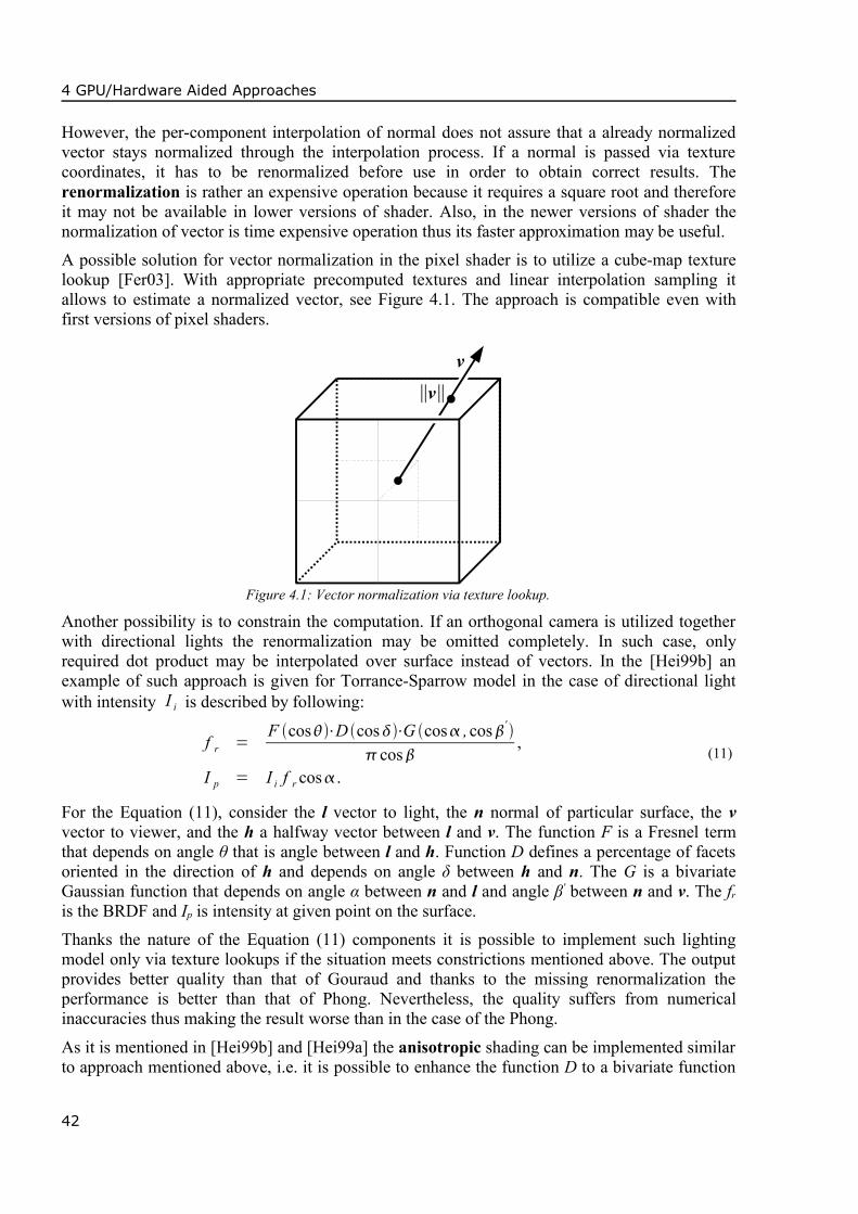
4 GPU/Hardware Aided Approaches
However, the per-component interpolation of normal does not assure that a already normalizedvector stays normalized through the interpolation process. If a normal is passed via texturecoordinates, it has to be renormalized before use in order to obtain correct results. Therenormalization is rather an expensive operation because it requires a square root and thereforeit may not be available in lower versions of shader. Also, in the newer versions of shader thenormalization of vector is time expensive operation thus its faster approximation may be useful.
A possible solution for vector normalization in the pixel shader is to utilize a cube-map texturelookup [Fer03]. With appropriate precomputed textures and linear interpolation sampling itallows to estimate a normalized vector, see Figure 4.1. The approach is compatible even withfirst versions of pixel shaders.
∥v∥
v
Figure 4.1: Vector normalization via texture lookup.
Another possibility is to constrain the computation. If an orthogonal camera is utilized togetherwith directional lights the renormalization may be omitted completely. In such case, onlyrequired dot product may be interpolated over surface instead of vectors. In the [Hei99b] anexample of such approach is given for Torrance-Sparrow model in the case of directional lightwith intensity I i is described by following:
f r =F cos⋅D cos⋅G cos ,cos'
cos,
I p = I i f r cos .(11)
For the Equation (11), consider the l vector to light, the n normal of particular surface, the vvector to viewer, and the h a halfway vector between l and v. The function F is a Fresnel termthat depends on angle θ that is angle between l and h. Function D defines a percentage of facetsoriented in the direction of h and depends on angle δ between h and n. The G is a bivariateGaussian function that depends on angle α between n and l and angle β' between n and v. The fr
is the BRDF and Ip is intensity at given point on the surface.
Thanks the nature of the Equation (11) components it is possible to implement such lightingmodel only via texture lookups if the situation meets constrictions mentioned above. The outputprovides better quality than that of Gouraud and thanks to the missing renormalization theperformance is better than that of Phong. Nevertheless, the quality suffers from numericalinaccuracies thus making the result worse than in the case of the Phong.
As it is mentioned in [Hei99b] and [Hei99a] the anisotropic shading can be implemented similarto approach mentioned above, i.e. it is possible to enhance the function D to a bivariate function
42
4.1 Local Illumination
depending on an angle δ and an angle between facet normal and surface tangent vector. Besidesthat, it is possible to utilize Banks model that represents an approximation of anisotropicshading. For details on that model, refer to both [Hei99b] and [Hei99a].Another common operation utilized by many approach is a operation that modifies the renderedsurface thus allowing to simulate various small details such as dents or scratches. Themodification is only visual, i.e. the geometry and thus silhouette remains the same. One ofcommonly used techniques that allows to create such effect is a normal mapping.
The normal mapping [Fer03, Ern98] is a modification of normal per pixel that is utilized duringper-pixel shading according to application supplied texture. The original normal may be onlyperturbed but in a majority of cases it is replaced completely. This allows to fake the surface inorder to hide coarseness of the model, i.e. it allows a model with low polygonal count pretend tobe a highly detailed one.
In order to utilize a normal from the normal map during per-pixel computation, the space andother components such as lights has to be transformed to a tangent space. The tangent space isdefined by an orthogonal basis of original unperturbed normal n, tangent vector t, binormalvector b for particular triangle. A transformation of point p to a vector vTS in the tangent spacewith origin in a point ps can be expressed as matrix-vector multiplication:
vTS = vT⋅[ t ∣ b ∣ n ] ,v = p− ps .
(12)
Afterwards, the triangle lies in the of base plane xy and its normal nTS is pointing straight up, i.e.it is basically a vector 0 ;0 ; k , k0 . This allows a replacement of the normal nTS with anormal loaded from the normal map. For more details, refer to [Ern98, Fer03, Hei99a].
4.1.1.1 Procedural Solid Textures
The drawback of textures as a base of material is a possibility of a pattern to emerge whenrelatively small texture is mapped to a large surface. Such pattern is rather disturbing because itis a feature that an eye easily catches on. The solution for such surface is to utilize a mechanismcommon in off-line renderers: a procedural texture.
Procedural texture is a texture defined by a function with surface coordinates as parameters.However, computation of such function for each pixel may introduce visual artifacts due to viewdependency of function arguments interpolated over surface. Also, the function may be far toocomplicated to be computed in a single pass together with other visual effects generated in real-time. Therefore, a mechanism has to be utilized to that allows preprocessing in order to reducethe procedural texture sampling to a texture lookup during object rendering.
A solution proposed in [Car02a] utilizes a known mechanism of mesh atlas and tries to improvesthe visual quality of the output by employing a mip-mapping and thus reducing aliasing duringprocedural texture application. Also, it handles artifacts appearing close to a triangle edge thatare caused by an application of bilinear texture sampling together with tight packing of trianglesin the mesh atlas, i.e. the samples may be disturbed by values from other triangles. The algorithmutilizes following steps that are with exception of the first one performed on the GPU:1. Unwrap mesh to a 2D texture thus create a mesh atlas, i.e. compute texture coordinates.
2. Store surface coordinates to the texture by rendering unwrapped mesh.3. Compute surface texture utilizing a precomputed surface coordinates from previous step.
4. Map the texture to real object during real-time rendering similar to regular texture mapping.
43
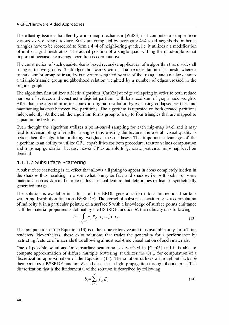
4 GPU/Hardware Aided Approaches
The aliasing issue is handled by a mip-map mechanism [Wil83] that computes a sample fromvarious sizes of single texture. Sizes are computed by averaging 4×4 texel neighborhood hencetriangles have to be reordered to form a 4×4 of neighboring quads, i.e. it utilizes a a modificationof uniform grid mesh atlas. The actual position of a single quad withing the quad-tuple is notimportant because the average operation is commutative.
The construction of such quad-tuples is based recursive application of a algorithm that divides alltriangles to two groups. Such algorithm works with a dual representation of a mesh, where atriangle and/or group of triangles is a vertex weighted by size of the triangle and an edge denotesa triangle/triangle group neighborhood relation weighted by a number of edges crossed in theoriginal graph.The algorithm first utilizes a Metis algorithm [Car02a] of edge collapsing in order to both reducenumber of vertices and construct a disjoint partition with balanced sum of graph node weights.After that, the algorithm refines back to original resolution by expansing collapsed vertices andmaintaining balance between two partitions. The algorithm is repeated on both created partitionsindependently. At the end, the algorithm forms group of a up to four triangles that are mapped toa quad in the texture.
Even thought the algorithm utilizes a point-based sampling for each mip-map level and it maylead to oversampling of smaller triangles thus wasting the texture, the overall visual quality isbetter then for algorithm utilizing weighted mesh atlases. The important advantage of thealgorithm is an ability to utilize GPU capabilities for both procedural texture values computationand mip-map generation because newer GPUs as able to generate particular mip-map level ondemand.
4.1.1.2 Subsurface Scattering
A subsurface scattering is an effect that allows a lighting to appear in areas completely hidden inthe shadow thus resulting in a somewhat blurry surface and shadow, i.e. soft look. For somematerials such as skin and marble is this a crucial feature that determines realism of syntheticallygenerated image.
The solution is available in a form of the BRDF generalization into a bidirectional surfacescattering distribution function (BSSRDF). The kernel of subsurface scattering is a computationof radiosity bi in a particular point xi on a surface S with a knowledge of surface points emittanceei. If the material properties is defined by the BSSRDF function Rd the radiosity bi is following:
bi= ∫x j∈S
e j Rd x j , xid xi . (13)
The computation of the Equation (13) is rather time extensive and thus available only for off-linerenderers. Nevertheless, these exist solutions that trades the generality for a performance byrestricting features of materials thus allowing almost real-time visualization of such materials.One of possible solutions for subsurface scattering is described in [Car03] and it is able tocompute approximation of diffuse multiple scattering. It utilizes the GPU for computation of adiscretization approximation of the Equation (13). The solution utilizes a throughput factor fij
then contains a BSSRDF function Rd and describes a light propagation through the material. Thediscretization that is the fundamental of the solution is described by following:
bi=∑j=1
N
f ij E j (14)
44
4.1 Local Illumination
Besides that, the solution utilizes a multidimensional mesh atlas defined in the Subsection4.1.1.1. The mesh atlas introduces a hierarchy into the mesh and it allows selection of the LODvia the mip-map mechanism. The algorithm requires off-line preprocessing step to generate meshatlas and during the rendering it requires three passes.
The preprocessing step deals with creation of links between patches in order to be able toevaluate the Equation (14). Also, it estimates the throughput factor. First, it builds a mesh atlasand then it utilizes a priority queue to build links between given patch and l patches and/orgroups of patches with most highest throughput factor by utilizing a mesh atlas hierarchy.The selection start from the root and it is based on expanding of top of a throughput factorordered queue. Selection stops when the queue contains l links with appropriate throughputfactor. Links are then stored to textures, each link containing an uv-coordinate to a mesh atlastexture, throughput factor, and LOD of target patch/patch group.
The computation the runs in three steps:
1. Emittance map computation that lights the mesh stored in the mesh atlas texture modulated bythe Fresnel term. The output is stored to a texture.
2. Scattered irradiance map generation that utilizes precomputed links and output of previousstep. The LOD for a particular link is computed via automatic mip-map generation. As in theprevious step, the output is rendered to a texture similar to mesh atlas texture. This is the mosttime extensive step.
3. Final rendering of object that samples a scattered irradiance map and modulates it by inverseFresnel term to obtain radiosity of the object outside. The value is further modulated by acommon surface lighting forming a color for a given surface pixel.
The performance of the solution allows real-time or at least interactive generation of outputwhose computation time depends on a resolution of the mesh atlas texture and a maximumnumber of links. The preprocessing step has to be performed off-line because its computationtime is out of interactivity boundary. Nevertheless, the preprocessing has to be executed onlyonce because it depends on a shape of the object. Thank to the nature of the last step, the solutionmay be mixed with other shadowing techniques freely.
4.1.2 Shadows
4.1.2.1 Stenciled Shadows
Shadows are one of the important depth cue known, i.e. they allows estimation of relative objectspositions. Shadow may be divided into two categories: soft and hard shadows. While there aremany solutions for the hard shadow real-time rendering, the realistic soft-shadow in the real-timeis still an area of almost basic research. One of the first solutions for hard shadows able to utilizegraphic hardware and therefore able to reach real-time frame rates is a technique basedestimation of a shadow volume [Cro77].
Shadow volume is a volume formed by a shadow caster. If a polygon model is rendered it ispossible to estimate the shadow volume from the edges of a silhouette visible from the light.Such edge is detected by a dot product of incident faces with a light direction: if signs of dotproducts are different than the edge is a silhouette edge.A silhouette edges form a loop of lines that when extruded according to a light direction forms aloop of quads that defines edges of shadow volume. In order to apply a shadow volume to the
45

4 GPU/Hardware Aided Approaches
scene the algorithm utilizes a stencil buffer that allows pixel discarding according to twoconditions. Shadows are rendered in following steps:
1. Render scene including depth information in the depth buffer and clear the stencil buffer.2. Construct a shadow volume mesh for given light and object.
3. Render all back-facing triangle from the shadow volume geometry without modifying thedepth buffer. Increment stencil buffer for particular pixel if a depth test fails, i.e. detect pixelsthat may be inside the shadow volume.
4. Render all front-facing polygon from the shadow volume geometry similar to the previousstep. Decrement a stencil buffer if a depth test fails, i.e. omit pixels that are in front of theshadow volume from the viewer viewpoint.
5. Rendering a shadow color quad over the whole scene and modify pixels whose stencil buffervalue is larger then zero, i.e. pixels that lie inside the shadow volume.
The algorithm allows real-time hard shadow rendering on the hardware that support stencilbuffers. The resulting shadows does suffer from aliasing issues and offers high quality hardshadows along the complete scene. The drawback of the algorithm is its requirement ofadditional geometry that has to be recomputed whenever a light-object relative position changes.Also, the implementation may suffer from higher requirements on a fill rate and triangleprocessing performance and the fact that is does not allow reduction of quality for the sake ofbetter performance.
4.1.2.2 Shadow Map
Generation of hard shadows from the geometry described above is a task that is rathercomputationally extensive because it requires rendering of geometry whose complexity dependson the particular model. Also it has additional requirements on fill-rate capabilities of graphichardware and requires additional geometry to be computed according to a light-object relativeposition. The only benefit is that it is able to render precise hard shadows on almost everygraphic hardware with stencil buffer support.Nevertheless, thanks to the programmability the GPU is able to perform various per-pixeloperation for shading during which a shadow may be estimated as well according to a shadowalgorithm proposed in [Wil78]. The algorithm is rather simple and benefits from a hardwaresolution of visibility issue: the depth buffer. The hard shadow computation is performed in twosteps:
1. Compute a shadow map, i.e. depth information for a scene from a viewpoint of the light.
2. Render scene and for each generated point on a surface apply the shadow map by a texturelookup. A point p is transformed to the light space point p l u , v , d and utilized for ashadow map texture lookup in order to obtain a depth of nearest pixel for given positionvisible from the light. If the depth is higher then p lies in the shadow.
The algorithm is simple and offers a real-time framerates even for complex scene. The drawbackof the algorithm is a limited resolution of the shadow map: for an object with high distance fromlight an aliasing issue occurs. The solution is either to increase the resolution thus moving thealiasing issue further in distance or to utilize hierarchical approach to estimate accurate hardshadow or to limit the light range. Nevertheless, for a majority of real-time application such asgames the aliasing issue is ignored for a sake of the performance.
46

4.1 Local Illumination
4.1.2.3 Soft Shadows
A hard shadow is a product of lighting by a point light such as bulb or sun. This is usuallysatisfactory for a majority of scenes but in the case a non-point light such as artificial lightingwith a lampshade a soft shadow has to be generated, i.e. a half-shadow has to be added to theedge of hard shadow.
A possible solution for this problem would be to sample the area light with point light and thenblend resulting shadows together. This produce reasonable realistic results but is rathercomputationally extensive because it requires very high number of samples for a single light.Thus, it is not applicable for real-time rendering. Another possibility is to utilize anotherapproach that is able to simulate believable soft shadow.A solution proposed in [Arv04] emulates a soft shadow by preparing a two lights map for asingle shadow caster. The algorithm utilizes basically an enhanced version of shadow mappingwith additional geometry and light/shadow maps. In order to provide believable result a half-shadow is divided to a outer half-shadow fading from original hard shadow edge to fully litspace and a inner half-shadow fading inside the shadow volume.
Each half-shadow part is stored in a separate light map that is computed for each rendered frameby utilizing additional geometry denoted as penumbra quads. During the rendering the algorithmselect which light map to utilize according to a primary shadow map that is a classical depthinformation of the scene for the light viewpoint and secondary shadow map that is similar tothe primary one, but it contains second facing surfaces only.
Penumbra quad is an additional geometry. It is a quad: a wing attached to a copy of every edgeon the model and it consist of two triangles. At a setup phase, the every quad has zero size andeach vertex contains additional information: a stretching normal estimated as an average ofincident faces normals and normals of both faces that shares particular edge that is utilized forsilhouette detection. Quads are prepared only once and does not disturb original geometry.The real-time visualization of soft shadows has basically three streps where the first and thesecond step has to be performed per single light:
1. Shadow map rendering step during which both primary and secondary shadow map arerendered.
2. Light map rendering step during which both inner penumbra map containing inner shadowsand outer penumbra map containing outer shadow are rendered. This step utilizes penumbraquads and in a vertex shader it computes a distance to which these quads have to be extruded.Only quad attached to silhouette edges are extruded.
The distance is computed according to the light area and the fact that for far plane of the lightsource the distance is zero. Besides the distance it also assigns a color coefficient value tovertices according to computed type of the half-shadow, e.g. for outer shadow a quad has togenerate values fading from 0.5 (half lit) to 1.0 (fully lit).
3. Scene rendering and soft shadow visualization step that is performed in the pixel shader.Similar to a hard shadow a particular pixel is transformed to a light space and tested againstthe primary shadow map. If successful the pixel is either fully lit or hit by the outer half-shadow and therefore its color is modulated by the sample from the outer penumbra map.
The pixel that fails the primary shadow map test is tested against the secondary shadow map.If this test succeeds the pixel is either shadowed or is inside an area of inner half-shadow, i.e.
47
4 GPU/Hardware Aided Approaches
the inner penumbra map is sample to modulate the color. Otherwise, the pixel is even behindthe second layer of light facing surfaces and thus can be considered as shadowed.
Proposed solution is able to deliver realistic soft shadow in real-time for up to two-manifoldmeshes without high number of passes. Nevertheless, it suffers from several visual artifacts thatmay disturb the visual quality: aliasing that is caused by a limited resolution of all generatedmaps and concave objects. The latter one appears when a shadow is casted by an object withdeep concave corner thus resulting to a situation that a part of an object is behind a secondshadow map. A possible solution may be achieved by dividing the object or increasing thenumber of shadow maps generated.
4.1.2.4 Subsurface Scattering and Shadow Maps
Shadow mapping is a technique that allows to estimate if a given surface is point in inside theshadow volume or not, i.e. if it should by lighted by the given light or not. Nevertheless, in areality, the object lighting and shadow does not usually depends only on a particular point andlight sources: also other points on the surface contributes to a lighting of the object by a lighttransfered under the surface, i.e. by subsurface scattering, see Subsection 4.1.1.2.One of these solutions is proposed in [Dac03]. It is allows computation of materials with highreflectance by utilizing a multiple scattering only because for such materials it is possible toneglect a single scattering and for multiple scattering it is possible to neglect relation of exitedand incident light directions.
The solution is theoretically based on a computation of sub-surface scattering that for a givenoutput point xout and set of light incidence points xin. The approach is divided into three steps:1. Computation of incident light intensity E(xin) arriving to a surface.
2. Computation of light diffusion B(xout) through the material according to a sub-surfacereflectance function Rd x in , xout in a form of integral described by the Equation (15). Theequation assumes that there are a direct connection between xin and xout that lies completelyinside the objects surface S.
B xout =∫S
E x inRd x in , xout d x in . (15)
3. Computation of light radiance from the surface according to diffused light.
The algorithm proposed in the solution is similar to the shadow mapping described above. Allcomputations are performed in the light space in a plane perpendicular to light direction. Thealgorithm utilizes two steps:1. Computation of translucency shadow map (TSM) from a viewpoint of a light. For each point
xin visible from a light, an arriving light, a surface normal, and a distance from light iscomputed and stored to a two textures.
2. Apply translucency step that is basically a merge of a second and a third step of the approachdescribed above. First, during the rendering it transforms a given surface point p to light spacepoint p l u , v , d with associated distance from the light source. Such point pl is thenutilized for addressing of shadow map computed in previous step.
Due to performance reasons, the translucency application step is divided into two parts: a localresponse and global computation. Both these steps evaluates integral in the Equation (15). Localresponse is a basically a contribution of nearest points and thanks to that it is possible to express
48

4.1 Local Illumination
it as a weighted sum of 7×7 neighborhood of the point pl. Only texels of specified proximity aretaken into account in the neighborhood. If distance of texel at pl is significantly lower then thedistance of pl then point p is shadowed.
Global response is a contribution of points that are further then points utilized in local response.In this case the integral in the Equation (15) is approximated by a hierarchical filter that performsweighted sums of light contributions in the TSM. For a filter form, refer to Figure 4.2.
Figure 4.2: Hierarchical TSM filter of 21 samples
The hierarchy of the filter is based on mip-maps generated from the TSM. In order to mask outbackground pixels from the TSM during the mip-map computation the solution utilizes an alphachannel. After averaging a value of 1/ where is a averaged alpha channel is utilized gainresult consisting only from averaged non-background pixels.
Function Rd in the Equation (15) is then approximated by a precomputed texture. However, anoriginal function requires five parameter: a vector r=x in−xout and normal of surface in thepoint xout
24. Nevertheless, it is possible to reduce the normal to a single coordinate. The secondcoordinate is then a depth distance between xin and xout and the third has relation to a relativeposition in the filter25. According to the [Dac03] a texture of 64×64×32 is satisfactory.The solution is able to deliver image with sub-surface scatter at at least interactive ratesaccording to a complexity of the object with a possibility to improve the performance bycomputing a global response per-vertex utilizing vertex textures. Nevertheless, the solution is notable to take hollows and concavity into account.
4.1.2.5 Shadows of Human Hairs
Human hairs are important feature of human models in both games and virtual realityenvironments. When applied correctly they increases the visual realism of the image. However,due to their complexity it is not possible to render them in real-time because according to[Kos04] acceptable framerates may not be achieved if more the 105 of hair strands are rendered.Also the fact that hairs exhibit anisotropic reflection and self-shadowing makes it nearlyimpossible to render hairs in per-hair manner as it may be done by off-line renderers.Therefore, the hairs have to simplified by creating an approximation. In a majority of cases hairsare approximated by a simple solid geometry in order to save computational power but suchsimplification is not able to deliver realistic images for variety of hair styles. Much better resultsthat exhibit almost all features with aim on shadows of hairs are presented in [Kos04].
24 Normal points toward light and therefore the third component is always positive thus it can be omitted.25 Second and third coordinate forms together the vector r.
49
4 GPU/Hardware Aided Approaches
The solution proposed in the paper approximates a hairstyles by a configuration of hair wisps.Each hair wisps is geometrically represented as a triangle strip and allows emulation of almostevery hairstyle. During the rendering phase, the visual feature of anisotropic rendering iscomputed in the pixel shader. The solution utilizes normal mapping in order to suggestindividual hairs.Projected shadows as well as self-shadowing is also computed on the fly by utilizing a modifiedversion of opacity maps. Depth volume of shadow casting object is evenly divided by n parallelplanes that are perpendicular to a light direction. To each plane, an alpha-channel image ofvolume between this and previous plane is rendered. Such plane is denoted as the opacity map.Precomputed opacity maps are then utilized during scene rendering where they act similar to 3Dtexture, i.e. they define a volume from a viewpoint of the light and values between precomputedplanes are estimated by linear interpolation.The rendering of opacity maps is performed only when a relative position of the shadow casterand the light changes and it is completely done on the GPU. Due to the fact the depth volume ofthe shadow caster is computed from the bounding box and linear interpolation between opacitymaps is utilized, a self-shadowing artifacts may appear. In order to avoid them, it is possible toeither increase the density of opacity maps or introduce an offset for opacity map plane position.
The solution allows real-time visualization of hairs even with moving light source exhibitingmajority of hair visual features without requirements of additional geometry. The hairstyleapproximation allows implementing all possible hairstyles without performance change. Theutilized approach for shadowing can be utilized for other situations such a visualization of poroussemitransparent material because it is sensitive to light permeability changes in the volume.
4.2 Global Illumination
4.2.1 Ray tracingRay tracing is widely utilized global illumination technique in off-line renderers. It allows simpleyet powerful control of quality-performance ratio and it is able to visualize many real-worldeffects such as various atmospheric mirages. All these features are available for off-linerendering due to computational requirements.Real-time ray tracing is currently available only by utilizing either a massive parallelization or aspecial hardware. None of both is available for common user due to its cost. However, thanks tothe fact that the ray tracing may be performed on a pipeline architecture, a possible solution is toutilize the computation power of the GPU.
For the GPU is programmable, it allows computation of various other values than just pixels. Inthis case a ray-triangle intersection test may be implemented thus allowing an implementation ofprobably real-time ray tracer. Nevertheless, such solution would require a GPU→CPUcommunication that is an usual bottleneck due to its time demands and stalling of the GPUpipeline. A better solution would be to implement a ray tracer completely on the GPU.
4.2.1.1 Ray-Triangle Intersection
One of the possible solutions for the GPU aided ray tracing is a hybrid system described in[Car02b] that utilizes the GPU for ray-triangle intersection. The idea of utilizing the GPU for
50
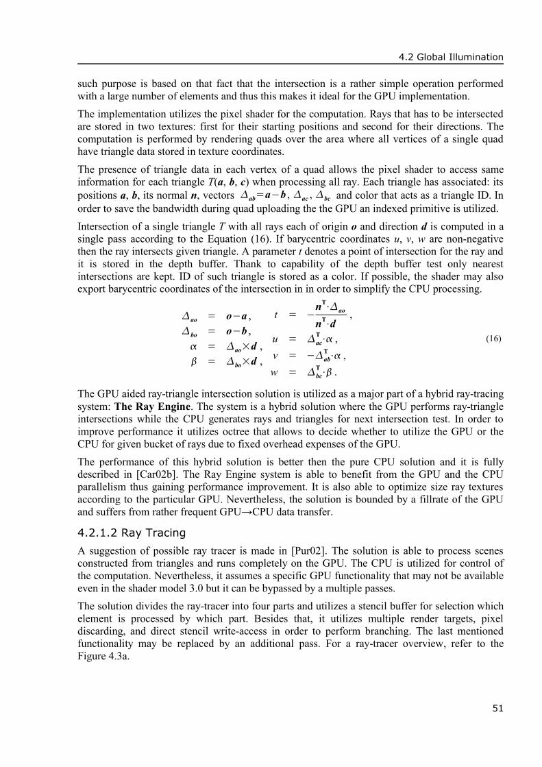
4.2 Global Illumination
such purpose is based on that fact that the intersection is a rather simple operation performedwith a large number of elements and thus this makes it ideal for the GPU implementation.The implementation utilizes the pixel shader for the computation. Rays that has to be intersectedare stored in two textures: first for their starting positions and second for their directions. Thecomputation is performed by rendering quads over the area where all vertices of a single quadhave triangle data stored in texture coordinates.
The presence of triangle data in each vertex of a quad allows the pixel shader to access sameinformation for each triangle T(a, b, c) when processing all ray. Each triangle has associated: itspositions a, b, its normal n, vectors ab=a−b , ac , bc and color that acts as a triangle ID. Inorder to save the bandwidth during quad uploading the the GPU an indexed primitive is utilized.Intersection of a single triangle T with all rays each of origin o and direction d is computed in asingle pass according to the Equation (16). If barycentric coordinates u, v, w are non-negativethen the ray intersects given triangle. A parameter t denotes a point of intersection for the ray andit is stored in the depth buffer. Thank to capability of the depth buffer test only nearestintersections are kept. ID of such triangle is stored as a color. If possible, the shader may alsoexport barycentric coordinates of the intersection in in order to simplify the CPU processing.
ao = o−a ,bo = o−b , = ao×d , = bo×d ,
t = −nT⋅ao
nT⋅d,
u = acT⋅ ,
v = −abT⋅ ,
w = bcT⋅ .
(16)
The GPU aided ray-triangle intersection solution is utilized as a major part of a hybrid ray-tracingsystem: The Ray Engine. The system is a hybrid solution where the GPU performs ray-triangleintersections while the CPU generates rays and triangles for next intersection test. In order toimprove performance it utilizes octree that allows to decide whether to utilize the GPU or theCPU for given bucket of rays due to fixed overhead expenses of the GPU.The performance of this hybrid solution is better then the pure CPU solution and it is fullydescribed in [Car02b]. The Ray Engine system is able to benefit from the GPU and the CPUparallelism thus gaining performance improvement. It is also able to optimize size ray texturesaccording to the particular GPU. Nevertheless, the solution is bounded by a fillrate of the GPUand suffers from rather frequent GPU→CPU data transfer.
4.2.1.2 Ray Tracing
A suggestion of possible ray tracer is made in [Pur02]. The solution is able to process scenesconstructed from triangles and runs completely on the GPU. The CPU is utilized for control ofthe computation. Nevertheless, it assumes a specific GPU functionality that may not be availableeven in the shader model 3.0 but it can be bypassed by a multiple passes.The solution divides the ray-tracer into four parts and utilizes a stencil buffer for selection whichelement is processed by which part. Besides that, it utilizes multiple render targets, pixeldiscarding, and direct stencil write-access in order to perform branching. The last mentionedfunctionality may be replaced by an additional pass. For a ray-tracer overview, refer to theFigure 4.3a.
51

4 GPU/Hardware Aided Approaches
RayGeneration
SceneTraversing
generate rays:while any ray is active:
if ORACLE(rays):traverse(rays)
else:intersect(rays)
shade(rays)
ShadingTriangleIntersection
a)
b)
Figure 4.3: Ray tracer structure (a) and ray tracing algorithm (b).
The implementation utilizes the pixel shader for all operations and the code for the ray tracerparts is available in the Figure 4.3b. The ORACLE function decides when to run the intersection.It prevents the intersection to be executed too frequently because execution of that part for everyray when such requirement appears is not effective. Therefore, the intersection is utilized when atleast 20 % of all rays are ready for intersection, i.e. they know triangle possibly intersecting them.
The ray tracer parts are:
• Ray generation part that generates rays according to camera settings into a texture.
• Scene traversing part that traverses the scene in order to find triangles that may be intersect bythe ray. Based on performance reasons the scene is divided by a regular grid stored as a 3Dtexture. Each voxel of the grid contains an index to a beginning of indexed triangle list thateither are contained inside or intersect the voxel.
• The grid is traversed by the 3D-DDA algorithm and for each pass a single step in the raytraversal is done. When the ray hits a non-empty voxel that contains a link to the triangle list,it is marked so it can be processed in the intersection phase.
• Triangle intersection phase that performs intersection according to marked ray-voxel coupesgenerated by the previous step26. The algorithm utilizes a voxel address together triangle list toaddress a triangle stored in three texture, a vertex per texture. Each such triangle in thetriangle list is tested for an intersection with given ray. Each test takes exactly one pass. If anintersection appears, it is tested against voxel boundary in order to detect intersection outsidethe voxel and if successful it is passed to the next phase.
• Shading phase process detected intersections similar to a lighting in the hard-wired hardwarepipeline. The computation utilizes both output from previous phase and material informationassociated with triangle to compute the color. If required, shadow rays may be generated.Shadow rays are processed similar to regular eye ray.
Due to the lack of functionality of GPUs at the time the paper was releases the proposed solutionwas implemented on a software simulator. Various modification of ray tracer were implementedsuch as a simple shadow caster, Whitted ray tracer, and a path tracer. It is expected that the pureGPU implementation outperforms the CPU version thus allowing a real-time ray tracing on acommon personal computer. The implementation also shows that the solution has betterperformance when flow control is available instead of multiple passes.
26 Marking is denoted by an appropriate value in the stencil buffer.
52
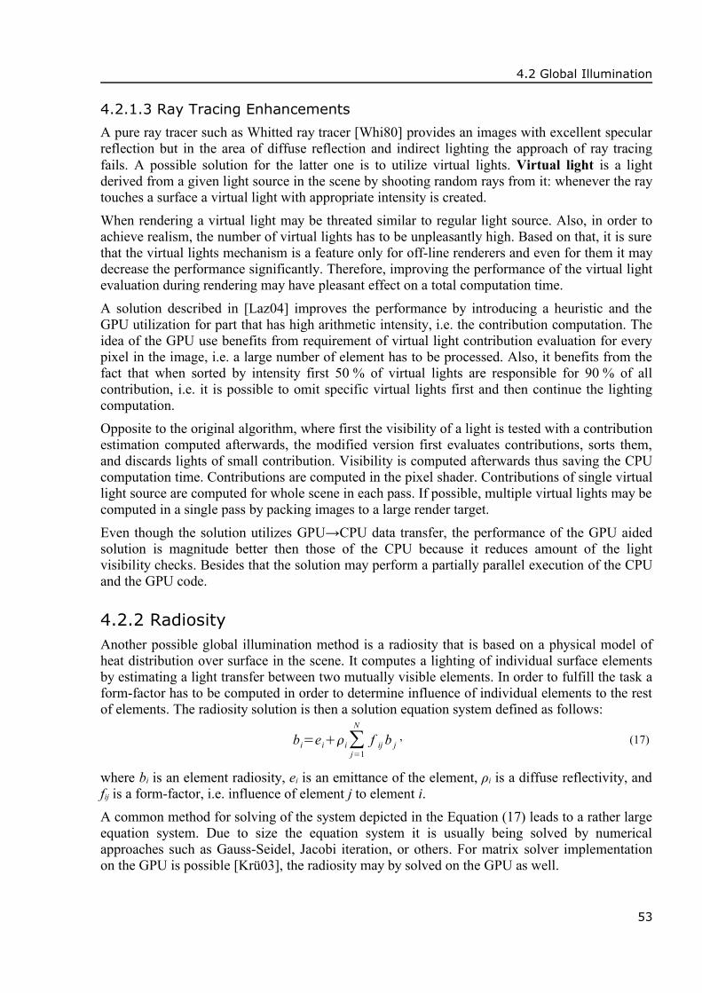
4.2 Global Illumination
4.2.1.3 Ray Tracing Enhancements
A pure ray tracer such as Whitted ray tracer [Whi80] provides an images with excellent specularreflection but in the area of diffuse reflection and indirect lighting the approach of ray tracingfails. A possible solution for the latter one is to utilize virtual lights. Virtual light is a lightderived from a given light source in the scene by shooting random rays from it: whenever the raytouches a surface a virtual light with appropriate intensity is created.When rendering a virtual light may be threated similar to regular light source. Also, in order toachieve realism, the number of virtual lights has to be unpleasantly high. Based on that, it is surethat the virtual lights mechanism is a feature only for off-line renderers and even for them it maydecrease the performance significantly. Therefore, improving the performance of the virtual lightevaluation during rendering may have pleasant effect on a total computation time.
A solution described in [Laz04] improves the performance by introducing a heuristic and theGPU utilization for part that has high arithmetic intensity, i.e. the contribution computation. Theidea of the GPU use benefits from requirement of virtual light contribution evaluation for everypixel in the image, i.e. a large number of element has to be processed. Also, it benefits from thefact that when sorted by intensity first 50 % of virtual lights are responsible for 90 % of allcontribution, i.e. it is possible to omit specific virtual lights first and then continue the lightingcomputation.Opposite to the original algorithm, where first the visibility of a light is tested with a contributionestimation computed afterwards, the modified version first evaluates contributions, sorts them,and discards lights of small contribution. Visibility is computed afterwards thus saving the CPUcomputation time. Contributions are computed in the pixel shader. Contributions of single virtuallight source are computed for whole scene in each pass. If possible, multiple virtual lights may becomputed in a single pass by packing images to a large render target.
Even though the solution utilizes GPU→CPU data transfer, the performance of the GPU aidedsolution is magnitude better then those of the CPU because it reduces amount of the lightvisibility checks. Besides that the solution may perform a partially parallel execution of the CPUand the GPU code.
4.2.2 RadiosityAnother possible global illumination method is a radiosity that is based on a physical model ofheat distribution over surface in the scene. It computes a lighting of individual surface elementsby estimating a light transfer between two mutually visible elements. In order to fulfill the task aform-factor has to be computed in order to determine influence of individual elements to the restof elements. The radiosity solution is then a solution equation system defined as follows:
bi=eii∑j=1
N
f ij b j, (17)
where bi is an element radiosity, ei is an emittance of the element, ρi is a diffuse reflectivity, andfij is a form-factor, i.e. influence of element j to element i.A common method for solving of the system depicted in the Equation (17) leads to a rather largeequation system. Due to size the equation system it is usually being solved by numericalapproaches such as Gauss-Seidel, Jacobi iteration, or others. For matrix solver implementationon the GPU is possible [Krü03], the radiosity may by solved on the GPU as well.
53

4 GPU/Hardware Aided Approaches
An approach that utilizes Jacobi iteration for radiosity solution is described in [Car03] and allowsto compute rather large equation system. The performance of the solution is better the that of theCPU one thanks to parallelism of the GPU: the GPU exhibits almost linear increase of time.
Nevertheless, these exists an iterative approach denoted as progressive refinement radiositythat is based on a simulation of light propagation form light sources. The approach requiresrepetitive computation of numerous elements by applying a rather simple equation and thus it isan ideal candidate for GPU implementation.A solution that is able to estimate the global illumination of the scene via progressive refinementradiosity is described in [Coo04]. It is able to evaluate radiosity for 104 elements in less thensecond for a scene that consist of planar quads. With the exception of data preparation for bothcomputation and result visualization, the solution run completely on the GPU. An overview ofthe algorithm is available in the Figure 4.4.
set light source quads to particular energy and others to zerowhile not converged:
emitter ← quad with highest residual energy Erender scene from emitter point of view:
compute item bufferselect visible quads according to occlusion query tests
for every visible quad:for every element of such quad:
if element visible from the emitter according to item buffer:compute form-factor FFΔE = ρ ∙ FF ∙ Emodify residual by ΔEmodify radiosity by ΔE
set emitter energy E to zeroFigure 4.4: Progressive refinement algorithm aided by the GPU.
Each quad requires two sets of radiosity data, namely two textures: the residual texture thatcontains information about an amount of energy that is left to be emitted from the surface and theradiosity texture. Due to a limitation of older GPUs, these textures have to be stored eitherseparately thus leading to a multiple passes or packed in a form of 2×16-bits packed to a 32-bitsthus requiring an unpack operation before every operation. Nevertheless, the newer GPUs areable to utilize multiple render targets that allows computation of both in a single pass.A the beginning of algorithm execution depicted in the Figure 4.4 a quad of highest residualpower is selected, i.e. quad for which residual energy multiplied by its area is the highest of allquads. Such quads is then considered as an emitter that emits its light energy to all elementsvisible from it. The evaluation of element visibility a fundamental of form form-factorevaluation.The original CPU-based algorithm utilizes a hemicube erected over the emitter thus requiringcomputation of five sides of the cube. Such solution leads to multiple passes when copied to theGPU. Therefore the GPU solution utilizes a stereographic projection of vertex v v x , v y , v z transformed to a emitter view described by following:
v' = v /∣v∣,x = v x
' ,y = v y
' ,
z = −2 v zz farznear
z far−znear.
(18)
54
4.2 Global Illumination
The projection is able to convert all visible space from a particular emitter to a plane andtherefore allows visibility estimation. Nevertheless, it also introduces a non-linear deformation toa scene which may cause inaccuracies for larger quads because it transforms only ends of edgesthat defines straight lines during rendering. In order to approximate the deformation properly, fora nearer and/or larger quads an uniform refinement has to be applied by either a manualrefinement at the CPU or N-patches [Vla01].
The visibility computation is then similar to a mechanism known from shadow mapping:complete scene from a viewpoint of the emitter is rendered. Each quad is assigned an ID in aform of color that allows identification of pixel affiliation thus forming an item buffer. Afterthat a hardware occlusion query is utilized to determine, which quads are visible from theemitter.
For each visible quad a form-factor together with modifications of associated radiosityinformation is evaluated by rendering to a texture containing new radiosity data. Each element ofthe quad is transformed to the item buffer according to the Equation (18) and the item bufferlookup is utilized to gather ID of surface that owns elements on that position. If such ID is the IDof currently processed quad, the element is considered visible from the emitter and form-factor iscomputed.The computation of form-factor assumes that the value of distance between emitter and particularelement is much higher than the size of the element. If the condition is not satisfied a disturbingartifact may appear at adjoining quads such as corners. The possible reduction is based onapproximation of element by a disc. This approximation modifies only the form-factor equationdescribed in the paper [Coo04].
After all elements of particular quad were processed, the algorithm has to select a new emitterfor evaluation. The selection is based on an amount of residual energy and the selected emitter isan emitter with highest amount. The selection is implemented utilizing the depth buffercomparison and rendering to a 1×1 area.
For each quad an average residual power is computed via the lowest level of the mip-map andmultiplied by the quad area. Obtained value is utilized as a new depth value of the pixel and theID of the quad is stored as a color. After all quads were rendered the render target contains the IDof quad with the highest energy that is the new emitter. This step also allows to stop in iterativeprocessing by setting a threshold of highest residual energy.
A solution described in the [Coo04] also introduces a adaptive version of the GPU aidedradiosity that decreases the aliasing caused by undersampling areas with significant changes inthe radiosity. The adaptive solution is based on building of a quad tree over a texture withradiosity data.After the quad modification is done, the algorithm evaluates a gradient of each radiosity textureelement and compares it to a threshold. If the threshold is overlapped the pixel is discarded andocclusion queries are utilized to count the number of such pixels. If the count is high enough asubdivision is performed by creating four child textures of the same size as its parent that eachholds an enlarged copy of particular part of its parent.
During the computation each leaf node node of the quad tree is considered as a single quad and itis processed alike. The division maximum depth is limited and thus the child textures may bepacked into a single larger textures saving both space and computational power. During therendering, the geometry has to be refined according to the generated quad tree of particular quad.
55

4 GPU/Hardware Aided Approaches
The performance of the solution is measured and compared to a commercial CPU solutionforming of up to 30× faster evaluation of the scene radiosity. Even thought the adaptive versionprovides a better performance for the CPU-based solution because it avoids oversampling, in thecase of the GPU the uniform one is faster. The worse performance of the adaptive version iscaused by both frequent context switches such as shader program switching and frequentocclusion queries that stalls the GPU pipeline then in the case of the uniform version.
4.3 Data Visualization
4.3.1 Surface Representation
4.3.1.1 Parallel Occlusion Estimation
Image synthesis is the major purpose of the graphic hardware, which is able to visualize scene inreal-time rates. However, for some application such as CAD/CAM the scene may far toocomplicated beyond the boundaries of real-time visualization due to low filtrate or pipelinebandwidth of the common hardware. In such case a specialized hardware may be the solution.Nevertheless, such specialized is expensive and even such hardware has its limitation. Thereforethere are attempts to optimize the scene for visualization purposes at run-time according to a rulethat the fastest rendering of a triangle is skipping its rendering.
A possible solution is proposed in [Bax02]. This solution aims primary on a parallel environmentand multiple GPUs: it expects two GPUs and one or multiple CPUs utilizing shared memory.The solution makes no assumption about both scene and camera motion thus providing a tool forrendering custom views. The algorithm utilizes following three block of step:
• Occluder rendering (OR) block is performed on the first GPU. It computes depthinformation of the scene according to the visible objects from the previous frame by renderingthe geometry without color buffer writes. The gathered information is read back to the CPUaccessing memory and passed to the next stage (STC) that is computed completely on theCPU. In order to reduce the waiting time for the STC step, the OR may utilize list of visibleobjects from last two successive frames.
• Scene traversal, culling and LOD selection (STC) block utilizes a hierarchical z-buffer(HZB) [Bax02] that is derived from depth information computed in the OR block. Then, thealgorithm traverses the scene tree in postorder manner and performs culling of node boundingbox against view frustum and HZB.If processed node is visible then a hierarchical level of detail (HLOD) is computed togetherwith pixel error estimation. If the error is acceptable the node is placed into a list of visiblenode. Otherwise, children of node are processed similar to their parent in order to reduce theerror. The visibility list is then passed to RVG for rendering and back to OR for estimation ofa next frame depth information.
• Rendering visible geometry (RVG) block performs rendering of visible nodes obtained fromthe STC completely on the second GPU. However, in some cases the GPU may be waiting forthe STC. Therefore, the RVG may utilize asynchronous rendering by utilizing possible framecoherency, i.e. starting the rendering of visible geometry from previous frame in advance.
The scene rendered by the proposed solution is stored in a form of node tree containing geometryincluding precomputed LOD and bounding boxes of node including its children. In a CAD/CAM
56
4.3 Data Visualization
models the hierarchy is already present but it follows different goal then an optimal organizationfor fast visualization.Therefore, the solution reorganizes the scene by a combined approach of node splitting andmerging. At the beginning the algorithm assumes no explicit hierarchy and starts by splitting oflarger objects into smaller fragments thus forming new objects. Then, it tries to cluster objectsaccording to their spatial proximity and utilize these clusters as an input for further splitting inorder to avoid clusters of uneven shape.
As a final step, the algorithms forms a AABB bounding-box hierarchy based on either center ofobjects or their group of mass. The tree is utilized for computation of the geometry LOD for leafnodes and HLOD for inner nodes as combination of its children. The tree is the utilized for bothocclusion and LOD estimation.The solution offers visualization of rather large scene of 107 triangle in almost real-time eventhought the preprocessing is rather slow. Thank to the nature of the solution it is possible todeclare a level of quality in a form of maximum pixel error that influences the performance. Forexact results, refer to [Bax02].
The parallel implementation utilizes SGI Onyx with three CPUs and two GPUs. This is rather aspecial expensive machine but the solution may run on two networked PCs as well. Nevertheless,then next presented solution allows nearly interactive rates on a cluster of common hardware.
4.3.1.2 Distributed Occlusion Estimation
Another possible enhancement of rendering towards a better performance is similar to theprevious one, i.e. it tries to improve the performance by culling occluded thus invisible objects.However, in a solution proposed in [Gov03a] the occlusion test utilizes a system with distributedmemory connected with Ethernet network.
This solution is based on two fundamentals: frame coherency and occlusion query. Framecoherency assumes that for major means of visualization the view changes rather continuously,i.e. a majority of currently visible object is being visible in next frame too. The occlusion queryis then is a hardware feature27 [Kil04, GLE04] that allows to estimate the number of depth-buffermodifications. If an application utilizes occlusion query and performs rendering of a bounding-box a two resultsmay appear: either the box is invisible thus everything contained within is occluded or it isvisible thus a contained geometry may be visible too. The drawback of the occlusion query is arequirement of GPU→CPU communication that may stall the pipeline. Nevertheless, newerversions of occlusion query may allow accumulation of several queries in order to preventfrequent pipeline stalling.
Rendered scene is a basically a tree of node with a bounding box for each node containing all itschildren. The solution then utilizes up to three GPU in distributed memory manner. Each GPUhas a particular function assigned to:
• Hardware culling (HC): Performs occlusion test utilizing the occlusion query and the depthbuffer of a current frame. The depth buffer is not modified by the occlusion query test duringwhich the algorithm traverses the scene tree and test bounding boxes of nodes for visibility. Ifocclusion query fails the node including all its children is considered occluded thus invisible.In the rest of the cases the algorithm considers the node visible.
27 In a case of the OpenGL, the feature is a extension NV_occlusion_query or HP_occlusion_query that allows onlydetection if depth buffer was modified or not without additional information.
57

4 GPU/Hardware Aided Approaches
The occlusion query also returns a number of depth buffer modification, i.e. number of visiblepixels. This number is then upper bound of all visible pixels from geometry contained withinthe node and thus it is utilized to compute the LOD of the node. If such number of pixels ishigher then defined pixels-of-error value the algorithm process children of the node in similarmanner.All changes in visibility of node is stored to a list that is transmitted over the network to therest of GPUs in a form of update. This is possible because the algorithm assumes continuouschange in the view thus assuming the update list to be much shorter then a complete list.
• Occlusion representation (OR): Computes depth information for next frame according to alist of visible objects from a current frame received from the HC GPU. The information isgathered by rendering visible object without color buffer update and it is utilized by the HCGPU in the next frame.
• Rendering visible geometry (RVG): Perform rendering of visible geometry for current frameaccording to a list received from the HC GPU.
In order to limit the communication ration the algorithm switches role of the HC and the ORGPU between successive frame thus allowing the HC to access estimation of scene depthinformation of current frame computed by the OR without data physical transfer. The importantfeature of the algorithm is that all three GPUs work in parallel manner with an exception of thefirst frame where the HC has to wait for the OR to render the depth of the whole. If required, HCand OR may be performed on a single GPU.The drawback of the algorithm is that it provides the output with latency of at least one frameand it may produces incorrect images due to LOD with an error of up to approximately 20 pixels.Nevertheless, the performance of the algorithm that was estimated by testing it on three models:each with at least 107 triangles and at least 104 objects, is according to the [Gov03a] better thenmajority of existing rendering system including Gigawalk [Bax02], see Subsection 4.3.1.1. Also,the solution utilizes only a common hardware rather than special custom systems thus reducingthe cost.
4.3.2 Volume RepresentationVolumetric data are extension of image data to the space. Through them it is possible to capturea complete sampled image of the scene and similar to image for a plane and thus the volumetricapproach suffers from both discretization and low sampling rate due to storage requirements.Nevertheless, opposite to surface representation it allows store a complete information and thus itis ideal for storing structures such as data generated from CT/MRI/3D scanners or it may beutilized as an intermediate result of other representations such as implicit functions or CSG trees.
One of the major problem with volumetric data is its visualization. As opposite to the 2D image,the 3D volume is not suited to be visualized on 2D displaying device and thus a projections isrequired. There are many methods that allows to project a volume to a plane but only a few ofthem properly solves occlusion and visibility that are crucial for the visualization.A possible solution for this task is a conversion of volume data to another representation thatmay be suited better for the visualization, i.e. an iso-surface extraction. Output of such methods28
allows utilization of visual quality improving effects with the GPU support but on the other handthey require a long preprocessing step prior to visualization.
28 Marching cubes, marching tetrahedra, and marching triangles.
58
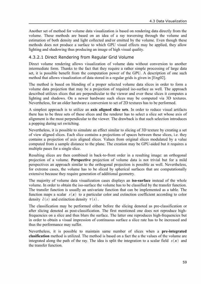
4.3 Data Visualization
Another set of method for volume data visualization is based on rendering data directly from thevolume. These methods are based on an idea of a ray traversing through the volume andestimation of both density and light collected and/or emitted by the volume. Even though thesemethods does not produce a surface to which GPU visual effects may be applied, they allowlighting and shadowing thus producing an image of high visual quality.
4.3.2.1 Direct Rendering from Regular Grid Volume
Direct volume rendering allows visualization of volume data without conversion to anotherintermediate form. Thanks to the fact that they require a rather simple processing of large dataset, it is possible benefit from the computation power of the GPU. A description of one suchmethod that allows visualization of data stored in a regular grids is given in [Eng02].
The method is based on blending of a proper selected volume data slices in order to form avolume data projection that may be a projection of required iso-surface as well. The approachdescribed utilizes slices that are perpendicular to the viewer and over these slices it computes alighting and shadows. On a newer hardware such slices may be computed via 3D textures.Nevertheless, for an older hardware a conversion to set of 2D textures has to be performed.
A simplest approach is to utilize an axis aligned slice sets. In order to reduce visual artifactsthere has to be three sets of these slices and the renderer has to select a slice set whose axis ofalignment is the most perpendicular to the viewer. The drawback is that such selection introducesa popping during set switching.Nevertheless, it is possible to simulate an effect similar to slicing of 3D texture by creating a setof view aligned slices. Each slice contains a projections of spaces between these slices, i.e. theycontains a projection of axis aligned slices. Values from original slices modulated by a valuecomputed from a sample distance to the plane. The creation may be GPU-aided but it requires amultiple pases for a single slice.
Resulting slices are then combined in back-to-front order in a resulting image: an orthogonalprojection of a volume. Perspective projection of volume data is not trivial but for a mildperspectives an approach similar to the orthogonal projection is possible as well. Nevertheless,for extreme cases, the volume has to be sliced by spherical surfaces that are computationallyextensive because they require generation of additional geometry.
The majority of volume data visualization cases displays an iso-surface instead of the wholevolume. In order to obtain the iso-surface the volume has to be classified by the transfer function.The transfer function is usually an univariate function that can be implemented as a table. Thefunction maps a scalar s x to a particular color and extinction coefficient according to colordensity c s and extinction density s .
The classification may be performed either before the slicing denoted as pre-classification orafter slicing denoted as post-classification. The first mentioned one does not reproduce high-frequencies on a slice and thus blurs the surface. The latter one reproduces high-frequencies butin order to obtain a visual impression of continuous surface a slice rate has to be increased andthus the performance may suffer.
Nevertheless, it is possible to maintain same number of slices when a pre-integratedclasification method is utilized. The method is based on a fact the a the values of the volume areintegrated along the path of the ray. The idea is split the integration to a scalar field s x andthe transfer function.
59

4 GPU/Hardware Aided Approaches
When the segment of the ray is linear between two slices, the transfer function may be reduced toa lookup into a precomputed table. The position in the table is the evaluated from a scalar valueof the front slice ray intersection, back slice ray intersection, and length of path segment.The length may be considered constant and by that the table can be stored as a texture. Theassumption of constant length is correct for both orthogonal projection and perspective withspherical slices. For mild perspective, the assumption of constant length provides an acceptableapproximation.
During the rendering, values from front and back slice are sampled according to the ray and theyare utilized as lookup table coordinates. The pre-integrated classification provides accurateoutput without increase the slice rate at the same time. The drawback is that the lookup tablecomputation is rather time extensive due to integral evaluation [Eng02].Besides the proper classification, an important aspect of visual quality of the output is a properlighting and shading. In order to perform a shading the approach requires a normal for givenvolume element computed from its gradients. The computation of the gradient utilizes the firstterm of Taylor expansion. The gradient Ix for the x-axis is evaluated as follows:
I x x , y , z = s x1, y , z −s x−1, y , z 2
, x , y , z∈ℕ (19)
The lighting computation the normal to estimate the lighting according to equations similar tothose in the GPU. In order to save the GPU computation power, the normal may be precomputedand stored in a form of a volume sample. For an older hardware, the lighting may be replaced bylookup into a cube-map with a light information that avoid sampled normal renormalization.
Also, the direct volume rendering allows computation of shadows and self-shadowing. One ofthe possible solutions utilizes an approach similar to a shadow map, see Subsection 4.1.2.2. Itbuilds a shadow volume from the viewpoint of the light and utilizes it to modulate values duringvolume data rendering. The drawback of the method is an appearance of blurry shadows and darksurfaces caused by a coarseness of precomputed shadow volume.
Another approach is based on an accumulation of light that arrives to a particular volumeelement on each. In ideal case the slices are perpendicular to the light direction but the approachis able to share same the set of slices with the rendering by creating a slices perpendicular to ahalf-vector between the light and the viewer. If the angle between these two vectors is larger then90º, the half-vector estimation utilizes a negative view vector instead of the original one.Before the rendering starts, the algorithm creates a light map initialized to a light intensity. Thelight map allows creating a visual effects such as a spot light by setting it to an arbitrary image.Then, for each slice it performs two steps:
1. Render slice from the viewpoint modulated by the light map.2. For each light compute an intensity of light that pass actual slice by rendering a slice from the
light viewpoint. During the rendering it utilizes opacity of elements from the current slice tomodify the light map, i.e. it accumulates the opacity from the light point of view.
The approach described in the [Eng02] allows visualization of volumetric data in regular gridswith interactive and/or real-time frame rates on the GPU. It allows both lighting and shadowingcomputations in order to improve the visual quality without requirement of any special hardware.Base on a nature of utilized algorithm, it can be expected that the higher version of shadermodels improves the performance by number of passes reduction.
60

4.3 Data Visualization
4.3.2.2 Frequency Domain Rendering from Regular Grid Volume
Frequency volume rendering (FVR) is a method that allows projection of volume data and it isbased on a fact that projection of volume in the spatial domain is equal to slicing in a frequencydomain. The important feature is the complexity of this process: when the preprocessing phase isomitted the projection has complexity of O M 2 for M×M slice.
Such complexity is much better then a complexity of the direct volume rendering for N×N×Nvolume: O N 3 . Also, the approach allows a dynamic control output quality by controlling aslice sampling rather thus allowing to easily implement progressive refinement of the output.Nevertheless, the output of the frequency volume rendering is X-ray-like orthogonal projectionof the volume that may not be desirable for viewing purposes.The algorithm first requires a preprocessing step for transformation to frequency domain byutilizing a Fast Fourier and/or Hartley Transformation with complexity of O N 3 log N .Afterwards, transformed data are sliced with a complexity of O M 2 and transformed back tospatial domain with complexity of O M 2 log M resulting in a X-ray-like image.
The solution described in [Vio04] is a direct implementation of the approach described above onthe GPU. The only exception is a preprocessing step that has to be performed on the CPU due tothe GPU limitations in both 3D texture handling and memory size29. During the preprocessingvolume is first wrapped around to move the original from a volume corner to the center and thenthe FFT is applied. Afterwards the result wrapped around again to move the lowest frequenciesto the middle of the transformed volume.
During the visualization phase the transformed data are uploaded to the GPU in a form of a 3Dtexture. Slicing is then equal to rendering of a quad perpendicular to the viewer directioncentered to the origin of the volume. Proper setting of texture coordinated in corners of the quadthen allow data sampling from the volume.
The sampling is an important aspect of the method because it greatly influence the visual qualityof the result: improper sampling causes ghost-like artifacts to appear in the image. Based on thatthe solution utilizes a high-order sapling in a form of a filter. The filter is stored as a 1D texturecontaining weights for four samples and it is applied to each direction separately, i.e. it requiredthree passes. Then, results are summed during the fourth pass thus forming a resulting image.
The last step is an application of an inverse FFT to the slice. The solution utilizes animplementation of GPU-based FFT described in Subsection 4.4.3.3. Before the FFT is applied,data are wrapped around and after the FFT is applied, data are wrapped-around again in order toreturn the origin to the corner of the image.The solution provides real-time frame rate during the visualization phase; the preprocessingphase is slower but it has to be performed only once. It has even better performance than thedirect volume rendering method and the optimized CPU frequency volume rendering. For thelatter one, the reported speed is 17× speed of the CPU version. The drawback of the method is anX-ray-like look of the result. Nevertheless, for larger volumes this method may be the only onecapable to provide real-time frame rates on a weaker hardware.
4.3.2.3 Silhouette Extraction from Regular Grid Volume
In a medical area of research but not even in there, a majority of volumetric data are produces bya CT/MRI scans rather than algorithmic approaches based on mathematical description. No
29 For such operation, the video memory have to contain both source and target volume, i.e. 2N3 samples.
61

4 GPU/Hardware Aided Approaches
matter which visualization method is chosen, the resulting image tries to resemble the real-worldlook. Nevertheless, in some cases the realism is not appropriate because it may hide features thatmay be crucial also the resulting image is rather complicated even if depth/position clues such asshadows and shading are available. In that case, a non-photorealistic rendering is a solution.A non-photorealistic rendering allows emphasizing of features or it allows simplification towardsbetter understanding of the image. An important element of the non-photorealistic rendering is asilhouette. It is an important feature of illustrations because it allows the viewer to easilydistinguish parts of image from each other.
There are many approaches for silhouette generation from volume data directly. It is also possibleto compute the silhouette from intermediate representation such as surface representation but thisgenerally requires greater amount of time then direct rendering. Direct rendering approach thenmay utilize a gradient but that approach leads to silhouette of various thickness and also it issensitive to coarseness of the volume data. Another approaches may provide better results butrequires significant amount of both space and time.A solution described in [Nag04] allows extraction of the silhouette of constant thickness and it isable to utilize the GPU for such purposes efficiently thus providing a better performance. Theinput of the algorithm is a volume sliced according to the viewer direction. Also, the knowledgeof which elements are inside or outside the object volume is required in a form of either a alreadyclassified volume data or a threshold value for volume data elements.
The algorithm then performs the computation by rendering slices in a front-back order accordingto a viewer position. This allows extraction of fragments that are hidden if the volume would berendering and thresholded afterwards. The algorithm utilizes a buffer t that contains intermediateresults. Each pixel of the buffer is labeled and at the begging the label is equal to empty, seebelow.
For each slice, the algorithm sets a label to each pixel to filled, if particular voxel is inside theobject. Otherwise, it is labeled as empty. The classified slice is then merged with intermediatebuffer and labels in this buffer are modified to either empty, filled, contour that denotes apossible candidate for silhouette, or silhouette according to the scheme in the Figure 4.5.
empty
filled
contour
silhouette
intermediate buffer
slic
e
Figure 4.5: Slice × intermediate buffer merging operator.
At the end, the intermediate buffer is thresholded to contain only pixels labeled as silhouette.Then it contains results one pixel thick silhouette. Nevertheless, in some application a silhouetteof such thickness is not appropriate and thus the silhouette may be broaden by convolution of theintermediate buffer with a Gauss filter:
g x , y= 1 2
e−1
2x2 y2
. (20)
The resulting image is then thresholded to obtain the silhouette of required thickness. Thethreshold is determined from the Gauss filter, which is radial symmetric, i.e. it is possible to
62
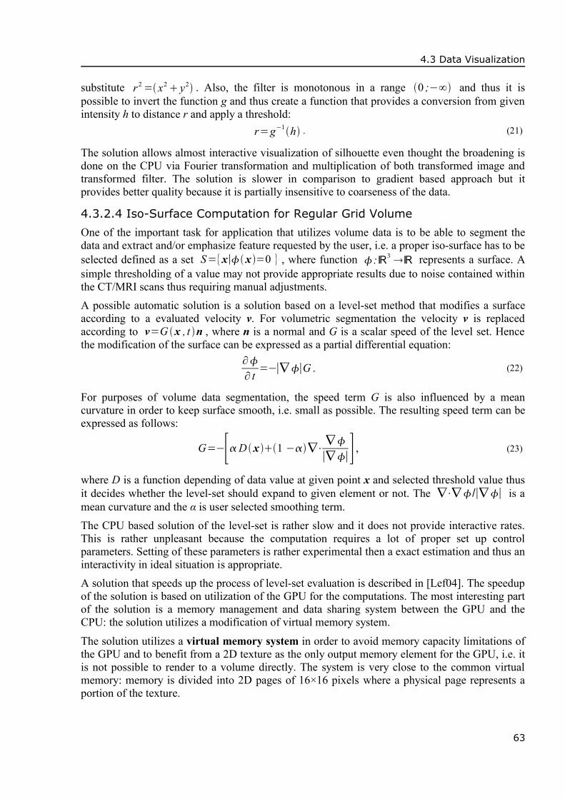
4.3 Data Visualization
substitute r2 = x2 y2 . Also, the filter is monotonous in a range 0 ;−∞ and thus it ispossible to invert the function g and thus create a function that provides a conversion from givenintensity h to distance r and apply a threshold:
r=g−1h . (21)
The solution allows almost interactive visualization of silhouette even thought the broadening isdone on the CPU via Fourier transformation and multiplication of both transformed image andtransformed filter. The solution is slower in comparison to gradient based approach but itprovides better quality because it is partially insensitive to coarseness of the data.
4.3.2.4 Iso-Surface Computation for Regular Grid Volume
One of the important task for application that utilizes volume data is to be able to segment thedata and extract and/or emphasize feature requested by the user, i.e. a proper iso-surface has to beselected defined as a set S={x∣x =0 } , where function :ℝ3 ℝ represents a surface. Asimple thresholding of a value may not provide appropriate results due to noise contained withinthe CT/MRI scans thus requiring manual adjustments.A possible automatic solution is a solution based on a level-set method that modifies a surfaceaccording to a evaluated velocity v. For volumetric segmentation the velocity v is replacedaccording to v=G x , t n , where n is a normal and G is a scalar speed of the level set. Hencethe modification of the surface can be expressed as a partial differential equation:
∂∂ t
=−∣∇∣G . (22)
For purposes of volume data segmentation, the speed term G is also influenced by a meancurvature in order to keep surface smooth, i.e. small as possible. The resulting speed term can beexpressed as follows:
G=−[D x 1 −∇⋅∇∣∇∣] , (23)
where D is a function depending of data value at given point x and selected threshold value thusit decides whether the level-set should expand to given element or not. The ∇⋅∇/∣∇∣ is amean curvature and the α is user selected smoothing term.
The CPU based solution of the level-set is rather slow and it does not provide interactive rates.This is rather unpleasant because the computation requires a lot of proper set up controlparameters. Setting of these parameters is rather experimental then a exact estimation and thus aninteractivity in ideal situation is appropriate.A solution that speeds up the process of level-set evaluation is described in [Lef04]. The speedupof the solution is based on utilization of the GPU for the computations. The most interesting partof the solution is a memory management and data sharing system between the GPU and theCPU: the solution utilizes a modification of virtual memory system.
The solution utilizes a virtual memory system in order to avoid memory capacity limitations ofthe GPU and to benefit from a 2D texture as the only output memory element for the GPU, i.e. itis not possible to render to a volume directly. The system is very close to the common virtualmemory: memory is divided into 2D pages of 16×16 pixels where a physical page represents aportion of the texture.
63

4 GPU/Hardware Aided Approaches
Swap-space, mapping tables, and page requests are handled by the CPU. The GPU performs thecomputation and requests for virtual page at the end of each execution loop. The CPU alsohandles mapping from the virtual page space to the physical page space be setting of renderedprimitive texture coordinates due to the fact that the remapping process would both introduce adependent texture lookup to the shader code and increase memory requirements for storage of thetable.Based on the fact that the computation follows Equations (22) and (23), the computation kernelrequires to access a 3×3×3 neighborhood of each element. If such element is on a boundary of thepage, the kernel has to access an adjacent virtual page and it has to store to the result to the sameposition in different buffer.
Due to lack of scatter operation of the GPU, this has to be handled at the CPU level by renderinga proper primitive: a quad for interior element, a line for boundary element, and a point forcorner element. Also, the CPU assures that required adjacent page is uploaded to the GPU beforethe computation starts.
The computation is performed over active pages, i.e. pages that contains a part of a level-set.These pages are processed by the computational kernel and based on performance reason itwould be suitable to keep their number low. For purpose the solution tries to maintain constantlevel-set density by embedding the function. This is done by introducing a rescaling speedterm Gr that ensures gradients further from boundary being zero:
G r= g−∣∇∣ , (24)
where the g is a target gradient magnitude.
During the computation, the solver identifies active pages by inspective their gradient. If a pagescontains at least one pixel with non-zero gradient, it is considered as a active page andrecomputed. In order to improve the effectiveness of the active page identification process, thedata are clamped by a distance transform: outside voxels are black, inside voxels are white.In order to save the CPU-GPU data transfer, two static pages are created: a page of outsidevoxels and page of inside voxels. These pages are considered as inactive pages and whenever aninactive page is requested as a adjacent page to an active one, a particular static page is utilizedinstead of uploading a copy.At a startup time an initial set of active pages is uploaded. The initial set is provided either by theuser as an approximation of the level-set or by a threshold. During the computation it is possibleto influence the actual level-set in order to gain better results. The level-set evaluation executessequentially following steps:
1. Computation of 1st and 2nd partial derivate for active pages. Computed values are stored tofour temporary buffer to be used during the active page selection.
2. Computation of speed function according to speed terms described at equations (20) and (21).
3. Modification of the level-set according to speed function. For details, refer to [Lef04].4. Selection of active pages for update according to active page definition, see above. The update
utilizes a automatic mip-mapping capabilities of the GPU to obtain an average for gradientcomponents that is thresholded and transformed to a bit-fields denoting pages that areconsidered active. Bit-wise operations are emulated by additions of 2k , k∈ℤ values. Thisstep is executed completely on the GPU.
64

4.3 Data Visualization
5. Handling of new active pages and adjacent pages upload that utilizes flag computed in theprevious step. The GPU memory then contains current level-set.
In order to allow the user to view the result immediately, the solution utilizes a direct volumerendering approach utilizing a axis aligned slices, see Subsection 4.3.2.1. The evaluated level-setis combined with the original volume on the fly during reconstruction of individual slices andthus it does not utilize a preprocessing step that would involve a reconstruction of the volume.For efficiency reasons, the solution utilizes a gradient precomputed during level-set evaluationfor lighting purposes.
The computation performance depends on a number of active voxels. Nevertheless, the solutionis able to achieve interactive framerates. When compared to a CPU-based solution, the speedupof the GPU solution is in the order of magnitudes. The solution assumes a sparse level-sets andthus may not be suitable for dense structures. The solution introduces a GPU controlled memorymanagement that saves a computation time even though the creation and processing of themessages requires almost a 1
6 of total GPU instruction count.
4.3.2.5 Direct Rendering from Tetrahedral Volume
Besides regular grid organization for volume data there are other organization based onunstructured grids. One the of possibilities is a volume composed of tetrahedrons. Thevisualization of such volume is a task similar to that of structured grid: it is possible to utilizeeither intermediate form or direct volume rendering. Besides the computation time, the drawbackof the intermediate from is a large amount of generated triangles that makes the resultinappropriate for interactive visualization.
The direct volume rendering approach utilized for tetrahedral volumes is a modification of anapproach possible for structured grid: a splatting of individual volume elements. This approachrequires requires a volume elements sorted in correct depth order according to the view direction.Afterwards, individual cells are projected to a screen space thus forming an objects withsilhouette of a triangle or a quadrangle.Each projected cell is then classified according to the Figure 4.6 and mass thickness in thethickest part of the cells is estimated. Afterwards, according to the classification and thickness ageometry consisting of triangles is constructed. Such geometry is then rendered using a regulargraphic hardware. If effective, a depth sorting may be performed with plane projections oftetrahedrons instead of with tetrahedron themselves.
class 3
class 1 class 2
class 4
Figure 4.6: Tetrahedral projection classification.
A solution described in [Wyl02] is almost direct implementation of approach mentioned above.With an exception of depth sorting, the solution utilizes the GPU for all steps of the algorithm, inparticular the vertex shader that performs the classification, geometry construction, and massthickness evaluation.
65
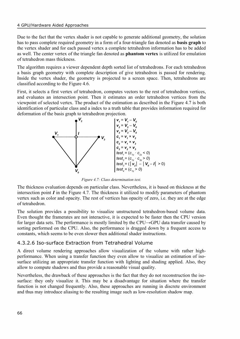
4 GPU/Hardware Aided Approaches
Due to the fact that the vertex shader is not capable to generate additional geometry, the solutionhas to pass complete required geometry in a form of a four-triangle fan denoted as basis graph tothe vertex shader and for each passed vertex a complete tetrahedron information has to be addedas well. The center vertex of the triangle fan denoted as phantom vertex is utilized for emulationof tetrahedron mass thickness.The algorithm requires a viewer dependent depth sorted list of tetrahedrons. For each tetrahedrona basis graph geometry with complete description of give tetrahedron is passed for rendering.Inside the vertex shader, the geometry is projected to a screen space. Then, tetrahedrons areclassified according to the Figure 4.6.
First, it selects a first vertex of tetrahedron, computes vectors to the rest of tetrahedron vertices,and evaluates an intersection point. Then it estimates an order tetrahedron vertices from theviewpoint of selected vertex. The product of the estimation as described in the Figure 4.7 is bothidentification of particular class and a index to a truth table that provides information required fordeformation of the basis graph to tetrahedron projection.
I
V2
V1V3
V0
v1 = V1 – V0
v2 = V2 – V0
v3 = V3 – V0
c1 = v1 × v2
c2 = v1 × v3
c3 = v2 × v3
test1 = (c1z ∙ c2z < 0)test2 = (c1z ∙ c3z > 0)test3 = (│v2│ – │V0 – I│ > 0)test4 = (c1z > 0)
Figure 4.7: Class determination test.
The thickness evaluation depends on particular class. Nevertheless, it is based on thickness at theintersection point I in the Figure 4.7. The thickness it utilized to modify parameters of phantomvertex such as color and opacity. The rest of vertices has opacity of zero, i.e. they are at the edgeof tetrahedron.
The solution provides a possibility to visualize unstructured tetrahedron-based volume data.Even thought the framerates are not interactive, it is expected to be faster then the CPU versionfor larger data sets. The performance is mostly limited by the CPU→GPU data transfer caused bysorting performed on the CPU. Also, the performance is dragged down by a frequent access toconstants, which seems to be even slower then additional shader instructions.
4.3.2.6 Iso-surface Extraction from Tetrahedral Volume
A direct volume rendering approaches allow visualization of the volume with rather high-performance. When using a transfer function they even allow to visualize an estimation of iso-surface utilizing an appropriate transfer function with lighting and shading applied. Also, theyallow to compute shadows and thus provide a reasonable visual quality.
Nevertheless, the drawback of these approaches is the fact that they do not reconstruction the iso-surface: they only visualize it. This may be a disadvantage for situation where the transferfunction is not changed frequently. Also, these approaches are running in discrete environmentand thus may introduce aliasing to the resulting image such as low-resolution shadow map.
66

4.3 Data Visualization
A solution described in [Kle04] performs an extraction of the iso-surface from tetrahedralvolume and creates a mesh. Both surface extraction and visualization runs completely on theGPU without any GPU→CPU data transfer thus gaining reasonable performance. In order toavoid the data transfer, it utilizes an experimental implementation of extension based on a pixelbuffer [GLE04] that makes possible direct rendering to an array of vertices instead the texture.The feature mentioned above allows the solution to utilize the pixel shader30 for computationkernel and thus gain performance thanks to its high throughput. Therefore, input data containedin three textures: first two textures are utilized to store the volume and the third one contains atetrahedron classification. Each corner of the tetrahedron is classified according the value of iso-surface c and its scalar value s thus forming a four-component vector β, where component i isone if c is greater then given si and zero otherwise.
The volume is stored in a 2D texture for indices and a 3D texture for vertices, i.e. position andvalue. This indexed approach allows to reduce the number of floating point values required for asingle tetrahedron to 24 in contrary to 80 for non-indexed approach and thus it is possible toupload much larger volume in a limited texture memory. Even thought this approach requiresdependent texture lookups it provides much better performance then in a case of CPU→GPUdata transfer during the computation.The output is then a 2D buffer that contains a geometry for intersection of iso-surface and a giventetrahedron. Thanks to the fact that each tetrahedron may produce a quad as the mostcomplicated shape, four pixels stored in a row are utilized. The solution assumes that a quad maydegenerate to a triangle without any visual side-effects and quad of zero area is not rendered atall.
This structure allows to store approximately 106 quads31 and thus it is possible to process sameamount of tetrahedron in single pass. Also, thanks to this output structure, for given pixelp px , p y in the texture, the algorithm can easily determine index of a vertex in the quad as= px mod 4 . Tetrahedron index to the index texture can be determined as following:
=⌊ px
4 ⌋p y (25)
Computation then utilizes a lookup table in order to obtain which edge determined by twotetrahedron corners V 1 ,V 2 is intersected by the iso-surface for given quad vertex. The table itaddressed via the classification vector 32 and vertex index . Resulting vertex is thencomputed via a linear interpolation V=t V 1 1−t V 2 , where t is evaluated from the scalarvalue of tetrahedron vertex.The output are plain quads. Nevertheless, for visualization purposes is it possible to estimate anormal: either per-face from gradient of tetrahedron or per-vertex as interpolation of gradients intetrahedron vertices. Both of these require additional pass. If multiple render targets aresupported, the computation may be performed in a single pass.
Nevertheless, some GPUs may have limitations on number of dependent texture lookups. Thus,it required to reduce the number of these texture lookups. Due to limited texture memory it is not
30 Tetrahedron vs. iso-surface intersection is simple enough and does not exhibit singularities such as those ofmarching cubes algorithm. This allows to implement the algorithm in a rather length-limited environment of thepixel shader.
31 For a hardware with a capability of handling a render target with maximum dimension of 2048×2048.32 The classification vector β is basically a binary vectors and thus it is possible to handle it as an integer.
67

4 GPU/Hardware Aided Approaches
possible to remove the indexed nature of the volume. However, it is possible to omit the lookuptable utilized for determination of intersection edges by implementing it in the shader.
For triangle shape the solution is pretty simple because only a single vertex lies on one side ofthe intersection and thus vector β has only a single component of non-zero value. The secondvertex of the edge is determined according to the fact that all intersected edges are growing fromthe first one. For quad shape the situation is more complicated because it leads to a selection oftwo edge pairs. Nevertheless, even this is possible to express as a set of mathematical operations.For details as well as exact equations, refer to [Kle04].
The performance of the solution strongly depends on availability of data in the video memory: ifdata have to be uploaded during computation, the performance may drop to 1/3 of original. Thevisualization of the result depends on performance of actual GPU. In the case of data and/ortransfer function change, the solution is able to compute 106 tetrahedrons in interactive rateswithout any sorting or preprocessing done on the CPU.
4.3.2.7 Iso-surface Visualization from Tetrahedral Volume
Another approach for visualization of iso-surface in tetrahedral volume is described in [Pas04].Similar to the previous approach described in Subsection 4.3.2.6, this one utilizes a conversion toan intermediate form for visualization purposes. However, unlike the previous approach it doesstore this intermediate form for further visualization: it does both extraction and visualization ina single execution.As it was mentioned, the output of the algorithm is a triangle mesh and therefore the input has tobe a mesh either because the GPU shaders are not capable to generate additional element. In thiscase, the input is a quad as the most complicated shade that is a result from tetrahedron×iso-surface intersection. The quad is sent in a form of its index in the quad primitive and tetrahedrondata such as positions of corners and their scalar values. Index is stored in quad vertex positionand associated tetrahedron data are stored in texture coordinates.
The computation kernel resides in the vertex shader because of its capability to both executelonger code and manipulate with individual vertices of render primitive. The computationutilized two lookup tables, both stored in an array of constants. The first table provides an indexof four edges that are intersected by the iso-surface. The table is indexed via a classification ofthe tetrahedron according to an iso-surface value and scalars in tetrahedron corners and thesefour edges corresponds to four vertices of the quad.First, the algorithm performs a lookup to the first table in order to obtain four edge. Then, itselects an appropriate edge index according to index of current quad vertex33. This edge index isutilized for the second table lookup to provide indices of the tetrahedron corners that definesintersected edge for given quad vertex. Exact position of the quad vertex is then determined viathe linear interpolation of obtained vertices. Besides that, the algorithm computes a per-quadnormal n from vectors v i=c i−c0 , where c i x , y , z , s is a corner of the tetrahedron includingits scalar value and sT is a tetrahedron orientation:
n=sT⋅det∣v1 y v1 z v1 s
v2 y v2 z v2 s
v3 y v3 z v3 s∣,det∣v1 z v1 s v1 x
v2 z v2 s v2 x
v3 z v3 s v3 x∣,det∣v1 s v1 x v1 y
v2 s v2 x v2 y
v3 s v3 x v3 y∣ (26)
33 This selection is performed as a dot product of edge index vector and quad vertex index bit field, i.e. for thirdvertex the bit field is a vector (0; 0; 1; 0).
68

4.3 Data Visualization
The solution is further improved by utilizing a view dependent division based on division of thelongest edge in the tetrahedron. When utilized for regular grid, it produces similar results asoctree division and thus allows to control number of generated quad. Nevertheless, this step hasto be performed on the CPU.
The performance of the solution is hardware dependent. Nevertheless, it is capable to processapproximately 106 tetrahedrons per second on older hardware. The solution utilize the vertexshader for computation thus making it available with first shader models, i.e. shader model 1.1.However, this also causes lower performance due to the fact that the vertex shader is not buildfor high throughput.Further improvement in performance can be achieved by precomputing normals thus savingvertex shader computation time or by utilizing strip of tetrahedrons. The latter one allows toreduce to CPU→GPU data traffic to 40 % or original by sending a modification of onetetrahedron corner instead of all four.
4.3.3 Scattered Data and Point Representations
4.3.3.1 Scattered Data Filtering
Another possible representation of data are scattered data, i.e. point clouds. These data areusually generated by various 3D scanners and coordinate measuring system and utilized as inputto various surface reconstruction techniques. Nevertheless, these data usually contains aparticular amount of noise that has to be removed prior the reconstruction.
A possible solution for the problems of noise removal is described in [Wan03]. This technique isaimed primary on remove the noise outside the surface assuming that only one object iscontained in a set of points. The original solution does not utilize the GPU for the computationbut thank to its nature it seems possible to move the solution completely on the GPU.The idea utilizes for noise removal is based on morphologic operators, see below. In its simplestform, these operators allows removing of independent points or clusters from a binary 2D image.Thus, converting a point cloud to such image would allow removing of these noisy points fromthe data set.
Morphologic operators are based on operation with sets. If utilized for binary images, input ofthese operations are sets of points A={a1 x , a1 y , ...} and B={b1 x ,b1 y , ...} . If Bv denotes atranslated set Bv={x∣x=bv , b∈B} and B denotes a reflection B={x∣x=−b , b∈B} thenMinkowski addition also known as dilatation is then defined as A⊕B={x∣ Bx∩A≠∅} andMinkowski subtraction also known as erosion is defined as A⊖B={x∣Bx⊆A} .
Based on these operation it is possible to define another two operation: opening and closing.Both are a composition of erosion and dilatation and they differ in their order. The opening isdefined as A○ B=A⊖B⊕B and closing as A● B=A⊕B⊖B . The set is usually a rathersmall set denoted as structural element.In order to obtain such set, the algorithm first projects points to a plane by applying anorthogonal projection in 23 directions: three for major axes and twenty for normals oficosahedron faces. On each of such newly created binary images a morphological operationutilizing a 3×3 morphological element described in the Figure 4.8 is applied to perform operationof opening.
69

4 GPU/Hardware Aided Approaches
Then, the algorithm identifies a connected set of points and denotes the largest one as the setcontaining noisy free points because the algorithm assumes that only a single continuous objectis available in the input data. Afterwards, the algorithm removes noise points by projecting oforiginal point to all binary images. If an original point is projected to a zero point in a singleview, then it is considered a noisy point and removed from the set.
111
111
111
Figure 4.8:Morphological element
The solution is able to remove almost all noise points that lies outside the surface. It can alsoadjust the surface for removing of fringes possibly caused by the noise. The limitation of themethod is the fact that it cannot remove noisy points inside the object volume. The solutionutilizes the CPU only. However, thanks to its nature it is possible to move it to the GPUcompletely including the connected region detection that can be handled by rendering lines inmultiple passes, i.e. a modification of coloring algorithm known from computer vision.
4.3.3.2 Point-Based Rendering
Traditional rendering based on displaying of triangles is supported very well in the GPU that areable to render impressive high number of triangles per second. Nevertheless, for large scene, thiscomputation power is not enough and LOD solution is utilized. Still, for distant objects even acoarse triangular mesh is far too detailed and thus a computational power is wasted onunimportant details.In such case instead of a surface representation a point representation may be utilized withoutalmost any visible artifacts at all. Such hybrid solution is then able to achieve real-timeframerates for large walk-through scenes such as urban areas. The only drawback of suchsolution is the lack of advanced point based representation support in the current GPUs.
The solution described in the [Coc02] benefits from the GPU capability of point sprites and triesto bypass an advanced support required for smooth rendering process such a support of a depthcorrect order-independent alpha blending. The solution is a hybrid solution for triangle-basedmodels utilizing point representation for lower LODs.
The model is divided by a octree utilizing a loose LDI tree (LLDI): a modified version of LDItree [Cha99] for storing sample points. The LDI tree is an octree with layered depth image (LDI)attached to each node. The LDI is build from a given object by sampling each surface element,i.e. triangle. If two generated points are projected to the same position, the more distant one isstored on a particular position but in the next layer hence the layered depth image.The LDI tree is the constructed from the triangular model by storing such model into an octree.Then, each leaf contains triangles that are sampled from given viewpoint by orthogonal camerathus forming the LDI. The solution utilizes the GPU rasterizer to sample triangles. Even thoughit provides results of lower quality then a ray-tracer, it is faster by of a several magnitudes.
Afterwards, the octree is traversed bottom-up computing coarser representation in each innernode according to its children, i.e a lower LOD is constructed. At the end of preprocessing step,three LDI trees exist: each from a view in a direction of an axis. These three LDI tress aremerged together to form the LLDI. Besides the position, each point in the LDI contains normaland texture coordinated based on original triangle. Each leaf in the LLDI octree contains alsooriginal triangles in order to being able to render higher LODs.
70
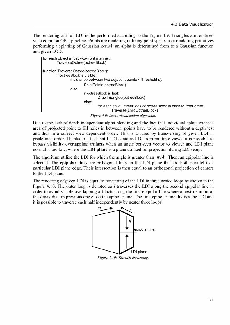
4.3 Data Visualization
The rendering of the LLDI is the performed according to the Figure 4.9. Triangles are renderedvia a common GPU pipeline. Points are rendering utilizing point sprites as a rendering primitivesperforming a splatting of Gaussian kernel: an alpha is determined from to a Gaussian functionand given LOD.
for each object in back-to-front manner:TraverseOctree(octreeBlock)
function TraverseOctree(octreeBlock):if octreeBlock is visible:
if distance between two adjacent points < threshold dt:SplatPoints(octreeBlock)
else:if octreeBlock is leaf:
DrawTriangles(octreeBlock)else:
for each childOctreeBlock of octreeBlock in back to front order:Traverse(childOctreeBlock)
Figure 4.9: Scene visualization algorithm.
Due to the lack of depth independent alpha blending and the fact that individual splats exceedsarea of projected point to fill holes in between, points have to be rendered without a depth testand thus in a correct view-dependent order. This is assured by transversing of given LDI inpredefined order. Thanks to a fact that LLDI contains LDI from multiple views, it is possible tobypass visibility overlapping artifacts when an angle between vector to viewer and LDI planenormal is too low, where the LDI plane is a plane utilized for projection during LDI setup.
The algorithm utilize the LDI for which the angle is greater than /4 . Then, an epipolar line isselected. The epipolar lines are orthogonal lines in the LDI plane that are both parallel to aparticular LDI plane edge. Their intersection is then equal to an orthogonal projection of camerato the LDI plane.
The rendering of given LDI is equal to traversing of the LDI in three nested loops as shown in theFigure 4.10. The outer loop is denoted as I traverses the LDI along the second epipolar line inorder to avoid visible overlapping artifacts along the first epipolar line where a next iteration ofthe I may disturb previous one close the epipolar line. The first epipolar line divides the LDI andit is possible to traverse each half independently by nester three loops.
II
epipolar line
LDI plane
IIII
Figure 4.10: The LDI traversing.
71

4 GPU/Hardware Aided Approaches
The actual LOD is determined as an estimation of maximal distance between two adjacent pointsthresholded by a threshold dt. In order to avoid LOD popping when LOD changes from triangularto point-based representation, the algorithm blends both representations. In the case of the LODchange to coarse level between two point-based representations, the algorithm benefits from thefact that the lower LOD contains a subset of higher LOD points. Thus, it is possible tocontinuously omit points that are not contained in the lower LOD.The shading is handled by the vertex shader as well as transformation to a position in screenspace according to a model-view-projection matrix. Both operations are equal to lighting in theclassical hardwired pipeline. Besides that, the vertex shader also computes additional informationthat is utilized for deforming a Gauss function in the pixel shader according to the view direction.
The Gauss function is stored in a texture utilized from modification of the α-channel of theoutput and it reflects a given LOD determined by a threshold dt of a distance between twoadjacent points. The threshold then determines the Gauss function for in the distance of d t /2from the center, the value has to be equal to 0.5. It is implemented via precomputed mip-mapsand retrieved alpha is utilized for blending with current background color c:
c= c splat1 −c (27)
In order to provide correct image, the kernel has to be rotated according to components nx, ny ofnormal projected to a camera space and =1 /cos , where θ is an angle between view directionand normal. The deformation is the applied by deforming texture coordinate t=t x , t y by arotation transformation R based on projected normal components34:
t '=R t . (28)
The solution allows displaying of over 105 points at real-time rates for objects of 106 triangles.The algorithm is capable to mix both triangular and point representations with smooth LODchanges. This allows effective visualization of large scenes or it allows effective rendering oftiny details on the surface that would require high number of small triangles and thus higher loadon the GPU, otherwise.
4.3.4 Other Representations
4.3.4.1 Fast Planar Data Visualization
In a data visualization area there are situations where a huge amount of planar objects is requiredto be displayed. Example of such area are a geographical application with highly detailed maps,which are far too complicated to be utilized for purposes of high quality real-time visualizationeven if the solution uses various techniques for visibility culling.
Therefore, there is a requirement for simplification of these planar object to a level depending onparticular view, i.e. to remove invisible or nearly-invisible details. This goal can be achieved byremoving a vertices thus replacing a polyline segment by a single, i.e. shortcut. Nevertheless, theresult has to meet several criteria based on geometrical constraints in order to prevent animportant features to vanish, e.g. modified polyline should not intersect other polyline if notavailable in original, polyline should have specified relation to given point even if simplified.
A possible solution for problem mentioned above is proposed in [Mus01]. It allowssimplification with preserving of features in real-time with a preprocessing by utilizing a graphic
34 In order simplify and thus speedup the computation it is possible to utilize an approximation describedin [Coc02].
72
4.3 Data Visualization
hardware. The idea of the algorithm is based on a fact that a shortcut may be considered valid ifit is contained completely within a unique neighborhood of a original polyline, i.e. if it does notintersect with neighborhood of different polyline.The neighborhood of the polyline can be constructed via the Voronoi diagram because areasconstructed according to different polyline are unbroken. In order to provide a speedup, it ispossible to utilize hardware solution described in Section 4.4.2. Instead of the Voronoi diagram,a ε-neighborhood can be used that is defined as a set of points with distance of up to ε fromoriginal polyline.The algorithm then utilizes following steps:
1. Preprocessing step in which the algorithm forms a set of possible shortcuts, i.e. shortcuts thatare both of smallest size and of specified maximum distance to original polyline.
2. Construction of the ε-neighborhood to a stencil buffer. For each neighborhood assign anumerical ID.
3. Selection of shortcuts by setting a stencil test and rendering all available shortcuts for givenpolyline with a unique color ID assigned to each shortcut. Then, read the pixel buffer and lookfor color pixels, i.e. look for shortcuts that lie outside the neighborhood of given polyline.Such shortcuts may cause disturbance of preserved features and thus they are removed fromthe list of shortcuts. The rest of the shortcut set is examined again in order to detect shortcutthat were overlapped by other shortcuts outside the neighborhood.
4. Construction of shortest path from a set of valid shortcut in order to create a modifiedpolyline. For such purposes a greedy algorithm that selects a shortcut that skips largestnumber of original polyline vertices and moves to the vertex connected by selected shortcut.The algorithm starts at polyline start and runs until end of polyline is reached.
The proposed solution allows visualization of large planar scenes such as maps with a capabilityto preserve features such as line-to-line and line-to-point relation. The algorithm is able to deliverthe image in real-time with a off-line preprocessing step. The visualization steps utilizes acommon GPU and can be improved even further by taking into account of new GPU featuressuch as occlusion query35 that may greatly speedup the shortcut selecting step of the algorithm.
4.4 Others
4.4.1 Computer Vision and Image Processing
4.4.1.1 Disparity Map Estimation
For a computer vision a depth information from a scene is a crucial because it is required forsuccessful obstacle avoiding. In the case of a real scene, the depth has to be estimated from oneor more images. If a pair of images is available, the first step for depth estimation is estimation ofa disparity map, i.e. map of pixels with offsets to corresponding pixel in the second map. Forsuch purpose, the images has to compared on a per-pixel basis.Even though there is the knowledge of camera relative positions that allows to reduce a searchingdirection and/or radius for each pixel, it still requires a unpleasant high number of independent
35 Occlusion query is available in both OpenGL and Direct3D. For details, refer to [GLE04].
73
4 GPU/Hardware Aided Approaches
per-pixel operation. That makes the disparity map generation ideal candidate for the GPUimplementation because it allows to benefit from parallelism of the GPU.A solution described in [Zac04] utilizes GPU for all computations and thus it gains animprovement in performance. The solution assumes a stereo pair of images that allows to limitthe searching for a scan-line based matching of images. In order to further improve theperformance, the solution utilizes a hierarchical approach based on the GPU capability ofautomatic mip-map generation.
The algorithm starts by comparing a coarser version of images in a rather large range in order toestimate a startup disparity map. Then, it moves to higher level and the comparison step isrepeated but in this time, only a limited range based on coarseness difference between levels isutilized, i.e. it refines the output. The disparity map from previous level is utilized for setting asearch startup position.The comparison of images is rather a simple. The algorithm utilize a simple absolute differenceof pixel values in order to find a configuration with the lowest sum of absolute difference (SAD)possible. First, it places a window from the second image over the first one and computes anestimation of the SAD by utilizing a bilinear interpolation36. Afterwards, the result is blendedwith actual disparity map by selecting a disparity with the lowest SAD.
At the end, a verification is utilized to discard a possible invalid pixels. For such purpose thealgorithm computes a left-to-right disparity map of offsets DL that is computed by matching awindow from left image to the right image and right-to-left map DR. Then, for each given pixelposition p and given threshold ε, the pixel is discarded if it fails following:
∣DR pDL pDL p∣ . (29)
Thanks to the hierarchical approach, the solution is able to inspect a large range in the left imagesand it is able to discard invalid matches. It utilizes an absolute difference that does not change therange of value and thus it is possible to utilize the approach for various low-cost mobile devicesthat are usually capable only of low shader model version. Nevertheless, the solution may fail forimages with high frequencies because the average utilized in the hierarchy building process actsas an low-pass filter.
4.4.1.2 Epipolar Geometry Computation
The scene depth estimation utilized by both computer vision or scene reconstruction is based oncorrespondence of element such as points, lines, or rectangles between two or more images. In aideal situation it possible to determine corresponding point but in a real situation such point maybe only estimated due to noise or lighting conditions. Also, a false correspondence may occur.Therefore, there has to be an option for manual adjustment of computation towards betteraccuracy. In order to provide an effective adjusting of the computation, the processing has to beperformed at almost interactive rates. However, due to large amount of possibly correspondingpoints it is not possible to achieve a performance close to a interactivity rate. Also, in order toimprove the accuracy usually more then two arbitrary views of known camera parameter areutilized and thus the performance is dragged down even further.
The solution described in the [Rod04] utilized a capability of projective texturing available incommon graphic hardware in order to improve the performance. The solution is based on a
36 Bilinear approximation allows to compute an average of four adjacent pixels, i.e. their sum. Thus, the n×nwindow may be handled as ½n×½n windows at the beginning of the sum operation.
74
4.4 Others
correspondence estimation of two points and for such purpose it utilizes an epipolar lines thatallow to reduce influence of error caused by noise or slightly incorrect camera settings.
The epipolar line is basically a line that is projected to a point cip in the view Ii while it isprojected to a line in the rest of views, i.e. I j , i≠ j. According to that, the epipolar line is a rayprojected from a camera position ci through the point cip. In an ideal case for two views, theepipolar line contains points cjp from the view Ij. In the real situation, almost no point lies directlyon the epipolar line in the view Ij and thus an error function has to be applied to estimate whichpoints are probably part of the line.For multiple views is the situation even more complicated. Candidates points vri found for eachcouple r of views I i , I j , i≠ j , i=const. may not coincide even thought they denote sameposition in the original scene. In such case, the correspondence is estimated according to a sumof errors of given candidate vri on epipolar line for individual views Ij: candidate is projected toview Ij and error is evaluated. Candidates with appropriate low sum of errors are then consideredpoints in the real scene.
The algorithm utilized in the solution is a slight modification of epipolar mechanism intendedfor multiple view. Each ray is rendered to a buffer in a form of a line from utilizing an orthogonalcamera perpendicular to such ray. This samples the ray and thus creates candidates that eachutilizes an error map texture lookup in order to obtain an error for given view Ij. The error mapfor given view Ij is basically a distance map where a point value in the map is distance to anearest extracted point cjp. The map may be computed similar to the Voronoi diagram (seeSubsection 4.4.2.1).
For a system of two view, the algorithm may stop right now and pixels with error lower than agiven threshold are considered as points in the scene. For a multiple view, this projection has torepeated for each of the views I j , j≠i utilizing an add blending operation for accumulation oferrors. Similar to two view situation, the pixels of low values are then considered as real pointsin the scene.However, if a point is occluded from a view Io then an unpleasant high error value may bygenerated because such occluded point is probably far too distant from any cop points. Such pointmay be then considered as a false match even though it is a correct one. In order to bypass it, thealgorithm clamps the distance error to a given value.
The solution is able to find scene points for 105 epipolar lines with a speed magnitude faster then
the CPU thanks to the fact that the approach is similar to regular rendering of primitive. Theperformance has no linear dependence on number of selected candidates, i.e. samples per ray.Thus, it can provide speed of 70× speed of the CPU-based solution even for older graphichardware37.
4.4.2 Computational Geometry
4.4.2.1 Generalized Voronoi Diagram Computation
Voronoi diagram is a structure that provides partitioning of the space and/or plane to cellsaccording to a set of input sites {A1, A2, ... , Ak} and given distance function dist that allows toevaluate distance between input site Ai and point p; the input site is of arbitrary shape. Voronoicell V Ai for given input site Ai is then defined as follows:
37 It does not use any programmable capabilities. These may be utilized in a point cip detection.
75
4 GPU/Hardware Aided Approaches
domAi , A j = {p∣dist p , Ai≤dist p , A j},V Ai = ∩
j≠idom Ai , A j.
(30)
The Voronoi diagram is utilized for preprocessing of data in order to obtain space partition.Through such partition it is then possible to plan route for robot, evaluate proximity queries,perform location optimization, etc. The major drawback of the diagram is its construction timefor generalized versions or input sets that consist of other primitive then points. In such case,edges of cell can be a general high-degree curves.A possible solution that allows construction of all possible Voronoi diagram generalizationwithout performance drop-down is described in [Hof99]. It utilizes graphic hardware to constructdiscretization of the Voronoi diagram. Thanks to that it is possible even 3D enhancement of thediagram.
The solution is based on idea of distance function evaluation by rendering of proper geometry.The hardware then handles solution of distance function comparison as described in theEquation (30) by utilizing a depth-buffer test: the color contains ID of given input set that ownsparticular pixels, i.e. space element. The diagram is then reconstructed by walking along edges inthe color image.In the case of 2D Voronoi diagram, the required geometry is simple and depends in type of inputset. Maximum height of such geometry is set to a maximum depth value38 in order to utilizecomplete accuracy of the depth-buffer. Base of geometry is resized to possibly influence allpixels in the discretization. Input sets supported by the solution are:
• Point for which the geometry has form of a cone. For M×M discretization of the Voronoidiagram, the base of the cone is a circle with diameter of 2 ⋅M with depth set to minimum,an apex of the cone is the position of the point in the plane with depth set to maximum. Thedensity of the mesh depends on selected error level.
• Line is replaced by a tent-like geometry in a form of two quads and two point as describedabove at a line endpoints if a line segment is utilized.
• Polygon and curve is decomposed to line and points thus utilizing same geometry asdescribed above.
Besides the 2D version, the solution is able to compute Voronoi-based partitioning of 3D space.In such case, the 3D space is discretized by horizontal slices : z=z0 and each slice is handledindependently. As distinct to the 2D version, the geometry39 is more complicated because it hasto consider the distance of given primitive to the slice according to a modified distance functiondist x , y=dist Ai , x , y , z0.
Similar to the planar version, complicated input sets are decomposed, e.g. a triangle is composedof the inside, edges, and points. For these input sets then geometry is following:
• Inside of the triangle/polygon influence only an orthogonal projection of the triangle throughthe space. Thus, it forms triangle or mesh of triangles equal to original polygon with verticestransformed by the distance function distα. If the polygon intersect the slice it is divided andboth parts are handled separately.
38 For depth-test set to greater-or-equal, the value is one. The depth-buffer is initialized to zero.39 The geometry represents the distance function.
76
4.4 Others
• Lines are handled by a geometry of elliptical cone with an apex at intersection point andeccentricity according to the angle between line and the slice. In the case of line segment, thegeometry is clipped by two parallel planes each containing respective line segment endpointthat are perpendicular to the slice.
• Point distance function forms a hyperboloid.
Besides the 3D enhancement, the solution is also able to compute weighted and farthest-sitemodifications. Weighted input set are handled either by translation along distance axis foradditive weights or linear scaling along distance axis for multiplicative weights. In the case offarthest-site modification40, the solution reverses both depth-buffer initialization and depth-testfunction.
Due to the discretization, the solution suffers from various errors: mesh error caused either byinappropriate approximation of the distance function by the mesh or by inaccuracy of therasterizer and combinatorial error caused by inaccuracy of the depth-buffer. The latter one maycause wrong ID evaluation for given pixel or it may omit details, i.e. small regions. Nevertheless,it is possible to decrease such error by adaptive approach that generates detailed version of areaaround edges.The solution allows computation of all Voronoi diagrams without any significant performancepenalty caused by complicated distance function or input set. The performance may be improvedeven further by assuming a maximum distance and thus reducing a number of generated pixels.Nevertheless, the drawback of the solution is possible lower accuracy due to discretization.
4.4.2.2 Collision Detection between Complex Models
Collision detection is an important part of environment and/or physical simulation and in amajority of interactive applications, this is one of the most time consuming part that therefore anappropriate a performance is required. For a simple and/or simplified models this task is easy.For complicated models a hierarchy and heuristics is utilized. Nevertheless, it still requiressignificant amount of computation that may increases according to complexity of O N 241.
A possible aid is to utilize the GPU and thus convert the solution to its discrete version and solveit in the screen space. These solutions provide better performance then strictly CPU-based one.Nevertheless, they are limited either by type of object because they may require closed objectonly in order to utilize stencil buffer or by bandwidth of GPU→CPU communication or both.Also, in few cases they are able to compute collision between pairs of objects only.
A solution that tries to avoid limitations mentioned above is described in [Gov03b]. It make notassumption about objects and the scene, i.e. it allows processing of open deformable objects andscene that changes rapidly. It is a hybrid solution that utilizes the GPU for estimation of possiblecollision and the CPU for computation of exact collision.
The estimation of collision is based on estimation of potentially colliding set (PCS) that isbasically a set of object who collide or are in a close proximity. The PCS is constructed from acomplete set of objects O1 , ... ,On in the scene by pruning of fully visible object from givenview. An object Oi is fully visible if it is not occluded by both objects O1 , ... ,Oi−1 and objectsO i1 , ... ,On . Fully visible object is also considered as not colliding.
40 Furthest-site Voronoi diagram is a digram of point with negated inequality sign in the Equation (29).41 This complexity is true for checking each object with each other.
77

4 GPU/Hardware Aided Approaches
The implementation requires two passes. Before the first pass, it clears the depth buffer, setsorthogonal projection, and sets depth function to less-or-equal. Then, objects O1 , ... ,On arerendered and for each object it detects if it is fully visible. Afterwards, it does the same but withobjects in opposite order, i.e. On , ... ,O1 . Objects that are fully visible in both pass are excludedfrom the PCS.The fully visible test is done via occlusion query42: the depth test is disable and depth function ischanged to greater-or-equal. Inspected object Oi is rendered with occlusion query to test whetherit is fully occluded. If not a single pixel passes the depth test using these negated depth functionthen no object occludes the object Oi. Afterwards, object is rendered to allow processing ofsubsequent object.
The approach above is first performed with complete objects to compute first estimation of thePCS. In order the improve the result, the second step test full-visibility on per-object-fragmentbasis. Each fragment of given object Oi is tested for full-visibility with objectsO1 , ... ,Oi−1 ,O i1 , ... ,On . Self-collision is not considered.
In order to further improve the performance, the algorithm first tests axis-aligned bounding boxes(AABB boxes) and then it tests at triangle representation level in each step. This allows to reducerequirements on the pipeline performance and thus allows to obviously non-colliding objectsquickly. Also, the AABB orthogonal projection is simple: two quads. This allows to perform theocclusion query together with rendering at the same time.
The performance of the solution shows linear dependency on both complexity of objects and itsnumber. It is capable to achieve interactive framerates for with of 106 triangles. The majoradvantage of the algorithm is the fact that it is bounded by a fillrate rather than by a bandwidthwhose throughput is not changing as fast as does the fillrate. Also, the solution does not requireprogrammability of the GPU and thus it is possible to utilize it even for older devices.
4.4.3 MathematicsNumerical mathematics is an important branch of mathematics utilized in the computer sciencebecause it allows result estimation in tasks where the analytical solution is either almostimpossible or cannot be automated. Numerical approaches usually a rather large number of rathersimple operation over individual elements that allows to employ parallelism. Also, the iterativenature of these operation allows to utilize streaming architecture for efficient solving.
According to attributes mentioned above, it can be assumed that for a proper result estimation therunning time may be unpleasantly hight and thus either an optimization or a hardware muchcloser to their attributes is required. A hardware that may serve well for this task is the GPU: inparticular the GPU capable of shader model 2.0 or newer.Such hardware then allows to benefit from hight throughput of the pixel shader with only a fewlimitations such as lower accuracy that may be either considered negligible or avoided byapproaches of numerical mathematics. Also, a communication between the GPU and the CPU inparticular GPU→CPU data transfer has to be kept at minimum, i.e. in ideal situation, the methodshould be implemented completely on the GPU and the CPU should fetch results only.
42 Occlusion query mechanism is described in specifications of extensions HP_occlusion_query andNV_occlusion_query, see [GLE04].
78

4.4 Others
4.4.3.1 Basic Operators for Linear Algebra
A crucial factor for successful numerical method implementation is an appropriate as well aseffective implementation of basic operation and data structures such as matrix and vectors. Theproposed solution is described in the [Krü03] and it aims on storing of matrices consideringefficient matrix-to-matrix operations.
The basic structure utilized in the numerical mathematics is a vector. Even thought this is 1Dstructure, the actual storage may not utilize 1D texture at all due to its inefficiency and sizelimitations. Each GPU has its own limitation of maximum texture sizes and thus storing a vectorto 2D texture enlarges its maximum size to second power of 1D texture case43. Also, GPUs tendsto have fast access rate to the 2D texture because it is the most utilize texture form forvisualization.
Another important structure is a matrix. For a matrix a possible solution is to store it directly to a2D texture. Nevertheless, this may not be efficient storage for several common matrix operationssuch as transposing. The more efficient solution is to decompose the N×N matrix M to Ndiagonal vectors, where the i-th vector vi starts at i-th column of the matrix and its elementsequal to elements of matrix M={mi , j} according to following:
v ji =m j ,i j mod N (31)
This structure allows to store large matrices, even larger than the maximum size of the 2Dtexture. Also, it allows to benefit from performance of the 2D texture accesses and its allowssimple implementation of both vector-to-matrix product and matrix transposing. The latteroperation requires only reordering of vectors that may be implemented as index shifting directlyin the GPU without any additional requirements.
Basic operations with these two basic structures such as addition, subtraction, and per-elementmultiplication are rather simple: a single pass per vector that accesses all elements and computesthe result. A slightly complicated is a matrix-to-vector product: b=M⋅a . For a given N×Nmatrix this operation requires N passes. Each pass multiplies given diagonal vector element withcorresponding element in the vector a: for the i-th diagonal vector and its the j-th element, thevector element ai j mod N
44 is accessed.
The result in a form of N multiplied diagonal vectors is then summed together to form a singlevector b. If supported, the summation may be implemented by pixel blending. However, themajority of GPUs is not able to perform the blending on 32-bit floating-point render targets andthis multiple passes has to be employed. The performance of the product operation may befurther improved by multiplying more than one vector at time up to maximum number ofsamplers45.
Another important operation operation with matrices and vectors is a vector reduction. Thisoperation allows to sum the vector thus providing a final step for dot product operation46. Due tolack of advanced flow control, the implementation of N-component vector reduction requires
1 2 log2N −1 passes. In each pass, the 2D texture is divided to four quarters that are merged
43 For current hardware, the maximum size of 2D texture is from 20482 up to 40962 of elements.44 The modulo operation may be implemented as proper texture addressing mode, i.e. wrapping of texture
coordinates.45 Exactly, number of samplers minus one: one sampler is utilized for original vector.46 Dot product first multiplies vectors per-element and then sums the result.
79
4 GPU/Hardware Aided Approaches
according to a given operation to the left-upper one. For the next pass, the approach utilizes theleft-upper quarter instead the whole texture.For a larger number of numeric tasks such as simulation an input and/or an output form a specialmodification of a matrix, i.e. the sparse matrix. It is sure that these tasks case successfullyoperate with common dense matrix but utilizing features of sparse matrices usually reducescomputation time significantly. Nevertheless, in the case of the GPU, the sparse matrix may noteffective in comparison to common dense matrix representation.
In the case of banded matrix, the implementation is rather simple: zeroed diagonal vectors areomitted and thus matrix-to-vector product computation is reduced in number of passes. Thesituation in the case of random sparse matrix is little bit complicated. A possible solution isdescribed in the Subsection 4.4.3.2.
A slightly different approach is based on point sprites: each point represents a non-zero elementin the matrix with color equal the a value. During the product computation, points aretransformed in the vertex shader to access proper element in the vector a, see above.
Nevertheless, this solution employs the vertex shader that has lower throughput than the pixelshader. Such representation of the matrix is read-only if the GPU is not capable to either utilizevertex textures or proper pixel buffer object, see Subsection 2.2.2.1. Otherwise, the solution hasto utilize GPU→CPU data transfer thus degrading the performance.
The performance of the GPU solution is much better than the CPU: speed of the GPU matrix-to-vector and vector-to-vector operation is 12—15× speed of the CPU version. The onlylimitations is the fill-rate and number render target switch operations, i.e. number of passes.Nevertheless, for the real application the speedup is only in the range 2—5 due to additionalfixed costs and CPU-GPU communication, especially the GPU→CPU data transfer47. Thus, forthe performance reasons the GPU computing is not efficient for performing only a singleoperation followed by an immediate result fetch back to the CPU.
4.4.3.2 Sparse Matrix and Sparse Matrix Solver
One of numerical tasks is a simulation of various processes. In a majority, these simulation leadsto partial differential equations (PDE). These may be solved by approaches of numericalmathematics based on iterative process of result refining. According to a previous subsection, itis possible to gain the performance by utilizing the GPU as it is described in [Bol03].
In the case of unstructured grid it is possible to utilize the PDE to perform optimization taskssuch as mesh smoothing. The input of approach is 2-manifold triangle mesh with n vertices, setof edges E={eij} , where eij is edge between vertices of indices i, j, and boundary condition f.Also, a state of two incident triangles is given in a form of matrix A. The goal is to estimatevertex associated degree of freedom x such as position, texture coordinates, scalar value forneighborhood N i={ j∣eij∈E } of vertex i. The solution is then equal to solution of systemA x= f :
∀ i=1 , ... , n : aii xi ∑j∈N i
a ij x j= f i . (32)
If such system is symmetric positive definite then it is possible to utilize a conjugate gradientmethod. This method is an iterative process of finding solution by following of path with thhighest gradient in residuum that is initialized from an initial guess of x as r= f −A x . For moredetails, refer to [Bol03, Krü03].47 For current hardware, the download of 1024×1024 32-bit floating-point RGBA texture costs tens of milliseconds.
80

4.4 Others
Among others, the method utilize a matrix-vector product and vector inner-product. In the caseof the latter one, it is possible to utilize approach similar to previous subsection. Also, all vectorsare stored in a 2D texture according to same rules as in the previous subsection: vector x is storedas a 2D texture X, vector f is stored as a 2D texture F.Nevertheless, in the cast of matrix-to-vector product the situation is little bit complicated becausethe matrix is a random sparse matrix and thus utilizing an approach similar to dense matricesmay not be efficient enough. Opposite to previous section where sparse matrices wereimplemented via point render primitive, the approach described in the [Bol03] utilizes a texture-based storage that allows updates of the sparse matrix even on the GPU of shader model 2.0.The sparse matrix A is decomposed to a texture A containing diagonal a vector of the matrix Aand a texture A∗ that contains off-diagonal non-zero matrix elements. Elements stored in roworder packed tightly, i.e. with no gap. In order to be able to decode the contents of the textureA∗ another set of texture is generated: indexing texture R and correspondence texture C.
The texture R contains indexes of row beginnings in the texture A∗ and therefore it is closeequivalent of vertex neighborhood N i , see above. The texture C has same layout as textureA∗ but instead coefficient it contains addresses of corresponding elements in the texture X. The,
computation as described in the Equation (32) can be then expressed as following:j = R [i ] ,
Y [i ] = A[i ]⋅X [i ]∑c=0
k i−1
A∗[ jc ]⋅X [C [ jc ]] .(33)
If the matrix A depends on values x, the solution allows to update the matrix withoutdownloading result back to the CPU and utilizing approach common for CPU-based solvers, i.e.to compute stiffness matrix. Instead, it performs an update utilizing three additional textures thatallow to find vertices vertices for triangles incident on given edge eij for the off-diagonalelements in the texture A∗ and thus it allows to bypass scatter operation required otherwise.Diagonal vector stored in the texture A is handled separately. For more details and exactequations, refer to [Bol03].
The performance of the GPU-based approach is better than the CPU-based by coefficient ofalmost 2× speed of the optimized. The solution is able to perform a single step of the iterationprocess with real-time framerates. Also, it allows modification of the values in the matrix Awithout the GPU→CPU data transfer thus enlarging the set of task of possible efficient GPUimplementation.
4.4.3.3 Fast Fourier Transformation
Fourier transformation provides a facility to convert from spatial domain to frequency domain. Itis based on a fact that it is possible to describe every periodic function as a combination ofinfinite set of sinus functions. For a non-periodic function, the whole definition domain isconsidered as a single period. Based on that, the transformation determines correlation of theinput function f x with set of frequencies in order to form a transformed complex functionF u :
ℱ { f x } = F u = 1 N ∑x=0
N−1 f xW Nux ,
ℱ −1 {F u} = f x = ∑u=0N−1 F uW N
−ux ,W N=e−
1 N i 2 .
(34)
81
4 GPU/Hardware Aided Approaches
The drawback of the transformation is its time complexity: for M×N image it is O MN 2 .Therefore the most utilized version of Fourier transformation is Fast Fourier Transformation(FFT) that has time complexity of O MN log Nlog M . The algorithm is based on splittingthe Equation (34) and input into two halves: half with even indices and half with odd indices.Each half is computed separately thus forming a recursive description:
F u = 1 N F ' u ,
F ' u = F even' uW N
u F odd' u .
(35)
The application of the FFT is in area of loss-compression algorithm and reconstruction of imageswith en example in the Subsection 4.3.2.2. Also, the FFT may be utilized for improving offiltering performance because a convolution in spatial domain is equal to multiplication infrequency domain. Thus, filtering of M×N image with M×N filter in frequency domain is atcomplexity of O MN while the spatial domain requires O MN 2 .
For GPU-aided solutions, the FFT utilization is problematic because it is performed on the CPUand thus requires a transferring of large data set such as images from the GPU to the CPU. If theFFT would be available on the GPU a possible performance improvement of various methodswould be possible by limiting their GPU→CPU communication.
A solution described in [Mor03] is an attempt to implement the FFT on the GPU. It is a almostdirect implementation of the FFT as described and for 2D image the forward FFT utilizes twomajor step: application of the FFT on rows and application of the FFT on columns. The inverseversion approach similar to the forward one and at the end the output does not requires additionalreordering of the its layout.In order to convert 2D image to a frequency domain, the algorithm has to perform the FFTdescribed by the Equation (35) on rows first. The solution of this steps benefits from the fact thatthe output of the FFT for input of real numbers are complex numbers that exhibit a certainsymmetry Fℜu=F ℑN−u ,∀ u , u≠0, u≠ 1
2 N . Values of F 0 , F 1 2 N does not have a
imaginary part.Based on that symmetry, it is possible to reduce computation time to its half by propercombination of two input rows rc x=r1 xi r2x . After the transformation, it is possible todecompose the transformed row Rcu to individual rows. The symmetry is also utilized toreduce storage requirements by omitting of 1
2 N−1 complex values thus allowing to store Ncomplex number to N real value slots as described in the Figure 4.11.
index
real part
imaginary partN20 N−1 N
21 N2−1 N−1
Figure 4.11: The packed complex values generated by the 1D FFT.
The second step in 2D image transformation is to apply the FFT on columns of the the imagetransformed row-by-row in the previous step. The application of the FFT benefits from a fact thatwith exception of columns C0 and CN/2 the rest can be merged to a complex numbers. ColumnsC0 and CN/2 are combined similar to row prior to application of the FFT.Both described parts of the transformation are implemented in a form of four steps. The inverseFFT utilizes same sequence of step as does to forward one with an exception in step two and fourwhere no scaling is applied. The forward FFT is a sequence of steps:
82

4.4 Others
1. Application of the FFT on rows of the images. Rows are combined as it was described byutilizing upper half of row as real parts and lower half as imaginary parts. Then the FFT isapplied in log N passes according to the Equation (35). Computation of both real andimaginary parts utilizes similar code with difference in indexing.
2. Conversion to packed format described by the Figure 4.11. The conversion performdecomposition of transformed function Rc back to individual transformed rows R1 and R2 .Then, values are scaled by 1
M as described by the Equation (34).
3. Application of the FFT on columns formed by the result from the previous step. Due to thefact that columns C0 and CN/2 contains real parts only they are handled separately similar torows in first step. The rest of columns contains either real or imaginary parts only and thusthey form a complex number when merged.
4. Conversion to packed format similar to the second step. Due to the fact that with only a singleexception the composition of two real values to single complex one is not utilized, onlyscaling is performed. The exception is composition of columns C0 and CN/2 that has to bedecomposed similar to the second step.
The performance of the solution is under the level of interactivity for image of 1024×1024. It iseven slower than optimized CPU-based FFT by a factor of two due to large number of passes andshader code changes. It can be expected that the performance improves when a shader modelwith dynamic flow control is utilized. Nevertheless, the GPU-based does not require anyGPU↔CPU data transfer and thus is may lead to performance improvement for pure GPUsolutions.
83


5 Conclusion
This document provides a view on the GPU and its possible applications. Similar to the graphicalhardware previous to the GPU, it outperforms common and comparable CPUs in many tasks.Thank to its capability of being customized by the user supplied code, the area of possibleapplication of the GPU became much larger then it was during previous attempts to utilizegraphic hardware. At most, the general processing area was affected by the availability of theGPU and the GPU became a tool that allows a performance improvements of several algorithms.This leaded to a explosion of papers among conferences that aimed on the GPU application.Approaches described in these papers utilized GPU to improve the performance by thinking of itas a second processor available on a machine; some of the even considers the GPU as thedominant processing unit. Nevertheless, both views benefit from the fact that the GPU has highperformance, low cost in comparison to dedicated hardware, and it is becoming a standardcomponent in a majority of home computers.
Currently, the GPU utilization for general processing is in the state of an implementation. Basedon capabilities and limitations of the GPU it is quite easy to decide whether particular algorithmis suitable for GPU implementation or not and/or to modify particular algorithm to suit the GPU.In a fact GPU application of general processing became a rather a question of conversionbetween platforms with different limitation and/or runtime requirements than a question of activeresearch aimed on are of possible GPU applications.When implementing algorithm, for a success it is just required to follow rather simple andintuitive rules that are easily distinguishable from previous GPU applications. Also, it isnecessary to keep eye on limitations such as limited flow control capabilities that preventstraversing of sophisticated memory structures and restricted memory access that disallows scatteroperations.
Therefore, the GPU is suitable for speedup of brute-force based algorithms that need to process alarge number of elements using a simple set of operations. Examples described in this documentutilize the GPU for such purposes and their description is aimed on that. Thus, this can beconsidered as an tutorial on conversion of algorithms to the GPU.A little bit different area of GPU applications is the area outside the general processing, i.e. areaof graphical applications. Thanks to the programmability of the GPU it is possible toimplement real-time effects that were only available using off-line renderers before. Such effectsare then only limited by fillrate, memory latency, and program length issues. In contrast togeneral processing, this field offers better possibilities for further research but such research israther restricted because it is tied to a specific hardware configuration, i.e. GPU pipeline.Besides the GPU application area, it is possible to further investigate the question of the GPUperformance improvement based on either its multiplication or multiplication of its parts. Theapproaches based on multiplication of GPUs and/or complete graphic boards requires only a
85
5 Conclusion
slight modification of the hardware due to synchronization issues and almost none modificationof the GPU itself.The problems that has to be solved in this area is concerning with a proper data distributionamong GPUs over either a bus or a network. The goal is to minimize both redundant work donedue to inaccurate distribution and communication required for cooperation of individual GPUs.This also means that the research in this area is highly task dependent in order to improveeffectiveness of the solution and thus it rather an impossible task to handle it generally.
A similar situation governs the area of increasing the number of individual GPU parts. This isa branch of research that leads to a construction new architectures based on triangle renderingand it is concerned with a solution of work distribution between individual multiplied parts of theGPU. Also, it tries to answer the question of placement of such distribution in the GPU pipeline.This area of research is rather low-level and thus very close to the hardware itself. Theoreticalsolutions have to be followed by practical experiments with modified hardware in order toestimate the real benefit of particular solution.
The last area of possible research that aims the GPU is an area of GPU modificationsconcerning with introduction of new features rather then multiplying of existing parts. Besidesfurther improvement of the GPU programmability, this field aims on possible modification of theGPU pipeline towards image generation of either better quality, better performance, or both, e.g.input of the pipeline may by modified by support for high-order primitives and effective view-dependent LOD.
Also, the output can be further enhanced by introducing an order-independent transparencysupport, reduction of anti-aliasing complexity based on view-dependence mechanism, and scatteroperation support, i.e. ability to modify target pixel position. Besides that, the inside of thepipeline may be modified as well by introducing a performance improvement such as earlyvisibility estimation in the vertex pipeline or addition of new rendering primitive as it was shownin this document.In the fact, this is a possible place for real research on the GPU that is not bounded by thesolution application and it is not tied to the current architecture as tight as in previous areas. It iseven possible to modify the pipeline on a block level and test it on a software emulation in orderto measure features such as throughput or fillrate that are easily comparable to possibilities ofcurrent and/or future hardware components.
Thanks to that, it is possible to search for improvements without any low-level games with thephysical hardware and yet still have a reasonable probability of real implementation in futureGPUs. Thus, this is why this area aimed by the future work presented in this state of the art andconcept of doctoral thesis.
86

6 Future Work
Current GPUs are able to synthesize 2D images as a view of 3D scene with very highperformance. The reason for generating of 2D images is based on requirements of commondisplay device that is able to display only 2D objects. Currently, thanks to the technology, there isexpansion of 3D display devices [Hal97] that either displays a complete volume or tries toreconstruct light waves flowing from the scene and thus recreate almost complete informationthat can be captured by the human visual system.
Therefore, the question is whether the GPU may be adjusted to fit requirements of 3D displaydevices. The actual state of the GPU capabilities allows only limited use of the GPU: at majorityin similar manner as that of general processing. Such use is not effective because it cannot utilizefull power of the GPU that is available in the image generation area. On the other hand, somedevices may require a set of images and thus it is possible to utilize the GPU for imagegeneration similar as its developers intended.The only flaw of this use it that the GPU ignores some information based on the nature ofimages. That additional information such coherency may then be utilized for improvement of theperformance. This is caused by the fact that the GPU does not assume any additional informationavailable even thought such information may reduce the amount of computation significantlysuch as the case of occlusion tests described in Subsection 4.3.1.
An example that requires series of images is parallax display device. This device type is basedon discretization of viewing angles, producing a pair of images for each single discretizedposition. Images are delivered to particular direction by directing of a light thus not requiringhead-tracking or similar devices. When user changes a position in front of the device, a differentset of images is presented that evokes the feeling of presented scene being actually a solid object,i.e. motion parallax.
Besides that, each eye obtain a slightly different images resulting to a generation of a ratherimportant stereoscopic disparity that evokes feeling of depth. This together with motion parallaxand visual realism of individual images, device can convince the viewer that the displayed objectis real. The important fact of parallax displays is that there is already a partial technologicalsolution for it that provides full stereoscopic disparity on horizontal motion parallax[Jon95, Yan04] without requirement of user and/or head tracking device.Based on the nature of this display device type it is possible to utilize the GPU for generation ofindividual images. The only drawback is the fact, that it requires a set of 2N images for N viewsat once, e.g. if a framerate of 25 fps48 is required for 8 view, the graphical device has to generateapproximately 400 frames per second. Such high framerate is not achievable by current rendering
48 25 fps is close to a point in framerates where the human visual system can distinguish between set of images andfluent animation.
87
6 Future Work
device if high quality image with proper anti-aliasing is requested because a single GPU solutionis bounded by both cost of render target switching and limited fillrate.A possible and straightforward solution is to multiply the GPU on graphic board level. Thissolution is possible even with current GPUs and allows to generate images with highperformance. The only drawback is its price and requirement of additional hardware device thathandles synchronization of output images as well as data distribution between GPUs eventhought they do not need to solve the distribution of primitive similar to that of partitioneddisplay [Mit00].
The interesting attribute of the parallax display device is that images required by them aregenerated from different viewpoints that are located on sphere and looking at a single place.Thus, there is a possibility of coherence in the images. This is basically a fundamental idea of thewhole future work that leads to following approach that is close to idea of deferred shading asspecified in Subsection 2.2.3.2:1. Generate all images at once. In ideal situation, only a single rendering pass is required in order
to generate both color and depth information.
2. Perform post-processing step with generated image and/or images in order to obtainindividual images that can be utilized for the actual output device.
Image generation is the most important part of the whole process. It is based on a fact that whenplaced in space, individual images from a plane approximation of a sphere or another surfacecentered at the look-at point, for simplicity let us assume that the surface is spherical. Thus, thisapproximation of the sphere may be replaced by a real spherical surface that can be unwrapped toa plane without any shearing. Also, there is an inverse transformation back to individual imagesis possible. This approach is inspired by a sub-step of form-factor computation described inSubsection 4.2.2.
The question that has to be answered is suitability of given surface for these purposes andperforming of the mapping. The latter one has to be solved with a respect to a hardwareimplementation at least from a theoretical point of view because an evaluation of complicatedequations as well as operations such division or square root are not acceptable due to both theircomplexity and performance costs.Based on knowledge of current GPUs, it can be assumed that a major modification has to done tothe rasterizer. It is expected that mapping may be handled by a clever modification of a triangleand/or other primitive through the rasterization thus leaving the rest of the pipeline intact. In thecase of the reconstruction, the solution expected a new component at the end of the pipeline:either before data are written to the back buffer or after that. In both cases the solution has tohandle situations where from two different view the visibility of two objects changes betweeneach other.
For the output of the solution, there is assumption of a lower quality than the of individual imagerendering due to transformation and post-processing step. On the other hand, it is expected thatthe solution, if possible, improves the performance thank to utilizing of the coherence. Also, ifbuilt, the cost of the device should be lower than the cost of brute-force multiplication ofindividual GPUs.The solution requires determination of mapping primitive together with solution of linearinterpolation on mapped surface as it is common in projection space. There is a possibility tobenefit from mathematical evaluation of both mapping transformation and mapping primitivedefinition that may well help to simplify the interpolation.
88

6 Future Work
The goal of the future work is to modify the GPU, but to left as much as possible unmodified inorder to allow compatibility with 2D image generation and integration with other enhancement ofclassical pipeline as described in Section 2.3. Also, the solution should investigate a possibilityof application of this approach to a stereoscopic display device that is able to generatestereoscopic disparity that is a rather important clue when estimating depth and distance. Theactual stereoscopic device is available at department of the author.Also, the solution has to determine a suitable basic primitive that produces lowest amount ofinaccuracies when rasterized on non-planar surface, i.e. whether it is still solution to utilize adeformed planar triangle or to switch to spherical one. Besides that, the solution has to determinewhether common graphical effects, such as shadows, fog, etc., are still possible utilizingmodified GPU or whether there have to be modifications applied. It is expected that the majoramount of problems will be experienced when exploring effects that benefit from 2D nature ofthe output image.
The future work is a part of the 3DTV NoE project that is being solved at the department. Thisproject is aimed on capture, processing, transmission, and display of 3D scenes as well as the 3Dspace that is the area close to the proposed future work. The major concern of the 3DTV projectin an area of displaying is with the holography [Har96] and therefore, the future work will alsoexplore possibility how to incorporate the future work to a process of holography, i.e. basically,how to convert between recorded holographic image and image generated by the solution inorder to allow displaying of resulting output utilizing different displays.Presented future work is a part of research aimed on modification of the GPU. Based onexamples described in this work, this is the only place for theoretical research on the GPU.Besides that, it is close to fundamental algorithms of computer graphic because it may happedthat a proposed solution based on rendering on non-planar surface may have a slightly differentrequirements then current rendering to a planar 2D image in order to be effective and thus requireeither different algorithms or modification of existing algorithms.
89


References
[Ail03] Aila, T., Miettinen, V., Nordlund, P. (2003). Delay Streams for Graphics Hardware.ACM Transactions on Graphics, Vol 22, No 3, pp. 792—800.
[Arv04] Arvo, J., Westerholm, J. (2004). Hardware Accelerated Soft-Shadows UsingPenumbra Quads. Proc. of WSCG, Pilsen, Czech Republic, pp. 11—17.
[Bax02] Baxter, W. V., Sud, A., Govindaraju, N. K., Manocha, D. (2002). GigaWalk:Interactive Walkthrough of Complex Environments. Proc. of the EurographicsWorkshop on Rendering, Pisa, Italy, pp. 203—214.
[Bol03] Bolz, J., Farmer, I., Grinspun, E., Schrooder, P. (2003). Sparse matrix solvers on theGPU: conjugate gradients and multigrid. ACM Transactions on Graphics, Vol 22,No 3, pp. 917—924.
[Buc03] Buck, I. (2003). Brook Spec v0.2. [WWW]http://merrimac.stanford.edu/brook/brookspec-v0.2.pdf (Frebruary 5 2005).
[Buc04] Buck, I., Foley, T., Horn, D., Sugerman, J., Fatahalain, K., Houston, M., Hanrahan,P. (2004). Brook for GPUs: Stream Computing on Graphic Hardware. ACMTransactions on Graphics, Vol 23, No 3, pp. 777—786.
[Car02a] Carr, N. A., Hart, J. C. (2002). Meshed atlases for real-time procedural solidtexturing. ACM Transactions on Graphics, Vol 21, No 2, pp. 106—131.
[Car02b] Carr, N. A., Hall, J. D., Hart, J. C. (2002). The ray engine. Proc. of the ACMSIGGRAPH/Eurographics Workshop on Graphics Hardware, Saarbruecken,Germany,pp. 37—46.
[Car03] Carr, N. A., Hall, J. D., Hart, J. C. (2003). GPU algorithms for radiosity andsubsurface scattering. Proc. of the ACM SIGGRAPH/Eurographics Workshop onGraphics Hardware, San Diego, USA, pp. 51—59.
[Cat80] Catmull, Ed, Smith, E. R. (1980). 3D-Transformations of Images in Scanline Order.Computer Graphics, Vol 14, No 3, pp. 279—285.
[Cha99] Chang, C., Bishop, G., Lastra, A. LDI tree: a hierarchical representation for image-based rendering. Proc. of the 26th conf. on Computer graphics and interactivetechniques, Los Angeles, USA, pp. 291—298.
[Cha02] Chan, E., Ng, R., Sen, P., Proudfoot, K., Hanrahan, P. (2002). Efficient partitioningof fragment shaders for multipass rendering on programmable graphics hardware.Proc. of the ACM SIGGRAPH/Eurographics Workshop on Graphics Hardware,Saarbrucken, Germany, pp. 69—78.
91

[Coc02] Coconu, L., Hege, H. (2002). Hardware-accelerated point-based rendering ofcomplex scenes. Proc. of the Eurographics Workshop on Rendering, Pisa, Italy,pp. 43—52.
[Coo84] Cook, R., L. (1984). Shade Trees. Computer Graphics, Vol 18, No 3, pp. 223—231.
[Coo04] Coombe, G., Harris, M. J., Lastra, A. (2004). Radiosity on graphics hardware. Proc.of the 2004 conf. on Graphics interface, London, Canada, pp. 161—168.
[Cro77] Crow, F. C. (1997). Shadow algorithms for computer graphics. Proc. of the 4th conf.on Computer graphics and interactive techniques, San Jose, USA, pp. 242—248.
[Dac03] Dachsbacher, C., Stamminger, M. (2003). Translucent shadow maps”, Proc. of theEurographics Workshop on Rendering, Leuven, Belgium, pp. 197—201.
[Die99] Dietrich, S. (1999). Guard Band Clipping. Game Developer Conference.
[Die04] Diepstraten, J., Weiskopf, D., Kraus, M., Ertl, T. (2004). Vragments and Raxels –Relocatability as an Extension to Programmable Rasterization Hardware. Proc. ofWSCG, Pilsen, Czech Republic, pp. 181—187.
[Dog00] Doggett, M., Hirche, J. (2004). Adaptive View Dependent Tessellation ofDisplacement Maps. Proc. of the ACM SIGGRAPH/Eurographics Workshop onGraphics Hardware, Interlaken, Switzerland, pp. 59—66.
[DX05] Microsoft DirectX 9.0 SDK (February 2005) Documentation. (2005). [WWW]http://msdn.microsoft.com/library/default.asp?url=/library/en-us/directx9_c/directx/directx9cpp.asp (March 17 2005).
[Eng02] Engel, K., Ertl, T. (2002). Interactive High-Quality Volume Rendering with FlexibleConsumer Graphics Hardware. Proc. of Eurographics, Saarbrucken, Germany, Stateof the Art Report.
[Ern98] Ernst, I., Russeler, H., Schulz, H., Wittig, O. (1998). Gouraud bump mapping. Proc.of the ACM SIGGRAPH/Eurographics Workshop on Graphics Hardware, Lisbon,Portugal, pp. 47—ff.
[Fer03] Fernando, R., Kilgard, M. J. (2003). The Cg Tutorial. Addison-Wesley.
[GLE04] OpenGL Extension Registry. (2004). [WWW] http://oss.sgi.com/projects/ogl-sample/registry/ (March 17 2005).
[Gov03a] Govindaraju, N. K., Sud, A., Yoon, S., Manocha, D. (2003). Interactive visibilityculling in complex environments using occlusion-switches. Proc. of the 2003symposium on Interactive 3D graphics, Monterey, USA, pp. 103—112.
[Gov03b] Govindaraju, N. K., Redon, S., Lin, M. C., Manocha, D. (2003). CULLIDE:Interactive Collision Detection Between Complex Models in Large Environmentsusing Graphics Hardware. Proc. of the ACM SIGGRAPH/Eurographics Workshopon Graphics Hardware, San Diego, USA, pp. 25—32.
[Hak97] Hakura, Z. S., Gupta, A. (1997). The design and analysis of a cache architecture fortexture mapping. Proc. of the 24th symposium on Computer architecture, Denver,USA, pp. 108—120.
[Hal97] Halle, M. (1997). Autostereoscopic displays and computer graphics. ACMSIGGRAPH Computer Graphics, Vol 31, No 2, pp. 58—62.
92
References
[Han90] Hanrahan, P., Lawson, J. A language for shading and lighting calculations. Proc. ofthe 17th conf. on Computer graphics and interactive techniques, Dallas, USA,pp. 289—298.
[Har96] Hariharan, P. (1996). Optical Holography. Cambridge University Press.
[Hei99a] Heidrich, W. (1999). High-quality Shading and Lighting for Hardware-acceleratedRendering. Ph.D. thesis, University of Erlangen, Erlangen, Germany.
[Hei99b] Heidrich, W., Seidel, H. (1999). Realistic, hardware-accelerated shading andlighting. Proc. of the 26th conf. on Computer graphics and interactive techniques,Los Angeles, USA, pp. 171—178.
[Hof99] Hoff, K. E., Keyser, J., Lin, M., Manocha, Culver, T. (1999). Fast computation ofgeneralized Voronoi diagrams using graphics hardware. Proc. of the 26th conf. onComputer graphics and interactive techniques, Los Angeles, USA, pp. 277—286.
[Hor04] Hormann, K., Tarini, M. (2004). A Quadrilateral Rendering Primitive. Proc. of theACM SIGGRAPH/Eurographics Workshop on Graphics Hardware, Grenoble,France, pp. 7—14.
[IEE85] 754:1985. IEEE Standard for Binary Floating-Point Arithmetic.[Jon95] Jones, M. W., Nordin, J. H., Kulick, J. H., Lindquist, R. G., Kowel, S. T. (1995).
Real-time three-dimensional display based on the partial pixel architecture. OpticalLetters, Vol 20, No 12, pp. 1418—1420.
[Kes04] Kassenich, J., Baldwin, D., Rost, R. (2004). The OpenGL Shading Language.[WWW] http://oss.sgi.com/projects/ogl-sample/registry/ARB/GLSLangSpec.Full.1.10.59.pdf (March 17 2005).
[Kil99] Killgard, M. J. (1999). Improving Shadows and Reflection via the Stencil Buffer.[WWW] http://developer.nvidia.com/object/Stencil_Buffer_Tutorial.html(March 17 2005).
[Kil04] Killgard, M. J. ed. (2004). NVIDIA OpenGL Extension Specifications. [WWW]http://www.nvidia.com/dev_content/nvopenglspecs/nvOpenGLspecs.pdf(March 17 2005).
[Kle04] Klein, T., Stegmaier, S., Ertl, T. (2004). Hardware-accelerated Reconstruction ofPolygonal Isosurface Representations on Unstructured Grids. Proc. of the 12thPacific Conf. on Computer Graphics and Applications, Seoul, Korea, pp. 186—195.
[Kos04] Koster, M., Haber, J., Seidel, H. (2004). Real-Time Rendering of Human Hair usingProgrammable Graphics Hardware. Proc. of Computer Graphics International,Crete, Greece, pp. 248—256.
[Krü03] Krüger, J., Werstermann, R. (2003). Linear algebra operators for GPUimplementation of numerical algorithms. ACM Transactions on Graphics, Vol 22,No 3, pp. 908—916.
[Las95] Lastra, A., Molnar, S., Olano, M., Wang, Y. (1995). Real-time programmableshading. Proc. of the 1995 Symposium on Interactive 3D graphics, Monterey, USA,pp 59—ff.
93
[Laz04] Lazányi, I., Szirmay-Kalos, L. (2004). Speeding up the virtual light sourcesalgorithm. Proc. of the 20th spring conf. on Computer graphics, Budmerice,Slovakia, pp. 112—120.
[Lef04] Lefohn, A. E., Kniss, J. M., Hansen, C. D., Whitaker, R. T. (2004). A StreamingNarrow-Band Algorithm: Interactive Computation and Visualization of Level Sets.Computer Graphics, Vol 10, No 4, pp 422—433.
[Lin01] Lindholm, E., Kilgard, J. M., Moreton, H. (2001). A User-Programmable VertexEngine. Proc. of the 28th conf. on Computer graphics and interactive techniques, LosAngeles, USA, pp. 149—158.
[Mar03] Mark, W. R., Glanville, R. S., Akeley, K., Kilgard, M. J. (2003). Cg: A system forprogramming graphics hardware in a C-like language. ACM Transactions onGraphics, Vol 22, No 3, pp. 896—907.
[McC02] McCool, M. D., Qin, Z., Popa, T. S. (2002). Shader metaprogramming. Proc. of theACM SIGGRAPH/Eurographics Workshop on Graphics Hardware, Saarbruecken,Germany, pp. 57—68.
[McC04] McCool, M. D., Toit, S., D., Popa, T. S., Chan, B., Moule, K. (2004). ShaderAlgebra. ACM Transactions on Graphics, Vol 23, No 3, pp. 787—795.
[Mit00] Mitra, T., Chiueh, T. (2000). Three-dimensional computer graphics architecture.Current Science, Vol 78, No 7, pp. 838—846.
[Mor99] Moreton, H. (1999). High Order Surfaces. [WWW]http://developer.nvidia.com/object/higher_order_surfaces.html (March 17 2005).
[Mor03] Moreland, K., Angel, E. (2003). The FFT on a GPU. Proc. of the ACMSIGGRAPH/Eurographics Workshop on Graphics Hardware, San Diego, USA,pp. 112—119.
[Mus01] Mustafa, N., Koutsofios, E., Krishnan, S., Venkatasubramanian, S. (2001).Hardware-Assisted View-Dependent Planar Map Simplification. Proc. of the ACMSymposium on Computational Geometry, Medford, USA, pp. 50—59.
[Nag04] Nagy, Z., Klein, R. (2004). High-Quality Silhouette Illustration for Texture-BasedVolume Rendering. Proc. of WSCG, Pilsen, Czech Republic, pp. 301—307.
[NVG04] NVIDIA GPU Programming Guide Version 2.2.0. (2004). [WWW]http://developer.nvidia.com/object/gpu_programming_guide.html (March 17 2005).
[NVT05] NVIDIA Technical Brief: SLI Technology. (2005). [WWW]http://www.nvidia.com/object/IO_18075.html (Match 17 2005).
[Pas04] Pascucci, V. (2004). Isosurface Computation Made Simple. Proc. of Symposium onVisualization, Konstanz, Germany, pp. 293—300.
[Pho75] Phong, B. T. (1975). Illumination for computer generated pictures. Communicationof the ACM, Vol 18, No 6, pp. 311—317.
[Pur02] Purcell, T. J., Buck, I., Mark, W. R., Hanrahan, P. (2002). Ray tracing onprogrammable graphics hardware. ACM Transactions on Graphics, Vol 21, No 3,pp. 703—712.
94

References
[Rod04] Rodrigues, R., Fernandes, A. R. (2004). Accelerated epipolar geometry computationfor 3D reconstruction using projective texturing. Proc. of the 20th spring conf. onComputer graphics, Budmerice, Slovakia, pp. 200—206.
[Seg04] Segal, M., Akeley, K. (2004). The OpenGL Graphics System: A Specification,Version 2.0. [WWW] http://www.opengl.org/documentation/specs/version2.0/glspec20.pdf (March 17 2005).
[Ska04] Skala, V. (2004). A New Line Clipping Algorithm with Hardware Acceleration. Proc.of Computer Graphics International, Crete, Greece, pp. 270—273.
[Szi04] Szijártó, G., Koloszár, J. (2004). Real-time Hardware Accelerated Rendering ofForests at Human Scale. Proc. of WSCG, Pilsen, Czech Republic, pp. 443—449.
[Vio04] Viola, I., Kanitsar, A., Groller, M. E. (2004). GPU-based frequency domain volumerendering. Proc. of the 20th spring conf. on Computer graphics, Budmerice,Slovakia, pp. 55—64.
[Vla01] Vlachos, A., Peters, J., Boyd, C., Mitchell, J. L. (2001). Curved PN Triangles. Proc.of the 2001 Symposium on Interactive 3D graphics, North Carolina, USA,pp. 159—166.
[Wan03] Wang, C. L., Yuen, M. F. (2003) A binary morphology based filtering algorithm forreverse engineering. International Journal of Advanced Manufacturing Technology,Vol 21, No 4, pp.257—262.
[Wat99] Watt, A. (1999). 3D computer graphics. 3rd ed. Addison Wesley.
[Wil78] Williams, L. (1978). Casting curved shadows on curved surfaces. Proc. of the 5thconf. on Computer graphics and interactive techniques, Atlanta, USA, pp. 270—274.
[Wil83] Williams, L. (1983). Pyramidal parametrics. Proc. of the 10th conf. on Computergraphics and interactive techniques, Detroit, USA, pp. 1—11.
[Whi80] Whitted, T. (1980). An improved illumination model for shaded display.Communication of ACM, Vol 23, No 6, pp. 343—349.
[Wyl02] Wylie, B., Moreland, K., Fisk, L. A., Crossno, P. (2002). Tetrahedral projectionusing vertex shaders. Proc. of the 2002 IEEE symposium on Volume visualizationand graphics, Boston, USA, pp. 7—12.
[Yan04] Yan, J., Kowel, S. T., Cho, H. J., Ahn, C. H., Nordin, G. P., Kulick, J. H. (2004).Autostereoscopic tree-dimensional display based on micromirror array. AppliedOptics, Vol 43, No 18, pp. 3686—3696.
[Zac04] Zach, C., Karner, K., Bischof, H. (2004). Hierarchical Disparity Estimation withProgrammable 3D Hardware. Proc. of WSCG, Pilsen, Czech Republic,pp. 275—282.
[3DL04] New Wildcat Realizm Graphics Techology. (2004). [WWW]http://content.3dlabs.com/Datasheets/TechnologyLaunchWhitepaper.pdf(March 17 2005).
95

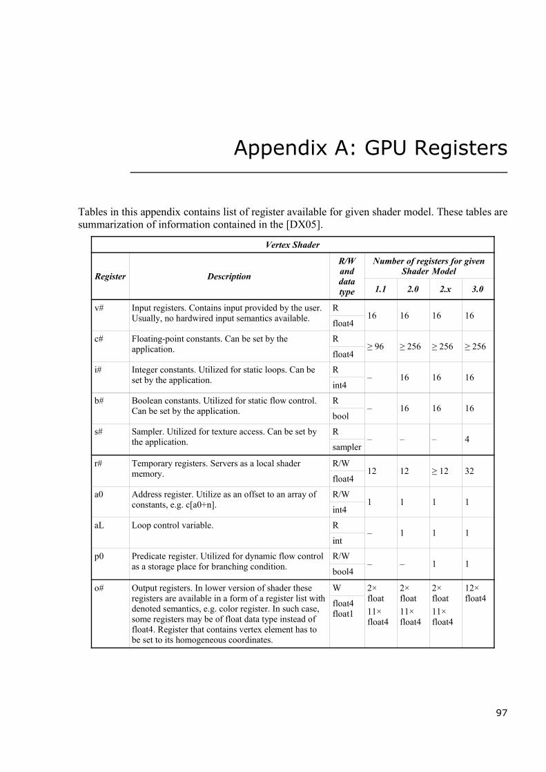
Appendix A: GPU Registers
Tables in this appendix contains list of register available for given shader model. These tables aresummarization of information contained in the [DX05].
Vertex Shader
Register DescriptionR/Wanddatatype
Number of registers for givenShader Model
1.1 2.0 2.x 3.0
v# Input registers. Contains input provided by the user.Usually, no hardwired input semantics available.
R
float416 16 16 16
c# Floating-point constants. Can be set by theapplication.
R
float4≥ 96 ≥ 256 ≥ 256 ≥ 256
i# Integer constants. Utilized for static loops. Can beset by the application.
R
int4– 16 16 16
b# Boolean constants. Utilized for static flow control.Can be set by the application.
R
bool– 16 16 16
s# Sampler. Utilized for texture access. Can be set bythe application.
R
sampler– – – 4
r# Temporary registers. Servers as a local shadermemory.
R/W
float412 12 ≥ 12 32
a0 Address register. Utilize as an offset to an array ofconstants, e.g. c[a0+n].
R/W
int41 1 1 1
aL Loop control variable. R
int– 1 1 1
p0 Predicate register. Utilized for dynamic flow controlas a storage place for branching condition.
R/W
bool4– – 1 1
o# Output registers. In lower version of shader theseregisters are available in a form of a register list withdenoted semantics, e.g. color register. In such case,some registers may be of float data type instead offloat4. Register that contains vertex element has tobe set to its homogeneous coordinates.
W
float4float1
2×float11×float4
2×float11×float4
2×float11×float4
12×float4
97
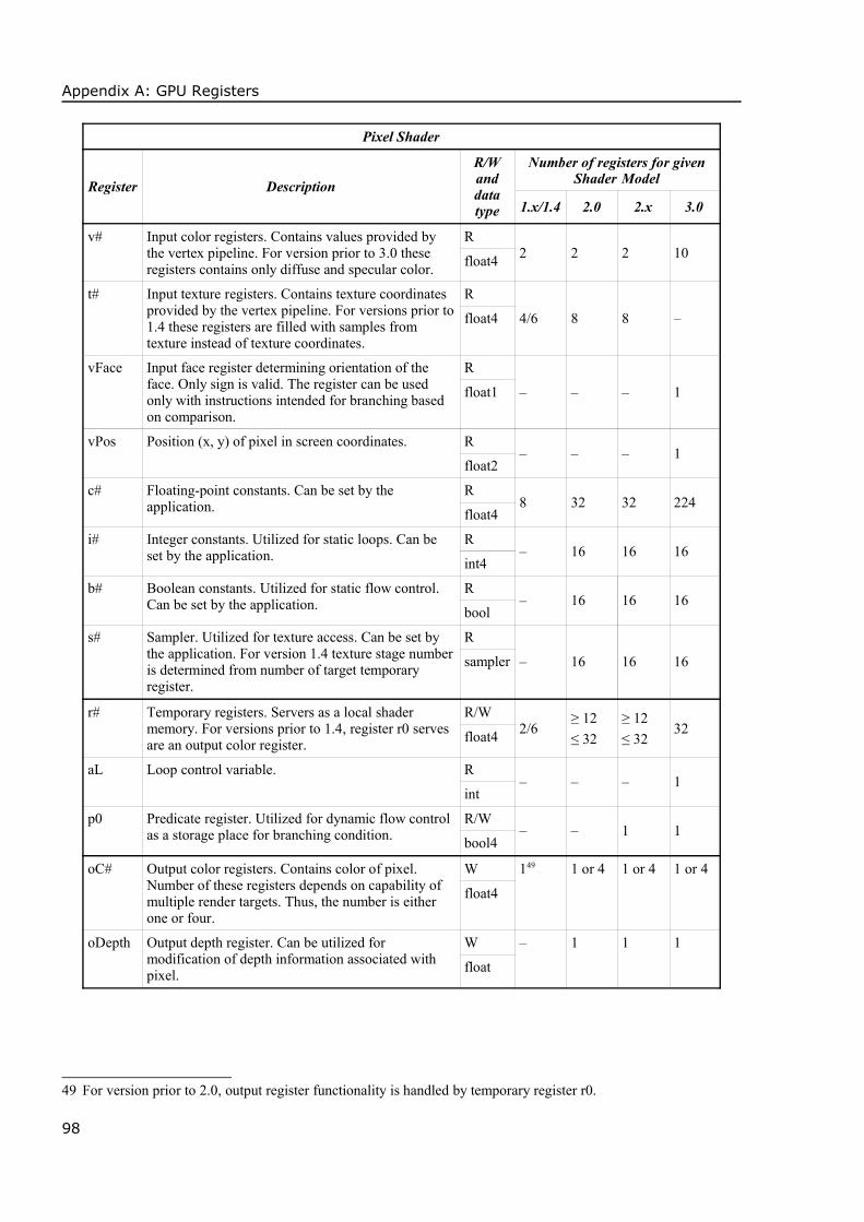
Appendix A: GPU Registers
Pixel Shader
Register DescriptionR/Wanddatatype
Number of registers for givenShader Model
1.x/1.4 2.0 2.x 3.0
v# Input color registers. Contains values provided bythe vertex pipeline. For version prior to 3.0 theseregisters contains only diffuse and specular color.
R
float4 2 2 2 10
t# Input texture registers. Contains texture coordinatesprovided by the vertex pipeline. For versions prior to1.4 these registers are filled with samples fromtexture instead of texture coordinates.
R
float4 4/6 8 8 –
vFace Input face register determining orientation of theface. Only sign is valid. The register can be usedonly with instructions intended for branching basedon comparison.
R
float1 – – – 1
vPos Position (x, y) of pixel in screen coordinates. R
float2– – – 1
c# Floating-point constants. Can be set by theapplication.
R
float48 32 32 224
i# Integer constants. Utilized for static loops. Can beset by the application.
R
int4– 16 16 16
b# Boolean constants. Utilized for static flow control.Can be set by the application.
R
bool– 16 16 16
s# Sampler. Utilized for texture access. Can be set bythe application. For version 1.4 texture stage numberis determined from number of target temporaryregister.
R
sampler – 16 16 16
r# Temporary registers. Servers as a local shadermemory. For versions prior to 1.4, register r0 servesare an output color register.
R/W
float4 2/6≥ 12≤ 32
≥ 12≤ 32
32
aL Loop control variable. R
int– – – 1
p0 Predicate register. Utilized for dynamic flow controlas a storage place for branching condition.
R/W
bool4– – 1 1
oC# Output color registers. Contains color of pixel.Number of these registers depends on capability ofmultiple render targets. Thus, the number is eitherone or four.
W
float4
149 1 or 4 1 or 4 1 or 4
oDepth Output depth register. Can be utilized formodification of depth information associated withpixel.
W
float
– 1 1 1
49 For version prior to 2.0, output register functionality is handled by temporary register r0.
98

Appendix B: GPU Limitations
Maximum number of instructions is limited. Flow control instructions have limitations in itsnesting depth. There are several kinds of nesting depth such as static, dynamic, loop, andsubroutine call nesting depth. Usually, particular flow control instruction influences particularnesting depth, e.g. a dynamic if-branching modifies only actual dynamic flow control depth.
In addition, static flow control instructions may have limitations in total counts that may appearwithin a single shader code. Maximum nesting depths as well as total count of instruction issummed in following tables. For more details on specific instructions, refer to [DX05] that issource for tables contained within this appendix.
Vertex Shader
Value DescriptionValue for given Shader Model
1.1 2.0 2.x 3.0
Total maximum number of instruction slots. 128 256 256 ≥ 512
Maximum static flow control instructions pershader‡. – 16 16 ∞
Maximum static flow control nesting depth. – viz. staticflow count‡
viz. staticflow count‡ 24
Maximum dynamic flow control nesting depth. – – ≤ 24 24
Maximum loop/rep flow control nesting depth. – 1 ≥ 1; ≤ 4 4
Maximum subroutine call nesting depth. – 1 ≥ 1; ≤ 4 4
Pixel Shader
Value DescriptionValue for given Shader Model
1.x/1.4 2.0 2.x 3.0
Total maximum number of instruction slots. Forlower versions, the instruction count is dividedbetween texture (first number) and arithmetic(second number) instructions.
4 + 8/6 + 8 32 + 64 ≥ 96 ≥ 512
Maximum static flow control nesting depth. – – 24 or 0 24
Maximum dynamic flow control nesting depth. – – ≤ 24 24
Maximum loop/rep flow control nesting depth. – – ≤ 4 4
Maximum subroutine call nesting depth. – – ≤ 4 4
99
Copyright © 2022 FDOKUMEN