Efficient Irregular Wavefront Propagation Algorithmson Hybrid CPU-GPU Machines

George Teodoro∗, Tony Pan, Tahsin Kurc, Jun Kong, Lee Cooper, Joel Saltz

Center for Comprehensive Informatics and Biomedical Informatics Department,Emory University, Atlanta, GA 30322

Abstract

In this paper, we address the problem of efficient execution of a computationpattern, referred to here as the irregular wavefront propagation pattern (IWPP),on hybrid systems with multiple CPUs and GPUs. The IWPP is common inseveral image processing operations. In the IWPP, data elements in the wave-front propagate waves to their neighboring elements on a grid if a propagationcondition is satisfied. Elements receiving the propagated waves become part ofthe wavefront. This pattern results in irregular data accesses and computations.We develop and evaluate strategies for efficient computation and propagation ofwavefronts using a multi-level queue structure. This queue structure improvesthe utilization of fast memories in a GPU and reduces synchronization over-heads. We also develop a tile-based parallelization strategy to support executionon multiple CPUs and GPUs. We evaluate our approaches on a state-of-the-art GPU accelerated machine (equipped with 3 GPUs and 2 multicore CPUs)using the IWPP implementations of two widely used image processing opera-tions: morphological reconstruction and euclidean distance transform. Our re-sults show significant performance improvements on GPUs. The use of multipleCPUs and GPUs cooperatively attains speedups of 50× and 85× with respectto single core CPU executions for morphological reconstruction and euclideandistance transform, respectively.

Keywords: Irregular Wavefront Propagation Pattern, GPGPU, CooperativeCPU-GPU Execution, Heterogeneous Environments, MorphologicalReconstruction, Euclidean Distance Transform

∗Corresponding authorEmail addresses: george.teodoro@emory.edu (George Teodoro), tony.pan@emory.edu

(Tony Pan), tkurc@emory.edu (Tahsin Kurc), jun.kong@emory.edu (Jun Kong),lee.cooper@emory.edu (Lee Cooper), jhsaltz@emory.edu (Joel Saltz)

Preprint submitted for peer review January 8, 2014

arX

iv:1

209.

3314

v1 [

cs.D

C]

14

Sep

2012

1. Introduction

This paper investigates efficient parallelization on hybrid CPU-GPU sys-tems of operations or applications whose computation structure includes whatwe call the irregular wavefront propagation pattern (IWPP) (see Algorithm 1).Our work is motivated by the requirements of analysis of whole slide tissueimages in biomedical research. With rapid improvements in sensor technolo-gies and scanner instruments, it is becoming feasible for research projects andhealthcare organizations to gather large volumes of microscopy images. We areinterested in enabling more effective use of large datasets of high resolutiontissue slide images in research and patient care. A typical image from state-of-the-art scanners is about 50K×50K to 100K×100K pixels in resolution. Awhole slide tissue image is analyzed through a cascade of image normalization,object segmentation, object feature computation, and object/image classifica-tion stages. The segmentation stage is expensive and composed of a pipelineof substages. The most expensive substages are built on several low-level oper-ations, notably morphological reconstruction [55] and distance transform [53].Efficient implementation of these operations is necessary to reduce the cost ofimage analysis.

Processing a high resolution image on a single CPU system can take hours.The processing power and memory capacity of graphics processing units (GPUs)have rapidly and significantly improved in recent years. Contemporary GPUsprovide extremely fast memories and massive multi-processing capabilities, ex-ceeding those of multi-core CPUs. The application and performance benefits ofGPUs for general purpose processing have been demonstrated for a wide rangeof applications [14, 41, 49, 43, 6, 34]. As a result, CPU-GPU equipped machinesare emerging as viable high performance computing platforms for scientific com-putation [52].

The processing structures of the morphological reconstruction and distancetransform operations bear similarities and include the IWPP on a grid. TheIWPP is characterized by one or more source grid points from which waves origi-nate and the irregular shape and expansion of the wave fronts. The compositionof the waves is dynamic, data dependent, and computed during execution as thewaves are expanded. Elements in the front of the waves work as the sourcesof wave propagations to neighbor elements. A propagation occurs only whena given propagation condition, determined based on the value of a wavefrontelement and the values of its neighbors, is satisfied. In practice, each element inthe propagation front represents an independent wave propagation; interactionbetween waves may even change the direction of the propagation. In the IWPPonly those elements in the wavefront are the ones effectively contributing forthe output results. Because of this property, an efficient implementation of ir-regular wavefront propagation can be accomplished using an auxiliary containerstructure, e.g., a queue, set, or stack, to keep track of active elements formingthe wavefront. The basic components of the IWPP are shown in Algorithm 1.

In this algorithm, a set of elements in a multi-dimensional grid space (D) areselected to form the initial wavefront (S). These active elements then act as wave

2

Algorithm 1 Irregular Wavefront Propagation Pattern (IWPP)

1: D ← data elements in a multi-dimensional space2: {Initialization Phase}3: S ← subset active elements from D4: {Wavefront Propagation Phase}5: while S 6= ∅ do6: Extract ei from S7: Q← NG(ei)8: while Q 6= ∅ do9: Extract ej from Q

10: if PropagationCondition(D(ei),D(ej)) = true then11: D(ej)← Update(D(ei))12: Insert ej into S

propagation sources in the wavefront propagation phase. During propagationphase, a single element (ei) is extracted from the wavefront and its neighbors(Q ← NG(ei)) are identified. The neighborhood of an element ei is defined bya discrete grid G, also referred to as the structuring element. The element eitries to propagate the wavefront to each neighbor ej ∈ Q. If the propagationcondition (PropagationCondition), based on the values of ei and ej , is satisfied,the value of the element ej (D(ej)) is updated, and ej is inserted in the container(S). The assignment operation performed in Line 11, as a consequence of thewave expansion, is expected to be commutative and atomic. That is, the order inwhich elements in the wavefront are computed should not impact the algorithmresults. The wavefront propagation process continues until stability is reached;i.e., until the wavefront container is empty.

The IWPP is not unique to morphological reconstruction and distance trans-form. Core computations in several other image processing methods containa similar structure: Watershed [56], Euclidean skeletons [28], and skeletonsby influence zones [23]. Additionally, Delaunay triangulations [33], Gabrielgraphs [15] and relative neighborhood graphs [51] can be derived from thesemethods. Another example of the IWPP is the shortest-path computations ona grid which contains obstacles between source points and destination points(e.g., shortest path calculations in integrated circuit designs). A high perfor-mance implementation of the IWPP can benefit these methods and applications.

The traditional wavefront computation is common in many scientific ap-plications [57, 3, 2]. It is also a well-known parallelization pattern in highperformance computing. In the classic wavefront pattern, data elements arelaid out in a multi-dimensional grid. The computation of an element on thewavefront depends on the computation of a set of neighbor points. The clas-sic wavefront pattern has a regular data access and computation structure inthat the wavefront starts from a corner point of the grid and sweeps the griddiagonally from one region to another. The morphological reconstruction anddistance transform operations could potentially be implemented in the form of

3

iterative traditional wavefront computations. However, the IWPP offers a moreefficient execution structure, since it avoids touching and computing on datapoints that do not contribute to the output. The IWPP implementation on ahybrid machine consisting of multiple CPUs and GPUs is a challenging problem.The difficulties with IWPP parallelization are accentuated by the irregularityof the computation that is spread across the input domain and evolves duringthe computation as active elements change.

In this paper, we propose, implement, and evaluate parallelization strategiesfor efficient execution of IWPP computations on large grids (e.g., high resolutionimages) on a machine with multiple CPUs and GPUs. The proposed strategiescan take full advantage this computation pattern characteristics to achieve effi-cient execution on multicore CPU and GPU systems. The contributions of ourwork can be summarized as follows:

• We identify a computation pattern commonly found in several analysisoperations: the irregular wavefront propagation pattern.

• We develop an efficient GPU implementation of the IWPP algorithm usinga multi-level queue structure. The multi-level queue structure improvesthe utilization of fast memories in a GPU and reduces synchronizationoverheads among GPU threads. To the best of our knowledge this is thefirst work to implement this pattern for GPU accelerated environments.

• We develop efficient implementations of the morphological reconstruc-tion and distance transform operations on a GPU using the GPU-enabledIWPP algorithm. These are the first GPU-enabled IWPP-based imple-mentations of morphological reconstruction and distance transform. Themorphological reconstruction implementation achieves much better perfor-mance than a previous implementation based on raster/anti-raster scansof the image. The output results for morphological reconstruction anddistance transform are exact regarding their sequential counterparts.

• We extend the GPU implementation of the IWPP to support processingof images that do not fit in GPU memory through coordinated use ofmultiple CPU cores and multiple GPUs on the machine.

We perform a performance evaluation of the IWPP implementations using themorphological reconstruction and distance transform operations on a state-of-the-art hybrid machine with 12 CPU cores and 3 NVIDIA Tesla GPUs. Signif-icant performance improvements were observed in our experiments. Speedupsof 50× and 85× were achieved, as compared to the single CPU core execution,respectively, for morphological reconstruction and euclidean distance transformwhen all the CPU cores and GPUs were used in a coordinated manner. Wewere able to compute morphological reconstruction on a 96K×96K-pixel im-age in 21 seconds and distance transform on a 64K×64K-pixel image in 4.1seconds. These performances make it feasible to analyze very high resolutionimages rapidly and conduct large scale studies.

4

The manuscript is organized as follows. Section 2 presents the use of theIWPP on image analysis, including preliminary definitions and the implemen-tation of use case algorithms: morphological reconstruction and euclidean dis-tance transform. The IWPP parallelization strategy and its support in GPUsare discussed in Section 3. The extensions for multiple GPUs and cooperativeCPU-GPU execution are described in Section 4. The experimental evaluationis presented in Section 5. Finally, Sections 6 and 7, respectively, present therelated work and conclude the paper.

2. Irregular Wavefront Propagation Pattern in Image Analysis

We describe two morphological algorithms, Morphological Reconstructionand Euclidean Distance Transform, from the image analysis domain to illus-trate the IWPP. Morphological operators are basic operations used by a broadset of image processing algorithms. These operators are applied to individualpixels and are computed based on the current value of a pixel and pixels in itsneighborhood. A pixel p is a neighbor of pixel q if (p, q) ∈ G. G is usually a4-connected or 8-connected square grid. NG(p) refers to the set of pixels thatare neighbors of p ∈ Zn according to G (NG(p) = {q ∈ Zn|(p, q) ∈ G}). Inputand output images are defined in a rectangular domain DI ∈ Zn → Z. Thevalue I(p) of each image pixel p assumes 0 or 1 for binary images. For grayscale images, the value of a pixel comes from a set {0, ..., L − 1} of gray levelsfrom a discrete or continuous domain.

2.1. Morphological Reconstruction Algorithms

Morphological reconstruction is one of the elementary operations in imagesegmentation [55]. When applied to binary images, it pulls out the connectedcomponents of an image identified by a marker image. Figure 1 illustratesthe process. The dark patches inside three objects in image I (also called themask image) on the left correspond to the marker image J . The result of themorphological reconstruction is shown on the right.

Figure 1: Binary morphological reconstruction from markers. The markers are the darkpatches inside three of the objects in the image on the left. The image on the right showsthe reconstructed objects and the final binary image after the application of morphologicalreconstruction.

5

Morphological reconstruction can also be applied to gray scale images. Fig-ure 2 illustrates the process of gray scale morphological reconstruction in 1-dimension. The marker intensity profile is propagated spatially but is boundedby the mask image’s intensity profile. The primary difference between binaryand gray scale morphological reconstruction algorithms is that in binary recon-struction, any pixel value change is necessarily the final value change, whereas avalue update in gray scale reconstruction may later be replaced by another valueupdate. In color images, morphological reconstruction can be applied either toindividual channels (e.g., the Red, Green, and Blue channels in an RGB image)or to gray scale values computed by combining the channels.

Figure 2: Gray scale morphological reconstruction in 1-dimension. The marker image intensityprofile is represented as the red line, and the mask image intensity profile is represented as theblue line. The final image intensity profile is represented as the green line. The arrows showthe direction of propagation from the marker intensity profile to the mask intensity profile.The green region shows the changes introduced by the morphological reconstruction process.

The morphological reconstruction ρI(J) of mask I from marker image J isdone by performing elementary dilations (i.e., dilations of size 1) in J by G,the structuring element. An elementary dilation from a pixel p corresponds topropagation from p to its immediate neighbors in G. The basic algorithm car-ries out elementary dilations successively over the entire image J , updates eachpixel in J with the pixelwise minimum of the dilation’s result and the corre-sponding pixel in I (i.e., J(p) ← (max{J(q), q ∈ NG(p) ∪ {p}}) ∧ I(p), where∧ is the pixelwise minimum operator), and stops when stability is reached, i.e.,when no more pixel values are modified. Several morphological reconstructionalgorithms for gray scale images have been developed by Vincent [55] based onthis core technique. We present brief descriptions of these algorithms below andrefer the reader to the original paper for more details.

Sequential Reconstruction (SR): Pixel value propagation in the marker image iscomputed by alternating raster and anti-raster scans. A raster scan starts fromthe pixel at (0, 0) and proceeds to the pixel at (N − 1,M − 1) in a row-wise

6

manner, while an anti-raster starts from the pixel at (N − 1,M − 1) and movesto the pixel at (0, 0) in a row-wise manner. Here, N and M are the resolutionof the image in x and y dimensions, respectively. In each scan, values frompixels in the upper left or the lower right half neighborhood are propagated tothe current pixel in raster or anti-raster fashion, respectively. The raster andanti-raster scans allow for changes in a pixel to be propagated in the current it-eration. The SR method iterates until stability is reached, i.e., no more changesin pixels are computed.

Queue-based Reconstruction (QB): In this method, a first-in first-out (FIFO)queue is initialized with pixels in the regional maxima. The computation thenproceeds by removing a pixel from the queue, scanning the pixel’s neighborhood,and queuing the neighbor pixels whose values have been changed. The overallprocess continues until the queue is empty.

Fast Hybrid Reconstruction (FH): The computation of the regional maximaneeded to initialize the queue in QB incurs significant computational cost. TheFH approach incorporates the characteristics of the SR and QB algorithms toreduce the cost of initialization, and is about one order of magnitude faster thanthe others. It first makes one pass using the raster and anti-raster orders as inSR. After that pass, it continues the computation using a FIFO queue as in QB.A pseudo-code implementation of FH is presented in Algorithm 2, N+

G and N−Gdenote the set of neighbors in NG(p) that are reached before and after touchingpixel p during a raster scan.

2.2. Euclidean Distance Transform

The distances transform (DT) operation computes a distance map M froma binary input image I, where for each pixel p ∈ I the pixel’s value in M , M(p),is the smallest distance from p to a background pixel. DT is a fundamental op-erator in shape analysis, which can be used for separation of overlapping objectsin watershed based segmentation [56, 39]. It can also be used in the calculationof morphological operations [8] as erosion and dilation and the computation ofVoronoi diagrams and Delaunay triangulation [53].

The definition of DT is simple, but historically it has been hard to achievegood precision and efficiency for this operation. For a comprehensive discus-sion of algorithms for calculation of distance transform, we refer the reader tothe survey by Fabbri et al. [12]. The first DT algorithms were proposed byRosenfeld and Pfaltz [38]. These algorithms were based on raster/anti-rasterscans strategies to calculate non-Euclidean metrics such as cityblock and chess-board, which at that time were used as approximations to the Euclidean dis-tance. Danielsson proposed an algorithm [11] to compute Euclidean DT thatpropagates information of the nearest background pixel using neighborhood op-erators in a raster/anti-raster scan manner. With this strategy, a two-elementvector with location information of the nearest background pixel is propagatedthrough neighbor pixels. Intrinsically, it builds Voronoi diagrams where regionsare formed by pixels with the same nearest background pixel.

7

Algorithm 2 Fast Hybrid Gray scale Morphological Reconstruction Algorithm

Input

I: mask image

J : marker image.

1: {Initialization Phase}2: Scan I and J in raster order.3: Let p be the current pixel4: J(p)← (max{J(q), q ∈ N+

G (p) ∪ {p}}) ∧ I(p)5: Scan I and J in anti-raster order.6: Let p be the current pixel7: J(p)← (max{J(q), q ∈ N−G (p) ∪ {p}}) ∧ I(p)8: if ∃q ∈ N−G (p) | J(q) < J(p) and J(q) < I(q)9: queue add(p)

10: {Wavefront Propagation Phase}11: while queue empty() = false do12: p← dequeue()13: for all q ∈ NG(p) do14: if J(q) < J(p) and I(q) 6= J(q) then15: J(q)← min{J(p), I(q)}16: queue add(q)

Danielsson’s algorithm is not an exact algorithm. The Voronoi diagram isnot connected in a discrete space, though it is in the continuous space. Hence,the Voronoi diagram computation through a neighborhood based operator intro-duces approximation errors as illustrated in Figure 3. Nevertheless, approxima-tion errors introduced by the algorithm are small and bound by a mathematicalframework. Approximations computed by this algorithm have been found to besufficient in practice for several applications [9, 13, 50]. Moreover, some of theexact euclidean distance transform algorithms [8, 42, 30] are implemented as apost-processing phase to Danielsson’s algorithm, in which approximation errorsare resolved.

Algorithm 3 presents an irregular wavefront propagation based approachto efficiently compute the single neighborhood approximation of DT. In theinitialization phase a pass on the input is performed to identify and queue pixelsforming the initial wavefront. In Lines 2 and 3, Voronoi diagram (VR) that holdsthe current nearest background pixel for each image pixel is initialized. Eachbackground pixel will itself be its nearest pixel, while the foreground pixels willinitially point to a pixel virtually at infinite distance (inf). The inf pixel issuch that for each pixel p, p is closer to any other pixel in the image domainthan it is to the inf pixel. At the end of the initialization phase, backgroundpixels with a foreground neighbor (contour pixels) are added to a queue forpropagation (Lines 4 and 5).

The wavefront propagation phase of the EDT is carried out in Lines 7 to12. During each iteration, a pixel p is removed from the queue. The pixel’s

8

Figure 3: Errors introduced by neighborhood propagation in the euclidean distance transformoperation using an 8-connected neighborhood method (Cuisenaire and Macq [8]). Pixel qis closer to object B than it is to A and C. However, q is not neighbor to any pixel in theconnected Voronoi diagram starting at B. The distance value assigned to q, M(q), would be√170 (about 13.038), instead of

√169 (13) in the exact case.

nearest background pixel is propagated to the neighbors through a neighborhoodoperator. For each neighbor pixel q, if the distance of q to the current assignednearest background pixel (DIST(q, V R(q))) is greater than the distance of q tothe nearest background pixel of p (DIST(q, V R(p))), the propagation occurs.In that case, the nearest background pixel of q is updated with that of p (Line11), and q is added to the queue for propagation. After the propagation phaseis completed, the distance map is computed from the Voronoi diagram.

As presented in [8], using a sufficiently large neighborhood (structuring ele-ment) will guarantee the exactness of this algorithm. In addition, the wavefrontpropagation method could be extended as shown in [53] to compute the ex-act distance transform. To include these extensions, however, another queuewould have to be used, increasing the algorithm cost. As discussed before,Danielsson’s distance transform provides acceptable results for a large numberof applications [9, 13]. We have employed this version in our image analysisapplications.

3. Implementation of Irregular Wavefront Propagation Pattern on aGPU

We first describe the strategy for parallel execution of the IWPP on GPUs.We then present a parallel queue data structure that is fundamental to efficientlytracking data elements in the wavefront. In the last two sections, we describethe GPU-enabled implementations of the two operations presented in Section 2.

3.1. Parallelization Strategy

After the initialization phase of the IWPP, active data elements forming theinitial wavefront are put into a global queue for computation. To allow parallel

9

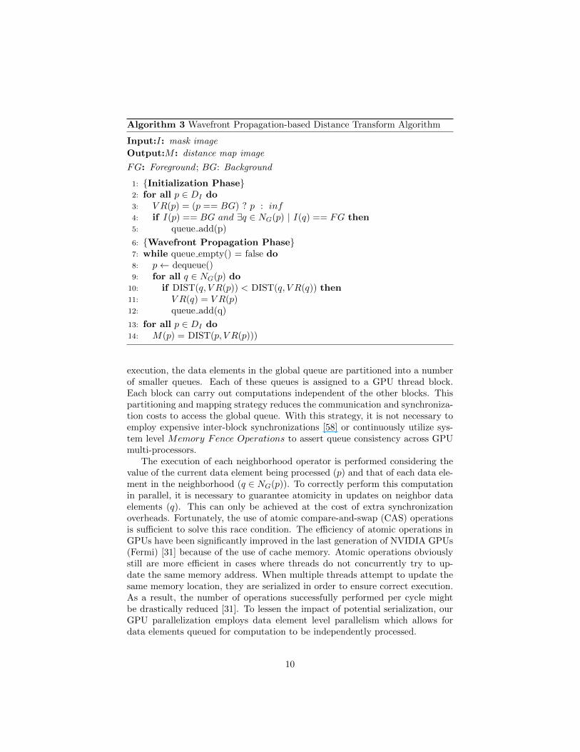
Algorithm 3 Wavefront Propagation-based Distance Transform Algorithm

Input:I: mask image

Output:M : distance map image

FG: Foreground ; BG: Background

1: {Initialization Phase}2: for all p ∈ DI do3: V R(p) = (p == BG) ? p : inf4: if I(p) == BG and ∃q ∈ NG(p) | I(q) == FG then5: queue add(p)

6: {Wavefront Propagation Phase}7: while queue empty() = false do8: p← dequeue()9: for all q ∈ NG(p) do

10: if DIST(q, V R(p)) < DIST(q, V R(q)) then11: V R(q) = V R(p)12: queue add(q)

13: for all p ∈ DI do14: M(p) = DIST(p, V R(p)))

execution, the data elements in the global queue are partitioned into a numberof smaller queues. Each of these queues is assigned to a GPU thread block.Each block can carry out computations independent of the other blocks. Thispartitioning and mapping strategy reduces the communication and synchroniza-tion costs to access the global queue. With this strategy, it is not necessary toemploy expensive inter-block synchronizations [58] or continuously utilize sys-tem level Memory Fence Operations to assert queue consistency across GPUmulti-processors.

The execution of each neighborhood operator is performed considering thevalue of the current data element being processed (p) and that of each data ele-ment in the neighborhood (q ∈ NG(p)). To correctly perform this computationin parallel, it is necessary to guarantee atomicity in updates on neighbor dataelements (q). This can only be achieved at the cost of extra synchronizationoverheads. Fortunately, the use of atomic compare-and-swap (CAS) operationsis sufficient to solve this race condition. The efficiency of atomic operations inGPUs have been significantly improved in the last generation of NVIDIA GPUs(Fermi) [31] because of the use of cache memory. Atomic operations obviouslystill are more efficient in cases where threads do not concurrently try to up-date the same memory address. When multiple threads attempt to update thesame memory location, they are serialized in order to ensure correct execution.As a result, the number of operations successfully performed per cycle mightbe drastically reduced [31]. To lessen the impact of potential serialization, ourGPU parallelization employs data element level parallelism which allows fordata elements queued for computation to be independently processed.

10

Algorithm 4 Wavefront propagation phase on a GPU

1: {Split initial queue equally among thread blocks}2: while queue empty() = false do3: while (p = dequeue(...))! = EMPTY do in parallel4: for all q ∈ NG(p) do5: repeat6: curV alueQ = I(q)7: if PropagationCondition(I(p), curV alueQ) then8: oldval = atomicCAS(&I(q), op(I(p)), curV alueQ)9: if oldval ! = curV alueQ then

10: queue add(q)11: break;

12: else13: break;

14: until True15: queue swap in out()

The GPU-based implementation of the propagation operation is presentedin Algorithm 4. After splitting the initial queue, each block of threads enterinto a loop in which data elements are dequeued in parallel and processed, andnew data elements may be added to the local queue as needed. This processcontinues until the queue is empty. Within each loop, the data elements queuedin the last iteration are uniformly divided among the threads in the block andprocessed in parallel (Lines 3—14 in Algorithm 4). The value of each queueddata element p is compared to every data element q in its neighborhood. Anatomic operation is performed when a neighbor data element q should be up-dated (PropagationCondition is evaluated true). The value of data elementq before the compare and swap operation is returned (oldval) and used to de-termine whether its value has really been changed (Line 9 in Algorithm 4).This step is necessary because there is a chance that another thread might havechanged the value of q between the time the data element’s value is read toperform the propagation condition test and the time the atomic operation isperformed (Lines 6–8 in Algorithm 4). If the atomic compare and swap opera-tion performed by the current thread has changed the value of data element q,q is added to the queue for processing in the next iteration of the loop. Evenwith this control, it is possible that between the test in line 9 and the additionto the queue, the data element q may have been modified again. In this case,q is added multiple times to the queue. Although it impacts the performance,the correctness of the algorithm is not affected because the update operationsreplace the value of q via a commutative and atomic assignment operation.

After computing the data elements from the last iteration, data elementsthat are added to the queue in the current iteration are made available forthe next iteration. Elements used as input in one iteration and those queuedduring the propagation are stored in different queues. The process of mak-

11

ing elements queued available includes swapping the input and output queues(queue swap in out(); Lines 15). As described in the next section, the choice toprocess data elements in rounds, instead of making each data element insertedinto the queue immediately accessible, is made in our design to implement aqueue with very efficient read performance (dequeue performance) and withlow synchronization costs to provide consistency among threads when multiplethreads read from and write to the queue. When maximum and minimum oper-ations are used in the propagation condition test, atomicCAS may be replacedwith an atomicMax or atomicMin operation to improve performance.

Since elements in the queue are divided among threads for parallel computa-tion, the order in which the elements will be processed cannot be pre-determined.It is thus necessary for the correctness of the parallel execution that the updateand assignment operations in the wave propagation phase are commutative andatomic. In practice, the order is not important for most analysis methods basedon the IWPP, including the example operations presented in this paper.

3.2. Parallel Queue Implementation and Management

A parallel queue is used to keep track of elements in the wavefront. An effi-cient parallel queue for GPUs is a challenging problem [17, 20, 27]. A straightforward implementation of a queue, as presented by Hong et al. [17], could bedone by employing an array to store items in sequence and using atomic addi-tions to calculate the position where the item should be inserted, as presentedin the code bellow.

AddQueue(int* q_idx, type_t* q, type_t item) {

int old_idx = AtomicAdd(q_idx, 1);

q[old_idx] = item; }

Hong et al. stated that this solution worked well for their use case. Theuse of atomic operations, however, is very inefficient when the queue is heav-ily employed as in our case. Moreover, a single queue that is shared amongall thread blocks introduces additional overheads to guarantee data consistencyacross the entire device. It may also require inter-block synchronization prim-itives [58] to synchronize threads from multiple block that are not standardmethods supported by CUDA.

To avoid these inefficiencies, we have designed a parallel queue that operatesindependently in a per thread block basis to avoid inter-block communication.In order to exploit the fast memories in a GPU for fast write and read ac-cesses, the queue is implemented as multiple levels of queues (as depicted inFigure 4): (i) Per-Thread queues (TQ) which are very small queues private toeach thread, residing in the shared memory; (ii) Block Level Queue (BQ) whichis also in the shared memory, but is larger than TQ. Write operations to theblock level queue are performed in thread warp-basis; and (iii) Global BlockLevel Queue (GBQ) which is the largest queue and uses the global memory ofthe GPU to accumulate data stored in BQ when the size of BQ exceeds theshared memory size.

12

Figure 4: Multi-level parallel queue.

In our queue implementation, each thread maintains an independent queue(TQ) that does not require any synchronization to be performed. In this waythreads can efficiently store data elements from a given neighborhood in thequeue for computation. Whenever this level of queue is full, it is necessaryto perform a warp level communication to aggregate items stored in the localqueues and write them to BQ. In this phase, a parallel thread warp prefix-sumis performed to compute the total number of items queued in individual TQs. Asingle shared memory atomic operation is performed at the Block Level Queueto identify the position where the warp of threads should write their data. Thisposition is returned, and the warp of threads write their local queues to BQ.

Whenever a BQ is full, the threads in the corresponding thread block aresynchronized. The current size of the queue is used in a single operation tocalculate the offset in GBQ from which the BQ should be stored. After thisstep, all the threads in the thread block work collaboratively to copy in parallelthe contents of QB to GBQ. This data transfer operation is able to achieve highthroughput, because the memory accesses are coalesced. It should be notedthat, in all levels of the parallel queue, an array is used to hold the queuecontent. While the contents of TQ and BQ are copied to the lower level queueswhen full, GBQ does not have a lower level queue to which its content can becopied. In the current implementation, the size of GBQ is initialized with afixed tunable memory space. If the limit of GBQ is reached during an iterationof the algorithm, excess data elements are dropped and not stored. The GPUmethod returns a boolean value to CPU to indicate that some data elementshave been dropped during the execution of the method kernel. In that case, thewavefront propagation algorithm has to be re-executed, but using the outputof the previous execution as input, because this output already holds a partialsolution of the problem. Recomputing using the output of the previous step as

13

input will result in the same solution as if the execution was carried out in asingle step.

While adding new items to the queue requires a number of operations toguarantee consistency, the read operations can be performed without introduc-ing synchronization. This is possible by partitioning input data elements stati-cally among threads, which keep consuming the data elements until all items arecomputed. The drawbacks of a static partition of the queue and work withina loop iteration are minimum, because the computation costs of the queueddata elements are similar; only a minor load imbalance is introduced with thissolution. Moreover, the queued data elements are repartitioned at each new it-eration of the loop. A high level description of the dequeue function is presentedbellow. In this function, the value of the item is initialized to a default codecorresponding to an empty queue. Then, the queue index corresponding to thenext item to be returned for that particular thread is calculated, based on thesize of the thread block (block size), the number of iterations already computedby this thread warp (iter), and the identifier of that thread in the block.

type_t DeQueue(int q_size, type_t* q, int iter) {

type_t item = QUEUE_EMPTY;

queue_idx = tid_in_block + iter * block_size;

if(queue_idx < q_size){

type_t item = q[queue_idx];

}

return item; }

3.3. GPU-enabled Fast Hybrid Morphological Reconstruction

In this section, we present how the GPU-based version of the Fast HybridReconstruction algorithm, referred to in this paper as FH GPU, is implemented(see Algorithm 5).

The first stage of FH, as is described in Section 2.1, consists of the raster andanti-raster scans of the image. This stage has a regular computation patternthat operates on all pixels of the image. An efficient GPU implementation of theSR algorithm, including the raster and anti-raster scan stage, has been done byPavel Karas [20]. This implementation is referred to as SR GPU in this paper.We employ the SR GPU implementation to perform the first phase of FH on aGPU. Note that the raster scan is decomposed into scans along each dimensionof the image. The neighborhoods are defined as N+,0

G and N0,+G for the sets of

neighbors for the row-wise and column-wise scans, respectively. Similarly, forthe anti-raster scan, N−,0G and N0,−

G are defined for the respective axis-alignedcomponent scans.

The transition from the raster scan phase to the wavefront propagation phaseis slightly different from the sequential FH. The SR GPU does not guaranteeconsistency when a pixel value is updated in parallel. Therefore, after the rasterscan phase, pixels inserted into the queue for computation in the next phase arenot only those from the anti-raster neighborhood (N−G ) as in the sequential

14

Algorithm 5 Fast Parallel Hybrid Reconstruction

Input

I: mask image

J : marker image, defined on domain DI , J ≤ I.

1: {Initialization phase}2: Scan DI in raster order.3: for all rows ∈ DI do in parallel4: Let p be the current pixel5: J(p)← (max{J(q), q ∈ N+,0

G (p) ∪ {p}}) ∧ I(p)6: for all columns ∈ DI do in parallel7: Let p be the current pixel8: J(p)← (max{J(q), q ∈ N0,+

G (p) ∪ {p}}) ∧ I(p)9: Scan DI in anti-raster order.

10: for all rows ∈ DI do in parallel11: Let p be the current pixel12: J(p)← (max{J(q), q ∈ N−,0G (p) ∪ {p}}) ∧ I(p)13: for all columns ∈ DI do in parallel14: Let p be the current pixel15: J(p)← (max{J(q), q ∈ N0,−

G (p) ∪ {p}}) ∧ I(p)16: for all p ∈ DI do in parallel17: if ∃q ∈ NG(p) | J(q) < J(p) and J(q) < I(q)18: queue add(p)19: {Wavefront propagation phase}20: while queue empty() = false do21: for all p ∈ queue do in parallel22: for all q ∈ NG(p) do in parallel23: if J(q) < J(p) and I(q) 6= J(q) then24: oldval = atomicMax(&J(q),min{J(p), I(q)})25: if oldval < min{J(p), I(q)} then26: queue add(q)

15

algorithm, but also pixels from the entire neighborhood (NG) satisfying thepropagation condition (See Algorithm 5, Lines 16–18).

When two queued pixels (e.g., p′ and p′′) are computed in parallel, it ispossible that they have common neighbors (NG(p′) ∩ NG(p′′) 6= ∅). This canpotentially create a race condition when updating the same neighbor q. Up-dating the value of a pixel q is done via a maximum operation, which can beefficiently implemented to avoid race conditions by employing atomic Compare-and-Swap (CAS) based instructions (atomicMax for GPUs). The value of pixelq before the update (oldval) is returned, which is used in our algorithm to test ifq was updated due to the computation of the current pixel p′. If the oldval is notsmaller than min{J(p′), I(q)}, it indicates that the processing of another pixelp′′ updated the value of q to a value greater than or equal to min{J(p′), I(q)}.In this case, q has already been queued due to the p′′ computation and does notneed to be queued again. Otherwise, q is queued for computation. The overallprocess continues until the queue is empty. Note that the update operation isa maximum, hence an atomicMax is used instead of the atomicCAS operationin the generic wavefront propagation skeleton. It leads to better performanceas the repeat-until loop in Algorithm 4 (Lines 5–14) is avoided. We also referthe reader to a previous technical report [46] with additional details on ourGPU-based implementation of the Morphological Reconstruction.

3.4. GPU-enabled Euclidean Distance Transform

The GPU implementation of distance transform is shown in Algorithm 6.The implementation is very similar to the sequential version. The initial-ization phase assigns initial value to the Voronoi diagram and adds contourpixels or those background pixels with foreground neighbors for propagation(Lines 2 to 5).

In the wavefront propagation phase, for each pixel p queued for computation,its neighbor pixels q are checked to verify if using V R(p) as path to a backgroundpixel would result in a shorter distance as compared to the current path storedin V R(q). If it does, V R(q) is updated and q is queued for computation. Onceagain, concurrent computation of pixels in the queue may create a race conditionif multiple threads try to update the same V R(q). To prevent this condition,a compare and swap operation is employed when updating V R. V R is onlyupdated if the value used to calculated distance (curV RQ) is still the valuestored in V R(q). Otherwise, the algorithm reads the new value stored in V R(q)and calculates the distance again (Line 12). The final step, as in the sequentialcase, computes the distance map from V R. It is performed in parallel for allpoints in the input image.

A given VR diagram may have multiple valid solutions. If two pixels, p′ andp′′, are equidistant and the closest background pixels to a foreground pixel q,either of the pixels can be used as the closest background pixel of q (V R(q) = p′

or V R(q) = p′′). In other words, a foreground pixel could initially be assignedone of multiple background pixels, as long as the distance from the foregroundpixel to those background pixels is the same. In our algorithm, the order inwhich the wave propagations are computed defines whether p′ or p′′ are used

16

Algorithm 6 Distance Transform Algorithm for GPUs

Input:I: mask image

Output:M : distance map image

FG: Foreground ; BG: Background

1: {Initialization phase}2: for all p ∈ DI do in parallel3: V R(p) = (I(p) == BG) ? p : inf4: if I(p) == BG and ∃q ∈ NG(p) | I(q) == FG5: queue add(p)6: {Wavefront propagation phase}7: while queue empty() = false do8: for all p ∈ queue do in parallel9: for all q ∈ NG(p) do

10: repeat11: curV RQ = V R(q)12: if DIST(q, V R(p) < DIST(q, curV RQ) then13: old = atomicCAS(&V R(q), curV RQ, V R(p))14: if old 6= curV RQ then15: queue add(q)16: break;

17: else18: break19: until True20: for all p ∈ DI do in parallel21: M(p) = DIST(p, V R(p))

17

in such a case. However, since both pixels are equidistant to q, using either ofthem would result in the same distance map. Thus, the results achieved by theparallel distance transform are the same as those of the sequential version ofthe algorithm.

4. Parallel Execution on Multiple GPUs and CPUs

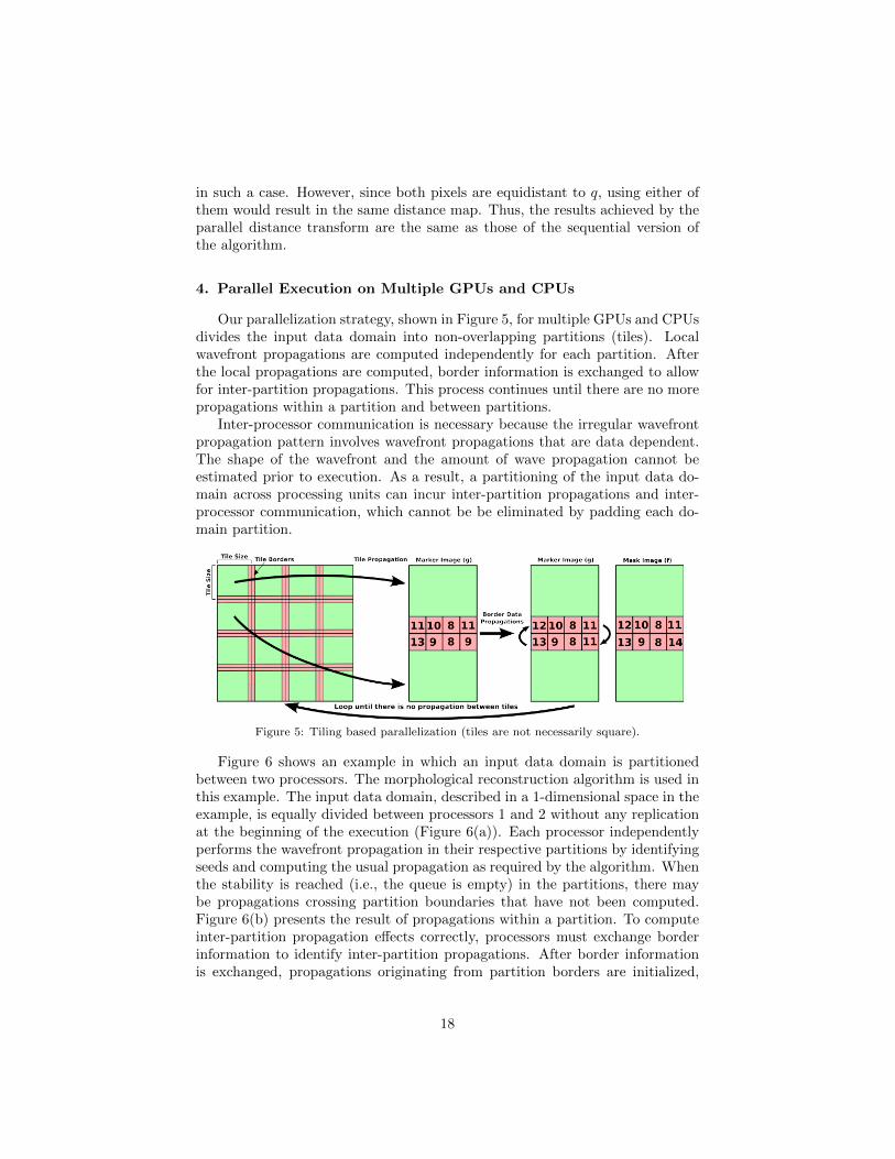
Our parallelization strategy, shown in Figure 5, for multiple GPUs and CPUsdivides the input data domain into non-overlapping partitions (tiles). Localwavefront propagations are computed independently for each partition. Afterthe local propagations are computed, border information is exchanged to allowfor inter-partition propagations. This process continues until there are no morepropagations within a partition and between partitions.

Inter-processor communication is necessary because the irregular wavefrontpropagation pattern involves wavefront propagations that are data dependent.The shape of the wavefront and the amount of wave propagation cannot beestimated prior to execution. As a result, a partitioning of the input data do-main across processing units can incur inter-partition propagations and inter-processor communication, which cannot be be eliminated by padding each do-main partition.

Figure 5: Tiling based parallelization (tiles are not necessarily square).

Figure 6 shows an example in which an input data domain is partitionedbetween two processors. The morphological reconstruction algorithm is used inthis example. The input data domain, described in a 1-dimensional space in theexample, is equally divided between processors 1 and 2 without any replicationat the beginning of the execution (Figure 6(a)). Each processor independentlyperforms the wavefront propagation in their respective partitions by identifyingseeds and computing the usual propagation as required by the algorithm. Whenthe stability is reached (i.e., the queue is empty) in the partitions, there maybe propagations crossing partition boundaries that have not been computed.Figure 6(b) presents the result of propagations within a partition. To computeinter-partition propagation effects correctly, processors must exchange borderinformation to identify inter-partition propagations. After border informationis exchanged, propagations originating from partition borders are initialized,

18

and another round of local propagations is executed. The process of performinglocal propagations and exchanging border information continues until no morepropagations are possible within and between partitions. The final result ofthe morphological reconstruction for the 1-dimensional example is presented inFigure 6(c). The area recomputed because of the inter-partition propagationsis represented in dark green.

(a) Marker g and mask f images. (b) Processor local reconstruction.

(c) Reconstruction after inter-processor propagation.

Figure 6: Evaluating Scalability According to the Number of Blocks.

The parallel implementation consists of a pipeline of two stages (Figure 7):Tile Propagation (TP) and Border Propagation (BP). The TP stage performslocal propagations in tiles. An instance of this stage is created for each tile.The BP stage, on the other hand, computes propagations from data elementsat tile borders. In essence, BP transmits propagations from one tile to another.When there is a need for propagation between tiles, BP will re-instantiate thepipeline. In that case, a TP instance is created for each tile receiving propagationand scheduled for execution. It computes propagations within the tile thatare initiated from the borders. A new instance of BP is also created with adependency on the new TP instances. That is, it is not scheduled for executionuntil all of the new TP instances finish their propagation computations. Thiscycle is repeated until there are no more intra-tile and inter-tile propagations.

The instances of the two stages are dispatched for execution on availableCPUs and GPUs, as long as a stage has an implementation for those devices.We employ the concept of function variant, which is a group of functions withsame name, arguments, and result types [25, 29]. In our implementation a func-tion variant for a task is the CPU and GPU implementations of the operation.

19

Figure 7: Pipeline representation of the CPU-GPU wavefront propagation. Instances of Tile-based Propagation (TP) compute propagation in each tile as shown at the top. A BorderPropagation (BP) stage, which depends on TP instances for execution, is also created toresolve propagation among the tiles. If a propagation exists between tiles, BP re-instantiatesthe pipeline. This process continues until stability is reached. The multi-level tiling strategy,in which a tile is repartitioned into micro-tiles for multi-core execution, is shown at the bottom.This strategy is implemented to reduce CPU vs GPU computational load imbalance.

Binding to a function variant enables the runtime system to choose the ap-propriate function or functions during execution, allowing multiple computingdevices to be used concurrently and in a coordinated manner. We should notethat a function variant provides opportunities for runtime optimizations, but anapplication is not required to provide CPU and GPU implementations for all ofthe stages.

Figure 8 presents an overview of our system support [47, 45] to schedulepipeline applications in machines equipped with multiple CPUs and GPUs.Tasks (TP and BP instances) dispatched for execution by the wavefront prop-agation pipeline are either queued as ready to execute or inserted in a queueof pending tasks, respectively, depending on whether their dependencies are re-solved or not. Tasks ready for execution are consumed by computing threadsresponsible for managing CPU cores and GPUs. A computing thread is assignedto each CPU-core or GPU available in the default mode. Assignment of tasksto computing devices is done in a demand-driven manner. When a CPU core orGPU remains idle, one of the tasks is assigned to the idle device. The defaultscheduling policy for choosing the task to be execute into a device requestingwork is FCFS (first come, first served). In the case of our application, since theBP instance will be dependent on all TP instances, the BP is only dispatched

20

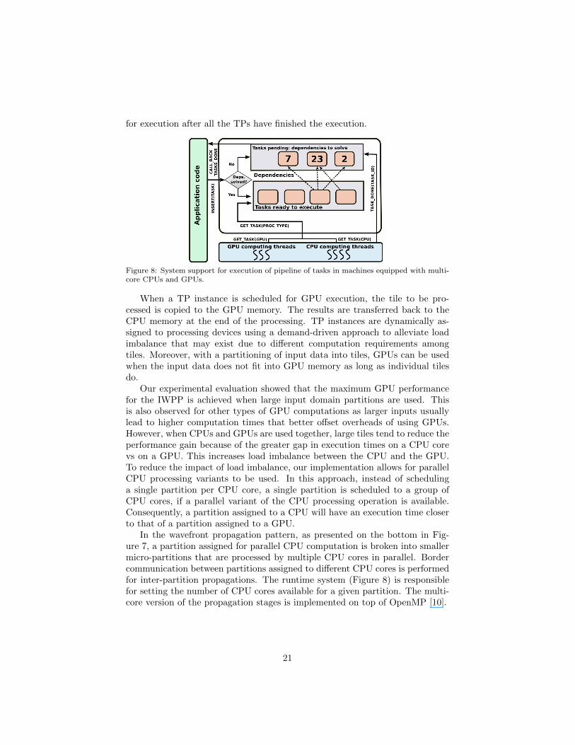
for execution after all the TPs have finished the execution.

Figure 8: System support for execution of pipeline of tasks in machines equipped with multi-core CPUs and GPUs.

When a TP instance is scheduled for GPU execution, the tile to be pro-cessed is copied to the GPU memory. The results are transferred back to theCPU memory at the end of the processing. TP instances are dynamically as-signed to processing devices using a demand-driven approach to alleviate loadimbalance that may exist due to different computation requirements amongtiles. Moreover, with a partitioning of input data into tiles, GPUs can be usedwhen the input data does not fit into GPU memory as long as individual tilesdo.

Our experimental evaluation showed that the maximum GPU performancefor the IWPP is achieved when large input domain partitions are used. Thisis also observed for other types of GPU computations as larger inputs usuallylead to higher computation times that better offset overheads of using GPUs.However, when CPUs and GPUs are used together, large tiles tend to reduce theperformance gain because of the greater gap in execution times on a CPU corevs on a GPU. This increases load imbalance between the CPU and the GPU.To reduce the impact of load imbalance, our implementation allows for parallelCPU processing variants to be used. In this approach, instead of schedulinga single partition per CPU core, a single partition is scheduled to a group ofCPU cores, if a parallel variant of the CPU processing operation is available.Consequently, a partition assigned to a CPU will have an execution time closerto that of a partition assigned to a GPU.

In the wavefront propagation pattern, as presented on the bottom in Fig-ure 7, a partition assigned for parallel CPU computation is broken into smallermicro-partitions that are processed by multiple CPU cores in parallel. Bordercommunication between partitions assigned to different CPU cores is performedfor inter-partition propagations. The runtime system (Figure 8) is responsiblefor setting the number of CPU cores available for a given partition. The multi-core version of the propagation stages is implemented on top of OpenMP [10].

21

5. Experimental Results

We evaluate the performance of the irregular wavefront propagation imple-mentation using the morphological reconstruction and distance transform op-erations. These operations were applied on high-resolution RGB images fromdatasets collected by research studies in the In Silico Brain Tumor ResearchCenter (ISBTRC) [39] at Emory University. The experiments were carried outon a machine (a single computation node of the Keeneland cluster [52]) withIntel R© Xeon R© X5660 2.8 GHz CPUs, 3 NVIDIA Tesla M2090 (Fermi) GPUs,and 24GB of DDR3 RAM (See Figure 9). A total of 12 CPU computing coresavailable because hyper-threading mechanism is not enabled. Codes used in ourevaluation were compiled with “gcc 4.2.1”, “-O3” optimization flag, and NVidiaCUDA SDK 4.0. The experiments were repeated 3 times, and, unless stated, thestandard deviation was not observed to be higher than 1%. The speedup valuespresented in the following sections are calculated based on the performance ofsingle CPU-core versions of the operations.

Figure 9: Hybrid, Multi-GPU computing node.

5.1. Multi-core CPU Parallelization

Two different multi-core CPU parallelization strategies were implemented ontop of OpenMP: (i) Tile-based parallelization that partitions an input image intoregions and iteratively solves propagations local to each partition and performsinter-region propagations, as described in Section 4; (ii) Non-Tiled paralleliza-tion is an alternative parallelization in which points in the initial wavefront aredistributed in round-robin among CPU threads at the beginning of the execu-tion. Each thread then independently computes propagations associated withthe points assigned to it. To avoid inter-thread interference in propagations, itis necessary to use atomic compare-and-swap operations during data updates.

The performances of both parallelization strategies are presented in Fig-ure 10. The non-tiled parallelization of the morphological reconstruction re-sulted in slowdown as compared to the sequential algorithm for most of theconfigurations; only a slight improvement was observed on 8 CPU cores. Inorder to understand this poor performance, the algorithm was profiled usingperf profiling tool [21] to measure the effects of increasing number of threads tocache and bus cycles. Additional bus cycles are used for data read and write as

22

well as for data transfers to assert cache coherence among threads. An increasein the number of threads from 1 to 2 in the non-tiled parallelization results intwice more cache misses and three times more bus cycles. Similar behavior isobserved as the number of threads keep increasing, preventing the algorithmfrom having gains as more CPU cores are used. For this parallelization, threadsmay be concurrently computing in the same region of the input domain, andupdates from one thread will invalidate cache lines of all the other threads pro-cessing the same region. This makes the cost of maintaining cache coherencevery high.

Figure 10: Multicore performance of morphological reconstruction. Different parallelizationstrategies are compared.

The performance of the tile-based parallelization is much better with aspeedup of 7.5× in the configuration with 12 threads. This is a result of avoidinginter-thread interference. Because threads are assigned to independent parti-tions, they do not modify the same regions and affect each other. Nevertheless,the speedup performance of the algorithm is sub-linear. This is an inevitableconsequence of the threads’ having to share the processor cache space and thebus subsystem. Since the algorithm is very data intensive, larger cache andfast access to memory are primordial to achieve maximum performance, andcontention on these resources limits gains in CPU multicore systems.

5.2. GPU Parallelization

The experiments in this section examine the impact on performance of thequeue design as well as tile size and input data characteristics for the GPU-enabled implementations of irregular wavefront propagation computations.

5.2.1. Impact of Queue Design Choices

This set of experiments evaluates the performance of three different parallelqueue approaches: (i) Naıve. This is the simple queue implementation basedon the atomic add operations only; (ii) Prefix-sum (PF). PF performs a prefix-sum among GPU threads to calculate the positions where items are storedin the queue, reducing the synchronization cost due to the atomic operations;and, (iii) Prefix-sum + Per-Thread Queue (TQ). TQ employs local queues in

23

addition to the prefix-sum optimization in order to reduce the number of prefix-sum/synchronization phases. In the experiments we present results from themorphological reconstruction implementation – there is no significant differencebetween these results and those from the distance transform implementation.

The different queue versions are compared using a 4-connected grid and a4K×4K input image tile with 100% of tissue coverage. As a strategy to initializethe queue with different number of pixels and evaluate its performance undervarious scenarios, the number of raster and anti-raster scans performed in theinitialization is varied. A single thread block is created per Stream Multipro-cessor (SM) of the GPU. The execution times reported in Table 1 correspondto the wavefront phase only.

Initial Total #Raster Scans Naıve PF TQ

534K 30.4M 7 685 291 228388K 22.2M 9 527 223 175282K 16.7M 11 409 164 134210K 12.7M 13 323 133 106158K 9.9M 15 255 118 98124K 7.7M 17 207 99 8397K 6.2M 19 162 84 70

Table 1: Execution times in milliseconds (ms) for different versions of the queue: Naıve, Prefix-sum (PF), and Prefix-sum + Per-Thread Queue (TQ). The columns Initial and Total indicatethe number of pixels initially queued before the wavefront propagation phase is executed andthe total number of pixels queued/dequeued during the execution, respectively.

The results show that the Naıve queue has the highest execution times in allthe experiments. The PF implementation was on average able to improve theperformance compared to Naıve version by 2.31×. These performance improve-ments indicate that atomic operations, while they are much faster in modernGPUs [31], still introduce significant overhead and that the heavy use of atomicoperations should be considered carefully. The results in the table also showthat TQ, which uses local queues to further reduce synchronization, achievedperformance improvements of 1.24× on top of PF. These gains with the differentversions of the queue demonstrate the benefits of employing prefix-sum to reducethe number of atomic operations and local queues to minimize synchronizationamong threads.

5.2.2. Effects of Tile Size

The experiments in this section evaluate the impact of the tile size to theperformance of the morphological reconstruction and distance transform algo-rithms. Figure 11 presents the morphological reconstruction algorithm perfor-mance using an 8-connected G grid and an input image of 64K×64K pixels with100% tissue coverage. Two versions of this algorithm were evaluated: FH GPUthat is implemented using the irregular wavefront propagation framework; and,SR GPU [20] that is based on raster and anti-raster scans. SR GPU was thefastest GPU implementation of morphological reconstruction available before

24

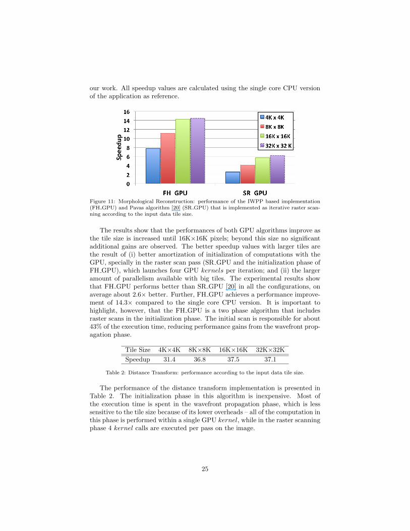
our work. All speedup values are calculated using the single core CPU versionof the application as reference.

Figure 11: Morphological Reconstruction: performance of the IWPP based implementation(FH GPU) and Pavas algorithm [20] (SR GPU) that is implemented as iterative raster scan-ning according to the input data tile size.

The results show that the performances of both GPU algorithms improve asthe tile size is increased until 16K×16K pixels; beyond this size no significantadditional gains are observed. The better speedup values with larger tiles arethe result of (i) better amortization of initialization of computations with theGPU, specially in the raster scan pass (SR GPU and the initialization phase ofFH GPU), which launches four GPU kernels per iteration; and (ii) the largeramount of parallelism available with big tiles. The experimental results showthat FH GPU performs better than SR GPU [20] in all the configurations, onaverage about 2.6× better. Further, FH GPU achieves a performance improve-ment of 14.3× compared to the single core CPU version. It is important tohighlight, however, that the FH GPU is a two phase algorithm that includesraster scans in the initialization phase. The initial scan is responsible for about43% of the execution time, reducing performance gains from the wavefront prop-agation phase.

Tile Size 4K×4K 8K×8K 16K×16K 32K×32K

Speedup 31.4 36.8 37.5 37.1

Table 2: Distance Transform: performance according to the input data tile size.

The performance of the distance transform implementation is presented inTable 2. The initialization phase in this algorithm is inexpensive. Most ofthe execution time is spent in the wavefront propagation phase, which is lesssensitive to the tile size because of its lower overheads – all of the computation inthis phase is performed within a single GPU kernel, while in the raster scanningphase 4 kernel calls are executed per pass on the image.

25

5.2.3. Impact of Input Data Characteristics

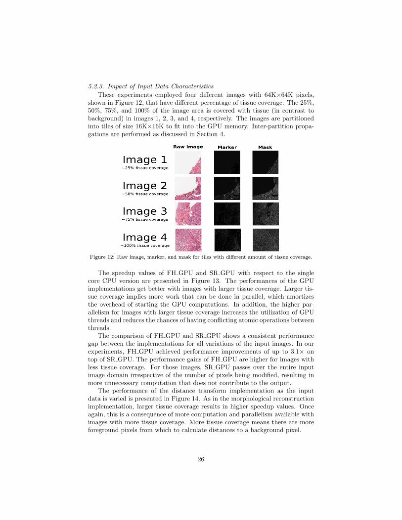
These experiments employed four different images with 64K×64K pixels,shown in Figure 12, that have different percentage of tissue coverage. The 25%,50%, 75%, and 100% of the image area is covered with tissue (in contrast tobackground) in images 1, 2, 3, and 4, respectively. The images are partitionedinto tiles of size 16K×16K to fit into the GPU memory. Inter-partition propa-gations are performed as discussed in Section 4.

Figure 12: Raw image, marker, and mask for tiles with different amount of tissue coverage.

The speedup values of FH GPU and SR GPU with respect to the singlecore CPU version are presented in Figure 13. The performances of the GPUimplementations get better with images with larger tissue coverage. Larger tis-sue coverage implies more work that can be done in parallel, which amortizesthe overhead of starting the GPU computations. In addition, the higher par-allelism for images with larger tissue coverage increases the utilization of GPUthreads and reduces the chances of having conflicting atomic operations betweenthreads.

The comparison of FH GPU and SR GPU shows a consistent performancegap between the implementations for all variations of the input images. In ourexperiments, FH GPU achieved performance improvements of up to 3.1× ontop of SR GPU. The performance gains of FH GPU are higher for images withless tissue coverage. For those images, SR GPU passes over the entire inputimage domain irrespective of the number of pixels being modified, resulting inmore unnecessary computation that does not contribute to the output.

The performance of the distance transform implementation as the inputdata is varied is presented in Figure 14. As in the morphological reconstructionimplementation, larger tissue coverage results in higher speedup values. Onceagain, this is a consequence of more computation and parallelism available withimages with more tissue coverage. More tissue coverage means there are moreforeground pixels from which to calculate distances to a background pixel.

26

Figure 13: Performance variation of the morphological reconstruction implementation withrespect to input data characteristics.

Figure 14: Performance variation of the distance transform implementation with respect toinput data characteristics.

5.2.4. Impact of Exceeding Queue Storage Limit

This set of experiments vary the memory space available for the queue tostore pixels. When the queue storage limit is exceeded, our implementationthrows away excess pixels. Then it is necessary to perform another round ofcomputations to compute any missing wavefront propagations. To stress thealgorithm, we reduced the space available for the queue until we created twoscenarios. In the first scenario, the queue storage limit is exceeded once, and thewavefront propagation execution phase has to be re-launched to fix any missingpropagations. In the second scenario, the queue storage limit is exceeded in thesecond iteration of the wavefront propagation phase as well. As a result, a thirditeration of this phase is needed to finish computation correctly.

The experimental results were obtained using the morphological reconstruc-tion implementation and an single input tile of 4K×4K pixels. The results showthat performance penalty due to exceeding the queue storage limit is small. Forinstance, the performance hit is 6% when the queue is exceeded once during the

27

execution and 9% when it is exceeded twice. In general, we observed that settinga storage limit that is 10% larger than the initial queue size was sufficient.

5.3. Cooperative Multi-GPU Multi-CPU Execution

These experiments evaluate the implementations when multiple GPUs andCPUs are used cooperatively for execution. The input images have 100% tissuecoverage. The resolutions of the images are 96K×96K pixels and 64K×64Kpixels for the morphological reconstruction implementation and the distancetransform implementation, respectively; these are the maximum size imagesthat can fit in the main CPU memory for each algorithm.

The multi-GPU scalability of the morphological reconstruction algorithmis presented in Figure 15(a). The speedups achieved for one, two, and threeGPUs, in comparison to the CPU single core version, are about 16×, 30× and43×. The overall performance improvement is good, but the 3-GPUs executionachieves 2.67× speedup with respect to the 1-GPU version which is below lin-ear. To investigate the reasons, we calculated the average cost of the wavefrontpropagation phase by breaking it down into three categories: (i) Computation,which is the time spent by the application kernels; (ii) Download, which cor-responds to the time to download the results from GPU to CPU memory; and(iii) Upload, which includes data copy from CPU to GPU. The results, presentedin Figure 15(b), show that there is an increase in data transfer costs as moreGPUs are used, limiting the scalability. We should note that we efficiently uti-lized the architecture of the node, which is built with two I/O Hubs connectingCPUs to GPUs (see Figure 9). In our approach, the CPU thread managing aGPU is mapped to a CPU closer to the corresponding GPU. This allows formaximum performance to be attained during data transfers. When this place-ment is not employed, the performance of the multi-GPU scalability is degradedand only small performance improvements are observed when more than twoGPUs are utilized.

(a) Multi-GPU scalability. (b) Per Task Execution profile.

Figure 15: Performance of the morphological reconstruction implementation on multiple GPUsand using multiple CPUs and GPUs together.

Figure 15(a) also presents the cooperative CPU–GPU execution perfor-mance. In this scenario, when the multi-core version of the CPU operation

28

is used (parallel variant), the multi-CPU multi-GPU executions achieve extraperformance improvements of about 1.17× with respect to the 3-GPU config-uration, or a total of 50× speedup on top of the single core CPU execution.As is shown in the figure, the use of sequential CPU variants results in perfor-mance loss with respect to the multi-GPU only execution. This performancedegradation is the result of load imbalance among devices, which is higher withthe sequential variants due to the larger gap in execution times between a GPUexecution and a single CPU core. The computation time for the 96K×96K pixelimage in the cooperative execution mode using all the CPUs and GPUs was 21seconds.

Figure 16: Performance of the distance transform implementation on multiple GPUs andusing multiple CPUs and GPUs together.

Finally, Figure 16 presents the cooperative multi-GPU/-CPU execution re-sults for distance transform. Similar to that of the morphological reconstructionimplementation, the multi-GPU scalability is good, but it is sub-linear becauseof increasing data transfer costs. The cooperative CPU—GPU execution, inthis case, resulted in a speedup of 1.07× on top of the execution with 3 GPUs.The smaller improvement percentage, as compared to the morphological recon-struction algorithm, is simply because of the better GPU acceleration achievedby distance transform. The overall speedups of the algorithm when all GPUsand CPU cores are employed together is about 85.6×, as compared to the singleCPU core execution. For reference, the distance transform computation on the64K×64K pixel image took only 4.1 seconds.

6. Related work

The irregular wavefront propagation pattern has similarities to some funda-mental graph scan algorithms, such as Breadth-First Search (BFS), but modifiedto support multiple sources. Much effort has been put into the development ofparallel implementations of BFS on multi-core CPUs [1] and GPUs [17, 27].The GPU implementation proposed in [27] is based on a sequence of iterationsuntil all nodes are visited. Each iteration visits all nodes on the graph and

29

processes those that are on the propagation frontier. The work by Hong etal. [17] targeted new techniques to avoid load imbalance when nodes in a graphhave a highly irregular distribution of degrees (number of edges per node). Inimage operations with IWPP the approach proposed by Hong et al. would notdo any better than what was suggested by Karas [20], since the degree of allnodes (pixels) is the same and defined by the structuring element G. Moreover,the irregular wavefront propagation based approach visits those nodes (data el-ements) that are modified – i.e., queued in the last iteration –, instead of all thenodes to compute only those that are in the frontier as in [17].

The queue in our case is heavily employed and hundreds of thousands tomillions of nodes (pixels) may be queued per iteration. The solution introducedin earlier work [27], if employed in the IWPP, would require expensive inter-block communication at each iteration of the application. This synchronizationis realized by synchronizing all thread blocks, stopping the kernel execution,and re-launching another round of computation. Unlike the previous work [27],we propose that a scalable hierarchical queue be employed in a per-block basis.This avoids communication among blocks and permits the entire computationto be efficiently carried out into a single kernel call. Moreover, since the connec-tivity of a pixel is known a priori, we can employ local queues more aggressivelyto provide very fast local storage, as well as use parallel prefix-sum based reduc-tions to avoid expensive atomic operations when storing items into the queue.Additionally, in our solution, an arbitrary large number of blocks may be used,which enables the implementation to leverage GPU’s dynamic block schedulerin order to alleviate the effects of inter-block load imbalance.

Various image processing algorithms have been ported to GPUs for efficientexecution [14, 22, 41]. In addition, there is a growing set of libraries, suchas the NVIDIA Performance Primitives (NPP) [32] and OpenCV [5], whichencapsulate GPU-implementations of a number of image processing algorithmsthrough high level and flexible APIs. Most of the algorithms currently availablewith this APIs, however, have more regular computation patterns as comparedto IWPP.

Morphological reconstruction has been increasingly employed by several ap-plications in the last decade. Efficient algorithms [55, 24] and a number of appli-cations were presented by Vincent [53]. Other variants of Vincent’s fast hybridalgorithm (FH) have been proposed, such as the downhill filter approach [35].We have tested this approach on our datasets and found it to be slower than FH.The high computational demands of morphological reconstruction motivatedother works that employed specialized processors to speedup this algorithm.Jivet et al. [19] implemented a version using FPGAs, while Karas et al. [20]targeted GPUs. In both cases, however, the parallel algorithms were designedon top of a sequential baseline version that is intrinsically parallelizable, butabout one order of magnitude slower than the fastest sequential version. In oursolution, on the other hand, we extend the fastest baseline algorithm which ex-hibits the irregular wavefront propagation pattern. This approach has resultedin strong and consistent performance improvements on top of the existing GPUimplementation by Karas [20].

30

Euclidean distance transform is also important in image analysis and used inseveral tasks as watershed based segmentation. This algorithm is very computedemanding, which has attracted considerable attention in the last few years re-garding strategies for GPU acceleration [37, 36, 40, 7]. Among the proposedsolutions, the work of Schneider et al. [40] is the most similar to our distancetransform algorithm, because it also implements an output that is equivalent tothat of Danielsson’s distance transform [11]. This GPU implementation, how-ever, is based on sweeps over the entire dataset, instead of using propagationsthat process only those elements in the wavefront as in our case. MoreoverSchneider’s algorithm only performs propagation of pixels in one row at time,considering 2D problems, which limits GPU utilization. Unfortunately, thiscode is not available for comparison, but the levels of acceleration achieved inour case are higher than what Schneider’s algorithm attained. No multi-CPUmulti-GPU algorithms have been developed for morphological reconstructionand euclidean distance transform in the previous works.

The use of CPUs and GPUs cooperatively has gained attention of the re-search community in the last few years. Several works have developed sys-tem and compiler techniques to support efficient execution on heterogeneousCPU-GPU equipped machines [25, 26, 48, 43, 44, 4, 34, 18, 16]. In this paper,differently from previous work, we present a domain specific framework for par-allelization of irregular wavefront propagation based applications in CPU-GPUequipped machines. This framework leverages the computation power of suchenvironments to a large class of applications by exporting a high level set oftools, which may used by a programmer to accelerate applications fitting in theirregular wavefront propagation pattern.

7. Conclusions

The efficiency of the irregular wavefront propagation pattern relies on track-ing points in the wavefront and, consequently, avoiding unnecessary compu-tation to visit and process parts of the domain that do not contribute to theoutput. This characteristic of the IWPP makes it an efficient computation struc-ture in image analysis and other applications [55, 53, 56, 28, 23, 54, 33, 15, 51].Nevertheless, the parallelization of the IWPP on hybrid systems with multi-core CPUs and GPUs is complicated because of the dynamic, irregular, anddata dependent data access and processing pattern. Our work has showed thata multi-level queue to track the wavefronts provides an efficient data structurefor execution on a GPU. The multi-level queue structure enables the efficient useof fast memory hierarchies on a GPU. Inter- and intra-thread block scalabilitycan be achieved by per block queues and parallel prefix-sum index calculationto avoid heavy use of atomic operations.

We also have proposed a multi-processor execution strategy that dividesthe input domain into disjoint partitions (tiles) and assigns tiles to computingdevices (CPU cores and GPUs) in a demand-driven fashion to reduce load imbal-ance. The tile based parallelization is critical to achieving scalability on multi-core systems, since it reduces inter-thread interferences because of computation

31

of the same regions of the domain without tiling. Inter-thread interferencescause inefficient use of cache.

In order to evaluate the proposed approaches we have developed IWPP-basedimplementations of two widely used image processing operations, morphologi-cal reconstruction and euclidean distance transform, on a state-of-the-art hybridmachine. In our experimental evaluation, these implementations have achievedorders of magnitude performance improvement (of upto 85×) over the sequen-tial CPU versions. Our results showed that coordinated use of CPUs and GPUsmakes it feasible to process high resolution images in reasonable times, openingthe way for large scale imaging studies.

Limitations of the Current Work. This work focuses on the developing sup-port for execution of the IWPP on shared memory hybrid machines equippedwith multicore CPUs and GPUs. The current implementation does not sup-port use of distributed multi-node machines. The parallelization strategy weemploy for multiple GPUs and CPUs (Section 4), however, can be extended forthe multi-node case. In this scenario, a messaging passing mechanism should beemployed to exchange information necessary for propagations to cross partitionsof the input domain assigned to different machines.

Acknowledgments. This research was funded, in part, by grants from theNational Institutes of Health through contract HHSN261200800001E by the Na-tional Cancer Institute; and contracts 5R01LM009239-04 and 1R01LM011119-01 from the National Library of Medicine, R24HL085343 from the NationalHeart Lung and Blood Institute, NIH NIBIB BISTI P20EB000591, RC4MD005964from National Institutes of Health, and PHS Grant UL1TR000454 from theClinical and Translational Science Award Program, National Institutes of Health,National Center for Advancing Translational Sciences. This research used re-sources of the Keeneland Computing Facility at the Georgia Institute of Tech-nology, which is supported by the National Science Foundation under ContractOCI-0910735. The content is solely the responsibility of the authors and doesnot necessarily represent the official views of the NIH. We also want to thankPavel Karas for releasing the SR GPU implementation used in our comparativeevaluation.

References

[1] V. Agarwal, F. Petrini, D. Pasetto, and D. A. Bader. Scalable Graph Ex-ploration on Multicore Processors. In Proceedings of the 2010 ACM/IEEEInternational Conference for High Performance Computing, Networking,Storage and Analysis, SC ’10, 2010.

[2] C. Ancourt and F. Irigoin. Scanning polyhedra with DO loops. In Proceed-ings of the Third ACM SIGPLAN symposium on Principles and Practiceof Parallel Programming, PPOPP ’91, pages 39–50, New York, NY, USA,1991. ACM.

32

[3] U. Banerjee. Unimodular Transformation of Double Loops. In Advances inLanguages and Compilers for Parallel Computing, pages 192–219, London,UK, 1991. Pitman Publishing.

[4] G. Bosilca, A. Bouteiller, T. Herault, P. Lemarinier, N. Saengpatsa, S. To-mov, and J. Dongarra. Performance Portability of a GPU Enabled Factor-ization with the DAGuE Framework. In 2011 IEEE International Confer-ence on Cluster Computing (CLUSTER), pages 395–402, sept. 2011.

[5] G. Bradski. The OpenCV Library. Dr. Dobb’s Journal of Software Tools,2000.

[6] I. Buck, T. Foley, D. Horn, J. Sugerman, K. Fatahalian, M. Houston, andP. Hanrahan. Brook for gpus: stream computing on graphics hardware.ACM Trans. Graph., 23(3):777–786, 2004.

[7] T.-T. Cao, K. Tang, A. Mohamed, and T.-S. Tan. Parallel Banding Algo-rithm to compute exact distance transform with the GPU. In Proceedingsof the 2010 ACM SIGGRAPH symposium on Interactive 3D Graphics andGames, I3D ’10, pages 83–90, New York, NY, USA, 2010. ACM.

[8] O. Cuisenaire and B. Macq. Fast euclidean distance transformation bypropagation using multiple neighborhoods. Computer Vision and ImageUnderstanding, 76(2):163 – 172, 1999.

[9] R. da S. Torres, A. Falcao, and L. da F. Costa. A graph-based approach formultiscale shape analysis. Pattern Recognition, 37(6):1163 – 1174, 2004.

[10] L. Dagum and R. Menon. OpenMP: an industry standard API for shared-memory programming. IEEE Computational Science and Engineering,5(1):46–55, Jan-Mar 1998.

[11] P.-E. Danielsson. Euclidean distance mapping. Computer Graphics andImage Processing, 14:227–248, 1980.

[12] R. Fabbri, L. D. F. Costa, J. C. Torelli, and O. M. Bruno. 2D Euclidean dis-tance transform algorithms: A comparative survey. ACM Comput. Surv.,40(1):2:1–2:44, Feb. 2008.

[13] A. X. Falcao, L. da Fontoura Costa, and B. S. S. D. Cunha. Multiscaleskeletons by image foresting transform and its application to neuromor-phometry. Pattern Recognition, 35(7):1571–1582, 2002.

[14] O. Fialka and M. Cadik. FFT and Convolution Performance in ImageFiltering on GPU. In Proceedings of the conference on Information Visu-alization, pages 609–614, 2006.

[15] R. K. Gabriel and R. R. Sokal. A New Statistical Approach to GeographicVariation Analysis. Systematic Zoology, 18(3):259–278, Sept. 1969.

33

[16] T. D. Hartley, U. V. Catalyurek, A. Ruiz, M. Ujaldon, F. Igual, andR. Mayo. Biomedical image analysis on a cooperative cluster of gpus andmulticores. In 22nd ACM Intl. Conference on Supercomputing, Dec 2008.

[17] S. Hong, S. K. Kim, T. Oguntebi, and K. Olukotun. Accelerating CUDAgraph algorithms at maximum warp. In Proceedings of the 16th ACMsymposium on Principles and Practice of Parallel Programming, PPoPP’11, pages 267–276. ACM, 2011.

[18] X. Huo, V. Ravi, and G. Agrawal. Porting irregular reductions on hetero-geneous cpu-gpu configurations. In 18th International Conference on HighPerformance Computing (HiPC), pages 1 –10, dec. 2011.

[19] I. Jivet, A. Brindusescu, and I. Bogdanov. Image contrast enhancementusing morphological decomposition by reconstruction. WSEAS Trans. Cir.and Sys., 7:822–831, August 2008.

[20] P. Karas. Efficient Computation of Morphological Greyscale Reconstruc-tion. In MEMICS, volume 16 of OASICS, pages 54–61. Schloss Dagstuhl -Leibniz-Zentrum fuer Informatik, Germany, 2010.

[21] L. Kernel. Perf profiling tool. GNU, 2012.

[22] A. Korbes, G. B. Vitor, R. de Alencar Lotufo, and J. V. Ferreira. Advanceson watershed processing on GPU architecture. In Proceedings of the 10thInternational Conference on Mathematical Morphology, ISMM’11, pages260–271, 2011.

[23] C. Lantuejoul. Skeletonization in quantitative metallography. In R. Haral-ick and J.-C. Simon, editors, Issues in Digital Image Processing, volume 34of NATO ASI Series E, pages 107–135, 1980.

[24] C. Laurent and J. Roman. Parallel implementation of morphological con-nected operators based on irregular data structures. In Third InternationalConference on Vector and Parallel Processing, VECPAR ’98, pages 579–592, London, UK, UK, 1999. Springer-Verlag.

[25] M. D. Linderman, J. D. Collins, H. Wang, and T. H. Meng. Merge: aprogramming model for heterogeneous multi-core systems. SIGPLAN Not.,43(3):287–296, 2008.

[26] C.-K. Luk, S. Hong, and H. Kim. Qilin: Exploiting parallelism on het-erogeneous multiprocessors with adaptive mapping. In 42nd InternationalSymposium on Microarchitecture (MICRO), 2009.

[27] L. Luo, M. Wong, and W.-m. Hwu. An effective GPU implementation ofbreadth-first search. In Proceedings of the 47th Design Automation Con-ference, DAC ’10, pages 52–55, 2010.

34

[28] F. Meyer. Digital Euclidean Skeletons. In SPIE Vol. 1360, Visual Com-munications and Image Processing, pages 251–262, 1990.

[29] T. Millstein. Practical predicate dispatch. SIGPLAN Not., 39:345–364,October 2004.

[30] J. C. Mullikin. The vector distance transform in two and three dimensions.CVGIP: Graphical Models and Image Processing, 54(6):526 – 535, 1992.

[31] Nvidia. Fermi Compute Architecture Whitepaper.

[32] NVIDIA. NVIDIA Performance Primitives(NPP), 11 February 2011.

[33] F. P. Preparata and M. I. Shamos. Computational geometry: an introduc-tion. Springer-Verlag New York, Inc., New York, NY, USA, 1985.

[34] V. Ravi, W. Ma, D. Chiu, and G. Agrawal. Compiler and runtime supportfor enabling generalized reduction computations on heterogeneous parallelconfigurations. In Proceedings of the 24th ACM International Conferenceon Supercomputing, page 137146. ACM, 2010.

[35] K. Robinson and P. F. Whelan. Efficient morphological reconstruction: adownhill filter. Pattern Recogn. Lett., 25:1759–1767, November 2004.

[36] G. Rong and T.-S. Tan. Jump flooding in GPU with applications to Voronoidiagram and distance transform. In Proceedings of the 2006 symposium onInteractive 3D graphics and games, I3D ’06, pages 109–116, 2006.

[37] G. Rong and T.-S. Tan. Variants of Jump Flooding Algorithm for Com-puting Discrete Voronoi Diagrams. In Proceedings of the 4th InternationalSymposium on Voronoi Diagrams in Science and Engineering, ISVD ’07,pages 176–181, 2007.

[38] A. Rosenfeld and J. L. Pfaltz. Sequential operations in digital pictureprocessing. J. ACM, 13(4):471–494, Oct. 1966.

[39] J. H. Saltz and et al.. Multi-scale, integrative study of brain tumor: In sil-ico brain tumor research center. In Annual Symposium of American Medi-cal Informatics Association 2010 Summit on Translational Bioinformatics(AMIA-TBI 2010), Mar 2010.

[40] J. Schneider, M. Kraus, and R. Westermann. GPU-based Real-time Dis-crete Euclidean Distance Transforms with Precise Error Bounds. In A. Ran-chordas and H. Araujo, editors, VISAPP (1), pages 435–442. INSTICCPress, 2009.

[41] I. Scholl, T. Aach, T. M. Deserno, and T. Kuhlen. Challenges of medicalimage processing. Comput. Sci., 26:5–13, February 2011.

35

[42] F. Y. Shih and Y.-T. W. Y.-T. Wu. The efficient algorithms for achievingeuclidean distance transformation. IEEE Transactions on Image Process-ing, 13(8):1078–1091, 2004.

[43] N. Sundaram, A. Raghunathan, and S. T. Chakradhar. A framework forefficient and scalable execution of domain-specific templates on GPUs. InIPDPS ’09: Proceedings of the 2009 IEEE International Symposium onParallel and Distributed Processing, pages 1–12, 2009.

[44] G. Teodoro, T. D. R. Hartley, U. Catalyurek, and R. Ferreira. Run-timeoptimizations for replicated dataflows on heterogeneous environments. InProc. of the 19th ACM International Symposium on High PerformanceDistributed Computing (HPDC), 2010.

[45] G. Teodoro, T. M. Kurc, T. Pan, L. A. Cooper, J. Kong, P. Widener, andJ. H. Saltz. Accelerating Large Scale Image Analyses on Parallel, CPU-GPU Equipped Systems. In IPDPS ’12: Proceedings of the 2012 IEEEInternational Symposium on Parallel and Distributed Processing, 2012.

[46] G. Teodoro, T. Pan, T. M. Kurc, J. Kong, L. Cooper, and J. H. Saltz. AFast Parallel Implementation of Queue-based Morphological Reconstruc-tion using GPUs. Technical Report CCI-TR-2012-2, Emory University,Jan. 2012.

[47] G. Teodoro, T. Pan, T. M. Kurc, J. Kong, L. Cooper, and J. H. Saltz.High-throughput Execution of Hierarchical Analysis Pipelines on HybridCluster Platforms. Technical Report CCI-TR-2012-4, Emory University,May 2012.

[48] G. Teodoro, R. Sachetto, O. Sertel, M. Gurcan, W. M. Jr., U. Catalyurek,and R. Ferreira. Coordinating the use of GPU and CPU for improvingperformance of compute intensive applications. In IEEE Cluster, 2009.

[49] S. Tomov, R. Nath, H. Ltaief, and J. Dongarra. Dense Linear AlgebraSolvers for Multicore with GPU Accelerators. IPDPS ’10: Proceedingsof the 2010 IEEE International Symposium on Parallel and DistributedProcessing, 2010.

[50] R. Torres, A. Falcao, and L. Costa. Shape description by image forest-ing transform. In 2002 14th International Conference on Digital SignalProcessing, 2002. DSP 2002., volume 2, pages 1089 – 1092 vol.2, 2002.

[51] G. T. Toussaint. The relative neighbourhood graph of a finite planar set.Pattern Recognition, 12(4):261–268, 1980.

[52] J. S. Vetter, R. Glassbrook, J. Dongarra, K. Schwan, B. Loftis, S. Mc-Nally, J. Meredith, J. Rogers, P. Roth, K. Spafford, and S. Yalamanchili.Keeneland: Bringing heterogeneous gpu computing to the computationalscience community. Computing in Science and Engineering, 13, 2011.

36

[53] L. Vincent. Exact Euclidean Distance Function By Chain Propagations. InIEEE Int. Computer Vision and Pattern Recog. Conference, pages 520–525,1991.

[54] L. Vincent. Morphological area openings and closings for grey-scale images.In Proc. of the Workshop ”Shape in Picture”, pages 197–208. Springer,1992.

[55] L. Vincent. Morphological grayscale reconstruction in image analysis: Ap-plications and efficient algorithms. IEEE Transactions on Image Process-ing, 2:176–201, 1993.

[56] L. Vincent and P. Soille. Watersheds in Digital Spaces: An Efficient Al-gorithm Based on Immersion Simulations. IEEE Transactions on PatternAnalysis and Machine Intelligence, 13(6):583–598, June 1991.

[57] M. Wolfe. Loops skewing: The wavefront method revisited. InternationalJournal of Parallel Programming, 15:279–293, 1986. 10.1007/BF01407876.

[58] S. Xiao and W. chun Feng. Inter-block GPU communication via fast barriersynchronization. In IPDPS ’10: Proceedings of the 2010 IEEE InternationalSymposium on Parallel and Distributed Processing, pages 1–12, 2010.

37