GPU ACCELERATED QUANTUM CHEMISTRY

A DISSERTATION

SUBMITTED TO THE DEPARTMENT OF CHEMISTRY

AND THE COMMITTEE ON GRADUATE STUDIES

OF STANFORD UNIVERSITY

IN PARTIAL FULFILLMENT OF THE REQUIREMENTS

FOR THE DEGREE OF

DOCTOR OF PHILOSOPHY

NATHAN LUEHR

February 2015

http://creativecommons.org/licenses/by-nc/3.0/us/

This dissertation is online at: http://purl.stanford.edu/hb803mt5913

© 2015 by Nathan Luehr. All Rights Reserved.

Re-distributed by Stanford University under license with the author.

This work is licensed under a Creative Commons Attribution-Noncommercial 3.0 United States License.

ii

I certify that I have read this dissertation and that, in my opinion, it is fully adequatein scope and quality as a dissertation for the degree of Doctor of Philosophy.

Todd Martinez, Primary Adviser

I certify that I have read this dissertation and that, in my opinion, it is fully adequatein scope and quality as a dissertation for the degree of Doctor of Philosophy.

Hans Andersen

I certify that I have read this dissertation and that, in my opinion, it is fully adequatein scope and quality as a dissertation for the degree of Doctor of Philosophy.

Vijay Pande

Approved for the Stanford University Committee on Graduate Studies.

Patricia J. Gumport, Vice Provost for Graduate Education

This signature page was generated electronically upon submission of this dissertation in electronic format. An original signed hard copy of the signature page is on file inUniversity Archives.

iii

iv

v

ABSTRACT

This dissertation develops techniques to accelerate quantum chemistry calculations

using commodity graphical processing units (GPUs). As both the principle bottleneck

in finite basis calculations and a highly parallel task, the evaluation of Gaussian

integrals is a prime target for GPU acceleration. Methods to tailor quantum chemistry

algorithms from the bottom up to take maximum advantage of massively parallel

processors are described. Special attention is taken to make maximum use of

performance features typical of modern GPUs, such as high single precision

performance. After developing an efficient integral direct self-consistent field (SCF)

procedure for GPUs that is an order of magnitude faster than typical CPU codes, the

same machinery is extended to the configuration interaction singles (CIS) and time-

dependent density functional theory (TDDFT) methods. Finally, this machinery is

applied to molecular dynamics (MD) calculations. To extend the time scale accessible

to MD calculations of large systems, an ab initio multiple time steps (MTS) approach

is developed. For small systems, up to a few dozen atoms, an interactive interface

enabling a virtual molecular modeling kit complete with realistic ab initio forces is

developed.

vi

ACKNOWLEDGEMENTS

I thank my advisor Dr. Todd Martínez for his guidance, advice, and patience

over the past six years of work. Working in his lab has provided tremendous

professional and personal growth and has been much more fun than graduate school

has any right to be. I am also indebted to my predecessor, Ivan Ufimtsev, who began

the GPU effort and gently brought me up to speed. I have also had the advantage of

working with Dr. Tom Markland, and Dr. Christine Isborn on various projects and

have benefited tremendously in learning from them. I thank my father, Dr. Craig

Luehr, for his life-long encouragement to pursue interesting questions, and his

patience in reviewing even the least interesting sections of this dissertation. Finally, I

thank my wife, Tracy, for her unfailing encouragement and support in pursuing this

work.

vii

TABLE OF CONTENTS

CHAPTER TITLE PAGE

Title Page i

Abstract v

Acknowledgements vi

Table of Contents vii

List of Tables viii

List of Illustrations ix

Introduction 1

1 Background and Review 7

2 Integral-Direct Fock Construction on GPUs 33

3 Dynamic Precision ERI Evaluation 53

4 DFT Exchange-Correlation Evaluation on GPUs 71

5 Excited State Electronic Structure on GPUs: CIS and TDDFT 91

6 Multiple Time Step Integrators for Ab Initio MD 115

7 Interactive Ab Initio Molecular Dynamics 141

Bibliography 165

viii

LIST OF TABLES

TABLE TITLE PAGE

1.1 Runtime Comparison for GPU ERI Algorithms 27

3.1 RHF Energies Computed in Single and Double Precision 60

3.2 Double and Dynamic Precision Final RHF Energies 64

3.3 Runtime Comparison of Dynamic and Full Double Precision 66

4.1 Comparison of Becke Grid Calculations by Precision 78

4.2 Performance of CPU and GPU Becke Weight Calculations 79

4.3 Timing Breakdown: CPU and GPU Grid Generation for BPTI 80

5.1 Accuracy and Performance of GPU CIS Algorithm 103

5.2 TD-BLYP AX Build Timings for Various Quadrature Grids 106

5.3 Properties for First Bright State of Several Dendrimers 109

6.1 Performance of MTS and Velocity Verlet Integrators 134

7.1 Small Molecule TeraChem Optimization Improvements 157

7.2 Wall Time per MD Time Step for Various Small Molecules 160

ix

LIST OF ILLUSTRATIONS

FIGURE TITLE PAGE

1.1 1 Block – 1 Contracted ERI Mapping 23

1.2 1 Thread – 1 Contracted ERI Mapping 25

1.3 1 Thread – 1 Primitive ERI Mapping 26

1.4 ERI Grid Sorted by Angular Momentum 30

2.1 GPU J-Engine Algorithm 38

2.2 Organization of Coulomb ERIs by Schwarz Bound 42

2.3 GPU K-Engine Algorithm 48

3.1 Arrangement of Double and Single Precision Coulomb ERIs 59

3.2 Geometries Used for Benchmarking Mixed Precision 60

3.3 Mixed Precision Error versus Precision Threshold 61

3.4 Additional Test Systems for Dynamic Precision 65

3.5 Fock Construction Speedups by Precision 66

4.1 Pseudo-code of Serial Becke Weight Calculation 75

4.2 Benchmark Molecules for Becke Weight Kernels 79

4.3 Linear Scaling of CPU and GPU Becke Weight Kernels 80

4.4 One-Dimensional and Three-Dimensional SCF Test Systems 84

4.5 First SCF Iteration Timing Breakdown 85

4.6 Parallel Efficiency for SCF Calculations on Multiple GPUs 87

4.7 TeraChem vs. GAMESS: SCF Performance for Water Clusters 89

5.1 Geometries of Four Generations of Oligothiophene Dendrimers 99

x

5.2 Additional Systems to Benchmark Excited State Calculations 99

5.3 CIS Convergence Using Single and Double Precision 101

5.4 Timing Breakdown for Construction of AX Vectors on GPU 104

5.5 TDDFT First Excitation Energy versus System Size 108

6.1 H2O/OH- Dissociation Curves for CASE and RHF 124

6.2 Total Energy for 21ps MTS-LJFRAG Simulation 125

6.3 Energy Drift for Ab Initio MTS Integrators 127

6.4 Power Spectra: Velocity Verlet and MTS Integrators 129

6.5 Power Spectra: MTS Integrators with Various Model Forces 130

6.6 Power Spectra: CASE Verlet and CASE MTS Integrators 131

6.7 Energy Conservation of 21ps MTS-CASE Trajectory 133

7.1 Schematic of Interactive MD Communication 145

7.2 Histogram of Step Times for Interactive and Batch MD 148

7.3 Schematic of Visualized and Simulated Systems 152

7.4 Multi-GPU Parallelization Strategies 155

7.5 Total Energy Curve for AI-IMD Simulation of HCl 159

7.6 Geometries for AI-IMD Benchmark Calculations 160

7.7 Snapshots of an Interactive Simulation 161

7.8 Interactive Proton Transfer in Imidazole 162

1

INTRODUCTION

For the field of quantum chemistry, the circumvention of computational

bottlenecks is a key concern. After all, the non-relativistic Schrödinger equation in

principle describes the chemistry of a great many important organic and biological

systems.1 In practice, however, the generality and accuracy of this equation can only

be accessed at a tremendous computational cost that scales factorially with the size of

the system. Many sophisticated ab initio approximations2 have been developed to

reduce the required effort to a polynomial function of the system’s size while retaining

the general applicability of the Schrödinger equation along with an absolute accuracy

in the computed energy of at least 0.5 kcal/mol, which is ~kBT at 300K and thus the

threshold at which energies become chemically relevant.

The history of quantum chemistry has developed through a series of

algorithmic developments. However, the impact of computer hardware has been

equally important. Because each algorithm was developed to run on a particular

machine, the performance characteristics of each computer shaped the algorithms that

were developed. For example, the expression of correlated wavefunction methods

exclusively in terms of dense linear algebra operations is arguably a direct result of the

efficiency of BLAS on traditional processors. As clock speeds and serial CPU

performance ramped up in the 90’s and early 2000’s, processor architectures were

heavily consolidated until only a few remained, most notably Intel’s x86. Given the

favorable cost and performance of CPUs, it is not surprising that quantum chemistry

methods have extensively targeted the CPU.

2

However, in recent years the CPU’s serial performance has essentially

stagnated. As a result, alternative architectures are gaining traction for many

workloads. Multi-core CPUs have become commonplace. Massively parallel

streaming architectures designed for use in graphics processing units (GPUs) provide a

more extreme contrast with traditional serial processors. Today’s widening landscape

of processor designs raises the question of what shape quantum chemistry methods

will take as they move beyond the CPU.

In the following chapters we seek to answer this question by tailoring various

quantum chemistry algorithms to GPUs. This is a particularly attractive architecture

both because key computational bottlenecks in quantum chemistry map extremely

well onto massively parallel GPU processors and because low-cost high-performance

hardware is readily available and continuously improved. The introduction of the

Compute Unified Device Architecture3 (CUDA) as an extension to the C language

also greatly simplifies GPU programming, making it easily accessible for scientific

programming. The methods described in the following chapters form the foundation of

the TeraChem quantum chemistry program, which was designed from the ground up

to make optimal use of GPU hardware.4,5

The importance of this work is at least threefold. First, the methods presented

here are important in themselves because they dramatically accelerate certain quantum

chemistry calculations and make previously difficult calculations routine.6-9 Second, as

finite size constraints become dominant in hardware design, machines will become

increasingly parallel. As a result, many features and limitations that exist on modern

GPUs will become ubiquitous on high-performance architectures of the future, making

3

our work highly transferable. Third, the discussion of how to map quantum chemistry

calculations onto computer hardware goes beyond mere code optimization, since there

is a kind of natural selection at play in method development. If certain operations can

be accelerated, then methods that exploit these operations may gain advantages and be

chosen for future development. The present work follows this pattern. For example,

after introducing and optimizing the Coulomb and exchange operators for use in self-

consistent field (SCF) calculations10,11 in chapters 2-4, these same operations are

exploited to accelerate excited state methods6 in chapter 5.

At the same time that traditional processors are reaching their performance

limits, it is becoming much cheaper to fabricate custom architectures. The present

work focuses on optimizing quantum chemistry methods for a particular alternative

architecture. Perhaps in the future the inverse process will be feasible, and processors

will be tailored as much to quantum chemistry as vice versa. The series of ANTON

machines that are designed for classical MD are perhaps early examples of this

trend.12-18 The less successful GRAPE-DR architecture is similar,19 but perhaps shows

how much must be gleaned from the study of existing architectures before efficient

custom hardware can be designed for quantum chemistry.

The following chapters are organized as follows. Chapter one gives a brief

introduction to quantum chemistry and introduces the electron repulsion integrals

(ERIs) which represent an important computational bottleneck. We also review the

McMurchie-Davidson20 approach that can be used to evaluate these integrals as well

as early work to evaluate ERIs on GPU processors.21,22 Chapter two covers the

efficient implementation of Coulomb and exchange operators in TeraChem.11,23

4

Chapter three introduces dynamic precision, which is an important technique to tailor

integral evaluation to GPUs that provide much more single than double precision

performance.10 Chapter four discusses the implementation of density functional theory

(DFT) exchange-correlation potentials on GPUs.24,25 In chapter five we extend our

Coulomb and exchange operators to excited state configuration interaction singles

(CIS) and linear response time-dependent DFT (TDDFT).6 Finally, we consider

methods that leverage GPU quantum chemistry to extend the reach of ab initio

molecular dynamics (AIMD). In chapter six we discuss the use of multiple time step

(MTS) integrators to accelerate AIMD in large systems.8 And in chapter seven we turn

to accelerating calculations on small systems and introduce an interactive quantum

chemistry interface built on real-time AIMD.

REFERENCES

(1) Dirac, P. A. M. P R Soc Lond a-Conta 1929, 123, 714.

(2) Helgaker, T.; Jørgensen, P.; Olsen, J. Molecular electronic-structure theory; Wiley: New York, 2000.

(3) Schwegler, E.; Challacombe, M.; HeadGordon, M. J. Chem. Phys. 1997, 106, 9708.

(4) PetaChem, L.; Vol. 2010.

(5) Ufimtsev, I. S.; Martinez, T. J. J. Chem. Theo. Comp. 2009, 5, 2619.

(6) Isborn, C. M.; Luehr, N.; Ufimtsev, I. S.; Martinez, T. J. J. Chem. Theo. Comp. 2011, 7, 1814.

(7) Kulik, H. J.; Luehr, N.; Ufimtsev, I. S.; Martinez, T. J. J. Phys. Chem. B 2012, 116, 12501.

(8) Luehr, N.; Markland, T. E.; Martinez, T. J. J. Chem. Phys. 2014, 140, 084116.

5

(9) Ufimtsev, I. S.; Luehr, N.; Martinez, T. J. J. Phys. Chem. Lett. 2011, 2, 1789.

(10) Luehr, N.; Ufimtsev, I. S.; Martinez, T. J. J. Chem. Theo. Comp. 2011, 7, 949.

(11) Ufimtsev, I. S.; Martinez, T. J. J. Chem. Theo. Comp. 2009, 5, 1004.

(12) Grossman, J. P.; Kuskin, J. S.; Bank, J. A.; Theobald, M.; Dror, R. O.; Ierardi, D. J.; Larson, R. H.; Ben Schafer, U.; Towles, B.; Young, C.; Shaw, D. E. Acm Sigplan Notices 2013, 48, 549.

(13) Grossman, J. P.; Towles, B.; Bank, J. A.; Shaw, D. E. Des Aut Con 2013.

(14) Kuskin, J. S.; Young, C.; Grossman, J. P.; Batson, B.; Deneroff, M. M.; Dror, R. O.; Shaw, D. E. Int S High Perf Comp 2008, 315.

(15) Larson, R. H.; Salmon, J. K.; Dror, R. O.; Deneroff, M. M.; Young, C.; Grossman, J. P.; Shan, Y. B.; Klepeis, J. L.; Shaw, D. E. Int S High Perf Comp 2008, 303.

(16) Shaw, D. E.; Deneroff, M. M.; Dror, R. O.; Kuskin, J. S.; Larson, R. H.; Salmon, J. K.; Young, C.; Batson, B.; Bowers, K. J.; Chao, J. C.; Eastwood, M. P.; Gagliardo, J.; Grossman, J. P.; Ho, C. R.; Ierardi, D. J.; Kolossvary, I.; Klepeis, J. L.; Layman, T.; McLeavey, C.; Moraes, M. A.; Mueller, R.; Priest, E. C.; Shan, Y. B.; Spengler, J.; Theobald, M.; Towles, B.; Wang, S. C. Conf Proc Int Symp C 2007, 1.

(17) Shaw, D. E.; Dror, R. O.; Salmon, J. K.; Grossman, J. P.; Mackenzie, K. M.; Bank, J. A.; Young, C.; Deneroff, M. M.; Batson, B.; Bowers, K. J.; Chow, E.; Eastwood, M. P.; Ierardi, D. J.; Klepeis, J. L.; Kuskin, J. S.; Larson, R. H.; Lindorff-Larsen, K.; Maragakis, P.; Moraes, M. A.; Piana, S.; Shan, Y. B.; Towles, B. Proceedings of the Conference on High Performance Computing Networking, Storage and Analysis 2009.

(18) Towles, B.; Grossman, J. P.; Greskamp, B.; Shaw, D. E. Conf Proc Int Symp C 2014, 1.

(19) Makino, J.; Hiraki, K.; Inaba, M. 2007 Acm/Ieee Sc07 Conference 2010, 548.

(20) McMurchie, L. E.; Davidson, E. R. J. Comp. Phys. 1978, 26, 218.

(21) Yasuda, K. J. Comp. Chem. 2008, 29, 334.

(22) Ufimtsev, I. S.; Martinez, T. J. J. Chem. Theo. Comp. 2008, 4, 222.

(23) Titov, A. V.; Ufimtsev, I. S.; Luehr, N.; Martinez, T. J. J. Chem. Theo. Comp. 2013, 9, 213.

6

(24) Hwu, W.-m. GPU computing gems; Elsevier: Amsterdam ; Burlington, MA, 2011.

(25) Yasuda, K. J. Chem. Theo. Comp. 2008, 4, 1230.

7

CHAPTER ONE

BACKGROUND AND REVIEW

In this chapter we provide a brief review of the Hartree-Fock (HF) and Density

Functional Theory (DFT) quantum chemistry methods within atom-centered Gaussian

basis sets. We focus particularly on the evaluation of electron repulsion integrals

(ERIs) because these play an important role in the following chapters. The

performance of Self-consistent field (SCF) methods such as HF and DFT depends on

two principal bottlenecks. The first is the evaluation of ERIs. Formally, for a basis set

containing N functions, a total of O(N4) ERIs must be evaluated. In the limit of large

systems, efficient screening of negligibly small ERIs can reduce this number to O(N2)

or, for certain insulating systems, even O(N).1-5 The second bottleneck is the update of

the orbitals/density between SCF iterations. This is traditionally performed by

diagonalizing the N-by-N Fock matrix to obtain its eigenvectors and eigenvalues.

Eigensolvers applied to dense matrices run with a complexity of O(N3). However,

using sparse matrix algebra it is possible, again in asymptotically large systems, to

achieve O(N) scaling for this step as well.6 Thus, formal asymptotic analysis is of

limited use since the dominant bottleneck results from prefactors rather than scaling

exponents. Empirically, for systems up to at least 10,000 basis functions, integral

evaluation dominates the SCF runtime, and thus the following chapters focus

primarily on the GPU acceleration of ERI evaluation.

Numerous ERI evaluation schemes have been developed for use in traditional

CPU codes. For very high angular momentum, Rys quadrature methods7 may provide

8

an advantage on GPUs due to their smaller memory footprint.8-10 For low angular

momentum basis functions, however, the Rys and simpler McMurchie-Davidson11

approaches provide comparable performance, and the simplicity of the latter is

preferred here.

QUANTUM CHEMISTRY REVIEW

Full derivations of the HF and DFT methods as well as in-depth descriptions of

various ERI evaluation algorithms can be found elsewhere.12-14 Here we provide a

brief background in order to put the subsequent chapters in context. Unless otherwise

noted, we assume a spin-restricted wavefunction anstatz and atomic units.

Self-Consistent Field Equations in Gaussian Basis Sets

A primitive Gaussian function is defined as follows.

! i

!r( ) = Ni

!rx " xi( )ni !ry " yi( )li !rz " zi( )mi e"# i!r"!Ri

2

(1.1)

Here !r is the three-dimensional electronic coordinate,

!Ri = xi , yi , zi( ) is the

primitive’s Cartesian center (usually coinciding with the location of an atom), !i is an

exponent determining the spatial extent of the function, and Ni is a normalization

constant chosen so that the following holds.

! i!r( )! i

!r( )d!r = 1"#

#

$ (1.2)

The nonnegative integers, ni, li, and mi, fix the function’s angular momentum in the

Cartesian x-, y-, and z-directions. Their sum, "i = ni + li + mi, gives the primitive’s

total angular momentum. Functions with !i = 0,1,2 are termed, s-, p-, and d-functions

9

respectively. The set of !i +1( ) !i + 2( ) / 2 primitive functions that differ only by the

distribution of !i into n, l, and m is referred to as a primitive shell.

! I = ! i

!r( ) |!Ri =

!RI ," i =" I ,#i = #I{ } (1.3)

We use the lower case indices i, j, k, and l to refer to primitive functions and the

capital letters I, J, K, and L for primitive shells.

In order to more closely approximate solutions to the atomic Schrödinger

equation, several primitive functions (all sharing a common center, Rµ , and angular

momenta, nµ , lµ , and mµ ) are combined together into contracted basis shells using

fixed contraction weights, ci.

!µ (r) = ci" i (r)i#µ$ (1.4)

Here a segmented basis is assumed in which each primitive contributes to a single

basis function. Greek indices are used for contracted AO quantities. The notation

i !µ specifies that the primitive ! i (r) belongs to the AO contraction !µ (r) . These

contracted functions are termed atomic orbitals (AOs) in analogy to the Hydrogen

atom’s one-electron orbitals which they resemble and form the basis in which the

Schrödinger equation will be solved.

The AOs are further combined by linear contraction into molecular orbitals

(MOs), each of which represents a one-particle spatial probability distribution for an

electron in the multi-atom system.

! i!r( ) = Cµi"µ

!r( )µ

N

# (1.5)

10

The MO coefficients, Cµi , are free parameters, and their determination is the primary

objective of the SCF procedure. In order to describe an n-electron system, the one-

electron MOs are combined with spin functions in a Slater determinant.

! !x1,!x2,...,

!xn( ) = 1n!

" 1(!x1) " 2 (

!x1) " " n (!x1)

" 1(!x2 ) " 2 (

!x2 ) " " n (!x2 )

# # $ #" 1(!xn ) " 2 (

!xn ) " " n (!xn )

(1.6)

For the spin-restricted case in which two electrons occupy each spatial orbital, the spin

orbitals (depending on both spatial and spin electronic degrees of freedom) can be

defined as follows (where !k is the spin degree of freedom for the kth electron):

! 2n"1(!xk ) = #n (

!rk )$ (% k )! 2n (

!xk ) = #n (!rk )&(% k )

(1.7)

The energy of the wavefunction, ! , representing n electrons in a system

containing A fixed atomic nuclei (each with charge Za and located at position !Ra ) is

derived from the expectation value of the electronic Hamiltonian, H :

H =Za!ri !!Raa

A

" !#i

2

2+ 1

21!ri !!rjj$i

"%

&''

(

)**i

n

" (1.8)

�ERHF =

!�H�!

! != 2 " i h" i +

i

n/2

# 2 " i" i�" j" j( )i, j

n/2

# $ " i" j�" i" j( )i, j

n/2

# (1.9)

Here the MOs are assumed, without loss of generality, to be orthonormal.

!i ! j = " ij (1.10)

11

The one-electron core Hamiltonian operator, h , accounts for electron-nuclear

attraction and electron kinetic energy,

h(!r ) =

Za!r !!Raa

A

" ! #2

2 (1.11)

and the two-electron repulsion integrals (ERIs) account for pairwise repulsive

interactions between electrons.

�! i! j�!k! l( ) = d 3!r1 d 3!r2""

! i* !r1( )! j

!r1( )!k* !r2( )! l

!r2( )!r1 #!r2

(1.12)

For Kohn-Sham DFT, a similar energy expression is obtained by using the

determinant to describe non-interacting pseudo-particles whose total density matches

the ground state electron density.15

!(!r ) = 2 " i(

!r )2

i

n/2

# (1.13)

In this case, components of the Hartree-Fock energy provide good approximations for

the DFT kinetic energy and classical electron repulsion. An additional density-

dependent exchange-correlation functional, EXC !"# $% , corrects for the relatively small

energetic effects of electron exchange and correlation as well as errors from

approximating the kinetic energy as that of the Kohn-Sham determinant.

�EDFT = 2 ! i h! i +

i

n/2

" 2 ! i! i�! j! j( )i, j

n/2

" + EXC[#] (1.14)

Given the exact exchange-correlation functional, EXC !"# $% , equation 12 would provide

the exact ground state energy. Unfortunately, the exact functional is not known in any

computationally feasible form. In practice a variety of approximate functionals are

12

often employed. For simplicity, we focus on the remarkably successful class of

generalized gradient approximation (GGA) functionals. These take the form of an

integral over a local xc-kernel that depends only on the total density and its gradient.

EXC[!]= fxc(!(r), "!(r)

2 )d!r# (1.15)

To calculate the HF or DFT ground state electronic configuration, we vary the MO

coefficients, Cµi , to minimize ERHF or EDFT under the constraint of equation 8 that the

MOs remain orthonormal. Functional variation ultimately results in the following

conditions on the MO coefficients.

F(P)C = !SC (1.16)

Here P is the density matrix represented in the AO basis;

Pµ! = Cµi

i

n

" C!i* (1.17)

! is a diagonal matrix of MO energies (formally, this matrix is the set of Lagrange

multipliers enforcing the constraint that all the molecular orbital remain orthogonal,

i.e. equation 8); S is the AO overlap matrix;

Sµ! = "µ "! (1.18)

and F(P) is the non-linear Fock operator, defined slightly differently for HF and DFT

as follows.

�Fµ!

HF (P) = hµ! + P"#"#

N

$ 2 µ!�#"( )% µ"�!#( )&' () (1.19)

�Fµ!

DFT (P) = hµ! + 2 µ!�"#( )P#"#"

N

$ +Vµ!XC (1.20)

Here h is the core Hamiltonian from equation 9 in the AO basis,

13

hµ! = "µ

Za!r1 #!Raa

A

$ #%1

2"! (1.21)

and the two electron ERIs are defined in the AO basis as follows.

�

µ!�"#( ) = d 3!r1 d 3!r2$$%µ!r1( )%! !r1( )%"

!r2( )%# !r2( )!r1 &!r2

= ci c jck cll'#(

k'"(

j'!(

i'µ( d 3!r1 d 3!r2$$

) i!r1( )) j

!r1( )) k!r2( )) l

!r2( )!r1 &!r2

= ci c jck cll'#(

k'"(

j'!(

i'µ( ij�kl*+ ,-

(1.22)

Note that round braces refer to ERIs involving contracted basis functions while square

braces refer to primitive ERIs. Finally, for DFT, VXC is determined by functional

differentiation of the exchange-correlation energy expression.

Vµ!

XC = "µ

# EXC

#$"! (1.23)

Because the HF and DFT Fock operators are non-linear, equation (1.16) cannot

be solved in closed form. Instead an iterative approach is used. Starting from some

guess for the density matrix, P, the Fock matrix is constructed and then diagonalized

to obtain a matrix of approximate MO orbitals, C. The MO coefficients are then used

to construct an improved guess for the density matrix using equation (1.17), and the

process is repeated until F and P converge to stable values.

Evaluating Electron Repulsion Integrals

Having described the basic SCF working equations we turn now to the

evaluation of primitive ERIs.

14

�

ij�kl!" #$ = d 3!r1 d 3!r2%%& i!r1( )& j

!r1( )& k!r2( )& l

!r2( )!r1 '!r2

(1.24)

Efficient evaluation of the coulomb integrals within Gaussian basis sets begins by

invoking the Gaussian product theorem (GPT) of equation (1.25). This allows a pair of

Gaussian functions at different centers to be rewritten as a combined Gaussian

function centered at a point, !P , between the original centers.16

e!" i!r!!Ri( )2e!" j

!r!!Rj( )2 = Kije

!#ij!r!!Pij( )2

#ij =" i +" j

Kij = e!" i" j

" i+" j

!Ri!!Rj( )2

!Pij =

" i

!Ri +" j

!Rj

" i +" j

(1.25)

Applying equation (1.25) separately to the bra, ! i!r1( )! j

!r1( ) , and ket, ! k!r2( )! l

!r2( )

primitive pairs of equation (1.24), results in two charge distributions, ! ij and !kl and

reduces the four center ERI to a simpler two-center problem.

�

ij�kl!" #$ = % ij�%kl!" #$ (1.26)

The pair distributions, ! ij , can be factored into x-, y-, and z-components, which will

greatly simplify the problem.

! ij = Ni N j Kij

x! ijy! ij

z! ij (1.27)

The x-component of the bra distribution is shown below, the other terms being

analogous.

x! ij (x1) = x1 " xi( )ni x1 " x j( )nj e

"#ij x1"Xij( )2 (1.28)

15

Following McMurchie and Davidson we expand the pair distributions of

equation (1.28) exactly in a basis of Hermite Gaussians, {!t}.11

x! ij (x1) = x Et

nin j"tx (x1)

t

ni+nj

# (1.29)

!t

x (x1) = ""Xij

#

$%

&

'(

t

e)*ij x1)Xij( )2

(1.30)

Again, analogous expressions expand the y- and z-components. The expansion

coefficients, x Et

ij

are calculated from simple recurrence relations given below.11

x Etmn = 0, where t < 0 or t > m+ n

x Etm+1,n = 1

2 px Et!1

mn + X Pij Ri

x Etmn + (t +1) x Et+1

mn

x Etm,n+1 = 1

2 px Et!1

mn + X Pij Rj

x Etmn + (t +1) x Et+1

mn

(1.31)

Here XPQ is shorthand for Px – Qx. The pair distribution from equation (1.27) is then

written as follows.

! ij (r1) = Ni N j Kij Etuv

ij

v

mi+mj

" #tuv (r1)u

li+l j

"t

ni+nj

" (1.32)

Etuvij = x Et

nin j y Eulil j z Ev

mimj

(1.33)

!tuv (r1) = !tx (x1)!u

y ( y1)!vz (z1) (1.34)

And the overall integral from equation (1.24) is expanded as follows.

[ij | kl]= Ni N j Nk Nl Kij Kkl Etuv

ij E !t !u vkl

!v

mk+ml

" Vtuv!t !u !v

!u

lk+ll

"!t

nk+nl

"v

mi+mj

"u

li+l j

"t

ni+nj

" (1.35)

16

Here Vtuv!t !u !v represent Hermite Coulomb integrals, which are defined through equations

(1.30) and (1.34) as partial derivatives of an s-function Coulomb integral.

Vtuv!t !u !v = ["tuv |" !t !u !v ]

= (#1) !t + !u + !v $$Xij

%

&'

(

)*

t+ !t$$Yij

%

&'

(

)*

u+ !u$

$Zij

%

&'

(

)*

v+ !ve#+ij

!r1#!Pij( )2e#+kl

!r2#!Pkl( )2

!r1 #!r2

,, d!r1d!r2

(1.36)

To evaluate Vtuv!t !u !v , the simple Coulomb integral on the right in equation (1.36)

is first expressed in terms of the Boys function, Fn.

e!"ij!r1!!Pij( )2e!"kl

!r2!!Pkl( )2

!r1 !!r2

## d!r1d!r2 =

2$ 5/2

"ij"kl "ij +"kl

F0

"ij"kl

"ij +"kl

Pij ! Pkl( )2%

&'

(

)*

(1.37)

Fn (x) = t 2ne! xt

2

dt0

1

" (1.38)

In practice the Boys function is computed using an interpolation table and downward

recursion.14 Next we define the auxiliary functions, Rtuvn , as follows.

Rtuv

n = !!Xij

"

#$

%

&'

t!!Yij

"

#$

%

&'

u!

!Zij

"

#$

%

&'

v

(2)ij)kl

)ij +)kl

"

#$

%

&'

n

Fn

)ij)kl

)ij +)kl

!Pij (!Pkl( )2"

#$

%

&' (1.39)

Noting that

Rtuv

0 = !!Xij

"

#$

%

&'

t!!Yij

"

#$

%

&'

u!

!Zij

"

#$

%

&'

v

F0

(ij(kl

(ij +(kl

!Pij )!Pkl( )2"

#$

%

&' (1.40)

Equation (1.36) now becomes the following.

Vtuv!t !u !v = ("1) !t + !u + !v 2# 5/2

$ij$kl $ij +$kl

Rt+ !t ,u+ !u ,v+ !v0 $ij$kl

$ij +$kl

,!Pij "!Pkl( )2%

&'

(

)* (1.41)

17

The utility of the auxiliaries, Rtuvn , is that they can be efficiently computed from the

Boys function starting at R000n using the following recurrence relations.

Rt+1,u ,vn = tRt!1,u ,v

n+1 + Xij ! Xkl( )Rt ,u ,vn+1

Rt ,u+1,vn = uRt ,u!1,v

n+1 + Yij !Ykl( )Rt ,u ,vn+1

Rt ,u ,v+1n = vRt ,u ,v!1

n+1 + Zij ! Zkl( )Rt ,u ,vn+1

(1.42)

This brings us to the final expression for evaluating the ERI of equation (1.24).

[ij | kl]= Nij Nkl Etuvij E !t !u !v

kl

!v

mk+ml

" (#1) !t + !u + !v

$ij +$kl

Rt+ !t ,u+ !u ,v+ !v0

!u

lk+ll

"!t

nk+nl

"v

mi+mj

"u

li+l j

"t

ni+nj

" (1.43)

Nij =

Ni N j Kij 2! 5/4

"ij (1.44)

Here Nij is a convenience factor that combines all scalar factors for the bra (or ket) pair

distribution. In practice, the AO contraction coefficients from equation (1.22), cicj in

the case of the bra, are also included in this factor.

For s-functions, each quartet of primitive shells, [ij|kl], generates a single

integral. For shells with higher angular momentum a shell quartet generates multiple

integrals, since each primitive shell contains multiple functions. For example, each

shell quartet with the momentum pattern [sp|sd] will generate 18 functions (since there

are three functions in the p-shell, six in the d-shell and one in each s-shell. These 18

integrals, however, involve the same set of auxiliary integrals, Rtuv0 , and Hermite

contraction coefficients, xEtmn . As a result, it is advantageous to generate the

intermediates once, and then evaluate equation (1.43) repeatedly, once for each

integral in the shell quartet.

18

Screening Negligible Integrals

The Fock contributions in equations (1.19) and (1.20) nominally involve

contributions from N4 ERIs. However, several strategies are routinely used to avoid

calculating most of these integrals. First, the ERIs possess eight-fold symmetry so that

[ij|kl] = [kl|ij] = [ij|lk]. The point group symmetry of the molecule is sometimes also

used to eliminate even more redundant integrals. However, large systems rarely

possess such symmetry, so this approach is not applicable to the present work.

Many of the remaining integrals are so small that they can be neglected

without affecting the computed molecular properties. Because each AO basis function

is localized in space, a pair distribution, !ij , will approach zero exponentially as the

distance between primitive functions increases. Thus, an AO ERI, �µ!�"#( ) , will be

non-negligible only if µ is centered near ! and ! is near ! . For large systems, this

reduces the number of integrals to a more manageable N2. In order to efficiently

identify significant ERIs, a Cauchy-Schwarz inequality can be applied to either

contracted or primitive integrals.17

�

ij�kl!" #$ % ij�ij!" #$1/2

kl�kl!" #$1/2

(1.45)

For primitive integrals, this Schwarz bound is easily computed, because in

[ij|ij] integrals the bra and ket pair distributions share a common center greatly

simplifying the integral expressions. Thus, by checking the integral bound for each

shell quartet, it is possible to avoid computing many small integrals all together.

Another advantage of the Schwarz bound is that it can be decomposed into bra and ket

19

parts, and thus quantities of [ij|ij]1/2 can be computed once and stored with each pair

distribution rather than being recomputed for every shell quartet.

INTRODUCTION TO CUDA AND GPU PROGRAMMING

Each GPU is a massively parallel device, containing thousands of execution

cores. However, the performance of these processors results not only from the raw

width of execution units, but also from a hierarchy of parallelism that forms the

foundation of the hardware architecture and is ingeniously exposed to the programmer

through the CUDA programming model.18 Developers must understand and respect

these hierarchical boundaries if their programs are to run efficiently on GPUs.

At the lowest level, the CUDA programmer writes a small procedure – called a

kernel in “CUDA-speak” – that is to be executed by tens of thousands of individual

threads in parallel. Although each CUDA thread is logically autonomous, the

hardware does not execute each thread independently. Instead, instructions are

scheduled for groups of 32 threads, called warps, in single-instruction-multiple-thread

(SIMT) fashion. Every thread in a warp executes the same instruction stream, with

threads masked to null operations (no-ops) for instructions in which they do not

participate.

Warps are grouped into larger blocks of up to 1024 threads. Blocks are

assigned to local groups of execution units called streaming multiprocessors (SMs).

The SM provides hardware-based intra-block synchronization methods and a small

on-chip shared memory often used for intra-block communication. CUDA blocks can

be indexed in 1, 2, or 3 dimensions at the convenience of the programmer.

20

At the highest level, blocks are organized into a CUDA grid. As with blocks,

the grid can be up to 3 dimensional. In general, the grid contains many more blocks

and threads than the GPU has physical execution units. When a grid is launched, a

hardware scheduler streams CUDA blocks onto the processors. By breaking a task into

fine-grained units of work, the GPU can be kept constantly busy, maximizing

throughput performance.

In CUDA the memory is also structured hierarchically. The host memory

usually provides the largest space, but can only be accessed through the PCIe data bus

which suffers from latencies on the order of several thousand instruction cycles. The

GPU’s main (global) memory provides several gigabytes of high-bandwidth memory

capable of more than 250 GB/s of sustained throughput. In order to enable this

bandwidth, global memory accesses incur long latencies, on the order of 500 clock

cycles. Global memory operations are handled in parallel mirroring the SIMT warp

design. The large width of the memory controller allows simultaneous memory access

by all threads of a warp as long as those threads target contiguous memory locations.

Low-latency, on-chip memory is also available. Most usefully, each block can use up

to 64 KB of shared memory for intra-block communication, and each thread may use

up to 255 local registers in which to store intermediate results.

Consideration of the hardware design suggests the following basic strategies

for maximizing the performance of GPU kernels.

1) Launch many threads, ideally one to two orders of magnitude more threads than

the GPU has execution cores. For example, a Tesla K20 with 2496 cores may not

reach peak performance until at least O(105) threads are launched. Having

21

thousands of processors will only be an advantage if they are all saturated with

work. All threads are hardware scheduled, making them very lightweight to create,

unlike host threads. Also, the streaming model ensures that the GPU will not

execute more threads than it can efficiently schedule. Thus oversubscription will

not throttle performance. Context switches are also instantaneous, and this is

beneficial because they allow a processor to stay busy when it might otherwise be

stalled, for example, waiting for a memory transaction to complete.

2) Keep each thread as simple as possible. Threads with smaller shared-memory and

register footprints can be packed more densely onto each SM. This allows the

schedulers to hide execution and memory latencies by increasing the chance that a

ready-to-execute warp will be available on any given clock cycle.

3) Decouple your algorithm to be as data parallel as possible. Synchronization

between threads always reduces the effective concurrency available to the GPU

schedulers and should be minimized. For example, it is often better to re-compute

intermediate quantities rather than build shared caches, sometimes even when the

intermediates require hundreds of cycles to compute.

4) Maintain regular memory access patterns. On the CPU this is done temporally

within a single thread, on the GPU it is more important to do it locally among

threads in a warp.

5) Maintain uniform control flow within a warp. Because of the SIMT execution

paradigm, all threads in the warp effectively execute every instruction needed by

any thread in the warp. Pre-organizing work by expected code-path can eliminate

divergent control flow within each warp and improve performance.

22

These strategies have well known analogues for CPU programming; however,

the performance penalty resulting from their violation is usually much more severe in

the case of the GPU. The tiny size of GPU caches relative to the large number of in-

flight threads defeats any possibility of cushioning the performance impact of non-

ideal programming patterns. In such cases, the task of optimization goes far beyond

simple FLOP minimization, and the programmer must consider tradeoffs from each of

the above considerations on his design.

GPU ERI EVALUATION

Parallelization Strategies

The primary challenge in implementing ERI routines on GPUs is deciding how

to map the integrals onto the GPUs execution units. Because each ERI can be

computed independently, there are many possible ways to decompose the work into

CUDA grids and blocks. For simplicity we will ignore the screening of negligible

integrals until the next chapter, and consider a simplified calculation in which each

AO is formed by a contraction of s-functions only. In this case, equation (1.43)

simplifies tremendously to the following expression.

[ij | kl]=Nij Nkl

!ij +!kl

F0

!ij!kl

!ij +!kl

Pij " Pkl( )2#

$%

&

'( (1.46)

Since we are now interested in integrals over contracted AO functions, we note that

the pair prefactors, Nij, now include the AO contraction coefficients.

A convenient way to organize ERI evaluation is to expand unique pairs of

atomic orbitals, !µ!" µ #"{ } , into a vector of dimension N(N-1)/2. The outer product

23

of this vector with itself then produces a matrix whose elements are quartets,

!µ!" ,!#!$ µ %" ,# %${ } , each representing a (bra|ket) contracted AO integral. This is

illustrated by the blue square in figure 1. Due to (bra|ket) = (ket|bra) symmetry among

the ERIs, only the upper triangle of the integral matrix need be computed. Clearly ERI

evaluation is embarrassingly parallel at the level of AOs. However, each AO integral

in the grid can include contributions from many primitive integrals. In order to

parallelize the calculation over the more finely grained primitives, a degree of

coordination must be introduced among threads. Here we review three broadly

representative decomposition schemes10,19 that will guide our work in later chapters.

Figure 1: Schematic of 1 Block – 1 Contracted Integral (1B1CI) mapping. Cyan squares on left represent contracted ERIs each mapped to the labeled CUDA block of 64 threads. Orange squares show mapping of primitive ERIs to CUDA threads (green and blue boxes, colored according to CUDA warp) for two representative integrals, the first a “contraction” over a single primitive ERI and the second involving 34=81 primitive contributions.

The first strategy assigns a CUDA block to evaluate each contracted AO ERI

and maps a 2-dimensional CUDA grid onto the 2D ERI grid. The threads within each

block work together to compute a contracted integral in parallel. This approach is

termed the one block – one contracted integral (1B1CI) scheme. It is illustrated in

figure 1. Each cyan square represents a contracted integral. The CUDA block

responsible for each contracted ERI is labeled within the square. Lower triangular

block(2, 0)

|11)

(11|

|12) |13) |22) |23) |33)

(12|

(13|

(22|

(23|

(33|

block(0, 0)

block(3, 3)

block(0, 5)

idle blocks

(0)Block (2, 0), Integral (11|13)

[22|33](1)

[idle](31)[idle]

(63)[idle]

(32)[idle]

(0)Block (3, 3), Integral (22|22)

[11|11](16)

[12|32](31)

[21|22](63)

[32|11](32)

[21|23][32|12] [33|33]

(17)[12|33][idle] [idle] [idle] [idle]

24

blocks, labeled idle in Figure 1, would compute redundant integrals due to

�bra�ket( ) = ket�bra( ) symmetry. These blocks exit immediately and, because of the

GPUs efficient thread scheduling, contribute negligibly to the overall execution time.

Each CUDA block is made up of 64 worker threads arranged in a single dimension.

Blocks are represented by orange rectangles in Figure 1. The primitive integrals are

mapped cyclically onto the threads, and each thread collects a partial sum in an on-

chip register. The first thread computes and accumulates integrals 1, 65, etc. while the

second thread handles integrals 2, 66, etc. After all primitive integrals have been

evaluated, a block level reduction produces the final contracted integral.

Two cases deserving particular consideration are illustrated in Figure 1. The

upper thread block shows what happens for very short contractions, in the extreme

case, a single primitive. Since there is only one primitive to compute, all threads other

than the first will sit idle. A similar situation arises in the second example. Here an

ERI is calculated over four AOs each with contraction length 3 for a total of 81

primitive integrals. In this case, none of the 64 threads are completely idle. However,

some load imbalance is still present, since the first 17 threads compute a second

integral while the remainder of the warp, threads 18-31, execute unproductive no-op

instructions. It should be noted that threads 32-63 do not perform wasted instructions

because the entire warp skips the second integral evaluation. Thus, “idle” CUDA

threads do not always map to idle execution units. Finally, as contractions lengthen,

load imbalance between threads in a block will become negligible in terms of the

runtime, making the 1B1CI strategy increasingly efficient.

25

Figure 2: Schematic of 1 Thread – 1 Contracted Integral (1T1CI) mapping. Cyan squares represent contracted ERIs and CUDA threads. Thread indices are shown in parentheses. Each CUDA block (red outlines) computes 16 ERIs with each thread accumulating the primitives of an independent contraction, in a local register.

A second parallelization strategy assigns entire contracted integrals to

individual CUDA threads. Since all primitives within a contraction are computed by a

single GPU thread, the sum of the final ERI can be accumulated in a local register,

avoiding the final reduction step. This coarser decomposition, which is termed the one

thread – one contracted integral (1T1CI) strategy, is illustrated in figure 2. The

contracted integrals are again represented by cyan squares, but each CUDA block,

represented by red outlines, now handles multiple contracted integrals rather than just

one. The 2-D blocks shown in Figure 2 are given dimensions 4x4 for illustrative

purposes. In practice, blocks sized at least 16x16 threads should be used. Because

threads within the same warp execute in SIMT fashion, warp divergence will result

whenever neighboring ERIs involve contractions of different lengths. To eliminate

these imbalances, the ERI grid must be pre-sorted by contraction length so that blocks

handle ERIs of uniform contraction length.

(0, 0) (0, 0)(3, 0)

(3, 3)

(1, 1)

(0, 0)

(1, 1)

(0, 3)

(0, 0) (3, 0)

(0, 3)

(12|13

)

|11)

(11|

|12) |13) |22) |23) |33)

(12|

(13|

(22|

(23|

(33| idle threads

block (0, 0)

26

Figure 3: Schematic of 1 Thread – 1 Primitive Integral (1T1PI) mapping. Cyan squares represent two-dimensional tiles of 16 x 16 primitive ERIs, each of which is assigned to a 16 x 16 CUDA block as labeled. Red lines indicate divisions between contracted ERIs. The orange box shows assignment of primitive ERIs to threads (grey squares) within a block that contains contributions to multiple contractions.

The third strategy maps each thread to a single primitive integral (1T1PI) and

ignores boundaries between primitives belonging to different AO contractions. A

second reduction step is then employed to sum the final contracted integrals from their

constituent primitive contributions. This is illustrated in Figure 3. The 1T1PI approach

provides the finest grained parallelism of the three mappings considered. It is similar

to the 1B1CI in that contracted ERIs are again broken up between multiple threads.

Here however, the primitives are distributed to CUDA blocks without considering the

contraction of which they are members. In Figure 3, cyan squares represent 2D CUDA

blocks of dimension 16x16, and red lines represent divisions between contracted

integrals. Because the block size is not an even multiple of contraction length, the

primitives computed within the same block will, in general, contribute to multiple

contracted ERIs. This approach results in perfect load balancing (for primitive

evaluation), since each thread does exactly the same amount of work. It is also notable

in that 1T1PI imposes few constraints on the ordering of primitive pairs, since they no

longer need to be grouped or interleaved by parent AO indices. However, the

|11)(1

1||12)

(12|

block(0, 0)

block(3, 3)

block(0, 5)

block(5, 5)

block(4, 1)

idle threads

Thread(0, 0)

[35|55]

Thread(7, 0)

[35|66]

Thread(0, 15)[62|55]

Thread(7, 15)[62|66]

Thread(8, 0)

[35|11]

Thread(15, 0)[35|22]

Thread(8, 15)[62|11]

Thread(15, 15)[62|22]

Block (4, 1) contributes to(11|12) and (11|13)

27

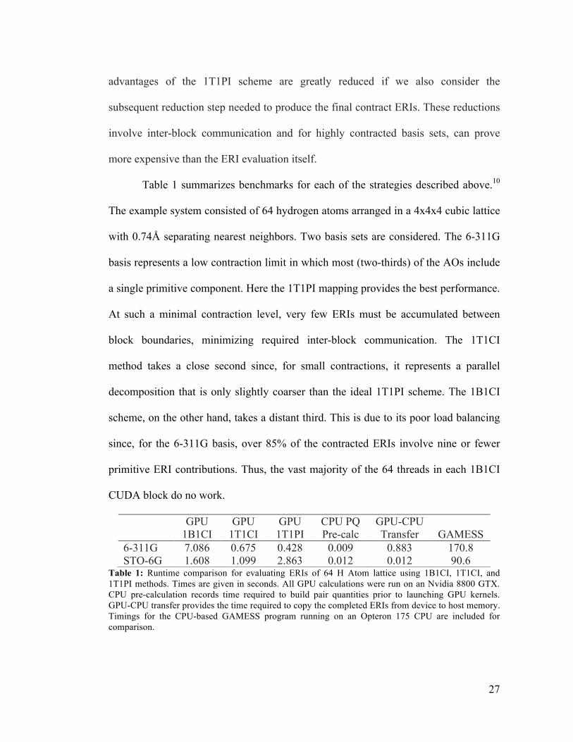
advantages of the 1T1PI scheme are greatly reduced if we also consider the

subsequent reduction step needed to produce the final contract ERIs. These reductions

involve inter-block communication and for highly contracted basis sets, can prove

more expensive than the ERI evaluation itself.

Table 1 summarizes benchmarks for each of the strategies described above.10

The example system consisted of 64 hydrogen atoms arranged in a 4x4x4 cubic lattice

with 0.74Å separating nearest neighbors. Two basis sets are considered. The 6-311G

basis represents a low contraction limit in which most (two-thirds) of the AOs include

a single primitive component. Here the 1T1PI mapping provides the best performance.

At such a minimal contraction level, very few ERIs must be accumulated between

block boundaries, minimizing required inter-block communication. The 1T1CI

method takes a close second since, for small contractions, it represents a parallel

decomposition that is only slightly coarser than the ideal 1T1PI scheme. The 1B1CI

scheme, on the other hand, takes a distant third. This is due to its poor load balancing

since, for the 6-311G basis, over 85% of the contracted ERIs involve nine or fewer

primitive ERI contributions. Thus, the vast majority of the 64 threads in each 1B1CI

CUDA block do no work.

GPU 1B1CI

GPU 1T1CI

GPU 1T1PI

CPU PQ Pre-calc

GPU-CPU Transfer GAMESS

6-311G 7.086 0.675 0.428 0.009 0.883 170.8 STO-6G 1.608 1.099 2.863 0.012 0.012 90.6

Table 1: Runtime comparison for evaluating ERIs of 64 H Atom lattice using 1B1CI, 1T1CI, and 1T1PI methods. Times are given in seconds. All GPU calculations were run on an Nvidia 8800 GTX. CPU pre-calculation records time required to build pair quantities prior to launching GPU kernels. GPU-CPU transfer provides the time required to copy the completed ERIs from device to host memory. Timings for the CPU-based GAMESS program running on an Opteron 175 CPU are included for comparison.

28

The STO-6G basis provides a sharp contrast. Here each contracted ERI

includes 64 or 1296 primitive ERI contributions. As a result for the 1T1PI scheme, the

reduction step becomes much more involved, in fact requiring more time than

primitive ERI evaluation itself. This illustrates that, for massively parallel

architectures, organizing communication is often just as important as minimizing

arithmetic instructions when optimizing performance. The 1T1CI scheme performs

similarly to the 6-311G case. The fact that all ERIs now involve uniform contraction

lengths provides a slight boost, since it requires only 60% more time to compute twice

as many primitive ERIs compared to the 6-311G basis. The 1B1CI method, improves

dramatically, as every thread of every block is now responsible for at least 20

primitive ERIs.

Finally, it should be noted that simply transferring ERIs between host and

device can take longer than the ERI evaluation itself, especially in the case of low

basis set contraction. This means that, for efficient GPU implementations, ERIs can be

re-evaluated from scratch faster than they can be fetched from host memory, and much

faster than they can be fetched from disk. This will prove an important consideration

in the next chapter.

Extension to Higher Angular Momentum

Some additional considerations are important for extension to basis functions

of higher angular momentum. For non-zero angular momentum functions, shells

contain multiple functions. As noted above, all integrals within an ERI shell depend on

the same auxiliary integrals, Rtuv0 , and Hermite contraction coefficients, xEt

mn . Thus, it

is advantageous to have each thread compute an entire shell of primitive integrals. For

29

example, a thread computing a primitive ERI of class [sp|sp] is responsible for a total

of nine integrals.

The performance of GPU kernels is quite sensitive to the register footprint of

each thread. As threads use more memory, the total number of concurrent threads

resident on each SM decreases. Fewer active threads, in turn, reduce the GPU’s ability

to hide execution latencies and lowers throughput performance. Because all threads in

a grid reserve the same register footprint, a single grid handling both low and, more

complex, high angular momentum integrals will apply the worst-case memory

requirements to all threads. To avoid this, separate kernels must be written for each

class of integral.

Specialized kernels also provide opportunities to further optimize each routine

and reduce memory usage, for example, by unrolling loops or eliminating

conditionals. This is particularly important for ERIs involving d- and higher angular

momentum functions, where loop overheads become non-trivial. For high angular

momentum integrals it is also possible to use symbolic algebra libraries to generate

unrolled kernels that are optimized for the GPU.20

Given a basis set of mixed angular momentum shells, we could naively extend

any of the decomposition strategies presented above as follows. First, build the pair

quantities as prescribed, without consideration for angular momentum class. Then

launch a series of ERI kernels, one for each momentum class, assigning a compute

unit (either block or thread depending on strategy being extended) to every ERI in the

grid. Work units assigned to ERIs that do not apply to the appropriate momentum

class could exit immediately. This strategy is illustrated for a hypothetical system

30

containing four s-shells and one p-shell in the left side of Figure 4. Each square

represents a shell quartet of ERIs, that is all ERIs resulting from combination of the

various angular momentum functions within each of the included AO shells. The

elements are colored by total angular momentum class, and a specialized kernel

evaluates elements of each color. Unfortunately, the number of integral classes

increases rapidly with the maximum angular momentum in the system. The inclusion

of d-shells would already result in the vast majority of the threads in each kernel

exiting without doing any work.

Figure 4: ERI grids colored by angular momentum class for a system containing four s-shells and one p-shell. Each square represents all ERIs for a shell quartet (a) Grid when bra and ket pairs are ordered by simple loops over shells. (b) ERI grid for same system with bra and ket pairs sorted by angular momentum, ss, then sp, then pp. Each integral class now handles a contiguous chunk of the total ERI grid.

A better approach is illustrated on the right side of Figure 4. Here we have

sorted the bra and ket pairs by the angular momenta of their constituents, ss then sp

and last pp. As a result, the ERIs of each class are localized in contiguous sub-grids,

and kernels can be dimensioned to exactly cover only the relevant integrals.

REFERENCES

(1) Challacombe, M.; Schwegler, E. J. Chem. Phys. 1997, 106, 5526.

(2) Burant, J. C.; Scuseria, G. E.; Frisch, M. J. J. Chem. Phys. 1996, 105, 8969.

11 12 13 14 15 22 23 24 25 33 34 35 44 45 55

1112

1314

1522

2324

2533

3435

4445

55

11 12 13 14 22 23 24 33 34 44 15 25 35 45 55

1112

1314

2223

2433

3444

1525

3545

55

|λσ)

(μν|

|λσ)

(μν|

(b)(a)

31

(3) Schwegler, E.; Challacombe, M. J. Chem. Phys. 1996, 105, 2726.

(4) Schwegler, E.; Challacombe, M.; HeadGordon, M. J. Chem. Phys. 1997, 106, 9708.

(5) Ochsenfeld, C.; White, C. A.; Head-Gordon, M. J. Chem. Phys. 1998, 109, 1663.

(6) Rudberg, E.; Rubensson, E. H. J Phys-Condens Mat 2011, 23.

(7) Rys, J.; Dupuis, M.; King, H. F. J. Comp. Chem. 1983, 4, 154.

(8) Yasuda, K. J. Comp. Chem. 2008, 29, 334.

(9) Asadchev, A.; Allada, V.; Felder, J.; Bode, B. M.; Gordon, M. S.; Windus, T. L. J. Chem. Theo. Comp. 2010, 6, 696.

(10) Ufimtsev, I. S.; Martinez, T. J. J. Chem. Theo. Comp. 2008, 4, 222.

(11) Mcmurchie, L. E.; Davidson, E. R. J. Comp. Phys. 1978, 26, 218.

(12) Parr, R. G.; Yang, W. Density-functional theory of atoms and molecules; Oxford University Press: Oxford, 1989.

(13) Szabo, A.; Ostlund, N. S. Modern Quantum Chemistry; McGraw Hill: New York, 1982.

(14) Helgaker, T.; Jørgensen, P.; Olsen, J. Molecular electronic-structure theory; Wiley: New York, 2000.

(15) Kohn, W.; Sham, L. J. Phys Rev 1965, 140, 1133.

(16) Boys, S. F. Proc. Roy. Soc. Lon. A 1950, 200, 542.

(17) Whitten, J. L. J. Chem. Phys. 1973, 58, 4496.

(18) NVIDIA In Design Guide; NVIDIA Corporation: docs.nvidia.com, 2013.

(19) Ufimtsev, I. S.; Martinez, T. J. Comp. Sci. Eng. 2008, 10, 26.

(20) Titov, A. V.; Ufimtsev, I. S.; Luehr, N.; Martinez, T. J. J. Chem. Theo. Comp. 2013, 9, 213.

32

33

CHAPTER TWO

INTEGRAL-DIRECT FOCK CONSTRUCTION

ON GRAPHICAL PROCESSING UNITS

Because ERIs remain constant from one SCF iteration to the next, it was once

common practice to pre-compute all numerically significant ERIs prior to the SCF. At

each iteration the two-electron Fock contributions of equation (2.1) would then be

generated from contracted ERIs, �µ!�"#( ) , stored, for example, on disk.

�Gµ! (P) = P"#

"#

N

$ 2 µ!�"#( )% µ"�!#( )&' () (2.1)

This procedure certainly minimized the floating-point operations involved in the

calculation. However, for systems containing thousands of basis functions, ERI

storage quickly becomes impractical. The integral-direct approach, pioneered by

Almlof,1 avoids the storage of ERIs by re-computing them on the fly with each

formation of the Fock matrix.

ERI evaluation represents a tremendous bottleneck in the integral-direct

approach. Thus, early implementations were careful to generate only symmetry-unique

ERIs, �µ!�"#( ) where µ !" , ! "# , and µ! " #$ . Here µ! and !" are compound

indices corresponding to the element numbers in an upper triangular matrix. Each ERI

was then combined with various density elements and scattered into multiple locations

in the Fock matrix. This reduces the number of ERIs that must be evaluated by a factor

of eight compared to a naïve implementation (based on the eightfold symmetry among

the ERIs).

34

Beyond alleviating storage capacity bottlenecks, the direct approach offers

performance advantages over conventional algorithms based on integral storage. As

observed above, ERIs can sometimes be re-calculated faster than they can be recalled

from storage (even when this storage is just across a fast PCIe bus). As advances in

instruction throughput continue to out pace those for communication bandwidths, this

balance will shift even further in favor of integral-direct algorithms. Another

advantage results from knowledge of the density matrix during Fock construction.1 By

augmenting the usual Schwarz bound with density matrix elements as follows,

�µ!�"#( )P"# $ µ!�µ!( )1/2

"#�"#( )1/2P"# (2.2)

the direct approach is able to eliminate many more integrals than is possible for pre-

computed ERIs since even quite large integrals are often multiplied by vanishing

density matrix elements.

Almlof and Ahmadi also suggested dividing the calculation of G into separate

Coulomb, J, and exchange, K, contributions, double calculating any ERIs that are

common to both.2

�Jµ! = µ!�"#( )P"#

"#

N

$ (2.3)

�Kµ! = µ"�!#( )P"#

"#

N

$ (2.4)

This division offers two primary advantages. First, for the Coulomb operator in

equation (2.3), the density elements, P!" , can be pre-contracted with the ket, !" ) .

This provides an important optimization as described later in this chapter. Second for

the exchange operator in equation (2.4) only a few non-negligible contributions need

35

to be computed. The density matrix in insulating systems with finite band gap decays

exponentially with distance.3,4 Because Gaussian basis functions are localized, the AO

density matrix remains sparse. As noted in the previous chapter, the bra, µ! , and ket,

!" , pairs are also sparse due to the locality of the Gaussian basis set. Thus, equation

(2.4) couples the bra and ket through a sparse density matrix, and few ERI

contributions survive screening in large systems. Separately calculating the exchange

term in equation (2.4) then adds few ERIs compared to the number of ERIs required

by equation (2.3) alone.

The considerations above apply perhaps even more forcefully on GPUs. As

already observed in the context of forming contracted ERIs, the GPU’s wide execution

units benefit from longer contractions of primitive ERIs. In the previous chapter, this

explained the improved performance of the 1B1CI approach for the hydrogen lattice

test case in moving from the 6-311G basis to the more highly contracted STO-6G.

Longer contractions parallelize more evenly across many cores. Expanded in terms of

primitive ERIs, the sums in Eqs. (2.3) and (2.4) include many more contributions than

any contracted ERI considered in chapter 1. Thus to simplify the parallel structure of

the Coulomb and exchange algorithms and improve GPU performance, the

construction of contracted ERIs, �µ!�"#( ) , is abandoned in the present chapter in

favor of direct construction of Coulomb and exchange matrix elements from primitive

Gaussian functions.

36

Even within the Coulomb and exchange operators, ERI symmetry must not be

taken for granted. For example, although each ERI, �µ!�"#( ) , makes multiple

contributions to the exchange matrix,

�

µ!�"#( )P!# $ Kµ" "#�µ!( )P#! $ K"µ

!µ�"#( )Pµ# $ K!" "#�!µ( )P#µ $ K"!

µ!�#"( )P!" $ Kµ# #"�µ!( )P"! $ K#µ

!µ�#"( )Pµ" $ K!# #"�!µ( )P"µ $ K#!

(2.4)

gathering disparate density matrix elements introduces irregular memory access

patterns and scattering outputs to the Fock matrix creates dependencies between

threads computing different ERIs. GPU performance is extremely sensitive to these

considerations, so that even the eight-fold reduction in work available from exploiting

the full symmetry among ERIs could be swamped by an even larger performance

slowdown resulting from fragmented memory accesses. It is helpful to start, as below,

from a naïve, but completely parallel algorithm, and then exploit ERI symmetry only

where it provides a practical benefit.

The remainder of the chapter describes the algorithm used to implement

integral-direct Coulomb and exchange operators in TeraChem. A final performance

evaluation will be delayed until the implementation of DFT exchange-correlation

terms have also been described in chapter 4.

GPU J-ENGINE

The strategies for handling ERIs developed in the previous chapter provide a

good starting point for the evaluation of the Coulomb operator in equation (2.3).5 As

37

in the previous chapter, we first consider ERIs involving only s-functions in which

each quartet of AO functions produces a single integral. This provides a clear context

in which to describe the overall structure of our approach. Later, details for evaluating

higher angular momentum functions will be provided. The first step is again to

enumerate AO pairs, !µ!" , for the bra and ket. For the moment we consider the full

lists of N2 function pairs and consider the integral matrix, I, constructed as the N2-by-

N2 product of the bra-pair column vector, µ! |( , with the ket-pair row vector, | !" ) .

Iµ! ,"# = µ! | "#( ) (2.5)

Inserting equation (2.5) into (2.3) casts the Coulomb operator as a matrix vector

product between the integral matrix and a vector of length N2 built by re-dimensioning

the usual N-by-N one-particle density matrix.

With this picture in mind, several plausible mappings to CUDA threads and

blocks suggest themselves. A simple strategy is to assign each thread to a single bra-

pair, µ! |( , and have it sweep over all kets, | !" ) , and density elements, P!" ,

accumulating the products, �µ!�"#( )P#" , to compute an independent Coulomb

element, Jµ! . This strategy is similar to the 1T1CI scheme of chapter 1 and maximizes

the independence of each thread but at the cost of rather coarse parallelism. In order to

saturate a massively parallel GPU (or ideally several GPUs) it is preferable to employ

multiple threads to compute each Jµ! . Thus a preferred approach uses 2D thread

blocks so that threads in each row stride across the integral matrix, each accumulating

a partial sum. This is shown in figure 1 for an illustrative block size of 2x2. In practice

38

a block size of 8x8 was shown to be near optimal across a range of empirical test

calculations. Once all integrals have been evaluated, a final reduction within each row

of the CUDA block produces final Jµ! elements. The reduction step adds negligibly to

the runtime regardless of primitive contraction length, because it is performed only

once per Coulomb element, rather than once per contracted ERI as in the 1B1CI case

described in the previous chapter.

Figure 1: Schematic representation of a J-Engine kernel for one angular momentum class, e.g., (ss|ss). Cyan squares represent significant ERI contributions. Sorted bra and ket vectors are represented by triangles to left and above grid. The path of a 2x2 block as it sweeps across the grid is shown in orange. The final reduction across rows of the block is illustrated within the inset to the right.

The above discussion ignored ERI symmetry for clarity. However, having

determined an efficient mapping of the Coulomb problem onto the GPU execution

units, it is important to consider what symmetries can be exploited without upsetting

the structure of the algorithm. We first note that Jµ! is symmetric. Thus it is sufficient

39

to compute its upper triangle and only the N(N+1)/2 bra pairs where µ !" need to be

considered. Similarly for ket pairs, the terms �µ!�"#( )P"# and �

µ!�"#( )P"# can be

computed together as �µ!�"#( ) P"# + P#"

1+$"#

, where the Kronecker delta is used to handle

the special case along the diagonal of the density matrix. Thus, using a slightly

transformed density, ERI symmetry again allows a reduction to ket pairs where ! "# .

If the AO shells are ordered by angular momentum, as suggested in the

previous chapter, then these symmetry reductions will also conveniently reduce the

number of specialized momentum-specific kernels that are needed. For example,

assuming a basis including s-, p-, and d-functions, the reduced pairs will include a

total of six momentum classes, ss, sp, sd, pp, pd, and dd, and require 36 specialized

Coulomb kernels, less than half of the 34 = 81 total momentum classes that might be

expected.

It is not possible to exploit the final class of ERI symmetry,

�µ!�"#( ) = "#�µ!( ) , without creating dependencies between rows of the ERI grid

and, as a result, performance sapping inter-block communication. Thus, ignoring the

screening of negligibly small integrals discussed below, the GPU J-Engine nominally

computes N4/4 integrals.

For clarity, the discussion of ERI symmetry has been carried out in terms of

contracted ERIs. However, building such contracted intermediates would require

many sums of irregular length that are difficult to parallelize efficiently across many

cores. Thus it is advantageous to construct the Coulomb operator directly from

40

primitive ERIs. Continuing with s-functions for the moment, the primitive Coulomb

matrix elements are calculated as follows.

�Jij = ci c j ij�kl!" #$ck cl P%k%l

kl& (2.6)

Here we define the AO index vector, !i , to select the contracted AO index to which

the ith primitive function belongs. (Since at present our discussion is limited to s-

functions, we ignore the structure of functions organized within shells). The

coefficients, c j , represent weights of primitive functions within AO contractions. The

final Coulomb elements are then computed in a second summation step as follows.

Jµ! = Jiji"µj"!

# (2.6)

The evaluation of equation (2.6) can be carried out as described above, except

that the bra and ket AO pairs, !µ!" , are now replaced by expanded sets of primitive

pairs, ! i! j | i "µ, j "# ,µ $#{ } . The bra prefactor from equation (1.44) is now

augmented with the contraction coefficients.

Nijbra = cicjNij (2.7)

In constructing the ket pairs, the prefactor is pre-multiplied by both the contraction

coefficients and the appropriate density matrix element.

Nklket = ckclNkl

P!k!l + P!l!k1+"!k!l

(2.8)

Along with these prefactors, the quantities !ij and !Pij from equation (1.25) and each

pair’s Schwarz contribution, Bijbra = ij | ij[ ]1/2 and Bkl

ket = kl | kl[ ]1/2 P!k!l for each bra and

41

ket pair, is transferred to the GPU. As illustrated in figure 1, a CUDA kernel then

processes the primitive ERI grid formed as the outer product of bra and ket pair arrays.

The resulting primitive Coulomb elements are returned to the host where the sum of

equation (2.6) is carried out to provide the final matrix elements.

As noted above, screening small ERIs can reduce the computational

complexity of Coulomb construction from O(N4) to O(N2). Screening is introduced in

three passes. During the initial enumeration of primitive pairs, a conservative bound is

used to remove all primitive pairs for which Bijbra < ! pair "10#15 Hartrees.a Next, when

building the bra and ket arrays, pairs are further filtered that satisfy equations (2.9) and

(2.10), respectively.

Bijbra ! " screen

maxklBklket (2.9)

Bklket ! " screen

maxijBijbra (2.10)

Here 10-12 is a typical value of ! screen .b Finally, prior to evaluating each ERI, the GPU

kernel evaluates the four-center density-weighted Schwarz bound, and the

computationally intensive ERI evaluation is skipped where the following holds.

�BijbraBkl

ket = ij�ij( )1/2 kl�kl( )1/2 P!" # $ screen (2.11)

a ! pair corresponds to the variable THREPRE in TeraChem. b ! screen corresponds to the variable THRECL in TeraChem.

42

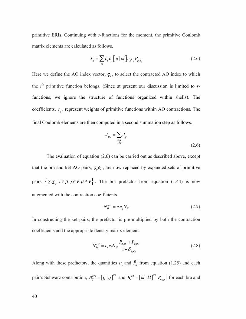
Figure 2: Organization of ERIs for Coulomb formation. Rows and columns correspond to primitive bra and ket pairs respectively. Each ERI is colored according to the magnitude of its Schwarz bound. Data is derived from calculation on ethane molecule. Left grid is obtained by arbitrary ordering of pairs within each angular momentum class and suffers from load imbalance because large and small integrals are computed in neighboring cells. Right grid sorts bra and ket primitives by Schwarz contribution within each momentum class, providing an efficient structure for parallel evaluation.

The left half of figure 2 shows a typical distribution of Schwarz bounds for

ERIs in the primitive Coulomb grid. Merely skipping small integrals still requires

evaluating the bound of every cell in this grid. Also, because large and small integrals

are interspersed throughout the grid, CUDA warps will suffer from divergence

between threads that are evaluating an ERI and threads that are not. A more efficient

approach to screening can be achieved by sorting the final lists of bra and ket pair

quantities in descending order by Bijbra and Bkl

ket , respectively. The resulting grid,

shown on the right in figure 2, eliminates warp divergence because the significant

integrals are condensed in a contiguous region for each momentum class of ERI.

Furthermore, the bounds are now guaranteed to decrease across each row, so each

block may safely exit when the first negligible ERI is located. This eliminates the

overhead of even checking the Schwarz bound for negligible quartets.

43

For clarity, the discussion above has considered only s-functions. For integrals

involving higher angular momentum functions, it is advantageous to compute all ERIs

belonging to a shell quartet simultaneously. In order to maintain fine-grained

parallelism, it would be desirable to distribute a shell quartet among threads in a block.

However, ERI evaluation involves extensive recurrence relations such as equation

(1.42) which cannot be efficiently parallelized between many SIMT processing cores.

Thus, it is preferable to assign an independent thread to compute all ERIs within a

shell quartet. The final algorithm follows the basic pattern described for s-functions,

except that instead of function pairs, the bra and ket vectors are now built from

primitive shell pairs, ! I! J .

The quantities NIJbra , !IJ , and

!PIJ are uniform for all functions within the shell

pair and are thus organized in pair data arrays as above. The Schwarz contributions,

Bijbra/ket , are not strictly uniform for d-type functions and above. However, to maintain

rotational invariance, the Schwarz bound is computed treating both primitives as

spherical s-functions, a quantity which is uniform across the shell pair. Because each

shell pair now spans several functions, the ket bound, Bklket , must use the maximum

density element over the shell block.

BKLket = KL |KL[ ]1/2 PKLmax (2.12)

PKLmax = max

!k"!K

!l"!L

P#k#l (2.12)

Additional pair data is required to compute ERIs of non-zero angular

momentum. Since the density elements differ for each function within the shell block

44

they can no longer be included in the ket prefactor, Nijket , as in equation (2.8). The

Hermite expansion coefficients, Etuvij , from equation (1.33) are also needed for every

function pair ij in the shell pair IJ.

An important simplification both in terms of the required pair data and

computational cost of the final integral is available by inserting equation (1.43) into

equation (2.3).2

Jµ! = Nijci c ji"µj"!

# Etuvij Nklck cl

$ij +$klkl# (%1) &t + &u + &v P'k'l

E &t &u &vkl Rt+ &t ,u+ &u ,v+ &v

0

&t &u &v#

tuv#

(2.12)

Because the quantities Nkl, ck cl, and !kl are uniform for all function pairs within the

shell pair, the above sum can be segmented by primitive shell pair, KL, as follows.

Jµ! = Nijci c ji"µj"!

# Etuvij N KLcKcL

$ij +$KLKL# D %t %u %v

KL Rt+ %t ,u+ %u ,v+ %v0

%t %u %v#

tuv#

(2.12)

D !t !u !vKL = ("1) !t + !u + !v P#k#l

E !t !u !vkl

k$Kl$L

% (2.12)

Rather than separately packing McMurchie-Davidson coefficients and density

elements for every primitive function pair, combined coefficients are generated

through equation (2.12) for each pair of ket shells.

Equation (2.12) is computed in two steps in TeraChem. First the pair data

described above is copied to the GPU where the following Hermite Coulomb

contributions are computed.

Jtuvij =

Nijci c j N KLcKcL

!ij +!KLKL" D #t #u #v

KL Rt+ #t ,u+ #u ,v+ #v0

#t #u #v"

(2.12)

45

In exact analogy to the algorithm described for s-functions above, each row of CUDA

threads is assigned a bra shell pair, !I! J

, and strides across the list of kets,

accumulating all associated Jtuvij

values in separate registers. After all significant

Coulomb contribions have been computed, reductions within the rows of each block

produce the sums of equation (2.12). The Hermite Coulomb contributions are then

copied back to host memory where, in analogy to equation (2.6) the bra expansion

coefficients are used to produce the final Coulomb elements as follows.

Jµ! = Etuvij Jtuv

ij

tuv"

i#µj#!

" (2.12)

GPU K-ENGINE

The GPU-based construction of the exchange operator in equation (2.4)

follows a similar approach to that employed in the GPU J-Engine algorithm.5 Here we

highlight adjustments that are required to accommodate the increased complexity of

exchange which results from the splitting of the output index, µ! , between the bra

and ket. As a result rows of the bra-by-ket ERI grid do not contribute to a single

matrix element but scatter across an entire row of the K matrix. Additionally,

symmetry among the ERIs is more difficult to exploit for exchange since symmetric

pairs, e.g., �µ!�"#( )$ µ!�#"( ) , now contribute to multiple matrix elements. The

split of the density index, !" , between bra and ket, also precludes the pre-contraction

of density elements into the pair quantities as was done for the ket pairs in the J-

Engine above.

46

Such complications could be naïvely removed by changing the definitions of

bra and ket to so called physicist notation, where pairs include a primitive from each

of two electrons.

�µ!�"#( ) = µ" !# (2.13)

With such µ! and !" pairs, a GPU algorithm analogous to the J-Engine could easily

be developed. Unfortunately, the new definitions of bra and ket also affect the

pairwise Schwarz bound, which now becomes the following.

�µ! µ!

1/2"# "#

1/2= µµ�!!( )1/2

""�##( )1/2 (2.14)

As the distance, R , between !µ and !" increases, the quantity �µµ�!!( ) decays

slowly, as 1/ R . This should be compared to a decay of e!R2

for �µ!�µ!( ) . This

weaker bound means that essentially all N4 ERIs would need to be examined leading

to a severe performance reduction compared to the N2 Coulomb algorithm. Thus, the

scaling advantages of the µ! /!" pairing are very much worth maintaining, even at

the cost of reduced hardware efficiency.

The K-Engine begins with the usual step of enumerating AO shell pairs, !µ!" .

Because the !µ!" and !"!µ pairs contribute to different matrix elements, we neglect

symmetry and construct AO pairs for both µ ! " and µ > ! pairs. As with Coulomb

evaluation, the pairs are separated by angular momentum class, and different kernels

are tuned for each type of integral. Inclusion of µ > ! pairs requires additional pair

and kernel classes compared to the J-Engine, since, for example, kernels handling ps

pairs are distinct from those handling sp pairs.

47

Simply sorting the bra and ket primitive pairs by Schwarz bound would leave

contributions to individual K elements scattered throughout the ERI grid. In order to

avoid inter-block communication, it is necessary to localize these exchange

contributions. This is accomplished by sorting the primitive bra and ket pairs by µ -

and ! -index, respectively. Then the ERIs contributing to each element, Kµ! , form a

contiguous tile in the ERI grid. This is illustrated in figure 3. Within each segment of

µ -pairs, primitive PQs are additionally sorted by Schwarz contributions, �µ!�µ!( )1/2

,

so that significant integrals are concentrated in the top left of each µ! -tile.

Since the density index is split between bra and ket, density information cannot

be included in the primitive expansion coefficients or Schwarz contributions. Instead

additional vectors are packed for each angular momentum class, Pss , Psp , etc. The

packed density is ordered by shell pair and organized into CUDA vector types to allow

for efficient fetching. For example, each entry in the Psp block contains three

elements, spx , spy , and spz , packed into a float4 (assuming single precision) vector

type. The maximum overall density element in a shell pair, P!"

max is also pre-

computed for each shell pair, in order to minimize memory access when computing

the exchange Schwarz bound.

�!µ!"�!# !$%& '(P"$ ) !µ!"�!µ!"

%& '(1/2

!# !$�!# !$%& '(1/2

P"$

max (2.15)

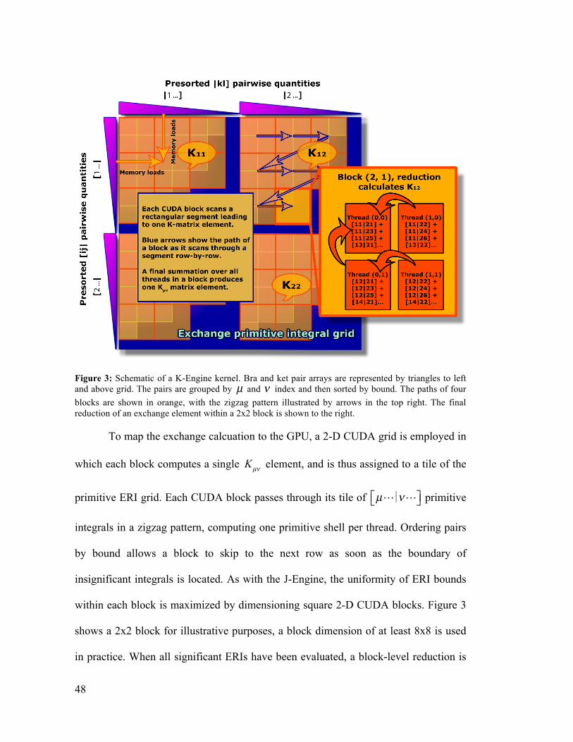
48

Figure 3: Schematic of a K-Engine kernel. Bra and ket pair arrays are represented by triangles to left and above grid. The pairs are grouped by µ and ! index and then sorted by bound. The paths of four blocks are shown in orange, with the zigzag pattern illustrated by arrows in the top right. The final reduction of an exchange element within a 2x2 block is shown to the right.

To map the exchange calcuation to the GPU, a 2-D CUDA grid is employed in

which each block computes a single Kµ! element, and is thus assigned to a tile of the

primitive ERI grid. Each CUDA block passes through its tile of � µ!�!!"# $% primitive

integrals in a zigzag pattern, computing one primitive shell per thread. Ordering pairs

by bound allows a block to skip to the next row as soon as the boundary of

insignificant integrals is located. As with the J-Engine, the uniformity of ERI bounds

within each block is maximized by dimensioning square 2-D CUDA blocks. Figure 3

shows a 2x2 block for illustrative purposes, a block dimension of at least 8x8 is used

in practice. When all significant ERIs have been evaluated, a block-level reduction is

49

used to compute the final exchange matrix element. As with the J-Engine above, this

final reduction represents the only inter-thread communication required by the K-

Engine algorithm and detracts negligibly from the overall performance. The K-Engine

approach is similar to the 1B1CI ERI scheme described in chapter 1. However,

because each block is responsible for thousands of primitive ERIs, exchange

evaluation does not suffer from the load imbalance observed for the 1B1CI algorithm.

The structure of the ERI grid allows neighboring threads to fetch contiguous

elements of bra and ket data. Access to the density matrix is more erratic, because it is

not possible to order pairs within each µ!-tile simultaneously by Schwarz bound and "

or # index. As a result, neighboring threads must issue independent density fetches

that are in principle scattered across the density matrix. In practice, once screening is

applied, most significant contributions to an element, Kµ!, arise from localized "#-

blocks, where " is near µ and # is near !. Thus, CUDA textures can be used to

ameliorate the performance penalty imposed by the GPU on non-sequential density

access.

Another difficulty related to the irregular access of density elements is that the

density weighted Schwarz bounds for primitive ERIs calculated through equation

(2.15) are not strictly decreasing across each row or down each column of a µ!-tile.

As a result, the boundary between significant and negligible ERIs is not as sharply

defined as in the Coulomb case. Yet, using the density to preempt integral evaluation

in exchange is critical. This can be appreciated by comparison with the Coulomb

operator in which the density couples only to the ket pair. Since in general both the

50

density element, P!" , and Schwarz bound, �!"�!"( )1/2

, decrease as the distance r!"

increases, density weighting the Coulomb Schwarz bound has the effect of making

already small �!"�!"( )1/2

terms even smaller. In exchange, on the other hand, the

density couples the bra and ket so that small density matrix elements can reduce

otherwise large bounds and greatly reduce the number of ERIs that need to be

evaluated. In fact, for large insulator systems, we expect the total number of non-

negligible ERIs to reduce from N2 Coulomb integrals to just N exchange ERIs.

In order to incorporate the density into the ERI termination condition, the usual

exit threshold, !screen ,a is augmented by an additional guard multiplier, G=~10-3.b Each

warp of 32 threads then terminates ERI evaluation across each row of the ERI-tile

when it reaches a contiguous set of primitive ERIs where the following holds for every

thread.

�!µ!"�!µ!"#$ %&

1/2!' !(�!' !(#$ %&

1/2P"(

max< G) (2.16)

In principle, this non-rigorous exit condition could neglect significant integrals in

worst-case scenarios. However, in practice, empirical tests demonstrate that the exit

procedure produces the same result obtained when density information is not

exploited.

For SCF calculations, the density and exchange matrices are symmetric. In this

case, we need only compute the upper triangle of matrix elements. This amounts to

exploiting �µ!�"#( )$ "#�µ!( ) ERI symmetry and means that we calculate N2/2

a ! screen corresponds to the variable THREEX in TeraChem. b G corresponds to the variable KGUARD in TeraChem.

51

ERIs (in the absence of screening). This is four times more ERIs than are generated by

traditional CPU codes that take full advantage of the eight-fold ERI symmetry.

However, comparisons by instruction count are too simplistic when analyzing the

performance of massively parallel architectures. In the present case, freeing the code

of inter-block dependencies boosts GPU performance more than enough to

compensate for a four-fold work increase.

Because the AO density matrix elements, Pµ! , in insulating systems rapidly

decays to zero with increasing distance, rµ! , it is possible to pre-screen entire

exchange elements, Kµ! , for which the sum in equation (2.4) will be negligibly small.

A rigorous bound on each exchange matrix element can be evaluated using the

Schwarz inequality as follows.6

�Kµ! = µ"�!#( )P"#

"#

N

$ % µ"�µ"( )1/2P"# !#�!#( )1/2

"#

N

$ (2.17)

Or casting the AO Schwarz bounds in matrix form, �Qµ! = µ!�µ!( )1/2

:

Kµ! " (QPQ)µ! (2.18)

Whenever !Rµ is far from

!R! , P!" will be zero for all !" near !µ and !" near !" . In

practice, it is possible to impose a simple distance cutoff so that Kµ! is approximated

as follows.

�

Kµ! =µ"�!#( )P"#

"#

N

$ if rµ! < RMASK

0 otherwise

%

&'

('

(2.19)

52

The mask condition is trivially pre-computed for each element, Kµ! , and packed in a

bit mask, 1 indicating that the exchange element should be evaluated and 0 indicating

that it should be skipped. Each block of CUDA threads checks its mask at the

beginning of the exchange kernel, and blocks that are assigned a zero bit exit

immediately. As will be shown for practical calculations in chapter 4, this simple

distance mask accelerates the K-Engine algorithm to scale essentially linearly with the

size of the system without introducing book keeping overhead7-10 that could easily

reduce the K-Engine’s overall efficiency.

REFERENCES

(1) Almlof, J.; Faegri, K.; Korsell, K. J. Comp. Chem. 1982, 3, 385.

(2) Ahmadi, G. R.; Almlof, J. Chem. Phys. Lett. 1995, 246, 364.

(3) Kohn, W. Phys Rev 1959, 115, 809.

(4) des Cloizeaux, J. Phys Rev 1964, 135, A685.

(5) Ufimtsev, I. S.; Martinez, T. J. J. Chem. Theo. Comp. 2009, 5, 1004.

(6) Kussmann, J.; Ochsenfeld, C. J. Chem. Phys. 2013, 138.

(7) Burant, J. C.; Scuseria, G. E.; Frisch, M. J. J. Chem. Phys. 1996, 105, 8969.

(8) Ochsenfeld, C.; White, C. A.; Head-Gordon, M. J. Chem. Phys. 1998, 109, 1663.

(9) Schwegler, E.; Challacombe, M. J. Chem. Phys. 1999, 111, 6223.

(10) Neese, F.; Wennmohs, F.; Hansen, A.; Becker, U. Chem. Phys. 2009, 356, 98.

! "#!

CHAPTER THREE

DYNAMIC PRECISION ERI EVALUATIONa

$%&'!()*+*,-../!01'*+,10!-'!2(,'341)!5*01(!+-41!6-)07-)1!6-51!'6(7,!

8)141,0(3'! 9(81,8*-.! :()! 4-,/! 8-';'! *,! 2(4938-8*(,-.! 2614*'8)/<! *,2.30*,+!

1.128)(,*2! '8)3283)1! 861()/<=>=?! !"# $%$&$'# 4(.123.-)! 0/,-4*2'<==! -,0! 149*)*2-.!

:()21>:*1.0! @-'10! 4(.123.-)! 0/,-4*2'AB<=C>=D! E61! 141)+1,21! (:! 861! F&GH!

0151.(941,8! :)-417();! :)(4! IJKGKH! 6-'! '*49.*:*10! 861! )193)9('*,+! (:! 86*'!

6-)07-)1! :()! '2*1,8*:*2! 2(4938*,+<="! 2(49-)10! 8(! 1-)./! 1::()8'! (,! '*4*.-)!

-)26*81283)1'!86-8!6-0!)1.*10!(,!1L9.*2*8./!)12-'8*,+!'2*1,8*:*2!-.+()*864'!*,!81)4'!

(:! .(7! .151.! +)-96*2'! *,'8)328*(,'AB<=M! I151)861.1''<! @12-3'1! $%&'! 6-51! @11,!

2-)1:3../! 01'*+,10! :()! 4-L*434! 91):()4-,21! *,! '912*:*2! +)-96*2'! 9)(21''*,+!

8-';'<! *8! *'! '8*..! *49()8-,8! 761,! -0-98*,+! '2*1,8*:*2! 2(01'! 8(! )3,! (,! $%&'! 8(!

)1'9128! '912*-.*N10! 6-)07-)1! 2(,'8)-*,8'! '326! -'!414()/! -221''! 9-881),'! -,0!

,(,>3,*:()4! 1::*2*1,2/! (:! :.(-8*,+! 9(*,8! -)*86418*2! *,! 0*::1)1,8! 9)12*'*(,A! K8! *'!

3,.*;1./!86-8!861'1!.*4*8-8*(,'!7*..!151)!@1!:3../!1.*4*,-810!'*,21!861/!9)(5*01!861!

:(3,0-8*(,! (:! 861! $%&'! 2(4938-8*(,-.! 9)(71''A! $%&! 6-)07-)1! 1L21.'! *,!

4-''*51./!9-)-..1.! :.(-8*,+>9(*,8! 2(4938-8*(,! *,!9-)8!@12-3'1! *8! *'! +((0!-8! .*88.1!

1.'1A!

E61! F(3.(4@! -,0! OL26-,+1! -.+()*864'! 0151.(910! *,! 26-981)! C! 6-51<! (:!

2(3)'1<!-.)1-0/!@11,!2-)1:3../!01'*+,10!8(!4-L*4*N1!:*,1>+)-*,10!9-)-..1.*'4!-,0!

!!!!!!!!!!!!!!!!!!!!!!!!!!!!!!!!!!!!!!!!!!!!!!!!!!!!!!!!-!H0-9810!7*86!91)4*''*(,!:)(4!IA!P316)<!KAQA!&:*48'15<!-,0!EARA!S-)8*,1N<!()#*+,-)#.+,')#*'-/0&A!!"##<!T<!UDU>U"DA!F(9/)*+68!VC??UW!H41)*2-,!F614*2-.!Q(2*18/A!

!"D!

)1+3.-)! 414()/! -221''! 9-881),'A! E61! 9)1'1,8! 26-981)! 1L81,0'! 86-8! 7();! 8(!

2(,'*01)!861!(98*4-.!3'1!(:!:.(-8*,+>9(*,8!9)12*'*(,!*,!861!F(3.(4@!-,0!OL26-,+1!

(91)-8()'A!

OXK!5-.31'!'9-,!-!7*01!0/,-4*2!)-,+1!:)(4!Y=?#!0(7,!8(!Y=?>=?!Z-)8)11'!

@1.(7!76*26!OXK'!2-,!@1!,1+.12810!76*.1!4-*,8-*,*,+!2614*2-.!-223)-2/A!Q*,+.1!

9)12*'*(,!2-,,(8!-223)-81./!-22343.-81!,34@1)'!-2)(''!86*'!7*01!0/,-4*2!)-,+1!

(:!86*)811,!012*4-.!()01)'A!E63'<!1-)./!'2*1,8*:*2!9)(+)-4'!)1.*10!(,!8)*2;'!'326!-'!

2(491,'-810! '344-8*(,! *,! ()01)! 8(! 4-*,8-*,! 9)12*'*(,! 03)*,+! .-)+1!

2-.23.-8*(,'A=T![*86!861!-051,8!(:!6-)07-)1>@-'10!0(3@.1!9)12*'*(,!*,'8)328*(,'!

:()! 2(44(0*8/! F%&'! *,! 861! =UB?'<! *8! @12-41! '8-,0-)0! 9)-28*21! 8(! 3'1! 0(3@.1!

9)12*'*(,! 3,*:()4./! :()! -..! :.(-8*,+>9(*,8! (91)-8*(,'! *,! \3-,834! 2614*'8)/!

2-.23.-8*(,'A! K,! :-28<! :()! 5-)*(3'! -)26*81283)-.! -,0! -.+()*864*2! )1-'(,'<! '*,+.1!

9)12*'*(,! -)*86418*2! (::1)10! (,./! -! '.*+68! 91):()4-,21! -05-,8-+1! (51)! 0(3@.1!

9)12*'*(,A!!

P*;1!1-)./!F%&'<! 861! :*)'8!F&GH>1,-@.10!$%&'!6-0!,(!'399()8! :()!0(3@.1!

9)12*'*(,! -)*86418*2<! 014-,0*,+! 2-)1! *,! 861*)! 3'1! :()! \3-,834! 2614*'8)/!

-99.*2-8*(,'A! F(,51,*1,8./! 861! .-81'8! $%&'! :3../! '399()8! 0(3@.1! 9)12*'*(,!

-)*86418*2!7*86!91):()4-,21!*,!861!)-,+1!(:!'151)-.!63,0)10!$]P^%Q<!'391)*()!8(!

86-8!(::1)10!@/!F%&'A!I151)861.1''<!151,!861!.-81'8!$%&'!2(,8*,31!8(!9)(5*01!39!

8(! #CL! 4()1! 91):()4-,21! 8(! '*,+.1! 9)12*'*(,! (91)-8*(,'A! E6*'! 0*'9-)*8/! '814'!

:)(4! 861!6-)07-)1_'!910*+)11! *,!+)-96*2'<!761)1! 861)1! *'! .*88.1!,110! :()!0(3@.1!

9)12*'*(,!-223)-2/!-,0!861!,121''-)/!*,2)1-'1!*,!2*)23*8)/!*'!0*::*23.8!8(!`3'8*:/A!^,!

-,/! 9)(21''()<! '*,+.1! 9)12*'*(,! 1L6*@*8'! :3)861)! 91):()4-,21! -05-,8-+1'! -'! -!

! ""!

)1'3.8! (:! *8'! '4-..1)! 414()/! :((89)*,8<! 76*26! )10321'! 0-8-! @-,07*086!

)1\3*)141,8'C!-,0!*,2)1-'1'!861!,34@1)!(:!5-.31'!86-8!2-,!@1!2-2610!*,!(,>26*9!

)1+*'81)'A! E63'<! :()! 4-L*434! 91):()4-,21! (,! $%&'<! *8! )14-*,'! *49()8-,8! 8(!

:-5()!'*,+.1!9)12*'*(,!-)*86418*2!-'!4326!-'!9(''*@.1A!

! E(!@-.-,21!$%&!91):()4-,21!7*86!2614*2-.!-223)-2/<!\3-,834!2614*'8)/!

*49.141,8-8*(,'! 6-51! -0(9810! 4*L10! 9)12*'*(,! -99)(-261'! *,! 76*26! 0(3@.1!

9)12*'*(,! (91)-8*(,'! -)1! -0010! '9-)*,+./! 8(! -,! (861)7*'1! '*,+.1! 9)12*'*(,!

2-.23.-8*(,A! S-8)*L! 43.8*9.*2-8*(,! *,! 861! 2(,81L8! (:! )1'(.38*(,>(:>861>*01,8*8/!

Sa..1)>%.1''18! 91)83)@-8*(,! 861()/! 6-'! @11,! '6(7,! 8(! 9)(5*01! -223)-81!4*L10!

9)12*'*(,!)1'3.8'<!151,!761,!861!4-`()*8/!(:!(91)-8*(,'!-)1!2-))*10!(38!*,!'*,+.1!

9)12*'*(,AD<M! Q*,+.1! 9)12*'*(,! OXK! 15-.3-8*(,! 6-'! @11,! '3221'':3../! -3+41,810!

7*86!0(3@.1!9)12*'*(,!-22343.-8*(,!*,8(!861!4-8)*L!1.141,8'!(:!861!F(3.(4@!-,0!

1L26-,+1! (91)-8()'A#<"! bG(3@.1! 9)12*'*(,! -22343.-8*(,c! '*49./! 41-,'! 86-8! 861!

OXK'!-)1!15-.3-810!*,!'*,+.1!9)12*'*(,!@38!-!0(3@.1!9)12*'*(,!5-)*-@.1! *'!3'10!8(!

-22343.-81!861!9)(0328'!(:!01,'*8/!4-8)*L!1.141,8'!-,0!OXK'!76*26!4-;1!39!861!

:*,-.!(91)-8()! V1A+A!F(3.(4@!()!1L26-,+1WA! ! ]()!1L-49.1<! 861!F(3.(4@!(91)-8()!

2-,!@1!2(,'8)32810!-'d!!

Jµ!64+ = P"#

32 µ! | "#( )32 (3.1)

761)1!861!'391)'2)*98'!*,0*2-81!861!,34@1)!(:!@*8'!(:!9)12*'*(,!3'10!8(!2(49381!

861!.-@1.10!81)4!-,0!861!OXK'!-)1!+*51,!-'d!

µ! | "#( ) = $µ (r1)$! (r1)$" (r2 )$# (r2 )r1 % r2

& dr1dr2 (3.2)

!"M!

F(4938*,+!-!:17!(:!861!.-)+1'8!OXK'!*,!:3..!0(3@.1!9)12*'*(,!6-'!-.'(!@11,!'6(7,"!

8(!*49)(51!-223)-2/!2(49-)10!8(!2-.23.-8*(,'!3'*,+!(,./!'*,+.1!9)12*'*(,!:()!-..!

OXK'A! K,2)141,8-.! 2(,'8)328*(,! (:! 861! ](2;! 4-8)*L=B! 2-,! -.'(! *49)(51! 861!

-223)-2/!(:! '*,+.1!9)12*'*(,!OXK!15-.3-8*(,A#!]*,-../<! *8!6-'!@11,!'3++1'810<! 86-8!

:3..! '*,+.1!9)12*'*(,!2-,!@1!'-:1./!149.(/10! *,! 861!1-).*1'8!QF]! *81)-8*(,'A"!Q326!

'8)-81+*1'!6-51!9)(51,!1::128*51! *,! *49)(5*,+!4*L10!9)12*'*(,! )1'3.8'! :()!4-,/!

2-.23.-8*(,'! )19()810! 8(!0-81A!Z(7151)<!,(! '/'814-8*2! '830/!(:!4*L10!9)12*'*(,!

OXK!15-.3-8*(,!6-'!@11,!3,01)8-;1,A!K,!:-28<!861!9)12*'*(,!238(::'!43'8!@1!26('1,!

2-)1:3../!:()!1-26!4(.123.-)!'/'814!'830*10!8(!+3-)-,811!86-8!861!-@'(.381!1))()!

*'!7*86*,!-!8(.1)-@.1!)-,+1A!

K,! 861! 9)1'1,8! 26-981)<! 71! *,8)(0321! -! '/'814-8*2! 4186(0! (:! @(86!

2(,8)(..*,+!1))()!-,0!4*,*4*N*,+!0(3@.1!9)12*'*(,!(91)-8*(,'!*,!4*L10!9)12*'*(,!

](2;!4-8)*L!2(,'8)328*(,A![1!@1+*,!@/!01'2)*@*,+!-!4*L10!9)12*'*(,!'26141<! *,!

76*26! -..! *,81+)-.'! -)1! 2(493810! (,! 861!$%&<!7*86! .-)+1!OXK'! 2-.23.-810! *,! :3..!

0(3@.1! 9)12*'*(,! -,0! '4-..! *,81+)-.'! *,! '*,+.1! 9)12*'*(,! 7*86! 0(3@.1! 9)12*'*(,!

-22343.-8*(,A! [1! '6(7! 86-8! 861! )1.-8*51! 1))()! *,! '326! 2-.23.-8*(,'! *'! 71..!

@16-510! :()! -,! -))-/! (:! '/'814'! -,0! 2-,! @1! 2(,8)(..10! 8(! 9)(5*01! -,! 1::128*51!

9)12*'*(,! -,0!91):()4-,21! *,81)410*-81!@18711,! 86-8! (:! '*,+.1! -,0! :3..! 0(3@.1!

9)12*'*(,A! K,!()01)! 8(! :3)861)!012)1-'1! 861!,34@1)!(:!0(3@.1!9)12*'*(,! *,81+)-.!

15-.3-8*(,'<!71!'3++1'8!-!,17!4186(0!86-8!71!81)4!12%!-$3#/4,3$5$'%! *,!76*26!

861! 1::128*51! 9)12*'*(,! *'! -0`3'810! 0/,-4*2-../! @18711,! QF]! *81)-8*(,'A! K,! 86*'!

7-/!861!4*,*434!,34@1)!(:!0(3@.1!9)12*'*(,!*,81+)-.'!2-,!@1!3'10!8(!(@8-*,!-,/!

! "T!

01'*)10!.151.!(:!-223)-2/A!]*,-../<!71!9)1'1,8!91):()4-,21!-,0!-223)-2/!)1'3.8'!8(!

@1,264-);!861!0/,-4*2!9)12*'*(,!-99)(-26!-'!*49.141,810!*,!E1)-F614A=U!!

MIXED PRECISION IMPLEMENTATION

E61! 4-+,*8301! (:! -,! OXK! *'! 2(44(,./! @(3,010! 3'*,+! 861! Q267-)N!

*,1\3-.*8/AC?! K,! 0*)128! QF]! 2(01'<=B! 861! @(3,0! 2-,! @1! :3)861)! )103210! 3'*,+!

1.141,8'!(:!861!01,'*8/!4-8)*L!-'d!

µ! | "#( )P"# $ µ! | µ!( )1/2 "# | "#( )1/2 P"# (3.3)

e12-3'1! (,./! -@'(.381! -223)-2/! *'! )1\3*)10! *,! 2614*2-.! -99.*2-8*(,'<! f-'30-!

*,8)(03210!-! 238(::! (,! 861!01,'*8/>71*+6810!Q267-)N!@(3,0! 8(!+)(39!OXK'! *,8(!

87(!@-8261'A"!E6('1!76('1!@(3,0!:1..!@1.(7!861!238(::!71)1!2-.23.-810!*,!'*,+.1!

9)12*'*(,! (,! 861! $%&A! K,81+)-.'! 76('1! @(3,0! 7-'! .-)+1)! 86-,! 861! 238(::! 71)1!

15-.3-810!*,!0(3@.1!9)12*'*(,!(,!861!F%&A!

Jµ!64+ =

P"#32 µ! | "#( )32 if P"# µ! | µ!( ) "# | "#( ) $ % prec

P"#64 µ! | "#( )64 if P"# µ! | µ!( ) "# | "#( ) > % prec

&'(

)(

(3.4)

H'! 6-'! @11,! 9)15*(3'./! ,(810<=! 7*86! 861! -051,8! (:! )(@3'8! 0(3@.1! 9)12*'*(,!

'399()8!(,!861!$%&!*8! *'!,(!.(,+1)!,121''-)/!8(!15-.3-81!'(41!OXK'!(,!861!F%&A!

[1!6-51!*49.141,810!-!4*L10!9)12*'*(,!](2;!4-8)*L!15-.3-8*(,!'26141!'*4*.-)!

8(! 86-8! '3++1'810!@/!f-'30-A! K,'81-0! (:! 3'*,+! 861!F%&<! 6(7151)<!71!0151.(910!

0(3@.1!9)12*'*(,!-,-.(+31'!(:!(3)!9)15*(3'./!)19()810!'*,+.1!9)12*'*(,!F(3.(4@!

-,0! 1L26-,+1! )(38*,1'A#! K49.141,8-8*(,! 018-*.'! -)1! 01'2)*@10! *,! 861! 9)15*(3'!

26-981)A!

!"B!

K,! ()01)! 8(!4-;1! 861!4('8! (:! 861!$%&_'!414()/! @-,07*086<! 861! 0(3@.1!

-,0!'*,+.1!9)12*'*(,!*,81+)-.'!-)1!6-,0.10!*,!-!87(>9-''!-.+()*864A!H'!9)15*(3'./!

01'2)*@10<! (3)! OXK! -.+()*864! (91)-81'! 0*)128./! (,! 861! @)-! -,0! ;18! 9)*4*8*51!

$-3''*-,!9-*)'<!76*26!-)1!'()810!@/!012)1-'*,+!Q267-)N!@(3,0A!K,!861!:*)'8!9-''<!

0-8-!:()!861!.-)+1'8!9)*4*8*51!9-*)'!*'!9-2;10!*,8(!0(3@.1!9)12*'*(,!-))-/'!-,0!-,/!

OXK! 76('1! @(3,0! *'! +)1-81)! 86-,! 861! 9)12*'*(,! 86)1'6(.0! *'! 2-.23.-810! 3'*,+!

0(3@.1! 9)12*'*(,! $%&! ;1),1.'A! K,! 861! '12(,0! 9-''<! '4-..1)! 9)*4*8*51! 9-*)'! -)1!

-0010!8(!861!@)-!-,0!;18!0-8-<!76*26!*'!)1-''14@.10!*,8(!'*,+.1!9)12*'*(,!-))-/'!

-,0!9)(21''10!@/!'*,+.1!9)12*'*(,!;1),1.'A!

e12-3'1! 861! :(3)>*,01L<! 01,'*8/>71*+6810! Q267-)N! @(3,0! *'! 2(493810!

(,./!7*86*,!861!$%&!;1),1.'<!'(41!039.*2-8*(,!(223)'!@18711,!861!'18'!(:!'*,+.1!

-,0!0(3@.1!9)12*'*(,!9)*4*8*51!9-*)'<!-,0!1-26!;1),1.!43'8! :*.81)!(38! *,0*5*03-.!

OXK'!76('1! @(3,0! :-..'! (38'*01! (:! 861! )1.15-,8! )-,+1A! Q*,21! -'! @1:()1! 861! 9-*)!

\3-,8*8*1'! -)1! ()01)10! @/! Q267-)N! @(3,0<! 861! '*,+.1! -,0! 0(3@.1! 9)12*'*(,!

*,81+)-.'!)1'*01!*,!2(,8*+3(3'!@.(2;'!-'!'6(7,!*,!:*+3)1!=A!E6*'!4*,*4*N1'!7-)9!

0*51)+1,21!(,!861!$%&<!'*,21!,1*+6@()*,+!86)1-0'!7*..!*,!+1,1)-.!';*9!()!2(49381!

*,81+)-.'! 8(+1861)A![61,!:*.81)*,+<! *8! *'!1''1,8*-.! 86-8!@(86!861!'*,+.1!-,0!0(3@.1!

9)12*'*(,! ;1),1.'! 6-,0.1! 861! @(3,0'! *01,8*2-../A! ^861)7*'1<! 861! 0*::1)1,8!

)(3,0*,+!@16-5*()!1L6*@*810!@/!'*,+.1!-,0!0(3@.1!9)12*'*(,!-)*86418*2!7*..!2-3'1!

*,81+)-.'! 2.('1! 8(! 861! @(3,0! 8(! @1! ';*9910! ()! 0(3@.1! 2(3,810A! K,! (3)!

*49.141,8-8*(,<!861!0(3@.1!9)12*'*(,!;1),1.'!2-'8!861!@(3,0!\3-,8*8*1'!8(!'*,+.1!

9)12*'*(,! @1:()1! 0181)4*,*,+! 761861)! 861! -''(2*-810! *,81+)-.'! -,0! 861*)!

2(,8)*@38*(,'!7*..!@1!15-.3-810A!

! "U!

Figure 1: Organization of double and single precision workloads within Coulomb ERI grids. Rows and columns correspond to primitive bra and ket pairs. On left each ERI is colored according to the magnitude of its Schwarz bound. On right ERIs are colored by required precision. Yellow ERIs require double precision while those in green may be evaluated in single precision. Blue ERIs are neglected entirely.

MIXED PRECISION ACCURACY

E61!4(.123.1'!'6(7,!*,!:*+3)1!C!71)1!26('1,!-'!)19)1'1,8-8*51!81'8!2-'1'!

8(! '830/! 861!-223)-2*1'!(:! '151)-.!4*L10!9)12*'*(,! 86)1'6(.0'A!$1(418)*1'!71)1!

9)19-)10! -8! @(86! -,!(98*4*N10!XZ]gM>#=$!4*,*434!-,0!-!0*'8()810! +1(418)/!

(@8-*,10! @/! 91):()4*,+! IJE! 0/,-4*2'! -8! YC???hA! E61! 0(3@.1! 9)12*'*(,! $%&!

*49.141,8-8*(,! 7-'! :*)'8! @1,264-);10! -+-*,'8! $HSOQQC=! 3'*,+! 861! 01:-3.8!

$HSOQQ!2(,51)+1,21!-,0! 87(>1.128)(,! 86)1'6(.0'A!E61! )1'3.8*,+! :*,-.! 1,1)+*1'<!

'6(7,! *,! 8-@.1! =<! *,0*2-81! +((0! -+)1141,8A! Q7*826*,+! 8(! '*,+.1! 9)12*'*(,! OXK'!

01+)-01'! 861! )1'3.8! @/! #>"! ()01)'! (:! 4-+,*8301A! Z(7151)<! *8! '6(3.0! @1!

1496-'*N10!86-8!:()!4(.123.1'!2(,8-*,*,+!-'!4-,/!-'!(,1!63,0)10!-8(4'<!'*,+.1!

9)12*'*(,!9)(5*01'!-01\3-81!)1'3.8'!i!861!-@'(.381!1))()!(:!861!1,1)+/!2(493810!

7*86!'*,+.1!9)12*'*(,!OXK'! *'!71..!@1.(7!=!;2-.g4(.!151,! :()!I13)(;*,*,!H!7*86!

="T!-8(4'A!!

!M?!

Figure 2: Molecular geometries used to benchmark the correlation between precision cutoff and the effective precision of the final energy. Optimized geometries (shown here) were used in addition to distorted nonequilibrium geometries prepared by carrying out RHF/STO-3G NVT dynamics at 2000 K (1000 K for Ascorbic Acid).

! H'2()@*2!H2*0! P-28('1! F/-,(@-281)*-.!E(L*,!$HSOQQ! >MB?A"BCBUDT! >=CBUAMMMMC"?! >CDU=AC?"BBU#!E1)-F614!G%! >MB?A"BCBUDT! >=CBUAMMMMC"?! >CDU=AC?"BBU?!E1)-F614!Q%! >MB?A"BCB?T=! >=CBUAMMMDCMM! >CDU=AC?"#MM?!! ! ! !! I13)(;*,*,!H! "LM!I-,(83@1! !$HSOQQ! >D?BUAMBB#TT?! >=#TU?A=D="=T=! !E1)-F614!G%! >D?BUAMBB#TMC! >=#TU?A=D="=TM! !E1)-F614!Q%! >D?BUAMBTUBCD! >=#TU?A=#BUUBT! !Table 1: RHF/6-31G final energies in Hartrees compared between GAMESS (set at default convergence and two-electron thresholds), our GPU accelerated TeraChem code performing all calculations in double precision (TeraChem DP), and TeraChem using single precision for ERIs with double precision accumulation into the Fock matrix elements (TeraChem SP). Distorted nonequilibrium geometries from RHF/STO-3G NVT dynamics at 2000K (1000K for Ascorbic Acid) were used.

I1L8!71!15-.3-810!861!4*L10!9)12*'*(,!-99)(-26!@/!5-)/*,+!861!9)12*'*(,!

86)1'6(.0! @18711,! =?>U! Z-)8)11'! V,1-)./! -..! *,81+)-.'! -)1! 15-.3-810! *,! 0(3@.1!

9)12*'*(,W! -,0! =A?! Z-)8)11'! V1''1,8*-../! -..! *,81+)-.'! 3'1! '*,+.1! 9)12*'*(,WA!

I1+.*+*@./!'4-..!OXK'!71)1!'2)11,10!-22()0*,+!8(!861!01,'*8/!71*+6810!Q267-)N!

3991)!@(3,0!(:!1\3-8*(,!V#A#W!3'*,+!-!2(,'1)5-8*51!86)1'6(.0!8(!1,'3)1!86-8!-,/!

! M=!

0*::1)1,21'! *,! 861! :*,-.! 1,1)+/! -@(51! Y=?>T! Z-)8)11'! 7(3.0! @1! 0(4*,-810! @/!

4*L10! 9)12*'*(,! 1))()'A! E61! -51)-+1! )1.-8*51! 1,1)+/! 0*::1)1,21! @18711,! :3..!

0(3@.1! -,0!4*L10!9)12*'*(,! QF]! 1,1)+*1'! :()! 861! 81,! 81'8! +1(418)*1'!01'2)*@10!

-@(51! *'! 9.(8810! -'! -! :3,28*(,! (:! 9)12*'*(,! 86)1'6(.0! *,! :*+3)1! #A! H.86(3+6! 861!

-@'(.381! 1))()! *,2)1-'1'! -.(,+! 7*86! 861! 8(8-.! 1,1)+/! (:! 861! '/'814'<! 861!

)1.-8*(,'6*9!@18711,!861!9)12*'*(,!238(::!-,0!)1.-8*51!1))()!*'!)(3+6./!.*,1-)!-,0!

*'! *,0191,01,8! (:! '/'814! '*N1! -,0! @-'*'! '18A! E63'<! 1-26! 86)1'6(.0! 2-,! @1!

-''(2*-810!7*86!-,!1::128*51!)1.-8*51!1))()!*,!861!1,1)+/A!

!

Figure 3. Average relative precision error in final RHF energies versus the precision threshold. Both minimized and distorted non-equilibrium geometries for the molecules in figure 2 are included in averages. Error bars represent two standard deviations above the mean. The black line represents the empirical error bound given of equation (3.5).

&'*,+!:*+3)1!#!*8!*'!9(''*@.1!8(!149*)*2-../!9)1>'1.128!-!9)12*'*(,!86)1'6(.0!

2())1'9(,0*,+!8(!-,/!-223)-2/!)1\3*)141,8!3'*,+!(,./!861!1'8*4-810!8(8-.!1,1)+/!

V8(! 2-.23.-81! )1.-8*51! 1))()WA! H! )1-'(,-@./! 2(,'1)5-8*51! 149*)*2-.! @(3,0! (,! 861!

9)12*'*(,! 1))()! *'! +*51,! *,! 861! :(..(7*,+! :()43.-! -,0! 9.(8810! :()! )1:1)1,21! *,!

:*+3)1!#A!

!MC!

Err Thre( ) = 2.0 !10"6Thre0.7 (3.5)

e/!*,51)8*,+!1\3-8*(,!V#A"W<!71!2(3.0!'1.128!-,!-99)(9)*-81!9)12*'*(,!86)1'6(.0!-8!

861! '8-)8! (:! 861! QF]! 9)(2103)1! -,0! 3'1! 861! 4*,*434! -..(7-@.1! 1::128*51!

9)12*'*(,A!Z(7151)<! 86*'!7(3.0! )1\3*)1! 1-)./! *81)-8*(,'!76('1!01,'*8/!4-8)*21'!

-)1!6*+6./!-99)(L*4-81!8(!3'1!861!:3..! .151.!(:!9)12*'*(,!,11010!-8!2(,51)+1,21A!

E6*'! *'! 1'912*-../!7-'81:3.! *,! 51)/! .-)+1! '/'814'! '*,21! 861!-223)-2/! )1\3*)10!-8!

2(,51)+1,21! ,1-)'! 86-8! (:! :3..! 0(3@.1! 9)12*'*(,A! E(! :3)861)! )10321! 861! 3'1! (:!

0(3@.1!9)12*'*(,!*,!1-)./!*81)-8*(,'!76*.1!'8*..!-26*15*,+!861!)1\3*)10!-223)-2/!-8!

2(,51)+1,21<!71!*,8)(0321!-!0/,-4*2!9)12*'*(,!-99)(-26<!01'2)*@10!@1.(7A!

DYNAMIC PRECISION IMPLEMENTATION

E61!1''1,21!(:!861!0/,-4*2!9)12*'*(,!-99)(-26!*'!8(!3'1!1\3-8*(,!V#A"W!8(!

'1.128! -! 0*::1)1,8! 86)1'6(.0! :()! 1-26! *81)-8*(,! (:! 861! QF]! 9)(2103)1A! O-)./!

*81)-8*(,'!6-51!@11,!'6(7,!8(!8(.1)-81!)1.-8*51./!.-)+1!1))()'!*,!861!](2;!4-8)*L!

7*86(38! 6-491)*,+! 2(,51)+1,21A#<CC![1! 8-;1! 861!4-L*434!1.141,8! (:! 861!GKKQ!

1))()! 5128()C#! :)(4! 861! 9)15*(3'! *81)-8*(,! -'! -!418)*2! (:! 86*'! 8(.1)-,21<! -,0! -8!

1-26! *81)-8*(,! 71! '1.128! -! 86)1'6(.0! 9)(5*0*,+! 9)12*'*(,! '-:1./! @1.(7! 861! GKKQ!

1))()A! E6*'! 1,'3)1'! 86-8! 861! 9)12*'*(,! 1))()! *'! -! '4-..! 2(,8)*@38()! 8(! 861! 8(8-.!

1))()A!e/!)1032*,+!861!9)12*'*(,!86)1'6(.0!+)-03-../!-'!2(,51)+1,21!9)(+)1''1'<!

*8! *'! 9(''*@.1! 8(! -99)(-26! :3..! 0(3@.1! 9)12*'*(,! )1'3.8'! 76*.1! 4*,*4*N*,+! 861!

,34@1)!(:!-283-.!0(3@.1!9)12*'*(,!(91)-8*(,'A!

E(!*49)(51!91):()4-,21<!(3)!QF]!2(01!3'1'!-,!*81)-8*51!390-81!-99)(-26!

V-.'(!;,(7,!-'!*,2)141,8-.!](2;!4-8)*L!:()4-8*(,W!8(!@3*.0!39!861!](2;!4-8)*L!

! M#!

(51)! 861! 2(3)'1! (:! 861! QF]! 9)(2103)1A=B! E61! 390-81! -99)(-26! 012(49('1'! 861!

](2;!4-8)*L!-'!!

Fi+1 Pi+1( ) = Fi Pi( ) + F Pi+1 ! Pi( ) , (3.6)

'(!86-8!(,./!861!.-'8!81)4!,110'!8(!@1!2-.23.-810!*,!1-26!QF]!*81)-8*(,A!Z1)1!Pi !-,0!

Fi Pi( ) !-)1! 861! 01,'*8/! -,0! ](2;! 4-8)*21'! -8! 861! $>86! QF]! *81)-8*(,A! e12-3'1!

26-,+1'!*,!861!01,'*8/!4-8)*L!@12(41!51)/!'4-..!,1-)!2(,51)+1,21<!861!*81)-8*51!

](2;! -99)(-26! -..(7'! 4-,/! -00*8*(,-.! *,81+)-.'! 8(! @1! '2)11,10A! E/9*2-../! 86*'!

9)(5*01'! -,! (51)-..! '911039! @18711,! CL! -,0! #L! (51)! 861! 2(,51,8*(,-.! QF]!

-99)(-26A! Z(7151)<! 861! ,-j51! *49.141,8-8*(,! (:! 0/,-4*2! 9)12*'*(,! 01'2)*@10!

-@(51! 2-3'1'! 861! *81)-8*51! ](2;! 4186(0! 8(! 2(,51)+1! *,2())128./<! @12-3'1! 1-26!

390-81!(:!861!](2;!4-8)*L!2-,!,(8!2())128!:()!861!9)12*'*(,!1))()!(:!861!9)15*(3'!

'819A!

X-861)! 86-,! -@-,0(,*,+! 861! *81)-8*51! ](2;! -.+()*864! -.8(+1861)<! 71!

*,8)(0321!861!:(..(7*,+!-0`3'841,8A![61,!861!)1.-8*51!GKKQ!1))()!0)(9'!@1.(7!861!

1))()! @(3,0! (:! 861! 23))1,8! 9)12*'*(,! 86)1'6(.0<! 861! 86)1'6(.0! *'! )103210! 8(!

9)(5*01!1,(3+6!-223)-2/! :()! '151)-.! ()01)'!(:!4-+,*8301! )10328*(,! *,! 861!GKKQ!

1))()A!O-26!8*41!861!9)12*'*(,!*'!*49)(510<!861!](2;!4-8)*L!*'!)12-.23.-810!:)(4!

'2)-826A!e18711,! 86)1'6(.0! )10328*(,'<! 861! :-'81)! *81)-8*51!](2;!390-81! '26141!

2-,!@1!'-:1./!149.(/10A!

RESULTS

E(! @1,264-);! (3)! 0/,-4*2! 9)12*'*(,! -99)(-26<! 71! 91):()410! XZ]!

1,1)+/! 2-.23.-8*(,'! (,! 861! 81'8! +1(418)*1'! 9)1'1,810! -@(51<! -'! 71..! -'! '(41!

!MD!

.-)+1)!'/'814'!'6(7,!*,!:*+3)1!DA!E-@.1!C!014(,'8)-81'!861!-223)-2/!9)(5*010!@/!

(3)! 0/,-4*2! 9)12*'*(,! -99)(-26A! K,! 1-26! 2-.23.-8*(,<! 861! 0/,-4*2! 9)12*'*(,!

4186(0!*'!'3221'':3.!*,!)19)(032*,+!861!:3..!0(3@.1!9)12*'*(,!)1'3.8'!8(!7*86*,!861!

2(,51)+1,21! 2)*81)*-A! ]3)861)4()1<! 861! ,34@1)! (:! QF]! *81)-8*(,'! )1\3*)10! 8(!

)1-26! 2(,51)+1,21! V-.'(! '6(7,! *,! 8-@.1! CW! *'! 1''1,8*-../! *01,8*2-.! @18711,!

0/,-4*2! -,0! 0(3@.1! 9)12*'*(,A! ]*,-../<! 861! QF]! 1,1)+/! 0*::1)1,21! @18711,!

0/,-4*2! -,0! 0(3@.1! 9)12*'*(,! )14-*,'! :-*)./! 2(,'8-,8! (51)! 861! )-,+1! (:! 81'8!

'/'814'<!*,0*2-8*,+!86-8!(3)!149*)*2-.!1))()!@(3,0!*'!)1-'(,-@./!2-.*@)-810A!

Double Precision Dynamic Precision Precision Error

Conv Thres Final Energy Iter Final Energy Iter

Ascorbic Acid (Minimum)

-680.6986413210 16 -680.6986413153 16 5.70E-09 10-7

-680.6986413213 12 -680.6986413898 12 6.85E-08 10-5

Ascorbic Acid (1000K)

-680.5828947151 17 -680.5828947066 17 8.50E-09 10-7

-680.5828947060 12 -680.5828947665 12 6.05E-08 10-5

Lactose (Minimum)

-1290.0883460632 14 -1290.0883460414 14 2.18E-08 10-7

-1290.0883460086 10 -1290.0883459660 10 4.26E-08 10-5

Lactose (2000K)

-1289.6666249592 15 -1289.6666249614 15 2.20E-09 10-7

-1289.6666249365 11 -1289.6666248603 11 7.62E-08 10-5

Cyano Toxin (Minimum)

-2492.3971992758 19 -2492.3971992873 19 1.15E-08 10-7

-2492.3971992730 13 -2492.3971985116 13 7.61E-07 10-5

Cyano Toxin (2000K)

-2491.2058890235 21 -2491.2058890017 21 2.18E-08 10-7

-2491.2058889916 13 -2491.2058886707 13 3.21E-07 10-5

Neurokinin A (Minimum)

-4091.3672645555 19 -4091.3672645944 20 3.89E-08 10-7

-4091.3672645489 14 -4091.3672644494 14 9.95E-08 10-5

Neurokinin A (2000K)

-4089.6883762179 21 -4089.6883761946 21 2.33E-08 10-7

-4089.6883760772 15 -4089.6883758130 15 2.64E-07 10-5

Nanotube (Minimum)

-13793.7293925221 24 -13793.7293925323 23 1.02E-08 10-7

-13793.7293924922 15 -13793.7293928287 15 3.37E-07 10-5

Nanotube (2000K)

-13790.1415175662 29 -13790.1415175584 27 7.80E-09 10-7

-13790.1415175332 18 -13790.1415191026 18 1.57E-06 10-5

Crambin

-17996.6562925538 18 -17996.6562926036 18 4.98E-08 10-7

-17996.6562925535 12 -17996.6562927894 12 2.36E-07 10-5

Ubiquitin

-29616.4426376594 24 -29616.4426376596 24 2.00E-10 10-7

-29616.4426376302 18 -29616.4426376655 18 3.53E-08 10-5

T-Cadherin EC1

-36975.6726049407 21 -36975.6726049394 21 1.30E-09 10-7

-36975.6726049265 16 -36975.6726048777 16 4.88E-08 10-5

Ribonuclease A

-50813.1471248227 19 -50813.1471248179 19 4.80E-09 10-7

-50813.1471247051 12 -50813.1471250247 12 3.20E-07 10-5

Table 2. Comparison of double and dynamic precision final RHF/6-31G energies (listed in Hartree). Precision error is taken as the absolute difference between double and dynamic precision energies. The number of SCF iterations required to reach convergence is listed (Iter) as well as the threshold used to converge the maximum element of the DIIS error matrix.

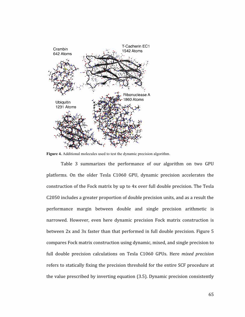
! M"!

!

Figure 4. Additional molecules used to test the dynamic precision algorithm.

E-@.1! #! '344-)*N1'! 861! 91):()4-,21! (:! (3)! -.+()*864! (,! 87(! $%&!

9.-8:()4'A! ^,! 861! (.01)! E1'.-! F=?M?! $%&<! 0/,-4*2! 9)12*'*(,! -221.1)-81'! 861!

2(,'8)328*(,!(:!861!](2;!4-8)*L!@/!39!8(!DL!(51)!:3..!0(3@.1!9)12*'*(,A!E61!E1'.-!

FC?"?!*,2.301'!-!+)1-81)!9)(9()8*(,!(:!0(3@.1!9)12*'*(,!3,*8'<!-,0!-'!-!)1'3.8!861!

91):()4-,21! 4-)+*,! @18711,! 0(3@.1! -,0! '*,+.1! 9)12*'*(,! -)*86418*2! *'!

,-))(710A! Z(7151)<! 151,! 61)1! 0/,-4*2! 9)12*'*(,! ](2;! 4-8)*L! 2(,'8)328*(,! *'!

@18711,!CL!-,0!#L!:-'81)!86-,!86-8!91):()410!*,!:3..!0(3@.1!9)12*'*(,A!]*+3)1!"!

2(49-)1'!](2;!4-8)*L!2(,'8)328*(,!3'*,+!0/,-4*2<!4*L10<!-,0!'*,+.1!9)12*'*(,!8(!

:3..! 0(3@.1! 9)12*'*(,! 2-.23.-8*(,'! (,! E1'.-! F=?M?! $%&'A! Z1)1!-$6,1# /4,3$5$'%!

)1:1)'!8(!'8-8*2-../!:*L*,+!861!9)12*'*(,!86)1'6(.0!:()!861!1,8*)1!QF]!9)(2103)1!-8!

861!5-.31!9)1'2)*@10!@/!*,51)8*,+!1\3-8*(,!V#A"WA!G/,-4*2!9)12*'*(,!2(,'*'81,8./!

!MM!

(3891):()4'! 861! '*49.1)! 4*L10! 9)12*'*(,! '26141! 01'9*81! )1\3*)*,+! 91)*(0*2!

)1@3*.0'! (:! 861! ](2;! 4-8)*LA! S()1! *49()8-,8./<! 0/,-4*2! 9)12*'*(,! 2(,'*'81,8./!

9)(5*01'! @18711,! T?! -,0! B?k! (:! 861! 91):()4-,21! (:! '*,+.1! 9)12*'*(,! 76*.1!

9)(5*0*,+! )1'3.8'! 2(49-)-@.1! 8(! :3..!0(3@.1!9)12*'*(,<! -,0! 86*'!9-881),! )14-*,'!

*,8-28!151,!:()!861!.-)+1'8!'/'814'A!

Nvidia Tesla C1060 Nvidia Tesla C2050 Dynamic

Runtime Fock Speedup

Total Speedup

Dynamic Runtime

Fock Speedup

Total Speedup

Ascorbic Acid 2.23 sec 4.0 3.4 2.93 sec 2.0 1.4 Lactose 9.70 sec 4.1 3.8 8.41 sec 2.2 1.9 Cyano Toxin 87.66 sec 4.2 4.0 68.44 sec 2.4 2.3 Neurokinin A 197.91 sec 3.8 3.7 149.76 sec 2.3 2.3 Nanotube 1716.88 sec 3.0 2.7 1155.58 sec 3.0 2.6 Crambin 1104.22 sec 2.9 2.5 762.09 sec 2.1 1.8 Ubiquitin 11833.58 sec 2.8 2.5 7517.68 sec 2.3 2.0 T-Cadherin EC1 17408.21 sec 2.7 2.4 10781.42 sec 2.3 1.9 Ribonuclease A 21869.37 sec 2.7 2.3 --- --- --- Table 3. Runtime comparison between dynamic and full double precision for RHF/6-31G single point energy calculations converged to a maximum DIIS error of 10-5 a.u. Calculations were run on a dual Intel Xeon X5570 platform with 72 gigabytes of ram. Smaller systems (from ascorbic acid to neurokinin) utilized a single GPU, while 8 GPUs operated in parallel for the larger systems. The speedups for Fock matrix construction (coulomb and exchange operator evaluation, including all data packing and host-GPU transfers) are listed along with the speedup of the entire energy evaluation. The Tesla C2050 could not treat Ribonuclease A at the RHF/6-31G level due to memory constraints.

Figure 5. Speedups for the construction of the Fock matrix accumulated over all SCF iterations using single, dynamic, and mixed precision relative to full double precision performance. Calculations were run on Nvidia Tesla C1060 GPUs and were converged to a DIIS error of 10-7 a.u. Mixed precision calculations used a static precision threshold chosen for each system to give an absolute accuracy of 10-7 Hartree. A single GPU was employed for the smaller systems (from 20 to 200 atoms), while the larger systems utilized 8 GPUs in parallel. Single precision failed to converge for ubiquitin.

! MT!

CONCLUSION

[1!6-51!014(,'8)-810!86-8!@/!0/,-4*2-../!-0`3'8*,+!861!)-8*(!(:!*,81+)-.'!

2-.23.-810!*,!'*,+.1!-,0!0(3@.1!9)12*'*(,!(,!861!$%&!*8!*'!9(''*@.1!8(!4*,*4*N1!861!

,34@1)! (:! 0(3@.1! 9)12*'*(,! -)*86418*2! (91)-8*(,'! *,! 2(,'8)328*,+! 861! ](2;!

4-8)*L!76*.1! '8*..! '/'814-8*2-../! 2(,8)(..*,+! 861! 1))()A! OL9.(*8*,+! 86*'! :.1L*@*.*8/!

71!6-51!23'8(4*N10!(3)!](2;!4-8)*L!)(38*,1'!:()!4-L*434!91):()4-,21!(,!861!

$%&A!^3)!0/,-4*2!9)12*'*(,!*49.141,8-8*(,!*'!-@.1!8(!-26*151!*,!1L21''!(:!T?k!

(:!'*,+.1!9)12*'*(,_'!91):()4-,21!76*.1!4-*,8-*,*,+!-223)-2/!2(49-)-@.1!8(!:3..!

0(3@.1!9)12*'*(,A!

]()! 1L8)141./! .-)+1! '/'814'<! 861! )1\3*)10! )1.-8*51! -223)-2/! 4-/! 71..!

1L81,0! @1/(,0! 861! 2-9-2*8/! (:! 0(3@.1! 9)12*'*(,ACD! K,! 86*'! .*4*8! 861! -99)(-26!

(38.*,10! -@(51! 7*..! -+-*,! 9)(51! 3'1:3.! *,! '/'814-8*2-../! *49)(5*,+! 0(3@.1!

9)12*'*(,! 7*86! -! 4*,*434! (:! 6*+61)! 9)12*'*(,! -)*86418*2! (91)-8*(,'A! H! 4()1!

2(49)161,'*51! 43.8*>9)12*'*(,! '8)-81+/! 2-,! @1! 1-'*./! 1,5*'*(,10<! :()! 1L-49.1!

3'*,+! '*,+.1<! 0(3@.1! -,0! \3-0)39.1! 9)12*'*(,! 15-.3-8*(,! (:! 0*::1)1,8! OXK'<!

-22()0*,+! 8(! 861*)! 4-+,*8301A! ]3)861)4()1<! 861! '-41! 0/,-4*2-.! 9)12*'*(,!

-99)(-26!2-,!@1!-99.*10!8(!861!2-.23.-8*(,!(:!861!1L26-,+1>2())1.-8*(,!(91)-8()!

*,!01,'*8/!:3,28*(,-.!861()/!-,0!'*4*.-)!91):()4-,21!+-*,'!7*..!@1!(@8-*,10A!

REFERENCES

(1) Ufimtsev, I. S.; Martinez, T. J. J. Chem. Theo. Comp. 2008, 4, 222.

(2) Ufimtsev, I. S.; Martinez, T. J. Comp. Sci. Eng. 2008, 10, 26.

(3) Ufimtsev, I. S.; Martinez, T. J. J. Chem. Theo. Comp. 2009, 5, 1004.

!MB!

(4) Vogt, L.; Olivares-Amaya, R.; Kermes, S.; Shao, Y.; Amador-Bedolla, C.; Aspuru-Guzik, A. J. Phys. Chem. A 2008, 112, 2049.

(5) Yasuda, K. J. Comp. Chem. 2008, 29, 334.

(6) Olivares-Amaya, R.; Watson, M. A.; Edgar, R. G.; Vogt, L.; Shao, Y. H.; Aspuru-Guzik, A. J. Chem. Theo. Comp. 2010, 6, 135.

(7) Asadchev, A.; Allada, V.; Felder, J.; Bode, B. M.; Gordon, M. S.; Windus, T. L. J. Chem. Theo. Comp. 2010, 6, 696.

(8) Anderson, J. A.; Lorenz, C. D.; Travesset, A. J. Comp. Phys. 2008, 227, 5342.

(9) Genovese, L.; Ospici, M.; Deutsch, T.; Mehaut, J.-F.; Neelov, A.; Goedecker, S. J. Chem. Phys. 2009, 131, 034103.

(10) Yasuda, K. J. Chem. Theo. Comp. 2008, 4, 1230.

(11) Ufimtsev, I. S.; Martinez, T. J. J. Chem. Theo. Comp. 2009, 5, 2619.

(12) Friedrichs, M. S.; Eastman, P.; Vaidyanathan, V.; Houston, M.; Legrand, S.; Beberg, A. L.; Ensign, D. L.; Bruns, C. M.; Pande, V. S. J. Comp. Chem. 2009, 30, 864.

(13) Harvey, M. J.; Giupponi, G.; DeFabiritiis, G. J. Chem. Theo. Comp. 2009, 5, 1632.

(14) Stone, J. E.; Phillips, J. C.; Freddolino, P. L.; Hardy, D. J.; Trabuco, L. G.; Schulten, K. J. Comp. Chem. 2007, 28, 2618.

(15) Kirk, D. B.; Hwu, W. W. Programming Massively Parallel Processors: A Hands-On Approach; Morgan Kauffman Burlington, MA, 2010.

(16) Levine, B.; Martinez, T. J. Abst. Pap. Amer. Chem. Soc. 2003, 226, U426.

(17) Kahan, W. Comm. ACM 1965, 8, 40.

(18) Almlof, J.; Faegri, K.; Korsell, K. J. Comp. Chem. 1982, 3, 385.

(19) Luehr, N.; Ufimtsev, I. S.; Martinez, T. J. J. Chem. Theo. Comp. 2011, 7, 949.

(20) Whitten, J. L. J. Chem. Phys. 1973, 58, 4496.

(21) Schmidt, M. W.; Baldridge, K. K.; Boatz, J. A.; Elbert, S. T.; Gordon, M. S.; Jensen, J. H.; Koseki, S.; Matsunaga, N.; Nguyen, K. A.; Su, S. J.; Windus, T. L.; Dupuis, M.; Montgomery, J. A. J. Comp. Chem. 1993, 14, 1347.

(22) Rudberg, E.; Rubensson, E. H.; Salek, P. J. Chem. Theo. Comp. 2009, 5, 80.

! MU!

(23) Pulay, P. J. Comp. Chem. 1982, 3, 556.

(24) Takashima, H.; Kitamura, K.; Tanabe, K.; Nagashima, U. J. Comp. Chem. 1999, 20, 443.

!

!

!

!

!

!

!

!

!

!

!

!

!

!

!

!

!

!

!

!

!T?!

!

71

CHAPTER FOUR

DFT EXCHANGE-CORRELATION EVALUATION ON GPUS

The exchange-correlation potential is the final ingredient for a complete GPU

accelerated SCF program. Although not as intensive as the Coulomb and exchange

procedures, the evaluation of the exchange-correlation potential represents a second

major bottleneck for DFT calculations. We limit our consideration here to the common

class of generalized gradient approximation (GGA) functionals. In the general spin-

polarized case, where !" # !$ , equations (1.15) and (1.23) for the exchange-

correlation energy and potential become the following.1,2

EXC = fxc(!" (

!r ),!# (!r ),$ "" (

!r ),$ "# (!r ),$ ## (

!r ))d 3!r% (4.1)

Vµ!

XC" = # fxc#$"

%µ%! + 2 # fxc#& ""

'$" +# fxc#& "(

'$(

)

*+,

-./'(%µ%! )

0

122

3

455

6 d 3!r (4.2)

Where an analogous expression to equation (4.2) is used for the beta-spin Vµ!XC" , and

! represents the gradient invariants as follows.

! " #" (!r ) = $%" (

!r ) &$% #" (!r ) (4.3)

Unlike the Gaussian ERIs used to construct the Coulomb and exchange

operators, typical xc-kernel functions, fxc , are not amenable to analytical integration.

Instead, real-space numerical quadrature is employed to evaluate equations (4.1) and

(4.2). The quadrature grid itself proves to be non-trivial, and we consider it first before

discussing the evaluation of the exchange-correlation potential more properly.

72

QUADRATURE GRID GENERATIONa

Because molecular potentials and charge densities exhibit discontinuous cusps

at each nucleus, accurate numerical integration requires very dense quadrature grids at

least in these local regions. Thus efficient quadrature schemes introduce spherical

grids centered at each atom with integration points becoming more diffuse at larger

radial distances. For example, combining Euler-Maclaurin3 radial and Lebedev4

angular quadratures for each atom-centered grid allows integration around an atom

centered at !a as follows,

f (!r )d 3!r! " EiLj

j# f (!a + !rij )

i# = $p f (

!a + !rp )p# (4.4)

where Ei and Lj represent radial and angular weights respectively, p is a combined

ij index and ! p = Ei Lj . Each atomic grid independently integrates over all !3 but is

most accurate in the region of its own nucleus. In forming molecular grids, quadrature

points originating from different atoms must be weighted to normalize the total sum

over all atoms and to ensure that each atomic quadrature dominates in the region

around its nucleus. An elegant scheme introduced by Becke5 accomplishes this by

defining a spatial function, wa (!r ) , for each atomic quadrature, a , that gives the non-

negative weight assigned to that quadrature in the region of !r . Double counting is

avoided by constraining the weight function so that the following holds for all !r .

wa (!r )a! = 1 (4.5)

a Adapted from GPU Computing Gems, Emerald Edition, N. Luehr, I. Ufimtsev, T. Martinez, “Dynamical Quadrature Grids, Applications in Density Functional Calculations,” 35-42, Copyright (2011), with permission from Elsevier.

73

Constructing wa (!r ) so that it is near unity in the region of the ath nucleus also causes

each atomic quadrature to dominate in its most accurate region. The final quadrature is

then evaluated as follows.

f (!r )d 3!r! " wa (

!Ra +!rp )#p f (

!Ra +!rp )

p$

a$ = wap#p f (

!rap )p$

a$ (4.6)

Because the quadrature grid is now slaved to the molecular geometry, it must

provide well-defined gradients with respect to nuclear motion.6 This is easily

accomplished by ensuring that wa (!r ) is differentiable. Thus, Becke proposed the

following weighting scheme.5

wnp =Pn(!rnp )

Pm(!rnp )m! (4.7)

Pa (!r ) = s(µab)

b!a" (4.8)

µab(!r ) =

!Ra !!r !!Rb !!r

!Ra !

!Rb

=!ra !!rb!

Rab

(4.9)

s(µ) = 1

21! g(µ)( )

(4.10)

g(µ) = p( p( p(µ))) (4.11)

p(µ) = 3

2µ ! 1

2µ3 (4.12)

As is easily verified from the equations above, the effort to compute the Becke

weight at each grid point is determined by the denominator of equation (4.7) and

scales as O(N2) with the number of atoms in the system. Since the total number of grid

points also increases linearly with number of atoms, the total effort to compute the

74

quadrature grid is O(N3). Although the prefactor is modest if compared to Coulomb

and Exchange evaluation, generating the quadrature grid still becomes the dominant

bottleneck for calculations on large systems that are now routinely handled by the

methods described in chapters 2 and 3.

In order to reduce the formal scaling of grid generation, Stratmann and

coworkers replaced Becke’s switching function, s(µ) defined in equation (4.10), with

the following piecewise definition, where the parameter a is given the empirically

determined value of 0.64.7

s(µ) =

1 !1" µ " !a121! z(µ)( ) !a " µ " +a

0 +a " µ " +1

#

$%%

&%%

(4.13)

z(µ) = 116

35(µ / a)! 35(µ / a)3 + 21(µ / a)5 ! 5(µ / a)7"# $% (4.14)

Equation (4.13) drives the Becke weight to zero significantly faster for distant

quadrature points than equation (4.10). This allows a distance cutoff to be introduced

so that the sum and product of equations (4.7) and (4.8) need only consider a small set

of atoms in the neighborhood of !rnp . For large systems, the number of significant

neighbors becomes constant leading to linear scaling.

In our implementation, the GPU is used to evaluate equation (4.7) for each grid

point since this step dominates the runtime of the grid setup procedure. Before the

kernel is called, the spherical grids are expanded around each atom by table lookup,

the points are sorted into spatial bins, and lists of neighbor atoms are generated for

each bin. These steps are nearly identical for CPU and GPU implementations. The

75

table lookup and point sorting are already very fast on the CPU, and no GPU

implementation is planned. Building atom lists for each bin is more time consuming

and may benefit from further GPU acceleration in the future, but is not a focus of the

present chapter.

The serial implementation of Becke weight generation falls naturally into the

triple loop pseudo-coded in figure 1. Since the denominator includes the numerator as

one of its terms, we focus on calculating the former, setting aside the numerator in a

local variable when we come upon it.

Figure 1: Pseudo-code listing of Becke Kernel as a serial triple loop.

In order to accelerate this algorithm on the GPU, we first needed to locate a

fine-grained yet independent task to serve as the basis for our device threads. These

arise naturally by dividing loop iterations in the serial implementation into CUDA

blocks and threads. Our attempts at optimization fell into two categories. The finest

level of parallelism was to have each block cooperate to produce the weight for a

single point (block-per-point). In this scheme CUDA threads were arranged into 2D

01 for each point in point_array 02 P_a = P_sum = 0.0f 03 list = point.atom_list 04 for each atomA in list 05 Ra = dist(atomA, point) 06 P_tmp = 1.0f 07 for each atomB in list 08 Rb = dist(atomB, point) 09 rec_Rab = rdist(atomA, atomB) 10 mu = (Ra-Rb) * rec_Rab 11 P_tmp *= S(mu) 12 if(P_tmp < P_THRE) 13 break 14 P_sum += P_tmp 15 if(atomA == point.center_atom) 16 P_a = P_tmp 17 point.weight = point.spherical_weight * P_a/P_sum

76

blocks. The y-dimension specified the atomA index, and the x-dimension specified the

atomB index (following notation from figure 1). The second optimization scheme split

the outermost loop and assigned an independent thread to each weight (thread-per-

point).

In addition to greater parallelism, the block-per-point arrangement offered an

additional caching advantage. Rather than re-calculating each atom-to-point distance

(needed at lines 5 and 8), these values were cached in shared memory avoiding

roughly nine floating-point operations in the inner loop.

Unfortunately, this boost was more than offset by the cost of significant block

level cooperation. First of all, lines 11 and 14 required block-level reductions in the x

and y dimensions respectively. Secondly, because the number of members in each

atom list varies from as few as 2 to more than 80 atoms, any chosen block dimension

was necessarily suboptimal for many bins. Finally, the early exit condition at line 12

proved problematic. Since s(µ) falls between 0.0 and 1.0, each iteration of the atomB

loop can only reduce the value of P_tmp. Once it has been effectively reduced to zero,

we can safely exit the loop. As a result, calculating multiple “iterations” of the loop in

parallel required wasted terms to be calculated before the early exit was reached by all

threads of a warp.

On the other hand, the coarser parallelism of the thread-per-point did not

reduce its occupancy on the GPU. In the optimized kernel each thread required a

modest 29 registers and no shared memory. Thus, reasonable occupancies of 16 warps

per SM were obtained (using a Tesla C1060 GPU). Since a usual calculation requires

77

millions of quadrature points (and thus threads), there was also plenty of work

available to saturate the GPU many execution cores.

The thread-per-point implementation was, however, highly sensitive to

branching within a warp. Because each warp is executed in SIMD fashion,

neighboring threads can drag each other through non-essential instructions. This can

happen in two ways, 1) a warp contains points from bins with varying neighbor list

lengths or 2) threads in a warp exit at different iterations of the inner loop. Since many

bins have only a few points and thus warps often span multiple bins, case one can

become an important factor. Fortunately, it is easily mitigated by presorting the bins

such that neighboring warps will have similar loop limits.

The second case is more problematic and limited initial versions of the kernel

to only 132 GFLOPS. This was only a third of the Tesla C1060’s single issue

potential. Removing the early exit and forcing the threads to complete all inner loop

iterations significantly improved the GPU’s floating-point throughput to 260

GFLOPS, 84% of the theoretical single-issue peak. However, the computation time

also increased, as the total amount of work more than tripled for our test geometry. To

minimize branching, the points within each bin were further sorted such that nearest

neighbors were executed in nearby threads. In this way, each thread in a warp behaved

as similarly as possible under the branch conditions in the code. This adjustment

ultimately provided a modest performance increase to 187 GFLOPS of sustained

performance, about 60% of the single issue peak. However, thread divergence remains

a significant barrier to greater efficiency.

78

After the bins and points have been sorted on the host, the data is moved to the

GPU. We copy each point’s Cartesian coordinates, spherical weights (!p in equation

(4.4)), central atom index, and bin index to GPU global memory arrays. The atomic

coordinates for each bin list are copied to the GPU in bin-major order. This order

allows threads across a bin barrier to better coalesce their reads, which is necessary

since threads working on different bins often share a warp. Once the data is arranged

on the GPU, the kernel is launched, calculates the Becke weight and combines it with

the spherical weight in place. Finally, the weights are copied back to the host and

stored for later use in the DFT calculation.

Precision Number of Electrons Difference from Full Double Precision

Kernel Execution Time

Single 1365.9964166131 3.5x10-6 306.85 (ms) Mixed 1365.9964131574 3.9x10-8 307.68 (ms) Double 1365.9964131181 N/A 3076.76 (ms) Table 1: Comparison of single, mixed, and full double precision calculation of total charge for Olestra, a molecule with 1366 electrons.

Because the GPU is up to an order of magnitude faster using single rather than

double precision arithmetic, our kernel was designed to minimize double precision

operations. Double precision is most important when accumulating small numbers into

larger ones or when taking differences of nearly equal numbers. With this in mind we

were able to improve our single precision results using only a handful of double

precision operations. Specifically, the accumulation at line 14 and the final arithmetic

of line 17 in figure 1 were carried out in double precision. This had essentially no

impact on performance, but improved correlation with the full double precision results

by more than an order of magnitude.

79

The mixed precision GPU code can be compared to a CPU implementation of

the same algorithm. To level the playing field, the CPU code uses the same mixed

precision scheme developed for the GPU. However, the CPU implementation was not

parallelized to multiple cores. The reference timings were taken using an Intel Xeon

X5570 at 2.93 GHz and an nVidia Tesla C1060 GPU. Quadrature grids were

generated for a representative set of test geometries shown in figure 2. These ranged in

size from about 100 to nearly 900 atoms.

Figure 2: Test Molecules

Molecule Atoms (Avg. List)

Points GPU Kernel Time (ms)

CPU Kernel Time (ms)

Speedup

Taxol 110 (19) 607828 89.1 12145.3 136X Valinomycin 168 (25) 925137 212.0 26132.2 123X Olestra 453 (18) 2553521 262.9 30373.6 116X BPTI 875 (39) 4785813 2330.3 364950.8 157X Table 2: Performance comparison between CPU and GPU Becke weight calculation. Sorting and GPU data transfers are not included. Along with the total number of atoms in each molecule, the mean length of the neighbor list for that molecule is reported in parentheses. Times are reported in milliseconds.

Table 2 compares the CPU and GPU treatments of the Becke weight

evaluation (code corresponding to figure 1). The observed scaling is not strictly linear

with system size. This is because the test molecules exhibit varying atomic densities.

When the atoms are more densely packed, more neighbors appear in the inner loops.

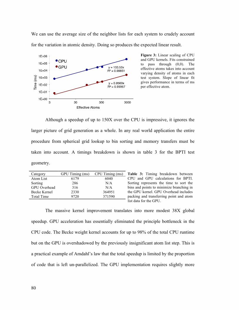
80

We can use the average size of the neighbor lists for each system to crudely account

for the variation in atomic density. Doing so produces the expected linear result.

Figure 3: Linear scaling of CPU and GPU kernels. Fits constrained to pass through (0,0). The effective atoms takes into account varying density of atoms in each test system. Slope of linear fit gives performance in terms of ms per effective atom.

Although a speedup of up to 150X over the CPU is impressive, it ignores the

larger picture of grid generation as a whole. In any real world application the entire

procedure from spherical grid lookup to bin sorting and memory transfers must be

taken into account. A timings breakdown is shown in table 3 for the BPTI test

geometry.

Category GPU Timing (ms) CPU Timing (ms) Table 3: Timing breakdown between CPU and GPU calculations for BPTI. Sorting represents the time to sort the bins and points to minimize branching in the GPU kernel. GPU Overhead includes packing and transferring point and atom list data for the GPU.

Atom List 6179 6040 Sorting 286 N/A GPU Overhead 316 N/A Becke Kernel 2330 364951 Total Time 9720 371590

The massive kernel improvement translates into more modest 38X global

speedup. GPU acceleration has essentially eliminated the principle bottleneck in the

CPU code. The Becke weight kernel accounts for up to 98% of the total CPU runtime

but on the GPU is overshadowed by the previously insignificant atom list step. This is

a practical example of Amdahl’s law that the total speedup is limited by the proportion

of code that is left un-parallelized. The GPU implementation requires slightly more

81

time to generate the atom lists due to the additional sorting by length required to

minimize warp divergence on the GPU.

The final weights for many individual quadrature points are negligibly small.

These are removed from the final grid, and the Cartesian coordinates and weights of

all remaining points are stored for use in later integration.

wap!p "# i!rap "

!ri (4.15)

EXCHANGE-CORRELATION POTENTIAL EVALUATION

With the numerical quadrature grid in hand, we now consider the evaluation of

the exchange-correlation potential, Vxc in equation (4.2). Following Yasuda’s GPU

implementation,2 the calculation of Vxc is broken down into three parts. First, the

electronic density and its gradient are evaluated at each grid point. Second, the DFT

functional is evaluated at each grid point. And third, the functional values are summed

to produce the final matrix elements.

As with the ERI kernels considered previously, the calculation is segmented by

the angular momenta of the basis functions. For GGA functionals, however, the

exchange-correlation potential involves only one-electron terms, so that kernels deal

with pairs rather than quartets of basis shells. Thus, for a basis limited to s- , p-, and d-

functions, only six kernel classes are needed, ss, sp, sd, pp, pd, and dd. Threads

assigned to higher angular momenta shells again compute terms for all primitive

functions within the shell pair.

82

The alpha-spin electronic density and density gradient at each grid point, !ri ,

are calculated from the one particle density matrix P! as follows (with analogous

expressions for the beta spin case).

!" (!ri ) = Pµ#

" $µ (!ri )$# (!ri )µ#% (4.16)

!"# (!ri ) = 2 Pµ$

# %µ (!ri )!%$ (!ri )µ$& (4.17)

To compute these quantities, each CUDA thread is assigned a unique grid point and

loops over significant primitive shell pairs. As a result of the exponential decay of the

basis functions, !µ , the sum for each grid point need only include a few significant

AOs. Significant AO primitive pairs are spatially binned by the center of charge, !Pij in

equation (1.25), and sorted by increasing exponent. Each thread loops over all bins,

but exits each bin as soon as the first negligible point-pair interaction is reached. The

quadrature points are similarly binned to minimize warp divergence by ensuring that

neighboring threads share similar sets of significant basis functions.

Next, the density at each quadrature point is copied to host memory and used

to evaluate the xc-kernel function and its various derivatives on the grid. Specifically,

the following values are computed for each grid point.

ai =! i fxc "# (!ri ),"$ (

!ri ),% ## (!ri ),% #$ (

!ri ),% $$ (!ri )( )

bi =! i

& fxc!ri( )

&"#

ci =! i 2& fxc

!ri( )&% ##

'"# +& fxc

!ri( )&% #$

'"$

(

)*+

,-

(4.18)

83

This step has a small computational cost and can be performed on the host without

degrading performance. This is desirable as a programming convenience since

implementing various density functionals can be performed without editing CUDA

kernels, and because the host provides robust and efficient support for various

transcendental functions needed by some functionals. During this step, the functional

values, ai , are also summed to evaluate the total exchange-correlation energy per

equation (4.1).

The final step is to construct AO matrix elements for the exchange-correlation

potential. This task is again performed on the GPU. For all non-negligible primitive

pairs, !K! L , the pair quantities KKL ,

!PKL , and !KL from equation (1.25) are packed

into arrays and transferred to device memory. The grid coordinates, !ri , are spatially

binned and transferred to the GPU with corresponding values bi and ci . A CUDA

kernel then performs the summation,

!Vµ! = "µ ("ri )

bi2"! ("ri )+ ci#"! (

"ri )$%&

'()i

*

= ckcll+!*

k+µ* , k (

"ri )bi2, l ("ri )+ ci#, l (

"ri )$%&

'()i

* (4.19)

and the final matrix elements are computed as follows.

Vµ!XC = !Vµ! + !V!µ (4.20)

This calculation can be envisioned as a 2D matrix in which each row

corresponds to a primitive shell pair, !K! L , and each column is associated with a

single grid point. The CUDA grid is configured as a 1-D grid of 2-D blocks, similar to

the GPU J-Engine described in chapter 2. A stack of blocks spanning the primitive

84

pairs sweeps across the matrix. The points are spatially binned so that entire bins can

be skipped whenever a negligible point-primitive pair combination is encountered. As

in the Coulomb algorithm, each row of threads across a CUDA block cooperates to

produce a primitive matrix element, !Vkl . These are copied to the host where the final

summation into AO matrix elements takes place.

SCF PERFORMANCE EVAULATION

Having completed our discussion of GPU acceleration of SCF calculations we

illustrate the application of our work to practical calculations. All GPU calculations

described below were carried out using the TeraChem quantum chemistry package. To

elucidate the computational scaling of our GPU implementation with increasing

system size, we consider two types of systems. First, linear alkene chains ranging in

length between 25 and 707 carbon atoms provide a benchmark at the low-dimensional

limit. Second, cubic water clusters containing between 10 and 988 molecules provide

a dense, three-dimensional test system that is more representative of interesting

condensed phase systems. Examples of each system type are shown in figure 4.

Figure 4: One-dimensional alkene and three dimensional water-cube test systems. Alkene lengths vary from 24 to 706 carbon atoms and water cubes range from 10 to nearly 850 water molecules. A uniform density is used for all water boxes.

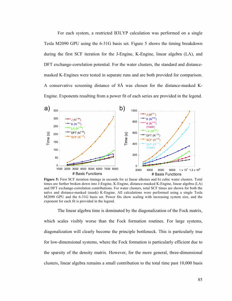
85

For each system, a restricted B3LYP calculation was performed on a single

Tesla M2090 GPU using the 6-31G basis set. Figure 5 shows the timing breakdown

during the first SCF iteration for the J-Engine, K-Engine, linear algebra (LA), and

DFT exchange-correlation potential. For the water clusters, the standard and distance-

masked K-Engines were tested in separate runs and are both provided for comparison.

A conservative screening distance of 8Å was chosen for the distance-masked K-

Engine. Exponents resulting from a power fit of each series are provided in the legend.

Figure 5: First SCF iteration timings in seconds for a) linear alkenes and b) cubic water clusters. Total times are further broken down into J-Engine, K-Engine, distance-masked K-Engine, linear algebra (LA) and DFT exchange-correlation contributions. For water clusters, total SCF times are shown for both the naïve and distance-masked (mask) K-Engine. All calculations were performed using a single Tesla M2090 GPU and the 6-31G basis set. Power fits show scaling with increasing system size, and the exponent for each fit is provided in the legend.

The linear algebra time is dominated by the diagonalization of the Fock matrix,

which scales visibly worse than the Fock formation routines. For large systems,

diagonalization will clearly become the principle bottleneck. This is particularly true

for low-dimensional systems, where the Fock formation is particularly efficient due to

the sparsity of the density matrix. However, for the more general, three-dimensional

clusters, linear algebra remains a small contribution to the total time past 10,000 basis

86

functions. If the more efficient masked K-Engine can be employed, the crossover

point, at which linear algebra becomes dominant, shifts to about 8,000 basis functions.

Although the time per basis function is lower for the alkene test series, the

overall scaling is similar for both test series. This behavior is good evidence that we

have penetrated the asymptotic regime of large systems, where the dimensionality of

the physical system should impact the prefactor rather than the exponent. That we

easily reach this crossover point on GPUs is itself noteworthy. Even more noteworthy

is the fact that the K-Engine exhibits sub-quadratic scaling without imposing any of

the assumptions or book-keeping mechanisms such as neighbor lists common among

linear scaling exchange algorithms.8-11 The further imposition of a simple distance

mask on exchange elements provides an effective linear scaling approach for

insulating systems. The scaling of the SCF with the masked K-Engine further

exemplifies the impact of the linear algebra computation on the overall efficiency. The

N3 scaling of LA becomes significantly more dominant in large systems. The validity

of the distance-based exchange screening approximation was confirmed by comparing

the final converged absolute SCF energies of each water cluster calculated with and

without screening. The absolute total electronic energy is accurate to better than 0.02

kcal/mol in all systems considered, which is well within chemical accuracy.

Our GPU J-Engine scales quadratically with system size, which comports well

with our scaling analysis in chapter 2. Further acceleration would require modification

of the long-ranged Coulomb potential, for example by factorization into a multipole

expansion.12 Extrapolating beyond figure 5, this may become necessary for water

clusters beyond 12,000 basis functions, when the J-Engine finally becomes the

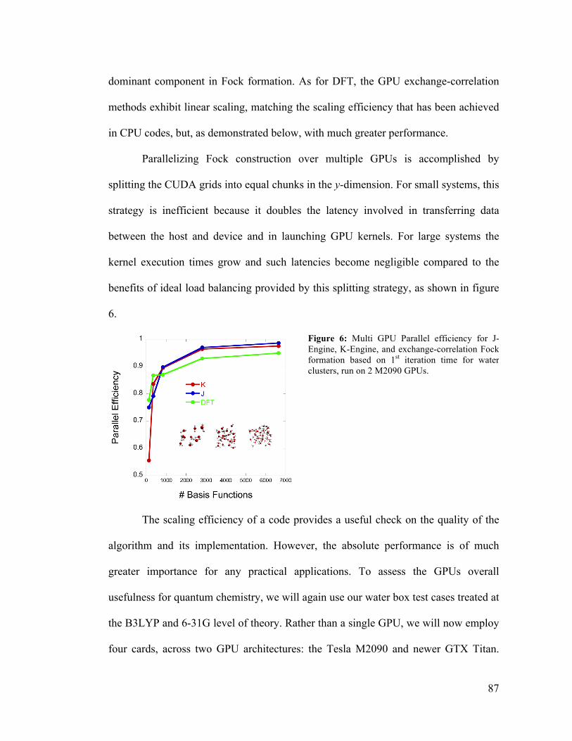
87

dominant component in Fock formation. As for DFT, the GPU exchange-correlation

methods exhibit linear scaling, matching the scaling efficiency that has been achieved

in CPU codes, but, as demonstrated below, with much greater performance.

Parallelizing Fock construction over multiple GPUs is accomplished by

splitting the CUDA grids into equal chunks in the y-dimension. For small systems, this

strategy is inefficient because it doubles the latency involved in transferring data

between the host and device and in launching GPU kernels. For large systems the

kernel execution times grow and such latencies become negligible compared to the

benefits of ideal load balancing provided by this splitting strategy, as shown in figure

6.

Figure 6: Multi GPU Parallel efficiency for J-Engine, K-Engine, and exchange-correlation Fock formation based on 1st iteration time for water clusters, run on 2 M2090 GPUs.

The scaling efficiency of a code provides a useful check on the quality of the

algorithm and its implementation. However, the absolute performance is of much

greater importance for any practical applications. To assess the GPUs overall

usefulness for quantum chemistry, we will again use our water box test cases treated at

the B3LYP and 6-31G level of theory. Rather than a single GPU, we will now employ

four cards, across two GPU architectures: the Tesla M2090 and newer GTX Titan.

88

Notably, a 1533 atom single-point energy calculation on a cubic water cluster required

only 2.47 hours for the entire SCF procedure, and ab initio dynamics, requiring

thousands of single point evaluations are feasible for systems containing thousands of

basis functions.

As a point of comparison, the same calculations were carried out using the

CPU implementation available in the GAMESS program.13 Parameters such as

integral neglect thresholds and SCF convergence criteria were matched as closely as

possible to the previous GPU calculations. The CPU calculation was also parallelized

over all 8 CPU cores available in our dual Xeon X5680 3.33GHz server. Figure 7

shows the speedup of the GPU implementation relative to GAMESS for the first SCF

iteration including both Fock construction and diagonalization, the latter of which is

performed in both codes on the CPU. Performance is similar between the two GPU

models on small structures for both alkenes and water clusters. However, GTX Titan

exhibits a larger speedup relative to GAMESS above 100 orbitals and reaches 400x at

the largest systems examined. During Fock construction, the CPU cores are left idle in

our implementation. It is also possible to reserve some work for the CPU,14 but given

the performance advantage of our GPU implementation, this would offer a rather

small performance improvement.

89

Figure 7: Total SCF time of TeraChem on 8 CPUs and 4 GPUs, relative to GAMESS on 8 CPUs for water clusters.

REFERENCES

(1) Pople, J. A.; Gill, P. M. W.; Johnson, B. G. Chem. Phys. Lett. 1992, 199, 557.

(2) Yasuda, K. J. Chem. Theo. Comp. 2008, 4, 1230.

(3) Murray, C. W.; Handy, N. C.; Laming, G. J. Mol. Phys. 1993, 78, 997.

(4) Lebedev, V. I.; Laikov, D. N. Dokl Akad Nauk+ 1999, 366, 741.

(5) Becke, A. D. J. Chem. Phys. 1988, 88, 2547.

(6) Johnson, B. G.; Gill, P. M. W.; Pople, J. A. J. Chem. Phys. 1993, 98, 5612.

(7) Stratmann, R. E.; Scuseria, G. E.; Frisch, M. J. Chem. Phys. Lett. 1996, 257, 213.

(8) Burant, J. C.; Scuseria, G. E.; Frisch, M. J. J. Chem. Phys. 1996, 105, 8969.

(9) Ochsenfeld, C.; White, C. A.; Head-Gordon, M. J. Chem. Phys. 1998, 109, 1663.

(10) Schwegler, E.; Challacombe, M. J. Chem. Phys. 1999, 111, 6223.

(11) Neese, F.; Wennmohs, F.; Hansen, A.; Becker, U. Chem. Phys. 2009, 356, 98.

(12) White, C. A.; Head-Gordon, M. J. Chem. Phys. 1994, 101, 6593.

(13) Schmidt, M. W.; Baldridge, K. K.; Boatz, J. A.; Elbert, S. T.; Gordon, M. S.; Jensen, J. H.; Koseki, S.; Matsunaga, N.; Nguyen, K. A.; Su, S. J.; Windus, T. L.; Dupuis, M.; Montgomery, J. A. J. Comp. Chem. 1993, 14, 1347.

90

(14) Asadchev, A.; Gordon, M. S. J. Chem. Theo. Comp. 2012, 8, 4166.

91

CHAPTER FIVE

EXCITED STATE ELECTRONIC STRUCTURE

ON GPUS: CIS AND TDDFTa

In the previous chapters we described GPU algorithms to accelerate the

construction of the Fock matrix for use in SCF calculations. We now demonstrate how

those efficient Fock methods can be applied more widely to dramatically increase the

performance of post-SCF calculations such as single excitation configuration

interaction (CIS),1 time-dependent Hartree-Fock (TDHF) and linear response time-

dependent density functional theory (TDDFT).2-6 These single-reference methods are

widely used for ab initio calculations of electronic excited states of large molecules

(more than 50 atoms, thousands of basis functions) because they are computationally

efficient and straightforward to apply.7-9 Although highly correlated and/or multi-

reference methods such as multireference configuration interaction (MRCI10),

multireference perturbation theory (MRMP11 and CASPT212), and equation-of-motion

coupled cluster methods (SAC-CI13 and EOM-CC14,15) allow for more reliably

accurate treatment of excited states, including those with double excitation character,

these are far too computationally demanding for large molecules.

CIS/TDHF is essentially the excited state corollary of the ground state Hartree-

Fock method, and thus similarly suffers from a lack of electron correlation. Because

a Adapted from C.M. Isborn, N. Luehr, I.S. Ufimtsev, and T.J. Martinez, J. Chem. Theo. Comput. 2011, 7, 1814-1823. This is an unofficial adaptation of an article that appeared in an ACS publication. ACS has not endorsed the content of this adaptation or the context of its use.

92

of this, CIS/TDHF excitation energies are consistently overestimated, often by ~1eV.8

The TDDFT method includes dynamic correlation through the exchange correlation

functional, but standard non-hybrid TDDFT exchange-correlation functionals tend to

underestimate excitation energies, particularly for Rydberg and charge transfer states.5

The problem in charge-transfer excitation energies is due to the lack of the correct 1/r

Coulombic attraction between the separated charges of the excited electron and hole.16

Charge transfer excitation energies are generally improved with hybrid functionals and

also with range separated functionals that separate the exchange portion of the DFT

functional into long and short range contributions.17-21 Neither CIS nor TDDFT (with

present-day functionals) properly include the effects of dispersion, but promising

results have been obtained with an empirical correction to standard DFT

functionals,22,23 and there are continued efforts to include dispersion directly in the

exchange-correlation functional.24,25 Both the CIS and TDDFTa single reference

methods lack double excitations and are unable to model conical intersections or

excitations in molecules that have multi-reference character.26,27 In spite of these

limitations, the CIS and TDDFT methods can be generally expected to reproduce

trends for one-electron valence excitations, which are a majority of the transitions of

photochemical interest. TDDFT using hybrid density functionals, which include some

percentage of Hartree-Fock (HF) exact exchange, have been particularly successful in

modeling the optical absorption of large molecules. Furthermore, the development of

new DFT functionals and methods is an avid area of research, with many new

a By TDDFT we here refer to the adiabatic linear response formalism with presently available functionals.

93

functionals introduced each year. Thus it is likely that the quality of the results

available from TDDFT will continue to improve. A summary of the accuracy currently

available for vertical excitation energies is available in a recent study by Jacquemin et

al. which compares TDDFT results using 29 functionals for ~500 molecules.28

Although CIS and TDDFT are the most tractable methods for treating excited

states of large molecules, their computational cost still prevents application to many

systems of photochemical interest. Thus, there is considerable interest in extending the

capabilities of CIS/TDDFT to even larger molecules, beyond hundreds of atoms.

Quantum mechanics/molecular mechanics (QM/MM) schemes provide a way

to model the environment of a photophysically interesting molecule by treating the

molecule with QM and the surrounding environment with MM force fields.29-33

However, it is difficult to know when the MM approximations break down and when a

fully QM approach is necessary. With fast, large scale CIS/TDDFT calculations, all

residues of a photoactive protein could be treated quantum mechanically to explore the

origin of spectral tuning, for example. Explicit effects of solvent-chromophore

interactions, including hydrogen bonding, charge transfer, and polarization, could be

fully included at the ab initio level in order to model solvatochromic shifts.

GPUs provide a promising route to large-scale CIS and TDDFT calculations.

GPUs have been applied to achieve speed-ups of 1-2 orders of magnitude in ground

state electronic structure,34-36 ab initio molecular dynamics37 and empirical force field-

based molecular dynamics calculations.38-41 In this chapter we extend the

implementation of GPU quantum chemistry beyond the SCF methods36,42 described in

previous chapters to the calculation of excited electronic states. The performance

94

provided by GPU hardware for evaluating ERIs allows full QM treatment of the

excited states of very large systems – both large chromophores and chromophores in

which the environment plays a critical role and should be treated with QM. In this

chapter we present the results of implementing CIS and TDDFT within the Tamm-

Dancoff approximation using GPUs to drastically accelerate the bottlenecks of two-

electron integral evaluation, density functional quadrature, and matrix multiplication.

This results in CIS calculations over 200x faster than those achieved running on a

comparable CPU platform. Benchmark CIS/TDDFT timings are presented for a

variety of systems.

CIS/TDDFT IMPLEMENTATION USING GPUS

The linear response formalism of TDHF and TDDFT has been thoroughly

presented in review articles.4,7,8,43 Only the equations relevant for this work are

presented here. The TDHF/TDDFT working equation is

A BB A

!"#

$%&

XY

!"#

$%&=' 1 0

0 (1!"#

$%&

XY

!"#

$%&

, (5.1)

where for TDHF (neglecting spin indices for simplicity)

Aai,bj = ! ij!ab "a # " i( ) + ia | jb( ) # ij | ab( ) , (5.2)

Bai,bj = ia | bj( )! ib | aj( ) , (5.3)

and for TDDFT

Aai,bj = ! ij!ab "a # " i( ) + ia | jb( ) + ij | fxc | ab( ), (5.4)

Bai,bj = ia |bj( ) + ib | fxc | aj( ) . (5.5)

The ERIs are defined as usual.

95

ia | jb( ) =! i(r1)!a (r1)! j (r2)!b (r2)

r1 " r2## dr1dr2 (5.6)

Within the adiabatic approximation of DFT, the exact time-dependent exchange-

correlation potential is approximated using the time-independent ground state

exchange-correlation functional Exc[!] as follows.

ia | fxc | jb( ) = ! i(r1)!a (r1)" 2Exc

"#(r1)"#(r2)$$ ! j (r2)!b (r2)dr1dr2 (5.7)

The i,j and a,b indices represent occupied and virtual MOs, respectively, in the

Hartree-Fock/Kohn-Sham (KS) ground state determinant.

Setting the B matrix to zero within TDHF results in the CIS equation, while in

TDDFT this same neglect yields the equation known as the Tamm-Dancoff

approximation (TDA):

AX =!X . (5.8)

In part because DFT virtual orbitals provide a better starting approximation to the

excited state than HF orbitals, the neglect of the B matrix within TDA is known to

accurately reproduce full TDDFT results for non-hybrid DFT functionals.7,8,44

Furthermore, previous work has shown that a large contribution from the B matrix in

TDDFT (and to a lesser extent also in TDHF) is often indicative of a poor description

of the ground state, either due to singlet-triplet instabilities or multi-reference

character.45 Thus, if there is substantial deviation between the full TDDFT and TDA-

TDDFT excitation energies, the TDA results will often be more accurate.

A standard iterative Davidson algorithm46 has been implemented to solve the

CIS/TDA-TDDFT equations. As each AX matrix-vector product is formed, the

96

required two-electron integrals are calculated over primitive basis functions within the

atomic orbital (AO) basis directly on the GPU. Within CIS, the AX matrix-vector

product is calculated as follows.

ACISX( )bj = ! ij!ab "a # " i( ) + ia | jb( ) # (ij | ab)[ ]Xiaia$ (5.9)

ia | jb( ) ! (ij | ab)[ ]Xiaia" = Cµj

µ#" C#bFµ# (5.10)

Fµ! = T"#"#$ µ! |"#( ) % µ" |!#( ){ } (5.11)

T!" = Xiaia# C!iC"a (5.12)

Here C!i are the SCF MO coefficients of the HF/KS determinant, and T!" is a non-

symmetric transition density matrix. For very small systems there is no performance

advantage with GPU computation of the matrix multiplication steps in equations

(5.10) and (5.12), in which case we compute these quantities on the CPU. For larger

systems, the matrix-vector multiplications are performed on the GPU using dgemm

calls to the CUBLAS library, a CUDA BLAS implementation.47

Equation (5.11) represents the dominant computational bottleneck of this

integral direct CIS algorithm. Fortunately, this equation is equivalent to the Coulomb

and exchange matrix builds described in chapters 2 – 4 except that the non-symmetric

transition density, T, replaces the symmetric one-particle density matrix, P. Thus, the

portion of the F matrix from the product of T!" with the first integral in equation (5.11)

is computed with the GPU J-engine algorithm. The portion of the F matrix from the

product of T!" with the second integral in equation (5.11) is computed with the K-

engine algorithm. The coulomb matrix remains symmetric even with a non-symmetric

97

transition density matrix. Thus, it is possible to continue to eliminate redundant µ# "

#µ bra and !" " "! ket pairs as in the SCF routine as long as the sum of transpose

density elements is used as follows.

Jµ! = J!µ = µ! | "#( ) T"# + 1$%"#( )T#"( )

"&#'

(5.13)

The excited state exchange matrix is not symmetric. We must thus calculate both the

upper and lower triangle contributions with separate calls to the ground state GPU K-

engine routines. Since the SCF K-engine already ignores µ# " #µ bra and !" " "!

ket symmetries, the result is that, ignoring screening, all O(N4) ERIs are computed for

the excited state K contribution, while the J term requires the same O(N4/4) ERIs

computed in the ground state.

Compared to the J-engine, the K-engine suffers from a second disadvantage for

both ground and excited state calculations. Unlike the J-matrix GPU implementation,

the K-matrix algorithm cannot map the density matrix elements onto the ket integral

data, since the density index now spans both bra and ket indices. This leads to two

negative consequences. First, each thread must load an independent density matrix

element which results in slower non-coalesced GPU memory accesses. Second, the

sparsity of the density cannot be included in the pre-sorting of ket pairs. Thus, the

integral bounds are not guaranteed to strictly decrease and a mix of significant and

insignificant ERIs must be computed. As a result of these drawbacks, the exchange

algorithm is less efficient on the GPU and actually takes longer to calculate than its

Coulomb counterpart even though density screening should in principle leave many

fewer significant ERI contributions in the case of exchange. In practice a K/J timing

98

ratio for ground state SCF calculations is observed to be between 3 and 5 for systems

studied below.

Evaluation of the derivative of the exchange-correlation potential needed for

TDDFT excited states7 is performed using the same numerical quadrature as the

ground state exchange-correlation potential. We again use a Becke type quadrature

scheme48 with Lebedev angular49 and Euler-Maclaurin radial50 quadrature grids. The

same basic approach described in the previous chapter is again employed to compute

the exchange-correlation matrix elements of equation (5.7).35,51 The expensive steps

are evaluating the electron density/gradient at the grid quadrature points to

numerically evaluate the necessary functionals and summing the values on the grid to

assemble the matrix elements of the exchange-correlation potential. For the excited

state calculations, we generate the second functional derivative of the exchange

correlation functional only once, saving its value at each quadrature point in memory.

Then, for each Davidson iteration, the appropriate integrals are evaluated, paired with

the saved functional derivative values and summed into matrix elements using GPU

kernels analogous to the ground state case detailed in the previous chapter.

RESULTS AND DISCUSSION

We evaluate the performance of our GPU-based CIS/TDDFT algorithm on a

variety of test systems: B3PPQ – 6,6’-bis(2-(1-triphenyl)-4-phenylquinoline - an

oligoquinoline recently synthesized and characterized by the Jenekhe group for use in

OLED devices52 and characterized theoretically by Tao and Tretiak;53 four generations

of oligothiophene dendrimers that are being studied for their interesting photophysical

properties54-56; the entire photoactive yellow protein (PYP)57 solvated by TIP3P58

99

water molecules; and deprotonated trans-thiophenyl-p-coumarate, an analogue of the

PYP chromophore59 that takes into account the covalent cysteine linkage, solvated

with an increasing number of QM waters.

Figure 1. Structures, number of atoms, and basis functions (fns) using the 6-31G basis set for four generations of oligothiophene dendrimers, S1-S4. Carbon atoms are orange, sulfur atoms are yellow.

Figure 2. Structures, number of atoms, and basis functions (fns) for the 6-31G basis for benchmark systems photoactive yellow protein (PYP), the solvated PYP chromophore, and oligoquinoline B3PPQ. For PYP, carbon, nitrogen, oxygen and sulfur atoms are green, blue, red, and yellow, respectively. For the other molecules, atom coloration is as given in figure 1, with additional red and blue coloration for oxygen and nitrogen atoms, respectively.

Benchmark structures are shown in figures 1 and 2 along with the number of

atoms and basis functions for a 6-31G basis set. For the solvated PYP chromophore,

only three structures are shown in figure 2, but benchmark calculations are presented

100

for 15 systems with increasing solvation, starting from the chromophore in vacuum

and adding water molecules up to a 16 Ångstrom solvation shell, which corresponds to

900 water molecules.

For our benchmark TDDFT calculations, we use the generalized gradient

approximation with Becke’s exchange functional60 combined with the Lee, Yang, and

Parr correlation functional61 (BLYP). During the SCF procedure for the ground state

wavefunction, we use two different DFT grids. A sparse grid of ~1000 grid

points/atom is used to converge the wave function until the DIIS error reaches a value

of 0.01, followed by a more dense grid of ~3000 grid points/atom until the ground

state wave function is fully converged. This denser grid is also used for the excited

state TDDFT timings reported herein, unless otherwise noted. The Coulomb and

exchange integral screening thresholds are set to 1x10-11 atomic units. Coulomb and

exchange integrals with products of the density element and Schwarz bound below the

integral screening threshold are not computed, and exchange evaluation is terminated

when the products of density element and Schwarz bound fall below this value times a

guard factor of 0.001. The timings reported were obtained using a dual quad-core Intel

Xeon X5570 platform with 72 GB RAM and eight Tesla C1060 GPUs.

All CPU operations are performed in full double precision arithmetic,

including one-electron integral evaluation, integral accumulation, and diagonalization

of the subspace matrix of A. Calculations carried out on the GPU (Coulomb and

exchange operator construction and DFT quadrature) use mixed precision unless

otherwise noted. The mixed precision integral evaluation is a hybrid of 32-bit and 64-

bit arithmetic. In this case, integrals with Schwarz bounds larger than 0.001 a.u. are

101

computed in full double precision, and all others are computed in single precision with

double precision accumulation into the final matrix elements. To study the effects of

using single precision on excited state calculations, we have run the same CIS

calculations using both single and double precision integral evaluation for many of our

benchmark systems.

Figure 3. Plot of single and double precision convergence behavior for the 1st CIS/6-31G excited state of five benchmark systems. A typical convergence threshold of 10-5 in the residual norm is indicated with a straight black line. Convergence behavior is generally identical for single and double precision integration until very small residual values well below the convergence threshold. Some calculations do require double precision for convergence. One such example is shown here for a snapshot of the PYP chromophore (PYPc) with 94 waters.

In general we find that mixed (and often even single) precision arithmetic on

the GPU is more than adequate for CIS/TDDFT, with convergence being achieved in

as many or fewer iterations than is required for the identical convergence criterion for

GAMESS. In most cases we find that the convergence behavior is nearly identical for

single and double precision until the residual vector is quite small. Figure 3 shows the

typical single and double precision convergence behavior as represented by the CIS

residual vector norm convergence for B3PPQ, the 1st and 3rd generations of

oligothiophene dendrimers S1 and S3, and a snapshot of the PYP chromophore

surrounded by 14 waters. A common convergence criterion on the residual norm is

102

shown with a straight black line at 10-5 a.u. Note that for the examples in figure 3, we

are not using mixed precision – all two electron integrals on the GPU are done in

single precision. This is therefore an extreme example (other calculations detailed in

this paper used mixed precision where large integrals and quadrature contributions are

calculated in double precision) and serves to show that CIS and TDDFT are generally

quite robust, irrespective of the precision used in the calculation. Nevertheless, a few

problematic cases have been found in which single precision integral evaluation is not

adequate and where double precision is needed to achieve convergence.a During the

course of hundreds of CIS calculations performed on snapshots of the dynamics of the

PYP chromophore solvated by various numbers of water molecules, a small number

(<1%) of cases yield ill-conditioned Davidson convergence when single precision is

used for the GPU-computed ERIs and quadrature contributions. For illustration, the

single and double precision convergence behavior for one of these rare cases, here the

PYP chromophore with 94 waters, is shown in figure 3. In practice, this is not a

problem since one can always switch to double precision and this can be done

automatically when convergence problems are detected.

Timings and excitation energies for some of the test systems are given in table

1 and compared to the GAMESS quantum chemistry package version 12 Jan 2009

(R3). The GAMESS timings are obtained using the same Intel Xeon X5570 eight-core

machine as for the GPU calculations (where GAMESS is running in parallel over all

eight cores). The numerical accuracy of the excitation energies for mixed precision

a Of course, if the convergence threshold was made sufficiently small, all calculations would require double (or better) precision throughout.

103

GPU integral evaluation is excellent for all systems studied; the largest discrepancy

between GAMESS and our GPU implementation is less than 0.0001eV. Speedups are

given for both the total SCF time and CIS computation time, with a large increase in

performance times obtained using the GPU for both ground and excited state methods.

The speedups increase as system size increases, with SCF speedups outperforming

CIS speedups. For the largest system compared with GAMESS, which is the 29 atom

chromophore of PYP surrounded by 487 QM water molecules, the speedup is well

over 400# for SCF and 200# for CIS.

molecule (atoms; basis functions) CIS timings (s) Speedup DES0/S1 (au) GPU GAMESS SCF CIS GPU GAMESS

B3PPQ oligoquinoline (112; 700) 38.6 371.5 15 10 0.1729276 0.1729293 S2 oligothiophene dendrimer (128; 958) 117.5 755.9 15 6 0.1511511 0.1511509 PYP chromophore + 101 waters (332; 1501) 164.8 3032.7 52 18 0.1338027 0.1338021 PYP chromophore + 146 waters (467; 2086) 286.7 8654.9 90 30 0.1337468 0.1337463 PYP chromophore + 192 waters (605; 2684) 431.5 20546.8 133 48 0.1338623 0.1338617 PYP chromophore + 261 waters (812; 3581) 715.4 57800.5 212 81 0.1339657 0.1339651 PYP chromophore + 397 waters (1220; 5349) 1459.3 243975.7 353 167 0.1341203 0.1341196 PYP chromophore + 487 waters (1490; 6519) 2408.1 562606.6 421 234 0.1343182 0.1343174 Table 1. Accuracy and performance of the CIS algorithm on a dual Intel Xeon X5570 (eight CPU cores) with 72 GB RAM. GPU Calculations use eight Tesla C1060 GPU cards.

The dominant computational parts in building the CIS/TDDFT AX vector can

be divided into Coulomb matrix, exchange matrix and DFT contributions. Figure 4

plots the CPU+GPU time consumed by each of these three contributions (both CPU

and GPU times are included here, although the CPU time is a very small fraction of

the total). J and K timings are taken from an average of the ten initial guess AX builds

for a CIS calculation, and the DFT timings are from an average of the initial guess AX

builds for a TD-BLYP calculation. The initial guess transition densities are very sparse

and thus this test highlights the differing efficiency of screening and thresholding in

104

these three contributions. The J-timings for CIS and BLYP are similar, and only those

for CIS are reported. Power law fits are shown as solid lines and demonstrate near-

linear scaling behavior of all three contributions to the AX build. The coulomb matrix

and DFT quadrature steps are closest to linear scaling, with observed scaling of N1.2

and N1.1, respectively, where N is the number of basis functions. The exchange

contribution scales as N1.6. These empirical scaling data demonstrate that with proper

sorting and integral screening, the AX build in CIS and TDDFT scales much better

than quadratic, with no loss of accuracy in excitation energies.

Figure 4. Contributions to the time for building an initial AX vector in CIS and TD-BLYP. Ten initial X vectors are created based on MO energy gaps, and the timing reported is the average time for building AX for those ten vectors. The timings are obtained on a dual Intel Xeon X5570 platform with eight Tesla C1060 GPUs. Data (symbols) are fit to power law (solid line, fitting parameters in inset). Fewer points are included for the TD-BLYP timings because the SCF procedure does not convergea for the solvated PYP chromophore with a large number of waters or for the full PYP protein.

a This is due to the well-known problem with non-hybrid DFT functionals having erroneously low-lying charge transfer states that can prevent SCF convergence.

y=7.3!10-5 x1.2 R=0.97 y=5.0!10-5 x1.6 R=0.99 y=4.9!10-4 x1.04 R=0.97

105

Of the three integral contributions (Coulomb, exchange, and DFT quadrature),

the computation of the exhcange matrix is clearly the bottleneck. This is due to the

three issues with exchange computation previously discussed: 1) the J-engine

algorithm takes full advantage of density sparsity because of efficient density

screening that is not possible for our K-engine implementation, 2) exchange kernels

access the density in memory non-contiguously, and 3) exchange lacks the µ! " !µ

and #" " "# symmetry. It is useful to compare the time required to calculate the

exhcange contribution to the first ground-state SCF iteration (which is the most

expensive iteration due to the use of Fock matrix updating62) and to the AX vector

build for CIS (or TDDFT). We find that the exchange contribution is on average 1.5x

slower in CIS/TDDFT compared to ground state SCF. One might have expected the

excited state computation to be 2x slower because of the two K-engine calls, but the

algorithm is able to exploit the greater sparsity of the transition density matrix

(compared to the ground state density matrix).

Due to efficient screening of ERI contributions to the Coulomb matrix, the J-

engine similarly exploits the increased sparseness of the transition density, and

therefore is faster than the ground state 1st iteration J-engine calculation. In the current

implementation the Coulomb evaluation profits more from transition density sparsity

than that for exchange since it scales better with system size (N1.2 vs N1.6).

As can be seen in figure 4, the DFT integration usually takes more time than

the Coulomb contribution, in spite of the fact that DFT integration scales more nearly

linearly with system size. This is because of the larger prefactor for DFT integration,

which is related to the density of the quadrature grids used. It has previously been

106

noted63 that very sparse grids can be more than adequate for TDDFT. We further

support this claim with the data presented in table 2, where we compare the lowest

excitation energies and average TD-BLYP integration times for the initial guess

vectors for six different grids on two of the test systems. For both molecules, the

excitation energies from the sparsest grid agree well with those of the more dense

grids, but with a substantial reduction in integration time, suggesting that a change to

an ultra sparse grid for the TDDFT portion of the calculation could result in

considerable time savings with little to no loss of accuracy. The TD-BLYP values

computed with NWChem64 using the default ‘medium’ grid are also given to show the

accuracy of our implementation. The small (<0.001eV) differences in excitation

energies between our GPU-based TD-BLYP and NWChem are likely due to slightly

differing ground state densities, which differ in energy by 0.000008 a.u. for the

chromophore and 0.0019 a.u. for the S2 dendrimer.

PYP chromophore (29 atoms) Table 2. TD-BLYP timings (average time for the DFT quadrature in one AX build for the initial 10 AX vectors) and first excitation energies using increasingly dense quadrature grids. For comparison, NWChem excitation energies are also given using the default ‘medium’ grid. Number of points/atom refers to the pruned grid for TeraChem and the unpruned grid for NWChem. NWChem was run on a different architecture, so timings are not directly comparable.

grid points points/atom time (s) $E (au) 0 29497 1017 0.06 0.08516162 1 81461 2809 0.11 0.08516510 2 182872 6305 0.22 0.08516472 3 330208 11386 0.38 0.08516266 4 841347 29011 0.91 0.08516267 5 2126775 73337 2.30 0.08516268

NWChem/medium

21655 n/a 0.08516691 S2 dendrimer (128 atoms) Grid points points/atom time (s) $E (au)

0 141684 1106 0.28 0.08394399 1 382576 2988 0.51 0.08394430 2 848918 6632 0.98 0.08394427 3 1506502 11769 1.64 0.08394433 4 3770640 29458 3.72 0.08394431 5 9472331 74002 9.24 0.08394431

NWChem/medium

25061 n/a 0.08395211

107

GPU-accelerated CIS and TDDFT methods can calculate excited states of

much larger molecules than can currently be studied with previously existing ab initio

methods. For the well-behaved valence transitions in the PYP systems, CIS

convergence requires very few Davidson iterations. The total wall time (SCF+CIS)

required to calculate the 1st CIS/6-31G excited state of the entire PYP protein (10,869

basis functions) is less than 7 hours, with ~5.5 hours devoted to the SCF procedure,

and ~1.5 hours to the CIS procedure. Most (1.2 hours) of the CIS time is spent

computing exchange contributions. We can thus treat the protein with full QM and

study how mutation within PYP will affect the absorbance. For any meaningful

comparison with the experimental absorption energy of PYP at 2.78 eV,59 many

configurations need to be taken into account. For this single configuration, the CIS

excitation energy of 3.69 eV is much higher than the experimental value, as expected

with CIS. The TD-B3LYP bright state (S5) is closer to the experimental value, but still

too high at 3.33 eV.

Solvatochromic studies in explicit water are problematic for standard DFT

methods, including hybrid functionals, due to the well-known difficulty in treating

charge transfer excitations.16,65 In calculating the timings for the first excited state of

the PYP chromophore with increasing numbers of waters, we found that the energy of

the CIS first excited state quickly leveled off and stabilized, while that for TD-BLYP

and TD-B3LYP generally decreased to nonsensical values, at which point the ground

state SCF convergence was also problematic. This behavior of the first excitation

energies for the PYP chromophore with increasing numbers of waters is shown in

figure 5 for CIS, TD-BLYP, and TD-B3LYP. While the 20% HF exchange in the

108

hybrid TD-B3LYP method does improve the excitation energies over TD-BLYP, the

energies are clearly incorrect for both methods, and a higher level of theory or a range-

corrected functional19,21 is certainly necessary for studying excitations involving

explicit QM waters.

Figure 5. The first excitation energy (eV) of the PYP chromophore with increasing numbers of surrounding water molecules. Both TD-BLYP and TD-B3LYP exhibit spurious low-lying charge transfer states. The geometry is taken from a single AMBER dynamics snapshot.

The recent theoretical work by Badaeva et al. examining the one and two

photon absorbance of oligothiophene dendrimers was limited to results for the first

three generations S1-S3, even though experimental results were available for S4.54-56

In table 3, we compare our GPU accelerated results on the first bright excited state

(oscillator strength > 1.0) using TD-B3LYP within the TDA to the full TD-B3LYP

and experimental results. Results within the TDA are comparable to those from full

TD-B3LYP, for both energies and transition dipole moments. Our results for S4 show

the continuing trend of decreasing excitation energy and increasing transition dipole

moment with increasing dendrimer generation.

109

Exp GPU TD-B3LYP CPU TD-B3LYP $E $E µge $E µge

S1 3.25 3.13 9.2 3.00 8.0 S2 3.25 2.98 10.6 2.92 10.1 S3 3.20 2.93 12.0 2.89 11.9 S4 3.19 2.83 13.3

Table 3. Experimental and calculated vertical transition energies (eV) and transition dipole moments (D) for the lowest energy bright state. Experimental results were taken from Refs. 54 and 56. GPU accelerated TD-B3LYP was computed within the Tamm-Dancoff approximation. TD-B3LYP results taken from Ref. 56.

CONCLUSION

We have implemented ab initio CIS and TDDFT calculations using GPUs,

allowing full QM calculation of the excited states of large systems. The numerical

accuracy of the excitation energies is shown to be excellent using mixed precision

integral evaluation. A small percentage of cases require full double precision

integration. For these occasional issues, we can easily switch to full double precision

to achieve the desired convergence. The ability to use lower precision in much of the

CIS and TDDFT calculation is reminiscent of the ability to use coarse grids when

calculating correlation energies, as shown previously for pseudospectral methods.63,66-

69 Recently, it has also been shown70 that single precision can be adequate for

computing correlation energies with Cholesky decomposition methods which are

closely related to pseudospectral methods.71 Both quadrature and precision errors

generally behave as relative errors, while chemical accuracy is an absolute standard

(often taken to be ~1 kcal/mol). Thus, coarser grids and/or lower precision can be

safely used when the quantity being evaluated is itself small (and therefore less

relative accuracy is required), as is the case for correlation energies and/or excitation

energies.

110

For some of the smaller benchmark systems, we present speedups as compared

to the GAMESS quantum chemistry package running over 8 processor cores. The

speedups obtained for CIS and TDDFT calculations range from 6x to 234x, with

increasing speedups with increasing system size.

The increased size of the molecules that can be treated using our GPU-based

algorithms exposes some failings of DFT and TDDFT. Specifically, the charge-

transfer problem16 of TDDFT and the delocalization problem72 of DFT both seem to

become more severe as the molecules become larger, especially for the case of

hydrated chromophores with large numbers of surrounding quantum mechanical water

molecules.

REFERENCES

(1) Foresman, J. B.; Head-Gordon, M.; Pople, J. A.; Frisch, M. J. The Journal of Physical Chemistry 1992, 96, 135.

(2) Runge, E.; Gross, E. K. U. Physical Review Letters 1984, 52, 997.

(3) Gross, E. K. U.; Kohn, W. Physical Review Letters 1985, 55, 2850.

(4) Casida, M. E. In Recent Advances in Density Functional Methods; Chong, D. P., Ed.; World Scientific: Singapore, 1995.

(5) Casida, M. E.; Jamorski, C.; Casida, K. C.; Salahub, D. R. The Journal of Chemical Physics 1998, 108, 4439.

(6) Appel, H.; Gross, E. K. U.; Burke, K. Physical Review Letters 2003, 90, 043005.

(7) Hirata, S.; Head-Gordon, M.; Bartlett, R. J. The Journal of Chemical Physics 1999, 111, 10774.

(8) Dreuw, A.; Head-Gordon, M. Chem. Rev. 2005, 105, 4009.

(9) Burke, K.; Werschnik, J.; Gross, E. K. U. The Journal of Chemical Physics 2005, 123, 062206.

111

(10) Dallos, M.; Lischka, H.; Shepard, R.; Yarkony, D. R.; Szalay, P. G. J. Chem. Phys. 2004, 120, 7330.

(11) Kobayashi, Y.; Nakano, H.; Hirao, K. Chem. Phys. Lett. 2001, 336, 529.

(12) Roos, B. O. Acc. Chem. Res. 1999, 32, 137.

(13) Tokita, Y.; Nakatsuji, H. J. Phys. Chem. B 1997, 101, 3281.

(14) Krylov, A. I. Ann. Rev. Phys. Chem. 2008, 59, 433.

(15) Stanton, J. F.; Bartlett, R. J. J. Chem. Phys. 1993, 98, 7029.

(16) Dreuw, A.; Weisman, J. L.; Head-Gordon, M. The Journal of Chemical Physics 2003, 119, 2943.

(17) Iikura, H.; Tsuneda, T.; Yanai, T.; Hirao, K. The Journal of Chemical Physics 2001, 115, 3540.

(18) Heyd, J.; Scuseria, G. E.; Ernzerhof, M. The Journal of Chemical Physics 2003, 118, 8207.

(19) Tawada, Y.; Tsuneda, T.; Yanagisawa, S.; Yanai, T.; Hirao, K. The Journal of Chemical Physics 2004, 120, 8425.

(20) Rohrdanz, M. A.; Herbert, J. M. The Journal of Chemical Physics 2008, 129, 034107.

(21) Rohrdanz, M. A.; Martins, K. M.; Herbert, J. M. The Journal of Chemical Physics 2009, 130, 054112.

(22) Grimme, S. J. Comp. Chem. 2004, 25, 1463.

(23) Grimme, S. J. Comp. Chem. 2006, 27, 1787.

(24) Vydrov, O. A.; Van Voorhis, T. J. Chem. Phys. 2010, 132, 164113.

(25) Dion, M.; Rydberg, H.; Schroder, E.; Langreth, D. C.; Lundqvist, B. I. Phys. Rev. Lett. 2004, 92, 246401.

(26) Maitra, N. T.; Zhang, F.; Cave, R. J.; Burke, K. The Journal of Chemical Physics 2004, 120, 5932.

(27) Levine, B. G.; Ko, C.; Quenneville, J.; Martinez, T. J. Mol. Phys. 2006, 104, 1039.

(28) Jacquemin, D.; Wathelet, V.; Perpeate, E. A.; Adamo, C. J. Chem. Theo. Comp. 2009, 5, 2420.

112

(29) Warshel, A.; Levitt, M. J. Mol. Biol. 1976, 103, 227.

(30) Virshup, A. M.; Punwong, C.; Pogorelov, T. V.; Lindquist, B. A.; Ko, C.; Martinez, T. J. J. Phys. Chem. B 2009, 113, 3280.

(31) Ruckenbauer, M.; Barbatti, M.; Muller, T.; Lischka, H. J. Phys. Chem. A 2010, 114, 6757.

(32) Polli, D.; Altoe, P.; Weingart, O.; Spillane, K. M.; Manzoni, C.; Brida, D.; Tomasello, G.; Orlandi, G.; Kukura, P.; Mathies, R. A.; Garavelli, M.; Cerullo, G. Nature 2010, 467, 440.

(33) Schafer, L.; Groenhof, G.; Boggio-Pasqua, M.; Robb, M. A.; Grubmuller, H. PLoS Comp. Bio. 2008, 4, e1000034.

(34) Vogt, L.; Olivares-Amaya, R.; Kermes, S.; Shao, Y.; Amador-Bedolla, C.; Aspuru-Guzik, A. The Journal of Physical Chemistry A 2008, 112, 2049.

(35) Yasuda, K. J. Chem. Theo. Comp. 2008, 4, 1230.

(36) Ufimtsev, I. S.; Martinez, T. J. J. Chem. Theo. Comp. 2009, 5, 1004.

(37) Ufimtsev, I. S.; Martinez, T. J. J. Chem. Theo. Comp. 2009, 5, 2619.

(38) Stone, J. E.; Phillips, J. C.; Freddolino, P. L.; Hardy, D. J.; Trabuco, L. G.; Schulten, K. J. Comp. Chem. 2007, 28, 2618.

(39) Anderson, J. A.; Lorenz, C. D.; Travesset, A. J. Comp. Phys. 2008, 227, 5342.

(40) Liu, W.; Schmidt, B.; Voss, G.; Muller-Wittig, W. Comp. Phys. Comm. 2008, 179, 634.

(41) Friedrichs, M. S.; Eastman, P.; Vaidyanathan, V.; Houston, M.; Legrand, S.; Beberg, A. L.; Ensign, D. L.; Bruns, C. M.; Pande, V. S. J. Comp. Chem. 2009, 30, 864.

(42) Ufimtsev, I. S.; Martinez, T. J. J. Chem. Theo. Comp. 2008, 4, 222.

(43) Grabo, T.; Petersilka, M.; Gross, E. K. U. Journal of Molecular Structure: THEOCHEM 2000, 501-502, 353.

(44) Hirata, S.; Head-Gordon, M. Chem. Phys. Lett. 1999, 314, 291.

(45) Cordova, F.; Doriol, L. J.; Ipatov, A.; Casida, M. E.; Filippi, C.; Vela, A. J. Chem. Phys. 2007, 127, 164111.

(46) Davidson, E. R. J. Comp. Phys. 1975, 17, 87.

113

(47) White, C. A.; Head-Gordon, M. J. Chem. Phys. 1994, 101, 6593.

(48) Becke, A. D. The Journal of Chemical Physics 1988, 88, 2547.

(49) Lebedev, V. I.; Laikov, D. N. Dokl. Akad. Nauk 1999, 366, 741.

(50) Murray, C. W.; Handy, N. C.; Laming, G. J. Mol. Phys. 1993, 78, 997.

(51) Brown, P.; Woods, C.; McIntosh-Smith, S.; Manby, F. R. J. Chem. Theo. Comp. 2008, 4, 1620.

(52) Hancock, J. M.; Gifford, A. P.; Tonzola, C. J.; Jenekhe, S. A. The Journal of Physical Chemistry C 2007, 111, 6875.

(53) Tao, J.; Tretiak, S. J. Chem. Theo. Comp. 2009, 5, 866.

(54) Ramakrishna, G.; Bhaskar, A.; Bauerle, P.; Goodson, T. The Journal of Physical Chemistry A 2007, 112, 2018.

(55) Harpham, M. R.; Suzer, O.; Ma, C.-Q.; Bauerle, P.; Goodson, T. J. Am. Chem. Soc. 2009, 131, 973.

(56) Badaeva, E.; Harpham, M. R.; Guda, R.; Suzer, O.; Ma, C.-Q.; Bauerle, P.; Goodson, T.; Tretiak, S. J. Phys. Chem. B 2010, 114, 15808.

(57) Yamaguchi, S.; Kamikubo, H.; Kurihara, K.; Kuroki, R.; Niimura, N.; Shimizu, N.; Yamazaki, Y.; Kataoka, M. Proceedings of the National Academy of Sciences 2009, 106, 440.

(58) Jorgensen, W. L.; Chandrasekhar, J.; Madura, J. D.; Impey, R. W.; Klein, M. L. The Journal of Chemical Physics 1983, 79, 926.

(59) Nielsen, I. B.; Boye-Peronne, S.; El Ghazaly, M. O. A.; Kristensen, M. B.; Brondsted Nielsen, S.; Andersen, L. H. Biophysical Journal 2005, 89, 2597.

(60) Becke, A. D. Physical Review A 1988, 38, 3098.

(61) Lee, C.; Yang, W.; Parr, R. G. Phys. Rev. B 1988, 37, 785.

(62) Almlof, J.; Faegri, K.; Korsell, K. J. Comp. Chem. 1982, 3, 385.

(63) Ko, C.; Malick, D. K.; Braden, D. A.; Friesner, R. A.; Martinez, T. J. J. Chem. Phys. 2008, 128, 104103.

(64) Valiev, M.; Bylaska, E. J.; Govind, N.; Kowalski, K.; Straatsma, T. P.; VanDam, H. J. J.; Wang, D.; Nieplocha, J.; Apra, E.; Windus, T. L.; deJong, W. A. Comp. Phys. Comm. 2010, 181, 1477.

114

(65) Grimme, S.; Parac, M. ChemPhysChem 2003, 4, 292.

(66) Martinez, T. J.; Carter, E. A. J. Chem. Phys. 1993, 98, 7081.

(67) Martinez, T. J.; Carter, E. A. J. Chem. Phys. 1994, 100, 3631.

(68) Martinez, T. J.; Carter, E. A. J. Chem. Phys. 1995, 102, 7564.

(69) Martinez, T. J.; Mehta, A.; Carter, E. A. J. Chem. Phys. 1992, 97, 1876.

(70) Vysotskiy, V. P.; Cederbaum, L. S. J. Chem. Theo. Comp. 2010, Articles ASAP; DOI: 10.1021/ct100533u.

(71) Martinez, T. J.; Carter, E. A. In Modern Electronic Structure Theory, Part II; Yarkony, D. R., Ed.; World Scientific: Singapore, 1995, p 1132.

(72) Cohen, A. J.; Mori-Sanchez, P.; Yang, W. Science 2008, 321, 792.

115

CHAPTER SIX

MULTIPLE TIME STEP INTEGRATORS

FOR AB INITIO MOLECULAR DYNAMICSa

The GPU-accelerated electronic structure methods developed in previous

chapters provide an excellent foundation for ab initio molecular dynamics (AIMD)

simulations. For ab initio dynamics, the calculation of the electronic structure at each

time step is the dominant bottleneck, and GPU acceleration does little to alter this

balance. However, with GPUs, AIMD can be routinely applied to very large systems,

containing up to one thousand atoms. As is well understood from classical dynamics

simulations, such large systems include a mix of fast and slow degrees of freedom.

The fastest modes determine the maximum acceptable time step, while the slower

modes typically represent the motions of scientific interest. In the present chapter we

discuss the application of multiple time step (MTS) integrators to extend the

simulation time scale accessible to large AIMD simulations.

MTS integration techniques1-7 are standard tools used to increase the

computational efficiency of molecular dynamics calculations based on empirical force

fields. These MTS schemes exploit the fact that the forces in chemical systems can

typically be split into fast-varying and slow-varying parts. This splitting is then

leveraged to integrate the slow-varying parts with a longer time step and the fast-

varying parts with a shorter time step. Since the “slow forces”, such as the long-range

a Adapted with permission from N. Luehr, T.E. Markland, and T.J. Martinez, J. Chem. Phys. 2014, 140, 084116. Copyright 2014, AIP Publishing LLC.

116

electrostatic interactions, are typically more computationally expensive to evaluate

than the “fast forces”, such as covalent bond stretches, the ability to evaluate them less

often affords significant speed-ups. For empirical potentials this separation is often

straightforward as the Hamiltonian is typically written as a sum of terms such as van

der Waals, bond stretching, torsional, and electrostatic interactions which can be easily

assigned to the “slow” or “fast” part.

In contrast, ab initio molecular dynamics (AIMD) schemes compute the

potential energy surface on which the nuclei evolve by solving the electronic

Schrodinger equation at each time step. This introduces significant flexibility,

allowing for bond rearrangement (difficult with empirical force fields that generally

assume a prescribed bonding topology),8 electron transfer,9 and transitions between

electronic states.10,11 The most straightforward AIMD approach is the Born-

Oppenheimer scheme (BOMD).12-14 In BOMD, the electronic degrees of freedom are

assumed to relax adiabatically at each nuclear geometry, and an electronic structure

problem is solved fully self-consistently at each time step. An advantage of this

approach is that dynamics always occur on a Born-Oppenheimer potential energy

surface. In contrast, other AIMD methods employ an extended Lagrangian scheme

(Car-Parrinello or CPMD),15,16 where new fictitious degrees of freedom corresponding

to the coefficients in the electronic wavefunction are integrated simultaneously with

the nuclear motion. The CPMD method avoids iteration to self-consistency in the

solution of the electronic wavefunction at each time step, at the expense of introducing

electronic time-scales that are faster than those of atomic motion and thus

necessitating smaller time steps for CPMD than would be possible using BOMD.

117

MTS schemes have been developed to mitigate the computational cost of integrating

fast electronic degrees of freedom in CPMD.17-19 These exploit the time-scale

separation between the fictitious electronic and nuclear degrees of freedom and allow

the outer (nuclear) time step to approach the BOMD limit.

Applying MTS schemes to decompose nuclear motions in AIMD methods

presents a much greater challenge since ab initio forces do not naturally separate into

fast-varying and slow-varying components. Thus, for a long time it has appeared that

MTS schemes could not be applied straightforwardly to BOMD (or, equivalently, to

the nuclear degrees of freedom in CPMD). Recent work has shown that this

conclusion is too harsh, demonstrating that one can treat different components of the

electronic structure problem (specifically, the Hartree-Fock and Moller-Plesset

contributions) with different time steps in an MTS scheme.20 This approach leverages

the well-known fact that the dynamic electron correlation correction to the Hartree-

Fock potential energy surface varies slowly with molecular geometry.

In this chapter, we demonstrate two ways of splitting the electronic

Hamiltonian that enable AIMD calculations to exploit MTS integrators. The first of

these relies on a fragment decomposition of the Hamiltonian. Such fragment

decompositions have been previously proposed to accelerate electronic structure

computations for large molecular systems.21-30 In those cases, the energy expression in

terms of fragments is viewed as an approximation to the true potential energy surface,

and neglected interactions (e.g., relating to charge transfer between fragments) are

rarely quantified or corrected. In contrast, our scheme uses the fragment

decomposition only as an intermediary representation during inner time steps with

118

corrections included at outer steps. As such, the dynamics occurs on the potential

surface without any fragment approximations.

The second MTS scheme we introduce exploits a splitting of the Coulomb

operator in the electronic Hamiltonian. This is closely related to the Coulomb-

Attenuated Schrödinger Equation (CASE) approximation that has been proposed to

accelerate electronic structure calculations.31,32 Again, the advantage of our approach

is that unlike the CASE approximation, which entirely neglects long-range

electrostatic effects, our scheme yields results which are equivalent to those obtained

in a calculation employing the usual Coulomb operator while simultaneously allowing

for the computational speedups afforded by the CASE approach.

THEORY

Trotter factorization of the Liouville operator provides a systematic approach

to derive symplectic time-reversible molecular dynamics integrators for systems

containing many time-scales.3 We begin by briefly reviewing this formalism in order

to highlight its desirable properties for the AIMD force splitting schemes presented

below. The classical Liouville operator for n degrees of freedom with coordinates, xk,

and conjugate momenta, pk is

iL = !xk

!!xk

+ fk

!!pk

"

#$

%

&'

k

n

( (6.1)

where fk is the force acting on the kth degree of freedom. The classical propagator,

eiLT , exactly evolves the system by a time period T from an initial phase space point

119

!(t) = x(t),p(t){ } at time t to its destination at time t + T via the operation

! t +T( ) = eiLT! t( ) .

For a multidimensional system with a general choice of interactions, this

operation cannot be performed analytically for the full propagator. The Trotter

factorization method solves this problem by splitting the Liouville operator,3

iL = iLx + iLp = !xk

!!xkk

n

" + fk

!!pkk

n

" (6.2)

and applying the symmetric Suzuki-Trotter formula.33,34

ea+b ! ea/2 M eb/ M ea/2 M( )M

+O 1M 2

"#$

%&' (6.3)

Thus one obtains

!(t +"T ) = eiLp"T /2eiLx"T eiLp"T /2!(t) (6.4)

where !T = T / M is the time step. This expression becomes exact as M ! " i.e. !T

! 0. In practice one uses a finite time step, which is sufficiently small to well

represent the fastest varying force in the system. Regardless of the time step, the

family of Trotter factorized integrators retains important symplectic and time-

reversible properties.3,35

The above Trotter factorized integrator is identical to the traditional Velocity

Verlet scheme.36 The operator eiLp!T

can be shown to perform the operations of a

momentum shift through a time interval #T:3

x(t),p(t){ }! x(t), p(t) + "T f (x(t)){ } (6.5)

120

while eiLx!T performs a coordinate shift:

x(t),p(t){ }! x(t)+"Tp(t) / m, p(t){ } (6.6)

where m is the vector of masses for the degrees of freedom.

The strength of the Trotter factorization, however, is that it allows much more

general decompositions of the Liouville operator. We now consider the case where the

total force on each degree of freedom can be separated into fast and slow components.

fi = fiF + fi

S (6.7)

Splitting the momentum shift operator, the Liouville operator can now be decomposed

into three terms.

iL = iLx + iLp

F + iLpS = !xk

!!xkk

n

" + fkF !!pkk

n

" + fkS !!pkk

n

" (6.8)

Proceeding as above with Suzuki-Trotter expansion, one obtains the following MTS

integrator.3

!(t + "T ) = eiLp

S "T /2 eiLpF#T /2eiLx#T eiLp

F#T /2( )N

eiLpS "T /2!(t)

(6.9)

Here, !T = N"T is the outer time step, and the bracketed term evolves the positions

and momenta of the system by the smaller inner time step, !T , under the action of

only the fast varying forces. The advantage of the MTS scheme is that the outer time

step can be chosen with respect to the fastest slow force and evaluated 1/Nth as often

compared to traditional Verlet integrators. Since force evaluation is the dominant

computational step in AIMD calculations, the MTS approach can in principle provide

121

an N-fold speedup over traditional integrators, as long as the appropriate

decomposition into slow and fast forces can be found.

In BOMD both long- and short-range atomic forces depend on nonlinear SCF

equations. Thus, a strict algebraic force decomposition of the type commonly used in

classical MTS integrators is not possible. Fortunately, the RESPA strategy is flexible

enough to allow a broad range of numerical decompositions. We introduce the

following, almost trivial, scheme.

iL = !xk

!!xkk

n

" + Fkmod !

!pkk

n

" + FkAI # Fk

mod( ) !!pkk

n

" = iLx + iLpF + iLp

S

(6.10)

Here FkAI

is the full ab initio force acting on the kth degree of freedom while Fkmod is

an approximate model force intended to capture the short-range behavior of FkAI .

Assuming the model force is smooth and numerically well behaved, the resulting ab

initio MTS integrators evolve dynamics on the same potential energy surface as

traditional BOMD approaches. Of course, a poor choice of the model force could

leave short-range, high-frequency components in the difference force, FkAI ! Fk

mod ,

limiting the outer time step and defeating any speedup. However, the same logic also

works in reverse. We are free to relax an exact model for the short-range force until

short-range discrepancies appear in FkAI ! Fk

mod with the same timescale as the fastest

long-range forces. In other words, the outer time step retains some ability to correct

errors in our short-range model force. In practice we will show that sufficiently

accurate model forces are easily computed, so it is the latter line of reasoning that is

most relevant.

122

Our first approach to model the short-range ab initio force is to split an

extended system into small independent fragments. A very general approach would

require a method to fragment macro-molecules across covalent bonds as well as

automatically distribute electrons among fragments. For simplicity, the present work

focuses on systems where these refinements are not needed, in particular, large water

clusters. In the method we christen MTS-FRAG, the model force is constructed as a

sum of independent ab initio gradient calculations on each water molecule in vacuo.

Because all molecular calculations require equal computational effort, the work to

compute the model force scales linearly with the size of the system (i.e., number of

fragments). On the other hand, the global ab initio gradient needed in the outer time

step requires computational effort that is at least quadratic in the system size [for

conventional implementations of Hartree-Fock (HF) or density functional theory

(DFT)]. Thus, for large systems, the short-range force calculation becomes essentially

free and we expect the overall speedup to increase linearly with the size of the outer

MTS time step. The same analysis applies to other ab initio methods such as

perturbation theory and coupled cluster. In these cases, the scaling of effort with

respect to molecular size is often considerably steeper, which will make our MTS-

FRAG scheme even more efficient compared to an implementation where the ab initio

force is evaluated using HF or DFT.

As presented above, the fragment approach completely ignores all

intermolecular interactions during the inner time steps. It is illustrative to also consider

a simple refinement, in which we add Lennard-Jones and Coulomb terms between all

W water molecules to the model force.

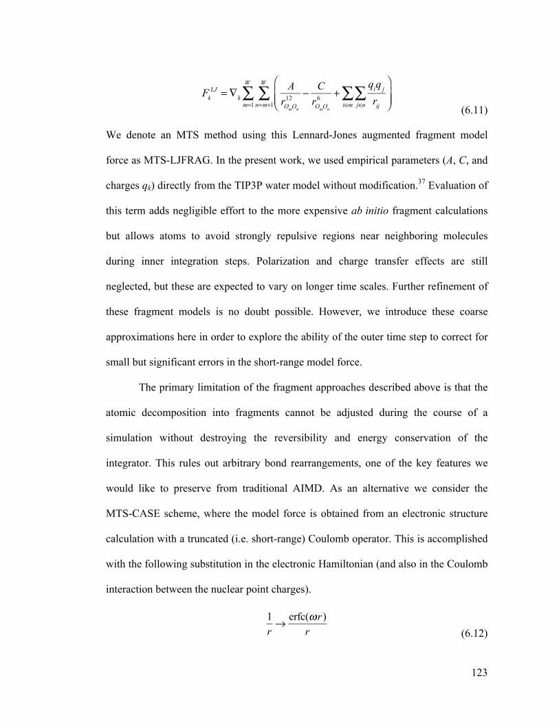
123

Fk

LJ = !k

ArOmOn

12 " CrOmOn

6 +qiq j

rijj#n$

i#m$

%

&''

(

)**n=m+1

W

$m=1

W

$ (6.11)

We denote an MTS method using this Lennard-Jones augmented fragment model

force as MTS-LJFRAG. In the present work, we used empirical parameters (A, C, and

charges qk) directly from the TIP3P water model without modification.37 Evaluation of

this term adds negligible effort to the more expensive ab initio fragment calculations

but allows atoms to avoid strongly repulsive regions near neighboring molecules

during inner integration steps. Polarization and charge transfer effects are still

neglected, but these are expected to vary on longer time scales. Further refinement of

these fragment models is no doubt possible. However, we introduce these coarse

approximations here in order to explore the ability of the outer time step to correct for

small but significant errors in the short-range model force.

The primary limitation of the fragment approaches described above is that the

atomic decomposition into fragments cannot be adjusted during the course of a

simulation without destroying the reversibility and energy conservation of the

integrator. This rules out arbitrary bond rearrangements, one of the key features we

would like to preserve from traditional AIMD. As an alternative we consider the

MTS-CASE scheme, where the model force is obtained from an electronic structure

calculation with a truncated (i.e. short-range) Coulomb operator. This is accomplished

with the following substitution in the electronic Hamiltonian (and also in the Coulomb

interaction between the nuclear point charges).

1r! erfc("r)

r (6.12)

124

Here ! is a constant parameter with units of inverse distance that determines the

range at which the Coulomb interaction is effectively quenched. Because the CASE

model force does not require an explicit molecular decomposition, it should, in

principle, have no difficulty with bond rearrangements. However, the accuracy with

which the CASE approximation can describe distorted transition geometries is a

serious concern. Figure 1 shows potential energy scans at the restricted Hartree-Fock

(RHF) and CASE levels of theory for the pictured dissociation of a hydroxide ion and

water molecule. While CASE accurately reproduces the RHF minimum-energy

oxygen-oxygen distance, the binding energy is catastrophically underestimated. Such

artifacts imply that physically relevant trajectories cannot be obtained from the CASE

potential surface. However, in MTS-CASE the outer time step corrects for the

difference between the CASE potential and the full RHF surface. Hence the MTS-

CASE trajectory evolves on the full potential surface and so should accurately

describe transition geometries.

Figure 1: Dissociation curves for an H2O/OH- cluster at the CASE and RHF levels of theory using the 6-31G basis set. Potential curves are generated from optimized geometries at constrained oxygen-oxygen distances. The energy for each curve is taken relative to its minimum value. The equilibrium bond distances are very similar. However, CASE severely under-estimates the binding energy, and includes an unphysical kink near 5 Angstroms.

125

RESULTS AND DISCUSSION

Figure 2: Energy conservation for 21ps simulation of an (H2O)57 water cluster using the MTS-LJFRAG integrator with outer and inner time steps of 2.5 and 0.5fs respectively. The simulation was run at the RHF/3-21G level of theory in the NVE ensemble after 5ps NVT equilibration at 350K. The cluster was confined by a spherical boundary chosen to lead to a density of 1g/mL. The blue curve shows total energy in kcal/mol shifted by +2.72x106 kcal/mol. The cyan line is a least-squares fit of total energy to show drift. Slope is 1.39x10-2 kcal/mol/ps for all degrees of freedom, i.e. 2.74x10-5 kcal/mol/ps/dof. The red curve shows total kinetic energy for scale.

In order to test these approaches, we implemented the ab initio MTS methods

described above in a development version of TeraChem.38 We first simulated the

dynamics of an (H2O)57 cluster at the RHF/3-21G level of theory. In all calculations,

the cluster was confined to a density of 1g/mL by applying a spherical quadratic

repulsive potential to oxygen atoms beyond the sphere’s radius. The barrier potential

was included in the inner time step of the MTS trajectories due to its negligible

126

computational cost compared to the ab initio force evaluation. The system was first

equilibrated for 5 ps using a standard Velocity Verlet36 integrator with the Bussi-

Parinello thermostat.39 During equilibration we used an MD time step of 1.0 fs, the

target temperature was 350K, and the thermostat time constant was 100 fs.

After equilibration, we collected a series of 21ps micro-canonical (NVE)

trajectories using a range of time steps for each of the MTS-FRAG, MTS-LJFRAG,

and MTS-CASE integrators outlined above. All simulations were started from

identical initial conditions. Baseline dynamics using the standard Velocity Verlet

integrator were collected with time steps between 0.5 and 1.5fs, since higher values

lead to unstable trajectories. Ab initio MTS trajectories used an inner time step of

0.5fs, with outer time steps ranging from 1.5 to 3.0fs. For the MTS-CASE integrator,

two screening ranges were tested: $=0.33 Bohr-1, which corresponds to an effective

screening distance of only 1.6 Å, and $=0.18 Bohr-1, which corresponds to 2.9Å.

The drift in total energy over the course of a simulation provides a test for the

quality of an integrator. An energy curve for an MTS-LJFRAG simulation using an

outer time step of 2.5fs is shown in figure 2. The drift was extracted by performing a

linear fit of the total energy over the 21ps trajectory and is almost unnoticeable on the

scale of the natural kinetic energy fluctuations of the system. The extracted slope is

2.74x10-5 kcal/mol/ps/dof, i.e. during the entire 21ps trajectory 5.75x10-4 kcal/mol of

energy is added to each degree of freedom due to inaccuracies in the integration of the

equations of motion. To put this in perspective, this is equivalent to a 0.289 K rise in

temperature of the system over that time. Current AIMD trajectories are generally

limited to around 100ps and hence even on this time-scale the increase in temperature

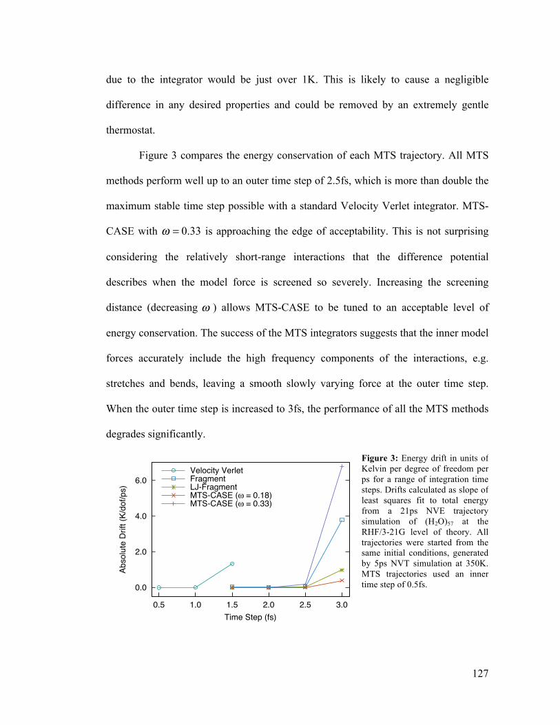
127

due to the integrator would be just over 1K. This is likely to cause a negligible

difference in any desired properties and could be removed by an extremely gentle

thermostat.

Figure 3 compares the energy conservation of each MTS trajectory. All MTS

methods perform well up to an outer time step of 2.5fs, which is more than double the

maximum stable time step possible with a standard Velocity Verlet integrator. MTS-

CASE with ! = 0.33 is approaching the edge of acceptability. This is not surprising

considering the relatively short-range interactions that the difference potential

describes when the model force is screened so severely. Increasing the screening

distance (decreasing ! ) allows MTS-CASE to be tuned to an acceptable level of

energy conservation. The success of the MTS integrators suggests that the inner model

forces accurately include the high frequency components of the interactions, e.g.

stretches and bends, leaving a smooth slowly varying force at the outer time step.

When the outer time step is increased to 3fs, the performance of all the MTS methods

degrades significantly.

Figure 3: Energy drift in units of Kelvin per degree of freedom per ps for a range of integration time steps. Drifts calculated as slope of least squares fit to total energy from a 21ps NVE trajectory simulation of (H2O)57 at the RHF/3-21G level of theory. All trajectories were started from the same initial conditions, generated by 5ps NVT simulation at 350K. MTS trajectories used an inner time step of 0.5fs. 0.0

2.0

4.0

6.0

0.5 1.0 1.5 2.0 2.5 3.0

Abso

lute

Drif

t (K/

dof/p

s)

Time Step (fs)

Velocity VerletFragmentLJ-FragmentMTS-CASE (! = 0.18)MTS-CASE (! = 0.33)

128

The failure of all methods with a 3fs outer time step is not surprising since

MTS integrators such as RESPA are known to suffer from non-linear resonance

instabilities.40,41 These instabilities, which arise due to interactions between the fast

forces and long time steps, mean that the fastest forces in the system limit how

infrequently the slowest interactions must be calculated at the outer time step. In the

case of our system the fastest modes, due to OH stretches of the dangling hydrogen

atoms at the surface of the cluster, oscillate at 4000 cm-1 (figure 4), corresponding to a

time period of %=8.5 fs. For a harmonic oscillator one can show that the maximum

stable outer time step is given by &Tmax = %/' which yields a resonance limit on the

time step of 2.7fs.42,43 This matches our observations precisely, and suggests that the

present limitations of our method do not stem from inadequacy of the model

potentials. It has been shown that resonance instabilities can be effectively mitigated

using specially designed Langevin thermostats.41,44 The application of these

techniques here is beyond the scope of the present study, but should increase the outer

time step by a further factor of 2-4 fold and thus further improve the computational

speedups reported here.

129

Figure 4: Power spectrum comparison between Velocity Verlet with 0.5fs time step (red), Velocity Verlet with 1.0fs time step (blue) and MTS-LJFRAG integrator with 2.5 and 0.5fs outer and inner time steps respectively (green). Spectra are based on 21ps NVE trajectories at the RHF/3-21G level of theory. System consists of 57 water molecules confined by a spherical boundary to a density of 1g/mL.

While energy conservation provides a test of the stability of MTS methods one

would also like to ensure that more subtle properties of the system remain unchanged.

For example, figure 4 shows the power spectrum of the system using 0.5fs and 1.0fs

time steps with a traditional Velocity Verlet integrator. Although in figure 3 we found

these both to provide acceptable energy conservation, the 1.0fs Verlet integrator shows

a clear frequency shift at high frequencies compared to the 0.5fs Verlet and MTS

integrators. Hence, although using standard Velocity Verlet may be stable, one should

take care regarding the properties obtained when large time-steps are employed.

0

0.1

0.2

0.3

0.4

0 1000 2000 3000 4000

Rel

ativ

e Po

wer

Wavenumber (cm-1)

Verlet 0.5fsVerlet 1.0fs

LJ-FRAG

130

Figure 5: Power spectrum comparison between standard Velocity Verlet (red), and MTS trajectories. Upper box compares simple fragment (blue), and Lennard-Jones augmented fragment (green) methods. Lower box compares MTS-CASE integration using two values of omega, 0.33 (blue) and 0.18 (green), which represent 1.6 and 2.9Å cutoffs of the Coulomb potential respectively. Spectra are based on 21ps NVE trajectories at the RHF/3-21G level of theory. System consists of 57 water molecules confined by a spherical boundary to a density of 1g/mL. MTS integrators use 2.5fs and 0.5fs for outer and inner time steps respectively. Verlet integrator uses 0.5fs time step.

Figure 5 shows the power spectra from the MTS trajectories using a 2.5fs

outer time step and 0.5fs inner time step compared with that obtained using standard

Velocity Verlet with a 0.5fs time step. In all cases the agreement is very good, with the

peak positions being very well reproduced. Remarkably all MTS methods with a 2.5fs

outer time step capture the power spectrum better than a Verlet integrator using a 1.0fs

time step. Peak intensities show greater variation, though this is likely due to the large

statistical error bars on power spectra obtained from a single 21ps trajectory.

It is clear from figure 5 that the empirically fit terms in the LJFRAG model

improve on the simpler FRAG approach. This suggests that the unmodified TIP3P

0

0.2

0.4R

elat

ive

Pow

erVerlet 0.5fs

FRAGLJ-FRAG

0

0.2

0.4

0 1000 2000 3000 4000Wavenumber (cm-1)

Verlet 0.5fsCASE (0.33)CASE (0.18)

131

force field is capturing some of the relevant high frequency intermolecular forces,

such as those from hydrogen bonds that are not included by the simpler monomer

fragment approach. Among the CASE spectra, the $=0.18 model shows only marginal

improvement over the coarser $=0.33 cutoff. Both outperform the simple fragment

approach, and are roughly equivalent to the Lennard-Jones fragment model.

Figure 6: Power spectra resulting from Velocity Verlet integrated dynamics on the CASE (blue) and RHF (red) potential energy surfaces compared with MTS-CASE (green) integration. The CASE approximation uses a cutoff of 0.33 Bohr-1 (1.6 Å) for both the Verlet and MTS integrators. Verlet-RHF and MTS-CASE spectra are based on 21ps NVE trajectories using the 3-21G basis set. Verlet-CASE spectrum is based on a shorter 14ps trajectory at the same level of theory. The system consists of 57 water molecules confined by a spherical boundary to a density of 1g/mL. Outer and inner timesteps for the MTS integrator are 2.5fs and 0.5fs respectively. Verlet integrators use 0.5fs time steps.

It is also instructive to compare MTS-CASE dynamics with that obtained by

traditional (Velocity Verlet) integration on the CASE potential surface. Figure 6

compares the power spectrum obtained from a 14ps simulation of dynamics on the

CASE (!=0.33) potential energy surface using a 0.5fs Velocity Verlet integrator to

that obtained from 0.5fs (RHF) Verlet and 2.5fs/0.5fs MTS-CASE (!=0.33). The

Verlet-CASE power spectrum is in pronounced disagreement with that obtained from

dynamics on the RHF surface. This is not surprising given the major quantitative

0

0.1

0.2

0.3

0.4

0.5

0 1000 2000 3000 4000

Rel

ativ

e Po

wer

Wavenumber (cm-1)

Verlet-RHFVerlet-CASE (!=0.33)MTS-CASE (!=0.33)

132

differences between the RHF and CASE potential surfaces shown in figure 1. It is

notable that the differences are most pronounced at the highest frequencies since one

might expect the O-H stretch to be relatively well preserved within CASE, given that

the Coulomb operator is unmodified at short ranges. However, this peak shows much

less structure in the CASE spectra and is significantly red-shifted from 4000 to

3600cm-1. Given these significant differences, it is remarkable that the MTS-CASE

trajectory gives a power spectrum close to that obtained on the RHF surface despite

using the CASE potential as the model for high-frequency force updates.

Thus far we have only considered water clusters, which do not undergo

covalent bond rearrangements on the simulated time-scale. However, one of the main

advantages of AIMD simulation is the ability for the system to undergo spontaneous

covalent bond breaking and formation during the simulation. Hence to evaluate the

ability of our MTS-CASE approach to describe bond rearrangements, we simulated

the proton transfer dynamics of a hydroxide ion solved in a cluster of 64 water

molecules. The system was equilibrated using the same procedure and boundary

conditions as the (H2O)57 cluster described above. A 21ps microcanonical simulation

was run at the RHF/3-21G level of theory using the MTS-CASE ($=0.33) integrator.

Figure 7 shows a 2ps window of the total trajectory. The energy drift of 1.54x10-4

kcal/mol/ps/dof (0.077K/ps/dof) was calculated by a linear fit to the entire 21ps

trajectory. For each frame the hydroxide oxygen atom was determined by assigning

each hydrogen atom to the nearest oxygen atom and then reporting the index of the

oxygen atom with a single assigned hydrogen (red line in figure 7).

133

Figure 7: Energy conservation of MTS-CASE integrator. Plot shows 2ps window from a longer 21ps trajectory. The NVE simulation was run at the RHF/3-21G level of theory after 5ps of NVT calibration to 350K. The inner and outer time steps were 0.5 and 2.5fs. The Coulomb attenuation parameter was 0.33 Bohr-1. The system was made up of a hydroxide ion solvated by 64 water molecules and was confined by a spherical barrier to a density of 1g/mL. A representative snapshot shows a proton transition between two oxygen atoms highlighted in blue. The blue curve shows the total energy in kcal/mol shifted by -3.10x106 kcal/mol. The green line gives a least squares fit of the total energy curve for the entire 21ps trajectory. Its slope records a drift of 8.7x10-2 kcal/mol/ps for the entire system or 1.5x10-4 kcal/mol/ps/dof. The red line indicates the index of the hydroxide oxygen atom for each time step. This was determined by assigning each hydrogen atom to its nearest oxygen neighbor, and then reporting the oxygen with a single assigned hydrogen. The magenta curve shows the total kinetic energy for scale.

As shown in the upper panel of figure 7, a proton oscillates primarily between

two oxygen atoms (shown in blue in the lower panel). During the entire 21ps

trajectory we observed over 500 proton transfer events. However, the total energy drift

is comparable to that reported above for the nonreactive (H2O)57 cluster. This is

remarkable on two counts. First, it demonstrates that the MTS scheme is applicable

even when bonds are being formed and broken – a difficult task for empirical force

fields and also for the fragment-based MTS-FRAG and MTS-LJFRAG schemes

134

described above. Second, the CASE approach we are using here is the most

aggressively screened of the two we have considered. With a screening factor of

$=0.33 bohr-1, the Coulomb interaction between any two charged particles is already

being attenuated at a distance of 1.6Å. Hence, in the inner time step, the proton barely

interacts with any electronic orbitals other than those on the two nearest heavy atoms.

All other interactions are corrected in the outer time step, which demonstrates

remarkable robustness by its ability to maintain the energy conservation observed

above.

Integrator Time Step (fs) Time/Step (sec) Steps/Day fs/day Speedup Velocity Verlet 0.5 430 201 100 1.0 Velocity Verlet 1.0 422 204 204 2.0 MTS-LJFrag 1.5 460 188 282 2.8 MTS-LJFrag 2.0 471 183 367 3.7 MTS-LJFrag 2.5 485 178 446 4.4 Table 1: Performance of MTS Lennard-Jones fragment compared to standard Velocity Verlet integrator. The system consists of 120 water molecules confined by a spherical boundary to a density of 1g/mL. The simulation was run at the RHF/6-31G level of theory using a single NVIDIA Tesla C2070 GPU. Step sizes for MTS integrator refer to the outer time step; 0.5fs inner time steps were used throughout. Timings are averaged over 100 MD steps and are in units of wall-time seconds per outer step. Speedups are computed by comparison to the 0.5fs Velocity Verlet integrator.

Finally, we consider the computational efficiency of our ab initio MTS

approach based on our initial implementation in TeraChem. Table 1 summarizes the

performance of the Lennard-Jones fragment MTS scheme relative to a standard

Velocity Verlet integrator with a time step of 0.5fs. Even though the Velocity Verlet

integrator is stable with a 1fs time step (figure 3), such a large time step noticeably

alters the dynamics, as demonstrated by the shift of the high frequency peak in the

power spectrum (figure 4). Hence, Velocity Verlet with a 0.5fs time step is the

appropriate comparison. These calculations were carried out with a larger (H2O)120

cluster treated at the RHF/6-31G level of theory and confined to a density of 1g/mL by

135

a spherical boundary. All calculations used a single Tesla C2070 GPU. Because the

outer time step still requires a full SCF gradient evaluation, the best that can be

achieved is a 5x speedup, if we compare an MTS integrator with a 2.5fs outer time

step to a standard Velocity Verlet method with a time step of 0.5fs. We are able to

achieve up to 4.4x speedup, which is over 88% efficient.

As with the fragment models, the CASE approximation leads to linear scaling

computational effort in evaluating the inner time steps.32 This is now due to improved

screening of electron repulsion integrals afforded by a short-range coulomb operator.

The present experimental code does not yet exploit the improved CASE screening.

However, previous work has shown that CASE at the screening levels employed here

offers significant computational speed-ups.32

CONCLUSION

In this paper we have demonstrated new approaches that allow MTS

integrators to be applied generally to AIMD calculations. We exploited the ability of

the outer MTS time steps to correct low frequency modeling errors within the inner

time steps. Thus we were able to employ drastically simplified short-range

approximations to the ab initio forces in the inner time steps. Despite these

computational savings, the resulting methods remain robust, exhibiting symplecticity

and time-reversibility and providing excellent energy conservation and even improved

dynamical properties compared to Verlet integrators with moderately large time steps.

As with single-step integrators our ab initio MTS methods can be systematically

improved by reducing the time steps or, for MTS-CASE, also by increasing the

screening distance.

136

The model forces used here are inspired by linear scaling approximations.

However, while linear scaling methods attempt to globally capture all significant

interactions, MTS model forces need only represent the highest frequencies within the

system, and even here low frequency differences between the model and ab initio

systems can be tolerated. This means that much looser thresholds can be employed in

the case of MTS model forces. Thus, even for systems too small to reach the crossover

point for traditional linear scaling methods, our MTS scheme can provide a significant

speedup. For larger systems where linear scaling approaches are applicable, the MTS

approaches introduced here can still be applied, since its looser thresholds should

allow the model forces to be computed more cheaply than the more accurate linear-

scaling gradient.

Other model forces are obviously possible. For example, our use of the TIP3P

force field suggests a completely empirical model force. However, the benefits of such

models are limited by the cost of the global gradient calculation in the outer time step.

In the present case, reducing the computational effort of the inner time step would at

best yield a 13% speedup over the fragment approaches described above. Thus, future

work should focus on extending the outer time step and on reducing the cost of the

global gradient evaluation. For example, employing existing Langevin thermostats44 to

remove spurious resonance effects should allow the outer time step to be extended to

10 or even 20 fs and provide greater performance gains.

REFERENCES

(1) Tuckerman, M. E.; Berne, B. J. The Journal of Chemical Physics 1991, 95, 8362.

137

(2) Tuckerman, M. E.; Berne, B. J.; Martyna, G. J. The Journal of Chemical Physics 1991, 94, 6811.

(3) Tuckerman, M. E.; Berne, B. J.; Martyna, G. J. The Journal of Chemical Physics 1992, 97, 1990.

(4) Tuckerman, M. E.; Berne, B. J.; Rossi, A. The Journal of Chemical Physics 1991, 94, 1465.

(5) Tuckerman, M. E.; Martyna, G. J.; Berne, B. J. The Journal of Chemical Physics 1990, 93, 1287.

(6) Grubmuller, H.; Heller, H.; Windemuth, A.; Schulten, K. Mol. Sim. 1991, 6, 121.

(7) Streett, W. B.; Tildesley, D. J.; Saville, G. Mol. Phys. 1978, 35, 639.

(8) Carloni, P.; Rothlisberger, U.; Parrinello, M. Acc. Chem. Res. 2002, 35, 455.

(9) VandeVondele, J.; Sulpizi, M.; Sprik, M. Ang. Chem. Int. Ed. 2006, 45, 1936.

(10) Virshup, A. M.; Punwong, C.; Pogorelov, T. V.; Lindquist, B. A.; Ko, C.; Martinez, T. J. J. Phys. Chem. B 2009, 113, 3280.

(11) Ben-Nun, M.; Martinez, T. J. Adv. Chem. Phys. 2002, 121, 439.

(12) Barnett, R. N.; Landman, U.; Nitzan, A.; Rajagopal, G. J. Chem. Phys. 1991, 94, 608.

(13) Leforestier, C. J. Chem. Phys. 1978, 68, 4406.

(14) Payne, M. C.; Teter, M. P.; Allan, D. C.; Arias, T. A.; Joannopoulos, J. D. Rev. Mod. Phys. 1992, 64, 1045.

(15) Car, R.; Parrinello, M. Phys. Rev. Lett. 1985, 55, 2471.

(16) Tuckerman, M. E.; Ungar, P. J.; von Rosenvinge, T.; Klein, M. L. J. Phys. Chem. 1996, 100, 12878.

(17) Hartke, B.; Gibson, D. A.; Carter, E. A. Int. J. Quant. Chem. 1993, 45, 59.

(18) Gibson, D. A.; Carter, E. A. J. Phys. Chem. 1993, 97, 13429.

(19) Tuckerman, M. E.; Parrinello, M. J. Chem. Phys. 1994, 101, 1316.

(20) Steele, R. P. J. Chem. Phys. 2013, 139, 011102.

(21) Yang, W. T. Physical Review Letters 1991, 66, 1438.

138

(22) Yang, W. T. Physical Review A 1991, 44, 7823.

(23) Gordon, M. S.; Freitag, M.; Bandyopadhyay, P.; Jensen, J. H.; Kairys, V.; Stevens, W. J. J. Phys. Chem. A 2001, 105, 293.

(24) Gordon, M. S.; Smith, Q. A.; Xu, P.; Slipchenko, L. V. Ann. Rev. Phys. Chem. 2013, 64, 553.

(25) He, X.; Zhang, J. Z. H. J. Chem. Phys. 2006, 124, 184703.

(26) Steinmann, C.; Fedorov, D. G.; Jensen, J. H. PLOS One 2013, 8, e60602.

(27) Xie, W.; Orozco, M.; Truhlar, D. G.; Gao, J. J. Chem. Theo. Comp. 2009, 5, 459.

(28) Fedorov, D. G.; Nagata, T.; Kitaura, K. Phys. Chem. Chem. Phys. 2012, 14, 7562.

(29) Pruitt, S. R.; Addicoat, M. A.; Collins, M. A.; Gordon, M. S. Phys. Chem. Chem. Phys. 2012, 14, 7752.

(30) Collins, M. A. Phys. Chem. Chem. Phys. 2012, 14, 7744.

(31) Adamson, R. D.; Dombroski, J. P.; Gill, P. M. W. Chem. Phys. Lett. 1996, 254, 329.

(32) Adamson, R. D.; Dombroski, J. P.; Gill, P. M. W. J. Comp. Chem. 1999, 20, 921.

(33) Suzuki, M. Commun Math Phys 1976, 51, 183.

(34) Trotter, H. F. Proc. Amer. Math. Soc. 1959, 10, 545.

(35) Sanz-Serna, J. M.; Calvo, M. P. Numerical Hamiltonian Problems; Chapman and Hall: London, 1994.

(36) Swope, W. C.; Andersen, H. C.; Berens, P. H.; Wilson, K. R. J. Chem. Phys. 1982, 76, 637.

(37) Jorgensen, W. L.; Chandrasekhar, J.; Madura, J. D.; Impey, R. W.; Klein, M. L. The Journal of Chemical Physics 1983, 79, 926.

(38) Ufimtsev, I. S.; Martinez, T. J. J. Chem. Theo. Comp. 2009, 5, 2619.

(39) Bussi, G.; Donadio, D.; Parrinello, M. J. Chem. Phys. 2007, 126, 014101.

(40) Biesiadecki, J. J.; Skeel, R. D. J. Comp. Phys. 1993, 109, 318.

139

(41) Ma, Q.; Izaguirre, J. A.; Skeel, R. D. Siam J Sci Comput 2003, 24, 1951.

(42) Barth, E.; Schlick, T. J. Chem. Phys. 1998, 109, 1633.

(43) Han, G. W.; Deng, Y. F.; Glimm, J.; Martyna, G. Comp. Phys. Comm. 2007, 176, 271.

(44) Morrone, J. A.; Markland, T. E.; Ceriotti, M.; Berne, B. J. J. Chem. Phys. 2011, 134, 014103.

140

141

CHAPTER SEVEN

INTERACTIVE AB INITIO MOLECULAR DYNAMICS

The previous chapter was focused on extending AIMD to large systems, where

long time scales are important. In this chapter we explore the impact of accelerated

AIMD applied to small systems containing up to a few dozen atoms. In this regime,

the steady advance of computers could soon transform the basic models used to

understand and describe chemistry. In terms of quantitative models in general,

researchers no longer seek human comprehensible, closed-form equations such as the

ideal gas law. Instead algorithmic models that are evaluated through intensive

computer simulations have become the norm. As a few examples, ab initio electronic

structure, molecular dynamics (MD), and minimum energy reaction path optimizers

are now standard tools for describing chemical systems.

Despite their often-impressive accuracy, quantitative models sometimes

provide surprisingly little scientific insight. For example, individual MD trajectories

are chaotic and can be just as inscrutable to human understanding as the physical

experiment they seek to elucidate. Qualitative cartoon-like models, it seems, are

essential to inspire human imagination and satisfy our curiosity. As an illustration,

consider the pervasive use of primitive ball-and-stick type molecular models in

chemistry. The success of these physical models lies as much in their ability to capture

human imagination and support interesting geometric questions as it does in their

inherent realism. Useful models must be both accurate and playful.

142

Fortunately, computers are capable of much more than crunching numbers for

quantitative models. With the development of computer graphics and the explosion of

immersive gaming technologies, computers also provide a powerful platform for

human interaction. Starting with works by Johnson1 and Levinthal2 in the 1960’s,

molecular viewers were developed first to visualize and manipulate x-ray structures

and later to visualize the results of MD simulations as molecular movies. The next

goal was to allow researchers to interact with realistic physical simulations in real time

as they ran. Along these lines, the Sculpt project provided an interactive geometry

optimizer that included a user-defined spring force in a modified steepest descent

optimizer.3 By furnishing the molecular potential from a classical force field further

simplified with rigid bonds and strict distance cutoffs for non-bonded interactions,

Sculpt could achieve real-time calculation rates for protein systems containing up to

eighty residues, which was certainly impressive at the time.

Later work replaced Sculpt’s geometry optimizer with a MD kernel.4,5 Rather

than being limited to minimum energy structures, the user could then probe dynamical

behavior of protein systems, watching the dynamics trajectory unfold in real time and

insert arbitrary spring forces to steer the dynamics in any direction of interest. Force-

feedback devices have also been used to control molecular tugs.6 These allow users to

feel as well as see the molecular interactions and increase the precision of user control.

Of course, arbitrary user interaction is a (sometimes large) source of energy flow into

the simulation. Aggressive thermostats are necessary to reduce this heating.4 As a

consequence, the results of interactive dynamics are not immediately applicable, for

example, in calculating statistical properties. However, for small forces the trajectories

143

will explore phase space regions that are still relevant to dynamics on standard

ensembles, and thus offer many qualitative mechanistic insights.

Classical force fields suffer from two disadvantages that hamper their

application to general-purpose chemical modeling. First they are empirically tuned,

and as a result are valid only in a finite region of configuration space. This is

particularly problematic for interactive simulations, where the user is free to pull the

system into highly distorted configurations. The second, more important disadvantage

is that covalent bonds modeled by classical springs cannot be rearranged during the

simulation. Ab initio forces, calculated from first principles electronic structure theory,

do not suffer from these disadvantages and provide ideal potentials for use with

interactive dynamics. However, due to prohibitive computational costs, it remains

difficult to evaluate ab initio forces at the fast rate necessary to support real-time

dynamics.

Recently, a divide-and-conquer implementation of the semi-empirical atom

superposition and electron delocalization molecular orbital (ASED-MO) model has

been developed to support real-time energy minimization and MD in the SAMSON

program.7,8 SAMSON offers impressive performance, able to perform real-time

calculations on systems containing up to thousands of atoms. User interaction is

implemented by alternating between “user action steps” in which the user moves or

inserts atoms, and standard optimization or MD steps. In order to keep the

computational complexity manageable, SAMSON applies several approximations

beyond those inherent in ASED-MO. The global system is split into overlapping sub-

problems that are solved independently in parallel. Also for large systems, distant

144

atoms are frozen so that only forces for atoms in the region of user interaction need to

be calculated in each step.

Several previous attempts at full ab initio interactive dynamics have been

reported. In early work, Marti and Reiher avoided on the fly electronic structure

calculations by using an interpolated potential surface.9 The potential surface is pre-

calculated over some relevant configuration space. Then during dynamics, the force at

each time step is obtained from a simple moving least-squares calculation. However, it

is difficult to predict a priori what regions of configuration space will be visited. A

partial solution is to periodically add additional interpolation points where and when

higher accuracy is desired.10 However, the number of needed interpolation points

grows exponentially with the dimensionality of the system. Thus, for non-trivial

systems, it is essential to evaluate the ab initio gradient on the fly. Recently the

feasibility of such calculations has been tested using standard packages and tools.

Combining the Turbomole DFT package, minimal basis sets, effective core potentials

and a quad core processor, Haag and Reiher achieve update rates on the order of a

second for systems containing up to 8 atoms.11

In the following we present the results of our own implementation of

interactive ab initio dynamics. By using the GPU accelerated TeraChem12 code and

carefully streamlining the calculation, interactive simulations are possible for systems

up to a few dozen atoms. The final result is a virtual molecular modeling kit that

combines intuitive human interaction with the accuracy and generality of an ab initio

quantum mechanical description.

145

METHOD

The ab initio interactive MD (AI-IMD) system described below is based on the

interactive MD (IMD) interface that was previously developed to enable interactive

steered molecular dynamics in the context of classical force fields.6 A high level

overview of the original scheme is shown in figure 1. Molecular visualization and

management of the haptic (or “touch”) interface is handled by VMD.13 Along with the

current molecular geometry, VMD displays a pointer that the user controls through a

3D haptic device (shown in figure 5). Using the pointer, the user can select and tug an

atom feeling the generated force through feedback to the haptic device. VMD also

sends the haptic forces to a separate MD program, in our case TeraChem,12 where they

are included with the usual ab initio gradient in the following haptic-augmented force.

F (R,t) = !" Eqm (R)+ Fhap (t) (7.1)

After integrating the system forward in time, TeraChem returns updated coordinates

for display in VMD.

Figure 1: Schematic representation of the IMD interface previously developed for classical MD calculations. VMD is responsible for visualization while TeraChem performs AIMD calculations in real time.

A major advantage of the IMD scheme is that it uses spring forces to cushion

the user’s interaction with the system, rather than raw position updates. This allows

the user to add weak biases that do not totally disrupt the initial momentum of the

TeraChemVMD MD Coords

Haptic Forces

Forc

e Fe

edba

ckPo

inte

r Pos

ition

MD Coords

Pointer Position

3D Display

Haptic Device

146

system. It also avoids severe discontinuities that would overthrow the numerical

stability of standard MD integrators. As a result, the system’s dynamics and energy are

always well-defined, albeit for a time-dependent Hamiltonian, and the magnitude of

haptic perturbations can in principle be accurately measured and controlled.

Communication across the IMD interface is asynchronous. In VMD the render

loop does not wait for updated coordinates between draws and force updates are sent

to TeraChem continuously as they happen rather than waiting for the next MD time-

step. Similarly, TeraChem does not wait to receive haptic force updates between time

steps. This scheme was designed to minimize communication latencies.6

Asynchronous communication also logically decouples the software components and

allows each to operate in terms of generic streams of coordinates and simplifies the

process of adapting the system from classical to ab initio MD as detailed below.

Due to the considerations above, the IMD approach provides a robust starting

point for AI-IMD. However, several adjustments to the classical IMD approach are

needed to accommodate ab initio calculations. These are detailed in the following

sections.

Simulation Rate

A primary benefit of interactive modeling is that molecular motions, as well as

static structures, can be intuitively represented and manipulated. Thus it is critical to

maintain a sensation of smooth motion. To achieve this, past research has targeted

simulation rates of at least ten or twenty MD steps per second.4,5,8 Such update rates

are comparable to video frame rates and certainly result in smooth motion. At present,

however, quantum chemistry calculations requiring less than fifty milliseconds are

147

possible only for trivially small systems. In order to reach larger molecules and basis

sets, it is important to decouple graphical updates from the underlying MD time steps.

Ultimately, the necessary simulation rate is dictated not by graphics considerations,

but by the time scale of the motion being studied. The goal of interactive MD is to

shift the movement of atoms to the time scale of seconds on which humans naturally

perceive motion. For molecular vibrations, this requires simulating a few

femtoseconds of molecular trajectory per second of wall time. Assuming a 1 fs time

step, each gradient evaluation is then allowed at least 200ms to execute. Experiments

show that up to a full second between ab initio gradient evaluations is workable,

though the resulting dynamics become increasingly sluggish.

In addition to high performance, an interactive interface requires a uniform

simulation rate. Each second of displayed trajectory must correspond to a standard

interval of simulated time. This is critical both to convey a visual sensation of smooth

motion as well as to provide consistent haptic physics. For example, the effective

power input of a given haptic input will increase with the simulation rate, since the

same duration of pull in wall time translates into longer pulls in simulated time.6

Problematically, the effort needed to evaluate the ab initio gradient varies widely

depending on the molecular coordinates. For many geometries, such as those near

equilibrium, the SCF equations can be converged in just a few iterations by using

guess orbitals from previous MD steps. For strongly distorted geometries, however,

hundreds of SCF iterations are sometimes required. Even worse, the SCF calculation

may diverge causing the entire calculation to abort. Since users tend to drive the

system away from equilibrium, difficult to converge geometries are more common in

148

interactive MD than in dynamics run on traditional ensembles (see figure 2). To

handle these distorted geometries, we employ the very robust ADIIS+DIIS

convergence accelerator.14,15 However, for well-behaved geometries, ADIIS+DIIS was

found on average to require more iterations than DIIS alone. Thus, the best approach

is to converge with standard DIIS for up to ~20 iterations, and switch over to

ADIIS+DIIS only where DIIS fails.

Figure 2: Histogram of wall-times for 1000 steps of MD run with user interaction (red) and without haptic input (blue). The system was the uncharged imidaloze molecule pictured. The simulation used the unrestricted Hartree-Fock electronic structure method with the 3-21G basis. Each step of the SCF was converged to 2.0e-5 in the maximum element of the commutator SDF-FDS.

In order to establish a fixed simulation rate we consider the variance in timings

for individual MD steps illustrated for a particular system in figure 2. Noting that the

large variance in MD step timings is primarily the result of a few outliers, the target

wall time for a simulation step, Twall, can be set far below the worst-case gradient

evaluation time. For the vast majority of steps, the ab initio gradient then completes

before Twall has elapsed and the MD integrator must pause briefly to allow the display

to keep pace. For pathologically long MD steps, such as those requiring many ADIIS

iterations, the displayed trajectory is frozen and haptic input ignored until the MD step

completes.

149

Integrating the haptic force

A key strength of AI-IMD is that it allows users to make and break bonds

between atoms. However, this level of control requires haptic forces that are stronger

than the bonding interactions between atoms. The situation in classical IMD is very

different. Classical force fields in general cannot handle bond reorganization. Thus,

IMD was originally conceived to control only weak non-bonded interactions. In

practice, the inclusion of this strong haptic force in equation (7.1) can produce

noticeable energetic artifacts in the MD simulation. For example, an unbound atom

vibrating around a fixed haptic pointer might visibly gain amplitude with each

oscillation. Such non-conservative dynamics result in rapid heating of the system that

quickly swamps the user’s control. The cause is simply that the MD time step that

would appropriately integrate a closed system is too long to accurately handle the

stronger haptic forces. An obvious solution is to use a shorter time step. However,

reducing the time step would adversely slow the simulation rate, severely reducing the

size of systems that can be modeled interactively. As the system becomes more

sluggish, the user will also tend to increase the haptic force, exacerbating the problem.

A more elegant solution is to use a multiple time step integrator, such as

reversible RESPA,16 to separate the haptic forces from the ab initio interactions. The

weaker ab initio forces can then use a longer MD time step and be evaluated less

frequently (in wall time) than the stronger haptic forces. Between each ab initio

update, l sub-steps are used to accurately integrate the haptic force as follows.

150

Vi(n+1/2,0) !Vi

(n,l ) +Ai(n) "t2

l #

Vi(n+1/2,m+1/2) !Vi

(n+1/2,m ) +Fihap (tn,m )2mi

$ t

Xi(n,m+1) !Xi

(n,m ) +Vi(n+1/2,m+1/2)$ t

Vi(n+1/2,m+1) !Vi

(n+1/2,m+1/2) +Fihap (tn,m+1)2mi

$ t

%

&

'''

(

'''

Xi(n+1,0) !Xi

(n,l )

Ai(n+1) ! )*iE

qm (Xi(n+1,0) )

mi

Vi(n+1,0) !Vi

(n+1/2,l ) +Ai(n+1) "t

2

(7.2)

Here !t is the MD time step between ab initio force updates while the inner

time step, "t=!t/l, governs the interval between haptic force evaluations. A is the

acceleration due only to the ab initio forces, while Fhap (tn,m ) is the haptic force vector

evaluated at time tn,m = n!t +m" t . Compared to the computational costs of an

electronic structure calculation, it is trivial to integrate the haptic force in each sub-

step. Thus, the MTS scheme runs at the full speed of the simpler velocity Verlet

algorithm.

A second difficulty arises when incorporating strong haptic forces in MD. As

shown in figure 1 above, in the classical IMD scheme, VMD is responsible for

calculating the haptic force based on the currently displayed positions of the targeted

atom and haptic pointer. However, due to communication latencies and the time

required for VMD to complete each graphical update, the forces received by

TeraChem lag the simulated trajectory by at least 7ms. Importantly, this lag shifts the

forces in resonance with the system’s nuclear motion. The result is again uncontrolled

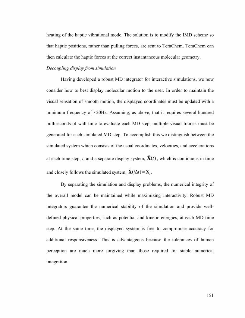
151

heating of the haptic vibrational mode. The solution is to modify the IMD scheme so

that haptic positions, rather than pulling forces, are sent to TeraChem. TeraChem can

then calculate the haptic forces at the correct instantaneous molecular geometry.

Decoupling display from simulation

Having developed a robust MD integrator for interactive simulations, we now

consider how to best display molecular motion to the user. In order to maintain the

visual sensation of smooth motion, the displayed coordinates must be updated with a

minimum frequency of ~20Hz. Assuming, as above, that it requires several hundred

milliseconds of wall time to evaluate each MD step, multiple visual frames must be

generated for each simulated MD step. To accomplish this we distinguish between the

simulated system which consists of the usual coordinates, velocities, and accelerations

at each time step, i, and a separate display system, !X(t) , which is continuous in time

and closely follows the simulated system, !X(i!t) " Xi .

By separating the simulation and display problems, the numerical integrity of

the overall model can be maintained while maximizing interactivity. Robust MD

integrators guarantee the numerical stability of the simulation and provide well-

defined physical properties, such as potential and kinetic energies, at each MD time

step. At the same time, the displayed system is free to compromise accuracy for

additional responsiveness. This is advantageous because the tolerances of human

perception are much more forgiving than those required for stable numerical

integration.

152

Figure 3: Schematic of simulated and visualized systems. Visualized frames (right boxes) lag the simulated coordinates (left boxes) by one ab initio gradient evaluation. The visualized coordinates are interpolated between MD time steps, but the simulated and visualized coordinates match after each step. The visualized haptic position is read from the device at each visual frame, but is sampled by the simulation once per MD step. The l MTS substeps of equation 7.2 calculate the haptic forces from a common haptic position.

Consider a simplified case in which the simulated trajectory is integrated using

the velocity Verlet integrator.17 In each MD step, the simulated system is propagated

t femtoseconds forward in simulation time as follows.

Step 1: X(n+1) = X(n) +V(n)!t + 12A(n)!t 2

Step 2: Ai(n+1) = "#iE

ai (X(n+1) )+ Fihap ((n +1)!t)

mi

Step 3: V(n+1) = V(n) + A(n) +A(n+1)

2!t

(7.3)

Here the evaluation of the ab initio gradient dominates the wall time required to

compute each MD step, Twall. Latency between haptic inputs and the system’s

response would be minimized by immediately displaying each coordinate vector,

X(n+1), as it is calculated in step 1. However, in this case displaying further motion

VisualizationTeraChemSimulation

Wal

l Tim

e

Update Xn-1 → Xn

Calculate

-∇E(Xn) → Fn

Sample hn-1

Update Xn → Xn+1

Calculate

-∇E(Xn+1) → Fn+1

Sample hn

Update Xn → Xn+1

Sample hn

Hap

tic P

ositi

on

153

during the time consuming calculation of A(n+1) in step 2 would require extrapolation

forward in time. In practice such extrapolation leads to noticeable artifacts as the

simulated and displayed coordinates diverge. An alternative is to buffer the displayed

trajectory by one MD step. Thus X(n) is displayed as X(n+1) is calculated in step 1, and

the display can then interpolate toward a known X(n+1) during the succeeding gradient

evaluation. In this way, smooth motion is achieved. The distinction between simulated

and visualized systems is illustrated in figure 3.

A variety of interpolation schemes are possible for !X . For example, linear

interpolation would give the following trajectory.

!X(nTwall + t) = X

(n) + X(n+1) !X(n)

Twallt (7.4)

Here t is given in wall time. While equation (7.4) provides continuous molecular

coordinates, the visualized velocity jumps discontinuously by

! !V = A(n+1) !t 2

Twall (7.5)

after each MD step. These velocity jumps can be reduced to

! !V = A

(n) "A(n"1)

2!t 2

Twall (7.6)

by continuously accelerating the display coordinates over the interpolated path as

follows.

!X(nTwall + t) = X

(n) +V(n) !tTwall

t + 12A(n) !t 2

Twall2 t 2 (7.7)

154

This trajectory is again continuous in coordinate space, and additionally, in the special

case of a constant acceleration, the velocity is also continuous between MD steps.

Since for MD simulations, molecular forces change gradually from step to step,

equation (7.7) is sufficient to reduce velocity discontinuities below the threshold of

human perception.

The simple approach of equation (7.7) is easily extended to the more

complicated MTS integrator developed above. For example, the displayed trajectory

can be defined piecewise between sub steps as follows.

!X n +ml( )Twall + t( ) = X(n,m ) +V(n,m ) !t

Twallt + 12A(n,m ) !t 2

Twall2 t 2 (7.8)

However, since the ab initio gradient “kicks” the velocity only at the outer time step,

equation (7.8) corresponds to a linear interpolation in the ab initio forces similar to

equation (7.4). Amortizing the ab initio acceleration over the time step, while applying

each haptic acceleration over its own sub-step produces a smoother trajectory.

!X n +ml( )Twall + t( ) = X(n,0) +V(n,0) !t

Twallt + 12A(n) !t 2

Twall2 t 2 (7.9)

As a result of this smoothing, the simulated and displayed systems do not

match at each sub-step. However, by applying the same haptic forces calculated for

the simulated system to the visual system, the systems will match to within machine

precision at the outer time steps. To avoid any buildup of round-off error, the display

coordinates are re-synced to the simulated system after each step.

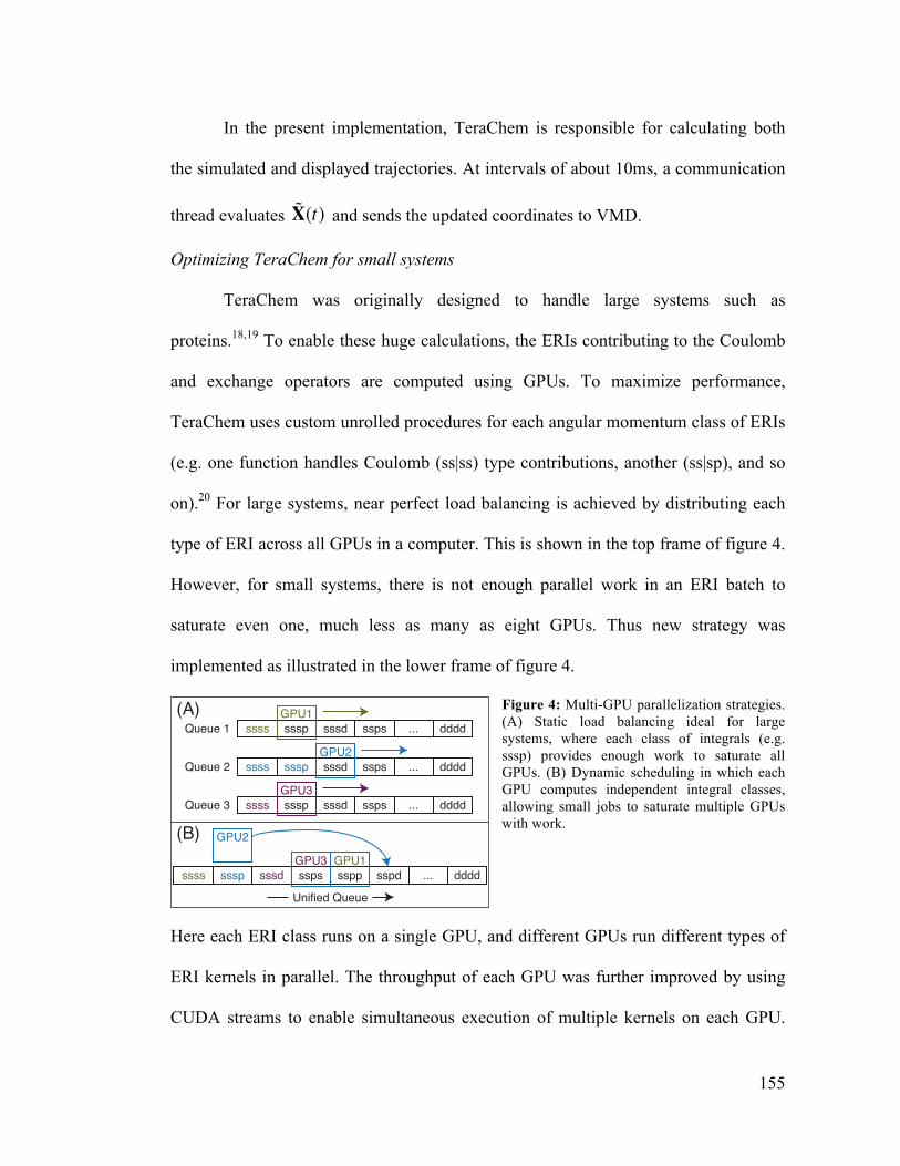
155

In the present implementation, TeraChem is responsible for calculating both

the simulated and displayed trajectories. At intervals of about 10ms, a!communication

thread evaluates !X(t) and sends the updated coordinates to VMD.

Optimizing TeraChem for small systems

TeraChem was originally designed to handle large systems such as

proteins.18,19 To enable these huge calculations, the ERIs contributing to the Coulomb

and exchange operators are computed using GPUs. To maximize performance,

TeraChem uses custom unrolled procedures for each angular momentum class of ERIs

(e.g. one function handles Coulomb (ss|ss) type contributions, another (ss|sp), and so

on).20 For large systems, near perfect load balancing is achieved by distributing each

type of ERI across all GPUs in a computer. This is shown in the top frame of figure 4.

However, for small systems, there is not enough parallel work in an ERI batch to

saturate even one, much less as many as eight GPUs. Thus new strategy was

implemented as illustrated in the lower frame of figure 4.

Figure 4: Multi-GPU parallelization strategies. (A) Static load balancing ideal for large systems, where each class of integrals (e.g. sssp) provides enough work to saturate all GPUs. (B) Dynamic scheduling in which each GPU computes independent integral classes, allowing small jobs to saturate multiple GPUs with work.

Here each ERI class runs on a single GPU, and different GPUs run different types of

ERI kernels in parallel. The throughput of each GPU was further improved by using

CUDA streams to enable simultaneous execution of multiple kernels on each GPU.

(A)

(B)Queue 3 ssss sssp sssd ssps ... dddd

GPU3Queue 2 ssss sssp sssd ssps ... dddd

GPU2Queue 1 ssss sssp sssd ssps ... dddd

GPU1

ssss sssp sssd ssps sspp sspdGPU1

...GPU3

GPU2

ddddUnified Queue

156

Dynamic load balancing was enabled through Intel Cilk Plus work-stealing queues.

Together these schemes significantly increase the parallelism exposed by a small

calculation.

When handling small systems, it is also essential to minimize execution

latencies that may not have been apparent in larger calculations. In GPU code,

communication across the PCIe bus is a common cause of latency. This was

minimized by using asynchronous CUDA streams which are provided as part of the

CUDA runtime. CUDA streams reduce latencies for host-GPU communication and

enable memory transfers to overlap kernel execution. Another important cause of

latency is the allocation and release of GPU memory. While memory allocation is an

expensive operation on most architectures, allocations are particularly costly on the

GPU, triggering synchronization across devices and even serializing the execution of

kernels run on separate GPUs. To eliminate these costs, large blocks of memory are

pre-allocated from each GPU at the start of the calculation. Individual CPU threads

request these pre-allocated blocks as needed. A mutual exclusion lock is used to

guarantee thread safety during the assignment of GPU memory blocks. Once assigned,

the memory block is the sole property of a single thread and can be used without

further synchronization. Extending this system, blocks of page-locked host memory

are also pre-allocated and distributed along with the GPU memory blocks. By

assembling GPU input data in page-locked host memory, the driver can avoid staging

transfers through an internal buffer, further improving latency.

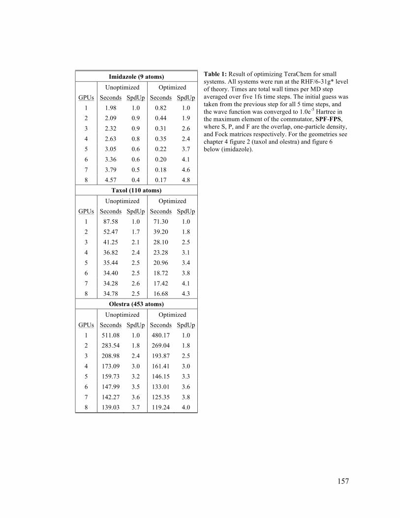
157

Table 1: Result of optimizing TeraChem for small systems. All systems were run at the RHF/6-31g* level of theory. Times are total wall times per MD step averaged over five 1fs time steps. The initial guess was taken from the previous step for all 5 time steps, and the wave function was converged to 1.0e-5 Hartree in the maximum element of the commutator, SPF-FPS, where S, P, and F are the overlap, one-particle density, and Fock matrices respectively. For the geometries see chapter 4 figure 2 (taxol and olestra) and figure 6 below (imidazole).

Imidazole (9 atoms)

Unoptimized Optimized GPUs Seconds SpdUp Seconds SpdUp

1 1.98 1.0 0.82 1.0 2 2.09 0.9 0.44 1.9 3 2.32 0.9 0.31 2.6 4 2.63 0.8 0.35 2.4 5 3.05 0.6 0.22 3.7 6 3.36 0.6 0.20 4.1 7 3.79 0.5 0.18 4.6 8 4.57 0.4 0.17 4.8

Taxol (110 atoms)

Unoptimized Optimized GPUs Seconds SpdUp Seconds SpdUp

1 87.58 1.0 71.30 1.0 2 52.47 1.7 39.20 1.8 3 41.25 2.1 28.10 2.5 4 36.82 2.4 23.28 3.1 5 35.44 2.5 20.96 3.4 6 34.40 2.5 18.72 3.8 7 34.28 2.6 17.42 4.1 8 34.78 2.5 16.68 4.3

Olestra (453 atoms)

Unoptimized Optimized GPUs Seconds SpdUp Seconds SpdUp

1 511.08 1.0 480.17 1.0 2 283.54 1.8 269.04 1.8 3 208.98 2.4 193.87 2.5 4 173.09 3.0 161.41 3.0 5 159.73 3.2 146.15 3.3 6 147.99 3.5 133.01 3.6 7 142.27 3.6 125.35 3.8 8 139.03 3.7 119.24 4.0

158

ASSESSMENT

In order to benchmark the numerical stability of the AI-IMD integrator, we

first consider the trivial diatomic system, HCl. Because the user does work through the

haptic forces, interactive dynamics will not in general conserve the total energy of the

system. Energy is conserved, however, in the special case of a fixed pulling position

since the spring force can be construed as a function of only the molecular geometry,

and the Hamiltonian becomes time independent. Indeed, in this case, the resulting

dynamics simply evolves on a force-modified potential energy surface.21 Using this

special case, the AI-IMD integrator is validated as follows. First the HCl molecule is

minimized at the RHF/6-31G** level of theory. The resulting geometry is aligned

along the y-axis with the chlorine atom located at the origin and the hydrogen at

y=1.265 Angstroms. The test system also includes a haptic spring connecting the

hydrogen atom to a fixed pulling point at y=1.35 Angstroms.

Starting from the above initial geometry, AI-IMD calculations were run using

varying haptic spring constants and MTS sub-steps. All calculations used a fixed time

step of 1.0fs to integrate the ab initio forces. For smaller haptic force constants, below

0.7 Hartree/Bohr2, the haptic-induced motions occur on timescales comparable to ab

initio forces encountered in near-equilibrium MD. Thus, a simple velocity Verlet

integrator conserves energy about as well as the MTS approach developed above. At

larger forces, however, velocity Verlet becomes increasingly unstable. Figure 5

demonstrates the stability of our AI-IMD integrator for a spring constant of 2.6

Hartree/Bohr2. Here the velocity Verlet integrator rapidly diverges, while an MTS

integrator using 5 sub-steps remains stable. Although overall energy drifts increase at

159

higher forces, the MTS approach does not exhibit wild divergence even at a force

constant of 4.0 Hartree/Bohr2. This is important because explosive divergence is a

much greater obstacle to controlling the system than is a slow energy drift. In general,

the motion of the haptic tugging point will itself induce heating so that a thermostat is

already required to counter the slow accumulation of energy during long simulations.

Figure 5: Total energy for IMD simulation of HCl with fixed tugging point. HCl was aligned with y-axis, with Cl intially at the origin and H at y=1.265 Angstoms. The haptic force pulled toward y=1.35 Angstroms with a force constant of 2.6 Hartree/Bohr2. A standard veloctiy Verlet integrator (red) suffers from wild energy oscillations and diverges before reaching 500fs. The AI-IMD MTS integrator (blue) used 5 sub-steps per ab initio force evaluation and shows no instability throughout the entire 5ps trajectory (of which 1ps is shown).

We turn next to more interesting systems that better illustrate the potential of

AI-IMD. As currently implemented in TeraChem, AI-IMD can be applied to systems

containing up to a few dozen atoms using double-zeta basis sets at the SCF level of

theory. For smaller systems polarization functions can also be employed. AI-IMD is

thus well suited to treat reactions of small organic molecules. Table 2 shows the

average wall time per MD step for simulations on a variety of representative

molecules. Here the average is calculated from short 250 step non-interactive

trajectories using the spin-restricted Hartree-Fock method and various basis sets. The

initial geometries were optimized at the Hartree-Fock/3-21G level of theory and are

shown in figure 4. At each MD step, the wave function was converged to 1.0e-4

Hartree in the maximum element of the commutator, SPF-FPS, where S, P, and F are

0

50

100

150

200

250

300

350

0 0.2 0.4 0.6 0.8 1

Tota

l Ene

rgy

- E0

(kca

l/mol

)

Time (ps)

velocity VerletMTS, 5 sub-steps

160

the overlap, one-particle density, and Fock matrices respectively. The initial density

for each SCF is obtained from the converged density of the previous MD step. The

Coulomb and exchange operators are computed predominantly using single precision

floating-point operations, with double precision used to accumulate each contribution

into the Fock matrix. This scheme has been shown to be accurate for systems up to

100 atoms.22

Molecule (atoms) STO-3G 3-21G 6-31G** Table 2: Wall time per MD time step. Times listed in ms and averaged over 250 steps of AIMD at RHF level of theory. Initial geometries are shown in figure 6. The MD time step was 1.0fs. Simulations used 8 Nvidia GTX970 GPUs in parallel.

HCl (2) 3.16 3.84 39.52 CH3F+OH- (7) 11.60 15.40 92.24 Imidazole (9) 21.64 36.00 157.28 Caffeine (24) 101.60 195.56 717.88 Quinoline (30) 112.72 201.68 858.84 Spiropyran (40) 246.88 401.84 2492.20

Figure 6: Initial geometries for benchmark calculations listed in table 2. All structures represent minima at the RHF/3-21G level of theory.

Figure 7 illustrates a typical interactive simulation. Here the quinoline system

introduced above is interactively modeled using RHF and the STO-3G basis set. Each

ab initio gradient is allowed 200 ms of wall time. The MTS integrator uses 10 sub-

steps and the force constant of the haptic spring is set to 0.15 Hartree/Bohr2.

Throughout the simulation, the coordinates of the three ammonia nitrogen atoms are

161

frozen to avoid their diffusion into the vacuum. This system has been previously used

to experimentally study long distance proton transfer.23 In a similar spirit, we use a

haptic tug to remove a proton from the central ammonia and form an ammonium ion

on the right as shown in panels (B) and (C) of figure 7. The system then spontaneously

responds by transferring three additional protons and lengthening the central C-C bond

between the quinoline rings to form 7-ketoquinoline as shown in panel (D).

Figure 7: Snapshots of interactive simulation of 7-hydroxyquinoline with three ammonia molecules. (A) The simulation is started from the geometry shown in figure 4. The cartesian coordinates of the ammonia nitrogen atoms are fixed to avoid diffusion. (B) Force is applied to transfer a proton from the central ammonia to form an ammonium ion on the right (C). Subsequently, three protons spontaneously transfer ultimately converting 7-hydroxyquinoline to a tuatomeric 7-ketoquinoline (D).

We find force-feedback through the haptic device to be an important feature in

AI-IMD for several reasons. First, it improves user control by providing a cue to

pulling distance. Even with a 3D display, it is sometimes difficult to estimate exact

positions within the simulated system. Since the force increases as the spring is

162

stretched, the feedback force helps the user determine where and how hard they are

pulling on the system. Second, feedback can provide vector field information that is

not easily represented visually. For example, in simulating the imidazole molecule

shown in figure 8, the N-H bonds can in general be bent much more easily than

stretched. In attempting to transfer the N-H proton between nitrogen atoms, the user

feels that a bending motion is easier and naturally moves the proton along a realistic

path. It the user tries to pull the atom into a forbidden region, here the middle of the !-

bonding structure of the aromatic ring, the proton resists and instead follows the path

shown around the perimeter. It is difficult to represent the field of such repulsions

visually. Thus, a force-feedback interface provides a unique and useful perspective.

Figure 8: Interactive proton transfer in imidazole molecule. The haptic pointer is attached to a proton originally on the far side of the molecule (translucent atom) and used to pull it across to the nearer nitrogen atom. The path of the haptic pointer is shown in green while that of the transfering proton is colored in white.

CONCLUSION

Interactive models have a long history in chemical research. The venerable ball

and stick model, invented more than a century ago still plays an important role in

shaping our understanding of Chemistry. In that same spirit, interactive ab initio

calculations represent a new synthesis of intuitive human interfaces with accurate

numerical methods. AI-IMD can already be applied to systems containing up to a few

dozen atoms at the Hartree-Fock level of theory. And, as computers and algorithms

163

continue to improve, the scope of on-the-fly calculations will continue to widen. Work

is already in progress to extend our work here to higher-level DFT methods and to

provide on-the-fly orbital display. These features present no technical challenges

beyond what has already been accomplished for Hartree-Fock calculations above.

The integration methods presented here provide robust energy conservation for

strong haptic forces as long as the ab initio forces are similar to those encountered in

equilibrium MD. Of course, the user is free to slam the system into much higher-

energy configurations where this assumption simply does not hold. More research is

needed to develop graceful ways to conserve the system’s energy in such cases, for

example by switching to an empirical description which can be rapidly evaluated at a

much shorter time step than is possible for the ab initio forces. Such developments

would greatly improve the resilience of AI-IMD simulations particularly for non-

expert users. The final test of any model is whether it provides fertile ground in which

researchers can formulate and test imaginative scientific questions. This explains the

longevity of existing interactive models in chemistry and surely recommends AI-IMD

as an area deserving much future research.

REFERENCES

(1) Johnson, C. K. OR TEP: A FORTRAN Thermal-Ellipsoid Plot Program for Crystal Structure Illustrations, Oak Ridge National Laboratory, 1965.

(2) Levinthal, C. Sci Am 1966, 214, 42.

(3) Surles, M. C.; Richardson, J. S.; Richardson, D. C.; Brooks, F. P. Protein Sci 1994, 3, 198.

(4) Leech, J.; Prins, J. F.; Hermans, J. Ieee Comput Sci Eng 1996, 3, 38.

164

(5) Prins, J. F.; Hermans, J.; Mann, G.; Nyland, L. S.; Simons, M. Future Gener Comp Sy 1999, 15, 485.

(6) Stone, J. E.; Gullingsrud, J.; Schulten, K. ACM Symposium on 3D Graphics 2001, 191.

(7) Bosson, M.; Grudinin, S.; Redon, S. J. Comp. Chem. 2013, 34, 492.

(8) Bosson, M.; Richard, C.; Plet, A.; Grudinin, S.; Redon, S. J. Comp. Chem. 2012, 33, 779.

(9) Marti, K. H.; Reiher, M. J. Comp. Chem. 2009, 30, 2010.

(10) Haag, M. P.; Marti, K. H.; Reiher, M. Chemphyschem 2011, 12, 3204.

(11) Haag, M. P.; Reiher, M. Int J Quantum Chem 2013, 113, 8.

(12) Ufimtsev, I. S.; Martinez, T. J. J. Chem. Theo. Comp. 2009, 5, 2619.

(13) Humphrey, W.; Dalke, A.; Schulten, K. J Mol Graph Model 1996, 14, 33.

(14) Hu, X. Q.; Yang, W. T. J. Chem. Phys. 2010, 132.

(15) Pulay, P. J. Comp. Chem. 1982, 3, 556.

(16) Tuckerman, M.; Berne, B. J.; Martyna, G. J. J. Chem. Phys. 1992, 97, 1990.

(17) Swope, W. C.; Andersen, H. C.; Berens, P. H.; Wilson, K. R. J. Chem. Phys. 1982, 76, 637.

(18) Kulik, H. J.; Luehr, N.; Ufimtsev, I. S.; Martinez, T. J. J. Phys. Chem. B 2012, 116, 12501.

(19) Ufimtsev, I. S.; Luehr, N.; Martinez, T. J. J. Phys. Chem. Lett. 2011, 2, 1789.

(20) Ufimtsev, I. S.; Martinez, T. J. J. Chem. Theo. Comp. 2008, 4, 222.

(21) Ong, M. T.; Leiding, J.; Tao, H. L.; Virshup, A. M.; Martinez, T. J. J. Am. Chem. Soc. 2009, 131, 6377.

(22) Luehr, N.; Ufimtsev, I. S.; Martinez, T. J. J. Chem. Theo. Comp. 2011, 7, 949.

(23) Tanner, C.; Manca, C.; Leutwyler, S. Chimia 2004, 58, 234.

165

BIBLIOGRAPHY

Adamson, R. D., J. P. Dombroski, and P. M. W. Gill. "Chemistry without Coulomb Tails." Chemical Physics Letters 254.5-6 (1996): 329-36.

---. "Efficient Calculation of Short-Range Coulomb Energies." J. Comp. Chem. 20 (1999): 921-27.

Ahmadi, G. R., and J. Almlof. "The Coulomb Operator in a Gaussian Product Basis." Chemical Physics Letters 246.4-5 (1995): 364-70.

Almlof, J., K. Faegri, and K. Korsell. "Principles for a Direct Scf Approach to Lcao-Mo Ab Initio Calculations." Journal of Computational Chemistry 3.3 (1982): 385-99.

Anderson, Joshua A., Chris D. Lorenz, and A. Travesset. "General Purpose Molecular Dynamics Simulations Fully Implemented on Graphics Processing Units." Journal of Computational Physics 227.10 (2008): 5342-59.

Anglada, E., J. Junquera, and J. M. Soler. "Efficient Mixed-Force First-Principles Molecular Dynamics." Physical Review E 68.5 (2003): 055701.

Appel, H., E. K. U. Gross, and K. Burke. "Excitations in Time-Dependent Density-Functional Theory." Physical Review Letters 90.4 (2003): 043005.

Asadchev, A., et al. "Uncontracted Rys Quadrature Implementation of up to G Functions on Graphical Processing Units." Journal of Chemical Theory and Computation 6.3 (2010): 696-704.

Asadchev, A., and M. S. Gordon. "Mixed-Precision Evaluation of Two-Electron Integrals by Rys Quadrature." Computer Physics Communications 183.8 (2012): 1563-67.

---. "New Multithreaded Hybrid Cpu/Gpu Approach to Hartree-Fock." Journal of Chemical Theory and Computation 8.11 (2012): 4166-76.

Badaeva, E., et al. "Excited-State Structure of Oligothiophene Dendrimers: Computational and Experimental Study." J. Phys. Chem. B 114 (2010): 15808-17.

166

Barnett, R. N., et al. "Born-Oppenheimer Dynamics Using Density Functional Theory - Equilibruium and Fragmentation of Small Sodium Clusters." J. Chem. Phys. 94 (1991): 608-16.

Barth, E., and T. Schlick. "Extrapolation Versus Impulse in Multiple-Timestepping Schemes. Ii. Linear Analysis and Applications to Newtonian and Langevin Dynamics." Journal of Chemical Physics 109.5 (1998): 1633-42.

Becke, A. D. "A Multicenter Numerical-Integration Scheme for Polyatomic-Molecules." Journal of Chemical Physics 88.4 (1988): 2547-53.

---. "A Multicenter Numerical Integration Scheme for Polyatomic Molecules." The Journal of Chemical Physics 88.4 (1988): 2547-53.

---. "Density-Functional Exchange-Energy Approximation with Correct Asymptotic Behavior." Physical Review A 38.6 (1988): 3098.

Ben-Nun, M., and T. J. Martinez. "Ab Initio Quantum Molecular Dynamics." Adv. Chem. Phys. 121 (2002): 439-512.

Bhaskaran-Nair, K., et al. "Noniterative Multireference Coupled Cluster Methods on Heterogeneous Cpu-Gpu Systems." Journal of Chemical Theory and Computation 9.4 (2013): 1949-57.

Biesiadecki, J. J., and R. D. Skeel. "Dangers of Multiple Time-Step Methods." Journal of Computational Physics 109.2 (1993): 318-28.

Bosson, M., S. Grudinin, and S. Redon. "Block-Adaptive Quantum Mechanics: An Adaptive Divide-and-Conquer Approach to Interactive Quantum Chemistry." Journal of Computational Chemistry 34.6 (2013): 492-504.

Bosson, M., et al. "Interactive Quantum Chemistry: A Divide-and-Conquer Ased-Mo Method." Journal of Computational Chemistry 33.7 (2012): 779-90.

Boys, S. F. "Electronic Wave Functions. 1. A General Method of Calculation for the Stationary States of Any Molecular System." Proceedings of the Royal Society of London Series a-Mathematical and Physical Sciences 200.1063 (1950): 542-54.

Brown, P., et al. "Massively Multicore Parallelization of Kohn-Sham Theory." J. Chem. Theo. Comp. 4 (2008): 1620-26.

Burant, J. C., G. E. Scuseria, and M. J. Frisch. "A Linear Scaling Method for Hartree-Fock Exchange Calculations of Large Molecules." Journal of Chemical Physics 105.19 (1996): 8969-72.

167

Burke, Kieron, Jan Werschnik, and E. K. U. Gross. "Time-Dependent Density Functional Theory: Past, Present, and Future." The Journal of Chemical Physics 123.6 (2005): 062206-9.

Bussi, G., D. Donadio, and M. Parrinello. "Canonical Sampling through Velocity Rescaling." Journal of Chemical Physics 126.1 (2007): 014101.

Car, Roberto, and Michele Parrinello. "Unified Approach for Molecular Dynamics and Density-Functional Theory." Phys. Rev. Lett. 55 (1985): 2471-74.

Carloni, P., U. Rothlisberger, and M. Parrinello. "The Role and Perspective of Ab Initio Molecular Dynamics in the Study of Biological Systems." Acc. Chem. Res. 35 (2002): 455-64.

Case, David A., et al. "The Amber Biomolecular Simulation Programs." Journal of Computational Chemistry 26.16 (2005): 1668-88.

Casida, Mark E. "Time Dependent Density Functional Response Theory for Molecules." Recent Advances in Density Functional Methods. Ed. Chong, D. P. Singapore: World Scientific, 1995.

Casida, Mark E., et al. "Molecular Excitation Energies to High-Lying Bound States from Time-Dependent Density-Functional Response Theory: Characterization and Correction of the Time-Dependent Local Density Approximation Ionization Threshold." The Journal of Chemical Physics 108.11 (1998): 4439-49.

Challacombe, M., and E. Schwegler. "Linear Scaling Computation of the Fock Matrix." Journal of Chemical Physics 106.13 (1997): 5526-36.

Cohen, A. J., P. Mori-Sanchez, and W. Yang. "Insights into Current Limitations of Density Functional Theory." Science 321 (2008): 792-94.

Collins, M. A. "Systematic Fragmentation of Large Molecules by Annihilation." Phys. Chem. Chem. Phys. 14 (2012): 7744-51.

Cordova, F., et al. "Troubleshooting Time-Dependent Density Functional Theory for Photochemical Applications: Oxirane." J. Chem. Phys. 127 (2007): 164111.

Dallos, M., et al. "Analytic Evaluation of Nonadiabatic Coupling Terms at the Mr-Ci Level. Ii. Minima on the Crossing Seam: Formaldehyde and the Photodimerization of Ethylene." J. Chem. Phys. 120 (2004): 7330-39.

Davidson, E. R. "Iterative Calculation of a Few of Lowest Eigenvalues and Corresponding Eigenvectors of Large Real-Symmetric Matrices." Journal of Computational Physics 17.1 (1975): 87-94.

168

Davidson, Ernest R. "The Iterative Calculation of a Few of the Lowest Eigenvalues and Corresponding Eigenvectors of Large Real-Symmetric Matrices." Journal of Computational Physics 17.1 (1975): 87-94.

Daw, M. S. "Model for Energetics of Solids Based on the Density-Matrix." Physical Review B 47.16 (1993): 10895-98.

DePrince, A. E., and J. R. Hammond. "Coupled Cluster Theory on Graphics Processing Units I. The Coupled Cluster Doubles Method." Journal of Chemical Theory and Computation 7.5 (2011): 1287-95.

DePrince, A. E., et al. "Density-Fitted Singles and Doubles Coupled Cluster on Graphics Processing Units." Molecular Physics 112 (2014): 844-52.

Deraedt, H., and B. Deraedt. "Applications of the Generalized Trotter Formula." Physical Review A 28.6 (1983): 3575-80.

des Cloizeaux, J. "Energy Bands + Projection Operators in Crystal - Analytic + Asymptotic Properties." Physical Review 135.3A (1964): A685-+.

Devadoss, C., P. Bharathi, and J. S. Moore. "Energy Transfer in Dendritic Macromolecules: Molecular Size Effects and the Role of an Energy Gradient." Journal of the American Chemical Society 118.40 (1996): 9635-44.

Dion, M., et al. "Van Der Waals Density Functional for General Geometries." Phys. Rev. Lett. 92 (2004): 246401.

Dirac, P. A. M. "Quantum Mechanics of Many-Electron Systems." Proceedings of the Royal Society of London Series a-Containing Papers of a Mathematical and Physical Character 123.792 (1929): 714-33.

Dreuw, A., and M. Head-Gordon. "Single-Reference Ab Initio Methods for the Calculation of Excited States of Large Molecules." Chemical Reviews 105.11 (2005): 4009-37.

Dreuw, Andreas, Jennifer L. Weisman, and Martin Head-Gordon. "Long-Range Charge-Transfer Excited States in Time-Dependent Density Functional Theory Require Non-Local Exchange." The Journal of Chemical Physics 119.6 (2003): 2943-46.

Fedorov, D. G., T. Nagata, and K. Kitaura. "Exploring Chemistry with the Fragment Molecular Orbital Method." Phys. Chem. Chem. Phys. 14 (2012): 7562-77.

Foresman, James B., et al. "Toward a Systematic Molecular Orbital Theory for Excited States." The Journal of Physical Chemistry 96.1 (1992): 135-49.

169

Friedrichs, Mark S., et al. "Accelerating Molecular Dynamic Simulation on Graphics Processing Units." Journal of Computational Chemistry 30.6 (2009): 864-72.

Genovese, L., et al. "Density Functional Theory Claculation on Many-Cores Hybrid Cpu-Gpu Architectures." J. Chem. Phys. 131 (2009): 034103.

Gibson, D. A. , and E. A. Carter. "Time-Reversible Multiple Time Scale Ab Initio Molecular Dynamics." J. Phys. Chem. 97 (1993): 13429-34.

Gordon, M. S., et al. "The Effective Fragment Potential Method: A Qm-Based Mm Approach to Modeling Environmental Effects in Chemistry." J. Phys. Chem. A 105 (2001): 293-307.

Gordon, M. S., et al. "Accurate First Principles Model Potentials for Intermolecular Interactions." Ann. Rev. Phys. Chem. 64 (2013): 553-78.

Grabo, T., M. Petersilka, and E. K. U. Gross. "Molecular Excitation Energies from Time-Dependent Density Functional Theory." Journal of Molecular Structure: THEOCHEM 501-502 (2000): 353-67.

Grimme, Stefan. "Accurate Description of Van Der Waals Complexes by Density Functional Theory Including Empirical Corrections." Journal of Computational Chemistry 25.12 (2004): 1463-73.

---. "Semiempirical Gga-Type Density Functional Constructed with a Long-Range Dispersion Correction." Journal of Computational Chemistry 27.15 (2006): 1787-99.

Grimme, S., and M. Parac. "Substantial Errors from Time-Dependent Density Functional Theory for the Calculation of Excited States of Large Pi Systems." ChemPhysChem 4 (2003): 292-95.

Gross, E. K. U., and Walter Kohn. "Local Density-Functional Theory of Frequency-Dependent Linear Response." Physical Review Letters 55.26 (1985): 2850.

Grossman, J. P., et al. "Hardware Support for Fine-Grained Event-Driven Computation in Anton 2." Acm Sigplan Notices 48.4 (2013): 549-60.

Grossman, J. P., et al. "The Role of Cascade, a Cycle-Based Simulation Infrastructure, in Designing the Anton Special-Purpose Supercomputers." 2013 50th Acm / Edac / Ieee Design Automation Conference (Dac) (2013).

Grubmuller, H., et al. "Generalized Verlet Algorithm for Efficient Molecular Dynamics Simulations with Long-Range Interactions." Mol. Sim. 6 (1991): 121-42.

170

Guidon, M., et al. "Ab Initio Molecular Dynamics Using Hybrid Density Functionals." Journal of Chemical Physics 128.21 (2008): 214104.

Haag, M. P., K. H. Marti, and M. Reiher. "Generation of Potential Energy Surfaces in High Dimensions and Their Haptic Exploration." Chemphyschem 12.17 (2011): 3204-13.

Haag, M. P., and M. Reiher. "Real-Time Quantum Chemistry." International Journal of Quantum Chemistry 113.1-2 (2013): 8-20.

Han, G. W., et al. "Error and Timing Analysis of Multiple Time-Step Integration Methods for Molecular Dynamics." Computer Physics Communications 176.4 (2007): 271-91.

Hancock, Jessica M., et al. "High-Efficiency Electroluminescence from New Blue-Emitting Oligoquinolines Bearing Pyrenyl or Triphenyl Endgroups." The Journal of Physical Chemistry C 111.18 (2007): 6875-82.

Harpham, Michael R., et al. "Thiophene Dendrimers as Entangled Photon Sensor Materials." Journal of the American Chemical Society 131.3 (2009): 973-79.

Hartke, B. , D. A. Gibson, and E. A. Carter. "Multiple Time Scale Hartree-Fock Molecular Dynamics." Int. J. Quant. Chem. 45 (1993): 59-70.

Harvey, M. J., G. Giupponi, and G. DeFabiritiis. "Acemd: Accelerating Biomolecular Dynamics in the Microsecond Time Scale." J. Chem. Theo. Comp. 5 (2009): 1632-39.

He, X., and J. Z. H. Zhang. "The Generalized Molecular Fractionation with Conjugate Caps/Molecular Mechanics Method for Direct Calculation of Protein Energy." J. Chem. Phys. 124 (2006): 184703.

Helgaker, Trygve, Poul Jørgensen, and Jeppe Olsen. Molecular Electronic-Structure Theory. New York: Wiley, 2000.

Heyd, Jochen, Gustavo E. Scuseria, and Matthias Ernzerhof. "Hybrid Functionals Based on a Screened Coulomb Potential." The Journal of Chemical Physics 118.18 (2003): 8207-15.

Hirata, So, and Martin Head-Gordon. "Time-Dependent Density Functional Theory within the Tamm-Dancoff Approximation." Chemical Physics Letters 314.3-4 (1999): 291-99.

171

Hirata, So, Martin Head-Gordon, and Rodney J. Bartlett. "Configuration Interaction Singles, Time-Dependent Hartree--Fock, and Time-Dependent Density Functional Theory for the Electronic Excited States of Extended Systems." The Journal of Chemical Physics 111.24 (1999): 10774-86.

Hu, X. Q., and W. T. Yang. "Accelerating Self-Consistent Field Convergence with the Augmented Roothaan-Hall Energy Function." Journal of Chemical Physics 132.5 (2010).

Humphrey, W., A. Dalke, and K. Schulten. "Vmd: Visual Molecular Dynamics." Journal of Molecular Graphics & Modelling 14.1 (1996): 33-38.

Hwu, Wen-mei. Gpu Computing Gems. Amsterdam ; Burlington, MA: Elsevier, 2011.

Iikura, Hisayoshi, et al. "A Long-Range Correction Scheme for Generalized-Gradient-Approximation Exchange Functionals." The Journal of Chemical Physics 115.8 (2001): 3540-44.

Isborn, C. M., et al. "Excited-State Electronic Structure with Configuration Interaction Singles and Tamm-Dancoff Time-Dependent Density Functional Theory on Graphical Processing Units." Journal of Chemical Theory and Computation 7.6 (2011): 1814-23.

Jacquemin, Denis, et al. "Extensive Td-Dft Benchmark: Singlet-Excited States of Organic Molecules." Journal of Chemical Theory and Computation 5.9 (2009): 2420-35.

Johnson, B. G., P. M. W. Gill, and J. A. Pople. "The Performance of a Family of Density Functional Methods." Journal of Chemical Physics 98.7 (1993): 5612-26.

Johnson, Carroll K. Or Tep: A Fortran Thermal-Ellipsoid Plot Program for Crystal Structure Illustrations. Oak Ridge, TN: Oak Ridge National Laboratory, 1965.

Jorgensen, William L., et al. "Comparison of Simple Potential Functions for Simulating Liquid Water." The Journal of Chemical Physics 79.2 (1983): 926-35.

Kahan, W. "Further Remarks on Reducing Truncation Errors." Communications of the Acm 8.1 (1965): 40-&.

Kirk, D. B., and W. W. Hwu. Programming Massively Parallel Processors: A Hands-on Approach. Burlington, MA: Morgan Kauffman 2010.

172

Ko, C., et al. "Pseudospectral Time-Dependent Density Functional Theory." J. Chem. Phys. 128 (2008): 104103.

Kobayashi, Y., H. Nakano, and K. Hirao. "Mutlireference Moller-Plesset Perturbation Theory Using Spin-Dependent Orbital Energies." Chem. Phys. Lett. 336 (2001): 529-35.

Kohn, W. "Analytic Properties of Bloch Waves and Wannier Functions." Physical Review 115.4 (1959): 809-21.

Kohn, W., and L. J. Sham. "Self-Consistent Equations Including Exchange and Correlation Effects." Physical Review 140.4A (1965): 1133-&.

Krylov, A. I. "Equation-of-Motion Coupled Cluster Methods for Open-Shell Adn Electronically Excited Species: The Hitchiker's Guide to Fock Space." Ann. Rev. Phys. Chem. 59 (2008): 433-62.

Kulik, H. J., et al. "Ab Initio Quantum Chemistry for Protein Structures." Journal of Physical Chemistry B 116.41 (2012): 12501-09.

Kuskin, J. S., et al. "Incorporating Flexibility in Anton, a Specialized Machine for Molecular Dynamics Simulation." 2008 Ieee 14th International Symposium on High Peformance Computer Architecture (2008): 315-26.

Kussmann, J., and C. Ochsenfeld. "Pre-Selective Screening for Matrix Elements in Linear-Scaling Exact Exchange Calculations." Journal of Chemical Physics 138.13 (2013).

Langlois, J.-M., et al. "Rule-Based Trial Wave Functions for Generalized Valence Bond Theory." J. Phys. Chem. 98 (1994): 13498-505.

Larson, R. H., et al. "High-Throughput Pairwise Point Interactions in Anton, a Specialized Machine for Molecular Dynamics Simulation." 2008 Ieee 14th International Symposium on High Peformance Computer Architecture (2008): 303-14.

Lebedev, V. I., and D. N. Laikov. "Quadrature Formula for the Sphere of 131-Th Algebraic Order of Accuracy." Doklady Akademii Nauk 366.6 (1999): 741-45.

---. "Quadrature Formula for the Spehre of 131-Th Algebraic Order of Accuracy." Dokl. Akad. Nauk 366 (1999): 741-45.

Lee, Chengteh, Weitao Yang, and Robert G. Parr. "Development of the Colle-Salvetti Correlation-Energy Formula into a Functional of the Electron Density." Physical Review B 37.2 (1988): 785.

173

Leech, J., J. F. Prins, and J. Hermans. "Smd: Visual Steering of Molecular Dynamics for Protein Design." Ieee Computational Science & Engineering 3.4 (1996): 38-45.

Leforestier, C. "Classical Trajectories Using the Full Ab Initio Potential Energy Surface H-+Ch4 -> Ch4 + H-." J. Chem. Phys. 68 (1978): 4406-10.

Levine, B., and T. J. Martinez. "Hijacking the Playstation2 for Computational Chemistry." Abst. Pap. Amer. Chem. Soc. 226 (2003): U426.

Levine, Benjamin G., et al. "Conical Intersections and Double Excitations in Time-Dependent Density Functional Theory." Molecular Physics 104.5-7 (2006): 1039-51.

Levinthal, C. "Molecular Model-Building by Computer." Scientific American 214.6 (1966): 42-&.

Li, X. H., V. E. Teige, and S. S. Iyengar. "Can the Four-Coordinated, Penta-Valent Oxygen in Hydroxide Water Clusters Be Detected through Experimental Vibrational Spectroscopy?" Journal of Physical Chemistry A 111.22 (2007): 4815-20.

Li, X. P., R. W. Nunes, and D. Vanderbilt. "Density-Matrix Electronic-Structure Method with Linear System-Size Scaling." Physical Review B 47.16 (1993): 10891-94.

Liu, Weiguo, et al. "Accelerating Molecular Dynamics Simulations Using Graphics Processing Units with Cuda." Comp. Phys. Comm. 179.9 (2008): 634-41.

Luehr, Nathan, Thomas E. Markland, and Todd J. Martinez. "Multiple Time Step Integrators in Ab Initio Molecular Dynamics." Journal of Chemical Physics 140 (2014): 084116.

Luehr, N., I. S. Ufimtsev, and T. J. Martinez. "Dynamic Precision for Electron Repulsion Integral Evaluation on Graphical Processing Units (Gpus)." Journal of Chemical Theory and Computation 7.4 (2011): 949-54.

Ma, Q., J. A. Izaguirre, and R. D. Skeel. "Verlet-I/R-Respa/Impulse Is Limited by Nonlinear Instabilities." Siam Journal on Scientific Computing 24.6 (2003): 1951-73.

Ma, W. J., et al. "Gpu-Based Implementations of the Noniterative Regularized-Ccsd(T) Corrections: Applications to Strongly Correlated Systems." Journal of Chemical Theory and Computation 7.5 (2011): 1316-27.

174

Ma, Z. H., and M. E. Tuckerman. "On the Connection between Proton Transport, Structural Diffusion, and Reorientation of the Hydrated Hydroxide Ion as a Function of Temperature." Chemical Physics Letters 511.4-6 (2011): 177-82.

Maitra, Neepa T., et al. "Double Excitations within Time-Dependent Density Functional Theory Linear Response." The Journal of Chemical Physics 120.13 (2004): 5932-37.

Makino, J., K. Hiraki, and M. Inaba. "Grape-Dr: 2-Pflops Massively-Parallel Computer with 512-Core, 512-Gflops Processor Chips for Scientific Computing." 2007 Acm/Ieee Sc07 Conference (2010): 548-58.

Marti, K. H., and M. Reiher. "Haptic Quantum Chemistry." Journal of Computational Chemistry 30.13 (2009): 2010-20.

Martinez, T. J., and E. A. Carter. "Pseudospectral Double-Excitation Configuration Interaction." J. Chem. Phys. 98 (1993): 7081-85.

---. "Pseudospectral Moller-Plesset Perturbation Theory through Third Order." J. Chem. Phys. 100 (1994): 3631-38.

---. "Pseudospectral Methods Applied to the Electron Correlation Problem." Modern Electronic Structure Theory, Part Ii. Ed. Yarkony, D. R. Singapore: World Scientific, 1995. 1132-65.

---. "Pseudospectral Multi-Reference Single and Double-Excitation Configuration Interaction." J. Chem. Phys. 102 (1995): 7564-72.

Martinez, T. J., A. Mehta, and E. A. Carter. "Pseudospectral Full Configuration Interaction." J. Chem. Phys. 97 (1992): 1876-80.

Marx, D., A. Chandra, and M. E. Tuckerman. "Aqueous Basic Solutions: Hydroxide Solvation, Structural Diffusion, and Comparison to the Hydrated Proton." Chemical Reviews 110.4 (2010): 2174-216.

Mcmurchie, L. E., and E. R. Davidson. "One-Electron and 2-Electron Integrals over Cartesian Gaussian Functions." Journal of Computational Physics 26.2 (1978): 218-31.

McMurchie, Larry E., and Ernest R. Davidson. "One- and Two-Electron Integrals over Cartesian Gaussian Functions." Journal of Computational Physics 26.2 (1978): 218-31.

175

Minary, P., M. E. Tuckerman, and G. J. Martyna. "Long Time Molecular Dynamics for Enhanced Conformational Sampling in Biomolecular Systems." Physical Review Letters 93.15 (2004): 150201.

Morrone, J. A., et al. "Efficient Multiple Time Scale Molecular Dynamics: Using Colored Noise Thermostats to Stabilize Resonances." Journal of Chemical Physics 134.1 (2011): 014103.

Murray, C. W. , N. C. Handy, and G. J. Laming. "Quadrature Schemes for Integrals of Density Functional Theory." Mol. Phys. 78 (1993): 997.

Neese, F., et al. "Efficient, Approximate and Parallel Hartree-Fock and Hybrid Dft Calculations. A 'Chain-of-Spheres' Algorithm for the Hartree-Fock Exchange." Chemical Physics 356.1-3 (2009): 98-109.

Nielsen, I. B., et al. "Absorption Spectra of Photoactive Yellow Protein Chromophores in Vacuum." Biophysical Journal 89.4 (2005): 2597-604.

NVIDIA. Cuda C Programming Guide. 2013. Design Guide. March 7, 2014.

Ochsenfeld, C., C. A. White, and M. Head-Gordon. "Linear and Sublinear Scaling Formation of Hartree-Fock-Type Exchange Matrices." Journal of Chemical Physics 109.5 (1998): 1663-69.

Olivares-Amaya, R., et al. "Accelerating Correlated Quantum Chemistry Calculations Using Graphical Processing Units and a Mixed Precision Matrix Multiplication Library." Journal of Chemical Theory and Computation 6.1 (2010): 135-44.

Ong, M. T., et al. "First Principles Dynamics and Minimum Energy Pathways for Mechanochemical Ring Opening of Cyclobutene." Journal of the American Chemical Society 131.18 (2009): 6377-+.

Parr, Robert G., and Weitao Yang. Density-Functional Theory of Atoms and Molecules. International Series of Monographs on Chemistry. Oxford: Oxford University Press, 1989.

Payne, M. C., et al. "Iterative Minimization Techniques for Ab Initio Total Energy Calculations - Molecular Dynamics and Conjugate Gradients." Rev. Mod. Phys. 64 (1992): 1045-97.

PetaChem, LLC. "Http://Www.Petachem.Com." Web. November 30, 2010 2010.

Polli, D., et al. "Conical Intersection Dynamics of the Primary Photoisomerization Event in Vision." Nature 467 (2010): 440-43.

176

Pople, J. A., P. M. W. Gill, and B. G. Johnson. "Kohn-Sham Density-Functional Theory within a Finite Basis Set." Chemical Physics Letters 199.6 (1992): 557-60.

Prins, J. F., et al. "A Virtual Environment for Steered Molecular Dynamics." Future Generation Computer Systems 15.4 (1999): 485-95.

Pruitt, S. R., et al. "The Fragment Molecular Orbintal and Systematic Molecular Fragmentation Methods Applied to Water Clusters." Phys. Chem. Chem. Phys. 14 (2012): 7752-64.

Pulay, P. "Improved Scf Convergence Acceleration." Journal of Computational Chemistry 3.4 (1982): 556-60.

Ramakrishna, Guda, et al. "Oligothiophene Dendrimers as New Building Blocks for Optical Applications†." The Journal of Physical Chemistry A 112.10 (2007): 2018-26.

Reza Ahmadi, G., and Jan Almlof. "The Coulomb Operator in a Gaussian Product Basis." Chemical Physics Letters 246.4-5 (1995): 364-70.

Rohrdanz, Mary A., and John M. Herbert. "Simultaneous Benchmarking of Ground- and Excited-State Properties with Long-Range-Corrected Density Functional Theory." The Journal of Chemical Physics 129.3 (2008): 034107-9.

Rohrdanz, Mary A., Katie M. Martins, and John M. Herbert. "A Long-Range-Corrected Density Functional That Performs Well for Both Ground-State Properties and Time-Dependent Density Functional Theory Excitation Energies, Including Charge-Transfer Excited States." The Journal of Chemical Physics 130.5 (2009): 054112-8.

Roos, B. O. "Theoretical Studies of Electronically Excited States of Molecular Systems Using Multiconfigurational Perturbation Theory." Acc. Chem. Res. 32 (1999): 137-44.

Rubensson, E. H., E. Rudberg, and P. Salek. "Density Matrix Purification with Rigorous Error Control." Journal of Chemical Physics 128.7 (2008).

Ruckenbauer, M., et al. "Nonadiabatic Excited-State Dynamics with Hybrid Ab Initio Quantum-Mechanical/Molecular-Mechanical Methods: Solcavtion of the Pentadieniminium Cation in Apolar Media." J. Phys. Chem. A 114 (2010): 6757-65.

177

Rudberg, E., and E. H. Rubensson. "Assessment of Density Matrix Methods for Linear Scaling Electronic Structure Calculations." Journal of Physics-Condensed Matter 23.7 (2011).

Rudberg, E., E. H. Rubensson, and P. Salek. "Automatic Selection of Integral Thresholds by Extrapolation in Coulomb and Exchange Matrix Constructions." Journal of Chemical Theory and Computation 5.1 (2009): 80-85.

Runge, Erich, and E. K. U. Gross. "Density-Functional Theory for Time-Dependent Systems." Physical Review Letters 52.12 (1984): 997.

Rys, J., M. Dupuis, and H. F. King. "Computation of Electron Repulsion Integrals Using the Rys Quadrature Method." Journal of Computational Chemistry 4.2 (1983): 154-57.

Sanz-Serna, J. M., and M. P. Calvo. Numerical Hamiltonian Problems. London: Chapman and Hall, 1994.

Schafer, L., et al. "Chromophore Protonation State Controls Photoswitching of the Fluoroprotein Asfp595." PLoS Comp. Bio. 4 (2008): e1000034.

Schmidt, M. W., et al. "General Atomic and Molecular Electronic-Structure System." Journal of Computational Chemistry 14.11 (1993): 1347-63.

Schwegler, E., and M. Challacombe. "Linear Scaling Computation of the Hartree-Fock Exchange Matrix." Journal of Chemical Physics 105.7 (1996): 2726-34.

---. "Linear Scaling Computation of the Fock Matrix. Iv. Multipole Accelerated Formation of the Exchange Matrix." Journal of Chemical Physics 111.14 (1999): 6223-29.

---. "Linear Scaling Computation of the Fock Matrix. Iii. Formation of the Exchange Matrix with Permutational Symmetry." Theoretical Chemistry Accounts 104.5 (2000): 344-49.

Schwegler, E., M. Challacombe, and M. HeadGordon. "Linear Scaling Computation of the Fock Matrix. 2. Rigorous Bounds on Exchange Integrals and Incremental Fock Build." Journal of Chemical Physics 106.23 (1997): 9708-17.

Shaw, D. E., et al. "Anton, a Special-Purpose Machine for Molecular Dynamics Simulation." Isca'07: 34th Annual International Symposium on Computer Architecture, Conference Proceedings (2007): 1-12.

178

Shaw, D. E., et al. "Millisecond-Scale Molecular Dynamics Simulations on Anton." Proceedings of the Conference on High Performance Computing Networking, Storage and Analysis (2009).

Stanton, J. F. , and R. J. Bartlett. "The Equation of Motion Coupled Cluster Method. A Systematic Biorthogonal Approach to Molecular Excitation Energies, Transition Probabilities, and Excited Satte Properties." J. Chem. Phys. 98 (1993): 7029-39.

Steele, R. P. . "Communication: Multiple-Timestep Ab Initio Molecular Dynamics with Electron Correlation." J. Chem. Phys. 139 (2013): 011102.

Steinmann, C., D. G. Fedorov, and J. H. Jensen. "Mapping Enzymatic Catalysis Using the Effective Fragment Molecular Orbital Method: Towards All Ab Initio Biochemistry." PLOS One 8 (2013): e60602.

Stone, John E., Justin Gullingsrud, and Klaus Schulten. "A System for Interactive Molecular Dynamics Simulation." ACM Symposium on 3D Graphics (2001): 191.

Stone, John E., et al. "Accelerating Molecular Modeling Applications with Graphics Processors." Journal of Computational Chemistry 28.16 (2007): 2618-40.

Strain, M. C., G. E. Scuseria, and M. J. Frisch. "Achieving Linear Scaling for the Electronic Quantum Coulomb Problem." Science 271.5245 (1996): 51-53.

Stratmann, R. E., G. E. Scuseria, and M. J. Frisch. "Achieving Linear Scaling in Exchange-Correlation Density Functional Quadratures." Chemical Physics Letters 257.3-4 (1996): 213-23.

Streett, W. B., D. J. Tildesley, and G. Saville. "Multiple Time-Step Methods in Molecular Dynamics." Mol. Phys. 35 (1978): 639-48.

Surles, M. C., et al. "Sculpting Proteins Interactively - Continual Energy Minimization Embedded in a Graphical Modeling System." Protein Science 3.2 (1994): 198-210.

Suzuki, M. "Generalized Trotters Formula and Systematic Approximants of Exponential Operators and Inner Derivations with Applications to Many-Body Problems." Communications in Mathematical Physics 51.2 (1976): 183-90.

Swope, W. C., et al. "A Computer-Simulation Method for the Calculation of Equilibrium-Constants for the Formation of Physical Clusters of Molecules - Application to Small Water Clusters." Journal of Chemical Physics 76.1 (1982): 637-49.

179

Szabo, Attila, and Neil S. Ostlund. Modern Quantum Chemistry. New York: McGraw Hill, 1982.

Takashima, H., et al. "Is Large-Scale Ab Initio Hartree-Fock Calculation Chemically Accurate? Toward Improved Calculation of Biological Molecule Properties." Journal of Computational Chemistry 20.4 (1999): 443-54.

Tanner, C., C. Manca, and S. Leutwyler. "7-Hydroxyquinoline Center Dot(Nh3)(3): A Model for Excited State H-Atom Transfer Along an Ammonia Wire." Chimia 58.4 (2004): 234-36.

Tao, Jianmin, and Sergei Tretiak. "Optical Absorptions of New Blue-Light Emitting Oligoquinolines Bearing Pyrenyl and Triphenyl Endgroups Investigated with Time-Dependent Density Functional Theory." Journal of Chemical Theory and Computation 5.4 (2009): 866-72.

Tawada, Yoshihiro, et al. "A Long-Range-Corrected Time-Dependent Density Functional Theory." The Journal of Chemical Physics 120.18 (2004): 8425-33.

Titov, A. V., et al. "Generating Efficient Quantum Chemistry Codes for Novel Architectures." Journal of Chemical Theory and Computation 9.1 (2013): 213-21.

Tokita, Y., and H. Nakatsuji. "Ground and Excited States of Hemoglobin Co and Horesradish Peroxidase Co: Sac/Sac-Ci Study." J. Phys. Chem. B 101 (1997): 3281-89.

Towles, B., et al. "Unifying on-Chip and Inter-Node Switching within the Anton 2 Network." 2014 Acm/Ieee 41st Annual International Symposium on Computer Architecture (Isca) (2014): 1-12.

Trotter, H. F. "On the Product of Semi-Groups of Operators." Proc. Amer. Math. Soc. 10 (1959): 545-51.

Tuckerman, M., B. J. Berne, and G. J. Martyna. "Reversible Multiple Time Scale Molecular-Dynamics." Journal of Chemical Physics 97.3 (1992): 1990-2001.

Tuckerman, Mark E, and Bruce J Berne. "Molecular Dynamics in Systems with Multiple Time Scales: Systems with Stiff and Soft Degrees of Freedom and with Short and Long Range Forces." The Journal of Chemical Physics 95 (1991): 8362-64.

Tuckerman, Mark E, Bruce J Berne, and G J Martyna. "Molecular Dynamics Algorithm for Multiple Time Scales: Systems with Long Range Forces." The Journal of Chemical Physics 94 (1991): 6811-15.

180

---. "Reversible Multiple Time Scale Molecular Dynamics." The Journal of Chemical Physics 97 (1992): 1990-2001.

Tuckerman, Mark E, Bruce J Berne, and A Rossi. "Molecular Dynamics Algorithm for Multiple Time Scales: Systems with Disparate Masses." The Journal of Chemical Physics 94 (1991): 1465-69.

Tuckerman, M. E., A. Chandra, and D. Marx. "Structure and Dynamics of Oh-(Aq)." Accounts of Chemical Research 39.2 (2006): 151-58.

Tuckerman, Mark E, G J Martyna, and Bruce J Berne. "Molecular Dynamics Algorithm for Condensed Systems with Multiple Time Scales." The Journal of Chemical Physics 93 (1990): 1287-91.

Tuckerman, M. E., D. Marx, and M. Parrinello. "The Nature and Transport Mechanism of Hydrated Hydroxide Ions in Aqueous Solution." Nature 417.6892 (2002): 925-29.

Tuckerman, M. E., and Michele Parrinello. "Integrating the Car-Parrinello Equations. Ii. Multiple Time-Scale Techniques." J. Chem. Phys. 101 (1994): 1316-29.

Tuckerman, M. E., et al. "Ab Initio Molecular Dynamics Simulations." J. Phys. Chem. 100 (1996): 12878-87.

Ufimtsev, I. S., N. Luehr, and T. J. Martinez. "Charge Transfer and Polarization in Solvated Proteins from Ab Initio Molecular Dynamics." Journal of Physical Chemistry Letters 2.14 (2011): 1789-93.

Ufimtsev, I. S., and T. J. Martinez. "Quantum Chemistry on Graphical Processing Units. 1. Strategies for Two-Electron Integral Evaluation." Journal of Chemical Theory and Computation 4.2 (2008): 222-31.

---. "Graphical Processing Units for Quantum Chemistry." Computing in Science & Engineering 10.6 (2008): 26-34.

---. "Quantum Chemistry on Graphical Processing Units. 3. Analytical Energy Gradients, Geometry Optimization, and First Principles Molecular Dynamics." Journal of Chemical Theory and Computation 5.10 (2009): 2619-28.

---. "Quantum Chemistry on Graphical Processing Units. 2. Direct Self-Consistent-Field Implementation." Journal of Chemical Theory and Computation 5.4 (2009): 1004-15.

Valiev, M., et al. "Nwchem: A Comprehensive and Scalable Open-Source Solution for Large Scale Molecular Simulations." Comp. Phys. Comm. 181 (2010): 1477.

181

VandeVondele, J., M. Sulpizi, and M. Sprik. "From Solvent Fluctuations to Quantitative Redox Properties of Quinones in Methanol and Acetonitrile." Ang. Chem. Int. Ed. 45 (2006): 1936-38.

Virshup, A. M., et al. "Photodynamics in Complex Enviroments: Ab Initio Multiple Spawning Quantum Mechanical/Molecular Mechanical Dynamics." J. Phys. Chem. B 113 (2009): 3280-91.

---. "Photodynamics in Complex Environments: Ab Initio Multiple Spawning Quantum Mechanical/Molecular Mechanical Dynamics." J. Phys. Chem. B 113 (2009): 3280-91.

Vogt, L., et al. "Accelerating Resolution-of-the-Identity Second-Order Moller-Plesset Quantum Chemistry Calculations with Graphical Processing Units." Journal of Physical Chemistry A 112.10 (2008): 2049-57.

Vogt, Leslie, et al. "Accelerating Resolution-of-the-Identity Second-Order Moller‚Àíplesset Quantum Chemistry Calculations with Graphical Processing Units‚Ć." The Journal of Physical Chemistry A 112.10 (2008): 2049-57.

Vydrov, O. A., and T. Van Voorhis. "Implementation and Assessment of a Simple Nonlocal Van Der Waals Density Functional." J. Chem. Phys. 132 (2010): 164113.

Vysotskiy, V. P., and L. S. Cederbaum. "Accurate Quantum Chemistry in Single Precision Arithmetic: Correlation Energy." J. Chem. Theo. Comp. Articles ASAP; DOI: 10.1021/ct100533u (2010).

Warshel, A., and M. Levitt. "Theoretical Studies of Enzymatic Reactions: Dielectric, Electrostatic and Steric Stabilization of the Carbenium Ion in the Reaction of Lysozyme." J. Mol. Biol. 103 (1976): 227-49.

Watson, M. A., et al. "Accelerating Correlated Quantum Chemistry Calculations Using Graphical Processing Units." Computing in Science & Engineering 12.4 (2010): 40-50.

White, C. A., and M. Head-Gordon. "Derivation and Efficient Implementation of the Fast Multipole Method." Journal of Chemical Physics 101.8 (1994): 6593-605.

Whitten, J. L. "Coulombic Potential-Energy Integrals and Approximations." Journal of Chemical Physics 58.10 (1973): 4496-501.

---. "Coulombic Potential Energy Integrals and Approximations." The Journal of Chemical Physics 58.10 (1973): 4496-501.

182

Xie, W., et al. "X-Pol Potential: An Electronic Structure Based Force Field for Molecular Dynamics Simulation of a Solvated Protein in Water." J. Chem. Theo. Comp. 5 (2009): 459-67.

Yamaguchi, Shigeo, et al. "Low-Barrier Hydrogen Bond in Photoactive Yellow Protein." Proceedings of the National Academy of Sciences 106.2 (2009): 440-44.

Yang, W. T. "Direct Calculation of Electron-Density in Density-Functional Theory." Physical Review Letters 66.11 (1991): 1438-41.

---. "Direct Calculation of Electron-Density in Density-Functional Theory - Implementation for Benzene and a Tetrapeptide." Physical Review A 44.11 (1991): 7823-26.

Yasuda, K. "Accelerating Density Functional Calculations with Graphics Processing Unit." Journal of Chemical Theory and Computation 4.8 (2008): 1230-36.

---. "Two-Electron Integral Evaluation on the Graphics Processor Unit." Journal of Computational Chemistry 29.3 (2008): 334-42.