GPU Accelerated Feature Algorithms for

Mobile Devices

A thesis submitted to the Auckland University of Technology,

In fulfilment of the requirements for the degree of

Doctor of Philosophy (PhD)

Seth George Hall

School of Computing and Mathematical Sciences

March 2014

Primary Supervisor: Dr. Andrew Ensor

Secondary Supervisor: Dr. Roy Davies

2 | P a g e

Table of Contents

List of Figures ........................................................................................................................... 5

List of Tables ............................................................................................................................ 7

Attestation of Authorship ........................................................................................................ 8

Acknowledgements ................................................................................................................... 9

Abstract ................................................................................................................................... 10

Chapter 1 Introduction .......................................................................................................... 11

Chapter 2 Literature Review ................................................................................................ 22

: Augmented Reality ................................................................................................... 22 2.1

: Mobile Smartphone Platforms Overview ................................................................. 24 2.2

: Computer Vision: ..................................................................................................... 28 2.3

2.3.1 : Fiducial Markers ................................................................................................ 29

2.3.2 : Feature Detection ............................................................................................... 30

2.3.3 : Image Convolutions ........................................................................................... 31

2.3.4 : Canny Edge Detection ....................................................................................... 32

2.3.5 : FAST.................................................................................................................. 34

2.3.6 : SIFT ................................................................................................................... 35

2.3.7 : SURF ................................................................................................................. 36

2.3.8 : Lucas Kanade..................................................................................................... 36

: General Purpose Computing on the GPU: ............................................................... 38 2.4

2.4.1 : GPU programming and Shaders: ....................................................................... 38

2.4.2 GPU based feature descriptors ............................................................................. 43

: Cluster Analysis ....................................................................................................... 44 2.5

2.5.1 : DBSCAN ........................................................................................................... 45

2.5.2 : K-means Clustering ........................................................................................... 46

: Location Based Services .......................................................................................... 47 2.6

3 | P a g e

: Existing Computer Vision and MAR Applications: ................................................ 49 2.7

Significance for Mobile Augmented Reality .............................................................. 51 2.8

Chapter 3 GPU Based Canny Edge Detection ..................................................................... 53

: Image Analysis on Mobile Devices ......................................................................... 54 3.1

: Canny Shader Implementation ................................................................................. 57 3.2

3.2.1 : CPU side setup ................................................................................................... 58

3.2.2 : Gaussian Smoothing Steps ................................................................................ 59

3.2.3 : Sobel XY Steps .................................................................................................. 59

3.2.4 : Non-Maximal Suppression & Double Threshold Steps .................................... 59

3.2.5 : Weak and Strong Pixel Tests ............................................................................. 60

Chapter 4 Performance Comparison of Canny Edge Detection on Mobile Platforms ... 62

Mobile Performance Results ...................................................................................... 62 4.1

Results Discussion ...................................................................................................... 65 4.2

Chapter 5 GPU-based Feature point detection ................................................................... 67

Feature Detection and Description ............................................................................. 67 5.1

: GPU FAST implementation ..................................................................................... 69 5.2

: ColourFAST Feature Point Detection Implementation ............................................ 71 5.3

5.3.1 : CPU Side Setup and Android Camera Capture ................................................. 72

5.3.2 : Colour Conversion ............................................................................................. 73

5.3.3 : Smoothing .......................................................................................................... 74

5.3.4 : Half Bresenham and Feature Strength Calculation ........................................... 74

5.3.5 Feature Direction Calculation .............................................................................. 76

ColourFAST Results and Comparison to FAST ........................................................ 78 5.4

Chapter 6 GPU-based Feature Tracking ............................................................................. 83

: GPU-based Lucas Kanade implementation .............................................................. 84 6.1

: ColourFAST Feature Search implementation .......................................................... 85 6.2

6.2.1 Feature Point Difference Calculation .................................................................. 87

4 | P a g e

6.2.2 : Two-Step Hierarchical Approach ...................................................................... 87

6.2.3 Feature Blending .................................................................................................. 88

Results and Comparison with Lucas-Kanade ............................................................. 89 6.3

6.3.1 : Frame rate throughput tests ............................................................................... 89

6.3.2 : Tracking accuracy tests...................................................................................... 90

6.3.3 : Feature value repeatability tests......................................................................... 93

Chapter 7 Cluster Analysis & GPU-based Feature Discovery .......................................... 98

: GPU Feature Discovery Implementation ................................................................. 98 7.1

: Point Clustering ...................................................................................................... 101 7.2

: Results and Testing ................................................................................................ 105 7.3

: Future Work ........................................................................................................... 107 7.4

Chapter 8 GPU-based Object Recognition ........................................................................ 109

: Object Recognition and Feature Descriptions ........................................................ 109 8.1

: GPU-based Object Recognition version 1.............................................................. 110 8.2

: GPU Based Object Recognition Version 2 ............................................................ 114 8.3

: Results and testing .................................................................................................. 116 8.4

8.4.1 : Match Accuracy test ........................................................................................ 116

8.4.2 : Match Speed Test ............................................................................................ 122

: Future Work ........................................................................................................... 124 8.5

Chapter 9 Conclusion .......................................................................................................... 126

Appendix A: Canny Edge Detection Shaders .................................................................... 129

Appendix B: ColourFAST Feature Detection Shaders .................................................... 132

Appendix C: ColourFAST Feature Tracking Shaders .................................................... 134

Appendix D: Feature Discovery Shader ............................................................................ 137

Appendix E: ColourFAST Object Recognition Shaders .................................................. 138

References ............................................................................................................................. 140

5 | P a g e

List of Figures

Figure 1-1: Full ColourFAST GPU pipeline ........................................................................ 21

Figure 2-1: Milgrams reality-virtuality continuum [21] ...................................................... 23

Figure 2-2: 6DOF motion of a device in three-dimensional space ...................................... 23

Figure 2-3: Example types of fiducial markers .................................................................... 30

Figure 2-4: Example convolution kernels ............................................................................ 31

Figure 2-5: 16 pixel Bresenham circle around a possible FAST feature point .................... 35

Figure 2-6: Comparison of graphics pipelines ..................................................................... 40

Figure 2-7: An example of two clusters being split with the DBSCAN algorithm. ............ 46

Figure 3-1:GPU-based Canny edge detection pipeline. ..................................................... 58

Figure 3-2: Screenshots of Auckland skyline with GPU-based Canny edge detection ...... 61

Figure 5-1: GPU FAST pipeline implementation. ............................................................... 70

Figure 5-2: GPU ColourFAST feature detection pipeline.. ................................................. 72

Figure 5-3: YUV colour space using the NV21 format ....................................................... 73

Figure 5-4: Bresenham used by FAST and ColourFAST. ................................................... 75

Figure 5-5: Actual neighbourhood pixel contributions to ColourFAST. ............................. 76

Figure 5-6: Texture for feature direction vector calculations .............................................. 77

Figure 5-7: Outdoor scene with GPU FAST versus ColourFAST (lower) .......................... 80

Figure 5-8: FAST vs ColourFAST feature strengths at a 90 degree corner......................... 81

Figure 5-9: FAST vs ColourFAST feature strengths at soft 90 degree corner. ................... 81

Figure 5-10: FAST vs ColourFAST feature strengths at a 135 degree corner. .................... 82

Figure 5-11: FAST vs ColourFAST feature strengths at a 45 degree corner ....................... 82

Figure 5-12: Fast vs ColourFAST feature strengths at the end of a pixel thin line. ............ 82

Figure 6-1: Lucas-Kanade GPU pipeline ............................................................................. 85

Figure 6-2: GPU ColourFAST feature search pipeline. ....................................................... 87

Figure 6-3 Two pass feature description search ................................................................... 88

Figure 6-4: Boxplot of successful feature tracking time for up to 10 seconds motion. ...... 91

Figure 6-5: Pedestrian Tracking screenshot ......................................................................... 92

Figure 6-6: Graph showing the frequency of fluctuation for controlled environment ......... 95

Figure 6-7: Graph showing the frequency of fluctuation for uncontrolled environment ..... 96

Figure 7-1: GPU feature discovery pipeline. ....................................................................... 99

Figure 7-2: Six component Haar mask applied five times on the contour of the object. ... 100

6 | P a g e

Figure 7-3: GPU feature discovery screenshots ................................................................. 101

Figure 7-4: Average smoothed cluster movement of tracking windows ........................... 102

Figure 7-5: Screen shots of DBSCAN. .............................................................................. 104

Figure 7-6: Setup for tracking accuracy using clusters test. .............................................. 106

Figure 7-7: Graph shows tracking accuracy for clustered and non-clustered points. ...... 107

Figure 8-1: Textures generated on the CPU to describe objects to be matched. ............... 112

Figure 8-2: GPU-based object recognition pipeline version 1 ........................................... 113

Figure 8-3: GPU Object Recognition Pipeline version 2 ................................................... 114

Figure 8-4: Object recognition shader output textures ....................................................... 116

Figure 8-5: Object recognition testing screenshots ............................................................ 120

Figure 8-6: Logo dataset used for object matching ............................................................ 121

Figure 8-7: Object Recognition match accuracy for four consecutive tests. ..................... 122

7 | P a g e

List of Tables

Table 4-1: Render pass and reloading texture times with standard deviation...................... 64

Table 4-2: Frame rates and standard deviation for image capture for Canny ...................... 65

Table 5-1: Feature point throughput comparisons in frames per second (fps) .................... 79

Table 6-1: Feature tracking throughput comparisons .......................................................... 90

Table 6-2: Percentage of fluctuation of feature values for FAST vs ColourFAST. ............ 97

Table 7-1: Clustering times and standard deviation for 50 feature points ......................... 105

Table 7-2: Frame rates for tracking feature points with clustering vs non-clustering ....... 107

Table 8-1: Pipeline throughput with object recognition enabled and disabled .................. 123

Table 8-2: Average object recognition speeds for a number of feature points .................. 123

8 | P a g e

Attestation of Authorship

"I hereby declare that this submission is my own work and that, to the best of my

knowledge and belief, it contains no material previously published or written by another

person (except where explicitly defined in the acknowledgements), nor material which to a

substantial extent has been submitted to the award of any other degree or diploma of a

university or other institution of higher learning."

Signed: ______________________________

9 | P a g e

Acknowledgements

Firstly I would like to thank my primary supervisor Dr. Andrew Ensor for his total

dedication and willingness to help with the research and keeping me on track with

completing it. I really could not have finished it without his guidance, wisdom and

friendship; instead I would have leaped off the building after being driven mad from

OpenGL ES and GPU coding. I would also like to thank my secondary supervisor Dr. Roy

Davies and the rest of the AUT staff who helped me in any way. I would also like to

greatly acknowledge CoLab for granting me a generous financial scholarship so that I

could do this research without having a diet which mainly consists of two-minute noodles

and Homebrand peanut butter on budget brand toast. Also AUT’s School of Computing

and Mathematical Sciences for also providing me with fees scholarship, financial aid and

with the resources and time needed for the completion of this project. The Saeco Royal

Cappuccino Professional™ coffee making machine was put to very good use and I

probably cost AUT a fortune in coffee beans, sugar and milk alone. I would like to

dedicate this thesis to my family and friends, especially my father Danny and my amazing

Nana Carol whom have given me lots of help, advice and support over the duration of my

study. Finally thanks to my rabbit Oscar for giving me joy on those depressing days.

Good luck to the rest of the PhD students I shared the room with in the past and currently, I

enjoyed being the “go-to” guy for everything New Zealand related and I wish them all well

in their studies and lives.

World Peace!

10 | P a g e

Abstract

Mobile devices offer many new avenues for computer vision and in particular mobile

augmented reality applications that have not been feasible with desktop computers. The

motivation for this research is to improve mobile augmented reality applications so that

natural features, instead of fiducial markers or pure location knowledge, can be used as

anchor points for virtual mobile augmented reality models within the constraints imposed

by current mobile technologies. This research focuses on the feasibility of GPU-based

image analysis on current smart phone platforms. In particular it develops new GPU

accelerated natural feature algorithms for object detection and tracking techniques on

mobiles. The thesis introduces ColourFAST features which contain a compact feature

vector of colour change values and an orientation for each feature point. The feature

algorithms presented in this thesis process information in “real time”, with the objective on

high data throughputs, whilst still maintaining suitable accuracy and correctness. It

compares these new algorithms with well-known existing techniques as well as against

their modified GPU-based equivalents. The research also develops a new GPU-based

feature discovery algorithm for finding more feature points on an object, forming a cluster,

which can be collectively used to track the object and improve tracking accuracy. It looks

at clustering algorithms for tracking multiple objects and implements an elementary GPU-

based object recognition algorithm using the generated ColourFAST feature data.

11 | P a g e

Chapter 1

Introduction

Mobile technology is virtually ubiquitous and rapidly evolving, giving rise to many new

and exciting application domains through the convergence of computing and

communication technologies. Next generation devices are capable of capturing high

quality images and video with their embedded camera, contain rapidly improving central

processing units (CPU) and usually contain a dedicated Graphics Processing Unit (GPU)

for high quality graphics and rendering capabilities. They also contain many other

properties such as an internal global positioning system (GPS), accelerometer and digital

compass receivers. These combined capabilities could lay foundations for new and

interesting mobile augmented reality (MAR) applications which would be a valuable asset

to both personal and commercial interests. Mobile augmented reality is a young and

vibrant research field with an active research community but still has many interesting

avenues yet to be explored. There are plenty of commercial applications which over the

last couple of years have employed this technology and it continues to grow. At the start

of this thesis there were several pioneering groups worldwide working with mobile

augmented reality such as Graz University, the University of Canterbury’s Hit Lab and

Google. The first two groups and others have primarily employed fiduciary markers which

have limited the applicability of their results and other groups, such as Google, have

utilized server based object recognition off device for their algorithms which incurs

communication overhead.

Augmented reality has the potential to play a significant role in enhancing the mobile and

wearable computing paradigm [1]. It has brought a new dimension to augmented reality

and poses many research questions, as mobile devices have quite distinct limitations and

capabilities from desktop computers. Modern mobile devices can provide location

tracking, compass direction, a variety of network connectivity options, camera and video

capabilities, together with powerful processing and graphics rendering. Mobile devices

can use their camera for image recognition and visual tag identification, which has been

utilized in several recent research projects [2-4]. However, one of the main problems with

12 | P a g e

such approaches to mobile augmented reality is the requirement for a model or

instrumentation of the environment through markers. Both of these conditions severely

constrain the applicability of augmented reality to predetermined environments. There is a

growing awareness of the importance of mobile augmented reality research and its ability

to fundamentally change the way information is used and organised [5]. Mobile

augmented reality is considered one of the five technologies that will “change everything”

[6].

Mobile devices often have access to location-based and directional information. While a

GPS has satisfactory accuracy and performance in open spaces its quality deteriorates

significantly in urban environments. A mobile vision-based localization component can

provide both accurate localization and robustness [7]. This enables a new class of

augmented reality applications which use the phone camera to initiate search queries about

objects in visual proximity to the user [8]. If the absolute location and orientation of a

camera is known, along with the properties of the lens, it is theoretically possible to

determine exactly what parts of the scene are viewed by the camera [9], although much

research still needs to be undertaken to make this approach practical.

There is a lot of research underway investigating the possibilities of augmented reality

however a lot of it is for commercial use and closed source. ARToolKit and its extended

version ARToolkitPlus are open-source software C-libraries available to developers for

building augmented reality applications that render 3D object models overlaid on physical

world fiducial markers [10]. They have also been ported to Symbian, Android and iPhone

systems to support mobile augmented reality, but are now no longer being updated. Their

successor Studierstube Tracker targets mobile phones as well as PCs but is closed source

and not available for download without a commercial license [11]. There has also been

some work with mobile augmented reality and location-based services, Layar is a

commercial product for smart phones and claims to be the world’s first mobile augmented

reality browser [12]. Other research that is underway includes natural feature tracking on

mobiles, where instead of fiducial markers, the camera is used to detect and track naturally

occurring scene features such as colour, texture, corners and edges of objects in the view of

the camera [13]. Similar research has been utilized to try to recognize landmarks, the main

13 | P a g e

idea being that the user will capture the image of the landmark or building, and the system

will analyze, identify and inform the user of the name of the captured landmark together

with its related information [14].

There are many applications for MAR that can be exploited which include location-based

games, improved navigation and image recognition tools as well as other artistic and

performance endeavors. More research into MAR may even assist disabled and vision

impaired people with navigation by the incorporation of voice and sound feedback in the

software. There are also benefits for more commercial interests, including the travel and

tourism sector, advertising, education, law enforcement agencies, and telecommunication

providers.

This project investigates how to feasibly process images captured on a mobile device at

high frame rates, using the embedded GPU for the purpose of improving the speed of

computer vision algorithms on smart phone devices. Performance of current vision

algorithms on mobiles has been quite poor, so this work has followed the trend in high

performance computing applications which has shifted numerically intensive CPU based

computing toward the GPU. It looks at the development of new algorithms which work

more efficiently on mobiles and GPU. In particular it investigates using the GPU to

improve feature point detection and tracking of real world entities on current mobile

devices. This research hopes to aid in the improvement of mobile augmented reality

applications by using naturally occurring feature points calculated on objects or structures

rather than markers or location information which the majority of mobile augmented

reality applications already use. Many of the existing computer vision applications for

feature detection and tracking were originally developed for CPU use as they require

frequent conditionals, which can be disadvantageous when developing GPU based

applications. This work looked at how these algorithms can be optimized for GPU use.

Many developments and changes to the algorithms ended up resulting in new algorithms

especially on the feature detection and tracking side of the project.

14 | P a g e

A big part of this thesis involved becoming familiarized with several of the smart device

platforms available at the beginning of the thesis, including iPhone, Blackberry, Windows

Mobile, Symbian^3 and Android, which each have their own programming language and

development tools. Writing small programs to test camera capabilities and rendering

through a graphics pipeline was very important. It is difficult to simulate a real GPU

pipeline, so the GPU on the mobile devices were directly used to test the algorithms

developed in this thesis. Performing GPU processing on a real mobile device offered

numerous challenges over simulated applications such as MATLAB. These include the

presence of noise in images, being constrained by the overhead of image retrieval from the

device camera, and limited GPU API support. OpenCV [15] is considered the de facto

standard for computer vision algorithms and has highly optimized performance. Desktop

versions even contain GPU accelerated computer vision algorithms, but to date mobile

versions only have CPU implementations. This work investigated using OpenCV on

mobiles, which was used as a performance comparison to the GPU accelerated algorithms

implemented here.

The main work began by testing the feasibility of GPU programming on mobile devices by

creating an optimized GPU pipelined version of Canny edge detection. GPU-Canny was

implemented on several mobile platforms and devices using OpenGL ES 2.0 and GLSL

shader language for the GPU parts of the algorithm. Canny was a suitable test as it is a

popular computer vision algorithm which demonstrates many problems associated with

implementing image processing algorithms on a GPU. This is because of its large amounts

of conditionally executed code, texture transfers for each frame captured and dependent

texture reads. As such it is not considered an ideal candidate for implementation on a

GPU. Several programmable shaders for the different steps of the algorithm were used and

a number of modifications were made to remove thresholds and conditional code from

Canny. This resulted in a distinct algorithm to the original version of Canny. Several

differing mobile devices were tested to determine whether GPU-Canny was able to

outperform its OpenCV CPU counterpart in terms of frame rate output. The results

showed a positive trend towards using a GPU to perform some computer vision on “new”

devices especially those released after 2010. This work was published in the proceedings

of the Image Vision Computing New Zealand 2011 (IVCNZ), conference [16].

15 | P a g e

The work then looked at the main algorithms for feature detection and tracking and how

GPU-based processing could be used to modify and improve them. A GPU based version

of FAST feature detection was implemented and showed a huge speedup compared to the

OpenCV version. Because FAST is typically applied on a greyscale input image and gives

not many details about the actual feature point itself, questions arose how this could be

enhanced without affecting performance too much. ColourFAST was created, which

although inspired by FAST and sharing some similarities, is a different algorithm which

improves on FAST using several modifications and obtains richer information about the

feature point. ColourFAST creates a four component compact feature vector which

includes three channel colour changes such as RGB or YUV formats as well as a direction

for the feature point. ColourFAST showed little to no performance penalty in terms of

frame rates compared to the GPU version of FAST implemented in this project.

Once feature points were generated in the scene, the feature vectors that come along with

each point were then tested to see if they are unique enough to track across multiple

frames. A GPU-based version of Lucas-Kanade was implemented and tested on some

mobile devices and used to track ColourFAST feature points. It was tested against the

OpenCV implementation of Lucas-Kanade which used “Good Features to Track” [17] for

determining feature points in the scene. The GPU version demonstrated a significant

speedup compared to the OpenCV version. The tracking accuracy results were a little

disappointing as Lucas-Kanade usually is just used on greyscale input images.

ColourFAST feature search was implemented to do a search for the best feature match

within a predetermined tracking window around where the point has been estimated to

have moved. Because of the high frame rates generated by ColourFAST, it was found that

the algorithm could run feature detection inside the tracking windows on every frame.

This allows the tracked points to update their feature vectors allowing for gradual changes

in lighting, scale and rotations when tracking across frames. The algorithm resulted in

several advantages over Lucas Kanade in both the GPU and the OpenCV version,

including an increase in frame rates and tracking accuracy. More sophisticated CPU side

algorithms were also used to grow and shrink the search window and to also predict where

the window should be placed by calculating velocity for the points over three consecutive

16 | P a g e

frames. The work involving ColourFAST feature detection and tracking was published

and presented was published in the proceedings of the Image Vision Computing New

Zealand 2013 (IVCNZ), conference [18].

Tracking in the thesis with a single feature point was found to work well, however objects

can contain multiple feature points which all move in the same direction. Combining these

points to form a cluster gives an overall movement for the object being tracked, where

points that are getting good matches count more toward the average movement than

weaker matched points. This results in even better tracking accuracy, but also gave other

advantages such as allowing some points to be lost for a while or allowing the object to be

partially occluded but still being tracked. The work covers a new GPU-based algorithm

which can be used to discover more feature points from a starting point. The feature

discovery algorithm follows the contours of an object, progressively adding strong feature

points. It uses a special feature discovery point which uses a Haar descriptor to follow the

ridges and valleys of ColourFAST features around an object. These features are clustered

together to give average movement for the object being tracked. The scene may also

contain multiple objects which are moving in different directions, so cluster analysis

algorithms were investigated which are able to determine which points belong to a certain

cluster. Point movements were used to determine clusters, with points moving similar

directions placed into the same cluster. Two of the main clustering algorithms, K-Means

and DBSCAN, were implemented, tested and compared on mobile devices to detect

multiple objects. The clustering of feature points demonstrated great tracking of multiple

objects in a scene with the ability to split and merge clusters as needed.

Finally, as a proof of concept the ColourFAST feature point values are used in a simple

object recognition algorithm. A couple of different implementations were tested, with the

second implementation giving better than expected results. Object recognition worked

using two GPU shader passes. It bound multiple known objects with many of their

associated ColourFAST feature point values as a big input texture. The algorithm uses the

feature points being tracked on screen and looks up the information in the input texture to

obtain the best matches for each object in which the application should try to match. The

developed algorithm was tested on a small data set of common logos and showed

17 | P a g e

surprising matching accuracy on live camera video sequences even after various

movements and loss of feature points. Matching was done using multiple feature points

using only the four component compact feature vector given from ColourFAST for each

point being tracked. It also showed remarkable speed for match times only impeding the

throughput of the pipeline by mere milliseconds. More work is being undertaken

enhancing the algorithm for more advanced object recognition.

This thesis also devised several standardized tests which are used for frame rate

throughputs and accuracy tests for the each of the developed algorithms. The algorithms

were tested on mobiles using video frames captured from the mobile device camera. The

algorithms are not tested offline nor tested on pre-recorded image sequences as this thesis

primarily investigates how well the algorithms perform in “real life” conditions using the

images obtained from the camera. The tests developed for this thesis are as follows:

• Office environment controlled lighting test. The setup of this test was done in a

standard office environment in good lighting conditions that didn’t change, except

any small light changes from the windows of the office. This location was

primarily the focus for testing frame rates of the algorithms developed in the thesis

including GPU Canny Edge Detection vs OpenCV Canny (Chapter 4),

ColourFAST full frame features vs OpenCV FAST vs GPU FAST (Chapter 5),

GPU Lucas Kanade vs OpenCV Lucas Kanade vs ColourFAST feature tracker

(Chapter 6), ColourFAST tracking with clustering (Chapter 7), and ColourFAST

logo recognition (Chapter 8). Frame rate tests were developed to test the speed of

the algorithms using visual information from camera of the office environment.

The tests usually involved several devices that had fully charged batteries and were

in their default factory. This ensures that no unnecessary background applications

were taking up CPU or GPU resources. The tests were run on each device at a

fixed resolution for 5 minutes with averaged frame rates reported every 5 seconds,

with the test repeated for each algorithm. The readings are taken as frames per

second and included the capture rate from the device, time required to copy

captured image to the texture and all the pipelined shader passes required for use in

the algorithm. This environment was also used for millisecond timing tests.

Similar in setup to the frame rate throughput tests with the only difference being

18 | P a g e

that only the algorithm or parts of the algorithm is timed in milliseconds and does

not include the other tasks like device camera capture and texturing. This was

usually done to time steps in the shader pipeline so that bottlenecks could be found

in the algorithm and improvements made to make each shader programme more

efficient in terms of processing speed

• Clustering scene test: This test was held in an office environment with controlled

lighting conditions. It involved having the device look at an LCD display at a

distance of 30cm. The LCD screen displayed three different colour rectangles

which moved about in random directions and accelerations. This test was devised

to determine how well feature points would track within a cluster, thus giving all

feature points within the cluster an average predicted movement. Twelve feature

points are placed on the corners of each square. Each test is run for one minute for

both clustered and non-clustered feature points and then recording how many

features are lost at the end of each test. This test is repeated fifty times for both

clustered and non-clustered tests.

• Common logo scene test: This experiment was held in an office environment in

controlled lighting conditions. It involved having the mobile device view an LCD

screen which displayed one of 50 common logos. The test then involved cycling

through each logos and moving the device into four different positions facing the

screen. These included starting at a fixed initial position of keeping the device

30cm away from the screen, then zooming closer to the screen, moving back from

screen, panning left. The device was moved to each position consecutively without

restarting the test to also demonstrating tracking of logos. This test was especially

used to determine whether ColourFAST feature points can be used for object

recognition (Chapter 8). The logos scene test was also used to test GPU feature

discovery algorithm which found features along the contours of the logos (Chapter

7). Finally, the test was also used to determine how much feature fluctuation

occurs over time using both ColourFAST feature descriptors with the FAST

intensity values. It involved taking a reading of values on the first placement of a

feature point and reporting average fluctuation of values every second whilst the

device was moving to each of its four positions in this test (Chapter 5).

19 | P a g e

• Uncontrolled environment, pedestrian scene test: This devised a randomized

experiment of tracking pedestrians from several observation points. It was done so

to test the algorithms in a more uncontrolled lighting environment with unpredicted

movements and background changes. This scene was the used to compare

successful tracking of ColourFAST feature tracking with OpenCV Lucas-Kanade

(Chapter 6). It involved placing a single feature point on 200 passing pedestrians

tracking algorithm and recording how long the tracker successfully followed a

feature during a 10 second period. This window of time was determined as

appropriate as that is how long the pedestrians took to pass by the observation point

and keeping the targets within view of the camera. Because of the high frame rates

this equated to a pedestrian target being tracked over 200-450 image frames

depending on the device. To avoid any lighting or location bias, each tracker was

switched every five tests and the testing was changed to a new observation location

every 40 tests. The fact that pedestrians were chosen is not important, as they were

just used as a medium for tracking ColourFAST features and were ideal due to the

random nature and colour of each pedestrian. This environment was also used to

test feature fluctuation of ColourFAST feature descriptors with the FAST intensity

value between a reading on the first placement of a feature point to the end of each

tracking target obtaining averaged results of frames elapsed every second (Chapter

5).

Although the algorithms developed in this thesis were designed and implemented on

mobile platforms, they would also work well on more powerful computer platforms. Since

the developed algorithms are pipeline based, CUDA or OpenCL implementations would

also be possible. However the main objective of this thesis was purely focused on mobile

platforms, so only OpenGL ES 2.0 shader implementations of the algorithms in this thesis

are developed as that is the only option for GPU processing on most mobile devices.

Specifically, this research began asking the following research questions:

• Is the embedded GPU and software architecture suitable for developing GPU-based

computer vision applications on current mobile devices?

• How can existing or newly developed algorithms use the GPU to aid in detecting

and tracking features of interest from a mobile device camera in real time?

20 | P a g e

• Can the new natural feature detection and tracking algorithms developed in this

paper be fast and accurate enough to be used for mobile augmented reality

applications?

This thesis demonstrates an affirmative answer to the first research question, and claims

that a mixture of existing algorithms and some new algorithms specifically designed for

GPU pipelines can successfully detect and track features answers the second question. It

is believed that this work supports an affirmative answer to the third research question.

Chapter 2 covers the literature and background topics needed to understand the thesis.

Chapters 3 and 4 are based on work done on the author’s conference proceedings paper

titled “GPU-Based Image Analysis on Mobile Devices” presented at IVCNZ 2011. They

discuss using a GPU to perform image processing on a variety of mobile devices through a

programmable shader implementation of Canny edge detection. Chapters 5 and 6 are

based on the author’s conference proceedings paper titled “ColourFAST GPU-based

Feature Point Detection and Tracking on Mobile Devices” which was presented at IVCNZ

2013. They cover using the GPU to perform feature detection and tracking. Chapter 7

covers feature discovery where more features are found from an existing feature by

following the contour of an object resulting in a cluster of features which can improve

tracking. It also discusses cluster analysis algorithms for feature points so that multiple

objects can be tracked. Chapter 8 provides a brief overview of simple object recognition

from feature point clusters using the compact feature vector of each, which are generated

from the ColourFAST feature detection pipeline. Finally, Chapter 9 wraps up the project

and gives an overview of the findings and conclusions. The full pipeline and how the parts

of the project relate are shown in Figure 1-1.

21 | P a g e

Figure 1-1: Full ColourFAST GPU pipeline. Shows the separate parts of the project and how they all relate. Shaders are in yellow, bound input and output textures are in white

and important uniform values are in grey.

22 | P a g e

Chapter 2

Literature Review

This section covers the literature review of the thesis and essential background knowledge

of topics surrounding it. These topics were some of the more important background

aspects for this research and were investigated over the entire duration of this work. It first

covers augmented reality and smartphone platforms which is the application focus of this

thesis, essentially how this thesis can improve mobile augmented reality applications.

Computer vision applications and some popular feature detection, description and tracking

algorithms are then briefly discussed as these are later used for comparison against my own

implementations. Then GPUs and GPU-based processing is covered, how the OpenGL ES

2.0 pipeline works and advantages of using the GPU to do computationally expensive

algorithms which is a common topic across the entire thesis, and especially used in Chapter

3 and Chapter 5. The use of newly created GPU-based computer vision algorithms for

feature detection and tracking is essentially the backbone of this work. Clustering

algorithms are then looked at which are used in the algorithm in Chapter 7. Some of the

main existing commercial computer vision and augmented reality applications for mobiles

are then discussed as well as location based services which is investigated in the object

recognition part of the project to narrow down feature matches depending on the location

of the user which is briefly touched on in Chapter 8.

: Augmented Reality 2.1Augmented reality (or mixed reality) is a powerful user interface technology that combines

the user’s environment, which might be obtained through a camera’s video stream, with

computer generated entities concurrently rendered on a display in a mixed form.

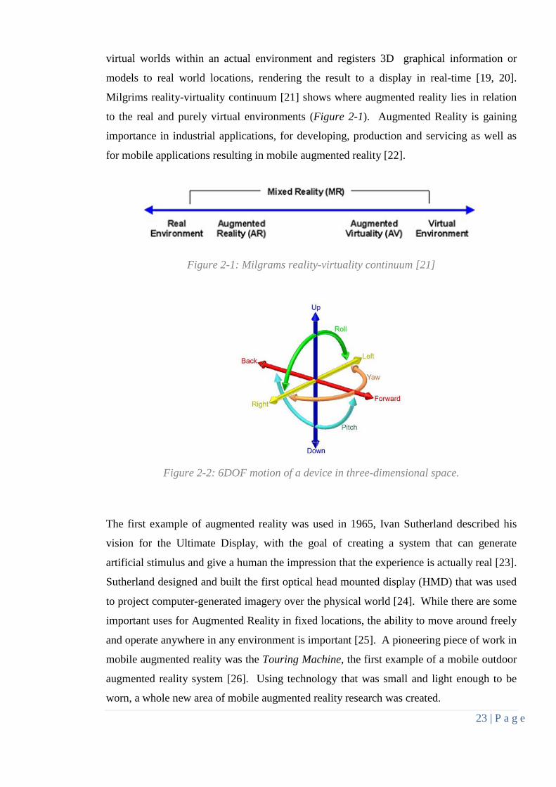
Augmented reality on devices requires highly accurate and fast six degrees of freedom

(6DOF) tracking in three-dimensional space (Figure 2-2), with the ability to move in three

perpendicular axes forward/backward, up/down and left/right translations combined with

rotation about three perpendicular axes (pitch, yaw, roll). In contrast to virtual reality

which completely replaces the physical world, augmented reality blends the physical and

23 | P a g e

virtual worlds within an actual environment and registers 3D graphical information or

models to real world locations, rendering the result to a display in real-time [19, 20].

Milgrims reality-virtuality continuum [21] shows where augmented reality lies in relation

to the real and purely virtual environments (Figure 2-1). Augmented Reality is gaining

importance in industrial applications, for developing, production and servicing as well as

for mobile applications resulting in mobile augmented reality [22].

Figure 2-1: Milgrams reality-virtuality continuum [21]

Figure 2-2: 6DOF motion of a device in three-dimensional space.

The first example of augmented reality was used in 1965, Ivan Sutherland described his

vision for the Ultimate Display, with the goal of creating a system that can generate

artificial stimulus and give a human the impression that the experience is actually real [23].

Sutherland designed and built the first optical head mounted display (HMD) that was used

to project computer-generated imagery over the physical world [24]. While there are some

important uses for Augmented Reality in fixed locations, the ability to move around freely

and operate anywhere in any environment is important [25]. A pioneering piece of work in

mobile augmented reality was the Touring Machine, the first example of a mobile outdoor

augmented reality system [26]. Using technology that was small and light enough to be

worn, a whole new area of mobile augmented reality research was created.

24 | P a g e

: Mobile Smartphone Platforms Overview 2.2A mobile phone is a handheld electronic device that uses two-way radio

telecommunication over a cellular network of base stations. A smartphone is a more

advanced version of a mobile phone, with features going beyond just making and receiving

telephone calls and messages. They are often thought of as handheld mini-computers, and

can be perceived to be tangible embodiments of pervasive computing [27]. In recent times,

there has been rapid progression in smart phones, with advances in high-capacity graphics,

abundant memory, multiple high resolution cameras, high resolution displays, GPS-

positioning, gyroscopes and accelerometers, making the smart phone a necessary item for

many consumers and businesses. Access to mobile networks is now available to 90% of

the world population and 80% of the population living in rural areas [28]. There is an

estimated 5.3 billion mobile phone cellular subscriptions worldwide with a rising

percentage of them being in the smart-phone category, high performance devices are

becoming more a regular household item [29]. Just in the 3rd quarter of 2013 alone, smart

phone sales reached over 250 million units sold worldwide with Android devices

accounting for 72.6% of the market share [30].

During the course of this thesis there were several competing smart phone platforms

available to consumers on the market. The most popular smartphones today are Android

and iPhone devices however some of the other platforms that are now less popular are

Symbian, Blackberry, Meego and Windows Phone.

Symbian is an open source operating system and platform designed specifically for

embedded devices and is programmed in C++ [31]. It was originally developed by

Symbian Ltd, but now owned and being maintained by Nokia since December 2008. The

Symbian operating system previously used a Symbian-specific C++ version for application

development along with Carbide.c++ integrated development environment for native

application development, but from 2010, Symbian switched to using standard C++

with Qt as the SDK, which can be used with either Qt Creator or Carbide. Applications

for the Symbian operating system can also be developed with JavaME, Python and Ruby

languages as well as web widgets using HTML, CSS, JavaScript and XML. On 11th

February 2011, Nokia announced a partnership with Microsoft which would see it adopt

25 | P a g e

Windows Phone 7 for smartphones, reducing the number of devices running Symbian over

the coming two years [32]. Nokia has now ceased to support the Symbian operating

system, instead shift its focus towards collaboration with the Windows Phone operating

system [33].

BlackBerry OS is a mobile operating system, developed by Research In Motion(RIM) for

its BlackBerry line of smartphone devices [34]. The first BlackBerry device was

introduced in 1999 as a two-way pager in Munich, Germany. In 2002, the more commonly

known smartphone BlackBerry was released. Because the BlackBerry operating system is

proprietary, no significant information about its architecture is made public. The newer

devices support BlackBerry 10, which is the successor to the older Blackberry OS, and is

programmed natively in C++. BlackBerry OS allows developers to write software for the

device which is executed on the Java Virtual Machine (JVM) using Java ME and the

available BlackBerry API, however the newest version BlackBerry 10 allows Android

runtime support.

Meego is an open-source Linux based mobile operating system project which brings

together the Moblin project, headed up by Intel, and Maemo, by Nokia, into a single open

source activity and is hosted by the Linux Foundation. According to Intel, MeeGo was

developed because Microsoft did not offer comprehensive Windows 7 support for the

Atom Processor [35]. MeeGo is programmed in C++ and is intended to run on a variety of

hardware platforms including handhelds, in-car devices, netbooks and televisions. These

platforms share the MeeGo core, with different “User Experience” (UX) layers for each

type of device. The officially endorsed way to develop MeeGo applications is to use the

Qt framework and Qt Creator as the development environment, but writing GTK

applications is also supported in practice [36]. Like Symbian, Nokia has announced that it

is walking away from the operating system to focus on Windows Phone [33].

Windows Phone is a mobile operating system developed by Microsoft and is the successor

to its Windows Mobile platform [37]. The Windows Mobile platform was originally

designed for enterprise users with Windows CE and Windows Mobile 6/6.5, with a suite of

26 | P a g e

business applications like Mobile Office and Outlook. Microsoft changed its approach to

the consumer market when Windows Phone 7 was released in October 2010 and is a

complete overhaul from the previous Windows Mobile platforms. Windows Phone

applications are developed using the C# programming language. On October 29, 2012,

Microsoft released Windows Phone 8, a new generation of the operating system. Windows

Phone 8 replaces its previously Windows CE-based architecture with one based on the

Windows NT kernel with many components shared with Windows 8, allowing applications

to be easily ported between the two platforms.

iPhone is a device that is designed and manufactured by Apple Inc. First introduced in

January 2007, there have now been several generations of the device. It runs the iOS

operating system which is currently at version 7. Development of iPhone applications are

written in Objective-C, an object-oriented derivative of the C language. The application

environment is called Cocoa, and contains a suite of object-oriented software libraries, as

well as a runtime and integrated development environment [38]. The application-

framework iOS is called the Cocoa Touch framework and can be broken down into several

layers.

• Core OS layer contains the kernel, file system, networking infrastructure, security,

power management, and device drivers.

• Core Services layer provides services such as string manipulation, collection

management, networking, URL utilities, contact management and preferences. This

layer also provides services for the hardware, such as GPS, compass, accelerometer

and gyroscope.

• Media layer depends on the Core Services layer and provides graphical and

multimedia services to the Cocoa Touch layer, it includes Core Graphics, OpenGL

ES and AVFoundation frameworks for allowing camera and video playback.

• The Cocoa Touch layer directly supports applications based on iOS.

27 | P a g e

The Cocoa Touch layer and the Core Services layer each have an Objective-C framework

that is especially important for developing applications for iOS which are the UIKit and

Foundation frameworks.

• UIKit, provides the components an application displays in its user interface and

defines the structure for application behaviour, including event handling and

drawing.

• Foundation framework defines the basic behaviour of objects, establishes

mechanisms for their management, primitive data types, collections and OS services.

Android is an open-source software stack developed by Google for mobile phones and

tablets which includes an operating system, middleware and applications. The core

operating system is written in C with some C++, and is based on a modified version of

the Linux kernel. Applications are written in the Java language using the Android SDK

and are executed on the Dalvik Virtual Machine which features JIT compilation [39]. The

architecture of the Android operating system can be broken down into 5 major component

layers:

• Applications, consists of a set of core applications including an email client, SMS

program, calendar, maps, browser, contacts which are written using the Java

programming language.

• The Application Framework provides access to device hardware, access location

information and runs background services. It contains a set of underlying services

and systems, including Views that can be used to build GUI applications, Content

Providers that enable applications to access or share data between applications,

Resource Manager providing access to non-code resources such as localized

strings, graphics, and layout files, Notification Manager that enables all

applications to display custom alerts in the status bar, and Activity Manager that

manages the lifecycle of applications and provides common navigation.

• Libraries, include a set of C/C++ libraries used by various components of the

Android system. These capabilities are exposed to developers through the Android

application framework. Some of the core libraries include the System C

28 | P a g e

library which is a BSD-derived implementation of the standard C system library,

Media libraries to support playback and recording of audio and video formats, as

well as static image files, Surface Manager to access the display subsystem and

composite 2D and 3D graphic layers from multiple applications,

LibWebCore engine which powers both the Android browser and an embeddable

web view, SGL engine for underlying 2D graphics, 3D libraries based on OpenGL

ES APIs which use either hardware 3D acceleration if available or the highly

optimized 3D software rasterizer, FreeType for bitmap and vector font rendering,

and SQLite which is a powerful and lightweight relational database engine

available to all applications.

• Android Runtime, which includes a set of core libraries that provides most of the

functionality available in the core libraries of the Java programming language.

Every Android application runs in its own process, with its own instance of the

Dalvik virtual machine. Dalvik has been written so that a device can run multiple

VMs efficiently. The Dalvik Virtual Machine executes files in the Dalvik

Executable (.dex) format which is optimized for a minimal memory footprint. The

virtual machine is register-based, and runs classes compiled by a Java language

compiler that have been transformed into the .dex format by the included "dx" tool.

The Dalvik virtual machine relies on the Linux kernel for underlying functionality

such as threading and low-level memory management.

• Linux Kernel, for core system services such as security, memory management,

process management, network stack, and driver model. The kernel also acts as an

abstraction layer between the hardware and the rest of the software stack.

: Computer Vision: 2.3The field of Computer Vision is concerned with the acquisition, processing and analysis of

images. It often involves image restoration, object recognition, motion estimation and

scene reconstruction in real time. It involves the transformation of data from a still or

video camera into either a decision or a new representation, this transformation is always

done to satisfy a particular goal, including detection, segmentation, localization and

29 | P a g e

recognition of certain objects in images [40]. Computer vision can be considered a form of

image analysis, taking a 2D image and converting it into a mathematical description [41].

It studies and describes the processes implemented in software and hardware behind

artificial vision systems. Computer Vision can be considered the inverse of computer

graphics. Computer graphics can be considered image synthesis in that it often produces

image data from three-dimensional models of the scene, whereas computer vision often

produces three dimensional models from image data [42].

On mobile platforms computer vision application development has been limited.

However, over the last few years with the development of the smartphone, mobiles have

significantly improved especially with the embedded camera, GPU and CPU technology.

Mobile gaming has become popular as well as mobile augmented reality all of which drive

the ever increasing demand for more powerful processing capabilities. Mobile computer

vision algorithms are usually used through the OpenCV library [15], which is an open

source library ported to most computer operating systems and made available on all the

popular mobile platforms.

2.3.1: Fiducial Markers Many real-time computer vision algorithms for recognition of generic objects have fairly

substantial processing requirements which might not be available on mobile devices as

they only have limited processing power, so more restricted recognition algorithms are

often instead used. The simplest object recognition systems rely on fiduciary markers

which are simple two dimensional patterns and are often manually applied to physical

objects in a scene so that they can be recognized in images of the scene and to help solve

the correspondence problem, automatically finding features in different camera images that

belong to the same object [43]. They also can be used as two-dimensional bar codes for

providing object information, as reference points where three dimensional augmented

reality models should be positioned in relation to the marker, and for pose estimation

where the position and orientation of the camera relative to the scene is estimated [44]. By

placing fiduciary markers at known locations in the scene, the relative scale in the

produced image may be determined by comparison of the locations of the markers in the

30 | P a g e

scene. Mostly fiducial markers are black and white images with clearly distinguishable

contours that are easily separated from the background due to their high contrast.

Figure 2-3: Example types of fiducial markers. ARToolkit/Studierstube tracker markers, QRCode and Shot Code

Square based fiducial markers can be recognized in a greyscale image by applying a

threshold, determining the connected components or contours and then extracting the

corners of the marker (or the center of the marker for the circular Shot Code marker).

Once the corners of the maker have been identified additional information usually encoded

in black and white are extracted to identify the specific marker or obtain its code.

2.3.2: Feature Detection Instead of using markers for computer vision based applications, it may be more

convenient to detect naturally occurring points of interest in a scene. Feature Detection

refers to methods that aim to compute abstractions of image information and make

decisions as to whether or not there is an image feature of a given type in the image. There

is no universal or exact definition of what constitutes a feature, and the exact definition

often depends on the problem or the type of application [49]. A feature is defined as an

"interesting" part of an image, and is used as a starting point for many computer vision

algorithms. Features could be a combination of extracted edges, corners, shapes or patches

of colour.

31 | P a g e

2.3.3: Image Convolutions Convolutions are the basis of many transformations that are done in computer vision and

are especially used for techniques such as blurring images and edge detection.

Convolutions are performed on every pixel in an input image, what a particular

convolution does is determined by the form of the convolution kernel being used on the

image. The kernel is essentially just a fixed size array of numerical coefficients along with

an anchor point in that array which is generally in the centre. The resulting output of the

convolution at a particular point is calculated by placing the kernel anchor on top of a pixel

in the input image with the rest of the kernel overlaying its corresponding neighbouring

pixels. Each of the values in the kernel is multiplied with their overlaid input image

values, with their results added together into one sum. The current pixel in the output

image is then set to this sum [45]. When convolutions come to the border of an image,

parts of the kernel not corresponding to the input image are either clamped to zero,

wrapped to the other side of the image or have the pixels on the border replicated.

-1 -2 -1

2

115

4115

5

115

4115

2

115 0 0 0

1/9 1/9 1/9 4

115

9115

12

115

9115

4

115 1 2 1

1/9 1/9 1/9 5115

12

115

15115

12

115

5115

1/9 1/9 1/9 4

115

9115

12

115

9115

4

115 -1 0 1

2

115

4115

5

115

4115

2

115 -2 0 2

-1 0 1

Figure 2-4: Example convolution kernels for a simple box blur (left), 5x5 Gaussian smoothing (center), and two 3x3 kernels for vertical and horizontal Sobel operators

(right).

Image processing convolutions can be expressed in the form of an equation. Suppose the

image intensity (possibly within one channel) at pixel coordinate x,y is I(x,y), the kernel is

G(i,j) and the size of the square kernel is M (where 0≤i<M and 0≤j<M). If the anchor

32 | P a g e

point in the kernel is to be located at (a,b), then the convolution H(x,y) is defined by the

expression:

𝐻(𝑥,𝑦) = � � 𝑀−1

𝑗=0

𝑀−1

𝑖=0𝐼(𝑥 + 𝑖 − 𝑎 , 𝑦 + 𝑗 − 𝑏) 𝐺(𝑖, 𝑗)

2.3.4: Canny Edge Detection Edge detection is one of the key research works in image processing which aim at

identifying points in an image at which the image brightness changes sharply or has

discontinuities. There are a few techniques for edge detection the first being the Roberts

cross operator proposed by Lawrence Roberts in 1963 [46]. The Sobel operator can be

also used for edge detection algorithms [47]. Technically Sobel is a discrete differentiation

operator, it calculates the gradient of the image intensity at each point, giving the direction

of the largest possible increase from dark to light and the rate of change in that direction.

The results show how sudden or smoothly the image changes, therefore indicating whether

pixels represent edges, and how each edge is oriented. At each point in the image, the

result of the Sobel operator is either the corresponding gradient vector or the normal of this

vector. Edge detection using the Sobel operator is based on convolving an input image

with a two small 3x3 integer valued matrix filters (Figure 2-4) for both horizontal and

vertical directions, and is therefore relatively inexpensive in terms of computations.

Canny edge detection is a multistage algorithm developed by John Canny in 1986, which

detects edges of objects in an image scene in a very robust manner and is now one of the

most commonly used image processing tools [48]. An edge can be characterized by an

abrupt change in intensity indicating a boundary between two regions of an image [49].

John Canny’s aim was to discover the optimal edge detection algorithm, which marks as

many edges in the image as possible, has good localization, minimal response time and

noise reduction so that it doesn’t allow noise to create false edges. Starting with a

greyscale input image, the algorithm is run in 4 separate steps to produce an image whose

pixels with non-zero intensity represent the edges in the original image.

• Noise Reduction - It is inevitable that all images taken from a camera will contain a

certain amount of noise. To prevent this noise creating false edges, the noise must be

33 | P a g e

reduced. The raw image is convolved with a Gaussian filter. The result is a

slightly blurred version of the original image which is not affected by a single noisy

pixel to any significant degree.

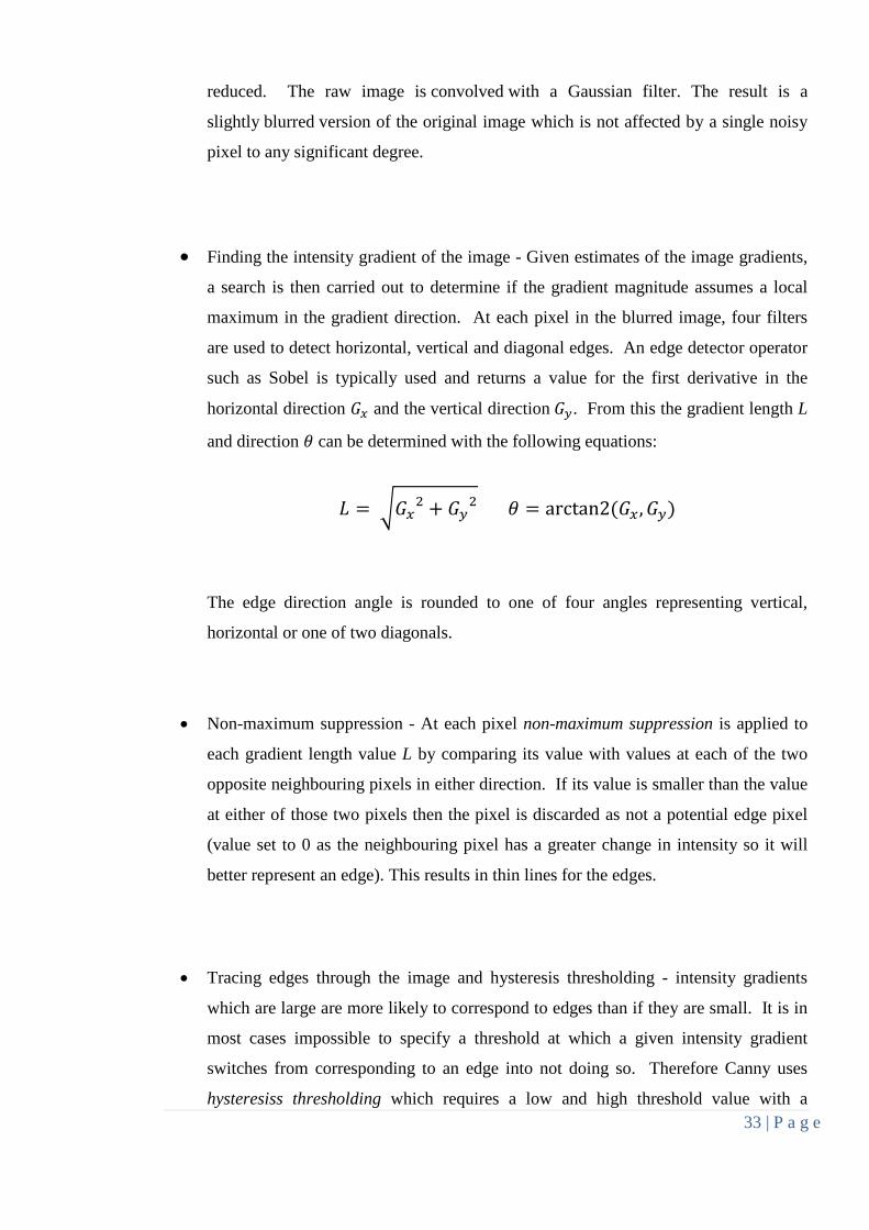
• Finding the intensity gradient of the image - Given estimates of the image gradients,

a search is then carried out to determine if the gradient magnitude assumes a local

maximum in the gradient direction. At each pixel in the blurred image, four filters

are used to detect horizontal, vertical and diagonal edges. An edge detector operator

such as Sobel is typically used and returns a value for the first derivative in the

horizontal direction 𝐺𝑥 and the vertical direction 𝐺𝑦. From this the gradient length L

and direction 𝜃 can be determined with the following equations:

𝐿 = �𝐺𝑥2 + 𝐺𝑦2 𝜃 = arctan2(𝐺𝑥 ,𝐺𝑦)

The edge direction angle is rounded to one of four angles representing vertical,

horizontal or one of two diagonals.

• Non-maximum suppression - At each pixel non-maximum suppression is applied to

each gradient length value L by comparing its value with values at each of the two

opposite neighbouring pixels in either direction. If its value is smaller than the value

at either of those two pixels then the pixel is discarded as not a potential edge pixel

(value set to 0 as the neighbouring pixel has a greater change in intensity so it will

better represent an edge). This results in thin lines for the edges.

• Tracing edges through the image and hysteresis thresholding - intensity gradients

which are large are more likely to correspond to edges than if they are small. It is in

most cases impossible to specify a threshold at which a given intensity gradient

switches from corresponding to an edge into not doing so. Therefore Canny uses

hysteresiss thresholding which requires a low and high threshold value with a

34 | P a g e

upper:lower ratio between 2:1 and 3:1. Making the assumption that important edges

should be along continuous curves in the image allows us to follow a faint section of

a given line and to discard a few noisy pixels that do not constitute a line but have

produced large gradients. At each pixel if the value of the gradient is greater than the

upper threshold, then it is accepted as a strong edge pixel, however if the gradient

value is less than the lower threshold then it is not considered an edge pixel and is

discarded. If a pixels gradient value is between the upper and lower thresholds, then

it is referred to as a weak edge pixel and is only accepted if it is connected to a strong

edge pixel.

2.3.5: FAST Corners are commonly used in computer vision systems as feature points in an image and

later used to track and map objects. There are many corner detection algorithms which

exist including, Moravec [50], Harris-Stephens [51], Wang-Brady [52], and SUSAN

corner detection [53]. FAST (Features from accelerated segment test) is a corner detection

method originally developed by Edward Rosten and Tom Drummond [54]. The most

promising advantage of FAST corner detector is its computational efficiency, as the

acronym in its name suggests, it is faster than many other well-known feature extraction

methods.

FAST calculates corners by taking 16 pixels in a Bresenham circle of radius 3 around the

centre pixel p where at least N (usually chosen to be 12) pixels should each have an

intensity differing from p above some threshold for that pixel to be considered a corner

feature (see Figure 2-5). Once corner points have been calculated non-maximum

suppression is used around the neighbourhood of each potential corner to remove adjacent

neighbour feature points, typically the strongest feature point is taken (the one that has the

greatest intensity difference between it and its N neighbours). There has been several

improvements made to FAST including using a machine learning approach discussed in

[55] as well as FAST-ER (FAST: Enhanced Repeatability) which uses simulated annealing

[56].

35 | P a g e

Figure 2-5: Shows the 16 pixel Bresenham circle around a possible FAST feature point p [54]

2.3.6: SIFT Scale-invariant feature transform (SIFT) is an algorithm in computer vision used to detect

and describe local features in images, it was published by Daniel Lowe in 1999 [57]. SIFT

has applications in object recognition, robotic mapping and navigation, image stitching, 3D

modelling, gesture recognition and video tracking. SIFT combines key point localization

and feature description. It can also be used for defining descriptive image patches. For

any object in an image, key points of interest in the object can be extracted to provide a

feature description. This description is extracted from a training image, which can be

stored in a database alongside features from other reference images, it can be used later to

identify the object when attempting to locate the object in a scene containing many other

objects. To perform reliable recognition, it is important that the features extracted from the

training image are detectable even under changes in image scale, image rotation, noise,

illumination, clutter and partial occlusion [58].

To detect an object in a scene using SIFT first Gaussian filters are applied, and then scale-

space minima and maxima in the Difference of Gaussian (DoG) are calculated to locate its

key points. Difference of Gaussian (DoG) is a greyscale image enhancement algorithm

that involves the subtraction of a blurred version of an original greyscale image from

another, less blurred version of the original [59]. Because DoG can be computationally

expensive, key points are estimated and gradient orientations and magnitudes around the

36 | P a g e

key point are calculated forming a histogram of orientations. Key points in the new image

are used to create object features in the scene and are individually compared to existing

features in the database, finding candidate matches based on the Euclidean distance of their

feature vectors. From the full set of matches, subsets of key points that agree on the object

and its location, scale, and orientation in the new image are identified to filter out good

matches. The determination of consistent clusters is performed rapidly by using an

efficient hash table implementation of the generalized Hough transform. Each cluster of 3

or more features that agree on an object and its pose is then subject to further detailed

model verification and subsequently outliers are discarded. Finally the probability that a

particular set of features indicates the presence of an object is computed, given the

accuracy of fit and number of probable false matches. Object matches that pass all these

tests can be correctly identified as a known object.

2.3.7: SURF SURF (Speeded Up Robust Features) is a robust scale and rotation invariant feature point

detector and descriptor, and is partly inspired by the SIFT descriptor. It was first presented

in [60], and can be used in computer vision tasks like object recognition or 3D

reconstruction. SURF approximates or even outperforms SIFT and other previously

proposed schemes with respect to repeatability, distinctiveness, and robustness, yet can be

computed and compared much faster [61]. SURF is based on sums of 2D Haar

wavelet responses and makes an efficient use of integral images. It uses an integer

approximation to the determinant of Hessian blob detector, which can be computed

extremely quickly with an integral image. For features, it uses the sum of the Haar wavelet

response around the point of interest. Again, these can be computed with the aid of the

integral image.

2.3.8: Lucas Kanade Feature descriptions can be extracted from sequential frames taken from a moving scene to

recognize previously identified features and so perform motion tracking. However, feature

descriptions algorithms can often be computationally expensive to calculate, so an optical

flow algorithm such as Lucas-Kanade [62] or its variant Kanade-Lucas-Tomasi

(collectively known as the KLT feature tracker) [63] is often used for tracking once feature

37 | P a g e

points have been initially found. The Lucas-Kanade algorithm solves the optical flow

equation 𝜕𝜕𝜕𝑥ṽx + 𝜕𝜕

𝜕𝑦ṽ𝑦 = −𝜕𝜕

𝜕𝜕 for a greyscale image with intensity I to find the movement

ṽ of a feature between frames. It presumes that all the pixels in a small patch of an image

have the same movement. This results in an overdetermined system of equations for the

movement, which can be solved via least squares to find v. Typically the patch is taken to

be the neighbourhood around a corner feature point so that both 𝜕𝜕𝜕𝑥

and 𝜕𝜕𝜕𝑦

are significant

compared to noise in the image. KLT feature tracker is faster than traditional techniques

and examines far fewer potential matches between the images. An additional stage of

verifying that features are tracked correctly is discussed in [17]. An affine transformation

is fit between the image of the currently tracked feature and its image from a non-

consecutive previous frame. If the affine compensated image is too dissimilar the feature

is dropped.

Lucas-Kanade is considered a local differential optical flow technique in which movement

of pixels across image frames is confined to a local patch. When used to track multiple

features, the flow for each feature is determined separately from the other features in the

image. A popular global differential optical flow technique used for tacking is the Horn–

Schunck [64] algorithm which assumes that brightness patterns within an image vary

smoothly everywhere. Local differential techniques bare known to have robustness under

noise, whilst global techniques are able to produce dense optical flow fields. There has

been work combining both local and global approaches using Lucas-Kanade and Horn-

Schunck respectively as demonstrated in [65] and [66]. There are other algorithms that can

be used to track features such as the kernel based or particle filter-based trackers such as

Kalman and others described in [67], [68] and including a colour based particle filtering

described in [69]. However the work in this research is purely compared with Lucas-

Kanade as that is possibly the most popular and best performing algorithm for feature

tracking.

38 | P a g e

: General Purpose Computing on the GPU: 2.4A Graphics Processing Unit (GPU) is a piece of dedicated hardware which is

predominantly used to render graphical 3D scenes with either a fixed or programmable

pipeline [70]. General purpose computing on a graphics processing unit (GPGPU) is the

technique of using a GPU to perform computation in applications traditionally handled by

the central processing unit (CPU). It is made possible by the addition of programmable

stages to the rendering pipeline which allows software developers to use stream processing

on non-graphics data. Instead of using the GPU for rendering a graphical scene, if it has a

programmable pipeline, it can be used to perform calculations that would usually require a

lot more central processing unit (CPU) time, taking advantage of data parallelization that is

inherent with the graphics processing unit architecture. Current GPUs contain hundreds of

compute cores and support thousands of light-weight threads, which hide memory latency

and provide massive throughput for parallel computations [71].

Unlike GPUs, CPUs have little hardware support for thread synchronization, which

therefore must be emulated in software, so the cost of synchronization could be several

orders of magnitude higher for CPUs, reducing application performance [72]. Because of

the multi-billion dollar video game market being the pressure cooker for GPU evolution,

the GPU has become an extremely fast and flexible processor. They offer

programmability, precision and power which makes them an attractive platform for general

purpose computation capable of very high computation and data throughput [73]. There

are many applications in which GPGPU has been used, including in high performance

computer clusters, grid computing, physical based simulations, physics engines, fast

fourier transforms, audio and video signal processing, weather forecasting, medical

imaging, cryptography, cryptanalysis and intrusion detection, as well as computer vision.

2.4.1: GPU programming and Shaders: GPU programming can be used to efficiently execute computer vision algorithms on

mobile devices by using a graphics API intended for limited devices, such as OpenGL ES

2.0 or Direct X9, with the use of a programmable shader pipeline, where mathematical

parts of algorithms and operations can be done with small programs called shaders. A

39 | P a g e

shader is a simple program which contains a set of software instructions that describe the

traits of either a vertex or a pixel and are primarily used to calculate rendering effects on

graphics hardware in the GPU programmable rendering pipeline. Two of the main shader

languages are the OpenGL Shading Language, or GLSL and High Level Shader Language

(HLSL) [74] [75]. Open GL ES 2.0 and GLSL is supported on many smart phone devices

with an embedded GPU, including iPhone and Android, whereas the Windows Mobile

range instead uses Direct X9 and HLSL for graphics and GPU programming.

From version 2.0 OpenGL ES supports programmable shaders, so parts of an application

can be written in GLSL and executed directly in the GPU pipeline. The graphics pipeline

typically accepts some representation of a three-dimensional scene as an input and results

in a 2D raster image as output. Previously, graphical rendering was used in a fixed

function pipeline, which performs lighting and texture mapping in a hard-coded manner.

This meant that applications had to rely on fixed functions to produce a scene, with the

only control being via configurations. Shaders provide a programmable alternative to this

approach by allowing developers to create custom vertex and pixel (also called fragment)

calculations that can be implemented more concisely with far better performance than the

fixed functional pipeline [76]. The graphics pipeline is well suited to the rendering process

because it allows the GPU to function as a stream processor since all vertices and

fragments can be thought of as independent. This allows all stages of the pipeline to be

used simultaneously for different vertices or fragments as they work their way through the

pipe. In addition to pipelining vertices and fragments, their independence allows graphics

processors to use parallel processing units to process multiple vertices or fragments in a

single stage of the pipeline at the same time.

In the OpenGL ES 2.0 Pipeline Structure, the CPU sends the compiled shader

language program and geometry data to the graphics processing unit. The GLSL shader

code is usually compiled at runtime. The vertex shader is then used to provide vertex

positions and colours for the following stages of the pipeline and can be used for

computing lighting effects and generating or transforming texture coordinates. The vertex

shader is used for translation and rotation of input geometry as well as perspective

projection. Clipping, Perspective Division and Viewport transformations are done to

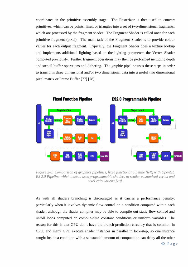
40 | P a g e

coordinates in the primitive assembly stage. The Rasterizer is then used to convert

primitives, which can be points, lines, or triangles into a set of two-dimensional fragments,

which are processed by the fragment shader. The Fragment Shader is called once for each

primitive fragment (pixel). The main task of the Fragment Shader is to provide colour

values for each output fragment. Typically, the Fragment Shader does a texture lookup

and implements additional lighting based on the lighting parameters the Vertex Shader

computed previously. Further fragment operations may then be performed including depth

and stencil buffer operations and dithering. The graphic pipeline uses these steps in order

to transform three dimensional and/or two dimensional data into a useful two dimensional

pixel matrix or Frame Buffer [77] [78].

Figure 2-6: Comparison of graphics pipelines, fixed functional pipeline (left) with OpenGL ES 2.0 Pipeline which instead uses programmable shaders to render customized vertex and

pixel calculations [79].

As with all shaders branching is discouraged as it carries a performance penalty,

particularly when it involves dynamic flow control on a condition computed within each

shader, although the shader compiler may be able to compile out static flow control and

unroll loops computed on compile-time constant conditions or uniform variables. The

reason for this is that GPU don’t have the branch-prediction circuitry that is common in

CPU, and many GPU execute shader instances in parallel in lock-step, so one instance

caught inside a condition with a substantial amount of computation can delay all the other

41 | P a g e

instances from progressing. The same holds for dependent texture reads, where the shader

itself computes texture coordinates rather than directly using unmodified texture

coordinates passed into the shader. The graphics hardware cannot then prefetch texel data

before the shader executes to reduce memory access latency. Unfortunately, many

computer vision algorithms require dependent texture reads when implemented on a GPU.

Another issue that must be considered is the latency in creating and transferring textures.

Ideally, all texture data for a GPU should be loaded during initialization and preferably not

changed while the shaders execute, to reduce the dataflow between memory and the GPU.

However, for real-time image analysis to be feasible on a GPU image data captured from

the camera should preferably be loaded into a preallocated texture at least 30 frames per

second (fps), quite contrary to GPU recommended practices. This can be partially

compensated for by reducing the image resolution or changing its format from RGB vector

float values to integer or compressed. There are performance benchmarks for the GPU

commonly found in mobile devices [80]. However, the benchmarks typically only compare

the performance for graphics rendering throughput, not for other tasks such as image

processing, so do not significantly test the implications of effects such as frequent texture

reloading and dependent texture reads

OpenGL ES 2.0 allows byte, unsigned byte, short, unsigned short, float, and fixed data

types for vertex shader attributes, but vertex shaders always expect attributes to be float so

all other types are converted, resulting in a compromise between bandwidth/storage and

conversion costs. It requires that a GPU must allow at least two texture units to be

available to fragment shaders, which is not an issue for many image processing algorithms,

although most GPU support eight texture units. Textures might not be available to vertex

shaders and there are often tight limits on the number of vertex attributes and varying

variables that can be used (16 and 8 respectively in the case of the PowerVR SGX series of

GPU).

42 | P a g e

Unlike the full version, OpenGL ES uses precision hints for all shader values:

• lowp for 10 bit values between −2 and 1.999 with a precision of 1/256 (which for

graphics rendering is mainly used for colours and reading from low precision

textures such as normals from a normal map)

• mediump for 16 bit values between -65520 and 65520 consisting of a sign bit, 5

exponent bits, and 10 mantissa bits (which can be useful for reducing storage

requirements),

• highp for 32 bit (mostly adhering to the IEEE754 standard).

Furthermore, the GPU on a mobile device is most likely to be a scalar rather than vector

processor. This means that there is typically no advantage vectorizing highp operations, as

each highp component will be computed sequentially, although lowp and mediump values

can be processed in parallel. It is also common for GPU on mobiles to use tile-based

deferred rendering, where the framebuffer is divided into tiles and commands get buffered

and processed together as a single operation for each tile. This helps the GPU to more

effectively cache framebuffer values and allows it to discard some fragments before they

get processed by a fragment shader (for this to work correctly fragment shaders should

themselves avoid discarding fragments).

Some computer vision algorithms require several stages and cannot be efficiently

calculated via a single pass through the graphics rendering pipeline. Instead a multi-pass

rendering technique can be used to pass data through the pipeline multiple times, storing

the results of each render pass in buffers and using them to affect the rendering during later

passes. As information is fed through the pipeline during each pass, pixels and vertex data

may be processed by different vertex and fragment shaders. Between OpenGL ES 2.0

render passes, output information from the shader can only be held in a single attached

texture, whereas multiple input textures can be bound. Textures can be accessed internally

on the GPU through uniform sampler2D variables. Internally these textures contain four

floating points RGBA channel values to store data. However information stored in the

textures only has the value range between 0-1 so values stored in them for the next render

pass need to be encoded to be within that range.

43 | P a g e

2.4.2 GPU based feature descriptors Some of the computer vision algorithms discussed in this literature review have been

implemented using GPU and shader technology including SIFT [81, 82], which has shown

to be up to 100 times faster than a pure CPU implementation of SIFT while maintaining

robust performance, and Canny edge detection [83] which has shown up to be 50 times

faster than its CPU based implementation. SURF has also been implemented and

optimized for the GPU in [84]. GPU-based KLT feature tracking combined with a GPU

SIFT extractor has been implemented in [85] showing a substantial reduction in processing

time on video frames. GPGPU techniques are also used in [86], the work implemented a

SLAM (Simultaneous localization and mapping) [87] framework that could be

implemented on massively parallel platforms and address the monocular SLAM problem.

It takes camera tracking and 3D reconstruction from image sequences to achieve a high

level of accuracy at towards real time processing speed. More GPU-based features are

presented in [88] which uses a modified Fast Radial Blob Detector algorithm to detect and

track multiple visual targets at sea. It demonstrated good feature repeatability, however

was slower than FAST by a factor of four. It did have other advantages over FAST such as

computing a value for feature strength, calculating a scale value and making the algorithm

more resilient to image noise by using a Gaussian blur.

However especially at the start of this thesis there was little computer vision work done

using mobile GPUs which have more restricted capabilities. The mobiles used for

implementing and testing in this thesis only supported GLSL version 1.0 so the internal

functions that usually can be used are limited compared to later GLSL versions. Although

SIFT is a computationally expensive algorithm, there has been work to streamline the

feature detection and descriptor matching process so the algorithms can be ported to a

mobile device with the introduction of PhonySIFT which has shown some relatively

successful and interesting results [89]. SURF has been shown to be computationally faster

than SIFT, however it is still too slow to support emerging applications such as mobile

augmented reality on mobile devices [90]. However [90] has shown success in adapting

SURF to mobile devices boasting a 6-8x speedup with their dual techniques, tiled SURF

and gradient moment based orientation assignment. SURF also has been modified for

mobile GPU in [91] which they titled uSURF-ES and claimed to be multiple times faster

than the CPU variant on the same device. It proved the feasibility of modern mobile

44 | P a g e

graphics accelerators for GPGPU tasks, especially for the detection phase in natural feature

tracking used in augmented reality applications. However even on mid-range devices

such as the Samsung Galaxy S2 the average runtime is 117 milliseconds for feature

extraction using uSURF-ES which equates to under 10 frames per second and was done on

a data set of still images of size 512x384, well under the resolution of the 800x480 display.

These times also did not include initial image loading and keypoint detection with

OpenCV as well as downloading the resulting descriptors from video memory.

The mobile GPU based feature algorithms show varying improvement over CPU based

counterparts, however they still may not be fully suited for high frame rate applications

such as mobile augmented reality. So this thesis instead looks at alternative solutions for

feature detection, tracking and recognition as discussed in Chapters 5-8.

: Cluster Analysis 2.5Cluster Analysis or clustering divides data into groups (clusters) that are meaningful where

objects in the same cluster are more similar to each other than objects in other clusters [92]

[93]. Clustering is widely used in many fields including psychology, statistical data

analysis, machine learning, pattern recognition and image analysis. Cluster analysis itself

is not one specific algorithm, but the general task to be solved. It can be achieved by

various algorithms that differ significantly in their notion of what constitutes a cluster and

how to efficiently find them. Popular notions of clusters include groups with small

distances among the cluster members, dense areas of the data space, intervals or particular

statistical distributions. Cluster analysis is not an automatic task, but an iterative process of

knowledge discovery or interactive multi-objective optimization that involves trial and

error. It will often be necessary to modify data preprocessing and model parameters until

the result achieves the desired properties.

The notion of a cluster cannot be precisely defined, as a result there are over 100 published

clustering algorithms [94]. There is no objectively “correct” clustering algorithm and is

45 | P a g e

really just determined from the eye of the beholder. The most appropriate clustering

algorithm for a particular problem often needs to be chosen experimentally. Different

researchers employ different cluster models, for each of these models different cluster

algorithms can be given. Typical cluster models include connectivity models, centroid

models, density models and distribution models although there are many others. For this

work research was undertaken using centroid and density models which tested the most

popular algorithm for each which are k-means clustering and DBSCAN respectively.

Clustering of feature points can be used for motion segmentation, which is a means of

separating one or more moving objects in an image from a static background. There are

various motion segmentation algorithms as discussed in [95] and [96] which include

Generalized Principal Analysis (GPCA), Local Space Affinity (LSA), Multi-Stage

Learning (MSL) and Random Sample Consensus (RANSAC).

2.5.1: DBSCAN Density Based Spatial Clustering of Applications with Noise (DBSCAN) [97] as its name

suggests is a density based model for clustering points, which defines clusters as connected

dense regions in the data space and objects in sparse areas are considered to be noise [98].

It is one of the most common and most cited clustering algorithms in scientific literature.

DBSCAN’s definition of a cluster is based on the notion of density reachability. The

algorithm works by taking a data set of points and two predetermined values epsilon (ε)

distance and the minimum number of points (m) required to make a cluster. For each

“unvisited point” the algorithms retrieves all other points within the ε-neighbourhood, if

the number of points within that neighbourhood is less than m then that point is marked as

noise. If the number of points is greater or equal to m then a new cluster is formed with the

point and its neighbours if those points are not already part of a cluster. For each

neighbour the algorithm checks further neighbours within the ε-neighbourhood and above

the m threshold. It also adds them to the cluster if they are not yet visited by the algorithm

nor part of an existing cluster.

46 | P a g e

Figure 2-7: An example of two clusters being split with the DBSCAN algorithm. It also shows outlier points as noise which was either bigger than ε-distance or less than m

neighbours.

The advantage of using DBSCAN is that it does not require one to specify the number of

clusters in the data that it should create as opposed to k-means. It also has a notion of

noise and can find arbitrarily shaped clusters as well as being designed for use with

databases that can accelerate region queries. It has a disadvantage though for not being

able to cluster data sets well with large differences in densities, since m and ε cannot be

chosen to suit all clusters. The DBSCAN algorithm has also been parallelized so that it

could be made suitable for GPU and heterogeneous architectures [99].

2.5.2: K-means Clustering K-means clustering [100] is a centroid model based clustering algorithm, meaning clusters

are represented by a central vector which may not necessarily be part of the data set. K-

means aims to separate points into k number of clusters in which each observation belongs

to the cluster with the nearest central mean [101]. The algorithm works by initially taking

k number of random points which each become part of their own cluster, it then adds each

other point to the appropriate cluster depending on which of the k-number of random

points chosen has the minimal distance between the two points. Once partitioned a mean

centroid value (m) is then calculated using the points in each cluster. Every point is then

put into a cluster depending on which of the m values it is closest to. This process is

47 | P a g e

repeated until a either a maximum amount of iterations has been executed or until complete

convergence has been achieved (every point no longer switches cluster).

The main disadvantage with k-means is that prior knowledge is needed for how many

clusters the data is to be split which is equal to k therefore also forcing the split. Another

disadvantage is that the problem is computationally difficult (NP-hard) and can be very

slow to achieve convergence, potentially taking exponential time to complete, however the

average case running time of k-means is polynomial [102, 103].

: Location Based Services 2.6A location-based service (LBS) is an information or entertainment service, accessible with

mobile devices through the mobile network or satellite receiver and utilizing the ability to

make use of the geographical position of the mobile device [104]. Location providers,

such as GPS, can provide mobile devices with latitude, longitude and altitude data to assist

with navigation, surveying or having its position tracked. With the advent of smartphones

and other sophisticated technologies for users to interact with Web-based services,

Location-Based Services have seen a surge in popularity [105]. There are several

alternative technologies, or location providers that might be available for obtaining

location information:

Cell ID or GSM localization, finds the location of a mobile device in relation to its

connected cell sites. It relies on various means of multilateration based on the signal

strength to nearby antenna masts serving the mobile device. The geographical position of

the device is found through various techniques like Time Difference of Arrival (TDOA) or

Enhanced Observed Time Difference (E-OTD) of signals emitted from the device to three

or more receiving cell antennas.

Satellites, where the mobile device is equipped with a special receiver that uses time

signals from a system of satellites, for example the Global Positioning System (GPS),

which is a system of 24 satellites maintained by the US Department of Defence. Devices

48 | P a g e

with a GPS receiver can freely obtain fairly accurate location information, depending on

how many satellites are visible and ionosphere conditions. The GPS receiver calculates its

position using time delays of signals received from at least four visible satellites. GPS can

suffer from multipath effects where satellite signals reflect off buildings and canyon walls,

and getting an initial fix on satellites can be time consuming.

Positioning beacons, where local-range technologies such as Bluetooth, WLAN, infrared

or RFID and Near Field Communication technologies can be used to match devices to

nearby services. This application allows a person to access information based on their

surroundings and could be suitable for use indoors inside closed premises where GPS or

GSM may not work well.

Indoor positioning, can be used to obtain device location inside a building. Signals sent

by GPS satellites are relatively weak and these signals cannot penetrate the structure of

most buildings. This makes positioning within a building very difficult, if not impossible.

With the help of A-GPS, a position can be estimated to be within general proximity of the

building, but would never be able to take the next step to achieve accurate indoor

positioning using these methods. Qubulus [106] is an indoor positioning system that was

tested out near the start of this thesis, the developers claim up to 1 meter in accuracy,

however in practice it can be anywhere between 5-15 meters especially around metallic

structures. It works by taking fingerprints of the building at fixed positions which records

unique radio signatures. Once the building is mapped a device can then pick up on these

signatures and give approximations to its position in the building by comparing the radio

signature to previously mapped signatures.

Obtaining location based information was tested on various mobile devices midway

through the thesis to determine how accurate the information is. This was done as location

information can be used as anchor points for mobile augmented reality.

49 | P a g e

: Existing Computer Vision and MAR Applications: 2.7There are various commercial and open source applications for both augmented reality and

mobile augmented reality which are available to most of the major device platforms and

range from mobile augmented reality games, virtual tape measuring, star and constellation

mapping, car locators, free public Wi-Fi finders, and applications which act as a virtual

travel guides which brings up Wikipedia information on tourist sites through the mobile

camera. There are also more advanced applications under development that use facial

recognition technology to identify a person’s face and pull up online profile and contact

information [107] [108]. Even corporations are using mobile augmented reality to help

their customers, such as IKEA which offer an augmented reality application as a portable

planner for interiors, but with the customer’s own home as the background, it allows

customers to print a fiducial marker that corresponds to a furniture item that they are

interested in buying, place the marker in the room where they think it should go, then view

the room using their mobile phone or webcam to see how the item fits in with its new

surroundings [109]. Revenue generated from mobile phone augmented reality applications

has been forecast to reach over $5 billion by 2016 [110].

One of the most popular mobile augmented reality applications is Layar which is a

commercial application for smart phones founded in 2009 and claims to be the world’s first

mobile augmented reality browser. Layar is one of the leading providers of the underlying

software that make augmented reality possible [111]. Layar makes use of the mobile

device’s embedded camera, accelerometer, GPS and compass together to identify the

user’s location and field of view. It works by using the mobile device’s known location to

obtain information about geo-located points of interest via REST web services. It then

overlays virtual information about those points of interest and their distance from the user

over the camera view, adding an additional layer of digital information to the field of view.

Layers are maintained and developed by third parties using a free API [112]. Because GPS

can be inaccurate in urban environments, this thesis could complement location based

mobile augmented reality by providing basic feature detection and mapping for points of

interest (eg building structures and landmarks) in the users range to give more accurate

tracking.

50 | P a g e

Junaio which is developed by Munich-based company metaio GmbH and first released in

November 2009 [113]. It provides an API for developers and content providers to generate

mobile augmented reality experiences for end-users. Like Layar it can use location data as

a source for performing augmented reality but also uses closed-source computer vision

algorithms to render augmented models onto predetermined images. It allows users to

input a source image in which it uses as a marker and calculates feature points and

direction information with it. Then the user is able to assign and attach a 3D model to the

image, scaling and orientating it as necessary.

Google Goggles is a downloadable image recognition application created by Google Inc

[114]. It is used for searches based on pictures taken by handheld devices allowing users

to learn about such items without needing the more usual text-based search. With Goggles,

the user snaps a picture which is then transmitted across the cellular network to Google's

servers. Google's computers tell the phone what they have recognized in the photo,

corresponding information about the recognized object is then returned back to the device

in a matter of seconds [115]. So far Google Goggles can be used to identify various

landmarks as well as identify product barcodes or labels that allow users to search for

similar products and prices, and save codes for future reference. The system will also

recognize printed text, using optical character recognition (OCR) to produce a text

snippet, and in some cases even translate the snippet into another language. Google is

currently working to make the system able to recognize different plants and leaves, which

can aid curious persons to avoid toxic plants as well as helping botanists and

environmentalists searching for rare species. Google also have released Google Glass,

which is a wearable computer with an optical head-mounted display for augmented reality

[116]. Google Glass displays information in a smartphone-like hands-free format that can

communicate with the Internet via natural language voice commands [117].

This thesis differs from these technologies as it aims to purely use smart phones and also

keeping the computational processing of the majority of computer vision tasks on board

the device rather than offloading it to a server like Google Goggles. Although these

algorithms have been ported to smart phones, they would also be of benefit to other

camera-equipped devices with an on board GPU.

51 | P a g e

Significance for Mobile Augmented Reality 2.8The feature algorithms mentioned and referenced in this literature can be considered good

algorithms for computer vision and in particular augmented reality applications. However,

there is an issue for mobile devices as frame rates drop down critically below 24 frames

per second as given in the 24p standard, which is the emerging standard for digital

production for smooth animation [118]. To achieve better frame rates the literature drop

the resolution well below current mobile resolutions, and many of the GPU

implementations have been done on more powerful computers whereas mobile

implementations are much rarer. Furthermore, a mobile device GPU is much more

limited in capabilities compared to their more powerful desktop counterparts. GPU

programming is much more of a challenge on a mobile device as it is much harder to

debug errors in the shader programs and a higher level GPU library such as CUDA was not

available on most mobile devices at time of writing.

To achieve suitable mobile augmented reality without the need for fiducial markers and

instead use natural features for attaching augmented models requires new approaches for

current mobile devices. The computationally intensive feature descriptors SIFT and SURF

are take too long to calculate and process, and real world scenes are affected by conditions

such as lighting which change the values of the descriptors after several frames. Optical

flow algorithms such as Lucas-Kanade are good, but still fall a little short of great

performance on mobile devices in terms of frame rate and features being tracked can suffer

from drift. FAST feature points can be calculated very quickly, and as the evidence in

Chapter 5 shows, can be implemented on mobile devices using the GPU to achieve a

suitable frame rate. However FAST doesn’t give much information about the point itself,

therefore making it unsuitable for object recognition or tracking. FAST typically only uses

image intensity values and does not give other information such as a feature orientation

that descriptors like SIFT and SURF provide.

This work aims to attack these problems by creating GPU-based feature algorithms whose

values can be used for mobile augmented reality applications. It investigates how the

features can be used for detection, tracking and recognition of objects through the mobile

device camera. The thesis looks at how a simple feature descriptor can be easily calculated

52 | P a g e

via a GPU pipeline and used for feature detection and tracking. It looks to incorporate

colour values into the descriptor instead of pure intensity values and aims to update feature

values on every processed camera frame so that drift of features is minimized.

53 | P a g e

Chapter 3

GPU Based Canny Edge Detection

This chapter is based on my first paper presented in December 2011 [16], which is joint

work with my supervisor, Dr Andrew Ensor. It was presented and published in the Image

Vision Computing New Zealand 2011 conference proceedings. This chapter investigates

techniques for achieving real-time Canny edge detection through the processing of frames

from a mobile device camera by utilizing the embedded graphical processing unit. Frames

are processed through the OpenGL ES 2.0 pipeline using programmable shaders and multi-

pass rendering. Although the algorithm is based on Canny, it is heavily optimized so that it

runs on the GPU, so several original changes and improvements have been made to the

algorithm including the removal of conditionals and having no arbitrary accept/reject

thresholds on edges. OpenGL ES 2.0 was chosen as it is the main platform for GPU

processing on mobiles. Issues and limitations of image processing on mobile devices are

also discussed as well as ways to get around these limitations.

This work was undertaken to evaluate the suitability of GPUs for image processing

especially on mobile devices and to compare it to using CPU image processing. This

application also served as a template for other mobile GPU-based image processing

algorithms as it gives a working example of multi pass rendering and programmable

shaders which at the time of the creation of this paper, there was little to no content made

freely available. This code was made open source once the proceedings of the conference

were published and has been acquired by several universities worldwide including;

University of Applied Sciences in Berlin, Yale University, Technical University of Cluj-

Napoca, University College London and several US based software companies including

Sunset Lake Software and Boopsie. It was also used by a fellow post graduate student at

AUT as a template for GPU-based face detection. The GPU shader code for this algorithm

can be found in Appendix A: Canny Edge Detection Shaders.

54 | P a g e

: Image Analysis on Mobile Devices 3.1Mobile phone technology is commonplace and rapidly evolving, giving rise to new and

exciting application domains through the convergence of communication, camera and

computing technologies. Many of these applications, such as those for mobile augmented

reality, use the device camera for image recognition or visual tag identification, for

example [2-4, 10]. Mobile devices have quite distinct capabilities and limitations from

desktop computers, so many of the usual approaches for application development must be

reworked to be made suitable for deployment to actual mobile devices. For instance, the

procedure for capturing images varies from device to device, and the quality, contrast,

resolution and rates of image capture can be substantially different. The central processing

unit capabilities of many devices is a significant inhibiting factor for some applications, as

can be the network communication bandwidth, latency, and network transmission cost, as

well as demands on the finite battery charge. However, mobile computational capabilities

and memory specifications are rapidly evolving making more processor intensive

applications possible that were considered infeasible five years ago. It is now common for

newer smart phones to include a high resolution camera and display as well as powerful

CPU and GPU technology. However they still fall short and contain many limitations

compared to traditional desktop computers.

Images can be obtained by an application from a mobile camera by taking a photograph

snapshot. However, this can be a notoriously slow process, requiring between 520 ms and

8 s for some N-series devices [119]. Instead, it is far preferable to obtain preview frames

from the video. On Java ME supported mobiles the commonly available Multimedia API

provides access to video data. However, device implementations of this API usually

require that the video capture be stopped to obtain and then separately decode the video

segment (typically in 3GPP format) in order to obtain any frames. Some platforms, such as

Android, allow both RGB and greyscale preview frames to be captured (with typical rates

for a 640×480 image of 26 frames per second on a Google Nexus One and 30 frames per

second on an HTC Desire HD), whereas others, such as iOS, only return RGB frames by

default (with typical rates of 29 frames per second on an Apple iPhone 4) which can then

be converted by software to greyscale if necessary for further analysis.

55 | P a g e

Once captured there are two (non-exclusive) choices for processing an image:

• Off-device utilizing the network capabilities of the mobile, either a localized

network technology such as Bluetooth or Wi-Fi, or a cellular network to off-load

the image processing to a more powerful machine.

• On-device utilizing the computing capabilities of the mobile to itself perform the

processing via the CPU or GPU.

For instance, the Shoot & Copy application [120] utilizes Bluetooth to pass a captured

image to a Bluetooth server for identification and contextual information about the image.

The Touch Projector application [121] passes video and touch events via Wi-Fi to a

computer connected to a projector. However, off-device processing has some significant

disadvantages. Although many devices support Bluetooth 2.0 with enhanced data rates

providing a theoretical data transfer rate of 2.1 Mbps, it was found that in practice on most

devices the rate was closer to 430 kbps upload and 950 kbps download, which can result in

significant communication latency when transmitting image frames. Wi-Fi improves the

bandwidth and reduces latency but it has somewhat less support on older mobile devices

and can be quite demanding on the battery. Whereas both Bluetooth and Wi-Fi are only

suitable for localized processing solutions, utilizing a cellular network with a persistent but

mostly idle TCP connection to a processing server can provide a more suitable off-device

solution. However, this too can result in significant network-specific bandwidth limitations

(a 3G network has typical speeds of 150 kbps upload and 2 Mbps download), latencies,

and usage charges. The eventual availability of LTE promises to reduce this issue with 50

Mbps upload, 100 Mbps download, and round trip latencies reduced to around 10 ms.

With the evolving specifications of mobile devices there is a growing list of literature and

applications that choose to perform image processing on-device. On-device processing was

used by [7] for edge-based tracking of the camera pose by a tablet PC in an outdoor

environment. PhoneGuide [122] performed object recognition computations on a mobile

phone. SURF was implemented on a Nokia N95 to match camera images against a

database of location-tagged images [8] providing image matches in 2.8 seconds. Variants

of SIFT and Ferns algorithms were used in [13], and [123] tested them on an Asus P552W

with a 624 MHz Marvell PXA 930 CPU with the algorithms processing a 240 × 320 frame

56 | P a g e

in 40 ms. Studierstube ES [124] is a marker tracking API that is a successor to

ARToolKitPlus and available for Windows CE, Symbian, and iOS, but it is closed source.

Junaio [113] is a free augmented reality browser for iOS and Android platforms that

utilizes image tracking to display objects from a location based channel (showing points of

interest in surroundings) or a Junaio GLUE channel (attaching virtual 3D models to up to

seven visible markers). Most other mobile applications, such as Google Goggles [114] for

Android and iOS have entirely web based pattern matching, so no image analysis is

performed on the device. From version 2.2 the popular OpenCV API [15] has been

available for Android and Maemo/Meego platforms, and it also can be built for iOS.

Nvidia has contributed (non-mobile) GPU implementations of some computer vision

algorithms, and has contributed optimizations for the Android CPU implementation.

It is now commonplace for desktop and high performance computing applications to use

GPU for processing beyond only graphics rendering, particularly for tasks that are highly

parallel and have high arithmetic intensity, for which GPU are well suited. As most

computer vision algorithms take an array of pixel data as input and output a variable-length

representation of the image (the reverse of graphics rendering for which GPU were

originally designed) their implementation on GPU has somewhat lagged behind some other

fields. Some examples of computer vision algorithms implemented on GPU can be found

in [125], [126], and [81]. However, mobile devices containing programmable GPU only

became widely available in 2009 with the use of the PowerVR SGX535 processor, so to

date there has been very little literature available on mobile-specific GPU implemented

algorithms. Recent articles and potential power savings by utilizing GPU rather than CPU

on mobiles are discussed in [127]. In particular, [128] implements a Harris corner detection

on a OMAP ZOOM Mobile Development Kit equipped with a PowerVR SGX 530 GPU

using four render passes (greyscale conversion, gradient calculations, Gaussian filtering

and corner strength calculation, and local maxima), reporting 6.5fps for a 640 × 480 video

image.

57 | P a g e

: Canny Shader Implementation 3.2Canny edge detection [48] is one of the most commonly used image processing algorithms,

and it illustrates many of the issues associated with implementing image processing

algorithms on GPU. It has a texture transfer for each frame captured, a large amount of

conditionally executed code, and dependent texture reads. As such it might not be

considered an ideal candidate for implementation on a GPU. Canny edge detection was

implemented in [83] using CUDA on a Tesla C1060 GPU with 240 1.3 GHz cores. The

GPU implementation achieved a speedup factor of 50 times over a conventional

implementation on a 2 GHz Intel Xeon E5520 CPU, although both these GPU and CPU

were far more powerful than the processors currently found in mobile devices.

In this work a purely GPU-based implementation of the Canny edge detection algorithm

was created and its performance tested across a range of popular mobile devices that

support OpenGL ES 2.0 using the camera on each device. The purpose was to determine

whether it is yet advantageous to utilize the GPU in these devices for image analysis

instead of the usual approach of having the processing performed entirely by the CPU. To

achieve this the algorithm was implemented in GLSL via a total of five render passes using

four distinct fragment shaders all having mediump precision. In effect, the entire Canny

edge detection algorithm is implemented without any conditional statements whatsoever,

ideal for a GPU shader-based implementation on OpenGL ES. The entire pipeline is

discussed in the next subsections and illustrated below in Figure 3-1.

58 | P a g e

Figure 3-1:GPU-based Canny edge detection pipeline. Shaders are shown in yellow and the important input/output textures are in white.

3.2.1: CPU side setup For each of the mobile platforms tested, the camera callbacks are used to obtain frames

from video using the camera preview at a fast rate rather than taking actual camera capture

snaphots which take a long time to process. Depending on the device, the video frame

could be one of several different image formats but typically held in a byte array which is

wrapped up in a direct native buffer. For every step of the Canny shader pipeline a four

component RGBA output texture is setup and attached to a FrameBuffer object which

holds the output for each shader pass in its four channels. The output texture from one step

serves as the input for the next shader through the entire pipeline. For each step the

associated frame buffer is bound, so that shader output fragments are rendered to the bound

frame buffer rather than to the display. Between render passes values in the output texture

need to be encoded between 0 and 1 inside the shader as is required by OpenGL ES 2.0.

These are later decoded in the next shader to extract the correct information and for use in

necessary calculations. The last step in the pipeline renders to the display to demonstrate

the visual output of Canny, so no frame buffer is bound.

59 | P a g e

3.2.2: Gaussian Smoothing Steps Once a camera preview frame has been taken from the camera it is fed into the shader

pipeline as a texture. Some of the devices only gave RGB image format frames, so a

preliminary shader is used to convert into a single channelled greyscale image if needed.

To remove any noise in the image, Gaussian smoothing is first applied to the greyscale

texture using either a 3 × 3 or a 5 × 5 convolution kernel. Since a Gaussian kernel is

separable it can be applied as two one-dimensional convolutions so the Gaussian

smoothing is performed in two passes, trading the overhead of a second render pass against

the lower number of texture reads. Even for a 3 × 3 kernel using two render passes rather

than one was found to benefit performance on actual devices.

3.2.3: Sobel XY Steps The gradient vector is calculated and its direction is classified. First the nine smoothed

pixel intensities are obtained in the neighbourhood of a pixel, and used by the Sobel X and

Y operators to obtain the gradient vector. Then IF statements are avoided by multiplying

the gradient vector by a 2×2 116

-turn rotation matrix and then its angle relative to horizontal

is doubled so that it falls into one of four quadrants. A combination of step and sign

functions is then used to classify the resulting vector as one of the eight primary directions

(Δx,Δy) with Δx and Δy each being either −1, 0, or 1. These eight directions correspond to

the four directions in the usual Canny edge detection algorithm along with their opposite

directions. The shader then outputs the length of the gradient vector and the vector

(Δx,Δy). This approach to classifying the direction was found to take as little as half the

time of several alternative approaches developed in the thesis that utilized conditional

statements.

3.2.4: Non-Maximal Suppression & Double Threshold Steps Non-maximal suppression and the double threshold are applied together. Non-maximal

suppression is achieved by obtaining the length of the gradient vector from the previous

pass for the pixel with the length of the gradient vector for the two neighbouring pixels in

directions (Δx,Δy) and (−Δx,−Δy). The length at the pixel is simply multiplied by a step

function that returns either 0.0 or 1.0 depending whether its length is greater than the

60 | P a g e

maximum of the two neighbouring lengths. For the double threshold a GLSL smoothstep

operation is used with the two thresholds to output an edge strength measurement for the

pixel between 0.0 (reject) and 1.0 (accept as a strong pixel).

3.2.5: Weak and Strong Pixel Tests The final shader handles the weak pixels differently from Canny’s original algorithm.

Rather than simply accepting a pixel as a weak pixel if one of its neighbouring eight pixels

is a strong pixel, more information is available since the previous render pass has provided

an edge strength measurement for each pixel. This shader obtains the nine edge strength

measurements in the neighbourhood of a pixel, and takes a linear combination of the edge

strength measurement at the pixel with a step function that accepts a weak pixel if the sum

of the nine edge strength measurements is at least 2.0. This avoids the usual IF statement

with eight OR conditions, greatly increasing performance of this render pass and giving a

small improvement in the weak pixel criterion. Once this shader has completed, the final

texture is rendered to the display showing edges in black as demonstrated in the screen

shot in Figure 3-2.

61 | P a g e

Figure 3-2: Screenshots of Auckland skyline which shows original RGB output image (top) and GPU-based Canny edge detection (below)

62 | P a g e

Chapter 4

Performance Comparison of Canny Edge Detection

on Mobile Platforms

This chapter is based on results from [16] and the previous chapter. It discusses

performance of graphical processing units on a range of devices measured through a

programmable shader implementation of Canny edge detection. This GPU-based

implementation of Canny edge detection is compared to the OpenCV CPU-based version

of Canny. The devices used in this paper were current at the time of this research.

Mobile Performance Results 4.1The GPU version of the Canny edge detection described in section 3.2 was implemented

on the following devices, chosen as they were all released within the same year and

commonplace at the time of this writing.

• Google Nexus One, released January 2010, operating system Android 2.3, CPU 1

GHz Qualcomm QSD8250 Snapdragon, GPU Adreno 200, memory 512 MB RAM,

camera 5 megapixel, video 720 × 480 at minimum 20 fps.

• Apple iPhone 4, released June 2010, operating system iOS 4.3.5, CPU Apple A4

ARM Cortex A8, GPU PowerVR SGX 535, memory 512 MB RAM, camera 5

megapixel, video 720p (1280 × 720) at 30 fps.

• Samsung Galaxy S, released June 2010, operating system Android 2.3, CPU 1 GHz

Samsung Hummingbird S5PC110 ARM Cortex A8, GPU PowerVR SGX 540 with

128 MB GPU cache, memory 512 MB RAM, camera 5 megapixel, video 720p

at 30 fps.

• Nokia N8, released September 2010, operating system Symbianˆ3, CPU 680 MHz

Samsung K5W4G2GACA- AL54 ARM 11, GPU Broadcom BCM2727, memory

256 MB RAM, camera 12 megapixel, video 720p at 25 fps.

63 | P a g e

• HTC Desire HD, released October 2010, operating system Android 2.3, CPU 1

GHz Qualcomm MSM8255 Snapdragon, GPU Adreno 205, memory 768 MB

RAM, camera 8 megapixel, video 720p at 30 fps.

• Google Nexus S, released December 2010, operating system Android 2.3, CPU 1

GHz Samsung Hummingbird S5PC110 ARM Cortex A8, GPU PowerVR SGX

540, memory 512 MB RAM, camera 5 megapixel, video 800 × 480 at 30 fps (not

720p).

The Android devices directly supported obtaining the video preview in YUV format, and

the Y component could be used as input as a greyscale image without the requirement for

any preliminary processing. However, the iOS and Symbianˆ3 devices only supported

obtaining the preview in RGB, so they required an additional preliminary render pass to

convert the RGB image to greyscale. An additional point worth mentioning for the iPhone

is that any pending OpenGL ES commands must be flushed before the application is put

into the background, otherwise the application gets terminated by the operating system.

Table 4-1 shows average times and standard deviation in milliseconds for each of the

render passes for some of the devices. The algorithm was left to run for five minutes with

average millisecond times captured and reported every five seconds. Depending on device

frame rates, sample sizes were anywhere between 2000 – 5000 readings. Testing was also

done on a fully charged battery and using mobile devices under the default factory settings

to make sure no extra background applications were taking up CPU or GPU resources. To

obtain these times the OpenGL ES glFinish command was used to flush any queued

rendering commands and wait until they have finished. Note this removes the ability of the

GPU to commence further commands, so although useful for comparing the times required

for each render pass, their sum only gives an upper bound on the total algorithm time. The

two Gaussian smoothing render passes were timed using a 3 × 3 convolution kernel. Using

instead a Gaussian 5 × 5 kernel was found to add between an extra 3 ms (for iPhone 4 and

Desire HD) and an extra 10ms (Nexus One) to each of the two Gaussian render passes, but

did not have any visibly noticeable effect on the edge detection results. The calculation of

the gradient vector is the most burdensome render pass, explained by the nine texture reads

64 | P a g e

it performs and relatively complex computation used to classify its direction. This number

of texture reads is also performed in the weak pixels render pass, whereas the other two

render passes only require three texture reads. The table also gives the time required to

copy captured image data to the texture, which is an important quantity for real-time

processing of images captured from the device camera, and dictated by the GPU memory

bandwidth. A 640 × 480 (VGA, non-power-of-two) image was used, a common resolution

available for video preview on all the devices, although most supported greater resolutions

as well. No texture compression was used which would introduce conversion latency but

assist texture data to better fit on the memory bus and in a texture cache.

Operation Nexus One iPhone 4 Desire HD

Greyscale n/a 8.9 ± 3.0 n/a

Gaussian X 29.9 ± 4.9 12.2 ± 0.8 11.1 ± 3.3

Gaussian Y 29.0 ± 4.5 12.0 ± 0.1 11.2 ± 3.7

Gradient 138.2 ± 3.9 60.2 ± 0.4 22.5 ± 1.4

Non-max Supression 50.1 ± 6.0 25.1 ± 2.7 11.2 ± 1.8

Weak Pixel Test 78.8 ± 2.5 28.9 ± 4.4 19.7 ± 1.0

Reload texture 86.6 ± 12.8 36.8 ± 4.3 5.2 ± 4.8

Table 4-1: Average render pass and image reloading texture times with standard deviation

in milliseconds.

The results in Table 4-2 show the actual overall average frame rates and standard deviation

that were achieved in practice on each device. The experimental setup used the same

approach as defined in the first experiment. As the OpenGL ES glTexImage2D command

used to update a texture with new image data blocks until all the texture data has been

transferred, for efficiency the (non-blocking) render pass commands were performed

before glTexImage2D was called to set the texture with an image capture for the next set of

render passes, this was found to help increase frame rates. To provide some comparison

with the CPU performance on each device, an OpenCV version of Canny edge detection

was also timed (unlike the iOS build of OpenCV, the Android version currently has an

optimized platform-specific build available). No specific Symbianˆ3 release of OpenCV

was available during testing. As the OpenCV edge detection relies on the performance of

the CPU, wherever practical any applications running in the background on the device

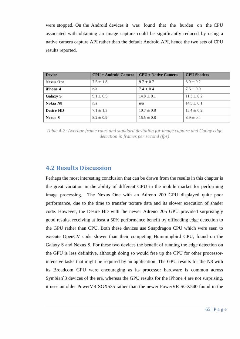
65 | P a g e

were stopped. On the Android devices it was found that the burden on the CPU

associated with obtaining an image capture could be significantly reduced by using a

native camera capture API rather than the default Android API, hence the two sets of CPU

results reported.

Device CPU + Android Camera CPU + Native Camera GPU Shaders

Nexus One 7.5 ± 1.8 9.7 ± 0.7 3.9 ± 0.2

iPhone 4 n/a 7.4 ± 0.4 7.6 ± 0.0

Galaxy S 9.1 ± 0.5 14.8 ± 0.1 11.3 ± 0.2

Nokia N8 n/a n/a 14.5 ± 0.1

Desire HD 7.1 ± 1.3 10.7 ± 0.8 15.4 ± 0.2

Nexus S 8.2 ± 0.9 15.5 ± 0.8 8.9 ± 0.4

Table 4-2: Average frame rates and standard deviation for image capture and Canny edge

detection in frames per second (fps)

Results Discussion 4.2Perhaps the most interesting conclusion that can be drawn from the results in this chapter is

the great variation in the ability of different GPU in the mobile market for performing

image processing. The Nexus One with an Adreno 200 GPU displayed quite poor

performance, due to the time to transfer texture data and its slower execution of shader

code. However, the Desire HD with the newer Adreno 205 GPU provided surprisingly

good results, receiving at least a 50% performance benefit by offloading edge detection to

the GPU rather than CPU. Both these devices use Snapdragon CPU which were seen to

execute OpenCV code slower than their competing Hummingbird CPU, found on the

Galaxy S and Nexus S. For these two devices the benefit of running the edge detection on

the GPU is less definitive, although doing so would free up the CPU for other processor-

intensive tasks that might be required by an application. The GPU results for the N8 with

its Broadcom GPU were encouraging as its processor hardware is common across

Symbianˆ3 devices of the era, whereas the GPU results for the iPhone 4 are not surprising,

it uses an older PowerVR SGX535 rather than the newer PowerVR SGX540 found in the

66 | P a g e

Galaxy S and Nexus S. It should be reiterated that the iPhone CPU results were taken using

an OpenCV build that was not optimized for that platform.

It is worthwhile to compare the frame rates with some of the OpenGL ES rendering

benchmarks that are available. For instance, [80] reports comparative benchmark results

for Nexus One (819), iPhone 4 (1361), Galaxy S (2561), Desire HD (2377), and Nexus S

(2880). These results do depart somewhat from the GPU fps results in this chapter,

indicating differences between benchmarking GPU for typical graphics rendering versus

performing an image processing algorithm such as Canny edge detection.

The general pattern in the GPU ability for image processing appears to have reached a

tipping point during the 2010 release period of the investigated devices, with some devices

clearly being able to benefit from offloading processing to the GPU. As GPU continue to

rapidly evolve, with the release of Adreno 220 and PowerVR SGX543, along with new

GPU such as the Mali and the Tegra 2 for mobile devices available on devices in 2011, this

benefit is only continuing to increase. For instance, modest performance improvements are

observed in the Sony Ericsson Xperia Arc, released in April 2011 with same CPU and

GPU as the Desire HD, with the CPU+Android Camera tests achieving 10.0±1fps and

GPU shaders achieving 17.5 ±0.1fps. More impressive are the results for the Samsung

Galaxy S2, first released in May 2011 with a 1.5 GHz Snapdragon S3 CPU and

Mali-400 GPU. Its CPU+Android Camera tests achieved 14.2 ± 0.7fps, which were

dwarfed by the GPU shader results of 33.8 ± 3.6fps. Since the writing of this paper even

more powerful devices have proven that using the GPU for image analysis is beneficial for

performance frame rates. For example testing this GPU-based Canny edge detection

implementation on the latest Samsung Galaxy S4 phone model with a PowerVR SGX

544MP3 GPU, boasts a frame rate of 20.6 ± 2.3 fps on the full resolution (1920x1080)

high definition display and achieving 58.4 ± 2.6 fps on 640x480 images. This severely

outmatched its OpenCV CPU based counterpart by a factor of up to 4 times the average

framerate.

67 | P a g e

Chapter 5

GPU-based Feature point detection

This chapter is joint with my supervisor Dr Andrew Ensor and discusses a real-time feature

point detection algorithm which we have called ColourFAST [18] which was presented

and published in the Image Vision Computing New Zealand 2013 conference proceedings.

ColourFAST extracts vector-based feature strength and direction measures from the colour

channels of any pixel in an image. The algorithm has a pipeline design which is optimized

for GPU processors. Results of the algorithms are provided for an implementation on

mobile devices developed using programmable shaders. Its performance demonstrates

several improvements over conventional FAST which is good for mobiles but doesn’t give

much information describing the feature point which is detected. The work in [16] has

shown mobile GPU to be advantageous to image analysis in regards to processing speed.

This work was focused on quick processing of feature points for improving object

detection, tracking and recognition on mobile devices without affecting accuracy. These

detected features are relatively unique and are processed very quickly through the pipeline.

These characteristics combined play an important factor for mobile augmented reality

applications. The GPU shader code for this algorithm can be found in Appendix B:

ColourFAST Feature Detection Shaders

Feature Detection and Description 5.1The term feature is used to refer to some region or point within an image that is

considered distinctive in some way, such as an edge, corner or blob. Features are

widely used for image segmentation, matching, image stitching, motion tracking, object

recognition, and 3D scene reconstruction. Popular feature detection algorithms include

Canny edge detection [48], Shi-Tomasi corner detection [17], SUSAN corner detection

[53], and Laplacian of Gaussian for blob detection. Features from Accelerated Segment

Test (FAST) [55], [56] is a particularly efficient and simple corner detection algorithm for

a greyscale image. FAST uses the idea of taking 16 pixels in a Bresenham circle of radius

three around the pixel being tested, where at least 12 of these should have an intensity

68 | P a g e

differing from the centre pixel above some threshold for the pixel be considered a

corner feature.

Features are also often accompanied by feature descriptions (also called feature vectors),

which are numbers that help describe the distinctive characteristics of a feature, assisting in

the identification of the feature in later frames or against sought objects. Popular feature

descriptions include Scale Invariant Feature Transform [129] , Histogram of Oriented

Gradients (HOG) [130], and Speeded Up Robust Features (SURF) [60]. Feature

descriptions can be extracted from sequential frames taken from a moving scene to

recognize previously identified features and so perform motion tracking. However, feature

descriptions can often be computationally expensive to calculate, so an optical flow

algorithm such as Lucas-Kanade [62] or its variant Kanade-Lucas-Tomasi [63] is often

used for tracking once feature points have been initially found. Tracked features can often

be used for mobile augmented reality applications as demonstrated in [131], which

comments that much work still needs to be undertaken to make good real time solutions

possible.

Graphical Processing Units (GPU) have become popular for many image processing tasks

due to their excellent performance with highly parallel floating point calculations [81],

[132]. Of particular interest in this research is the role of the GPU for image processing on

mobile devices, particularly for the extraction of features and their tracking for mobile

augmented reality applications, although this work is relevant for any system with GPU

hardware acceleration. Mobile devices place numerous challenges on computer vision

algorithms, they have varying camera capture qualities and resolutions, different

processing capabilities, and many vision algorithms that perform well on desktop

workstations suffer from unacceptably low frame rates on mobile devices. This helps

explain why there are still no widely used standardized test videos for mobile platforms

against which to compare algorithms. Previous work undertaken with GPU-based image

processing on mobiles devices was discussed in [127], [128]. In particular, [16]

demonstrated that mobile devices reached a tipping point in 2010, where mobile GPUs

started to demonstrate superiority over their CPU counterparts for performing some image

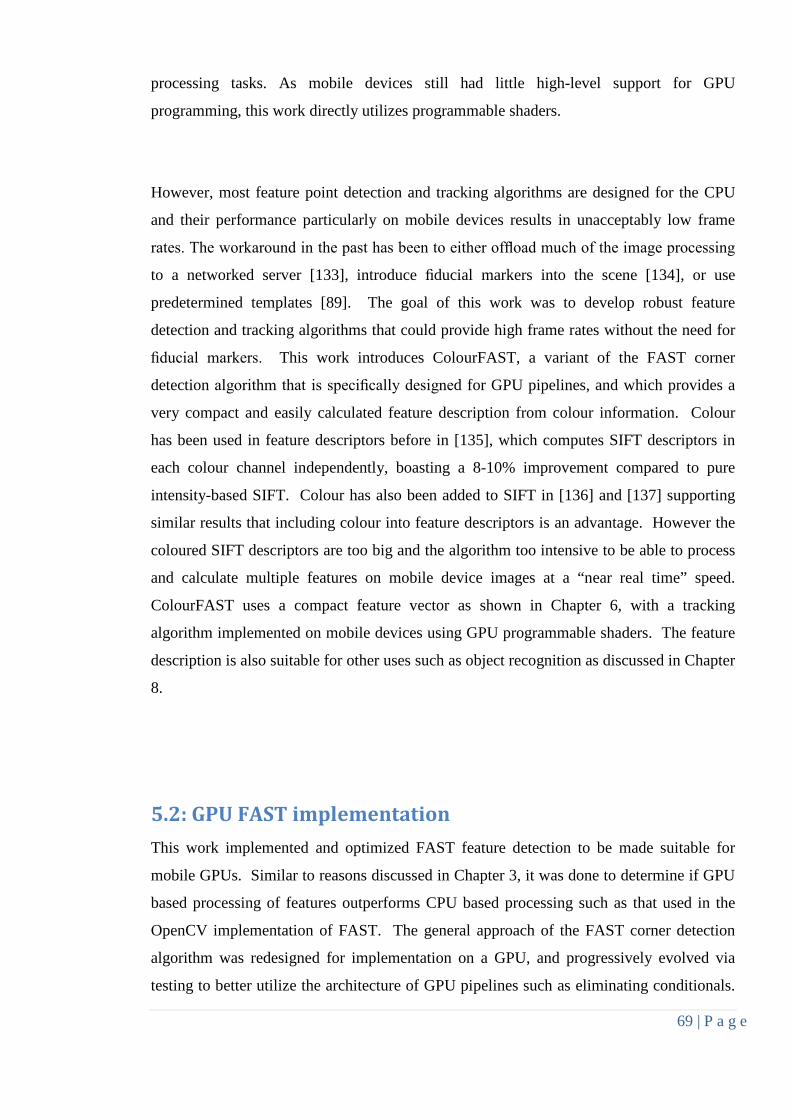
69 | P a g e

processing tasks. As mobile devices still had little high-level support for GPU

programming, this work directly utilizes programmable shaders.

However, most feature point detection and tracking algorithms are designed for the CPU

and their performance particularly on mobile devices results in unacceptably low frame

rates. The workaround in the past has been to either offload much of the image processing

to a networked server [133], introduce fiducial markers into the scene [134], or use

predetermined templates [89]. The goal of this work was to develop robust feature

detection and tracking algorithms that could provide high frame rates without the need for

fiducial markers. This work introduces ColourFAST, a variant of the FAST corner

detection algorithm that is specifically designed for GPU pipelines, and which provides a

very compact and easily calculated feature description from colour information. Colour

has been used in feature descriptors before in [135], which computes SIFT descriptors in

each colour channel independently, boasting a 8-10% improvement compared to pure

intensity-based SIFT. Colour has also been added to SIFT in [136] and [137] supporting

similar results that including colour into feature descriptors is an advantage. However the

coloured SIFT descriptors are too big and the algorithm too intensive to be able to process

and calculate multiple features on mobile device images at a “near real time” speed.

ColourFAST uses a compact feature vector as shown in Chapter 6, with a tracking

algorithm implemented on mobile devices using GPU programmable shaders. The feature

description is also suitable for other uses such as object recognition as discussed in Chapter

8.

: GPU FAST implementation 5.2This work implemented and optimized FAST feature detection to be made suitable for

mobile GPUs. Similar to reasons discussed in Chapter 3, it was done to determine if GPU

based processing of features outperforms CPU based processing such as that used in the

OpenCV implementation of FAST. The general approach of the FAST corner detection

algorithm was redesigned for implementation on a GPU, and progressively evolved via

testing to better utilize the architecture of GPU pipelines such as eliminating conditionals.

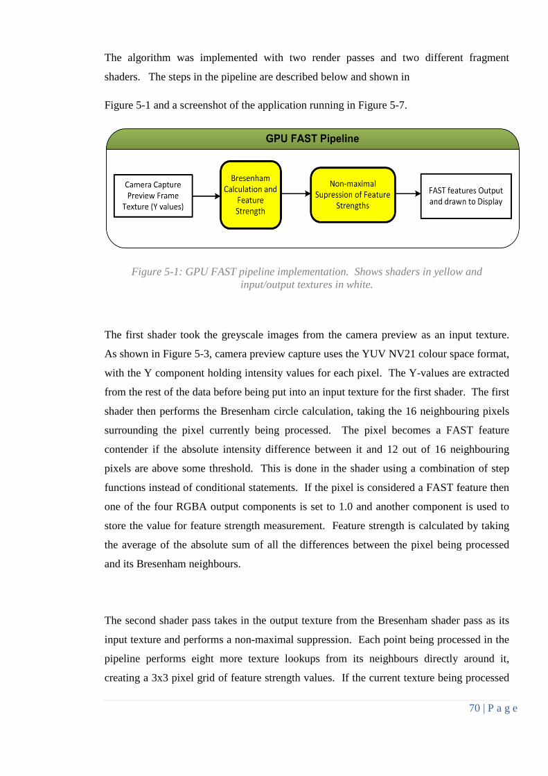
70 | P a g e

The algorithm was implemented with two render passes and two different fragment

shaders. The steps in the pipeline are described below and shown in

Figure 5-1 and a screenshot of the application running in Figure 5-7.

Figure 5-1: GPU FAST pipeline implementation. Shows shaders in yellow and input/output textures in white.

The first shader took the greyscale images from the camera preview as an input texture.

As shown in Figure 5-3, camera preview capture uses the YUV NV21 colour space format,

with the Y component holding intensity values for each pixel. The Y-values are extracted

from the rest of the data before being put into an input texture for the first shader. The first

shader then performs the Bresenham circle calculation, taking the 16 neighbouring pixels

surrounding the pixel currently being processed. The pixel becomes a FAST feature

contender if the absolute intensity difference between it and 12 out of 16 neighbouring

pixels are above some threshold. This is done in the shader using a combination of step

functions instead of conditional statements. If the pixel is considered a FAST feature then

one of the four RGBA output components is set to 1.0 and another component is used to

store the value for feature strength measurement. Feature strength is calculated by taking

the average of the absolute sum of all the differences between the pixel being processed

and its Bresenham neighbours.

The second shader pass takes in the output texture from the Bresenham shader pass as its

input texture and performs a non-maximal suppression. Each point being processed in the

pipeline performs eight more texture lookups from its neighbours directly around it,

creating a 3x3 pixel grid of feature strength values. If the current texture being processed

71 | P a g e

has higher feature strength than its neighbours, then it becomes a FAST feature point,

otherwise it is discarded to allow the neighbour with the higher feature strength to instead

be the feature. The resulting feature points are then drawn overlaid onto the original

camera image and rendered to the display.

: ColourFAST Feature Point Detection Implementation 5.3After testing FAST, several disadvantages of the algorithm were noted. The first being

that only features with a large change in intensity were detected, even if the colours were

completely different such as the corner of a dark red object on a dark blue background.

Secondly the presence of noise and the use of thresholds in the image to determine valid

feature points resulted in features “appearing” and “disappearing”. To counteract these

disadvantages, colour was added to the calculations by binding UV camera values into

another texture and passing it into the pipeline. Colour channels provided valuable

information about feature points which could be utilized with little added computation by

exploiting the single instruction multiple data (SIMD) nature of GPUs. Change across

pixels also gave an orientation for the feature, so a direction calculation was added to the

shader. This combined with the Bresenham colour values for feature points gave a more

unique and compact descriptor to each of the features than purely a single intensity value

which FAST typically uses. To reduce noise a 3x3 smoothing step was added as extra

shader passes. It was decided that the minimum 12 requirement of neighbours should be

removed to allow all features of interest and not just corners, this also meant that features

stayed in place over frames and didn’t phase in and out. Removing the intensity difference

threshold was found useful when implementing GPU Canny edge detection from Chapter

3, so this implementation also removed the FAST intensity threshold. This allows the host

application to control thresholds if desired, making the threshold not an integral part of the

algorithm. After some number modelling, it was shown that using the smoothing step in

the pipeline allowed the number of texture lookups in the Bresenham circle to be reduced

by half. These combined changes led to the algorithm ColourFAST feature detection to be

termed for this thesis. The full pipeline is shown below in Figure 5-2.

72 | P a g e

Figure 5-2: GPU ColourFAST feature detection pipeline. Shaders are shown in yellow and the input/output textures are in white. The shader shown with the dotted border is optional

if a direction vector in all 3 components is desired.

5.3.1: CPU Side Setup and Android Camera Capture The CPU side of the algorithm and setup of the pipeline is similar to section 3.2.1. Only

devices on the Android platform were used, however with minor changes in the setup, this

algorithm will work on any OpenGL ES supported devices. ColourFAST takes a coloured

image frame as input. On Android devices images are often made available in the NV21

format, a YUV colour space format where the 8-bit Y samples are followed by an

interleaved VU plane containing 8-bit 2x2 sub-sampling. A Y value is stored for every

pixel, followed by a U value for each 2×2 square block of pixels, and finally a V value for

each 2×2 block. Corresponding Y, U and V values are shown using the same colour in the

diagram in Figure 5-3.

73 | P a g e

Figure 5-3: YUV colour space using the NV21 format for a 6x4 pixel texture and their positions in a byte stream [138].

As is common in GPU image processing the camera image was loaded as read-only

textures after splitting the data, the first texture which contains the Y values and the second

containing the interleaved VU values, ready for use by the programmable shaders.

Because of the large size of the data being obtained from the camera preview it is best to

preallocate memory using a buffered array instead of letting the camera callback constantly

create a new array every frame. However care needs to be taken as since this is done in a

separate thread, the buffer may still be in use from the thread passing information into the

pipeline. After some testing it was found that using three pre allocated buffers for the

camera capture with some synchronization worked well. These get cycled by the program

to be optimal in ensuring a smooth run through the pipeline avoiding contention and

allowing the camera capture thread to populate buffers while the previous buffer is still

being used in the shader pipeline.

5.3.2: Colour Conversion On the GPU a preliminary render pass is performed, taking a texture for the Y values and

another for the interleaved VU values, and outputting a single texture with either YUV

values or RGB values for each pixel in the image. This avoids the rest of the pipeline

having to look up two textures when a shader wants to access the original colour values for

74 | P a g e

each pixel, it also ensures less calculations later as pixel information can be calculated

using single vectors. The conversion to RGB colour space has little effect on the overall

performance of the algorithm but no noticeable advantage was found in practice using

either colour space over the other. RGB colour information can be taken from a YUV

information using the following formula:

�𝑅𝐺𝐵� = �

Y + V ∗ 1.402 − 0.701 Y − U ∗ 0.344 − V ∗ 0.714 + 0.529

Y + U ∗ 1.772 − 0.886�

5.3.3: Smoothing Unlike FAST, the ColourFAST feature point algorithm performs a smoothing (blur) via a

3×3 convolution kernel on each of the colour channels. Smoothing is relatively uncommon

in feature point detection algorithms but this work found that it gave unexpected benefits

with improvement in feature point detection. Using a Gaussian smoothing kernel has been

used before in [88] and ensures that the features are more resilient to image noise. Since a

Gaussian kernel is separable it can be applied as two one-dimensional convolutions in the

X direction and then the Y direction of the image, trading the overhead of having an

additional render pass for three less texture reads and fewer calculations. This was found to

provide a small performance benefit on actual devices. In practice, a slightly modified

smoothing kernel is applied to give a smoother distribution across the 65 pixels used in

feature point calculations as shown:

�0.09 0.12 0.090.12 0.16 0.120.09 0.12 0.09

� = �0.30.40.3

� · (0.3 0.4 0.3)

5.3.4: Half Bresenham and Feature Strength Calculation The next render pass is similar to FAST in that it calculates feature point values by taking

a pixel and subtracting it from the average of the neighbouring pixels around it in the

Bresenham circle to give the change in intensity. However, in ColourFAST this

calculation is performed in each colour channel rather than on a greyscale image. It also

does not use a threshold which is common in FAST to filter out just corners opting instead

to generate all features. Unlike FAST which uses 16 neighbouring pixels, this algorithm

75 | P a g e

halves the number of texture lookups using only 8 neighbouring pixels as illustrated in

Figure 5-4. Because of the smoothing performed earlier in the pipeline the pixels being

looked up in the modified Bresenham circle are actually blended with their eight

neighbouring pixels. This gives a total of 65 pixels used in the feature calculation, shown

in Figure 5-5, as opposed to the 17 in the conventional FAST approach. Yet this approach

only uses a total of 15 texture lookups overall (including those required for the smoothing),

two less than that required by FAST. Some initial testing showed this made ColourFAST

more robust than FAST in the presence of noise. The formula below shows how the three

channel feature point values (FR, FG, FB) are calculated from colour of the current pixel P

less the average colour of its eight half-Bresenham neighbours N.

�𝐹𝑅𝐹𝐺𝐹𝐵� = �

𝑃𝑅𝑃𝐺𝑃𝐵� − ��

𝑁𝑖,𝑅𝑁𝑖,𝐺𝑁𝑖,𝐵

�𝑛=8

𝑖=0

× 18

Figure 5-4: Bresenham circle (left) used by FAST and half-Bresenham circle (right) used by ColourFAST.

Once the feature point values are calculated for a pixel the three colour channel

values can be weighted to also give an overall (scalar) feature strength value. The U

and V changes for feature point calculations were found to be significantly less than the Y

changes. Empirical weighting values with a multiplier of 2 for Y values and 7 for

each of the U and V values were found to give good results in practice. If RGB colour

space was instead used, then a weighting of 2 for each component gives good results. The

weighting factors were passed as uniform values to the programmable shader so they could

be altered whenever feature points in particular channels were of interest. Although the

76 | P a g e

scalar feature strength values are convenient for finding strong features, typically corners,

the three feature point values considered together as a vector were found to provide richer

and more useful information about features.

Figure 5-5: Actual neighbourhood pixel contributions to ColourFAST.

5.3.5 Feature Direction Calculation Another render pass also takes the output from the smoothing and calculates a vector

orientation for features, either as 𝑋𝑑𝑖𝑑 and 𝑌𝑑𝑖𝑑 components or an angle direction θ =

arctan2(𝑋𝑑𝑖𝑑 ,𝑌𝑑𝑖𝑑). The orientation can be combined with the three YUV/RGB feature

point values as a compact feature description to help identify a feature, or else determine

the rotation of a feature relative to the camera. The orientation is calculated by first taking

the vector sum of the eight RGB changes in the half-Bresenham circle around a pixel as

shown in Figure 5-6, subtracting pixels below the centre pixel from the corresponding

pixels above to calculate ∆𝑌, and the right pixels minus the corresponding left pixels for

∆𝑋. Before this calculation is performed and assuming a distance of 1 unit from the centre

pixel to each neighbour, a simple Pythagoras equation is used to calculate two constants to

multiply each RGB value in the X and Y directions. This creates a vector for each of the

three colour components, which are then combined together into a single 𝑋𝑑𝑖𝑑, 𝑌𝑑𝑖𝑑 vector

by taking the dot product with the vector formed from the feature point description values

F (so colour components with stronger changes have their orientations weighted more

heavily). This is then divided by the length of the feature point description to keep the

77 | P a g e

information between 0 and 1 so that it can be passed out of the shader in the output texture.

The formula for the 𝑋𝑑𝑖𝑑, 𝑌𝑑𝑖𝑑 vector is shown below:

𝑋𝑑𝑖𝑑 = �𝐹𝑅𝐹𝐺𝐹𝐵

�∙�∆𝑋𝑅∆𝑋𝐺∆𝑋𝐵

�

��𝐹𝑅𝐹𝐺𝐹𝐵

�� 𝑌𝑑𝑖𝑑 =

�𝐹𝑅𝐹𝐺𝐹𝐵

�∙�∆𝑌𝑅∆𝑌𝐺∆𝑌𝐵

�

��𝐹𝑅𝐹𝐺𝐹𝐵

�� 𝜃 = atan2(𝑋𝑑𝑖𝑑,𝑌𝑑𝑖𝑑)

Figure 5-6: Shows texture for feature direction vector calculations giving ∆𝑋 and ∆𝑌in each colour space channel

Instead of using 𝑋𝑑𝑖𝑑 and 𝑌𝑑𝑖𝑑direction vector components it is also possible to just use

the single θ value, this has the advantage that a feature description then only has four

components, YUV/RGB feature point values and a single feature change angle, which can

fit into a single four-component texture. This also means that this step can be combined

with the half Bresenham and feature strength render pass discussed in the previous section

to avoid a drop in performance. Another option was to perform this render pass twice,

once for the 𝑋𝑑𝑖𝑑 and once for 𝑌𝑑𝑖𝑑 to give direction vectors in each of the three

colour channels, however the overall vector orientation combined over all channels was

found to be sufficient to determine the rotation of features relative to the camera. The

following formulas show the calculation of 𝑋𝑑𝑖𝑑, 𝑌𝑑𝑖𝑑 and then using them to create a single

direction measure θ for the feature descriptor.

78 | P a g e

ColourFAST Results and Comparison to FAST 5.4One advantage ColourFAST has over most contemporary feature detection algorithms

such as FAST is the use of colour instead of greyscale, using three colour channels in

either the native camera format YUV or the RGB colour space. This allows the extraction

of features that are distinguished by a change in colour but not necessarily a large change

in overall intensity. The shader calculations are all done using vector SIMD calculations,

for which GPU are optimised so little or no performance penalty is incurred. The three

feature point values combined with optional feature orientation give a compact feature

description which can be efficiently recalculated each frame, enabling tracking of features

over time or with changing lighting conditions, which can be difficult with scalar-based

feature values, particularly when there are other features nearby. Another significant

difference with ColourFAST is that no threshold is used to ensure that a point is a

corner rather than some type of edge. Thus, ColourFAST can be used for identifying

features in any non-uniform region, not only those that lie at corners. For instance, the

features of edges can be followed to find the contour of objects, giving a cluster of points

which can be used to better identify and track an object.

Testing was performed on two devices, the Samsung Galaxy S2 model I9100 with the

ARM Mali-400 MP4 GPU, and the Samsung Galaxy S4 model GT-I9505 with the Adreno

320 GPU. The devices were programmed with Android 2.3 and 4.2 respectively and both

used the Open GL ES 2.0 pipeline with GLSL version 1.0 GPU shader language. OpenCV

version 2.4.1 was used for the CPU implementation. It is important to note that the

ColourFAST algorithm is designed for any device with pipeline hardware acceleration, and

on many (non-mobile) platforms could instead be implemented via OpenCL or CUDA.

Table 5-1 compares the average frame rates for Android implementations of FAST and

ColourFAST on both the Samsung Galaxy S2 and S4 across a range of available image

resolutions. Each algorithm test for each device and resolution was run on the device for

five minutes with average frame rates recorded every five seconds giving a sample size

between 5000 – 20,000 readings depending on the device, resolution set and algorithm.

The readings were also taken from fully charged mobile devices set in their default factory

settings. In practice, the camera resolution might first be scaled down before feature

79 | P a g e

detection is undertaken. The stated results are the sustained frame rates for the entire

pipeline, including camera capture and all processing for feature detection each frame.

The usual CPU-based OpenCV implementation of FAST on Android using greyscale

images was tested along with a modified version optimised specifically for GPU pipelines,

replacing all conditional statements by combinations of step functions. Neither included

the additional step where the greatest FAST feature value in a neighbourhood is typically

sought as the feature point, which would lower the frame rates if included. A GPU

implementation of ColourFAST was tested on the same Android devices. As might be

expected the GPU implementations outperformed the CPU-based OpenCV

implementation. Although the ColourFAST algorithm extracts richer information from

features than the FAST algorithm it does have comparable performance, in fact being

surprisingly faster on the Galaxy S2, and only marginally slower on the Galaxy S4 with

HD resolution images. Figure 5-7 demonstrates ColourFAST feature values (in three

colour channels with orientation held in the alpha channel) for an outdoor scene.

Device and Resolution FAST (OpenCV) FAST (GPU) ColourFAST (GPU)

Galaxy S2 (640x480) 25.1 30.5 39.8

Galaxy S2 (800x480) 20.6 25.5 32.4

Galaxy S4 (640x480) 21.3 53.7 51.4

Galaxy S4 (1920x1080) 8.3 23.3 21.3

Table 5-1: Average feature point throughput comparisons in frames per second (fps)

80 | P a g e

Figure 5-7: Outdoor scene with GPU FAST (upper) with features shown in green versus ColourFAST (lower) feature values evaluated at each pixel.

Another interesting comparison between ColourFAST and FAST are how they can be used

to distinguish corners from edges. Modelling was done to see which algorithm can

produce more distinct features, assuming that there is no threshold used for both algorithms

and only a single channel used for calculations. The tables in Figure 5-8 to Figure 5-12

show five different situations of FAST (left of tables) vs ColourFAST (right of tables). It

models a single channel white object on a black background. The different corners

modelled are shown in grey and their calculated pixel values populated in the table. FAST

is known for its ability to distinguish corners from edges, however ColourFAST has shown

to have a higher corner to edge ratio in all but one of the examples modelled here. Another

81 | P a g e

interesting observation is the outer rim features in ColourFAST (shown on the table with

blue numbering) which occur as a result of the smoothing step, these features are weaker

but with opposite values to the inner rim of feature points (with high values shown as red

numbering) and also resulting in opposing direction vectors. This creates a valley in

between the ridges with very low feature point values and used later in the thesis in

Chapter 7 in which a GPU-based algorithm for feature discovery is developed. This

algorithm is used to navigate the contour of the object by following the channel between

opposing features and extracting more feature points along the way creating a cluster of

feature points for the object which is then used for improved tracking. It is important to

note that the ColourFAST corner is detected slightly in from the true corner of the real

world image and thus used as the high value in the corner to edge calculation.

0.0 0.0 0.0 0.0 0.0 0.0 0.0 0.0 0.0

0.0 0.0 0.1 0.2 0.4 0.5 0.6 0.6 0.6

0.0 0.0 0.0 1.0 2.0 3.0 3.0 3.0 3.0 0.0 0.0 0.2 0.5 0.9 1.2 1.4 1.4 1.4

0.0 0.0 1.0 2.0 3.0 4.0 5.0 5.0 5.0 0.1 0.2 0.6 1.0 1.6 2.0 2.4 2.5 2.6

0.0 1.0 2.0 3.0 4.0 5.0 6.0 7.0 7.0 0.2 0.5 1.0 0.7 0.3 0.0 0.5 0.8 1.0

0.0 2.0 3.0 4.0 -11.0 -10.0 -9.0 -7.0 -7.0 0.4 0.9 1.6 0.3 -1.3 -2.6 -1.9 -1.4 -1.0

0.0 3.0 4.0 5.0 -10.0 -9.0 -8.0 -5.0 -5.0 0.5 1.2 2.0 0.0 -2.6 -4.6 -3.8 -3.1 -2.6

0.0 3.0 5.0 6.0 -9.0 -8.0 -6.0 -3.0 -3.0 0.6 1.4 2.4 0.5 -1.9 -3.8 -2.8 -2.0 -1.4

0.0 3.0 5.0 7.0 -7.0 -5.0 -3.0 0.0 0.0 0.6 1.4 2.5 0.8 -1.4 -3.1 -2.0 -1.2 -0.6

0.0 3.0 5.0 7.0 -7.0 -5.0 -3.0 0.0 0.0 0.6 1.4 2.6 1.0 -1.0 -2.6 -1.4 -0.6 0.0

0.0 3.0 5.0 7.0 -7.0 -5.0 -3.0 0.0 0.0 0.6 1.4 2.6 1.0 -1.0 -2.6 -1.4 -0.6 0.0

0.0 3.0 5.0 7.0 -7.0 -5.0 -3.0 0.0 0.0 0.6 1.4 2.6 1.0 -1.0 -2.6 -1.4 -0.6 0.0

Figure 5-8: FAST vs ColourFAST feature strengths at a 90 degree corner. Corner to edge

ratios are 1.57:1 and 1.77:1 respectively.

0.0 0.0 0.5 1.0 1.5 1.5 1.5 1.5 1.5

0.0 0.1 0.3 0.6 0.8 1.0 1.0 1.0 1.0

0.0 0.5 1.0 2.0 3.0 4.0 4.0 4.0 4.0 0.1 0.3 0.6 1.0 1.5 1.8 2.0 2.0 2.0

0.5 1.0 2.0 3.0 4.0 5.0 6.0 6.0 6.0 0.3 0.6 0.6 0.7 0.8 1.3 1.6 1.8 1.8

1.0 2.0 3.0 -4.0 -3.0 -2.0 -0.5 0.0 0.0 0.6 1.0 0.7 -0.3 -1.1 -1.0 -0.4 -0.1 0.0

1.5 3.0 4.0 -3.0 -10.0 -9.0 -7.0 -6.0 -6.0 0.8 1.5 0.8 -1.1 -3.0 -3.2 -2.5 -2.0 -1.8

1.5 4.0 5.0 -2.0 -9.0 -7.5 -5.5 -4.0 -4.0 1.0 1.8 1.3 -1.0 -3.2 -3.7 -2.9 -2.3 -2.0

1.5 4.0 6.0 -0.5 -7.0 -5.5 -3.0 -1.5 -1.5 1.0 2.0 1.6 -0.4 -2.5 -2.9 -2.0 -1.3 -1.0

1.5 4.0 6.0 0.0 -6.0 -4.0 -1.5 0.0 0.0 1.0 2.0 1.8 -0.1 -2.0 -2.3 -1.3 -0.6 -0.3

1.5 4.0 6.0 0.0 -6.0 -4.0 -1.5 0.0 0.0 1.0 2.0 1.8 0.0 -1.8 -2.0 -1.0 -0.3 0.0

1.5 4.0 6.0 0.0 -6.0 -4.0 -1.5 0.0 0.0 1.0 2.0 1.8 0.0 -1.8 -2.0 -1.0 -0.3 0.0

1.5 4.0 6.0 0.0 -6.0 -4.0 -1.5 0.0 0.0 1.0 2.0 1.8 0.0 -1.8 -2.0 -1.0 -0.3 0.0

Figure 5-9: FAST vs ColourFAST feature strengths at soft 90 degree corner. Corner to

edge ratios are 1.66:1 and 1.85:1 respectively.

82 | P a g e

0.0 0.0 0.0 0.0 3.0 5.0 7.0 7.0 -7.0

0.0 0.0 0.2 0.7 1.5 2.5 2.6 1.2 -1.2

0.0 0.0 0.0 3.0 5.0 7.0 7.0 -7.0 -7.0 0.0 0.1 0.5 1.3 2.4 2.5 1.2 -1.2 -2.6

0.0 0.0 2.0 4.0 6.0 7.0 -7.0 -7.0 -5.0 0.1 0.3 1.1 1.9 2.3 1.0 -1.2 -2.6 -2.5

0.0 1.0 3.0 5.0 6.0 -8.0 -7.0 -5.0 -3.0 0.2 0.7 1.5 1.7 0.6 -1.6 -2.7 -2.6 -1.5

0.0 2.0 4.0 5.0 -9.0 -8.0 -6.0 -3.0 0.0 0.4 1.0 2.0 0.9 -1.3 -3.3 -2.9 -1.7 -0.7

0.0 3.0 4.0 6.0 -9.0 -7.0 -5.0 0.0 0.0 0.5 1.3 2.2 0.4 -2.0 -3.5 -2.3 -1.1 -0.2

0.0 3.0 5.0 6.0 -8.0 -6.0 -3.0 0.0 0.0 0.6 1.4 2.4 0.6 -1.5 -3.1 -1.7 -0.7 0.0

0.0 3.0 5.0 7.0 -7.0 -5.0 -3.0 0.0 0.0 0.6 1.4 2.5 0.9 -1.2 -2.7 -1.5 -0.6 0.0

0.0 3.0 5.0 7.0 -7.0 -5.0 -3.0 0.0 0.0 0.6 1.4 2.6 1.0 -1.0 -2.6 -1.4 -0.6 0.0

0.0 3.0 5.0 7.0 -7.0 -5.0 -3.0 0.0 0.0 0.6 1.4 2.6 1.0 -1.0 -2.6 -1.4 -0.6 0.0

0.0 3.0 5.0 7.0 -7.0 -5.0 -3.0 0.0 0.0 0.6 1.4 2.6 1.0 -1.0 -2.6 -1.4 -0.6 0.0

Figure 5-10: FAST vs ColourFAST feature strengths at a 135 degree corner. Corner to

edge ratios are 1.28:1 and 1.35:1 respectively.

0.0 0.0 0.0 0.0 0.0 0.0 0.0 0.0 0.0

0.0 0.0 0.1 0.1 0.2 0.1 0.1 0.0 0.0

0.0 0.0 0.0 1.0 1.0 1.0 0.0 0.0 0.0 0.0 0.0 0.2 0.4 0.5 0.5 0.3 0.1 0.0

0.0 0.0 1.0 1.0 2.0 2.0 2.0 0.0 0.0 0.1 0.1 0.4 0.6 1.0 0.9 0.9 0.5 0.2

0.0 1.0 1.0 2.0 2.0 3.0 3.0 3.0 0.0 0.2 0.4 0.6 0.1 0.3 0.7 1.5 1.1 0.7

0.0 2.0 2.0 2.0 -13.0 3.0 4.0 5.0 3.0 0.4 0.7 1.1 -0.7 -1.6 -1.0 1.3 2.0 1.5

0.0 3.0 3.0 3.0 -13.0 -12.0 4.0 7.0 5.0 0.5 1.1 1.5 -0.9 -3.3 -3.6 -0.2 2.0 2.5

0.0 3.0 5.0 4.0 -12.0 -12.0 -10.0 7.0 7.0 0.6 1.3 2.1 -0.3 -3.4 -5.1 -2.6 0.6 2.6

0.0 3.0 5.0 7.0 -10.0 -10.0 -10.0 -7.0 7.0 0.6 1.4 2.4 0.3 -2.5 -5.1 -4.0 -1.8 1.2

0.0 3.0 5.0 7.0 -7.0 -8.0 -8.0 -7.0 -7.0 0.6 1.4 2.6 0.8 -1.7 -4.1 -3.9 -3.2 -1.2

0.0 3.0 5.0 7.0 -7.0 -5.0 -6.0 -5.0 -7.0 0.6 1.4 2.6 1.0 -1.2 -3.3 -2.9 -3.1 -2.6

0.0 3.0 5.0 7.0 -7.0 -5.0 -3.0 -3.0 -5.0 0.6 1.4 2.6 1.0 -1.0 -2.8 -2.1 -2.1 -2.5

Figure 5-11: FAST vs ColourFAST feature strengths at a 45 degree corner. Corner to

edge ratios are 1.86:1 and 1.82:1 respectively.

0.0 0.0 0.0 0.0 0.0 0.0 0.0 0.0 0.0

0.0 0.0 0.1 0.2 0.3 0.3 0.2 0.1 0.0

0.0 0.0 0.0 1.0 2.0 2.0 1.0 0.0 0.0 0.0 0.0 0.2 0.5 0.7 0.7 0.5 0.2 0.0

0.0 0.0 1.0 2.0 2.0 2.0 2.0 1.0 0.0 0.1 0.2 0.5 0.8 1.0 1.0 0.8 0.5 0.2

0.0 1.0 2.0 2.0 2.0 2.0 2.0 2.0 1.0 0.2 0.5 0.8 0.2 -0.7 -0.7 0.2 0.8 0.5

0.0 2.0 3.0 2.0 -14.0 -14.0 2.0 3.0 2.0 0.4 0.9 1.2 -0.6 -2.9 -2.9 -0.6 1.2 0.9

0.0 3.0 4.0 2.0 -14.0 -14.0 2.0 4.0 3.0 0.5 1.2 1.5 -1.2 -4.6 -4.6 -1.2 1.5 1.2

0.0 3.0 5.0 3.0 -14.0 -14.0 3.0 5.0 3.0 0.6 1.4 1.8 -0.9 -4.3 -4.3 -0.9 1.8 1.4

0.0 3.0 5.0 4.0 -12.0 -12.0 4.0 5.0 3.0 0.6 1.4 1.9 -0.6 -3.9 -3.9 -0.6 1.9 1.4

0.0 3.0 5.0 4.0 -12.0 -12.0 4.0 5.0 3.0 0.6 1.4 2.0 -0.4 -3.6 -3.6 -0.4 2.0 1.4

0.0 0.0 0.0 0.0 0.0 0.0 0.0 0.0 0.0 0.6 1.4 2.0 -0.4 -3.6 -3.6 -0.4 2.0 1.4

0.0 0.0 0.0 1.0 2.0 2.0 1.0 0.0 0.0 0.6 1.4 2.0 -0.4 -3.6 -3.6 -0.4 2.0 1.4

Figure 5-12: Fast vs ColourFAST feature strengths at the end of a pixel thin line. Corner

to edge ratios are 1.17:1 and 1.28:1 respectively.

83 | P a g e

Chapter 6

GPU-based Feature Tracking

This chapter is also based on [18] which is joint work with my supervisor Dr. Andrew

Ensor. It was presented and published in the Image Vision Computing New Zealand 2013

conference proceedings. Effort was invested in this thesis to implement efficient feature

tracking, particularly devising a GPU-optimized implementation of the Lucas-Kanade

optical flow algorithm. Given the high frame rates at which ColourFAST features can be

extracted from a frame it seems natural to ask whether the compact descriptions that are

produced might be sufficient to perform feature tracking by searching for a nearest-

matching feature in successive frames. The algorithm is GPU-pipeline designed and

implemented with programmable shaders on mobile platforms. The ColourFAST feature

search was compared to the OpenCV CPU-based version of Lucas-Kanade as well as my

own GPU-based version demonstrating improvements in both frame rate throughput and

tracking accuracy in real world scenes. The GPU shader code for this algorithm can be

found in Appendix B: ColourFAST Feature Detection Shaders.

There is a small amount of literature that discusses implementing tracking on mobile

devices. In particular [89], feature tracking is achieved using either a simplified SIFT or a

simplified FERNS [139] together with a patch tracker algorithm which tracked 15 frames

per second using a known image set not actual real time camera footage which incurs a

substantial overhead on mobile devices. Their testing was run on the highest performance

benchmarked mobile on the market at the time of publication, the Asus P552W, which has

a Marvell PXA930 SOC. The resolution of images tested was at a scaled down effective

resolution of 160x120 pixels. This thesis instead tests on devices that are three to five

years more recent and using actual camera footage with resolutions between 16-72 times

larger than that of the Asus P552W. More recently “real time” feature tracking has been

achieved on mobiles in [140] using their TLD (tracking-learning-detection) algorithm.

TLD uses learning-based approaches for detecting and tracks features in a small selectable

region using Lucas-Kanade tracking. It overlays an augmented bounding box over the

tracked region and appears to show good tracking accuracy even with changes of scale and

84 | P a g e

rotation. It has now been developed into an open source framework for Android called

OpenTLD.

: GPU-based Lucas Kanade implementation 6.1Lucas-Kanade is a well-known optical flow algorithm that can be used to track features.

This was investigated to see how it could be used to track our ColourFAST feature points.

Considerable time was invested looking at the OpenCV source code, which was used to

create a GPU-optimized version of Lucas Kanade. However this was a complicated task

and required several changes to the algorithm, notably reducing branching in the code and

combining calculations to be vector based to take full potential of the GPU. This was

achieved with five GPU shader passes as illustrated in Figure 6-1.

The OpenCV implementation of Lucas-Kanade is heavily optimized and has had several

improvements over the original version of Lucas-Kanade, it is primarily based on

improvements suggested in the papers [17, 141]. It requires two single channel greyscale

images for the current frame image as well as the previous frame. With these 2 image

snapshots it creates a further seven output images, the first four using X and Y Sobel

operations on the previous and current input frames (SNx,SNy,SPx,SPy). The next three

output images use the current frame to compute second derivative Sobels in the X, Y and

XY directions (Dxx,Dyy,Dxy). Similar to the discussion in Section 3.2.2, to reduce the

number of multiplications and texture lookups, these matrix operations were separated into

horizontal and vertical components with the expense of another render pass. The first four

shader passes work in two pairs both horizontally and vertically and calculate these seven

output image values from the two greyscale input textures. These result in 2 output

textures for these four shader passes with seven out of eight RGBA channels storing the

output images needed for the next step, the previous greyscale input image is used to fill

the 8th channel so that the next shader only needs to bind three input textures instead of

four.

The 5th shader pass takes the resulting output values generated from the previous four steps

as well as the previous and current image snapshots from the camera. This shader then

85 | P a g e

performs the rest of the Lucas-Kanade operations and calculates the number of movement

for each of the points which it stores in the output texture. Because of the amount of

texture lookups that are required, only a 7x7 tracking window was used with no

pyramiding, however this was found to be sufficient for tracking accuracy and in particular

keeping high frame rates. Because of the complexity of this shader, some devices (for

example even the newer Adenro GPU on the Samsung S4) were unable to compile the

shader code, so instead the shader had to be either split or have the number of texture

lookups further reduced, resulting in a smaller tracking window. However both these

approaches reduce frame rates and tracking accuracy respectively. These difficulties

confirmed that a GPU shader implementation of Lucas-Kanade may not be suitable for

current mobiles.

Figure 6-1: Lucas-Kanade GPU pipeline. Shaders are shown in yellow and the important input/output textures are in white.

: ColourFAST Feature Search implementation 6.2Since Lucas-Kanade isn’t well suited for a mobile GPU implementation, instead simpler

approaches were sought so that the number of operations and texture lookups could be

reduced therefore increasing frame rates, preferably without compromising tracking

accuracy. Given the high frame rates of ColourFAST and the compact feature vector that

it produces the question arose whether these features were unique enough to track.

86 | P a g e

ColourFAST feature search was developed which essentially searches for the nearest

matching feature description within a rectangular tracking window near where the point

was in the previous frame. The center of the search window can be set by the CPU host

application depending on prior knowledge of any ColourFAST feature points and their

expected locations in future frames. If a close match is not found then the application can

decide whether to move or resize the window before repeating the search. By default the

search window is taken to be a square (2m + 1) × (2m + 1) pixel window around the

expected next location of each feature point, assuming the point will not move more than m

pixels beyond that expected between consecutive frames. For testing points placed on the

screen by the user, this sets the search area window around the point that was selected.

This quad is passed through the pipeline and initially the actual point that is chosen is the

pixel in the search window with the greatest feature strength (highest total value in the

colour channels), allowing the tracking point to lock onto the best feature in the search

window to track initially. Once this is determined, the four component feature values for

that pixel are instead used to track the feature point. Essentially the GPU pipeline is

responsible for calculating the feature values, determining best match within the tracking

window, outputting the updated feature values and determining how much the point has

moved from the previous frame. The CPU host application is responsible for maintaining

where the points are on the screen and where to move the tracking window. In this

implementation the movements for each point over the last three frames were used to give

a smoothed velocity for the point, this was used to assist predicting where the tracking

window should be moved to next. ColourFAST feature search was achieved using three

shader passes and is discussed in the following subsections and shown in Figure 6-2.

87 | P a g e

Figure 6-2: GPU ColourFAST feature search pipeline. Shaders are shown in yellow and the important input/output textures are in white. Sought feature point is passed in as a

uniform vec4 shown above in grey.

6.2.1 Feature Point Difference Calculation The first shader pass takes in the four channel feature point, which includes the

ColourFAST colour changes and orientation from the previous frame, for the sought

feature point as a (uniform) four-component vector. It also binds the output texture

generated from the ColourFAST feature detection pipeline (Figure 5-2) as its input texture.

It uses the feature description for each pixel in the search window, stored as textures, to

calculate an L2-norm (Euclidean) distance between each pixel’s feature description and that

of the sought feature point, with the expectation that the nearest matching feature

description is the sought feature. When a new feature point is initially placed in a search

area, the sought feature can be set to be the feature with the biggest feature strength. This

gives the best feature in the area to initially track, which then can be used to track the

actual feature description and direction in the next successive frames. Care had to be taken

when calculating direction values as a feature point with a value just above 0 should be

considered to be a close match to an angle just below 2π.

6.2.2: Two-Step Hierarchical Approach The second and third shader passes simply perform the search in a manner suitable for

exploiting GPU parallelization. This is accomplished with a two-step hierarchical

approach. Firstly the second shader operates on a one-dimensional column of pixels in the

88 | P a g e

middle of the search window, and each pixel in this column looks across at its row to find

the least L2 distance, setting its output to indicate the offset to the pixel in its row

containing that value and how close the match is. The third render pass simply repeats this

by operating on the centre pixel of the window and finding the nearest feature match in its

column. All the neighbours in the column are compared so that on completion the centre

pixel will hold which location in the grid the nearest match has been found. This is

illustrated in Figure 6-3. The search can then be repeated in the next image frame using

the updated feature location. While the feature matching is being compared in these

two render passes, a small epsilon value is multiplied by the distance away from the

centre pixel and subtracted from the feature value for that pixel in order to slightly bias

pixels toward the centre of the window. The idea of this is that the further a pixel is away

from the expected feature location, the less likely it is the sought feature.

Figure 6-3 Two pass feature description search

6.2.3 Feature Blending Due to possible changing conditions in the scene such as lighting or scale and rotation

changes of tracked objects across camera frames, one question arose is how to update the

feature vector values so that it remains a good model of the tracked object avoiding

“drifting” of feature points. One solution to this problem can be found in [142] which

demonstrates that the naïve approach to simply updating a template for features with new

values every frame is not suitable. Each time the template is updated, small errors are

introduced in the location of the template. With each update these errors accumulate and

cause the drift of features over time. Their solution was to introduce a threshold in which

89 | P a g e

the second gradient descent of the feature does not diverge too far from the first. If it does

there must be a problem so the template is not updated.

In this work, once the feature point and tracking parts of the pipeline have been completed,

a final render pass simply draws the feature point to the display. On the CPU side, the

previous point position is read with two components of the pixel used to determine how far

the feature point has moved. Once this offset is added to the point’s previous position the

new feature point description is read from the ColourFAST feature detection output texture

and blended with the sought point using a 1:40 ratio for the feature point values. This is

done so that the sought feature description is gradually evolved over time to account for

changing features, such as due to lighting adjustments. Also this was found to be very

useful when the feature was lost temporarily, as only a fraction of it gets blended with the

feature being tracked. This approach to updating feature values or templates differs from

the one proposed in [142]. A similar approach is done with the feature orientation

component, it is blended with the feature point’s previous orientation at a ratio of 1:20, a

smaller ratio is used so that the features can more quickly adapt to rotations.

Results and Comparison with Lucas-Kanade 6.3For testing the ColourFAST feature search algorithm was compared to the OpenCV and

the programmable shader version of the Lucas-Kanade. Three main tests were performed

to determine how fast each algorithm ran in terms of frame rates and their accuracy of

tracking as well as how much the feature values change over time.

6.3.1: Frame rate throughput tests The first test was done to see how fast ColourFAST feature search is in comparison to the

two Lucas-Kanade implementations. Although both were modified primarily for

performance they were expected to successfully track any chosen corners on a specific test

image and pedestrians moving in a street scene under real lighting conditions. A 7 × 7

pixel tracking window (instead of the recommended default of 15) with no pyramiding was

found to be sufficiently accurate for Lucas-Kanade, and a 21 × 21 search window was used

90 | P a g e

for the ColourFAST feature search. The test used “out of the box” devices still in the

factory condition so that no extra user installed applications are taking up processor time.

Each algorithm was run for 5 minutes while plugged into a power source to maintain high

battery level, with the results averaged to give the overall frame rates, so over 300 samples

were taken.

Device and

Resolution

Lucas-Kanade

(OpenCV)

Lucas-Kanade

(GPU)

ColourFAST feature

search (GPU)

Galaxy S2 (640x480) 18.4 25.1 32.5

Galaxy S2 (800x480) 12.6 17.4 26.5

Galaxy S4 (640x480) 12.3 40.4 45.6

Galaxy S4 (1920x1080) 4.2 17.6 19.6

Table 6-1: Average feature tracking throughput comparisons measured in frames per

second (fps)

As Table 6-1 shows, both the ColourFAST feature search and the GPU implementation of

Lucas-Kanade significantly outperformed the OpenCV implementation in terms of frame

rates. The GPU implementations were found to be more stable and consistent in terms of

frame rate, running with only a few frames per second variation over time, whereas the

OpenCV implementation had large fluctuations in frame rates, likely due to the CPU time

being shared with other background tasks. Using the GPU to do image processing

frees up the CPU to perform those tasks whilst keeping a relatively consistent image

processing performance. Between the two GPU tracking implementations, the

ColourFAST feature match algorithm demonstrated between approximately 10% and 50%

improvements in frame rates despite the Lucas-Kanade implementation only using a small

tracking window and no pyramiding to assist its frame rate performance.

6.3.2: Tracking accuracy tests The tracking accuracy of the feature search was compared with the OpenCV

implementation of Lucas-Kanade by a randomized experiment tracking a single feature

point placed on 200 pedestrians with each tracking algorithm, recording how long the

tracker successfully followed a feature during a 10 second camera capture (250-450

91 | P a g e

frames total depending on the device). To mix things up and to avoid any lighting or

location bias, each tracker was switched every five tests and the testing was changed to a

new observation location every 40 tests. There are specialized pedestrian tracking

algorithms that already exist, the ColourFAST algorithm is not trying to compete with

them as it is purely a feature point tracking algorithm.

Figure 6-4: Boxplot of successful feature tracking time for up to 10 seconds motion.

The results are shown in Figure 6-4, where a 15 × 15 tracking window was used for Lucas-

Kanade along with Good Features to Track [17] to assist its accuracy and obtain the best

point to track within a local region where the user selected. Even though one could make

the argument to increase the tracking window further, this would result in too much of a

performance drop possibly dropping below 10fps. The tests were all done on the full

screen display Samsung Galaxy S2 as this device gave good performance results on both

CPU and GPU versions of the algorithm. The results demonstrate that overall

ColourFAST may be slightly more accurate, although it should be noted on particularly

strong corners Lucas-Kanade was seen to have more stable tracking, whereas ColourFAST

was more accurate with weaker features or when a feature got temporarily occluded. The

GPU implementation of Lucas-Kanade was not tested in this as a 15x15 tracking window

required too many operations for the GPU to execute, further enforcing the idea that the

algorithm is unsuitable for the limited mobile GPU. Figure 6-5 shows a screenshot of the

0 2 4 6 8 10 12Seconds

ColourFAST search

Lucas-Kanade

92 | P a g e

feature search tracking in action, with features selected on a pedestrian head, foot and

handbag, to illustrate the ability to track a variety of ColourFAST features.

Figure 6-5: Pedestrian Tracking screenshot shows enlarged tracking boxes with ColourFAST feature values in the RGBA channels.

Just using the feature point values in the three colour channels as a compact vector

for tracking was found to work very well in terms of performance and accuracy.

However the tracking accuracy was improved further when the feature orientation was

included. Using just a single angle component for the orientation meant that the entire

feature vector could be held in a single output texture with negligible drop in performance.

Lucas-Kanade worked effectively tracking corners that are clearly distinguishable in

greyscale images, but much less so with edges or with changes in colour (as would be

expected). The ColourFAST feature search showed surprising success at tracking not only

corners but also features chosen along edges, especially when the feature orientation was

taken into consideration. Of course, along a straight uniform edge ColourFAST tracking

suffers from the aperture problem, so that only the component of motion perpendicular to

the edge is determinable. However, the feature orientation does provide some tracking

capabilities along curved edges and straight textured edges. Other disadvantages found

with the Lucas- Kanade implementation were that if the feature were lost in one frame, for

example if it got occluded, then the feature point would typically be lost in all future

frames, and there was a gradual drift from the feature points over time. ColourFAST

93 | P a g e

feature search approach would often find and snap back to the feature point again if it had

only been lost for a few frames.

Using the high definition display of the S4 (set at 1920x1080) caused initial problems for

all the trackers including the ColourFAST feature search, as the search areas are very small

in comparison to the scene resolution. Increasing the search window did help at a small

cost of performance, but an alternative approach was to use a preliminary shader to scale

down the texture before it went through the pipeline and another to scale up the results at

the end of the pipeline. Another approach which proved particularly effective was the use

of velocity for each feature point to suitably centre the search area in the next frame. The

velocity was estimated based on a weighted sum of the feature point movement across

three frames using the formula below where ∆𝑋𝜕 and ∆𝑌𝜕 are the actual movement of a

feature point in the X and Y direction in the frame t which was used to predict how far the

tracking window should be moved in the next frame.

∆𝑋𝑝𝑑𝑝𝑑𝑖𝑝𝜕𝑝𝑑 = 0.5 ∗ ∆𝑋𝜕 + 0.333 ∗ ∆𝑋𝜕−1 + 0.167 ∗ ∆𝑋𝜕−2

∆𝑌𝑝𝑑𝑝𝑑𝑖𝑝𝜕𝑝𝑑 = 0.5 ∗ ∆𝑌𝜕 + 0.333 ∗ ∆𝑌𝜕−1 + 0.167 ∗ ∆𝑌𝜕−2

Another option is to have multiple feature points on the object to form a cluster, then using

a weighting where good matches are ranked more than poorer matches between frames.

An overall weighted average movement for an object can be used to track to give even

better tracking accuracy, which is discussed more in Chapter 7.

6.3.3: Feature value repeatability tests As discussed in [142] feature descriptors calculated at one point in time may not be a good

model for the feature being tracked in later frames. This can cause drifting of feature

points over time due to environmental conditions such as lighting or background changes.

Calculating a descriptor such as SIFT or SURF periodically is too computationally

expensive and would affect the smooth running operation of the tracker. Since

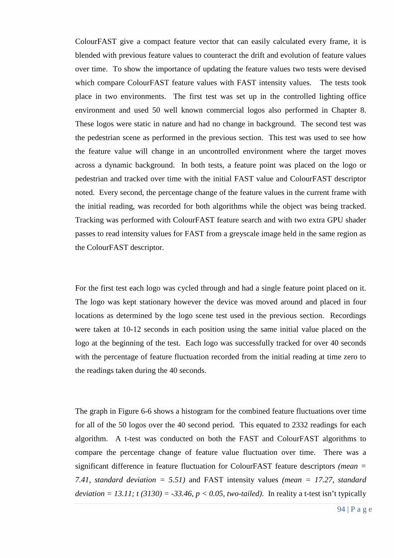
94 | P a g e

ColourFAST give a compact feature vector that can easily calculated every frame, it is

blended with previous feature values to counteract the drift and evolution of feature values

over time. To show the importance of updating the feature values two tests were devised

which compare ColourFAST feature values with FAST intensity values. The tests took

place in two environments. The first test was set up in the controlled lighting office

environment and used 50 well known commercial logos also performed in Chapter 8.

These logos were static in nature and had no change in background. The second test was

the pedestrian scene as performed in the previous section. This test was used to see how

the feature value will change in an uncontrolled environment where the target moves

across a dynamic background. In both tests, a feature point was placed on the logo or

pedestrian and tracked over time with the initial FAST value and ColourFAST descriptor

noted. Every second, the percentage change of the feature values in the current frame with

the initial reading, was recorded for both algorithms while the object was being tracked.

Tracking was performed with ColourFAST feature search and with two extra GPU shader

passes to read intensity values for FAST from a greyscale image held in the same region as

the ColourFAST descriptor.

For the first test each logo was cycled through and had a single feature point placed on it.

The logo was kept stationary however the device was moved around and placed in four

locations as determined by the logo scene test used in the previous section. Recordings

were taken at 10-12 seconds in each position using the same initial value placed on the

logo at the beginning of the test. Each logo was successfully tracked for over 40 seconds

with the percentage of feature fluctuation recorded from the initial reading at time zero to

the readings taken during the 40 seconds.

The graph in Figure 6-6 shows a histogram for the combined feature fluctuations over time

for all of the 50 logos over the 40 second period. This equated to 2332 readings for each

algorithm. A t-test was conducted on both the FAST and ColourFAST algorithms to

compare the percentage change of feature value fluctuation over time. There was a

significant difference in feature fluctuation for ColourFAST feature descriptors (mean =

7.41, standard deviation = 5.51) and FAST intensity values (mean = 17.27, standard

deviation = 13.11; t (3130) = -33.46, p < 0.05, two-tailed). In reality a t-test isn’t typically

95 | P a g e

used on non-independent samples, but does show here a substantial difference in feature

value fluctuation over time between the two algorithms.

Figure 6-6: Graph showing the frequency of fluctuation of FAST vs ColourFAST feature values for controlled environment logo test.

The second test recorded the same information as the first test but used the pedestrian

scene. This was done to see how the feature values in both FAST and ColourFAST

fluctuate in an uncontrolled environment. The experiment was done on 100 passing

pedestrians with the percentage change of feature fluctuation recorded every second that

the tracker followed the pedestrian. Each pedestrian was tracked at varying times up to 15

seconds and recordings were immediately stopped if the tracker lost the pedestrian. This

equated to 1379 readings for each algorithm. The histogram for the combined feature

fluctuations over time is shown in Figure 6-7. Once again a t-test was conducted on both

the FAST and ColourFAST algorithms but this time for the pedestrian scene. In this

situation both algorithms showed a close similarity in feature fluctuation for ColourFAST

0

100

200

300

400

500

600

700

800

900

10005 10 15 20 25 30 35 40 45 50 55 60 65 70 75 80 85 90 95 100

Freq

uenc

y

% of fluctuation

Histogram of Feature Variation- Logo Scene

ColourFAST

FAST

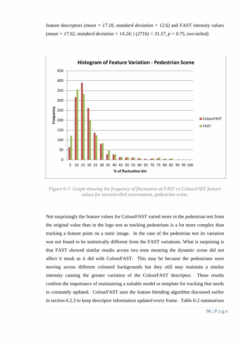
96 | P a g e

feature descriptors (mean = 17.18, standard deviation = 12.6) and FAST intensity values

(mean = 17.02, standard deviation = 14.24; t (2716) = 31.57, p = 0.75, two-tailed).

Figure 6-7: Graph showing the frequency of fluctuation of FAST vs ColourFAST feature values for uncontrolled environment, pedestrian scene.

Not surprisingly the feature values for ColourFAST varied more in the pedestrian test from

the original value than in the logo test as tracking pedestrians is a lot more complex than

tracking a feature point on a static image. In the case of the pedestrian test its variation

was not found to be statistically different from the FAST variations. What is surprising is

that FAST showed similar results across two tests meaning the dynamic scene did not

affect it mush as it did with ColourFAST. This may be because the pedestrians were

moving across different coloured backgrounds but they still may maintain a similar

intensity causing the greater variation of the ColourFAST descriptor. These results

confirm the importance of maintaining a suitable model or template for tracking that needs

to constantly updated. ColourFAST uses the feature blending algorithm discussed earlier

in section 6.2.3 to keep descriptor information updated every frame. Table 6-2 summarizes

0

50

100

150

200

250

300

350

400

450

5 10 15 20 25 30 35 40 45 50 55 60 65 70 75 80 85 90 95 100

Freq

uenc

y

% of fluctuation bin

Histogram of Feature Variation - Pedestrian Scene

ColourFAST

FAST

97 | P a g e

the results of the two tests and shows the mean and standard deviation of feature

fluctuation percentage of the values from the initial reading to the end of each tracking

target.

Algorithm Office Scene, Logo Test Outdoor Scene, Pedestrian Test

ColourFAST 7.4% ± 5.5 17.2% ± 12.6

FAST 17.3% ± 13.1 17.0 % ± 14.2

Table 6-2: Mean and standard deviation of the percentage of fluctuation of feature values for FAST vs ColourFAST.

98 | P a g e

Chapter 7

Cluster Analysis & GPU-based Feature Discovery

This chapter describes techniques for finding multiple feature points on objects from a

single feature point. Instead of tracking an object with a single feature point, more points

could be discovered on the same object giving a cluster of feature points. More feature

points are found using a new feature discovery algorithm which uses a special discovery

point, progressively following the contour of the object and recorning new features as it

explores. It uses Haar-like features to follow the ridges and valleys created around objects

from the ColourFAST feature detection pipeline. Once multiple feature points are found

on an object, their movements can be used to calculate a weighted average of overall

movement for the actual object therefore greatly improving tracking accuracy. This also

gives the benefit of allowing the object to be partially occluded as long as some of the

points still track a portion the object successfully. An object in this chapter is described as

something where the multiple feature points detected on it are on the same contour and are

all moving in the same direction. It also discusses how these clusters of points can be

broken off and grouped together if it is determined that two or more objects are found with

movements in different directions. The GPU shader code for the GPU-based feature

discovery is in Appendix D: Feature Discovery Shader

: GPU Feature Discovery Implementation 7.1As discussed in the previous chapter, ColourFAST features were found to be suitable to

track an object. However, there are still problems with the tracker in certain situations,

such as if a neighbourhood of features has similar feature descriptions, or trying to track

features on a straight edge which could suffer from the aperture problem. Instead of

tracking a single feature point on the object this work investigated how multiple feature

points could be discovered from a single point by following the feature contours generated

from the ColourFAST feature detection algorithm. ColourFAST smooths an image and

generates features for each pixel in a scene, including edges, and results in a distinctive

valley between feature shapes of different intensity and colour changes. This work used

this information to create a special “feature discovery point” that can trace around an

99 | P a g e

object and create more feature points as it navigates around the contour of the object until a

desired number of feature points have been extracted. If the number of feature points hits a

maximum, the feature discovery algorithm replaces weaker features that it previously

found with newly found stronger features.

Figure 7-1: GPU feature discovery pipeline. Shows input and output textures in white and the GPU shader in yellow.

The feature discovery algorithm is implemented using both the CPU and GPU. The

algorithm can be initiated from any feature point. The CPU keeps track of where the

feature discovery point is and uses the weighted average movements from the other

ColourFAST features in the cluster to correct movement. On the GPU side of the

algorithm, feature discovery is implemented with a single shader, it binds the output

texture from the ColourFAST feature detection pipeline as an input texture as shown in

Figure 7-1. Because of the unique ridges and valley that are generated around the contour

of an object, a Haar-like detector [143] is used to lock the feature discovery point on the

contour of the object by using the inner and outer ridges of feature points and following the

valley around the object. After some modelling a six component (1,2,1,-1,-2,-1)

combination of Haar masks was found to give the best results for keeping the feature

discovery point on the contour. The Haar mask combination is applied five times in the

shader across ten pixels moving up to two pixels on each side of the ridges and valley. The

highest absolute value given from the five Haar masks is used to clamp the discovery point

onto the maximum feature strength in the inner ridge of feature points on the object.

Figure 7-2, models the five Haar masks being placed over six ColourFAST single channel

feature values generated on a white and black edge. Once the algorithm has clamped

onto the feature point, a vector is calculated to give the direction of the feature and the

discovery point is then moved perpendicular to the feature direction where the feature

strength is calculated, and stored in the output texture along with the X and Y direction

100 | P a g e

movements of the feature discovery point. This allows the point to travel around the

contours of an object and allowing the CPU side of the algorithm to put more ColourFAST

feature points on the object or replace a weaker feature with it. Four screenshots taken at

various times show the algorithm discovering points as it moves around the contour of the

object is shown in Figure 7-3.

0 0.6 1.4 2.6 1 -1 -2.6 -1.4 -0.6 0

0 0.6 1.4 2.6 1 -1 -2.6 -1.4 -0.6 0

0 0.6 1.4 2.6 1 -1 -2.6 -1.4 -0.6 0

Figure 7-2: Six component combination of Haar masks applied five times on the contour of the object. The mask is shifted left and right up to two pixels. The values in the table are single channel ColourFAST features which were generated from a white and black edge.

Having a cluster of feature points on the object which gives weighted movements for all

the feature points in the cluster is shown in Section 7.3 to improve accurate tracking. The

feature discovery point worked well as long as the camera is kept relatively steady,

especially for when only a few feature points are in the cluster. This occurs because the

feature discovery point is only capable of following the contour determined from the Haar

descriptor which uses ten pixel fragments in its calculation allowing the point to clamp

onto the strongest feature up or down, up to two pixels relative to the direction of the

feature. On the CPU side the feature discovery point is moved on screen relative to the

other points in its cluster. As the number of points in the cluster increases, the feature

discovery point is able to better follow the contours of the object.

101 | P a g e

Figure 7-3: GPU feature discovery screenshots. Shows the discovery point finding suitable ColourFAST features until a maximum number of features has been found. The algorithm then replaces weaker features with stronger ones which are usually found on

corners.

: Point Clustering 7.2Feature points in the same cluster can give a combined weighted average for the movement

of an object. Weighted averages are calculated by taking a measure of how close a feature

point matches its previous value, so features that are tracking correctly over multiple

frames get weighted more towards the overall movement of an object than features which

may have moved slightly off its intended position or have been occluded this frame, this is

also combined with the velocity calculation in section 6.3.2 to give average smoothed

movement over 3 frames. The overall movement is used to move the tracking window for

each feature point in the cluster, but still allow each feature to correct its movement to the

best feature match within the tracking window. This is demonstrated Figure 7-4 which

shows three feature points and their movements between frames, where the average

smoothed movement for the cluster is (𝑈𝜕𝑎𝑎,𝑉𝜕𝑎𝑎) and each point’s offset movement within

the tracking window as (𝑋𝑝𝑖,𝑌𝑝𝑖).

102 | P a g e

avtV

avtV

avtV

avtU av

tU

avtU

2Xp

1Xp

3Xp

1Yp

2Yp3Yp

Figure 7-4: Average smoothed cluster movement of tracking windows (𝑈𝜕𝑎𝑎,𝑉𝜕𝑎𝑎) calculated from previous movements, with individual feature point movements(𝑋𝑝𝑖,𝑌𝑝𝑖)

within the window giving the best feature match.

The smoothed cluster movement (𝑈𝜕𝑎𝑎,𝑉𝜕𝑎𝑎) can be calculated first taking the position of

point i for i=1,2,…..,n in frame by (𝑥𝑖𝜕,𝑦𝑖𝜕) and its movement from frame t-1 to frame t by:

(𝑢𝑖𝜕, 𝑣𝑖𝜕) = (𝑥𝑖𝜕 − 𝑥𝑖 𝜕−1,𝑦𝑖𝜕 − 𝑦𝑖 𝜕−1)

Then the cluster position in frame t is given by:

(𝑋𝜕,𝑌𝜕) = �1𝑛

�𝑥𝑖𝜕

𝑛

𝑖=0

,1𝑛

�𝑦𝑖𝜕

𝑛

𝑖=0

�

Its clustered movement for frame t:

(𝑈𝜕,𝑉𝜕) = �1𝑛

�𝑢𝑖𝜕

𝑛

𝑖=0

,1𝑛

�𝑣𝑖𝜕

𝑛

𝑖=0

�

103 | P a g e

The smoothed clustered movement over three frames from t-2 to t using a weighted

average:

(𝑈𝜕𝑎𝑎,𝑉𝜕𝑎𝑎) = 12

(𝑈𝜕,𝑉𝜕) + 13

(𝑈𝜕−1,𝑉𝜕−1) + 16

(𝑈𝜕−2,𝑉𝜕−2)

If several feature points are exhibiting a significant change of movement compared to the

other features in the cluster, then there may be two or more individual objects in the scene

that are moving in different directions. The tracking feature points should be split

according to the directions. Several cluster analysis algorithms were investigated, however

it seemed that either density or centroid based models were appropriate for this work to

achieve good clustering. The most popular algorithms for each model were chosen,

DBSCAN and K-Means clustering and were implemented on the CPU side of the project.

Although it is possible to optimize the algorithms for the GPU [99, 144, 145], this was

avoided in this project because the information that is needed to cluster is already on the

CPU side of the project as well as the nature of the algorithms which require several

conditionals and loops makes porting it to a GPU less beneficial.

Initially all feature points that are being tracked belong to one cluster assuming that only

one object is being tracked. To determine whether the cluster of feature points lie on more

than one object moving in different directions a variance formula is used for both

clustering implementations. Similar to the formula in section 6.3.2, the actual movements

of the points (not the average cluster movement) is used to create a smoothed velocity

movement for each tracking point over three consecutive frames. The variance of

movement of the feature points is given by:

(𝑣𝑎𝑣𝑋𝜕,𝑣𝑎𝑣𝑌𝜕) = 1𝑛��𝑢𝑖𝜕2 − ��𝑢𝑖𝜕

𝑛

𝑖=0

�2𝑛

𝑖=0

,�𝑣𝑖𝜕2 − ��𝑣𝑖𝜕

𝑛

𝑖=0

�2𝑛

𝑖=0

�

If the sum 𝑣𝑎𝑣𝑋𝜕 + 𝑣𝑎𝑣𝑌𝜕 is greater than some upper bound threshold then the clustering

algorithm is run resulting in several separate clusters of feature points. This can be

repeated to further split clusters as the scene changes. Similarly if the average movement

104 | P a g e

of points in a cluster are similar to movements in another cluster, then the two clusters can

merge into one.

Figure 7-5: Screen shots of DBSCAN. The coloured borders shown around the feature points are drawn by the application to show points in the same cluster. The top screen

shot shows still rectangles and their feature points all in one cluster. The bottom screen shot shows rectangles moving in different directions therefore becoming three separate

clusters.

In both DBSCAN and K-Means clustering implementations clusters were determined by

using point movements over three frames rather than point screen positions and taking L1-

norm distances between the movements to determine whether or not points belong in the

same cluster or not. Because the K-means algorithm needs to know the value of K (the

number of clusters that should be produced), K was chosen to be 2. If the variance in any

of the produced clusters was high, then K-Means can be repeated on that cluster to split it

into further clusters.

105 | P a g e

: Results and Testing 7.3Both clustering implementations showed comparable accuracy for splitting feature points

into clusters, so it was hard to determine which worked best. Timing of the algorithms

involved placing a total of 50 feature points on the screen and timing how long the

algorithms took to cluster the points, which was done on the Samsung Galaxy S2 and

Galaxy S4 devices with preview frame resolutions set to match the screen resolution on

both. For this test the points were re-clustered every frame and the results averaged after

several seconds. K-means was set to K=2 with no further splitting of the two clusters for

this frame.

The results in Table 7-1 show that K-Means runs slightly faster than DBSCAN in this

implementation, however the times would increase more if there are more than two objects

moving in the scene as the K-Means algorithm has to be repeated on the resulting clusters.

The Galaxy S2 showed faster clustering rates overall, perhaps because of the overhead of

the CPU on the S4 extracting such high resolution images (1920x1080) from the camera as

well as processing other background tasks. DBSCAN was chosen in this thesis as it has

the advantage of splitting into any number of clusters, and includes the detection of

“noisy” features, with little cost to speed.

Clustering Algorithm Galaxy S2 Times Galaxy S4 Times

K-Means 2.1 ± 0.5 3.65 ± 0.8

DBSCAN 3.45 ± 0.75 5.77 ± 1.3

Table 7-1: Average clustering times and standard deviation for 50 feature points in

milliseconds on two devices.

A single ColourFAST feature point was demonstrated to track very well in Chapter 6, so

testing was done to determine whether the average movement for a cluster of points

collectively track better than feature points on their own. The testing was also to give a

general idea on how well the points can cluster and merge together to track multiple

objects moving in different directions. The test involved setting up a Java program and

106 | P a g e

placing three different coloured rectangles (different colours were chosen after every 10

tests) on screen with four feature points on each. These rectangles move about the screen

in different directions and speeds. They bounce off the edges and each other at random

angles and can randomly increase and decrease in speed. Initially when the rectangles are

stable, all points belong to the same cluster, however once the test application starts, the

clustering algorithm is able to determine that the feature points actually belong to three

different objects from their differing movements and uses the average weighted

movements for each point in a cluster to determine the overall movement for the object.

Testing was done on two mounted devices, the Samsung Galaxy S2 (set at full screen

resolution 800x480) and the Galaxy S4 (set at 1280x720) as shown in Figure 7-6 with

screenshots from the device in Figure 7-5. The tests were run for one minute each and

repeated 50 times for both clustered and non-clustered movements and noting down how

many feature points out of the 12 were lost.

Figure 7-6: Setup for tracking accuracy using clusters test.

As Table 7-2 shows, using the clustering algorithm dropped the performance on both

devices slightly less than 2fps on average. However this small drop in performance is

compensated by the accuracy of tracking objects using clustered movements as shown in

the graph in Figure 7-7.

107 | P a g e

Phone Clustered Frame Rates Non-Clustered Frame Rates

Galaxy S2 20.2 ± 1.7 22.1 ± 2.1

Galaxy S4 24.7 ± 1.2 26.5 ± 1.4

Table 7-2: Average frame rates and standard deviation for tracking 12 feature points,

comparing clustering with non-clustering in frames per second (fps)

Figure 7-7: Graph shows tracking accuracy for clustered and non-clustered points. It gives the number of tests that passed only losing a specified number of points.

: Future Work 7.4Work is still continuing on the feature discovery algorithm. At the moment feature

discovery finds features progressively over camera preview frames, only moving a small

distance between each frame. This can cause problems especially when there are only few

feature points currently being tracked on the object as the discovery point moves relative to

them. This means a sudden movement of the camera causing one of the ColourFAST

points getting tracked to come off, can then cause the discovery point to also come off the

0

5

10

15

20

25

30

35

40

45

50

0 1 2 3 4 5 6 7 8 9 10 11 12

Num

ber o

f Tes

ts

Points Lost

Number of tests that lost ≤ specified points

Not Clustered

Clustered

108 | P a g e

contour of the object more easily. Having more points in the cluster allows a more

smoothed movement. One idea to improve this algorithm is to use a separate thread which

processes a still frame while the rest of the feature detection and tracking pipeline continue

processing frames from the camera. As the feature discovery algorithm finds new features,

it could notify the tracking part of the pipeline as more features are found and they could

be updated to the moving frame relative to the feature points on the still frame.

Periodically a new still frame could be taken from the tracking part of the pipeline so it

isn’t outdated for too long.

Clustering of feature points worked well for tracking multiple objects, however in this

work the algorithms were CPU based as movements are already held on the Android CPU

side of this application. Future work will involve investigating using the GPU instead to

do the bulk of the clustering calculations for the DBSCAN algorithm and comparing its

performance with CPU implementations. DBSCAN has been parallelized before in [99].

Very recently DBSCAN has been ported to desktop GPU in [146], albeit there seems to be

no mobile GPU versions of the algorithm which exist at the time of this writing.

109 | P a g e

Chapter 8

GPU-based Object Recognition

Using the compact feature vector which is created from ColourFAST feature points works

well for tracking especially once combined with clustering to create an overall movement

for an object. Although the main objective of this thesis was purely doing natural feature

point detection and tracking on mobile GPUs, the question arose whether or not the

compact feature vector created from ColourFAST for feature points could also be used for

quick and elementary object recognition using only the four-component feature vectors for

each of the feature points generated from the ColourFAST feature detection algorithm.

The GPU shader code for version 2 of the GPU-based object recognition algorithms are

found in Appendix E: ColourFAST Object Recognition Shaders.

: Object Recognition and Feature Descriptions 8.1Object recognition is a complex task in computer vision which detects and identifies

objects within an image or video sequence. Object recognition differs from object

detection; object detection is mainly focused on finding an arbitrary object in the scene,

whereas recognition aims to exactly identify what the object is. Humans are adept at

recognizing multiple objects even when they exhibit differing viewpoints, scale, rotation,

partial obstruction and under various lighting and shaded conditions. However this task is

still a challenge for computer vision systems and many approaches to the task have been

implemented.

Object recognition is an entire discipline in itself and is a combination of multiple

algorithms which work together to detect and recognize an object. Many object

recognition techniques use feature descriptions, which calculate a unique vector of values

to identify or describe a feature point. The work in this chapter only investigates the

potential for whether feature descriptors generated from ColourFAST could be used for

110 | P a g e

object recognition. In this chapter an object recognition algorithm is developed

specifically for ColourFAST feature points. However, this thesis has not compared this

new algorithm with other recognition algorithms as the primary focus is on the compact

feature descriptor. More sophisticated object recognition algorithms such as those using

neural networks could be adapted to use ColourFAST instead of techniques such as SIFT

and Lucas Kanade.

Objects can be identified by comparing the features found in an image to features

descriptions of previously known objects, held in a database. SIFT [57] and SURF [60]

are two common feature detector and descriptor algorithms. SURF is known to be

computationally faster than SIFT [61], however if speed is not essential then SIFT

outperforms SURF in terms of accuracy [147]. There are many variations and similar

algorithms to SIFT and SURF including PCA-SIFT (Principal Component Analysis –

Scale Invariant Feature Transform) [148], GLOH (Gradient Location and Orientation

Histogram) [149] and HOG (Histogram of Oriented Gradients) [130]. Feature descriptions

are typically very large in these object recognition algorithms, for example SURF uses a

64-component feature description whereas SIFT typically uses 128 components. PCA-

SIFT in [148] has reduced the SIFT descriptor to a 36-component feature using principal

component analysis [150], increasing its matching speeds. It claims to have a more

distinctive feature vector leading to significant improvements in matching accuracy for

controlled and real-world conditions. Both SURF and SIFT have also been modified for

mobile device platforms in the past by further reducing the descriptors and using other

modifications [89, 90], however these are CPU based. To speed up detection [89] uses a

simplified 36 component SIFT descriptor alongside FAST for feature detection.

: GPU-based Object Recognition version 1 8.2Since ColourFAST generates a four component feature vector, the question arose whether

it can be useful for recognizing simple objects. This part of the research undertook a

feasibility study using a cluster of tracked feature points which gets matched to feature

points for predetermined objects. It was not compared to the other known object detection

111 | P a g e

algorithms for performance nor accuracy. It was done to see if ColourFAST features could

be used for rudimentary recognition and ways they could be incorporated into a more

sophisticated recognition algorithm.

Matching was done with a single shader pass and binding the following five input textures:

1. Output texture from the ColourFAST feature detection pipeline which contains the

four channel feature vector values.

2. Output texture from the ColourFAST feature search pipeline, this gives how much

a point has moved (where the best match is) within the tracking window.

3. Texture created on CPU side which has the previous positions (x,y) for each

tracking point on the screen encoded between zero and one.

4. Texture created on CPU side which contains all objects and their features that can

be matched. The two dimensional texture is created with height equal to the

number of objects that are getting matched against and width is the maximum

number of features in any of the objects. Each row holds a single object, with its

associated features in each of columns in the texture. If an object has less features

than the maximum amount number of features for objects, then padded zero values

are instead placed into the texture. See Figure 8-1.

5. Single column texture created on CPU side which has the number of features for

each object in the above object texture. The height of this texture matches the

height of the texture 4. See Figure 8-1.

112 | P a g e

O1 = 5 O1f1(r,g,b,a) O1f2(r,g,b,a) O1f3(r,g,b,a) O1f4(r,g,b,a) O1f5(r,g,b,a) padding

O2 = 4 O2f1(r,g,b,a) O2f2(r,g,b,a) O2f3(r,g,b,a) O2f4(r,g,b,a) padding padding

O3 = 2 O3f1(r,g,b,a) O3f2(r,g,b,a) padding padding padding padding

. . . . . . .

. . . . . . .

. . . . . . .

. . . . . . .

Om = n Omf1(r,g,b,a) Omf2(r,g,b,a) . . . Omfn(r,g,b,a)

Figure 8-1: Two textures generated on the CPU side to hold and describe objects that

could be matched. The left texture gives the number of features held in each object. The right texture holds each objects feature point values.

On the CPU side the textures are bound so that each of the old position values (texture 3)

for the tracking points on screen are in separate fragments. Inside the shader this value is

used to first get an updated value for the ColourFAST feature vector by using the previous

position value to look up how much the point has moved (from texture 2), these values are

encoded between 0 and 1 in the texture as required in OpenGL ES 2.0. The size of the

tracking window is passed in as a uniform float so that the values in texture 2 can be

decoded to give the pixel movement to the best match. The movement values are then

added to the previous position values and used to obtain the current ColourFAST feature

vector (from texture 1). This value is then matched against each feature vector values for

each of the possible objects. The shader is passed two more uniform floats which specify

the number of candidate objects being matched against and the maximum number of

features for each of those objects. This is used to convert between texture coordinates and

rows and columns in the candidate object texture. The shader code simply moves across

each of the potential objects that are being matched (in texture 4) and calculates L2 norm

distances between the target feature point vector and a potential match feature vector. The

number of times it needs to move across depends on the number of feature points the

potential matching object has (held in texture 5). The two best matching values and the

distance value, which specifies how close of a match they are, are encoded and placed in

the four components of the output texture. The object recognition pipeline with the

important uniform inputs and bound input and output textures are shown below in Figure

8-2.

113 | P a g e

Figure 8-2: GPU-based object recognition pipeline. Shows five input textures being fed into the pipeline with the output texture storing the best object matches for the features

being tracked on screen.

On the CPU side the texture is read and decoded, giving the best two matching feature

values for each point and a value for how close of a match they were. These are then all

tallied up to give the best matching objects overall and how close of a match they are to the

object being tracked.

114 | P a g e

: GPU Based Object Recognition Version 2 8.3Performing some initial tests from the GPU based object recognition discussed in the

previous section showed some success, but the match accuracy of objects being recognized

was lower than expected. After some modelling a new approach was implemented that

instead uses two different shader passes overviewed below in Figure 8-3.

Figure 8-3: GPU Object Recognition Pipeline. Shows two shaders in yellow, with some important uniform values passed in grey. In white are the three input textures being fed into the pipeline, and also the output texture storing values for the best match for each

object.

The first shader takes three input textures, two of them the same as the previous version of

this algorithm (which were textures 4 and 5, See Figure 8-1), the first holding each match

candidate object and its feature point values (referred now as texture 1) and the other

holding the number of features in each candidate object (referred now as texture 2). The

third texture is created and populated with feature point values being tracked on the CPU

side (texture 3). This gives a big advantage over the previous version of the algorithm as it

uses feature values which have been blended over successive frames, meaning that if some

of the feature points get lost for a frame or two, they don’t affect the match criteria as

much. Previously only the current feature value for this frame was used, so it also had to

be looked up to find where it has moved. This means that only three bound input textures

are used instead of five. The width of the texture is equal to the number of tracked feature

points that are being matched and the height is equal to the amount of candidate objects

115 | P a g e

that are to be matched against. The rendered quad coordinates inputted into the shader

matches the size of this texture. The idea is that features on screen should find the best

matches for features in every object, thus giving an estimate how well each of the features

match each candidate object which is held on every row.

Inside the shader each tracked feature fragment looks up its own ColourFAST feature point

values from texture 3. It then searches for the best feature match for the object candidate

in the row that it is trying to match with by performing a GLSL distance calculation (L2-

norm) between its own feature value and each of the feature values held in the candidate

object (using textures 1 and 2). The coordinates to extract each feature point from the

candidate object texture are calculated using the maxFeatures uniform value giving the s-

coordinate, the t-coordinate just matches the t-coordinate of the current shader. Each

feature fragment stores the best match value (minimum distance) for a single feature for

that candidate object. Each row in the inputted quad represents a different candidate object

that the algorithm is trying to match. The output texture holds values for best feature

matches for each feature point being tracked on screen in the columns and for each object

candidate being matched held in the rows of the texture. See Figure 8-4.

The second shader pass binds the output texture from the first shader as its input. The

rendered quad is set to the height of the amount of candidate objects being matched and

width set to one. Each fragment in the quad holds a sum of the feature values matched

against the candidate object held in the same row as it from the previous render pass.

Before the value of each feature is read and added to the sum a square root of the value

multiplied by two is taken so that bad matches are pushed out further and good matches are

distributed more. The sum of these values then gets encoded between 0 (perfect match)

and 1 (bad match) by dividing the result sum by the number of feature points being tracked

which is passed in as a uniform float value. The output texture then holds the encoded

feature sum for each candidate object, with the lowest values being the best match for the

feature points being tracked. Once rendered on the CPU side, the application keeps track

of the top five matches by using the values held in output texture of the object recognition

pipeline. See Figure 8-4.

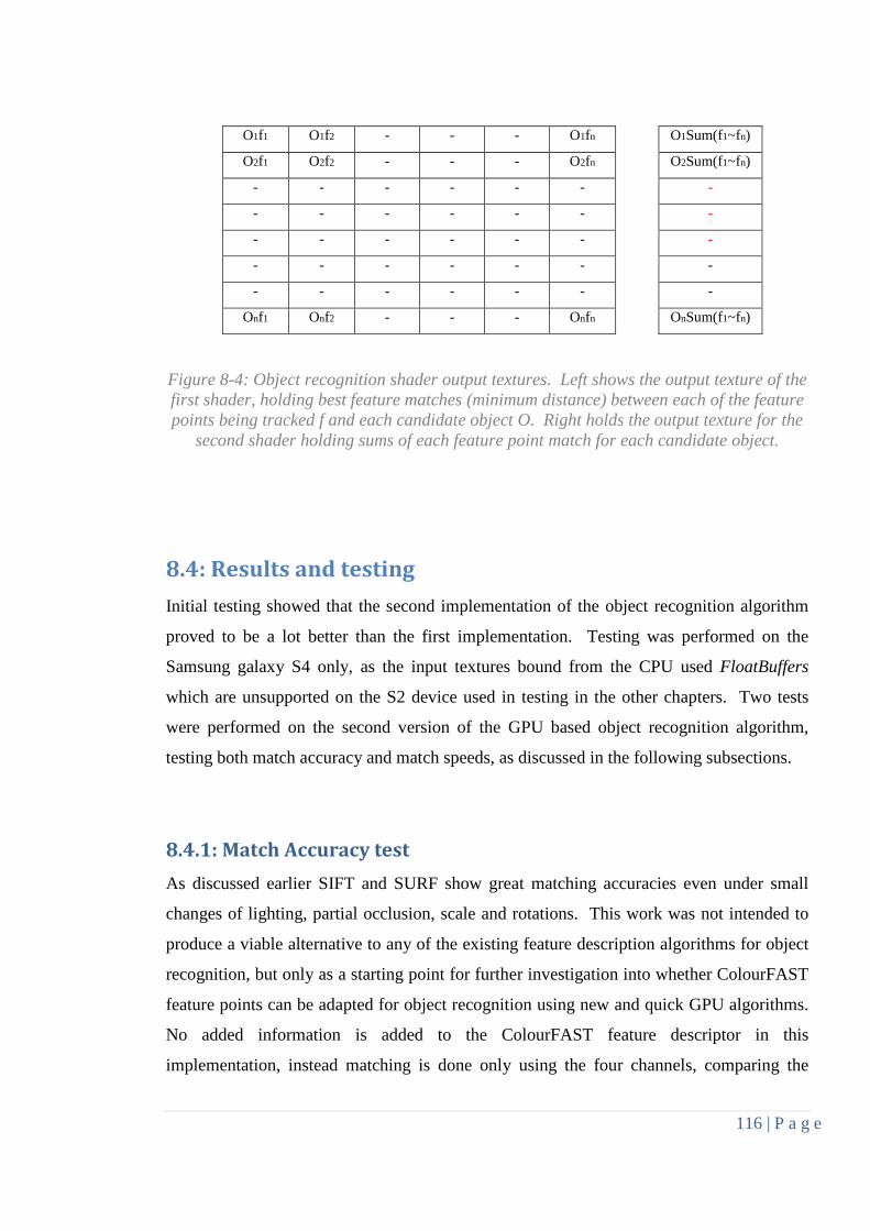
116 | P a g e

O1f1 O1f2 - - - O1fn O1Sum(f1~fn) O2f1 O2f2 - - - O2fn O2Sum(f1~fn)

- - - - - - -

- - - - - - -

- - - - - - -

- - - - - - -

- - - - - - -

Onf1 Onf2 - - - Onfn OnSum(f1~fn)

Figure 8-4: Object recognition shader output textures. Left shows the output texture of the first shader, holding best feature matches (minimum distance) between each of the feature points being tracked f and each candidate object O. Right holds the output texture for the

second shader holding sums of each feature point match for each candidate object.

: Results and testing 8.4Initial testing showed that the second implementation of the object recognition algorithm

proved to be a lot better than the first implementation. Testing was performed on the

Samsung galaxy S4 only, as the input textures bound from the CPU used FloatBuffers

which are unsupported on the S2 device used in testing in the other chapters. Two tests

were performed on the second version of the GPU based object recognition algorithm,

testing both match accuracy and match speeds, as discussed in the following subsections.

8.4.1: Match Accuracy test As discussed earlier SIFT and SURF show great matching accuracies even under small

changes of lighting, partial occlusion, scale and rotations. This work was not intended to

produce a viable alternative to any of the existing feature description algorithms for object

recognition, but only as a starting point for further investigation into whether ColourFAST

feature points can be adapted for object recognition using new and quick GPU algorithms.

No added information is added to the ColourFAST feature descriptor in this

implementation, instead matching is done only using the four channels, comparing the

117 | P a g e

points being tracked to the multiple feature points for each previously recognized object in

the data set.

Many of the standardized data sets for object recognition use still images or video. Using

extracted video frames for mobile is difficult as many formats are still unsupported or need

certain codecs. This work aimed to also test the algorithm on real life conditions, taking

the limitations of the device camera on live feed into consideration such as camera capture

frame rate and noise in the image. A small data set was made containing fifty different

common logos which were downloaded from the internet. Each logo was cycled through

and carefully had a number of typical features picked on it or had the feature discovery

algorithm from Chapter 7 run on them to find features along the contours of the logo. This

was done on a still frame going through the pipeline and then saving each object to a data

file. This gave 50 candidate objects which the algorithm can match against. Once the

application starts up, the data file is read, each object and associated four component

ColourFAST features are then saved into a texture which is fed into the first shader from

section 8.3.

Logo recognition has been done before in [151] using a string matching technique and

separating the logo from the foreground of video frames of a football game. It did

however have a high false positive detection rate of finding many non-logo regions in

some areas of the video. Logo recognition has also been done using SIFT descriptors as

demonstrated in both [152] and [153]. The work in [153] used vehicle logos on cars as a

data set and was able to achieve a 91% recognition success rate on, however the times that

it took to calculate both detection and recognition of the logo was 1400 milliseconds.

Mobile logo detection has been achieved in [154] which runs SIFT on the first camera

frame in order to locate the logo location and then by using an online calibration of colour

within the SIFT detected area to detect and tract the logo in subsequent frames. Mobile

logo recognition has also been done in [155] using a combination of SURF keypoint

detector, FREAK (Fast Retina Keypoint) [156] descriptor calculator and a background

subtraction method to achieve a very high 97% recognition success rate. However the

recognition of a logo takes an average execution time of 1.7 seconds on ordinary single

core smart phones. It appears so far that mobile logo recognition has only been achieved

118 | P a g e

with CPU based algorithms. This work looks to utilize the GPU to achieve a much faster

“real time” recognition rate whist still maintaining suitable match accuracy.

The test involved cycling through the same logos in four different scenarios and trying to

match them with the object candidates held in the texture and outputting the top five

matches to the device screen. The objects were just displayed on a typical LCD desktop

display with the mobile device aimed at straight at it. The object recognition part of the

pipeline is only run once an observe button is pressed. The four scenarios were run

consecutively on each logo:

• The first involved placing feature points intuitively on the logo, so some of the

points were in different positions from the object candidates, to measure the

robustness of the object recognition to having some different feature points.

• The second test involved unfreezing the frame so live camera frames are passed

through the pipeline instead whilst still maintaining the camera stationary (except

for minor hand movements), and attempting to recognize the object after a 20

seconds of tracking. This was done to measure the robustness of object recognition

during tracking.

• The third test directly followed the second test and involved moving away from the

object by approximately a factor of two while still tracking the object, to measure

robustness to object scale, waiting another 20 seconds before performing the object

recognition again.

• The last test involved zooming in slightly but panning left or right of the display 45

degrees, waiting another 20 seconds and performing object recognition again. This

was done to measure the robustness of object recognition to skew.

The waiting 20 second waiting periods were done to allow the features to settle and to

remove any doubt that objects are only being recognized from new values in the test and

not because of the feature blending with previous values. This allows enough time to pass

between tests so that any portion of the feature value from the previous test has effectively

been removed. Figure 8-5 gives example screenshots of the tests undertaken and shows

119 | P a g e

the object being tracked and then matched as the correct first pick decided from the object

recognition algorithm and the logos used in the data set shown Figure 8-6.

It is important to reiterate that these tests were done back to back leaving the features

where they are across tests as they are being tracked. Therefore the feature points for

objects being recognized in the fourth test are the same as the features in the first test,

meaning they have been tracked for over 60 seconds in duration over the four condition

tests and any movements between tests. A failed test was decided by not having the object

recognized in the top five picks. Out of 50 objects, the algorithm picked 23 perfect

matches which were the first pick across all four tests. Only 1 object failed all four tests by

not being in the top five picks. None of the other objects failed more than one test being a

mixture of first-fifth picks. Out of all 200 tests there were 156 correct first place picks.

The picks for each scenario is shown below in the graph in Figure 8-7.

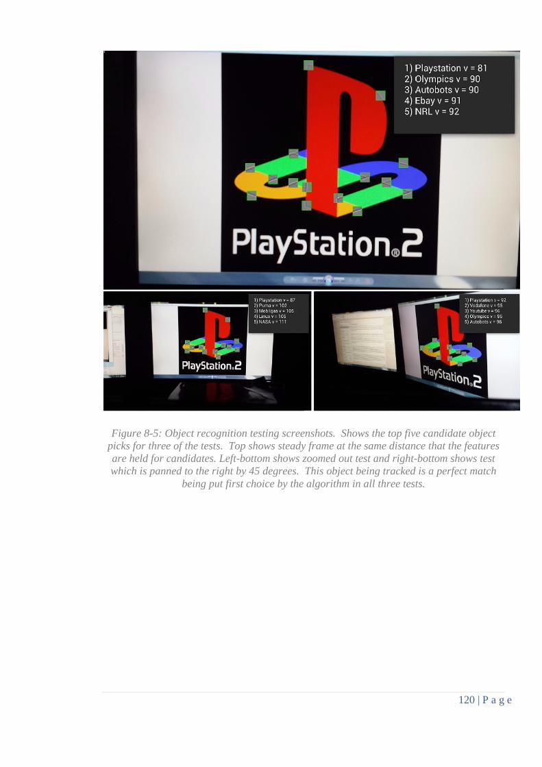
120 | P a g e

Figure 8-5: Object recognition testing screenshots. Shows the top five candidate object picks for three of the tests. Top shows steady frame at the same distance that the features are held for candidates. Left-bottom shows zoomed out test and right-bottom shows test which is panned to the right by 45 degrees. This object being tracked is a perfect match

being put first choice by the algorithm in all three tests.

121 | P a g e

Figure 8-6: Logo dataset used for object matching. Perfect matches in red (all four tests identified the object as its first pick), good matches in blue (mostly first choices but some between second and fifth choice), average matches that failed one test in yellow, and in

black the logo that terribly failed all four tests.

122 | P a g e

Figure 8-7: Object Recognition match accuracy for four consecutive tests.

Matching was done using features in the RGB colour space and performed in the same

office condition over two days however there may have been changes in lighting from the

window which affected the result. The YUV colour space could have instead been used, as

changes in intensity in the scene only affect the Y component whereas it affects all three

components in the RGB colour space. This could perhaps improve matching results

further if lighting was an issue.

8.4.2: Match Speed Test Matching accuracy was higher than expected however the real advantage of performing

GPU based object recognition on ColourFAST features was expected to be the speed of

matching. Speed was tested on output frame resolution 1280x720 on the Samsung Galaxy

S4. The test involved comparing frame rates of the entire GPU ColourFAST detection and

tracking pipeline with and without the object recognition render passes constantly running

on every frame. Matching accuracy was ignored for this test, instead a number of random

0

5

10

15

20

25

30

35

40

45

50

1st Pick 2nd Pick 3rd Pick 4th Pick 5th Pick Unknown

Number of Tests

Object Recognition Result

Object Recognition Match Accuracy

Single Frame

Real-Time Frame

Zooming Out

Panning

123 | P a g e

points were placed on screen and given random ColourFAST values every frame. This

prevents potential caching on the GPU so that a more fair and accurate reading can be

calculated. The algorithm uses these randomized values to match against the same 50

candidate objects used in the match accuracy tests. The application was run for a few

minutes for each test, with frame rates recorded and averaged as shown in Table 8-1.

Average object recognition speeds are calculated by subtracting the frame rates of the

pipeline with object recognition running from the rates of the pipeline without object

recognition running and shown below in Table 8-2.

ColourFAST pipeline 5 features 10 features 20 features 50 features

Without Object Rec 38.41 ± 0.7 32.98 ± 1.0 23.04 ± 1.0 11.42 ± 0.5

With Object Rec 33.56 ± 1.0 29.52 ± 1.1 20.33 ± 0.8 10.67 ± 0.5

Table 8-1: Average pipeline throughput and standard deviation measured in frames per second (fps), with object recognition enabled and disabled, for a number of randomized

feature points.

ColourFAST Pipeline 5 features 10 features 20 features 50 features

Object Recognition Speed 3.76 3.56 5.78 6.12

Table 8-2: Average object recognition speeds for a number of feature points measured in

milliseconds.

The GPU based object recognition algorithm shows remarkable speed being able to match

each of the 50 feature point to a data set of 50 objects in only few hundred microseconds.

Due to the parallel nature of the GPU algorithm, the GPU appears to be underutilized by

having only a few features on screen, this shows the reason why processing 10 features has

comparable time to processing 5 features in this test.

The 50 objects stored in the candidate match texture have their feature points stored as four

float values. This means that if an average object to match stored has 20 feature points, the

50 object texture is only of size 16KB. The GPU can easily store this texture in its Level 2

(L2) cache which on the Galaxy S4 is of size 2MB. This means that 5000 candidate

124 | P a g e

objects could be stored in the cache using 1.6MB of space and would still result in

extremely fast match speeds. To save even more cache memory the values could be stored

as bytes, since the rest of the ColourFAST pipeline already stores values as bytes, therefore

reducing the size of cache memory by a factor of four.

: Future Work 8.5GPU based object recognition using ColourFAST features appears to be promising in

terms of speed and has shown good matching accuracy. However this work was just the

gateway in what still needs to be explored. To compete with SIFT and SURF, this

algorithm needs to improve accuracy further although its performance is already

substantially better. Matching can be improved by increasing the size of ColourFAST

feature vectors to contain more than four components. One way could be to combine

actual colour space values for the pixel with the ColourFAST feature values creating a 7

component feature descriptor. Furthermore, four small grids could be smoothed on each

quadrant of the feature direction and its orthogonal vector to create more feature descriptor

components. SIFT uses a more advanced version of this approach, however perhaps the

more simplistic way investigated here could also work without significantly slowing the

matching speed. Feature point matching could also include relative position between

expected feature points and their values, further enhancing match accuracy, so including a

spatial component to the feature points.

Using a four component feature vector worked well for matching simple logos, however an

increase in the number of feature components could result in recognizing more advanced

objects such as landmarks or structures. This work will investigate taking advantage of the

unique capabilities of mobile devices by utilizing the built in compass and GPS receiver.

Using the directional information combined with location data, the application could obtain

localized candidate matches within the area of the mobile device, reducing the number of

potential objects that need to be compared during recognition. There could be hundreds of

thousands of landmark objects in an online database with associated geographic

coordinates. The device could periodically retrieve feature sets for landmark objects

125 | P a g e

within its vicinity and direction the camera is facing via the cellular network or Wi-Fi.

This could improve location based mobile augmented reality applications by pin pointing

exactly where the landmark of interest is. GPS often loses accuracy in urban environments

due to multipath effects, so having a quick matching system for structures or landmarks

would be of benefit.

Other improvements that are currently being investigated include matching under differing

lighting conditions. Using an extra shader pass to perform histogram equalization on the

image from the camera could aid in matching by reducing the effects of light and

shadowing. Greater changes in scale need to be investigated as well as adding rotation

invariance. The directions for each of the feature points in a cluster for an object could be

combined to give an overall direction measure for the object. When matching candidate

objects, its overall direction measure can be matched to the object being tracked and

relative directions for features could instead be compared.

126 | P a g e

Chapter 9

Conclusion

The technological evolution of mobile devices has rapidly increased over the last few

years, especially with the advent of the smart phone. Now the GPU, CPU and camera

capabilities of mobiles have greatly improved, opening the door to many interesting

computer vision and mobile augmented reality applications that were not feasible only

several years earlier. The GPU is now especially suitable for real time image analysis,

feature detection, feature recognition and tracking, easily outperforming its CPU

counterparts on many image processing algorithms. Most current mobile devices support

OpenGL ES 2.0 and GLSL programmable shaders which can be used to create GPU based

applications.

Canny edge detection is a common image analysis algorithm and it illustrates many of the

issues associated with implementing image processing algorithms on GPU. Canny was

implemented and optimized to be made suitable for GPUs in Chapter 3. The new

implementation of Canny took advantage of the parallel nature of the GPU by using the

programmable shader pipeline with multipass rendering techniques. The developed

algorithm was performed on real time video frames from the embedded camera and tested

on a wide range of different device platforms. As demonstrated in Chapter 4, the GPU-

based implementation of Canny edge detection showed its superiority, in terms of frame

rate, over OpenCV’s CPU implementation on devices released in 2011 and later.

GPU-based image processing was then used for implementing FAST feature detection on

real time video frames from the device camera in Chapter 5. FAST was optimized to be

made suitable for the GPU pipeline and demonstrated a significant speed advantage over

OpenCV’s implementation. After numerous modifications to FAST, including the use of

colour, smoothing of the image, and removal of thresholds, the ColourFAST feature

detection algorithm was created. ColourFAST made several improvements over FAST

features, including the production of a four channel compact feature vector which included

127 | P a g e

colour changes as well as an orientation for the feature. Taking advantage of the SIMD

nature of GPU allows valuable information about feature points to be calculated and

utilized with very little performance penalty. ColourFAST was comparable to FAST in

terms of performance frame rates and in some cases actually performed slightly better.

A GPU-based feature search algorithm was then implemented in Chapter 6, which was

used to track ColourFAST features. ColourFAST feature tracking finds the best feature

match across camera frames by rendering a small search window around where each

feature is predicted to be based on its movements across three previous frames. This gives

a movement from the centre of the search window to where the best matching point is.

The movement values are then added to the feature point position and used in the next

frame to centre the search window. The movement of windows is controlled by the host

application, so velocity and acceleration of features are also taken into consideration to

perform effective tracking. The ColourFAST feature tracker was compared to a GPU-

based implementation of Lucas-Kanade and showed an improvement in tracking accuracy

and an increase in frame rates. It also showed several other improvements including the

feature being able to be occluded for a few frames, and also allowing the feature to adapt

quickly to gradual changes in the environment, such as rotations, scale, and changing

lighting conditions by the gradual blending of new features values with existing features.

A new GPU based feature discovery algorithm was implemented in Chapter 7, allowing

more features to be found from a single feature point. It exploits the nature of

ColourFAST feature points around object contours, having a distinctive ridge-valley

pattern to feature point strengths. This pattern was exploited via a Haar mask to stay

accurately locked onto the contour while moving along the object. The feature discovery

algorithm produced a group of features, called a cluster that can collectively track an object

using an average weighted movement calculated from the individual movements of

features. The weightings in the overall object movement are computed so that features

which consistently obtain good matches add more to the movement than the features with

weaker matches. The application was then modified to allow the tracking of multiple

objects which may be moving in different directions, separating features into several

clusters, using the DBSCAN clustering analysis algorithm. The clusters of features are

128 | P a g e

used to track only their associated objects. The application can also merge clusters into

one if the objects are moving in the same direction.

Finally a new GPU based object recognition algorithm was also implemented Chapter 8.

Previously known objects and their ColourFAST feature values are stored in a big texture.

The algorithm uses a cluster of points being tracked on screen to match against the objects

held in the texture and output the best candidate matches for the object being tracked. The

algorithm only uses the four component ColourFAST feature descriptor for matching each

feature point. The GPU based object recognition algorithm worked really well on simple

objects, such as logos, giving high match accuracies. However these tests didn’t take

rotation invariance, changes in lighting and large changes in scale into consideration. The

real power of the algorithm was demonstrated by its matching speed, showing remarkable

performance compared to existing object recognition algorithms, essentially creating a

feasible real time recognition algorithm. This is just preliminary work, but serves as a

promising investigation into using ColourFAST features for more advanced object

recognition which is currently being undertaken. Future work is investigating using

location information to retrieve small subsets of candidate objects via the cellular network

from a vast online database of known landmark objects and exploiting the relative spatial

positions of the feature points.

The feature algorithms implemented in this thesis were designed for the mobile GPU

OpenGL ES pipeline. However they can also be of benefit to any device with a camera

and GPU, they could be ported to CUDA or OpenCL platforms. The feature algorithms

were developed with the main objective of improving processing speed, without

significantly compromising accuracy and correctness of features. Combined together the

algorithms could be used to create some interesting applications, especially for mobile

augmented reality where high tracking accuracy of generated features combined with

speed is essential. They could be used to remove the need for fiducial markers and could

also be combined with location based mobile augmented reality applications to improve

the geographic accuracy where landmarks or structures are situated. They also could play

a significant role in other object detection and recognition applications, augmented

virtuality games, and navigation.

129 | P a g e

Appendix A: Canny Edge Detection Shaders /* gaussblur55_f.txt fragment shader performs a one-dimensional 5x1 Gaussian blur, This is done twice both horizontally and vertically so that a 5x5 Gauss is performed on the input image. */ precision mediump float; varying vec2 vTexCoord; uniform sampler2D inputImage; uniform vec2 pixelStep; void main() { float sum = 0.0625*texture2D(inputImage, vTexCoord - (pixelStep + pixelStep)).r + 0.25*texture2D(inputImage, vTexCoord - pixelStep).r + 0.375*texture2D(inputImage, vTexCoord).r + 0.25*texture2D(inputImage, vTexCoord + pixelStep).r + 0.0625*texture2D(inputImage, vTexCoord + (pixelStep + pixelStep)).r; gl_FragColor = vec4(sum); } /* gaussblur33_f.txt fragment shader performs a one-dimensional 3x1 Gaussian blur, This is done twice both horizontally and vertically so that a 3x3 Gauss is performed on the input image. */ precision mediump float; varying vec2 vTexCoord; uniform sampler2D inputImage; uniform vec2 pixelStep; void main() { float thisV = texture2D(inputImage, vTexCoord).r; float sum = 0.25*(texture2D(inputImage, vTexCoord - pixelStep).r + thisV+thisV + texture2D(inputImage, vTexCoord + pixelStep).r); gl_FragColor = vec4(sum); }

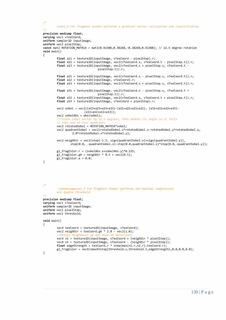
130 | P a g e

/* sobel_f.txt fragment shader performs a gradient vector calculation and classification

*/ precision mediump float; varying vec2 vTexCoord; uniform sampler2D inputImage; uniform vec2 pixelStep; const mat2 ROTATION_MATRIX = mat2(0.92388,0.38268,-0.38268,0.92388); // 22.5 degree rotation void main() { float a11 = texture2D(inputImage, vTexCoord - pixelStep).r; float a12 = texture2D(inputImage, vec2(vTexCoord.s, vTexCoord.t - pixelStep.t)).r;

float a13 = texture2D(inputImage, vec2(vTexCoord.s + pixelStep.s, vTexCoord.t - pixelStep.t)).r;

float a21 = texture2D(inputImage, vec2(vTexCoord.s - pixelStep.s, vTexCoord.t)).r; float a22 = texture2D(inputImage, vTexCoord).r; float a23 = texture2D(inputImage, vec2(vTexCoord.s + pixelStep.s, vTexCoord.t)).r; float a31 = texture2D(inputImage, vec2(vTexCoord.s - pixelStep.s, vTexCoord.t + pixelStep.t)).r; float a32 = texture2D(inputImage, vec2(vTexCoord.s, vTexCoord.t + pixelStep.t)).r; float a33 = texture2D(inputImage, vTexCoord + pixelStep).r; vec2 sobel = vec2((a13+a23+a23+a33)-(a11+a21+a21+a31), (a31+a32+a32+a33)- (a11+a12+a12+a13)); vec2 sobelAbs = abs(sobel);

//rotate sobel vector by 22.5 degrees, then double its angle so it falls // into one of four quadrants

vec2 rotatedSobel = ROTATION_MATRIX*sobel; vec2 quadrantSobel = vec2(rotatedSobel.x*rotatedSobel.x-rotatedSobel.y*rotatedSobel.y, 2.0*rotatedSobel.x*rotatedSobel.y); vec2 neighDir = vec2(step(-1.5, sign(quadrantSobel.x)+sign(quadrantSobel.y)), step(0.0, -quadrantSobel.x)-step(0.0,quadrantSobel.x)*step(0.0,-quadrantSobel.y));

gl_FragColor.r = (sobelAbs.x+sobelAbs.y)*0.125; gl_FragColor.gb = neighDir * 0.5 + vec2(0.5); gl_FragColor.a = 0.0; }

/* nonmaxsuppress_f.txt fragment shader performs non-maximal suppression

and double threshold */ precision mediump float; varying vec2 vTexCoord; uniform sampler2D inputImage; uniform vec2 pixelStep; uniform vec2 threshold; void main() { vec4 texCoord = texture2D(inputImage, vTexCoord); vec2 neighDir = texCoord.gb * 2.0 - vec2(1.0); //Obtain neighbours up and down of directions vec4 n1 = texture2D(inputImage, vTexCoord + (neighDir * pixelStep)); vec4 n2 = texture2D(inputImage, vTexCoord - (neighDir * pixelStep)); float edgeStrength = texCoord.r * step(max(n1.r,n2.r),texCoord.r); gl_FragColor = vec4(smoothstep(threshold.s,threshold.t,edgeStrength),0.0,0.0,0.0); }

131 | P a g e

/* weakpixeltest_f.txt fragment shader performs modified weak pixel test

*/ precision mediump float; varying vec2 vTexCoord; uniform sampler2D inputImage; uniform vec2 pixelStep; void main() { float edgeStrength = texture2D(inputImage, vTexCoord).r; float a11 = texture2D(inputImage, vTexCoord - pixelStep).r; float a12 = texture2D(inputImage, vec2(vTexCoord.s, vTexCoord.t - pixelStep.t)).r;

float a13 = texture2D(inputImage, vec2(vTexCoord.s + pixelStep.s, vTexCoord.t - pixelStep.t)).r;

float a21 = texture2D(inputImage, vec2(vTexCoord.s - pixelStep.s, vTexCoord.t)).r; float a23 = texture2D(inputImage, vec2(vTexCoord.s + pixelStep.s, vTexCoord.t)).r; float a31 = texture2D(inputImage, vec2(vTexCoord.s - pixelStep.s, vTexCoord.t + pixelStep.t)).r; float a32 = texture2D(inputImage, vec2(vTexCoord.s, vTexCoord.t + pixelStep.t)).r; float a33 = texture2D(inputImage, vTexCoord + pixelStep).r; //Only accept as an edge pixel if neighbour strengths reach above 2.0 float strongPixel = step(2.0,edgeStrength+a11+a12+a13+a21+a23+a31+a32+a33);

gl_FragColor = vec4(1.0 - (strongPixel+(edgeStrength-strongPixel) * step(0.49,abs(edgeStrength-0.5)))); }

132 | P a g e

Appendix B: ColourFAST Feature Detection Shaders /* cameratoyuv_f.txt Converts the two textures from the CPU camera to one YUV texture */ precision mediump float; varying vec2 vTexCoord; uniform sampler2D yTexture; uniform sampler2D uvTexture; void main() { float y = texture2D(yTexture, vTexCoord).r; float u = texture2D(uvTexture, vTexCoord).a; float v = texture2D(uvTexture, vTexCoord).r; gl_FragColor = vec4(v,y,u,0.0); } /* cameratoyuv_f.txt Converts the two textures from the CPU camera to one RGB texture */ precision mediump float; varying vec2 vTexCoord; uniform sampler2D yTexture; uniform sampler2D uvTexture; void main() { float y = texture2D(yTexture, vTexCoord).r; float u = texture2D(uvTexture, vTexCoord).a; float v = texture2D(uvTexture, vTexCoord).r; //convert to RGB gl_FragColor.r = y + v * 1.402 - 0.701; gl_FragColor.g = y- u*0.34414 - v*0.71414 + 0.52914; gl_FragColor.b = y + u*1.772 - 0.886; gl_FragColor.a = 1.0; }

/*

smooth_f.txt fragment shader performs a one-dimensional 3x1 smoothing operation meant to be performed twice as two separable operations so that a 3x3 smoothing is done on the input texture.

*/ precision highp float; varying vec2 vTexCoord; uniform sampler2D inputTexture; uniform vec2 pixelStep; void main() { vec3 thisPixel = texture2D(inputTexture, vTexCoord).rgb; vec3 sum = 0.25*(texture2D(inputTexture, vTexCoord - pixelStep).rgb + thisPixel + thisPixel + texture2D(sTexture, vTexCoord + pixelStep).rgb); gl_FragColor = vec4(sum.r,sum.g,sum.b, thisPixel.a); }

133 | P a g e

/* colourfast_f.txt calculates 4 component feature descriptor using RGB or YUV ColourFAST values and a direction for each feature */ precision highp float; varying vec2 vTexCoord; uniform sampler2D inputTexture; uniform vec2 pixelStep; const float PITwo = 6.2832; const float PI = 3.1416; uniform vec2 powerup; //used for empirical weightings of RGB or YUV components void main() { //calculated to avoid more operations later float t3 = 3.0 * pixelStep.t; float s3 = 3.0 * pixelStep.s; vec3 centerTex = texture2D(sTexture, vTexCoord).rgb; //YUV in that order //lookup Colour for 8 neighbours in half-Bresenham around center pixel vec3 nB = texture2D(inputTexture, vec2(vTexCoord.s + pixelStep.s, vTexCoord.t + t3)).rgb; vec3 nA = texture2D(inputTexture, vec2(vTexCoord.s + s3, vTexCoord.t + pixelStep.t)).rgb; vec3 nH = texture2D(inputTexture, vec2(vTexCoord.s + s3, vTexCoord.t - pixelStep.t)).rgb; vec3 nG = texture2D(inputTexture, vec2(vTexCoord.s + pixelStep.s, vTexCoord.t - t3)).rgb; vec3 nF = texture2D(inputTexture, vec2(vTexCoord.s - pixelStep.s, vTexCoord.t - t3)).rgb; vec3 nE = texture2D(inputTexture, vec2(vTexCoord.s - s3, vTexCoord.t - pixelStep.t)).rgb; vec3 nD = texture2D(inputTexture, vec2(vTexCoord.s - s3, vTexCoord.t + pixelStep.t)).rgb; vec3 nC = texture2D(inputTexture, vec2(vTexCoord.s - pixelStep.s, vTexCoord.t + t3)).rgb; //calculate ColourFAST value vec3 yuvDiff = ((nA + nB + nC + nD + nE + nF + nG + nH) * 0.125) - centerTex; //calculate direction of colour change vec3 dirX = (nA*0.94868) + (nB*0.316227) - (nC*0.316227) - (nD*0.94868) - (nE*0.94868) - (nF*0.316227) + (nG*0.316227) + (nH*0.94868); vec3 dirY = (nA*0.316227) + (nB*0.94868) + (nC*0.94868) + (nD*0.316227) - (nE*0.316227) - (nF*0.94868) - (nG*0.94868) - (nH*0.316227); vec3 yuvDiffAbs = abs(yuvDiff); float componentLength = length(yuvDiff); //take dot product so that features heavy in one channel count more toward angle float avgX = dot(yuvDiffAbs,dirX)/componentLength; float avgY = dot(yuvDiffAbs,dirY)/componentLength; float angle = atan(avgY,avgX); //store for YUV and colour change, encode so values between 0-1. gl_FragColor.r = ((yuvDiff.r*powerup.s+1.0)*0.5); // V gl_FragColor.g = ((yuvDiff.g*powerup.t+1.0)*0.5); // Y gl_FragColor.b= ((yuvDiff.b*powerup.s+1.0)*0.5); // U gl_FragColor.a = (angle+PI)/PITwo; }

134 | P a g e

Appendix C: ColourFAST Feature Tracking Shaders /* colourfast_compare_f.txt used to compare an input ColourFAST feature point from the previous frame, with this point */ precision mediump float; varying vec2 vTexCoord; uniform sampler2D inputTexture; //ColourFAST point that is to be compared with this pixel uniform vec4 previousColour; //weight of angle AND also used to distinguish //whether to use absolute comparison or not uniform float angleWeight; void main() { //look up this pixels ColourFAST feature vector vec3 thisC = texture2D(inputTexture, vTexCoord).rgb*2.0 - vec3(1.0,1.0,1.0); float thisAngle = texture2D(inputTexture, vTexCoord).a; //Take the absolute value of texture if angleWeight is 0 Which happens //when point first placed on screen, so it can snap to the maximum value //to non bias a white corner on a black background and vice versa thisC = thisC*step(0.1,angleWeight) + (1.0-step(0.1,angleWeight))*abs(thisC); //encoded between 0-1, for angles -PI -> + PI, take the difference in angle float angleDiff = abs(thisAngle - previousColour.a); //decode the ColourFAST colour components

vec3 comparedColour = vec3(previousColour.r,previousColour.g,previousColour.b)*2.0 - vec3(1.0,1.0,1.0); //angle calculation if angleDiff is 0 or 1 (close), //else if angleDiff is 0.5 (far,opposite direction)

//Encode between 0-1, where 1 is good match, let all other values <0 clamp to 0 (bad match) float diff = 1.0 - (distance(thisC,comparedColour) + ((1.0-2.0*abs(angleDiff- 0.5))*angleWeight))*0.5;

//start this fragment pointing to itself as the best match 0.5,0.5. Where a value of 1,1 //in the RG output means move half window width and height to locate best match at

//bottom right edge of search window and the value 0,0 is the top left. gl_FragColor = vec4(0.5,0.5,diff,diff); }

135 | P a g e

/* featuresearch_f.txt intended to be performed twice as a two step hierachial approach to finding a feature point. The Blue component of the texture holds the value of the best match whereas the RG hold XY movement to where the best match is withing the 20x20 search window.. */ precision highp float; varying vec2 vTexCoord; uniform sampler2D inputTexture; uniform vec2 pixelStep; void main() { //small value to weight pixels more toward middle of search window float epsilon = -0.004; vec4 thisFrag = texture2D(inputTexture, vTexCoord); //Done for a 20x20 search window centered on thisFrag pixelStep ST coordinates //are is 1.0,0.0 for first pass and 0.0,1.0 for second pass vec4 direction = vec4(sign(pixelStep.s),sign(pixelStep.t),0.0,0.0); vec4 n1 = texture2D(inputTexture, vTexCoord - pixelStep) - 0.05*direction; vec4 p1 = texture2D(inputTexture, vTexCoord + pixelStep) + 0.05*direction; vec4 n2 = texture2D(inputTexture, vTexCoord - (2.0*pixelStep))- 0.1*direction; vec4 p2 = texture2D(inputTexture, vTexCoord + (2.0*pixelStep)) + 0.1*direction; vec4 n3 = texture2D(inputTexture, vTexCoord - (3.0*pixelStep)) - 0.15*direction; vec4 p3 = texture2D(inputTexture, vTexCoord + (3.0*pixelStep)) + 0.15*direction; vec4 n4 = texture2D(inputTexture, vTexCoord - (4.0*pixelStep)) - 0.2*direction; vec4 p4 = texture2D(inputTexture, vTexCoord + (4.0*pixelStep)) + 0.2*direction; vec4 n5 = texture2D(inputTexture, vTexCoord - (5.0*pixelStep))- 0.25*direction; vec4 p5 = texture2D(inputTexture, vTexCoord + (5.0*pixelStep)) + 0.25*direction; vec4 n6 = texture2D(inputTexture, vTexCoord - (6.0*pixelStep)) - 0.3*direction; vec4 p6 = texture2D(inputTexture, vTexCoord + (6.0*pixelStep)) + 0.3*direction; vec4 n7 = texture2D(inputTexture, vTexCoord - (7.0*pixelStep)) - 0.35*direction; vec4 p7 = texture2D(inputTexture, vTexCoord + (7.0*pixelStep))+ 0.35*direction; vec4 n8 = texture2D(inputTexture, vTexCoord - (8.0*pixelStep)) - 0.4*direction; vec4 p8 = texture2D(inputTexture, vTexCoord + (8.0*pixelStep)) + 0.4*direction; vec4 n9 = texture2D(inputTexture, vTexCoord - (9.0*pixelStep)) - 0.45*direction; vec4 p9 = texture2D(inputTexture, vTexCoord + (9.0*pixelStep)) + 0.45*direction; vec4 n10 = texture2D(inputTexture, vTexCoord - (10.0*pixelStep)) - 0.5*direction; vec4 p10 = texture2D(inputTexture, vTexCoord + (10.0*pixelStep)) + 0.5*direction; //if neighbouring value is better match than this vale then delta is positive //and take newthisFrag to be that neighbour, in the end newthisFrag will have //the position of the best match and the value of the best match float delta = (n1.b - thisFrag.b) + epsilon; vec4 newthisFrag = step(0.0,delta)*n1+(1.0-step(0.0,delta))*thisFrag; delta = (p1.b - newthisFrag.b) + epsilon; newthisFrag = step(0.0,delta)*p1+(1.0-step(0.0,delta))*newthisFrag; delta = (n2.b - newthisFrag.b) + 2.0*epsilon; newthisFrag = step(0.0,delta)*n2+(1.0-step(0.0,delta))*newthisFrag; delta = ( p2.b - newthisFrag.b) + 2.0*epsilon; newthisFrag = step(0.0,delta)*p2+(1.0-step(0.0,delta))*newthisFrag; delta = (n3.b - newthisFrag.b) + 3.0*epsilon; newthisFrag = step(0.0,delta)*n3+(1.0-step(0.0,delta))*newthisFrag; delta = (p3.b - newthisFrag.b) + 3.0*epsilon; newthisFrag = step(0.0,delta)*p3+(1.0-step(0.0,delta))*newthisFrag; delta = (n4.b - newthisFrag.b) + 4.0*epsilon; newthisFrag = step(0.0,delta)*n4+(1.0-step(0.0,delta))*newthisFrag; delta = (p4.b - newthisFrag.b) + 4.0*epsilon; newthisFrag = step(0.0,delta)*p4+(1.0-step(0.0,delta))*newthisFrag; delta = (n5.b - newthisFrag.b) + 5.0*epsilon; newthisFrag = step(0.0,delta)*n5+(1.0-step(0.0,delta))*newthisFrag; delta = (p5.b - newthisFrag.b) + 5.0*epsilon; newthisFrag = step(0.0,delta)*p5+(1.0-step(0.0,delta))*newthisFrag; delta = (n6.b - newthisFrag.b) + 6.0*epsilon; newthisFrag = step(0.0,delta)*n6+(1.0-step(0.0,delta))*newthisFrag;

136 | P a g e

delta = (p6.b - newthisFrag.b) + 6.0*epsilon; newthisFrag = step(0.0,delta)*p6+(1.0-step(0.0,delta))*newthisFrag; delta = (n7.b - newthisFrag.b) + 7.0*epsilon; newthisFrag = step(0.0,delta)*n7+(1.0-step(0.0,delta))*newthisFrag; delta = (p7.b - newthisFrag.b) + 7.0*epsilon; newthisFrag = step(0.0,delta)*p7+(1.0-step(0.0,delta))*newthisFrag; delta = (n8.b - newthisFrag.b) + 8.0*epsilon; newthisFrag = step(0.0,delta)*n8+(1.0-step(0.0,delta))*newthisFrag; delta = (p8.b - newthisFrag.b) + 8.0*epsilon; newthisFrag = step(0.0,delta)*p8+(1.0-step(0.0,delta))*newthisFrag; delta = (n9.b - newthisFrag.b) + 9.0*epsilon; newthisFrag = step(0.0,delta)*n9+(1.0-step(0.0,delta))*newthisFrag; delta = (p9.b - newthisFrag.b) + 9.0*epsilon; newthisFrag = step(0.0,delta)*p9+(1.0-step(0.0,delta))*newthisFrag; delta = (n10.b - newthisFrag.b) + 10.0*epsilon; newthisFrag = step(0.0,delta)*n10+(1.0-step(0.0,delta))*newthisFrag; delta = (p10.b - newthisFrag.b) + 10.0*epsilon; newthisFrag = step(0.0,delta)*p10+(1.0-step(0.0,delta))*newthisFrag; gl_FragColor = vec4(newthisFrag.r, newthisFrag.g ,newthisFrag.b,newthisFrag.a); }

137 | P a g e

Appendix D: Feature Discovery Shader /* feature_finder_f.txt uses a combination of Haar masks along direction of the feature and is used to move a special feature discovery point that is used on the CPU side to locate more features along the contour of an object. */ precision highp float; varying vec2 vTexCoord; uniform sampler2D inTexture; uniform vec2 pixelStep; const float PITwo = 6.2832; const float PI = 3.1416; void main() { //decode angle.. the calculate X and Y direction movements float angle = texture2D(inTexture, vTexCoord).a * PITwo - PI; vec2 directionXY = vec2(cos(angle),sin(angle)); vec2 dirXYTexCoords = directionXY*pixelStep; //calculate the lengths of each neighbour across 10 pixels in direction of this

//feature point, used so discovery point follows ridge and valley of features float an = length(texture2D(inTexture, vTexCoord+6.0*dirXYTexCoords).rgb*2.0 - vec3(1.0,1.0,1.0)); float a0 = length(texture2D(inTexture, vTexCoord+5.0*dirXYTexCoords).rgb*2.0 - vec3(1.0,1.0,1.0)); float a1 = length(texture2D(inTexture, vTexCoord+4.0*dirXYTexCoords).rgb*2.0 - vec3(1.0,1.0,1.0)); float a2 = length(texture2D(inTexture, vTexCoord+3.0*dirXYTexCoords).rgb*2.0 - vec3(1.0,1.0,1.0)); float a3 = length(texture2D(inTexture, vTexCoord+2.0*dirXYTexCoords).rgb*2.0 - vec3(1.0,1.0,1.0)); float a4 = length(texture2D(inTexture, vTexCoord+dirXYTexCoords).rgb*2.0 - vec3(1.0,1.0,1.0)); float a5 = length(texture2D(inTexture, vTexCoord).rgb*2.0-vec3(1.0,1.0,1.0)); float a6 = length(texture2D(inTexture, vTexCoord-dirXYTexCoords).rgb*2.0- vec3(1.0,1.0,1.0)); float a7 = length(texture2D(inTexture, vTexCoord-2.0*dirXYTexCoords).rgb*2.0- vec3(1.0,1.0,1.0)); float a8 = length(texture2D(inTexture, vTexCoord-3.0*dirXYTexCoords).rgb*2.0- vec3(1.0,1.0,1.0));

//Do Haar mask combinations float upMove2 = (a4+2.0*a3+a2)-(a1+2.0*a0+an); float upMove = (a5+2.0*a4+a3)-(a1+2.0*a1+a0); float stayMove = (a6+2.0*a5+a4)-(a3+2.0*a2+a1); float downMove = (a7+2.0*a6+a5)-(a4+2.0*a3+a2); float downMove2 = (a8+2.0*a7+a6)-(a5+2.0*a4+a3); //obtain the maximum value for Haar masks float maxPoint = max(max(max(upMove,upMove2),max(downMove,downMove2)),stayMove); //Move either up 1 or 2, down 1 or 2 or stay. Depending on which was the maximum vec2 clampedMove = 2.0 * dirXYTexCoords * step(maxPoint, upMove2) + dirXYTexCoords * step(maxPoint, upMove) - dirXYTexCoords * step(maxPoint, downMove) - 2.0 * dirXYTexCoords * step(maxPoint, downMove2); //Look right to the angle and move vec2 movement = directionXY.ts*vec2(2.0,-2.0); vec2 movementInTexCoords = movement*pixelStep; //Need to add the clamp to the movements so CPU knows that it clamped float strength = length(texture2D(inTexture, vTexCoord + clampedMove + movementInTexCoords).rgb * 2.0 - vec3(1.0,1.0,1.0)); vec2 movementEncoded = ((clampedMove/pixelStep + movement) + vec2(4.0,4.0))*vec2(0.125,0.125); //encoded between 0-1 for length of 3 channel vector (srt 3) gl_FragColor = vec4(movementEncoded.s,movementEncoded.t,strength*0.5773,strength*0.5773); }

138 | P a g e

Appendix E: ColourFAST Object Recognition Shaders /* or_mindistances_f.txt - this shader is performed for each point being tracked on screen

and is used to find the best matching feature point for each object by iterating through each feature held in the object being compared to the features on screen.

*/ precision mediump float; varying vec2 vTexCoord; //texture for the features being tracked on screen uniform sampler2D blendedFeaturesTexture; //texture that holds the number of features in the object being compared uniform sampler2D numberOfFeaturesTexture; //texture the holds each object in rows and its feature points in columns uniform sampler2D objectInputTexture; //holds the maximum amount of features for an object uniform int maxNumberOfFeatures; void main() { vec4 featurePoint = texture2D(blendedFeaturesTexture, vec2(vTexCoord.s,0.5)); float numberOfFeatures = float(maxNumberOfFeatures)*texture2D(numberOfFeaturesTexture, vec2(0.5, vTexCoord.t)).r; float stepBetweenFeatures = 1.0/float(maxNumberOfFeatures); int featureNumber = 0; float minDistance = 10.0; vec2 featureTexels = vTexCoord; vec3 objectColour = vec3(1.0,1.0,1.0); float angleDiff = 0.0; float compare = 0.0; //decode this feature point vec3 outputColour = featurePoint.rgb *2.0 - vec3(1.0,1.0,1.0); //find the best match (minimum distance value) in the object input texture while(float(featureNumber) < numberOfFeatures) { featureTexels = vec2(stepBetweenFeatures * float(featureNumber) + 0.004, vTexCoord.t); float ang = texture2D(objectInputTexture, featureTexels).a; //decode the object being compared feature point objectColour = texture2D(objectInputTexture, featureTexels).rgb * 2.0 - vec3(1.0,1.0,1.0); //calculate differences in angle angleDiff = abs(featurePoint.a - ang); //compare featurepoint on screen with the feature in this object texture

compare = distance(objectColour,outputColour) + (1.0-2.0* abs(angleDiff-0.5))*0.25;

minDistance = min(minDistance,compare); featureNumber++; } gl_FragColor = vec4(minDistance*0.288,minDistance,1.0,1.0); }

139 | P a g e

/* or_distancesums_f.txt iterates through each feature point for the object being compared and summing the best feature matches from the previous shader. It then takes a sqrt of 2.0 x sum so that good matches are spread out more and bad matches are maxed out to 1.0. */ precision mediump float; varying vec2 vTexCoord; uniform sampler2D inputTexture; //Take in the amount of points being tracked on screen uniform int pointListSize; void main() { int featureNumber=0; float distanceSumSq = 0.0; float stepBetweenPoints = 1.0/float(pointListSize); float minDist = 0.0; //loop for each feature point in this object and sum while(featureNumber < pointListSize) { minDist = texture2D(inputTexture, vec2(float(featureNumber) * stepBetweenPoints + 0.004,vTexCoord.t)).r; distanceSumSq += minDist; featureNumber++; } gl_FragColor = vec4((sqrt(2.0*distanceSumSq))/float(pointListSize),1.0, 1.0 1.0); }

140 | P a g e

References

1. Sehwan, K., et al., Implicit 3D modeling and tracking for anywhere augmentation, in Proceedings of the 2007 ACM symposium on Virtual reality software and technology2007, ACM: Newport Beach, California.

2. de Santos Sierra, A., et al. Silhouette-based hand recognition on mobile devices. in Security Technology, 2009. 43rd Annual 2009 International Carnahan Conference on. 2009.

3. Karodia, R., et al. CipherCode: A Visual Tagging SDK with Encryption and Parameterisation. in Automatic Identification Advanced Technologies, 2007 IEEE Workshop on. 2007.

4. Lee, J.A. and Y. Kin Choong. Image Recognition for Mobile Applications. in Image Processing, 2007. ICIP 2007. IEEE International Conference on. 2007.

5. Grifantini, K. What's Augmented Reality's Killer App? September 2009 [cited 2010 December]; Available from: http://www.technologyreview.com/computing/23515.

6. Fleishman, G., Five technologies that will change everything, October 2009, ACM Tech News.

7. Reitmayr, G. and T.W. Drummond. Going out: robust model-based tracking for outdoor augmented reality. in Mixed and Augmented Reality, 2006. ISMAR 2006. IEEE/ACM International Symposium on. 2006.

8. Takacs, G., et al., Outdoors augmented reality on mobile phone using loxel-based visual feature organization, in Proceedings of the 1st ACM international conference on Multimedia information retrieval2008, ACM: Vancouver, British Columbia, Canada. p. 427-434.

9. Schmeil, A. and W. Broll. MARA - A Mobile Augmented Reality-Based Virtual Assistant. in Virtual Reality Conference, 2007. VR '07. IEEE. 2007.

10. ARToolKitPlus. [accessed 2011 March]; Available from: http://studierstube.icg.tu-graz.ac.at/handheld_ar/artoolkitplus.php.

11. Studierstube Tracker. [accessed 2011 March]; Available from: http://studierstube.icg.tu-graz.ac.at/handheld_ar/stbtracker.php.

12. Layar. [accessed 2011 March]; Available from: http://www.layar.com/.

13. Wagner, D., et al. Pose tracking from natural features on mobile phones. in Mixed and Augmented Reality, 2008. ISMAR 2008. 7th IEEE/ACM International Symposium on. 2008.

14. Tao, C., et al. A multi-scale learning approach for landmark recognition using mobile devices. in Information, Communications and Signal Processing, 2009. ICICS 2009. 7th International Conference on. 2009.

141 | P a g e

15. WillowGarage. OpenCV. 21 January 2014]; Available from: http://opencv.org/.

16. Ensor, A. and S. Hall. GPU-based image analysis on mobile devices. in The 26th International Conference on Image and Vision Computing New Zealand. 2011. Auckland, New Zealand.

17. Shi, J. and C. Tomasi. Good features to track. in Computer Vision and Pattern Recognition, 1994. Proceedings CVPR '94., 1994 IEEE Computer Society Conference on. 1994.

18. Ensor, A. and S. Hall. ColourFAST: GPU-based Feature Point Detection and Tracking on Mobile Devices. in The 28th International Conference on Image and Vision Computing New Zealand. 2013. Wellington, New Zealand.

19. Gerhard, R. and S. Dieter, Location based applications for mobile augmented reality, in Proceedings of the Fourth Australasian user interface conference on User interfaces 2003 - Volume 182003, Australian Computer Society, Inc.: Adelaide, Australia.

20. Ryong, L., et al., Interoperable augmented web browsing for exploring virtual media in real space, in Proceedings of the 2nd International Workshop on Location and the Web2009, ACM: Boston, Massachusetts.

21. P. Milgram and F. Kishino, A Taxonomy of Mixed Reality Visual Displays. IEICE Transactions on Information Systems, December 1994. Vol. E77-D.

22. Beier, D., et al. Marker-less vision based tracking for mobile augmented reality. in Mixed and Augmented Reality, 2003. Proceedings. The Second IEEE and ACM International Symposium on. 2003.

23. Sutherland, I., The Ultimate Display, in IFIP Congress1965: New York. p. 506-508.

24. Sutherland, I., A head-mounted three dimensional display, in Proceedings of the December 9-11, 1968, fall joint computer conference, part I1968, ACM: San Francisco, California.

25. Azuma, R.T., The Challenge of Making Augmented Reality Work Outdoor. Mix Real, 1999: p. 379-390.

26. Feiner, S., et al. A touring machine: prototyping 3D mobile augmented reality systems for exploring the urban environment. in Wearable Computers, 1997. Digest of Papers., First International Symposium on. 1997.

27. Hoshi, K. and J. Waterworth. Tangible presence in blended reality space. in Proceedings of the 12th Annual International Workshop on Presence. 2009.

28. International Telecommunication Union. January 2011; Available from: http://www.itu.int/ITU-D/ict/.

29. Want, R., iPhone: Smarter Than the Average Phone. Pervasive Computing, IEEE. 9(3): p. 6-9.

142 | P a g e

30. Gartner. Gartner Says Smartphone Sales Accounted for 55 Percent of Overall Mobile Phone Sales in Third Quarter of 2013. 14 November 2013 January 2014]; Available from: http://www.gartner.com/newsroom/id/2623415.

31. Symbian. Symbian Developers. Available from: http://symbian-developers.net/.

32. Ricker, T. RIP: Symbian. 11 February 2011 [accessed 2013 December]; Available from: http://www.engadget.com/2011/02/11/rip-symbian/.

33. Reisinger, D. Nokia officially walks away from Symbian, MeeGo. 2 January 2014 [cited February 2014; Available from: http://news.cnet.com/8301-1035_3-57616457-94/nokia-officially-walks-away-from-symbian-meego/.

34. BlackBerry. BlackBerry - Developer Program. [cited 2014 January]; Available from: https://developer.blackberry.com/.

35. Branscombe, M. Intel: MeeGo exists because Microsoft let us down. Interview: Even Windows 7 doesn't do enough for Atom, says chip giant. 20 April 2010 [accessed 2014 January]; Available from: http://www.techradar.com/news/computing-components/processors/intel-meego-exists-because-microsoft-let-us-down-684665.

36. Meego. [cited 2014 January]; Available from: http://meego.com/.

37. Windows. Windows Phone Developer Center. Available from: http://dev.windowsphone.com/en-us.

38. iOS Dev Centre - Apple Developer. [accessed 2014 January]; Available from: http://developer.apple.com/.

39. Google. Android Developers. [accessed 2014 January]; Available from: http://developer.android.com/develop/index.html.

40. Bradski, G., Learning OpenCV2008: O'Reilly Media.

41. Fung, J. and S. Mann. Computer vision signal processing on graphics processing units. in Acoustics, Speech, and Signal Processing, 2004. Proceedings. (ICASSP '04). IEEE International Conference on. 2004.

42. Rockwood, A. and J. McAndless, Through the looking glass: the synthesis of computer graphics and computer vision. Multimedia, IEEE, 1999. 6(3): p. 8-11.

43. Fiala, M. Comparing ARTag and ARToolkit Plus fiducial marker systems. in Haptic Audio Visual Environments and their Applications, 2005. IEEE International Workshop on. 2005.

44. Jia, J., Y. Qi, and Q. Zuo. An Extended Marker-Based Tracking System for Augmented Reality. in Modeling, Simulation and Visualization Methods (WMSVM), 2010 Second International Conference on.

45. UtKarsh. Convolutions. [accessed April 2011]; Available from: http://www.aishack.in/2010/08/convolutions/.

143 | P a g e

46. Roberts, L., Machine Perception Of Three-Dimensional Solids, in Lincoln Laboratory 1963, Massachusetts Institued of Technology

47. Wenshuo, G., et al. An improved Sobel edge detection. in Computer Science and Information Technology (ICCSIT), 2010 3rd IEEE International Conference on.

48. Canny, J., A Computational Approach to Edge Detection. Pattern Analysis and Machine Intelligence, IEEE Transactions on, 1986. PAMI-8(6): p. 679-698.

49. Xin, W., Laplacian Operator-Based Edge Detectors. Pattern Analysis and Machine Intelligence, IEEE Transactions on, 2007. 29(5): p. 886-890.

50. Moravec, H., Obstacle Avoidance and Navigation in the Real World by a Seeing Robot Rover, 1980, Carnegie-Mellon University, Robotics Institute.

51. Harris, C. and M. Stephens, A combined corner and edge detector, in Proceedings of the 4th Alvey Vision Conference1988. p. 147–151.

52. Wang, H. and M. Brady, Real-time corner detection algorithm for motion estimation. Image and Vision Computing, 1995. 13(9): p. 695-703.

53. Smith, S.M. and J.M. Brady, SUSAN – a new approach to low level image processing. International Journal of Computer Vision, 1997. 23(1): p. 45-78.

54. Rosten, E. and T. Drummond. Fusing points and lines for high performance tracking. in Computer Vision, 2005. ICCV 2005. Tenth IEEE International Conference on. 2005.

55. Rosten, E. and T. Drummond, Machine learning for high-speed corner detection, in European Conference on Computer Vision2006. p. 430–443.

56. Rosten, E., R. Porter, and T. Drummond, Faster and Better: A Machine Learning Approach to Corner Detection. Pattern Analysis and Machine Intelligence, IEEE Transactions on, 2010. 32(1): p. 105-119.

57. Lowe, D.G. Object recognition from local scale-invariant features. in Computer Vision, 1999. The Proceedings of the Seventh IEEE International Conference on. 1999.

58. Gee-Sern, H., L. Chyi-Yeu, and W. Jia-Shan. Real-time 3-D object recognition using Scale Invariant Feature Transform and stereo vision. in Autonomous Robots and Agents, 2009. ICARA 2009. 4th International Conference on. 2009.

59. Youliang, Y., L. Weili, and Z. Lan. Study on improved scale Invariant Feature Transform matching algorithm. in Circuits,Communications and System (PACCS), 2010 Second Pacific-Asia Conference on.

60. Bay, H., T. Tuytelaars, and L. Van Gool, Surf: Speeded up robust features, in Computer Vision–ECCV 20062006, Springer. p. 404-417.

144 | P a g e

61. Bauer, J., N. Sunderhauf, and P. Protzel. Comparing several implementations of two recently published feature detectors. in Proc. of the International Conference on Intelligent and Autonomous Systems. 2007.

62. Lucas, B. and T. Kanade. An Iterative Image Registration Technique with an Application to Stereo Vision. in International Joint Conference on Artificial Intelligence. 1981.

63. Tomasi, C. and T. Kanade, Detection and Tracking of Point Features, in Carnegie Mellon University Technical Report1991.

64. Horn, B.K. and B.G. Schunck. Determining optical flow. in 1981 Technical Symposium East. 1981. International Society for Optics and Photonics.

65. Bauer, N., P. Pathirana, and P. Hodgson. Robust Optical Flow with Combined Lucas-Kanade/Horn-Schunck and Automatic Neighborhood Selection. in Information and Automation, 2006. ICIA 2006. International Conference on. 2006.

66. Birchfield, S.T. and S.J. Pundlik. Joint tracking of features and edges. in Computer Vision and Pattern Recognition, 2008. CVPR 2008. IEEE Conference on. 2008.

67. Comaniciu, D., V. Ramesh, and P. Meer, Kernel-based object tracking. Pattern Analysis and Machine Intelligence, IEEE Transactions on, 2003. 25(5): p. 564-577.

68. Zia, K., T. Balch, and F. Dellaert, MCMC-based particle filtering for tracking a variable number of interacting targets. Pattern Analysis and Machine Intelligence, IEEE Transactions on, 2005. 27(11): p. 1805-1819.

69. Nummiaro, K., E. Koller-Meier, and L. Van Gool, Object tracking with an adaptive color-based particle filter, in Pattern Recognition2002, Springer. p. 353-360.

70. Wu-chun, F. and X. Shucai. To GPU synchronize or not GPU synchronize? in Circuits and Systems (ISCAS), Proceedings of 2010 IEEE International Symposium on.

71. Martin, D., M. Mike, and Z. Huiyang, Understanding software approaches for GPGPU reliability, in Proceedings of 2nd Workshop on General Purpose Processing on Graphics Processing Units2009, ACM: Washington, D.C.

72. Jayanth, G., et al., Efficient implementation of GPGPU synchronization primitives on CPUs, in Proceedings of the 7th ACM international conference on Computing frontiers, ACM: Bertinoro, Italy.

73. David, L., et al., GPGPU: general purpose computation on graphics hardware, in ACM SIGGRAPH 2004 Course Notes2004, ACM: Los Angeles, CA.

74. Open GL Shading Language. [accessed 2011 April]; Available from: http://www.opengl.org/documentation/glsl/.

75. HLSL. [accessed 2011 April]; Available from: http://msdn.microsoft.com/en-us/library/bb509561(v=vs.85).aspx.

145 | P a g e

76. Munshi, A. and D. Ginsburg, OpenGL ES 2.0 Programming guide 2009: Addison-Wesley.

77. Freescale-Semiconductor, High-End 3D Graphics with OpenGL ES 2.0, 2011.

78. Segal, M. and K. Akeley, The OpenGLGraphics System:A Specification(Version 2.0 - October 22, 2004), 2004.

79. OpenGL ES - The Standard for Embedded Accelerated 3D Graphics. [accessed 2011 April]; Available from: http://www.khronos.org/opengles/2_X/.

80. Kishonti_Informations_Ltd. GLBenchmark 2.1 Egypt. 2011; Available from: http://www.glbenchmark.com/.

81. Junchul, K., et al. A fast feature extraction in object recognition using parallel processing on CPU and GPU. in Systems, Man and Cybernetics, 2009. SMC 2009. IEEE International Conference on. 2009.

82. Warn, S., et al. Accelerating SIFT on parallel architectures. in Cluster Computing and Workshops, 2009. CLUSTER '09. IEEE International Conference on. 2009.

83. Ogawa, K., Y. Ito, and K. Nakano. Efficient Canny Edge Detection Using a GPU. in Networking and Computing (ICNC), 2010 First International Conference on.

84. Cornelis, N. and L. Van Gool. Fast scale invariant feature detection and matching on programmable graphics hardware. in Computer Vision and Pattern Recognition Workshops, 2008. CVPRW'08. IEEE Computer Society Conference on. 2008. IEEE.

85. Sinha, S.N., et al. GPU-based video feature tracking and matching. in EDGE, Workshop on Edge Computing Using New Commodity Architectures. 2006.

86. Sánchez, J.R., H. Alvarez, and D. Borro. Towards real time 3D tracking and reconstruction on a GPU using Monte Carlo simulations. in Mixed and Augmented Reality (ISMAR), 2010 9th IEEE International Symposium on. 2010. IEEE.

87. Tiemersma, E.W., et al., Methicillin-resistant Staphylococcus aureus in Europe, 1999–2002. 2004.

88. Bibby, C. and I. Reid. Fast feature detection with a graphics processing unit implementation. in Proc. International Workshop on Mobile Vision. 2006.

89. Wagner, D., et al., Real-Time Detection and Tracking for Augmented Reality on Mobile Phones. Visualization and Computer Graphics, IEEE Transactions on, 2010. 16(3): p. 355-368.

90. Yang, X. and K.-T. Cheng, Accelerating SURF detector on mobile devices, in Proceedings of the 20th ACM international conference on Multimedia2012, ACM: Nara, Japan. p. 569-578.

91. Hofmann, R., H. Seichter, and G. Reitmayr. A GPGPU accelerated descriptor for mobile devices. in ISMAR. 2012.

92. Anderberg, M.R., Cluster analysis for applications, 1973, DTIC Document.

146 | P a g e

93. Kaufman, L. and P.J. Rousseeuw, Finding groups in data: an introduction to cluster analysis. Vol. 344. 2009: Wiley. com.

94. Estivill-Castro, V., Why so many clustering algorithms: a position paper. ACM SIGKDD Explorations Newsletter, 2002. 4(1): p. 65-75.

95. Tron, R. and R. Vidal. A Benchmark for the Comparison of 3-D Motion Segmentation Algorithms. in Computer Vision and Pattern Recognition, 2007. CVPR '07. IEEE Conference on. 2007.

96. Zappella, L., X. Lladó, and J. Salvi. Motion segmentation: A review. in Proceedings of the 2008 conference on Artificial Intelligence Research and Development: Proceedings of the 11th International Conference of the Catalan Association for Artificial Intelligence. 2008. IOS Press.

97. Ester, M., et al. A density-based algorithm for discovering clusters in large spatial databases with noise. in KDD. 1996.

98. Kriegel, H.P., et al., Density‐based clustering. Wiley Interdisciplinary Reviews: Data Mining and Knowledge Discovery, 2011. 1(3): p. 231-240.

99. Patwary, M., et al. A new scalable parallel dbscan algorithm using the disjoint-set data structure. in High Performance Computing, Networking, Storage and Analysis (SC), 2012 International Conference for. 2012. IEEE.

100. MacQueen, J. Some methods for classification and analysis of multivariate observations. in Proceedings of the fifth Berkeley symposium on mathematical statistics and probability. 1967. California, USA.

101. Hartigan, J.A. and M.A. Wong, Algorithm AS 136: A k-means clustering algorithm. Journal of the Royal Statistical Society. Series C (Applied Statistics), 1979. 28(1): p. 100-108.

102. Vattani, A., K-means requires exponentially many iterations even in the plane. Discrete & Computational Geometry, 2011. 45(4): p. 596-616.

103. Arthur, D., B. Manthey, and H. Roglin. k-Means has polynomial smoothed complexity. in Foundations of Computer Science, 2009. FOCS'09. 50th Annual IEEE Symposium on. 2009. IEEE.

104. Mohapatra, D. and S.B. Suma. Survey of location based wireless services. in Personal Wireless Communications, 2005. ICPWC 2005. 2005 IEEE International Conference on. 2005.

105. Yiming, L. and W. Erik, Personalized location-based services, in Proceedings of the 2011 iConference, ACM: Seattle, Washington.

106. Qubulus. Indoor Positioning. Available from: http://www.qubulus.com/.

147 | P a g e

107. 3SixtyFactory. Know More about The Top 7 Augmented Reality (AR) Applications This 2011. 31 March 2011 [accessed 2011 May]; Available from: http://www.3sixtyfactory.com/en/blog/159-know-more-about-the-top-7-augmented-reality-ar-applications-this-2011.html.

108. Par, B. Top 6 Augmented Reality Mobile Apps [Videos]. August 2009 [accessed 2011 April]; Available from: http://mashable.com/2009/08/19/augmented-reality-apps/.

109. lester. The Future of Home Shopping [accessed 2011 May]; Available from: http://www.augmentedplanet.com/2009/08/the-future-of-home-shopping/.

110. Kurzweil_AI. Global Augmented Reality Summit 2013. September 2013; Available from: http://www.kurzweilai.net/global-augmented-reality-summit-2013.

111. Wolde, H.T., Dutch Layar signs global augmented reality deals, in Reuters18 June 2010: Amsterdam.

112. Layar Developer Wiki. [accessed 2011 March]; Available from: http://layar.pbworks.com/w/page/7783228/FrontPage.

113. Junaio. [cited 2011 April]; Available from: http://www.junaio.com/.

114. Google. Google Goggles. [accessed 2011 April]; Available from: http://www.google.com/mobile/goggles/#text.

115. Milian, M., How Google is teaching computers to see, in CNN14 April 2011.

116. Google. Google Glass. 2014; Available from: http://www.google.com/glass/start/.

117. Newman, J., Google's 'Project Glass' Teases Augmented Reality Glasses, in PC World4 April 2012.

118. Gao, W., et al., AVS-The Chinese next-generation video coding standard. National Association of Broadcasters, Las Vegas, 2004.

119. Gu, J., R. Mukundan, and M. Billinghurst. Developing mobile phone AR applications using J2ME. in Image and Vision Computing New Zealand, 2008. IVCNZ 2008. 23rd International Conference. 2008.

120. Boring, S., et al., Shoot \& copy: phonecam-based information transfer from public displays onto mobile phones, in Proceedings of the 4th international conference on mobile technology, applications, and systems and the 1st international symposium on Computer human interaction in mobile technology2007, ACM: Singapore. p. 24-31.

121. Boring, S., et al., Touch projector: mobile interaction through video, in Proceedings of the SIGCHI Conference on Human Factors in Computing Systems2010, ACM: Atlanta, Georgia, USA. p. 2287-2296.

122. Bruns, E. and O. Bimber, Adaptive training of video sets for image recognition on mobile phones. Personal Ubiquitous Comput., 2009. 13(2): p. 165-178.

148 | P a g e

123. Wagner, D., et al., Real-Time Detection and Tracking for Augmented Reality on Mobile Phones. Visualization and Computer Graphics, IEEE Transactions on. 16(3): p. 355-368.

124. Schmalstieg, D. and D. Wagner. Experiences with Handheld Augmented Reality. in Mixed and Augmented Reality, 2007. ISMAR 2007. 6th IEEE and ACM International Symposium on. 2007.

125. Fung, J. and S. Mann, OpenVIDIA: parallel GPU computer vision, in Proceedings of the 13th annual ACM international conference on Multimedia2005, ACM: Hilton, Singapore. p. 849-852.

126. Allusse, Y., et al., GpuCV: an opensource GPU-accelerated framework forimage processing and computer vision, in Proceedings of the 16th ACM international conference on Multimedia2008, ACM: Vancouver, British Columbia, Canada. p. 1089-1092.

127. Kwang-Ting, C. and W. Yi-Chu. Using mobile GPU for general-purpose computing &#x2013; a case study of face recognition on smartphones. in VLSI Design, Automation and Test (VLSI-DAT), 2011 International Symposium on. 2011.

128. Singhal, N., P. In Kyu, and C. Sungdae. Implementation and optimization of image processing algorithms on handheld GPU. in Image Processing (ICIP), 2010 17th IEEE International Conference on. 2010.

129. Lowe, D.G., Distinctive Image Features from Scale-Invariant Keypoints. International Journal of Computer Vision, 2004. 60: p. 91-110.

130. Dalal, N. and B. Triggs. Histograms of oriented gradients for human detection. in Computer Vision and Pattern Recognition, 2005. CVPR 2005. IEEE Computer Society Conference on. 2005. IEEE.

131. Klein, G. and D. Murray. Parallel tracking and mapping on a camera phone. in Mixed and Augmented Reality, 2009. ISMAR 2009. 8th IEEE International Symposium on. 2009. IEEE.

132. Ohmer, J.F. and N.J. Redding. GPU-Accelerated KLT Tracking with Monte-Carlo-Based Feature Reselection. in Digital Image Computing: Techniques and Applications (DICTA), 2008. 2008.

133. Hile, H. and G. Borriello, Information overlay for camera phones in indoor environments, in Location-and Context-Awareness2007, Springer. p. 68-84.

134. Wang, J., S. Zhai, and J. Canny. Camera phone based motion sensing: interaction techniques, applications and performance study. in Proceedings of the 19th annual ACM symposium on User interface software and technology. 2006. ACM.

135. Van De Sande, K.E., T. Gevers, and C.G. Snoek, Evaluating color descriptors for object and scene recognition. Pattern Analysis and Machine Intelligence, IEEE Transactions on, 2010. 32(9): p. 1582-1596.

149 | P a g e

136. Abdel-Hakim, A.E. and A.A. Farag. CSIFT: A SIFT Descriptor with Color Invariant Characteristics. in Computer Vision and Pattern Recognition, 2006 IEEE Computer Society Conference on. 2006.

137. Van De Weijer, J. and C. Schmid, Coloring local feature extraction, in Computer Vision–ECCV 20062006, Springer. p. 334-348.

138. Wikipedia. YUV. November 2, 2014; Available from: http://en.wikipedia.org/w/index.php?title=YUV&oldid=630478850.

139. Ozuysal, M., P. Fua, and V. Lepetit. Fast keypoint recognition in ten lines of code. in Computer Vision and Pattern Recognition, 2007. CVPR'07. IEEE Conference on. 2007. Ieee.

140. Kalal, Z., K. Mikolajczyk, and J. Matas, Tracking-Learning-Detection. Pattern Analysis and Machine Intelligence, IEEE Transactions on, 2012. 34(7): p. 1409-1422.

141. Yves, B.J., Pyramidal implementation of the lucas-kanade feature tracker. Microsoft Research Labs, Tech. Rep, 1999.

142. Matthews, I., T. Ishikawa, and S. Baker, The template update problem. IEEE transactions on pattern analysis and machine intelligence, 2004. 26(6): p. 810-815.

143. Viola, P. and M. Jones. Rapid object detection using a boosted cascade of simple features. in Computer Vision and Pattern Recognition, 2001. CVPR 2001. Proceedings of the 2001 IEEE Computer Society Conference on. 2001. IEEE.

144. Mittal, K., PARALLEL K MEANS CLUSTERING USING GPU: IMPLEMENTATION USING CUDA. International Journal of Information Technology & Computer Sciences Perspectives, 2013. 2(3): p. 634-637.

145. DiMarco, J. and M. Taufer. Performance impact of dynamic parallelism on different clustering algorithms. in SPIE Defense, Security, and Sensing. 2013. International Society for Optics and Photonics.

146. Thapa, R.J., C. Trefftz, and G. Wolffe. Memory-efficient implementation of a graphics processor-based cluster detection algorithm for large spatial databases. in Electro/Information Technology (EIT), 2010 IEEE International Conference on. 2010. IEEE.

147. Oyallon, E. and J. Rabin, An analysis and implementation of the SURF method, and its comparison to SIFT. Image Processing On Line, 2013.

148. Ke, Y. and R. Sukthankar. PCA-SIFT: A more distinctive representation for local image descriptors. in Computer Vision and Pattern Recognition, 2004. CVPR 2004. Proceedings of the 2004 IEEE Computer Society Conference on. 2004. IEEE.

149. Mikolajczyk, K. and C. Schmid, A performance evaluation of local descriptors. Pattern Analysis and Machine Intelligence, IEEE Transactions on, 2005. 27(10): p. 1615-1630.

150 | P a g e

150. Abdi, H. and L.J. Williams, Principal component analysis. Wiley Interdisciplinary Reviews: Computational Statistics, 2010. 2(4): p. 433-459.

151. den Hollander, R.J.M. and A. Hanjalic. Logo recognition in video stills by string matching. in Image Processing, 2003. ICIP 2003. Proceedings. 2003 International Conference on. 2003.

152. Kleban, J., X. Xing, and M. Wei-Ying. Spatial pyramid mining for logo detection in natural scenes. in Multimedia and Expo, 2008 IEEE International Conference on. 2008.

153. Psyllos, A.P., C.N.E. Anagnostopoulos, and E. Kayafas, Vehicle Logo Recognition Using a SIFT-Based Enhanced Matching Scheme. Intelligent Transportation Systems, IEEE Transactions on, 2010. 11(2): p. 322-328.

154. George, M., et al. Real-time logo detection and tracking in video. in SPIE Photonics Europe. 2010. International Society for Optics and Photonics.

155. Nguyen, P.H., T.B. Dinh, and T.B. Dinh, Local logo recognition system for mobile devices, in Computational Science and Its Applications–ICCSA 20132013, Springer. p. 558-573.

156. Alahi, A., R. Ortiz, and P. Vandergheynst. Freak: Fast retina keypoint. in Computer Vision and Pattern Recognition (CVPR), 2012 IEEE Conference on. 2012. Ieee.