Printed Edition of the Special Issue Published in Processes

Feature Papers

Edited by

Michael Henson

www.mdpi.com/journal/processes

Michael Henson (Ed.)

Feature Papers

This book is a reprint of the Special Issue that appeared in the online, open access journal,Processes (ISSN 2227-9717) from 2013–2015 (available at: http://www.mdpi.com/journal/processes/special_issues/feature-paper).

Guest EditorMichael HensonDepartment of Chemical EngineeringUniversity of Massachusetts AmherstN527 Life Sciences Laboratories240 Thatcher WayAmherst, MA 01003USA

Editorial OfficeMDPI AGKlybeckstrasse 64Basel, Switzerland

PublisherShu-Kun Lin

Production EditorYurong Zhang

1. Edition 2015

MDPI • Basel • Beijing • Wuhan • Barcelona

ISBN 978-3-03842-070-5 (Hbk)ISBN 978-3-03842-071-2 (PDF)

Articles in this volume are Open Access and distributed under the Creative Commons Attribution license (CC BY), which allows users to download, copy and build upon published articles even for commercial purposes, as long as the author and publisher are properly credited, which ensures maximum dissemination and a wider impact of our publications. The book taken as a whole is © 2015 MDPI, Basel, Switzerland, distributed under the terms and conditions of the Creative Commons by Attribution (CC BY-NC-ND) license (http://creativecommons.org/licenses/by-nc-nd/4.0/).

III

Table of Contents

List of Contributors .............................................................................................................VII About the Guest Editor .........................................................................................................XI Michael A. Henson Editorial: Special Issue: Feature Papers Reprinted from: Processes 2015, 3(1), 71–74 http://www.mdpi.com/2227-9717/3/1/71 ................................................................................ 1 Kriti Kapoor, Kody M. Powell, Wesley J. Cole, Jong Suk Kim and Thomas F. Edgar Improved Large-Scale Process Cooling Operation through Energy Optimization Reprinted from: Processes 2013, 1(3), 312–329 http://www.mdpi.com/2227-9717/1/3/312 .............................................................................. 4 Guozhao Ji, Guoxiong Wang, Kamel Hooman, Suresh K. Bhatia and João C. Diniz da Costa Scale-Up Design Analysis and Modelling of Cobalt Oxide Silica Membrane Module for Hydrogen Processing Reprinted from: Processes 2013, 1(2), 49–66 http://www.mdpi.com/2227-9717/1/2/49 .............................................................................. 22 Seyed Soheil Mansouri, Muhammad Imran Ismail, Deenesh K. Babi, Lida Simasatitkul, Jakob K. Huusom and Rafiqul Gani Systematic Sustainable Process Design and Analysis of Biodiesel Processes Reprinted from: Processes 2013, 1(2), 167–202 http://www.mdpi.com/2227-9717/1/2/167 ............................................................................ 40 Carl Schaschke, Isobel Fletcher and Norman Glen Density and Viscosity Measurement of Diesel Fuels at Combined High Pressure and Elevated Temperature Reprinted from: Processes 2013, 1(2), 30–48 http://www.mdpi.com/2227-9717/1/2/30 .............................................................................. 77

IV

Said Alforjani Said, Mansour Emtir and Iqbal M. Mujtaba Flexible Design and Operation of Multi-Stage Flash (MSF) Desalination Process Subject to Variable Fouling and Variable Freshwater Demand Reprinted from: Processes 2013, 1(3), 279–295 http://www.mdpi.com/2227-9717/1/3/279 ............................................................................ 96 Hyun-Seob Song and Doraiswami Ramkrishna Complex Nonlinear Behavior in Metabolic Processes: Global Bifurcation Analysis of Escherichia coli Growth on Multiple Substrates Reprinted from: Processes 2013, 1(3), 263–278 http://www.mdpi.com/2227-9717/1/3/263 .......................................................................... 113 Florian M. Wurm CHO Quasispecies—Implications for Manufacturing Processes Reprinted from: Processes 2013, 1(3), 296–311 http://www.mdpi.com/2227-9717/1/3/296 .......................................................................... 129 Seon B. Kim, Ying Hsu and Andreas A. Linninger Interpretation of Cellular Imaging and AQP4 Quantification Data in a Single Cell Simulator Reprinted from: Processes 2014, 2(1), 218–237 http://www.mdpi.com/2227-9717/2/1/218 .......................................................................... 145 Amanda J. Rogers, Amir Hashemi and Marianthi G. Ierapetritou Modeling of Particulate Processes for the Continuous Manufacture of Solid-Based Pharmaceutical Dosage Forms Reprinted from: Processes 2013, 1(2), 67–127 http://www.mdpi.com/2227-9717/1/2/67 ............................................................................ 165 Richard Lakerveld, Brahim Benyahia, Patrick L. Heider, Haitao Zhang, Richard D. Braatz and Paul I. Barton Averaging Level Control to Reduce Off-Spec Material in a Continuous Pharmaceutical Pilot Plant Reprinted from: Processes 2013, 1(3), 330–348 http://www.mdpi.com/2227-9717/1/3/330 .......................................................................... 229 Marion Bruchet, Nicole L. Mendelson and Artem Melman Photochemical Patterning of Ionically Cross-Linked Hydrogels Reprinted from: Processes 2013, 1(2), 153–166 http://www.mdpi.com/2227-9717/1/2/153 .......................................................................... 248

V

Evan Mah and Raja Ghosh Thermo-Responsive Hydrogels for Stimuli-Responsive Membranes Reprinted from: Processes 2013, 1(3), 238–262 http://www.mdpi.com/2227-9717/1/3/238 .......................................................................... 262 Debjani Mukherjee, Shahzad Barghi and Ajay K. Ray Preparation and Characterization of the TiO2 Immobilized Polymeric Photocatalyst for Degradation of Aspirin under UV and Solar Light Reprinted from: Processes 2014, 2(1), 12–23 http://www.mdpi.com/2227-9717/2/1/12 ............................................................................ 288 Curtisha D. Travis and Raymond A. Adomaitis Dynamic Modeling for the Design and Cyclic Operation of an Atomic Layer Deposition (ALD) Reactor Reprinted from: Processes 2013, 1(2), 128–152 http://www.mdpi.com/2227-9717/1/2/128 .......................................................................... 300 Eliodoro Chiavazzo, Charles W. Gear, Carmeline J. Dsilva, Neta Rabin and Ioannis G. Kevrekidis Reduced Models in Chemical Kinetics via Nonlinear Data-Mining Reprinted from: Processes 2014, 2(1), 112–140 http://www.mdpi.com/2227-9717/2/1/112 .......................................................................... 326 Gene A. Bunin, Grégory François and Dominique Bonvin A Real-Time Optimization Framework for the Iterative Controller Tuning Problem Reprinted from: Processes 2013, 1(2), 203–237 http://www.mdpi.com/2227-9717/1/2/203 .......................................................................... 355

VII

List of Contributors

Raymond A. Adomaitis: Department of Chemical and Biomolecular Engineering, University of Maryland, College Park, MD 20742, USA. Said Alforjani Said: Maintenance and Projects Department, National Oil Corporation, P.O. Box 2655, Tripoli 00, Libya. Deenesh K. Babi: CAPEC, Department of Chemical and Biochemical Engineering, Technical University of Denmark, Building 229, Søltofts Plads, DK-2800 Kgs. Lyngby, Denmark. Shahzad Barghi: Department of Chemical and Biochemical Engineering, Western University, London, ON N6A5B9, Canada. Paul I. Barton: Department of Chemical Engineering, Massachusetts Institute of Technology, 77 Massachusetts Avenue, Cambridge, MA 02139, USA. Brahim Benyahia: Department of Chemical Engineering, Loughborough University, Loughborough LE11 3TU, UK.Suresh K. Bhatia: FIMLab–Films and Inorganic Membrane Laboratory, School of Chemical Engineering, The University of Queensland, Brisbane Qld 4072, Australia. Dominique Bonvin: Laboratoire d'Automatique, Ecole Polytechnique Fédérale de Lausanne, Lausanne CH-1015, Switzerland. Richard D. Braatz: Department of Chemical Engineering, Massachusetts Institute of Technology, 77 Massachusetts Avenue, Cambridge, MA 02139, USA. Marion Bruchet: Department of Chemistry & Biomolecular Science, Clarkson University, Potsdam, NY 13699, USA. Gene A. Bunin: Laboratoire d'Automatique, Ecole Polytechnique Fédérale de Lausanne, Lausanne CH-1015, Switzerland.Eliodoro Chiavazzo: Department of Chemical and Biological Engineering, Princeton University, Princeton, NJ 08544, USA; Energy Department, Politecnico di Torino, Torino 10129, Italy.Wesley J. Cole: McKetta Department of Chemical Engineering, The University of Texas at Austin, 200 E Dean Keeton St. Stop C0400 Austin, Austin, TX 78712-1589, USA. João C. Diniz da Costa: FIMLab–Films and Inorganic Membrane Laboratory, School of Chemical Engineering, The University of Queensland, Brisbane Qld 4072, Australia. Carmeline J. Dsilva: Department of Chemical and Biological Engineering, Princeton University, Princeton, NJ 08544, USA. Thomas F. Edgar: McKetta Department of Chemical Engineering, The University of Texas at Austin, 200 E Dean Keeton St. Stop C0400 Austin, Austin, TX 78712-1589, USA.Mansour Emtir: Industrial Department, National Oil Corporation, P.O. Box 2655, Tripoli 00, Libya. Isobel Fletcher: Department of Chemical and Process Engineering, University of Strathclyde, Glasgow G1 1XJ, UK. Grégory François: Laboratoire d'Automatique, Ecole Polytechnique Fédérale de Lausanne, Lausanne CH-1015, Switzerland.

VIII

Rafiqul Gani: CAPEC, Department of Chemical and Biochemical Engineering, Technical University of Denmark, Building 229, Søltofts Plads, DK-2800 Kgs. Lyngby, Denmark. Charles W. Gear: Department of Chemical and Biological Engineering, Princeton University, Princeton, NJ 08544, USA. Raja Ghosh: Department of Chemical Engineering, McMaster University, 1280 Main Street West, Hamilton, Ontario L8S 4L7, Canada. Norman Glen: TUV NEL Ltd., East Kilbride, Glasgow, G75 0QF, UK. Amir Hashemi: Department of Chemical and Biochemical Engineering, Rutgers University, Piscataway, NJ 08854, USA. Patrick L. Heider: Department of Chemical Engineering, Massachusetts Institute of Technology, 77 Massachusetts Avenue, Cambridge, MA 02139, USA. Kamel Hooman: School of Mechanical and Mining Engineering, The University of Queensland, Brisbane Qld 4072, Australia. Ying Hsu: Laboratory for Product and Process Design, Department of Bioengineering, University of Illinois at Chicago, 851 South Morgan St. 218 SEO, Chicago, IL 60607, USA. Jakob K. Huusom: CAPEC, Department of Chemical and Biochemical Engineering, Technical University of Denmark, Building 229, Søltofts Plads, DK-2800 Kgs. Lyngby, Denmark. Marianthi G. Ierapetritou: Department of Chemical and Biochemical Engineering, Rutgers University, Piscataway, NJ 08854, USA. Muhammad Imran Ismail: CAPEC, Department of Chemical and Biochemical Engineering, Technical University of Denmark, Building 229, Søltofts Plads, DK-2800 Kgs. Lyngby, Denmark. Guozhao Ji: FIMLab–Films and Inorganic Membrane Laboratory, School of Chemical Engineering, The University of Queensland, Brisbane Qld 4072, Australia. Kriti Kapoor: McKetta Department of Chemical Engineering, The University of Texas at Austin, 200 E Dean Keeton St. Stop C0400 Austin, Austin, TX 78712-1589, USA. Ioannis G. Kevrekidis: Department of Chemical and Biological Engineering, Princeton University, Princeton, NJ 08544, USA; Program in Applied and Computational Mathematics, Princeton University, Princeton, NJ 08544, USA. Seon B. Kim: Laboratory for Product and Process Design, Department of Bioengineering, University of Illinois at Chicago, 851 South Morgan St. 218 SEO, Chicago, IL 60607, USA. Richard Lakerveld: Department of Process & Energy, Delft University of Technology, Delft 2628, The Netherlands. Andreas A. Linninger: Laboratory for Product and Process Design, Department of Bioengineering, University of Illinois at Chicago, 851 South Morgan St. 218 SEO, Chicago, IL 60607, USA. Evan Mah: Department of Chemical Engineering, McMaster University, 1280 Main Street West, Hamilton, Ontario L8S 4L7, Canada. Seyed Soheil Mansouri: CAPEC, Department of Chemical and Biochemical Engineering, Technical University of Denmark, Building 229, Søltofts Plads, DK-2800 Kgs. Lyngby, Denmark. Artem Melman: Department of Chemistry & Biomolecular Science, Clarkson University, Potsdam, NY 13699, USA.

IX

Nicole L. Mendelson: Department of Chemistry & Biomolecular Science, Clarkson University, Potsdam, NY 13699, USA. Iqbal M. Mujtaba: School of Engineering Design & Technology, University of Bradford, Bradford, West Yorkshire BD7 1DP, UK. Debjani Mukherjee: Department of Chemical and Biochemical Engineering, Western University, London, ON N6A5B9, Canada. Kody M. Powell: McKetta Department of Chemical Engineering, The University of Texas at Austin, 200 E Dean Keeton St. Stop C0400 Austin, Austin, TX 78712-1589, USA.Neta Rabin: Department of Exact Sciences, Afeka Tel-Aviv Academic College of Engineering, Tel-Aviv 69107, Israel. Doraiswami Ramkrishna: School of Chemical Engineering, Purdue University, West Lafayette, IN 47907, USA.Ajay K. Ray: Department of Chemical and Biochemical Engineering, Western University, London, ON N6A5B9, Canada. Amanda J. Rogers: Department of Chemical and Biochemical Engineering, Rutgers University, Piscataway, NJ 08854, USA. Carl Schaschke: Department of Chemical and Process Engineering, University of Strathclyde, Glasgow G1 1XJ, UK. Lida Simasatitkul: CAPEC, Department of Chemical and Biochemical Engineering, Technical University of Denmark, Building 229, Søltofts Plads, DK-2800 Kgs. Lyngby, Denmark. Hyun-Seob Song: School of Chemical Engineering, Purdue University, West Lafayette, IN 47907, USA.Jong Suk Kim: McKetta Department of Chemical Engineering, The University of Texas at Austin, 200 E Dean Keeton St. Stop C0400 Austin, Austin, TX 78712-1589, USA. Curtisha D. Travis: Department of Chemical and Biomolecular Engineering, University of Maryland, College Park, MD 20742, USA.Guoxiong Wang: FIMLab–Films and Inorganic Membrane Laboratory, School of Chemical Engineering, The University of Queensland, Brisbane Qld 4072, Australia. Florian M. Wurm: Swiss Federal Institute of Technology Lausanne (EPFL), SV IBI LBTC 1015 Lausanne, Switzerland.Haitao Zhang: Department of Chemical Engineering, Massachusetts Institute of Technology, 77 Massachusetts Avenue, Cambridge, MA 02139, USA .

XI

About the Guest Editor

Michael Henson is a Professor of Chemical Engineering at the University of Massachusetts in Amherst, MA. He also holds the position of Co-director of the Institute for Massachusetts Biofuels Research. His research focuses on systems level modeling and analysis of complex biological systems and chemical processes with applications to microbial production of renewable chemicals, emulsion and nanoparticle processing, and circadian timekeeping. His research

accomplishments include over 100 referred journal publications and over 60 invited presentations and seminars. He has received several awards, including thee NSF Career Award (1995), the Alexander von Humboldt Fellowship (2001) and the UMass College of Engineering Outstanding Senior Faculty Award (2008). He has been an active member of the process engineering and systems biology communities by serving as the Founding Editor-in-Chief of the open access journal Processes (2012–present), Associate Editor for Journal of Process Control (2000–present), Automatica (2005–2011), IET Systems Biology (2009–present) and IEEE Life Science Letters (2014–present), Chair of the Chemical Process Control 7 (2006) and Foundations of Systems Biology in Engineering (2009) conferences, and International Program Chair of the Dynamics and Control of Process Systems conference (2013). He currently serves an Academic Trustee (2005–present) and Vice-President (2014–2016) of Computer Aids for Chemical Engineering (CACHE).

Reprinted from . Cite as: Henson, M. Special Issue “Feature Papers”. , ,71–74.

The Special Issue “Feature Papers” of the journal aims to establish the scope of this new open access journal in chemical, biological, environmental, pharmaceutical, and material-processengineering, as well as the development of general process engineering methods. The Special Issue is available online at: http://www.mdpi.com/journal/processes/special_issues/feature-paper.

A major focus of will be chemical process engineering with applications to both traditional industries and emerging industries for renewable chemicals and energy production. The special issue begins with a data driven study on the optimization of chiller plants at the University of Texas at Austin, where the solution of a multi-period optimal loading problem is shown to reduce energy costs by 8.57% [1]. Also energy related, the second paper focuses on transport modeling of molecular sieve cobalt oxide silica membranes for hydrogen processing, and demonstrates that multi-tube membrane modules should be designed to maintain an appropriate driving force for hydrogen permeation [2]. The third paper addresses the emerging problem of biodiesel process design through the development and screening of a generic superstructure that captures all possible process alternatives based on available technology [3]. This topic area is completed with the fourth paper, which reports the viscosity and density of diesel fuels obtained from British refineries at elevated pressures up to 500 MPa and temperatures in the range 298 K to 373 K [4].

The development of process engineering technology for biological and environmental applications is envisioned as a major focus area of . The first paper in this area concerns the development of a mathematical model of a multi-stage flash desalination process that is used to minimize the total daily operating cost by optimizing the number of stages, seawater rejected flowrate and brine recycle flowrate [5]. In the second paper, a cybernetic model of growth on mixed substrates is subjected to bifurcation analysis and theoretically shown to exhibit a steady-state multiplicity up to seven [6]. The third paper reviews the history of Chinese hamster ovary (CHO) cells commonly used to manufacture protein pharmaceuticals and argues that CHO cells are a prototypical example of a “quasispecies” due to their exposure to high mutation rate environments [7]. Finally, the fourth paper in this area reports on the development and experimental validation of a cell simulator that uses event-based stochastic simulations to capture transcription, translation, and trafficking events to predict protein expression dynamics [8].

Innovative process engineering methods for pharmaceutical manufacturing including new approaches for process analytical technology (PAT) and quality by design (QbD) is expected to represent a core area for . The special issue contains two papers that focus on pharmaceutical process engineering. The first paper provides a review of computational models and methods, which have applications to the continuous manufacturing of solid dosage forms [9]. In the second paper, a strategy for optimal-averaging level control of storage tanks in continuous pharmaceutical manufacturing processes is developed and shown to strongly outperform conventional PI control via simulation studies [10].

The development of advanced materials and scalable processes for their manufacture is envisioned to be an important research area of . The first paper in this area addresses the problem of developing biocompatible positive photoresists for photochemical patterning to manipulate cell cultures through cell growth on the surface or entrapment within the hydrogel [11]. The next paper continues the soft materials theme, providing a review of temperature responsive thermophilic hydrogels with tunable stimuli-responsive properties [12]. In the next paper, strategies for immobilizing titanium oxide powder as thin films on polymer substrates are developed and evaluated for the photocatalytic degradation of acetylsalicylic under both UV and solar light irradiation [13]. The area of hard materials is addressed in the next paper, where a mathematical model of a laboratory-scale atomic layer deposition reactor system is developed and used to discover limit cycle solutions and to gain insight into the effects of reactor design on deposition performance [14].

A major emphasis of will be the publication of papers that present generally applicable methods for process modeling, analysis, control and optimization. The final two papers of the special issue address the development of such process engineering tools. In the first paper, an automated method for generating reduced order models of complex reaction systems using the approach of diffusion maps is developed and applied to an illustrative turbulent combustion problem [15]. The final paper is focused on the formulation of general iterative controller tuning as a real-time optimization problem and the application of the proposed scheme for tuning model-predictive, general fixed-order and PID controllers for both simulated and experimental systems [16].

The Special Issue covers a broad range of topics consistent with the mission of to become a highly visible outlet for the publishing of novel process engineering methods and application studies. The journal will continue to solicit high quality contributions in chemical, biological, environmental, pharmaceutical, and material-process engineering.

1. Kapoor, K.; Powell, K.M.; Cole, W.J.; Kim, J.S.; Edgar, T.F. Improved Large-Scale Process Cooling Operation through Energy Optimization. , , 312–329.

2. Ji, G.; Wang, G.; Hooman, K.; Bhatia, S.K.; da Costa, J.C.D. Scale-Up Design Analysis and Modelling of Cobalt Oxide Silica Membrane Module for Hydrogen Processing. ,, 49–66.

3. Mansouri, S.S.; Ismail, M.I.; Babi, D.K.; Simasatitkul, L.; Huusom, J.K.; Gani, R. Systematic Sustainable Process Design and Analysis of Biodiesel Processes. , , 167–202.

4. Schaschke, C.; Fletcher, I.; Glen, N. Density and Viscosity Measurement of Diesel Fuels at Combined High Pressure and Elevated Temperature. , , 30–48.

5. Said, S.A.; Emtir, M.; Mujtaba, I.M. Flexible Design and Operation of Multi-Stage Flash (MSF) Desalination Process Subject to Variable Fouling and Variable Freshwater Demand.

, , 279–295. 6. Song, H.-S.; Ramkrishna, D. Complex Nonlinear Behavior in Metabolic Processes: Global

Bifurcation Analysis of Growth on Multiple Substrates. , , 263–278.

7. Wurm, F.M. CHO Quasispecies—Implications for Manufacturing Processes. ,, 296–311.

8. Kim, S.B.; Hsu, Y.; Linninger, A.A. Interpretation of Cellular Imaging and AQP4 Quantification Data in a Single Cell Simulator. , , 218–237.

9. Rogers, A.J.; Hashemi, A.; Ierapetritou, M.G. Modeling of Particulate Processes for the Continuous Manufacture of Solid-Based Pharmaceutical Dosage Forms. , ,67–127.

10. Lakerveld, R.; Benyahia, B.; Heider, P.L.; Zhang, H.; Braatz, R.D.; Barton, P.I. Averaging Level Control to Reduce Off-Spec Material in a Continuous Pharmaceutical Pilot Plant.

, , 330–348. 11. Bruchet, M.; Mendelson, N.L.; Melman, A. Photochemical Patterning of Ionically Cross-Linked

Hydrogels. , , 153–166. 12. Mah, E.; Ghosh, R. Thermo-Responsive Hydrogels for Stimuli-Responsive Membranes.

, , 238–262. 13. Mukherjee, D.; Barghi, S.; Ray, A.K. Preparation and Characterization of the TiO2 Immobilized

Polymeric Photocatalyst for Degradation of Aspirin under UV and Solar Light. ,, 12–23.

14. Travis, C.D.; Adomaitis, R.A. Dynamic Modeling for the Design and Cyclic Operation of an Atomic Layer Deposition (ALD) Reactor. , , 128–152.

15. Chiavazzo, E.; Gear, C.W.; Dsilva, C.J.; Rabin, N.; Kevrekidis, I.G. Reduced Models in Chemical Kinetics via Nonlinear Data-Mining. , , 112–140.

16. Bunin, G.A.; François, G.; Bonvin, D. A Real-Time Optimization Framework for the Iterative Controller Tuning Problem. , , 203–237.

This paper presents a study based on real plant data collected from chiller plants at the University of Texas at Austin. It highlights the advantages of operating the cooling processes based on an optimal strategy. A multi-component model is developed for the entire cooling process network. The model is used to formulate and solve a multi-period optimal chiller loading problem, posed as a mixed-integer nonlinear programming (MINLP) problem. The results showed that an average energy savings of 8.57% could be achieved using optimal chiller loading as compared to the historical energy consumption data from the plant. The scope of the optimization problem was expanded by including a chilled water thermal storage in the cooling system. The effect of optimal thermal energy storage operation on the net electric power consumption by the cooling system was studied. The results include a hypothetical scenario where the campus purchases electricity at wholesale market prices and an optimal hour-by-hour operating strategy is computed to use the thermal energy storage tank.

Reprinted from . Cite as: Kapoor, K.; Powell, K.M.; Cole, W.J.; Kim, J.S.; Edgar, T.F. Improved Large-Scale Process Cooling Operation through Energy Optimization. , ,312–329.

As global energy demand rises and climate change concerns grow ever larger, the importance ofusing energy more efficiently continues to increase. One method of improving energy efficiency of a complex process is to create an accurate system model, and then use optimization algorithms to determine more efficient operating strategies for the system. This is especially true of building systems, which consume nearly 40% of the primary energy in the United States [1].

Depending on a building’s heating ventilation and air conditioning (HVAC) system, a building may require heating and cooling year round. In the summer, air may be cooled to lower than required room temperatures in order to remove humidity, and then reheated to bring it back up to the desired temperature. In the winter, thermal zones in the middle of large buildings require cooling because they are not exposed to ambient conditions, thus, the thermal needs are driven by the internal gains of the zone. Chillers are generally used to meet building cooling needs, and boilers are often used to provide heating.

Steady-state chiller models have been used extensively for a variety of chiller types and sizes. Chiller models can be based on first-principles [2,3] or on purely empirical relationships, such asneural networks [4]. Often, models developed for one chiller work for other chiller types. For example, in [5], the authors found that model equations developed for reciprocating and absorption chillers also worked very well for centrifugal chillers. Lee [6] identified eleven different centrifugal chiller models that have been used in the literature:

Simple linear regression modelBi-quadratic regression modelMultivariate polynomial regression modelSimpler multivariate polynomial regression modelDOE-2 modelModified DOE-2 modelGordon-Ng universal model (based on the evaporator inlet water temperature)Gordon-Ng universal model (based on the evaporator outlet water temperature) *Modified Gordon-Ng universal modelGordon-Ng simplified modelLee simplified model

* This model is used in the current work.

All necessary equations for each model are included in Lee [6], thus, they will not be reproduced here. In comparing the different models against 2401 chiller datasets they find that most chiller models perform well under all scenarios, including the four Gordon-Ng models, which are the models considered in this paper.

Chiller models have been used to determine the best operation conditions of a chiller. For example, Ng [7] used a thermodynamic chiller model to determine the optimal operating points of a chiller. This allows chillers to operate more efficiently and can bring substantial savings in operating costs. It also has the potential to increase the chiller lifetime by avoiding operating regions that more quickly degrade the chiller.

Chillers can be used in conjunction with thermal energy storage (TES) to further improve system efficiency and reduce costs. Thermal energy storage is the storage of thermal energy (hot or cold) in some medium. Hot storage is used in applications such as district heating systems, where warm water is stored in large tanks, or in a concentrating solar power system, where solar energy is stored in the form of molten salts or synthetic oils. Cold storage is most commonly used for cooling buildings or district cooling networks where the cooling energy is stored as chilled water or ice. Thermal storage has been identified as a cost-effective way to reduce required thermal or electric equipment capacities (such as chillers or turbines) [8,9] and to reduce annual energy costs [10].

Nomenclature.

Total cooling demand for hour kWAmount of stored thermal energy at hour kWhMaximum capacity of the TES tank kWhLower bound on the cooling load on chiller kWPower consumed by the auxiliary equipment at station at hour kW

Total power consumed by chilling station at hour kWElectric power consumption of the chiller at hour kWMaximum charging/discharging rate of TES tank kWCondenser water inlet temperature at hour KChilled water outlet temperature KUpper bound on the cooling load on chiller kWCooling load on chiller at hour kWCondenser heat exchanger coefficient of the chiller W K 1

Evaporator heat exchanger coefficient of the chiller W K 1

Internal condenser heat loss rate in the centrifugal chiller kWInternal evaporator heat loss rate in the centrifugal chiller kWReal-time market rate of electric energy at hour $/kWhBinary variable representing on or off status of chiller at hour by having the value of 0 or 1 respectively Dimensionless

Coefficient of performance of the chiller at hour DimensionlessDry bulb temperature at hour KNumber of cooling stations DimensionlessTotal number of chillers upto the station; DimensionlessTotal number of chillers DimensionlessNumber of hours in the optimization horizon DimensionlessRelative humidity at hour DimensionlessWet bulb temperature at hour KTotal cooling load at station at hour kWPenalty coefficient $/kW

Pdata Actual power consumed by the cooling system operation in a day MWh

Popt Estimated power consumption by the cooling system operation in a day for the cooling load profile resulted from solving optimization

MWh

Modeling and optimizing a system that has both a large number of chillers or boilers and TES leads to complex optimization problems with binary or integer variables. For example, Tveit

[11] optimized a system that included long-term thermal storage in a district heating system. The problem was solved as a multi-period mixed integer nonlinear program (MINLP). Söderman [12] considered the design and operation of a district cooling system with thermal energy storage in the form of cold water. He used linear models and was able to formulate and solve the problem as a mixed integer linear program (MILP).

In this paper the cooling system of a large campus is modeled and optimal chilling loads are determined. As the modeling is based on real data, the optimal results are able to be benchmarked against an actual operating strategy in order to accurately assess the potential of the optimization scheme. The optimization formulation includes a penalty term to account for the cost of switching chillers on and off. Additionally, this paper is unique in that it also considers the benefits of using a thermal energy storage system to perform optimal load shifting in a wholesale electricity market using actual wholesale market prices. All the symbols used in this paper are defined in Table 1.

The University of Texas at Austin (UT Austin) has its own independent cogeneration basedpower plant (see Figure 1 for process schematic), which generates power typically at about 6 ¢/kWh.

Simplified schematic of the Hal C. Weaver power plant complex at the University of Texas at Austin.

About a third of the power generated by the power plant is used by the cooling system; primarily by chillers, cooling towers, and pumps. UT Austin has a large district cooling network to meet the cooling demands of the entire campus. The cooling system includes three chiller plants (also called cooling stations) and a four million gallon (15,100 m3) chilled water thermal energy storage tank. This tank has a storage capacity of 39,000 ton-hr (494 GJ). The tank can be filled with chilled water during the night and then discharged during the day when demand for cooling is highest. This cooling system serves over 160 buildings with approximately 17 million square feet (1.6 million m2) of space. The three active cooling stations are numbered as Station 3, Station 5, and Station 6 (Stations 1, 2, and 4 have either been decommissioned or are not currently in use).

Each station includes three centrifugal chillers, a set of cooling towers, condenser water pumps,and chilled water pumps. Station 6 has variable frequency drives installed on all equipment. The chillers in any Station X are named as X.1, X.2, and X.3.

A multi-component model of the cooling system has been developed with the purpose ofdetermining an expression for the power consumed by the cooling system in terms of several independent variables. These variables include the individual chiller loads, the ambient weather conditions and the chilled water temperature set point. The individual chiller loads are the decision variables in the optimal chiller loading (OCL) problem, as defined in the next section. The chilled water temperature set point ( ) is assumed at a constant value of 39 °F based on plant data. The ambient dry bulb temperature and relative humidity are variable. Hence, their forecasted estimates are used as model inputs for optimization. The following sub-sections describe the models used for different energy-consuming components of the cooling system. Each chiller is modeled individually based on the Gordon-Ng equation [5]. All auxiliary equipment in each station, , the cooling towers and pumps, are lumped together for modeling purposes. Hence, there are nine chillers and three auxiliary equipment models.

Chillers are responsible for providing chilled water to the 160 campus buildings. Hence they account for about 60% to 70% of the total cooling station power consumption. The UT Austin chiller plant, like most large-scale cooling systems, consists of several centrifugal electric chillers. Power consumption ( ) by each chiller in the cooling network is modeled independently as a function of its cooling load ( ) condenser water return temperature ( and chilled water temperature setpoint ( . Minimization of least squares is used to fit the plant data to the Gordon-Ng model (Equation (1)) [5] and estimate model parameters for each chiller. The parameters represented by symbols, , , and , in Equation 1 are the four model parameters that are assumed to have different values for each chiller.

Coefficient of performance ( ) of a chiller is defined as the ratio of its cooling load to its power consumption.

(1a)

(1b)

Data from nine chillers were individually fitted to the above models. Table 2 shows the mean and range of absolute percentage errors for all nine chillers. Figure 2 shows the variation of the power consumed by chiller 6.1 both as predicted by the model and as measured by the plant.

Error analysis for centrifugal chiller modeling.

3.1 0–6.18 1.413.2 0–9.70 1.363.3 0–30.08 2.255.1 0–7.11 1.615.2 0–6.5 0.995.3 0–13.71 1.196.1 0–23.02 1.346.2 0–31.22 0.936.3 0–3.17 0.64

Electric power consumed by chiller 6.1 in the month of September–Model . data.

Auxiliaries include the components of a chilling station other than chillers, , cooling towers, chilled water pumps, and condenser water pumps. Each station has a number of auxiliary components to distribute the chilled and condenser water flow in the best way. The total cooling load at a station has great impact on the auxiliary power consumption and hence on the total station power consumption value. Therefore, to determine the optimal chiller loading on a campus level, it is important to model the auxiliary power consumption at each station as a function of ambient weather conditions and station load. As flow rates, pressures, and power consumption for each

0 100 200 300 400 500 600 7000.5

1

1.5

2

2.5

3

Time (Hours)

Chi

ller 6

.1 e

lect

ric p

ower

con

sum

ptio

n (M

W) Model

Data

pump and cooling tower are not available, all auxiliary components in one station are lumped together and modeled as a single second order polynomial function (Equation (2a)). A second order polynomial is chosen in order to ensure a good model fit while keeping the model simple enough

1 10) is obtained by fitting the year round power consumption data collected at hourly time steps from the power plant historian.

(2a)

(2b)

By minimizing the sum of the squared error, the models show good agreement between the model’s predicted values and the data obtained from the plant (Figure 3), with Station 3 being the least accurate model with an average absolute error of less than ten percent. The mean and range of absolute percentage errors between the data and model predictions are shown in Table 3.

Total power consumed by the auxiliary equipment in the cooling station 6–Model data.

The total power consumption by a cooling station as a function of the cooling load distribution and ambient weather conditions is obtained by adding Equations (1) and (2):

(3)

0 100 200 300 400 500 600 7000.5

1

1.5

2

2.5

3

3.5

Time (Hours)

Sta

tion

6 au

xilia

ry p

ower

con

sum

ptio

n (M

W) Model

Data

Error analysis for auxiliary component modeling.

3 0–40.81 9.965 0–20.31 2.176 0–23.67 6.98

Total 0–26.48 5.85

The existing strategy for operating two out of the three chiller plants at UT Austin (plant 3 andplant 5), which do not have motors with variable speed drives, is based on heuristics and operators’ discretion drives, and hence may be suboptimal. Chiller plant 6 has variable speed drives (VSD) installed on all its equipment and the decisions regarding its chiller loads are based on equal marginal performance principal (EMPP) [13]. EMPP is an unconstrained gradient-based optimal control strategy. Therefore, the optimal chiller load values at an instant are expected to be dependent on the previous operating values of chiller loads. Moreover, the decision to turn chillers on and off is taken based on the rise and fall in cooling demand and not on the varying efficiencies of individual chillers.

It is proposed in this paper that independent optimization problems solved at regular intervals with wisely chosen initial conditions and satisfying constraints should give better results for all chiller plants, as compared to the current operating strategy. The optimal chiller loading problem is formulated in two ways, as described in detail in the following subsections. First, it is solved as hourly independent steady state optimization problems where the cooling system is considered without any thermal storage. Next, the thermal storage is included as part of the cooling system, and the time span of one optimization problem is expanded to 24 h in order to take advantage of the flexibility to shift cooling loads.

Optimal chiller loading is solved as a multi-period static optimization problem. The objective of this problem is to minimize the total power consumed by the cooling system. This objective is achieved by optimizing the cooling load distribution among various chillers operating in parallel. There are two decision variables for each chiller—the individual chiller load and a binary variable defining the chiller state, , on or off. Therefore, for a total of chillers, the static optimization problem has 2 decision variables, half of which are binary. The optimization problem also includes an inequality constraint requiring the chillers to satisfy the total cooling load. Mathematically, the static optimization formulation for any hour can be represented with the following set of equations:

(4a)

(4b)

(4c)

(4d)

In Equation (4a), and are defined by Equations (1b) and (2a) respectively. For a system of M chillers, the total number of possible sets at a given time (constant ) is

(2M 1). For any fixed set of , the objective function can be written as quadratic programming (QP) formulation, , in the form of the following equation, due to the nature of models.

(5)

The hessian of matrix H was verified to be positive definite for all possible cases. Hence, the optimization problem (Equation (4) with a fixed set of ) was a non-linear convex formulation. It was solved for each of the (29 1 = 511) possible sets of in MATLAB using the sequential quadratic programming (SQP) algorithm to obtain a unique global solution always. The case resulting in the least value of the objective function was accepted as the optimal solution. The total time taken by the MATLAB algorithm in solving this QP for 511 cases in order to obtain the optimal solution varied between 1 and 2 s.

Another goal of this research is to determine the advantage of using thermal energy storage (TES) with a large scale cooling system. Thermal storage is used to shift cooling load between different hours of the day. The extra chilled water generated during a given low-demand hour is sent to the storage tank and is retrieved during a high-demand hour to satisfy the extra cooling demand. The use of TES gives flexibility to shift cooling load across time periods and, hence, to use the most efficient chillers more often and the least efficient chillers less often. The addition of storage also makes the optimization problem dynamic because the current state of the storage depends on previous states. Optimal operation of the cooling system with storage should lead to additional energy savings.

Apart from savings on energy cost, the use of TES may benefit the chiller plant operation by flattening the cooling load profile over a day. Typically the total cooling load is at a lower level during the night and increases after sunrise and when occupants arrive on campus. After reaching a peak load, it again decreases in the evening. Depending on the fluctuations in the ambient temperature and building occupancy, this cooling load profile sometimes undergoes many fluctuations during the day (Figure 4). These fluctuations in the cooling load profile translate to frequent switching on and off of chillers, cooling towers, and pumps. There are energy losses or inefficiencies associated with the transient operation of chiller plant equipment. These losses are not accounted for while solving the static multi-period hourly chiller optimization problems, which are assumed to be independent from each other. Fluctuations in the cooling load profile also cause greater wear on chillers in addition to heat losses. However, while solving an optimization problem

with thermal energy storage, we can address the issue of frequent cold starts in plant operation by adding a penalty cost to the objective function. This penalty cost is proportional to the sum of absolute difference between the total plant cooling load values at any two consecutive hours. The proportionality constant can have an arbitrary positive value. The penalty cost is added to the objective function to limit the amount of fluctuations in the cooling load profile in the optimal solution. Hence, it is expected to reduce the number of times any chiller is turned on or off.

Hourly campus cooling load values (left axis) and ambient wetbulb temperature values (right axis) over 24 h period. This data is from 11 July 2012. It serves as an example for days with more than one maxima in the cooling load profile.

Therefore, optimization with thermal energy storage aims at two improvements in the energy efficiency by reducing the energy cost associated with (a) operating the chillers; and (b) frequent cold starts.

The optimization problem formulation for a time span over hours can be represented mathematically as follows:

(6a)

(6b)

(6c)

0 5 10 15 20 2570

75

80

85

Time (Hours)

Cam

pus

cool

ing

load

(MW

)

0 5 10 15 20 25295

296

297

298

Am

bien

t wet

bulb

tem

pera

ture

(K)

(6d)

(6e)

(6f)

(6g)An important thing to note is that the objective of this problem (Equation (6a)) is to minimize

the total cost ($) of power. On the other hand, the objective of the optimization problem without storage (Equation (4a)) was to minimize the total power consumed (kWh) by the cooling system.

This optimization problem is solved in two stages [14]. In the first stage, the total cooling load is optimally distributed among discrete time periods (hours), while satisfying the cooling demand at each hour with the help of thermal energy storage. In the second stage, the cooling load on hour is optimally distributed among independent chillers having different model characteristics, which is equivalent to the optimization problem without storage. Hence, the optimization problem with storage consists of number of static optimization problems without storage.

This section discusses the optimization results from several different cases. The cooling processsystem optimization problem was solved for the duration of a year. The problem of optimization without storage was solved hourly while optimization with storage was solved daily.

Hourly static optimization problems were solved for a year for the cooling system without storage. The model’s predicted optimal power consumption values were compared against real data collected from the UT chiller plants. The results predict energy savings as high as 40% for a single time step which is of one hour. The average energy savings over 8784 h of a year is predicted to be 8.57%. In an absolute sense, the static optimal chiller loading could save about 8.1 GWh (~$486,000) over the year in 2012. In the current operation, the cooling loads for six out of nine chillers (Stations 3 and 5) are determined based on operators’ discretion and some heuristics that are easy to follow but not based on optimal operation. The cooling loads for chillers in Station 6 are determined based on a gradient based control strategy [13], which is expected to converge at the nearest local minima. On the other hand, the proposed optimal chiller loading method is based on solving independent hourly optimization problems with deterministic models for individual components. Therefore, with a little computational effort and minimal capital investment, we are able to see significant savings in the energy consumption by the cooling system.

With the objective of adding more degrees of freedom to the optimization, thermal energy storage was included in the system for the next study. Assuming = 24, daily optimization problems were solved for a year for the cooling system with storage ( , a total of 366). At first, the problem was solved assuming an arbitrary constant price of electricity. This assumption eliminated the variable from the objective function expression. It also made the objective function equivalent to minimizing the total power consumption (kWh) in a day for the case when

. Midnight was chosen to be the initial time for each problem after iterating over other possible initial times. The 24-h cooling load profiles are compared for two chosen days in the month of September, named as Day 1 and Day 2 (Figures 5 and 6 respectively). Figure 5 presents

the comparison among various distributions of the optimal cooling load from the stage 1 of dynamic optimization, , the redistribution of cooling load among several hours. Figure 6 presents similar results for Day 2, which has less frequent cooling load variations as compared to Day 1. For each day, the optimization problem was solved for different values for the penalty

0.1 and 0.5 $/kW. It is clearly visible from the Figures 5 and 6 that the usage of thermal energy storage provides flexibility to shift cooling load across time and hence to opt for alternate cooling load profiles for a chosen time horizon (24 h in this case). This flexibility comes with the opportunities to save energy and/or to reduce fluctuations in the cooling load profile. These figures show various cooling load profiles for different optimization parameters, each profile independently satisfying the hourly cooling demand constraints.

Cooling load distribution among 24 h (Day 1) from different optimization conditions.

Cooling load distribution among 24 h (Day 2) from different optimization conditions.

Figure 7 compares the electricity consumption by the overall cooling system, as predicted by the proposed optimization strategies and as gathered from the historical data of the power plant. The comparison is done between the daily cost values of electricity. As a constant electricity price is assumed for this section, the electricity consumption is compared between the plant data and the optimization results with and without storage for a total of 366 data points over a year. Figure 7 summarizes the results for the year by showing the system’s electricity consumption for 50 representative days over the year.

Comparison of power consumption values from plant data, static optimization and dynamic optimization.

It can be observed from Figure 7, that solving OCL with storage does not seem to predict significant energy savings as compared to solving OCL without storage. The results from 366 days of the year 2012 predict a maximum of 6.3% of daily energy savings from using TES as compared to OCL without TES. On an average day, the usage of TES could save about 1.5% of energy consumed by the cooling system. This study does not take into account the heat losses associated with transporting chilled water to and from the storage tank. Hence, in reality the savings are expected to be less than the predictions from the above mentioned optimization study. This is in agreement with other work that has demonstrated minimal energy savings for TES in the Austin, Texas, climate [14]. As the wet bulb temperature is nearly constant during the summer time (the standard deviation of the wet bulb temperature from June through August is less than 2 °C), there is little opportunity to gain efficiency improvement through the shifting of loads.

However, an interesting observation is made from the above results (Figures 5 and 6) about the effect of optimization on the reduced amount of fluctuations of cooling load profile over 24 h. It

closer to flat cooling load profile for the 24 h at no or negligible extra energy consumption. Therefore as the

require fewer events of turning chillers on or off. This effect is quantitatively studied for Day 1

(Figure 5). A variable is defined as the number of chillers operating during the hour. The difference between the values of for any consecutive hours represents the number of turning on/off events occurring between those two hours. It is assumed that between any two hours, either some chillers are turned on (rise in cooling load) or some chillers are turned off (drop in cooling load) and not both.

Table 4 and Figure 8 show the results from the abovementioned study for Day 1. The number of times a chiller is turned on or off over a period of 24 h is compared for different cooling load profiles resulting from different optimization parameters, , the usage of TES and the penalty

sed, the penalty cost in the objective function due to the cooling load variation increases. Hence, the optimal cooling load profile seems to be more flat qualitatively and demonstrates less of a need to turn on/off chillers. As the introduction of the penalty coefficient moves the focus of optimization from minimizing the energy consumption, there is a small cost of energy to be paid for a lesser fluctuating cooling load profile. For example, for Day 1, by increasing the

a rise in energy consumption as little as 0.24% (Table 4). It comes out as an interesting trade-off can be another optimization problem.

Effect of optimal chiller loading (OCL) with thermal energy storage on the frequency of cold starts.

Plant data 4 356.45OCL Without storage 4 342.34

= 0 5 341.99= 0.1 1 342.81= 0.5 0 344.51

Comparison of the variations in the total number of operating chillers under different cooling load profiles.

0 5 10 15 20 254

5

6

7

Time (Hours)

Num

ber o

f chi

llers

turn

ed o

n

Without TESWith TES, = 0.5With TES, = 0.1

This section evaluates the advantages of using thermal storage in a scenario where electricity prices vary hourly. Real-time market prices from the Austin Load Zone in the Electricity Reliability Council of Texas (ERCOT) market, from 2012, were used for the analysis of optimization results. Such a variable cost scenario highlights the advantage of using thermal energy storage. The market price data (Figure 9) shows that prices do vary hourly and sometimes quite dramatically, , by orders of magnitude. A very large cost saving opportunity lies in shifting the cooling load from high cost hours to low cost hours with the help of energy storage.

Variation in the hourly real-time prices in the ERCOT wholesale market over the year 2012, in Austin, TX, USA.

For the purpose of studying the effect of using TES in the case of time varying prices, the value while solving the optimization problem with storage. Possible

savings from using TES in this case were simulated for 366 days of the year 2012 by solving 366 optimization problems. The daily optimal cost (with TES) is compared with the daily estimated cost (without TES) based on real hourly cooling load values and the variable price of electricity from ERCOT. The days with large variation in the electricity price demonstrate large savings in the cost of cooling. The percentage savings in the cooling cost for an hour are predicted to be up to 42.2% with a mean of 13.45%. In an absolute sense, it translates to a sum total of $400,000 saved over a year for a large system such as UT Austin.

Figure 10 shows the comparison between daily cost to cool the campus, with and without using thermal energy storage. For the purpose of clarity, this figure shows the results for only 75 consecutive days from the year 2012. The energy cost savings through the optimal usage of thermal storage is more pronounced in days with high electricity price fluctuation. On a day with high electricity price fluctuations, all or most of its cooling load is spread over hours with low cost and the least amount of chiller operation occurs during the peak cost hours. The excess chilled water generated during the low cost hours is sent to the thermal storage tank. This chilled water is used to satisfy the campus cooling demand during the peak cost hours. Therefore, a significant amount of money can be saved just by using the already existing thermal storage tank in an optimal fashion.

0 1000 2000 3000 4000 5000 6000 7000 8000 9000-500

0

500

1000

1500

2000

2500

Time (Hours)

ER

CO

T el

ectri

city

pric

e ($

/ M

Wh)

Comparison of the cooling cost in case of time varying electricity prices—With TES without TES.

In the current paper, the optimization of a large scale cooling system was performed usingvarious MINLP formulations. The optimization results were compared against the hourly real plant data from UT Austin chiller plants spanning over one year. Multi-period static optimal chiller loading yielded energy savings up to 40% for a time period (one hour). Assuming a constant electricity cost of 6 cents/kWh, annual savings of $486,000 were estimated for the year 2012. Hence, optimal chiller loading emerges as an effective way to reduce electrical energy consumption. As the cooling system at UT Austin consumes over 30% of the annual total power generation, efficient operation of cooling system will reduce the load on power generation equipment.

Addition of thermal energy storage to the cooling system provides additional flexibility in its operation. A multi-period optimization problem over a larger time horizon (24 h) was solved to study the effect of using TES on power consumption and operational stability. The results in this case did not translate to significant energy savings. Moreover, the objective function did not include the heat losses associated with the use of TES. Therefore in a real situation, the energy savings from using TES are expected to be somewhat lower. However, for a hypothetical scenario of time varying electricity prices, shifting of cooling load with the help of TES predicted economic savings up to 42.2% for a day.

The optimal operation of cooling system with TES was also shown to have a significant positive impact on the chiller plant operations in terms of the frequency of cold starts. Due to the added flexibility to adjust the cooling load profile, the cooling system with TES was able to generate a less fluctuating operating strategy with the help of the proposed optimization routine. It was shown that the number of occurrences of turning a chiller on or off over a period of 24 h can be reduced from 4 to 0 by using thermal storage. It is expected to even further reduce the energy losses that

occur during the transient phase of a chiller operation. Additionally, with a smoother cooling operation, the equipment wear is also expected to be reduced.

The findings from the current study suggest that optimal chiller loading is an effective energy saving operating strategy for large scale cooling systems with multiple chillers sharing a common cooling load. The installation and operation of thermal energy storage (TES) is marginally beneficial to save energy costs where the cost of electricity is constant with time. On the other hand, the use of TES can minimize the fluctuations in cooling load profile. In situations where time varying electricity prices are used, TES is shown to be quite useful in reducing electricity bills. The current study can be further extended in many ways. The choice of time horizon of the optimization problem with TES can have a significant impact on improving the cooling operation. The starting point of one optimization cycle was assumed to be midnight in the current study, assuming an empty TES tank at that time. Different starting points also need to be considered in order to expand the proposed study. For systems like UT Austin, shifting of cooling loads with the help of TES can also shift loads on the power generation equipment. Variable efficiency curves of turbines suggest another possible optimization problem to minimize the total natural gas consumption by the power plant.

The authors thank The Department of Utilities and Energy Management at UT Austin for providing the chiller data needed to perform the study. Apart from the data, the facility manager Ryan Thompson and the operators were also helpful and supportive in providing insight into the power plant operation.

The authors declare no conflict of interest.

1. DOE. ; US Department ofEnergy: Washington, DC, USA, 2008.

2. Browne, M.W.; Bansal, P.K. Steady-state model of centrifugal liquid chillers: Modèlepour des refroidisseurs de liquide centrifuges en régime permanent. , ,343–358.

3. Le, C.V.; Bansal, P.K.; Tedford, J.D. Three-zone system simulation model of a multiple-chillerplant. , , 1995–2015.

4. Monfet, D.; Zmeureanu, R. Ongoing commissioning of water-cooled electric chillers usingbenchmarking models. , , 99–108.

5. Gordon, J.M.; Ng, K.C.; Chua, H.T. Centrifugal chillers: Thermodynamic modeling and adiagnostic case study. , , 253–257.

6. Lee, T.-S.; Liao, K.-Y.; Lu, W.-C. Evaluation of the suitability of empirically-based models for predicting energy performance of centrifugal water chillers with variable chilled water flow. , , 583–595.

7. Ng, K.C.; Chua, H.T.; Ong, W.; Lee, S.S.; Gordon, J.M. Diagnostics and optimization of reciprocating chillers: Theory and experiment. , , 263–276.

8. Ehyaei, M.A.; Mozafari, A.; Ahmadi, A.; Esmaili, P.; Shayesteh, M.; Sarkhosh, M.; Dincer, I. Potential use of cold thermal energy storage systems for better efficiency and cost effectiveness. , , 2296–2303.

9. Cole, W.J.; Powell, K.M.; Edgar, T.F. Optimization and advanced control of thermal energy storage systems. , , 81–99.

10. Cole, W.J.; Rhodes, J.D.; Powell, K.M.; Edgar, T.F. Turbine inlet cooling with thermal energy storage. , doi:10.1002/er.3014.

11. Tveit, T.-M.; Savola, T.; Gebremedhin, A.; Fogelholm, C.-J. Multi-period MINLP model for optimising operation and structural changes to CHP plants in district heating networks with long-term thermal storage. , , 639–647.

12. Söderman, J. Optimisation of structure and operation of district cooling networks in urban regions. , , 2665–2676.

13. Hartman, T. Designing efficient systems with the equal marginal performance principle. , , 64–70.

14. Powell, K.M.; Cole, W.J.; Ekarika, U.F.; Edgar, T.F. Optimal chiller loading in a district cooling system with thermal energy storage. , , 445–453.

This work shows the application of a validated mathematical model for gas permeation at high temperatures focusing on demonstrated scale-up design for H2 processing. The model considered the driving force variation with spatial coordinates and the mass transfer across the molecular sieve cobalt oxide silica membrane to predict the separation performance. The model was used to study the process of H2 separation at 500 °C in single and multi-tube membrane modules. Parameters of interest included the H2 purity in the permeate stream, H2 recovery and H2

yield as a function of the membrane length, number of tubes in a membrane module, space velocity and H2 feed molar fraction. For a single tubular membrane, increasing the length of a membrane tube led to higher H2 yield and H2 recovery, owing to the increase of the membrane area. However, the H2 purity decreased as H2 fraction was depleted, thus reducing the driving force for H2

permeation. By keeping the membrane length constant in a multi-tube arrangement, the H2 yield and H2 recovery increase was attributed to the higher membrane area, but the H2 purity was again compromised. Increasing the space velocity avoided the reduction of H2 purity and still delivered higher H2 yield and H2 recovery than in a single membrane arrangement. Essentially, if the membrane surface is too large, the driving force becomes lower at the expense of H2 purity. In this case, the membrane module is over designed. Hence, maintaining a driving force is of utmost importance to deliver the functionality of process separation.

Reprinted from . Cite as: Ji, G.; Wang, G.; Hooman, K.; Bhatia, S.K.; da Costa, J.C.D. Scale-Up Design Analysis and Modelling of Cobalt Oxide Silica Membrane Module for HydrogenProcessing. , , 49–66.

total molar concentration (mol·m 3) Fick diffusivity in gas phase (m2·s 1) Maxwell-Stefan diffusivity in the membrane (m2·s 1) Maxwell-Stefan single gas diffusivity in membrane (m2·s 1) Inter-exchange coefficient between component and component (m2·s 1)

self exchange coefficient (m2·s 1)

d permeable area (m2) d molar permeate flow rate across membrane (mol·s 1)

2d molar permeate flow rate across membrane of component H2 (mol·s 1)

d computational volume (m3) flow rate (mol·s 1) flux (mol s 1·m 2)

2 permeate flux across membrane of component H2 (mol s 1·m 2)

permeate flux across membrane of component Ar (mol s 1·m 2) Henry’s constant (mol·m 3·Pa 1) axial coordinate (m)grid size (m)

the number of grid pressure (Pa)

concentration of adsorbed gas (mol·m 3) gas constant (8.314 J·mol 1·K 1)

radial coordinatesource term (mol·s 1·m 3)

1 source term for H2 permeation (mol·s 1·m 3)

temperature (K)time molar fraction

1 H2 molar fraction coefficient matrix in Maxwell-Stefan equation

inversed matrix of matrix of flux across membranematrix of pressure gradient

viscosity (Pa·s)chemical potential (J·mol 1)

0 chemical potential in the chosen standard state (J·mol 1)

fractional occupancy of adsorption

Global climate change is closely associated with energy production, particularly CO2 emissions from power generation and transportation using fossil fuels. One of the options to address this problem is the utilization of hydrogen, a clean energy carrier. In combustion or chemical processes to generate energy, hydrogen has the unique property of reacting with oxygen and producing water. Low temperature fuel cells are a clear example, where hydrogen disassociates into protons and electrons and, subsequently, recombines with oxygen from air to generate water. The major advantages of using hydrogen in fuel cell systems, such as polymer electrolyte fuel cells, include high efficiencies of up to 64% [1], high energy densities (relative to batteries) and the ability to operate on clean fuels, while emitting no pollutants [2].

The most viable process to produce hydrogen is via natural gas reforming or coal gasification [3]. The problem here is that fossil fuels are still being used and emitting greenhouse gases, such asCO2. However, as hydrogen can be generated by a single plant, this facilitates CO2 capture storage for a single point source, a major advantage to tackle greenhouse gases in non-diffuse sources. In

these processes, there is a need to separate hydrogen from CO2. Conventional industrial processes for gas separation include amine absorption strippers and pressure swing adsorption. These processes are energy intensive, because the gases produced at high temperatures (>800 °C) needed to be cooled down to meet the temperature requirements for these technologies in order to operate effectively at lower temperatures (<50 °C) [4,5]. Another process for consideration is the deployment of membranes. Organic (polymeric) membranes have been extensively used for gas separation, such as polydimethylsilane [6], though operations are generally limited to low temperatures owning to the poor thermo-stability and chemical stability of the polymeric matrix [7,8]. A more promising option is inorganic membranes, which can fulfil these requirements at high temperatures and have attracted great interest in hydrogen separation [9–11].

Metal- and silica-based inorganic membranes have been extensively investigated for hydrogen separation. Metal membranes are generally derived from palladium (Pd) and Pd alloy, where hydrogen is solubilised in the metal matrix, and its transport via the membrane follows the Sievert’s law, where the driving force is proportional to the square root of the partial pressure of hydrogen in the feed and the permeate streams. On the other hand, silica-derived membranes follow a molecular sieving transport, where the pore size allows for a very fast diffusion of hydrogen and, generally, hindering the diffusion of CO2. In this case, the driving force is proportional to the partial pressure difference of hydrogen in the feed and the permeate streams. The molecular sieving transport is temperature-dependent, and generally, the flux of hydrogen increases with temperature, whilst the flux of CO2 reduces. This is generally the case for silica membranes prepared with the silica precursors, tetraethoxy silane [12–14], ethoxysilane ES40 [15],or combined with surfactants [16] and metal oxides, such as nickel oxides [17] and cobalt oxides [18]. This is very attractive in industrial applications, as high temperature separation allows for high selectivities, which is defined as the ratio of hydrogen flux over CO2 flux. Furthermore, the driving forces for gas permeation in silica-derived membranes are more significant, as any small increase in the partial pressure in the feed stream will increase the driving force instead of the square root law for the metal membranes.

The best silica membranes are those prepared with metal oxides, particularly cobalt oxide. These membranes have been shown to be hydrostable [10] and deliver high H2/CO2 selectivities at high temperatures of 500 °C. However, inorganic membrane research has been mainly limited to laboratory scales, with the only exception to date being a multi-tube membrane module operating for 2000 h recently reported by Yacou and co-workers [19]. Small scale tests are generally carried out under special conditions, where the driving forces are mainly constant. This allows researchers to study the transport phenomena of gases under steady state conditions. However, when gas separation modules are scaled up for industrial sizes, there is a greater spatial variation of the driving force in the module [20–23]. This is caused by the preferential permeation of H2, reducing its partial pressure in the feed domain and affecting the driving force. In principle, the flux of a gas is proportional to the driving force, which is essentially the partial pressure difference of the gas species of interest. Hence, as gases permeate though a membrane, the driving force reduces along the length of a membrane tube. This tends to affect the membrane performance in terms of H2 production.

Traditional membrane mass transfer models treat the feed-interface boundary and permeate-interfaceboundary as constant. However, it is questionable that this constant condition cannot be considered for large-scale modules, due to driving force variation. Hence, a gas transport model must be developed and validated to predict gas separation performance in the process industry using appropriate scales. In this study, a mass transfer model is investigated by incorporating both driving force changes in the gas flow and the mass transfer across a membrane. The simulation is validated against a multi-tube membrane module and, thus, predicting the hydrogen gas separation. The model is therefore applied to membrane modules by taking into consideration important process engineering parameters, such as H2 recovery, yield and purity in terms of membrane tube length and the number of membrane tubes per module.

A membrane module is depicted in Figure 1 consisting of two parts named as feed domain and permeate domain. The membrane is assembled inside the module via Swagelok connections to steel tubes. The feed gas is introduced from the inlet to the feed domain, thus contacting the outer shell of the membrane tube. The permeable gas diffuses across the membrane to the permeate domain (or inner shell of the membrane tube), and the permeate stream is collected at the permeate outlet. The impermeable gas continues to flow in the feed domain along the longitudinal axis of the membrane tube and, finally, exits the module at another outlet, named as the retentate. The gases in both domains flow in the same direction in a co-current configuration.

The structure of the membrane separation module.

There are two important gas diffusion mechanisms, namely: gas-through-gas diffusion and gas diffusion through the membrane. Gas-through-gas diffusion is severe at high temperature, and gases are constantly mixed to maintain the chemical equilibrium. The gas phase diffusivity is about four orders of magnitude of diffusivity across the silica membrane [24]. Given this situation, the

concentration polarization phenomenon is very weak [23,24]. Therefore, in this case, we assume that the concentration polarization is negligible.

The basic mass balance in the gas phase can be described by the continuity equation:

(1)

where is the molar concentration, the bulk flux, time, the space coordinate in the module and is the source term, which represents the total mass transfer across the membrane. It must be noted that the source term is zero, except at the permeable region [22]. In the membrane feed side,the source term is negative, whereas it is positive in the permeate side.

The component mass balance of H2 is governed by the following solution conservation equation:

1 1 11 (2)

where 1 is the molar fraction of H2, the diffusivity of H2 in the other gas, which can be estimated from the Fuller equation [25], and 1 is the source term for H2 permeation, which will be

further discussed in the following.

It is important to observe that Equation (2) contains both the advection term, 1 , and the

diffusion term, 1 . In liquid or low temperature gas separation in small-scale modules,

advection is far more intense than diffusion, so diffusion is always omitted in the component mass balance equation [26–31]. This is not the case for industrial gas processes, as the diffusion term cannotbe overlooked. In addition, the intrinsic properties of molecular sieve silica membranes show temperature-dependent transport, where high selectivities can be expected at high temperatures [32–34].Consequently, the diffusion coefficient increases [25,35] and diffusion becomes prevalent over advection, in this case.

Pressure is an important parameter in determining the driving force for permeation. The correlationbetween permeate pressure and flow rate is governed by the Hagen-Poiseuille equation [36]

48

dd

(3)

where is pressure, viscosity, the bulk flow rate, the gas constant, the temperature and is the tube radius.

The source terms in Equations (1) and (2) represent the mass transfer between the feed side and the permeate side and are derived from the following formulas [37,38]:

dd

dd

(4)

dd

dd 22

2 (5)

where d and 2d are the total permeate flow rate and the hydrogen permeate flow rate, respectively, 2 is the hydrogen permeate flux, d is the permeable area and d is the computational cell volume. The source terms are zero if the computational cell is not in the permeable region (such as the Swagelok for sealing the membrane and the steel tube). The source terms apply to the permeable region only.

The major resistance of mass transfer occurs across the membrane; thus, this is a very important issue for consideration in modelling gas flux in membrane systems in the process industry. The membrane-mass-transfer mechanisms are always associated with the intrinsic properties of the membrane material. The widely used Fick’s law is proven to be less accurate than the Maxwell-Stefanmodel [39,40], so the latter is used to express the mass transfer across the silica membrane for a multiple component system

(6)

where is the permeate molar flux of component , in Equation (6) is the inter-exchange coefficient between component and component . A common method to estimate is the Vignes correlation [41,42]. is the molar fraction, and is the Maxwell-Stefan diffusivity of single gas

, which can be obtained from a single gas permeation test.Equation (6) is usually cast into matrix form [43]:

1(7)

For an H2/Ar binary gas system, the elements of are given according to Equation (6) (subscript 1 is for H2 and 2 is for Ar):

(8)

where 1 is the Maxwell-Stefan single gas diffusivity of H2 and 2 is that of Ar. 12 is the

Maxwell-Stefan interchange coefficient inside the membrane.The permeate flux can be derived from Equation (7) as:

11(9)

If the matrix is defined as [44]:

1(10)

then the flux of the two species can be obtained from an explicit expression:

1 (1,1) 1 (1,2) 2

2 (2,1) 1 (2,2) 2

1

1 (11)

As both and are functions of H2, fraction 1, it is necessary to solve the fraction 1

profile across the membrane thickness in advance by flux conservation.

0122112 (12)

where is the radial coordinate inside the membrane. The technique of obtaining 1 distribution across the membrane is reported in detail elsewhere [23].

The experimental data for this work were obtained from Yacou [19] for a metal oxide silica multi-tube membrane operating at high temperatures up to 500 °C. The data for the selected operating conditions are listed in Table 1. The simulations were carried out under the same operating conditions as the experiments, and results are also shown in Table 1. The simulation results fit seemingly well with the experimental work and show very low relative errors for both permeate flow and permeate fraction. Hence, the initial simulation confirmed that the model was accurate enough to carry out the process simulations in this work.

The operating conditions for mixture gas separation test.

500 °C

253.9 99% 249.2 251.7 100% 99% 0.01 0.01

49.6 82% 44.2 44.7 90% 88% 0.01 0.02

35.1 76% 30.7 31.3 85% 82% 0.02 0.03

13.4 18% 8.9 7.9 24% 26% 0.11 0.05

400 °C

142.7 98% 137.7 140.8 100% 98% 0.02 0.02

44.6 84% 39.8 40.8 91% 89% 0.03 0.03

32.4 71% 27.7 25.8 79% 81% 0.07 0.03

16.8 41% 12.2 10.8 51% 53% 0.11 0.05

The finite-difference method was used to solve the gas phase governing equations. The iteration stopped right after the calculation process reached a steady state, when the H2 mass balance converged to differences smaller than 1e 5. This value is sufficiently small to attain accurate simulations in this work. The boundary conditions were set as follows: (i) retentate pressure is 6 atm;

(ii) permeate outlet pressure is 1 atm; (iii) constant feed flow rate and (iv) constant gas composition at the feed inlet, in each case.

Different grid sizes were run by this model. A grid independence study in Figure 2 was performed to determine the suitable grid size for this model. It showed the H2 fraction profile along axial positions with different grid sizes. When the grid size, , is smaller than 0.02 m, further reducing the grid size did not lead to any significant changes of the H2 fraction. Therefore,

= 0.02 m was deemed adequate to provide accurate values for describing the physical problems in this work.

Grid independence simulation.

The process parameters of interest to be investigated in this work are: H2 purity, H2 yield and H2

recovery, as follows:

H2 purity is defined as the H2 permeate molar fraction at the permeate outlet. H2 yield is the permeate flow rate at the permeate outlet multiplied by H2 purity. H2 recovery is the H2 yield divided by the H2 feed flow rate.

The parameters of interest were simulated by solving the derivative equations by the finite difference method. The domain (e.g., feed or permeate side) was divided into numerous grids from first (entry) to th (exit) along the axis. Upon conversion of the simulated results at steady state conditions, the permeate flow rate and permeate fraction were determined from the th grid.

The properties of the membrane and the constant operating conditions were also sought from the work of Yacou [19] and are listed in Table 2 and based on H2 and Ar separation. The use of Ar instead of CO2 was to avoid the reverse of the water gas shift reaction, which would result in the production of CO and water. Hence, Ar was used as a subrogated molecule to maintain a binary gas

mixture of H2/Ar instead of a multiple transient gas mixture. In addition, Ar (dk = 3.42Å) and CO2

(dk = 3.3Å) have similar kinetic diameters (dk) and show similar trends and fluxes and negative apparent energy of activation in high quality silica membranes. These trends are contrary to the smaller kinetic diameter of H2 (dk = 2.89Å), showing a positive apparent energy of activation. The simulation in this work investigates these process parameters, which are affected primarily by changing the surface area of the membranes inside a module. This can be done by altering the design specification, either by increasing the length of the membrane tubes or by adding extra tubes of the same length to a membrane module in a parallel configuration.

Membrane properties and operating conditions [19].

Temperature 500 (°C)H2 permeance 5.80 × 10 8 (mol s m Pa )Ar permeance 5.67 × 10 10 (mol s m Pa )

Radius of module 0.05 (m)Membrane radius 0.007 (m)Retentate pressure 6 (atm)Permeate pressure 1 (atm)

Figure 3 displays the separation performance for a single membrane tube by varying the length from 1 m and 5 m to 10 m with a constant feed flow condition (feed flow rate = 1 NL min 1, feed H2 fraction = 0.5). The simulation shows that by increasing the membrane length, it benefited H2

yield and H2 recovery, though it was detrimental to H2 purity. In order to explain the decline of the H2 purity, it is important to understand the H2 fraction distribution in the feed side of the membrane in Figure 4. Longer membranes have a higher surface area, which favours a higher hydrogen flux (or yield) and, consequently, a higher hydrogen recovery. By the same token, the H2 feed fraction reduced from 0.5 to 0.35 for the 1 m length tube. By increasing the membrane length to 5 and 10 m,the hydrogen molar fraction reduced even further to 0.15 and 0.10, respectively. Hence, this caused a significant reduction in the driving force for the hydrogen permeation. Consequently, this allows for the flux of the less permeable gas to increase. As a result, the H2 purity decreases as a function of the membrane length.

H2 processing performance as a function of membrane length: ( ) H2 purity; ( ) H2 yield; ( ) H2 recovery.

( ) ( )

( )

H2 molar fraction distribution along the module for different membrane lengths.

In industrial process design, multiple membrane tubes can be fixed in a module. If the membranes are connected in series, then the membranes would be equivalent to a single long membrane with the same total membrane length. Therefore, this section focuses on the separation performance of a multi-tube membrane in parallel, as displayed in Figure 5. As membranes can be set up equidistantly in a parallel arrangement, this allows for increasing the membrane surface area

over the membrane module volume. This is an important process engineering parameter, as a high packaging ratio is desirable for industrial applications leading to small footprint units and, more importantly, reduction in capital cost.

The structure of quintuple membranes in parallel.

Figure 6 compares the separation performance in parallel arrangement. For the same membrane length, adding extra membranes to a module led to lower H2 purity, higher H2 yield and H2

recovery. The reduction of H2 purity as a function of the number of membrane tubes in parallel is associated with a reduction of the H2 molar feed fraction in the feed side, as shown in Figure 7.Again, adding extra tubes in parallel increase the surface area of the membranes and affects the process parameters in a similar manner as increasing the length of a membrane tube discussed above.

H2 processing performance as a function of the number of membranes in a module: ( ) H2 purity; ( ) H2 yield; ( ) H2 recovery.

( ) ( )

( )

H2 molar fraction distribution along the 1 m membrane of different membrane numbers.

However, in terms of process design, these results strongly suggest that full recovery of H2 is conflicting with H2 purity. Hence, excessive membrane area (five tubes of five metres in length) causes the membrane to deliver H2 purity almost similar to the H2 molar ratio in the feed stream. Inthis case, the membrane module has been over-designed, and its function to separate gases is no longer attainable. Hence, there is a need to maintain a driving force for H2 permeation through the membrane. If H2 is depleted because the surface area is too large, then this creates the conditions for other gas/gases to start permeating through the membrane and, likewise, reducing H2 purity in the permeate stream.

To meet H2 purity specification, membrane modules cannot have 100% full recovery. While the latter would be ideal for the process industry to reduce product losses, the advantage of using inorganic membranes is associated with separation of gases at high temperatures. To counter balance the losses of H2, membrane systems attract major gains by dispensing the requirement of conventional energy-intensive cooling down gas stream processes to separate H2. Further comparison of Figure 6a,c can be drawn for a single tube of 5 m in length and to five multi-tube module of 1 m in length each, thus equivalent to 5 m. In principle, both designs have the same surface area, though the single tube is delivering slightly better performance for H2 purity (~0.5%),

H2 yield (~2%) and H2 recovery (~2%). Although these values are modest, in terms of long-term production for large processing plants, this may translate into millions of dollars in savings in production costs.

The space velocity of gases inside a vessel or reactor is an important parameter in process design, particularly related to the sizing of a membrane module. In this case, space velocity correlates with the feed flow rate. This means that the faster the feed flow rate, the higher the space velocity or a lower retention time is, and . In the above examples, the feed flow rate was kept constant and quite low or a lower space velocity. The low feed flow rate was detrimental for H2 purity, as the surface area of the membrane module increased to a point of being over-designed. One strategy to increase H2 purity is to increase the feed flow rate or space velocity. Hence, the simulation was carried out for each type of membrane module by increasing the feed flow rate from 1 NL min 1 to 5 NL min 1. In Figure 8, it is observed that the H2 purity increased slightly with an increasing feed flow rate. Notably, the H2 yield rose significantly. However, the H2 recovery deceased as the retention time in the module was reduced.

H2 processing performance as a function of feed flow rate and number of membranes in a module: ( ) H2 purity; ( ) H2 yield; ( ) H2 recovery.

( ) ( )

( )

These results clearly show that using one membrane with a 1 NL min 1 feed flow rate delivered higher H2 purity, ~94%, as compared with the five membrane module, which reached up to ~83%. However, again, H2 recovery was compromised, as this high H2 purity was associated with low H2

recovery of ~50%. When the feed gas fraction is constant, it is not possible to have both high H2

purity and H2 recovery at the same time. However, it must be said that an H2 purity of ~84% with a recovery rate of ~85% is within industrial targets; in particular, this separation process is aimed atbeing achieved at 500 °C.

The H2 feed molar fraction also influences the overall separation performance of membrane modules. The variation of the H2 feed fraction provides different amounts of the H2 fraction along the length of the membrane module and, in turn, affects the overall driving force accordingly. In Figure 9, the H2 feed fraction is increased gradually from 0.3 to 0.7, whilst other operating conditions are kept constant, namely feed flow rate (1 NL min 1), membrane length (1 m), number of membrane tubes (5) and temperature (500 °C). It is observed that increasing the H2 feed fraction resulted in an increase of H2 purity, H2 yield and H2 recovery. H2 yield shows a linear correlation to H2 feed fraction, due to the fact that H2 partial pressure in the feed domain is proportional to the H2

feed fraction. However, both H2 purity and H2 recovery are convex functions to H2 feed fraction, and essentially, these process parameters will level off and converge to a single value of one.

H2 processing performance as a function of the H2 feed molar fraction: ( ) H2

purity; ( ) H2 yield; ( ) H2 recovery.

( ) ( )

( )

In terms of process, these results suggest that the H2 feed molar fraction is effective in controlling the driving force. If H2 purity cannot be achieved in a single pass, as the H2 feed fraction is too low, then the permeate stream can be fed in a second pass by another membrane module as a cascade system. For instance, in a first pass, 30% of the H2 feed fraction will be processed to 68% H2 purity in the permeate stream, which can be used as a feed stream in a second pass delivering an H2 purity of 88%. Similarly, H2 purities and H2 yields will also be affected accordingly. All of these parameters must be traded off to achieve the optimal membrane performance of an H2 product specification for industrial process separation.

This study presents a model to simulate the membrane separation performance in a scale-up single and multi-tube membrane module arrangement. Cobalt oxide silica membranes were used to validate the model for H2 separation at 500 °C. For constant feed flow conditions, longer membrane tubes increased H2 yield and H2 recovery, but did not deliver a higher H2 purity. Multiple membranes in parallel enhanced the H2 yield and H2 recovery compared to the single membrane, but the H2 purity decreased. Increasing the feed flow rate (and space velocity) avoided the reduction of H2 purity in the parallel arrangement, but at the expense of H2 recovery. Meanwhile, the H2 yield and H2 recovery are observed to be higher in a multi-tube configuration. Increasing the H2 feed fraction resulted in an increase in all the performance parameters. When the tubes are too long or there is sufficient large surface area to deplete the H2 concentration in the feed domain, then the driving force for H2 permeation across the membrane is greatly reduced. As a result, the permeation of the other gases increased slightly, resulting in the reduction of H2 purity. To improve the H2 purity, it is possible to increase the space velocity (feed flow rate), which, in turn, reduces H2 recovery. Hence, all these parameters are interlinked, of which the process conditions and product specification will dictate the optimal process conditions to be deployed in the industry.

Guozhao Ji gives special thanks for the scholarship provided by the University of Queensland and the China Scholarship Council. The authors acknowledge funding support from the Australian Research Council (DP110101185).

The authors declare no conflict of interest.

1. Oobatake, M.; Ooi, T. Determination of energy parameters in lennard-jones potentials from second virial coefficients. , , 2132–2143.

2. Hogarth, W.H.J.; da Costa, J.C.D.; Lu, G.Q. Solid acid membranes for high temperature (>140 Degrees C) proton exchange membrane fuel cells. , , 223–237.

3. Mclellan, B.; Shoko, E.; Dicks, A.L.; da Costa, J.C.D. Hydrogen production and utilisationopportunities for Australia. , , 669–679.

4. Park, J.-H.; Kim, J.-N.; Cho, S.-H. Performance analysis of four-bed H2 PSA process usinglayered beds. , , 790–802.

5. Yang, S.-I.; Choi, D.-Y.; Jang, S.-C.; Kim, S.-H.; Choi, D.-K. Hydrogen separation bymulti-bed pressure swing adsorption of synthesis gas. , , 583–590.

6. Koros, W.J.; Fleming, G.K. Membrane-based gas separation. , , 1–80.7. Li, F.Y.; Xiao, Y.; Ong, Y.K.; Chung, T.S. UV-Rearranged PIM-1 polymeric membranes for

advanced hydrogen purification and production. , , 1456–1466.8. Tomé, L.C.; Mecerreyes, D.; Freire, C.S.R.; Rebelo, L.P.N.; Marrucho, I.M. Pyrrolidinium-based

polymeric ionic liquid materials: New perspectives for CO2 separation membranes. , , 260–266.

9. Wang, J.; Tsuru, T. Cobalt-doped silica membranes for pervaporation dehydration ofethanol/water solutions. , , 13–19.

10. Igi, R.; Yoshioka, T.; Ikuhara, Y.H.; Iwamoto, Y.; Tsuru, T. Characterization of co-dopedsilica for improved hydrothermal stability and application to hydrogen separation membranesat high temperatures. , , 2975–2981.

11. Smart, S.; Lin, C.X.C.; Ding, L.; Thambimuthu, K.; da Costa, J.C.D. Ceramic membranes forgas processing in coal gasification. , , 268–278.

12. De Vos, R.M.; Verweij, H. Improved performance of silica membranes for gas separation., , 37–51.

13. De Vos, R.M.; Verweij, H. High-selectivity, high-flux silica membranes for gas separation., , 1710–1711.

14. Da Costa, J.C.D.; Lu, G.Q.; Rudolph, V.; Lin, Y.S. Novel molecular sieve silica (MSS)membranes: Characterisation and permeation of single-step and two-step sol–gel membranes.

, , 9–21.15. Miller, C.R.; Wang, D.K.; Smart, S.; da Costa, J.C.D. Reversible redox effect on gas

permeation of cobalt doped ethoxy polysiloxane (ES40) membranes. , , 1–6.16. Duke, M.C.; da Costa, J.C.D.; Lu, G.Q.; Petch, M.; Gray, P. Carbonised template molecular

sieve silica membranes in fuel processing systems: Permeation, hydrostability andregeneration. , , 325–333.

17. Kanezashi, M.; Asaeda, M. Hydrogen permeation characteristics and stability of Ni-dopedsilica membranes in steam at high temperature. , , 86–93.

18. Uhlmann, D.; Liu, S.; Ladewig, B.P.; da Costa, J.C.D. Cobalt-doped silica membranes for gasseparation. , , 316–321.

19. Yacou, C.; Smart, S.; da Costa, J.C.D. Long term performance cobalt oxide silica membranemodule for high temperature H2 separation. , , 5820–5832.

20. Coroneo, M.; Montante, G.; Catalano, J.; Paglianti, A. Modelling the effect of operatingconditions on hydrodynamics and mass transfer in a Pd–Ag membrane module for H2

purification. , , 34–41.

21. Coroneo, M.; Montante, G.; Paglianti, A. Numerical and experimental fluid-dynamic analysisto improve the mass transfer performances of Pd-Ag membrane modules for hydrogenpurification. , , 9300–9309.

22. Ji, G.; Wang, G.; Hooman, K.; Bhatia, S.; da Costa, J.C.D. Computational fluid dynamicsapplied to high temperature hydrogen separation membranes. , ,3–12.

23. Ji, G.; Wang, G.; Hooman, K.; Bhatia, S.; da Costa, J.C.D. Simulation of binary gas separationthrough multi-tube molecular sieving membranes at high temperatures. ,

, 394–404.24. Abdel-Jawad, M.M.; Gopalakrishnan, S.; Duke, M.C.; Macrossan, M.N.; Schneider, P.S.;

Costa, J.C.D.D. Flowfields on feed and permeate sides of tubular molecular sieving silica(MSS) membranes. , , 229–235.

25. Fuller, E.N.; Schettler, P.D.; Giddings, J.C. A new method for prediction of binary gas phasediffusion coefficients. , , 18–27.

26. Haraya, K.; Obata, K.; Hakuta, T.; Yoshitome, H. Performance of gas separator with high-fluxpolyimide hollow fiber membrane. , , 305–319.

27. Feng, X.; Ivory, J.; Rajan, V.S.V. Air separation by integrally asymmetric hollow-fibermembranes. , , 2142–2152.

28. Murad Chowdhury, M.H.; Feng, X.; Douglas, P.; Croiset, E. A new numerical approachfor a detailed multicomponent gas separation membrane model and AspenPlus simulation.

, , 773–782.29. Pan, C.Y. Gas separation by high-flux, asymmetric hollow-fiber membrane. ,

, 2020–2027.30. Kaldis, S.P.; Kapantaidakis, G.C.; Papadopoulos, T.I.; Sakellaropoulos, G.P. Simulation of

binary gas separation in hollow fiber asymmetric membranes by orthogonal collocation., , 43–59.

31. Kaldis, S.P.; Kapantaidakis, G.C.; Sakellaropoulos, G.P. Simulation of multicomponent gasseparation in a hollow fiber membrane by orthogonal collocation—Hydrogen recovery fromrefinery gases. , , 61–71.

32. Battersby, S.; Duke, M.C.; Liu, S.; Rudolph, V.; Costa, J.C.D.D. Metal doped silica membranereactor: Operational effects of reaction and permeation for the water gas shift reaction.

, , 46–52.33. Gopalakrishnan, S.; da Costa, J.C.D. Hydrogen gas mixture separation by CVD silica

membrane. , , 144–147.34. Battersby, S.; Tasaki, T.; Smart, S.; Ladewig, B.; Liu, S.; Duke, M.C.; Rudolph, V.;

da Costa, J.C.D. Performance of cobalt silica membranes in gas mixture separation., , 91–98.

35. Fuller, E.N.; Ensley, K.; Giddings, J.C. Diffusion of halogenated hydrocarbons in helium. Theeffect of structure on collision cross sections. , , 3679–3685.

36. Berman, A.S. Laminar flow in channels with porous walls. , ,1232–1235.

37. Coroneo, M.; Montante, G.; Baschetti, M.G.; Paglianti, A. CFD modelling of inorganicmembranemodules for gas mixture separation. , , 1085–1094.

38. Marriott, J.I.; Sørensen, E.; Bogle, I.D.L. Detailed mathematical modelling of membranemodules. , , 693–700.

39. Kapteijn, F.; Bakker, W.J.W.; Zheng, G.; Moulijn, J.A. Temperature- and occupancy-dependentdiffusion of -butane through a silicalite-1 membrane. , , 227–234.

40. Bettens, B.; Degrève, J.; van der Bruggen, B.; Vandecasteele, C. Transport of binary mixturesin pervaporation through a microporous silica membrane: Shortcomings of Fickian models.

, , 1–23.41. Krishna, R.; Baur, R. Modelling issues in zeolite based separation processes.

, , 213–254.42. Wesselingh, J.A.; Krishna, R. ; Delft University

Press: Delft, The Netherlands, 2000.43. Krishna, R.; Baur, R. Analytic solution of the Maxwell-Stefan equations for multicomponent

permeation across a zeolite membrane. , , 37–45.44. Krishna, R.; van Baten, J.M. Insights into diffusion of gases in zeolites gained from molecular

dynamics simulations. , , 91–108.

Biodiesel is a promising fuel alternative compared to traditional diesel obtained from conventional sources such as fossil fuel. Many flowsheet alternatives exist for the production of biodiesel and therefore it is necessary to evaluate these alternatives using defined criteria and also from process intensification opportunities. This work focuses on three main aspects that have been incorporated into a systematic computer-aided framework for sustainable process design. First, the creation of a generic superstructure, which consists of all possible process alternatives based on available technology. Second, the evaluation of this superstructure for systematic screening to obtain an appropriate base case design. This is done by first reducing the search space using a sustainability analysis, which provides key indicators for process bottlenecks of different flowsheet configurations and then by further reducing the search space by using economic evaluation and life cycle assessment. Third, the determination of sustainable design with/without process intensification using a phenomena-based synthesis/design method. A detailed step by step application of the framework is highlighted through a biodiesel production case study.

Reprinted from . Cite as: Mansouri, S.S.; Ismail, M.I.; Babi, D.K.; Simasatitkul, L.; Huusom, J.K.; Gani, R. Systematic Sustainable Process Design and Analysis of Biodiesel Processes.

, , 167–202.

2phM 2-phase mixingAF Accumulation factor

The cost function to be maximized or minimizedD DividingE EnergyEWC Energy waste costFAME Fatty acid methyl esterFFA Fee fatty acidH/C Heating/CoolingL LogicalL LiquidLCA Life cycle assessmentM MixingMIX- MixerMVA Material value addedMW Molecular weightO OperationalPBS Phenomena based synthesis

PC Phase contactPI Process intensificationPT Phase transitionR ReactionRM Raw materialsS StructuralSPBs Simultaneous phenomena building blocksTVA Total value addedV Vapor

, Matrices of constant coefficients, Upper bounds of the linear and non-linear equations

cT- Column-condenserE- Heat exchanger

Utility usageeq. Equivalent

A vector of non-linear equationsFobj Objective function

, Lower bounds of the linear and non-linear equationsMid Ideal mixingMrec Rectangular flow mixingMtub Tubular flow mixingNSPmax Total number of possible SPBsPhBB Total number of phenomena building blocksPhE Total number of energy transfer phenomenaPhM Total number of mixing phenomenaPIs PI screeningR- ReactorrT- Column-reboilerTb Boiling temperatureTc Critical temperatureTm Melting temperature

, Upper bounds and lower bounds of operational constraintsVm Molar volumeVVdW Van der Waals volume

Vectors which account for operational constraintsThe vector represents 0/1 binary variables

Today fossil fuels make up around 80% of the global primary energy consumption, of whichnearly 58% is solely used by the transportation sector [1]. Fuel consumption is growing dramatically, resulting in greenhouse gas emissions that affect global warming. Progressive depletion of conventional fossil fuels due to increasing energy consumption have led to a move to -effective energy sources and production processes with lesser emissions [2].

One of most promising fuel alternatives is biodiesel, which can be obtained from renewable resources such as palm oil. Biodiesel is a green fuel and has desirable characteristics compared to conventional diesel fuel. For example, it is non-toxic, biodegradable and has a very low concentration of sulfur. In addition it has a high cetane number (above 60 as compared to 40 for regular diesel), a high flash point (<130 °C) and it emits ~70% fewer hydrocarbons, ~80% less carbon dioxide and ~50% less particulates [3]. The interest in biodiesel can also be understood from its global production in recent years. Europe is currently the largest producer, while Brazil has the highest increase in production rate in the last years when compared to Europe and the United States an increase from 736 m3 in 2005 to 2,400,000 m3 in 2010 [4].

Biodiesel can be produced from different feedstocks, which is dependent on the geographical location and climate. Common feedstocks are vegetable oils, for example, sunflower oil, rape seed oil and palm oil [5]. Vegetable oil is the oil that comes from all-vegetable sources and it can be a blend of oils from several different plant sources. Note that not all vegetable oils are edible oils. Examples of non-edible vegetable oils are oils from Jatropha curcas and Pongamia glabra (karanja) while edible vegetable oils are oils from rape seeds, palm seeds and sunflower. The most important obstacle to biodiesel industrialization and commercialization is that these feedstocks are regarded as belonging to the food-chain. Therefore, the usage of waste edible oils that can also be used for biodiesel production is recommended [6,7]. Waste edible oils are normally characterized by relatively high free fatty acid (FFA) and water contents and these have a significant effect on the transesterification reaction, whereas vegetable oils have a very low FFA content.

Biodiesel can be produced using different reaction routes, depending on the feedstocks and catalysts used. Amongst them, the homogenous/heterogeneous acid-/alkali-catalyzed transesterification,enzymatic transesterification, supercritical methanol transesterification, microwave assisted and ultrasound assisted transesterification have been reported. The most commonly used approach,however, appears to be catalytic (alkaline-based) transesterification [8,9]. Different flowsheet alternatives for biodiesel production exist and therefore it is important to study their sustainability issues in order to find the most promising and sustainable alternative. One way to achieve this objectiveis to employ a systematic computer-aided framework for sustainable process design [10–12], which provides the flexibility of evaluating/screening different flowsheet alternatives for selecting the optimal (more sustainable) design and combine it with options to evaluate opportunities for process intensification [13]. A recent review [14] on the role of process synthesis related to bio-process synthesis and design have also highlighted the need for a systematic synthesis/design framework.

West . [15] have assessed four biodiesel production processes that employed homogeneous acid/alkali catalysts, a heterogeneous acid catalyst and a supercritical method to convert waste vegetable oil (waste Canola oil was represented by triolein and oleic acid) into biodiesel. They showed that process employing heterogeneous acid catalyst and the supercritical method have the smallest number of unit operations and heterogeneous acid catalyzed process has the smallest capital investment.

Martin and Grossmann [16] have proposed a mathematical approach to determine the optimal production of second-generation biodiesel using waste cooking oil (they assumed that the oil can be characterized as triolein and oleic acid) and algae oil (they assumed that oleic acid with no

impurities represents the oil) by simultaneous optimization and heat integration. They considered - or alkali-catalyzed,

heterogeneous basic-catalyzed, enzymatic, and supercritical uncatalyzed). They formulated theoptimization problem as an MINLP problem. Their aim has been to perform simultaneousoptimization and heat integration for the production of biodiesel from each of the di erent oil sources in terms of the technology to use and the operating conditions to apply. Processintensification options were, however, not included.

In this work, a systematic computer-aided hierarchical framework for combined process synthesis and process intensification is proposed for determining more sustainable process designs. This framework has been applied to identify a more sustainable process for the production of biodiesel using pure and waste palm oil as the feedstock. The choice of this feedstock is based on the information that in countries like Thailand and Malaysia, excess palm oil is available together with waste (cooking) palm oil. The objective (or target) for the more sustainable process design with/without intensification is to overcome the bottlenecks of the base case design through more sustainable process alternatives, which may include a reduction in the number of unit operations through the inclusion of intensified operations.

The framework consists of three parts where each part (sub-method) consists of its own set of calculation-analysis steps.

Part-1 defines a superstructure. Here, information on processing routes for theproduct-feedstock is collected from available data and literature, which is then used tocreate a generic superstructure of processing routes. The superstructure describes a networkof process configurations from which the optimal flowsheet can be found.Part-2 identifies a base case design. The superstructure from part-1 is evaluated in terms ofa sustainability analysis that identifies and orders structural (process) bottlenecks within itin terms of those having the highest impact for improvement with respect to the measures ofsustainability. Based on this analysis the number of process alternatives within thesuperstructure is screened and from the reduced set, a base case design is selected. This stepis necessary only if a “reference” base case design is not available.Part-3 determines a more sustainable process design with/without process intensification.Here, the identified process bottlenecks of the base case design from part-2 are addressedthrough the generation of new more sustainable alternatives that target resolving theidentified bottlenecks. In order to apply the phenomena based process intensification, thebase case design is represented in terms of tasks (operations) that need to be performed andthe phenomena associated with each task are then identified. Applying the phenomenabased method [13], new process alternatives with/without PI-options are generated. These arethen further reduced through economic and life cycle assessment (LCA) analysis todetermine the most promising alternative that best matches the specified design targets,thereby improving the performance criteria.

The process synthesis problem is represented mathematically by Equations (1–8). Equation (1)represents the objective function, which can either be maximized or minimized. Equations (2,3) define a system of linear and non-linear equations, for example, mass and energy balance(algebraic) equations representing a steady state process model. Equations (4,5) represent the physical constraints and design specifications, respectively; and Equation (6), because process intensification is also included in the process synthesis problem, represents a set of constraints that the intensified process must satisfy [13]. Equations (7,8) represent and define the bounds on the design variables, (real) and decision variables y (binary-integer), respectively.

min ( , , , , ). . (1)

( , , ) 0 (2)

( , , , , ) 0 (3)

1 2 (4)

( , ) (5)

( , ) (6)

( , ) (7)

0 /1, 1,2,... , 0 (8) The optimization problem given by Equations (1–8) represents a MINLP problem, which can be

difficult to solve if the process model together with its constitutive equations are highly non-linear. The size of the MINLP problem may also be an issue. In order to manage this complexity, an efficient and systematic solution approach is used where the problem is decomposed into a set of sub-problems that are solved according to pre-defined calculation order. This method is referred to as the decomposition based solution method [17]. Most of the sub-problems require bounded solution of a sub-set of equations. The final sub-problem is solved as a set of NLP or MINLP.Equation (4) is used to find the feasible combinations of phenomena and/or flowsheets, the generated combinations are reduced using physical and logical constraints (Equation (4)). The set of feasible phenomena combinations are then used to generate process flowsheet alternatives from which the feasible ones are identified by simultaneously solving the process model equations(Equations (2–5)) and operational constraints (Equation (7)). The feasible alternatives are then evaluated using a set of performance related constraints (Equation (6)). For the surviving process alternatives, the objective function (Equation (1)) is calculated and ordered. The highest or the lowest can be easily located. This is the “generate and test” option. Alternatively, if the number of feasible alternatives is not too high, a well-defined MINLP problem for a reduced size of the vector y is solved. In another variation, a set of NLPs for a fixed set of y can also be solved. The obtained sustainable process flowsheet is the best according to the problem definition, the selected performance criteria, constraints, availability of data, parameters and models [13]. A global optimal

solution cannot be guaranteed with this method. Note that in this work only the “generate and test” option has been tested.

Figure 1 illustrates work-flow of the three-part systematic and computer aided framework for process design, with/without process intensification.

Sustainable design and intensification framework.

2.1.1. Step 1.1: Collect Data/Information on Available Technologies

The objective of this step is to collect data/information on feedstocks, processing steps, products, catalysts, reaction conversions, ., so that a superstructure of process alternatives can be generated.

2.1.2. Step 1.2: Create Superstructure Configuration

Using the data from step 1.1 and relating tasks to processing routes and unit operations to tasks, a superstructure is created. Each task may involve more than one unit operation and each processingroute may involve more than one task. The resulting superstructure is generic, and represents all possible flowsheet alternatives. At this stage the supersctructure has M1 flowsheet alternatives.

2.1.3. Step 1.3: Screening of Alternatives

The objective here is to simplify the superstructure from step 1.2 by employing the screening method also used by Simasatitkul [9]. The screening method is divided into four sub-steps. First, the number of alternatives is reduced based on the type of feedstock where the criteria for selection are their availability and the cost of the raw materials. Second, the number of the processing routes is screened based on productivity of the catalyst. Since the productivity depends on the type of catalysts and operating conditions, the process that gives the highest productivity of main product for each catalyst type is only retained. Third, the number of alternatives is further reduced with respect to alternative downstream separation routes employing thermodynamic insights [18,19]. Here the number of separation tasks are determined first from the number of compounds present in the reactor effluent and the number of compounds to be recovered. Next, for each separation task, the ratios of pure compound properties of adjacent binary pair of compoundswithin the system are calculated. If the ratios are far from unity, the separation task can be linked to a corresponding separation process. For example, if for pair A-B, the ratio of vapor pressures is high, then separation of A-B (provided they do not form azeotrope) by distillation is feasible. Similarly, for the same pair, if the ratio of molar volumes is high, separation by pervaporation may also be feasible. This data would generate a very large number of alternatives. However, by adding the condition that for each separation task only the process that employs the largest available driving force would be employed, the number of alternatives is reduced significantly. In the final step, the alternatives are screened in terms of limitations of the separation technique (process). For example, separation by adsorption is removed if the temperature of operation is too high for the known adsorbents that are usually quite sensitive to the temperature, or, a suitable adsorbent could not be found. Membrane- and fouling problems. At the end of this step, the number of feasible flowsheet alternatives without PI-options is reduced to M2 < M1.

2.2.1. Step 2.1: Perform Process Simulation of Superstructure

In this step the superstructure representing the M2 flowsheets is simulated through a process simulator with appropriate choices of process and thermodynamic models. For phase equilibrium calculations involving the separation processes, an appropriate equilibrium constant model (a model for the liquid phase activity and a model for vapor phase fugacity) needs to be selected (for example, the NRTL or UNIQUAC models for liquid phase activity). The reactors are modeled assimple stoichiometric conversion reactors while for solid separations a simple compound splitter

is employed. For separations involving vapor-liquid or liquid-liquid equilibrium, the appropriate unit operation model together with the selected equilibrium constant model is needed.

The total superstructure is simulated by setting all binary variables to 1 and allowing equal split for all split streams. This ensures no bias for any specific route and all alternatives are evaluated on the same basis. There could be other ways to perform this simultaneous simulation of the total superstructure. For different types of catalysts, different reactors with conversions obtained from published reaction kinetics data are used. The result from this step is a stream summary, at steady state, consisting of temperature, pressure, compound-flows, enthalpy, ., for all streams in the superstructure as well as the duties for all equipments requiring energy addition/removal.

For process simulation PRO/II, Aspen, ICAS or any appropriate process simulation software.

2.2.2. Step 2.2: Indicator Calculation and Analysis of Superstructure

In this step steady state mass and energy balance data from Step 2.1 are used as input for asustainability analysis, which is based on the method of Carvalho . [10]. The sustainability analysis uses an indicator-based methodology where a set of calculated closed- and open-path indicators are used to identify the structural bottlenecks within any process flowsheet (in this case, the superstructure). Through an open-path, mass (of a compound) and energy (carried by a compound) come in and go out of the system (process), while in a closed-path, they go around in cycles without going out (they represent recycle streams). The indicators therefore indicate whether a material or its energy equivalent loose value as they leave a process or if a large amount go around in cycles without going out. Through the values obtained for the indicators, it is possible to identify the location within the process where the mass/energy “path” faces “barriers” with respect to costs, benefits and accumulation [10]. Through a sensitivity analysis, the process (design) variables that have the largest effect on the indicators are identified and the needed change in the indicators is set as a design target. Since the indicators are directly related to the sustainability metrics, achieving the design target also means a more sustainable process has been found. This also means that the carbon footprint would be reduced and the profit would be increased.

The details of the work-flow and the sustainability analysis method can be found in a series of articles published by Carvalho [10–12]. Using the sustainability analysis, the number of feasible flowsheet alternatives within the superstructure is further reduced (to M3 < M2) by selectingthose having the lowest sustainable impact based on the following sustainability indicators:

1. Material value added (MVA): This indicator gives the value added between the entranceand the exit of a given compound, that is, the value generated or lost between the start andthe end point of an open-path. Negative values of this indicator show that the compound haslost its value in this open-path and therefore point to a potential for improvement.

2. Energy and waste cost (EWC): This indicator is applied to both open- and closed-paths. Ittakes into account the energy costs (EC) and the costs related with the compound treatment(WC). The value of EWC represents the maximum theoretical amount of energy that can besaved in each path within the process. High values of this indicator show high consumption of

energy and waste costs and therefore these paths should be considered in order to reduce the indicator value.

3. Total value added (TVA): This indicator describes the economic influence of a compoundin a given path and is the difference between MVA and EWC. Negative values of thisindicator show high potential for improvements in terms of decrease in the variable costs.

4. Accumulation factor (AF): This indicator determines the accumulative behavior of thecompounds in the closed-paths. This corresponds to the amount that is recycled relative tothe input to the process and not the inventory. High values of this indicator show highpotentials for improvements.

It should be noted that having the indicator values is not enough. It is necessary to perform a sensitivity analysis to identify the operation requiring the least change to obtain the largest effect in the correct direction for the indicator. Also, the effect in the indicator needs to be evaluated against the improvement in the sustainability metrics. The result of this analysis is the identification of a target indicator with a target value for improvement that can be achieved through minimum changes in one or more operational variables related to the indicator. Based on this analysis, the indicators are ordered according to a scoring system [10]. That is, the indicators are ranked (high, medium, low) in terms of their potential to improve the process (or make it more sustainable).

The method developed by Carvalho [10,11] and its corresponding software-tool, SustainPro [12].

2.2.3. Step 2.3: Calculate and Analyze Economic and Lifecycle Assessment (LCA) Factors

In this step the remaining flowsheet alternatives (M3) from Step 2.2 are further analyzed using an economic and LCA evaluation. The economic evaluation provides an estimate of the operational cost and the LCA provides the environmental impact of the reduced flowsheet alternatives, for example, the carbon footprint.

For the economic evaluation: ECON [20], which is based on the economic evaluation model given in [21]. For the LCA: LCSoft [22], which uses US-EPA and IPCC emission factors to calculate the environmental impact and assesses the environmental impact and carbon footprint of a process.

2.2.4. Step 2.4: Screen Process Alternatives to Identify the Base Case Design

In this step the results from Step 2.3 are used for further reduction of the remaining flowsheet alternatives from Step 2.2 based on the economic and LCA evaluation. The flowsheet alternative that matches the specified production constraints with the least bottlenecks is selected as the base case design.

2.2.5. Step 2.5: Analyze Base Case Design

The objective in this step is to identify the potential bottlenecks through a more detailed and rigorous simulation and indicator based analysis. That is, the input flowrates and some process design variables are re-evaluated because the condition of all binary variables equal to unity and all

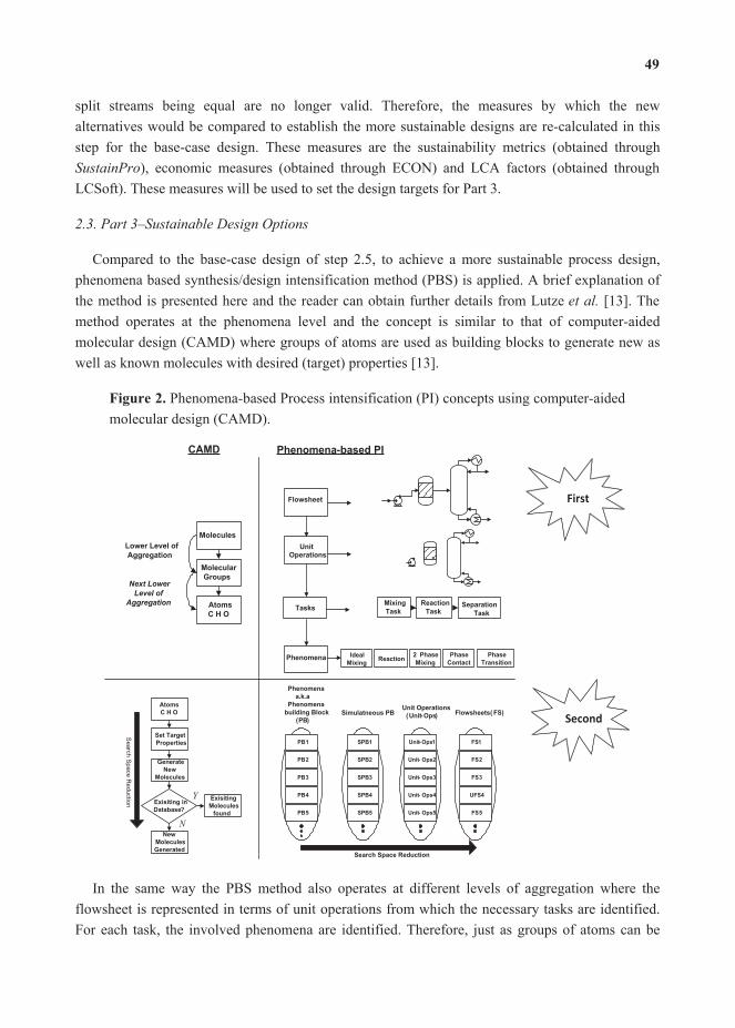
split streams being equal are no longer valid. Therefore, the measures by which the new alternatives would be compared to establish the more sustainable designs are re-calculated in this step for the base-case design. These measures are the sustainability metrics (obtained through

), economic measures (obtained through ECON) and LCA factors (obtained through LCSoft). These measures will be used to set the design targets for Part 3.

–

Compared to the base-case design of step 2.5, to achieve a more sustainable process design,phenomena based synthesis/design intensification method (PBS) is applied. A brief explanation of the method is presented here and the reader can obtain further details from Lutze [13]. The method operates at the phenomena level and the concept is similar to that of computer-aided molecular design (CAMD) where groups of atoms are used as building blocks to generate new aswell as known molecules with desired (target) properties [13].

Phenomena-based Process intensification (PI) concepts using computer-aided molecular design (CAMD).

Flowsheet

UnitOperations

Tasks

Phenomena

MixingTask

ReactionTask

SeparationTask

IdealMixing Reaction 2 Phase

MixingPhase

ContactPhase

Transition

Molecules

MolecularGroups

AtomsC H O

Lower Level of Aggregation

Next Lower Level of

Aggregation

CAMD

AtomsC H O

Set Target Properties

GenerateNew

Molecules

Exisiting in Database?

ExisitingMolecules

found

NewMoleculesGenerated

Search

Space

Reduction

Search Space Reduction

PB 1

PB 2

PB 3

PB 4

PB 5

SPB 1

SPB 2

SPB 3

SPB 4

SPB 5

Phenomenaa.k.a

Phenomenabuilding Block

(PB)Simulatneous PB

Unit-Ops1

Unit- Ops 2

Unit- Ops 3

Unit- Ops 4

Unit- Ops 5

Unit Operations (Unit-Ops)

FS1

FS 2

FS 3

UFS 4

FS 5

Flowsheets ( FS)

Phenomena-based PI

First

Second

In the same way the PBS method also operates at different levels of aggregation where the flowsheet is represented in terms of unit operations from which the necessary tasks are identified. For each task, the involved phenomena are identified. Therefore, just as groups of atoms can be

joined to form molecules, groups of phenomena can be joined to form existing as well as new tasks. In a similar way, groups of tasks can be joined to form operations and groups of operations can be joined to form process flowsheets. The number of alternatives that can be generated increases by going to a lower level of aggregation, just as in the case of molecular design. This concept is illustrated in Figure 2.

eight di erent classes. They are: mixing-M (mass flow within one or several phases), phase contact-PC (the contact and resistances at phase boundaries of phases), phase transition-PT (mass transfer of compounds between two phases), phase change-2phM (state change of a complete stream at no phase transition), phase separation-PS (the degree of separation of two phases), reaction-R (change in mass of a compound or compounds generated or consumed between inlet and outlet), energy transfer-H/C (energy transfer between sources and sinks of energy) and stream dividing-D (division of a stream into two or more streams).

2.3.1. Step 3.1: Problem and Objective Function Definition

In this step the synthesis/design problem and objective function is defined together with the process boundaries, underlying assumptions, and the performance metrics for screening PI options.

2.3.2. Step 3.2: Analyze the Process

In this step, the base case design is analyzed in order to further identify/classify the process bottlenecks through a knowledge-based and a model-based approach. All mass and energy data are collected from the rigorous simulation of the base case design and the flowsheet is transformed into a task and phenomena based flowsheet in order to decouple the analysis from physical unit operations. The identified process bottlenecks are subsequently linked to corresponding phenomena and tasks inside and outside of the unit operation in which they occur. For analyzing the properties of the compounds in the system in general the method developed by Jaksland [18] based on thermodynamic insights is used.

2.3.3. Step 3.3: Identification of Desirable Phenomena

In this step additional phenomena for synthesis of flowsheets, which match the targets defined in Step 3.1 and thereby improve the process performance of the necessary phenomena (identified in Step 3.2) are selected. That is, the identified process bottlenecks and the corresponding phenomena and tasks are used to identify tasks and phenomena that need to be improved to achieve the desired performance. For the selection of suitable (desirable) phenomena, property analysis of single compound and mixtures of compounds as well as reactions in the system are needed. From the set of suitable phenomena the most promising phenomena are selected. However, some phenomena cannot be used on their own; hence, additional accompanying phenomena are selected. Finally, the operating window of all identified phenomena in the search space is determined. These are needed as input for the next step.

2.3.4. Step 3.4: Generate Feasible Operation/Flowsheet Options

In this step all phenomena based process options are generated. They are screened according to logical and structural constraints. The input to this step is the initial search space of identified phenomena and its corresponding operating windows. Next, all phenomena are connected to form feasible simultaneous phenomena building blocks (SPBs). Note that SPBs are connected to form operations, which are translated into unit operations, which are then combined to form flowsheet alternatives. Not all SPBs when connected to form operations are feasible and structurallypromising and therefore, screening based on logical and structural constraints, which were defined in Step 3.1 is performed again to obtain the feasible set.

2.3.5. Step 3.5: Fast Screening Using Process Constraints

In this step the feasible SPBs are connected to form the feasible flowsheet alternatives. The flowsheet alternatives are then screened in terms of operational constraints and performance criteria at the unit operation level using process simulation and analysis tools.

2.3.6. Step 3.6: Solve the Reduced Optimization Problem

In this step the most promising feasible flowsheet alternatives inclusive of PI are identified. This is achieved by optimization of the objective function with respect to the full mathematical model simultaneously for each remaining flowsheet alternatives and ranking all options by their corresponding performance.

The application of the framework is highlighted through a case study. Due to the emergingdemand for sustainable fuels from renewable resources in order to have lower environmental impacts, production of biodiesel was selected as a case study highlighting the application of the computer-aided framework. Throughout the application of the framework on the biodiesel production process, several software and computer-aided methods and tools have been employed,as listed in Table 1.

Type of software used in the case study.

PRO/II Process simulation [23]Aspen Hysys Process simulation [24]

Sustainability analysis [10–12]ECON Economic analysis [20,21]LCSoft Life cycle assessment [22]ICAS-ProPred Chemical and physical properties [25]

3.1.1. Step 1.1: Collect Data/Information on Available Technologies

Available data for several biodiesel processing routes were collected from reported technologies in the literature. The different catalysts applied for biodiesel production can be classified in terms of alkali catalyst, acid catalyst, solid base catalyst, solid acid catalyst and enzyme catalyst [9]. Different types of catalysts were considered to design multiple processing routes and they are given in Table 2.

List of catalysts that may be used for production of biodiesel.

Palm oil Methanol KOH 1 wt.% 6:1 60 1 – 95 [26]

Waste oil Methanol KOH 1 wt.% 50:1 80 1 – 97 [26]

Waste oil Methanol KOH 1 wt.% 6:1 70 1 – 95 [26]

Palm oil Methanol KOH 3:1 – 1 – 99.8 [27]

Palm oil Methanol KOH – – 1 – 99.7 [27]

Palm oil Methanol KOH 1 wt.% 6:1 60 1 1 82.5 [28]

Waste cooking

oilMethanol H2SO4 4 wt.% 20:1 95 1 10 90 [29]

Waste cooking

oilMethanol

Carbon based

catalyst 10

wt.%

30:1 80 1 8 Yield = 92 [30]

Palm oil Methanol NaOH 0.2

wt.%6:1 60 1 1.33 94.3 [31]

Palm oil Methanol -carrageenan

52.5 wt.%7:1 30 1 72 99 [32]

Palm oil Methanol

20% /

DTPA/Clay,

5%

15:1 170 17 6 94 [33]

Palm oil

Immobilized

lipase

(

)

3.3%

/55 1 6 Yield = 82 [34]

3.1.2. Step 1.2: Create Superstructure Configuration

By using the information from Step 1.1, a generic superstructure of processing routes was created (see Figure 3). It describes a network of configurations representing multiple flowsheets. In principle, hundreds of flowsheet alternatives can be generated for the biodiesel production fromthis superstructure (M1 = 14256). Five main stages/tasks are identified for biodiesel production from waste oil and vegetable oil: feed, reaction, separation 1, separation 2 and separation 3. A pretreatment section has been considered as a black-box, that is, given the raw material resource,the output is the liquid raw material needed for the conversion step (reaction section). For the

1. The different types of the same group of catalysts were not considered, for example, for allalkaline catalyst options, only one option was considered: the alkali-catalyzed transesterification.

2. The triglycerides were only assumed to be Triolein.3. The design was based on the use of palm oil and waste palm oil as feedstock with low free

fatty acid content (5% FFA).4. The total operation time is assumed to be 350 days per year.5. The following reactions were considered to represent transesterification and esterification

steps [35]:Reaction 1: EsterificationOleic acid + Metha Methyl oleate + WaterReaction 2: TransesterificationTriolein + Methanol Methyl oleate + Glycerol

Finally, the superstructure was reduced to six process configurations to be considered in the next step of the framework.

3.2.1. Step 2.1: Perform Process Simulation of Superstructure

In this step the superstructure of feasible flowsheet combinations (M2 = 6) for producing biodiesel was simulated for all processing routes in order to obtain steady state mass and energy balance data needed in the next step. The flowsheet alternatives were simulated simultaneously by setting all binary variables to unity, by equally dividing all split streams and by using different reactors for different catalyst types (modeled by their different conversion values). The interested reader can obtain the total simulated superstructure flowsheet, the corresponding computed stream summaries from the simulator and associated details from the corresponding author.

The feed to the transesterification reactor and the operating conditions for each reactor are different, but because different reactors have been used, the superstructure can indeed be simulated simultaneously. For example, the reaction in one of the alkali catalyzed processes was carried out with a 6:1 molar ratio of methanol to oil while in the enzymatic processes the molar ratio was 3:1.In addition, the enzymatic process used immobilized enzyme catalyst while alkali catalyzed process used sodium hydroxide as the catalyst.

All data needed for input to the simulation, for example, kinetic data and product recoveries were obtained from collected data (from Step 1.1). The chemical composition of biodiesel is dependent upon feedstock from which it is produced, as the feedstocks such as palm oil and waste oil of differing origin have dissimiliar fatty acid composition. The compounds taken into account in the simulation are taken based on the average of palm oil and waste palm oil composition available in the literature. Typical fatty acid composition for palm oil and waste oil are given in Table 3. Oleic acid is the major fatty acid present in palm oil and also in waste palm oil. To reduce the complexity of the simulation problem, glycerol trioleate (triolein) is selected to represent the palm oil feedstock for tryglycerides, while the FFA is represented by oleic acid. Based on the selected compound, the fatty acid methyl esters (FAME) are represented by methyl oleate (moleate) as the

biodiesel product. The UNIQUAC model based phase equilibrium constant was employed for phase equilibrium calculations. Missing pure compound property data were generated through ICAS-ProPred [25]. The PRO/II commercial process simulation [23] was used to perform the steady state process simulation. The detailed process data for the biodiesel production wereobtained through process simulation (using PRO/II) and formed the basis for design decisions to obtain a base case design. For the simulation of this superstructure, the total number of equipment considered was 99 units with 154 streams and 6 compounds.

The generated steady state simulation data included mass/molar flowrates, temperature, pressureand enthalpy values for all streams in the superstructure, which are then used for the indicator based sustainability analysis in the next step.

Typical fatty acid composition.

Myristic acid 0.5–2.0Palmitic acid 32–45 20.4Stearic acid 2.0–7.0 4.8Oleic acid 38.0–52.0 52.9Linoleic acid 5.0–11.0 13.5Others 7.6

3.2.2. Step 2.2: Indicator Calculation and Analysis of Superstructure

The steady state mass and energy data obtained from Step 2.1 are used here. An example of results for the sustainability analysis is shown in Tables 4 and 5 for the open- and closed-paths, respectively.

The main open-paths in the superstructure that were identified as bottlenecks in terms of material value added (MVA), energy and waste cost (EWC), total value added (TVA) indicators.

OP 1 H2O 11.7 57.0 2.7 59.8OP 2 Methanol 8.2 55.3 3148.4 3093.1OP 3 H2O 6.9 34.1 26.8 60.9

The main closed-paths in the superstructure that were identified as process bottlenecks in terms of EWC and accumulation factor (AF) indicators.

CP1 Methanol 3.2 2671.3 1.1 High* a high score indicates a high potential for change.

It can be seen in Table 4 that there is a high material loss ( ve values) as well as energy consumption (+ ve values) of water and methanol in the given open paths. Furthermore, high energy consumption is also observed for methanol in the given closed-path in Table 5. In the same table, the accumulation factor (AF) is also high, which means that there is a high potential for improvement in this path. It should be noted that the paths having the higher values in terms of sustainability metrics have been considered as the bottleneck in the superstructure as presented in Figure 3.

Therefore, this information has been used to identify the path that leads to an optimal processing route. Carvalho [11] explained that the lower positive value of the metric indicates that either the impact of the process is less or the output of process is more.

3.2.3. Step 2.3: Calculate and Analyze Economic and Lifecycle Assessment (LCA) Factors

The remaining flowsheet alternatives from Step 2.2 were further analyzed using an economic and LCA evaluation.

In the biodiesel production process, heating, cooling and electricity are the main drivers for operating cost. The main utilities for heating/cooling are steam and cooling water, respectively. These are used by heat exchangers, reboilers, and condensers that are present in the flowsheet. The units that have a high utility cost relative to other units are identified as process bottlenecks in terms of operating cost. In this analysis, it was found that the reboiler of the columns to recover methanol, and biodiesel as well as the heat exchangers have the largest utility costs in the process. From Figure 4 it can be noted that heat exchangers E-110 and E-111 and the reboiler of column rT- 108 have the largest utility costs in the process that employs an acid-catalyst for converting a feedstock of waste cooking oil. Therefore, these units were identified as process bottlenecks in terms of high energy consumption.

Percentage of the total utility costs with respect to each activity/unit operation.

Life cycle assessment (LCA) was used to evaluate the inputs and outputs of the processes with respect to their carbon footprint and the unit operations that had a large carbon footprint relative to other units were identified as process bottlenecks. The environment impacts in terms of carbon footprint (CO2 equivalent) are presented in Figure 5. The process equipment with the highest carbon footprint is highlighted in black in this figure. For example, rT-T7 corresponds to the

reboiler of the distillation column in the acid-catalyzed process for pretreatment of waste cooking oil.

The carbon foot prints of different unit operations in the most promising processing routes.

3.2.4. Step 2.4: Screening of Alternatives to Identify Base Case Design

An example of comparison of the sustainability metrics in two processing routes obtained from the superstructure in order to reduce the search space is presented in Table 6. Here, the considered criteria for screening were the utility costs and carbon footprint for enzymatic catalyzed process (processing route 1) and supercritical methanol process (processing route 2). From Table 6, it can be seen that the processing route 1 is better in terms of carbon footprint and total utility cost. Processing route 2 operates at high temperature and pressure, resulting in higher utility consumption and the total amount of CO2 emitted. Therefore, processing route 2 is eliminated and not considered further.

An example of comparison of the sustainability metrics in two processing routes.

Total kg CO2 Equivalent 1.0447 1.0755Total utility costs ($) 2,350,000 2,680,000

The feasible alternative selected as the base case design is presented in Figure 6. The base case design was selected on the basis of having the least process bottlenecks (and likely operational costs) and carbon footprint. This alternative uses waste cooking palm oil as the feed over an enzyme as the catalyst [31]. The enzyme catalyzed process is recommended since it has several advantages over homogeneous catalysts, for example, high selectivity, lower energy consumption because of low temperature operation and high product yield.

Biodiesel is produced as the main product and glycerol as a value-added byproduct. There are 1 reactor, 4 distillation columns, 2 flash drums and 2 separators together with several heat exchangers and pumps in the process. Methanol is recovered throughout the process and is recycled to the feed stream by three recycle loops.

Biodiesel production process with glycerol as a value-added by product obtained from the superstructure which is the base case design.

3.2.5. Step 2.5: Analysis of Base Case Design

The feed in the base case design contains triglycerides and free fatty acids which correspond to a waste cooking oil feedstock. Therefore, having the base case flowsheet, a more detailed rigorous simulation was now performed. Note, in course of simultaneous simulation of the superstructure, less number of compounds and reactions were considered for the sake of simplicity of the simulations. Waste cooking palm oil consists of a mixture of triglyceride (e.g., trilaurin, tripalmitin, triolein, tristearin, trilinolein and trilinolenin) and free fatty acids (e.g., lauric acid, palmitic acid, stearic acid, oleic acid, linoleic and linolenic acid). The composition of the feedstock is given in Table 7.

Mole fraction of the compounds that form the waste cooking oil in the base case design.

Trilaurin 0.0010Trimyristin 0.0087Tripalmitin 0.3351Tristearin 0.0319Triolein 0.2892Trilinolein 0.0726Trilinolenin 0.0029Lauric acid 0.0003Myristic acid 0.0030Palmitic acid 0.1132Stearic acid 0.0107Oleic acid 0.0972Linoleic acid 0.0244Linolenic acid 0.0097

MIX-100FFA

P-101

Waste oilE-100

MIX-101

P-102

P-103

E-101Flash-1

MIX-103

R-101

E-102

Methanol

V-100Heavy oils

T-101Water

E-103RCY-1

MethanolRecycle

E-104

Cutter-1

V-101

Flash-2

Glycerol

Cutter-2

E-106

T-102Water

RCY-2

Triglycerides

Methanol Recycle

T-103

T-104

Methyl esters (Biodiesel)

Mono-, di-, tri-glycerides

RCY-3

MethanolRecycle

E-105

E-107

The main reaction for biodiesel production consists of the three-step transesterification of triglyceride (trilaurin, tripalmitin, triolein, tristearin, trilinolein and trilinolenin), diglyceride (dilaurin, dipalmitin, diolein, distearin, dilinolein, dilinolenin) and monoglyceride (monolaurin, monopalmitin, monoolein, monolinolenin) with methanol as shown below. Note that the RCOOCH3 is the biodiesel product which is a mixture of (methyl laurate, methyl myristate, methyl palmitate, methyl stearate, methyl oleate, methyl linoleate).

Triglyceride + CH3OH Diglycerides + RCOOCH3

Diglyceride + CH3OH Monoglyceride + RCOOCH3

Monoglyceride + CH3OH Glycerol + RCOOCH3

When an esterification is applied to reduce free fatty acids in waste cooking oil, the following reaction where water is produced as a by-product, takes place:

RCOOH + CH3OH RCOOCH3 + H2O

Calculated mass (in kg/h) and energy (GJ/h) balance for the base case design of biodiesel production process.

Biodiesel ProductionProcess

Waste Cooking oil43630 kg/h

Methanol5502 kg/h

1660.5 kg/h Water

42690 kg/h Biodiesel

1839.2 kg/h Waste oil (mono-, di-, tri-glycerides)

2924 kg/h Glycerol

Total heat added=119 GJ/h

Total heat removed=71 GJ/h

Presentation of closed- and open-paths that include process bottlenecks in the base design for production of biodiesel.

Simulation of biodiesel production is performed using the Aspen Hysys process simulator. All the triglycerides and free fatty acids mentioned above are defined using a “Hypo manager” tool. A waste cooking palm oil containing 10 wt.% of free fatty acids at the flow rate of 62.48kmol/h is used as feedstock for detailed simulation of biodiesel production base case design that was obtained in Step 2.4. Fresh methanol was supplied at the flowrate of 171.1 kmol/h. The mass and energy balance are simply depicted in Figure 7. Note that the recycle of excess methanol to the reactor is not shown on this figure. This is shown in Figure 8 and also the suggested excess amounts are listed in Table 2.

The updated sustainability indicators, metrics and LCA on the more detailed base case calculations are given in Tables 8 and 9 and the paths with which they are associated are given in Figure 8.

List of selected open-path indicators.

OP4 Methyl oleate 174.1 2047.2OP5 Methanol 3129.8 14174.3 14898.1

List of the principal closed-path indicators (EWC and AF).

CP2 Methanol 1402.6 496.7 0.246 High* a high score indicates a high potential for change.

It can be seen in the Table 8, that methanol has a very negative value in terms of MVA and TVA indicators; therefore, this indicates very high raw material loss and energy consumption in the OP4. The same also applies to methyl oleate in this path.

From Table 9, it can be observed that methanol has very high EWC value in a closed-path,which refers to a recycle stream. Thus, this path is identified as the one that contains the unit operations with potential bottlenecks. Table 10 gives a selected list of the sustainability metrics for the base case design.

Sustainability metrics for the base case design.

2.5 0.94 0.034 0.183 7,790,000

The economic and life cycle assessment analysis were also updated for the more detailed base case calculations and these are highlighted in Figures 9 and 10. From Figure 9 it can be seen that the reboilers of columns rT-103, rT-101 and rT-104 and heat exchanger E-101 have the largest utility costs in the process and therefore these are stored as process bottlenecks (high energy consumption) with respect to utility costs. This is not surprising, however, the analysis also points out the operation with the largest utility cost. From Figure 10, it can be seen that the same heat exchanger (E-101), reboilers of the same columns rT-103, rT-104 and rT-101, and the reactor

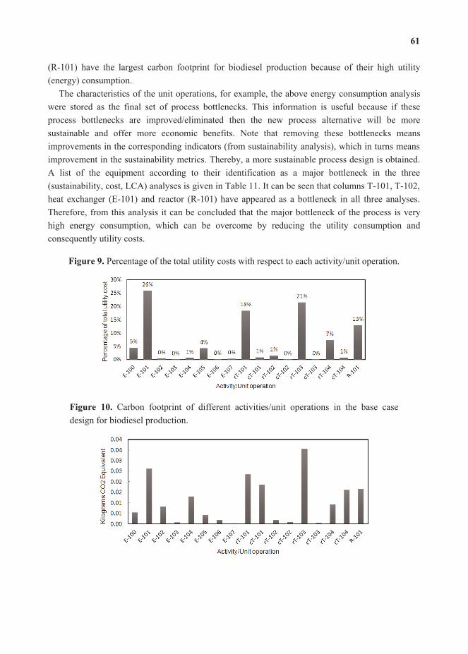
(R-101) have the largest carbon footprint for biodiesel production because of their high utility (energy) consumption.

The characteristics of the unit operations, for example, the above energy consumption analysis were stored as the final set of process bottlenecks. This information is useful because if these process bottlenecks are improved/eliminated then the new process alternative will be more sustainable and offer more economic benefits. Note that removing these bottlenecks means improvements in the corresponding indicators (from sustainability analysis), which in turns means improvement in the sustainability metrics. Thereby, a more sustainable process design is obtained. A list of the equipment according to their identification as a major bottleneck in the three (sustainability, cost, LCA) analyses is given in Table 11. It can be seen that columns T-101, T-102, heat exchanger (E-101) and reactor (R-101) have appeared as a bottleneck in all three analyses. Therefore, from this analysis it can be concluded that the major bottleneck of the process is very high energy consumption, which can be overcome by reducing the utility consumption and consequently utility costs.

Percentage of the total utility costs with respect to each activity/unit operation.

Carbon footprint of different activities/unit operations in the base case design for biodiesel production.

Main identified bottlenecks with respect to sustainability, economic and life cycle assessment (LCA) analysis.

Reactor R-101 x x xColumn T-101 x xColumn T-102 x xColumn T-103 x x xColumn T-104 x x xHeat exchanger E-100 xHeat exchanger E-101 x x x

3.3.1. Step 3.1: Problem and Objective Function Definition

The PI problem is defined as follows: to achieve and identify an intensified process flowsheet for the production of biodiesel and glycerol with maximum purity and conversion of raw materials that is >97% vegetable/waste oil while reducing the operating costs of the process.

Performance metrics and their associated constraints at logical (L), Structural (S), Operational (O) and PI screening (PIs) levels.

Reactor

x Reaction is presentx Reaction is inside the first unit operation

x The reactor effluent is connected to a separation sequence according to the product purity defined in the base case design

Capital Costs xIdentify possible units and allow only a number of units (defined in step 1 or by screening)

Efficiency

xDo not integrate phenomena which inhibit each other’s performance

x Product-yieldx Higher separation efficiency

x Do not connect phenomena in a series of co-current stages with decreasing efficiency/equilibrium

Energyx

Do not connect phenomena to a series with alternating heat addition and heat removal

x Remove options in which phenomena are heated/cooled leading to a decrease of the efficiency

Operational Costsx Utility costs

x Utility costs

Simplificationx Remove options with redundant stages

x Identify possible units and allow only a number of units (defined in step 1 or by screening)

Waste minimization xEnsure that phenomena are connected so that the best use of or recycle of raw materials is achieved

Raw materialsx Raw materials are purex

Equipment x PI screening equipment: Novel equipment

The objective function is shown in Equation (9) where represents the cost of raw materials and the cost of energy, represents the mass flowrate of the raw materials, represents the mass flowrate of products and represents the utility usage. Note that subscripts , , represent

raw material, energy and products, respectively. It should be mentioned that as a result of intensification the number and/or volume of unit operations may decrease which will consequently result in a reduction of capital costs.

min (9)

The performance metrics were selected and categorized in terms of logical (L), structural (S), operational (O) and PI screening constraints and are given in Table 12. The product specifications are defined to be the same as the base case design.

3.3.2. Step 3.2: Analyze the Process

In this step the mass and energy balance steady state data were collected from the rigorous simulation of the more detailed simulated base case design. The base case design flowsheet was then transformed into a task based flowsheet, which identifies different tasks in the process in terms of mixing, reaction and/or separation tasks. This task based flowsheet was then transformed into a phenomena based flowsheet using a PI knowledge base. The task-based and phenomena-based flowsheets are shown in Figures 11 and 12, respectively.

Using the task and phenomena based flowsheets of the base case design; the previously identified process bottlenecks of the base case design are linked to the phenomena and the tasksinside and outside of the unit operation in which they occur. To further analyze the system to identify the bottlenecks, the needed pure compound properties are retrieved from ICAS database [24] for computing the binary ratio matrix of properties. Excerpts of these results are given in Tables 13 (for pure compound properties) and 14 (for binary ratio matrix).

Task-based flowsheet of the base case design for biodiesel production process.

Reaction Task

Separation Task

Separation Task

Separation Task

Separation Task

Separation Task

Water

Separation Task

Separation Task

MethanolRecycle

Water

Separation Task

Glycerol

MethanolRecycle

Separation Task

Biodiesel

Waste Oil

Mixing MethanolRecycle

Mixing

MethanolFeed

Waste cooking oilFeed

Phenomena-based flowsheet of the biodiesel production process according to the existing phenomena in the base case design.

M, 2phM, C/H, R

M, 2phM, C/H,PC(VL),

PT(VL), PS(VL)

M, C/H, PC(LL),PS(LL)

M, C/H, PC(LL),PS(LL)

M, 2phM, C/H,PC(VL),

PT(VL), PS(VL)

M, C/H, PC(LL),PS(LL)

Water

M, 2phM, C/H,PC(VL),

PT(VL), PS(VL)

M, 2phM, C/H,PC(VL),

PT(VL), PS(VL)

MethanolRecycle

Water

M, 2phM, C/H,PC(VL),

PT(VL), PS(VL)

Glycerol

MethanolRecycle

M, 2phM, C/H,PC(VL),

PT(VL), PS(VL)

Biodiesel

Waste Oil

M, PCMethanolRecycle

M, PC

MethanolFeed

Waste cooking oilFeed

Tab

le 1

3.Li

st o

f the

pur

e co

mpo

und

prop

ertie

s of s

ome

of th

e co

mpo

unds

in th

e sy

stem

.

Com

poun

dM

W (g

/mol

)T c

(K)

P c(b

ar)

Tb

(K)

T m(K

)

Solu

bilit

y

para

met

er

(MPa

^0.5

)

Rad

ius o

f gyr

atio

n

(Å)

VV

dWV

m

Met

hano

l32

.051

2.4

72.8

337.

617

5.3

29.6

11.

5520

0.02

174.

08×

10

Wat

er18

.074

7.1

218.

437

3.0

273.

047

.79

0.61

500.

0123

1.79

× 10

2

Gly

cero

l92

.072

4.8

65.8

561.

829

1.2

34.9

93.

5199

0.05

137.

13×

102

Laur

ic a

cid

200.

373

3.8

19.0

557

1.7

342.

3119

.96

6.60

090.

1354

90.

2262

Met

hyl l

aura

te21

4.3

711.

819

.953

9.2

278.

119

.74

18.6

656

0.14

480.

2067

Mon

olau

rin27

4.4

857.

417

.362

5.6

351.

318

.81

7.04

45–

0.30

76

Dila

urin

456.

791

6.7

11.2

703.

137

2.5

14.6

18.

8250

–0.

5109

Trila

urin

639.

099

8.7

9.5

767.

238

6.8

13.9

79.

6796

–0.

7151

Tab

le 1

4.C

ompu

ted

bina

ry ra

tio m

atrix

for s

ome

of th

e co

mpo

unds

of t

he sy

stem

.

Rat

io o

f pro

pert

ies o

f

bina

ry p

airs

Prop

erty

rat

io

MW

Cri

tical

tem

pera

ture

(Tc)

Cri

tical

pres

sure

(Pc)

Boi

ling

tem

pera

ture

(Tb)

Mel

ting

tem

pera

ture

(Tm)

Solu

bilit

y

para

met

erR

adiu

s of g

yrat

ion

VV

dWV

mB

inar

y az

eotr

ope

at P

= 1

atm

Met

hnol

/Wat

er1.

781.

443.

031.

671.

561.

612.

521.

762.

28N

o

Met

hano

l/Gly

cero

l2.

851.

411.

111.

591.

671.

172.

272.

381.

75N

o

Met

hano

l/Met

hyl l

aura

te6.

661.

393.

641.

851.

591.

5012

.50

6.67

5.00

No

Met

hano

l/Lau

ric a

icd

6.25

1.43

3.82

2.08

1.96

1.48

4.17

6.25

5.56

No

Met

hano

l/Mon

olau

rin8.

331.

674.

212.

272.

001.

574.

550.

007.

69N

o

Met

hano

l/Dila

urin

14.2

91.

796.

501.

042.

132.

035.

560.

0012

.50

No

Met

hano

l/Tril

aurin

20.0

01.

967.

681.

112.

222.

126.

250.

0016

.67

No

Wat

er/G

lyce

rol

5.00

1.03

3.32

1.25

1.06

1.37

5.88

4.17

4.00

No

Wat

er/M

ethy

l lau

rate

12.5

01.

0510

.92

1.37

1.02

2.42

33.3

311

.11

11.1

1N

o

Wat

er/L

auric

aci

d11

.11

1.02

11.4

61.

161.

252.

3911

.11

11.1

112

.50

No

Wat

er/M

onol

aurin

14.2

91.

1412

.63

1.10

1.28

2.54

11.1

10.

0016

.67

No

Wat

er/D

ilaur

in25

.00

1.21

19.4

81.

521.

373.

2714

.29

0.00

33.3

3N

o

65

T cP c

T bT m

P

Wat

er/T

rilau

rin33

.33

1.33

23.0

31.

301.

413.

4216

.67

0.00

33.3

3N

o

Gly

cero

l/Met

hyl l

aura

te2.

331.

023.

291.

431.

051.

775.

262.

862.

94N

o

Gly

cero

l/Lau

ric a

cid

2.17

1.01

3.45

1.12

1.18

1.75

1.89

2.63

3.13

No

Gly

cero

l/Mon

olau

rin2.

941.

183.

811.

221.

201.

862.

000.

004.

35N

o

Gly

cero

l/Dila

urin

5.00

1.27

5.87

1.09

1.28

2.40

2.50

0.00

7.14

No

Gly

cero

l/Tril

aurin

7.14

1.37

6.94

1.67

1.33

2.51

2.78

0.00

10.0

0N

o

Met

hyl l

aura

te/L

auric

acid

1.07

1.03

1.05

1.59

1.23

1.01

2.83

1.07

1.10

No

Met

hyl l

aura

te/M

onol

aurin

1.28

1.20

1.16

1.85

1.27

1.05

2.65

0.00

1.49

No

Met

hyl l

aura

te/D

ilaur

in2.

131.

281.

782.

081.

331.

352.

120.

002.

50N

o

Met

hyl l

aura

te/T

rilau

rin2.

941.

412.

112.

271.

391.

411.

930.

003.

45N

o

Laur

ic a

cid/

Mon

olau

rin1.

371.

161.

101.

041.

031.

061.

060.

001.

35N

o

Laur

ic a

cid/

Dila

urin

2.27

1.25

1.70

1.11

1.09

1.37

1.33

0.00

2.27

No

Laur

ic a

cid/

Trila

urin

3.23

1.37

2.01

1.25

1.14

1.43

1.47

0.00

3.13

No

Mon

olau

rin/D

ilaur

in1.

671.

061.

541.

371.

061.

291.

250.

001.

67N

o

Mon

olau

rin/T

rilau

rin2.

331.

161.

821.

161.

101.

351.

370.

002.

33N

o

Dila

urin

/Tril

aurin

1.41

1.09

1.18

1.10

1.04

1.05

1.10

0.00

1.41

No

Dec

isio

ns fo

r fin

ding

the

desi

rabl

e ta

sk fo

r ove

rcom

ing

the

proc

ess b

ottle

neck

s cau

sed

by p

rimar

y ta

sk.

Act

ivat

ion

prob

lem

xx

xx

Con

tact

pro

blem

s of r

aw m

ater

ials

/lim

ited

mas

s tra

nsfe

rx

xx

Form

atio

n of

und

esira

ble

side

pro

duct

sx

xx

x

Hig

h en

ergy

con

sum

ptio

n/de

man

dx

xx

x

Hig

hly

endo

ther

mic

reac

tion

xx

x

Lim

iting

equ

ilibr

ium

xx

xx

Diff

icul

t sep

arat

ion

due

to lo

w

xx

x

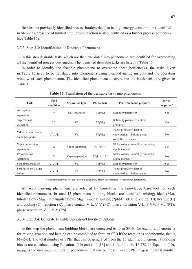
Besides the previously identified process bottlenecks, that is, high energy consumption (identified in Step 2.5), presence of limited equilibrium reaction is also identified as a further process bottleneck (see Table 15).

3.3.3. Step 3.3: Identification of Desirable Phenomena

In this step desirable tasks which are then translated into phenomena are identified for overcoming all the identified process bottlenecks. The identified desirable tasks are listed in Table 15.

In order to identify the feasible phenomena to overcome these bottlenecks, the tasks given in Table 15 need to be translated into phenomena using thermodynamic insights and the operating window of each phenomenon. The identified phenomena to overcome the bottlenecks are given in Table 16.

Translation of the desirable tasks into phenomena.

Absorption

separationV Gas-separation PT(VL) Solubility parameter Yes

Supercritical

extractionL/V VL PT(VL)

Solubility parameter, critical

pressureYes

V-L separation based

on boiling pointsV/VL/L VL PT(VL)

Vapor pressure *, heat of

vaporization *, boiling point,

solubility parameter

No

Vapor permeation

separationL Vapor-separation PT(P:VV)

Molar volume, solubility parameter,

dipole momentNo

Pervaporation

separationV Vapor-separation PT(P:VL) **

Molar volume, solubility parameter,

dipole moment *No

Stripping separation V/VL/L VL PT(VL) Solubility parameter Yes

Separation by Boiling

pointsV/VL/L VL PT(VL)

Vapor pressure *, heat of

vaporization *, boiling pointNo

* The parameter was not considered in calculating binary ratio matrix; **(P:) denotes permeation.

All accompanying phenomena are selected by consulting the knowledge base tool for each identified phenomena. In total 15 phenomena building blocks are identified: mixing; ideal (Mid), tubular flow (Mtub), rectangular flow (Mrec), 2-phase mixing (2phM): ideal; dividing (D); heating (H) and cooling (C); reaction (R); phase contact V-L, V-V (PC); phase transition V-L, P:VV, P:VL (PT); phase separation V-L, V-V (PS).

3.3.4. Step 3.4: Generate Feasible Operation/Flowsheet Options

In this step the phenomena building blocks are connected to form SPBs, for example, phenomena for mixing, reaction and heating can be combined to form an SPB if the reaction is endothermic, that is,M=R=H. The total number of SPBs that can be generated from the 15 identified phenomena building blocks are calculated using Equations (10) and (11) [13] and is found to be 16,278. In Equation (10), nPh,max is the maximum number of phenomena that can be present in an SPB, PhBB is the total number

of phenomena building blocks, 15, PhE is the total number of energy transfer phenomena, 2, PhM is the total number of mixing phenomena and PhD is the dividing phenomena, 1. In Equation (11) NSPBmax is the total number of possible SPBs,

, ( 1) ( 1) = 11 (10)

,max

1

1 !1

1 ! ! = 16278 (11)

Using connectivity rules, for example, heating and cooling cannot exist in the same SPB (see SPB 5 and 6 in Table 17) or simultaneous reaction and separation can exist in the same SPB (see SPB 16 and 18 in Table 17); and the information regarding the operating window of each phenomenon, a total number of 73 SPBs were found to be feasible. Considering the three different types of mixing that isMid, Mtub and Mrec, the total number of SPBs are 24 × 3 +1 = 73, including dividing (D) as a separate phenomenon. An example of feasible SPBs is given in Table 17. In this table, mixing (M), 2-phase mixing (2phM), dividing (D); heating (H) and cooling (C); reaction (R); phase contact V-L, V-V (PC); phase transition V-L, P:VV (V-V permeation), P:VL (V-L permeation) (PT); phase separation V-L, V-V (PS); are connected as the phenomena in order to form the SPBs.

The SPB’s were then connected to form an operation (which is a collection of SPBs) and these operations are then translated into unit operations which make up the flowsheet alternatives. An example of the generation of a flowsheet alternative is presented below.

In order to produce the products, a change of raw materials state must occur and in order to achieve this, the following task is identified: Reaction task. For overcoming the bottleneck caused by the limiting equilibrium, a task for the recovery and recycle of the unreacted raw materials to the reaction task would shift the equilibrium toward the product side. Therefore, the task identified is: Use of a recycle task. This is shown in Figure 13.

The effluent from the reactor consists of the reactants and products which must be separated. Using the binary ratio matrix (see Table 14) which is based on the pure compound properties (see Table 13) the values for ratios of the boiling points for Methanol/Glycerol, Water/Methanol, Methanol/Methyl-laurate, Methanol/Mono-, Di-, Tri-laurin are 1.67, 1.10, 1.59, 1.85, 2.08 and 2.27 respectively, which makes separation by VL very feasible for separation of methanol and water from glycerol, methyl esters, mono-, di- tri-glycerides [17]. Hence, two of the main involved phenomena are PT(VL)–phase transfer involving vapor-liquid and PS(VL)–phase separation involving vapor-liquid. Therefore the following task is identified for the recovery of methanol: Separation task.The task and phenomena based flowsheets are shown Figure 14.

Task for product production.

Reaction TaskMeOH

Recycle Mono/Di/Tri-glycerides, Biodiesel, Glycerol, Water

FFA + Tri-glycerides

Recycle

Task and phenomena based flowsheets for generation intensified operation.

Reaction TaskMeOH

Recycle

Separation Task

MeOH, Water

Mono/Di/Tri-glycerides, Biodiesel,Glycerol

M RPC PT

PSFFA + Tri-glycerides

MeOH

Recycle

Mono/Di/Tri-glycerides, Biodiesel,Glycerol

MeOH, Water

FFA + Tri-glycerides

Recycle

Recycle

The identified feasible SPBs, interconnection phenomena, inlet and outlet conditions of an SPB.

1 M 1..n(L) 1(L)2 M=R 1..n(L) 1(L)3 M=H 1..n(L) 1(L)4 M=C 1..n(L) 1(L)5 M=R=H 1..n(L) 1(L)6 M=R=C 1..n(L) 1(L)7 M=2phM=PC(VL)=PT(VL) 1..n(L,VL) 1(V/L)8 M=R=2phM=PC(VL)=PT(VL) 1..n(L,VL) 1(V/L)9 M=R=2phM=PC(VL)=PT(P:VL) 1..n(L,VL) 1(V/L)

10 M=R=2phM=PC(VL)=PT(P:VL)=PS(VL) 1..n(L,VL) 2(V;L)11 M=R=2phM=PC(VL)=PT(VL)=PS(VL) 1..n(L,VL) 2(V;L)12 M=R=2phM=PC(VV)=PT(P:VV)=PS(VV) 1..n(V,VV) 2(V;V)13 M=C=2phM=PC(VL)=PT(VL) 1..n(L,VL) 1(V/L)14 M=H=2phM=PC(VL)=PT(VL) 1..n(L,VL) 1(V/L)15 M=H=R=2phM=PC(VL)=PT(P:VL) 1..n(L,VL) 1(V/L)16 M=C=R=2phM=PC(VL)=PT(P:VL) 1..n(L,VL) 1(V/L)17 M=C=R=2phM=PC(VL)=PT(P:VL)=PS(VL) 1..n(L,VL) 2(V;L)18 M=H=R=2phM=PC(VL)=PT(P:VL)=PS(VL) 1..n(L,VL) 2(V;L)18 M=H=R=2phM=PC(VL)=PT(VL)=PS(VL) 1..n(L,VL) 2(V;L)20 M=C=R=2phM=PC(VL)=PT(VL)=PS(VL) 1..n(L,VL) 2(V;L)21 M=H=R=2phM=PC(VV)=PT(P:VV)=PS(VV) 1..n(L,VV) 2(V;V)22 M=C=R=2phM=PC(VV)=PT(P:VV)=PS(VV) 1..n(V,VV) 2(V;V)23 M=2phM=PC(VL)=PT(P:VL)=PS(VL) 1..n(L,VL) 2(V;L)24 M=2phM=PC(VL)=PT(P:VV)=PS(VV) 1..n(L,VL) 2(V;L)73 D 1(L;VL,V) 1..n(L/V/VL)

Note: V, vapor; L, liquid; “/” means “or”; “;” means “and”.

From the system properties; transesterification reaction and limiting equilibrium reaction; and theavailable SPBs reaction and separation can occur simultaneously within an SPB, for example, SPB 18 (see Table 17) indicates M=H=R=2phM=PC(VL)=PT(VL)=PS(VL). Therefore, using this option provided by the SPB (at the phenomena level) and knowledge that simultaneous reaction and separation task (see Table 15, for example, for ) increases the raw materials conversion, the possibility exists for combining the reaction and separation. Therefore, the following task is identified: Reaction-separation task. The task and phenomena-based flowsheets are shown in Figure 15.

Task and phenomena based flowsheets for combining reaction and separation tasks.

Reactive Separative Task

MeOH

RecycleMeOH

M RPC PT

PSFFA + Tri-glycerides

MeOH

RecycleMeOH

Mono-, Di-, Tri-glycerides, Biodiesel, Glycerol

MeOH, Water

FFA + Tri-glycerides

Recycle

Recycle

Mono/Di/Tri-Laurin, Biodiesel,Glycerol

MeOH, Water

M RPC PT

PS

M=R=H=2phM=PC=PT=PSFFA + Tri-

glycerides

MeOH

Recycle

Recycle

Mono-, Di-, Tri-glycerides, Biodiesel, Glycerol

MeOH, Water

However, SPB 18 cannot by itself fulfill process requirements because it does not include complete separation of the raw materials/products, which can then be recycled to increase the raw materialconversion (which is desired). Therefore, more SPBs are added to the current SPB, which now includes non-reactive SPBs and this can now be termed as an operation and is shown in Figure 16.

The phenomena building block as a result of connecting SPBs.

M=2phM=R=PC(VL)=PT(VL)=PS(VL)

Methanol

FFA + Tri-glycerides

M=2phM=PC(VL)=PT(VL)=PS(VL)

M=2phM=PC(VL)=PT(VL)=PS(VL)

Methanol

Mono/Di/Tri-glycerides, Biodiesel,Glycerol, Water

Figure 17 shows the operation, which is then transferred to the final flowsheet to replace the reaction and separation after it, in the base case design. The operation has the following characteristics: (a) simultaneous reaction and separation of raw materials and products, (b) the raw materials and products can now be purified for obtaining the raw materials for recycle and the product for collection. However in order to have the existence of VL due to the difference in boiling points of the raw materials and products, heating and cooling are added at the bottom and top of the operation, respectively.

The generated intensified unit operations to combine reaction and separation task: Reactive distillation.

Reactive Zone

Non- reactive Zone

Non- reactive Zone

M=2phM=R=PC(VL)=PT(VL)=PS(VL)

M=2phM=PC(VL)=PT(VL)=PS(VL)

M=2phM=PC(VL)=PT(VL)=PS(VL)

M(V)=C=2phM=PC(VL)=PT(VL)=PS(VL)

M(L)=H=2phM=PC(VL)=PT(VL)=PS(VL)

It was found that pure methanol could be obtained at the top of this operation but the biodiesel product at the bottom (besides having glycerol) also has some methanol, which has also been shown by Simasatitkul [9] based on the analysis of the ternary reactive phase diagram. Therefore, the final operation, which fulfills the process requirements, must now be translated to a unit operation. This is done by using a knowledge base, which contains SPBs in terms of unit operations and the result found was a reactive distillation column presented in Figure 17.

3.3.5. Step 3.5: Fast Screening Using Process Constraints

This step is not applicable in the present application of the framework since an intensified unit operation was highlighted in the previous step that combines the reaction and separation tasks in the base case design. Generation of further alternatives and their screening has not been considered in this work.

3.3.6. Step 3.6: Solve the Reduced Optimization Problem

In order to check the feasibility of the proposed intensified operation (given in Step 3.4) for production of biodiesel and recovery of methanol; the reactive distillation column was simulated using rigorous models (Using Aspen Hysys process simulator). The total number of stages for this reactive distillation was found to be 6 including reboiler and condenser. Methanol and waste cooking oil are fed

to the column from the second stage with a 10:1 mole ratio of methanol to triglycerides and FFA mixture after connecting all the other separation units in the flowsheet and recycle loops. The reflux ratio should be kept at a very low value since refluxing the water back to the column will consequently shift the equilibrium toward the reactants. Due to this, the separation section of the base case for the separation of methanol, biodiesel and glycerol was reused since the compounds within the stream entering this section is the same as the base case. The final flowsheet inclusive of an intensified unit operation (reactive distillation column) is given in Figure 18. Note that the controllability of the reactive distillation has not been investigated in this work and it is a subject for future studies. The optimality of this process alternative cannot be guaranteed unless all the possible alternatives are generated at the phenomena level and then screened to find the optimal solution. In this work, only the adjacent reaction and separation steps were targeted for intensification. However, it can be claimed that a more sustainable alternative has been found.

The most important performance criteria, including the sustainability metrics for the base case and the intensified alternative are given in Table 18. Note that, at this point of the work, the capital investment was not considered. However, we plan to include this in future studies where it will be shown that the payback time due to extra capital investments for the new intensified alternatives is very short due to the extra profits. Therefore, what are considered in this work are the performance metrics (inclusive of operational costs) and the LCA metrics. Looking at these metrics it can be seen that the objective function that was defined in Step 3.1 has been fulfilled.

Final flowsheet inclusive of an intensified unit operation which is a reactive distillation column.

Waste cookingoil

MeOH

Water

Glycerol

Water

Tri-glycerides

MethanolRecycle

Biodiesel

WasteOil

MethanolRecycle

MethanolRecycle

Reactive DistillationColumnFFA

Comparing the base case design presented in Step 2.4, with the alternative design inclusive of PI given in Step 3.6 of this framework; it can be observed that the alternative design is more environmentally sustainable and economically profitable. It can be seen that in analyzing the base case

design the reactor and the separation were identified as bottlenecks because they were in the path of the selected indicator (OP4; see Table 8). In terms of overcoming the bottlenecks that were identified through the intensification approach (see Table 15), the following process bottlenecks have been overcome as a result of combining the reaction and separation tasks: contact problem of raw materials in the reactor; high energy consumption (reduced utility costs as given in Table 18); limiting equilibrium was overcome due to the simultaneous removal of reactants and products; and difficult separation due to the low driving force has been to some extent overcome since pure methanol (raw materials) is recovered at the top of the reactive distillation column. It should also be noted, that all performance and LCA metrics have been either improved or remained neutralin the intensified process alternative.

Comparison of the sustainability metrics in the base case design and the alternative design inclusive of PI.

Perf

orm

ance

met

rics

Total utility cost ($/year) 7,790,000 4,660,000 40.2

Total energy consumption (GJ/h) 119.163 73.104 38.6

product/raw material (kg/kg) 0.94 0.94 0

Energy/ products (GJ/kg) 0.0025 0.0017 32

Net water added to the system (m3) 0 0 0

Water for cooling/product (m3/kg) 0.017 0.017 0

Waste/raw material (kg/kg) 0.032 0.026 18.8

Waste/products (kg/kg) 0.034 0.028 17.6

Hazardous raw material/product (kg/kg) 0 0 0

Number of unit operations 9 7 22

LCA

Total carbon footprint (kg CO2 eq.) 0.183 0.143 21.8

HTPI—Human Toxicity Potential by Ingestion (1/LD50) 0.51811 0.51111 0

HTPE—Human Toxicity Potential by Exposure (mgemiaaion/m3) 0.03558 0.03564 0

GWP—Global Warming Potential (CO2 eq.) 0.55214 0.55241 0

ODP—Ozone Depletion Potential (CFC-11 eq.) 5.18 × 10 9 5.18× 10 9 0

PCOP—Photochemical Oxidation Potential (C2H2 eq.) 0.04968 0.04976 0

AP—Acidification Potential (H+ eq.) 0.00010 0.00010 0

ATP—Aquatic Toxicity Potential (1/LC50) 0.00366 0.00366 0

TTP—Terrestrial Toxicity Potential (1/LD50) 0.51811 0.51111 0

HTC (Benzene eq.)—human toxicity (carcinogenic impacts) 2062.7 1794.5 13

HTNC (Toluene eq.)—human toxicity (non-carcinogenic impacts) 1.3301 1.1795 11.3

ET (2, 4-D eq.)—Fresh water ecotoxicity 0.00525 0.00490 6.7

LC50 is lethal concentration (mg emission/kg fathead minnow); LD50 is one kg body weight of rat administered in milligrams of toxic

chemical by mouth (mg emission/kg rat).

The question of uncertainty of data and/or model parameters on the final more sustainable design that has been obtained has not been investigated. Steimel . [38] have proposed a framework for optimizing flowsheet superstructures under uncertainty. A natural next step of this work would be to extend our computer aided framework for more sustainable design to include also uncertainty issues.

In this work, a systematic framework for sustainable design and process intensification has been presented together with its application to a biodiesel production process. The framework is divided into 3 main parts: superstructure generation, base case design selection, and identification of sustainable design options. The framework is generic and can be applied to any chemical or biochemical process. In this work, it has been applied to biodiesel production, where the most promising process alternative in terms of economic, LCA and sustainability metrics was obtained in a systematic and efficient manner, taking into account the use of a number of different methods and tools and data from various sources. The final, intensified option was found by first setting a target for improvement on the selected base case and then by matching and evaluating alternatives to find the more sustainable design option. For the evaluation of alternatives, the measures used included sustainability metrics, economic potential and LCA factors. It was found that the alternative option for production of biodiesel is more economic and environmentally sustainable. Current and future work is extending the problem solution by considering all the chemicals present in the system and also by adding other likely feedstocks so that a truly optimal production process for biodiesel can be found. In this case, because the price and availability of the feedstock may vary in different geographical locations, this factor would also be added in the analysis. Therefore, using the framework and the collected data, different, more sustainable options for different geographical locations would be possible to generate without too much extra effort.

1. Escobar, J.C.; Lora, E.S.; Venturini, O.J.; Yáñez, E.E.; Castillo, E.F.; Almazan, O. Biofuels:Environment, technology and food security. , , 1275–1287.

2. Singh, A.; Pant, D.; Korres, N.E.; Nizami, A.S.; Prasad, S.; Murphy, J.D. Key issues in life cycleassessment of ethanol production from lignocellulosic biomass: Challenges and perspectives.

, , 5003–5012.3. Kiss, A.A.; Bildea, C.S. A review of biodiesel production by integrated reactive separation

technologies. , , 861–879.4. International Energy Statistics. Available online: http://1.usa.gov/13Or0Bn (accessed 6

March 2013).5. Biomass Research & Development Initiative. Available online: http://www.esd.ornl.gov/eess/

(accessed 1 June 2013).6. Lam, M.; Lee, K.; Mohamed, A. Homogenoues, heterogenous and enzymatic catalys for

transesterification of high free fatty acid oil (waste cooking oil) to biodiesel: A review., , 500–518.

Talebian-Kiakalaieh, A.; Amin, N.A.S.; Mazaheri, H. A review on novel processes of biodieselproduction from waste cooking oil. , 683–710.

8. Leung, D.; Wu, X.; Leung, M. A review on biodiesel production using catalyzedtransesterification. , , 1083–1095.

9. Simasatitkul, L.; Arpornwichanop, A.; Gani, R. Design methodology for bio-basedprocessing: Biodiesel and fatty alcohol production , doi:10.1016/j.compchemeng.2013.01.018.

10. Carvalho, A.; Gani, R.; Matos, H. Design of sustainable chemical processes: Systematic retrofitanalysis generation and evaluation of alternatives. , ,328–346.

11. Carvalho, A.; Matos, H.A.; Gani, R. Design of batch operations: Systematic methodology forgeneration and analysis of sustainable alternatives. , , 2075–2090.

12. Carvalho, A.; Matos, H.A.; Gani, R. SustainPro—A tool for systematic process analysis,generation and evaluation of sustainable design alternatives. , ,8–27.

13. Lutze, P.; Babi, D.K.; Woodley, J.M.; Gani, R. A phenomena based methodology for processsynthesis incorporating process intensification. , , 7127–7144.

14. Yuan, Z.; Chen, B.; Gani, R. Applications of process synthesis: Moving from conventionalchemical processes towards biorefinery processes. , , 217–229.

15. West, A.H.; Posarac, D.; Ellis, N. Assessment of four biodiesel production processes usingHYSYS. Plant. , , 6587–6601.

16. Martín, M.; Grossmann, I.E. Simultaneous optimization and heat integration for biodieselproduction from cooking oil and algae. , , 7998–8014.

17. Karunanithi, A.T.; Achenie, L.E.K.; Gani, R. A new decomposition-based computer-aidedmolecular/mixture design methodology for the design of optimal solvents and solvent mixtures.

, , 4785–4797.18. Jaksland, C.A.; Gani, R.; Lien, K.M. Separation process design and synthesis based on

thermodynamic insights. , , 511–530.19. Gani, R.; Bek-Pedersen, E. Simple new algorithm for distillation column design. ,

, 1271–1274.20. Saengwirun, P. ECON: A Software for Cost Calculation and Economic Analysis. M.S. Thesis,

Chulalongkorn University, Bangkok, Thailand, 2011.21. Peters, M.S.; Timmerhaus, K.; West, R. ;

McGraw-Hill: Singapore, 2004.22. Kalakul, S. Development of Software for Life Cycle Assessment. M.S. Thesis, Chulalongkorn

University, Bangkok, Thailand, April 2013.23. ; Simulation Sciences, Inc.: Brea, CA, USA, 2011.24. ; Aspen Technology, Inc.: Burlington, MA, USA, 2009.25. Marrero, J.; Gani, R. Group-contribution based estimation of pure component properties.

, , 183–208.26. Zhang, Y.; Dubé, M.A.; McLean, D.D.; Kates, M. Biodiesel production from waste cooking oil: 1.

Process design and technological assessment. , , 1–16.27. Sotoft, L.F.; Rong, B.; Christensen, K.V.; Norddahl, B. Process simulation and economical

evaluation of enzymatic biodiesel production plant. , , 5266–5274.28. Darnoko, D.; Cheryan, M. Kinetic of palm oil transesterification in a batch reactor.

, , 1263–1267.

29. Wang, Y.; Ou, S.; Liu, P.; Xue, F.; Tang, S. Comparison of two different processes to synthesizebiodiesel by waste cooking oil. , , 107–112.

30. Lou, W.; Zong, M.; Duan, Z. Efficient production of biodiesel from high free fattyacid-containing waste oils using various carbohydrate-derived solid acid catalysts.

, , 8752–8758.31. Nárvaez, P.; Rincón,S.; Sánchez, F. Kinetic of palm oil methanolysis. ,

, 971–977.32. Jegannathan, K.; Seng, C.; Ravindra, P. Economic assessment of biodiesel production:

Comparison of alkali and biocatalyst processes. , , 745–751.33. Bokade, V.; Yadav, G. Transesterification of edible and nonedible vegetable oils with alcohols

over heteropolyacids supported on acid-treated clay. , , 9408–9415.34. Chew, Y.; Chua, L.; Cheng, K.; Sarmidi, M.; Aziz, R.; Lee, C. Kinetic study on the hydrolysis of

palm olein using immobilized lipase. , , 516–520.35. Edgar, L.; Yijun, L.; Dora, L.; Kaewta, S.; David, B.; Goodwin, J.G. Synthesis of biodiesel via

acid catalysis. , , 5353–5363.36. Ma, F.; Hanna, M.A. Biodiesel production. , , 1–15.37. Karmakar, A.; Karmakar, S.; Mukherjee, S. Properties of various plant and animals feedstocks for

biodiesel production. , , 7201–7210.38. Steimel, J.; Harrmann, M.; Schembecker, G.; Engell, S. A framework for modeling and

optimization of process superstructures under uncertainty. . doi:10.1016/j.ces.2013.04.052i.

We report the measurement of the viscosity and density of various diesel fuels, obtained from British refineries, at elevated pressures up to 500 MPa and temperatures in the range 298 K to373 K. The measurement and prediction procedures of fluid properties under high pressure conditions is of increasing interest in many processes and systems including enhanced oil recovery,automotive engine fuel injection, braking, and hydraulic systems. Accurate data and understanding of the fluid characteristic in terms of pressure, volume and temperature is required particularly where the fluid is composed of a complex mixture or blend of aliphatic or aromatic hydrocarbons.In this study, high pressure viscosity data was obtained using a thermostatically-controlled falling sinker-type high pressure viscometer to provide reproducible and reliable viscosity data based on terminal velocity sinker fall times. This was supported with density measurements using a micro-pVT device. Both high-pressure devices were additionally capable of illustrating the freezing points of the hydrocarbon mixtures. This work has, thus, provided data that can extend the application of mixtures of commercially available fuels and to test the validity of available predictivedensity and viscosity models. This included a Tait-style equation for fluid compressibility prediction.For complex diesel fuel compositions, which have many unidentified components, the approach illustrates the need to apply appropriate correlations, which require accurate knowledge or prediction of thermodynamic properties.

Reprinted from . Cite as: Schaschke, C.; Fletcher, I.; Glen, N. Density and ViscosityMeasurement of Diesel Fuels at Combined High Pressure and Elevated Temperature.

, , 30–48.

attraction parameter, m6·mol viscometer constant, mPa 1

repulsion parameter, m3·mol 1

0, 1, 2 constants used in the Tait equation constant used in Tait equation (Table 2), MPa constant used in Tait equation (-)

g gravitational acceleration, m·s 2

0, 1, 2 constant used in Tait equation (Table 2), MPaS length of sinker wall, m T length of tube between detection coils, m sinker mass, kg constant used in the Tait equation

pressure, MPa

0 ambient pressure, MPaC critical pressure, MPa

Rem modified Reynolds number, (-) 1 radius of sinker, m 2 inner radius of tube, m universal gas constant, kg·mol 1·K 1

2 statistical correlation coefficient (-) temperature, K

0 ambient temperature, KC critical temperature, K

sinker fall time, s 0 constant used in the Tait equation S terminal velocity of sinker, m·s 1

volume mol·mC critical volume (mol·m )

compressibility factor (-) (o), (r) compressibility factors of the simple and reference fluid

Greek symbols

thermal expansion coefficient, Kpressure compression factor, MPa

viscosity, mPa·s liquid density, kg·m 3

liq density of the liquid, kg·m 3

S sinker density, kg·m 3

, )( acentric factors of the fluid and reference fluid

The demand for transport, together with the increasing scarcity of world fuel resources, has beenresponsible for many of the advances in crude oil recovery, fuel development, and the internal combustion engine. Depleted oil reservoirs are increasingly being revisited with more sophisticated ways of recovering the remaining oil deep below ground level. Above land, developments over the past century have led to modern domestic automobiles and heavy goods vehicle units bearing little resemblance to the noisy, polluting, low power, and efficiency engines of the early pioneering models. The diesel engine, in particular, originally developed by Dr Rudolph Diesel at the end of the nineteenth century, has been completely revolutionized in recent times. The development of diesel engine technology has, to a large extent, been driven by legislation and the public demand for lower emissions of noise, particulates, and gas emissions including carbon monoxide, carbon dioxide, and the oxides of sulphur and nitrogen.

Unlike the early pioneering models, modern automotive diesel engines now operate using ahigh-pressure common rail system. This involves injecting fuel into the cylinders at very high pressure. The rapid atomization of the fuel with thorough mixing with air and compression ensures rapid and complete combustion. The result is high power efficiency, minimum noise, and low particulate emissions. This has consequently either reduced or eliminated the requirement for costly NOx after-treatment devices [1]. Within the European Union, such engines are also expected to start up and operate within a range of fuel compositions available from country to country, producedand available season to season and across a wide range of ambient and sub-ambient temperatures.

The common rail form of injection system has been successfully developed to meet the stringent requirements governing emissions of all types of diesel engines. This involves a single high-pressure fuel pump that feeds the fuel to a manifold (or common rail) from which the fuel is fed to the fuel injectors of each cylinder in the diesel engine. High-pressure injector nozzles to the engine cylinder are used provide a more complete combustion and reduction of soot emissions and noise levels and thus meet necessary legislative requirements [2].

The effective design of a fuel injection system requires the understanding of the thermophysical properties of the fuels over the range of conditions experienced by the common rail where pressure may be as high as 200 MPa. Leakage from the system is an important aspect of the design in which clearances must be sufficiently tight to prevent gross displacement of liquid fuel. However, there is a requirement for some free movement of moving parts. To assess the leakage rate, it is necessary to have an accurate estimate of the viscosity and density of the fuel and the flow behavior with respect to temperature and pressure. During leakage, pressure-volume energy is converted to thermal energy, raising the temperature of the fuel thereby affecting both the density and viscosity.An accurate measurement of the physical properties of viscosity and density of fuels is therefore essential to minimize errors in the design of diesel engines. Such knowledge is additionally essential in the accurate measurement of fuels such as crude oil at conditions experienced at source since crude oil is increasingly being sourced at greater depths, and thus higher pressures. It is essential to possess accurate estimates of the properties of a given crude composition with respect to pressure for fiscal flow accountancy purposes. High temperatures and extreme pressures are also encountered braking and hydraulic systems. The need for knowledge and understanding of the characteristics of complex fluids in terms of pressure, volume, and temperature is essential if designs are to be safe, reliable, economic, and efficient.

For the common rail system, both density and viscosity of the diesel fuels can vary significantly under high pressure and temperature. There may also be a change of phase with potential blockage of narrow pipes and tubes. Equally, low ambient temperature diesel waxes can also cause blockage, which is a major issue particularly in the colder climes. Understanding of the behavior of these hydrocarbon fuels is therefore crucial [3]. While there are reports on the measurement and prediction of diesel properties at ambient or high temperature conditions, comparatively little work has been reported at high pressure and temperature [4,5]. Temperature effects on the dynamic viscosity and density of hydrocarbon and petroleum distillation cuts at high pressure are well known as is the phenomenon of pressure-freezing [6]. Fortunately, high temperatures and pressures are unlikely to affect the performance of the engine due to the time to reach equilibrium in running

engines, particularly at the point of starting an engine from ambient temperatures. While there is agrowing body of information concerning the variations of viscosity of substances with both temperature and pressure, we have, in this work, examined the combined effect of high pressure typically used in common rail engines and above at ambient and temperatures of up to 373K in terms of density prediction and viscosity measurement for a number of mineral diesel fuels taken directly from two British petrochemical refineries with and without additives.

The (summer) diesel fuels examined in this work were obtained directly from two Britishrefineries. These were

Fuel 1: Refinery 1 with no performance or handling additives. Fuel 2: Refinery 1 with both handling and performance additives. Fuel 3: Refinery 2 with both handling and performance additives. Fuel 4: Refinery 2 with 5% rape methyl ester.Fuel 5: A commercially available retail fuel.

The viscosity of the fuels was measured using a falling sinker high-pressure viscometer. This type of viscometer, designed and constructed by the National Engineering Laboratory consists of a vertical tube through which the sinker falls at terminal velocity, and has been previously used to measure the viscosity of both pure liquids and complex mixtures [7]. Both the tube and sinker were fabricated from a single piece of the same material (either non-magnetic En 58J stainless steel or titanium; for this work titanium was used), thereby minimizing compressibility and thermal expansion effects. The viscometer design is based on a falling sinker in which gravity is used to provide the applied force. Viscosity measurements are determined from the time taken for a cylindrical sinker to descend down a vertical tube containing the sample liquid. The entire viscometer tube was contained within a high-pressure vessel rated to 1 GPa. Having a hemispherical nose, and being self-centering, the descent of the sinker was detected by way of electrical signal induced by a ferrite core embedded into the sinker as it passed copper coils surrounding the tube. A change in inductance as the ferrite core of the sinker passed each coil wastransmitted through a bridge circuit and amplified for capture on a PC and recorded as peaks. The time taken to pass two coils, a given distance apart, and the dimensions of the viscometer and sinker were sufficient to determine the viscosity of the liquid with an appropriate calibration.

Falling body viscometer.

The viscometer assembly, shown in Figure 1, was approximately 23 cm in length, with an external diameter of 2.4 cm and an internal diameter of 7.645 mm. The sinker had a diameter of 7.420 mm with a small cylinder of ferrite embedded within the core. The sinker dimensions are significant in that the sinker is designed to be self-centering allowing it to descend through the center of the vertical tube containing the sample liquid. The viscosity was determined directly from the time taken for the sinker to descend at terminal velocity a fixed vertical distance of 14 mm between the two lacquered copper detection coils each with an approximate equal electrical resistance and wrapped around the outside of the tube. Terminal velocity was confirmed to have been reached, experimentally, far in advance of reaching the two coils. Both coils were connected in series and formed the active arm of a balanced bridge circuit. The three other arms of the bridge were remote from the viscometer and outside the vessel. The electrical connections passed out of the vessel through a ceramic seal. The out-of-balance electrical signal from the bridge was amplified and passed through an AC and DC converter for data-logging on a PC. As the sinker passed the detection coils, the DC signal increased to a maximum at the point where the ferrite core of the sinker was positioned at the center of the coil. In this way, it was possible to have a peak corresponding to the sinker passing each coil. The sinker fall-time was measured in milliseconds and the duration of the sinker fall between the coils was dependent on the viscosity, typically ranging between 6000 and 30,000 milliseconds.

The pressure within the viscometer was generated and transmitted by a two stage pressurizing system using a paraffin/Shell Tellus oil mixture as the hydraulic medium. Pressures up to 200 MPa were generated directly via an air-driven pump operating from a 7 bar airline. Higher pressures (up to a possible maximum of 500 MPa) were generated using a piston intensifier. The hydraulicpressure was transmitted to the sample fuels using a PTFE expansion sheath located at the bottom of the viscometer tube to allow for compression of the samples. A calibrated Kistler piezo-resistive pressure gauge type 4618A0 was used to measure the high pressure within the pressure vessel.Over the course of a fall time measurement, the pressure in the vessel was normally stable to within 0.2 MPa. The viscometer operated with the vertical descent of the sinker down the tube. To return the sinker to its original starting position between each measurement the entire pressure vessel was inverted.

From the time taken for the sinker to pass the two detection coils, the viscosity was able to be determined analytically from the free descent of the sinker under the influence of gravity based on the shear stress profile across the annular gap [8].

The equations of motion of a cylindrical body falling axially down a vertical circular tube with laminar flow have been previously given by Isdale [9]. For the sinker, which falls a defined distance between the two detected coils a distance LT apart in time the viscosity is determined to be:

)(21)((21(

1

00

(1)

where A is based on the physical dimensions of the sinker and tube given by:

21

22

21

22

1

2ln

2

(2)

In practice, however, there is a discrepancy between the actual viscosity and determined viscosity due to vortex shedding from the tail of the sinker present, even at very low Reynolds numbers. This has been previously confirmed by both experiment and CFD analysis [8]. It is also known that fully developed laminar flow does not exist within the annulus.

Calibration data using iso-octane, hexadecane and S20 oil at temperatures from 298.14 to 373.17 K were obtained in triplicate and examined in relation to a modified Reynolds number (Rem) within the annulus between the sinker and tube of the form:

)(2

Re12

21

(3)

The derivation of Rem has been shown previously [10]. High viscosity fluids provide longer sinker fall times in which the fluid exhibits a lower Reynolds number. From the physical dimensions of the sinker and using the properties of iso-octane, hexadecane and S20 oil, the calibration coefficients were determined for the various temperatures studied [11] (Table 1).

Viscometer calibration.

AIso-octane 298.1 2.089 77.0 3.852

323.2 1.618 126.7 3.941348.2 1.323 191.0 4.122373.2 1.171 258.1 4.550

Hexadecane 298.2 13.529 2.047 3.768323.2 8.026 5.618 3.734348.2 5.425 12.11 3.775373.1 3.913 22.72 3.783

S20 Oil 298.2 137.82 0.022 3.702323.2 50.448 0.161 3.731348.2 24.524 0.161 3.745373.1 14.265 1.943 3.755

Two correlations for A were found, one for low Reynolds numbers and another for higher Reynolds numbers:

)60Re25(Re10024.7792.3)25Re0(Re0978.0645.03

5.27

1.0

(4)

The temperature of the viscometer tube was thermostatically controlled; the entire pressure vessel containing the viscometer tube was immersed in 240 liters of oil with temperature generation and control provided by steel-sheathed, mineral-insulated heating coils. Five coils provided constantbackground heating for high temperature operation. In conjunction with a thermostatically-controlledcoil, this enabled the oil to be set and maintained at any temperature between 298 K and 373 K. In addition, the oil tank containing the pressure vessel was insulated to reduce heat loss, with at least one hour allowed to reach equilibrium for each of the temperatures. The average temperature of the oil in the bath was measured using two calibrated 100 platinum resistance thermometers. Over the course of a fall-time measurement the average temperature of the oil was normally stable to within 0.05 K. Previous work [9] had shown that this corresponds to temperature stability of 0.005 K in the viscometer, due to the thermal inertia of the pressure vessel. For this work, set point temperatures of 298 K, 323 K, 348 K, and 373 K were used.

At each temperature and pressure, a minimum of three fall-time measurements were made or until three consecutive measurements agreed to within 0.2% of the mean value. However, a full uncertainty analysis indicates that the uncertainty in viscosity at elevated temperature and pressure is 2.0% (at = 2), primarily due to the contribution arising from the calibration process.

The determination of accurate viscosity data using the high-pressure viscometer requires the availability of accurate liquid density data. Compressed liquid density at elevated pressure and temperature can be measured with some certainty using experimental methods. Usually, in the absence of an accurate experimental procedure, density data are obtained using equations of state

or various empirical formulae, often with a high degree of certainty [12,13]. In this case, equations of state, the Lee-Kesler and experimental procedures were used and compared.

Density data were determined experimentally with pressures also up to 500 MPa using a micro-PVT device at temperatures of 298 K, 323 K, 348 K, and 373 K. This device was based on apiston-in-bottle design and operated by means of translational-rotary displacement of a metal rod, which compressed the liquid sample at constant rate. The force exerted on the fluid was measured directly by a pressure sensor within the cell and the volume change determined from the displacement of the rod. Rotation of the rod minimized the friction between the rod and the seals. Pseudo-isothermal conditions were maintained during compression by using a low-speed of rotation and circulating water from a constant temperature water bath through a thermostatic jacket surrounding the high-pressure cell. The initial liquid volume was calculated from the reference position of the rod and the change in position of the rod from this reference position. The uncertainty of pressure measurement for the apparatus has been estimated to be better than 0.5 MPa over the 500 MPa range with an allowance being made for change in cell volume due to temperature and pressure [11].

In principle, the micro-PVT device can be used in an absolute mode but like the falling sinker viscometer, improved accuracy can be obtained by calibration, in this case with fluids of known density. For this work iso-octane was used as the calibration fluid and a correction function derived. A full uncertainty analysis indicates that the density at elevated temperature and pressure is within 0.2% (at = 2).

To support the experimental density determinations, density determinations were obtained from well-known cubic equations of state of the form:

21(5)

and using critical point data to determine and where:

Van der Waals:3

,3,0,0 221 (6)

Redlich-Kwong: 0866.0,4275.0,1,022

21 (7)

Peng-Robinson: 0778.0,4572.0,1,122

21 (8)

While the Peng-Robinson equation of state provides the best estimate for hydrocarbons an uncertainty of better than 1% should be considered in proportion to the uncertainty of fall-time measurement and consequent influence on viscosity estimation. For more accurate work, a versatile method for the prediction of dense fluid thermodynamic properties is that of Lee and Kesler [14]. Unlike other methods, this method uses published critical property and acentric factor data directly without the calculation of intermediary characteristic parameters. This uses a three corresponding states principle to calculate the compressibility factor of the fluid of interest with respect to those of a simple fluid and a reference fluid defined by:

)( (9)

and represent the compressibility factors of the simple and reference fluid, and)( are the acentric factors of the fluid of interest and the reference fluid. The Lee-Kesler equation,

however, is an interpolation of the supposed straight-line relation between the acentric factor and compressibility with the special case of 0 as one of the reference points. For a more general case of the two fluids being chosen as the reference fluid, the interpolation equation is:

12

1211 (10)

As a method, it is desirable that the fluids used cover the range of acentric factors encountered in diesel fuel. A GC-FID analysis of several diesel fuels has shown that n-alkanes follow a normal distribution between C9 and C24, with C15 being the most abundant mass fraction. While straight chain n-alkanes between C10 and C19 individually constitute less than 1% of the total mass of diesel fuel mixture, the chain length of many of the components varies significantly [9]. As a consequence, iso-octane (2,4,4-trimethylpentane) and heptadecane were chosen as the reference fluids. Data were then fitted to a Tait-style equation to determine the compressibility factor as a function of both pressure and temperature of the form:

1.0log1 10

'0

(11)

where and are the Tait coefficients for the fluid with being a constant for each fluid and alinear function temperature. is expressed as a function of temperature as:

122100 1000 (12)

where M is a constant and: 2

210 (13)

The constants are given in Table 2.

Constants used in the Tait equation.

k k k b b biso-octane 1.3549 1.0667 4.6851 300.94 1.1327 1.0926 0.207

heptadecane 1.1382 0.047394 1.878 316.76 0.93033 0.69114 0.203

Density and viscosity measurements were made over a range of conditions for five differentdiesel fuels. The variation of viscosity and density with pressure for different temperatures are shown in Figures 2–11. The experimental viscosity and density correlations are presented in Tables 3 and 4.

Variation of viscosity for Fuel 1 with temperature. 298 K 323 K,348 K, and X 373 K.

Variation of density for Fuel 1 with temperature. 298 K 323 K,348 K, and X 373 K.

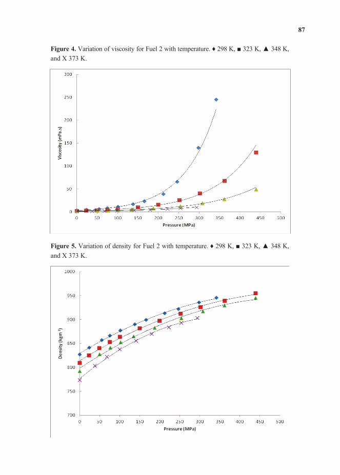
Variation of viscosity for Fuel 2 with temperature. K, and X 373 K.

Variation of density for Fuel 2 with temperature. K, and X 373 K.

Variation of viscosity for Fuel 3 with temperature. 298 K 323 K, and 348 K.

Variation of density for Fuel 3 with temperature. 298 K 323 K, and 348 K.

Variation of viscosity for Fuel 4 with temperature. 298 K 323 K, and 348 K.

Variation of density for Fuel 4 with temperature. 298 K 323 K, and 348 K.

Variation of viscosity for Fuel 5 with temperature. 298 K 323 K, and 348 K.

Variation of density for Fuel 5 with temperature. 298 K 323 K, and 348 K.

Viscosity correlations with pressure for Fuels 1 to 5.

1 3.20e0121p 1.99e0.0096p 1.44e0.0081p 0.972e0.0077p

2 3.09e0.0126p 2.10e0.0097p 1.44e0.0082p 0.987e0.0081p

3 2.82e0.0123p 1.75e0.0101p 1.20e0.0090p nd4 2.91e0.0119p 1.82e0.9974p 1.25e0.0090p nd5 2.80e0.0122p 1.83e0.0102p 1.26e0.0088p nd

Values of 2 varied between 0.9935 and 1; nd: not determined.

Density correlations with pressure for Fuels 1 to 5.

1 827 + 0.590p 0.0009p2 813 + 0.545p 0.0005p2 796 + 0.574p 0.0005p2 776 + 0.682p 0.0008p2

2 829 + 0.508p 0.005p2 814 + 0.513p 0.0004p2 798 + 0.553p 0.0005p2 798 + 0.553p 0.0005p2

3 826 + 0.582p 0.0009p2 809 + 0.638p 0.0010p2 809 + 0.638p 0.0010p2 nd

4 829 + 0.566p 0.0008p2 812 + 0.639p 0.0010p2 794 + 0.727p 0.0013p2 nd

5 845 + 0.561p 0.0007p2 829 + 0.590p 0.0007p2 813 + 0.632p 0.0008p2 nd2 for each of the above multiple regressions were between 0.995 and 0.999; nd: not determined.

In general terms, the variation of viscosity with pressure for each of the fuels was found to be logarithmic in nature and was conveniently correlated with the exponential barus equation of the form (Table 3). These correlations were found to fit up to the point that the sinker was unable to descend due to a change in phase as the result of blockage caused by the phase change of the larger hydrocarbon components. This pressure-induced metastable condition has potentiallysevere implications in blockage of common rail systems. The condition is alleviated with the immediate reduction of pressure.

The expected increase in viscosity with pressure is attributed to the reduction of volume restricting movement of the long chain hydrocarbon molecules. In addition to the increase viscosity with pressure, each of the fuels was also noted as being temperature dependent with the lowering of viscosity with the increasing temperature. This phenomenon is to be expected due to the increase inmolecular vibration and movement.

The ranked increase in viscosity with pressure across the temperature range was found to be Fuel 4 < Fuel 5 < Fuel 3 < Fuel 1 < Fuel 2. While it can be concluded that the viscosities increased with increasing pressure and decreased temperature, Fuel 2 which contained both handling and performance additives from Refinery 1, the viscosities were higher than those of Fuel 1 from the same refinery which did not contain the additives (Figures 2 and 4). However, Fuel 3 from another British refinery also with handling and performance additives did not feature the same viscosity effects (Figure 6). There was a marginal increase in comparative viscosities for Fuel 3 when mixed with 5% rapeseed biodiesel (Figure 8). This is perhaps to be expected since biodiesels generally feature higher pressure-induced viscosities [15]. Interestingly, the fuels from the two refineries

were compared with diesel fuel obtained from the forecourt fuel of a commercial fuel retailer (Fuel 5). This fuel was most comparable to Fuel 1 without additives (Compare Figures 2 and 10).

Figure 12 illustrates the variation of the viscosities of the five fuels at 298 K for comparative purposes in which it can be seen that Fuel 2 from Refinery 1, with both handling and performance additives, has the highest viscosity over the widest range. The viscosity of the mineral Fuel 3 from Refinery 2 was found to be similar to the viscosity of the same fuel with the 5% biodiesel additive (Fuel 4).

In terms of density variation with temperature and pressure, each of the fuels illustrated an increase in density variation with increasing pressure, and decrease in density with temperatureelevation (Table 4). Both phenomena are expected due to the compression of molecules and reduction of molecular vibration, respectively. However, it was also noted that Fuels 1, 2, and 3 from the two refineries, with and without additives, had very similar densities (Figures 3, 5, and 7), only marginally increasing for Fuel 3 with the biodiesel additive (Fuel 4, Figure 9). The highest density was found for the retail Fuel 5 (Figure 11). There is clearly a variability in the density of fuels with both temperature and pressure, and the influence of additives, which are added by the refineries.

Comparison of the viscosities at high pressure at 298 K. + Fuel 1, Fuel 2, Fuel 3, X Fuel 4, and Fuel 5.

In this work, experimental data for both viscosity and density was obtained for the diesel fuels. For accurate and reliable data, it was necessary to calibrate accurately the micro-pVT and high-pressure viscometer instruments. This required the use of calibration fluids that have known

temperature and pressure variations. While useful, the use of equations of state and other correlations are limited to pure liquids or the use of simple mixtures. This is therefore problematic when considering the complexity of such refinery diesel fuels. Equations such as the Tait equation are useful and reliable but rely of the evaluation of many constants. More simple models have been developed, with some success, which require a single constant [4,5]. Certainly, the reliability and accuracy of experimental data from the high-pressure viscometer and micro-pVT instruments areimperative if the data is to be meaningful for design, operational, and fiscal purposes.

The variation of the falling-sinker viscometer coefficient A was examined with respect to the variation of the modified Reynolds number. It is noted that the thermal expansion coefficient and compressibility of the sinker are small (7.6 × 10 6/K and 3.075 × 10 6/MPa, respectively) and can thus be ignored. In contrast, small measurement errors in radii of the tube and sinker, r1 and r2,result in significant errors; the effects of which have been studied by Wehbeh [16]. Ideally, the coefficient A is based on the physical dimensions of the sinker as shown. In practice, however, there is often a deviation in viscosity determined experimentally due to wall and end effects [17–20].The coefficient A is therefore adjusted using a calibration liquid of known properties under high pressure [21]. To confirm the cause of these deviations, 2-D and 3-D CFD studies have previously shown the presence of vortices shedding from the trailing edge of the sinker. The simulations have shown that fully developed laminar flow is not met within the annular gap [22,23]. It has, however, been confirmed that the coefficient A tends towards the theoretical value for modified Reynolds numbers below 60.

An incidental feature of the high-pressure viscometer is the detection of phase change in mixtures. This was highlighted by measurements made using diesel fuel with no additives at 298 K (Figure 12). A phase change of the heavier components prevents the movements of the sinker in the tube. In the fuel injector of the common rail diesel engine, the phenomenon of phase change is, however, unlikely to be a cause for concern in normal operation as the temperature of the engine will be higher than those used in the laboratory and the processes too fast for thermodynamic equilibrium to be obtained. However, from a thermodynamic viewpoint, these measurements provide useful information on the nature of freezing in mixtures and their detection. They also confirm reported problems of power loss and poor engine performance in cold start situations, where the fuel temperature entering the injector may be low enough to allow partial freezing and, hence. incomplete combustion.

The viscosity data for five diesel fuels was found by measurement of the terminal sinker falltimes at pressures up to 500 MPa for temperatures up to 373 K. The viscosities of each of the fuels were found to increase exponentially with both increasing pressure and increasing temperature. This relationship is confirmed with the logarithmic plot of viscosity with pressure shown in Figure 12. The accuracy of the data is dependent on sound experimental set up and requires the careful selection of a self-centering sinker and need for its calibration prior to testing. With the need for thermal stability for the equipment and long sinker descent times and subsequent restart by returning the sinker back down the tube by inverting the pressure vessel, this is a lengthy and time

consuming process. The viscosity evaluations were also dependent on good density data with pressure. In this case, the equations of state, the Tait equation and experimental data using a micro-PVT apparatus provided the necessary data. The demand for accurate liquid data with pressure and temperature is essential if such data is to be of value and successfully used in an increasing number of high-pressure processes and applications.

The authors are grateful for the support of Stewart Vant, University of Strathclyde, and Gordon Reid, Delphi Diesel Systems in Gillingham ME8 0RU.

The authors declare no conflict of interest.

1. Lee, S.W.; Tanaka, D.; Kusaka, J.; Daisho, Y. Effects of diesel fuel characteristics on sprayand combustion in a diesel engine. , , 407–414.

2. Yamaki, Y.; Mori, K.; Kohketsu, S.; Mori, K.; Kato, T.. Japanese Society of Automotive Engineers:

Tokyo, Japan, 1995.3. Riazi, M.R.; Al-Otaibi, G.N. Estimation of viscosity of liquid hydrocarbon systems.

, , 27–32.4. Duncan, A.M.; Noorbahiyah, P.; Depcik, C.D.; Scurto, A.M.; Stagg-Williams, S.M.

High-pressure viscosity of soybean-oil-based biodiesel blends with ultra-low sulfur diesel fuel., , 7023–7036.

5. Duncan, A.M.; Ahosseini, A.; McHenry, R.; Depcik, C.D.; Stagg-Williams, S.M.; Scurto,A.M. High-pressure viscosity of biodiesel from Soybean, Canola, and Canola Oils.

, , 5708–5716.6. Park, N.A.; Irvine, T.F. The falling needle viscometer—A new technique for viscosity

measurements. , , 201–206.7. Harris, K.R.; Kanakubo, M.; Woolf, L.A. Temperature and pressure dependence of the

viscosity of the ionic liquids 1-hexyl-3-methylimidazolium hexafluorophosphate and1-butyl-3-methylimidazolium bis(trifluoromethylsulfonyl)imide. , ,1080–1085.

8. Davis, A.M.J.; Brenner, H. The falling-needle viscometer. , , 3086–3088.9. Isdale, J. Viscosity of Simple Liquids including Measurement and Prediction at Elevated

Pressure. Ph.D. Thesis, University of Strathclyde, Glasgow, UK, 1976.10. Kumagai, A.; Kawase, Y.; Yokoyama, C. Falling capillary tube viscometer suitable for liquids

at high pressure. , , 1441–1445.11. Vant, S.C. Investigation of Fluid Properties at Non-Ambient Conditions. Ph.D. Thesis,

University of Strathclyde, Glasgow, UK, 2002.

12. Dymond, J.H.; Isdale, J.D.; Glen, N.F. Density-measurement at high-pressure. , , 305–314.

13. Belonenko, V.N.; Troitsky, V.M.; Belyaev, Y.E.; Dymond, J.H.; Glen, N.F. Application of amicro-(p, V, T) apparatus for measurement of liquid densities at pressures up to 500 MPa.

, , 1203–1219.14. Lee, B.I.; Kesler, M.G. Generalized thermodynamic correlation based on 3-parameter

corresponding states. , , 510–527.15. Paton, J.M.; Schaschke, C.J. Viscosity measurement of biodiesel at high pressure with a

falling sinker viscometer. , , 1520–1526.16. Wehbeh, E.G.; Ui, T.J.; Hussey, R.G. End effects for the falling cylinder viscometer.

, , 25–33.17. Huang, P.Y.; Feng, J. Wall effects on the flow of viscoelastic fluids around a circular-cylinder.

, , 179–198.18. Lommatzsch, T.; Megharfi, M.; Mahe, E.; Devin, E. Conceptual study of an absolute

falling-ball viscometer. , , 531–534.19. Stalnaker, J.F.; Hussey, R.G. Wall effects on cylinder drag at low reynolds-number.

, , 603–613.20. Ristow, G.H. Wall correction factor for sinking cylinders in fluids. , ,

2808–2813.21. Park, N.A.; Irvine, T.F. Falling cylinder viscometer end correction factor.

, , 3982–3984.22. Schaschke, C.J.; Abid, S.; Fletcher, I.; Heslop, M.J. Evaluation of a falling sinker-type

viscometer at high pressure using edible oil. , , 51–58.23. Gui, F.L.; Irvine, T.F. Theoretical and experimental-study of the falling cylinder viscometer.

, , 41–50.

This work describes how the design and operation parameters of the Multi-Stage Flash (MSF) desalination process are optimised when the process is subject to variation in seawater temperature, fouling and freshwater demand throughout the day. A simple polynomial based dynamic seawater temperature and variable freshwater demand correlations are developed based on actual data which are incorporated in the MSF mathematical model using gPROMS models builder3.0.3. In addition, a fouling model based on stage temperature is considered. The fouling and the effect of noncondensable gases are incorporated into the calculation of overall heat transfer co-efficient for condensers. Finally, an optimisation problem is developed where the total daily operating cost of the MSF process is minimised by optimising the design (no of stages) and the operating (seawater rejected flowrate and brine recycle flowrate) parameters.

Reprinted from . Cite as: Said, S.A.; Emtir, M.; Mujtaba, I.M. Flexible Design and Operation of Multi-Stage Flash (MSF) Desalination Process Subject to Variable Fouling and Variable Freshwater Demand. , , 279–295.

AH Heat transfer area of brine heater (m2) Aj Heat transfer area of stage j (m2) AS cross sectional area of storage tank (m2) B0 Flashing brine mass flow rate leaving brine heater (kg/h) BBT Bottom brine temperature (°C)BD Blow-down mass flow rate (kg/h) Bj Flashing brine mass flow rate leaving stage j (kg/h) CB0 Salt concentration in flashing brine leaving brine heater (wt. %) CBj Salt concentration in flashing brine leaving stage j (wt. %) CBNS Salt concentration in brine recycle (R) (wt. %) CR Salt concentration in feed seawater (WR) (wt. %)CS Salt concentration in makeup seawater (F) (wt. %)CW Rejected seawater mass flow rate (kg/h)Dj Distillate flow rate leaving stage j (kg/h) D Diameter of storage tank (m)EXj Non-equilibrium allowance at stage jF Make-up seawater mass flow rate (kg/h) fjH Brine heater fouling factor ( h m2 °C/kcal)fji Fouling factor at stage j ( h m2 °C/kcal)

h freshwater level in the storage tank (m)hBj Specific enthalpy of flashing brine at stage j (kcal/kg) hR Specific enthalpy of flashing brine at TF (kcal/kg)hvj Specific enthalpy of flashing vapor at stage j (kcal/kg) hW Specific enthalpy of brine at TF (kcal/kg)Hj Height of brine pool at stage j (m) LH Length of brine heater tubes (m)L Length of storage tank (m) Lj length of tubes at stage j (m)M storage tank holdup ID Internal diameter of tubes (m)OD External diameter of tubes (m)Wsteam Steam mass flow rate (kg/h) R Recycle stream mass flow rate (kg/h) SBj Heat capacity of flashing brine leaving stage j (kcal/kg/°C)SDj Heat capacity of distillate leaving stage j (kcal/kg/°C)SRj Heat capacity of cooling brine leaving stage j (kcal/kg/°C)TBT Top brine temperature (°C)TBj Temperature of flashing brine leaving stage j (°C)TBNS Temperature of the brine in the recycle flowrate (°C)TBO Temperature of flashing brine leaving brine heater (°C)TDj Temperature of distillate leaving stage j (°C)TEj Boiling point elevation at stage j (°C)TFj+1 Temperature of cooling brine leaving stage j (°C)TFNR+1 Temperature of makeup flowrate (F) (°C)TFm Temperature of the brine in feed entering recovery stage (°C)TVj Temperature of flashed vapour at stage j (°C)Tsteam Steam temperature (°C)Tseawater Seawater temperature (°C)UH Overall heat transfer coefficient at brine heater (Kcal/m2 h K) Uj Overall heat transfer coefficient at stage j (Kcal/m2 h K)wwj Width of stage j (m)WS Seawater mass flow rate (kg/h) X LMTD, logarithmic mean temperature difference at stagesY LMTD, logarithmic mean temperature difference at brine heater

Temperature loss due to demister (°C) Brine density (kg/h)

Latent heat of steam to the brine heater (kcal/kg)

IDEX

H Brine heaterj Stage index * Reference value

At present, there is a shortage in the freshwater resources all over the world. About 40% of theworld’s populations are suffering from the water crisis. This is due to the continuous growth of the world population and economic activities. Moreover, 96% of the water on the earth is located in oceans and seas and out of 1.7% groundwater only 0.8% is considered to be the freshwater [1].Desalination is a technique of producing freshwater from saline water. Industrial desalination of sea water is becoming an essential part in providing sustainable source of freshwater for a large number of countries around the world [2]. Among different desalination processes, thermal process is the oldest and most dominating for large scale production of freshwater in today’s world. Amongst various thermal processes, the Multi-Stage Flash (MSF) distillation process has been used for many years and now is one of the largest sectors in the desalination industry.

During the last decades, modelling played a very important role in the simulation, optimisation and control of multistage flash (MSF) desalination process. Many models have been developed to find a functional relationship between the design and operating variables [3]. For a given design, optimisation of operating variables led to an increase in distillate production rates and lower operating costs. The top brine temperature, brine recirculation rate, intake flow rate, and steam condition and flow rate can be manipulated to enhance plant performance and achieve an incremental increase in plant capacity. In addition, the selection of optimum design and operation of MSF desalination is aimed at reducing energy and operation costs such as steam, electric power, anti-scale, .

A recent study [4] shows that for a fixed design and operating conditions the production of fresh water from MSF process can significantly vary with seasonal variation of seawater temperature producing more water in winter than in summer. However, the freshwater demand is continuously increasing and of course there is more demand in summer than in winter. Furthermore, to supply freshwater meeting a fixed demand, the operation of MSF process has to be adjusted with the variation of seawater temperature to reduce the energy and operation cost such as steam and antiscale [5,6]. Also, apart from seasonal variation, the seawater temperature varies during the day [7]. More importantly, there is variation in water demand during 24 h of a day (peak and off-peak hours) [8]. These variations in the seawater temperature will affect the rate of production of freshwater using MSF process during a day and throughout the year. Therefore, an optimal design and operation of MSF processes should be performed to cope with these variations so that the freshwater demand during a day and throughout the year is maintained.

Most recently, [9] provided a study on the design and operation of the MSF process with constant fouling resistance in the brine heater only and variable seawater temperature and freshwater demand during a day and throughout the year. However, the dynamic variation in

freshwater demand during the week days is not the same as weekends [10]. Also, the changing seawater temperature during the day will affect the stage temperature which will affect the fouling profile of the stages. Unlike Hawaidi and Mujtaba [9], we have proposed a fouling model [11,12] as a function of stage temperature which is incorporated into the MSF process model. In addition to fouling, the effect of non-condensable gases [13] on the condenser overall heat transfer co-efficient is built up in the process model. Like Hawaidi and Mujtaba [9], an intermediate storage tank between the plant and the client is considered to provide additional flexibility in operation and maintenance of the MSF process throughout the day. However, instead of a neural network based freshwater demand model, simple polynomial based dynamic freshwater demand correlation isdeveloped using actual data from literature. These correlations with a dynamic model for the storage tank and the CaCO3 fouling resistance model developed earlier [11,12] are incorporated in the full steady state MSF mathematical model by using gPROMS model builder 3.0.3 [14]. For adifferent number of flash stages, operating parameters such as seawater rejected flow rate and brine recycle flow rate are optimised, while the total daily operating cost of the MSF process is selected to minimise.

Figure 1 shows the average freshwater consumption for the 24 h of a weekend (Saturday) [10].The average consumption slopes down from 0.00 to 6.00 and grows up from 6:00 am till 12:00 am. From 14:00 the curve goes down till 24:00. In addition and by using linear regression analysis, the following polynomial relationship (Equation (1)) is obtained with a correlation coefficient greater than 90%.

Fresh water consumption profile on holiday (Saturday).

Demand1 = 16.46 + 1.71 × 2.15 × 2 + 0.35 × 3 0.014 × 4 0 Demand2 = 1351.77 + 315.8 × 26.3 × 2 + 0.95 × 3 0.012 × 4 13 (1)

The variation in seawater temperature throughout the day is shown in Figure 2 [7]. By usingregression analysis, the relationship between the seawater temperature and time (h) can be

represents by Equation (13). The temperature at = 0 represents the seawater temperature at night-time.

Tseawater1 = 0.0001 × 5 + 0.0029 × 4 0.0259 × 3 + 0.0913 × 2 0.116 × + 28.84Tseawater2 = 0.0009 × 4 + 0.0649 × 3 1.73 × 2 + 20.14 × 55 13

(2)

Seawater temperature profile during the day and night.

Note, between 0 and 10 h, 5th order polynomial shows a very good mapping with the actual data. Beyond 10 h, although the polynomials do not show a close map, the trend of temperature change is retained.

The MSF process mainly consists of three sections: brine heater section, recovery section with NR stage and rejection sections with NJ stage (Figure 3). Seawater enters into the last stage of the rejection stages (WS) and passes through series of tubes to remove heat from the stages. Before the recovery section seawater is partly discharged to the sea (CW) to balance the heat. The other part (F) is mixed with recycled brine (R) from the last stage of the rejection section and fed (WR) before the last stage of the recovery section. Seawater is flowing through the tubes in difference stages to recover heat from the stages and the brine heater raises the seawater temperature to the maximum attainable temperature (Top brine temperature TBT). After that it (B0) enters into the first flashingstage and produce flashing vapour. This process continues until the last stage of the rejection section. The concentrated brine (BN) from the last stage is partly discharged to the sea (BD) and the remaining (R) is recycled as mentioned before. The vapour from each stage is collected in a distillate tray to finally produce the fresh water (DN). Vapour from each stage is collected in a distillate tray to finally produce the fresh water (DN).

Typical Multi-Stage Flash (MSF) Process.

With reference to Figure 3, models for flash stages; brine heater, mixers, splitter, ., are developed using gPROMS software. The steady state model is based on the total and component mass balances and enthalpy balances coupled with heat and mass flowrate coefficients. The model also includes the thermodynamic losses from stage to stage, tube velocity, tube materials, and chamber geometry. The model equations presented here are reported by [13,15]. The physical properties correlations are defined in the original references [15–17]. Note, a calcium carbonate fouling resistance model (Equation (11)) has been implemented in the MSF steady state model in this work. This model takes into consideration the effect of stage temperature on the calcium carbonate fouling resistance and consequently on the overall heat transfer coefficient in the flashing champers in the heat recovery section, heat rejection section, and brine heaters of MSF process at fluid velocity 1 m/s.

The following assumptions are made in the model:

The distillated from any stage is salt freeHeat of mixing are negligibleNo sub cooling of condensate leaving the brine heaterThere are no heat losses andThere is no entrainment of mist by the flashed vapour.

The model equations are presented below for the sake of completeness.

4.2.1. Stage Model

Mass Balance in the flash chamber:

Bj 1 = Bj + Vj (3)

Mass Balance for the distillate tray:

Dj = Dj 1 + Vj (4)

Enthalpy balance on flash brine:

Bj = (hBj 1 hvj)/(hBj hvj)Bj 1 (5)

hjv = (TVj) (6)

hBj = (CBj,TBj) (7)

Overall Energy Balance:

WRSRj TFj TFj+1 = Dj 1SDj 1 TDj 1 T* + Bj 1SBj 1 TBj 1 T*

(8) DjSDj TDj T* BjSBj TBj T*

Heat transfer equation:

WRSRj TFj TFj+1 = UjAj LMTDj (9)

(replace WR for WS rejection stage)

Uj =4.8857

(yj + Zj + 4.8857 × Rfj) (10)

Where,

Rfj = 3 × 1011e(42,000

Rg) (11)

Zj = 0.102 × 10 2 0.747 × 10 5 × TDj + 0.997 × 10 7 × TDj2 0.430 × 10 9 × TDj

3

+ 0.620 × 10 12 × TDj4 (12)

yj =[v × ID]2

[(160 + 1.92 × TFj) × v] (13)

The logarithmic mean temperature difference in the recovery and rejection stages:LMTDj TFj TF TDj TFj+1 / TDj TFj } (14)

(replace WR for Ws rejection stage)Heat capacity of cooling brine leaving stage j:

SRj = TFj,TFj+1,CR (15)

Heat capacity of distillate leaving stage j

SDj = TDj (16)

Heat capacity of flashing brine leaving stage j

SBj = TBj,CBj (17)

Distillate and flashing brine temperature correlation:

TBj = TDj + TEj + EXj + j (18)

Distillate and flashing steam correlation:

TVj = TDj + j (19)

Temperature loss due to demister

j = (TDj) (20)

Boiling point elevation at stage j

TEj = TDj,CBj (21)

Non-equilibrium allowance at stage j

EXj = (Hj,w j,TBj) (22)

4.2.2. Brine Heater Model

Mass and salt balance for the brine heater

Bo = WR (23)

CBo = CR (24)

Overall enthalpy balance

BoSRH TBo TF1 = Wsteam S (25)

S = Tsteam (26)

Heat transfer equation

WRSRH TBo TF1 = UHAH LMTDH (27)

The logarithmic mean temperature difference in brine heater ( )

LMTDH =(Tsteam TF1) Tsteam TBo

(Tsteam TF1) Tsteam TBo(28)

Overall heat transfer coefficient in brine heater

UH = Tsteam,TBo,TF1,Tsteam,DHi ,DH

o ,fHi (29)

Heat capacity of brine in brine heater

SRH = (TBo,TF1) (30)

4.2.3. Splitter Model

Mass balance on seawater splitter

= BN R (31)

CW = WS F (32)

4.2.4. Mixers Model

Mass balance on mixer

WR = R + F (33)

CBNS + FCS = WRCR (34)

Enthalpy balance on mixer:

WRhW = RhR + FhFhW = (TFm,CR) (35)

hF = (TFNR+1,CF) (36)

hR = (TBNS,CBNS) (37)

These models are taken from Hawaidi and Mujtaba [9] and are presented here for the sake ofcompleteness of the process model.

The dynamic mathematical model of the tank process shown in Figure 4 is as the follows:Mass balance

dMdt

= Flowin Flowout (38)

Relation between liquid level and holdup:

M = Ash (39)

Note, Flowout represents the freshwater demand described by Equation (1).

Storage tank.

The storage tank described above is assumed to operate without any control on the level ,therefore and during the MSF operation process, the tank level goes above the maximum level (hmax or below the minimum level (hmin as shown in Figure 5(a). At any time, this violation (V1, V2) of safe operation can be defined as [9]:

V1 = h hmax2 if h > hmax

0 if h < hmax(40)

and

V2= h hmin 2 if h < hmin

0 if h > hmin(41)

A typical plot of V1 and V2 versus time is shown in Figure 5(b). The total accumulated violation for the entire period can be written using

V = (f= 0 V1 + V2 )d (42)

Therefore,dVd

= V1 + V2 = (h hmax)2 + (h hmin)2 (43)

Equation (43) is added to the overall process model equations. Also the following addition terminal constraint is added in the optimisation problem formulations.

0 VT( f) (44)

where is a very small finite positive number. The above constraint will ensure that will always be max and min throughout the 24 h operation.

( ) Tank level profile and ( ) tank level violations during the MSF operation.

The seawater temperature and the freshwater demand are subject to vary during a day.Therefore, to supply freshwater meeting a variation in the seawater temperature and variable freshwater demand throughout the day, the operation parameters of the MSF process has to be adjusted. In this section, the MSF process model and the CaCO3 fouling resistance model coupled with the storage tank model developed has been used to adequate the variations in the seawater temperature and freshwater demand during a day. For different number of flash stages, operating parameters such as seawater rejected flow rate and brine recycle flow rate are optimised, while the total annual operating cost of the MSF process is selected to minimise using gPROMS models builder 3.0.3 (version 3.0.3.; PSE: London, UK).

The optimisation problem is described as:Given: Design specifications of each stage, fixed amount of seawater flow, heat exchanger areas

in stages, variable seawater temperature, steam temperature, freshwater demand profile, and volume of the storage tank.

Optimise: Recycle brine flow rate, rejected seawater flow rate, at different time intervals within 24 h.

To minimise: The total operation cost (TOC, $/day).The optimisation problem (OP) can be described mathematically by:

OP Min TOCR, Cw

Subject to:

TBT = TBT*

1 × 105 kg/h RL R RU 6.5 × 106 kg/h

1 × 105 kg/h CwL Cw Cw

U 6.5 × 106 kg/h

2 m hL h hU 10 m

0 VT(tf)

Where, is the top brine temperature and TBT* is the fixed top brine temperature. R is the recycle flowrate and Cw is the rejected seawater flowrate. Subscripts L and U refer to lower and upper bounds of the parameters.

The objective function, TOC (total operating cost) is defined as [18]:

TOC, $ = C1 + C2 + C3 + C4 + C5 (45)

Where,

C1(steam cost, $ d ) = WS × TS 40 85 × 0.00415 (46)

Where, WS is steam consumption in kg/hr, Ts is steam temperature in °C

C2(chemical treatment cost, $ ) = WM B × 0.024 (47)

Where, WM is make-up flow rate in kg/hr, B is brine density in kg/m3

C3(power cost, $ ) = Wd w × 0.109 (48)

Where, Wd is distillate product in kg/hr, is water density in kg/m3

C4(spares cost, $ ) = Wd w × 0.082 (49)

C5(labor cost, $ ) = Wd w × 0.1 (50)

This optimisation problem minimises the total operating cost while optimises R and Cw for variable seawater temperature and freshwater demand throughout 24 h. Note, the actual freshwater consumption at any time is assumed to be 40,000 times more than that shown in Figure 1.

A steady state process model for the MSF process coupled with a dynamic model for the storagetank (as described earlier) has been used in the case study. The constant parameters of the MSF process model equations including various dimensions of the brine heater and flash stages are listed in Table 1. The rejection section consists of three stages but the number of stages in the recovery section varies in each case (see Table 2) considered here. The feed seawater flow rate is 1.13 × 107 kg/h with salinity 5.7 wt. %. The intermediate storage tank has diameter D = 18 m, and aspect ratio = L/D = 0.5.

Constant parameters.

Brine heater 3530 0.022 0.0244 12.2Recovery stage 3995 0.022 0.0244 12.2 0.457Rejection stage 3530 0.024 0.0254 10.7 0.457

. Summary of optimisation results.

1 16 46,184,583 37,498,047 17,220,256 12,954,688 15,798,400 129,655,9732 17 44,026,301 37,597,628 17,358,817 13,058,927 15,925,521 127,967,1943 18 41,403,746 37,222,956 17,250,642 12,977,547 15,826,277 124,681,167

Six time intervals within 24 h are considered within which both R and CW are optimised with the interval lengths. The total operating cost on daily basis and the other plant cost (steam cost (C1), chemical cost (C2), power cost (C3), spare cost (C4) and labour cost (C5)) for three different number of stages (16, 17 and 18) are listed in Table 2. The total daily operating cost (TOCrepresented as $/day) is found to decrease as the number of stage increases. This is due to lower steam consumption rate with increasing number of stages contributing significantly to the TOC compared to any other cost components (chemical, power, .). Note, there is a small change in the C2, C3, C4 and C5 while a change in the C1 is relatively high (Table 2).

Figure 6 shows the stage temperature (calculated using the process model) and fouling resistance (calculated using Equation (11)) at different stages for = 18 and seawater temperature at time t = 00:00. The fouling resistance in stage 1 is about 300 times more than that in stage 1 and certainly it will affect the overall heat transfer co-efficient profile (calculated using Equation (10))significantly. Figure 6 clearly shows that the fouling resistance is not constant throughout the stages as considered earlier by Hawaidi and Mujtaba [9] and Rosso . [15].

Stage temperature and fouling profile ( = 18). Note: In y axis, E+00 = 100;E 06 = 10 6 and likewise.

Figures 7 and 8 show the optimum results of seawater rejected flow rate (Cw) and recycle flow rate (R) throughout 24 h at different number of stages. The plant operates at the high flow rate of Cw (Figure 7) and low R (Figure 8) from 00:00 to 08:00 when the water production rate is low due to low water demand (Figures 9 and 10). However, the water production rate is sufficient to cover the demand (decreasing between 00:00 and 05:00) as well as to store meeting the increasing demand (beyond 06:00) (Figures 10 and 11).

Optimum rejected seawater flow rate throughout profile. Note: In y axis, E+05 = 105 and likewise.

Optimum brine recycle flow rate throughout profile. Note: In y axis, E+05 = 105 and likewise.

Fresh water plant production profile. Note: In y axis, E+05 = 105 and likewise.

Fresh water demand profile. Note: In y axis, E+05 = 105 and likewise.

Storage tank level profiles (case 1).

As the water demand increases between 05:00 and 12:00 (Figure 10), Cw and R reverse their profiles (Figures 7 and 8) to increase the water production rate (Figure 9). Interestingly, up to 09.00, the water production rate is still more than the demand (thus increasing the storage tank level). Beyond 09:00, the water production rate is not sufficient to meet the demand and therefore it is being subsidized from the stored water (thus decreasing the tank level) (Figure 11). Although, the water demand drops down beyond 12:00, the trend of Cw, R and water production rate continues at the same level right up to 18:00. During this period, storage tank level continues to drop down to the minimum. Beyond 18:00 Cw are R are adjusted to have sufficient water production to meet the demand until 24:00 and to store at the same time.

However, the intermediate storage tank adds the operational flexibility, and maintenance could be carried out without interrupting the production of water or full plant shut-downs at any time throughout the day by adjusting the number of stage. Note, the optimal results in this case are almost the same for the all the number of stages considered.

In this work, for a given design, an optimal operation scheme for an MSF desalination processsubject to variable seawater temperature and variable freshwater demand is considered. An intermediate storage tank is considered between the MSF process and the customer to add flexibility in meeting the customer demand. A dynamic model for the storage tank level has been implemented with steady state MSF process model using gPROMS 3.0.3 model builder. Unlike previous work, a stage temperature based fouling correlation is added and the effect of non-condensablegases on the condenser heat transfer co-efficient is reflected into the process model.

For several process configurations (the design), some of the operation parameters of the MSF process such as seawater recycle flow rate and brine recycle flow rate at discrete time interval are optimised, while minimising the total daily operating costs. The optimisation results show increase in the total operating cost with decreasing number of stages. During the low consumption of freshwater, there is an increase in the tank level and plant production. Consequently, the plant operates at maximum value of rejected seawater flowrate and at minimum value of recycled brine flowrate. On the other hand, optimum results show decrease in the plant production and tank level when there is an increase in the freshwater consumption and consequently the plant operate at minimum value of rejected seawater flowrate and slightly increase in recycled brine flowrate. The results also clearly show that the use of the intermediate storage tank adds flexible scheduling in the MSF plant to meet the variation in freshwater demand with varying seawater temperatures without interrupting or fully shutting down the plant at any time during the day by connecting thedesired number of stages (see [19] for the concept).

The authors declare no conflict of interest.

1. Assiry, A.M.; Gaily, M.H.; Alsamee, M.; Sarifudin, A. Electrical conductivity of seawaterduring ohmic heating. , , 7–19.

2. El-Dessouky, H.T.; Eltouney, H.M. ; Elsevier Science,Ltd.: Amsterdam, The Netherlands, 2002.

3. Alasfour, F.N.; Abdulrahim, H.K. Rigorous steady state modeling of MSF-BR desalinationsystem. , , 259–276.

4. Tanvir, M.S.; Mujtaba, I.M. Optimisation of MSF desalination process for fixed water demandusing gPROMS. , , 763.

5. Tanvir, M.S.; Mujtaba, I.M. Optimisation of design and operation of MSF desalination processusing MINLP technique in gPROMS. , , 419–430.

6. Hawaidi, E.A.; Mujtaba, I.M. Freshwater production by MSF desalination process: Copingwith variable demand by flexible design and operation. , ,1180–1184.

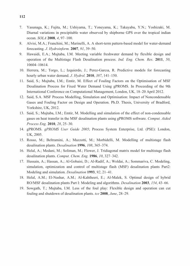
7. Yasunaga, K.; Fujita, M.; Ushiyama, T.; Yoneyama, K.; Takayabu, Y.N.; Yoshizaki, M.Diurnal variations in precipitable water observed by shipborne GPS over the tropical indianocean. , , 97–100.

8. Alvisi, M.A.; Franchini, M.; Marinelli, A. A short-term pattern-based model for water-demandforecasting. , , 39–50.

9. Hawaidi, E.A.; Mujtaba, I.M. Meeting variable freshwater demand by flexible design andoperation of the Multistage Flash Desalination process. . , ,10604–10614.

10. Herrera, M.; Torgo, L.; Izquierdo, J.; Perez- Predictive models for forecastinghourly urban water demand. , , 141–150.

11. Said, S.; Mujtaba, I.M.; Emtir, M. Effect of Fouling Factors on the Optimisation of MSFDesalination Process for Fixed Water Demand Using gPROMS. In Proceeding of the 9thInternational Conference on Computational Management, London, UK, 18–20 April 2012.

12. Said, S.A. MSF Process Modelling, Simulation and Optimisation: Impact of NoncondensableGases and Fouling Factor on Design and Operation. Ph.D. Thesis, University of Bradford,Yorkshire, UK, 2012.

13. Said, S.; Mujtaba, I.M.; Emtir, M. Modelling and simulation of the effect of non-condensablegases on heat transfer in the MSF desalination plants using gPROMS software.

, , 25–30.14. gPROMS. ; Process System Enterprise, Ltd. (PSE): London,

UK, 2005.15. Rosso, M.; Beltramini, A.; Mazzotti, M.; Morbidelli, M. Modelling of multistage flash

desalination plants. , , 365–374.16. Helal, A.; Medani, M.; Soliman, M.; Flower, J. Tridiagonal matrix model for multistage flash

desalination plants. , , 327–342.17. Hussain, A.; Hassan, A.; Al-Gobaisi, D.; Al-Radif, A.; Woldai, A.; Sommariva, C. Modeling,

simulation, optimization and control of multistage flash (MSF) desalination plants Part2:Modeling and simulation. , , 21–41.

18. Helal, A.M.; El-Nashar, A.M.; Al-Kahtheeri, E.; Al-Malek, S. Optimal design of hybridRO/MSF desalination plants Part I: Modeling and algorithms. , , 43–66.

19. Sowgath, T.; Mujtaba, I.M. Less of the foul play: Flexible design and operation can cutfouling and shutdown of desalination plants. , , 28–29.

The nonlinear behavior of metabolic systems can arise from at least two different sources. One comes from the nonlinear kinetics of chemical reactions in metabolism and the other from nonlinearity associated with regulatory processes. Consequently, organisms at a constant growth rate (as experienced in a chemostat) could display multiple metabolic states or display complex oscillatory behavior both with potentially serious implications to process operation. This paper explores the nonlinear behavior of a metabolic model of growth on mixed substrates with sufficient detail to include regulatory features through the cybernetic postulate that metabolic regulation is the consequence of a dynamic objective function ensuring the organism’s survival. The chief source of nonlinearity arises from the optimal formulation with the metabolic state determined by a convex combination of reactions contributing to the objective function. The model for anaerobic growth of was previously examined for multiple steady states in a chemostat fed by a mixture of glucose and pyruvate substrates under very specific conditions and experimentally verified. In this article, we explore the foregoing model for nonlinear behavior over the full range of parameters, (the fractional concentration of glucose in the feed mixture) and (the dilution rate). The

observed multiplicity is in the cybernetic variables combining elementary modes. The results show steady-state multiplicity up to seven. No Hopf bifurcation was encountered, however.Bifurcation analysis of cybernetic models is complicated by the non-differentiability of the cybernetic variables for enzyme activities. A methodology is adopted here to overcome this problem, which is applicable to more complicated metabolic networks.

Reprinted from . Cite as: Song, H.-S.; Ramkrishna, D. Complex Nonlinear Behavior in Metabolic Processes: Global Bifurcation Analysis of Growth on Multiple Substrates. , , 263–278.

Historically, microorganisms have been utilized for the production of valuable products in ourdaily life, e.g., bread, vinegar, wine and beer. With the advent of recombinant DNA technology several decades ago, it is common practice to make genetic modifications to microbes for the industrial production of food, energy, medicine and other valuable products. Towards ensuring the economic competitiveness of those commercial processes, maximizing productivity is one of the goals to achieve.

It is a challenge to manipulate cellular metabolism due to its complexity. Metabolic systems often exhibit intricate nonlinear behaviors, such as steady-state multiplicity and dynamic oscillations. It is necessary to understand what triggers this breadth of behavior and to predict when

and under what conditions they would occur. Such a study is also practically important, as nonlinear behavior should be avoided if it prevents stable operations [1] or may be induced if it can lead to higher productivity [2].

A basic source of nonlinearity in a metabolic system is the intrinsic kinetics of biochemical reactions. More importantly, however, nonlinear metabolic behavior becomes much more complex and diverse due to regulation that dynamically drives individual reactions in response to environmental changes. Dramatic shift between multitudes of metabolic pathways often arises in a dynamic environment as a consequence of metabolic regulation. For the nonlinear analysis of metabolic systems, therefore, it is essential to employ metabolic models that are able to appropriately account for dynamic regulation. Various modeling ideas have been developed for the analysis of metabolic systems, including metabolic pathway analysis [3,4], constraint-based approaches [5,6], kinetic models [7] and the cybernetic approaches [8]. In the discussion of the conceptual distinctions and commonalities among different modeling frameworks, Song . [9] highlighted the essential need for dynamic modeling frameworks in a wide range of applications,such as the study of complex nonlinear behavior of metabolic processes. Our preference for cybernetic models has been based on its comprehensive accounting for dynamic regulation, not present in other dynamic approaches.

A full kinetic description of metabolic regulation requires detailed knowledge of its molecular mechanism, which is incomplete in most cases. Alternatively, the cybernetic approach [8] provides a rational description of regulation based on optimal control theory. The cybernetic description of metabolic regulation is based on the assumption that a cell is frugal in using its resources and optimally allocates them among a subset of enzymes to achieve a certain metabolic objective (such as the carbon uptake rate or growth rate). The resulting selective activation of reactions is realized by the cybernetic control variables without introducing additional parameters.

Cybernetic models have been successfully used to perform bifurcation analysis of metabolic systems, such as [10], hybridoma cells [11] and [12]. While these analyses were made using lumped reaction networks, it is possible to consider a detailed network structure using the hybrid cybernetic modeling (HCM) framework [13–15]. Recently, Kim . [16] built an HCM of the anaerobic growth of on glucose and pyruvate. Using this model, they predicted three and five steady states in a chemostat and experimentally validated them. These predictions were made by generating hysteresis curves using continuation methods [17] only at a selected set of parameter values, however.

In this article, Kim .’s HCM is subjected to more comprehensive nonlinear analysis for the following two purposes. First, we revisit this model to construct bifurcation maps over a wide range of parameter space. This will lead to the complete identification of domains where the model exhibits qualitatively different behavior. Second, we develop a practical method that facilitates the nonlinear analysis of the cybernetic models containing the non-differentiable max function. While examples for the rigorous nonlinear analyses of cybernetic models are available in the literature [10,12], we test a more practical method that can readily be realized using an automated software package, such as MATCONT [18,19].

This paper is organized as follows. In the subsequent sections, we provide a summarized description of the Kim .’s HCM of and discuss an idea of introducing an approximate function as a replacement of the non-differentiable max function. Using this idea, we perform comprehensive nonlinear analysis of the model to construct global bifurcation diagrams in a two-parameter space of dilution rate and feed composition. The effect of the total sugarconcentration in the feed on bifurcation behavior is also discussed.

Dynamic mass balances of extracellular metabolites in a chemostat can be representedas follows:

(1)

where is time, is the biomass concentration, x and xIN are the vectors of concentrations of extracellular components in the reactor and feed, respectively, including substrates, products and biomass, r is the vector of fluxes, Sx is the ( × ) stoichiometric matrix and is the dilution rate.

Under the quasi steady-state approximation, the flux vector, r, can be represented as non-negative (or convex) combinations of basic pathways, termed elementary modes (EMs) [20], ,

(2)

where Z is the ( × ) matrix composed of EMs as its columns and rM is the vector of fluxes through EMs. EMs may be viewed as metabolic pathways composed of a minimal set of reactionsthat can operate alone in steady state. Nonnegative combinations of EMs can represent any feasible metabolic state ( , flux distribution) in a network.

The cybernetic approach assumes a certain metabolic objective, such as the maximization of the carbon uptake rate (or growth rate) for which metabolic reactions are optimally regulated. The HCM framework views EMs as metabolic options to achieve such an objective and describe metabolic regulation in terms of their optimal combinations. Flux through the th EM is modeled as regulated by the control of enzyme level and its activity, ,

, , , , (3)

where is the cybernetic variable controlling enzyme activity, is the kinetic term, and is the relative enzyme level to its theoretical maximum, , / .

Enzyme level is governed by the following dynamic equation, :

,, , , , , , (4)

where is the cybernetic variable regulating the induction of enzyme synthesis, is the kinetic part of the inducible enzyme synthesis rate, is the degradation rate and is the specific growth rate. The four terms of the right-hand side denote constitutive and inducible rates of enzyme synthesisand the decrease of enzyme levels by degradation and dilution, respectively. The cybernetic control variables, and , are computed from the Matching and Proportional laws [21,22], respectively:

, ,;max( ) (5)

where the return-on-investment, , denotes the carbon uptake flux through the th EM, ,, and denotes the factor converting EM flux to the carbon uptake rate. Dynamic shifts among

different pathways are realized by two controlling variables, and .

E. coli

Kim . [16] used the HCM framework to model the anaerobic growth of GJT001 on glucose and pyruvate. The metabolic network contains 14 reactions (one reversible and 13 irreversible) and 18 metabolites (eight extracellular and 10 intracellular). Among 49 EMs obtainedusing METATOOL 5.1 [23], four key modes that can represent yield data of fermentation products [15] were extracted for modeling. Each mode is associated with the consumption of different substrates, , EM1 and EM2 with respective consumption of glucose and pyruvate, while EM3 and EM4 are with simultaneous consumption of both sugars. Model equations and parameters are summarized in Table 1. For a full description of the model, refer to [24].

Bifurcation analysis of cybernetic models requires special treatment of the non-smooth maxfunction contained in the -variables. Among many possibilities, we discuss two ideas of handling this issue, , the combinatoric approach used by Namjoshi and Ramkrishna [10] and the smooth approximation to the max function.

Namjoshi and Ramkrishna [10] proposed a strategy to enumerate all combinatorial cases, in each of which the model equations are fully differentiable. This leads to four cases by setting one of the variables to be 1, while the others are less than or equal to 1 (Table 2).

Model equations and parameter values. EM, elementary mode.

Extracellularmetabolites and biomass

Glucose: 4

, , , , ,1

Pyruvate: 4

, , , , ,1

Acetate: 4

, , , ,1

Ethanol: 4

, , , ,1

Formate: 4

, , , ,1

Biomass: 4

, , ,1

where

Enzymes ,, , , , , , 1 4

Cybernetic variables

, , , , , ,, ,4

, , ,1 4, , ,1

; 1 4max

Kinetics

2max

, , , , , 2 2

,1

,,2

, ,

; ( 1 4);

where

( 1)

( 2)

( 3,4)

Parameters and stoichiometric coefficients

max max max1 2 3

max4

,1 ,3 ,4

,2 ,3 ,4

, ,

,1 ,2

0.394, 0.171, 0.410,

0.339, 7.998 mmol/ gDW ;

0.08, 0.133, 0.04,

0.07, 0.8, 0.2, 6.997 mM ;

0.004 1/h 1 4 ; 0.05 1/h 1 4 ;

0.44, 0.2 ,1 ,117, 0.456, 0.385 1/h ;

,1 ,1 ,3 ,4

,1 ,1 ,3 ,4

,1 ,1 ,3 ,4

,1 ,1 ,3 ,4

,1 ,1 ,3

35.76, 0, 13.55, 8.81,0, 150.49, 66.62, 85.59,31.01, 133.42, 75.43, 89.65,26.95, 0, 4.74, 0

57.96, 133.42, 80.17, ,4

,1 ,2 ,3 ,4

89.65 mmol/gDW ,

214.53, 451.48, 281.15, 309.61 C-mmol/gDW

Notations

: biomass concentration, g/L : dilution rate, 1/h

, : level of enzyme that catalyzes the th EM flux and its maximal level : factor converting the EM flux ( , growth rate) to the carbon uptake rate,

C-mmol/gDW (DW = dry weight): rate constant for formate decomposition

max : maximal rate constant for the th EM flux, 1/h : Michaelis constant for formate decomposition, mM , , , : Michaelis constants for the th EM flux, mM

: specific rate of formate decomposition into CO2 and H2, mmol/(gDW h) , , : regulated and unregulated fluxes through the th EM, mmol/(gDW h) : kinetic part of inducible enzyme synthesis rate, 1/h

, , , , , , , , , : stoichiometric coefficients, mmol/gDW : time, h

, : cybernetic variable regulating the enzyme induction , : cybernetic variable regulating the enzyme activity, , , , : concentrations of acetate, ethanol, formate, glucose and pyruvate, mM, , , : feed concentration of glucose and pyruvate, mM

, : constitutive enzyme synthesis rate, 1/h , : rate of enzyme degradation, 1/h

: growth rate, 1/h

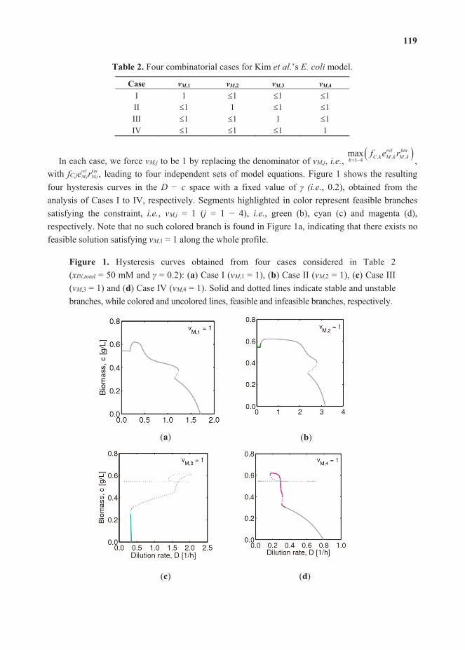
Four combinatorial cases for Kim .’s model.

vM vM vM vMI 1 1 1 1II 1 1 1 1III 1 1 1 1IV 1 1 1 1

In each case, we force to be 1 by replacing the denominator of , , , , ,1 4max

,with , leading to four independent sets of model equations. Figure 1 shows the resulting four hysteresis curves in the space with a fixed value of , 0.2), obtained from the analysis of Cases I to IV, respectively. Segments highlighted in color represent feasible branches satisfying the constraint, , = 1 ( = 1 4), , green (b), cyan (c) and magenta (d), respectively. Note that no such colored branch is found in Figure 1a, indicating that there exists no feasible solution satisfying ,1 = 1 along the whole profile.

Hysteresis curves obtained from four cases considered in Table 2 ( , = 50 mM and = 0.2): ( ) Case I ( ,1 = 1), ( ) Case II ( ,2 = 1), ( ) Case III ( ,3 = 1) and ( ) Case IV ( ,4 = 1). Solid and dotted lines indicate stable and unstable branches, while colored and uncolored lines, feasible and infeasible branches, respectively.

( ) ( )

( ) ( )

Finally, we put together individual pieces of feasible branches of each case to obtain the hysteresis curve over the whole range of (Figure 2a). Throughout this article, we use colors to distinguish one branch from others characterized with different dominant ( , most activated) modes. That is, blue, green, cyan and magenta lines imply that their dominant modes are EM1, EM2, EM3 and EM4, respectively. The black line, on the other hand, indicates the trivial solution with nonzero biomass ( , wash-out as marked with W). In Figure 2a, other than typical limit points (also called folds, turning points or saddle nodes), there are two sharp corners (C) (solid red circles), as well. These non-smooth folds represent catch-up points at which the maximally activated mode is overtaken by another. That is, around catch-up points in Figure 2a, the most dominant mode is switched between EM2 and EM4 (left) and between EM3 and EM4 (right). This clearly manifests the pathway shift by regulation.

The shape of the hysteresis curve becomes somewhat different at a higher fractional concentration of glucose, = 0.4 (Figure 2b). The dominant mode at lower values of is EM1 (instead of EM2), the mode taking up glucose only. Interestingly, one of the two catch-up points (open red circle) does not correspond to a limit point. Thus, we differentiate this simple transition (T) (open red circle), which does not form a sharp limit point, from non-smooth catch-up points (C). The existence of simple transition points has not been reported in earlier studies using lumped network-based cybernetic models. As simple transitions are not bifurcation points, we do not trace them.

Overall hysteresis curve generated by integrating individual pieces of feasible branches: ( ) = 0.2, ( ) = 0.4.

While the combinatoric approach described above allows for rigorous bifurcation analysis in theory, it is ineffective in cases where the number of EMs is large. Alternatively, we may mollify the pain of handling non-smooth functions by making smooth approximations. -norm is

considered as an accurate approximation to the max function when is sufficiently large. That is,

we may approximate , , ,1 4max

with

1/4

, , ,1 .

Figure 3 shows the reproduction of the hysteresis curve using the -norm approximation with different -values. No appreciable errors are found when 30, while some deviations are observed when -values are lower than that.

Figure 4 provides an enlarged view of two red windows in Figure 3 around the catch-up points. Approximate models progressively approach the rigorous solution (obtained with the combinatoric method described above) as the value of increases. While small deviations are unavoidable regardless of how large is, these tiny errors of below 1 percent are acceptable. Stable and unstable branches are also successfully reproduced using this approximate function. In all calculations hereafter, therefore, we use the -norm approximation with a value of 70.

The usefulness of the smooth approximation depends on THE cases in consideration [25]. In a number of studies, introduction of smooth approximation facilitated the bifurcation analysis by providing the system with global differentiability. On the other hand, approximate functions may become stiffer to integrate or may generate more complex bifurcation diagrams than the original function. Thus, it would be critical to have a previous check if smooth approximation yields any unexpected difficulties or errors.

Reproduction of the hysteresis curve of Figure 2a using the -norm approximation with different -values.

Magnified views of two red windows around the catch-up points in the lower-right panel of Figure 3: ( ) left upper window, ( ) right lower window.

If the approximate representation is acceptable as in our case, nonlinear analysis of piecewise-smooth functions is greatly facilitated by using an automated software, such as MATCONT, a standard continuation software package [18].

As a compromise, we may integrate combinatoric enumeration and smooth approximation. That is, we can sketch a bifurcation diagram conveniently using the smooth approximation and refine non-smooth folds using rigorous computations based on the combinatoric approach, because they are only the regions where errors may occur. Catch-up points are readily identified from the hysteresis curve using the approximate function. This combined approach is more accurate than the approximate function alone and more convenient than the full combinatoric enumeration.

Among three methods discussed in the previous section, we use the -norm approximation(Section 3.2) to explore the nonlinear behavior of the HCM model by Kim . presented in Table 1. The smooth approximation is conveniently implementable with no appreciable errors in our case.The main parameters subject to variation include dilution rate ( ) and the fractional molar concentration of glucose in the feed ( ), ,

/ (6)

,

, ,(7)

where is the volume flow rate of the feed, V is the culture volume and , and , are concentrations of glucose and pyruvate in the feed, respectively. The total sugar concentration ( , ) is the sum of , and , .

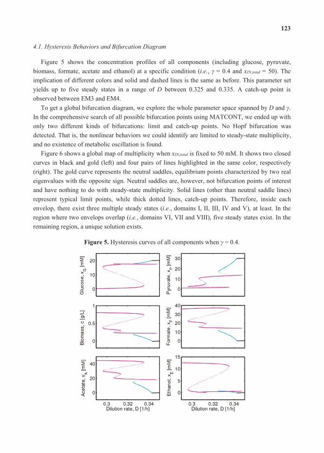
Figure 5 shows the concentration profiles of all components (including glucose, pyruvate, biomass, formate, acetate and ethanol) at a specific condition ( , = 0.4 and , = 50). The implication of different colors and solid and dashed lines is the same as before. This parameter set yields up to five steady states in a range of between 0.325 and 0.335. A catch-up point is observed between EM3 and EM4.

To get a global bifurcation diagram, we explore the whole parameter space spanned by and .In the comprehensive search of all possible bifurcation points using MATCONT, we ended up with only two different kinds of bifurcations: limit and catch-up points. No Hopf bifurcation was detected. That is, the nonlinear behaviors we could identify are limited to steady-state multiplicity, and no existence of metabolic oscillation is found.

Figure 6 shows a global map of multiplicity when , is fixed to 50 mM. It shows two closed curves in black and gold (left) and four pairs of lines highlighted in the same color, respectively (right). The gold curve represents the neutral saddles, equilibrium points characterized by two real eigenvalues with the opposite sign. Neutral saddles are, however, not bifurcation points of interest and have nothing to do with steady-state multiplicity. Solid lines (other than neutral saddle lines) represent typical limit points, while thick dotted lines, catch-up points. Therefore, inside each envelop, there exist three multiple steady states ( , domains I, II, III, IV and V), at least. In the region where two envelops overlap ( , domains VI, VII and VIII), five steady states exist. In the remaining region, a unique solution exists.

Hysteresis curves of all components when = 0.4.

A global bifurcation diagram in the space when , = 50 mM.

To clarify the implication of this global bifurcation diagram, hysteresis curves drawn with nine different values of are presented in Figure 7.

Hysteresis of biomass concentration profiles with different values.

The effect of the total sugar concentration in the feed ( , ) on nonlinear behavior of the model is examined. When lowering the total sugar concentration from 50 to 25 mM, no

qualitative change is observed in bifurcation behavior. Increasing , to 100 mL, on the other hand, leads to an additional domain not observed previously.

Figure 8 shows a global bifurcation diagram in the space at , of 100 mL. The implication of lines and colors is the same as before. Unlike the previous case, this condition leads to multiplicity regimes with up to seven steady states. That is, seven steady states emerge in the domain (IX) where three different envelops ( , red, orange and purple ones) are overlapped. We have highlighted this domain in the figure.

Figure 9 shows hysteresis curves of biomass (a) and pyruvate (b) concentrations when = 0.83.We can see seven steady states in a small range of D around 0.34. The figure also provides zoomed-in views of seven steady states existing between two vertical dashed lines. For instance, pyruvate can have seven different concentrations in this domain, ., if enumerated from the top, one on the black line, one on the cyan, two on the magenta and three on the blue.

A global bifurcation diagram in the space when , = 100 mM.

Hysteresis curves of all components when = 0.83.

Kim . [16] have provided an experimental verification of the stable steady states for the foregoing two sets of conditions, , at = 0.2 and , = 50, yielding a total of three steady states and five steady states, = 0.4 and , = 25, with a total of five steady states.

Through the comprehensive bifurcation analysis in this work, we could identify a new domain with seven steady states. Experimental verification would require precise control of conditions and concentration measurements, however.

Since the cybernetic variables for enzyme activity control are max functions and, therefore,non-smooth, nonlinear analysis of cybernetic models has had to rely on a suitably convenient methodology to confront this issue. The -norm approximation of the max function tested in this work is a practically useful idea, as it is applicable to general cases considering a large number of metabolic pathway options ( , EMs). Replacement of the max function with the -norm representation allows for accurate computation of bifurcation points. While slight errors around non-smooth folds (or catch-up points) are unavoidable, they are negligibly small in our case. When these errors are appreciable in certain cases, however, we can redo rigorous computation for

the non-smooth folds based on the combinatoric idea of Namjoshi and Ramkrishna [10]. Such a combination of these two methods guarantees rigorous results at a minimal level of inconvenience, thus serving as a promising strategy.

Using the approximate function, we could construct global bifurcation diagrams on the space to identify various multiplicity domains, including the one with seven steady states. Considering the narrowness of that domain, however, there are some issues to be resolved for experimental validation. Despite such a comprehensive analysis performed in this work, dynamic nonlinear behaviors, such as metabolic oscillations, were not detected. This could be a consequence of the condensed set of elementary modes in the model.

Clearly, more detailed models comprising more EMs could produce a considerably greater number of steady states, which may be difficult to observe experimentally without accurate analytical measurements and precise control of experimental conditions. It is our premise that this is an area for extensive future exploration by researchers concerned with modeling metabolism.

The authors acknowledge support for this work from the Center for Science of Information (CSoI), a National Science Foundation (NSF) Science and Technology Center, under grant agreement CCF-0939370.

The authors declare no conflict of interest.

1. Alzate, C.A.C.; Astudillo, I.C.P. Importance of stability study of continuous systems forethanol production. , , 43–55.

2. Elnashaie, S.S.; Grace, J.R. Complexity, bifurcation and chaos in natural and man-madelumped and distributed systems. , , 3295–3325.

3. Trinh, C.T.; Wlaschin, A.; Srienc, F. Elementary mode analysis: A useful metabolic pathwayanalysis tool for characterizing cellular metabolism. , ,813–826.

4. Wagner, C.; Urbanczik, R. The geometry of the flux cone of a metabolic network. , , 3837–3845.

5. Orth, J.D.; Thiele, I.; Palsson, B.O. What is flux balance analysis? , ,245–248.

6. Reed, J.L.; Palsson, B.O. Thirteen years of building constraint-based models of, , 2692–2699.

7. Wiechert, W.; Noack, S. Mechanistic pathway modeling for industrial biotechnology:Challenging but worthwhile. , , 604–610.

8. Ramkrishna, D.; Song, H.S. Dynamic models of metabolism: Review of the cyberneticapproach. , , 986–997.

9. Song, H.S.; DeVilbiss, F.; Ramkrishna, D. Modeling metabolic systems: The need fordynamics. , in press.

10. Namjoshi, A.A.; Ramkrishna, D. Multiplicity and stability of steady states in continuousbioreactors: Dissection of cybernetic models. , , 5593–5607.

11. Namjoshi, A.A.; Hu, W.S.; Ramkrishna, D. Unveiling steady-state multiplicity in hybridomacultures: The cybernetic approach. , , 80–91.

12. Simpson, D.J.; Kompala, D.S.; Meiss, J.D. Discontinuity induced bifurcations in a model ofSaccharomyces cerevisiae. , , 40–49.

13. Kim, J.I.; Varner, J.D.; Ramkrishna, D. A hybrid model of anaerobic GJT001:Combination of elementary flux modes and cybernetic variables. , ,993–1006.

14. Song, H.S.; Morgan, J.A.; Ramkrishna, D. Systematic development of hybrid cyberneticmodels: Application to recombinant yeast co-consuming glucose and xylose.

, , 984–1002.15. Song, H.S.; Ramkrishna, D. Reduction of a set of elementary modes using yield analysis.

, , 554–568.16. Kim, J.I.; Song, H.S.; Sunkara, S.R.; Lali, A.; Ramkrishna, D. Exacting predictions by

cybernetic model confirmed experimentally: Steady state multiplicity in the chemostat., , 1160–1166.

17. Seydel, R. ; Springer Verlag: New York, NY, USA,2009; Volume 5.

18. Dhooge, A.; Govaerts, W.; Kuznetsov, Y.A. MATCONT: A MATLAB package for numericalbifurcation analysis of ODEs. , , 141–164.

19. Dhooge, A.; Govaerts, W.; Kuznetsov, Y.A.; Meijer, H.; Sautois, B. New features of thesoftware MatCont for bifurcation analysis of dynamical systems.

, , 147–175.20. Schuster, S.; Fell, D.A.; Dandekar, T. A general definition of metabolic pathways useful for

systematic organization and analysis of complex metabolic networks. ,, 326–332.

21. Kompala, D.S.; Ramkrishna, D.; Jansen, N.B.; Tsao, G.T. Investigation of bacterial-growth onmixed substrates—Experimental evaluation of cybernetic models. ,

, 1044–1055.22. Young, J.D.; Ramkrishna, D. On the matching and proportional laws of cybernetic models.

, , 83–99.23. Von Kamp, A.; Schuster, S. Metatool 5.0: Fast and flexible elementary modes analysis.

, , 1930–1931.24. Kim, J.I. A Hybrid Cybernetic Modeling for the Growth of in

Glucose-Pyruvate Mixtures. Ph.D. Thesis, Purdue University, West Lafayette, IN, USA,May 2008.

25. Simpson, D.J.W. ; World ScientificPublishing Co.: Hackensack, NJ, USA, 2010.

Chinese hamster ovary (CHO) cells are a source of multi-ton quantities of protein pharmaceuticals. They are, however, immortalized cells, characterized by a high degree of genetic and phenotypic diversity. As is known for any biological system, this diversity is enhanced by selective forces when laboratories (no sharing of gene pools) grow cells under (diverse) conditions that are practical and useful. CHO cells have been used in culture for more than 50 years, and various lines of cells are available and have been used in manufacturing. This article tries to represent, in a cursory way, the history of CHO cells, particularly the origin and subsequent fate of key cell lines. It is proposed that the name CHO represents many different cell types, based on their inherent genetic diversity and their dynamic rate of genetic change. The continuing remodeling of genomic structure in clonal or non-clonal cell populations, particularly due to the non-standardized culture conditions in hundreds of different labs renders CHO cells a typical case for “quasispecies”. This term was coined for families of related (genomic) sequences exposed to high mutation rate environments where a large fraction of offspring is expected to carry one or more mutations. The implications of the quasispecies concept for CHO cells used in protein manufacturing processes are significant. CHOgenomics/transcriptomics may provide only limited insights when done on one or two “old” and poorly characterized CHO strains. In contrast, screening of clonal cell lines, derived from a well-defined starting material, possibly within a given academic or industrial environment, may reveal a more narrow diversity of phenotypes with respect to physiological/metabolic activities and, thus, allow more precise and reliable predictions of the potential of a clone for high-yielding manufacturing processes.

Reprinted from . Cite as: Wurm, F.M. CHO Quasispecies—Implications for ManufacturingProcesses. , , 296–311.

Chinese hamster ovary (CHO) cells are, today, the gold standard for the manufacturing oftherapeutic proteins. The overall value of products derived from these cells exceeds 50 billion US $ annually, and significant research and development efforts are underway to further improve both protein quality and quantity from CHO cultures in bioreactors. Proteins like ENBREL (a TNF inhibitor) and HERCEPTIN (an anti-HER-2 breast cancer antibody) are each produced at more than one metric ton per year, and thousands of patients benefit from these protein drugs. Recent publications have expressed hope that a detailed knowledge of DNA sequences and transcription patterns of one specific CHO cell strain could provide urgently needed tools to improve the manufacture of protein pharmaceuticals [1]. However, this research does not take into account a

profoundly adverse problem with CHO cells that could very much limit “omics” approaches and/ordeliver entirely irrelevant data.

As cell biologists would agree for any immortalized cell line, CHO cells are - whether being referred to as “K1”, “DG44”, “DX B11”, “CHO-Toronto”, “CHOpro3-”, or “CHO-S” - members of a widely distributed family of related, but profoundly different cell lines, as their individual behaviors/phenotypes (responsiveness to different environmental conditions) in cell culture differ quite significantly. The extent of their relatedness in genome structure, genomic sequence composition, and in transcription patterns has not been studied, and reasonable conclusions on their similarities are therefore not available. In fact, if one considers the observed variability and diversity of genomic structures in immortalized cells in general, each one of the above-mentioned CHO cell lines is a “Quasispecies”. This term was first coined by Eigen and Schuster in 1977–1978 in a series of landmark papers describing a high mutation rate environment where a large group or “cloud” of related offspring exists and where one would expect that a large fraction of the offspring carries at least one mutation [2–4].

Understanding and appreciating the above reasoning requires a history of CHO cells prior to their use in modern biotechnology. Fortunately, most of the history of the cells has been recordedin an enormous wealth of publications resulting from fundamental research executed with CHO cells from the 1960s to the 1980s. In addition, Michael Gottesmann [5] edited, in 1985, approximately at the time of the emergence of interest for CHO cells in the biotechnology industry, a 900-page compendium entitled that contains work exclusively dedicated to the Chinese hamster and the cells derived from this species. Unfortunately, this compendium is out of print today but was available to the author for this review.

Few of today’s users of CHO cells know that they were extremely popular for studies in molecular and classical cell genetics from 1957 to the late 1970s. Their popularity was based on their practicality in cell culture, their large chromosomes (in comparison to human chromosomes), and the ease with which metabolic and other mutations could be identified and subsequently studied in elegant experimental approaches. During this period, the identification of genes and their expression profiles was a “hot topic”. Indeed, besides the bacterium , CHO cells have been a preferred study object for gene and genome-based research. Induced and spontaneous mutations lead with a high success rate to physiological deficiencies (metabolic mutants), whichcould easily be identified through culture in selective media. Mammalian cell culture technology had matured at the time to an extent that media with partially defined compositions could be generated with ease [6–10]. These procedures permitted the application of concepts of microbial genetics to mammalian cells.

CHO cells were established in the laboratory of Dr. Theodore T. Puck in 1957 [11], then at the Eleanor Roosevelt Institute for Cancer Research, and later at the Department of Biochemistry of

the University of Colorado in Denver, from 0.1 gram of ovary tissue of a Chinese hamster. Theoutbred hamster was provided by Dr. George Yerganian of the Boston Children’s Cancer Research Foundation [12]. Out-breeding tries to avoid homozygocity and, thus, maintains a vigorous and diverse genetic background of diploid animals or plants.

From the trypsinized ovary tissue a culture emerged that appeared to be predominantly of a fibroblast type and had a near diploid karyotype with only 1% of the cell population differing in chromosome number by one less or more from the expected chromosome number of 22 (11 pairs) [12]. However, even this small diversion from the strictly diploid character of primary cells must beconsidered unique and is not observed in primary cells of human origin where a fully diploid karyotype is prevalent until senescence occurs (“Hayflick limit”) after about 50 population doublings and the cells die [13].

A scheme representing the generation of the early “original” CHO cell line.

The culture of the primary ovary cells was maintained in culture for more than 10 months and that is longer than the time limit being established for human fetal cells by Hayflick. At an unknown time thereafter the morphology of some cells changed, and these cells overgrew the strictly fibroblast cell type seen initially. It appears that cells in culture derived from the Hamster ovary have experienced some type of spontaneous immortalization while remaining close to a diploid character. However, the mentioning of morphological changes after 10 months in culture points towards additional modifications, most likely with a genetic cause, whose origin are (still) not understood today. Subsequent recloning of these cells with a modified morphology resulted in the cell line that is now called CHO. The change of morphology from a fibroblast type of culture to

a more epitheloid morphology of cells is mentioned in Puck’s early papers. Unfortunately, no further detailed information on this cloning step or the potential diversity of CHO cell lines is available. For clarity in this text, I refer to these original CHO cells as CHO-ori (see Figure 1).

The scheme in Figure 1 depicts my personal knowledge about the origin, history and early handling of CHO cells which, under today’s standards of scrutiny in our industry, would be unsatisfying. Clearly, in retrospect, several questions arise, particularly with respect to theimmortalization of these cells, their assumed genomic constitution and their apparent phenotype change as described in the literature.

CHO-ori cells were provided to many laboratories. The cells were described as “hardy”, growing very well and fast in adherent culture, and having a high cloning efficiency, even at very low fetal bovine serum concentrations in the culture medium. 10%–20% FBS in commercial media were standard in cell culture at the time. However, Hamilton and Ham (9) reported, already, in 1977 the growth of these cells in serum-free media. The cells required the addition of proline to the culture medium, a nutritional requirement for all CHO cell lines in use today. The first reference to this is from 1963 (!). Thus, it appears that the loss or inactivation of proline synthesis is an early event in the history of these cells.

The very first product made by CHO cells, and thus the starting point of the biotechnology erainvolving recombinant mammalian cells, employed a cell line called CHO-DXB11. This line was generated at Columbia University by Drs. Urlaub and Chasin, being interested in the enzyme dihydrofolate reductase (DHFR) and its genetics [14]. The cells in Chasin’s lab were derived fromCHO-K1, after a co-worker in Puck’s lab (Dr. F.T. Kao) had cloned the CHO-ori cells. According to Dr. Chasin (personal communication), the CHO-K1 subclone was established in the late 1960s.Thus as much as a decade elapsed before the well-known CHO-K1 cells were established. Similar to CHO-ori cells, CHO-K1 cells were also supplied to many laboratories around the world and experiments with these cells were described in a large number of publications. Vials of frozen CHO-K1 cells were also deposited at the American Type Culture Collection (ATCC).

Dr. Chasin established the cell line CHO-DXB11 (also called DUK-XB11). The purpose of the work was to delete DHFR activity. These cells carry a deletion of one locus for DHFR and a missense mutation (T137R) of the second DFHR locus rendering the cells incapable of reducingfolate, a precursor for thymidine and hypoxanthine synthesis [14]. The cell line is not named in the paper quoted, but it is one of the gamma-ray induced mutants described. It is interesting to note that this cell line, the first to become a host system for the production of hundreds of kilograms of human tissue plasminogen activator (TPA), was the product of mutagenesis. The reasons why this and not any other CHO cell line became the pioneering cell line in biotechnology is rapidly explained: the dual inactivation of the DHFR locus rendered this cell line very useful for transgenesis with a functional DHFR gene [15]. Transfer of a functional DHFR gene via plasmid transfection could repair the DHFR deficiency and allow easy selection of recombinant cells in well-defined media. In addition, a second, unrelated gene of interest (GOI), encoded by the same plasmid vector, could easily be transferred simultaneously and recombinant clones expressing both

the functional transgenic DHFR gene and the desired co-transferred GOI could be recovered [16]. This 1983 publication is the first to describe co-transfer of two genes into cells whereby the two corresponding DNA sequences were provided on two separate plasmids. They were simply co-transfected at different ratios. In the case of this paper quoted here, a 1:10 ratio of the DHFR plasmid to the gamma-interferon plasmid gave the highest yielding clones.

The DHFR-negative cells were grown in media containing 5%–10% fetal bovine serum (FBS).A risk factor mediated by the use of sera from cows, bovine spongiformous encephalopathy (BSE),became an important consideration for the pharmaceutical manufacturing in the 1990s. In industry,sera were generally obtained from BSE-free sources (Australia, New Zealand). Whether thispractice was followed in academic labs is difficult to assess. Transfection and cloning occurred in an adherent mode, whereby cloning was done by using “cloning rings” or cotton-swaps. In both cases, an identified colony, visible to the naked eye, was targeted and many cells from such a colony were transferred into a well of a multiwell plate. Regulatory concerns, difficult to explain scientifically in view of what is discussed in this paper, requires today “single cell cloning”, frequently even twice in order to “prove” clonality.

For the researchers of metabolic studies with these cells, a low but detectable rate of reversion to DHFR activity in CHO-DXB11 cells presented a problem. In order to fully eliminate this possibility and to also provide a better DHFR-negative host system for eventual gene transfer, Dr.Chasin engaged in another round of DHFR elimination, but not with cells derived from the K1 populations. Instead, CHO-ori cells from the lab of Dr. Siminovitch lab were sourced, but inanother convoluted way. Dr. Flintoff, a coworker of Siminovitch, had generated a useful mutant of CHO-ori cells, named CHO-MtxRIII that proved to be suitable for deletion of both DHFR alleles [17]. In the same year (1976), Siminovitch published a highly instructive minireview on genetic diversity of cultured somatic (immortalized) cells that discusses the quasispecies conceptwithout using the term [18].

The elegant work by Chasin and Urlaub showing the full deletion of the two DHFR loci onchromosome 2 (actually on chromosome 2 and on a shortened marker chromosome variant Z2) resulted in the now widely-used CHO-DG44 cells [19,20].

The availability of these two DHFR-negative cell lines (CHO-DXB11 and CHO-DG44) allowedan approach to amplify genes with the help of an antagonist of DHFR, the chemical component methotrexate (MTX). The selection of recombinant cell lines using stepwise increases in the MTX concentration in the culture medium resulted in amplified copies of the transfected DHFR gene together with the GOI. Such induced gene amplification usually increased the productivity of the GOI [21–23]. This approach was a key approach for enhancing protein production in clonal subpopulations of transfected CHO cell lines over a 20-year period in the biotechnology industry. During this period, most of the recombinant protein products were derived from CHO cells that had

undergone MTX-induced gene amplification. Gene amplification also results in large genomic reorganizations, visible to the eye when karyotyping cells. Briefly, new chromosomal structures, known as “homogeneously staining regions” (HSRs), can be found in metaphases of MTX selected human (cancer) derived cells, as well as in CHO cells. These regions show multiple (up to thousands) repetitions of smaller chromosomal regions (amplicons), all containing DNA encoding, at least in part, sequences with DHFR activity. In fluorescence hybridizations on recombinant CHO cells, large chromosomes were found which contained entire arms and long segments within chromosomal arms, hybridizing with DHFR sequences. Copy-number analysis of such cell lines revealed hundreds and thousands of copies of DHFR in these cells [24–26]. The genetic stability of these unusual chromosome structures within a given cell population is poorly understood [26].

In Gottesman (1987) we find the following: “One subline of the original isolate, called CHO-K1 (ATCC CCL 61) was maintained in Denver by Puck and Kao, whereas another subline was sent to Tobey at Los Alamos. This latter line was adapted to suspension growth by Thompson at the University of Toronto (CHO-S) in 1971 and has given rise to a number of Toronto subclones with similar properties including the line CHO Pro-5 used extensively by Siminovitch and numerous colleagues in Toronto, CHO GAT of McBurney and Whitmore, subline 10001 of Gottesman at the NIH, and subline AA8 of Thompson. There are some differences in the karyotypes of the CHO-K1 and CHO-S cell lines, and CHO-S grows well in spinner and suspension culture, whereas CHO-K 1 does not. Both sublines seem to give rise readily to mutant phenotypes.” This statement shows the handling of CHO cells by many laboratories, their diversity in phenotypes (one grows the other not in suspension) and the reason for their popularity: “give rise readily to mutant phenotypes”. Today’s popularity of CHO-K1 cells is based on the successful use of these cells by a well-known contract manufacturing company that licenses them as a substrate in connection with a unique gene-transfer system based on the enzyme glutamine synthetase (GS-system). This system was originally designed for NS0 cells (a myeloma-derived cell line also used for the fusion with B cells in the generation of hybridomas) [27] and was quickly applied to CHO cells as well. The origin of the CHO-K1 cells in the hands of the above mentioned contract manufacturer goes back to a vial of frozen cells derived in November 1989 from the European Collection of Animal Cell Cultures (ECACC). A serum-free, suspension culture was frozen in the year 2000 (11 years later) as a “development bank”. Eventually, a subline was generated that gave rise in October 2002 to a “CHO K1 SV” Master Cell Bank under “protein-free” conditions (Dr. Hilary Metcalfe, personal communication). Worldwide, at the time of writing of this review, there are five licensed pharmaceutical products that were made with the help of the GS system in combination with CHO-K1 cells.

Briefly, recombinant CHO-K1 cells can be obtained after co-transfection with a functional glutamine synthetase gene together with GOI on the same plasmid followed by selection in the absence of glutamine. In addition, the application of a GS inhibitor (methionine sulphoximine, MSX) allows either an increase of the stringency of selection or the selection for subpopulations of

cells with an amplified copy number of the GS gene and the GOI. One has to assume that the principles of gene amplification with the GS system are similar to the ones discussed above for the DHFR system. Unfortunately no publications with respect to karyotypic characterization of GS/MSX amplified sequences in CHO cells have been published.

About 50 years ago it was recognized that some CHO cells have the capacity to grow in single-cell suspension culture [28]. In 1973, Thompson and coworkers described suspension cultures of CHO cells [29] and CHO-S cells were mentioned (see above quote from Gottesman 1987). Thompson’s CHO-S cells were derived from the CHO-Toronto cell line (a sister cell line of CHO-K1), also referred to as CHO pro . Unfortunately, there is lack of clarity and scientific credit for the origin of CHO-S cells. CHO-S cells mentioned by Thompson and/or Gottesman, were passed on eventually through Dr. R. A. Tobey’s laboratory at the Los Alamos National Laboratory, New Mexico to a company interested in growing and eventually commercially using such cells.These cells were further cultivated by this company and have been marketed since 2002 as CHO-S. Here, I will call the CHO-S from Thompson’s lab as CHO-So (o = original) and CHO-S from that company as CHO-Sc (c = commercial). In view of their nebulous culture history it must be assumed that these two cell lines will differ with respect to optimal culture conditions and other phenotypic/genetic features. I assume that CHO-So are in freezers/liquid nitrogen tanks of labs that have worked with them, but I have not been able to locate these cells.

Neither of these CHO-S cell lines was used at Genentech in the mid-1980s for culture in single-cell suspension. Instead, recombinant clonal subpopulations derived from CHO-DUXB11, first established in adherent cultures with FBS in the medium, were individually adapted to suspension. The suspension adapted, serum-free subpopulations were not recloned prior to generation of Master Cell Banks (personal information provided by the author). This fact appears surprising, but is scientifically defendable, since “stability” and “identity” of a recombinant cell population has a higher chance of being maintained when cloning is avoided (see also discussion on stability and microevolution, below). The approach to suspension-adapt clonally derived cell lines, grown prior and during cloning in serum-containing media, without another recloning step was the basis for the first large-scale (10,000 L) stirred-tank bioreactor-based culture of CHO cells for the production of human recombinant TPA and it was also used for other products developed by Genentech in the 1990s.

CHO cells have been maintained by hundreds of different laboratories under highly diverse conditions. Therefore, the fluidity of genomic structures in immortalized cells will have to be considered. Decades of research into culture of immortalized cells have taught one important lesson: any culture of clonal or non-clonal cell lines will have a dramatic and lasting effect on the diversity of genotypes exhibited by the cell population. Insights into the persistent and continuing fluidity of genomes of immortalized cells go back to the 1960s. The “father of mammalian cytogenetics”,

Dr. T.C. Hsu, published, in 1961 a landmark paper entitled “Chromosomal Evolution in Cell Populations” [30] that summarized more than a decade of work after the visual analysis of chromosome structures and their identification had become a standard technique. Chromosomes could be counted and identified and, thus, provided a suitable means to begin to understand the genomic organization of plants and animals. However, in contrast to the clearly recognizable and stable (in structure) chromosomes of diploid animals and plants, chromosomes of animal-derived immortalized cells showed a strong tendency to be non-identical in number (from cell to cell) and apparently were able to change their organizational structures. Chromosomes of cell lines were notstable and unchanged for the long periods of time that are assured in (wild-type) biological species.The extremely rapid genome modifying impact of immortalization is strikingly visible in the unique and highly unusual chromosomal structures of such cells. For CHO cell lines, nothing different was seen. An example of this is given in Figure 2, in which the diploid chromosomes of the Chinese hamster are shown together with those of an ancestral CHO-K1 cell line, based on the karyotyping work of Deaven and Peterson [31].

The 22 chromosomes of the Chinese hamster and of the 21 chromosomes of CHO-K1 as identified by G-banding techniques. Redrawn by C.P. Wurm after the publication of Deaven and Peterson (1973) [31]. Part of this figure was first published in Nature Biotechnology, 2011 [32].

More recently, Omasa and his group constructed genomic BAC libraries of lines of availableCHO-K1 and CHO-DG44 cells in order to establish a map of the hamster chromosomes as fragments of them are distributed in the chromosomes of those cell lines. The BAC based maps solidify the earlier made karyotyping based findings by Deaven and Peterson: Dramatic rearrangement of chromosomal fragments as compared to the diploid (Hamster) genome in both cases. Also, only few structures appear “stable” when comparing DG44 and K1 cells [33]. All immortalized cells present similar restructuring of their genomic DNA. What is not shown is the

fact that the genomic structure of CHO-K1 shown in Figure 2 is only one of many different genomic organizations present in a population of CHO-K1 cells. Other cells may show certain similarities to this pattern, but they will rarely (or never?) exhibit one that is identical when studying 100 karyotypes of individual cells. Deaven and Peterson observed a distribution of chromosome numbers per cell, ranging from 19–23. 60%–70% of the cells had 21 chromosomes. Although CHO-K1 cells do not have the 11 pairs of chromosomes of the hamster genome, the majority of the chromosome structures of the hamster genome are present albeit rearranged, with only a few elements (G-banding pattern fragments) not clearly accounted for. Much more recently,in PhD work (2006) done under the guidance of Prof. Alan Dickson (University of Manchester) byE. Hazelwood, a similarly complex genomic situation of K1 cells as they are/were used by the above mentioned contract manufacturer was revealed: A CHO-K1 cell line showed metaphase spreads over a broad chromosome number range with 16 to 30 chromosomes (100 cells studied),with 18%, 23%, and 18% of cells showing 19, 20, or 21 chromosomes, respectively. A CHO-K1 SV cell line, grown under protein free conditions (mentioned earlier), showed also a very broad chromosome number distribution of 10–30 chromosomes. In this instance, 10%, 13%, 17%, 7%,and 12% (total 59%) of cells showed 16, 17, 18, 19, or 20 chromosomes, respectively. Studies with clonal subpopulations of these cells revealed similar complexities of the karyotypes – none of them matching even approximately the statistics shown for the “parental” cells [34]. The American Type Culture Collection describes the CHO-K1 cell line’s genotype as “Chromosome frequency distribution 50 cells: 2 = 22. Stemline number is hypodiploid.” Thus, the same name “CHO-K1” refers to very different cell populations, most clearly represented by their karyotype.

This is not surprising: In cultivated, immortalized animal cells, single-cell cloning, with and without prior gene transfer, but also just the modification of cell culture conditions for a given cell population, leads to new and genetically diverse cells as pointed out by T.S. Hsu. Each of these populations of cells represents a new quasispecies family in the terminology of Eigen and Schuster. If cloning is performed, as is now essential for a manufacturing cell lines, we never know the genomic composition of the one cell that gives rise to the resulting population of cells. For example, we don’t even know whether cloning efficiencies of cells with 19, or 20, or 21 chromosomes are different. However, it is not unreasonable to assume that they are different. Whenever we have a chance to do karyotype analysis on a clonal population, we find diversity in chromosome structures. Clonal cell populations analyzed post-transfection and subjected to stringent selective forces show a bewildering genomic restructuring, as judged by simple karyotyping or chromosome counting.Each clonal population analyzed is different. The modal chromosome numbers vary and individual, recognizable chromosomes show rearrangements [35].

A recent paper [36] on the genomic landscape of one particular strain of HeLa cells [37], theimmortalized cell line that was the foundation of animal cell culture technologies used today, sheds a revealing light on the dynamics of genome remodeling under continuous cultivation. A remarkably high level of aneuploidy and numerous large structural variants were found at unprecedented resolution. Almost a quarter of this HeLa cell line genome showed “Loss of Heterzygosity”. The original genome of Henrietta Lacks, the unfortunate woman who developed cervical cancer and whose cells are the source of the many HeLa cell lines being studied over the

last 50 years, would be close to 100% heterozygote and thus would show significant sequence variations between the allelic DNAs representing the two sets of the 23 chromosomes. The HeLa cell line studied shows an average chromosome number of 64 and many segments of the original chromosome have a ploidy status ranging from triploid to octoploid. One large homozygote fragment of chromosome 5 with a size of about 40 million basepairs is apparently present with eight copies in HeLa cells. Another fragment, about 90 million base pairs, essentially the entire q-arm of chromosome 3 is present as three copies. These karyotype features result obviously from losses of fragments or arms of chromosomes while the corresponding allelic fragments are duplicated or multiplied. The authors state: “The extensive genomic rearrangements are indicative of catastrophic chromosome shattering”. Up to 2000 genes in HeLa cells are expressed at higher ranges than those seen in human tissues. More than 700 large deletions and almost 15,000 small deletions (as compared to the human genome) were detected. Most interesting in view of the major chromosomal rearrangements in CHO are the results of multiplex fluorescent hybridizations (MFISH), a chromosome-painting method. Unfortunately, only 12 metaphase spreads were analyzed in this way. As with CHO, these 12 metaphase spreads show common structural rearrangements of the karyotype, but also a number of “single cell events”. The latter show unique translocations of chromosomal fragments, not seen in any of the other cells, indicative of a continuing dynamic of restructuring of the HeLa genome. Since HeLa cells usually do not undergo single cell cloning as CHO cells do, the fate of cells with unique rearrangements is difficult to predict. They may be passed on as a more or less constant and small part of the entire population, ifthey do not negatively affect the duplication of a cell. Unfortunately, the term “unique” and “single cell observations” are not to be taken at face value. An analysis of the karyotype of 12 cells does not provide a sufficient basis to make conclusions about populations of hundreds of millions of dividing cells.

Only very recently a few papers [36,38,39] have been published that shed a light on mechanisms for these catastrophic events in human cancer cells. It remains to be seen how similar such events are between spontaneously ( ) immortalized (animal) cells and human cancer cells.

In the context of pharmaceutical production, stability is defined as the reproducible protein yield and quality from a given cell line over extended periods of time, from thawing of the cell line from a master cell bank until a given time point that is considered the longest period allowed for production. The minimal accepted period for requested proof of stability is about three months, based on the fact that manufacturing processes at large scale take significant time and will involve many cell population doublings. The expansion of cells towards the large-scale production vessel from a frozen vial can take up to four weeks. Subsequently, the production phase in the large-scale reactor can take up to three weeks for a fed-batch process and even longer for a perfusion-based manufacturing approach. Since several batches of product are typically being produced sequentially from one thawed vial of cells, a three-month time window for this work is calculated very tightly.For approved protein products, stability studies that cover at least six months of cultureare standard.

It is difficult to imagine the huge number of cells that can be generated within a three-month time window that are needed for scale up and manufacturing. I need to elaborate, in order to highlight the occurring genetic “bottlenecking”: CHO cells double their number about once a day (and shorter times have been reported), thus within three months about 90 doublings of the initial cell population will occur. Cell banks, the starting population of cells in vials for pharmaceutical manufacturing, are typically made with 1–2 × 106 cells per vial, corresponding to about 30 L of cell biomass (compacted cells). If unrestricted for subsequent growth after thawing, this biomass could multiply within the three-month time window to a biomass volume of approximately 10192 Lor 10180 km3! However, a single 10,000 Liter bioreactor will contain “only” about 5 × 1012 cells (corresponding to a biomass of about 300 L). Thus, any large-scale production run will only use aminute fraction of the progeny of cells derived from the starting culture after thawing the cells. Thus, scale-up is, in biological terms, equivalent to the expansion of a single invading species into an unexploited environment (where most progeny die/are selected against). In scale-up and maintenance of cells, many restrictions on the growth of these cells occur and thus a new population of quasispecies will evolve. Due to the genetic diversity of the invading population of quasispecies, the final bioreactor will certainly contain a quasispecies different from the starting one deposited in the master cell bank.

Independent of the diversity in CHO populations, the stability of the transgene(s) within these populations represents another problem that is not sufficiently studied and understood. Due to the lack of control over the site(s) of integration of the GOI within a single CHO cell, the issue of its stability within the genome is another unresolved problem. In this context it is noteworthy that regulators and some companies are insisting more and more on “true” clonality and that a single cell cloning exercise is not satisfactory. In view of the discussion above, this level of scrutiny is difficult to justify scientifically. In spite of decades of research in this field, no controllable and reproducible gene transfer system has been developed for CHO cells so far. For this reason, manufacturers screen thousands of clonal cell populations (all of which are to be considered quasispecies populations) and study them in extended subcultivations in order to predict with a reasonable probability that the productivity is maintained a) over time at small scale and b) aftertransfer to large scale for manufacturing. Essentially, what we do is to generate, each time we clone cells, a founder population that undergoes micro-evolution while we optimize and scale up our cells into large bioreactors. The diversity of these founder populations must be significant, since cloning efficiencies in CHO cells are high (>80%), yet cells differ dramatically in their individual genomic composition. The hardiness of these cells however allows rapid expansion of the number of cells derived from the unique genome composition of the founder cell while rapidly restructuring it, as had already been shown by T.S. Hsu in 1961 [30].

Since true clonality cannot be preserved and thus does not solve the perceived stability problem,the best approach for maintaining a balanced gene pool in a given quasispecies population is to minimize growth-restricting (selective) conditions. Clearly, for commercial pharmaceutical manufacturing, the maintenance of the gene pool composition of the cells in a Master Cell Bank must be assured by all means. By keeping cell populations in environments with little environmental changes one can hope that a trend towards a modified gene pool would be

minimized. Unfortunately, many standard cell culture techniques are possibly favoring or selecting for modifications of a given gene pool in a quasispecies population of CHO cells. For example, the shift of cells from adherent culture to suspension cultures represents a major environmental modification and thus will lead to the selection of subpopulations. In addition, the composition of media that either prevent or allow cells to grow to high density can be considered a selective condition. Finally, even work with controlled bioreactors may be a cause for a population bottleneck. For example, certain reactors have poor gas exchange capacities and thus need to be stirred or otherwise mixed vigorously and, frequently in addition, need to be sparged with pure oxygen gas, just to maintain basic metabolic activities for the few million cells cultivated. Suchconditions can kill sensitive cells and will select for populations of cells that are adapted to theseharsher conditions. Other bioreactor systems are known to have higher gas transfer rates than stirred-tank bioreactors and, thus, require less energy (correlated to shear stress and liquid turbulence) in order to distribute oxygen to cells. The milder conditions of such bioreactors would be expected to maintain sensitive cells and thus would not be that restrictive/selective on a population of cells that is scaled from milliliter cultures to hundreds and thousands of liters.

Awareness of the importance of environment conditions in cell culture for maintaining stability have only recently been discussed in groups of scientists who deal with manufacturing issues. In this context, however, the complexity of genomic compositions and the diversity of genomes in cell populations has not been a topic.

CHO cells have been known for decades to be highly robust and flexible, one of the mainreasons for their popularity in manufacturing. Their gold-standard status is rooted in the many successful products that have been made without risks to transmit unknown infectious agents. To the contrary, the quality of these products and, more importantly, the volumetric yields obtained for such products have surpassed the productivity of microbial systems. This further encourages the use of these cells.

However, the long and uncontrolled historic pathway of these cells, resulting in an enormous genetic and physiological diversity, combined with a large variety of culture conditions used in hundreds of labs represents a problem in assessing the genomic composition of any cell line analyzed. In view of the recent genome paper on HeLa cells and their apparent capacity to loose and gain chromosomes and chromosome fragments it must be assumed that these individual cell lines will also show a high degree of homozygosity. Surely, each population of cells can be considered a quasispecies in the sense of Eigen and Schuster. Each cell line will represent its own unique genome/transcriptome/proteome and, therefore, an evaluation of data in comparison to other cell lines will be difficult. This problem is even more highlighted by the fact that companies will have their own, undisclosed ways to engineer their cell lines for more efficient protein manufacturing. Each of these efforts will generate population bottlenecks of quasispecies. In addition, the work in companies involves different culture media, transfection approaches, reagents, selection steps, bioreactors, freezing and thawing protocols, cloning approaches, and bioprocesses, all of them proprietary. Thus, each clonal cell line in a large-scale manufacturing facility will be

unique and surely be different from the next clonal cell line and from the clonal cell lines generated by any other company even when the same protein is the target—this being an interesting point in today’s drive to generate “biosimilars”.

What we can hope when working with cell lines of CHO origin in a given laboratory over many years is learning to appreciate this diversity and to address it with a large panel of standardized methods. It is a pragmatic approach and continues to be dependent on screening for favorable phenotypes. In essence, the genetic diversity problem can be managed by finding the best conditions for a cell population and then keeping the environmental conditions constant in order to minimize subsequent gene-pool drifts in the populations.

What role could genomics and transcriptomics have in all of this? One CHO K1 genomesequence has been published [1,32] and, recently, two new papers shed additional light on the structure of the Hamster genome by sequencing sorted chromosomes and the “genomic landscape” of five additional CHO sequences in reference to the Hamster genome [40,41]. These papers need to be analyzed carefully and practical conclusions need to be drawn from this. This has not occurred and the public is left without any clear outlook. The reader is reminded of the fact that the one female hamster, chosen for the origin of CHO cells, was an “outbred” hamster, whose degree of homozygosity was expected to be low. However, in the process of using CHO cells, and mutagenizing them for cytogenetic studies and for the application of microbial genetics to mammalian cells, chromosome losses and rearrangements and copy-number compensations occurred that would favor a higher degree of homozygosity in each of the decendant cell populations used in our industry. In addition, it is important to have eventually genomic data fromseveral CHO cell lines represented on a physical chromosome map of the Chinese hamster,preferably linking Giemsa banding data with gene loci. The goal would be to find those chromosomes and chromosome fragments that match the typical diploid Hamster chromosomes (allowing a karyotype based identification of a stable part of the CHO genome). For example,chromosome 1, chromosome Z1, chromosome 2, and chromosome Z2 (see Figure 2) appear to be relatively stable structures, at least from the perspective of the available karyotyping with Giemsa banding techniques. Active gene loci on these chromosomes are an important resource. Other smaller chromosomes or fragments of chromosomes, if recognizable, may fall into the same category. This, I am very convinced about, would represent a CHO-core genome providing a highly useful and readily applicable starting point for more fine-tuned studies. Such studies could then lead to the identification of a functional core transcriptome of CHO.

Eventually, we should hope for first insights into the understanding of a founder genome towards the shaping of resulting quasi-species genomes in generated clonal subpopulations, all expressing the same gene of interest. The founder genome, derived from the clonal event, is expected to shape the expression profiles, the physiology, the physical, and chemical sensitivity of the resulting cells under production conditions. Possibly, a more profound set of data, for example from a 1000 CHO genomes project would further enhance our understanding in this context. Isuspect that some studies concerning a core genome of CHO cells will be done within the context of several pharmaceutical companies that use one or two preferred members of the CHO

quasispecies. It remains to be seen whether such data would eventually be placed into the public domain and thus benefiting a larger group of interested scientists.

The author is grateful for the careful editing of this paper by David L. Hacker.

The author declares no conflict of interest.

1. Xu, X.; Nagarajan, H.; Lewis, N.E.; Pan, S.; Cai, Z.; Liu, X.; Chen, W.; Xie, M.; Wang, W.;Hammond, S.; . The genomic sequence of the Chinese hamster ovary (CHO)-K1 cell line.

, 735–741.2. Eigen, M.; Schuster, P. The Hypercycle. A Principle of Natural Self-Organization. Part A:

Emergence of the Hypercycle. , , 541–565.3. Eigen, M.; Schuster, P. The Hypercycle. A Principle of Natural Self-Organisation. Part B: The

Abstract Hypercycle. , , 7–41.4. Eigen, M.; Schuster, P. The Hypercycle. A Principle of Natural Self-Organisation. Part C: The

Realistic Hypercycle. , , 341–369.5. ; Gottesman, M.M., Ed.; John Wiley and Sons: New York, NY,

USA, 1985.6. Barnes, D.; Sato, G. Methods for growth of cultured cells in serum-free medium.

, , 255–270.7. Gasser, F.; Mulsant, P.; Gillios, M. Long-term multiplication of the Chinese Hamster Ovary

(CHO) cell line in a serum-free medium. In Vitro , , 589–592.8. Ham, R.G. Clonal growth of mammalian cells in a chemically defined, synthetic medium.

, , 288–293.9. Hamilton, W.G.; Ham, R.G. Clonal growth of Chinese Hamster cell lines in protein free media.

, , 537–547.10. Taub, M.; Chuman, L.; Saier, M.H.; Sato, G. Growth of Madin-Darby canine kidney epithelial

cell (MDCK) line in hormone-supplemented, serum free medium. , , 3338–3342.

11. Puck, T.T. The genetics of somatic mammalian cells. , ,75–101.

12. Puck, T.T. Development of the Chinese Hamster Ovary (CHO) Cell for Use in Somatic CellGenetics. In ; Gottesman, M.M., ed.; John Wiley and Sons: New York,NY, USA, 1985; pp. 37–64.

13. Hayflick, L.; Moorhead, P.S. The serial cultivation of human diploid cell strains. , , 585–621.

14. Urlaub, G.; Chasin, L.A. Isolation of Chinese Hamster Cell Mutants Lacking DihydrofolateReductase Activity , , 4216–4220.

15. Subramani, S.; Mulligan, R.; Berg, P. Expression of the mouse dihydrofolate reductasecomplementary deoxyribonucleic acid in simian virus 40 vectors. , ,854–864.

16. Scahill, S.J.; Devos, R.; Van der Heyden, J.; Fires, W. Expression and characterization of theproduct of a human immune interferon cDNA gene in Chinese Hamster Ovary cells.

. , , 4654–4658.17. Flintoff, W.F.; Davidson, S.V.; Siminovitch, L. Isolation and partial characterization of three

methotrexate-resistant phenotypes form Chinese Hamster Ovary cells. , , 245–261.

18. Siminovitch, L. On the Nature of Hereditable Variation in Cultured Somatic Cells. , ,, 1–11.

19. Urlaub, G.; Käs, E.; Carothers, A.M.; Chasin, L.A. Deletion of the diploid dihydrofolatereductase locus form cultured mammalian cells. , , 405–412.

20. Urlaub, G.; Mitchell, P.J.; Kas, E.; Chasin, L.A.; Fumanage, V.L.; Myoda, T.T.; Hamlin, J.Effect of gamma rays at the dihydrofolate reductase locus: Deletions and inversions.

, , 555–566.21. Kaufman, R.J.; Schimke, R.T. Amplification and loss of dihydrofolate reductase genes in a

Chinese hamster ovary cell line. , , 1069–1076.22. Kaufman, R.J.; Wasley, L.C.; Spiliotes, A.J.; Gossels, S.D.; Latt, S.A.; Larsen, G.R.; Kay, R.

M. Coamplification and co-expression of human tissue-type plasminogen activator and murinedihydrofolate reductase sequences in Chinese Hamster Ovary cells. . , ,1750–1759.

23. Weidle, U.H.; Buckel, P.; Wienberg, J. Amplified expression constructs for human tissue typeplasminogen activator in CHO cells: Instability in the absence of selective pressure.

, , 193–203.24. Biedler, J.L.; Spengler, B.A. A novel chromosome abnormality in human neuroblastoma and

antifolate resistant Chinese hamster cell lines in culture. . , ,683–689.

25. Pallavicini, M.G.; DeTeresa, P.S.; Rosette, C.; Gray, J.W.; Wurm, F.M. Effects ofMethotrexate (MTX) on Transfected DNA Stability in Mammalian Cells.

, , 401–404.26. Wurm, F.M. Integration, amplification and stability of plasmid sequences in CHO cell cultures.

, , 159–164.27. Bebbington, C.R.; Renner, G.; Thomson, S.; King, D.; Abrams, D.; Yarranton, G.T.

High-level expression of a recombinant antibody from myeloma cells using a glutaminesyntheses gene as an amplifiable selectable marker. , , 169–175.

28. Puck, T.T.; Sanders, P.; Petersen, D. Life cycle analysis of mammalian cells. II Cells from theChinese Hamster Ovary grown in suspension culture. , , 441–450.

29. Thompson, L.H.; Baker, R.M. Isolation of Mutants of Cultured Mammalian Cells. In ; Prescot, D.M., ed.,publisher: New York, NY, USA 1973; Volume 6,

pp. 209–281.30. Hsu, T.S. Chromosomal Evolution in Cell Populations. . , , 69–161.31. Deaven, L.L.; Peterson, D.F. The Chromosomes of CHO, an Aneuploid Chinese Hamster Cell

Line: G-Band, C-Band and Autoradiographic Analyses. , ,129–144.

32. Wurm, F.M.; Hacker, D.L. First CHO genome. , , 718–719.33. Cao, Y.; Kimura, S.; Itoi, T.; Honda, K.; Ohtake, H.; Omasa, T. Construction of BAC-based

physical map and analysis of chromosome rearrangement in Chinese Hamster Ovary cell lines., , 476–484.

34. Hazelwood, E. Molecular analysis of clonal variation in GS-CHO cell lines. PhD Thesis,University of Manchester, 2006.

35. Derouazi, M.; Martinet, D.; Besuchet, N.; Schmutz, N.; Flaction, R.; Wicht, M.;Bertschinger, M.; Hacker, D.L.; Beckmann, J.S.; Wurm, F.M. Genetic characterization of CHO production host DG44 and derivative recombinant cell lines.

, , 1069–1077.36. Landry, J.; Pyl, P.T.; Rausch, T.; Zichner, T.; Tekkedil, M.M.; Stütz, A.M.; Jauch, A.;

Aiyar, R.S.; Pau, G.; Delhomme, N.; . The genomic and transcriptomic landscape of a HeLa cell line. . , , 1213–1224.

37. Gey, G.O.; Coffman, W.D.; Kubicek, M.T. Tissue culture studies of the proliferative capacityof cervical carcinoma and normal epithelium. , , 264–265.

38. Meyerson, M.; Pellman, D. Cancer genomes evolve by pulverizing single chromosomes. , , 9–10.

39. Liu, P.; Erez, A.; Sreenath Nagamani, S.C.; Dhar, S.U.; Kolodziejska, K.E.; Dharmandhikari, A.V.;Lance Cooper, M.; Wiszniewska, J.; Zhang, F.; Withers, M.A.; . Chromosome catastrophesinvolve replication mechanisms generating complex genomic rearrangements. ,

, 889–903.40. Lewis, N.E.; Liu, X.; Li, Y.; Nagarajan, H.; Yerganian, G.; O’Brien, E.; Bordbar, A.; Roth, A.M.;

Rosenbloom, J.; Bian, Ch.; . Genomic landscapes of Chinese hamster ovary cell lines as revealed by the Cricetulus griseus draft genome. , , 759–767.

41. Brinkrolf, K.; Rupp, O.; Laux, H.; Kollin, F.; Ernst, W.; Linke, B.; Kofler, R.; Romand, S.;Hesse, F.; Budach, W.E.; . Chinese hamster genome sequenced from sorted chromosomes.

, , 694–695.

The goal of the present study is to integrate different datasets in cell biology to derive additional quantitative information about a gene or protein of interest within a single cell using computational simulations. We propose a novel prototype cell simulator as a quantitative tool to integrate datasets including dynamic information about transcript and protein levels and the spatial information on protein trafficking in a complex cellular geometry. In order to represent the stochastic nature of transcription and gene expression, our cell simulator uses event-based stochastic simulations to capture transcription, translation, and dynamic trafficking events. In a reconstructed cellular geometry, a realistic microtubule structure is generated with a novel growth algorithm for simulating vesicular transport and trafficking events. In a case study, we investigate the change in quantitative expression levels of a water channel-aquaporin 4-in a single astrocyte cell, upon pharmacological treatment. Gillespie based discrete time approximation method results in stochastic fluctuation of mRNA and protein levels. In addition, we compute the dynamic trafficking of aquaporin-4 on microtubules in this reconstructed astrocyte. Computational predictions are validated with experimental data. The demonstrated cell simulator facilitates the analysis and prediction of protein expression dynamics.

Reprinted from . Cite as: Kim, S.B.; Hsu, Y.; Linninger, A.A. Interpretation of CellularImaging and AQP4 Quantification Data in a Single Cell Simulator. , , 218–237.

b, DNA activation rate; , DNA inactivation rate; , mRNA transcription rate;, AQP4 translation rate; , mRNA decay rate; , AQP4 decay rate; DNA*, activated

DNA molecule.

Advancements in optical imaging, microscopy, and quantitative techniques in molecular biologyallow the measurement of protein expression levels, localization, and dynamic trafficking events in a single cell or a population of cells. The entire “life-story” of a protein including the transcriptional activation of its gene, mRNA generation and processing, translation, transport of the mature protein to its subcellular destination and its eventual degradation dynamics can be measured with different molecular biology techniques. For example, the temporal evolution of protein expression after exposure to a pharmacological agent is commonly detected by techniques like western blotting. Quantitative methods like proteomics profiling or pulse-chase radioisotope labeling can measure the kinetic rates of transcription, translation and degradation. The dynamics of protein trafficking and transport are captured by using immunofluorescence labeling techniques or through the use of fusion proteins, where the target protein is tagged with a fluorescent molecule for visualization [1,2].

With fluorescent tags like quantum dots [3], single molecule tracking of surface proteins [4,5],motor proteins [6,7], and intracellular protein trafficking [8] can reveal spatial trajectories of proteins of interest within a live cell or on the cellular membrane. If these datasets on gene activation, protein expression and dynamic spatial localization can be integrated, it could lead to the prediction of cellular behavior under different conditions. However, the joint interpretation of quantitative data collected at discrete time points (such as western blotting and quantitative PCR) with imaging data that describes protein localization and transport (such as immunofluorescence) requires a model that contains subcellular to account for the discrete nature of intracellular events occurring in signaling and control of cellular domains, including the cytoskeleton which serves as the backbone for trafficking events. The successful integration of cellular data with spatial information and temporal quantitative measurements by means of a mathematical, mechanistic model of the whole cell can enable the precise prediction of expression level changes in the cellular system.

For the prototype cell simulator, we use stochastic simulations transcription and translation [9,10]. Our methodology further incorporates imaging data of cellular morphology and allows the delineation of subcellular organelles, compatible with image sets derived from confocal microscopy or electron microscopy. The model receives different types of biological data as input, in the forms of absolute concentrations, relative concentrations, or kinetic rates. This computational model also enables derivation of rates of transcription, protein synthesis, and degradation from a combination of indirect measurements that do not contain rate information (such as expression level changes of protein and transcripts). Hence, the simulator can function to extract additional information about a system from existing data points by the simultaneous interpretation of various datasets.

By incorporating kinetic data of protein synthesis and transport rates into the cell simulator, we can (1) predict the spatiotemporal distribution of a protein in response to a pharmacological stimulus; (2) quantify how a drug can alter the expression levels of a protein to better understand the mechanism behind its dynamic response; and (3) discover hidden kinetic rates that are difficult to measure experimentally using inversion methods.

In this study, we use the cell simulator to capture the transcriptional and translational mechanisms behind dynamic changes of aquaporin 4 (AQP4) expression in a single astrocyte. The aquaporin family proteins play a central role in homeostasis. Among the discovered 13 aquaporin families [11],AQP4 is the most abundant water channels in the brain, and they are primarily expressed in astrocytes. Located on astrocytic endfeet opposing the vascular and fluid barriers [12], the regulation and localization of AQP4 in a cell have implications for modulating brain water balance in brain disorders. A beneficial effect of AQP4 down-regulation has been observed in cellular edema [13],and its upregulation improves survival in vasogenic edema [14]. Among several inducers of AQP4, sulforaphane (SFN), an isothiocyanate naturally-derived from cruciferous vegetables, is known to activate a neuroprotective transcription factor (TF)-nuclear factor (erythroid-derived 2)-like 2 (Nrf2) [15–17]. Nrf2 is a putative TF of the AQP4 gene and SFN has been found to effectively upregulate AQP4 [18,19]. We use the cell simulator to investigate the transcriptional mechanisms behind the upregulation of AQP4 upon SFN stimulation in our case study, utilizing temporal expression data from western blotting, spatial localization information from immunofluorescence imaging, and incorporating existing measurements of AQP4 half-life and

mRNA stability. In our cell simulator, we are able to reproduce the dynamic upregulation of AQP4 proteins, and derive additional insights about the kinetics of aquaporin 4 gene activation, the generation of its transcripts, and trafficking events of newly synthesized AQP4 after exposure to SFN.

The mathematical modeling of the life-cycle of AQP4 proteins from gene activation to membrane expression is composed of sequential kinetic reaction processes for gene transcription, translation, and the transport of AQP4 proteins in vesicles towards the astrocytic endfeet. Event-based stochastic simulation mimics the random fluctuations of gene activation in a single cell. The kinetic rate constants are estimated from deterministic representation. Alternatively, kinetic rates can be determined by inversion of stochastic differential equation models [20]. The predicted AQP4 upregulation agree well with experimental results. This case study demonstrates the potential of the single cell simulator to integrate datasets on protein and transcript levels with cellular imaging to generate important quantitative information about dynamic processes in a cell, and to predict cellular behavior.

Powerful cellular simulators exist that can describe dynamic cellular activities with deterministic or stochastic mathematical formulations. For example, is one of the representative simulation tools including diffusion and reaction using the exact Markov process [21]. is a modeling tool for 3d realistic sub-cellular dynamics using algorithms [22]. However, these programs have not incorporated the hybrid algorithm for integrating stochastic and deterministicmodels with a shared spatial and temporal domain. ( ) is a comprehensive cell simulation tool integrating theoretical and experimental cellular information. is capable of spatial deterministic as well as non-spatial deterministic and stochastic simulations [23]. 3dalso provides intuitive visualization of highly complex biological systems [24].

One of the advantages of modeling cellular events with a single cell simulator as opposed to using partial differential equations that describe an entire cell population is the ability to portray the trafficking and polarized protein distribution in the cell in a way that is comparable to microscopic images. Protein trafficking through vesicular transport on the cytoskeleton is a key event that brings it to its functional destination. Birbaumer and Schweitzer have simulated the dynamics of vesicle fusion and transport as stochastic transitions with the Langevin equation [25]. Their approach captures realistic size distribution of vesicles, as well as spatial patterns that could be matched by experimental observations. De Heras Ciechomski . developed ZigCell3D that employs a particle-based model which includes the directed movement of molecules on the microtubule [26]. Using a novel growth algorithm to stochastically generate a microtubule network that originates from the centrosome, our cell simulator captures the motion of AQP4-containing vesicles on the microtubules leading to the polarized expression of AQP4 on the endfeet. The comparison of existing cell simulators and our simulator is tabulated in Table 1.

Overview of cell simulators.

Kim, 2013 This work

Loew, 2001 [23]

Tomita, 1999 [24]

Hattne, 2005 [21]

Raymond, 2003 [27]

Ander, 2004 [28]

Stiles, 1996 [22]

Plimpton, 2003 [29]

Andrews, 2004 [30]

Boulianne, 2008 [31]

Le Novère, 2001 [32]

For simulating AQP4 upregulation and its endfeet polarization, our model needs to compute gene transcription, translation and protein transport in a spatially distributed system at the single cell level. For proteins that are expressed in a specific cellular location in order to carry out their physiological functions, the trafficking and polarized expression of these proteins after translation becomes very important in understanding the temporal dynamics of cellular response to a stimuli. In our particular case study, the directed transport of mature AQP4 on the microtubules toward the endfoot membrane requires an accurate mathematical representation of the packaging of AQP4 into vesicles, association with motor proteins, and realistic transport kinetics along the cytoskeleton. A major portion of protein trafficking events occurs through active transport by motor proteins along the microtubules.Taking advantage of the discrete population-based stochastic algorithm, our simulator will be able to capture the transport and reaction events of molecules in a single cell, and track the localization of each molecule at any moment in time.

The rationale of our simulator is to integrate experimental observations of cell morphology (confocal microscopy), transcription factor activation (immunofluorescence), and induced target protein expression (western blot) using a cell simulator based on stochastic simulations, and predict future behavior of the cell based on existing experimental data.

Realistic cell geometry was reconstructed from confocal microscopic images of a single astrocyteincluding detailed intracellular organelles such as nucleus, endoplasmic reticular, microtubules, .Our proposed simulator will be compared with experimental measurements of AQP4 upregulation for validation of the simulation outcomes. The detailed stepwise procedures for generating a cell-specific model will be described in the following sections.

Cultured primary astrocytes were loaded with calcein-AM and a single stellate astrocyte was scanned with confocal microscopy using a BioRad microscope (Biorad, Hercules, CA, USA) with a Z-plane resolution of 0.5 microns. The model was then reconstructed from the stack of confocal images using an image reconstruction software, MIMICS (Materialize, Leuven, Belgium), as shown

in Figure 1. The reconstructed model containing the astrocyte soma, processes and nucleus was discretized into tetrahedral volumes for computer simulations. The volume mesh with intracellular compartments is generated with Ansys ICEM-CFD.

Reconstruction of a single astrocyte cell in 3d. A series of confocal microscopic images ( ) were reconstructed to build the 3d model of a single astrocyte ( ). The computational mesh of the stellate astrocyte has 11,390 tetrahedron volume elements.

(a) (b)

To complete the cell model, intracellular compartments and cell organelles including the nucleus, endoplasmic reticula (ER), Golgi apparatus (GA), and microtubules (MTs) were added. These cell compartments were integrated with the volumetric mesh of the astrocyte body. The nucleus surrounded by the ER was placed with mesh tools offered by Mimics as in Figure 2a and MTs originating from the centrosome and terminating at the cellular membrane were generated using an artificial growth algorithm as shown in Figure 2b. All microtubules start at the microtubule organizing center (MTOC) and terminate mainly at the endfeet of the astrocytic processes.

Implementation of nucleus ( ) and microtubules ( ) into the reconstructed 3d cell model.

(a) (b)

For the growth of the microtubule cytoskeleton, we developed the smooth and shortest path finding algorithm, which aims at finding the smoothest and the shortest path in the presence of obstacles. This algorithm begins with a random directional growth of MT segment from the MTOC to the neighboring mesh. Then, it uses the directional information from the target vector, ( ), which is a unit vector connecting a current point to the selected end point. To keep the smooth curvature, it also takes the information of the tangent vector, ( ), from the current growing point. In each growth step, the next point will be determined by the summation vector, D(t), of both vectors with a small variation generated by a random vector.

1

1

( , , ) ( , , )( , , ) ( , , ) (1)

target 1

target 1

( , , ) ( , , )( , , ) ( , , ) (2)

The pseudocode for implementing Smooth and Shortest path finding algorithm to model the microtubular cytoskeleton is described as follows:

Step 1. Select a starting mesh of MT growth (the MTOC) and a target mesh located atthe endfoot.

Step 2. Generate the first growth step with a random direction, with the length of thesegment equal to the distance to the connecting mesh.

Step 3. Grow a segment to the neighboring mesh adjusting its direction and length with theinformation of tangent vector and target vector (direction to the final destination).

Step 4. Repeat step 3 until it encounters the boundary of the endfoot process.Step 5. If the growth does not encounter the boundary of an endfoot process, the growthwill be terminated and a new MT growth will start from step 1. Otherwise, the MT segment grows into the process which contains a target mesh selected in step 1.

Step 6. Grow a segment to the neighboring mesh adjusting its direction and length with theinformation of tangent vector, target vector, and distance to the normal surface.

Step 7. Repeat step 6 until it comes into contact with the endfoot boundary.Step 8.Upon reaching a member of the mesh at the endfoot boundary, the smooth andshortest path finding algorithm will stop and finalize the trajectory to the target mesh selected in step 1.

Step 9. The defined end criterion for the total number of MTs will terminate the algorithm.

At each growth step, the position can be recorded as the mesh id number or as the absolute position. Each step of growth will have a slight directional and longitudinal variation to avoid running into an obstacle or the boundary of the cell. The combined consideration for path smoothness using the tangent vector and for shorter path using the distance to the closest surface from the current point will gradually modify the direction of growth.

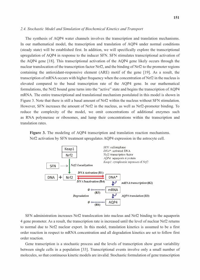
The synthesis of AQP4 water channels involves the transcription and translation mechanisms. In our mathematical model, the transcription and translation of AQP4 under normal conditions (steady state) will be established first. In addition, we will specifically explore the transcriptional upregulation of AQP4 in response to the inducer SFN. SFN stimulates transcriptional activation of the AQP4 gene [18]. This transcriptional activation of the AQP4 gene likely occurs through thenuclear translocation of the transcription factor Nrf2, and the binding of Nrf2 to the promoter regions containing the antioxidant-responsive element (ARE) motif of the gene [19]. As a result, the transcription of mRNA occurs with higher frequency when the concentration of Nrf2 in the nucleus is elevated compared to the basal transcription rate of the AQP4 gene. In our mathematical formulations, the Nrf2 bound gene turns into the “active” state and begins the transcription of AQP4 mRNA. The entire transcriptional and translational mechanism postulated in this model is shown in Figure 3. Note that there is still a basal amount of Nrf2 within the nucleus without SFN stimulation. However, SFN increases the amount of Nrf2 in the nucleus, as well as Nrf2-promoter binding. To reduce the complexity of the model, we omit concentrations of additional enzymes such as RNA polymerase or ribosomes, and lump their concentrations within the transcription and translation rates.

The modeling of AQP4 transcription and translation reaction mechanisms. Nrf2 activation by SFN treatment upregulates AQP4 expression in the astrocyte cell.

SFN administration increases Nrf2 translocation into nucleus and Nrf2 binding to the aquaporin 4 gene promoter. As a result, the transcription rate is increased until the level of nuclear Nrf2 returns to normal due to Nrf2 nuclear export. In this model, translation kinetics is assumed to be a first order reaction in respect to mRNA concentration and all degradation kinetics are set to follow first order reaction.

Gene transcription is a stochastic process and the levels of transcription show great variability between single cells in a population [33]. Transcriptional events involve only a small number of molecules, so that continuous kinetic models are invalid. Stochastic formulation of gene transcription

can be represented in the form of chemical master equation (CME) [34–37] and it can be computationally simulated by the Gillespie algorithm [38] which considers only one scenario of each reaction event based on the Monte Carlo scheme. Using Gillespie algorithm with random sampling from Poisson distribution, we can track a discrete population of molecules undergoing discrete number of reaction and translocation events during a given time period.

In addition to transcriptional and translational reaction mechanisms, we also incorporate the transport phenomenon in the model. Two different transport mechanisms have been applied to describe movement in the cytoplasm; passive pure diffusion and active motor-protein driven convective transport. For the stochastic simulation of pure diffusion, we used fractional Gillespie multi-particle algorithm (fGMP) which is an approximation of the Gillespie method [38] with discrete time interval. This method is also based on the Gillespie multi-particle (GMP) method proposed by Rodriguez . [39], which is a discrete population-based spatial stochastic method to simulate biochemical networks.

An information flow diagram for the stochastic simulation of reactions and intracellular transport is shown in Figure 4. In each iteration, we compute ( ) reaction events; ( ) microtubular transport; and ( ) random diffusion events. Gillespie algorithm gives the number of molecules reacted in each reaction. For the microtubular transport, we compute each molecule’s positional change along a microtubule for a given time period. Finally, the fractional Gillespie multi-particle method determines the number of molecules and directional change inside the cellular domain for the given time step.

. In implementing reaction mechanisms, we incorporated reaction propensityfunctions to calculate an integer number of reaction events per each simulation time step, in whichthe propensity functions, , are updated with the population of each species in the current state, .These propensity functions are shown in Equations (3) to (5) for the synthesis of AQP4 and Equations (6) to (8) for the inactivation of the DNA or the degradation of the species. 0 and

0 denote the degradation of each species in those propensity functions. Discrete numbers of all reaction events (R1–R6) are then sampled by distribution. The random number sampling is advantageous because it always gives rise to positive integers; however, it sometimes overestimates the total number of events when the simulation time step is too large. In this study,

= 1 sprovides reasonable time-step for the current system.

R1. *( , ) [ ] [ ] (3)

R2. *( , ) [ ] (4)

R3. ( , 4) [ ] (5)

R4. *( , ) [ ] (6)

R5. 0( , ) [ ] (7)

R6. 0( , 4 ) [ 4] (8)

Flowchart of the cell simulator.

Tau leaping method is an approximation method that leaps over many reaction events to approximate the exact stochastic simulation, while maintaining reasonable computing performance. Our discrete time approximation method uses a constant time interval for simulation, regardless of the number of events during each interval. The advantage of this method is that user-defined fixed time steps can be implemented. In discrete time approximation method, all events pertaining to the time interval are implemented before updating the values of the propensity function. The time step is adjusted according to the system complexity.

. . Assuming that the diffusivity of the molecules in the cell is homogeneousand isotropic, all diffusion probabilities are described with traveling times given in Equation (9), which are inversely proportional to the diffusion coefficient [39]. We assumed slow diffusion with,

s = 0.125 2/s. It also depends on the mean distance to the neighboring subvolumes as expressed by the grid spacing parameter, , which has units length. is the system dimensionality, where = 3 in our current system.

212 (9)

The event times for all volumes in the cellular domain are initially computed and simulation follows the increasing order of the least traveling time, . Accordingly, all volumes have

directional diffusion depending on the ratio to the volume which has . If the traveling time is shorter, the fraction of diffusing molecules is greater and vice versa. This fGMP method computes also fractional diffusion in a single volume proportional to the distances to the neighboring subvolumes from current tetrahedron volume with a normal distribution, ( , ). is the probability obtained by calculating the Equation (10) with , the distance from current volume to neighboring subvolume .

2

42

1

1/

1/ (10)

. The active transport by motor proteins along the microtubule iscomposed of three steps: (i) association to the microtubules; (ii) dissociation from the microtubules; and (iii) convective transport along the microtubules. For the purpose of simplicity, we only consider anteriograde transport by kinesin in the positive direction to the cell membrane. The association rate constant of the motor-protein with the microtubules is high in comparison to the dissociation constant. Transport of AQP4 alongside microtubules was interpreted with convective movement with the speed of 0.4–0.6 /s [40–42]. The directional transport along the microtubule is modeled deterministically whereas the association and dissociation reaction events are modeled stochastically.

In order to integrate the spatial coordinates of the cytoskeletal network and that of the cellular subvolumes where diffusion and reactions occur, these two meshes exchange coordinate information in our cell simulator. One mesh serves as the domain for diffusion and reaction, and the other mesh serves to compute convective transport along the microtubules. In our algorithm, the mesh for the convective transport contains the microtubule structural identity and shares the mesh information with the volumetric cell mesh such as sub-volume id and absolute geometric information of all microtubule tracks. Therefore, a molecule associated with the microtubule track is allowed to propagate along the microtubule, updating its position along the microtubule. When the dissociation from the microtubule occurs, it communicates with the cell mesh to move that vesicle into that neighboring sub-volume.

To better characterize intracellular dynamics, the stochastic simulation for AQP4 synthesis was compared to a deterministic model. Averages of cell states obtained from repeated stochastic simulations were used for the side-by-side comparison with the continuous simulation results. The mathematical model for the intracellular kinetics using ordinary differential equations is described in Equations (11) to (14)

*[ ] [ ][ ] [ ] (11)

**[ ] [ ] [ ][ ] (12)

*[ ] [ ] [ ] (13)

[ 4] [ ] [ 4] (14)

where denotes DNA activation, for reverse inactivation, for transcription, and for translation. and are degradation rates of mRNA and AQP4, respectively. DNA* stands for the activated state of the aquaporin 4 gene due to the binding of Nrf2 at the promoter region.

The kinetic rates of our steady state model are determined from published AQP4 protein half-life. Since data on the stabilities of AQP4 transcripts are not available, we employ averaged properties of mRNA transcripts measured from more than four thousand mammalian genes [43]. In this model, we used relative expression levels obtained from our western blot data to compare the concentrations between initial steady state and SFN-induced dynamic state.

We performed two sets of experiments in astrocyte cell culture; ( ) the first set was used to determine the kinetic parameters for Nrf2 nuclear translocation in response to SFN treatment and ( ) the second set served as a validation of AQP4 upregulation caused by SFN treatment using western blotting. The model was used to analyze the status of gene activation, and the kinetics of transcription. The experimental results of Nrf2 translocation and AQP4 protein levels after SFN exposure are presented in Sections 0 and 0, respectively. In addition, the detailed description of experimental procedures can be found in appendices A and B.

The steady state of the system describing AQP4 synthesis and transport was matched with existing data. AQP4 proteins have a known half-life of 24 h in the cell [44], providing information about its degradation kinetics. The precise number of transcripts and AQP4 proteins per cell is not known, so only relative expression levels can be matched. For this case study, we ensure that the number of AQP4 mRNA and proteins per cell falls within the range of four thousand genes measured in mammalian cells [43].

Kinetic parameters shown in Equations (11) to (14) were determined to arrive at physiological AQP4 protein and transcript levels. These levels agree with known data that on average approximately 2 copies of mRNA are synthesized per hour and 900 proteins from each mRNA are translated per hour [43]. SFN treatment increased mRNA transcription to 8 copies per hour. The degradation rate of AQP4 is set to have a 24 h half-life and its corresponding AQP4 mRNA is assumed to have a half-life of ~4.8 h due to the fact that on average mRNAs are 5 times less stable than the corresponding proteins [43]. This information is converted to kinetic rate constants as in Table 2. These kinetic rates are derived based on specific data on AQP4 along with data on general mammalian transcripts when AQP4-specific data is unavailable. The accuracy of the estimated kinetic rates is therefore constrained by data availability and it can be improved by using data on AQP4 transcripts instead of data on averaged mammalian transcripts. Using these rates, we obtained the number of AQP4 protein as 3.59 × 105 at steady state.

Kinetic rates of AQP4 synthesis.

Transcription rate with no SFN treatment 5.55 × 10 4

Transcription rate with SFN treatment 2.08 × 10 3

Translation rate 0.25Degradation rate of mRNA 4.01 × 10 5

Degradation rate of AQP4 8.02 × 10 6

Upon sulforaphane (SFN) administration, the transcription factor Nrf2 becomes phosphorylated and translocates into the nucleus, and the transcription of the AQP4 gene is activated by Nrf2 in this model. The degree of induced gene activation in the cell model is derived from experimentally measured Nrf2 translocation in normal and SFN treated cells, see appendix for detailed procedures. Briefly, to determine the level of Nrf2 activation, levels of phosphorylated Nrf2 (pNrf2) within the nucleus were quantified with immunofluorescence images obtained under controlled staining and imaging conditions. After continuous SFN treatment, the fluorescence levels of pNrf2 increased by about 63% compared to control at 15 min, and returned to normal levels by the 9-h time point.

Our observation of rapid Nrf2 nuclear translocation is in agreement with findings by Jain .stating that Nrf2 translocation occurs as early as 15 min [45]. The time point of pNrf2 normalization after treatment is in agreement with observations by Jain . reporting that after nuclear translocation, Nrf2 starts to exit the nucleus between 1 and 4 h and achieves normal levels at 8 h [45]. Based on this experimental finding, the cell model is adjusted to generate a 63% increase in transcription, and dynamic changes of AQP4 transcripts and proteins are predicted and validated with western blot data.

The dynamics of the SFN-induced AQP4 upregulation is predicted with the cell simulator. Adiscrete event simulation was performed with the approximated Gillespie method, using a discretized

= 1 s. Stochastic simulations were repeated for 100 times and we confirmed that the average of 100 realizations converged to the deterministic simulation as shown in Figure 5.

Figure 5 shows that simulated AQP4 expression levels increased by 47.5% after 9 h and 68.0% after 18 h. The proportion of time that the aquaporin-4 gene is in the activated state rises after SFN treatment and returns to normal after 8 h due to the Nrf2 export out of the nucleus. Interestingly, even though the AQP4 protein has a sustained period of upregulation, we predict that the mRNA level reaches a peak around 8 h and begins to drop thereafter. Computational results show that the AQP4 protein level reaches its peak at 17 h and returns to normal level after 9 days. Even though the stochastic model generates absolute number of molecules as shown in Figure 5, the current study only uses the relative expression levels for experimental validation of the model since the absolute number of AQP4 channels per cell is not known.

Stochastic simulation results of AQP4 transcripts and proteins after sulforaphane exposure. Each red solid line represents one stochastic realization and dotted black line is the solution of the deterministic simulation. The upregulation of AQP4 normalized to control was 1.48 ± 0.11 at 9 h and 1.68 ± 0.20 at 18 h.

In brain astrocytes, AQP4 channels are highly expressed in the endfeet [46]. After the translation of the protein, AQP4 proteins are packed into vesicles and transported towards the endfeet via the cytoskeleton [47]. The modeling of the AQP4 packing mechanism into the vesicle is initiated by the generation of a random number from 1 to 50. Initially, the diffusivity of the vesicle is assumed to be zero, while the “packing” of AQP4 occurs. Once the number of AQP4 proteins reaches the selected random number, the vesicle now assumes a non-zero diffusivity and goes into diffusion followed by directed transport.

Finally, we demonstrate a qualitative comparison of the spatial AQP4 distribution in a single astrocyte cell with our simulated results as shown in Figure 6. Immunofluorescence image of a single astrocyte stained with anti-AQP4 antibody in Figure 6a shows AQP4-immunopositive vesicles inside the cell body as well as within astrocytic processes. Concentrated AQP4 immunoreactivity is observed in the endfeet processes. The simulated result of spatiotemporal intracellular trafficking of AQP4 in transport vesicles (blue spheres) on the microtubule cytoskeleton (red) of an astrocyte is shown in Figure 6b. In the cell simulator, AQP4 molecules are concentrated at the endfeet of the processes, in agreement with the physiological expression of AQP4. We compared the spatial distribution of AQP4 in our cell simulator with observed patterns of AQP4 expression as shown in Figure 6a.

However, the number of AQP4 containing vesicles or AQP4 tetramers concentrated at a single endfoot cannot be quantified with the immunofluorescence technique that was employed in this study due to limitations in resolution. In future studies, a quantitative validation of AQP4 spatial polarization at the astrocytic endfeet in the model could be performed with techniques such as freeze fracture electron microscopy [48] to quantify the number of AQP4 tetramers concentrated at a given endfoot membrane.

AQP4 trafficking in primary cultured astrocytes ( ) and in the cell simulator( ). In ( ), AQP4 proteins are seen in vesicles in the cell body as well as along astrocytic processes during their transport towards the endfeet. In ( ), microtubules (red) and associated transport vesicles containing AQP4 (blue) in the reconstructed astrocyte cell are visualized.

10(a) (b)

Western blot (WB) was performed to quantify the upregulation of AQP4 by 13 M of SFN. For SDS-PAGE gel electrophoresis, cell lysates were prepared after 9 and 18 h of continuous SFN exposure. The results show that AQP4 expression was 1.48 and 1.68 fold higher than control after 9 and 18 h of SFN exposure as shown in Figure 7. The data confirmed that SFN induces upregulation of AQP4 in astrocyte cells, in agreement with previous findings that SFN injection induces AQP4 upregulation in the brain. Zhao . found a 65% upregulation of AQP4 24 h after SFN administration in an model of traumatic brain injury [18].

The comparison between measurement and simulated AQP4 upregulation is shown in Figure 7b. A close agreement is observed between the measured AQP4 levels and simulations. By employing data on transcription factor translocation and the resultant change in protein levels, the model derives interesting insights on the frequency of “on” and “off” states of the gene, the dynamic increase and drop of its transcripts, and the intracellular trafficking of proteins during the SFN-induced upregulation.

Western blotting shows that SFN induced a 48% upregulation of AQP4 after 9 h of continuous exposure, and 68% upregulation after 18 h compared to control ( ); Cell simulator results agree with measured expression levels of AQP4 ( ).

(a) (b)

Many different molecular biological assays and biochemical techniques can be used to investigateintracellular process encompassing events starting at gene activation to the final expression of its encoded protein. These datasets provide time profiles of gene activation, transcripts, or protein levels and its spatial distribution pattern in a cell or in a population of cells. In order to derive a complete understanding of the dynamics of protein expression in a particular system, however, it is difficult to quantitatively measure every species involved in the biogenesis of a protein at every step in a time-dependent fashion due to limitations in time and resources. Oftentimes, data on relative expression levels allows the postulation of transcription and translation dynamics of the system, but these hidden kinetics cannot be extracted without using quantitative tools. Furthermore, time-dependent protein localization in specific cellular domains observed by fluorescence microscopycan be incorporated to derive the kinetics of trafficking and expression, after the transcription and translation step. Our case study derived additional insights about the unknown aspects of the chosen system: gene activation status and dynamic transcript levels, based on experimental observations on the transcription factor translocation and the target protein upregulation.

The single cell simulator provides a platform for performing quantitative analysis of cellular events using and integrating biological data from various common molecular biology techniques. To simulate trafficking events, the microtubule cytoskeleton was generated by a novel growth algorithm. In addition, the event-based stochastic simulation technique allows the tracking of individual molecules at any point in time. The approximated Gillespie algorithm reduced the computational cost and captured the discrete and stochastic nature of transcriptional and translational events inside a single cell. Conversely, the average of repeated stochastic simulations is suitable for representing the behavior of an entire cell population. Finally, we used a deterministic model to validate the averaged trajectories from our stochastic computations with good agreement. The analysis of cellular events incorporating experimental data acquired with various modalities can reveal hidden kinetics and facilitate the efficient design of future experiments in systems biology by making robust predictions of cellular response.

The authors gratefully acknowledge Simon Alford for generating the images of primary astrocytes with confocal microscopy.

The authors declare no conflict of interest.

Nrf2 is a putative TF of the AQP4 gene [18,19]. To see the activation level of Nrf2 by SFN, the nuclear translocation of Nrf2 phosphorylated at the serine 40 position (pNrf2) was quantified by immunofluorescence. It has been shown that the phosphorylation of Nrf2 at this site is required for Nrf2 translocation [49]. Cells grown in 12-well plates were treated with media containing 13 M of SFN for 15 min, 30 min, 1.5, 3, 9, and 18 h. Since SFN was dissolved in DMSO prior to dilution in media, cells treated with DMSO-vehicle for these time points were used as controls. At the end of the exposure period, cells were fixed in 4% paraformaldehyde, permeabilized with acetone, and blocked in 1% bovine serum albumin. Primary antibody specific for Nrf2 phosphorylated at serine 40 site was purchased from Biorbyt and primary antibody incubation was carried out overnight. On the next day, samples were incubated with secondary anti-rabbit antibody conjugated to Alexa594 (Santa Cruz Biotechnology, Santa Cruz, CA, USA) and subsequently stained with DAPI. Samples were imaged with Zeiss AxioScope fluorescence microscope (Carl Zeiss Microscopy, Göttingen, Germany). For the purpose of quantifying fluorescence intensity inside the nuclear region, all parameters were held constant during the staining procedure and fluorescence images were acquired with a fixed exposure time. The fluorescence intensity of pNrf2 inside the nucleus was quantified with ImageJ [50], and the mean intensity was derived by averaging 20 cells per treatment group.

Rat primary cortical astrocytes were purchased from Lonza. Cells were grown at 37 degrees Celsius with 5% CO2. Astrocyte growth media (Gibco, Madison, WI, USA) contains 10% FBS supplemented with 1% penicillin/streptomycin and 1:500 amphotericin B. Growth media was changed twice a week and cells were passaged when confluent.

To quantify AQP4 upregulation by SFN, cell lysates were prepared by lysing with RIPA buffer after 9 h and 18 h of continuous SFN treatment at 13 M. Bradford assay was performed to ensure equal loading of proteins. SDS-PAGE gel electrophoresis was performed on a TetraCell Mini system (BioRad, Hercules, CA, USA) using AnykD polyacrylamide gels (Biorad, Hercules, CA, USA). After transfer and blocking in bovine serum albumin, membrane was incubated with mouse anti-AQP4 primary antibody (Abcam, Cambridge, MA, USA) overnight. On the next day, secondary antibody (anti-mouse tagged with HRP) was applied for 1.5 h followed by washing steps. Membrane was imaged with BioRad Chemiluminescence detection system (BioRad, Hercules, CA, USA). Large molecular weight aggregates were excluded from the quantitative analysis. Densitometry was performed with Image J [50].

Diffusion of GFP-tagged fusion proteins inside distinct cellular compartments (ER, Golgi, cytoplasm) have been measured, and there is a wide range of diffusion rates depending on the size of the molecule and the specific cellular compartment. For example, diffusion of GFP (which is very

small in size) inside the cytoplasm is 25 m2/s [51]. On the other hand, diffusion of GFP-tagged E-cadherin on the plasma membrane is 0.03–0.04 m2/s [52]. Inside the nucleoplasm, diffusion of GFP fusion proteins has the diffusivity of 0.24–0.53 m2/s [53]. For simplicity, we have implemented a diffusion coefficient = 0.125 m2/s in our model, which is a reasonable estimate for computing the diffusion of molecules with a larger size.

1. Wacker, I.; Kaether, C.; Kromer, A.; Migala, A.; Almers, W.; Gerdes, H.H. Microtubule-dependenttransport of secretory vesicles visualized in real time with a GFP-tagged secretory protein.

, , 1453–1463.2. Balla, T.; Varnai, P. Visualizing cellular phosphoinositide pools with GFP-fused

protein-modules. , , pl3.3. Cui, B.X.; Wu, C.B.; Chen, L.; Ramirez, A.; Bearer, E.L.; Li, W.P.; Mobley, W.C.; Chu, S. One

at a time, live tracking of NGF axonal transport using quantum dots. , , 13666–13671.

4. Dahan, M.; Levi, S.; Luccardini, C.; Rostaing, P.; Riveau, B.; Triller, A. Diffusion dynamics ofglycine receptors revealed by single-quantum dot tracking. , , 442–445.

5. Howarth, M.; Takao, K.; Hayashi, Y.; Ting, A.Y. Targeting quantum dots to surface proteins inliving cells with biotin ligase. , , 7583–7588.

6. Courty, S.; Luccardini, C.; Bellaiche, Y.; Cappello, G.; Dahan, M. Tracking individual kinesinmotors in living cells using single quantum-dot imaging. , , 1491–1495.

7. Seitz, A.; Surrey, T. Processive movement of single kinesins on crowded microtubulesvisualized using quantum dots. , , 267–277.

8. Schwartz, A.L. Cell biology of intracellular protein trafficking. , ,195–229.

9. Klann, M. Development of a Stochastic Multi-scale Simulation Method for the Analysis ofSpatiotemporal Dynamics in Cellular Transport and Signaling Processes. Ph.D. Thesis,University of Stuttgart, Stuttgart, Germany, 2011.

10. Klann, M.T.; Lapin, A.; Reuss, M. Stochastic simulation of signal transduction: Impact of thecellular architecture on diffusion. , , 5122–5129.

11. Verkman, A.S. Aquaporins at a glance. , , 2107–2112.12. Nielsen, S.; Nagelhus, E.A.; Amiry-Moghaddam, M.; Bourque, C.; Agre, P.; Ottersen, O.P.

Specialized membrane domains for water transport in glial cells: High-resolution immunogoldcytochemistry of aquaporin-4 in rat brain. , , 171–180.

13. Manley, G.T.; Fujimura, M.; Ma, T.; Noshita, N.; Filiz, F.; Bollen, A.W.; Chan, P.; Verkman,A.S. Aquaporin-4 deletion in mice reduces brain edema after acute water intoxication andischemic stroke. , , 159–163.

14. Papadopoulos, M.C.; Manley, G.T.; Krishna, S.; Verkman, A.S. Aquaporin-4 facilitatesreabsorption of excess fluid in vasogenic brain edema. , , 1291–1293.

15. Zhao, H.D.; Zhang, F.; Shen, G.; Li, Y.B.; Li, Y.H.; Jing, H.R.; Ma, L.F.; Yao, J.H.; Tian, X.F.Sulforaphane protects liver injury induced by intestinal ischemia reperfusion through Nrf2-AREpathway. , , 3002–3010.

16. Thimmulappa, R.K.; Mai, K.H.; Srisuma, S.; Kensler, T.W.; Yamamato, M.; Biswal, S.Identification of Nrf2-regulated genes induced by the chemopreventive agent sulforaphane byoligonucleotide microarray. , , 5196–5203.

17. Kraft, A.D.; Johnson, D.A.; Johnson, J.A. Nuclear factor e2-related factor 2-dependentantioxidant response element activation by tert-butylhydroquinone and sulforaphane occurringpreferentially in astrocytes conditions neurons against oxidative insult. , ,1101–1112.

18. Zhao, J.; Moore, A.N.; Clifton, G.L.; Dash, P.K. Sulforaphane enhances aquaporin-4 expressionand decreases cerebral edema following traumatic brain injury. , ,499–506.

19. Umenishi, F.; Verkman, A.S. Isolation and functional analysis of alternative promoters in thehuman aquaporin-4 water channel gene. , , 373–377.

20. Yenkie, K.M.; Diwekar, U.; Linninger, A.A.; Kim, S. A New Method for Parameter Estimationin Stochastic Differential Equations. In Proceedings of the AICHE Annual Meeting, SanFracisco, CA, USA, 3–8 November 2013; p. 589.

21. Hattne, J.; Fange, D.; Elf, J. Stochastic reaction-diffusion simulation with mesoRD., , 2923–2924.

22. Stiles, J.R.; Van Helden, D.; Bartol, T.M.; Salpeter, E.E.; Salpeter, M.M. Miniature endplatecurrent rise times <100 mu s from improved dual recordings can be modeled with passiveacetylcholine diffusion from a synaptic vesicle. , ,5747–5752.

23. Loew, L.M.; Schaff, J.C. The virtual cell: A software environment for computational cellbiology. , , 401–406.

24. Tomita, M.; Hashimoto, K.; Takahashi, K.; Shimizu, T.S.; Matsuzaki, Y.; Miyoshi, F.; Saito,K.; Tanida, S.; Yugi, K.; Venter, J.C.; E-cell: Software environment for whole-cellsimulation. , , 72–84.

25. Birbaumer, M.; Schweitzer, F. Agent-based modeling of intracellular transport. , , 245–255.

26. De Heras Ciechomski, P.; Klann, M.; Mange, R.; Koeppl, H. From Biochemical ReactionNetworks to 3D Dynamics in the Cell: The Zigcell3d Modeling, Simulation and VisualisationFramework. In Proceedings of the 2013 IEEE Symposium on Biological Data Visualization(BioVis), Atlanta, GA, USA, 13–14 October 2013; pp. 41–48.

27. Raymond, G.M.; Butterworth, E.; Bassingthwaighte, J.B. Jsim: Free software package forteaching physiological modeling and research. , , A390.

28. Ander, M.; Beltrao, P.; Ventura, B.D.; Ferkinghoff-Borg, J.; Foglierini, M.; Lemerle, C.;Tomás-Oliveira, I.; Serrano, L. Smartcell, a framework to simulate cellular processes thatcombines stochastic approximation with diffusion and localisation: Analysis of simplenetworks. , doi:10.1049/sb:20045017.

29. Plimpton, S.J.; Slepoy, A. ; Department of Energy: Albuquerque, NM, USA, 2003.

30. Andrews, S.S.; Bray, D. Stochastic simulation of chemical reactions with spatial resolution andsingle molecule detail. , , 137.

31. Boulianne, L.; Al Assaad, S.; Dumontier, M.; Gross, W.J. Gridcell: A stochastic particle-basedbiological system simulator. , , 66.

32. Le Novere, N.; Shimizu, T.S. Stochsim: Modelling of stochastic biomolecular processes., , 575–576.

33. Arkin, A.; Ross, J.; McAdams, H.H. Stochastic kinetic analysis of developmental pathway-infected escherichia coli cells. , , 1633–1648.

34. Khanin, R.; Higham, D.J. Chemical master equation and langevin regimes for a genetranscription model. , , 31–40.

35. Paulsson, J.; Berg, O.G.; Ehrenberg, M. Stochastic focusing: Fluctuation-enhanced sensitivityof intracellular regulation. , , 7148–7153.

36. Isaacson, S.A.; Isaacson, D. Reaction-diffusion master equation, diffusion-limited reactions,and singular potentials. , , 066106.

37. Baras, F.; Mansour, M.M. Reaction-diffusion master equation: A comparison with microscopicsimulations. , , 6139–6148.

38. Gillespie, D.T. Exact stochastic simulation of coupled chemical reactions. ,, 2340–2361.

39.the phosphoenolpyruvate-dependent phosphotransferase (pts) pathway in .

, , 1895–1901.40. Vale, R.D.; Reese, T.S.; Sheetz, M.P. Identification of a novel force-generating protein, kinesin,

involved in microtubule-based motility. , , 39–50.41. Steinberg, G.; Schliwa, M. Characterization of the biophysical and motility properties of kinesin

from the fungus neurospora crassa. , , 7516–7521.42. Von Massow, A.; Mandelkow, E.M.; Mandelkow, E. Interaction between kinesin, microtubules,

and microtubule-associated protein 2. , , 562–571.43. Schwanhausser, B.; Busse, D.; Li, N.; Dittmar, G.; Schuchhardt, J.; Wolf, J.; Chen, W.; Selbach,

M. Global quantification of mammalian gene expression control. , , 337–342.44. Neely, J.D.; Amiry-Moghaddam, M.; Ottersen, O.P.; Froehner, S.C.; Agre, P.; Adams, M.E.

Syntrophin-dependent expression and localization of aquaporin-4 water channel protein. , , 14108–14113.

45. Jain, A.K.; Bloom, D.A.; Jaiswal, A.K. Nuclear import and export signals in control of Nrf2., , 29158–29168.

46. Rash, J.E.; Yasumura, T.; Hudson, C.S.; Agre, P.; Nielsen, S. Direct immunogold labeling ofaquaporin-4 in square arrays of astrocyte and ependymocyte plasma membranes in rat brain andspinal cord. . , , 11981–11986.

47. Rossi, A.; Baumgart, F.; van Hoek, A.N.; Verkman, A.S. Post-Golgi supramolecular assemblyof aquaporin-4 in orthogonal arrays. , , 43–53.

48. Furman, C.S.; Gorelick-Feldman, D.A.; Davidson, K.G.V.; Yasumura, T.; Neely, J.D.; Agre, P.;Rash, J.E. Aquaporin-4 square array assembly: Opposing actions of M1 and M23 isoforms.

, , 13609–13614.49. Niture, S.K.; Jain, A.K.; Jaiswal, A.K. Antioxidant-induced modification of iNrf2 cysteine 151

and PKC- -mediated phosphorylation of Nrf2 serine 40 are both required for stabilization andnuclear translocation of Nrf2 and increased drug resistance. , , 4452–4464.

50. Rasband, W.S. , US National Institutes of Health: Bethesda, MA, USA, 1997.51. Swaminathan, R.; Hoang, C.P.; Verkman, A.S. Photobleaching recovery and anisotropy decay

of green fluorescent protein GFP-s65t in solution and cells: Cytoplasmic viscosity probed bygreen fluorescent protein translational and rotational diffusion. , ,1900–1907.

52. Adams, C.L.; Chen, Y.-T.; Smith, S.J.; Nelson, W.J. Mechanisms of epithelial cell-cell adhesionand cell compaction revealed by high-resolution tracking of E-cadherin-green fluorescentprotein. , , 1105–1119.

53. Phair, R.D.; Misteli, T. High mobility of proteins in the mammalian cell nucleus. ,, 604–609.

The objective of this work is to present a review of computational tools and models for pharmaceutical processes, specifically those for the continuous manufacture of solid dosage forms. Relevant mathematical methods and simulation techniques are discussed, as is the development of process models for solids-handling unit operations. Continuous processing is of particular interestin the current study because it has the potential to improve the efficiency and robustness of pharmaceutical manufacturing processes.

Reprinted from . Cite as: Rogers, A.J.; Hashemi, A.; Ierapetritou, M.G. Modelingof Particulate Processes for the Continuous Manufacture of Solid-Based Pharmaceutical Dosage Forms. , , 67–127.

In recent years, the pharmaceutical industry has experienced significant changes in theprevailing economic and regulatory environments. Increased global competition, particularly from manufacturers of generic products, has resulted in decreasing competition-free lifespan of products and reduced profit margins as drugs come off-patent [1,2]. Meanwhile regulatory agencies worldwide, including the US Food and Drug Administration (FDA) and the European Medicines Agency (EMA), have begun to adopt the quality by design (QbD) paradigm introduced by the ICH Q8 guidance on pharmaceutical development. QbD requires that companies demonstrate understanding of the way in which variability in raw materials as well as process design and operating conditions affect product quality and use this understanding to implement effective quality control strategies [3–5].

Despite the challenges faced by the industry, pharmaceutical manufacturing processes remain relatively inefficient and poorly understood as compared with other those in other chemical process industries [4]. This can be attributed in part to the unique challenges associated with pharmaceuticalprocess design. Throughout the drug development process, material is required for clinical trials. The corresponding timeline for delivery of clinical materials may limit the available resources for process development [6]. In addition, each active pharmaceutical ingredient (API) has its own set of physical and chemical properties which can affect the success of various drug product formulations and manufacturing routes [4]. Perhaps in part as a result of the aforementioned challenges, sequential scale-up of batch processes remains the predominant process development trajectory within the pharmaceutical industry [6]. Unfortunately this does not necessarily result in the most efficient or robust manufacturing processes. Under the current process development paradigm, manufacturing costs consume a large portion of revenue for many pharmaceutical companies, as much as 27% by some estimates [7]. In many cases more is spent on manufacturing than on research and development [6,7]. Insufficient process understanding and lack of robust

process development can also result in variability in product quality [8]. In order meet the challenges associated with current economic and regulatory realities, the pharmaceutical industry will need to invest in efficient and reliable manufacturing technologies [8,9]. Continuous processing has a great deal of potential to address issues of cost and robustness in the development of pharmaceutical manufacturing processes. From an economic perspective, continuous processes tend to involve smaller equipment than batch processes. This corresponds to decreased capital investment in equipment and plant space as well as decreased utility requirements. Continuous processes scale readily through increases in operating time, total flow rate or parallelization, reducing the need for scale-up studies throughout the development process. This can reduce time to market, which in turn may increase competition-free lifespan. It can also decrease the amount of potentially expensive API required for process development, as continuous processes can generate a large quantity of data relatively quickly [2,8,10,11]. Finally, continuous processing can mitigate issues of product variability through implementation of on-line process control [8–10].

Process systems engineering tools have the potential to play a significant role in the transition from batch to continuous processing in the pharmaceutical industry. Predictive process models can be used as a supplement to experiments throughout process development, enhancing understanding of process variability and contributing to design space exploration [12,13]. Modeling and computationaltools such as flowsheet simulations and global sensitivity analysis can also contribute to identificationof critical process parameters to support quality risk assessment (QRA) [14–16]. Predictive process models can be used to develop and assess control strategies for continuous processes and set the stage for the implementation of model predictive control (MPC) for pharmaceutical processes. These advanced control strategies can help to ensure consistent product quality [10,17–19]. Process models can also be used to optimize manufacturing processes and suggest optimal design and operating conditions [20,21].

The objective of this review is to describe the application of process modeling tools to the study of continuous manufacturing processes for pharmaceutical solid dosage forms, specifically tablets. Three common manufacturing routes, direct compaction, wet granulation and dry granulation, are considered. Available unit operation models and relevant computational methods for the study of these processes are discussed. References are provided to specific applications of these tools for modeling and simulation of solids-based pharmaceutical processes. The remainder of this paper is organized as follows. Section 2 provides an overview of continuous tablet manufacturing processes and the unit operations involved. Processing equipment and key design and operating parameters for each unit operation are described. In Section 3 various computational tools for process modeling and simulation are discussed. Section 4 provides an overview of existing process models for the unit operations involved in continuous tablet manufacture. An emphasis is placed on equation-oriented modeling approaches that can be used for process simulation. In section 5 several techniques for model validation and verification are discussed. Section 6 summarizes the state of process modeling and identifies areas for future work.

Tablets are among the most common oral solid dosage forms for drugs [22]. The exact manufacturing process for solid dosage forms vary from compound to compound, as the properties of the active pharmaceutical ingredient (API) molecule play a significant role in the development of an appropriate formulation. This work will describe a general process for transforming raw materials (API and excipients) into tablets and provide a summary of several manufacturing routes available for tablet production.

Downstream pharmaceutical processes typically begin with the feeding of raw materials to the process. These materials include active pharmaceutical ingredients, excipients such as microcrystalline cellulose or lactose, and lubricants like magnesium stearate. In most cases the concentration of excipient is significantly greater than that of API or lubricant. The material may then be passed through a comill to eliminate any large, soft lumps within the powder. Thereafter the material is mixed (blended) to ensure uniform distribution of active ingredient.Optionally the blend may be granulated via wet or dry granulation. The use of wet granulation necessitates a granule drying step prior to further processing. If a granulation process has been implemented, a milling step is typically required to reduce the granule size to the desired level before tableting. In the absence of a granulation step material may be sent directly to the tablet press after blending. In a continuous tablet press the powder is typically fed via a hopper and a rotary feed frame. The powder blend fills a die and is subsequently compressed to create a tablet. An example flow sheet for a continuous tableting process showing several design alternatives (e.g. wet granulation, dry granulation, direct compaction) is shown in Figure 1.Certain units including feeders, hoppers and tablet presses are common to all manufacturing routes. Mills are present in both wet and dry granulation. Roller compactors are unique to dry granulation while wet granulation equipment such as twin screw extruders and granule dryers are present only in wet granulation based processes. A summary of relevant processing equipment along with design and operating parameters is provided in Section 2.2 and in Table 1.

The success of a tableting process is assessed based on the quality attributes of the tablets produced. Properties of interest include tablet strength (hardness, friability), tablet API composition and relative standard deviation, tablet weight, weight variability and tablet dissolution.

Three manufacturing routes for the continuous production of pharmaceutical tablets are shown. Common processing steps for all three routes include feeding, blending and tableting. The dry granulation route involves roller compaction followed by milling of the produced ribbons while the wet granulation route involves wet granulation followed by drying and then by granule milling. In the case of direct compaction there is no granulation step and therefore milling is not required prior to tableting.

Processing equipment for continuous tablet manufacturing including the adjustable design and operating parameters.

Hopper Shape (conical, wedge)Width

Outlet diameter Wall angle

Material of construction

Powder flow rate

LIW Feeder Tooling (screw, screen)Hopper size

Operating mode

Screw speedFlow rate set point

Continuous Mixer Vessel length and diameterAgitator size and configuration

Agitator rpmMixer fill level

Twin Screw Extruder

Number of screwsScrew geometry

Barrel length Binding solution properties

and addition location

Screw speedGranulation temperature

Liquid to solid ratioPowder Flow Rate

Binder content

.

Roller Compactor Roll configurationRoll diameter Roll surface Powder feed

Powder feed rateRoll speed

Compaction pressureRoll gap

Mill Mill typeMill configuration

Geometry Screen/selector size

Equipment size Air nozzle arrangement

Solids feed rateRotor speed

Grinding pressure

Tablet Press Die and punch size and geometry

Die feeding method Number of compression stations

Die filling method Lubrication method

Powder feed rateCompression force

Tableting speed

2.2.1. Hoppers

Hoppers are commonly used in solids processing as a means of holding materials and conveying them gravimetrically. In pharmaceutical tablet production, hoppers are typically found in conjunction with other operations like feeders and tablet presses. In a well-design hopper, powder should flow consistently towards the outlet of the unit at an approximately constant flow rate. This is described as the “mass flow” regime. Hoppers come in a variety of geometries including conical and wedge shaped, both of which are used in pharmaceutical applications. In addition to geometry, hoppers can vary in width, outlet size and wall angle as well as material of construction. The hold-up in the hopper is an important operating parameter that should be monitored to avoid overfilling or, in the case of feed hoppers, running empty while the process is still operational [23,24]. Segregation and poor flow are potential concerns in the operation of industrial hoppers. Flow problems include arching and bridging, which can stop flow from the hopper, and ratholing—the stagnation of material at the hopper walls which effectively reduces capacity. These issues can be addressed via changes in hopper design or modification of the flow path using inserts [23,25,26]. Segregation is a significant concern in pharmaceutical applications, as it can result in variability in composition over time. In a hopper attached to a tablet press, segregation could affect content uniformity. Powder properties play a significant role in segregation behavior. Segregation is more likely to occur in polydisperse materials with wide particle size distributions and a large degree of density variability among the particles [27,28].

Hopper refilling dynamics and their effect on downstream operations are also a concern in continuous processes. The impact of hopper refilling on discharge rate and on the performance of a continuous tableting process has been studied both computationally and experimentally [14,29–31].

Flow and discharge behavior of pharmaceutical powders from several different hopper geometries has also been studied experimentally by Faqih [26] who developed a quantitative flow index that was shown to correlate with hopper flow behavior based on data from a gravitational displacement Rheometer.

2.2.2. Loss-in-Weight Feeders

Loss-in-weight feeders, as the name implies, feed powders into a process by mass. Feeding by mass provides the desired accuracy for pharmaceutical processes, where low feed rates may be needed, particularly for APIs and lubricants [30,32]. Loss-in-weight feeders generally consist of a hopper, a load cell that is integrated with a gravimetric controller and a conveying mechanism such as a screw feeder. A secondary conveying mechanism at the base of the hopper may be used to transfer powder to the screws. A discharge screen at the exit of the feeder can be used to break-up any lumps in the powder entering the process. The preferred tooling (screw, discharge screen) for a loss-in-weight is a function of the material properties of the feed powder and the intended flowrate. Engisch and Muzzio [30] have described a characterization method for loss-in-weight feeder equipment that can aid in determining appropriate tooling for a given application. The key operating parameter for loss-in-weight feeders is the screw speed, which dictates the powder flow rate. The hopper fill level can also affect feeder performance. Specifically, feeder accuracy may decrease at low hopper fill levels [33].

2.2.3. Continuous Mixers

The purpose of mixing in downstream pharmaceutical applications is to reduce composition variability in multi component powder blends. In continuous mixing spatial and temporal variations in the composition of the material exiting the mixer are of concern. Therefore a well-designed continuous mixer should be able to produce evenly distributed (not segregated) blends with good control of composition over time.

A summary of available equipment for continuous mixing along with studies used to characterize these mixers is given in Pernenkil and Cooney [34]. Of particular interest in pharmaceutical applications are continuous convective mixers, in which the primary mixing mechanism is convection induced by rotating blades [35]. Key design parameters for these types of mixers include the vessel length and diameter and the agitator size, configuration and geometry [36]. Important operating parameters include mixing angle, agitator rpm and powder flowrate. Powder properties, particularly cohesiveness and flow properties, can also affect mixing performance [35,37–39]. As is the case for hoppers, if components in the blend have very different properties (particle size and density) segregation may occur [40]. Several metrics can be used to monitor mixing efficiency. Relative standard deviation (RSD) and variance reduction ratio (VRR) are based on composition variability at the outlet and, in the case of VRR, inlet of the mixer. These metrics are discussed at greater length in Section 4.3, as is the residence time distribution (RTD). These characteristics can be calculated from experimental data such as concentrationmeasured at the outlet of the mixer. Composition can be assessed using near infrared spectroscopy

(NIR) [34,35,41–44]. In addition, flow trajectories within the mixer can be studied using positron emission particle tracking (PEPT) [39].

The effect of operating parameters and powder properties on mixing performance within continuous convective blenders has been studied extensively [35–39,41,45]. Marikh . [36,45] have studied the influence of mass flow rate, impeller speed and bulk powder properties on the hold up within a pilot-scale continuous mixer for different agitator types. Based on experimental studies a correlation between agitator speed and the bulk mean residence time was developed which could potentially be used for scale-up. Portillo . [39] have studied flow behavior in continuous convective mixers as a function of impeller speed, flow rate and powder cohesiveness. Flow behavior is characterized by particle trajectories, axial dispersion coefficient and residence time. In a separate study Portillo . [37] have examined the effect of mixing angle in addition to impeller speed and cohesion on residence time and blend content uniformity. Two mixers that differed according to geometric parameters such as vessel length and diameter and blade size, shape and configuration were compared in this study. Finally Vanarase and Muzzio [38] have studied the impact of impeller rotation rate, flow rate and blade configuration on mixer performance as characterized by RSD and VRR.

Extensive modeling efforts have also been conducted for continuous mixers. These will be discussed in Section 4.3.

2.2.4. Wet Granulation

The purpose of granulation is to create agglomerates, or granules, of powder blends. These granules are of higher bulk density than the bulk powder and thus tend to have better flow properties. The granulation process also contributes to improved control of content uniformity and compactibility [46]. Wet granulation involves combining a dry powder blend with a liquid, known as a binding solution, in the presence of some sort of agitation. When the powder is wetted granule nuclei consisting of binder droplets that have taken up powder begin to form. Thereafter the granule grows and densifies through coalescence and consolidation. Finally breakage may occur as the granules collide at high speed or experience significant shear. The properties of the powder blend, choice of binder, binding solution content relative to the amount of powder, and granulation method all have the potential to affect granule properties [47,48].

Wet granulation can be performed using a variety of techniques and equipment, including high shear mixers, fluid bed granulators and single or twin screw extruders. High shear mixers are primarily used in batch applications although so-called “instant agglomerators”, which are similar to high shear mixers that process very small volumes of material and therefore have an extremely short residence time, can be used for continuous processing [46,49]. Fluid bed granulators, the most common of which are horizontal moving bed granulators, operate by spraying binding solution from above onto a powder bed that is fluidized with air (or an inert gas such as nitrogen) from below. The granules are partially dried by the air flow and granule drying is readily completed within the fluid bed granulators when the addition of binding solution is stopped. Fluid bed granulators tend to operate at relatively high production rates, e.g., 20 kg/h or more [46,50].Therefore they are not necessarily suited to pharmaceutical processes which may operate at lower

throughput, particularly during the formulation development process. Extrusion equipment consists of one (single) or two (twin) screws within a barrel. Often pharmaceutical granulation is carried out in twin-screw extruders with co-rotating screws. Mixing and agglomeration occur as the material is conveyed along the length of the barrel. Binding solution is injected into the process at a certain point or points along the length of the barrel [47,51]. Depending on the degree of densification that occurs within the extruder it may be necessary to mill the granules resulting from an extrusion process down to an appropriate size prior to using them in subsequent processing steps. For all processes except fluid bed granulation, a granule drying step is also required [46,50].

Extrusion processes have been studied most for continuous pharmaceutical processes. This is due in part to the fact that extrusion is readily scaled-up via increased throughput and therefore lends itself to the development environment within the pharmaceutical industry. In these processes, the main design parameters include the length of the barrel, the number of screws (one or two), the geometry of the screws, and the location of a point or points along the barrel where binding solution is added [46,50]. Operating parameters of interest include screw speed, granulation temperature and liquid to solid ratio [51]. Powder properties and binder properties including viscosity and surface tension have the potential to influence the process as well [52]. Performance indicators for wet granulation are related to the granule properties, including the granule density and porosity, mean granule size and granule size distribution and the granule composition with respect to active ingredient [47,52]. In addition, the yield or recovery from a granulation process is important. The loss of material to fines during the granulation process impacts the overall yield and could affect granule composition if the active ingredient forms fines more readily during the granulation process [47,51].

Lee . [47] have compared twin screw extrusion (TSE) with high shear mixing (HSM) by measuring the properties of the resulting granules and have found that TSE tends to elicit multimodal granule size distributions with greater porosity. This is consistent with the need for a size reduction step following some extrusion-based granulation processes. Dhenge . [52] have studied the effect of binder solution properties including viscosity and surface tension on residence time and torque in a TSE granulation process as well as on granule properties including size distribution and granule strength. Tu . [51] have experimentally studied granule properties as a function of operating conditions including screw speed and liquid to solid ratio in two different twin screw extruders. This enabled the authors to develop regime maps for the process, describing the extruder geometry in terms of granulation, extrusion and breakage regimes. Regime maps are useful in the characterization of granulation equipment like twin screw extruders. Several authors have studied wet granulation in the context of other unit operations. Cartwright . [53] have addressed the importance of accurate powder feeding for successful granulation performance in a twin screw extruder by comparing two types of loss in weight feeders. The impact of granulation conditions, including throughput, screw speed, screw configuration, angle of kneading elements and barrel temperature, on both granule and tablet properties have been examined by Vercruysse

. [54]. Finally the continuous drying of wet agglomerates in a fluid-bed dryer has been studied by Palzer [55], who found, among other things, that average residence time in the dryer significantlyaffects the propensity for undesired secondary agglomeration to occur during the drying process.

Extensive research has also been conducted into the modeling of granulation processes, as will be discussed in section 4.4.

2.2.5. Roller Compactors

Granulation can also be accomplished via dry granulation. Dry granulation is carried out continuously through roller compaction. Dry granulation differs from wet granulation in that granules are formed only through compression. Thus the powder properties of the raw materials are important in determining whether dry granulation via roller compaction is an acceptable approach. Powders that have low bulk density, small particle size (e.g., micronized materials) or are very cohesive may not perform well in roller compaction [56]. Powders with good flowability and compressibility tend to be better candidates for roller compaction [57,58]. The development of a robust granulation process can be more challenging via dry granulation than wet granulation, but dry granulation offers advantages including the elimination of the granule drying step, shorter processing time and lower capital investment and utility costs. Additionally, roller compaction can be used for moisture-sensitive APIs [50,59,60].

In the roller compaction process, powder is fed into a set of counter rotating rolls, conveyed forward with the motion of the rolls and as it reaches the point where the rolls are closest together undergoes compression and forms a compact ribbon. The ribbon is then conveyed forward and released from the rolls. When the particles are fed to the rolls they are initially considered to be in the region of the process, characterized by the particles slipping at the surface of the rolls. Relatively little pressure is exerted on the powder in this region. As the powder is drawn towards the point where the rolls are closest together, the wall velocity of the powder begins to match that of the rolls and the pressure exerted on the powder increases substantially. This is known as the region, and it is in this part of the process that powder is compacted. The nip angle, typically

to the no-slip (nip) region [61]. Once the roll gap begins to increase again, after the point where the rolls are closest, the ribbon produced in the region is said to be in the region [62]. The ribbons can subsequently be milled to obtain appropriately sized granules [60].

The different equipment available for roller compaction varies mostly in terms of configuration. Rolls can be arranged either horizontally (with ribbons coming out parallel to the floor) vertically (with ribbons coming out perpendicular to the floor) or at some intermediate angle. In addition, it is possible that both rolls will be fixed, resulting in a constant roll gap throughout the process, or that one roll can be adjustable allowing for a change in roll gap during processing. The roll diameter and width vary from one piece of equipment to another. The surface of the rolls can also vary from smooth to knurled (rough/with grooves) to pocketed design. Finally the powder can be fed either gravimetrically or using a screw feeder [50,56]. In addition to the previously discussed powder properties and equipment design parameters, several operating parameters affect the performance of roller compaction processes. These include the feed rate of powder to the rolls, the roll speed and the compaction pressure applied to the powder, which is a function of the roll gap [60,63]. The nip angle, which is related to the length of the compaction zone and therefore to the degree of compression, is an important indicator of the performance of a roller compaction process, as is the

peak or maximum pressure [57,62]. The performance of roller compaction processes is assessed according to metrics similar to wet granulation. The propensity for fines can be greater in roller compaction depending on the properties of the powder being formulated [50]. In addition, ribbon density and ribbon density variability can also be used to evaluate the process performance.

Many studies of roller compaction focus on understanding the relationship between design and operating parameters. Bindhumadhavan . [62] have studied the influence of roll speed and roll gap on pressure profiles during roller compaction. The influence of rotation angle, feed rate and roll speed on pressure distribution and drive torque applied to the rolls has been experimentally evaluated by Lecompte . [58]. In addition to varying the angle at which powders are fed to the rolls Miguélez-Morán . [64] have examined the relationship between lubrication and ribbon density, which is an important performance indicator for roller compaction processes. In general lubrication was found to reduce variability in ribbon density. Yu . [57] have studied the relationship between powder properties and compaction performance and have shown that powders with better flowability achieve higher peak pressures during roller compaction, resulting in improved compaction behavior.

2.2.6. Milling

Milling is a broad term that describes a wide variety of size reduction techniques. The current work will focus on dry milling techniques that are relevant for downstream pharmaceutical processes. Milling can be used to delump powders, to reduce the particle size of raw materials, particularly APIs, or to reduce the size of granules generated through either wet or dry granulation [65].

Conical screen mills, such as comills, can be used for delumping of powders, or for coarse to fine control of wet or dry granule size. Conical screen mills consist of a cone shaped screen with an impeller inserted into the center. The impeller rotates and material is ground between the impeller and the screen until it is small enough to pass through the holes in the screen and leave the mill. The key design parameters for a conical mill include the screen mesh size, the size of the cone, the impeller shape and the impeller to screen distance, which can be adjusted using spacers. Important operating parameters include powder feed rate and agitator speed [60,66]. The properties of granules entering the process also play a significant role in dictating the degree of size reduction that can be achieved [67]. Granule size can also be reduced using oscillating granulators, which are essentially screens integrated with the roller compaction process. The compact ribbon is forced through a screen using an oscillating rotor, so called because rotor speed and direction can vary in time. Screen size and rotor speed and rotation angle dictate particle size [68].

Comills are often used for granule size reduction but other milling technologies may be used if a smaller final particle size is desired. These include air jet mills and impact mills. For each type of mill a variety of configurations is available. Air jet mills generally consist of a grinding chamber, where particles are broken, and a classification chamber, where particles are separated according to size. Sufficiently small particles are passed to the next unit operation while fines can be collected in a dust filter. For these types of mills the main design parameters of interest include the geometry, number and configuration of the air nozzles. Significant operating parameters include the solid feed

rate and the grinding pressure [65]. Impact mills include pin mills and hammer mills. In both types of mills, material is fed through the center of the mill and exits at the outer edge of the chamber. A selector grid can be used to allow only sufficiently small particles to exit the milling chamber. Pin mills grind the product between two disks to achieve size reduction while hammer mills rely on high impact particle wall, particle blade and particle-particle collisions. For pin mills, the mill size is the main design variable. For hammer mills the equipment size, blade configuration and selector grid size are all relevant design variables. Variable operating parameters for pin and hammer mills include solids feed rate and the rotor speed [65,67].

Regardless of the equipment used, the objective of milling is to achieve the desired particle size. The performance of a milling process can thus be assessed in terms of its ability to achieve the desired mean size or size distribution [16]. Specific surface area, which is related to particle size, can also be used to determine milling performance. Yield is also a concern in milling operations, as the production of a large quantity of fines that are recovered in the dust filter could result in significant losses of potentially expensive raw material (e.g., API) [67].

Comills have been studied more extensively for granule size reduction than have impact or air jet mills. Experimental studies have shown that screen size, impeller speed and impeller shape can be varied to affect granule size distribution [66,69]. It has also been demonstrated that decreasing screen size coupled with increased impeller speed results in smaller granule size [70]. Some correlation between granule properties and milling performance has also been demonstrated. Inghelbrecht and Remon [71] have found that low friability corresponded to reduced dust formation during milling. Verheezen . [67] have studied impact milling for granule size reduction and found that granule strength has a significant effect on the final particle size achieved. In addition, fines formation was found to be related to the total degree of size reduction.

2.2.7. Tablet Press (with Integrated Hopper and Feed Frame)

The tableting process involves the compaction of powder blends to form a hard compact. This is achieved in a tablet press, which contains several components integrated as a single processing unit. A hopper conveys material into the tablet press. A feed frame is then used to move the powder or granular material into the die, a cavity that defines the tablet size and shape. A punch compresses the material within the die to form a tablet. Cam tracks guide the continuous movement of the dies so that they can be filled, compacted, and discharged [14].

Material properties can significantly affect tableting performance. Wide particle size distributions or variability in density can result in segregation during die filling, causing non-uniform tablet composition. Low bulk density, poor compressibility or flow properties can affect die filling and the pressure profile during compaction, resulting in tablet weight variability and insufficient tablet hardness [72,73]. Experimentally a correlation between the particle size and specific surface area of the material to be compacted and the hardness and dissolution properties of tablets has been demonstrated [74,75]. Compression problems such as capping can occur due to the presence of excessive fines within the particle size distribution [76,77]. Particle or granule moisture content can impact drug product stability, compressibility and tablet physical properties [78]. In addition, the physiochemical properties of the active ingredient could affect the propensity for form

change due to temperature increase during the compaction process [79]. Drug and lubricant properties can also affect tableting performance, particularly as drug loading or lubricant content increases [74,80–82].

The variable design parameters for a tablet press are related to tooling and method of operation.The tooling includes the die and punch size and geometry, which can be changed according to the desired tablet weight and shape. The number of compression stations also differs between tablet presses. The die can be filled via force feeding or suction filling [83]. Finally lubrication can be internal, mixed with the powder or granule blend, or external, applied directly to the punch and die assembly. Internal lubrication is common in the pharmaceutical industry, though some studies have indicated that external lubrication can mitigate the effect of lubricant on tablet hardness [82]. Operating parameters of interest for a tablet press include the powder feed rate and the compression force applied to the tablets as well as the rate of tablet production. Tableting speed and powder feed rate are related to tablet weight and weight variability while compression force affects tablet properties like hardness and density [22,76]. The performance of tableting processes can be assessed based on tablet active ingredient content, content uniformity, weight variability, and physical properties such as friability, hardness and dissolution performance. Drug content can be measured continuously using near infrared (NIR) spectroscopy [42,78]. Hardness, friability and dissolution must be measured offline, but models can be implemented to predict hardness and dissolution performance based on operating conditions or spectroscopic measurements [73,74,84,85].

Particulate systems are of tremendous importance within the pharmaceutical and numerous other industries, yet they remain relatively poorly understood. In order to enhance understanding of macroscopic behavior in solids processes, it is helpful to first understand the particle-particle and particle-environment interactions that give rise to it. Discrete Element and Finite Element Method (DEM/FEM) models are particle level computational tools that can be used to develop this understanding [86]. An extensive review of theoretical developments and applications in discrete particle simulation has been provided by Zhu . [87,88]. This review will focus on the application of DEM to pharmaceutically relevant processes.

DEM can be used to understand particle packing, which is important for problems involving powder bed densification and compaction like the manufacture of pharmaceutical tablets. The ability of DEM to accurately model particle packing has been well documented in the literature through studies comparing simulated with experimental behavior [89,90]. Specifically it has been shown that DEM can adequately represent packing density (porosity), coordination number, radial distribution function and the force network within a packed bed [88,91,92]. For instance, Yi . [92] have studied systems of multi sized spheres and shown that the porosity and coordination number obtained via DEM agree well with those obtained experimentally.

Particle and particle-fluid flow behavior has also been studied extensively using DEM. Particle flows, and specifically confined flows, are relevant in pharmaceutical operations such as

continuous mixing, fluidized bed drying, and powder feeding and conveying. It has been shown that DEM can accurately model confined flows like direct and annular shear, vertical flow and biaxial or triaxial compression [88]. McCarthy . [93] have compared solids fraction and particle velocity profiles as well as granular temperature distributions for simulated and experimental studies of a horizontally aligned annular shear cell and shown that as long as the system and particle geometries are well represented the DEM and experimental profiles agree well.In addition, Wu . [94] have modeled the flow of powder in confined space in order to study a die filling process and found that appropriately calibrated DEM models can reproduce the powder flow behavior observed experimentally using high speed cameras.

DEM has been used to model several aspects of the tableting process, including die-filling, compression of materials within a die and crushing of particles during compression [95,96]. Mehrotra . [72] have used DEM to explore the impact of powder flow properties, specifically cohesiveness, on the die filling and compression process. It was found that as material cohesion increases the time it takes to fill the die also increases, which is consistent with the experimental observation that the tablet weight variability decreases at lower tableting speeds for cohesive powders. Several authors have also coupled DEM with computational fluid dynamics (CFD) to investigate suction filling of dies and to evaluate the effect of air or lack thereof on segregation during die filling [97–100]. One significant challenge associated with the use of DEM to model compression processes is the issue of deformation at high relative densities. In many computational studies of compression and compaction processes, FEM has been combined with DEM to improve the representation of particle deformation during compaction [76,95,96,101–103]. Specifically Frenning [102] has shown that finite and discrete element methods may be combined to simulate the behavior of granules in a densely packed bed and to understand the relationship between individual granules and the behavior of the granule bed under compression. Gethin . [101] have demonstrated that a combined DEM/FEM method can be used to determine particle packing in a die as a function of particle shape.

DEM has also been used to study powder mixing processes. Several authors have demonstrated qualitative agreement between DEM simulations and experimentally obtained mixing behavior [104]. For instance, Marigo . [105] have obtained qualitative agreement between experimentally obtained axial and radial dispersion trends and those obtained through DEM simulation for a tubular mixer. Remy . [106,107] have compared experimental and DEM results for granular flows in a bladed mixer. This work has demonstrated qualitative agreement between the segregation profiles obtained via DEM and experimental studies for polydisperse, cohesionless spheres and has also shown that DEM can reproduce observed surface velocities, granular temperature profiles and mixing kinetics at varying surface and wall roughness. Of particular interest for continuous pharmaceutical manufacturing applications is the use of DEM to study continuous convective mixers. DEM has been used to validate the periodic section approach to modeling continuous convective mixers through demonstrating that the velocity profiles obtained from periodic section simulation are in agreement with those obtained from full blender simulation [108]. DEM simulations have been used to calculate the residence time distribution (RTD) in various

blending equipment, including continuous convective mixers [41,109]. Data from DEM has also been used to inform reduced-order mixing models for process simulation [110].

Due to the importance of hoppers in a variety of industries, including agriculture, food processing and pharmaceuticals, numerous detailed studies of hopper flow have been conducted using DEM as well. DEM has been used to study the impact of powder properties, hopper geometryand operating parameters on segregation and flow patterns in hoppers [23–25,27–29,84,88,95].

The population balance equation can be used to describe the development of a set of properties of interest for a group of entities over time. Population balance equations have been used to model particulate processes including crystallization, mixing, milling, granulation, drying and dissolution, all of which are of great interest in the manufacture of solid dosage forms for pharmaceutical products [66,111–115] The general form of the population balance equation in 2 dimensions is given below.

(1)

is referred to as the population distribution function, and describes the state of particles with respect to internal and external coordinates in time. reflects the internal coordinate(s) such as particle size, mass or volume. reflects the external coordinate(s) such as axial or radial position and

indicates time. The right hand side of the population balance equation (PBE) indicates the rate of formation and depletion of particles, which can occur through a variety of mechanisms including nucleation, aggregation and breakage. Analytical expressions for these mechanisms can be used to express the formation and depletion terms on the right hand side of the population balance equation [116,117].

Population balance models are often discretized with respect to the internal and external coordinates. In this case the differential terms with respect to and in Equation (1) are replaced by finite differences. Discretized population balance models can also be parameterized, as show in Equation (2).

(2)

( ) are the discretized states and are the model parameters, which can be estimated based on experimental or simulated data. The parameter estimation can be formulated as an optimization problem with a least squares objective as outlined in Ramachandran [118]. Sen . [119] have demonstrated the use of a parameterized population balance equation to model a continuous mixer. The parameters were fit by minimizing error between measured and predicted relative standard deviation (RSD) of the product composition and the API mass fraction at the mixer outlet.

High (three or four) dimensional population balance equations, such as those often encountered in modeling wet granulation processes, can be computationally expensive to evaluate [113]. The implementation of hierarchal solution techniques has been discussed extensively in the literature as a means of reducing the computational time associated with solving these equations [120–123]. In

order to implement a hierarchal solution strategy the multidimensional PBE is discretized withrespect to both internal and external coordinates. The partial differential equations in the PBE can then be rewritten as ordinary differential equations which can be integrated over time using a first order Euler predictor/corrector method [122].

The aforementioned methods are summarized in Table 2 with respect to their applications, the level of detail with which they model the process and the relative computational cost.

Comparison of modeling techniques discussed in section 3 of the current work.

DEM particle level simulation of powder behavior

powder flow, powder mixing, and compaction

Particle level information

high

PBM describes the evolution of populations of entities (particles, granules, droplets) over time

mixing, crystallization, granulation, milling

Description of population of particles

moderate to high—depending on problem dimensionality

ROM approximation of high fidelity models using a variety of estimation and interpolation techniques

various unit operations, simulation-based optimization

Unit operation level description

low

Reduced order models (ROM) are a class of models that represent high fidelity or full scale models in a lower dimensional space. The order reduction can be achieved through multivariate analysis techniques as in principal component analysis (PCA) or proper orthogonal decomposition. [124–128]. Alternatively a computationally expensive model can be replaced by lower dimensional surrogate model obtained through fitting of experimental or simulated data using techniques such as kriging, response surface methodology (RSM), artificial neural networks (ANN) or high dimensional model representation (HDMR) [12,129–134]. The motivation for using ROMs is that they are less computationally expensive than the original models and are therefore suitable for process simulation and optimization purposes.

3.3.1. Kriging

Kriging is a black-box interpolating technique that can be used to generate metamodels or response surfaces from input-output data for a process [135,136]. Originally developed for the purpose of predicting mineral deposit distributions, in recent years Kriging has been increasingly used for modeling in a variety of fields [136,137]. Its popularity can be attributed in part to its ability to model complex nonlinear and dynamic processes [138]. In addition, Kriging generates error estimates associated with each predicted point that can be used to assess prediction accuracy and direct future sampling [12,139,140]. This combined with the fact that Kriging models do not rely on a pre-defined closed form allows for the development of accurate model representations from relatively sparse datasets as compared with those obtained through traditional experimental designs [131,139]. The primary disadvantage associated with Kriging is that it does not provide a

simple closed-form expression for the relationship between inputs and responses the way that other response surface methods do (see section 3.3.5) [131].

In Kriging models, the predicted response associated with a new input point is determined as a weighted sum of the known function values associated with previously sampled inputs as shown in Equation (3). The weight, , attributed to each decreases with increasing Euclidian distance between the points and . Thus Kriging is considered an inverse distance weighting method. In general some maximum distance is defined such that only points within some distance of are considered [131,136,140].

(3)

The weights in Equation (3) are unknown and their determination is a critical step in the development of the Kriging model. The objective is to select the weights such that the mean square error of prediction is minimized. In practice these weights can be obtained using a fitted variogram model based on points that are sufficiently close to . The weights must sum to unity, a constraint which arises in part from the condition that the Kriging predictor should be unbiased [138,140]. In addition, if input points are closely clustered together they are given lower weight in order to prevent biased estimation [12,131]. For purposes of the subsequent discussion the Euclidian distance between points ( ) and the variogram corresponding to a dataset consistingof sample points ( ) will be define as in Equation (4).

(4)

As can be seen in Equation (4) the variogram is calculated for individual pairs of points. This type of variogram is sometimes referred to as semi-variance while the variogram is described as ( ), but for the purposes of the subsequent discussion ( ) will be referred to as the variogram [138]. For a dataset containing sample points there are a total of ( )/2Euclidian distances and corresponding values to be determined. The resulting . data is usually smoothed and is then fitted to one of five basic models; sphereical, gaussian, exponential, linear or power-law. These are summarized in Jia . [131] and Boukouvala and Ierapetritou [139]. The form of the variogram model is chosen such that it minimizes prediction error, though computational efficiency may also be considered in making the selection. If necessary combinations of the various model types may be used to obtain appropriately low error. [131,138] Once an expression for the variogram has been obtained, it can be used to obtain a complementary function known as the covariance function shown in Equation (5).

(5)

The term corresponds to the maximum variance of the variogram function and is also referred to as the sill. The kriging weights for a given test point can then be obtained from the covariance function by solving the system of Equation (6).

(6)

represents the distance between two points and while represents the distance between a point and the test point . Likewise represents the covariance between data corresponding to input vectors that are distance apart, obtained from Equation (5). are the Lagrange multipliers associated with the constraint that the weights must sum to unity. The variance associated with the test point is calculated from Equation (7), in which the term

is the right hand side of Equation (6).

(7)

Algorithm for Kriging with the option for updating the sampling space in order to achieve sufficiently low prediction variance.

Briefly, the Kriging algorithm, depicted in Figure 2 can be described as follows:

1. Select an initial sample set consisting of sample points and evaluate the process ormodel at these points to obtain the corresponding function evaluations .

2. Using the data obtained in step 1, calculate the Euclidian distances and thecorresponding semi-variances ( ) using Equation (4) for all ( )/2sampling pairs.

3. Smooth the ( ) . data and fit it to an appropriate variogram model accordingto a least squares error minimization criterion and/or a secondary criterion forcomputational efficiency.

4. Based on the variogram model, determine the covariance function as in Equation (5).5. For a test point calculate the weights from Equation (6). Calculate the predicted

response from Equation (3) and the associated variance from Equation (7).6. Optional—If the predicted variance is larger than desired, collect additional sample

points in the region of the test point and add those to the set to develop an updatedKriging model.

Kriging has been used in a variety of applications related to pharmaceutical process modeling. Jia . [131] have demonstrated Kriging models to represent the flow variability in a loss-in-weight feeder as a function of flowability and feed rate. Boukouvala . [129] have proposed an extension of this model that includes a Kriging-based imputation of missing data.Boukouvala . [138] have demonstrated the use dynamic Kriging to study the roll gap and ribbon density in a roller compaction process with respect to variable feed speed, roll speed and hydraulic pressure. Boukouvala . [138] have also demonstrated the use of Kriging to map the design space for a continuous convective mixer and a loss-in-weight feeder and Boukouvala and Ierapetritou [139] have described the use of a Kriging-based method for feasibility analysis of a roller compaction process.

3.3.2. Response Surface Methodology (RSM)

Response surface methodology describes a set of computational tools that can be used to establish relationships between a system or process response and multiple input variables. Box and Wilson first proposed RSM in 1951 as a means of optimizing operating conditions for a chemical processing [130]. In recent years RSM has been increasingly used for pharmaceutical applications [12,129,131,134,141,142]. The goal of RSM is to develop a functional representation for the response as a function of input variables. The functional representation, or response surface, is an approximation because the true form of the variable-response relationship is not known explicitly. The response surface is generated through a local sampling and optimization process within a region of interest. This region may be defined as the full operating space of the process or a subset of this space near an optimum or other point of interest [133].

Algorithm for response surface modeling with optimal model development around a region of interest.

The main steps in implementing RSM are given below for a system with a single response, , and input variables . The algorithm for developing a response surface model is also depicted in Figure 3.

1. Establishment of an experimental designA design, , consisting of samples can be generated using a design of experiments (DOE)

or other appropriate statistical approach. .

The proper selection of is critical to ensure that the generated response surface will be an accurate predictor for the response of interest. The number of sampling points should be greater than the number of coefficients to be fitted for the response surface model. For noisy data, the number of sampling points needed may be greater. Further discussion of appropriate designs is provided in the literature [131–133].

2. Development of a response surface model in the region of interestThe initial response surface model is developed around the nominal sampling point. Theform of the model is defined by the modeler. Typically second-order polynomial functionsas in Equation (8) are selected for the response functions. Justification for the selection of

second order polynomials is provided in the literature [132,133]. The sampled data can then be regressed to the specified model using least squares or other appropriate fitting techniques.

(8)

is the estimated response. and are the model coefficients. and are the input variables.

3. Local model optimizationModel optimization is performed in order to determine the region where expected processimprovement can be maximized. The optimization can be completed using a steepestdescent search over the sampling region. In this case the local optimum is found iteratively.An initial model is built based on the first sampling point. The optimum of this model thenbecomes the nominal point for the next iteration and a new response surface is built andoptimized, with the addition of new sample points. As the algorithm converges, the nominaland optimal points become one and the same [131]. Other optimization techniques such asridge analysis can also be applied [132]. If different process designs are to be considered,binary variables can be introduced to indicate the design configuration. This results in amixed integer nonlinear program (MINLP) optimization problem formulation [12].RSM has been used to model pharmaceutically relevant unit operations, includingloss-in-weight feeding [129,131] and granulation [134,142]. It has also been used to exploredesign space and aid in the identification of critical process parameters for pharmaceuticalapplications [12,141].

3.3.3. High Dimensional Model Representation (HDMR)

High dimensional model representation (HDMR) describes a set of techniques that can be efficiently used to describe input-response relationships in high dimensional systems. HDMR expresses the system output as a finite hierarchal correlated function expansion of the various inputs. This functional representation accounts for the effect of individual inputs and the effect of interaction between inputs on a particular output [143–145].

(9)

in Equation (9) is a zero order term which indicates the average value of the output over the domain of in random sampling HDMR or the value of at a specified reference point in cut-HDMR. indicates the individual contribution of variable to the output whileindicates the contribution from the interaction of variables and .

If Equation (9) is expanded to include all potential parameter interactions the number of component functions to be calculated can become intractable as the number of variables increases. However in most applications it is sufficient to include terms up to second order interactions only. Most higher order terms represent only a small contribution to the overall response [143,145]. Thus Equation (9) can be approximated as a second order expansion.

(10)

The form of each of the component functions in Equation (10) can be optimally selected in order to accurately represent the available data. Objective functions and algorithms for selecting optimal component functions are discussed extensively in the literature [143,145,146].

Component functions can be determined differently depending on whether or not the data is randomly sampled. If it is, Random sampling HDMR (RS-HDMR) can be used. The HDMR expansion is determined from the average value of over the entire domain of the input space.Cut-HDMR can be used when ordered sampling is used for data collection. In this case is defined relative to a specified reference point which is used to determine the component functions. Multiple cut-HDMR is an extension of cut-HDMR in which the expansions are determined relative to several different reference points and then combined to represent .Cut-HDMR generally requires fewer samples than RS-HDMR, as the latter relies on the evaluation of high dimensional integrals to obtain the constant terms [12,147]. However the use of analytical basis functions, including orthonormal polynomials or spline functions can reduce the computational expense of fitting RS-HDMR component functions. In terms of basis functions Equation (10) can be written as:

(11)

where and are coefficients for the basis functions and and , and are integers [143]. The use of variance reduction methods has also been shown to reduce the sampling required for accurate Monte-Carlo integration of coefficients for RS-HDMR expansions [148,149].An overview of the algorithm for developing high dimensional model representations is provided in Figure 4.

Algorithm for high dimensional model representation based on a minimum prediction error criteria.

In pharmaceutical applications, Banjeree . [150,151] have used HDMR to generateinput-output maps for use in feasibility analysis of black-box processes. Boukouvala . [12,123] have extended this methodology to determine the design space for a continuous mixing process using cut-HDMR. RS-HDMR can also be used as a tool for variance based global sensitivity and uncertainty analysis. The total and partial variances can be calculated based on the HDMR component functions where represents the total variance, represents the contribution of variable to the total variance and represents the contribution of the interaction between variables and to the total variance.

(12)

Based on the variances and partial variances the sensitivities can be determined as:

(13)

The use of HDMR for sensitivity and uncertainty analysis has been demonstrated for several applications in environmental and atmospheric chemistry [152,153]. Ziehn and Tomlin have developed a Matlab® based tool for the implementation of HDMR and HDMR-based sensitivity

analysis called GUI-HDMR. This tool has been used for sensitivity analysis of air flow models, complex reaction models of pollutants in air and cyclohexane oxidation [154]. An example of HDMR component functions generated using the GUI-HDMR tool developed by Ziehn and Tomlin is given in Figure 5.

Example of fit for of a first order HDMR metamodel for tablet API concentration in a direct compaction process obtained using the GUI-HDMR software of Ziehn and Tomlin [154].

3.3.4. Artificial Neural Networks

Artificial Neural Networks (ANN) have become quite popular in a variety of fields as a tool for addressing complex science and engineering problems and for developing empirical process models [155]. In particular they are useful in modeling pharmaceutical processes due to their ability to accurately represent nonlinear system behavior [138,156]. Neural networks can be defined in terms of the transfer functions defined by their neurons, the learning rule applied and the connectivity of the system. The neurons are arranged in layers: an input layer which consists of data entering the network, hidden layers containing the neurons that transform the input data, and the output layer which contains the network output corresponding to a specific input or set of inputs. Each hidden layer can contain a single neuron or a group of neurons operating in parallel. The neurons, or processing elements, consist of weights and transfer functions. The weights are coefficients by which the inputs to the neuron are multiplied and the transfer functions are simple linear or nonlinear functions that transform the weighted inputs. The architecture of a network can be described as feedback or feedforward. Feedback networks include connections from output neurons back to input neurons and therefore have some memory of prior states while feedforward networks do not. The architecture of the network can be adjusted through a learning process which involves the use of a training dataset for which the true values corresponding to each set of inputs are known. The learning process is iterative, with weights being modified in order to minimize

prediction error, most often via back propagation of the error. Training involves a trade-off between the ability of the network to accurately predict the training set and its ability to generalize to data not included in the training set [138,155,156].

The general procedure for developing an artificial neural network, depicted in Figure 6, involves

1. Obtain a training data set e.g., via DOE;2. Define the network: the number of hidden layers, the number of neurons to include in each

layer and the type of transfer functions to be implemented;3. Use a training procedure to optimize the weights in such a way that prediction error is

minimized. The number of neurons in each layer can also be determined based on thetraining set, via cross validation;

4. Test the developed network against data that was not contained in the original training set toverify that the network has not been over fitted.

Artificial neural networks (ANNs) have been used to model a variety of pharmaceutically relevant processes. They can be used to recognize patterns for analytical chemistry purposes, to evaluate the influence of molecular structure on material properties, to evaluate pharmacokinetic and pharmacodynamics profiles, [156] and to model pharmaceutical unit operations [16,138].

Algorithm for development of an Artificial Neural Network with the option to add points to the training set or to redefine the network structure in order to improve model predictive ability.

3.3.5. Comparison of HDMR, RSM, Kriging and Neural Networks

Previous works have compared Kriging, RSM, HDMR and ANN as black box modeling techniques for pharmaceutical operations [12,131,138]. In these studies it has been found that

Kriging tends to outperform other methods with respect to prediction accuracy. For instance, Kriging resulted in a lower prediction error than RSM for predicting flow rate variability in a loss-in-weight feeder [131]. It also provided a more accurate prediction of design space for this unit operation [12]. This may be due in part to the fact that, unlike RSM and HDMR, Kriging provides a measure of prediction uncertainty through the calculation of prediction variance at each point. This uncertainty prediction can be used to suggest regions where additional sampling would be beneficial [139]. In addition, because Kriging does not assume a closed form for the fitted process model it may perform better in modeling complex nonlinear processes [138]. However the selection of a reduced-order modeling methodology is application dependent. In some cases it may be preferable to have a closed-form representation of the process model, in which case RSM would be appropriate. For global sensitivity analysis HDMR provides a convenient framework and thus this modeling methodology might be preferred. Artificial neural networks have the capacity to model pharmaceutical processes accurately, but may require large training sets. In addition,defining the network requires some trial and error which can be quite time consuming [138,155].A brief comparison of these reduced-order modeling techniques in terms of the number of and type of fitted parameters and basis functions is provided in Table 3.

Comparison of reduced order modeling methodologies, Kriging, response surface models, high dimensional model representation and artificial neural networks.

Kriging variogram coefficients, regression coefficients

21 correlation models: exponential, gaussian, linear, spherical, cubic, spline regression models: polynomial

RSM polynomial coefficients 15 PolynomialHDMR component function

coefficients20 Analytical basis functions: orthonormal polynomials,

spline functionsANN neuron weights 40 Transfer functions: linear, threshold, sigmoid

* The number of fitted parameters for second order model with 4 inputs and a single output. For kriging modelassume that the correlation model is exponential and the regression model is a second order polynomial. For neural networks look at a feedforward model with 3 layers (1input 1output and 1 hidden) and 4 nodes per layer with sigmoid units.

3.3.6. PCA Based ROM

High fidelity process models like those obtained through CFD, DEM or FEM provide detailed information about distributed parameters like fluid and particle velocities. However these models are computationally expensive to evaluate and thus may not be useful for simulation and optimization purposes. Reduced order modeling based on principal component analysis was introduced by Lang . [128] for the co-simulation of CFD models with unit operation models for process equipment. Boukouvala . [110] have shown that the same approach can be applied to the reduction of DEM data for use in solids process models.

Principal Component Analysis (PCA) is a statistical tool that can be used to reduce the dimensionality of a dataset through orthogonal transformation. The original dataset, denoted as ,consists of observations of variables, which may or may not be correlated. The principal

components obtained through PCA are orthogonal to one another and are arranged in order of decreasing variance such that the first component explains the greatest amount of variance in the original dataset and the last component explains the least. The number of components in the model ( ) can be selected to achieve the desired percent variance explained and must be less than or equal to the number of variables in the original dataset.

The results of PCA can be expressed in terms of the component scores ( ), which are the variables transformed into the latent space, and loadings ( ), by which the original variables can be multiplied to obtain the scores. The number of columns in the scores and loadings matrices is given by the number of principal components in the model ( ). The original dataset can be reconstructed from the scores and loadings as shown in Equation (14).

(14)

where is a matrix of residuals. An advantageous feature of PCA from a modeling perspective is that it can tolerate missing

elements in the original dataset reasonably well Several methods for handling missing data have been proposed in the literature including Expectation-Maximization PCA, the iterative NIPALS algorithm and a nonlinear programming based strategy [157–160].

The objective of PCA based ROM is to develop a mapping between input variables and the scores or loadings obtained from PCA. The scores and loadings can then be used to approximate the high dimensional data as in Equation (14). In the case of DEM this information can include particle velocities, energies and forces at a number of discrete locations within a processing unit.The basic algorithm for developing a PCA based ROM is outlined below and is also depicted in Figure 7 [110,124].

1. Identification of the input space ( , the state space ( ) and the output space ( )The input space consists of operating parameters that can be controlled. The output spacecontains measured responses at the end or outlet of the process. The state space containsvariables monitored within the processing unit at various discrete points. Thedimensionality of the state space depends on the spatial discretization of the unit. In the caseof a continuous mixing operation the inputs might include blade rpms and configurations aswell as fill level and total feed rate while API concentration and relative standarddeviation (RSD) at the mixer outlet would make up the output space. The state space couldinclude average particle velocities and energies at discrete positions within the geometryof the mixer.

2. Determination of the domain of the input space and implementation of an experimentaldesign to define the input sampling space. Performing the computer simulations at thedefined sampling points.The levels of input variables to be investigated can be defined based on the operatingregime for the process of interest. A design of experiments (DOE) can be used to samplethe input space appropriately, resulting in a total of distinct sampling points withinthe input space. Simulating the process at each of the sampling points provides thecorresponding state space and output space data.

3. Definition of the discretization of the process geometry in order to extract the statespace dataBoukouvala . [110] have indicated that the choice of discretization is critical tosuccessful ROM development. Therefore care should be taken in selecting the meshfor the geometry.

4. Performing PCA on the state space dataPCA can be performed as discussed above. Note that PCA is conducted separately for eachstate. Thus if particle velocity data in the axial and radial directions is extracted from asimulation PCA must be conducted on each velocity component separately.

5. Mapping the input space to the output space and to the scores or loadings for the state spaceThe functional form of the input-output mapping and the input-scores or input-loadingsmapping is determined by the modeler. Lang . [124,128] have described the useof Neural Networks for this mapping, while Boukouvala . [110] have described the useof Kriging. Regardless of the type of mapping used, it is important verify the modelaccuracy e.g., via cross validation.

Algorithm for reduced order modeling based on principal component analysis.

Once a ROM has been developed, it can be used to predict output and state space data for new input points that were not part of the original experimental design. The mapping developed is applied to the new point to predict a new vector of scores or loadings for the state space and a new vector of responses in the output space The full dimensional state space data can then be reconstructed from the loadings using Equation (14).

Boukouvala . [110] have demonstrated the use of PCA based ROM to predictively model distributed particle properties including total force, kinetic energy and velocity within a continuous

mixer. The developed model was also used to optimize the blending efficiency of the mixer. It would have been impractical to use the original DEM model for optimization purposes due to its high computational cost. Thus the benefit of PCA based ROM is clearly demonstrated by this work.

Individual unit operation models can be combined into integrated flowsheets using process simulators, which allow for the collection of various types of process models in a single programming environment. This facilitates the development of integrated flowsheet models that can be used for process simulation and optimization as well as design space exploration and sensitivity and uncertainty analysis [14,161,162]. Flowsheet models can also be used to evaluate control strategies for continuous processes [17,19]. The use of process models can reduce the experimental burden associated with process development and help to anticipate and resolve challenges in process scale up [15]. An overview of commercially available for software packages for process simulation is provided in reference [163]. The current work will focus on simulators that can be used to model continuous solids processes, specifically gPROMS™ and ASPEN™.

3.4.1. gPROMS™

gPROMS™ is a modeling platform developed by Process Systems Enterprise, Ltd. It consists of a model development environment (ModelBuilder) that comes with several built-in model libraries. Related PSE applications for solids processing include gSOLIDS and gCRYSTAL, which contain their own model development environment and unit operation models for many solids processes including but not limited to batch, semibatch and continuous crystallization, roller compaction, granulation, milling and fluidized bed drying. Users can also take advantage of custom modeling capabilities. This facilitates the implementation of data-based or hybrid models in conjunction with existing process model library components. gPROMS™ ModelBuilder supports complex models including algebraic, differential, partial differential and integral equations [164,165].

The use of gPROMS™ for the simulation of continuous pharmaceutical processes is documented extensively in the literature. The simulation of continuous tablet manufacturing via wet granulation has been described by Boukouvala [161]. The simulation of manufacturing and control of tableting processes including roller compaction and direct compaction has been documented by multiple authors [14,17–19]. A gPROMS™ flowsheet describing a direct compactionprocess along with corresponding simulation results is shown in Figure 8. gPROMS™ has also been used for combined simulation of upstream and downstream pharmaceutical processes [162].

In addition to process simulation, the development environment has parameter estimation and optimization capabilities. gPROMS™ can be used to perform both steady state and dynamic optimization. It can handle both equality and inequality constraints and can optimize over both continuous and discrete variables. gPROMS™ parameter estimation tool uses a maximum likelihood framework to estimate parameters within process models [166,167]. The use of both of these functionalities has been documented in the literature for industrial processes [168,169]. Both

functions have also been used extensively in the simulation and optimization of batch crystallization processes for pharmaceutical applications [170–172].

Direct compaction flowsheet simulated in gPROMS™ showing simulated tablet hardness as a function of lubricant concentration.

While a large number of models are available in the gPROMS™ model libraries, the connection of these models and their integration into processes that will run without error is not always straightforward. Models may take different connection types, and while units akin to stream converters can be used to address this issue it is not always immediately apparent when and why these are required. In addition, some models have a large number of parameters which require specification. The proper values to select may not always be intuitive, though they can usually be determined via heuristics if direct measurement is not possible. Default parameter values are provided by the software, and these can be used if appropriate values cannot be selected any other way. Additional training, provided by Process Systems Enterprise, can supplement the extensive user manual associated with the development environment to familiarize users with the proper implementation of unit operations.

3.4.2. Aspentech’s AspenOne® utilizing AspenPlus® (V7 and V8) and AspenCustomModeler®

AspenTech developed a suite of engineering tools by focusing on chemical analysis in areas such as process control, process engineering, optimization, and supply chain management. Aspen Plus® is the spearhead of AspenTech process modeling products which simulates industrial chemical processes. With the recent acquisition of SolidSim Engineering GmbH, Aspen Plus®

Version 8 can model particle behavior with solids handling and separating units [173]. Aspen describes the particulate systems in discrete size classes by a user set number of intervals; each interval varies equally from a lower to upper bound with units selected from angstroms to kilometers. For solids processing, Aspen can handle conventional and non-conventional solid streams alongside mixed liquid/vapor streams with or without particle distribution. These streams

can then be manipulated under 19 different types of physical property methods; the most common method as ideal property method including Raoult’s Law and Henry’s Law [174]. The process models in the current Aspen Plus® package consist of convective drying, granulation and agglomeration, crushing and milling, as well as classification and separation units [173,174]. Within varying units, the operating mode and type of unit can be altered; for example, a crystallizer’s operating mode can vary from “Crystallizing”, “Dissolving or melting,” or “Either” while a crusher can vary from cage mill, to cone, to 8 other options; this trend continues for avariety of the available process units [174].

In addition, users can add their own models that utilize unique differential and algebraic equations to simulate behavior of their unit operations. Custom units can be programmed into Aspen Plus® through Fortran, C++, and visual basic; AspenTech also includes a Custom Modeler (ACM) to program user-defined units that can handle any system described by logical, nonlinear, differential and algebraic equations [174,175]. These user defined units can be exported from ACM to the drag and drop interface to interact with the Aspen Plus® simulation [175]. After a user programmed unit becomes exported into Aspen Plus, the unit can be manipulated without programming knowledge; this allows for quicker manipulation and testing of processes. Also, since the unit can be simply drag, dropped, and defined in contrast to reprogramming variables, an additional accessibility encompasses the scientist that’s knowledgeable in chemical processing but not coding. Units exported into Aspen Plus gain the advantage of interacting with the default set of Aspen unit models, the Aspen Plus optimization and analysis utilities, as well as the ease of access that comes with a drag and drop interface.

Within Aspentech software, manipulating the required set of input variables either through the calculation block or equation-oriented modeling becomes available. The user can set up the calculation block to determine certain input parameters using a predefined algorithm and variables within the simulation [176]. The equation oriented modeling can switch inputs and calculated outputs; for example, one can switch from defining the reflux ratio input to the product purity output in a distillation column. AspenTech software can handle both steady state and dynamic process simulation and contains its own optimization software for model and equation oriented simulation based optimization. In order to model time varying conditions, Aspen Plus Dynamics®

can add time dependent factors into steady state dynamics developed in Aspen Plus® [175]. Although many Aspen Plus® applications involve continuous processes, the software also can handle batch processes.

One advantage to using AspenTech software is the availability of resources such as guides and forums to aid the user. These can be found both through AspenTech and from independent sources [173,174,176]. The software also comes with an extensive manual along with an integrated guide within the software to ensure proper inputs are given in the varying screens. Along with theincluded manuals and guidelines, AspenTech software includes an extensive physical property and thermodynamic property library [175].

Use of the AspenTech suite of tools for modeling of continuous, solids-based processes for pharmaceutical applications is not extensively reported in the literature. However pharmaceutically relevant solids-based processes have been successfully modeled using this software. For instance,

Aspen Plus® has been used to model batch crystallization processes, which include both liquid and solid phases [177,178]. Given the recent acquisition of SolidSim Engineering by Aspen Technology, Inc. it is possible that publications related to modeling of continuous solids-based pharmaceutical processes in Aspen Plus® will increase in the coming years.

The challenges accompanying model integration in AspenPlus® are comparable to those experienced within the gPROMS™ platform. In addition, while custom built gPROMS™ models can be readily integrated with built-in model library elements (provided inputs and outputs are properly specified) the incorporation of custom models with pre-existing models in AspenPlus®

requires a model export process from Aspen Custom Modeler to AspenPlus®. This model export process relies on third party software like Microsoft Visual Studio®. Alternatively custom models can be developed within AspenPlus using Fortran. It would be preferable to be able to integrate existing model library elements with custom models within AspenPlus® itself using the Aspen Custom Modeler language, which is more straightforward than Fortran for unit operation modeling.

The focus of this section will be equation-oriented modeling for unit operations that are used indownstream pharmaceutical processes. Many of the operations discussed have also been studied extensively via discrete element or finite element method models. While reference may be made to these studies so that the reader can pursue them further, they will not be considered at length in the current work because such models are not readily used in process simulation and optimization on account of their computational cost.

Several authors have proposed continuum models for the flow of cohesionless granular materials in hoppers. Early efforts focused on empirically describing mass flux out of hoppers for free flowing, frictionless, cohesionless materials under steady flow. For instance Brown [179] proposed that for a cone geometry flow can be described as in 15 wall half angle ( )when the hopper is operating in the mass flow regime.

(15)

These models tended to assume that behavior near the hopper outlet determines flow rate. Savage [180] and Savage and Sayed [181] introduced an approach based on the laws of motion to predict flow rates for frictional materials in conical and wedge shaped hoppers. For conical hoppers that are sufficiently full mass outflow can be obtained from 16 where is the internal friction angle of the granular material.

(16)

Equation (16) was found to significantly over estimate flow rates. Numerous extensions to the approach based on laws of motion have been proposed. The introduction of a perturbation to account for the effect of wall friction was found to significantly improve predictive quality [180,181]. Subsequent authors have modified the perturbation method to improve model convergence and predictive ability [181–183]. Models of granular flows have continued to increase in complexity to describe additional process physics. Plastic potential models, which consider rigid-plastic or elastic-plastic materials, and the double-shearing model, which can be used to extend models from incompressible to compressible flows, are models that have been used to this end [184]. Recently Weir . [24] have proposed a continuum model for variable-density, fully plastic, granular flow. The model was applied to study steady radial flow of a cohesionless granular material in steep-walled wedge and conical hoppers. This model extends previous continuum models by considering compressible flows, allowing for the consideration of pressure effects on density within the hopper. The variation in bulk density as a function of pressure is based on the relationship between pressure and voidage empirically determined by Weir [185].

(17)

In Equation (17) is the change in pressure and is the corresponding change in voidage. is the solid density, is the particle diameter and is gravitational acceleration. The flow rate

out of the hopper ( ), is determined using a set of linear and nonlinear algebraic and partial differential equations given in [24]. The proposed model has shown a qualitative agreement with the observed density variation in hoppers and approximate agreement with experimentally obtained discharge rates for both conical and wedge hoppers.

Sun and Sundaresan [184,186] propose a constitutive model for rate independent granular flows with microstructure evolution, which can be used to determine internal properties of the granular material. This model has been applied to the flow of an incompressible, cohesionless granular material in a conical hopper. The model has been validated against DEM simulations, both with respect to its ability to predict hopper flow rate and its ability to qualitatively describe microstructure within the hopper.

The previously discussed models are particularly relevant in cases where the pressure exerted on material at the hopper outlet by the powder bed above is significant. However in many continuous pharmaceutical processing applications the hoppers used are relatively small and the residence time therein may be quite short. Boukouvala [14] propose a straightforward equation oriented approach that can be applied for such processes.

(18)

(19)

Equation (18) describes a basic mass balance around the hopper while Equation (19) describes the mass holdup in the hopper, , as a function of the height of the powder within the hopper ( ), the cross sectional area of the hopper, , which may vary as a function of the height and the bulk density of the powder. Equation (19) assumes that bulk density is constant throughout the hopper, which is a reasonable assumption for small hoppers with relatively low holdup.

There is also a mean residence time associated with the hopper. This is accounted for by applying a time delay to the propogation of material properties through the hopper as shown inEquation (20).

I.C. (20)

is any relevant property for component and is the mean residence time for the hopper, which can be determined experimentally.

The above model is appealing due to its relative simplicity. However it should be noted that the model makes several significant assumptions, including that the hopper is operating in the mass flow regime, that the bulk density is constant throughout the hopper and that the experimentally determined mean residence time does not vary significantly over the course of time. These assumptions should be validated experimentally prior to implementing this model.

Feeders are not typically considered in the absence of other processing equipment, so model development for loss-in-weight feeders is not as extensive as for other unit operations. Engisch and Muzzio [30] have described a combined experimental and statistical approach to characterize the performance of loss-in-weight feeders as a function of screw speed, discharge screen size and screw rpms. Analysis of variance (ANOVA) was used to determine the effect of these parameters and their binary interactions on feeder performance. Fast fourier transforms (FFT) were also used to obtain analyze the feed rate data from the equipment. The resulting power spectra could be used to help determine the feeder’s characteristic time.

Boukouvala . [12] have demonstrated the use of response surface models, high dimensional model resolution and Kriging to optimize feeder design and operating parameters for a given material. The model is built based on experimental data. Its inputs include screw speed (rpm), screw size, screw configuration (open or closed helix) and powder flow index. The response chosen to indicate feeder performance is relative standard deviation of the outlet flowrate–an indication of variability.

Boukouvala . [14] have also described a semi-empirical equation oriented approach to dynamically model a loss-in-weight feeder. Equation parameters that are fitted from experimental data include the process gain , a time constant and a time delay factor . For thepurposes of this model, material bulk density and mean particle size is assumed to be constant throughout the feeder.

(21)

I.C. (22)

(23)

In Equation (21) is the screw speed (rpms). Equation (22) represents the time delay associated with the feeder, where is the time delay domain, is the experimentally determinedtime delay and is the output feed rate. Equation (23) indicates that for invariantproperties, like material bulk density, the feeding process has no effect. This should be experimentally verified prior to using this model for a particular process.

The objective of a powder mixing process is to produce a blend within minimal composition variability. For continuous mixing the blend composition variability is considered with respect to both space and time. Continuous blending processes can be characterized based on several metrics related to product homogeneity including the relative standard deviation (RSD) of the composition at the blender exit, the variance reduction ratio (VRR) and the residence time distribution (RTD) [34]. The relative standard deviation can be calculated based on the exit concentration of a particular component, the API in most pharmaceutical applications, over time.

(24)

The variance reduction ratio can be calculated based on the composition variance at the input and output of the blender.

(25)

The residence time distribution is a probability distribution that describes the amount of time a solid or fluid element is likely to remain in a particular unit or process. The residence time distribution can be calculated experimentally by injecting pulses of a tracer molecule into the blender and then monitoring the concentration of these particles at the mixer exit over time [41,187]. RTD can be expressed mathematically as an integral in terms of the concentration of tracer particles over time.

(26)

It has also been shown that the residence time distribution can be used as a modeling tool for the design of mixing processes. The performance of a mixing process can be viewed as the result of

local mixing rate and total mixing time, which is function of residence time. Thus the RTD can be used as a means of determining appropriate throughput such that material remains in the unit long enough to become well mixed [109].

Continuum models for continuous mixing processes have consisted largely of population balance models [14,115,119,123]. A general form of a multidimensional balance that could be used to describe a mixing process is given in Equation (27), where is the number of components in the mixture, and are external (axial and radial) spatial coordinates that describe the position in the blender and is an internal coordinate that describes the particle size. For pharmaceutical applications the value of is often three; API, excipient and lubricant.

(27)

The number density function indicates the number of particles of type with size at position at time . Thus the particle velocities in the and directions are given by and

. For implementation, the process geometry is usually discretized in space so that the differentials

with respect to and can be replaced with finite differences. The same can be done for the particle size. It is typically broken up into size categories or bins defined by upper and lower limits on particle size. In order to calculate the right hand size of Equation (27) the material balance for the mixer is needed. This is provided in Equation (28). Equation (29) provides a means of determining composition-dependent properties at the mixer outlet.

for i=1,2,..n for i=1,2,..n

(28)

(29)

Finally Equation (30) describes the calculation of active ingredient concentration in terms of mole fraction at the mixer outlet. From this RSD and VRR can be calculated [14,115].

(30)

Predictive models for particle velocities and that appear in the PBM can be developed

based on DEM data. Boukouvala . [110] have demonstrated the use of a technique called DE-ROM to develop predictive models based on data obtained from DEM and have shown that it can be used to develop a predictive model for particle velocities throughout the mixer as a function of input parameters like blade rpm. The developed reduced order model can then be implemented to provide velocity information for the population balance model.

Periodic section modeling is a method whereby a continuous mixer is modeled as a series of mixer segments in which transverse mixing occurs. Each segment represents a cross sectional slice of the mixer with a limited axial size. Periodic section modeling operates on the principle that continuous mixing can be viewed of as a combination of two processes; powder flow along the

length of the blender (axial movement) and transverse powder mixing within the blender. Axial movement is characterized by the axial velocity and the dispersion coefficient . Within a periodic section, transverse mixing is understood to occur in a manner similar to batch mixing. The batch-like mixing can be characterized in terms of the variance profile. As variance decreases, the homogeneity of the blend increases. For a periodic section the decay of variance over time has been modeled as an exponential function as shown in Equation (31), where is the variance decay rate for the batch mixing process. and describe the composition variance within the periodic section as a function of time, at steady state, and initially (before mixing begins).

(31)

Variance can also be expressed as a function of position within the mixer. This empirical relation can be used to determine the mixer length required to ensure homogeneity of the mixture at the outlet.

(32)

In Equation (32) is the residence time distribution at position is the variance at position and can be calculated as in Equation (33) where is the variance decay rate for a continuous mixing process

(33)

This allows continuous mixing processes to be readily compared with batch processes. The relationship between the batch and continuous mixing efficiency can be defined in terms of the variance decay rate as in Equation (34). This equation also allows for estimation of based on the values of and which are readily obtained through DEM simulation.

(34)

Gao . [188] have demonstrated the application of a periodic section model to mixing case studies with segregating and non-segregating materials. This type of model is shown to accurately characterize the continuous mixing process with respect to variance decay and relative standard deviation of the mixture under steady state conditions. In a subsequent publication the authors have described the use of a periodic section model to optimize a continuous mixing process [20]. In this instance the periodic section model is applied to cases with varying particle properties (diameter, density and cohesiveness) and operating parameters (fill level and blade speed). The results indicate that mixing performance cannot be improved by simply increasing blade speed due to the corresponding increase in axial velocity. The authors suggest strategies which increase impeller speed without significantly increasing axial velocity, such as reducing the blade angle or increasing the weir height at the end of the periodic section. Both of these strategies have been shown to significantly improve the mixing performance. Thus the periodic section modeling method can be used to suggest improved mixer design and operating parameters. [20] An example of a DEM simulation of a periodic section of a continuous convective mixer is shown in Figure 9.

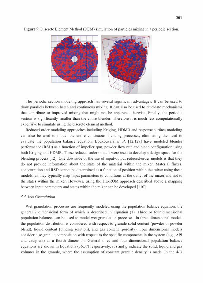
Discrete Element Method (DEM) simulation of particles mixing in a periodic section.

The periodic section modeling approach has several significant advantages. It can be used to draw parallels between batch and continuous mixing. It can also be used to elucidate mechanisms that contribute to improved mixing that might not be apparent otherwise. Finally, the periodic section is significantly smaller than the entire blender. Therefore it is much less computationally expensive to simulate using the discrete element method.

Reduced order modeling approaches including Kriging, HDMR and response surface modeling can also be used to model the entire continuous blending processes, eliminating the need to evaluate the population balance equation. Boukouvala . [12,129] have modeled blender performance (RSD) as a function of impeller rpm, powder flow rate and blade configuration using both Kriging and HDMR. These reduced-order models were used to develop a design space for the blending process [12]. One downside of the use of input-output reduced-order models is that they do not provide information about the state of the material within the mixer. Material fluxes, concentration and RSD cannot be determined as a function of position within the mixer using these models, as they typically map input parameters to conditions at the outlet of the mixer and not to the states within the mixer. However, using the DE-ROM approach described above a mapping between input parameters and states within the mixer can be developed [110].

Wet granulation processes are frequently modeled using the population balance equation, the general 2 dimensional form of which is described in Equation (1). Three or four dimensional population balances can be used to model wet granulation processes. In three dimensional models the population distribution is considered with respect to granule solid content (powder or powder blend), liquid content (binding solution), and gas content (porosity). Four dimensional models consider also granule composition with respect to the specific components in the system (e.g., APIand excipient) as a fourth dimension. General three and four dimensional population balance equations are shown in Equations (36,37) respectively. , and indicate the solid, liquid and gas volumes in the granule, where the assumption of constant granule density is made. In the 4-D

equation and are two different solid phases whose compositions in the granule are defined [46,113,161,189].

(35)

(36)

The right hand side of the population balance equation for wet granulation typically includes a nucleation kernel, a coalescence or aggregation kernel and may also include a breakage kernel. These describe granule birth (nucleation), granule growth and attrition and are indicated by

and respectively in Equations (35,36) [120,190]. In practice it is preferable to solve lower dimensional PBMs, as 4-D models can become

prohibitively computationally expensive to solve. In order to reduce the dimensionality of a population balance model, one or more of the granule properties can be lumped into the other distributions [113]. For instance, if it is assumed that all granules of the same solid and liquid content also have the same gas content then it is possible to describe the 4-D population balance in 36 as a set of two 3 dimensional equations; the reduced PBE (Equation (37)) and a gas balance equation (Equation (38)). The gas balance equation relates the total gas volume in a particular discretization bin to the volume of gas in each particle and the inflow and outflow of gas for the entire bin [113,191,192].

(37)

(38)

Barrasso and Ramachandran [113] have investigated a variety of model reduction options and have determined that the best performance is obtained when the gas volume is the lumped parameter, as in Equations (37,38). This reduction gave performance closest to that of the full 4-Dpopulation balance model. This is consistent with expectations because gas volume is known to have little effect on aggregation and prior work has indicated that lumped parameters should be chosen such that they have little effect on aggregation rates in order to minimize the error resulting from order reduction [191].

The development of kernels for the nucleation, aggregation and breakage represents a major research area in population balance modeling for wet granulation. Of these the aggregation kernel has been studied most extensively [193]. Kernels can be developed mechanistically or empirically. Often a combination of the two approaches is used and kernels are determined semi-empirically, with parameters fitted based on experimental or simulated data [189,194,195].

Nucleation accounts for the creation of new granule nuclei from primary powder particles. Poon . [195] and have described a mechanistic kernel for nucleation that accounts for both wetting kinetics and nucleation thermodynamics. The kernel can be expressed generally as Equation (39) for zero order and Equation (40) for first order dependency on primary particle concentrations. A droplet-controlled nucleation regime is assumed.

(39)

(40)

is the number of primary particles in the nucleus and is the fraction of particles with properties , , within the nucleus. The nucleation coefficient depends on the binder solution flow rate ( ) and process temperature ( ) as well as the ideal gas constant ( ). is an adjustable parameter and is described as a spreading coefficient, which relates the nucleation coefficient to the particle properties ( , , ).

(41)

and can be determined based on the volume of the nucleus, the effective porosity and the liquid and solid granule volume.

Aggregation or coalescence kernels describe the rate of granule growth, which can occur through consolidation of wetted particles or through layering of fines onto existing granules [48]. The rate of aggregation depends on the probability of wetted particles colliding as well as on the likelihood that they will adhere to one another upon making contact. This in turn is influenced by liquid binder content and granule size as well as the particle velocities [190]. Numerous aggregation or coalescence kernels have been proposed in the literature. While it is beyond the scope of this work to consider them all here, interested readers are referred to Cameron . [190] and Liu . [193], both of which provide tabular summaries of coalescence kernels discussed in the literature with associated references. The general form of a coalescence kernel contains two terms; a rate constant that relates growth rate to operating conditions and size dependence term that shows the relationship between granule size and growth rate. It is the latter term which dictates the size distribution of the granules and it is thus of great interest to be able to model it accurately [193]. Theoretical models that have been developed to predict the likelihood of aggregation based on powder properties and binder properties often rely on force or energy balances. For instance, several authors [122,193,196] have implemented a coalescence kernel in which granules combine if the kinetic energy of the granules is dissipated through viscous interactions or through plastic deformation of the particles.

Despite the development of mechanistic aggregation kernels, empirical or semi-empirical kernels are often used in simulations due to the difficulty associated with developing mechanistic kernels that are detailed enough to accurately model the process without becoming too computationally expensive to evaluate [193]. For instance, Immanuel . [122] describe the theoretical development of a rigorous, mechanistic aggregation kernel, but in order to demonstrate a robust solution strategy for 3D population balances use a semi-empirical kernel.

Many of the aforementioned aggregation kernels apply to single component systems. However in cases where binder is added continuously it may be appropriate to consider the binder as a separate component. Marshall . [197] have described a 2 component aggregation kernel for continuous fluid bed granulation where the binder and powder are treated as separate components. Matsoukas . [198] have proposed a multi-dimensional aggregation kernel to consider the effect of granule composition on aggregation rate. This is particularly useful for pharmaceutical applications, as multi component powder blends are typically the material being granulated in the pharmaceutical industry. Composition dependence is particularly important in cases where blends are not well mixed prior to granulation or where the materials being blended have disparate properties that affect their propensity for coalescence.

Breakage kernels are relevant for both granulation and milling population balance models and are therefore discussed in section 4.6.

Granule drying is an inherent part of the wet granulation process. It typically carried out in a fluidized bed, so the models discussed will focus on fluidized bed drying. Mathematical models for granule drying vary in their level of detail from lumped parameter models to more detailed distributed parameter models. Distributed parameter models include continuum models, which use macroscopic laws to describe phenomena like heat and mass transfer, and discrete models like the pore network model which explicitly describe microscopic behavior [199]. Discrete models based on CFD can be used to describe granule fluidization within the dryer. Distributed models based on the population balance equation can be used to represent the distribution of properties like liquid content [112,161,200]. These models can be coupled with experimental information or data from more detailed mechanistic drying models to develop semi-empirical relations for drying rate or granule size as a function of dryer parameters like gas temperature and velocity [112,199]. For instance, Mortier . [112] have described a one-dimensional population balance model for granule drying that incorporates information obtained from more detailed mechanistic model. The PBM, shown in Equation (42), contains a single internal coordinate, the wetted radius , and a negative growth term, , associated with the reduction in particle size due to granule drying.

(42)

The growth term in Equation (42), can be determined empirically as a function of the drying gas temperature based on a more detailed mechanistic model as described in Mortier, Van Daele

[201]. A comprehensive review of various mechanistic models for fluidized bed drying is provided in Mortier, De Beer [200].

One of the first models to describe behavior of roll compaction processes was the rolling theory of granular solids proposed by Johanson [202]. Bindhumadhava . [62] have shown that this theory can accurately predict pressure profiles in the nip region of a roller compaction process, as well as the influence of material properties on nip angle and peak pressure. Johanson’s model

makes several simplifying assumptions, including isotropic, cohesive material, no-slip between the powder and the roll surface in the nip region (the material is frictional) and that all material within the nip region is compressed to a ribbon with a thickness equal to the exact gap between the rolls [203]. The required model inputs include effective angle of internal friction and angle of friction, which can be found experimentally, and the relationship between pressure and density for the powder of interest, which can be determined experimentally using a punch-die system similar to that found in a tablet press. The assumptions associated with Johanson’s model are reasonable for gravity fed roller compaction systems with smooth rollers of relatively large diameter (>500 mm) and powders with a high enough friction coefficient that the no-slip condition holds. In such cases this model agrees well with experimental data [63].

Johanson’s model describes the pressure gradients for the slip and nip regions according to Equations (43,44) tes the roll angle, S denotes the roll gap, D indicates the roller diameter, is the friction coefficient between the powder and the roll, is the effective angle of internal friction, the constant K indicates material compressibility rmal stress applied to the powder. The parameter A can be calculated from Equation (45), where is the angle of wall friction [61].

(43)

(44)

(45)

The nip angle ( ) is determined based on the assumption that the pressure gradients at the boundary between the no-slip and nip regions are equal. Thus setting Equations (43,44) equal to one another it is possible to calculate [62].

Based on Johanson’s model, the relative density exiting the process can be calculated from Equation (46), where is the pre consolidation relative density, is the roll force, and W is the roll width. The roll force can be calculated based on the roll diameter and width, the roll gap, the

[61].

(46)

The relevant equipment parameters in Equations (43–46) can generally be determined from the equipment geometry [63]. In some cases the roll force is determined experimentally as a function

of the hydraulic pressure set point for the equipment. The material properties such as the effective angle of internal friction, angle of wall friction, compressibility and preconsolidation relative density must be determined experimentally [61]. The use of instrumented roller compaction equipment to empirically obtain pressure profiles and torque information has been demonstrated by several authors [58,62]. This information can be used to empirically determine friction coefficients and angles as well as roll force. In addition, the obtained pressure profiles can be used to verify the pressures predicted by Johanson’s model.

One of the drawbacks of Johanson’s model is its inability to accurately predict ribbon density for incompressible materials. This is due to the use of the Jenike-Shield yield criterion. An alternative model has been proposed by Marhsall [204] which facilitates modeling of both compressible and incompressible materials by using the Coulomb-Mohr criterion. Although it is more generally applicable, the resulting model is far more complicated than Johanson’s model.Another alternative is the so called “slab method”, which uses a force balance on a slab of material to predict pressure distribution in powder under compression. The yield criterion for this model can also be adjusted to consider incompressible material such as metals [63,203]. Since most pharmaceutically relevant powders are compressible it is not typically necessary to consider alternate yield criterion, but other assumptions within Johanson’s model (e.g., that of smooth, relatively large rolls) are not always accurate.

Finite element models, which are akin to the discrete element method models discussed in section 3.2, have been shown to describe roller compaction processes with a high degree of accuracy [63,205]. The accuracy of these models can be attributed to the fact that they consider particle-particle and particle-roll interactions at a fundamental level. Information about the friction conditions, contact angles, process geometry, roll surface texture can thus be considered. However the utility of these models is limited by computational expense [203].

For simulation and optimization purposes, Hsu . [203] have proposed a dynamic model that is based on Johanson’s theory of rolling granular solids but incorporates the effect of changing roll gap on ribbon density. Johanson’s model assumes a constant roll gap. The ability to consider the process response to dynamic variability in roll gap is useful, as the roll gap typically varies with changes in the feed rate to the roller compactor. The model in Hsu . [203] combines Johanson’s model with a material balance to account for the variability in roll gap as a function of powder feed rate. In addition, delay differential equations are incorporated to account for the time dependent response of the feed rate, roll speed, and roll pressure to changes in the set point. This model has been implemented in gPROMS™ by Boukouvala . [14] for the simulation of a continuous tablet manufacturing process that incorporates dry granulation.

Size reduction by milling is common at both the drug substance and the drug product step of pharmaceutical manufacturing. Milling can be used to reach the desired particle size for an active pharmaceutical ingredient or granule size for a pharmaceutical blend to be used in tableting. Milling processes are often modeled using population balance equations similar to those discussed in sections 3.2 and 4.4. The PBEs used to describe a milling process can be discretized with respect

to time or spatial coordinates depending on the mill design and residence time [206,207]. Both one-dimensional and multi-dimensional population balance models for milling have been described in the literature [16,206,208]. However for pharmaceutical applications it is preferred to implementa multi-dimensional model as the materials being milled are typically granules, which may consist of multiple solid phases as well as a gas phases. A multi-dimensional population balancefacilitates consideration of composition variability with respect to each internal coordinate [207].

A general form of a multi-dimensional population balance that incorporates breakage is given by Equation (47) where s1 and s2 represent two different solid phases (e.g., API and excipient) and represents a gas phase and is time. For a wet milling process a liquid phase could also be included.

(47)

The breakage term, , in Equation (47) accounts for the likelihood that a particle in a particular size class will break into smaller particles (breakage probability) and the distribution of sizes into which the particle will fragment (breakage distribution) [206,208]. Ageneral form of the breakage term is given in Equation (48), where the integral portion indicates the formation of particles in smaller size classes due to breakage of larger particles into smaller fragments and the second term indicates the loss of particles from a larger size class due to breakage. The breakage kernel, and the breakage function, , account for the rate at which particles break and the size distribution into which they fragment [14,66,198,209].

(48)

If it is assumed that the breakage rate is constant for a given size class, a simpler linear breakage kernel may be used. For short milling durations this assumption may be valid [16]. However, if this assumption is not made then the associated breakage rate expression should be formulated to incorporate nonlinear effects [206,208]. Breakage kernels can vary in complexity depending on the level of detail accounted for in the model. For multi-component systems a composition specific breakage kernel may be used to account for variable breakage rates and size distribution as a function of granule API or excipient content [14,198]. Semi-empirical breakage functions in which parameters are estimated from experimental data are common in the literature [66,208]. Heuristic approaches are also used in which breakage distributions of a particular form, often corresponding to the limiting case for an assumed fragmentation pattern, are applied [209,210].

Modeling of the tablet press unit operation includes modeling of powder flow into the dies and modeling the compaction process for powder blends. The modeling of flow into dies includes consideration of the feed frame, which supplies powder to the dies. Relatively little work has been

done in the literature to independently model the feed frame aspect of the tablet press, but Boukouvala [14] have described a response surface model for the residence time in the feed frame as a function of feed frame rotation rate and disk rotation rate.

The compaction of powders in confined geometries has been modeled extensively. Detailed modelsoften rely on discrete or finite element methodology as discussed in section 3.1 [72,95,96,98–100]. Semi-empirical models that describe the compaction behavior of granular materials by relating compaction pressure to relative density are also well established in the literature. A review of models describing compression behavior is provided in Patel [75]. Of particular interest are the Heckel [211,212] and Kawakita [213,214] equations, variations of which have been extensively used to model the compaction behavior of powder blends within tablet presses [74].

The Heckel equation (Equation (49)) assumes that the relationship between powder densificationand applied pressure is first-order.

(49)

In Equation (49) is the relative density, is applied pressure and is a material-specific constant. A is a constant densification term, where relates to the initial die filling process

and corresponds to densification from slippage and rearrangement of particles [75,211,212]. The Kawakita equation (Equation (50)) assumes that the relationship between applied pressure and powder volume is constant because particles are at equilibrium throughout the compression process.

(50)

is the initial porosity of the material and is the pressure that would result in a compression of the powder by one half of the total possible volume reduction [213,214]. The parameters for the Heckel and Kawakita equations can be found experimentally from force-displacement data [75].

Kuentz and Leuenberger [215] have described a modified Heckel equation that accounts for the effect of relative density on susceptibility to pressure, defined as the change in relative density in response to applied pressure. This model also incorporates a critical density, beyond which pressure susceptibility cannot be defined due to a lack of rigid structure. Singh . [216] describe a detailed model that can be used for process modeling and control of a tablet press which is based on the Kawakita equation. This model also incorporates an equation for tablet hardness as a function of compression force, proposed by Kuentz and Luenberger [73].

Modifications to the Kawakita equation to consider binary powders have been proposed to predict compaction behavior for powder blends. This is applicable in pharmaceutical case studies, as the material being compressed in a tablet press typically contains at least two components, an API and excipient. Frenning . [217] suggest the use of effective Kawakita parameters for mixtures, which are calculated based on the parameters for the individual components and a mixing

rule that assumes the component volumes are additive. Mazel . [218] propose a method that does not use effective Kawakita parameters, but applies the Kawakita equation to each component in the blend separately and assumes that volumes are additive. The implementation of these mixture models is particularly useful for blends in which the various components have very different physical properties.

Model verification and validation is a necessary part of the development process. Specificallyverification describes the process of determining whether the desired conceptual or mathematical model has been properly implemented while validation describes the process of ensuring that the developed model is sufficiently accurate for its intended purpose [219,220]. Verification and validation can be used to establish the predictive ability of the model and justify the use of the underlying theories and assumptions associated with the model equations [221]. Model validation is also an inherent part of the quality by design paradigm outlined in the ICH Q8 guidance for pharmaceutical development [3]. Model verification and validation should be carried out in parallel with process and model development, so that at each stage the existing model can be assessed and potential gaps in process knowledge and the associated model equations can be identified [222]. Issues with model implementation can also be addressed [219,221,223].

In order to validate a model, it is first necessary to identify its intended purpose, as this will dictate the validation criteria in terms of the model outputs to be considered, the domain over which the model should be valid and the level of prediction accuracy required [221,223]. The approach to model verification also depends on its planned use. Sargent [221] outlines four basic approaches: evaluation by the model development team, evaluation by the end users of the model in collaboration with the model development team, independent verification and validation (IV&V) by a third-party and evaluation using a scoring model. For the types of models discussed in the current work, the first two approaches are most likely to apply. These models are typically used in a process development context, and often the development team creates the model or collaborates closely with the group that creates the model. However in cases where models are included in a regulatory filing the regulatory agency may become involved in assessing the model as an independent third party.

In order to carry out model validation for pharmaceutical unit operations it is necessary to conduct experiments to which model predictions can be compared. These experiments should be carried out in processing equipment comparable to the modeled units. If data-based models have been implemented, the validation data must be distinct from the data used in model development. In some cases it may be appropriate to verify a model against a more detailed simulation such as a discrete or finite element simulation [221]. For instance, in the case of a reduced-order model developed to approximate a detailed simulation using a semi-empirical or black box method such a validation process is appropriate [110].

Model validation can include both qualitative and quantitative assessments. Qualitative evaluations can be done through data visualization and sensitivity analysis. Preliminary evaluation of model predictive ability may be conducted through visualizing the model output in conjunction

with experimental data to determine how similar the predicted and observed behaviors are. For instance, parity plots may be used to qualitatively assess the discrepancy between predicted and experimentally obtained model outputs. Alternatively the predicted and observed data may be plotted on the same set of axes for visual comparison [119,221]. Model results may also be qualitatively validated by observing process trends or trajectories and confirming that they correspond with expected process behavior based on prior knowledge of process behavior [113,120]. Sensitivity analysis is the process of attributing variability in model outputs to uncertain model parameters and input variables [224]. Sensitivity metrics, which quantify the sensitivity of a model output to a particular input or collection of inputs, can be used as an indicator of qualitative model agreement with observed process behavior [221,225]. Sensitivity analysis also indicates which model parameters the process outputs are most sensitive to. Thus additional experimental effort can be directed towards fitting these parameters accurately [120,226].

Qualitative model assessment can be helpful in visualizing model performance, but isinsufficient to justify the use of a model for quantitative prediction of process outputs. A variety of metrics can be used to quantitatively assess model prediction accuracy [221,227]. In linear regression, the coefficient of determination (R2) can be used as an indicator of model fit. The coefficient of determination describes the strength of the linear relationship between the model inputs and responses, indicating the proportion of variance in the response that can be accounted for by a particular input [228]. In pharmaceutical modeling applications, more frequently used metrics of model performance are based on prediction error, including the sum of square error(SSE), the mean square error of prediction (MSEP) and root-mean square error of prediction (RMSEP) [229,230]. The mean square error of prediction can be defined as the expected squared distance between the predicted and true value of a model output and the root-mean square error of prediction is simply its square root. Unlike correlation-based metrics, such as the coefficient of determination, the mean square error of prediction and root mean square error of prediction aresensitive to the scale of the data [231].

Metrics like the coefficient of determination and the sum of square error and can be calculated based on direct comparison between experimental and simulated data that correspond to the samedesign and operating configuration. These metrics are relatively easy and computationally inexpensive to calculate and can characterize model accuracy under the specific conditions studied.However they do not provide any information about the error associated with model predictions of points not included in the original dataset. To obtain an estimate of the prediction error (MSEP, RMSEP) alternative validation procedures such as cross-validation and bootstrapping are needed.

Cross-validation, in which a subset of available data is excluded from the model building process and subsequently used to compare with model predictions, can be used to evaluate model performance metrics. In leave-one-out cross validation, a sample of size is partitioned into a calibration (model-building) set of size N-1 and a validation set of size 1. Cross-validation calculations are then carried out times with a different sample left out of the calibration set at each iteration. An average error over the cross validation calculations is then used to indicate model performance. Similar methods wherein a somewhat larger subset ( ) of the samples isused for validation and the calibration set is of size can also be implemented [231]. An

advantage of cross-validation is that it can provide a nearly unbiased estimate of prediction error. However, for relatively small sample sizes the variability in the estimates can be high, resulting in unstable error estimation [232,233]. Cross-validation, particularly as it pertains to multivariate regression and latent variable methods, is discussed extensively in the literature [234,235]. An alternative to cross validation is the bootstrap procedure. In this process, a bootstrap size ( ) is selected and the input space is randomly sampled times with replacement. Each set of samples is referred to as a bootstrap sample. The model evaluation metric of interest (e.g., SSE) is determined for the bootstrap sample. This process is repeated with a large number ( ) of bootstrap samples and the resulting metric is averaged over the bootstraps to provide an estimation of model error. The bootstrapping procedure can provide accurate error estimation for large values of

. In several cases bootstrapping has been shown to provide a more stable estimator of the error than cross validation procedures. This is particularly true for instances with small sample sizes [232,233,236,237].

Quantitative metrics like the mean square error of prediction are straightforward to calculate and useful in determining the validity of model predictions [230]. However the conclusions drawn from these metrics depend on the intended purpose of the model. In early process development a relatively large prediction error may be acceptable since the objective is simply to obtain a general understanding of process behavior. For applications like model predictive control (MPC) large model errors can prove problematic and are generally not acceptable [238,239].

Beyond metrics associated with prediction error, a number of statistical techniques can be used to objectively decide whether a model is sufficiently predictive for a given application. Statistical model validation involves the formulation of a null hypothesis (“the API concentration of a blend predicted from model X is within ±5% of the experimentally determined concentration”) and an alternative that may be the direct opposite of the null hypothesis. Subsequently a statistical metric that will be used to evaluate the hypothesis must be defined. Finally, a rejection criterion for the developed hypothesis should be determined [227,240]. A variety of statistical approaches for model validation are discussed in the literature. The most well-known is classical hypothesis testing in which the -test, -test or -test statistics may be used as a criterion for rejecting or accepting the null hypothesis [227,241]. Bayesian hypothesis testing uses the Bayes factor as a validation metric. The Bayes factor expresses the ratio between the conditional probability of observing the experimentally obtained results given that the null hypothesis is true and the conditional probability of observing the experimental data given that the alternative hypothesis is true [241]. An advantage of using the Bayes factor is that it can be applied to prediction accuracy for a single point or for an entire probability distribution function as described in Ling [227]. Statistical tests can also be used to determine confidence intervals for the model predictions relative to experimental observations. These can be used to define the range of model accuracy. In defining confidence intervals care should be taken to set appropriate confidence levels and consider the associated sampling requirements [221].

This section provides only a brief overview of model validation techniques. Model validation is an extensive topic in itself has been the subject of numerous publications. The validation methods discussed in the current work are summarized in Table 4 along with references in which they have

been applied to validate various types of models. Any of the aforementioned validation methods can be used alone or in conjunction with other techniques. The choice of model verification and validation approach as well as the validation criteria selected should be consistent with the intended use of the model.

Summary of validation methods discussed in the current work, including references in which the proposed validation methodology is implemented.

Data

visualization

Qualitative Straightforward to implement

and interpret

-Relies on visual assessment to

determine model quality;

-Preferable to use in conjunction

with quantitative model

assessment [242]

[62,113,120,

189,192,193]

Sensitivity

analysis

Qualitative Identifes important sources of

process variability

-Can require many model

runs to calculate some

sensitivity indices;

-Requires knowledge of factors

that contribute significantly to

sensitivity in practice

[14,225]

Direct

comparison

Quantitative (R2, SSE) -Straightforward and

inexpensive to calculate;

-Indicates model accuracy for a

specific design and operating

configuration

Does not provide an estimate of

the prediction error

[191,242]

Cross-

Validation

Quantitative (MSEP,

RMSEP)

Provides a nearly unbiased

estimate of prediction error

Can be an unstable error

estimator, particularly

for small datasets

[42,78,85,110,

234,235,243]

Bootstrapping Quantitative (MSEP,

RMSEP, .)

-Provides a nearly unbiased

estimate of prediction error;

-More stable error estimator

than cross-validation,

particularly for small sample

sizes

Can become computationally

expensive as the number of

bootstraps increases

[244,245]

Hypothesis

Testing

Qualitative result (reject

or accept model) based

on a Quantitative

decision making criteria

( -test, -test, or -test

statistic or Bayes factor)

-Provides objective decision-

making criterion;

-Can be used to provide

confidence intervals for

model predictions

-Does not provide an exact

indication of model

prediction error;

-Can be difficult to implement

relative to other methods

[41,241]

Economic and regulatory pressures have led to increased interest in continuous processing forpharmaceutical applications in recent years [4,8,9]. Process systems engineering tools have a

significant role to play in the transition from batch to continuous processing. Predictive models are of particular interest, as they can contribute to cost effective and robust process development while enhancing process understanding in a fashion consistent with the ICH Q8 guidance on quality by design [3,10,15]. The use of process systems engineering tools for modeling and simulation of pharmaceutical processes has been increasingly reported in the literature in recent years [13–15,95,161,222]. This review has focused specifically on process modeling tools related to the production of tablets via continuous processing. An overview of continuous tableting processes including direct compaction, wet granulation and dry granulation manufacturing routes has been provided, along with a discussion of relevant processing equipment and equation-oriented unit operation models. Computational tools, including those related to detailed process modeling, reduced-order modeling and integrated flowsheet simulation have been discussed in some detail. Finally approaches for model validation have been discussed.

Significant work remains to be done in the area of solids-based process modeling, specifically as it pertains to pharmaceutical manufacturing. Understanding how variability in material properties of APIs and pharmaceutical blends that include these active ingredients affects the quality attributes of drug products remains a challenge in pharmaceutical process development [4,246]. Many existing process models do not sufficiently account for the impact of API physical properties on the performance of unit operations such as powder blending and conveying and the compaction of pharmaceutical blends. DEM simulation has contributed to understanding of the influence of particle-level properties on flow and compaction behavior as described in section 3.1, but connecting particle level properties in DEM to the bulk powder properties that are typically measured throughout process development remains a challenge. Another area where continued development is needed is in the area of tablet properties prediction. While models exist in the literature to predict tablet properties like hardness and dissolution performance as a function of operating conditions, these are relatively simplistic and may not sufficiently account for the effect of all relevant sources of variability in the tablet manufacturing process [73,161,216,247]. An ongoing challenge in the development of mathematical models for particulate processes is the inherent trade-off between the level of detail included in a model and computational efficiency. Detailed models may be more predictive and provide additional insight into the underlying system behavior, but their computational expense can become prohibitive for process simulation, optimization and MPC applications. Thus the development of reduced order or constitutive models to supplement detailed process models for applications where computational efficiency is important is an area where continued efforts will be needed.

The authors would like to acknowledge financial support from Bristol-Myers Squibb as well as from the Engineering Research Center for Structured Organic Particulate Systems at Rutgers University (NSF-0504497, NSF-ECC 0540855).

The authors declare no conflict of interest.

1. Suresh, P.; Basu, P.K. Improving pharmaceutical product development and manufacturing:Impact on cost of drug development and cost of goods sold of pharmaceuticals.

, , 175–187.2. Shah, N. Pharmaceutical supply chains: Key issues and strategies for optimisation.

, , 929–941.3.

; The International Conference on Harmonisation: Geneva, Switzerland, August 2009.4. McKenzie, P.; Kiang, S.; Tom, J.; Rubin, A.E.; Futran, M. Can pharmaceutical process

development become high tech? , , 3990–3994.5. Food and Drug Administration. ;

Food and Drug Administration: Silver Spring, MD, USA, 2006.6. Reinhardt, U.E. Perspectives on the pharmaceutical industry. ,

, 136–149.7. Basu, P.; Joglekar, G.; Rai, S.; Suresh, P.; Vernon, J. Analysis of manufacturing costs in

pharmaceutical companies. , , 30–40.8. Plumb, K. Continuous processing in the pharmaceutical industry—Changing the mind set.

, , 730–738.9. Buchholz, S. Future manufacturing approaches in the chemical and pharmaceutical industry.

, , 993–995.10. Aksu, B.; de Beer, T.; Folestad, S.; Ketolainen, J.; Linden, H.; Lopes, J.A.; de Matas, M.;

Oostra, W.; Rantanen, J.; Weimer, M. Strategic funding priorities in the pharmaceuticalsciences allied to quality by design (QBD) and process analytical technology (PAT).

, , 402–405.11. Schaber, S.D.; Gerogiorgis, D.I.; Ramachandran, R.; Evans, J.M.B.; Barton, P.I.; Trout, B.L.

Economic analysis of integrated continuous and batch pharmaceutical manufacturing: A casestudy. , , 10083–10092.

12. Boukouvala, F.; Muzzio, F.J.; Ierapetritou, M.G. Design space of pharmaceutical processesusing data-driven-based methods. , , 119–137.

13. Gernaey, K.V.; Gani, R. A model-based systems approach to pharmaceutical product-processdesign and analysis. , , 5757–5769.

14. Boukouvala, F.; Niotis, V.; Ramachandran, R.; Muzzio, F.J.; Ierapetritou, M.G. An integratedapproach for dynamic flowsheet modeling and sensitivity analysis of a continuous tabletmanufacturing process. , , 30–47.

15. Gernaey, K.V.; Cervera-Padrell, A.E.; Woodley, J.M. A perspective on PSE inpharmaceutical process development and innovation. , , 15–29.

16. Akkisetty, P.K.; Lee, U.; Reklaitis, G.V.; Venkatasubramanian, V. Population balancemodel-based hybrid neural network for a pharmaceutical milling process.

, , 161–168.17. Ramachandran, R.; Arjunan, J.; Chaudhury, A.; Ierapetritou, M.G. Model-based control-loop

performance of a continuous direct compaction process. , , 249–263.18. Singh, R.; Ierapetritou, M.; Ramachandran, R. System-wide hybrid MPC-PID control of a

continous pharmaceutical tablet manufacturing process via direct compaction. , doi:10.1016/j.ejpb.2013.02.019.

19. Singh, R.; Ierapetritou, M.; Ramachandran, R. An engineering study on the enhanced controland operation of continuous manufacturing of pharmaceutical tablets via roller compaction.

, , 307–326.20. Gao, Y.J.; Muzzio, F.J.; Ierapetritou, M.G. Optimizing continuous powder mixing processes

using periodic section modeling. , , 70–80.21. Troup, G.M.; Georgakis, C. Process systems engineering tools in the pharmaceutical industry.

, , 157–171.22. Järvinen, M.A.; Paaso, J.; Paavola, M.; Leivisk, K.; Juuti, M.; Muzzio, F.; Järvinen, K.

Continuous direct tablet compression: Effects of impeller rotation rate, total feed rate anddrug content on the tablet properties and drug release. ,doi:10.3109/03639045.2012.738681.

23. Anand, A.; Curtis, J.S.; Wassgren, C.R.; Hancock, B.C.; Ketterhagen, W.R. Predictingdischarge dynamics from a rectangular hopper using the discrete element method (DEM).

, , 5821–5830.24. Weir, G.J. A mathematical model for dilating, non-cohesive granular flows in steep-walled

hoppers. , , 149–161.25. Gremaud, P.A.; Matthews, J.V.; Schaeffer, D.G. On the computation of steady hopper flows

III: Model comparisons. , , 443–454.26. Faqih, A.M.N.; Alexander, A.W.; Muzzio, F.J.; Tomassone, M.S. A method for predicting

hopper flow characteristics of pharmaceutical powders. , ,1536–1542.

27. Ketterhagen, W.R.; Curtis, J.S.; Wassgren, C.R.; Kong, A.; Narayan, P.J.; Hancock, B.C.Granular segregation in discharging cylindrical hoppers: A discrete element and experimentalstudy. , , 6423–6439.

28. Ketterhagen, W.R.; Hancock, B.C. Optimizing the design of eccentric feed hoppers for tabletpresses using DEM. , , 1072–1081.

29. .; .; Mróz, Z.; Sielamowicz, I. Discrete-particle investigation offriction effect in filling and unsteady/steady discharge in three-dimensional wedge-shapedhopper. , , 159–174.

30. Engisch, W.E.; Muzzio, F.J. Method for characterization of loss-in-weight feeder equipment., , 395–403.

31. Gao, Y.J.; Muzzio, F.; Ierapetritou, M. Characterization of feeder effects on continuous solidmixing using fourier series analysis. , , 1144–1153.

32. Yang, S.; Evans, J.R.G. Metering and dispensing of powder; the quest for new solidfreeforming techniques. , , 56–72.

33. Berthiaux, H.; Marikh, K.; Gatumel, C. Continuous mixing of powder mixtures withpharmaceutical process constraints. , , 2315–2322.

34. Pernenkil, L.; Cooney, C.L. A review on the continuous blending of powders. , , 720–742.

35. Portillo, P.M.; Ierapetritou, M.G.; Muzzio, F.J. Characterization of continuous convectivepowder mixing processes. , , 368–378.

36. Marikh, K.; Berthiaux, H.; Gatumel, C.; Mizonov, V.; Barantseva, E. Influence of stirrer typeon mixture homogeneity in continuous powder mixing: A model case and a pharmaceuticalcase. , , 1027–1037.

37. Portillo, P.M.; Ierapetritou, M.G.; Muzzio, F.J. Effects of rotation rate, mixing angle, andcohesion in two continuous mixers—A statistical approach. , ,217–227.

38. Vanarase, A.U.; Muzzio, F.J. Effect of operating conditions and design parameters in acontinuous powder mixer. , , 26–36.

39. Portillo, P.M.; Vanarase, A.U.; Ingram, A.; Seville, J.K. Investigation of the effect of impellerrotation rate, powder flowrate, and cohesion on powder flow behavior in a continuous blenderusing pept. , , 5685–5668.

40. Koller, D.M.; Posch, A.; Horl, G.; Voura, C.; Radl, S.; Urbanetz, N.; Fraser, S.D.; Tritthart,W.; Reiter, F.; Schlingmann, M.; Continuous quantitative monitoring of powder mixingdynamics by near-infrared spectroscopy. , , 87–96.

41. Gao, Y.J.; Vanarase, A.; Muzzio, F.; Ierapetritou, M. Characterizing continuous powdermixing using residence time distribution. , , 417–425.

42. Jarvinen, K.; Hoehe, W.; Jarvinen, M.; Poutiainen, S.; Juuti, M.; Borchert, S. In-linemonitoring of the drug content of powder mixtures and tablets by near-infrared spectroscopyduring the continuous direct compression tableting process. , ,680–688.

43. Vanarase, A.U.; Alcala, M.; Rozo, J.I.J.; Muzzio, F.J.; Romanach, R.J. Real-time monitoringof drug concentration in a continuous powder mixing process using NIR spectroscopy.

, , 5728–5733.44. Martínez, L.; Peinado, A.; Liesum, L.; Betz, G. Use of near-infrared spectroscopy to quantify

drug content on a continuous blending process: Influence of mass flow and rotation speedvariations. , , 606–615.

45. Marikh, K.; Berthiaux, H.; Mizonov, V.; Barantsev, E. Experimental study of thestirring conditions taking place in a pilot plant continuous mixer of particulate solids.

, , 138–143.46. Faure, A.; York, P.; Rowe, R.C. Process control and scale-up of pharmaceutical wet

granulation processes: A review. , , 269–277.

47. Lee, K.T.; Ingram, A.; Rowson, N.A. Comparison of granule properties produced using twinscrew extruder and high shear mixer: A step towards understanding the mechanism of twinscrew wet granulation. , , 91–98.

48. Iveson, S.M.; Litster, J.D.; Hapgood, K.; Ennis, B.J. Nucleation, growth and breakagephenomena in agitated wet granulation processes: A review. , ,3–39.

49. Betz, G.; Junker-Burgin, P.; Leuenberger, H. Batch and continuous processing in theproduction of pharmaceutical granules. , , 289–297.

50. Vervaet, C.; Remon, J.P. Continuous granulation in the pharmaceutical industry. , , 3949–3957.

51. Tu, W.D.; Ingram, A.; Seville, J. Regime map development for continuous twin screwgranulation. , , 315–326.

52. Dhenge, R.M.; Cartwright, J.J.; Hounslow, M.J.; Salman, A.D. Twin screw wet granulation:Effects of properties of granulation liquid. , , 126–136.

53. Cartwright, J.J.; Robertson, J.; D’Haene, D.; Burke, M.D.; Hennenkamp, J.R. Twin screw wetgranulation: Loss in weight feeding of a poorly flowing active pharmaceutical ingredient.

, , 116–121.54. Vercruysse, J.; Cordoba Diaz, D.; Peeters, E.; Fonteyne, M.; Delaet, U.; van Assche, I.;

de Beer, T.; Remon, J.P.; Vervaet, C. Continuous twin screw granulation: Influence ofprocess variables on granule and tablet quality. , , 205–211.

55. Paltzer, S. Drying of wet agglomerates in a continuous fluid bed: Influence of residence time,air temperature and air-flowrate on the drying kinetics and the amount of oversize particles.

, , 463.56. Kleinebudde, P. Roll compaction/dry granulation: Pharmaceutical applications.

, , 317–326.57. Yu, S.; Gururajan, B.; Reynolds, G.; Roberts, R.; Adams, M.J.; Wu, C.Y. A comparative

study of roll compaction of free-flowing and cohesive pharmaceutical powders. , , 39–47.

58. Lecompte, T.; Doremus, P.; Thomas, G.; Perier-Camby, L.; Le Thiesse, J.-C.; Masteau, J.-C.;Debove, L. Dry granulation of organic powders—Dependence of pressure 2d-distribution ondifferent process parameters. , , 3933–3940.

59. Boswell, S.; Smith, G. Improving solid dosage forms with dry granulation., , 31.

60. Sharma, A.; Sharma, A.; Chauhan, C.S. Roller compaction: Imperative process for tabletmanufacturing: A review. , , 40–47.

61. Reynolds, G.; Ingale, R.; Roberts, R.; Kothari, S.; Gururajan, B. Practical application of rollercompaction process modeling. , , 1049–1057.

62. Bindhumadhavan, G.; Seville, J.P.K.; Adams, N.; Greenwood, R.W.; Fitzpatrick, S. Rollcompaction of a pharmaceutical excipient: Experimental validation of rolling theory forgranular solids. , , 3891–3897.

63. Dec, R.T.; Zavaliangos, A.; Cunningham, J.C. Comparison of various modeling methods foranalysis of powder compaction in roller press. , , 265–271.

64. Miguélez-Morán, A.M.; Wu, C.-Y.; Seville, J.P.K. The effect of lubrication on densitydistributions of roller compacted ribbons. , , 52–59.

65. Nakach, M.; Authelin, J.R.; Chamayou, A.; Dodds, J. Comparison of various millingtechnologies for grinding pharmaceutical powders. , ,S173–S181.

66. Reynolds, G.K. Modelling of pharmaceutical granule size reduction in a conical screen mill., , 383–392.

67. Verheezen, J.J.; van der Voort Maarschalk, K.; Faassen, F.; Vromans, H. Milling ofagglomerates in an impact mill. , , 165–172.

68. Vendola, T.A.; Hancock, B.C. The effect of mill type on two dry-granulated placeboformulations. , , 72–86.

69. Samanta, A.K.; Ng, K.Y.; Heng, P.W. Cone milling of compacted flakes: Process parameterselection by adopting the minimal fines approach. , , 17–23.

70. Motzi, J.J.; Anderson, N.R. The quantitative evaluation of a granulation milling process ii.Effect of output screen size, mill speed and impeller shape. , ,713–728.

71. Inghelbracht, S.; Remon, J.P. Reducing dust and improving granule and tablet quality in theroller compaction process. , , 195–206.

72. Mehrotra, A.; Chaudhuri, B.; Faqih, A.; Tomassone, M.S.; Muzzio, F.J. A modelingapproach for understanding effects of powder flow properties on tablet weight variability.

, , 295–300.73. Kuentz, M.; Lunenberger, H. A new model for the hardness of a compacted particle systems,

applied to tablets of pharmaceutical polymers. , , 145–153.74. Gentis, N.D.; Betz, G. Compressibility of binary powder formulations: Investigation and

evaluation with compaction equations. , , 777–793.75. Patel, S.; Kaushal, A.M.; Bansal, A.K. Effect of particle size and compression force on

compaction behavior and derived mathematical parameters of compressibility. , , 111–124.

76. Wu, C.Y.; Ruddy, O.M.; Bentham, A.C.; Hancock, B.C.; Best, S.M.; Elliott, J.A. Modellingthe mechanical behaviour of pharmaceutical powders during compaction.

, , 107–117.77. Podczeck, F. Methods for the practical determination of the mechanical strength of

tablets—From empiricism to science. , , 214–232.78. Corredor, C.C.; Bu, D.; Both, D. Comparison of near infrared and microwave resonance

sensors for at-line moisture determination in powders and tablets. ,, 84–93.

79. Zavaliangos, A.; Galen, S.; Cunningham, J.; Winstead, D. Temperature evolution duringcompaction of pharmaceutical powders. , , 3291–3304.

80. Onuki, Y.; Kawai, S.; Arai, H.; Maeda, J.; Takagaki, K.; Takayama, K. Contribution of thephysicochemical properties of active pharmaceutical ingredients to tablet properties identifiedby ensemble artificial neural networks and Kohonen’s self-organizing maps.

, , 2372–2381.81. Govedarica, B.; Ilic, I.; Sibanc, R.; Dreu, R.; Srcic, S. The use of single particle mechanical

properties for predicting the compressibility of pharmaceutical materials. , , 43–51.

82. Wang, J.; Wen, H.; Desai, D. Lubrication in tablet formulations. , , 1–15.

83. Jackson, S.; Sinka, I.C.; Cocks, A.C. The effect of suction during die fill on a rotary tabletpress. , , 253–256.

84. Hancock, B.C.; Ketterhagen, W.R. Discrete element method (DEM) simulations of stratifiedsampling during solid dosage form manufacturing. , , 265–272.

85. Otsuka, M.; Yamane, I. Prediction of tablet properties based on near infrared spectra of rawmixed powders by chemometrics: Scale-up factor of blending and tableting processes.

, , 4296–4305.86. Yu, A.B. Discrete element method—An effective way for particle scale research of

particulate matter. , , 205–214.87. Zhu, H.P.; Zhou, Z.Y.; Yang, R.Y.; Yu, A.B. Discrete particle simulation of particulate

systems: Theoretical developments. , , 3378–3396.88. Zhu, H.P.; Zhou, Z.Y.; Yang, R.Y.; Yu, A.B. Discrete particle simulation of particulate

systems: A review of major applications and findings. , , 5728–5770.89. Persson, A.S.; Frenning, G. An experimental evaluation of the accuracy to simulate granule

bed compression using the discrete element method. , , 249–256.90. Siiria, S.M.; Antikainen, O.; Heinamaki, J.; Yliruusi, J. 3d simulation of internal tablet

strength during tableting. , , 593–603.91. Jerier, J.F.; Hathong, B.; Richefeu, V.; Chareyre, B.; Imbault, D.; Donze, F.V.; Doremus, P.

Study of cold powder compaction by using the discrete element method. , , 537–541.

92. Yi, L.Y.; Dong, K.J.; Zou, R.P.; Yu, A.B. Coordination number of the packing of ternarymixtures of spheres: DEM simulations measurements. , ,8773–8785.

93. McCarthy, J.J.; Jasti, V.; Marinack, M.; Higgs, C.F. Quantitative validation of the discreteelement method using an annular shear cell. , , 70–77.

94. Wu, C.Y.; Cocks, A.C.F. Numerical and experimental investigations of the flow of powderinto a confined space. , , 304–324.

95. Ketterhagen, W.R.; Ende, M.T.A.; Hancock, B.C. Process modeling in the pharmaceuticalindustry using the discrete element method. , , 442–470.

96. Wu, C.Y. DEM simulations of die filling during pharmaceutical tabletting. , , 412–418.

97. Wu, C.-Y.; Guo, Y. Numerical modelling of suction filling using DEM/CFD., , 231–238.

98. Guo, Y.; Kafui, K.D.; Wu, C.Y.; Thornton, C.; Seville, J.P.K. A coupled DEM/CFD analysisof the effect of air on powder flow during die filling. , , 49–62.

99. Guo, Y.; Wu, C.-Y.; Kafui, K.D.; Thornton, C. Numerical analysis of density-inducedsegregation during die filling. , , 111–119.

100. Guo, Y.; Wu, C.Y.; Kafui, K.D.; Thornton, C. 3D DEM/CFD analysis of size-induced segregation during die filling. , , 177–188.

101. Gethin, D.T.; Yang, X.S.; Lewis, R.W. A two dimensional combined discrete and finite element scheme for simulating the flow and compaction of systems comprising irregular particles. , , 5552–5565.

102. Frenning, G. Compression mechanics of granule beds: A combined finite/discrete element study. , , 2464–2471.

103. Nwose, E.N.; Pei, C.L.; Wu, C.Y. Modelling die filling with charged particles using DEM/CFD. , , 229–235.

104. Bertrand, F.; Leclaire, L.A.; Levecque, G. DEM-based models for the mixing of granular materials. , , 2517–2531.

105. Marigo, M.; Davies, M.; Leadbeater, T.; Cairns, D.L.; Ingram, A.; Stitt, E.H. Application of positron emission particle tracking (PEPT) to validation a discrete element method (DEM)model of granular flow and mixing in the turbula mixer. , , 1811–1824.

106. Remy, B.; Khinast, J.G.; Glasser, B.J. Polydisperse granular flows in a bladed mixer: Experiments and simulations of cohesionless spheres. , , 1811–1824.

107. Remy, B.; Canty, T.M.; Khinast, J.G.; Glasser, B.J. Experiments and simulations of cohesionless particles with varying roughness in a bladed mixer. , ,4557–4571.

108. Sarkar, A.; Wassgren, C.R. Comparison of flow microdynamics for a continuous granular mixer with predictions from periodic slice DEM simulations. , ,325–336.

109. Gao, Y.J.; Muzzio, F.J.; Ierapetritou, M.G. A review of the residence time distribution (RTD)applications in solid unit operations. , , 416–423.

110. Boukouvala, F.; Gao, Y.J.; Muzzio, F.; Ierapetritou, M.G. Reduced-order discrete element method modeling. , , 12–26.

111. Griffin, D.W.; Mellichamp, D.A.; Doherty, M.F. Reducing the mean size of api crystals by continuous manufacturing with product classification and recycle. , ,5770–5780.

112. Mortier, S.T.F.C.; Gernaey, K.V.; de Beer, T.; Nopens, I. Development of a population balance model of a pharmaceutical drying process and testing of solution methods.

, , 39–53.113. Barasso, D.; Ramachandran, R. A comparison of model order reduction techniques for a

four-dimensional population balance model describing multi-component wet granulation process. , , 380–392.

114. Langham, Z.A.; Booth, J.; Hughes, L.P.; Reynolds, G.K.; Wren, S.A.C. Mechanistic insights into the dissolution of spray-dried amorphous solid dispersions. , ,2798–2810.

115. Sen, M.; Ramachandran, R. A multi-dimensional population balance model approach to continuous powder mixing processes. , , 51–59.

116. Ramkrishna, D.; Academic Press: London, UK, 2000.

117. Majumbder, A.; Kariwala, V.; Ansumali, S.; Rajendran, A. Lattice boltzmann method for population balance equations with simultaneous growth, nucleation, aggregation and breakage. , , 4884–4893.

118. Ramachandran, R.; Barton, P.I. Effective parameter estimation within a multi-dimensional population balance model framework. , , 4884–4893.

119. Sen, M.; Singh, R.; Vanarase, A.; John, J.; Ramachandran, R. Multi-dimensional population balance modeling and experimental validation of continuous powder mixing processes.

, , 349–360. 120. Ramachandran, R.; Immanuel, C.D.; Stepanek, F.; Litster, J.D.; Doyle, F.J. A mechanistic

model for breakage in population balances of granulation: Theoretical kernel development and experimental validation. , , 598–614.

121. Immanuel, C.D.; Doyle, F.J. Computationally efficient solution of population balance models incorporating nucleation, growth and coagulation: Application to emulsion polymerization.

, , 3681–3698. 122. Immanuel, C.D.; Doyle, F.J. Solution technique for a multi-dimensional population balance

model describing granulation processes. , , 213–225. 123. Boukouvala, F.; Dubey, A.; Vanarase, A.; Ramachandran, R.; Muzzio, F.J.; Ierapetritou, M.

Computational approaches for studying the granular dynamics of continuous blending processes, 2—Population balance and data-based methods. ,

, 9–19. 124. Lang, Y.D.; Zitney, S.E.; Biegler, L.T. Optimization of IGCC processes with reduced order

CFD models. , , 1705–1717. 125. Zitney, S.E. Process/equipment co-simulation for design and analysis of advanced energy

systems. , , 1532–1542. 126. Brenner, T.A.; Fontenot, R.L.; Cizmas, P.G.A.; O’Brien, T.J.; Breault, R.W. A reduced-order

model for heat transfer in multiphase flow and practical aspects of the proper orthogonal decomposition. , , 68–80.

127. Liberge, E.; Hamdouni, A. Reduced order modelling method via proper orthogonal decomposition (POD) for flow around an oscillating cylinder. , ,292–311.

128. Lang, Y.D.; Malacina, A.; Biegler, L.T.; Munteanu, S.; Madsen, J.I.; Zitney, S.E. Reduced order model based on principal component analysis for process simulation and optimization.

, , 1695–1706.

129. Boukouvala, F.; Muzzio, F.J.; Ierapetritou, M.G. Predictive modeling of pharmaceutical processes with missing and noisy data. , , 2860–2872.

130. Box, G.E.P. On the experimental attainment of optimum conditions. , , 1–35.

131. Jia, Z.; Davis, E.; Muzzio, F.J.; Ierapetritou, M.G. Predictive modeling for pharmaceutical processes using kriging and response surface. , , 174–186.

132. Khuri, A.I.; Mukhopadhyay, S. Response surface methodology. ,, 128–149.

133. Myers, R.H.; Montgomery, D.C.; John Wiley & Sons, Inc.: New York, NY, USA,

2002.134. Ranjbarian, S.; Farhadi, F. Evaluation of the effects of process parameters on granule mean

size in a conical high shear granulator using response surface methodology. , , 186–190.

135. Metheron, G. Principles of geostatistics. , , 1246–1266. 136. Calder, C.A.; Cressie, N. Kriging and Variogram Models. In

; Kitchin, R., Thrift, N., Eds.; Elsevier Science: Oxford, UK, 2009; Volume 1, pp. 49–55.

137. Krige, D.G. A Statistical Approach to Some Mine Valuations and Allied Problems at the Witwatersrand. Master Thesis, University of Witwatersrand, Johannesburg, North Africa, 1951.

138. Boukouvala, F.; Muzzio, F.J.; Ierapetritou, M.G. Dynamic data-driven modeling of pharmaceutical processes. , , 6743–6754.

139. Boukouvala, F.; Ierapetritou, M.G. Feasibility analysis of black-box processes using adaptive sampling kriging based method. , , 358–368.

140. Kleijnen, J.P.C. Kriging metamodeling in simulation: A review. , ,707–716.

141. Huang, J.; Kaul, G.; Cai, C.; Chatlapalli, R.; Hernandez-Abad, P.; Gosh, K.; Nagi, A. Quality by design case study: An integrated multivariate approach to drug product and process development. , , 23–32.

142. Braumann, A.; Kraft, M.; Mort, P.R. Parameter estimation in a multidimensional granulation model. , , 196–210.

143. Li, G.Y.; Wang, S.W.; Rabitz, H. Practical approaches to construct RS-HDMR component functions. , , 8721–8733.

144. Li, G.Y.; Rabitz, H.; Hu, J.S.; Chen, Z.; Ju, Y.G. Regularized random-sampling high dimensional model representation (RS-HDMR). , , 1207–1232.

145. Li, G.; Rosenthal, C.; Rabitz, H. High dimensional model representations. , , 7765–7777.

146. Ziehn, T.; Tomlin, A.S. Global sensitivity analysis of a 3d street canyon model—Part I: The development of high dimensional model representations. , ,1857–1873.

147. Li, G.; Wang, S.-W.; Rabitz, H. High dimensional model representations (HDMR): Concepts and applications. Available online: http: //www.ima.umn.edu/talks/workshops/3-15-19.2000/li/hdmr.pdf (accessed on 10 April 2013).

148. Li, G.; Rabitz, H.; Wang, S.-W.; Georgopoulos, P.G. Correlation method for variance reduction of Monte Carlo integration in RS-HDMR. , , 277–283.

149. Li, G.; Rabitz, H. Ratio control variate method for efficiently determining high-dimensional model representations. , , 1112–1118.

150. Banerjee, I.; Pal, S.; Maiti, S. Computationally efficient black-box modeling for feasibility analysis. , , 1515–1521.

151. Banarjee, I.; Ierapetritou, M.G. Model independent parametric decision making. , , 135.

152. Li, G.Y.; Wang, S.W.; Rabitz, H.; Wang, S.Y.; Jaffe, P. Global uncertainty assessments by high dimensional model representations (HDMR). , , 4445–4460.

153. Ziehn, T.; Tomlin, A.S. A global sensitivity study of sulfur chemistry in a premixed methane flame model using HDMR. , , 742–753.

154. Ziehn, T.; Tomlin, A.S. GUI–HDMR—A software tool for global sensitivity analysis of complex models. , , 775–785.

155. Basheer, L.A.; Hajmeer, M. Artificial neural networks: Fundamentals, computing, design, and application. , , 3–31.

156. Agatonovic-Kustrin, S.; Beresford, R. Basic concepts of artificial neural network (ANN)modeling and its application in pharmaceutical research. , ,717–727.

157. De la Fuente, R.L.N.; Garcia-Munoz, S.; Biegler, L.T. An efficient nonlinear programming strategy for PCA models with incomplete data sets. , , 301–311.

158. Walczak, B.; Massart, D.L. Dealing with missing data: Part I. , , 15–27.

159. Walczak, B.; Massart, D.L. Dealing with missing data: Part II., , 28–42.

160. Noonan, R.; Wold, H. NIPALS path modelling with latent variables. , , 33–61.

161. Boukouvala, F.; Chaudhury, A.; Sen, M.; Zhou, R.J.; Mioduszewski, L.; Ierapetritou, M.G.; Ramachandran, R. Computer-aided flowsheet simulation of a pharmaceutical tablet manufacturing process incorporating wet granulation. , , 11–27.

162. Sen, M.; Chaudhury, A.; Singh, R.; John, J.; Ramachandran, R. Multi-scale flowsheet simulation of an integrated continuous purification-downstream pharmaceutical manufacturing process. , , 29–38.

163. Papavasileiou, V.; Koulouris, A.; Siletti, C.; Petrides, D. Optimize manufacturing of pharmaceutical products with process simulation and production scheduling tools.

, , 1086–1097. 164. ; Process Systems Enterprise, Ltd.: London, UK,

October 2012.

165. ; Process Systems Enterprise, Ltd.: London, UK, October 2012.

166. Process Systems Enterprise, Ltd.: London, UK, October 2012.

167. ; Process System Enterprise, Ltd.: London, UK,February 2004.

168. Minceva, M.; Rodrigues, A.E. Two-level optimization of an existing SMB for p-xylene separation. , , 2215–2228.

169. Asteasuain, M.; Brandolin, A. Modeling and optimization of a high-pressure ethylene polymerization reactor using gPROMS. , , 396–408.

170. Nowee, S.M.; Abbas, A.; Romagnoli, J.A. Optimization in seeded cooling crystallization: A parameter estimation and dynamic optimization study. , ,1096–1106.

171. Nowee, S.M.; Abbas, A.; Romagnoli, J.A. Antisolvent crystallization: Model identification,experimental validation and dynamic simulation. , , 5457–5467.

172. Bermingham, S.K.; Verheijen, P.J.T.; Kramer, H.J.M. Optimal design of solution crystallization processes with rigorous models. , , 894–903.

173. Beck, R. ; Aspen Technology, Inc.:Burlington, MA, USA, 2012.

174. Levine, J. ; Aspen Technology, Inc.: Burlington, MA, USA, 2012.

175. Chemical engineering: Software. Available online: https://uwaterloo.ca/chemical-engineering/resources-services/computing-facilities/software#AspenCustomModeler (accessed on 5 January 2013).

176. Aspen Plus. , Version v7.1; Aspen Technology, Inc.: Burlington, MA, USA, 2009.

177. Wei, H.-Y. Computer-aided design and scale-up of crystallization processes: Integrating approaches and case studies. , , 1377–1380.

178. Lau, S.-Y.; Gonawan, F.N.; Bhatia, S.; Kamaruddin, A.H.; Uzir, M.H. Conceptual design and simulation of a plant for the production of high purity (S)-ibuprofen acid using innovative enzymatic membrane technology. , , 726–737.

179. Brown, R.L. Minimum energy theorem for flow of dry granular materials through apertures. , , 458–461.

180. Savage, S.B. The mass flow of granular materials derived from coupled velocity-stress fields. , , 1885–1888.

181. Savage, S.B.; Sayed, M.S. Gravity flow of coarse cohesionless granular materials in conical hoppers. , , 125–143.

182. Brennen, C.; Pearce, J.C. Granular material flow in two dimensional hoppers. , , 43–50.

183. Nguyen, T.V.; Brennen, C.; Sabersky, R.H. Gravity flow of granular materials in conical hoppers. , , 529–535.

184. Sun, J.; Sundaresan, S. A constitutive model with microstructure evolution for flow of rate-independent granular materials. , , 590–616.

185. Weir, G.J. Sound speed and attenuation in dense, non-cohesive air-granulator systems. , , 3699–3717.

186. Sun, J.; Sundaresan, S. Radial hopper flow prediction using a constitutive model with microstructure evolution. , , 81–85.

187. Danckwerts, P.V. Continuous flow systems: Distribution of residence times. , , 1–13.

188. Gao, Y.; Ierapetritou, M.; Muzzio, F. Periodic section modeling of convective continuous powder mixing processes. , , 69–78.

189. Bouffard, J.; Bertrand, F.; Chaouki, J. A multiscale model for the simulation of granulation in rotor-based equipment. , , 106–117.

190. Cameron, I.T.; Wang, F.Y.; Immanuel, C.D.; Stepanek, F. Process systems modelling and applications in granulation: A review. , , 3723–3750.

191. Hounslow, M.J.; Pearson, J.M.K.; Instone, T. Tracer studies of high-shear granulation: II. Population balance modeling. , , 1984–1999.

192. Biggs, C.A.; Sanders, C.; Scott, A.C.; Willemse, A.W.; Hoffman, A.C.; Instone, T.; Salman, A.D.; Hounslow, M.J. Coupling granule properties and granulation rates in high-shear granulation. , , 162–168.

193. Liu, L.X.; Litster, J.D. Population balance modelling of granulation with a physically based coalescence kernel. , , 2183–2191.

194. Gannt, J.A.; Cameron, I.T.; Litster, J.D.; Gatzke, E.P. Determination of coalescence kernels for high-shear granulation using DEM simulations. , , 53–63.

195. Poon, J.M.-H.; Immanuel, C.D.; Doyle, F.J.I.; Litster, J.D. A three-dimensional population balance model of granulation with a mechanistic representation of the nucleation and aggregation phenomena. , , 1315–1329.

196. Liu, L.X.; Litster, J.D.; Iveson, S.M.; Ennis, B.J. Coalescence of deformable granules in wet granulation processes. , , 529–539.

197. Marshall, C.L.J.; Rajniak, P.; Matsoukas, T. Multi-component population balance modeling of granulation with continuous addition of binder. , , 211–220.

198. Matsoukas, T.; Kim, T.; Lee, K. Bicomponent aggregation with composition-dependent rates and the approach to well-mixed state. , , 787–799.

199. Sahni, E.K.; Chaudhuri, B. Contact drying: A review of experimental and mechanistic modeling approaches. , , 334–348.

200. Mortier, S.T.F.C.; de Beer, T.; Gernaey, K.V.; Remon, J.P.; Vervaet, C.; Nopens, I.Mechanistic modelling of fluidized bed drying processes of wet porous granules: A review.

, , 205–225. 201. Mortier, S.T.F.C.; van Daele, T.; Gernaey, K.V.; de Beer, T.; Nopens, I. Reduction of a single

granule drying model: An essential step in preparation of a population balance model with a continuous growth term. , , 1127–1138.

202. Johanson, J.R. A rolling theory for granular solids. , , 842–848.

203. Hsu, S.H.; Reklaitis, G.V.; Venkatasubramanian, V. Modeling and control of roller compaction for pharmaceutical manufacturing. Part I: Process dynamics and control framework. , , 14–23.

204. Marshall, E.A. A theory for the compaction of incompressible granular materials by rolling. , , 21–36.

205. Muliadi, A.R.; Litster, J.D.; Wassgren, J.R. Modeling the powder roll compaction process: Comparison of 2-D finite element method and the rolling theory for granular solids (Johanson’s model). , , 90–100.

206. Bilgili, L.; Capece, M. Quantitative analysis of multi-particle interactions during particle breakage: A discrete non-linear population balance framework. , ,162–173.

207. Verkoeijen, D.; Pouw, G.A.; Meesters, M.H.; Scarlett, B. Population balances for particulate processes—A volume approach. , , 2287–2303.

208. Bilgili, E.; Scarlett, B. Population balance modeling of non-linear effects in milling processes. , , 59–71.

209. Tsoy, E.N. A modelling approach for derivation of the breakage functions. , , 361–364.

210. Bilgili, E.; Yepes, J.; Scarlett, B. Formulation of a non-linear framework for population balance modeling of batch grinding: Beyond first-order kinetics. , ,33–44.

211. Heckel, R.W. An analysis of powder compaction phenomena. , , 1001–1008.

212. Heckel, R.W. Density pressure relationships in powder compaction. , , 671–675.

213. Kawakita, K.; Ludde, K.H. Some considerations on powder compression equations. , , 61–68.

214. Kawakita, K.; Hattori, I.; Kishigami, M. Characteristic constants in kawakita’s powder compression equation. , , 3–8.

215. Kuentz, M.; Leuenberger, H. Pressure susceptibility of polymer tablets as a critical property: A modified Heckel equation. , , 174–179.

216. Singh, R.; Gernaey, K.V.; Gani, R. Icas-pat: A software for design, analysis and validation of PAT systems. , , 1108–1136.

217. Frenning, G.; Nordström, J.; Alderborn, G. Effective Kawakita parameters for binarymixtures. , , 270–275.

218. Mazel, V.; Busignies, V.; Duca, S.; Leclerc, B.; Tchoreloff, P. Original predictive approach to the compressibility of pharmaceutical powder mixtures based on the Kawakita equation.

, , 92–98. 219. Robinson, S.; Brooks, R.J. Independent verification and validation of an industrial simulation

model. , , 405–416. 220. Davies, P.K.

; RAND: Santa Monica, CA, USA, 1992.

221. Sargent, R.G. Verification and Validation of Simulation Models. In Proceedings of the 2010 Winter Simulation Conference, Baltimore, MD, USA, 5–8 December 2010.

222. Kremer, D.M.; Hancock, B.C. Process simulation in the pharmaceutical industry: A review of some basic physical models. , , 517–529.

223. Balci, O. Golden rules of verification, validation, testing, and certification of modeling and simulation applications. , No. 4.

224. Saltelli, A.; Chan, K.; Scott, E.M. ; John Wiley & Sons Ltd.: Chichester,UK, 2000.

225. Saltelli, A.; Tarantola, S.; Campolongo, F. Sensitivity analysis as an ingredient of modeling. , , 377–395.

226. Sin, G.; Gernaey, K.V.; Eliasson Lantz, A. Good modelling practice (gmop) for pat applications: Propagation of input uncertainty and sensitivity analysis. ,

, 1043–1053.227. Ling, Y.; Mahadevan, S. Quantitative model validation techniques: New insights.

, , 217–231. 228. Rodgers, J.L.; Nicewander, W.A. Thirteen ways to look at the correlation coefficient.

, , 59–66. 229. Min, F.Y.; Yang, M.; Wang, Z.C. Knowledge-based method for the validation of complex

simulation models. , , 500–515. 230. Tedeschi, L.O. Assessment of the adequacy of mathematical models. , ,

225–247.231. Browne, M.W. Cross-validation methods. , , 108–132. 232. Efron, B.; Gong, G. A leisurely look at the bootstrap, the jackknife and cross-validation.

, , 36–48. 233. Efron, B. Estimating the error rate of a prediction rule: Improvement on cross-validation.

, , 316–331. 234. Tomba, E.; de Martin, M.; Facco, P.; Robertson, J.; Zomer, S.; Bezzo, F.; Barolo, M. General

procedure to aid the development of continuous pharmaceutical processes using multivariate statistical modeling—An industrial case study. , , 25–39.

235. Hassani, S.; Martens, H.; Qannari, E.M.; Hanafi, M.; Kohler, A. Model validation and error estimation in multi-block partial least squares regression. ,

, 42–53. 236. Steyerberg, E.W.; Harrell, F.E.J.; Borsboom, G.J.J.M.; Eijkemans, M.J.C.R.; Vergouwe, Y.;

Habbema, J.D.F. Internal validation of predictive models: Efficiency of some procedures for logistic regression analysis. , , 775–781.

237. Gong, G. Cross-validation, the jackknife, and the bootstrap: Excess error estimation in forward logistic regression. , , 108–113.

238. Ji, G.; Zhang, K.; Zhu, Y. A method of MPC model error detection. ,. 635–642.

239. Zhu, Y.; Patwardan, R.; Wagner, S.B.; Zhao, J. Toward a low cost and high performance MPC: The role of system identification. , , 124–135.

240. Robinson, A.P.; Froese, R.E. Model validation using equivalence tests. ,, 349–358.

241. Rebba, R.; Mahadevan, S. Validation of models with multivariate output. , , 861–871.

242. Capece, M.; Bilgile, E.; Dave, R. Identification of the breakage rate and distribution parameters in a non-linear population balance model for batch milling.

, , 195–204. 243. Vanarase, A.U.; Jarvinen, M.; Passo, J.; Muzzio, F.J. Development of a methodology to

estimate error in the on-line measurements of blend uniformity in a continuous powder mixing process. , , 263–271.

244. Babamoradi, H.; van den berg, F.; Rinnan, A. Bootstrap based confidence limits in principal component analysis—A case study. , , 97–105.

245. Afanador, N.L.; Tran, T.N.; Buydens, L.M.C. Use of the bootstrap and permutation methods for a more robust variable importance in the projection metric for partial least squares regression. , , 49–56.

246. Ng, K.M. Design and development of solids processes—A process systems engineering perspective. , , 205–210.

247. Kimber, J.A.; Kazarian, S.G.; , F. Microstructure-based mathematical modelling and spectroscopic imaging of tablet dissolution. , , 1326–1339.

229

Averaging Level Control to Reduce Off-Spec Material in aContinuous Pharmaceutical Pilot Plant

Richard Lakerveld, Brahim Benyahia, Patrick L. Heider , Haitao Zhang , Richard D. Braatzand Paul I. Barton

Abstract: The judicious use of buffering capacity is important in the development of future

continuous pharmaceutical manufacturing processes. The potential benefits are investigated of using

optimal-averaging level control for tanks that have buffering capacity for a section of a continuous

pharmaceutical pilot plant involving two crystallizers, a combined filtration and washing stage and a

buffer tank. A closed-loop dynamic model is utilized to represent the experimental operation, with

the relevant model parameters and initial conditions estimated from experimental data that contained

a significant disturbance and a change in setpoint of a concentration control loop. The performance

of conventional proportional-integral (PI) level controllers is compared with optimal-averaging level

controllers. The aim is to reduce the production of off-spec material in a tubular reactor by

minimizing the variations in the outlet flow rate of its upstream buffer tank. The results show a

distinct difference in behavior, with the optimal-averaging level controllers strongly outperforming

the PI controllers. In general, the results stress the importance of dynamic process modeling for the

design of future continuous pharmaceutical processes.

Reprinted from Processes. Cite as: Lakerveld, R.; Benyahia, B.; Heider, P.L.; Zhang, H.;

Braatz, R.D.; Barton, P.I. Averaging Level Control to Reduce Off-Spec Material in a Continuous

Pharmaceutical Pilot Plant. Processes 2013, 1, 330–348.

1. Introduction

Continuous manufacturing holds promise to improve the reliability and profitability of future

pharmaceutical processes [1–6]. Significant progress has been achieved to exploit continuous

operation of various unit operations that are typically used in pharmaceutical processes [7–34].

Furthermore, system-wide benefits may exist by, for example, exploiting material recycling and

improved process control based on real-time understanding of the final product quality, as well as

critical material attributes of streams within the process. Consequently, pharmaceutical companies

are interested in the potential benefits of transforming the manufacturing of pharmaceutical products

from a conventional batch-wise mode of operation to continuous flow mode [35]. The role of process

modeling is expected to increase significantly during this transition to enable improved design and

operation [33,36–43].

A key ingredient in enabling the reliable operation of continuous pharmaceutical manufacturing

processes is the development of automated control strategies. In particular, judicious use of the

buffering capacity of tanks is needed to avoid high concentrations of impurities in a small fraction of

the produced tablets and to avoid sharp variations in flow rate propagating throughout the complete

230

process. However, on the downside, extensive use of buffering capacity will lead to sluggish process

behavior. Therefore, an appropriate design of automated control strategies around buffer tanks is of

importance for the viability of continuous pharmaceutical manufacturing.

The aim of this paper is to identify the potential benefits of using optimal-averaging level

control [44] over conventional proportional-integral (PI) feedback level control for an integrated

continuous pharmaceutical pilot plant. The pilot plant was constructed within the Novartis-MIT

Center for Continuous Manufacturing to produce a pharmaceutical product from start (raw materials

for intermediate compounds) to finish (tablets in final dosage form) in a fully continuous fashion [45]

and features several cascades of well-mixed tanks. The level of all tanks within the pilot plant were

initially controlled with proportional (P)-feedback control only. A plant-wide dynamic model is used

to investigate the potential benefits of replacing these level control loops with more advanced control

strategies. The plant-wide dynamic model is presented in detail elsewhere [42] and has been extended

with control loops in subsequent work [43].

The focus of this paper is on a characteristic sequence of unit operations within the continuous

pharmaceutical pilot plant. A closed-loop model is used to simulate the behavior of the unit

operations, including automated control loops with P-feedback control. The unknown parameters

and initial conditions are estimated from experimental data, which includes the behavior of several

level control loops and a concentration control loop in the presence of a significant disturbance and a

setpoint change. The focus is on the main compounds in the system to obtain a realistic description

of at least the overall mass balance, such that control strategies for buffering can be investigated.

Subsequently, the closed-loop dynamic model is used to investigate the potential benefits of replacing

the P-feedback level controllers with more extended controllers. First, we will focus on PI level

controllers with tuning rules that specifically aim to achieve averaging level control (PI-ALC).

Second, process simulations are investigated, where the conventional level controllers are replaced

with optimal averaging level control (OALC). The advantage of OALC over conventional PI-ALC is

that with OALC, flow optimality can be achieved for a known magnitude of an input disturbance. The

results illustrate the importance of advanced control strategies to exploit systematically the buffering

capacity of a cascade of buffer tanks in future continuous pharmaceutical processes.

2. Approach

2.1. Process Description and Control Structure

A schematic representation of the studied part of the integrated continuous pharmaceutical pilot

plant is given in Figure 1. A detailed description of the design of the pilot plant is presented

elsewhere [45]. In this section, key elements are summarized that have a direct connection to the

work presented in the present paper. An intermediate compound A is synthesized and dissolved

in solvent S1 upstream. Compound A is a reagent for the synthesis of an active pharmaceutical

ingredient further downstream and is separated from solution via a cascade of two continuous

crystallization steps followed by a continuous wash and filtration step. Supersaturation is generated

231

in the crystallizers via cooling and addition of an anti-solvent (S2) to the second crystallizer, which

reduces the solubility of compound A four-fold [22]. The temperature within the crystallizers is kept

constant via thermostatic baths connected to the jackets of the crystallizers. Both crystallizers are

equipped with level sensors (Omega LVCN414) that are calibrated to measure the total volume of the

material in each crystallizer. The outlet flows of the crystallizers consist of a slurry with suspended

crystals in mother liquor, which are largely separated in a continuous wash and filtration stage (W1).

The purified slurry of compound A is collected in a buffer tank that can be used for dilution (D1) to

which solvent can be added to dilute the slurry. The dilution tank is also equipped with a calibrated

level sensor (Omega LVCN414) and an online density meter (Anton Paar DPRn 417) calibrated to

measure the concentration of compound A in the tank. The outlet flow rate of the buffer tank is fed

to a tubular reactor downstream for synthesis of a second intermediate compound. The variations

in composition and flow rate of the material leaving the buffer tank have a significant impact on the

performance of the reaction downstream. Therefore, to reduce the production of off-spec material in

the complete process, a feedback concentration control loop is used to maintain the concentration of

compound A in D1 close to a desired setpoint. The outlet flow rate of the buffer tank is manipulated

to control the level in the tank. The variations in concentration and outlet flow rate should be

minimized to maintain a constant residence time in the tubular reactor downstream. A Siemens

SIMATIC PCS7 process control system was used for data archiving and implementation of the

experimentally tested control loops. Such a control system allows for the flexible implementation

of desired control strategies.

Figure 1. Process flowsheet of a section of a continuous pharmaceutical pilot plant that

consists of two crystallizers in series (Cr1–2), a washing and filtration stage (W1), and a

buffer tank that can be used for dilution (D1). The section has three automated feedback

level control loops (LC1–3), two automated temperature control loops (TC1–2) and an

automated feedback concentration control loop (CC1).

From reactor 1sp

D1

LC1 LC2Cr1 Cr2

W1

LC3

spsp

sp

CC1sp

P1 P3

P6

TC1

S 2 P2

P4

P5

To reactor 2

sp

TC2

1 2

3

4

5

S 1

S 1

The tuning of the P-only feedback level controllers of the crystallizers aims to provide both

stability and flow filtering to damp out fluctuations in flow rate. Therefore, the gains of the level

controllers of the crystallizers, as implemented in the pilot plant, are chosen, such that the outlet flow

232

rate of a crystallizer is approximately at the maximum flow rate when the level in the crystallizer

reaches an upper limit (Vmax). In case a steady-state offset in level is not desired, integral action can

be added. The following tuning rules are recommended for PI-ALC [46,47]:

Kc =100%

ΔV(1)

τc =4VSP

Kcφmax

(2)

with, for our case:

ΔV = Vmax − VSP (3)

where Kc is the controller gain, τc is the controller integral time, V is the volume of the material in

the tank and φmax is the maximum outlet flow rate. Equation (1) states that the outlet flow rate will be

at a maximum value when the volume in a tank reaches the upper limit. Derivative controller action

is not desired, due to the noisy signal from the level measurement devices.

Finally, a scheme that utilizes OALC is investigated. When inlet flow measurements are available,

the following optimal-averaging level controller can be used [44]:

φo = φo +Kc (V − VSP ) +Kc

τc

∫(V − VSP ) dt (4)

dφo

dt=

(φi − φo

)22 (Vm − V )

with Vm =

{Vmax if dV/dt > 0

Vmin if dV/dt < 0(5)

where φi and φo are the measured inlet flow rate and manipulated outlet flow rate, respectively,

and Vm represents a constraint on the maximum or minimum volume, depending on the direction

of change of the volume, that should not be violated. The first term of Equation (4) minimizes

the maximum change in outlet flow rate for a given flow imbalance, which has been augmented

with equations for a PI controller. The latter does compromise on flow optimality, but also ensures

that the steady state of the system will eventually move to a setpoint value, such that future

disturbances can be mitigated effectively, as well. The reader is referred to McDonald et al. [44]

for further details on the derivation of Equations (4) and (5). When inlet flow measurements

are not available, a discrete-time optimal flow level controller could be utilized [48]. In this

particular pilot plant (Figure 1), measurements of the inlet flow rate of crystallizer Cr1 are not

readily available, in contrast to the measurements of the inlet flow rate of crystallizer Cr2, which

can be obtained from the volumetric pumps P1 and P2. The buffer tank D1 has two inlet flow

rates, i.e., stream 4 from W1 and the solvent stream (pump P5). The latter flow rate is readily

available from measurements, whereas the former can be obtained from the outlet of crystallizer Cr2

(pump P3) with the assumption that the performance of the filter (W1) does not change over time.

For the application of OALC, level controller LC1 utilizes P control, as was implemented in the

pilot plant, and level controllers LC2 and LC3 are extended according to the schemes described by

Equations (1)–(3) and, in separate simulations, by Equations (4) and (5). Note that OALC for a

crystallizer is only suitable within a range in which the residence time of the crystallizer does not

233

have a significant impact on the crystallizer performance, which calls for a conservative strategy

when designing the continuous crystallization stage and for a limited allowable buffering capacity.

The tuning of the optimal-averaging level controllers requires a trade-off between flow optimality

and the speed at which the level of the tank moves towards the setpoint after a disturbance, which has

to be selected based on the frequency and direction of the expected disturbances. For this case study,

the settings as given by Equations (1)–(3) are used as a reference for tuning the PI part of the OALC

controller. In particular, the gain of the OALC controller has been taken two orders of magnitude

smaller compared to the gain used for the PI-ALC controller, as given by Equation (1). Furthermore,

the controller integral time has been taken as two orders of magnitude larger compared to the PI-ALC

controller, as given by Equation (2). The aim is to assure that the PI part of Equation (4) does not

dominate the behavior of the OALC controllers, but also that the system does move slowly to a

setpoint somewhere in between the desired upper and lower limits of the tank. The resulting gains

and controller integral times for the studied controllers are given in Table 1, including the nominal

setpoints. Note that the setpoints for OALC correspond to the setpoints of the corresponding P level

controllers, including steady-state offset.

2.2. Process Modeling and Parameter Estimation

A closed-loop simulation is utilized to evaluate the effectiveness of OALC for the continuous

pharmaceutical pilot plant as described in the previous section. The model equations that are relevant

for the network of unit operations illustrated in Figure 1 are extracted from a plant-wide dynamic

model inspired by the experimental pilot plant, as described in detail elsewhere [42]. The model

contains component balances for all chemical species, moment balances to describe the dynamic

evolution of the crystal size distribution and thermodynamic expressions related, for example, to

solubilities. In general, the stream coming from the reactor upstream contains several impurities.

However, the effect of impurities is expected to have a limited impact on the description of the

overall mass balance, which is the main requirement for the present study. Therefore, the model

has been simplified by considering only the component balances of the intermediate compound A

and the solvents. Finally, the model has been extended with P-feedback control loops to mimic the

closed-loop behavior of the pilot plant.

Several key parameters in the dynamic model were unknown and had to be estimated to ensure

that the dynamic model gives an accurate description of the dynamic development of the key control

objectives, i.e., the concentration of compound A in buffer tank D1 and the variations in the outlet

flow rate of tank D1. Experimental data covering a period of 24 h of operation were used to estimate

the unknown parameters. The time period started at t = 24 h, where t = 0 approximately corresponds

to the start of the filling of the first crystallizer (Cr1). Consequently, the experimental data do

not necessarily represent steady-state conditions. The experimental data contain at least one major

disturbance, which was caused by blocking of the transfer line from the second crystallizer (Cr2) to

the continuous washing and filtration stage (W1). Starting at t = 30.0 h, a number of plugging events

occurred within a period of 30 min, which temporarily prevented any flow from Cr2 to W1. Note

234

that such blocking cannot be directly observed, as volumetric pumps are used to obtain flow rates.

However, the onset of plugging can easily be determined by careful examination of the measurements

of the level in the tanks, and plugging events have been implemented in the model by multiplying the

outlet flow rate of Cr2 with a binary variable, whose value depends on the existence of plugging for

the given time. Furthermore, a setpoint change in the feedback concentration control loop (CC1) was

implemented experimentally at t = 26.7 h to increase the concentration of compound A in buffer

tank D1, as indicated in Table 1. Note that such a change in setpoint reduces the solvent flow rate

going into buffer tank D1, which impacts the level and, thus, outlet flow rate of the tank.

Table 1. Tuning parameters and setpoints of the studied controllers: P, implemented

in the pilot plant (proportional only); PI-ALC, implemented in a process simulator

(proportional-integral tuned according to averaging level-control criteria); OALC,

implemented in process simulator (optimal averaging level control).

Controller Setpoint Kc τc Comments

LC1 P 1.05× 10−2 m3 8.3× 10−4 s−1 –

LC2 P 1.15× 10−2 m3 8.3× 10−4 s−1 –

PI-ALC 1.24× 10−2 m3 7.5× 10−4 s−1 5.0× 103 s

OALC 1.24× 10−2 m3 7.5× 10−6 s−1 5.0× 105 s Vm = VSP ± 0.20× 10−2 m3

LC3 P 3.00× 10−3 m3 1.7× 10−3 s−1 –

PI-ALC 3.08× 10−3 m3 3.3× 10−4 s−1 1.4× 104 s

OALC 3.08× 10−3 m3 3.3× 10−6 s−1 1.4× 106 s Vm = VSP ± 0.10× 10−2 m3

CC1 P 2.62× 10−1 g/g 2.5× 10−5 m3s−1 – wA,SP = 0.24 if t < 26.7 h

The available experimental data consist of the measured level in both crystallizers (Figure 2), the

outlet flow rate of both crystallizers (Figure 3), the level in the buffer tank and the corresponding

outlet flow rate (Figure 4) and the controlled concentration of compound A in buffer tank D1 with

the corresponding flow rate of the solvent for dilution (Figure 5). Each data point represents the

median value of a series of 30 measurements obtained within a period of 300 s. The dynamic

model is implemented in JACOBIAN (RES Group, Inc.), which is a process simulator equipped

with routines for parameter estimation. A maximum-likelihood objective function was used for

the parameter estimation, with equal weight given to each data point. The input and output of the

parameter estimation problem to fit the closed-loop dynamic model to the experimental data are

presented in Table 2. These parameters characterize the properties of the material coming from the

reactor upstream, the initial solid fraction in both crystallizers and the solid fraction of the slurry

leaving the filter plate. The resulting dynamic model is well capable of describing the experimental

data, including the dynamics during the main disturbance and the change in setpoint of the feedback

concentration control loop, as illustrated in Figures 2–5.

235

Figure 2. Dynamic development of the volume of crystallizers Cr1 and Cr2 (see Figure

1) for a period of 24 h describing experimentally measured data from level sensors

(circles and diamonds) and a model-based computation (solid lines). The volume in each

crystallizer is a controlled variable within an automated P-only feedback level control

loop (LC1 and LC2). A number of plugging events occurred at t = 30.0 h in the outlet

tubing of crystallizer Cr2.

0.0105

0.0110

0.0115

0.0120

0.0125

0.0130

24 30 36 42 48

Volu

me

/ m3

Time / hours

Volume Cr1 (computed) Volume Cr1 (measured) Volume Cr2 (computed) Volume Cr2 (measured)

Figure 3. Dynamic development of the outlet flow rates of crystallizers Cr1 and Cr2

(see Figure 1) for a period of 24 h describing experimentally measured data obtained

from volumetric pumps (circles and diamonds) and a model-based computation (solid

lines). The outlet flow rate of each crystallizer is a manipulated variable within an

automated P-only feedback level control loop (LC1 and LC2). A number of plugging

events occurred at t = 30.0 h in the outlet tubing of crystallizer Cr2.

20

30

40

50

60

24 30 36 42 48

Flow

rate

/ m

l min

-1

Time / hours

Outlet w rate Cr1 mputed) Outlet w rate Cr1 (measured) Outlet w rate Cr2 mputed) Outlet w rate Cr2 (measured)

236

Figure 4. Dynamic development of the volume (A) and outlet flow rate (B) of buffer

tank D1 (see Figure 1) for a period of 24 h describing experimentally measured data

(diamonds) obtained from a level sensor and a volumetric pump (P6) and a model-based

computation (solid lines). The outlet flow rate of buffer tank D1 is a manipulated

variable, and the level is a controlled variable within an automated P-only feedback

level control loop (LC3). Note that a setpoint change of a concentration control loop

constructed around buffer tank D1 (CC1) at t = 26.7 h caused the volume to drop and,

furthermore, a number of plugging events occurred at t = 30.0 h in the outlet tubing of

crystallizer Cr2 upstream.

0.00302

0.00306

0.00310

0.00314

Volu

me

/ m3

Volume D1 (computed) Volume D1 (measured)

3

5

7

9

11

24 30 36 42 48

Flow

rate

/ m

l min

-1

Time / hours

Outlet w rate D1 (computed) Outlet w rate D1 (measured)

(A)

(B)

Table 2. Input for parameter estimation and results.

Parameter Estimated value Initial guess Bounds

Flow rate of stream 1 5.0× 10−4 kg s−1 4.9× 10−4 [2.8× 10−6, 8.3× 10−4]

Mass fraction of A in stream 1 7.4× 10−2 kg/kg 1.5× 10−1 [6.0× 10−2, 7.5× 10−1]

Slurry liquid fraction at outlet of W1 2.1× 10−1 kg/kg 6.5× 10−1 [1.0× 10−1, 8.5× 10−1]

Initial liquid fraction in Cr1 9.7× 10−1 m3/m3 8.8× 10−1 [6.0× 10−1, 9.8× 10−1]

Initial liquid fraction in Cr2 9.6× 10−1 m3/m3 9.6× 10−1 [6.0× 10−1, 9.8× 10−1]

237

Figure 5. Dynamic development of the concentration of compound A in buffer tank D1

(A) and the flow rate of solvent added to tank D1 (see Figure 1) (B) for a period of 24 h

describing experimentally measured data (diamonds) obtained from an online density

meter and a volumetric pump (P5) and a model-based computation (solid lines). The

outlet flow rate of buffer tank D1 is a manipulated variable, and the level is a controlled

variable within an automated P-only feedback level control loop (LC3). Note that a

setpoint change of a concentration control loop constructed around buffer tank D1 (CC1)

caused the volume to drop, and furthermore, a number of plugging events occurred at

t = 30.0 h in the outlet tubing of crystallizer Cr2 upstream.

24

25

26

27

Conc

entr

atio

n / w

t%

Conc. of A in D1 (computed) Conc. of A in D1 (measured) Setpoint

0

2

4

6

8

10

12

24 30 36 42 48

Flow

rate

/ m

l min

-1

Time / hours

Flow rate of S1 into D1 (computed) Flow rate of S1 into D1 (measured)

(A)

(B)

In the next section, the model is used to investigate the potential benefit of replacing each

of two P level control loops with PI-ALC level control loops and OALC, which have both been

implemented in the model-based process simulator in differentiated form, with the initial condition

corresponding to the measured outlet flow rate at the beginning of the investigated time interval.

The simulated scenario mimics, for the first 24 h, the operation of the pilot plant, including the

observed disturbances. Subsequently, the simulation is extended for another 48 h to investigate via

model-based simulations the performance of the controllers when a large and temporary step change

in throughput would be implemented in the process. The disturbances observed during experimental

operation of the pilot plant were significant as a flow rate came to a complete stop. However, since

the disturbance was relatively short, the total amount of material that was blocked was limited. Even

if the OALC controller takes no corrective action, the levels of tanks are not expected to cross the

upper or lower boundary. Therefore, the simulation is extended beyond the experimental period to

238

investigate the performance of the controllers in case the levels in the tanks approach a critical value

to obtain broader insight. In particular, the following step changes in the flow rate of Stream 1 are

implemented in the process simulator:

F1 =

⎧⎪⎨⎪⎩5.0× 10−4 kg s−1 if t < 72

7.5× 10−4 kg s−1 if 72 ≤ t ≤ 76

5.0× 10−4 kg s−1 if t > 76

(6)

where F1 is the inlet flow rate of the first crystallizer.

3. Results and Discussion

Figure 6 illustrates the dynamic development of the volume and the outlet flow rate of crystallizer

Cr2 with P-feedback level control as implemented experimentally, with PI-ALC and with OALC.

The difference in behavior is striking. Initially, after the first disturbance at t = 30.0 h, the

volume for all cases rises sharply as the outlet flow rate of the crystallizer ceases (Figure 6A). In

the experimentally tested case, the controller increases the outlet flow rate significantly (Figure 6B),

which causes the level to return to its steady-state value within approximately 2 h. The PI-ALC

controller shows a similar behavior as the P-only controller with a peak value in the outlet flow

rate that is slightly higher. However, for OALC, the automated level control loop utilizes the

buffering capacity of the crystallizer and brings the volume of the tank only gradually back to

the setpoint. As a result, the outlet flow rate of crystallizer Cr2 hardly changes after the first

disturbance hits the system (Figure 6B), which will essentially eliminate any sustained impact of

this disturbance downstream. The maximum volume of the crystallizer is not yet approached after

the first disturbance, which warrants the full use of buffering capacity. When the second disturbance

hits the system, at t = 72.0 h, a different response can be observed. In this case, the volume of the

crystallizer approaches the maximum allowable value, which results in a significant increase of the

outlet flow rate in the case of OALC (Figure 6B). For all tested cases, the outlet flow rates increase

temporarily with approximately 50% compared to their steady-state value. The behavior in the OALC

case can be understood by the notion that the first term on the right-hand side of Equation (4) becomes

dominant compared to the loosely-tuned PI part of the OALC controller when the volume approaches

the upper or lower limit. In the case that only the PI part of the OALC controller would be used, the

vessel would simply overflow. Note that the changes in flow rate in the case of OALC are slightly

delayed compared to using only P control or PI-ALC, which causes the system to use more buffering

capacity. In general, the simulation results clearly demonstrate the anticipated effectiveness of OALC

to mitigate flow disturbances and to smooth changes in setpoints for the studied section of the pilot

plant of a continuous pharmaceutical process.

239

Figure 6. Dynamic development of the volume (A) and outlet flow rate of crystallizer

Cr2 (B) as predicted by a dynamic model of the process illustrated in Figure 1. The

former variable is a controlled variable, and the latter variable is the manipulated variable

within an automated level control loop (LC2). The black solid line (triangles) describes

the simulated behavior with P-only feedback control, as was done experimentally. The

blue line (circles) is the predicted behavior if PI controllers are implemented with

tuning tailored for ALC. The red line (diamonds) describes the predicted behavior if

OALC is implemented.

0.010

0.011

0.012

0.013

0.014

Volu

me

Cr2

/ m3

P PI-ALC OALC

(A)

40

45

50

55

60

65

70

24 30 36 42 48 54 60 66 72 78 84 90 96

Flow

rate

/ m

l min

-1

Time / hours

(B)

Figure 7 illustrates the dynamic development of the concentration of compound A in buffer tank

D1 (controlled variable) and the flow rate of solvent into buffer tank D1 (manipulated variable) for the

experimentally implemented P-feedback control for all level control loops and the expected behavior

if PI-ALC or OALC were implemented for LC2 and LC3. Note that the concentration control loop

itself is identical in all cases. Therefore, the behavior of all control schemes is identical in the first

part of the time interval. The concentration control loop saturates at a minimum flow rate for the

manipulated variable when the setpoint change is implemented and resumes to operate the closed

loop when the concentration exceeds the setpoint. Since the schemes respond differently to the first

disturbance occurring in the outlet flow rate of crystallizer Cr2, some differences can be observed

after t = 30.0 h. Initially, the concentration, and, thus, solvent flow rate, drops sharply for all

schemes, which is caused by a blocked supply of slurry from crystallizer Cr2. With P level control

and PI-ALC control, the accumulated material in crystallizer Cr2 is pushed out within a relatively

240

short amount of time to the continuous filtration and washing, which causes the concentration in the

buffer tank D1 to peak slightly (Figure 7A) and, consequently, the solvent flow rate to peak, as well

(Figure 7B). If OALC were implemented in the plant around the crystallizer, Cr2, the accumulated

material of compound A would be pushed out at a much slower pace, which would prevent a peak in

concentration of compound A in the buffer tank D1 (Figure 7A) and solvent flow rate (Figure 7B),

such that steady state is approached more rapidly in the first part of the tested time interval. The

behavior of the concentration control loop strongly correlates to the outlet flow rates of the crystallizer

upstream for all tested controllers (Figure 6B) towards the end of the simulated period when the

second disturbance hits the system, i.e., around t = 70.0 h. Note that the flow rate of solvent that is

added to control the concentration of compound A also has a significant impact on the volume and,

thus, on the behavior of the level control loop, of the buffer tank.

Figure 7. Dynamic development of the concentration of compound A in the buffer tank

D1 (A) and the flow rate of solvent going into the buffer tank (B) as predicted by a

dynamic model of the process illustrated in Figure 1. The former variable is a controlled

variable, and the latter variable is the manipulated variable within an automated

concentration control loop (CC1). The black line (triangles) describes P-feedback control

implemented for crystallizer Cr2 and buffer tank D1, as was implemented experimentally.

The blue line (circles) is the predicted behavior if PI-ALC feedback controllers are

implemented for crystallizer Cr2 and buffer tank D1. The red line (diamonds) describes

the predicted behavior if OALC were implemented for crystallizer Cr2 and buffer tank

D1. The concentration control loop utilizes P-feedback control in all cases.

24

25

26

27

POALCPI-ALC Setpoint

0

2

4

6

8

24 30 36 42 48 54 60 66 72 78 84 90 96

Flow

rate

/ m

l min

-1

Time / hours

Conc

entr

atio

n of

A /

wt% (A)

(B)

26.3

26.4

26.5

26.6

29.2 29.8 30.4 31.0 31.6 32.2 32.8

241

The influence of the combined effect of the disturbance upstream and the change in setpoint of

the concentration control loop CC1 on the volume and outlet flow rate of buffer tank D1 is illustrated

in Figure 8 for all investigated control schemes. The results show a significantly different behavior.

In the case of P level control and PI-ALC, both the disturbance in flow rate from upstream and

the setpoint change of the concentration control loop strongly affect the outlet flow rate of buffer

tank D1. First, a sharp drop in the outlet flow rate can be observed when the change of setpoint

is implemented at t = 26.7 h, which causes the inlet flow rate of the tank to decrease as a result

of the decreased solvent flow rate set by the concentration control loop. Once the concentration

reaches the new setpoint, the flow rate increases again to approach the new steady state. Secondly,

a sharp decrease in outlet flow rate followed by a sharp increase in outlet flow rate can be observed

around t = 30.0 h, which is caused by the temporarily blocked transfer line from crystallizer Cr2 to

the filtration and washing stage, W1. Note that such sharp changes in the outlet flow rate directly

translate to variations in the residence time of tubular Reactor 2 downstream, which would impact

the synthesis of the subsequent intermediate compound and impurities. The behavior of P-only level

control and PI-ALC is comparable when the second disturbance hits the system at t = 72.0 h, with

the volume in the case of PI-ALC reaching a slightly higher value, because of the smaller controller

gain in that case.

Figure 8. Dynamic development of the volume (A) and outlet flow rate of buffer tank D1

(B) as predicted by a dynamic model. The former variable is a controlled variable, and the

latter variable is the manipulated variable within an automated level control loop (LC3).

The black solid line (triangles) describes the simulated behavior for P-only feedback

control, as was done experimentally. The blue line (circles) is the predicted behavior for

PI-ALC. The red line (diamonds) describes the predicted behavior for OALC.

0.0026

0.0028

0.0030

0.0032

0.0034

0.0036

Volu

me

/ m3

P OALC PI-ALC

3

5

7

9

24 30 36 42 48 54 60 66 72 78 84 90 96

Flow

rate

/ m

l min

-1

Time / hours

(A)

(B)

242

The expected behavior is distinctively different if OALC were implemented. For OALC, the

change in setpoint of the concentration control loop does not lead to a significant drop in outlet flow

rate (Figure 8B). Instead, the buffering capacity of the tank is used by reducing the volume of the

tank, and a slowly increasing volume can be observed once the concentration control loop reaches its

new setpoint. A similar behavior occurs when the first disturbance from upstream around t = 30.0 h

causes the inlet flow rate of the tank to decrease, i.e., the volume of the material in the tank reduces

significantly, while minimizing the changes in outlet flow rate. Once both inlet flow rates of buffer

tank D1 are re-established at their nominal value, a gradual increase in volume to compensate for the

offset can be observed until the second disturbance hits the system at t = 72.0 h. In this last part of the

investigated time period, application of OALC shows a significantly lower variation in the outlet flow

rate of buffer tank D1 compared to the investigated conventional schemes. This different behavior

can be understood from the more gradual supply of material from upstream units (Figure 6B) and

the automated use of buffering capacity in buffer tank D1 (Figure 8A). Clearly, the significantly

reduced variations in outlet flow rate with OALC combined with no expected additional impact on

the concentration control loop (Figure 7A) would minimize the propagation of disturbances within

the studied pilot plant of an integrated continuous pharmaceutical process.

Figure 9. Dynamic development of the outlet flow rate of buffer tank D1 (A) and volume

(B) as predicted by a dynamic model with OALC level control in crystallizer Cr2 and

buffer tank D1 for various allowable ranges in volume. In the legend, ΔV = Vmax−Vmin,

and the numbers in the legend are given in cubic meters.

6

7

8

9

10

Flow

rate

/ m

l min

-1

VCr2 = 0.004, D1 = 0.002VCr2 = 0.002, D1 = 0.001VCr2 = 0.006, D1 = 0.003

0.0024

0.0026

0.0028

0.0030

0.0032

0.0034

0.0036

24 30 36 42 48 54 60 66 72 78 84 90 96

Volu

me

/ m3

Time / hours

(A)

(B)5

243

The central thought behind the application of OALC is to allow little control action in response

to inlet disturbances when the volume of the material in a tank is sufficiently far from critical

boundaries. Consequently, a more aggressive response is needed when inlet disturbances push the

volume close to a critical boundary. The presented results clearly demonstrate this strong difference

in behavior depending on the value of the measured volume. These observations raise the question

of how to design the excess capacity of buffer tanks. Figure 9 illustrates the simulated process

behavior for various allowable ranges in volume as defined by the upper and lower limit of the

volume in crystallizer Cr2 and dilution tank D1. The results demonstrate that increasing the range in

volume (orange squares in Figure 9) only has a modest effect on the variations in the outlet flow rate.

However, upon reducing the range (blue circles in Figure 9), a distinctly different behavior can be

observed with a significantly higher variation in outlet flow rate. In the latter case, the volume in the

tank approaches the upper limit, and consequently, a peak value of the outlet flow rate comparable to

what can be expected when applying conventional P level control or PI-ALC (Figure 8B) is observed.

The results stress the attractiveness of introducing specific buffer tanks, without tight constraints on

residence time and equipped with automated OALC, to damp out fluctuations in flow rate in future

continuous pharmaceutical processes. In addition, exploiting an allowable range in residence time for

processing units, such as crystallizers, can further strengthen automated control strategies to damp

out fluctuations.

4. Conclusions

The presented dynamic model gives an accurate description of the closed-loop dynamic behavior

of a section of a continuous pharmaceutical pilot plant involving continuous crystallization, filtration,

washing and buffering of an intermediate pharmaceutical compound, at least for the studied

conditions. The studied section involves three automated level control loops and one automated

concentration control loop. The experimental data included a significant disturbance in the outlet

flow rate of a crystallizer and a change in the setpoint of a concentration control loop around

the buffer tank. Model-based simulations of the system in which two of the experimentally

implemented proportional-only feedback level controllers are exchanged with optimal-averaging

level controllers showed a clear benefit of using optimal-averaging level control to automatically

exploit the buffering capacity of tanks within a continuous pharmaceutical process. The model-based

simulations predict a significant reduction in the variation of the flow rate leaving the buffer tank for

the experimentally observed disturbances, which would result in reduced variation of the residence

time of a tubular reactor downstream. The performance of optimal averaging level control, at

least for the investigated conditions, also strongly outperforms the performance in the case of

conventional proportional-integral control with the values for the tuning parameters tailored for

averaging level control.

In general, it is expected that dynamic process models will play an important role in the design of

future continuous pharmaceutical processes by, for example, judicious design of buffer tanks within

a plant, as illustrated in this work, or advanced model-predictive control strategies.

244

Acknowledgments

Novartis International AG is acknowledged for support. The study presented in this paper is based

on a pilot plant that was constructed within the Novartis-MIT Center for Continuous Manufacturing.

The members of the team that developed this pilot plant are acknowledged, in particular: Soubir

Basak, Erin Bell, Stephen C. Born, Louis Buchbinder, Ellen Cappo, Corinne Carland, Alyssa N.

D’Antonio, Joshua Dittrich, James M.B. Evans, Ryan Hartman, Devin R. Hersey, Rachael Hogan,

Bowen Huo, Anjani Jha, Ashley S. King, Tushar Kulkarni, Timur Kurzej, Aaron Lamoureux, Paul

S. Madenjian, Salvatore Mascia, Sean Ogden, Ketan Pimparkar, Joel Putnam, Anna Santiso, Jose

C. Sepulveda, Min Su, Daniel Tam, Mengying Tao, Kristen Talbot, Chris Testa, Justin Quon,

Forrest Whitcher and Aaron Wolfe (from MIT). Michael Hogan from Siemens is acknowledged for

assistance with the implementation and operation of the SIMATIC PCS 7 process control system.

Conflicts of Interest

The authors declare no conflict of interest.

References

1. Schaber, S.D.; Gerogiorgis, D.I.; Ramachandran, R.; Evans, J.M.B.; Barton, P.I.; Trout, B.L.

Economic analysis of integrated continuous and batch pharmaceutical manufacturing: A case

study. Ind. Eng. Chem. Res. 2011, 50, 10083–10092.

2. Plumb, K. Continuous processing in the pharmaceutical industry: Changing the mind set.

Chem. Eng. Res. Des. 2005, 83, 730–738.

3. Roberge, D.M.; Ducry, L.; Bieler, N.; Cretton, P.; Zimmermann, B. Microreactor technology:

A revolution for the fine chemical and pharmaceutical industries? Chem. Eng. Technol. 2005,

28, 318–323.

4. Roberge, D.M.; Zimmermann, B.; Rainone, F.; Gottsponer, M.; Eyholzer, M.; Kockmann, N.

Microreactor technology and continuous processes in the fine chemical and pharmaceutical

industry: Is the revolution underway? Org. Process Res. Dev. 2008, 12, 905–910.

5. Jimenez-Gonzalez, C.; Poechlauer, P.; Broxterman, Q.B.; Yang, B.S.; Am Ende, D.; Baird, J.;

Bertsch, C.; Hannah, R.E.; Dell’Orco, P.; Noorrnan, H.; et al. Key green engineering research

areas for sustainable manufacturing: A perspective from pharmaceutical and fine chemicals

manufacturers. Org. Process. Res. Dev. 2011, 15, 900–911.

6. LaPorte, T.L.; Wang, C. Continuous processes for the production of pharmaceutical

intermediates and active pharmaceutical ingredients. Curr. Opin. Drug Discovery Dev. 2007,

10, 738–745.

7. Kockmann, N.; Gottsponer, M.; Zimmermann, B.; Roberge, D.M. Enabling continuous-flow

chemistry in microstructured devices for pharmaceutical and fine-chemical production.

Chem. Eur. J. 2008, 14, 7470–7477.

245

8. Hartman, R.L.; McMullen, J.P.; Jensen, K.F. Deciding whether to go with the flow: Evaluating

the merits of flow reactors for synthesis. Angew. Chem. Int. Ed. 2011, 50, 7502–7519.

9. Wegner, J.; Ceylan, S.; Kirschning, A. Ten key issues in modern flow chemistry.

Chem. Commun. 2011, 47, 4583–4592.

10. Wegner, J.; Ceylan, S.; Kirschning, A. Flow chemistry— A key enabling technology for

(multistep) organic synthesis. Adv. Synth. Catal. 2012, 354, 17–57.

11. Pollet, P.; Cope, E.D.; Kassner, M.K.; Charney, R.; Terett, S.H.; Richman, K.W.; Dubay, W.; Stringer, J.;

Eckertt, C.A.; Liotta, C.L. Production of (S)-1-benzyl-3-diazo-2-oxopropylcarbamic acid

tert-butyl ester, a diazoketone pharmaceutical intermediate, employing a small scale continuous

reactor. Ind. Eng. Chem. Res. 2009, 48, 7032–7036.

12. Christensen, K.M.; Pedersen, M.J.; Dam-Johansen, K.; Holm, T.L.; Skovby, T.; Kiil, S.

Design and operation of a filter reactor for continuous production of a selected pharmaceutical

intermediate. Chem. Eng. Sci. 2012, 26, 111–117.

13. Chen, J.; Sarma, B.; Evans, J.M.B.; Myerson, A.S. Pharmaceutical crystallization.

Cryst. Growth Des. 2011, 11, 887–895.

14. Griffin, D.W.; Mellichamp, D.A.; Doherty, M.F. Reducing the mean size of API crystals by

continuous manufacturing with product classification and recycle. Chem. Eng. Sci. 2010, 65,

5770–5780.

15. Wong, S.Y.; Tatusko, A.P.; Trout, B.L.; Myerson, A.S. Development of continuous

crystallization processes using a single-stage mixed-suspension, mixed-product removal

crystallizer with recycle. Cryst. Growth Des. 2012, 12, 5701–5707.

16. Alvarez, A.J.; Myerson, A.S. Continuous plug flow crystallization of pharmaceutical

compounds. Cryst. Growth Des. 2010, 10, 2219–2228.

17. Alvarez, A.J.; Singh, A.; Myerson, A.S. Crystallization of Cyclosporine in a multistage

continuous MSMPR crystallizer. Cryst. Growth Des. 2011, 11, 4392–4400.

18. Lawton, S.; Steele, G.; Shering, P.; Zhao, L.H.; Laird, I.; Ni, X.W. Continuous crystallization

of pharmaceuticals using a continuous oscillatory baffled crystallizer. Org. Process Res. Dev.2009, 13, 1357–1363.

19. Eder, R.J.P.; Schmitt, E.K.; Grill, J.; Radl, S.; Gruber-Woelfler, H.; Khinast, J.G. Seed loading

effects on the mean crystal size of acetylsalicylic acid in a continuous-flow crystallization

device. Cryst. Res. Technol. 2011, 46, 227–237.

20. Eder, R.J.P.; Schrank, S.; Besenhard, M.O.; Roblegg, E.; Gruber-Woelfler, H.; Khinast, J.G.

Continuous sonocrystallization of acetylsalicylic acid (ASA): Control of crystal size.

Cryst. Growth Des. 2012, 12, 4733–4738.

21. Quon, J.; Zhang, H.; Alvarez, A.J.; Evans, J.M.B.; Myerson, A.S.; Trout, B.L. Continuous

crystallization of aliskiren hemifumarate. Org. Process Res. Dev. 2012, 12, 3036–3044.

22. Zhang, H.; Quon, J.; Alvarez, A.J.; Evans, J.M.B.; Myerson, A.S.; Trout, B.L. Development

of continuous anti-solvent/cooling crystallization process using cascaded mixed suspension,

mixed product removal crystallizers. Org. Process Res. Dev. 2012, 16, 915–924.

246

23. Mortier, S.T.F.C.; De Beer, T.; Gernaey, K.V.; Vercruysse, J.; Fonteyne, M.; Remon, J.P.;

Vervaet, C.; Nopens, I. Mechanistic modelling of the drying behaviour of single pharmaceutical

granules. Eur. J. Pharm. Biopharm. 2012, 80, 682–689.

24. Gonnissen, Y.; Remon, J.P.; Vervaet, C. Development of directly compressible powders via

co-spray drying. Eur. J. Pharm. Biopharm. 2007, 67, 220–226.

25. Gonnissen, Y.; Goncalves, S.I.V.; De Geest, B.G.; Remon, J.P.; Vervaet, C. Process design

applied to optimise a directly compressible powder produced via a continuous manufacturing

process. Eur. J. Pharm. Biopharm. 2008, 68, 760–770.

26. Wang, M.; Rutledge, G.C.; Myerson, A.S.; Trout, B.L. Production and characterization of

carbamazepine nanocrystals by electrospraying for continuous pharmaceutical manufacturing.

J. Pharm. Sci. 2012, 101, 1178–1188.

27. Brettmann, B.; Bell, E.; Myerson, A.; Trout, B. Solid-state NMR characterization of

high-loading solid solutions of API and excipients formed by electrospinning. J. Pharm. Sci.2012, 101, 1538–1545.

28. Brettmann, B.K.; Cheng, K.; Myerson, A.S.; Trout, B.L. Electrospun formulations containing

crystalline active pharmaceutical ingredients. Pharm. Res. 2013, 30, 238–246.

29. Dubey, A.; Vanarase, A.U.; Muzzio, F.J. Impact of process parameters on critical performance

attributes of a continuous blender A DEM-based study. AIChE J. 2012, 58, 3676–3684.

30. Dubey, A.; Sarkar, A.; Ierapetritou, M.; Wassgren, C.R.; Muzzio, F.J. Computational

approaches for studying the granular dynamics of continuous blending processes, 1-DEM based

methods. Macromol. Mater. Eng. 2011, 296, 290–307.

31. Portillo, P.M.; Ierapetritou, M.G.; Muzzio, F.J. Effects of rotation rate, mixing angle, and

cohesion in two continuous powder mixers–A statistical approach. Powder Technol. 2009,

194, 217–227.

32. Hamdan, I.M.; Reklaitis, G.V.; Venkatasubramanian, V. Exceptional events management

applied to roller compaction of pharmaceutical powders. J. Pharm. Innov. 2010, 5, 147–160.

33. Singh, R.; Ierapetritou, M.; Ramachandran, R. An engineering study on the enhanced control

and operation of continuous manufacturing of pharmaceutical tablets via roller compaction.

Int. J. Pharm. 2012, 438, 307–326.

34. Wiles, C.; Watts, P. Continuous flow reactors: A perspective. Green Chem. 2012, 14, 38–54.

35. Poechlauer, P.; Manley, J.; Broxterman, R.; Gregertsen, B.; Ridemark, M. Continuous

processing in the manufacture of active pharmaceutical ingredients and finished dosage forms:

An industry perspective. Org. Process Res. Dev. 2012, 16, 1586–1590.

36. Singh, R.; Gernaey, K.V.; Gani, R. Model-based computer-aided framework for design of

process monitoring and analysis systems. Comput. Chem. Eng. 2009, 33, 22–42.

37. Gernaey, K.V.; Cervera-Padrell, A.E.; Woodley, J.M. A perspective on PSE in pharmaceutical

process development and innovation. Comput. Chem. Eng. 2012, 42, 15–29.

38. Cervera-Padrell, A.E.; Skovby, T.; Kiil, S.; Gani, R.; Gernaey, K.V. Active pharmaceutical

ingredient (API) production involving continuous processes—A process systems engineering

(PSE)-assisted design framework. Eur. J. Pharm. Biopharm. 2012, 82, 437–456.

247

39. Gernaey, K.V.; Gani, R. A model-based systems approach to pharmaceutical product-process

design and analysis. Chem. Eng. Sci. 2010, 65, 5757–5769.

40. Gernaey, K.V.; Cervera-Padrell, A.E.; Woodley, J.M. Development of continuous

pharmaceutical production processes supported by process systems engineering methods and

tools. Future Med. Chem. 2012, 4, 1371–1374.

41. Boukouvala, F.; Niotis, V.; Ramachandran, R.; Muzzio, F.J.; Ierapetritou, M.G. An integrated

approach for dynamic flowsheet modeling and sensitivity analysis of a continuous tablet

manufacturing process. Comput. Chem. Eng. 2012, 42, 30–47.

42. Benyahia, B.; Lakerveld, R.; Barton, P.I. A plant-wide dynamic model of a continuous

pharmaceutical process. Ind. Eng. Chem. Res. 2012, 51, 15393–15412.

43. Lakerveld, R.; Benyahia, B.; Braatz, R.D.; Barton, P.I. Model-based design of a plant-wide

control strategy for a continuous pharmaceutical plant. AIChE J. 2013, 59, 3671–3685.

44. McDonald, K.A.; McAvoy, T.J.; Tits, A. Optimal averaging level control. AIChE J. 1986, 32,

75–86.

45. Mascia, S.; Heider, P.L.; Zhang, H.; Lakerveld, R.; Benyahia, B.; Barton, P.I.; Braatz, R.D.;

Cooney, C.L.; Evans, J.M.B.; Jamison, T.F.; et al. End-to-end continuous manufacturing of

pharmaceuticals: Integrated synthesis, purification, and final dosage formation. Angew. Chem.Int. Ed. 2013, 52, 12359–12363.

46. Seborg, D.E.; Edgar, T.F.; Mellichamp, D.A.; Doyle, F.J., III. Process Dynamics and Control,3rd ed.; John Wiley & Sons: Hoboken, NJ, USA, 2011; pp. 107–108.

47. St. Clair, D.W. Controller Tuning and Control Loop Performance: “PID without the Math",

2nd ed.; Straight-line Control Co. Inc.: Newark, NJ, USA, 1993.

48. Campo, P.J.; Morari, M. Model predictive optimal averaging level control. AIChE J. 1989, 35,

579–591.

248

Photochemical Patterning of Ionically Cross-Linked Hydrogels

Marion Bruchet, Nicole L. Mendelson and Artem Melman

Abstract: Iron(III) cross-linked alginate hydrogel incorporating sodium lactate undergoesphotoinduced degradation, thus serving as a biocompatible positive photoresist suitable for photochemical patterning. Alternatively, surface etching of iron(III) cross-linked hydrogel contacting lactic acid solution can be used for controlling the thickness of the photochemical pattering. Due to biocompatibility, both of these approaches appear potentially useful for advanced manipulation with cell cultures including growing cells on the surface or entrapping them within the hydrogel.

Reprinted from Processes. Cite as: Bruchet, M.; Mendelson, N.L.; Melman, A. Photochemical Patterning of Ionically Cross-Linked Hydrogels. Processes 2013, 1, 153–166.

1. Introduction

Ionically cross-liked hydrogels based on natural polysaccharides are commonly used in modern biomedical practice owing to their biocompatibility and slow dissolution under physiological conditions. The most common representative of these hydrogels is alginic acid (alginate) which is a linear heteropolymer composed from 1-4 linked guluronate (G) and mannuronate (M) residues. These residues are present in the form of homopolymeric GG and MM blocks as well as heteropolymeric GM blocks. In the presence of polyvalent metal cations, particularly Ca2+, GG blocks of alginate chains form “egg-box” domains which ionically cross-link two neighboring GG blocks [1–3]. The resultant hydrogels are non-immunogenic, porous, and thermally stable. These properties are used for drug delivery [4–7], wound treatment [4,6,8], and cell encapsulation in calcium cross-linked alginate hydrogel [8,9].

Macroporous calcium alginate sponges with pore size of 70–300 m are prepared by freezing of the hydrogel followed by lyophilization [10]. These sponges are widely employed as a degradable scaffold for tissue engineering [11]. While the surface of calcium cross-linked alginate hydrogel is highly hydrophilic and prevents direct cell attachment, the covalent derivatization of carboxylic group of alginate with RGD peptides provides excellent attachment to integrin receptors of cells [8,12]. Easy biodegradation of alginate hydrogels constitute their critical advantage for cell scaffolding allowing replacement of the scaffold with newly grown cells. The hydrogel undergoesslow dissolution under physiological conditions due to exchange of Ca2+ cations to Na+ [13,14].Renal clearance of the resulting alginate can be improved by its partial oxidative cleavage of diol groups in urinary residues without compromising its gel forming capabilities [15].

Fabrication of alginate proceeds in contact with calcium cations allowing easy encapsulation of a variety of cells in alginate beads and microbeads [16,17]. The instantaneous cross-linking substantially complicates fabrication of more sophisticated structures necessary for drug release and cell scaffolding. To overcome this problem, formation of the hydrogel can be slowed down by using suspensions of weakly soluble calcium salts such as calcium carbonate [16] and calcium

249

sulfate [18] allowing production of bulk calcium alginate hydrogels. Currently, the creation of responsive ionically cross-linked hydrogels is done mainly through utilization of their pH and thermal responses. This approach was used for fabrication of calcium cross-linked alginate membranes actuated by chemoenzymatic systems [19,20], thermoresponsive alginate-PNIPAAm hydrogels [21,22], and electrical responsive alginate/poly(diallyldimethylammonium chloride) [23].However, neither of these systems provides the spatial control that is necessary for fabrication of complex porous scaffolds and dynamic control of the gel formation and dissolution. Recently, several promising approaches have been reported. The most sophisticated approach to fabrication of alginate hydrogels involves inkjet printing [24,25] and photochemical UV photolysis of chelate calcium complex resulting in release of calcium cation and formation of ionic cross-links [26].However, the problem of photodegradation of ionically cross-linked hydrogels has not been solved despite its importance for applications such as dynamically controlled cell detachment and migration as well as for 2D and 3D microfabrication.

Light is a particularly attractive tool for controlling biomaterials. Application of photochemical methods to biomaterials allows obtaining both high spatial selectivity (up to 1 m) and easy fabrication of complex shapes. Conventional photolithographic methods that use short wave UV light and organic solvents are not suitable for sensitive macromolecules and cells. However, by using visible and to a lesser degree long wave UV light, it is possible to fabricate materials and dynamically change properties of biomaterials with already attached or embedded living cell cultures [27,28]. Photoisomerizable groups, including the azobenzene group [29], stilbenes [30],and spiropyrans [31,32] have been used to induce disassembly or dissolution of biomaterials. The most commonly used approach to control this material involves photolysis of covalent cross-links, such as 2-nitrobenzyl derivatives [27,28,33–35]. These materials were suggested for applications involving controlled drug release from micelles [36] and liposomes [37] as well as gene delivery using photoisomerizable cationic surfactants [38]. Similar methodology can be used for light induced release of cells encapsulated in a cross-linked hydrogel through photodegradable 2-nitrobenzyl bridge [39].

Micrometer sized patterning of surfaces with proteins is known to control a number of processes in attached cells including immunological and neural synapse activation [40,41], integrin clustering [42], motility [43], and differentiation [44]. This approach can rely on functionalization of surfaces with biotin through a photocleavable linker [45] or cage [46,47] followed by attachment of biotinylated proteins to non-exposed surface using standard streptavidine chemistry. This approach has been extended for patterning of surface with two different biotinylated proteins using pH sensitive photoresist [48]. Photochemical patterning can also be applied to detachment of cells using a combination of a spirobenzopyran with thermosensitive N-isopropylacrylamide by a combination of UV exposure and low-temperature washing [49].

Patterning of hydrogels can be extended to 3D for preparation of scaffolds used in tissue engineering. The hydrogel can be 3D functionalized with cell binding RGD sequences in two steps. On the first step, agarose gel covalently derivatized with 2-nitrobenzyl or coumarine protectedcysteine is irradiated by multiphoton excitation on a computer-controlled confocal microscope resulting in formation of free SH functionality inside the irradiated 3D pattern. On the next step

250

the SH group is covalently derivatized with maleimide derivatives carrying cell-responsive glycine-arginine-glycine-aspartic acid-serine (GRGDS) ligand making the patterned path suitable for cell attachment [50]. An alternative approach involves 3D patterning by photoinduced cleavage of 2-nitrobenzyl group breaking cross-links in modified PEG diacrylate hydrogel followed by erosion of the hydrogel creating 3D channels using confocal-based laser scanning lithography [51].The second approach permits external real-time spatial and temporal control over hydrogel properties allowing directed migration of cells attached to the surface. The main problemsassociated with hydrogels prepared from synthetic and semisynthetic photoresponsive polymers arebiocompatibility and biodegradation. These hydrogels are prepared through free-radical or UV induced polymerization monomers which can affect the viability of cells that have to be placed inside. Biodegradation of the resultant hydrogels requires hydrolytic transformations that are substantially slower and less predictable than cation exchange in ionically cross-linked hydrogels while yielding potentially toxic degradation products.

Our attempts to combine advantages of ionically cross-linked and photoresponsive covalently cross-linked hydrogels are based on use of iron(III) cation as a responsive cross-link. Two common oxidation states of iron possess substantially different coordination properties. Iron(II) can be considered as a “soft” metal cation that tends to bind neutral ligands containing nitrogen and sulfur atoms and in smaller degree anionic ligands such as carboxylate group. In contrast, the iron(III) cation is a typical example of a “hard” metal cation that preferentially binds oxygen atoms in negatively charged ligands such as carboxylate, phenolate, or hydroxamate groups [52]. This difference in coordination chemistry of iron(III) and iron(II) cations has been previously utilized forspeciation of iron(II) and iron(III) cations in solution, for preparation of molecular switches [53],and for mechanical actuation of hydrogels [54]. Iron(III) cations form stable alginate hydrogels [55]that have been successfully used as a support for growth of cell cultures [56,57]. While iron(II) cations are also capable of cross-linking of alginate [58] this process requires substantially higher concentration of ferrous cations while 20–30 mM solutions of iron(II) salts in 0.8%–1.2% w/vsodium alginate are viscous homogeneous liquids. Our recent experiments [20] demonstrate that oxidation of iron(II) cations to iron(III) results in formation of cross-linked alginate gel. Electrochemical oxidation of iron(II)-alginate solution at +0.8 V produces a film of iron(III)alginate on the anode that can grow up to 1 mm thickness. Reversing the electrode polarity results in dissolution of the film or in the case of sufficiently thick film of the gel, in detachment of the hydrogel film from the electrode surface.

Exposure of the iron(II)-alginate solution to air results in slow oxidation and formation of a homogeneous iron(III) cross-linked alginate gel. The resultant iron(III) cations in the gel can be reduced photochemically in the presence of 10–20 mM of -hydrocarboxylic acids salts such as sodium lactate that work as sacrificial reductants (Figure 1). Incorporation of lactic acid into iron(II)-alginate solution before the air oxidation stage produces photoresponsive gel that easily dissolves upon irradiation with UV or visible light after treatment with water or 0.9% saline [59].

251

Figure 1. Scheme of spatially selective photoinduced dissolution of iron(III) cross-linked alginate gel containing sodium lactate by 405 nm light. Binding of iron(III) cations by guluronate residues of alginate is shown schematically in analogy to the egg-box model established for calcium cross-linked alginate hydrogel.

Here we report on using the photoresponsive iron(III) cross-linked alginate hydrogel as a biocompatible photoresist and photochemical patterning of the hydrogel under biocompatible conditions.

2. Experimental Section

2.1. Materials and Instruments

Alginic acid sodium salt from brown algae was purchased from Sigma (BioReagent, MW 100–200 kD and low viscosity, 100–300 cP, catalog number 71238 and A2158). Iron(II) chloride,L(+)-Lactic acid and potassium ferrocyanide trihydrate were purchased from Fisher Scientific andused as supplied, without any pretreatment or additional purification. The preparation of the solution has been done using a Thermix stirrer model 120 M (Fisher Scientific, Pittsburg, PA, USA). Visible irradiation was done using a 300 mW focusable 405 nm laser. Light intensity was measured by a Hioki 3664 optical power meter. UV-Vis spectra of gels were measured using Agilent 8453 UV-visible spectrophotometers (Santa Clara, CA, USA).

2.2. General Procedure for Preparation of Iron(III) Cross-Linked Alginate Gel by Air Oxidation

To a solution of sodium alginate in distilled water (2.0% w/v, 3.0 mL) were added 2.7 mL of distilled water containing 0 to 44 mM of pH 7.0 sodium lactate and then a freshly prepared solution of iron(II) chloride in distilled water (0.3 mL of a 500 mM solution). To prevent formation of iron(II) alginate clumps the addition was done using an oval or octagonal stir bar. The addition decreased pH of the solution to 4.0–4.5 depending on the amount of sodium lactate. The resultant homogeneous solution (1.5 to 2.0 mL) was transferred to a

252

Petri dish (30 mm in diameter) forming 1.5–2.0 mm layer that was oxidized by air for 24 to 48 h at 25 °C and 100% humidity.

2.3. Photochemical Patterning of Homogeneous Iron(III) Cross-Linked Alginate Hydrogel Containing Sodium Lactate

Homogeneous iron(III) cross-linked hydrogel containing 20 mmol of iron(II) chloride and 20 mmol of sodium lactate was prepared according the abovementioned general procedurefollowed by oxidation at 100% humidity for 48 h was irradiated for 60–390 s through a mask, in the center of the Petri dish by the 405 nm laser focused to give a 3 cm spot at distance of 50 cm from the sample with a light intensity of 44 mW/m2. The exposed zone was dissolved by treatment with 0.9% saline (3 mL) using an orbital shaker (10 min, 50 rpm).

2.4. Determination of Rates of Surface Photodegradation of Iron(III) Cross-Linked Alginate Hydrogel Contacting Solution of Lactic Acid

Homogeneous iron(III) cross-linked hydrogel containing 20 mmol of iron(II) chloride and no sodium lactate was prepared in Petri dish according the abovementioned general procedure followed by oxidation at 100% humidity for 16 h. The Petri dish was topped with a solution of lactic acid (20 to 80 mM) and covered with a glass slide to prevent movement of the solution surface. A mask with a 5 mm round transparent window in the center was laid on the glass. The assembled system was irradiated for 60–360 s through the mask with the 405 nm laser distanced of 50 cm from the sample and focused to give a spot having a light intensity of 44 mW/m2 in the center. The exposed zone was then treated with distilled water (3 mL) using orbital shaker (10 min, 50 rpm) to partially dissolve the alginate hydrogel from the exposed zone.

2.5. Photochemical Patterning of Surface Layer of Iron(III) Cross-Linked Hydrogel Contacting aSolution of Lactic Acid

Homogeneous iron(III) cross-linked hydrogel containing 20 mmol of iron(II) chloride and no sodium lactate was prepared in Petri dish according the abovementioned general procedure followed by oxidation at 100% humidity for 48 h The resultant iron(III) cross-linked hydrogel was then incubated with a solution of potassium ferrocyanide (5 mM, 3 mL) for 5 min using an orbital shaker (50 rpm) to stain the surface of the hydrogel through formation of Prussian Blue particles.After removal of ferrocyanide solution the Petri dish was topped with a solution of lactic acid (20 mM) and covered with a glass slide to prevent movement of the solution surface. A mask with a 13 mm radial resolution chart printed on polyester film in the center was laid on the glass, and thesystem was irradiated for 10 min through the mask with the 405 nm laser distanced of 50 cm from the sample, focused to give a spot having a light intensity of 44 mW/m2 in the center. The exposed zone was then treated with distilled water (3 mL) using orbital shaker (10 min, 50 rpm) to reveal the radial pattern of the mask duplicated on the surface of the hydrogel as the blue stain.

253

3. Results and Discussion

3.1. Preparation of Iron(II) Alginate Solutions and Its Conversion to Iron(III) Cross-Linked Hydrogel

As reported previously, at concentrations up to 20 mM iron(II) cation can form homogeneous solutions with 1% w/v solutions of sodium alginate. Presence of sodium lactate in the gel increases this maximum concentration from 20 mM to 30 mM [59]. At higher concentrations of either iron(II) chloride or sodium alginate, the formation of white precipitate of iron(II) alginate took place, as has been observed in the literature [58]. Formation of the precipitate happened also during rapid addition of even small amounts iron(II) salts to sodium alginate solution as high viscosity of the solution causes locally high concentration of iron(II) cations. To prevent formation of the precipitate addition of 250 L of a 500 mM solution of iron(II) to a solution containing 2.5 mL of a 2% w/v solution of sodium alginate and 2.25 mL of water. The solution of sodium lactate and iron(II) chloride has to be added on the side of an octagonal stirring bar to arrange instantaneousmixing. The initial pH of the alginates is 6.0–7.0 but after addition of the acidic FeCl2 solution, the pH of the resultant solution decreased to 4.0–4.5 depending on the amount of added sodium lactate.

The obtained homogeneous colorless viscous aqueous solution of iron(II) chloride and sodium alginate undergoes slow oxidation of iron(II) cations into iron(III) which cross-link alginate to form a homogeneous hydrogel. Because cross-linking of alginate with the resultant iron(III) cations is instantaneous the rate of gelling is limited by rate of oxidation of iron(II) cations which proceeds rather slow and is accompanied by corresponding increase in absorbance below 400 nm.

Rates of the oxidation and hydrogel formation depend on concentration of iron(II) cations and lactate (Table 1). An iron(II) alginate solution that contains 20 mM of iron(II) chloride but no sodium lactate requires 12 h to form the hydrogel in a layer with 1.6 mm thickness. The analogous solution containing 20 mM of sodium lactate in addition will need at least 24 h to form the hydrogel. Smaller concentration of lactate vs. iron(II) chloride results in marginal decrease of gelling time.

Table 1. Minimal time required for production of hydrogel in solution containing 0.93% w/v of sodium alginate, 1 mm thickness.

Entry [FeCl2] [Lactate] Gelling process1 15 mM 20 mM >1 month2 15 mM 15 mM >7 days3 20 mM 20 mM 24 h4 25 mM 20 mM 20 h5 25 mM 25 mM 20 h6 30 mM 30 mM <20 h

Even small excess of sodium lactate over the 1:1 ratio with iron(II) chloride causes a dramatic increase is gelling time. This change can be explained assuming arrangement of the resultant hydrogel that each iron(III) cation binds two carboxylate groups of alginate and one molecule of

254

lactate. Presence of more than 1 equivalent of lactate would displace binding of alginate, thus preventing formation of hydrogel.

3.2. Photochemical Patterning of Iron(III) Cross-Linked Alginate Hydrogel Containing Lactate

Based on previously reported process of photodegradation of iron(III) cross-linked alginate hydrogel [59] we investigated properties of this material for photochemical patterning of surfaces. A layer of the hydrogel (2.0 mm thickness) was irradiated through a mask. The mask was prepared on a conventional laser printer on a transparent polyethylene terephthalate film. The irradiation was performed by diffused 300 mW 405 nm laser beam with intensity 44 mW/cm2. After 6 min 30 s of irradiation, the hydrogel sample was treated with 0.9% saline solution for 10 min, which resulted in complete dissolution of exposed regions leaving shaded regions of the hydrogel intact (Figure 2).

Figure 2. (a) Schematic representation of photochemical patterning of iron(III) cross-linked alginate hydrogel containing sodium lactate; (b) enlarged image of the patterned surface.

(a) (b)

The obtained results demonstrate the potential of iron(III) cross-linked hydrogels as positive photoresists. This application is of particular interest because of very mild conditions of preparation of the hydrogel, its photochemical degradation, and use of biocompatible materials. These features are particularly attractive for application of photochemical patterning to cell cultures attached to the surface of the hydrogel [4,60,61].

3.3. Photodegradation of Iron(III) Cross-Linked Alginate Hydrogel in the Presence of Lactate

In contrast to known examples of photoresponsive hydrogels [62], photochemical degradation of iron(III) cross-linked alginate hydrogels requires presence of an -hydroxycarboxylic acid such as lactic acid. The mechanism of photoreduction is most likely similar to well studied photoreduction of iron(III) citrate [63]. The latter process was reported to involve a photochemical ligand to metal charge transfer in a -oxo dimeric complex of iron(III)- -hydroxycarboxylate resulting in formation of -hydroxycarboxylate radical and the first iron(II) cation. The resultant

-hydroxycarboxylate radical is immediately oxidized thermally by another iron(III) cation forming a ketone or aldehyde, carbon dioxide, and the second iron(II) cation.

4.5 mm

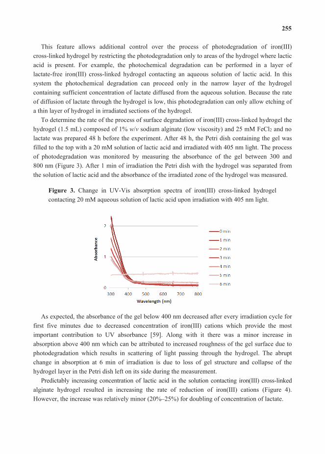
255

This feature allows additional control over the process of photodegradation of iron(III) cross-linked hydrogel by restricting the photodegradation only to areas of the hydrogel where lactic acid is present. For example, the photochemical degradation can be performed in a layer of lactate-free iron(III) cross-linked hydrogel contacting an aqueous solution of lactic acid. In this system the photochemical degradation can proceed only in the narrow layer of the hydrogel containing sufficient concentration of lactate diffused from the aqueous solution. Because the rate of diffusion of lactate through the hydrogel is low, this photodegradation can only allow etching of a thin layer of hydrogel in irradiated sections of the hydrogel.

To determine the rate of the process of surface degradation of iron(III) cross-linked hydrogel thehydrogel (1.5 mL) composed of 1% w/v sodium alginate (low viscosity) and 25 mM FeCl2 and no lactate was prepared 48 h before the experiment. After 48 h, the Petri dish containing the gel was filled to the top with a 20 mM solution of lactic acid and irradiated with 405 nm light. The process of photodegradation was monitored by measuring the absorbance of the gel between 300 and 800 nm (Figure 3). After 1 min of irradiation the Petri dish with the hydrogel was separated fromthe solution of lactic acid and the absorbance of the irradiated zone of the hydrogel was measured.

Figure 3. Change in UV-Vis absorption spectra of iron(III) cross-linked hydrogel contacting 20 mM aqueous solution of lactic acid upon irradiation with 405 nm light.

As expected, the absorbance of the gel below 400 nm decreased after every irradiation cycle forfirst five minutes due to decreased concentration of iron(III) cations which provide the most important contribution to UV absorbance [59]. Along with it there was a minor increase in absorption above 400 nm which can be attributed to increased roughness of the gel surface due to photodegradation which results in scattering of light passing through the hydrogel. The abrupt change in absorption at 6 min of irradiation is due to loss of gel structure and collapse of the hydrogel layer in the Petri dish left on its side during the measurement.

Predictably increasing concentration of lactic acid in the solution contacting iron(III) cross-linkedalginate hydrogel resulted in increasing the rate of reduction of iron(III) cations (Figure 4).However, the increase was relatively minor (20%–25%) for doubling of concentration of lactate.

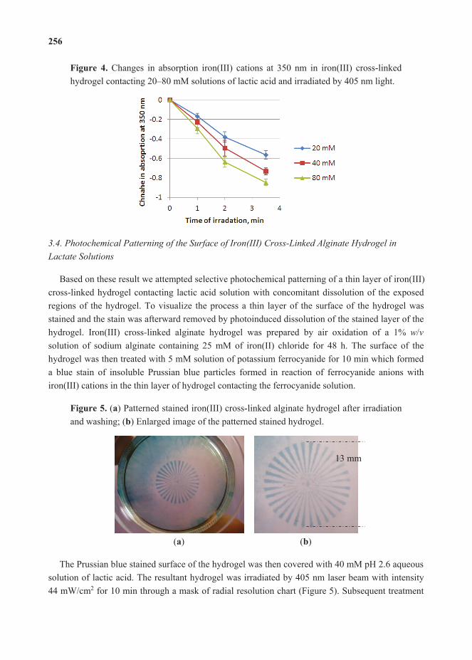
256

Figure 4. Changes in absorption iron(III) cations at 350 nm in iron(III) cross-linked hydrogel contacting 20–80 mM solutions of lactic acid and irradiated by 405 nm light.

3.4. Photochemical Patterning of the Surface of Iron(III) Cross-Linked Alginate Hydrogel in Lactate Solutions

Based on these result we attempted selective photochemical patterning of a thin layer of iron(III) cross-linked hydrogel contacting lactic acid solution with concomitant dissolution of the exposed regions of the hydrogel. To visualize the process a thin layer of the surface of the hydrogel was stained and the stain was afterward removed by photoinduced dissolution of the stained layer of the hydrogel. Iron(III) cross-linked alginate hydrogel was prepared by air oxidation of a 1% w/vsolution of sodium alginate containing 25 mM of iron(II) chloride for 48 h. The surface of the hydrogel was then treated with 5 mM solution of potassium ferrocyanide for 10 min which formed a blue stain of insoluble Prussian blue particles formed in reaction of ferrocyanide anions with iron(III) cations in the thin layer of hydrogel contacting the ferrocyanide solution.

Figure 5. (a) Patterned stained iron(III) cross-linked alginate hydrogel after irradiation and washing; (b) Enlarged image of the patterned stained hydrogel.

(a) (b)

The Prussian blue stained surface of the hydrogel was then covered with 40 mM pH 2.6 aqueous solution of lactic acid. The resultant hydrogel was irradiated by 405 nm laser beam with intensity 44 mW/cm2 for 10 min through a mask of radial resolution chart (Figure 5). Subsequent treatment

13 mm

257

of the irradiated hydrogel with distilled water resulted in dissolution of the surface layer of the hydrogel and removal of the blue stain in the light exposed areas.

This qualitative experiment demonstrate the potential of photolithography of iron(III) cross-linked hydrogel for introduction of 3D control over the thickness of the photodegradation. The possibility for facile patterning or complete removal of a thin layer of the hydrogel under biocompatible conditions can be of interest for a number of applications, particularly for use of hydrogels for 2D and 3D scaffolding of cell cultures and photoinduced detachment of cells.

4. Conclusions

In conclusion, we demonstrate successful photochemical patterning of iron(III) cross-linked alginate hydrogel in the presence of lactate. Layers of homogeneous iron(III) cross-linked alginate hydrogel with 1–3 mm thickness incorporating 20 mM sodium lactate undergo photoinduced degradation thus serving as a biocompatible positive photoresist suitable for photochemical patterning. Alternatively, thickness control of the photochemical patterning can be done through surface etching of iron(III) cross-linked hydrogel contacting lactic acid solution. Due to biocompatibility, both of these approaches appear potentially useful for advanced manipulation with cell cultures, including the growth of cell cultures on the surface of the hydrogel or cells,entrapping them within the hydrogel.

Acknowledgments

This work was supported by NSF grant CHE 1150768.

Conflicts of Interest

The authors declare no conflict of interest.

References

1. Morris, E.R.; Rees, D.A.; Thom, D.; Boyd, J. Chiroptical and stoichiometric evidence of a specific, primary dimerisation process in alginate gelation. Carbohydr. Res. 1978, 66, 145–154.

2. Li, L.B.; Fang, Y.P.; Vreeker, R.; Appelqvist, I. Reexamining the egg-box model in calcium-alginate gels with X-ray diffraction. Biomacromolecules 2007, 8, 464–468.

3. Donati, I.; Holtan, S.; Morch, Y.A.; Borgogna, M.; Dentini, M.; Skjak-Braek, G. New hypothesis on the role of alternating sequences in calcium-alginate gels. Biomacromolecules2005, 6, 1031–1040.

4. Augst, A.D.; Kong, H.J.; Mooney, D.J. Alginate hydrogels as biomaterials. Macromol. Biosci.2006, 6, 623–633.

5. Gombotz, W.R.; Wee, S.F. Protein release from alginate matrices. Adv. Drug Deliv. Rev. 1998,31, 267–285.

6. Lee, K.Y.; Mooney, D.J. Alginate: Properties and biomedical applications. Prog. Polym. Sci.2011, 37, 106–126.

258

7. Shi, X.W.; Du, Y.M.; Sun, L.P.; Yang, J.H.; Wang, X.H.; Su, X.L. Ionically crosslinked alginate/carboxymethyl chitin beads for oral delivery of protein drugs. Macromol. Biosci.2005, 5, 881–889.

8. Rowley, J.A.; Madlambayan, G.; Mooney, D.J. Alginate hydrogels as synthetic extracellular matrix materials. Biomaterials 1999, 20, 45–53.

9. Uludag, H.; de Vos, P.; Tresco, P.A. Technology of mammalian cell encapsulation. Adv. Drug Deliv. Rev. 2000, 42, 29–64.

10. Shapiro, L.; Cohen, S. Novel alginate sponges for cell culture and transplantation.Biomaterials 1997, 18, 583–590.

11. Kuo, C.K.; Ma, P.X. Ionically crosslinked alginate hydrogels as scaffolds for tissue engineering: Part 1. Structure, gelation rate and mechanical properties. Biomaterials 2001, 22,511–521.

12. Alsberg, E.; Anderson, K.W.; Albeiruti, A.; Rowley, J.A.; Mooney, D.J. Engineering growing tissues. Proc. Natl. Acad. Sci. USA 2002, 99, 12025–12030.

13. Bajpai, S.K.; Sharma, S. Investigation of swelling/degradation behaviour of alginate beads crosslinked with Ca2+ and Ba2+ ions. React. Funct. Polym. 2004, 59, 129–140.

14. Draget, K.I.; Braek, G.S.; Smidsrod, O. Alginic acid gels: The effect of alginate chemicalcomposition and molecular weight. Carbohydr. Polym. 1994, 25, 31–38.

15. Bouhadir, K.H.; Lee, K.Y.; Alsberg, E.; Damm, K.L.; Anderson, K.W.; Mooney, D.J. Degradation of partially oxidized alginate and its potential application for tissue engineering.Biotechnol. Prog. 2001, 17, 945–950.

16. Tan, W.H.; Takeuchi, S. Monodisperse alginate hydrogel microbeads for cell encapsulation.Adv. Mater. 2007, 19, 2696–2701.

17. Peirone, M.; Ross, C.J.D.; Hortelano, G.; Brash, J.L.; Chang, P.L. Encapsulation of various recombinant mammalian cell types in different alginate microcapsules. J. Biomed. Mater. Res.1998, 42, 587–596.

18. Cohen, D.L.; Malone, E.; Lipson, H.; Bonassar, L.J. Direct freeform fabrication of seeded hydrogels in arbitrary geometries. Tissue Eng. 2006, 12, 1325–1335.

19. Tam, T.K.; Zhou, J.; Pita, M.; Ornatska, M.; Minko, S.; Katz, E. Biochemically controlled bioelectrocatalytic interface. J. Am. Chem. Soc. 2008, 130, 10888–10889.

20. Jin, Z.; Guven, G.; Bocharova, V.; Halámek, J.; Tokarev, I.; Minko, S.; Melman, A.; Mandler, D.; Katz, E. Electrochemically controlled drug-mimicking protein release from iron-alginate thin-films associated with an electrode. ACS Appl. Mater. Interfaces 2011, 4, 466–475.

21. Casalbore-Miceli, G.; Yang, M.J.; Li, Y.; Zanelli, A.; Martelli, A.; Chen, S.; She, Y.; Camaioni, N. A polyelectrolyte as humidity sensing material: Influence of the preparation parameters on its sensing property. Sens. Actuator B 2006, 114, 584–590.

22. Ju, H.K.; Kim, S.Y.; Lee, Y.M. pH/temperature-responsive behaviors of semi-IPN and comb-type graft hydrogels composed of alginate and poly (N-isopropylacrylamide). Polymer2001, 42, 6851–6857.

259

23. Kim, S.J.; Yoon, S.G.; Lee, S.M.; Lee, J.H.; Kim, S.I. Characteristics of electrical responsive alginate/poly(diallyldimethylammonium chloride) IPN hydrogel in HCl solutions.Sens. Actuators B 2003, 96, 1–5.

24. Nishiyama, Y.; Nakamura, M.; Henmi, C.; Yamaguchi, K.; Mochizuki, S.; Nakagawa, H.;Takiura, K. Development of a three-dimensional bioprinter: Construction of cell supporting structures using hydrogel and state-of-the-art inkjet technology. J. Biomech. Eng.-Trans. ASME 2009, 131, 035001:1–035001:6.

25. Delaney, J.T.; Liberski, A.R.; Perelaer, J.; Schubert, U.S. Reactive inkjet printing of calcium alginate hydrogel porogens—A new strategy to open-pore structured matrices with controlled geometry. Soft Matter 2010, 6, 866–869.

26. Chueh, B.H.; Zheng, Y.; Torisawa, Y.S.; Hsiao, A.Y.; Ge, C.X.; Hsiong, S.; Huebsch, N.;Franceschi, R.; Mooney, D.J.; Takayama, S. Patterning alginate hydrogels using light-directed release of caged calcium in a microfluidic device. Biomed. Microdevices 2010, 12, 145–151.

27. Kloxin, A.M.; Kasko, A.M.; Salinas, C.N.; Anseth, K.S. Photodegradable hydrogels for dynamic tuning of physical and chemical properties. Science 2009, 324, 59–63.

28. Kloxin, A.M.; Tibbitt, M.W.; Anseth, K.S. Synthesis of photodegradable hydrogels as dynamically tunable cell culture platforms. Nat. Protoc. 2010, 5, 1867–1887.

29. Wang, G.; Tong, X.; Zhao, Y. Preparation of azobenzene-containing amphiphilic diblock copolymers for light-responsive micellar aggregates. Macromolecules 2004, 37, 8911–8917.

30. Eastoe, J.; Dominguez, M.S.; Wyatt, P.; Beeby, A.; Heenan, R.K. Properties of a stilbene-containing gemini photosurfactant: Light-triggered changes in surface tension and aggregation. Langmuir 2002, 18, 7837–7844.

31. Tazuke, S.; Kurihara, S.; Yamaguchi, H.; Ikeda, T. Photochemically triggered physical amplification of photoresponsiveness. J. Phys. Chem. 1987, 91, 249–251.

32. Lee, H.I.; Wu, W.; Oh, J.K.; Mueller, L.; Sherwood, G.; Peteanu, L.; Kowalewski, T.;Matyjaszewski, K. Light-induced reversible formation of polymeric micelles. Angew. Chem.-Int. Ed. 2007, 46, 2453–2457.

33. Luo, Y.; Shoichet, M.S. Light-activated immobilization of biomolecules to agarose hydrogels for controlled cellular response. Biomacromolecules 2004, 5, 2315–2323.

34. Brown, A.A.; Azzaroni, O.; Huck, W.T.S. Photoresponsive polymer brushes for hydrophilic patterning. Langmuir 2009, 25, 1744–1749.

35. Chandra, B.; Subramaniam, R.; Mallik, S.; Srivastava, D.K. Formulation of photocleavable liposomes and the mechanism of their content release. Org. Biomol. Chem. 2006, 4,1730–1740.

36. Jiang, J.Q.; Tong, X.; Zhao, Y. A new design for light-breakable polymer micelles. J. Am. Chem. Soc. 2005, 127, 8290–8291.

37. Bisby, R.H.; Mead, C.; Morgan, C.G. Active uptake of drugs into photosensitive liposomes and rapid release on UV photolysis. Photochem. Photobiol. 2000, 72, 57–61.

38. Liu, Y.C.; Le Ny, A.L.M.; Schmidt, J.; Talmon, Y.; Chmelka, B.F.; Lee, C.T. Photo-assisted gene delivery using light-responsive catanionic vesicles. Langmuir 2009, 25, 5713–5724.

260

39. Griffin, D.R.; Kasko, A.M. Photodegradable macromers and hydrogels for live cell encapsulation and release. J. Am. Chem. Soc. 2012, 134, 13103–13107.

40. Dustin, M.L.; Colman, D.R. Neural and immunological synaptic relations. Science 2002, 298,785–789.

41. Grakoui, A.; Bromley, S.K.; Sumen, C.; Davis, M.M.; Shaw, A.S.; Allen, P.M.; Dustin, M.L. The immunological synapse: A molecular machine controlling T cell activation. Science 1999,285, 221–227.

42. Wu, M.; Holowka, D.; Craighead, H.G.; Baird, B. Visualization of plasma membrane compartmentalization with patterned lipid bilayers. Proc. Natl. Acad. Sci. USA 2004, 101,13798–13803.

43. Jiang, X.Y.; Bruzewicz, D.A.; Wong, A.P.; Piel, M.; Whitesides, G.M. Directing cell migration with asymmetric micropatterns. Proc. Natl. Acad. Sci. USA 2005, 102, 975–978.

44. Ericson, J.; Norlin, S.; Jessell, T.M.; Edlund, T. Integrated FGF and BMP signaling controls the progression of progenitor cell differentiation and the emergence of pattern in the embryonic anterior pituitary. Development 1998, 125, 1005–1015.

45. Sundberg, S.A.; Barrett, R.W.; Pirrung, M.; Lu, A.L.; Kiangsoontra, B.; Holmes, C.P. Spatially-addressable immobilization of macromolecules on solid supports. J. Am. Chem. Soc.1995, 117, 12050–12057.

46. Blawas, A.S.; Oliver, T.F.; Pirrung, M.C.; Reichert, W.M. Step-and-repeat photopatterning of protein features using caged-biotin–BSA: Characterization and resolution. Langmuir 1998, 14,4243–4250.

47. Holden, M.A.; Cremer, P.S. Light activated patterning of dye-labeled molecules on surfaces.J. Am. Chem. Soc. 2003, 125, 8074–8075.

48. Doh, J.; Irvine, D.J. Photogenerated polyelectrolyte bilayers from an aqueous-processible photoresist for multicomponent protein patterning. J. Am. Chem. Soc. 2004, 126, 9170–9171.

49. Edahiro, J.; Sumaru, K.; Tada, Y.; Ohi, K.; Takagi, T.; Kameda, M.; Shinbo, T.; Kanamori, T.;Yoshimi, Y. In situ control of cell adhesion using photoresponsive culture surface.Biomacromolecules 2005, 6, 970–974.

50. Wosnick, J.H.; Shoichet, M.S. Three-dimensional chemical Patterning of transparent hydrogels. Chem. Mater. 2008, 20, 55–60.

51. Hahn, M.S.; Miller, J.S.; West, J.L. Laser scanning lithography for surface micropatterning on hydrogels. Adv. Mater. 2005, 17, 2939–2942.

52. Gillard, R.D.; McCleverty, J.A.; Wilkinson, G. Comprehensive Coordination Chemistry: The Synthesis, Reactions, Properties, & Applications of Coordination Compounds, 1st ed.;Pergamon Press: Oxford, UK; New York, NY, USA, 1987.

53. Zelikovich, L.; Libman, J.; Shanzer, A. Molecular redox switches based on chemical triggering of iron translocation in triple-stranded helical complexes. Nature 1995, 374,790–792.

54. Fei, S.T.; Phelps, M.V.B.; Wang, Y.; Barrett, E.; Gandhi, F.; Allcock, H.R. A redox responsive polymeric gel based on ionic crosslinking. Soft Matter 2006, 2, 397–401.

261

55. Sreeram, K.J.; Shrivastava, H.Y.; Nair, B.U. Studies on the nature of interaction of iron(III) with alginates. Biochim. Biophys. Acta 2004, 1670, 121–125.

56. Machida-Sano, I.; Matsuda, Y.; Namiki, H. In vitro adhesion of human dermal fibroblasts oniron cross-linked alginate films. Biomed. Mater. 2009, 4, 1–8.

57. Machida-Sano, I.; Matsuda, Y.; Namiki, H. A novel harvesting method for cultured cells using iron-cross-linked alginate films as culture substrates. Biotechnol. Appl. Biochem. 2010, 55,1–8.

58. Hernandez, R.; Sacristan, J.; Mijangos, C. Sol/Gel transition of aqueous alginate solutions induced by Fe(2+) cations. Macromol. Chem. Phys. 2010, 211, 1254–1260.

59. Narayanan, R.P.; Melman, G.; Letourneau, N.J.; Mendelson, N.L.; Melman, A. Photodegradable iron(III) cross-linked alginate gels. Biomacromolecules 2012, 13, 2465–2471.

60. Machida-Sano, I.; Hirakawa, M.; Matsumoto, H.; Kamada, M.; Ogawa, S.; Namiki, H. Evaluation of ionically cross-linked alginate films as culture substrates for human fibroblasts.J. Tissue Eng. Regener. Med. 2012, 6, 186.

61. Drury, J.L.; Mooney, D.J. Hydrogels for tissue engineering: Scaffold design variables and applications. Biomaterials 2003, 24, 4337–4351.

62. Katz, J.S.; Burdick, J.A. Light-responsive biomaterials: Development and applications.Macromol. Biosci. 2010, 10, 339–348.

63. Abrahamson, H.B.; Rezvani, A.B.; Brushmiller, J.G. Photochemical and spectroscopic studies of complexes, of iron(III) with citric acid and other carboxylic acids. Inorg. Chim. Acta 1994,226, 117–127.

262

Thermo-Responsive Hydrogels for Stimuli-Responsive Membranes

Evan Mah and Raja Ghosh

Abstract: Composite membranes with stimuli-responsive properties can be made by coating a thermo-responsive hydrogel onto a micro- or macroporous support. These hydrogels undergo a temperature induced volume-phase transition, which contributes towards the compositemembrane’s stimuli-responsive properties. This paper reviews research done on complimentary forms of temperature responsive “thermophilic” hydrogels, those exhibiting positive volume-phase transitions in aqueous solvent. The influences of intermolecular forces on the mechanism of phase-transition are discussed along with case examples of typical thermophilic hydrogels.

Reprinted from Processes. Cite as: Mah, E.; Ghosh, R. Thermo-Responsive Hydrogels for Stimuli-Responsive Membranes. Processes 2013, 1, 238–262.

1. Thermo-Responsive Hydrogels

By applying an adaptive property to a sedentary membrane, a membrane’s utility or productivity,or both, may be improved. Inspired by this concept, stimuli-responsive membranes are becoming increasingly prevalent in membrane research. For membranes employed in processes that make use of aqueous based solvents, hydrogels can be combined with a membrane substrate to create an environmentally adaptive technology. The hydrogel can be applied to the membrane substrate through simple submersion coating [1,2] or grafted through more complicated techniques, such as atom-transfer radical polymerization (ATRP) or surface initiation plasma treatment [3–5].Hydrogels are water-soluble polymer gels that, instead of dissolving, entrap water in the interstitial spaces between polymer segments. Hydrophilic pendant groups like alcohols, carboxylic acids and amides are what enable the gels to be water-soluble. There are several forms of stimuli that will invoke a response from hydrogels such as temperature [6–10], electric fields [11–13], solvent composition [14,15], ionic strength [1,16,17], pH [18,19] and interaction with analytes like glucose [20,21]. Thermo-responsive hydrogels are of specific interest where chemical modification of the feed solvent is undesirable or impractical. This has implications for developments in membrane chromatography separations [10,22] and drug delivery [23].

There are a few well known models for gel structure such as those put forward by Flory for covalently bonded networks and Rees for non-covalent networks [24,25]. As we are considering hydrogels as a constituent of composite membranes, the focus of discussion in this review will predominantly be macrogels with a permanent covalently bonded network structure, avoiding specific microgel discussion and purposely excluding sol-gel systems. This will greatly affect the classification of thermo-responsive behavior observed in hydrogels. Typically sol-gel systems can be classified as having either an upper or lower critical solution temperature. On one side of this critical solution temperature, the system has two phases, as marked by a cloud point while on the other side, the system has one phase. For the permanent hydrogels that will be discussed in this

263

review, this classification of temperature responsiveness is inaccurate as the polymer gel network is solvated but not dissolved meaning that there are always two physical phases. Instead of observing solution phase, volume-phase is a better basis of classification. Volume-phase transition is the response of a thermo-responsive hydrogel to heating and cooling. Tanaka et al. claim that volume phase transition is universal to all gels [26], however not all gels are able to have their volume affected by temperature in water. Additionally, temperature is typically an easy variable to control and predict in most practical setups, which makes these hydrogels an interesting and practical study.

Considering volume-phase transitions give us a volume-phase transition temperature (VPTT) instead of a critical solution temperature, there are still two main classifications of observed behavior, positive volume-phase transitions and negative volume-phase transitions. A positive volume-phase transition or “thermophilic” hydrogel will swell upon heating, increasing its volume. A negative volume-phase transition or “thermophobic” hydrogel will collapse upon heating, decreasing its volume. Thermophilic hydrogels typically maintain a collapsed conformation at temperatures below their VPTT while thermophobic hydrogels are able to swell at lower temperatures. The volume-phase transition may be reversible but not in all cases and hysteresis is frequently experienced [27–31].

Thermophilic behavior in water is uncommon for polymer gels, while the monomers of a polymer may be water soluble, the increased molecular weight from polymerization may cause the polymer not to be. Large hydrocarbon-based polymers tend to be hydrophobic, a property that favors negative volume-phase transition. Studies of both behavior types in aqueous based polymers have their roots in a similar time frame. Notable publications on thermophobic polymers were published in 1957 ((polyethylene glycol) [32] and 1968 (poly(N-isopropylacrylamide)) [33] while notable thermophilic polymers were published in 1964 (poly(N-Acryloylglycinamide)) [34].Thermophobic hydrogels have been very popular since the early 1990’s reflected by the research and discussion concerning a single example, poly(N-isopropylacrylamide) (PNIPAm). Between 1984 and 1991, yearly research citations of PNIPAm quadrupled, as has been determined by other workers [11,22]. What made these hydrogels so popular was the novel concept that the thermophobicbehavior of gels in aqueous solution is contrary to the majority of polymers in organic solution. Both single chain and crosslinked networks of PNIPAm exhibit negative volume-phase transition between 30 °C and 35 °C [33,35]. PNIPAm hydrogels and others that similarly exhibit thermophobic behavior are primarily enabled by water-polymer interactions, while polymers with thermophilic behavior are driven by both water-polymer and polymer-polymer interactions [36].The heavy interest thermophobic hydrogels have garnered has made it difficult to find any information on thermophilic hydrogels, leading many researchers and reviewers to either quickly dismiss the positive volume-phase transition aspect of temperature responsive gels or ignore it altogether [37–39]. This review is a highlight of thermophilic hydrogels, the compliment thermo-responsive material to very popular thermophobic hydrogels, and will look at the specific mechanisms of classic thermophilic hydrogels as well as modern developments and applications.

264

2. Theory: Phase Transition of Thermophilic Hydrogels

There are several cooperative and competing forces active between polymer chains within hydrogels and from the solvent. Theoretically, thermophobic and thermophilic behavior should be possible for all hydrogels as represented by a closed loop coexistence curve on a phase diagram. This is providing that phase change of the solvent to gas or solid doesn’t occur [40].Experimentally this may not be a practical observation due to the scarcity of substances with a small enough temperature range to display both solution behavior types without phase change, or due to the pressure conditions required to prevent phase change [14]. Much of the theoretical and experimental work for the phase change of gels has been transported from work done on single polymer chains in solution. Single polymer chains are easier to observe and characterize than gel networks and polymer gels are networks of single polymer chains. Literature concerning gels or single polymers in solution often reference theoretical work initiated by P.J. Flory [24]. Flory’s work explains that it can be expected that at sufficiently high temperatures or in good solvent conditions, a polymer system will be in an expanded state. At sufficiently low temperatures or in poor solvent conditions a polymer system will be in a collapsed state. Early work characterizing the volume-phase transition of gels found that transitions between collapsed and extended states of polymer chains were smooth and continuous or abrupt and discrete [15,41]. Other significant concepts were identified through this work such as collective diffusion theory [42]. A major factor governing volume-phase transition that is difficult to control and evaluate is the rubber elasticity of the gel as a result of the varying degrees of crosslinking that had been attained in the gels. Tanaka et al. (1979) identified that the rate of forming covalent crosslinks in a gel is logarithmic, once the initial fast gelation had occurred, the final curing process was slow due the movement of large molecule chains and low concentration of free chain ends. So depending on the time allotted to curing, two gel samples of the same composition may have considerably different solution properties. Due to the complexity of available models for polymer swelling and collapse, theoretical models that have been used to describe the volume-phase transition of hydrogels will not be examined. Instead, a brief overview of the forces that enable phase transition will be presented as background for later sections.

As briefly introduced, gels can be held together by either covalent bonds or non-covalent bonds [24,25]. Covalent bonds are chemical crosslinks between polymer chains and non-covalent bonds are physical crosslinks. The idea is that the covalent bonds are permanent while thenon-covalent ones are not. The macrogels discussed in this review are held together by covalent bonds while the volume-phase transitions are dependent on non-covalent bonding interactions. Within the non-covalent physical bonds, there are those that can be classified as either strong physical bonds or weak physical bonds. Strong physical bonds are complexes like microcrystals and triple helices. They are stable over experimental time frames but can be broken by certain environmental conditions [43]. Weak physical bonds are driven by intermolecular forces that can be formed and broken over experimental time frames such as hydrogen bonding or van der Waals forces. Hydrogel polymer networks rely on chemical bonds for structure and physical bonds in order to undergo volume-phase transition. Weak physical bonds that are formed or broken

265

during a phase transition are a combined effect of cooperative polymer-polymer interactions and polymer-solvent interactions [39–41]. A phase transition then becomes an equilibrium between repulsive forces that reduce polymer-polymer interactions and move to swell the gel and attractive forces that reduce the polymer-solvent interactions and move to collapse the gel. In terms of polymer-polymer interactions, attractive forces are hydrophobic interactions and van der Waals interactions while electrostatic interactions and hydrogen bonding may act as both attractive and repulsive forces depending on the environmental conditions. The following sections on intermolecular forces are not meant to be an exhaustive characterisation but instead to put the forces in context for this review.

2.1. Electrostatic Forces

Early work on hydrogels undergoing volume phase transitions surmised that the transition was driven by ionized pendant groups in the network and discrete or continuous change was determined by the degree of ionization [21,30,42]. Ionization of a gel was induced by copolymerization or hydrolysis. Toyoichi Tanaka had observed that “new PAm gels” that were tested after a shorter curing time showed continuous volume change while “old PAm gels” with a longer curing time showed discrete volume change [31]. Curing time was related to a natural hydrolysis process causing the “old gels” to have a higher degree of ionization than the “new gels”. From this work he determined that electrostatic forces due to ionization are the most effective repulsive force. Later works examining phase transition shows this to be an incomplete investigation since; other intermolecular forces must be considered, at least in the case of PAm gels, and electrostatic interactions are also an effective attractive force. Polyelectrolytes are the clearest example of a hydrogel where the phase transition is dominated by attractive and repulsive electrostatic forces. The phase transition is decided by the conformations of multiplets of ionomers induced by external stimuli. Electrostatic interactions are strongly affected by pH as well as the present of salts. Electrostatic interactions are capable of driving both thermophobic and thermophilic behaviors.

2.2. Van der Waals Interactions

Phase transitions driven by van der Waals interactions tend to be of thermophilic nature, where reference to van der Waals forces is in terms of permanent dipole interactions. Thermophilic behavior requires relatively strong associative intra and interpolymer-chain interactions at ambient conditions, causing the solvent (water) to be poor. Dipole interactions decrease upon heating effectively increasing the solvent quality [14]. Amide-amide interactions are a typical example in polymer gels where solubility in water is primarily controlled by dipole interactions. External stimuli can change the solution properties by affecting the strength and the alignment of these dipoles [44].

2.3. Hydrogen Bonding

Hydrogen bonding can be considered significant for phase transition in two ways; solvent interactions and solute interactions [14]. Researchers that consider solute interactions,

266

polymer-polymer hydrogen bonding, observe hydrogen bonding to be characteristic of associative polymers and thermophilic behavior [26,43]. Consideration of polymer-solvent hydrogen bonding is typical of work concerning thermophobic hydrogels, as it is the dominant force allowing these gels to be water soluble at lower temperatures [35]. For hydrogels where phase transition is primarily driven by hydrogen bonding, thermophobic volume-phase transition is considered typical by many workers since hydrogen bonds are broken at elevated temperatures and therein should not be an influencing force [45]. Hydrogen bonding between the polymer and water is what permits water solubility. Formation of h-bonds between the polymer and water is both exothermic and forms higher structure order in the system. Adversely, where there is strong polymer-polymer hydrogen bonding causing gel collapse and preventing swelling, increasing temperature breaks the associative bonds effectively increasing the solvent quality to a similar effect as with dipole interactions. Interactions between carboxylic acid and amide functional groups can yield these strong polymer-polymer hydrogen bonds [26,46]. This was shown by Garay et al. through potentiometry in protic solvent. As carboxylic acid-amide bonds were formed, pH of the solvent increased reflecting a decrease in dissociated acid group concentration.

2.4. Hydrophobic Interactions

Hydrophobic interactions are an entropic effect induced mainly by the solvent. Aggregation of hydrophobic particles is driven by water to reduce the amount of interfacial area exposed. As mentioned above, higher temperatures typically raise the entropy of a system, which favorshomogenous mixtures and better solvent quality, however, the solubility of small hydrophobic molecules increases with decreasing temperature. Heating reduces solubility and can lead to phase separation or precipitation. After reaching a minimum, the solubility sharply increases upon further heating. If phase separation occurred, one phase is again achieved on the condition boiling point has not been reached [47]. Hydrophobic interactions occur with polymers composed of primarily non-polar groups, such as phenyls, and tend to cause thermophobic behavior. As has already been suggested, volume phase transition is a result of a sum of several forces. Hydrophobic interactions tend to be thought of as being between water and non-polar solutes; however, they can also influence polar particles. Inclusion of hydrophobic functional groups in the pendant chains or as a co-monomer of polymer gels reduces the strength of the dipole interactions, increasing the significance of polymer-solvent hydrogen bonding. Enthalpy of dissolution becomes negative and enhances the water solubility of the polymer [44].

3. Ionic Polymer Hydrogels

Hydrogels composed of charged polymers are a main group of thermo-responsive hydrogels. There are several classifications of ionic polymer hydrogels, each one more specific in description than the last. A polyelectrolyte polymer has charged pendant groups, consisting of either cationic groups, anionic groups or both. Thus, they can have a net positive, net negative or neutral charge depending on environmental pH and ionic strength. Polyzwitterions refer specifically to those polymers that contain both positively and negatively charged pendant groups. Polyampholytes are

267

those polyzwitterions where the charged groups are on different repeating monomer units while polybetaines are those where the charged groups are on nonadjacent sites of the same monomer unit and the cation doesn’t have an associated hydrogen (Figure 1). There isn’t consensus between researchers for the terminology of polyampholytes and polyzwitterions. Often their use can be the reverse of what is written above or polyzwitterion is used for what was described as a polybetaine with polyampholyte remaining the same [27,28,48]. There are some fundamental differences in their aqueous solution behaviors that can aid in identifying the uses of the above terms. As it is described above, electrostatic repulsions between charged groups on polyelectrolyte chains force an extended chain formation in deionized water at low concentrations. These repulsions can be disrupted by the addition of small electrolytes or changes to the system pH causing the chain to collapse. This is the polyelectrolyte effect. There is a complimentary antipolyelectrolyte effect where the polymer chain maintains a collapsed chain formation in deionized water at low concentrations and expands upon the addition of small electrolytes or change to the system pH. The antipolyelectrolyte effect is characteristic of polyampholytes and polybetaines. Polyampholytes can also exhibit polyelectrolyte behavior depending on solution conditions such as pH and tonicity. Polyampholytes are typically composed of weak acid and base monomers, causing them to have isoelectric points, further aiding in their identification [48]. Polybetaines are the most significant class of polyelectrolyte for this review as some are temperature responsive, a unique quality not typical of other polyzwitterions. Specifically, polysulfobetaines are of great interest to researchers of stimuli responsive materials.

Figure 1. Sulfobetaine functional unit.

Early workers were required to synthesize their own sulfobetaines monomers, limiting the amount of research done for solution behavior. After polymerization, lengthy fractionation was also required to achieve adequately narrow polydispersity [49]. Soto and Galin worked with five unnamed polysulfobetaines determining their solubility in various solvents and the effect of adding salt. It was concluded that solubility for polysulfobetaines is limited to protic solvents and that addition of salt improves solubility in water specifically. It was suggested that this is because electrolytes disrupt the intra- and inter-molecular ionic network and that this effect is dependent on the polarizability of the anion. This is a clear example of antipolyelectrolyte effect. The commercial availability of sulfobetaine monomers enabled more research into solution properties of single polymers and gels in solution. N-(2-methacryloyloxyethyl)-N,N-dimethyl-N-(3-sulfopropyl) ammonium betaine was one of the first such monomers, offered under the name SPE by Raschig GmbH [17]. Along with the other IUPAC names for the compound (CAS# monomer: 3637-26-1, polymer: 41488-70-4), this monomer has been called sulfobetaine methacrylate (SBMA), DMMAPS and MEDSAH by other workers [27,28,50–52]. It was noted by Soto and Galin that

268

although polysulfobetaine solubility is good in protic solvents, solubility in water above 20oC was unusual and was reaffirmed later [48]. However, it was found that solubility of polySPE in water was achieved at room temperature or upon heating. This signified that polySPE and possibly other polysulfobetaines have temperature dependent solution properties. Schulz was able to confirm this using cloud point titrations in both deionized water and salt water and map out the first full phase diagram for a sulfobetaine polymer in solution (Figure 2). The region above a coexistence curve represents one phase while the region below represents separation in two phases.

Figure 2. Effect of polymer concentration and salt on polySPE phase behavior with respect to temperature. Polymer Mw = 4.35 × 105

(0.51 M) [17].

Both lower and upper critical solution temperature behaviors were observed at 16 °C and 33 °Crespectively. These behaviors correspond to thermophobic and thermophilic VPTT in hydrogels of polySPE. It was mentioned in the previous section both behaviors should be possible for a single species and the claim is exemplified by this early work of Schulz. In agreement with Soto, it was also observed that salt solutions improve the solubility of polysulfobetaines. Thus when applied to temperature responsive solution properties, increasing salt concentrations decreases the thermophilic VPTT. Schulz was able to identify that the solution properties of polySPE are due to intra-chain and intra-group associations. Intra-chain associations are hydrogen bonds and dipole attractions on the same chain and the intra-group association is the ion pairing of the betaine. Strong intra-chain associations are what cause insolubility of the polymer. With the mention of inter-chain associations, the concept of thermophilic hydrogels was suggested but not discussed. Schulz was able to propose a model for the effect of salt on solution properties but was unable to account for the temperature responsiveness of the polySPE. Along with work on unperturbed

-conditions, characterisation of single polySPE chains in solution allows better understanding of the behavior of the gels [53].

A study of polySPE chains grafted to a surface, by surface initiated atom-transfer radical polymerization, gives great insight into the mechanics of a hydrogel with positive volume-phase transition properties [27]. Azzaroni exhibits two main cases in this research: a surface with low molecular weight (short) chains, and a surface with high molecular weight (long) chains. The two cases are comparable to gels with high and low degrees of crosslinking respectively. Low

269

molecular weight chains represent short polymer sections between crosslink nodes while high molecular weight chains are similar to long polymer sections between crosslink nodes. Azzaroniexpands upon the description given by Schulz for the forces of thermophilic behavior of polybetaines. He invokes discussion of the dielectric properties of water, solvation effects and excluded volume effects from hydration of the charged sites in breaking chain associations for gel swelling. The energy of the electrostatic forces must exceed the energy required for dehydration of the charged sites in order to form high degrees of inter and intra-chain associations. The degree of chain association was measured by water contact angle in this study and qualified in terms of hydrophobicity and hydrophilicity of the hydrogel surfaces. Azzaroni claims that in the case of short polymer chains, there are no chain association as the density of electrostatic interactions is too low, allowing complete hydration. Conversely, long polySPE chains present a high number of charged sites increasing the probability of electrostatic interaction and chain association, hindering hydration. The long grafted chains were poorly soluble in water at 22 °C, however, upon heating to 52 °C the gel coating shifted from a hydrophobic surface to a hydrophilic one. The shift was found to be reversible and the polySPE coatings maintained a stable composition for several months, able to undergo thermal cycling with similar results. Although this work is comparable to a true gel, it doesn’t clearly qualitatively examine the equilibrium of interactions as the polybetaine is heated through its VPTT nor does it present the extent of hydration quantified by the volume increase of the polymer network.

The work done by Azzaroni borrows the model of chain and group associations from research by Georgiev, presenting one of the first direct investigations of a polySPE hydrogel as it undergoes positive volume-phase transition [28]. Georgiev describes the reversible swelling of the hydrogel as an equilibrium between inter and intra associations further developing the theory of Schulz and providing a basis for Azzaroni. The associations are described as intragroup ion pairs and entropy driven zwitterionic clusters (Figure 3).

Figure 3. Short zwitterionic cluster (A), intragroup ion pair (B), long zwitterionic cluster (C), nucleated from a short cluster with entropy driven propagation outwards. Figure adopted from [28].

Georgiev is able to describe the shift of the equilibrium of the chain associations during the volume-phase transition. At low temperatures, zwitterionic clusters form as the enthalpy of the water decreases, making dehydration of the charged sites easier. The entropy of the solution also

A

B

C

A

B

C

270

decreases, promoting higher order and a collapsed gel conformation. At high temperatures, increasing entropy and hydration energy favors ionic pairs allowing osmotic pressures to swell the gel. Dehydration of the charged sites is not mentioned by Georgiev as a factor in the volume transition of the hydrogel. The involvement of a dehydration activation energy is explored by Kamenova et al. [54], extending the model to include solvation factors in consolidation with the model of Azzaroni. This work assumes the model of associations established by Georgiev and uses an “isoconversional” method of thermogravimetric analysis to approximate the activation energy of dehydration for the gels [55]. While attempting to correlate the results of the analysis on the dehydration activation energy to the equilibrium swelling ratio of the gels, the data and results are poorly presented restricting the usefulness of the work by Kamenova et al. to affirming the theory of Georgiev. Missing from all three works was whether any pendant chains remain unpaired as the charged sites are solvated by the water.

The discussion above on the effect of polymer segment length that was extrapolated from the grafted polySPE chains of Azzaroni is also addressed, confirming the contentions presented. Hydrogels synthesized with low amounts of crosslinker provide long polymer segments between covalent nodes. It is observed that this leads to the abrupt positive change in swelling ratio observed across the VPTT. This transition in swelling ratio become smoother and then disappears altogether at higher incorporation of crosslinker in the hydrogel.

In the quantification of the swelling ratio transition, Georgiev presents the partial Flory-Huggins equation of osmotic pressure used by Tanaka [15,41] with a modification to account for charge distribution in the polyzwitterionic gel. It is found that the equation is adequate for describing the critical values of observable parameters but not the temperature dependence of interactions within the hydrogel through the transition. Additionally hysteresis is experienced upon cooling which is typical of dipole interactions seen in proteins undergoing coil-globule transition. These observations are used by Georgiev to infer that dipole-dipole associations as well as electrostatic interactions between ionic groups account for the large volume phase transition in the polybetaine hydrogels.

The progression of research with thermo-responsive polysulfobetaines has continued towards characterization and optimization of gel properties. Ethylene glycol dimethacrylate (EDMA) and N,N'-methylene bisacrylamide (MBAm) are typical crosslinkers when synthesizing polysulfobetainegels. Attempts to optimize the hydrogel properties have used other crosslinking agents, with similar structure to SPE monomer, to improve the mechanical properties of polySPE gels [56]. This work shows that the concentration of crosslinker used in the synthesis of the hydrogel is more important for solution behavior than selection of crosslinker. However, it is shown that different crosslink distances due to linker selection will have an impact of mechanical properties such as Young’s modulus. Polysulfobetaines have also gained much interest as a biocompatible material with high protein fouling resistance [50]. Copolymerizations with other biocompatible thermo-responsivepolymers have formed temperature triggered cell-detachment surfaces [57].

271

4. Acrylamide Based Hydrogels

It has been seen that polysulfobetaine-based hydrogels are the most studied ionic polymer hydrogel. Electrostatic interaction between the charged sites on the polymer side chains is the primary driving force for volume-phase transition. As mentioned prior, the phase transitions are in fact an equilibrium between several forces. Although electrostatic forces driven by the ionic nature of the gel composition is the primary force, dipole-dipole interactions from the permanent, non-adjacent and opposite charges as well as minor hydrogen bonding play a part. Unmentioned are hydrophobic interactions between the long hydrocarbon based polymer chains of the hydrogel. They were unaddressed by most workers as the hydrophobic interactions were not significant compared to the others. Another significant class of thermophilic hydrogel is that of acrylamide (Am)-based hydrogels. Many thermo-responsive hydrogels are Am-based as seen by work with PNIPAm and work on polysulfobetaines with an Am backbone [28,35]. As will be shown, this class of hydrogel is dominated by hydrogen bonding. However, it is not as dominating as the electrostatic forces in the polysulfobetaine gels. Dipole interactions, electrostatic interactions and hydrophobic interactions play a larger part in balancing the forces of phase-transition for Am-based hydrogels. These gels are water soluble above 0 °C and able to swell several times their dry-weight to an extent highly dependent on their synthesis methods [58–61]. Although Am itself can be polymerized to form hydrogels, they do not undergo volume-phase transition. To form thermophilic hydrogels, Am is typically combined with acrylic acid (AA) either as a random copolymer or as an interpenetrating network of the homopolymers. The isolated homopolymers of Am and AA in solution behave like a polymer in good solvent with near constant solubility upon heating while a mixture of the two in solution behaves like a polymer in poor solvent with improving solubility upon heating [62]. It is known that hydrogen bonded complexes are formed between the two monomers and that these complexes break down upon heating [63,64].

4.1. Interacting Forces

Although volume-phase transition had been shown for Am and AA polymer gels, complexation of the polymers by hydrogen bonding between the amide and carboxyl functional groups was first shown by Klenina [62]. Earlier work had examined interactions between the functional groups of Am and AA in acidic aqueous conditions [31,65]. It was believed that the inclusion of AA accounted for ionization of the gel network and was responsible for discontinuous volume phase transition. However, it was unsure as to whether complexation occurred when AA was not ionized. Stable complexes between polyacrylamide (PAm) and polyacrylic acid (PAA) in solution were developed without dissociating the carboxyl groups. In hydrogel structure, the hydrogen bonding forms a ladder structure between polymer segments (Figure 4). The ladder structure is formed and broken by a “zipping” action nucleated from an individual hydrogen bond similar to the long zwitterionic clusters of the polysulfobetaine gels. Dissolution of the structure occurs upon heating, hydration forces are generated as hydrogen bonds are broken by thermal energy and break adjacent hydrogen bonds resulting in rapid dissolution as there are now two functional destructive forces.

272

Similarly, upon cooling, polymer-polymer hydrogen bonded structure is favored as thermal energy decreases and is aided in forming bonds by propagating dehydration between adjacent side groups.

Figure 4. Competing hydrogen bond complexations in PAm and PAA hydrogels.Adapted from [36].

Dipole-dipole interactions between the amide groups present another strong influence over the volume-phase transitions. Water solubility of PAm is primarily controlled by the dipole interactions of the amide groups. In the homopolymer, it is expected that the energy produced by the amide dipole interactions is larger than that provided by solvent interactions and other solute interactions [44]. In the gel network, hydrogen bonding becomes dominating weakening the effect of the dipole interactions but not making them negligible. The amide dipoles may be affected by temperature just as the hydrogen bonds are. External stimuli can change the strength and alignment of the dipoles modifying the solution properties [14]. For Am-AA based hydrogels, there are two main competing intermolecular complexation mechanisms. Am can form complexes with itself, the discussion to whether this is due to hydrogen bonding or dipole interactions is not complete, meaning that complete equimolar complexation with AA shouldn’t possible as seen in Figure 4 [36].

Confirmation of hydrogen bonding in Am-AA based hydrogels is often provided using urea [35,66], a known hydrogen bond and hydrophobic interaction disrupting analyte [67].One worker reported complete dissolution of Am-AA complexation at 10 wt% urea in water as confirmed by light transmittance [68]. The effectiveness of urea does not clearly identify hydrogen bonding as the sole force causing dissolution. Hydrophobic interactions are enhanced at higher temperature and are a strong attractive force significant in negative volume-phase transitions. However, considering that a thermophilic hydrogel swells upon heating as well as with the addition of aqueous urea at low temperatures suggests that Am-AA based hydrogel networks experience negligible associative hydrophobic interactions. In addition to work with urea, varying the Am-AAmonomer ratio can show that the hydrogen bond between amide and carboxyl functional groups is essential to positive volume-phase transition. Both PAm and PAA homopolymers show negligible

273

volume change with temperature change in pure water [14,15,41]. It has been shown that in a gel network, the monomer ratio (Am:AA) must be between 1:9 and 8:2 for any volume phase transition to occur [68].

The swelling and collapse of a covalently crosslinked Am-AA based hydrogel is reversible and appears complete under light transmittance observation [68], however when viewed by mass or volume, reversibility is not complete with the absolute swelling volume becoming larger after each temperature cycle. Along with this, structure formation is kinetically slower than dissolution and hysteresis is often observed between heating and cooling cycles (Figure 5) [14,36,67,68]. Both these effects have similar root causes. The typically high swelling ratios of Am-AA based hydrogels above their VPTT impose great distances between polymer chains. These large interstitial spaces allow reduction in chain entanglement through the swelling and collapsing cycles, and, the polymer complexes formed below the VPTT are not reformed as they once were, their conformation changed as some chain segment may not reform complex at all [29]. Other aspects to consider which will be discussed in following sections are ionic dissociation of carboxyl groups and hydrophobic composition of the polymer chains.

Figure 5. Hysteresis as observed by light transmittance characteristic of many Am-AAbased hydrogels [30].

Stabilizing the polymer complex of thermophilic hydrogels has become a great topic of research as workers attempt to optimize the gels’ responsive qualities. There are several strategies to do so: Increasing the amide density by using monomers with pendant groups with multiple amide functionality [69]; Increasing the hydrophobic content by copolymerization with a hydrophobic monomer [44,68,70,71]; Suppress amide-amide interactions to promote more efficient amide-carboxylcomplex formation [36,72].

4.2. Synthesis

There are different volume-phase transition profiles that are attainable dependent on the microstructure of the Am-AA based hydrogel. The two most common structures are a random copolymer gel as well as an interpenetrating polymer network (IPN). The copolymers are typically prepared in a single polymerization step while the IPNs are prepared by sequential polymerization with the PAm network prepared first and then the PAA network throughout it. Workers have found

274

that the random copolymerized hydrogels undergo smooth continuous volume transition through temperature change. The same workers have discovered IPNs to exhibit an abrupt volume change as the VPTT of the hydrogel is attained. This abrupt change is often described as a discontinuous or discrete transition profile. It has been asserted that both the continuous and discrete Am-AA hydrogel transition behaviors are reversible in the sense described above [29,31,70].

There are common methods and recipes for synthesis of Am-AA based hydrogels. N'-methylene bisacrylamide is a double functional amide monomer that is frequently used as a crosslinking agent for these gels due to its similar structure (Figure 6).

Figure 6. Chemical similarities between acrylamide, acrylic acid and N'-methylene bisacrylamide.

Initiation for Am-AA based hydrogels is typically by free radical initiation. Thermally activated persulfate initiators like ammonium persulfate (AP) or potassium persulfate and often combined with an accelerator like tetraethylmethylenediamine (TEMED) to reduce the temperature of initiation. The crosslinker and choice of initiator are also common to other thermo-responsive hydrogels using N-alkyl substituted amide monomers [35]. Additional methods of initiation that have been used are irradiation and plasma treatment (see Table 1) as well as reversible addition-fragmentation chain transfer (RAFT) [73]. Hydrogel polymerization is usually carried out in glass pipettes, between glass plates with spacers or in glass dishes. Earlier it was mentioned that a range of monomer ratios were acceptable for a Am-AA hydrogel to posses thermophilic behavior,however, as shown in single polymer chain solutions of PAm and PAA, precipitate that forms below the VPTT has a stoichiometric ratio of 1:1 by refractive index analysis [62]. Results of this nature lead researchers who are developing hydrogels for functional applicability do design gels to have a 1:1 Am-AA monomer ratio in the final gel. Consistent of all workers, Am quantity is used to determine the amount of AA to satisfy the ratio.

275

Table 1. Various recipes for Am-AA based hydrogels.

AA AA Crosslinker Initiator Type Source5 g - MBAm AP & TEMED Homopolymer [15,31,41]5g 5g MBAm AP & TEMED Sequential IPN [66]

7.2 g 7.3 g MBAm AP Sequential IPN [36]

15–30 mol%Various

molar ratios- 60Co- Random copolymer [74]

1:1 molar ratio MBAmPotassium

peroxodisulfateRandom copolymer [75]

1.775 g 1.800 g MBAm -Ketoglutaric acid Random copolymer [19]

1–3 wt% 0.2–2 wt% MBAmPlasma treatment,

potassium persulfateSequential IPN [76]

Tanaka was one of the first researchers to work with thermophilic hydrogels. Initial work solely observed PAm gels and found discrete swelling behavior with respect to temperature in partial organic solvent [15]. As asserted above, PAm does not exhibit temperature responsiveness in purely aqueous solvent. Work to discover conditions that would allow PAm hydrogels a volume phase transition in water was extensive, even leading Tanaka to develop the spinodal curve for PAm [77]. It was discovered serendipitously that the gels needed to cure or “ionize” in order for thermophilic behavior to occur without partial organic solvent [41]. Older gels underwent volume collapse upon cooling while more freshly synthesized gels did not. Tanaka’s “ionization” turned out to be inclusion of carboxyl groups in the gel network [31]. This was possible by either hydrolysis of the amide groups or incorporation of AA as a co-monomer. Tanaka only synthesized random copolymers in early works positive volume-phase transition was induced by partial hydrolysis of the amide groups in a basic reaction medium (pH 12). It was discovered that while only a small fraction of AA units were necessary for volume-phase transition to occur in water, increasing fractions promoted discrete volume phase transitions. Tanaka surmised that the swelling transitions in aqueous media could be accounted for by osmotic pressure driven by dissociation of hydrogen ions from the carboxyl groups, leading to his use of Flory-Higgins solution theory as previously mentioned [15,41].

The results of Tanaka showing discrete swelling transition was primarily based on solvent composition, never truly able to show a direct correlation between temperature and volume-phase transition, deriving a “reduced temperature” instead from the Flory-Higgins’ osmotic pressure formula. The failure to show a direct relationship between temperature and hydrogel volume phase transition made Tanaka’s work difficult to reproduce. First works developing Am-AA IPNs discovered this as only smooth, continuous swelling profiles were observed for random copolymer gels while the IPNs displayed an abrupt discrete transition [29,70]. It was determined that rapid polymer complex formation and dissolution was responsible for the sharp volume transition observed for the IPN gels. The dull swelling of the copolymer was assumed to be due to structural discontinuities causing isolation of any Am-AA complexes that did form. As discussed above, complex formation and dissolution are both nucleated at specific sites and then aided in outward propagation by hydration forces. The random ordering of amide and carboxyl groups as well as the

276

isolated Am-AA complexes in the copolymer gel prevents large range influence of nucleation sites. The homopolymer chain segments between crosslink nodes in the IPN promote more efficient complex formation and therefore dissolution. Equimolar composition of the IPN was perpetrated as the optimum condition for complete complexation of the hydrogel below the VPTT. This was not confirmed by the researchers as it was assumed that there was no concentration gradient through the initial PAm gel as it swelled with AA monomer solution prior to the secondary polymerization.

Application of Am-AA IPNs is well exemplified by work done grafting the hydrogels onto a porous nylon-6 substrate to create function gates to control permeability [76]. Consistent with the sequential polymerization method, PAm gels were surface initiated by plasma treatment to graft the initial gel onto the inside of the substrate pores. The initial gel was then swelled in an aqueous AA, MBAm, and potassium persulfate mixture before the secondary gel was polymerized. The functional gates showed that water permeability of the nylon substrate could be increased at temperatures below the VPTT as the hydrogel collapsed, opening the pores. The pores would close above the VPTT as the hydrogel gates swelled. Scanning electron microscopy and x-ray photoelectron spectroscopy were used to verify the structure of the membrane and the synthesis of the IPN. It was found that although the entire membrane was soaked in the secondary gel reaction mixture, it was only retained in the PAm gel (Figure 7). The thermophilic behavior of the IPN hydrogel gates was observed to be reversible through several temperature cycles varying between 10 °C and 40 °C.

Figure 7. Scanning electron microscope image of nylon-6 membrane after sequential polymerization of a Am-AA IPN [76].

4.3. Increasing Hydrophobic Content

Hydrophobic co-monomer is incorporated either randomly copolymerized along with the Am and AA monomers or randomly copolymerized with Am into the initial gel of a sequential IPN. Hydrophobic functional groups affect the complexation of amide and carboxyl groups in two main ways. Firstly, the hydrophobic groups increase the density of hydrophobic interactions. Hydrophobic interactions are strengthened at higher temperatures, so as hydrogen bonds break

277

upon heating, hydrophobic interactions become more significant. Secondly, the hydrophobic functional groups in the polymer segments reduce the proximity of the amide groups from each other as well as from carboxyl groups, increasing the significance of polymer-solvent hydrogen bonding. This enhances the overall water solubility of the polymer as interchain associations are reduced [44]. Table 2 shows the quantities of hydrophobic monomer used in several studies. Butyl methacrylate (BMA) is the most commonly used hydrophobic monomer.

It is the consensus of these workers that incorporating a hydrophobic monomer into the hydrogel network increases the stability of the associative forces preventing swelling. This stability is observed as an increase in the VPTT for the complex. Further increases in hydrophobic content raises the VPTT even more, however a critical point where the gel is no longer water soluble is not reached by any worker. This is observed by several workers [29,36,70,71]. However, the VPTT may not be made to be lower than the same hydrogel without incorporation of the hydrophobic monomer. As well, at high BMA loadings, the volume-phase transition ceased to be significant and was only attainable at temperatures above 60 °C. One researcher suggested that the reduced swelling of hydrogels with higher BMA content was that the porosity of the gel network decreased, however this explanation was flawed due to the setup of the experiment [71]. This presented model failed to discuss the effect of higher polymer loading potentially causing a denser network.

Table 2. Various recipes for hydrogels incorporating hydrophobic monomer.

Am AAHydrophobic

monomerInitiator Type Source

3.80 g * 3.85 g * BMA (0.2 g) t-Butyl peroctanoate, AP Sequential IPN[29,70]

3.60 g * 3.65 g * BMA (0.4 g) AP Random copolymer6.408 g 6.497 g BMA (1.584 g) AP Sequential IPN [36]1.6 g 1.6 mL BMA (1.6 mL) AP Random copolymer [71]

1:1 molar ratioOctylphenol

polyoxylethylene ether (3 mol%)

Potassium persulfate Random copolymer [68]

* various monomer ratios and quantities were used in these studies. BMA, butyl methacrylate.

The work using octylphenyl polyoxyethylene ether (OP7-AC) as the hydrophobic monomer was interesting as a crosslinking agent was not used [68]. First, it should be noted that the monomer needed to be modified by adding an acryloyl chloride group in order for it to be polymerized into the Am chain. The hydrogel synthesized incorporating OP7-AC was crosslinked by interconnecting micelles of the OP7-AC pendant chains stabilized by sodium dodecyl sulfate (SDS) (Figure 8). These micelles acted as the physical crosslinks.

278

Figure 8. Micellular crosslinks of OP7-AC and SDS [68].

The effects of different concentrations of SDS and OP7-AC were investigated. SDS, as the micelle stabilizing molecule, becomes more effective at higher concentrations raising the VPTT with increasing concentration. Increasing OP7-AC content in the hydrogel initially decreased the VPTT sharply to a minimum of ~12 °C at 1.5 wt% of the monomer as the hydrophobic group disrupted amide-amide interactions and competed with the carboxyl groups for hydrogen bonding with the amide groups. Hydrophobic interactions became more dominant at higher OP7-ACinclusion, gradually increasing the VPTT. In the earlier work of Katono et al. it had been observed that inclusion of BMA in the hydrogel composition improved the mechanical strength of the gel and although this was a qualitative observation, suggested this to be typical effect for the inclusion of any hydrophobic monomer [29]. This was investigated for hydrogels containing OP7-AC as well. Stress-strain curves were prepared for several hydrogel recipes showing higher Am content promoted better stress properties while higher AA content promoted better elongation properties. Gels with the hydrophobic monomer were not compared to gels without OP7-AC making the results quantitatively inconclusive as to whether the mechanical properties were indeed improved.

4.4. Stabilizing Am-AA Complexation

The suppression of amide-amide interactions is one of the effects of incorporating a hydrophobic co-monomer into the hydrogel network. However copolymerization of the hydrophobic monomer doesn’t always lead to more efficient hydrogen bonding between the amide and carboxyl groups as was seen with OP7-AC which had its own competing hydrogen bonding. There is another way to include hydrophobic functional groups which disrupt the dipole interactions between amide groups but do not hydrogen bond or create a steric hindrance which disables volume-phase transition. Substituting alkyl groups on the nitrogen of the amide introduces a hydrophobic property without another monomer. There is a balance however between the size of the substituted alkyl group and the strength of the amide-carboxyl hydrogen bond. NIPAm is one such N-substituted Am where the isopropyl group fully disrupts the interchain hydrogen bonding and hydrophobic interactions become dominant, promoting thermophobic behavior.N,N'-dimethylacryamide (DMAm) is a N-substituted Am that has been used with AA in IPN hydrogels to improve the amide-carboxyl group hydrogen bonding efficiency [36]. Like other IPNs,

279

the DMAm monomer is copolymerized with Am to form the initial gel for a sequential IPN synthesis. MBAm and AP are used, respectively, as the crosslinking agent and initiator. Concentrations of DMAm used in the synthesis of the initial poly(DMAm-co-Am) gel varied between 0 mol% and 27 mol%. Similar to the other hydrogels incorporating a hydrophobic co-monomer, increasing DMAm content in the composition of poly(DMAm-co-Am)/PAA IPNs caused the VPTT to rise. This was confirmed by UV-transmittance, the VPTT rose from 25 °Cat 0 mol% DMAm to 40 °C at 20 mol% (Figure 9A).

As briefly discussed, PAm can form hydrogen bonded complexes with itself which means that it shouldn’t be able to form a completely equimolar complex with PAA since there will be competing intermolecular complexations. PAm is a hydrogen donor and acceptor. PAA is a hydrogen donor. PDMAm is a hydrogen acceptor. This work argues that DMAm cannot form hydrogen bonded complexes with itself, which allows equimolar complex formation with PAA (See Figure 9B). This assertion by Aoki et al. is not wholly correct. If PAm can form hydrogen bonds with itself as both a donor and acceptor, it should be able to form hydrogen bonds with PDMAm where the Am unit acts a donor. Instead, it is possible that the Am self associations due to dipole-dipole interaction of the amide are a stronger associative force than the amide-amide hydrogen bonding. Am dipole-dipole interactions are disrupted by the non-polar n-alkyl substituted group. The substituted alkyl groups on the pendant chains of PDMAm prevent the amide from undergoing dipole-dipole interactions hence it cannot associate with PAm.

DMAm promotes more efficient amide-carboxyl in Am-AA based hydrogels only when incorporated as a comonomer with Am in the initial gel of an IPN. While PDMAm and PAA homopolymers can form strong complexes with each other in solution, poly(DMAm-co-AA) does not form a complex nor does PDMAm-graft-PAm [72]. Neither does the DMAm monomer unit impart temperature dependent solution properties, Am is required.

Figure 9. Effect of DMAm content on poly(DMAm-co-Am)/PAA IPN (A). Percentagesare by mol. Complexation of PDAm with PAA (B).

(A) (B)

5. Novel Thermophilic Hydrogels

N-Acryloylglycinamide (NAGA), or N-(carbamoylmethyl)prop-2-enamide (Figure 10), is a monomer compound whose homopolymer (PNAGA) is capable of forming a thermally reversible,

280

non-covalently bonded gel network in water. This temperature dependent hydrogel was first observed and extensively studied by Haas et al. [34,78–82]. Since this first observation and study there have been very few works further investigating the characteristics and mechanisms of complexation of NAGA as either homopolymer or co-monomer [83].

Figure 10. N-Acryloylglycinamide.

A renewed interest in 2007 in patent literature [84,85] and again in 2010 in the solution properties of single polymer chains and synthesis methods for PNAGA [30,86,87] suggests that more investigations of the characteristics and properties of NAGA-based gels may be expected in the future. The only previous work discovered to observe the thermophilic behavior of NAGA-based gels was with IPNs by Sasase et al. [69]. Based on the observation of a VPTT of 35 °C for hydrogen bonded complexes of PNAGA and PAA in solution, sequential IPNs were synthesized incorporating BMA. Poly (NAGA-co-BMA)/PAA IPNs were synthesized and showed increased swelling with heating. Similar to other gels, the swelling ratio decreased at higher BMA content. These IPNs were compared to poly(Am-co-BMA)/PAA IPNs. When NAGA was substituted for Am in the hydrogel, the extent of swelling was lesser and the VPTT was higher. These results suggested that NAGA groups were capable of forming stronger hydrogen bonds than Am groups with AA groups.

The early works by Haas et al. did not actually determine volume-phase transition for PNAGA polymers. Thermo-reversible sol-gel gelation driven by randomly distributed hydrogen bonding was all that was observed. PNAGA is one of the rare temperature responsive polymers where thermophilic behavior was observed with the hydrogel prior to being characterized as single chains in solution. The more recent works are inspired by the work of Seuring et al. exhibiting the positive volume-phase transition of PNAGA in water [30]. The significant difference between a polymer in water undergoing sol-gel thermo-gelation versus thermophilic behavior in a hydrogel is that phase separation occurs below the VPTT for the sol-gel. The novel aspect of PNAGA having a VPTT in water is that it does so as a homopolymer and it is non-ionic. All the temperature responsive hydrogels that have been discussed so far are either ionic, which complicates their functionality in physiological and environmental milieu, or multiple monomer specie networks. Similar to the polysulfobetaines previously discussed, the pendant chains of PNAGA are capable of forming both inter and intra complexes without requirement of an additional hydrogen acceptor monomer species. The primary amide acts as the hydrogen donor and the carbonyl acts as the hydrogen acceptor. The VPTT was determined to be ~22.5 °C upon heating and ~12.3 °C upon cooling by a turbidity photometer at 670 nm at a heating rate of 1 °C min 1. A later publication by Seuring et al.investigated why thermophilic behavior for PNAGA had not been observed while it had been know

281

to undergo thermo-reversible gelation for near half a century [87]. It was determined that any ionized groups in the polymer prevent phase separation, ionic groups can be introduced unintentionally by either “acrylate impurities in the monomer, hydrolysis of the polymer side chains, and/or usage of ionic initiators or chain transfer agents”. This work presents explanation for alternate synthesis attempts to polymerize PNAGA [86]. RAFT polymerization is attractive to many polymer scientists as is can be used to control the chain length of the polymers synthesized. It was observed that PNAGA synthesized in this method did not show a VPTT in water but instead reflected the work of Haas et al. The PNAGA that did show a VPTT in water was synthesized by free radical initiation with azo-bis-isobutyronitrile (AIBN).

The work by Seuring et al. was extended to examine NAGA in copolymerization with N-Acetalacrylamide (NAcAm) [30], an hydrogen acceptor, to investigate the nature of the hydrogen bonds proliferated by NAGA. NAcAm was chosen as it is similar in structure to NAGA but without the terminal primary amide. This structure difference, although showing both hydrogen donating and accepting functionalities, did not display VPTT behavior in water. Copolymers with a NAGA mol fraction of 0.645 or lower did not exhibit a VPTT either, although at higher NAGA mol fractions in the copolymer, the transition of solution to gel became smoother, less abrupt. This shows that the inter and intrachain associations of the NAGA pendant groups are stronger than the interchain associations with other species since VPTT increases with higher NAGA content in the copolymer and the transition becomes slower.

Following the example of characterizing previously discovered polymers, Glatzel et al.,attempted RAFT polymerization of N-Acryloylasparaginamide (NAAm), a monomer unit again similar to NAGA but with two primary amides instead of one (Figure 11).

It was thought that by increasing the amide density, thermophilic polymers would result from a RAFT polymerization process. In addition, the water solubility of the NAAm monomer suggested strongly that the polymer would undergo volume-phase transition. Although this work presented another novel characterization of a thermophilic polymer, it is a rudimentary first look into the volume-phase transition of polyNAAm in water and there is much work between this and development of a functional hydrogel.

Figure 11. N-Acryloylasparaginamide.

6. Conclusions

Volume-phase transition, in any case, is a balance between attractive and repulsive intermolecular forces. For a definitive transition, one set of forces must be dominant and in the case

282

of thermo-responsive hydrogels, the forces must be sensitive to changes in temperature. As discussed in the preceding sections, hydrogen bonding, certain electrostatic interactions and certain van der Waals forces can be influenced by temperature change. Water-soluble thermophilic polymer gels require that any attractive polymer-polymer interactions formed at ambient temperature are be stronger than any polymer-solvent interactions. These polymer-polymer interactions must also be weak enough to be disrupted by temperature. The design constraints of thermophilic hydrogels have limited research to exploration on only a few unique hydrogel chemistries. Early in the development of thermo-responsive hydrogels, both positive and negative volume-phase transition materials received similar research interest. Negative volume-phase transition hydrogels became the mainstream thermo-responsive hydrogel, as more substance variation was possible. Although less numerous, work involving positive volume-phase transition hydrogels has mirrored that of their vastly more popular counterpart finding similar application and utility. While researchers attempt to modify the composition or microstructure of thermophobic hydrogels to fit special applications, many issues may be resolved by substituting for thermophilic hydrogels. New studies identifying thermophilic behavior in polymers, such as the works of Seuring et al., shown in previous sections mostly feature polymers from works on solution properties. Control of the VPTT is important for any application of thermo-responsive hydrogel. Creating membranes with temperature sensitive properties often requires that the coated or grafted hydrogel maintain a stable chemistry and physiology before and after the volume-phase transition. Future work on thermophilic hydrogels will most likely follow the development path already set by work on thermophobic hydrogels. Optimization of VPTT by chemical composition, gel microstructure, polymer microstructure and monomer sequence are all aspects that should be considered.

Conflicts of Interest

The authors declare no conflict of interest.

References

1. Mah, K.Z.; Ghosh, R. Paper-based composite lyotropic salt-responsive membranes for chromatographic separation of proteins. J. Membr. Sci. 2010, 360, 149–154.

2. Yu, D.; Chen, X.; Pelton, R.; Ghosh, R. Paper-PEG-based membranes for hydrophobic interaction chromatography: Purification of monoclonal antibody. Biotechnol. Bioeng. 2008,99, 1434–1442.

3. Kuroki, H.; Ito, T.; Ohashi, H.; Tamaki, T.; Yamaguchi, T. Biomolecule-recognition gating membrane using biomolecular cross-linking and polymer phase transition. Anal. Chem. 2011,83, 9226–9229.

4. Rattan, S.; Sehgal, T. Stimuli-responsive membranes through peroxidation radiation-induced grafting of 2-hydroxyethyl methacrylate (2-HEMA) onto isotactic polypropylene film (IPP). J. Radioanal. Nuclear Chem. 2012, 293, 107–118.

283

5. Zhao, Y.-H.; Wee, K.-H.; Bai, R. A novel electrolyte-responsive membrane with tunable permeation selectivity for protein purification. ACS Appl. Mater. Interfaces 2009, 2, 203–211.

6. Chu, L.-Y.; Niitsuma, T.; Yamaguchi, T.; Nakao, S.-i. Thermoresponsive transport through porous membranes with grafted PNIPAM gates. AICHE J. 2003, 49, 896–909.

7. Liang, L.; Feng, X.; Peurrung, L.; Viswanathan, V. Temperature-sensitive membranes prepared by UV photopolymerization of N-isopropylacrylamide on a surface of porous hydrophilic polypropylene membranes. J. Membr. Sci. 1999, 162, 235–246.

8. Park, Y.S.; Ito, Y.; Imanishi, Y. Permeation control through porous membranes immobilized with thermosensitive polymer. Langmuir 1998, 14, 910–914.

9. Ying, L.; Kang, E.T.; Neoh, K.G. Synthesis and characterization of poly(N-isopropylacrylamide)-graft-poly(vinylidene fluoride) copolymers and temperature-sensitive membranes. Langmuir 2002, 18, 6416–6423.

10. Zhang, K.; Wu, X.Y. Temperature and pH-responsive polymeric composite membranes for controlled delivery of proteins and peptides. Biomaterials 2004, 25, 5281–5291.

11. Kwon, I.C.; Bae, Y.H.; Kim, S.W. Electrically credible polymer gel for controlled release of drugs. Nature 1991, 354, 291–293.

12. Ly, Y.; Cheng, Y.-L. Electrically-modulated variable permeability liquid crystalline polymeric membrane. J. Membr. Sci. 1993, 77, 99–112.

13. Tanaka, T.; Nishio, I.; Sun, S.-T.; Ueno-Nishio, S. Collapse of gels in an electric field. Science1982, 218, 467–469.

14. Briscoe, B.; Luckham, P.; Zhu, S. On the effects of water solvency towards non–ionic polymers. Proc. Math. Phys. Eng. Sci. 1999; 455, 737–756.

15. Tanaka, T. Collapse of gels and the critical endpoint. Phys. Rev. Lett. 1978, 40, 820–823.16. Kontturi, K.; Mafé, S.; Manzanares, J.A.; Svarfvar, B.L.; Viinikka, P. Modeling of the salt and

pH effects on the permeability of grafted porous membranes. Macromolecules 1996, 29,5740–5746.

17. Schulz, D.N.; Peiffer, D.G.; Agarwal, P.K.; Larabee, J.; Kaladas, J.J.; Soni, L.; Handwerker, B.; Garner, R.T. Phase behavior and solution properties of sulphobetaine polymers. Polymer1986, 27, 1734–1742.

18. Siegel, R.A.; Firestone, C.A. pH-dependent equilibrium swelling properties of hydrophobic polyelectrolyte copolymer gels. Macromolecules 1988, 21, 3254–3259.

19. Zhou, X.; Weng, L.; Chen, Q.; Zhang, J.; Shen, D.; Li, Z.; Shao, M.; Xu, J. Investigation of pH sensitivity of poly(acrylic acid-co-acrylamide) hydrogel. Polym. Int. 2003, 52, 1153–1157.

20. Cartier, S.; Horbett, T.A.; Ratner, B.D. Glucose-sensitive membrane coated porous filters for control of hydraulic permeability and insulin delivery from a pressurized reservoir. J. Membr.Sci. 1995, 106, 17–24.

21. Chu, L.-Y.; Li, Y.; Zhu, J.-H.; Wang, H.-D.; Liang, Y.-J. Control of pore size and permeability of a glucose-responsive gating membrane for insulin delivery. J. Control. Release 2004, 97,43–53.

22. Chu, L.; Xie, R.; Ju, X. Stimuli-responsive membranes: Smart tools for controllable mass-transfer and separation processes. Chin. J. Chem. Eng. 2011, 19, 891–903.

284

23. Jeon, G.; Yang, S.Y.; Kim, J.K. Functional nanoporous membranes for drug delivery. J. Mater.Chem. 2012, 22, 14814.

24. Flory, P.J. Priciples of Polymer Chemistry; Cornell University Press: Ithica, NY, USA, 1953.25. Rees, D.A. Polysaccharide Shapes; Chapman and Hall: London, UK, 1977.26. Tanaka, T. Phase Transitions of Gels. In Polyelectrolyte Gels; American Chemical Society:

Cambridge, MA, USA 1992; pp. 1–21.27. Azzaroni, O.; Brown, A.A.; Huck, W.T.S. UCST wetting transitions of polyzwitterionic

brushes driven by self-association. Angew. Chem. 2006, 118, 1802–1806.28. Georgiev, G.S.; Mincheva, Z.P.; Georgieva, V.T. Temperature-sensitive polyzwitterionic gels.

Macromol. Symp. 2001, 164, 301–312.29. Katono, H.; Maruyama, A.; Sanui, K.; Ogata, N.; Okano, T.; Sakurai, Y. Thermo-responsive

swelling and drug release switching of interpenetrating polymer networks composed of poly(acrylamide-co-butyl methacrylate) and poly (acrylic acid). J. Control. Release 1991, 16,215–227.

30. Seuring, J.; Agarwal, S. Non-ionic homo- and copolymers with h-donor and h-acceptor units with an UCST in water. Macromol. Chem. Phys. 2010, 211, 2109–2117.

31. Tanaka, T.; Sun, S.-T.; Nishio, I.; Swislow, G.; Shah, A. Phase transitions in ionic gels. Phys. Rev. Lett. 1980, 45, 1636–1639.

32. Malcolm, G.N.; Rowlinson, J.S. Thermodynamic properties of aqueous solutions of polyethylene glycol, polypropylene glycol and dioxane. Trans. Faraday Soc. 1957, 53, 921–931.

33. Heskins, M.; Guillet, J.E. Solution properties of poly(N-isopropylacrylamide). J. Macromol.Sci. Part A 1968, 2, 1441–1455.

34. Haas, H.C.; Schuler, N.W. Thermally reversible homopolymer gel systems. J. Polym. Sci. Part B 1964, 2, 1095–1096.

35. Schild, H.G. Poly(N-isopropylacrylamide): Experiment, theory and application. Progr. Polym.Sci. 1992, 17, 163–249.

36. Aoki, T.; Kawashima, M.; Katono, H.; Sanui, K.; Ogata, N.; Okano, T.; Sakurai, Y. Temperature-responsive interpenetrating polymer networks constructed with poly(acrylic acid) and poly(N,N-dimthylacrylamide). Macromolecules 1994, 27, 947–952.

37. Gil, E.S.; Hudson, S.M. Stimuli-reponsive polymers and their bioconjugates. Progr. Polym.Sci. 2004, 29, 1173–1222.

38. Nath, N.; Chilkoti, A. Creating “smart” surfaces using stimuli responsive polymers.Adv. Mater. 2002, 14, 1243–1247.

39. Urban, A.M.; Urban, M.W. Stimuli-Responsive Macromolecules and Polymeric Coatings. In Stimuli-ReponsivePolymeric Films and Coatings; Urban, M.W., Ed.; American Chemical Society: Washington, DC, USA, 2005; pp. 1–25.

40. Yalkowsky, S.H. Solubility and Solubilization in Aqueous Media; American Chemical Society: Washington, DC, USA, 1999; Volume 1, p. 480.

41. Tanaka, T. Phase transitions in gels and a single polymer. Polymer 1979, 20, 1404–1412.42. Matsuo, E.S.; Tanaka, T. Kinetics of discontinuous volume-phase transition of gels. J. Chem.

Phys. 1988, 89, 1695–1703.

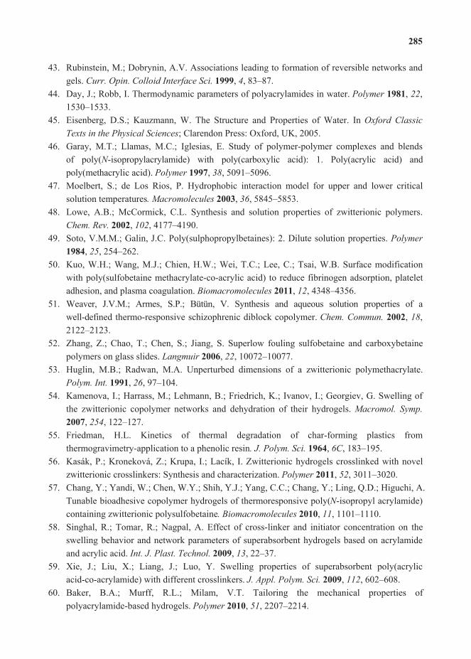
285

43. Rubinstein, M.; Dobrynin, A.V. Associations leading to formation of reversible networks and gels. Curr. Opin. Colloid Interface Sci. 1999, 4, 83–87.

44. Day, J.; Robb, I. Thermodynamic parameters of polyacrylamides in water. Polymer 1981, 22,1530–1533.

45. Eisenberg, D.S.; Kauzmann, W. The Structure and Properties of Water. In Oxford Classic Texts in the Physical Sciences; Clarendon Press: Oxford, UK, 2005.

46. Garay, M.T.; Llamas, M.C.; Iglesias, E. Study of polymer-polymer complexes and blends of poly(N-isopropylacrylamide) with poly(carboxylic acid): 1. Poly(acrylic acid) and poly(methacrylic acid). Polymer 1997, 38, 5091–5096.

47. Moelbert, S.; de Los Rios, P. Hydrophobic interaction model for upper and lower critical solution temperatures. Macromolecules 2003, 36, 5845–5853.

48. Lowe, A.B.; McCormick, C.L. Synthesis and solution properties of zwitterionic polymers. Chem. Rev. 2002, 102, 4177–4190.

49. Soto, V.M.M.; Galin, J.C. Poly(sulphopropylbetaines): 2. Dilute solution properties. Polymer1984, 25, 254–262.

50. Kuo, W.H.; Wang, M.J.; Chien, H.W.; Wei, T.C.; Lee, C.; Tsai, W.B. Surface modification with poly(sulfobetaine methacrylate-co-acrylic acid) to reduce fibrinogen adsorption, platelet adhesion, and plasma coagulation. Biomacromolecules 2011, 12, 4348–4356.

51. Weaver, J.V.M.; Armes, S.P.; Bütün, V. Synthesis and aqueous solution properties of a well-defined thermo-responsive schizophrenic diblock copolymer. Chem. Commun. 2002, 18,2122–2123.

52. Zhang, Z.; Chao, T.; Chen, S.; Jiang, S. Superlow fouling sulfobetaine and carboxybetaine polymers on glass slides. Langmuir 2006, 22, 10072–10077.

53. Huglin, M.B.; Radwan, M.A. Unperturbed dimensions of a zwitterionic polymethacrylate. Polym. Int. 1991, 26, 97–104.

54. Kamenova, I.; Harrass, M.; Lehmann, B.; Friedrich, K.; Ivanov, I.; Georgiev, G. Swelling of the zwitterionic copolymer networks and dehydration of their hydrogels. Macromol. Symp.2007, 254, 122–127.

55. Friedman, H.L. Kinetics of thermal degradation of char-forming plastics from thermogravimetry-application to a phenolic resin. J. Polym. Sci. 1964, 6C, 183–195.

56. Kasák, P.; Kroneková, Z.; Krupa, I.; Lacík, I. Zwitterionic hydrogels crosslinked with novel zwitterionic crosslinkers: Synthesis and characterization. Polymer 2011, 52, 3011–3020.

57. Chang, Y.; Yandi, W.; Chen, W.Y.; Shih, Y.J.; Yang, C.C.; Chang, Y.; Ling, Q.D.; Higuchi, A.Tunable bioadhesive copolymer hydrogels of thermoresponsive poly(N-isopropyl acrylamide) containing zwitterionic polysulfobetaine. Biomacromolecules 2010, 11, 1101–1110.

58. Singhal, R.; Tomar, R.; Nagpal, A. Effect of cross-linker and initiator concentration on the swelling behavior and network parameters of superabsorbent hydrogels based on acrylamide and acrylic acid. Int. J. Plast. Technol. 2009, 13, 22–37.

59. Xie, J.; Liu, X.; Liang, J.; Luo, Y. Swelling properties of superabsorbent poly(acrylic acid-co-acrylamide) with different crosslinkers. J. Appl. Polym. Sci. 2009, 112, 602–608.

60. Baker, B.A.; Murff, R.L.; Milam, V.T. Tailoring the mechanical properties of polyacrylamide-based hydrogels. Polymer 2010, 51, 2207–2214.

286

61. Zhu, X.F.; Yang, M.; Zhang, H.X.; Nie, Y.J. The synthesis and characteristic properties of poly (AAc-co-AAm). Adv. Mater. Res. 2011, 213, 534–538.

62. Klenina, O.V.; Fain, E.G. Phase separation in the system polyacrylic acid-polyacrylamide-water.Polym. Sci. USSR 1981, 23, 1439–1446.

63. Osada, Y. Equilibrium study of polymer–polymer complexation of poly(methacrylic acid) and poly(acrylic acid) with complementary polymers through cooperative hydrogen bonding. J. Polym. Sci. Polym. Chem. Ed. 1979, 17, 3485–3498.

64. Painter, P.C.; Graf, J.; Coleman, M.M. A lattice model describing hydrogen bonding in polymer mixtures. J. Chem. Phys. 1990, 92, 6166–6174.

65. Klenina, O.V.; Fain, E.G.; Phase separation in the hydrolyzed polyacrylamide-water-hydrochloricacid system. Kolloidnyi Zhurnal 1980, 42, 558–561.

66. Ilmain, F.; Tanaka, T.; Kokufuta, E. Volume transition in a gel driven by hydrogen bonding. Nature 1991, 349, 400–401.

67. Cecil, R. Model system for hydrophobic interactions. Nature 1967, 214, 369–370.68. Yang, M.; Liu, C.; Li, Z.; Gao, G.; Liu, F. Temperature-responsive properties of

poly(acrylic acid-co-acrylamide) hydrophobic association hydrogels with high mechanical strength. Macromolecules 2010, 43, 10645–10651.

69. Sasase, H.; Aoki, T.; Katono, H.; Sanui, K.; Ogata, N.; Ohta, R.; Kondo, T.; Okano, T.; Sakurai, Y. Regulation of temperature-response swelling behavior of interpenetrating polymer networks composed of hydrogen bonding polymers. Die Makromol. Chem. Rapid Commun.1992, 13, 577–581.

70. Katono, H.; Sanui, K.; Ogata, N.; Okano, T.; Sakurai, Y. Drug release off behavior and deswelling kinetics of thermo-responsive IPNs composed of poly(acrylamide-co-butyl methacrylate) and poly(acrylic acid). Polym. J. 1991, 23, 1179–1189.

71. Singhal, R.; Gupta, I. A study on the effect of butyl methacrylate content on swelling and controlled-release behavior of poly (acrylamide-co-butyl-methacrylate-co-acrylic acid) environment-responsive hydrogels. Int. J. Polym. Mater. 2010, 59, 757–776.

72. Shibanuma, T.; Aoki, T.; Sanui, K.; Ogata, N.; Kikuchi, A.; Sakurai, Y.; Okano, T. Thermosensitivephase-separation behavior of poly(acrylic acid)-graft-poly(N,N-dimethylacrylamide) aqueous solution. Macromolecules 1999, 33, 444–450.

73. McCormick, C.L.; Sumerlin, B.S.; Lokitz, B.S.; Stempka, J.E. RAFT-synthesized diblock and triblock copolymers: Thermally-induced supramolecular assembly in aqueous media.Soft Matter 2008, 8, 1760–1773.

74. Duran, S.; Solpan, D.; Güven, O. Synthesis and characterization of acrylamide-acrylic acid hydrogels and adsorption of some textile dyes. Nuclear Instrum. Methods Phys. Res. Sect. B1999, 151, 196–199.

75. Katime, I.; Novoa, R.; de Apodaca, E.D.; Mendizábal, E.; Puig, J. Theophylline release from poly(acrylic acid-co-acrylamide) hydrogels. Polym. Test. 1999, 18, 559–566.

76. Chu, L.-Y.; Li, Y.; Zhu, J.-H.; Chen, W.-M. Negatively thermoresponsive membranes with functional gates driven by zipper-type hydrogen-bonding interactions. Angew. Chem. Int. Ed.2005, 44, 2124–2127.

287

77. Hochberg, A.; Tanaka, T.; Nicoli, D. Spinodal line and critical point of an acrylamide gel. Phys. Rev. Lett. 1979, 43, 217–219.

78. Haas, H.C.; Moreau, R.D.; Schuler, N.W. Synthetic thermally reversible gel systems. II.J. Polym. Sci. Polym. Phys. Ed. 1967, 5, 915–927.

79. Haas, H.C.; Chiklis, C.K.; Moreau, R.D. Synthetic thermally reversible gel systems. III.J. Polym. Sci. Part A 1970, 8, 1131–1145.

80. Haas, H.C.; MacDonald, R.L.; Schuler, A.N. Synthetic thermally reversible gel systems. IV. J. Polym. Sci. Part A 1970, 8, 1213–1226.

81. Haas, H.C.; Manning, M.J.; Mach, M.H. Synthetic thermally reversible gel systems. V. J. Polym. Sci. Part A 1970, 8, 1725–1730.

82. Haas, H.C.; MacDonald, R.L.; Schuler, A.N. Synthetic thermally reversible gel systems. VI. J. Polym. Sci. Part A 1970, 8, 3405–3415.

83. Seuring, J.; Agarwal, S.; Harms, K. N-Acryloyl glycinamide. Acta Crystallogr. Sect. E 2011,67, o2170.

84. Nagaoka, H.; Ohnishi, N.; Eguchi, M. Thermoresponsive Polymer and Production Method Thereof; Chisso Corporation: Alexandria, VA, USA, 2007.

85. Ohnishi, N.; Furukawa, H.; Kataoka, K.; Ueno, K. Polymer Having an Upper Critical Solution Temperature; Nathional Institute of Advanced Industrial Science and Technology, Chisso Corporation: Alexandria, VA, USA, 2007.

86. Glatzel, S.; Badi, N.; Päch, M.; Laschewsky, A.; Lutzm, J.-F. Well-defined synthetic polymers with a protein-like gelation behavior in water. Chem. Commun. 2010, 46, 4517–2519.

87. Seuring, J.; Bayer, F.M.; Huber, K.; Agarwal, S. Upper critical solution temperature of poly(N-acryloyl glycinamide) in water: A concealed property. Macromolecules 2011, 44,8962–8971.

288

Preparation and Characterization of the TiO2 Immobilized Polymeric Photocatalyst for Degradation of Aspirin under UVand Solar Light

Debjani Mukherjee, Shahzad Barghi and Ajay K. Ray

Abstract: The traditional use of TiO2 powder as a photocatalyst for degradation of organic compounds has several post-degradation treatment problems, such as filtration, precipitation, etc. A novel method was developed to immobilize TiO2 to minimize/eliminate such problems. Polymeric membrane was used as a base material, over which the TiO2 photocatalyst was immobilized as a thin layer. Preparation and characterization of five different types of polymeric/TiO2 film photocatalysts were elucidated. The catalysts’ films were cross-linked by physical, chemical, and combination of these two processes. The polymers used in the formulation of the catalysts membranes are nontoxic in nature (approved by the World Health Organization (WHO) and Food and Drug Administration (FDA). The morphology of the films were studied by SEM. Photocatalytic degradation of acetylsalicylic acid was carried out to study the efficacy and efficiency of the polymeric membrane based TiO2 as photocatalysts under both UV and solar light irradiation. The degradation was observed to be dependent on the catalyst loading as well as the film thickness. The effects of the types of cross-link bonds on the photocatalytic degradation were also investigated.

Reprinted from Processes. Cite as: Mukherjee, D.; Barghi, S.; Ray, A.K. Preparation and Characterization of the TiO2 Immobilized Polymeric Photocatalyst for Degradation of Aspirin under UV and Solar Light. Processes 2014, 2, 12–23.

Nomenclature

C and Co Concentration, ppmK Langmuir-Hinshelwood rate constantK Langmuir constantPVA Polyvinyl alcoholPVP Polyvinyl pyrrolidoneP25 TiO2 Degussa P25 Titanium dioxideSEM Scanning Electron MicroscopyCL Cross link

Subscripts

Sl slurryf-d Freeze driedAld AldehydeUV Ultraviolet

289

H Heat treatedf-d/UV Freeze dried UV treated

1. Introduction

One of the most pressing environmental issues of present and future is the effective protection and utilization of the precious fresh water resources of the world. According to the World Health Organization (WHO) more than one billion people in the world are suffering from the lack of access to clean potable water. Waterborne infections account for 80 percent of all infectious diseases in the world. Pharmaceuticals, in general, enter the environment through different pathways, resulting in the contamination of ground/underground water, where bacteria are most likely the primarily affected organisms. Due to high intake of non-steroidal anti-inflammatory drugs (NSAIDs), their presence in drinking water has been widely reported [1]. Aspirin belongs to this class of medications called NSAIDs. NSAIDs are the most frequently prescribed agents to treat fever, pain, arthritis, etc. In addition to its effects on pain, fever, and inflammation, aspirin also has an important inhibitory effect on platelets in blood. This antiplatelet effect is used to prevent blood clot formation inside arteries, particularly in individuals who have atherosclerosis (narrowing of the blood vessels), or are otherwise prone to develop blood clots in their arteries preventing heart attack and strokes. Molecular structure of aspirin is shown in Figure 1.

In aqueous solutions, organic compounds can undergo photochemical transformations with sunlight via direct or indirect photoreactions [2]. Such photochemical degradation can be one of the major transformation processes and one of the factors that control the ultimate fate of organic pollutants in the environment. Various technologies are in use to purify aqueous municipal and industrial effluents containing pharmaceutical substances, before entering surface waters. Among them, advanced oxidation processes (AOPs) have been of major interest in recent years.

Figure 1. Molecular structure of aspirin.

Among all the Advance Oxidation Processes (AOPs), Titanium Dioxide (TiO2) photocatalytic oxidation holds a great deal of promise to address this issue due to the low cost of TiO2 and its chemical stability. It is also remarkably active, and non-toxic over a wide range of pHs. In general, the goal of photocatalysis in water treatment is transformation, deactivation, and, finally,mineralization of environmentally persistent compounds. The TiO2 photocatalyst is able to utilize sunlight and air to produce many reactive species, including the powerful and non-selective oxidant hydroxyl radicals, to destroy organic compounds. One of the major drawbacks is expensive filtration technique needed to remove the slurry TiO2 from the purified water [3,4]. This problem

290 has resulted in development of several kinds of immobilization techniques to immobilize the TiO2

powder, which may reduce the post degradation expenses and time. TiO2 in anatase, Degussa form has been immobilized by several methods. The design and development of an immobilized thin catalyst film facilitates commercial-scale applications of TiO2-based photocatalytic processes for water treatment significantly. The dimensionality associated with the structure of a TiO2 material can affect its properties and functions, including its photocatalytic performance, and also,more specifically, its surface area, adsorption, reflectance, adhesion, and carrier transportation properties [5]. Immobilization of TiO2 photocatalyst eliminates the need for the separation of the catalyst particles from the treated liquid and enables the contaminated water to be treated continuously. The catalyst film is porous and can therefore provide a large surface area for the degradation of contaminant molecules. If a conductive material is used as the support, the catalyst film can be connected to an external potential source to remove excited electrons to reduce electron-hole recombination, thereby, significantly improving the process efficiency [6–9]. Di Paola et al. [10] reviewed different type of TiO2 catalysts and claimed that although many of these photocatalysts were effective for the photodecomposition of many pollutants, most of them do not allow a complete mineralization of the starting compounds.

Several researches have been carried out on immobilization of the TiO2 [11,12]. Two obvious problems arising from this arrangement: the accessibility of the catalytic surface to the photons and the reactants and a significant influence of the external mass transfer resistanceparticularly at low fluid flow rate, due to the increasing diffusion length of the reactant from thesolution to the catalyst surface [13]. Maedaa [14] presented a comprehensive review of different reactor designs for air- or water-purification with the main emphasis on the enlargement of reactive surface area and improvement of mass transfer. Several kinds of film photocatalysts have been formulated by researchers, such as TiO2 loaded carbon fiber [15], silicone-TiO2 polymeric composite [16], Polypropylene/clay with TiO2 composite [17], and TiO2-PVP (Polyvinyl pyrrolidone)nano-composite [18]. Ochiai and Fujishima [19] fabricated a novel photocatalytic filter, titanium-mesh sheet modified with TiO2. The titanium mesh sheet was claimed to be highly flexible with a large contact area with a minimum pressure drop. Modification of the photocatalyst with a suitable cocatalyst was carried out to provide an active redox site for water slitting [20]. Due to challenges associated with the use of UV light, several attempts have been made to use visible light instead. Pelaeza et al. [21] presented different strategies for the modification of TiO2

photocatalyst for the utilization of visible light along with comprehensive studies on the photocatalytic degradation of contaminants.

These immobilization techniques have been reported to reduce the cost of filtration and also in some cases increase the efficiency of TiO2 as photocatalyst, due to the synergistic effect of the substrate and TiO2. All these techniques have been proved to be successful though being expensive and time consuming their use has been limited. In this study, a polymeric film was prepared as a substrate for immobilization. The degradation of aspirin was carried out to measure and compare the photocatalytic efficiency of the films. Mass transfer limitations become a dominant factor when immobilized photocatalyst film is used, which usually lead to a lower overall degradation rate compared to the suspended catalyst systems [22,23].

291

The degradation kinetics of aspirin follows the Langmuir-Hinshelwood (L-H) model.

(1)

where r is the photocatalytic degradation rate, k is the L-H kinetic rate constant, and K is the Langmuir adsorption constant. A linear plot of 1/r against 1/C is often used to estimate the L-H rate constants, k, and the Langmuir adsorption constant, K, for aspirin in the photocatalytic degradation reaction. The analysis is based on the occurrence of the reactions on the active site of the catalysts where hydroxyl radicals are actually formed.

(2)

2. Experimental Section

2.1. TiO2 Immobilization Procedure

2.1.1. Preparation of Polymeric/TiO2 Membranes

9% w/v of PVA and 4% w/v Gelatin were dissolved and mixed properly in distilled water to get a transparent solution. Next, 8% w/v of PVP was dissolved in a solution of ethyl alcohol and water (in 2:1 ratio) and added to the PVA-Gelatin solution and the reaction was carried out at room temperature. The solution was stirred for 15 min, followed by dispersion of 16% w/w TiO2 DegussaP25 powder in the mixture. Thereafter, the polymeric/TiO2 solutions were cross-linked by physical, chemical, and physico-chemical methods. The polymer matrix used for immobilization may be degraded under ultraviolet light however in the context of this research and during all the experiments such a phenomenon was observed. Apparently the degradation rate of polymer matrix is much longer than the duration of the experiments.

2.1.2. Physical Cross-Linking Methods

2.1.2.1. Freeze Drying

The TiO2 dispersed polymeric solution was then physically cross-linked by storing the solution below zero degrees centigrade. The polymeric solutions were stored at different temperatures ranging from 0 to 10 °C for different time intervals of 1, 3, 5, 7, 10, 15, 24 (h). It was found that the samples stored for 5 h showed the best results under solar and UV lights. Solutions stored for less than 5 h showed very soft and flexible films, which were partially dissolved in water during the photo-degradation reaction, while the ones stored for longer than 5 h formed mechanically strong catalysts due to more cross linking, but showed lower degradation. The lower degradation rate was most probably due to blockage of the TiO2 active site by the cross-linked polymers. Therefore, the freeze-dried film was cross-linked physically at 2 °C for 5 h (optimum condition).

KCkKC

dtdCr

1

kCkKr1111

292 2.1.2.2. Heat Treatment

Cross-linking also occurs at higher temperatures. Generally, cross-linking increases with increasing temperature, therefore the prepared polymeric/TiO2 solution was placed in an oven for different times, at different temperatures, to cross-link. Due to deactivation of PVP at 120 °C and due to uneven distribution of temperature in the oven, it was found that 105 °C was the optimum temperature for cross-linking. Samples were kept at 105 °C for different period of times between 5and 120 min. The solution, which had been kept for 10 min, showed the best results with respect tothe desired mechanical properties and degradation efficiency.

2.1.3. Chemical Cross-Linking Methods

2.1.3.1. Acetaldehyde Treatment

Aldehydes are known to initiate cross-linking of PVP polymer solution instantly. Acetaldehyde chemically cross-links with PVP in the polymeric solution and instantly forms a membrane. After several experiments, it was found that 0.5 mL of 2% acetaldehyde at room temperature was sufficient to crosslink the polymer solution completely. The membrane was then dipped in distilled water and washed 3 times to remove the unreacted acetaldehyde traces.

2.1.3.2. UV Treatment

Polymeric solutions with dispersed TiO2 were exposed to UV light of 275 nm wavelength for different periods of time (2, 5, 7, 10, 20, 30, and 60 min). It was observed that exposure for 10 min provided the best results among all the samples. Samples exposed for 2–7 min did not form mechanically strong films, which in turn degraded in the aqueous solution during the photo-degradation process. The catalyst films formed by exposure of 20–60 min was mechanically strong but, due to high cross-linking effects, the TiO2 particles got entangled within polymer matrix, resulting in blockage of the active sites and lower degradation efficiency.

2.1.3.3. Freeze-Dried and UV Treated

The polymeric solution was prepared following the aforementioned freeze drying method(kept at 0 °C for 5 h) and then exposed to UV lamp of 275 nm wavelength for 10 min to cure the polymeric membrane.

3. Characterization and Degradation of Aspirin

Optical microscopy, Scanning Electron Microscopy (SEM, Hitachi F-4000) and Fourier transform Infra Red were employed to characterize the immobilized TiO2 photocatalyst film. SEM studies of the film photocatalysts revealed the specific pore volume and pore density. The measuring scale was 2.5 m. Catalyst films were also subjected to Fourier Transform Infra Red (FTIR) Spectroscopy. The specimens were prepared as thin and homogenous films. FTIR spectra were measured in the wave number range 400–4000 cm 1.

293

The photodegradation reactions were carried out in batch reactors, in presence of both solar and UV lights with five different kinds of polymeric/TiO2 catalyst films. The batch reactors were250 mL in volume, containing aspirin solutions under a UV lamp of 22 mW/cm2 intensity and the solar stimulator of light intensity 27 mW/cm2. The concentrations of the degraded aspirin solutionswere analyzed using a UV-Vis Agilent spectrophotometer at 270 nm.

4. Results and Discussions

4.1. Optical Microscopy

The polymeric/TiO2 catalyst films were subjected to optical microscopy (OM) to observe their porous structures. The freeze-dried film showed a spongy porous structure. The heat-treated films were observed to have a highly porous 3D structure, which made the filmsremain buoyant in water. The acetaldehyde and UV treated films showed solid matrices with very few pores. The UV-Freeze-dried treated films showed a spongy structure similar to freeze-dried but with fewer number of pores. Figures 2–6 show the structures of the five different immobilized photo-catalyst films.

Figure 2. Optical Microscope image of freeze-dried film.

Figure 3. Optical Microscope image of heat-treated film.

294

Figure 4. Optical Microscope image of UV-treated film.

Figure 5. Optical Microscope image of UV-treated and freeze dried film.

Figure 6. Optical Microscope image of acetaldehyde-treated film.

4.2. Scanning Electron Microscopy (SEM) Study

The polymeric/TiO2 catalyst film thickness ranged from 0.45 mm to 2 mm. The micrographs taken by scanning electron microscopy revealed a three-dimensional network structure, which wastypical for a porous material. Figure 7 shows the porous structure of the freeze-dried catalyst film.Obviously, the freeze-dried membrane is rather homogeneous, interspersed with pores of various diameters, ranging from 50 to 300 m. The average pore area was found to be 572 m2. The pore density ranged from 7 to 10 pores per mm2 for the freeze-drying film. The pore density was 12–15 pores per mm2 for the heat-treated polymeric/TiO2 catalyst film. The acetaldehyde and

295

UV treated samples showed almost no pores and the freeze-dried-UV treated film showed3–5 pores per mm2. Figures 7–11 show the SEM images of the samples.

Figure 7. SEM image of freeze-dried polymeric/TiO2 catalyst membrane.

Figure 8. SEM image of heat-treated membrane.

Figure 9. SEM image of UV-treated membrane.

Figure 10. SEM image of UV treated and freeze-dried membrane.

296

Figure 11. SEM image of acetaldehyde-treated composite membrane.

4.3. Degradation of Acetylsalicylic Acid (Aspirin)

Cross-linking affected degradation of aspirin under UV and solar light over different photocatalyst films. As shown in Figures 11–13, the freeze-dried catalyst was more efficient in degrading aspirin compared to the other photocatalyst films in presence of solar light. Although,the freeze-dried catalyst showed higher degrading efficiency under UV light, the efficiencydecreased rapidly with time. UV radiation activates cross-linking and, with more cross-linking, less TiO2 active site would be available, resulting in gradual decrease of the degradation rate with time.The freeze-dried catalysts were useable for a short period of time as some polymeric flakes leached out into the aqueous system after six to seven hours of use. Although these polymers are nontoxic and have been approved by the FDA and WHO, and can be removed by a simple filtration method,such a phenomenon may restrict their application and more investigation is required to improve their mechanical stability. On the other hand, the heat-treated photocatalyst film was buoyant and could be used several times for the degradation of organic model compound. The UV treated and UV-freeze-dried catalysts showed the slowest degradation rate. The aldehyde treated catalyst was found to remain in submerged condition in water during the reaction and also showed a slower degradation rate. The UV treated catalyst membrane showed morphological characteristics, the same as UV-freeze-dried catalyst, and both catalysts were observed to follow almost the same rate of degradation in presence of solar light and UV light. The UV treated catalyst showed higher tensile strength due to formation of strong cross-linking bonds but became blue after the UV treatment. This blue colorization is due to the entrapped electrons, which delay the degradation rate. Table 1 shows the reaction rate constant, k, for different TiO2 immobilized catalysts under UV and solar radiation.

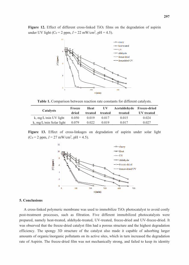
297

Figure 12. Effect of different cross-linked TiO2 films on the degradation of aspirin under UV light (C0 = 2 ppm, I = 22 mW/cm2, pH = 4.5).

Table 1. Comparison between reaction rate constants for different catalysts.

CatalystsFreeze dried

Heat treated

UVtreated

Acetaldehyde treated

Freeze-dried UV treated

k, mg/L/min UV light 0.050 0.019 0.017 0.015 0.024k, mg/L/min Solar light 0.079 0.022 0.019 0.017 0.027

Figure 13. Effect of cross-linkages on degradation of aspirin under solar light(C0 = 2 ppm, I = 27 mW/cm2, pH = 4.5).

5. Conclusions

A cross-linked polymeric membrane was used to immobilize TiO2 photocatalyst to avoid costly post-treatment processes, such as filtration. Five different immobilized photocatalysts were prepared, namely heat-treated, aldehyde-treated, UV-treated, freeze-dried and UV-freeze-dried. It was observed that the freeze-dried catalyst film had a porous structure and the highest degradation efficiency. The spongy 3D structure of the catalyst also made it capable of adsorbing largeramounts of organic/inorganic pollutants on its active sites, which in turn increased the degradation rate of Aspirin. The freeze-dried film was not mechanically strong, and failed to keep its identity

298 after six to seven hours. The UV-treated catalyst films showed very few or almost no pores, whilethe heat-treated photocatalyst film contained several air pockets, which made it buoyant in aqueous solutions. The buoyant nature of the heat-treated film may be exploited to keep the catalyst film afloat and exposed to solar light for the continuous degradation of pollutant in water. The toxic nature of aldehyde reduces the chance of using aldehyde-treated catalyst films for drinking water purification. The UV-treated catalysts showed higher tensile strength, however, due to strong cross-linkage effect of UV light, these films have fewer active sites of TiO2 available for interacting with the photons.

Conflicts of Interest

The authors declare no conflict of interest.

References

1. Liu, C.-C.; Hsieh, Y.-H.; Lai, P.-F.; Li, C.-H.; Kao, C.-L. Photodegradation treatment of azo dye waste water by UV/TiO2 process. Dye. Pigment. 2006, 68, 191–195.

2. Fujishima, A.; Honda, K. Electrochemical photolysis of water at a semiconductor electrode. Nature 1972, 238, 37–38.

3. Photocatalytic Purification and Treatment of Water and Air; Al-Ekabi, H.A., Ollis, D., Eds.;Elsevier: Amsterdam, The Netherlands, 1993.

4. Andronic, L.; Duta, A. The influence of TiO2 powder and film on methyl orange degradation.Mater. Chem. Phys. 2008, 112, 1078–1082.

5. Vincenzo, A.; Marianna, B.; Vittorio, L.; Giovanni, P.; Leonardo, P.; Sedat, Y. Overview on oxidation mechanisms of organic compounds by TiO2 in heterogeneous photocatalysis.J. Photochem. Photobiol. C 2012, 13, 224–245.

6. Daneshvar, N.; Salari, D.; Khataee, A.R. Photocatalytic degradation of azo dye acid red 14 in water: Investigation of the effect of operational parameters. J. Photochem. Photobiol. A 2003,157, 111–116.

7. Akira Fujishima, A.; Rao, T.N.; Tryk, D.A. Titanium dioxide photocatalysis. J. Photochem.Photobiol. C 2000, 1, 1–21.

8. Chen, D.; Ray, A.K. Photocatalytic kinetics of phenol and its derivatives over UV irradiated TiO2. Appl. Catal. B 1999, 23, 143–157.

9. Rizzo, L.; Koch, J.; Belgiorno, V.; Anderson, M.A. Removal of methylene blue in a photocatalytic reactor using polymethylmethacrylate supported TiO2 nanofilm. Desalination2007, 211, 1–9.

10. Di Paola, A.; García-López, E.; Marcìa, G.; Palmisano, L. A survey of photocatalytic materials for environmental remediation. J. Hazard. Mater. 2012, 211–212, 3–29.

11. Dung, N.T.; van Khoa, N.; Herrmann, J.-M. Photocatalytic degradation of reactive dye RED-3BA in aqueous TiO2 suspension under UV-visible light. Int. J. Photoenergy 2005, 25,250–255.

299

12. Kalfa, O.M.; , Ö.; Türker, A.R. Synthesis of nano B2O3/TiO2 composite material as a new solid phase extractor and its application to preconcentration and separation of cadmium.J. Hazard. Mater. 2009, 166, 455–461.

13. Rashed, M.N.; El-Amin, A.A. Photocatalytic degradation of methyl orange in aqeous TiO2

under different solar irradiation sources. Int. J. Phys. Sci. 2007, 2, 73–81.14. Maedaa, K. Photocatalytic water splitting using semiconductor particles: History and recent

developments. J. Photochem. Photobiol. C 2011, 12, 237–268.15. Shi, J.; Zheng, J.; Wu, P.; Ji, X. Immobilization of TiO2 films on activated carbon fiber and

their photocatalytic degradation properties for dye compounds with different molecular size.Catal. Commun. 2008, 9, 1846–1850.

16. Ochiai, T.; Hoshi, T.; Slimen, H.; Nakata, K.; Murakami, T.; Tatejima, H.; Koide, Y.; Houas,A.; Horie, T.; Moritobe, Y.; et al. Fabrication of a TiO2 nanoparticles impregnated titanium mesh filter and its application for environmental purification. Catal. Sci. Technol. 2011, 1,1324–1327.

17. Li, J.; Chen, C.; Zhao, J.; Zhu, H.; Orthman, J. Photodegradation of dye pollutants on TiO2

particles dispersed in silicate under UV-Vis irradiation. Appl. Catal. B 2002, 37, 331–338.18. Kansal, S.K.; Singh, M.; Sud, D. Studies on photodegradation of two commercial dyes in

aqueous phase using different photocatalysts. J. Hazard. Mater. 2007, 141, 581–590.19. Ochiai, T.; Fujishima, A. Photoelectrochemical properties of TiO2 photocatalyst and its

applications for environmental purification. J. Photochem. Photobiol. C 2012, 13, 247–262.20. Nakataa, K.; Fujishima, A. TiO2 photocatalysis: Design and applications. J. Photochem.

Photobiol. C 2012, 13, 169–189.21. Pelaez, M.; Nolan, N.T.; Pillai, S.C.; Seery, M.K.; Kontos, P.F.G.; Dunlop, P.S.M.; Hamilton,

J.W.J.; Byrne, J.A.; O’Shea, K.; Entezari, M.H.; et al. A review on the visible light active titanium dioxide photocatalysts for environmental applications. Appl. Catal. B 2012, 125, 331–349.

22. Yamashita, H.; Harada, M.; Tanii, A.; Misaka, J.; Nakao, H.; Anpo, M. Design of TiO2 activated carbon filter systems by an Ionized Cluster Beam Method and their application for photocatalytic water purification. Mol. Cryst. Liq. Cryst. 2002, 388, 453–458.

23. Lin, L.-H.; Lee, H.-T. A new modified silicone–TiO2 polymer composite film and its photocatalytic degradation. J Appl. Polym. Sci. 2006, 102, 3341–3344.

300

Dynamic Modeling for the Design and Cyclic Operation of anAtomic Layer Deposition (ALD) Reactor

Curtisha D. Travis and Raymond A. Adomaitis

Abstract: A laboratory-scale atomic layer deposition (ALD) reactor system model is derived for

alumina deposition using trimethylaluminum and water as precursors. Model components describing

the precursor thermophysical properties, reactor-scale gas-phase dynamics and surface reaction

kinetics derived from absolute reaction rate theory are integrated to simulate the complete reactor

system. Limit-cycle solutions defining continuous cyclic ALD reactor operation are computed with

a fixed point algorithm based on collocation discretization in time, resulting in an unambiguous

definition of film growth-per-cycle (gpc). A key finding of this study is that unintended chemical

vapor deposition conditions can mask regions of operation that would otherwise correspond to

ideal saturating ALD operation. The use of the simulator for assisting in process design decisions

is presented.

Reprinted from Processes. Cite as: Travis, C.D.; Adomaitis, R.A. Dynamic Modeling for the Design

and Cyclic Operation of an Atomic Layer Deposition (ALD) Reactor. Processes 2013, 1, 128–152.

1. Introduction

Atomic layer deposition (ALD) is a thin-film manufacturing process in which the growth surface

is exposed to an alternating sequence of gas-phase chemical precursor species separated by purge

periods to prevent gas-phase reactions [1,2]. ALD is characterized by self-limiting heterogeneous

reactions between the gas-phase precursor species and surface-bound species, which, when allowed

sufficient conditions to reach saturation, results in highly conformal thin films, on both planar

and non-planar geometries, with atomic level control of film deposition [1,3]. With advances in

current technologies alongside a growing body of knowledge on the ALD process, ALD functions

have expanded to accommodate a wide range of applications, including photovoltaics [4], energy

devices [5–7], nanofabrication [8], environmental issues [6] and even medical devices and biological

systems [9].

A simplified view of the ALD binary reaction sequence for growing metal-oxide compound,

“MO”, from the metal precursor (denoted M with a red dot) and the oxygen precursor (denoted

O with a blue dot) is schematically illustrated in Figure 1. Generally, during the first exposure

period (Exposure A), the metal precursor adsorbs onto an oxygenated substrate, undergoing

a ligand-exchange reaction with the surface-bound oxygen species and, thereby, becoming

permanently bound to the growth surface. After a sufficient purge period leaving no reactive

species in the gas phase, the oxygen precursor (e.g., H2O, O2, O3) is introduced during Exposure

B, initiating a subsequent reaction, which proceeds analogously to the reaction in Exposure A,

whereby the oxygen precursor adsorbs onto the surface, undergoes a ligand-exchange reaction with

301

the surface-bound metal species and, consequently, becomes permanently bound to the growth

surface [3].

Figure 1. An idealized view of the atomic layer deposition (ALD) process cycle.

O O O O O O O O

MM

M

M

M

Exposure A

M

O

M

O

M

O

M

O

M

O

M

O

M

O

M

O

OO

OO

O

Exposure B

O

M

O

O

M

O

O

M

O

O

M

O

O

M

O

O

M

O

O

M

O

O

M

O

Purge

M

O

M

O

M

O

M

O

M

O

M

O

M

O

M

O

Purge

ALD and the more widely understood chemical vapor deposition (CVD) share a number of

common characteristics. For example, both deposition processes are inherently nonlinear and

time-dependent, and mathematical model elements describing the deposition surface reaction and

gas-phase precursor transport are strongly coupled. In particular, the transport and reaction models

must describe chemical and physical phenomena over multiple time and length scales. Because of

this phenomenological overlap, some modeling concepts and computational tools developed by the

CVD community can be directly put to use in the analysis of ALD systems.

One important distinction, however, can be made between the two deposition processes: the

notion of the steady-state deposition rate in CVD does not exist for ALD. The rate of ALD depends

strongly on the instantaneous state of the growth surface, and this state changes continuously

through each exposure and purge period. The completely dynamic nature of the ALD process

adds considerably to the difficulty of developing simulators, because the entire process cycle

must be modeled, i.e., the extent of reactions taking place during half-cycle A influence those

taking place during half-cycle B, and vice versa. Due to the heterogeneous nature of these ALD

reactions, adsorption, desorption and surface reaction kinetics play a crucial role in the deposition

process [2,10]. Careful chemical and mathematical analysis is required to resolve the multiple time

scales present in this process to identify the rate-limiting steps.

The focus of this paper will be on the development of a dynamic ALD process model

(Figure 2) based on a laboratory-scale reactor system currently under construction. The primary

contributions of this paper are its use of physically-based reaction kinetics models derived from

transition state theory [11] and limit-cycle calculations describing the steady operation of these

reactor systems.

302

Figure 2. Elements of a complete ALD reactor system mathematical model.

1.1. Review of ALD Models

A range of ALD models has been developed at various levels of detail and theory [12] to

accommodate specific modeling objectives. Of these, atomic-scale models have produced insightful

results by employing ab initio methods, such as density functional theory (DFT), to investigate

reaction mechanisms, energetically favored reaction pathways, proton transfer mechanisms,

structures of surface reaction intermediate species and reaction energetics corresponding to reactions

along each stage of ALD growth (see [13] for a comprehensive review of atomic-scale ALD models).

Results of such studies have been combined with kinetic Monte Carlo (kMC) simulations to quantify

nucleation [14] and growth [15,16] kinetics. Empirical growth models have also been developed

to describe ALD kinetics during the initial stages of nucleation [17,18] and island growth [19–21].

Additionally, surface reaction models have been developed to predict growth kinetics and the effects

of operating parameters (e.g., temperature, pressure, precursor exposure time) during undersaturating

conditions and leading to self-limiting ALD growth [11,22–25].

A number of detailed ALD reactor simulations have been reported in the literature, generally

comprised of transport equations coupled with a surface reaction model to describe the evolution of

the ALD growth surface. For example, [26] developed a 1D reactor model comprised of the species

conservation equation to describe precursor concentration through the reactor vessel and a surface

coverage equation, which relates adsorption to an experimentally-determined sticking coefficient

based on time-dependent surface coverage and precursor concentration at the reactor outlet. The

model was further used to study temperature effects on surface coverage [27] and the effects of

secondary reactions on film thickness [28]. A 1D plug-flow model is presented by [29], which also

employs the species conservation equation to determine the spatially- and time-dependent pressure

profile in the reactor starting with solid precursor evaporation, and uses a kinetic expression based on

an estimated sticking coefficient. A simple plug flow model, based largely on empirical sticking and

recombination probabilities, also was developed by [30] to study film conformality as a function of

aspect ratio, but the details of the mathematical model were omitted.

303

A transient plug-flow model for a tubular ALD reactor was developed by [31], where the

continuity equation is used to describe transport and the reactive sticking coefficient was based on

earlier work of the author [32]. Additionally, see [33] for a similar approach and a more general

discussion of ALD reactor modeling. Furthermore, [34] describe a dynamic reactor model for

alumina ALD processing that combines precursor flow modeling through the reactor and a ballistic

flux model for precursor transport and reaction in substrate trenches. In that study, the reactive

sticking coefficient was attributed to quantum-chemical simulations of the ALD surface reactions,

but the connection between the two was not made clear.

Up to this point, the ALD transport/reaction models discussed have incorporated a reactive

sticking coefficient or reaction probability, combining the quantitative effects of many reaction

phenomena into a single parameter, which may be determined empirically or theoretically. Although

the sticking coefficient is widely used in modeling work, the experimental and computational manner

in which it is determined varies, such that absolute values are rarely reported in the literature [35]. An

alternative to the sticking coefficient approach is to couple transient plug-flow reactor dynamics with

kinetic expressions containing rate constants derived from ab initio quantum-chemical calculations

and the quantum-statistical theory of chemical reactions [36]. Yet another approach is to use the

absolute reaction rate theory and statistical thermodynamics to derive kinetic expressions without the

use of adjustable parameters [11]. Furthermore, [37,38] developed a rigorous 2D transport model,

which is coupled to a heterogeneous surface reaction model based on estimated kinetic parameters

from ex situ film thickness measurements. In this two-part paper series, the researchers examine film

growth and thickness uniformity as a function of process operating parameters, reactor system design

and gas flow distribution as a guide for future ALD process optimization.

1.2. The Reactor

The ALD reactor system considered in this work is based on a laboratory-scale research reactor

currently under construction and to be used in evaluating ALD for a range of spacecraft-related

thin-film applications [39]. As illustrated in Figure 3, the reactor vessel consists of a stainless

steel process tube surrounded by a bench-top tube furnace, containing the substrate(s) and a quartz

crystal microbalance (QCM) for real-time mass deposition measurements. The reactor performance

will be initially tested with the commonly used ALD precursors of trimethylaluminum (TMA) and

water; both are contained in the liquid state in temperature-controlled laboratory bottles. Each of

the precursors flows through a separate sequence of needle valves/orifices to control their flow rates

and, then, through solenoid-activated control valves, CV1-5, to regulate the precursor dosages and

the lengths of the purge periods. The details of the valve sequencing will be described in the Process

Recipe section that follows.

304

Figure 3. A schematic diagram of the laboratory-scale ALD reactor system to

be modeled.

pump

MFC Ar purge

H2O

needle valve

TMA

orifice /

needle valve

ballast ch

substrate QCM

RGA

pump

CV1

CV3

R

L

CV4 CV5

tube furnace P1

P2

CV2

A mass flow controller (MFC) is used to regulate the purge gas (Argon) flow rate, and

low-pressure manometers (denoted P1 and P2) respectively record gas pressure at the reactor outlet

and the small gas chamber used to regulate the TMA dose. Residual gas analysis (RGA) is performed

using a mass spectrometer; the primary vacuum pump is located downstream of the RGA, and a

smaller pump is used to vent water vapor between water doses. Reactor dimensions and other reactor

component specifications are listed in Table 1.

Table 1. Reactor dimensions and primary system component design parameters of the

ALD reactor system shown in Figure 3. TMA, trimethylaluminum.

Parameter Description Value

As substrate growth surface area 6.45× 10−4 m2

Arxr total growth surface area 0.207 m2

L reactor length 0.864 m

mI Ar mass flow controller range 0− 500 sccm

R reactor internal radius 0.0381 m

Vrxr reactor volume 3.94× 10−3 m3

Vbc TMA ballast chamber volume 7.85× 10−7 m3 (0.02% of Vrxr)

St primary exhaust pump capacity 14.6 ft3/min

1.3. Process Recipe

The overall reaction involves trimethylaluminum Al(CH3)3 (precursor A) and water (precursor B)

2Al(CH3)3(g) + 3H2O(g) −→ Al2O3(s) + 6CH4(g)

305

producing the amorphous Al2O3 film and by-product methane gas; the CH4 does not react with any

of the other species in the deposition process and, so, can be considered inert. As described in

the Introduction, each precursor is introduced sequentially, separated by a purge period to prevent

gas-phase reactions:

Exposure A → purge → Exposure B → purge → Exposure A → . . .

τA sec τAP sec τB sec τBP sec τA sec . . .

where the AB cycle repeats—potentially thousands of times—building the film one sub-monolayer

at a time. After the initial nucleation transient following a change in the precursor system (e.g.,

when depositing a nanolaminate consisting of alternating thin-film materials), the deposition behavior

during each AB cycle approaches a limit-cycle solution, the computation of which is the main focus

of this simulation study. The exposure time periods (in seconds) for the AB exposures and purge

periods are denoted as τA, τB, τAP and τBP . A nominal A-purge-B-purge process recipe will be

described later in this manuscript.

Referring to Figure 3, control valves, CV2 and CV5, normally are open during all exposure and

purge periods and, so, will not be discussed further. During the purge period prior to Exposure A,

CV1 is closed to allow TMA to fill the ballast chamber; the TMA partial pressure in this chamber

can potentially reach the vapor pressure of TMA in the supply bottle containing liquid-phase TMA.

During Exposure A, CV1 is opened to allow TMA vapor to flow into the reactor, reducing the pressure

in the ballast chamber. We note that a small flow of TMA will continue through the orifice/needle

valve during Exposure A. At the end of Exposure A, CV1 is closed, and the pressure rebuilds in the

TMA ballast chamber.

Regardless of the position of CV4, Ar purge gas flows continuously during all purge and exposure

periods. During both purge periods and during Exposure A, CV3 is open between the water source

and the water purge pump, as well as to CV4; however CV4 is closed in the direction of CV3,

resulting in no water flow to the reactor. During the water dose, CV4 is switched to the all-open

position, but CV3 is closed in the direction of the water purge pump, allowing the flow of Ar and

water to the reactor. This configuration was designed to prevent condensation in the water delivery

system and to improve the reproducibility of the water dose [40].

2. Precursor Characteristics

The ALD reactor system model development begins with the precursor thermophysical property

and gas delivery system dynamics modeling. From the National Institute of Standards and

Technology (NIST) WebBook [41], we find the Antoine’s equation coefficients for TMA (between

337–400 K) and water (between 293–343 K) as:

log10 PvapTMA = 4.67984− 1724.231

T − 31.398+ log10

760

1.01325

log10 PvapH2O

= 6.20963− 2354.731

T + 7.559+ log10

760

1.01325

306

where the vapor pressure units are Torr and T is in K. The vapor pressures calculated by these

relationships corresponding to the TMA and water sources are given in Table 2. As pointed out

in [42], at lower temperatures and higher TMA partial pressures, the dimer of TMA (d-TMA) is

favored over the monomer (m-TMA) in the gas phase. This is important in determining the true dose

values for the precursor delivery system. The d-TMA dissociation extent as a function of temperature

was studied in [43], where values for the degree of dissociation, α, were given as a function of

temperature; the degree of dimer dissociation is defined as follows:

α =moles of m-TMA

moles of m-TMA + 2(moles of d-TMA)=

moles of m-TMA

noA

(1)

where noA is the total number of Al(CH3)3 molecules whether in monomer or dimer form. Using

a least-squares procedure, we fit the following expression to the data contained in the cited

source to find:

lnKd = −13756.5425

T+ 32.2019

where T again is in K. For a binary mixture of d-TMA and m-TMA, we can solve:

(ymPvapTMA/P

o)2

(1− ym)PvapTMA/P

o= Kd

for the mole fraction, ym, of the monomer with P o = 760 Torr. We note that the m-TMA mole

fraction is related to the degree of dissociation, α [43], by ym = 2α/(1 + α) when considering a

binary mixture.

In a mixture containing additional species that do not participate in the dimerization reaction,

defining nN as the total moles of species not participating in the d-TMA/m-TMA reaction, the

gas-phase m-TMA and d-TMA mole fractions, ym and yd, can be written in terms of α, as follows:

ym =2α

1 + α + 2φ, yd =

1− α

1 + α + 2φ

where φ = nN/noA. If Kd corresponds to the d-TMA dissociation equilibrium coefficient determined

above, defining:

y2myd

= κ =P oKd

P

allows us to compute:

α =−κφ+

√κ2φ2 + κ(4 + κ)(1 + 2φ)

4 + κ(2)

Given the conditions inside the TMA source (T = 300 K, P = P vapTMA and φ = 0), the extremely

small values of Kd and α listed in Table 2 show that TMA leaves the bubbler essentially entirely as

307

the dimer, d-TMA. This can also be observed in Figure 4, where the TMA vapor pressure and degree

of dissociation are plotted.

Table 2. Nominal ALD reactor conditions. d-TMA, dimer of TMA.

Parameter Description Value

mI nominal Ar molar flow 7.44× 10−6 mol/s (10 sccm)

Tamb ambient temperature 300 K

Tbc ballast chamber temperature 300 K

Trxr reactor temperature 500 K

Prxr,base reactor base pressure 0.02 Torr

mrxr,base reactor base molar capacity 2.55× 10−6 mol

τres reactor base residence time 0.343 s

PvapTMA TMA vapor pressure at Tamb 13.67 Torr

PvapH2O

water vapor pressure at Tamb 26.82 Torr

Kd d-TMA dissociation equilibrium constant at Tamb 1.176× 10−6

α d-TMA dissociation degree at Tamb 4.04× 10−3

C1 ballast chamber/reactor flow coefficient 2× 10−8 mol/s/Pa

C2 TMA bubbler/ballast chamber flow coefficient 5× 10−9 mol/s/Pa

C3 H2O supply/reactor flow coefficient 1× 10−8 mol/s/Pa

τA Exposure A 0.2 s

τAP post-A purge 2 s

τB Exposure B 0.1 s

τBP post-B purge 2 s

Figure 4. TMA vapor pressure and degree of dissociation, α, as a function of

temperature; data presented in Table II of [43] are shown as filled red circles.

308

2.1. TMA Delivery System Model

The objective of this model element is to predict the time-dependent TMA molar flow rate,

mAin(t), as this precursor enters the reactor chamber. As seen in Figure 3, the precursor delivery

system is designed to inject a TMA dose regulated by the size of a ballast chamber and the TMA

pressure, P2, in this chamber prior to the opening of control valve, CV1. The dependence of gas molar

flow rate through CV2 and the downstream orifice/needle valve would be a significant challenge to

predict by a purely physically-based modeling approach. Therefore, under the condition that the gas

flow is not in the choked-flow regime, we propose the model:

dmbc

dt= C2 [P

vapTMA − Pbc(t)]

1 + αbc

1 + αsource

− C1γ1(t) [Pbc(t)− Prxr(t)] (3)

where αsource and αbc are the degrees of d-TMA dissociation in the TMA source and ballast chamber,

respectively, computed using Equation (2) with φ = 0. The reactor and ballast chamber pressures are:

P1 ≈ Prxr =mrxrRgTrxr

Vrxr

, P2 = Pbc =mbcRgTbc

Vbc

(4)

where Prxr is the reactor pressure, approximately measured by manometer P1. The function, γ1,

indicates the time-dependent position of CV1. We note that it is possible to measure the effective

flow coefficients, C1 and C2, experimentally using time-dependent measurements of P2. CV2 is

always open under typical operating conditions, allowing for finite gas flow rate whether or not CV1

is open. We note that for this model, any back-diffusion of reactor Ar or other gas species is neglected.

2.2. Water Delivery System Model

Because of the potential for condensation of water in a ballast chamber for this precursor, the

alternative design developed by [40] is used where water evaporating in the H2O source is vented

using an auxiliary purge pump during the TMA dose and purge periods (a similar approach cannot

be used for TMA, because of the expense of discarding unused precursor). This configuration gives

rise to a relatively simple model for the water dose:

mBin = C3γ3(t) [P

vapH2O − Prxr(t)] (5)

The function, γ3, indicates the time-dependent position of CV3. Methods for measuring mBin are

described in [40] and, so, can be used to identify the effective flow coefficient, C3.

3. Reactor Model

The definitions of the instantaneous consumption rates of the precursors, TMA, ΓA, and water,

ΓB, and methane production, ΓC , per unit area of the growth surface, due to the deposition reactions,

will be derived in Section 4.5 as Equations (21)–(23). Defining mrxr(t) as the total moles of

309

gas-phase species in the ALD reactor, min, the total reactor feed molar flow rate, and mout, the

molar flow of residual gas out of the reactor, an overall reactor material balance gives:

dmrxr

dt= min − mout −

(ΓA + ΓB + ΓC

)Arxr

Vacuum pump capacity is rated by the volumetric pumping capacity per unit time, St, given in

Table 1. Over the pump’s operating range, this value is considered pressure-independent. Based

on mrxr, the reactor instantaneous total pressure is computed using the ideal gas law Equation (4);

so, the residual gas molar flow rate can be computed by:

mout =StPrxr

RgTrxr

=mrxrSt

Vrxr

The total molar feed to the reactor is the sum of the precursor and inert flow rates, and so:

min = mAin(t) + mB

in(t) + mIin(t)

= C1γ1(t) [Pbc(t)− Prxr(t)]1 + αrxr

1 + αbc

+ C3γ3(t) [PvapH2O − Prxr(t)] + mI

in(t) (6)

where αrxr is the d-TMA dissociation degree under reactor pressure and composition conditions and

is computed using Equation (2) and φrxr. Under steady flow conditions with no precursor feed, such

as at the end of a very long purge period, no surface reactions take place, and so, the base-line reactor

pressure is defined using mout = min = mIin and:

Prxr,base =RgTamb

St

mIin

which for a nominal argon flow, mIin, and assuming that the residual gas has cooled to ambient

temperature, Tamb, by the time it reaches the pump, gives Prxr,base, listed in Table 2. Total reactor

molar capacity (mrxr), residence time (τres) and other parameters evaluated at the nominal conditions

also are given in Table 2.

Defining yA as the gas-phase mole fraction of m-TMA plus d-TMA and yB, yC and yI as,

respectively, the gas-phase water, methane and argon mole fractions, the reactor dynamic material

balances can be written as follows:

310

dmrxr

dt= min − mrxrSt

Vrxr

− (ΓA + ΓB + ΓC)Arxr (7)

mrxrdyAdt

+ yAdmrxr

dt= mA

in −mrxrSt

Vrxr

yA − ΓAArxr (8)

mrxrdyBdt

+ yBdmrxr

dt= mB

in −mrxrSt

Vrxr

yB − ΓBArxr (9)

mrxrdyCdt

+ yCdmrxr

dt= −mrxrSt

Vrxr

yC − ΓCArxr (10)

mrxrdyIdt

+ yIdmrxr

dt= mI

in −mrxrSt

Vrxr

yI (11)

subject to initial conditions, yA(0), yB(0), yC(0), yI(0), mrxr(0), the time-varying state of the growth

surface and the total molar inlet flow min, given by Equation (6).

4. Surface Reaction Mechanisms and Kinetics

During Exposure A, the gas-phase m-TMA molecules (A) adsorb onto surface hydroxyl groups

(X) or surface oxygen bridges (O), the latter corresponding to alumina film oxygen atoms located on

the growth surface. In the first case, a Lewis acid/base reaction results in a chemisorbed surface

adduct species (AX) comprised of a TMA and hydroxyl group, a mechanism examined by the

DFT studies of [44]. The second case results in a dissociative adsorption reaction, where TMA

adsorbs onto an oxygen bridge and breaks an Al-C bond, leaving three Me groups on the growth

surface [45] (we will not consider this reaction in this study). Subsequent to either of these

adsorption steps, H migration and reaction with surface Me groups releases CH4, which desorbs

immediately [10], effectively resulting in an irreversible reaction and depopulating the surface of

hydroxyl groups. The reactions taking place during the water exposure follow structurally similar

reaction pathways and are described in more detail in [11]. Further details also are given in the

excellent review by [13] of atomic-scale ALD reaction mechanisms and the quantum-chemical

computations used to uncover the reaction mechanisms.

4.1. The Surface State

To characterize the growth surface, we denote [X], [O], [S], [AX], [BS] and [Me] as the hydroxyl,

oxygen, aluminum, TMA-OH adduct, water-Al adduct and methyl group surface concentrations

(species/nm2), respectively. Despite the amorphous nature of the alumina film, we represent the

instantaneous state of the surface in the manner shown in Figure 5, where the X,O,S checkerboard

pattern corresponds to a grid of 0.295 nm × 0.295 nm squares and the Me group radius of

0.2 nm [11]. How the maximum surface density values, [X], [O], [S], [Me], were computed

also is described in the cited reference. Using these definitions, we can now define the surface

coverage fractions.

311

θX =[X]

[X], θO = 1− θX =

[O]

[O], θMe =

[Me]

[Me](12)

Figure 5. A snapshot of a 35 nm2 portion of the ALD growth surface corresponding to

θO = 0.6 and θMe = 0.5.

4.2. Surface Reaction Equilibria and Reaction Rates

The Exposure A reactions between TMA and a surface hydroxyl group follow a sequence

of adsorption, adduct formation, transition state and irreversible final reaction steps; the reaction

mechanism postulated by [44] can be written as reaction R0:

O

Al∗

H+ AlMe3

ε0, K0

� O

Al∗

H AlMe

MeMeε‡0, K

‡0

� O

Al∗

H AlMe

MeMeH v0→ O

Al∗

AlMeMe

+ CH4

X+A adsorbed adduct AX transition state AX‡ products

where ε0 ≤ 0 and ε‡0 ≥ 0 are the adsorption and single irreversible reaction activation

energies, respectively, and K0 and K‡0 are equilibrium coefficients. In this reaction sequence, the

rate-determining step is the final irreversible reaction that adds Al(CH3)2 to the growth surface and

produces one methane molecule that desorbs to the reactor gas phase. The two equilibrium reactions

define the surface concentrations of the adduct, AX, and the transition state, AX‡, between the adduct

and the final reaction products.

A rate expression for v0 was developed in [11]; for this study, we consider the alternative reaction

mechanism of [10], written as the following reaction sequences:

312

R1: HO

Al∗+ AlMe3

K1

� HOAlMe3

Al∗+ OH

Al∗

K‡1

� HOAlMe3HO‡

Al∗ Al∗

v1→ HOAlMe2O

Al∗ Al∗+ CH4

R2: Me

Al∗+ OH

Al∗

K‡2

� MeHO‡

Al∗ Al∗

v2→ OAl∗ Al∗

+ CH4

R0 and R1 begin with the same TMA adsorption process: with A as the gas-phase TMA species

and X the surface sites to which the precursor can be adsorbed to form surface adduct species, AX:

[AX]

[A] ([X]− [AX])= K1 =

ZAX

ZAZX

exp

(−ε1kBT

)with units m3 (13)

assuming ideal gas behavior for A. ε1 ≤ 0 is the potential energy change associated with TMA

adsorption and adduct formation. The reaction energies for each reaction and the sources of those

values are given in Table 3. ZAX , ZA and ZX are the adduct, gas-phase TMA and surface OH group

partition functions, respectively. Solving for [AX] and considering all thermodynamic quantities to

be on a per-molecule basis, we recover the Langmuir isotherm:

[AX] =K1[A]

1 +K1[A][X] =

K1PA

kBT +K1PA

[X].

Moving on to the adduct/transition-state equilibrium, AX + X � AXX‡ of R1, we observe that the

primary difference between R0 and R1 is that the latter forms a transition state by reacting with a

neighboring surface H rather than the hydrogen associated with the original OH adsorption site. The

equilibrium relationship is written as:

[AXX‡][AX][X]

= K‡1 =

ZAXX‡

ZAXZX [X]exp

(−ε‡1kBT

)(14)

with ε‡1 = ΔEP ≥ 0 the activation energy or change in potential energy associated with going from

the adduct species to the transition state. ZAXX‡ is the partition function for the transition state, and

the [X] is included as a means of approximating an infinitely slow surface diffusing X [46]. We

note that AXX‡ has one fewer vibrational modes relative to the maximum number possible for this

species, because of its role in the rate-limiting reaction [47], and this is reflected in the definition of

ZAXX‡ . Combining the adsorption and reaction steps, the final R1 reaction sequence rate expression

is found to be:

v1 =kBT

hK‡

1[AX][X] =kBT

hK‡

1

K1PA

kBT +K1PA

[X]2 (15)

313

Table 3. Reaction rate energetics information.

Parameter Description Value (eV) Source

ε1 R1 adsorption energy −0.7 [10]

ε‡1 R1 activation energy 0.2 [10]

ε‡2 R2 activation energy 1.09 [10]

ε3 R3 adsorption energy −0.57 [44]

ε‡3 R3 activation energy 0.7 [44]

ε4 R4 adsorption energy −0.74 [44]

ε‡4 R4 activation energy 0.91 [44]

Each of the two surface Me groups left after R1 can undergo subsequent reactions with surface

OH groups by the mechanism depicted as R2. One can immediately write:

[MeX‡][Me][X]

= K‡2 =

ZMeX‡

ZMeZX [X]exp

(−ε‡2kBT

)(16)

giving the reaction rate:

v2 =kBT

hK‡

2[Me][X] (17)

We note that surface oxygen sites, O, are produced by every X consumed in R1 and R2. The

partition functions for the equilibrium coefficients are as follows:

Zs = Zvibs Zrot

s Z transs

where s = A, X, AX, AXX‡, Me or MeX‡ and Zvibs , Zrot

s and Z transs are the vibrational, rotational

and translational components of each partition function, respectively. These partition function

components are described in detail in [11]. ZA has units of m−3, and all other partition functions

are dimensionless.

4.3. Water Reactions

Following [44], we write the water-exposure reactions as:

R3: AlMe2

O∗+ H2O

K3

� Me2AlOH2

O∗

K‡3

� Me2AlOH‡2

O∗

v3→ MeAlOH

O∗+ CH4

R4: HOAlMe

O∗+ H2O

K4

� HOAlMeOH2

O∗

K‡4

� HOAlMeOH‡2

O∗

v4→ HOAlOH

O∗+ CH4

Because reactions R3 and R4 essentially follow the same sequence of the equilibrium-limited

adsorption and irreversible reaction steps of R0 and R1, we can immediately write:

314

vi =kBT

hK‡

i [BS] =kBT

hK‡

i

KiPB

kBT +KiPB

[S] (18)

with i = 3, 4 and partition functions that are likewise similar to those of the TMA reactions. The

difference between R3 and R4 is related to the surface OH concentration: R4 is more likely to take

place with increasing X concentration relative to R3. We note, however, that the Al of reactions R3

and R4 has a coordination number of three, while R1 produces Al with a coordination number of

four; as discussed in [10], the latter is energetically more favorable relative to the three-coordinated

Al. Reconciling these surface reaction details will be the subject of a follow-up study.

4.4. Surface State Dynamics

Surface Me are produced by R1 and are consumed by R2, R3 and R4. Likewise, surface X are

converted to O by R1 and R2, while X is created by R3 and R4. The essential self-limiting behavior

of ALD processes results from surface Me saturation ([Me] → [Me]) shutting down reaction R1.

Combining these effects, we can write the surface species balances for Me and X as:

[Me]dθMe

dt= 2(1− θMe)v1 − v2 − (1− θX)v3 − θXv4 (19)

[X]dθXdt

= −(1− θMe)v1 − v2 + (1− θX)v3 + θXv4 (20)

subject to initial conditions, θMe(t = 0) and θX(t = 0), at the start of each exposure and purge period.

4.5. Gas-Phase Species Flux at the Growth Surface

We see that the surface phase rate equations are coupled to the gas phase through the precursor

partial pressure, PA and PB, in Equations (15) and (18), respectively (Note that at this time, it is

unclear whether d-TMA or only m-TMA can participate in the adsorption reactions, and so, the total

pressure, PA, is used). To compute the rate of gas-phase depletion of the precursors, due to the surface

reactions and the rate of production of the methane by-product, we need the rates of consumption

(positive quantities) of TMA, water and methane, denoted as ΓA, ΓB and ΓC , respectively:

ΓA = (1− θMe)v1 molecules/(nm2s) (21)

ΓB = (1− θX)v3 + θXv4 (22)

ΓC = −(1− θMe)v1 − v2 − (1− θX)v3 − θXv4 (23)

5. Limit-Cycle Computations

At this point, we write the complete model as:

dξ

dt= f(ξ) (24)

315

and collect the differential equation right-hand sides, model variables and process recipe parameters

in the following table:

modeling differential equations f = [(3), (7)–(10), (19), (20)]T

process variables ξ = [mbc,mrxr, yA, yB, yC , θMe, θX ]T

process recipe τA, τAP , τB, τBP , Vbc, T = 500 K

where yI = 1− yA − yB − yC and the length of the full process cycle is:

τcycle = τA + τAP + τB + τBP (25)

All of our simulations are implemented in the Python programming language, making extensive

use of the PyLab (www.scipy.org/PyLab) and Numdifftools (pypi.python.org/pypi/Numdifftools)

modules. Therefore, any computationally specific discussions that follow will be in the context of a

Python implementation.

5.1. Time Discretization

Our solution strategy for the dynamic ALD process is to only consider the limit-cycle solutions

that describe steady (but periodic) operation of the reactor system. Nucleation and other events

leading to transients spanning multiple exposure cycles are not considered in this work. Computation

of limit-cycle solutions naturally lend themselves to a two-step procedure, where the modeling

Equation (24) is first discretized in time over each exposure and purge period using global

collocation over each of the four periods (τA, τAP , τB, τBP ), enforcing continuity between each

interval, effectively resulting in periodic boundary conditions between the end of the BP purge and

the start of the next A dose. The resulting nonlinear equations, then, are solved using the

Newton-Raphson method.

To implement the collocation procedure, we must first define the format of the Python array

used to represent the time-discretized vector of state variables, ξ ∈ Rn, as Ξ ∈ Rmn. For reasons

advantageous to computing the Jacobian array elements in the Newton procedure, we define the

Python list, Ξ, as a list of the process variables, where Ξ(i, j) is state j at point i in time; defined in

this manner, Ξ(i) is a list representing a snapshot of the states at a specific time. Given this format

for the discretized states, we can write the discretized form of Equation (24) as:

ˆAΞ− f(Ξ) = 0 (26)

where the Ξ list is flattened to the shape appropriate for matrix multiplication using the Python ravel

method, andˆA is defined below.

With An×n corresponding to the standard Lobatto first-order differentiation array (computed

using either finite differences or using polynomial collocation techniques), the discretization array

316

suitable for vectors of discretized states, A, is created from diagonal m × m arrays from elements

of A:

Amn×mn =

⎡⎢⎢⎢⎢⎣I1,1 0 . . . 0

... a2,2

. . .

an,1 an,n

⎤⎥⎥⎥⎥⎦ with ai,j =

⎡⎢⎢⎢⎢⎣Ai,j 0

Ai,j

. . .

0 Ai,j

⎤⎥⎥⎥⎥⎦m×m

Note that the identity array, I1,1, has dimensions n × n and is used to satisfy the initial conditions.

In this study, each of our discretized intervals uses n collocation points (including both endpoints).

Writing the vector of discrete points in time over each exposure and purge period:

t =

⎡⎢⎢⎢⎣tA

tAP

tB

tBP

⎤⎥⎥⎥⎦ , ˆA =

⎡⎢⎢⎢⎣AA 0 0 P

C AAP 0 0

0 C AB 0

0 0 C ABP

⎤⎥⎥⎥⎦where the off-diagonal blocks, C, are used for continuity across the spline point, and the off-diagonal

block P is used to enforce periodicity.

5.2. Newton-Raphson Procedure

With the discretization complete, we write the Newton-Raphson procedure in terms of the

residual, r, update, u, and refined solution estimate, Ξ, at iteration ν:

rν = ˆAΞν − f(Ξν)

uν = [Jν ]−1rν

Ξν+1 = Ξν + uν

While perfectly standard, we present the Newton-Raphson procedure to point out the structure of

the Jacobian array. Numerical approximation of the full Jacobian array does not take advantage of

its structure:

Jmn×mn = ˆA−

⎡⎢⎢⎢⎢⎢⎢⎣

[∂f∂ξ

]i=0

0 · · · 0

0[∂f∂ξ

]i=1

· · · 0

......

. . ....

0 0 · · ·[∂f∂ξ

]i=n−1

⎤⎥⎥⎥⎥⎥⎥⎦ (27)

This limits the extent to which a finite-difference procedure must be applied to compute the

block-diagonal Jacobian elements corresponding to the relatively complicated, nonlinear terms in

the rate expressions, precursor thermodynamics descriptions and reactor material balances. The

Jacobian array, J, then, is constructed in a block-diagonal manner, calling the Python function,

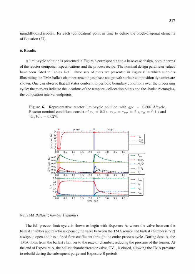
317

numdifftools.Jacobian, for each (collocation) point in time to define the block-diagonal elements

of Equation (27).

6. Results

A limit-cycle solution is presented in Figure 6 corresponding to a base-case design, both in terms

of the reactor component specifications and the process recipe. The nominal design parameter values

have been listed in Tables 1–3. Three sets of plots are presented in Figure 6 in which subplots

illustrating the TMA ballast chamber, reactor gas phase and growth surface composition dynamics are

shown. One can observe that all states conform to periodic boundary conditions over the processing

cycle; the markers indicate the locations of the temporal collocation points and the shaded rectangles,

the collocation interval endpoints.

Figure 6. Representative reactor limit-cycle solution with gpc = 0.806 Å/cycle.

Reactor nominal conditions consist of τA = 0.2 s, τAP = τBP = 2 s, τB = 0.1 s and

Vbc/Vrxr = 0.02%.

6.1. TMA Ballast Chamber Dynamics

The full process limit-cycle is shown to begin with Exposure A, where the valve between the

ballast chamber and reactor is opened; the valve between the TMA source and ballast chamber (CV2)

always is open and has a fixed flow coefficient through the entire process cycle. During dose A, the

TMA flows from the ballast chamber to the reactor chamber, reducing the pressure of the former. At

the end of Exposure A, the ballast chamber/reactor valve, CV1, is closed, allowing the TMA pressure

to rebuild during the subsequent purge and Exposure B periods.

318

As seen in Figure 6, top, the ballast chamber pressure behaves exactly as expected, with a rapid

initial drop in pressure, due to the small volume, Vbc. However, what is interesting to observe is the

degree of d-TMA dissociation αbc in the bottom plot of Figure 6: except for a slight upward deviation

during the ballast chamber depressurization, αbc ≈ 0, indicating that virtually all of the TMA is in

dimer form while in the TMA ballast chamber.

6.2. Reactor-Scale Dynamics

As seen in the center plot of Figure 6, during Exposure A, the total reactor pressure, TMA

partial pressure and methane partial pressure all increase as expected, while the Ar carrier gas partial

pressure remains constant. During the subsequent purge period, the total pressure relaxes to the

base-line pressure. It is now interesting to observe that the TMA monomer fraction in the reactor is

essentially unity (αrxr ≈ 1), indicating that the d-TMA dissociates as it enters the lower-pressure,

higher-temperature reactor chamber. We note that the energy required to heat the incoming reactant

and inert gases is negligibly small compared to the rates of radiative heat transfer in the reactor, and

so, we do not explicitly model the thermal dynamics of the gases as they are heated to Trxr from Tamb

or Tbc.

During Exposure B, we observe a much more linear increase in total pressure, because water is

fed to the reactor from a water vapor source held at constant pressure with P vapwater � Prxr,base. Again,

the system relaxes to the base-line pressure, Prxr,base, after valves CV3 and CV4 are switched to their

purge positions.

6.3. Growth Surface Dynamics

At the start of dose A in the limit-cycle solution, θMe ≈ 0.08 and θX ≈ 0.25. As TMA enters

the reactor, a small fraction rapidly reacts with the surface OH, leading to a reduction in θX and

the increase in θMe shown in Figure 6. With sufficient TMA dosage levels, θMe → 1 very rapidly,

indicating the aggressiveness of reaction R1. As the growth surface saturates with Me groups, the

rate of R1 slows, and R2 becomes the rate-controlling step. We observe that R2 continues throughout

the purge period, reducing both the surface Me and OH ligand density.

When H2O is introduced during Exposure B, θMe rapidly drops as the surface Me groups are

replaced with OH in reactions R3 and R4. As the water partial pressure rapidly drops during the

post-B purge, all reactions, except R2, come to a stop, leaving a nearly unchanging growth surface

for much of the second purge period. The full length of the purge period is required, however, to

prevent remaining gas-phase H2O from reacting with surface Me once the dose-A period resumes.

7. Mapping the gpc Behavior

As described earlier, a distinguishing feature of ALD processes is the self-limiting nature of the

surface reactions, leading to a fixed rate of growth-per-cycle (gpc) during steady, but cyclic, reactor

operation. The total number of Al and O atoms deposited per unit area over one deposition cycle

319

are denoted as NAl and NO atoms/nm2, respectively; these values are computed by integrating the

consumption rates of both precursors, Equations (21) and (22), over the limit-cycle:

NAl =

∫ τcycle

0

ΓA dt and NO =

∫ τcycle

0

ΓB dt (28)

using the quadrature weights of the collocation procedure. The relative ratio of Al to O, thus, can be

determined; for a ratio of Al/O = 2/3:

gpc = 10ΔzNAl

[S]Å/cycle (29)

where Δz is determined from the density of amorphous Al2O3 [11]. Alternatively, if η1 is the extent

of reaction R1, the only reaction involving gas-phase TMA, we can write:

NAl = η1 =[Me]f − [Me]o + [X]o − [X]f

3(30)

where the subscripts, o and f , denote surface concentrations at the start of dose A and the end of

post-A purge, respectively. We note this relationship holds only when no reactions take place under

CVD conditions (where both gas-phase precursors are found in the reactor, resulting in the possibility

of reactions R1–R4 all taking place simultaneously). Under these idealized ALD reactor operating

conditions and under fully saturating conditions, [Me]o = [X]f = 0 and [Me]f = [X]o = [Me],

resulting in Equation (30), reducing to the maximum gpc possible for an idealized ALD process, a

value denoted as GPC:

GPC = 20Δz[Me]

3[S]= 1.231 Å/cycle (31)

We note the value of GPC correlated well with previous theoretical and experimental studies of the

alumina ALD process [48].

The gpc = 0.806 Å/cycle of our base-case design corresponding to the limit-cycle solution of

Figure 6 is considerably less than the maximum indicated by Equation (31) for idealized, saturating

ALD conditions. We now examine two modes of increasing the dose of each precursor. During

Exposure B, the water dose is regulated by the timing of the gas delivery system valves, CV3 and

CV4. With a base-case design of τB = 0.1, we observe in Figure 7, left, that gpc → 0 as τB →0, while keeping Vbc fixed, exactly as expected. We note that τB = 0 actually corresponds to a

bifurcation point, where the branch containing the limit-cycle solution shown in Figure 6 meets a

trivial solution characterized by θX = θMe = 0 for all points in time. The physical meaning of

the multiple solutions will be explored in follow-up work. As τB is increased from the nominal

operating conditions, the rate of gpc increase lessens; the CVD conditions and the slower surface

reactions contribute to the gradual increase in gpc with no self-limiting regime to be found under the

selected set of operating conditions of the plot.

The base-case ratio of TMA ballast chamber/reactor chamber volume is 0.02%, and one expects

that increasing this ratio will result in an increased TMA dose in the reactor vessel. Keeping the H2O

320

dose fixed, the overall results are seen in Figure 7, right. As Vbc → 0, gpc → 0.78 Å/cycle—not

zero—because τA is nonzero, and the TMA bleeding through valve CV2 always results in a nonzero

TMA dose. We observe that gpc grows with Vbc, but again, while the rate of gpc increase declines with

ballast chamber volume, a plateau indicating saturating growth is not observed under the operating

conditions of the plot.

Figure 7. Growth per cycle (gpc) as a function of τB (left) and Vbc/Vrxr (right).

7.1. The Vbc-τB Plane

Because the gpc values of Figure 7 neither reach a limiting value nor the predicted theoretical

maximum, gpc → GPC = 1.231 Å/cycle, we present the gpc as the contour plot in the Vbc-τB plane

in Figure 8. In this figure, the base-case design corresponds to the lower-left corner of the plot.

Figure 8. Growth per cycle (gpc) as a function of τB and Vbc/Vrxr. The black curves

correspond to moles of TMA/cycle fed to the reactor.

321

In Figure 8, we mark gpc = GPC = 1.231 Å/cycle by the white contour line found over this

range of τB and Vbc values. The large region above and to the right of the curve corresponds to large

doses of both TMA and water, resulting in growth exceeding what would be possible for a pure,

surface reaction-limited ALD process. Examining the limit-cycle solution in this region reveals that

because the amount of TMA and water is so large, a significant amount remains after each purge

period, resulting in each of the precursors being found in the gas phase at the start of the other dose

period. During Exposure A, excess water in the gas phase reacts with surface Me deposited by TMA,

increasing the ability of TMA to adsorb and react during dose A. Likewise, excess TMA present at

the start of dose B generates surface Me, which subsequently react with gas-phase H2O, adding to

the overall consumption of that reactant.

These unintentional reactions are characterized as being under CVD conditions instead of true

ALD reactions. Because CVD conditions are generally undesirable in ALD processes, due to the

poor film quality and reduced conformality produced by the resulting reactions, we mark the curve

corresponding to gpc = GPC to indicate an approximate lower limit, where reactions under CVD

conditions are significant. Thus, ALD reactor operation should be limited to the region below and

to the left of this curve. The practical upshot of this computation is immediate: we see there is

little incentive for process designs where Vbc/Vrxr > 0.25% and that, generally, τB > 0.2 s (given

that all other parameters are fixed, of course). The rationale for these limits is further clarified by

considering the economics of this ALD process: given the relative value of TMA to water, plus the

costs of disposing unused TMA downstream of the reactor, a simple yet reasonable optimization

objective would be to minimize TMA use alone. To quantify TMA use, we integrate the TMA flow

rate through CV1 using the mAin term of Equation (6):

mAcycle =

∫ τcycle

0

C1γ1(t) [Pbc(t)− Prxr(t)]1 + αrxr

1 + αbc

dt.

These curves are shown in black in Figure 8, where the values indicated correspond to moles of

TMA/cycle fed to the reactor. As expected, the contours show a reduction of TMA use as Vbc is

decreased, but we note that for large dose volumes, both τB and Vbc affect mAcycle, due to the increased

time for regenerating the TMA pressure in the ballast chamber during dose B.

8. Conclusions

In this paper, a laboratory-scale atomic layer deposition (ALD) reactor system model

was developed by integrating components describing the precursor thermophysical properties,

reactor-scale gas-phase dynamics and surface reaction kinetics derived from absolute reaction rate

theory. ALD reactor operation was limited to steady cyclic operation with limit-cycle solutions

computed using a collocation discretization scheme in time. We demonstrated that a key advantage to

the fixed-point approach was the resulting unambiguous definition of growth-per-cycle (gpc), making

possible parametric studies of film growth rates to that expected for ideal ALD.

322

The utility of the resulting ALD system simulator was demonstrated by the strong interactions

found between different reactor, reaction and process recipe elements, interactions that would be

otherwise difficult to predict without such simulators. In particular, we demonstrated that surface

reactions normally associated with one specific precursor exposure can take place during the purge

or even during exposures to the other of the two precursors. The ability to model the interaction

between dose and purge periods was critical to uncovering the surface reactions occurring under CVD

conditions and identifying processing regimes where these reactions are most likely to take place.

The ability to predict both gpc and cyclic precursor feed rates for a real reactor and gas delivery

system made it possible to generate simple, but physically meaningful, design rules for adjusting the

precursor doses to minimize TMA consumption and undesirable CVD conditions, while maintaining

a high value of gpc necessary for acceptable reactor throughput. One of the most important

contributions of reactor system-level models for thin-film processes is the ability to use dynamic

models to accurately characterize the time-dependent composition of the reactant gases to which the

growth surface is exposed. Because direct experimental measurement of gas-phase characteristics

local to the growth surface are challenging at best, physically-based reactor models are needed to

interpret measured gpc levels. The utility of models of this form extend to other ALD process

chemistries, other gas delivery systems and more complex (e.g., multi-wafer) reactor systems.

The extension of our modeling work to the tubular geometry of our ALD system is underway.

Likewise, the use of our reactor models in more sophisticated dynamic optimization studies, as well

as controller development to fully decouple binary precursor doses are planned.

Acknowledgments

The authors acknowledge the support of the National Science Foundation through grant CBET

1160132. Support for C.D.T. also was provided by the Gates Millennium Scholars Program.

Conflicts of Interest

The authors declare no conflict of interest.

References

1. George, S.M. Atomic layer deposition: An overview. Chem. Rev. 2010, 110, 111–131.

2. Puurunen, R.L. Surface chemistry of atomic layer deposition: A case study for the

trimethylaluminum/water process. Appl. Phys. Rev. 2005, 97, 121301:1–121301:52.

3. Suntola, T. Atomic layer epitaxy. Mater. Sci. Rep. 1989, 4, 262–312.

4. Van Delft, J.A.; Garcia-Alonso, D.; Kessels, W.M.M. Atomic layer deposition for

photovoltaics: Applications and prospects for solar cell manufacturing. Semicond. Sci. Tech.2012, 27, 074002.

5. Kim, H. Atomic layer deposition of metal and nitride thin films: Current research efforts and

applications for semiconductor device processing. J. Vac. Sci. Technol. B 2003, 21, 2231–2261.

323

6. Marichy, C.; Bechelany, M.; Pinna, N. Atomic layer deposition of nanostructured materials for

energy and environmental applications. Adv. Mater. 2012, 24, 1017–1032.

7. Meng, X.; Yang, X.; Sun, X. Emerging applications of atomic layer deposition for lithium-ion

battery studies. Adv. Mater. 2013, 24, 3589–3615.

8. Kim, H.; Lee, H.; Maeng, W.J. Applications of atomic layer deposition to nanofabrication and

emerging nanodevices. Thin Solid Films 2009, 517, 2563–2580.

9. Skoog, S.A.; Elam, J.W.; Narayan, R.J. Atomic layer deposition: Medical and biological

applications. Int. Mater. Rev. 2013, 58, 113–129.

10. Elliott, S.D.; Greer, J.C. Simulating the atomic layer deposition of alumina from first principles.

J. Mater. Chem. 2004, 14, 3246–3250.

11. Travis, C.D.; Adomaitis, R.A. Modeling ALD surface reaction and process dynamics using

absolute reaction rate theory. Chem. Vapor Depos. 2013, 19, 4–14.

12. Elliott, S.D. Models for ALD and MOCVD growth of rare earth oxides. Topics Appl. Phys.2007, 106, 73–86.

13. Elliott, S.D. Atomic-scale simulation of ALD chemistry. Semicond. Sci. Technol. 2012,

27, 074008.

14. Dkhissi, A.; Mazaleyrat, G.; Jeloaica, L.; Rouhani, M.D. Nucleation and growth of atomic layer

deposition of HfO2 gate dielectric layers on silicon oxide: A multiscale modelling investigation.

Phys. Chem. Chem. Phys. 2009, 11, 3701–3709.

15. Dkhissi, A.; Estéve, A.; Mastail, C.; Olivier, S.; Mazaleyrat, G.; Jeloaica, L.; Rouhani, M.D.

Multiscale modeling of the atomic layer deposition of HfO2 thin film grown on silicon: How to

deal with a kinetic Monte Carlo procedure. J. Chem. Theory Comput. 2008, 4, 1915–1927.

16. Mazaleyrat, G.; Estéve, A.; Jeloaica, L.; Djafari-Rouhani, M. A methodology for the kinetic

Monte Carlo simulation of alumina atomic layer deposition onto silicon. Comput. Mater. Sci.2005, 33, 74–82.

17. Alam, M.A.; Green, M.L. Mathematical description of atomic layer deposition and its

application to the nucleation and growth of HfO2 gate dielectric layers. J. Appl. Phys. 2003,

94, 3403–3413.

18. Yim, S.; Lee, D.; Kim, K.; Kim, S.; Yoon, T.; Kim, K. Nucleation kinetics of Ru on silicon

oxide and silicon nitride surfaces deposited by atomic layer deposition. J. Appl. Phys. 2008,

103, 113509:1–113509:9.

19. Nilsen, O.; Mohn, C.E.; Kjekshus, A.; Fjellvåg, H. Analytical model for island growth in atomic

layer deposition using geometrical principles. J. Appl. Phys. 2007, 102, 024906:1–024906:13.

20. Puurunen, R.L.; Vandervorst, W.; Besling, W.F.A.; Richard, O.; Bender, H.; Conard, T.; Zhao,

C.; Delabie, A.; Caymax, M.; de Gendt, S.; et al. Island growth in the atomic layer deposition of

zirconium oxide and aluminum oxide on hydrogen-terminated silicon: Growth mode modeling

and transmission electron microscopy. J. Appl. Phys. 2004, 96, 4878–4889.

21. Puurunen, R.L.; Vandervorst, W. Island growth as a growth mode in atomic layer deposition: A

phenomenological model. J. Appl. Phys. 2004, 96, 7686–7695.

324

22. Lim, J.; Park, J.; Wang, S. Kinetic modeling of film growth rates of TiN films in atomic layer

deposition. J. Appl. Phys. 2000, 87, 4632–4634.

23. Lim, J.; Park, H.; Wang, S. Analysis of a transient region during the initial stage of atomic layer

deposition. J. Appl. Phys. 2000, 88, 6327–6331.

24. Lim, J.; Park, H.; Wang, S. Kinetic modeling of film growth rate in atomic layer deposition.

J. Electrochem. Soc. 2001, 148, C403–C408.

25. Park, H.; Min, J.; Lim, J.; Kang, S. Theoretical evaluation of film growth rate during atomic

layer epitaxy. Appl. Surf. Sci. 2000, 158, 81–91.

26. Aarik, J.; Siimon, H. Characterization of adsorption in flow type atomic layer epitaxy reactor.

Appl. Surf. Sci. 1994, 81, 281–287.

27. Siimon, H.; Aarik, J. Modelling of precursor flow and deposition in atomic layer deposition

reactor. J. Phys. IV 1995, 5, C5:245–C5:252.

28. Siimon, H.; Aarik, J. Thickness profiles of thin films caused by secondary reactions in flow-type

atomic layer deposition reactors. J. Phys. D 1997, 30, 1725–1728.

29. Ylilammi, M. Mass transport in atomic layer deposition carrier gas reactors. J. Electrochem.Soc. 1995, 142, 2474–2479.

30. Knoops, H.C.M.; Elam, J.W.; Libera, J.A.; Kessels, W.M.M. Surface loss in ozone-based

atomic layer deposition processes. Chem. Mater. 2011, 23, 2381–2387.

31. Yanguas-Gil, A.; Elam, J.W. Simple model for atomic layer deposition precursor

reaction and transport in a viscous-flow tubular reactor. J. Vac. Sci. Technol. A 2012, 30,

01A159:1–01A159:7.

32. Elam, J.W.; Routkevitch, D.; Mardilovich, P.P.; George, S.M. Conformal coating on

ultrahigh-aspect-ratio nanopores of anodic alumina by atomic layer deposition. Chem. Mater.2003, 15, 3507–3517.

33. Shankar, S.; Simka, H.; Haverty, M. Density functional theory and beyond-opportunities for

quantum methods in materials modeling semiconductor technology. J. Phys-Condens. Mat.2008, 20, 064232.

34. Prechtl, G.; Kersch, A.; Schulze Icking-Konert, G.; Jacobs, W.; Hecht, T.; Boubekeur, H.;

Schröder, U. A Model for Al2O3 ALD Conformity and Deposition Rate from Oxygen Precursor

Reactivity. In Proceedings of the International Electron Devices Meeting, Washington, DC,

USA, 8–10 December 2003.

35. Rose, M.; Bartha, J.W. Method to determine the sticking coefficient of precursor molecules in

atomic layer deposition. Appl. Surf. Sci. 2009, 255, 6620–6623.

36. Deminsky, M.; Knizhnik, A.; Belov, I.; Umanskii, S.; Rykova, E.; Bagatur’yants, A.; Potapkin,

B.; Stoker, M.; Korkin, A. Mechanism and kinetics of thin zirconium and hafnium oxide film

growth in an ALD reactor. Surf. Sci. 2004, 549, 67–86.

37. Holmqvist, A.; Törndahl, T.; Stenström, S. A model-based methodology for the analysis and

design of atomic layer deposition processes—Part I: Mechanistic modelling of continuous flow

reactors. Chem. Eng. Sci. 2012, 81, 260–272.

325

38. Holmqvist, A.; Törndahl, T.; Stenström, S. A model-based methodology for the analysis and

design of atomic layer deposition processes—Part II: Experimental validation and mechanistic

analysis. Chem. Eng. Sci. 2012, in press.

39. Dwivedi, V.; Adomaitis, R.A.; Travis, C.D. Passively Controlled Thermal Material Deposited

by Atomic Layer Deposition. In Proceedings of AIChE Annual Meeting, Pittsburgh, PA, USA,

28 October–2 November 2012.

40. Kimes, W.A.; Maslar, J.E. In situ Water Measurements as a Diagnostic of Flow Dynamics in

ALD Reactors. In Proceedings of the ALD 2011, Cambridge, MA, USA, 26–29 June 2011.

41. NIST Chemistry WebBook, NIST Standard Reference Database Number 69; National

Institute of Standards and Technology: Gaithersburg, MD, USA, 2005. Available online:

http://webbook.nist.gov (accessed on 7 February 2013).

42. Wind, R.A.; George, S.M. Quartz crystal microbalance studies of Al2O3 atomic layer deposition

using trimethylaluminum and water at 125 ◦C. J. Phys. Chem. A 2010, 114, 1281–1289.

43. Laubengayer, A.W.; Gilliam, W.F. The alkyls of the third group elements. I. Vapor phase studies

of the alkyls of aluminum, gallium and indium. J. Am. Chem. Soc. 1941, 63, 477–479.

44. Widjaja, Y.; Musgrave, C.B. Quantum chemical study of the mechanism of aluminum oxide

atomic layer deposition. Appl. Phys. Lett. 2002, 80, 3304–3306.

45. Puurunen, R.L. Correlation between the growth-per-cycle and the surface hydroxyl group

concentration in the atomic layer deposition of aluminum oxide from trimethylaluminum and

water. Appl. Surf. Sci. 2005, 245, 6–10.

46. Laidler , K.J. Chemical Kinetics, 3rd ed.; Harper and Row: New York, NY, USA, 1978.

47. Vannice, M.A. Kinetics of Catalytic Reactions; Springer: New York, NY, USA, 2005.

48. Puurunen, R.L. Growth per cycle in atomic layer deposition: Real application examples of a

theoretical model. Chem. Vap. Dep. 2003, 9, 327–332.

326

Reduced Models in Chemical Kinetics viaNonlinear Data-Mining

Eliodoro Chiavazzo, Charles W. Gear, Carmeline J. Dsilva, Neta Rabin andIoannis G. Kevrekidis

Abstract: The adoption of detailed mechanisms for chemical kinetics often poses two types of

severe challenges: First, the number of degrees of freedom is large; and second, the dynamics

is characterized by widely disparate time scales. As a result, reactive flow solvers with detailed

chemistry often become intractable even for large clusters of CPUs, especially when dealing with

direct numerical simulation (DNS) of turbulent combustion problems. This has motivated the

development of several techniques for reducing the complexity of such kinetics models, where,

eventually, only a few variables are considered in the development of the simplified model.

Unfortunately, no generally applicable a priori recipe for selecting suitable parameterizations of

the reduced model is available, and the choice of slow variables often relies upon intuition and

experience. We present an automated approach to this task, consisting of three main steps. First,

the low dimensional manifold of slow motions is (approximately) sampled by brief simulations of

the detailed model, starting from a rich enough ensemble of admissible initial conditions. Second,

a global parametrization of the manifold is obtained through the Diffusion Map (DMAP) approach,

which has recently emerged as a powerful tool in data analysis/machine learning. Finally, a simplified

model is constructed and solved on the fly in terms of the above reduced (slow) variables. Clearly,

closing this latter model requires nontrivial interpolation calculations, enabling restriction (mapping

from the full ambient space to the reduced one) and lifting (mapping from the reduced space to the

ambient one). This is a key step in our approach, and a variety of interpolation schemes are reported

and compared. The scope of the proposed procedure is presented and discussed by means of an

illustrative combustion example.

Reprinted from Processes. Cite as: Chiavazzo, E.; Gear, C.W.; Dsilva, C.J.; Rabin, N.;

Kevrekidis, I.G. Reduced Models in Chemical Kinetics via Nonlinear Data-Mining. Processes 2014,

2, 112–140.

1. Introduction

The solution of detailed models for chemical kinetics is often dramatically time consuming,

owing to a large number of variables evolving in processes with a wide range of time and space scales.

As a result, fluid dynamic flow solvers coupled with detailed chemistry still present a challenge, even

for modern clusters of CPUs, especially when dealing with direct numerical simulation (DNS) of

turbulent combustion systems. Here, a large number of governing equations for chemical species (a

few hundred for mechanisms of standard hydrocarbon fuels) are to be solved at (typically) millions of

distinct discretization points in the computational domain. This has motivated the development of a

327

plethora of approaches aiming at reducing the computational complexity of such detailed combustion

models, ideally by recasting them in terms of only a few new reduced variables. (see, e.g., [1]

and references therein). The implementation of many of these techniques typically involves three

successive steps. First, a large set of stiff ordinary differential equations (ODEs) is considered

for modeling the temporal evolution of a spatially homogenous mixture of chemical species under

specified stoichiometric and thermodynamic conditions (usually fixed total enthalpy and pressure for

combustion in the low Mach regime). It is well known that, due to the presence of fast and slow

dynamics, the above systems are characterized by low dimensional manifolds in the concentration

space (or phase-space), where a typical solution trajectory is initially rapidly attracted towards the

manifold, while afterwards, it proceeds to the thermodynamic equilibrium point, always remaining

in close proximity to the manifold. Clearly, the presence of a manifold forces the ODEs state to visit

mostly a low dimensional region of the entire phase-space, thus offering the premise for constructing

a consistent reduced description of the process, which accurately retains the slow dynamics along

the manifold, while neglecting the initial short transient towards the manifold. In a fluid dynamic

simulation, stoichiometry and thermodynamic conditions may vary throughout the computational

domain. Hence, when implementing reduction techniques, the second step consists of parameterizing

and tabulating the manifolds arising in the homogeneous reactor for a variety of stoichiometric and

thermodynamic conditions. Finally, as a third step, the fluid dynamic equations are reformulated in

terms of the new variables, with the latter tables utilized to close the new reduced set of equations

(see, e.g., [2]). It is worth stressing that the above description briefly outlines only one possible

approach for coupling a model reduction method to a flow solver: the case where the low dimensional

manifolds of the homogeneous problem are identified in advance in the entire phase-space. For

completeness, it is important to mention that, due to the rapidly increasing difficulty in storing and

interpolating data in high dimensions, this approach remains viable in cases with a few reduced

variables. As an alternative to this global method, techniques have been introduced for locallyconstructing the low dimensional manifold only in the (tiny) region of interest in the phase-space,

as demanded by a reacting flow code during simulations [3–5]. Local constructions can certainly

cope with higher dimensional manifolds. However, their usage seems computationally advantageous

only in combination with efficient algorithms for adaptive tabulation, where data is computed when

needed, stored and re-utilized if necessary (see, e.g., [6]).

In this work, we focus on the global construction and parameterization of slow invariant manifolds

arising in the modeling of spatially homogeneous reactive mixtures. In particular, upon identification

of the slow manifold, we propose a generally applicable methodology for selecting a suitable

parameterization; we also investigate various interpolation/extrapolation schemes that need to be

used in the solution of a reduced dynamical system expressed in terms of the variables learned.

This latter step, and its integration with the previous two in an overall computer-assisted approach,

constitute the methodological novelty of the paper.

The manuscript is organized as follows. In Section 2, Diffusion Maps are briefly reviewed.

In Section 3 and the subsections therein, we discuss the computation of points on the manifold,

their embedding in a reduced (here, two-dimensional) space, the formulation of a reduced set of

328

equations and their solution through several interpolation/extension techniques. Results are reported

and discussed in Section 4, where the proposed approach is applied to a reactive mixture of hydrogen

and air at stoichiometric proportions with fixed enthalpy and pressure. The reader may prefer a

quick glance at Section 4 before the detailed presentation of the procedure in Section 3. Finally, we

conclude with a summary and brief discussion of open issues in Section 5.

2. Diffusion Maps

The Diffusion Map (DMAP) approach has emerged as a powerful tool in data analysis and

dimension reduction [7–9]. In effect, it can be thought of as a nonlinear counterpart of Principal

Component Analysis (PCA) [10] that can be used to search for a low-dimensional embedding of

a high-dimensional point set {y1,...,yM}, if an embedding exists. For completeness, we present a

simple description of the DMAP process. The points, yi, could exist in some n-dimensional Cartesian

space (as they are in our combustion example) or they could be more abstract objects, such as images.

What is important is that there exists a dissimilarity function, dij = dji, between any pair of points,

yi and yj , such that the dissimilarity is zero only if the points are identical (in those aspects that are

important to the study) and gets larger the more dissimilar they are. Although, for points in �n, an

obvious choice for dij is the standard Euclidean distance, this is not necessarily the best option. For

instance, a weighted Euclidean norm may be considered when different coordinates are characterized

by disparate orders of magnitude. As discussed below, this is indeed the case encountered in many

combustion problems, where the data are composition vectors in concentration space and major

species (i.e., reactants and products) are characterized by much higher concentrations compared to

minor species (i.e., radicals). From dij , a pairwise affinity function wij = w(dij) is computed, where

w(0) = 1 and w(d) is monotonically decreasing and non-negative for d > 0. A popular option is the

heat kernel:

wij (dij) = exp

[−(dijε

)2]

(1)

The model parameter, ε, specifies the level below, whose points are considered similar, whereas

points more distant than a small multiple of ε are, effectively, not linked directly. For this

presentation, we will assume that d is a distance measure in (suitably scaled) Cartesian coordinates,

so that each point, yi, is specified by its coordinates, yi,α with α = 1, ..., n, in n-dimensional space.

In the DMAP approach, starting from the M × M (not n × n, as in PCA) symmetric matrix

W = {wij}, a Markov matrix, K, is constructed through the row normalization:

K = D−1W (2)

with the diagonal matrix, D, collecting all the row sums of matrix W. Owing to similarity with a

symmetric matrix, D−1/2WD−1/2, K has a complete set of real eigenvectors, {φi}, and eigenvalues,

{λi}. Moreover, a projection of the high-dimensional points {y1,...,yM} into an m-dimensional

space (hopefully, m << n) can be established through the components of m appropriately selected

eigenvectors (not necessarily the m leading ones, as in PCA). Specifically, let the eigenvalues be

329

sorted in decreasing order: 1 = λ1 ≥ |λ2| ≥ ... ≥ |λM |. The diffusion map, Ψt, is defined based on

the right eigenvectors of K, Kφl = λlφl, with φl = (φ1,l, ..., φM,l), for t > 0, as follows:

Ψt (yi) =

⎛⎜⎜⎜⎜⎝λt1φi,1

λt2φi,2

...

λtMφi,M

⎞⎟⎟⎟⎟⎠ (3)

and it assigns a vector of M new coordinates to each data point, yi. Here, K represents a (unit time)

application of a diffusion process on the data points, so that t (in Kt) indicates the length of time over

which this process is applied. Notice that all points have the same first coordinate in Equation (3),

since φ1 is proportional to the all-ones vector (with eigenvalue one). Notice that the diffusion map

coordinates are time-dependent; using longer times in the diffusion process damps high frequency

components, so that fewer coordinates suffice for an approximation of a given accuracy. However, in

order to achieve a drastic dimension reduction, for a fixed threshold 0 < δ < 1, it is convenient to

define a truncated diffusion map:

Ψδt (yi) =

⎛⎜⎜⎜⎜⎝λt2φi,2

λt3φi,3

...

λtm+1φi,m+1

⎞⎟⎟⎟⎟⎠ (4)

where m + 1 is the largest integer for which |λm+1|t > δ. Below, we will consider only

the eigenvector entries (i.e., take t = 0) and will separately discuss using the eigenvalues (and

their powers) to ignore noise.

If the initial data points, {y1,...,yM}, are located on a (possibly non-linear) low dimensional

manifold with dimension m, one might expect (by analogy to PCA) that a procedure exists to

systematically select m diffusion map eigenvectors for embedding the data. If the points are fairly

evenly distributed across the low-dimensional manifold, it is known that the principal directions of

the manifold are spanned by some of the leading eigenvectors (i.e., those corresponding to larger

eigenvalues) of the DMAP operator [11,12]. In the illustrations below (Figure 1), the corresponding

eigenvalues are approximately:

λ = 1− δ[kπd/Lα]2 (5)

where δ ≈ exp(−d/ε2), d is the typical spacing between neighbors and Lα is the length of the

α-th principal direction. Here, k = 1, 2, · · · indicates the successive harmonics of the eigenvectors.

(This approximation can be obtained by considering the regularly-spaced data case, assuming that ε

is comparable to d and that δ is small enough, so that higher powers can be ignored.) Section 2.1

below discusses how to ignore eigenvectors that are harmonics of previous ones by checking for

dependence. Equation (5) provides a tool for deciding when to ignore the smaller eigenvalues.

Suppose, for example, that we know that our data accuracy is approximately a fraction, γ, of the

330

range of the data. This range roughly corresponds to the longest principal direction, say L1. There

is little point in considering manifold directions of the order of γL1, since they are of the order of

the errors in the data. Hence, by applying Equation (5), we should ignore any eigendirections whose

eigenvalue is less than 1− (1− λ2)γ−2, where λ2 is the first non-trivial eigenvalue.

Figure 1. Data manifold, dimensionality and independence of DMAP eigenvectors

(a) 2000 uniformly random points initially placed in a unit square are stretched and

wrapped around three-fourths of a cylinder; (b) the entry in the first non-trivial

eigenvector of the Markov matrix, K, vs. the first cylindrical coordinate, θ, for each

data point; (c) entry in the second non-trivial eigenvector of K vs. the first one; the

quasi-one-dimensionality of the plot implies strong eigenvector correlation; (d) entry in

the third non-trivial eigenvector of K vs. the first one. The evident two-dimensional

scatter implies that a new direction on the data manifold has been detected.

2.1. Issues in the Implementation of the Algorithm

While the formulas above appear to provide a simple recipe, a number of important,

problem-dependent issues arise, having to do with the sampling of the points to be analyzed,

the choice of the parameter, ε, etc.; we now discuss these issues through illustrative caricatures.

Consider 2000 uniformly random points initially placed in a unit square, then stretched and

wrapped around three fourths of a cylinder of radius one and length two (see Figure 1a). In

Figure 1b, the first non-trivial eigenvector, ψ2, is reported against the first cylindrical coordinate,

θ: the i-th component of this eigenvector is plotted against the θ angle of the i-th point. The

331

clearly apparent one-dimensional nature of the plot confirms that ψ2 parametrizes this principal

geometric direction. However, a plot of ψ3, the eigenvector corresponding to the next leading

eigenvalue, against ψ2 clearly shows a strong correlation: ψ3 is not representative of a new,

independent direction on the data manifold. In Figure 1d, the two-dimensional scatter of the plot

of the entries of the fourth eigenvector vs. the entries of the second one indicates independence

between ψ2 and ψ4; ψ4 does represent a new, independent direction along the data manifold and

becomes our second embedding coordinate. Visually testing independence between two DMAP

eigenvectors is relatively easy: we can agree that Figure 1b,c appear one-dimensional and Figure 1d

appears two-dimensional. However, testing independence in higher dimensions (for subsequent

DMAP eigenvectors) becomes quickly visually impossible and even computationally nontrivial.

Subsequent eigenvectors should be plotted against previous important ones (in the example just

considered, against ψ2 and ψ4), and the dimensionality of the plot should be assessed; this is still

visually doable for, say, ψ5, and the plot appears as a 2D surface in 3D: ψ5 is not a new data

coordinate. Beyond visual assessment (and in higher dimensions), one can use the sorted edge-length

algorithm for dimensionality assessment: a log-log plot of the graph edge-length vs. edge number is

constructed, with the manifold dimension being the slope in the middle part of the plot. Algorithms

for detecting the dimension of attractors in chaotic dynamical systems can also find use here [13,14].

Figure 2. More on the effect of data sampling: noise. (a) One thousand six hundred

points are initially randomly placed in each of the 40 by 40 array of small squares,

forming the unit square, and, afterwards, bent around a cylinder; (b) entry in the first

non-trivial eigenvector of the Markov matrix, K, vs. the first cylindrical coordinate, θ,

for each data point; (c) entry in the second non-trivial eigenvector of K vs. the first one;

(d) entry in the third non-trivial eigenvector of K vs. the first one.

332

The irregularity of sample points can be easily seen to lead to problems in this simple example.

Consider, however, an additional case where 1600 points are initially randomly placed in each of the

40 by 40 array of small squares, forming the unit square, and, afterwards, bent around the cylinder

(Figure 2a). As clearly visible in Figure 2b–d, these time dependencies between eigenvectors are

very well defined.

Figure 3. The analogy between traditional diffusion on domains and diffusion on

graphs from sampled data. (a) The solution to the finite element method (FEM)

formulation of the PDE (partial differential equation) eigenvalue problem ∇2φ = λφ

with no flux boundary conditions is reported for a narrow two-dimensional rectangular

stripe. The second and seventh eigenfunctions are found to be uncorrelated and

suitable to parametrize the two relevant dimensions of the manifold; (b) Entries in the

first non-trivial eigenfunction of the problem in figure (a) vs. entries in the fourth

eigenfunction (sampled at scattered locations of the computational domain) reveals a

strong correlation between those two functions: the fourth eigenvector (which we know

corresponds to the third harmonic, cos(3x)) does not encode a new direction on the data

manifold. Right-hand side: Entries in the first non-trivial eigenfunction of the problem

in (a) vs. entries in the seventh eigenfunction (at the same scattered locations) confirms

that the seventh eigenvector (which we know corresponds to cos(y), encodes a new,

second direction; (c) A different domain, but the same premise: The solution to the finite

element method (FEM) formulation of the PDE (partial differential equation) eigenvalue

problem ∇2φ = λφ with no flux boundary conditions is reported for a two-dimensional

manifold with a complicated boundary. The second and seventh eigenfunctions are

found to be uncorrelated and suitable to parametrize the two relevant dimensions of the

manifold (an “angular” and a “radial” one).

While the first non-trivial eigenvector, ψ2, always characterizes the principal direction on

the manifold, no general recipe can be formulated for an a priori identification of the subsequent

uncorrelated eigenvectors parameterizing other dimensions. We have already seen that eigenvectors

333

in Equation (3) are often dependent; this implies that they do not encode new directions along

the data manifold; in this sense, they are redundant for our embedding. In order to obtain more

insight into eigenvector dependency (and, in other words, in how diffusion is linked with manifold

parametrization), consider, as our domain of interest, a narrow two-dimensional stripe, or, in our case,

data points densely sampled from it. Figure 3a reports the solution to the discretized (through the

finite element method, FEM) eigenvalue problem ∇2φ = λφ with Neumann boundary conditions.

The first non-trivial eigenfunction is analytically given by cos(x), where x denotes the horizontal

space direction, and is very well approximated by the FEM numerics; the point to notice is that

cos(x) is one-to-one with x between zero and 2π; so, the first nontrivial diffusion eigenvector

parameterizes one manifold direction (the x). Several subsequent eigenfunctions still correlate with

the x direction: they are simply higher harmonics (cos(2x), cos(3x),...). We have to go as high as

the seventh eigenfunction (which analytically is cos(y)) to find something that is one-to-one with the

second, independent, vertical direction, y (see Figure 3b, where the first non-trivial eigenfunction is

plotted against both the fourth and seventh eigenfunction at scattered locations). A more complex

two-dimensional geometry is considered in Figure 3c. Similarly to the above example, the first

non-trivial eigenfunction parameterizes one of the manifold “principal dimensions” (the angular

coordinate), while the next (seventh) uncorrelated eigenfunction can be used to parameterize the

other relevant (radial) coordinate (it is just an accident that we had to go to the seventh eigenfunction

in both cases). In practical applications, only a discrete set of sample points on the manifold in

question is available as an input. Starting from those points, the Diffusion Maps create a graph,

where the points are the graph nodes and the edges are weighted on the basis of point distances,

as described above. Noticing that the (negatively defined) normalized graph Laplacian, L, is given

by [15]:

L = D−1W − I (6)

with I being the M × M identity matrix, we immediately recognize the link between the

eigenvalue problem in Figure 3 and mapping Equation (3) based on the spectrum of Markov matrix

Equation (2).

Diffusion on this graph (i.e., obtaining the spectrum of the graph Laplacian) approximates, at the

appropriate limit [7], the usual diffusion in the original domain; it provides an alternative, different

from our FEM, irregular mesh-discretization of the Laplace equation eigenproblem in the original

domain, and asymptotically recovers the spectrum of the Laplace operator there.

3. The Proposed Approach

We demonstrate the feasibility of constructing reduced kinetics models for combustion

applications, by extracting the slow dynamics on a manifold globally parameterized by a truncated

diffusion map. We focus on spatially homogeneous reactive mixtures of ideal gases under fixed total

enthalpy H and pressure P . Such a set-up is relevant for building up tables to be used in reactive

flow solvers in the low Mach number regime. In such systems, a complex reaction occurs with n

334

chemical species {A1,...,An} and q chemical elements involved in a (typically) large number, r, of

elementary steps:n∑

p=1

ιspAp→←n∑

p=1

κspAp, s = 1, ..., r (7)

where ιsp and κsp represent the stoichiometric coefficients of the p-th species in the s-th step. Time

evolution of chemical species can be modeled by a system of ordinary differential equations (ODEs)

cast in the general form:

dy

dt=

r∑s=1

γsΩs (y, T ) (8)

with γs = (κs1 − ιs1, ..., κsn − ιsn), while the reaction rate function, Ωs, is usually expressed

in terms of the concentration vector, y, by mass action laws and Arrhenius dependence on the

temperature, T . Clearly, a constraint on a thermodynamic potential is required in order to close

the system Equation (8), thus providing an additional equation for temperature. Below (without loss

of generality), we consider reactions under fixed total enthalpy, H .

The first step of our method consists in the identification of a discrete set of states lying in

a neighborhood of the low-dimensional attracting manifold. While many possible constructions

have been suggested in the literature (see, e.g., [1,4,5,16]), here, in the spirit of the equation-freeapproach [17,18], we assume that we have no access to the analytical form of the vector field; instead,

we only have access to a “black box” subroutine that evaluates the rates, f(y), and, when incorporated

in a numerical initial value solver, can provide simulation results.

3.1. Data Collection

To start the procedure, we need an ensemble of representative data points on (close to) the

manifold we wish to parametrize. To ensure good sampling, our ensemble of points comes

from integrating Equation (8) starting from a (rich enough) set of random states within

the admissible phase-space (a convex polytope defined by elemental conservation constraints

and concentration positivity). After sufficient time to approach a neighborhood of the

manifold, samples are collected from each such trajectory. As a result, a set of points

{yi, i = 1, ...,M} in �n (hopefully dense enough within the region of interest) becomes

available for defining the manifold. To construct the required initial conditions, we first

search for all vertices of the convex polytope defined by a set of equalities and inequalities

as follows:n∑

α=1

yαcαβ/Wα =n∑

α=1

yeqα cαβ/Wα, ∀β = 1, ..., q

yα > 0, ∀α = 1, ..., n(9)

where cαβ and Wα denote the number of atoms of the β-th element in the species α and the

molecular weight of species α, respectively, while the state vector y = (y1, ..., yn) expresses species

concentration in terms of mass fractions. The selection of random initial conditions is performed by

convex linear combinations of the v polytope vertices, {ypoli }:

335

yin =v∑

i=1

wiypoli (10)

with {wi} being a set of v random weights, such as∑v

i=1 wi = 1. Clearly, owing to convexity,

Equation (10) always provides states within the admissible space. In combustion applications,

the phase-space region of interest goes from the fresh mixture conditions to the thermodynamic

equilibrium, yeq; hence, in Equation (10), we consider a subset of the polytope vertices, {ypoli },

based on their vicinity to the mean point of the mixing line connecting the fresh mixture point to

equilibrium. Due to a disparity of the magnitudes of species concentrations, dij is taken as the

Euclidean distance between properly rescaled points y′i and y′j , with y′i = Ryi using the fixed

diagonal matrix R = {rββ}, rββ = 1/max(yβ). Here, max(yβ) represents the largest β-th

coordinate among all available samples. Below, distances in the concentration space are intended

in this sense. It is worth noticing that, upon the choice of v random numbers {wi, i = 1, ..., v}uniformly distributed over the range 0 ≤ wi ≤ 1, weights might be straightforwardly obtained by

normalization: wi = wi/∑v

j=1 wj . However, such an approach leads to poor sampling in the vicinity

of the polytope edges and, at the same time, to oversampling within its interior. Therefore, in order to

achieve a more uniform sampling in the whole phase-space region of interest, the weights are chosen

as follows:

wi = [− ln (zi)]p , wi = wi/

v∑j=1

wj, i = 1, ..., v (11)

with zi representing random values uniformly distributed within the interval 0 ≤ zi ≤ 1 and

1 ≤ p ≤ 2 a free parameter (see also Figure 4).

It is worth stressing that Equation (9) always defines a convex polytope; hence, all samples

computed by Equation (10) necessarily belong to the admissible domain, and no sample rejection

is needed at any time. Clearly, such a procedure is only one possible approach for uniformly

sampling a high-dimensional convex polytope. While a detailed study of alternative methods are

beyond the scope of this work, we remind that other algorithms are also possible, such as Gibbs or

hit-and-run sampling [19,20]. Trajectories starting at the random initial conditions, yin, computed

by Equation (10) are evolved for τf , after which, samples are collected as they proceed towards the

equilibrium point, yeq. Samples from the same trajectory are retained if their distance exceeds a

fixed threshold. We would like the sample to be as uniform as possible in the original space (which

we will call the ambient space), because doing so yields a better parameterization with Diffusion

Maps [21,22]. However, such a condition is not naturally fulfilled by samples of time integration:

the trajectories (hence, also, our sampled points) often show a tendency to gather in narrow regions

(especially close to the equilibrium point, governed by the eigenvalue differences in the linearized

dynamics). Hence, we also performed an a posteriori data filtering (subsampling), where neighbors

within a minimum distance, dmin, are removed.

336

Figure 4. On sampling initial conditions in a convex polytope in �3 with vertices

A = (1.8, 0.5, 0), B = (1, 0, 3), C = (0, 1, 1.5) and D = (0.2, 0, 0). (Left) Five

hundred points are generated by Equation (10) with uniformly random values 0 ≤ wi ≤ 1

and wi = wi/∑4

j=1 wj; notice the poor sampling close to the boundaries; (Right) Five

hundred points are generated by Equation (10) with uniformly random values 0 ≤ zi ≤ 1,

wi = [− ln (zi)]1.5

(i.e., p = 1.5) and wi = wi/∑4

j=1 wj . The latter approach generates a

more uniform sampling of the polytope interior.

The Diffusion Map approach is performed as outlined in Section 2, whereas the parameter, ε, in

Equation (1) can be chosen as a multiple of the quantity, maxj mini �=j dij [21–23]. A better choice

for ε is to make it a multiple of what we will call the critical diffusion distance: the maximum edge

length such that, if all edges of at least that length are deleted in the distance graph, the graph becomes

disconnected. The reason this distance is important is that if ε is much smaller than this, the diffusion

map will find disjoint sets.

The Diffusion Map process provides a mapping from each point, yi, in the ambient space to the

reduced representation ui = [ψi,2, ψi,3, ..., ψi,m+1]T in the m-dimensional reduced space. We will

refer to this as the u-space. The manifold, Ω, in the ambient (y) space is known only by the finite

set of points, {yi}, on Ω, and its mapping to u-space is known only up to the mapping of that set of

points to the corresponding set, {ui}. Clearly, we can use any interpolation technique to compute y

for any other value of u. Let us call this y = Θ(u). If u is in an m-dimensional space, this mapping

defines an m-dimensional manifold in y-space, Ωc. If we chose an interpolation method, such that

yi = Θ(ui), then Ωc contains the original set, {yi}, but is an approximation to the slow manifold, Ω.

We will also assume that we can construct a mapping in the other direction, u = ψ(y), where

ui = ψ(yi) for all i. Finally, in the third step, we need to conceptually recast Equation (8), which has

the form dy/dt = f(y), into the reduced space as:

du

dt= g (u) (12)

In other words, given a value of u, we need a computational method to evaluate g(u); yet, all we have

available is a method to compute f(y). To do this, we have to execute the following three sub-steps:

337

1. Compute the y on Ωc corresponding to the current u (using whatever form of interpolation we

chose earlier);

2. Compute dy/dt = f(y);

3. Compute the equivalent du/dt.

Since Ωc is only an approximation to Ω, it is highly unlikely that dy/dt lies in the tangent plane of Ωc

at the point, y. (If it did, the problem of computing an equivalent du/dt would be straightforward.)

Two possible solutions to this dilemma are: (i) project dy/dt onto the tangent plane; or (ii) extend

the mapping u = ψ(y) to include a neighborhood of Ωc (a many-to-one map). If we do the latter, we

can write:du

dt=

∂ψ

∂y

dy

dt(13)

These two approaches are really the same, since a local extension of ψ to a neighborhood on Ωc

implies a local foliation, and Equation (13) is simply a projection along that foliation. If an orthogonal

projection is used, we simply write:

du

dt=(JTJ)−1

Jdy

dt(14)

where J = ∂Θ∂u

and ψ(y) is possibly needed only for initializing Equation (13) in the case initial

conditions are available in the ambient space.

3.2. Interpolation/Extension Schemes

In the following, we will review a number of possible extension (in effect, interpolation/

extrapolation) schemes that might be adopted for solving system Equation (13) on a learned low

dimensional manifold.

3.2.1. Nyström Extension

An established procedure for obtaining the α-th DMAP coordinate, ψα, at an arbitrary state,

y ∈ �n, is the popular Nyström extension [24]:

ψα = λα−1

M∑i=1

k (yi, y)ψi,α

k (yi, y) =

(M∑j=1

w (yj, y)

)−1

w (yi, y)

w (yi, y) = e−(di/ε)2

, di = ‖y′i − y′‖

(15)

where λα and (ψ1,α, ..., ψM,α) are the α-th eigenvalue and eigenvector of the Markov matrix, K,

respectively. For the combustion case below, the di denote the Euclidean distances between rescaled

points (y′ = Ry, y′i = Ryi). The Jacobian matrix at the right-hand side of Equation (13) can be

obtained by differentiation of Equation (15) as follows [22,25]:

∂ψα

∂yβ= λ−1

α

(M∑i=1

w (yi, y)

)−2 M∑i,j=1

w (yj, y)∂w(yi,y)

∂yβ[ψi,α − ψj,α]

∂w(yi,y)∂yβ

= 2ε−2r2ββw (yi, y) (yi,β − yβ)

(16)

338

where, in the case of point rescaling, rββ is computed as specified above, otherwise rββ = 1, ∀β. The

Nyström extension can be utilized for implementing the restriction operator, as well as for computing

its Jacobian matrix.

3.2.2. Radial Basis Functions

Both lifting and restriction operators may be also obtained by local interpolation through radial

basis functions. Let u be a new state in the reduced space; the corresponding point in the full space

y = Θ(u) can be generally expressed by the following summation:

yβ =nn∑i=1

αi,βφ (‖u− ui‖) , β = 1, ..., n (17)

over the nn nearest neighbors of u with the radial function, φ(•), only depending on a distance ‖•‖.

In this work, we focus on the following special form of Equation (17):

yβ =nn∑i=1

αi,β ‖u− ui‖p, β = 1, ..., n (18)

where p is an odd integer, while ‖•‖ denotes the usual Euclidean distance in the reduced space.

The coefficients, αi,β , are computed as:

[α1,β, ..., αnn,β]T = Λ−1 [y1,β, ..., ynn,β]

T , Λ (i, j) = ‖ui − uj‖p , i, j = 1, ..., nn (19)

Similarly, restriction can be expressed in the form:

ψβ =nn∑i=1

αi,β ‖y′ − y′i‖p , j = 1, ..., k (20)

where data in the full space have been possibly rescaled (y′ = Ry, y′i = Ryi). The Jacobian matrix

at the right-hand side of Equation (13) can be obtained by differentiation of Equation (20) as follows:

∂ψβ

∂yγ= pr2γγ

nn∑i=1

αi,β

[n∑

ω=1

(y′ω − y′i,ω

)2] p2−1

[yγ − yi,γ ] (21)

3.2.3. Kriging

Kriging typically refers to a number of sophisticated interpolation techniques originally

developed for geostatistics applications. Provided a function, f , known on scattered data, its

extension to a new point is performed via a weighted linear combination of the values of f at

known locations. A noticeable feature of Kriging is that weights may depend on both distances

and correlations between the available samples. In fact, one possible disadvantage of schemes

only based on the quantities ‖•‖ (e.g., radial basis functions) is that samples at a given distance

from the location where an estimate is needed are all equally treated. In contrast, Kriging offers

the possibility of performing a weighting that accounts for redundancy (i.e., sample clustering)

339

and even sample orientation. This is done by choosing an analytical model that best fits the

experimental semivariogram of the dataset. More details on Kriging can be found in [26]. In this

work, both interpolated points and derivatives are computed by the readily available Matlab toolbox,

DACE [27].

3.2.4. Laplacian Pyramids

Laplacian Pyramids are a multi-scale extension algorithm, where a function only known at M

(scattered) sample points can be estimated at a new location. Based on a chosen kernel and pair-wise

distances between samples, this algorithm aims at generating a sequence of approximations with

different resolutions at each subsequent level, l [28]. Let y be a new point in the full space. The α-th

coordinate of the corresponding state in the reduced space u is evaluated in a multi-scale fashion as

follows: ψα ≈ s(0)α + s

(1)α + s

(2)α + ..., with:

s(0)α =

M∑i=1

k(0) (yi, y)ψi,α for level l = 0

s(l)α =

M∑i=1

k(l) (yi, y)d(l)i,α otherwise

(22)

and the differences:d(1)α = ψα − s

(0)α for level l = 1

d(l)α = ψα −

l−1∑i=0

s(i)α otherwise

(23)

are updated at each level, l. The functions, kl, in Equation (22) are:

k(l) (yi, y) = q−1l w(l) (yi, y)

ql =∑j

w(l) (yj, y)

w(l) (yi, y) = exp[−‖y′i − y′‖2 /σl

] (24)

In Equation (24), a Gaussian kernel is chosen, where the parameter σl = σ0/2l decreases

with the level, l, σ0 is the fixed coarsest scale, while y′i and y′ denote the rescaled states

(y′ = Ry, y′i = Ryi). A maximum admissible error can be set a priori, and the values,

s(l)α , are only computed up to the finest level, where:

∥∥∥ψα −∑k s(k)α

∥∥∥ < err. The use

of Laplacian Pyramids for constructing a lifting operator, yα ≈ s(0)α + s

(1)α + s

(2)α + ..., is

straightforward and only requires the substitution of ψi,α with yi,α in Equations (22) and (23),

while Euclidean distances in the reduced space are adopted for the kernel in Equation (24).

Based on the resemblance of Equation (22) with the Nyström extension Equation (15),

it follows that:

340

∂s(0)α

∂yβ=

(M∑i=1

w(0) (yi, y)

)−2 M∑i,j=1

w(0) (yj, y)∂w(0)(yi,y)

∂yβ[ψi,α − ψj,α]

∂s(1)α

∂yβ=

(M∑i=1

w(1) (yi, y)

)−2 M∑i,j=1

w(1) (yj, y)∂w(1)(yi,y)

∂yβ[ψi,α − ψj,α]− ∂s

(0)α

∂yβ

∂s(2)α

∂yβ=

(M∑i=1

w(2) (yi, y)

)−2 M∑i,j=1

w(2) (yj, y)∂w(2)(yi,y)

∂yβ[ψi,α − ψj,α]− ∂s0α

∂yβ− ∂s1α

∂yβ

...

(25)

with:

∂w(l) (yi, y)

∂yβ= 2σ−2

l r2ββw(l) (yi, y) (yi,β − yβ) (26)

and the Jacobian at the right-hand side of Equation (13) is given by:

∂ψα

∂yβ=∑l

∂s(l)α

∂yβ(27)

Similarly to RBF, LPcan be applied to a subset of the sample points, where, in the above

procedure, only nn nearest neighbors of the state, y (u), are considered for restriction (lifting).

A brief explanatory illustration of the use of Laplacian Pyramids for interpolating a multi-scale

function at four different levels of accuracy is given in Figure 5; in Figure 6, the same scheme

provides an extension of the function f(ϑ) = cos(3ϑ), defined on the circle in �2 given by

X2 + Y 2 = 1 with ϑ = arctan(Y/X).

Figure 5. Illustrating Laplacian Pyramids for a multiscale target function (see the text).

The sample dataset is formed by 2000 points evenly distributed in the interval [0, 10π].

(Top) Laplacian Pyramids used as an interpolation procedure at levels 2, 5, 8 and 11 with

σ0 = 30; (Bottom) The difference between the true function values and the Laplacian

Pyramids estimates.

341

Figure 6. The function f = cos(3ϑ), with ϑ = arctan(Y/X), is extended to the

plane (X, Y ) by Laplacian Pyramids (with the finest level l = 10 and σ0 = 10). The

sample set, {y1, ...,yM}, is given by M = 350 points randomly selected on the unit

circle black symbols).

3.2.5. Geometric Harmonics

This is an alternative multi-scale scheme for extending functions only available at M scattered

locations, inspired by the Nyström method, and making use of a kernel, w [29]. Let W be the

symmetric (M ×M) matrix, whose generic element reads as:

W (i, j) = exp[−d2ij/ε0

], i, j = 1, ...,M (28)

with {φα=1,...,M} being its full set of orthonormal eigenvectors sorted according to descending

eigenvalues {λα=1,...,M}. For δ > 0, let us define the set of indices Sδ = {α such that λα ≥ δλ0}.

The extension of a function, f , defined only at some sample points in Z ⊂ Z to an arbitrary new

point in Z is accomplished by the following projection step (depending on the purpose, Z can be

either the ambient space, y, or the reduced one, u):

f → Pδf =∑α∈Sδ

〈f, φα〉φα (29)

and the subsequent extension of Pδf :

Ef =∑α∈Sδ

〈f, φα〉Ψα (30)

342

where 〈•, •〉 denotes the inner product, while Ψj reads:

Ψα = λ−1α

M∑i=1

w (yi, y)φi,α, α ∈ Sδ (31)

where w (yi, y) is computed as indicated in Equation (15). The above is only the first step of a

multi-scale scheme, where the function, f , is initially projected at a coarse scale with a large value of

the parameter, ε0, in Equation (28). Afterwards, the residual f − Pδf in the initial coarse projection

is projected at a finer scale, ε1, and so forth at even finer scales εl>1. A typical approach is to fix

ε0 and then project with εl = 21−lε0 at each subsequent step l till a norm of the residual f − Pδf

remains larger than a fixed admissible error. Clearly, both our restriction and lifting operators can be

based on Geometric Harmonics.

Similarly to RBF and LP, Geometric Harmonics (GH) can be applied to a subset of the sample

points, where, in the above procedure, only nn nearest neighbors of the state, y (or u), are considered

for restriction (or lifting).

Figure 7 provides an illustrative multi-scale example, where the Geometric Harmonics approach

is used for interpolation purposes for the same multiscale function used in Figure 5. As expected, in

the region with low-frequency components, a few steps are sufficient for accurately describing the

true function, whereas more iterations are required in the high frequency domain.

Figure 7. Geometric Harmonics on a multiscale target function (see the text). The sample

dataset is formed by 2000 points evenly distributed in the interval [0, 10π]. (Top) The

Geometric Harmonics (GH) scheme is used as an interpolation procedure with ε0 = 3;

(Bottom) The difference between the true function values and GH estimates. From left

to right: Results corresponding to one, two and eight steps are reported.

343

We also illustrate the use of Geometric Harmonics in extending the function f(ϑ) = cos(3ϑ),

defined on the circle in �2, given by X2 + Y 2 = 1 with ϑ = arctan(Y/X) in Figure 8.

Figure 8. The function f = cos(3ϑ), with ϑ = arctan(Y/X), is extended to the plane,

(X, Y ), by Geometric Harmonics using ε0 = 0.25 (top) and ε0 = 0.5 (bottom). The

sample set, {y1, ...,yM}, is given by M = 350 points randomly selected on the unit circle

(black symbols).

4. Application to an Illustrative Example: Homogeneous Combustion

We employ our proposed approach described in Section 3 above to search for a two-dimensional

reduced system describing the combustion of a mixture of hydrogen and air at stoichiometric

proportions under fixed total enthalpy (H = 300(kJ/kg)) and pressure (P = 1[bar]). We assume

that the detailed chemical kinetics is dictated by the Li et al. mechanism [30], where nine chemical

species (H2, N2, H , O, OH , O2, H2O, HO2, H2O2) and three elements (H , O, N ) are involved in

the reaction. As shown in Figure 9, the manifold is described by 3810 points and parameterized with

respect to the two diffusion map variables, ψ2 and ψ3. This two-dimensionality is also consistent with

the two slowest stable eigenvalues of the linearization in the neighborhood of the equilibrium point,

that are followed by a sizeable gap before the third, much faster stable eigenvalue; this indicates a

separation of time scales and suggest a two-dimensional stable submanifold close to the equilibrium.

344

Figure 9. Homogeneous reactive mixture of hydrogen and air at stoichiometric

proportions with fixed enthalpy (H = 300[kJ/kg]) and pressure (P = 1[bar]). Two

dimensional Diffusion Map (DMAP) parameterization of 3810 points in terms of the two

nontrivial leading eigenvectors, ψ2 and ψ3, of the Markov matrix, K. Colors represent

mass fractions, while the black filled circle and the black diamond represent the fresh

mixture condition and equilibrium state, respectively.

It is worth stressing that this two-dimensionality does not persist over the entire phase

space.Judging from the sample density in the Diffusion Map space, the considered cloud of points

clearly lies on a manifold with different dimensions in different regions. As expected, indeed, low

temperature regions (e.g., T < 1000 [K]) require a larger number of reduced variables (m > 2)

to be correctly described (see Figures 10 and 11) [4]. Therefore, in the example below, we only

utilize the portion of the manifold with high temperature (say T > 1200 [K]). Coping with manifolds

with varying dimension is beyond the scope of this paper and should be addressed in forthcoming

publications. We mention, however, that attempts of automatically detecting variations of the

manifold dimension in the framework of Diffusion Maps have been also recently reported in [23].

345

Figure 10. (Top) Projection of the manifold onto the ψ2 − ψ3 plane, where colors refer

to the mass fraction of H2O (left-hand side) and OH (right-hand side). From the three

dimensional views reported in the insets, we can infer that a two-dimensional reduced

description is suitable for most of the domain. (Bottom) Projection of the manifold onto

the ψ2 − ψ3 plane, where colors refer to the mass fraction of HO2 (left-hand side). A

three-dimensional view (right-hand side) highlights that in the zoomed region, a higher

dimensional description is needed.

We discretized the reduced space by a 60×60 uniform Cartesian grid with −0.025 < ψ2 < 0.035

and −0.035 < ψ3 < 0.04. At every grid node, the values of the right-hand side of Equations (13)

or (14) are computed according to several interpolation schemes chosen form the ones described

above in Section 3, and stored in tables for later use. In particular, tables were created using the

following methods:

1. The lifting operator consists of radial basis function interpolation with p = 3 performed over

50 nearest neighbors of an arbitrary point in the reduced space, u. Restriction is done by radial

basis function interpolation with p = 3 performed over 50 nearest neighbors of an arbitrary

point in the ambient space, y. The reduced dynamical system is expressed in the form of

Equation (13).

2. The lifting operator consists of radial basis function interpolation with p = 3 performed over

50 nearest neighbors of an arbitrary point in the reduced space, u. Restriction is done by the

Nyström method. The reduced dynamical system is expressed in the form of Equation (13).

346

3. The lifting operator is based on Laplacian Pyramids up to a level l = 20 with σ0 = 0.5 over

80 nearest neighbors of an arbitrary point in the reduced space, u. Restriction is based on the

Laplacian Pyramids up to a level l = 7 with σ0 = 0.5 over 80 nearest neighbors of y. The

reduced dynamical system is expressed in the form of Equation (13).

4. The lifting operator is based on Laplacian Pyramids up to a level l = 20 with σ0 = 0.5.

Restriction is done by the Nyström method. The reduced dynamical system is expressed in the

form of Equation (13).

5. The lifting operator is based on Geometric Harmonics locally performed over 15 nearest

neighbors of an arbitrary point in the reduced space, u. Refinements are performed until the

Euclidean norm of the residual is larger than 5 × 10−4. Restriction is done by the Nyström

method. The reduced dynamical system is expressed in the form of Equation (13).

6. The lifting operator is based on Kriging performed over eight nearest neighbors of an arbitrary

point in the reduced space, u (DACE package [27], with a second order polynomial regression

model, a Gaussian correlation model and parameter θ = 10−3). Restriction is done by the

Nyström method. The reduced dynamical system is expressed in the form of Equation (13).

7. The lifting operator is based on Geometric Harmonics locally performed over 10 nearest

neighbors of an arbitrary point in the reduced space, u. Refinements are performed until the

Euclidean norm of the residual is larger than 10−3. Restriction is done using the Nyström

method. The reduced dynamical system is expressed in the form of Equation (13).

8. The lifting operator is based on Kriging performed over eight nearest neighbors of an arbitrary

point in the reduced space, u (DACE package [27], with a second order polynomial regression

model, a Gaussian correlation model and parameter θ = 10−3). Restriction is done by the

Nyström method. The reduced dynamical system is expressed in the form of Equation (14).

9. The lifting operator is based on Kriging performed globally over all samples (package [27],

with a second order polynomial regression model, a Gaussian correlation model and parameter

θ = 13). Restriction is done by the Nyström method. The reduced dynamical system is

expressed in the form of Equation (14).

10. The lifting operator is based on the Laplacian Pyramids up to a level l = 20 with σ0 = 0.5 over

80 nearest neighbors of an arbitrary point in the reduced space, u. Restriction is based on the

Laplacian Pyramids up to a level l = 3 with σ0 = 0.5 over 80 nearest neighbors of an arbitrary

point in the ambient space, y. The reduced dynamical system is expressed in the form of

Equation (13).

11. The lifting operator is based on the Laplacian Pyramids up to a level l = 20 with σ0 = 0.5 over

80 nearest neighbors of an arbitrary point in the reduced space, u. Restriction is based on the

Laplacian Pyramids up to a level l = 9 with σ0 = 0.5 over 80 nearest neighbors of an arbitrary

point in the ambient space, y. The reduced dynamical system is expressed in the form of

Equation (13).

12. The lifting operator is based on the Laplacian Pyramids up to a level l = 20 with σ0 = 0.5 over

80 nearest neighbors of an arbitrary point in the reduced space, u. Restriction is based on

Laplacian Pyramids up to a level l = 12 with σ0 = 0.5 over 80 nearest neighbors of an

347

arbitrary point in the ambient space, y. The reduced dynamical system is expressed in the form

of Equation (13).

Each of the above tables was utilized for providing systems Equations (13) and (14) with a

closure, where the rates of reduced variables are efficiently retrieved via bi-variate interpolation in

the Diffusion Map space. In Figure 11, a sample trajectory (starting from u = [0, 0]) is reported in

the top part, while the Euclidean norm of the absolute deviation between the reduced and detailed

solution (in the ψ2−ψ3 plane) is reported in the lower part of the figure as a function of time. A more

detailed comparison is reported in the Table 1. In our (not optimized) implementation, all trajectories

are computed by the Matlab’s solver, ode45, with the reduced system showing a speedup of roughly

four times compared to the detailed one.

Figure 11. (Top) A sample detailed transient solution is shown in the plane, ψ2 − ψ3.

Restriction is done by the Nyström method, while colors refer to the temperature (Kelvin)

of the gas mixture; (Bottom) Time evolution of the absolute deviation between detailed

and reduced solution trajectories (in the reduced space)∥∥ψred − ψdet

∥∥. Numbers in the

legend correspond to the first six methods in Table 1.

348

Table 1. Comparison of reduced and detailed solution trajectories (with initial condition

u = [0, 0] and 0 ≤ t ≤ t = 1 × 10−4[s]) corresponding to several schemes

implementing lifting and restriction operators (see the text). ‖δψ‖ indicates the mean

deviation between the reduced and detailed solution trajectory (in the reduced space):

‖δψ‖ = t−1∫ t

0

∥∥ψdet − ψred∥∥dt, with ψdet, ψred and ‖•‖ denoting the restricted detailed

solution, the reduced solution and the Euclidean norm, respectively. Similarly, |δyα| is

the mean deviation for species α (in the ambient space): |δyα| = t−1∫ t

0

∣∣ydetα − yredα

∣∣dt.Method ‖δψ‖ |δy1| |δy3| |δy4| |δy5| |δy6| |δy7| |δy8| |δy9|

1 2.28 × 10−4 2.07 × 10−5 8.52 × 10−6 3.58 × 10−5 4.39 × 10−5 1.80 × 10−4 3.16 × 10−4 2.48 × 10−6 1.15 × 10−5

2 5.66 × 10−5 4.09 × 10−6 1.31 × 10−6 5.53 × 10−6 1.03 × 10−5 3.78 × 10−5 8.59 × 10−5 2.18 × 10−6 9.65 × 10−6

3 8.11 × 10−4 6.90 × 10−5 2.58 × 10−5 1.04 × 10−4 1.62 × 10−4 6.86 × 10−4 8.00 × 10−4 2.33 × 10−6 9.98 × 10−6

4 2.64 × 10−4 2.83 × 10−5 9.44 × 10−6 5.37 × 10−5 1.35 × 10−4 2.88 × 10−4 2.71 × 10−4 1.86 × 10−6 7.64 × 10−6

5 1.27 × 10−4 1.26 × 10−5 4.23 × 10−6 2.16 × 10−5 4.29 × 10−5 1.17 × 10−4 1.47 × 10−4 2.08 × 10−6 8.63 × 10−6

6 7.31 × 10−5 8.38 × 10−6 2.30 × 10−6 9.15 × 10−6 1.78 × 10−5 6.76 × 10−5 9.46 × 10−5 5.70 × 10−6 2.68 × 10−5

7 7.39 × 10−4 7.25 × 10−5 2.86 × 10−5 1.24 × 10−4 1.97 × 10−4 5.96 × 10−4 9.94 × 10−4 1.87 × 10−6 7.93 × 10−6

8 8.81 × 10−4 5.90 × 10−5 4.95 × 10−5 1.74 × 10−4 1.14 × 10−4 4.99 × 10−4 6.36 × 10−4 6.27 × 10−6 2.83 × 10−5

9 0.0058 3.83 × 10−4 2.45 × 10−4 0.00107 9.66 × 10−4 0.0034 0.0061 6.50 × 10−6 3.75 × 10−5

10 0.0140 0.00126 7.24 × 10−4 0.00283 0.00184 0.0123 0.0162 2.27 × 10−5 9.89 × 10−5

11 8.08 × 10−4 9.03 × 10−5 4.10 × 10−5 1.63 × 10−4 1.75 × 10−4 8.33 × 10−4 0.00116 2.79 × 10−6 1.19 × 10−5

12 0.0237 0.00331 0.00103 0.00424 0.00453 0.030 0.0331 1.11 × 10−4 5.45 × 10−4

Figure 12. Illustrating a possible pathology. Samples (circles) are uniformly chosen in

X , with Y = sin(X). Laplacian Pyramids are adopted for interpolation between samples

with σ0 = 10. Estimated values with the finest level l = 5, l = 9 and l = 13 are denoted

by LP05, LP09 and LP13, respectively. At the latter level, the estimates of derivativesare no longer accurate.

In terms of accuracy, we found that the best performances are achieved combining a local

lifting operator (e.g., interpolation/extension over nearest neighbors) with the Nyström method

for restriction. For instance, we notice that a proper combination between radial basis function

349

interpolation (for lifting) and Nyström extension may offer excellent accuracy (in terms of deviation

errors ‖δψ‖ and |δyi|), as shown in Table 1 for the solution trajectory in Figure 11. Clearly, radial

basis functions are simpler to implement and require less computational resources compared to other

approaches, such as Kriging and Geometric Harmonics. We should stress, though, that the latter

techniques present similar performances and are certainly to be preferred in cases where (unlike

Figures 9 and 11) samples are not uniformly distributed (i.e., sample clustering). Moreover, we

observe that approaches based on Laplacian Pyramids (for restriction) present poorer performances

even with large values of l.

An explanation for this is a possible inaccurate estimate of the derivatives at the right-hand side

of the reduced dynamical system, which we attempt to illustrate through the caricature in Figure 12.

Figure 13. Time evolution of the two diffusion map variables along the solution

trajectory of Figure 11 as obtained by Method 2 (top) and by Method 3 (bottom) (see

Table 1). The initial condition in the Diffusion Maps’ space [0, 0] is first lifted into

�9 and then relaxed towards the equilibrium point by the detailed kinetics Equation (8)

using the readily available Matlab solver, ode45. The latter time series is afterwards

restricted to the Diffusion Maps’ space and reported with a continuous line. Symbols

denote the corresponding solution directly obtained in the reduced space by solving

system Equation (13) by the same Matlab solver, ode45.

350

We finally find that solutions to system Equation (14) typically lead to larger errors compared to

those obtained solving Equation (13).

For completeness, in Figure 13, we report the time series of the Diffusion Maps’ variables as

obtained by Methods 2 and 3 in Table 1, as well as the restriction of the corresponding detailed

solution. Moreover, in Figures 14 and 15, a comparison of the time series in the detailed space is

reported as obtained by reconstruction of the states in �9 from the reduced solutions in Figure 13.

Figure 14. The initial condition in the Diffusion Maps’ space [0, 0] is first lifted into

�9 and then relaxed towards the equilibrium point by the detailed kinetics Equation (8)

using the readily available Matlab solver, ode45 (continuous line). Symbols report

the corresponding time series as obtained by lifting the reduced solution at the top of

Figure 13 (i.e., Method 2).

351

Figure 15. The initial condition in the Diffusion Maps’ space [0, 0] is first lifted into

�9 and then relaxed towards the equilibrium point by the detailed kinetics Equation (8)

using the readily available Matlab solver, ode45 (continuous line). Symbols report the

corresponding time series as obtained by lifting the reduced solution at the bottom of

Figure 13 (i.e., method 3).

5. Conclusions

In this work, we showed that the Diffusion Map (DMAP) technique is a promising tool for

extracting a global parameterization of low-dimensional manifolds arising in combustion problems.

Based on the slow variables automatically identified by the process, a reduced dynamical system

352

can be obtained and solved. Both lifting and restriction operators (i.e., mapping of any point in the

region of interest of the reduced space into the full space and vice versa) lie at the heart of such an

approach. To construct these operators, methods for extending empirical functions only known at

scattered locations must be employed, and we have tested several.

For chemical kinetics governing a non-isothermal reactive gas mixture of hydrogen and air, a

comparison is carried out on the basis of the deviation error between sample detailed solutions

and the corresponding reduced ones in both the full and reduced spaces. Several combinations

of interpolation schemes were implemented in the procedure restrictions/liftings, with the reduced

rates, du/dt, pre-computed and stored in tables to be utilized at a later time for providing system

Equation (13) with a closure. In the considered case, approaches based on a local lifting operator, i.e.,interpolation/extension over nearest neighbors, combined with the Nyström method (for restriction)

have shown superior performances in terms of accuracy in recovering the (longer-time) transient

dynamics of the detailed model.

While the feasibility of the presented approach has been demonstrated here, a number of open

issues remain. In particular, future studies should focus on computationally efficient implementations

of the method without pre-tabulation, since handling tables at high dimensions (say m > 4) becomes

computationally complex. Clearly, the approach can only start after the initial collection of a (rich

enough) dataset from simulations. It is worth noting, however, that the reduced coordinates that

result from data mining can also be helpful in designing subsequent data collection to furtherextend the manifold if necessary: Taylor-series-based extensions close to the boundaries (in a

reduced-dimension Diffusion Map space) of the dataset collected can provide initial conditions for

further data-collection simulations. The idea has been, in principle, proposed in the past [31] in the

context of navigating effective free energy surfaces, and its incorporation in our Diffusion Map-based

approach here is worth pursuing.In this paper the initially collected data came from a detailed set of

kinetic ordinary differential equations, and the effective model for the reduced variables was also

assumed to be a set of ODEs in these variables. The approach, however, can also, in principle,

be used when the data do not need to come from a large set of ODEs, but, for example, from

multiscale Stochastic Simulation Algorithm descriptions of chemical kinetic schemes (for such a

recent application, see [32]). Moreover, as demonstrated also in the presented combustion example,

the method should be able to cope with manifolds, whose dimensions possibly vary across distinct

regions of the phase-space (see [23]); how to consistently express and solve reduced systems across

manifolds with disparate dimensions remains out of reach of the present method, requiring further

investigation.

Acknowledgments

E.C. acknowledges partial support of the U.S.-Italy Fulbright Commission and the Italian

Ministry of Research (FIRBgrant RBFR10VZUG). I.G.K. and C.W.G. gratefully acknowledge

partial support by the U.S. DOE. C.J.D. acknowledges support by the U.S. Department of Energy

Computation Science Graduate Fellowship (grant number DE-FG02-97ER25308).

353

Conflicts of Interest

The authors declare no conflict of interest.

References

1. Maas, U.; Goussis, D. Model Reduction for Combustion Chemistry. In Turbulent CombustionModeling; Echekki, T., Mastorakos, E., Eds.; Springer: New York, NY, USA, 2011;

pp. 193–220.

2. Chiavazzo, E.; Karlin, I.V.; Gorban, A.N.; Boulouchos, K. Coupling of the model reduction

technique with the lattice Boltzmann method for combustion simulations. Combust Flame2010, 157, 1833–1849.

3. Ren, Z.; Pope, S.B.; Vladimirsky, A.; Guckenheimer, J.M. The invariant constrained

equilibrium edge preimage curve method for the dimension reduction of chemical kinetics.

J. Chem. Phys. 2006, 124, 114111.

4. Chiavazzo, E.; Karlin, I.V. Adaptive simplification of complex multiscale systems.

Phys. Rev. E 2011, 83, 036706.

5. Chiavazzo, E. Approximation of slow and fast dynamics in multiscale dynamical systems by

the linearized Relaxation Redistribution Method. J. Comp. Phys. 2012, 231, 1751–1765.

6. Pope, S.B. Computationally efficient implementation of combustion chemistry using in situadaptive tabulation. Combust Theory Model 1997, 1, 41–63.

7. Coifman, R.R.; Lafon, S.; Lee, A.B.; Maggioni, M.; Nadler, B.; Warner, F.; Zucker, S.W.

Geometric diffusions as a tool for harmonic analysis and structure definition of data: Diffusion

maps. Proc. Natl. Acad. Sci. USA 2005, 102, 7426–7431.

8. Coifman, R.R.; Lafon, S.; Lee, A.B.; Maggioni, M.; Nadler, B.; Warner, F.;

Zucker, S.W. Geometric diffusions as a tool for harmonic analysis and structure definition

of data: Multiscale methods. Proc. Natl. Acad. Sci. USA 2005, 102, 7432–7437.

9. Coifman, R.R.; Lafon, S. Diffusion maps. Appl. Comput. Harmon. Anal. 2006, 21, 5–30.

10. Jolliffe, I.T. Principal Component Analysis; Springer-Verlag: New York, NY, USA, 2002.

11. Jones, P.W.; Maggioni, M.; Schul, R. Manifold parametrizations by eigenfunctions of the

laplacian and heat kernels. Proc. Nat. Acad. Sci. USA 2008, 105, 1803–1808.

12. Lafon, S. Diffusion Maps and Geometric Harmonics. Ph.D. Thesis, Yale University, New

Haven, CT, USA, 2004.

13. Grassberger, P. On the Hausdorff dimension of fractal attractors. J. Stat. Phys. 1981, 26,

173–179.

14. Grassberger, P.; Procaccia, I. Measuring the strangeness of strange attractors. Physica D 1983,

9, 189–208.

15. Coifman, R.R.; Shkolnisky, Y.; Sigworth, F.J.; Singer, A. Graph laplacian tomography from

unknown random projections. IEEE Trans. Image Process. 2008, 17, 1891–1899.

16. Maas, U.; Pope, S. Simplifying chemical kinetics: Intrinsic low-dimensional manifolds in

composition space. Combust Flame 1992, 88, 239–264.

354

17. Kevrekidis, I.G.; Gear, C.W.; Hyman, J.M.; Kevrekidis, P.G.; Runborg, O.; Theodoropoulos, C.

Equation-free, coarse-grained multiscale computation: Enabling mocroscopic simulators to

perform system-level analysis. Comm. Math. Sci. 2003, 1, 715–762.

18. Kevrekidis, I.G.; Gear, C.W.; Hummer, G. Equation-free: The computer-aided analysis of

complex multiscale systems. AIChE J. 2004, 50, 1346–1355.

19. Kroese, D.P.; Taimre, T; Botev, Z.I. Handbook of Monte Carlo Methods; Wiley: Hoboken, NJ,

USA, 2011.

20. Kaufman, D.E.; Smith, R.L. Direction choice for accelerated convergence in hit-and-run

sampling. Oper. Res. 1998, 46, 84–95.

21. Gear, C.W. Parameterization of Non-Linear Manifolds. Available online: http://www.

princeton.edu/wgear/ (accessed on 23 September 2013).

22. Sonday, B.E.; Gear, C.W.; Singer, A.; Kevrekidis, I.G. Solving differential equations by model

reduction on learned manifolds. Unpublished, 2011.

23. Rohrdanz, M.A.; Zheng, W.; Maggioni, M.; Clementi, C. Determination of reaction

coordinates via locally scaled disffusion map. J. Chem. Phys. 2011, 134, 124116.

24. Nyström, E.J. Über die praktische Auflösung von linearen integralgleichungen mit

anwendungen auf randwertaufgaben der potentialtheorie. CommentationesPhysico-Mathematicae 1928, 4, 1–52 (in German).

25. Sonday, B.E. Systematic Model Reduction for Complex Systems through Data Mining and

Dimensionality Reduction. Ph.D. Thesis, Princeton University, Princeton, NJ, USA, 2011.

26. Isaaks, E.H.; Srivastava, R.M. An Introduction to Applied Geostatistics; Oxford University

Press: New York, NY, USA, 1989.

27. Lophaven, S.N.; Nielsen, H.B.; Søndergaard, J. DACE A Matlab Kriging Toolbox. In

Technical Report IMM-TR-2002-12; Technical University of Denmark: Kongens Lyngby,

Denmark, 2002; pp. 1–26.

28. Rabin, N.; Coifman, R.R. Heterogeneous Datasets Representation and Learning Using

Diffusion Maps and Laplacian Pyramids. In Proceedings of the 12th SIAM International

Conference on Data Mining, Anaheim, CA, USA, 26–28 August 2012; pp. 189–199.

29. Coifman, R.R.; Lafon, S. Geometric harmonics: A novel tool for multiscale out-of-sample

extension of empirical functions. Appl. Comput. Harmon. Anal. 2006, 21, 31–52.

30. Li, J.; Zhao, Z.; Kazakov, A.; Dryer, F.L. An updated comprehensive kinetic model of

hydrogen combustion. Int. J. Chem. Kinet. 2004, 36, 566–575.

31. Frewen, T.A.; Hummer, G.; Kevrekidis, I.G. Exploration of effective potential landscapes

using coarse reverse integration. J. Chem. Phys. 2009, 131, 134104.

32. Dsilva, C.J.; Talmon, R.; Rabin, N.; Coifman, R.R.; Kevrekidis, I.G. Nonlinear

intinsic variables and state reconstruction in multiscale simulations. J. Chem. Phys. 2013,

139, 184109.

355

A Real-Time Optimization Framework for the IterativeController Tuning ProblemGene A. Bunin, Grégory François and Dominique Bonvin

Abstract: We investigate the general iterative controller tuning (ICT) problem, where the task is

to find a set of controller parameters that optimize some user-defined performance metric when the

same control task is to be carried out repeatedly. Following a repeatability assumption on the system,

we show that the ICT problem may be formulated as a real-time optimization (RTO) problem, thus

allowing for the ICT problem to be solved in the RTO framework, which is both very flexible and

comes with strong theoretical guarantees. In particular, we propose the use of a recently released

RTO solver and outline a simple procedure for how this solver may be configured to solve ICT

problems. The effectiveness of the proposed method is illustrated by successfully applying it to

four case studies—two experimental and two simulated—that cover the tuning of model-predictive,

general fixed-order and PID controllers, as well as a system of controllers working in parallel.

Reprinted from Processes. Cite as: Bunin, G.A.; François, G.; Bonvin, D. A Real-Time Optimization

Framework for the Iterative Controller Tuning Problem. Processes 2013, 1, 203–237.

1. Introduction

The typical task of a controller consists in tracking a user-specified trajectory as closely as

possible while observing certain additional specifications, such as stability, the satisfaction of safety

limits and the minimization of expensive control action when it is not needed. Mathematically, we

may define such a controller by the mapping Gc(ρ), where ρ ∈ Rnρ denote the parameters that

dictate the controller’s behavior and represent decision variables (the “tuning parameters”) for the

engineer intending to implement the controller in practice. In the simplest scenario, this often leads

to a closed-loop system that may be described by the schematic in Figure 1. No assumptions are

made on the nature of Gc, which may represent such controllers as the classical PID, the general

fixed-order controller, or even the more advanced MPC (model-predictive control). To be even more

general, Gc may represent an entire system of such controllers—one would need, in this case, to

simply replace yref (t), y(t,ρ), u(t,ρ) and e(t,ρ) by their vector equivalents.

As with any set of decision variables, it should be clear that there are both good and bad choices

of ρ, and in every application, some sort of design phase precedes the actual implementation and acts

to choose a set of ρ that is expected to track the reference, yref , “well”, while meeting any additional

specifications. The classic example for PID controllers is the Ziegler-Nichols tuning method [1], with

methods such as model-based direct synthesis [2] and virtual reference feedback tuning [3] acting as

more advanced alternatives. Though not as developed, both theoretical and heuristic approaches exist

for the design of MPC [4] and general fixed-order controllers [5,6] as well.

356

Figure 1. Qualitative schematic of a single-input-single-output system with the

controller Gc(ρ). Elements such as disturbances and sensor dynamics, as well as any

controller-specific requirements, are left out for simplicity. We use the notation y(t,ρ) to

mark the (implicit) dependence of the control output on the tuning parameters ρ (likewise

for the input and the error).

( )cG ρ Plant

+

−

( )refy t ( , ρ)e t ( , ρ)u t ( , ρ)y t

( , ρ)y t

In the majority of cases, the set of controller parameters obtained by these design methods will

not be the best possible with respect to control performance. There are many reasons for this, with

some of the common ones being:

• assumptions on the plant, such as linearity or time invariance, that are made at the design stage,

• modeling errors and simplifications,

• conservatism in the case of a robust design,

• time constraints and/or deadlines that give preference to a simpler design over an

advanced one.

To improve the closed-loop performance of the system, some sort of data-driven adaptation

of the parameters from their initial designed values, denoted here by ρ0, may be done online

following the acquisition of new data. These are generally classified as “indirect” and “direct”

adaptations [7] depending on what is actually adapted—the model (followed by a model-based

re-design of the controller) in the indirect variant or the controller parameters in the direct one.

This paper investigates direct methods that attempt to optimize control performance by establishing

a direct link between the observed closed-loop performance and the controller parameters, with

the justification that such methods may be forced to converge—at least, theoretically—to a locally

optimal choice, ρ∗, regardless of the quality or the availability of the model, which cannot be said for

indirect schemes [8].

Many of these schemes attempt to minimize a certain user-defined performance metric (e.g., the

tracking error) for a given run or batch by playing with the controller parameters as one would in

an iterative optimization scheme—i.e., by changing the parameters between two consecutive runs,

trying to discover the effect that this change has on the closed-loop performance (estimating the

performance derivatives), and then using the derivative estimates to adapt the parameters further

in some gradient-descent manner [9–13]. This is essentially the iterative controller tuning (ICT)

problem, whose goal is to bring the initial suboptimal set, ρ0, to the locally optimal ρ∗ via

iterative experimentation on the closed-loop system, all the while avoiding that the system become

dangerously unstable from the adaptation (a qualitative sketch of this idea is given in Figure 2).

A notable limitation of such methods, though rarely stated explicitly, is that the control task for

357

which the controller is being adapted must be identical (or very similar) from one run to the

next—otherwise, the concept of optimality may simply not exist, since what is optimal for one

control task (e.g., the tracking of a step change) need not be so for another (e.g., the tracking of

a ramp). A closely related problem where the assumption of a repeated control task is made formally

is that of iterative learning control [14], although what is adapted in that case is the open-loop input

trajectory, rather than the parameters of a controller dictating the closed-loop system.

Figure 2. The basic idea of iterative controller tuning. Here, a step change in the setpoint

represents the repetitive control task. We use ρ∗ to denote a sort of “anti-optimum” that

might be achieved with a bad adaptation algorithm.

t

trefy

y

Performance with Initial Design

Performance after Good Adaptation

0ρ →

*ρ

t

Performance after Bad Adaptation0ρ→

*

ρ

We observe that, as the essence of these tuning methods consists in iteratively minimizing a

performance function that is unknown, due to the lack of knowledge of the plant, the ICT problem

is actually a real-time optimization (RTO) problem as it must be solved by iterative experimentation.

Recent work by the authors [15–17] has attempted to unify different RTO approaches and to

standardize the RTO problem as any problem having the following canonical form:

minimizev

φp(v)

subject to Gp(v) � 0

G(v) � 0

vL � v � vU

(1)

where v ∈ Rnv denote the RTO variables (RTO inputs) forced to lie in the relevant RTO

input space defined by the lower and upper limits, vL and vU , φp denotes the cost function to

358

be minimized, and Gp and G denote the sets of individual constraints, gp, g : Rnv → R (i.e.,

safety limitations, performance specifications), to be respected. We use the symbol � to denote

componentwise inequality.

The subscript p (for “plant”) is used to indicate those functions that are unknown, or “uncertain”,

and can only be evaluated by applying a particular vk and conducting a single experiment (with k

denoting the experiment/iteration counter), from which the corresponding function values may then

be measured or estimated:

φp(vk) = φp(vk) + wφ,k

gp(vk) = gp(vk) + wg,k

(2)

with some additive stochastic error, w. Conversely, the absence of p indicates that the function is

easily evaluated by algebraic calculation without any error present.

Owing to the generality of Problem (1), casting the ICT problem in this form is fairly

straightforward and, as will be shown in this work, has numerous advantages, as it allows for a

fairly systematic and flexible approach to controller tuning in a framework where strong theoretical

guarantees are available. The main contribution of our work is thus to make this generalization

formally and to argue for its advantages, while cautioning the potential user of both its apparent and

hypothetical pitfalls.

Our second contribution lies in proposing a concrete method for solving the ICT problem in

this manner. Namely, we advocate the use of the recently released open-source SCFO (“sufficient

conditions for feasibility and optimality”) solver that has been designed for solving RTO problems

with strong theoretical guarantees [17]. While this choice is undoubtedly biased, we put it forward

as it is, to the best of our knowledge, the only solver released to date that solves the RTO

problem (1) reliably, which is to say that it consistently converges to a local minimum without

violating the safety constraints in theoretical settings and that it is fairly robust in doing the same

in practical ones. Though quite simple to apply, the SCFO framework and the solver itself need

to be properly configured, and so we guide the potential user through how to configure the solver

for the ICT problem.

Finally, as the theoretical discussion alone should not be sufficient to convince the reader that

there is a strong potential for solving the ICT problem as an RTO one, we finish the paper with a

total of four case studies, which are intended to cover a diverse range of experimental and simulated

problems and to demonstrate the general effectiveness of the proposed method, the difficulties that

are likely to be encountered in application, and any weak points where the methodology still needs

to be improved. Specifically, the four studies considered all solve the ICT problem for:

• the tracking of a temperature profile in a laboratory-scale stirred tank by an MPC controller,

• the tracking of a periodic setpoint for a laboratory-scale torsional system by a general fixed-

order controller with a controller stability constraint,

• the PID tracking of a setpoint change for various linear systems (previously examined

in [13,18]),

359

• the setpoint tracking and disturbance rejection for a five-input, five-output multi-loop PI system

with imperfect decoupling and a hard output constraint.

In each case, we do our best to concretize the theory discussed earlier by showing how the resulting

ICT problem may be formulated in the RTO framework, followed by the application of the SCFO

solver with the proposed configuration.

2. The RTO Formulation of the Iterative Controller Tuning Problem

In this section, we go through the different components of the RTO problem (1) and state their

ICT analogues, together with any assumptions necessary to make the links between the two clean.

We then finish by reviewing the benefits and limitations of this approach.

2.1. The Cost Function φp → The Control Performance Metric

The intrinsic driving force behind iteratively tuning a controller so that it performs “better” is the

somewhat natural belief that there is some sort of deterministic link between the parameters and the

observed performance. We qualify this via the following assumption, which was originally stated in

the MPC context in [19] and then extended to the general controller in [20].

Assumption 1 (Repeatability). Let ρ ∈ Rnρ denote the tuning parameters of a controller and Jk

the observed value of the user-defined performance metric at run k for a fixed control task that isidentical from run to run. The closed-loop process is repeatable with respect to performance if:

Jk = J(ρk) + δk (3)

where ρk are the parameters of the controller at run k, J : Rnρ → R is a purely deterministic relationbetween the performance metric and the parameters, and δk is the “non-repeatability noise”, a purelystochastic element that is independent of ρk.

In layman’s terms, the (unknown) function, J , is precisely the intrinsic link that we believe in,

while δk is a representation of reality, which most often manifests itself by means of measurement

noise and differs unpredictably from run to run. The discussion of the validity of such an assumption

is deferred to the end of the section.

Comparing (2) and (3), both of which involve a deterministic function that is sampled with

additive noise, we establish our first RTO → ICT connection:

minimizev

φp(v) → minimizeρ

J(ρ) (4)

A common general performance metric, given here in continuous form for the

single-input-single-output (SISO) case, may be defined as:

Jk := λ1

∫ tb

0

[yref (t)− y(t,ρk)]2 dt+ λ2

∫ tb

0

u2(t,ρk)dt+ λ3

∫ tb

0

y2(t,ρk)dt+ λ4

∫ tb

0

u2(t,ρk)dt

(5)

360

where tb denotes the total length of a single run and where the weights, λ � 0, may be set as needed

to trade off between giving preference to tracking error, the control action, the smoothness of the

output response, and the aggressiveness of the controller. Modifications that include other criteria,

such as frequency weighting [10], or that modify the time interval for which the performance is

analyzed by adding a “mask” [18], are of course possible as well.

2.2. The Uncertain Inequality Constraints Gp → Safety and Economic Constraints

Many control applications may have strict safety specifications that require a given output, y(t,ρ),

to remain within a certain zone, defined by y and y, throughout the length of the run:

y ≤ y(t,ρ) ≤ y, ∀t ∈ [0, tb] (6)

While it is not difficult to propose methods to enforce such behavior for the general controller,

many of which would likely try to incorporate the constraints as setpoint objectives, such approaches

remain largely ad hoc. This drawback has shifted particular emphasis to MPC as being the advanced

controller to be able to deal with output constraints systematically [21], but even here no rigorous

conditions for satisfying (6) are available for the general case where any amount of plant-model

mismatch is admissible.

Since rigorous theoretical conditions are available for satisfying Gp(v) � 0 in the RTO

framework [15], we may exploit this advantage by casting the hard output constraints for the

ICT problem in RTO form. To do this, we start by replacing the two semi-infinite constraints of

Equation (6) by their equivalent finite versions:

y ≤ mint∈[0,tb]

y(t,ρ)

maxt∈[0,tb]

y(t,ρ) ≤ y

At this point, we need to apply a version of Assumption 1 for the constraints. For a particular

run, k, we assume that the closed-loop process is repeatable with respect to the control output range:

mint∈[0,tb]

y(t,ρk) = ymin(ρk) + δmin,k

maxt∈[0,tb]

y(t,ρk) = ymax(ρk) + δmax,k

, (7)

i.e., that the minimum and maximum values of the trajectory y(t,ρk) observed for a given run

k are (unknown) deterministic functions (ymin, ymax) of the parameters plus a stochastic element

(δmin,k, δmax,k).

Making the link with Equation (2), we may now restate the hard output constraints in

RTO form as:

Gp(v) � 0 → −ymin(ρ) + y ≤ 0

ymax(ρ)− y ≤ 0(8)

where the function values ymin and ymax can be measured for a given ρ with the additive errors δmin

and δmax.

Alternatively, it may occur that there are economic constraints with respect to the inputs. As

an example, consider a reactor where one of the control inputs is the feed rate of a reagent. While

361

effective for the purposes of control, the reagent may be expensive and so only a limited amount may

be allotted per batch, with the constraint:∫ tb

0

u(t,ρ)dt ≤ uT

imposed, where uT is some user-defined limit. Following the same steps as above, we suppose that:∫ tb

0

u(t,ρk)dt = uT (ρk) + δu,k

with uT the deterministic component and δu the non-repeatability noise, and make the connection:

Gp(v) � 0 → uT (ρ)− uT ≤ 0

It should be clear that extension to multiple-input-multiple-output (MIMO) cases is trivial, as this

only adds more elements to Gp.

2.3. The Certain Inequality Constraints G→ Controller Specifications and Stability Considerations

In some controllers, analytically known inequality relations may need to be satisfied. One such

example is the case of the MPC controller, where one may tune both the control and prediction

horizons (m and n, respectively) with the built-in rule [21]:

m ≤ n (9)

which, if we define ρ1Δ=m and ρ2

Δ=n, leads to the following link with Equation (1):

G(v) � 0 → ρ1 − ρ2 ≤ 0

As another example, we may want to adapt the parameters of the discrete fixed-order controller:

Gc(ρ) =ρ1z

2 + ρ2z + ρ3z2 + ρ4z + ρ5

(10)

but would like to limit our search to stable controllers only. Employing the Jury stability

criterion [22], we generate the first four rows of the Jury table for the denominator of Gc(ρ):

row 1 : 1 ρ4 ρ5

row 2 : ρ5 ρ4 1

row 3 : 1− ρ25 ρ4 − ρ4ρ5 0

row 4 : ρ4 − ρ4ρ5 1− ρ25 0

from which the sufficient conditions for controller stability are obtained as:

|ρ5| < 1

|ρ4 − ρ4ρ5| < |1− ρ25|→ |ρ5| ≤ 1− ε

|ρ4 − ρ4ρ5| ≤ |1− ρ25| − ε(11)

with the constraint set on the right representing an implementable non-strict version with negligible

conservatism for ε > 0 small. Controller stability may now be ensured in the RTO form with

the correspondence:

G(v) � 0 → |ρ5| − 1 + ε ≤ 0

|ρ4 − ρ4ρ5| − |1− ρ25|+ ε ≤ 0(12)

362

Finally, we note that nominal closed-loop stability constraints may also be incorporated in this

manner. As a simple example, consider the unstable plant that is modeled as:

G(s) =1

s− 1

and that is to be controlled by a PD controller with ρ1 and ρ2 the proportional and derivative

gains, respectively:

Gc(ρ) = ρ1 + ρ2s

From the analysis of the characteristic equation, 1 + GGc = 0, we have the stability condition,

together with its implementable version:

1− ρ11 + ρ2

< 0 → 1− ρ11 + ρ2

≤ −ε

which, again, allows the correspondence:

G(v) � 0 → 1− ρ11 + ρ2

+ ε ≤ 0 (13)

Extensions to robust nominal stability follow easily and would simply involve a greater number

of constraints.

2.4. The Box Constraints vL � v � vU → Controller Parameter Limits

Given the RTO-ICT correspondence of v → ρ, the box constraints of the RTO problem are

simply the lower and upper limits, ρL and ρU , on the adapted controller parameters. We note that

certain limits will be obvious for certain controllers—e.g., the integral time should be superior to zero

in a PI controller, while the prediction and control horizons of an MPC controller should be equal

to or greater than one. In other cases, one may have to think a little before deciding on appropriate

limits. In Section 3, an easy way to set parameter bounds for the general controller will be provided.

2.5. The ICT Problem in RTO Form: Summary

Having now gone through all the components of Problem (1) and having provided their ICT

analogues, we may make certain remarks and observations.

To start with the positive, almost all of the possible desired specifications in a standard ICT

problem are easily stated in RTO terms, although this is not surprising, given the generality of the

formulation (1). Of particular interest with regard to this point are the constraint terms, as the

flexibility of the RTO formulation has allowed for us to include limits on the control outputs and

inputs, as well as any controller specifications, very easily. To the best of the authors’ knowledge,

constraints are generally avoided in the majority (though not all [23]) of direct tuning formulations.

This is likely because the most commonly used method—the gradient descent—is not well-equipped

to deal with them (apart from certain simple kinds, such as the box constraints [19]). Casting the ICT

problem in the RTO framework therefore allows us to ignore this limitation.

The other big advantage is that no assumptions are needed on the nature of the controller (or

their number, if a system of controllers is considered)—it simply has to be something that can be

363

parametrically tuned, and so one could adapt just about anything. Likewise, the standard restricting

assumption of linearity is also not needed, even formally, as the black-box nature of the RTO

formulation does not make use of such assumptions since it ignores the actual dynamic behavior

of the closed loop and only considers the RTO inputs (the tuning parameters) and RTO outputs

(performance, proximity to constraints), both of which are static quantities with a static map between

them. As such, the methodology applies just as readily to nonlinear systems as it does to linear ones.

There are, however, points to be contested. The key linking element between RTO and ICT is

Assumption 1, which is, at best, only an approximation and merits justification. The driving force

behind this assumption is the fact that any deterministic controller with fixed tuning parameters,

when applied repeatedly to a closed-loop process to perform the same control task, should always

yield the exact same performance (and the exact same input/output trajectories) in the absence

of non-repeatable effects such as input/measurement noise, process degradation and disturbances.

Indeed, the absence of such effects implies that the δk term in Equation (3) is equal to zero and

that the repeatability assumption holds exactly. For cases when these effects are minor and do

not influence controller behavior significantly, we expect that a given controller will yield the same

performance “more or less”, with variations being lumped into δk and the major deterministic trends

being described by J . This neat way of decoupling the deterministic and stochastic components may

not be valid when the non-repeatable effects become large and exert a significant influence on the

controller behavior, however. As such, we may view this assumption as an approximation of reality

that tends to perfection as the magnitude of the noise/degradation/disturbances in the closed-loop

system tends to zero.

There is, as well, the issue of stability. Even with the direct incorporation of constraints in the

RTO problem formulation (e.g., via Equations (12) or (13)), there is no true way to incorporate

a real constraint on closed-loop stability, as stability is not a real-numbered value that can be

measured following a closed-loop experiment (if it were, it would be trivial to include it as an

uncertain constraint in Gp). Unfortunately, this is a much bigger problem that is not limited

to just ICT—one cannot, for the general unknown plant, ever guarantee stability via any means

without making additional assumptions on the nature of the plant. The bright side is that any of the

standard stability-guaranteeing methods are easily incorporated into the RTO formulation as certain

constraints, G, and may be used to limit the adaptations to those controllers that are at least nominally

stable. Other workarounds could also be proposed—if the fear of having an unstable closed-loop

system stems from having some control output leave its safe operating range, then one could simply

introduce an output constraint on that quantity, which, as already shown, is easily integrated into the

RTO formulation as Gp.

3. The SCFO Solver and Its Configuration

Having now presented the formulation of the ICT problem as an RTO one, we go on to

describe how Problem (1) may be solved. Although (1) is posed like a standard optimization

problem, the reader is warned that it is experimental in nature and must be solved by iterative

364

closed-loop experiments on the system—i.e., one cannot simply solve (1) by numerical methods,

since evaluations of functions φp and Gp require experiments. A variety of RTO (or “RTO-like”)

methodologies, all of which are appropriate for solving (1), have been proposed over the years and

may be characterized as being model-based (see, e.g., [24–27]), model-free [28,29], or as hybrids of

the two [30,31]. In this work, we opt to use the SCFO solver recently proposed and released by the

authors [15–17], as it is the only tool available to theoretically guarantee that:

• the RTO scheme converges arbitrarily close to a Karush-Kuhn-Tucker (KKT) point that is, in

the vast majority of practical cases, a local minimum,

• the constraints Gp(v) � 0 and G(v) � 0 are never violated,

• the objective value is consistently improved, with φp(vk+1) < φp(vk) always,

with these properties enforced approximately in practice.

The basic structure of the solver may be visualized as follows:

Solver

Configuration⏐⏐*SCFO Solver ←− Measurements⏐⏐*

vk+1

where the majority of the configuration is fixed once and for all, while the measurements act as the

true iterative components, with the full set of measured data being fed to the solver at each iteration,

after which it does all of the necessary computations and outputs the next RTO input to be applied.

This is illustrated for the ICT context in Figure 3 (as an extension of Figure 1).

Figure 3. The iterative tuning scheme, where the results obtained after each closed-loop

experiment on the plant (denoted by the dashed lines) are sent to the RTO loop (denoted

by the dotted box), which then appends these data to previous data and uses the full data

set to prompt the SCFO solver, as well as to update any data-driven adaptive settings (we

refer the reader to Table 1 for which settings are fixed and which are adaptive).

( )cG ρ

ρ

Plant+

−

SCFO Solver

1: k+= v

Calculation of

Performance and

Constraint Values

Augment

Data Set

ˆ ( )p kφ v ˆ ( )p kG v

0ˆ ( ),...,pφ v ˆ ( )p kφ v

Adaptive

Settings

Fixed

Settings

k

0ˆ ( ),...,pG v ˆ ( )p kG v

t

( )refy t ( , ρ )e t ( , ρ )u t ( , ρ )y t

( , ρ )y t

k k k

k

k

1k+

v0 ,...,vk

: 1k k= +

ρk

365

The natural price to pay for such simplicity of implementation is, not surprisingly, the complexity

of configuration. Table 1 provides a summary of all of the configuration components, how they are

set, and the justifications for these settings. Noting that most of these settings are relatively simple

and do not merit further discussion, we now turn our focus to those that do.

Table 1. Summary of SCFO configuration settings for the ICT problem.

Solver Setting Chosen As Justification Type

Initialization nρ + 1 closed-loop experiments See Section 3.1 –

Optimization target Scaled gradient descent See Section 3.2 Adaptive

Noise statistics Initial experiments at ρ0 See Section 3.3 Fixed

Constraint concavity None assumed No reason for assuming this

property in ICT context

Fixed

Constraint relaxations None assumed For simplicity (should be

added if some constraints are

soft)

Fixed

Cost certainty Cost function is uncertain The performance metric is an

unknown function of ρ

Fixed

Structural assumptions Locally quadratic structure Recommended choice for

general RTO problem [17]

Fixed

Minimal-excitation radius 0.01(ρU1 − ρL1

)Recommended choice for

general RTO problem [17]

Fixed

Lower and upper limits, vL

and vU

Controller-dependent or set

adaptively

See Section 3.4 Fixed/

Adaptive

Lipschitz and quadratic

bound constants

Initial data-driven guess

followed by adaptive setting

See Section 3.5 Fixed/

Adaptive

Scaling bounds Problem-dependent; easily

chosen

See [17] Fixed

Maximal allowable adapta-

tion step, Δvmax

0.1(ρU − ρL

)TRecommended choice for

general RTO problem [17]

Fixed

3.1. Solver Initialization

Prior to attempting to solve Problem (1), it is strongly recommended that the problem be well-

scaled with respect to both the RTO inputs and outputs. For the former, this means that:

vU1 − vL1 ≈ vU2 − vL2 ≈ ... ≈ vUnv− vLnv

≈ 1

where “≈” may be read as “on the same order of magnitude as”. For the RTO outputs, it is advised

that both the cost and constraint functions are such that their values vary on the magnitude of 100.

Once this is done, one may proceed to initialize the data set.

366

As the solver needs to compute gradient estimates directly from measured data, it is usually

needed to generate the nv+1 measurements (whose corresponding RTO input values should be well-

poised for linear regression) necessary for a rudimentary (linear) gradient estimate (see, e.g., [25,32]).

In the case that previous measurements are already available (e.g., from experimental studies carried

out prior to optimization), one may be able to avoid this step partially or entirely.

We will, for generality, assume the case where no previous data are available. We will also assume

that the initial point, v0 := ρ0, has been obtained by some sort of controller design technique. In

addition, we require that the initial design satisfy Gp(v0) ≺ 0, G(v0) ≺ 0, and vL ≺ v0 ≺ vU—this

is expected to hold intrinsically, since one would not start optimizing performance prior to having at

least one design that is known to meet the required constraints with at least some safety margin. The

next step is then to generate nv additional measurements, i.e., to run nv (nρ) closed-loop experiments

on the plant.

A simple initialization method would be to perturb each controller parameter one at a time, as

this would produce a well-poised data set with sufficient excitation in all input directions, thereby

making the task of estimating the plant gradient possible. However, such a scheme could be wasteful,

especially for ICT problems with many parameters to be tuned. One alternative would be to use smart,

model-based initializations [25], but this would require having a plant model. In the case of no model,

we propose to use a “smart” perturbation scheme that attempts to begin optimizing performance

during the initialization phase, and refer the reader to the appendix for the detailed algorithm.

3.2. The Optimization Target

The target, v∗k+1, represents a nominal optimum provided by any standard RTO algorithm that is

coupled with the SCFO solver and, as such, actually represents the choice of algorithm. This choice

is important as it affects performance, with some of the results in [16] suggesting that coupling the

SCFO with a “strong” RTO algorithm (e.g., a model-based one) can lead to faster convergence to the

optimum. However, the choice is not crucial with respect to the reliability of the overall scheme, and

so one does not need to be overly particular about what RTO algorithm to use, but should prefer one

that generally guides the adaptations in the right direction.

For the sake of simplicity, the algorithm adopted in this work is the (scaled) gradient descent with

a unit step size:

v∗k+1 = vk −H†

k∇φp(vk) (14)

where both Hk and ∇φp(vk) are data-driven estimates. We refer the reader to the appendix for how

these estimates are obtained.

3.3. The Noise Statistics

Obtaining the statistics (i.e., the probability distribution function, or PDF) for the stochastic error

terms δ in Equations (3) and (7) is particularly challenging in the ICT context. One reason for this is

that these terms do not have an obvious physical meaning, as both Equations (3) and (7), which model

367

the observed performance/constraint values as a sum of a deterministic and stochastic component, are

approximations. Furthermore, even if this model were correct, the actual computation of an accurate

PDF would likely require a number of closed-loop experiments on the plant that would be judged as

excessive in practice.

As will be shown in the first two case studies of Section 4, some level of engineering

approximation becomes inevitable in obtaining the PDF for an experimental system. The basic

procedure advocated here is to carry out a certain (economically allowable) number of repeated

experiments for v0 := ρ0 prior to the initialization step. In the case where each experiment is

expensive (or time consuming) and the total acceptable number is low, one may approximate the δ

term by modeling the observed values by a zero-mean normal distribution with a standard deviation

equal to that of the data. If the experiments are cheap and a fairly large number (e.g., a hundred or

more) is allowed, then the observed data may be offset by its mean and then fed directly into the

solver (as the solver builds an approximate PDF directly from the fed noise data).

3.4. Lower and Upper Input Limits

Providing proper lower and upper limits vL and vU can be crucial to solver performance. As

already stated, for the ICT problem these are simply vL := ρL and vU := ρU , but, as these values

may not be obvious for certain controller designs, the user may use adaptive limits that are redefined

at each iteration k:

ρLk := ρk − 0.5

ρUk := ρk + 0.5

(15)

As the solver can never actually converge to an optimum that touches these limits, the resulting

problem is essentially unconstrained with respect to them, thereby allowing us to configure the

solver without affecting the optimality properties of the problem. We note that, while one could

use very conservative choices and not adapt them (e.g., ρL := −1,000 and ρU := 1,000), this is

not recommended as it would introduce scaling issues into the solver’s subroutines.

3.5. Lipschitz and Quadratic Bound Constants

The solver requires the user to provide the Lipschitz constants (denoted by κ) for all of the

functions φp, Gp and G. These are implicitly defined as:

κφ,i <∂φp

∂vi

∣∣∣v< κφ,i, κp,i <

∂gp∂vi

∣∣∣v< κp,i, κi <

∂g

∂vi

∣∣∣v< κi

for all v ∈ {v : vL � v � vU}. Quadratic bound constants (denoted by M ) on the cost function are

also required and are implicitly defined as:

M ij <∂2φp

∂vi∂vj

∣∣∣v< M ij, ∀v ∈ {v : vL � v � vU}

For G, which is easily evaluated numerically, we note that the choice is simple since one can, in

many cases, compute these values prior to any implementation.

368

For κφ,i, κp,i and Mij , the choice is a very difficult one. This is especially true for the ICT problem,

where such constants have no physical meaning, a trait that may make them easier to estimate for

some RTO problems [16]. When a model of the plant is available, one may proceed to compute

these values numerically for the modeled closed-loop behavior and then make the estimates more

conservative (e.g., by applying a safety-factor scaling) to account for plant-model mismatch.

For the pure model-free case, we have no choice but to resort to heuristic approaches. As a choice

of κφ,i, we thus propose the following (very conservative) estimate based on the gradient estimate for

the initial nv + 1 points (23):

κφ,i, κφ,i := ±10‖∇φp‖∞, i = 1, ..., nv

as we expect these bounds to be valid unless ‖∇φp‖∞ is small, which, however, would indicate that

we are probably close to a zero-gradient stationary point already and would have little to gain by

trying to optimize performance further if this point were a minimum.

A similar rule is applied to estimate κp,i, with:

κp,i, κp,i := ±2‖∇gp‖∞, i = 1, ..., nv

where the estimate ∇gp is obtained in the same manner as in Equation (23). The choice of 2, as

opposed to 10, is made for performance reasons, as making κp,i too conservative can lead to very

slow progress in improving performance—this is expected to scale linearly, i.e., if the choice of

±2‖∇gp‖∞ leads to a realization that converges in 20 runs, the choice of ±10‖∇gp‖∞ may lead to

one that converges in 100. Note, however, that this way of defining the Lipschitz constants does not

have the same natural safeguard as it does for the cost, and it may happen that ‖∇gp‖∞ ≈ 0 at the

initial point even though the gradient may be quite large in the neighborhood of the optimum. When

this is so, an alternate heuristic choice is to set:

κp,i, κp,i := ±2−g

p

vUi − vLi, i = 1, ..., nv

where gp

denotes the smallest value that the constraint can take in practice, with gp≤ gp(v),

∀v ∈ {v : vL � v � vU}. Combining the two, one may then use the heuristic rule:

κp,i, κp,i := ±2max

(‖∇gp‖∞,

−gp

vUi − vLi

), i = 1, ..., nv

However, it may still occur that this choice is not conservative enough. This lack of conservatism

may be proven if a given constraint, gp(v) ≤ 0, is violated for one of the runs, since sufficiently

conservative Lipschitz estimates will usually guarantee that this is not the case (provided that the

noise statistics are sufficiently accurate). As such, the following adaptive refinement of the Lipschitz

constants is proposed to be done online when/if the constraint is violated with sufficient confidence:

gp(vk) ≥ 3σg → κp,i := 2κp,i, κp,i := 2κp,i

where σg represents the estimated standard deviation of the non-repeatability noise term, δ, for gp.

For the quadratic bound constants M , which represent lower and upper bounds on the second

derivatives of φp, we propose to use the estimate of the Hessian, Hk, as obtained in Section 3.2 (see

Appendix), together with a safety factor, η, to define the bounds at each iteration k as:

369

M ij,M ij := Hk,ij ± η|Hk,ij| (16)

with η initialized as 1. Since such a choice may also suffer from a lack of conservatism, an adaptive

algorithm for η is put into place. Since a common indicator of choosing M values that are not

conservative enough is the failure to decrease the cost between consecutive iterations, the following

law is proposed for any iterations where the solver applied the SCFO conditions but increased (with

sufficient confidence) the value of the cost [17]:

• If φp(vk)− 4σφ ≥ mini=0,...,k−1

φp(vi), then set η := η + 1;

• otherwise, set η := η − 0.5, with η < 0 → η := 0,

where σφ is the estimated standard deviation for the non-repeatability noise term in the measurement

of Jk. The essence of this update law is to make M more conservative (by increasing η) whenever

the performance is statistically likely to have increased in the recent adaptation and to relax the

conservatism otherwise, though at only twice the rate that it would be increased. Such a scheme

essentially ensures that the M constants become conservative enough to continually guarantee

improved performance with an increasing number of iterations.

4. Case Studies

The proposed method was applied to four different problems, of which the first two are of

particular interest, as they were carried out on experimental systems and demonstrate the reliability

and effectiveness of the proposed approach when applied in settings where neither the plant nor the

non-repeatability noise terms are known. Of these two, the first represents a typical batch scenario

with fairly slow dynamics and time-consuming, expensive experiments for which an MPC controller

is employed (Section 4.1), while the latter represents a much faster mechanical system, where the

optimization of the controller parameters for a general fixed-order controller must be carried out

quickly due to real-time constraints, but where a single run is inexpensive (Section 4.2).

The last two studies, though lacking the experimental element, are nevertheless of interest as

they make a link with similar work carried out by other researchers (Section 4.3) and generalize the

method to systems of controllers with an additional challenge in the form of an output constraint

(Section 4.4). In both of these cases, we have chosen to simplify things by assuming to know the

noise statistics of the relevant δ terms and to let the repeatability assumption hold exactly.

In each of the four studies, we have used the configuration proposed in Section 3 and so will not

repeat these details here. However, we will highlight those components of the configuration that are

problem-dependent and will explain how we obtained them for each case.

4.1. Batch-to-Batch Temperature Tracking in a Stirred Tank

The plant in question is a jacketed stirred water tank, where a cascade system is used to control

the temperature inside the tank by having an MPC controller manipulate the setpoint temperature of

370

the jacket inlet, which is, in turn, tracked by a decoupled system of two PI controllers that manipulate

the flow rates of the hot and cold water streams that mix to form the jacket inlet (Figure 4). As this

system is essentially identical to what has been previously reported [33], we refer the reader to the

previous work for all of the implementation details.

Figure 4. Schematic of the jacketed stirred tank and the cascade control system used to

control the water temperature inside the tank. The reference (Fj,ref ) for the water flow to

the jacket (Fj) was fixed at 2 L/min.

jT

T

TT DecouplerMPC,j refT

hot water

FCFT

cold water

FCFT

,j refF

jF

As the task of tracking an “optimal” temperature profile is fairly common in batch processes

and the failure to do so well can lead to losses in product quality, a natural ICT problem arises in

these contexts as it is desired that the temperature stay as close to the prescribed optimal setpoint

trajectory as possible. In this particular case study, the controller that is tasked with this job is the

MPC controller, whose tunable parameters include:

• the output weight that controls the trade-off between controller aggressiveness and output

tracking,

• the bias update filter gain, which acts to ensure offset-free tracking,

• the control and prediction horizons that dictate how far ahead the MPC attempts to look

and control,

all of which act to change the objective function at the heart of the MPC controller [33]. For this

problem, we decided to vary the output weight between 0.1 and 10 (i.e., covering three orders of

magnitude) and defined its logarithm as the first tunable variable, ρ1. Our reason for choosing

the logarithm, instead of the actual value, was due to the sensitivity of the performance being

more uniform with respect to the magnitude difference between the priorities given to controller

aggressiveness and output tracking (e.g., changing the output weight from 0.1 to 1.0 was expected

to have a similar effect as changing it from 1.0 to 10). The bias update filter gain, defined as the

371

second variable ρ2, was forced to vary between 0 and 1 by definition. The control and prediction

horizons, m and n, were both allowed to vary anywhere between 2 and 50 and, as this variance

was on the magnitude of 102, were divided by 100 so as to have comparable scaling with the other

parameters, with ρ3Δ=m/100 and ρ4

Δ=n/100. We note as well that the horizons were constrained to

be integers, whereas the solver provided real numbers, and so any answer provided by the solver had

to be rounded to the nearest integer to accommodate these constraints.

As this system was fairly slow/stable and controller aggressiveness was not really an issue and

as there was no strong preference between using hot or cold water, the performance metric simply

consisted of minimizing the tracking error (i.e., the general metric in Equation (5) with λ1 := 1 and

λ2 := λ3 := λ4 := 0) over a batch time of tb = 40 min. The setpoint trajectory to be tracked

consisted of maintaining the temperature at 52 ◦C for 10 min, cooling by 4 ◦C over 10 min, and then

applying a quadratic cooling profile for the remainder of the batch. Each batch was initialized by

setting the jacket inlet to 55 ◦C and starting the batch once the tank temperature rose to 52 ◦C.

The certain inequality constraint ρ3 ≤ ρ4 was enforced as this was needed by definition—see

Equation (9)—thereby contributing to yield the following ICT problem in RTO form:

minimizeρ

1

J0

∫ 40

0

[Tref (t)− T (t,ρ)]2 dt

subject to ρ3 − ρ4 ≤ 0

−1 ≤ ρ1 ≤ 1

0 ≤ ρ2 ≤ 1

0.02 ≤ ρ3 ≤ 0.50

0.02 ≤ ρ4 ≤ 0.50

}φp(v)}G(v) � 0⎫⎪⎪⎪⎬⎪⎪⎪⎭vL � v � vU

(17)

where we scaled the performance metric by dividing by its initial value (thereby giving us a base

performance metric value of 1, which was then to be lowered). We also note that in practice

measurements were collected every 3 s, and so the integral of the squared error was evaluated

discretely. The initial parameter set was chosen, somewhat arbitrarily, as ρ0 := [−0.7 0.5 0.3 0.3]T .

Prior to solving (17), we first solved an easier problem where ρ3 and ρ4 were fixed at their initial

values and only ρ1 and ρ2 were optimized over (these two parameters being expected to be the more

influential of the four):

minimizeρ1,ρ2

1

J0

∫ 40

0

[Tref (t)− T (t, ρ1, ρ2)]2 dt

subject to −1 ≤ ρ1 ≤ 1

0 ≤ ρ2 ≤ 1

}φp(v)}vL � v � vU

(18)

In order to approximate the non-repeatability noise term for the performance, a total of 8 batches

were run with the initial parameter set ρ0, with the (unscaled) performance metric values obtained for

those experiments being: 13.45, 13.31, 13.46, 14.25, 13.80, 13.44, 13.72 and 13.98 (their mean then

being taken as the scaling term, J0). Rather than attempt to run more experiments, which, though it

could have improved the accuracy of our approximation, would have required even more time (each

batch already requiring 40 min, with an additional 20–30 min of inter-batch preparation), we chose

372

to approximate the statistics of the non-repeatability noise term by a zero-mean normal distribution

with the standard deviation of the data, i.e., 0.32.

The map of the parameter adaptations and the values of the measured performance metric are

given in Figure 5, with a visual comparison of the tracking before and after optimization given in

Figure 6. It is seen that the majority of the improvement is obtained by about the tenth batch, with

only minor improvements afterwards, and that monotonic improvement of the control performance

is more or less observed.

We also note that the solution obtained by the solver is very much in line with what an engineer

would expect for a system with slow dynamics such as this one, in that one should increase both the

output weight so as to have better tracking and set the bias update filter gain close to its maximal

value (both of these actions could have potentially negative effects for faster, less stable systems,

however). As such, the solution is not really surprising, but it is still encouraging that a method

with absolutely no knowledge embedded into it has been able to find the same in a relatively low

number of experiments. It is also interesting to note that the non-repeatability noise in the measured

performance metric originally puts us on the wrong track, as increasing the bias update filter gain does

not improve the observed performance for Batch 1, though it probably should, and so the solver then

spends the first 6 adaptations decreasing the bias filter gain in the belief that doing so should improve

performance. However, it is able to recover by Batch 7 and to go in the right direction afterwards—

this is likely due to the internal gradient estimation algorithm of the solver having considered all of

the batches and having thereby decoupled the effects of the two parameters.

Figure 5. The parameter adaptation plot (left) and the measured performance metric

(right) for the solution of Problem (18). Hollow circles on the left indicate batches that

were carried out as part of the initialization (prior to applying the solver). Likewise, the

dotted vertical line on the right shows the iteration past which the parameter adaptations

were dictated by the SCFO solver.

−1 −0.5 0 0.5 10

0.2

0.4

0.6

0.8

1

ρ1 (Logarithm of Output Weight)

ρ2 (B

ias

Filte

r Gai

n)

0 5 10 15 202

4

6

8

10

12

14

16

Batch Number

J k (uns

cale

d)

SCFO

373

Figure 6. The visual improvement in the temperature profile tracking from Batch 1 to

Batch 20. The dotted (red) lines denote the setpoint, while the solid (black) lines denote

the actual measured temperature.

0 10 20 30 4040

42

44

46

48

50

52

54

Time (minutes)

Tem

pera

ture

(°C

)

0 10 20 30 4040

42

44

46

48

50

52

54

Time (minutes)Te

mpe

ratu

re (°C

)

Batch 1 Batch 20

Problem (17) was then solved by similar means, though we used all of the data obtained

previously to help “warm start” the solver. As the results were similar to what was obtained for

the two-parameter case, we only give the measured performance metric values and the temperature

profile at the final batch in Figure 7. We also note that the parameter values at the final batch were

ρ30 = [0.89 0.95 0.07 0.12]T , from which we see that, while all four variables were clearly adapted

and the solver chose to lower both the control and prediction horizons, any extra performance gains

from doing this (if any) appear to have been marginal when compared to the simpler two-parameter

problem. This is also in line with our intuition (i.e., that the output weight and bias filter gain are more

important) and reminds us of a very important RTO concept: just because one has many variables

that one can optimize over does not mean that one should, as RTO problems with more optimization

variables are generally expected to converge slower and, as seen here, may not be worth the effort.

Figure 7. The measured performance metric for the solution of Problem (17), together

with the tracking obtained for the final batch.

0 5 10 15 20 25 302

4

6

8

10

12

14

16

Batch Number

J k (uns

cale

d)

SCFO

0 10 20 30 4040

42

44

46

48

50

52

54

Time (minutes)

Tem

pera

ture

(°C

)

Batch 30

374

4.2. Periodic Setpoint Tracking in a Torsional System

In this study, we consider the three-disk torsional system shown in Figure 8 (the technical details

of which may be found in [34]). Here, the control input is defined as the voltage of the motor located

near the bottom of the system, with the control output taken as the angular position of the top disk.

Figure 8. The ECP 205 torsional system.

output

input

Figure 9. The generalization of “run-to-run” tuning to a system with a periodic setpoint

trajectory. Only the setpoint is given here.

0 6 12 18 24 30 36 42 48 54−3

−2

−1

0

1

2

3

Time (seconds)

Posi

tion

of T

op D

isk

(Rad

ians

)

Run 0 Run 1 Run 2 Run 3

To define an ICT problem, we generalize the idea of a “run” or a “batch” as seen in the previous

example and consider, instead, a “window” of a periodic sinusoidal trajectory defined by:

yref (t) = −2 cosπt

6

375

with t given in seconds. As the same trajectory is repeated every 12 s, we can essentially consider

each 12-second window as a “run” (or a “batch”), as shown in Figure 9, and adapt the relevant

controller parameters in the sampling time period between two consecutive windows.

Not surprisingly, this presents a computational challenge, as the sampling time for this system

is only 60 ms, which is, with the current version of the solver, insufficient—the solver needing at

least a few seconds to provide a new choice of parameters. While a much simpler implementation

that satisfies this real-time constraint has already been successfully carried out on the same system

[20], we choose to apply the methodology presented in this paper by using a wait-and-synchronize

approach. Here, the solver takes all of the available data and starts its computations, with no

adaptation of the parameters being done until the solver’s computations are finished. Afterwards,

the solver waits until these new parameters are applied and the results for the corresponding run

obtained, after which the new data is fed into the solver and the cycle restarts. The noted drawback

of this approach is that we have to wait, on average, 2–3 runs (24–36 s) for an adaptation to take

place, although the positive side of this is that the resulting data is generally less noisy due to the

repeated experiments.

The controller employed is the discrete fixed-order controller given in Equation (10), with the

numerator and denominator coefficients being the (five) tuned parameters. The performance metric

used is, again, a case of the general metric (5), but this time equal priority is given to tracking,

controller aggressiveness, and the smoothness of the output trajectory, with λ1 := λ3 := λ4 := 1 and

λ2 := 0.

As the poles of the controller are also being adapted (due to the adaptation of the denominator

coefficients), controller stability constraints, as already derived in Equations (11) and (12), are added

to the ICT problem (with a tolerance of ε := 0.01):

|ρ5| − 0.99 ≤ 0

|ρ4 − ρ4ρ5| − |1− ρ25|+ 0.01 ≤ 0

and are recast into differentiable form (as the solver requires G to be differentiable):

ρ5 − 0.99 ≤ 0

−ρ5 − 0.99 ≤ 0

ρ4 − ρ4ρ5 − (1− ρ25) + 0.01 ≤ 0

−ρ4 + ρ4ρ5 − (1− ρ25) + 0.01 ≤ 0

where we have used |ρ5| ≤ 0.99 ⇒ |1− ρ25| = 1− ρ25 in the reformulation of the second set.

The adaptive limits of Equation (15) are used to constrain the individual parameters, thereby

leading to the (adaptive) ICT-RTO problem:

376

minimizeρ

1

100

∫ 12

0

([yref (t)− y(t,ρ)]2 + u2(t,ρ) + y2(t,ρ)

)dt

subject to ρ5 − 0.99 ≤ 0

−ρ5 − 0.99 ≤ 0

ρ4 − ρ4ρ5 − (1− ρ25) + 0.01 ≤ 0

−ρ4 + ρ4ρ5 − (1− ρ25) + 0.01 ≤ 0

ρk,1 − 0.5 ≤ ρ1 ≤ ρk,1 + 0.5

ρk,2 − 0.5 ≤ ρ2 ≤ ρk,2 + 0.5

ρk,3 − 0.5 ≤ ρ3 ≤ ρk,3 + 0.5

ρk,4 − 0.5 ≤ ρ4 ≤ ρk,4 + 0.5

ρk,5 − 0.5 ≤ ρ5 ≤ ρk,5 + 0.5

}φp(v)⎫⎪⎪⎪⎬⎪⎪⎪⎭G(v) � 0

⎫⎪⎪⎪⎪⎪⎪⎬⎪⎪⎪⎪⎪⎪⎭vL � v � vU

(19)

where we scale the performance metric by 102 so as to make it vary on the magnitude of 100.

An initial parameter set of ρ0 := [1.00 2.77 − 2.60 1.00 0.50]T was chosen and corresponds to

an ad hoc initial design found by a mix of both simulation and hand tuning. To estimate the noise

statistics of the non-repeatability noise term in the performance metric, the system was operated at

ρ0 for 20 min, which produced a total of 100 performance metric measurements (see Figure 10).

These were then offset by their mean to generate the estimated noise samples, with the latter being

fed directly into the solver, which would then build an approximate distribution function for them.

Problem (19) was solved a total of three times for 20 min of operation (100 runs), with the

performance improvements for the three trials given in Figure 11 and the visual improvement for

the middle case (“middle” with regard to the final performance metric value) given in Figure 12.

We note the variability in convergence behavior for the three cases (both in terms of speed and the

performance achieved after 100 runs), which was largely caused by the solver converging to different

minima, but note as well that all three follow the same “reliable” trend, in that performance is always

improved with a fairly consistent decrease in the metric value over the course of operation.

Figure 10. A twenty-bin histogram representation of the observed scaled performance

metric values for a hundred runs with the initial parameter set (Problem (19)).

1.65 1.7 1.75 1.8 1.85 1.9 1.95 20

2

4

6

8

10

12

14

16

Observed Scaled Performance Metric Value

Num

ber

of O

bser

vatio

ns

377

Figure 11. Performance improvement over 100 runs of operation for three different trials

(dashed lines) of Problem (19).

0 20 40 60 80 1000

0.5

1

1.5

2

Run

J k (sca

led)

SCFO

Figure 12. Difference in control input and output profiles between the first and final

runs of Problem (19), with the dashed green line used to denote the input (motor

voltage) values.

0 2 4 6 8 10 12

−2

−1

0

1

2

Time (sec)

y(t)

−0.4

−0.2

0

0.2

0.4

1188 1190 1192 1194 1196 1198 1200

−2

−1

0

1

2

Time (sec)

y(t)

−0.4

−0.2

0

0.2

0.4

u(t)

u(t)

Run 0 Run 100

4.3. PID Tuning for a Step Setpoint Change

We consider the problem previously examined in [13,18], where the parameters of a PID

controller are to be tuned for the closed-loop system given by:

Y (s) =Gref (s)Gp(s)

1 +Gy(s)Gp(s)Yref (s)

with the PID parameters Kp, τI , and τD being used to define Gref (s) and Gy(s) as:

Gref (s) = Kp

(1 +

1

τIs

)Gy(s) = Kp

(1 +

1

τIs+ τDs

)and Gp(s) being the plant, whose definition will be varied for study purposes. The case of a setpoint

step change (Yref (s) = 1/s) is considered, with only the tracking error to be minimized over a

378

“masked” operating length, where a mask of tm is applied so as not to penalize for errors on the

interval t ∈ [0, tm], as proposed in [18].

Since the controller gain, Kp, is expected to vary on a magnitude of about 100, it does not need

scaling and so we define ρ1Δ=Kp. For both τI and τD we assume the possibility of greater variations,

on the magnitude of 101 (as has been suggested in both [13,18]), and thus define the scaled second

and third parameters as ρ2Δ= τI/10 and ρ3

Δ= τD/10. Since we do not know a priori what ρL and ρU

for a PID controller should be, but do realize that both τI and τD should be positive, the adaptive

definition of the lower and upper limits with the positivity constraints respected is chosen to yield the

ICT problem in RTO form:

minimizeρ

1

J0

∫ tb

tm

[yref (t)− y(t,ρ)]2 dt

subject to ρk,1 − 0.5 ≤ ρ1 ≤ ρk,1 + 0.5

max(ρk,2 − 0.5, 0.01) ≤ ρ2 ≤ ρk,2 + 0.5

max(ρk,3 − 0.5, 0.01) ≤ ρ3 ≤ ρk,3 + 0.5

}φp(v)⎫⎪⎬⎪⎭vL � v � vU

(20)

where we scale the cost function by dividing by the performance metric value for the original

parameter set.

As done in [13], the original parameter set is chosen as the set found by Ziegler-Nichols tuning.

The following three studies are considered here:

Study 1 : Gp(s) =1

1 + 20se−5s, tm := 10, tb = 100, ρ0 := [4.06 0.93 0.23]T

Study 2 : Gp(s) =1

1 + 20se−20s, tm := 50, tb = 300, ρ0 := [1.33 3.10 0.65]T

Study 3 : Gp(s) =1

(1 + 10s)8, tm := 140, tb = 500, ρ0 := [1.10 7.59 1.90]T

So as to study the effect of non-repeatability noise, each observed performance metric value

is corrupted with an additive error from N (0, (0.05J0)2), i.e., by an additive error with a standard

deviation that is chosen as 5% of the original performance metric value (assumed known for solver

configuration). Noiseless scenarios were simulated as well.

The results for the three studies are provided in Figures 13–15. On the whole, we see that the

solver reliably optimizes control performance in both the noiseless and noisy scenarios, even though

we note that the rate of improvement can vary from problem to problem. For the noisy cases, we

generally see more “bumps” in the convergence trajectory, which should not be surprising given (a)

the added difficulty for the solver in estimating local derivatives and (b) the reduced conservatism

in the estimation of the quadratic bound constants M , for which the safety factor η in Equation (16)

is generally augmented less frequently when noise is present. However, for the latter point, we see

that there is an upside with regard to convergence speed. Because the values of M tend to be less

conservative in the presence of noise, the algorithm tends to take larger steps and progresses quicker

towards the optimum, as is witnessed in both Figures 13 and 15. We do note the occasional danger

of performance worsening due to tuning, but this is almost always restricted to the earlier runs when

the solver is relatively “data-starved”.

379

Figure 13. Performance obtained by iterative tuning for both the noiseless (left) and

noisy (right) cases of Study 1 of Problem (20), with the solid blue line used to denote the

“true” performance of the closed-loop system and the green dashed line used to denote

what is actually observed (and provided to the solver). In both cases, the SCFO solver

brings the closed-loop performance metric value close to its global minimum of zero

(marked by the black dashed line in the lower plots).

0 20 40 60 80 100−0.5

0

0.5

1

1.5

2

Time

y(t)

0 20 40 60 80 100−0.5

0

0.5

1

1.5

Run

Scal

ed P

erfo

rman

ce

0 20 40 60 80 100−0.5

0

0.5

1

1.5

2

Time

0 20 40 60 80 100−0.5

0

0.5

1

1.5

Run

SCFO

SCFO

0( , )y t ρ 0( , )y t ρ

100( , )y t ρ 100( , )y t ρ

Figure 14. Performance obtained by iterative tuning for Study 2 of Problem (20).

0 50 100 150 200 250 300−0.5

0

0.5

1

1.5

2

Time

y(t)

0 20 40 60 80 100−0.5

0

0.5

1

1.5

Run

Scal

ed P

erfo

rman

ce

0 50 100 150 200 250 300−0.5

0

0.5

1

1.5

2

Time

0 20 40 60 80 100−0.5

0

0.5

1

1.5

Run

0( , )y t ρ 0( , )y t ρ

100( , )y t ρ 100( , )y t ρ

SCFO SCFO

380

Figure 15. Performance obtained by iterative tuning for Study 3 of Problem (20).

0 100 200 300 400 500−0.5

0

0.5

1

1.5

2

Time

y(t)

0 20 40 60 80 100−0.5

0

0.5

1

1.5

Run

Scal

ed P

erfo

rman

ce

0 100 200 300 400 500−0.5

0

0.5

1

1.5

2

Time

0 20 40 60 80 100−0.5

0

0.5

1

1.5

Run

0( , )y t ρ 0( , )y t ρ

100( , )y t ρ 100( , )y t ρ

SCFO SCFO

4.4. Tuning a System of PI Controllers for Setpoint Tracking and Disturbance Rejection

Here, we consider the following five-input, five-output dynamical system:

y1(t) + y1(t) + y1(t) = u1(t)− 0.033u3(t)− 0.067u4(t)− 0.1u5(t)

y2(t) + 0.1y2(t) + y2(t) = 0.1u1(t) + 2u2(t) + 0.033u3(t)− 0.033u5(t)

y3(t) + 5y3(t) + y3(t) = 0.167u1(t) + 0.133u2(t) + 3u3(t) + 0.067u4(t) + 0.033u5(t)

y4(t) + 2y4(t) + y4(t) = 0.233u1(t) + 0.2u2(t) + 0.167u3(t) + 4u4(t) + 0.1u5(t)

y5(t) + 3y5(t) + y5(t) = 0.3u1(t) + 0.267u2(t) + 0.233u3(t) + 0.2u4(t) + 5u5(t)(21)

While the user cannot be assumed to know the plant (21), we will assume that they have been able

to properly decouple the system with the input-output pairings of ui → yi, i = 1, ..., 5 (as this is

evidently the superior choice if one considers the relative gains). A system of five PI controllers is

used for the pairings:

ui(t) = Kp,i

(ei(t) +

1

τI,i

∫ t

0

ei(t)dt

), i = 1, ..., 5

which, of course, is not perfect, since the decoupling is not either, and so what one controller does

will inevitably affect the others.

The ICT problem that we define for this system consists of starting with all yi(0) = 0 and defining

the setpoints of y1, y3 and y5 as 1 (which makes this a tracking problem with respect to these outputs)

and the setpoints of y2 and y4 as 0 (which makes it a disturbance rejection problem with respect to

these two outputs). The total sum of squared tracking errors for all of the outputs is used as the

performance metric, with the interval of t ∈ [2, 15] being considered in the metric computation (a

“mask” of 2 time units being employed).

381

The first five tuning parameters are simply defined as the controller gains, with ρiΔ=Kp,i,

i = 1, ..., 5. As in the previous example, we use a scaled version of the integral times to define

the rest, with ρi+5Δ= τI,i/10, i = 1, ..., 5. Once again, as we do not know a priori what lower and

upper limits should be set on these parameters (save the positivity of the τI,i), adaptive inputs with

the positivity limitation (as shown in the previous case study) are used.

Furthermore, we suppose the existence of a safety limitation in the form of a maximal value that

y1 is allowed to take, with the constraint y1(t) ≤ 1.2 to be met at all times. Using the reformulation

shown in Section 2.2, we may proceed to state this problem in RTO form as:

minimizeρ

1

J0

5∑i=1

∫ 15

2

[yi,ref (t)− yi(t,ρ)]2 dt

subject to y1,max(ρ)− 1.2 ≤ 0

ρk,1 − 0.5 ≤ ρ1 ≤ ρk,1 + 0.5

ρk,2 − 0.5 ≤ ρ2 ≤ ρk,2 + 0.5

ρk,3 − 0.5 ≤ ρ3 ≤ ρk,3 + 0.5

ρk,4 − 0.5 ≤ ρ4 ≤ ρk,4 + 0.5

ρk,5 − 0.5 ≤ ρ5 ≤ ρk,5 + 0.5

max(ρk,6 − 0.5, 0.01) ≤ ρ6 ≤ ρk,6 + 0.5

max(ρk,7 − 0.5, 0.01) ≤ ρ7 ≤ ρk,7 + 0.5

max(ρk,8 − 0.5, 0.01) ≤ ρ8 ≤ ρk,8 + 0.5

max(ρk,9 − 0.5, 0.01) ≤ ρ9 ≤ ρk,9 + 0.5

max(ρk,10 − 0.5, 0.01) ≤ ρ10 ≤ ρk,10 + 0.5

}φp(v)}Gp(v) � 0⎫⎪⎪⎪⎪⎪⎪⎪⎪⎪⎪⎪⎪⎪⎪⎪⎪⎪⎪⎬⎪⎪⎪⎪⎪⎪⎪⎪⎪⎪⎪⎪⎪⎪⎪⎪⎪⎪⎭

vL � v � vU

(22)

We note that this problem is a bit more challenging than the ones considered in the previous three

studies due to the increased number of tuning parameters, and point out that, were the problem

perfectly decoupled, we would be able to solve it as five two-parameter RTO problems in parallel.

However, seeing as all of the parameters are intertwined, we have no choice but to optimize over

all ten simultaneously—the expected price to pay being a slower rate of performance improvement

obtained by the solver. Alternate strategies that are based on additional engineering knowledge, such

as optimizing only the parameters of specific controllers or optimizing only the controller gains,

could of course be proposed and are highly recommended.

As a somewhat arbitrary design, the initial set is chosen as ρ0 := [2 2 2 2 2 1 1 1 1 1]T . Like

with the previous example, an additive measurement noise of N (0, (0.05J0)2) is added to corrupt

the performance metric value that is observed for a given choice of tuning parameters. An additive

measurement noise of N (0, 10−4) is added to corrupt the observed values of y1,max. Both sets of

statistics are assumed to be known for the purposes of SCFO solver configuration. As before, the

noiseless scenarios are also considered.

We present the results in Figure 16, which show that the solver is able to obtain significant

performance improvements within 50 iterations for both the noiseless and noisy cases without once

violating the output constraint on y1. In this case, we see that the noise has the effect of slowing

down convergence, which may be explained by the fact that the solver must take even more cautious

382

steps so as not to violate the output constraint. Additionally, the performance that is observed after

200 iterations is a bit worse for the noisy case, which may be seen as being due to the back-off from

the output constraint being larger (to account for the noise).

Figure 16. Performance obtained by iterative tuning for the system of PI controllers in

Problem (22)—the noiseless case is given on the left and the noisy case on the right. For

the output profiles, we note that the initial profiles are given as dashed lines, with the final

profiles given by solid lines of the same color.

0 5 10 15−0.5

0

0.5

1

1.5

Time

(t)

0 50 100 150 200−0.5

0

0.5

1

1.5

Run

Scal

ed P

erfo

rman

ce

0 50 100 150 200

1

1.2

1.4

Run

Max

imum

Val

ue o

f y1(t

)

0( , )y t ρ1

200( , )y t ρ1

0 5 10 15−0.5

0

0.5

1

1.5

Time

0 50 100 150 200−0.5

0

0.5

1

1.5

Run

0 50 100 150 200

1

1.2

1.4

Run

200( , )y t ρ1

0( , )y t ρ1

SCFO SCFO

To test the effect of this constraint and to see if it is even necessary, we also run a simulation

where the constraint is lifted from the problem statement. The results for this study are given in

Figure 17 and show that not having the constraint in place certainly leads to runs where it is violated.

This is not surprising, given that a lot of the performance improvement is obtained by tracking the

setpoint of y1 faster, which is easier to do once there is no constraint on its overshoot. It is also seen

that the performance obtained after 200 iterations is generally better than what would be obtained

with the constraint—this is, again, not surprising, as removing a limiting constraint should allow

for greater performance gains. We do note that the noisy case is more bumpy without the constraint,

which is expected, as there is less to limit the adaptation steps and more “daring” adaptations become

possible. While some of the bumps may be quite undesired (particularly, the one noted just after the

150th run), the algorithm remains, on the whole, reliable, as it keeps the performance metric at low

values for the majority of the runs despite significant noise corruption.

383

Figure 17. Performance obtained by iterative tuning for the system of PI controllers in

Problem (22) (without an output constraint).

0 5 10 15−0.5

0

0.5

1

1.5

Time

(t)

0 50 100 150 200−0.5

0

0.5

1

1.5

Run

Sca

led

Pe

rfo

rma

nce

0 50 100 150 200

1

1.2

1.4

Run

Ma

xim

um

Va

lue

of

y 1(t

)

0 5 10 15−0.5

0

0.5

1

1.5

Time

0 50 100 150 200−0.5

0

0.5

1

1.5

Run

0 50 100 150 200

1

1.2

1.4

Run

0( , )y t ρ1

200( , )y t ρ1 200( , )y t ρ

1

0( , )y t ρ1

SCFO SCFO

5. Concluding Remarks

The goal of this paper has been to propose the idea of posing the iterative controller tuning (ICT)

problem in the real-time optimization (RTO) framework, and it has been shown how one can easily

formulate most ICT problems as RTO ones with the use of a repeatability assumption that, though

only an approximation of reality in the presence of noise, disturbances, or degradation, appears to

suffice for application purposes (at least, in the two experimental case studies considered here). A

major advantage of this reformulation is that a number of previously unaddressed challenges in ICT,

the majority of which take the form of constraints in the performance metric minimization problem,

may be addressed in a fairly straightforward manner. To make the message more concrete, we have

also shown how the ICT problem may be solved by the SCFO real-time optimization solver and have

384

provided the reader with the necessary solver settings to do so. Four case studies have shown the

method to work very well for a diverse range of problems.

Though we hope to have convinced the reader that the method proposed makes for a strong

candidate for solving general ICT problems in practice, its potential drawbacks should be clear:

• No solution has been proposed for how to treat the case where the repeatability assumption

is not a good approximation of reality. Instead of hoping that the approximation suffices

in practice, it would be beneficial to propose alternatives that would still allow one to use

the RTO framework to deal with the problem. In particular, one could attempt to make the

repeatability assumption on the input and output trajectories rather than making it directly on

the performance metric. This could allow one to establish a closer link between the lack of

repeatability and the input/output noise in the control system.

• Although the proposed configuration has been shown to be largely successful here, many of

the elements involved still remain heuristic in nature. Either improving on these heuristics or

finding ways to avoid them are desired.

• The method is currently limited to solving ICT problems where the control task remains the

same, which may significantly limit its domain of applicability. It would be interesting to

attempt to extend it to cases where the control tasks were similar, rather than identical, and

then somehow penalize the method based on the degree of similarity (e.g., one could attempt

to lump non-similarity into the noise element δ of the repeatability assumption).

We finish by noting that an abstract advantage of the RTO-ICT formulation is that we are now

able to attack the ICT problem from two directions—that of control and that of RTO. For the

former, we note that the proposed method applies very few control principles (unlike other direct

tuning methods [9,10], which make heavy use of control theory). While this is, in some sense, an

advantage—as it allows us to use the proposed method to tune almost any controller for almost any

system—there is undoubtedly something lost due to the “black-box veil” that the RTO formulation

places on the problem, and incorporating additional knowledge for specific controllers would very

likely allow for further improvements to the techniques discussed here. At the same time, the RTO

methods themselves are in a fairly nascent stage theoretically. Many improvements to both RTO

theory and solution methods are expected to appear in the coming years, which could only improve

on the results presented here and make the solution of the ICT problem both faster and more reliable.

Acknowledgments

The authors would like to acknowledge Fernando Fraire Tirado for having contributed to the birth

and development of the idea of using RTO approaches to solve the iterative controller tuning problem

via a number of student projects, the results of which ultimately led to this publication. We would

also like to thank Christos Georgakis, Kyongbum Lee and Emily Edwards, as well as others at the

Chemical and Biological Engineering Department of Tufts University for allowing the first author

to spend two weeks there and to use the laboratory equipment to obtain the results for the first case

study. Finally, we want to thank Timm Faulwasser for several useful discussions.

385

Conflicts of Interest

The authors declare no conflict of interest.

References

1. Ziegler, J.G.; Nichols, N.B. Optimum settings for automatic controllers. Trans. ASME 1942,

64, 759–765.

2. Ogunnaike, B.A.; Ray, W.H. Process Dynamics, Modeling, and Control; Oxford University

Press: Oxford, UK, 1994; pp. 648–665.

3. Campi, M.C.; Lecchini, A.; Savaresi, S.M. Virtual reference feedback tuning: A direct method

for the design of feedback controllers. Automatica 2002, 38, 1337–1346.

4. Garriga, J.; Soroush, M. Model predictive control tuning methods: A review. Ind. Eng. Chem.Res. 2010, 49, 3505–3515.

5. Burke, J.V.; Henrion, D.; Lewis, A.S.; Overton, M.L. HIFOO—A MATLAB Package for

Fixed-order Controller Design and H∞ Optimization. In Proceedings of the Fifth IFAC

Symposium on Robust Control Design, Toulouse, France, 5–7 July 2006.

6. Khatibi, H.; Karimi, A.; Longchamp, R. Fixed-order controller design for systems with

polytopic uncertainty using LMIs. IEEE Trans. Autom. Control 2008, 53, 428–434.

7. Landau, I.D.; Lozano, R.; M’Saad, M.; Karimi, A. Adaptive Control; Springer:

Berlin/Heidelberg, Germany, 2011; pp. 11–18.

8. Hjalmarsson, H.; Gunnarsson, S.; Gevers, M. Optimality and Sub-optimality of Iterative

Identification and Control Design Schemes. In Proceedings of the American Control

Conference, Seattle, DC, USA, 21–23 June 1995; pp. 2559–2563.

9. Hjalmarsson, H.; Gevers, M.; Gunnarsson, S.; Lequin, O. Iterative feedback tuning: Theory

and applications. IEEE Control Syst. 1998, 18, 26–41.

10. Kammer, L.C.; Bitmead, R.R.; Bartlett, P.L. Direct iterative tuning via spectral analysis.

Automatica 2000, 36, 1301–1307.

11. Hjalmarsson, H. Iterative feedback tuning—An overview. Int. J. Adapt. Control SignalProcess. 2002, 16, 373–395.

12. Karimi, A.; Miškovic, L.; Bonvin, D. Iterative correlation-based controller tuning. Int. J.Adapt. Control Signal Process. 2004, 18, 645–664.

13. Killingsworth, N.J.; Krstic, M. PID tuning using extremum seeking: Online, model-free

performance optimization. IEEE Control Syst. 2006, 26, 70–79.

14. Wang, Y.; Gao, F.; Doyle III, F.J. Survey on iterative learning control, repetitive control, and

run-to-run control. J. Process Control 2009, 19, 1589–1600.

15. Bunin, G.A.; François, G.; Bonvin, D. Sufficient conditions for feasibility and optimality of

real-time optimization schemes—I. Theoretical foundations. Available online: http://arxiv.org/

abs/1308.2620v1 (accessed on 12 August 2013).

386

16. Bunin, G.A.; François, G.; Bonvin, D. Sufficient conditions for feasibility and optimality of

real-time optimization schemes—II. Implementation issues. Available online: http://arxiv.org/

abs/1308.2625v1 (accessed on 12 August 2013).

17. Bunin, G.A.; François, G.; Bonvin, D. The SCFO Real-Time Optimization Solver: Users’Guide (version 0.9); Ecole Polytechnique Fédérale de Lausanne: Lausanne, Switzerland, 2013.

Available online: http://infoscience.epfl.ch/record/186672 (accessed on 1 June 2013).

18. Lequin, O.; Bosmans, E.; Triest, T. Iterative feedback tuning of PID parameters: Comparison

with classical tuning rules. Contr. Eng. Pract. 2003, 11, 1023–1033.

19. Bunin, G.A.; Fraire, F.; François, G.; Bonvin, D. Run-to-run MPC tuning via gradient descent.

Comput. Aided Chem. Eng. 2012, 30, 927–931.

20. Bunin, G.A.; François, G.; Bonvin, D. Iterative Controller Tuning by Real-time Optimization.

In Proceedings of the Dynamics and Control of Process Systems (DYCOPS), Mumbai,

India, 2013.

21. Maciejowski, J.M. Predictive Control : With Constraints; Pearson: Essex, UK, 2002; pp. 1–32.

22. Gopal, M. Digital Control Engineering; New Age International: New Delhi, India, 1988;

pp. 79–81.

23. Åkerblad, M.; Hansson, A.; Wahlberg, B. Automatic Tuning for Classical Step-response

Specifications Using Iterative Feedback Tuning. In Proceedings of the 39th IEEE Conference

on Decision and Control, Sydney, Australia, 12–15 December 2000; Volume 4, pp. 3347–3348.

24. Jang, S.; Joseph, B.; Mukai, H. On-line optimization of constrained multivariable chemical

processes. AIChE J. 1987, 33, 26–35.

25. Brdys, M.; Tatjewski, P. Iterative Algorithms for Multilayer Optimizing Control; Imperial

College Press: London, UK, 2005.

26. Gao, W.; Engell, S. Iterative set-point optimization of batch chromatography. Comput. Chem.Eng. 2005, 29, 1401–1409.

27. Marchetti, A.; Chachuat, B.; Bonvin, D. Modifier-adaptation methodology for real-time

optimization. Ind. Eng. Chem. Res. 2009, 48, 6022–6033.

28. Box, G.; Draper, N. Evolutionary Operation: A Statistical Method for Process Improvement;John Wiley & Sons: Hoboken, NJ, USA, 1969.

29. Conn, A.; Scheinberg, K.; Vicente, L. Introduction to Derivative-Free Optimization; Cambridge

University Press: Cambridge, UK, 2009.

30. Alexandrov, N.; Dennis, J.; Lewis, R.; Torczon, V. A Trust Region Framework for Managingthe Use of Approximation Models in Optimization; Technical Report; Langley Research Center:

Hampton, VA, USA, 1997.

31. Myers, R.; Montgomery, D.; Anderson-Cook, C. Response Surface Methodology; John Wiley

& Sons: Hoboken, NJ, USA, 2009.

32. Marchetti, A.; Chachuat, B.; Bonvin, D. A dual modifier-adaptation approach for real-time

optimization. J. Process Control 2010, 20, 1027–1037.

387

33. Bunin, G.A.; Lima, F.V.; Georgakis, C.; Hunt, C.M. Model predictive control and dynamic

operability studies in a stirred tank: Rapid temperature cycling for crystallization. Chem. Eng.Commun. 2010, 197, 733–752.

34. Educational Control Products. Manual for Model 205/205a: Torsional Control System;

Educational Control Products, 2008.

A. Appendix

A.1. Description of the Initialization Scheme

The algorithm used to initialize the SCFO solver is as follows:

1. Initialize P ∈ Rnv×nv as a diagonal matrix with P11 := 1 and all other elements set to 0. Set

k := 1. Define by Δvpert ∈ Rnv++ the perturbation vector, and set Δvpert := Δvmax.

2. Define vk := v0 +PΔvpert, and compute the following matrix:

ΔV :=

⎡⎢⎢⎢⎢⎣(v0 − v1)

T

(v1 − v2)T

...

(vk−1 − vk)T

⎤⎥⎥⎥⎥⎦If the condition number of ΔV is greater than 50, re-define vk as vk := vk−1 + RkΔvpert,

where Rk is a diagonal matrix of zeros with the sole kth diagonal element equal to 1.

3. Obtain the corresponding φp(vk) := Jk by running a closed-loop experiment with the

controller parameters ρk := vk. Define:

ΔΦ :=

⎡⎢⎢⎢⎢⎣φp(v0)− φp(v1)

φp(v1)− φp(v2)...

φp(vk−1)− φp(vk)

⎤⎥⎥⎥⎥⎦and compute:

∇φp := (ΔV)† ΔΦ (23)

with † denoting the Moore-Penrose pseudoinverse.

4. Re-define P as a diagonal matrix with the diagonal elements set as:

Pii :=

⎧⎪⎪⎪⎨⎪⎪⎪⎩1, ∇φp,i ≤ 0 and i ≤ k

−1, ∇φp,i > 0 and i ≤ k

1, i = k + 1

0, i > k + 1

where ∇φp,i denotes the ith element of ∇φp.

5. Set k := k + 1. If k > nv, terminate. Otherwise, return to Step 2.

We make the following remarks:

388

• This scheme starts like the simple perturbation scheme, where only one parameter is perturbed

at a time (only ρ1 is perturbed for the first experiment), but adapts based on the results

of the perturbation. For example, if we see that setting ρ1,1 := ρ0,1 + Δvpert,1 improves

performance, then we will maintain this perturbation while additionally perturbing ρ2 in the

following experiment. On the other hand, if we see that this perturbation leads to worse control

performance, then we simply negate it for the following experiment, with this experiment being

defined by the perturbations ρ2,1 := ρ0,1 − Δvpert,1 and ρ2,2 := ρ0,2 + Δvpert,2. The (partial)

linear estimate (23) of the gradient acts as a guide in which directions to perturb.

• Due to the pseudo-inversion of ΔV, it follows that we also require an additional safeguard

to ensure that the matrix remains well-conditioned, as not doing this could lead to a poor

estimate of the gradient (assuming the inputs v to be well-scaled, which we do). Since the

perturbation scheme alone does not ensure this, an override is introduced, where only a single

input is perturbed once the condition number goes over a certain threshold (chosen here as 50).

This essentially ensures that the conditioning does not get any worse as it forces ΔV to be

block diagonal.

• The choice of Δvpert := Δvmax is only a recommendation, as the recommended definition

for Δvmax as given in Table 1 (i.e., 0.1(ρU − ρL)) tends to provide sufficient excitation

without perturbing “too far”. However, if there is a fear that applying perturbations of this

size will violate some of the problem constraints or destabilize the system, then Δvpert should

be reduced accordingly.

A.2. Data-Driven Estimations of the Performance Gradient and Hessian

Estimates of the gradient and Hessian are obtained via response-surface modeling as follows:

• If k < 2nv + 1, fit a linear model to all of the available data:

φp(v) ≈ a0 +nv∑i=1

aivi

and define:

∂φp

∂vi

∣∣∣vk

:= ai, Hk,ij :=

{0.5κφ,i, i = j

0, i �= j

i.e., the gradient is estimated as the coefficients of the linear model, and the Hessian, in the

absence of more measurements, is defined as a diagonal matrix, whose diagonals are equal

to half of the Lipschitz constants of the cost (we note that κφ,i = κφ,i = −κφ,i here—see

Section 3.5 for how these are chosen). The latter choice is justified as it (a) does not affect

the relative scaling of the different RTO input directions (the Lipschitz constants being equal

for all inputs in this case—see Section 3.5) and (b) yields a fairly small step size due to the

expected conservatism of κφ,i (which may be desired, since ∇φp(vk) is unlikely to be small

for earlier runs). In the case where the data are not well-poised for linear regression and the

coefficients of the linear model are poorly estimated, the following control step is applied to

trim potentially bad estimates:

389

∂φp

∂vi

∣∣∣vk

> κφ,i → ∂φp

∂vi

∣∣∣vk

:= κφ,i

∂φp

∂vi

∣∣∣vk

< −κφ,i → ∂φp

∂vi

∣∣∣vk

:= −κφ,i

(24)

• If 2nv + 1 ≤ k < 2nv + 1 +∑nv−1

i=1 i, fit a diagonal quadratic model to the data (quadratic

without interaction terms):

φp(v) ≈ a0 +nv∑i=1

aivi +nv∑i=1

aiiv2i

and define:

∂φp

∂vi

∣∣∣vk

:= ai + 2aiivk,i, Hk,ij :=

{2aii, i = j

0, i �= j

where the trimming (24) is applied, as well as:

Hk,ij > 0.5κφ,i → Hk,ij := 0.5κφ,i

Hk,ij < −0.5κφ,i → Hk,ij := −0.5κφ,i

(25)

where the latter supposes a certain degree of “flatness” in φp by supposing that no second

derivative should ever be greater in magnitude than half of the maximal first derivative.

• If k ≥ 2nv + 1 +∑nv−1

i=1 i, fit a full quadratic model to the data:

φp(v) ≈ a0 +nv∑i=1

aivi +nv∑i=1

nv∑j=1

aijvivj

where aij = aji. Define:

∂φp

∂vi

∣∣∣vk

:= ai +nv∑j=1

aijvk,j, Hk,ij := 2aij

and apply the trimmings (24) and (25) if necessary.

We note that while this scheme is not guaranteed to generate a positive-definite Hessian, the

consequences of failing to do so are not expected to be very detrimental in our context, since the

optimization target is, again, only a guide and does not affect the general reliability of the solver.

MDPI AG Klybeckstrasse 64

4057 Basel, Switzerland Tel. +41 61 683 77 34 Fax +41 61 302 89 18 http://www.mdpi.com/

Processes Editorial Office E-mail: processes@mdpi.com

http://www.mdpi.com/journal/processes

MDPI • Basel • Beijing • Wuhan • BarcelonaISBN 978-3-03842-071-2www.mdpi.com