DEPARTMENT OF ECONOMICS

AND BUSINESS ECONOMICS

AARHUS UNIVERSITY

Economics

Working Papers

2019-7

Does system instability harm development?

A comparative empirical study of the long run

Martin Paldam

Abstract:

The paper looks at the effect of instability of political and economic institutions, using the Polity and the Fraser

indices to characterize the two dimensions of society. The indices are used to derive three measures of

instability: VP and VF are the average numerical annual change in each index, and ZP is the fraction of years

under anarchy. All three have a negative correlation to growth. Two main theories are considered: One is the

long-run transition-link: High growth in low- and middle-income countries gives a faster transition and hereby

more system instability. The second is the short-run investment link: System instability gives an uncertain and

unpredictable environment that harms investment, and hence growth. The combination of the two links is a

main reason why the potential high growth of less developed countries is so difficult to achieve.

1

Aarhus May 7th - 2019

Does system instability harm development?

A comparative empirical study of the long run

Martin Paldam, Aarhus University, Denmark1

Abstract: The paper looks at the effect of instability of political and economic institutions, using the

Polity and the Fraser indices to characterize the two dimensions of society. The indices are used to

derive three measures of instability: VP and VF are the average numerical annual change in each index,

and ZP is the fraction of years under anarchy. All three have a negative correlation to growth. Two

main theories are considered: One is the long-run transition-link: High growth in low- and middle-

income countries gives a faster transition and hereby more system instability. The second is the short-

run investment link: System instability gives an uncertain and unpredictable environment that harms

investment, and hence growth. The combination of the two links is a main reason why the potential

high growth of less developed countries is so difficult to achieve.

Keywords: Instability, institutions, development

Jel code: O11, O43

Acknowledgement: The paper closes a gap in the papers of a project that is joint work with Erich

Gundlach, Universität Hamburg and GIGA. I want to thank Erich for many fruitful discussions. In

the vein of Peter Bernholz, I include some broader historical perspectives. I was so lucky as to have

three referees to the first version of the paper. This has greatly improved the present version. I have

also benefitted from discussions with several colleagues, notably Martin Møller Andreasen and

Christian Bjørnskov.

1. Department of Economics and Business, Fuglesangs Allé 4, DK-8210 Aarhus V, Denmark.

E-mail: mpaldam@econ.au.dk. URL: http://www.martin.paldam.dk.

2

3

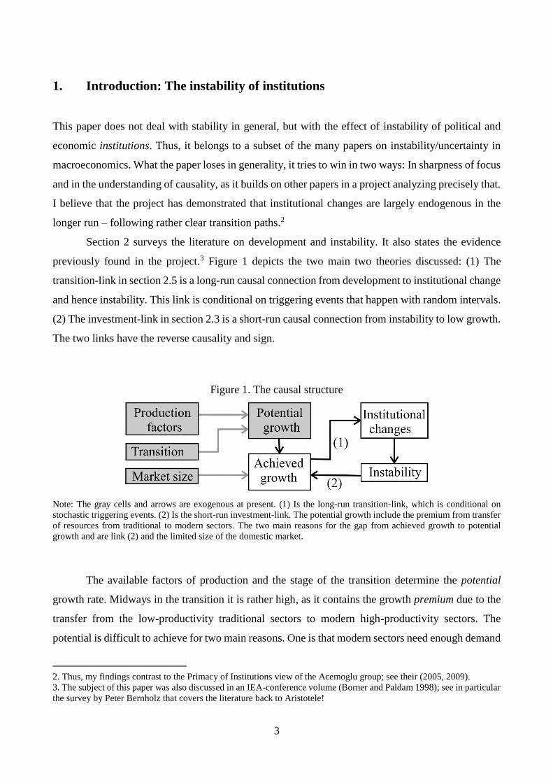
1. Introduction: The instability of institutions

This paper does not deal with stability in general, but with the effect of instability of political and

economic institutions. Thus, it belongs to a subset of the many papers on instability/uncertainty in

macroeconomics. What the paper loses in generality, it tries to win in two ways: In sharpness of focus

and in the understanding of causality, as it builds on other papers in a project analyzing precisely that.

I believe that the project has demonstrated that institutional changes are largely endogenous in the

longer run – following rather clear transition paths.2

Section 2 surveys the literature on development and instability. It also states the evidence

previously found in the project.3 Figure 1 depicts the two main two theories discussed: (1) The

transition-link in section 2.5 is a long-run causal connection from development to institutional change

and hence instability. This link is conditional on triggering events that happen with random intervals.

(2) The investment-link in section 2.3 is a short-run causal connection from instability to low growth.

The two links have the reverse causality and sign.

Figure 1. The causal structure

Note: The gray cells and arrows are exogenous at present. (1) Is the long-run transition-link, which is conditional on

stochastic triggering events. (2) Is the short-run investment-link. The potential growth include the premium from transfer

of resources from traditional to modern sectors. The two main reasons for the gap from achieved growth to potential

growth and are link (2) and the limited size of the domestic market.

The available factors of production and the stage of the transition determine the potential

growth rate. Midways in the transition it is rather high, as it contains the growth premium due to the

transfer from the low-productivity traditional sectors to modern high-productivity sectors. The

potential is difficult to achieve for two main reasons. One is that modern sectors need enough demand

2. Thus, my findings contrast to the Primacy of Institutions view of the Acemoglu group; see their (2005, 2009).

3. The subject of this paper was also discussed in an IEA-conference volume (Borner and Paldam 1998); see in particular

the survey by Peter Bernholz that covers the literature back to Aristotele!

4

for their production, and the domestic market in most less developed countries is small, so to achieve

the potential requires the development of exports. The second is discussed in the paper as link (2):

Growth causes institutional change, which the population often experiences as instability. Hence, it

reduces investments and growth. It should be added that many of the policies caused by the instability

may work to create and protect rents in the sectors hit by the instability.

Section 3 deals with data: The term system means the set of institutions of a country, so a

system has to be measured by an index that weights together a set of primary indicators. Both the

selection of the indicators and the weights have to be assessments. The paper uses the Polity index,

P, for the political system and the Fraser index of Economic Freedom, F, for the economic system.

The primary indicators used for the two indices differ; thus, the correlation of about 0.45 of the indices

(see note to Table 4) is not by construction.

The P-index gives the instability measures VP and ZP, while the F-index gives VF. The V’s are

the average annual numerical change in the respective index, while ZP is the fraction of years under

anarchy. These measures differ greatly between countries, so they can be used to analyze how much

system instability matters. The economic data used in the paper is the cgdppc-series for 1960-2016

from the 2018 version of the Maddison Project Database. These data are the gdp (GDP per capita) in

real PPP prices. The (natural) logarithm to gdp is termed income.

Section 4 brings a set of correlations and regressions analyzing the relation of average growth

and the instability variables. Finally, section 5 concludes.

2. Theory and the aspect analyzed

Many theories connect instability to development. Sections 2.1 and 2.2 are brief surveys, while 2.3

states the investment link. Section 2.4 looks at the long run and surveys prior findings, while section

2.5 states the transition-link. Section 2.6 illustrates the link by countries where long time-series exist.

Instability is a measure of passed variability. Uncertainty is the expected future instability. To

the extent expectations are stable, instability becomes uncertainty. I distinguish between variability

within systems and variability of systems – the paper only deals with the latter.

2.1 Political instability/uncertainty

Some countries, such as Argentina and Haiti, have had many institutional changes and low growth.

Other countries, such as Thailand and Turkey, combine a fine economic development with an even

5

greater instability of the political system.4 However, the literature does find that instability has a

negative effect on growth – not always, but in the main. It is also worth mentioning that one of the

most thoughtful and successful practitioners of development, Lee Kuan Yew, often claimed that

political stability is a key to development.5

Most of the literature looks at within-system instability: Much research show that constitu-

tional changes of governments in democracies have little effect on the growth rate due to the

competition of the parties for the median voter. The median voter theorem applies in established

democracies with a stable and well-defined issue-space. Such democracies are mainly in wealthy

countries. A family of studies deals with the interaction of elections and economic policies, studying

cyclicality, notably budget cycles, see Paldam (1997) and Carmignani (2003). Such fluctuations have

a small effect on the medium-term growth rate, though they may affect the public debt.

Most countries have not (yet) reached such stability, but it is still possible to study within-

system instability using the change of governments or even ministers as the instability indicator, see

e.g. Aisen and Veiga (2013). Many authors do not distinguish the within-system and between-systems

relation, and some even say that the distinction is irrelevant (Alesina et al. 2009). Others, notably

Jong-A-Pin (2009), study a wide range of instability measures; see also Bergh et al. (2012).

I define political system changes as a change in an index trying to measure all aspects of the system.

Here I use the Polity index. It appears to be the most widely used such index. It has well-known

weaknesses, but so have other indices. Therefore, I take it that it measure what it should, but that it

has some measurement error.

2.2 Economic instability/uncertainty

This literature is even larger, and more diverse. Studies of the within-system instability analyze the

longer-run consequences of economic fluctuations. A rather broad approach is Gavin and Hausmann

(1998), who find that countries with high economic variability have low growth.6

Later the literature has splintered into many sub-literatures dealing with the effect of specific

types of instability/uncertainty on growth. Newer studies look at different types of uncertainty shocks

and conclude that they affect growth, though sometimes only temporarily (Bloom 2009 and Basu and

Bundick 2017). Another family of studies analyzes the effect of policy regimes and changes in such

4. The stories of the four countries Haiti, Argentina, Thailand and Turkey are covered by: Lundahl and Silé (2005), Tanzi

(2017), Terwiel (2011) and Pope and Pope (2011), respectively.

5. Lee Kuan Yew ruled Singapore for all the 45 years of ‘miracle’ growth, where he practiced what he claimed. Polity

has been constant in Singapore at P = −2 since 1965 after the failed union with Malaysia.

6. Their findings are a part of IDB (1995), discussing why Latin America has fared relatively poorly.

6

regimes. A regime is defined as a set of preferences for outcomes and policy instruments (Wilson

2000 and Fernández-Villaverde et al. 2015). The mechanisms analyzed are most diverse. The main

one is probably the investment-link discussed below, but authors also discuss links to the propensity

to consume and others as well.

I define economic system changes as a change in an index trying to measure all aspects of the

system. Here I use the Fraser index of Economic Freedom. It measures the freedom to run a private

business. The researchers who made the index believe that this is the prescription for the ideal society.

It is not the shared ideal of everybody, but given the ideal, the index is carefully compiled. The F-

index starts the annual series in year 2000. Since then the index has had small movements as shown

on Figure A4 (Appendix). The 5-year data goes back to 1970, but does not cover the socialist

countries of Eastern Europe.

This change in 1988-92 from socialism in Eastern Europe is, by far, the largest change of the

economic system in our period. The F-index does not cover this change, but the related Transition

Index from the EBRD (European Bank for Reconstruction and Development) covers it. Thus, I assess

that the change amounted to more than half of the range of the F-index. Its effect is documented in a

large literature, see e.g., Åslund (2002), Paldam (2002) or Gross and Steinherr (2004). It had costs

that peaked at about 40% in GDP, and it typically took a decade to recover.7

The causal structure of these events has two steps: (i) The triggering events were an

unexpected domestic political shock in the USSR, where the Communist party imploded. It led to a

wave of external shocks throughout the Socialist World. (ii) The shocks led to large jumps in both

the political and economic system in the direction of the systems at the same income level in the rest

of the world, as predicted by the jump-model in section 2.5. While the socialist system lasted, it

strongly influenced both the long-run GDP-level and the political system; see e.g. the table of country-

twins with different economic systems in Paldam and Gundlach (p 81, 2008).

2.3 The investment link: Instability low investments low growth

The investment link has the two parts indicated in the section headline: Many studies of the invest-

ment motive, since Borner et al. (1995), have pointed out that the predictability and transparency of

political decisions are of great importance for the willingness to invest. Obviously, system instability

causes a loss of predictability and transparency and hence low investments. This is confirmed in many

7. The same countries had the reverse change 70-45 years before, when they changed from a market (or feudal) system

to a socialist one. This change (i.e. the revolution) is also covered by a large literature. Even when it suffers from poor

statistics, it is clear that it was even more costly economically and, in addition, it was much more violent.

7

papers (at least) since Aizenman and Marion (1993).

Even more studies points to the second part of the link: Investment gives growth; see e.g.,

Barro (1991). By combining the two parts, instability becomes a strong impediment for growth. It

does not appear that there is a difference between instability of the political and economic system in

this theory. Both links in this theory apply rather generally to all types of uncertainty, so it might be

difficult to sort out what is due to institutional instability.

2.4 The long run: Transitions and the high growth potential

By a crude simplification, the study of economic development has found two main steady states. The

traditional steady state used an almost stable traditional technology that produced a low and stable

income. The modern steady state uses international technology yielding a much higher productivity

and incomes and moderate growth. The change from the traditional steady state to the modern one is

the Grand Transition. It can be simplified by a model with two sectors representing the two steady

states, where the modern sector gradually replaces the traditional one.

Growth consists of three parts during the transition: The two first are the internal growth in

the two sectors, giving growth of 1-2% as the weighted sum of the two growth rates. The third part is

the growth premium from the transfer of resources from the low productivity traditional sector to the

high productivity modern one. The premium is quite large: Imagine that it is possible to transfer 1%

of the labor force per year. If the productivity gap is 5 times, such a transfer will produce an extra

growth of 5 percentage points. Thus, countries may potentially grow by 6-7% at the middle of the

Grand Transition.8 This potential is hard to achieve for many reasons, one of which is that the many

changes that take place cause losers in the short run and much uncertainty that harms social stability

and investments, as mentioned.9

The Grand Transition consists of transitions in most (if not all) socio-economic variables. A

handful of previous papers in the project study the transition by looking at a range of socio-political

variables: Paldam and Gundlach (2018) analyze the democratic transition (using the P-index) and

find the robust curve shown as Figure 2a. The curve is driven by the cross-country pattern in the data,

which gives a perfect transition curve with a flat section at both ends. The transition covers about

60% of the range of the index [-10, 10].

8. This is the standard explanation of the growth miracle of some East Asian ’tiger economies’ and now China and India.

9. Gundlach and Paldam (2019) find that growth in the average country does peak midways in the transition, but the

excess growth is only 1-1½.

8

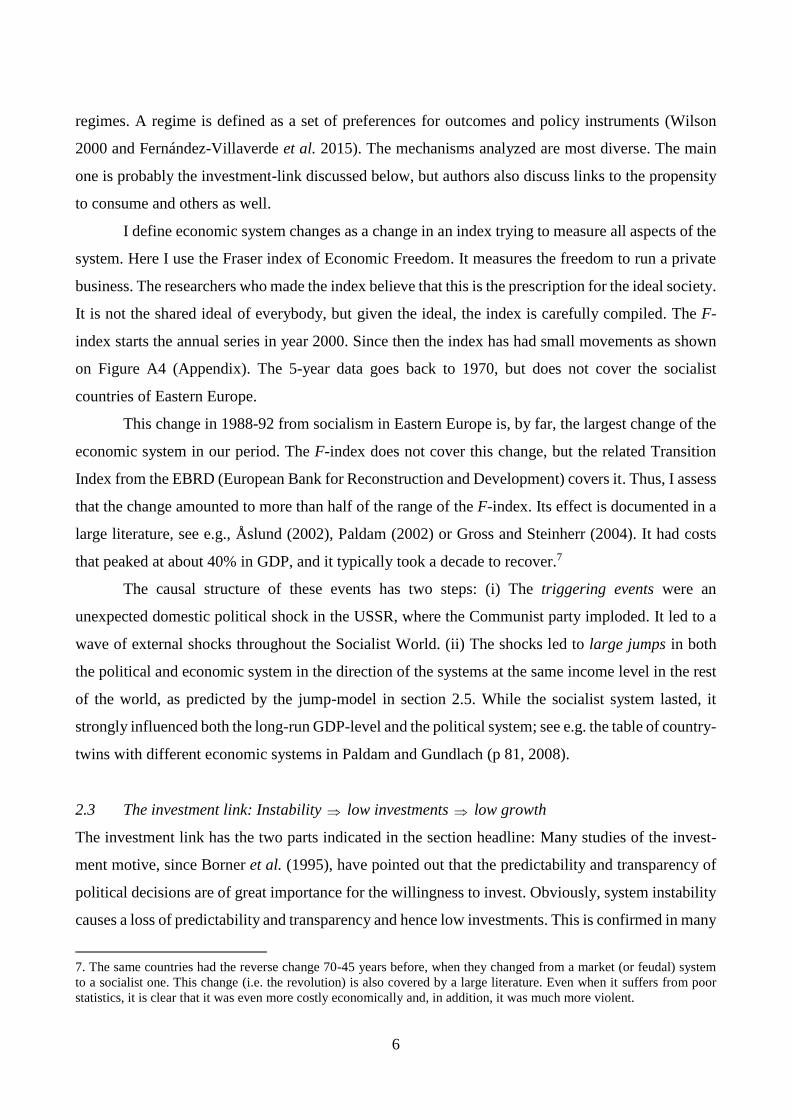
Figure 2. Kernel regressions for the transition in the political and economic system

Fig. 2a. The democratic transition (Polity) Fig. 2b. The transition to the market (Fraser)

Note: Figure 2a is estimated on 6,953 joint observations from the P-index and income in non-OPEC countries from 1960

to 2016. The thick line excludes the outlier Singapore, and the dashed line includes the outlier. Figure 2b is estimated on

the 1,965 joint observations of the Fraser index and income from 2000 to 2016. Both figures use Epanechnikov’s kernel

with bandwidth 0.4. The gray lines give 95% confidence intervals.

Bjørnskov and Paldam (2012) analyze the transition in the economic system by an alternative

index. It is calculated from the ownership item in the World Values Surveys, and shows people’s

preferences for private vs public ownership of businesses. It gives a pattern that looks as Figure 2b.

The curve on Figure 2b is not fully as predicted by the transition theory: It lacks the flat sections at

the two ends, and it covers only 25% of the range of the index [0, 10]. We also know that if data could

be made for a longer period, they would show large movements over time.

The narrow confidence intervals around the two curves are due to the large number of

observations, and the scatter of data-points around the curves is random. Thus, the countries do not

cluster in groups with different paths. Hence, the high correlation to income for both institutional

indices suggests the common underlying transition.

2.5 The transition-link and the jump-model

Figure 2a indicates that the correlation of Polity and income is 0.56. Gundlach and Paldam (2009)

report a formal causality test using the development potential variable from Olsson and Hibbs (2005)

as instrument. The test shows that the dominating long-run causality is from income to Polity.10 This

10. Paldam and Gundlach (2012) show that the same causal story holds for the Freedom House (Gastil) index. The two

papers give references to the large literature on democracy and growth/income.

9

is the reverse causality of the one expected from the PoI (Primacy of Institutions) view. The PoI-

group (notably Acemoglu at al. 2009) showed that a standard regression model explaining Polity by

initial income, lagged Polity and fixed effects gives fickle results. Paldam and Gundlach (2018) make

two points:

(i) Polity and income have a statistical structure that makes them unfit for a standard

regression model. Income (which is in logs) is close to linearity, but Polity is a stepwise constant

variable with a bounded range, and infrequent jumps that may be quite large relative to the range.

(ii) We present a new jump-model that explains the transition.11 The key to the model is the

notion that the transition path is an attractor for jumps that happen randomly after a highly variable

spell of system stability, which on average lasts about 15 years. The mechanics of the model use three

variables: E is a binary variable for when the index changes. J is the size of the change. T termed the

tension is the distance to the transition path.

E is an (almost) random variable relative to economic development, as measured by initial

income, growth, average past growth and the tension variable. The randomness of triggering events

is further analyzed on a sample of 262 jumps in Paldam (2019). They are all found in the historical

archive of The Economist, which allows us to see what well-informed observers thought were the

triggering events. The events cover a wide range, of which most are related to domestic politics.

J is explained rather well by T, the tension variable. The coefficient to T is about 1.5, so jumps

tend to overshoot the transition path, giving some system cycling, see section 2.6.

The only non-random explanatory variable in the Jump-model is income. Hence, it is causal,

but it works indirectly through the transition path, which is a long-run relation. As the actual Polity-

values are scattered around the transition curve, income works poorly explaining Polity. Thus,

democracy is a poor explanatory variable for growth.

However, it would be nice if growth was a reward for democracy, and many researchers have

tried to show that it is. Barro (1996) finds a small negative effect, but most later authors such as

Tavares and Wacziarg (2001), Gründler and Krieger (2016) and Acemoglu et al., (2019) find a small

positive effect. It may cumulate to something in the end, but it still seems inadequate to explain the

high correlation of the main political indices and income, discussed above.12

Given that the two curves on Figure 2 represent the two long-run transitions, they imply that

11. A jump is a change in the Polity index that is (numerically) larger than three points. This includes sequences of

changes to the same side in sequential years. The model does not explain smaller changes.

12. The key mechanism in the democracy-causing-growth theory is that democracies are more likely to increase

education, causing growth. This might be right, but the lags involved are surely counted in decades.

10

high growth will mean nothing for the change in the political system at the flat sections at the bottom

and the top of the income scale, but in-between – where the potential growth is largest – it will

generate system changes. As system changes tend to overshoot the transition path, countries have a

rather unstable system during the transition. This instability does fall by a factor of no less than 7

times measured by the standard deviation when countries reach the modern steady state. As regards

the transition in the economic system, the path on Figure 2b looks as a straight line, so that the first

difference becomes almost constant, and hence it looks as the path of income. This contributes to the

confluence found below.

The Grand Transition normally takes a couple of centuries, and the paper covers only half a

century. Thus, the data cover countries at all stages in the transition, including countries that have

passed the transition and reached stability. How much it matters requires a short digression looking

at the two dozen countries where the data cover more than 200 years.

2.6 Digression on two centuries: The Democratic Transition in old kingdoms

The P-data start in 1800, where they cover 23 of the present countries,13 including Germany that

consisted of a handful of independent states before 1871. The USA had left colonial status just 17

years before, but the other 22 countries all had old royal systems with an average P-level of –8.14 The

king was from a ‘royal’ family. He ruled in alliance with the national ‘church’ and a small ‘noble’

class of large landowners. Thus, it was a feudal-religious system headed by a king. Such systems

typically lasted a handful of centuries, though crises erupted from time to time.15 The Grand Transi-

tion undermines two of the three pillars in this power structure:

(a) The Agricultural Transition reduced the agricultural sector from 40-50% of GDP to well

below 5%, greatly weakening the relative income and power of landowners. New sectors of manu-

facturing and services grew to produce both capitalists, a large labor class, and eventually an even

larger middle class, which became the main recipient of the large increase in human capital. The new

classes wanted political influence. Compared to the old ruling elite the new classes were much more

numerous, so they demanded mass representation.

13. Year 1800 was at the start of the Napoleonic Wars, where the political system in several countries was in a flux, so

for three countries I have made assessments to reach 23. Two of the countries in this group – Korea and Morocco – had

a period of about 40 years as colonies.

14. The equivalence hypothesis says that the time-series and the cross-country patterns are roughly the same, as is the

case for the P-index even when the traditional level was lower in the long time series than in the cross-country sample.

15. The theory of coalitions predicts instability in systems with three strong players; see e.g. Schofield (1993). It appears

that the king often managed to be stronger than the two other players, but sometimes the nobility or the church became

so strong that the power balance shifted, giving a crisis.

11

(b) The Religious Transition reduced religiosity by 60-70%.16 This reduced the power of the

Church. The reduction in religiosity also seemed to have reduced the amount of religious fundamen-

talism and hereby the number of democratically problematic people with supreme values, as

described in Bernholz (2017).

The result of all these changes proved to be democratic societies. If the king managed to

remain on the throne, he (she) turned into a constitutional figurehead. The democratic transition is

never smooth: Old players try to hold on to power, and the new classes grab power through demon-

strations/riots/revolutions, where the first mover runs a large risk. Thus, he needs to hide in a crowd,

so these processes take place in large steps that often overshoot the transition path, resulting in

cyclical jumps for some time before the system settles down as mentioned. Often there are periods of

military rule during the transition.

This development is illustrated by Thailand. By the V-measure it is the most unstable country,

see Table 1 below. For the 58 years covered, the numerical changes add to 98 points. This corresponds

to five changes from the top to the bottom of the scale, due to over/undershooting cycles. Thailand

has P-scores since 1800, and the Maddison GDP data exists for as many years, though they are very

thin before 1950. Figure 3 looks at all 217 years and tells the transition story.

Figure 3. The history of Thailand over two centuries as told by income and Polity

Note: Income is the logarithm to real GDP per capita in the Maddison project database. Income is rescaled by multiplying

by 5 and deducing 42.5. See further Terwiel (2011) on the history of Thailand. The rest of the paper covers the period

after 1960 only. Democracy has not yet stabilized in Thailand, but I predict that it will.

16. See Paldam and Gundlach (2012) and Paldam and Paldam (2017) on the religious transition.

12

Until the 1930s, Thailand was in the traditional steady state with a stable absolute kingdom

and a stable low income. The transition became strong around 1950. Since then Thailand has been

unusually unstable politically, but P does have a rising trend, and in addition, the country has a stable

real growth per capita of no less than 4½% pa. The main difference between Thailand and the typical

western country is that the transition in the West started earlier and was slower. Consequently, the

West experienced the zigzag of the democratic transition earlier and less compressed, though it was

as dramatic, especially in Germany and the South European countries.17

3. The measures of system instability

Section 3.1 defines the three measures, while section 3.2 considers the path over time for the V-data.

Section 3.3 looks at the dynamics of the changes, while section 3.4 deals with the inertia.

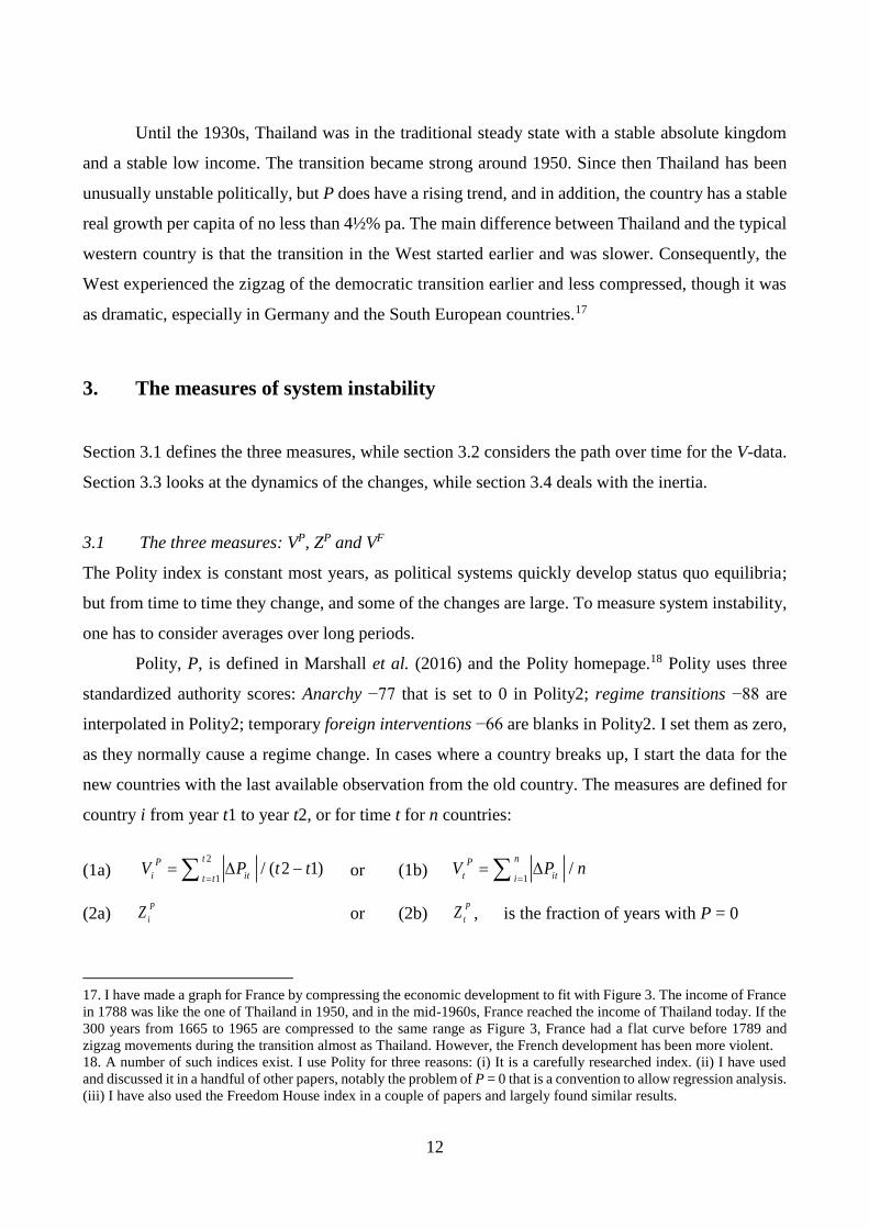
3.1 The three measures: VP, ZP and VF

The Polity index is constant most years, as political systems quickly develop status quo equilibria;

but from time to time they change, and some of the changes are large. To measure system instability,

one has to consider averages over long periods.

Polity, P, is defined in Marshall et al. (2016) and the Polity homepage.18 Polity uses three

standardized authority scores: Anarchy −77 that is set to 0 in Polity2; regime transitions −88 are

interpolated in Polity2; temporary foreign interventions −66 are blanks in Polity2. I set them as zero,

as they normally cause a regime change. In cases where a country breaks up, I start the data for the

new countries with the last available observation from the old country. The measures are defined for

country i from year t1 to year t2, or for time t for n countries:

(1a) 2

1/ ( 2 1)

tP

i itt tV P t t

or (1b)

1/

nP

t itiV P n

(2a) P

iZ or (2b)

P

tZ , is the fraction of years with P = 0

17. I have made a graph for France by compressing the economic development to fit with Figure 3. The income of France

in 1788 was like the one of Thailand in 1950, and in the mid-1960s, France reached the income of Thailand today. If the

300 years from 1665 to 1965 are compressed to the same range as Figure 3, France had a flat curve before 1789 and

zigzag movements during the transition almost as Thailand. However, the French development has been more violent.

18. A number of such indices exist. I use Polity for three reasons: (i) It is a carefully researched index. (ii) I have used

and discussed it in a handful of other papers, notably the problem of P = 0 that is a convention to allow regression analysis.

(iii) I have also used the Freedom House index in a couple of papers and largely found similar results.

13

ViP is the average numerical change per year. Given that the Polity index is a good measure of the

political system (1a) is the most straightforward measure of system instability possible.19 The indices

can be used to analyze the development over time for one country, or across countries for one year.

The period covered is 1960 to 2017, where data are available for 167 countries. Of these countries 19

have perfect stability for all years covered.20

Lawson et al. (1996) defined the Fraser index, F. Since then it has been discussed in the annual

volumes, latest Gwartney et al. (2018). For the period 1970 to 2000 it uses a time unit of 5 years –

since 2000 it is annual. The instability measure VF is calculated in parallel with VP as follows:

(3a) 2

1/ ( 2 1)

tF

i itt tV F t t

or (3b)

1/

nF

t itiV F n

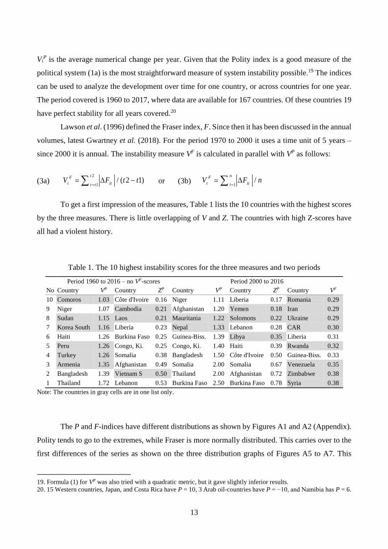
To get a first impression of the measures, Table 1 lists the 10 countries with the highest scores

by the three measures. There is little overlapping of V and Z. The countries with high Z-scores have

all had a violent history.

Table 1. The 10 highest instability scores for the three measures and two periods

Period 1960 to 2016 – no VF-scores Period 2000 to 2016

No Country VP Country ZP Country VP Country ZP Country VF

10 Comoros 1.03 Côte d'Ivoire 0.16 Niger 1.11 Liberia 0.17 Romania 0.29

9 Niger 1.07 Cambodia 0.21 Afghanistan 1.20 Yemen 0.18 Iran 0.29

8 Sudan 1.15 Laos 0.21 Mauritania 1.22 Solomons 0.22 Ukraine 0.29

7 Korea South 1.16 Liberia 0.23 Nepal 1.33 Lebanon 0.28 CAR 0.30

6 Haiti 1.26 Burkina Faso 0.25 Guinea-Biss. 1.39 Libya 0.35 Liberia 0.31

5 Peru 1.26 Congo, Ki. 0.25 Congo, Ki. 1.40 Haiti 0.39 Rwanda 0.32

4 Turkey 1.26 Somalia 0.38 Bangladesh 1.50 Côte d'Ivoire 0.50 Guinea-Biss. 0.33

3 Armenia 1.35 Afghanistan 0.49 Somalia 2.00 Somalia 0.67 Venezuela 0.35

2 Bangladesh 1.39 Vietnam S 0.50 Thailand 2.00 Afghanistan 0.72 Zimbabwe 0.38

1 Thailand 1.72 Lebanon 0.53 Burkina Faso 2.50 Burkina Faso 0.78 Syria 0.38

Note: The countries in gray cells are in one list only.

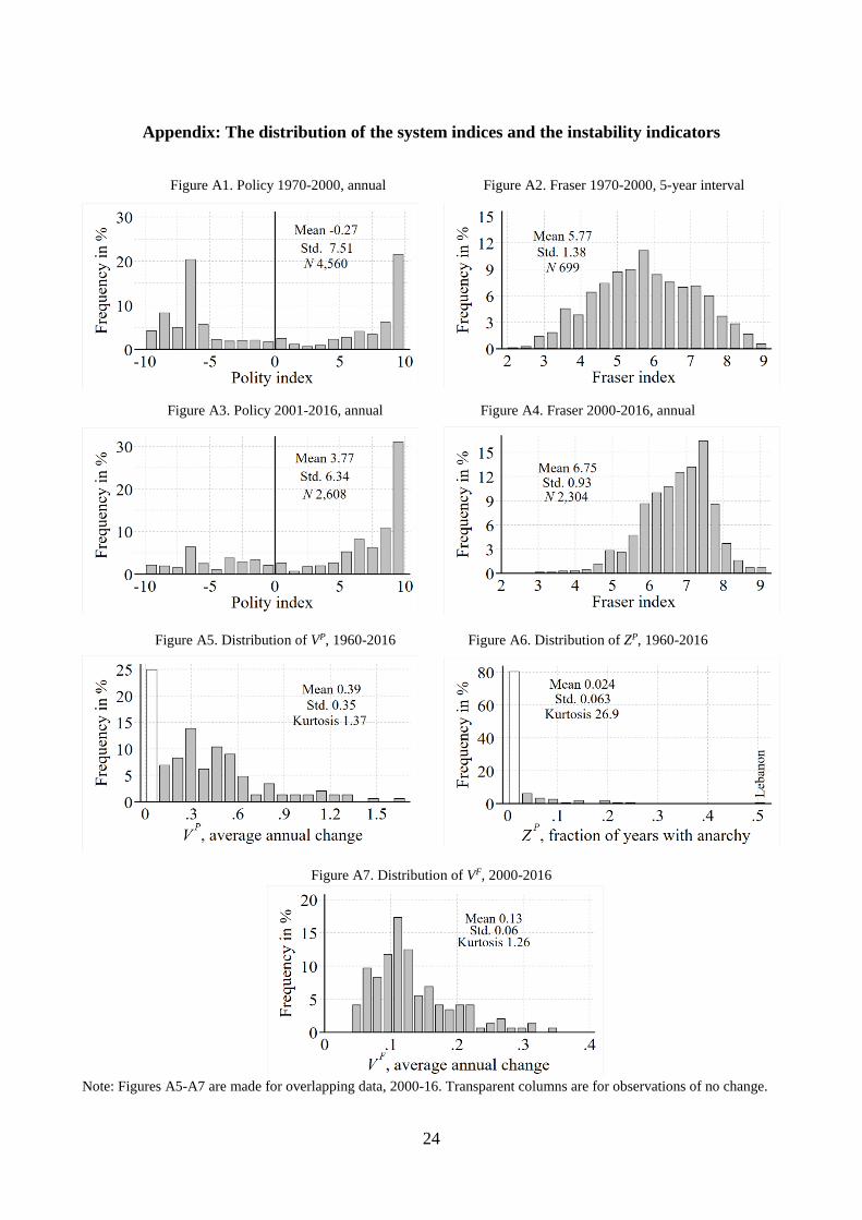
The P and F-indices have different distributions as shown by Figures A1 and A2 (Appendix).

Polity tends to go to the extremes, while Fraser is more normally distributed. This carries over to the

first differences of the series as shown on the three distribution graphs of Figures A5 to A7. This

19. Formula (1) for VP was also tried with a quadratic metric, but it gave slightly inferior results.

20. 15 Western countries, Japan, and Costa Rica have P = 10, 3 Arab oil-countries have P = −10, and Namibia has P = 6.

14

tallies with the bang-bang nature of the political system in many middle-income countries. It is

possible to change the political system from dictatorship to democracy or vice versa within one year,

but large changes in the economic system take time.

Note also that the Vs have only moderately skew distributions, while Z has a very skew distri-

bution. More than half of the Zs are zero, so the explanatory power of the Z-variable hinges upon few

countries, and the utmost observation is indeed an outlier.

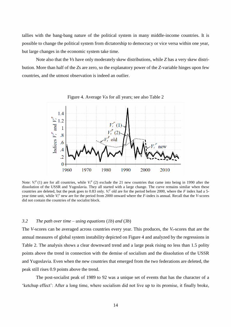
Figure 4. Average Vts for all years; see also Table 2

Note: VtP (1) are for all countries, while Vt

P (2) exclude the 21 new countries that came into being in 1990 after the

dissolution of the USSR and Yugoslavia. They all started with a large change. The curve remains similar when these

countries are deleted, but the peak goes to 0.83 only. VtF old are for the period before 2000, where the F index had a 5-

year time unit, while VtF new are for the period from 2000 onward where the F-index is annual. Recall that the V-scores

did not contain the countries of the socialist block.

3.2 The path over time – using equations (1b) and (3b)

The V-scores can be averaged across countries every year. This produces, the Vt-scores that are the

annual measures of global system instability depicted on Figure 4 and analyzed by the regressions in

Table 2. The analysis shows a clear downward trend and a large peak rising no less than 1.5 polity

points above the trend in connection with the demise of socialism and the dissolution of the USSR

and Yugoslavia. Even when the new countries that emerged from the two federations are deleted, the

peak still rises 0.9 points above the trend.

The post-socialist peak of 1989 to 92 was a unique set of events that has the character of a

‘ketchup effect’: After a long time, where socialism did not live up to its promise, it finally broke,

15

and this created a large demonstration effect.21 First, the Communist Party of the USSR collapsed,

then the whole regime, the union of the 15 countries, and the Russian superpower.

The collapse of socialism in the Soviet Block also caused a collapse of socialism in many

other counties, including the Yugoslavian Federation. The large shock to the political system gave

big change in the economic system and a deep crisis lasting 5-10 years throughout the ex-socialist

countries. This whole process caused most state-owned enterprises to close or drastically downsize,

and it had large social consequences, but the process was amazingly peaceful.

Table 2 shows the significance of the pattern on Figure 4. A trend of -0.014 gives a fall of

0.08 V-points over the 58 years, so it is no wonder that it is insignificant. The table shows that the

trend and the peak do not interact. We are dealing with two independent phenomena.

Table 2. VtP explained by trends and the post socialist peak, 1988-93

N = 58 (1) (2) (3) (4)

Decade -0.010 (-0.5) -0.014 (-1.6) -0.013 (-1.6)

Du

mm

y fo

r year

1988 -0.043 (-0.4) -0.042 (-0.4)

1989 0.394 (3.6) 0.392 (3.6) 0.393 (3.6)

1990 0.659 (6.0) 0.657 (6.0) 0.657 (5.9)

1991 1.257 (11.5) 1.255 (11.5) 1.253 (11.3)

1992 0.515 (4.7) 0.513 (4.7) 0.510 (4.6)

1993 0.162 (1.5) 0.156 (1.4)

Constant 2.234 (0.6) 3.025 (1.8) 2.933 (1.7) 0.292 (19.2)

R2 0.005 0.800 0.790 0.789

R2 adj -0.013 0.771 0.770 0.764

Note: 58 years are 5.8 decades. Parentheses hold t-ration. Coefficients are bolded if they are significant at the 5% level.

3.3 Dynamics

Section 3.1 argued that the weak trend (from Table 2) is due to the increasing income in the period

that pushes countries along the Democratic Transition. The political systems stabilize in modern

countries. Income data are available for 146 countries with P-data for the period analyzed. The

average growth rate for the 146 countries is 2.24. It amounts to an increase in real GDP per capita of

3.86 times. Consequently, a substantial group of countries has reached the income level that gives a

more stable political system.

21. Afterwards many have explained these events, but the lonely few who predicted them, were not believed.

16

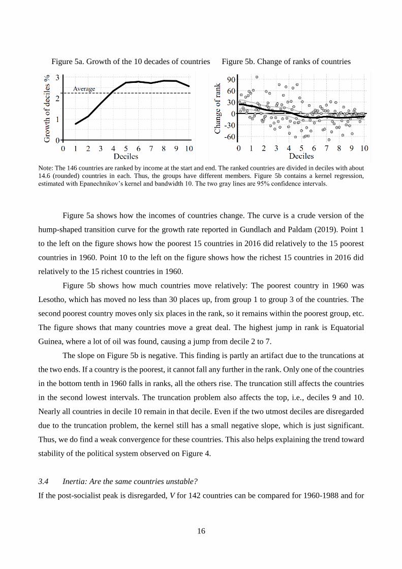
Figure 5a. Growth of the 10 decades of countries Figure 5b. Change of ranks of countries

Note: The 146 countries are ranked by income at the start and end. The ranked countries are divided in deciles with about

14.6 (rounded) countries in each. Thus, the groups have different members. Figure 5b contains a kernel regression,

estimated with Epanechnikov’s kernel and bandwidth 10. The two gray lines are 95% confidence intervals.

Figure 5a shows how the incomes of countries change. The curve is a crude version of the

hump-shaped transition curve for the growth rate reported in Gundlach and Paldam (2019). Point 1

to the left on the figure shows how the poorest 15 countries in 2016 did relatively to the 15 poorest

countries in 1960. Point 10 to the left on the figure shows how the richest 15 countries in 2016 did

relatively to the 15 richest countries in 1960.

Figure 5b shows how much countries move relatively: The poorest country in 1960 was

Lesotho, which has moved no less than 30 places up, from group 1 to group 3 of the countries. The

second poorest country moves only six places in the rank, so it remains within the poorest group, etc.

The figure shows that many countries move a great deal. The highest jump in rank is Equatorial

Guinea, where a lot of oil was found, causing a jump from decile 2 to 7.

The slope on Figure 5b is negative. This finding is partly an artifact due to the truncations at

the two ends. If a country is the poorest, it cannot fall any further in the rank. Only one of the countries

in the bottom tenth in 1960 falls in ranks, all the others rise. The truncation still affects the countries

in the second lowest intervals. The truncation problem also affects the top, i.e., deciles 9 and 10.

Nearly all countries in decile 10 remain in that decile. Even if the two utmost deciles are disregarded

due to the truncation problem, the kernel still has a small negative slope, which is just significant.

Thus, we do find a weak convergence for these countries. This also helps explaining the trend toward

stability of the political system observed on Figure 4.

3.4 Inertia: Are the same countries unstable?

If the post-socialist peak is disregarded, V for 142 countries can be compared for 1960-1988 and for

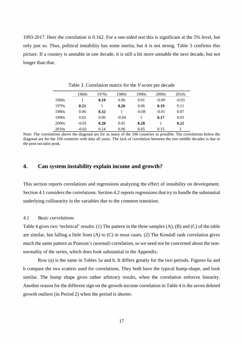
17

1993-2017. Here the correlation is 0.162. For a one-sided test this is significant at the 5% level, but

only just so. Thus, political instability has some inertia, but it is not strong. Table 3 confirms this

picture. If a country is unstable in one decade, it is still a bit more unstable the next decade, but not

longer than that.

Table 3. Correlation matrix for the V-score per decade

1960s 1970s 1980s 1990s 2000s 2010s

1960s 1 0.19 0.06 0.01 -0.00 -0.03

1970s 0.21 1 0.26 0.06 0.19 0.11

1980s 0.06 0.32 1 -0.08 -0.01 0.07

1990s 0.02 0.00 -0.04 1 0.17 0.03

2000s -0.01 0.20 0.01 0.28 1 0.21

2010s -0.02 0.14 0.06 0.05 0.15 1

Note: The correlations above the diagonal are for as many of the 166 countries as possible. The correlations below the

diagonal are for the 104 countries with data all years. The lack of correlation between the two middle decades is due to

the post-socialist peak.

4. Can system instability explain income and growth?

This section reports correlations and regressions analyzing the effect of instability on development.

Section 4.1 considers the correlations. Section 4.2 reports regressions that try to handle the substantial

underlying collinearity in the variables due to the common transition.

4.1 Basic correlations

Table 4 gives two ‘technical’ results: (1) The pattern in the three samples (A), (B) and (C) of the table

are similar, but falling a little from (A) to (C) in most cases. (2) The Kendall rank correlation gives

much the same pattern as Pearson’s (normal) correlation, so we need not be concerned about the non-

normality of the series, which does look substantial in the Appendix.

Row (a) is the same in Tables 5a and b. It differs greatly for the two periods. Figures 6a and

b compare the two scatters used for correlations. They both have the typical hump-shape, and look

similar. The hump shape gives rather arbitrary results, when the correlation enforces linearity.

Another reason for the different sign on the growth-income correlation in Table 4 is the seven deleted

growth outliers (in Period 2) when the period is shorter.

18

Table 4a. Cross-country correlations to the income level, y

Sample Period 1: 1960-2016 Period 2: 2000-2016

Correlation Pearson Kendall Pearson Kendall

Sample (A) (B) (C) (A) (B) (C) (A) (B) (C) (A) (B) (C)

N, countries 111 127 156 111 127 156 103 115 140 103 115 140

(a) g, growth 0.45 0.34 0.33 0.29 0.24 0.22 -0.02 -0.03 -0.01 -0.07 -0.07 -0.07

(b) P, Polity 0.69 0.45 0.44 0.50 0.35 0.36 0.44 0.22 0.24 0.44 0.32 0.36

F, Fraser 0.78 0.69 0.68 0.63 0.55 0.53

(c) VP -0.39 -0.41 -0.36 -0.34 -0.35 -0.29 -0.40 -0.39 -0.40 -0.28 -0.29 -0.27

ZP -0.25 -0.24 -0.25 -0.25 -0.23 -0.20 -0.44 -0.43 -0.43 -0.15 -0.14 -0.12

VF -0.59 -0.51 -0.46 -0.43 -0.37 -0.32

Table 4b. Cross-country correlations to the growth rate, g

Sample Period 1: 1960-2016 Period 2: 2000-2016

Correlation

Pearson Kendall

Pearson Kendall

Sample

(A) (B) (C) (A) (B) (C)

(A) (B) (C) (A) (B) (C)

N, countries 111 127 156 111 127 156 103 115 140 103 115 140

(a) y, income

0.45 0.34 0.33 0.29 0.24 0.22

-0.02 -0.03 -0.01 -0.07 -0.07 -0.07

(b) P, Polity

0.22 0.16 0.10 0.15 0.10 0.07

-0.15 -0.16 -0.14 -0.19 -0.20 -0.16

F, Fraser

0.02 -0.10 -0.05 -0.06 -0.13 -0.09

(c) VP

-0.18 -0.17 -0.19 -0.11 -0.09 -0.12

-0.14 -0.13 -0.15 0.02 0.05 0.04

ZP

-0.07 -0.07 -0.09 -0.12 -0.11 -0.11

-0.34 -0.34 -0.33 -0.08 -0.08 -0.08

VF

-0.17 -0.06 -0.07 -0.02 0.05 0.06

Note: Rows (a) are the same. Bolded correlations are significant at the two-sided level of 5%. The country samples are:

(A) is without OPEC and post-communist countries, (B) is without post-communist countries and (C) is all countries. The

Fraser index is available for fewer countries. So period 2 is estimated for fewer observations. The correlations of P and F

for period 2 are 0.50, 0.43 and 0.44 for the samples A, B and C, respectively.

Figure 6a. The growth-income scatter 1960-16 Figure 6b. The growth-income scatter 2000-16

Note: Kernel curve included has bw = 0.5. Seven outliers are deleted from the data for Figure 6b. This does not affect the

form of the curve – the confidence intervals of the two curves overlap. However, a linear approximation gives a positively

sloped curve for Figure 6a and a negative one for Figure 6b as in rows (a) of Tables 4.

19

Table 4a reports the correlates to income: Rows (b) and (c) have a highly significant and

consistent pattern. Rows (b) shows that income is positively correlated to the levels of both the Polity

and the Fraser index. One reason for that correlation is that the transitions in the two system variables,

as depicted on Figure 2. The next section shows that there are more reasons. Rows (c) report that

income is negatively correlated to all three variability measures (VP, ZP and VF) – especially to VF.

Table 4b reports the correlates to the growth rate: Row (a) is the same as in Table 4a, rows

(b) have the same problem as row (a). The correlations in rows (c) are (nearly) all negative and often

significant. It is important that the short- and long-run connection is the reverse. Thus, the short-run

connection does not aggregate to the long run. We need a mechanism that reverses the short-run

effect. The interpretation is that it has short-run costs to change the system, even when the changes

have fine long-run consequences.

4.2 Some regressions: Can variability explain growth?

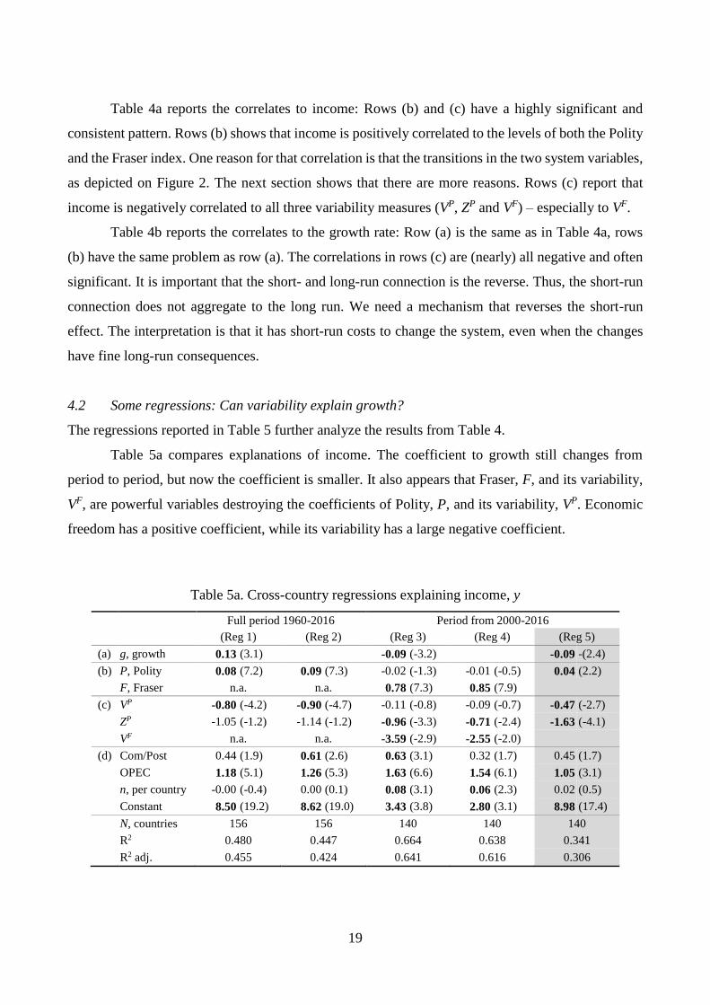
The regressions reported in Table 5 further analyze the results from Table 4.

Table 5a compares explanations of income. The coefficient to growth still changes from

period to period, but now the coefficient is smaller. It also appears that Fraser, F, and its variability,

VF, are powerful variables destroying the coefficients of Polity, P, and its variability, VP. Economic

freedom has a positive coefficient, while its variability has a large negative coefficient.

Table 5a. Cross-country regressions explaining income, y

Full period 1960-2016 Period from 2000-2016

(Reg 1) (Reg 2) (Reg 3) (Reg 4) (Reg 5)

(a) g, growth 0.13 (3.1) -0.09 (-3.2) -0.09 -(2.4)

(b) P, Polity 0.08 (7.2) 0.09 (7.3) -0.02 (-1.3) -0.01 (-0.5) 0.04 (2.2)

F, Fraser n.a. n.a. 0.78 (7.3) 0.85 (7.9)

(c) VP -0.80 (-4.2) -0.90 (-4.7) -0.11 (-0.8) -0.09 (-0.7) -0.47 (-2.7)

ZP -1.05 (-1.2) -1.14 (-1.2) -0.96 (-3.3) -0.71 (-2.4) -1.63 (-4.1)

VF n.a. n.a. -3.59 (-2.9) -2.55 (-2.0)

(d) Com/Post 0.44 (1.9) 0.61 (2.6) 0.63 (3.1) 0.32 (1.7) 0.45 (1.7)

OPEC 1.18 (5.1) 1.26 (5.3) 1.63 (6.6) 1.54 (6.1) 1.05 (3.1)

n, per country -0.00 (-0.4) 0.00 (0.1) 0.08 (3.1) 0.06 (2.3) 0.02 (0.5)

Constant 8.50 (19.2) 8.62 (19.0) 3.43 (3.8) 2.80 (3.1) 8.98 (17.4)

N, countries 156 156 140 140 140

R2 0.480 0.447 0.664 0.638 0.341

R2 adj. 0.455 0.424 0.641 0.616 0.306

20

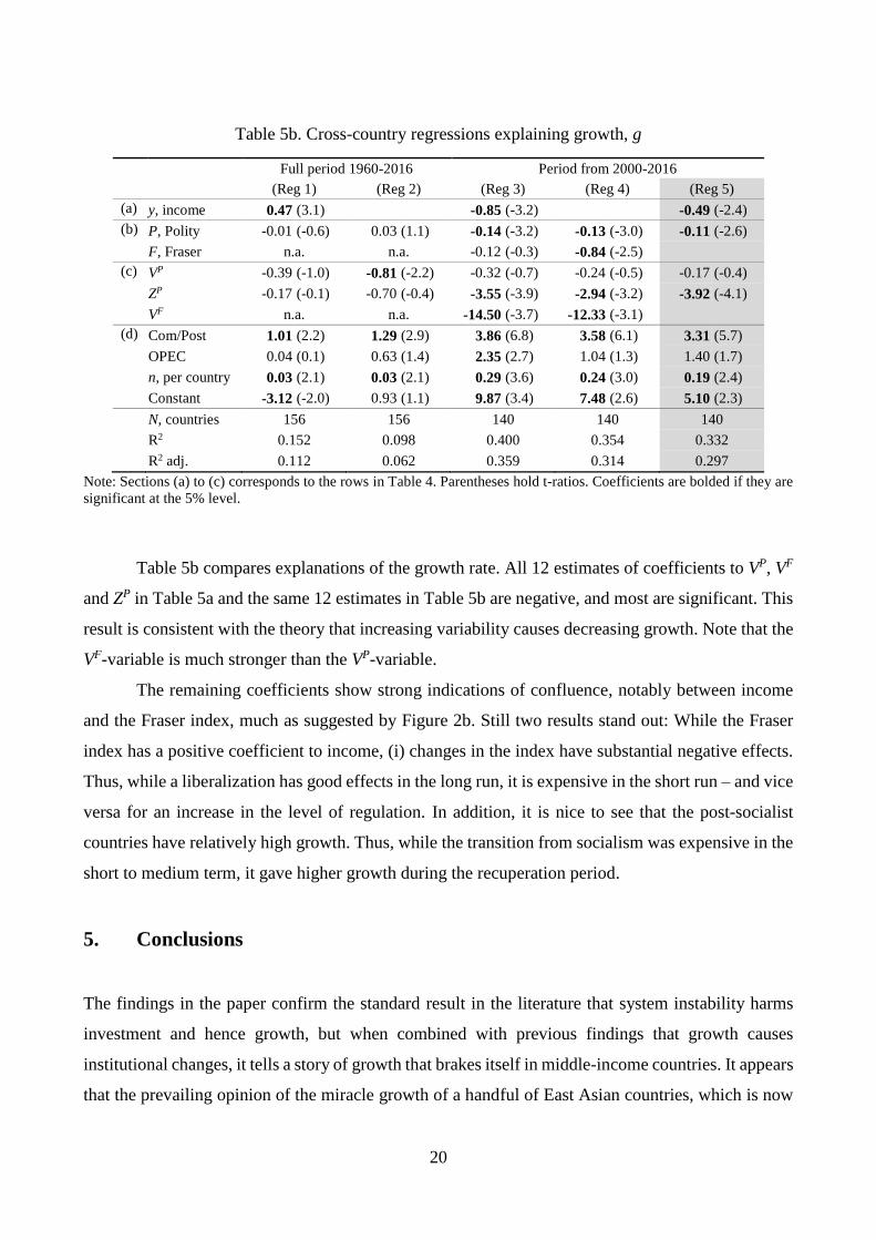
Table 5b. Cross-country regressions explaining growth, g

Full period 1960-2016 Period from 2000-2016

(Reg 1) (Reg 2) (Reg 3) (Reg 4) (Reg 5)

(a) y, income 0.47 (3.1) -0.85 (-3.2) -0.49 (-2.4)

(b) P, Polity -0.01 (-0.6) 0.03 (1.1) -0.14 (-3.2) -0.13 (-3.0) -0.11 (-2.6)

F, Fraser n.a. n.a. -0.12 (-0.3) -0.84 (-2.5)

(c) VP -0.39 (-1.0) -0.81 (-2.2) -0.32 (-0.7) -0.24 (-0.5) -0.17 (-0.4)

ZP -0.17 (-0.1) -0.70 (-0.4) -3.55 (-3.9) -2.94 (-3.2) -3.92 (-4.1)

VF n.a. n.a. -14.50 (-3.7) -12.33 (-3.1)

(d) Com/Post 1.01 (2.2) 1.29 (2.9) 3.86 (6.8) 3.58 (6.1) 3.31 (5.7)

OPEC 0.04 (0.1) 0.63 (1.4) 2.35 (2.7) 1.04 (1.3) 1.40 (1.7)

n, per country 0.03 (2.1) 0.03 (2.1) 0.29 (3.6) 0.24 (3.0) 0.19 (2.4)

Constant -3.12 (-2.0) 0.93 (1.1) 9.87 (3.4) 7.48 (2.6) 5.10 (2.3)

N, countries 156 156 140 140 140

R2 0.152 0.098 0.400 0.354 0.332

R2 adj. 0.112 0.062 0.359 0.314 0.297

Note: Sections (a) to (c) corresponds to the rows in Table 4. Parentheses hold t-ratios. Coefficients are bolded if they are

significant at the 5% level.

Table 5b compares explanations of the growth rate. All 12 estimates of coefficients to VP, VF

and ZP in Table 5a and the same 12 estimates in Table 5b are negative, and most are significant. This

result is consistent with the theory that increasing variability causes decreasing growth. Note that the

VF-variable is much stronger than the VP-variable.

The remaining coefficients show strong indications of confluence, notably between income

and the Fraser index, much as suggested by Figure 2b. Still two results stand out: While the Fraser

index has a positive coefficient to income, (i) changes in the index have substantial negative effects.

Thus, while a liberalization has good effects in the long run, it is expensive in the short run – and vice

versa for an increase in the level of regulation. In addition, it is nice to see that the post-socialist

countries have relatively high growth. Thus, while the transition from socialism was expensive in the

short to medium term, it gave higher growth during the recuperation period.

5. Conclusions

The findings in the paper confirm the standard result in the literature that system instability harms

investment and hence growth, but when combined with previous findings that growth causes

institutional changes, it tells a story of growth that brakes itself in middle-income countries. It appears

that the prevailing opinion of the miracle growth of a handful of East Asian countries, which is now

21

repeated by China and India, is the growth premium reached from transfers of resources – notably

labor – from the traditional to the modern sector. The paper argues that this transfer is normally quite

problematic as it appears as system instability that generates uncertainty and thus harms investment.

Thus, the growth miracle may rather be that the political systems of these countries were

sufficiently stable to permit the good effects of the change to become visible to the majority of the

population, and also that they managed to use the world market to overcome the limitations of the

domestic market so that the modern sector could expand rapidly.

22

References:

Åslund, A., 2002. Building capitalism. The transformation of the former Soviet Bloc. Cambridge UP, Cambridge, UK

Acemoglu, D., Johnson, S., Robinson, J.A., 2005. Institutions as a fundamental cause of long-run growth. Chpt 6, 385-

472 in Aghion, P., Durlauf, S.N., eds. Handbook of Economic Growth, Vol 1A. North-Holland, Amsterdam

Acemoglu, K.D., Johnson, S., Robinson, J.A., Yared, P., 2009. Reevaluating the modernization hypothesis. Journal of

Monetary Economics 56, 1043-58

Acemoglu, K.D., Naidu, S., Restrepo, P., Robinson, J.A., 2019. Democracy does cause growth. Journal of Political

Economy 127, 47-100

Aisen, A., Veiga, J.F., 2013. How does political instability affect economic growth? European Journal of Political

Economy 29, 151-167

Aizenman, J., Marion, N., 1993. Policy uncertainty, persistence, and economic growth. Review of International

Economics 1, 145-63

Alesina, A., Özler, S., Roubini, N., Swagel, P., 2006. Political instability and economic growth. Journal of Economic

Growth 1, 189-211

Barro, R.J., 1991. Economic growth in across section of countries. Quarterly Journal of Economics 106, 407-43

Barro, R.J., 1996. Democracy and growth. Journal of Economic Growth 1, 1-27

Basu, S., Bundick, A., 2017. Uncertainty chocks in a model of effective demand. Econometrica 85, 937-58

Berggren, N., Bergh, A., Bjørnskov, C., 2012. The growth effects of institutional instability. Journal of Institutional

Economics 8, 187-224

Bernholz, P., 1998. Causes of change in political-economic regimes. Chpt. 4, 74-96 in Borner and Paldam (1998)

Bernholz, P., 2017. Totalitarianism, terrorism and supreme values: History and theory. Springer, Heidelberg

Bjørnskov, C., Paldam, M., 2012. The spirits of capitalism and socialism. A cross-country study of ideology. Public

Choice 150, 469-98

Bloom, N., 2009. The impact of uncertainty chocks. Econometrica 77, 623-85

Borner, S., Brunetti, A., Weder, B., 1995. Political credibility and economic development. Macmillan, London

Borner, S., Paldam, M., eds., 1998. The political dimensions of economic growth. Macmillan, London and New York

Carmignani, F., 2003. Political instability, uncertainty and economics. Journal of Economic Surveys 17, 1-54

Fernández-Villaverde, J., Guerrón-Quintana, P., Kuester, K., Rubio-Ramírez, J., 2015. Fiscal Volatility Shocks and

Economic Activity. American Economic Review 105, 3352-84

Fraser index of economic Freedom. URL:https://www.fraserinstitute.org/studies/economic-freedom. See also Gwartney

et al. (2018)

Gavin, M., Hausmann, R., 1998. Macroeconomic volatility and economic development. Chpt.4, 97-116 in Borner and

Paldam(1998), see also IDB(1995)

Gross, D., Steinherr, A., 2004. Economic Transition in Central and Eastern Europe: Planting the Seeds. Cambridge UP,

Cambridge (updated 2009)

Gründler, K., Krieger, T., 2016. Democracy and growth: Evidence from a machine learning indicator. European Journal

of Political Economy 45, 85-107

Gundlach, E., Paldam, M., 2009. A farewell to critical junctures. Sorting out the long-run causality of income and

23

democracy. European Journal of Political Economy 25, 340-54

Gundlach, E., Paldam, M., 2019. The transition in the growth rate. P.t. WP at URL: http://martin.paldam.dk/Papers/GT-

Main/11a-Hump.pdf

Gwartney, J., Lawson, R., Hall, J., Murphy, R., 2018. Economic Freedom of the World 2018 Annual Report. Fraser

Institute, Vancouver, B.C.

IDB, 1995. Inter-American Development Bank, Economic and Social Progress in Latin America 1995 report. Part 2 pp

189-258. Special report: Overcoming Volatility, see also Gavin and Hausmann (1998)

Jong-A-Pin, R., 2009. On the measurement of political instability and its impact on economic growth. European Journal

of Political Economy 25, 15-29

Lawson, R., Gwartney, J., Block, W., 1996. Economic Freedom of the World. Fraser Institute, Vancouver, BC

Lundahl, M., Silé, R., 2005. Haiti: nothing but failure. Chpt 14, pp 272-301 in Lundahl, M., Wyzan, M.L., eds., 2005.

The political economy of reform failure. Routledge, London

Marshall, M.G., Gurr, T.R., Jaggers, K., 2016. Polity IV project. Users’ manual. University Center for Systemic Peace.

See Polity index for home page

Olsson, O., Hibbs, D.A. Jr., 2005. Biogeography and long-run economic development. European Economic Review 49,

909-38

Paldam, E., Paldam, M., 2018. The political economy of churches in Denmark, 1300-2015. Public Choice 172, 443-63

Paldam, M., 1997. Political Business Cycles. Chpt 16 pp 342-79 in Mueller, D.C., ed., Perspectives on Public Choice.

A Handbook. Cambridge UP, Cambridge

Paldam, M., 2002. Udviklingen i Rusland, Polen og Baltikum (The development in Russia, Poland and the Baltic states).

Aarhus UP, Aarhus

Paldam, M., 2019. A study of triggering events. When do political regimes change? P.t. WP at URL: http://martin.pal-

dam.dk/Papers/GT-Main/10-Reverse.pdf

Paldam, M., Gundlach, E., 2008. Two Views on Institutions and Development: The Grand Transition vs the Primacy of

Institutions. Kyklos 61, 65-100

Paldam, M., Gundlach, E., 2012. The Democratic Transition: Short-run and long-run causality between income and the

Gastil index. The European Journal of Development Research 24, 144-68

Paldam, M., Gundlach, E., 2013. The religious transition. A long-run perspective. Public Choice 156, 105-23

Paldam, M., Gundlach, E., 2018. Jumps into democracy. Integrating the short and long run in the Democratic Transition.

Kyklos 71, 456-81

Polity index: URL: http://www.systemicpeace.org/polityproject.html. See also Marshall et al. (2016)

Pope, H., Pope, N., 2011 (3rded.). Turkey unveiled: A history of modern Turkey. Overlook Duckworth, New York

Schofield, N., 1993. Political competition and multiparty coalition governments. European Journal of Political

Research 23, 1-33

Tanzi, V., 2018. Argentina, from Peron to Macri: An economic chronicle. Jorge Pinto Books

Tavares, J., Wacziarg, R.T., 2001. How democracy affects growth. European Economic Review 45, 1341-78

Terwiel, B.J., 2011. Thailand’s political history. From the 13th century to recent times.2nded., River Books, Bangkok

Wilson, C.A., 2000. Policy regimes and policy changes. Journal of Public Policy 20, 247-77

24

Appendix: The distribution of the system indices and the instability indicators

Figure A1. Policy 1970-2000, annual Figure A2. Fraser 1970-2000, 5-year interval

Figure A3. Policy 2001-2016, annual Figure A4. Fraser 2000-2016, annual

Figure A5. Distribution of VP, 1960-2016 Figure A6. Distribution of ZP, 1960-2016

Figure A7. Distribution of VF, 2000-2016

Note: Figures A5-A7 are made for overlapping data, 2000-16. Transparent columns are for observations of no change.

Economics Working Papers

2018-07: Tom Engsted: Frekvensbaserede versus bayesianske metoder i

empirisk økonomi

2018-08: John Kennes, Daniel le Maire and Sebastian Roelsgaard: Equivalence

of Canonical Matching Models

2018-09: Rune V. Lesner, Anna Piil Damm, Preben Bertelsen and Mads Uffe

Pedersen: Life Skills Development of Teenagers through Spare-Time

Jobs

2018-10: Alex Xi He, John Kennes and Daniel le Maire: Complementarity and

Advantage in the Competing Auctions of Skills

2018-11: Ninja Ritter Klejnstrup, Anna Folke Larsen, Helene Bie Lilleør and

Marianne Simonsen: Social emotional learning in the classroom:

Study protocol for a randomized controlled trial of PERSPEKT 2.0

2018-12: Benjamin U. Friedrich and Michał Zator: Adaptation to Shocks and

The Role of Capital Structure: Danish Exporters During the Cartoon

Crisis

2019-01 Ran Sun Lyng and Jie Zhou: Household Portfolio Choice Before and

After a House Purchase

2019-02: Mongoljin Batsaikhan, Mette Gørtz, John Kennes, Ran Sun Lyng,

Daniel Monte and Norovsambuu Tumennasan: Daycare Choice and

Ethnic Diversity: Evidence from a Randomized Survey

2019-03: Dan Anderberg, Jesper Bagger, V. Bhaskar and Tanya Wilson:

Marriage Market Equilibrium, Qualifications, and Ability

2019-04: Carsten Andersen: Intergenerational Health Mobility: Evidence from

Danish Registers

2019-05 Michael Koch, Ilya Manuylov and Marcel Smolka: Robots and Firms

2019-06: Martin Paldam: The Transition of Corruption - Institutions and

dynamics

2019-07: Martin Paldam: Does system instability harm development? A

comparative empirical study of the long run