Warwick Economics Research Papers

ISSN 2059-4283 (online)

ISSN 0083-7350 (print)

A BLP Demand Model of Product-Level Market Shares

with Complementarity

Ao Wang

April 2021 No: 1351

A BLP Demand Model of Product-LevelMarket Shares with Complementarity

Ao Wang∗

January 2021

AbstractApplied researchers most often estimate the demand for differentiated prod-ucts assuming that at most one item can be purchased. Yet simultaneousmultiple purchases are pervasive. Ignoring the interdependence among mul-tiple purchases can lead to erroneous counterfactuals, in particular, becausecomplementarities are ruled out. I consider the identification and estima-tion of a random coefficient discrete choice model of bundles, namely setsof products, when only product-level market shares are available. This lastfeature arises when only aggregate purchases of products, as opposed to in-dividual purchases of bundles, are available, a very common phenomenon inpractice. Following the classical approach with aggregate data, I considera two-step method. First, using a novel inversion result in which demandcan exhibit Hicksian complementarity, I recover the mean utilities of prod-ucts from product-level market shares. Second, to infer the structural pa-rameters from the mean utilities while dealing with price endogeneity, I useinstrumental variables. I propose a practically useful GMM estimator whoseimplementation is straightforward, essentially as a standard BLP estimator.Finally, I estimate the demand for Ready-To-Eat (RTE) cereals and milkin the US. The demand estimates suggest that RTE cereals and milk areoverall complementary and the synergy in consumption crucially depends ontheir characteristics. Ignoring such complementarities results in misleadingcounterfactuals.

∗University of Warwick, UK (ao.wang@warwick.ac.uk). I am indebted to Xavier D’Haultfœuilleand Alessandro Iaria for the fruitful discussions and continued encouragement at each stage ofthis paper. I am grateful to Jaap Abbring, Philippe Choné, Laurent Lamy, Roxana FernándezMachado, Isabelle Méjean, Eric Renault, and Matt Shum for their insightful suggestions. I wouldlike to thank seminar and conference participants at CREST, University of Surrey, University ofWarwick, HEC Montréal, University of Western Ontario, VIOS China, SEA 90th Annual Meeting.I would also like to thank IRI for making the data used in this paper available. All estimates andanalyses in this paper, based on data provided by IRI, are by mine and not by IRI. All errors aremy own.

1

1 IntroductionSince the seminal work of Berry (1994) and Berry et al. (1995) (henceforth BLP),BLP-type models have been widely used in empirical literature of demand esti-mation.1 Researchers most often estimate models of demand for single products,assuming that individual purchases at most one single product. Yet, the behaviourof making multiple simultaneous purchases is pervasive. In many economic analyses(e.g. multi-category demand, nonlinear pricing, supermarket competition), interde-pendence among multiple purchases in demand is key, which is, however, assumedaway in models of demand for single products. In particular, Hicksian complemen-tarities are ruled out.2 As a result, estimating demand models of single productsmay lead to biased estimates and misleading policy counterfactuals.3

This paper proposes a random coefficient discrete-choice model of demand forbundles.4 This model has various notable advantages. First, its application onlyrequires the availability of aggregate demand data at product level (e.g. aggre-gate choice probability, or sales quantities, of products) defined in form of “marketshares”. Such data is widely accessible in most industries.5 Differently, modelsof demand for bundles routinely used in the empirical literature often rely on theavailability of individual-level choice data of bundles (e.g. individual transactiondata), which may be costly to obtain. Second, different from models of demand forsingle products, the proposed model does not restrict products to be substitutes.It incorporates individuals’ behaviour of multiple purchases, allowing for Hicksiancomplementarities among products. Notably, the model enables to encompass var-ious mechanisms that can drive Hicksian complementarity, while still allowing forendogenous prices.6 Third, the identification arguments are constructive and leadto a practically useful Generalized Method of Moments (GMM) estimator. In par-ticular, it can handle potentially large choice sets in multiple purchases. Finally, theimplementation of the GMM estimator is straightforward, essentially as a standardBLP estimator.

To motivate the identification discussion, I distinguish two sets of demand prim-1BLP-type models also gain popularity outside of empirical industrial organisation, e.g. anal-

ysis of voting data (Rekkas (2007), Milligan and Rekkas (2008), Gordon and Hartmann (2013),Merlo and Paula (2017), Gillen et al. (2019)), asset pricing (Koijen and Yogo, 2019).

2Hicksian complementarity is defined as negative (compensated) cross-price elasticity betweentwo products. For a survey of different concepts of complementarity, see Samuelson (1974).

3See section 3.3 for Monte Carlo evidences of such bias in various counterfactual analyses.4In the empirical literature, the terminology “bundle” is often referred to as a set of products

purchased by individuals. In this paper, I use this terminology and formalise it in Assumption 1.5This data requirement is the same as classical BLP models of single products.6Examples of such mechanisms include shopping cost (Pozzi (2012), Thomassen et al. (2017)),

preference for variety (Hendel (1999), Dubé (2004)), and synergies in consumption (Gentzkow,2007).

2

itives that are sufficient for different kinds of economic analyses in models of de-mand for bundles. The first set includes product-level market share functions; Ishow that they are sufficient for economic analyses (e.g. identification of price elas-ticities, marginal costs, and mergers) under linear pricing.7 The second set includesbundle-level market share functions; I prove that they are sufficient for the analysesunder nonlinear pricing.8

I then organise the identification discussion in two parts. In the first part, asin classical demand models using aggregate data, I use a two-step strategy to iden-tify product-level market share functions. In the first step, I invert the observedproduct-level market shares to the mean utilities of products. Because of possibleHicksian complementarities among products, the typical conditions that guaranteethe invertibility of product-level market share functions (connected substitutes con-ditions, see Berry et al. (2013)) may not hold. To solve this challenge, I use a noveldemand inverse argument that hinges on two elements. First, the affine relationshipbetween the utilities of bundles and its single products: the average utility of anybundle equals the sum of those of its single products plus an extra term capturingtheir potential demand synergy. Second, the P-matrix property by Gale and Nikaido(1965) which crucially does not restrict the products to be Hicksian substitutes. Inthe second step, I use instrumental variables (IVs) to deal with endogenous pricesand construct conditional moment conditions. Based on these moment conditions,the identification can be achieved under the general but high-level completeness con-ditions along the lines of Berry and Haile (2014).9 To complement the discussion,I also propose low-level sufficient conditions for the identification of product-levelmarket share functions in a mixed-logit model of demand for bundles. In particular,I show that under some common regularity conditions, product-level market sharefunctions are identified when demand and supply shocks are jointly normal, or thedata generating process (DGP) is a model of demand for multiple products acrosscategories.

In the second part, assuming the identification of product-level market sharefunctions, I study that of bundle-level market share functions. This is to disentan-gle the demand synergies among products from the unobserved correlations in theutilities of products (Gentzkow, 2007). Because only product-level market sharesare observed, this task is more challenging than the usual case in which bundle-level

7Under linear pricing, firms set prices for single products and the price of a bundle is the sumof the prices of its single products.

8Under nonlinear pricing, the price of a bundle can be different from the sum of the prices ofits single product, and firms can further set discounts or surcharges on the bundles of their ownproducts.

9For various forms of completeness conditions, the testability, and the sufficient conditions ofcompleteness, see Mattner (1993), D’Haultfoeuille (2011), Canay et al. (2013), Andrews (2017),Freyberger (2017), Hu and Shiu (2018).

3

market shares are observed. I provide both positive and negative results. First, Iprove that the identification can be achieved in mixed-logit models of demand forbundle up to size two that are often used in the empirical literature.10 Second, Ishow that using only product-level market shares may have limited power in iden-tifying bundle-level market share functions in other types of models. I provide anexample of non-identification in a model of demand for multiple units.

I propose a GMM estimation procedure that is similar to that in BLP models ofsingle products. In the first step, given a guess of the demand synergy parametersand the distribution of the random coefficients, I invert the observed product-levelmarket shares to the mean utilities of products. In the second step, I instrumentout the unobserved demand shocks in the mean utilities of products and constructthe GMM objective function. There are nontrivial challenges that BLP models ofsingle products do not have. In particular, the implementation of the demand in-verse is complicated due to possible Hicksian complementarities among products:when used to implement the demand inverse in the first step, the fixed-point al-gorithm proposed by Berry et al. (1995) may not have the contraction-mappingproperty and therefore may not converge. To solve this challenge, I propose touse Jacobian-based algorithms. To enhance their numerical performance, I suggestusing a starting value of parameters directly constructed from the observed product-level market shares. In Monte Carlo simulations, I show that using this startingvalue significantly improves the numerical performance of Jacobian-based methods,reducing the convergence time by 70% compared to using standard starting valuein large applications (the number of bundles being about 5000).

Finally, I illustrate the practical implementation of the methods and estimatethe demand for Ready-To-Eat (RTE) cereals and milk in the US. First, the demandestimates suggest that RTE cereals and milk are overall Hicksian complementary.Moreover, the extent to which a RTE cereal product and a milk product are com-plementary crucially depends on the match of their characteristics (e.g. flavours,grain type, fat content), some pairs being less complementary than others. Second,I simulate a merger between a major RTE cereal producer and a milk producer.The results are aligned with Cournot (1838)’s insight: in the presence of Hicksiancomplementarity, mergers can be welfare enhancing. Third, I estimate the demandand replicate the same merger exercise using two alternative models: a model thatcompletely ignores demand synergy between RTE cereals and milk, and a modelthat restricts all synergies to be the same across bundles of RTE cereal and milk.The first alternative model imposes that the demand of RTE cereals and that of milkare independent, predicting the merger to have no effect on welfare. The secondalternative model seems to overestimate the amount of complementarity between

10See Gentzkow (2007), Fan (2013), Grzybowski and Verboven (2016).

4

RTE cereals and milk, overestimating the consumer welfare gain due to the merger.

Related Literature Empirical literature dealing with multiple purchases typi-cally employs models of demand for bundles that rely on individual-level choicedata of bundles (e.g. individual transaction data).11 Differently, the methods inthis paper only requires the availability of aggregate product-level demand data(e.g. aggregate choice probability, or sales quantities, of products) and can be ap-plied when bundle-level demand data is not accessible. In particular, this paperis different from Iaria and Wang (2019) in three aspects. First, the methods pro-posed by two papers work under different data availabilities; those in this paperwork when only aggregate product-level demand data is available, while those ofthe other paper apply when individual-level choice data of bundles is accessible.Second, identification strategies are different; in this paper, I exploit the exoge-nous variation in IVs to achieve identification, while that paper fully exploits theaffine relationship between the utilities of the bundle and its single products dueto the availability of bundle-level demand data. Third, estimation methods aredifferent; this paper uses a GMM estimation procedure, while that paper proposesa likelihood-type estimator that resolves the dimensionality challenge due to manymarket-product fixed effects.

Identifying and estimating models of demand for bundles from aggregate demandat product level is a challenging task. Moreover, prices are often endogenous, whichintroduces additional difficulty in identification. To the best of my knowledge,this is the first paper that provides a systematic treatment of both issues in BLP-type models of demand for bundles that may exhibit Hicksian complementarity.12

In particular, the paper proposes a novel demand inverse argument to deal withpossible Hicksian complementarities among products. Berry et al. (2013) proposethe connected substitutes conditions that guarantee the invertibility of the marketshare functions. In model of demand for bundles with only product-level marketshares being available, these conditions rely on the products to be substitutes. Somepapers have employed similar concepts of demand inverse of product-level marketshares in model of demand for bundles. Fan (2013) studies newspaper market in

11Examples include consumer choice in supermarket (Hendel (1999), Dubé (2004), Lee et al.(2013), Kwak et al. (2015), Thomassen et al. (2017), Ershov et al. (2018)), household choiceamong motor vehicles (Manski and Sherman, 1980), choice of telecommunication services (Liuet al. (2010), Crawford and Yurukoglu (2012), Grzybowski and Verboven (2016), Crawford et al.(2018)), subscription decision (Nevo et al. (2005), Gentzkow (2007)), firms’ decision on technologyadoptions (Augereau et al. (2006), Kretschmer et al. (2012)). See Berry et al. (2014) for a survey ofcomplementary choices and sections 4.2-4.3 of Dubé (2018) for a survey of econometric modellingof complementary goods.

12Dunker et al. (2017) also deal with price endogeneity in identification. However, instead ofusing the product-level market shares, they assume the availability of a vector of bundle-levelmarket shares that has the same dimension as the number of products.

5

the US and assumed households subscribe to at most two newspapers. She givessufficient conditions for the connected substitutes conditions and therefore rules outHicksian complementarities among different newspapers. In a model of demand formultiple products across categories, Song and Chintagunta (2006) implement thedemand inverse of brand-level market shares. However, they do not have theoreticalresults on the invertibility of the brand-level market share functions. Iaria andWang(2019) employ the demand inverse to concentrate out fixed effects in estimationwhen individual-level choice data of bundles is available. In contrast, I prove theinvertibility of product-level market share functions in general models of demand forbundles (e.g. mixed-logit, probit) and use the demand inverse as a key identificationargument when only product-level market shares are available.

This paper also contributes to the recent literature of random-utility modelsof demand in the presence of multiple purchases and potentially complementarity.Fosgerau et al. (2019) employ a different approach and model Hicksian comple-mentarity via overlapping nests. Sher and Kim (2014)’s identification argumentscrucially rely on substitutes assumptions in consumers’ utility,13 while this paperdoes not restrict utility functions to be submodular or supermodular. Allen andRehbeck (2019a)’s main results imply the identification of product-level marketshare functions in discrete choice models with additively separable heterogeneity.The following paper, Allen and Rehbeck (2019b), gives identification results of cer-tain distributional features of the random coefficients in the case of two products(and therefore one bundle). Differently, the current paper achieves the identifi-cation using IVs and further provides identification results of bundle-level marketshare functions that allow for any finite number of products (and bundles). No-tably, except for Fosgerau et al. (2019), all the other papers mentioned assume awayendogenous prices.

Organisation In section 2, I introduce the model and necessary notations. Insection 3, I motivate the model from three aspects. First, I provide various examplesin the literature that can be formulated via the model. Second, I illustrate howthe model can allow for Hicksian complementarity. Third, I provide Monto Carloevidences that accent the economic relevance of the proposed model to variouscounterfactual analyses. In section 4, I present the main identification results. Insection 5, I describe the GMM estimation procedure and its implementation. Insection 6, I illustrate the practical implementation of the methods with an empiricalapplication. Section 7 concludes. All proofs are in Appendices A-G. Figures andtables can be found in Appendix I. Additional Monte Carlo simulations can be

13When each consumer is assumed to consume at most one unit of each good, they imposesubmodularity restriction in consumers’ utility (see their Assumption 2); when multi-unit demandis allowed, they use a stronger “M-natural concavity” restriction (see their Assumption 3).

6

found in Appendix K.

2 ModelDenote market by t = 1, ..., T . The definition of market depends on the concreteapplication. For example, one could have different geographic areas in the case ofcross sectional data, or different periods in the case of panel data, or a combinationof these. For individuals in market t, let J be the set of J market-specific productsthat can be purchased in isolation or in bundles. A bundle b is defined as a collectionof single products in J and denote the set of available bundles in market t by C2.14

Denote the outside option by 0. Individuals in market t can either choose a productj ∈ J, a bundle b ∈ C2, or the outside option denoted by 0. Denote by C1 = J∪C2

the set of available products and bundles, and by C = C1 ∪ 0 the choice set ofindividuals in market t. Let ptj denote the price of product j in market t, andxtj ∈ RK the market-product specific vector of other characteristics of j in t.

For individual i in market t, the indirect utility from purchasing product j ∈ Jis:

Uitj = uitj + εitj

= xtjβi − αiptj + ηij + ξtj + εitj

= x(1)tj β

(1) + x(2)tj β

(2)i − αiptj + ηij + ξtj + εitj

= [xtjβ − αptj + ξtj] + [x(2)tj ∆β(2)

i −∆αiptj + ηij] + εitj

= δtj + µitj + εitj,

(1)

where uitj = δtj+µitj with δtj = xtjβ−αptj+ξtj being market t-specific mean utilityof product j ∈ Jt and µitj = x

(2)tj ∆β(2)

i −∆αiptj + ηij being an individual i-specificdeviation from δtj, while εitj is an idiosyncratic error term. x(1)

tj ∈ RK1 is the vectorof product characteristics that enter Uitj with deterministic coefficient(s), β(1), i.e.consumers have homogeneous taste on x(1)

tj , while x(2)tj ∈ RK2 and ptj enter Uitj with

potentially individual i-specific coefficients, β(2)i and αi. They capture consumers’

heterogeneous tastes on characteristics x(2)tj and sensitivities to price change. The

term ηij captures individual i’s (unobserved) perception of the quality of productj.15 ξtj is a market-product specific demand shock, observed to both firms andindividuals but not observed to the researcher.Throughout the paper, denote by j ∈ b the relationship of product j being in

14The set of products and bundles can be both market-specific, i.e. Jt and Ct2, and the resultsof the paper do not change. In the empirical illustration, I will adopt market-specific Jt and Ct2;while in the theory part, having Jt = J and Ct2 = C2 greatly facilitates the exposition.

15Any characteristic of product j that does not vary across markets is encapsulated by the meanpart of ηij . Equivalently, one can specify this mean as part of β(2), i.e. product-specific interceptsin δtj and the results in this paper do not change.

7

bundle b. The indirect utility for individual i in market t from purchasing productsin bundle b ∈ C2 is:

Uitb =∑j∈b

uitj + Γitb + εitb

=∑j∈b

(δtj + µitj) + Γtb + (Γitb − Γtb) + εitb

=∑j∈b

δtj + Γtb +∑j∈b

µitj + ζitb

+ εitb

= δtb(Γtb) + µitb + εitb,

(2)

where δtb(Γtb) = ∑j∈b δtj + Γtb is market t-specific mean utility of bundle b,

µitb is an individual i-specific utility deviation from δtb(Γtb), Γitb and Γtb are theindividual-market it- and market t-specific demand synergies among the productsof bundle b, ζitb is (observed or unobserved) individual deviation from averagedemand synergies Γtb, and εitb is an idiosyncratic error term. Demand synergiesΓitb’s capture the extra utility individual i obtains from purchasing the productsin bundle b’s in market t jointly rather than separately. Consequently, individualsmay find it more (or less) appealing to purchase products jointly than separately.

Finally, the indirect utility of choosing the outside option 0 is normalized as:

Uit0 = εit0,

where εit0 is an idiosyncratic error term. To complete the model, I write µitj =x

(2)tj ∆β(2)

i −∆αiptj+ηij = µj(θit;x(2)tJ , ptJ) and µitb = ∑

j∈b µitj+ζitb = µb(θit;x(2)tJ , ptJ)

as functions of random coefficients θit = (∆β(2)i ,∆αi, (ηij)j∈J, (ζitb)b∈C2) and θit is

distributed according to F ∈ ΘF .16 Moreover, εit = (εit0, εitjj∈J, εitbb∈C2) areassumed to be i.i.d. according to a known continuous distribution Φ (e.g. Gumbel,Gaussian), and θit and εit are independently distributed.Denote the vector of market t-specific mean utilities for products in J by δtJ =(δtj)j∈J, and the vector collecting all average demand synergies by Γt = (Γtb)b∈C2 .Define δt(Γt) = (δtJ, (δtb(Γtb))b∈C2). The market share function of b ∈ C1 in market

16Typically, the distribution of θit depends on individual i’s demographic characteristics di ∈ D.In this case, F is a mixture of distributions of θi|di: F =

∑di∈D πt(di)F (·|di), where πt(·) is the

distribution of demographics in market t.

8

t is:17

sb(δt(Γt);x(2)tJ , ptJ, F ) =

∫ ∫1Uitb > Uitb′ for any b′ 6= b,b′ ∈ CdΦ(εit)dF (θit)

=∫sb(δt(Γt);x(2)

tJ , ptJ, θit)dF (θit),(3)

where sb(δt(Γt);x(2)tJ , ptJ, θit) is individual i’s choice probability of b in market t

given θit.18 Then, product-level market share function of j ∈ J is defined as aweighted sum of the market share functions of b’s that contain j:

sj.(δtJ;x(2)tJ , ptJ,Γt, F ) =

∑b∈C1

wjbsb(δt(Γt);x(2)tJ , ptJ, F )

= wj s(δt(Γt);x(2)tJ , ptJ, F )

(4)

where wj = (wjb)b∈C1 is of dimension 1×C1, wjb is the number of times j appearsin b (and known to the researcher), and s(δt;x(2)

tJ , ptJ, θit) = (sb(δt;x(2)tJ , ptJ, θit))b∈C1

is the vector of market share functions of products and bundles and of dimensionC1×1. If j /∈ b, then wjb = 0 and the market share of bundle b does not contributeto the product-level market share of j; if j ∈ b, then wjb is a positive integer. Whenthere is no bundle that contains multiple units of the same product, i.e. a situationof qualitative choice, wjb = 1 for j ∈ b. Then, (4) represents the population-levelmarginal choice probability of j. When a bundle contain multiple units of the sameproduct, i.e. a situation of quantity choice, wjb is equal to the units of product jpurchased in the form of bundle b and may be greater than 1. Then, (4) representsthe population-level total purchases of product j. In both cases, the aggregation in(4) is consistent with the typical product-level aggregate demand data available tothe researcher.

3 Demand Synergies in Model (4)Demand model (4) exhibits two features that are crucial in many economic analysesthat models of demand for single products do not have. First, it allows for simul-taneous purchases of multiple products and/or quantities. Second, it captures richsubstitution patterns among products, and in particular, Hicksian complementarity.Demand synergy parameters Γitb’s are the key to generate both features.

In this section, I illustrate the economic relevance of demand synergies fromthree aspects. First, I show that by imposing specific restrictions on Γitb, model(4) covers a wide range of economic models. I provide various examples in the

17I abuse the expression b ∈ C1 for both product j and bundle b.18Because Φ is a continuous distribution, then the event of having equal indirect utilities between

two alternatives is zero.

9

literature and explain the economic interpretation of Γitb’s in each setting. Second,I demonstrate how Γitb’s generate flexible substitution patterns in demand and,in particular, Hicksian complementarity. Finally, I report Monte Carlo evidences,showing that ignoring these synergy parameters in demand estimation results inconsiderable bias in counterfactual analyses.

3.1 Examples and Interpretations of Demand Synergies

Example 1: Demand for Single Products, within Category This examplecan be seen as a particular case of (4) with C2 = ∅, or equivalently, Γitb = −∞, forall b ∈ C2. This restriction on Γitb rules out simultaneous purchases of more thanone product and restricts products to be substitutes.

Example 2: Demand for Multiple Products, within Category. Gentzkow(2007) considers household’s choice over bundles of at most 2 different newspapers:C2 = (j1, j2) : j1 < j2, j1, j2 ∈ J and C = 0 ∪ J∪C2. In general, one can allowfor choice over bundles of up to L different products: C2 = (j1, ..., jl) : j1 < ... <

jl, j1, ..., jL ∈ J. As shown in Iaria and Wang (2019), demand synergy Γitb canproxy, for example, preferences for variety, synergies in consumption.

Example 3: Demand for Multiple Products, across Categories. Grzy-bowski and Verboven (2016) and Ershov et al. (2018) consider purchases of prod-ucts across different categories. In the simplest case in which a bundle is definedas a collection of 2 different products (chips and soda) with each belonging to adifferent category (salty snacks and carbonated drinks), we have C2 = J1 × J2 =(j1, j2) : j1 ∈ J1, j2 ∈ J2. In the example of potato chips and carbonated soda(Ershov et al., 2018), Γitb’s are interpreted as synergies in consumption.

Example 4: Quantity Choice, Multiple Units. As a deviation from Ex-ample 1, individuals purchase not only one out of J products but also a discretequantity of the chosen product. This can be captured by C2 = (j, ..., j) : j ∈J, the length of (j, ..., j) ≤ L., where L is the maximal units individuals can pur-chase. In the simplest case, individuals can purchase the outside option 0, aunit of product j ∈ J (single product), or a bundle of two identical units (j, j),j ∈ J. Demand synergy Γit(j,j) is then interpreted as extra utility individual iobtains from purchasing an additional unit of product j relative to the first unit:Γit(j,j) < 0(> 0) implies a decreasing (increasing) marginal utility of purchasingproduct j. If Γit(j,j) = 0, then individual i’s utility from purchasing the second unitof product j remains the same as that from purchasing the first unit.

10

Example 5: Multiple Discreteness. Demand model of multiple discreteness(see Hendel (1999) and Dubé (2004)) can be seen as an extension of Example 4 thatfurther includes bundles defined as a collection of multiple units of different prod-ucts: b = ( (j, ..., j︸ ︷︷ ︸

nj

) )j∈J, where nj is the number of units of product j. As shown in

Iaria and Wang (2019) (Appendix 8.1), Dubé (2004)’s model of multiple discrete-ness can be formulated by specifying Γitb = ∑

j∈J Γit(j,...,j), where Γit(j, ..., j︸ ︷︷ ︸nj

) ≤ 0

for any nj > 1 and j ∈ J. The non-positive Γit(j,...,j) represents non-increasingmarginal utility of consuming additional units of product j during one consump-tion moment and the additivity in Γitb across j ∈ J represents the independencebetween consumption moments.19

Example 6: Multi-Category Multi-Store Demand. Thomassen et al. (2017)study a multi-category multi-store demand model, in which individual purchasesmultiple units in each ofK product categories and purchase all the units of the samecategory in the same store. Consider a simple case in which individual purchasesat most one unit in each of 2 product categories (k1 and k2) from 2 stores (S1 andS2). This can be captured by J = j = (j1, j2) : j1 = k1, k2, j

2 = S1, S2 andC2 = (j, r) : j, r ∈ J, j1 6= r1. A product is defined as a Cartesian productof categories and stores with first coordinate being category and the second beingstore (category 1 in store 2) and a bundle is defined as a Cartesian product of twoproducts that differ in their first coordinate (category 1 in store 2 and category 2 instore 2). Demand synergy Γit(j,r) is interpreted as shopping cost due to store choice:Γit(j,r) = 0 if j2 = r2 (one-stop shopping, buy products of both categories from thesame store), and negative otherwise (multi-stop shopping, purchase products in onecategory from store 1 and those in the other category from store 2).

3.2 Hicksian Substitutions and Demand Synergies

Using a mixed-logit model of demand for multiple products across categories (seeExample 3 of section 3), I illustrate how the signs of cross-price elasticities in model(4), i.e. Hicksian substitutability (positive cross-price elasticities) or complemen-

19Due to Dubé (2004)’s perfect substitute specification, individual will consume up to oneproduct during one consumption moment.

11

tarity (negative cross-price elasticities) are determined by demand synergies Γitb.20

To ease exposition, I drop the notation of market t and product characteristicsin product-level market share functions. Let’s consider the cross-price elasticitybetween products j ∈ J1 and r ∈ J2:21

εjr = prsj.

∫αi[sj.(δ(Γ); θi)sr.(δ(Γ); θi)− sjr(δ(Γ); θi)]dF (θi),

where αi > 0. Different from models of demand for single products, the cross-priceelasticity εjr has an additional term −sjr(δ(Γ); θi). When this term is relativelylarge, i.e. the joint purchase probability for products j and r is relatively large,we may have a negative εjr, i.e. Hicksian complementarity between j and r. Inthe case of two products and one bundle, i.e. J = 1, 2 and C2 = (1, 2),Gentzkow (2007) shows that Γjr = 0 is the cut-off value for Hicksian substitutabilityand complementarity: ε12 < 0 if and only if Γ(1,2) > 0. When there are morethan 2 products, even though Γ(j,r) = 0 may not be the cut-off value for Hicksiansubstitutability and complementarity between j and r, the intuition remains similar.Note that whether j and r are substitute, complementary or independent, i.e. εjr >0, εjr < 0 or εjr = 0, is determined by the weighted average of sij.sir. − sijr. Thelatter is further determined by the magnitude of synergy between j and r, Γjr,relative to other demand synergies. If Γjr is sufficiently negative, then sijr is closeto zero and thus εjr > 0. As an extreme case, when Γjr = −∞, i.e. bundle (j, r) isnot in the choice set, j and r are always substitute and therefore εjr is positive. IfΓjr is positive and large enough relative to Γj′r′ for all (j′, r′) 6= (j, r), then sij.−sijrand sir.−sijr are negligible relative to sijr. Then, the sign of εjr is determined by thepopulation average of s2

ijr − sijr. Since sijr is strictly between 0 and 1, s2ijr − sijr is

always negative and therefore εjr < 0. If Γjr takes some medium value in (−∞,∞),we can expect εjr = 0 and j and r are independent.

3.3 Ignoring Demand Synergies in Demand Estimation: Biasin Counterfactual Simulations

I provide Monte Carlo evidences and show that ignoring demand synergies in de-mand estimation potentially leads to substantial bias in counterfactual analyses.

20In both (1) and (2), income effect is ruled out (or enters linearly in the direct utilities ofall alternatives). Consequently, in most part of the paper, Hicksian complementarity (substi-tutability) coincides with negative (positive) cross-price elasticities. One can adopt income effectby using a different specification of indirect utilities. For example, one specification in Berryet al. (1995) is that price pj enters the indirect utility via −αi log(yi − pj), where yi is individ-ual i’s income. Note that if pj yi, i.e. the income is much larger than product price, then−αi ln(yi − pj) ≈ −αi ln yi − αi

yipj , and the specification in (1) and (2) is suitable.

21See Appendix A for details of the computation.

12

To simplify the exposition while still capturing the economic essence, in each ofthe scenario below, I will suppose that the data generating process (DGP) is amultinomial-logit model of demand for bundles.22 Consider a simple setting inwhich there are two product categories J1 = 1, 2 and J2 = 3, 4. An individualcan purchase a product j ∈ J1 ∪ J2, or a bundle (j1, j2), where j1 ∈ J1 and j2 ∈ J2,or the outside option denoted by 0. Each product j ∈ J1 ∪ J2 has a price pj and acharacteristic xj, and the price of a bundle (j1, j2) is equal to pj1 + pj2 , i.e. there isneither discount nor surcharge. For each bundle (j1, j2), the corresponding demandsynergy is Γj1j2 , constant across individuals. Demand synergy parameters are notzero in the true DGP of each scenario below. In addition, I estimate a model ofdemand that ignores synergies in demand and imposes Γj1j2 = 0 for all j1 ∈ J1 andj2 ∈ J2. Note that this estimated model is equivalent to two independent models ofdemand for single products in J1 and in J2. I use this estimated model to predictthe counterfactuals in each scenario and compare the outcomes to those predictedby the true model. For details of the DGPs, see Appendix J.

Multi-category demand. First, I consider multi-category demand in whichproducts in J1 and J2 are complementary in consumption (i.e. demand syner-gies are positive). Suppose that all synergy parameters are equal to Γ. Moreover,there are an equal number of producers to that of products, each producing oneproduct. I simulate two counterfactual scenarios: cross-category merger and tax onproducts in J1. Table 1 summarise the results.

In the upper panel, I simulate a merger between the producer of product 1 ∈ J1

and the producer of 3 ∈ J2. The outcomes predicted by the true model (columns 1and 3) confirm Cournot (1838)’s intuition: the merged producer internalises comple-mentarity between 1 and 3 and prices decrease after the merger, enhancing consumersurplus. Moreover, the more products are complementary, the more consumer sur-plus is enhanced after the merger. In contrast, the estimated model imposes Γ = 0and restricts the demand of products in J1 and J2 to be independent, ruling outthe complementarity. As a result, the estimated model predicts neither an increasenor a decrease in prices after the merger (columns 2 and 4).

In the lower panel, I simulate a scenario in which the government imposes a25-cent tax on the prices of products in J1. Excise tax may have both positiveand negative consequences on consumers’ welfare. As pointed out by Dubois et al.

22There are two reasons for this choice. First, a multinomial-logit model of demand for bun-dles rules out unobserved correlation in utilities of products and therefore accents the economicconsequences of synergies in demand. Second, I will estimate a model of demand that rules outthe demand synergies using IV’s, and compare the counterfactual outcomes predicted by this es-timated model to those by the true model. Using a multinomial-logit DGP makes the estimationprocedure transparent (a linear IV regression), and minimises econometric errors.

13

(ming), on one hand, soda taxes may considerably reduce sugar consumption. Con-sumers then benefit from the averted internalities achieved by the tax (e.g. lesshealth problem in the future); on the other hand, there is also a direct consumerwelfare loss from higher prices induced by the tax. In the recent literature usingdiscrete-choice models to study the impact of excise tax, this direct welfare loss isquantified by models of demand for single products, and in most cases, within aproduct category.23 However, these models may not take into account the external-ities of taxes on the consumption of products in other categories. Depending on theshape of multiple-category demand, this could under or over-estimate the welfareloss, biasing the evaluation of net effect of taxes on consumer welfare.

As shown in the last row of Table 1, in the presence of synergy in consumption,the direct consumer welfare loss due to the tax is substantially underestimated bythe estimated model. When the synergy in consumption (Γ) is moderate (columns1 and 2), the estimated model underestimates the consumer welfare loss by about13.5%;24 when Γ is large (columns 3 and 4), the estimated model underestimatesthe consumer welfare loss by about 25.5%. Intuitively, the estimated model withΓ = 0 switches off externality of the tax on the consumption of products in J2. Evenif the predicted price and demand changes in category J1 are quantitatively similaracross the true and the estimated models, the estimated model fails to predict thedecreasing demand in category J2, underestimating the consumer surplus loss.

Table 1: Counterfactual simulations, multi-category demand

Synergy in consumption Moderate (Γ = 2) Large (Γ = 5)Model True Estimated True Estimated

Γ = 2 Γ = 0 Γ = 5 Γ = 0Merger across categories

∆p, cat.1 −1.27% 0% −1.55% 0%∆p, cat.2 −2.19% 0% −1.11% 0%

∆ Consumer Surplus 5.88% 0% 6.24% 0%25-cent tax on prods. in cat. 1

∆p, cat.1 11.61% 11.55% 8.80% 8.59%∆s, cat.1 −23.54% −24.20% −16.31% −16.77%

Pass-through 87.10% 86.77% 87.84% 86.38%∆p, cat.2 −0.72% 0% −1.04% 0%∆s, cat.2 −7.10% 0% −6.41% 0%

∆ Consumer Surplus −16.08% −13.91% −14.85% −11.07%

23See Bonnet and Réquillart (2013), Wang (2015), Griffith et al. (2018, 2019), Dubois et al.(ming) among others. Note that Dubois et al. (ming) employs a model of demand for non-alcoholicdrinks with an outside option that include snacks.

24The number is obtained using the welfare losses in columns 1 and 2: 13.5% = (16.08% −13.91%)/16.08%.

14

Supermarket competition. Second, I consider supermarket competitions. Sup-pose that there are two supermarkets, S1 and S2. S1 owns product 1 ∈ J1 and3 ∈ J2; S2 owns product 2 ∈ J1 and 4 ∈ J2. In the factual scenario, S1 and S2

simultaneously set prices for their own products and implement linear pricing. Isimulate two counterfactual scenarios: a merger between S1 and S2, and duopolyunder nonlinear pricing. Table 2 summarises the results.

In the upper panels, I suppose that S1 and S2 are geographically distant and buy-ing products from different supermarkets incurs a shopping cost: Γ14 = Γ23 = Γ < 0;purchasing products from the same supermarket does not incur such shopping cost:Γ13 = Γ24 = 0. As argued in Thomassen et al. (2017), individuals may preferto purchase products of different categories from one shop, rather than from dif-ferent shops (captured by Γ). This behaviour of one-stop shopping can generatecomplementary cross-category pricing effects and may have different implicationsfor supermarket competition from the multiple-stop shopping behaviour. Conse-quently, the extent to which individuals are one-stop shoppers, i.e. the magnitudeof Γ, is crucial when studying supermarket competition; using a model of demandthat ignores shopping cost Γ may lead to substantial bias. I simulate a merger be-tween S1 and S2, and find that the estimated model imposing Γ = 0 (i.e. ignoringthe shopping cost) substantially underestimates price increases in both categories,and therefore underestimates consumer welfare loss due to the merger.25 Whenthe shopping cost is large (columns 3 and 4), the consumer welfare loss is almostunderestimated by 50%. As found by Thomassen et al. (2017), in the presence ofshopping cost (Γ < 0) and supermarket competition, one-stop shoppers may createcross-category complementarity in pricing and have greater pro-competitive impact.Once S1 and S2 are merged, purchasing products from the same or different super-markets is irrelevant to the profit of the merged firm and this pro-competitive effectdisappears. The estimated model imposes Γ = 0, ruling out this pro-competitiveeffect from one-stop shoppers. As a result, the consumer surplus loss due to themerger is underestimated.

In the lower panels, I suppose that S1 and S2 are geographically close (e.g. ex-press stores in city centre) and study nonlinear pricing competition when consumerspurchase products from complementary categories (Γj1j2 = Γ > 0, e.g. sandwichand soft drink). It is largely acknowledged that supermarkets offer bundles of (com-plementary) products with a discount and there may exist several rationales for thebundling behaviour, with or without complementarity in demand.26 The welfareimplication of nonlinear pricing competition is ambiguous and crucially depends

25Both supermarkets are still physically distant after the merger and the synergy parametersremain the same.

26See Adams and Yellen (1976), McAfee et al. (1989), Matutes and Regibeau (1992),Armstrongand Vickers (2010), Armstrong (2016a) among others.

15

on the shape of demand (Armstrong and Vickers, 2010). As shown in the bottompanel, in both scenarios of moderate (column 1) and large synergies (column 3) inconsumption, the true model predicts an increase in prices of single products (con-sumer surplus loss when consumers purchase single product), but a discount onthe bundles provided by the same supermarket (consumer surplus gain when con-sumers purchase bundles of products from the same supermarket). The net welfareeffect is then determined by the magnitude of synergy in consumption, i.e. Γ: whenΓ is large, consumers tend to purchase more bundles from the same supermarket(relative to single product) and therefore there is an overall consumer welfare gain(column 3); when Γ is small or moderate, more consumers tend to purchase singleproduct and therefore there is an overall consumer welfare loss (column 1). Theestimated model (columns 2 and 4) imposes Γ = 0 and predicts too much purchaseof single products, amplifying the consumer welfare loss. This leads to overestimateconsumer surplus loss when Γ is moderate, and underestimate consumer surplusgain when Γ is large. Moreover, the profit change predicted by the estimated modelis also misleading (last row); even the sign can be wrongly predicted (column 2).

Table 2: Counterfactual simulations, supermarket competition

Shopping cost Moderate (Γ = −2) Large (Γ = −5)Model True Estimated True Estimated

Γ = −2 Γ = 0 Γ = −5 Γ = 0Supermarket merger

∆p, cat.1 15.76% 8.61% 17.49% 8.56%∆p, cat.2 15.95% 8.77% 17.69% 8.72%

∆ Consumer Surplus −22.36% −12.35% −24.01% −12.27%Synergy in consumption Moderate (Γ = 2) Large (Γ = 5)

Model True Estimated True EstimatedΓ = 2 Γ = 0 Γ = 5 Γ = 0

Nonlinear pricing∆p, cat.1 11.10% 9.64% 10.70% 12.08%∆p, cat.2 11.12% 9.66% 10.61% 12.00%Discount 16.34% 17.65% 14.02% 16.54%

∆ Consumer Surplus −0.29% −0.46% 6.34% 2.99%∆ Profit −0.79% 2.25% −8.38% −5.62%

4 IdentificationI first give the assumptions the identification and estimation will rely on.

Assumption 1. For any t ∈ T,

16

(i). (Data availability) Product-level market shares, stj. = ∑b∈C1 wjbstb, are ob-

served to the researcher for j ∈ J.

(ii). (Mix and match) If bundle b ∈ C2, then j ∈ J, for any j ∈ b.

(iii). (Many-market) The total number of products, |J|, and bundles |C2|, are fixedwhile the number of markets, T = |T|, is large.

Assumption 1(i) specifies the data environment in which only product-level (ratherthan bundle-level) market shares are available to the researcher. To simplify theexposition, I assume that product-level market shares are observed without error,i.e. the number of individuals in each market is sufficiently large. In estimation,one can allow for the number of individuals to increase fast enough relative to thenumber of markets; the results of the paper still hold.27 Assumption 1(ii) clarifiesthat bundle is a result of individuals’ multiple purchases, i.e. a bundle is definedas a set of products purchased by individuals. The definition of product may varyfrom application to application. If some single products are always sold together(e.g. business-class flight is only available via bundle of business-class seat and largeallowance of luggage), as long as purchase data of such combinations is available,i.e. Assumption 1(i) holds, then one can define such combination as a product andAssumption 1(ii) is not violated. Assumption 1(iii) focuses on the many-marketsetting in which the numbers of products and bundles are fixed while the numberof markets increases asymptotically.

As a result of Assumption 1(iii), without further restrictions, the number ofdemand synergy parameters to be identified (i.e. Γt for all t ∈ T) increases asT increases. This challenge of dimensionality introduces substantial difficulty inidentification and estimation.28 To overcome this challenge, I propose the followingassumption along the lines of Gentzkow (2007)’s model of demand for bundles (andalso its generalised version in Iaria and Wang (2019)):

Assumption 2. For any b ∈ C2 and t ∈ T,

Γtb = g(xtb; Σg) + Γb,

where xtb a vector of observed market-bundle specific non-price characteristics,g(·; Σg) a function of xtb parametrized by and continuously differentiable with respectto Σg ∈ ΘΣg , and Γb is a bundle-specific fixed effect.

27In models of demand for single products, Freyberger (2015) allows for sampling errors inthe observed market shares. He shows the consistency and asymptotic normality of the GMMestimator by requiring the number of individuals to increase fast enough relative to the numberof markets.

28In particular, these parameters become incidental in estimation. Providing a solution to thisproblem is beyond the scope of the current paper.

17

Assumption 2 reduces the dimension of demand synergy parameters to the sum ofdim(Σg) and dim(Γ) = dim((Γb)b∈C2) = |C2|, which remains fixed as T increases.The main motivation for this assumption is that bundle-level market shares arenot observed to the researcher. If they were all available, then one could directlyidentify and estimate model (3), rather than model (4), à la BLP with bundle-levelinstruments. In this case, Assumption 2 is redundant.

Different from the model used in Iaria and Wang (2019), Assumption 2 assumeslinear pricing in the factual, i.e. the observed price of a bundle is the sum of theprices of its single products. This excludes market-specific nonlinear pricing in thefactual, i.e. bundle-specific discounts or surcharges. While it is possible to extendthe main results of the paper to allow for nonlinear pricing in the factual, I fo-cus on the situations covered by Assumption 2 and will explore this extension infuture research. Note that Assumption 2 does not rule out the possibility of simu-lating counterfactuals under nonlinear pricing. In such scenarios, this assumptionimplies that the source of unobserved variations across markets is limited to themarket-product specific demand shocks ξtJ. As a result, conditional on the ob-served characteristics of products and bundles, prices vary across markets only dueto variations in ξtJ.

Assumption 2 summarises situations with or without exogenous characteristicsof bundles. Both situations can be similarly treated in the discussion of identifi-cation and estimation. To simplify the exposition, I will focus on the leading caseg ≡ 0, i.e. Γtb = Γb.

4.1 Economic Analyses and Sufficient Demand Primitives

Under Assumptions 1 and 2, the identification problem the researcher faces is thefollowing: for any j ∈ J and t ∈ T,

stj. = sj.(δtJ;x(2)tJ , ptJ,Γ, F ), (5)

where δtJ = (δtj)j∈J with δtj = xtjβ − αptj + ξtj, (stj., xtj, ptj) is observed to theresearcher, and (α, β,Γ, F ) are the structural parameters. Identifying (α, β,Γ, F )does enable to conduct most economic analyses in practice. However, this may beoverly sufficient and challenging.

In this section, I characterise two sets of demand primitives that are respectivelysufficient for two classic types of economic analyses in model of demand for bun-dles: those under linear pricing and under nonlinear pricing. Under linear pricingstrategy, firms set prices of their single products; the price of a bundle is definedas the sum of the prices of its single products. Under nonlinear pricing strategy,firms can not only set prices of its single products but also the bundles of their own

18

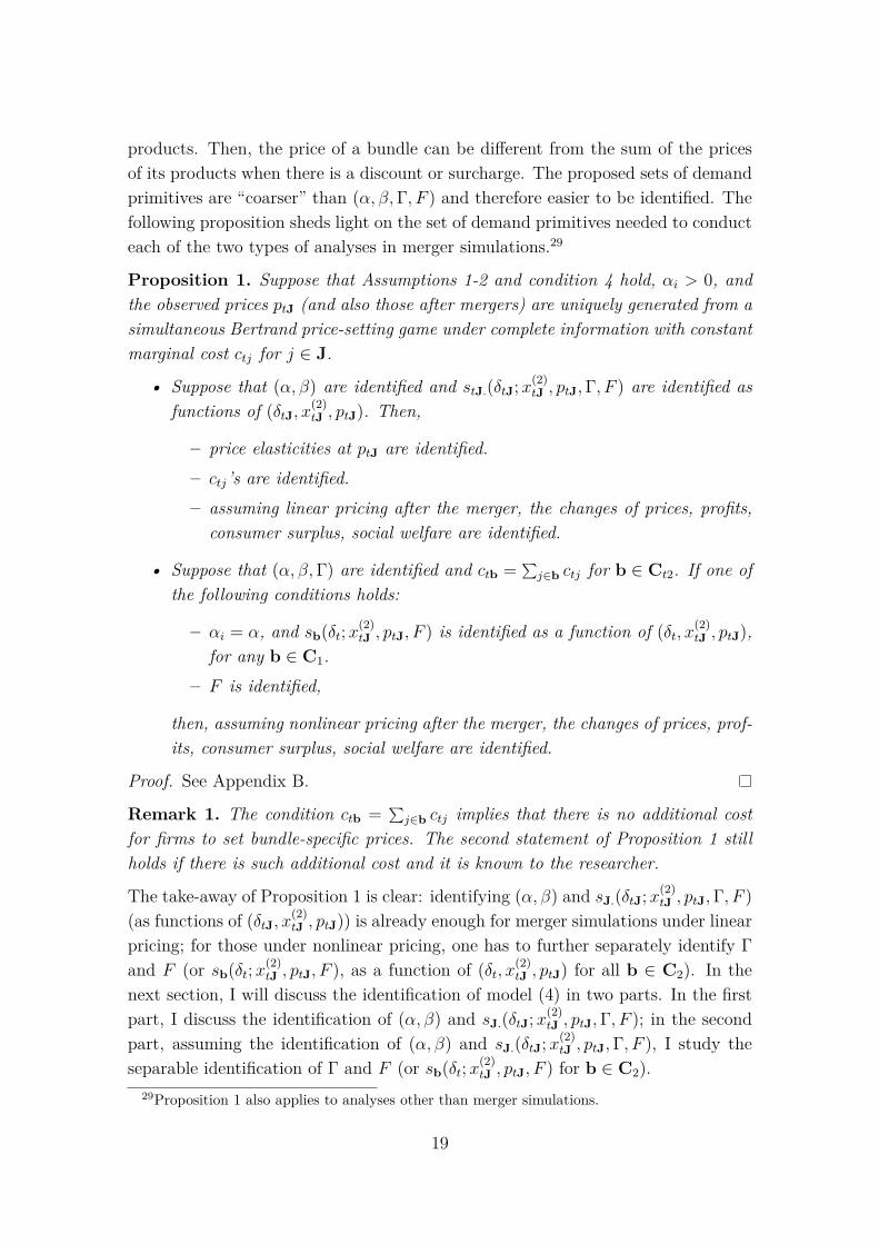
products. Then, the price of a bundle can be different from the sum of the pricesof its products when there is a discount or surcharge. The proposed sets of demandprimitives are “coarser” than (α, β,Γ, F ) and therefore easier to be identified. Thefollowing proposition sheds light on the set of demand primitives needed to conducteach of the two types of analyses in merger simulations.29

Proposition 1. Suppose that Assumptions 1-2 and condition 4 hold, αi > 0, andthe observed prices ptJ (and also those after mergers) are uniquely generated from asimultaneous Bertrand price-setting game under complete information with constantmarginal cost ctj for j ∈ J.

• Suppose that (α, β) are identified and stJ.(δtJ;x(2)tJ , ptJ,Γ, F ) are identified as

functions of (δtJ, x(2)tJ , ptJ). Then,

– price elasticities at ptJ are identified.– ctj’s are identified.– assuming linear pricing after the merger, the changes of prices, profits,

consumer surplus, social welfare are identified.

• Suppose that (α, β,Γ) are identified and ctb = ∑j∈b ctj for b ∈ Ct2. If one of

the following conditions holds:

– αi = α, and sb(δt;x(2)tJ , ptJ, F ) is identified as a function of (δt, x(2)

tJ , ptJ),for any b ∈ C1.

– F is identified,

then, assuming nonlinear pricing after the merger, the changes of prices, prof-its, consumer surplus, social welfare are identified.

Proof. See Appendix B.

Remark 1. The condition ctb = ∑j∈b ctj implies that there is no additional cost

for firms to set bundle-specific prices. The second statement of Proposition 1 stillholds if there is such additional cost and it is known to the researcher.

The take-away of Proposition 1 is clear: identifying (α, β) and sJ.(δtJ;x(2)tJ , ptJ,Γ, F )

(as functions of (δtJ, x(2)tJ , ptJ)) is already enough for merger simulations under linear

pricing; for those under nonlinear pricing, one has to further separately identify Γand F (or sb(δt;x(2)

tJ , ptJ, F ), as a function of (δt, x(2)tJ , ptJ) for all b ∈ C2). In the

next section, I will discuss the identification of model (4) in two parts. In the firstpart, I discuss the identification of (α, β) and sJ.(δtJ;x(2)

tJ , ptJ,Γ, F ); in the secondpart, assuming the identification of (α, β) and sJ.(δtJ;x(2)

tJ , ptJ,Γ, F ), I study theseparable identification of Γ and F (or sb(δt;x(2)

tJ , ptJ, F ) for b ∈ C2).29Proposition 1 also applies to analyses other than merger simulations.

19

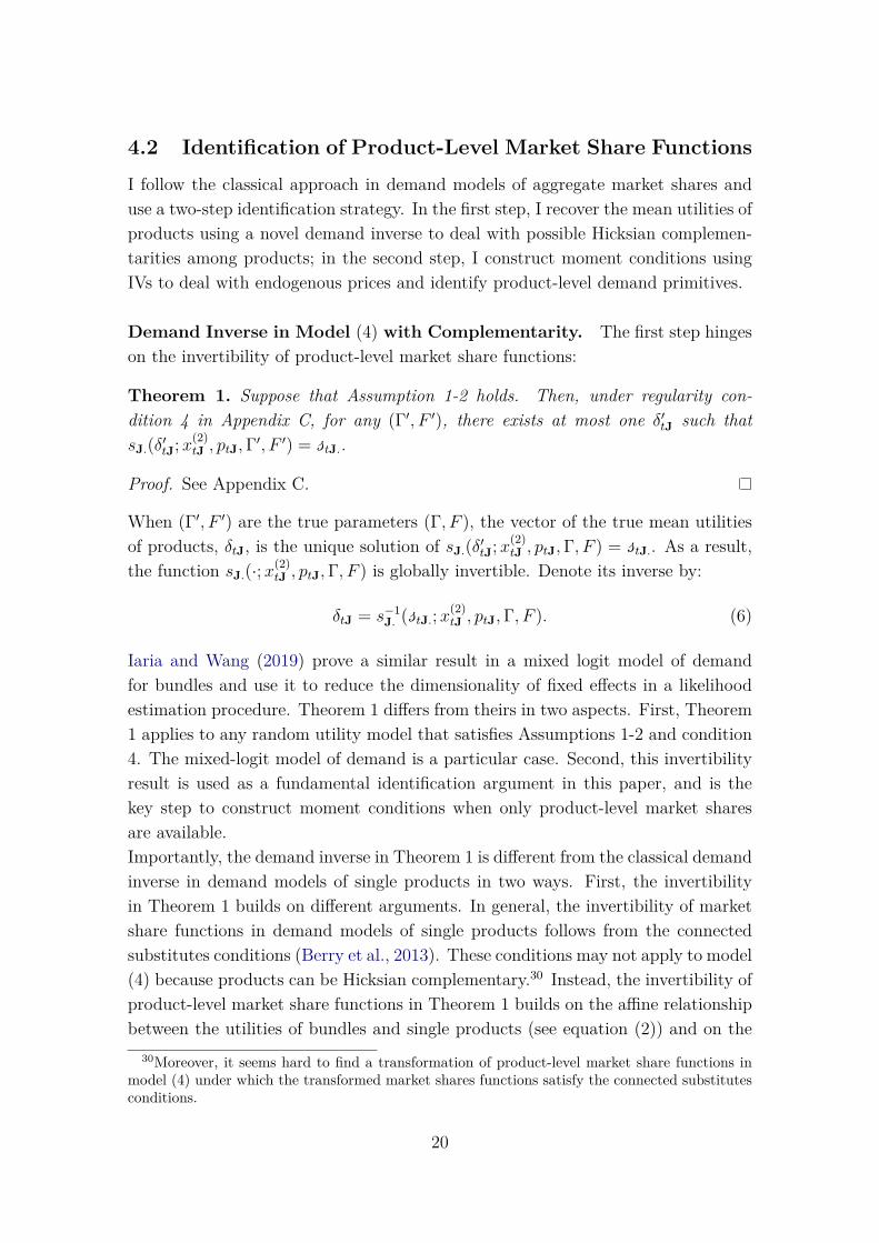
4.2 Identification of Product-Level Market Share Functions

I follow the classical approach in demand models of aggregate market shares anduse a two-step identification strategy. In the first step, I recover the mean utilities ofproducts using a novel demand inverse to deal with possible Hicksian complemen-tarities among products; in the second step, I construct moment conditions usingIVs to deal with endogenous prices and identify product-level demand primitives.

Demand Inverse in Model (4) with Complementarity. The first step hingeson the invertibility of product-level market share functions:

Theorem 1. Suppose that Assumption 1-2 holds. Then, under regularity con-dition 4 in Appendix C, for any (Γ′, F ′), there exists at most one δ′tJ such thatsJ.(δ′tJ;x(2)

tJ , ptJ,Γ′, F ′) = stJ..

Proof. See Appendix C.

When (Γ′, F ′) are the true parameters (Γ, F ), the vector of the true mean utilitiesof products, δtJ, is the unique solution of sJ.(δ′tJ;x(2)

tJ , ptJ,Γ, F ) = stJ.. As a result,the function sJ.(·;x(2)

tJ , ptJ,Γ, F ) is globally invertible. Denote its inverse by:

δtJ = s−1J. (stJ.;x(2)

tJ , ptJ,Γ, F ). (6)

Iaria and Wang (2019) prove a similar result in a mixed logit model of demandfor bundles and use it to reduce the dimensionality of fixed effects in a likelihoodestimation procedure. Theorem 1 differs from theirs in two aspects. First, Theorem1 applies to any random utility model that satisfies Assumptions 1-2 and condition4. The mixed-logit model of demand is a particular case. Second, this invertibilityresult is used as a fundamental identification argument in this paper, and is thekey step to construct moment conditions when only product-level market sharesare available.Importantly, the demand inverse in Theorem 1 is different from the classical demandinverse in demand models of single products in two ways. First, the invertibilityin Theorem 1 builds on different arguments. In general, the invertibility of marketshare functions in demand models of single products follows from the connectedsubstitutes conditions (Berry et al., 2013). These conditions may not apply to model(4) because products can be Hicksian complementary.30 Instead, the invertibility ofproduct-level market share functions in Theorem 1 builds on the affine relationshipbetween the utilities of bundles and single products (see equation (2)) and on the

30Moreover, it seems hard to find a transformation of product-level market share functions inmodel (4) under which the transformed market shares functions satisfy the connected substitutesconditions.

20

P-matrix property by Gale and Nikaido (1965), which-crucially-does not requirethe products to be Hicksian substitutes. Second, the demand inverse in Theorem 1may not be implemented by the fixed-point contraction mapping algorithm proposedby Berry et al. (1995). This is because the contraction mapping property of thealgorithm may not hold when (some) products are Hicksian complementary in model(4). I propose to use Jacobian-based algorithms to implement this demand inverse.31

See section 5.2 for details of the implementation.When (Γ′, F ′) 6= (Γ, F ), it is possible that there is no δ′tJ such that sJ.(δ′tJ;x(2)

tJ , ptJ,Γ′, F ′) =stJ..32 In this case, such (Γ′, F ′) are directly ruled out of the identification set of(Γ, F ). The following identification discussion will restrict to (Γ′, F ′) such that δ′tJexists.

Instrumental Variable Approach. Combining equation (6) and δtJ = xtJβ −αptJ + ξtJ, I obtain:

xtJβ − αptJ + ξtJ = s−1J. (stJ.;x(2)

tJ , ptJ,Γ, F ). (7)

The source of price endogeneity is ξtJ: ξtJ are observed to firms and therefore ptJ areset based on ξtJ. Consequently, ptJ and ξtJ are correlated, while ξtJ are not observedto the researcher. Beyond the price endogeneity, Γ and F constitute parametersthat cannot be pinned down without further assumption. I use IVs to solve thesechallenges:

Assumption 3. There are random variables ztJ = (ztj)j∈J, such that E[ξtJ|ztJ, xtJ] =0 almost everywhere.

Assumption 3 gives rise to conditional moment restrictions:

E [ξj(β, α,Γ, F ; stJ., xtJ, ptJ)|ztJ, xtJ] = 0 a.e., (8)

for j ∈ J, where ξj(β, α, η,Γ, F ; stJ., xtJ, ptJ) = s−1j (stJ.;x(2)

tJ , ptJ,Γ, F )−xtjβ+αptj.

The identification of sJ.(δtJ;x(2)tJ , ptJ,Γ, F ) (or equivalently its inverse s−1

J. (stJ.;x(2)tJ , ptJ,Γ, F ))

by moment conditions (8) can follow from general arguments in nonlinear modelsusing IVs. In demand models of single products, one can leverage completeness con-ditions of the joint distribution of (ztJ, xtJ, stJ., ptJ) with respect to (stJ., ptJ) (Berryand Haile, 2014). Intuitively, this requires sufficiently rich variation in (ztJ, xtJ)

31Conlon and Gortmaker (2020) provide a review of numerical methods for implementation ofdemand inverse in demand models of single products.

32For example, if the DGP is such that the sum of observed product-level market shares is largerthan one, then any demand models of single products (Γb = −∞ for any b) cannot rationalise theobserved product-level market shares and hence the demand inverse is not feasible with Γ′ = −∞.

21

that can distinguish any function of the endogenous variables (stJ., ptJ) from oth-ers. In the context of (8), the same general arguments also apply. One needsvariation in (ztJ, xtJ) to distinguish ξJ(β, α,Γ, F ; · · · ) from ξJ(β′, α′,Γ′, F ′; · · · ) forany (β′, α′,Γ′, F ′) 6= (β, α,Γ, F ). As long as such variation is available, having de-mand synergy parameters Γ does not conceptually introduce additional difficultyfor identification.

Despite the generality, these arguments and required conditions are often high-level. In what follows, I propose low-level sufficient conditions for the identificationof product-level market share functions in the case of mixed-logit models of demandfor bundles. In the following, I will focus on cost-type variables.33 In Appendix L,I propose similar sufficient conditions for other commonly used instruments (e.g.BLP-type instruments, exogenous product characteristics).

Denote by D(1)x the support of x(1)

tJ and by D(2)x the support of x(2)

tJ . Moreover,both D(1)

x and D(2)x open. Suppose that the ownership of each product is the same

across markets and that prices are generated from a simultaneous Bertrand pricinggame under complete information with constant marginal cost ctj, for j ∈ J. With-out loss of generality, I specify ctj = ztj + wtj, where ztj is cost shifter for productj and wtj is exogenous supply shock that is observed to firms but not observedto the researcher. The main identification result of the product-level market sharefunctions is the following:

Theorem 2. Suppose that Assumptions 1-3 and regularity condition 1 in AppendixD holds. Moreover, the following conditions hold:

1. (xtJ, ztJ) is independent of (ξtJ, wtJ), the support of ztJ is RJ .

2. αi = α > 0

3. Given x(2)tJ , ptJ = pJ(βxtJ + ξtJ, ctJ;x(2)

tJ ) is a continuous function of (βxtJ +ξtJ, ctJ).

4. F has compact support.

Then,

• If (ξtJ, wtJ) is Gaussian distributed, then (α, β) is identified and sJ.(δJ;x(2)J , pJ,Γ, F )

are identified as functions of (δJ, x(2)J , pJ) ∈ RJ ×D(2)

x × RJ .

• If the DGP is a model of demand for multiple products across categories (seesection 3.1), then under regularity condition 2 in Appendix D, (α, β) are iden-tified and sJ.(δJ;x(2)

J , pJ,Γ, F ) are identified as functions of (δJ, x(2)J , pJ) ∈

RJ ×D(2)x × RJ .

33Common examples of cost-type variables and its proxies are input prices, variables correlatedwith marginal costs, prices of the same products in other markets (e.g. Hausman-type instru-ments).

22

Remark 2. The two statements of Theorem 2 are complementary: the first state-ment achieves the identification by restricting the distribution of demand and supplyshocks and remains agnostic on the DGP.34 The second statement restricts the DGPand does not posit on the distribution of (ξtJ, wtJ).

Proof. See Appendix D.

The first condition reinforces Assumption 3 to strong exogeneity of (xtJ, ztJ) andassumes large support of ztJ. The second condition simplifies the price coefficient tobe homogeneous for all individuals but still allows for random coefficients on otherproduct characteristics. The third condition imposes the uniqueness of the Bertrandprice competition in the factual scenario. The fourth condition is technical and canbe further relaxed to allow for “thin tail” distributions F .

Relying on the same data availability, the main result of Allen and Rehbeck(2019a) implies the identification of product-level market share functions in thecontext of model (4) with additive separable unobservable heterogeneity. Whiletheir identification strategy crucially relies on the assumption of additively separa-ble unobservable heterogeneity and does not allow for endogenous prices, I exploitexogenous variation in cost shifters and product characteristics to deal with endoge-nous prices and market shares, achieving the identification of product-level marketshare functions.

4.3 Identification of Bundle-Level Market Share Functions

In this section, I assume that product-level market share functions are identifiedand aim to separately identify Γ and F .35 To simplify the notation, I include ptJin x

(2)tj . The task of separable identification s challenging because only product-

level (rather than bundle-level) market shares are available. First,I provide anidentification result for a class of mixed-logit models of demand for bundles widelyused in the empirical literature.36

Theorem 3. Suppose that C2 = (j, j′) : j < j′, j, j′ ∈ J, or C2 = (j1, j2) :j1 ∈ J1, j2 ∈ J2, Γitb = Γb for b ∈ C2, and sJ.(δJ;x(2)

tJ ,Γ, F ) is identified for(δJ, x

(2)tJ ) ∈ RJ ×D(2)

x . Then,

• Γ and sb(δt;x(2)tJ , F ) are identified in RC1 ×D(2)

x , for any b ∈ C1.34The identification in Theorem 2 can also be achieved when the distribution of (ξtJ, wtJ) has

“fat tail”. See Mattner (1992) and D’Haultfoeuille (2011) for details.35As shown in the second statement of Proposition 1, one can also aim to identify Γ and

sb(δt;x(2)tJ , ptJ, F ) when αi = α.

36See Gentzkow (2007), Fan (2013), Kwak et al. (2015), Grzybowski and Verboven (2016).

23

• If D(2)x is open, and (∆β(2)

i ,∆αi) and (ηij)Jj are mutually independent givenxtJ, then Γ and F are identified.

Proof. See Appendix E.

Remark 3. If for some bundle b, the true Γb is equal to −∞, i.e. bundle b is notin the choice set, then Theorem 3 implies that Γb = −∞ is identified.

The first statement of Theorem 3 achieves the separable identification of Γ andsb(δt;x(2)

tJ , F ). The second statement achieves the separable identification Γ and Funder a mild support on x

(2)tJ and the conditional independence between random

slopes (∆β(2)i ,∆αi) and random intercepts (ηij)Jj=1. This independence condition is

employed in many empirical papers.37

Theorem 3 shows that observing demand data at product level already suffices toidentify bundle-level demand primitives in models of demand for multiple productswithin/across categories. Consequently, researchers are able to conduct nonlinearpricing counterfactuals using these models (see Proposition 1). However, the sepa-rable identification in Theorem 3 may not be achieved in some other types of model(4). The following corollary gives an example.

Corollary 1 (Non-separable identification of Γ and F ). Suppose that the datagenerating process is a model of demand for multiple units: J = 1 and C2 =(1, 1), Γi(1,1) = Γ > −∞. Moreover, product-level market share function

s1.(δ; Γ, F ) =∫ eδ+µ + 2e2δ+2µ+Γ

1 + eδ+µ + e2δ+2µ+ΓdF (µ). (9)

is identified. Then, there exists (Γ, F ), such that Γ and F are not separably identi-fied.

Proof. See Appendix F.

Corollary 1 illustrates the limited power of product-level market shares in modelsof demand for multiple units to separably identify Γ and F . Intuitively, one cannotdistinguish Γ and F because it is impossible to shift the mean utility of the firstunit without shifting that of the second unit. When bundle-level demand datais available, Iaria and Wang (2019) shows how to identify and estimate model ofdemand for bundles by exploring the same bundle-specific fixed effects Γb acrossmarkets. This gives rise to additional moment restrictions that separately identify

37In particular, when the random intercepts are degenerated (see Nevo (2000, 2001), Petrin(2002), Berto Villas-Boas (2007), Fan (2013) among many others), or the random coefficients(rather than the random intercepts) are degenerated (see Gentzkow (2007) for example), thiscondition is automatically satisfied.

24

Γ and F . With only product-level demand data, this source of identification is nolonger available in model (9). Then, unless imposing additional assumptions onsynergy parameters or the distribution of random coefficients, the availability ofbundle-level demand data may be necessary to disentangle Γ and F and to conductnonlinear pricing counterfactuals in models of demand for multiple units.38

5 Estimation and ImplementationIn this section, I propose a GMM estimation procedure for model (4) and discussits implementation. The proposed estimation procedure is conceptually similar tothat used in BLP models of single products. However, due to multiple purchases,the implementation has non-trivial challenges. I consider parametric estimation ofmodel (4) and F is characterised by Σ ∈ ΘΣ ⊂ RP . Define the true value of pa-rameter vector as θ0 = (α0, β0,Σ0,Γ0). Suppose that (xtJ, ztJ) are valid instrumentsand θ0 is identified.

5.1 Estimation Procedure

I construct unconditional moment conditions from (D.1) using a finite set of func-tions of (xtJ, ztJ), Ψ = φg(xtJ, ztJ)Gg=1:

m(θ′; stJ., ptJ, xtJ, ztJTt=1,Ψ) = (E [ξj(β′, α′,Γ′, F ′; stJ., xtJ, ptJ)φg(ztJ, xtJ)])Gg=1 ,

The finite-sample counterparts are:

mT (θ′; stJ., ptJ, xtJ, ztJTt=1,Ψ) = 1T

T∑t=1

1J

J∑j=1

[s−1j (stJ.;x(2)

tJ , ptJ,Γ′,Σ′)− xtjβ′ + α′ptj]φg(xtj, ztj)

Gg=1

.

Then, the GMM estimator of θ0, θGMMT , is defined as:

θGMMT = argmin

θ′∈ΘmT (θ′; stJ., ptJ, xtJ, ztJTt=1,Ψ)TWTmT (θ′; stJ., ptJ, xtJ, ztJTt=1,Ψ),

(10)where Θ is a compact set and WT ∈ RG×G is a weighting matrix that convergesin probability to a positive-definite matrix W . If θ0 lies in the interior of Θ, thenunder standard regularity conditions (see Newey and McFadden (1994)), θGMM

T isconsistent and asymptotically normal.39

38For other papers on the identification with bundle-level demand data, see Fox and Lazzati(2017), Allen and Rehbeck (2019b).

39If some parameters (e.g. distributional parameters Σ) are on the boundary, the GMM estima-tor may not be asymptotically normal. See Ketz (2019) for an inference procedure that is validwhen distributional parameters are on the boundary and Andrews (2002) for a general treatment.

25

A basic requirement for the good finite-sample performance of (10) is that wehave at least as many moment conditions as the dimension of (α0, β0,Γ0,Σ0). Inparticular, we have dim(Γ0) demand synergy parameters in (10) that BLP modelsof single products do not have. Therefore, we need at least dim(Γ0) more momentconditions. If the number of valid instruments or variability of these instrumentsis limited, one can also specify Γ0 and reduce its dimensionality according to theeconomic setting. For example, two products of the same producer (products ofthe same store), or of complementary ingredients (flavoured RTE cereals with un-flavoured milk), may have greater demand synergies. Then, one can specify demandsynergy as a function of product characteristics in a bundle.

In BLP models of single products, a suggested practice is to approximate theoptimal instruments in the form of Amemiya (1977) and Chamberlain (1987) thatachieve the semi-parametric efficiency bound. Reynaert and Verboven (2014) andConlon and Gortmaker (2020) report significant gain when impelenting Berry et al.(1995)’s GMM estimator using optimal instruments. However, the difficulty ofapproximating optimal instruments still remains in estimation procedure (10). Agood approximation of optimal instruments relies on the knowledge of the trueparameters. Moreover, when the number of products is large, even low order of suchapproximation may be subject to a curse of dimensionality and the number of neededbasis functions is exponentially proportional to the number of products. Gandhi andHoude (2019) provide a solution that breaks the dependence of basis functions onproduct identity under symmetry conditions among products. The number of basisfunctions is then invariant with respect to the number of products. However, dueto potentially heterogeneous synergy parameters across bundles, product identitymatters in (10). The extension of their method to models of demand for bundles isbeyond the scope of this paper and I leave it as future research.

5.2 Implementation of Demand Inverse

A key step of the estimation procedure is implementation of the demand inversein Theorem 1. Given (x(2)

tJ , ptJ,Γ′, F ′), it seeks for the solution of the followingequation:

sJ.(δ′tJ;x(2)tJ , ptJ,Γ′, F ′)− stJ. = 0. (11)

In most cases, sJ.(·;x(2)tJ , ptJ,Γ′, F ′) does not have an analytic form. In practice,

researchers often use Monte Carlo method to approximate sJ.(·;x(2)tJ , ptJ,Γ′, F ′). In

this method, one first draws a finite set of random numbers and then use these fixedrandom numbers to approximate F ′.40 As a result, F ′ is numerically implemented

40A typical method is to simulate a fixed set of random numbers from uniform distribution in[0, 1] and use (F ′)−1 to transform these random numbers to those under distribution F ′.

26

by a discrete distribution with finite (and therefore compact) support. For thisreason, I will assume that F ′ has compact support when analysing the numericalperformance of the implementation of the demand inverse (11).

In models of demand for single products, Berry et al. (1995) propose a fixed-pointiterative algorithm to implement the demand inverse. An essential property of thisalgorithm is contraction mapping, which guarantees the convergence of the iteration.However, the contraction-mapping property may not hold if one uses the sameiterative algorithm to solve (11) because products can be Hicksian complementary.To solve this challenge, I propose to use Jacobian-based approach to solve (11).This approach has been adopted in the literature. Conlon and Gortmaker (2020)tests performances of different Jacobian-based algorithms to implement the demandinverse in models demand for single products, and find supportive evidences for thenumerical efficiency of Jacobian-based methods. A leading example is Newton-Raphson method:

δ(0) = δ(0),

δ(n+1) = δ(n) − J−1s (δ(n))[sJ.(δ′tJ;x(2)

tJ , ptJ,Γ′, F ′)− stJ.],(12)

where Js(δ′tJ) = ∂sJ.(δ′tJ;x(2)tJ ,ptJ,Γ

′,F ′)∂δ′tJ

. To solve (11), Algorithm (12) is well-defined be-cause Js(δ′tJ) is everywhere symmetric and positive-definite. Moreover, the unique-ness of solution is guaranteed by Theorem 1: if (12) converges, then it must convergeto the unique solution of (11).

It is well-known that the numerical performance of Jacobian-based algorithmssuch as (12) crucially depends on the quality of starting value δ(0) : the closer δ(0)

is to the solution δ′tJ, the faster Algorithm (12) converges.41 In the setting of (11),we can leverage econometric properties of the demand model to construct such astarting value that is directly constructed from data and “close” to the solution of(11). The next proposition gives an example:

Proposition 2. Suppose that stJ. in (11) are generated from a model of demandfor multiple products across K categories, for K ≥ 1 (see Section 3.1) and thedistribution F ′ has compact support DF . Denote the solution to (11) by δ′J. Forproducts of category k, define δ(0)

k∗ =(δ

(0)jk∗

)j∈Jk

, where δ(0)jk∗ = ln stj.

1−∑

j∈Jkstj.

, and

δ(0)∗ = (δ(0)

k∗ )Kk=1. Then, there exists a constant A(DF ,Γ′) > 0 such that

|δ′J − δ(0)∗ | ≤ A(DF ,Γ′).

Proof. See Appendix G.41One basic result on global convergence of Newton-Raphson method in numerical analysis is

Newton-Kantorovich Theorem. See Ortega (1968) for the statement and one proof.

27

Even though it is hard to derive similar results in a general model (4), Proposition2 sheds light on how to find a good starting value for Jacobian-based algorithms:it suggests to use a starting point as if the DGP is a multinomial logit model. In amodel with the bundle size being up to size K, an starting value along the lines ofProposition 2 can be defined as

δ(0)j∗ = ln sj.

K −∑j∈J sj.. (13)

for j ∈ J. Here K −∑j∈J sj. serves as the “market share” of the outside option.42

In Appendix K, I report numerical gains of using δ(0)∗ in Monte Carlo simulations.

6 Empirical IllustrationIn this section, I illustrate the practical implementation of the proposed methodsand estimate the demand for Ready-To-Eat (RTE) cereals and milk in the US.In particular, I demonstrate the economic importance of having (flexible) demansynergies between RTE cereal and milk products in demand.

To do so, I first estimate three models of demand for bundles: model I in whichdemand synergy parameters Γb = 0 for all b, model II in which Γb = γ0 for any bbut not necessarily zero (it will be estimated), and a full model in which Γb’s varyacross bundles as functions of product characteristics in the bundle. In model I,the demand for RTE cereals and that for milk are restricted to be independent foreach household (the cross-price elasticities between RTE cereals and milk are hencezero); in model II, the single synergy parameter γ0 captures the prevalent synergyin consumption of RTE cereals and milk, but not the potential heterogeneity insynergies across different bundles; the full model allows such synergies to dependon the composition of a bundle, i.e. how well RTE cereal and milk characteristicsare matched. I simulate a merger between a major RTE cereal producer and amilk producer using each model. Comparisons of the merger simulations across thethree models show that ignoring the synergies (model I), or restricting them to beuniform (model II) may result in important bias in welfare prediction.

6.1 Data and Definitions

I use the store-week level datasets of the RTE cereal and milk categories from theIRI data. The IRI data has been used in the empirical literature of demand (see

42When the bundle size is up to K, since product-level market shares of two different productsoverlap on up to K − 1 bundle-level market shares. Consequently, the sum of all product-levelmarket shares is strictly smaller than K.

28

Nevo (2000, 2001)). I will give a succinct description and refer to these papers andalso Bronnenberg et al. (2008) for a thorough discussion.

I focus on the period 2008-2011 and the city of Pittsfield in the US. I definea market t as a combination of store and week and obtain 1387 markets. In eachmarket, the sales (in lbs and dollars) of RTE cereals and fluid milk are observedat Universal Product Code (UPC) level. For the RTE cereal category, similarly toNevo (2001), I define a product as a combination of brand, flavour, fortification,and type of grain. For fluid milk category, I define a product as a combinationof brand, flavour, fortification, fat content, and type of milk. Then, the sales ofproduct j of category k ∈ K = RTE cereal, f luid milk in market t is the sumof the sales in lbs of all the UPC’s that this product collects. The price of j ofcategory k in market t, pktj, is defined as the ratio between its sales in dollars andin lbs. I define the choice set of RTE cereals as that of the 25 largest RTE cerealproducts (in terms of sales in lbs), collecting all the other smaller products in theoutside option for cereal category. Similarly, I define the choice set of milk as thatof the 20 largest fluid milk products.43 Denote the choice set by Jk for k ∈ K.

For each market, I consider the weekly consumption of breakfast cereals as themarket size for RTE cereal category, and weekly consumption of fluid milk for milkcategory. To calibrate the market size for each category, I assume that householdsgo shopping once per week for breakfast cereals and fluid milk. Then, the marketsize for RTE cereal category (or milk) is the product of the weekly per capitaconsumption of breakfast cereals (or fluid milk) and the sampled population size.I obtain the former information from external sources and the latter from the IRIdata. Finally, for each market, the product-level market share of j ∈ Jk is then theratio between its total sales in lbs and the market size for category k. AppendixH provides computational details of the construction of the product-level marketshares. Tables 9-10 in Appendix I summarise product characteristics.

6.2 Model Specification

For each store-week combination t, denote the set of available products in categoryk ∈ K by Jtk ⊂ Jk. Denote by 1 the RTE cereal category, 2 the milk category, andJt = Jt1 ∪ Jt2. The set of bundles Ct2 is defined as Jt1 × Jt2, where each bundlecontains a RTE cereal product and a milk product.44 Household’s choice set is thendefined as Ct = Jt ∪ Ct2 ∪ 0, where 0 represents the outside option.45 The size

43The purchase of the 25 RTE cereal products represents 38% of the total purchase of RTEcereals in the IRI data, and that of the 20 fluid milk represents around 88%.

44I do not include bundles of products of the same category.45According to the definition of products and the market sizes, the outside option collects RTE

cereals or milk products that are not included in Jk, relevant products not present in the categories(e.g. cereal biscuits), and the bundles of these products (e.g. cereal biscuits and milk).

29

of Ct is up to 546 (45 products, 500 bundles, 1 outside option) if all products in Jare available in market t.For household i in market t, the indirect utility from purchasing product j ∈ Jtk is:

Ukitj = −pktjαi + ηkij + ξktj + εkitj

= [−pktjα + ηkj + ξktj] + [∆ηkij −∆αipktj] + εkitj

= δktj + µkitj + εkitj,

µkitj = ∆ηkij − (di∆α + vi)pktj,

and

∆ηkij =

∆ηi,flavor(j) + ∆ηi,fortification(j) + ∆η1i,brand(j), if k = 1,

∆ηi,flavor(j) + ∆ηi,fortification(j) + ∆η2i,brand(j) + ∆η2

i,fat content(j), if k = 2,

where δktj is market t-specific mean utility for j ∈ Jtk, µkitj is a household i-specificutility deviation from δktj, and εkitj is an idiosyncratic error term. α is population-average price coefficient, and ∆αi = di∆α + vi is household i-specific price co-efficient deviation from α and is the sum of an observed part that is a functionof the household characteristics di (income groups) and an unobserved compo-nent vi. ∆ηkij is an unobserved household i-specific preference for product j ofcategory k, where ∆ηi,flavor(j) captures household i’s unobserved preference for theflavour of j of category k (unflavoured, flavoured), ∆ηi,fortification(j) captures i’s unob-served preference for the nutrition in product j of category k (unfortified, fortified),∆ηki,brand(j) captures i’s unobserved preference for the brand of j of category k,and ∆η2

i,fat content(j) captures i’s unobserved preference for the fat content in milk j(whole fat, low fat, skimmed). Note that because RTE cereals and milk have bothflavour and fortification characteristics. Then, for products j ∈ J1 and r ∈ J2, ifthey have the same flavour (or fortification type), then ∆ηi,flavor(j) = ∆ηi,flavor(r) (or∆ηi,fortification(j) = ∆ηi,fortification(r)).The indirect utility of household i in market t from purchasing bundle b = (j, r) is:

Uitb =[−p1

tjαi + η1ij + ξ1

tj

]+[−p2

trαi + η2ir + ξ2

tr

]+ Γb + εitb

=[δ1tj + δ2

tr + Γb]

+[µ1itj + µ2

itr

]+ εitb

= δtb(Γb) + µitb + εitb,

where δtb(Γb) = δ1tj + δ2

tr + Γb is market t-specific mean utility for bundle b, µitbis household i-specific utility deviation from δtb, Γb = Γ(j,r) is demand synergybetween RTE cereal j and milk r, and εitb is an idiosyncratic error term. Demandsynergy parameter Γ(j,r) captures the extra utility household obtains from buying

30

RTE cereal j and milk r jointly rather than separately. One prominent reasonfor the joint purchase is synergy in consumption, i.e. members in the householdconsume together RTE cereals and milk for their breakfasts.46 The quality of matchbetween the characteristics of RTE cereal j and milk r may determines the extrautility Γ(j,r). Consequently, I specify Γ(j,r) as a function of the characteristics of jand r:

Γ(j,r)(γ) = γ0 + 1j is multi-grainγ1 + 1j is granolaγ2

+ 1r is skimmedγ3 + 1r is low fatγ4

+ 1j is flavouredγ5 + 1r is chocolate milkγ6

+ 1j is flavored and r is chocolate milkγ7

+ 1j is fortified, r is chocolate milkγ8 + 1j is fortified, r is fortifiedγ9.

(14)Parameter γ0 represents the synergy in consumption of the reference bundle (un-flavoured unfortified uni-grain RTE cereal and unflavoured whole-fat milk).γ1 andγ2 quantify additional synergies due to other types of grains (multi-grain, granola).γ3 and γ4 measures additional synergies due to lower fat content (skimmed, lowfat). γ5, γ6 and γ7 proxy additional synergies due to flavour combinations. γ8 andγ9 quantify additional synergies due to combinations of fortified nutrition in RTEcereals and milk products.

Finally, the indirect utility of household i in market t from purchasing the outsideoption is normalised to be Uit0 = εit0. Denote the random coefficients by

θit = (vi,∆ηi,unflavoured,∆ηi,flavoured,∆ηi,unfortified,∆ηi,fortified,∆η1

i,br.br.∈B1 , ∆η2i,br.br.∈B2 ,∆η2

i,whole fat,∆η2i,low fat,∆η2

i,skimmed),

where Bk denotes the set of brands in category k. I assume that θit follows acentred Gaussian distribution F and the components are uncorrelated. Note thatthis specification already allows for unobserved correlation among products of thesame characteristics within and across categories (e.g. same flavour). Define δtJt =(δ1tJt1 , δ

2tJt2) and ptJt = (p1

tJt1 , p2tJt2). Write µkitj = µktj(di, θit, pktj). Finally, assume

that εit0, ε1itj’s, ε2

itj’s, and εitb’s are i.i.d. Gumbel. Then, the product-level market46Another reason can be shopping cost, i.e. household may not want to go shopping twice to

buy RTE cereals and milk. However, this is ruled out in this application because the purchasesare made within the same store.

31

share function of j ∈ Jt1 in market t is:

sj.|Jt(δtJt ; ptJt , γ, F )

=∫ eδ

1tj+µ

1tj(di,θit,p

1tj)[1 + ∑

r∈Jt2eδ

2tr+µ2

tr(di,θit,p2tr)+Γ(j,r)(γ)

]1 + ∑∑

k=1,2 j′∈Jtkeδktj′+µ

ktj′ (di,θit,p

ktj′ ) + ∑

(j′,r)∈Jt1×Jt2eδ1tj′+δ

2tr+µ1

tj′ (di,θit,p1tj′ )+µ

2tr(di,θit,p2

tr)+Γ(j′,r)(γ)dF (θit)dΠt(di),

(15)where Πt(·) is the distribution function of demographics di in market t. The formulafor r ∈ Jt2 is similar.

6.3 Demand Estimates

Table 3 summarises demand estimates. In column “IV regression”, I estimate amultinomial logit with Γb = 0 for all b ∈ C2. Columns “Model I”, “Model II”, and“Full Model” show the estimates by using model I, model II, and the full model,respectively. In all the models, I control for product-specific intercepts and usethe same Hausman-type instruments. These instruments include prices of the sameproducts in the same store and week but in other cities (Boston for RTE cerealsand Hartford for milk), the prices of other products of the same category with thesame product characteristics.

Price coefficient (α) is estimated −0.59 in the multinomial logit model. Theestimates of the other three models with random coefficients show important het-erogeneity in price sensitivities across income groups. Without surprise, householdswith higher income are estimated to have a lower (in absolute value) price coef-ficient and therefore less sensitive to price change. The standard variance of theunobserved heterogeneity in the price coefficient (σv) is estimated small. Moreover,after controlling for the product-specific intercepts, households’ preference seems tobe almost homogeneous for products within some types (e.g. unflavoured, fortifi-cation, fat content). One potential reason is that products are little differentiatedwithin each of these types. In contrast, households’ preference for flavoured prod-ucts seems to be more heterogeneous. This is also intuitive because flavours of RTEcereals and milk are much more horizontally differentiated and different householdsmay have their favourite flavours. I also find that households’ preference for RTEcereal brands is more heterogeneous than that for milk brands.

In model II, synergy parameter γ0 is estimated to be 0.902 and significant.This specification constraints all bundles of RTE cereal and milk to have the samesynergy, regardless of their characteristics. In the full model, the demand synergiesare allowed to vary across bundles. In column “Full Model”, γ0 = −1.540 representsthe synergy in consumption between the unflavoured unfortified uni-grain RTEcereal and unflavoured whole-fat milk. Regarding the characteristics of RTE cereals,

32

γ1 is estimated positive, meaning that multi-grain cereals are preferred (over uni-grain ones) when consumed with milk. Moreover, granola, which contains oats andother whole grains as well as ingredients such as dried fruit and nuts, is estimated tobe even preferred over multi-grain cereals (γ2 > γ1). For the characteristics of milk,products with lower fat are estimated to be preferred when consumed with cereals(γ3 > γ4 > 0). Another interesting finding is households’ preference for flavourcombinations of cereals and milk. Flavoured cereals are estimated to be preferredover unflavoured ones (γ5 > 0). For chocolate milk, households’ preference seems tobe more complicated. When consumed with unflavoured cereals, chocolate milk ispreferred over unflavoured milk (γ6 > 0). While, I find that it is seldom consumedwith flavoured or fortified cereals, i.e. γ7 and γ8 are estimated very negative.47 Onepotential reason is that flavoured (or fortified) RTE cereals are more likely frosted.Very negative γ7 and γ8 may reflect households’ disutility for bundles with too muchsugar. Finally, I also find that bundles of fortified cereals and milk are less appealingthan the reference one (γ9 < 0). In the data, the types of added nutrition in RTEcereals and milk are the same, e.g. vitamins, calcium. γ9 < 0 may reflect that thesame types of added nutrition in cereals and milk are substitute.

6.4 Price Elasticities

I compute the average (across markets) estimated self- and cross-price elasticitiesobtained from the full model. Because there is no income effect in the specifi-cation, negative (positive) cross-price elasticities are then interpreted as Hicksiancomplementarity (substitutability). To facilitate the exposition, I report the priceelasticities at the level of product characteristics and producers. This illustrateshow RTE cereals and milk are complementary along each of these dimensions. Theresults are illustrated in Tables 4-7. Each entry reports the percent change in thesum of the product-level market shares of the products collected by the row pro-ducer (or characteristics) with respect to a 1% increase in the prices of the productscollected by the column producer (or characteristics).48

Overall, RTE cereals are estimated to have larger self-price elasticities than47In Table 3, the estimates of γ7 and γ8 are −∞. This means that the model with γ7, γ8 = −∞,

i.e. the corresponding bundles are not in the choice set, performs statistically as well as theone without these restrictions in terms of the value of GMM objective function. Concretely, Ifirst estimate a model with γ7 and γ8 being finite. I find that the estimated γ7 and γ8 are verynegative. Then, I estimate the model with γ7, γ8 = −∞. The difference in the value of the twoGMM objective functions is less than 10−9, or equivalently, one cannot reject the “hypothesis”that γ7, γ8 = −∞. In the future, I will consider a formal testing procedure.

48Concretely, denote by Cm the set of products that row (column) producerm represents. Then,

the price elasticity between brands m and n, Emn, is defined as Emn =∑

j∈Jmsj.

∑r∈Jn

εjr∑j∈Jm

sj., where

εjr is the price elasticity between products j and r.

33

milk. This may reflect that households view milk more necessary than RTE cerealsand therefore are less sensitive to price change of milk. Given the specificationof model (15), RTE cereals are always substitutes to each other and the cross-price elasticities among them are positive. Similarly, the cross-price elasticitiesamong milk products are also positive. These are shown by the positive off-diagonalelements in the diagonal blocks (RTE cereals-RTE cereals, Milk-Milk) of Tables 4-7.Differently, the cross-price elasticities between RTE cereal and milk products, i.e.the elements in the off-diagonal blocks (RTE cereals-Milk, Milk-RTE cereals), canbe either positive or negative.

Table 4 shows the substitution patterns along the dimensions of grain type andfat content. Granola is estimated to be complementary to milk with any level offat and skimmed milk is complementary to cereals with any kind of grain. More-over, milk with lower fat content is uniformly more complementary to any kindof grain than milk with higher fat content. This reveals that households do notseek for fat in milk when consuming it with RTE cereals. As to flavours (Tables5-6), unflavoured cereals and flavoured milk (and the reverse) are shown to be com-plementary. In contrast, flavoured cereals and chocolate milk are estimated to be(strong) substitutes. Coherent with the estimates of γ’s in Table 3, the relationshipbetween chocolate milk and RTE cereals is more complicated. Chocolate milk isestimated to be complementary to unflavoured or unfortified cereals. However, it isestimated to be substitute to flavoured or fortified cereals. Finally, I find that mostRTE cereals and milk are complementary at producer level.

As a comparison, the demand synergies in model I are constrained to be zero.The cross-price elasticities between RTE cereals and milk are therefore mechanicallyzero. In model II, all the bundles are restricted to have the same demand synergywhich is estimated to be positive (see the column “Model II” of Table 3). I re-dothe exercises in Tables 4-7 using the demand estimates from model II (see Tables11-14 of Appendix I). In contrast to those obtained from the full model, the resultsshow that RTE cereals and milk are complementary along every dimension.

34

Table 3: Demand Estimates

IV Regression Model I Model II Full ModelΓb = 0 Γb = 0 Γb = γ0

Price Coef.uniform, α −0.59

(0.011)

(baseline) low income, α1 −1.369(0.042)

−1.128(0.060)

−1.062(0.075)

medium income, ∆α2 0.218(0.164)

0.148(0.096)

0.164(0.0764)

high income, ∆α3 0.947(0.045)

0.718(0.029)

0.712(0.0269)

Random Coef.σv 0.115

(0.070)0.086(0.072)

0.046(0.1244)

σunflavoured 0.015(2.754)

0.018(1.490)

0.023(2.6772)

σflavoured 2.353(0.259)

1.684(0.038)

1.010(0.1615)

σunfortified 0.048(3.047)

0.004(3.870)

0.017(2.2994)

σfortified 0.010(5.393)

0.010(2.388)

0.015(6.8129)

σfat 0.077(1.099)

0.062(0.660)

0.034(1.6161)

σcereal brand 0.780(0.049)

0.660(0.058)

0.847(0.0705)

σmilk brand 0.005(6.156)

0.003(5.368)

0.004(6.9505)

Demand Synergiesγ0 0.902

(0.155)−1.540(0.3437)

multi-grain, γ1 0.533(0.0359)

granola, γ2 4.363(0.0891)

skimmed, γ3 2.880(0.2111)

low fat, γ4 0.514(0.1282)

flavoured cereal, γ5 1.816(0.2324)

chocolate milk, γ6 13.625(0.2621)

flavoured cereal and chocolate milk, γ7 −∞fortified cereal, chocolate milk, γ8 −∞

fortified cereal and milk, γ9 −1.538(0.3512)

GMM Objective Function 0.1636 0.1599 0.1434

Notes: Standard errors are reported in brackets. For all the models, instruments are thesame and product-specific intercepts are included. In the “IV Regression”, week dummiesand store dummies are also included.

35

Table 4: Average Estimated Own- and Cross-Price Elasticities (Full Model), GrainType and Fat Content

RTE cereals Milkuni-grain multi-grain granola skimmed low fat whole fat

RTE cereals, uni-grain −1.407(0.221)

0.194(0.049)

0.009(0.002)

−0.032(0.007)

0.007(0.003)

0.009(0.003)

multi-grain 0.266(0.063)

−1.492(0.221)

0.009(0.011)

−0.034(0.007)

0.001(0.003)

0.009(0.003)

granola 0.220(0.054)

0.168(0.182)

−1.335(0.207)

−0.084(0.015)

−0.071(0.011)

−0.005(0.006)

Milk, skimmed −0.350(0.068)

−0.243(0.051)

−0.053(0.010)

−0.252(0.043)

0.047(0.029)

0.023(0.013)

low fat 0.010(0.012)

−0.005(0.007)

−0.020(0.003)

0.018(0.012)

−0.262(0.040)

0.028(0.018)

whole fat 0.056(0.023)

0.045(0.018)

−0.005(0.004)

0.018(0.011)

0.054(0.036)

−0.307(0.055)

Notes: Each entry reports the percent change in the sum of the product-level market shares ofthe products collected by the row characteristics with respect to a 1% increase in the prices of theproducts collected by the column characteristics. Standard errors are reported in brackets andcomputed from a parametric bootstrap as in Nevo (2000, 2001) with 200 draws.

Table 5: Average Estimated Own- and Cross-Price Elasticities (FullModel), Flavours

RTE cereals Milkunflavoured flavoured unflavoured chocolate

RTE cereals, unflavoured −1.397(0.242)

0.190(0.062)

0.016(0.004)

−0.014(0.003)

flavoured 0.145(0.047)

−1.381(0.240)

−0.051(0.007)

0.003(0.001)

Milk, unflavoured 0.031(0.007)

−0.130(0.017)

−0.214(0.029)

0.001(0.001)

chocolate −1.319(0.273)

0.378(0.141)

0.071(0.049)

−0.264(0.045)

Notes: Each entry reports the percent change in the sum of the product-level mar-ket shares of the products collected by the row characteristics with respect to a 1%increase in the prices of the products collected by the column characteristics. Stan-dard errors are reported in brackets and computed from a parametric bootstrap asin Nevo (2000, 2001) with 200 draws.

36

Table 6: Average Estimated Own- and Cross-Price Elasticities (FullModel), Fortification and Flavours

RTE cereals Milkunfortified fortified unflavoured chocolate

RTE cereals, unfortified −1.263(0.261)

0.060(0.021)

−0.029(0.004)

−0.006(0.002)

fortified 0.393(0.132)

−1.668(0.349)

0.043(0.009)

0.002(0.000)

Milk, unflavoured −0.124(0.017)

0.025(0.006)

−0.214(0.029)

0.001(0.001)

chocolate −1.004(0.320)

0.063(0.007)

0.071(0.049)

−0.264(0.045)

Notes: Each entry reports the percent change in the sum of the product-levelmarket shares of the products collected by the row characteristics with respectto a 1% increase in the prices of the products collected by the column character-istics. Standard errors are reported in brackets and computed from a parametricbootstrap as in Nevo (2000, 2001) with 200 draws.

37

Table7:

AverageEs

timated

Own-

andCross-P

riceElastic

ities

(FullM

odel),Br

ands

RTE

cereals

Milk

Gen

eral

Mills

Kashi

Kellogg

’sPo

stPr

ivateLa

belGarelickFa

rmsGuida

sHighLa

wnFa

rmHoo

dPr

ivateLa

bel

RTE

cereals,

Gen

eral

Mills

−1.

444

(0.2

29)

0.00

9(0.0

03)

0.14

6(0.0

34)

0.03

7(0.0

09)

0.00

9(0.0

04)

−0.

007

(0.0

01)

−0.

034

(0.0

05)

−0.

005

(0.0

01)

−0.

004

(0.0

01)

−0.

022

(0.0

03)

Kashi

0.15

4(0.0

44)

−1.

678

(0.2

54)

0.15

2(0.1

76)

0.03

5(0.0

46)

0.01

1(0.0

23)

−0.

005

(0.0

01)

−0.

005

(0.0

01)

−0.

0003

(0.0

00)

−0.

0002

(0.0

00)

−0.

001

(0.0

02)

Kellogg

’s0.

152

(0.0

36)

0.01

0(0.0

12)−

1.42

4(0.2

12)

0.03

2(0.0

24)

0.00

9(0.0

12)

−0.

002

(0.0

01)

0.00

6(0.0

01)

−0.

0005

(0.0

00)

−0.

0003

(0.0

00)

0.00

2(0.0

01)

Post

0.17

3(0.0

43)

0.01

0(0.0

16)

0.14

6(0.1

28)−

1.54

1(0.2

10)

0.01

0(0.0

15)

−0.

005

(0.0

01)

−0.

013

(0.0

02)

−0.

002

(0.0

00)

−0.

001

(0.0

00)

−0.

009

(0.0

02)

PrivateLa

bel

0.17

5(0.0

69)

0.01

3(0.0

29)

0.16

3(0.1

78)

0.03

8(0.0

47)

−1.

335

(0.2

07)

−0.

044

(0.0

06)

.−

0.01

2(0.0

02)

−0.

011

(0.0

02)

−0.

094

(0.0

12)

Milk

,GarelickFa

rms

−0.

092

(0.0

14)

−0.

002

(0.0

01)−

0.01

8(0.0

07)−

0.01

4(0.0

03)

−0.

032

(0.0

05)

−0.

323

(0.0

79)

.0.

005

(0.0

07)

0.00

5(0.0

06)

0.05

4(0.0

46)

Guida

s−

0.04

4(0.0

06)

−0.

0003

(0.0

00)

0.00

04(0.0

01)−

0.00

4(0.0

01)

..

−0.

173

(0.0

24)

0.01

2(0.0

06)

0.00

2(0.0

01)

0.01

4(0.0

06)

HighLa

wnFa

rm−

0.10

9(0.0

16)

0.00

1(0.0

00)−

0.00

6(0.0

08)−

0.01

1(0.0

02)

−0.

020

(0.0

04)

0.01

5(0.0

17)

0.11

9(0.0

62)

−0.

479

(0.1

21)

0.00

4(0.0

06)

0.04

6(0.0

41)

Hoo

d−

0.15

4(0.0

23)

−0.

001

(0.0

01)−

0.03

2(0.0

11)−

0.01

8(0.0

04)

−0.

030

(0.0

07)

0.01

5(0.0

17)

0.11

4(0.0

60)

0.00

7(0.0

09)

−0.

497

(0.1

12)

0.04

5(0.0

40)

PrivateLa

bel

−0.

076

(0.0

11)

0.00

1(0.0

00)

0.01

1(0.0

06)−

0.00

7(0.0

01)

−0.

022

(0.0

03)

0.01

6(0.0

14)

0.12

3(0.0

56)

0.00

7(0.0

06)

0.00

5(0.0

04)

−0.

251

(0.0

45)

Not

es:Ea

chentryrepo

rtsthepe

rcentchan

gein

thesum

oftheprod

uct-levelm

arketshares

oftheprod

ucts

colle

cted

bytherow

prod

ucer

with

respectto

a1%

increase

intheprices

oftheprod

ucts

colle

cted

bythecolumnprod

ucer.Stan

dard

errors

arerepo

rted

inbrackets

andcompu

tedfrom

apa

rametric

bootstrapas

inNevo(2000,

2001)with

200draw

s.The

.refers

tothesit

uatio

nwhere

theprod

ucts

oftherow

andcolumnbran

dsareno

tavailableat

thesametim

ein

anymarketin

theda

ta.

38

6.5 Counterfactual Simulations

I simulate a merger between a major RTE cereal producer (General Mills) and a milkproducer (Garelick Farms). To do so, I assume constant market-product specificmarginal production costs and these marginal costs remain unchanged after themerger, i.e. there is no efficiency gain from the merger. Moreover, I assume that inboth factual and counterfactual scenarios producers play a simultaneous Bertrandprice-setting game with complete information and linear pricing strategies. Then,I can back out these marginal costs from the estimated demand and the observedprices by inverting the First-Order Conditions of the pricing game in the factualscenario. Finally, I simulate the merger using the estimated demand and marginalcosts. I replicate this merger simulation using the full model, model I (Γb = 0),and model II (Γb = γ0). Table 8 summarises the results.

Model I restricts all the demand synergies between RTE cereals and milk tobe zero. As a result, their cross-price elasticities are always zero and the mergerbetween General Mills and Garelick Farms will not lead to any change in pricesand consumer surplus (row “Model I” in Table 8). In contrast, both model IIand the full model allow for demand synergies and estimate that RTE cereals andmilk products exhibit substantial complementarity at the producer level (Tables7 and 14). The merged producer internalises the complementarity in the pricingand therefore reduces the prices of General Mills RTE cereals and Garelick Farmsmilk. As a result, the overall prices in both categories decrease after the mergerand consumer surplus increases. This is coherent with Cournot (1838)’s intuitionthat mergers between producers selling complementary products can be sociallydesirable.

It is worth noting that model II seems to overestimate the consumer surplus gain,nearly 70.3% more than the full model. This is due to the specification Γb = γ0

that restricts all RTE cereals and milk to have the same level of synergy in con-sumption, regardless of their characteristics, resulting in too much complementarity.In contrast, the full model specifies the synergy as a function of characteristics ofRTE cereals and milk, allowing for flexible synergy patterns in consumption. Con-sequently, as shown in Tables 4-6, the cross-price elasticities between RTE cerealsand milk depend crucially on the match of their characteristics (flavours, grain type,fat content, etc.), some pairs creating less synergy than others (e.g. flavoured RTEcereal and milk in Table 5). Even though both model II and the full model cap-ture the first-order effect of complementarity between RTE cereals and milk, thecross-price elasticities and this merger exercise suggest that it is plausible in empir-ical research to use a model of demand for bundles that allows for flexible synergypatterns in demand.

39

Table 8: Merger Simulation, General Mills and Garelick Farms

Price change Consumer SurplusRTE Cereals Milk change

Model I, Γb = 0 0% 0% 0%Model II, Γb = γ0 −0.49% −4.49% 3.44%Full Model −0.67% −3.49% 2.02%

Notes: The Table reports average price changes (first two columns)and consumer surplus change (last column) after the merger be-tween General Mills and Garelick Farms, with respect to the observedoligopoly. The first row refers to the model of demand imposing Γb = 0for any b in demand estimation (column “Model I” in Table 3). Thesecond row refers to model II that restricts all Γb = γ0 in estimation(column “Model II” in Table 3). The third row refers to the full modelmodel II (column “Full Model” in Table 3). The counterfactual is sim-ulated for markets in which all RTE cereal products and private labelproducts are available.

7 ConclusionThis paper considers the identification and estimation of a random coefficient dis-crete choice model of bundles, namely sets of products, when only product-levelmarket shares are available. This last feature arises when only aggregate purchasesof products, as opposed to individual purchases of bundles, are available, a verycommon phenomenon in practice. Following the classical approach with aggregatedata, I consider a two-step method. First, using a novel inversion result in whichdemand can exhibit Hicksian complementarity, I recover the mean utilities of prod-ucts from product-level market shares. Second, to infer the structural parametersfrom the mean utilities while dealing with price endogeneity, I use IVs. I propose apractically useful GMM estimator whose implementation is straightforward, essen-tially as a standard BLP estimator. Finally, I estimate the demand for RTE cerealsand milk in the US. The demand estimates suggest that RTE cereals and milk areoverall complementary and the synergy in consumption crucially depends on theircharacteristics. Ignoring such complementarities results in misleading counterfac-tuals.

As shown in Proposition 1, merger simulations under linear pricing only requirethe identification of product-level market share functions. This implies that one maynot need to point estimate the demand synergy parameters and the distribution ofrandom coefficients in the GMM procedure to conduct such analyses. However,the estimation procedure in the current paper still assumes that the full model

40

is identified. An interesting avenue for future research is to develop an adaptedinference procedure for these counterfactuals that do not require the identificationof the full model.

In practice, even though bundle-level market shares may not available, otherbundle-level information may still be accessible. For example, household with mem-bership card may receive a discount if she/he purchases a specific bundle of products.An extension of the current paper is to explore identification under endogenous andobserved bundle-level discounts.

Similar to Allen and Rehbeck (2019a), the identification of product-level marketshare functions remains agnostic about whether a bundle is in the choice set, i.e.Γb 6= −∞. As shown in Theorem 3, one can identify whether Γb 6= −∞ in somemodels of demand for bundles. However, allowing for some Γb being −∞ mayintroduce boundary problems in estimation and therefore complicates inference (seeAndrews (2002)). In practice, an important question is how to select out (and test)those Γb that are potentially −∞.

Finally, in the context of models of demand for single products, Reynaert andVerboven (2014) report remarkable efficiency gain by using optimal instruments.As mentioned in section 5, one may have non-trivial difficulties to construct theoptimal instruments in the context of demand for bundles. An important questionis whether and the extent to which a similar approach can be used to further improvethe practical performance of the proposed methods.

ReferencesAdams, W. J. and Yellen, J. L. (1976). Commodity bundling and the burden ofmonopoly. The quarterly journal of economics, pages 475–498.

Allen, R. and Rehbeck, J. (2019a). Identification with additively separable hetero-geneity. Econometrica, 87(3):1021–1054.

Allen, R. and Rehbeck, J. (2019b). Latent complementarity in bundles models.Available at SSRN 3257028.

Amemiya, T. (1977). The maximum likelihood and the nonlinear three-stage leastsquares estimator in the general nonlinear simultaneous equation model. Econo-metrica (pre-1986), 45(4):955.

Andrews, D. W. (2017). Examples of l2-complete and boundedly-complete distri-butions. Journal of econometrics, 199(2):213–220.

41

Andrews, D. W. K. (2002). Generalized method of moments estimation when a pa-rameter is on a boundary. Journal of Business & Economic Statistics, 20(4):530–544.

Armstrong, M. (2016a). Nonlinear pricing. Annual Review of Economics, 8:583–614.

Armstrong, M. and Vickers, J. (2010). Competitive non-linear pricing and bundling.The Review of Economic Studies, 77(1):30–60.

Armstrong, T. B. (2016b). Large market asymptotics for differentiated productdemand estimators with economic models of supply. Econometrica, 84(5):1961–1980.

Augereau, A., Greenstein, S., and Rysman, M. (2006). Coordination versus differ-entiation in a standards war: 56k modems. The RAND Journal of Economics,37(4):887–909.

Berry, S., Gandhi, A., and Haile, P. (2013). Connected substitutes and invertibilityof demand. Econometrica, 81(5):2087–2111.

Berry, S., Khwaja, A., Kumar, V., Musalem, A., Wilbur, K. C., Allenby, G., Anand,B., Chintagunta, P., Hanemann, W. M., Jeziorski, P., et al. (2014). Structuralmodels of complementary choices. Marketing Letters, 25(3):245–256.

Berry, S., Levinsohn, J., and Pakes, A. (1995). Automobile prices in market equi-librium. Econometrica: Journal of the Econometric Society, pages 841–890.

Berry, S. T. (1994). Estimating discrete-choice models of product differentiation.The RAND Journal of Economics, pages 242–262.

Berry, S. T. and Haile, P. A. (2014). Identification in differentiated products marketsusing market level data. Econometrica, 82(5):1749–1797.

Berto Villas-Boas, S. (2007). Vertical relationships between manufacturers and re-tailers: Inference with limited data. The Review of Economic Studies, 74(2):625–652.

Bonnet, C. and Réquillart, V. (2013). Tax incidence with strategic firms in the softdrink market. Journal of Public Economics, 106:77–88.

Bronnenberg, B. J., Kruger, M. W., and Mela, C. F. (2008). Database paper—theiri marketing data set. Marketing science, 27(4):745–748.

42

Canay, I. A., Santos, A., and Shaikh, A. M. (2013). On the testability of identifica-tion in some nonparametric models with endogeneity. Econometrica, 81(6):2535–2559.

Chamberlain, G. (1987). Asymptotic efficiency in estimation with conditional mo-ment restrictions. Journal of Econometrics, 34(3):305–334.

Conlon, C. and Gortmaker, J. (2020). Best practices for differentiated productsdemand estimation with pyblp. Technical report.

Cournot, A. (1838). Researches into the Mathematical Principles of the Theory ofWealth. Macmillan Co.

Crawford, G. S., Lee, R. S., Whinston, M. D., and Yurukoglu, A. (2018). The welfareeffects of vertical integration in multichannel television markets. Econometrica,86(3):891–954.

Crawford, G. S. and Yurukoglu, A. (2012). The welfare effects of bundling inmultichannel television markets. American Economic Review, 102(2):643–85.

D’Haultfoeuille, X. (2011). On the completeness condition in nonparametric instru-mental problems. Econometric Theory, 27(3):460–471.

Dubé, J.-P. (2004). Multiple discreteness and product differentiation: Demand forcarbonated soft drinks. Marketing Science, 23(1):66–81.

Dubé, J.-P. H. (2018). Microeconometric models of consumer demand. Technicalreport, National Bureau of Economic Research.

Dubois, P., Griffith, R., and O’Connell, M. (forthcoming). How well targeted aresoda taxes? American Economic Review.

Dunker, F., Hoderlein, S., and Kaido, H. (2017). Nonparametric identification ofrandom coefficients in endogenous and heterogeneous aggregated demand models.Technical report, cemmap working paper.

Ershov, D., Laliberté, W. P., and Orr, S. (2018). Mergers in a model with comple-mentarity. Working Paper, pages 1–50.

Fan, Y. (2013). Ownership consolidation and product characteristics: A study ofthe us daily newspaper market. American Economic Review, 103(5):1598–1628.

Fosgerau, M., Monardo, J., and de Palma, A. (2019). The inverse product differen-tiation logit model. Working Paper.

43

Fox, J. T. and Lazzati, N. (2017). A note on identification of discrete choice modelsfor bundles and binary games. Quantitative Economics, 8(3):1021–1036.

Freyberger, J. (2015). Asymptotic theory for differentiated products demand modelswith many markets. Journal of Econometrics, 185(1):162–181.

Freyberger, J. (2017). On completeness and consistency in nonparametric instru-mental variable models. Econometrica, 85(5):1629–1644.

Gale, D. and Nikaido, H. (1965). The jacobian matrix and global univalence ofmappings. Mathematische Annalen, 159(2):81–93.

Gandhi, A. and Houde, J.-F. (2019). Measuring substitution patterns in differ-entiated products industries. Technical report, National Bureau of EconomicResearch.

Gentzkow, M. (2007). Valuing new goods in a model with complementarity: Onlinenewspapers. The American Economic Review, 97(3):713–744.

Gillen, B. J., Montero, S., Moon, H. R., and Shum, M. (2019). Blp-2lasso foraggregate discrete choice models with rich covariates. The Econometrics Journal,22(3):262–281.

Gordon, B. R. and Hartmann, W. R. (2013). Advertising effects in presidentialelections. Marketing Science, 32(1):19–35.

Griffith, R., Nesheim, L., and O’Connell, M. (2018). Income effects and the welfareconsequences of tax in differentiated product oligopoly. Quantitative Economics,9(1):305–341.

Griffith, R., O’Connell, M., and Smith, K. (2019). Tax design in the alcohol market.Journal of public economics, 172:20–35.

Grzybowski, L. and Verboven, F. (2016). Substitution between fixed-line and mo-bile access: the role of complementarities. Journal of Regulatory Economics,49(2):113–151.

Hendel, I. (1999). Estimating multiple-discrete choice models: An application tocomputerization returns. The Review of Economic Studies, 66(2):423–446.

Hu, Y. and Shiu, J.-L. (2018). Nonparametric identification using instrumentalvariables: sufficient conditions for completeness. Econometric Theory, 34(3):659–693.

44

Iaria, A. and Wang, A. (2019). Identification and estimation of demand for bundles.Working Paper, pages 1–92.

Ketz, P. (2019). On asymptotic size distortions in the random coefficients logitmodel. Journal of Econometrics.

Koijen, R. S. and Yogo, M. (2019). A demand system approach to asset pricing.Journal of Political Economy, 127(4):1475–1515.

Kretschmer, T., Miravete, E. J., and Pernías, J. C. (2012). Competitive pressureand the adoption of complementary innovations. American Economic Review,102(4):1540–70.

Kwak, K., Duvvuri, S. D., and Russell, G. J. (2015). An analysis of assortmentchoice in grocery retailing. Journal of Retailing, 91(1):19–33.

Lee, S., Kim, J., and Allenby, G. M. (2013). A direct utility model for asymmetriccomplements. Marketing Science, 32(3):454–470.

Liu, H., Chintagunta, P. K., and Zhu, T. (2010). Complementarities and the demandfor home broadband internet services. Marketing Science, 29(4):701–720.

Manski, C. F. and Sherman, L. (1980). An empirical analysis of household choiceamong motor vehicles. Transportation Research Part A: General, 14(5-6):349–366.

Mattner, L. (1992). Completeness of location families, translated moments, anduniqueness of charges. Probability Theory and Related Fields, 92(2):137–149.

Mattner, L. (1993). Some incomplete but boundedly complete location families.The Annals of Statistics, 21(4):2158–2162.

Matutes, C. and Regibeau, P. (1992). Compatibility and bundling of complementarygoods in a duopoly. The Journal of Industrial Economics, pages 37–54.

McAfee, R. P., McMillan, J., and Whinston, M. D. (1989). Multiproduct monopoly,commodity bundling, and correlation of values. The Quarterly Journal of Eco-nomics, 104(2):371–383.

Merlo, A. and Paula, Á. d. (2017). Identification and estimation of preference distri-butions when voters are ideological. The Review of Economic Studies, 84(3):1238–1263.

45

Milligan, K. and Rekkas, M. (2008). Campaign spending limits, incumbent spend-ing, and election outcomes. Canadian Journal of Economics/Revue canadienned’économique, 41(4):1351–1374.

Mityagin, B. (2015). The zero set of a real analytic function. arXiv preprintarXiv:1512.07276.

Nevo, A. (2000). Mergers with differentiated products: The case of the ready-to-eatcereal industry. The RAND Journal of Economics, pages 395–421.

Nevo, A. (2001). Measuring market power in the ready-to-eat cereal industry.Econometrica, 69(2):307–342.

Nevo, A., Rubinfeld, D. L., and McCabe, M. (2005). Academic journal pricing andthe demand of libraries. American Economic Review, 95(2):447–452.

Newey, W. K. and McFadden, D. (1994). Large sample estimation and hypothesistesting. Handbook of econometrics, 4:2111–2245.

Ortega, J. M. (1968). The newton-kantorovich theorem. The American Mathemat-ical Monthly, 75(6):658–660.

Petrin, A. (2002). Quantifying the benefits of new products: The case of theminivan. Journal of political Economy, 110(4):705–729.

Pozzi, A. (2012). Shopping cost and brand exploration in online grocery. AmericanEconomic Journal: Microeconomics, 4(3):96–120.

Rekkas, M. (2007). The impact of campaign spending on votes in multiparty elec-tions. The Review of Economics and Statistics, 89(3):573–585.

Reynaert, M. and Verboven, F. (2014). Improving the performance of random coeffi-cients demand models: the role of optimal instruments. Journal of Econometrics,179(1):83–98.

Samuelson, P. A. (1974). Complementarity: An essay on the 40th anniversaryof the hicks-allen revolution in demand theory. Journal of Economic literature,12(4):1255–1289.

Sher, I. and Kim, K. i. (2014). Identifying combinatorial valuations from aggregatedemand. Journal of Economic Theory, 153:428–458.

Song, I. and Chintagunta, P. K. (2006). Measuring cross-category price effects withaggregate store data. Management Science, 52(10):1594–1609.

46

Thomassen, Ø., Smith, H., Seiler, S., and Schiraldi, P. (2017). Multi-category com-petition and market power: a model of supermarket pricing. American EconomicReview, 107(8):2308–51.

Wang, A. (2020). Identifying the distribution of random coefficients in blp demandmodels using one single variation in product characteristics. Available at SSRN3569077.

Wang, E. Y. (2015). The impact of soda taxes on consumer welfare: implications ofstorability and taste heterogeneity. The RAND Journal of Economics, 46(2):409–441.

Appendix

A Cross-Price ElasticitiesFor the cross-price elasticity between j and r:

∂sj.∂pr

=∫ ∑

b:b3j

∂sib∂pr

dF (θi)

= −∫αi

∑b:b3j

∂sib∂δir

dF (θi)

= −∫αi

− ∑b:b3j,r /∈b

sir.sib + sijr − sir.sijr

dF (θi)

=∫αi [sij.sir. − sijr] dF (θi).

B Proof of Proposition 1Without loss of generality, I fix xtJ = x and drop it in the proof. Moreover, I alsodrop the notation t to simplify the exposition. Denote the ownership matrix in thefactual by Ω and that after the merger by Ωm.Under Assumptions 1-2 and condition 4, due to Theorem 1, δJ are identified. More-over, because (α, β) are identified, then ξJ is identified.

First statement. For the price elasticity εjr at pJ between j and r, I obtain:

εjr = pjsj.

[−α∂sj.(δJ; pJ,Γ, F )

∂δr+ ∂sj.(δJ; pJ,Γ, F )

∂pr

],

47

where −α∂sj.(δJ;pJ,Γ,F )∂δr

captures the variation of pr that enters via the index δr,and ∂sj.(δJ;pJ,Γ,F )

∂prcaptures the variation of pr that enters via the unobserved devia-

tion in uitr. If α and sj.(δJ; pJ,Γ, F ) are identified, then both −α∂sj.(δJ;pJ,Γ,F )∂δr

and∂sj.(δJ;pJ,Γ,F )

∂prare identified, and therefore, εjr is identified.

For the marginal costs cJ, I first derive the first-order conditions (FOCs) of theBertrand game in the factual:[

Ω dsJ.

dpJ

](pJ − cJ) + sJ.(δJ; pJ,Γ, F ) = 0.

First, note that dsJ.dpJ

= −α∂sJ.∂δJ

+ ∂sJ.∂pJ

is identified. In addition, when αi > 0 andcondition 4 hold, as shown in the proof of Theorem 1 (see Appendix C), dsJ.

dpJis

negative definite and therefore Ω dsJ.dpJ

is also negative-definite and invertible. Then,cJ = pJ +

[Ω dsJ.

dpJ

]−1sJ.(δJ; pJ,Γ, F ) is identified.

Given the uniqueness of the prices after the merger, it suffices to examine theFOCs of the Bertrand pricing game after the merger that uniquely determine theprices. In the case of mergers under linear pricing, the FOCs are:[

Ωm dsJ.

dpJ

](pmJ − cJ) + sJ.(δmJ ; pmJ ,Γ, F ) = 0, (B.1)

where pmJ are the prices after merger and δmJ = −αpmJ + βx + ξJ are the meanutilities of products after merger. Note that dsJ.

dpJis an identified function of pmJ .

In addition, ξJ and cJ are already identified. Then, pmJ is uniquely determined by(B.1). Because the profit after merger is a function of pmJ − cJ and product-levelmarket shares after merger, the profit change is also identified. Finally, denote theconsumer surplus function by

V (δJ; pJ,Γ, F ) = E[uitb] = E

ln1 +

∑b∈J∪C2

eδb(Γb)+µb(θi;pJ)

.Note that ∂V

∂δJ= sJ.(δJ; pJ,Γ, F ), for any pJ. Then, for any δJ and pJ, ∂V

∂δJand

therefore V (δJ; pJ,Γ, F ) are identified. Given (α, β, ξJ) and prices before and afterthe merger, the consumer surplus change, ∆V = V (δmJ ; pmJ ,Γ, F )− V (δJ; pJ,Γ, F ),is identified.

Second statement. First, because ctb = ∑j∈b ctj, then bundle-level marginal

costs are also identified. When there is nonlinear pricing after the merger, bundle-level market share functions will further depend on the discounts or surcharges setby firms, which is written as sb(δC1 ; pC1 , F ), where pC1 = (pJ, pC2).

48

Suppose (α, β,Γ) are identified. For the first case in which F is further identified,then sb(δC1 ; pC1 , F ) is directly identified as a function of (δC1 , pC1). For the secondcase, note that if αi = α, then prices enter market share functions only via themean utilities of products or bundles. As a consequence, bundle-level market sharefunctions sb(δC1 ; pC1 , F ) do not directly depend on pC1 and they can be re-writtenas: sb(δC1 ; pC1 , F ) = sb(δC1 ;F ). Similarly, in the factual scenario, sb(δt; ptJ, F )can be re-written as sb(δt; ptJ, F ) = sb(δt;F ). If identifying sb(δt;F ) in the factualimplies the identification of sb(δC1 ;F ) in the counterfactual. In either case, one canthen apply similar arguments to those in the proof of the first statement to mergersunder nonlinear pricing.

C Proof of Theorem 1We need the following regularity condition:

Assumption 4. ∂s(δt;x(2)tJ ,ptJ,θit)∂δt

is symmetric and positive definite.

In fact, when Φ is continuous, the inclusive value function of individual i in markett,∫maxuitbb∈CdΦ(εit), is already convex function of δt.49 As a result, the Hessian

matrix of the inclusive value function, ∂s(δt;x(2)tJ ,ptJ,θit)∂δt

, is symmetric and semi-positivedefinite. This assumption strengthens the Hessian matrix to be positive-definite.This assumption is generically true and holds for often used distributions Φ (e.g.Gumbel, Gaussian).I drop the notation t to simplify the exposition. Denote by W a matrix of dimensionJ × C1 and the jth row is wj. Note that the first J × J component is the identifymatrix of size J × J . Therefore, W is of full row rank. We can re-write (4) as:

sJ. = sJ.(δJ;x(2)J , pJ,Γ, F )

= W s(WTδJ + (0, ..., 0,Γ)T;x(2)J , pJ, F )

(C.1)

Then,

∂sJ.(δJ;x(2)J , pJ,Γ, F )∂δJ

= W∂s(WTδJ + (0, ..., 0,Γ)T;x(2)

J , pJ, F )∂δ

WT. (C.2)

Note that∂s(δ;x(2)

J , pJ, F )∂δ

=∫ s(δ;x(2)

J , pJ, θi)∂δ

dF (θi).

49Or equivalently, the expenditure function of individual i in market t is concave in δt, whenthe price coefficient αi is negative.

49

Because of Assumption 4, s(δ;x(2)J ,pJ,θi)∂δ

is symmetric and positive definite for each θi.Then, ∂s(δ;x

(2)J ,pJ,F )∂δ

is also symmetric and positive definite. Moreover, W is of full rowrank. Consequently, ∂stJ.(δJ;x(2)

J ,pJ,Γ,F )∂δJ

is still symmetric and positive definite, andtherefore positive quasi-definite. Then, given (x(2)

J , pJ,Γ, F ), for δJ ∈ RJ , accordingto Theorem 6 of Gale and Nikaido (1965), sJ.(δJ;x(2)

J , pJ,Γ, F ) defines a bijectionfrom RJ to sJ.(RJ ;x(2)

J , pJ,Γ, F ).Similarly, for any (x(2)

J , pJ,Γ′, F ′), sJ.(δJ;x(2)J , pJ,Γ′, F ′) defines a bijection from

RJ to sJ.(RJ ;x(2)J , pJ,Γ′, F ′). If the true sJ. ∈ sJ.(RJ ;x(2)

J , pJ,Γ′, F ′), then there isa unique δ′J such that sJ. = sJ.(δ′J;x(2)

J , pJ,Γ′, F ′). If sJ. /∈ sJ.(RJ ;x(2)J , pJ,Γ′, F ′),

then there is no such δ′J. The proof is completed.

D Proof of Theorem 2In what follows, I fix x(2)

tJ = x(2) and prove the conclusion for each x(2) ∈ D(2)x . To

start with, I plug the definition of ξJ(·) into (8):

E[s−1J. (stJ.;x(2), ptJ,Γ, F ) + αptJ − βxtJ|ztJ = z, xtJ = x] = 0, (D.1)

where z ∈ Dz, x ∈ Dx = D(1)x × D(2)

x , and Dz denote the support of ztJ. I alsoassume the following regularity condition:Condition 1. For any (Γ′, F ′) and any z ∈ Dz, there exists Mz > 0, such that

E[∣∣∣s−1

J. (stJ.;x(2), ptJ,Γ, F )∣∣∣ ∣∣∣z] ,E [|ptJ| ∣∣∣z] ≤Mz.

Sketch of the proof. The proof is proceeded in three steps. In the first step, Iprove that under conditions 1-3 in Theorem 2, the identification by moment restric-tions (8) is equivalent to uniquely solving a convolution equation. This convolutionequation is generated by the distribution of demand and shocks, and the trans-lation in the convolution equation is defined by ztJ ∈ RJ . In the second step,using condition 4 in Theorem 2 and that D(1)

x and D(2)x are both open, I prove

that the property that the zero function is the unique solution to the convolutionequation is sufficient for the identification of α and sJ.(δJ;x(2),Γ, F ) as functionsof (δJ, x

(2)) ∈ RJ × D(2)x . In the final step, by leveraging the completeness of lo-

cation families in Mattner (1992), I demonstrate that when (ξtJ, wtJ) is Gaussiandistributed (or their joint distribution satisfies some “fat-tail” conditions), the prop-erty that the zero function is the unique solution to the convolution equation willhold; under regularity condition 1 of Appendix D, by leveraging the polynomialcompleteness in D’Haultfoeuille (2011), I prove that the same property will holdwhen the DGP is a model of demand for multiple products across categories.

50

D.1 Moment Restrictions (D.1) and Convolution Equation

When αi = α, sJ.(δtJ;x(2), ptJ,Γ, F ) depends on ptJ only via the index δtJ. Then,sJ.(δtJ;x(2), ptJ,Γ, F ) can be written as sJ.(δtJ;x(2),Γ, F ). The following theoremtransforms (D.1) to a convolution equation:

Theorem D.1. Suppose that Assumptions 1-3 and regularity condition 1 hold.Moreover, the following conditions hold:

1. ztJ is independent of (ξtJ, wtJ).

2. αi = α 6= 0

3. Given x(2), ptJ = pJ(βxtJ + ξtJ, ctJ;x(2)) is a continuous function of (βxtJ +ξtJ, ctJ).

Then, for any z ∈ Dz and x ∈ Dx, (α′, β′,Γ′, F ′) satisfies moment conditions (D.1)if and only if the following convolution equation∫

G(t;α′, β,Γ′, F ′)ΛG(t− z; fξ,w)dt = 0, (D.2)

holds, where

G(t;α′, β,Γ′, F ′) = s−1J. (sJ.(−αpJ(0, t;x(2));x(2),Γ, F );x(2),Γ′, F ′)

+ α′pJ(0, t;x(2)) +(α′

αβ − β

)x,

ΛG(λ; fξ,w) =∫αfξ,w(α(w − λ)− βx, w)dw,

and fξ,w is the density function of (ξtJ, wtJ).

Proof. Since x(2) is fixed, I drop this notation in this proof and also the notation ofpJ(·) and sJ.(·; Γ′, F ′). To start with, I prove the following Lemma:

Lemma 1. Suppose that αi = α and pJ(βx+ξtJ, ctJ) is a function of (βx+ξtJ, ctJ).Then, for any ∆ ∈ RJ ,

pJ(βx+ ξtJ + α∆, ctJ + ∆) = pJ(βx+ ξtJ, ctJ) + ∆.

Proof. Denote by Ω the factual ownership matrix. Then, I can derive the FOCs ofthe simultaneous Bertrand pricing game:

− α[Ω ∂sJ.

∂δtJ

](ptJ − ctJ) + sJ.(δtJ; Γ, F ) = 0, (D.3)

51

where δtJ = −αptJ +βx+ξtJ. Suppose that ctJ increases by ∆ and βx+ξtJ increasesby α∆. Then, the FOCs (D.3) with p′tJ = pJ(ξtJ, ctJ) + ∆, c′tJ = ctJ + ∆ and δtJstill hold because δtJ and ptJ − ctJ remain unchanged. Due to the uniquenessof ptJ as function of (βx + ξtJ, ctJ), I obtain that pJ(βx + ξtJ + α∆, ctJ + ∆) =pJ(βx+ ξtJ, ctJ) + ∆.

First, I prove the sufficiency part of Theorem D.1. For any ∆ ∈ RJ , by usingLemma 1, I obtain:

E[ptJ|ztJ = z, xtJ = x] =∫pJ(βx+ ξtJ, z + wtJ)fξ,w(ξtJ, wtJ)d(ξtJ, wtJ)

=∫ [

pJ(0, z + wtJ −βx+ ξtJ

α) + βx+ ξtJ

α

]fξ,w(ξtJ, wtJ)d(ξtJ, wtJ)

=∫pJ(0, z + wtJ −

βx+ ξtJα

)fξ,w(ξtJ, wtJ)d(ξtJ, wtJ) + βx

α(D.4)

Similarly, for (α′, β′,Γ′, F ′) satisfying (D.1), I compute

E[s−1J. (stJ.; Γ′, F ′)|ztJ = z]

=∫s−1

J. (sJ.(βx+ ξtJ − αpJ(βx+ ξtJ, ztJ + wtJ); Γ, F ); Γ′, F ′)fξ,w(ξtJ, wtJ)d(ξtJ, wtJ)

=∫s−1

J. (sJ.(−αpJ(0, z + wtJ −βx+ ξtJ

α); Γ, F ); Γ′, F ′)fξ,w(ξtJ, wtJ)d(ξtJ, wtJ)

(D.5)I now plug (D.4) and (D.5) in (D.1) evaluated at (α′, β′,Γ′, F ′), and transform(ξtJ, wtJ) to (z + wtJ − βx+ξtJ

α, wtJ):

E[s−1J. (stJ.; Γ′, F ′) + α′ptJ − β′x|ztJ = z]

=∫

[s−1J. (sJ.(−αpJ(0, t); Γ, F ); Γ′, F ′) + α′pJ(0, t) +

(α′

αβ − β′

)x]αfξ,w(α(z + wtJ − t)− βx, wtJ)d(t, wtJ)

=∫

[s−1J. (sJ.(−αpJ(0, t); Γ, F ); Γ′, F ′) + α′pJ(0, t) +

(α′

αβ − β′

)x]ΛG(t− z; fξ,w)dt.

The proof of sufficiency is completed. To obtain the necessity part, one can reversethe argument of the sufficiency.

D.2 Unique Solution for Convolution Equation (D.2) andIdentification of Product-Level Market Share Functions

Denote the identification set derived from moment conditions (D.1) by

Θ = (α′, β′,Γ′, F ′) : (D.1) holds at (α′, β′,Γ′, F ′) for any z ∈ Dz, x ∈ Dx,

52

and that derived from (D.2) by

ΘG = (α′, β′,Γ′, F ′) : (D.2) holds for any z ∈ Dz, x ∈ Dx.

Theorem D.1 establishes Θ = ΘG. Define Θ0G = (α′, β′,Γ′, F ′) : G(·;α′, β′,Γ′, F ′) =

0, the set of parameters that deliver G(·) = 0. Note that Θ0G ⊂ ΘG and the true

parameters (α, β,Γ, F ) ∈ Θ0G ⊂ ΘG = Θ. Then, a necessary condition for the

identification of (α, β,Γ, F ) by moment conditions (D.1), i.e. Θ = (α, β,Γ, F ), isΘ0G = ΘG, i.e. G = 0 is the unique solution of convolution equation (D.2). This is

the completeness of the location families generated by ΛG(·; fξ,w). The next theoremcharacterises the implications of this completeness for identification:

Theorem D.2. Suppose that conditions of Theorem D.1 hold.

1. If Θ = (α, β,Γ, F ), then Θ0G = ΘG.

2. If Θ0G = ΘG, then (α, β) are identified and sJ.(δJ;x(2),Γ, F ) are identified as

functions of (δJ, x(2)) ∈ RJ ×D(2)

x .

Remark 4. The first statement of Theorem D.2 shows that the completeness of thelocation families (Θ0

G = ΘG) is necessary for the identification of the full model bymoment conditions (8). The second statement shows that the completeness conditionis also sufficient for the identification of (α, β) and sJ.(·;x(2),Γ, F ).

Proof. We have proven the first statement in the previous paragraph. We provethe second statement for any fixed x(2). Note that if G(t;α′, β′,Γ′, F ′) = 0 for anyt ∈ RJ , then we have

sJ.(−αpJ(0, t); Γ, F ) = sJ.(−α′pJ(0, t) + v; Γ′, F ′), (D.6)

for any t ∈ RJ , where v =(α′

αβ − β′

)x.

We first prove that Dp = p′ ∈ RJ : p′ = pJ(0, t), t ∈ RJ is an open set inRJ . As shown in the proof of Proposition 1 (Appendix B), marginal costs ctJ areidentifiable: for any p′tJ, there exists a unique c′tJ such that the FOCs of the Bertrandpricing game hold. Moreover, this mapping from p′tJ to c′tJ is C1. Because pJ(0, c′tJ)is a continuous function, then p′tJ = pJ(0, c′tJ) defines a continuous bijection betweenprices and marginal costs. Consequently, Dp is an open set in RJ and (D.6) holdsin Dp.

According to Iaria and Wang (2019) (Theorem Real Analytic Property), givenany (Γ′′, F ′′), sb(δ′tJ; Γ′′, F ′′) is real analytic with respect to δ′tJ. Then, sJ.(δ′tJ; Γ′′, F ′′)is real analytic with respect to δ′tJ. Consequently, sJ.(−αp′tJ; Γ, F ) and sJ.(−α′p′tJ +v; Γ′, F ′) are both real analytic with respect to p′tJ. Because these two real analytic

53

functions coincide on open set Dp ⊂ RJ , then they coincide for all ptJ ∈ RJ : (D.6)holds for any ptJ ∈ RJ .

We now prove α = α′. To do this, we first let the ptj’s, j 6= 1, tend to infinity.Then, we obtain a choice set that only include product 1 and the outside option0. As a consequence, Γ (Γ′) do not enter the left-hand (right-hand) side of (D.6).Then,

s1(−αp1;F ) =∫ exp−αp1 + µ1(θi)

1 + exp−αp1 + µ1(θi)dF (θi)

= s1(−α′p1 + v;F ′)

=∫ exp−α′p1 + v + µ1(θi)

1 + exp−α′p1 + v + µ1(θi)dF ′(θi).

(D.7)

We prove α = α′ by contradiction. Without loss of generality, suppose that 0 < α′ <

α. Denote the compact supports of F and F ′ by DF and DF ′ , respectively. Then,for sufficiently large p1 > 0, the set −αp1 +µ1(θi) : θi ∈ DF will be completely onthe left of −α′p1 +v+µ1(θi) :, θi ∈ DF ′.50 Since the function expx/(1+expx)is a strictly increasing function, we obtain that s1(−αp1;F ) < s1(−α′p1 + v;F ′),which contradicts (D.7). α = α′ is proved.

Plugging α′ = α in (D.6), we obtain that for any p ∈ RJ :

sJ.(−αp; Γ, F ) = sJ.(−αp+ v; Γ′, F ′).

where v on the right-hand side is equal to(α′

αβ − β′

)x = (β − β′)x. Because x(1)

varies in open set D(1)x , then we obtain β(1) = β′(1). We now prove β(2) = β′(2). Note

that given β(1) = β′(1) and α = α′, we have:

sJ.(−αp+ β(2)x(2); Γ, F ) = sJ.(−αp+ β′(2)x(2); Γ′, F ′).

We re-use the technique used to prove α = α′:

∫ exp−αp1+(β(2)+∆β(2)i )x(2)+ηi1

1+exp−αp1+(β(2)+∆β(2)i )x(2)+ηi1

dF (θi) =∫ exp−αp1+(β(2)+∆β(2)

i )x(2)+ηi11+exp−αp1+(β(2)+∆β(2)

i )x(2)+ηi1dF ′(θi).

(D.8)Then, according to Theorem 1 of Wang (2020), the distribution of (β(2)+∆β(2)

i )x(2)+ηi1 conditional on x(2) is identified. Then, its mean (conditional on x(2)) is also iden-tified: β(2)x(2) + EF [ηi1] = β′(2)x(2) + EF ′ [ηi1]. As a result, for any x(2), x′(2) ∈ D(2)

x ,we obtain (β(2) − β′(2))(x(2) − x′(2)) = 0. Since D(2)

x is open, we obtain β(2) = β′(2)

and v = 0. The proof holds for any x(2) ∈ D(2)x . Finally, we proved sJ.(δJ; Γ, F ) =

50When F and F ′ have unbounded support, the two sets are not disjoint. However, if the tailsof F and F ′ are sufficiently thin, then the probability weights are mostly concentrated around−αp1 + µF and −α′p1 + µF ′ , where µF and µF ′ are the mean of F and F ′, respectively. Since−αp1 + µF and −α′p1 + µF ′ are still sufficiently distant, the argument here will still go through.

54

sJ.(δJ; Γ′, F ′) for (δJ, x(2)) ∈ RJ ×D(2)

x . The proof is completed.

D.3 Sufficient Conditions for the Completeness of LocationFamilies

In general, depending on the regularity of G(·) (bounded, polynomially bounded,integrable with respect to ΛG(·), etc.), the completeness of location families can beachieved with different sufficient conditions on ΛG(·) (and hence on fξ,w).51 Thenext theorem establishes two sets of sufficient conditions for the completeness oflocation families (Θ0

G = ΘG):

Theorem D.3. Suppose that (D.2) holds for z ∈ RJ .

• If fξ,w is Gaussian, then Θ0G = ΘG.

• If the DGP is a model of demand for multiple products across categories, thenunder regularity conditions 2, Θ0

G = ΘG.

Proof. Note that the location families are generated by ΛG(·; fξ,w), which is thedensity function of a translation of demand and supply shocks in model (4). Whenfξ,w is Gaussian, ΛG(λ; fξ,w) is also Gaussian. Then, the first statement followsdirectly from Theorem 2.4 of Mattner (1993).For the second statement, I leverage Theorem 2.1 of D’Haultfoeuille (2011). To doso, I require the following regularity conditions:

Condition 2.

(i). (ξtJ, wtJ) are continuous random variables with finite moments.

(ii). The characteristics function of ΛG is infinitely often differentiable in RJ exceptfor some finite set. Moreover, the characteristics function of ΛG does notvanish on RJ .

(iii). There exists B and l, such that |ptJ(0, ctJ)−ptJ(0, 0)| ≤ B|ctJ|l, where |.| refersto Euclidean norm.

Condition 2(i) implies Assumption A3 of D’Haultfoeuille (2011). Condition 2(ii)implies his Assumption A4. The differentiability requirement and the zero-freenessrequirement are satisfied by many commonly used distributions. Condition 2(iii)restricts pricing behaviours to be controlled by a polynomial of marginal costs andis satisfied at least by mixed logit models of demand for single products. Moreover,together with Condition 2(i), it implies Assumption A5 of D’Haultfoeuille (2011).

51For different concepts of completeness, see Mattner (1992, 1993), D’Haultfoeuille (2011), andAndrews (2017).

55

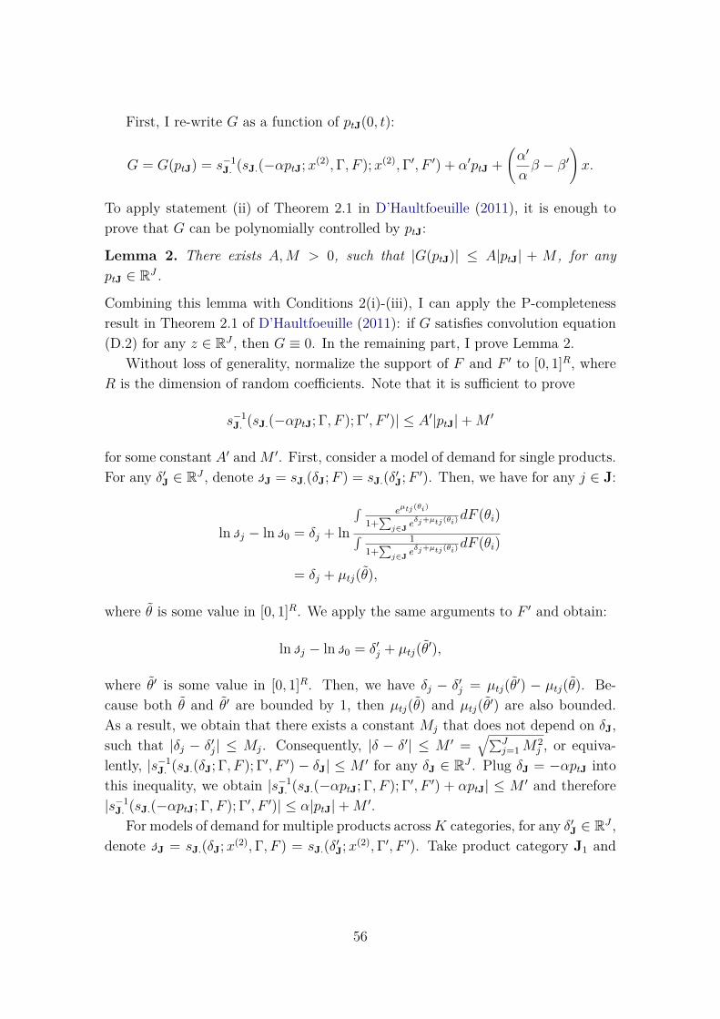
First, I re-write G as a function of ptJ(0, t):

G = G(ptJ) = s−1J. (sJ.(−αptJ;x(2),Γ, F );x(2),Γ′, F ′) + α′ptJ +

(α′

αβ − β′

)x.

To apply statement (ii) of Theorem 2.1 in D’Haultfoeuille (2011), it is enough toprove that G can be polynomially controlled by ptJ:

Lemma 2. There exists A,M > 0, such that |G(ptJ)| ≤ A|ptJ| + M , for anyptJ ∈ RJ .

Combining this lemma with Conditions 2(i)-(iii), I can apply the P-completenessresult in Theorem 2.1 of D’Haultfoeuille (2011): if G satisfies convolution equation(D.2) for any z ∈ RJ , then G ≡ 0. In the remaining part, I prove Lemma 2.

Without loss of generality, normalize the support of F and F ′ to [0, 1]R, whereR is the dimension of random coefficients. Note that it is sufficient to prove

s−1J. (sJ.(−αptJ; Γ, F ); Γ′, F ′)| ≤ A′|ptJ|+M ′

for some constant A′ andM ′. First, consider a model of demand for single products.For any δ′J ∈ RJ , denote sJ = sJ.(δJ;F ) = sJ.(δ′J;F ′). Then, we have for any j ∈ J:

ln sj − ln s0 = δj + ln

∫ eµtj(θi)

1+∑

j∈J eδj+µtj(θi)dF (θi)∫ 1

1+∑

j∈J eδj+µtj(θi)dF (θi)

= δj + µtj(θ),

where θ is some value in [0, 1]R. We apply the same arguments to F ′ and obtain:

ln sj − ln s0 = δ′j + µtj(θ′),

where θ′ is some value in [0, 1]R. Then, we have δj − δ′j = µtj(θ′) − µtj(θ). Be-cause both θ and θ′ are bounded by 1, then µtj(θ) and µtj(θ′) are also bounded.As a result, we obtain that there exists a constant Mj that does not depend on δJ,such that |δj − δ′j| ≤ Mj. Consequently, |δ − δ′| ≤ M ′ =

√∑Jj=1M

2j , or equiva-

lently, |s−1J. (sJ.(δJ; Γ, F ); Γ′, F ′) − δJ| ≤ M ′ for any δJ ∈ RJ . Plug δJ = −αptJ into

this inequality, we obtain |s−1J. (sJ.(−αptJ; Γ, F ); Γ′, F ′) + αptJ| ≤ M ′ and therefore

|s−1J. (sJ.(−αptJ; Γ, F ); Γ′, F ′)| ≤ α|ptJ|+M ′.For models of demand for multiple products acrossK categories, for any δ′J ∈ RJ ,

denote sJ = sJ.(δJ;x(2),Γ, F ) = sJ.(δ′J;x(2),Γ′, F ′). Take product category J1 and

56

define s0 = 1−∑j∈J1 sj.. Note that

s0 =∫ ∑

b=((jk)jk∈Jk,k=2,...,K) e∑K

k=2 δjk+Γb+∑K

k=2 µtjk (θi)∑b=(jk)jk∈Jk,k=1,...,K e

∑K

k=1 δjk+Γb+µtb(θi)dF (θi)

and for j ∈ J1,

sj. =∫ ∑

b=((jk)jk∈Jk,k=2,...,K) eδj+µtj(θi)e

∑K

k=2 δjk+Γb∪j+∑K

k=2 µtjk (θi)∑b=(jk)jk∈Jk,k=1,...,K e

∑K

k=1 δjk+Γb+µtb(θi)dF (θi).

Then, similar to demand models of single products, we obtain:

ln sj. − ln s0 = δj + µtj(θ) + Γb∪j − Γb,

where θ is some value in [0, 1]R and b is some bundle without j ∈ J1. We apply thesame arguments to (Γ′, F ′) and obtain:

ln sj. − ln s0 = δ′j + µtj(θ′) + Γb′∪j − Γb′ ,

where θ′ is some value in [0, 1]R and b′ is some bundle without j ∈ J1. Then, similararguments in the model of demand for single product apply and |δj−δ′j| is boundedby some constant that only depends on the support of θ and θ′ and the bounds ofΓ. The proof of the second statement is completed.

Combining Theorems D.1-D.3, we obtain Theorem 2.

E Proof of Theorem 3The proof is proceeded in two steps. In the first step, I prove Γ(j,r) is identifiedfor j, r ∈ J, j 6= r. In the second step, I prove that the sb(δt;x(2)

t , F ) is identifiedfor b ∈ C1 and (δt, x(2)

t ) ∈ RC1 × D(2)x . Steps 1 and 2 prove the first statement.

The proof of the second statement is a combination of that of the first statementand a direct application of Theorem 3 of Wang (2020). We prove steps 1 and 2 forany given x

(2)tJ ∈ D(2)

x . To simplify the exposition, I drop x(2)tJ from the notation.

Throughout the proof, denote the Fourier transformation of function φ by F(φ).Suppose that there exist (Γ′, F ′) such that

sj.(δJ; Γ′, F ′) = sj.(δJ; Γ, F )

for any j ∈ J and δ ∈ RJ .

57

Step 1: Γ′ = Γ. Without loss of generality, we show Γ(1,2) = Γ′(1,2). First, notethat by letting all δ′tl’s, l 6= 1, 2 tend to −∞, market shares of single products l andof all bundles that contain any product l 6= 1, 2 converge to zero. Consequently, weobtain:

s1.(δ′t1,2; Γ′(1,2), F′) = s1.(δ′t1,2; Γ(1,2), F ),

s2.(δ′t1,2; Γ′(1,2), F′) = s2.(δ′t1,2; Γ(1,2), F ),

(E.1)

for any δ′t1,2 = (δ′t1, δ′t2) ∈ R2. Take the first equation in (E.1) and compute thepartial derivatives with respect to δ′t2:

∂s1.(δ′t1,2; Γ′(1,2), F′)

∂δ′t2=∫ (eδ′t1+δ′t2+µt1(θit)+µt2(θit))(eΓ′(1,2) − 1)

(1 + eδ′t1+µt1(θit) + eδ

′t2+µt2(θit) + e

δ′t1+µt1(θit)+δ′t1+µt1(θit)+Γ′(1,2))2dF ′(θit),

∂s1.(δ′t1,2; Γ(1,2), F )∂δ′t2

=∫ (eδ′t1+δ′t2+µt1(θit)+µt2(θit))(eΓ(1,2) − 1)

(1 + eδ′t1+µt1(θit) + eδ

′t2+µt2(θit) + eδ

′t1+µt1(θit)+δ′t1+µt1(θit)+Γ(1,2))2

dF (θit),

∂s1.(δ′t1,2; Γ′(1,2), F′)

∂δ′t2=∂s1.(δ′t1,2; Γ(1,2), F )

∂δ′t2.

I can then cancel out eδ′t1+δ′t2 in the nominators of ∂s1.(δ′t1,2;Γ

′(1,2),F

′)∂δ′t2

and ∂s1.(δ′t1,2;Γ′(1,2),F

′)∂δ′t2

.Letting δt2 → −∞, I obtain:

[eΓ′(1,2) − 1]∫ eµt1(θit)+µt2(θit)

(1 + eδ′t1+µt1(θit))2dF

′(θit) = [eΓ(1,2) − 1]∫ eµt1(θit)+µt2(θit)

(1 + eδ′t1+µt1(θit))2dF (θit).

(E.2)From (E.2), if Γ(1,2) = 0, then Γ′(1,2) = Γ(1,2) = 0.Suppose Γ(1,2) 6= 0. Denote thedensity functions of µit = (µit1, µit2) = (µt1(θit), µt2(θit)) for θit ∼ F and θit ∼ F ′

by fµ and f ′µ, respectively. Then, I can re-write (E.2) as:

[eΓ′(1,2)−1]∫ eµit1+µit2

(1 + eµit1)2f′µ(µit1−δ′t1, µit2)dµit = [eΓ(1,2)−1]

∫ eµit1+µit2

(1 + eµit1)2fµ(µit1−δ′t1, µit2)dµit.

Define g(λ) = eλ

(1+eλ)2 . Then,

[eΓ′(1,2)−1]∫g(µit1)f ′µ(µit1−δ′t1)dµit1 = [eΓ(1,2)−1]

∫g(µit1)fµ(µit1−δ′t1)dµit1, (E.3)

where f ′µ(µit1) =∫eµit2f ′µ(µit1, µit2)dµit2 and fµ(µit1) =

∫eµit2fµ(µit1, µit2)dµit2. Ei-

ther side of (E.3) defines a convolution. Note that g(·), f ′µ, fµ ∈ L1(R). Conse-quently, I apply Fourier transformation on both sides of (E.3) and obtain:

[eΓ′(1,2) − 1]F(g)(t)F(f ′µ)(t) = [eΓ(1,2) − 1]F(g)(t)F(fµ)(t),

58

for any t ∈ R. Particularly, at t = 0, F(g)(0) > 0. Then,

[eΓ′(1,2) − 1]F(f ′µ)(0) = [eΓ(1,2) − 1]F(fµ)(0), (E.4)

Note that F(f ′µ)(t) = Ef ′ [eµit2 ] and F(fµ)(t) = Ef [eµit2 ]. If they are equal, thenΓ′(1,2) = Γ(1,2). In particular, if Γ(1,2) = −∞, i.e. bundle (1, 2) is not in the choiceset, I obtain that Γ′(1,2) = −∞ and therefore identify that bundle (1, 2) is not in thechoice set. In what follows, we prove Ef ′ [eµit2 ] = Ef [eµit2 ].

Take the second equation of (E.1) and let δ′it1 → −∞. I then obtain:

∫ eδ′t2+µit2

1 + eδ′t2+µit2

f ′µ(µit) =∫ eδ

′t2+µit2

1 + eδ′t2+µit2

fµ(µit). (E.5)

I cancel out eδ′t2 from the nominators on both sides of (E.5) and let δ′2t → −∞. Ithen obtain

∫eµit2f ′µ(µit) =

∫eµit2fµ(µit), i.e. Ef ′ [eµit2 ] = Ef [eµit2 ].

Step 2: sb(δC1 ;F ′) = sb(δC1 ;F ) for any b ∈ C1 and δC1 ∈ RC1. I prove thisresult for for the model of demand for multiple products within category. The proofis similar for the model of demand for multiple products across two categories.

Recall that the density function of µitJ = µtJ(θit) for θit ∼ F ′ and θit ∼ F aref ′µ and fµ, respectively. It suffices to prove that f ′µ = fµ almost everywhere. Inthe model of demand for multiple products within category in Theorem 3, plugΓ′ = Γ into the product-level market share function of j. I then have for anyδ′tJ ∈ RJ , sj.(δ′tJ; Γ, F ) = sj.(δ′tJ; Γ, F ′). According to the arguments in Appendix8.13 of Iaria and Wang (2019), given the product-level market share functions andΓ, one can uniquely determine the bundle-level market shares, as function of δtJ.Because both the product-level market share functions and Γ are identified, thensb(δt(Γ);F ), where δt(Γ) = (δt1, ..., δtJ , (δtb)b∈C2 + Γ), is identified as a function ofδtJ, for any b ∈ C1. Consequently, the market share function of the outside option,s0(δt(Γ);F ), is identified as a function of δtJ: for any δ′tJ ∈ RJ

s0(δ′tJ(Γ);F ) = s0(δ′tJ(Γ);F ′). (E.6)

I compute the higher-order cross derivative of both sides of (E.6):

∂Js0(δ′tJ(Γ);F )∂δ′t1, ..., ∂δ

′tJ

=∫ PΓ(δt1 + µit1, ..., δtJ + µitJ)QΓ(δt1 + µit1, ..., δtJ + µitJ)fµ(µit)dµit,

∂Js0(δ′tJ(Γ);F ′)∂δ′t1, ..., ∂δ

′tJ

=∫ PΓ(δt1 + µit1, ..., δtJ + µitJ)QΓ(δt1 + µit1, ..., δtJ + µitJ)f

′µ(µit)dµit,

∂Js0(δ′tJ(Γ);F )∂δ′t1, ..., ∂δ

′tJ

= ∂Js0(δ′tJ(Γ);F ′)∂δ′t1, ..., ∂δ

′tJ

,

(E.7)

59

whereQΓ(uit1, ..., uitJ) = 1 +

∑j∈J

euitj +∑j<j′

eΓ(j,j′)euitj+uitj′ .

and

PΓ(uit1, ..., uitJ) =∑S∈S

A(S)∏

(j,j′)∈S

euit(j,j′)

QΓ(uit1, ..., uitJ)∏j∈S

∑b:b3j e

uitb

QΓ(uit1, ..., uitJ)

=∏j∈J

euitj∑S∈S

A(S)∏

(j,j′)∈S

eΓ(j,j′)

QΓ(uit1, ..., uitJ)∏j∈S

1 +∑j′ 6=j e

uitj′+Γ(j,j′)

QΓ(uit1, ..., uitJ)(E.8)

where S is a partition of 1, ..., J with each part being at most size 2, S collects allsuch partitions which are the results of the higher-order cross derivative ∂J

∂δ′t1,...,∂δ′tJ,

and A(S) is a constant depending on the partition S ∈ S. An example of S is1, 2, 5, 4, 3, 6. Each term in the products of PΓ corresponds to the choiceprobability of either bundle (j, j′) or the product-level choice probability of productj, evaluated at uitJ and Γ, and bounded by 1. From (E.7), I obtain:

∫ PΓ((eλitj)j∈J)QΓ((eλitj)j∈J) [fµ(λitJ − δ′tJ)− fµ(λitJ − δ′tJ)]dλitJ = 0, (E.9)

for any δ′tJ ∈ RJ . I prove the following lemma:

Lemma 3.

• PΓ((eλj )j∈J)QΓ((eλj )j∈J)

∈ L1(RJ).

• The zero set of F(PΓ((eλj )j∈J)QΓ((eλj )j∈J)

)in RJ is of zero Lebesgue measure.

Note that the right-hand side of (E.9) is a convolution. Because of the first state-ment of Lemma 3, I can apply Fourier transformation on both sides and obtain:

F

(PΓ((eλj)j∈J)QΓ((eλj)j∈J)

)F(fµ − f ′µ) = 0.

Applying the second statement of Lemma 3, I obtain F(fµ) = F(f ′µ) almost ev-erywhere. Due to the continuity of characteristics functions, F(fµ) = F(f ′µ) every-where and hence the distribution of µit is identified. In the remaining part, I proveLemma 3.

Proof. First, we make the transformation of variables λJ to eλJ :

∫ ∣∣∣∣∣PΓ((eλj)j∈J)QΓ((eλj)j∈J)

∣∣∣∣∣ dλJ =∫RJ+

∣∣∣∣∣PΓ(y1, ..., yJ)QΓ(y1, ..., yJ)

1∏Jj=1 yj

∣∣∣∣∣ dyJ.

60

For the first statement, because of (E.8), it suffices to prove that for each S ∈ S,∣∣∣∣∣∣ 1QΓ(y1, ..., yJ)

∏(j,j′)∈S

eΓ(j,j′)

QΓ(y1, ..., yJ)∏j∈S

1 +∑j′ 6=j yj′e

Γ(j,j′)

QΓ(y1, ..., yJ)

∣∣∣∣∣∣ (E.10)

is integrable in RJ+. To show this, I divide RJ

+ into 2J regions: RJ+ = ×Jj=1Ij,

where Ij = (0, 1], (1,+∞). Then, it is enough to prove that (E.10) is integrablein each of these regions. Without loss of generality, suppose that the region isRk = (y1, ..., yJ) : yj ∈ (0, 1), j = 1, ..., k; yj′ ≥ 1, j′ = k + 1, ..., J. Then, for agiven j, we have four cases to control:

1. j ≤ k and j appears in S as (j, j′).

2. j ≤ k and j appears in S as j.

3. j > k and j appears in S as (j, j′).

4. j > k and j appears in S as j.

Note that for cases 1 and 2, the corresponding terms in (E.10) can be controlled byeΓm with Γm = max0, (Γ(j,j′))j≤j′. For case 3, e

Γ(j,j′)

QΓ(y1,...,yJ ) ≤eΓm

yj. For case 4,

1 +∑j′ 6=j yj′e

Γ(j,j′)

QΓ(y1, ..., yJ) ≤1 +∑

j′ 6=j yj′eΓ(j,j′)

yj +∑j′ 6=j yjyj′e

Γ(j,j′)= 1yj≤ eΓm

yj.

Moreover,

QΓ(y1, ..., yJ) ≤ 1∑j>k yj +∑

k<j<j′ yjyj′eΓ(j,j′)

≤ 2

(J − k)(J − k + 1)(∏k<j<j′ eΓ(j,j′))

2(J−k)(J−k+1)

∏Jj=k+1 y

2J−k+1j

.

The last step is due to the inequality of arithmetic and the geometric means. Then,for all the four cases, we have:∣∣∣∣∣∣ 1QΓ(y1, ..., yJ)

∏(j,j′)∈S

eΓ(j,j′)

QΓ(y1, ..., yJ)∏j∈S

1 +∑j′ 6=j yj′e

Γ(j,j′)

QΓ(y1, ..., yJ)

∣∣∣∣∣∣ ≤ A(J, k,Γ)J∏

j=k+1y−1− 2

J−k+1j ,

(E.11)whereA(J, k,Γ) = 2eJΓm

(J−k)(J−k+1)(∏k<j<j′ e

Γ(j,j′) )2

(J−k)(J−k+1). Note that∏J

j=k+1 y−1− 2

J−k+1j

is integrable in Rk and A(J, k,Γ) is a constant. Then,∣∣∣∣∣∣ 1QΓ(y1, ..., yJ)

∏(j,j′)∈S

eΓ(j,j′)

QΓ(y1, ..., yJ)∏j∈S

1 +∑j′ 6=j yj′e

Γ(j,j′)

QΓ(y1, ..., yJ)

∣∣∣∣∣∣61

is integrable in (y1, ..., yJ) : yj ∈ (0, 1), j = 1, ..., k; yj′ ≥ 1, j′ = k + 1, ..., J. Theproof of the first statement is completed.

To prove the second statement, according to Mityagin (2015), it suffices to showthat the real (or imaginary) part of F

(PΓ((eλj )j∈J)QΓ((eλj )j∈J)

)is non-constant real analytic

function. In order to prove the real analytic property, the key is to control thehigher order derivatives of F

(PΓ((eλj )j∈J)QΓ((eλj )j∈J)

)(y):

∂LF(PΓ((eλj )j∈J)QΓ((eλj )j∈J)

)(y)∏J

j=1 ∂yljj

= F

J∏j=1

(−iλj)ljPΓ((eλj)j∈J)QΓ((eλj)j∈J)

(y), (E.12)

where ∑Jj=1 lj = L and i is the imaginary unit. I now prove that this higher order

derivative can be controlled by(J+1

2

)L∏Jj=1 lj!. This result will then imply that

for any y ∈ RJ , there exist 0 < ε < 2J+1 such that for y′ ∈ RJ and |y′ − y| <

ε, the Taylor expansion of F

(PΓ((eλj )j∈J)QΓ((eλj )j∈J)

)(y′) around y uniformly converges to

F

(PΓ((eλj )j∈J)QΓ((eλj )j∈J)

)(y′). Consequently, F

(PΓ((eλj )j∈J)QΓ((eλj )j∈J)

)(y) is everywhere real analytic

in RJ . It is not constantly zero because PΓQΓ

is not constantly zero. In the remaing

part of the proof, I prove (E.12) can be controlled by(J+1

2

)L∏Jj=1 lj!.

It suffices to study∫ ∣∣∣∣∏J

j=1(|λj|)lj PΓ((eλj )j∈J)QΓ((eλj )j∈J)

∣∣∣∣ dλ, or equivalently,∫RJ+

∣∣∣∣∣∣J∏j=1

(| ln yj|)ljPΓ((yj)j∈J)QΓ((yj)j∈J)

1∏Jj=1 yj

∣∣∣∣∣∣ dyJ.

I follow the same technique as in the proof of the first statement and evaluate, foreach S ∈ S,∣∣∣∣∣∣

J∏j=1

(| ln yj|)lj1

QΓ(y1, ..., yJ)∏

(j,j′)∈S

eΓ(j,j′)

QΓ(y1, ..., yJ)∏j∈S

1 +∑j′ 6=j yj′e

Γ(j,j′)

QΓ(y1, ..., yJ)

∣∣∣∣∣∣ (E.13)

in each of the 2J regions. Without loss of generality, for region Rk, using (E.11),we have:∣∣∣∣∣∣

J∏j=1

(| ln yj|)lj1

QΓ(y1, ..., yJ)∏

(j,j′)∈S

eΓ(j,j′)

QΓ(y1, ..., yJ)∏j∈S

1 +∑j′ 6=j yj′e

Γ(j,j′)

QΓ(y1, ..., yJ)

∣∣∣∣∣∣≤ A(J, k,Γ)

k∏j=1| ln yj|lj

J∏j=k+1

| ln yj|ljy−1− 2

J−k+1j .

62

Finally,

∫ 1

0, ...,

∫ 1

0

∫ ∞1

...∫ ∞

1A(J, k,Γ)

k∏j=1| ln yj|lj

J∏j=k+1

| ln yj|ljy−1− 2

J−k+1j dyJ

= A(J, k,Γ)(J − k + 12 )L+J−k

J∏j=1

lj!

≤ A(J, k,Γ)(J + 12 )J(J + 1

2 )LJ∏j=1

lj!

Consequently, when I sum over all the integrals in the 2J regions and all S ∈ S,

∫RJ+

∣∣∣∣∣∣J∏j=1

(| ln yj|)ljPΓ((yj)j∈J)QΓ((yj)j∈J)

1∏Jj=1 yj

∣∣∣∣∣∣ dyJ

will be bounded by (J+12 )L∏J

j=1 lj! multiplied by some constant only depending onJ and Γ. The proof is completed.

F Proof of Corollary 1I will construct (Γ0, F

′0) and (Γ′0, F0) such that Γ0 6= Γ′0 and F0 6= F ′0, while

s1.(·; Γ0, F′0) = s1.(·; Γ′0, F0). Because F0 6= F ′0, then s(1,1)(·;F0) 6= s(1,1)(·;F ′0).

First, I compute the derivative of s1.(δ; Γ, F ) with respect to δ:

∂s1.(δ; Γ, F )∂δ

=∫ eδ+µ + 4e2δ+2µ+Γ

(1 + eδ+µ + e2δ+2µ+Γ)2dF (µ)

=∫R(δ + µ; Γ)dF (µ),

(F.1)

where R(x; Γ) = ex+4e2x+Γ

(1+ex+e2x+Γ)2 . Note that R(·; Γ) ∈ L1(R). Define γ = eΓ and

V (γ) =∫RR(x; Γ)dx =

∫R+

1 + 4γt(1 + t+ γt2)2dt

V (γ) is a continuous function of γ ∈ [0,∞), with V (0) = 1 > V (∞) = 0. Moreover,limγ→0+

dVdγ

= +∞ > 0. As a consequence, there exist γ0 6= γ′0 and γ0, γ′0 > 0, such that

V (γ0) = V (γ′0). Therefore, there exists Γ0 = ln γ0 > −∞ and Γ′0 = ln γ′0 > −∞,such that Γ0 6= Γ′0 and V0 =

∫RR(x; Γ0) =

∫RR(x; Γ′0)dx. Note that R(·;Γ0)

V0and R(·;Γ′0)

V0

are both well-defined but different density functions. Denote the correspondingdistribution functions by F0 and F ′0, respectively: dF0

dµ= R(µ;Γ0)

V0and dF ′0

dµ= R(µ;Γ′0)

V0.

63

Based on (F.1), consider the Fourier transformation of ∂s1.(δ;Γ0,F ′0)∂δ

and ∂s1.(δ;Γ′0,F0)∂δ

:

F

(∂s1.(δ; Γ0, F

′0)

∂δ

)(t) = F (R(·; Γ0)) (t)F

(dF ′0dµ

)(t),

F

(∂s1.(δ; Γ′0, F0)

∂δ

)(t) = F(R(·; Γ′0))(t)F

(dF0

dµ

)(t).

Then,

F

(∂s1.(δ; Γ0, F

′0)

∂δ

)(t) = F

(∂s1.(δ; Γ′0, F0)

∂δ

)(t),

Consequently, ∂s1.(δ;Γ0,F ′0)∂δ

= ∂s1.(δ;Γ′0,F0)∂δ

for δ ∈ R, and s1.(δ; Γ′0, F0)− s1.(δ; Γ0, F′0) is

a constant function in R. Taking δ = +∞, we obtain that this constant is zero andhence s1.(δ; Γ′0, F0) = s1.(δ; Γ0, F

′0) for δ ∈ R. The construction is completed.

G Proof of Proposition 2The proof directly follows from that of Lemma 2.

H Construction of Product-Level Market SharesIn this appendix, I illustrate the construction of product-level market shares frommarket-level sales data. I suppress t to simplify the exposition. Suppose that thereare I households and the size of household i = 1, ..., I is ni ∈ 1, ..., N. Denote by qkthe weekly per capita consumption of the relevant products of category k (breakfastcereals or milk). Then, for product j in category k, the total consumption Djk, is:

Djk =I∑i=1

∑b:b3j

1i buys bniqk

= qkN∑n=1

n∑

b:b3j

I∑i=1

1i buys b, ni = n

= IqkN∑n=1

n∑

b:b3j

∑Ii=1 1i buys b, ni = n

I.

64

Denote by snb the average purchase probability of bundle b among households ofsize n. Then, when I is very large,

Djk

Iqk=

N∑n=1

n∑

b:b3j

∑Ii=1 1i buys b, ni = n

I

≈N∑n=1

nπn∑

b:b3jsnb

=N∑n=1

nπnsnj.,

Djk

INqk≈

N∑n=1

πnsnj. = sj.,

where N = ∑Nn=1 nπn is the average household size and πnNn=1 is the distribution of

household sizes weighted by size. Note that when computing product-level marketshares, one should use the weighted distribution πnNn=1 rather than πnNn=1 toproperly take into account heterogeneous consumption across households of differentsizes.

Under the assumptions in section 6, Djk is equal to the sales in lbs of product j ofcategory k. Moreover, the IRI dataset contains information the sampled householdswith which we can infer the number of households I and the distribution of theirdemographics. Finally, for dk, k ∈ K, I use external sources: the weekly per capitaconsumption of breakfast cereals is 0.19 lbs and that of fluid milk is 3.4 lbs.52 Basedon these pieces of information, we construct sj.’s.53

I Main Tables

52See https://hypertextbook.com/facts/2006/LauraFalci.shtml for a collection of these reports.53Another implicit assumption is that the ratio of consumption between breakfast cereals and

fluid milk is the same across households of different sizes. However, it is possible that this is nottrue. For example, households with children may consume relatively more fluid milk.

65

Table 9: RTE Cereal Products

Brand Flavour Fortification GrainGeneral Mills Cherrios Toasted Missing WHOLE GRAIN OATGeneral Mills Cinnamon TST CR Cinnamon Toast 12 ESSNTL VTMN&MNRL WHOLE WHEAT AND RICEGeneral Mills Cinnamon TST CR Cinnamon Toast Missing WHOLE WHEAT AND RICEGeneral Mills Honey Nut Cheer Honey Nut Missing WHL GRAIN OAT & BRLYGeneral Mills Honey Nut Cheer Honey Nut Missing WHOLE GRAIN OATGeneral Mills Lucky Charms Toasted CALCIUM & VITAMIN D WHOLE GRAIN OATGeneral Mills Lucky Charms Toasted Missing WHOLE GRAIN OATGeneral Mills Multi Grain Che. Regular 10 VITAMINS&MINERALS MULTI GRAINKashi Go Lean Crunch Regular Missing MULTI GRAINKellogg’s Apple Jacks Apple Cinnamon Missing 3 GRAINKellogg’s Corn Flakes Regular Missing CORNKellogg’s Frosted Flakes Regular VITAMIN D CORNKellogg’s Frosted Mini Wheats Regular Missing WHOLE GRAIN WHEATKellogg’s Raisin Bran Regular Missing WHL GRN WHT WHT BRNKellogg’s Rice Krispies Toasted Missing RICEKellogg’s Special K Toasted Missing RICEKellogg’s Special K Fruit & Yo Regular Missing OAT RICE WHEATKellogg’s Special K Red Berrie Regular Missing RICE AND WHEATKellogg’s Special K Vanilla AL Regular Missing RICE AND WHEATPost Grape Nuts Regular Missing WHOLE GRN WHT & BRLYPost Honey Bunches of Oats Honey Missing WHOLE GRAIN OATPost Honey Bunches of Oats Honey Roasted Missing WHOLE GRAIN OATPost Raisin Bran Regular Missing WHOLE GRAN WHT & BRNPost Selects Great Grains Regular Missing MULTI GRAINPrivate Label Regular Missing GRANOLA

Table 10: Milk Products

Brand Flavour Fortification Fat Content Type of MilkGARELICK FARMS WHITE VITAMIN A & D skimmed dairyGARELICK FARMS WHITE VITAMIN A & D low fat dairyGARELICK FARMS WHITE VITAMIN D whole fat dairyGARELICK FARMS TRUMOO CHOCOLATE MISSING low fat dairyGUIDAS WHITE VITAMIN A & D skimmed dairyGUIDAS WHITE VITAMIN A & D low fat dairyGUIDAS WHITE VITAMIN D whole fat dairyHIGH LAWN FARM WHITE VITAMIN A & D whole fat dairyHIGH LAWN FARM WHITE VITAMIN A & D skimmed dairyHIGH LAWN FARM WHITE VITAMIN A & D low fat dairyHOOD WHITE VITAMIN A C D W CLCM skimmed dairyHOOD WHITE VITAMIN A C D W CLCM low fat dairyHOOD WHITE VIT C D CALCIUM whole fat dairyHOOD LACTAID WHITE VITAMIN A & D low fat dairyHOOD SIMPLY SMART WHITE VIT A & D W/CALC&PROTN skimmed dairyPRIVATE LABEL CHOCOLATE MISSING low fat dairyPRIVATE LABEL WHITE VITAMIN A & D skimmed dairyPRIVATE LABEL WHITE VITAMIN A & D W/CALC skimmed dairyPRIVATE LABEL WHITE VITAMIN A & D low fat dairyPRIVATE LABEL WHITE VITAMIN D whole fat dairy

66

Table 11: Average Estimated Own- and Cross-Price Elasticities (Model II), Grain Typeand Fat Content

RTE cereals Milkuni-grain multi-grain granola skimmed low fat whole fat

RTE cereals, uni-grain -1.512 0.231 0.009 -0.007 -0.017 -0.008multi-grain 0.318 -1.642 0.010 -0.007 -0.018 -0.009

granola 0.214 0.185 -1.518 -0.009 -0.019 -0.009Milk, skimmed -0.078 -0.061 -0.005 -0.327 0.056 0.029

low fat -0.079 -0.061 -0.005 0.022 -0.280 0.029whole fat -0.078 -0.061 -0.005 0.022 0.056 -0.319

Notes: Each entry reports the percent change in the sum of the product-level market shares ofthe products collected by the row characteristics with respect to a 1% increase in the prices of theproducts collected by the column characteristics.

Table 12: Average Estimated Own- and Cross-Price Elasticities (Model II),Flavours

RTE cereals Milkunflavoured flavoured unflavoured chocolate

RTE cereals, unflavoured -1.504 0.179 -0.036 -0.0003flavoured 0.137 -1.425 -0.028 -0.001

Milk, unflavoured -0.071 -0.072 -0.235 0.002chocolate -0.036 -0.185 0.096 -0.366

Notes: Each entry reports the percent change in the sum of the product-level marketshares of the products collected by the row characteristics with respect to a 1%increase in the prices of the products collected by the column characteristics.

Table 13: Average Estimated Own- and Cross-Price Elasticities (ModelII), Fortification and Flavours

RTE cereals Milkunfortified fortified unflavoured chocolate

RTE cereals, unfortified -1.355 0.070 -0.032 -0.001fortified 0.454 -1.804 -0.033 -0.001

Milk, unflavoured -0.123 -0.019 -0.235 0.002chocolate -0.197 -0.023 0.096 -0.366

Notes: Each entry reports the percent change in the sum of the product-levelmarket shares of the products collected by the row characteristics with respectto a 1% increase in the prices of the products collected by the column charac-teristics.

67

Table14:Av

erageEs

timated

Own-

andCross-P

riceElastic

ities

(Mod

elII),

Prod

ucer

RTE

cereals

Milk

Gen

eral

MillsKashi

Kellogg

’sPo

stPr

ivateLa

belGarelickFa

rmsGuida

sHighLa

wnFa

rmHoo

dPr

ivateLa

bel

RTE

cereals,

Gen

eral

Mills

-1.556

0.00

90.18

80.05

20.00

8-0.006

-0.026

-0.002

-0.002

-0.016

Kashi

0.15

1-1.829

0.17

80.03

80.01

3-0.007

-0.028

-0.003

-0.002

-0.020

Kellogg

’s0.18

70.01

1-1.572

0.03

80.01

1-0.007

-0.031

-0.003

-0.002

-0.019

Post

0.22

20.01

10.17

6-1.710

0.01

1-0.007

-0.029

-0.003

-0.002

-0.020

PrivateLa

bel

0.15

90.01

50.18

50.03

9-1.518

-0.008

.-0.003

-0.002

-0.023

Milk

,GarelickFa

rms

-0.072

-0.006

-0.074

-0.018

-0.005

-0.356

.0.00

60.00

60.05

9Guida

s-0.029

-0.002

-0.033

-0.006

..

-0.189

0.01

30.00

20.01

5HighLa

wnFa

rm-0.059

-0.005

-0.064

-0.015

-0.005

0.01

70.13

2-0.528

0.00

50.05

0Hoo

d-0.058

-0.005

-0.063

-0.014

-0.005

0.01

70.12

60.00

7-0.562

0.05

0Pr

ivateLa

bel

-0.063

-0.005

-0.068

-0.016

-0.005

0.01

70.12

90.00

70.00

5-0.273

Not

es:Ea

chentryrepo

rtsthepe

rcentchan

gein

thesum

oftheprod

uct-levelm

arketshares

oftheprod

ucts

colle

cted

bytherow

prod

ucer

with

respectto

a1%

increase

intheprices

oftheprod

ucts

colle

cted

bythecolumnprod

ucer.

The

.refers

tothesit

uatio

nwhere

theprod

ucts

oftherow

andcolumnbran

dsareno

tavailableat

thesametim

ein

anymarketin

theda

ta.

68

Online Appendix

J Data Generating Process in Section 3.3In this appendix, I provide details on the DGP used in the counterfactual simula-tions in section 3.3. There are t = 1, ..., T markets and T = 1000. In each market,we have two product categories J1 = 1, 2 and J2 = 3, 4. The indirect utility ofindividual i from purchasing product j ∈ J1 ∪ J2 in market t:

Uitj = −2ptj + xtj + ξtj + εitj,

the indirect utility from purchasing a bundle b = (j1, j2) ∈ J1 × J2 is

Uitb = −2(ptj1 + ptj2) + (xtj1 + xtj2) + (ξtj1 + ξtj2) + Γj1j2 + εitb,

and the indirect utility from purchasing the outside option 0 is Uit0 = εit0, whereεitj, εitb and εit0 are i.i.d. Gumbel, for j ∈ J1 ∪ J2, b ∈ J1 × J2. Prices ptj aregenerated from a Bertrand-price setting game in which the marginal productioncost of product j in market t is positive and constant:

ctj = 0.5 exp0.5 expztj + 0.2wtj,

where ztj is a product-market specific cost shifter and wtj is a product-marketspecific supply shock. I solve the first-order conditions (FOCs) of the pricinggame, from which I derive the price for each product in each market.54 Finally,(xtj, ztj, ξtj, wtj) are mutually independent and i.i.d. across j’s and t’s, with eachbeing generated from a centred normal distribution with a variance 0.5. When es-timating the model of demand with Γ = 0, I use (xtj, ztj) as instruments. Whensimulating the supermarket nonlinear pricing competition, I also assume that thereis no additional cost of implement discounts, i.e. ctb = ∑

j∈b ctj.

K Implementing (11) Using Jacobian-based Meth-ods: Numerical Performance

In this appendix, I explore the numeric performance of Jacobian-based algorithmsin implementing the demand inverse in (11). I compare convergence time acrossdifferent algorithms and starting values—particularly, the proposed starting valuein section 5.2—for various sizes of choice set.

54When solving the FOCs, I use the vector of marginal costs as starting value. The algorithmin Matlab returns an unique price vector.

69

Table 15 summarises the main results of the simulations. The DGP is a discretechoice model of bundles up to size two and the prices are generated from a Bertrandpricing game under complete information with constant marginal costs. I simulate50 markets with the same structural parameters. The unobserved demand shocksξtJ are Gaussian and i.i.d. across markets and products. I implement the demandinverse using the true model and also using a demand model of single products.55

I report the median convergence time (in seconds). Moreover, I compare the per-formances of these inverses using the starting value δ(0)

∗ defined in (13) and thestandard starting value δ(0) = 0. I replicate this setting for various sizes of choiceset (J = 10, 50, and 100). For example, when J = 100, the true model has 5051alternatives (100 single products, 4950 bundles of two different products, and anoutside option). The demand inverse s−1

J. will then treat the observed market sharesas those generated from the true model, while the demand inverse s−1

J will treat thesame observed market shares as if they are generated from a demand model of 100single products.

Table 15: Demand Inverse of Product-Level Market Shares: Convergence Time

Algorithm Trust-Region-Dogleg Trust-Region-Reflective Levenberg-Marquardts−1

J. s−1J s−1

J. s−1J s−1

J. s−1J

Init. Point δ(0)∗ 0 δ

(0)∗ 0 δ

(0)∗ 0 δ

(0)∗ 0 δ

(0)∗ 0 δ

(0)∗ 0

# ProductsJ = 10 0.04 0.09 0.03 0.08 0.05 0.09 0.04 0.08 0.08 0.09 0.07 0.09

50 0.49 1.45 0.10 2.64 0.41 1.31 0.13 0.34 1.31 1.92 0.19 0.12100 4.50 12.22 0.12 3.21 3.32 12.15 0.27 0.60 12.25 20.21 0.33 0.18

Notes: Trust-region-dogleg, trust-region, and Levenberg-Marquardt algorithms are built-in algo-rithms of function fsolve in Matlab. All of them are large-scale and minimise the sum of squaresof the components of (11). Median convergence time (in seconds) of 50 independently simulatedmarkets is reported. Tolerance level in the stop criterion of all algorithms is set to 10−16.

There are two main observations. First, for s−1J. , using the recommended starting

value δ(0)∗ remarkably reduces convergence time in all cases. The gain is larger

when the number of products is larger. When J = 100, trust-region-dogleg andtrust-region-reflective algorithms reduce around 70% convergence time by usingδ

(0)∗ than using δ(0) = 0. The numerical gain for s−1

J using δ(0)∗ is similar.56 Second,

as the problem size increases, using δ(0)∗ does not seem to increase the number of

iterations required to converge. For example, the convergence time for J = 100 by55The structural parameters are chosen so that the sum of the simulated product-level market

shares is always smaller than one. This allows to implement the inverse of these simulated product-level market shares using models of demand for single products

56In this demand inverse, K in (13) is 1.

70

using the three Jacobian-based algorithms with δ(0)∗ is roughly 100 times of that for

J = 10. Because the bundle size is at most two, then the size of choice set increasesquadratically with respect to the number of products. Therefore, the number ofrequired computations for one evaluation of market share functions also increasesquadratically. While, the total convergence time when using δ(0)

∗ seems to increaseonly quadratically for s−1

J. with respect to the number of products, implying thatthe number of iterations does not increase as J increases.

L Identification of Product-Level Market ShareFunctions Using Other IVs.

In this Appendix, I develop similar identification arguments with other types of IVs.I will focus on BLP-type instruments and exogenous product characteristics.

BLP-type instruments Cost shifters are not always available to the econometri-cian. Moreover, the validity of Hausman-type instruments requires independence ofdemand shocks across markets of the same region or of the same time period. Thiscan be violated whenever there is unobserved correlated demand shock across mar-kets, such as national advertisement. In demand models of single products, Berryet al. (1995) proposed to use characteristics (and their functions) of other prod-ucts in the same market as instruments. Their validity follows from the intuitionthat products with similar characteristics are closer substitutes. Then, “distance”in the space of product characteristics will be a good proxy of substitution amongproducts.

Because such variables for product j, denoted as xt,−j, are excluded from indirectutility of j, then, they can provide useful variation in price ptj via the markup ofproduct j that identifies (Γ, F ). Formally, in (D.1), for the equation of product j,one can fix xtj = xj and let xt,−j = (xtr)r 6=j varies in RJ−1.

It is worth noting that, different from cost shifters, BLP instruments may notalways be able to provide useful variation even though they vary exogenously. Forexample, if prices ptj’s are not responsive to xt,−j, then there is no variation inptj due to the variation of xt,−j. The unresponsiveness of prices with respect toBLP instruments can occur in a large-market setting when the number of productsincreases to infinity and therefore the competition between two products becomes

71

very weak.57 Asymptotically, product prices are no more functions of characteristicsof other products, but only of their own characteristics. Then, BLP instruments(say, xtj for product different from j) does not enter pricing functions of any otherproduct (pt,−j) and hence do not produce any exogenous variation in prices. In thispaper, because I focus on many-market settings and the number of products is fixed(see Assumption 1(iii)), BLP instruments are still valid for the identification of theprice coefficient, demand synergy parameters, and the distribution of the randomcoefficients.

L.1 Exogenous product characteristics

Suppose that prices are generated from a linear pricing simultaneous Bertrand gameunder complete information with constant marginal cost ctj for j ∈ J. I abstractfrom cost shifters in ctj and denote the joint density function of (ξtJ, ctJ) by fξ,c. Ipropose the following identification result:

Theorem L.1. Suppose that Assumptions 1-3 and regularity condition 2 hold. Ifthe following conditions hold:

1. xtJ is independent of (ξtJ, ctJ) and the domain of xtJ is an open set in RK1.

2. αi = α 6= 0, and there exists a k such that βik = βk and βk/α is identified.

3. Given x(2), ptJ = pJ(βx + ξtJ, ctJ;x(2)) is a continuous function of (βx +ξtJ, ctJ).

4. F has compact support.

• If (ξ, c) is Gaussian distributed, then (α, βk) and sJ.(·;x(2)tJ ,Γ, F ) are identified.

• If the DGP is a model of demand for multiple products across categories,then under regularity condition 2 in Appendix D, α and stJ.(·;x(2),Γ, F ) areidentified.

The proof is similar to that of Theorem 2 and will proceed in three steps. I willskip similar parts and accent differences.

57Assuming that the distribution of random coefficients is priorly identified, Armstrong (2016b)provides conditions under which BLP instruments are weak for prices and therefore invalid for theidentification of price coefficient. Intuitively, because prices and BLP instruments are correlatedvia markups, in his large-market setting, when the number of products increases fast enough,markups converge to constants fast enough that this correlation disappears.

72

Conditional Moment Restrictions and Convolution Equation.

Theorem L.2. Suppose that Assumptions 1-3, regularity condition 1, and condi-tions of Theorem L.1 hold. Then, for any xk ∈ Dxk , (α′, β′k,Γ′, F ′) satisfies momentconditions (D.1) if and only if the following equation

∫H(t;α′, β′,Γ′, F ′)ΛH(t+ βk

αxk; fξ,c)dt = 0, (L.1)

holds, where

H(t;α′, β′,Γ′, F ′) = s−1J. (sJ.(−αpJ(0, t;x(2));x(2),Γ, F );x(2),Γ′, F ′) + α′pJ(0, t;x(2))

+(α′ − β′k

βkα

)(µc − t)−

(β′−k −

β′kβkβ−k

)x−k,

ΛH(λ; fξ,c) =∫αfξ,w(α(c− λ)− β−kx−k − η, c)dc,

where fξ,c is the density function of (ξ, c) and µc is the expectation of c.

The proof is similar to that of Theorem D.1.According to Condition 2 of Theorem L.1, βk/α is identified. Then, we can furthersimplify H:

H(t;α′, β′,Γ′, F ′) = s−1J. (sJ.(−αpJ(0, t;x(2));x(2),Γ, F );x(2),Γ′, F ′) + α′pJ(0, t;x(2))

−(β′−k −

β′kβkβ−k

)x−k.

Unique Solution for Convolution Equation (L.1) and Identification ofProduct-Level Market Share Functions. Define

Θ = (α′, β′,Γ′, F ′) : (D.1) hold at (α′, β′,Γ′, F ′) for xk ∈ Dxk,

andΘH = (α′, β′,Γ′, F ′) : (L.1) holds for xk ∈ Dxk

Theorem L.2 establishes Θ = ΘH . Define Θ0H = (α′, β′,Γ′, F ′) : H(·;α′, β′,Γ′, F ′) =

0. Note that the true parameters (α, β,Γ, F ) ∈ Θ0H ⊂ ΘH = Θ. Then, a neces-

sary condition for the identification of (α, β,Γ, F ) by moment conditions (D.1), i.e.Θ = (α, β,Γ, F ), is Θ0

H = ΘH , i.e. H = 0 is the unique solution for convolu-tion equation (L.1). This is the completeness of the location families generated byΛH(·; fξ,c). Similar to Theorem D.2, the next theorem characterises the implicationsof this completeness:

Theorem L.3. Suppose that conditions of Theorem L.2 hold.

73

1. If Θ = (α, β,Γ, F ), then Θ0H = ΘH .

2. If Θ0H = ΘH , then α and sJ.(·;x(2)

tJ ,Γ, F ) are identified.

The proof is similar to that of Theorem D.2.

Sufficient Conditions for the Completeness of Location Families. As inTheorem D.3, we propose the following result:

Theorem L.4. Suppose that (L.1) holds for xk ∈ RJ .

• If fξ,c is Gaussian, then Θ0H = ΘH .

• If the DGP is a model of demand for multiple products across categories, thenunder regularity conditions 2, Θ0

H = ΘH .

Note that H can be written as

H(p;α′, β′,Γ′, F ′) = s−1J. (sJ.(−αp;x(2),Γ, F );x(2),Γ′, F ′) + α′p−

(β′−k −

β′kβkβ−k

)x−k.

The proofs of both statements are then similar to those of Theorem D.3. Finally,combining Theorems L.2-L.4, I obtain Theorem L.1.

74