
WRAP_THESIS_Silva_1978.pdf - Warwick WRAP
341
University of Warwick institutional repository: http://go.warwick.ac.uk/wrap A Thesis Submitted for the Degree of PhD at the University of Warwick http://go.warwick.ac.uk/wrap/73386 This thesis is made available online and is protected by original copyright. Please scroll down to view the document itself. Please refer to the repository record for this item for information to help you to cite it. Our policy information is available from the repository home page.
-
Upload
khangminh22 -
Category
Documents
-
view
2 -
download
0
Transcript of WRAP_THESIS_Silva_1978.pdf - Warwick WRAP

University of Warwick institutional repository: http://go.warwick.ac.uk/wrap
A Thesis Submitted for the Degree of PhD at the University of Warwick
http://go.warwick.ac.uk/wrap/73386
This thesis is made available online and is protected by original copyright.
Please scroll down to view the document itself.
Please refer to the repository record for this item for information to help you tocite it. Our policy information is available from the repository home page.

NEH CI~LIBHATION TECHNIQlJES for ONE-PORT MEASUREHENTS
using a Cm-WUTER-CORr"lECTED NETI'lORK ANALYSER
by;
. E. F. da SILVA, H.Se., C.Eng., M.I.E.l~.E.
A Thesis submitted for the Degree of Doet.or of Philosophy
.. School of Engineering Science
university of l'1arwick
september, 1978.

IMAGING SERVICES NORTH Boston Spa, Wetherby
West Yorkshire, LS23 7BQ
www.bl,uk
BEST COpy AVAILABLE.
VARIABLE PRINT QUALITY

( i)
CON'rENTS
Chap'ter I PAGE A BRIEF REVImi OF SOHE REFLECTION COEFFICIENT' MEASUREHENT SYS,)~EHS
1:0 Introduction 1 1: 2 The Reflection Bridge 7 1:3 Time Domain Reflectometry Measurements 10 1: 4 Swept Frequency Slotted Line Heasurements 15 1: 5 Directional Couplers 18 1: 6 Conclusions 21 1:7 References 23
.Qhapte'r II THE THEORY OF THE MEASURING SYSTEH ----
2:0 2:1 2:2 2:3 2:4
2:5 2:6
Chapter :rg
Introduction The Theory of Reflectometer Measurement Reflection Coefficient Directional Couplers The Measurement Uncertainty of Incident
and Reflected Power Conclusions References
THE HEASURING SYSTEM (Hardware)
3:0 3:1 3:2 3:2.1 3:2.2 3:3 3:3.1 3:3.2 3:3.3 3:3.4 3:3.5 3:4 3:5 3:6 3:7
J~ntroduction ,,:j",'.
. Description of the Measuring sys't~T .' . The Signal Source Bloc]e Frequency stability 2:~ '." The Importance of Source Ma tell," ,,~ <'\
Cl10ice of the Reflectometer ..... Directivity Vol tage Standing 'Vlave Ratio (VSWR) Frequency Range Coupling Coefficient Transmission Loss 'I'he Det.ection and Indication Block System Accuracy Conclusions References
24 25 29 33
45 50 51
53 53 55 56 57 65 6G 68 69 69', , 70 70 74 77 78

( ii)
Chapter IV lmCOH ... 'lliGTt~D REFLECTOHETER HEASUREHENT
4:0 4:1 4:2 4:3 4:4 4:5 4:6
4:6.1 4:7 4:8 4:9
Chap_tg?; .. y
Introduction The Limits of Reflectometer Accuracy Directivity Error Source Mis-Match'Error ' The Combined Heasurement Errors The Effects of Adapter/Connect.or Errors An Alternative l1ethod of Specifying
Reflectometer Accuracy Application of Error Equations System Accuracy Conclusions References
REFLEC'l'OHETER CORRECTION HETHOD~
5:0 5:1 5:2
5:3
5:3.1 5:3.2 5:4 5:4.2 5:4.3
5:4.4 5:4.5
5:4.6
5:5 5:5.1.1
5:5.1.2
5:5.1.3
5:5.1.4 5:5.2 5:6
5:7 5:8
Introduction The Elements of the Error Correction Model Correction Me-thods Using the Invariance of
the Bilinear Transformation Cross Ratios A General Review of One-P ort Reflectometer
Error Correction . Theoretical Error Model Practical Error Model Specific Calibration Procedures The Three Short Circuits Correction Method 'I'he Short/Offset Short/Matched 'l'ermination
Correction Nethod The Three Open Circuit Correction Method The Three Identical Non-1-iatched 'l'ennination Correction NeLhod
The Short/Offset Short/Open Circuit Correction Nethod
The Four Termination Correction Methods Difficulty in Specifying
Calibration Lengths Difficulty in Defining the
Calibration Terminations Changing the Po si tion of the
Heasurement Plane Construction Problems The Four Termination Correc·tion Methods 'rhe Evaluation of the Reflection Coefficient of the 'rest P .i.eces
Conclusions References
79 79 83 85 87 88
94 98 99
101 103
104 105
110
11.2 112 115 118 118
120 121
122
122 123
123
124
124" 125 125
129 130 132

6:0 6:1
6:2
6:3
6:3.1
6:3.2
6:4
6:5
6:5.1 6:5.2 6:5.3 6: 5.4 .
6:5.5 6:5.6 6:6
6:7 6:8
ChaP.-teE, V:g;
(iii)
Introduction The Three Short Circuits
Calculator P rograrrune The Three Shorts Sigma V P rogramlne
for Hanual Use The Four Shorts Sigma V Programme
for Manual Use The Four Shorts (Single Precision)
Programme for Manual Use on the Sigma V Computer
The Four Shorts (Double Precision) Prograrrmle for Hanual Use on the Sigma V Computer .
The Four Unknown/Reference Short Termination for Manual Use on ·the Sigma V Computer
The Aut~mated Computer Correction Programme
Basic principles Interface Between Operator and Computer The Control of the Signal Frequency Measurement, storage and Calculation
of Data Reproduction of Results Supplementary Tasks The Automated Progra~me for the Three
Short Circuits correction Hethod Conclusions References
THE FABRICATION OF TEST A:ND C]\LIBRA'l'I.ON PIECES 7:0 Introduction 7: 1 General Details of the Calibration
7:1.1 7:2
7:3 7:4
7:5 7:5.1 7:5.2 7:5.3 7:5.4 7:5.5 7:6 7:7
Standards Choice of Off set Lengt.hs The 7mm Short Circuit Co-Axial
Calibration Pieces 3mm Short Circuit Calibration pieces Construction. of the Open Circuit and Reference Short CO-Axial Calibration
Standards Fabrication of Microstrip Circuits Maskroaking Photo-Li thography substrate preparation Photoresist Application and Etching Electroplating Concl'lwions References
134
136
138
140
142
143
146
150 150 155 160
161 164 170
172 175 176
178
178 178
182 187
190 197 197 199 200 203 205 206 207

(iv)
£hapt?-r vrrr PRACTICAL PROBLEHS IN COJ'1PUTER CORREC'fED MEASUHEMENTS
8:0 8:1
8:2
8:2.1 8:3
8:3.1'
8:3.2
8:4
8:4.1 8:4.2 8:5 8:6
Ch1?-pter T~ FESUL'rs OF E~crrION
9:0 9:1
9: 1.1 9: 1. 2 9:1.3 9:2
9:2.1 9:2.2 9:3
9:3.1
9:3.2 9:4
9:5 9:6 9:6.1 9:7
9;7.1
9:7.1.2 9:7.2
Intrcduction A Drief Review of the Measurement
Equipment Sources of Errors in Automatic
Network Analyser The Instability (Non-repetlotivc) Problem Practical Difficulties in Measuring
Large Reflection Coefficients; Amplifier Limiting Problems
Modification of Error Scattering Parameters
The Effect of the Multiplication Factor "k" on Line Propagation Properties
Preliminary Computer Corrected MeCl.8urements
A Manual Correction Test An Automated Correction Test Conclusions References
MEASTJREMEN'rs (incl,!ding accur_<?:~'y) USING THE l'-!-r::W COEFPICIEN'l' CORREqTION MEASURgHENT SYSTEM~
209
209
213 213
215
216
218
218 218 220 220 226
Introduction 227 Measurement Results Using the Three Short
Circui t Correction Hcthods of section 5: 4.2 228 Measurement of a Short Circuit 228 Measurement of a Matched Load 233 Errors in Correction 233 Neasurements Results Using the Four Short
Circuits Correction Nethod of section 5:5 233 Measurement of a Sliding Load Termination ~33 Meaf3urement of a Short Circuit 237 Measurement Results Using the Four Unlmown
Ter.TIlinations, and Reference Short Hethod of Section 5:5 238
Measurement of an Attenuator Terminated by a Short Circuit 238
Measurement of a Short Circuit 243 Co~parison of Results Using Different
Correction Techniques 243 Accuracy of Measurements 247 The Practical Aspects of Correction Accuracy 252 Avallabili ty of }feasurement Standards 253 General Procedure Used for Verifying
System Aecuracy 254 Accuracy of Measurements Using the 3-Short
Circuit Correction Method of section 5:4.2 and the Cornpnter Programme Described in section 6: 5 258
Measured Accuraci0.G of the Heans 260 Accuracy of Meal:~urements Using the 4-Short
,Circuit Correct.ion Nethod of section 5:5 and the Computer Programme Described in scct.i o:n 6: 5 261

(v)
.Qh;:pt.~r IX • ~. Continuation 9:7.3
9:8
9:8.1 9:8.2 9:9 9: 10
Cha12ter X
10:Q 10:1 10: 1.1 10:1.2 10 ~ 1. 3
1012 10:3 10:4
~endice~
11:1
11:2
111 3
11:4
11:5
1116
11:7
11:3
11:9
11:10 11:11
Accuracy of Measurements Using the 4 Unknovm Terminations and a Reference Short Circuit Correction Method of Section 5: 5 and the Computer Programme of Section 6:5
Comparison of Results for the Three New' Types of Measurements
Comparison of Results at 4 GHz Comparison of Results at 6 GHz Conclusions References
Final Review Achievement of Objective The Three Short Circuit Correction Method The Four Short Circuit Correction Method The Four Unknmvn Termination/Reference
Short Circuit Correction Method Final Conclusions FutL/re Work References'
The Usefulness ·of the Bilinear Transformation
Bilinear Tra~sformations of scattering Parameters
The Bilinear Transformation of a Circle in the Complex Plane
'l'he Invariancc of the Bilinear Transformation Cross-Ratio Applied to Micro'iTave Analysis
Programme for Reflection Coefficient Correction Using the 3 Short Circuit Method of Section 5:4.2
Hannal Programme Using Sigma V Computer for Reflection Coefficient Correction Using Three Short Circuits
Hanual Progranune Using Sigma V Computer for Reflection Coefficient Correction Using Four Short Circuits
Hanual Programme (Double P recision) Using sigma V computer for Reflection Coefficient Using Four Short Circuits
Manual P rograITh'110 Using Sigma V Computer for Reflection Coefficient Correction U sing Four Unk.nown Termina·tions and C! Reference Short Circuit
Some Statistical Definitions References
PAGE
268
271 272 277 279 280
281 282 283 285
285 287 269 291
292
297
301
305
308
313
314
316
318 320 324

(vi)
.Appendix 12 - Publications
12:2
12:3
Calibration of Hicrowave NetworJc Analyser for Computer Corrected S Parameter Measurements
Calibration of an Automatic Network Analyser Using 'rransmission Lines of UnknOivn Impedance, Loss and Dispersion
. Calibration Techniques for One Port Measurements
* * * * * * * * * *
PAGE
325
328
337

(vii)
ACKNOHLEDGEHENTS
I wish to eA~ress my gratitude to Professor J.A. Shercliffe,
Chairman of the Department of Engineering Science, and Professor
J. Douce, Head of the Electrical Department of the University of
War.vick for the facilities provided for conducting these
investigations • •
This work was supervised by Dr. M.le }fcPhun to whom I am
most grateful for his technical and friendly guidance dud.ng the
past years and for his constructive comments in the preparation
of this manuscript. Thanks are also due to }ir R • .l\nderson of
Lanchester ~olytechnic for many . constructive discussions.
In the Department of Engineering, I am indebted to
Dr. H.V. Shurmer and in particular to a former graduate student
Dr. N. Hosseini who offered most valuable advice in the writing
of the automated programmes. Thanks are also due to }fr A. BUlne,
Mrs K. Stoneman and }fiss L. Harvey of the Departmental Computer
section.
Acknowledgement is also made to the Science Research
Council for partial financial support.
Finally, I would like to thanlf. my wife Ann, who endured
the many months of "wido·whood" whilst this thesis 'vas being
finalized.
* * * * * * * * * *

(viii)
ABSTRACT
The thesis presents three ne,,: computer correction methods
for me<::.suring immittanccs and reflection coefficients using an
automatic network analyser. 'I'he first correction method
called the "Three Short Circuit Correction Hethod" was invented
to overcome the 'difficulty of measuring components embedded in
microstrip or in conf~ned environments where sliding nlatched
terminations required by normal correc·tion m8thods cannot be
used. With this nevT method, error correction is carried out
based on'calibration measurements produced using three unevenly
spaced short circuits. This method was subsequently published
in the I.E.E. journal "Electronic Letters" of 22nd March, 1973.
The second correction method using four evenly spaced
short circuits '\vas introduced t.O overcome the difficulty of
accurately specifying electrical lfmgths in microstrip or in a transmission line with non-hmnogenous medium. The third
correction m~thod 'I-laS evolved to overcome the practical
difficulties of constructing good short circuits ,dthin micro
strip lines. with this method, direct knm\Tleug0. of the
terminations of the calibration stcmdardG is Ul1!1.ecessary.
Rigorous theoretical derivations for the last two correction
methods have been published in the I.E.R.E. journal "Radio
and Electronic Engineer" issue of }fay, 1978. Detailed
n1Gasurcment results and comparisons of the different types
of correction measurements have been published in the "Micro
wave ,Journal" i~sue of June, 1978.

( ix)
'I'be last t.wo correction methods also provide a means
of measuring the attenuation and phase changes of transmission
lines, and ·the effective dielectric constant of a non
homoger.ous line may be calculated if its physical length is k.."lown •
Comparative measurements carried out using the new
correction systems as opposed to the older established
correction syst.ems are included in this thesis. They agree most favourably.
Results obtained using a.ny of the new correction systems have s!1own that measurement accuracies of + 0.5% with a
confidence level of 99% are attainable. These results have been con finned by statistical data obtained from repeated
meas'J.rements (100 in some cases) of an accurately defined
test standard.
* * * * * * * * * *

(x)
DECLARATION
Unless othel\vise credited, all the theoretical and
practical work described in this "thesis is my own.
This worlt has not been submitted at any other university
or institution although some parts of this thesls have been
published in tec1mical -journals.
I
* * * * * * * * * *

(xi)
PREFACE
Overall Aims
The overall aims of this thesis evolved from necessity.
'rhe necessity arose when a team of researchers at t11e
University 'of Warwick were invest.igating the applicution of
lumped components, (transistors, resistors, inductors and
capacitors) for use at microw·ave freqtlencies. As these
elements were constructed, it was found that there w·ere no
convenient means for accurately charaC?terizing these devices.
The author trlen undertooJc the tas}~ of remedying this deficiency.
This worle proved to be a far greater tasle than originally
a.nticipated and the ·author's original research on inductors
had to be cast aside in favour of the measurement problems.
Investigati.ons originally began with the then currently
used rapid measurement techniques for evaluating immittcmces
a.nd after this survey (ChapterI), it ,·,ras decided that the
reflectometer. "lQuld be used. The principles of the reflcct.o
meter was subsequently investigated in Chapter II. The
peripheral equipment associatc:·d with it were investigated in
Chapter III.
For measurement accuracy, inherent measurement errors
must be recognised and el,iminated· if possible. Hence, the
errors associ.ated with reflectometers had to be investigat.ed.
TIle two main errors, directivity and sourca match, have been
discussed extensively in Chapter IV. A study of these
equipment ei~rOL'S revealed that they are extremely difficult
t.o elil!1il1d.1:-I~ over large measurement bandwidths. Hmvever I
these errors can be recognised and cancelled out mathemat.ically by the use of ~pecif:i.c cal:i.brat.ion procedures. This led to a
hitherto unpublished general mathematical solution for these
errors and the invention of the three ne"T corr(~ction methods
described in Cha.pter V. These correction methods have now
been publi Ghed. Sofb-rare correction methods require considerable mathematical manipulation of complex numbers and five
manual computer programmes and two automated programmes had
to be written. These have been described extensively in Chapter VI.
The calibration procedures required the construction of several calibration pieces SUdl as short-circuits, off-set
short circuits etc. These have been shown in considerable detail-in Chapter VII.
The determination of the suitability of the equipment
for use ill computer correction measurements has been established in Chapt.er VIII.
The results of some measurements carried out with the new correction systems are shown ill Chapter IX. p.. substantial purt of this lengthy chapter has been devoted to establishing the accuracy of the corrected measurements. To minimise random errors, many measurements (up to 100 in some ca.ses)
have been carried out to detennine the accuracy of the
measurement procedures.
The final conclusions of the thesis are summarized in
Chapter X. Suggestions for further work has also been
included in this chapter.
Appendices 11.1 to 11.10 contain details of some
fundamental principles used throughout the thesis whilst
appendices 12.1 to 12.3 include the published papers that
have result.ed from this work.
* * * * * * * * * *

- 1 -
CHAPTEH I
A BRIEF REVIEW OF SO}ill REFLECTION COEFFICIENT MEASUREHENT SYSTEMS
1:0 Introduction
The purpose of this thesis is to establish new computer corrected measurement procedures for determining the
irrunittances of lumped components (-transistors, resistors,
i.nductors, capacitors etc.,) used at microwave frequencies.
The necessity for this thesis arose when a team of research-· ers at the Uni versi ty of l'larwick were engaged in the
application of lumped components. As thcr;e fundamental
devicer:; were constructed, it was found tha.t there "\'las no
convenient means for accurately characterizing the devices. The inability t'o characterize these devices affected the
author's work most profoundly as.he was then involved in
the construction and application of lumped inductors for
micrmvave use. The test jig for measuring these inductors
(Figure 1.1) had already been built and specimen components
(Figure 1.2) had already been constructed. The same problem "\vas also experienced by fellow researchers D. Nichie
in his measurement of capacitance and A. Kwesah in his
characterization of transistors.
The cl.ifficul ties shared in common "d th these fellow
researchers were that computer correct.cd measurements using
reflectometers could only take place at a reference plane
where calibration standards such as a sliding load could be
used. Hence if a device \vas embedded in a dielectric medium some dist~nce uway from this reference plane, then
only the t.rans.ferred immi ttancc i. C!., device im.-ni ttance
transferred t.hrough a length of transmission line could be
measured.

- 2 -
F:igure 1 . 1 : Test. J' ig designed by the author for the measurement of lumped components.
Fi9ure 1 . 2 :
' .
- -_. __ .. - ---- . -------_.--- ~- ........ _- .. *._---_ .... _ ..
A typical lumped tune d ci r cuit cons t.ructed by the author on a 10 x 10 mm substrate f or the test jig of figure 1 . 1
- 3 -
'1'his deficiency had to be resolved and the author then
abandoned his own 1vor]{, on inductors and und8rtook the tasle
of providing a solution t.o the measurement dilenuna. Hm:ever,
before thi s tasle could be carried out, a survey of the many
different methods of measuring irnmittances had to be invest
igated.
This chapter presents a brief review' of some of the more
commonly used systems for measuring irmnittances using
reflection coefficients methods. The measurement systems
chosen for discussion are the Rhotector (Section 1:1), the six Element Reflection Bridge (section 1:2), Time Domain Reflectometry (Section 1:3) and Swept Slotted Line Frequency l1easurements (Section 1:4), Directional Coupler (Section 1:5).
The above methods were selected for investigations
chiefly because of the ease of measurement over wide
frequency bands. Many other methods of measuring reflection
coefficients are also Y~own e.g., Deschamps Method etc., and
a comprehensive explanation of these methods may be obtained from tbe excellent series of books on rnicrm'lave measurements
by Sucher and Fox (Reference 1.1).
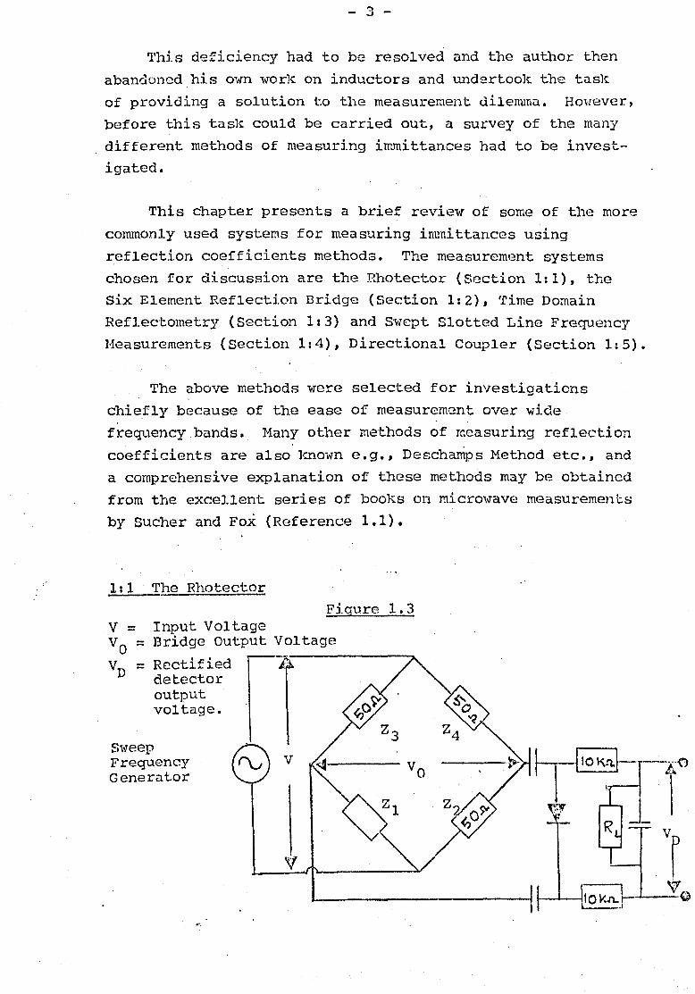
1:1 The Rhotector Figure 1.3
Input Voltage Bridge Output Voltage
Rectified J.. detector output voltage.
Siveep Frequency Generator
v

- 4 -
The Rhotector (ref. 1.2) is a reflection coefficient
measurement device based on the '~heatstone Bridge principle.
Its corifiguration is shown in figure 1.3 where Z3 andZ4 are
equal resis·tances (usually 50 ohms). Zl represents the
impedance to be measured and Z2 is tl")e reference impedance.
l'llicn the bridge is balanced, the bridge output voltage
(Vo) is zero and the detector output voltage (Vn) is also
zero. When the bridge is unbalanced, i.e., ZI f- Z2 an out
put voltage Yo' causes the R.F. diode detector to produce a
voltage YD'
The rhotector is constru.cted with a 50.n. coax.ial
measuring port and is supplied with a kit of 8upp1cmentar.f
coaxial loads having "volt<1ge standing wave ratios (VSHR) of
1.0, 1.5, 2.0, and 3.0. For wide band measurements, a
s.·vleep signal generator is connected tc;> the input terminal s
and the detector output signal is nonnally connected to an
oscilloscope whose time base is synchronized ·to the s"V,Teep
frequency. Z2 is externally terminated with a load of
VSWR = 1 and Val~E.~S of Zl using the calibration st.andards
are used to calibrate the appropriate VS\~R t S on the display
oscilloscope. The device to be measured is then inserted
in place of tl1.e calibration stan9ards and the VS-vR displayed
is interpolated.
Referring to figure 1.3 it is seen tha't provided the
diode detector does not load the bridge networ}.::, then
::. V z, - '7 J z%.~ Z4-Z, +Z~

- 5 -
and since Z3 :: Z4 = Z by construction and if Z2 is chosen
to be Z, then
y'~, \1 +}
· .... 1.1
The above measurements are usually carried out at low
.si.gnal·po"iers (-10 aBm) in ""hieh case the diode detector
characteristics may be assumed to be square la",' i. e, ,
. IDIODE' :: k vin (DIODE') where 1{. == diode constant.
Th!? detector output voltage (VD)
where 1\ :: Diode Load Resistance hence, sUbstitut.ing
in equation 1.1
v~ • • • • • 1.2
If l':---Rl.:.. is defined as K then equation 1.2 becomes
4
· .. , . 1.3
It vrill be shm·m later (equation 2.19) that r == .,'?:.-z.. where r is ca.lled the refle'ction coefficient "Z, +"'Z-

- 6 -
The voltage standing ....... ave ratio (VS\~R) is related to
the reflection coefficient ( " ) by the expression
r= and substituting in equation 1.3 yields
V;p =
• • • • •
Figure .1. 3( a) is constructed b¥ snbs,ti tuting various
valuca of VSNR in equa.t.ion 1.4.
Figure 1. 3{ a.l RE~lati ve Ou.:9:2.ut Vql taqe vs VSNE
~ ~~~ 0> ;I~
~
f.iI 0
fS .. ~ 0 :>
b ~ p 0
f.iI :> H 8 ~ H
~
40
35
30
25 1----
20
*5
10 -
.-, 5
~ o 1.0
. . L ---- --/ .
V
/
/ V
/
I V --
I ,/
1.2 1.4
VSl'lR
1.4

- 7 -
A more detailed analysis of the Rhotector may be found
in reference 1.2.
The rhotector is a relcA.tively simple and useful device
for measuring re~lection coefficients over wide frequency
bands and it is an ideal production test instrument as it
is relatively robust. It 'vas not selected as the main
measurement system because:-
1: Only the modulus of the reflection coefficient is
measured.. Phasor values cannot be obtained.
2: The reflection coefficient measured is dependent on
t.he ac"curacy of the !:lain calibration tes'!:. standards.
3: The reflection ~oefficient measured is directly
proportional to the square of the value of the
input voltage (equation 1.2) and over a ,vide
frequency band of measurement the input vOltage
may vary considerably.
4: The detector output voltage is not linearly
related to the reflection coefficien·t or VSWR
(figure 1.2). Furthermore, this output is subject
to the temperature vagaries of the diode character
istics.
5: The signal applied to the device under test (ZI) is
always less than the generator applied voltage and
could lead to poor signal to noise ratios when low
reflection coefficients are measured.
1:2 The RQ,flp.ction Bridge
Figure 1. 4( a}
The Six Element Reflection Bd.d~
r-----~izol-----~--
V D n
'1 Impedance under test
- 8 -
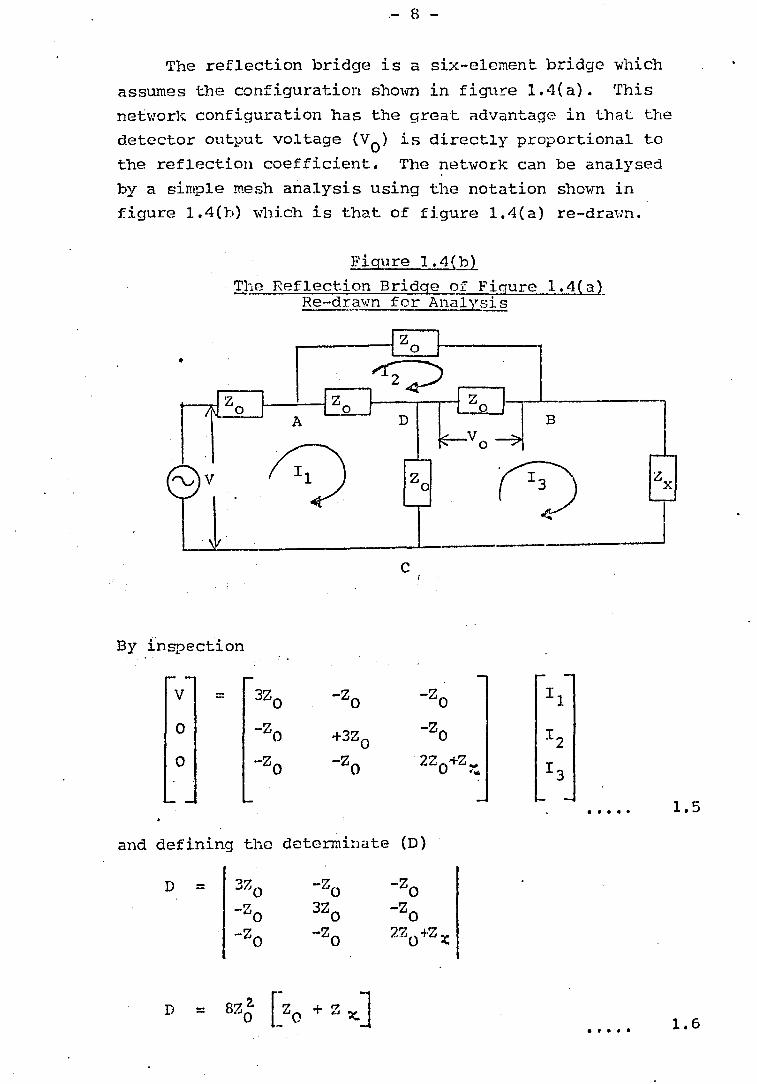
The reflection bridge is a six-element bridge which
assumes the configuration shmm in figu:r-e 1.4(a). This
neb·:orlc configuration has the grea"t advantage in that the detector output voltage (Vo) is directly proportional to
the reflection coefficient. The network can be analysed
by a simple mesh analysis using the notation shown in figure 1.4(b) "i-rhich is that of figure 1.4(a) re-draHn.
By
•
Figure 1. 4(hl
The Reflection Bridge of Fiaure 1.4i.~1 Re-dra\·m for Analysi s
B
c
fnspection
V = 3Z0 -Z 0
-Z 0
0 -ZO +3Z0 -Z
0
0 -Z -z " 220+Z ... 0 0 < ...
• • • • •
and defining the determinate (D)
D =
D =
-z o 3Zo -z o
• • • • •
1.5
1.6

- 9 -
The detector ou·tput voltage (Vn) is
VD
using Cramer's Rule to solve for I2 gives
12 = 3Zo V -Z 0
-Z 0 -z 0
0
. -Zo 0 2"Z{"Z . . _1
• ~ [ 3VZo2 J / I2 + VZOZ OX D
and
I., = 3Z0
-Z ..) 0
.-ZO 3Z0
n
-z . 0 -ZO
• 13 ~ [4 V Zo 2J / D • •
Combining equatiors 1.6, 1.7, 1. [: and 1.9,
or
v 0 = V [z:.c ..,. Z 0]
8 [z.~ + zoJ
v [rJ 8
where r = Z:.:, - Zo --- as shm·m in equation 2. 19. z" + Zo
· .. . . . 1.7
· . . . . 1.8
· . . . . 1.9
••••• 1.10
..... 1.11
..,. 10 -
Hence the output voltage V 0
to the reflection coefficient ~ In;~:recr~ ~ (ReF' l . .3) '~lISIZl>.
is directly proportional
• PA.e","~ 1"" ... 1\, A L\~EAil
The insertion loss of the bridge is high, the out.put
voltage being ~:me eighth of the open circuit generator
voltage or ~ of the voltage that would be delivered by the
generator if it ,,;as correctly terminated by an impedance
Zo in place of the bridge. Thus the insertion loss is 12dB. Practical realisations of the bridge circuit have losses
slightly greater than this. This high insertion loss has
t.he adv·antage that source mismatch error (cectio:1 4 ~ 3) is
reducGd but.it also causes reduced signal level to the
device under test.
The greatest: problem "d th the bridge described is that
aball.:t.n;· must. be provided for the R.F. Source or the detector.
This condition is most difficult. to satisfy where microwave
frequencies operating over several octave bandwidths are
desired. If a crystal detector is placed across the
detector load such as in the Wil tron Autotest.er (reference 1.4)
. the baluns problem is overcon1c but then only the magnitude
of . the reflection coefficient I r I will be obtained and
many of the disadvantages common to the Ehotector (section 1: 1)
'vill be evident. A more detailed analysis of this bridge
may be found ip references 1.3 and 1.4.
This bridge was not favoured for t:hc measurement of
complex reflection coefficients for the' reaSOnf.l discussed in
sections 1: 1 and 112. in spite of its higher directivity.
The problem of directivity errors will be discussed fully in
section 4:2.
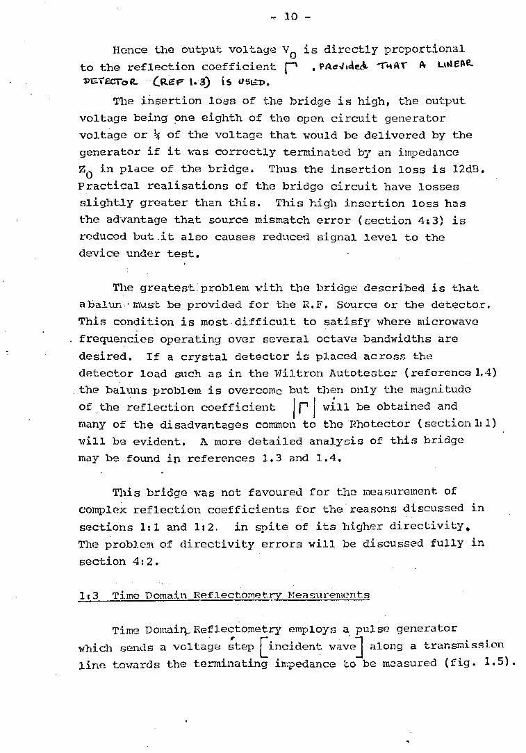
~ Time Domain Rpflectorn.etry Neasurement.~
Time DOmain,. Reflectometry employs a pulse generator , [0 0 .. J 0 0 '\V'hich sends a voltagE! step lncl.dent wave along a tranSlU1581.0n
line tm,mrds the t.erminating impedance to be measured (fig. 1.5).

- 11 -
If the terminating impedance is not matched to the line,
then reflection occurs. Both the incident and reflected
steps are monitored by an oscilloscope at a fixed point.
STEP
Figure 1.5
. Bloc1~ Diagram of a Simple Ti.me Domain Reflectomet£Y SYsts~
OSCILLOSCOPE
fEi BRIDGED
rr UNKNOWN
GENEHATOR TEE IHPEDANCE
--
The following can be deduced from an intelligent
comparison of the incident and reflected ·step waveforms.
11 Any discontinuities in the line can be located by virtue of the propagation velocity of the step
function and the time (measured on th~ time base of the oscilloscope) required for the reflected voltage
to return. This feature is 'extremely usefUl for
locating poor connections etc., within a system.
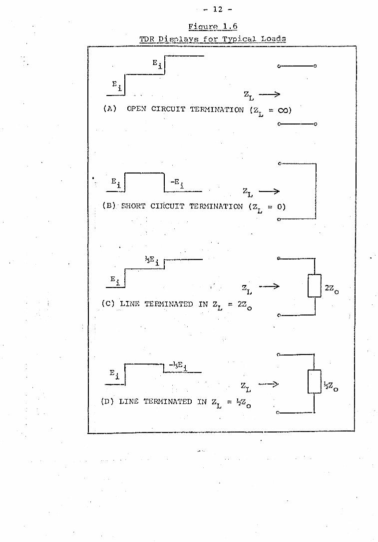
2: The waveform of the reflected wave from any dis-
continuities or terminations is most valuable for it
reveals both the nature and the magnitude of the
mismatched 'termination.· Eight ideal oscilloscope
displays o~ this nature are shown in. figures 1.6 and
1.7. TheEG diagrams have been taken. from reference 1.5. The terminating impedance and/or reflection
coefficients may also be calCUlated using the
expressions 'vi th figure 1.6 and 1.7.
- 12 -
Figur~ 1.6 TDR Displays for Typical~oags
--------------------------. 0.---0
ZL ---:;;.
(P. ) OPEN CIRCUIT TERMINATION (ZL = 00)
~J -E. 1.
0-----0
0----,
> (D) - SHORT CIRCU!'!' TEIDUNA'I'ION (ZL = 0)
o
z --> I ..
(C) LINE TEPJUNATED IN ZL = 2Zo
~. ;_0-
ZL --> (D) LINE TERHINA'l'ED IN ZL = ~'Z 2 0
(";
~z o

(, --
SERIES R-L
- 13 -
Fignre 1.7
Q8cl110sco~p'isplays for Complox Load Im}20danc€s ZL
( R-2 R-l -V) .[. (I + _Q.) + ( I - __ 0) e T
(I R+l R+Z o 0
WHERE T" __ L _ R+£o
~--+.-
t--+ t o
R-l (I + -_OJ E·
R+Z I T 0
z ... · L
I
R
L
R
:In Z-+
L C
0- T

- 14 -
These (-?xprE!ssions may be derived by recalling that the
reflection coefficient (~ ) is given by:
ER E' .. =
1.
••••• (Ref 1.5)
where E R = Reflected Waveform
EI = Incident S·t.ep Waveform
~L = Terminating Impedance
Zo .. Characteristic Impedance of the 'l'ransmission Line.
Assuming Zo is real, it become only a mat.ter of simple substit.ution in the above expression to c~erive the four expressions sho\~n in figure 1.6. The waveforms for figure
1 .. 7 .can be verified by resorting to the use of Laplace Transform i.e., w·riting the expression for \-,( s) in tenns
of the specific ZL for eac~ example (Zr ~ R~sL, l+r
C' etc.) .c;1. ~.... s roul tiplying r( s) by --;;--, the transfonu of a step
Q
function of height. E. I and then transforming this product 1.
back into the time domain to find an exact expression for
ER (t ) .
Time Domain Reflectometry was used in the development
of the test jig shown in figure 1.1.
Time Domain Reflectometry ,.,as not chosen for the main
measurement system because of:
1: Difficulty in measuring "the gradients of the
display waveforms accurately.
2 t N\.:~ltiple reflect.ions in a practical syst.em.
3: Relatively poor rise time of step generator at
that ti.me for high frcqu.cncy wor)t ( 6 GIl ) z
4: Difficulty in observing the waveform accurately,
resulting in relatively poor accuracy.

- 15 -
1:4 Swept Frgg:L2cncy Slotted Line Neasurements
A basic block diagram of hml a slotted line may be used in s"\'lept frequency measurements is shown in figure
1.8.
Fiqure 1.8
Dlock Diagram of VSWR Measurements Using the Sweep Fregvency Slotted Line Method
MODULATED DISPLAY SWEEP FREQUENCY GENERATOR t-------~------~
Time Base
STORAGE OSCILLOSCOPE OR PEN RECORDER
INPUT SENSOR
fTTENUATOR
)......_----1.
~ PROBE
SLOT'rED LINE
Ref. Signal.
Ir . ~ .~mpl. •
,
output . signal in dB
DEVICE ur,mER TES'r
Neasurement j.s relatively easy to carry out. The
frequency generator is set to S'tleep the desired freque:r.cy
band. The device under .test is removed and a power meter
is connected to the output port of the slotted line. The
generator is adjusted until the desired output power e.g.,
adBm is obtained.

- ·16 -
The power meter is removed and replaced by a good
terminaticn e.g., a sliding load. One input (carriage input)
of the differential amplifier is grounded and the other
input (reference input) is adjusted by the attenuator to
I>roduce a sui table output e. g. ,- 25dBm. The carriage input
to the differential amplifier is then re-introduced and the
probe penetration adjusted until the two inputs are equal,
i.e., no output from the differential amplifier. At this
stage, movement of the carriage assembly on the line should
theoretically produce no change in output from the
differential amplifier. In practice slight changes occur
because of an imperfect slotted line and termination. The
.advant:nge of using a differential amplifier lies in the fact
that small changes in input. power do not introduce large
errors in VSWR measurements (reference 1.6). The output of
the amplifier is then connected to a pen recorder or storage
scope whose ordinate axis is initially set at its mid-
. position in order to al1mY' measurement' in ei thc~r direction.
The slotted 'line terminatio!1. is then removed and the device
under tes·t (DUT) is reconnected. The probe carriage on the
slotted line is slid manually to and fro over a distance (d). The distcmce (d) must exceed half an electrical ,-ravelength
of the lO"'lest frequency to be measured. The resultant plot
of a typical set. of measurements is shown in figure 1.9.
Fig~re 1.~
Tl'nJcal VSWRP lot of a $'v~...Qt Slottesl Line Neasurement
-·---,.-----+-------t----T -.----I-----I----+----t-.----t-----t
• IEmax(dB j ~-. '-"K .. -~----.~~
~ }-"--.I\,._n-j-· --:;A..--=:::-..:~~:-..:::::::-=_t-=:..--!:==--: I
~ f·--------~~-------+--------~ ({; i
~' ------~------~ 12 13 14 15 16 17 18
FREQUENCY (GHZ)

- 17 -
The SWR(dB) at a particular frequency is deno·ted by the
distance between El1AX (dB) and EH1N(dB) (figure 1.9) at that particular frequency. The VE:\\fR ratio and hence the magnitude of the reflection coefficient can be calculated
in the usual manner.
A simple e~~lanation of the above procedure can be
obtained by first considering operation at one frequency
only. EMAX
and EMIN of this particular frequency can be obtained by sliding the carriag8 probe along the slotted
line over a distance (d) greater than half a wavelength.
This information will enable the.VSWR to be calculated.
Phase infonnation will only be obtained in the distance
through ",hich a fixed reading t e.g., E ... ..f. has moved is l.111
lcrlOwn when the device under test at the end of the slotted
line has been substituted for a reference ·termination e. g. ,
a short circuit. If the recorder or storage scope is
capable of recording EMAX. and EMIN in dB then since
VSvTR(dB) = 20 log " ~}L~X EMIN
= 20 log IE I Y..AX
I .'
-20 log J ENIN I
it. fo1101'1s that· the d:i.fference between I EMAX(dB) I and
I~HIN(dB) I ,.;rill yi.eld VSWR in dB. If another frequency is chosen, EMAX and EMIN "vi11' occui 'at different points along
the slotted line. For a series of different frequencies
(swept frequencies), the series of EMAX and EMIN will be
locat.ed as the carriage probe is moved slm'11y along the
slott.ed line and their amplitudes will be recorded. Hence
the VSNR at anyone frequency can be obtained. It shoUld
be noted that there is no phase information in this series
of measurements.
An alternative but similar method of carrying out
swept frequency slotted line measurements has also been
described by Hewle·tt P aC.kard in reference 1.7.

·- 18 -
This type of measurement was not selected as the phase'
information cannot be ea.sily obtained in theG(~ swept mear.;ure
l11ents.
1:5 Directional CaU'olers
Directional, Couplers are devices which sample a wave
moving in one direction but not in the other. Such a device can be used to measure the reflected and incident waves in a measurement system and penuit the calculation of the reflection coeffici.ent., The construction ~f a very simple directional coupler is nbm.,rn in figure 1.10 and a simplified circuit sho1'ring the capaci ti ve and mutual inductive coupling and the
irmer conductor of the coaxial line is shown in figure 1.11.
An extensive analysis of the dual directional coupler is carried out in Chapter II. The analysis carried out in
this section is a very approximat2 solution and is based on
that by Carson (reference 1.8) but it does demonstrate the principle of single frequency operation clearly. It also
. explains why the directional coupler "Joan iJ.dcptcd as the main
device for measurement of reflection coefficients and impedances.
Fi!J..ure 1 !.LQ
Ba~ic;:s.onstruct.ion of One Type of Directional C01.lPl er
-r--' R <
,..-----\ - - -
Loop coupled to Inner Conductor
LINE

- 19 -
F:i,oure 1,11
Simplified Circuit Sho11T.ing Capaci ti ve and Nutua1 Inductive Coupling Between the loop and Inner Conductor of a CoaxiC!l IJine Coupler,
OUTER CONDUCTOR
-~ VR
Output Input Jc L + V n n End k-VL-~ C
End
M
INNER ---1 CONDUCTOR
I
By inspection of figure 1.11, it can be seen that
R
V ;-~'-,-L JWc
=
If R /<,.1- then VR
A...J jw CRY "", JWc • • • • •
Current I in the inner conductor induces VL in the loop.
Thus,
• • • • •
The output volt~ge . ~s
Vo - V - R + vL = jw CHV -jw MI • • • • •
If the coupler is designed such that
_tL CR = HO • • • • •
1 •• 12
1.13
1.14
1.15

- 20 -
-\-.. here RO = characteristic resistance of the coaxial line,
then equation 1.14 becomes
vo = jw M ( __ Y-- - I) RO
The voltage and current decomposition equations are
v = V· J. + Vr · . . . . V. Vr
and I I· Ir J.
'= - = ). RO 1\0 • • • • •
where the subscripts i and r represent the incident and reflected directions.- Thus equation 1.16 becomes
v. + V V 0 = j vtM (- l. HO r
• • • • •
1.16
1.17
1.1:7(a)
1.18
Therefore the output voltage is proportional to the
reflected phasor current (or phasor voltage) because the incident components cancel when the coupler is connected as
sho'Ym in figure 1.ll. If the coupler is reversed, its out-
put voltage is proportional to the incident phasor current
and the reflected components cancel. In many caSE~S, it is
not convenient to keep reversIng the coupler, and dual
directional couplers, one to measure the incident wave and
the ot.her to measure the reflected "lave are used. A reflect
ometer is a dual direc'cional coupler specially manufactured
for good amplitude and. phase coupl:i.ng match over C\ wide
frccJ,lency band of operation.' Reflectometer design is
complicated. Hanrey (rE':-ference 1.10) offers a good bibliography
on the subject.

- 21 -
In practice, the directional effect is not perfect and
leads to a tl'Pe of error called "Directivity Error".
Directivity Error is investigated extensively in Chapter IV. However in spite of the errors associated with reflecto
meter measurements, this method was chosen as the most suitable because~
1: The reflectometer method provides a quick and easy
method of measuring reflection coefficient and hence
impedances if the reference impedance is well defined.
2& Swept frequency measurements a~e easily carried out.
3: The reflected and incident measurements carried out
yield both amplitude and phase information. See
equati.on 1.18 where Ir. is a phasor quantity •
. 4: Error correction systems are relatively easy to
incorporate.
5: The signal loss bet"\veen the' S\veep frequency signal generator and the device to be measured can be Ie sa
tha.n IdB. Thus low-pow'er signal generators can be used or alternatively larger powers can be fed to
devices such as transistors if desired. ~
6: The sampling loss associated with the incident and
reflected waves can be easily controlled in the
initial design of the reflectometer. A commonly
used coupling factor is 20dB nominally.
rrhe necessity for new rapid and computer correction
systems has been established in the early par-t of this
chapter. The latter p~rt of this chapter has presented a brief review of some of the various methods of measuring reflf~ction coefficients rapidly. Each of the methods

- 22 -
investigated has several desirable properties. The Rhotector
and the \AI il tron Auto tester are ideal production test·
instrUtltents, robust and simple to use for rapid magnitude
measurements of reflection coefficients. Time Domain
Reflectome·try locates discontinuities rapidly and Loeb
(reference 1.9) and his team have used it most successfully
in the measurement of lumped components. The Swept Slotted
Line }feasurements Technique, although relatively accurate
does not provide phase information. The Directional Coupler
provides both amplitude and phase information rapidly and
does not suffe.r from the haluns and higher loss problems
associated wi-th the reflection bridge. Herlce, the Directional
Coupler was- selected as the basis for the measurement system.
'l'he remuining chapters will be devot.ed -to the application
and error correction methods published by the author for the
measurement of reflection coefficients and immittances using
reflectometers.
* * * * * * * * * *

- 23 -
References
1.1 Sucher; H and Fox, J; "HandbooJc of Microwave Neasurements" 3rd Edition, Volumes I, II, III, John vliley & Sons J.Jtd., London.
1.2 Te10nic Engineering Co "FHO-Tector VS~~R Detector" Application Bulletin 301.
1.3 Oldfield, W. 11. "P resent-Day S:i.mplici t.y in Broadband SWR Measurements" l'liltron Technical Review Vol 1, No 1, 930 Meadow Drive Palo Alto, Ca.
1.4 Dunwoodie, D, & Lacy, P "Why Tolerate Unnecessary Measurement Errors?" Wiltron Technical Review No 5 Harch 1975. 930 Meadow Drive, Palo Alto, Ca.
1.5 Hewlett Packard Application Note 62 "Time Domain Reflectometry" Hevllett Packard Ltd., 1501 P age Hill Road, Palo Alto, Ca.
1 ~ 6 1'?einsche1, B "M8asurement of Hicrowave Parameters by the Ratio Method" Publication by Weinschel
- Engineering, Gaithersburg, Hd, U. S.A.
1.7 Hewlett Packard Application Not.e 183 "High Frequency Swept Heasurements" Hewlett Packard Ltd., 1510 Page
_ Mill Road, Palo Alto, Ca, U.S.A.
1.8 Carson, R. S. "High Frequency -J~mplifiers" JOfm Wiley &.Sons 1975.
1.9 Loeb, H "Private Visit to Cranfield Institute of Technology" Bedfordshire.
1.10 Hal."'Vey, A. F. "Nicrmmve Engineering" Academic Press, London 1963.
* * * * * * * * * *

- 24 -
CHAPTER II ----_ .. _----,
TIm THEORY of the MEASURING SYSTEH
The correct:. choice of a measurement system must ultimately
depend on 'the type of mea suremen't required and on the financial
resources av'ailable. Various measuring systems 'Were considered
for the rapid measurement of reflection coefficients. Among
the systems investigated ''1ere the Rhotector (section 1: 1), the
Reflection Bridge (Section 1:2), Time Domain Reflectometry
(Section 1: 3) and Sv.Tep't Slo'cted Line H,easurements (Section 1: 4).
The advantages and disadvantages of each ,system has been
discussed extensively in Chapter I and only a brief sUlnmary is
necessary here. Time Domain Reflectometry (TDR) is ideal for
physically locating a discontinuity with a system. In fact, it
was used extens~velY for that purpose in the ~inal measurement
system. Single frequency or swept frequency slotted lIne
measurements provide accurate results but the measurement met.hod
is extremely tedious and time consuming.
The Rhotector, Reflection Bridge and the D,ual IJirectional
Coupler (reflectometer) certainly excel as rapid wide band
reflection coefficient measurement.:, systems. The first two are
variants of the l'lheatstone Bridge' Principle. with the
Rhotector and the Reflection Bridge, the signal l~vel available
for test is inhe'rently 12 dB less than the applied level from
the signal generator and this could result in poorer signal to
noise ratios vThen large return losses are measured. Dual
Directional Couplers (Reflectometers) may be constructed to
have 10\'1 inherent ,losses~ which means that the difference
betwe2n t,ne signal level available for test purposes and that
available from the signal generator could be less thaI:. 1 dB.

- 25 -
Commercial wide frequency band coa..· .. dal directional couplers
have relatively poor directivity characteristics 'When compared
"ivi th bridgp.s and.. "i-taveguide directional couplers. 1 ... t the
commencement of this investigation, wide frequency band,
coaxial couplers with a directivity ratio of more than 30 db
"ivere not generally available. HO"i'lever, commercial coaxial
couplers (Ref 2.1) with greater than 50 db directivity ratios
are now common. After much deliberation and discussion, the
reflectometer method of measurement using dual directional
couplers 'las finally chosen as the desired measurement system.
This chapter will be devoted ·to the theoretical aspects of such a.measurement system.
A brief summary of fundamentals concerning the measure
ment system is presented in Sections 2:1 and 2:2. A more
detailed analysis can be found in any text book (Ref 2.15,
2.16, 2.17). However, the .above :sections are required to
establish the foundations for the analysis of Section 2:3
v;hich has not been presented elsewhere. section 2: 4 analyses
the problems associated with the measurement of incident and
reflected powers and the errors resulting from it. This is
an adaption of an analysis carried out by Warner (Ref 2.8 ).
2: 1 The The~?ty of Reflectometer Heas:LH·~.!: ..
The use of reflectometers for measuring the incident (a)
and reflectc9 wave (b) has been described by many authors,
e.g., Hunton and Pappas (Ref 2.4) and Engen and Beatty (Hef 2.5).
'In this 'rhesis, the incident wave (a i ) and the reflected "i'lave
(b i ) '1ith. respect to the ni" th pQrt are defined in the manner
described in detoil by Warner (Ref 2.8 - Appendix 1).

a 0<. a 1
- 26 -
Figure 2.1
~~'i;i.mpl§'.:-Ref lect"o~5? .. ter ~stem
Al1PLITUDE/PHASE i J-- J COHPARATOR -<E~TECTOR
b l ><4 a( incident) ..r ~ b(refl)
COUPLERS " "" /"" , G~KNOW~ --0 Op1\TE
t~_..;:.O ..... R..;:.T __ 1
,-------0,-------------
In its simplest fona, the reflectometer measures a portion
( a 1 ) of the inciden"t wave (ai) and a portion (bl) of the
reflected wave (bi ) a"t a specified plane in a syst(~m. For the
system to function correctly, it is es::-mntial to establish
thai~ there is no mutual interaction bet.ween the incident and . "
reflected power flow w"hen the ~vave impedance (Zw) is real.
Hence some fundamental concepts ,vill inevitably have to be
reviewed.
Propagation conducting, homogeneous
F i 9.1!r? __ ?...:1. of a TEIO mode wave in a perfectly infini tely long T;l~ve guide '-lith a loss free dielectri.~c:..!.. ______ _
Longit.udinal the magnetic
component of ~ field _~ ~ .. <: ~~
~~
A
. t ~2 j E3
B ~1 ~ l... A' : p
t\E = ~2 Ft ~ ~
tOl t/metn;'~I3 ~"...----- Direct.ion of
"~ ,. T-l ~l~ 0 .r"" propagation 0'= .... x H
B'
.1H ::: amps/metre

- 27 -
Consider the propaga·U.on of electro-magnetic energy
(Fig 2.2) in a mediu ... rn bound(~d by AJ."\I BBI e.g., an infinitely
long wave guide. 'The modes of ,.,ave discussed "Jill be limited
to those modes which possess transverSl~ components of both
electric and magnetic fields i.e., 'l'EM, TE or TH ,.,aves.
since Jche longitudinal component of the field may alvays be
found if the transverse components are known, there is no
need.to retain the former explicitly in theory. In fact, for
convenience, it vril1 suffice to· "TOrJ~ entirely in terms of
the transversa components of the electric and magnetic field
strengths dc:motcd respectively by the symbol s E and H. Both
these quanti·ties, E and II vary over the cross-section of the
transmission system but because the spatial distribution is
the same in each case (Fig 2.2), their ratios E3 = E2 = El IT} HZ lTf
remains unchanged. Schelkunoff (Refs 2 .2; 2.3) recogni sed
"t:his important generalization and introduced the concept of
wave impedance (Zw) which is the ratio of these field
strengths so that at a given point along' the guide, '-le have
in general:
Zw = E tl- • • • • • 2.1
where Zw impedance . ohms· = 1.n
E = volts per metre
H .- amperes per metre.
When the wave guide is not infinitely long or perfectly'
terminated, then the total transverse electric field (E) at
any point will consist of incident and reflected parts. Each
of these parts must, of course, be compounded of the transverse
electric field 'components of all waves travelling in the
appropriate direction. The same arguemetl:. may be applied to
the r.!agnetic field (H)
equations belovl apply,
E
II
at a . ~. e. ,
=
=
given
E+ +
H+ +
point. Hence t.he two
E • • • • • 2.2
H • • • • • 2.3

- 28 -
wherG the plus ~mperscript denotes an incident ,,,ave (direction
OP in Fig 2.2) and the minus superscript denotes a reflected
wave (direction PO in Fig 2.2). For this case, the iolave
impedance (Zw) is then. defined as:
Zw :::: E+ H-F • •••• 2.1(a)
or
Ziv :::: -E H- • • • • • 2.1(b)
substit.ution of .equations 2.1(a) and 2.1(b) into equation 2.3
will ~-8sul tin:
H • • • • • 2.4
If the symbols € and X are used to represent the
instantan8ou's values of the complex quanti ties E and H for a
sinusoidal time variation, then:
Re Ee.~"~ Re He iswi:- ,
and writing equ.ations 2.2, 2.3 and 2.4 in il1stantaneous
values will result in:
e s+ -:::: + E. • • • • •
g, + 'lIt-=: ~ + .~ • • • • •
'{ = £+ e:.: Zw Z\f • ••••
2.2 ( a)
2.3(a)
2.4{a)
The instantaneous pO\Ver. flux or poynting Vector, p." is
given by R = E x H. As "He have defined E and?( as the
transverse components, w'hich are at right angles, then P :::: E.l}i ,\ .... here P is in the longintudinal direction so that:
P :::: (r+ .- -) _\.~"-__ - __ C:: ..
Z~I

p
or
P
P
v7hi~h . the desired loS
=
= E+
= p+
result.
- 29 -
J.+ 1
P
(f~-) 2
Zvl
<c.- H -
• • • • •
The reflection coefficient (r) is defined as the complex r.<?-ot.:to of the reflected to 0 incident wave at any
specified point along the ~xis of propagation (Fig ~l).
2.5
On the basis of this definition, it. follows that there
are two alternative ratios which can be used, because the
coefficient may be expressed either in terms of the electric
or mclgnetic field. The former definition yields:
EE+ • • • • • 2.6
"There rc: = .. Electric Reflection Coefficient and as before E+ - Incident Electric Field E- = Reflected Electric Field.
The latter definition yields:
· , . . . 2.7
where Magnetic Reflection Coefficient and as before
Irlcident Nagnet.ic Field
Reflected Magnetic Field
Ei ther of the defini t:iOl1S of 2.6 or 2.7 may be used.
lImvever, as it is more convc~nient t.o measure the electric
</. fielct the definition of 2.6 will b(~ used throughout this
Thebis. Henceforth, all refl0.ction coefficients will be

- 30 -
assumed to be with respect to the electric field unless other
\d se sta ted.
At this stage, it ¥Jould be best to refer to Fig 2.2 once , +, " ,
agal.n. If Eo l.S the l.ncldent wave at 0, then at any pOl.nt
P, distant "t" to the right of 0 in the direction of
propa.gation, t.he elecmc field Ep + is given by:
E + p :: E + o
e -pl
where the propagation constant (1))=. 0{ -+ JP
• • • • •
0{ :: the attenuation constz.nt (Nepers/Hetres)
f3 = the phase constant (Radians/Hetre).
-
2.8
and
and
c!' 'I 1 ... ,l.ml. a.r y if E 0
is the value of the reflected "rave at 0, then E - point is given by: at the P p
E = Eo +pl e 2.9 p • • • • •
The nomencla·ture "incident" . ~nd "reflected" assumes the
,\-rave source to be somewhere to the left of "0" and the point
of reflection some\vhere to the' right of P. Equation 2.8 is
merely a mathematical statement of the well-known fact that -~t ' the field at P~ suffers attenuation by a factor e and lags
pi!. radians' on the field at 0 for an incident '\-rave. Equation
2.9 is merely a mathematical statement of the same? argument
for a reflected wave.
Similarly for t.be magnetic field, ,\"e have:
II + p
II P
=
=
HO+ e -pI
p - e+p1 "0
• • • • • 2.10
• • • • • 2.11
Hence the resultant transverse, electric and magnetic
fields .at any point P rnay be expressf:>d in terms of the values
of their forward and back'\-rard travelling components at the

-. 31 -
point Os thus:
E E -}- -pl
E +pl = e - + p 0 0 e • • • • • 2.12
11 Ho + -pI
Ho - e +pl = e + p · . . . . 2.13
-Defining r E
= 0
E+ 0 • • • • • 2.14
.~ H -and = -2-
Ho+ • • • • • 2.15
then from equations 2.l(a) and 2.1(b),r =-~ · . . ., . 2.16
Division of equation 2.12 by 2.13 and using the substitutions
of 2.14, 2.15 and 2.16 gives:
E = E+ --R 0
H P
H~ ·0 • • • • •
If Schellcunoff' s definition in equation 2.1 is substituted:
z'- 1 + r e. +2pl
r e,.+2pl • • • • •
2.17
2.18
The above stat.ement is general. Z t.. signifies the vrave
impedance at any arbitrary point point P, situated a distance
liD.." from the reference point 0 (Fig 2.2) Zw is the character
istic wave impedance of the line.
If constraints are placed on the line length to ma]ce
t = 0, equation 2.18 reduces t.o another 'veIl-known expression:
Z L- = Z (I + r ) ...]L ____ _
(1 - r ) • • • • • 2.18(a)
, or

- 32 -
r = z '-Z L
• • • It • 2.19
Equation 2. 19 is the very important relationship ,-rhich
forms the basis of these measurements. It follmvs that if
the characteristic impedance Z can be accurately defined w
then measuring the complex quantityr; will allo", Z L. to be
evaluated.
In practice, it is not always possible to measure a
reflection coefficient,ro directly at the point 0 (Fig 2.3) . . , . 'and J.ll most cases, J.t J.S customary to place the measuring
device at any point ou separat.ed from the measuring plane
AB by a distance i' 'e' The relationship between the desired
reflection coefficient (~ ) at point 0 and tbat ( r ) measured at point 0" will be derived.
Figure 2.3
Relationship's bet-~lcen Reflection Coefficients
A" A G
4 t t> r 0" 0 1:; ,. "
o~--··-------------------B" B
LGt E + and Eo represent the incident and reflected o
,,,aves at AB. Let E+';' and E - 'I represent the incident and o 0 reflected '\~~aves respectively on the plane A" B" of Fig 2.3.
Using the basic equations of 2.8, 2.9 and 2.14 it follmvs
that:
=
or
E -...JL E + a
=
," ~
"'1, ~ Eo e... . E +" -f~ o e
r = ., .. , I I' -~.~
<:> e
= • • • • •
• • • • •
2.20
2. 21

- 33 -
Being complex, the reflection coefficients .r and ~ may
be written as jr jeSf and I~ \c!t.:. respec·t.ively ,{here 1) and CPo represent the angle in radians. substitution in 2.21 results
in:
I I.; .l ; ,/. -.z ~ l . I fi.!. .< 3e: r e. 'r ~ \~ Ie 10 e r = r~ I e t ~.Ju e 2,.0( i d I
I rll9'>= [i ~ I e.-0at] e j. (¢o -2.1'12:) • • • • •
From which it is easily seen that the modulus of the
measured reflection coefficient i's att:enuat.ed by a factor n~ .
2 ex x... from the,true modulus, Vlhi1st the angle of the
2.22
measured reflection coefficient is modified by t.he difference
2 I~ from the true angle •
. 2.3 Di.rectiona1 Couplers
:Hany papers (Ref 2.4, 2.5, 2.6, 2.13, '2.14, 2.15) have
. been published on directional co~p1ers. Harvey (Ref 2.16) ,
gives an extensive list of references. In its basic form
(Fig 2.4) 'a single directional coupler is essentially a 4
port network with one port ideally matched. It has been
shown (Ref 2.15 that such a net'\vork manifests 'directiona1
properties. For example, if Port 3' is terminated, then it
is theoretically possible to arrange for Port 4 t.o sample
power travelling in the direction from Port 1 to Port 2' but
not vice-versa.
port 4
port 1
Figure 2.4
Sinqle alld Dual Directional Couplers
u---Dual Directional Coupler--;".
:- - - --~-" - - - 'A~1'v - - - - - -: 3
0..... ',_ ,_ _ _ _ _ _I 3' 4' _ _ ____ ..1 J P Port TC=--_. I --~
I I I '. " T ' I I I I .u1ne I . -0 o 0- 0 . ~ Port 2 Ii. J" I • i ," i I . Slng .. e 2' 1 I 5 7ng1G. Ii I'Direct.ional l I Dl.rectl.onal 'i II Coupler I I Coupler 'I t I' 1 , II 1 II , __ ._ --I ----.---~II ____________ ,...----;:0---

- 34 -
In a practical reflectometer systems, two directional
coup1 ers are required, on(~ to sample the inciden·t "Jave and
the other to sampl(:! the reflected wave. The use of . two
separate couplers joined by a connecting line is undesirable
because of mis-matches between the units. Difficulty is experienced with attaining amplitude and phase tracking.
To alleviate these undesirable effects, manufacturers tend
to offer dual directional couplers units for 1vhich claims
arc made that the internal couplers are matched for amplitude and phase.
A dual direc·tional coupler may be analysed as a four
port netvrorlc (Fig 2.4) vli th the general scattering matrix of eq~ation 2.23.
identified by a subscript where ','n" denot.es the port number.
In the diagram of figure 2.4(a), port 1 is the main input
port (i. e. connected to the signal source). Port 2 is the
main output port. Ports 3 and 4 are intended for sampling
the reflected and incident waves respectively. H3 and 1-14.
are the indica·ted sampled reflected and incident pOlvers 1vi th
the incorporated conversion const.ants.

Samples t-i <11_
Incident POIver
Source
- 35 --
. Fiqnre 2 .4( al Signc.l Flow G.r-aph of a Dual __ ..:::D:;...:irect:is:mal G.oupler
C = Desired coupling paths CD = Back coupling paths
Load
Tbe F0;l'lvard ~.9uRling Patq (C) I is' the desired signal path
from one por~ to another •. These are 8 41 for port 1 to port 4
and 8 32 for port 2 to 3.
!.11g--1}_~.£.1~ CQllPlj..ng P_~IJ:}lf1 (CD ) I are the undesired signal paths
to a particular port. The paths are 542 for por·t. 4 and 531
for port 3.
'The Traqsmission Pa·ths ('1'), are the main signal propagation
paths.' These are S21 and 512 for the main signal paths
between port.s 1 and 2.

!
- 36 -
Incident POvler to Port 1
Incident PO·v:er to Port 4
· . . . . 2.24
Direct:i vi ty Fact.or (DIE1=10 log r POv:er to Port 4
POi'lCr to Port 3
· . . . . 2.25
w'hen port 2 is perfectly matched.
For the case of the ideal dual directional coupler, it
is ass1.~med that there, are no undesirable coupling pcl.ths and
that the signal source,' coupler and detectors are perfectly
matched. For such a 'system, Figure 2.4 may be considerably
simplified and reduced to that s1'1own in Figure 2.5 "there
and .b4 :":: S41Q;,) 'b.3= S2.\S32..~Q..1
b3 = £.21 S.~?. ~ b4- S4'
is independent. of CV1
Figure 2.~
Signal Flow Graph of the Ideal Dual Directional Coupler
_-",-",-,;;~..:.o- ___ • • .---____ _
· . . . . 2.26
Perfect Detectors are assumed.
(c)

- 37 -
Equation 2.26 states that the ratio of
Sampled Reflected Power = is directly proportional
Sampled Incident Pm.,rer
to the unknown reflection coefficient of the load. The
constant of proportionality is the factor
For the more practical case of fini te coupler directi vi ty
and reflection coefficient, .let us first assume that the
detectors are perfectly matched, i. e., no pOvler is incident
on a 3 and a4 Figure 2.4 may then be reduced to Fig 2.6.
' ..
e
Legenq:
figure 2.~
The Dual Directional Coupler with Perfectly Hatched De.te~t;ore __
/ 1'13
/
C)
Direct Transmission Path (T)
Back Coupling Path (CD)
Coupler VSt'm
Forward Coupling Path (C)

- 30 -
By Inspe~t:.ion of the signal flow
Q'Z, ::: ~. ( S 210." of· S 2,2.. Q,;:,. ) or Q.2..=
• • •
\ :::.
, D4 •
. . b 4 +
Hence,
Indicated Reflected Pm\'er (M3)
Indicated Incid~nt POyo'er (M4)
= $2.\ 5 32 C
5 41.
graph, it is seen that
S..:l,iQ Cr.",
l- SZ2. rz
=
• • • • • 2.27
comparison of the ideal case (equation 2.26) and the
more practical case (equation 2.27) show that the latter
differs by the ratio of the error terms within the bracJ~ets.
This leads to the conclusions that for accurate measurement,
522 1 531 cmd 842 should be zero. These are partially met by
making the maJ,n line VSWR (522) as 1m" as -possible and by
careful spacing of the two couplers, usually a quarter wave-
1eng,th apart. This latter condition is not easily met in
wide band couplers.

- 3~ -
The complexity of the analysis of the dual directional
coupler increases for the really practical case where it can no longer be assmned that the detectors are perfectly
matched i. e. I pO'YTer is incident on 013
and a4
"\vi thin the system.
Consider again the signal flow graph of figure 2.4; inspection,
by
0", = e·+ I; b, = e 0 0 0 -t l-h~ 0 0 0
Ctz \: "'2., 0 0 0 0 o .~b1.0 0
Q3 Gb3 0 0 0 0 0 o f;h; 0
Q,4- r; b'f- 0 0 0 0 0 0 o rtt14.
. . . . . 2.28
Substitution'Qf·2.28 irito 2.23 gives:
b, ~ ~" 5,.,! S~ SI4- e 0 0 0 + Sll S'Z S,,; Slit 'Bb. 0 0 0
bi!. cf C; <:" <:" 0 0 0 0 C! $)2. Sz; SUt o ~~zo 0 ... l~1 .. l:!. .. ,~~ "'24 "');'.1
b.iI
~ 5.32. S33- S* 0 0 0 0 • SSI S~l.. 5n, Syt 0 o r.ib3 o ;,
b"f- S,l 8.tz c S~+ 0 0 0 0 S .. ~l
c ~ 0 0 of),
"~-i3 • It-! 9-+3 4
.. DI l 0 0 0 . b, ~ fs I,e + S \I Pc. S 12. tz. C! ,.., , s\'+G·
• l1 .:;11.;'3
0.· 0 0 "'2, SZle c! \-' S,17 .. t: Co P Sklr.' D.t .. Ill & "'23 J Ii
0 0 0 b,3 lS~le c! S32C C! r' C! f1 b.~ "'3,q' .:;I.:J1J .:;I;'t 4·
0 0 0 b oi·• 8.--tl e S~i-I~ S/t2.r.: ~T3G S44i' b'1-' 4
Sile = (Sll~-J) SI2.~ S131; S I4-C; b'l C! ~2.\~ Szz12-1 S'2,;r; Sz.;.f+ b2,. ")'2,1 e S~le 5;\ fa S32~ 8 3:;11-1 S.;4~ bJ _b: Co e c! n C! r C" {.-, S4Ar:-1 "'41 .:;1"+1 IS oJ4 Z L. ":1; 3 .,.
. . . . . . 2.29

- 40 -
For the ratio b ~ / 64 , using Cramers rule:
-e (S\\S'-I) c' r. .. 11'2. 1- s" S14~
b3 s~\~ (S~:(f2-I') S 2.1 S?4£; :::
b4 S~I 11 S~'2.12 S31 S34-G_ e \:' S41.(' 0 (S4A~.-I) '-':>4\ 2 "" 41
---e (~-;\I~-I) SI'2.~ S I?>r; c.'
.-.:> 1\.
C' I; .:12,1 '" 0' (Sn\Z-i) S'Z~ G c
"'7-1
8.:;, fi o [' 1:>32- I- (S;;::. 1;'-1) S31 e ,\' ":'4\ ~ S42~ S4-3 G C!
I:> 41
Simplification m.ay be' obtained by lr1ul tiplying t.he 3rd and 4th .' . h d d' r-' columns respectJ..vely J..n t e numerat~or an. enoJnJ..nator by 1%
and substracting them from their respective column 1 to yleld:
(S221"2-1) 8,2.1 C! C i:.> 2.~ A .
. 83~~ 8 3\ 8.3,,-t;
b3 C! r. ":~2 L.
0 ~4.' (E'4./.J~'-/)
-- :::
b1- (822 ~-I) o ,.., 1:>2.!:. 3 'S '2.1
83.2 f2. (S:;;,r3- I) 82,1
842 r;: S4'?>f3 S4-1
• • • • • 2.30
'livhich 1¥hen expanded will result in:
_ ($nr;:,..\)~(~!>IS44 .s34S4J-S.Jl-S2g~(S.3~$4i~~2~)+S:l~+ S24\~~iZ\J -Sol S.~J --""---'--- .. -- --- ---,~-= ......... , .... G;7.,'GIi'.- \)~{St,;,S .. u -S_~l ~~,.~).-s.;J+ S ~\ It:. G~(5~zSll-:,-S::?"\-2>~]+S2.3 G ~ ~~l ~"'~2.-.:.~,,!~J
. .. . . . 2.31

- 41 -
Equations 2.26 and 2.27 may also be obtained from equation
2 31 b k · t" . t' A' t t d tl • Y rna 1n9 i1C prev10us SUPPOS1- ~ons. s 1 s an os, - 1e
equa.tion does not prescn-t a very clear picture of what is
happenin~. However, by expanding the expression and by
judicious collection of the t.erms, some conclusions w-ill be
found.
..
II 'I) I '3
J.l .. ;..l
;-'1 r1)
V) I
- _ l ('I l'"
V)
IL !._...J 1 __ ! '. \j-
\/1
iI
r';l c-.J ..-n
IJ) I Y I -q' n ! \..n
VI I
II I
~I ...... _D 1 _.0
N
('\1
\.j)
N . N
o .p
OJ ..0
o {/)
... -1 III
r..: ro u
..
~I

43
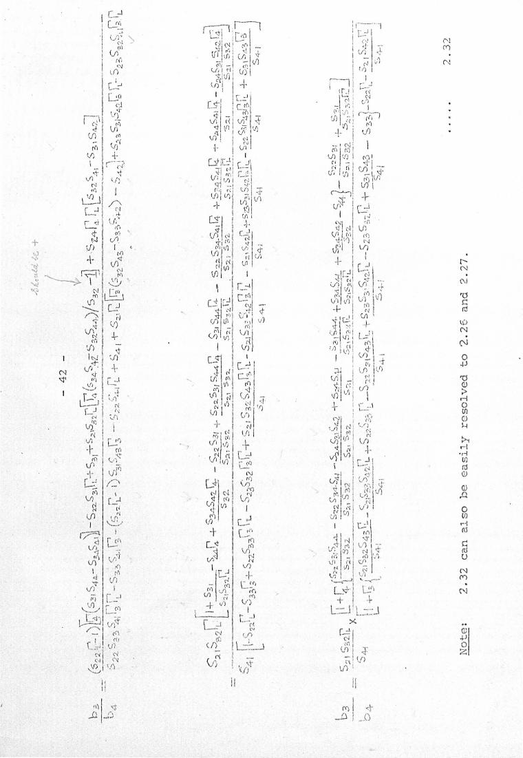
Eql.:tation 2.32 may also be ,"lri tten in t he for:;.-n :
63
b4-
Let
r <.. ( - " C; r \:1, <:::. c: r fI r r -I-r' S r r -s s r n. S S ~ n) _ (' r ~ lI ) r rS _.~ r f' .; ,.. \l}. _ l~2\·>'~2. ' .2132;:)44- 4 -r -21 ..J34~4:>-'4- - ~22.."::>=., · :::<;z 31~44 4- 27.. ~')4\ 1 4-""'" ~ 3'2.~4- ! 4 ~.;l.4.J '>\~L" • .'~\ L~ JII.-+131 ~~I:::>44I4- + .34-~II4- . - r -----
) -5 ~ +S c ~ if r 5 ,... Ii S c:: l' r · ~ r r> n L sec c n c> S S· r::"'! \1 L... S f: \:-1 . c: . -::: n i L 224{ v ."'3,Y4h, -~13 ?".?~4i '3 +- ~"":,'2...J4313 -:::'21~3S:>+L 13 - '::> 2 1 4.2 -\- .- 2.3 .... .31 J..:..2 1.3 - J :n. 3 \ 4:' 3 .5 · !.... -\- t'Lq - ::.3. 4\ 3 .. ~ 3\ -·4-~'3 ... T
b~ b 4 ..
~/
= frm... .. i.e. the measured reflection coefficient~ ·then
r Al L + B
,...-, C \L +- D 2.33
1-f:l'1ere
A
B
c
D
== f. t' _ C' S S \1 ,... .-, _ C" ·r.l-. r " C r-l\ S s;, r '-'\ , C' ' c -\1 _ C S rt ! l..S Z-i '::>3'2. ::>21 32 44 14+S:2.I~.?A.-S4.'2. \ G... ..)L2~SI· '::-'~'2..~::' i::'>4A4 - .n34-.J4-\++ ::>2.4-~~?..~~"4- '"'..<43; I4-J
~ . n 'c:: r-- (11 = {S3! - ;:)3 1 S44l4- -t- ~ 3+ ':>4! ·-4"J
=
( .. \ r r C (- <: S S"· r r S \i .s ~ (' i' - <: ~ -!- c S S 1'0\ '? c Sri L $.:l.~541 "" ::'~:<.:::>33 " '.~}3 - ·-'2;:' 37 .. ~ \ \3 -t- ~Z.I :>.?, t( ~:,13 - 2 \ 33-"'J-L:3. - 2\ 4-'2. ::>~:, 31 4-?_ 3 - :::').:t":Z ~'3 \ 4'3 3)
(5 ~ ,, 11 S-i) 1. 41 ~ " 3? "::>4/:- -;- S3 1 43 \ ~ .'r
. .. ~ ...
2.33(a)
2. 33(b)
2 .33(c)
2 . 33(d)

_. 44 ..
Equation 2.33 io vitally important bcc<:;,use:
(1)
( 2)
I't ShovTS that the measured reflection coefficient
. II' t rwv" is related to the true C by a bilinear
transformation (Appendix ll.l).
The const.ants of a passive bilinear. transformation,
A, B, C, D, may be obtained by three meaS'J.rement:s
(Ref 2.17). It is unnecessary to ]U10W the
individu~l IS' parameters but the scattering
parameters may be calculated by use of Appendix 11.2.
(3) If th(~ constants A, B, C, D of the bilinear trans
formation are kno,m. then f2 may be calculated.
(Fig 2.7).
(4) Item 3 is of the utmost importance for it clearly
demonstrates that an imperfect. dual 'directional
coupler used ,vi th un--mat.ched detectors may be us~x1
to yield the true measurement of a reflection
coefficient 'if the constants of item 2 are knmm.
Thl1LJs the basis of Compute):" _g0f.~ted !-,lea.§l:!.:r..9.!.!!5lnt . .,§
in One Port Reflection Measuremcnts.
Fiaure 2.7 I __ ._
---7 O-___ ...,.... __ ---.->~-_-.__r--I- ' __ -.
.1 Heasured I f... Reflection
('Y'r\..- Coefficient I I
I
I
C!
""21
8 12 • ..J ---< __ ..... _.-.. ____ .. _ p ~
I --'"
Bilinear Transformatiori
rrrue Refleci:ion Coefficient

- 45 -
2:4 The Neasurcment. Unc0rtdj.n~..9f Inci~ent and Reflected Power
In the foregoing section (2.3) analyses have been made of the process of identifying the incident and the reflected
waves. This section expounds the problems associated with
the measurement of the incident and reflected waves in
coaxial couplers.
For these purposes, the incident ( a. ) and the reflected 1-
( b i ). complex voltage wave amplit.udes are normalized with
respecJ: to the real characteristic impedance (z ) * in the o
manner defined by i'larner (Hef 2.8).
Hencp:
kLd'l. = PI. '7 "-0 • • • • • 2.34
M = Pr 70
I. t • • • •
PI· where _ = incident. pOl·ler. and p~. _ reflected power
* The effect of conductor resi stance on t.he character
istic impedance is negligible at frequencies above 2 GHz
and for: practical purposes, the line is assumed to have
negligible loss.
2.35
Consider for example, the transfer of power from port 1
to port 4 (Figs 2.8 and 2.9) of a directional coupler in which the effects of the other ports are negligible.

- 46 -
Fiqurc~ 2.8
Po:~(~_ T~9nsi~r through a .. 2 Port Nebvor~
a.., ~
Ger..erato .-(Z1) <-~
<-.----. b,
2 Port Nebvork
[ ]
b.:r --~ •... --.., ->
--- Detector r-4 '4 '
<;-"'-4- '"------'
Let r;. and f4 be the respective source und load
reflection coefficients. Let the pow'er dissipated in the
load be denot.ed by ~ when the generator and load are
connected directly.
Let F?t- be the pO"iver dissipated in the load when the
t"i'lO port n.etvTork r>hmln in Figs 2.8 and 2.9 is connected
bet"iveen the generator and the load.
By definition, the power inserti.on loss (I.L.) of this
2 'port networh: is given in decibels by:
1:. L ...
• • • • •
Figu];e ~.~,
S i.<J.!2 i:1 t.E 1. Oiy . Graph f2_L}=.h§;...Q onr i 9£!,a t iq,n' :~p'mm in Fiqure 2.8
~ 51) SA4 r Q ·t I \ ,II '.1-L ____ ._~_S_\_4 ____ -.l_.' __ --'
b I Cl.'.:r
2.43
If the scatt.ering co('=!fficients of Figure 2.8 are used t:o
define tht':! b·~o per't nebwr,'j(, th(~ complex v,:-ave amplitudes are'
related as follows:

- 47 -
b, = .. Sn.Cl\ + 5 14 0.,4-
If Mason' s non-t.ouching loop rule (He.iJ3 2.11 and 2.12) is
used,
- ----' •. _----- ----~-.-.-.... --------1-(s 1\ r; + 8 r
444 + 8 \4 S4l 18~. ) + 8 (J 8 44 ~ C;
• • • • •
rrhe po"'"",cr absorbed by the detector ( Z 4-) is:
p = '4·
is
• • • • •
2.44
2.45
If equation 2.44AinsertE.~d into 2.45 and the denominator
is re-arranged:
~ .-
. , ... 2.46
The power ~ ~ dissipated in 24- '''hen the generator is
connected directly to it can be found from 2.46 by letting
8 11 = S~4 = 0 and 8 14 = 841 = 1.
Thus:
••••• 2.47

- 48 -
substitution of 2.46 and 2.47 in 2.43 would result in:
I.L.
.. , . , 2.48
w'hich can be simplified fU.rther to
. . . . .. 2.49
In. a.n ideal coupler $ the insert.ion loss between port 1
and port 4 is really the coupling loss (eL) ",Then the source
r; a.nd d(~tector 74 are matcbed. In such a case, equation
2.49 reduces to:
CL
. . . , . 2.50 ,.
'\'lhich is the usual definition for coupling factor (Section 2: 3)
No·te also tha·t in such a case, the insertion loss (I. L.)
becomes equal to the at.tenuation (A) of t.he networlc.
, l~eturning to eCfl'lation 2.46, the measured power P4- is
dependent on Inany factors, most of \.".hich are controlled in
the design of the coupler. However r; is definitely not a
. feat.un~ of the coupler and its magnitude and phase will
undoubtedly ·affect. P4' Hence it. becomes necessary to
investigate the mi s-match errors and pm'ler uncertaini ty which
will ari.se.
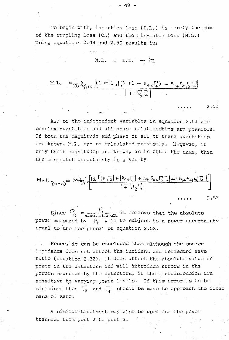
- 49 -
To begin with: insertion loss (I.L.) is merely the sum of ·the coupling loss (eL) and the mis-match 1058 (M.L.) Using equations 2.49 and 2.50 results in:
M • L • = I • L • CL
M.L.
• • • • • 2.51
All of the independen·t variables ill equation 2.51 a.re
complex quantities and all phase rela·tionships are possible. If both the magnitude and phase of all of these quantities
areknovm, M.L. can be calculated precisely. HO'yever, if
only their magnitudes are known, as is often the case, then
the mis-match uncertainty is given by
••••• 2.52
since B-1. - 6 ___ it follo-ws that the absOlute / - ~~O'V \..1>$1; ~<iXto
pOvrcr measured by P'1- will be subject to a power uncl"!rtainty
equal to 'the reciprocal of equat:i.on 2.52.
Hence, it can be concluded that although the source
impedance does not. affect the incidc:mt and reflected wave ratio (equation'2.32), it does affect the absolute value of
power in the detectors and will introduce errors in the powers measured by. t.he detectors, if the:i.r. efficiencies nre sensitive to varyin9 power levels. If this error is to be
minimissd then r;; and ~_ should be madE! to npproach the ideal
case of zero.
A similar,treatment may a1:::0 be used for the power
transfer from port 2 to port 3,

- 50 -
The principle of how an impedance or admittance may
be measured using incident and reflected i'laves has been established in sr~ctions 2, 1 and 2: 2. p.. thorough analysis
of the dual directional coupler has been made to demonstra'te hmv it measures the incident and reflected iv-aves.
The errors associated with the coupler have been derived and the basis for computer corrected systems have been
shown in section 2:3. The equations relating the
uncertainty in the measurement of pOI·rer in. the measuring
ports \Jith respect to the source match has 'also been
derived.
* * * * * * * * * *

- 51 -
2.1 stager C, and Kartasc110ff P, ",Heas1.lremen't Accuracy Hinges on Coupler Design" Hicrowave Journal, April 1977.
2. 2 Sche11~unoff S. A., Ilirhe Impedance Concept" B.S.T,J" 1938 17,7.
2.3 Sche1kunoff S. A., "Impedance Concept in '~aveguides" Quarterly Applied Matherniltic, 1944. 2 pp1.
2. 4 Hunton~ J, K. and Pappas N. L. "The hp Hicro"V:ave Ref1ectometers" Hewlett PacKard J. Vol 6 pp 1-7 sep't-Oct 1954.
2.5 Engen G.F, and Beatty R.H., "Hicrowave Reflect-ometer Techniques" I.R~E. Trans on Nicrowave
,Theory and Techniques 'Vol HrrT - 7 pp 351-355 July 1959.
2.6 Kuhn N" ,"Simplified Signal Flo,.". Graph Analysis" l1icrowave Journal Nov 1963 pp 59-66.
2.7 Hewlett Pacl(ard Catalogue 1973 - pg 336. Directional Couplers 8690B Series.
2.8 Warner F, "Microwave Attenuation Measurement" I.E.E. Monograph Series 19 - Appendix 1 pp 270-272
2.9 Woods D, "Concepts of Vol tage '~aves, Current Waves and Power v.Taves in S P arilmeter Definitions and Neasurements" Nanttscript H32 (1 st May 1972) which is deposited in the I.E.E. library, Savoy Place, London.
2.10 Noods D. "Concepts of Vol tage \~aves, Current Waves and Power '~aves in S Parameter Definit.ions and H(~as1.lrements". Proe I,E.E. Vol 119 No 12 Dec 1972.
2.11 Mason S.J., "Feedbac}( Theory - Some Properties of Signal Flow Graphs" Proe I.R.E. Vol 41 pp 1144-1156 sept 1953; also Mason S.J. "FeedbacJ( Theory - Further P roperti.es of Signal Flow Graphs" Proe I.R.E. Vol 44 pp 920-926 July 1956.
2.12 Hunton J. 1\., "Analysis of Micro\>lave l1E.~asurement ']~echniques by Means of Signal Flow Graphs" Trans I. R. E. Vol }1rl'T--8 pp 206-212, March 1960.
2.13 Carson R, "High Frequency Amplifiers" John \'Ii1ey am Sons 1975 pp 165-167
2.14 Sucher M; and Fox, "J •. Handbook of. HicrO\vave ,Measurements. Volume TI, John Hiles and Sons,
London 1963.
2.15 Montgomery C.G., Dicke R.B. and Purcell E.:H. "P rinciples of Microwave Cireui"lis • McGra-,~' Hill, New York 1948).

2.16
2.17
- :52 -
/
Harvey A. F., "Hic.rovlave Engineering" Academic Press, New York 1963.
Barlow H.H. and Cullen A.I.., Hicx'ovlave Heasurcrnen:ts, Constable & Co., London 1950.
* * * * * * * * * *
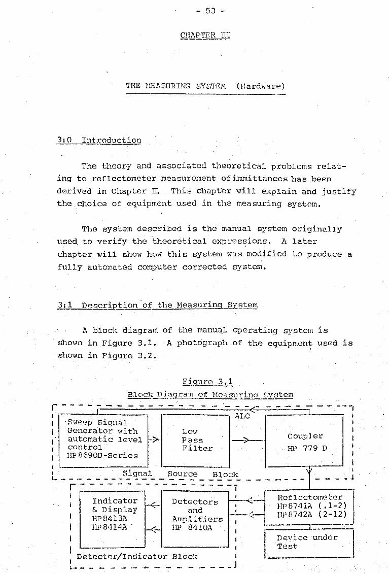
- 5J -
CHAP'rER m:
THE l-1EASURING SYSTEM (Hardvlare)
3:0 Introduction
The theory and associated theoretical problems relat
ing to reflectometer measurement of irnmi ttC1l1CeS has been
derived in Chapter lIe This chapt'cr will explain and justify
the choice of equipment used in the rneasuring syst~m.
The system described is the manual sys·tem originally
used. to verify the theoretical exprcs~ions. A later
chapter will show how this system was modified to produce a
fully automated computer corrected ::::ystem.
3: 1 D es£!ZiP.t~on of the Measuring ~~y!:?t~!!! .
A bloc]\: diagram of the manua,l operating system is
shown in Figure 3.1. A photogr.aph of the equipment used is , shown in Figure 3.2.
F~guro 3.1
Dl(!£!~ D j~~~gr~;'~f MC'2!2~1Zil2SL sy~;t~ r-------- - -----I -- • L... .----.
.- - .- - - - L- - - .- - - ... - -, "'--= .:1 'Sweep Signal Genera'tor ,vi th automatic level -> control lIP 8690B-Series
,-----_._-Lmv Pass Filter
ALe· .~----~
->-- Coupler
HI"' 779 D
I I
L ... - - - - - - -S}~n~l __ ~o::.rc:.e - Y2:°5l~ - - - -i ----j r - - .- - - .- - - - - - - - - - - - T -
i r-' Indi~:~:;- Detect~r:- I <_~-Reflectometcr i & Display and:.__ I-r:8741A (.1-2)
llP8413A Amplifiers ':;.- HP8742A (2-12) I m1 8414A' -<_ HP 8410A ' .--:--:::=r===--=:
Detect.or/Indicator Blocle
... - -.- _ _ .... .,- "'- -- - - - .-
I
I ___ J
Device under Test

- 54 -
f..i9~:tr2 3.2
~:Ylo.l~qr.~l~.1}_.9f Eg~m?.~.!::_VS22
Hew l ~!t-Pac!<ard Model (;4 J CA Nc tw:>tk Ana lyze r.
8741il
rl J ___ I
87t12A
f!41/frl Polar Disp lal' Plug·in mo'dulc lor 84 ] 0/\ mainframe CRT pul'l l' Lli5jl lJY for direc t rU:1dout of r c~lrct i o n coefficient il nd aogle. Sm ith Chart over :ays illcluded for direct im· pedance or adm ittance readout .
8413 Phase-Gain Inliiciltor (Optional) Alternate plUg'lll modu le for 8'11OA mainframe provici r.s rnc tr.r display of clB return loss and reflection coefficiel1l Jilgil'.
8741A lle1fectiol1 'fest Unit 0.11 to 2.0 Gllz Widpband r ;: fl ectomctcr phase balanced for swept 01 spot freq \Jf;ncy irnp edanc~ t f:S :~ be low 2.Ll Gllz. Accepts '<F input and pro · vides connectil.lns for unkno'NIl trst devic~ il nd 841 lA Cali· brated var iable reference ~!?ne
1l742A Reflec ti cn Test Unit 1. .0 to 12,4 Gllz \vid \~brt IHI re Hect ometer phase U.1 lal1 C8 cJ for impcdJl1ct.! Ie b :1bove 2.0 GHz. Calibrated variab le ref erence 1' ''111':.

i I i - 55 ..
The syst.em mc!y be divided into three basic blocks. A
s:i.gnal source block which generates the signal, a reflecto
meter bloc]{ which recognises the incident and reflected
waves from 1:he .device under test(DUT) and a Detector
Indicator system block which interprets the reflectometer
output.s. Detai.ls of ·the three basic blocks will be discussed
in sections 3:2, 3:3 and 3:4 respectively.
In using the cy'U.ipment the desired frequency is selected,
and two calibration pieces, a sliding load ( I r' I = 0 ) and 2.
short (r :: 1/'8'~ ) are used to establish the limits of r: in the m2a:3'L~ring system. The device under test (DD'r) or test
piece ( L. L ) is then measured t.o yield r: The test piece impedance ( -Z \..) is then calculated by
means of Equation 2.18, hEmce;
ZL. = 7o ( 1 ~t.) (1-1""2.)
or
YI.. - Yo(\-T:) (\+1:) . . . . . 3.0
The signal source block comprises a signal generator, a
lOT/T pass filter and a directional coupler-detector system for
automatic level control.
'l'he basic requiremcmts of the signal genr~rator may be
summed up as
(a) Good frequency stability.
(b) A good source mat:ch, i.e. 1m'1 51'lH .•
(c) Sufficient output le~n~l (-'20 d13rr. t·::> +IO.:!Srll)
(d) LOTtT distortion, i.e.., low harmonic content.
(e) An' elcctronic means of keeping the signal output cons·tant.

The signal
,·li th a sp(~ctrqJ
unmeasurable.
- 56 -
source should be ide;:lly a ph<.:isE:~ locJced source
puri ty of such order that all harrctonics are
In addition, there must be complete reliability
and repeClt:i.bi1i ty in frequency s~l ection. l1icrmvave Synthesized
f)i.gna1 Generators (Ref. 3.1) r.tpproaching the idealized case are
nm'l ava.ila.ble. Hmvcver, these generators were net available
and one had to manually phuse lock the signal generator to a
c:omb ·generator (Ref 3.2). 'This unit incorporates "ten 'pre-s'elected
cr"ystals "1:::0 stabilize an. oscillator operating in the region
of 15 MHz:. This stable 1m" frequency signal is used t.o drive
a harmonic .generator. By sui. table choice of crystal md.t.ching,
it would be possible to derive a harmonic to mix ",ri th the
main R. F. signal to provide aD. C. cont.rol vol t.age to th(~
signal generator to maintain the desired radio frequency
constant.
In practice, it was found that phase locj~ could only be
maintai.ned for about 20 minutes because the drift in t.he R. F
generator would be such that it would d=ift outside the "loc]~
range" of the system. A slightly longer period of "phase lock"
could be, maintc.ined if the R. F. generator 'vas switched on for
approximately bolO hours before measurement.
The main H.P. signal source used in all the measurements
is the HevTlett Packard 869GB Series of Generators (Ref 3.4).
These consi 81: of a main control unit 8706}\, a signal multiplexer
8705A, and a R.F. unit Holder 8707A wit.h three Grid or PIN
levelled DWO R.P. Plug-ins. The ·plug-·ins are 869gB (0.1-2GHz
and 2-4GHz) 8693A (4-8GHz) and 8694A (8-12.4GHz).
Full details of the equipment is of course available In the
respective h"'1ndboo1,:s but it can generally be said that these
gencratCJrs are capable of fixed or s,~'ecp frequency operation,
usjng ei.ther manual or elect.ronlc controls. When levc~11ed,
t.he po~rer output is greater t:han 25 nW . (~14 dDm ). The
~~pu.riO\~s s.i.gnills~ i. e., harmonic and non har:nonic siqn<lls for
all the 3 pJ.U9-in units are 20 and 40 dB dm\'n on the? desirE:d
signal rnspectively. The output port reflection coefficient.
is c;.Il.J.ot.ed as £.0.25 {lSWH .f:.l. 67 ). Such a poor SOU1~ce • . ' l' match i.s definitely d1sadv3nt:.ugeouB and 1S cxpl<1J.nec.. ].n
Sf:~ction 3: 2.2.

- ~)7 -
The i mpor-Lance of source mat.er) can be easily visua.lized
by a study O f7 the incidcmt, reflected and re-reflect_ed i.,raves
1n a typica l measuremen-t enviroment . Such a situation 18
dep ict.ed in Figure 3 . J ';-There a dua l direct.ional coupler under-
going mu l -tiple reflec tions is u sed to measure \ a reflec-Clon
coeff icient . The dual directional coupler
generator vi-th a re f lect.ion coefficient R: a I,rave ( e) i ncident a t (J.." and emergent at
1S driven from a
iv-hich produces
b , and it is
used to mea s ure the re f l ection coefficient \:' of an unlmOHn
d evice. To simpli f y matters in 8igure 3 . 3 the effects of
Sll anr,:i 522 of t -11e coupler have b een temporarily ignore d .
Figure 3 . 3
Hul!:iP.le l.~eflections 1n a Reflectometcr §Ts-tem
.' - :.c...----- E 1.
ef" suLTAr-l T
\
----" .... Ctz

- 58 -
In Figure 3.3, the first inciden·t and reflected paths are
denoted by the liold lines and larger arrm.,rs, whilst the second
incident and reflected patbs are denot.ed by the bold lines and
smaller arrows.
The dotted lines represent the um-lanted coupling to the
j.ndividual couplers. E' I and EIII represent the undesired
waves to the first coupler and E' R and Ell R represent the
undesired waves to the second coupler. The superscripts) I
and II denote t.hat the components an~ due to the first and
second incident and reflected yTavE;s respectively.
Lft the desired and undesired c0upling for the first
coupler be Cl and CDl respectively. Let C2 and CD2 be the
desired and undGsired. coupling for the second cotApler.
The first incident and reflected waves are denoted by
eLI and b I respectively.. The second incident and reflected I ,-!. d waves by O~I' and I.,) I respectl. vely and so on. Tl an T2
r~present the main transmission paths.
By inspcc{;:ion from figure 3.3;
>::;:
• • • • • 3.1
• • • • • 3.2
-, -:= CzQ.i C;t \\,.. l, Ov, • • • • • 3.3
· . . . . 3.4
comparison of the above terms gives:
EIz. = .-- · . . . . 3.5
;
• •••• 3.6 .

- 59 -
Hence for each complete w'ave journey around the loop both
EI ... r..;andF~rr(,are altered by the same quantity, i.e., r;(T,T2. . The resL1l tant reflected versus incident ratio ~8,.{:c\2!"'I.) remains
;:1:("'-~"TA'-)
unaltered.· (Figure 3.3). Note particularly t.hat. the above is
true regardless of the directivity of the individual couplers.
'1'h0 above resuJ.t is not surprising as it has already been
proven indirectly in section 2:3. However, in theory, the
loop product (~'l""2 T, T7. ) could be I II~oo in which case the
incident:. and reflect.ed signals would cancel each other render
ing the coupler useless on these qccasions. In practice,
(I~ ~ I; T ~ ') is seldom I LI2cE a.nd this does not occur.
If the product ('% 12T,T2.) is examined, it is evident that
-f, and \~ are determined by the coupling, attenuation, source
and load match. For example, a 20 dD coupler with no line
losses would result in T, ..c::.O .. qqS (Hef. 3.3). The reflection
coefficient, r~'" , of the test device may range from a
perfect match I 0 I to a perfect open or short circuit I .1. I . Hence, if (~r;: T, T,.)is to approach 0 then. r; must be
controlled and should ideally be .zer.:o.
It was mentioned earlier that the S1veep generator system
used (Ref 3.4) has an output VSWR L 1.67 (q = 0.25). A
trivial calculation for the case 'of a 20 dB coupler and. a
load reflect~.oii coefficient \1\ will show that it is possible
for t.he signal to 1")(~ reflected thrice before it is reduced to
less ·that 1% of its original value.
'rhese reflections cause a poor passband response in a
measuring system, particularly if Sivept frequency measure
ments arr~ being t-.aken. If wide band at:tenuators are used to
improve t.he passband characteristics, then for the same
oscillator power, the incident wave is reduced, and for Ule
same reflection coefficient, the magnitu.de of the reflected
"laves will also be reduced and in the lirni t, it w'ill b8
comparable to the inherent noise povwr ",ri thin the d(~tecting
system. 'I'his results in further unecessary errors in the measurement. Poot' passband response also introd'uces errors in
the measurement of pOI-ler sensitive devices e.g., transistors, var~ctor diodes etc.

- 60 -
Source mc"1.tch may b e improved by ·the use of i solators/
ci rculator s a n d even attenuation .- matching neb·lOrJ(s . The
former 'are more eff icient but usually l ack the mUlti-octave
b2.ndHidtb.s required and as mentioned above, the attenua tors
introduce unnecessary loss . In e i ·ther case, bot.h methods do
n o t inh ibit. the outpu·\.: v 2. ri a l: ions vi thin theS\veep g e nera tor .
'I'he well established me thods to minimise signal output
varicd:ions and also to present a good source ma tch is the
system presented in Figure 3 .1. rfhis system is s i mil.a r t o
that des c r ibed by Engen ( Ref . 3.5 ) . The sweep signal gener
ator s u sed incorpora·te vol ·tage v ari able att e nua t .ors . The
output: signi3.J. ( forvard Ifa v e ) is detected by tl1.e direct. iona l
couple r j ust p r ior to entr y i nto the .ref lect:ometer. The
entire sigr..a l sou.cce bloc]( of Fig 3.1 ,,:ill now be shmvn to be
equi v a l ent. to a constanJc l evelle d source Hi th an ou·t.put match
approaching tha t o f the direc·tiona l coupler , which is
considerably bet1:er Jchan that of the Slveep generator itself .
,- - - -- -
F ig~re __ ~..!...::!
~ffecti~::,,~.So'!.:::s.e S~!-eE}
........
[
A~;I'IFIER J--<I1-- DE~EC~" OR --1 '--'1 - -----__ J
Sweep b31L} " a
3 Jnerato~_l ____ ~ ___ 1 I
6)~ - ATTENUA TOR. - a~ COUPLER ---~-~~71--' L. __ "_~ -.--it; 1 _ _____ .. ..:. ___ -1----' --<,!,,;-' '-
Port 1 I L __ .. ___ . . _ _. ._ .. ~ ._ _ __ _ "_ ._ _ _ -- - - - .-l

- 61 -
In Figure 3 . 4 J le t OJ I represent the incident ,-rave "ihich
the generator presents , to the coup ler. By reference to the
signal flow graph o f F igure 3 . :), it. :1. :3 seen i:ha~:
8 -'
e. +r;b,
F ig.u r...£..2..:...? Signal Flmv Graph foL' Effective _si (,inal ~;ource of Fi.92~l~e 3~_
\
c "'21
-----<~+-,-.-- .. -----~_{J
3 . 7
.~ ~.---.

- 62 -
With the coupler netlvorJ: of Figure 3 . 5 connected , Port 2
is t.he ma in signal output p orL \.;iLh the ,:ave b einq en:c:rgcnL
at b 2.. , and 0,,2. is \'lhe J.:-ethe l'ef lected. wave r e-entcrs U1e
system . Hence,
3 . 8
s~ \ ~ \ 3 .8a
From 3 . 8
5"2.. \
and SUbstituting in 3 .8a
b3 [ + q(5,<3 S31 - S33)1= SS~I b 2.- Q[S~ __ ~~ - S3';}
. 5.2 1 ). 21 ~, 2 1 j
. and b 2 = b3[~~i -1- ~(S? :, - 5~~~~214-Q ~ rz~- ~~~2J .... . 3.9
,or b1.. == e / + 1(; ' Q '2.. 3 . 10
where e/= o_r ~2.' + r (s _ - S21 5 33,'\]
.:1 [.5'32 l el 2::> , 53l / 3 . l0A
3 . l0B
Not.e the first terln o f 3 . 9 rep rese n t s the ALe generator
output whilst the second t erm is the effective generator
ref lectio n coefficient .
The d ire ctivity of the coup l e r h~s already been defi n ed
as:
D ::: 20k r ~~ I I and 5).nee ~ IO 53'l.
S:u ic close to unity (~O . 95 & 0 . 99 .;5 for a 10 au and a 20 dB
coupler resp - ~ef 3.3) it can be written :
~3.L == \ 0 - (D/20 ) ) 3 1 3 . 11
t • • ,. f

- 63 -
I f 3 . 11 l s substituted in 3 . lOB for the 'ivorst c a. se
source match
~~ o p::; 1 . 4 ::s: (fj
:->
rr: l- I·s 'I + 22 I -(D/2°)1
10
fi gure 3 . ~
Maximum vsvm o f the Effective Source
whe n u sed i n a clo s e d Loop Control
Circu i i: . -------_. ....~-.--~----.
VSWR
\-40 COUPLER - - --
30 40 50 60
DIl~EC'l'IVITY (DB )
3 . 12

- 64 -
In t.he actual test set used, the directional coupler
used was the He'\vlett Packard Type 779D (Ref. 3.1) This has
a mean coupling of 20:! 0.5 dB and a main and uuxillary line
1 . h" d' L." t fClr thi s SI'dR of .2 maxunum. T e m1.n1.InU!!l l.recL.1.v1.Y
coupler is 30 dB (1.7 - 4 GHz) and 26 dB (4 - 12.4 GHz).
Nhen this coupler is used in a good closed loop auto!l1at.ic
level control system, the worst case source match: ca.leulated
from equation 3.10B is su.mmarized as f01lmfS:
4 - 12.4 26 1.2
* Assuming .. sufficient loop gain.
~: Hewlett Packard quotes an effE~ctive source of 1.2 SKR
(Ref 3.i) but. does n'ot state the frequency. How'ever,
the figures calculated are considerably better than
t.he 1.67 S'lR quoted for the generator alone.
The Low Pc!S8 Hi1nnonic Filter -.--.... ..---
'rhis should be us'ed whenever possible i:<nd should be pluced
before the levelling coupler, as the coup1.er detector is
frequency insensitive and might be affected by the spurious
signals. '1'he ~~purious signals do not effect the measured results
in th(~ Sclme manner because the signals are detected through
tuned amplifiers.
"

- 65 -
Cboice of thf2 ReflecLoTnE."'ter
Tw'o reflect.ometcrs were used. rrhGsC' are the HP 8741i\ for
0.11 to 2.0 GHz and HP 8742lc. for 2.0 t.o 12.4GHz. A block
diagl-am of these systems is shmffi in Figure 3. '7. The signal
is fed to 'the device under t,est via a dual direc,tional coupler.
The incident and reflect,ed Rignals ar'e fed i.nto a dual channel
receiver for processing.
Ref " Plane
Figu,n? 3.7
Basic D iaqram of the H? 8741A and - HP __ 874.~A-13~~fTect2inet~_f.~----
'f . -, r /,1 ~" Llne Stretcher
Manual ]l.djustor
Ref. Channel Output
P -II Reflected Signal
Test Channel Output
TO TES'r DEVICE
Both reflectometers employ' a calibrated line stretcl1er
to enable the electrical pat~h lengths to the n~ceiver to be
identical. Thi s is of considerable advantage as it allmrs
direct readings of the display systems for phase changes.
The coupling factors for all the reflectometers are a nominal
20 eLl) and the ins(~r-tion loss is less than 1 dB.
T'\'/o sets of Directivity Figun~s are claimed by the ,
manufacturerf~ (Hef 3.6 and 3.9), these are tabulated belo ...... :

- 66 -
T.TI...~ Erg.9:'1eng,-.LC?Jl.~ ,
8741A 0.11 to 1.0 ::::.:... 40 dB ~ 36 dB
1.0 to 2.0 ..... -~ 34 dB ~ 32 dB
8742A 2.0 to 12.4 ~- 30 dB ~ 30 dB
------
As the reflectometer forms the "hc~art" of the measuring
syst.em, its choice is of considerable impor'cance. The
mathematical analysis of sect:Lon (2.3) has s'hmffi what is
desired. The l.mport.an-t characteristics may be classified
into five important properties, n.amelYi
Is Directivi~y.
2: svm 3: Frequency Ra.nge.
'4: Coupling Coefficient.
5: Transmission Loss.
The following sub-sections are c:m intuitive discussion of
t.he mathematical .analysis carried ou·t in Chapter 2.
Directivity is a measure of the abili.t:y of a cot,lpler to
isolate two signals, for example, the incident and 'reflected
wave. It therefore set;s the li.mits on bow' accurCltely a coupler
can perform a specific measurement. As an example when making
reflection me~surements a dual directional cO"llpler is required
and the directivity of the t.est port is the most important
paramet.er. Subsequent math8matical treatment '·l.ill confirm
this. Ideally, it ",QuId be desirable to measure t.he reflected
signal alone. However, because of directivity, the reflected
signal i3 combined '\'1i t.h a St-nall portion of the incident. ,\-lave.
This can be easily explained by reference to the phasor diagram
of Figure 3.8.

F i9"\..~.re 3 . 8 EFFE CT OF DIHECTIVITY ON REFLECTION COEFFICIENT HEASUREtvIENT .
, c+-;vity D ., re ~_. , .- <:: -. gna_~ Error ~ ).J.. ______
Incident signal E. C1 ln
1st Coupler
Measured In2ident Signal EM I
Di rectivity E 1:'ror S ignal
'~ /.r~;:j \ 1
i / il / Reflec ted . Signal E
RC2
V
Measured :2ef lec·ted Sianal E'l~' . , l' L
2nd Coupler
-I " 1- 1 ~ l _ _ I L. ted Wave -~.. . . Roflec
J £i .-
CD 2 I
t
C2 ----, r I I' CD 1 ~ 4-
1-- . C1 ~_I- I> r--'
-4l -----l 0-'--, . dent. tl ave
.- "<l -.;. .... ,
~~ InCl , ~ (.~
L-l
I
TEST I !
DEVICE i 1 I t
fS:. ' E in __ . _ _ _ _ ___ _ ~--~~_::~ C1 and C2 EMl & EH2
= desired coupling factors;
= measured signals ; E. = In
CD 1 and CD 2 = undesired coupling factors;
input signal; ER = r e flected signal
O'l ~J

- 68 -
In the 1st coupler, the small portion of t11C reflected
"lave '\olhich combines v;i th the incident si£mal leads to an
error in the measured incident signal. However as the
incident signal is much larger than the directi vi ty ert"or
signal, the magnit.ude of the measured incident signal is
approximately unaltered.
In the 2nd .coupler, the small port.ion of the incident
signal which combines with the reflected signal results in
a phase which is directly additive t.o the measurement
uncertainty. Thus the higher the direct.i vi ty {i. e 'I a
smaller dir~ctivity error signr~l} the higher ,vill be the
measurement accuracy.
\,lhen measuring large reflections, the small portion of
the incident signal that mixeEl with the reflected signal is
very small, and it adds a negligible amount of uncertainty
as in the first coupler. As the reflected signal becomes
smaller 1 the small por-tion of t"he incident signal becomes
more significant. Nhen the reflected signal in dB (return
loss) equals the directivity of the· coupler, the measurement
can recu1 t in a -6dB to ;.. cO dB error. The importance of
thi.s cannot be overlooked and a mathemat.ical analysis shmving
t.he practical limits of measurement ,.;rill be given in Chapter IV.
3:3.2
The VSWR of the coupler is importan1: since it minimises
the simple and multiple miso-watch errors tl1us improving the
accuracy of the measurement. For example, when making S'·'Cpt
reflection measurements, it is customary to set a full
reflection (OdB return loss) referenC'2 by connecting a short
circui t at. the out.put of the coupler. Some of the reflected
signal will be re-ref1ected due to th(~ output port (test port)
of t.he coupler. This re-reflectcd signal 'vill go. through (l
wide phase variation due to the widt:l of the frequency S1,'eep,
adding and subtracting from the reflection signal, tbus creating a ripple in the full reflection (OdE return loss).
The above cff0.cts can also be caused by detect:or mis-matches.

- 69 -
The magnitude of the rc-reflectcd ~3ignal and thus the
measurcmen't unc(~rtainty can be minimised by selecting
couplers ,,,,ith as 1m., a SWR Z,G possible, and by the use of
detect.ors "d. th 10v! SWR' s.
Broadband operation is important because it eliminates
the necessity for several octave band coup1os to cover a
wide frequency range. For example, "lith brot:ldband sources
capable of up to four octave ban~ sweeps, it is a real
convenience. to be able to have a .wideband coupler to obviate
the need for t:imE~ consuming costly calibration techniques.
3:3.4 coupling Coefficient
The choice of coupling coefficient is importan-t because
it determines the level of signal with '\V'hich the detection
cireui ts will have t.o opera-te. :Most sweep generators have
limited outputs (usua.lly +5 t~ + 10 dB~ at 12 GH:?;) and a
convenien't coupling coefficient is 20dB dmm on the main
s~gnal. Such a coupler would extract 1% of the main signal.
On the other hand, a lOdE coupler would extract a full 10%
of the main signal, Furthermore; in pOvrer 'sensi ti ve measure
ments, e.g., transistors, it is important that the coupling
coefficient remains con~tant over the fre~!Ucncy range of
measurement. Hewlet·t PacJ~ard cla:lms t.hat this feature is
enhanced in their couplers by the use of exponential coupling
designs and lovler coupling coefficients which introduce less
perturbations into the main signal line, thus favouring
lower Sh'R's and better directivity,

- 70 -
Transil1ission loss is the total loss in the mainline of
a direct.ional device and includes insertion loss and coupling
loss. It aSSUmG8 importance ut the higher frequencies ,.,.,here
sweep generators have a limited output often less than
+ lOdBm.
In general, broadband coaxial couplers have transmission
losses of the order of 1 dB.
with frequency. as possible.
This loss should be as constant
3: 4 'fhe Detection and Indication-131oclc
The detection system used is the Hewlett Pac}card Network
Analyser 8410A operating with its auxiliaries HP e411A and
lIP 8413A or HP 8414A. Detailed descriptions of all these can
be found in their respective hand-bOOks. The information
given here is only for the understanding of the measuring
system used.
Figl.lre_~
Basic System used in t,he NetworH: Analyser to achieve __ =-F.=.r..;:::e.g.ll...ency Translation by a Samp,ling Technique
S~ampling > }fixer
Electroni.c Tuned Gate
1st I. F.
- - T - - - - - - - - - _ .. -
2nd " Subs·t. Mixer IA.tten.
'---'--- ---
If .... ~ >~ An~pl t. .~ Log I Detect. Conv.! I -
t ~I 7
Log O/p
---)0 Nag O/p
Local Limi te _. I ~--~ 2nd t ,'1 Phase Generato!: Osc. I Detect Phase olp
.. ~ -1 I'P:h;';';W 1'.<, I-T;~ASE/GAIN ~~~: 'i' Osc. - -'I ~'l Y I INDICATOR
~ s~mplin;J 1t"-E!Jlt 11 2~d·-·T ._~._._: r;~:se I Hl.xcr -1----"> ,I.F. ;7 MIxer r" I 1 Offset
j '-___ .--1 __ _ ___ . I _ . ____ .L. _ - .... - '. -
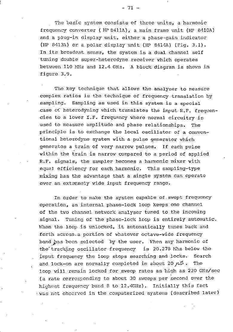
- 71 _.
1'he basic system consi sts of three units, a harmonic
frequency converter (HP 8411A), a main frame unit (HP 8410A)
and a plug-in display unit, either a phase-gain indicator
(HP 8413A) or a polar display unit (HP 841111'1.) (Fig. 3.1).
In its broa.dest sense, the system is a dual channel self
tuning double super-heterodyne receiver which operates
betl18en 110 HHz and 12.4 GHz. A block dio.gram is shm,m in
figure 3.9.
The Jrey techniqu(~ that allows the analyser to meas~re
complex ratios is the technique of frequency translation by
sampling. Sampling as used in this system is a special
.case m:- heterodyning "lhich translates the input R. F. frequen
cies t.o a lm.,rer I.F. frequency where normal circuitry is
used to measure amplitude and phase relationships. The
principle is to exchange the local oscillator of a conven
tional heterodyne system with a pulse generator ",hieh
generates a t.rain of very narrow pulses. If each pulse
w'ithin the train is narrow compared to a. period of applied
R.F. signals,the sampler becomes a harmonic mixer with
eq.uC1] efficiency for each harmonic. This sampling-type
mixing has the advantage that a single system can operate
over an extre;mely wide input frequency range •
. In order to make the system capable of. s,.".ept frequency
operal:ion, an internal phase-loclc loop keeps one channel
of the two channel networJ( analyser tuned to the incoming
signal. Tuning of the phase-lock loop is entirely automatic.
Nhen the loop is unlocked, it automatically tunes back and
forth across. a portion of whatever octave-'\vide frequency
band _~1(l8 been selected by the user. vlhen any harmonic of
t.he' trac}~~ng oscillator frequency is 20.278 Nhz beloyl the
input frequency the loop stops searching and loc}es. Search
and loc}<:-on are normally completed in ab~\..1t 20 IL.$. The
loop will·rc:nain locked for .sweep rates as l1igh as 220 GHz/scC
(a r.ate corrcro,ponding to about 30 sweeps per second over the
highpst freq'.l0~cy ba.nd 8 to 12 .4GHz) . Initially this fact
\ war; not obscl"'ved in the computerized systems (described later)

- 72 -
and considerable measurement error ' .... as experienced. Rytt1ing
and Sanders (Ref 3.11) provides further details of this
sampling, search and phase-locJdng design.
The I.F. signals reconstructed from the sampler outputs
have the same relative amplitudes and phases as the micro
w'ave reference and test signals, because the frequency
conversion is a linear process Referring again to Figure 3.9,
the 1.F. signals are first applied to a pair of matched AGC
(automatic gain control) amplifiers. 'rhese ]I.GC amplifiers
perform bvo funct.ions; they )).:eep the signal level in the
reference channel constant and they.vary the gain in the test
channel so that the test signal level does not change when
variations conrrnon to both channels occur. This action is
equi valent:. to ta.ld.ng a ratio. It JEmOV(D' the effects of power
variations in. the signal source, .. frequency response 'i~'
characteristics common to both channels and other similar
common-mode variations.
The bm signals (reference and test) are then down
converted once more to 278 kHz (2nd.I.F.) to enable good
amplitude and phase detection •. This intermediate frequency
of 278 v...H.z has proved useful in checking the phase accuracy
of the receiver. This is because the period (T)
T = _J_._~ .. i. e 3. 6~C; corrf:!s'Ponds to 3600 of phase or
278 kHz
10 picoseconds = 10
To obt.ain the desired magnitude (dB) and phase comparisons
(degrees) the pnar::e-gain indicator plug-in display unit
(HP 8413,A) con·tains a linear phase detec·tor and an analogue to
10garit11.Tllic converter which is claimed to be accurate to
,.,ithin.± .2 dB over a 60 dB overall range of test signal
arnplit.uc1es. Voltage Rat'ios (dB) and relative phase (degrees)
can be rc~d on the meter of the display unit (used for manual
readings) but the plug-in also provides calibrated d.c. , '( l' t' coupled vol tL'.lges proport.lonal to galn a.s a lnear ra "10 or
in dB) and phane for graphical or electronic displays.
An al ternati ve display used ,.;as the Polar Display unit
(HI> .8414.1\). A bloc1~ dif:Jgram of this is sho-wn in Figure 3.10.

. ,
- 73 -
F i5:E:t:re 2.!-.1 Q ~E.9c1.~oJ?JG~(]tam 0L!>o~oa.r DisplaY unit
Da12'Oced ~ A Cos e }10d.ulo~tor 1 0
B :o~~{_ _ c;,R_e_f_e_r_c_r_lc_e ___ , Ir ~~f~~ter/
Input r l L',ITI'te.r_
Test --] t rOO-gOo -I r Balancedl \ 0-
0 -..---f Ampl. -->- Phase 1-rJ . ~J-;
Input __ / l Shiftr J jllodulato1
A Cos(wt + Q)
l-A Sin G
-r 0 Vertical
1-----'----1 o/p Lew Pass
I~il_t_e_r __ •
'f'he unit converts polar quanti ties into a form sui table , . . .
for display 011. the cathode ray tube (CRT). This is
accomplished. by using byo balanced modulator phase detectors.
The phase of the test channel is shifted gOO with respect to
the reference channel before being applied -to the balanced
modulators. The outpu l:. of one modulat.or is proportional to
A Sin G. 'l'l1is signal is amplified and fed to the vertical
deflection plates of the CR'r. The output of the other
modulator is proportional to A Cos e and this signal is
applied to the horizontal deflecOtion plates of the CRT.
Thus the polar phasor can be displayed in the rectangular
coordinates of an oscilloscope or an X-Y recorder.
'I'he polar display' "Tas the unit 0 most' 0
frequently u::;8d (especially in computer controlled measure-
rrtenl:s) as it "rould instantly demonstrate any mal-function in
the equiprn2nt, c.g., loss of phase lock, improper calibration
of standards etc.

·. 74 -
Hewlett Pacl<ard (Ref 3.9) claim the follmd.ng 1'lhen the
system is used vri thout COlnputc~r correction:
Overall Uncertain·ty* Reflection coeffi.cient magnitude of
unkno';>m ( \2 ) is measured to vTi thin r:' =
... (0.01 + 0.02 'r: I + If" ) I 0.11 to ) 0.05 k I l- I. a GHZ)HP8742.~ + (0.02 + 0.02 J r: I + O. 05 '(' I '2. ), 1.0 to 2. a GHz)
+ (0.032 + .052/ r: I + O. 036 If: 12 ) I 2.0 to ) 8.0 GHZ)HP 8742A
+ (0.032 + 0.04 I r:'! + 0.07 1 C 12 ) I 8.0 to 12.4 GHz)
Reflecti£n COE:;_ffici~l!t. al]Sl!e ~1l1certainty:
+ Arc Sin ~ I for . L. 90 . r'''' f 0
f2 .
*Noi:e: ---Overall unc(~.::.·tainty includes the effects of coupler
directivity, source match, and system tracking with
frequency~
The follo,ving information on t.he system is taken
from the Hewlett P acJ\:ard Catalogue Sheet (Ref. 3.9).

8410,0. !'tETWORI( ANAlYLER (Operat ing with 8411M
Instrurnrnt Type: / casu es relali Ie arnpliiude and pbao(! of two RF inpu t Si g il~;S . choice of to'lO p; l~g·jli r.i~. p :ay module':; for meter read ou t (34!3A). or CRT polar display (84 14A).
Frcq cncy Range: 0.11 to 12.4 GHL. Tuning: Autolnil!ic O'ler octave band selected by froill p3nc i
switch. $1 'ept Operation: SI'IU:P~ in octave bands: apply sweep r eler·
ence vo ltace for fast sVlepp operation (cori1pJtib ie with s'mep re ference out of Model 8690A S'Neep Oscillators')
In, l t Irnped nee: 50~! . SWR < 1.4 to 8 GHz. < 2.0 to 12.4 GHz. connectors p;ec i:; ion 7 mm coax (APC) ).
Ch;;nnei Isol3tioll: . 70 dB. 0.1 1 to 6.0 GHz; > GO dB. to 12.4 CHI.
~ rnplitudc Illpu rov/er Range
Rr·ference Channe l: 20 df! variat ion cc i.jses less than :.- 0.75 dO iJnd ~- 2 chaiigc in amp:itucie c;nd phase readings. 20 dS r an~e Viiij be withir, ' .- J6 to - 44 dBrn .
T(;' \ Ch anne l: - 10 (,- 2) dBm max imum. Not to e~ce(:d refere r.cr; channel pO'lIer cy more than 20 [lB.
Dyn:1 '!lic Range Ref ill cnGr. Channel: 20 d8 or more. Yest C!iai1o l; l: GO dB or more.
l st Channel Nols P, : los:. th i1n -- 78 dBrn equ ivalent inpu t noi:.e (mEasured Oil 8~ 13f\ Meter).
Maximum Rf Input to tither Ch :J llnc l: 50 mW (damage level). Maximulll DC on HF Line: ~ . 3 V (damage !evel). A nplitllde Con trol: ;tdju') ts gain of tr:st channel l elalive to
reference c ncl~ner. f <lnge: 69. dB to!,,1 in 10 a:1d 1 dE! ~ t eps; vernier provides
(;ontinl ' ~)lJs ildjostrnent over at leas t 2 dB. I'ccuracy: -::: 0.1 dB per !O dB step. not to erceed _ 0.2 dB
cumulative. _: 0.05 dB per I dB step, not to (lxceed ,. 0.1 dB r.u111~Jl a! iv e.
Genel al Phase CO!1trol: Vern ier provides ccnt irwous phase reference
adjustnlent over at least 90 . OiJtputS: Two rear ~an -I aux ili ::w,1 0 tpu ts provide 278 kHz IF
signals; outputs :nay be. used for s!gnal analysis . special applications, and convenient test pC ll1t~. ; rn od:JlatlO!1 band· wid th nomi ,lally iO kHz.
Refel cl1ce Ch?lIn cl if: 2 vo lts peak·to·peak nominal. Te ~ t Channel If: 10 volts peak· to·pea k ur less, depending en
signfll leve l and test cil3nne! gain setting. Swe ep Rdcrence In! 'If! . AC (,CI.t 5 OC voliflge propor:i(Jn~ 1 to
frequency for pLrr:unl swept ·fr eqllc;,cy opera tion : com· pati~ !t) will ; i) to·1(: .0: ; i" ' oL!a ,~( n Omi" .iI ) sweep rcferr.nce oulput of 8G90Sti i·~ ~I.f " p (lSC;liJiliO~S .
Powel: 115 or 230 \fc·lb lOo~. 50 to 1;00 liz. 70 v;a!ls ( ir~ cllld~s 84 J 1/\:.'
Wei .ht: 84lOfi .. 32 ~ls .. R~! lA. 61 ; I~)~
Dimensions' ~'.110A. 71 • '11 Hgn ]8', in deep. j 6J~ in wid e. 84 1 It I ." III I','; <,'. :'1 d·,,·p ~) if1. widc /.'xc ius: ';c of cunnec tors. c) fl (..:I;:t; p.;u;.v·;,;nt!y c.' !Jcli('i! 1(" C"lIr: dicll' tn 8,11 (ll\ .
Price: 84 iOf·. :; 1 7U Z l i i ;,. F ?c:r
- 75 -
3~13A PHtlSE·GAIH ! WICnOR (Installed in 84 10A)
Instrument Type: P!c!p,i ll rrc ler ci s,13Y u:-:i t for 1!.I~O·'l,. Dis· plays relat iVe ampiituce iil dB b.::!· ... 2cn rf:ieren:e :,,;0 tesi chann t:: 1 inruts or relat ive pr,ase in degrees . Push button seiect ion of metel function ~Ild rcngc.
Amp litude Ranp,e: - 30,10 iind 3 dG full scale . Accu racy: ; 3% of end 5c;:18 Amplitude Output: JU rTIl:livolts per rm I!p to ... 30 dl.! !c'31:
bandwirltil ]0 kHz nJm inal d t.'lJr.ndi'1~ all signal IC':ei; ',(lu ree impr; dance i k~! ; accuracv. . 3~r.
Lin ear Output (rea r p:3f1c l): 0 to 1 V rn:? )if1111nl . 10 kHl bar:d· .... idt~: source impedance approx. 250~).
Maxi:num Drift l og: < - I: 0.1 d8 per degree C. lin f.ar: < _.: 5 mV ptr degree C.
Ph ase Range: ...:_ 180. GO. 18. 6 degrees full scale . Accuracy: '. 2% of end scale. Phase Outpu t: 10 milli olts per ri egrer : 10 kHz bandwidTh : I:, !)
source irnpedaf1ce. Accurac.y . 2 ~~ of reading on ;llJxiliary disp lay.
Maximum Oiift: < ' O.? degree PCi degree C. Phase Offset: :-'. 180 degrees in JO degree steps. Accuracy: j~ 0.2 ' 0.3 . 110 step. not to exceed .' 1.5
degrees cumuiiltive. Phase Respons e Vmus Signal Amplitude: 4 degrees maximum
phase change for GO dB amplitude c.hange in test channel.
Genera l Power: Add itiolla l J 5 watts supplied by 84 1 OA. W£ ir,1 t: 11 Ibs. Uimensions: G in. high. 15'\6 in. cteep. ;'Y{2 in. wide \·~). cludes
front panel knobs). PI ice: $82').
8 1 ~ A PO LAR !)IS LJ\ Y (Install ed in 84101\\
Instrument Type: P!up,·in CRT displJ\' unit for 84 lOA. Displays amplilude and l,hJse c,l ta in polar cocrdlna l8S on 5·in. cathode ra: tube.
Range: Norma lized pola l coordinate display: magnitude cel i· briltion ?O~~ of fil II scale per division SC.l !e fiJcter is a func· tion of GAI N set ting on 8·1l0A. Anirnu fn sca ie fitctC}! 10. (for 0 d8 se tting) decreasing to at leas 0.0316 rfc;- ~Q dB ~e ting); phase CilJ!br,~ ed In 10 c!c?-Iee lI ;r IC ~le lll s (. 'rr 360 degr ee range .
Accuracy: tlf Of circle 1Jf1 CR T · 3 111m radius. Ol! tpu s: Two DC o~:lr,:ts pl ".idr h ,'/olda' ililcl \' I::r. I r om
ponents of p01 ar q·I.lIlllly Ma" l11uIII ou pili :LI \ l:!S , 100'! wurCl: ifl1 peddllc.;. IJ3 nd l·;icit li •. dB 10 hHL
Dlift: Rcar:l ceniel dri l l : \~r\T . . 0.2 1I11ll ; C: iHJx;li:,IY output.
. 5 rn 'l C. i.le.1 SI ,refllent dl. I: dmp:it(idi' IeS5 than ?~, of r 2j:ng C.
p l :d ~e. Ic~s " :JII 0 1 C n(" rf1CI! .. ~lnr, be.'lll c~nt·-,r dll!:'. !l earn Center: rr .. '~3 Ifh: BUI '.: C(~, if Jl :;1I;l:J.a~, S 7e' 0 signJI
inpul · tD ti: ! cinp;k: f·!!;-.;,~ c:nn:e ll lcnt be,wI p~s't,un "d · :'.J~,t rl!en' 10' r['[,·[ll ,V-' .

Ge nlJial Cr.T: 5·incil , 5 xV post (Jccc'erat or tube with P·2 pnosphGr;
internal polar gr.1ticulc. Muker Input (reM panel): Accepts frequency marl\ ~ r Gutput
pulse from HP 8G90·series and 690·ser i e ~ Swrr p Osci!lators, '-" 5 volts peal\. Markel s displayed as intensified dot 011 CRT display.
tHat king Input (rear .panel ): Accepts -- 5 volt bl ill1y.inr, pulse from liP 869Q.ser lcs and G90·serie~ S\/d:<:: P O~ c ili a tu l s io blank retrace durirg swept or.e r3tion.
B a?kgr~ H rjf~ !!Ium inati()n : Controls inte nsity of crn background IlIumlni: i lOn for photography. Fl iminates need fo r 1,Itrav ioiei light source in uscilloscope Cilrner(J when pliotographing in· tern21 graticulc.
I cces sorie" FllrPisheo: Three Sm it h Cha rt overi i:Ys for CRT. PC'.VH: /\ddit ional 3S watts SGPp l i~d lly 84 J OA. Weight: 13 Ibs.
I1imensions: 6 in. high, 15J(6 in. deep, 7YJ2 in. wide (exciudc~ iront pan e l l(ll ob~) .
r ice: $825.
8740A n nS' iiSSlmJ IE oJ m.lT I ,strurr.ent Type: RF power spli tter and cal ibrated line stretcher
fer cOlmniant transmission tests with 84IQA. Provides reference and tes t clHlf1ne l RF outputs for conner.t ion to unknown device and th e a.111A Converter.
Frcqucncy Hangc: DC to 12.4 GHz. rrgquency Respons!!: Me:Jsurement errors from frequency reo
sponse variations between reference and test channels < :1: 0.5 dB amplit lJ(ie and :l- 3 liegr!'es pnas e t() 8.0 GHz; ± 0.75 dB and =': 5 degrees to 12.4 GHz (inclL'des fl cquency response of 8411A Converter).
CI :1tput 1i!l~cllal1 c~ : 50 ohms, reflection coefficient 0.07 (1.15 SWR, 23 dB return loss) DC to 8 GHz; 0.11 (1.25 SWR, 19 dB return loss) 8.0 to 12.4 GHz.
Mi'.xLnu!l1 Rf Input Power: 1 watt. 0.5 rrtili iwalt wilen connected directly to 8411A Converter.
Insertion Loss: 17 dB nomina l. Connectors: Input, compatible Type. N female stai nless stee lj
output, APC). Ref"rcllce Pian e f.x tcnsion:
Electrical; 0 to 30 centimeters. Mechanica lj () to 10 centimeters. 130tli er lensions cal iblated by digiial indicators. Electrical ex tens ion ii1dica tor adjustable for init ia l calibra·
ti on.
- 7 6 --
flower: f)ass ivl' . no primary pov:2r reCJuircd. Wc ip;lIt: 171/2 ilJ 5. U im r. n ~ i u l1~ : 6 in. Ilip, h, 1 6\~ ill . deep, r;2 ill . Yi ide (exclud ing
! \I1 ol;~ uno connec :ors) . Price: $1,100.
874l;, 11W 8742h iiEH EGTlON iEST UHITS Instrllltleltt Ty pe: WidEuand 'C f;8ctom eler. p h~se · bala llc (: d fe(
swept or spot freque ncy ir ilpedil ilce test s .. ith 84 10A. Cali· brated va riable rr: ferell t::c piane.
freq:J enr.y R;Hle;e : 0. 11 to 2.0 GHz (87ti 1 I\) j 2.0 to 12.4 GHz (8742A).
Impedance: 50 ohms. Overa ll Ur,c \: rtain ty: Reflection coe ff icient ma gnitude of un·
kr. own (r' I.) is measured to ','/iUJin r .. _ . ± (0.0) + 002 r' 1. ' + Q 05 r I. 2), 0 11 to LO GHr. ± (0.02 -I- 0.02 . r I. , + 0.05 r I. . 2), 1.0 to 2.0 Gill. =!: (0.032 + 0.052 : r'1. + 0.036 I. 1i, 2.0 to 8.0 GHz. ±: (0.032 + 0.04 ' r I . . + 0.07 r I. 1), 8.0 to 12.4 GHz
Hd l:lc tio:l Cor ~ i i::ie nl Anile U: i:crtain ty: :!: ar c sin ~~~ ,for I.
(1) ~ 90" .
Note: (\ver?11 Uncer t3inty i n~ I ud es the ef fects of coupler directivity. source match, and sys tem t r ac ~ i ng witli fr equency. OircGtivi l y: ~ 4(l dB, 0.11 to 1.0 GHz; ~ 34 dB. 1.0 to 2.0 GH!
Ul741 A' I; ~ 30 dB. 2.0 to i 2.4 GHz (il742Al.
Maxiwllm RF Inpil t: 30 WBItS . 1 mill iwatt whe n connected to 841!A CIJIlVertEi·.
Insert!l'n l os s to Test Devir.e: 1 (m I'lomi na l. He1Iectorr.!;ter C[l upling ClIctiicient: 20 dB nominal. fl efa wnc l' ,P1C:llv Extens io : 0 to 15 cm (374 J !~) ; 0 to 17 em
(87~2A) ; cJiibra tcd by di i:it2 i dial ind icator. ! r. ~I ! c" t !l r is adjusl3ble TOi ini tia l calib ra tion.
Cor llectvfS: Inpu t, Type N fel lale, ~t ain l es :; stee l; ilicident, refl ecled. 8nd tln~n OYi n rcficctorncter ports APC- I
Accessory f u r. isl etl: 11 5G5A lipe-7 shorl for i1 eflcctemeler C,,!ibr3tio;1.
POl'fCr: Pasc; i'IC, no primary p~we r required.
W(;i f~hl ; l GI/2 !b<; : (3741 A); 15112 ibs . (874~A) .
Oimf'!lsions: 6 ill . hiEh, 16) 16 in. d?ep, 7 ?~1 in. wide (not in· . eluding CO ll !l 2ctors and knobs) Prices: Mnde l ?'7·HA: $ l, ~Ci() . OO .
Mode l &~:42 r;, : $1,50().OO.
• 87~ I,h. dil tc ti vi ty typ ica ll y > 30 tl8. 2.0 to ?4 CH z.
IMP [U AHCE OVERL AYS FURNISHED WITH A4 14A PO LAR DI SPLAY ._--

- 77 -
3.6 Conclusions.
A brief description of tbe equipment used in this
t.hesis for t.he measurement of reflection coefficients has
been presented in Chapter III. Detailed descriptions of
the individual circuits have not been given as these can be
easily obtained from the individual handbooks.
The blO main errors ~ssociatE~d "Hi th the equipment have
been introduced. The first error, poor source match, can be
alleviated by the use of a suitable automatic gain control
system. Thi~3 has been discussed 'in section 3.2.2. An
introduction into the errors caused by poor direct.ivity
has been carried out "in section 3.3.1. Both these errors
and the manner in whi.ch they limit the measurement accuracy
will be extensively discussed in Chap~er IV.

- 78 -
3.1 Hc·\·rlett P acl:ard "Co-axial and Waveguide Catalogue 1977-1978.
3. 2 PhacE~ LocJ~ Source in Department.
3.3 Hewl(;~tt PacJeard "High Frequency Swept Heasuremcnts" Application Report 183 •.
3.4 IIewlett Packard "Electronic Instrument.s and Systems for Measnrelt'.ent/Analysi s/Computation 1973 Cat~loyue.
3.5
3.6
3.7
3.8
3.9
3.10
3.11
E!1gen~ Glen. F. Micl'Ql.vu.ve Signal pp 202-206.
"Amplitude Stabilization of a Source" -r.R.E. M.'l'.T. April 1958
He'll} ett: P aclcard - Network Ana1ysor Dai:a Catalcgue Sheet - 1st March 1970.
Dunwoadie,D. and Lacy, P. "vlhy 'l'olerate Unnecessary Measurement Errors" Wilt.ron Technical Hevielv Number 5 - ~1arch 1975.
Lacy, P. and Oldfield, W. "A. Precision Swept Reflectorneter" Micro':lave· Journal April 1973 pp 31 to 34 & 50.
Hewlett. Packard - Net1.vork Analyser Data Catalogue Publication 1st June 1967.
Anderson, R.W. & Dennison, a.T. "An Advanced New NcbmrJc Analyser for Sw·eep--Measuring Arr.pli·tude and Phase from 0.1 to 12.4 GHz". Hewlett Paclcard Journal, February 1967 pp 2-10.
Ryttling,D.I{' and Sanders,S.lJ. "A System for Automatic Network ... ~nalysis" Hewlett Paclcard Hewlett Packard Journal February 1970 pp 2-10.
J •
* * * * * * * * * *

- 79 -
CHAPTER IV
UNCORRECTED REFLECTOMETER NEASUREMENT
4: 0 Introd~~ctioy!
The Qv(:!rall a,ims of t"his ch.ap·t(~r a.re to discuss the errors I I
and to establish the accuracy limits to 'f.vhich a reflectometer
may be used'.
section 4:1 establishes the directivity and mis-match error.
The fonner is analysed in section 4: 2, whilst the latter is
examined in section 4: 3. 'rhe effec·t of the errors in measurement
vary with the device being measured. For example, the direct-
i vi t.y error becomes increasingly large as smaller reflection
coefficients are measured. Graphs are therefore provided t,o
establish quic]ny the accuracy limits to w·hich measurements r.:lay
be made for a given system. These are given in Section 4:4.
TIle effects of inter-series connectors and adapters are examined
in section 4:5.
An alternative method of deriving accuracy specificatins
is given in section 4: 6. This m(:~thod is important because the
instruments used,for the measurements of this thesis are
specified by the manufacturer in this manner. Finally compar
isons are made between the various methods to determine the
accuracy limits for the uncorrected measurement system •
.1.!.1 __ --'T.he !Jimii~s of Reflectometer Accuracy
The theory of the reflectometcr (dual direction~l coupler)
has already b(?en derived in section 2:3. Equat.ion 2.33 ha.s
established that the measured reflection coefficient (Pmv )
is related to t.he reflection coefficient. ( f2 ) of the device
under test (DUT) by a bilinear transformCltion of the form:

- 80 ..
f rm.- = + B
C C + D •••••
wl1erc A, B, C and D are the complex constants defined by
equations 2.33(a.) to 2.33(d) respectively.
In appendix 11:2, it has been shm·..-n that. a bilinear
transformation of equation 4.1 can also be expressed by a
general se't.of scattering'parameters of the form :=:;hmm in
figure 4.1, where:
A = -('SII c ;:)22 8 12 C" ). .:.121 ' B = c ull
C = - c • "')22 ' D = 1
4.1
as defined by equations 11.2.7(a) to 11.2.7(d) respectively.
Figure 4.1' General Scatter..::i.ng PC!.r~~et~
. . . t' Representatlon of a B.1.11!lear Tr~n~fonpa~.!Q!}
c:; ~ ________ r-__ ~,~~21,~ ________ ~
b, 0--,--
The general set of scattering parameters (Fig 4.1)
used ;here,' should rot be' confused with the set l~sed in
ChC:tpter I], for the cieri v'at.ion . of the bilil;ear relati'onship
in the reflectorneter.
In. future, unless specifically stated, the general form
of the scattering parameters ,viII be used throughout this
thesis.
In figure 4.1, b 1 rcpre8Emts the reflect.ed Wave sampled
by the reflectometer, and aI' represeht~ the incident ,.,rave
sampled })y the ref1 ec(ometer. 511
is t}ie p'atr~ of

- 81 -
the signal leaked directly from the incident ,,,ave to the
reflected vlave detector of the reflectometer independent. of
the device under test. Directivity is the major contributor
in the practical case.
821 represents the forward inci.dentsignal path to the
device under tes·t and 512 represen·ts its return path to the
det.ector. 522
is the effective reflection c08fficient at t.he
output port.
The follO\"ling are defined:
I:
2: =
b, OJ,
= indica·ted measured reflection coefficient.
= Indicated true reflection coefficient and is that measured when the directivity is infinite and a perfect output port match exists.
Hence, using Mason's non-touching rule:
b ,
0", =
and for the perfect casol
/
b, eL,
= = s s r 12,21A L
• • • • •
•••••
The relat.ive measurement uncertainty is defined as
4.2
4.3
+ True Indicated Reading - Measured Indicated Reading
True Indicated Reading
f{ Prrrv c 8 21 ~
c c 821 C - = .::112 .:111 ;::)12 1 - S22 r'
1: J:; f (Yl't- = tIl + ~ S c 1.:",2] "1\' :\:~.?C -

By defining
equation 4.3,
= =
- 82 -
= and substituting
+ s r
22 IL
· .... from which both ma.gnitude and phase uncertainty may be
calculated. The phase angle can be ascertained by an inverse tangent series (Ref 4.1) of the form:
-1 Tan
•
when~
· ....
Equat.ion 4.4 may also be written inmodulus form, hence:
Ed., -I- E/~ • • • • •
4.5
4.6
where Cd. = s 11~_ or if effective directivity 5 12 8 21 ('
(D) is defined as S~412 8 21/ then
Cd- = · . . . . 4.6(a)
and
• • • • • 4.6(b)
Both Cct(Directivity Error) and frr'1,...(Mis-match Error) are phasors and because of their great importance, a detailed exam
ination of each is essential.

-- [33 -
The directivity er:::'or arises from physical deviations
from the ideal ,vithin t he directiona l devices and can come
from many sources, such as d eviations f.-com t11e prescribed
ge omc-!1: ry, connector mis-matchos or imperfect in t.e rnal term
in-=>t.i ons. rrhe mo.Dll E:'Y.' in whi ch direct:ivity i nf luences an
aC'\:u al mea surement is shown in figure 4 . 2 where the amplitude
o f -L:he sampled i ncident wave ( a, I ) is considere d to be
uni ty. The resul ·tant vaves at b , is the phasor u rn of the
d:i.rec·ti vi ty error -Vlav e ( tel ) and the ref l ected wave ( c,- ) from t he d evi ce under test. Tl1 e measured r ef l ection
coefficient' ( Prrft./ ) i s 1:he phasor sum ( b , ) r eferenced t.o
( ~I) unity . .
f:i.gure 4~.
Eo ssibl~:-_~gor Cqused by Directivi"!::y
b 2 -~ -,~.- - ~"""""''''I I c I
Direc·tivl ty - 0 . 1 o r 20 d B Return Lo ss D b,
T,.rrv = a 1.
1
.0316-7 ' ::- -
~L ~ :
EL = 20 dB below Re fe rence ._-+ _._ Signa l or 0 . 1 of Re-_ ~ a 2 ference Signal.
E~= 30 dB b elmi Reference C;ignal o r 0.0 316 o f Reference Signal
LoC's) 1. 30)
or
\ U )
O :-iV(-p~ 23 . 31 d B ( Return Lo ~s ) (VSHR ::: 1.15)
Ripple resulting from Phase Changes
o r

- 84 -
The ref1ectometcrs used in the measurements are He'-llett
Packard Models 8741A (0.11 to 2.0 GHz) and 8742A (2.0 to
12.4 GHz). The directivities quoted (Ref 4.2) are ~ 36 dB
(0.11 - 1 GHz) ~32 dB(l ..: 2 GHz) and ~ 30 dB (2 - 12.4 GHz).
The case presented in figure 4.2 is the case '\{here a coupler
with an effective directivity of 30 dB is used to measure a
device having a reflect.ion coeffici(~nt of 0.11 (SWR = 1.22
or. 20 dB return loss) •
If the directivity error is in pl1ase with Er.:- J the
resultant is 0.1 -I" 0.0316 = 0.1316 or 17.61 dB down on the
incident waye. If the directivity ~rror ( EJ.,). opposes the
l-eflected wave, the resultant is 0.1 - 0.0316 = O~0684 or
23. 30 dB down on' the incident '\vave.
Surruning up, it is seen tl1at if a 30 oB coupler is used to
meaarre a 20 dB return loss, the resul-t would be a return loss
20 0 + 2.39 d . tl' t . t . 5 7 of • 3.30 B, ~. e lere ~ s an uncer 'a~n'y reg~on of· • dB
because of the poor coupler direc'ci vi ty. Thi s error w'il1
increase with smaller measured reflection coefficients and
will decrease when larger ref1(:~ction coefficients are measured.
A curve (Ref 4.3) shmdng the possible return loss error for
a 35dBcoup1er is shown in figure 4.'1. 'Similar curves to Figure
4.3 are a1su given by Lacy and Oldfield (Ref. 4.4)
Fi-gure 4.3 p_ossib1e R'2turn LOS£LE .. p::'Qr._g.32..?;.9.0~ by '! Directivity of 35dB as a Function of R(~turn Less Measurement.
~ ~l -6 :;j .jJ -4 OJ 14 ~ e-2 ClJ 14 0 M~ ,Q +2 "M
Ul (I) t4 U) (I)
/
~~ .=-- .~\ -'---.-00+6
o~ H 0 10 20
v--~ Curve for - 35 dB directivity
-30 40
Re-turn Loss Measured (dB)

- 85 -
Source mi s-ma·tch error ( E rnL..- ) OCC'..lrs wl1en a rc[lcctom(~ter
is i ncapable of comple t e l y a b sorbing tJle reflected ,,?ave from a
dr:Nice undeJ~ test. . '1'hi f3 error ari s es beca u se ·the VSHR o f t.he
output por t. o f t .he r ef.lectome t er whi ch is also t.11e source po."(t.
fo r the devie .. ::: u ndert.e sl:. i s n ot:. unity .
'rhe error consequence of t est. port m:i. :::;-ma·tch i s demon s t rat
ed in figure 4 .4 '..,h er2 U w ma in reflected s igna l (solid lines )
u ndergoes mul ·tip:l. e reflections at 2 ( dasl1ed l ines ) and
eme rge s as
Ef fectire Sou r ce
rv S\'J R == 1 : 1 ~J"
[r;\ ~= 0. 0 6 OJ. ~4 . 44 ~B return loss .
E L
F icrure 4. /1 ___ .l ______ _
a 2 I _. _ __ _
\. == 1 L1800 L --
II t ... .... "' ,
I
.Ire := ... I'IY'v
O . os! x 1.
In figu rG <1.4 1 t.he gcJ.p lieal d isplay 1S shOl,rn foe tJle case
of a r ef l ectOnlL t~e}::- (V Sl~R 1.]. 3 ) terminated by a s"bort: circui t.
The r esultant phasor ( CTf\...+ E. I.. ) varies bet\>Je2l! 0.911 und 1.06 .

- 8 6 .-
'rhis may s eem some\{hc:tt c ontradictory t.O trC3nsmissj on line theo ry
where f o r the c ase o f r e al n ormali z3.tion aDd p os:!. L-.i ve r'ea l loads
the reflection coefficient L 11 I H0'vever,this r esultant.
is really tlle re:::..,ul t of mul t:ipl e r eflect"ions a nd should 11oi: be
conf used Ivi Ul a single reflected I·lave. No te thi s error is at
i ts vorst w'hen the d c!vice under t "'''"t ( DDT') 11 ~ "" ~ r ·"' ·"' l "" ,-. ... ~ orl c u C! ~ ), a t _.L "'-~\.... l ... J _ _
coefficien t 0:::· uni t y. In c ases ,{here it has b e en necessary t.o
estab li 8h a reference coefficient of u n i t:y, !E.:: op.en/ sh~!:.
E..ef~rencC::_2'!.let.:.h~d ( Ref 4 .3 ) has b een u sed . ( Fig 4 . 5 ). '1'his
method i s not exact and pro rides a mar~JinalJ.y better refe rence.
,--
i1l '0 '-"
(I) (/)
0 I~
~ :::> E-;
fQ
0
3.
2
3
-4 2 3
FRE QlillN CY ( GHz )
4
'l'he figu re is l argely self --explanato ry and sho·ys how tho
average rcfc'L'ence may b e establ i shed j )y t:ald.ng the mean bet,,; ·.en
a reference short ci r cuit. and a reference open circuit . Some
times dif f iculties h ave b een encountered i n loca ting the zeroes
to the presence of har monics in the signa l. In such a case, a
low pass f ilte r has helped considerably .

- 87 -
The b70 errors; direct.ivi-ty ( ~cl ) and mis-match ( E rrrc- )
di scuss ed p reviously hav e been combined by DUEwoodic? ( Ref 4 .10)
into Cl. v ery convenient graph to establish the accuracy limits
of Cl. r eflec tomc l:er. Th is is shm.,rn in figure 4.6
-4
. .,.-... -3 co. '0 ........
p:; -2 0 p:; p:;
-1 ~
UJ lfj
0 0 ....:I
~ ~
+1
ffi +2
~ 0'-<
H :x; ~
r C()
fi~e 4~
Gel}.er21 J~ . .rror Limit Cur..v~e s for a Direction~1 - Dev~~
TEST PORT MA TCH V S~\I R EFFECTIVE
DIRECT I VITY ( dB)
20 30 RETURN LOSS BEING ME.T:.,SU1:mD
1-")--3,00 1. 92 1.37. 1.22 1. 10 1. 06
VS'JR BEING :t-mASURED
40 (dB)
1. 0 3 1. 02

- 88 -
For the case of the reflectOmctcr used, (HP8742A) with
a directivity of 30 dB and un effect.ive source match of 1.13,
the follm'ling can be establislled.
Retuxn Loss H~a 8nrp:iLl.dB ~
o 0.2
Ta\?le 4.1
0.6 0.8 ----------------~-------------------.-~---------------------+--------------------~
10 0.9 0.8 1.7 r------------------~------------------~------------------I------------·------·~
. ,0 I 3.3 I 2.39 5.67
00 30 I 00 ~."'tc~ .. ~,.....alf~.r 1\i.'oWJt-_~~",.........t .. H"SIt~,io,. "'~""'''''~~''il~_~ ,. _ ""'_ ... ,.u. ___ ~ _____
6.0 a ....
4: 5 The Effects of Adapter/Connect.or Errors
Refelectome·ter measurements frequent.ly have to be made on
devices vlhich are fitted wi th a different cop..nector to that of
the reflectometcr measurement port. ~'lhen this occurs, an inter-
series adapter/connector is used and the measurement accuracy
is degraded. Tbe effective directi vit~y (magnitude and phase)
of the reflectometer is reduced and the test port (source)
match is degraded because of the additional wave reflections
from the adapter.
An analysis of adapter degradation may be carried out by
reference to the signal flmV' graphs of figure 4.7(a) and its
t.opologici3.l equivalent in figure 4. 7(b).

- 89 -
F ..iguJ.;e <1,_7j a )
~L.qn.E2....1"'lm". -,,2 raph of _ _ ~.§ fJect(")!:!]et.eE a.nq. Adapt.er
Device
NehlOtl>:
. under Test
E'i.qure 4 , 7 (b)_
TQ.pologi~ill_~:i .. Y2-,!-ent of Iia,-l~ . .r'e_,!~ 7 ( cl
Let \1 = If.::
Let f,'(YI..QJ ==
I I S C ~ ) \5 +- . 2.") v'3PLt
22. .- - -~
\ - 5.53 1-1;
ref lection coeff icient of device to be mea sured .
b,!CL. \ = t he measured reflection coeff i cient "i-lhen an ad"pter is used.
2nd fp."T.1.; = b . / 0.. I
used . vlhen no adapte r is

- 90 -
The additional reflection coeffici ent measurement
u ncertainty ( !}o.._r ) is def i ned as 'the differenc0~ betuc:'l_n
, D and f M~ • Hence : I~r.o-, ".
f~ -- S \2_ S:).\ 1;.' \ - S22. ~
4 .7
A1 though mat hcma ·tically u sef'L:l, equa·t i on 4 .7 des not
present a very lucid picture o f the . adapt.cr ' s effects b e cause
the p arame ters involved are se l dor .. known.. Ho s 't manufacturers
pre fer to issue thoir adapter specif j,cat.ions in ten1S of VSWR.
However use ful i nformation may be obtained by c onsideration of
the v ecto r ial properties . In f igure 4 . 8 ( a ), 4.8 (b) and 4 . 8 ( c )
l e t
k' =
Air =
t~ = fmv --
fp.- =
the true re f l ection c oefficient .
the error vect.or due to t .he imperfect r ef l ect.omet.er .
the measure d reflection 60ef f icient without adapter .
t .he measu red reflection coeff i cient vl i ,th ada p ·ter .
t'b-e adGl i t .ional error due to t he a dap ·ter .
f -m-_ (""!'~
fi fa. ~ I ~----~----~~~-~
FiB_· _L8~ Lowest Heturn Loss
-------t> , ~
f i g. 4.B~ Highest Heturn Loss
Fi~ 4 . 8c Largest Phase Error

- 91 -
From figures 4.8(a) 4.8(b), it can be seen that fer the
\'Torst case errors, the magnitude error simply udds or
subtracts from the true reflection coefficient. From figure
4. 8( c) the maximum phase error occurs when P Nfl" is tangential
to the circle del:;cribcd by Pa .. and ,\,1hen Pr'rn" is tangential to
the circle dcscribed by P~. The additional phase error
I..JJ = ,tan -1 (fA- IfmJ . . . . . 4.8
..... 4.8(a)
Consider the case for the Hewlett Pac]~ard 8742A reflec'to
meter used when it has an effective source reflection coeffic
ient of "0.061 , (VSlr:R = 1.3) and a directi vi ty of 30dD i. e •
(.IE rerl/l8. incl = 1°.03161).
Let an a.dapter 'vi th a VS~~R of 1.05 (32dB return loss or . reflection coefficient of 0.025) be used with the coupler
(Fig. 4.9).
The two r:.eflections when in phase can add up to
(0.0316 + 0.025) i.e., 0.0566 of the incident wave v1hich mal ... es
the nc'\\1' effective directivit.y approximately 25c1B.
. ~I ) The test port match. of [INR 1.13 ( \"a ::: 0.06 can become
0.06 + 0.025 = 0.085/when the adapter reflection adds in phase.
'rhe ne1v effective test port source match is VSWR = 1.18 or a
return loss of 21.4dB. lIence it can be concluded that there
is a considerable degradation of the measurement system.

- 92 -
Fiqurc_tl.9
l-,dC}pter Error Ef.fecb~ _on ReJlect.snneter
ll.dapter with Sl,{R = 1.05 . Test Port Hatch (r =0.025) (32 dB R.I..)
. 1.13 VSWR<13=.06)(2~ ____ --,
- I 'l under 30 dB I I L Test
J- ,/1 (DUT)
~_______ ~DUT) . . _--_ ..... Effc>.cti ve Dircctivi ty._
Direction~l Coupler = 0.0316
Effective 'rest Port Match
Coupler ~~R 1.13 = 0.06 Adapter SWR 1.05 - 0.025 Ne\v Hatch ~. = 0.085
Adapter = 0.025 .0.0566
or VSWR ::, .1.18 New Directivity is· -20 10g(1/.0566) -- 25 dB
It is important to examine the measnrement limits for
a 20 cB return loss when the ref1ectometer (I-W 8742A) is used
"d th and wi thOl:lt an adapter (VSWR 1.05). Using the figures
above and going through the calculations of this section, it
can be written:
Return Loss Measurement uncertainty of Device --
-COUPl ~r onE.. (dl:Jj::?UP 1 e.:~ Ad apter ( dB) (dB) - +2.39 to -3.30 +3.87 to -7.18 20 = 5.7 dB (total) = 10.0 dB (total)
-, ...... " . .-
Note that a 5.7 dB return loss uncertaint.y has been
in.creased to a 10 dB unccrtainity simply as a result of adding
an adaptp.e "rii:h a VSWR of 1. 051

-- 93 -
To - avoid having to c a lculate t he above r08ul ts, Dumvoodie
and Lacy ( Hef . 4 . 3) l !ave prt::sented anothe r g ri1ph ( F ig Lj . 10) •
F iqUH~ 4 .10
QncC?rtainty du e to .~da12tefJ~~or
v S~'m OF ADAP TER
+21---~
+3 .. -------"---o 10
ADAPTER RETURN LOSS ( dB )
20 30
RETURN LOSS BEING HEA SURED ( dB)
This graph - may be used in tHO Ifays , ( a ) t .o evalua te the
effect s of the adapter alone or ( b) in conjunction wi th
Figure 4.6 'i"hEn used in the la·tt.er manner, th e maximum return
loss uncertain·ty ( dB ) of bo th graphs are added togc t:hQ l' to
yield the t ot:al ret.urn loss mE:!asurem'2nt uncertainty.

- 94 -
4 :6 An Alternative Method o f Snecifvino _ ______ _____ __ __ •. --1.. _ _ _ '-'--"-
Reflectomete r 1 ... 'CUJ: CiCY
},nothe r f orm f r equer:.tly used t o quanti.f~ re f lection
coeff icient measur ement unce rtainty is t .hC\t give n by a p m'12r
series equation whe re
= A .,. .,.
[' -
Measured Ref l ection Coeffic ient Uncertaint:y
Actua l Reflection Coeff icie nt o f the Device Under Te st and As B ;. Care Phasor Constants .
These . constants A, B & C can be r eadi l y d erived by
ieference to the signal fl ow graph o f figure 4 . 11, ~here
·the justification for using a bilinear transfo rmatioD [l a S
already been shown in section 2 : 3.
a P O'vl e r e-LIncident
D =- b, /~ --
Q."
ReflEctc~d
Fig'Jre LJ. ~1
fli gn!l l Flow Qraph of .eo
Reflection H.ea ~urj:Dq f0'.§.:~enJ
(1 + T) ---f," - -~--- 2
b
under rr e ~~ t (~) I
P DIve r @-__ , _____ -<;r-L ~~--I----
b I

- 95 -
In this di2.gram, 811 represent.s t.h(~ pOl{er transferred
directly from the input terminal ( a"l) of the reflectometer
to its output ( b, ) independent of the device under test.
Directivity in the coupler is the major contributor but this
also includes leLl](age between ·the various connectors and the
detection systems.
T represent.s "the system scaling factor. The coupling
of the test set and t.he detector and display sensitivities
are the major .contributors to the scaling factor.
822 represents the effective source match to the device
under test, i.e. the effective reflection coefficient
"loo}cing back" into the test coupler from the device under
test.
f~v is the measured reflection coefficient.
~l is the true reflection coefficient.
From figure 4.11 and the o.pplication of Nason's Non
'l'ouching Loop Law (Refs 4.11 and 4.12) it can be wri-t:ten:
+ 1 (1 +T) t:'
1 _. f,22 k . , . . . and since 8
22 f~ <.< 1,· the binomial (?;'xpansion is
applico."ble,
The higher order teri11S are sufficiently small to be
neglected, hence
4.9

- 96 -
. S r-''2... • t' 1 11 51.nee T 22'L 1.8 compara 1.ve y sma
· .... 4.10
The difficulty ,vi th equu.-tion 4.10 is tha-t "T" is unknO"';'ll1
as yet but. it can be found by the use of a calibrating short
circuit provided the bilinear transformation constants remain
:invarian-t. Hence,' if ~ = 1 LI8o() and the measured short
circuit coefficient is ~(short:), egua-tion 4.10 becomes:
. . and by oet-t:.ing f rm..,( short) on the instrument output t~o
be the reference .- 1 /180°, the above equation rE!duces to
T = + • • • • •
and substituting equation 4.11 into 4.10 results in
_D __ f rr'1"V - +
· .... If the refl.9.<2tJ;.on coeffici.~J1t uncert(:d.ntY_l_l!~ is
defined 'as f:rr .... - (' , then -from equation 4.12
or in modulus form for maximum magnitude error
or ,-12 P)..t.:'-' +Dr +C 1
• t •••
· . . . . · , ...
4.11
4.12
4.13
4.14
4.14(a)
where \., =- Scalar equivalent of ~; A = 8 11 ~ Effective
Directivity. B = (S11+S2~) = Calibration Error; C = Effective Source Hatch.

- 97 --
'l'he reflection co(~ff icie!1t 3ng]..~_uncertc;ir~tY __ .L._.2. __ 1 can be
derived di r ectly by a tr igon omet rical derivation similar to
tha t o f equat: ion L;· . 5 or by refere nce to t:11e phaso r diagram
o f f igure 4.12. . " .[) , The measur..::;d reflect lon coefflclent. ! Ij'"('v 15
at c:d. l times Jche p}1asor sum o f the true reflect:. ion coefficient
( PJ:- ) and the reflection coefficient. uncert.ainty ( f )..t. ). The a ngle ¢ rep .r esents t he erro r angle bet:vleen th~ t .rue
r e f l ec-tion coefficient ( P -j:;" ) and the . measured re f l ection
f ' · ( D ) " be , f~ , c oef · 1CJ.ent r /,;Y'_ and J. t w1IIAat lt s rnax1lnUm ,,,hen n-YL- 1S
t an.g e n ·tial t o the circle of movernent of PI..)_ '
Hen.ce:
E.L9tu:~. 12
Phasor Diaaram the Reflect 'on Co~fficj~§nt AriSiie ~u!}i~e.r(;·] .. iJt.y
S ItJ c? M{lo.)(
fJ..~ _. --_ .. - OJ: -fi:.
er M~}( + Arc Sin p.(0
= -D IJ;. ... ..
Fo r small ang l es , f-t:: ~ PI"(lV and eq·ua ·tion 4.15 may be
vrri tten a~.3:
+ Arc Sin pJ.l,
-"._"--'
PlY':"\"
4 . 15
4 .1 6

- 98 -
The equations 4.13, 4.14, 4.15 and 4.16 are reasonably
good approxima.tions. Take for example the Hewlett P acJ~ard
reflectometer type 8742A which is used in theme3surcment
system. The manufacturer's data (HeiS4.2 and 4.7) quote
the following for 8-12 GHz operation:-
Directivity > 30 dB, Residual Reflection Coefficient
=- 0.03 and cO'_lpling factor _. 20 dB.
Hence,· tak . .i..ng t:he transmission fac·tor as 0,995 applying
equation 4.14(a) and 3.10(b),
. • •
A = 5 11 = 0.03162;
C = Effective Source Match .( see equation 3.10{b»
= 0.03 + .995 x -.03162 = 0.06142
B = A + C = .09308
D = Ip... + [0.0316 + 09371~'1
..... 4.17
When it was desired to corroborate these figures with the
HevTlett Packard figu:::-es, great difficuJ. ty 1'las experienced
because the manufiJ.cturer does not publish figures for the
reflectometer on its own. Hovlever, values can be inserted
into equation
of figure 4.6. of 20 dB,
+
4.17 and the results compared t,oJith the graph
For example if C = O.J. i. e., a return loss
0.04172
giving a mea sured Piw...- of O. 1 + O. 04172
= 0.14172 or 0.05828
i.e., a return loss of 16.64 dB or 24.69 .dB. When this 'vas
comp<:lrecl 'vi th the m,;.ximu:'!1 rE·!turn loss given by figure 4.6, it
'v(38 found to be vd. thin 1 dB of t.he cnlculilted \~alues.

- 99 -
The reflectometcr system used for uncorrected measure
ments is the Hevllett Packard HP8410A. (Ref 4.2). For the
overall uncertainty of the cOTI,plete system i. e., including
the effects of coupler directivity, source match and system
tracking with frequency, t.ne manufacturer's claim that the
reflection coefficient magnitude of the unknm·m ( P/"Y'r"V) is
measured to 'vithin ( P.lJ;.~ ) where
fa.. = + (0.01 0.02 I R.ll + 0.05 Ip IZ for 0.11 - + to 1.0 Ghz · .. 1m
f-u- = + (0.02 + 0.02 /Pmt.! ... 0.05 lPllTll2. for 1.0 to 2.0 Ghz - · . . •
. fAJ- = + (0.032 + o. 0521~"?1 + - O. 036 IPtrl1I L for 2 to 8 Ghz
+ (0.032 + 0.04 .IP,-m ! + 0.07 IPrn.J?' for 8.0 to 12.4 Ghz = - · .. and the reflection coefficient angle uncertainty is givenby
+ Arc Sin f,-u for.,.h L-. 900•
7;:;;:; y
The results of equation 4.18 to 4.21 for the magnitude
and phase angle system uncertainty are 8hO';.,n in figurER 4.13
4.18
4.19
4.20
4.21
and 4.14. The ca3~ for the same equations ';-7hen the directivity
'error is cancelled are shm·m in figures 4.15 and 4.16.
Hew'lett Packard a.rri ve at the figures by using a single
combined bilinear transformation to represent all the errors
in the system. The justification and the conditions by ·which
such an assumption may be made are disc'.lssed in detail in
Chapter 5. They then follow a derivation similar to that
of Section 4.6. Their method 'for the determination of the
magnitude error can be found in Appendix B of Reference 4.9.
The phase error is not derived but it is atmost. certainly
derived in the maruler of section 4.6.
, i
l :f:

TYP I CAL S Y ST £ lINCERTA I HT Y 'I~. P. EFLECTION COE FFi CIE NT MEASURED
.001 .005 .01 .O~ T ---- I .os -~,
FIGURE 4 .13 ~ I --- i I
0 .1 1.0
~ .06 t- I I § I-=+-+--I ---+--+--A-i -i
~ .04 ~.! ~~ ~ I i ~ . ....
· z ~ .02 ~
'-
S.C ·· I? 4 GH', ... ____ _
1-----'--A
eo ~ F'-r=G--_U=R',:E-C -~I: .-1 <1_, ----:11 I[ -------1-1 r I t -------+--l '" ~ I ., _ _ 0 r I't I I; t i , _0 - '2.0 i.'" <,v - :>" : , I
~ • I J --..l ___ .J.. ! I
~ :' I 0 >-,0 ' '' ' ~" \ ,'j-"f---l--i ~: I _~---l \ -\4 I -----' t: Ar> --- -t-- -~ w v
<; i 11,, ~, 1 - I --1-~' i I ~
I It · ' --~--i I l ' .. ( - :~~bgg I
'" t-
.001 .. OO!) .Oi ,a :; 0 .1 .:> '/)
.oo~
I I .04 r 1 I -T -·t--I -
. I
o,~_ 1 ~ il • I ,...._......,J;"'~,,:;.,:,-',~*-;:.:..-'~
8
r-,----I--I R r----t-~-11-----+I---~----+_-I
, ::'l! QfC j i "lf <, (CU: ~:'" ~ l~ l: l t\"' F0 ~ I 1-- -·\- -I -. - [-.----r--. . ! '. I ' , ; I
f. t--~r-+--l---- I '---r--'1
~r----- - \~\' I --- ---j- - ---~-- l • ---- ' '"r; "'.j C -r-':"1 --------~' .. ' 1>'''~~-''\[ -~-'1 .. -----. 1 -~\'I'::;:: -- . --. L ____ J .....-l. I ----J. ;) .. 1" ..... , ___ ;';--\ ' 1
I - 1- I - J t--- --.- 1 -~~'0 Clt l -~:J 1-- ------ -.~-==-t-~ 0 0 1 vt.'j tY. . {J ~ 0 .1 ~ 1.0
HU1.fC1 I') ~J C 'J c::rFICIE~T ..... ['\ ~uREO
I-' o o

- 101 -
One interesting item that has emerged [l.·om Appendix 1 ...
of Reference 4.9 is that He"ivlett. Pacl~ard do not always
calculate the full effect of the effective source match in
their reflect.ometer. '1'he follo'\';i.ng paragraph is t.aken
from Appendix 'A' of reference 4.9:
"The above solutions do reprc'~sent absolute' worst cases
but are usually modified somewhat. The through-line
mis-ma·tch of a coaxial coupler is largE!ly due to the
effects of both input. and output connectors. Since
the input~ connector is vrithin the loop and its effect
thus r~moved, some recommend i~cluding only 50 to 7D:;{,
of the specified through-line mat:ch."
Hewlett PaCkard ·also quote their accuracy SlJecifications
with the directivity error cancelled. Such curves are sho~~
in fig. 4.15 and 4.16. Cancellation of directivity errors
within a' small frequency band is practical. For example in
some microstrip reflectometers (Ref. 4.13) the secondary
line load is adjusted for magnitude and pbase so that equal
but opposite signals cancel the directivity error signals at . the detector. An alternative met.hod is described in Ref. 4 .1·~
In ,,,ide band frequency measurements, this cancellation
is not really practical as both the magnitude and phase
required for· cancellation at each frequency should be lcnown.
4:8 Concl.usion§
The two main errors of reflectometE:~r m2asurements,
directivity and source·match have been discussed extensively
:i.n this chapter. DUnivoodie's chart of figure 4.6 is extremely
uS8ful for it determines the maximum return loss error for
various directivites and source match. The limits of measure
ment accuracy of the equipElent used in thi s thcsi s has been
sununarized in Table 4.1 but. :H:. may also be calculated using
the alternative methods d(~rived in Section 4~6 and 4~7.

- 102 -
Addi tional errors dUI:~ to connc-~ctor/3dai)tGr transistions
can d(~terio:cate disast.rouslY . _ a meaSlJ.I'cment. system. Both a
mathematical trea·tmcnt and () resultant chart .for this error'
has been included in section 4:5.
For this chapter, an ex.tensive search had to be made of
-the li teratu.n:> because many of the instrument specifications
had been changed by the mcmufacturers as production problems
were encountered. Careful cross-checks had to be made to
ensure tha·t the data obtained vrere pertinent to the equipment
used.
* * * * * * * * * *

- 103 -
4: 9 Referr,':ncGS
4.1
4.2
4.3
4.4
4.5 •
4.6
4.7
4.8
4.9
4.10
4.11
4.12
4.13
4.14
Dwight, H. B. '''rabIes of Integrals and other Mathenlatical Data. MaD'1illan & Co. , New YorJ,-, 4th Edition, 1972 pp 118.
Hewlet.t Packard Technical Data Sheets "Net\{Qr}: Analyser Model 8410A" dab?d 1st July 1967 8 pages.
Dum<loodie, D and Lacy P, "Vn1Y Tolerate Unnecessary Measurelnent. Error?'~. Sil tron Technicul Revie"l'l Vol 3 No I, 1975.
Lac:;r, P and Oldfield, H "A Precision S1.;ept Reflectometer" Microwave Journal, April 1973, pp 31-34 & 50.
He1vlett Packard Catalogue "Electronic Instruments and Systmes for M\~asurement/An.alysi.s/Computation 1973.
Hewlett Packard "Coaxial & Haveguide Catalogue and Nicrm-rave }ieasurement Handbook" 1977-78.
Anderson, R.W. & Dennison, G.T. "An Advanced New' Net1-TOrk Analyser for S'. ..... eep~Hcasuring l,mpli tude and Phase from 0.4 to 12.4 Ghz" Hewlett Pacl.:ard
·Journal s Feb. 1967, 'pp 2-10.
HewlE!tt Packard Technical Data Sheet "NetworJc Analyser 84108 (options)" dat.ed 1 st Harch 1970.
Hewlett Pacl{.ard "High Frequency SW'ept Heasurcments" Application Report 183, Nov 1975.
Dunwoodie, D.E., "Pin-point Errors in Mismatch Measurements", MicrO'lvaves, Narch 1975. pp 50-60.
Hason, S.J. "Feedback Theory; Some Properties of Signal Flow Graphs" Proc. I.R.E. Vol 41, l'J09 pp1144-56, sept 1953.
Hason, S.J. '''Feedbacl<: Theory - Further Properties of Signal Flow Graphs" Proc I.R.E. Vol 44, No 7 pp 920-926. July 1955.
Foster, K "P ri vate COI11.'nunicat.ion 'Ivi th K Foster of Lcmchester Polytechnic, Coventry. 1978 •.
He,.r1ett Packard Application Note 117 -1 "H~cJ:owav(? Net1';orK Analyser Applications." June 1970
* * * * * * * * * *

- 104 -
5.0 Introduction
The purpose of this chapter is to establish a general
error correction bilinear trral-:"sformation model that ,,!ill
enable the true reflection coeffcient of a device under test
to be determined even when measurement" is carried out with
imperfec·t instrumen'cs. At the comm"mcement of this research
in 197,2, there Here two preferred methods of one port
measurement correction. One method was that su.ggested by
Bar1ml and Cullen (R~f. 5.1) in 1950 for determing the con
stants of the bilinear transformation and the ot.her 'vas that.
due to Hackborn (Ref. 5.9). Bar1oy,' and Cullen suggested using
a short circuit, an open circuit made by using a short-circuit
a quarter of a wavelength a,;.,ray, and a matched load. With the
event of broadband measurements, this method lost favour bl~cause
the" open circuit became virtually indefinable; a fixed length
of quarter ,·;ave1ength can vary by as' much as 100"'0 for octave
band measurements.
The other method which Hac1-;:bo:cn described ,vas that
using a short circuit, an off-set short, and a sliding load
for calibration measurements. The purpose for using the
sliding load at three settings was to describe the locus of
a circle ~"'hose theoretical centre could be calculated to
resemble a perfectly matched termination. This method ,,·as
applied by Adams (Ref. 5.8) in phase-loc]~ correction systems,
by Shurmer (Ref. 5.11) in comput:er controlled measurements and
by Reich (Ref. 5.10) in ~icrcstrip measu~ement3. Reich used
a sliding rnicrost.rip load ".,i th a length of 100 mm. Twistleton
(Ref. 5.12) has alEo made some sliding mi"crostrip matched
loads vd th VS"lH' s of 1.03 to 1.05 for the 8-12 GHz frequency
band but these loads were lurge - approximately 500 Iron long.

- 105 -
Al though these correction systems perform,~d satisfactorily,
two main proble.1l1s remained. Due to dispersion, it is difficult
to accurately define an offset elec·trical le:1gth in microstrip
and t.he usc of a sliding load particularly on microstrip
imposes seve:te restrictions.
For example two of the requirement.s at t.hat time were to
measure luinpod components for u.Sc;:! at microvlave frequencies , .
and to r,1easure th(~ input ~md output admi ttanc(-~s of transi stors.
It llas clear that the physical size of the components in situ
would l"!.ot~ permit the use of a slidinq loc:.d. Hence new
correction methods had to be inv(~.stigated.
In this chapter, various me·thods of corrc?ct:ion including
the three methods invented by the author during this research
"Till be presented. The first corrcc·tion method ('1'he Three
Short Circuits) ,vas published in Harch 1973 (Ref 5.13) The
two other correction methodG (the "Four Short Circuit Correction
Method" and the "Four UnY'.now·~ Terminations z.nd a Reference Short
Nethod") w'ere submi tt.ed for publicction to "Electronic Lettl::rs"
in February 1976. This .was rejE?ct.<;d by th~ I.E.E. as being
too lengthy to print. in' the above publication. Consequently
two full papers were prepared fo1:" publiqation. One was
published in the "Radio and Electronic Engin(~el:-n (Ref 5.23) o.nd
the other 'vas published. in t:he "MicroW'ave Journal (Ref 5.24).
5: 1 The Elempnt.s of the Error. Correct:i on Nod(~l --_.---_._. __ ._ ... _-----_._--, - ...... - --~ *--
.... '.
For the saJ.::.e of clarity) some rc.i t.eration of the points
di scussed previously is necessary. 'rh~ system described
throughout and represented in Fig 5.1 is t.hc Hew-lett. P acl~ard
Nehwrk Analyser 8410A which comrJrises \l dual chiJnncl recciver
(Type 84l1A & 8410A) and a polar display unit (type 8411 A).
The reflectomeLe:cs used can be ei thcr the Hm.;rlett Pac]~ard Type
874l0A or 8742A. '1.'he connector error m·:!t'\{ork represents any
connector or between-series adaptor (e. g., l'1icrostrip to APe7)
tha·t connect.s t.he device under test to the reflectometer.
The signal f~ource used "ras one of the HCI'Tlett Pac}:ard 8G90A
series oscillators.

-- 106 -
F i q}~~0 ~.!.1
B 19 ck D j~09. r ~22-_?!:-1~ r ~2[."H e t 1oTO ~=!~2
SOURCE
Ie RECE IVE R AND <>_ DISPLAY SYS- I TEH EHROR NETWORK I
,0 ,
DEVICE UNDEl{ TEST
P lane A 1 -- . A , ---.- '-1- - -9- 1-
-->--·--'B']· I r HEFLECT01vlETEH _('~ , CO?,,"NECTOR ERROR . I ERROR NETVJORK . i NETWORK.
Ic , I J!,...' ----
~L ______ -1
Plane cc1--·1 '--- Plane nD1
Briefly, the incident. wave at B goes through the
connector and enters the device under test at A. 'l;hc reflected
sign2.1 from the test device is returned tl1rough the connect.or,
through the ref1.ectcmetcr and then ent.ers one channel of the
dual' channel re'cei ver • Thi s signa 1 is then compared wi th a
sample of the incident. wave which we: s fed to the other channel
by the reflectometer. The two signals are then displayed on
the Polar Display.
To establiE:h' an error cClrrection nc't.work for the sys'tem,
it w'ill b~~ shmvn t.ha·t thE> planes l~Al" BBI' and ce l 2lre
related by, the U::-ansformatJons ShOYffi in figure 5.2. .~nd
finally, a system bilinear transformation will be derived to
replace the three transformations of figure 5.2.

Rece i ver and Di f-~!..J lay Error Neb-wrk
- 107 --
Le t [ rep resent t.he reflec'l:ed to incident. · \'l<lVe ratio <I t . plane AA l
D l ! represent 1:;he refl e cted ·to incident. y.rave r a;.J.o a i.: plc:me BBI
represent the refl ect .ed to incident I{ave r ut.i o at plail.e eel
a nd p'"\"fV r E';p l-esen·t the ref lected to incident. 'w'ave ratio In
the d i sp lay plane .
I i.: h as b e en shoWl1 in appencLx 11 . 1 that.:
PI ._--_._----C \--::1 .,... c:l
2- L. 2 5 . 1
I'There (1.. 2 , b 2, " 2 and d. 2 are the complex constants of the
biU.nea r transforma tion bet."Tee n p lan~. A_~l and plane BBl'

- 108 -
In. equation 2.33 it hr.tS been shovm tha t f, is al so
related to P by a. bilinC?ar 'tr<1nsformation of t"b.c~ form
p- Sp -.--.:;.-. =
A, ~ +b, c, P, + ci l ..... 5.2
,...-herc Q.l' b ).' eland eLl are the complex constants of the reflectolllet'2r.
However I :~p is t:hc complex ratio of the reflected wave
E R. to the incident wave E.::i:. 'rhe reflec'ted wave E R. is
subj ected to frequency transla'tion and amplification in one
channel of the receiver. Let this effect be denoted by a
complex cons'to.nt. "a". The Ga.me reflected ""{ave, f. R. is also
subjected to detector and amplifier offset voltages etc.
Let this effect be denoted by another complex constant. "b".
Hence, the combined effects on the reflected signal
results in "Q, C·R. + b ".
Similar conditions are <11S0 experienced by the incident
signal 'E IJ: , and its final output may. also be described by
" C E~ + d.. U where "c" is the complex amplificat::i.on factor
of the incident receiver channel a.nd II d tl rpprescnts the complex
setector and amplifier offset voJ,.t,ages etc.
'rhe detE~etion and display cireui ts tak.e the ratio of the
reflect.ed signal ( 0 ... IE' ~ + b) to "1:.118 incident signal ( C r; i: + eU to produce a .reflection coefficient:. RYr'.l hel1-ee, , ,
Ifm').= a., Ep.+b c f:-r. ~(L
rrhis is another bilinear transformation.
..... 5.3
The results of appendix 11.2 can be utiliz.ed t.o ShO'" that
equations 5.2 and 5.3 may be combined t.o produce
a.Cl, P, + o..,b,· +b
c c., P, '" C.ci'l + d. . . . . . Equations 5.1 ~nd 5.4 may aleo be combined in a
similar manner to produce
5.4

- 109 -
[CL~,O":<+ Cl-b,c2. + b ~J_\:·._+~,O~.~)~_+ (~_~)I ct~ __ h:l~ • • fn c r. + C C ~ + r ·1" + i "l-' ., (- oj- c... rl, '!.~ .;.. ,.1 (~;I L"""'t "I 2. (..(~ I - Q. c:.J I
l. L" 2. 1-. I :,A. V_ (.:. c.A.. ....... ~
• . • • • 5.5
Equation 5.5 is a bilineartransfol"iFltion and may be
written in the general form:
A ~ + B
C \~ + D · . . . . · ....
· . . . . · . . . .
5.6
5. 6( a)
5.6(b)
5.6(c)
5.6(d)
Equ.ation 5.6 is of vital irllportancc for this eq'.lation is the
basis of all single port reflect~n~ter corrected measurements.
However, it must-be emph<lsized that for corrected measure
ments, it is of' the utmost importance that the cmiplex
constc:mts A, B I C and D remain consti'.!.nt throughout. all the
measurements. Checks and. counter-checl(s lClllst De ntucle to
ascertain that this i.s the case if accura'Lc mea::;ur(-~ments an~
to be obtained.
Theoretical deri vat.ion of the bilinl.?c.r constants of
equation 5.6 is simply not practical because t.he const.ants
themsel ves arc~ the results of many Inore unl<:nm'ln constants
derived in cqu~tions 5.1, 5.2 and 5.3. This can be clearly
demonstrated by reference to equation 2.33 'Ivl!.ich is tho. basic
derivation of e(~ation 5.2.
Thcrtdorc~ the practic<ll approach would be t.o dtC~b2n'1ine
tTle bi1 inca r constants by measurement. To begin w'i th any one of tile four constants may b6 divided by itself to produce
uni i:y prov:i.c1ed tha-t the remaining three constants are also
divided by t.he· su;ne const.(ln-t. It fo110W8 that if -three

- 110 -
calibration measurements, -p, , Pz. -P3 are rr.adc using
II, , r-2.' , r-<3' three accurately defined calibration pieces, \. I \-:>
then the complex constants of equation 5.6 may be calculated.
If a fourth measurement, p~, is then made of a device ,.".ith
an unknmm reflection coefficien-t ~ 1 use of equation 5.6
"lill permit the accurate calculation of ~ •
Many authors (Ref 5.1, 5.2, 5.3,) have suggested means
of de·te.nnining the constants of equation 5. G. One method
suggested by BarlOlv and Cullen (Ref 5.1) is to use a short
circui t, an op,en circuit and a matched load. Other metb.ods
invol ve the use of a shor·t, an off -set short and a sliding
load. In theory, there are numer.ous possibilities that may
be used. HOI-lever, due to practical difficulties; for exarrple,
the charact.erization ,of an open circuit or a practical matched
load, t.he choice becomes limi t:ed. Further details concerning
the methods invented by the author ",Till be given in section 5',3,
5: 2 Correction Metllods U~ing the I!1varJanc£. of the Bil:i.nCo~ar 'l'ransforma,!'.ion CrosS-Rilt:ios
In 'Correction systems involving bilin(~ar transformations,
the calculation of the correct.ed'result is often tedious and
especially time consuming if t.he complex constants of trJ(~
bilinear transformations arc to .. be derived. Beatty (ref 5.4)
has proposed a simpler mathematical approach by utilising
the invariance properties of the cross-ratios of bilinear
transformations. It has beE:ll shm-~n in appendix 11.4 that any
four reflection' coefficients T7, G: , f;' , [4. at a measure-·
ment plane, \AI, can be bilincarly transformed to another
measurement pla~e, 'Z., to produce reflection coefficic-mts
p, , f z.. ' f'~, P 4. See figure 5.3. Furthermore, it.
has also b<?en shown (appondix 11.4) that their result.ing
cross ratios i.. e. I (r;, - \2 ), (p, - f2 ) etc ar'e invari.~nt and
are related by:

(P, - P2 ) -(p;..-t3)
I I
- 111 -
( P3 - f4 .) (" - \~) (~~ - ~ ) = ----
( P 4- - f~ ) ( \~ - r;:) (T:. _ ~l )
Fiqure 5.3 , .
rl'he Invariance of the Bil inear -'I' ran sf Q.rll1a tion C ro s s- ra t i 0 s
Po - PC'+- A -~-~--....".-T
{:.,:I ,
L-
Measurement at .. z" pl~~ Heasurement at "wit J21;:'lnQ
Equation 5.7 ifJ extremely useful for it bypasses the
5.7
need to };now the complex constants of equation 5,6 directly.
Hov,rever, it stij.l r"0.quires the same three calibration measun?
ments. For example in equation 5.7 I let r., r;: , ~ represent
three knO'. ... n reflection coefficients (calibration pieces) and
let f, , fz ,f3 represent t:heirrespective measurement values.
Let a fourt.h measurement, {~., be made of an unknmvn oFl t' .. r' l' . re_ ec lon coefflclcnt '4' It follows tlat a trlvlal
manipt:<lation of equdtion 5.7 "will permit the calculation of
r;;:., Hence, in practical appl ications, equation 5.7 is
invaluable as it pennits (!;;H':Y calcl1.1ation of the corrccUJd

- 112 -
measurUlllents. Hmvcver, in the analysis of corrected measure
ment f>.lstems, this equation is not uS useful for its math
em;;,tical simplification has inevitably disguised many
practical measuring problel11s. For example, direct knowledge
of the corr'plex constant "B" in equation 5.6 help s to ascertain
the effective directivity of the measurement system (see
eq';.<J.tio~ 11.2.7(b) and section 5.3). Directivity should be
relntively constant at a given frequency in a measurement
system. If this differs radically in another set of measure
ments then F..!q".lipr!lcmt malfunction can be eaF;ily traced. 'rhis
problem will not be so easily identified if equation 5.7 was
used. Hence the three measurement. qorrection systems
presented l:y th8 author will be based all. the general correction expression of eC~lation 5.6.
A General Rpview of One Port Reflectometer Error Correction
Port 1 I
b 1 P = a 2
I I
I
Port 2
--+ I b r:;cattering ---0'-:2..-.
1 Parameters of the comp'lete Reflectometer I ,!, System 1
.--~--~ .0-- a ~14~'-'1
I ·l _____________ . ________ _ I 2
r'.,
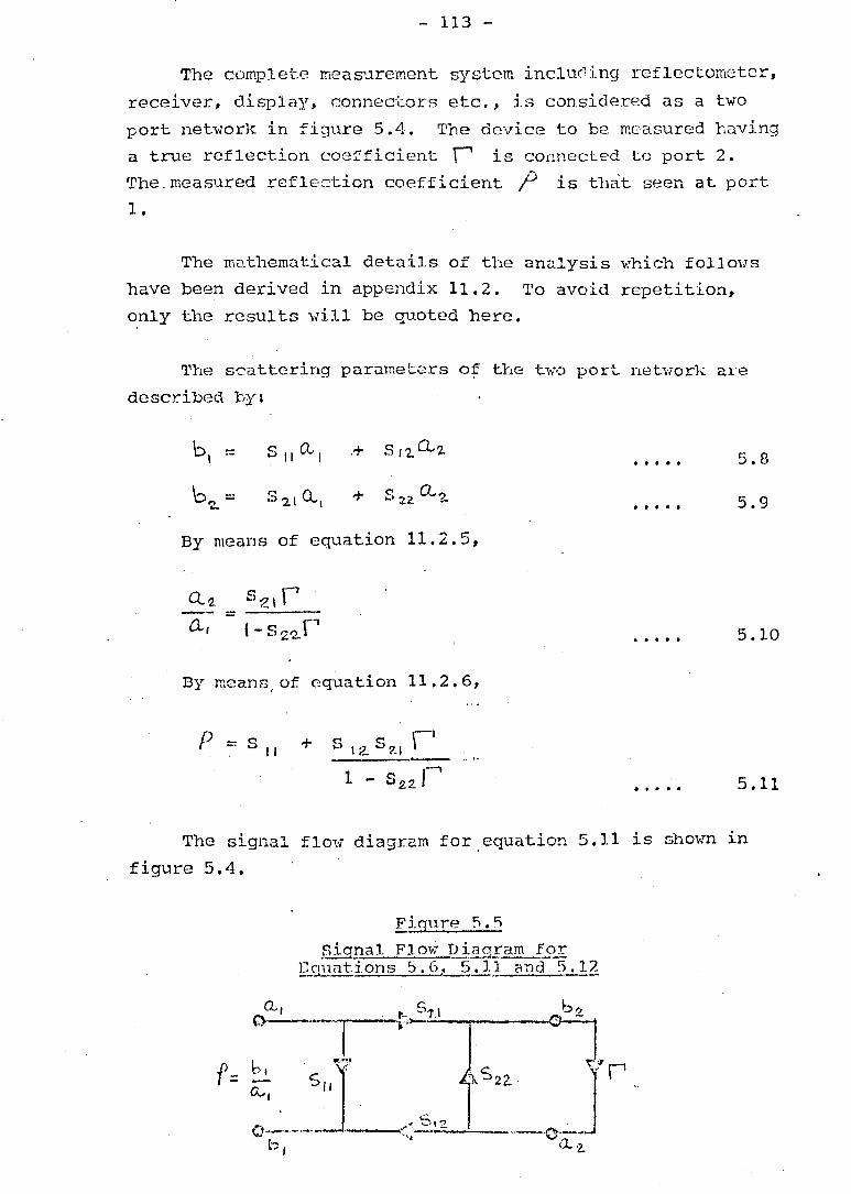
- 113 -
The complet.e measurement system incltv"ling reflectomctcr,
receiver, display, connee-cors etc., is considered as a two
port network in figure 5.4. 'I'he dev'icc to be measured having
a true ref1ect.ion coefficient r is connected to port 2.
The. measured reflection coefficient ? is tha't seen at port
1 •
The mathematical details of the an<llysis v,Thieh fo11m1S
have been derived in appendix 11.2. To avoid repetition,
only the results v;il1 be quoted here.
'l'he sca.ttering parameters of the t\\-o port. neb-lork are
describ(::!c.1 by:
8,,0... 1 · .... 5.8
+ S n a..'2,. · .... 5.9
By means of equation 11.2.5,
Q2 S21 r =
Ll, (- SZ'2..r · .... 5.10
By means, of equation 11.2.6,
p _. C h) II + c ~-., ~) ) - 12.. h ?I
1 - S 2.2.1--"1 · .... 5.11
The signal f1m., diagram for equa·tion 5.11 is shOvln ~n
figure 5.4.
Figurc~ 5. '1
.signal Flo","" D iaqram fOL E('Jll<1t.ions ~,6. 5.11 and 5.17---~ . --..... .

- 114 -
Equa·tion 5.11 may also be modified to the form:
f :=
• It ••• 5.12
Equations 5.6 and 5.12 are of the same form, and for
equivalence, then we must have
A := (- 5) - c co + c S21 .- ""11 ":>22 1-'12 · . . . . 5.12(a)
B := c "')11 · . . . . 5.12(b)
c = (- 522 ) • •••• 5.12(c)
D = 1 • • It •• 5.J2(d)
Hence it may b2 concluded that the signal f10\-1 graph of
figure 5.5 is applicable for rcf1cctcrneter error correction.
'1'he physicill meaning of ·the scatt;.ering parameters when
applied in this context, may be likened to the fo1lmdnQ'
prope:.-ties 'vhere:
8 11 represents the effective directivity errors which
in addition to the directivity of the measuring coupler also
include residual reflection effects of test cables, adapters
and l(~akage signals bet"\e?een the. inciden t (J:-eference) and
reflected (test) channels of the receiver etc.
'l'he jusU.fication for thi s representation can be clearly
dcnlOnstrCl.ted in eql~.at.ion 5.12 for the case of a perfectly
matched load ( i\ := 0 ). In this case, .the only signal
detf~cted ,d.ll be that due to. S11 i. e., the cffecl:i ve direct
ivit.y.
S22 may be seen t:o h~ the rE~sul t of an j mperfect source
match wh?n~by tbp 'vaVQ reflcctpd by the device being moasurecl
is not con",pletely absorbed and part. of t.his .r-eflecb:!d v,';JVC is . , , 'd t rc-reflectC'u to appear as an J.l1cremer.t to the maln InC! ~en

- 115 -
wave. (Note: This source match should not. be confused v:it.h
that of the genera.tor source ma.tell mentioned in s2ction 2: 4).
5 12. S are referred to as the frequency trackinq errors --=-:;;:.. .. _ 21
of the system. These are caused by s!llall deviations in gain,
phase and frequency response. The errors are caused by
differences in the t.est and reference chanr:(!l signal s due to
imperfectly matched cables, differences bet'veen the incident
and reflected test couplers, differenc<.~ in receiver channel
gain etc.
• t 't . In the pract~cal measurernen case, 1 18 not al\lays
possible to connect the devices to be measured directly to the
reflectometer system and the signal f101" graph of figure 5.5
must be modified to include the effects of transformations
due to ~:laveguide/cable/connector lengths etc. Furt.hermore, . d -'!. '} h rn'2asu:rements are frequently requJ.re, on '-leVJ.ces w~ t 1 t e same
reflection coefficient separated by different electrical
1eng'l:hs of uniform transmission line e.g., a short circuit,
an offset short circuit etc.
Figurp 5.§.
r_~~ct~ical SiriIL~l F19.::!.-..r-;]~.ill?2} .. .0J_~he ~ls.ctom(~t_Q! }lea f3:u:-ing syst·f':~D
5'2.1 D2, -.ct e.. 1 eL,
~-'-... -'--- ~------~----~ ,--------~
.. , () S -~~ 1~\~. e~ 01---" .-----_ .. --. -_ .. _ ... ,,--'<: .. '-.--.-----.(} ---.. ---
0 1
"

- 116 -
The resulting modified sign<ll :EJ.m·l graph is shm-ln in . 5 6 F . d . . . h f 11 . fl.gure •. . or ease l.n erl vl.ng tIlt:! equatl.cns 1 te-o mnng
are defined:-
-fY = (eX + if> )Q.
",here -p" represent:.s the total propagation effect.s for a given
uniform transmission line of length It '- " ,
oZ is
p is
1.. is ,-0 . J.8
the
the
any
the
attenuation constant per unit length
phase constant per unit length
fixed length
reflection coefficient of a termination.
The suffices, 1 .to 4 indicate t.he ordered set of measure-
ments. For example ./f/, -- ( 0( + c.f,8 ) 2., r ,vould refer to the
total propagation effects due to a line of length " £," 'vi th
an attenuation and phase constants of ex and f3 respectively.
Hence the general equation of 5.11 adopts the:' forms shown
below:-
For the case £::: t, = 0
· .... 5.13
For the r.Q·se J..,:::: R., ~ , . .
· .... 5.14
For thc~ case i = £. 3 ,
• •••• 5.16
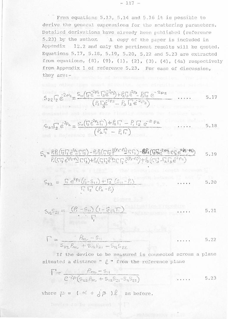
- 117 -
Fro:n equaLions 5.13 7 5.J.4 and. ~\ . 16 it is possible to
derive i-:,he gcn .... --. Cn :L cxpre s d.ons for U1C.~ s;;attcd.ng pararneters .
Detailed deri v3. t.:L~ns 11avc alre2.dy bee n [:ubl 1. sll t:' r.l ( referenC'e
A copy of tJ:l2 p a:ner is included in Appl~ndix 12.2 and 011 1y th e pertinent results ,,;ill be q'.lotcd .
Equations 5 . ~.7, 5.18, 5.19, 5 . 20, 5.22 and 5.23 are extracted
from e(:T1.1~tions; (0), (9 ) , ( l )J (2), (3). ( 4) , (4<:l) respectively
from Appendix 1 of reference 5.23 . For ease of discussions
i:hel un=.!:-
5 . 17
(' t4 · '2f>~ " . " J) r. c>".- ,':; .. t ) _ - /.r., c' I ,. e.. \ +-" I .- I , ..., D lJ:;t, /"' \1 YQ, '::>1\ ,2 -')"" I "'-- ,_
?.::l~12 e = '----- ..... "" .... -.. ------... - .. - ... ( P~ f7 - P ~.)
5 . 18
5. J 9
5.20
•
•• , • f 5 . 21
/;) ~ rI7('I.. ,;> ' " "' ! :
__ .' ... . _ ,t • ;w,.. . _ _ " . .... ·9 ... '_ . • ., ..... "'·.· ... __ • • "' ....... ..... _. 5 . 22
If the devicE-~ to b(? meo.sured is connected iJC1~OSS a plane
. t i ",l (1 1' c' l' ~ncc. " n II from the l:C.!:cJ."ence r.Jl i:tlie 81. ua :".-,~). a ,I . ,j.W '.;:. ~ L'
5 . 23

- 118 -
Several authors (references 5.8, 5.9) have solved
specific cases but a general f30lution for both lossle~;s and
loss-free calibration standards have not been available before.
5: 4.1 'P. considerable amount of wor]\: "ras expended investiga-
t.ing the many methods of measurement correction. The idea of
using other than short circuits, opell circuits and matched
loads as calibrat.ion terminations Ilas disliked because of the
uncertainty)' of the charac·terization of the terminations.
Many alterriative methods ~,vere tried but three methods pre
dominated and t.hese Ilere finally choscm for further work.
The three methods arc (a) The rrhree Short Circuit Method
(b) '1lhe Four Short Circuit Hethod and (c) The Four Termination
and. a Reference Short Circuit Met.hoo.
5:4.2 The Three. Short Cir~uitl? Correction Method
In this case, the three t.c!1~minations used are
~ or ~ :: \-;: :;:: " ll~{l~ The electrical leng·th bet\.Jeen f; and r.' is 2-2 a~d the electrical length between 'G and 12 is
(- 2-3 - J!.,Z)' These are shown in, f:i.guI..-t:~ 5.7 •
..-1~Jft. =. (d" + J (3) £2-~ = J{3e z
-,p/~ -.<:: (cz -t-~ (=3) Q. '3
'(:3 :.::: if (£3-,£2)
Devic2 to be measured
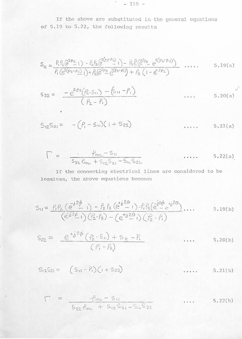
- 119 -
If the above are substituted in the general equations
o f 5.19 to 5.22, the follm'ling resul ts
- e2P2(~_SIl) - 6 It - f,) ( P7_ - Pr)
-P rr("l~ - S 1/
CD '" S S -'22. I I'l'n..- +- S i 2.. '::) 2.1 - 1\ 2."2.-
5.19(~)
5 . 20 ( a)
5 . 21(a}
5 ,22( a )
If the connecting elect.ricCtl lines ;::tre considered to be
lossl e ss, t h e above equat.ions beco:nc :
5 .19(b)
+j{)c~ ( co "\ _ P, e '1~' -. I I) + S 1/ .-~-----. --'-- 5 . 20(b)
(P, -. P'2)
5 . 21(b)
.i; _. C I _____ ~I.;:0~~ __ ...;_!.... ___ ._._ .. ____ ~ 5.22(b)
S P to. .1" 0, (. ,:~.,,... rz:2.. ryy... ...1 •. ::'> \ ,~~ ~ ~ \ -.. _, I \ . ~ L'l ~.

- 120 -
o f cquaL:.iurJ.::; 5 . 19(b) to 5 . 22(b) experiment.allY. Ver:y good
results were obtained. ThesE: resuJ~s were published in
E18ctrcrd.c ·Lett.c.i.."S ( Hef 5.13) in March 1973. SincE.~ thc:1.,
Lhis nwLhod of ln2.asurement has been \'8d.fied by Gould and t
Rhodo s ( Ref 5. 14) and Kwesah ( Ref 5 . 15) . Warner ( Ref 5.1G)
dnd Woods ( Hef 5,17) h:rve recognised the n:ethod as acceVr'able
i n t h eir ri9o'COUS analysis of ref.lecto!nc-te:r: r~r~~ors.
'f1-d. s lS th~ ca. ~~~c de '·~cribed by Hac]<:born (Ref 5 . 9) . For
t his,
r-"" -\ I .-
. j
From equation 5.19 to 5 . 22
S -, r I -- f) :j
. ) t;:-o
E' t ' 5 J9 ( ) J. '''' O V11ly t .:r·UG f o r a m;:tlCDcd termination . qua 1011 •. c ~
From equ<: t.ion 5 . 20 n I ' /p . ", ... , £-r~ _ '-," \
';:;. t \ -- A + e l 2- ,,; . ' . ./ ---------... --.. - i)-----
-f, -r'L . I f 1.:he t:rans'l1j ':'3sion line is 10ss1 ss i. e .
F rOIn equa·tion :; . 2 1 .
(s t I .-. f '.,Ie \ + c: 2;>.,)
From quatirn 5 . 22
-Prlon.- .- S II c: I) .,' r _ c... ." :> 'L'I l' /- i., + ... ' \ ~-..:: ~- f ~,. 'I ~ ~_2..
5 . 19(c)
5 . 20(c)
5 . 21(c)

- 121 -
This method has b?en compared by the author ( Her 5 .23)
against other methods and has bee n found to be that l east.
sensitive to length errors L1 the offs2t short.
In thi s method J
r~'::: r iQ_~) 12::: ' L 0° ) ~::: I I C)0
~rorr. equation 5.],9 I _ .
5 '1 ::- -PI e~J5?~-= I) .-- ~ p,? (e'2Li~~~C22 I) - f3 PI Ce-'-~: e,z~?>--p~ __ _
p, (e"{1'3-1J2) I) + .~ (e2P~ f/(-P3-.f>IZ)) + P3 (I (~ e2P2.) • •••. 5. 19 ( d)
From cq11ation 5.20
5 (2..2 =: e 'LP2 { ~ - S I ~±_ ~L~ -- PI -f?. -. PI .
From equat.ion 5 . 21
S { '2. S 2{ -::::: (PI - S \;)( I - S 2. '2.}
From equation 5.22
r c () -1.. C! S - s (. ~ 2.2. rl")'Yt....-' ..... 1'2... 2 1 1\ -> 2l_
'l'his method cari be used provided one c an really define an
~~ . 20 ( d)
5.21(d)
5.22(d)
open circuit termination . Tests with this method (Ref. 5.7) h ave 8hO\{n that the corrected resuits are susceptible to errors in defining the open circuit terminations.
For co-axial cables , HeYllet_t Pac)card ( Hef S . 7) and , \-J oods (Hef 5.18 ) have given figures for various si~andan1
conn(~ctors. They are tabled belm.-
C<2Emec"l:or T:tl?c .~~9hm L:L!2~§
APe7 -~---
N -- MALE N .. - Fm·~ALE
SW\ -" M.L"\LE C;HA - FEMAL .~
14 .2 825 mm (Jnt. nidm) 19.05 mm (Int. Diam)
--2E.~n C ircni t ·CapaC·i tance;,:;rHewlr'lt Packard \-;ooos , D.!. --0.081·---------0--07----
0 . 032 • - 0 .1 80 - 0.064
0.032 O. J. 64 9 0 . 22Cl2
-_._------- _._---_._-------_ .. _------------- --'-' --_ .. -

- 122 -
Hov.Tcv(,:r" \~}lOn micro s t.cip is measured the open cireui t
capacitance is i LL -defined . J ames and 'I'se ( Ref.5 .1 9 ) have
given some informati.on on calculating microstrip end effects .
The author ha s ~_nventc(~ a met1D:3. vThe reby the t e rm:i na tion
inuni ti:anc e can bc cal r'u lated directly from the c alibration
measur~men-ts . rf'h i s i s explained fOully in Sec t rimS : 5 .
5.4.5 The Thro (:? Id e ntical Non--Hat~ched Termination Correction - .----- -----------------_.- ---- --_._-----------------:Het110d. , . - r I' --'--- TIn s 1 s the ca se \\Then .1 == 12 = r; == \; , whe r e I""\:.
itially un1'>:nmm. Its use \'lill b e shmm in. Sec·tioD 5 . 5
c ...)2'2.
5 .~21
\' (j) - S 1''\) / \ - -I , \.. I I \...
l From equation 5 . 22
frrr:.- - 5 I I
'5 :1.: frrru +- S 1 'L S :-=-:S \ I S~~~
i s in-
5.19( 6 )
5 . 20(e)
5 . 21(c)
5 . 22(e )
It should be noted that 5 11 is u J1affect.ed by any
·termination hut S22 and 812
8 2 1 are affected by the
recip r ocal of t:he termina t.ion r eflec1:ion CO E.f ficient..
'J.':his is ·the _;"l <'58 vlhen :
r~' = \ L \ 80\7' ,. , r-' .- I I' $'0° 12 - 0' , ..
)
5 . 19(f )
5 . 20{f)
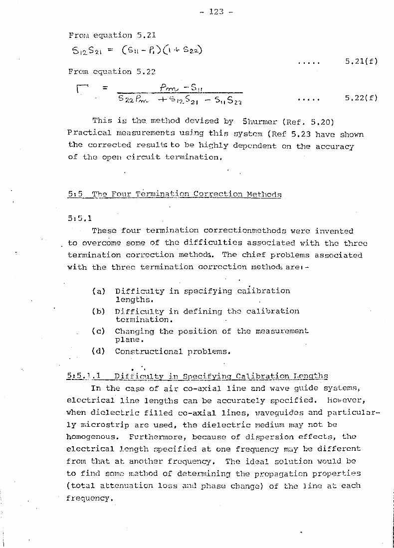
- 123 -
From equation 5.21
5,2.52\ :: (Sit - p.)(, + 52.2..} ..... 5.21(f)
From cqu':l.tion 5.22
r 5.22(f)
This is the method devised by 5hurmer (Ref. 5.20)
Practical measurements using t.his system (Ref 5.23 have shown
the correct.cd n:~sul tc to be highly dependent on the accuracy
of the open circui'l: termination.
5:5.1 These four terminat.ion correc'l:ionmethods were inven·ted
to overcome some of the difficulties associated '~Ti th the three
termination correction methods. The chief problems a.ssociated
with the three terminiltion aorrection method~ are:-
(a) Difficulty in specifying caiibration lengths.
(b) Diffieul ty in defining t.he calibration termination.
(c) Chan9ing thc position of the rr.easun~ment plane.
(d) Constructional problems.
. . 2.!~_.1:_L_l2i-j:Ji"'£lllkiD SP~7...cjJying CllJ ibr2J::iol) Length.§
In the case of air co-axial line and ,,,,ave guide sYf3t.ems)
electrical line lengths can be accurately specified. Hm\lcver,
when dielect.ric filled co-axial lines, ,·raveguides and particulilr-
ly microstrip arc used, the dielectric medium may not. be
homogenous. Furthermore, because of dispersion effects, the
electrical length specified at one frequency may be different
from t.hat at another frequency. The idGal solution would be
to find 80m2 ly.2tlJod of dE~termlning the propagation propertl.l?s
(total attenuation loss aad phase change) of t.he line at. each
frequency.

- 124 -
5:5.1.2 DjLficuliy in Defininq th~ CaU.bra'cion 'rermin<:1.t.ions
It has already been mentioned in Section 5:4 that
because of difficulty in specifying 'Lhe calibration
terminations, these are generally lir:li·ted to short cireui ts,
open circuits and mat.ched loads. The short circuit presents
little difficulty for co-axial lines and \vaveguides as the
losses associated \'lith electrical conductivity are minimal.
'rhe effective plane of an open cireui t termination is
difficult to determine especially in microstrip. Further
more, for certc::.in calibration proec'dures, (Sections 5: 4~1
and 5:4.5) the 'corrected accuracy may be seriously impaired
if the open circuit tf; not correctly defined. The difficulty
associated with producing a perfect matched load are well
known and need no further comment. An ideal solution would
be a method '\lhich was independent of th~ calibration term
ination.
515.1.3 Chanqinq the Posi~ion of the ME'~asurement Plane
In the measurement of some 'Cowponents, e.9., capu.citors,
inductors etc~, it is frequently desir(:~d to alter the plane
of measurement to determine the actual componE·nt. value· of
·the item at its place of origin instead of its value trans
formt:~d by a :r,_~ngth of transmission line. rl'his chunge of
the measurement plane can be carried out by using equation
5.23. Ho~wever, the electrical length must. be accurately
known at the frequency concerned.

- 125 -
Difficulty io often encountered in the con::;truction of
short circuits in microstrip especially when the line is
terminated ai'lay front the edge of t.he substrat.e. This problem
is compounded when brittle substrates such as sapphire,
quartz, glass etc., are used. Some "Shattering" experiences
were encountered 1.;hen holes had to be drilled to construct
short-circuits. A solution independent of the calibration
termination "muld avoid these problems.
5: 5.2 The Four Termination Correct.ion Hei:hod s ,----
This method 1-laS invented and initially submitted to
"E1ect.ronic Letters" on 11th February, 1976 (Reference 5.21).
The ca1fbration procedure requires the construction of four
test pieces. All test pieces must have identical terminat
ions, identical "'trahsi t.ions to the nctvlOrk analyser terminals
and identical trans~'l1ission. lines (except for length) connect
ing the transitions and the terminat'ions. rfhe lransi tions
and transmission lines (Z02 in figure 5.8) must also be
identical to that used for connecting thc~ device to be
measured to the network analyser terminals. It fol10yTS that ~
all the transmission lines used will have identical attenua-
tion constants, identical phase constants and identical
'characteristic ,impedances at each measurement frequency but •
none of them? values need be Jmown at this stage.

---------------.--------._---...,. --."-"-~-~.--........ ..,~~--.'-------~ ...... , .. - ... --......-..--... --~
+ Reference Plane
P. I Perfect ) 0, 1 ~ s., ·1
c' )I Reflecto- ~511 S2.2.-~ V r l mete!: '-0 I <: 1--0-' . I / s,z ~L I ;>1 ~
Ole;. J . ""'I.
I Nea.sured Reflection Coefficients
Error Network.
L = any arbitrarI length
,.... -.-Q. ..... e'
I o e--rv 1r
/
\< 1? ;>1 I
~,.,
Identical terminations and trans:nission lines of Zo2 characteristic
impeda.nce ./;/ '
r- I Qi3 1 -PI = (0<. ..\- Jf3 )Q
~ =~Attenuation constant.
// o e .... ·(:lJ
o e-2 ;v }r 1< z2 >1
c!~
f3 e;= Phase constant J?. =: Line length
0
"
e.- 3 --(U
p-3 -f2' lr I
. \ ...... 31-I"
. ..1
I --f
A I Reference Plane
FIGURE 5.8 SIGNAL FLOH GRi\PH OF THE FCUR TERt\fINATION COFRRCTION ME1:HOD
I-' 1>J (J'\

- 127 -
The physical lengths of the uniform transmission. lines
usC:?d in the test pieces must. h'J tf L ", .. t_ -;. Q.", It L +2Q" ,
It L + 3'.e ", I>lhere "L" and ., r~ It 'e 0 t t 1: t "-1.-- 1 f 1. ar..· c nf3 an S:JU I_l~e va ue 0
" L" need not be Jmown.
For calibration purposes, each test piece is connected
to the net'\'mrk analyser terminals and meClsured. From these
measurement.s, it is possible to calculate the total atten
uation and phase change of the line length "t". To derive
the scattering paramet.ers of the error netw'ork, it is
necessary to knmT the complex reflection coefficient of each
test piece. No difficulty exists if the termination is a
.short t:ircuit. However, if the termination is unJ~nO\m, e.g.,
an impcrfec·t open circuit, then i·ts stray immittance must
be found. '1'his can be obtained by placing a short circuit
across the reference plane .(Fig- 5.8) and maJdng an additional
(fifth) measurement. Then by using the informat.ion from all
the calibration measurements and. equations 5.28, 5.31, 5.32
and 5.35, it will be possible to calculate the scattering
paramet.ers of the error nebwrk. This information mQ)" t.hen
be utilized for t.he correction met.hods of section 5: 4.2.
If the line impedance of the test pieces is not that
of the reflectometer, the cor.r·ected reflection coefficient
derived ,rill be that normalized to the line impedance of
the test peices. This is of course, the established custom
used ,·d th non-TEM '\v-aveguides lv-here a uniCj'l.'i.e definition of
impedance does not exist. Hence this method is applicable
even when the measured device is embeddl?d in a line impedance
other than that of the rcflect.ometer system.
The signal flmf graphs of figure 5.8 yield:-
p-I
c c: r' - 4'9-+- ;:) ,? .:::> ;>. 1 1 f'" ---
· ....
· ...
· ...
· ...
5.24
5.25
5.26
5.27

128 -
'I'he m~.thcmatical basis for these corred:ion syste:lls
have b2en derived by the author in reference 5.23 ,..-hich is
included in this thesis as Appendix 12.2.
OnlY the results of this paper will be repeated here.
r~1 '2 Ceo~·3>.2i;p~q ~ +- ~ f4 ~fi Ps - ~ P4-). + ~ 2.,/:; (p, ~:l.-fl/~ •. -~f3 + f3~) . + (-P,P1.+2R~-P,P4--hP3-R.fi+2~~)f •.•.. 5.28
Hence, provided ~d 0, a soluticn. cf the quadratic
equation i.e.; G.oRJ 2-jV is possible. Furr.hermore, It..-P"
may be resolved into its real and quadrate parts to yield
the total line attenuation and phase change. In addition,
if the.phYf:3ical len9th of the line up... tI is known or m(~asurcdJ
the effect:i ve dielecJcric constant may be calculated.
Let on8 root of the quadratic equation of 5.28 be
denot.ed by ()...L.- + J ~"' .... ) whe~e "/L." and" '1)' \I are real numbers.
lilriting G.')-;;..Pv 2..-p in its exponential form will result in
· ..... 5.29
If one root of the quadratic of equat.ion 5.29 is denoted
by (X_ + ~ ~ ), then
e2-·~ __ e 21X P-12F12. =J%~'+'a-2 l.1:!.~~I(~V(Y · . . . . 5.30
Hence,
2 ex Q = fbrv J :c.2 +:J 2 Nepers · . . .. . 5.31
• •••• 5.32
If thc-! reflection coefficient f-' of the test pieces are
lmO"l.m, then equations 5.31 and 5.32 may be used in conjuncticn
wi th thc~ measured parameters A , P'2. I!~ (equations 5.24, 5.25
and 5.26) t.O sol va the scattering parameters of the error
nebfOl'l.;: (equations 5.19, 5.20 i:md 5.21). Neasuremr:nt. correct
ion can them be applied to an unl~nov.'11 device as det.niled in
section 5:3.

- 129 -
If the reflection coefficients, r·.., of the test pieces
are unJmmm, then it must be found (:ither frOM tables
(Section 5:4.4) or by meilGUreJT\Ont and/or calculation. The
procedure used is detailed in section 5:6.
5:0 'J'hp. EV'll1Ju~:iC)n oft:he Reflect.i on Coefficient of the Tes·t F'ieces _____ -e. __ _
Research into this problem wa:::; initially started because
of the difficulty of producing good short circuits in micro
strip. It had been obvious for some time tha·t correction
(Section 5:4.4) using open circuits· with their inherently
simple construction is especially desirable in microst.rip.
However, previous attempts (Ref 5.19) at calculating the
stray immitl:ances were not sufficiently accurate.
. .. r (?·"'·d(~) In t.his procedure, t.he reflectlon coefflclent (I ::=: e t)
of the test pieces is obtained by an additional (fifth)
measurement. 'I'his additional measurelf,ent, fs is that made
when a short cireui t termination is placed at the reference
plane sho'\om in figure 5.8.
From equation 5.19, 5.20 and 5.21, it is readily deduced
that provided
(a) S" is unaffected by the type of termination
. I
Sl2. -(.JL+d"'P)C' I
qJ) e':')22..
• •••• 5.33
where 5 2 2./ [ eZf)~ ( P?_ - S 1/ ) + 5 II - P, 1 · .... 5.33a
'~2.. - P,
C: 2.;::' ~ ,.;:~-:.. -. (SL + jq») c I
5.34 ( c) -.>/ - ... e VI2.S 2.1 · .... ~ S/ __ - (PI - 5 11)(1
.'\
where .. ,,,- 21-- - 522) 5.34a · ....

_. 130 -
From the fifth Z'1(;aSUrement
Ps = '5 II + S I 2, S 2. i I L'..?:_? () I -- S:? 2_ ( I! I?':;~--
Transposing $
••••• 5.35
Hence from equations 5.35, 5.34(a), 5.33(a) and 5.19,
the real and quadrate parts of the reflection coefficient
of the test. pieces Jl1ay be calculated. Subsequent experimental
tests prove tha·t. this method is ac:!C'..lrate to 1% of the published
figures.
5:7 .. Conclus~
'1'11e information pn~scnt(-;d in t.his chapter is vi tally
important. D(Jtailed mathematical c:.rgucments have been used . . to establish why it is po~,siblo to measure reflection
coefficients correctly in spi te of imperfect. insi:.J:.'umcnts.
An error correction model has been derived in section 5:1. The general theory regarding correction procedures has been
extensively . expounded in S(~ctions 5: 2 and 5: 3. General
fO!1nul~e for calibration and correction using three calib-
. rat.i.on piece::;:: haVl~ been derived for the first tirr.0., c:md
applied to prc~v:Lously established special cases. Several
ne,,, calibra·tion procedures havE~ bell!} e\101 ved in SE~cUon 5: 4.
Fur thennore, some oJ: tIle method s invented are 11m, accepted
as sta.nc1ard method~ of correct.ion.

- 131 -
The m(~t_hods of Section 5: 5 are exceptional fr,ethods in
that they have shown how the attenuation consla.nt, the
phase constant, dispersion and even 110"\'1 the reflection
coefficient of the test pieces may be obtained. Hitherto
these properties have no-t been taken into account a.s these
t · . losses were no edslly ascertalned. Finetlly this theoretical
analysis has established clearly tha-t error correction
procedures are possible wi tbout the usc of eX}.:)cnsive pre-
calibrated test pieces.
* * * * * * * * * *
.. ; ..

- 132 -
5 .1 Barlow, Hand Ct::.llcm, A lI}1icrowavl~ Neasurement.s -Constable & Co., London 1950
5.2 Adam, S.F. "Microwave rrheory and Application" Prentice Hall, New .ork.
5.3 Sucher H and Fox J "Handbook of Hicrowave Neasurement.s, Vols. 11 2, 3 - Pergalnmon Press Nevl Yor1~ 1963.
5.4
5.5
5.6
5.7
5.8
5.9
5.10
.. 5.11
5.12
5.13
5.14
5.15
Beatty, R.W. "Invariance of the Cross-Ratio Applied to Hicrowave NetvTOr)~ AnaJ.ysis" National Bureau of Standards. Boulder, Colorado, issued septem .. 1Jer 1972.
Biancq B and Parodi, M "Measurement of the Effective Relative Permittivities of Microstrip" Electronic Letters 1975, II, pp 71-72.
Ajose, S, Matthews, N, Aitchisor~ C "Characterization of Co-Axial to Microstrip Connector suitable for Evaluat.ion of Microstrip 2··Ports" Electronic Letters Vol 12 No. 17 pp 430-431 August 1976.
Hewlett Packard Applicati oa Note 221 - Semi- . Automatic Heasurements using th<? 8401B NicrO'.·lave NeblO.rli: Analys(::?r and the 9825.Zl,. Des)t-Top Computer
Adams S. "A Nmv Precision Automatic Microwt'lve Heasurcmcnt System·! I.E.E. 'I'rans. on Instrl.l111entatiorl
. and Heasurement. Vol IN 17 No 4 Dec. 1968.
Hac].;:born, Richard "An Automa.tic Network Analyser Sy-'stem" Nicrm'lave Journal, Vol 11 No.5 Hay1968.
R~~ich, Volker "Microstd.p-Hessingen mit Netzwer]~analysator'" Nachrichten 'I'echnische zcitung 1975, Heft 5 pp 255-259.
Shurmer, H.V • .#. uLow .. Leve1 programming for the . On Line Correction of IVIicrmYave Measurements" The Radio and Electronic Engineer, August 1971 pp 357-364.
. . t' L 'l',ncleton, J,R.G., "}11.crm..;ClVC Inser .J.on oss Neasurenv.:m·ts" I.E.E. Colloquium on R.P.Measuremerrl:s on Solid sta-te D0vices, London 25th Hay 1971 •.
da 8i1 va, E, F. and HcPhun M.IL "Calibration of Hicrmlave NeblOrk Ana1ysnr for Compu·ter Correct-ed S Parameter Measuremel1ts~t Electronic Letters 1973 9, pp 126-128.
Gould, ~r and Rhodes, G "Computer Correction [or a NicroTdave net1-;'ork analyser wi thout accurate freCJl.H:mcy measurement" E1ectroni c Letters 1973 9, pp 494-49S.
E'i·msah, 'A "Characterization of Inteqrated Di-polar Transistors using Computer Aided Measuroments and Optimisatio~! Ph.D Thesis - University of vlarwic}<:,Nov. 1976.
5.16
5.17
5.18
5.19
5.20
5.21
5.22
5.23
5.24
- 133 -
Warner, F. "Microwave Att.enuation l1E:"asurement" 1977 Peter Peregrinus Lte (I.E.E. Monograph SeJries 19).
l100ds, D "Rigorous Derivation of Compu.t.:.er Corrected Neb~·ork Analyser Calibration Equations" Electronic Letters 21 Auaust 1975 Vol 11 No 17 pp 403-~04. -
Woods, D "Immittance Transforma.tion using P recision Air-Dielectric Co-Axial lines and Connectors': Proc I.E.E. Vol 110 No 11, Nov 1971.
James, D.S. and Tse, S.H. "Micros·trip End Effects" Electronic Letters 1972, 8 pp 46-47
Shurmer, H. V. "Calibration Procedure for Computer Corrected S P arame·ter of Devices Hounted in Microst . .rip" Electronic Letters 1973 9, pp 323-324.
Hills, T.D. "Private Communication dated 18.2.76" I.E.E. Reference R 1495.
Cox, T D.Sc. Final Year Project 1974 Engineering DepartmeD-t, Uni versi ty of Warwic]t.
da Silva, E. F. and McPhun, N. K. "Calibration of an AutomC'ltic Net1'lOrk Analyser using Transmission Lines of Unknovm Characteristic Impedance) Loss and D'ispcrsion" The nadio aJ1d Electronic Engineer Vol 48, No 5 Miy 1978 pp 227~234.
da Silva, E.P. and McPhun, H.K. "A Revievl of Networ}c Analyser Calibration 'I'echn1ques for One Port Measurements" Hicrowave Journill, June 1978 .
.#.. •• fr.
* * * * * * * * * *

- 134 -
HEASUREHENT EQLJIP1'IlENT (Seftvlare)
6:0 Introduction .. ~-~--------
Practical applications of the equ2.tions in Chapter V •
·require long and ·tedious computations of complex numbers ar:d
a desk-t.op programmable calculator (Hew-lett-Packard 9100A)
was used in t.he initial stages. with 'chis calculator, the
calibrations for each frequency had to be keyed in manually
Clnd the answers WGre returned on a printed sheet .•
Later, when measurement automation was introduced, the
Hevi1et.t P ac}~ard Calct-..lator 'fas replaced by the Rank Xerox
Sigma 5 computer. Considerable difficul t.ies \vere initially
experienced in using this computer as the idiosyncracies of
the computer-nGti-lOrl( analyser int.crface had to be learnt,
and t.he large storage requi rement s of ·the programme made it
feasible t.O use Jche computer only late at night. How·ever,
the many months S'J?ent producing the progranune has been amply
rei-larded "!::>y the speed and th9 (;~fficiency of the automated
systens.
The computing programmes described in this chapter 111ay
be divided into two main categories:-
(a) Progr,)mmcs for manual operation.
(b) Automated programmes.
The In<lnual progralm'lles vd 11 be fully described. Com:)lete
clescr·1.pLions of the rn::torrmte::!d prcgrarnmcE; Cl.re impracUclll
bC'canse of the length of the pro~Tl::-anen(~8.

( I
- 125 -
I __ igurc 6,1
pj cJ:~ __ 9_~L_He~i:L3J:-i- Packi?r< Pr()qranuna~le Cill c ulu LGT jledel 9 1 C:)A
t 9lDOA
Printer mowl.ted on calculator
\ --~ \ ---'------------,-,
9l0DA/ 9 J?O/-,
I I J
/

- 136 -
No·te: It is assunH:;:d tbat tlle read(~r is conversant 1'lith
th8 cc:;,lculator. If no·t please consul t the manual (Ref 6.1).
'l'he prograrmm:" 1'las 1'lri ttcn for use on the Hew'lett P C:lckard
Programable Calculi:.~tor 9100A (Fig 6.1). The p.-ogramme
accept.s input del,ta; calculates them according to the equations
5.19(b), 5.20(b) .. 5.21(b) and 5.22(b) speficied in section 5:4.2; and print.:: the output dat.a.
rl'be ca.lcnlat:or "Till accept t.'VlO. i tt-".:l1"lS of information at
a time; on(~ i,tc,n must b'2 put int.o its "oX." regi ster and the
oth(;l:' m~,l!:lt be put int.o its ",&" rC9ister. In the display,
the 1I,(~" regi ster is -8i tuab~d llLoVE~ the 11::(.11 regi ster. Each
set of informa tion contains hm items af informati on. Five
sets of input. data must be read from the mc~asuring in=;trument~s
by the operator. 'This information must be h:md fed into the
calculat~o:r. in the order specified in 'l'able 6.1.
T'2.t~le 6.l' InE'lJ,LFonnd t::
. set [-'---.---1------. -. -----, 1- -) l -- "XU RC01 pt.er !Iv" Reg] E~'ce:r' :<ema!.....<:".§ Ord~r ----=----.- --1._--- .. - ---- --------.-.~-- ..
f"-- fhanl.· -- 'Freq-:-- in-'G'i-rz F·rE~q'JE.mc~y -'of 'Operation
of 1st: short Clrcult
Nagni L1·1(:!· l\ngle/Degrcc He~su!~ed RCflectio~ Co(.fficient I of 2nd r:;hort circult
Hagnitude Angle/Degree Neasured Reflection COGfficient
3
4 of 3rd short circuit
5 Magnitude
.1-_____________ . __
Anglc/Dcg)~ee Heasured Reflecti on _ J~~_ un}:;:nOl>Jn d~V __ J··._c_e ________ ....:
Coefficient
'fhC! output-. d;).ta iG printod out in the fannat S]10\·m in
Table 6.2.

*
__ '_0 __ -.
1 Magnitude
2 Magnitude
3 Hagnitude
4
5 Nagnitude
6 Magnitude
7 Magnitude
8 Magnitude
9 Magnitude
10 Real
11
- 137 -
:.t'abl e 6-2
OU"l:.e..~lt Forrn('1.t
---.------4-~.-------------- ----\ Angle/Degrees Heflection Coefficient
of 1 si.. sllOrt cireui t*
Angle/Degrees Reflection Coefficient of 2nd short circuit*
Angle/Degrees Re1:1ection Coefficient of 3r:d short. circuit*
Angle/Degrees S11 - Error Nr",b{orJ{ . P aramet.er
Angle/Degrees S22 - Error Netvmrk Parameter
Angle/Degrees 8 128 21 - Error Networ){. Parameter
Angle/Degrees Neasured Reflection Coeff't of Unknm-rn Device*
Angle/Degrees Corrected Reflection (beff' t of unknm"rn Device
Angle/Degrees Actna1 Series Impedance· (Polar Form) .#:
Quadrat.e Actual Series Impedance (Rectangular Fonn).::L:'
of Set 9; only one figure will be printed J
This data is merely prin,.ted o~t t<;> ensurt; that a copy of the input data to the machine 1S ret<:uned.
:#:: l'li t.h reference t.o a 50 SL line system.
The programme is pre-recorded in machine language on
Magnetic Cards (Hew'lett Pac)<:ard Type 5060-5919). Each magnetic
card is approximat.e1y 93mm x 51mm in size and each card contains
two standard programmf~s. Each standard programme 'Hill store
196 prog1:"().ln steps of j.nstructions but 1'1 steps are automat.ica11y
lost within th2 machine .wh(~never one storage regist.er is used.
If the m:lcrd.ne is programmc~d correctly, it is possible to
SUCCf'::,sively feE~d 0(18 standard programme set of inst .. t'nctions
after anothl~r into the machine without destroying the inform-:
at:i.on retc.d.ncd· in the storago registers .1"He. ~\..c;w t-\.\f\I'P.."f" (!:>
Gr\"'E\1 ON ""'~E N~)('T"" PAI'i!5:.

- 13\7.1 -
Floy Chart of the Programme used on the HP9100A Calculator
Enter Card .A.
Clears machine.
Input frequency data. in GHz. Continue
Prints out frequency entered in ODs.
Calculates and stor-as the phase shift for tb~ •• lecta6 lj. De 1 ength in re~i ster a '. Generates a cons1.~nt. s.t.op
Input 1st reflection coefficient. Continue.
Prints out 1st reflection coefficient and processes values for storage in register' ~. Stop
Input 2nd reflection coeffiCient. Continue.
Prints out 2nd reflection coefficient and proc.s.e~ values for storage in register c. Stop_
Input 3rd reflection coefficient. Continue.
Print. out 3rd reflection coefficient and proce ••• s values for storage in regi.ter d
Calculates 1st and 2nd tenaB of the numerator of ~11 End.
Enter Card B Continue.
Enter Card C
Calculates 3rd nuaerator tera of S11 and stores the total n erator result in registerl Z and 9.
Calculates the denoaiaator of Sll
Calculates the total value of Sll And stores results' in registers 9 and d. End.
Continue
Calculates 822
and stores the results .in registers f and e.
Calculates 812
S21
and stores the results in registers Y and b. Stop_
Input measured reflection coefficient. Continue.
Prints out measured reflection coeffcient •. .
Commences calculation to yield corrected r~flection coefficip.nt. End.
EnLer 'Card D Continue
/ 6
Continues calculations to yield correcteri refl. coet.
Print~ out reflection coefficient. in polar form, its cquivnl~nt impedance refprenced to 50 ohms in b~th polar and TI~ctangular form, and itA equivalent capacitance or indue tanc e.
End.
- 138 -
T"lO lU2giK'tic cards (4 stvnd;J.nl progr anunes) vere u-tilizcd
to produce the output data of 'l'able 6.2. In spite of these
standard programmes, tbe_n~ 'were st.ill s-torage problems and
t:.his restricted the use of the progr3mmc~ to tbe C0_se where
there is an equal electrical leng-th betwEen the short circuit calibration piE'::cer.:;. The lengths' 'are pre-set into the magnetic
cards but it anI TJ.,T tal\:e~~, a fe,T." sec'on('! c:' to alt'C>l~ I" _ • -..;;J .~..... ~ ,-.~- '::'1118 .leIigtn.
In·the coded pT-int-out of tbe complete programme given in
Appendix 11.5 t..hi s lengt.h has beer:. set for Gmm. To avoid
errors, t.hc cO~2d progranuT'J:: print-out has b(::en taken directly
from the machine, but it can be easily decoded by reference
to t.he decoding table also included in Appendix 11.5. '1'he
.other ,estrict.ion on the calculator is that its associat:ed
plotter must be discol'"!:lected.
The prograj.nm2 ,yorks sa.tisfactorily and t.he complete
calculat.ion procC!ss (including the loading of the magnetic
cards) takes about three minutes. This i::> s1m., in computer
terms bu.t it saves about half an hoar of band calcula·tions
for each set of measurement.s. Wit.h t.he advent. of t.be auto
rna·ted pro9ram:mc[? of J.;hc Sigma V Computer) this system is 110".':
relega·ted to manual mf~aGUremGnts cr to those cases 1-1h<?re a
few' quic}( set. of results are required wl)en the Sigma V
Computer is unavailable.
This progral1'me . ., t' . tl wr1t:ten for use 1.n COrlJuc . .1.on ,n 1
t.heXerox Sigma V Computer. D uta f loom the netvlOr1,,-analyser
has to be rGad a::1d punched into data cards. rfhe progranune
,,,as originally used in the calculation of data for a puper
(Ref 6.2) on the three 8hort circuit correction met.hod
described in section 5:4.2.
The flow chart for thi s progr;:-<mmc~ is 811m-:n in FigurC!
6.2.

- 139 -
Figure 6.2
Flo,;-; Chal~t_ of 3··-S-~C)rt~~l!~t~::U_LE-~~9:.JTamme
( STAR~ '-J-~
Y ~U'l' 7 DATA
. I
.~
INITIAL
CALCULATIONS
_ t [
MAIN
CALCU.LArrIONS
PHINT ou'r] ,--~.' ~~~~:~--,-1
Ini tiate Fortran P rogl'amme
Reads Input Data which consists of frequency, magnitude & angle of Refl. Coef. of 1 st., 2nd, 3rd Short, 0, Ur-]-w"10wn
Sentinel to test input data, if data STOV card is blanJ{, programme stop s .
. Calculation of effective electrical length8 bebleCl1 81wrt. circui ts.
Calculates Error Network Parameters and corrected reflec-tion coefficient of. the .d<pvic(~ under test.
w ri tes 0:..11: input data and corrected reflection coefficient of unknown device.
Returns to read more data.

- 140 -
The prograrrune is relatively short c.lnd is given in
Appendix 11.6. By the alt~eration of two constants it may
be modified for any offset hmgth of short. circuits.
The entire prograrrune is punched on cards. This is
useful as it is loaded onto the bac]~ground system of the
Sigma V 1 'which means that result.s may virtually be obtained
at any fn~e int:erval betw'een t,he top priority foreground
programmes. Loading and running time is about two and a
half minutes.
6: ]_-1.h? Four Sho rts Sig~a V ~~J::9gra!!.lmg for l1gnual Us~
This progranm18 was 1vri t.ten for use on the Sigma V
Computer for three main purposes:-
1: To calculate from the measured data ,of Section 5:5.2
the to·tal attenuation and phase change of the equi
distant offse't lines and then to use -this result for
the correction procedure of section 5:4.2.
2: To form the bas:Ls of the calculation sub-routine for
the automated prograrrune.
3: To compare the results of tne single precision (six
significant figures) of the Si9ma V computer against
those obtained using double preccision (fifteen
significant figures).
The flow-c".\1.art of this programme
6.3.
.: c' oJ. .) shO'vn in figure

- 141 -
Figure 6.3
Flow-Cha£LQ.f 4 Shorts {}1a~.uaJJJ rO.9..f.'2.rI1me
START
INPUT DATA
f
r CALCULATION OF LINE
-TROPER'rIES
SEIJE CTI ON OF LINE PROPERTIES.
ERROR CO[{RECTION
OUTPUT
DATA /-L-----<c-__ •I - _.
Initiates Fortran Prograrr~e
Reads input data which consists of 5 sets of refl. coe§; 4 calibration on~& one from the device under test
. sentinel to test input data' if . ?-@.~ data card is blanl<:, program~e stops
Calculat.es the total attenuation and phase of the transmission lines associated with the calibration pieces.
Selects tl1e roots of the quadratic equation t.o obtain the correct valu.es of the attenuation and phase of the offset lengths.
Calculates the net"lork error parameters, and the correct:ed reflection coefficient of the device under test
Prints out bot.h the input dati'l and the corrected data.

-- 142 -6: 3~!he !:~_~r E;'hort_s __ L.~.t'!'"192:!::_P r~ct~i~n) P rograrnme f.22: -- Nanual_.l1..§.~....2!l.. ·t'he !:;i9.:!lE_y-_COmR.~!'~~~
The p~ograMne is listed in Appendix 11.7. The entire
programme is punched on paper cards and is suitable for back
ground use on the Sigma V Comput_er. Loadin.9 and running time
is about ·three minutes. Addit.ional sets of data require
about one minute \'lhich is mostly printing time.
As this programme vraG t.o be incorporated in the auto
mated programmes, it had to be thoroughly chec}~ed. This was
carried out as follows:-
(a) Practical. values of the error neblOr];;:: parameters 311
,
S22 a.nd 8 12 S21 were assumed, An electrical line length
having· practical attenuation' and phase characteristics
was also chosen.
(b) These chosen values 'vere used in conjunction "lith
theoretically perfect short circuits and a ell.osen
reflecti:>n coefficient for the test piece to calculate
P, , fi ' ~ , 1'4 ,Ps- the apparent ref'lection coefficients
of the calibration and test pieces. These calculati.ns
were carried out. using Cl }1cind calculator (Hewlett
Packard Hodel HP 21) which displays ten significant
figures.
(c) 'I'hese theoretical coefficients P, , Pz., Pa , ~~ , P::r . were , fed in·t.o the Sigma V programme, and i i:8 resultant. outp'l.lt
.... • • I.'
values, i.e., S11' S12 8 21 , S22 and the corrected
reflection coeff iciemt of tbe tes·t piece were compared
againbt the values initially assumed for them. In all
cases, the .results agreed to' within the fifth decimal
place. This is extremely good as the Sigma V in single
precision form only calculates up t.o six significa.nt
fi9ures and rounding-off errors are bound to rest.1.1 t.
Intermediat(~ calculation values VJere also compared to
ensure that the att.enuation and phase chan~ aSGociat-ed wi th
th(? offse·t lengths w·ere correct.. This '\-Tas ma.de possible by
t.E~mporu.ry alteration of t.he output statements in the progran:mc
to provide ~le .intermediate calculations.

- 143 -
The entire system was repeated for different sets
of results to ensure that the first verific3.tion "las not a coincidence.
Finally I in using this prograrmne, the rest.rict.ions
on the minimmTI off set ler.gths detail(;d in section 6.3
should be observed for minimal computational erl·ors.
A corr.ection programJUe for Section 5: 5 carries out
many mathematical operations on small numbers. The Sigma V
computer calculates ,.,i th only six digit accuracy when ope
rated in the. single precision mode. ",r11en operated in the
double precision mode, the Si'lme comput.er calculates with a
fifteen digit l1ccuracy. In order to investigate ·,.,rhether
"rounding off" errors would be troublesome, a double pre
cision programme with a flow chart similar to that of figure
6.3 was ",ri tten.
Practical values of error scattering parameters,
offset line length att(~nuation and associated phase changes
were assumed. These figures were fed into both the single
precision and ~the double precision programmes. Doth pro
grammes were slightly modified for thes(; purposes t.o print
out intermediate resultr;. The results obtained from both
these prograrm-,10s were"! compared ,vith the initially assumed . . values. These results are .tabulatE~d on the nex·t page.

r Total I EleCtrical Item
19ffSgt compa.red Lenqth
I -[lior.;3.l:"d ) I !. and Return)
0.25 A IA::teriuatio~'l (900) (r-J'eper/cr,l)
I Phase (Radians)
Comparison of Sinale and Double p reci sion p roqrcuTh.'TIe Rpsul ts
I
Assumed values
1.2000000000000 E-3
1.68179512023926
Double Precision Sinale Precision Calculated Calculated Values Values
l 1.199999999999537 E-31 1.199079 E-3
1.68179512023926
~ I ~ ~~O) Attenuation 11~20000000000000 E-3 (nepers/cm)
I 1.68!79 ~
1.199999999999537 E-31 1.186839 E-3 l I I I
• 02777 A.. (100)
Phase (P.~di~ns)
Attenuation (Nepers/cm)
Phase 1 (Radians)
.747464358806610
1.20000000000000 E-3
.1868660L~499 8169
.747464358806610 I .747472 I 1.200000000177164 E-3j' 3. 248334 E--3~---1
. I I
.186866044998770 .200133 i
!-' .r" ~

- 145 -
The main conclusions are:
(a) Computationa.l error is small "i'lben tJ1e uDi t offset
electrical length (forward and reflect.ed pat.h) is
a quarter vTavelength ( 1\./4) at the frequency of
measurement.. The unit offset length is defined as
tvd.ce tbe electrical di stance beb"een any of the
evenly spaced calibration pieces.
(b) Computation error begins to be troublesome ;til single
precision mode when the unit offset electrical
lengt.h (forward and reflected path) is O.111lA.~A/l0 at the frequency of measurement.
Gross computatiopal error occurs in the single precision
mode ",,,hen ·tbe unit. electrical offset length (folivard and
retu.rn path) is O.0277A at the measurement frequency.
Hence, the restriction that the minimum unit offset
electrical length (fODr,lard a.nd return pat.h). is greater than
')~/5 must be applied whenever the idnqle precision measure
ment. programme for section 5: 5 is used'.
It: has not been possible to incorporate double precision
computation wi thin the automated programm(~s dUE~ to computer
s·torage problems. Hence, the restricU.on mentioned above
also applies to t.he automated programme of section 6: 5.
. . The det~aiJ.s of t.Ile double precision progranum;~ are
included in JI..ppendix 11.8. 'l'he pr?grarrGtl(:! is extremely useful
for ct~cking out suspect computational errors. It is also
used for manual measurements when th(~ Si~1;,r.a V computer is
unavailable for automatic measurements.

- 146 -
This programme ,.,as i{ritten to chec}~ out the theories of
sections 5:4.4, 5;5.2 and 5: 6 10lhich are that:
(a) The unknmffi reflec·tion coefficientr:; of the
calibration pieces can be calculated from
the calibration measurements.
(b) The Jcotal attenuation and phase change of
the offset lengths may be calculated.
(c) The results ca.n be used for error calculation.
(d) To form the basis of a sub-routine for the
automated progra~ne.
The flow-chart for this progranune is Shown in figure
6 .. 4.

·- ILl7 _.
Initiab:::s Fortran Programme
I~[ INPUT~' DATA " . -
Heads G input data sets (4 'open' J
1 short circuit) and onG set from the device under test.
I~
/\
. :
CALCtJLATION OF LINE PROPEHTIES
-'-
Sentinel to test input data; if da"ta card is blanlc,
7(STOP) program!nl= stops.
Calculat:es and selects the correct total attenuation and phase of the offset lengths.
CALCULATION OF REFLEC'l'ION COEFFICIENT
T~~
Calculates the reflection coefficient of the 'open' pieces to enable'the error network to be found.
CALCUIJA'rION OF ERROR • PARAHETERS
C ALCUTJATION OF CORREC'l'ED MEJI.SUr{El-lEN'l'
-
Calclllat.es the error netw"ork parameters to enable correction to t.aJ<:c place.
Calculates the corl-ected reflection coefficient of the device uncler test.
Prints out the input data, thG line prop2rties s reflection co-
, , 'b ' . cfflclent of the call ratIon plCCGS, ar~"d t.:he corrected and uncorrected reflection coefficient of the device under test.

- 148 -
The progran1m,p is punclJec1 on cards and being relat.i vely
short (104 st.atements) it has bo('n included in Appendix 11: 9.
As this progr~Trune is vi tally importa.nt:, it had to be thoronghly
chec](ed. This v{a~3 cClrried out in the follm,ring manner:-
(1) Values based en practical results were chosen to
produce the bput data. to t.he prograllline. These were:.-
C! ':>22
r
Frequency
- 0.9980757 L1.3~~090o
= 0.01385706 1122..!..:,1584300 '
= Un]mmffi reflection coefficient of the calibration pieces
= 1. 000 I 5.4000
- Reflection coefficient of the device
:: 0.023900 [-12.0.695702
:: 3 CHz (;',:: 100rrun in cdr)
unit off- 10mrn set Len9th::
(2) From the datu. in (I), the expected measured reflection
coefficients, R ' P2 J ~ , fir. J R- and ·f!,n,were
calculated by using equations 5.24, 5.25, 5.26, 5.27,
5.24 and 5. 24 respectively. Calcula'l:'.ion was carried
out. using a ten digit 'hand 'c'alculator (Hewlett Pac}card
Typ~ HI' 21). The val uo s obtained v1ere:-
P, :: 0.999998 {13.613Q130
Pz - 0.999999 /-57 ~9719lo p; = 1.000000 [-135.722251°
P4- - 0.999999 /148.718243° p',. .~ = 1.000000 l1.I9. 999855*~
,,,",
0.020000 L60.0.9,OOOOO t:r(I.. =

- 149 -.
(3) The values obt.ained in (2) were then fed into the
computer programnK'. P rovidC'd no "rounding cffll errors
have occurred, the results produced by th(:: programme
should agree with the origina.l d.ata in (1). A comparison
table is given belm.".:-
I't:em C~narec!
c ':>11
5125 21
1--... ------.--
8 22
j~ttcnuation
Phase
(Calibration) (Refl. Coeff)
(Devic3 ) ( R(~fl. Coeff)
-------_ ... , A §'""b'l1ed _ DC! ta I C?lcCll lll~e Para. 1 L -.i Se~
--0.04385706 0.043
L§J~!1~7l}} 0 ~ l.§.
lated Data -par~;..! .. 3)
--0.9980757
H. 345090~ -' 0.04385706
L122.L~5843° . -
1.00000
720
1.000000 0
12.d.90000_ ..
.. _ .... -0.99f3 071
~3488390 --.----
0.043 929-· /12~
. . . 0 ?- •. 438152 •.
---. 0.999 999
'7 1.9982°
--------0.999
I -- .. ----........ ---.----f
0.023900 /-J20.69570?
-
0.023 972 ,---0.845939 ; -1 ~l
-
The following conclusions ",ere drmm:·-
(1) 'I-be computer progruIn.'ne is correct.
(2) Slight rounding-off errors occur. This is inevitable
.... rith siX-digit computation. It was not. possible with this
o:r ,vi th the other ari tbmetical cases tried to ascertain how
th0 "rounding-off" errors could be propori.:ioH8d between the
manual calculator and th<= computer. HOvJ"ever, computational
accuracy t.o '\d thin 0.0001 has been achieved.
(3) The idea that a reference short cj.~-cuit meusurement
could be us~d to calculate the reflection coefficient of thE::
unk:novm calibration termina.tions 'W'aFJ confirmed arithmetically.

- 150 -
(4) Finally, all the points mentioned in the early part of
section 6:4,(a)~ (b), (c) and (d) have been verified.
The main purpose of the a"..ltomat.ed progranunes is to
enable computer corrected measurements over: a wide frequency
band to be made quic)~ly and accurately. Two prograrruneS '-[ere
used
(a) 'fhe Four Shorts/Five 'l'erminationProgramme.
(b) The Three Shorts 0, Allied Correction Progranune.
The i t.ems discussed in this section are applicable to
both programmes. Items peculiar to a particular program.TT.".e
will. be identif::'ed by reference to i:he programme concerned.
6:5.1 Basic principles
The automated progranune initially developed by Duc).;:ett
(reference 6.7) ~as used as a starting point, and new
calculation s-t.orage and display sub-rout.ines were 1.vri tten
and inserted by t.he (:l_1J:thor. sections of the inter-active
control structures were also modified.
Wh · ., '1 t f en on-ll.nc computer·-correctl.on 18 usee, se's 0
reflection coefficien·t measurements using the appropriat.e
calibration pieces are ma.de at. fixed frequenci es 1.d thin the
band of interest. The number of ineasurement sets made is
determined by the number of calibration pieces used. Each
set of measurements is stored within the computer. The
device to be measured is ·then connec·ted and a further set
of reflection coefficien·t measurements at~ the same fixed
frequencies ar~ mc..d(~ and stored wi thin the computE'!r. When
t.he correctedmeasurement· results are required, the computE.'r
wi thdrmvfJ from st.ore the informat.ion required, calculates
and prints out. all the measured and corrected S'2ts 0::measurem(;;nts. ,subsequent me:wurement. of other devices at
the same fixed freLJUcncies may be made ,·rithout further
calibration. Facili t.ics arE:~ a1. so provid2d "Ti thin the

- 151 -
programme foy graphical displays on a video display unit of
the mea~nJred reflection coefficien-ts in eitbe.r- polar or co-ordinate forms.
Additional facilities arc also provi.ded for over b\T<".mty features. These include data storage on extcl:nal tape, repetition of readings etc.
The programmes may be examined more closely by ref
erence to the photograph of the measuring equipment (Fig.3.2)
and the diagram shO\ving the inter-face between the measure
ment_equipment and the computer, (Fig 6.5). Flow-charts of
the pr~grammes may be found in figures 6.6 and 6.7. Only
the main features of the programme will be discussed.
verbatim listing of the prograrrunes will no·t be given because!
of length; for example, the five termination programme
involves one-thousand two-hundred and sixty-eight (1,268)
Fortran statements and two-hundred andseventy-nine (279)
machine code instructions making a total of 1,547 statements.
The main functions of the progranune are;-
(1) To prompt the operator into follovring the correct calibration and measurement procedure (Section 6~5.2).
(2) To calculate, step, and control the frequency of tlle
signal generator ~,vithin the desired frequency 1::-and.
(Section 6:5.3).
(3) To measure, averagc, store and 'calculate the data
obtained. (Section 6:5.4).
(4) To reproduce the results graphically on the video
display unit, to print-out the results on the line
printer, and if desired to store measured data on a
separate data tape for later use. (~ection 6:5.5).
(5) To pennit the use of supplementa:cy tasks such as
measu.r-ing line. attenuat.icn and phase changes, to allO"loJ
repeti tion of sorne m(2!asurGments to correct for errors
during calibration etc. (Section 6:5.6).

Figure 6.5'
Block Diaqram of the Com~uter Corrected Microwave Analyser System
FRE Qt..TENCY C01.JNTER
I Ii\
1 1 I ImFLECTO-1
SIGNAL SOURCES I. PROGRI\HMABLE I-- - - - ::-f HP 8693B/8694B/ ~ VOLTAGE 1- - - - < I
869gB I SUPPLY • - - -~ SIG~AL _ MU~~IPLEX;ER ! . I. I HP u70'JA/. :06A/ , _ <E: ___ ~ __ I
8707A_: . I I I I
~---! I POLAR DISPLAY }IP 8414A
NE'TI'V'ORK ANALYSER
1-->-1 BUFFER (20 dB) AHPLIFIERS r--> .- - '- ---,
I
I METER I j . I HP 8410A
'
I l __ ~i-------------- r J I->-=-i, HARMONIC HIXER
A, HP 8411A ~. I
i , l .~l __________________ ~
DEVICE UNDER TEST
VIDEO . DISPLAY
lJNIT ,- ---~
L J I
XER()x SIGl-'JA 5 COMPlJTER
including
Card Reader Tape Reader Line Printer Display unit D to A and A to D Converters Disc Files etc
CO}iPUTER IS SITUATED n~ 1::'\ DIFFERENT BUILDING
I Tv-risted Pairs .of // I Cables connecting ! the measurement ~------------------~ equipment and the computer.
I-' Ul N

- 153 -.
GR'r)
FHEQUEN~~ SET -.-J . '--t-
-."<~--------------~~~--- --------
r-;.TOPS OR
MAIm & STORE
READ INGS FOR EACH FREQ. SEE FIG. 6.7 '---"--_._-----
. ~ND~ H /' NEW DEVICE'
: READ ING S? .
COHPUTE ERROR P 1\ R},HE 'I'E HS l-, T EACH FEEQtTENCY FOR DEVICE AND STORE RESULTS FOR PEINTU;G.
REQUESTS USER I TO CONNECT I
_ TERMIN~;:'~N __
/18 -~E IDUNA 'I'I ON
~~
DIS:E'lL}lY OF
I ~:'E.HFOR}!S 1. USER SELECTED TASK (SEE FIG. 6.17) Al\'D RE'l'UPu\T '1'0 A ;.u1'rABLE POINT IN THE M2\IN
P R 08 HAl'-fl'1E
RE8UL'l'S ON __ ;>-_ VIDEO DI~:;PLliY m~IT
/
~ REQUIRED?,.

- 154 -
K.i~l'2.re _h'Z Dl~tail.R __ 9f Fn:'C)'l)ency Stgrnqe:.., Pros!?dure an<U i q Xl (~L i'1 §' 2 Sl).,::-e)ne!2:L ...
~-----.-
ARH IN'I'EI<RUPT -CLOCK PULSE S NO\~ TRIGGEHING 100 THiES PER ~)ECOND
HAVE READINGS
BEEN }1ADE FOT{ ., ALL FREQUl~NCIES
" REQUIRED?
"yU .. 111ARE ! 0'-RElID ING S
.. 'l.ND ~I'I ORE
I .. :\~E~_GE _______ _
Y
N
HAVE 180 CLOCK pm~SES BEEN
ENCOUNTERED?
DISARH
INTERRUPT
COHPUTE SIGNAL PULSE S REQUn~ED -->:TO S'rEP TO NEX'l FREQUENCY
_. __ ._--
OUTPU'!' SIG~AL
PULSES

- 155 -
Communications between the operator and the computer is
ci'l.rrh-..!d out via a graphics tel.ll1J.nal (Video Display Unit (VDU)
wi-th an input keyboard) situated remotely from the computer.
A typical qt~cstion and anm,rer routine is show'll in figures 6.8(a) and 6.S(b).
Upon recc'!ipt of the uppropriate operator commanG1
the
VDU prints out the first five lines of figure 6.8(a).
3jnitialisation in the progra:rnmc refers to the measurement
frecJUency band1:'!idth required and to the number of measurement
steps requ.ircd. The option to use an external data tape to
store all tli.e measurement data is also given. If the
external data tape is- desired, the computer ,vill search the
tape until it finds the last stored dai:-a position. For this
particular case, the display indicate~ that 37 data set-s
have been stored. The next duta set to be stored will be
indicated as Test 38 (see figure 6.8(b»:
The amplifiers referred to in the programme are thebm
20dB Voltage ampiifiers inserted betw-een the neb.,rork
a.nalyser a.nd the remotely sited computer. When these
amplifiers are used, the computer: must b(~ informed.
The programme then presents two options either (a) the . ... . . f'
standard calibrution using 4 short circuits (figures 6.8(a)
or (b) the non-standard calibration using 4 unkn01m term
inations and a reference short circuit (figures 6.9(a) and
6.9(b). The above mentioned figu-res are photo-copies of the
video display. Nost of the remainder of the display is
devoted t.o the initialisation procedure. The "no. of points
per reading = 10" "Timing Interval (N# 0.01 sec). N = 30" indicates that the averug8 of 10 readings is taken at each
frecr.:ency ste.p aT'.d that the interval betvlCen cuch reuding
is 0.3 seconds. The next three lines indicate to the computer
,.,hat instnlments are in use.

~ Figure ~1U Communications bet~~~~Operator and Com2uter
REflE CTIO N COEffICIENT ME~SURENENT CORRECTION
USING 1- SHORT S OR oJ UtlKt'FJWN TERMIUATIONS AN!:' A REfERENCE SHORT VEP.SION 0VL2/R2 J -B~IW) FAC IL I TIES I rKLUDEf) It!ITIALlSHTION REQ UIP.ED r! TiPE Y I)P' t~ ')YES USE or ('AT A TAPE REOU IRED ", T .,.p£ Y OR rl ~ '( ES DhT~ Tn?E lOA~ED : 37
RE AMPLIFIERS IN USE ~ T(PE Y OR N fYE S INPUT TYPE CO~X ONLY
: STAHD~.RD C?LIBRATIOII U·;[S SHORT CIRCUITS ONLY
tKINSTANDARD CAL lBRAT I Or-~ USES .,. UN I<UOt.IN TERMH~AT IONS litH) A REFERENCE SHORT
~iA!m(l:;L> ~flLI8RHTIOt! REOUIRED I) (r(PE )' OR NO) ~YES JOYS1Ii~i:' IS tj:)T IN USE . HO. OF ?0! Wts PER ~EAD ItJG =10 TIMI!!G Il·n[p.!JkL ( H(t~)'01 SEC) . N=30 H~PUrS TA!<[q FP.Oi1 POLAR DISPLAY OR PHHSE GAIN WHT ?
(IL ~'e, PO :':: .. l :Hi1LE: TYPING ANY CH ARA CTER P
6 IN:~iU:i f~.=~";U:rSCY (GHZ> = +
NO. or ?O!NTS = 21 S~!iCH TOLt:C RESET TO 3!J •
• R£CT:O~ TO rREO. IN MHZ = 0
f-' VI ())
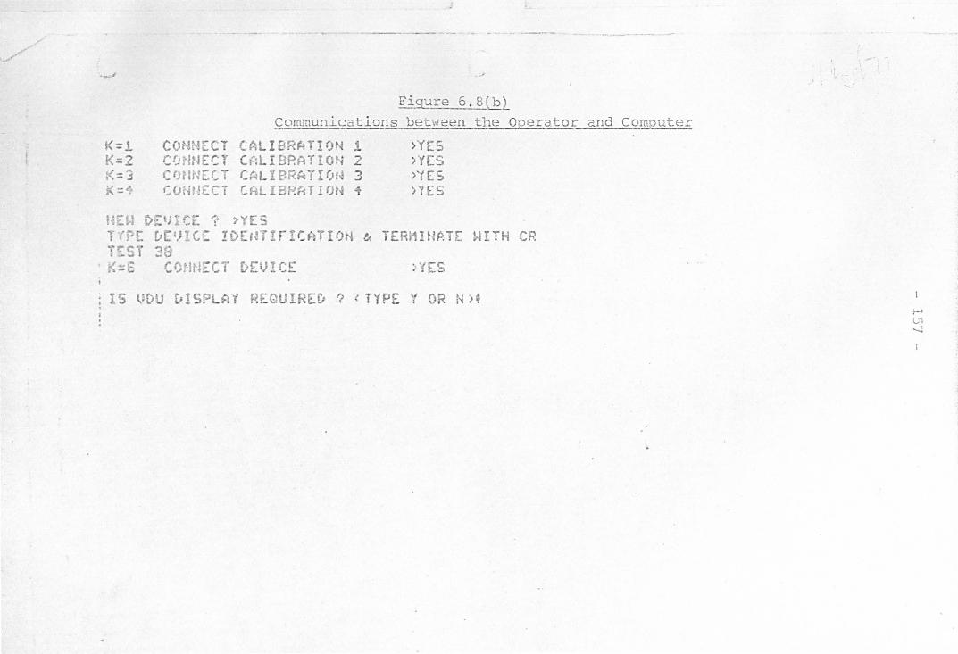
- - ..,. - _. - .-.------
~d
Figure 6 . 8(Q2-
Com..munications betlveen the Operator 2nd Computer
K=t CONNEC T CALIeRATION 1 >YES K:;Z Cf)dtJ[(T U::LI8RATION 2 iYES ~=3 ({Hm[CT CHLIBRATlt),-$ 3 >,(ES 1< ::~, ~()rH!£CT C~lI2P.KTION i ) YES
HE!·: f){;:lHCr. ~, ~,,(E5
Tn~E (;['}I(Z !OE,·H'IrrCAYION & TERI1!t./P1T !.HTH CR )~ESY 3" .~ ::E (.OHtJECT £>[lJ!CE ) '(ts
IS VDU ~IS?LAY REQU!RE~ ? tTYPE V OR N).
-..'
>-' Cl -..J

I....
F iqu~e 6.9 ( G\l~oml'll~D:~cations bet.:'!~ee~Q2era tor and Comput~r
R£ ? ~[(YI OH COEfFICIENT HEASUREME~T CORRECTION
USING 4 SHORTS OR f UN~NOWN T£RMINATIO NS AND A REFERENCE SHORT ')ERS ~ 0l! (,UL 2' /R 2 ...r-~:A~~l> rACIL!TI£S ItlCLlJu£D I~ITI~LlSATI0N REQUIRE D ? TYPE Y OR ~ ~,ES llSE ~Jr !;.~~rk TAPE: R£0UIRED '? "'!'(P£ --( OR t$ >Y£S DRTH TAPE LOADEO: 3B ARE AMPL!Ft£~5 IN USE? 11PE Y OR N ~YES INPUT Y l'P£ (O~il: (.IfH .. (
S TF1!'~O~RD C~L! 8R~T! ot~ USES SHORT C I R':: U I TS ONLY
f-WHST Aj~ r;;!r\j CAL.! eRA r 1 ()N USES ,,- Ut~XNOt.-lH T£Ri'1H~AT I eNS ?l~~rJ A REFERENCE SKORT
ST~HDAR0 CALIBRATION REQUIRED ? <TYPE Y OR NO) 'NO ':Ol'ST!CK ts :.01" IN USE. NI). or PC I NTS P£r~ R [(~iy.n-iG ==10 Trn!r~G H~'I':'{~ !)ML ( i~!~0.ld:1 ::r:.":-C). N=33 INPUTS T~¥EN FROM P0LAR [rSPLA~ OR PH~SE GAIN UNIT ~ TYPE L(jG,,t .. ! t j .. t:~ r~Ot ~!~ f-'(iL C[!--lTHL d£~~~i j..;HILL 1\'P!1l(; ANY Ci--:ARf-iCT£R r:: MA><ii';Wt nu::)ut:ncy ((~H::~) ::.: B MIlEIWii fR£OUENC'! ,GHZ) :;> B N~. OF ?nI~T~ ~ 31 S t·U Y C H T D L F. eRE S e. T TO J!;. MINIMUM ~REQUE"CY S£T ~? ..... ,~ "'···c-·· !.: ... ~' T/' e:'"~l-·~ '! ~~ M:.; .... ~. "" t.. .. ,1r.............. ):,.}., ,';J . , ", (..~.. ~ f .. f .tS\£ .....
f-' Ul (Xl

,J
Figure 6.9(b) Communications beb!een the Operator 2nd the Computer
t~ = 1 CO~N[ ( T CALI BRATION 1 K::1 (J)"m£CT C. ALI BRATION '1. t~ ::) ((nmE(.r Cf1LI8RArIOH ~
~~=i ~ONNE CT CALIBRATION i ' -~ (0~~rH: (T REFEP.E rKE SHORT .- .J
HEW DEJ!C[ ~ ~ (ES
Tf?E DEVICE I0£NT lfiCAiION ~ TP.IAl or i~/ie/ ?7 ~=6 (ON~ECT DEVICE
>'r(s > YES ;" tE S ~ \' ES
:.YES
TERMIN~TE WITH CR ,
irES
IS UDU ~rSPLAt ~EQUIRED ? <TYPE Y OR N>, t-' t.,1
'.0

- lEO -
For t.his particular case, the rninimurr. and maximum
frec;nencie;3 have been chosen ·to be 4 2.nd 6 8Hz respectively
and mea.surements will be ca.rriE"~d out at 21 frequencies evenly
spaced bet.ucen 4 and 6 GHz. A facili·l:.y for adjusting the
ini t:ial s·tarting frequency t.o the correct value is also
incorporat:pd in this po.rt.:Lcular case, no frequency correct
ion 'VTaS considered nec'2ssary.
No explanation vrill be given for figures 6.8(b) and
6.9(b) as they are considered to be self-explcmatory.
To control ·the signal freC;.rttency, bvo signals are
required, one to select t11e desired R. F. Oscillator Unit
and the other to alter the vol tagE~ cont.rolling the , f..requ.ency of the chosen oscillator. There are three R. P.
SI.,reep oscillators with the signal source unit and the
desired oscillator 1S selected by means of a direct voltage
which is int.erpreted as a 4 bit binary 'ilcrd by the Con'erel
'Uni t (lIP S706A).
The direc'c voltage controlling the frequency . ~s
obtained from an electronically p'rogrammable vol tage pO~Ner
supply v,Thich is in its turn controlled by the computer.
A Voltage range of 0 volts to 73 volts is required from
the pmlTer supply to control the ent.ire frequency range of
each osci.llatc.~:-:· The resolution of thi s voltage is
controlled in increments of'l millivolt by each voltage
pulse from the computer and these are supplied at the rate
of 30,000 pulses per second. The particu.lar voltage level
to provid.e a given frequency at any stage of calibration
or test:ing is determined by the dab:t stored and calculat.ed
wi thin the computer.
Wh(~n the maximum frequency (8Hz), the minimum
frequency (GHz) and the nun'J.x~r of frequencies for measure
ment are spE~cificd (Fig. G.8(a», tbe computer calculates
- 161 -
the nwnbf~r of pulses required for the minimum frequency, th8
number of pu.18es required for each increment in frequency
and the number ofpulscs required for the maximum frequency.
It commences by select.ing the appropriate sweep oscillator
calibration table and displaying ,·,hat it considers to be
the minimu.rn frequency. 'rhe operut.or is at liberty to al ter
this fr.equency if it: does not agree wi-th t.hat shm.;n on the
frequency counter. The computer receives the additional
instructions and will alter the minimum frequency to suit
the operator. It also stores the new number of required
clocle pulses as that required for the minimum frequency and
r~-adjusts Lhe n(!cessary freq-uency stepping procedure
described earlier.
'r"TO other important points must be mentioned here.
l{hen the oscillator frequency is altered a small amount of
waiting time is required for the frequency to strtbilize.
T·he amount of waiting time built into· the programme is
one second a.~ thi s is incorporated in the flow-diagram
of 6.7. In addition to this, 300 milliseconds is normally
allO\·red behicen each of ten readings carried out at any
one frequency to· nullify ·the effects of noise voltage
transients etc.' The operator has the choice of altering
the timing interval between measurements by calling up the
pertinent sub-routine (Section 6:5.6).
The programme incorporates facilities for accepting
the non-identical output voltages from tvm different display
units, namely, .the phase gain indicator unit (UP 8413A) and
the polar display unit (lIP 8414A). The phase gain unit
provides input information in polar co-ordinates i. e.,
magnitude either in lineur form (0 to 1 volt max) or in I. -
ded.bels (50 TiN/dB) cui phase 10 mV per degree}. The polar
display unit providGs linear outputs (± 10v Max) in the
form of rectangular co-ordinates. 'r'be computer must be
informed as to 'vhich display unit is used. In most cases,

- 162 -
the polar display unit is invariablY used because (<1) it
provides a better signal to noise ratio to the comput0r
especially after the 20dB buffer anplifiers and (b) it
provides 2Ti instant display, of a.ny instrument malfunct.ion during measurer.:tent.
It was mentioned briefly in Section 6:5.3 ~)at ten reflection coefficient measurements are taken at anyone
freq1.1ency to minimise the effects of noise transients etc.
These readings are put into a temporary storage register,
nveragcd and only the final result is put into 'the main
data storage. The other reac1ir.gs are discarded •
• Calculations are carried out in a sUb-routine called
"Calc" (Not shovm). ';['his sub-rout:.ine features several "IP"
statements to detenuine whether the standard calibration or
non-standard calibrilt.ion calculation procedure is required.
If the non-standard procedure (i~e.s 4 unknown terminations
and a reference short) is used, then the unJmovm termination
will also have to be calculated. The atte:nuation and phase
properties of the t.ransmisiion 1 ines used in t.he calibra'tion
procedures are calculated in both cases and are available in
t.he printed results.
The error parameters and the corrected ~eflection coefficient of the device under test are also calculated in
this sub-routine.
1\.11 the above data, calibration (lnd Ineasured results
can also ,be stored on an external data tape. This procedure
allO'l,"s: -
(a) An almost unlimi b?d sot: of rr.easurernent.s to be performed
and stored.
(b) Measured data to be readily available without recourse
to tb.e measuring equipment • •
(c) There is no pl'\ot,o·-C'o~ying facili t,iPG allied to the video
el:i sp)"ay un.i t in th(~ mC(]Silrcments 1abcratory but one .is
available in thf~ computer room si tuated some distance
oW2.y. ri'he ability to n:cal1 mea::mrcd data on the video
dl sp1cty unit in 1::.he computer room permits easy pl1oto-

.j
', ....
~ OJ +l ;j
§" o C)
<1J
~I ~I ru ~ o +l ru ~ (!;
o OJ
..c: . -I-J
•
W Ll ,Z LJ "::;)
C'
_. .... ......
hi t:'- • >- '1"J o 1..' Wz Z )- Il.. l>..J <t: <.t 1..' ::3")000 ..J ~_I
Cl i....' ~ ~ W -:;: I.f) ':'!: l ... O.:W t·· .. 0
.,:-, I...i.. ::)~.:'I l,l"l
(jJ ~" CI U' W !"'J L.J 1.<1 ::;. C'.: ::> (I.....'":) t;':: L. ... to- .:c ::: 1...1 .... l ... ! 0 1....1 I .. J ::.1 Q.. ;:) 4..") til ..J ..J ::.: C:'- 1.: ,:;, ::J ::-:;> ll. ~., :J WI- 121.10 ~ ~··c t,J ~ .-... t'!j
. ~.J Vt ';:l,; 1..:.1 .... vi ~. (~. ,::.. _I ::: v ,_t'1 .. 1: ,;: ::t: < .... <~ ... " I- ::::. _J <I G-Q..Z ..... ~ (!.. •• - ..:r (~ W Cr-..:t (...... :r: 7. ") ,-:') .,,J ~~ W o .:1: . • a. ::: lit,., Cl (t.:
- 163 -
I'X (,,)
::t: ... ..... 3 .,... .
W -.... .... • .;:a: I/) 0:: -.,. ... ~ ! .... .:> ..-of -w-'"'-
.... )-
ex.: w " •. J 1-- G.
~
~ >*. .... ..... .....
0 .~
..... ..- U ,,!: W U 0:: .... 1.." -l.- I..) ~ ~ 10 .. 0
If) l- :7- t~.1 w:: ld U.: '-w (") ..... ",,,,:) ;,... - .- .:t <:- r.n t..' ....I
W,·l'1I .. .J 0.. L.J ~) '.;:: f.J)
~.-' ~ _c'Z .... ~:::l -XO ~ ;;. hI ... , ~) It..l '-) 0': ':) ... ') I- ,')
W :::> ~ 41n a t~ l ... .1 )-• . :J-:: II (f')
:.::.: t- N ':',c. H . . - .- .- '. _ .

- 164 -
6:.1~~2~?proc1uction of Results
Facilities are provided for three types of graphical
display of t.."le results on the video display uni-t. rfhe
provision for entry into the display sub-routine is made
availabl_e automatically at the end of each device measure
ment (rig. 6.9{b» by the query "Is VDU Display Required?
(Type Y or N)". The operator then has the choice of three
displays (see Figure 6 .10). rrypical photo-capies of some
of th8 graphical plots for a short circuit are given in
Figure 6.11 (Amplit.ude vs Frequency), Fig. 6.12 (Phase vs
Frequpncy) and Fig. 6.13 (Polar D ~splay) • In all cases,
the points joined by a line are the uncorrected values;
. the corrected values are denot-ed by separatf:;! symbols. The
abOVe-olY,('l1tioned figur~s are actual size photo copies of the
display which is a convenient scale for most applications • . However 1 expansion facili t.ies for both the abscissa and
ordinate-scales are provided if desired. This facility
may be obtained by answering the query II}1AX X = "in the
bottom left hand corner of each display. For example in
the measurement: of a Ina-tched loaq (r:ig. 6.14) the difference
between the corrected and the uncorrected reflection
coefficient was found to be-impractically small for full
scale display and it was -decided to expand the ordinate
scale to produce a meaningful graph. This ,vas carried ou-t by the fOllo,,[iiig sequence:
"MAX .X = " 6 CR (Carriage Return) I'
liNIN X ::: " 4 CR " III1AX Y = .. .1 CR .. "MIN Y = .. a CR I'
The first two replies designate thf~ frequency band
width to be displayed whilst the last bvo replies set the
ampli tude range required. The result is tb.e graph of
Figure 6.14.

IS) 1
"It'
U ~
i£I'I r,~ 4.J
.... ~ (.J .., . ~ f , Cd) "'I .~)
""~ .. , ~ ~
~)
"14
-~ ........ -............ ~ .. -.. .
... . -",
. >~ I'
~.,._ .__ ~~ .. ,. .. ___ ." 1"--;-- ... ., .- I'
·-165 -
, .... .... ~U .. , . .......-u.---.. . .. , "-.w.. .. ,, . •
.... , I
-, { .... ! .. W
I •
. .... .. -., _ ..
, .... • rJlti, .4 " . ~ . .

-~
Q
• o .. c;3
o
•
\\I r-l
....... :- ..... -- ..... "... ..... -
- 166 .-
C N
l!W:_ ..... ,.,.ro"' .. "'~rlW'I:'"' JIJI..-.............. :,.
'.
, . .. ( ..
.. I;.)
J .. '
-6 ., ='1 4' ".;) " " G,
~ :; • ..
" , ~
~
c: • J ,., ... \ - .. . .... ... . .
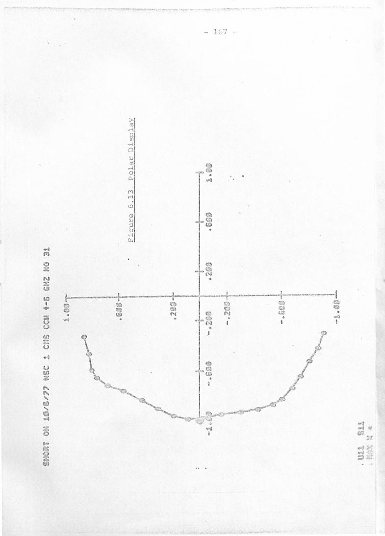
. ,..- -- ..
- 1.~) 7 -
>'1 :'d .--l 0-fJl
'M 0 ~ rtl r-i I 01 jl. '
·1 M rl
\.0
OJ l--! :J 0 • 'r' "-'
~ p)
... N .....
ct!) --... '--1~'I-'--'+'-"'''''''--i-'''--'--''''''-~ • .. Q
• W U
0
U
r;.) ~ ~j
N ~~, (!!! • a.. .. ~ f' 1 •
01 .... U I
",,'J
U 1/# I'
I
.d.

~ 0"'
tl rIJ' >' (1)
'0 ~ +l
~ ~ I
~ I ~I
0 ) c~1 N :"j
U 0 (j~ - rei 2 (])
U '0 ~, C
iCl
U ~ ~I ..
u ~I t1) ..., \.0 \ -N ~I :.t #JJ
::s
~ -81
• r:r.d .,
~ ~ , SD ", .04
'"'" >
t •. ;)
'U
'l' , c· .,)
~ I> o
....
- 1 6 8 --
4r .-( "\
1-... ... ~~
J t-,
~ I
~ .
Co
I J.ii1 . ..
~_(.li
[' ) • it I
'. ' ~
"., " ;~
~)') i~
. ! ;' f.,., t I - ., .. ,

~
l~
~
~
'T~H LO~D ON 10/6/77 4 - 6 GH7 NS C 1 C~S CC W Ne 29
FREQUENC'!' t!;iZ
... 00-1 4 , ~ 00 4,200 4.:)00 ';''''00
.!l~C'
4.oeO ... 70C iI.BOO ~.9:>()
5.0C~O
5. a. 00 3.2,10 5. 30 J 5 ... 0= 5.500 5.600 !}.700 5.300 ~.90J
6.000
FREQUENC'!' 6HZ
" ' OOG 4· 1(:0 ... 2CC 4.30C
'f ... 00 4 . 500 ~.6;)~
!>.70o ., . 800 .. ·900 5'000 u.~(;['1
E - 2Do 5,300 S·'tOO ~ .~OQ 5., 6~(, Ij .7::; :;',300 5·900 6 · (;00
CALI6RATICtI 1 AMPLT PH.IoSE
'~73 .9:J 8 .91" • ~' 99 -::36 .:;)69
·91'1 · ~56
· $36 . 938 ·~ 59 .. eE6 - 977 - 562 .9 51 .S 6 1 .9S 4
! ·018 " .008 1·(106
. 97 ..
~;9 . S
-7 ... 2 -60" (.., ~5,.5
-45.7 - ~?s
-37.5 -31. 8 -2 1+., ~! n·S
-3.5 -l, . ~
! • g·o
~5~ b
2:' .(} :?D." 36.2 ~l .e 47·1 52.5
c .!. L!an.nreN 2 AI"PLT Pk bSE
.993
. 963
.;::6
. ~21
.952
. ssz
. <;8 ..
.s ~ o
. 935
. 33 ..
.952
. s71
. ':i59
. 9~3
.52 -94.0 .968
' .• 952 . 983 a9 83 .sS7
- 176 d .r.~73 ·2
-H.8 . 1; -1£;>-:; -155.5 -152.9 -1 .. 5·9 -1 ~'; ·6
- j41 ·9 -136.5 -1 ::; 1 .3 ui?8.3 -1?5.2 -!?G' " -l1S.2 -1 O!h 7 -~04 . 6
- 10e.5 - 97 .. 9 -9 4 . 2 - 91- 0
REF C6E FF l'lEAL IMAG
-. 00:3 -.C'O" -.OCl ·-t.' C;.
.(lC l - ·000 - .002 -. c05 ~.006
-.O O~
".011 -. 011 - .O ~l
-·011 - .(;09 -c O~2
- .oe8 -·015 - .012 -. 017 ·-0 16
-a? ? ~02 Q
. 017 0\)13 . otn . 00 7 · 005 .OO?
... nc':> -. 011 -.Ol5 -.S15 -·r,<'l -. OlQ - . 02? -· Q1P. -· OlR .... n'3 -. O~?
-. O!,')
·· Ol?
~.
CALIBRATION :;) .ir-:PLT PI-1ASE
CALI BRA; I aN .. AHPL T PHASE
. 968 ·9 3<; . 905 .SSt .921
· . 9:'9 . 952 . 930 .910 .: 9l! .935 .951 .. 9:'7 . 930 . 9~3
.932
. 963
.993
.9al
.ges
. 957
86.9 ' 87.6 90.2
1. 002 .966 . 937
3. 9 -920 97 • 8 '- -- . 9 I; 8 99·1 .979 99.t, . 9S7
! OO. 7 103 . 0 106. :; 108.8 ~OS.5
111.0 112.6 !1 6, 7 11S,~
122 .6 122.6 123.8 12 a 6)3 120"0
. 961
. 932
. 936
.960
. 973
. 973 . 955 · 938 .958 - 989
1.020 1 ·00b :- 006
.977
-7 .8 - 9 · 6 -9.6 ~7.9
6 ·3 -7.5: .. 9.:;
"11.:? -11,0
- 9 .9 15 10.3 "'12 · 0 -1 3 . 4 - 1 J, .. 1 -1 2.~
~ ll · S
wl1.5 -13. 8 -l!l. C - 16. 9 -17.6
REF CeEFF ;'MP Of' P .... ASE
. 024
.C20
. 017
.013
. 01 0
.007
.006
.005
. 007
. 014
.C18
. 01 9
. 023
.022 . 024 .022 . 020 . 020 . 0~ 7
. 021
.020
"3C .5C7 109.3 ""3; " OvG 1~O.2 - 3:i.~ :; 3 5':' . 6 -3i.999 ~~.B - 1;(; ·392 85 .2 "'l,.:·~985 90 . 5 - .. 5.:)97 11 &.1 1045. g7~ 155.0 - !i2 .. 931 "'1"9 a5 ·37.23: -1 2<; . 5 ~3 .. ·8 g! -125. 9 - 3'- • .. :n -1 25.50 - 32 ·i20 - 11 7. 3 - 33·18.,. -1 2 1.0 ~ )c..53<; -1l<';5 " 33 .:95 "'12.s.. , .q. - ::l~o163 -1 15 .5 w3:;.973 - 131< 01:. - 35.1+83 ~13 5 . 8
- 33 ·7 '>5 -1 "£'.0 - 34 . 01~ ··1 ~3 . 3
~F.:F. S HOR T Ar<P L T PHASE
. 918
. 91+ 1 ·!l 9b
t·e03 .S82 . 9'13 . 935 . 9"'8 . 974 .:'89 ,975 · 96 1 .976
1.008 1.032 1· 0?6 !. 00 3
. 987
. 96 7
. 972
. 961
1 10.6 19. "
126 . '-' 130.::; 136.1 1:;:::·3 152 .5 1 61.0 1 68 .6 175.1
w17 8.7 -1 70 . 2 ~161.8
-15'1.4 "'1.;.8.3 -1 l,::.S -137 .6 -131·2 -123.3 - 11.6 e li -1 08 .9
VS rR
1, O ~ 9 1.041 1.O::l5 !.0?6 t ~ o~9
i e Ollf. 1 . 01 1 1.010 1. ,11,,+
1.02 8 1. OJ , 1.039 1 , 0,, 7 : • O~5 1.048 1· 0~5 ·
1 · 040 1. 04 1
!' 03't 1. 042 1. Dol! 1
U~CP.T D::;VIC£ toHPLT P HIISE
. 01'1
.011
. 009
. OOB
. 007
. 0 0'1
.002
. 003
. 001,
. 010
.Ol~
-015 .02:) . 021 .023 . 022 . 020 . 020 . 01E . 021 . 021
- l • .,
-· 4 !l.1
13.2 26 . 6 24 . 6 33.6
177 . 7 .... 151. C - 125.8 - ll3.6 - 102.2 -90.4 -77 .9 - 68.5 u 66 . g -57.8 - 57.0 ~ 52 -1 - 55. 2 " 53$7
FIGUP.E 6 . 15
6"E LTNE LEN(ii H ~JEPERS DEGREES
• C 1 · el . C1 ·C1 .C1 ·00 · 00 ·CO .C O ·CO .CO . 00
• co ·CO .00 ·00 . 00
• co ·CO ·00 ' 00
I; 7. 9 1 ·.9 .16 50.l,b 6 1.72 52.96 t.,4.14 55.3 1 5(' . 58 57 .7 3 58.85 60 .13 61.26 62.33
. 63.68 .:. 1+. 61 65.9B 66.91 68.34 69 . 30 70·67 71.66
DATA SHEET OF
P RINTED RE SUL'I'S
.1"., . \
!-' ...... V·
~

- 170 -
The data sheet produced by the line pd.nter at the end
of each measurement. is shown in figure 6.1.5. The informa1.-.ion
presented is fairly comprehensive and includes;
(a) rl'he frequ(~ncy of measurement.
(b) Trle n~flection coefficients of all the calibration measurements.
(c) The reflection coefficient of the device under test.
(d) The total one-way attenuation and phase of the incremental length of line beb-men the calibration pieces.
(e) The corrected reflection coefficient of the device under tes·t aiven in the lower rectanaular data
~ ;;:.
b1 k T""· . I • J- 1 d . . oc. nlS 1S glven J.n rec·,.angu ar co-or J.nates (columns 2 & 3) polar co-ordinat.es (cols 4, 5, 6 ) and in VSVlR relative to a 50 ohm line.
The programme has facilities'for various supplementary
tasks. These are lisb?d in detail in figure 6.16. Entry
into these sub-routines arc only permitted at certain
points in the programme. These points are obtained by
typing "No" to any of the' follm·ling questions displayed on
the video display unit.
( a) connect Calibration l? - No
(b) Connect Calibration 2? - No
( c) Connect Calibration 3? - No
(d) Conn(~ct Calibration 4? - No (e) Connect Device ? - No
(f) Is display required ? - No ( g) Di~)lay Re~Jired ? - No
(h) New Device ? - N'o
This ,·d.ll result in t:hefollmd.ng r:entcro.ce:
"Tas]c? (Type LI for list of opticns) t!"

'"
{ r '. ,
Figure 6.16 List of Supplementary Tasks
< OPTIONS - TWO LETTER KEYS REQUIRED LI LIST OPTIONS ZE RESTART PROGRAM BG RESTART CALIBRATION RE REPEAT LAST READING SK RESET K (SEEBELOI.J) ND GO TO NEW DEVICE CA CALCULATE PR PRINT Dl ENTER DISPLAV DU DUMP READINGS UP UNDUMP READINGS ST RELEASE PROGRAM CO I riSERT COr'1P1ENT CE CENTRE BEAr-1 AM RESET AMPLIFIERS IN' RESET IN?UT TYPE WA WAVEGUIDE OR COAX CL DEFINE CALIS PIECES JO JOYSTICK SWITCH 'FR RESET FREQ RANGE ,r1F COf<RECT I"lIN FREQ NO RESET NO. POINTS : T1 RESET TIMING INT TF' UPDATE TAPE FORMAT DC DISC FILE CLEAR
~
SETTINGS FOR K IN SK OPTION K=1 CONNECT SHORT CIRCUIT K""2 COr1!~ECT OFFSET SHORT 1 * K.:.:3 COi"--iNECT OFF5E-i SHOt<T 2 1<>4 CON;-·IECT OFFSET SHORT 3 V:er.:; '" ,-
:~':~6 CO!{,"·iZC:-r DEV!CE
TASK '? ("rvp~ LI FOR LIST OF OPTIONS) t,
......
......}
......

- 172 _.
AtU:lis stage, the operator is free to select the
tasl~s listed by t.}}l:i.ng the key code listed und terminating
wi th a carriacge return (CR). ~ 1 t' t' 1 . f '-, 1rey - 8 .. en'Jo. .lve y l_ t,,~e r~_
codes cannot b2 romembered then typing LI i'l:Ll1 result in
the display of figure 6.16 and any of the procedures listed
may be sl~lected by typing in the appropriate key code.
The progr~r;une is termi.nated by typing "ST" at t.he
task ent~J point.
Finally, when t.1d. s programme is used, the restriction
mentioned in Sect.ion 6:3 should be observed.
6: 6 The A'J.t.omated Progr2mme for the Three Short circuits Correction Met:.hod ---_._--_ .. _-----.--
This programme operat.E.~s in a similar manner to that
der.;cribed for the 5 termination program_me except for the
fqllowing points:-
(a) All lines are ass~~cd to be lossless.
(b) All the electrical offset lengths r,:mst be stated.
(c) All calibration termlnat.:i.ons must be known.
A tIPical operating format is sh01';11 in Figure 6.17 and
a t~{picaJ. line printer data sheet. can be seen in Figure 6.18.
. .. The programme also incorp01;ates bw other correction
systems (Ref. 6.5 and 6.6). These are useful when the
cross-checking of measurements are required. This programn1c
w'as writt.en by Stoneman (Ref. 6.3). Other than providing
the deriva.tions for the three shorts correction procedure,
no credit is claimed for the 'vriting of this programme.

Figure 6.17 orJcrating Fonnat foE. th.e Three ShoJ."ts Automated p'rogramme
REFLECTION COEFFICIENT MEASUREMENT CORRECTION
USING MATCHED LOAD WITH SHORT OR OPEN CIRCUIT OR SHORT AND OPEN CIRCUITS VERSION OUl2/R2 J-BAND FACILITIES INCLUDED INITIALISATION REQUIRED ? TYPE Y OR N )YES USE OF DATA TAPE REQUIRED ? TYPE V OR N )NO ARE A~PLIFIERS IN USE? TYPE Y OR N !YES INPUT TYPE COAX ONLY
STANDARD CALIBRATION USES SLIDING LOi~D# SHOHT AND OFFSET SHORT. STANDARD CALIBRATION REQUIRED? (TYPE Y OR NO) !NO CALIBRATION WITH MATCHED LOAD REQUIRED? (TYPE V DR N) !NO CALIBRATION PIECE 1 IS SHORT CIRCUIT. CALIB. ?lECE 2 IS OFFSET SHORT. CALlE. PIECE 3 CAN EE OPEN CIRCUIT CR OFFSET SHORT.
CALlE PIECE 2: LENGTH OF OFFSET SHORT (eM) 2 4 C(tLIB PIECE 3 ? (TYPE op· OR OF) !! OFFSET LENGTH OF OFFSET SHORT (eM) ~ 2 JOVSTICK IS NOT IN USE. NO. CF POINTS PER RZADING =10 TIMING INTERUAL( N*0.01 SEC). N=30 !NPUTS TAKEN FRori POLA:-< DI5PLAV OR PBr~S~ GAIN UNIT ? TVPC LOG, LIN ... or.( POi. ! ~! POL CENTRE EE};r~ iJHILE TV?ING f;NV C:-;AR{:~c·rER y f··~8~<!t·~lj~·~ FR:QtJ:::t'~:C'yf (GHZ) :z 4 r·aHl~;lun FF{EQU~NCV (GHZ) "'" 2 HO. OF POINTS c 21 St . .l!TCH 1'OLEC RESET TO 3t.J. MINIMU~ FREGUE~CY SET UP CC~RECTICN TO FREQ. I~ MHZ =
,I-' ...J w

:l
: <
310 MA7CHEO LO~D eN 2/7/77 ~-~ G ~ 7 S /. 46/1 '16
FRE QUEN CY 01-'-
.... 000 .... 1 Co ~.~Oo
".30e ~';'OG
"" · !lOo ' ('On
4,100 ;;· .. ZOo '- . 900 SdlO;') h.1 00 5.200 5. :;'10 5,"00 5.500 5 · . .100 '>,Jeo ~ . 80()
5 . 9:>0 1" 000
FREQ UENC Y "' .. z -~ . O~!') -<It. 1 Co .... 200 .. . 300 .. ·1;00 ... 500 ~·600
".700 ... aoo 4.:300 5 . .... 00 5 . :'0 0 5 · 2CO ~.3C()
3.4~0
~ . 5::'n
:i-en\) ::;.70n ::;.~Co
~6~C:')
£, . 00
K"'l A:'IP
.965
.93(. 1.035 1<0 2 0 1· 022
- SlO .s .. , . 961> .. 5~ ~
l-QC'9 . 583 ·97 ~ . 535
:.~19
1'0 .. 5 :·0-'49 1- 03 1
.003
.9~O
· 95 9 -9 8 ,.
P~ASE
17A.6 1 7,} .7 17".9 175.9 "~a 17 1.,3
.l 7b.i'. I J 7. lr ,7A .2 177 . 1 .; 76 . b
' :-8 . 4 17Q .O
-: :"3. 6 , 79. 1 177 .1 173.1 175 .:; 175 . 2 17 5 . 0 175. ::
REF ceEFF RttL
· 00:: .co .0,0 _ 007 ,co2 .C 2n _ OGS
. nc~
")(jC3 . rOl < Cl :
"'-~ . 00 3 · O~G
' 01':' - ~ ,jOb .0.2 · r04
~· o: ... --013 -.006 • • 01 7
K"? AMP
• 96" - . 994 , · 0;: q
. 994
. 96 ;>
.S At O
.. 93h
.96'<'
• <;7 "3 • 37 ~i . S5t . 9S ~
• 9~ :> 1.0\f,
1 • nO? . 9 1<; .967 . 9~ ;>
• <)6 '! .9£>J.:
- ·~~6"
;11116
• nl'; ;"
.05. - • 05<
• r .... fl . n,," .. 04 7
' 0" :> .041 · ,n n · 03R J t~~ 7
.03£>
• ~/ 3C; . 03 ..
• O ~~ " . 034 • :")3-. .. v:; Cj · OJn . 1)40 · 03<
P~ .lSE
~3"".6
,33.5 ~ 30.3
l26·0 1;:>5. ? 126 . 8 j?6· f; 25,,?
123 .7 , 21.5 1?1·5 12 1 .4 120 .7 119. 8 115 . 0 112 . 2 1 11 . 9 li O .5 :0 8 .9 la8 .3 05.6
K- 3 .l.t1?
1.001 1.015
. 996
. 9'10
. 9 4 !
. 96~
. 98 0
.995 ·97 1 . 9<. 3 · 959 . 990
1. 00 0 .99 ! .973 .96 6 . 988
1.01 8 1·00 7 1·021
. ~8 5
;>;';:'SE
64-3 59 · 0 53.6 50·9 50,9 49 · 0 '16'" .,.1 · 2 37.:1 35 . 2 3 3.3 3 0 ·:' 25.5 2 ). 7 19" :.. 17.7 1~ · 9
12.1 7 . 6 3."
·0
1( ....
.!.HP
·00 0 · 000 ·000 ' 000 ' QOO - oco
' . oco · 00 0 '000 '000 · 000 ·000 .oeo · oco ·000 ·00 0 · oeo . nco .000 • OC ()
· OCJ
REF COEFF ' :O M? n~ PtlA f;E
-('j ..:>6
..05 1 ,oS .!,. ~ ()i .. 0 ~O .. 5 ., USt . 0:"2 . 0,. 1
·-- . 040 . C1:;l! - 039 .0 3 6 . li3':. . n.1R .. O:'-j~
. 026
. ~35
.042 .. 03~ ~ 0'.0 . 0:37
~?fo.690
~25 . 8 09
- :>5.420 -? 6 d32 7 .... :' t~ . 9~ 7 - ;;." . 8 82 u27.S07 -=-7 . (,44 ·?7.955 -?8 . 318 -~"'f; ~ ;:3;; - ?1\.9 3 - :')" ... 7 b -i' :; + ~ 3
8 1.' 0 ' ~5 . 2 7q-O 81 .3 57 .. 4
i.7 . 3 .~ :; . <: 1\ ... . 1 c!> . ; BS .6 7~.H 9~. o
7 .... 8 e ... l
-2S- OO J 99.9 - 2 8 .. 9; 1 lC 9 ~ s -?9. ?:1 S~"n
- 27 · :'OiO 1 l0 . 2 -? 3 . b5 0 11~ .3 ~ ? :· . d,,! 6 5 $\ _2 - ;:>((~613 :17 ....
PHASE K .. S AM?
·0 .0 ·0 · 0 ' 0 ' 0 ' 0 -0 ' 0 • a ·0 · 0 . 0 · 0 .0
' 0 ·0 · 0 ·0 · 0 '0
VS.JR
1.097 1. 108 t . · 1 ! 3
t·09:1 1.0Q4
!~1 0 7
1 • n ;~ 8 1. Oil 7 !.0~3
I.OSO 1 • " il l 1 · 07 ... 1. 0 7 6 \· 07& 1·073 1.07 .. 1. rl7 2 t. 0:1 7 !· 068 1 . 08 fl
1 -077
, 000 ' 000 iOOO ' 000 ;;000 '000
' . 000 '000 - 00 0 • 000 - 0 0 0 ' 00 0
• · 000 '00 0 '000 ' 000 '000 ~OOO "000 -00 0 -coo
PHASE
. 0
. 0
.0 ·0 .0
'0 . r,
' 0 '0 ·0 -0 . 0 .0 ·0 .0 .0 ' 0 '0 -0 · 0 ·0
K",,; OE v ICt:: AMP PHo\.SE
·015 .012 . 011 .011 ·009 -007 -006 '003 'COl '00 5 ·OCB · 01 3 .015 · 0 17 .01B . C15 .01 7 .016 • 0 15 .015 .. C13
54.41 51.? 51 .3 50. 1 45.8 45. 3 42 .7 38 .3 ~56.4
"1?1.9 -107 . ':)
- 99 .2 .. 91 .7 - 51 .2 -89.9 -R B./; - 8 7.8 - 92.3
":00.1 -1tO. 4 - 12 •• (j
FIGURE 6.18
DATA SHEET OF
P RINTED HESULTS
~ J
"~
1--~ .p.

- 175 -
Five n:anua.l and ti\TO automated computat.ion programmes
have been presented. These· computer progranmes form. a very
necessary and important. part of the research programme to
verify the theory e:xperimentally. Of these programmes~
great difficulty was experienced in writing the automated
five Termination Progranune. As this programme was unfunded,
cornpu·ter programming assistance was not available and
considerable t.ime and effort had t.o be inve~~t.ed in gaining
the familiarity with the compu'ler hardware needed for this
type of work.
* * * * * * * * * *

- 176 .-
6: 8 Hef. e re11CC' S .---_._ .. ------ _ ... .... __ .. ..-
6.1 Hc ..... rlett Pacl~<lrd Co., Page Hill r~~d, Palo Alto, Ca.liforni<:1., ItHE~\'11ett-P ac!{anl Calculcc tor }lodel 9100A Operating and P rogramIHin9" •
6.2 eta Eiilva, E.F. and HcPhull. ~vf.K. "Calibration of Micrm'lave Ne tv,ork j\nal}"ser for Computer Corrected S P arar;lci:er Bee. 8un-::meY1ts" Electronic Letters 1972, 9 , pp 126-128.
6.3 Shurmer, H.V., L'l:n':.ton, H., Hosseini, N. and Eatie A Stoneman "the Application of an On-J..Iine Computer ·to MicrO\'rav(~ l1easurement" Il1EKO VIr - 10-14 Hay 1976 (London).
6.'± H0.vllett. Pac}..:anl /Net.wor]);. lI.nalyser Data Sheet" Model 8410A issued l~t.July 1967.
6.5 Adams,. S.F. ment. System" pp 300-313.
"A New P recision Automatic HeasureI.E.E.E. Trans. 1968, IN 17,
6.6 Shurmer, H.V., HCalibration Procedure for Computer Corrected S ParametpZ' Charactr.?]:sat.ion of Devices Mounted in l1icrostrip" Electronic Letters 1973, 9, pp 323-324.
6. 7 Duc}~et, J. "P rivatf~ Communications" Computer Programmer, Depart.ment of Engineering J Uni versi ty of Narwicl~.
* * * * * * * * * *

- 177 -
CHAP '1'E R VII ~-':':'-"---. -----
The FABRICATION of rfEST and CALIBHATION PIECES
7: Q_Introduction
The theory of the new mea.surement systems have been
dl:.~scri0ed in Cha.pter V. The associated computer programmes (software) for calculating the required correction results
have been explained in Chapter VI. rfhis chap·t.er provides
details of the construction of the calibration pieces used
to verify the theory of the previous two c:hapters.
It was ob-v·ious in the initial conception of these
calibration pieces that any design conceived must incorpor
at.e the following vi tally important: properties:-
(a) Electrical and tr..echanical stability in use.
(b) Uniformity in reproduct.ion.
(c) Ease of construction (economy).
(d) Easy interface with the measuring instruments.
After much thought, it "'3S· decided to construct the
majority of thes8 calibration pieces in air coaxial line
using APC-7 cOlmectors for the follovring reasons:-
( a)
(b)
( c)
The characteristic impedance of a precision air coaxial line can be accurately defined.
APC-7 connect.ors are kn·:rvffi to be electrically stable and provide more consistent VSWR's.
The mechanical dimensions of these cmmectors are hr~ld within tolerances cf + 0.0025 m. m.

- 178 -
(d) Inner and Outer conductors I'd th dirnensions c:.n.d toJ.ercmcr~s identical to that of the APC-7 connectors arc available and may be purchased separately to permit easier fabrication of precision air-coaxial lines.
(e) Various transitions, e.g., co-axial to microstrip etc., are available.
(f) Easy interface with the measurement reflectmeters 'I,hose ports arc als:J connected with AP C -7 connect.o:r.s.
(g) Easy machinil"2g of the inner and outer conductors due to their physical dimensions.
7: 1 General D('~tails of the CalibrCl.tion Strlfldards
'rhis section describes the points conunon to the coaxial
calibration standards. Particular details of the individual
standards will be described in later sections (7:2; 7:3 & 7:4).
7:11 Choice of Offset Lengths
The choice of offset lengths within the calibration
pieces is important for the following reasons:-
(a) At a particular ,frequency of mGdSUrem8nt the offset lengths must not be chosen sO that the calibration reflection coefficients measured are r I_~L , r /e"·2:rT_, r-' ~~-='?':.01 etc., 'lI11ere rr.... is any interger. For, if this ',o1ere the case, then t.be error network cannot: be solved.
(b) The offset lengths should be chosen to produce large calibratIon reflection coefficient angles differences to minimise the inaccuracies involved in bpE:cifying offset lengths. For example if t.he ability to measure a mechanical length is limi t~ed to .! O. Olmm , then ~boosing an off!?et length of O.llTUTl is obviously unwise for a - 10'10 t.m.cer'c.ain·ty vlould be involved in specifying the offset length.
() , ",... 'f- 1 c For maxU:1Um acc~...lracy .In locatlng tue Vlr _n~ centre of a Smith Chart, the calibration reflection coefficients sho'.:IJ d be L~paced 1200
for any three termination calibration IT'.(~t.hod (secticns 5:4) and 900 fOJ:: any four termination method (Section 5:5).-

- 179 -
(d) Unn8ccessary r.lechani:cal dif£ ieul ties would arise in maintaining the concentricity of the inner conductor if the offset lengths ,,,ere made too long. support. by bead etc., is not favoured as discontinuities albeit small, will be produced unnecessarily. Furthermore, errors inaccurately spe:d.fying the:! electr.ical length of the offset, especially with changes in frequencies, could rE!sult.
In vie,,! of the above considerations, tables 7.1 and 7.2
were conr;;tructed to permit u more detailed study of optimum
offset length. Each table contains' SE!Ven sets of "preferr.ed"
offset lengths. set 1 to 6 are chosen for optimum offset
lengths for a particular frE~quency. For example, ::et 1 is
chosen for optimum operation at 12 G!Iz. Similarly, Sets 2,
3, 4, 5 and 6 are chosen for operation at 10, 8, 6, 4 and 2
GHz respect.i vely.
From t.he~.~~ '~~ableq it is clear thr.:tt if the ideal electrical
offset length Sets are to be chosen, t.hen r~u.ny Sets will be
required. This is obv~.ously financially unacceptable and a
compromise had to be raade into choosing one set of calibriltion
pieces for the short circuit measurements and one set for open
circuit mcusurements.

.. Offset Lenqth . LnlllLl
1---1 Set
4.167 8.333
§..<?.t_~ 5.000
10.000 Bet 3
6.250 12.500 set 4 8.333 16.667 set 5 12.500 25.000 Set b 25.-600 50.000 §et 7..
4.670 9.340
- 180 -
:r'able 7·.1·
iQ.,= =!. x 1 Ollw..:.n/ 81 . 3 Termlnatlon HeQsur~l1.nen"t§
~
!?ffecth~§.' Pb?se Clv.l.ng.UPegreesl
2GIIz 4GHz .~
6GHz 8GHz lCXmz ...----
20.0 40.0 60.0 80.0 100.0 40.0 80.0 120.0 160.0 200.0
24.0 48.0 72.0 96.0 120.0 48.0 96.0 144.0 J~92. 0 240.0
30.0 60.0 90.0 120.0 150.0 60.0 120.0 180.0 240.0 300.0
40.0 80.0 120.0 160.0 200.0 80.0 160.0 240.0 320.0 400.0
60.0 120,0 180.0 240.0 300.0 120.0 240.0 360.0 480.0 600.0
• • 120.0 240.0 360.0 480.0 600.0 240.0 480.0 720.0 9GO.O 1200.0
22.4 44.8 67.2 89.7 112.1 44.8 89.7 134.5 179.3 224.2
---_.
-
12GHz
120.0 240.0
144.0 288.0
180.0 360.0
240.0 480.0
360.0 720.0
720.0 1440.0
134.5 269.0 I
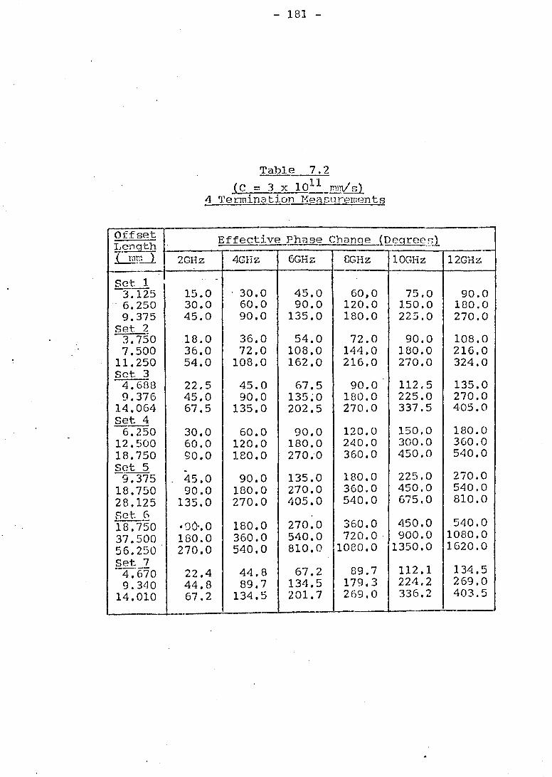
- 181 -
Table 7.2
{C == 3 x 1011 mm/ s) 4 ')~ermina tion HeaslJ.rements
OffS~ Effective Pha8~ Chanqe JDcgree_~~l l!eng·th ' .LE!I'.:..~ 2GHz 4CHz 6GHz 8GHz 10GHz 12GHz
r-···· -Set 1 -
3.125 15.0 . 30.0 45.0 60,0 75.0 90.0 . 6.250 30.0 60.0 90.0 120.0 150.0 180.0
9.375 45.0 90.0 135.0 180.0 225.0 270.0 Set. 2
3.750 18.0 36.0 54.0 72.0 90.0 108.0 7.500 36.0 72.0 108.0 144.0 180.0 216.0
11.250 54.0 108.0 162.0 216.0 270.0 324.0 Set. 3
4.6BB 22.5 45.0 67.5 90.0 112.5 135.0 9.376 45.0 90.0 135~0 180.0 225.0 270.0
14.064 67.5 135.0 202.5 270.0 337.5 405.0 set 4
6.250 30.0 60.0 90.0 120.0 150.0 180.0 12.500 60.0 120.0 180.0 240.0 300.0 360.0 18.750 90.0 180.0 270.'0 360.0 450.0 540.0 set 5 ~
-9.375 45.0 90.0 135.0 180.0 225.0 270.0 18.750 90.0 180.0 270.0 360.0 450.0 540.0 28.125 135.0 270.0 405.0 540.0 675.0 810.0
fie \:' .. 0. 450.0 540.0 18.750 • ')0-. 0 180.0 270.0 360.0
37.500 180.0 360.0 540.0 720.0 900.0 1080.0
56.250 270.0 540.0 810.0 10eO.0 1350.0 1620.0
set 7 --4.'(>70 22.4 44.8 67.2 89.7 112.1 134.5
9.340 44.8 89.7 134.5 179.3 224.2 269.0 14.010 67.2 134.5 201. 7 269.0 336.2 403.5
- -.--

The short circuit set cons·tructed J.S t nat 5hm-1n in s e t 7
o f 'rable 7.2 rn(ln~ly 4 . 67JThll., 9. 34niffi an~l 14 .0 1nun. Tbe open
ci rcui t calibration set chosen ·\.;ere 4. 8 3ni!n, 14. 83mm, 24 . 83ITJr.1
and 34. 83mm. These 13.re obviously not: the Eelectrical ideals"
but were cnosen as a. compromise be'bleen .he conflicting
electrical and rllechanical reqairement s
7: 2 The 7nun Sl1or-t Circuit Co-·axi al calibrc.t iGl1. Pieces -_._----- --------- ----_._---------
Photo copies of these short ·ci;:·cuib·) are shmm l!'1 Figure 7.1.
The machine d r-aFing::~ rela·ting to t .heir construction are shm-Tn
in Figures 7 .2 and 7 . 4 to 7.7. Those were designc'd by the
author . fj...9ur~7 .1
Photo9l::~b 0::' the Short Circuit ,Qalil.?rC!tton P icces------

-- 183 .-
PI GUlIE 7. 2 .
A~C-7 Locking Nut
E~3 I on Short f;irCldt . \~;~I);':1bly
Sco10: 2 :1 u~~r0X . · pinin.ll : Clp .• n
• a. t. e ! 1 .'1 i, ,J u 1 y, ] n 1
............... --.. --..:.----.. -~--.......-..----.............. ______ .~ •• __________ ... ____ 'RIlI ..........
Off f1c t Sh (Jr t Circui t Do y
~---'-
I H, rom d in.:n
APC-7 Lockinc; N t,
APC-·7 Body
n 'nil (~j, [\'ll1
FoJlS 101 orf~ct, ~hl).t CiI'cnit . r·!' c"lh 1.r . S(~(t1e: 2:1 rl.''''lJro :~
l"irlinh: Cln Fl.>-' 'r()1C'1~tm cer:: -----Da.te ~nd, July, 107 ·

- 184 -
The rr,achinir:g was carri(~d out in the ,.".orkshops of the
Univ2rsity of Han-delc. General Assembly and gold plating
were carried out by the author. Details for gold plating are explained in Section 7:5.
No difficulty was experif~nced in the machining cf the
short circuit block Figure 7.2 as extreme accuracy is not
required. Th(~ crit.ical part of this assembly is that t.he
surface nA"(Figure 7.2) is completely flat. This is
essentia.l for both the inner and out.er conductors of the
mating APe 7 connector butt up against this surface. 'l'he
intern;;l diameter of the mating APe 7 outer conductor is
7mm and the diameter of gmm of surface "A" allOiis an annulus
contact. width of Imm •. Good inner conductor contact is
assured by the spring loaded inner conductor mechanism.
(Ref 2 - Amphenol Patent).
For the'construction of the offset short circuits, it
",ras ini tally proposed that the construction of Figure 7.3
should apply wi t.h the provision that the offset line length be count.er bored ~/.ri th a hollow reamer. This method proved
to be impractical because such a reamer was not available.
SEcondly even if such a reamer was obtained, the lathes
available for use in the workshop could not be relied upon
to hold a turning diameter to within a tolerance.! O.0025mm.
An alternative design was required and the a~;sembly produced
is shown in Figure 7.4.
The assembly of figure 7.4 has two main features. The
larger diameter of the inner conductor (Fig 7.5) is held
to 3.04 ~ 0.00254mm (Ref 3) and the outer conductor (Fig 7.6) to 7'i. O.00038rnm (F!.ef 3). concentricity between the inner
and outer conductors were ensured by care:r:ul boring of the
plug (Fig 7.6) and careful as?cmbly. 'l'he inner conductor, plug and outer conductor assenlbly "laS then gold plated.

'RDS 10,1-Outer
E;':S 103 Inner Conductor
APC-7 ./king Nut
b0 ~ /'0 __________ " APC-7 Sl '-=i _ Body I •
Err~ 10.:; !'lug
.AJ?(",-1 Outer ConG.llctor
Uemarks: The ':!mtcria.l s "1~cd for E':)S 103-5 Ilre I .. l~lc: from. _'1rn-rher.ol l'rcci?ion nod 131-2f>2G and Tube 1 :n-~O~!7. 'l'hc ttrce i tC!i!S ~.re
.. oft ~oldered tCGeth~r;::.t the edg-ea 'l'hn n.ss0::thly i!) t:Hm plated hefore be:i.n~ fully ass-:;:nbl eel ..
I
FI GCR'R 7.4
.-
Cent,re Line
__ ---. J:rC-7 31 ir1 ing Sl ee-ve
EDS 102 Offset Short Circuit Assc~bly.(Becdlc~s) Scale: ~il n~prox Finj sh: Cl COl!
Tolere.nces: Dnt.e: ,tth Jhly, 1971.
I-' OJ l)1

- ] 86 -,). ______ .!:.,.:L.,~,~~ _ ______ '. -'
-~ 1
L ._---p
1.5 mm ( i am I, [ ---.-~(--.. ----.--
~- I- --------- ---E-=- '-----~ ) r ---- l. _______ _ _
AHs emhly
A B C
Length
4.67 -9.34,
J 4. OJ
(L)
FI GUnJ!:: ,'.5 ---~--
1,04 rom __ SL diatn
r' ED~- 'l()~;' -~-:-cr Conr:ct::---
I Mr.t 1: i\nnheno 1 1 :11 -2026' Fini911: Clean, no ,.mrr!~ Si ze:- 1-: 1 D'men. il ns : ni l linetrc9 To JcrnJ1 Cc~" ·el·"t'~ + 0 (}9~
- J 1., ' i~ •• + . _ .~ u Dl ~IS .- 0.011 -------._-----_._--------,---------
7 rom ' diaD! to _. force .!>it EDS 101
~ ,*
Assemb) y A n C
Le'igth{ rum ) 21.00 16.3:) 11.66
r ;..J
r - ---L . ___ _
mm
r l~ o r.1 in a 1 Diom 1.5 rmn
j To forc e fit 1 . 5 ~~ diam
, of EllS 103 Inner Conductor
--... ~
l , -~-.. -,-------,---EDS 1 .5 Plu g Y.~C! .tl: Copper . Finish: Clean, no burrs 'Sj zo ~ I{ : 1 Di non I' i Oll A : 1111 II . rw trJ. Fl
- 'r o lcrrmc s : J.(;:n '~th.q - 0.02!) DiN'lS ! O.Ol ~ --...------------.. ., . --.--~. -----_. ______ -L _____ . ____ ~_
Hex, l\ut .
21.00
11 nnn l o,cross ' flats C:~ __ . r,_, _-__ 12_,_0_0 __ -"I. I
~ - - -
_. - - C = .~ _-_1.'------,·,-'--'---.. -' --_'---1' -
---.. --~ .. '--7/16 i nch-28 NBF -2 TH'D Specir.l r.n . ;;: . 110G'}'.1Of)'3u l'~ TJ ID ulICle 'cn /.. t. ( ) lllirH/ din. .•
F GUilE T. 't ---
7.00 run diom cl j til
DDS 101 o'ter C0n~uctor llu.t l : ,Am h no 1 131-20~7 Firdrht Cl fi.)J~ no lllrr.'"
Di l!l enH io1l9: m' 11 inc':,rt~0 . 'rclc.!'oncc!!: J Cll ;Tt!\!j :t 0.(' ['.1
..10 llin"k .:. n.~} 0
DA'!''R· ~·t' \ July Ifl74
ijunl c3/', nt-n ' p. d ot .. 1ct'wl ~: o.

- 187 ..
All t.he abcv2 offset short circuits were constructed
in this manner. They all have t.he same external dimensions
(Fig 7.4) but differ in the-offset line lengths by the
corresponding assemblies s11m-in in figures 7.5 and 7.6.
The offset length of 4. 67mm was decided by ease of
construction b(~C2.use the eli stance between the end of the
inner conductor and t'he surface of the bead on an APC 7
connector is 4.()7mm. Hence, if the first offset 1\Tere set
to this length, good electr:lcal contact can be made
betvlE"!Cn the outer conductors of the short circuit and the
connector.
7:3 3mm Short Circuit. Calibration pj_ec(~s --------.. ---... ----.--.... ~
Shortly after publication of the paper (Ref 7.4) on the . three short circuit calibration methods, one of my colleagues,
A. Kwesah (Ref 7.5) decided to use the above method for . h' t' d . measur~ng t. e ~npu - ~mpe ance of tran~:a stors. Discussions
,,,ere carried out between us and t.he short circul.t cal:'Lbration
pieces evolved are shown in Figure 7.8.
These calibration pieces are design8d to be used "d th
3mm (OSM) connectors. Details of these can be fonnd in most -R.F. conn<.~ctor catalogues (Ref 7.6. These dielectrl.c filled
coaxial conn,-:~ctors have tl. nominal charact(~ri stic impedancr~
of 50 011:n8 ,,,hich is pr.oduced by _ an inner conductor diameter.
of 1.270mm and an outer conductor "71108e int.ernal
diameter is 3mm (nominal) •. The dielectric used is poly
tetrafluorethylene (Teflon) which has an effective dielectric
constant of 2.1 (Ref 7.7).

3 mm 'hnr1. Ci I'cni'!:. --' - .---~--...;...
o · ().
~ ::.::.::.:;.:::;/
3 !'11m Strnigh t. ))£LnlJ 1 J a ck Rc c (' 1:"1;. G c1 e
16' rom dir.m
-_."--
Solder Fi I ) ct.
MatcriBlt Drasa 17i rd sf : Cl can nd Go 1 d PI 0..4 ed' Sc~le~ 2: 1 'pproximatc y .

- 189 -
After much delibera.t.ioi1, it llas decided not to construct
bhe offset coaxial lines usingtefl.on as a dielectric as the
offset l(>ngths must be accurately k·nown. Idr filled coaxial.
lines ,.,ere choSGn instead. In order to minimise the
discontinui ties, the inner conc~uctor of the air line; was
choseii··to be of the same diameter {1. 270 mm} as tha t of the
3mm connector. For Ct. 50..n... alr line, t.he outer conductor
internal diametGr was calculated to be 2. 925mnl.
The calibration pieces were constructed from solid
brass cylin?crs (Fig 7. S). rfhe cylinders for the offset
short circuit standards ,{ere centrally bored to a depth of
25nun uith a 2.90mrn reamer. The inner conductors ,.,ere lathe
turned from solid br"s8 I
to the dimensions shown ,
p1.eces 1.n I
Figure 7.8. The 1nners w'ere construc·ted in this manner to
minimise the high current density losses at the short
circuit ~oints. A concentric ring of solder was placed
around the larger diameter of each inner piece before they
were inserted into the bore-holder of the brass cylinders.
The brass cylinder assembly "las then heated until the
solder flowed to ensure good electrical· contact between the
inner and outer. Each compl.eted assembly 'vas :then cleaned
and gold plated. '"
The 3mm connectors (straight panel jacl~ receptacles')
were ground and, polished to present a flclt mating surfaco • •
to the bra.ss cylinder a8s(~mblJe8. TvTO diametrically
opposed locating spigots vTere fixed to the brass cylinder
to minimj.se concentricity problems between thl'1 two pieces.
Finally two 8 DA brass screws were used to ensure reliable
contact between the connector and the calibrating pieces.
ThefJC short circui tr:: have "lOrk(~d remarkably well.
Excellent repe~tibility of measurements carried ou·t using
these calibr.ation pieces have been reported by Kvesah
(Ref 7.5).
I
I
I ,

- 190 -
Photo c opies of ·these standards are shm"rn in Figure "1 . 9.
The a ssembly drcrv .. ings o f the open cireui t. standards and tll.e
r eference sho rt: ci rcui t st.andards are given in IT igures 7 . IO
and 7.13 respec·ti ve l y. Detc.\iled dra,vings are g i ven in
Figures 7. 11 and 7. 1.2 f o r the open circui'l:s and Figures 7. 14,
7 . 15 and 7 .16 sho\v details f o r ' t he reference short circuits
:J.:.9U rr~ 7.:..2. p'hotograIil.L.2.f t.he Tl1.rQe Open C:Lrcui~t:. p..i:ecg§

"'..L - • lJen"re LIDI"'
I nner Conductor EDS 201
nut,,,,}, , Conctlctor EnS 202
FIGURE 7« 1 (I
Arnnhenol
Gouplin~ ]'-Iut
' 7 rron connector
I--- ~
I I
EIJS ?OO
COllr 1 in~ Sl ~eye
Inner Conriuctor ~echn~jRm
Bend
A~~er1bl:y D~·n.~1in;.::
.,. .
.L::.ne
CRlib~ntion riocc (n~~n Ci rc uit) Scnlc: KQt to sca le ,, \1'.(.(' 1;:)/0, 177 ~';Ot0~ : A-:1T"H'nol 7 'm, co-'nector
to ':.,; ~ll;)'~ 1 i c
1-' tD l--'

- ~ SurfcceA to be perpendiclJln.r to ~c 04, m:n dia,in &. J. ~ 54 en dio.m .'7. t.h 0.013 T. 1. R. 3/64(O . 04G) diam drill
6 '.35 deep_ 0- 30 N.F. 2TI Thtd 4.76 deep MinI c'bore' as shom!
0.013 'i'~ I. R.
I I 'I I !
I~"""'-'" --.:..-.-~)~~-~' ~~'"""',f. ~~~ '~"""""'.- S~~~~ d
I, . ! ( ~ . i 1 I ~~~ DL~ d;"" I )! ~~~~~~J r .~ 1-'
\.0 t'..) I
I I 14 r----
semhly
A
D
C
D
I.,
L (IT.:::i) • I
4.83
l"!:~83
2'1. B3-
34.83
FIGURE 7.11
- -11.98 L [ Surfnco A
----fL~ !
EDS ?01 H,1'~n. c''\yn'tJ'":TO?l
I,~[d,()rinl; l~:l l!Cllol ITlnf~r nr}(!_
13~-2026 (nu~nliecl)
Fi;li~h: Clen.n , no burr!;.
Size: 10 :1
'l'olerr.1lce: J ,e!"[~tlls :!:... O~O?V .ent!'(:,,,:; + O . Ol;'~
:;) i ;r;oasionn : I:r.U 'uil0.[)F; oU;o;',, :i;)('I .'~(,o.tcd .
D/lI " 1: 15/r./,-·

l~' T!! ' D undercut to -Bi Dor diameter .
Surface i_ to be perpendicu1~r t,c 7 . 00 ~.
a.nd 9 . 51 illr.J dia.os with 0 . 013 1\I . R. 7/16"- 28 !\""F:F- 2A T : 1D
i , ... 1 . 91 !W1 .. f :.. 1n:ti ..
j
~
rt • 1 -- l' 410~;~" Jlnr ..... i ,,) -:1CC:;' e.. J • .!J. =. \)/ . ',h10 u
I. t 0 01" ~ T R . J. ~ 1 ~ () L" - • •
I ! / 1--' -----~--------..---,.!:.,..---~~:-::-.':'Y1~ ---1 x-
,
i- - - - -\ ~( - - - -. . - - - - O.4"J7~l - -:- -1111- - I li-~ t '. 7 .~o im1 9~51 ~
I - < --- --.- -.---- ... -- . ~~~~:s __ -111'- j 'LC ~_ dia m d~a.a j-- - - ;/------ ----- ~- ~ ·-- ~I-..xaL~·· t 'Y ------~ I I
1 .. 9.53 I III L 8038 ;:oiL Sur f ace .A
r ~ t"-. I i ~ 13. 34 ~: I _ r . 17.78 1
~~ .L ~. t
As!'>c-nhly T { ~ ,r.t::i1 ET';:; 202
1-' \.0 W
\ 30~OO ~ FIGURE 7 . 12 Outer COTHluctor. AI=; ;':,(=11bJy . :,in.t- l: A 11':10""10 J Ou L~r
n 40.0.0 . J
C 50.00
D 60.00
C 'i11 (l u~ t or 131 - 202 ( SUll p J i(' d )
Si z o: ~ :J.
~ o]e r n.n c e~ : icn~t~R * 0.025 11 L r ~ I~' ± {) . Q I 3
Dimcnsion ~ : nn unless Ht~tcd o the n ri s e.
Dn.t c : l!) t:.h JI.'lSW~'t , lu7'i
...

EDS 20,-('-,:i: C,Cl' Cnnductcr
EDS 2GE. rlug
RVS 204 Inner Conductor
APC- 7 Outer "'-nouet-or J\.!'C-7
. S-,~_pr>ort. Bca1
FIGURE 7.13'
A!,C- 7 I,oc1dng Nut
CDnductor Mechanism
Body
S1iding" ~}lcc·-.t; ·c
EDS 203
!-' \.0 ~
Offset Short Circ~it Assembly S~ale: 2:1 ~pprox Finish: f;lean Tolcr~~cGs : ----- -D['.. te~ 15th August, 1977
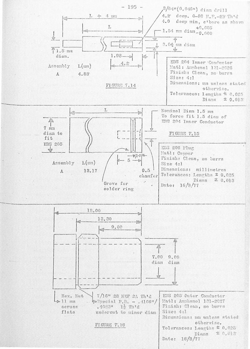
o th er· ..... l IH) . Ii' 'tU n., 'i. 1 4 -----..-~ ....... --.
Di r:1enF;ions: I
Toler~nces: J.engt hs * 0.025 __________ . ____ . ____ . __ ~ ________________ ._J _____ , __ ._~i fj.::l~ ___ ~ O. OJ :i~. I ~}----- IJ .-.---~ . [
~;):-.- I-~r ---~ _ -.1 _ Non; ntt 1 Di nm 1.5 rom '1'0 fo rc e fit 1 , 5 diom of . )S 2(14 Inner COYl rlu~tor
J!l GUn.}; T. 1 f
._--------di= to ~ I j :~; 205 Jc) '--- .~ . -~, ---r--
L :..D ') 206 1)1 ug
'):? --,- ---- -. '''---1 -=~11'i"'- '\ ~ \tvt . = Cotner
() ~_ 5 .. -t . Fin). s11: CI e(),ll f no iJU1TB
A3sembly L mm Size 1-1
A 13.1'( O.t> I>imenni-cn: chJ.rnf ! t' ToJ ern.nco::!:
m:i 11 il'le (;.rcs Le)H~th~l :t o. O~~) ])jnm~ :t 0.013
16/8/77 . Grove :tor solder ring
.'
Dr .. tc:
---_.--. ,-------_. --_._-------------~-.--.------, -,
~ 'l .OO fl.C.O di ~linm
- ~ .. - - - - - - - - --"---'- '- ,~-.
lI0'\:. 1: ~ I 7/J Gil 2e 1BF' . :. Th ' ~ J 1 mm IT, 1."r:1HJ\:d ft,l P.)'). _ •. j.lnnfl / a.cr'OIH· .10g;J " 1'~ 'rh1d I
fJ o.ts undN'cut '('() mi nor cliam
FI GUR}t.:: T. 1 G ---"' ..
I EDS 20[; utur Com uctor J.!a.t.l: AmTlheno 1 J:n -2(~:' 7 ::!'i • .1 1)1.: Cl ')t:~t), no lmrl"l c;'i %e: 4:1 ))il:-:cnniohfl: mill un cn~ ~tt tl~ ~
o thf!L'l~i l1e . Tole l'cmces : I. 1 9t1).'~ ± 0.(1 1)1')
]} ' WJ ':t(.l't.
Dfl.tO: 16/3/71

- 196 -
The construction of 1:he open circuit. calibration
standards havo been dictated by the m,;cc8si ty to retain the
standard support: bead v1i thin the APe 7 to centralize the
inner conductor. Insu1ative supports were not used at the
far end of the conductor to retain un:lformit:y within the " , , edt' t' prec1s1cn a1r 11ne. on' UC'"lVe suppor "s, sueil as a short
circui t placed a, quarter of a 1·mvelongth away '\vcre rej ected
because these would immediately make the calibration piE!ces
narrOvl frequency band devices. It ,,'as realized thC1t support
ingth2 inner at one end only will cause concentricity
problems at the unsupported end (£<11:-" end) between the inner
and out.er conductors. Adams (Ref 7.1) has given some
figures relating to this problem. In practice, tIle concent.
rici ty problem has nO.t proved to be troublesome. This is
believed to be due to the fact that the ncar end is rigidly
held by the support bead and that it is centralized by the
inner COl:lductor of the mating APe 7 connector.
In order to minimize the effects of the supporting
bead, and to provide sUffici.ent thread length for a rigid
support, the first open circuit plane' (Fig 7.11 A S8 .~) '\'13.8
placed 4. 83mm a\lay from the far surface of t.he support bl:!ad
"Thich is a physical length of 7. 671mn (14.01 ele::trical) from
the contact edge of the inner conductor. The other reference
planes are spacc:~d apart at 10mn1 increments (Ass B, C and D
of Figure 7.9). The outer conductor (Figure 7.10) was
orig:LnallY drmH: for four assemblies. Each outer wa s • •
meant to exceud the length of the inner condu.ctor by
approximately 16rnm thus providing nearly 100dB of evanescent
mode attenuation at 12GHz for the THOI mode. A later cost.ing
exercisE:! shovled that this method 'vas prohibitive and it was
decided to use a common outer ana APe 7 connect.or and to
change t.he inner conductors as desired. This method has not
proved to be particularly troublesome but does require more . computer time during calibrati.on becausE:~ of the longer
time required for' ch;mging the calibration pieces.

- 197 -
The reference short circuit 'vas constructed using the
principles derived for both the short circuits (Section 7:2)
and the open circuits described in this section. The short
circui t plane has been placed 4.83mm av;ay from the far side
of the support bead to coincide "lit.ll the plane of the first
open circuit ca1ihration standard.
Hence, all measurements are referenced to a plane 4.83rrun
a"\-lay from the far. side of the support bead (i. e. , 14. Olrrun
electrical) from the contact edge of tbe inner conductor.
The fabrication of the microstrip pieces ",ere carried
out on the premises. The general principles are w'e11 ltnown
(Refs 7.8 to 7.18) but as the majority of the it.ems ",rere
fabricated by the author using non-commercial equipment
developed wi thin the Uni versi ty, a brief rCf~ume of the
methods used "I"i11 be mentioned. 'l'he main fabrication
processes are shown in Pigure 7.17.
. . F i gu r~~ 7. 1 7 MalD._Fabrl·cation Processes C?f Mi£!2§trill
[--;rt."o~HotOli thog.r~9
l' .- J-Cl]bc~t" 'r'ltp. •. ) • .' "' • G .' .. --_._- .'~
E1:£.[Jn ratin.!1 'fj.i
1 t 5.1 Maskma}:i!!£1
Phot.o R(~s:i.st ill~(~ ~.£: t c11i n q
Tbe desired arhvorlc "ms drav1TI 011 "Cut N strip" film
using a co-ordinatog:r-aph ",ith a Flha.t"p cutting blade. "Cut
N Strip" film may' be dCGcrib(~d as a teflon transparent sheet
film 'vith a thin reddish (strip away) plastic film ~ttached
to it. rl'he film is claimed by the manufacturers to be

, ;
l.
~ I
I I
I
I I I I I I !
1 i I
I I
I
I ~" ,
1:0 1' ,....1 . :1 Pi,1 01 "n '..I I HI r1;
Ii (l ) 1
j I • f
\ .
: f

- 199 -
.. dimensionally stable and to provide excellent contrast for
subsequent photographic "mrk. The coordinatograph has
vernier scales vlhich permit. accuratc~ posi tioninq of the
cutting blade to wi thin.! O. 01IT,m. The dra\"ings were
normally made ten or t'iventy times the actual size required
so that any cutting or stripping irt'egulari ties ' ..... ould be
reduced significantly. '1'he masked produced ''laS tabm into
the photographic laboratory for photo-reduction.
7: 5.2 Pl!oto-li thC29ra.phy
The photographic equipment used ",·o.s developed on the
premises. Kelland (R~f 7.15) did the preliminary 'i>lork and
Hichie (Ref 7.16) finalised the system. A picture of the
photographic laboratory is shown in Figure 7.18. The
I photographic bench is on the left; the wash basin and
general fi1m'development equipment is on thE) right. All
photographic equipment is attached to a riqid beam suspend-
d t {-" • •• 'I .... d' e by spr~ngs ..:rom a m;:un frame to m~n~m~se ~u~l .tng
vibrations. The back 1i t art"lOrJc is fixed ·to one end of
the beam. The simple box camera and t~he focussing
microscope has slide attachment.s to permit movement along
the beam. various lenses may be used 'with the";! camera body.
Dimensionally sta.ble photographic plates are attached to
the other end of the camera by a va.cuum chuc1c. No shutter
is provided "li thin t.hG carnGra. Exposure is controlled by
exposi.ng the film to bacJ.: lighting cr,tanating from b(~bind
h c· d" . d 1 b . th t e arbmrl(. ..:)~ze re uct~on ~s carr~e OUt:' y mov~ng e
cam(~ra body along the bench until the desired image on a
dununy photo plate is obtained. The same image is: also
exami.ned by a travelling microscope t.o ensure sharp focussing.
Focul:;siDg and aperature control is carried out by adjustments
within the lens used.
Exposure time u~3ually b~ti'n~en 8-30 seconds was varied
to suit the reduction S1.7e and the }\odal{ high rE~soluti.on
plat.es used (Hef 7.11). Development timc;;' waG rigidly
controlled and was carried out according to the folJowing;-

- 200 -
____ ~h~W;;;~.;~':~'_.."I!!!II: _ ...... ~.,.-p;aaq:c"e; '_-UIIiIIIUII~~.
Developer
Stop Bath
Solu tion
- -_._-1 part I~odal;,: DG de-ionized wate
3 parts Glacial to 8 parts de-i
10 to 6 parts r.
Acetic Acid onized water
Time...lgen.,!;.le ?-9.?-_ta t ion} ------, --6 minutes
-45 seconds
~--------~------------------- ---Rinse De-·ionizc·d Wate r ---_.- ,.-- .-
o .
Fl.xer 130 gr.1S of Kod<A pOi>Tder per Ii t.r ionized vTat.er
k Unifi.x
---~--,-------
Rinse De-i.onized wate .----.- . ------HypoClear
e of
r
Hyop d in
61 gms of I\odalc Powder di ssol ve litres of de-io nized
r
dc-
-----Clear
2.25 water _._ . . ... -
1 minute - ...
8 rnim.'ttes
1 minute -
10 minutes
--- . . 20 minutes
-Rins;=-t ~e~ior:i::;:~~;; ... _. ' ........ , .... --
•
Two main tYlJes of substrates "iere u.sed, metal deposit.ed
substrates, e.'g., alumina." and sapphir'e substrates. In the
case of the latter, metallic deposition 'vTas carried out
o t' Th' 1 h t.1S1ng vacu.um evapora 10n. e eq'.1:Lpment usee ",ras t.8
Ed1,'Jard!3/Bil.·v (,f: Hodel TA-150. 1~ close-up vlew of t.he
evaporation chamber with th8 bell Jar removed is ShOl:11 in figure 7.19. The method of using this unit has been
substa.ntially described (Ref 7.8, 7.17 and 7.18) and only
a resume of the preparation and vacuum deposition of the
• b • substr<:l.tes w~ll ~e g1ven:-

Vl Vl tJ
..:-:::: .. u
.C
E
.. -
<1-' .. ':l :J ;::r :Jl
f)
.r:. (])
u c 0
L. .. ~ Vl
Q) .Q
C :J n II/
~
.... 0 .. -
' .. .... 0 a. a. :J til til-
(\)
..-~i. 0
C .. (11
(.1 .0
() :J .... 'J)
-201-
t::
Ul
> 1 L.
()
L.
0 .. -c: 0
E
~I '7
b ~I H
I' (-: :S18
~ r.~ IH °If.~ 8
1
o..H .:r;IO
t-: ~ I ~ ti..
c.
c o \..
~ ,
III
CJ
>,
, - .. J'.
---I .'(
" a "J • ~ . ~ .:
. I
'I
. '-:;.";
:J
E

,;
- 202 -
(a) First Wash Substrates ,.: .. ashed in a solnt.ion of 5cc teepo1 and 100 cc de-ionized water in an ultra-sonic bath for 3 minutes (Fig 7.20).
(b) Second Wash
(c) 'rhird l''lash
Same as First 11o.8h.
Sl.lbstrat.G "lashed in 100cc of carbon tetrachloride for three minutes in ul t.L~a soni c bath.
(d) Fourth ~~ash Substrate "lashed in 100 cc of 180-
propanol in ultrasonic bath.
(e)
( r)
( gj
(h)
( i)
(j)
(k)
d '.' (1 )
(m)
(n)
( 0)
(p)
Substrat.e dried in oven at 70°c for :ive minutes.
Substrate placed in vacuum chamber, Dirvac TA-150.
System evacuated to 0.1 torr.
SY:3tem' heatf.:!d to 150°c for fifteen minutes of outgassing.
Heater s'\"itched ,off J but glow cleaning applied at 1Kv for ten minutes.
Filament current switched on at 25 Amps and left for five minutes.
Nichrome heated and allo'wed to deposit on target shield for two minutes. This is to'minimise any ni~hrome oxide on th0 substrate later. , " .
Nichrome deposited on substrat.e for 60 sE~conds. Target vOltage was set to ;2.. 5Kv I recorded current "Jas 25rnA. P reS81.lre was 5 x H'P rrorr; thickn(?8S of deposition about 400 Angstroms.
Copper heated and alloi';ed to deposit on target sheild for two minutes. This is tQ minimise the deposition of copper oxide on the substrate later.
Copper ct0.posi tcd for twenty minutes ,,;i th target vol tage set at 3I{v. r~ecorch::-cl current was 65 rru\. TId.cl.ness of deposition about 1 micron.
System left t.o cool. After thirty minutes, air. "ms , allowed in by the bleeder value. If the subst,'Cr.:'.te
was not dGsired immediately lit 'van stored in the vacuum unt.il required.
Removal from the vacuum chamber 'vas l.lnrn(;:!diat.ely follmled ,vi th photorcsisi: cO<lting to minimise oxida.tion.

- 203 -
'J~wo type1':i of photoresist '\o;:ere used, the negative type
Roda}:. Thin Film Resist (KTFR) and the positive type resist,
Shipley l>.Z 111. The negative resist w'as used when it vias
desired that all image parts eXposed t.o ultra-violet. light
,·muld be w'ashed away in the developer. The posi ti ve
resist vlaS usC?d when it. "ras desired that all the parts not
exposed to ultra-violet light ,{Quld be washed a1vdY in the
developer.
In both cases, the method of application is the same.
H:.F.T.R. is. applied \dth a syringe f:i.tted with a negative
resist filter (MillipOB Type AfI.vIP Ol300-A), Shipley AZ 111
is. applied vi th a' syringe fitted v1i th a posi ti ve resi st
fil ter (Hillipore Type UHWP 01300;-.A). 'rho equipment used for this work is shm.,n in figure 7.20.
The substrate was vacuum held on'a rotating spinner.
A thin layer of resist was allo~ed to flOW over the substrate,
wllich was then spun at 3000 rpm for 20 seconds. A s~col1d
coat of resist was similarly applied and spun. Pre-etch
baking t:i.me was 10 mlnut.es at 70°c. Exposure time was 3
minutes followed by development in KFTR developer for th(~
KC?dalc t:ype and ~hipley AZ 303 for the posltive resist.
Post-developing baking time ",as 10 minutes at 70°c •
.#, . .• f. .
The copper etch used vms a solution of ferric chloricl.e
prepared by mixing 80 gms of ferric chloride 1vi th 400cc of
wat0.r. Etching ,.,ras by gentle agi t.ation and the complete
etching time \va~ about 20 seconds.' The substrate vlas
inunedia·te1y removed and washed as soon as the nichrome lay(~r
underneath 'vas visible. The nichrome etching solution ,.,ras
prepared from 40gms of potassium ferrocynio.e, lOgms of
sodium hydroxide dissolved in a solution of deionized water
to make a solution of 200cc. The solution was used at
50°c. 'rhis :::olution \.,real(cns ~dth time and should be
di scarded 'vi thin sc.~vcn days. In practice, it was noted
thfit even after 3 days, thH etching qualities \vere impaired.
Electroplating was them usod to t.he required thicJmcss.

-~ ~ a.. ::J II)
L. <1.J .... 0 ~
l-i
0
I .
<i CJ) Q~ <V .....; "'0
'-0 '.-0 L
OJ C OJ 01
U
C 0 (/}
0 ,. ;:)
a.. C.J... :J 1.1,1
'-Q)
'- .> Cll ~~
E 0 ..c u
0 O. ..... 0 c:: t... Cll E- u C <!. 0 Col '-> C (l)
~, .
;-.., til
0 Vi
0) 01 C. '0
..c: u >' 0.) , C 0
", . • • 1 ~ .", ., • . ,.,
.. , .. ., ... ~ . ~~.,
c: E .. :) 0 u
Ul 0.. 0 u (/) 0
..... o -.-o u
'- 204
Vi 0 a.. (/}
E ". u (]) ... "
ij) (.1 .... >-Vi (fl
U 3:
. '. , . ........... , . . _,
U
C ()
til
iJ C '- 0 - .. -::J
'-I ' --- ' . I '
I r, ~ • "'. I.~ ·:I .i. I
"
~I a.. 0 :J
(/} V CJ '-"- QJ Q.J .. -
't- o '+- ~
-Qj C \.1 0..
'0 ..... .....
.... :/l
'iii to ,
01 QI
\., C (') C .. ~ 0 0.. ..c Vi 0..
.... C OJ
lIi 0'1
ttl
'""" ('J L...
0
0 .c 0..
-- .... ----- ~
~I r--
~ I.r. 0 0 H ~
C
Vi
t? vjl Z (.Ll H H if; E-I (jj H r.rJ ...:l (.) H 0 ') p::; ~ 0.. (:L.I
......
.c ... I .. O. Q)
C C .... C\..
:J
lfl
'-'0
0 C
" ~
~ '--,
...... C Q)
E c ,:fl
~
\.,
OJ C C
a.. (/}

- 205 .-
Most of the plating techniy\.les Cal(l8 from (Refs 7,13,
7.14, 1.16 and 7.18). The book by Raub and Mueller is
excellent on fundamentals and helped considerabl:r towards
understanding t.he ot:1::er rt'ferences. Graehme (Ref 7.18)
is particularly good Clnd goes into considerable detail on
thin and thick film plating. .l\lt.ho'..:lg11 copper plating was
achieved fairly easily, considerable difficulty WdS
experienced in plating after etching. 'l'his ,,,as finally
traced to photoresist contamination and a cleaning process
had to be derived.
After the etchir:g of the chron',e film; the remaining
photoresist '\vas removed; 1~FTR by a spray of carbon tet
rachloride; Shipley AZ 111 by a spray of Acetone. Both
actions "Here follOvH::d by a spray of Isopropanol. By this
time, the copper surface 'was well and truly 9xidised and
had to be once again acid dipped. Various solutions of
11i tric and hyd~·ochloric acid dips Vl?r(;: t.ried. The one
finally decided upon was a 20,% of sulphuric acid used for
a 20 seconds dip. The substrate was then immediately
connect0.d to the plating bath. A solution of copper sulphate
and dilute sulphuric acid ",vas uSE~d as the p1atin;J electrolyte.
The soluti.on, was made by dissolving 850gms of copper
sulphate in a "Teak solution of dilut.e SUlphuric acid made·
from mixing 198 gms of concentrated sulphuric acid mixed
wi th 9 )j, t.ref:;· of: deionized '\vater. '1'he age-old~· precaution
of. always adding acid to 'vater was adopted in preparing the
sOlution. The C'.lrrcnt used "las 300 rna per square centimetre
of plating surface.
Copper plating vias follmved by a gold flash using' a
gold plating solution, a commercial product called
Transt.bcrm Solution made by PHD Ch(~m1.cals Limi t(~d. This • ".. l t r. 1"':0 d' . solution must be mc:nntalnea. a- v:J C ur:tng pl;"\tJ.ng. f1'11e
solution is used undiluted. Hemoval from the gold plating
bath must be follovred immediately by u dip in I Elopropanol

- 206 -
follOvie(} by inunediate drying with compr2::;sed air to provide
a shiny gold finish. '1'he curr.ent used was 100 ma per square
centimetr.e of plating surface.
rrhis chapter has explained and described in detail the
construction of the calibration and test peices used in the
oystem. Considerable effort vlaS expended in trying t.o
produce "theoretically perfect caJ:ibration standards. vfuilst
not all of these aims have proved practicable, the majority
and vital principles have been achieved.
'rhe consistency of the various standards have also
. been verified by I{wesah (Ref 7.5) and Hosseini (Ref 7.20).
* * * * * * * * * *"
•

7.1
7.2
7.3
7.4
7.5
7.6
7.7
7.8
7.9
7.10
7.11
7.12
7.13
7.14
7.15
7.16
- 207 -
Adams S. F., "A New' Precision Autcmatic :!'-1easuremcnt System" I. E.E. E. rrrans. 19(,8, IM17 pp 308-313.
Ampheno1 Catalogue Sheets "Series 131 - Precision' 7nun Conncct.orsH Micro\-,ii.tVe P roduct. Dat_E~ D i n~ctory 1973. Ampheno1 Specificution Sheets 0:::1 ou'ter Conductor Tubing 131-2027 and Conductor Rod 131 - 2026.
da silva E. F. & McPlml1 M. "Calibration Microwave Net'worle Analyser for Computer Corrected S-P arame'ter Measurements" E1ec'tronic Letters 9, pp 126-1~8, March 1973.
l\wesah 1\, "Characteiiza'::-.ion of Inb2grated Bi-polar 'I'ransistors using Cc)mputer Aided Heasurements and Optimisation" Chapter 4 Ph.D rrhesis •. University of Warwick 1976.
. . h . tlM1.crowave Engl,neers' Tee nl.cal and Buyers Guide Handboo}.;:" 1970 Edition published by Micro'ivave Journal, Horizon House, Dedham, }1a.
Military Standards. p-19468 on Plastics published by the Joint Arrlled Services. U.S.A.
Hai,sse1 L. I. and G1ang M.H. "Handboo}: of Thin Film Technology" He GravT H i.1l, Ne'\oV York 3970.
Keu.ffel & Esser Publication "Uses of Stabi1ine 'Cut N Strip' Film Data She(~t 1964.
J\oda}c Publication "An Introduction to Phot.o-f b · t' . "d 1 . t' ",', tI 'a rl.ca J.on uSl.ng hQ ak P :lOtOSfI:tlS1.'.1. vr:. healS'::'8
l~oda.k Publication Book No. P 79.
r\odaJ\: Pub1icat.ion "Kodak High Resolution Plat.e" Data Sheet. ~.,
Chemical P rocesses Ltd., "12/1,s Resist Stripperfl
Data Sheet by Ch8mica1 P rocesses Ltd., Chidburgh, Suffoll(.
W. Canning & Co. Ltd., "Handboo}c on Electroplating" Binningham, 20t.h Edit.ion, Jan. 1966.
Haub E. and }1uel1er I{ "Fundamentals of }ictal ]1)ep08i tion" El sevier Publishing Co. 1967.
Ree1and G "The Cdmmissionin9 of a Hpduction Camerall Uni yersi ty of ~'1arwic)q Internal Report 1969.
Hichie D, "H:i,crov.~av0 Integrated Circuits; P repara tiOll of and Neasurement Techniques for Overlay Capacitor" Ph.D 'l'hesis, Univcrsitr of Wanviel.:;, 1978.

7.17
7.18
7.19
7.20
- .
- 208
da. Silva E. F., "Inductors as Lumped Elements in Hicrowave Integra.ted circu.its" H.Se Thesis University of NanTic}>:, 1971.
Pender R. S., "Thin Film Hicroelectronics" I.E.E. students t Quart8rl~{ Journal, sc~ptem.ber 1970 pp 153-157.
Graehme A., "Electroplating Engineering Handboo1<.1t Hhei.nho1d Bool\: Co. 1969.
Hosseini, N. H., '''fhe Application of Computer Aided Design to Hicrostrip Cireui ts" Ph.D Thesis, Uriiversity of Harwiclc, July 1977.
* * * * * * * * * *
. ..

- 209 -
CH.i",PTEH VITI
,
PRAC'I'ICAL PP.OBLENS IN COMPUTER CORREC'l'ED MEl'.SUfillHEN'I'S _._.,---
8:0 Introduction -------
Tl·.l,e main purpose of this chapter is to examinEe:! the
problems ",hieh are cnconnte:r.cd when theoretical ideas are
applied to practical problems. A brief survey of the
complete measurement equipment is initially made. This is
followed by a more detailed review of the polar display unit
to establish, the principles by which the magnitude and phase
components of the reflection coefficient are detected. The
problems associated with non-li~earity in the amplifiers arc
also analysed and the solution used to overcome this problem
is explained.
< Tests are then carried ou·t to E!stablish the viability
of the equipment for computer corrr~cted measlll:-ement.s. These
are folloi.J'ed by further tests to confinll t.hat both manual '
and automated corrections have been satisfactorily achieved.
1\ bloc){ diagram of the measurement equipment is shown
in figure 8.]. and a det,ailed block diagram of the polar
display unit is shO\~-n in figure 8.2. 'r'bese nrc based on the
manufactur'cr's information (reference 8.1).

REI; •
SIG.
• nEF • SIGNAL
- 210 -
Fioure 8.1 . -... --<..;..;,.;;;----.. ~
SIGNAL GENERATOR HP 8690B SEHIES
J-----'-1---NEASUHEHENT
PLANE , I
=l- INC. I -<!-- . __ h.... I HARHONIC REFLEC'rOHE'rER V""
MIXER A!'-;1) LINE 1----1 HP 8411A.~.. ... '---~ ______ ~ ... ~ STRETCHER ~--
HP 8742A REFL.
rrEST SIGNAL
HEA SUREl-liNT PLANE
I F.:. ]\HPLIFICATION
POLAR l DISPLAY UNI'!'
HP 8410A _-{> .... ' HP 8414A
-------'

Fiaure 8 .2 • .c p 1 ~r D~ splay (h"1'S414A) Overal l B l 0cl<:. Dlagram 0.1.. 0,,_0. ......
--- .--;.-.
• - rT1 • i ,/-ortical out:put c~:n,~~£ A~;f\ I; I D I ~ V ~. C •
~~9~~llO~rorll i"'~J900 PHl1SE J J SIN ¢ .-~D .. c.>-4ID"7 ~c. ~l /~~\ SjN ~ ~'. I ') - ::,., r-'D'Prrr.:'CT''H-' I ~ / I I . '\/ >-- 1 ------jX~J I isnIFTER · I' ~".. U~ It· V 0 i . : {]!L\ ' /<! I / I I I I , . .. _ , I I .I'd, \ L-<t <:?-, y' \. /i\ r' A SIN cb VertlCcI.L . . _ i~ __ -I __ _
rh I !. I Shift M] , ! --A-- 'y !BE.r~M CE~~;'-:-~ I . II I I L . VOLTAGJ, I ) \ I " IIADJUST. '" I I II ' I & FILAMENT \V j... ~ A CO S d\ . I • I ! SUPPLY / __ ./ r
I PHASE! I· I POL. y--l ~ --- . ~~ITTER 14 180< 11 ~ DI~:/ >-- I TT~R I - 1i\ 278 KHz Phase I LIM...L .~ '" I . 1 Ref en,,'mce . Signal I i I HIGH
fro:n HP 84::'OA I I VOLTA~EI I i j SUPPLY I ; ! 1, I
-Ii , j . r "" f
leos" rp '·--1 L"" I J ~ >1 . -I-V' Qi17V1' c. . J - -------7"!DETECl'OR i 11 . I If, HOJ;~zon';al
i J . I, V Shlrt AOJ •
; I A COS~ Lt ____________ ~ ___ ~~=-_~ I,' Horizontal output 'INTENSITY I
~ :==lMODULATOR LI-------_____ _ > ~ I
$..-------'
I',,) ~ ......
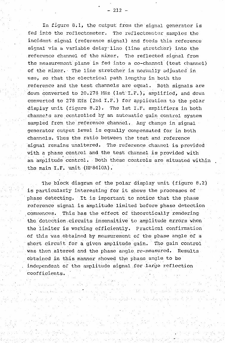
- 212 -
In figure 8.1, the output from the signal generator is
fed int.o the re£lectorneter. The reflectometer samples the
incident signal (reference signal) and feeds this reference
signal via a variable delay-line (line stretcher) into the
reference chalUlel of the mixer. The reflected signal from the measurement plane is fed into a co-channel (test channel)
of the mixer. The line st.re·tcher is norlnally adjusted in
US!?, so that the electrical path lengths in bot.h the
referenc(~ and the test channels are equal. Both signalS are
dOim converted to 20.278 11Hz (1st I. F. ), amplified, and dOvIn
converted to 278 KHz (2nd I.F.) for applica.tion. to the polar
display unit (figure 8.2). The 1st I.F. amplifiers in both .channE:!~.s are cont.rol1ed by an automatic gai.n con"trol system
sampled from the reference channel. Any change in signal
generator output level is equally compensated for in both
channels. 'rhus the ratio between the test and reference signal remains unaltered. The referenc.e channel is provided
with a phase control and the test channel is provided with
an amplitude control. Both these controls are situated within
the main I.F. unit (HP8410A).
'rhe bioCk diagram of the polar display unit (figure 8.2)
is particularly interesting for it ShOvlS t,he processes of
phase detecting. It is important to notice that the phase
rl~ference signal is amplitude limited before phase detection
commenc(~s. This has the effect of theoretically rendering
the detcc"tion cireui ts insensi ti ve to amplitude errors when
the "limiter is working efficiently. Practical confirmation
. of this i{aS obtained by measurement of the phase angle of a
shor.t circuit for a given amplitude gain. The gain control
was then altered and the phase an91e re-meas.ured. Resul ts
obtained in this manner showed t~e phase angle to be independei1t of the amplitude signal for large reflE?ction coefficients. .

- 213 -
Hands, (reference 8.2), \'ioods (references 8.3 and 8.4),
l~dams (references 8.5 and 8.6), Ridclla (reft~rences 8.7 and
8.8) and Harner (reference 3.9) are so:nc of the authors who
have investigat.ed sources of errors in automatic network
analysers.· Harner has issued a comprehensive list. This
is includ~d below:-
(a) Instability i.e., the inability to produce
identic(1l results for the sarr:e measurement.
(b) Nois(~ • •
(e) Non-infinit.e directivity in the couplers.
(d) Imperfect matching at the t.est point.
(e) Departures from identical traeldng in the
test and reference charuLels.
( f) Leakage between the tw·o channel s.
(g) Imperfections in calibration standards such
as incorrect dimensions of thf! connectors,
contact resistances, errors in offset length
specifications etc.
(h) Imperfections in instrumentat.ion such uS freqt..lency and power level non-lineari ties,
gain and phase drifts in the I.F. amplifiers,
detect.ors, attenuat:or and di splay cireui ts.
(i) Quantatization errors, SUC~1 as errors in the
analogue t.o di.gi tal conversi.ons, rounding off
errors in computation etc.
It has alre~dy been S110wJi. in Chapt.er V that the
me;1sured reflection coefficient, P is related to the true
reflection coefficient r , by a system bilinear transform·-.;,.' p Ar +B 1 a .... ~on of the - C\-l '+U- 'vlcre ~., B, C, and Dare
compl(~x constants. Furt.h(~rmore, it 'vas 0.1 so sho'\Vl1 that by
mo.l'>:in9 a S(!t of co.li.brat:ions, the complex constants can be
solved mathc:matically and h011ce yield the the true reflectJ.on
cOl?'fficicnt,

- 214 -
This mathematical solution is. only possible if the four
complex consta.nt.s remain invariant throughout the set of
me<l sur-emen·t 1 i. e., the en ti re measurement system f rom the
calibration standards to the computer output terminals
1 · . must be stable. If tus J.S not the case, then computer
correction is not possible. Henc(~, it is essent.ial that
testB ar.e carried out to ascertain wheth(~r the equipment
is suitable for ,con:puter correction.
The method used to verify tl1.e stability of the system
v.ras the repetitive measurement of t.he same calibration
piece twenty time's.
The condi Lion.s of meaSUrCitient '\V'ere:-
(a) The same test piece (short circuit) was
disconnected and re-connected for each
measurement.
(b) The frequency ",;ras selected by the computer
for each meClsurenlcnt. Hence any errors
introduced by frequency drifts t:tc., '\-lere . included.
(c) The measurement. result is that taken from
the print-out frOITl the'computer. Hence
q1.l,aritatization errors, etc., "J(~re included.
(d) '1\lle amplitude gain was dt::!liberately set to
Pl:"("~:c'pt. r(~flection coefficients less than . ' unity to ensur(~ that amplifier limiting
would be minimal. A full discussion "rill be given in Sect.ion 8,3.
The results of the measurer;:cnts carried out at 6 GHz
are tabulated iri figure 8.3.

- 215 -
FicH'l.re G. 3 _. -"'''-'-
- .... -.~~,..----.,---... - .. ~--.~-AII1l?.1 i t.~de !?~X£:g§ A 1llP.]. i t l?~} E· Degr:.ce§
.~--... - _.-0.92B 175.6 0.919 176.2 0.928 175.6 0.925 177.1 0.925 175.4 0.919 175.5 0.933 175.5 0.919 175.6 0.925 175.5 0.915 175.5 0.927- 175.5 . 0.916 175.2 . 0.921 175.8 0.915 175.3 0.923 175.8 0.915 175.0 0.923 176.0 0.915 175.0 0.921 175.9 0.938' 177.1
--,.
From the table sho",m in fig-ure 8.3 the following w(~re calculated.
Hean Amplitude ::: 0.9223 St.andard Deviat.ion of Mean Amplitude:::: 0.00617 • '. Standard Deviation 0.67%
11ean Phase (Deqrees)::: 175.7050
Standard Deviation of Mean Phase ;:: 0.5633° • • Standard Deviat.ion 0.32%
In t.he rQsults calculated above, the amplitude and the ... '.. 1 • , I'
phase have been calcuiated as if the numbe):s arc t,-lO
independent quanti tics. 'rhe bllsis for this t.reat.ment has
been discussed in Section 8~1 • •
The final conclusion from the above measurements was
that although the measurement syst.em was not perfectly
stable, it did appear that computer correction wns a 'b'l't pass). ~ ~ "y.
In the Ineasurement system used, t.he HC"rlett P aclcard
Reflectomcter System is situated some distance away from
the comput(::lr. The signal lines connecting the- t1m pieces
f ' b' " T ' o cq1.upment are Em Ject to no~se-plc}t-Up et.c. 0 ~mprove . +
the signal to noise ratio, tho t.WO outputs (- 10" volt.:> Mw:)

- 216 -
of t.he pola r display a re applied to two external 2Cc1B . ~ . b ~ . t' 2.l11p lL( lf~rs e:L o.'.::e appllca· J.on to signal line s . I deally
i f a reflecti on coefficie nt o f unity is set to produce
maximum output, then no lil!1iting of the external
ampl:i.fi(~rs will resu lt. Unfortunately in pra ctice, due to
errors i n t.he measurement equipment, it is possible to
measure apparent reflection coeff icients greater than unity .
Wlen this occurs some limiting of the external amplifier
occurs. ,'1'0 avoid 1.:hi8 the amplifier gain setting 1'1ith the
Hevrlett Packard eq-uipmE:nt is reduced by approx imately
1- 2dB so tha t '" reflection coefficient of unity is presented
to the c ompu 'ter tc=rmina1 s as slight1 y less than unity
rv 0. 9 . If ·this mult.i plica'tion ' factor is denoted by r ~ then any measured reflect.ion coe ffici. en'c , I?rv , presented to
tlx.;! c Clt pu'ler terminals become p~ and the follO'iV'ing relation-·
ship appl i es
• I
Prv := .fi f ryu .. ... 8 .1
T o ascertain the effect o f the above on the error
netvlOrl: se ·tt ring parameters and the fina l corrected results,
t:he follow'ing a~alys:i.s was used~
From conation 5 . 19, "
and usin9 equati.on 8.1 and defining S11 /( as tbe neiV' modi fie d
value of S11 , (11 -2.p. n n '\ 0.2. P f (""'rI -Z(f:.-i J
.) \4 r:! \ 0.'2. f) f, ('" ...... i' - 2(;. l"" f"' '-(f\- ",) S I ~/ ::-:::J~?'P.&J.!Zqs.:' II IEl. - -r<~. ;\.I , I;;' e ," ~~ 11~_1--.._~~I~I::~- :""2e- :..L:
.l.J. f Cr.' r-' ?.(t~· {';4) r. (-. ) - .Y~ fj (1'--' j ' I - .. of". f' 1-:' E:;(P.r~ ~·)'\ +,{}, II (1.1 ~J )"' r: ,,...,1'.) r..:: , .. \ ;~ e.' -.,.. I 3 I - Q. 2 '? e - I 3 • ) 1'':' 3 I :;; ,- :~ :-. '-- .
Herl':".: Lhc conclusion i c,;
C 1/ ;) \ I ~_ S! I ... .. 8.2

_. 217 -
. r 20 From equatlon ~ •. ,
S 2?. ::: r~~~{/l:-::,~' 1_+ F (5 I'. - ,r, ) ~ .~1 0~- p/)-"-"
Using equat.:i ons 8.1 and 8. 2 and defining 822
1/ as the new
modified fa.Ille of S22
S I I
'2'2.. -
The conclusion j;s that S /1 .. 22 4. ••• •
822
i s uni:l.ffected by the ltlul t.iplicat.i.on factor k.
c c . ")J2':>2 ~
From equation 5.21,
S I 2. S 2 \ = (P, -- ~. I ) (\ -- r- 271. f1 ) \ I
I
~ II Using equat ions 8.1, 8.2 and 8.3 an d dp.fining S12:':121 as
the n ew modified value of 8 128 21 ,
c r II ~I<l. ~2\ =
. .
,£2. C PI - S I 0{ I - S 22 r") ) .1,'
.....
8 12 821 is affected by the multiplication factor k.
ThE2_~ ort"ect~d_ ReflectiqL,r __ _
F l"Ol'n =!(JUCl tion 5. 22
8.3
8,4
"I;' U sing C~i'n . t i or; s 8. <1, 8.5 , 8. 6 and 8. 7 and def ining as
l18 modified value of I
/I ..-. I t .~ R-f't"V -- ·Y~-, S', I
"-"_ .. --._--_ .... __ .. -_ ..... _, .....
\
'''"111 . - •. ...- \ I
- I • it ••• 8.5

- 218 -
The conclusion is that t.he corrected reflection
coefficient result i.s un<lf fected by the multiplication
f a. c t <:.11'_' \I lc'!
The result of equatic'Tl 8.5 can be cross-chr~cked by
recalling the invariance of the cross·-rat.io of the bilinear
transformation of equation 5 . 7
( P! - fr) ) ( ~ - f+ ) ( " -- Q ) ( \; - ~-"- \ \ ---_. -- .. _----_ ._- -
( f~ - f3 ) ( H,- PI ) ( ~ - \=' ::. ) ( \-, t' ...
:--" - \ \
and using equation 8.1 again , it is seen ·that " k" has no • 'effect on the correc·ted result.
8: ~..?_ Thc_ Effect _of 'the Mul tJ:Qli.ca.tion Factor "k " ,9n_ Line P rOp'aqation Properties
From equat.ion 5 . 28 whi ch is repea ·tc.:;d here
)
)
r t 2 Ce-:J'} ~? (- P, f3 + P, f2r + ~ P3 -- f2 (~') -I-~ 2 -p (f, p.,. _. P, f4 -R r3 -i· -f~ t~.)
-t(- P, P? +- 9. P, ~:, .. ~ P4- - P? P3 t- 2. P';t Pf )}:::- 0
it. i 8 clear t.hat t~he multiplication factor "k" has no effect
on t he results for ·t he propagation properties of a l ine,
8:4.1 A Manual correction Test
One of the earlies·t tests carried out to check t.he
ffecti Veness of omputer correction ''''as the measurement of
a test p ie ce ( coaxial termin tion) t.hrough t:lu" .e differ nt
transi i:ions. '1'he correcl:ed reflection coefficient repul ts
,,,,ould bE. . dentical in all three cases as "the s ame test piece
was measured. Vastly different r.s 11 t8 w'ould have pointed
t o errors in the system . 'l'he SUCC(:!ss of these;, corr ctions
were ultimately pnblished by the aui-.1y l~ ( refer.nce 8.10)
and .his is in J.udeJ as App0ndix 12.1 in this thesis.
HC':·lOV'_,!" as many dct.CJilr.; of the practical ltlcasur ment.s had
'r.O be deleted i!l l:be pnbli ation, they \v.ill be provide d here.

- 219 -
'rhe mc;,;umrcments "Tore carried out using 7rmn air coaxial
lines aad short circuits. The method of correction chosen
was the three shorts method of section 5:4.2 using the
correc-tion prGgrc..I:1.:1~e of section 6: 2. The teet piece chosen
was a He",lett: Packard Type 909A coaxial termination. All
calibration and t:est. pieces were fi tt-ed \V·i th 'PJ)C7 connectors.
At the time -of verification, st:d-table one piece off-set short
cireui ts were not available and they 'fere cons-tructed by
using a standard Hewlett Packard Coaxial Air Lines (Type
11566A - 10.25 ems and Type 11567A - 20.25 cms) t.erminat.ed
wi th a coaxial short circui t (He~vJ.ett Packard Type 11565A).
rEha three sets of calibrations and measurements w-ere
carried out usi~g;-
(a) s(~t 1; consisted of connecting the calibration
pieces direc-tly to the network a:naly8(~r for
measurement correction.
(b) Set 2; the neblOrk analyser was connected to
a pair of 3mm (aSH) to 7mm (APe 7) adc:ptors
bacK-to-bacJo;.:. Hr~nce 'the i:ef.erence plane -h'c.tS
transferred to the 7mm side of the final 3mm
to 7nml adap-cer. All calIbrations and measure
ments '-Jere then made re[erencl7~d t.o the new
plane.
(c) Set 3; the net"Tor.k analyser was connected to
a paJr of 7ll'Jn (APe 7) to General Radio Ad3pb:~rs
(GP.~,74) connected bac1c-to-bac}(, thus t.ransf(~rr
ing the mc:asurement reference plan!~ to the end
of the APe 7 side of the final GH874 connector.
The Game calibration pieces and coaxial term
inations were used for measurenlent.
The re~l'.llts of t.he three 8(~t::; of llll=:!asurements al.e given
in Table 1 of Appendix 12: 1. From this table, it was
concluded that the . corrccV~d resul ts could be cont.ained ,d thin
a circle corresponding to I r I ;: 0.0035. Hence the measurement
system was considered to be Gufficiently stable and an auto
mated computerized system wuf: ,.,rorth producing.

.-. 220 -~
'rhe above inforll1.ation was subsequent'.ly used by Gould
and Rhcdes (rcfe:c8i1c8 8.11) for further expcrimr;mtal "lOrk.
It sho'-lld also be noted t.hat Gould and Rhodes reported that
their results compilrcd most favourably ";viUlthe results
produced above i.e., all their measured reflected coefficients
'Vlere .... ri thin an error circle of 0.0033. Some of the otb.er
authors 'which have since ac}\:nowledgaJ the paper are l'~oods
(reference 8.3). Shurmer (reference 8.12), HossE~ini (reference
8.13t Menzel (reference 8.14 and Warner (reference 8.9).
8:4.2 An Automated Correction Test -----_._-_._---_._--_ .. _----_. ~
One of the earliest automated measurements carried out
on the three short circuit correction lnGthod of section 5:4.2
was reported by K .... resah (reference 8.15). Kwesah's results
were obtained using the 3mrn short circuit calibration pi~2ces
described in figure 7.8 of section 7:3. For his test piece,
Kwesah us(~d a Tek Nave thin film chip resistor (Type 20-01320-
50) whose nominal value 'vas 50Q. -:- 2%. His measurements ".rerc
made in the 1 to 8 GHz band.
Kwesah's rE;!8u1 ts for the 2-4 GHz band are given in
figures 8.4, 8.5, 8.6 and 8.7. Attempts at combining his
results onto one grapl1 were unsuccessful because of the
closeness of his results. Hence. KW'esah' s independent ,,,ork
has also shov.'TI. that the three short circuit correction
method is a good one. .. .. ., ...
This chapter has shmm how the theory derived and
developed in the earlier chapters may be applied practically.
A brief review of the equipment for computer correction was
carried out in section 8: 2 .1. A. full mathematical treatment
has also been presented to show how the effect,s of amplifier
1 · , . . · . d 1ffi1t1ng may h0 mlnlffilse- o

221
.,.
.• It
.'
\\ , \ , \ \ I t J I • J f ' , , t , , r \
\ • .1 , t , f f
r , , f I 1 , . I \ \ \
~ t~
*~ · "'~
C'\t • ~
t.t') - . • ~
, ... . ~ -I-
\\ 0
~ f;,i -.. -~~!!,..., ...... "-.",~:,.,..,..-:~ ... ,..-.----- .... ,., ..... ----------}-,,,, •.. -.-, -----+t·--~- ...... --·i .....
r~
~ ~
" >-; !.:.)
t~ Cy 1:>1 r:~ ~t.
!I) (..) .~
N ~ ..... ' N f.,' ... I:: .,~
~ , .. .... ~ .~
G ',.l C; ..... ~
f'41
~ s.! 0
',.:. ~ tl ~
N ' ..... ~ ~
•

., .. ,
I.
..
, ' "
" , ,,' . '
f ! ------'--r~-----'~,.--- .....
• • •
\ \ \ \ \ \ \ \ 1
j\ I J \ \ \ \ \ \ \ \ \ , I f r f , \ \ \ \ \ \ \ \ \ ~
~ -1'"
If)
0)

223
t~ I'~
~~ .. :.;
t) _ (0 ~ . ~J ~ tj
QI 14 ~ ~
. t.~
r I I I
'I I , I I I •
I I
I I I f J J \ \ \ \
i I I I (
I I t I I ,
\ \
" I.·J ~. .. . I l _. ____ ~.~~--.-i-,~-t-4-.. ·----· , .. -f.-
(J
• co 1:0 to; I'> ,
oC3':).;:.f;Da '-asr:':U
"
. CO • l'.!)
'.-)
k.;

. t<;)
a ..." • ~.
C.) ~i ..
224
. ,
C.;) -............... ~~,-......--
I I I 1 I I I I I I I ,
I I I J I I I t I I
I I
I I
I , , , , \ \ \
, \
\ \ \ ,
.'
~J'-_1-~ ·---·~-1-... ~ r, o c"', M 1"-1 I' ,
•

- 225 -
'l'wo metbods, one manual and thE.' ot.her automatic, to
prove the feasibili t.y of the three' 611or·t: circuit correction
system have been pres(mted. Fin;J.lly, rC8ul ts obtained
independent.ly by another researcher an~ producC'd to shO\·!
that thi s correction system ";OrkfJ very 1Jell.
* * * * * * * * * *
..
..
..

., ,
8.1
8.2
8.3
8.4
8.5
'8.6
0.7
8.8
8.9
8.10
8.11
- 226 -
Hei,rlet t P acl:ard; ltEi c r:m·;r ave NetlJOrl-c .P.naly se:r Applicat.ions" Application Heport AN 117-·1, Palo Alto, Califon:d.a.
Hand, B.P; IlDeveloping F,ccuracy Specifications for Automa·tic. Network Analyser" He"\vlctt P ack3.rd Journal, Feb 1970, No 21, pp 16·-19.
Noods, D; "nigorous Derivation of Computer Corrected NetYTOr}~. ".nalyser Calibra{:ion Equation s" Electroni cs Lt-~·tter.sJ 1975, 11, pp 403-405.
vJood, J); liRe-appraisal of Compu·ter-Corrected Networl( Analyser Design and Caiibrationlt P rcc. I,E.E. VOl 124 No 3, March 1977 pp 205-211.
Adarr(s, S; tlA NC1-T Precision Automatic Micrm>favc Measurement system" I.E.E.E, Trans 1968, HI-17 PP. 30?-313, Adams, S; "Automatic Neb..J'orlc Neasurement.c" P rcc I.E.B.E. Vol 66, No 4 April 1978, pp 384-391.
R idE~lla, S;' "Computerized Hicro\'Hlve Heast.'trements Accuracy lmalysis" Proceedings of the European Microwave Conference, Paper B34, 1973.
Hldella, S; "Computerized R :-flection l1casu.rcmc.:mt:3 C~P.E.M. Digest 1973, PP 51-~3~ t~arner, l-!'; tlHicr01{aVG Z-\ttenuation Mea.st1.rC:lncnt.s" (I.E.E. Monograph 19) Peter Pen·-;grinus I,td 1977 pp 208.
diA Silva, E.P. and HcPhun, ILK. "Calibr3ticr. of a Microv,rave Network Analyser for. Commltcl' C-:H'l~cctE:d "S" P arcHoet.er Measurementstt Electro;lics Lett.ers, Barch 1973, 9, pp 126-128.
Gould, J. W. and Hhoc1es," G .H; "Computer Corr(~ct.ion of a HicrO'\~ave Network Analys(~r wi t.Lout Accurate Frequency Ncasun~m0nt" Electron:L~ Let.ters 1973, No 9, pp 4~4-495:' ...
8.12 Shurmer, II.V: "Calibration. Procedur.e for C0mpt1t.E~rCorrected S Parameter Char~ctcrization of Deviceo No'Unted in Hicrostrip" ElectronicsLcttcrs 1973, 9, pp 323-324.
8.13 Hosseini, N; tlOptimisat.ion }!cthods for Hicrovlave Circui ts" Ph,D Thesis) Univer::;i ty of WaJ:'\vic1;: 1977.
8,14 MGrlzei, H: ,IINet'vork Analyser Eof'lect:Lon. N0.aEu.t:'(;~-• • • • "t:>.' mcnts of H:tcrostr1p C1rcu11:8 no.:. ,.~cq1..Urlng exactly
reprcducibl e Coaxial to Microstrip 'l'ransi tions" Elect.ronic-:fT.0.tters; 8 July 1976 J Vol 12, No 14 pp 351-353.
8.15 l~wesw.h, l~j "Charactcrizat.:ion of Int.egratcd Bipolz:.r Transistors using CornputC!r lddcd NE-~a nUl'ePlcll.ts and Opt.imb·';:ll.:.ionH Ph.D tl'11/':S.tS, U111 vorsi ty cf i~anric}:, 1976.
* * * * * * * * * *

•. 227 -
CHAP'l'ER IX ---_._-
RESULTS OF MEASUREHENTS (including accuracy) USING THE NEU --.----~
----, ... _._-_. -"'-
FEFLEC'I'IOlIj' COEFFICIEN'r CORP.'i:~~C'rION tf.S.A SUREJ-A..EN'I' SY STEMS
~~o Introduc~ion
. No attempt will be made i.n. this chapter to present all
the data measurE:'d for reasons of space; only a cro8l::.i-scction
of the measured data will be presented. 'I'he da.ta shown will
include mCClf;UrClnents of matched loads, offset 8hort ci:::ct1.its,
short circuits etc., USil1g the three ne';l rae0.5urcment correct·
ion Dystem:3 of ~ections 5: 4.2, (three short cireui tn) a:J.d
5,5 (the four and five termination methodE]).
Data will also be presented to show how the corrected
measurements tend to V<'iry "lith calibrat.ion errors such as '
errors resulting from specifying the incorrect offset. lengths.
CompL1.ri8ons arc~ al~o made b(:!twr~eIl the corrected m~;:.snrcmt~~nts
on a coaxial load using t~he nml reflect.ion r~flection
correction systems of section 5:5 and that of the older and
more established r;Y!Ttem ( short/off set short/mi:ltchcd 100.<1) of
section 5:1.3.
Finally data pert.a:i.ning to mE':'l8Urr'Mcnt acc'Lu'(1cics
provid~d in scction~ 9:7 a~d 9:8.
. J. ;"

- 228 -
9~l.l M"~~u~eTn~n·t_.2..L§. ~:rh9rt. ct~~d.t:
A short circuit., an offse·t short c.ircuit of length 3.0mm
and ar..other offset short cirelli t of length 4. 6mm ·\ofaS used as
calibra tion devices to computer correct the rcfE:lction
coefficient of a short circuit. The resLllts are shown in
figures 9.1 to'9.3. The cal.ibration and device measurements
were carried 01. .... t bearing in mind the practical considerations
mentioned in section 8:3 i.e~ calibration and measured values
",ere taken. with reduced gains on the networl<. analyser •
• Figure 9.1 sholls a polar display of the reflection
coeffi.cient for the frequency range 4-6 GHz. A glance on the
polar disl)lay will quickly reveal ,·rhether good correction has
been achieved. However ,beca.use in this case both the
measured and corrected sets of values are virtually super
imposed upon· themselves, the display is not particularly
useful for identifying a particular result against a part
icular frequency. rl'o overcome this problem, alternative
graphs have been provided. Firugre 9.2 is a· graphical display
of the reflection coefficient. amplitude vo frequency. This
graph 8hm'ls clearly the measured anc1 corre'.::b~d reflecti.on
coefficient for a particular frequency. Figure 9.3 :i.s
similar except that instead. of amplitude, the angle has been ,
plotted against frequency. From these graphs, it can be
seen that measurem(~nt correction 11<3.8 been successfully
carried out. A print-out sheet relating to the for.egoing
measuremt~nts is given in figure·g.4. In t.his t.ablf.!1 columns
k :: 1; k ::: 2; k :: 3 are the calibration m8asurements.
Columns k :: 4 and k :: 5 are not rela.ted to t.his set of
measurer.:lents at all. '1'hcy have becn left in the programn~e
store from other correction systems. Crhe print out. sub
routine is corrUClon to the different: calibritt:i.on. systernsj. . -
Column l~ :::: 6 is thcmeasured (uncorrected) val un of the
device. 'l'he correcLed set of. values is g1 ven in the low·or
set of columns, ,:"hcre the results are first given in
rectangular co-ordinatc,!!:: anct t.hen in polar co-ordinates.
From the foregoing, it is clear that vf:~ry good COtTGCt.
ion has l;.~~en achieved.

41i I':t' <::, (' . ::..~ ~~~./S\",
... -X '"'CD rjL' n'f'E:J p,' ~ ._\1" .... 1.. •• 7 ~1..
/ '~
i.gc;: .......
$
i . o0~~·
I i I
• 20C1t ,
Frequency Range 4-6 GHz
"~' __ ~4 -+--t--t----, -.6:,6 ",:, .. 2u~ II · 2e~
\ \.
co.;:;::.;; CTED
!"! ~ ¢ 51'" t..-'_._ .r...
~~:~~ !( ~
~ .... ~~ -. ~:;;!1 T
! I r I
E .. , t
_ ",.f~6""':'''-
C .vi. ~ t
I -l.fH';--
.'e:, .~ to. :c.() }') 1.S0
FIGVi<S 9 . 1 P-f~FJ,EcrrION COI~FFICIr:Nri.'
(POU\R DJSPLl~Y) OF ShORT CIG:CUI'l'
[o.)
t·) :1)

.- 2~~O -
E-< H ':.) U Q
(!)
\ t-~ ~ ,"" :fi) ZH ~ • t:r.: 0
1 w
.~
C E- ~
I "-'~ ~o I ' '""'
(t.) 1-"-1 0.! ,u J
0
I\~' c~ • -0 ''''-... 0
~. ~ "- C'J Z OW
~'-..~ '7l 8 8 ~ " ~
~ CJ E-'
! U ~t4 H
(;) ~ 8 ~ t·~ • C.l ~l ~ 1 p:; i 0
l-i ~ ~.t. • ~ I <D
U r ;/' Z /' 8 I c
(!) ! / ~,;;; ' (!)
l ,
~ T'~ I!> l i ~ t
1 I t~ -;ti- I ::r:
() . ;4
('r. m ~2:
M '1f'
~ () t .' r·,
0 (J)
W ::..)
::-. l (~
U f:l
~ t\
~ I.t.
'/'/"~/ 0 ~ " -;9 0 . . _ '11:
~. . .
<to (~./ ,
. ;
r:t
i 'SIW'W- ___ ~ __ ,.+ ___ '" ...... -. : .. . ..,.".'T ...... ---1--- - .. --r----... --.. -- /of -'\:
(!)
V If';
:1'1 I;' .:, 'i.')
~ m t'_ -'t"
, . ... • • , . , .. , ."" . " ...

u u.
,. ,> ••
- 231 -
I,~~ (~
__ -----------~-.. T.f...;----~ --_ .. -.... ~--,--.. -.--.. ~-"" I
t,::,"-.-........ --
0
0".
""" (?)
Q)
')
• .. ' .... J
"-
/
0 ril 1:--1 u r.il
ffi 0 C)
--- .... _-
..
Z 0 H 8 0 W H ~.I
~ 01
(1'1
------.-... -~
ir-..~-.--
E·, H :::1 0 ~ : .. ~ U
E-~ ~ 0 :r. til
(:t ( 0
.... _ 60 --.-... -.----. --" .......... -~ '.I) ----.:.";.
I I I '; )' ,
i I
.~~
.)
J ~
"
I ._-_.~~ __ l~ __ .~ ~ .... "",...,.. • ...- ....... -- ....... • ~..-. .. --... -, ... ""._ .. I ..... --· ..
f
I .... _ ... __ . __ ...... _.1. ...f l ;~ • 4_ _" .. ~ .. __ ...... _. .
o .. ~ ..
, :.~ . ., I
~J r

Hai ~ O:-'/bC
f"I"CuU[NCY :i,.\'Z
~, ceo "'.00 " 2')0 ... ::'0:> ~,"JI)
'., "'00 11,6('0 ... 7 ~10 ~: E>10 ... (;,'1'\ " ". - ..... ...J
s .oC'o 5 •• :"0 ~,,,:' :. SIJ ~ C
5f'~· ao
~f ': c,G ::, too 5 t -; O( 5.F:;{, 5,~CO
orOCe
Fi<ECUENCY - ... U'"
~, Jeo I.o\oc ... <.'00
'"I.3'CJO .;.~Co
4, S( o· 1;.600 .: > 700 ... soo :. . '300 5· ~!·o 5.~OO
S.2vll 5.300 ~: .. O(\
5 , 5CO S . bJO 5.7CO 5,('00 5.9C'D ~.OOo
FIGuRE 9.4 . CORRECTIONS' '. OF A S!.:rORT_ CIRCUI7 TJSING TF..E 3 SHORT CIRCUITS HETHOD
X-l ;..t"lP
• F.7 9 s l. i' .I':!> 5 · , . • r ~ 1 ,r7? af.i':) . HeS ,!'f 6 . C)r.:: • i;!' 0 · :;72 ........ • _;t J
• ~;: 1 . f.5 2
• a!-'5 ,~!6
91& .$90
• He 5 oI.;S 0
?:-1.5£
t 7 ... 7 17R .5 17B.9 li9.~
"'~7E\r3 .. 1. 71). 1 -17:'.3 -17 7.'S .~7 6 .:
-17 8 .2 ... ~7~.3 ~ .. 1;a.3 ... 177.;;'
!79 .S -179.7 - !73.9 ~1 7d.:;.
1/3.7 1 i 7. b 179.5 !79t:!
flU ( ufrf Rf.AL
.. ! • OO~ ~- l. • ro2 -.'JS~ • • C;:)J
-.!;;S6 -. 999 ~ltOD]
- .99'5 -.9:1<. -. 596
.oco ~1 .0'lt
~. 3:;9 - 1 d){)O -.~9<;
.. ~ . ·:0 ~ -. 956
·1, 003 ..... 595
·1·CC3 -l.CJl
K:. ? AM?
• ~70 • fit. ') , Pol, 1 .R':'4
• J\7 0 • f,f>9 . 355 • f~5 7 • 8e 3 . 81' 1 , 1'55
• t.f ~ , e~ 6
• R~ It . 8L6 . 87 .... .. f.s5 , C.:o 7
84 r. .851
• B7 5
!MAG
~ ,C2C
~.OU7
..... 011 -f CC:)
.0:3 -·00'1 " .G:>~
.oCle OC~
.0;)2
.00 ... - ,01 ::
•. u! 1 -. 0:)6
. OOS -. en-.:;~2
,oc~
•• eli ? . Oll
-.C20
P~ ASE
l!:>i.o 1'.'3.3 ~,,9't 6 ~:'S'.7
:48. 5 ~ .. 7.9 1; .,. ~ 1:' 7. !.I 1'.6,7 l!' s.Q 1 J, 3,5 1:' 3 J 7 lit 2.0 1 .. 0.5 139. 1 t3S.2 ! 37.2 135 .2 i 35 .5 136. 0 13 6,,0
1~ .. 3 A~P
• R65 • ~o4 .1H 1 • 1!!>9 • Pob 3 • R!;> 1 .850 . 85 i ; 810 a Rb2
• 8~ 7 . 859 _ 37!l
.86 ..
. 8 55
.866 _ 89 '_ E59
. 2" 1
. 3~O
.873
iiEF COEFF
PH:.SiO
1:?4.J 132.9 132.6 132.3
:>3,9 1 2Rol:~
129.0 128. 2 12 6,9 123.7 1 23.4 1~2·3
1 20.9 11,.7 117.3 1:! 6. 3. 11 .6 11 .? 11 .6 11 o!l 11 .7
K-!+ AI'P
1, i 1 ~ 1 • 111 1·1 0R
. oeo ,oeo . 000 .cno .000 .0:10 .oeo ,000 .000 .0,:)0 . OCO .000 .oeo ,")00 .000 .O·CO .OCO .000
Al1P 08 PHAS E
1. 002 1.002
. ~n
• '193 .
• =9L ~ · 9~L:;
1 ·007 .95:5 • ~ 9£, .9';,ob
1.~UO
! lCC4 1.000 1.000
• s:;~ 1 .. Of}8
. )5" ~. 00R
,~::5
1 . 0;) ... :.00:
.1)15 ~!"B.8
. 01,\ ~179.6 ... 070 - 119.1,• • 062 ~1 7~.!~
• • 03~ -.00'3
.058 - . 0(;1 •• 038 - . 039
. 001
. 033
Us. 2 - 1"i9 .8 - 179 . 'J
1;;0.0 179,8 17'1.5 ... l9.R
"' 17'),,3 •• OG~ !o7'),""
. 00 : - i79.7 ... O~b 179,7
. 063 · . C ~ lt
,Ob7 ... C" ~
,030 .O.!O
... !. 7 9~ 2 175 a 9 179ds
~:79 .. 3 179·4
- .1. 7 ~f 9
Pl'1A6E
1( .. 5 AM P
13'1·9 13 4 . 9 134.':)
·0 · 0
• 0 . 0 ,0 .0
·0
• a ·0 -0 · 0 .0
• C: .0 .0 ·0 .0 .0
VSIJR
-:;_'J~;:
.:;~J~il
t ' ~::fJJ: -er~i:##
tl"~It1
t t l ,1ft .,::, f.
fif'l##
" ~ .. : i ;;. #, ; t I II
~;'J'V~
Jt'~J)' ;$tJ4"
"J"~~$ :]"J1} •
HI""~ t 1.iJli
# fiihl
".IIJ:~ ,t1:I :ft
,,114"
1· 11 0 t. 1 ~ 0 l' 109
- 000 - 000 -000 '000 '000 -000 · 000 coo
'000 .coo eCIJO • Q ,')()
• 000 '00 0 • uOO ' 000
~. 000 lOCO
PHASE
134.9 l:; ~.R
l34d; .0 . 0 .0 .0 . 0 _ 0 _ 0
. 0 to • C .0 . c . 0 .0
• a · " .0 .0
K"6 DEVICE A~P PhASE
.82 1 17 9. 7 • 8l! 1 17 11.3 dl,!;O 179.1) .a!:3 . "~ 79 .0
• a 7 7 • 1 7 ~ • ()
• :;77 . !D6 . 86 J;
• JS 1 , 9C ~
,279 , 87 5 . 3 56
" 9C 1 .390 .139 :2 if 511 ,525 • Sa b . 863 1 tiS !
~!7 S · 9
- 171::. 0 -17i- 5 - . 7<.-3 - 1'l8.3 -17 Y. 1 - 177,6 w 17 ad -1 79 .. 2 Q t80·0 .., 1 i '3 f 1 w179.0
17 11.5 ! 78 ·::1 178·S
oJI17!j · b N lU N

- 233 .•
The corrected reflection coefficient measurement of a
matched loa.d will not be given here bec2.use th2 results of
such a measurement by Kwesah (n~ferenc(~ 8.15) have alreCidy
been included in figures 8.4 to 8.7 of section 8:4.2.
Kvesah has report8d excellent results.
9~1.J __ ~rrors in CorrectiQD
From repcrts by other authors (referenc,'.?s 8 .11 and 8.15)
and by comparative measurement.s with other n,-;flection
coefficient'systems (references 9.1 and 9.3) the correction f • .t= •
system appears to functJ.on satJ. s .... a.ctorJ.ly. HOI"c'\rer" for
good correction, it is essentii-J.l that the additional phase
changes associated with the offset shorL circuitn are
accu,rately knovrn.
lines but trouble
etc. In order to
Tl " . J • f' d • • • us 1S eas)..Y f;pecl~e J.n cc·ax.1.al aJ..r
b . . l' .. can e experJ.enced vn.t:1 lnJ.crost.rJ.p IJ.nes
inver,tigate this problem, a termination
was constructed and correction was ca.rried out using the
true orfs(:!'!::. leng'ths of 4.6mm c-md 11.6mm. FaJ.~x~ correction
was then calculated using the same measured data but vll th + . ' - 2% errors J.n the offset lengths. The reSUlts of such measurements are shown .in figure ,9.5. From this graph, it is clear that t.ht~ nC'1cessi t.y for accurate off8(~t phase sh:i.ft.
specif.ications are nl0st: im8ortay~t. It shoUld also be noted
that s.igna,l frequency drift during- measurenl0nt. is tantm:'tount
to additional phas9 ~hift er.ror. Furtl~er informaticm on ort'ors in calibration standa:rcls may be obtained from ref.erence
9.1 which is included as z.ppendii 12.3.
9: 2J. Npa8t1nC!mf:~n:: of a. SJ :i.d. h!0 LOC3(i 'l'f'l.rm:i.nat.i.on .~ .. -----.............. -.--~--,--..... -.---... - .... ,""'--.. --.-"'-----'----'.-
The reflection coofficient amplitude me()suremr:.!nt of one
pos:it.:ion of :;1 sliding Joad is shov.tn in figure 9.6. The
measurement "ras made u~;ing a sliding load short: cireui t
coaxial line to prcduce t.he;! four S!10rt circuit ci":.llibrations.

II d
c~£;L~§~ 8~~>~~~
... ~I.0<;J'OJ E] • • • ., ~ r - I 1- : I--! r'"" ill r~ ... ~ .... 1 ~
'1' II \I \I II .;-1 (.! d N
It .-~ c.-< d::)
() Q \)
()
o o
.~ .... . ~
I 2\ o (. )( I I I () x ~~ I x I
_. 2J4 -
' r
ol·-----~d------'--~---'-' ----;)1 r - I ,- I 0
•
.,~ J
~) ; ~l
"
I I 'Y,
f \ ! j
x
I
1
N - - .
~)
0
.;;t'
N ~,
G ~ .. <
"' t
ti') . 0'1' f.Ll !Y. :.,) (') :-~ u~
F-' O~ o ~r ' )-, ~
If)
'.".,.r

-- 235 -
~.
(YJ
c~ z .-J. U U
fJ) 11: U
.. <4
0 (.1)
N :x.
i.~ , -.
...... 1
U) , v'l "' .. ~ C
4-(;, • ...f
W ", . . ~ .. , 9'iJ
('.:., • ~ ... .,.J
'J~
. .,., ~ .. --,---.< .. -,-................
• •
~ ...;- ~ "'~ ... 0
~'I tJ ~~ (-, 'Cl X • • , ~ .' - ....
vf t<!,= .. ...:

st.!O!I><G
Fi\COUEN::V Gh!
.--000
.. ·100 ".?QC J,.3,J0 4.:';:'0
".500 ... t&OO ,..1\)0-".BOO ;.900 5.000 5·100 5.200 5·:;00 5,1,CO "j.5;)()
5.6')0 5.7'::0 ~.aO)
5-900 Q 000
fr:CCUEhCY Ghl
~.ooo
... · 1vO 4.20e ~.3;:)o
4, :")0 ~.!:,CO
~.6Co
't'lOe ~;, ero
.SOO 5.0(\~
·10 5·20C S.3eo '3.40(, ~.SOo
5·:>~O 5.7Ce :;, 3(;~
5. S.,"l~ 0.)00
FIGURE 9.7 CCRRECTIO~S OF A SLIDING LOAD USING Th~ 4 SHORT CIRCUIT· }ffiTHOD N i!/bI17 ~ ~ 6 G~Z SC i eNS CC~ N~ 3~
C,\LI31<t.: !~N t .:.!1PL T F~:'SE
UL:SFitT:eN ? to/-·p!... 1 r HllI SE
. 9~2 • :' 35 .9 89 ~.(,' C£:. ~ ~-
.979
.. 53 ;
.9:31
.. 3~3 .S t.(> Q,'~
*_tJ..J
. o;SS
.9:"7
.~t-, 1
.::~::
'-1 , .. 17 !.Cl~
• :;;~n ,961$
.~'5 ,::-51 ~~:'3
11' • E l?C ... J 1.~7.~
l :-: t c . ..:,
137" ... 1 t.4.:;?
1~3 'b 1 b! .6 loS.? 175.1\
-1/ i' .? -. 6~.7
.-.1.6: .1 ~::;3 .7 "'1!;1c~
"'l~~.~
·1 ); • ~ -*13.C, .. 4 ·1?2. li -ltS-.:' . - ., .... .&. OlS _ _
.r.;'i~
.SS9 1.001'1 1.::09
.9 g9 'Is~2
.930
.~ 3~
. <;5~
. 96~
.:l51
.931 • q :l~)
."70 ''19~ .,,95 .S6:> f 3 >t:J ~; 2:; ~ 9:;b.92
~'6.J
?~ eO "S-l fb d~ ~O.O
3,<·7
'" \ .7 c.7·2 c.;:>.5 SO,S ~"C~'9 6",.;3
73.3 7!'!.:: $12·5 ~.1j·7
R8.t 92·g 9~ • .{,
! ,13·1 107.S
RfF CflEF? ;;'E .,.lL ! "(-:;
- 01"3 ,O~9
.Q()7 • C.C!i
- CO) .O «'l
• • Q!l1 -.:02 .... 005 -. cc;. ..... CO~ ~. OC:?
-. C;J: - .eo? ~OC~
diD) . ~C5
· OO~ .C02 . (11)4
toes
.oo?-~ aCG •
... c~C:.,
.000
.OC?
.OO? ·00;:> .CO~
.,OOn ¥,0 D2 -. COI. ··ao"} -· 01? -. Ollo ~·o:~
- -e.l!::l -.0"? -.n!? ..... Cl~ ~. Ci:'9 -. O::!')
CA:...IF.RLT:::e!ll 3 CALlBRA'T lOt: • :.MPL.l PH4Se: MiPLi Prl~SF:
·913 .933 .S};l .9;'4 . 96,. .921 .9t? .9?3 .946 .957 . 9 50 .930 .9 .. 6 .977
1.()ot 1.0J':'
.5R3
.96Jt • 31~ 5 ,·552 .940
-so.s - 77 . 0 -"75.? -76.0 -75 .0 -72 .6 -67.S - 611 .5 ... (,.! • ~
-59·0 .. :i8.·i ·5".5 -~ \) .3 -"-7.4 - ":0 .1 -'-,0.2 -1.,5.r: ft ;'3.5 ":19.9 "':l8.3 -36.3
.~34
d54 1 . 005 l·006
.985
.9 .. 2
.932
. 9';3 ·9 60 .973 .96'1 ·:1 .. 4
S ···• • ::> ,
• 9 ~l\ 1 • O~ S !.C13
.596
.976
.957
. 962'
.950
-177.3 .... 170.2 - 176.6 -1i'')·7 ~79.C
tiB.7 .... 1,9,,0 ~ 1 78. () ",177.5 - 178.0 ~179.0
.,177.8 -l i6.2 -: ,5.8 -l i6.9 .. 119.4
)75.1 ~'2.5 179 . ~ 17a.9 178.9
REF ~ '!5C:FF ",HP OS PHA5E
.o: ~
"co:) .0::)7 .0(,5 • :04 .O-(';!"
.C02
.O O?
. (105
.oo~
• C :,;';
)O~3
.012
. O!
.01if
.013
.C~3
.013
.012
. C10
. 01v
03·1.3~ 1--.,0.572 - 43 ·:; 94 -4:;.,,68 -,.&.627 -47.712 -')].01,7
7eD . "--~.c
3.E 2'9 .. 3 ?7.;'
101,.5 - 530130 14 g.1, ~ "''3-. 93S )79.0 -Q.7.711t "'15~.6
• 41- ,300 -:!? 0 - 4().;>l,S -l()S.O .. 3 ~ r 6 j 0 - 9 :-! • .3 -37.09~ -37 r 1 CJ9
.... '.Bl1 -37·5<,7 -:n . ~52 -3 B .~ O~ ~40.4C5
-~ O ·2Gl
-97." 30 .)
- 77.8 - bP..3 - ,,6 . 0 -:?C - Ed •• "2 ... E: ~ Ii .,
REF. S~ORT
AHPL T PHASE" UseRY DEVICE :'l1PL T PH.\ SE
,~'#'" ,.'i" tl,I': ::J#~:"
h "., ':~'~r flit:;"
"",.,til ~~$'j
ei'~$) H"$Id;1~
fl-Ji1 '
;H'~U li.llCf
"d'# -:1
;:"""/1 ~ tl #,.~,
'.;."'~ f'J!"'~ 3$1;1' #t14':;~~
.OP'
.016
.01'<
.012
.Ol l
.'J10
.008
.005
.OO~
. 002 ,003 .009 .012 aD! ..
"til': :;' :~'6 '!t~lIt :;
tt#~-;'
~~I.;"#
'"1 ,I ~ t,. 1J#"# : ~t
;,:J-I;:< ;J.~"#'" • 0 14 .. ~.U'j
't!~"f~
'(J.C:!" . 'J#",jJ
~,i~/~ ._ .012 ., t: "#., ;J ., . ---- .. 01 2'
e:'i ". #:;f#t.
i-IIC:lI:J f;~";') • $# ~.,
''I'' ,<'
, 'JS ~~R
1.e28 1. ot 9 t.O~4
1.0:~
1.007 1. 008 1 a r.O~;.
1.00~
~.:)1)
1. 00 <> 1.010 t, 01 E .02"
1.028 1 . 028 1. D? £,
t.,:,:?1 1. C2 7 t.O?~
1.019 ~. 0:; 0
.0 10
.CC8
.C03
.CO" ·
2.2 4 • ~l 6.6
1: ,4 19.7 20·1 44.10 49.9 67.0
-!30·0 -111 .1
w 86 .~ .. ;3,2 ~6?·3
-55.,1 ,Jt /y .• 8 .. 32·5 "23.5 ~c 8.9
"3·3 -.7
e"~ U NE LENGTH NEP~RS Dt:G R[[ ~
• CO' .00 .co ceO .co ·00 .CO . co .co - 00 • C \) oCO · 00
CO • C 0 .00 ·00 ·co .eo -00 . 00
-'le.23 -=t9.S" 50.80 51.~6
53. 12 SJr.33 55. ':;>0 r.,b.i.~
57.83 53. 98 6:J.l" 61.32 62·'108 b3.":':; 6'1'£'+ 66.02 67.2i 6811 ~ 7 £.9 . 6) 7 a ~ ~)9 72·13
l~
.F
~ \;.
"
:: .~
.'
N uJ (j)

- 237 -
The phy::::icaJ. spLlci.ng betVJeen each calibration \\TClS 1 cent:i.metr(:;-.
A print:. ou:t which gives dptail s cf the calibration, measnrpd
and corrected values is shom1 in figure 9.7. 'I'his print O1.xt
differs from Ul~t of figare 9.4 for it contain8 additional
infoJ:"rnation not sllcnm in the gr.aphical displays. These are
the atb.:!nuation and phase c11ange aGscciated vlith the evenly
spacod lengths between 'ell'=! cal ibration piecE~s. For a 1 crn
length of geod aj r coaxial iinE~, the attenuation is as
expected, practically zero.
Comparisonsbet:vleen the t.hs:oretical ;..:nd measured electrical
offset lengths yi€·ld the table below:-
r~F' ='"""~~. l·r~"~r~c~;=:7·:7;~:::;7'~(;~.::::~"j-~"·---p~'-~~,"' ..:. rcglJ.en_<2Y ~~,.;;-;:;;: .. :::;_~,.:::::::-..: __ '~;..:::-~_::.:::~:;L~_ .... ______ . ~r.£§!l.'..7_a 9.9 ~ GH~ 'J'l:teoretj.c<.'t+ :JtJ~eaSu.r.('!d!Ca}c.'~J:at·'~~QDj5)s:r.~pn!}~X ~
~_"" __ "_ •• _g',,~~::.t2IMftIfD.. ~,.~m~"""""'''':a'Jl'''~~ >.......,....... ..... ~ .. ~.....,~' ....... ,....- ............. li~1
4 . 48. 48 • 23 0 • 48% i 5 60 60 • 14 0 • 2 3r}~ ~
6 72 72.13 O.lC;b t "1'9Mii.·=· ... MD'Rn'f'fUI~art .. «.~l~~~~~~tt1",.. 'iIIIIl:u._~,~ .. ~.:1~~· ...... ~ .... cw .. ... s u...;J.
r d' .' 1 t .. .• () rhe J.screpanc~es Cl.re C'L1C 0 lnaccuraCH~S :I.n a manual
setting of the lOmm offsets; (b) sett.i119 t.he frequency of
measurement; (c) c01'nput.ational el:'rors. The discrepancies
are greatest\'lhen the electrical length is shortest.. 'l'h(~
reasons for .thGSC computational errors have been ext.cns.i vely
discusued in section 6:3.
. , It shoulJ be. noted that this programmo can be u[)(?d to
measure tl:.c attenuation and phase change associated with
short lengths of 1 inc:"! , e.g. J microst.rip. Th8 effective
dielectric constant of such a line may also be ascertained
if the physical length of the line is )mown.
In normal mea f>U remcntE; c~rried out on a net.wor};: analyser,
the electricallcngthc of the rcfcn,'Ece and test ch::mncl are
sot to bc~ equal, Hence .. t.he reflection coefficient.s of a good
s110rt circuit. can be expected to hover around tllc 1 L1flQ~, point.
on a pOlardist:.lay ns tho rm.?:asun~mcnt freqll(:mcy is al t.OJ~ed.

- 238 -
If the elec'trica.l lengths of the reflecJc.ion and test channels
are not equal, then t.ne an91e of the measured reflect,i..':~m
coefficients would appear to alt2r with frcqut?>.ncy on t.he
polar displcq. A good computer correction scheme shoald
resolve thesG apparent discrepancies and produce corruct(~d
results t.o prove that: the device is in fact a short circuit
and all i t.s reflection. coeff.i.r..ient valves should cluster
about the 1L1800 point.
This effect is very clearly demonstrated in figuJ.:";2S
9.8, 9.9: and ,9.10 where a. short circuit mea.sured with the
above-stated conditions is Sh01·.rtl. to be a short. circuit 2.fter
computer correction.
One of the preliminary chccl{s card.cd out .. on this
correction techn~ql.1e was the measurement of Cl lOd)) attenuator
terminated by a. short circuit. If the vmm of t.he attenuator
is temp~'rarllY ignored and if one assumes the short circuit
to be perfect, then a return loss of 20 dB (VSWR 1.22) can be
expected. In practice this would net be so because of the
input and output match of the att.el1uator and al so because of
slight variaticns in the attenuator loss. However, such a
set of measarements does provide a crude but eff!?~ctivC!
approximation. rr-he results of such a corrected mea8uren't(~nt
are shown in figure 9.11. The correction vras carried out
using the cc.librat.ior. pfuces. described in section 7:4. It is
easily seen that the corrected results tend to behave as
predicted.

~!{1.)~~ OW iSJG,'" S GH~ SC 1 eNS CCW NO
!c0~~ 1 I I
~-'--®
I i -"' J , ~ . . . ,
'3~
~""
r'IGTJ&S 9. 8 I .509-[
('ORR7CTt:D ~ !. '-' ~- I. J..- i I
PCLAR DISPLAY OF A SHORT CIRCUIT CSING 'rHE FOUR SHOR'1' CIRCUI'l' CORRECTION !'1ETHOD . 'Ii .
\ f I
\ J; l \ 0 I .\ I ! \ ;
'\ 1 aZ£0t J i , . , t;~:----+--~~r -1------- ·-·i-···~ . =,
- ~ d'~ ~ SIr.C! - '"}[.\t.i.J. I 7~r:t .. ~~~ i • ,';1';' • ..., Yo • . .,..,- ., & .f";" t.J , .. -a- ... W ... ....,. ~ .. ; - ~~-
\ : .'. L ~\ - 2~"'-i-· • !Jt~ t
~ UNCORRECT2D ~ ,/ t . / I I· . ~ I "\ / r , 1 ~. I :
'\., t/ - . I~~~ .L "'" . -~~ I ,. \.:."'-- I "-~ ~---'--t>,
'of ' I
_ i ~. ~..J ..,. tit ...... ..,;
:;- .):U. ~ .t~X ::<
t'.) W \.0

6~ 11~CI~~ ~-e GHZ SC 1 ~~S CCW NO 3~
, \1" 'i. I .m,oT
8 I r,. L r_.
~ ,-I", G S=;!1 ~ u ,- I ,.., I ~ t r.r.. !
~ I ~ }'
~.- • .;. f::H3 .... r ~ .... U r.r~
,-=1 I r~
i I
U' ~ -, t1M".
• 20~ iI I
I
i' .. "
" s~ " (1\ t) _ ~~I~r ..... ~~.l!.. ~ .,;:"'..........,
~/
~ ""'~ /,y"
", .. "t'.
-~:,~::-
$ ~ ~ $ S--~\5~ , 'iI!
~ "'---~ ~~------- ...
G ~ 'A (.) G ~ ~~.~~.
---- ...... , '~
c Cm.F.,ECTED UNCORRECTED
F:::GURE 9.9 '\l'iPLITUDE DISPLAY OF 1\ SHORT CIRcurr USING r[HE FOUr:z ~,HORrf' CIRCUIT CORHE CTI ON :-mTHOD
--.---r-----~..........--___i .- ; t f) i· ~ 1f} >:.2
FREQUr::NCY HJ GEe
S.B
t·~ r' ,,~
o

$HO~n~ OH l~l"r:,f'/ 4-6 fi~2 S( 1. eMS eel.! NO ~5
l.e ·~ ... '4 ~t ..... { t
/~ !Z e . ;/\-::-""
3£ • ;;; .... i,., w I
\
! •
~':.~ V
'-~ ... ..t~ "'""
v
U':. ~ ,-------------------tS c
~,.:.~ • (;-':};)I
t ~ r o -..,.... c:;; .: ... ~,:~ .. ~; ,. - I
I j
i -lee'l~
t I I
.!I a·3 .;.oln ... ~ ~" .. ~ "" ,
:)1~ "',{ ".Jo"~ ~ 0 ..............
H~l>-~ X :.:
CORRECTED
/ \ \
\ I \, -4,-t,
a e e ft ~- e
.~
'\ \ \
\
0 ffc--"!~
FIGURE 9.10 PI-L~SE DISPLAY OF I,> SHORT' CIRCOIT USING THE FOUR SHORT CIH.CUIrl' CORRECI'ION HETHOD
FREQUENCY IN GHZ
:~
~ e a e ~) e 0 e:; 0 Il
~J ..:::, I--'
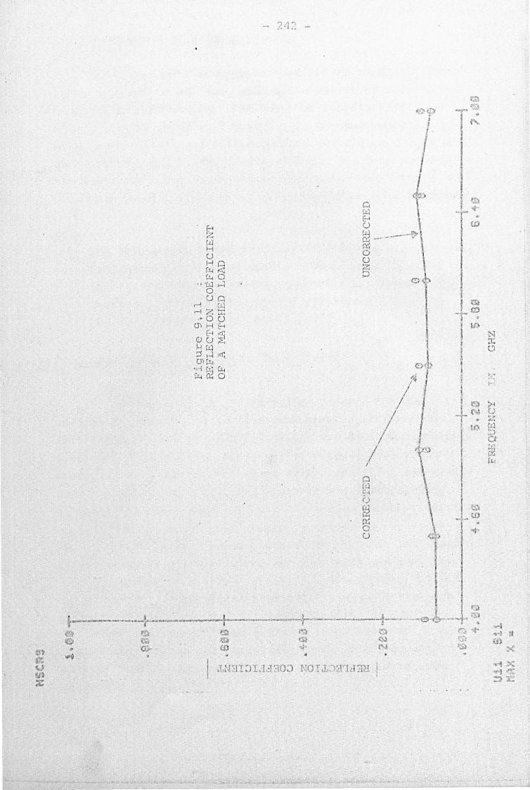
.I
~)~ . .g
'<" , ,'t I
/f / I
/ J
/ f
I
t . "r'~ I I
1'2
t IG _"- m i j
1 1.1)
• I
i
4- .3 f: I ~
J I ~., l- (.11 .
_._-' ______ -+_.-- ---]---.----1--........... I - -~.::. () Q T"\, ....
' •. :d
N :r: l':l
: ~~ 1 .... 1
~ () ~'" ,.., fit :::J 0 ;:.1' r.~ fLl
1 • 1 • ~
~

- 243 -
1'110 measurement results carried out on a short ci rcui t
using t'his mcthcd ar..d the calibration pieces of section 7: 4
is shO'liTn in figure 9.12. The table of results associated
vd th it can be found in figure 9.13. rrhe main differenct?
'bet\;'een this t2.blr~ Clnd that describ9d fo'!'- figr!re 9.7 is that , , 1 'b ~' f' an addl.tlonal set. of ca.,l. ral:'J.on 'l.gures 11ar:l been added to
the print out under the Reference Short Circuit Col1..unn. Th(~
corrected rC~8ults are particularly consist:.ent i<Ti th frequonc::y.
li0,.t;£ s
. 9: 4
. The information given in figure 9cl3 may be used in
conjunct.ion with the computer pr0gr2mrne of Appendix.
11 t 9 to calculate t.he ac1mi ttance of the l.ml-::nmm t2rm·
ination. The theoretical work for this calculation
has been referred to in section 5s6 •
To provide a means of comparison b(~tween the nC\'1
correction met:hods and an older and morE! established one ..
(reference 9.3 D.nd section 5:4.3), it ";{as d8Cit.:18d to ml=!anurc
a matched termination. The results of t.hese mCl1Emrcmcnts
are shOi\Tn in figure 9.14. Apart from a small ird. tial' cross
over, it can be seen that the Dhort/offset: short/sJ.idinS}
load and thG Three Short Clrcul. t Corre::tion }Iethod reGul ts
agree very ClosE;~ly. The .resul ts obtained by U)O Four
Evenly Spac(;d Sbort Circuits He thod and the Four 'I'8nninr.Ation/
Reference Short Circuit Met.hod 'it"e also very similar. It
might'be argued. that there is a slight discrepancy between
the former set (3 termination methods) (llJ.d the latt.er set
of measurement. BOlvever, it sl10uld bt:.! borne ~.n mind that
the former set assumes thC'.tt lossless linc?s arc used in t.11C
calibrations 1-thilst the .latter set taJ~cs line attenuation
into account, therefore identical results shoUld not be
e:xp(~ct.ed •

~ ... _ .. ' - ....• -•. - .~ .. ",,-.~ .... _". .. --}.--.-J!J lSI lSI -S!
UJ
- 7·:11:\ --
•
- -.,-.~ .. -.. - .. _. '-i" ~--'-'------1 ~ ... f~ I ': ~
N t ...-i I

, ........ \ -. , -'\
\
~IGtrro~ 9 . 1 3 CORRECTIONS OF A SHORT CIRCUIT US ING 4 TERMI NATIOl'JS & A RE F. SHORT CIRCUrr
r':.SC9
~-q: ()U t l~ CY C t. L! a~At leN 1 O!..P3i< ATIeN ? CAL l f)RJ..rlft hl 3 CA(.l BRAT leN 4 RE F . SH(}RT UNCR, DEvIC£ c,,!:: LINE' LE~.:Gi H
G~, Z AhPLT PH jI ~ E: Af"'PL l' PHA S( AMP L T FHA S£ AM PLT P H :' SE At-.P t. Y PHASS AI"YLT P «{.Sf :;r P[ RS l! E. GRrt:~
11 .000 .9 0 6 -1 !; 4,0 • 91 D. 1 t9 · 9 . . 91,1; . 2 3·3 . R 29 · 7 S - 3 . 93<1 1,3.3 . 937 lt3 , 5 • C 1 .Ii 7.75
1o .SCO s!Jl 1 &l6 0 -0 .. '3:04 87.3 .920 p 17· 7 . 8 ?C "12 4' .3 .9 33 25.3 . 936 2~) .. 3 .01 51;.2 7
5.000 . 9 ~7 ~ 171 .6 . 0.: 0 9 '5~ .9 .89.1 - 55 . 0 . 92 1 - l7!5·2 . 923 13.0 . 923 12.9 • C:) bO d O
5 .500 .9) 1 ! :')3 . 1 . _ os 11 31 fl ·,:) . . ~89 .. 98. 1 . 92 2 125 -7 .953 - 2.1 . 953 ... 2 .2 · 01 66. :Jj
... 000 . 9 J 1 !.:,.3 . 9 . 9 ~ 3 4 .6 .9 11 ·1~4 . 1 . ~~ s 7c.2 .937 .. ~7 . 8 . 9 ':'1 -17 . 8 · c :) "7 2 ·37
",:'(,0 .h98 !29 . 2 . 9 1 f D 21 .1 . 921 1 7 3 '.2 .9 17 -2 3 . 3 <9 0~ w32. 1 . 90 2 ~ 3 2.0 .G ~ 78 . 77
7,000 · !l 1 2 11 :> .? "C' '3 9 " 55.7 .913 137 . 1 , S :) 6 - 29 ,1 .885 -54 .2 .2 &11 .. Sit . ! . co 1' 3.69
FliEQUENCY i'EF CfEfS' RE F Ce E F" f"
Gt1Z REA L 11'110 :3 AM," , !:iB P;;~ S E VSIo:R
.:;, 000 -1 . 000 ~cOO 3 1. {)00 a. OO4 -1 79.8 :,#:,t1 ';f~OO .. 1·00'1 ,::>01 - 1 .004 . 0 32 179 . 9 ;!~I # ~~ '
'3,0 0,) toI IIIOCC .. co~ ! .000 ' - .·OO? 130 .0 tv~: ;f 'tS
5.5!)0 -. 999 .OO~ . • 5 S'9 ~. OC5 ·l ilO . a " tI~:fli
!,. coa .. 1· 00~ - .OCo 1 • co~ . q 36 ~1~ 0 .0 . ~.t: = iI:j j C
6.500 ". 999 "':tOO2 . ';)= 5 ~ .C08 -17 9 .9 : :Je,(JI: 7 . QOO .. . 9S9 ~.COl ;9.93 - .COO ",1 80 .0 '~H " .:Jl
N ~ l..'l
n ._

fI
I I
__ .06-J ~; I -",
~ ~ ~ u I H . (:t, i.l.! tIl o u I ~ J', o !;l .. 04-
G I ~,~ ;.-1 i r.r.. I ~ I
~ I
.... ~)(-;:-- CorreC"ciorl usina Short/Offset Short/Sliding Load
- -- -- Correction using 3 Short Circu its
- - 0 -(;; - Co=rection usir~g 4 evenly spaced short circuits
-- Correcti on usin9 4 " Open" terminations and a Reference Short
.1' - <> - 0 ~- ~-=-~~-------O --c -------.. - - -~ ! _ c"-'-:::--. ~ - <:> -0-0-0 - CI - 6 - 0-0 -0---=-0
", -C~ " ---- - - ---, ~- , -. . -- ------- -- - .----.-1----- _ ~ _- - ;. -;::.::,.: . - ;0< - ~ - ;;~ - X -~'--K _.}<'--X--?'-'_ -~ ~-,(, ~-(. J -----,i-Y - ,.. .
-f "::::" :; ::::. )( --
-. 02-4 .-.:.----f- 1-- -l !. ---;
5.0 5.2
Figu.re 9.14
5.4 5.5 5. 8 FP.EQiJEt.YC? I N SHZ
comparision of Corrections using Four Di fferent'. Methods for the measurement of t h e same termination(matched l oad).
6 . 0
.-..,.
N .j::. (J\
/

- 247 -
Ho.ny more set::::; of rr~flect.ior! coeffi c iE:."nt: measu rements
s i ng the 0 (:her correcti on b~chniques arl::. g i ven i.n a paper
( reference 9 . 1 ) publi s J.led by t .he a uthor. '1hi s publication
i s included in Appendix 12::3.
9 : 5 .-A~cur:.:.-:!~Y of Mea. sure!!!.§n·t_~ /
Seve:t"al 'Q)xthor s such as Hand ( reference 9.2), ],dams
( r e fe ren c e 9 . 3 and 9.4) Ridell~ ( r~ferences 9 .5 and 9.6 ) and
Woods (r2fer-ences 9.7 and 9.8 ) have irlvestiga ted the problems
ofaccur -:tcy in c omp u ·l::.et" cor):"ecl::.ed measarerr,e1.ts . Each a ut.ho r
h as placed part icul 3.r emph as :i.s on several errors . Hand ( Reference 9.2) ha s mad e a det~iled st.udy o f errors -with
p a rticula r reference to noi se , gain erro r and ·the particul a .. r
erro:cs in 1:he c a1. ibr-a·\: ion. standards on ·the He1v.1.et.t P ae:l;:ard
8542A system . '1'hi8 system is a transmi ,sien <;.nd r eflection
me asu. r :lng , yr3i:.em and i s not . dire c ·t J.. y applicC'..ble to the measur-·
ing system used here. However: some of his principles can b~
used .
Consider the ignal fl o ,I graph'J r; an idc<Jl ized rcflecto ···
meter syst .m ( f igure 9 . 15):
p=b a
~ iquy::~ ~J~
Flo~~haJ:"t 9f an Ideal:i. z~d RC;;:F1.§:;;.tC?..met~L
'r-'~
. . I , ~
01 11
It can easily be seen tllat f o r a di r ectl: connect d
calibration. piece ( p.. :-:: 0 )
c:.~
.:;. t I ... . 1

- 248 -
Consid :>2-:' n 1,1 t.he case when t here is gain e:-ror ( c.~ ) noise error ( E'n . ..- ) and r(~flection coet'f icient er.:.", r ( tr ) J
and u s:i n9 t .lL suff:Lx 1 to dellote the e:c.ro rG fo:(" equat.ion
9. 1, the r:el"T reflect i orJ. coeffi;:.~ient becomf~S :-
1& ., • , • c 1 ( \ :J. a I
For the ideal i zc:::d ca .. :,'e of an offset calibration pi f.?ce ~
it: can b e S2en [1:'om '\:.he flmv chnrt t "bat;
.0. I ~
" ,. .. .
and for the non-idealized case; 'taking gai.n, 11oise, reflection
coefficient errors and t.h~: addit.iona J. eJ:-rors of offset lengths
( E..2. ) equat.ion 9.2 becomes:-
9.2(a) .# ..
J t· • \;1,.(1 _.
Similal'."ly foJ:' the third calil;y:at:ion the idealized ca sp. 1.8 :
.. .. . 9.3
and foJ': the non--idea lized case it i",,:
I-
f: "" (I + t~?/l- 1\
" .. , ~ 9.3(0.)

- 2,49 --
case 1 8 :
1- ....... --: p .~ ,r'Y(\...f - 51 I +- ~")! '2.. :::'~.1 L.
----:---.,:,. .. _, -\ -- S 1.::>...l \..
\v11 icl-, "eSll] ts il)
f"L n ~
r~/)'i't,..- - ' - : t
f J 50 " . S··--~-~-1\-, .... ' . 2/, -r '-:; 12 ?.i·- \ t \ .... ':....l.
and for the non-idealize d case
! - ';,. ... ,'"""'I , ~.~ ' \.-
9 . 4
,y-hich results 1.n
\~: I ;::::. _L (r~~n_,:~_~._, :::: c: I'~. ___ , _____ . __
(/"5 '2.'4 P 11<t1~ C' (':> c..; q, ~., , ... 9 4 ( "' "\ • (;( J
-~E~tJ + '':::> [ h ;::,~ \ _.- ~ \\ -2'1.. -. ·;;;':l·:~ . .'=rr~Z!..
It is clear that the ide a l erro r sc-tcering pa~ameters
S11 ' 5 125 21 and 5 22 Will b e derived from equdtiODS 9 . 1, 9 . 2
and 9 . 3 . ( section 5:4). The non-idea.lizE'.u erro!;' scac·. l:ering
p a ramaters SIll , S12SZ1( and £22 / are c a lcul a ted from
equations 9 . 1(a) , 9 . 2( a ) and 9 . 3(a). Th e co:-nputer is noL
aW'are of t he idealized parameters . It can or:.ly sub s ti tute thE.! . d l' d l' '"' ISS I / r') I . . • non-J. ea lze .va. Ul? S, wi 1' 12'"21 1822' and <'- ', ln t o egu3t1on
9.4 to solve for the reflecti.on coef f ic::. Gnt. Thi.s \fi11 rw
doubt result in furt.her error, If ·-~II • • .. I L. ) 8 dc=f lne d a s tnt.
calculated erroneous reflection c02ff icir':l1t then eq'L<a'l..' on
9 . 4 ( a) may be written as
. .. . . " 9. -1(b)
'vhich :i.s real l y the calcul teu rl2['ult i-hen g< in, J'1.Oi se ,
calibration termination error and of fset errors are cons idecJd .
The problem is how to di stingui sh thl. calculated re .. u1 t ('-...., 1/
1-. ( calcu1a'l:ecJ. by equat.ion, 9.4(b)' from the ideal :'z2d one ,
r= A direct solution is not p ractica l be cause ccurtlte
lrnm<Ledqe of ' -he individua l e rror.J ar.e not }mnwn. Hand
( ref erencf.:! 9.2) ,,,ho hClR fun. acc(;!ss to th,~. manufa ct.t'~ rer's
data ha s point.ed out ·that: any att ~mp .. at a complHt 8XJ.Jli it
solution is ainU .. ess · s ince \vhilc t.;1 maximnrn mag n i ·UdE:.8 of
the variou.s terms may be .movn , t ·h.eir p h,; s(-!s arc i n gene.;:-a1 q1 i t.e

- 250 -
unpredictable. Hand al so tri(0d combining the r'undom-pha S8
errors ... .".i th the root of the sum of tile squares (F'J'lS) values
of <2mpli tt. ... des but finz.o.J.ly decided on a stat,istical me·thod of
analysis.
His statistical method i.nvolved ta"jdng t 'n .. • sets of
calibration measnrc'!I!lerlb3 (Hand does not e;peciiically stat.e
what '1"J1,' is but his released data seem3 to be baaed on 2 to
12 measurements). From thf~se calibrations, he calculated the
error parc::.met.e.cs. He then assigned magnitudes, {based on
production lir...e limits} to the error pc:.ra.meters. The phase . error limit '!,vas set bet'i-Teen 0 and 2lf radians and phar:.;p
"'\-ras selected by a computer driven random nUlr,ber generator.
Selected values of the device to be me2\sured "Jere then inserted
into his corn:!ctiol1 p"rogrammc. The l:'esul t,G obtained wer(~
then corcipared against his original input values and the
difference noted. Hand described 'his device to be measured
In his calculations 8 11 and 8 22 were made eq'tJ.Cll i~ phase
and magnitude [:0 that in effect there were 200 calculated
values of the £ame quant.ity compared.
Froi.'. these 200 values, 8 of the i,lorst values ,ITcre discard~~d,
" .. hich meant that· the remaining ;values had a pro::,abilj,ty of
192/200 or a 96% confidence level of being \dthin C1 certain
region V,'110se outer limit ' .... as determ:i.n(-::d by t.he 9th worst value.
Hand claims that this procedurt~ can be used to establish
the limiting curves for the syst~)m or for that rr.atter any
degree of confidence level.
Adams' paper (t'eferel1c(~ 9.3) is ext.remely useful in that
it does provid~= detaiied error infol.'111ation O!'l individual i terns
such as contact resistance, eccentricity of coaxial line,
connector mismatch Qrror , etc., Adamn also list.s some errors
on phase-loc1~c:d systems v.'h.1. ch do not. sec...~m to b(' available else
where.

- 251 .-
For reflection type n~ea tilJ.re~('.(;~nts, 1'1dar:lS claiI:m the
c"!oJ..culab-:d syster:: l..mcert:.~:inty to bc~;-
without a Phase T.oc:l< Source: ------•• -----~--- ...... -- .. ¥ --.. ---~-.~...-•• ~ ....
Magnitude of Uncertainty :-: ::[O·OC~.d-D.o \'5"P .4- 0-0\ p~.]
Nith a J?J).as~.1!2_C:~S.....:?S~~: Hagnitude of Uncert.;::d.nty == [email protected]'+ O.~a5p +O.OC?lpiJ
Angle ~f Uncertainty
where P ::.: \ T: \ and \S 11\« p
m .± \Q .25°+ J:c..;;J _~:..?' ~~ +- 4- ~~I (0 .cC)5'f~ p
in th(? e~JL'tat:ions rCl(~t:ing to angle error.
It is not }cnmvn .to which E'YB.t-ern the ab9ve J;-igurcs apply.
Adams does not give t.h2 informa.t.icn and ned ther does be
indicate clearly as t.o how tlv::s('! fi.gures w'ere deduced or
obt.ained:
Ridella (references 9.5 o.nd 9.6) in addit:ion t.o having
given some equat.ions (deriva.ti.ons not 8hm'ln) for the calibration
.repeat.ibility, the meas'..l!'cment .t:epcat{bility etc., h.as
reported the res1.l1 ts obtai. ned '\'lhen various devices "i,ren:! mcas1.1rc:"!d
on four d:i.fferent networJ;;: ana1.ysers. HO'w'ever, rddel1 a l:'E.ports
that the error expressi.ons which he h("!s arrived at differ ~
I
considernbly· from those of Adams (reff:~rencc 9.3). He also
points out that the error curves issued by Hr;!1·tl!?t:t Packard , d ' ~, J •
hav~~ been. mo 1.1.. J;ec.l. very often over tl1~~ ycaxs. 'flus 'h'c:l.S also . . noted by 'Lhe {'..athor when irlVest.igating ha.rdi,rare data in
chapter 4 (section 4: 3) •
Woods (references 9.7 and 9,8) notes that the calibration
procE-!durc describ~d by Hand (n~ferenc0 9.2) overlooJ~s ·the small
impedance changes t.hat occur whr:m the reflection/tr:ansnd.ssion
swi tchcs are changed over 2.nd Woods h3S suggest.ed tJH~ tlSC~ of
t.hree receiving channels :instead of t.he prcs(;;l1tbJo to over
come this. Fortunately this probl(~m doE.!s not exist in the
m(-~a8\,tremcnt. system u.sed by the author becc:usc only reflection
measurement is c:o!1.sid8rcd here.

that:
.- 252 _.
Nevert:helE":!:3r;, from t.he above p3:-()graphs, it. is cleal'
(a) Different opinions exist as to ho'''' the ()ccura~~
of an automatic net1.lork analyser should be
E:pecified.
,(b) Detailed information on the errors of ir~dividual
items are virtually unobtainr.;'}.)le.
The pd me purp0f.je is to Df.;! able to determine the trnc
reflection coefficient of a device and to be able to predict
the accuracy of the measurement ': and its confidence level.
Indi vidual errors exi st.ing '\vi thin the instruments are accepted
and efforts to correct them will not be made for the re-deidcrn J
of the instruments is not intended here. However, it is vitally
important that the bilincox tr.ansformation corr,plex. constan't:1,
A, B, C and D (representing in.:struemeri.t system (~l.·rors) n~main
invariant during all thc"'meaourements, this has been
discussed e~tcnsivclY in section 812.1.
In the ·case of correction systenu; using short arid/or
open circuits, many of the s'Jurces of errors mentioned in
sectibn 0: 2 sur.h, as (b) to (h) are minimized because: •
(a) The reflected or test signal is larcJc ( 1 r\ ~ 1. ) during calibration and tends to mas]" the effects
f . • f" l' .• o no~se, leakage, non-J.n~nJ.te (l.rectlvlty etc.
(b) rl'h8 magnitude of t.he reflect.ed signal E remain
at similar levels t.hrougbout t.be calibration
procedure and the ~mrl:ing dynamic rlln90 of the
amplifiers, det.ector.s etc is redt1Ced. This
reduct.i on i ~3 even lriore evident. ",-[wn tho devl ce
to be measured also has a largo reflection . . l ' ,.. .. coeffJ.c].cnt. 'I'le rnJ.n~nusat~on of non-ll_n(2arl. ty
and limi t,ing prol?18!l!8 hetve; nlso been discussed
in detail in section 8s3.

- 253 -
Confirlnat:iol'l of measu.rC:~:·J.tl.i?!1t aCCllr~ac.~y (~a_rl ])e Ifh'JrG ea~sil~{
ascertained if SOTne acc'tll'"dt(::ly defin,;d calibration standurds ,
traceable:! to Nat ionaJ. Standards cu:-e Clva.ilab10 for comparati VI:?
measurements. Ri.d2l1a (rcfercnces9.5 and 9.6) was particularly
fortunate in this respect for he had access to the tlS~ of four
different netwprl;: ancl.lyf~ers in differc~nt coantries and Ol:e of
t.hesE'~ analysers (HevJlett P c.c1\:.ard. in Gcnl~va) ,,;as traceable to
a National Standards T...abor?'to.ry. For tbe \,'01:'J<:: at Harv.'icl( ... ., 1" d' t . . Dnl verSl ty, such flnanCl.a. cxpen.1" ',ure \-las l.rnpractlcal and
considerable effort had to be made into acquiring SOJn2
·accura~ely defined st.andarcs. To b(=gin vit.h the use of
existing "standards" ,.,ithin ·the laboratorie::; of the University
of Nan1icl~ were lmpractical for a.l though some of the match,~d
~oads and offset short circuit:s had been. calibra·ted at 01:'8
tin1f~, there wa.s no assurance that the calibration values were
still valid.
Ideas introduced by l'1oodf~ (reference 9.9) for the const,ruct
ion of lmmittance standards were also inv<?Bt.igtltcd but <lfter
(~xami.nation of his equipment and s(~.;Jdng ll.:i.s advice, it w,'-;.s
decided that the fin~ncial costs would be prohib:i.tiv~.
'1'he construction of test pieces whose el(~ct.rical !
properties can be '-Jell deflnp.d has bl"'.2t1 suggcst:cd by H;llncr
(reference 9.10) as a me:lns of c'l1.ecking the correct o!,!cration
of a net'\wrlc analyser system. 1"1'11is idea was seri.ously
considered and J cd to t~he adoption of a modified EC\vlctt
Packard ;'PC7 Coa.x:i.al Short Circuit. (Type 11555A) as the main
measurement standard.
The main constructional features of 'this short circuit
have been described in Chapter VII and d~tailed in figure
7.2.

- 254 -
From an inspection of figure 7.2, it: is clear that the
electri.cal contact. n:quired for a good short circuit is
dependeDt on the mnt.act area and conductivity of Surface A.
This surface was eXnmined more closely after dismantling
the entire short cireui t assembly. Af-tor Surface A had been
cleaned and poli sl'led it 'vlaS checked for surface roughness on
the Tallysurf machine. The sU4"face irregularities were
less than O.002rrun. 'I'his su:r.face was then re-clC.:'!aned ,again.
Visual ins;>ccticn of the surface revealed sufficient gold
plating on tl-le short circuit surface!. Ha.d this not. been so,
then re-plating would have been carried out.
rl'he advant.ages of using such a device as thr-.! main
calibration standard are:-
., .. . 1 ( a) The f ~nanc~ al co st \~ m~nl_:r.1a •
(b) The reflection coefficient can be accurately
defined without expensive recourse to
calibration laboratories.
(c) 'l'he APC-7 on the short ci.rcuit ensures minimal
interface problems w'ith its mating connector on
the reflectometer.
The general procedure udop~·.cd for assessing tlJe accuracy
of mea surement '<Tas that of repeating rna:1Y Gets of mcasllre:nents.
For example, in corr(~cted measurements involving the Three
Short circui.t Correct.ion Nethod of Section 5:4, one hundred
sets of measurement:s of the same t(n~t piece was carried out.
Each set of n~easurements involved:
(a) Rcpec.ting the m:r.1C ca.Ii bration procedure at
,the same frequency of interest using the same
co.l ibro.tion st?ndards.
(b) Heasurirlq the same t.est piec(~ after calibrating_
(c) Calclllating the correct' reflection cocffic~entG.

The fonnul;)c!' of ClDpendix J.1: 10 '\-[C1-(' used to calc'..llatc the . ~
r('lc;:~n value and to predict:. from tables t.he expectea dcviationr:;
fr.om the mean a·t the requirecl confidence le"/(;'18. 'r}le resu:!..ts
obtain(~d from statist.ical tables werE~ then compar-ed against.
the known reflect.ion coefficien·t of t.1H·) tE?st pieces -to shm..;·
the f~rror of mea8urenH~nt.
For this a.ssesslL1c.:mt, one-hundred sets of measurement.s
(calibration and test piece ev<:t.luation) 'w(,~re carried cut. 'rhc-?
test piece used was t.he modified Hewlett. P acl<::ard Short Circuit
described in section 9: 6.1 ~ ,]~he networ};: analys'2.r and i t:s
per iphE:.~ral instruments (excluding the computer) "yere s,';ri tched
on for two hours prior to t:he conmlcncement. of mc~s'-lrements.
The 1st and 2nd off Get short circuits used in the calibrations
had off set lengths of 3nun and 4. 6rmn respectively. '1'he
calibration a.nd test pieces were f.~pray cleaned after every ten
sets of readings.
The measurements were carried out at 4Gllz without the use
of the phase locJc system. Heasurements 'vere car):ied out I
continuously ar,ld required a]ntt 8 hours of comput.er tif\1c. To
avoid prejudicing the results, shown in figure 9.16 J no
measurement. 'vas discarded. This has r2r:mltcd ~.n some particularly
bad sets of lnP':l.F'!llrE;~mel1t.s e. g., set 32, v.'h(~re t.11G corrE~cted . . . reflectiOll coefficient. was calculated to be 0.975 [1J}}. 0 ~ Analysis carried out later af'ter e~amir-d.nq tbe cOlilL')uter pdnt
out revealed the .third calibration reading to be a't faul t.
The reoul ts in figure 9.16 ,,,ere processed by ma)<;:ing tho
assumption that the magnitude and phase angles measured for
large reflectipl1. coefficient a!'e indepenc:ent events. '1'his has
already been jtlst.:i.fi(~d by the ar9'\.J.(~m(?nt.s of. section 8.1.
Nex't:, the magnitudes and phase n.ngles (figures 9.17 a.~Ald 9.18)
were plotted and it. vms observed that:. the distribution "r;:U3
close to the normal (:!rror CU1-ve. By using equations 11.10.1,
11.10.3 and 11.10.5, t;he mean and the best estimat.e of the

~ -~,.- --
Figure 9.16
Table of 100 Corrected Reflec tion Coefficient Measur ements Taken at 4 GHz
I .. w---~~~-~ . Ico~rected 1~1 Corrected 'I )corrected 'I ICorrected
Ref1ect.ion i "Reflection I I Reflection I IReflection No.~oefficient t ,No,!coefficient Nq coefficientl . No. Coefficient I
'}.fagni- ?haS8! t IMagn-'Phase ' 1 ~'lagniIPh2, seJ.I· ~ hrc:g l1i-tpha. se I
r:-~1tgde De) it ,tude (Dec) ' tude Dea~ I It'.ld~~3LJ 1 1 .998 ,180.0} . 26\ . 9951 80 .1 '1 511.003 179.l9 1: 7611.0011179.3 i 2!l.OOO p 79.8 1 2711 . 002 180 . 01 52.! .993 17S, 8 1 7 7 1.002 1 180. 0' 3 !1.003 179.8 1 28 1 . 996 179 . 4 53 1.001 180.0 7811.000 179.9 41 .?93~81.529! . ~~2 18~.~ 1 1 ~4 1.OOll. ~80. 41 . :911.0~4 ~80.2 5
11 .004 .1.80.5 , 3° 1 • ..,/ 4 18.l.7i . :>5. .9981179.0 1~'-' 0 1 . 9':18 .l79.2
6 .994 180 . 3 If 31 t l . 002 179.3 156 , .9961181.1, 1 81 .9981 80 . 1 7 /
1 0999 .. 180.11"32; . . 975/ 1 33 .0 , J57!1 . 009
1180 . 4
1!82 J1.003 180 . .. ·3
8 1.0091178 . 8 133 1 . 995[180.3 ! 5S' . 998 180.5 , 83 1 .994 ,180 . 7 91 09931180.8 lt 34 !1 .001 180 . 3 1 ! 59 . 998 ~~0 . 2 11 84 1.OO~ ~29 . 7
10 i l.008 178.9 35i . 9951180 . 7 '160 . 999 1!9 .7 ; 85;1.003 i/9.6 II I . 997
1
179.8 1361100001180 . 81,611 1.009 180 . 7 , 86\1;009 ]80.1 121 .997 179 .9 37 1000411 79.8 1162 . 979 181 . 6 ; 87j .991 , 181 . 5 13 ; 1. 001 19~.0 138 1 . 9951180 .7 1! 63 .991 180.71 88 11. 0081181 05 14 1 . 9961180.4 >39
1
. 997 :1~ 1.0. 64 ,999 179,8 1 89!1 . 0001:!.80.2 15 , .996!18D.l 40 . 997 ! 180 . 8 i 165 .996 1179.81 90' . 998,1180 . 1 16 1 ,996 180 . 7.41 .9961180.9 1166, 1.0121179 .2, , 91 1.007 , 179 .9 17 : . 9991179 . 8!,42, , 998,180.41167 . 995 180.9 1t 92 1.004\ 180.3 . 1.8 11.0041180.1 143 , .997/180.21 168 .999 ~!.79.1 1 19 3 .9921181.7. ; -9 11 . 0071179,7 1"44 11 . 00511P.;0 . . Il 59 1 . 0 00 180. 2119.4
1 ,999 1 80.1 I'
20 , . 994f180.7 4511 . 004 1 80 .J.f 70 1.006 180 . 811951 . 997 180.5 21 t' .991·179 . 1 . 45!, . 996!1 81 . :)J 71 ,999 179 . B 196 . • 997 ,1 80.5 22 , 1 .004 180 . 4:147 1.005 \ 179.61 72 ! .992 l79 .5 197i .999 1180.4 1 23 11.003 181 . 0I i 4 8 r'1.00sI180 .0 1 7311.003 11 8 0 . 4 98 11 ,005 1180.4 I 24 \ .999 · 180. 4!~49 . • 9841183 .8 1'41 . 997 179.9} 99, . 994/180 . 7 i 25 ! 1.oooh {~o.0 50!1.005 ; 180 .'4 i75 __ ~98!180.1ll~L~.~O_5~?/'9 .0 J
~ .
N U1 G

• I .-l j'
C- I
U rz:l 1-1 , I-t4 I' : P.' , • -- - i ~ d •
• l. _
I-
0, • I
-j

- 6 :..:... , o
I
~ '.-ci t :z W :
.::::>.- 4 -' 0 -
, .. J.;: _ •. . I I
--I . I i .. ;
. _.L~~
. ..J ,180 1-- .-
180 . 5 !
PP.r.ASE_ O~~rFI:!~Ct:IOl'·~ COEFFICI£:NT _
.\ , .. I .~.,r.........- ...
.1 L_ '
j
" 1~1 !.
J -1-' -, r (DEG,?-EES)
i .\
_. ·-1 182 1 82 . 5
1 '
.,

Fi gu.re 9 .19
Rene ction. Coefficient Resu! ts 'vi th Confidence Levels for Measurements on a Shor-t Circuit (based on 100 Neasurems!}-ts Using tIle Three Short-=Circuit Correction Hethod)
.. ...... :z:;::::::a;::;a::iI;;::z ,",~_==-:::"",!C.~~"=,, ____ ~~~...cr~""'~ :a::; 2..... L.a:a:t S!5SC;t .. SL::a!lLllHLs:w::sr:uu:::a:itizt£&1a:::JL..~"'~1
~ Reflection Coefficient at 4 GHz
Item
.; !:i ~~
~
~ Nagnitude ~ Phase r¥WJ%Z &1:ae.z~~~""! ===.~ :::::zcc:a::::::~· ' ....... ---h -~~"""-""'-!!II'.n::::.~~~~..I':'f! ... ' f' . ~ ~ f)
~ True Reflec~lon Coef lC1.ent. ~ 1 . OGO ~ 1800 ~ i of Test Devlce ~ , J E - ~ i
!::::L I Hean of 100 Hec.. surement.s
Best Estimate of Standard Deviation '
0.99884 0 . 999 180 .290
-- -','------=---, ~ 6.6038 E -3
r-- * ~~. ----------------.------~----------"Expected Range for 90% ; . 9988 ::: .0109 i.e.
Confidence Level ~ 1.010 (Max) or + 1.0% 0.988 tHin ) 1.2%
I • !'i ft
0.780°
.... 180.29 .
181. 57 (Max) l ~ Q OC' ' l ' ~ ) / J • I \ ·l..Ln
1.287 1 . 8 . or ~ 8 7:7~
.- ,55%
·i ~ i ~
~ !,
~ } }----- --.
E:Arpect.ed Range*for 95% Confidence ~evel
Expected Range''< for 99:b Confidence Level
.9988 :: 1 . 012 (Hax)
.986 (I'·lin)
.J,.
.9988 .: 1 01(:' ( -') _ . _ 0 Hax
. 982 (Hin)
.0129 i.e. or + 1.2%
- 1. 410
.0170 i.e. or + ],. 6?-b
- 1. 8~;
, '1
tt ~
180.29 .: 181 . 31 (Max ) 178.76 (Min)
.J,.
1 00.29 .: 182.30 (Nax) 178.28 (Hin)
1 .. 52 '3 i . e. or + 1.00%
6G~1 ~ ~ ,o
2.013 or + 1.28~
- 0.95%
J !
~ ~ c ~
~:J2"..::=c~~=:o:eJ.P;sa:s:aag, 4i)!;s:::pt •. ~~~~.r::.~(.;;;J~# ~~~":!.~:'~.':''''N.~~'""'-.. ", ...... 1tT'''...r.~.t\I:~'l..''"k!D"''~~.:a'; I
*Calculated by mea~s of statistical table (Taple 1 of Rcier8nce 3 in Appendix 1113) 11 yercentagE' l:'tlnges are rE~l ati ve to 1 U_~Q~
~v Ul '-0

" .
- 260 -
standard deviati on "la s --:alcuLJ.t.ed. These v a lues we rE:! then
u sed in co ljunction I,ri th T,3bl _ 1 of J:<efen:mce :3 o f Appendix
11: 10 to p~oduce the table ~lown in figur~ 9 . 19. Fr om thi s .1-
·t ablf:~ it i s seen that me :::l SU!-E'me nt Clccur clcy to "\d.thin -~1. 4X
with a 95% confidence level c an be obtaine d , tor a 99%
1 eve J 1 accuracy toO .: 1.. 8%' i s attain abl e .
9:7 . 1 . 2 Measured Accur:cies of the Means -----.- .. --~-... . - -.-- ---.. -.-.. - .-~ .. ---.-------...
'I'he mearmred accuracies of the means of the r agni t ude
and ph ase are of courSE:! bette r ·l:han t bese value£ . Using
equations 11 .1 0.9 and 11.10.10 of Appendix 1 1 :1, i . e .
X = V -'.> 1", (y\.1 .:. -'S fYV
the f ol l owing tacle Cf igure 9 .1 9 ( a ) ) may be construct:ed.
Fj:..9~~~9Q .
Accu ra"y of tll.e Mei:ln Measu1:'emellts --Obtainesl t rom F igure 9 .. 19
C f ' d Mea sured Means ll OO He asurementsl tori ~ erlce ~~,. '"' :: .. _ ______ ~-""==l;:.- ,.;"':"'_~~_.-__ n)O~.~
Level ~1aqn ' t.Ud C?:·k f11a£.g* ( de~re('l s) - ~",:iIIWk;,.""",~~ -- ~-
·' (Max) or -- .01..% lBQ,4J.9 ( Max) or ;- . i3 3'Y~ 90o~ .
1< . 997'7 = (Min) - 2 .: · % 180. 161 (}Ilin) +. ,0901. " ., ~ :0 ---r 99993
----------~.
1.0001 ( Hax) or ;-.0 131<- 180". 443 Hax ) or -1-. 246)~ 95% , . "
j.997 5;5 (Min) (Min ) +.O76~ - , , --- _ .. .....-- ........ _ ... _ ... _---_ .... _ . __ ._-
1. 0005 (Hax ) or + .05 % ·80. 491 (Max.) 01:- 1· . 273'1, 9 9°6 I ,
- . 29 .. % l80.0B9 (Min) ,·.049('; , r~J} l~l .• J~2:!!.~ ~~ ...., ...-
1:Referred to 1 Llf~OO
From figur _ 9 • . 19a, i t is seen ·t.ha ·t ,[:,he mean.~ )f i:he
magni tude aad phase angles of the test pie ~e ( reference rme rt. , ') C l.J:CU t t 48Hz haVe J een measu red with i:l co fiden.ce l::>vel
o f 99% t: o vTi t:h: n O .~;G of· the t ru _ val ue .

- 261 -
'l'he proc,:::duH~ used for determining tlH'~ 2ccuracy cf the
4 Short Cireui t Correction Hethod 'V(~s similar to that: card (10
O'.lt for the Three Short Cireui t System (section 9: 7.1) excC':)t
that 20 meas1J.rer0.cnts per frequency were carried out. The
resu1 ts obtained at 4 GHz are sho'l\T!1 in figures 9.20 nnd 9.21
respectively. For this nurnber of l'.leasurements, t.he application
of statistica.l theory is vo.lid only who11 tht! me3Sl::.remcnL is a
stationary sta.i..:i.stieal process i, e. 1 i::he repeated resul t.s arc
consistent. 'J:'he test used to d2terminE'~ this i.s similar to
t.h3t descrl.bed by Harner. (refererlce 9.10). Por th:i. s test,
the 20 corrected mr:!<1suren:ents of figure 9. 20'i\Tcre dividc!d into -b:lO groups of 10 each. The mean valu£~f.i, A.. , , and '):.,?, and
the variances d,2. and oJ; of the magni tudf-~s of each group ""as
calculated. 'I'he variances were then um)d in the Snedcor' 8
F Test (Variance Ratio rr(~st) which j s defined a e" ... -:.. .
. Greater Estim:3te of the Variance o[ on8 Hea~mrem(.;j·lt. Group F = ------------------------------ -------_ .. --
Lesser Estimate of the V<lriance of Othpr. H~asun?'IlJent. GrOl~p
From table 6 of reference 11:10.3, it \las noted tha.t. for
'Il.. -- 10, and for the vC'.riance td be consid(.;!r.ed stc-:'adi tb:m
F b 3.13 (5% leV(~l of varic:,nce ratio). ", .f II
The means, :::(.,and :(.2.. were also tested using t.he \ I
student . t tests i. e,
Error in He;:m t = ,---.. -- .
standard Error of Nean j 0', '2.
For a 5% probability curve t L 2.1. This informatioll
'vas obtained from tClble 4 of reference 3 of Appendix lIt 10.

5 6 7 8 9
10
- 262 -
F t9.~~LQ_2,_.?_q
Corrected ReflAct0~ Coefficients obtained at." -4 c;Tiz"'u Eli 11(-;-:t}:~(?·-f. ou r '-f;lj t) rt-r;-{"r.ctij t ---corre~CiorL 1'f~~11C,d'-of. sr.!.~:.tLCi:2_2 ;'5"-"-----
F iru:u:g_9~J . .90r.r.:.~~1ion .... Re..fl.£ctj. on....Cq,~ffis.i cEt.:'i Oht~dr~ed ll.i.6 GHz~~g th~~ Fou.r ShoFt Cj.r£:..iJc CorrectJ.on Method of Sect.ion 5: 5 .-._ .... -.--.... ------ . --------;;.,.,
I

- 263 -
The 8a11I.0 procedure was adopted for pl'ocessing tlH::
measurements on phase.
The follOl{ing table vras produo?d~
r----I'~~-~~~~P.M'=-~~~~~~.;;_'-~r----~.=~ ... ~~~:::"--.''"-='~~''''1' I (4 Short Cl.rcul. t -------- . __ ._-,
·;:ti;-;::~~t;;'''"r·~~~;'-- --;~-""I'-~~~~~: r-;~~---l . I 1" -;e"an Test (t)---;'-:;~;---I .2.1 --r O. 99. ---;~ .... -, I....,..,... ....... _,., .... _., ..... ~,~, __ .~~ .... _._,_ .. ,_, __ ....... _."""".~_.~ ... < ..... _.,....-.. , •• - ... - ..... -,.~,. ,,,_J
. .
From these results, it is seen t.llat. the I:lCi:lSun."'ment data.
is of a stationary statistical nature~ Hence thf-~ UBe of
t.,.,(;~nt_y rn~asurernents is justified.
The analyses for these rJ(~asurementsare given in figures
9.22 and 9.23. It should be noted th::.t the correction fer s!1~aJ.l
samples (20 measurements) have been mad~~ t,o th9 statistic:)l
data.
For the 4 GHz set of measur.ement.s; it is S2(~n tha.t
m~asurf~rrent Clccur~cies of about + 1% with a confidence J.c~vel of 95% can be achieved with one riH?asurCm(::!nt.
Similar results have ~lso b~en obtained for.tl18 set of
meaE\UrCments carried out at 6 GHz.

~
.. KisLure 9.22
Ar.alysis of Results obtained in Fiqure 9.20
(Fo1:r Sbor-t Circuit correction Heti-:od)
rJlJJl:ilCCi(;OSiW ...... :iJ!UQ!_a'~~xa,.,!C!::szz::a:a:a::u::!!lSi-.. L ••• ''';J:--J~..;.iirr.r!C;';~CtS ssw. OlI<L&llfli:!ii't..~ ..... X"". .... ... au .................... SA!I ..... iiN :_ ~,Jd .. wss:s .. A_ ..... __ ., %&A&4L.= we_.B. :z:s:s: ",:oa"Ci_~
I i ~ , • • ••• ~ ,..,! ij
< • ~ HeflectlOn Coef-F1C).en-:: at... 4 GLZ • ~ I --~ ~ I te;n r"'-- .... "r"'--- _. .... - L • _.--_ ... - ·'i ! . I ~ Maqnl tude' i pr;:3.se (dearees) ~ ~_k._!1$1"""_""_ _·m::u:>>>>JONP"*,,_a ...... "" at '~-- .. ""'""_.. __ -;.. _ __...""1_'_'_". __ , 'i""oas"".=-_ .... ,., _== ..... _.~ ',..., ~ fl t . C ff .. I i « I ~rue rle eC,lcn oe lClent ~ 1 000 I 1800 ~ I of Test DeVlce ~ '.. j <-- < ~ ..1 I Nean of 20 Neasurements 0.99825. ! 180.2 j I J ~ . . r ~ I Best Estlmate of Standard g , Deviation 0.0053693 , 0.72475 !
1 i i , i ~
.• 99825:t 9.23519 E-3 i.e"j' 180.2 :::: 1.24657 i.e., I Expected Range*for 90'10 Confidence Level 1.007 (Max) or + O. 77~ . 181.45 (}fax) or + O.SO;.~ '.'.i
O 089 ' "1' ) 1 1°' ~ ~ 8 Q 5 ( '-'1 • ) 0 5 8"" ~ ~ • ~. \ J. J.n -. 70 1 / ..... r. ln • I£' 1
I ......! . .I. il -, t dR' + qr:;-I 00825 "1 1~7'8 r.' ~ lCO ~" 1 51"72 ' r:.xpec e ange')l' ..:or _..J~;O .J"- -. L._ .... ."j-E., ~ v' • .<. - 0_ <± ~.e.,
Confidence Level 1.009 (Nax) or + 0.9% ~ 181.71 (Hax) or + 0.95% t I O. 987 (Mi~) - 1.1% i 178.68 (Min) 0.73% ; r- . J
I Expected Range*for 99% .99825:t 1.53025 E-2 '130.2 :t 2.06553' i.e., ~ i Confidence Level 1.013 (Max) or + 1 .. 3% ~ 182.26 (Nax) or ". 1.257& : L_ z_ .. go 0.932 (r:in) 1_08% _t ,"1:~13 (~~ __ j*,':":~
1t Calcula·ted by means of statistical tables (Table 4 or Reference 3 in Appendix 11: 3) • All percentage fi~Jures are relative to 1 li§..O°.,
N VI ~
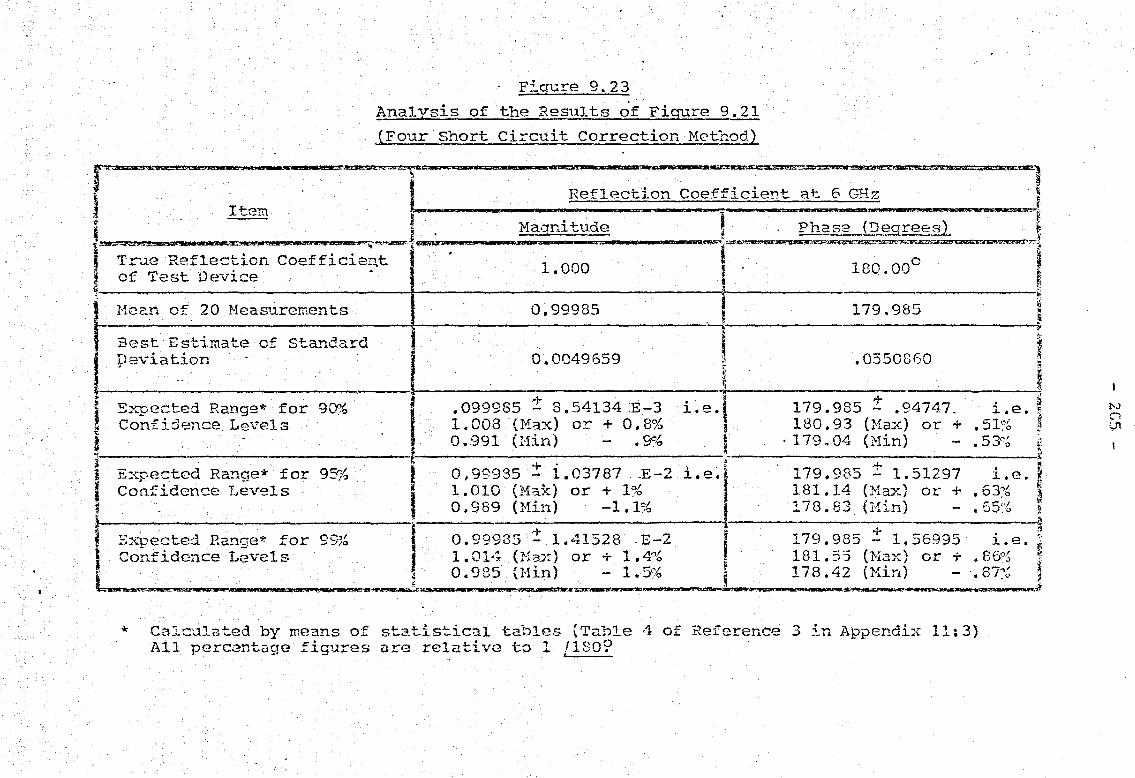
F';gure 9.23
AnalYsis of the Results of Figure 9.21
(Four Short Circuit correction Method)
r .... >::aJIia&JSitL.JlKecs:e::s:ua>JkLiS .. J(Q .. ~..... • !.zatL:»i!U2J! ..... __ .,.c=:.w:o:w;::..... ..waat::a1i:sa&L !JMczar • JIIJa:::e ... nA::c:::a;;::a;;JiJSt.:.-."':::O:x:z::;_ •. 1JSEa!DM1a:a:au::ceu:t::1l!WJ~~
i .' Reflection Coefficient at 6 GHz i r
Item I ~~ i i . tlagnitl~ ~ '. '. Phase (Deq~-ees) J
1S8Z;;~~_;;;,;:;;'i~~a;=;~~ci:;;=-"-~ . · ,- · .. ·"la
000 -- d ·--r-=-sr-~::~~~i . of Test Dev1ce . ' 1 . • g ~ ,~
Hec:.n of 20 Neasurements 0.99985 I 179. 985 ~ ~------------------------------------~~--------------------------------~~ ~
Best Estimate cf Standard p2viation 0.0049659
~ ~
I .0550860 i ! i
f--_ ~ .~ 1 Expec;ted Range* for 90% .099985 ! 8.54134 :B-3 i.e.1 179.985 t .94747, i.e. ~ l; Conf1dence Levels 1.008 (Ma.x) or + 0.8% I 180.93 (Max) or + • 51~~ ~ i 0.991 (llin) • ge,6 , 179.04 (}lin) • 5Jc~ ~ i ~ ,t-' t + - ~ • Expected Ra!1ge* for 95% I 0.99935 - 1.03787.E-2 i.e'l 179.985 - 1.51297 1.e. ~ I Confidence Levels I 1.010 (Max) or + 1% 181.14 (Max) or + • 63:'{, S ~ O. 989 (Hin) -1.1% 1.78.83 (Hin) • 65:'s ~ ira I E~-pected Range* for 99% I 0.99935 '! 1.41528 E-2 I 179.985 .! 1.56995 i.e. ~ I Confidence Levels 1.014 (:';3X) or + 1.4"'0 ~ 181.5'5 (Nax) or -;- • 86"~ ~
L.~4'_& ___ ._"_ __'@ __ .""' .. 44 .. ~L' .. _O·",~'::'::, .. {:~a~_~M::~'''_''R:'?:~~~.u: ... :: ':~'::idJ * CalC'<.llated by means of sta.tistical tables {Table 4 of Reference 3 in Appendix 11; 3)
All percentage figures are relative to 1 f1SO?
t-.} c~
Vl

- 266 -
If the proc,2'Iure outlined in section 9: 7.1.2 is adopted
the following to.bles (figures 9. 22a and 9. 23a) resul b
Ficmre 9. 22C"t !-qcuracy. of_ t;h? Hean l'1§~i~:~;ire13~<?I!~t._9b.L_<ainf~Sl. f.!qr~FiquJ;"Q...~z. ~ ....... ~~_~ __ ,."jI';\'~~"'MIX __ .~·I"'· •• $M •• *I,_""·JI;'''''':'f*lodftI'a..;: ..... .!Ir.~, ...... ~~'~'.'>('.""""~. __ ""'"""'IIIIt'UI~"'~M"-r.o-__ ;:. .... ,.. u-l
• l ~~1eaf>ur~,g Means J20 }f~:il§~Iel!!~ts) .£Qnfl~~ce ____ _
Lpill . t d ---..,- . - ----~ HCAgP:f.. .... l1.. . ..?!.. Pha 8(;*.
~~~-...-, ..... ~ .~~."."rn.----..r1'>."1'I'~1l.~'IIr"""'Q'-.""I .... _ bi"iL:t;:.Il\o;~ ..... ~......-.-.~~_,.-.. '¥ ___ I'MlllIiIlr'l.
90% 1.0003 (Hax.) or of- .03';6 180.478 (Max) or + • 2 6n~ .• 9962 CHin) .38% 179.92.1 (Hin) .04"{'
I-----------~------------
From Figure 9. 22'a, it: is SE:~en that the means of the
magnitude and phase angle of the test piece (reference short
circui t) at 4 GlI:;.; have be(~n obtained with a confidence l(~vel
of 99% to "Ti,thin O. 5?~ und 0.2% respectively of the tnw value •
95% 1.002 0.997
• (l.lax) or + CHin
"Cl/ • ", .. 0
• 3:'~ 180.24 (Ha:x) or + 179.73 (}fin)
1.003 (Hax) +.3% 180.34 (Hen:) or + 0.9966 (Hin) .4(\~ 179.63 (Min)
.13)~
• 15"':'
.18%
.21"; ___ " .... ____ '1iJ;.t'~A~.~~ .. ~~J!t!~t;u_~~;>O_, __ I ____ .... _......,.,NI$IIit:: ................
Referenced to 1 Llf300
From figure 9.23u , it is seen 'th;;t the 111eans of the
TIlr'>.gn:l tudE~ and the phase an91e of the t(!st pi.(~<.:e (refer(~nce short:
circuit) at 6'3Hz IleNe beC!1 cbt<li11(~d ",ith a confidence level
of 99~b to within 0.£):10 and O.2ob rr~sppc'tiVt:ly of the true value.

- 267 -
9 : 7 • 3 l~ ccurc:.sLQ.f...l~.~a§u.ry-m~l}_~:Js._ .. 1~~si:.~th~L~. __ IT_111-~novrn 'l'ermina·tions and. ;:0, HE'fC'n::~ncc: Short. Cix-cait Co-rr,....c·t·~cn ~.f(.."t·~J-:-10··..:l of C;;:c··:-:t·--';on 5:-:-;;--~'~~-h~\-C-n!"r1.'tpr ....:::- c .. ~t.. J J.!~:::"-=.:_~_>:':"._-l' \..):"- . .1... - .. ..:._~_~~l..:..;~~~_"- .. # l., __ ~r::::'-:'
p rogsa!'llI!~_Qf !:i.0ctJ-gD: 6:~
Twent:y sets of calibrations (4 opcn' cireui ts a!ld 1 refer
ence short) 'Kcre used for this met:hod. The results of the
measurements obtained are shown in figures 9.24 and 9.25. The
tests mentioned in section 9:7.2 to determine the validity of
the stati stical data at 4 eH:.? yielded the follo\dng results:
From the above -table, it was decided that: Cl statistical
treatment of the data "laS valid.
Tl 1 f t 'h t"...· ~"f 1e ana yses or -_.lese measuremE:~n s are fJuOvrn ~n ,l.,l.g'.1reS
9.26 and 9.27. F •. t t.1 GHz, it is Geen that m8;).8urcm2nt accu.racies
to within :t 1.3% with a confidence level of 95% arc obtained fo:c
t'he 6 GIlz set of measurr~ments.
If the p.,roccdure outlined in sect.ion 9: 7.1.2 is a~lopt.eds
the folloiving tables (figures 9.26a and 9.27a) result;
fj.:.q·~:tr(l' 9,. 2.§.~
!,·~:c;~I~L.9LJ:he.J'feci.n J1e~_~!:l'!91:.1gn!::fLQ1?t.::1.i!1.!lq, . .1'J;:Q.t~L.fi(ml:C ~. 2q

- 268 -
Fl' C") '1"0 9 7~ ~-,'-- .. --
.~;;":"~.:··!f:_r,~a~~~h~~.?.fJ~0~.JA:-?...,~S"';~:,~~~~-::-"S~'f,.5i'l--:"':W;- .. lVt~*Iof,Mi,~.~.:r'r;~n-.1t-r~r,"";:t-!_I ... ft\~ .. a-i_t""_ ..... ~1.~.)
.Qg.r~ecte'£',.BefJ:,psti-g __ !1 ~ 'f9.I.~ __ (~~~_~,:g.J3.~~fl~_c..!:i2D: I-
N C2'!ff.:L".i?c~"-'-...'L.9H " 'I No £oef H c,;smt at 4 GIl"
~ _Q'~;~~~~:wi~;~a:~==;;:;l ,- -~:~i;:;~~-;:~i ~--- 1. 0·~;--1~~~~-~-;;~·"1-=~;~M.Q;-~
I: ~ 1.001 1[;0.0 12 ,998 179.9 i 3 1.003 180.0 13 1.009 178.7 ., 4 1.002 179.9 14 1.000 180.3 ~ 5 .998 179.9 15. .999 180.1
6 .999 180.1 16 1
1 1.000 180.2
7 1.007 178.5 17 1.002 180.1 8 1.003 180.0 181 .999 I 180.1 I 9 1.000 iBO.2 19 1.003 ~ 180.0 _
i 10 .999 180.0 20 .999 i 180.3 "'Il_ .. ..,.t.,_ ..... __ ~_~__ !Vl.~,~,~~1Il~~~
. " -, ,m";.'mw:,Jt~J'I"It.-~lIlf~J"'J" .. -'i;,·~· .. _..-:!_~'~lt'Ittnt~_C~~'GI!"._&.iI~.iII."_~ .... n.
I COJ;_;:'~~-~~d_13 __ ~.J.:..(i.ct::t...Q.~ I' -,-, ~o.x"re_ -~.tS~.:tJ.~~f~_g._9t5:9..n, ~_1_-! No goeff~c}~llt aL..LGHz NO! fS.0.Lfl.£1s;n~-~_q_t_j GI-L~ ~
-'r;;;7:'~;~l;;;:!o~;;~ . '·-r·;;~;;i;'~;;;'t;~~~ l-f-'~~I~="'~ ~~~;~'~·'~·ii'~i·--j
3 1.003 180.2 131 .996 178.9 H 4 1.007 181.1 14 1.006 180.6 I._
5 .995 179.4 1~ ~.003 180.0 ~ 6 1.003 180.0 16, ~.004 180.0 H 7 1.004 180.0 171 .991 180.2 d 8 1.001 180.1 18 .999 179.9 n 91 1.004 180.0 19 - 1.003· 180.0 ~
10, .999 p, 179.9 20e _ 1.006 180.6 ~ :t!l\"~;"'~!;;:!:'~~~'f&'~~%~.Ln\i~'tf~til.~Y.~_~·:~~'~&t'''~~'_a~:~ff.~;t-e~\rfll;:~~~~~~~W":~~~~~-\;~;;"4&~~xcri

Fiqu.re 9.26
Analysis of the Results obtained in Ficrure·g.24
(4 Open Circuits/Reference Short Correc'::ion Hethod )
~~~~~~~~,e .• _.::o:a:a::r-~ .• i"an£:f3r .. <t~.:::aea:::w""!4.""":"!2:R'Z3i!ll4AWiZJJi!;iS:;_:.:n:::gq~":-rY'~~4?,.r8~~~JIt
~ ~ " '1 U ~ . R2flect1.on CopffJJ~1.ent 2.t ':"1" GHz \l 2 Item - ~~n"-~~:c;::;zu~,, ... ~~~.~~~~z ___ ... ~~ ~... -co: ~~5
3 - , ~1agnitnde . I Phase (Decreesl R
i";ruc a;;fX;~';i;~-~~i;t;=i;~;=-r-· "---'=;'-~oo -- - ""--r·"---·ww kl~O' ~ -:::.~::.------. ~i I of Test .ueVl.ce • I · ~
I .. }lea.n of 20 Measurerr:ents I 0.99825 .. 180.2 ~ Ix. li,---------.-----------1~r-----...,...-------------~, i B t E' t' . .(::~.... A d I ~ ~ " es ... S J..ma-ce 0... ;:;, \..an, .... ar I I. ~ ~ Deviation 5. 36S259 E-3 • 0.72475 ! ~ f "1~ -/
~ Expected Rcmge* for 9O;~ 10.99825 :t 9.23512. ,B-3 i.e. i 1$0.2 t,1-..24657. :L.i~.; ~ Confidence I.evel i 1.007 (Max) or + 0.7% a 181.45 (Hax) or + .,80% i i. . ,0.989 (}:lin) 1.1% ~ 178.95 CHin) ,58~~ n
I Expected Range* for 95<}6 10,,99825 ! 1.12217. E-2 i.e.i 180.2! 1.51472 i.e.~ ! Confidence Level I 1.009 (lvlax) or '!- 0.9"/0 t 181.72 (Ha..x) or + .95% !f i, ~ 0 c37 {~ .. ~ ..... ) .. 3'V 1, ~70 r;8 '-'K';n) 7i!"l! 2 . f·":;' ; ;'..1.. J.. ol .1. •. ,co ~.A. u. \0.... \. J."1_'- - • -. '0 ~
1 Expe::ted Ra~ge* for 99~~~ 10.99825 :: 1.53023 E-2 i.:.1-180.-2! 2.06553 i-.e.~
I Conf~dc~nce Level i .1.014 (l'viax) or + 1. 4 js • 182.27 (Hax) or + 1.,26% a
. __ '_" _____ £1.'_._ • __ • ___ ... -..~':~~.... .; .. :::.," ,t_~~.::~~~ ___ ~ ~~~~~«,. ucam»~ * Calculated by means of statistical Tables (Table 11 of Reference 3 in Appendix 11;3)
All percentage figures are relative to 1 L!80o
:-v Q ~

Figure 9.27 ',.., , d' . q 2-A!1.alysls of t.:.,!~ Results Obtalne In F:tO,"'..lre ~. J
l1 Open Circui ts/R'eference Short Correction JlIethod)
F'""!"~:..1..1..~';" 'i.;"llT~:J::!.~·;!saa::,.:iSiliN:S~.'i$:h...!'_,,,,,,-,_.·-=_"':""·· MO ..... '''"''0:-,,_5 "·'j;l22'-::;W~''''''''·--u:.!"~'.a.;.;;;,..r,"""§'!!:r::;T·~~_'·;::::7~,.,,mc;;::!lJJ'''''>~.---=:SW:, .••• """''1.~~,., ..• ~.~,-7,
~ Reflecti8n Coefficie:1t at 6 GHz ~j '" T~'em . ..j !',~...!:.. *_::a_2'q~~. __ a;: ........ L'..,;::"~~."">&M!£iIUi:Sl~"'!"r_~~'~~
~ ,~0 ~ , t1,sgnJ.tude i. Phase (Degre?s) ~ ~ IS· '" ; "-=~~ ... ~C;:'!"' .... " ... "",a::;;; ..... ,,;:S;"'l#ltiiiOi::o::t:~ ~~t~,...,!'f.. .... _ ....... 9';M4~>;j.. ____ , 1·"':';"~!u-"~7.~~.~"""~~""~~"'i.~:r..~~l":""-~~~~~$'::-:-"'::~~.~~~r.»-:
'~'T' c> ..... efl ,-..::..' C .L!'-F' 'on+- .. ,; \: '- ru .... 1'_ • e __ l..lOn oe.!. ~lCl_J._..... .' 0""0 l' .. 80 00° '. 1 of Test Devi:::e - I - .... iJ .l - • \ ~ ~ g • .\ ~;:
~ Neall. of 20 Neasuremen.ts 0.99985 I 179.985 }
Il I :1 I Best Estimate of Standard ~ ~ Deviation i 4.96593 'E-3 t 0.55086 ~i ~. ~ ~ Iii
~. :expected Range* for 9O;~ 1.99985 :t 8.54141 E-3 i.e. r 179.985! .94748 i.e.--~.' :~ Ccnfiden::::e Level I. 1.0089 O~~) or + .8% I 1~O.93 o-f<;X) or + .52% 3 ~ i : .991 (l1J..n) .9% i 11.9.04 O'hn) • 53~~ ~. ~ . .... . -F iFxpected Range* for 95% .99985 ! 1.037E8 E-2 i.e. I ~179.955':' 1.15129. i.e. ~ ~~ Confide:lc{:1 Level ~ 1.010 (Hax) or + 1. (l<:.{, ~ 181.14 (}fax) or + .63~b ~ ~ I ,989 (Ninj - 1.1% j 178.83 (Min) .65%--·- ~ ~ ~ i' t ~ Bxpect9d Rancre* for 99% 1.99985 ! 1.41529 E-2 i.e. ~ 179.985 -r- 1.56995 i.e. r ; Conf.id·~nce Level f 1.014 (l1a..x) or + 1.4% t lE1.55 ({-fax) or + "8;:S~6 ~ i i .935 CHin) - 1.5% E 178.41 (Hin) .88:':':" rl !Y. , ~ ". ;2....r:~i<.it2l!~,1'~~~~~~...}~ ... ~:.u:d..;..'",.:it'.·:.r~;~,. ... ~·-.,..-::~~.::;::;.~3'","~:4J,,~1r.a"_~.$a·~:~"iJ.:~:.t:i~~...$"~":f:~J:i";;<:~n;~·",";~~1."'-r;;~~.1t£~"lfK'S'~tt':'~~~~=~r.d:;l
* Calculated by mea.l1.S of Statistical Tables (Table 4 of Heference 3 in Appendix 11: 3)
1 ' . l' 0 .lI.l percentage flgures a:..-~ relatlve to _ Ll:..§Q
r-..l ...... i o

- 271 -
From figure 9.26a, it . 1.8 SE'~Em that the mea.ns of the
magni t:ude a.nd the phase eng·le of the test: piece: (reference
short . .) ClrC1.1.J..t at -1 GlIz h,,"l.VE~ been obtained ,d th a confidence
level of 99Cl{, to ;d thin O. 5v~ and 0.2% rer:;;pecti vely of the true
value for t,.;cnty measurenent:3.
E..i..~~~12J: \? Q.!.2-2.9: ~fE~g_9.Y-2i thejl0.<;.n Nes,:"!ur~~!:~~~~1ts 01?t·sJned fJom Figure...2..27
From figun."! 9. 27a, lt is seen tha:t the means of the
magni tudc~ and the phase angle of the t.est pi(-=ce (n!ferenct'!
short cireui t) at 6 GHz have ber·m obt:.cii:.ed ,v-ith a confidencE!
level of 99)G to wit.1d.n 0.4% and O.2~G n;spectively of the t.ruc
value.
9! 8 COTiiDari !;;on of Results for the T1n:ee _____ • ___ ,.L .. _. ___ • ______ ... ~ .. _ .. _. ___ .. _.,~_ ..... ___ •• _ .... _____ ....... _ ..
Ne"\·! Tvpes of 1·1f"~asurc~m(:~nts __ .... :..J..-.---.... --------....... --... ___ .....
In section 9: 7.1, tl1C! measurement conel usions were based
011 100 sets of measurements. In sections 9:7.2 nnd 9:7.3 the
measurement conclusions were each based on 20 sets of meaSl.l!"G
ments. In order to provide a similar basi.s for comparison, the fin:::t 20 sotE) of t.he results (figure 9.16) of the ThreE.!
Short Circul.t CC"J:,rec:t.ion Hl~t.hod were analysed and 1 ts resul t.s
are shO"~·m in fi~u.ro 9.28. Thus t.hrce different sots of data, ..
each obt.ain8d by a eli ff,,~rent correction method but each based
on 20 sets of meaGur~nent8 at 4 GHz could be used for co~par-• J.son.

. Figure 9.28
The Ana1 ysis o~ 20 Measurements carried Out at 4 GHz usigg the Three S"!lort Circuit Correction Method of s2ction 5:4.2.
T:"1e T"Jentv ?1e3.s ..... 1rements used are tl:>.ose of Fiqure 9 • 16No .1 ·to No. 20
ir~~.eo:::;f • ..t.:;::X::;;;.;'i::::SI!U:::S:S::&;-..!.:~~:·sret~~~3 ___ ~~2·~YJIie>-!"&i.'t.'~~~.a.~~~;~~~.;a,«:i~it:.:l!~ .... :r::::;,!,~~.~AlJ!J.:.",~~~~,,~~·r.:t~~.:&.'t"W'_1i~J.:.~
i I Reflection Coefficient at 4 GHg: . B >i I tem ~-~."'iI'4Z\U!tisZ!&!a.i&iU''1.ii;: .. _a:a'~·''''·>Mt'&C;;;<L~J~Q;~"·-.:w.<.4A7~4;J7~z:~~w:~.Z:A!.~.:'Z.~~;'f;~~.f~~~;;;_
~ --- .. I Hagni tude I Ph;:lse (Desg:ees) ~ ~·:':"~~'IioL!i .. "U;V'~i~~,~~~~.".:':;.~.:L~~~~::s::.~,~.."..;.:~ ... t·J;:;,"~v~7~,i:.-:;ri;:'~7~~:;"-'v""k-::~·~.f~~"!.7;;.~.i'.~:,:::::r;..:;,r~, ~~:;;;.=;--~:r=;;J;:_ ... ~,,;,,,,,::,(x=~~4':.o.A.:.J. .... -:?~:!:Jf?4;"i~·.:,·
l.T~le Reflection Coefficient i·· 1.000 I 180.000 ~ ~ O:l: Test Devl.ce ~~; g ! ~ ,:' , ~ ~ ~ ~ }lean of 20 Heasurerr..ent.s! 0.9994 I 130. 085 ~ ;.r < .l _··:t ., <=l, • ., .I- "-" •• -1-';."., .1-<:> o.t:: ~-'- d d ~ I ~ ~ .v~S_ .t::.::S_-.l!.;,a",t_ .I." "'. l-an ·ar 'f. '= ~; . .,..~ -' .... ' '. 4 0-784 ~ 3 ~ 0 6J "11 :4 tl..le\.r]_a~~on ; .JI .r.;- ~ •. £:1.: ~
, q I W )1 i ., :;: ~ 1.....1. ~-.: ~Expected Range* for 90"'b ;10.9994 ~ 8.56189. E-3 i.e. ~180.085 '1.05626 i.e. f? ~ Ccnfidence Level i 1. eC8 (Max) or + • 8~b i 181.'14 (Nax) or -}- • 63% ~ p ~ "'0* ('1' \ 00' I' 17c '"'3 {M'·) "4"'-' ~ tI .::1 ... 1 1 \,l.\~l.nJ • .Jo . ':i. v .... l.~.t .~ ';I:> 1~ t . ~~. . ~
o • ~ , • , '. ~ rl-. ,,'
bEA-pectGd Range"" for 95~{' SO.9994 :: 1.04036 E-2 i.e. 1180.085 ..:. 1.28349 i.e. ~ ~1 Confidence level I 1.010· (Hax) or + 1.0)b. ,.. 181.37 (N3.x) or + .76:°.' ~ i{ , 0 '"'89 f.y.,r.!) 1 101 ~ 1 78 no fV' 'f6t'>' ~i 1 ~ .~ \i"'l.1.n -. ,0 ,~ .... 0. \l.ll1.; .).,,;;! ;i- ~ --<':---- . ~~ ~Expected Ra!1ge* for 99% 0.9994 ..:. 1.41868 E-2 i.e. ~180.085 ::: 1;75021 .. i.e. 1 ~? Confidel1.::e Level 1.014 (Nax) or + 1.4% i 181.84 (}lax) or '7 1.02% G i: 0 c 8 r::: (-:vr ' ) 1 50 / .. 1'-8 "') 3 (M • ) 9?:> - . ;, 0::: J l.ll.n -. /0 ~ f. J. ,.ll.n • _J~O ;', ~ ~ ~ ~~-.::.~~~ .... !? "...!!'~~:n~~·~:.".3:i4;(--:::am;rx.~41""'':-~~;~- <I':;"L-ii>-:;;O.x;Z~,E7...a:'1.1' .. ~~'i-3::1Lt:.:e~··it·,:',t0;4Uf..-.,.»·'iUR'i,_t3+U":", i3'!. ..... I:-Jl~.~~~~,.~~~=~~~~i'D··.::,t~:'7~!~m;,~:!?:y.,-:!-7:~~,
*Calculated by reeans of statistical Tables (Table 4 of Reference 3 in Appendix 11:3)
All pe:>:centage figures are relati~-e to 1 ! 1800
I'''> ~ IV-

- 273 -
rro prov:i.de comparison <1t a different. frE:qucncy c. g. ,
6 GHz, furt:hl~r data based on 20 S(.~ts of me,)fmremc!nts using
the Three Short Circuit, Correct.ion ME:~thod had to be obtained.
The re51.1l ts of the~~e measuremen·ts arc s110wn in fig1.1r'c 9.29
and t'he analysed data is given in figu1.-e 9.30. Hence this , " 't ' , t 1 tl·1 • 9 J.nformacJon ~n c011.Junc ·1.on ,on :.1 . ".l(~ ("ata of f1.gure .23 c..nd
9.27 could be used as a basis for comp~rison at 6 QIz.
The j.nformcrtion presented in figure 9.31 bas bsen
extracted from figures 9.22: 9.25 and 9.28. The resul·ts of
these'measUrelTICnts have bc(:!:t1 ba.sed on the corrected reflf.!ction
coefficient measurements (20 set.s for each method) of a
specially prepared coaxial short circuit.
The conclusions are:-
1 t From the best estimate of the starldard deviation, it , '1' l' . . . 1.8 seen that there 1.S very 1.ttlc C J,fferencc J.n t.he prec:.r81on
of measurerncnt for three different corr(;.'ct.ion systems. f£he
reader should riot be misled by the;:! fact that the t.hre2 short
circuit correction method c:ppcars marginally better ·than the
other two methods in Figure 9. 31 ~ Referral bach: to figure
9.19 will ShOll t.hat the best estimates for ·the sta!lda.rcJ. ,. , • f'
deviatjons based on 100 measurements are 0.00660 and
0.780 0 for the magnitude and plmse an91e respectivGly.
These figures are slightly 'HorSE~ than t:he data present.ed for
the three short, circuit cClrrec·tion m(~thod in figure 9.31,
even though they come from th~~ same stat.istical data.
2: It sr..ould also be noted t.hat the conclusions of (1) are
based on the fac·t that. the lines 1088£8 associated \vi th the
offset short circuits are ~ero. If t.his is not the case,
t.hen the three short circuit correction met.hod should be
used 'vi t11 caution.

•. 274 -

F; Cf1.lro 9.30
Analysis of the Resu1ts of Fig~re 9.29
F tJe7!':::st'_JIiit!if!l!£!_'i ~,t 'd**~~.~.n.. Uii:i§;~G&:.a:u£L!iW;U£ ;m"!l1:"~t:aIlBU"-.s:a:= G'5ZIO!A...~:.:tW!zza:2za.o::ea===== E£AX.!c!.W~
iii t:i • '" _ 1
Ref1ection Coefficient at 6 GHz I ~~~~~~mg.~~'~~~~~~ ~ 2 _I_t_E:_m_ ~WSJAt&::::u::::JIit£iIItlW~"$Ji== ;"~~""J~~_2n!t ""ZI'IIIfiSJ ..... &.:;;JI*;g::It~n. .. ~w~:~
~ ; Haqn~ tude. . ,- Phase (12..~~'- ~
~_~;~~;n;;;~:sc«;=:L~~;;;i;:;~-=r12UagW~.~~~:;;~uQ&=k=i~~'=i~~~~~;~~-~~=-~z- ~-·1 I of 'rest Devlce ~ • r;., • ~ f ~ ~ ~
:~ Nean of 20 Heasurements j 1. 001 ~ 179.88 I I Best Estimate of Standard !I~ -~I~- i ~ Deviation 4 & 99368 E-3 O. 752259 ~ ~ . h f$- .. e ~ ~ , )'l '.
I Expected Range* for 90'10 I 1.0001 + 8.589E-3 i.e. I 179.88 + 1.2939 -i.e. -".~.: ~ Confidence Level i: 1.0087 (1-1ax) or + 0.87% ~ 181~17 (Max) or + .65% ~ .~ ." .9915 (Min) . • 85;& ~ 178.58 (Hin) .• 79% ~ :{ ~:l '.: ~;. .L ~:l~.. ,t}
~ EA""f)ected Range* for 95% 1.,0001' 1.04368E-2i.e. ~ 179.88' 1.5722 i.e. ~ I Confidence Level " 1.010 (Hax) or + 1-.0;& ~ 181.45 (}1ax) or + .80]~ r, ~ i .S90 (Min) -:- 1.0% ~ l78.31 CHin) .94%~· ! ,J 'If IJ
~ Expected Range* for 99:~; ~ 1.0001 + 1.4232E-2 i.e. ! 179.88 + 2.1439 i.e. -~ ':f .... on.r:::~ OJ n"o Lev 1 ii , r.14 ,~~..,,"V"'\ or + 1 4"/ WI 182 0" (M--) or + .. 12'"" (1! ....... ~J.. ..Loe _c'- . e . .. .1.. 'J. \.l.~u..<_1 _ • /Q ii....... ...JC..x 1. .;0 !;:
~< t. 0. 8 :::" ("r ' ) 1 50 / - ~ 177 74 (' . ) ~ 250/' . \~ ~ r; • J J .uln. -. /0 1~1 • }dn - J... /0 .~ '1·;:::Z'~~~:':"'~c,~ ,. .. ,~ .. ~~.:w'1Ii.~~~'U;;~_-i2 .. ;:.t-..r.0Ii\.ii-~~ .... _:g:;~",_",;.~~~==-r:l,li!:::-A3S2;:::t#44-"'!it~~~~.t!'1"')";:;~e::::;;!. .... !,-;a~,~~~Q .• MI&:nj&.'a!t~~t:.~Z1:.'~
* Calculated by means of Statistical Table (Table 4 of RefE~rence 3 in Appendix 11: 3)
All per:-cent<::.ge figures are relati va t.o 1 i l800
r--) ~
"-"

-Fiqure 9.31
~ompari son of the Three Ne~.,.. T'ypes of Correction Me-t.h9ds Based on 20 Measurements of 3. Short Circui-t at 4 GHz
,JIIIIae: ,.,.. ___ a wae;;a::wc:a:xwa::at a c,...,~~ :ss _ .pc _ -';::<iA!&.J ::aus. SUZL ;;_0, ~
i . 3 Sh .,..t c· ,-",. t' " £! Sh t C" ,. t i 4 Unknm\rn. Terminati~m2 ~
!
i 90:;~ n .,ef., l.:On ..... 1(.tenCe
,''1
~ --. i 0_ l.r ~ .... 1. - . 4 or l.rcu1. r d R -F c- -i- ~ l"i : , • 'h d . "-h d .~ an' a G .... erence ~Lhor·_ i· 'l! Correct1.on Let 0 Correct1.on Me<- 0 l C· . t ,... , . --=-t- d ~ ~ Ite""'- i l.rCU1. \....orreC1:1.0n I!.e .no f..< t~"co. ; -- ~ ,,: ~. __._ :.t 1--. .' ~:~~";d" j. Phase (Deg) Magni tude 'Ph::,!... ~~'!l..L M~~;it,:~e I P~!.lD..!l.'l.L.1 Ii I I I f,
~ Best Estimate of' 0 00497 .... 8 Ji": 0 6' 411 0053693 0 72475 005':>""9') I 0 7~4'75 ~ I,' S-I- ~ "''''-d D • ~ +- • • I; ...\.. • I·' .J 0 '-' i "L.. ,~ i1 .... ancu_ ev1.a. ...... 1.on • II
~ I ~ : " I t;
~ ~ I ~~
.. 6"'::!n' I ..!- 7<'1 !II • 8 r,'LI .L ~-I • + 8 ("0/ ~ • • ->70 99 8 ' • A:> ~ 180 ' 2 T. VI, '> Q 9 0 -. ", r;,'" i 1 R 0 2 ", '"', ','0 ~,' 5 /i0,I' 1 10/ .j' 50-I' - U l."' c' ~ c." c~, , • "/0' • iot~ • Li-;v .~~-c - .• -,~ .... ~o:;
ij "f.J
t " i ~ ;~ . I ' ~ ... a . ~.,
• 01 01" . I OC;c 00' . n:::::·,; ".1 1/0 ., 00 1 +. 76/0 008 ..,. .9;o lI180 2 + ..... ~·YoII 098 IT- • ..-7.:>1 180 '2 lor. ::..-'/o~: 1 10/ t ...... • 660/' -'..; 1 '(>/1 . - -.~/. .;oJ ., ')",' -. 7~O' (J
• ,0 • /0 • J../O • J ...)/'0 J.. • ..JIb - • ...1/0 ;' .•
I '1< . " ! !i1 :Jt ,fli _ -, n ·l ...-...:.. ... '\ 'j , ' l;.. ' " ~ GO-I I + 1 40/" + 1 02'" + l' -:>.,;;0 + 1 "'51:'1 II + ' 40 ,1 .L'" 2 ~ol ~ ~,' _';),0 " gog , • -/O~ 1 ~o 1 • ~/O, '90P .... .J;"'~' ., 80 2 .L. .C!i 9 ..... 8 .L. ,0 100 2 r.1., ti,,, ,;' ~Co':';d~"'" L" 1 II_oJ 1 "''''1 U/. 9?o" ;J'J 1 00/ .' 10/1<'1~' '::1, 18/ u. 10" .'. 1'1 i1J- ....... e.:.tt.-e (~·l"e ~ • :)/0 . -. ~J>.:I .O-;Ot - • '"":tt~O~ - _. ;0 _ ... .I<~o~ ~"l .~ ~ tl iI ' '. ~.-!lO.~""""'''$&£Z~~'--=-' ~~.!.t;~ .... _ .. ~ _ ........ ..,..... 1 t &.ZJi04~C"""'=e;ioM"SJ.== .......... ~r":I .=pu~w..cI~
Level
.,.
tv ~ (J'\
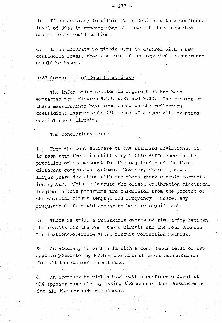
- 277 -
3: If an accuracy to ''lit-hin 1% 1. s de:s:Lred \ii th c:t confidencE:":'
level of 99'}'o, iJe appean> that the mea!1 of three n~PQut('~d
measurements would suffice.
4: If an a.ccuracy to within 0.5% is desired "i"ith a 99%
confidence level 1 then the mqan of ten rep€;a.ted measurements
s'hould be ta}~en.
The information printed in figure 9.32 has been
extracted from figures 9.23, 9.27 and 9.30. rrhe results of
these measurements have been based on the rE"?flection
coefficient measurements (20 sets) of a specially prepared
coaxial short circui:t.
The conclusions are:-
1: From the best estimate of the standard deviations, it
is seen that there is still very Ii ttle diffen:mce in the
prcciDion of measurement for the magnit:udes of t.l1r..~ three
different correction sys·tems. I-iowever, there is now (-1
larger phase deviation ,lith t:he three short. circuit corrr!ct.
ion Sy8tcH~. This is because the offset calib:caticn e1f.'!ctrica1 " .
lengths in thi's programme are caicl.llated from the prod\Jct of
the physical offset lengths and frequency. Hel1cf:.~, any .I. • ,.
frequency drift would appear to be more significant.
2: There is still a remarkable degree of similarity betlrcen
the resul ts fOr the Four Short c'ircui t and ·the Foul' Ur..1mo'W11
Terr;'tination/I~eference Short cil:cuit Correction methods.
3: An accuracy to wi thin 1~'6 with a confidence level of 99'~
appears possiblQby taldng the meun of t.hree meas'urcments
for all tllc cort'cction methods.
4: 1\n accuracy t.o w·itJ).in O.~il~ with a confidence level of
99% appear::; possible by ta}dng the In(;;c:m of t.en measuremenls
for all the correction methods.

Ficrl1re 9.32
Comoarison of the Three Nevi TJ':Q.?s of Measurenent~ Based on 20 l'·feasurements of a. Short Circuit C'tt 6GFz
i-.""';'''l!f¥.M~..:LC!i~ _:xa""'.!,=_U .. A:a._ 3 S"h&'#fiu:""'ce£·-=:- t ·1-zuowwc
4 Sh t" C . ~ ""'t'Kati_m~S --~-=:';:·~o::' ;~:~7:;::~:~ .. -~a-l " I 1. or~ l.rCUl or lrCU.1.. . I d R - C"h I ! ' '.:j an a' eterence .... ort ~
iTt" Correctlon t1:ethod Correctlon Bethoa c' l··t c ,.. __ ·t· r' M"'t"'" r' ! i .=-?B! ' , . ,lrc_u ,or~.ec ],,),1. "- 1:~J
I , Hagni tude 'Phase (Dea) H::lg!1i tude Pha.se (Deg) 1" M;c:~:;~:;--I ;;~;s~ (~~~""i
f~~~~~~d:~D=;~~~t'~~~~i'-;'~~~:-;~-" O. 7522 0.0049659 0.55086 'I o. ~'l:~,;;-! ... ~~:::;:e_&'~T-~i I Li _anGa.... - ~-'l' _c. l.on l , I I 1 190){' " C\oo + .87%'1'79 9 + .65%1 999 + .&/0 "'79 9 + .51%1' 999 -+ o C'lai 170 . 0 + .52% J ~ . ~ L - ..... ~j 0 R -01'...· 7 en/ ('hI t' 5 ~)/' - anI ~ -' • e >-: 3"/ i< I ConfJ..a.ence ,c'Vel -:- .... ::>/0 • _;0 .::r1O • _,0, .-'/o~ -.-, /O~ , i1-. II . t ,; ---1 ~ll -01 .. I : I '>/..L r- ?ol .J. I '-'01 f ~ ~:J~ • t¢ , .. ,~ C\ _. 11.000 + 1.~; ,179.9 + .8~~ .999 + 1.0~~ 179.9' .o~~~1 .999' 1·~~1179.B + .6~:,~ ~ ~.' ._O •• f1Q,.D,-" L ... 'iiel {; 1.0;0 .9""'/0 1.1;0 .6 ..... ,.-'j, 1.J...:Inp. - .6::.>.< < !- --l~ i I . ·-3 ;, , ~
f< Q 0"/ ("/" ')0/ Lt,~i.l. 0/ /lo/ ~ . q --:0/ .;: ~.- ~~/.O , ('\0'" + 1.4/01 170 9 + .!..I""o 99'"' + 1 •. ;<> 179 9' .86,0 999 + 1,;,.,01~79 <;:,.,+ ".JlJ/"~. i Ccnfide:1ce L~~vel f-'v v - 1.5% I ~. --1.25% • ';1 - 1. 5/61- . - .87%' _ 1.5%.L. .0 - ,88%! ~~~~~r..G'JIt:.X:u.e:-~~~l.;"~~~;~;;;rGt.&l-:u:'n.,~~..;:tt",;:u.,'t~_T- . ~ ~_·~\I.:;-.~~!,,.~~'Wafil'~~~~~~?~~>-:W:: .... Q·~.::ti..?!.~ ... ~~J;.~Q.;ji,.~~~~&:··Z'-i~t·
N -...J 0)

- 279 -
Thi s leng-t1-"y but none-t.he-1ess very ir\tpo):"Lant chapt.(:"r
bas verifi.ed expC:l:-imcnta.11y the tt~2oretical idc-!as d;.?velop(?(~
in t.hp early chapters of the thesis. Tr,e::~ first half of this
h t h ' th' h' , c op'-er 2,S S,10i·m . e Vi:rlOUS grap l.cal plots a~1d the pt"l.r.~-
out rpSll.l t:. sheei:.s which lTIoy be obta.i.n~d ,{hen corrected
measurements are made.
'1'he seco.i.1d half of 1-.hi s c11Glpt,er has been d'2votcd to
obtaining, COii1p~~ring a.nd interpreting the statist.ieal datil
amassed. Consider2.ble t:J.rrte and effor": had to be devoted ,to
cclrrying out these 0.11 important task.s for vri thout them,
onG i'lOuld a1viays be in doubt as to the d-.;grr;>E? of accuracies
\vhich can be obtain.ed when t.hese correction methods are used.
Direct comparison with measurements carried out by other
met.hods e. g., the Short/Off Short/Sliding Load/Het.hod (sect-Lon
'5:4.3) have not been included because there is no assurance
that such a method' (section 5: 4.3) is perfect.
HOvlever, grapn.ical comparisons and some measurern,~r:..t e!"rors
hu.ve been inc1ud,~d by t"!:1e author in a published. paper
(reference 9.1)~
The general conclusions from the measurement of the
test. piece indicate that accuracies t.o within 1% with
confidence level s of 99~\6 are possible with 3 m(~asurements <, It'
and'that. ac(:uracies to 0.5% vrith confide-nce 1ev'218 of 9£.«;6
are possible .... d th 10 measurements. These con-:::'usi0l1t3 a.ppJ.y
to any of the nelV correction systems.
* * * * * * * * * *

-' 220 .. ,
H,-"'ferE;l1CC'S -----..... -.~ .. . - ....
9~1
9.2
9.3
da Silva, E.F. und :HcPhun, M,l\:. "Cal:i.bration 'l'cchniques for One Port Me(2SI1r2wents" Nicrovfave Journal, June 1978 pp 97-10C.
'LT1and B~ 'P tlDI':'ve:>.lo'j'l' ~'lg ')\cr<~'r-'("''V' r~")'~c·J'.(.:'; ('-'al": ""')'1'" I: 1. 1 /If.a.. -",.:' J - /.~ ,_ \.A • (.1 ---.J. ..... i~ ('_ _ . J... __ .... ___ ~~ . _ ~
for JI.uto;r:.t.ltic N2t"w:nk Analy:;,ers" Hewlett P ac}..:a:rd Journal, February 1970, No 21 pp 16-19.
AdalnE!, S.}."". :He a suremcnt: pp 30~-313.
"A Nev[ Precision l\utomatic Nicrowave SystGmil I.E.E.E. 'l'rans. 1968, Il1-17
9.4 Adams, S.F. "AU.tOffi<:lt.ic Net'tv-orJ .. l1·':::i:lsurement.s" Proc. I.E.E.E. Vol 66, No 4 April 1978, Pp 384-391.
9.5 Ridcl1a, S "Comput.c:cized HicrOi'r(:lv~ MeaE;1ue:ncnt.s Accuracy AnalysisH P roc.:(::;·~dj.ngs of t.he European l~icro\vave Conference, Pcq:.·cr B34, J.J73.
9.6 Ridel1a, S "Comp1.1.te.1::ized Rr:!flection Heasurements" C.P.E.N. Digest 1973, pp 51-53.
C). 7 v~oodf:l, D. "Rigorous D(")ri va U.on of Computer Corrected Network P"naly::;er. Calibratibn Equations" Electronic Letters, 197~, 11 pp 403-405.
9. 8 ~'1oods, D. "Re-.!-\pprair:>al of Computer-Corrected Network Analyser Desi.gn and Calibrat:icnH P roc. I.E.E. Vol. 124, No 3, March 1977 1 PP 205-·211.
9.9 Woods, D. "Inuni ttance 'I'l'ansformat.ion Using P recision Air-Dielectric Coaxial Lines and Connectors" Proc. I.E,E. Vol 118, No 11 Nov 1971 pp 1667-1673. .
9.:tO Harner, F. uHicrowave [l.tb.:muation Heasurements" (I.E.E. Monograph 19) Peter Peregr:inu8 Ltd., London 1977.
* * * * * * * * * * •

- 281 -
CONCLUSIONS OF THE THESIS _ .... __ .. _ .. - .. _-----.. _----------..
. 10: 0 Fin?l Pe-..tiew·
The information presented in tJJis thesis is the
a.ccumulation of several years of research worle direct0d
towards producing a systeHl for the rapid and accurate measurc-•
lnent of irn.11li ttances over 3. ".ride frequency bancli.,ridth.
project was commenced by carrying out a su.rvey of the The
existing rapid wideband measui.-ing techniques. (see Chapter I). This
survey resulted in the selection of the reflectometer as the
desired measurement system. A thorougll understandi11g of
principle of reflectometry was then considered essF.mtial
considerable theoretical ,,,ork was carried out in Chapter .
the
and
II • This work was mainly directed to establl.sh.i.ng t.he deslr2.ble
and undesirable properties of reflectomet.ers. The principle
of computer corrected reflectometry, i. e., acceptirlg the
defects of the reflectometer hanliorare and con:ecting these
defects by calculation (software) "ras establish(~d in this
chapter.
Knowledge of the peripheral equipment associated ,·li th
the reflectometer is considered e~:m(-:mtial and a brief descript
ion of the equipment used viaS p'reGented in Chapter III.
Measurement e;quipmcnt is seldom perfect and the rcflectomet(;r
method of rnec).surcmcmt is no exception, a!1d an extensive review
of these errors ,{ere carried out· in Chapter TV.
The establichm~nt of a bilinea:: tral1s:cor-rnation relation ..
ship bct,,,een the measured :cerlect.:i.on coefficient and th<~t Of
the device being measured. led to the at::v:;)lopmcnt of the nev1
calibrc:.tion and correction proce.dures described cxtE;l'lf::;:l.vellr in
Chapter V. 'rhe use of computer correcb~(.1 systems required

.~ 282-
considGrable computaticn, iI.nd t11e developm~nt of the computer
programmc~s described in Chapter VI vTaa inc'li table as mc.l1ual
calculations were found to be impractical. Consid()rable
effort was devoted to inv(l[.Jtigating computati onal errors.
The lind ts of accuracy associated with the use of single and
double precision numbers in the correctiC'!"1 programmes was also
establ.i shed. 'l'he de"'lclopment. of' the automated progr3.rrJ1~CS
were particularly time consuming as the lengt.h of these
programrltes required ·t.he use of computer oVGrlay progr;:.unming
t.echniques to reduce thE'.! at.orage requin:!ments within the
computer.
, Considerable effort was also put into the design of the
calibration standards for the vari.ous cQrrection m(;;~thods.
These standards (described in Chapt.er VII) hav~ been proven
to be electrically and mech;:.mically stable. They have also
been fabricated without much difficulty.
Initial tests to determine the suitability of the
equipment for computer corrected measurements v.;ere carried
out in Chapter VIII. The first hal·f of Chupter IX has bf::~en . .. devoted to the presentation of a cross sectJ.on of. measurement_'.i
carried out using t.he three new correction methods. The
second half of Chapt~er IX has been clevoted to a very e)'ten81.V(~' di scussion of the measurement acc~racy of the new' correctl.nJl , ,
. methods. These accuracy conclusions are summarized in
Sections lOI1.1, 101.1.2 and 10:1.3 •
. . \
lili.L.l\ c)1:i. cven~11!-_0_f Obj££!:.iY~
The objective of this thesis has been to renearch for an
accurate and rapid means of measuring lumped components over wide bandwid·the at microwave frequencie8.
'1'his objec~ive ,har:: been fulfilled by t:hl~ invention and
pUblication of three new' computer corrc:~ction net'v'ork ~lnalyscr
methods fo.r-. the rapid and accurate mr~asurerN::.'nt of :1mmit.tances.
These methods "rcre construed theoretically and havG been

·~ 283 ••
proven by experimentt';!.l measurements. 1~utomat2d measurement
procedure::; for these correction systems lnve also }x:~t:n
developed •
. The nevi correction systems hav(~ be(~n called:-
1t 'rlle '!'hree Short Circuit Correction Hethod.
2: The Four Short Cireui t Corr(~ction Method.
3: The Four Unknown 'rermination/RGfert:>nce Short Circuit Correction l{'3thod.
This method was'invented because previous to this method
there was no rapid and accurate means of measuring immitt,ances
~n confined spaces over wide frequency band,V"idths. 'rwo manual
computer programrnes (Appendices 11::.> and, 11; 6) and one auto-
y" mated programme have been produced for this correction system • . {
: Thr~ results obtained with this correction method for t.he
measurentent of ,a reference test piece (short circuit) are
given in figure 10.1.
The results. (section 9:7.1) have been based on a normal
ga'l.ls{sian distribution: of 100 mea$urem~~nts
det.ermined for a confidence lovel of 99%.
based on the table above indicate ,that:-
and have been
statistical data
(i), .. The mCO.n of 3 measurements ",.viI!
produce an accuracy to wi thin ± 1% •.
(].'].') The- f 10 t '11 _ mean 0 measuremen' s Wl.
t . tl' oj. 0 r:o' produce an accuracy 0 w]. ,un - • ;:)70.

Frequency Measured Reflection Coefficient Theoretical Reflection Coefficient
L GHz
I ' 4
Magnitude Phase (Degrees) Phase (Deorees}, Magnitude
I 180.09 ! 1.750 + • 999 - 1. 4 I 9E - 2 * 9 c 9· + • 1 .4% or .• J .. ....",
- • .L • .:);b 1.000
, L-I
I 6'
I· 1800
I or* 180.09 + 1.~/o E-... - .9~J
,__ I ' = •• I. __ 180
0
i _ .,_ . ..J.... .. i
0111#&=_. 'J~_ I .--= ....... 4
179 • 88 ~ 2.144 i or* 179; 88 + 1.12;6
1.25%
1.000 ! 1.423E-2 ~ 1 40 /
or* 1 000 + • ,0
• - 1.5%
1 .• 000
*Referenced to 1 /180°; The. improvement in accuracy is (;',pproxi!nately 5 times that quoted by Hewlett Packard (See section 4.7)
Fiql1re '10.1
l-1eaS'Jrement Results for the Refere!1.ce Short Cireni t USinq the Threr-s Shoct C~.rcui t Correct'; O!l :HeaS'.:trsment
N co ~
I

- 285 -
10: 1.2 The Four Short. Circuit. Correct~_o:! Nethad ._--_ .. _------------,,--_. -.-.-...... "-, ... -.~------ .... -, ..... -
This method 'iras invented to overcome tht:; difficUlty
of specifying accurate offset lengths i;:1 microstrip.
Two manual computer progr<1.mr!1.r~s (Appendices 11: 7 and>
11: 8) and an automated programme have been v!rit.ten for
this correction system. Two sets of culibration pieces
(sections 7: 2 and 7: 3) have been constX1.1cted for this
correction method •
. The results obtained with this method for the
measurement of :1 reference test. piece (short circuit)
are given in figure 10.2.
The results (section 9: 7 .2) have been based on a norr.1a 1
error curve corn:!cted for a small sample distribution of 20
measurements and determ:i.ned for a confidencc~ level of 9976.
statistical data based on the table above indicatE~ that.:
. (i) The mean of 3 measurements would produc(~
'h' + 1°/ an accuracy to W1t 1n - ~.
(ii) The mean of 10 measurements would produce
10:1.3
"; ' .. , . "+ . 0/ an accuracy, to WI. t.tll.n - 0.5/0.
The Four Unknown Terminat.:ion/ncfE)rl'?nc,~ Short Ci.!:££i:t correction M(~trK;,.:l ---
. This method ",as invented to overcome the difficulty
of producing short circuits for cal.ibrations within a
One lllanual computer programme (l,ppendix 11: 9) and an -
autom<lted pro~raltUne have been wri ttE:m for this corrcct:i.on
system. One set o~ calibration pieces (section 7:4) have
been constructed for this correction syst.em.

'. ~ &iiZ!4A if'] btU G.: ."~==L'S 1M eJe*'di5Cii&lit::::aw:s... if 9-"!t*::w:::szz:e:z:zU!iW!:s:ssaS:U==Q.WSWi& 9 ..... C:zs:x===SUW4. JUS =_~
~,~ F Measured Reflection Coefficient Theoretical Reflection Coefficient ~ ;;1 reqc..1ency ---!i ! ill::!!!" Nagni tude ~ Ph2cse (Degrees) ~i tude I Phase (Degre~ J. •• 1., +. 'I + ~ II ~ .998 - 1.~?OE-2 IS0.2 - 2.06 . 0 ~ c ~ oJ. 4 . * .. 998.+ 1.03% r* lS00') +1.25 1.000 ~ 180 ; ,; or. 1 8°/ 0 • ~ -1 04 ;! ~ ~:"J - • {o. ! ';i .y, . ;~
~ .999 ± 1.415£':"2 179.99:t 1.57 I ~ i~ 6 ...!o 1 40/ + SC:O' 1.000 I 1800 I ~l * 999" /0 '* 179 99 • VIO ~ 3 ~ or . • _ 1 50/ or • _ Sf}>-' :1 ~ '"':;" • /0" • '0.. ~ t; ;"'~~ .. ~:;:AiI:!$>i2WCi -...... -P'1IS.::m •. ·c:~~~~lIf'/Iilii·ac Q,Zl'--- :;:;=:: !;:"-;A::::a:;;:w:::::AJ£lI"'l!/Io1I:I:aY.ZI;;:;;.a .. ;a:z::t:e.:c:Cl~'":l¥t._as::dfit ... & *,1:. I~~
* Referenced to :: l1800; The improvement in accuracy· is a.pproximately 5 times
t11.at quoted by He~.ql$tt P 9-ckard. (see section 4. 7)
Figure 10.2
l1easurement Results for the F.eference Short Ci rcui t Using t.he Four Short Circuit corre..£!~.on Method
tv co 0"1

- 287 -'
The results obtainc(i 1,.,. ith thi s method for the meaSUl"e···
ment of a refere::1ce test piece (short ci rc':..lit.) are gi v(=,n in
fi~Jure 10.3.
The results (SE-~ct.ion 9: 7 • 3) have b<:?en based on a normal
error curve corrected for a small sample distribution of
20 r.1ea::mrcm~mts ;::l.l1d detennined for a 99% confidence level.
statistical data based on the above table indica.te that:
(i) The .mean of 3 m8aS1.lrements of t.he test. piece
wi.ll produce an accuracy to ,d thin :t 1%.
(ii) The mean of 10 measurements of the test piece will produce an accuracy to ,d thin ! 0.5%.
comparison of the ·three new correct.ion systems {section
9 r 7) have shown that the st;:mdard devia-t:ion of c.ll t.he:::e
methods are ·similar. (However, it should be noted in this
case, that. the 'offset line propagation losses in the calib
ration standards in the case of the Tbn::.e Short. Cireui t
Correction Method were negligible).
", , - ... 'I For most practical CaSeD., it is envisaged t.hat t.he choice
of the measurement system "rill be dictated more by the
convenience of usage than'by the accuracy requirements.
The Four Short Circuit and the Four UnJcnown 'rermination/
Rqf; Short Method should be used in measurement cases ,v-here .'
the:offset electrical lengths change ,·d.th frequency (e.g.,
microstrip) and where offset line attenua·tion may be object
ionable, or in any case where the propagation constant of . the transmission meditl..."l1· is unknmvn.

-- == • ..
* Referenced t,o 1 usoo; The improvement in accuracy is approximately 5 times
t.hat quoted by He ..... l1ett Packard. (see section 4.7)
FiT.lre 10.3
Heasurernent Results for the Refere~ce Short Circuit !ising the Four Un}~.own -Termi!l~ions_(Open Ci rc-uit.SI· Re~erence Short C; rcuit C('rr~ction Met.hod
l-.J co CD

}
- 289 -
If th(~ freql.1r::mcy of measurement is not }movm precisely
then more accurat(~ measurerr~en·ts "rill also be achieved by using
the last two named cDrrection methods b(:!cause these methods
obt.ain their calibrat.iol1 offset el':?ctrical lengths by measure
ment. (rfhe Three Short Circuit Correction Hetllod depends on
a knowledge of the frequ,ency an.d the physical length to .
calculate its calibrat.ion offse't .len.gtns),
It is the aut.hor's belief that the Four UnJmown
Termination/Rcferenc(;~ Short Cireui t Het'h.od -vTill prove to
be the more versatile of the three rlGiV' correction methods
in practica~, rneasu!:ements.
10:3 Futur~.~9rk
Research worle is never completed. In the case of the
present 'equipment, considerable improvement in accuracy ivill
be obtained when phase-loc}{ed signal·· generators are used in
the measurement system. Ref lectometers vii th ,dder band
widths and grE.~ater directlvltil~s v.ri.ll also provide greater
measurement versatility ..
Imp.rovements in operating ecollomy will. result "ri th tiH~
replace,ment o~ the prosent computer by (l microprocesso~. One such system 'such as that developed by Crane (Reference
10.1) could be used to control the mcc:umreme:mt C'quipment.
Ano·t.her success, at eliminati.ng the large computer have been < ...
carri(~d out by Hevrlett Packard (R(~ferencl: 10.2). It is
envi saged that future versions of the net"VlOrk analyser will . · . tl' th . . l.ncorporatc lUl.CrOprocessors Wl. un e l.nstrument casl.ng
and that computer correction facilities will be commonplace
in such measurements.
,New Hethological Systems are constantly appearing to
challenge the present ones. A typical example i8 the Six Port Reflectomcter which has been described by Engen
(References 10.3 and lO.4)~ This syst.em has been claim~d by Engen to be the alternative ·to the netviOr)~ anG11yser.
Engen also claims that less ccnr1'">licat.cd peripheral cquip-
, mont is required and 'that irwtrUI:18nt costs 'vill be drastically reduced.

- 290 _.
Authors such as Bpatty (Reference 10.5), Adams (Pc~ferenc0
10.6) and Engen (Re.f(~rence 10.7) pt1.blish l)(:~ri()dic rcvit~",.;s of
t.he st.ate of ll1icrm.,rave metrology. In th(~ case of net',;ork
analy~:;ers, the trend amung these authors set'.:!ffi to indicate
that future development 'Worl{ will bf~ directed to'wards t..he
• J'f' t' ft' i t ~ s1.mp.1. 1.ca 1.0n 0 nleasureUlen eq\.upmen.; 0 reO-uee costs,
arid that the Hubseq'J.ent det"c~r:lorat . .i.on in hcl.ro\.yare perform
ance ,-rill be compensat.ed for by more extc'nsi ve use of
computational equipment such as mic.roproces~30rs. If t.hese " '- , ~ ..
authors are correct in th(~ir assumpt.ions, then computel:.·
corre-ction sy~tcms will be with us for many y(::ars.
,
.. , . • ,i.

Refererlces - ,---10.1
10.2
10.3
10.4
1~.5
10.6
10.7
- 291 -
C "[:... .'''0. t D· t. ,t U· • t ra!le, J,'. l.r~va'e ~GCU8S~0l1 nl.versl. y o:t
l'larwick, Coventry, England, 1977.
He1.rlett Packard, "S2l1ii Au'tornatic Heasurcments using the 8410B Nicr.owave Neb-,;ork Analyser and the 9825A Desk,-Top Computer" Appl ication Note 221 - Palo Alto, California.
Engen, Glenn F. ttThe six Port RE~flect.cmeter~ An Alt.l?:rnative N!~t\·:ork Analyser" I.E.E.E. Trans on MicrO'\yaVf~ 'l'heory and Tec~Jnique8 Vol HTT-25, 12 Dec 1977. pp 1075-108 •
Enqen, Glen.n F HAn Improved Circuit for Implementing the Six Port Tec1mique of 1'1ir::1'o,\-rave Neasurements" I. E. E. E. Trans. on l'iicrowave 'rheory and Techniqaes 1 Vol H'I'T-25 J Dec. 1977. pp 1080-85.
Beatty, R. W. "Aut:Oli.latic }-!easu.rements of Net'work Parameters - A Survey'! National Bureau of Standards, Boulder, Colorado, l.'June 1st, 1976.
Adams, S'. "Automatic Hicro"rave Nct,'mr]';: Heasurements" Proc. I.E.E.E .. Vol 66, No 4 April, 1978. pp 384-391. Engen, Glenn. "Advances in Uic,cmvave Science"
. Froe. I.E.E.E. Vol. 66, No.4. April 1978. pp 374-383.
",. * * '* * * *: * 'if *

- 292 -
THE U~)Ert,TLNE.sS OF THE BILIhm;.p TR~NSFOPlv.Lr.".Tlm-J ------,-----_._-"_. -- ---- .. _-
rr:he principle of bi-linear transformation applied t.o
electro-magnetic fields is used extcnsi ,<,,rely in this thesis,
The purpose of th:LS appendix is to jUstify its use and to . .
clarify the fnndamental pos'tulates assumed irl its llse.
Il\J"PUT
I I I' r-----~------.-,-
TRANSMI s~n ON
SYSTEM e.g.
, , Waveguide
---____ .-.-.-___ ..... .t
AI
Z 2 ~--''''''''----'-,
OUTPU'f
PLANE PI . PLANE P2
+h d' • • In ... e J.agram above, the tr~ns!n1.ssJ.on system may
contain' any assortment of conductors, reactances, reslstances,
insulators etc., .... lhich need not be specified. HOv;cver, these
components do determine the electro-magnetic coupling bet't\'een
the input and output planes •. Ncm-lineai':' materials, i.e.,
those vlhoce electro-·~agnet1.c propertles (h~pend on the strength of the electric or magnetic fields an~ (,;!xclnded from the . .
transmission system.

Two fundamental pOG·tula~.c~s are r(-::ql1irc~d
1: The field at the output is zero if the field at th2
input is zero (i. e., n.D internal SOl.1rC8 of electro
magnetic energy other tha.n that su}::plicd fr.oi3 the
input)
2: All. field component vr~ct()rs (E, H) add line;'lrly in
t.be reqion between refE;rence planes PI and P 2' Hence
a field (~l' Hl ) added to a field .(E 2 H2) producr~s a
fie 1 d ( E 1 -l-E 2 I II 1 "'H 2) •
Let the field cDl-nponents at planes PI and P 2 be
represented by (E l' HI) and (E 2 , HZ) respecti vel}". Th(::!l1
from the usual two port theory
E1 = a E2 + b H2
Hl = C E2 +. d H2
•••••
• • • • •
(11.1.1)
(11.1.2)
where a,b,.c,d, are complex ·parameters defined in t.hl::
norma.l way.
\ .# ••
using Schc1'KUnoff' s definitions for w'ave il-:1pedance, i. (:~. ,
Zl = El/H l ' and Z2 ;:; E2/H2 and dividing (11.1.1) by (11.1.2)
a ~2 + b El . II a Z2 + b Zl· 2 -- = = :;; - .
. Hl E c '7 + d c ~1 .+ d
~2
l-I 2
or
= " . . . . (11.1.3)

- 294 -
Hence all transformations of i~mpedances throuqh trans-.. -' ., 1 . ,
mlSs~on systemo satl.SfYlng postulates and 2 :ITioY' be descr.lbec~
in this manner which is called a bilinea.r transfo::.~maticn as it
is 2, ratio of b'lO line~n- equations.
Division of the numerator and denominator of t.he right
hand side of equat.i.on (11.1.3) by any of its constants e.g., a, wIll rL~sult in three new constants, aid, bids c/d 2.!ld unity.
rfhe left-hand side of the equa!;:ion remainn unchanged •. It
follows that 1-1i th three St~t.s of data, solution of the constants
w'ill result and t.he eq11i valent bilinear tra.nsfo::.-mation beb:-ecn
Zl and Z2 can. be ascert:ained.
Three other general properties of bili.near transforma'tions
should be noted here:-
1: It can easily be shown that if Z 1 is a bilir ... ear
transformation of Z2'and vi~e-versa then,
-d r7 + b Z2 ::: Ll1
... _-c 2; 1 + a
• # .... (11.1.4)
2: If Zl is a bilinear transfo~at.i.on of Z2 and Z2 is a bilinear transform-3.tion of Z3' i.e., let
_ a Z2 -I- b Zi - c Z2 + d
, then it. follmvs that
and AZ 3 -+ 13
:::: CZ 3 + D"
Zl _ .a(Az3 + B) + b(CZ 3 + D) ''', (A'7. 3---::-, B-),.---..... --d:::-:(.-:,...---r':-"'-+-r·-» ~ u· -r . .....1J3 .
_. {aA + bC)Z3 +"'{aB '+ h.,D}
"( cA 1- ccOz3-- oj- (cB + dD) . " ., ... (11.1.5)

- 295 -
vJhich mr.~ans t.hat two impE.~d;;.\nc:c bilirJcar tral1Efcn:l:-::tions
oc:curinq in cascade can be replacExl by a thiJ':d bi U, near
transformatj.on \-'l}lich satisfi.~s the ccnditic:'.l of t.hc
cQ,nstituGll"t. bilin2.ar tranGfOrl11<itic)ns.
3~ Any two port netw'ork described ,vi th t1'lc convcnt:i.onal
lnpeuul'1cf.! matrix of the foem s:\C;w'11. in (Fig 11.1) 1':1.3:1
be sho';·m to be rela'ted by a hilinr::,:,:x tranSfO!1rtation.
V 2
F i.9.llr3-1!..*1 .2 ~p qrt ): m£..<?d sD:.£§":..': ~1:!? cl~Jjg]f:
•• of ....
. ,. . ... . '/
By inspectipn V'2 = -I ZT,;and substituting in 2 .. , equation (11:1.7) results in
I., ..
't t" . (1 1 6) Substl U lng In equ.atlon 1 •..
\
V 1 =
produces
(11.1.6)
0.1.1.7)

and defini ng i~ uS
thus
z
whore
'I.r Y 1
.~ 1 1
a
C
-- Z · 11 ~"
::- 1 . ,
b
rl
- 2.96 .-
=
::::
.7 .. , '('I. Z Z r>' '.Jl"'-'~ :r "-'11 ~..,? - J] ').£.''"'1) J .L. . .t.,~ ",' i!-::: --.------.-.--.--,-.-~.~ ......... - .. - -
'7. + r'I ""r.., " o!..J 22
n~IJ" .:_= cZ ... + d
J.J . .. . .. .
(Z z -'" '7. ) :1), ~22 .!412~'21 - ~Z
ZZ2'
(ll.l.,B)
* * * * * * * * * *
, ..

--"--,..,.
- 297 -
11: 2 .
The purpose of this appendix is twofold:-
(a) to show the relationship between scattering
parameters and bililear' transformations
(b) to note that two scattering bilinear trans-. formations may be replaced by a single, scattering bilinear transformation which '
satisfies the constituent :bilinear transformations.
fiC'lU(Jring C08fficientlL9f a 2 port Network
~. ,-ia..z.,. and bt • b2. arc; defined as the incident
andreflect.ed waves into the two port network
t.

298
J t I a 1
, b 2
I .... . I [sn 512
] t .
PORT PORT ONE
I " . 5 21
c . I b 1 "'22 a
. , TWO '
,<-f ('- _., ~ J . I
I
• •••• , (11.2.1)
• •••• (11:2.2) ....
. ' By definition, the reflection coefficient ( f.) is
defined by
Ref lC'cted W3V('!
Tncidlmt VI <.1 v!'!
Jhmtx~, Lhe reflection coefficient ( f) "looking to
into thp t\\'O port n:.'twork is
f = • • 4' •• (11.2.3)
.' ;~' . - .' . . . ,:",:",._~,. --+<~ .. .r .... ·,~ .. :....,..~l_ ........ ".£,; . .1. ... ,::0:.;" ;~~,_~_ ,.,,,,,. ;,.;~, .,'''; _.,: ....... ,~"""'~:.."'~:.·.,..,~_(~~,-" ... h":;.;.:~~'~. ~ ~L, ..... ~.~.,4:_ :;_ -.i _" .~'h,' '.,..,..r,.";.-. ,.".--.:.....,,;;n,.>""'~ .. .t' ... 1i!~''''';;,<_ .• ,.. ;'0.., .,:..,.,..> .... > <l;

- 299 -
.(.\-l) and the reflection coefficient, . l~
of the load t.erI!1ina·i'7.ir:g
port 2 is ~ -"
• '(t , • • (11.2.4)
SUbstituting equation (11.2.4) into equation 11.2.2
D..., • =::. O .. 'l. 52.1 Q...\ -\- S2.:t. [.:'2-
-- r Q z. ( /1- -:- s 2~) -- 'S 2.1 (J:.; r
Q ' S:i.\S~If2. . cL~ ~ C;;:' 52'4) --"I - S2,J~-
Subst.:Lt.uting equat::i.on (1.1.2.3) and (ll.2.5)
(11.2.1.) gives • b , - '511 Q..,I.+ SIl... <..1..2,
b , ~= f -- S If. 4-
ev!
c ("> t-'., ....:,. 1"'-.. ~?..I 11_
.... _---
or f ::= - (S\t ~?,2.. - S I? S::\.;) k -\- S \1
or
where a b
---
::
d ::
- S?~ r2 ..\- I
- (~. \\ S 2". - S I ~ C;:l0:== _4 /~ S 5"
.. . . . . (11.2.5)
into c::JUation
• • • • •
• • • • •
• • • f •
• • • t ..
• • • • •
· . .. . .
(11.2.C)
(11.2.7)
(II. 2 .71)
( 11. 2.7 c)
(11.2.7d)
Hence reflection coofficients bet,-.'cen two measuring planES
have also been shown to be related by a bilineal" transformation.

... 300 _.
" . . Let the J.1'!dJ.v~dual tranr:formations be denoted by
and
then frO!1:l equati.on 11.1.5
f, =
••••• (11.2.8)
"\.;hich is al":.othcr bili.nr::!ar transform~tiol1.
Hence .. it can be con.cl'l:lded that t'\'ro reflection coefficient
bil1near transformations in cascade can be replaced by a. single
bi.linear transi"ormation ·,,;rhi.ch sati.sflcs the conditions of the
con:::;titue-nt bilint1ar t.:X'ansf0!1natlon8.
A. similar exercise may be used to S1101'1 that three or • • t" d ,.. mor.e bl1l.near transforrna .10ns ~n ca::::ca e may J..:a. reduced to
that of a singlE'! bilinear "l.l::ans[ormat:ion. if and only if the
constants of the const.ituent bilinear transformations are truly constant,. i. e. they ar(~ unaffected by the act of
cascading the additional netvlOrks •
.,. . ....
* * * * * * * * * *
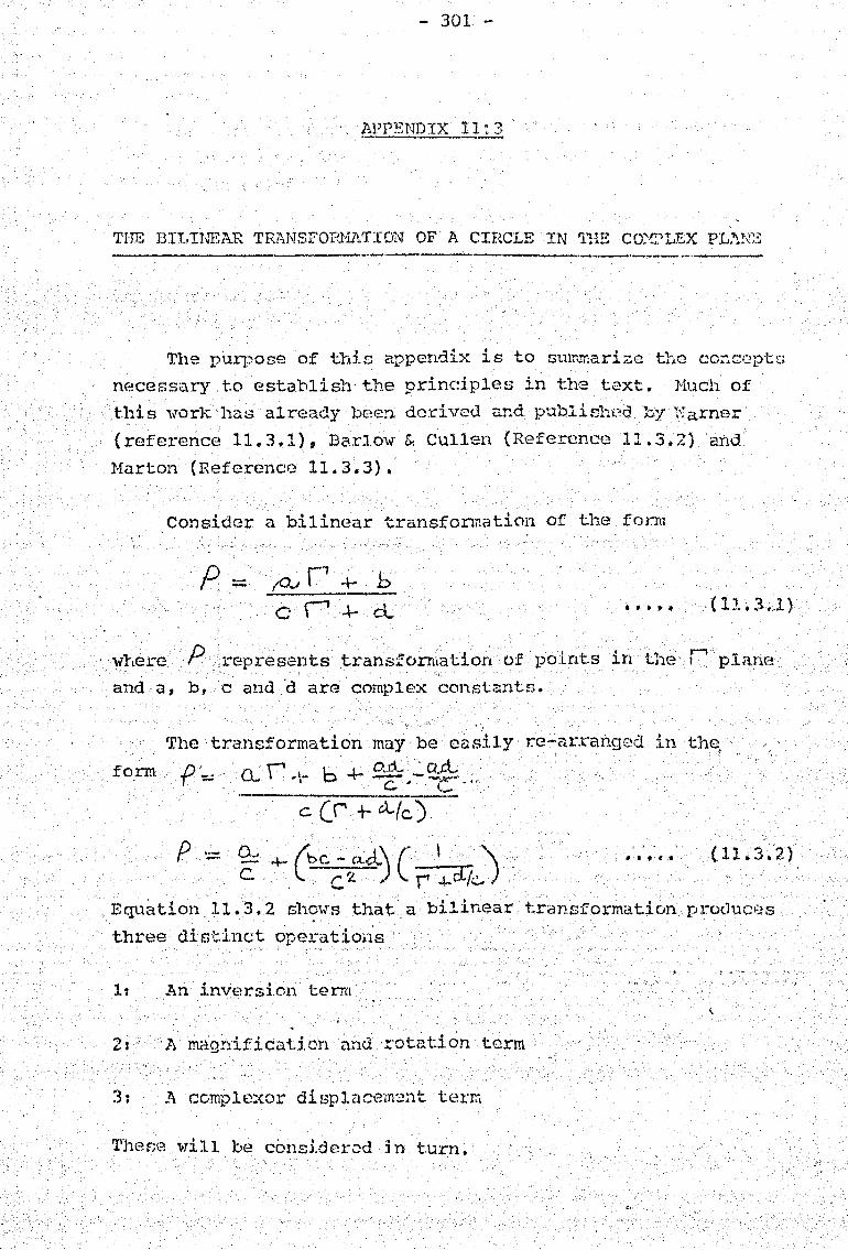
- 301 -
THE BII,INEA.R THANSFor~HLYrION OF A CIRC"LEIN 'l'HE CO:'f:>LEX PL.\!·~E -----------_._----._- ------_._--_.-_._---
, iI .. ~ 4 ...... ' The pUI1)ose of trUD appentllX 1.S ... 0 stnnmar1.ze triO COl"' ... copt:s
necessary t.o establish' the princi.ples in the text. Hnch of t.~1is i-vor}~ has already b(;~(;!~ derived and publishpd by 'i';arner
(reference 11.3.1), Boxl.ow &. Cullen (Reference 11.3.2) and
Marton (Reference 11.3.3).
Consider a bilinear transformation of the form
p= to..Ir1+ b c r '+-·.cl . . . .. .. (1J..3.1)
where P represents tl-ansfCJrmation of points in the r plan.e
and a, b, c and 'd are complex constants.
I
The tran8formation may be cns1.ly r.e-arJ~·anged in the I
'f;; CL r #~ b 4-~ ..:. £+1. , c·' . ( .... , -----. ..-c (r -\-. cA..(c.)
p -= Q~'4- (bC __ - c~.cl\(· \ r '\
c. .l c ~ ) r' J)Lk ... ) l' •• 4" • (11.3.2)
Equation ,11. 3.2 shows that a bilinear transformation product;::s
three dist.i.nct operations , '
11 An invE!rsl,on terra
2:' A m~gnification und 'rotation term
3: A complexordiBp1ac\~m:;mt te.t'r.i
""1 ' 1 b .• • ~leEe W1. 1 "8 cons~der~d In tUrn.

- 302 -
T'n-' -rrl"""" r",i '01' '['(' 1r' ___ ,,:_. _ __ '=-_'"'_,_,.::.:.......L • . ~, .• :::...:.:~
For 2 linear circlJ,lt1J::" loci f' , t1'1e inv -r SE~ i s a11.,jay 3
l ' . .. .. , 1 ,. , anot~er Clrc e prOV1G0Q on~y t~at the I lnear loc~ do not. PClSS
t .hrough t .h2 orig i n.
,--. ---J
I' do' ~ (" rl' bOt" " el' re'} of-,' _r ::..r.·)','· 'I'. !:~ . i '"' '-_;:; - ._ ' ... :, c,' . . , . _ .... ., ._ 3.nd C'entn~ If then f) des -:ribes a, circle of radiu8 0\ and c<:?I1.tre !3 in f:;. gure J 1 • 3 • 1
F.' i If" r ..,] 3' 1 _:....:!.:.::J.~ .. .i-:-_±-;:._. _ !-::..
I nve sion of ('l, Circl e .. __ ........... ... _----_.----_._--
I
(' I do' :
d and f3 are ..:bo'NT by Barl,m.; and Cullen ( Pt 'f 11.3 2)' to be
---
and
Note in bot.b ca.ses U e term
magnifict.1t ic.m tcrm ~
1• ... ", •• >
$f • " • , (1 1 . 3.2 )
• f. ••• (11. 3. 3
llH::.rely a
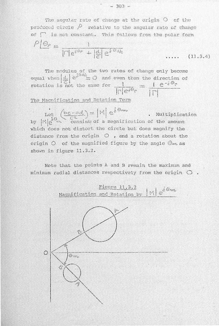
- 303 - '
. . ( '\ 'n::t-~ anq1J.lar J::ai..:.f~ of chiUc"ge at the o:c19lJ'l .....) of tht:!
PY.'oC.uce' ci~cle /~ re1at~1.ve to ::hF,; angula r rate CJ f. change
o f r-' j s not constcnt~. 'l'h is foJ.:!.o';{S f::-om t.~.e p lar form
n l /""\ ,- L 1"";1 I ': P ---_. -,...~
Th'~~ modulus :>f the i t ,,.. J.9cJ./c .
equa.l \"bl~jj I '~ I e. == 0 rotatioll is not thE, same
, .. ..
't vTO :cat.es of change only b ecome
?nd even t hen t.he direction of for t e -~ 8f'
Tr' leI e r rrT----- -'-1'11~ Hac; ific,;ation ~!.!..iJ~o·t(~.t.ton.;,. 'rerm
( 11 . 3 . 4)
· / I I ~ 0rrrv 'L' ..::> J_ ( b c. ,,{ \:;-:::. i'-1 e. <;;;;l. __ • __ _
I ~ I 1e ',-, CIt.... • ..1. f' . . ' . ' }ill} tipl icat .. ion
b y !"t lle Ntt.- cons] S'C; 0 a HlC'l.9rni .lea Clon o :f ·the amount: I . '
which does not di:J'tort t:he ci rcle but. does magnif y the
distance :from t he origin 0 , and a. rot.ation about the
origin 0 of t he llli:lgrli.fied f iguJ .. c by tb.e ang l e Otlt'l~ as
sho'vln in figure 11 . 3 , 2 .
Nob:~ t:bat. ·the points A and B r emain t .be maximum and
m:i..ni m;)m rad '" a l di stances J~e8pect.ive lf from 'the or i.9~.n ()

-- .104 -
• 1-.. i CL I , D:u.:;placcnl..-nt by ·t.l~C con:;;>l''::::'K 17: 1 ?-mounts 'co a SJ.lnp · e
~- ""' ~>n (";, ] :ltl'O' 11 o ·f '·'1e (;']~ '10 ·!. l' .1'~l"OI,·· ·t, ~·..,,·t:'t!Lon J' v -::. d ·j"" ........ 1~e l .. . .. (..l ~ • c.:. • _ L- r _ .•. . _ l_~... \' . .. L. J . "'-. l ) • u. .1. o. _ , ::0 l- (,1 ... , •
I c..\..- I ' ., ' "'~. . c:- 1.n t.be th rect1.on c:;. ~~ rclCJ.i:1.\Te Lo U:.e r ea l ax.lS as shown <-
in figure 11.3.3
0'0
NOi:;,e that. th, transformed points A,If and Sl are no
longer the maximum a.nel mini.Inurn radial di s ':":anC!es from t:he
oriq :Ln 0 of the po:.i.nts on i:he circle.
Ref{-~ren,c ~
11.3. 1 Warner, F " Mlcrohrave A1.:tenuaLLon Jv1easu. :n~men ." I.E,E. >Iorl.ogrc-:,p.l Sari:.:.!'" 19. Pete r pere9r'inu!'~ Ltd •• 1976.
11,3. 2 B?xlI.YW H j &. CuJ.1 (;~n A, "Hicrm-Tav e Heasur m .n'!: " Cor~sti.:d)le ~. Co Ltd.)- London 1950.
11.3.:~ Hor'tcn, A.FL " ldvanced E l -.ci'.J ical Eng :i nee:ctng pi tma n C' : 1971.
* * * * ~ * ~ * * ~
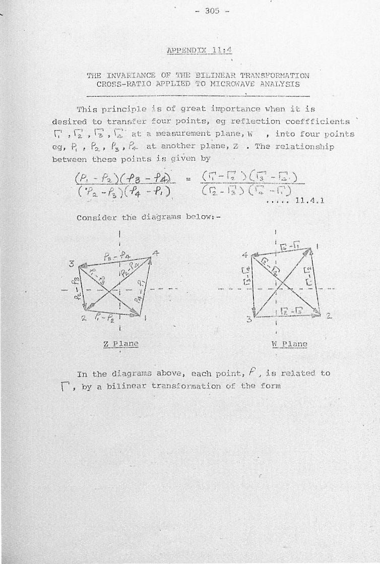
- 305 -
'fEE INVAF .. IANCE OF ~('HE BILnmA:f~ 'l'R\ 1~;FDRt"'J·~.'rIOF
CROSS ·-f-<AT·I O APPLIED '1'0 MICRrMAVEl1.NAI ,YSIS
-----.... ~--.-.-... - ' .. .. _-------_ ...... _._ ... _- _. ._------'J1his p :cind.plf:' ~. s o f great: importance '\vh en it l' c' . ::>
d esired to transfer f our poi.nts, eg r e f l ection coefff i cients
17 ,f~: ) \~' ~ C .... ' a t: i:i weadurcment plane, \.; , int.o f our points
"'. ~r , ~ • p- , "3 ' 10 .... '-"'~ " r . r at. anot.her plane , Z . The relationship
betvleen these poi nts is 9i\l'(:m b)"
•• .. to· • 11 . 4 , 1
Conside,L 't:he eli :-grarns be l ow' :-
N Plc:mc - --_ .. -
.. , . In the d iagra1l18 above , each poir:.t, I- J l8 r el;:- Jc(:!( t o
r, by a bilinear trci.Ylsfo l'ma·tion o f the f o r m
(

Hence , j'
Cl. \ ,?., .;- b --... -~ ... ---. ..., C \ 2 . + c""
P .- to I 2.
c:. 1--;' + cL
:: ... .." --, ~ ( c r, .y.. cl ) (c ~. ~~ (j .. )
• • . b C' \-1 P -Pz. i_a.d .. _..:._.~:.lJ_\ .-=-~. - ( c r.' + d )( c.r;,l + 0.. )
\ - "" ( 1.1.4 . 2) 't •• , •
Similarly it c an be shm·Jn tha t
n
- ~r J cu:L -=-~~2:....1.0:3 .: (; J. 1'-3 .. ( c\3 + d- )( c.r~ ·+ rJ., )
· , . , . ( ,.. 4. 3 ' ... .t. • .... . )
, ... , ;-1 .
f ';l. - P:~ J o..4!... - bC: .. J __ L\ .. ~ - 13_1 _. ( c:. rz. + d- )( c. r; i" c.l )
· .. . . ( J.1 . 4.4)
(-, rOT ~_ - P, .. i o..&.-.~::~J~~'4. --=-.'.-..J.
( c r: + ci. )( c.r; + d .. )
· ..... ( .. J II \ 1 . • -->: , :;',
Dividing equation 11 . 4.2 by equ3t.:LOn :1.1./1.4
. .
(1 1 . 4 . 6)

- 3C)7 -
Similarly div iding equation 11..4 .3 by 11.4 . 5 gl.VCS~
. .
. ... ' .. ( 11.4 7)
Finally mult!plying e~l ations 11.4 .6 and 11.4.7 together
gives:
"·Thich is t'h,e desircd resul-t of equation 11.4.:1..
* * * * * * * * * *

- 308 -
PR~R]lJvlME FOH HEFLEC'frON COEFFICIENT COrmECTTC~ USING '[HE 3 SHORrr CIRCUIT METHOD OF SECTION 5: 4 • 2
------"----------------------------
This appendix provides the m\"lchine code programme for operation on U'le Hewlett P acJcard P rogrammahle calculator
HP91'00'e. The programlne accepts the three short circuit calibration measur~~mepts in its polar form (modulus and angle
\
in degrees). ' From tht s dat.a, it calculates, stores and prints
out the error correction networle in polar fonn. T11(7
measured 'reflection coefficient is then entered i11 polar form
and the corrected result is printed out as:-
( a.)
(b)
( c)
a
as as
reflection coeffi.cient. normalized to 50 ..Q,..
an impeda.nce in polar form
impedance ,
rect.angular coordinatGs. an ~n
;" ,
"" 't f h ' Due to the ll.m~ ten capacl. Y 0 t. e machl.!"1c the pro'gram.r.ic
was writt.en' j.n four sections (2 magnet.ic cards) . and '-!as ,fed in sequentially as the C(llCllla1::.ions'proceeded and add.itional
storage bccamc~ available. The lengths of t.he off-sets al so . '
had to be preset within t.he progra.nl111e. However, the pre~set lengths can be easily altered.
To minimise the possibil.ity of any typhographicaJ. error's,
the progralIDlle is given directly from the act\.lal print-out from.
the Hewlett Packard machine. 'I'his print-ont uses numerical
codes to repreS(::l':i.1t:. the machine instructJons. A conversion
code i s given in Table 11. 5.1 to C0l1vert tlie nmn(;!rical codes
to t.he Jcey or roachine instr'Ucti0l1S. "

- 309 --

- 310 _.
-,
~t:p -~:~:-_.--:--_. I
~od~l ~ite; ··~~~de ] s'tep COUE!' step ---.---- ----. 0.0 ••• ~.20 3.0, •••• 17 ,;
6.0 ••••• 00 0.0 ••••• 47 0.1 ••••• 41 3.1 •••.• 33
.; 6. 1 ••••• 27 0.1 •• t • ,16
0.2 ••••• 4.5 3.2 ••••• 40 .J 6.2 ••••• 02 0.2 ••••• 27 0.3 ••••• 27 3.3 ••••• 16 I 6.3 ••• ".65 0.3 ••••• 64 0.4 ••• ~ .07 3.4 ••••• 41 " 6.4 ••••• 60 0.4 ••••• 34 0.5 .... .. 2! if 3~5 ••••• 45 " 5.5 ••••• 61 0.5 ••••• 30 0.6 ••••• 02 v. 3.6 ••••• 45 J 6.6 ••••• 63· O. 6 •••• " 1)5 o .7 ••• ~ .00 " 3.7 ••••• 22 " 6.7 ••••• 74 0.7 ••••• 60 0.8 ••••. 00 ,; 3.8 ••••• 15 ,j 6.8 ••••• 66 0.8 ••••• 17 o . 9 • ; • • • 00 1 J 3.9 ••••• 34 " 6.9 ••••• 22 o .9 ••••• 30 O.a •• ~ •• 36 ./ 3.d. ••••• 31 vi 6. a ••••• 10 O.a •••• ~17 0.b.,.~.40r 3. b ••••• 33 " 6.b ••••• 111 O. b ••••• 64 0.c~ •••• 13 I 3.e ••••• 17 " 6. c ••... 14 O. c ••••• 34 O:d:~' ••• 03 ./ 3. d .•••• 33 6 .. d ••••• 30 0.d ••••• 3D 1.0.' .••• 06 .; 4.0 ••••• 40 'I • O ••••• 14 1. O ••••• 65 1.1 ••••• 00 '# 4.1 ...... 17 1 7.1 ..•.• 6·4 1.1 ••••• 60 1.2 ••••• 33 " 4.2 ••••• 61 7.2 ••••• 34 1.2 ••••• 02 1 .. 3.' .' ... ' .17 " 4. :3 ••••• 63 7.3 ••••• 30 1.3 ••••• 30 1.4 •• ' •• ~ 0], I 4.4 ••••• 13 7.4 ••••• 65 1.4 ••• f .13 1.5." •••• 26 v 4.5 ••••• 73 7.5 ••••• 60 1.5 ••••• 36 1 ,·6 ••••• 32 ( 4.6 ••••• 62 7.6 .•••• 16 1.5 ••••• 01 1.7.· •••• 11 " 4.7 ••••• 65 7.7 ••••• 30 1.7 ...... 65 '1.0 ••••• 23 I 4.8 ••••• 50 7.8 ••••• 16 J. .8 ••••• 60 ·1.9 ••••• 15 .j 4.9 ••••• 13 7.9 ••.•• 64 1.9 ••••• 6J. 1. a ••••• 41 I 4. a ••••• 27 7. a ••••• 34 1. a .•• It .63 l..b.',;. •• 45 -I 4.b ••••• 01 7. b •• t •• 30 . 1. b ••••• 74 1. c •• ••• 22 ./ 4. e ••••• 65 7. c ••••. 65 1.e ••••• 66 1. d. " ••• 15 J 4. d. , •.• 60 7. d ••••• 60 1. d ••••• 32 2.0; ••.•• 34 " 5.0 ••••• 17 8.0, •••• 61 2.0, •••• 22 2. 1 •• ~, .', 31 ,j 5.1 ••••• 27 8.1 ••••• 63. 2. 1 •• , • •. 33 2.2.' •••• 33 J 5.2 ••••• 64 8.2 ••••• '"i4 2,2 ••••• 24 3.3.t •• '.li .; 5.3 ••• , .34 0.3, ~ .•• G6 2.3 ••••• 11 2.4 ••••• 33 J 5.4 ••••• 30 8.4 ••••• 31 2.4. t ••• 30 2 15 ••• 'f .40 .. I 5.5 1 •• I .65 8.5. 'f ••• 34 2.5 ••••• 22 2.6 •• ~~.14 ./ 5. 6 ••••• 60 I 8.6 ••••• 24 2.6 ••••• 34 2.7 ••••• 41 I 5.7 ••••• 14 8.7 ••••• 11 2.7 ••••• 14 2.8 •• ~ ~ ~ 45 .; 5.8 ••••• 27 ·8.8 ••••• 31 ·2.8 ••••• 27 2.9 ••••. 22 ./ 5.9 ••••• 64 8.9 •••• ."30 2.9 ••••• 64 2. a ••• ~ • 15 " 5. n ••••• 34 a.a ..... 34
1
2. a •••• • 3l 1 2. b ••••• 34 ..; 5.h ••••• 30 8.b ...... 47 2. b ••••• 30 2fC ••• ;~3l ./ 5. c ••••• 65 8.e ••••• 47 2. c ••• , .66 I
2.d ••• ~.33 " .5. d •• ••• 60 8.d. ~ .... 4~J 2.d ••••• 60 I --
..

t'
1 III 'Ill
step Code 1 3.0 ••••• 16 3. 1 ••••• 30 3.2 ••••• 16 3.3 ••••• 64 3.4 ••••• 34 3.5 ••••• 30· 3.6 ••••• 66 3.7 ••••• 63 3.8 ••••• 61 3.9 ••••• 63. 3. a ••••• 62 3.b ••••• 65 3. e •••.• 60 3.d ••••• 13 4.0 ••••• 30· 4.1 ....... 13 4.2 ••••• 33' 4.3 •••• ,,01 4.4 ••••• 65 4.5 ••••• 60. 4.6 ••••• 61 4. 7 ~ •••• 63 4.6 ••••• 74 4 .. 9 ...... 66 4 • a ••••• 60. 4"b ••••• 16 4. c •••.• 30 4.d ••••• 16 5.0 ••••• 64 5.1 ••••• 34 5.2 ••••• 30 5.3 ••••• 66' 5.4 ••••• 63 5.5 ••••• t7 5.6 ••••• 30 5.7 •••• ~ 17 5.8 ••••• 64 5.9 ••••• 34 5ta •• '. ".30 5.b ••••. 66 5.e ••••• 60 5.d ••••• 61
Step COd~ I 6.0.' ..... 63 6.1 ••••• 62 6.2 ...... 65 6.3 ••• ~ .• 63 6.4 ...... .24 6.5 ....... 11 6.6 ••••• 25 6.7 ••••• 62 6.8 ••••• 65
. 6.9 ••••• 60 6.a." .••• 61 6. b ••• " .63 6.e ....... 74 6. d ••••• 45 7.0., •••• 66 '7.1. " ••• 23 7.2 •.•••• 17. 7.3 •••• .,40 7.4 ••••• 11 7.5 ••••• 60 7.6 ••••• 16 7.7 ••••• 27 7.8 ••••• 64' 7.9 ••••• 34 7. a ••••• 30'· 7. b ...... 66 7. c ••• t. 63 'l.d ••••• 61. 8.0 ••••• 63· 8. 1 ••••• 62· B.2 ••••• 65 8.3 ••••• 60 8.4 ••••• 13 8.5 ••••• 27 8.6 ••••• 33 8.7 ••••• 01 8.8 ••••• 65 8.9 ••••• 60 .8.a ...... 47 8.b ...... 47 8.c ••••• 47 8.d ••••• 46
- 311 -
_;':;:=~Od; 1 0.0 ••••• 47 0.1 ••••• 61 0.2 ••••• 63 0.3 ••••• 74 0.4 ••••• 66 0.5 ••••• 63 0.6 ...... 14 0.7 ••••• 27 O. (3 ••••• 64 0.9 ••••• 34 0'. a ••••• 30 0.b ••••• 66 0#c ••••• G3 0.d ••••• 17 1.0 ...... 2'7 1.1 •• o •• 24 1 .. 2 ••••• 11 1.3 ••• " .40 1.4 ....... 17 1.5. It •• 60 1.6. to •• 61 1.7 ••••• 63 1.8 ...... 62 -1 ~ 9 .••••• 65 1. 0 .• •••.• 60 1 . b I • t •• 14 1. e •..••• 27 1. d ••••• 64 , Z.O ..... • 34 ll. 2.1 ••••• 30 2.2 ••••• 66 2.3 ••••• 27 2.4 ••••• 24 2.5 ••••• 16 2.6 •••••. 25 2.7 ••••• 27 2,8 •••• t 64 2.9 ....... 34 2. a ••••• 30 2.b ••••• 66 2.e .•• " .• 31 2. d t' ••• 34
step Code
3.0 ...... 26 3.1 ••••• 22 3.2 ••••• 34 3.3 ••••• 31 3.4. , .... 62 3.5 ••••• 66 3.6 •• , •• 63 3.7, •••• 61 3.8 ••••• 63 3.9 ••••• 74 3.a ••••• 45 3.b ••••• 66 3. c •• r' .60 3.d ••••• 23 4.0, •••• 16 4..1 ••••• 00 4.2 •. ~ ••• 27 4.3 ...... 01 4.4 ••••• 60 4.5 •.•••• 61 4.6 ••••• 63: 4.7 ••••• '52 4.8 ••••• 65 4.9 ••••. 60'
44,;a· .' ••.• 140
'1 • b ••••• 3
4.C ••••• 14·· .. ·II
. 4.d ••••• 64 5.0 ••••• 34 5.1 ••.•• 30
.5.2 ...... 66. 5.3 f •••• 24 '. 5.4 ••••• 11 5.5 ••••• 40 5.6 ••••• 14. 5.7 ••••• 34 ' :'.8 ••••• 30 '1 5.9 ••••• 24; S.a ••••• 11 5.b ••••• 31: r-: 24~ :".c .. -. .. S.d ••••• 17
t _____________ ~

st;,p cOd:') 6.0 ••••• 32 6.1 ...•. 30 6.2 .•••• 33 6. 3 ••••• 30 6.4 ••••• 22 6.5 ••••• 62 6.6 ••••• 65 6.7 •••• 160 6.8 ••••• 61 6.9 ••••• 63 6.a ••••• 74 6. b ••••• 45 6. c ••••• 45 6.d ••••• 24 7 .0 ••••• 14 7 • 1 ••••• 30 7.2 ••••• 24 7.3. I" .11
. 7 • 4 ••••• 30 7.5., ••• 31 7 • 6 ••••• 63 7.7 ••••• 41 7 • 8 ••••• 45 7 • 9 ••.••• 66 7. a .••••• 60 7.b., ••• 61 7. c ••..• 63 7.d ••••• 62 . 8.0 t· t ••• 65 8.1 ••••• 63 8.2 ••••• 24 a.3 ••••• 11 8.4 •••• ,30 8.5 ••••• 24 8.6 ••••• 14 8.7 ••••• 65 8 t 8 ••••• 60 8.9 ••••• 61 8 I a ••• ~ .63 8.b ••••• 74 8.c ••••• 47 8. d ••••• 46
Gte~'~~_ 0.0. It ... 47 0.1 ••••• 65 0.2 ••••• 60 0.3 ...... 17 0.4 ••••• 27 0.5 ••••• 16 0.6 ••••• 60 0.7 ••••• 61 0.8 ••••• 63 0.9 ....... 62 O. a ••••• 65 O. b ••••• 63
.0.c ••••• 13 O. d ...... 27 1.0 •.•••• 07 1.1 ...... 21 1.2 ••••• 02 1.3 •• I •• 00 1.4 ••••• 00 1.5 .•••• 00 1.6 ••••• 00 1.7 ••••• 35 1.8 ••••• 27 1.9 ••••• 6l
, 1. a, •••• 63 ·l.h ••••• 74 .. 1.C!.~ ••• 45 .1.d ••••. 45 2.0 •••• '.66 2.1 ••••• 60 '2.2., ••• 23 2.3 ••••• 17. 2.4 ••••• 40 2.5 ••• ;, .16 2.6 ••••• 00 2.7. I ••• 30 2.8 ••••• 01 2.9 ••• ~ .60 2.a ••••• 61 2. b ••••• 63 2. c ••••• 62 2 .. d •••• ,22
- 312 -
step Code
3.0 ••• " .23 3.1 ••••• 14 3.2 ••••• 05 3.3 ••••• 00 3.4 ••••• 36 3.5 ••••• 17 3.6 •. ~ ••• 24 3.7 ••••• 16 3.8 ••••• 63 3.9 ....... 00 3. a ••••• 30 3. b ...... 01 3.e ••••• GO 3.d ••••• 61 4.0 ••••• 63 4: 1 ••••• 62 4.2 ••••• 65 4.3 ••••• 63 4.4 •• ,' •• 25 4.5 ••••• 16 4.6. ~ ••• 65 4.7 ••••• 60 4.8 •• tf .61 4.9 ••••• 63 4.a ••••• 74 4. b •• l •• 45 4. c ••••• 66 4. d ••••• 45 S.D ••• t .23 5.J. ••••• 17 5.2 ••••• 40 .5.~3 ••••• 16 5.4 ••••• 00 5.5 ••••• 52 5.6 ••••• 07 5.7 ••••• 10.
. 5.8 •.••• 50 5.9 t to •• 07 5.a ••••• 10 5.b ••••• 47 5.c ••••• 47 5. d ••••• 47
step Codc~
6.0,. •••• 47 6. 1 ••••• 01 6.2. ' •••• 30 6 ., .lq
• .J • •••• 3 ...... 6.4 ••••• 14 6.5. ~ ••• 35 6.6 ••••• 56 6.7 ••••• 35 6.8 ••••• 02 6.9 ••••• 35 6.a ••••• 47 6.b ...... 47 6.e ••••• 47 6. d ...... 47 7.0 ••••• 47 7.1 ••••• 00 7.2 ••••• 44 7.3 •••• ·~lO 7.4 ••••• 06 7.5 ..... • 4·' .7.6 ••••• 47 7 .7 ••••• 47 7.8 ••••• 14 7 • 9 ••••• 35 7. a ••••• 02 7 • b ••••• 35 70 c •••.. 56 7 0 d ••••• 35 8.0 ••••• 47 8.1 ••••• .47 8.2 ••••• 47 8.3 ••••• 47 S.4 •• #0.47 8.5 ••••• 00 0.6 ••••• 45 8.7 ••••• 45-
. 8.8 ••••• 45 8.9 ••••• 46
L ____ • ___ .. J

_. 31:-s
("T [I/DED ~!V~t-.' VFflSll: t ; ;"),'1 ! fi r:: /, I t( J I , ,( R 1 , K r ?, K H 2} ¥. i ~I , t< n J , K 1 .. ) j( R I • • ' I: A '. , K R 'I
:> (1£:.41 MA r,t'f[; , M.C.II!::!; 3 r. E /> I MAr; S 1 ~ , 1:'/; r, 5 I 1, ~I" r, T I~ S,N r, TI~ ;; I Ii A G S ?:' , h , G !> ;1 ? I t' ,'. G." L 1.. I
~ rf,llG ':,l, F;H:~ 5 I< E /, I F I () t' F (i Ie • P sri r 11 E T I, I ~i 1 J ,~ H J X I • >: f{ } I: t, ! .' ,( il " , I-: I, 2 I ~: p. 2 I K I, 3 , K f I ~ , l: ! I e ,I 6 r O t~ PI £ X ~ I A " C I D J KIf K 2 If::l ,,(1, 1\-1, X J S 1 1 , S 21 S 1 ? • S 2 t! J r V t, l. uE
7 100 CO~T1NUF 8 II EAli (ln S, ?COI F' dUd . • I<Bld(A2J!(f'l2 , KA3d:'13 / K A",,:e,'1
. 9 !OO FeRMIT ( 9tl 10 IF( F .f.>l. 0.0 1 S'T'GP it A" r.,..PL>: (\. 0, 0,01 12 C11U;t. " c.C'l'J80 B?S l ~. r 13 !-' 51 0; .. 1' . 0 '" (HlfGA L~ ' THE TA u c.\ ~561650 • F l 5 fll .. I. (I , . !'i Pi (C', M r. G I.)
16 'OR", 1-n " C(~ S ( e ll En /II ~i' 0 .. rr1PI. '): (Il R .CI) 18 1<1 .. 1.· 0 If- Slt~ ( Pr.I1 1 !I h 1< .. 1; () v r: r. SIP 5 I I ~o w ,. r.,1PLX 1 \./11 ,1 / I I c t ): 1 " 1· rt .~ ~ T N ( 1' ;, c. r 101 22 r.H .. 1.(1 " Ct'SIH1E'f U :?3 ~ .. r:11PI)I l(P /X I ) ~'" I~Bl "K!H ~\ 3 .1 4 15~li'6/\ 8 0 i'li r.) 1 IJ I< h I 4' S J I' ( f:l'l l )
b2 63
I< R 1 " I: ,1.1 ~\ c: 0 S I K n I I )(1 .. C I',P I ;~ finn. K 11 l ~B2 Q KR? 4' ],1~159r6/1no KJ~ • K'~ .. Elh l~ n2l KR2 n KA? ~ r:C S I I<H2l r.2 .. Cl'IPI. X ~~:H21 ,,[;» roB3 1: 1'\3 ,',1 301. I, 159?.611g0
Ii 1:~ .. I( h:'l . ' 5 J I; I I( O:l ) KA3 ~ KA~ • rO S I I<D3 ) 1<3 " C:-;P I ;< (KR3, to:1::! 1 I: U'I " K n ~ .. a oil, l S 92 I'> I i 11 0 r.14 " ~h~ • SI~ ( ~R4 1 r.R' ~ KA4 ~ rMS( KB~ )
K ~ .. CMPI x r I<R I ; I 1< I 4 I n g KI.~?~(W·A l -K2~K3'(X. A) Kl ~K3. r WnX!
C ~ ( N·Alo ( K?-K3 ) ·(XMA l ~(K2 K\J 511 SIC S 22 " l !'i 1 1 R 1<1 oj- O{ 2 S U ) I III " ( I< 1 •• )( 2 ) S e l!>12 1> ( £ll "' I<\Hqh+~??) -,V/.J lJf: .. I V-I) • 5 11l/I S?~ IJ 1<'1 ~ . Gi?IS1? .. !';11 .. , S?;:>,
• 'F Rl:rJ rI F I ~A G~\ 1 .. CAAS (!)U) ,..tiG.dl .. !~7 .r !J57r. " AT!dO??(Alllh(l{51~)JnE/.I.(SI1))
I~ II G T " S " C A II $ I E; 2 1 S U! I "'~G lI~ S .. ! i' ,? 9~;7l) u Iti/>N2tAII1hGIH21G121/nOU S2 1S 1?11 ~AGS? 2 ~ C6A~ 1922 1 ANGSI' :~ " !i :> , ?95 7 B Il /, T.l. li/? {AJM AClI SZ21.iiE /,L!!l2211 ~AGV.L • CARS (T VALUF I 1,I~Gv~ L .. H7.,"!''37'' " Al'''N~{/,I11''G(T\,ALUE )/ f fI.L ITVALIl ' I I MAGMFS w ~. RG ( K~ I
ANGHf S ~7 . ?9S7H.ATAN?(AI HAGIK ~ I, "EA L( K' l)
f1Ulr'IIT (I cr.) Flccn , I~/, r.f;l \ I AI\G~ 111 IIA OTH , f.r:"""'5 ~ 11AGS~? rl>lIGs?? , I-A"VAL , ANGVAl
OUTPItT I \Ci\) t'AGH[ S, IdWKl,: S lUTi'lll (\ ~I\ l K!.l. fHdCI>2d<H2d;le3.:<C3Jl·A4,';1'\1,
Cie i ". l ()O
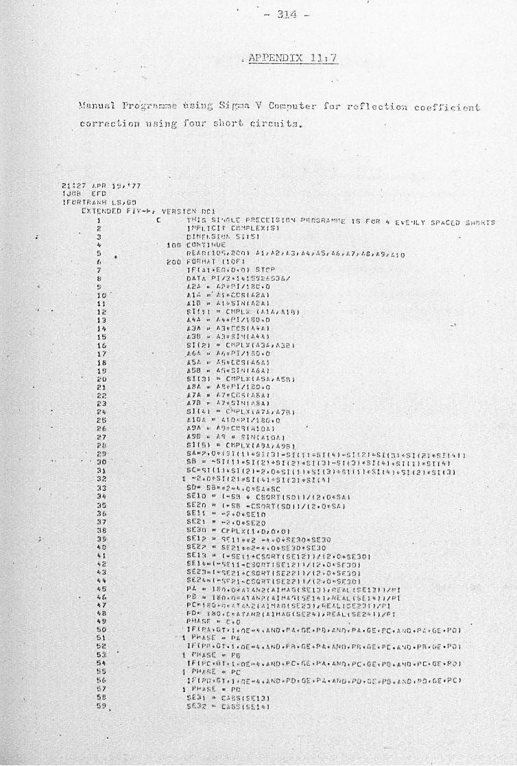
;
~
; ,
- 3 }A -'
j\P_PENDTX 11; 7 -_._---------
co r rr!C '\' i OD 1J:ri n g f our she rr. ei r cl.li t s .
2. : <: 7 I . P i? 1 9 I ! 77 ! J r:1i:l EF(l ! rt;HIT f~ t.t H U; I G (I
EXTENDE D FI V -~, VERS 1CN DCl I 2 3 h 5 • (,
7 n !J 1 () -11 1 2 13 '-If S.5 1 6 1 :! 18 19 2 {J 2 1. ;~ ~
<:3 ,! 4 25 ?r: 27 ~IJ
29 30 31 ~~ .,) t ,.
n 3 /• :i5 3(, :i7 38 3'9 ItO II I 4 2 1,3 H 45 "'{. "7 ', ll 4 9 !:>o 51 5f! 5 '" 54 !; 5 ~(,
'- "I 5 8 ~ 9
C ,'H I s Sl',r:U: pr~ SC E rSI() '1 p:-;r:GR'\'" ~ E TS F e H I, !: v ::'ILY 5P(,CELJ )W Ri5 I MPLTC l r CM~P LEX ( S I
CIt' FI. Sl'Jh Sr ( 5 1 100 ·COt-<"{) !,u t:
"EA n r l U~ , 2C 01 &l,a2.A J "" A5 , A6.A 7. lG,h 9" ,o 200 ;.:O M'11> r IIO F I
TfIAl. [Q .O.(i) ST(' P OATh pr/2~1~1 59~65 3 6 1
AcA • £ raP I /I S O. Q 1'.1 /. ",' . i ~ C C SIA2:' 1 Al0 ~ A I ~5 rN ( A 2 Al
!lI!lI " CI1PL X ( Alt. JA l il l AltA • A~.PI/\80 . 0
A3 A u A], reS ( ~~A I
~ 3B • AJ .R ! ~ ( A4 A)
S II ~ I U C I~P U I I :\ 3 /., ,',38 I t 6A • A~ .PI /' R0 . 0
A 5 ~ M £~ ~ C e SIA 6 Al ft~B • A ~ ~S I~ I A 6A I
51 13 1 • CM PLX I £5 a.A 5B I ABA A~r r l/ 1 0 0 . O
A7A • h 7 ~ cn~ r A6 AI
A73 ~ A7 .S INI A8 A) SI I ') « C~P L ~ \A7 A / A 7 a l ~ 1 0 A " 'ID ~P I / 18 0. C 1\910. " " ')··,· C r. ~f h! Cl f. ) ASS. Aq • S I NI Al OA) 51 1&1 ~ CHPLX(A 9A I A9B l SA .. ? • 0 '" I ? r I I 1 '" s 1. I 3 I - S i I I 1 .!i r I 4 1 ~:; 1. ( ? 1 >" 5 i ( :3 I .. S I f 2 I '" s rI '. 1 I 58 u -5" , I . SI ( 2 1+S 11 2 1.s r ( 3 1-S 1t 3 1.S It 4 1+RIl l l ¥S rt AI S C" .... ;1 ( 1 I ~ S 1 I 2 ) "~~ .0 ", S I I 1 I ~· s r i 3 1+ S \ I 1 I (. f; t I Ii ) i · S I I 2 ) .. S I f 3 )
I M2 .D ~S II21 .SI(~) . S Ir 3 1 .S [ I" SD ft s a.~2- ,.C .SA~ GC SEl.o '" ( ~S fl ~ CS OHT( SO ll/( ? .O -l'c,A l SE2n" I wSA ~ r.!lr)n T(SOII/ ( 2 . 0c. 5 "1/ SEt , .. "j? O,.S E10 S E2 1 .. ' ';! .O . S £2 0 SE3 n • C~PL X I\ 'DJn ' OI SE 1? • q ~ 11 .~ 2 -~.O~SE 30 .SE30 GE2? n S ~2 1'e 2.4 . 0 .SE3 0. SE30 S£l ~~ ,. I · SE 11."C Sr. ~T ( SE \ 2 1 111 2 .0 "-5 1-: 3 0 1 5£1 4 ... I Qr.; '- l l"C ~O'lf I SE : <: I 1/1 2 . J ~Sr30 I 5 £ 2 :·1., ( ~ <;r. 2 1 +C SO 101'( ( S E ~ 2 j 1/ I 2 • 0 "S€ 30 I S f. (~ 4 .. ( w <is: ? \ ~ C GO R i I ;, £ 2 2 ) I I ( 2 , 0 ' ,S J::3 0 ) pl ... U! t").O ~'A" ,. N2 (A l ~.\GI SE: l 3 )' P. t: t. L ($r13 1 )/ P! ,, 9 ,. l tl Oot1'; f\ 1 <l1-? ( AIM .r. 'lI -:i£ l', J/ kf.Al I Sfl" 'II P t PC ;" I iJ v • Il ' t, " I." j ~ ; .\ I ~1J. n ( s ~ c:3 I I r< E I.:. I :j S ?;l) 1 / r 1
. pO ~ \ ~O. C'A r ~ N 2 ( 61MA G t SE24 1/ REA L( SE2. II /F r flItA .r; s: " C .O
. rFI PA.GT'I.nEM,.A ND. PA. nE. PQ . AN". PA.G E'PC • .\~ C .p~.0E ,r D I \ Pk A~£ .. "1. Ifi pn .Gt . l . O E-4.A NO. PR .GE .PA.~~n . PR . GE . P C. A ~O . p~ . Ui . ro I
t. r'J 1 105€ .. PG TF t I-"C "iT, 1 .n:-;'~4 <I"'~ D . PC . r: t=. . 1> >\. A ~I !'). PC .Gt: . f'O . A"I() . PC. GE . PO I
1 1"14 ,1<;<: .. PC I F I Pf)'4 l'l . n c: ... II. I.ND.F' O.GE.P; •• hlifJ.(>() . J·~ P& A:\c.pa . f<E . ?C l
1 PI-' ~ .• f. .. r r. DEl ) • CABS I SE l l l SE3~ k C~B~ I &~ l ~ '

60 6 1 6 2 G3 6 " 6 ~
(,6
6 i (, 8
6 9 70 7l. 72 73 jllj
75 16 77 "18 79 no 8 1
B3 II .. I.l!'i 8& 87 fll; as ~)O
91 92 53 94 95
..... ,
S£3 ~ • C &qS I S~21 1 U ~3'l u C~~S ( SE 2 ~ )
t . rT F I.'.I '" \ (j
315
l r: (;' ... A ~':: .F O , f1A l " TT r:I U u SE::' ! " F : Prt/\ ~:"· , F: r;f rd ) :. TTC:! lJ ~ ~[32 I F I Pf. ... S>:,E r.~ . pc u. TrFIIL' ., St:-l3 l F I PH(\!j:;.· .• t-: f: .. Pi» ) h 1 1· ~· dJ ~ f,t:~ ' 1
PH AS~ n r 4A~ [ ~ P I/1 60. 0 li !;C.. :, r rF :Jl J "C :".1" l. x ( C ;~ s ( p ~ h S El l S I 'I ( i'f<l. S [ I I !.51", C: 'PLX tc rS ( .. r ·'-IASE 1, ':~i t j ( FHA~;E l )//O T TO'o\1 ,,','1 -,. I S! I I I • fl r ( 2 I • ! S 5 1 - S E 3 () I 1 - ( S r t 2 I .' S r ( ) I I ' ( :;;; 0 u ,; F 30 I I
t "' ( S r31 ~ st ( . i~1 { S5 1 4S50 1 )
S /!2l' ! S! 111 " t S5C-"SE301 ) ~ ( S 1( 2 l''1S<; ~ 550 ) H· (S I( ~;:';· ( SE30 - 551 1) 511 .. 5 '. 1 /,,'-2 SGAM • C ~PL X ( ~ l 0 . 0 . 0) S 2 2 \ " I S 5 (I " ( S 1 ( 2 ) u S 1 \ 1 ~ . S 11 w G l til f I I S r ( <: 1 - [.; I ( 1 ) 1 S2~ n S;>2 1/ S GJ"· S )r ?1: . ..: ( G:{!, .. S 1 1 ) 1 .. ( G[3C"'G22~S(i4r-i )
S 12 S? 1 • S l~2l \/ SG' H - . S J (. .. ( S I ( 5 I .. S 1 1 I I I Sf!?".. g I ( !i H S 1 (' S? t •• s 1.1 ~ S;> ~ )
/, 20 .. C t" S \ :5 ! (, 1 ... ~ l .. 1. !'.C.C ... HA t l?( h I Mt.G ( !'I 6 I ,RE I. U S16 lI /P l Z E P F I~ S '" "L ,H; ( t, r TF. N U ) r LGE Q P HA SE 1 80 . 0 / r I DUT PUf(: CR l SA , S~ , SC I SD / SE10 / SE2C,SEll / SE2 1. SC13 , SE 1 ~ ,
1 5E ;> 3 . SE?~ / Ph.~B . PC . P D
() U T Pu r l Ie a l S I I 1 ) I S j t 2 l , £ I ! 3 ) I [. r ( I, ) , 5 I ( ':) I , S 1 6 I ,\ T T f. NV I "~/. 5 E (1 U T P LJ r ( 1 C B I S 5 O . !; 'J t , S I I I S 2 2 1 1 S 1 ? 2 I 1 , ,.; G 1.11, S 2'2 J S l 2 S 2 ! O Ll i PlIT( 1(, 8 1 All A? ~:,J I A4 ,1, 5 , 1, 6 ,A 7 , ,1.1'1 . 119 , "' !. O /jUTf-'l;T ( \ t il) S Z6 OUT pUTl leDI 62 C. ft2 1 DUTP UT(I Ca , lePERS tl U1 PlJr I' C: 13 ) ',I, 1 ,542 Gll H l lO(; sTep END

31f
APPEl ~)IX 11: 8
H ) rT'O ~")l-t"> .":lJ',Ir.. \', D0~:l)1 e Pn~c:i ;lion ) ,.,n.)1ua , , , t. '"
[):rCNOEtl ;:) 1I"f'" YEr..S 1 ell n ot rt-i Pt ;CtT r/F!,: .1tB :.t, B,c,n ; L . ?1
2 TMP I rUT r:::~!JU:Y. .. H.rS I 3 (In' 1'' 0:; 1 ~1, >:r (1 5) 1; '
5 , (" " " ' , ..,
Ll '-9 ',. ,
1 () :' '11
1 r,' • '\3
:V,~ t 5" '1~ 11" ," n;,: 19
'elF 2( '~Cf., 2:(
" c ~ " 25
" 2{;. ,' . '1'7
' ;.~ -": . ~ ?
',30 ' ' :41 ' ,~;'l' rho "31>;' '3 5" ::3'6'. :ri J!f 3~
' ~O ' , t;'-' . 4-2-: ~:r"
~ J,~
I;T;-47 ' S' " "'9
- 50'~
fi 1 , S" 53
' ~~'
55 !5(.
!l7 58 59 60 61 b i! '
100 [ e~ i"r! ;U~
n F. .... !) I lOt, , ? C fl 1 A 1 , ,I., 2 I- 1.:._ ":~ ,. A .... ~ .... 5 , 4. 6 , I .. j ' , .• ~" I J.. 9 I I .. t 0 ~oa FOi" IH Y ' : \ :1" I
TF! t i .E:).c) .(H~DO 1 ST!'!:> . 1l~,T'\ Py I ~ .jl; 1 ~'~ » ( . !i3SRC;·/ 9nO I
/'.i:! I", "f,2+Pf / 1 .1I0C;)
~: A . Al~ncn~(.2hl A H3 .. A I"' os {I. ( Ac,\ )
R 1 r \ I ~ Dl": '" PI. Y. ( "'. /" 1113 1 h4A.A ~.P T/I. gOC~
~3~r ~3~nCBR ('~&I ' /,38 ', 1.3~, n c: TN (~ 'l-4 )
GII?)~Dt~P(~IA2~.A~ B ) h(; (.,,,,:.(,.',,;> T II .POu?
' ~5An{5 ~nrn~ l ~~~ )
,1.58,,(, (;"11'; I~. (I. ('A)
SI!'! "D r:I-'PI. . (AS, .. AS8 1 AgA"t.~ ;;.Pt II .)lOC:>
- A7/,"A7":lCfl~(t,f:t:. 1 11 7e I\A71;· rl~TI;(Ail/') .
.. 'n t { I, I "0:: 1' ;,'1 ):1 1\ '/I. I A 1 !H I.l Ch .. ~1rj"PT II d l (l1'l2' ~ 9k~A9~n(~5 !~1 0t. 1
1\ 9 r. "b !J .. (')", j ! ~ , A to :. I
nII',\ "'D("nrl '\:If.'JI,./.Si\\ f.~:lf') .. OCIIPL)c II. v.DO , O.ono I , sA .. ;>, 0 <' (S ,T ( !! ~S 1 ( 3 1 .. S T ( , I ~' s 1 1 It I ~~ I ( ?, ',< :1 ) , :~ \ +S', f?) ¥s r t ) I
-, S e.. B T ( \ I , 5 ! I,;' ,' . , ; ! ( ;:; , ":' ! I 3 1 ~ S T ( ::l ) < S r ( 'I I +;, r I 1 1 "s I : 0'1 )
!':: C" H t: Ii) ,,; s'! t ;> J":' • n ~ crt! ) '" C 1 ( 3 ) ~!'; r I 1 ) If. !: \ I; 1 + S r ( 2 ) .. S I , l , i -2 . ~ ~ S' ( ?I.Sl(~) .SI ( 1 ) .Srt~1 'APe SH~v'-~.C.SA~SC SC:ln " (qSf1 0} CO . (lHT t S I)I ) /I?'.O"S& I SEeD ~ ( -SA ' u · CDy ar T(Sn) 1 /12.0.~61 SE'11 " ":>.OKSE II
' r,Ei.!t OJ ,- ? .(l" ~I~? 'l
SE30 " ntI1 PI't l l, .OOOOo . O.OOO;)Cl)
!1Eli' u !~ r. ll .... 2 "4,O "S~::ln'.f.=3n SE2i » SF?I~.2 ·~.O'SE~o.sr 0 9 t' ~ N I -SE lt • CDBDAT(QrI2Il/(?OcSE301 • E14 .. ( .. El[:\ \ •• Cc\!'irlR)'ISEI?11/(?n'S C:>0 1 9~2l ~ (~ aF? i + CD90qTISE22 1 ) / t ~.O.~E30 ) SE2~" tw~, r.;.' , .. C(H;Pi~r (C;(? ? )I/t;~.()'IISClOI r.\ .. 1·" c: r; ? .... /1 A j hI~ 2 l or ~ A ('j ( S E 1:< ) J il R .:. to LI 5 E t 3 I I I P r pA " t. RCn?nATAN2 I DIMAnr~Cl_'lnR~AL I5 E \ 'II/P T PC 1.80D~~~ArAN~I01MfnI S~23 )/ O~~il( S F~Jll / pr PO .. ... 8 nr. ?.,n li r I , Nt' I r) 1 Ii I, n ( S r.;:.~ ) I Dr~~ I. L ( S F.'Z '. I : If'! PHAn~ a o.ano oo . t F ( f':" , a', • I , n n «~ • tIl D • P I, • r, E ,p 13 , .\" n • r A • (j [. , (" . h N () •
t I'1l.n E .I> . ) P~H,9(:, .. PA
r F(pn.GT ., .~ ~ ' .4 HD . p~.nE . PA .A~n . p~.GE . Pc .a~ n. I PU. r. c .r'r.) C)IIASr. ., i"1
r F I Pr.GT.I.nnu •• hNo . pc . nE .P A.AHn . rc . nE , PA .a ND. t PC.r::!: t ."nt "VIIS"· ,.. PC .-
rF<rn.OT.'.nn ~. ND .pntnr . p~ . 'Nn.pn . GE.PA.hHn. I PD.nErP~) PN~9r. _ 00 II II CD .~I' r;, ,;:'131 12 .. CIJ P <S(C;l't~ 1
L:~ .. COAP !'ilC;r.<'3 1 til . , ':!)trl ~ ( .. 1='~4 I

63 l>lj (, 5 66 ('7 6F:
69 10
--,7~
/2 'n 74
':"5 '---jt.
:'1 7 '7B
",' ''7!"r.' ' SO fH fie
"03 !II; .[I!; : 86 '87 81.1 '09 !JO
:!ll : ...
92 ,
317
ATT~~U ~ 'Otn ocn !r:-!f"II"s>,n)' '' ,\ I ATT[ '~ lI .. L1 Tf(r>~Jj\ 5 1=.F O .P R ) f'7 1t:NLJ I.? j F ( P I-~ A s ~· . c:r: .' pe l I. T T r: "w " I 3 t r (p r:~s !" .r r..pn)Ari[NI) .. ( .I,
P : 1AsFpP l-i t.Sf :;. "'I/~ .r.o n? I> ~;o <» /. T t r: '" III' DC t·! P L X ( C r. rH: I !' H 1, S r l I r'l~; r ~~ ( f> Hil S F 1 I fiG1, nCt1PI y.(nr. n S{~·PH t.\ 5J:" )J nS] ~ J i "' P~; A S;: } '/CATTrt-.!lJ} .'
' 1)11 .. (!':ltll'l5Yt;>I ~ (S'il"!) E30 1 .. !;Tt~) .', 5113 1 '.' I S !; u', 5 LlO ) \ " I'( :J I <!!::T II lc, (S!51-S5nlI/IST(11 l;. (!' !;, O_ G[3n ~' 5 T {;:-'" ,? C Sf; 1 c o S!': rl I ~ R 1 ( ~l 1 IJ ( fi F ~ I) .. S 5 1 : I
flOA t'. '" nrO'l ;' 1 ~ ( , ,ODOdl.O n U I
, S221 (r,~O,,'SI!?I"Sl' I +SllwSlll 11/( S1(? I M"j't~ I) 522 S??'/~~ (,dI1
-r; 1 c ~' l ~, " t 5 r t 1) S 11 I <, I S C 3 0 ~ S 1:' ;: '" 5 (H H I G12s?l ~ ,,'??11/GGAH
. S H, p , {s v ( !:I 1 ·.51 l I I' ( S ?? 1,1 S 1 ( \:I I ~, g 1 ? S 2 ). u f; 1 1 .. S?? I .~~O t" Cn/. F;~tl~rc, l
.. -tiel •• " . !' n?~f)~'·" N;'> (OI hMI ( S \ 61;DnrAi (S!I'; ;/I'Y :> EPrI? S u ni(\(; (,~"':'Et-:UI
f'l U T P IJ j ( I () Po I ' /. 1 ;i. :' , /. ':,1, " ..... h 5; '.,6 • I:. 7 • A 8 .,. /l 9 I " 1 n J' A'2 0 J to 2 ; flUT P IITt1t':I;1 r,l{, ' .
• (1 Ui P : IT i ~ Ui I ;:; III S f\. S'::. ~~fl, SF. j 0 I !~ r? (), S E 1, ~ .. SI::: 1 • :; E: :~, S E l. I; ,
\ SE?~,SF?_ ,P A ,p n.Pc,pf) .
'- [~ U) PIIT ( I en I h: ( j :, G 1 t ? I, S 1 ( :11 J 5 1' 1 " I, !:; I (!j , .!-i 1 6 1 An £ I<\JJ f'HtS ~r: ur PIIT ( \ (; R I ~ bO , f. 5 ~ , 5 , 1 , S 2i~ l ." S 1 ? ? l l, S G:.l1, ~; ~ . 2 J !; I 2S ? 1
''''- IWTPIIT ( l toR I ' ;:> EPrns (lO 'ff' l flC
'r::Ttlp !iNO
I '

- 318 --
.... ' : ... .
. . ~ Cl rctn v .
EXTEND CC Flv-~ I VERS I~N n~l
<.-
\ C i'f</er;rn: '1M f: 1",>1 4 lJ'<!(/,[l',/~~ ) i:JI~ll."J/tTT ~IN S /1 1/ 0 to p[rErlE ;< C[ """R i it C r,A1.l.Y If; Tr'F I. CndL OUTPUT L/:I.\ D Af)lqrrt.NCr. . 3 C (lu I-TO Tf, TIoj F r '1/dl ! f.l t.R,' Pl,;n UF _SA L LY D!V r D;,:c r.y ;:~~P I "' lO ' ~9 I, C 'it) ftFT f.TIU,Y Ct.PA :::ITh. ·,Ct: TN PF~ ,) 1 '1 0£ PI.Ft:'O llY F' .1'1 O;./. t)
'" 7 J\ 9 10 11 12 I :~ \ 1} I" .)
,.£> 17 1 8 . 19 <!CI <'1 7.2 ' ?3 i? it 25 26 27 c B 29 30 31 3i? 33 34 35 :i(,
3 7 :U! :~9
'10
'" 1 Itt! 43
"' .. 4 :~ ~6 • 7 "g .. 9 50 5 1 52 s:~
!l~
55 ~ G (;]
!'Hl ~ .
60 h1 (, i!
Itl P LTCI T Cln? EX I S I ~ Cl M~~S l ~ h c rl b l
In C C!lN rTI',lJr:'
Ill: A 0 ( 1 O"i • ? r; I.' 1 111 J h;~ I A 3 • G ~ • A fj ~·A (" I. '71 II H I J'.. ~. I f. 1 0 I I . 11 • f . t 2 200 F(H-~r1 .A r!1~ ;:- )
'I F(~l., r:IJ.~)'O l Sf !.!;>
DAT A Pi /~'14t 59~h536 1 , 2A A? ~ P II PQ .o AlA ~ ~ ' ~ CC~ ( A2A , A18 ~ AI .Rl~IA2A l S r ( 1 1 .. C I~P I \c I h 1 /1. , .\ 1 a I Alt A u A._Pi/tHO.O 6 3 & " A l .~C~IA ~h l A3D • A~ ~q !~I' th l
S I ( ? I .. C I"P I X (.'.:J A 11.3 Fl I A6t p ~ G G P!/1 DC .o
r. r;, A .. 1.. " ~ cr' " ( II" A I AGS n A" . R l ~ f~6A I !'; I I~ I " (',P I X IA 5t" ·" 5P. ) A8A • AR . ~I/I Hn .o
A7A p 1..7.C C" I ~S '1 1 7B » A7 .S '~ fA8A ) !) 1( III .. rl~P I ~ Ii. 71. d . 711 i
AID A· Aln .PT/ lac .Q ~9A ~ Aq ~ CeR ( A l 0A )
690 • Aq ~ ni~(~!OAI S II !i l '" CIlP I 'll (J, ') ... . A~H\ ) L1 2A" hl ?P! /I MO .O All' k Al, ~~eq 'Al? A I Ali1'1 .. Al 1 "'~; ·I I A1 21. ) S 1 (A I -CM PL ~ , A 11 J. t I, II B ' ~A~?O. I SI (l I.S! ( 3 1 ·~1 f:) .S! ( _ JM S I(21 ~~ lf~I +S I ' 21~G!t41 ) Ga ~'-SI " l og I(?1 . S l' ~ 1 .S! (31-S I(3 1 .S1 ' ~ I. S I(1 J. Sl l~1 S C .... r; T , 1 ) ~ s ~ I ~ ) u 2 . O ~ <; r I t' " S 1 (3 1+5 T I , ) I" S r ( ' i ) 4, S I ( 2 I t,:; 1 f 3 I
, -~. n ~S TI 2 1 .C I' ~ I .S lf 3 -S I, .) ',~ OI'J ~B:f.V? ~/I" l~.'!; I' . SC
SU n .. ' MSi.l' + CS('ilY I S f')l l/ i?.o "s<\ 1 C2 r. .. ' ''SA "CS(J. rr sl"l ) 1/ 12 .(j +SA I
SE ll " M?C<. S~: :o SE? , • ":".0 "'3E'2 0 51:.3,) " r.f· '~' L X ( 1.,1;,0.0 ) fi E l~ ~ ~F 'I .~ 2 -4 . 0.SF30uS£30 S[2? ~f? \ 'U?4 . 0~SE3 0. SE30 S£1 :~ .. ( ~!;" ' 1' < CS(jq1 !S r: t2 ) 1/12.0.' 5r :lI) ' SE 1._ 1~<; . ' \ .. r ~(jp Y I SI:. 1 2 11/ (i:'.()"f'f: :HJ ' S E?:? ", ( 'ft <; r.- :.' 1 .. r. s c ~ T I !l E? .:! : ) I ( ;.!.. 0>, S;-:; 0 ) 5E?'I\··' -<;r:?1 ~CSGfl" ( Sf?? ) )/( ?.O"Sf 201 PI, .. U II).O "hi'II I' '' I A I /'< ,.r;'SE1 3 1I flr A I . (~": 1:J1 1I "! p(l .. P~I'}.Cl ~ !' T ."N;>( ld M.\r; ( SEHI>l(E:'L f SE 1 ~ :I / P T ~> C " , no.I) ... A r4 1';'! I .~l"'l}'G l sr;>"l I , ' fl£ L ( SE~ 3 ) ' ,' (>1 pO .. lilO'C: "" Th/J 2 ( J.iKA (j {f,F.;:?~ldH: f. 1 (!; I: < ', II/Pr PHJ.S~' ,0 e.o 1 F I P A • U '( • 1 • OF. .!, • A tiD , r, '. n.( • r u , :' 1). PA • G C • PC • ~ NO • P A • liE . f' I) 1
I P ... . ·.S £ " P I.
' J F IP ;,.r:;T". ()E - +.I;I~D.P~\ . tl E .PA.Am. r"'. ;'lE. PC .... ' <O PR. Cf. . P I 1 P)1 h f.;( • pn rF(l'r, :, r.~ .n£ .. .." . AI-JQ,F'C.t::t:"f''' , flfl f) .PC; .G E .l' • • :..JO,;> ' , GE.PO I .
t PHI.Sf .... PC
..
63 64. 1 .. 5 ;, (,
£,7 68 (> '9 ~O
7! 7? 7.3 7':·
. '/ G .. ' 7 ~; -n 13 79 eO III 112 S;~,
r,l). fl5 lie. H7 81.1 r.9 90 91 92 !)::!
9 /; S5 96 97 98 C)!1 100
.' 101 10 ? 10 3 10q
319 ,-
iF" ( ? r~ • G T • \ • !, [ ~ ~ • I. lin. P OJ. C; f: • Pit. ,'''if: . PD. G ( • PC • t. '.:r) • f-' l~ • r, [ • pe l 1 Pi-1AS[ 11 f'r;
S£3 \ .. r..InSt SE 1 ~1
SE3~ N (:~ aS t SE1~ J
5E31 - CftRS( SE231 5E3, • r. ft~S t SE2~ 1
I, TTrh Li .. \ 0 lfIP I-'4SF' .(O.P !IlATT[IJU " S[3 1 rr· ( P i·I, S"'.EQ.pr~ I", TTENU n S[J2 [F( P~ASE.F~.PC:'TrENU ~ 5E33 y P ( PMASF .r;:i.. f> OI I, rrcliu " SE3', p H~. ~f" ... ;'H A<:F It· rr/P; n,fl 5 !) 0 .• t. T1 l' rw "c ~:? U: { L OS ( P Ii " <; E ) J 5 I N I nu. S f: , ) S~ l .. en.-( xc C('S ( "PH,\sr ), S I 'I ( .. P'~:. !':F ) 1/.\ T t!;: /, l)
Sil l IS l (ll "."l ( 2 ) ... C 5',; 1·· S~:30 / ) ~ ( S tl 2 / ~~;r ( ;.1 ).' (S50 .. SEJO ) 1 t ~ ( sr I 3 1 .sr(\l~ I S':i l 5501l
G~·2u I SI (11 " I ::;5C SE3G ll + ( SI( ;~ ) .y.(::;'31··S50 ) )tc ::jr(:} ; 'HS"30~!':;~~t) ) S1.1 '1. f,~t/S 'l~
52 2 1' '" ( C:;50~.(C;T(<!)~· !;1. 1).· r. l! .. sr (1')/I S1 ( ~ i" :'I C111 ' !':t2;>1 :. ·· U i TC 11 "5'1 ) <> CSF.1C w S?2! I
SGt. II.,Sl?r i til (;l \ ~ ~H I b 1 I~C'??t 5 22 La S?r~ 1/ r'Gt.-r~
3l?S?1 ~ S\~~ 11 /SS6"
S 17 (7 { S! t i<: l &.!' ~ \ 1 ; I l S 2? -l'- ~ r ( {, i -(. S 12S ii 1 ··S ! 1 ~\ S 22 ) a20.(685(917) . A~1 . 'fio.r . ArAN2('IMAO (S171I REAL I SI" )/P! ZEPFPS • AL "O ( hTT ENUJ 7 Epr~S~ LP S (Z E r ERS '
pH" SF" P)o. !';~' '" 1 8 0 • 0 I P I SALLY ~ C. O;>. (1 ~5GAH l/ll tSaA H) . pUFJ:'l'J to .~ri::'O( eAI. LY)/(, 002~PI )
. OUT I'll T ( 1 en I !J. I J A? I 1.3 J A I" 1; '5 , .H. , A 7 , :. [\ I 1.9 I A 1 01 1. l ! , " , ? tl U1' Pl! T ( \ (~I: ) S r ( t 1 > S r ( ? i , '3 I ( 3) , S 1 ( I; I J S 1 ( G I J 5 r ( 6 ) , : . r r r ~I u; PH 1,5 t QUTPII,lIC!lIS 711. 2('),A" t, ZE?rnS .
Oll'( P I) T ( , C fl. 1 S~ .. riB.;, C/. sn I S E 1 0 I BE ? o , !'; Eli. I S . :' I I S f I 1, SE I ~ , , S E~~ / SF2 •• ~h/pn'~C,PD
(l u r P II ';'1 , I ~ 1\ 1 S !; c , S S 1 , S 1 \ I S?? t ; S 1 <, ;:> l. 1 , !; r. "d·I. f. ; ' ;:; , S 1 ;:> c.; 21 il U t "1 J T ( \ ('II I !': 4 1 • ~ 10 ? OU)' PuT ( 1 C r; I S All. Y /. PUFF I'
. GtI Ttl i nc SToP END
' . .

- 320 -
f\PPENDIX 12: 10
SOl1E STATISTIC1"L DEFIIHTIO;-JS --------_.----------------------
The PUl:-pose of this appendix is to define and clar.ify the
procedure used in derivin.g the results of chanters 8 and 9. . ~
}1ost of the lnfo:nllation. comes froD". the three main rDferences given at the end of t.his appendix. Derivation of ·the
equations used here will not 1.>e givc::n ilS they have already
been derived 'in their references.
The definition.s Rnd eqUalities, are listed 'belavn-
1: X-L is a measurement value assigned tCI the It i. tI th measurement. '
2: "YL. is the total number of 'measurements
3:
4:
5:
The mean (X ~) is defined as the (lVer,lgc of t 'rr,; measurements of ;(..i.-
t ,
,A.. :: "YV
... / I '\"-=: J'~= ~L'GL
.t ::: I
yTej o'ht.ed nl8::tn ( ?C.. ) is defined -----......,..- ). -l_c Ij'~t. :(.1-,as
::c -::::::. I. ..... """, _____ _
-<.. :..ff1.,..
L~= wL i -= I
~ihe.t'e W l..::: nu~ber 'of measurements for that particular ;;(.,L.
.. . . . .
-. . . . -\
'l'ho devlation ($1..) of a mca1:;:uremcnt X,t in a set of "n/ nIE~a::n:trC!ments is defined
.. . . . .
(11.10.1)
(11.10.2)
(11.10.3)

6:
- 321 -
'rIle preci sion or st:andard de::..v1.f.:Jti211 (d ) of a set of 'r(l"",' measurements is given by
.. . . . . NQ.t£: This is not the definition given by many hand calculat.ors e.g. Commodore type (m::4148H) etc. They usc the definition given in 7.
(11.10.4)
7: ' The bef?t_g§.timat:e of the st~md_i1t9_deyi~!:ion .. {w,., ... >,
8:
is defined as
I ..... (ll.lO.S)
. • th d f' 't" b d Tlus 18 ·.e e ·1n1. l.on. g1.ven by some .;::ttl·
calculat.ors e. g. Conunodore Type (SR4148R) et.c.
The variance ( d.2) is defined as the·squure of the standard deviation
, ..t.::: ')'V
[ft··· L:: I
• • • • • (11.10 .. 5)
It follows from 11.10.4 and 11.10.5 that
.... " ~' (11.10,,7)

9:
10:
•
11:
- 322 -
The stcmdard d('vi~tj:on of t:'he mean Cd (.c f1"I-)J is given as
• • • • If
Th~ best, estimate of the standard deviat.ion gf trl2...mean Cc,.'1"\" (><. 'I"~)j ,is' d~fi~;d -as-
The above is also called the Btandard error.
• ••••
(11.10.8)
(ll.10.9)
If the avera].l resul L.gf t "lV' measur~m(~nts _{ X ) is vrritten as
• • • • • (11.10.1.0)
If a Gaussian distribution is assmned, and ir
Sm.,'= AJ tr1J ,,~-< is detennined ,-lith a confidence level of 68.27%
SMI = \. C;5f'"",,, .. II H It It It 90 .10~~
S ... ,., J~.1 'I ".,...... ... rr I'(\.J., It " It '" " 95.45%
S rt\1::: 3 {J/I'(I.J, .\ " tt " " It 99.73'~'b
12: If Z"Ir.:. ex +- (t ";(..+ b '&' where C>(, (1.., b.,are constants then W1 th t 'l'\..' measurements of ;::. <mel f I'ff't.! meaSUrt~r.1ents of )\~ , the best estimate of the true value 7- is :.?'r,'I.trV'\...o and -_ ....... __ .. - ... -.;;::;. -----.-:;;..
• ••••

•
13:
- 323 -
and
al"ld the measured value Z is given by
z ~ .... - S ~('f'I'\, C:Z .. )
· . . . .. (11.10.12)
· ., ... (11.10.13)
• 4Ii • • • (11.10.14)
0( .c.. b • If 7- -:.;: x.. ~ , where C;, a., b, are constants then wi th t ')'1....' rneasurements of -:t , and tfrn ... ' measurement.s of ~ the £§.:'5~~8t.i.m9~!-.§. . ..srL!:ll~ true v<1tue gf Z ~J2.~ .. ~y-r~ and is g.ivEm l;ly
' ..... (11.10.15)
. , . . . (11.10.16)
, ~,

14:
• . ..
- 324 -
and
which gl.ves the measured v<:llue Z aD
If
4., >
• • • • •
• • • • •
• • • .. t
... , , .
ReferenceR - -~
1 Barford, N.C. 'Experimental Measurements; P recision, Error and l'ruth t Addison-WBsley Publishing Company Incox"porated (1967).
( 11 • 1 O. 1,7)
(11.10.18)
(11.10.19)
(11.10.20)
(11.10.21)
2 Young, Hugh D' 'sta.tistical rrreatment of Experimental Data l NeGra"W Hill BooJ\: Co (1962)
3 Brai thvtai te G ['" Titmus C, 'Lancl1cstcr Sl)ort stat.istical 'l'ables f English University Press 1967 reprinted 1972, 1973 & 1975.
* * .• * * * * *. * •

IMAGING SERVICES NORTH Boston Spa, Wetherby
West Yorkshire, LS23 7BQ . www.bl,uk
PAGE/PAGES EXCLUDED . UNDER INSTRUCTION ......... .
FROMTHEU!NIVERSITY ..
r '. r _ ":, :_'.;
. '.