median-algebras.pdf - University of Warwick

MEDIAN ALGEBRAS

BRIAN H. BOWDITCH

Abstract. We give a self-contained account of the basic theory of medianalgebras. We explore notions of betweenness, convexity, walls, duality etc. Inthis context we include discussion of median metric spaces, cube complexes,spaces with measured walls, coarse median spaces, quasimedian graphs, andrelated structures.

Contents

1. Introduction 41.1. Conventions 62. Distributive lattices 72.1. Lattices and medians 72.2. Sublattices and Sperner families 92.3. Examples 103. Basic facts about median algebras 113.1. Definitions 113.2. Some fundamental constructs 123.3. Free median algebras 173.4. Examples 194. Intervals and betweenness 234.1. Description of median algebras in terms of intervals 234.2. The short distributive law 254.3. Isbell’s condition 285. Free median algebras 295.1. Some general notions 295.2. Flows and superextensions 305.3. The structure of a superextension 315.4. Description of the first few cases 336. Expressions and identities 366.1. Formal definitions 366.2. Verification of identities 376.3. Explicit proofs of identities 397. Convex sets 407.1. Some definitions 41

Date: First draft: 10th March 2022. Revised: 11th July 2022.1

2 BRIAN H. BOWDITCH

7.2. Parallel sets and translations 427.3. Gates 447.4. Convex hulls 477.5. Some final observations 508. Walls and rank 518.1. Walls and halfspaces 518.2. Properties of rank and subalgebras 548.3. Colourability 578.4. Pretrees 599. Halfspaces and duality 649.1. Prosets 649.2. Duality 669.3. The rank of a proset 699.4. The discrete case 719.5. Formulation in terms of ideals 7210. Cubes 7410.1. Cubes and their faces 7410.2. Construction of subdivisions and realisations 7510.3. Finite cubes 7611. Discrete median algebras 7911.1. Basic definitions and relation to cube complexes 7911.2. Some basic properties 8211.3. Links and local convexity 8311.4. Parallel edges and convex hulls 8511.5. Canonical paths 8711.6. Subalgebras 8911.7. More about free median algebras 9111.8. Subdivisions 9311.9. Universal discrete median algebras 9511.10. The Roller boundary 9911.11. Event structures 10412. Topological median algebras 10712.1. Definition and examples 10712.2. Gates and local convexity 11012.3. Rank and dimension 11212.4. Totally ordered sets and connectedness 11412.5. Totally disconnected median algebras and duality 11712.6. A compactification procedure 11912.7. Rank-1 topological median algebras 12013. Median metric spaces 12113.1. Definition and examples 12113.2. Some basic properties 123

MEDIAN ALGEBRAS 3

13.3. Connectedness, geodesics and embeddings 12813.4. Connections with CAT(0) and injective metric spaces 13014. R-trees 13114.1. Characterisations of R-trees 13114.2. Boundaries of R-trees 13414.3. Embedding in products of R-trees 13414.4. Guirardel cores 13615. Median graphs 13715.1. Characterisations of median graphs 13715.2. Equivalence with CAT(0) cube complexes 13915.3. Cubical structures 14716. Cube complexes 14916.1. Topologies, metrics, and statement of main results 14916.2. Proofs 15316.3. Subdivisions 15916.4. Subalgebras 15917. The CAT(0) property 16017.1. Definition and basic facts 16017.2. Hyperplanes and convexity in CAT(0) cube compexes 16317.3. Another description of the equivalence with median graphs 16518. Spaces with measured walls 16718.1. Definitions 16718.2. Duality with median metric spaces 16818.3. A construction of a median metric 17318.4. Examples 17419. Boolean functions 17519.1. Definitions and connections with median algebras 17519.2. Clones 17720. Gates 17920.1. General betweenness axioms and gates 17920.2. Applications to metric spaces and graphs 18121. Quasimedian graphs 18221.1. Definitions 18221.2. Examples 18421.3. Gates and prisms 18621.4. The prism complex 18921.5. Some consequences 19621.6. Existence and uniqueness of quasimedian triples 19721.7. Some further observations 19822. Coarse geometry 20122.1. Quasi-isometries and hyperbolicity 20122.2. Coarse median spaces 203

4 BRIAN H. BOWDITCH

22.3. An outline of some applications 20522.4. Coarse median algebras 20723. Injective metric spaces and helly graphs 20823.1. Injective metrics 20823.2. Helly graphs 20924. Notes 20924.1. Notes on Section 1 (Introduction) 20924.2. Notes on Section 2 (Distributive lattices) 21024.3. Notes on Section 3 (Median algebras) 21024.4. Notes on Section 4 (Intervals and betweenness) 21124.5. Notes on Section 5 (Free median algebras) 21224.6. Notes on Section 6 (Expressions and identities) 21224.7. Notes on Section 7 (Convex sets) 21224.8. Notes on Section 8 (Walls and rank) 21324.9. Notes on Section 9 (Halfspaces and duality) 21424.10. Notes on Section 10 (Cubes) 21424.11. Notes on Section 11 (Discrete median algebras) 21524.12. Notes on Section 12 (Topological median algebras) 21524.13. Notes on Section 13 (Median metric spaces) 21624.14. Notes on Section 14 (R-trees) 21724.15. Notes on Section 15 (Median graphs) 21724.16. Notes on Section 16 (Cube complexes) 21824.17. Notes on Section 17 (The CAT(0) property) 21824.18. Notes on Section 18 (Spaces with measured walls) 21924.19. Notes on Section 19 (Boolean functions) 22024.20. Notes on Section 20 (Gates) 22024.21. Notes on Section 21 (Quasimedian graphs) 22124.22. Notes on Section 22 (Coarse geometry) 22324.23. Notes on Section 23 (Injective metric spaces and helly graphs) 22424.24. Notes on Section 24 (Notes) 224References 224

1. Introduction

A “median algebra” is a set, M , equipped with a symmetric ternary operation,[(a, b, c) 7→ abc] : M3 −→ M , such that aab = a and (abd)cd = (acd)bd for alla, b, c, d ∈M .

This definition is easy to state, but perhaps not particularly illuminating. It isdifficult to use directly in this form. Nevertheless, these axioms (at least in one ofseveral equivalent forms) have been proposed, or rediscovered, several times sincethe 1940s. They give rise to a very rich theory. Examples of such structures arisenaturally in many different contexts, including algebra, geometry and computer

MEDIAN ALGEBRAS 5

science. They have found wide applications, in subjects as diverse as group theoryand biology. Many of the earlier accounts tend to focus on universal algebra andlattice theory, and there is now a very extensive literature on the subject fromthis perspective. The geometric applications have come to the fore more recently.In this account, we aim to focus on geometry (though this may not be apparentfrom the first few sections). Most of what we do can be viewed as exposition,though it includes various results and arguments that I have not been able to findin the literature.

From a geometric viewpoint, the median, abc, of three points a, b, c can bethought of as a canonically determined point which lies “between” any two pointsof the triple a, b, c.

A specific example which makes this explicit is a simplicial tree; that is, aconnected graph with no embedded cycles. The vertex set, V , of such a tree hasa natural structure of a median algebra. In this case, abc, is the unique vertexwhich lies on each of the three arcs of the tree pairwise connecting a, b, c ∈ V . Itis readily verified that this satisfies the axioms given at the beginning.

For a more algebraic example, let X be any set, and let P(X) be its power set.Given any A,B,C ∈ P(X), let

ABC = (A ∩B) ∪ (B ∩ C) ∪ (C ∩ A) = (A ∪B) ∩ (B ∪ C) ∩ (C ∪ A).

Again, the axioms are readily verified.These examples generalise in various directions. For example, simplicial trees

generalise both to R-trees and to CAT(0) cube complexes, both of which haveplayed a major role in geometric group theory in recent years. In fact, we will seethat “discrete” median algebras are essentially the same combinatorial structuresas CAT(0) cube complexes, viewed in a slightly different way. Similarly powersets generalise to distributive lattices, as well as to ternary boolean algebras. Allof these have natural median algebra structures. These, and many other exampleswill be described in due course.

We note that one can give a number of equivalent definitions of a medianalgebra: see Theorems 3.2.1, 4.1.1 and 4.3.1.

A key notion is that of an “interval” in a median algebra. This is the set ofpoints, x, lying between two other points, a and b: that is to say abx = x. Itwas shown by Sholander in the 1950s that one can equivalently define a medianalgebra in terms of intervals. An interval has a natural intrinsic structure as adistributive lattice, which is where we will begin our account. Intervals naturallygive rise to notion of “convexity”, another central tool in the subject. Indeed“convex structures” can be studied in their own right, and median algebras aresometimes viewed in these terms. Convexity in turn gives rise to the notion of a“wall”: that is a partition of a median algebra into two non-empty convex subsets.From there, one can develop a theory of duality, analogous to that of Stone dualityfor boolean algebras. Another key fact is that a free median algebra on a finite set

6 BRIAN H. BOWDITCH

is finite. Hence the subalgebra of a median algebra generated by a finite subsetset is finite. This is exploited in many arguments.

We will give a general account of these notions the first ten sections. Fromthere on, we mainly study particular cases, such as topological median algebras,median metric spaces, and discrete median algebras. In particular, discrete me-dian algebras have other descriptions in terms of median graphs and CAT(0) cubecomplexes. These are major topics in their own right. Another particular classare “rank-1” median algebras. These can be alternatively formulated in termsof treelike structures. These overlap with median metric spaces in the theory ofR-trees, another much-used notion. We devote a chapter to looking at these fromthe perspective of median algebras.

The final chapters concern structures which are not in general median algebras,but which are related, or make use of the theory of median algebras. These includequasimedian graphs, coarse median spaces and injective metric spaces.

Most of the main text is focused on giving a logical development of the subject.This is generally intended to be self-contained, modulo fairly standard resultsfrom geometry, topology etc. The final chapters represent more of a survey. Inorder not to interrupt to flow too much, we have mostly limited the backgroundmaterial and references to particular facts which are needed for the development.More historical background, related discussion, and fuller references are given inthe Notes to the different sections at the end.

I thank Victor Chepoi, Elia Fioravanti, Anthony Genevois and Graham Niblofor their interest and comments on a preliminary draft of this paper.

1.1. Conventions.

As usual, our account is by default conducted in the context of Zermelo-Fraenkelset theory (ZFC), though many of the formal arguments involving the medianoperation could be carried out in a much more restricted logical framework.

We will also by default be assuming the Axiom of Choice, though for muchof the discussion, this is not needed. We will generally make it clear when itis required. Where it is not needed, “finite” should be interpreted as being inbijective correspondence with a proper initial segment of the natural numbers.

We will use #A to denote the cardinality of a set (usually finite).In the text and formulae, we often use “&” to mean “and”. (The more con-

ventional symbol “∧” will be used to denote the meet operation in a lattice.) Asusual, “¬” denotes “not”.

We write “A := B” or “B =: A” to mean that A defined by equating it withB.

“LHS” and “RHS” are abreviations for the “left-hand side” and “right-handside” of an expression.

MEDIAN ALGEBRAS 7

The median of a, b, c is generally denoted by abc. In a few places, where theremight be some ambiguity (for example, with multiplication in a ring) we denoteit instead by µ(a, b, c).

We use P(X) to denote the power set of a set X. If X 6= ∅, the “proper powerset” is defined to be P0(X) = P(X) \ ∅, X. By default, P(X) will be takenwith its structure as a boolean algebra or median algebra, whereas P0(X) will beconsidered with its structure as a “proset” (to be defined in Section 9).

We will use the term “cube” to mean a median algebra isomorphic to P(X) ∼=0, 1X for some (possibly infinite) set X. If X is finite, we will refer to [0, 1]X

as a “real cube”. Viewed as a polyhedron, its 1-skeleton will be called a “cubicalgraph”. Note that its 0-skeleton is a finite cube in the above sense. Cubes (orreal cubes) will be referred to as “cells” when they are the building blocks of apolyhedral or CW-complex.

We will sometimes use the term “non-finite metric”. This is a metric, exceptthat we are allowing it to take the value ∞. In particular, it satisfies the triangleinequalities, with the obvious convention that x + ∞ = ∞ + ∞ = ∞ for allx ∈ [0,∞). Such a non-finite metric induces a topology in the usual way.

2. Distributive lattices

Distributive lattices arise as “intervals” in median algebras. They also providea rich source of examples. A great deal has been written about median algebrasfrom this perspective, so we will only touch on the subject here.

Here we will describe how the median can be defined in a distributive lattice,and give a brief account free distributive lattices. We give some examples oflattices at the end of the section.

2.1. Lattices and medians.

First, we recall some standard definitions.

Definition. A semilattice is a set, L, equipped with a binary operation, [(x, y) 7→x ∧ y], satisfying x ∧ x = x, x ∧ y = y ∧ x and (x ∧ y) ∧ z = x ∧ (y ∧ z) for allx, y, z ∈ L.

Definition. A lattice is a set, L, equipped with two binary operations, ∧ and∨, such that (L,∧) and (L,∨) are both semilattices, and which satisfies the ab-sorption laws , that is

x ∧ (x ∨ y) = x ∨ (x ∧ y) = x

for all x, y ∈ L.

Here ∧ and ∨ are commonly referred to as the meet and join operations.Given x, y ∈ L, we write x ≤ y to mean that x ∧ y = x. Note that in this

case x ∨ y = (x ∧ y) ∨ y = y, and so we see that this is equivalent to saying thatx ∨ y = y.

8 BRIAN H. BOWDITCH

If x ≤ y and y ≤ x, then x = x ∧ y = y. Moreover, if x ≤ y ≤ z, thenx ∧ z = (x ∧ y) ∧ z = x ∧ (y ∧ z) = x ∧ y = x, and so x ≤ z. In other words, wesee that ≤ is a partial order on L. We write x < y to mean x ≤ y and x 6= y. Wecall this a “strict” partial order.

Definition. A lattice is distributive if we have

(x ∧ y) ∨ z = (x ∨ z) ∧ (y ∨ z)

and

(x ∨ y) ∧ z = (x ∧ z) ∨ (y ∧ z)

for all x, y, z ∈ L.

A lattice is said to be bounded if there exist a, b ∈ L such that for all x ∈ L,a∧x = a and b∨x = b. In this case, a and b are unique, and from the absorptionlaws, we see that a∨x = b∧x = x for all x ∈ L. Although most of the distributivelattices we will be considering are bounded, we will not make that assumption inthis section.

Let L be a distributive lattice.The following is a key observation:

Lemma 2.1.1. For all x, y, z ∈ L we have

(x ∧ y) ∨ (y ∧ z) ∨ (z ∧ x) = (x ∨ y) ∧ (y ∨ z) ∧ (z ∨ x).

Proof.

(x ∧ y) ∨ (y ∧ z) ∨ (z ∧ x) = (x ∧ y) ∨ (z ∧ (x ∨ y))

= ((x ∧ y) ∨ z) ∧ ((x ∧ y) ∨ (x ∨ y))

= (x ∨ z) ∧ (y ∨ z) ∧ (x ∨ y).

We will write

xyz := (x ∧ y) ∨ (y ∧ z) ∨ (z ∧ x).

Thus [(x, y, z) 7→ xyz] is a ternary operation on L. It is symmetric in x, y, z.Moreover, xxy = x for all x, y ∈ L.

For future reference, we also note:

Lemma 2.1.2. If x, y, z, w ∈ L, then

(xyw)zw = (x ∧ y ∧ z) ∨ ((x ∨ y ∨ z) ∧ w).

Proof.

(xyw)zw =

(((x ∧ y) ∨ (y ∧ w) ∨ (w ∧ x)) ∨ z) ∧ (((x ∧ y) ∨ (y ∧ w) ∨ (w ∧ x)) ∨ w) ∧ (z ∨ w)

= ((x ∧ y) ∨ (y ∧ w) ∨ (w ∧ x) ∨ (z ∧ w)) ∧ (z ∨ w).

MEDIAN ALGEBRAS 9

Now:

(x ∧ y) ∧ (z ∨ w) = (x ∧ y ∧ z) ∨ (x ∧ y ∧ w),

(y ∧ w) ∧ (z ∨ w) = (y ∧ w ∧ z) ∨ (y ∧ w) = y ∧ w,(w ∧ x) ∧ (z ∨ w) = (w ∧ x ∧ y) ∨ (x ∧ w) = x ∧ w,(z ∧ w) ∧ (z ∨ w) = z ∧ w.

Taking the join of these four elements, we get

(xyw)zw = (x ∧ y ∧ z) ∨ (x ∧ w) ∨ (y ∧ w) ∨ (z ∧ w)

= (x ∧ y ∧ z) ∨ ((x ∨ y ∨ z) ∧ w).

In particular, we see that (xyw)zw is symmetric in x, y, z. We write

(xyz|w) := (xyw)zw.

We write x.z.y to mean that z = xzy. We note:

Lemma 2.1.3. x.z.y ⇔ x ∧ y ≤ z ≤ x ∨ y.

Proof. Suppose x.z.y. That is (x ∧ y) ∨ (y ∧ z) ∨ (z ∧ x) = z, so z ∧ (x ∨ y) = z,that is x ∧ y ≤ z. Similarly (swapping ∧ and ∨) we have z ≤ x ∨ y.

Conversely, suppose x ∧ y ≤ z ≤ x ∨ y. Then,

xyz = (x ∧ y) ∨ (y ∧ z) ∨ (z ∧ x) = (x ∧ y) ∨ (z ∧ (x ∨ y)) = (x ∧ y) ∨ z = z.

2.2. Sublattices and Sperner families.

Suppose that A ⊆ L. We write 〈A〉 for the sublattice generated by A. It isobtained by repeatedly applying meets and joins, starting with elements of A.Using the distributive laws, it is easily seen that any element, x ∈ 〈A〉 can be putinto a “standard form”. Namely, we can write

x = y1 ∨ y2 ∨ · · · ∨ yp,

where

yi = ai1 ∧ ai2 ∧ · · · ∧ aiqi ,for aij ∈ A, where p, qi ∈ N. Moreover, we can assume that the yi are all distinct,and that for any fixed i, the aij are all distinct. Therefore, if #A ≤ n <∞, thenthere are at most 2n possibilities for each yi, hence at most 22n possibilities for x.We deduce:

Lemma 2.2.1. If A ⊆ L with #A ≤ n <∞, then #〈A〉 ≤ 22n.

10 BRIAN H. BOWDITCH

We can elaborate on this a little. Suppose A is finite. Let I(A) = P(A) \ ∅be the set of all non-empty subsets of A. Given I ∈ I(A), let aI =

∧a∈I a. If

J ⊆ I(A) is non-empty, set a(J ) =∨I∈J aI . We can suppose that no element

of J is properly contained in another, since removing it would not change a(J ).Such a family is called a Sperner family . (In other words, it is an antichainwith respect to inclusion.) Every element of 〈A〉 is thus of the form a(J ) for someSperner family, J .

We can use this idea to construct the free distributive on an abstract finite setX. It consists of all formal expressions of the form a(J ) as J ranges over allSperner families for X (of course, modulo permuting the entries). It is easily seenhow one can formally define meet and join, and to verify the distributive latticeaxioms. To see that all the elements a(J ) are indeed distinct, suppose J 6= J ′are distinct Sperner families. We claim that we can evaluate J and J ′ in thelattice 0, 1 (see Example (Ex2.2) below) to give different answers. For supposenot. Let I ∈ J . Set a = 1 for all a ∈ I, and a = 0 for all a ∈ X \ I. In thisway, a(J ) evaluates to 1. So therefore must a(J ′). This means that there is someI ′ ∈ J ′ with I ′ ⊆ I. Conversely, there is some I ′′ ∈ I with I ′′ ⊆ I ′. Since J isa Sperner family, we have I = I ′ = I ′′. This shows that J ⊆ J ′. Conversely,J ′ ⊆ J , so we get the contradiction that J = J ′. In other words, there is anatural bijection between the elements of the free distributive lattice on X andSperner families for X.

We remark that Sperner’s Lemma says that the cardinality of a Sperner familyon a set with n elements is at most (

nbn/2c ). This would allow us to improve on

the above bounds somewhat. We will also return to it in Section 11 (see Lemma11.7.1).

Free distributive lattices are not essential to most of our discussion, but we willreturn to them briefly in Subsection 6.3.

2.3. Examples.

Here are a few examples of distributive lattices.

(Ex2.1): The empty set. Also, the one-point set.

(Ex2.2): The two-point set, 0, 1, is a distributive lattice, where 0 ∧ 1 = 0 and0 ∨ 1 = 1.

Here xyz represents “majority vote”, that is 000 = 001 = 0 and 011 = 111 = 1etc.

If we think of x, y, z, w all casting votes and taking as outcome (xyz|w), thenthe vote of w can only be overruled by the unanimous vote of x, y and z (as canbe seen from the formula given by Lemma 2.1.2).

MEDIAN ALGEBRAS 11

(Ex2.3): More generally, if (I,≤) is a totally ordered set, then by defining x∧y =min(x, y) and x ∨ y = max(x, y), (I,∧,∨) becomes a distributive lattice. Here,xyz is the point “in the middle” of x, y, z.

One obvious example is the real line, R, or any subset thereof.We could also take the long line, and, if we want, adjoin a maximum and a

minimum to it. We could also take any uncountable ordinal. Note that anysuccessor ordinal is a bounded distributive lattice. These last serve as cautionaryexamples. The total orders of genuine interest to us here can all be embedded in R.

(Ex2.4): The direct product of any family of distributive lattices is a distributivelattice, with meet and joins defined independently on each co-ordinate.

(Ex2.5): In particular, if X is any set, then the power, 0, 1X is a distributive lat-tice. We can naturally identify 0, 1X with the power set, P(X), so that A ⊆ Xgets identified with its characteristic function (i.e. taking the value 1 on elementsof A). Under this identification, we have A∧B = A∩B and A∨B = A∪B. Themedian of three sets, A,B,C, consists of the set, ABC, of elements of X whichlie in at least two of A,B,C. (This is not to be confused with the median definedby Example (Ex3.4) of Subsection 3.4.)

(Ex2.6): In the context of median algebras (to be defined in the next section),0, 1X , is generally referred to as a “cube”. It naturally embeds in the “realcube” [0, 1]X .

Example (Ex2.5) above is a boolean algebra.A boolean algebra is a bounded distributive lattice, B, equipped with an

involution [x 7→ x∗] : B −→ B, and minimum and maximum elements, 0 and1 = 0∗, respectively, such that x ∧ x∗ = 0 and x ∨ x∗ = 1 for all x ∈ B. Onecan verify that (x ∧ y)∗ = x∗ ∨ y∗ and (x ∨ y)∗ = x∗ ∧ y∗ for all x, y ∈ B. Thus,for example, P(X) is a boolean algebra, where the involution is defined by takingcomplements in X. We will discuss boolean algebras further in Subsections 3.4and 9.5.

3. Basic facts about median algebras

The main aim of this section is to get the subject of median algebras “off theground”. Most of the notions we introduce here will be revisited in more detaillater. We define various basic notions: intervals, convexity, gates, etc. Two keyfact shown here are that any median algebra embeds in a cube (Proposition 3.2.12)and that a subalgebra generated by a finite set is finite (Proposition 3.3.3). Thelatter entails a description of free median algebras (Proposition 3.3.1). We givesome examples of median algebras at the end of the Section.

3.1. Definitions.


We begin with a formal axiomatic definition, though this is not especially intu-itive and difficult to apply directly. A more intuitive formulation will appear inSubsection 4.1. One can also formulate them in terms of cube complexes as wediscuss Section 16.

Definition. A median algebra is a set, M , equipped with a symmetric ternaryoperation, [(x, y, z) 7→ xyz], such that for all a, b, c, d ∈M we have:

(M1): aab = a, and

(M2): (abd)cd = (acd)bd.

Recall that an operation is symmetric if it is invariant under permutation ofits arguments. In other words, we are assuming that abc = bac = bca.

Writing (abc|d) := (abd)cd, Axiom (M2) tells us that this expression symmetricin a, b, c. (This is sometimes referred to as the associative law of a medianalgebra.)

For the ternary operation defined on a distributive lattice, this property is animmediate consequence of Lemma 2.1.2. Moreover, (M1) follows directly from theabsorption rules. We therefore see:

Lemma 3.1.1. A distributive lattice is a median algebra, where the median isdefined by setting abc := (a ∨ b) ∧ (b ∨ c) ∧ (c ∨ a).

This immediately gives us a rich source of examples. (In fact, any median al-gebra embeds into a distributive lattice — see Proposition 3.2.12 — though it isnot necessarily natural to view it in this way.)

For more examples, note that any direct product of a family of median algebrasis a median algebra with the median defined independently on each coordinate.

Another class of examples are trees of various sorts (for example, simplicialtrees and R-trees as we discuss later: see Subsection 8.4 and Section 14). Anotherimportant source are CAT(0) cube complexes. Median metric spaces, which wediscuss in Section 13 can be viewed as a generalisation of both. Some furtherexamples will be discussed in Subsection 3.4.

3.2. Some fundamental constructs.

Let us now proceed with the general theory.

Definition. A subalgebra of a median algebra is a subset N ⊆ M , which isclosed under the ternary operation. We will write N ≤M .

Clearly N is intrinsically a median algebra.

Definition. The subalgebra generated by a subset A ⊆ M , is the smallestsubalgebra containing A. We denote it by 〈A〉.

MEDIAN ALGEBRAS 13

We see that 〈A〉 can be constructed by starting with elements of A, and re-peatedly applying the median operation. In this way, each element of 〈A〉 can bewritten as a median expression with with arguments in A. We will discusssuch expressions more formally in Section 6. (In some cases one can put a boundon the complexity of such an expression — see for example Proposition 8.2.4 —though in general this is not possible.)

A map φ : M −→ N , between two median algebras M,N , is a homomor-phism if it respects the ternary operation: that is φ(xyz) = φ(x)φ(y)φ(z) for allx, y, z ∈M . (Note this is equivalent to saying that its graph is a subalgebra of thedirect product M ×N .) A homomorphism a monomorphism if it is injective,an epimorphism if it surjective, and an isomorphism if it is both.

Let M be a median algebra.Suppose we fix some a ∈ M . We define a symmetric “meet” operation, ∧, on

M by setting x ∧ y = axy for x, y ∈M . Now x ∧ x = x (by (M1)), and by (M2),we have that (x ∧ y) ∧ z = (xya)za = (xyz|a) is symmetric in x, y, z. It followsthat (M,∧) is a semilattice.

Given a, b, c ∈ M , we write a.c.b to mean that abc = c. We say that c liesbetween a and b. We write

[a, b] := x ∈M | a.x.b.

Definition. [a, b] is the (median) interval from a to b.

We will write it as [a, b]M , if there is any ambiguity regarding M . Note that ifN ⊆M is a subalgebra, then [a, b]N = N ∩ [a, b]M .

If x ∈ M , then (abx)ab = (aax|b) = (aab)xb = axb = abx. Thus, a.abx.b. Thisgives us an equivalent way of defining an interval as

[a, b] = abx | x ∈M.Given x, y ∈ [a, b], we have already defined x ∧ y := axy. Note that ab(axy) =

(bxy|a) = ax(aby) = axy, so x ∧ y ∈ [a, b]. Thus, ([a, b],∧) is a semilattice. Wesimilarly define a ∨ b := bxy, so that ([a, b],∨) is also a semilattice. Moreover,x∧ (x∨ y) = ax(bxy) = (aby|x) = (abx)yx = xyx = x. Similarly, x∨ (x∧ y) = x.Therefore ([a, b],∧,∨) is a lattice. It is also bounded: a and b are the minimumand maximum respectively. In fact, writing x ≤ y to mean x ∧ y = x, we seethat x ∨ y = bxy = b(axy)y = (abx|y) = x(aby)y = xyy = y. It follows that thestatement x ≤ y is equivalent to x ∨ y = y, or to a.x.y, or to x.y.b.

In general, we will use the notation x1.x2. · · · .xn to mean that xi.xj.xk holdswhenever i ≤ j ≤ k. From the fact that ≤ is a partial order, we have the generalrule:

a.b.d & b.c.d⇒ a.b.c.d.

Indeed we can continue interplolating in this manner. For example, if in additionwe have b.e.c, then a.b.e.c.d. We will use this principle many times in what follows,often without further comment. We refer to it as the (linear) interpolation rule .


We would like to say that [a, b] is a subalgebra and a distributive lattice (andlots more). This is indeed true, but we would be struggling to make much fur-ther progress applying axioms (M1) and (M2) directly. The following identity(sometimes referred to as the short distributive law) is much more practical.

Given any a, b, c, d, e ∈M consider the identity:

(M3): ab(cde) = (abc)(abd)e.

Note that, given (M1), this immediately implies (M2) (since ab(ade) = (aba)(abd)e =ae(abd)). In turns out that the converse is also true:

Theorem 3.2.1. Any median algebra satisfies (M3) for all a, b, c, d, e ∈M .

In fact, this is surprisingly tricky to verify. The proof is not especially enlight-ening, and fits more naturally into the discussion in Section 4, so we postpone ituntil then. In the meantime, we could simply substitute (M3) for Axiom (M2)in the definition of a median algebra, and proceed on that basis. (In fact, theaxioms of a median algebra are frequently given as (M1) and (M3).) We can nowcontinue with our discussion of intervals.

Suppose a, b, z ∈ M and x, y ∈ [a, b]. Then ab(xyz) = (abx)(aby)z = xyz, soxyz ∈ [a, b]. We immediately see:

Lemma 3.2.2. Let a, b ∈M and c, d ∈ [a, b]. Then [c, d] ⊆ [a, b].

We also see:

Lemma 3.2.3. [a, b] is a subalgebra of M , and intrinsically a distributive lattice.

Proof. The fact that it is a subalgebra is an immediate consequence of Lemma3.2.2. We have already verified that it is a lattice. We need to check the distribu-tive laws. Now (x ∧ y) ∨ z = (xya)bz = (bzx)(bzy)a = (x ∨ z) ∧ (y ∨ z). Similarly(x ∨ y) ∧ z = (x ∧ z) ∨ (y ∧ z).

We also note that we can recover the median in [a, b] from the meet and joinoperations.

Lemma 3.2.4. If x, y, z ∈ [a, b], then xyz = (x ∧ y) ∨ (y ∧ z) ∨ (z ∧ x).

Proof.

(x∧y) ∨ (y ∧ z) ∨ (z ∧ x) = (x ∧ (y ∨ z)) ∨ (z ∧ y) = (ax(byz))(ayz)b

= (a(ayz)b)(x(ayz)b)(byz) = (a(ayb)z)((ayz)bx)(byz)

= (ayz)((ayz)bx)(byz) = (bx(byz)|(ayz)) = (b(byz)(ayz))x(ayz)

= ((bba)yz)x(ayz) = (byz)(ayz)x = (bax)yz = xyz.

MEDIAN ALGEBRAS 15

In particular, we see that a subalgebra of [a, x] is the same as a sublattice (thatis, closed under ∧ and ∨). Therefore, if A ⊆ [a, b], then the median algebra, 〈A〉generated by A also the sublattice generated by A. Thus, by Lemma 2.2.1, ifA is finite, then so is 〈A〉. One of the main remaining aims of this section is togeneralise this to all finite subsets of M : see Proposition 3.3.3.

Next, we note the following identity (sometimes referred to as the long dis-tributive law):

Lemma 3.2.5. If a, b, x, y, z ∈M , then (abx)(aby)(abz) = ab(xyz).

Proof. Applying (M3) three times, and using a.abx.b, we get:

(abx)(aby)(abz) = ab((abx)yz) = (ab(abx))(aby)z = (abx)(aby)z = ab(xyz).

This tells us that the gate map, ω : M −→ [a, b], defined by setting ω(x) =abx, is a homomorphism. (This an instance of a more general notion of “gatemap” defined in Subsection 7.3, and a yet more general notion defined in Section20.)

We proceed with a few more general observations, needed shortly.

Lemma 3.2.6. a.b.c & a.b.d & c.e.d⇒ a.b.e.

Proof. abe = ab(cde) = (abc)(abd)e = bbe = b.

Lemma 3.2.7.

a1.c1.b1 & a2.c2.b2 & c1.c.c2 & a1.a.c & a2.a.c & b1.b.c & b2.b.c

⇒ a.c.b.

Proof. Let m = abc. We want to show that m = c. We have a.m.c & b.m.c.Now a1.a.c & a.m.c gives a1.m.c by the linear interpolation rule. Similarly wehave a2.m.c, b1.m.c and b2.m.c. Now a1.m.c & b1.m.c & a1.c1.b1 gives c1.m.c byLemma 3.2.6. Similarly c2.m.c. Now c1.c.c2, and so c1.m.c.m.c2. In particular,m.c.m so m = c.

We next give a brief discussion of convexity. This is a key notion in the subject,and will be the topic of Section 7. We restrict the present discussion to moreimmediate requirements.

Definition. A subset, C ⊆M is convex if [a, b] ⊆ C for all a, b ∈ C.

Note that by Lemma 3.2.2, any interval [a, b] is itself convex. Also any in-tersection of convex sets is convex, and any increasing union of convex sets isconvex.

Given A,B ⊆M , write

J(A,B) =⋃[a, b] | a ∈ A, b ∈ B.


This is often called the join of A and B (of course not be confused with thejoin operation in a lattice).

Lemma 3.2.8. If A,B ⊆M are convex, so is J(A,B).

Proof. Let c1, c2 ∈ J(A,B), and let c ∈ [c1, c2]. Now ci ∈ [ai, bi] for some ai ∈ Aand bi ∈ B. Let a = a1a2c ∈ A and b = b1b2c ∈ B. By Lemma 3.2.7, c ∈ [a, b] ⊆J(A,B).

Definition. A halfspace is a subset, H ⊆M , such that H and M \H are bothnon-empty and convex.

Proposition 3.2.9. Let B ⊆ M be convex, and let a ∈ M \ B. Then there is ahalfspace, H ⊆M , with B ⊆ H and a /∈ H.

Proof. Consider the set, C, of all convex sets containing B but not a. This ispartially ordered by inclusion. As noted above, any chain in C has an upperbound, namely its union. Therefore by Zorn’s lemma, C has a maximal element,H. We claim that H is a halfspace, i.e. M \H is convex.

Suppose, for contradiction, that c1, c2 ∈M \H and c ∈ [c1, c2]∩H. By Lemma3.2.8, J(H, ci) is convex, and so a ∈ J(H, ci). In other words, a ∈ [ci, hi]for some hi ∈ H. Let h = h1h2a ∈ H. Now ci.a.hi & a.h.hi gives ci.a.h. Thenc1.a.h & c2.a.h & c1.c.c2 gives c.a.h by Lemma 3.2.6. But c, h ∈ H, so a ∈ H,contradicting H ∈ C.

In other words, this shows that any convex set is an intersection of halfspaces.For the moment, we will only need Lemma 3.2.9 when B is a singleton. A strongerversion of Lemma 3.2.9 will be given in Section 8: see Theorem 8.1.2.

Definition. A wall of M is a (by default, unordered) partition of M into twonon-empty convex sets, M = A tB.

Note that A,B are by definition halfspaces.

Definition. We say that a wall A,B separates a, b ∈M if (a ∈ A and b ∈ B)or (a ∈ B and b ∈ A).

In these terms, an immediate consequence of Proposition 3.2.9 is:

Proposition 3.2.10. Any two distinct points of M are separated by a wall.

Definition. A wall map on M is an epimorphism φ : M −→ 0, 1. We saythat φ separates a, b ∈M if φ(a) 6= φ(b).

Thus, if A,B is a wall, then the map φ : M −→ 0, 1 defined by φ(x) = 0 ifx ∈ A and φ(x) = 1 if x ∈ B, is a wall map. Conversely, a wall map gives rise toa wall. Of course, we could substitute 0, 1 with any two-point median algebra.

There is a particular case where one can give a much more direct proof ofProposition 3.2.10, without recourse to the Axiom of Choice.

MEDIAN ALGEBRAS 17

Definition. Two points, a, b ∈M are adjacent if a 6= b and [a, b] = a, b.

In this case, the gate map ω : M −→ a, b, is a wall map separating a and b.In particular, we give direct proof of the following:

Lemma 3.2.11. Any two distinct points in a finite median algebra are separatedby a wall.

Proof. Let Π be a finite median algebra, and let a, b ∈ Π be distinct. Choosec ∈ [a, b] \ a minimal with respect to the partial order ≤ defined above. ByLemma 3.2.2, [a, c] ⊆ [a, b]. Also [a, c] = a, c, for if d ∈ [a, c] then c ∧ d ≤ c,and so by minimality, either d = a or d = c. In other words a, c are adjacent inΠ. Since abc = c, the gate map to a, c separates a, b.

Note this argument only requires intervals to be finite, so it also applies to“discrete” median algebras to be discussed in Section 11.

We note that the above statements can be expressed in terms of embeddingsinto cubes as follows.

Let W(M) be the set of all walls of M , which we can identify with the set ofwall maps. Let Ψ(M) be the cube 0, 1W . Let ι : M −→ Ψ(M) be the evaluationmap: that is, ι(x)(θ) = θ(x). This is a median homomorphism (since all our mapshere are homomorphisms). Moreover, by Proposition 3.2.10, ι is injective. Notealso that if M is finite, so is Ψ(M). We deduce:

Proposition 3.2.12. Any median algebra embeds in a cube. Any finite medianalgebra embeds in a finite cube.

In fact, for the latter statement, we only require that W(M) is finite. As animmediate corollary we have:

Corollary 3.2.13. A median algebra with finitely many walls is finite.

In fact, the argument shows that #M ≤ 2#W(M).

Remark. We note that this gives rise to another way of characterising a medianalgebra: it is a set equipped with a ternary “median” operation which embedsvia a median monomorphism into P(X) for some set X. The median axioms arethen consequences of the corresponding statements in P(X). Indeed this servesas a general means of verifying median identities. We return to this observationin Section 6.

This leads on to a discussion of free median algebras.

3.3. Free median algebras.

Definition. Let F be a median algebra, and let A ⊆ F . We say that F is free onA if any map, φ : A −→M , into any median algebra, M , has a unique extensionto a homomorphism, φ : F −→M (that is, with φ|A = φ).


Note that F is generated by A. (Since the extension of the inclusion A → 〈A〉,postcomposed with the inclusion 〈A〉 → F , extends the inclusion A → F ; andso, by uniqueness of extensions this must be the identity on F .)

Note also that if F is free on A and F ′ is free on A′, then any bijection fromA to A′ induces a unique isomorphism from F to F ′. It therefore makes sense totalk about “the” free median algebra on a set X — assuming that it exists. It iswell defined up to isomorphism, and only depends on the cardinality, #X. Weshall denote it by F (X).

Regarding its existence, we will give an explicit construction of F (X) as follows.First, we make some general observations.Suppose E = E(α1, . . . , αp) is a formal expression which repeatedly applies a

ternary relation in some formal alphabet which includes the letters α1, . . . , αp.The entries α1, . . . , αp are called the “arguments” of the expression. (For exam-ple, E(α1, . . . , α5) might be any expression like (α1α2(α2α3α4))(α1α3α5)(α2α4α5),with arguments α1, . . . , α5.) We allow E(α) = α as an expression with a singleargument, α. (We will give a more formal treatment of expressions in Section 6.)Suppose we have a set X and any map f : X −→ M into a median algebra M .Given x1, . . . , xp ∈ X, we can take the expression E(fx1, . . . , fxp) and evaluate itin M . Note that if g : M −→ N is a homomorphism to another median algebra,N , then we have E(gfx1, . . . , gfxp) = gE(fx1, . . . , fxp), viewed as an identity inN .

Let X be any set. Let P = 0, 1X and let Ψ = Ψ(X) = 0, 1P . We give Ψthe product median structure as a cube. Let ι : X −→ Ψ be the evaluation map.That is, given any map f : X −→ 0, 1, we set ι(x)(f) = f(x). Clearly, ι isinjective. We write πf : Ψ −→ 0, 1 for the projection map to the f -coordinate.By the definition of the median on Ψ, this is a median homomorphism. Moreover,if x ∈ X, then πf (ιx) = f(x).

Let F = F (X) = 〈ιX〉 ≤ Ψ: that is, the median algebra generated by theimage of ι in Ψ. Now any element a ∈ F can be written as a median expressionwith arguments in ιX. In other words, we have a = E(ιx1, . . . , ιxp), for somex1, . . . , xp ∈ X, interpreted as an identity in Ψ. If f : X −→ 0, 1, then πf (ιxi) =f(xi) for all i. Since πf is a homomorphism, we get πf (a) = πfE(ιx1, . . . , ιxp) =E(πf ιx1, . . . , πf ιxp) = E(fx1, . . . , fxp) (evaluating in 0, 1).

Now suppose that φ : X −→ M is any map to any median algebra, M .Given any a ∈ F and an expression E representing a, as above, we set m =E(φx1, . . . , φxp) ∈ M . In fact, we claim that m is independent of the expressionwe chose to represent a in Ψ. For suppose that a = E ′(ιy1, . . . , ιyq) were anothersuch expression with y1, . . . , yq ∈ X. Let m′ = E ′(φy1, . . . , φyq). If m 6= m′,let θ : M −→ 0, 1 be a wall map separating m and m′, as given by Proposi-tion 3.2.10. Let f = θ φ : X −→ 0, 1. Now θ(m) = θ(E(φx1, . . . , φxp)) =E(θφx1, . . . , θφxp) = πf (ιx1, . . . , ιxp) = πf (a). Similarly, θ(m′) = πf (a), givingthe contradiction that θ(m) = θ(m′). This proves the claim.

MEDIAN ALGEBRAS 19

We can therefore unambiguously write φ(a) = m. This gives us a map φ :F −→M .

If x ∈ X, then we can represent ιx by the trivial expression E(ιx) = ιx, and so

φx = φx. This shows that φ|X = φ.If a1, a2, a3 ∈ F , we represent each ai by an expression Ei in elements of ιX.

The concatenation, (E1)(E2)(E3), is then an expression representing the mediana1a2a3 in Ψ. Replacing each the arguments ιx by φx in this expression andevaluating in M , we see that φ(a1a2a3) = φ(a1)φ(a2)φ(a3). This shows that φ isa homomorphism.

Note also that the construction of φ is completely determined if we want it tobe a homomorphism into M extending φ.

After identifying X with ιX ⊆ F , we have shown:

Proposition 3.3.1. Given any set X, the median algebra F (X) ⊆ Ψ(X) con-structed above is free on X.

This also shows that the free median algebra on any finite set is finite. In fact:

Proposition 3.3.2. If #X ≤ n <∞, then #F (X) ≤ 22n.

Proof. #Ψ(X) ≤ 22n .

As an immediate corollary we get:

Proposition 3.3.3. Let M be a median algebra, and let A ⊆M with #A ≤ n <∞. Then #〈A〉 ≤ 22n.

Proof. The inclusion A → M extends to a homomorphism F (A) −→ M . Itsimage is 〈A〉.

Another proof of Proposition 3.3.3 will be given in Section 8: see Proposition8.2.5 and subsequent discussion.

We will give alternative descriptions of the free median algebra in Sections 5and 6.

3.4. Examples.

We discuss a few examples of median algebras, in addition to the distributivelattices mentioned in Subsection 2.3, and free median algebras mentioned above.These are not essential to the logical development of the next few sections, thoughmost of these examples will appear again later.

(Ex3.1): Simplicial trees.These were mentioned briefly in the Introduction. A “simplicial tree”, T , is

a connected graph with no non-trivial embedded circuits. We write V for itsvertex set. Any two vertices, a, b ∈ V , are connected by a unique arc in T , andwe write I(a, b) for the set of vertices in this arc. If a, b, c ∈ V then I(a, b) ∩I(b, c) ∩ I(c, a) consists of a single vertex, denoted abc. It is readily checked that


the map [(a, b, c) 7→ abc] is symmetric and satisfies axioms (M1) and (M2) above.Moreover, I(a, b) is precisely the median interval [a, b].

Simplicial trees have various generalisations, for example to R-trees discussedin Section 14, and to CAT(0) cube complexes discussed in Section 16.

(Ex3.2): Simplex graphs.Let G be a graph with vertex set V = V (G). A clique of G is a complete

subgraph. By a “simplex” we mean the vertex set of a finite clique. Let S =S(G) ⊆ P(V ) be the set of all simplices. We can view S as an abstract simplicialcomplex. (We have included the empty set as the “(−1)-cell”.) One readily checksthat S is a subalgebra of P(V ), hence intrinsically a median algebra.

One can think if this geometrically as follows. For each element, β ∈ S, we takea real (#β)-cube, and glue these cubes together so that if one simplex is containedin a larger one then the corresponding cube is a face of the larger cube. This givesus a connected cube complex, with a central vertex (corresponding to the emptyclique) whose link is the realisation of the simplicial complex. The 1-skeleton ofthe cube complex is the adjacency graph of the median algebra S.

This example will arise again later as “stars” in discrete median algebras inSubsection 11.6.

(Ex3.3): Linear median algebras.We say that a median algebra, L, is linear if it arises from a total order on L,

as described in Example (Ex2.3) of Subsection 2.3. (Recall that a.b.c is equivalentto the statement (a ≤ b ≤ c or c ≤ b ≤ a).) Any subset of L is a subalgebra.Moreover, is easily seen that a median algebra is linear if and only if every finitesubalgebra is linear. Here is another description.

Suppose L is a median algebra such that abc ∈ a, b, c for all a, b, c ∈ M . Inother words, every subset of M is a subalgebra. Then M is either linear or a2-cube (that is, isomorphic to 0, 12).

To see this, we can suppose that L is finite. Choose a, b ∈ L so as to maximise#[a, b]. Then L = [a, b], and so L is a distributive lattice with minimum a andmaximum b. Suppose that the induced partial order on L not a total order.Choose c, d ∈ L such that neither c ≤ d nor d ≤ c holds. Then c ∧ d = a andc ∨ d = b. In other words, Q := a, c, b, d is a 2-cube.

We want to show that L = Q. To see this, suppose e ∈ L\Q. We claim that wecannot have a.e.c: that is e ≤ c. For if b.e.d, then d ≤ e ≤ c giving a contradiction.If b.d.e, then a = acd = ac(bde) = (acb)(acd)e = cae = e giving a contradiction.Similarly (swapping a with c and b with d) we get a contradiction to d.b.e. Thisshows that, as claimed, we cannot have e ≤ c. Similarly (swapping the roles of aand b) we cannot have c ≤ e. Therefore c.a.e holds. Similarly (swapping the rolesof c and d), we get d.a.e. In other words, we have c ∧ e = d ∧ e = a = c ∧ d, andso cde = a, giving a contradiction. This shows that L = Q, proving the claim.

MEDIAN ALGEBRAS 21

(We remark that this argument can be simplified by considering the “adjacencygraph”, Γ(a, b, c, d, e), as defined in Subsection 5.1.)

(Ex3.4): The algebra of nonempty convex subsets of a median algebra.Let M be a median algebra. Given subsets A,B,C ⊆ M , write ABC = abc |

a ∈ A, b ∈ B, c ∈ C. Clearly we have (ABD)CD = (ACD)BD for any sub-sets A,B,C,D. In other words, Axiom (M2) holds for this ternary operation. IfB 6= ∅, then A ⊆ AAB. If A is convex, then AAB ⊆ A. One can also check thatif ABC is convex, then so is ABC (see Lemma 7.1.2). This therefore defines amedian algebra structure on the set, K(M), of all non-empty convex subsets of M .This of course is different from the median on an arbitrary power set, as definedin (Ex2.5) of Subsection 2.3. Note that the map [x 7→ x] : M −→ K(M) is amonomorphism to this subalgebra. We will return to this example in Subsection7.1. It makes a few further appearances later.

(Ex3.5): Boolean algebras.Boolean algebras were briefly mentioned at the end of Subsection 2.3. They

can be viewed as median algebras with some additional structure, which we go onto describe.

To begin, recall that a boolean algebra is essentially the same structure as aboolean ring. A ring, B, is boolean if a2 = a for all a ∈ B. This implies that Bis commutative, and that 1 + 1 = 0. (To be precise, we will assume that 0 6= 1,though there is no particular reason to rule out B = 0 at this point.) To obtaina boolean algebra, we can define the meet and join respectively by a ∧ b = aband a ∨ b = a + b + ab, and set a∗ = 1 + a. Conversely, we can recover the ringstructure as ab = a ∧ b and a+ b = (a ∧ b∗) ∨ (b ∧ a∗).

In terms of the ring structure one can describe the median as µ(a, b, c) = ab +bc + ca. (We temporarily denote the median as µ(a, b, c) to avoid confusion withmultiplication in the ring.) In this case, we also have an involution, [a 7→ a∗],defined by a∗ = 1 + a. One easily checks that the median satisfies µ(a, b, c)∗ =µ(a∗, b∗, c∗), and µ(a∗, a, b) = b for all a, b, c ∈ B.

We note that one can define a new boolean ring structure on B as follows. Fixsome p ∈ B. Given a, b ∈ B, set a⊕ b = p+ a+ b, and a.b = pa+ pb+ ab. Then(B,⊕, .) is a boolean ring with zero p, and one p∗. The median and involutionremain unchanged. Note that the map [a 7→ a + p] gives us a ring isomorphismfrom the original structure to the new one.

The property of convexity can be described in terms of the ring structure asfollows. Note that if C ⊆ B is convex, then so is the translate, C + p, for anyp ∈ B. (We have noted that [a 7→ a+ p] preserves the median operation.) So letus suppose that 0 ∈ C. If x ∈ C and a ∈ B, then ax = µ(0, a, x) ∈ C. If x, y ∈ C,then x+ y+ xy = µ(x, y, x+ y) ∈ C, so x+ y = µ(0, x+ y, x+ y+ xy) ∈ C. Thisshows that C is an ideal of B. Conversely, suppose C is an ideal. If x, y ∈ C and


a ∈ B, then µ(a, x, y) = ax + bx + xy ∈ C, so C is convex. In other words, theconvex subsets of B are precisely the translates of ideals.

In this context, we briefly mention the notion of a “ternary boolean algebra”as defined by Grau. This can be thought of as equivalent to a boolean algebra,but without specifying a preferred 0 or 1.

Suppose that M is a median algebra, equipped with an involution denoted[a 7→ a∗] : M −→ M , which is an automorphism of the median structure (heredenoted µ(., ., .)). We also suppose that µ(a∗, a, b) = b for all a, b ∈ M . (Inother words M = [a, a∗] for all a ∈ M .) We also suppose that a∗ 6= a (otherwiseM = a). We refer to such a structure as a ternary boolean algebra .

Now choose any p ∈M , and redefine 0 = p, 1 = 0∗. We write a ∧ b = µ(0, a, b)and a ∨ b = µ(1, a, b). Since M = [0, 1], Lemma 3.2.3 tells us that (M,∧,∨)is a distributive lattice. Moreover, one readily checks that a ∧ 1 = a ∨ 0 = a,a ∧ a∗ = 0 and a ∨ a∗ = 1 for all a ∈M . Therefore, (M,∧,∨, 0, 1, ∗) is a booleanalgebra. From this, one sees from the de Morgan laws of a boolean algebra thatµ(a, b, c)∗ = µ(a∗, b∗, c∗).

Conversely, any boolean algebra gives rise such a ternary boolean algebra struc-ture. In other words, one can axiomatise a boolean algebra in terms of the medianand involution together with a preferred element designated as 0. As we observedearlier, we can modify the operations on any boolean algebra, so that any givenelement turns into the zero.

We will mention ternary boolean algebras again in Section 19. Some furtherdiscussion of boolean algebras is given in Subsection 9.5.

(Ex3.6): Rn.We equip Rn with the product median structure on each of its factors, where

R is given the usual median of betweenness. Of course, Rn is also a vector space.We write e1, . . . , en for the standard unit basis vectors, and 0 for the zero vector.It is natural to ask when a (vector) linear map is also a median homomorphism,or when a vector subspace is also a subalgebra. It is not hard to give a completeanswer.

First, consider a linear map, φ : Rn −→ R. Let λi = φ(ei). Suppose φ is also amedian epimorphism. We claim that there is precisely one i for which λi 6= 0. Forsuppose λi, λj 6= 0 for i 6= j. Now 0 ∈ [ei, ej] ∩ [ei,−ej], so 0 ∈ [λi, λj] ∩ [λi,−λj],giving a contradiction. This shows that, up to linear automorphism of one of thefactors of Rn, φ is projection to one of the coordinates.

We can apply this to any linear map Rn −→ Rm, treating each of the factorsof Rm independently. If φ : Rn −→ Rn is a linear automorphism, it follows that φconsists of permuting the coordinates, composed with with a linear automorphismof the factors. In other words, it is given by a matrix with precisley one non-zeroentry in each row and each column.

MEDIAN ALGEBRAS 23

An example of a vector subalgebra of Rn is the diagonal, Dn := (x, x, . . . , x) |x ∈ R ⊆ Rn. In fact, up to linear median automorphism of Rn (of the type justdescribed) every vector subalgebra is a direct product of such diagonals.

To see this, let M ⊆ Rn be an m-dimensional vector subspace of Rn. Up topermuting the factors of Rn, M is the graph of a linear map φ : Rm −→ Rn−m.If M is subalgebra, then φ is a median homomorphism. The projection to eachfactor of Rn−m is either identically zero, or else the projection to a coordinate of Rm

followed by a linear automorphism of R. It now follows that, up to permutationof the factors of Rn, and linear automorphism of the factors, M has the formDp1 ×Dp2 × · · · ×Dpm × 0, where pi ≥ 1.

Note that if M is median convex, then each pi = 1, so M has the form Rm×0up to linear automorphism of Rn (though this fact can be verified more directly).

Some other naturally occurring median algebras arise from spaces with mea-sured walls (Section 18), as asymptotic cones of various spaces (Subsection 22.3),as Guirardel cores (Section 14.4), and from quasimedian graphs (Section 21).

4. Intervals and betweenness

In this section we explore further the notion of betweenness and describe anequivalent formulation of a median algebra in terms of intervals (Theorem 4.1.1).We give a proof of Theorem 3.2.1, and describe anther characterisation of mediansalgebras due to Isbell (Theorem 4.3.1). Some more general notions of betweennesswill be discussed in Section 20.

4.1. Description of median algebras in terms of intervals.

Let M be a set, and suppose that to each pair of elements, a, b ∈ M , we haveassociated a subset I(a, b) ⊆M . Consider the following conditions:

(I1): (∀a ∈M) I(a, a) = a,(I2): (∀a, b ∈M) I(a, b) = I(b, a),

(I3): (∀a, b ∈M)(∀c ∈ I(a, b)) I(a, c) ⊆ I(a, b),

(I4): (∀a, b, c ∈M) #(I(a, b) ∩ I(b, c) ∩ I(c, a)) = 1.

The following is due to Sholander ([Sh]).

Theorem 4.1.1.(1) If M is a median algebra, then M satisfies (I1)–(I4), where I(a, b) = [a, b].In this case, I(a, b) ∩ I(b, c) ∩ I(c, a) = abc.(2) Suppose that M is a set with a family of subsets, I(a, b)a,b∈M satisfying(I1)–(I4), then M is a median algebra where the median is the unique point ofI(a, b) ∩ I(b, c) ∩ I(c, a). Moreover, I(a, b) = [a, b].

We set about the proof of Part (1).


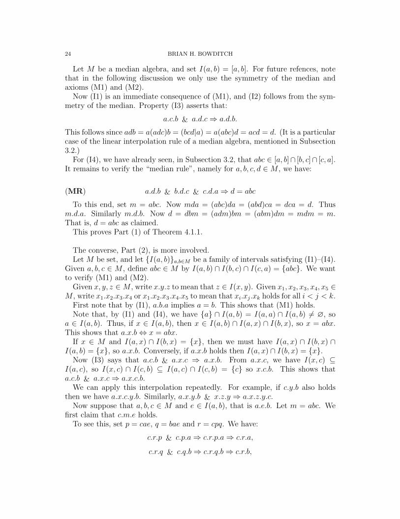
Let M be a median algebra, and set I(a, b) = [a, b]. For future refences, notethat in the following discussion we only use the symmetry of the median andaxioms (M1) and (M2).

Now (I1) is an immediate consequence of (M1), and (I2) follows from the sym-metry of the median. Property (I3) asserts that:

a.c.b & a.d.c⇒ a.d.b.

This follows since adb = a(adc)b = (bcd|a) = a(abc)d = acd = d. (It is a particularcase of the linear interpolation rule of a median algebra, mentioned in Subsection3.2.)

For (I4), we have already seen, in Subsection 3.2, that abc ∈ [a, b]∩ [b, c]∩ [c, a].It remains to verify the “median rule”, namely for a, b, c, d ∈M , we have:

(MR) a.d.b & b.d.c & c.d.a⇒ d = abc

To this end, set m = abc. Now mda = (abc)da = (abd)ca = dca = d. Thusm.d.a. Similarly m.d.b. Now d = dbm = (adm)bm = (abm)dm = mdm = m.That is, d = abc as claimed.

This proves Part (1) of Theorem 4.1.1.

The converse, Part (2), is more involved.Let M be set, and let I(a, b)a,b∈M be a family of intervals satisfying (I1)–(I4).

Given a, b, c ∈ M , define abc ∈ M by I(a, b) ∩ I(b, c) ∩ I(c, a) = abc. We wantto verify (M1) and (M2).

Given x, y, z ∈M , write x.y.z to mean that z ∈ I(x, y). Given x1, x2, x3, x4, x5 ∈M , write x1.x2.x3.x4 or x1.x2.x3.x4.x5 to mean that xi.xj.xk holds for all i < j < k.

First note that by (I1), a.b.a implies a = b. This shows that (M1) holds.Note that, by (I1) and (I4), we have a ∩ I(a, b) = I(a, a) ∩ I(a, b) 6= ∅, so

a ∈ I(a, b). Thus, if x ∈ I(a, b), then x ∈ I(a, b) ∩ I(a, x) ∩ I(b, x), so x = abx.This shows that a.x.b⇔ x = abx.

If x ∈ M and I(a, x) ∩ I(b, x) = x, then we must have I(a, x) ∩ I(b, x) ∩I(a, b) = x, so a.x.b. Conversely, if a.x.b holds then I(a, x) ∩ I(b, x) = x.

Now (I3) says that a.c.b & a.x.c ⇒ a.x.b. From a.x.c, we have I(x, c) ⊆I(a, c), so I(x, c) ∩ I(c, b) ⊆ I(a, c) ∩ I(c, b) = c so x.c.b. This shows thata.c.b & a.x.c⇒ a.x.c.b.

We can apply this interpolation repeatedly. For example, if c.y.b also holdsthen we have a.x.c.y.b. Similarly, a.x.y.b & x.z.y ⇒ a.x.z.y.c.

Now suppose that a, b, c ∈ M and e ∈ I(a, b), that is a.e.b. Let m = abc. Wefirst claim that c.m.e holds.

To see this, set p = cae, q = bae and r = cpq. We have:

c.r.p & c.p.a⇒ c.r.p.a⇒ c.r.a,

c.r.q & c.q.b⇒ c.r.q.b⇒ c.r.b,

MEDIAN ALGEBRAS 25

a.e.b & a.p.e & b.q.e⇒ a.p.e.q.b⇒ a.p.q.b,

a.p.q.b & p.r.q ⇒ a.p.r.q.b⇒ a.r.b.

By (I4), we have

a.r.b & c.r.a & c.r.b⇒ r = abc.

Therefore r = m, so c.r.p gives c.m.p. Now,

c.p.e & c.m.p⇒ c.m.p.e⇒ c.m.e.

This proves the claim.Now set n = mae. Given c.m.e, we have I(m, e) ⊆ I(c, e); and given a.m.c, we

have I(m, a) ⊆ I(c, a), both from (I3). Therefore

n ∈ I(m, e) ∩ I(m, a) ∩ I(a, e) ⊆ I(c, e) ∩ I(c, a) ∩ I(a, e) = ace,so n = ace.

In summary, we have shown that if a, b, c ∈M , and e ∈ I(a, b), then (abc)ae =ace.

Now let a, b, c, d ∈ M be arbitrary. Setting e = abd, we see that a(abc)(abd) =ac(abd). The left-hand side is symmetrically in c, d, so swapping c and d, we getac(abd) = ad(abc). In other words, we have verified (M2).

This proves Theorem 4.1.1.

Remark. We see retrospectively that if x, y ∈ I(a, b), then I(x, y) ⊆ I(a, b). Theargument above could be considerably simplified if we knew this at the outset.However I can see no very direct way of verifying this.

4.2. The short distributive law.

Our argument above is a variation on one in Sholander’s paper. (He bypassesdirect discussion of axiom (M2).) In fact, Sholander continues in a similar veinto deduce (M3). This still involves some amount of work. Instead of reproducingthat proof (we can do no better) we show how one can deduce (M3) from (M2),directly applying the axioms. The argument below is due to Knuth, Veroff andMcCune [VeroM] as we discuss in the Notes to this section. We will only makeuse of the median rule (MR) above, which we have already verified directly from(M1) and (M2).

Before giving the proof proper, we introduce the following condition which wewill say more about in Subsection 4.3

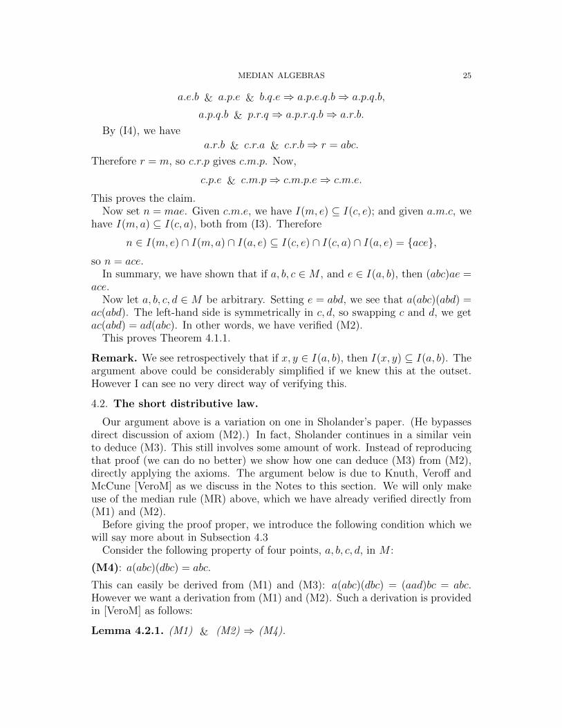
Consider the following property of four points, a, b, c, d, in M :

(M4): a(abc)(dbc) = abc.

This can easily be derived from (M1) and (M3): a(abc)(dbc) = (aad)bc = abc.However we want a derivation from (M1) and (M2). Such a derivation is providedin [VeroM] as follows:

Lemma 4.2.1. (M1) & (M2) ⇒ (M4).


Proof.

a(abc)(dbc) = a(ab(abc))(dbc) = (b(abc)(dbc)|a)

= ((dbc)ba)(abc)a = (adc|b)(abc)a = ((abc)bd)(abc)a

= (adb|(abc)) = (ab(abc))d(abc) = (abc)d(abc) = abc.

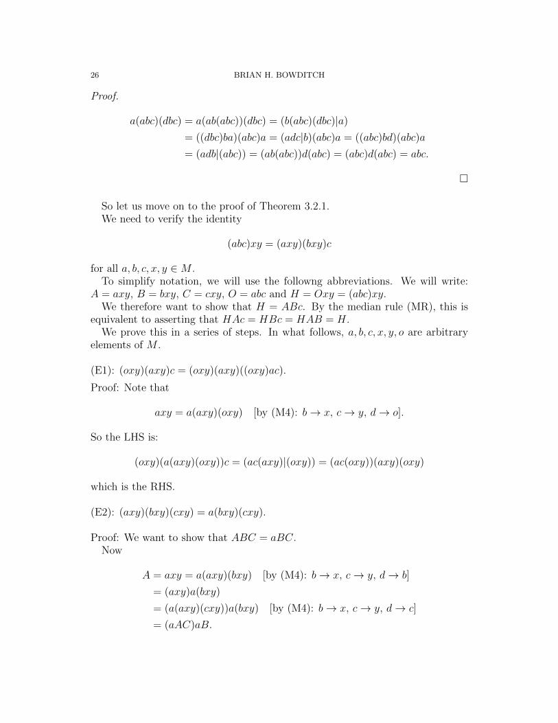
So let us move on to the proof of Theorem 3.2.1.We need to verify the identity

(abc)xy = (axy)(bxy)c

for all a, b, c, x, y ∈M .To simplify notation, we will use the followng abbreviations. We will write:

A = axy, B = bxy, C = cxy, O = abc and H = Oxy = (abc)xy.We therefore want to show that H = ABc. By the median rule (MR), this is

equivalent to asserting that HAc = HBc = HAB = H.We prove this in a series of steps. In what follows, a, b, c, x, y, o are arbitrary

elements of M .

(E1): (oxy)(axy)c = (oxy)(axy)((oxy)ac).

Proof: Note that

axy = a(axy)(oxy) [by (M4): b→ x, c→ y, d→ o].

So the LHS is:

(oxy)(a(axy)(oxy))c = (ac(axy)|(oxy)) = (ac(oxy))(axy)(oxy)

which is the RHS.

(E2): (axy)(bxy)(cxy) = a(bxy)(cxy).

Proof: We want to show that ABC = aBC.Now

A = axy = a(axy)(bxy) [by (M4): b→ x, c→ y, d→ b]

= (axy)a(bxy)

= (a(axy)(cxy))a(bxy) [by (M4): b→ x, c→ y, d→ c]

= (aAC)aB.

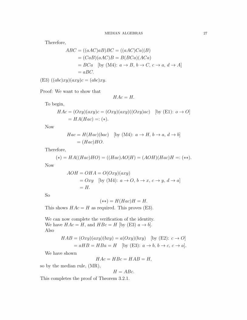
MEDIAN ALGEBRAS 27

Therefore,

ABC = ((aAC)aB)BC = ((aAC)Ca)|B)

= (CaB)(aAC)B = B(BCa)(ACa)

= BCa [by (M4): a→ B, b→ C, c→ a, d→ A]

= aBC.

(E3) ((abc)xy)(axy)c = (abc)xy.

Proof: We want to show thatHAc = H.

To begin,

HAc = (Oxy)(axy)c = (Oxy)(axy)((Oxy)ac) [by (E1): o→ O]

= HA(Hac) =: (∗).Now

Hac = H(Hac)(bac) [by (M4): a→ H, b→ a, d→ b]

= (Hac)HO.

Therefore,

(∗) = HA((Hac)HO) = ((Hac)AO|H) = (AOH)(Hac)H =: (∗∗).Now

AOH = OHA = O(Oxy)(axy)

= Oxy [by (M4): a→ O, b→ x, c→ y, d→ a]

= H.

So(∗∗) = H(Hac)H = H.

This shows HAc = H as required. This proves (E3).

We can now complete the verification of the identity.We have HAc = H, and HBc = H [by (E3) a→ b].Also

HAB = (Oxy)(axy)(bxy) = a(Oxy)(bxy) [by (E2): c→ O]

= aHB = HBa = H [by (E3): a→ b, b→ c, c→ a].

We have shownHAc = HBc = HAB = H,

so by the median rule, (MR),H = ABc.

This completes the proof of Theorem 3.2.1.


4.3. Isbell’s condition.

Although we will have no further use for it in our discussion, we show thatProperty (M4) of Subsection 4.2 provides another “four-point” characterisationof a median algebra, which is due to Isbell [I2]. We have already observed thatany median algebra satisfies (M4).

Conversely, suppose that we have a symmetric ternary operation satisfying(M1) and (M4). Note that ab(abc) = a(abb)(abc) = abc. We can therefore givetwo equivalent definitions of an “interval” in the usual way, namely: [a, b] = abc |c ∈ M = c ∈ M | abc = c. Given (M1), we see that (M4) can be equivalentlybe expressed as:

(F): If a, b, c ∈M and d ∈ [a, b], then abc ∈ [c, d].

(Note that cd(abc) = c(abd)(abc) = abc.)We claim:

Theorem 4.3.1. Let M be a set equipped with a symmetric ternary operation[(x, y, z) 7→ xyz]. Then M is a median algebra if and only if it satisfies (M1) and(M4).

Proof. We have already observed that the “only if” direction holds. We thereforesuppose that M satisfies (M1) and (M4). We proceed to verify the hypotheses(I1)–(14) of Theorem 4.1.1.

Now (I1) and (I2) are immediate, so we proceed to (I3). Let a, b ∈ M and c ∈[a, b]. We claim that [a, c] ⊆ [a, b]. To see this, let d ∈ [a, c] and let p = abd. Sincec ∈ [a, b], we have p ∈ [c, d] by (F) above. Therefore, p = pad = (pcd)a(acd) =acd = d, and so d = p ∈ [a, b], proving (I3).

To prove (I4) we first make the following two observations.

(1): Let a, b, c ∈M and m = abc. Then [a,m] ∩ [b, c] = m.Certainly, m ∈ [a,m] ∩ [b, c]. Suppose p ∈ [a,m] ∩ [b, c], that is p = pam = pbc.

Then p = pam = (pbc)a(abc) = abc = m as required.

(2): If a, b, c, t ∈M with [a, t] ∩ [b, c] = t, then t = abc.Since t ∈ [b, c] we have abc ∈ [a, t] by (F). Therefore abc ∈ [a, t] ∩ [b, c] = t,

so abc = t.

To verify (I4), let x, y, z ∈M , and let m = xyz ∈ [x, y]∩ [y, z]∩ [z, x]. Supposep ∈ [x, y] ∩ [y, z] ∩ [z, x]. Since p ∈ [x, z] we have [x, p] ⊆ [x, z] by (I3). Applying(1) above, we have [y,m]∩ [x, p] ⊆ [y,m]∩ [x, z] = m. Moreover, since p ∈ [y, z],we have m = xyz ∈ [x, p] by (F). Therefore, [y,m] ∩ [x, p] = m, and so by (2)we get m = yxp = p. We have shown that [x, y] ∩ [y, z] ∩ [z, x] = xyz.

This verifies (I4), and so by Theorem 4.1.1 (2), M is a median algebra wherethe median of x, y, z is xyz.

MEDIAN ALGEBRAS 29

From here, we could proceed to verify (M2) and (M3) as before (though theargument can be shortened a little since we already have a few of the necessaryingredients). Of course, this is all rather involved. Again it would be nice to havea short direct derivation of these identities.

5. Free median algebras

In this section, we will give a more concrete description of the free medianalgebra on a finite set. This will be in terms of “flows” on the proper power set(Theorem 5.2.3), though we will postpone the proof of that result until Subsection9.2. We give an explicit account of the free median algebra on a set with at mostfive elements. An understanding of the free median algebra on four elementswill be helpful in later discussions (see, for example, Subsection 13.2). First, weintroduce some general notions that will find further uses later.

5.1. Some general notions.

Let M be a median algebra. Recall that a, b ∈ M are “adjacent” if [a, b] =a, b. Let Γ = Γ(M) be the graph with vertex set V (Γ) = M , and with twoelements connected by an edge if they are adjacent. We refer to Γ(M) as theadjacency graph associated to M .

Lemma 5.1.1. If a, b ∈ M and [a, b] is finite, then a, b are connected by a pathin Γ(M).

Proof. In fact, we see that any maximal chain, a = x0 < x1 < · · · < xn = b givesus a path in Γ(M).

In particular, it follows that if M is finite, then Γ(M) is connected. In fact, onecan see in this case that a.c.b holds if and only if c lies in some shortest path froma to b in Γ(M). (One can check that such shortest paths are precisely the maximalchains in [a, b]: see Subsection 11.1.) From this one can read off the median inM from the graph Γ(M). We remark that all we really need in the above is thatintervals in M are finite. We will explore this in more detail in Sections 11 and15.

Let M be any median algebra. Given elements, a1, . . . , an, p ∈M , write

(a1a2 . . . an|p) = a1 ∧ a2 ∧ · · · ∧ an ∈M,

where ∧ is the meet operation, as defined in Subsection 3.2 by setting a∧ b = abp.Note that (abc|p) = (abp)cp, so this is consistent with the notation defined inSubsection 2.1. It is natural to set (a|p) = a for all a ∈M .

The element (a1 . . . an|p) does not change under permuting or repeating theelements ai. Given any nonempty finite subset A ⊆ M , we can therefore write(A|p) = (a1 . . . an|p), where A = a1, . . . , an.


In the case where M = 0, 1, this again has an interpretation in terms ofvoting. If the jurors A ∪ p each cast a vote, 0 or 1, with the outcome deemedto be (A|p), then the vote of p can only be overruled by the unanimous vote of A.

If we write m = (A|p), then clearly we have p.m.a for all a ∈ A. In fact, p.m.xholds for all x ∈ 〈A〉. This follows by iterating the median operation and notingthat pm(xyz) = (pmx)(pmy)(pmz) for all x, y, z ∈ M . (This has a geometricalinterpretation in terms of convex hulls, as we will see in Subsection 7.4.)

5.2. Flows and superextensions.

Now let X be any set, and let F (X) be the free median algebra on X. Givenany p ∈ X, write m(p) = ((A \ p)|p).

Lemma 5.2.1. For each p ∈ X, m(p) is the unique point of F (X) adjacent to p.

Proof. Since F (X) = 〈X〉, we saw above that p.m(p).x holds for all x ∈ F (X). Itremains to check that p 6= m(p). To this end, define a map φ : X −→ 0, 1 by

φ(p) = 1 and φ|(X \ p) ≡ 0. This extends to a homomorphism φ : F (X) −→0, 1. Now φ(m(p)) = (0 . . . 0|1) = 0 in 0, 1, and so m(p) 6= p.

Let Ψ = Ψ(X) = P(P0(X)), where P denotes power set, and P0 denotes theproper power set (removing the empty set and the whole set). This is essentiallythe same as the definition we gave in Subsection 3.3 after identifying a set withits characteristic function. (In Subsection 3.3, we used P(X) instead of P0(X),but this makes no essential difference, as we note below.) In these terms, theevaluation map ι : X −→ Ψ is given by setting ι(x) = A ⊆ X | x ∈ A. This isthe principal ultrafilter at x.

Given three families, A,B, C ∈ Ψ, recall that the median, ABC, is defined bysaying that a set A ∈ P0(X) lies in ABC if and only A lies in at least two of thefamilies, A,B, C.

Definition. We say that A ∈ Ψ is a flow if it satisfies the following threeconditions:

(P1): if A ∈ A, B ∈ P0(X) and A ⊆ B then B ∈ A,

(P2): if A,B ∈ A, then A ∩B 6= ∅, and

(P3): for all A ∈ P0(X), then either A ∈ A or A∗ ∈ A.

Here A∗ := X\A. Note that by (P2) exactly one of A and A∗ lies in A. (Indeed,given (P1), we could remove (P2) and replace (P3) with this stronger statement.)The terminology of “flow” will be explained in Subsection 9.1, where such thingswill be defined more generally.

Remark. We could, instead, have taken Ψ = P(P(X)). This gives rise to anessentially equivalent notion of “flow”. We would just have to add (or remove)the whole set, X, to A. (This is the definition of Ψ we gave in Section 3.3.) We

MEDIAN ALGEBRAS 31

have disallowed it here, because it fits better with our account of more generalflows in Section 9.

Definition. The superextension of X is the set of all flows. We denote itΦ(X) ⊆ Ψ(X).

(Again, it is common elsewhere to include X itself in the superextension, butthis makes no essential difference to the discussion.)

It is easy to check that Φ(X) is a subalgebra of Ψ(X). Moreover ι(X) ⊆ Φ(X).In Subsection 3.3, we constructed F (X) as F (X) = 〈ι(X)〉 ⊆ Ψ(X). From the

above we see:

Lemma 5.2.2. For any set X, F (X) ⊆ Φ(X).

In fact:

Theorem 5.2.3. If X is finite, then F (X) = Φ(X).

In other words for finite sets, free median algebras are the same as superexten-sions. The remainder of this section will refer to Φ(X).

5.3. The structure of a superextension.

Note that the halfspaces of Φ(X) correspond to proper subsets of X, and wallscorrespond to bipartitions (that is, partitions into two non-empty subsets).

Theorem 5.2.3 is equivalent to asserting that Φ(X) is generated by ι(X): thatis the set of principal ultrafilters on X. The discussion in Subsection 5.4 will giveexplicit verifications of this when when #X ≤ 5. We will postpone the generalproof for the moment. In fact, we will eventually see three different proofs. One,in terms of a duality principle, is discussed in Section 9 (see Lemmas 9.2.2 and9.2.3). It is also an immediate consequence of a more general result about “spaceswith walls”, namely Proposition 9.4.2. A third, more explicit proof, in terms ofboolean functions is given in Subsection 19.1: see Proposition 19.1.2.

Given A ∈ Φ(X), write M(A) for the set of minimal elements of A (that is,with respect to inclusion). Note that we can reconstruct A as the set of all subsetscontaining some element of M(A). In practice, it is often easiest to describe aparticular element of Φ(X) by specifying M(A).

To simplify notation, it will be convenient to identify X with ιX ⊆ Φ(X).In these terms, if a ∈ X, then M(a) = a. Given any a, b, c ∈ X, thenM(abc) = a, b, b, c, c, a. More generally, if a1, . . . , an, p ∈ X, are distinct,then

M(a1, , . . . , an|p)) = p, a1, p, a2, . . . , p, an, a1, a2, . . . , an.(Note that this has an interpretation in terms of voting which we mentioned inSubsection 5.1.)

We can describe intervals and adjacency in Φ(X) as follows.


Let A,B, C ∈ Φ(X). By Lemma 2.1.3, A.B.C holds if and only if A ∩ B ⊆C ⊆ A ∪ B. But A,B, C are all ∗-transversals and so A ∩ B ⊆ C ⇔ C ⊆ A ∪ B.Therefore:

Lemma 5.3.1. If A,B ∈ Φ(X), then

[A,B] = C ∈ Φ(X) | A ∩ B ⊆ C = C ∈ Φ(X) | C ⊆ A ∪ B.

Let A ∈ Φ(X), and let A ∈ M(A). Let B = (A \ A) ∪ A∗. It is easilyseen that B ∈ Φ(X), and that A∗ ∈M(B). We say that B is obtained from A byflipping A. Conversely, A is obtained from B by flipping A∗. We refer to suchan operation as a flip. Note that A,B differ by a flip if and only if #(A4B) = 2.In fact:

Lemma 5.3.2. A,B ∈ Φ(X) are adjacent if and only if they differ by a flip.

Proof. Suppose that B is obtained by flipping A ∈M(A). ThenA∩B = A\A =B \ A∗. If C ∈ [A,B], then by Lemma 5.3.2, we have A ∩ B ⊆ C, and so eitherA ⊆ C or B ⊆ C. Since these are all ∗-transversals, this implies either A = C orB = C. Thus A,B are adjacent.

Conversely, suppose that A,B are adjacent. Let A be a minimal element ofA \ B. Now A is also minimal in A. (For if B ∈ A were strictly contained inA, then B ∈ B, so we get the contradiction that A ∈ B.) Let C be obtained byflipping A in A. Then A∩ B ⊆ C, so C ∈ [A,B]. Since C 6= A, we get C = B.

In particular, we see that there is a natural bijection between M(A) and theset elements of Φ(X) adjacent to A.

This will allow us to construct the adjacency graph, Γ(Φ(X)), for small X.(Note that the above implies that the combinatorial distance between A andB in Γ(Φ(X)) is at most 1

2#(A4B). In fact, these are equal, as we discuss in

Subsection 11.7.) The structure of Φ(X) is a little different depending on whether#X is odd or even.

Suppose #X = 2N − 1, where N is a positive integer. In this case, Φ(X) hasa central element , namely the set of all subsets of X of size at least N . Interms of “voting” this can be thought of as “majority vote”: that is when we have2N − 1 jurors all casting votes 0 or 1, and the outcome is determined by a simplemajority. It is also not hard to see that the central vertex is the unique elementof Φ(X) invariant under all permutations of X.

Suppose #X = 2N , where N is a positive integer. In this case, we have a centralcube of Φ(X) described as follows. First, let Y be the set of subsets of X of sizeat least N + 1. Let W0 be the set of equal bipartitions of X: that is partitionsinto two subsets of size N . Note that #W0 = ν := 1

2( 2NN ) =

(2N−1N−1

). We can

view each element of W0 as a 2-element median algebra, and equip Q :=∏W0

with the product median structure. As such, Q is a ν-cube. We can view eachelement of Q as choosing some element from each equal bipartition so as to giveus a family, C, of subsets of X each of size N . We define a map φ : Q −→ Φ(X)

MEDIAN ALGEBRAS 33

by setting φ(C) = C ∪ Y . This is clearly a median monomorphism, and its image,φ(C), is a ν-cube in Φ(X). In fact, φ(Q) is convex in Φ(X). (For example, takeany C ∈ Q, and let D ∈ Q be the antipodal vertex: that is, from each bipartitionwe make the opposite choice of element. From Lemma 5.3.1, it is easily seen thatφ(Q) = [C,D], and so is convex.) We refer to φ(Q) as the central cube of Φ(X).

Remark. While we are on the subject, we note that the operation of “majorityvote” can be applied in any median algebra, M . One way to describe this is asfollows.

Let n = 2m + 1 for m ∈ N, and let x := x1, . . . , xn ⊆ M . Let Φ =Φ(1, . . . , n), and let φ : Φ −→ M be the homomorphism extending the map[i 7→ xi]. Let µ(x) be the image of the central element of Φ under φ. Thus, µis a symmetric n-ary operation on M . Note that one can define µ(x) explicitlyby applying any formula for majority vote. Thus, for n = 1, 3, 5 respectively, wehave µ(a) = a, µ(a, b, c) = abc, and µ(a, b, c, d, e) = a(bcd)((bce)de) (as discussedin the next subsection).

Another way to describe µ(x) is as follows. Let H be the set of halfspaces ofM , and let H(x) = H ∈ H | #i | xi ∈ H ≥ m + 1; in other words, the setof halfspaces which contain a majority of the points xi. Then

⋂H(x) = µ(x).

(The equivalence with the previous description can be seen from the fact that it isinvariant under all permutations of the xi, or directly in terms of the descriptionof the central element as majority vote.)

This has a simple interpretation for a simplicial tree, T . If x1, . . . , xn ∈ V (T ),then µ(x) is the unique vertex such that any branch of T at µ(x) contains fewerthan half of the xi. Similarly, if M is a total ordered set, then µ(x) is the “median”value of x in the commonly used sense of the word.

5.4. Description of the first few cases.

We now give an explicit description of Φ(X) when #X ≤ 5. It is natural tothink of Γ(Φ(X)) as the 1-skeleton of a cube complex, ∆. (One can imagine thecubes as euclidean cubes of unit side length, meeting along common faces.) Notethat the link of any vertex is a simplicial complex: the simplices corresponding tothe cubes which contain that vertex. It turns out that in our case, such a simplicialcomplex will always be a “flag complex”: any clique (that is complete subgraph)of its 1-skeleton lies in a simplex. We will discuss such matters in greater detailand generality in Sections 11 and 16. The situation starts out very simply, butthe complexity grows very rapidly.

If #X ≤ 2, then Φ(X) = X (after identifying X and ιX).

If X = a, b, c then we have Φ(X) = a, b, c, abc, and we see that Γ(Φ(X)) isa tripod with feet a, b, c and with central vertex abc.


Now let X = a, b, c, d. Suppose A ∈ Φ(X). If A contains a singleton, saya, then then A is just a (or more precisely ιa). If A has no singleton, then itmust contain a 2-element set. A convenient way to describe it is as follows. LetG = G(A) be the graph with vertex set X and with x, y ∈ X connected by anedge if x, y ∈ A (so x, y ∈ M(A)). Now any two edges of G meet. Moreover,any pair of vertices are either connected by an edge or else the complementary pairof vertices are. From this we see easily that either G is a triangle, with vertices,a, b, c, say, together with an isolated vertex, d; or else it is a tripod, with feeta, b, c, say, connected to a central vertex d. In the former case, A = abc, and inthe latter case, A = (abc|d) (after identifying a with ιa). Writing m(d) = (abc|d)as above, and h(d) = abc, we see that Φ(X) has precisely 12 elements, namely,a, b, c, d, m(a), m(b), m(c), m(d), v(a), v(b), v(c) and v(d). We also see thatΦ(X) = 〈a, b, c, d〉, so that F (X) = Φ(X) verifying Theorem 5.2.3 in this case.

To complete the description of Φ(X), we note that the 8 elements, m(a), m(b),m(c), m(d), v(a), v(b), v(c), v(d), form the central 3-cube of Φ(X). This is be-cause the minimal set of each of these elements is obtained by selecting one elementfrom each of the three equal bipartitions of X. Moreover, m(a) is adjacent eachof v(b), v(c), v(d), etc. Now m(a) is obtained by flipping a in a ∈ Φ(X), so wesee by Lemma 5.3.2 that a is adjacent to m(a). In summary, we see that Γ(Φ(X))is the 1-skeleton of a cube complex consisting of one central 3-cube together withfree edges attached at alternating vertices of this cube.

Now suppose X = a, b, c, d, e. Let A ∈ Φ(X). Again, if A is containsa singleton then it lies in X. So suppose not. We again construct a graph,G = G(A), with vertex set X and x, y adjacent if x, y ∈ A. In other words,the edge set consists of the 2-element sets in M(A). The remaining elements ofM(A) are the 3-element subsets of X which neither contain nor are disjoint fromany edge of G(A). In this way, G(A) determines M(A) and hence also A. As inthe previous case, any two edges of G(A) must be adjacent in G(A).

If G has no edges, then A is the central vertex of Φ(X): it consists of allsubsets of X with at least 3 elements. One can give various expressions for A.For example, it is given by a(bcd)((bce)de) or by (ab(cde))(cd(abe))e. This examplewill be discussed further in Subsections 6.2 and 19.1.

If G has at least one edge, then it is easily seen that it is either a triangle, or elseconsists of a vertex with one, two, three, or four edges attached (together withthe remaining isolated vertices). In other words up to permuting X, the edge-setis one of: a, b, b, c, c, a, a, e, a, e, b, e, a, e, b, e, c, e ora, e, b, e, c, e, d, e. One can verify that these correspond respectively tothe elements, abc, ae(bcd), (abe)(ace)(bde), (abc|e) and (abcd|e). We see explicitlythat Φ(X) is generated by a, b, c, d, e, again verifying Theorem 5.2.3 in this case.

MEDIAN ALGEBRAS 35

Summing the numbers of each type of element, we see that in total there are5 + 1 + ( 5

3 ) + ( 52 ) + 5( 4

2 ) + 5.4 + 5 = 81. In other words, for #X = 5, we have#Φ(X) = 81.

To describe the structure of Γ(Φ(X)) we can can think of Γ(Φ(X)) as the 1-skeleton of a cube complex ∆. This consists of five 4-cubes and ten 3-cubes, allmeeting at the central vertex, together with a free edge attached to the antipodalvertex of each 4-cube. Here is an explicit account of how these fit together.

First recall that the Petersen graph, P , is a graph with 10 vertices and 15 edges.(It can be described by taking 1-skeleton of the dodecahedron and quotienting bythe antipodal map.) We are really interested in the complement graph, P ∗ — thishas the same vertex set but complementary edge set. Note that P ∗ has 5 maximalcliques on 4 vertices, and 10 maximal cliques on 3 vertices. We can construct asimplicial (flag) complex, Σ, with 1-skeleton P ∗ by gluing in 3- and 2-simplicesto these maximal cliques. Now to construct ∆, we take our 5 4-cubes and 103-cubes, and glue them together so that they all meet at a common vertex, andwith Σ as the link of that vertex (cf. Example (Ex3.2) of Subsection 3.4). Finallywe attach a free edge to the vertex of each 4-cube antipodal the central vertex.

We relate this back to Φ(X) as follows. Recall that the Petersen graph, P , canalso be described as the graph whose vertex set is the set of 2-element subsets of X,and with adjacency given by disjointness. (This is the so-called “Kneser graph”,KG5,2.) Thus, in P ∗, two such subsets are adjacent if they intersect. The centralelement, A, of Φ(X) corresponds to the central vertex of ∆. By Lemma 5.3.2, anyadjacent element of Φ(X) is obtained by flipping some 3-element subset, A ∈ A.Writing A∗ = a, b ⊆ X, we see that gives us the element of Φ(X) with edgeset a, b in Γ(A). In this way, we get a bijective correspondence between thevertices of P ∗ and the elements of Φ(X) adjacent to the central element. Now anedge of P ∗ has incident vertices of the form a, b and a, c, where a, b, c ∈ X aredistinct. We have a third element of Φ(X) given by the edge set a, b, a, cin the above description. Together with the central element, these form a 2-cubein Φ(X). In other words, the edges of P ∗ correspond to the 2-cubes of Φ(X)which contain the central element. We can now fill in the 4-cubes, which haveantipodal vertices of the form a, b, a, c, a, d, a, e, and the 3-cubes whichhave antipodal vertices of the form a, b, b, c, c, a. Note that the 4-cubesalso contain the elements of the form a, b, a, c, a, d. Finally, we attacheach element a ≡ a to a, b, a, c, a, d, a, e by a free edge. This givesus our cube complex ∆, with 1-skeleton, Γ(Φ(X)).

Beyond this point, Φ(X) becomes too complicated to give a simple explicitdescription: when #X = 6, Φ(X) has a central 10-cube and a total of 2646elements. Nevertheless, one can make a number of further general observations.We say a bit more about this in Subsection 11.7, when we have some more factsabout cube complexes at our disposal.


6. Expressions and identities

We give a more formal treatment of median expressions. We go on to describea simple procedure for verifying identities, which is usually much simpler thanmessing with the axioms directly. At the end of the section, we explain howsuch identities can be systematically proven directly from the axioms, though theprocedure for carrying it out is somewhat involved.

6.1. Formal definitions.

Let X be any set, which we think of the alphabet . A (symmetric ternary)expression , E, in X consists of the following data. We have a finite tree, T = TE,with a preferred “root” vertex, r = rE ∈ V (T ), a set of leaves L = LE ⊆ V (T ),and a map λ = λE : L −→ X, such that r has valence 3, each element of L hasvalence 1, and every other vertex has valence 4. In addition, we allow for a trivialexpression where LE = V (TE) = rE. We think of the map λ as “labelling” theleaves of the tree. We view an expression as being defined up to isomorphism ofthe tree respecting the root and labelling.

Any vertex v ∈ V (T ) determines a branch , S, of T — that is the subtreeconsisting of those points (including v) separated from the root by v. This givesus an expression, F , defined by setting TF = S, rF = v, LF = LE ∩ S andλF = λE|LF . We refer to S as a subexpression of E.

Given three expressions, A,B,C, we can form an expression, D, by taking thedisjoint union TAtTBtTC and connecting rA, rB, rC , to a new vertex, rD, by threenew edges. This gives us a tree, TD, with root rD, and with LD = LA t LB t LC .We write D = ABC. Note that any non-trivial expression can we written in thisway.

Identifying an element a ∈ X, with the trivial expression labelled a, we seethat we can represent any expression as string in the alphabet X together withparentheses “(” and “)”. Note that we are allowing permutations. Thus forexample, ((abc)ad)(bce) and (ceb)(da(bac)) are the same expression, and (acb)dais a subexpression thereof. (Putting a preferred linear order on the entries of anexpression would be unnatural from our point of view.)

Let E = E(X) be the set of all expressions in X. Let ∼ be the smallest equiva-lence relation satisfying:

(1): if A,B ∈ E , then AAB ∼ A,

(2): if A,B,C,D ∈ E then (ABD)CD ∼ (ACD)BD, and

(3): if A,B,C,D ∈ E and C ∼ D, then ABC ∼ ABD.

Let Θ = Θ(X) = E/∼. We write [A] for the ∼-class of A. By (3), we have awell defined ternary operation on Θ defined by [ABC] = [A][B][C]. By (1) and

MEDIAN ALGEBRAS 37

(2), this satisfies axioms (M1) and (M2), and so Θ is a median algebra. Defineι : X −→ Θ by ι(a) = [a].

Let φ : X −→ M be any map into a median algebra, M . Given an expressionE ∈ E , we define φ(E) recursively by the rule φ(ABC) = φ(A)φ(B)φ(C), andtaking it to be given by the original map on trivial expressions. Thus φ(E) isthe evaluation of E in M . Directly from the axioms, (M1) and (M2) in M , we

see that of E ∼ F , then φ(E) = φ(F ). We therefore get a map φ : Θ −→ M ,

defined by setting φ([E]) = φ(E). By construction, φ is a median homomorphism

satisfying φ(ιa) = φ(a) for all a ∈ X. Note that ι is injective. (To see this,take M = 0, 1. If a, b ∈ M are distinct, let φ be any map with φ(a) 6= φ(b),

then φ(ι(a)) 6= φ(ι(b)).) After identifying X with ιX ⊆ Θ, we have shown thefollowing:

Proposition 6.1.1. Let X be any set, and let Θ ⊇ X be the set of ∼-classes ofmedian expressions in X, with the median operation as defined above. Then Θ isthe free median algebra on X.

We note that one can equivalently define the relation ∼ by saying that twoexpressions are equivalent if we can get between them by a finite sequence ofoperations which modify some branch of the tree by performing operations of type(1) or (2) above (i.e. interchanging AAB with A, or interchanging (ABD)CD with(ACD)BD when this is possible). This can be thought of as a finite sequence ofapplications of axioms (M1) and (M2).

6.2. Verification of identities.

A tautological identity between two median expressions is one that holdshowever it is evaluated in any median algebra. By Proposition 6.1.1, this isthe same as saying that the expressions are equivalent under the relation, ∼. Forexample, we have seen that the identity ab(xyz) = (abx)(aby)(abz) is tautological.From the above, we see that any tautological identity can be explicitly verified bya repeated application of the axioms (M1) and (M2).

However, there is a simpler way of doing this in practice. We have seen that anytwo distinct points in any median algebra, M , are separated by a wall. Equiva-lently, M can be embedded into a cube, see Proposition 3.2.12. (Of course, we hadto verify quite a few identities directly in order to get to that point, but that workis now done.) To check that an identity is tautological, it is therefore sufficient toverify that it holds in 0, 1 for all possible assignments of the arguments. Onecan often argue more efficiently in the contrapositive.

To illustrate this, we will write x↑ and x↓ to mean that x takes the value 0 and1 respectively. So for example, if abc↑ holds, then up to permuting a, b, c we canassume that a↑ and b↑ hold.

As an example, we stated in Subsection 5.4 that a(bcd)((bce)de) representsthe majority vote of five jurors. One consequence is that it symmetric under


permuting a, b, c, d, e. In particular (transposing a and e), the identity

a(bcd)((bce)de) = e(bcd)((bca)da)

is tautological.Suppose we had not noticed that this is majority vote, and wanted to verify

this identity. We might proceed as follows.Without loss of generality (swapping ↓ and ↑), we can suppose that a(bcd)((bce)de)↓

and e(bcd)((bca)da)↑. Also (swapping a and e) we can suppose that bcd↑. Fromthe first expression, it follows that a↓ and (bce)de↓.

Now if e↑, then the last statement implies that d↓ and bce↓. Given e↑, wetherefore get b↓, c↓, and so bcd↓, contradicting an earlier statement.

Therefore, e↓. Now e(bcd)((bca)da)↑ gives (bca)da↑. Given a↓, this imples d↑and bca↑. Again, given a↓, we get b↑, c↑, so bce↑. Thus, given d↑, we get (bce)de↑,again contradicting an earlier statement.

This shows that the identity is tautological as claimed.Of course, there are lots of possible variations on the above logic, but they all

lead quickly to a similar contradiction.One can proceed to verify the other symmetries of the expression or its equiv-

alence with (ab(cde))(cd(abe))e, for example.

A similar discussion applies to conditional identities. Let I1, . . . , In, I be ternaryidentities. We say that I1 & · · · & In tautologically implies I if any medianalgebra in which I1 & · · · & In holds for some assignment of the arguments, thenI also holds for that assignment of the arguments. (For example, we have seenthat a.x.y & a.y.c tautologically implies x.y.c. Here, of course, a.b.c is shorthandfor the identity abc = b.) By a similar argument as for tautological identities, wesee that a conditional identity can be verified by a repeated application of theidentities I1, . . . , In together with the axioms (M1) and (M2).

However, it is again sufficient to verify it in 0, 1. To see this, suppose that thetwo sides of I evaluate to different elements, say p and q, in some median algebra,M , in which I1 & · · · & In holds. We postcompose by a wall map separating pand q. Now I1 & · · · & In still holds in 0, 1, whereas I does not. This gives acontradiction.

We illustrate this with a few examples (which will be useful later).

(Ex6.1) a.b.c & b.c.d & a.d.e⇒ b.c.e

If not, we can suppose c↑, b↓ and e↓. From a.b.c, we get a↓. From b.c.d, we getd↑. But from a.d.e, we get d↓, giving a contradiction.

(Ex6.2) x.z.y & x.a.c & y.b.c & z.c.a⇒ a.c.b

If not, we can suppose c↑, a↓ and b↓. From x.a.c and y.b.c, we get x↓ and y↓.Now x.z.y gives z↓ and so z.c.a gives c↓, a contradiction. (We could alternatively

MEDIAN ALGEBRAS 39

use (Ex6.1) to deduce a.c.y, which together with y.b.c gives a.c.b.y.)

(Ex6.3) abc.y.def ⇒ y = (ady)(bey)(cfy)

If not, we can suppose y↑, ady↓ and bey↓. Then a↓, d↓, b↓ and e↓, and so abc↓and def↓, so y↓, a contradiction.

We can also eliminate variables:

(Ex6.4) aa′x = bb′y ⇒ b.aa′b.b′

If not, we can suppose aa′b↑, b↓ and b′↓. Thus, aa′x = bb′y↓, so either a↓ or a′↓,so aa′b↓, giving a contradiction.

Of course, one can prove these statements directly from the axioms, or identitieswe have already established, though this can be somewhat laborious and not veryinformative. For example, we can derive (Ex6.4) above as:

(aa′b)bb′ = ((aa′b)bb′)((aa′b)bb′)y = (((aa′b)bb′)(aa′b)b′)(b(aa′b)b′)y

= (((aa′b)bb′)by)(aa′b)b′ = ((bb′y)(aa′b)b)(aa′b)b′

= ((aa′b)bb′)(aa′b)(bb′y) = ((aa′b)bb′)(aa′b)(aa′x)

= ((aa′b)(aa′x)b)(aa′b)b′ = ((aa′(bxb))(aa′b)b′

= (aa′b)(aa′b)b′ = aa′b.

6.3. Explicit proofs of identities.

In summary, the above discussion gives a means of checking whether two ex-pressions are tautologically equivalent. It also shows that a tautological identitycan be proven by a finite sequence of applications of axioms (M1) and (M2). How-ever, the argument made appeal to Zorn’s lemma (via Proposition 3.2.9), and isthus non-constructive. It effectively gives a proof, within the framework of ZFCset theory, of the formal statement that “there exists a proof from the axioms ofa median algebra”. It does not exhibit such a proof. If we want an explicit recipeto do this, we need another approach. The idea is to refer to the case of a freedistributive lattice as discussed in Subsection 2.2.

First, we extend the alphabet, X, by adjoining two new letters, p, q, to giveX+ := X t p, q, and set E+ := E(X+) ⊇ E . Given any C ∈ E+, let C ′ = Cpq ∈E+. LetX ′ = a′ | a ∈ X. ViewingX ′ as a formal alphabet, we write E ′ = E(X ′),for the set of expressions with arguments in X ′. Viewing each element of X ′ asan expression in X+, we we can identify E ′ as a subset of E+. As with the longdistributive law (Lemma 3.2.5), we have (CDE)′ ∼ C ′D′E ′ for all C,D,E ∈ E+.(Just replace equality by ∼ everywhere in the proof.) By repeatedly applyingthis, given any C ∈ E(X), we can re-express C ′ as an expression in E ′. (Theend result simply substitutes each letter, a, by a′ in the original expression, C.)Given C,D ∈ E ′, write C ∧ D = CDp and C ∨ D = CDq. As in Lemma 3.2.4,we have an explicit proof that CDE ∼ (C ∧ D) ∨ (D ∧ E) ∨ (E ∧ C) for all


C,D,E ∈ E ′. (Again, just replace equality by ∼.) This allows us to rewrite ourexpression in terms of the operations ∧ and ∨, again with arguments in X ′. NowE ′ is a distributive lattice, modulo ∼. That is to say, the axioms of a distributivelattice hold modulo ∼. For example, we have (C ∧ D) ∧ E ∼ C ∧ (D ∧ E) and(C ∧D)∨E ∼ (C ∨E)∧ (D∨E) etc. Applying the distributive laws, we can nowput our expression into a “canonical” form a′(J ), where J is a Sperner systemfor X, and where a′(J ) =

∨I∈J a

′I and a′I =

∧a∈I a

′. Note that we can freelyapply the associative laws for ∧ and ∨, so it does not matter how we bracket theexpressions for a′(J ) and a′I . Note that all the above manipulations are explicitlyverified in terms of the axioms (M1) and (M2).

Suppose now we have two expressions, A,B ∈ E(X), and we know that A ∼ B(for example, by applying the earlier procedure of evaluating in 0, 1). We wantan explicit verification in terms of (M1) and (M2).

First note that it is enough to verify A′ ∼ B′ in E+. This is because we canconvert such a verification into a proof that A ∼ B in E by substituting p = Aand q = B throughout, and interpreting this in E . Finally, by (M1), we then havea proof that A ∼ AAB ∼ BAB ∼ B.

In order to achieve this, we first convert each of the expressions, A′ and B′,into a canonical form, with Sperner systems J1 and J2 on X respectively. Weclaim that J1 = J2: that is, the canonical forms are equal (modulo applyingthe associative laws for ∧ and ∨). To see this we evaluate in 0, 1. Set p = 0and q = 1. Then whatever values we assign to elements of X, for any C ∈ E ,the expressions C and C ′ interpreted in E+ will always evaluate to same thing.Moreover the values of A′ and B′, are always equal (since those of A and B are).Therefore the same argument as for a free distributive lattice in Subsection 2.2shows that J1 = J2 as claimed. The sequences of moves involved in puttingour expressions into canonical form now constitute an explicit verification thatA′ ∼ B′, as required.

Our argument gives an explicit computable (primitive recursive) bound on thenumber of applications of (M1) and (M2) needed in terms of the complexities ofA and B (though probably not a very efficient one).

A similar procedure can be applied to conditional identities. Again we canreduce to considering E ′. If the input identities imply that A and B alwaysevaluate to the same thing, then this can be explicitly verified in a boundednumber of steps in E .

7. Convex sets

Convexity is a central notion in the theory of median algebras. Indeed thesubject is sometimes approached from the point of view of convex structures. Wehave briefly discussed convex sets in Section 3. Here we start again with a moresystematic treatment.

MEDIAN ALGEBRAS 41

A fundamental fact is the Helly property (Lemma 7.1.1). We digress slightly todiscuss the notions of parallel sets and translations. We say more about gate mapsto convex sets, which were defined briefly in Subsection 3.2. We give a number ofdescriptions of the convex hull of a set, and show how this behaves when passingto subalgebras. We finish the section with a few additional observations that willbe used later.

It will be noted that some definitions and discussion only make direct referenceto the betweenness relation. Some of this can be set in a more general context,as we discuss in Section 20. Even if this is the case, the statements can often bemade stronger, and the proofs simpler, in the case of median algebras. We willrestrict attention to that case in this section.

7.1. Some definitions.

Let M be a median algebra. From Section 3, we recall:

Definition. A subset C ⊆M is convex if [a, b] ⊆ C for all a, b ∈ C.

Clearly any convex set is a subalgebra. The intersection of any family of convexsets is convex. Also, an interval, [a, b] ⊆M is itself convex.

A useful property is the “Helly property”:

Lemma 7.1.1. Let C1, . . . , Cn be a non-empty finite family of pairwise intersect-ing convex subsets of M . Then

⋂ni=1Ci 6= ∅.

Proof. For n = 3, choose points respectively in C1 ∩ C2, C2 ∩ C3 and C3 ∩ C1.Their median lies in C1 ∩ C2 ∩ C3.

We now proceed by induction. Suppose it holds for a given n ≥ 3. LetC1, C2, . . . , Cn+1 pairwise intersect. From the case n = 3, we see that the setsC1 ∩Cn+1, C2 ∩Cn+1, . . . , Cn ∩Cn+1 pairwise intersect, and we apply the induc-tive hypothesis.

The following also useful. Given subsets, A,B,C ⊆ M , write ABC = abc |a ∈ A, b ∈ B, c ∈ C (see Example (Ex3.4) of Subsection 3.4.)

Lemma 7.1.2. If A,B,C are convex, then so is ABC.

Proof. Let a, b, c, a′, b′, c′ ∈M . Let x = abc and x′ = a′b′c′, and suppose y ∈ [x, x′].In Example (Ex6.3) in Subsection 6.2, we showed that y = (aa′y)(bb′y)(cc′y) ∈ABC.

Here is another way of interpreting Lemma 7.1.2.Given sets, A,B ⊆ M , as in Subsection 3.2 we write J(A,B) =

⋃a∈A,b∈B[a, b].

Recall that Lemma 3.2.8 tells us that if A,B are convex, so is J(A,B).

Lemma 7.1.3. If A,B,C ⊆M , then ABC = J(A,B) ∩ J(B,C) ∩ J(C,A).


Proof. The inclusion ABC ⊆ J(A,B)∩J(B,C)∩J(C,A) is clear. For the reverseinclusion, let x ∈ J(A,B)∩J(B,C)∩J(C,A). That is, x = ab′x = bc′x = ca′x forsome a, a′ ∈ A, b, b′ ∈ B, and c, c′ ∈ C. We claim that x = (aa′x)(bb′x)(cc′x). Forif not, we can suppose x↑, aa′x↓, bb′x↓, so a↓, b′↓, so x↓, giving a contradiction.We see that x ∈ ABC as required.

From Lemmas 3.2.8 and 7.1.3, we see again that if A,B,C are convex, then sois ABC.

Let K = K(M) be the median algebra of all non-empty convex subsets of M ,as defined by Example (Ex3.4). As usual, we write [A,B]K ⊆ K for the medianinterval between the convex sets, A,B. It is easily checked that

⋃[A,B]K ⊆

J(A,B). We also note that A ∩ B ∈ [A,B]K. Also, if A ⊆ C ⊆ B, thenC ∈ [A,B]K.

(These observations will be useful when we come to discuss cube complexes, inSections 10 and 11.)

We note that the preimage of any convex set under a homomorphism is convex.Also:

Lemma 7.1.4. Let φ : M −→ N be an epimorphism between two median algebras,M and N . Then φ([x, y]) = [φx, φy] for all x, y ∈M .

Proof. Let φ : M −→ N be an epimorphism between two median algebras, Mand N . Certainly φ([x, y]) ⊆ [φx, φy]. For the reverse inclusion, and let a ∈[φx, φy] ⊆ N . Then a = φz for some z ∈ M . Let w = xyz ∈ [x, y]. Thenφw ∈ [φx, a] ∩ [a, φy] = a, so φw = a, so a ∈ φ([x, y]) as required.

In particular, it follows that the image of a convex set under an epimorphismis convex.

7.2. Parallel sets and translations.

Before continuing with convex sets, we make a digression concerning parallelsets and translations.

Let M be a median algebra. Given a, b, c, d ∈ M , we say that a, b, c, d formsa rectangle if a.b.c & b.c.d & c.d.a & d.a.c. It is readily checked that this isequivalent to saying that [a, c] = [b, d].

Given pairs a, a′ and b, b′ in M , we write aa′ ‖ bb′ to mean that a, a′, b′, b formsa rectangle. This is equivalent to saying that ab ‖ a′b′.

Definition. We say that the pairs a, a′ and b, b′ are parallel if aa′ ‖ bb′.

Note that if aa′ ‖ aa′′, then a′ = a′′.

Lemma 7.2.1. Parallelism is an equivalence relation on the set of pairs of M .

Proof. Suppose aa′ ‖ bb′ ‖ cc′. We have b.a.a′ & a.a′.b & a′.b′.c & c.b.b′. ByExample (Ex6.1) of Subsection 6.2, we have c.a.a′. By symmetry, swapping a

MEDIAN ALGEBRAS 43

with a′, and a with c, we also have c.a′.a, a.c.c′ and a.c′.c. In other words,aa′ ‖ cc′.

Lemma 7.2.2. Suppose aa′ ‖ bb′ and x ∈ M . Let d = abx and d′ = a′b′x. Thendd′ ‖ aa′.Proof. Note that abd′ = (aba′)(abb′)x = bax = d. Similarly, a′b′d = d′. Nowb.a.a′ & b.d.a gives b.d.a.a′ so d.a.a′. Similarly, d′.a′.a. Also, abd′ = d givesa.d.d′. Similarly a′.d′.d. It follows that dd′ ‖ aa′.

Lemma 7.2.3. Suppose a, a′, b, b′, c, c′ ∈M with aa′ ‖ bb′ ‖ cc′. Then (abc)(a′b′c′) ‖aa′.

Proof. Let d = abc. Since abd = d, we see by Lemma 7.2.2 that d(a′b′d) ‖ aa′ ‖ bb′.Similarly, d(b′c′d) ‖ bb′ ‖ cc′ and d(c′a′d) ‖ cc′ ‖ aa′. Thus d(a′b′d) ‖ d(b′c′d) ‖d(c′a′d). It follows that a′b′d = b′c′d = c′a′d. Writing d′ for this element, we havedd′ ‖ aa′. Moreover, we have a.d′.b & b.d′.c & c.d′.a and so d′ = a′b′c′.

Lemma 7.2.3 can be expressed by saying that any parallel class, viewed as asubset of M ×M , is a subalgebra of M ×M with the product median structure.

Definition. Given two subsets, A,B ⊆ M , a translation from A to B is abijection, τ : A −→ B, such that for all a, b ∈ A, ab ‖ (τa)(τb). We say that A,Bbe are parallel if there is a translation between them. We write A ‖ B.

Clearly the inverse of a translation is a translation. By Lemma 7.2.1, it is alsoclosed under composition. Therefore parallelism of sets is an equivalence relation.If a ∈ A and b ∈ B, then τa ∈ [a, b] (since a(τ−1b) ‖ (τa)b). It follows that thetranslation, τ : A −→ B is unique. (For if τ ′ were another, we would have a.τa.τ ′aand a.τ ′a.τa, so τa = τ ′a for all a ∈ A.) It follows that any self-translation of Ais the identity. If A ‖ B ‖ C, then translating from A to B then to C is the sameas translating directly from A to C. If A ‖ B and A ∩ B 6= ∅, then A = B. (Forlet b ∈ A∩B. If a ∈ A, then a.τa.b, and by the above, τa.a.b. Therefore a = τa.)We also note from Lemma 7.2.3 that if A ‖ B and A is a subalgebra of M , thenso is B, and the translation between them is an isomorphism.

As an example, if a, b ∈ M and aa′ ‖ bb′, then [a, a′] ‖ [b, b′]. The translationsbetween them are the gate maps [x 7→ bb′x] and [y 7→ aa′y].

Let A be a parallel class non-empty subsets of M . We fix some arbitraryrepresentative, say P ∈ A. For any A ∈ A, we have a translation, τA : P −→ A.

Let p ∈ P , and write Tp = τAp | A ∈ A. Thus Tp is a transversal of A.

Lemma 7.2.4. Tp is convex in M .

Proof. Let a ∈ [τAp, τBp] where A,B ∈ A. Define a map, θ : P −→ M byθ(x) = (τAx)(τBx)a. Thus θ(p) = a. If y ∈ P , then (τAx)(τBx) ‖ (τAy)(τBy).Equivalently, we have (τAx)(τAy) ‖ (τ|Bx)(τBy), and so by Lemma 7.2.2 we have(θx)(θy) ‖ (τAx)(τAy) ‖ xy. It follows that θ : A −→ θ(P ) is a translation, soθ(P ) ‖ P , so θ(P ) ∈ A and θ = τθ(P ). Therefore a = θ(p) ∈ Tp as required.


Lemma 7.2.5. If q ∈ P , then Tp ‖ Tq. Moreover, the map [τAp 7→ τAq] : Tp −→Tq is a translation.

Proof. If A,B ∈ A, then (τAp)(τAq) ‖ (τBp)(τBq), so (τAp)(τBp) ‖ (τAq)(τBq).

This gives A the structure of a median algebra, where the median is inducedfrom transversal Tp. That is, (τAp)(τBp)(τCp) = τABCp. By Lemmas 7.2.5 and7.2.3, this is independent of the choice of p.

Now let T be the entire parallel class of Tp in M . Thus, Tq ∈ T for all q ∈ P .Each A ∈ A is a subset of a transversal, A′, of T (constructed as above). LetA′ = A′ | A ∈ A. This is again a parallel class. By Lemmas 7.2.4 and 7.2.5applied to T , we see that each element of A′ is convex. For this reason, there isno essential loss in restricting attention to parallel classes of convex sets. In thiscase, A will be a subalgebra of K(M) (see Example (Ex3.4)).

Let A be a parallel class of convex sets. Thus⋃A ⊆ M is a disjoint union of

the elements of A.

Lemma 7.2.6.⋃A is convex in M .

Proof. Let x ∈ [τAa, τBb], where a, b ∈ P and A,B ∈ A. Let c = (τAa)(τAb)x ∈ Aand d = (τBa)(τBb)x ∈ B. Thus (by Lemma 7.2.2) c = τAq and d = τBq for someq ∈ P (namely q = abx), and so c, d ∈ Tq. We claim that x ∈ [c, d]. If not, wecan suppose x↑, c↓, d↓. Also (up to swapping a with b, and A with B), we cansuppose τAa↓. Thus c↓, giving a contradiction. By Lemma 7.2.4, Tq is convex,and so x ∈ [c, d] ⊆ Tq ⊆

⋃A.

We can put the product median structure on A× P .

Lemma 7.2.7. The map A×P given by [(A, a) 7→ τAa] is a median isomorphism.

Proof. By construction, the map is bijective. We therefore want to show thatfor all x, y, z ∈ P and A,B,C ∈ A, we have (τAx)(τBy)(τCz) = τABC(xyz). Ifnot, we can suppose that τABC(xyz)↑, τAx↓, τBy↓. Now (from the definition ofthe median on A) we have τABC(xyz) = (τA(xyz))(τB(xyz))(τC(xyz)), so (up toswapping A and B) we can suppose τA(xyz)↑. Now (by Lemma 7.2.3) τA(xyz) =(τAx)(τAy)(τAz). Given τAx↓, we have τAy↑. But τAx.τAy.τBy, and τAx↓, τBy↓,so τAy↓ giving a contradiction.

7.3. Gates.

We now move on to consider “gates” of convex sets. Much of this can be set ina more general context, and also applied to metric spaces, as we discuss in Section20.

Let A ⊆M be convex.

Definition. Let a ∈M . We say that b ∈ A is a gate for a in A if [a, b]∩A = b.

MEDIAN ALGEBRAS 45

This is equivalent to saying that for all c ∈ A, a.b.c holds (since abc ∈ [a, b]∩A).It follows that if a gate for a exists, then it is unique. Note also that if a ∈ A,then a is a gate for a in A.

Definition. A convex set, A, is gated if each point of M has a gate in A.

In this case, given a ∈M , we write ωa = ωAa for the gate of a in A. This givesus a map ω : M −→ A. It is called the gate map to A. Note that ω satisfiesω2 = ω and a.ωa.ωb for all a, b ∈M . (In fact, one can readily check for any suchmap, ω(M) is convex, and ω is the gate map to ω(M).)

Lemma 7.3.1. A gate map, ω : M −→ A, is a homomorphism.

Proof. From the median rule (MR) it is enough to show that for all x, y ∈M , wehave ω([x, y]) ⊆ [ωx, ωy]. Write a = ωx, b = ωy. Let z ∈ [x, y] and write c = ωz.Then x.z.y & x.a.c & y.b.c & z.c.a. Example (Ex6.2) of Subsection 6.2 tells usthat this implies a.c.b as required.

(One also readily checks that if ω : M −→ M is any homomorphism withω2 = ω and ωM convex, then ω is gate map to ωM .)

Given a convex set, B ⊆M , write AB = ωAB ⊆ A.

Lemma 7.3.2. AB is convex in M .

Proof. ωA : B −→ A is an epimorphism to A, so by Lemma 7.1.4, AB is convexin A, hence also convex in M .

Now suppose that B ⊆M is also gated. We write BA = ωBA ⊆ B.

Lemma 7.3.3. ωAωB : M −→ AB is a gate map to AB.

Proof. Let x ∈ M and c ∈ AB. Write b = ωBx ∈ B, a = ωAb ∈ A, and choosed ∈ B such that c = ωAd. We have x.b.d & b.a.c & a.c.d. We claim this impliesx.a.c. If not, we can assume a↑, x↓, c↓. Now b.a.c gives b↑, and a.c.d gives d↓,and then x.b.d gives b↓, which is a contradiction.

We have shown that x.ωAωBx.c holds for all x ∈ M and c ∈ AB, so ωAωB is agate map.

Now ωAωB|AB is the identity on AB. Similarly, ωBωA|BA is the identity on BA.Therefore ωB|AB and ωA|BA are inverse isomorphisms between AB and BA. Infact:

Lemma 7.3.4. ωB|AB is a translation of AB to BA.

Proof. Let a, a′ ∈ AB, and write b = ωBa and b′ = ωBa′. Since ωB is a gate map,

we have a.b.b′ and a′.b′.b. Also a = ωAb and a′ = ωAb′, and so b.a.a′ and b′.a′.a.

In other words, aa′ ‖ bb′.


This shows that AB ‖ BA. In particular, either AB = BA or AB ∩ BA = ∅.Since we always have A ∩ B ⊆ AB ∩ BA, it follows that if A ∩ B 6= ∅, thenA ∩B = AB = BA.

Note that as an immediate consequence, we have

Lemma 7.3.5. If A,B are gated convex sets and A∩B 6= ∅, then A∩B is gatedand ωAB = ωBA = A ∩ B. Moreover, ωAωB = ωBωA : M −→ A ∩ B is the gatemap to A ∩B.

By the Helly Property (Lemma 7.1.1) we see that the intersection of any non-empty finite family of pairwise intersecting gated convex sets is gated convex.

Given convex sets, A,B, we say that a ∈ A and b ∈ B are mutual gates if bis a gate for a in B and a is a gate for b in A.

We note:

Lemma 7.3.6. If A,B ⊆ M are gated convex sets, then there are mutual gatesa ∈ A and b ∈ B.

Proof. Choose any a ∈ AB and set b = ωBa ∈ BA.

Lemma 7.3.7. Any non-empty finite convex subset of a median algebra is gated.

Proof. Let M be a median algebra, and C ⊆M be non-empty finite and convex.Let a ∈ M , and choose any b ∈ A. Thus, [a, b] has a partial order, ≤, as definedin Subsection 3.2. Let c ∈ C ∩ [a, b] be minimal with respect to ≤. We claim thatc is a gate for for C. For suppose that d ∈ C ∩ [a, c]. Let m = c ∧ d = acd. Thenm ∈ C ∩ [a, b] and m ≤ c. Therefore m = c. In other words, a.c.d. But a.d.c, andso c = d. This shows that C ∩ [a, c] = c.

Of course, this applies to finite median algebras. We remark that the existenceof mutual gates (Lemma 7.3.6) is simpler in this case. If A and B are convex,choose a ∈ A and b ∈ B so as to minimise #[a, b]. Then a similar argument showsthat a, b are mutual gates.

For future reference (see Lemma 9.2.3) we make the following observation. Re-call (Ex3.4) that the set K of all non-empty convex subsets of M is itself a medianalgebra.

Lemma 7.3.8. Let A,B ∈ K and suppose that A is gated. Let ωA : M −→ A bethe gate map, and write C = ωAB ∈ K. Then C ∈ [A,B]K.

Proof. In other words, we want to show that ABC = C.To show C ⊆ ABC, choose any b ∈ B. If c ∈ C, then c = cbc ∈ ABC.To show that ABC ⊆ C, let a ∈ A, b ∈ B, c ∈ C, and set d = ωAb and

m = abc. We have a.d.b, c.m.a and c.m.b. By Lemma 3.2.6, this implies c.m.d.But c, d ∈ C, so since C is convex, m ∈ C.

We will see many more of examples of gated sets later (for example, in Sections12 and 14).

MEDIAN ALGEBRAS 47

7.4. Convex hulls.

We now move on to discuss joins and convex hulls.Given a subset, A ⊆M , write

J(A) =⋃a,b∈A

[a, b].

(Thus, J(A) = J(A,A) as defined in Subsection 3.2. Clearly J(A,B) ⊆ J(A∪B).If A,B are convex, then J(A,B) = J(A ∪B).)

Definition. J(A) is the join of A.

Given n ∈ N, we write Jn(A) for the nth iterated join of A. In other words,Jn(A) is defined by setting J0(A) = A, and Jn+1(A) = J(Jn(A)).

Definition. The convex hull , hull(A), of A is the intersection of all convexsubsets of M containing A.

Thus, for example, hull(a, b) = [a, b].We also note that hull(A) =

⋃∞n=0 J

n(A). In general, one needs to take an infi-nite union. (For example, consider the convex hull of 0, 1N in [0, 1]N.) However,in certain cases, a finite union is sufficient. This is true, for example, if A is finite:as can be seen by inductively applying Lemma 3.2.8, or using Lemma 7.4.4 below.Another example is given by Proposition 8.2.3 in the next section.

From this description of convex hulls, we also see that if A,B are parallel, thenso are hull(A) and hull(B).

We note the following elementary observation:

Lemma 7.4.1. hull(A) is the union of all sets hull(B) as B ranges over all finitesubsets of A.

Proof. The union is convex, since if x ∈ hull(B), y ∈ hull(B′), then [x, y] ⊆hull(B ∪B′).

For future reference, we also note:

Lemma 7.4.2. If A,B,C ⊆M , then hull(ABC) = hull(A) hull(B) hull(C).

Proof. By Lemma 7.1.2, hull(A) hull(B) hull(C) is convex, and clearly containsABC, therefore the inclusion ⊆ holds.

For the inclusion ⊇, we first claim that J(A)BC ⊆ J(ABC). To this end,let d ∈ J(A), b ∈ B, c ∈ C. Now d = aa′d for some a, a′ ∈ A. Thus, dbc =(aa′d)bc = (abc)(a′bc)d ∈ [abc, a′bc] ⊆ J(ABC), as claimed. Iterating this we getJn(A)Jn(B)Jn(C) ⊆ J3n(ABC) ⊆ hull(ABC). Thus, hull(A) hull(B) hull(C) =⋃∞n=0 J

n(A)Jn(B)Jn(C) ⊆ hull(ABC) as required.

Note that one consequence is that the set of convex hulls of finite sets is asubalgebra of K(M).

Here is another description of convex hulls.


Recall that, given any finite non-empty subset, B ⊆ M , and x ∈ M , we havedefined (B|x) = (b1 . . . bp|x), where B = b1, . . . , bp (see Subsection 5.1). Wenote the following properties. For any x, (B|(B|x)) = (B|x). If x ∈ B, then(B|x) = x. Also:

Lemma 7.4.3. If B ⊆ M is finite and non-empty, and x, y, z ∈ M , then(B|xyz) = (B|x)(B|y)z = (B|x)(B|y)(B|z).

Proof. This can be conveniently be thought of in terms of voting. Recall that ina vote with outcome (B|a), the vote of a can only be overruled by the unanimousvote of B. Therefore, if B is not unanimous, then in each of the three expressionsin the identity, the outcome is determined by the majority vote of x, y, z. (Moreformally, this shows that the expressions take the same value whenever they areevaluated in 0, 1.)

Lemma 7.4.4. Let B ⊆ M be finite and non-empty. Then hull(B) = x ∈ M |(B|x) = x. Moreover, [x 7→ (B|x)] : M −→ hull(B) is a gate map.

Proof. Write n = #B. Let H = x ∈ M | (B|x) = x. Clearly H ⊆ Jn−1(B) ⊆hull(B). Moreover, H is convex, for if x, y ∈ H and z ∈ [x, y], then (B|xyz) =(B|x)(B|y)z = xyz, so xyz ∈ H. Since (B|a) = a for all a ∈ B, we have B ⊆ H.Therefore hull(B) ⊆ H, and so H = hull(B).

To see that (B|x) is a gate for x, let y = (B|x) and suppose z ∈ [x, y] ∩ H.Then z = (B|z) = B(xyz) = (B|x)(B|z)y = yzy = y. Thus, [x, y]∩H = y.

Therefore hull(B) is gated. Also, we have shown that hull(B) = Jn−1(B),where n = #B. (One can no doubt do a lot better, though it’s not clear whatthe optimal result is.)

Now let A ⊆ M be any subset. We note that hull(A) is the union of all setshull(B) as B ranges over all finite subsets of A. As a consequence, we see:

Lemma 7.4.5. x ∈ hull(A) if and only if x = (B|x) for some finite subset B ⊆ A.

As a corollary, suppose N ≤ M is a subalgebra, and A ⊆ N . Write hullN(A)for the intrinsic convex hull of A in N .

Lemma 7.4.6. If A ⊆ N , then hullN(A) = N ∩ hullM(A).

Proof. The inclusion hullN(A) ⊆ N ∩ hullM(A) is clear. For the reverse inclusion,let x ∈ N ∩hullM(A). By Lemma 7.4.5, we have x = (B|x) for some finite subset,B ⊆ A ⊆ N . Applying Lemma 7.4.5 intrinsically to N we get x ∈ hullN(A).

Here are a couple of further observations.

Lemma 7.4.7. Let A ⊆ M , and let C = hullM(A). Suppose that x ∈ M andthat c ∈ C is a gate for x in C. Then there is a finite subset, B ⊆ A, such thatc = (B|x).

MEDIAN ALGEBRAS 49

Proof. By Lemma 7.4.5, there is some finite B ⊆ A such that c = (B|c). We claimthat c = (B|x). To see this, let d = (B|x). Since d ∈ C, we have x.c.d. Also, byLemma 7.4.3, xdc = x(B|x)(B|c) = (B|xxc) = (B|x) = d. In other words, x.d.c.Therefore c = d as claimed.

Lemma 7.4.8. Let N ≤ M be subalgebra, and suppose that A ⊆ N is convex inN . Let C = hullM(A). Suppose that C is gated in M , and let ωC : M −→ Cbe the gate map. Then ωC(N) ⊆ A, and ωC |N is a gate map to A in N . (Inparticular, A is gated in N .)

Proof. Let x ∈ N and let c = ωCx ∈ C. By Lemma 7.4.7, there is some finitesubset, B ⊆ A ⊆ N with c = (B|x). Since A is convex in N , we have c ∈ A. Forthe second statement, let d ∈ [x, c]N ⊆ [x, c]M . Since c is a gate for x in C insideM , we have d = c. It follows that c is also a gate for x in A.

To proceed we need the following generalisation of Lemma 7.4.3.

Lemma 7.4.9. Let x ∈ M and let A,B ⊆ M be non-empty finite subsets. LetC = (A|b) | b ∈ B. Then (A|(B|x)) = (C|x).

For the proof we will write X↑ to mean (∀x ∈ X)(x↑). Thus ¬X↑ means(∃x ∈ X)(x↓).

Proof. We want to show that LHS↑ precisely when RHS↑.Suppose A↑. Then LHS↑. Since (A|b)↑ for all b ∈ B, we have C↑, and so RHS↑.

Similarly, if A↓, we have LHS↓ and RHS↓. We therefore assume that ¬A↑ and¬A↓.

Now suppose B↑. Then (B|x)↑. Since ¬A↓, we have LHS↑. Also, for eachb ∈ B, we have (A|b)↑, so C↑, so RHS↑. Similarly, if B↓, we have LHS↓ andRHS↓. We therefore assume in addition that ¬B↑ and ¬B↓.

Now, without loss of generality, x↑. Since ¬B↓, we have (B|x)↑, so LHS↑.Again, since ¬B↓, there is some b ∈ B with b↑. Thus, (A|b)↑, and so ¬C↓.Therefore RHS↑.

The following is a variation on Example (Ex6.4) of Subsection 6.2.

Lemma 7.4.10. Suppose that A,B ⊆ M are non-empty finite subsets, and thatthere is some x ∈ M such that (A|x) = (B|x). Then for all b ∈ B we have(B|(A|b)) = (A|b).

Proof. Suppose not. We can assume that (B|(A|b))↑ and (A|b)↓, so B↑. Now(A|x) = (B|x)↑, so ¬A↓. Since (A|b)↓, we have b↓. But b ∈ B, so b↑, giving acontradiction.

Proposition 7.4.11. Let N ≤ M be a subalgebra, and A,B ⊆ N be any subsetsof N . Then hullM(A) ∩ hullM(B) = hullM(hullN(A) ∩ hullN(B)).


Proof. Since hullN(A) ∩ hullN(B) ⊆ hullM(A) ∩ hullM(B), and the latter set isconvex in M , the inclusion ⊇ is clear. We therefore want to prove that hullM(A)∩hullM(B) ⊆ hullM(hullN(A) ∩ hullN(B)).

First let us suppose that A,B are both finite. Let x ∈ hullM(A) ∩ hullM(B)(assuming such exists). By Lemma 7.4.4, interpreted in M , we have x = (A|x) =(B|x). By Lemma 7.4.4, interpreted in N , we have (A|b) ∈ hullN(A) for all b ∈ B.By Lemma 7.4.10, we have (A|b) = (B|(A|b)). By Lemma 7.4.4, interpreted in Nagain, we have (A|b) ∈ hullN(B). Let C = (A|b) | b ∈ B ⊆ hullN(A)∩hullN(B).By Lemma 7.4.9 and Lemma 7.4.4, interpreted in M , we have x = (A|x) =(A|(B|x)) = (C|x) ∈ hullM C ⊆ hullM(hullN(A) ∩ hullN(B)), as required.

Now suppose that A,B are arbitrary. If x ∈ hullM(A) ∩ hullM(B), then byLemma 7.4.1, interpreted in M , we have x ∈ hullM(A0) ∩ hullM(B0), for somefinite non-empty subsets, A0 ⊆ A and B0 ⊆ B. Thus, by the previous paragraph,x ∈ hullM(hullN(A0) ∩ hullN(B0)) ⊆ hullM(hullN(A) ∩ hullN(B)).

7.5. Some final observations.

We end this section with a couple of further observations which will be usedlater.

Lemma 7.5.1. Let M = M1 × · · · ×Mn be a direct product of median algebrasMi. Let C ⊆ M be convex. Then C = C1 × · · · × Cn, where each Ci ⊆ Mi isconvex.

Proof. By induction, it is enough to prove the statement for n = 2. Let Ci bethe image of C under the projection map to Mi. Clearly, C ⊆ C1 × C2. For thereverse inclusion, let x1 ∈ C1 and x2 ∈ C2. Then there exist y1 ∈M1 and y2 ∈M2

with (x1, y2), (y1, x2) ∈ C. Now (x1, y2).(x1, x2).(y1, x2), so (x1, x2) ∈ C.

Let M be any median algebra. We can identify the power set, P(M) with0, 1M via characteristic functions. In this way, P(M) can be given the producttopology, and as such is compact, by Tychonoff’s theorem. Given x ∈ M , letS(x) = A ∈ P(M) | x ∈ M. This is clopen in P(M). Given a, b, c ∈ M , letT (a, b, c) = S(a)∗∪S(b)∗∪S(c). This is also clopen. The set of all convex subsetsof M is thus equal to

⋂T (a, b, c) | a, b, c ∈M, a.c.b. This is closed in P(M), and

therefore inherits a compact topology. (Note however, that the ternary operation[(A,B,C) 7→ ABC] described above is not in general continuous in this topology.)

Now the involution [A 7→ A∗] is continuous. In particular, the set of subsetswhose complements are convex is also closed in P(M). Intersecting this with theset of convex subsets, we see that H(M) ∪ ∅,M is also closed. Here, H(M) isthe set of halfspaces of M , to which need to adjoin ∅ and M itself. Note thatH ∈ H(M) ∪ ∅,M | A ⊆ H is clopen in H(M) for any finite subset A ⊆M .

We can also factor P(M) by the involution. The quotient space is again acompact totally disconnected space. The image ofH(M)∪∅,M in this quotientis W∞(M) := W(M) t ∅,M; that is, the set of walls, W(M), to which we

MEDIAN ALGEBRAS 51

have adjoined the trivial partition of M , namely ∅,M. Thus, W∞(M) has anatural topology as a compact totally disconnected space. Finally note that ifx, y ∈M , then the set of walls W(x, y) separating x and y is clopen in W∞(M).

Topological median algebras will be discussed in Section 12. We will make useof above observations regarding P(M) in Sections 11 and 18.

8. Walls and rank

We defined the notion of a wall in Subsection 3.2. This is another central notionin the subject, and we explore it in more detail here. We also define the notionof “rank” of a median algebra, and show that it can be equivalently described interms of walls (Lemma 8.2.1). We define the notion of colourability, which is rel-evant to embedding theorems we consider later (for example, Proposition 14.3.1).We finish with a discussion of rank-1 median algebras. These are particular tree-like structures — a key example of which are R-trees, to be discussed in Section14.

8.1. Walls and halfspaces.

Let M be a median algebra. We begin by recalling two closely related definitionsfrom Subsection 3.2.

Definition. A wall , W = C,D, of M is a partition of M into two disjointnon-empty convex subsets, M = C tD.

Definition. A halfspace of M is a non-empty convex subset, H ⊆M , such thatM \H is non-empty and convex.

We can “direct” a wall, by representing it as an ordered pair, (C,D). In thisway, a directed wall is essentially equivalent to a halfspace (where we take C tobe our halfspace). By default however, walls are considered to be undirected.

We writeW =W(M) for the set of walls of of M . Given W ∈ W , we will oftenwrite W = W−,W+, though generally this is just for notational convenience,and does not imply a preferred direction on W .

Note that a directed wall is essentially equivalent to a wall map, also definedin Subsection 3.2; that is, an epimorphism φ : M −→ 0, 1. The correspondingdirected wall is (φ−1(1), φ−1(0)). We will mostly refer to walls from now on.

Definition. We say that a wall W ∈ W separates two subsets A,B ⊆ M ifeither (A ⊆ W− and B ⊆ W+) or (B ⊆ W− and A ⊆ W+). We write A|WB.

Although A|WB is equivalent to B|WA, we will usually adopt the conventionthat when writing A|WB we will take A ⊆ W− and B ⊆ W+. We write A|B tomean that A|WB for some W ∈ W . This clearly implies A ∩B = ∅.

If a, b ∈ M , we abbreviate a|Wb to a|W b, etc. By Proposition 3.2.10, andtwo distinct points are separated by a wall. In other words, a|b is equivalent toa 6= b.


We will writeW(a, b) = W ∈ W | a|W b. We make the following observations,all of which are easily verified:

Lemma 8.1.1. For a, b, c, d ∈M , we have:(1): W(a, b) =W(b, a).(2): W(a, b) ⊆ W(a, c) ∪W(c, b).(3): W(a, c) ∩W(c, b) = ∅⇔W(a, b) =W(a, c) ∪W(c, b)⇔ c ∈ [a, b].(4): c, d ∈ [a, b]⇒W(c, d) ⊆ W(a, b).(5): W(a, b) = ∅⇔ a = b.(6): #W(a, b) = 1⇔ a, b are adjacent.

For Part (6), recall that a, b ∈ M are “adjacent” if a 6= b and [a, b] = a, b.Now W(a, b) 6= ∅. Suppose W1,W2 ∈ W(a, b) are distinct. We can suppose thata ∈ W−

1 ∩W−2 , b ∈ W+

1 ∩W+2 , and that W+

1 ∩W−2 6= ∅. Let c ∈ W+

1 ∩W−2 . Then

abc ∈ W+1 ∩W−

2 . In particular, abc /∈ a, b, giving a contradiction. Therefore#W(a, b) = 1. In this case, if W(a, b) = W, we will write W (a, b) := W .

We move on the consider separation of convex sets. Suppose A,B ⊆ M aredisjoint convex subsets.

Suppose first that A and B are gated. Let a ∈ A and b ∈ B be mutual gates(as given by Lemma 7.3.6). Now (similarly as for adjacent points above) we seethat any wall separating a from b will also separate A from B. Therefore (sinceW(a, b) 6= ∅) we have A|B.

It follows immediately from Lemma 7.3.7 that any two disjoint convex sets,A,B, in a finite median algebra are separated by a wall. (As noted after Lemma7.3.7, the existence of mutual gates is easier in this case.)

In fact, this result holds generally. The following is often referred to as the“Kakutani separation property”.

Theorem 8.1.2. Any two disjoint convex sets in any median algebra are separatedby a wall.

Proof. The argument is similar to that of Proposition 3.2.9.Let A,B ⊆ M be disjoint convex subsets of a median algebra M . Let C be

the set of convex subsets, C, of M with B ⊆ C and A ∩ C = ∅. We order C byinclusion. By Zorn’s Lemma, C has a maximal element H. We claim that H is ahalfspace.

Suppose, to the contrary that c1, c2 ∈ M \H and c ∈ [c1, c2] ∩H. By Lemma3.2.8, J(H, ci) is convex, and so must intersect A. Let ai ∈ A ∩ J(H, ci).Then ai ∈ [ci, hi] for some hi ∈ H. Let a = a1a2c and h = h1h2a.

We claim that a ∈ [c, h]. For suppose not. We can suppose a↑ and c↓, h↓.Therefore a1↑ and a2↑. Also h1↓ and h2↓. Since ai ∈ [ci, hi], we must have ci↑.Now c1.c.c2, so c↑ given a contradiction. This proves the claim.

But now, c, h ∈ H, so a ∈ H, contradicting H ∈ C.

(Note that we have implicitly used Propositon 3.2.9 in arguing that a ∈ [c, h].)

MEDIAN ALGEBRAS 53

As a consequence, we see that A,B ⊆M are arbitrary subsets, then A|B holdsif and only if hull(A) ∩ hull(B) = ∅.

Suppose N ≤ M is a subalgebra. From the previous observation and Proposi-tion 7.4.11, we see that for any subsets, A,B ⊆ N , A|B holds in N if and only ifit holds in M . Note that we can apply this to the (halfspaces of) of any wall inN . This shows that any such wall has the form WN := N ∩W−, N ∩W+ forsome wall W of M . If M = hullM(N), then we have a map W(M) −→ W(N)given by [W 7→ WN ] which is surjective by the above observation.

Suppose now that M −→ N is an epimorphism. In this case, we have a naturalinjective map W(N) −→W(M) obtained by taking preimages of halfspaces.

Suppose (Mi)i∈I is a family of median algebras indexed by some set I. LetM =

∏i∈IMi be the direct product. Then we have a natural inclusion of the

disjoint union,⊔i∈IW(Mi), into W(M) induced by the projection maps to the

factors, as in the previous paragraph. It is easily checked that this is injective. IfI is finite, then it is also surjective:

Lemma 8.1.3. Let M1, . . . ,Mn be median algebras. Then the natural mapW(M1)t· · · t W(Mn) →W(M1 × · · · ×Mn) described above is a bijection.

Proof. By induction, it is enough to check this for n = 2. Let M = M1 ×M2 andsuppose W ∈ W(M1 ×M2). Let H±i be the image of W± under the projectionmap to Mi. By Lemma 7.5.1, W± = H±1 × H±2 . Now M = W− tW+ and itfollows easily that, up to swapping the indices, we have M1 = H−1 t H+

1 andH−2 = H+

2 = M2. Thus, W± = H±1 ×M2 and H−1 , H+1 is a wall of M1.

In particular, if Q = 0, 1I is a cube, then for each i ∈ I, we have a wallWi ∈ W(Q) arising from the projection to the i-coordinate. If I is finite, thenW(Q) = Wi | i ∈ I.

Remark. This need not be true if I is infinite. For example, let Q0 ⊆ Q bethe set of elements for which all but finitely many coordinates are 0. Similarlydefine Q1. Then Q0 and Q1 are disjoint convex subsets, and therefore separatedby a wall. But this wall cannot be any of the Wi. We return to this example inSubsection 11.9.

Definition. We say that as subset A ⊆ M and a wall W cross if A ∩W− 6= ∅and A ∩W+ 6= ∅. We write A t W .

Definition. We say that two walls, W1,W2 cross if each of the four subsetsW−

1 ∩W−2 , W−

1 ∩W+2 , W+

1 ∩W−2 and W+

1 ∩W+2 are all non-empty. We write

W1 t W2.

The following simple observation is worth noting:

Lemma 8.1.4. Suppose W,W ′ ∈ W(M) and C ⊆M is convex. Suppose C t W ,C t W ′ and W t W ′. Then WC t W ′

C intrinisically in C.


Proof. By the Helly property (Lemma 7.1.1), the sets C ∩ W± ∩ (W ′)∓ are allnon-empty.

Suppose W1, . . . ,Wn ∈ W(M) pairwise cross; that is, Wi t Wj for all i 6= j.Given ε = ε1, . . . , εn ∈ +,−n, we write O(ε) =

⋂ni=1 W

εii . We refer to O(ε)

as an orthant of this family of walls. By the Helly Property (Lemma 7.1.1) wehave O(ε) 6= ∅ for all ε. In fact, if C ⊆M is convex and crosses each of the wallsWi, then (applying the Helly property to the family W1, . . . ,Wn, C) we see thatC ∩O(ε) 6= ∅ for all ε. In particular, #C ≥ 2n. Suppose that #C = 2n. Let c(ε)be the unique point of C ∩O(ε). Then the map [ε 7→ c(ε)] is an isomorphism fromthe cube +,−n to C. In other words, C is an n-cube.

Lemma 8.1.5. Let W1, . . . ,Wn be pairwise crossing walls. Then there is an n-cube, Q ⊆M such that #(Q ∩O(ε)) = 1 for all ε ∈ +,−n.

Proof. First observe that we can reduce to the case where M is finite. To seethis, choose any c(ε) ∈ O(ε) and let Π = 〈c(ε) | ε ∈ +,−n〉. This is finite byProposition 3.3.3. The walls Wi give us pairwise crossing walls, (Wi)Π, in W(Π).Now replace M with Π.

So we assume that M is finite. Let Q ⊆M be a convex set with Q t Wi for alli and such that #Q is minimal with this property. We claim that Q is an n-cube.

If not, by the earlier discussion, we must have #(Q∩O(ε)) > 1 for some ε. Leta, b ∈ Q ∩O(ε) be distinct, and let W ∈ W(a, b). Note that W 6= Wi for any i.

Suppose first that there is some i such that W 6t Wi. We can suppose thatW−i ∩W+ = ∅, so W−

i ⊆ W−. Let C = Q ∩W−. Then C is convex. We claimthat C t Wj for all j. If j = i this follows directly from the construction. If j 6= i,note that W±

j ∩W− ⊇ W±j ∩W−

i 6= ∅, Q ∩W±j 6= ∅ and Q ∩W− 6= ∅, and so

by the Helly Property, we have C ∩W±j = Q ∩W− ∩W±

j 6= ∅, Thus C t Wj asclaimed.

On the other hand, if W t Wi for all i then (since Q meets all the orthants ofW1, . . . ,Wn,W) we again have C t Wi for all i, where C = W−.

We could therefore replace Q by C, thereby contradicting the minimality of#Q. This shows that Q is an n-cube as claimed.

8.2. Properties of rank and subalgebras.

We now make a key definition.

Definition. The rank , rank(M) of a median algebra, M , the maximal ν ∈ Nsuch that M contains an ν-cube. We write rank(M) = ∞ if there is no upperbound.

Note that any 2-element subset is a subalgebra, and so if M has rank 0, thenit is a single point. (In line with dimension theory conventions, it may be naturalto view the empty set as having rank −1, though that won’t concern us much.)

MEDIAN ALGEBRAS 55

Lemma 8.2.1. The rank of M is the maximal ν such that there is a set, W1, . . . ,Wν,of pairwise crossing walls in M .

Proof. The fact that ν ≤ rank(M) follows immediately from Lemma 8.1.5. To seethat rank(M) ≤ ν, let Q ⊆ M be a ν-cube. Then #W(Q) = ν. Moreover, asobserved above, each wall of Q has the form WQ = Q ∩W−, Q ∩W+ for someW ∈ W . These walls pairwise cross in M .

We make a few simple observations.If N ≤ M is a subalgebra, then rank(N) ≤ rank(M). If M −→ M ′ is an

epimorphism, then rank(M) ≥ rank(M ′) (since we have seen that there is anatural injective map W(M ′) −→W(M), and this respects crossing).

Lemma 8.2.2. If M1,M2 are median algebras then rank(M1×M2) = rank(M1)+rank(M2).

Proof. We have seen (Lemma 8.1.3) that there is a natural identification ofW(M1×M2) withW(M1)tW(M2). Moreover, any wall of M1×M2 arising from M1 crossesany wall arising from M2.

We mention the following result:

Proposition 8.2.3. Suppose rank(M) ≤ ν and A ⊆M . Then hull(A) = Jν(A).

(Recall that Jn(A) is the nth iterated join of A.)We just note, for the moment, that this reduces to the case where M is finite.

To see this, let x ∈ hull(A). By Lemma 7.4.1, x ∈ hull(B) for some finite B ⊆ A.Let Π = 〈B∪x〉. Now rank(Π) ≤ rank(M) ≤ ν, so assuming the finite case, wehave x ∈ Jν(B) in Π, so x ∈ Jν(B) ⊆ Jν(A) in M . The reverse inclusion is clear.

Although we have what we need to prove the finite case now, we will postponeit until Subsection 11.4 (see Proposition 11.4.4), since it fits more naturally withthe general discussion there.

One can doubtless do better than the νth iterate in this result. But it is notclear what the optimal statement would be.

We also mention a similar result regarding subalgebras. Let M be a medianalgebra. Given A ⊆ M , let T (A) = abc | a, b, c ∈ A. Define T n(A) inductivelyby T 0(A) = A and T n+1(A) = T (T n(A)). One sees easily that 〈A〉 =

⋃∞n=0 T

n(A).In fact, we have the following result:

Proposition 8.2.4. If rank(M) ≤ ν, then 〈A〉 = T 2ν(A).

The statement with 2ν replaced by some explicit function of ν can be found in[F5]. Again is not clear what the optimial statement should be.

We will again postpone the proof to Subsection 11.8 (see Lemma 11.6.3 andsubsequent proof). We just observe here that one can reduce to the case whereA is finite and where M = 〈A〉. (Note that if a ∈ 〈A〉, there is some finite C ⊆ A


such that a ∈ 〈C〉, and we can replace M by 〈C〉.)

While we are on the subject, we note that following gives another descriptionof the subalgebra generated by a subset of M .

LetH be the set of halfspaces ofM . Given p ∈M , letH(p) = H ∈ H | p ∈ H.

Proposition 8.2.5. Let A ⊆ M and p ∈ M . Then p ∈ 〈A〉 if and only ifH1 ∩H2 ∩ A 6= ∅ for all H1, H2 ∈ H(p).

Put another way, 〈A〉 is the intersection of all sets of the form H∪H ′ containingA, where H,H ′ are halfspaces of M .

Proof. For the “if” direction, suppose H1, H2 ∈ H(p) and H1 ∩ H2 ∩ A = ∅.Thus M \ (H1 ∩H2) is a subalgebra (being the union of two convex sets, namely(M \H1) ∪ (M \H2)) and it contains A. Therefore 〈A〉 ⊆M \ (H1 ∩H2), and sop /∈ 〈A〉.

For the converse, let us assume first that A is finite, and that H1∩H2∩A 6= ∅ forall H1, H2 ∈ H(p). Let C = C(p) = hull(H ∩A) | H ∈ H(p). By hypothesis, theelements of C pairwise intersect, so by the Helly Property (Lemma 8.1.1),

⋂C 6= ∅.

In fact, we claim that⋂C = p. For if q ∈

⋂C \p, then by Proposition 3.2.10,

there is some H ∈ H(p) with q /∈ H. But then q ∈ hull(H ∩ A) ⊆ H, giving acontradiction.

Now let C ′ = C ∩ 〈A〉 | C ∈ C. The elements of C ′ are all convex as subsetsof 〈A〉, and again pairwise intersect. Therefore, by the Helly property in 〈A〉,we have

⋂C ′ 6= ∅. But

⋂C ′ ⊆ 〈A〉 and

⋂C ′ ⊆

⋂C = p, and so p ∈ 〈A〉 as

required.For the general case, recall from Subsection 7.5 that H t ∅,M admits a

compact topology such that H(a) is clopen for all a ∈ M . Given any finiteB ⊆ M , let K(B) = (H1, H2) ∈ H2 | H1 ∩H2 ∩ B = ∅, p ∈ H1 ∩H2. This isclopen in H2.

Now suppose that p /∈ 〈A〉. By the finite case above, we have K(B) 6= ∅, forall finite B ⊆ A. Thus, the family of all such K(B) has the finite intersectionproperty in the compact space, H2, so there is some (H1, H2) in the intersection.We now get H1 ∩H2 ∩ A = ∅ as required.

Note that, in the proof, we have⋂C(p) = p, and so the map [p 7→ C(p)] is

injective. There are at most 2#A possibilities for the sets H ∩ A, and hence atmost 22#A possibilities for C(p). This shows that #〈A〉 ≤ 22#A , thereby givinganother proof of Lemma 3.3.3.

Many of the median algebras arising in geometry have finite rank. For example,finite dimensional CAT(0) cube complexes (see Sections 15 and 16) as well as thosearising as certain asymptotic cones (see Section 22).

MEDIAN ALGEBRAS 57

However, many do not. An obvious example is an infinite direct product ofnon-trivial median algebras. The median algebras arising from spaces of measuredwalls (Section 18) typically have infinite rank.

Here is an example of a median algebra in which all non-trivial convex subsetshave infinite rank.

Example. Let M be any median algebra with #M ≥ 2. Let MZ be the setof bi-infinite sequences, x = (xi)i∈Z, with the product median structure. Givenn ∈ N \ 0, let Pn ⊆ MZ consist of all n-periodic sequences (i.e. xi+n = xi forall i). This is a subalgebra of MZ, isomorphic to Mn. If p, q, r ∈ N \ 0, thenPpPqPr ⊆ Ppqr, and so P :=

⋃∞n=1 Pn is also a subalgebra of MZ.

Suppose x, y ∈ P . We have that x, y ∈ Pp for some p. If x 6= y, then there issome k ∈ Z such that xi 6= yi for all i ∈ I := pm+ k | m ∈ Z. Let I = [xi, yi]Mfor some i ∈ I. Given any n ∈ N \ 0, [x, y]P contains a copy of In, namely,those z ∈ Ppn for which zi ∈ [xi, yi] for all i ∈ I and zi = xi for all i ∈ Z \ I. Inparticular, [x, y]P contains an n-cube for all n ∈ N.

8.3. Colourability.

Here is another definition related to rank.

Definition. A median algebra, M , is ν-colourable if there is a map χ :W(M) −→1, . . . , ν, such that if W,W ′ ∈ W(M) with W t W ′, then χ(W ) 6= χ(W ′).

We write Wi(M) = χ−1(i). We think of these walls as labelled with the“colour”, i.

Remark. We are making no assumption at all regarding the regularity of thefunction χ. Indeed, this would make no sense for a general median algebra. Incertain cases, it may be possible to arrange for χ to have some degree of regularity.

From Lemma 8.2.1, we see that if M is ν-colourable, then rank(M) ≤ ν.

Remark. It is natural to ask conversely when rank(M) ≤ ν implies that thatM is finitely-colourable. This is true if ν ≤ 2 (the case ν = 1 is elementary) butfails in general for ν ≥ 5. These facts were proven in [ChepH]. (The authorsrefer to CAT(0) cube complexes rather than median algebras, but as we shall see,the statements are equivalent.) It remains an open question as to whether theimplication is true when n = 3 or 4.

In N is a subalgebra of M and M is ν-colourable, then so is N . (To see this,note that any wall of N has the form WN for some wall W of M . We choose anysuch W , and set the colour of WN to be χ(W ).)

If M −→M ′ is an epimorphism, and M ′ is colourable, then so is M . (Precom-pose the colouring of M with the natural map W(M ′) −→W(M).)

Typically, what one uses in practice is that any finite subalgebra of M is ν-colourable. Given the Axiom of Choice, this is in fact equivalent. For the proof,


we use the fact (from Proposition 3.3.3) that finite subalgebras from a directedset under inclusion. We will make use of this principle again.

For the proof, if Π ≤M and W,W ′ ∈ W(M), we write W tΠ W ′ to mean thatW t Π, W ′ t Π and WΠ t W ′

Π in Π.

Lemma 8.3.1. A median algebra is ν-colourable if and only if every finite subal-gebra is.

Proof. We have already noted that any subalgebra of ν-colourable median algebrais ν-colourable.

For the converse, suppose that every finite subalgebra of M is ν-colourable.Let Ψ = 1, . . . , νW(M). We give Ψ the product topology, which is compact byTychonoff’s Theorem. Let A be the set of finite subalgebras of M . Given Π ∈ A,let ΨΠ be the set of maps χ : W(M) −→ 1, . . . , ν such that if W,W ′ ∈ W(M)with W tΠ W ′ then χ(W ) 6= χ(W ′). Thus, ΨΠ is a closed subset of Ψ. Note thatif W t Π, then WΠ ∈ W(Π), and so any ν-colouring, χΠ, of Π gives rise to anelement, χ ∈ ΨΠ by setting χ(W ) = χΠ(WΠ) for all W ∈ W(M) with W t Π,and setting χ(W ) arbitrarily otherwise.

We claim that the family ΨΠΠ∈A has the finite intersection property. Tosee this, suppose that Π1, . . . ,Πν ∈ A. Let Π = 〈Π1 ∪ · · · ∪ Πν〉 ∈ A. Nowany ν-colouring of Π gives us some element of ΨΠ as described above. But ifW ∈ W(M) crosses some Πi, then it crosses Π, and so ΨΠ ⊆ ΨΠi for all i.Therefore ΨΠ1 ∩ · · · ∩ ΨΠν 6= ∅ as claimed. Since Ψ is compact,

⋂Π∈AΨΠ 6= ∅.

Moreover, W tΠi W′ implies W tΠ W ′.

Now choose any χ ∈⋂

Π∈AΨΠ. We claim that χ is a ν-colouring of M . For ifW,W ′ ∈ M with W t W ′, then Lemma 8.1.5 gives us a 2-cube, Q ⊆ M , withW tQ W ′. Since χ ∈ ΨQ, it follows that χ(W ) 6= χ(W ′) as required.

We now consider intervals in a median algebra. (The following few results can beinterpreted intrinsically to an interval, and are really about bounded distributivelattices.)

Let a, b ∈ M . We have W(a, b) = W([a, b]). Given W ∈ W(a, b), we will usethe convention that a ∈ W− and b ∈ W+. We write W1 ≤ W2 to mean thatW−

1 ∩W+2 = ∅. This is equivalent to saying W−

1 ⊆ W−2 or to W+

2 ⊆ W+1 . We

write W1 < W2 to mean W1 ≤ W2 and W1 6= W2. We therefore have the followingtetrachotomy: if W1,W2 ∈ W(a, b), then exactly one of the relations W1 = W2,W1 < W2, W2 < W1 or W1 t W2 holds. We note that ≤ is a partial order onW(a, b). An antichain in W(a, b) is then a set of pairwise crossing walls. Thus,any antichain has cardinality at most rank([a, b]).

We recall Dilworth’s Lemma [Di] which says that if we have a partially orderedset such that every antichain has cardinality at most n, then the set decomposesas disjoint union of at most n chains.

Lemma 8.3.2. Suppose that a, b ∈ M , and that rank([a, b]) ≤ ν. Then [a, b] isν-colourable.

MEDIAN ALGEBRAS 59

Proof. By Dilworth’s Lemma, we can write W(a, b) =W1 t · · · tWν , where eachWi is a chain. This means that if W,W ′ ∈ Wi, then either W ≤ W ′ or W ′ ≤ W .This therefore gives a ν-colouring of [a, b].

Recall that we also have a partial order on [a, b] (where x ≤ y is equivalent toa.x.y or to x.y.b). Note that x ≤ y is equivalent to saying W(a, x) ⊆ W(a, y).

Given n ∈ N, let In = 1, . . . , n, thought of as a finite rank-1 median algebra(with the standard notion of betweenness).

Lemma 8.3.3. Suppose a, b ∈M , rank([a, b]) ≤ ν and #W(a, b) = p <∞. Thenthere is a monomorphism, [a, b] →

∏νi=1 Ipi, where pi ∈ N and

∑νi=1 pi = p.

Proof. By Lemma 8.3.2, [a, b] admits a ν-colouring: W(a, b) = W1 t · · · t Wν .Let pi = #Wi. Given i ∈ 1, . . . , ν and x ∈ [a, b], let φi(x) = #(Wi ∩W(a, x)).If x ≤ y, then W(a, x) ⊆ W(a, y), and so φi(x) ≤ φi(y). It follows that φi :[a, b] −→ Ipi is a homomorphism. Now let φ(x) = (φ1(x), . . . , φν(x)), so thatφ : [a, b] −→

∏νi=1 Ipi is also a homomorphism. Moreover, φ is injective. For if

x 6= y, choose some W ∈ W(x, y) ⊆ W(a, b). Up to swapping x and y, we cansuppose that W ∈ W(a, y) \ W(a, x). Suppose W ∈ Wi. Since no two walls inWi cross, Wi ∩W(a, x) \W(a, y) = ∅, and so φi(x) < φi(y).

Note that it immediately follows that [a, b] is finite. In fact, we knew thisalready. We can identify W(a, b) is the set of walls of [a, b] as an intrinsic medianalgebra. It follows that #[a, b] ≤ 2p (see Corollary 3.2.13).

8.4. Pretrees.

We finally consider the case of rank-1 median algebras. This is equivalent tosaying that every interval is totally ordered by the relation ≤. Such spaces havebeen studied for some time under a variety of different names. Here we will usethe term median pretree . They are typically formulated by a different set ofaxioms. Here is one version.

Let T a set equipped with a ternary relation, denoted a.b.c for a, b, c ∈ T .Consider the following properties:

(R1): (∀a, b, c ∈ T ) (a.b.c⇔ c.b.a)

(R2): (∀a, b ∈ T ) a.a.b

(R3): (∀a, b, c ∈ T ) ((a.b.c & a.c.b)⇒ b = c)

(R4): (∀a, b, c, d ∈ T ) (a.b.c⇒ a.b.d or d.b.c)

(R5): (∀a, b, c ∈ T )(∃d ∈ T ) (a.d.b & b.d.c & c.d.a)

Suppose that T is a rank-1 median algebra. Interpreting a.b.c as the inducedbetweenness relation, one can easily check that properties (R1)–(R5) are satisfied.For (R4), set e = acd. Since [a, b] is totally ordered, we have either a.b.e.c ora.e.b.c. In the former case (given a.e.d), we have a.b.e.d so a.b.d. In the lattercase (given c.e.d), we have c.b.e.d so d.b.c.


Conversely, suppose that T satisfies (R1)–(R5). We claim that it admits aunique structure as a rank-1 median algebra inducing the given betweenness re-lation.

We first make the following observations which are simple consequences of Prop-erties (R1)–(R4). Suppose a, b, c, d ∈ T . We have:

(Q1): a.b.c & b.c.d & b 6= c⇒ a.b.c.d,

(Q2): a.b.c & a.c.d⇒ a.b.c.d,

(Q3): a.b.d & a.c.d⇒ (a.b.c.d or a.c.b.d).

We set set I(a, b) = x ∈ T | a.x.b. We need to check that the familyI(a, b)a,b∈T satisfies the axioms (I1)–(I4) of Subsection 4.1. Properties (I1) and(I2) are immediate from (R1)–(R3), and Property (I3) follows form (Q3) above.

To verify (I4), we need to show that the point d given by (R5) is unique.So suppose e were another such point. Now d, e ∈ I(a, b), so by (Q3), we canassume that a.d.e.b holds. Since d, e ∈ I(a, c), we must have a.d.e.c. Also, sinced, e ∈ I(b, c), we must have b.e.d.c. Now d.e.c & e.d.c gives d = e as required.

Theorem 4.1.1 now tells us that T has the structure of a median algebra, with[a, b] = I(a, b). Moreover T must have rank 1, since intervals are totally orderedby the above. (More directly, any 2-cube, a, b, c, d would violate axiom (R4).)

In summary, this shows that axioms (R1)–(R5) give us an equivalent formula-tion of the notion of a rank-1 median algebra.

More generally, we have the following notion.

Definition. A pretree is a set equipped with a ternary relation satisfying (R1)–(R4) above.

Clearly any subset of a pretree is a pretree with the induced ternary relation.In fact, any pretree arises in a canonical way as a subset of a median pretree. Onestatement of this is as follows.

Suppose that T is a median pretree, and that P ⊆ T . Consider the followingproperties.

(T1): If x ∈ T , then there exist a, b, c ∈ P with x = abc.

(T2): If x, y ∈ T are distinct, then [x, y]T ∩ P 6= ∅.

We claim:

Proposition 8.4.1. Let P be a pretree. Then we can embed P as subset of amedian pretree T , satisfying (T1) and (T2), such that if a, b, c ∈ P , then a.b.cholds in P if and only if a.b.c holds in T .

Moreover, if T ′ ⊇ P is another such median pretree, then there is a uniqueisomorphism from T to T ′ fixing P .

Note that if P is finite or countable, then (by (T1)) so is T .

MEDIAN ALGEBRAS 61

We first consider the case of a finite pretree, Π. (This will also serve to illustratea more general construction in Subsection 21.4.)

Given a, b ∈ Π, write [a, b] = [a, b]P = x ∈ P | a.x.b. We say that a, b areadjacent if [a, b] = a, b. Applying (Q1) and (Q2), we see that, in general,we have [a, b] = a0, a1, . . . , an, where a0 = a, an = b, a0.a1. · · · .an and ai isadjacent to ai+1 for all i. Conversely, suppose we have a0, a1, . . . , an ∈ Π withai 6= ai+2 and with ai adjacent to ai+1 for all i. Then (applying also (Q3)) we seethat a0.a1. · · · .an holds and that [a, b] = a0, a1, . . . , an.

Let Γ = Γ(Π) be the adjacency graph; that is, it has vertex set Π and edgesdetermined by adjacency. From the above, we see that Γ is connected. Let B bethe set of all maximal cliques of Γ. We construct a bipartite graph, Θ = Θ(Π),with vertex set, V (Θ) = Π t B, and with a ∈ Π deemed adjacent to B ∈ B ifa ∈ B. From the above, one sees that Θ has no embedded cycles. In other words,Θ is a finite simplicial tree. As such, V (Θ) has the structure of a median pretreeand induces the original pretree structure on Π. (In order to satisfy (T1), wewould need to remove the degree-2 vertices of V (Θ)\Π, but that does not matterfor the present argument.)

Remark. We see, in fact, that the elements of B are precisely the “blocks” of Γ;that is, the maximal 2-vertex connected subgraphs. For any connected graph, onecan similarly define a bipartite tree from the set of blocks. If the blocks are allcomplete graphs, as in our case, the graph is called a “block graph”. Such a graphis an example of a “quasimedian graph”, to be defined in Subsection 21.1. To anyquasimedian graph one can canonically associate a median graph (see Theorem21.4.11), which in our case is precisely the bipartite tree.

Suppose Π′ ⊆ Π is a nonempty subset. Then we have a retraction Θ(Π) −→Θ(Π′). This is obtained, first by collapsing every edge of Θ(Π) disjoint from Π′,and then collapsing those edges which are incident on degree-1 vertices which donot lie in Π′. Note that the induced map on vertex sets, V (Θ(Π)) −→ V (Θ(Π′)),is a median homomorphism which restricts to the identity on Π′.

We now move on to the existence part of Proposition 8.4.1 in the general case.Let P be any pretree. Let A be the set of all finite subsets of P . To any A ∈ A

we can associate a bipartite tree, Θ(A), taking the induced pretree structure onA. To avoid ambiguity, given any a ∈ A, we will write aA ∈ V (Θ(A)) for thecorresponding vertex of Θ(A). Note that if A ⊆ B ∈ A, then we have a retractionΘ(B) −→ Θ(A).

We define a relation, ∼, on the set of ordered triples, T (P ) by setting (a, b, c) ∼(a′, b′, c′) to mean that aAbAcA = a′Ab

′Ac′A for all A ∈ A with a, b, c, a′, b′, c′ ∈ A.

Clearly this is an equivalence relation on P 3. We write [(a, b, c)] for the equivalenceclass of (a, b, c). (Note that (a, b, c) ∼ (b, a, c) ∼ (b, c, a), so the order of the entriesis unimportant.) We write T = T (P ) = P 3/∼ for the quotient space.


Given x ∈ T , let A(x) be the set of A ∈ A such that x = [(a, b, c)] for somea, b, c ∈ A. In this case, we write xA = aAbAcA. This is well defined by thedefinition of ∼. If X ⊆ T , we write A(X) =

⋂x∈X A(x).

Given a ∈ P , let aT = [(a, a, a)] ∈ T . This gives us an injective map, [a 7→ aT ] :P −→ T . Note that (aT )A = aAaAaA = aA. Also, A(aT ) = A ∈ A | a ∈ A.

Note that by construction, if a, b, c ∈ A ∈ A, then a.b.c holds in P if and onlyaA.bA.cA holds in Θ(A). For later reference, we note:

Lemma 8.4.2. Suppose x ∈ T , A ∈ A(x) and xA = dA for some d ∈ P . Thenx = dT .

Proof. Let x = [(a, b, c)] with a, b, c ∈ A. Now aA.dA.bA, bA.dA.cA and cA.dA.aAall hold in Θ(A), so a.d.b, b.d.c and c.d.a hold in P , so aB.dB.bB, bB.dB.cB andcB.dB.aB hold for any B ∈ A with a, b, c, d ∈ B. It follows that (d, d, d) ∼ (a, b, c),and so dT = [(d, d, d)] = [(a, b, c)] = x.

We now define a ternary relation on T by writing x.y.z to mean that xA.yA.zAholds in Θ(A) for all A ∈ A(x, y, z). Note that if a, b, c ∈ P , then a.b.c holds inP if and only if aT .bT .cT holds in T .

Taking the contrapositive, if x, y, z ∈ T fails, then there is some A ∈ A(x, y, z)for which xA.yA.zA fails. Moreover, if B ∈ A with A ⊆ B, then xB.yB.zB alsofails (since the retraction Θ(B) −→ Θ(A) is a median homomorphism). We seethat we can take A ∈ A(x, y, z) above to contain any given finite subset of P .

Lemma 8.4.3. With the above ternary relation, T is a median pretree.

Proof. We need to verify properties (R1)–(R5). Properties (R1)–(R3) are imme-diate from the corresponding statements for Θ(A) for all A ∈ A.

To verify (R4), suppose for contradiction that x, y, z, w ∈ T with x.y.z, butthat x.y.w and w.y.z both fail. Therefore xA.yA.wA and wB.yB.zB both fail forsome A,B ∈ A. Let C = A ∪ B ∈ A. Then xC .yC .wC and wC .yC .zC both fail,but xC .yC .zC holds, contradicting (R4) for Θ(C).

To verify (R5), let x, y, z ∈ T . We want to find some w ∈ T , such that x.w.y,y.w.z and z.w.x all hold. We can suppose that none of the relations x.y.z, y.z.xor z.x.y hold. Thus, there is some A ∈ A(x, y, z) for which xA.yA.zA, yA.zA.xAand zA.xA.yA all fail. We have xA = a1

Aa2Aa

3A, yA = b1

Ab2Ab

3A, and zA = c1

Ac2Ac

3A

where ai, bj, ck ∈ A for all i, j, k. Let m = xAyAzA in Θ(A). Since Θ(A) is a tree,one can certainly find i, j, k so that m.xA.a

iA, m.yA.b

jA and m.zA.c

kA all hold. Write

a = ai, b = bj and c = ck, and set w = [(a, b, c)] ∈ T . By definition, we havewA = aAbAcA = m in Θ(A), and so wA.xA.aA, wA.yA.bA and wA.zA.cA all hold inΘ(A).

We claim that x.w.y holds in T . For if not, there is some B ∈ A for whichxB.wB.yB fails. We can assume that A ⊆ B. By definition of w, we have wB =aBbBcB in Θ(B). Since Θ(B) is a tree, we see easily that we must have eitheraB.wB.xB or bB.wB.yB (or both). Without loss of generality, we can assume

MEDIAN ALGEBRAS 63

aB.wB.xB. Since A ⊆ B, we then get aA.wA.xA. Together with wA.xA.aA, thisimplies wA = xA. But now bA.yA.wA.zA.cA, so we get yA.xA.zA, contradicting anearlier assumption. This shows that x.w.y holds as claimed.

Similarly, we have y.w.z and z.w.x. This proves (R5).

We can now use the usual notation for medians in T .

Lemma 8.4.4. Suppose x, y ∈ T are distinct. Then there is some c ∈ P withx.cT .y.

Proof. Since x 6= y, there is some A ∈ A(x, y, z) with xA 6= yA. Since Θ(A) isa tree, we can find a, b ∈ A with aA.xA.yA.bA. Moreover, since Θ(A) is bipartite,there is some c ∈ A with xA.cA.yA. Thus, aA.cA.bA, and so a.c.b holds in P .

We claim that x.cT .y holds in T . For if not, there is some B ∈ A for whichxB.cB.yB fails. We can assume that A ⊆ B. Now aB.cB.bB holds, so (since Θ(B)is a tree) we see easily that either aB.cB.xB or yB.cB.bB (or both) hold in Θ(B).These respectively imply aA.cA.xA or yA.cA.bA. Given aA.xA.cA.yA.bA, these inturn imply xA = cA or yA = bA. Lemma 8.4.2 now gives x = cT or y = cT . Eitherway, we have x.cT .y (formally a contradiction) proving the claim.

Now if a, b, c ∈ P , then a.b.c hold in P if and only if aA.bA.cA holds in Θ(A) forall A ∈ A with a, b, c ∈ A, which in turn holds if and only if aT .bT .cT holds in T .

Also note that if x = [(a, b, c)] ∈ T , then xA = aAbAcA for all A ∈ A, and sox = aT bT cT in T .

We can now identify a with aT for all a ∈ Π, so that P ⊆ T , and T induces theoriginal ternary relation on P . In view of the above, we see:

Lemma 8.4.5. P ⊆ T satisfies properties (T1) and (T2).

This proves the existence part of Proposition 8.4.1. For uniqueness, supposeconversely that P ⊆ T satisfies (T1) and (T2). The following observations aresimple consequences of the fact that any finite subset of T embeds in the vertexset of a finite simplicial tree.

Suppose a1, a2, a3, b1, b2, b3, c ∈ P . Let x = a1a2a3 and y = b1b2b3. Then x.c.yholds in T if and only if there exist i 6= j and k 6= l such that ai.c.bk, ai.c.bl, aj.c.bkand aj.c.bl all hold in P . Also, by (T2), if x, y ∈ T \ P , then x 6= y if and only ifthere is some d ∈ P with x.d.y. Note that all the above are all recognisable in P .

Suppose that x, y ∈ T and z ∈ T \ P . Then x.z.y fails in T if and only if thereis some d ∈ P with x.d.z and y.d.z. (Take d so that z.d.xyz by (T2).)

Now suppose that T ′ ⊇ P also satisfies (T1) and (T2). If a1, a2, a3, b1, b2, b3 ∈ P ,then a1a2a3 = b1b2b3 holds in T if and only if it holds in T ′. In view of (T1), thisgives a bijection between T and T ′, fixing P . From the previous paragraph, thisrespects the ternary relation, and is therefore a median isomorphism. It is clearlythe unique such isomorphism.

This completes the proof of Proposition 8.4.1.


9. Halfspaces and duality

In this section we study the structure of halfspaces in a median algebra. Thisgives rise to a duality between median algebras and certain structures which wecall “prosets”. A proset is almost the same thing as what Roller calls a “poc set”in [R] (except we are not allowing for the “zero” element of a poc set).

We give some examples of prosets. In particular, Example (Ex9.4) provides auseful way of visualising such a structure in terms of arrangements of lines (thoughit does not give a completely general picture). The duality alluded to is expressedin terms of “flows” on a proset. The flows on a proper power set described inSubsection 5.1 are an important examples. The duality is precise in the finitecase: the statements are given by Propositions 9.2.2 and 9.2.7. This will completethe proof of Theorem 5.2.3. In fact, a more general statement, due to Nica, isgiven here as Proposition 9.4.2. (There also are generalisations of the dualityresults to the infinite case, see for example, Theorem 12.4.2.) At the end of thesection, we return to a brief discussion of boolean algebras.

9.1. Prosets.

Here is our definition of a proset:

Definition. A proset is a set, Ω, equipped with an involution [a 7→ a∗], and apartial order, ≤, which satisfies:

(P1): For all a, b ∈ Ω, a ≤ b⇒ b∗ ≤ a∗, and

(P2): There is no element a ∈ Ω for which a ≤ a∗.

We write a < b to mean that a 6= b and a ≤ b. Note that, given (P1), axiom(P2) is equivalent to saying that for any a, b ∈ Ω, at most one of the six relations,a = b, a = b∗, a < b, b < a, a∗ < b, a < b∗, holds.

We write a t b, to mean than none of these six relations hold. Note thata t b⇔ b t a⇔ a t b∗.

Remark. If we assume that exactly one of these six relations holds for any a, b ∈ Ω(that is, we never have a t b) then we arrive at the definition of a “protree” asdefined by Dunwoody. This corresponds to the “rank-1” situation. (We will givethe definition of “rank” in this context in Subsection 9.3.)

Note that any ∗-invariant subset of Ω is also a proset: a subproset .

Definition. A flow on a proset is a subset R ⊆ Ω such that:

(F1): For all a ∈ Ω, exactly one of a ∈ R or a∗ ∈ R holds, and

(F2): If a ∈ R, b ∈ Ω and a ≤ b, then b ∈ R.

Thus, (F1) says that R is a ∗-transversal, and (given (F1)) (F2) is equivalentto saying that we never have a ≤ b∗, for a, b ∈ R. Note that a flow restricted to asubproset is also a flow.

MEDIAN ALGEBRAS 65

Let F(Ω) be the set of all flows on Ω. We can view F(Ω) as a subset of thepower set, P(Ω), with the standard median. (Recall that the median, RST , ofR, S, T ⊆ Ω, is the set of elements of Ω which lie in at least two of the sets,R, S, T .) It is readily checked that F(Ω) is a subalgebra.

By Lemma 2.1.3, the median interval, [R, S], between two subsets R, S ⊆ Ωis given by [R, S] = T ⊆ Ω | R ∩ S ⊆ T ⊆ R ∪ S. (Note that this canequivalently be written asR4S = (R4T )t(S4T ), where “4” denotes symmetricdifference, and “t” implies disjoint union. If R, S, T are all ∗-transversals, thenthe statements R ∩ S ⊆ T and T ⊆ R ∪ S are equivalent. In this case, R4S,R4T and S4T are all subprosets of Ω. In particular, this applies to any intervalin F(Ω).) Viewing a flow as selecting an element from a, a∗, for all a ∈ Ω, wecan express this by saying that T agrees with R and S wherever R and S agree.

Here are some examples:

(Ex9.1): Let X be any set, and let P(X) be its power set. Let P0(X) =P(X)\∅, X be the “proper power set” of X. Given A ∈ P0(X), let A∗ = X \A,and write A ≤ B to mean A ⊆ B. Then P0(X) is a proset. The notion of a flowon P0(X) coincides precisely with that defined in Subsection 5.1. (Note thatA∩B = ∅ is equivalent to A ⊆ B∗, which we are ruling out in both cases.) Thus,F(P0(X)) is precisely the superextension, Φ(X), of X, defined in Subsection 5.1.(We remark that, with the same definitions, P(X), is a poc set, as defined in [R],with 0 = ∅ and 0∗ = X.)

(Ex9.2): Let M be any median algebra. Then the set of halfspaces, H(M), of Mis a subproset of P(M). We can think of a flow on H(M) as choosing a preferreddirection on each wall W ∈ W(M), where we “choose” the halfspace W− to liein the flow. We think of the wall as directed away from W+ and towards W−.Property (P2) tells us that no two walls are directed away from each other. Thisgives the intuitive sense of a “flow”.

(Ex9.3): Let M be the vertex set of a simplicial tree. Then M has the structureof a rank-1 median algebra with the obvious betweenness relation (Ex3.1). Wecan naturally identify W(M) with the edge set of M . A directed wall is then adirected edge. A flow is then an assignment of directions which has no source.Such a flow either has exactly one sink in M , or else converges on an ideal pointin the “boundary” of M . We will explain this further in Subsection 11.10.

(Ex9.4): A geometric example, which might help to visualise some of the con-structions, comes from families of lines in the plane, D ∼= R2. By a “line” in D wemean a properly embedded copy of the real line. To avoid technical topologicalissues we can assume it to be piecewise linear (or we could take it to be smooth).Note that a line, α, cuts D into two connected components, or “halfpaces”. A


“transverse orientation” on α consists of a choice of one of the half spaces. Weimagine the transverse orientation pointing towards this halfspace.

By an “arrangement” we mean a locally finite family of lines such that any twomeet, if at all, transversely at a single point. We will also assume that no subsetof three lines intersect. The set of lines with their transverse orientations then hasthe structure of a proset. The involution reverses the transverse orientation, andwe write a < b to mean that the corresponding lines are disjoint, the orientationon a points away from b, and the orientation on b points towards a. In this way,a t b means that the underlying lines meet transversely at a single point.

A particular example is to take D = H2 to be the hyperbolic plane, and linesto be bi-infinite geodesics. We will return to this example in Subsection 9.4.

9.2. Duality.

Let M be a median algebra. We define a map η : M −→ F(H(M)) by settingη(x) = H ∈ H(M) | x ∈ H.Lemma 9.2.1. The map η is a monomorphism of median algebras.

Proof. The fact that η is a homomorphism is purely formal. Let x, y, z ∈ M .Then H ∈ η(xyz) ⇔ xyz ∈ H ⇔ at least two of x, y, z lie in H ⇔ H lies in atleast two of η(x), η(y), η(z) ⇔ H ∈ η(x)η(y)η(z).

To see that η is injective, let x, y ∈ M with x 6= y. By Proposition 3.2.10,there is some H ∈ H(M) with x ∈ H and y /∈ H. In other words, H ∈ η(x) andH /∈ η(y), so η(x) 6= η(y).

In general η need not be surjective. (See the discussion of Roller boundaries inSubsection 11.10.) However:

Lemma 9.2.2. If M is a finite median algebra, then η : M −→ F(H(M)) is anisomorphism.

Proof. It remains to show that η is surjective. Let R ∈ F(H(M)). Then R is afinite family of pairwise intersecting convex sets. By the Helly Property (Lemma7.1.1),

⋂R 6= ∅. Let x ∈

⋂R. Then R ⊆ η(x). But R and η(x) are both

∗-transversals, so R = η(x).

Now let X be any set, and let F (X) be the free median algebra on X.We have a map [H 7→ H ∩ X] : H(F (X)) −→ P0(X). In fact, this is a

bijection. Its inverse arises directly from the defining property of F (X). Givenany A ∈ P0(X), its characteristic function is a surjective map X −→ 0, 1,which has a unique extension to an epimorphism, φA : F (X) −→ 0, 1. NowH = φ−1

A (1) is a halfspace with H ∩ X = A. Its uniqueness comes from theuniqueness of the extension φA. Moreover, the map [H 7→ H ∩X] clearly respectsinclusion and complements. We have shown:

Lemma 9.2.3. The map [H 7→ H ∩X] : H(F (X)) −→ P0(X) is an isomorphismof prosets.

MEDIAN ALGEBRAS 67

This induces a canonical median isomorphism F(H(F (X))) −→ F(P0(X)) =Φ(X).

Now if X is finite, Lemma 9.2.2 tells us that η : F (X) −→ F(H(F (X))) is anisomorphism. The composition therefore gives us a canonical median isomorphismF (X) −→ Φ(X).

In fact, the explicit construction of F (X) gave us F (X) ⊆ Φ(X). We can nowprove Theorem 5.2.3 which asserted that for X finite, we have, F (X) = Φ(X).

Proof of Theorem 5.2.3. It is sufficient to observe that #F (X) = #Φ(X), sincethese are isomorphic.

Alternatively, unravelling the definitions, one sees that the inclusion F (X) ⊆Φ(X) agrees with the isomorphism constructed above: they both extend the nat-ural inclusion of X into Φ(X).

Remark. As noted in Subsection 5.1, Theorem 5.2.3 is equivalent to saying thatthe superextension, Φ(X), of a finite set X, is generated as a median algebra bythe principal ultrafilters. This is purely combinatorial statement about finite sets.As we have phrased it here, our proof uses the Axiom of Choice, via Theorem7.2.4 in the proof of Lemma 9.2.1. If we know that F (X) is finite, this can beavoided using Lemma 3.2.11 instead. The proof that F (X) is finite (Proposition3.3.1) also made use of Proposition 3.2.10 in order to verify that the F (X) weconstructed was indeed free. However, all we need here is that any map of X into0, 1 can be extended to a homomorphism of F (X) into 0, 1, so that again cancircumvented. We therefore have a combinatorial proof of the above statement,though the resulting argument is somewhat convoluted. Alternatively, more directarguments are given by Proposition 9.4.2 or Proposition 19.1.2.

So far, we have made no use of general prosets, other than as a source ofterminology.

We now want to show how to recover median algebras from prosets, so as toobtain a complete duality in the finite case.

Let Ω be a proset. By a partial flow on Ω we mean a flow on some subprosetof Ω. In other words, R ⊆ Ω is a partial flow if there does not exist a ∈ R suchthat a, a∗ ∈ R, nor do there exist a, b ∈ R with a < b∗.

Lemma 9.2.4. Every partial flow on a proset can be extended to a flow.

The proof uses Zorn’s Lemma, though for a finite proset it amounts to a simpleinduction.

Proof. Let U ⊆ Ω be a partial flow. Let R be the set of all partial flows thatcontain U , ordered by inclusion. Clearly R is closed under increasing union. LetR be a maximal element of R as given by Zorn’s lemma. We claim that R is aflow.

For suppose b ∈ Ω with b, b∗ /∈ R. If c < b for some c ∈ S, set T = R ∪ b. Ifd < b∗ for some d ∈ S, set T = R ∪ b∗. Note that these cannot both hold, as


they would imply c < b < d∗, contrary to the assumption that S is a partial flow.If neither holds, we set T = R ∪ b (or T = R ∪ b∗ arbitrarily).

We claim that T is a flow. In the first case, suppose e ∈ S with b < e∗,then c < b < e∗, contrary to the assumption that S is a partial flow. A similarcontradiction arises in the second case. In the third case, b < e∗ would implye < b∗ contrary to our assumption.

This contradicts the maximality of R, and so the lemma follows.

As a variation, we have:

Lemma 9.2.5. Suppose that Ω is a proset, and that Ω0 ⊆ Ω is a subproset suchthat either a = b∗ or a t b for all distinct a, b ∈ Ω0. Then there is a flow, R, onΩ \ Ω0 such that for any flow U on Ω0, R ∪ U is a flow on Ω.

(Note that in this case, any ∗-transversal on Ω0 will be a flow on Ω0.)

Proof. Let S be the set of partial flows, S, on Ω \Ω0 such that S ∪U is a flow onΩ for all flows U on Ω0. As with Lemma 9.2.4, S has a maximal element, R. Weclaim that R is a flow on Ω.

For suppose b ∈ Ω with b, b∗ /∈ R. If c < b for some c ∈ R∪Ω0, set T = R∪b.If d < b∗ for some d ∈ R ∪ Ω0, set T = R ∪ b∗. Again we claim that thesecannot both hold. For if they did, we would get c < d∗. In this case, c, d cannotboth lie in Ω0 by hypothesis; neither can they both lie R, since R is a partial flow.If c ∈ Ω0 and d∗ ∈ R, choose any flow U on Ω0 containing c, and we contradictthe assumption that R ∪ U is a flow. We get a similar contradiction if c ∈ R andd∗ ∈ Ω0. This proves the claim. If neither of these conditions holds holds, we(arbitrarily) set T = R ∪ b.

Similarly as with Lemma 9.2.4, we see that claim that T is a flow, contrary tomaximality of R.

Given a ∈ W , let H(a) = R ∈ F(Ω) | a ∈ R. Lemma 9.2.4 (applied to thepartial flow a) tells us that H(a) 6= ∅. Note that H(a) is convex in F(Ω). Wealso have H(a∗) = (H(a))∗. In other words, Ω = H(a) t H(a∗). Moreover, ifa ≤ b, then H(a) ≤ H(b) (since if R ∈ H(a), then a ∈ R, so b ∈ R since R is aflow, and so R ∈ H(b)).

This construction gives us a map: H : Ω −→ H(F(Ω)).

Lemma 9.2.6. H is a monomorphism of prosets.

Proof. We have already observed that H is a proset morphism, so it remains tocheck that H is injective.

Let a, b ∈ Ω with a 6= b. If b = a∗, then H(b) = (H(a))∗, so certainly H(a) 6=H(b). So suppose b 6= a∗. Let R be a flow on Ω \ a, a∗ as given by Lemma9.2.5. Thus S := R ∪ a and T := R ∪ a∗ are both flows on Ω. Now eitherb lies in both S and T , or neither. In other words, either S, T ∈ H(b) or elseS, T ∈ (H(b))∗. However, S ∈ H(a) and T ∈ (H(a))∗, and so H(a) 6= H(b).

MEDIAN ALGEBRAS 69

Proposition 9.2.7. If Ω is a finite proset, then H : Ω −→ H(F(Ω)) is anisomorphism of prosets.

Proof. It remains to check that H is surjective.Let G ∈ H(F(Ω)). That is, G is a halfspace of the finite median algebra, F(Ω).

By Lemma 7.3.6, there are mutual gates, R ∈ G, and S ∈ G∗. Since R 6= S, thereis some a ∈ Ω with a ∈ R and a∗ ∈ S. We claim that G = H(a).

To see this, let T ∈ G. Since R is a gate for S in G, we have T.R.S in themedian structure of F(Ω). This is equivalent to the statement R ⊆ S ∪ T . Nowsince a ∈ R and a∗ ∈ S, we must have a ∈ T . That is, T ∈ H(a). This showsthat G ⊆ H(a). Similarly (swapping the roles of a and a∗) we have G∗ ⊆ H(a∗).It follows that G = H(a) as required.

In summary, we have a complete duality between finite median algebras andfinite prosets, given by the maps [M 7→ H(M)] and [Ω 7→ F(Ω)], where H(M) isthe proset of halfspaces of M , and F(Ω) is the median algebra of flows on Ω.

There are more general duality results for infinite median algebras and pros-ets, though one needs to equip the spaces with appropriate topologies. One suchresult, due to Roller [R], is given as Theorem 12.5.1 here. Given some straight-forward facts about topological median algebras, the proof of this just involvesadapting the arguments we have already given. We will postpone discussion ofthis until Subsection 12.5.

We proceed to make some further observations regarding the constructions wehave described.

9.3. The rank of a proset.

First we can give some further description of intervals in F(Ω) for a proset Ω.Given R, S ∈ F(Ω), recall that R4S is a subproset of Ω. We have observed thatT ∈ [R, S] if and only if R4S = (R4T )t (S4T ). Note that T ∩ (R4S) is a flowon R4S. Conversely, given any flow, U , on R4S, (R∩S)∪U is a flow on Ω. (Tosee this, note that (R∩S)∪U is a ∗-transversal. Suppose, for contradiction, thata, b ∈ (R ∩ S) ∪ U , with a < b∗. We cannot have a, b ∈ R ∩ S or a, b ∈ U , sincethese are all flows. If a ∈ R ∩ S and b ∈ U , then without loss of generality b ∈ R,contrary to the fact that R is a flow. We get a similar contradiction if a ∈ U andb ∈ R ∩ S.) This gives us a natural bijection between [R, S] and F(R4S).

Note that any proset with at least four elements admits at least three flows. Itfollows that R, S ∈ F(Ω) are adjacent if and only if S = (R \a)∪a∗ for somea ∈ R. In other words, R, S differ by applying the involution to a single element.

Definition. The rank , rank(Ω) of a proset, Ω is the maximal cardinality of afinite subset A such that a t b for all distinct a, b ∈ A. We deem it to be ∞ ifthere is no such bound.

Lemma 9.3.1. rank(Ω) = rank(F(Ω)).


Proof. The fact that rank(Ω) ≤ rank(F(Ω)) follows easily from Lemma 9.2.5.(Note that any ∗-transversal on Ω0 := a, a∗ | a ∈ A is a flow, and these flowsform a cube of rank #A.)

To see that rank(F(Ω)) ≤ rank(Ω), suppose that Q ⊆ F(Ω) is an n-cube.Choose some R ∈ Q, and let S1, . . . , Sn ∈ Q be the adjacent vertices. For each i,choose some ai ∈ R \Si. We claim that ai t aj for all i 6= j. Since R is a flow, wehave ai 6< a∗j . Since R ∈ [Si, Sj] we have R ⊆ Si ∪ Sj, so ai ∈ R \ Si ⊆ Sj. Sincea∗j ∈ Sj, and Sj is a flow, we have ai 6< a∗∗j = aj. Similarly, aj 6< ai. Finally, letT ∈ Q be the fourth vertex of the square containing R, Si, Sj. Now Si ∈ [R, T ],so Si ⊆ R ∪ T , so a∗i ∈ Si \ R ⊆ T . Similarly, a∗j ∈ T . Since T is a flow, we geta∗i 6< a∗∗j = aj. This proves the claim. We set A = a1, . . . , an.

One can define a notion of an “unoriented” proset. Such a structure arises asa quotient, Ω/∗, of a proset, Ω, by the involution, [a 7→ a∗]. As such it inherits abinary “crossing” relation, and a ternary “betweenness” relation, as we describebelow. One can axiomatise such structures, so as to be able to recover a prosetin a canonical way. We will not do this explicitly here, since we do not need it.We will just describe a few of the basic properties which will be useful later.

As particular examples, we can think of P0(X)/∗ as the set of all non-trivialpartitions of X into two non-empty subsets. If M is a median algebra, then wecan identify H(M)/∗ with W(M). In the example of an arrangement of lines(Example (Ex9.4) above) we just forget the transverse orientations etc.

Let Ω be a proset. A typical element of Ω/∗ has the form α = a, a∗ for a ∈ Ω.Given α, β ∈ Ω/∗, write α t β to mean a t b for some (hence any) a ∈ α andb ∈ β. In this case, we say α crosses β. Given α, β, γ ∈ Ω/∗, write α : β : γ tomean that a < b < c for some a ∈ α, b ∈ β and c ∈ γ. Note that this impliesγ : β : α (since c∗ < b∗ < a∗) and that α, β, γ are pairwise non-crossing. We thinkof β as lying strictly between α and γ. (This has an obvious interpretation ineach of the examples of subsection 9.1.) We say that α, β, γ are nested if one ofthe statements α : β : γ, β : γ : α or γ : α : β holds. It is easily checked that thesecases are mutually exclusive.

We say that α, β, γ ∈ Ω/∗ are unnested if a∗ < b, b∗ < c and c∗ < a, for somea ∈ α, b ∈ β, c ∈ γ. Note that this is equivalent to b∗ < a, c∗ < b and a∗ < c, soit is independent of the order of α, β, γ. Again, α, β, γ are pairwise non-crossing,and not nested.

To justify the terminology, we note:

Lemma 9.3.2. If α, β, γ ∈ Ω/∗ are distinct and pairwise non-crossing, thenα, β, γ are either nested or unnested.

Proof. Since α 6t β, we have a∗ < b for some a ∈ α and b ∈ β. Also, we haveeither c < a∗ or a∗ < c for some c ∈ γ. Now one of the relations b < c, c < b,b < c∗ or c∗ < b must hold. These four cases give respectively α : β : γ, α : γ : β,the contradiction a∗ < c∗, and that α, β, γ are unnested.

MEDIAN ALGEBRAS 71

9.4. The discrete case.

The following construction will be referred to again in Section 18.Let Ω be a proset, and let F1(Ω) ⊆ F(Ω) be the set of flows R ∈ F(Ω) which do

not contain an infinite decreasing sequence (that is, any sequence a0 > a1 > a2 >· · · with each ai ∈ R must terminate). We claim that F1(Ω) is convex in F(Ω).To see this, suppose that R, S ∈ F1(Ω) and T ∈ [R, S]F(Ω). Then T ⊆ R ∪ S,and so any infinite decreasing sequence in T would have to contain an infinitesubsequence in either R or S, giving a contradiction. It follows that T ∈ F1(Ω)as required.

We say that a median algebra is discrete if all intervals are finite. (This willbe the topic of Section 11.)

Lemma 9.4.1. Suppose that Ω is a proset, and that any set of pairwise non-crossing elements of Ω/∗ is finite. Then F1(Ω) is a discrete median algebra.

Proof. Let R, S ∈ F1(Ω). Now Ω0 := R4S is a subproset of Ω. Moreover,[R, S]F(Ω) consists of those T ∈ F(Ω) for which Ω0 = (R4T ) t (S4T ). To showthat [R, S]F(Ω) is finite, we therefore need to show that Ω0 is finite.

First note that Ω0/∗ has no unnested triples. For suppose a, b, c ∈ Ω0 witha∗ < b, b∗ < c and c∗ < a. Without loss of generality, we can suppose thata, b ∈ R. Then a∗, b∗ ∈ S, and a∗ < b∗∗, contradicting the fact that S is a flow.

Now suppose for contradiction that Ω0 is infinite. We note that there is aninfinite subproset, Ω1 ⊆ Ω0, such that a 6t b for all a, b ∈ Ω1. (This follows byapplying Ramsey’s Theorem for infinite graphs to the complete graph on Ω0/∗,where we colour each edge, α, β, according to whether α t β or α 6t β. Byhypothesis there is no infinite monochromatic clique of the first colour, so theremust be one of the second. This gives us Ω1/∗.)

By Lemma 9.3.2, any three elements of Ω1 are nested. It follows that we canpartition Ω1 into two totally ordered sets, swapped by the involution on Ω1. Inparticular, Ω1 contains an infinite decreasing sequence, a0 > a1 > a2 > · · · . NowΩ1 ⊆ R∪S, and so this has an infinite subsequence in either R or S, contradictingR, S ∈ F1(Ω).

Note that the rank of Ω is also the maximal cardinality of any set of pairwisecrossing elements of Ω/∗. By Lemma 9.3.1, we have rankF1(Ω) ≤ rankF(Ω) =rank Ω.

Example. As an example, consider a locally finite family of bi-infinite geodesicsin the hyperbolic plane H2. Suppose that there is some θ > 0 such that no twoof these geodesics meet at an angle less than θ. A simple geometric argumentshows that there is some ν = ν(θ) ∈ N, such that any subset of pairwise crossinggeodesics has cardinality at most ν. It follows that F1(Ω) is a discrete medianalgebra of rank at most ν. (This is essentially the same as saying that it is aCAT(0) cube complex of dimension at most ν.) We will return to this examplelater.


Let X be any set, and let H ⊆ P0(X) be a subproset (i.e. closed under theinvolution ∗). Let F = F(H). We have a map η : X −→ F defined by η(x) =H ∈ H | x ∈ H as above. We say that H is discrete if η(x)4η(y) is finite forall x, y ∈ X. (This is a “space with walls” which we discuss further in Section18.)

We say that a flow, R ∈ F , is almost principal if R4η(x) is finite for some(hence any) x ∈ X. We write F0 ⊆ F for the set of almost principal flows.Note that this is a subalgebra of F . Also, if R, S ∈ F0, then R4S is finite. Itfollows that [R, S]F0 is finite, so F0 is a discrete median algebra. We also notethat F0 ⊆ F1(H) as defined above.

Note that we can get from S to R by a sequence of “flips”, replacing someelement A ∈ S by A∗ at each stage. (This follows from an earlier observation thattwo elements of F are adjacent if and only if they differ by a flip. Alternatively, wecan use induction on #(S \R): if A ∈ S \R is minimal with respect to inclusion,then (S \ A) ∪ A∗ ∈ F0.)

Let 〈η(X)〉 be the subalgebra of F generated by η(X). Clearly, 〈η(X)〉 ⊆ F0.In fact:

Proposition 9.4.2. F0 = 〈η(X)〉.

Proof. If not, by the above observation, we can find P ∈ 〈η(X)〉 and R ∈ F0 \〈η(X)〉, with P = (R \ A) ∪ A∗ for some A ∈ R. Let S = S ∈ 〈η(X)〉 |A ∈ S. Note that S 6= ∅ (since η(x) ∈ S for any x ∈ A). Choose S ∈ S with#(S \P ) minimal. We claim that S = R. For suppose B ∈ S \R. Since B 6= A∗,we also have B ∈ S \ P . Since A,B∗ ∈ R, and R is a flow, we have A ∩ B∗ 6= ∅.Choose x ∈ A ∩ B∗ and let T = η(x) and U = PST . Since P, S, T ∈ 〈η(X)〉,U ∈ 〈η(X)〉. Now A ∈ S ∩ T ⊆ U , and so U ∈ S. Since U ⊆ P ∪ S, we haveU \ P ⊆ S \ P . Also B∗ ∈ P ∩ T ⊆ U , so B /∈ U . Thus, U \ P is a propersubset of S \ P , contradicting the minimality of #(S \ P ). We have shown thatR ⊆ S, and so R = S, since they are both ∗-transversals. Since R /∈ S, this is acontradiction.

In the case where X is finite and H = P0(X), then F0 = F is the superex-tension, Φ(X), of X, as defined in Subsection 5.1. This gives another proof ofTheorem 5.2.3.

9.5. Formulation in terms of ideals.

To finish this section, we briefly return to the case of a boolean algebra, B,viewed with its structure as a boolean ring, as discussed in Example (Ex3.5) ofSubsection 3.4. Recall that convex subsets of B are precisely the translates ofideals. As noted there, we can put a new boolean ring structure on B by settingx ⊕ y = 1 + x + y and x.y = x + y + xy. This swaps 0 and 1 (and interchangesmeet and join).

MEDIAN ALGEBRAS 73

Let I ≤ B be an ideal. Let 1+I = 1+x | x ∈ I be its translate by 1. Clearly1+(1+I) = I. Note that 1+I is an ideal of the ring (B,⊕, .). This is because themap [x 7→ 1 + x] is an isomorphism between the two ring structures. (Or, moreexplicitly, if x, y ∈ 1 + I and r ∈ B, then x⊕ y = 1 + (1 +x) + (1 + y) ∈ 1 + I, andr.x = r + x+ rx = 1 + (1 + r)(1 + x) ∈ 1 + I.) Note also that if I ∩ (1 + I) 6= ∅,then 1 ∈ I, so I = B.

Lemma 9.5.1. Let I ≤ B be an ideal. The following are equivalent.(1) B = I t (1 + I),(2) I is a maximal ideal,(3) I is a prime ideal.

Proof. Suppose B = I t (1 + I). Then certainly I 6= B. Moreover, if x ∈ B \ I,then 1 +x ∈ I, so 1 = (1 +x) +x ∈ 〈I, x〉, so 〈I, x〉 = B. Therefore I is maximal.

Conversely, suppose that I is maximal. Since I 6= B, we have observed thatI ∩ (1 + I) = ∅. Suppose x ∈ B \ I. Then B = 〈I, x〉 = i + rx | i ∈ I, r ∈ B.Thus 1 = i+rx for some i ∈ I and r ∈ B. Now x+ix = (1+i)x = rx2 = rx = 1+i,so 1 + x = ix+ i = i(1 + x) ∈ I. This shows that B = I t (1 + I).

In any commutative ring, maximal implies prime. (Or more directly in this case:if x, y ∈ B, with xy ∈ I and with y /∈ I, then 1 + y ∈ I, so x = x(1 + y) +xy ∈ I.)Conversely, if I is prime, and x ∈ B, then x(1 + x) = 0 ∈ I, so either x ∈ I or1 + x ∈ I, and we see that I is maximal by (1).

Recall that I and 1+I are both convex in the median structure on B. Therefore,I is a halfspace of B if and only if it is a maximal ideal. We see that thereis a natural bijection between walls of B and prime ideals. We note that thecomplement of a prime ideal is also the same thing as an ultrafilter in the latticestructure on B. It also follows that any pair of distinct walls of B must cross: nomaximal ideal can be strictly contained in another.

As an example, let Ξ be a non-empty compact totally disconnected hausdorffspace (often called a Stone space in this context). Let B = B(Ξ) ⊆ P(Ξ) bethe set of clopen subsets of Ξ. This is a subalgebra of P(Ξ), hence intrinsicallya boolean algebra. Given a ∈ Ξ, let P (a) = x ∈ B | a ∈ x be the principalultrafilter at a. Let I(a) = 1 + P (a) and η(a) = I(a), P (a). As noted above,η(a) is a wall of B, and we get an injective map η : Ξ −→W(B(Ξ)). In fact, thisis surjective. For suppose I is a prime ideal of B. Then P := 1 + I is a family ofnon-empty closed subsets of Ξ, closed under finite intersection. By compactness,there is some a ∈

⋂P ⊆ Ξ. Then P ⊆ P (a), so I(a) ⊆ I, and so in fact, I = I(a).

In summary, this shows that there is a natural bijection from Ξ to the set of wallsof B(Ξ). (Cf. the discussion of universal discrete median algebras in Subsection11.9).

We remark that the Stone Duality Theorem tells us that every boolean algebracanonically arises this way from a Stone space. Given a boolean algebra B, wecan recover Ξ as the set of prime ideals equipped with the Zariski topology. This


has base of closed sets given by the family I(x) | x ∈ B, where I(x) is the setof prime ideals containing x.

10. Cubes

We describe some basic notions relating to cubes (both finite and infinite). Weintroduce a general construction which can be used to describe realisations andsubdivisions of cubes. These will be applied to discrete median algebras in Section11. We also give some results about constructing cubes in a given median algebra.

10.1. Cubes and their faces.

We originally defined a “cube” to be a median algebra isomorphic to 0, 1Xfor some set X, which we can identify with its power set, P(X). However, this isin some ways unnatural, in that it entails choosing a preferred element (where allthe coordinates are 0) to be identified with ∅ ∈ P(X).

So let us redefine a “cube” to be a median algebra, Ψ, isomorphic to a directproduct Ψ ≡

∏i∈I δi, where I is an indexing set, and each δi is a 2-point median

algebra (without a preferred element). This is clearly equivalent (at least giventhe Axiom of Choice) to the original formulation.

Let πi : Ψ −→ δi be the projection to the ith coordinate. This is an epimorphismand so determines a wall, Wi ∈ W(Ψ), by taking the preimages of the two pointsof δi. Note that Wi t Wj whenever i 6= j. More generally, if J ⊆ I, we have aprojection, πJ : Ψ −→ Ψ(J ), where Ψ(J ) is the cube

∏i∈J δi. Note that we can

write Ψ = Ψ(J )×Ψ(I \ J ).Given any subset J ⊆ I, we have an involution, θJ : Ψ −→ Ψ, where θJ (a)

swaps the ith coordinate of a whenever i ∈ J , and leaves all the other coordinatesalone. If a, b ∈ Ψ, then b = θJ a, where J is the set of coordinates for which aand b differ. In particular, we see that Ψ is homogeneous.

We refer to θI as the “antipodal map”. We say that a, b ∈ Ψ are antipodalpoints if b = θIa. It is easily seen that this is equivalent to saying that Ψ = [a, b].

Definition. A face of Ψ is a non-empty finite convex subset.

Let R ⊆ Ψ be a face, and write I(R) = i ∈ I | R t Wi. Referring back tothe discussion in Section 8, we see that the walls, Wi | i ∈ I(R) restricted to R,pairwise cross (by the Helly Property, Lemma 7.1.1). Moreover, Ψ∩O(ε) 6= ∅ foreach orthant, O(ε), for ε ∈ +,−I(R). Now any two points of R are separated byat least one of the walls, Wi (since this is true in Ψ). It follows (as in Subsection8.1) that #(R∩O(ε)) = 1 for all ε, and that R is isomorphic to Ψ(I(R)). In fact,it has the form Ψ(I(R))×a for some a ∈ Ψ(I \ I(R)), under the identificationΨ = Ψ(I(R))×Ψ(I \ I(R)). We refer to R as an n-face where n = #I(R). Wewrite Cn(Ψ) for the set of n-faces, and C(Ψ) =

⋃∞n=0 Cn(Ψ) for the set of all faces.

We can view C(Ψ) as a subset of the set, K(Ψ), of all non-empty convex subsetsof Ψ, as defined in Subsection 7.1. Recall that K(Ψ) is a median algebra, with

MEDIAN ALGEBRAS 75

the median defined by RST = abc | a ∈ R, b ∈ S, c ∈ T, for R, S, T ∈ K(Ψ).If R, S, T ∈ C(Ψ), then RST ∈ C(Ψ). (If R, S, T are all finite, then so is RST .)In other words, C(Ψ) is a subalgebra of K(Ψ), and so in particular, intrinsically amedian algebra. We can in turn view Ψ as a subalgebra of C(Ψ) via the embedding[x 7→ x].

10.2. Construction of subdivisions and realisations.

There is a very general construction for embedding Ψ into a product of medianintervals.

Suppose that for each i ∈ I, we have associated a median algebra, Υi, with δiidentified as a subset of Υi, and such that Υi = hull(δi). In other words, Υi is amedian interval with endpoints δi. (This is essentially the same thing as a boundeddistributive lattice, with δi consisting of its maximum and minimum, though wedon’t in general have a preferred order on δi.) We write Υ(Ψ) =

∏i∈I Υi for the

product median algebra. Thus Ψ is a subaglebra of Υ(Ψ). We note that Υ(Ψ) is

the convex hull of Ψ in Υ(Ψ). In fact, it is easily seen to be the median intervalbetween any two antipodal points of Ψ.

(In most cases of interest to us, Υi will be a linearly orderred set. For thefollowing discussion, it might be helpful to imagine it as a compact real interval,which is a particular case we will consider later.)

Given R ∈ C(Ψ), let Υ(R) ⊆ Υ(Ψ) be its convex hull. This can be describedexplicitly as follows. For each i ∈ I, write Υ(πiR) for the convex hull of πiRin Υi. Thus, if i ∈ I(R), Υ(πiR) = Υi, whereas if i /∈ I, then Υ(πiR) is oneof the endpoints of Υi. By Lemma 7.5.1, we see that Υ(R) =

∏i∈I Υ(πiR) (see

also Lemma 10.3.5). By Lemma 7.4.2, we have Υ(RST ) = Υ(R)Υ(S)Υ(T ) for allR, S, T ∈ C(Ψ).

Given any subset, D ⊆ C(Ψ), let Υ(D) =⋃Q∈DΥ(Q). (Note that there is no

loss in assuming that D is closed under inclusion.)We note:

Lemma 10.2.1. If D is a subalgebra of C(Ψ), then Υ(D) is a subalgebra of Υ(Ψ).Moreover, D′ ⊆ D is convex in D, then Υ(D′) is convex in Υ(D).

Proof. Let x, y, z ∈ Υ(D). The x ∈ Υ(R), y ∈ Υ(S), z ∈ Υ(T ), for someR, S, T ∈ C(D). Then xyz ∈ Υ(R)Υ(S)Υ(T ) = Υ(RST ) ⊆ Υ(D).

For the second statement, Let x, y ∈ Υ(D′) and z ∈ Υ(D). Then x ∈ Υ(R),y ∈ Υ(S), z ∈ Υ(T ), where R, S ∈ D′ and T ∈ D. We have RST ∈ D′. Therefore,xyz ∈ Υ(R)Υ(S)Υ(T ) = Υ(RST ) ⊆ Υ(D′).

Suppose Π ⊆ Ψ is any subalgebra of Ψ. Let C(Π,Ψ) = R ∈ C(Ψ) | R ⊆ Π.This is subalgebra of C(Ψ) in its median structure. (If R, S, T ⊆ Π, then RST ⊆Π.) We write Υ(Π,Ψ) = Υ(C(Π,Ψ)). If Π′ ⊆ Π is convex in Π, then C(Π′,Ψ) isconvex in C(Π,Ψ). (In fact, it’s not hard to see that any convex subset of C(Π,Ψ)


which is closed under inclusion has the form C(Π′,Ψ), where Π′ ⊆ Π is convex:namely the set of 0-cells.)

As an immediate consequence of Lemma 10.2.1, we get:

Lemma 10.2.2. If Π ≤ Ψ is a subalgebra of Ψ, then Υ(Π,Ψ) is a subalgebra of

Υ(Ψ). Moreover, if Π′ is convex in Π, then Υ(Π′,Ψ) is convex in Υ(Π,Ψ).

We will generally abbreviate: Υ(Ψ) := Υ(Ψ,Ψ). If Ψ is finite, then Υ(Ψ) =

Υ(Ψ).A particular example of the above construction is “binary subdivision”. Let

Ψ =∏

i∈I δi be a cube as above. For each i ∈ I, we adjoin a “midpoint”, mi, toδ to give a 3-point median algebra, Σi = δi ∪ mi. Here Σi is isomorphic to the

totally ordered set, −1, 0, 1, with mi corresponding to 0. We write Σ(Ψ) ≤ Σ(Ψ)etc. for the above constructions (with “Σ” replacing “Υ”). We refer to Σ(Ψ) asthe binary subdivision of Ψ.

Note that there is an isomorphism, φ : Σ(Ψ) −→ C(Ψ), where φ(a) is thesmallest face of Ψ containing a. The inverse map sends a face of Ψ to its centre.If Π ⊆ Ψ is a subalgebra, this restricts to an isomorphism of Σ(Π,Ψ) to C(Π,Ψ).

There are some other natural choices for Υi. For example, we could moregenerally take it to be a linear (p+ 1)-point median algebra with endpoints δi, inplace of each Υi we would obtain the the “p-ary subdivision” of Ψ. Indeed wecould use any family of finite linear sets to give us some “subdivision” of Ψ. Wewill discuss subdivisions further in Subsection 11.8.

Of particular interest later, is the case where take each Υi to be a compactreal interval, ∆i, with endpoints, δi. In this case, we will write ∆(Ψ) =

∏i ∆i

(for Υ(Ψ)). This gives us a real cube , ∆(Ψ), with corners Ψ ⊆ ∆. Again Ψ

is a subalgebra, with ∆(Ψ) the convex hull of Ψ. We refer to ∆(Ψ) as the fullrealisation of Ψ (viewed simply as a median algebra).

Given any subalgebra, Π ⊆ Ψ, we set ∆(Π,Ψ) =⋃R∈C(Π,Ψ) ∆(R) ⊆ ∆(Ψ).

Thus Lemma 10.2.2 tells us that ∆(Π,Ψ) is a subalgebra of ∆(Ψ). In particular,

we have ∆(Ψ) := ∆(Ψ,Ψ) ≤ ∆(Ψ). If Ψ is finite, then ∆(Ψ) = ∆(Ψ).We will return to this construction in Subsection 11.1. For the remainder of

this section, we restrict attention to finite cubes.

10.3. Finite cubes.

Let Q be an n-cube. We write I = 1, . . . , n. We have pairwise crossingwalls W1, . . . ,Wn. As in the above discussion of faces, we see that in fact,W = W1, . . . ,Wn in this case. (This also follows from Lemma 8.1.3, as discussedthere.)

Conversely, if Q is a finite median algebra whose walls pairwise cross, then thenatural embedding of Q into the cube

∏W(Q) is an isomorphism. We conclude:

Lemma 10.3.1. A finite median algebra is a cube if and only if all its walls cross.

MEDIAN ALGEBRAS 77

(For a more general statement which includes the infinite case, see Lemma11.9.5.)

We have observed that cubes are homogeneous. Indeed the converse is true inthe finite case:

Proposition 10.3.2. Any finite homogeneous median algebra is a cube.

This is not hard to see, though we will postpone the proof until Subsection11.8.

We also note:

Lemma 10.3.3. Suppose that π : Q −→ P is an epimorphism to a median algebraP . Then P is a cube. In fact, there is some J ⊆ I such that π = θ πJ , whereπJ : Q −→ Q(J) is the projection to the quotient cube, Q(J), and where and whereθ is an isomorphism from Q(J) to P .

Proof. There is a natural injective map, W(P ) −→ W(Q). Let J ⊆ I be the setof i ∈ I such that Wi lies in its image. Then π factors through πJ . If π(x) = π(y),then any wall that separates x and y must lie in I \ J , and so πJ(x) = πJ(y).Therefore the map from Q(J) to P in injective, hence an isomorphism.

The following notation will be useful in dealing with finite cubes.We choose some pair, a, b, of antipodal points of Q, so that Q = [a, b]. In this

way, Q has the structure of a bounded distributive lattice, with minimum a, andmaximum b. Let e1, . . . , en ∈ Q be the elements adjacent to a. Given J ⊆ I,write eJ =

∨i∈J ei, with the convention that e∅ = a. Thus ei = ei and eI = b.

We will abbreviate eij := ei,j. Note that eJ∩K = eJ ∧ eK and eJ∪K = eJ ∨ eK .In other words, [J 7→ eJ ] : P(I) −→ Q is an isomorphism.

Let S = eJ ∈ Q | #J ≤ 2.Lemma 10.3.4. Q = 〈S〉.Proof. For n ≤ 2, there is nothing to prove. We prove the statement inductivelyfor n ≥ 3. By the inductive hypothesis, we know that every (n − 1)-face of Qcontaining a lies in 〈S〉. The union of these faces is Q \ eI. But eI = eI1eI2eI3 ,where Ii = I \ i, so eI ∈ 〈S〉 also.

Let M be a median algebra. Suppose Q ⊆ M is an n-cube. Now the 1-cellsof Q crossing a given wall, Wi, of Q, are all parallel in Q, hence also in M . (Seethe definitions and discussion in Subsection 7.2.) Given any such edge, we cantake the interval in M between them. These intervals will also all be parallelin M and the translations between them will all be median isomorphisms. Inparticular, they will all be isomorphic to [a, ei] in the above notation. We writeDi for this isomorphism class. Note that the gate map from M to Di is welldefined independently of which representative of the parallel class we choose. LetD =

∏ni=1Di.

Lemma 10.3.5. There is a natural isomorphism from D to hullM(Q).


Proof. In the above notation, hullM(Q) = [a, b]M . Identifying Di with [a, ei]M , wedefine a map, φ : D −→ [a, b]M by setting φ(x1, . . . , xn) = x1 ∨ · · · ∨ xn. It hasinverse given by φ−1(y) = (y ∧ e1, . . . , y ∧ en). It is easily checked that these areisomorphisms of distributive lattices, hence also median isomorphisms.

This construction involved choosing some a ∈ Q. However, we get the samemaps regardless of this choice: note that the coordinates of φ−1(y) are given bygate maps to the factors Di.

In particular, we note that if rank(M) = ν, then the convex hull of any ν-cube isintrinsically a direct product of totally ordered intervals (since each of the factorshas rank 1).

We now move on to constructing homomorphisms from cubes to a general me-dian algebra, M . We begin with a uniqueness statement.

Lemma 10.3.6. A homomorphism φ : Q −→M is completely determined by thevalues of φ(a), φ(e1), . . . , φ(en).

Proof. In view of Lemma 10.3.4, it is enough to check this for n = 2.Write c = φ(e1), d = φ(e2), and suppose that e, f are two possible values of

φ(e12). Then aef = ae(cdf) = (aec)(aed)f = cdf = f . Similarly, afe = e, and soe = f .

We now consider existence. We assume n ≥ 3. Given distinct i, j ∈ I, writeQij for the 2-face, a, ei, ej, eij. Recall that we defined S = eJ ∈ Q | #J ≤2 =

⋃i,j Qij.

Lemma 10.3.7. Let M be a median algebra, and let φ : S −→M be a map suchthat φ|Qij is a homomorphism for all distinct i, j ∈ I. Then there is a unique

extension of φ to a homomorphism, φ : Q −→ M , such that φ|S = φ. Moreover,

if φ(ei) 6= φ(a) for all i, then φ is injective.

Proof. We first consider the case where M = 0, 1. We can assume that φ(a) = 0.

If φ(ei) = 0 for all i, then φ(eij) = 0 for all i, j, and we set φ ≡ 0. So we assumethere is some i with φ(ei) = 1. Then φ(ej) = 0 for all j 6= i (since ei.a.ej). We see

that φ(ejk) = 1 if and only if either j = i or k = i. We now set φ(eJ) = 1 if i ∈ Jand φ(eJ) = 0 if i /∈ J . This is clearly a homomorphism.

Now let M be any median algebra. By Proposition 3.2.12, M embeds into acube, say Ψ. This gives us a map φ : S −→ Ψ, with φ|Qij a homomorphism forall i, j. On projecting to any coordinate of Ψ, we get a map S −→ 0, 1 as in theprevious paragraph. We may therefore extend on each coordinate independently,and then combine them to give us a homomorphism φ : Q −→ Ψ, extending φ.By Lemma 10.3.4, Q = 〈S〉, and so φ(Q) ⊆ 〈φS〉 ⊆ M . Thus φ : Q −→ M is therequired extension.

The uniqueness of the extension follows by Lemma 10.3.7.The final statement regarding injectivity follows immediately from Lemma

10.3.3.

MEDIAN ALGEBRAS 79

We remark that is is not hard to give an alternative inductive proof of Lemma10.3.7 which avoids use of the Axiom of Choice (via Proposition 3.2.10).

11. Discrete median algebras

Discrete median algebras are essentially the same structures as (combinatori-ally) CAT(0) cube complex, which we will return to in a more geometrical settingin Section 17. There can also be reinterpreted as the vertex sets of median graphs,which we discuss in Section 13.

Here we develop the basic theory. We begin by describing the combinatorialmetric on a discrete median algebra, Π. We associate to Π a “cell complex”,C(Π), which is itself a discrete median algebra (Lemma 11.1.3). This can berealised as a CW complex, ∆(Π). (This will be discussed further in Section16.) We give a criterion for convexity in Π (Lemma 11.3.4) and observe thatall non-empty convex subsets are gated (Lemma 11.2.3). We also complete theproof of Proposition 8.2.3 regarding convex hulls (see Proposition 11.4.4). Wedescribe the notion of a “cube path” in Π, and relate this to the notion of a hellygraph, which will be mentioned again in Subsection 23.2. We give some furtherdiscussion of the structure of a free median algebra (Lemmas 11.7.1 and 11.7.2).We give a discussion of “subdivisions” of a discrete median algebra (see Lemma11.8.1), and show that any finite median algebra is canonically a subdivisionof a certain minimal subalgebra (Lemma 11.8.3). We give a construction, andvarious characterisations, of a universal discrete median algebra (Lemmas 11.9.4and 11.9.5). We go on to define the “Roller boundary” of Π and give a number ofdescriptions thereof. We also relate this to infinite cube paths in Π (Proposition11.10.8). This can be viewed as a canonical combing of Π from a given basepoint.We finish the section with a discussion of “event structures”, which give anotherdescription of discrete median algebras relative to a given basepoint.

11.1. Basic definitions and relation to cube complexes.

We have already mentioned discrete median algebras in Subsection 9.4. Hereis the definition again:

Definition. A median algebra, Π, is discrete if [a, b] is finite for all a, b ∈ Π.

Note that by Corollary 3.2.13, this is equivalent to saying thatW(a, b) is finite.Given a, b ∈ Π, we write ρ(a, b) = #W(a, b). Recall that for any c ∈ Π, we haveW(a, b) ⊆ W(a, c) ∪W(c, b). It follows that ρ is a metric on Π. Moreover, a.c.bholds if and only if W(a, c) ∩W(c, b) = ∅. Therefore, [a, b] = c ∈ Π | ρ(a, b) =ρ(a, c) + ρ(c, b). (This means that ρ is a “median metric”, which we will definein Section 13.) We also note that ρ(a, b) is the length, n, of any maximal chain,a = a0 < a1 < · · · < an = b in [a, b]. We refer to such a maximal chain as ageodesic path in Π. (Various equivalent definitions will be given later.)

More generally we define a 1-path , a, of length n, in Π to be a sequence,a0, a1, . . . , an, in Π with ai+1 adjacent to ai for all i. (It is convenient disallow


ai+1 = ai in what we do, though that is not an essential point.) It is easilychecked that a geodesic between a and b is precisely a 1-path of length ρ(a, b).If we take Wi ∈ W(Π) to be the wall with W(ai−1, ai) = Wi, then W(a, b) =W1, . . . ,Wn.

Put another way, we see that ρ is the combinatorial metric on the adjacencygraph Γ(Π) defined in Subsection 5.1. Recall that this has vertex set Π, andedges determined by adjacency in Π. Such a graph is a “median graph” as wewill discuss in Section 15.

Lemma 11.1.1. The convex hull of a finite subset of Π is finite.

Proof. Let A ⊆ Π be finite, and let H = hull(A). We can identifyW(H) with theset of walls of Π which cross H. This is equal to

⋃a,b∈AW(a, b), which is finite.

Therefore, by Corollary 3.3.3, H is finite.

(Lemma 11.1.2 also follows from the fact that one can obtain the convex hullin this case by iterating the join a finite number of times :see Lemma 3.2.8.)

Definition. An n-cell of Π is a convex n-cube in Π.

We write Cn(Π) for the set of n-cells of Π. (This is consistent with the notationof Section 10 in the case of a finite cube.) We write C(Π) =

⋃∞n=0 Cn(Π) for the

set of all cells of Π. In this way, we can view Π as an abstract “cube complex”.(More precise definitions will be given in Section 15.)

Let Ψ(Π) =∏W(Π) ≡ 0, 1W(Π). We can identify W(Π) as a subset of

W(Ψ(Π)). We have a natural embedding of Π as a subalgebra of Ψ(Π). Theembedding has the property that each cell of Π is a face of Ψ(Π). (Note thatif Q ∈ Cn(Π), then Q is the intersection of halfspaces of Q. These halfspacesaccount for all but n walls of Π, and so their intersection in Ψ(Π) will be ann-cube containing Q, hence precisely, Q.) In the notation of Section 10, this saysthat, under this identification, we have C(Π) = C(Π,Ψ(Π)).

Recall from Subsection 7.1 that the set, K(Π), of all non-empty convex subsetsof Π, has a natural structure as a median algebra. By definition, C(Π) ⊆ K(Π).In fact:

Lemma 11.1.2. C(Π) is a subalgebra of K(Π).

Proof. Let R, S, T ∈ C(Π) and let Q = RST . We need to check that Q is a cube.By Lemmas 8.1.4 and 10.3.1, it is enough to check that if W1,W2 ∈ W(Π) aredistinct with Q t W1 and Q t W2 then W1 t W2.

Suppose not. Then without loss of generality, we have W−1 ⊆ W−

2 (and soW+

2 ⊆ W+1 ). Since R is a cube, we cannot have both R t W1 and R t W2

(otherwise, this would give W1 t W2). It follows that either R ⊆ W−2 or R ⊆ W+

1

(or both). The same holds for S and T . Therefore, without loss of generality, wehave R, S ⊆ W+

1 , and so Q ⊆ W+1 , contradicting Q t W1.

MEDIAN ALGEBRAS 81

IfR, S ∈ C(Π), then⋃

[R, S]C(Π) ⊆ J(R, S). (Recall that J(R, S) =⋃x∈R,y∈S[x, y]

is the join of R and S.) Since R, S are finite, so is J(R, S). We deduce:

Lemma 11.1.3. C(Π) is discrete median algebra.

We also note:

Lemma 11.1.4. If R, S ∈ C(Π) are adjacent in C(Π), then either R is a corank-1face of S, or S is a corank-1 face of R.

Proof. Let R, S ∈ C(Π) be adjacent: that is, [R, S] = R, S.First note that if R ⊆ S, then R is a corank-1 face of S. Otherwise, let Q be

any face of S such that R ⊂ Q ⊂ S are strict inclusions. Then Q ∈ [R, S] givinga contradiction. We can therefore suppose that neither R ⊆ S nor S ⊆ R holds.

Let RS = ωRS and SR = ωSR, where ωR and ωS are the respective gatemaps as given by Lemma 7.3.7 (or see Lemma 11.5.2 below). Now RS, SR areconvex, by Lemma 7.3.6 and so RS, SR ∈ C(Π). In fact, by Lemma 7.3.8, wehave RS, SR ∈ [R, S]. Thus, RS, SR ∈ R, S. Now RS ⊆ R, and so we musthave RS = R. Similarly, SR = S. By Lemma 7.3.4, R and S are parallel. LetR ⊆ K(Π) be the parallel class. Now R ⊆ C(Π). By Lemma 7.2.6,

⋃R is

convex in Π. By Lemma 7.2.7,⋃R is isomorphic to R × R, where R is given

by the median structure induced from C. Since R, S are adjacent in R, R ∪ S isisomorphic to R×R, S, hence a cube. Moreover it is convex in

⋃R, hence also

in Π. Therefore, R ∪ S ∈ C(Π). But now R ∪ S ∈ [R, S] giving a contradiction.In summary, we conclude that either R ⊆ S or S ⊆ R, and that these are

corank-1 faces.

We will see that C(Π) is naturally isomorphic to the binary subdivision, Σ(Π),of Π.

We can “realise” C(Π) as a genuine cube complex ∆(Π), built out of real cubes.We give a brief description of this here, which will serve in this section mainly tomotivate a number of constructions. It is not logically essential to the develop-ment. We will return to it in more detail later (see Section 16).

Let Ψ(Π) = 0, 1W(Π). We can identify Π as a subalgbra of Ψ(Π) (via the

duality described in Subsection 9.2). By definition, we can identify ∆(Ψ(Π)) with

[0, 1]W(Π). In this way, Ψ(Π) is the set of corners ∆(Ψ(Π)), and Π is a subalgebra.Let ∆(Π) = ∆(Π,Ψ(Π)) =

⋃R∈C(Π) ∆(R), as defined in Subsection 10.2. By

Lemma 10.2.2, ∆(Π) is a subalgebra of ∆(Π,Ψ(Π)), hence intrinsically a medianalgebra. We refer to it as the realisation of Π. Note that Π is also a subalgebraof ∆(Π).

We remark that one can equip ∆(Π) with various metrics and topologies, aswe discuss in Section 16. One such topology gives ∆(Π) the structure of a CWcomplex, with 1-skeleton Γ(Π) and with n-cells the realisations of elements ofCn(Π).


11.2. Some basic properties.

We now consider some basic properties of Π.

Lemma 11.2.1. Let W1, . . . ,Wn ∈ W(Π) be pairwise crossing walls. Then thereis some Q ∈ Cn(Π) with Q t Wi for all i.

Proof. This is a slight variation on the proof of Lemma 8.1.5. To begin, we claimthat there is some finite convex set, C ⊆ Π, which crosses all the walls Wi. Tosee this, choose any a and b in antipodal orthants of the family W1, . . . ,Wn (forexample, a ∈

⋂ni=1 W

−i and b ∈

⋂ni=1 W

+i ). We can then set C = [a, b]. Note that

we can identify W(C) with W ∈ W(Π) | C t W.We now choose such a finite convex set, Q ⊆ Π, with #W(Q) minimal. By the

same argument as in the proof of Lemma 8.1.5, we see that #(Q ∩ O(ε)) = 1 forall orthants, O(ε), and so Q is an n-cube.

In fact, we see that the orthants of the family of walls W1, . . . ,Wn are preciselythe preimages of the elements of Q under the gate map of Π to Q.

Putting Lemma 11.2.1 together with Lemma 8.2.1, we immediately get:

Lemma 11.2.2. rank(Π) = supn ∈ N | Cn(Π) 6= ∅.

In other words, rank(Π) is the same as the dimension (possibly infinite) of therealisation ∆(Π), in the usual sense of a CW complex.

We also note the following generalisation of Lemma 7.3.7.

Lemma 11.2.3. Any non-empty convex subset of a discrete median algebra isgated.

Proof. Let C ⊆ Π be convex, and let a ∈ Π. The proof follows exactly as in thatof Lemma 7.3.7, since we only used the fact that C ∩ [a, b] is finite for any b ∈ C.

Alternatively, we could just take c ∈ C so as to minimise ρ(a, c). It is readilychecked that c is a gate for a.

The following observation will be used in the proof of Lemma 11.3.2 below, andis also relevant to the discussion of median graphs in Section 15.

Lemma 11.2.4. Suppose p, a, b, c ∈ Π with a, b distinct, both adjacent to c, andwith ρ(p, a) = ρ(p, b) = ρ(a, c)− 1. Then there is some d ∈ Π, adjacent to both aand b and with ρ(p, d) = ρ(p, c)− 2.

Proof. If a = b, let d be the penultimate vertex of any geodesic path from p to a.If a 6= b, Let d = abc. Since ρ(a, b) = 2, it follows that ρ(a, d) = ρ(b, d) = 1, andthat ρ(p, d) = ρ(p, c)− 2.

Note that if a 6= b, then d is unique and a, b, d, c is a 2-cell of Π (see Lemma10.3.6).

MEDIAN ALGEBRAS 83

11.3. Links and local convexity.

We next consider a couple of combinatorial properties of Π (the first local,and the second global) which will be central to the discussion of CAT(0) cubecomplexes in Section 15.

Definition. Given a ∈ Π, the link , L(a) ⊆ Π, is the set of elements adjacent toa.

In other words, L(a) = x ∈ Π | a, x ∈ C1(Π).We can equip L(a) with the structure of an abstract simplicial complex by

taking the simplices to be sets of the form Q ∩ L(a) for Q ∈ C(Π). (Thus the“link” of a in ∆(Π), in the usual sense of a polyhedral complexes, is the realisationof the abstract simplicial complex we have just defined.)

Recall that a simplicial complex is flag if every finite clique (i.e. completesubgraph) in the 1-skeleton is the 1-skeleton of a simplex of the complex.

Lemma 11.3.1. For all a ∈ Π, the link, L(a), is a flag complex.

Proof. Suppose A ⊆ L(a) be the vertex set of some finite clique in the 1-skeletonof L(a). By definition, this means that if b, c ∈ L(a), then there is some d ∈ Πsuch that a, b, c, d is a 2-cell of Π.

We claim that there is some cube Q in Π with Q ∩ L(a) = A. To see this,let Q0 =

∏ni=1a, ei. In the notation of Subsection 10.3, for all i 6= j, we have

a monomorphism of the 2-face, a, ei, ej, eij, into Π. By Lemma 10.3.7, Thisextends to a monomorphism of Q0 into Π, and we let Q be its image. This provesthe claim.

We also claim that Q is convex in Π. One way to see this is to apply Lemma10.3.5. In the notation there, Di ≡ [a, ei]Π = a, ei, and so D = Q. Lemma10.3.5 therefore tells us that hullΠ(Q) = D = Q.

This shows that Q is a cell of Π. Therefore A = Q ∩ L(a) is a simplex of thelink L(a).

Our global property relates to 1-paths in Π.Let a = a0, a1, . . . an be a 1-path. We consider the following two “moves”.

(1): If ai−1 = ai+1, we replace ai−1, ai, ai+1 with ai−1.

(2): If there is some b ∈ Π such that ai−1, ai, ai+1, b is a 2-cell of Π (with b antipodalto ai), we replace ai with b.

Lemma 11.3.2. Let a, b ∈ Π, and let Let a be 1-path from a to b in Π. Then wecan reduce a to a geodesic path from a to b, by applying a finite sequence of movesof type (1) and (2) described above.

Proof. Let A(a) =∑n

i=0 ρ(a0, an). We claim that if a is not geodesic, then thereis a move which strictly reduces A(a). We use the fact that W(ai−1, ai) = Wifor some Wi ∈ W(Π).


To verify the claim, let m > 0 be minimal such that ρ(a, am+1) ≤ m. Thenρ(a, am) = m and ρ(a, am−1) = ρ(a, am+1) = m−1. (Note that ρ(a, ai) changes by−1 or +1 at each step, depending on whether or notWi ∈ W(a, ai−1).) We see thatam−1, am+1 ∈ [a, am]. If am−1 = am+1 we do Move (1). So suppose am−1 6= am+1.Let d = aam−1am+1 (as in Lemma 11.2.4). Then am−1, am, am+1, d is a 2-cell ofΠ, with d antipodal to am. We now do Move (2). Since ρ(a, d) = m− 2, we havereduced A(a) (by at least 2).

After a finite number of such steps, we arrive at a geodesic as required.

We say that a path, a, is closed if an = a0.Clearly, the only geodesic from a0 to itself is the constant path, a0. Therefore

as an immediate consequence of Lemma 11.3.2, we have:

Lemma 11.3.3. Let a be a closed path in Π. Then we can reduce a to the constantpath a0, by applying a finite sequence of moves of type (1) and (2) described above.

Note that in the above procedure, A(a), reduces by at least 2 at each step.If a has length n, then (in the notation of the proof of Lemma 11.3.2) we haveA(a) ≤ n2/2. It therefore takes us at most n2/4 steps to reduce a to a constantpath.

In terms of the realisation, ∆(Π), we see that a path of length n in the 1-skeleton, Γ(Π) bounds a singular disc in ∆(Π) comprising at most n2/4 2-cells.This is a form of the quadratic isoperimetric inequality. Note in particular thatit implies that ∆(Π) is simply connected. We will say more about this in Section15.

We can also describe convexity in these terms.

Definition. A subset A ⊆ Π is locally convex if #(Q∩A) 6= 3 for all Q ∈ C2(Π).

This can be phrased more intuitively in terms of links. Let L(a) ⊆ Π be thelink in a ∈ A. Recall that a simplex of L(a) has the form Q ∩ L(a) for someQ ∈ C(Π). We define a subcomplex of L(a) taking as simplices those simplicesQ∩L(a) for which Q ⊆ A. This has vertex set A. In these terms, local convexityasserts that if b, c ∈ A∩L(a) are adjacent in L(a) (that is, if b, c is a 1-simplex)b, c are also adjacent in the subcomplex. (In fact, using Lemma 10.3.4, we seethat the subcomplex is a full subcomplex of L(a).) This therefore corresponds toa geometric notion of local convexity, which we will return to in Subsection 17.2.

Definition. A subset A ⊆ Π is 1-path-connected if any two points of A areconnected by a 1-path in A.

Lemma 11.3.4. A subset A ⊆ Π is convex if and only if it is 1-path-connectedand locally convex.

Proof. Suppose A is convex. Then any geodesic path between a, b ∈ A lies in[a, b] ⊆ A, so A is 1-path-connected. If Q ∈ C2(Π), then Q ∩ A is convex, so#(Q ∩ A) 6= 3.

MEDIAN ALGEBRAS 85

For the converse, supposeA is 1-path-connected and locally convex. Let a, b ∈ Abe distinct.

We first claim that there is some geodesic path in Π from a to b which lies en-tirely in A. To see this, connect a to b by some 1-path, a, and apply the procedurein the proof Lemma 11.3.2. Note that at each stage of the process, a remains asubset of A. This is because in each application of Move (2), ai−1, ai, ai+1 ∈ A,so by local convexity, b ∈ A. When the process terminates, we end up with therequired geodesic.

The geodesic we have constructed lies in [a, b]. It now follows in particular, thatL(a) ∩ [a, b] ∩ A 6= ∅.

We finally want to show that [a, b] ⊆ A. We proceed by induction on ρ(a, b).We first show that L(a)∩ [a, b] ⊆ A. By the previous paragraph, there is certainlysome d ∈ L(a) ∩ [a, b] ∩ A. Suppose that e ∈ L(a) ∩ [a, b] with e 6= d. Nowρ(d, b) = ρ(a, b) − 1, so by the inductive hypothesis, [d, b] ⊆ A. Let f = bde.Then f ∈ [d, b] ⊆ A. Also a, d, f, e is a 2-cell of Π, with e antipodal to d.Since a, d, f ∈ A, by local convexity, we have e ∈ A. We have shown thatL(a) ∩ [a, b] ⊆ A as claimed.

Finally, we observe that [a, b] = a ∪⋃e∈L(a)∩[a,b][e, b], and so [a, b] ⊆ A, again

by the inductive hypothesis.

11.4. Parallel edges and convex hulls.

Next we consider convex hulls in Π.Let W ∈ W(Π). Let E = E(W ) ⊆ C1(Π) be the set of 1-cells of Π that cross

W .

Lemma 11.4.1. E is a parallel class in Π.

Proof. Let ε, ε′ ∈ E . Then the gate map ωε|ε′ must be injective, hence an isomor-phism, and so ε ‖ ε′. Conversely, if ε′′ ‖ ε, then W(ε) =W(ε′′), so ε′′ ∈ E .

It follows from the discussion of parallelism in Subsection 7.2 that E has anatural structure as a median algebra. We write ΠW =

⋃E . Then ΠW is convex

in Π and is naturally isomorphic to E ×0, 1. (See Lemmas 7.2.6 and 7.2.7.) Wewrite Π±W = ΠW ∩W±, with the convention that Π−W gets identified with E × 0and Π+

W with E × 1. We note that Π−W and Π+W are also parallel in Π.

Remark. It might be helpful to think of walls of Π in terms of “hyperplanes” inthe realisation ∆(Π) in the following sense. If W ∈ W(Π), then we can embed∆(E) in ∆(Π) as ∆(E)×1

2 ⊆ ∆(E)× [0, 1] ≡ ∆(ΠW ) ⊆ ∆(Π). This is a convex

subset of ∆(Π) which cuts ∆(Π) into two pieces, one containing ∆(W−) and theother containing ∆(W+). We will say more about this in Subsection 17.2.

Lemma 11.4.2. rank(E(W )) ≤ rank(Π)− 1.

Proof. If Q ⊆ E is a cube in E , then Q × 0, 1 is a cube in E × 0, 1 ≡ ΠW ⊆Π.


Let ω = ωΠW : Π −→ ΠW be the gate map to ΠW . It is easily seen thatω(W±) = Π±W , and that ω|W± is the gate map to Π±W inW±. We can postcomposeω with the projection of ΠW to E , to give us an epimorphism, πW : Π −→ E . Thisinduces an inclusion ofW(E) intoW(Π). Its image isW(W,Π) := W ′ ∈ W(Π) |W ′ t W. Note that two such walls cross in Π if and only if they cross in E .

Suppose that a ∈ W− and b ∈ W+. Then [a, b]∩ΠW 6= ∅. (If a = x0, . . . , xn = bis a geodesic sequence from a to b, then xi, xi+1 ∈ E for some i, so xi, xi+1 ∈[a, b]∩ΠW .) Since gate maps are epimorphisms (Lemma 7.3.1) we have ω([a, b]) =[ωa, ωb]. Identifying ΠW ≡ E × 0, 1, we have ωa ∈ E × 0 and ωb ∈ E × 1.It follows that ω([a, b]) ≡ [πWa, πW b]E × 0, 1 (see for example, Lemma 7.5.1).

Let A ⊆ Π. Recall that the join of A is defined by J(A) :=⋃a,b∈A[a, b]. We use

JE to denote join in E . From the above observations we see:

Lemma 11.4.3. Suppose A ⊆ Π and A t Π. Then ω(A) ⊆ J(A). Moreover,J(A) ∩ ΠW ≡ JE(ΠWA)× 0, 1.

Recall that in general hull(A) =⋃∞i=0 J

i(A). We can now reduce this to a finiteunion in the finite-rank case as follows:

Proposition 11.4.4. Let Π be a discrete median algebra of rank at most ν. IfA ⊆ Π, then hull(A) = Jν(A).

Proof. We need to show that hull(A) ⊆ Jν(A). We proceed by induction on ν.Note that if ν = 0, then Π is a singleton. This case is trivial, so we assume ν > 0.We can also assume that #A ≥ 2.

To begin, let W ∈ W be any wall with A t W . Let ω : Π −→ ΠW bethe gate map. Since ω is an epimorphism, ω−1(hull(ωA)) is convex in Π andcontains A. Therefore hull(A) ⊆ ω−1(hull(ωA)), so ω(hull(A)) ⊆ hull(ωA). (Infact, these sets are equal.) Moreover, since A t W , hull(A) ∩ ΠW 6= ∅, andso, ω(hull(A)) = hull(A) ∩ ΠW (see Lemma 7.3.5). Therefore, hull(A) ∩ ΠW ⊆hull(ωA). By Lemma 11.4.3, ωA ⊆ J(A)∩ΠW , so hull(A)∩ΠW ⊆ hull(J(A)∩ΠW ).Again by Lemma 11.4.3, J(A) ∩ ΠW is just a product B × 0, 1 in E × 0, 1,where B = JE(πWA). By Lemma 11.4.2, rank(E) ≤ ν − 1. Therefore, by theinductive hypothesis in E , we have hullE(B) = Jν−1

E (B), and so in ΠW , we havehull(J(A) ∩ ΠW ) ⊆ Jν−1(J(A)) = Jν(A). Therefore hull(A) ∩ ΠW ⊆ Jν(A).

We now apply this to prove the proposition. Recall that we are assuming that#A ≥ 2. In this case, we claim that hull(A) ⊆

⋃ΠW | W t A. To see this,

let a ∈ hull(A). Choose any b ∈ A \ a. Choose c ∈ [a, b] adjacent to a. ThenW(a, c) = W for some W ∈ W(Π). Now a, c ∈ E , and so a ∈ ΠW , provingthe claim.

It now follows that hull(A) ⊆⋃WtA(hull(A) ∩ ΠW ) ⊆ Jν(A) as required.

As noted in Subsection 8.2, Proposition 11.4.4 holds without the assumptionthat Π is discrete, since it can be reduced to the case of finite median algebraswhich we have now proven. This therefore completes the proof of Proposition

MEDIAN ALGEBRAS 87

8.2.3.

We also note:

Lemma 11.4.5. Let C be any non-empty family of pairwise intersecting boundedconvex subsets of Π. Then

⋂C 6= ∅.

Proof. By the Helly property (Lemma 7.1.1), we can assume that C is closed underfinite intersection. Choose any a ∈ Π. Note that ρ(a, C) is bounded above forall C ∈ C (by diam(a ∪ B) for any choice of B ∈ C). Choose C ∈ C so asto maximise ρ(a, C). Let c ∈ C be the gate for a in C (which exists by Lemma11.2.3: it the unique c ∈ C with ρ(a, c) = ρ(a, C)). We claim that c ∈ D for allD ∈ C. To see this, let d ∈ C ∩D be the gate for a in C ∩D ∈ C. Since d ∈ C,we have a.c.d, and so ρ(a, d) = ρ(a, c) + ρ(c, d). But ρ(a, d) = ρ(a, C ∩D), so bymaximality, we have ρ(c, d) = 0, so c = d ∈ D as claimed.

We will give a generalisation of this statement in Subsection 13.3 (see Lemma13.3.8). Related results for complete metric spaces are given by Lemmas 20.2.1and 20.2.2.

11.5. Canonical paths.

We now consider certain canonical paths in a discrete median algebra.Let a, b ∈ Π. Recall that W(a, b) = W ∈ W(P ) | a|W b, and that ρ(a, b) =

#W(a, b). Given W ∈ W(a, b), we direct W so that a ∈ W− and b ∈ W+.Given W1,W2 ∈ W(a, b), we write W1 ≤ W2 to mean that W−

1 ⊆ W−2 . This

is equivalent to W+2 ⊆ W+

1 . We also note that this is intrinsic to [a, b]: it isequivalent to W−

1 ∩ [a, b] ⊆ W−2 ∩ [a, b] (since x ∈ W±

i if and only if abx ∈ W±i ).

Clearly ≤ is transitive. Moreover, if W1,W2 ∈ W(a, b), then exactly one of therelations, W1 = W2, W1 < W2, W2 < W1 or W1 t W2 holds. We say that asequence W1,W2, . . . ,Wn in W(a, b) is a chain (of length n) if W1 < W2 < · · · <Wn. We write σ(a, b) for the maximal length of a chain in W(a, b). Clearly,σ(a, b) ≤ ρ(a, b).

Lemma 11.5.1. σ is a metric on Π.

Proof. Clearly σ(a, b) = σ(b, a), and σ(a, b) = 0 if and only if a = b (by Lemma3.2.11). To check the triangle inequality, let c ∈ Π, and let W1 < W2 < · · · < Wn

be a chain in [a, b] with n = σ(a, b). Let m be maximal such that c /∈ W−m (with

the convention that W−0 = ∅). Then W1 < · · · < Wm and Wm+1 < · · · < Wn are

(possibly empty) chains in W(a, c) and W(b, c) respectively, so σ(a, c) ≥ m andσ(c, b) ≥ n−m. Thus σ(a, b) ≤ σ(a, c) + σ(c, b).

Note that if a 6= b, then σ(a, b) = 1 if and only if [a, b] is a cube (since the wallsof W(a, b) pairwise cross).

Definition. A sequence a = a0, . . . , an = b in Π is a cube-path from a to b ifai, ai+1 lie in a cell of Π for all i.


This is the same as saying that σ(ai, ai+1) ≤ 1. Therefore, σ(a, b) ≤ n. In fact:

Lemma 11.5.2. σ(a, b) is the minimal length of a cube-path from a to b. More-over, such a minimal cube-path can be constructed in [a, b].

In fact, there is a canonical cube-path from a to b constructed as follows.Let W0(a) be the set of all walls of Π adjacent to a. In other words, W0(a) =W(L(a)) is the set of walls which cross edges of Γ(Π) incident on a. Now the wallsofW0(a)∩W(a, b) pairwise cross. Therefore, there is a unique p = p(a, b) ∈ [a, b],such that [a, p] is a cell of Π withW([a, p]) =W(a, p) =W0(a)∩W(a, b). (Writing[a, b]∩L(a) = x1, . . . , xm, we can set p = x1∨· · ·∨xm in the lattice structure on[a, b].) Note that W(p, b) =W(a, b) \W0(a). We claim that σ(a, b) = σ(p, b) + 1.For let W1 < W2 < · · · < Wm be a chain in W(p, b) with m = σ(p, b). NowW1 /∈ W0(a), and so there is some W0 ∈ W0(a) ∩W(a, b) with W0 < W1. ThusW0 < W1 < · · · < Wm is a chain in W(a, b), so σ(a, b) ≥ m + 1. But we alsohave σ(a, b) ≤ m + 1, proving the claim. (We remark that ρ(a, b) can defined asthe projection of b to the “star”, S(a), as defined in SubsectionSESK-6, under thegate map to S(a).)

We now define a cube-path inductively by setting a0 = a and ai+1 = p(ai, b).This gives a cube path of length σ(a, b) from a to b in [a, b].

This proves Lemma 11.5.2.We also note that from the construction, a0, . . . , am is also the canonical cube-

path from a to am for all m ≤ n.Given a ∈ Π and r ∈ N, let Nσ(a, r) = x ∈ Π | σ(a, x) ≤ r.

Lemma 11.5.3. Nσ(a, r) is convex.

Proof. Suppose b /∈ Nσ(a, r). Let W1 < W2 < · · · < Wr+1 be a chain in W(a, b).Thus b /∈ W−

r+1. We claim that Nσ(a, r) ⊆ W−r+1. For if c /∈ Wr+1, then W1 <

W2 < · · · < Wr+1 is also a chain in W(a, c), so σ(a, c) ≥ r + 1. We see thatW−r+1 is a halfspace containing Nσ(a, r) but not b. In other words, Nσ(a, r) is an

intersection of halfspaces, hence convex.

Lemma 11.5.4. Let (ai)i∈I and (ri)i∈I be families in Π and N respectively, bothindexed by some set I. Suppose that σ(ai, aj) ≤ ri + rj for all i, j ∈ I. Then⋂i∈I Nσ(ai, ri) 6= ∅.

Proof. By Lemma 11.5.3, each Nσ(ai, ri) is convex. For each i, j ∈ I, Nσ(ai, ri) ∩Nσ(aj, rj) 6= ∅. (Take a cube-path of length σ(ai, aj) form ai to aj. Its rithelement lies in the intersection.)

By Lemma 11.4.5, any pairwise intersecting family of bounded convex sets indiscrete median algebra has non-empty intersection.

The statement now follows.

The above can be reinterpreted as follows.Let Γ = Γ(Π) be the graph with vertex set, V (Γ) = Π, and edges given by

adjacency in Π, as defined above. Let Γ4 ⊇ Γ be the graph with vertex set

MEDIAN ALGEBRAS 89

V (Γ4) = V (Γ) = Π, and where a, b are deemed adjacent in Γ∆ if they both lie insome cell of Π (in other words, σ(a, b) ≤ 1). By Lemma 11.5.2, σ is precisely thecombinatorial metric induced from Γ4. In these terms, the conclusion of Lemma11.5.4 is the statement that Γ4 is a “helly graph”: something we will mentionagain in Subsection 23.2.

Given any a, b ∈ Π, the canonical cube-path from a to b gives us a geodesic,α(a, b), in Γ4. Let Ta =

⋃b∈Π α(a, b). Then Ta is a maximal subtree of Γ4. This

is the combing of Γ4, as discussed in [NibR2]. It is also related to the Rollerboundary of Π, see Proposition 11.10.8.

11.6. Subalgebras.

We next turn to the proof of Proposition 8.2.4. We first define the notion of a“star” related to the notion of a link of a point defined earlier.

Let Π be a discrete median algebra and let a ∈ Π. Let L(a) be the link of a.Let S(a) be the union of all cells of Π which contain a. We refer to S(a) as thestar of a. Thus b ∈ S(a) if and only if [a, b] is a cube, and if and only if the wallsof W(a, b) pairwise cross. We note:

Lemma 11.6.1. S(a) is convex.

Proof. Let b, c ∈ Π and let x ∈ [b, c]. If x /∈ S(a), then there are distinct walls,W1,W2 ∈ W(a, x) which do not cross. We can assume that x ∈ W+

2 ⊆ W+1 . Up

to swapping b with c, we can also assume that b ∈ W+2 , so W1,W2 ∈ W(a, b), so

b /∈ S(a).

We therefore have a gate map, ω = ωS : Π −→ S. One sees easily thatω−1(a) = a. (In fact, as we noted in Subsection 11.5, if b 6= a, then ωb is thefirst vertex of the canonical cube path from a to b.)

Let G = G(a) be the graph with vertex set V (G) = L(a), where b, c ∈ L(a) aredeemed adjacent in G(a) if a, b, c lies in a 2-cell of Π. Let S(G) ⊆ P(L(a)) bethe discrete median algebra described by Example (Ex3.2) of Subsection 3.4. Letα = ∅ ∈ S be the central element. Given β ∈ S, write Q(β) = [α, β] for the cubewith antipodal vertices α, β. Then the map [β 7→ Q(β)] is a bijection from S tothe set, C(S), of cells of S. In fact this is a median isomorphism between theirrespective median structures.

We now move on to the proof of Proposition 8.2.4. Recall that if A ⊆ M isany subset of a median algebra, M , then we defined T (A) by T (A) := abc |a, b, c ∈ A. We will need the following simple observation. If φ : M −→ N is ahomomorphism of median algebras, and A ⊆ M , then T (φ(A)) = φ(T (A)). Also(by iterating, or more directly) and so by iterating, we get φ(〈A〉) = 〈φ(A)〉.

Lemma 11.6.2. Let Q be a n-cube and A ⊆ Q with Q = 〈A〉. Then Q = T n(A).

Proof. We can assume that n ≥ 3 (otherwise any subset is a subalgebra). Leta ∈ Q and let e1, . . . , en be the adjacent vertices. By collapsing the parallel class


of the edge a, ei, we can assume inductively that there is some ci ∈ a, ei withci ∈ T n−1(A). Now a = c1c1c3, and so the statement follows by induction.

Next we have following lemma regarding simplex graphs. Let G be a graph,and let S = S(G), and let α ∈ S be the central vertex.

Lemma 11.6.3. Suppose that rank(S) ≤ ν < ∞, and that S = 〈A〉 for someA ⊆ S. Then S = T 2ν(A).

Proof. Let S0 ⊆ S be the set of maximal elements of S with respect to inclusion(in other words, the vertex sets of maximal cliques of G). Since rank(S) < ∞,every element of S is contained in an element of S0. Let S1 ⊆ S be the set of thoseγ ∈ S such that there is precisely one β ∈ S0 with γ ⊆ β. We write β(γ) = β.Note that S0 ⊆ S1. In fact, if γ ∈ S0, then β(γ) = γ. Note also that if γ ∈ S1,and δ ∈ S with δ ⊇ γ, then δ ∈ S1 and β(δ) = β(γ).

Let γ ∈ S1. Let β = β(γ) and let Q = Q(β) ⊆ S. Given δ ∈ S, writeω(δ) = β ∩ δ. Thus, ω : S −→ Q is an epimorphism. (In fact, it is the gate mapto Q.) We note that ω−1(γ) = γ. (For if ω(δ) = β ∩ δ = γ, then γ ⊆ δ. Sinceγ ∈ S1, we have δ ⊆ β, so δ = β ∩ δ = γ.) Now Q = ωS = ω〈A〉 = 〈ωA〉, so byLemma 11.6.2, γ ∈ T ν(ωA) = ω(T ν(A)). Thus γ = ωε for some ε ∈ T ν(A), andso in fact γ = ε ∈ T ν(A).

We now claim that if n ≤ ν and γ ∈ S with #γ ≤ n, then γ ∈ T 2ν−n(A). Weprove this by downward induction on n.

By the above, the claim holds when γ ∈ S1. In particular, it holds for all γ ∈ Swith #γ = ν (since then γ ∈ S0 ⊆ S1), and so the induction starts.

We can therefore assume that γ /∈ S1. This implies that there are distinctelements d1, d2 ∈ V (G) \ γ such that δ1 := γ ∪ d1 and δ2 := γ ∪ d2 both lie inS.

We claim that there is some ε ∈ A with d1, d2 /∈ ε. For suppose not. LetF = ζ ∈ S | ζ ∩ d1, d2 6= ∅. Now F ≤ S is a subalgebra and A ⊆ F . ThusF = 〈A〉 = S. In particular α = ∅ ∈ F giving a contradiction.

Now δ1δ2ε ⊆ δ1 ∪ δ2 and d1, d2 /∈ δ1δ2ε. Therefore, δ1δ2ε = δ1 ∩ δ2 = γ. By theinductive hypothesis, δi ∈ T 2ν−(n+1)(A), and so γ ∈ T 2ν−n(A), proving the claim.

In particular we see that γ ∈ T 2ν−0(A) as required.

We can now finally prove Proposition 8.2.4:

Proof of Proposition 8.2.4. We have observed that we can assume that A is finiteand that M = 〈A〉. Let a ∈M , let S = S(a) be the star at a, and let ω : M −→ Sbe the gate map. Now S = 〈ωA〉. Also S is isomorphic to S(G(a)) by anisomorphism taking a to the central vertex, α, of S(G(a)). Therefore, by Lemma11.6.3, we have a ∈ T 2ν(ωA) = ω(T 2ν(A)). Now a = ωb for some b ∈ T 2ν(A), soin fact, a = b ∈ T 2ν(A) as required.

MEDIAN ALGEBRAS 91

11.7. More about free median algebras.

We return to the discussion of free median algebras in the finite case.Let X be a finite set. Recall from Subsection 5.1 that the free median algebra

on X can be identified with the superextension, Φ(X), of X, with the naturalinclusion, ι : X → Φ(X). A wall of Φ(X) determines a bipartition of X (takingthe preimages of the halfspaces under ι). This gives a natural bijection betweenW(Φ(X)) and the set of such bipartitions. If A ∈ Φ(X) and W ∈ W(Φ(X)), thenprecisely one element of the bipartition corresponding to W is contained in thefamily A. This is the halfspace of W which contains A in Φ(X). We have noted(Lemma 5.3.2) that each element of Φ(X) adjacent to A is obtained by flipping aminimal element of A. Thus the walls of Φ(X) adjacent to A correspond exactlyto the minimal elements of A (together with their complements in X).

If A,B ∈ Φ(X), then A4B is a subproset of P0(X) (that is, invariant under∗). The set of walls, W(A,B), separating A and B are precisely those which arecontained in A4B. Thus ρ(A,B) = 1

2#(A4B). This is maximised precisely when

A,B are distinct and lie in ι(X). In this case, ρ(A,B) = 2#X−2. In other words,the ρ-diameter of Φ(X) is 2#X−2.

On the other hand, clearly any chain of proper subsets of X has length at most#X − 1. Moreover, this is attained (by a chain of sets all of which contain oneelement of X and exclude another). Therefore the σ-diameter of X is #X − 1.

We can say more about σ as follows.Given A ∈ Φ(X), write h(A) = min#A | A ∈ A. Thus, h(A) = 1 if and only

if A ∈ ιX. If #X = 2N − 1 is odd, then h(A) attains the maximum, N , preciselyat the central vertex. If #X = 2N is even, then h(A) attains the maximum, N ,precisely when A lies in the central cube.

Let A ∈ Φ(X). We say that a subset L ⊆ A is flippable if each element ofL is minimal in A, and A ∪ B 6= X for all A,B ∈ L. In this case, let A[L] =(A \ L) ∪ A∗ | A ∈ L. It is readily checked that A[L] ∈ Φ(X). It is the resultof flipping each element of L simultaneously, or in any sequence. Clearly, anysubset of L is also flippable, and we get a map φ : P(L) −→ Φ(X) by settingφ(N ) = A[N ]. This is a median monomorphism. It image, φ(P(L)), is thus a(#L)-cube in Φ(X). In fact, it is a (#L)-cell: it is convex, since it is preciselythe interval [A,A[L]] in Φ(X).

Let N = bX/2c. Given A ∈ Φ(X) with h(A) < N , let L(A) be the set ofminimal elements of A which have size at most N . Then L(A) is flippable. SetA′ = A[L(A)]. Then h(A′) = h(A) + 1. By iterating this, we get a sequence,A = A0,A1, . . . ,Am, with m = N − h(A) and with h(Am) = N . If #X is odd,then Am is the central vertex of Φ(X). If #X is even, then Am lies in the centralcube of Φ(X). Thus N − h(A) is the σ-distance of A from the central vertex orcube. Moreover, the path A0, . . . ,Am is the canonical cube path from A to Am(as defined in Subsection 11.5).


One can also calculate the rank of Φ(X). We have noted that a wall of Φ(X)corresponds to a bipartition of X. We say that two bipartitions “cross” the allfour intersections arising from these bipartitions are non-empty. This is equivalentto saying that the corresponding pair of walls cross. (Note that the union of twohalf spaces is a subalgebra, so if this contains all of X, it must be all of Φ(X).)Therefore, by Lemma 8.2.1, the rank of Φ(X) is the maximal cardinality of afamily of pairwise crossing bipartitions.

The situation is perhaps more transparent if we consider the even and oddcases separately. Suppose #X = 2N is even. Note that the collections of all setsarising from a pairwise crossing set of bipartitions is a Sperner family on X. BySperner’s Lemma, it must have at most ( 2N

N ) elements. Therefore, there are atmost 1

2( 2NN ) =

(2N−1N

), bipartitions. In fact, this is realised by taking the set of all

equal bipartitions. In that case, the resulting walls are precisely those which crossthe central cube (which we we have previously noted has this rank). We thereforesee that rank(Φ(X)) =

(2N−1N

). (In fact, Sperner’s Lemma is sharp, which means

that the central cube is the unique cube of this rank.)Now suppose that #X = 2N − 1 is odd. In this case, we need a generalisation

of Sperner’s lemma as given in [ErKR]. Given any set of pairwise crossing bipar-titions, select the smaller set from each bipartition. Each set of this family hassize at most N − 1, and any two of them intersect. Now Theorem 1 of [ErKR]implies that such a family has at most

(2N−2N−2

)=(

2N−2N

)elements. Again, this

is realised. To see this, choose any a ∈ X, and consider the set of all subsets ofX \ a of size N . This has

(2N−2N

)elements, and the resulting bipartitions of

X of all cross. In fact, the corresponding walls all cross a cube of this rank: thiscube contains the central vertex of Φ(X) and its antipodal vertex is obtained byflipping each of these sets. (There are #X cubes which arise in this way.) Wetherefore see that rank(Φ(X)) =

(2N−2N

).

We can summarise the two cases together as:

Lemma 11.7.1. rank(Φ(X)) =(

#X−1d#X/2e

).

(Here d.e denotes the ceiling function.)Note that any permutation of X extends to an automorphism of Φ(X).

Lemma 11.7.2. Suppose Q ⊆ Φ(X) is a cell of Φ(X) which is invariant underall permutations of X. If #X is odd, then Q is the central vertex of Φ(X). If#X is even, then Q is the central cube of Φ(X).

Proof. Suppose #X is odd. It is easy to see that the central vertex is the onlyvertex of Φ(X) which is invariant under all permutations of X. Consider thegate of this vertex in Q together with the antipodal vertex of Q. These are alsoinvariant under permutations, hence equal to each other, hence Q is just thecentral vertex.

Suppose #X is even. Let Q0 be the central cube, and let F ⊆ Q0 be the imageof Q under the gate map to Q0. Thus, F is a face of Q0. Suppose Q 6= Q0.

MEDIAN ALGEBRAS 93

Since rank(Q0) = rank(Φ(X)), F is proper face. Suppose that A,A∗ is anequal bipartition of X. This corresponds to a wall of Φ(X) crossing Q0. Letπ : X −→ X be any permutation of X with πA = A∗. Choose any A ∈ F . Byconstruction of Q0, we can suppose that A ∈ A. Now A∗ ∈ πA ∈ F . This showsthat any wall of Φ(X) which crosses Q0 also crosses F . This contradicts the factthat F is proper face. Therefore Q = Q0 as required.

The above justifies our use of the term “central”. Let ∆ = ∆(Φ(X)) be therealisation of Φ(X) as a cube complex. Since the construction is canonical, anypermutation of X extends to an automorphism of ∆. Lemma 11.7.2 tells us thatany canonically determined point of ∆ must be the central vertex, or the centreof the central cube (depending on the parity of #X).

Suppose for example, we equip ∆ with the standard euclidean metric, so thateach cube is isometric to a euclidean cube with unit side lengths. As explained inSection 17, this metric is CAT(0). In any complete CAT(0) space, any finite setof points has a canonical centre: the unique point which minimises the maximaldistance to any of these points. Applying this to X ⊆ ∆, we see that this is thecentral point of ∆.

11.8. Subdivisions.

We now consider subdivisions of a discrete median algebra. We begin with aformal definition, and then relate it to a more geometrical interpretation.

Definition. A subalgebra Λ ⊆ Π is subdividing if every wall of Π crosses Λ,and every pair of crossing walls in Π also cross in Λ. We also say that Π is asubdivision of Λ.

Note that the first statement is equivalent to saying that Π = hullΠ(Λ).Given any Q ∈ C(Λ) let Σ(Q) = hullΠ(Q).Suppose that a, b ∈ Λ are adjacent in Λ, that is a, b ∈ C1(Λ). Then Σ(a, b) =

[a, b]Π. This has rank 1. (For suppose W,W ′ are walls of Π crossing a, b. IfW,W ′ cross in Π then they cross in Λ. In particular, there is some c ∈ Λ withc|Wa and c|W ′b. It follows that abc ∈ [a, b]Λ \ a, b, contradicting the fact thata, b are adjacent in Λ.) We see that, [a, b]Π is a finite totally ordered set, andtherefore median isomorphic to Ip = 1, . . . , p for some p > 2.

Now suppose Q ∈ Cn(Λ). The walls, W1, . . . ,Wn, of Q, each determine aparallel class of 1-cells of Λ which cross that wall. If εi ∈ C1(Q) crosses Wi, thenεi determines an interval, hullΠ(εi) ∼= Ipi . By Lemma 10.3.5, Σ(Q) is naturallyisomorphic to

∏ni=1 Σ(εi) ∼=

∏ni=1 Ipi . This accords with the more intuitive notion

of what we mean by a “subdivision” of Q.Suppose that R, S ∈ C(Λ). Now R, S are convex in Λ, and Σ(R),Σ(S) are

respectively, their convex hulls in Π. Therefore, by Proposition 7.4.11, we have


Σ(R)∩Σ(S) = Σ(R∩S). In this way we can think of Σ(Q)Q∈C(Λ) as a complexof subdivided cubes.

We can interpret this in terms of the construction of Subsection 10.2. We embedΛ into Ψ(Λ) = 0, 1W(Λ). For each W ∈ W(Λ) let Υ(W ) be a copy of Σ(a, b) =[a, b]Π, where a, b is any 1-cell of Λ crossing W . We can in turn embed Ψ(Λ)

into Υ(Ψ(Λ)) :=∏

W∈W(Λ) Υ(W ). Given Q ∈ C(Λ), let Υ(Q) = hullΥ(Ψ(Λ))(Q).

Let Υ(Λ) =⋃Q∈C(Λ) Υ(Q). By Lemma 10.2.2, Υ(Λ) is a subalgebra of Υ(Λ).

For each Q ∈ C(Λ) we can naturally identify Σ(Q) with Υ(Q). We can thereforeidentify U :=

⋃Q∈C(Λ) Σ(Q) ⊆ Π with Υ(Λ). As noted in Subsection 10.2, we

have Σ(RST ) = Σ(R)Σ(S)Σ(T ) for all R, S, T ∈ C(Λ), using the natural medianstructure on C(Λ) described earlier.

Finally we claim that U = Π. For this we show that U is 1-path-connected andlocally convex in Π. By Lemma 11.3.4 it then follows that U is convex, hence allof Π.

The fact that U is 1-path-connected is easy to see, since each of the sets Σ(Q)is 1-path-connected, and Λ is intrinsically 1-path-connected.

To see that U is locally convex, let Q ∈ C2(Π), and suppose that a, b ∈ Qare antipodal corners of Q, with a, b ∈ U . We claim that Q ⊆ U . (This isstronger than what we need.) To see this, let c ∈ Q \ a, b. Now the twowalls of Q cross also in Λ. There is therefore some d ∈ Λ with c = abd. Leta ∈ Σ(R), b ∈ Σ(S) and let T = d = Σ(d), where R, S, T ∈ C(Λ). Nowc ∈ Σ(R)Σ(S)Σ(T ) = Σ(RST ) ⊆ U as required.

In summary we have shown:

Lemma 11.8.1. Let Λ be a subdividing subalgebra of a discrete median algebra,Π. Given Q ∈ C(Λ), let Σ(Q) = hullΠ(Q) ⊆ Π. Then, Σ(Q) is isomorphic toa direct product of finite totally ordered sets with its corners at Q. Moreover,Π =

⋃Q∈C(Λ) Σ(Q), and Σ(R) ∩ Σ(S) = Σ(R ∩ S) for all R, S ∈ C(Λ).

This accords with the more intuitive notion that Π is a subdivision of Λ.

In the special case of a finite median algebra, Π, there is a unique minimalsubdividing subalgebra, which can be described in terms of extreme points.

If a, b ∈ Π are adjacent, we write W (a, b) be the unique wall of Π separatinga, b. Given a ∈ Π, we refer to the walls W (a, b) for b ∈ L(a) as the adjacentwalls to a.

Definition. We say a ∈ Π is extreme if its adjacent walls pairwise cross.

In other words, W (a, b) t W (a, c) for all distinct b, c ∈ L(a).We write ext(Π) for the set of extreme points. We will assume for the following

discussion that Π 6= ∅. Then it is easy to see that extreme points exist — anypoint b which maximises ρ(a, b) for any fixed a ∈ Π will be extreme. In fact:

MEDIAN ALGEBRAS 95

Lemma 11.8.2. Suppose Π is finite and non-empty. Let W1, . . . ,Wn ∈ W(Π) bea set of pairwise crossing walls, and let ε ∈ +,−n. Then ext(Π) ∩O(ε) 6= ∅.

Proof. By Lemma 11.2.1, there is some n-cell, Q ⊆ Π, with Q t Wi for all i. ThusQ ∩ O(ε) consists of a single point, a, and O(ε) = ω−1(a), where ω : Π −→ Qis the gate map. Choose b ∈ O(ε) so as to maximise ρ(a, b). We claim thatb ∈ ext(Π). To see this, suppose for contradiction that c, d ∈ L(b) with c 6= dand W (b, c) 6t W (b, d) (otherwise, a, b, c, d would all lie in distinct orthants ofW (b, c),W (b, d)). Then ρ(a, c) and ρ(a, d) cannot both be less than ρ(a, b), sowithout loss of generality, ρ(a, c) = ρ(a, b) + 1. By maximality of ρ(a, b) we seethat c /∈ O(ε), so W (b, c) = Wi for some i. It follows that W (b, d) /∈ W1, . . . ,Wn,and so W (b, d) separates b from Q. Since Wi 6t W (b, d), Wi cannot cross Q, givinga contradiction. Thus b ∈ ext(Π) as claimed.

In particular, this shows that 〈ext(Π)〉 is a subdividing subalgebra of Π.Conversely we claim that any subdividing subalgebra, Λ, contains ext(Π). To

see this, let a ∈ ext(Π). For each b ∈ L(a), let H(b) be the halfspace of W (a, b)containing a. By hypothesis Λ ∩H(b) 6= ∅. Also, if b, c ∈ L(a) with b 6= c, thenΛ∩H(b)∩H(c) 6= ∅. Thus, Λ∩H(b)b∈L(a) is a pairwise intersecting finite familyof convex sets. Thus, by the Helly Property (Lemma 7.1.1) Λ∩

⋂b∈L(a) H(b) 6= ∅.

But⋂b∈L(a) H(b) = a, and so a ∈ Λ as required.

In summary, this shows:

Lemma 11.8.3. Any finite median algebra contains a unique minimal subdividingsubalgebra, namely that generated by the set of extreme points.

While we are on the subject of extreme points, we give a proof of Proposition10.3.2, namely that any non-empty finite homogeneous median algebra is a cube.

Proof of Proposition 10.3.2. Let Π be such a median algebra. Since extremepoints certainly exist, every point of Π is extreme. We claim that this impliesthat all walls of Π cross. For suppose not. Choose a, b ∈ Π with ρ(a, b) minimalsuch that W(a, b) contains a pair of non-crossing walls. Let a = a0, a1, . . . , an = bbe a geodesic sequence from a to b. Write Wi = W (ai−1, ai), so that W(a, b) =W1, . . . ,Wn. By minimality of ρ(a, b) we have W1 6t Wn. We claim thatW1 6t W2. For suppose W1 t W2. The n ≥ 3, and there is some c ∈ Πsuch that a0, a1, a2, c forms a square. But then W(c, b) = W(a0, b) \ W2 andρ(c, b) < ρ(a, b) giving a contradiction. Therefore W1 6t W2 (and a2 = b). ButW1,W2 are adjacent to a1, and we get the contradiction that a1 is not extreme.

As observed in Subsection 10.3, any finite median algebra all of whose wallscross is a cube, as required.

11.9. Universal discrete median algebras.

We continue this section with a discussion of universal discrete median algebras.We first return to a brief discussion about cubes.


Let X be any set, and let P(X) be its power set. We view P(X) as a medianalgebra, naturally isomorphic to the cube 0, 1X . By Lemma 2.1.3, if A,B,C ∈P(X), then the statement A.C.B is equivalent to A ∩ B ⊆ C ⊆ A ∪ B. GivenA ∈ P(X), we write A∗ = X \A. Given A,B ∈ P(X), we write A4B = (A∪B)\(A ∩ B) = (A \ B) t (B \ A) for the symmetric difference. (Thus, (P(X),4,∩)is a boolean ring, as discussed in Subsection 3.4.) Given any P ∈ P(X), theinvolution [A 7→ A4P ] : P(X) −→ P(X) is a median automorphism. Underthe identification with 0, 1X , it corresponds to swapping 0 and 1 in each of thep-coordinates where p ∈ P . Note also that any permutation, θ : X −→ X, of Xalso induces an automorphism, [A 7→ θA], of P(X).

Let T (X) ⊆ P(X) the set of all finite subsets of X. Then T (X) is convex inP(X), hence intrinsically a median algebra. Note that if P is finite, then the map[A 7→ A4P ] preserves T (X). We refer to a map of this sort as a coordinateflip. Given that A4(A4B) = B, we see that T (X) is homogeneous. We alsonote that any permutation of X induces an automorphism of T (X). If Z ⊆ X,then we can naturally identify T (Z) as a convex subset of T (X). Note that T (X)is naturally isomorphic to the direct product, T (Z)× T (Z∗).

Clearly T (X) only depends up to isomorphism on the cardinality, #X, of X.Writing ℵ = #X, we can write Tℵ ≡ T (X). Thus Tℵ+i ∼= Tℵ × Ti for anycardinals, ℵ and i. If ℵ is finite, then Tℵ is an ℵ-cube. If ℵ is infinite, thenassuming the Axiom of Choice, #Tℵ = ℵ. Also Tℵ ∼= Tℵ × Tℵ ∼= Tℵ × 0, 1.

Definition. We will refer to a median algebra isomorphic to Tℵ for some cardinalℵ as a universal discrete median algebra .

This terminology will be justified in due course.Given a ∈ X, let W+

a = A ∈ T (X) | a ∈ A and W−a = A ∈ T (X) | a /∈ A,

and set Wa = W−a ,W

+a . Then Wa is a wall of T (X). (It corresponds to the

projection of 0, 1X to the a-coordinate.) We will see (Lemma 11.9.3) that everywall has this form. Note that if a, b ∈ X are distinct, then Wa t Wb (since∅, a, b, a, b lie in different orthants of Wa,Wb).

Suppose that Y ⊆ Z ⊆ X. Let A(Y, Z) = C ∈ T (X) | Y ⊆ C ⊆ Z. (Inthis notation, W+

a = A(a, X) and W−a = A(∅, a∗).) Note that A(Y, Z) 6= ∅

if and only if Y is finite. If A,B ∈ T (X), then (by Lemma 2.1.3) [A,B] =A(A∩B,A∪B). In particular, [A,B] is finite, and so T (X) is a discrete medianalgebra.

Lemma 11.9.1. If Y ⊆ Z ⊆ X, then A(Y, Z) is convex in T (X).

Proof. If A,B ∈ A(Y, Z) and C ∈ [A,B], then Y ⊆ A ∩ B ⊆ C ⊆ A ∪ B ⊆ Z, soC ∈ A(Y, Z).

Note that there is a natural isomorphism, T (Z \Y ) −→ A(Y, Z) given by [A 7→AtY ]. In particular, if Z is finite, then A(Y, Z) an n-cube, where n = #(Z \Y ).

It turns out that all convex subsets of T (X) have this form:

MEDIAN ALGEBRAS 97

Lemma 11.9.2. Let B ⊆ T (X) be convex. Let Y =⋂B and Z =

⋃B. Then

B = A(Y, Z).

Proof. Clearly B ⊆ A(Y, Z). We claim that A(Y, Z) ⊆ B.Let A ∈ A(Y, Z). If B ∈ B ⊆ A(Y, Z), then A4B is finite. We choose B ∈ B

with #(A4B) minimal. We claim that A4B = ∅. For suppose a ∈ A4B. SinceA,B ∈ A(Y, Z), we have Y ⊆ A ∩ B and A ∪ B ⊆ Z. Thus, a ∈ Z \ Y . Ifa ∈ A \ B, let B′ = B ∪ a. Since a ∈

⋃B, there is some C ∈ B, with a ∈ C.

Now B ∩ C ⊆ B′ ⊆ B ∪ C, so B.B′.C, so B′ ∈ B. If a ∈ B \A, let B′ = B \ a.Since a /∈

⋂B, there is some C ∈ B with a /∈ C. Again, B ∩ C ⊆ B′ ⊆ B ∪ C, so

B.B′.C, so B′ ∈ B. Either way, A4B′ = (A4B)\a, so #(A4B′) < #(A4B),contradicting minimality. Thus A4B = ∅ as claimed. Thus A = B ∈ B.

Since A(Y, Z) is median isomorphic to T (Z \ Y ), it follows that any convexsubset of T (X) is intrinsically a universal discrete median algebra.

In particular, we see that every finite convex subset of T (X) is a cube, hence acell of T (X).

Lemma 11.9.3. Let W be a wall of T (X). Then W = Wa for some a ∈ X.

Proof. Let W = B,B′. By Lemma 11.9.2, we have B = A(Y, Z) and B′ =A(Y ′, Z ′), where Y ⊆ Z ⊆ X and Y ′ ⊆ Z ′ ⊆ X, and Y, Y ′ are finite. We cansuppose that ∅ ∈ B′, so Y ′ = ∅ and Y 6= ∅. Now Z ′ 6= X. Let a ∈ (Z ′)∗, soa /∈ B′, so a ∈ B, so Y ⊆ a, so Y = a. If b ∈ a∗, then b /∈ B, sob ∈ B′, so b ∈ Z ′, so Z = a∗. It now follows that B = A(a, X) = W+

a andB′ = A(∅, a∗) = W−

a . Thus W = Wa.

It now follows that the walls of T (X) pairwise cross.We also note that W(A,B) = Wa | a ∈ A4B, where W(A,B) ⊆ W(T (X))

is the set of walls separating A and B. In particular, the combinatorial metric,ρT (X), on T (X), is given by ρT (X)(A,B) = #(A4B).

We next observe that any discrete median algebra can be embedded in a medianalgebra of this form.

Let Π be a discrete median algebra, and let X = W(Π). We have seen thatΠ naturally embeds into the cube

∏X. We can relate this to T (X) as follows.

Choose any basepoint, p ∈ Π. Given any W ∈ W(Π), direct W so that p ∈ W−.Given any a ∈ Π, let A(a) = W ∈ W(Π) | a ∈ W+ ∈ P(X). Note that A(a) isprecisely the set of walls separating a and p, so A(a) ∈ T (X). Now [a 7→ A(a)]is a median monomorphism, so its image, A = A(a) | a ∈ Π is a subalgebra ofT (X). In fact, it is 1-path-connected, and

⋃A = X. This shows:

Lemma 11.9.4. Any discrete median algebra embeds as a 1-path-connected sub-algebra of Tℵ, where ℵ = #W(Π).

We note (given the Axiom of Choice) that if Π is infinite, then #W(Π) = #Π.We can now give a number of characterisations of Tℵ.


Lemma 11.9.5. Let Θ be a discrete median algebra. Then the following areequivalent.(U1): Θ is a universal discrete median algebra.(U2): The walls of Θ pairwise cross.(U3): If a, b, c ∈ Θ are distinct with b, c adjacent to a, then a, b, c lies in a 2-cellof Θ.(U4): Every interval in Θ is a cube.(U5): Every finite convex subset of Θ is a cube.

Proof. We have seen that (U1) implies (U2), (U4) and (U5). Also (U3) followsfrom (U4) applied to the interval [b, c]. Trivially, (U5) implies (U4).

To see that (U2) ⇒ (U3), let a, b, c be as in (U3). We can suppose that b 6= c.Let W1 ∈ W(Θ) be the wall separating a and b, and let W2 ∈ W(Θ) be the wallseparating a and c. Now W1 t W2. We can suppose that a ∈ W−

1 ∩W−2 . Let

e ∈ W+1 ∩W+

2 , and let d = bce. Then a, b, c, d is a 2-cell of Π.We finally show that (U3) ⇒ (U1). By Lemma 11.9.4, we can embed Θ as a

1-path-connected subalgebra of T = Tℵ. By Lemma 11.9.3 and the subsequentremark, it is is enough to show that Θ is convex in T . By Lemma 11.3.4, it is inturn enough to show that it is locally convex. To this end, suppose that Q ⊆ T isa 2-cell with #(Q ∩Π) = 3. We have Q ∩Π = a, b, c where a ∈ [b, c]. By (U3),there is some d ∈ Θ such that a, b, c, d is a 2-cell of Θ, hence also of T . Therecan only be one such 2-cell containing a, b, c (see Lemma 10.3.6). It now followsthat d ∈ Q, giving a contradiction. Thus, Θ is convex in T as claimed.

We can say a bit more about the structure of such median algebras.Write Aut(T (X)) for the automorphism group of T (X). We have noted that

Aut(T (X)) contains all coordinate flips and permutations of X. In fact, the setof all coordinate flips form a normal subgroup, N . We claim that the quotient,Aut(T (X))/N , can be naturally identified with the permutation group of X.

To see this, let φ ∈ Aut(T (X)). After composing with a coordinate flip (onφ(∅)) we can assume that φ(∅) = ∅. Now φ permutes the walls of T (X).Therefore, by Lemma 11.9.3, there is some permutation, θ : X −→ X, such thatφ sends the wall Wa to Wθa, for all a ∈ X. Therefore after composing again bythe automorphism of T (X) induced by θ, we can suppose that φ fixes W(T (X)).Now, given A ∈ T (X), we haveW(∅, A) = Wa | a ∈ A. Therefore, since φ fixes∅ and W(∅, A), it must fix A. In other words, φ is the identity. This shows thatevery element of Aut(T (X)) is a product of a coordinate flip and a permutationof X.

Another observation is that Aut(T (X)) acts transitively on the set of n-cellsof T (X), for all n ∈ N. To see this, recall that by 11.9.2, any n-cell, Q, of T (X)has the form A(Y, Z), where Y ⊆ Z ⊆ X, and Y, Z are finite. After applying thecoordinate flip corresponding to Y , we can suppose that Y = ∅. Now there is a

MEDIAN ALGEBRAS 99

permutation, θ : X −→ X, sending Z to a fixed subset, say Zn, of X of cardi-nality n. The induced automorphism of T (X) now sends Q to the n-cell A(∅, Zn).

For future reference, we make the following definitions. Let Π be a discretemedian algebra.

Definition. An ℵ-cell of Π is a convex subset median isomorphic to Tℵ.

If ℵ is a finite cardinal, then this is consistent with earlier terminology. Bydefault, “cells” are assumed to be finite.

Definition. We say that Π is small if it contains no ℵ-cell for any infinite cardinalℵ.

Note that (assuming the Axiom of Choice) this is equivalent to saying that Πcontains to ℵ0-cell. It is also equivalent to saying that Π contains no increasingunion of (finite) cells.

Clearly if rank(Π) <∞, then it is small (by Lemma 11.2.2). More generally, ifΠ has no infinite family of pairwise crossing walls, then it is small. The converseis not true however. (Consider the subalgebra of N × T (N) consisting of thosepairs, (n,A), for which A ⊆ 0, . . . , n.)

11.10. The Roller boundary.

We next describe the “Roller boundary” of a discrete median algebra, Π.Recall from Subsection 9.2 that we have a monomorphism, η : Π −→ F(H(Π))

defined by setting η(a) = H ∈ H(Π) | a ∈ H. Here H(Π) is the proset ofhalfspaces of Π, and F(H(Π)) is the set of flows on H(Π).

Lemma 11.10.1. If Π is discrete, then η(Π) is convex in F(H(Π)).

Proof. Let a, b ∈ Π, and let R lie in the median interval, [η(a), η(b)]F in F(H(Π)).We want to find some c ∈ Π such that R = η(c).

From the definition of the median structure on F(H(Π)), we have R ⊆ η(a) ∪η(b). In other words, if H ∈ R, then a, b ∩ H 6= ∅, and so [a, b] ∩ H 6= ∅. IfH,H ′ ∈ R, then (from the definition of a flow) H ∩ H ′ 6= ∅. Therefore, by theHelly Property (Lemma 7.1.1) we have [a, b] ∩H ∩H ′ 6= ∅. Since [a, b] is finite,[a, b] ∩ H | H ∈ R is a finite family of pairwise intersecting convex sets. Soby the Helly Property again, we see that [a, b] ∩

⋂R 6= ∅. Let c ∈

⋂R. Then

R ⊆ η(c). Since R and η(c) are both flows, it follows that R = η(c), as we wanted.In summary, we have shown that [η(a), η(b)]F ⊆ η(Π), so η(Π) is convex.

We write ∂RΠ = F(H(Π)) \ η(Π). We refer to ∂RΠ as the Roller boundaryof Π. We mention a few simple examples.

(Ex11.1): If Π is finite, then by Lemma 9.2.2, ∂RΠ = ∅.


(Ex11.2): Suppose that Π has rank 1. Then the adjacency graph, Γ(Π), is a sim-plicial tree. We discussed this case in Example (Ex9.3) of Subsection 9.1. There isa natural boundary, ∂Γ(Π), which can be defined in many equivalent ways. (SeeSubsection 14.2 for some discussion in the context of R-trees.) Here a flow can bethought of as assigning a direction to each edge of Γ(Π) such that there are nosources. There is at most one sink. If a ∈ Π is a sink, then the flow must be η(a).If there is no sink then the the flow converges on some unique point in ∂Γ(R).Conversely, every point ∂Γ(R) has a unique flow converging on it. In this way, wecan naturally identify ∂RΠ with ∂Γ(Π).

(Ex11.3): As a special case of (Ex11.2), the integers Z are naturally a rank-1discrete median algebra with Γ(Z) identified with the real line, R. In this case,we can write ∂R = −∞,+∞. So ∂RZ = −∞,+∞.

(Ex11.4): If Π′,Π′ are discrete median algebras, one can check that there is anatural isomorphism F(H(Π×Π′)) ≡ F(H(Π))×F(H(Π′)). Thus ∂R(Π×Π′) =(∂RΠ × Π′) ∪ (Π × ∂RΠ′). For example, ∂R(Z2) consists of a “square” with fourcorners (±∞,∓∞) together with a copy of Z inserted into each of its four sides.

(Ex11.5): Let X be any set, and let Θ = T (X) be the universal discrete me-dian algebra as defined above. Then H(Θ) = W+

a | a ∈ X t W−a | a ∈ X.

Given Y ∈ P(X), let R(Y ) = W+a | a ∈ Y t W−

a | a /∈ Y ⊆ H(Θ).Since the walls of Θ pairwise cross, this is a flow, i.e. R(Y ) ∈ F(H(Θ)). Con-versely, if R ∈ F(H(Θ)), let Y (R) = a ∈ X | W+

a ∈ R ∈ P(X). We seethat the maps [Y 7→ R(Y )] and [R 7→ Y (R)] give us inverse bijections be-tween P(X) and F(H(Θ)). If A ∈ Θ = T (X), then A ∈ W+

a ⇔ a ∈ A andA ∈ W−

a ⇔ a /∈ A. Thus, η(A) = A ∈ H(Θ) | A ∈ H = R(Y ). It followsthat η(Θ) = R(A) | A ∈ T (X), which is identified with T (X) under the abovebijections. In this way we can naturally identify ∂RΘ with P(X) \ T (X), that is,the set of infinite subsets of X.

There are several, equivalent ways of describing the Roller boundary. Here isanother way of interpreting the above construction. A variation on this will bedescribed in Subsection 12.6: see Lemma 12.6.2.

Let Π be a discrete median algebra. Recall that we can identify Π as a subal-gebra of the cube Ψ = Ψ(Π) :=

∏W(Π). A wall W ∈ W(Π) determines a wall

of Ψ. Given p ∈ Ψ, we write H(W, p) ∈ H(Ψ) for the corresponding halfspace ofΨ which contains p. By construction, Π ∩H(W, p) ∈ H(Π) is the halfspace of Πdetermined by the W -coordinate of p in Ψ. Note that

⋂W∈W(Π) H(W, p) = p.

We equip Ψ with the product topology, which is compact by Tychonoff’s Theo-rem. A neighbourhood base of p in Ψ is given by the family

(⋂W∈V H(W, p)

)V as

V ranges over all finite subsets of W(Π).

MEDIAN ALGEBRAS 101

We can view Ψ as the set of all ∗-transversals to H(Π). In this way, F(H(Π)) ⊆Ψ. By definition, if p ∈ Ψ, then p ∈ F(H(Π)) if and only if Π ∩ H(W, p) ∩H(W ′, p) 6= ∅ for all W,W ′ ∈ W(Π). This is a closed property, so F(H(Π)) is aclosed subset of Ψ. Under the above identification, we have Π ⊆ F(H(Π)).

Now if p ∈ F(H(Π)) ⊆ Ψ, and V ⊆ W(Π) is finite, then by the Helly property(Lemma 7.1.1) in Π, we have Π∩

⋂W∈V H(W, p) =

⋂W∈V(Π∩H(W, p)) 6= ∅. We

therefore see that p lies in the closure of Π in Ψ.In summary, we have shown:

Lemma 11.10.2. Let Π be a discrete median algebra. Let Ψ(Π) =∏W(Π), and

identify Π ⊆ F(H(Π)) ⊆ Ψ(Π) as above. Then F(H(Π)) is the closure, Π, of Πin Ψ(Π).

We can thus identify ∂RΠ with Π \ Π.For example, consider the case of a universal discrete median algebra, Θ, as

in Example (Ex11.5) above. There is a natural bijection, P(X) ≡ Ψ(Θ) =∏W(Θ) =

∏a∈XW−

a ,W+a . (The a-coordinate of A ∈ P(X) is W+

a if andonly if a ∈ A.) In this case, Θ is dense in Ψ(Θ), and so we see once more that∂RΘ ≡ Ψ \Θ.

Another way to express this is in terms of “Busemann cocycles”. We brieflydescribe this as follows. LetR be the set of 1-lipschitz cocycles on Π. That is, func-tions, f : Π2 −→ N satisfying |f(x, y)| ≤ ρ(x, y) and f(x, y)+f(y, z)+f(z, x) = 0for all x, y, x ∈ Π. Thus, R is compact in the subspace topology of the producttopology on NΠ2

. Define ζ : Π −→ R, by setting ζ(a)(x, y) = ρ(a, y) − ρ(a, x).

This is injective, and we can identify ∂RΠ with ζ(Π) \ ζ(Π). (Such cocycles aregenerally termed “Busemann cocycles” with respect to the metric, ρ.) To relatethis to the above description, note that we have a map ξ : F(H(Π)) −→ R,given by setting ξ(R)(x, y) = #(R ∩H(x, y))−#(R ∩H(y, x)), where H(x, y) =H(Π) | x ∈ H∗, y ∈ H. In this way, ζ = ξη. We leave the details as an exercise.

In the case of small discrete median algebras there is yet another, perhaps moreintuitive, description of a Roller boundary given by Proposition 11.10.8 below.For the moment, Π can be any discrete median algebra.

Recall that H(Π) is the set of halfspaces of Π. Given a, b ∈ Π, let H(a, b) =H ∈ H(a, b) | a ∈ H∗, b ∈ H. Thus H(a, b) ⊆ H(a, c) ∪ H(c, b) for any c ∈ Π.Also c ∈ [a, b] if and only if H(a, b) ⊆ H(a, c) tH(c, b).

Recall that a sequence a = (ai)i∈N is monotone if ai.aj.ak holds wheneveri ≤ j ≤ k. If a is bounded, then it is eventually constant. On the other hand, ifthe ai are all distinct, then a is unbounded. We write S for the set of all monotonesequences in Π.

Suppose a ∈ S. Then a can cross any given wall, W ∈ W(Π), at most once. Inparticular, it must eventually lie in either W− or W+. Let R = R(a) ⊆ H(Π) bethe set of halfspaces, H ∈ H(Π), such that a eventually lies in H. Clearly R is aflow on H(Π), that is, R ∈ F(H(Π)). We say that a converges on R.


Recall that we have an injective map, η : Π −→ F(H(Π)). Note that R ∈ η(Π)if and only if

⋂R 6= ∅, in which case,

⋂R = a and R = η(a). Let ∂RΠ =

F(H(Π)) \ η(Π) be the Roller boundary.

Lemma 11.10.3. Let a ∈ S and let R = R(a). Then R ∈ η(Π) if and only if ais bounded.

Proof. If a is bounded, then it is eventually constant and equal to some a ∈ Π.In this case, R = η(a).

Conversely, suppose that R = η(a) for some a ∈ Π. We claim that ai ∈ [a0, a]for all i. For if not, there is some H ∈ H(Π), with a0, a ∈ H and ai ∈ H∗. SinceR = η(a), we have H ∈ R. Therefore, there is some j ≥ i with aj ∈ H. Butai ∈ [a0, aj] ⊆ H, giving a contradiction. Thus, a is contained in [a0, a], hencebounded (and is eventually a).

Note that if b is any subsequence of a, then R(a) = R(b). This leads to thefollowing definition.

We let ∼ be the smallest equivalence relation on S, such that any a ∈ S is∼-related to any subsequence of a. Note that if a ∼ b, then a is bounded if andonly if b is, in which case, they eventually stabilise on the same element of Π.Also by the above observation, if a ∼ b, then R(a) = R(b).

We claim that the converse is also true. To see this, we introduce the followingnotation.

Given R ∈ F(H(Π)) and a, b ∈ Π, we write a ≤R b to mean that H(a, b) ⊆ R.If a ≤R c and c ≤R b, then a ≤R b and a.c.b. (The former statement follows sinceH(a, b) ⊆ H(a, c) ∪ H(c, b). For the latter, if a.c.b fails, let H be the halfspacewith a, b ∈ H∗ and c ∈ H. Then H ∈ H(a, c) ⊆ R, and H∗ ∈ H(c, b) ⊆ R, givinga contradiction.

Lemma 11.10.4. Let a ∈ S and R = R(a). Then ai ≤R aj whenever i ≤ j.

Proof. Suppose not. There is some H ∈ H(ai, aj) with H∗ ∈ R. Thus ak ∈ H∗for some k ≥ j. But aj ∈ [ai, ak] ⊆ H∗, contradicting H ∈ H(ai, aj).

Lemma 11.10.5. Let a ∈ S and R = R(a). Given any b ∈ Π, we have b ≤ ai forall sufficiently large i.

Proof. Note that by Lemma 11.10.4 and transitivity of ≤R, it is enough to findsome i for which b ≤R ai. Now H(a0, b) is finite, and so there is some i such thatai ∈ H for all H ∈ H(a0, b) ∩R. Now H(b, ai) ⊆ H(b, a0) ∪H(a0, ai). By Lemma11.10.4, H(a0, ai) ⊆ R.

Suppose, for contradiction that there is some H ∈ H(b, ai) \ R. Then H /∈H(a0, ai), so H ∈ H(b, a0). Then H∗ ∈ H(a0, b) ∩ R, so ai ∈ H∗. But thiscontradicts H ∈ H(b, ai). We have shown that H(b, ai) ⊆ R, in other wordsb ≤R ai as required.

MEDIAN ALGEBRAS 103

Now suppose that a, b ∈ S with R(a) = R(b) = R, say. Applying Lemma11.10.5 to a, b0, we can find some i1 > 0 with b0 ≤R ai1 . Applying it again to b, ai1we find some j1 > 0 with ai1 ≤R bj1 . We similarly get i2 > i1 with bj1 ≤R ai2 .Continuing in this manner we find an infinite sequence, b0 ≤R ai1 ≤R bj1 ≤Rai2 ≤R bj2 ≤R · · · with (in)n and (jn)n both strictly increasing. This sequence ismonotone, and shares some common subsequence with both a and b. Thereforea ∼ b. We have shown:

Lemma 11.10.6. If a, b ∈ S, then R(a) = R(b) if and only if a ∼ b.

In fact, there is some c ∈ S which shares a common subsequence with both aand b.

This shows we have natural injective map S/∼ −→ F(H(Π)). In general, thisis not surjective (as the example of Tℵ0 shows). However, recall that Π is “small”if it contains no infinite increasing sequence of cells.

Lemma 11.10.7. If Π is small and R ∈ F(H(Π)), then there is some a ∈ S,with R = R(a).

If R = η(a), then we could just take a to be the constant sequence a. So wemight as well take R ∈ ∂RΠ.

In this case, we can say more. Given any a ∈ Π, there is a canonical monotonecube-path, a, with a0 = a and with R = R(a). This is essentially the sameconstruction of a canonical cube-path between two points, which we discussedearlier (see Lemma 11.5.2).

To describe this, let H0(a) be the set of H ∈ H(Π) adjacent to a, with a ∈ H∗.In other words, there is some b ∈ Π (adjacent to a) with H(a, b) = H. Now theelements of H0(a) ∩R pairwise cross (since, by definition of a flow, H1 ∩H2 6= ∅for all H1, H2 ∈ R). Since Π is small, it follows that H0(a)∩R is finite. Therefore,there is some p = p(a,R) ∈ Π, with [a, p] a cube, such that H(a, p) = H0(a) ∩R.Note that a <R p. We now proceed inductively, setting a0 = a, and ai+1 =p(ai, R). This gives us a monotone sequence, a, with a0 <R a1 <R a2 <R · · · .

We claim that R(a) = R. To see this, let H ∈ R. Suppose that a0 ∈ H∗. LetH1 > H2 > · · · > Hn = H be a chain inH(Π), with a0 ∈ H∗1 , and with n maximal.(Recall that > here means proper superset.) Since Hn ∈ R, Hm ∈ R for all m.In particular, H1 ∈ R. But also H1 ∈ H0(a). (For otherwise, we there would besome H0 ∈ H(Π), with a ∈ H∗0 with H0 > H1, contradicting maximality.) Byconstruction, a1 = p(a0, R) ∈ H1. Moreover, the maximal length of a chain ofhalfspaces between a1 and H is at most n−1. Continuing inductively, we see thatan ∈ H. It then follows that ai ∈ H for all i ≥ n. Therefore H ∈ R(a). In otherwords, R ⊆ R(a). Since these are both flows, R = R(a), as claimed.

This proves Lemma 11.10.7.In summary we have shown:

Proposition 11.10.8. If Π is a small discrete median algebra, then its Rollerboundary, ∂RΠ, can be naturally identified with the set of ∼-classes of unbounded


monotone sequences in Π. Moreover, given any basepoint in Π, there is a canonicalmonotone cube-path converging on any given element of ∂RΠ.

11.11. Event structures.

We finally note that discrete median algebras with a preferred basepoint canbe described in terms of event structures. Here is the definition:

Definition. An event structure on a set E consists of a pair of relations, ≤and #, on E such that ≤ is a partial order, and # is symmetric and antireflexive(that is, ¬(α#α), for all α), and such that for all α, β, γ ∈ E, we have:

(E1): (α ≤ β & α# γ)⇒ β# γ, and

(E2): ↓α := δ ∈ E | δ ≤ α is finite.

Note that this implies that α ≤ β and α# β cannot hold simultaneously.

Definition. A configuration on E is a finite subset, A ⊆ E, such that:

(C1): if α, β ∈ A, then ¬(α# β), and

(C2): if α ≤ β and β ∈ A, then α ∈ A.

We write D = D(E) for the set of configurations. It is easily seen that this isa subalgebra of the universal discrete median algebra, T (E) (that is, the medianalgebra of all finite subsets of E). Note that ∅ ∈ D and that ↓α ∈ D for allα ∈ E.

Event structures are essentially equivalent to pointed discrete median algebras.This equivalence can be described as follows.

Let Π be a discrete median algebra with preferred basepoint, p ∈ Π. LetW = W(Π) be the set of walls of Π. Given W ∈ W we write W = W−,W+with the convention that p ∈ W−. Given W,W ′ ∈ W , write W ≤ W ′ to meanthat W− ⊆ (W ′)− (or equivalently (W ′)+ ⊆ W+), and W #W ′ to mean thatW− ∪ (W ′)− = Π (or equivalently W+ ∩ (W ′)+ = ∅). It is easily seen that ≤,#is an event structure on W .

Given a ∈ Π, write D(a) = W(p, a) = W ∈ W | a ∈ W+. It is easily seenthat D(a) ∈ D. Note also that if D(a) = D(b), then W(a, b) = ∅, and so a = b.In fact:

Lemma 11.11.1. If D ∈ D(W) then D = D(a) for some (unique) a ∈ Π.

Proof. Note that (by (C1)) the set of halfspaces, W+, for W ∈ D pairwise inter-sect. Therefore, by the Helly property (Lemma 7.1.1), we have

⋂W∈DW

+ 6= ∅.Choose a ∈

⋂W∈DW

+ with ρ(p, a) = #D(a) minimal. Note that D ⊆ D(a). Weclaim that D = D(a).

To see this, suppose first that W0 ∈ D(a) is adjacent to a, that is W(a, b) =W0 for some b ∈ Π adjacent to a. Thus, b ∈ W+ for all W ∈ D \ W0.If W0 /∈ D, then b ∈

⋂W∈DW

+. But ρ(p, b) = ρ(p, a) − 1, contradicting theminimality of ρ(p, a). This shows that W0 ∈ D.

MEDIAN ALGEBRAS 105

Now if W0 ∈ D(a) is any element of D(a), then W ≤ W ′ for some W ′ ∈ D(a)adjacent to a. By the previous paragraph, W ′ ∈ D, and so it follows that by (C2)that W0 ∈ D. This shows that D(a) ⊆ D as required.

In summary, this shows that the map [a 7→ D(a)] : Π −→ D(W(Π)) is abijection for any pointed discrete median algebra, Π.

In fact, any event structure arises in this way as follows.Let ≤,# be an event structure in a set, E. Let D = D(E) be the set of

configurations, viewed as a subalgebra of T (E), and let p = ∅ ∈ D be thebasepoint. Let W =W(D) be the set of walls of D.

Given α ∈ E, let W+α = A ∈ T (E) | α ∈ A, and W−

α = A ∈ T (E) | α /∈ A.Then Wα := W−

α ,W+α is a wall of T (E). In fact, by Lemma 11.9.3,W(T (E)) =

Wα | α ∈ E. Note that ∅ ∈ W−α ∩ D, and ↓α ∈ W+

α ∩ D. In particular, thesesets are non-empty, and so WD

α := W−α ∩ D,W+

α ∩ D is a wall of D. Indeed,by Lemma 11.9.3, every wall of D has this form. (Recall that the natural mapW(T (E)) −→W(D) is surjective.)

In fact, this α is uniquely determined. To see this, suppose WDα = WD

β . Now

↓α ∈ W+α ∩ D, so α ∈ WD

β , so β ∈ ↓α, in other words, β ≤ α. Similarly, α ≤ β.Since ≤ is a partial order, this shows that α = β as required.

We have shown that [α 7→ WDα ] : E −→ W is a bijection. In fact, it is an

isomorphism of event structures.For suppose α ≤ β. If A ∈ W+

β ∩ D, then β ∈ A. Since A is configuration

on E, we get α ∈ A, so A ∈ W+α . This shows that W+

β ∩ D ⊆ W+α ∩ D, so by

definition of ≤ onW , we have WDα ≤ WD

β . Conversely, suppose WDα ≤ WD

β . Then

↓β ∈ W−β ∩ D ⊆ W+

α , so α ∈ ↓β, so α ≤ β.

Secondly, suppose α# β. If A ∈ W+α ∩W+

β ∩ D, we get the contradiction that

α, β ∈ A. Thus W+α ∩W+

β ∩D = ∅, so WDα #WD

β . Conversely, if W+α ∩W+

β ∩D =∅, then we cannot have α, β ∈ A for any A ∈ D, so α# β.

In summary, we have shown:

Proposition 11.11.2. Let E be a set equipped with an event structure, and letD = D(E) be the set of configurations with its structure as a discrete median alge-bra with basepoint ∅. Then the map [α 7→ WD

α ] : E −→W(D) is an isomorphismof event structures.

This gives the natural bijection between event structures and pointed discretemedian algebras which we alluded to earlier.

We can also describe event structures in terms of subalgebras of universal dis-crete median algebras as follows.

Let E be any set. We refer to a subalgebra A of T (E) as a configurationspace if it satisfies:

(A1): ∅ ∈ A, and


(A2): if α, β ∈ E, then there is some A ∈ A with #(A ∩ α, β) = 1.

Note that (setting α = β), (A2) implies:

(A3):⋃A = E.

Note that D(E) satisfies these conditions. (For example, if α 6= β, then WDα 6=WDβ , so choose some A ∈ WDα4WDβ ).

In fact, the converse also holds:

Proposition 11.11.3. A subalgebra A ≤ T (E) is a configuration space if andonly if A = D(E) for some (unique) event structure on E.

Proof. We have already observed the “if” direction. For the converse, supposeA ≤ T (E), satisfies (A1) and (A2). The definition of the event structure isforced: namely, we define ≤,# on E by setting α ≤ β to mean that for all A ∈ A,β ∈ A⇒ α ∈ A and setting α# β to mean that ¬(∃A ∈ A)(α, β ∈ A).

Thus, in the earlier notation, we have

α ≤ β ⇔ W−α ∩W+

β ∩ A = ∅

α# β ⇔ W+α ∩W+

β ∩ A = ∅.By (A2), α ≤ β & β ≤ α⇒ α = β, and so ≤ is a partial order on E. It follows

easily, that ≤,# is an event structure on E. Now let D = D(E) be the set ofconfigurations on E.

Note that, by (A3), W+α ∩A 6= ∅ for all α ∈ E. Also ∅ ∈ W−

α , and so by (A1),W−α ∩W−

β ∩ A 6= ∅ for all α, β ∈ E.Now let D = D(E). Then A ≤ D ≤ T (E). We claim that A = D.Suppose, for contradiction, that D ∈ D \ A. By Proposition 8.9, there are

halfspaces, H,H ′ of D, with D ∈ H ∩H ′ and H ∩H ′ ∩ A = ∅.Recall that W(D) = WD

α | α ∈ E. Now W−α ∩W−

β ∩ A 6= ∅, and so withoutloss of generality, we have either:(1): H = W+

α ∩ D and H ′ = W+β ∩ D, or

(2): H = W−α ∩ D and H ′ = W+

β ∩ D.

In case (1), we have W+α ∩W+

β ∩A = ∅, so α# β. But D ∈ W+α ∩W+

β ∩D, soα, β ∈ D, contradicting the fact that D is a configuration.

In case (2), we have W−α ∩W+

β ∩ A = ∅, so α ≤ β. Now D ∈ W+β , so β ∈ D,

so α ∈ D, so D ∈ W+α . But D ∈ W−

α , again giving a contradiction.This shows that A = D as claimed.

We briefly mention a couple of particular cases of event structures.

(1): Given any set, E, with a partial order, ≤, define # by setting α# β to meanthat neither α ≤ β nor β ≤ α holds. Provied ↓α is finite for all α ∈ E, then ≤,#is an event structure on E. In this case, D(E) has rank 1, so the adjacency graph,Γ := Γ(D(E)), is a tree, with edge-set identified with E. Under this identification,α ≤ β means that either α = β or α separates β from the basepoint, ∅ ∈ V (Γ).

MEDIAN ALGEBRAS 107

(2): If ≤ is empty, we can construct a graph, G, with vertex set, V (G) = E, bydeeming distinct α, β ∈ E to be adjacent if ¬(α# β). In this case, D(E) ⊆ T (E)is the subalgebra described by Example (Ex3.2) of Subsection 3.4. This hasbasepoint ∅. It is the vertex of a cube complex, which is a union of cubes allcontaining ∅. A particular case is where # is also empty. In this case, D(E) =T (E).

12. Topological median algebras

Many median algebras come equipped with a natural topology: for example,median metric spaces (Section 13) and cube complexes (Section 16). We considera number of convexity properties of topological median algebras, as well as di-mension and connectedness of such spaces. If one assumes that all intervals arecompact, then one can say more. This applies to a large class of examples. In sucha case, one can construct a compactification, which reduces to the Roller bound-ary in the discrete case (Lemma 12.6.2). We finish the section a brief discussionof rank-1 topological median algebras.

12.1. Definition and examples.

We begin with the definition:

Definition. A topological median algebra is a hausdorff topological space,M , equipped with the structure of a median algebra, such that the median map,[(x, y, z) 7→ xyz] : M3 −→M is continuous.

Here of course, we give M3 the product topology.Clearly this is closed under passing to a subalgebra with the subspace topol-

ogy. Also the direct product of any family of topological median algebras is atopological median algebra.

Here are a few examples.

(Ex12.1): Any median algebra with the discrete topology.

(Ex12.2): For any set X, we can take the cube Ψ = P(X) ≡ 0, 1X with the

product topology. We also have ∆(Ψ) ≡ [0, 1]X with the product topology. Theseare compact.

(Ex12.3): We can instead take the l1 non-finite metric on ∆(Ψ) (with the standardmetric on [0, 1] ⊆ R), and take the induced topology. (Recall that “non-finite”

means it takes values in [0,∞].) Identifying (∆(Ψ))3 with ∆(Ψ3), the l1 metrics

agree, and it is easily seen that the median map is 1-lipschitz. Therefore ∆(Ψ)is also a topological median algebra in the induced topology. This is at least asfine as the product topology, and strictly finer if X is infinite. These spaces are


discussed further in Section 16.

(Ex12.4): Let Π be any discrete median algebra. We can embed Π into Ψ(Π) =

0, 1W(Π). We can further embed Ψ(Π) into ∆(Ψ(Π)) to construct the realisation,∆(Π) = ∆(Π,Ψ(Π)), as described in Subsection 11.1. We can now put either theinduced metric topology or the product topology on ∆(Π). In either case, ∆(Π)will be a topological median algebra. We remark that in the induced l1 metric,∆(Π) is an example of a “median metric space”, which will be the topic of Section13.

(Ex12.5): Again, if Π is a discrete median algebra, there is a third topology wecan put on ∆(Π), namely the CW topology. Thus, a subset U ⊆ ∆(Π) is open ifand only if U ∩∆(Q) is open for all Q ∈ C(Π). (Here ∆(Q) is a finite-dimensionalreal cube.) This is at least as fine as the metric topology, and strictly finer ifΠ is infinite. This case is more subtle. We can identify (∆(Π))3 with ∆(Π3) asmedian algebras. Suppose we put the CW topology on ∆(Π3). Then again themedian map is continuous. (It is enough to observe that if R, S, T ∈ C(Π), then∆(R × S × T ) = ∆(R) × ∆(S) × ∆(T ) is a cell of ∆(Π3), and the median mapis continuous there.) However, we need that the map be continuous with respectto the product of the CW topologies on ∆(Π). If Π is countable, then thesetwo topologies agree [Mil]. However in general they do not. In summary, if Π isa countable discrete median algebra, then the realisation, ∆(Π) is a topologicalmedian algebra in the CW topology. The general situation for uncountable Π isunclear.

(Ex12.6): An important class of topological median algebras are median metricspaces: the topic of Section 13. More generally, we have “lipschitz median al-gebras”, where the median map is assumed to be lipschitz with respect to somemetric. Such spaces often arise as asymptotic cones. We will say more aboutthese in Subsections 12.2, 13.4 and 22.3.

(Ex12.7): Let Ω be a proset, as defined in Subsection 9.1. Let T be the directproduct

∏a, a∗ as a, a∗ ranges over Ω/∗. We can think of T as the set of

∗-transversals of Ω, which we equip with the product topology. This is a compacttopological median algebra. We can identify the set of flows, F(Ω), as a closedsubalgebra. As such, it is itself a topological median algebra, with the topologyof a Stone space (that is a compact totally disconnected space). Such spaces arisein the duality result stated as Theorem 12.5.1 below.

(Ex12.8): Let L be a totally ordered set. As described in Example (Ex2.2) ofSubsection 3.4, L is a median algebra with obvious notion of “betweenness”. (Inother words, the median of three points, x ≤ y ≤ z, is y.) Given a ∈ L, we write

MEDIAN ALGEBRAS 109

(−∞, a) = x ∈ L | x < a, for the open initial segment. We similarly define(a,∞) to be the open final segment. Given b > a, let (a, b) = x ∈ L | a < x <b = (a,∞) ∩ (−∞, b), for the open interval. Recall that order topology on Lis defined by taking as base the set of all open intervals, together with all openinitial and final segments. (The last are only required when L has a minimum ora maximum respectively.)

We claim that the median map is continuous in the order topology. To see this,suppose a1, a2, a3 ∈ L, with a1.a2.a3. Suppose that V is an open set containinga2. We choose base elements U1, U2, U3, with ai ∈ Ui as follows. If a1, a2, a3 are alldistinct, we take the Ui to be pairwise disjoint. If a1 = a2 6= a3, we take U1 = U2

to be disjoint from U3. We do likewise if a1 6= a2 = a3. If a1 = a2 = a3, we takeU1 = U2 = U3. Moreover, we can always assume that U2 ⊆ V . (It is easily checkedthat one can always do this.) Note that if xi ∈ Ui, then x1x2x3 ∈ V . This showsthat the median map is continuous as claimed. In fact, the argument shows thatthe median map is also continuous in any finer topology.

Conversely, any topology on L for which the median is continuous must be atleast as fine as the order topology. To see this, suppose x ∈ (a,∞). Then thestatement that y ∈ (a,∞) is equivalent to saying that axy 6= a, which is an openproperty in y. Therefore, (a,∞) is an open subset of L. The same applies to(−∞, a). It follows also that if a < b, then (a, b) is also open in this topology.Since these form the base for the order topology, the statement follows. In generalit may be strictly finer (for example, the discrete topology, as well as the Examples(Ex12.9) and (Ex12.10) below).

Such order topologies give rise to many exotic examples. For example, we couldtake L be the long line.

Another example would be to take L = 0, 1α for some infinite ordinal α, andequip it with the lexicographic order. (Of course, this is quite distinct from thecube 0, 1α with its product structure.) In this case, all non-trivial intervals havecardinality 2#α.

(Ex12.9): As another illustration of Example (Ex12.8), we could take the “K-topology” on the real line, R, as defined by Munkres (see [Mun]). Here the baseof the topology are all open intervals together with sets of the form (a, b) \ 1/n |n ∈ N, n > 0, for a < b. This is connected hausdorff, but not regular. With thestandard median of betweenness, it is a topological median algebra. However, theinterval [−1, 1] is not compact.

(Ex12.10): In a similar vein, let L ⊆ R be any subset with the induced me-dian, and let f : L −→ R be any function. We can identify L with its graph:(x, f(x)) | x ∈ L ⊆ R2, and take the induced topology. Since the projectionto the first coordinate is continuous, this is at least as fine as the order topology.Thus, as described in Example (Ex12.8) above, L is a topological median algebra.


If the graph is a closed subset, then it is locally compact. One such example isgiven by L = 0 ∪ 1/n | n ∈ N and f(0) = 0, f(2n) = 0 and f(2n + 1) = nfor n ∈ N. We mention example this again shortly as an example of a medianalgebra that is not weakly locally convex.

12.2. Gates and local convexity.

We now start on the general theory. Let M be a topological median algebra.Given a subset, A ⊆ M , we write A for the closure of A. It is easily seen that

if A is a subalgebra, so is A. If A is convex, so is A.Let a, b ∈ A. The property that abx = x is closed in x, and so [a, b] ⊆ M is

closed. The gate map [x 7→ abx] : M −→ [a, b] is continuous. So, for example,if M is connected, then so is [a, b], and it follows that any convex subset of M isconnected.

Lemma 12.2.1. A gated convex subset of a topological median algebra M isclosed.

Proof. Let C ⊆ M be convex and gated. Let a ∈ M \ C, and let b ∈ C bea gate for a in C. Let ω : M −→ [a, b] be the gate map to [a, b]. (That is,ω(x) = abx.) Then ω(C) = b. Since ω is a continuous, ω−1([a, b] \ b) is anopen set containing a and disjoint from C.

Lemma 12.2.2. Suppose C ⊆ M is convex, a ∈ M , c ∈ C, and [a, c] ∩ C iscompact. Then there is a gate for a in C.

Proof. Let C = [a, d] ∩ C | d ∈ C. Now C is a family of convex subsets ofM . Note that if d, e ∈ C, then ade ∈ [a, d] ∩ [a, e] ∩ C. Therefore, by the Hellyproperty (Lemma 7.1.1), any finite subset of C has non-empty intersection. Atleast one element, namely A := [a, c] ∩ C, of C is compact. Since intervals areclosed, A ∩ B is compact for all B ∈ C. Therefore D :=

⋂C 6= ∅. Let b ∈ D.

Thus b ∈ [a, x] for all x ∈ C, and so b is a gate for a.

Lemma 12.2.3. Any non-empty compact convex subset of a topological medianalgebra is gated. Moreover, the gate map is continuous.

Proof. The existence of the gate map is an immediate consequence of Lemma12.2.2. We need to check continuity.

Suppose, for contradiction that the gate map, ω, is not continuous at somepoint, a ∈ M . Let b = ωa. This means that there is some open set U ⊆ M withb ∈ U , such that for every open set V ⊆M with a ∈ V such that ω(V ) \ U 6= ∅.Now C\U is compact. Let d ∈ C\U be an accumulation point of the sets ω(V )\U ,as V varies over the directed set of open sets containing a. By continuity, we havea.d.b. But since d ∈ C, and b is gate, we also have a.b.d. Therefore d = b ∈ U ,giving a contradiction.

MEDIAN ALGEBRAS 111

We introduce the following properties, which will be satisfied by most of thetopological median algebras in which we are interested. (The terminology is nota standard one.)

Definition. M is weakly locally convex if for all a ∈ M and any open neigh-bourhood, U 3 a, there is an open set V ⊆ U with a ∈ V such that [x, y] ⊆ U forall x, y ∈ V .

Note that this is the same as saying that J(V ) ⊆ U , where J denotes the join,as defined in Subsection 7.1.

Definition. M is locally convex if every point of M has a base of convexneighbourhoods.

Clearly this implies weakly locally convex. We have the following converse:

Lemma 12.2.4. If M is weakly locally convex and has finite rank, then M islocally convex.

Proof. Let ν = rank(M) < ∞. Let a ∈ M , and let O 6= a be an open neigh-bourhood. Define open sets, Ui 6= a, inductively by setting U0 = O, and lettingUi+1 be such that J(Ui+1) ⊆ Ui. Thus, J i(Ui) ⊆ O for all i. By Proposition 8.2.3,hull(Uν) = Jν(Uν) ⊆ O. In other words, hull(Uν) is a convex neighbourhood of acontained in O.

We also observe that if M is locally convex, then so is any subalgebra.Not all topological median algebras are weakly locally convex. For example,

the linear median algebra described at the end of Example (Ex12.10) above isrank-1, locally compact and metrisable. However, it not weakly locally convex:note that 1/2n→ 0 in this topology, as n→ 0, but the median interval [0, 1/2n]is unbounded, and so leaves every compact set.

However, there are various conditions which do imply (weak) local convexity.

Lemma 12.2.5. If M is compact then M is weakly locally convex. If M is con-nected and locally compact then M is weakly locally convex.

Proof. Let M be a topological median algebra. Let U ⊆ M be open and a ∈ U .Given any b ∈M , we have aab = a, and so there are open sets, Vb 3 a and Ob 3 bsuch that if x, y ∈ Vb and z ∈ Ob, then xyz ∈ U .

Suppose K ⊆ M is compact. We can find a finite set b1, . . . , bn ∈ K such thatK ⊆

⋃ni=1 Obi . Let V =

⋂ni=1 Vbi . Then if x, y ∈ V and z ∈ K, then xyz ∈ U . We

can suppose that V ⊆ U .If M is compact, take K = M . Then [x, y] ⊆ U for all x, y ∈ V as required.If M is connected and locally compact, we can suppose that ∂U is compact.

Let K = ∂U . Then for any x, y ∈ V ⊆ U , [x, y] is connected, and [x, y] ∩ ∂U ⊆U ∩ ∂U = ∅. Therefore [x, y] ⊆ U as required.


As another example, suppose that M admits a metric, ρ, inducing the giventopology. We put the induced l1 metric on M3. We say that M is k-lipschitzif the median map, [(x, y, z) 7→ xyz] : M3 −→ M is k-lipschitz. In particular, ifa, b ∈ M , then the diameter of [a, b] in this metric is at most kρ(a, b). From thisit follows that M is weakly locally convex. We note that a median metric space(to be defined in Section 13) is 1-lipschitz (Lemma 13.2.2). More generally k-lipschitz median algebras arise as certain asymptotic cones (see Subsection 22.3).We will mention a general result about lipschitz median algebras in Subsection13.4 (Theorem 13.4.1).

12.3. Rank and dimension.

We now return to the general case.

Definition. A wall W ∈ W(M) strongly separates a, b ∈M , if there are openneighbourhoods, U 3 a and V 3 b, such that U |WV .

In other words (up to swapping − and +) a and b lie respectively in the interiorsof W− and W+.

Lemma 12.3.1. Suppose that M is locally convex, and a, b ∈ M are distinct,then a, b are strongly separated by a wall.

Proof. Let A and B be disjoint convex neighbourhoods of a and b. By Theorem8.1.2, A and B are separated by a wall.

Given W ∈ W(M), let P (W ) = W− ∩ W+. Note that, since W− and W+ areclosed and convex, so is P (W ).

Lemma 12.3.2. Suppose M is locally convex, and that rank(M) = ν < ∞. LetW ∈ W(M). Then rank(M) ≤ ν − 1.

(The statement is vacuously true if ν = 0, since then M is a singleton andW(M) = ∅.)

Proof. Let Q ⊆ P (W ) be an n-cube. Choose any a ∈ Q, and let e1, . . . , en be theadjacent vertices of Q. By Lemma 12.3.1, there is a wall Wi ∈ W(M) stronglyseparating a and ei. We can suppose that a ∈ W−

i . We see that Wi t Wj in Mfor all i 6= j (since this holds in Q).

We also claim that W t Wi for all i. To see this, note that we can finda± ∈ W−

i ∩W± and e±i ∈ W+i ∩W± (close to a and ei). From this, it follows that

the four orthants, W∓i ∩W±, are all non-empty, and so W t Wi as claimed.

Thus, W,W1, . . . ,Wn is a set of n+1 pairwise crossing walls of M . By Lemma8.2.1, we have n+ 1 ≤ ν, as required.

Definition. The locally compact dimension of a topological space is themaximal dimension of a locally compact subset.

MEDIAN ALGEBRAS 113

For a locally compact topological space, all the standard definitions of dimensionare equivalent. (See for example, [En]). For definiteness we could take it tomean the covering dimension. Note that a locally compact space has dimensionat most ν if any two distinct points are separated by a closed subset of dimensionν− 1. This leads to an inductive formulation of dimension where the empty set isdeemed to have dimension −1. (For non-locally compact spaces, one would needto separate disjoint closed sets, instead of just points, in order to arrive at thestandard definition.)

Lemma 12.3.3. Let M be a locally convex median algebra of rank at most ν <∞.Then M has locally compact dimension at most ν.

Proof. We prove this by induction on ν. The case when ν = 0 is trivial, since Mis just a singleton.

Let F ⊆ M be any locally compact subset, and let a, b ∈ F be distinct. ByLemma 12.3.1, there is a wall W ∈ W(M), strongly separating a and b. ByLemma 12.3.2, rank(P (W )) ≤ ν − 1. Let C = F ∩ W− and D = F ∩ W+. ThenF = C ∪ D and C ∩ D = F ∩ P (W ). Now F ∩ P (W ) is locally compact, andso by the inductive hypothesis, dim(C ∩ D) ≤ ν − 1. This shows that any twodistinct points of F are separated by a closed subset of dimension at most ν − 1.Therefore dim(F ) ≤ ν.

A certain converse to Lemma 12.3.3 will be given as Lemma 12.4.9. Lemma12.3.3 finds application to coarse geometry via asymptotic cones, as we discuss inSubsection 22.3.

Lemma 12.3.4. Let M be locally convex, and let A ⊆ M be subalgebra. Thenrank(A) = rank(A).

Proof. Clearly rank(A) ≤ rank(A). For the reverse inequality, let Q ⊆ A be ann-cube. Choose any a ∈ Q, and let e1, . . . , en be the adjacent vertices of Q. Inthe notation of Subsection 10.3, eij ∈ Q is the point such that a, ei, ej, eij is a2-face, with eij antipodal to a. By Lemma 12.3.1, there is a wall, Wi ∈ W(M),strongly separating a and ei. We can suppose that a ∈ W−

i . If j 6= i, then (sincethe gate map to [a, ej] in M is continuous, and sends ei to a) ei must lie in theinterior of W−

j . Note also that eij ∈ A∩W+i ∩W+

j . In fact (since the gate map to

[a, ei] is continuous and sends eij to ej), eij lies in the interior of W+i . Similarly,

eij lies in the interior of W+j . We claim that if i 6= j, then Wi and Wj cross also in

A. To see this, we take a′ ∈ A∩W−i ∩W−

j , e′i ∈ A∩W+i ∩W−

j , e′j ∈ A∩W−i ∩W+

j ,

and e′ij ∈ A ∩W+i ∩W+

j (respectively close to a, ei, ej, eij). This shows that Wi

and Wj cross in A as claimed. By Lemma 8.2.1, this shows that n ≤ rank(A),and so rank(A) ≤ rank(A) as required.

(We will give a variation of Lemma 12.3.4 for median metric spaces as Lemma13.2.6.)


Definition. We say that M is interval-compact if [a, b] is compact for alla, b ∈M .

We will see some natural conditions under which this holds in Section 13 (see,for example, Lemma 13.2.10). It also applies to realisations of discrete medianalgebras (that is CAT(0) cube complexes) in either the metric topology or theCW topology.

The following is an immediate consequence of Lemma 12.2.2 above.

Lemma 12.3.5. If M is interval-compact, then any non-empty closed convexsubset of M is gated.

We therefore have a gate map ω : M −→ C. It is not clear under whatconditions this must be continuous. (We give one such condition in Lemma 13.3.1.)

12.4. Totally ordered sets and connectedness.

We now make a slight digression concerning total orders.Let L be a set with a total order, ≤, and with the standard median of be-

tweenness. Then L is a topological median algebra of rank 1. As observed above(Example (Ex12.8)), the topology is at least as fine as the order topology. If Lis compact (in the given topology) then these two topologies must agree. In thiscase, we see that L has both a minimum and a maximum. (For example, if L hadno minimum, then the sets (a,∞) for a ∈ L would give an open cover with nofinite subcover.)

We note:

Lemma 12.4.1. Suppose that L is compact. Then L is connected if and only ifit has no adjacent pair of points.

Proof. Suppose that a, b ∈ L were adjacent with a < b. Then [minL, a]t[b,maxL]would give a partition of L into two disjoint non-empty closed sets.

Conversely, suppose that L = A t B, where A,B are closed and non-empty.We can suppose that maxL ∈ B. Let a = max(A). Then B ∩ [a,maxL] is closed,hence compact. Let B = min(B ∩ [a,maxL]). Then a < b, and a, b adjacent inL.

Lemma 12.4.2. Suppose that L is compact connected and metrisable. Then L isisomorphic, as a topological median algebra, to the real interval [0, 1].

Proof. This is one of the standard topological characterisations of an the intervalwith endpoints, a, b say: it is a metrisable continuum such that any point otherthan a, b separates a from b (see for example, Theorem 2-27 of [HoY]). Note alsothat the betweenness relation is determined by the topology: z lies strictly betweenx and y if and only if z separates x from y in L. Therefore, any homeomorphismmust be a median isomorphism.

MEDIAN ALGEBRAS 115

We remark that we could equivalently substitute a number of other conditionsin place of metrisability in the statement of Lemma 11.4.2. For example, we couldinstead assume L to be separable.

Now let M be any topological median algebra. Let a, b ∈ M . Recall fromSubsection 3.2 that [a, b] is partially ordered by the relation ≤, where x ≤ y isequivalent to a.x.y (or to x.y.b). A chain in [a, b] is a subset totally ordered by ≤.Note that a chain is a subalgebra of [a, b], hence of M . As such it is intrinsicallya topological median algebra of the type we have been describing.

Lemma 12.4.3. The closure of a chain is a chain.

Proof. This is an immediate consequence of the fact that the statement axy = xis a closed property in x and y.

Let L be the set of chains in [a, b]. We order L by inclusion. Note that anincreasing union of chains is a chain. Certainly, L 6= ∅, so by Zorn’s Lemma, Lcontains a maximal element, L. By Lemma 12.4.3, we see that L is closed. Inparticular, if [a, b] is compact, then so is L.

We next consider connectedness.

Lemma 12.4.4. A connected topological median algebra has no adjacent pairs.

Proof. Suppose a, b ∈ M are adjacent. Then M = x ∈ M | a.b.x t x ∈ M |b.a.x is a partition of M into two disjoint non-empty closed sets.

Conversely we have:

Lemma 12.4.5. If M is interval-compact and has no adjacent pairs, then M isconnected.

Proof. Let a, b ∈ M , and let L be a maximal chain in [a, b]M . Clearly, a, b ∈ L.Also, L has no adjacent pairs. (For if c, d ∈ L were adjacent, then we couldfind some x ∈ [c, d]M \ c, d, and then L ∪ x ⊆ [a, b]M would be a strictlylarger chain, giving a contradiction.) Since L is compact, by Lemma 12.4.1 it isconnected. It now follows that M is connected.

By a path in M we mean a continuous map γ : I −→ M , where I ⊆ R isconnected. An arc in M is an injective path.

Definition. A path, γ : I −→M , is monotone if for all t ≤ u ≤ v in I, we haveγ(t).γ(u).γ(v).

In other words, γ is a median homomorphism.

Lemma 12.4.6. Let M be connected, metrisable and interval-compact. Then anytwo points of M are connected by a monotone arc.


Proof. Let a, b ∈ M , and let L ⊆ [a, b] be a maximal chain, as in the proof ofLemma 12.4.5. Again, L has no adjacent pairs, and so by Lemma 12.4.2, there isan isomorphism of topological median algebras, γ : [0, 1] −→ L. In other words,γ is a monotone arc in M .

In summary, if M is metrisable and interval-compact, then M is connected ifand only if it is path-connected, and if and only if it has no adjacent pairs.

In this context, we also mention the following fact (pointed out to me by EliaFioravanti).

Proposition 12.4.7. Let M be a topological median algebra. Then every contin-uous map of a sphere Sn into M is homotopic to a constant map.

In other words, every singular sphere bounds a singular ball. This can be ex-pressed by saying that all the homotopy groups of each path-connected componentof M are trivial.

Proof. The proof is based on the following general construction. Let X be atopological space, and choose any p ∈ X. Let S(X) be the smash product oftwo copies of X; that is the quotient of X2 after collapsing the wedge, W (X) :=(X × p) ∪ (p × X) ⊆ X2. We can embed X into S(X) via the diagonal[x 7→ (x, x)].

Let f : X −→M be any continuous map. The map [(x, y) 7→ pxy] : X2 −→Msends W (X) to p, so we get a continuous map F : S(X) −→ M . IdentifyingX ⊆ S(X) via the diagonal, this restricts to f . In other words, any continuousmap of X into M extends to a map of S(X).

Now if X is an n-sphere, Sn, then S(X) is homeomorphic to S2n. The resultnow follows from the fact that πn(S2n) is trivial.

(Note the result is very general: that we have only used axiom (M1) of a medianalgebra here.)

Moving on, we have the following.

Lemma 12.4.8. Let M be connected, metrisable and interval-compact. If a, b ∈M and rank([a, b]) = 1, then [a, b] is homeomorphic to [0, 1] via a median isomor-phism.

Proof. This follows directly from Lemma 12.4.2.Alternatively, note that a monotone arc as given by Lemma 12.4.6 will be

surjective to [a, b] in this case.

Lemma 12.4.9. Let M be connected, metrisable and interval-compact. Supposerank(M) = ν <∞, and let Q ⊆M be a ν-cube. Then there is a homeomorphismof [0, 1]ν onto hull(Q) which is also a median isomorphism.

Proof. Let a ∈ Q, and let a1, . . . , aν be the adjacent points of Q. By Lemma10.3.5, there is a median isomorphism φ :

∏νi=1[a, ei] −→ hull(Q). Note that

MEDIAN ALGEBRAS 117

this map and its inverse were defined using medians, and so both are continuous.Lemma 12.4.8 gives us a monotone isomorphism θi : [0, 1] −→ [a, ei]. Thesecombine to give an isomorphism, θ : [0, 1]ν −→

∏νi=1[a, ei]. Then φ θ is the

required map.

Note that it follows that M has locally compact dimension at least ν. So ifM is also (weakly) locally convex, then by Lemma 12.3.3, it has locally compactdimension exactly ν.

Recall that a (connected) component of a topological space is a maximalconnected subset.

We can also define a relation, ∼, on M by writing a 6∼ b if there we can partitionM into two closed subsets, M = A t B, with a ∈ A and b ∈ B. This is easilyseen to be an equivalence relation. A ∼-class is called a quasicomponent . Eachquasicomponent is a union of components.

Lemma 12.4.10. Let M be a topological median algebra. Every component of Mis convex, and every quasicomponent of M is convex.

Proof. Let C be a component of M . Let a, b ∈ C, and let c ∈ [a, b]. Writeω : M −→ [a, c] for the gate map to [a, c]. Now ωa = a, ωb = c and ω(C) isconnected. Therefore c lies in the same component as a, namely C.

Let D be a quasicomponent of M . Let a, b ∈ D, and let c ∈ [a, b]. Writeω : M −→ [a, c] for the gate map to [a, c]. Suppose c /∈ D. Then we can writeM = A t B, with A,B closed and with a ∈ A and c ∈ B. This gives anotherpartition, M = ω−1(A ∩ [a, c]) t ω−1(B ∩ [a, c]), into disjoint closed sets, givingthe contradiction that a 6∼ b.

(In general, a component need not be a quasicomponent, but I do not have acounterexample in the case of a topological median algebra.)

We also note:

Lemma 12.4.11. Let M be an interval-compact topological median algebra. Sup-pose a, b ∈ M lie in different quasicomponents. Then there is a clopen halfspaceof M containing a but not b.

Proof. As in the proof of Lemma 12.4.5, there is an adjacent pair, c, d, in M witha.c.d.b. (Take an adjacent pair in any maximal chain in [a, b].) Let ω : M −→c, d be the gate map. Then ω−1(c) is a clopen halfspace as required.

12.5. Totally disconnected median algebras and duality.

Following on from this, we can give a duality result which generalises from thefinite case.

Definition. A Stone median algebra is a topological median algebra which iscompact and totally disconnected.


Let M be a Stone median algebra. By a clopen wall we mean a wall such thatone (equivalently both) of its halfspaces are clopen. This corresponds to a con-tinuous epimorphism to a two-point median algebra. By Lemma 12.4.11, any twodistinct points of M are separated by a clopen wall. We write H0(M) ⊆ H(M) forthe set of clopen halfspaces. This is a subproset of the proset, H(M), of all half-spaces of M . The inclusion H0(M) → H(M) induces a median homomorphism,F(H(M)) −→ F(H0(M)) (which by Lemma 9.2.4 is surjective).

Given any proset, Ω, the set of flows, F(Ω), is naturally a Stone median algebra(see Example (Ex12.7) above). If a ∈ Ω, then H(a) := R ∈ F(Ω) | a ∈ R isclopen. This tells us that the image of the map, η : Ω −→ H(F(Ω)), described inSubsection 9.2, lies in H0(F(Ω)).

Putting the above observations together, we see that there are natural maps,M −→ F(H0(M)) and Ω −→ H0(F(Ω)). Note that, in the case where M or Ωare finite, these are the same as the maps defined in Subsection 9.2.

The following result of [R] generalises Propositions 9.2.2 and 9.2.7.

Theorem 12.5.1.(1) Let M be a Stone median algebra. The natural map M −→ F(H0(M)) is anisomorphism of topological median algebras.(2) Let Ω be a proset. The natural map Ω −→ H0(F(Ω)) is an isomorphism ofprosets

Proof.(1) In Subsection 9.2, we described the monomorphism, M −→ F(H(M)). Here,we have postcomposed this with the homomorphism F(H(M)) −→ F(H0(M)).

The fact that this remains injective follows exactly as in Lemma 9.2.1. Herewe use the observation (Lemma 12.4.11) that any two distinct points of M areseparated by a clopen wall.

The fact that the map is surjective follows as in Lemma 9.2.2. Here we are takinga family of pairwise intersecting closed convex sets (halfspaces). By compactness,and the Helly property, this again has non-empty intersection.

We claim that our map is continuous. Let H ∈ H0(M). Recall that H,H∗is a factor of the product space used to define the topology on F(H0(M)). Wetherefore want to check that the postcomposition with projection to H,H∗is continuous. But this is just the map M −→ H,H∗ which tells us in whichhalfspace a given element of M belongs. Since H is clopen, this map is continuous,as required. This proves the claim.

It follows that the map M −→ F(H0(M)) is a continuous bijection betweencompact hausdorff spaces, hence a homeomorphism.

(2) This is the same as the map, H : Ω −→ H(F(Ω)), defined in Subsection 9.2,except that we have observed that its image lies in H0(F(Ω)), which we now viewas the target. By Lemma 9.2.6, this a proset monomorphism, so we need to checkthat its image is precisely H0(F(Ω)). For this we follow the proof of Proposition

MEDIAN ALGEBRAS 119

9.2.7. Here we take G ∈ H0(F(Ω)). Since G is clopen, it follows by Lemma 12.2.3that both G and G∗ are gated. By Lemma 7.3.6, there are mutual gates, R ∈ Gand S ∈ G∗. The argument can now be completed as before.

12.6. A compactification procedure.

We next describe a procedure for compactifying an interval-compact medianalgebra (though we don’t need to assume interval-compactness for the moment).This is based on a construction in [F3].

Let M be a topological median algebra. Let P =∏

a,b∈M [a, b] be the directproduct of all intervals in M . Then P is a topological median algebra equippedwith the product median and topology. We define a map π : M −→ P , by settingthe [a, b] coordinate of φ(x) to be abx ∈ [a, b]M . Clearly φ is injective. Also φ isa continuous monomorphism (since each of the maps [x 7→ abx] : M −→ [a, b]Mis a continuous homomorphism). We write M for the closure of φ(M) in P .

Given p ∈ P , write [abp] ∈ [a, b]M for the [a, b]-coordinate of p. By construction,if x ∈ M , then [ab(φx)] = abx. If c, d ∈ M , and p ∈ φ(M), then ab[cdp] =(abc)(abd)[abp]. (Setting p = φx, this is just the long distributive law: ab(cdx) =(abc)(abd)(abx) in M .) By continuity of the median in P , this also holds for allp ∈ M .

Lemma 12.6.1. φ(M) is convex in M .

Proof. Let c, d ∈M and let p ∈ [φc, φd]M = [φc, φd]P ∩ M . We want to show thatp ∈ φ(M). In fact, we claim that p = φe, where e = [cdp] ∈ [c, d]M .

To see this, first note that by the definition of the median on P , we have[abp] ∈ [abc, abd]M for all a, b ∈ M . In other words, [abp] = (abc)(abd)[abp].Moreover, since p ∈ M , we have (abc)(abd)[abp] = ab[cdp] = abe. Thus [abp] =abe = [ab(φe)]. In other words the [a, b]-coordinates of p and of φe agree for alla, b ∈M . Therefore p = φe as claimed.

We can now identify M with φ(M) in M , except that the induced subspacetopology on M might be coarser than the original. Note that by Lemma 12.3.4,we have rank(M) = rank(M). We also note that M inherits certain propertiesfrom M . (For example, if M is locally convex, then so is M .)

The main interest in this construction is when M is interval-compact. In thiscase, P is compact by Tychonoff’s Theorem, and so also is M .

In summary, any interval-compact median algebra has a continuous embeddingas a dense convex subset of a compact median algebra. The induced subspacetopology may be coarser than the original.

In the case of a discrete median algebra, Π, we recover the Roller boundary asfollows.

Let Ψ = Ψ(Π) :=∏W(Π), and let Π ⊆ F(H(Π)) ⊆ Ψ, be as described by

Lemma 11.10.2. Thus, F(H(Π)) is the closure, Π, of Π in Ψ, and ∂RΠ ≡ Π \ Π.


Let C(Ψ) be the set of faces of Ψ, and let B ⊆ C(Ψ) be some subset. LetΩ =

∏B. We equip Ω with the product topology, which is compact by Tychonoff’s

Theorem. We define a map f : Ψ −→ Ω as follows. Given p ∈ Ψ and Q ∈ C(Ψ),we let the Q-coordinate of f(p) be πQ(p), where πQ : Ψ −→ Q is projection tothe face, Q. Thus, f is a continuous homomorphism. Moreover, if B containsat least one 1-face crossing W for each W ∈ W(Π), then f is injective, hence ahomeomorphism to its range, f(Ψ) ⊆ Ω.

Now let B = [a, b]Ψ ⊆ Ψ | a, b ∈ Π. Note that [a, b]Π = Π ∩ [a, b]Ψ. Wecan thus view P =

∏a,b∈Π[a, b]Π as a closed subset of Ω =

∏a,b∈Π[a, b]Ψ. We

have continuous monomorphisms, Π → P → Ω and Π → Ψ → Ω, the last mapbeing f constructed above. The two compositions agree. By definition, Π is theclosure of Π in P , and by Lemma 11.10.2, F(H(Π)) is the closure of Π in Ψ. Afterapplying the maps P → Ω and Ψ → Ω, we get a natural identification of Π withF(H(Π)). In summary, this shows:

Lemma 12.6.2. Let Π be a discrete median algebra. Then there is a naturalidentification of ∂RΠ with Π \ Π.

12.7. Rank-1 topological median algebras.

We finish with a brief discussion of the rank-1 case.

Lemma 12.7.1. Let M be a locally convex median algebra of rank 1. Then Mcontains no topologically embedded circle.

Proof. Suppose that σ ⊆ M is homeomorphic to the circle. We choose any fourdistinct points a1, a2, a3, a4 in σ so as to cut it into four arcs: σ = σ1∪σ2∪σ3∪σ4

with σi−1∩σi = ai (where we are taking indices modulo 4). Then σ1∩σ3 = σ2∩σ4 = ∅. Let Ui ⊆M be an open set containing σi such that U1∩U3 = U2∩U4 = ∅.

Now σi has an open cover by the interiors of convex sets which lie in Ui. Bytaking a finite subcover, we can find a sequence of points, ai = xi0, xi1, . . . , xipi =ai+1 in σi such that for all j, there is some open set, Vij with xij, xi,j+1 ∈ Vij andwith Vij convex and contained in Ui. Let X = xij | 1 ≤ i ≤ 4, 0 ≤ j ≤ pi, andlet Π = 〈X〉 ⊆M be the subalgebra generated by X.

Now Π has rank 1, and so is naturally the vertex set of a simplicial tree, ∆(Π).Let βi ⊆ ∆(Π) be the arc connecting ai to ai+1 in ∆(Π), and let αij be the

arc connecting xij to xi,j+1 in ∆(Π). Then βi ⊆⋃pi−1j=0 αij. If y ∈ βi ∩ Π, then

y ∈ αij ∩Π for some j. Now xij, xi,j+1 ∈ Vij, so since xij.y.xi,j+1 and Vij is convex,we have y ∈ Vij ⊆ Ui. In other words βi ∩ Π ⊆ Ui.

Now β1∪β2∪β3∪β4 is a closed path in ∆(Π). From this one sees easily that atleast one of β1∩β3∩Π or β2∩β4∩Π is non-empty. But by the above observation,these are contained in U1∩U3 and U2∩U4 respectively, so we get a contradiction.

This shows that no such circle, σ, can exist.

MEDIAN ALGEBRAS 121

Lemma 12.7.2. Let M be locally convex, metrisable, interval-compact, and rank1. Then any two points are connected by a unique arc (that is a subset homeomor-phic to the closed real interval [0, 1]). Moreover, such any such arc is the medianinterval between its endpoints.

Proof. Let a, b ∈ M . Then by Lemma 12.4.8, [a, b] is homeomorphic to [0, 1], viaa median isomorphism. Thus a and b get sent to 0 and 1. By Lemma 12.7.1, Mcontains no topologically embedded circle. It is now a simple exercise to showthat [a, b] is the unique arc from a to b.

We can therefore think of such a space as a kind of “real tree”. Such objectshave been studied by a number of authors (see [AdeN, Bo1], and the referencestherein). For example, it is shown in [MayO] that such a space is homeomorphicto an R-tree, which will be the main topic of Section 14. We also note Lemma11.2.1 gives us a natural way to compactify such as space (modulo making thetopology coarser). The resulting space is then a “dendron”.

13. Median metric spaces

Median algebras often arise as median metric spaces (as illustrated by the ex-amples in Subsection 13.1). The property is closed under completion, so there isoften no loss in assuming completeness. In this case, all non-empty closed convexsubsets are gated (Lemma 13.3.6). If we also assume finite rank, then all inter-vals a compact (Lemma 13.2.10). A connected complete median metric spaceis geodesic (Lemma 13.3.2). There are also a number of results which allow usto construct or modify median metrics. A few of these are mentioned briefly atthe end of the section (Theorems 13.4.1, 13.4.2 and 13.4.3). We begin with thedefinition.

13.1. Definition and examples.

Let (M,ρ) be a metric space. Given a, b, x ∈ M , write a.x.b to mean ρ(a, x) +ρ(x, b) = ρ(a, b). We write

[a, b]ρ = x ∈M | a.x.b.

Definition. ρ is a median metric if for all a, b, c ∈M , we have

#([a, b]ρ ∩ [b, c]ρ ∩ [c, a]ρ) = 1.

We refer to M as a median metric space .Writing I(a, b) = [a, b]ρ, we see that M satisfies the Axioms (I1)–(I4) of Subsec-

tion 4.1: Axioms (I1)–(I3) are immediate from the metric space axioms, and (I4)is precisely the above definition. Therefore, by Sholander’s theorem (Theorem4.1.1 here) the median map defined by (I4) gives M the structure of a medianalgebra such that [a, b] = [a, b]ρ for all a, b ∈ M . We see that the betweennessrelation a.x.b is consistent with its earlier definition.

The following gives us an equivalent way of defining a median metric.


Lemma 13.1.1. Let M be a median algebra equipped with a metric ρ such thatρ(a, c) + ρ(c, b) = ρ(a, b) for all c ∈ [a, b]. Then ρ is a median metric.

Proof. We are assuming that [a, b] ⊆ [a, b]ρ. We claim that [a, b] = [a, b]ρ. To seethis, let c ∈M , and let m = abc. We have:

ρ(a,m) + ρ(m, c) = ρ(a, c)

ρ(b,m) + ρ(m, c) = ρ(b, c)

ρ(a,m) + ρ(m, b) = ρ(a, b),

and soρ(a, c) + ρ(c, b) = ρ(a, b) + 2ρ(m, c).

Therefore, if c ∈ [a, b]ρ, then ρ(m, c) = 0 and so c ∈ [a, b] as required.Since [a, b] ∩ [b, c] ∩ [c, a] = abc, ρ satisfies (I4).

Note that, in fact, we don’t need to assume that ρ satisfies the triangle in-equalities a-priori for this. These follow directly from the formulae given in theproof.

For some purposes it is convenient to allow for pseudometrics. We will say that apseudometric, ρ, on a median algebra is a median pseudometric if [a, b] ⊆ [a, b]ρfor all a, b ∈M . Note that we cannot in general recover the median structure fromthe pseudometric. However, the hausdorffification of a median pseudometric is amedian metric. (The hausdorffification process is discussed further in Subsection14.3.) It can be seen that much of what we say about median metrics can bereinterpreted for pseudometrics. By default in this section, ρ will be a metric.

We note that properties which only refer to the betweenness relation in a medianmetric space (such as (Ex6.1) and (Ex6.2) of Subsection 6.2 etc.) pass directly toany subspace even if it is not itself median. In view of this, we say that a metricspace is submedian if it isometrically embeds into a median metric space. Ex-amples of such arise from spaces of measured walls (Section 18) and quasimediangraphs (Section 21).

We will see (Lemma 13.2.2) that a median metric space, M , is a topologicalmedian algebra in the induced metric.

We also note that any subalgebra of a median metric space is a median metricspace in the induced metric.

Here are a few examples.

(Ex13.1): Let Π be a discrete median algebra, and let w : W(Π) −→ (0,∞) beany map. Given a, b ∈ Π, let ρ(a, b) =

∑W∈W(Π) w(W ). Then ρ is a median

metric. This follows from Lemma 13.1.1, given that for any a, b, c ∈ M , we haveW(a, b) ⊆ W(a, c)∪W(c, b), and that c ∈ [a, b] if and only ifW(a, c)∩W(c, b) = ∅.In fact, we will see (Lemma 13.2.4) that every discrete median metric space hasthis form. If we set w ≡ 1, then we recover the combinatorial metric defined in

MEDIAN ALGEBRAS 123

Subsection 11.1.

(Ex13.2): A particular case of (Ex13.1), which will be useful later, is whenΠ = F (X) is the free median algebra on a finite set X. Here W(F (X)) canbe identified with the set of partitions of X into two disjoint non-empty subsets.A median metric on F (X) arises from assigning a positive real number to eachsuch partition.

(Ex13.3): Example (Ex13.1) can be viewed as a special case of a “space withmeasured walls”. These give rise to median (pseudo)metrics, which will be thetopic of Section 18.

(Ex13.4): Let X be any set and let Ψ = 0, 1X . We can embed Ψ into the real

cube, ∆(Ψ) = [0, 1]X . Suppose w : X −→ (0,∞). Then as a median algebra,

∆(Ψ) is isomorphic to∏

a∈X [0, w(a)], where [0, w(a)] ⊆ R is the real interval. We

can now equip ∆(Ψ) with the l1 non-finite metric. (Recall that this means thatit may take infinite values.) It satisfies the hypotheses of Lemma 13.1.1 modulo

this qualification. Therefore any subalgebra of ∆(Ψ) on which the metric is finitewill be a genuine median metric space. For example, if Π is a discrete medianalgebra, then we can embed its realisation, ∆(Π), as the subalgebra of [0, 1]W(Π),as described in Subsection 11.1. If w : W(Π) −→ (0,∞), then this is medianisomorphic to

∏W∈W(Π)[0, w(W )]. Let ρ be the induced l1 metric on ∆(Π). Then

(∆(Π), ρ) is a median metric space. We discuss this example further in Section 16.

(Ex13.5): Such complexes as discussed in the previous example arise in grouptheory from right-angled Artin groups (often abbreviated to “RAAG”). By def-inition, such a group, G, has a presentation of the form G = 〈X|R〉, whereX = x1, . . . , xn is a finite set of generators, and R is the set of relators of theform xixjx−1

i x−1j | (i, j) ∈ P, for some subset P ⊆ 1, . . . , n2. (For example,

if P = ∅, then G is free on X. If P = 1, . . . , n2, then G ∼= Zn is free abelian.)One can show that the word metric on G with respect to X is median. We canconstruct the cube complex ∆(G) as in example (Ex13.4). Its 1-skeleton is pre-cisely the Cayley graph of G with generating set X.

(Ex13.6): As noted earlier, median metric spaces arise from spaces with measuredwalls which are the topic of Section 18. They also arise as Guirardel cores (Sub-section 14.4), and from asymptotic cones of certain spaces (Subsection 22.3).

We note that in Examples (Ex13.1) and (Ex13.2) above, we could allow w totake the value 0, in which case we get a median pseudometric space.

13.2. Some basic properties.


We move on to consider some basic properties of median metric spaces.The first observation holds in any metric space.

Lemma 13.2.1. Let a, c, d, b ∈M with a.c.d and c.d.b. Then ρ(c, d) ≤ ρ(a, b).

Proof. We just add the inequalities:

ρ(a, c) + ρ(c, d) = ρ(a, d) ≤ ρ(a, b) + ρ(b, d)

ρ(b, d) + ρ(c, d) = ρ(b, c) ≤ ρ(a, b) + ρ(a, c).

The following is an immediate consequence, but it is sufficiently fundamentalto the subject that it worth recording explicitly.

Lemma 13.2.2. Let (M,ρ) be a median metric space, and let a, b, c, d ∈M . Thenρ(abc, abd) ≤ ρ(c, d).

Note that Lemma 13.2.2 implies that M is 1-lipschitz in the sense defined inSubsection 12.2. That is to say, the median map [(x, y, z) 7→ xyz] : M3 −→ M is1-lipschitz with respect to the l1 metric on M3. In particular, M is a topologicalmedian algebra. We also note (since diam([a, b]) ≤ ρ(a, b) for all a, b ∈ M) thatM is weakly locally convex, as defined in Subsection 12.2.

Recalling the notion of parallelism defined in Subsection 7.2, the following isanother immediate consequence of Lemma 13.2.1.

Lemma 13.2.3. Suppose a, a′, b, b′ ∈M with aa′ ‖ bb′. Then ρ(a, a′) = ρ(b, b′).

This in turn has an immediate consequence for a discrete median metric space,Π (by which we mean that Π is discrete as a median algebra). This is a kind ofconverse to the construction of of Example (Ex13.1) above.

Recall that a wall, W ∈ W(Π), determines a parallel class, E(W ), of 1-cells ofΠ which cross W (see Lemma 11.4.1). We write w(W ) = ρ(c, d), where c, d ∈E(W ). By Lemma 13.2.3, this is well defined, independently of the choice of 1-cell.We refer to w(W ) as the width of the wall W .

Suppose a, b ∈ Π. Recall from Subsection 11.1 that a “geodesic path” in M isa maximal chain, a = a0 < a1 < · · · < an = b in [a, b]. We let Wi ∈ W(Π) bethe wall separating ai−1 and ai, i.e. for which ai−1, ai ∈ E(Wi). We then haveW(a, b) = W1, . . . ,Wn. Note also that ai.aj.ak whenever i ≤ j ≤ k.

Lemma 13.2.4. Let (Π, ρ) be a discrete median metric space. If a, b ∈ Π, thenρ(a, b) =

∑W∈W(a,b) w(W ), where w(W ) is the width of W .

Proof. By the above, we have

ρ(a, b) =n∑i=1

ρ(ai−1, ai) =n∑i=1

w(Wi) =∑

W∈W(a,b)

w(W ).

MEDIAN ALGEBRAS 125

We note that this is consistent with the discussion of Subsection 11.1, wherethe metric, ρ, there was defined by setting the width of each wall to be equal to1.

We note that Lemma 13.2.4 applies equally well to a discrete median pseudo-metric space, where we allow walls to have width 0.

Since any finite subset of a metric median space, M , lies in a finite subalgebra,this is a useful way of understanding the distances between them.

Suppose, for example, a, b, c, d ∈ M . Let F = F (a, b, c, d) be the free me-dian algebra on a, b, c, d. We gave a description of F in Subsection 5.4. It isthe vertex set of a cube complex with one central cube, and four “free edges”connecting alternate corners of the cube respectively to a, b, c, d. The walls ofF correspond to the three partitions of a, b, c, d into two disjoint non-emptysubsets. The homomorphism from F into M induces a width to each to eachwall (possibly 0), in the manner described above. We denote by A,B,C,D ≥ 0,the widths of the walls crossing the free edges with endpoints a, b, c, d respec-tively. Thus, A = ρ(a, (bcd|a)) etc. We denote by R, S, T , the widths of the threeremaining walls (crossing the central cube) corresponding respectively to the par-titions a, b, c, d, a, c, b, d and a, d, b, c. We can now read offthe distances between points in 〈a, b, d, c〉 ⊆M from this picture. For example,ρ(d, abc) = D + R + S + T : to get from d to abc, we cross the free edge at d andthen three edges of the central cube.

To illustrate this, we note that Lemma 13.2.2 can be verified in these terms. Infact, we get ρ(a, b) = ρ(abc, abd)+ρ(c, (abd|c))+ρ(d, (abc|d)), both sides equatingto C + S + T +D. We give another application of this principle below.

First, we introduce the following notation. Given any a, b, c ∈M , we write

〈a, b : c〉 =1

2(ρ(a, c) + ρ(c, b)− ρ(a, b)).

This is often referred to as the Gromov product of a, b based at c. Note that〈a, b : c〉 = ρ(c, abc). In particular 〈a, b : c〉 = 0 if and only if a.c.b.

Given a, b, c, d ∈M , write

G(a, b, c|d) = ρ(a, d) + ρ(b, d) + ρ(c, d)− 1

2(ρ(a, b) + ρ(b, c) + ρ(c, a))

= 〈a, b : d〉+ 〈b, c : d〉+ 〈c, a : d〉 ≥ 0.

Note that G(a, b, c|d) = 0 if and only if d = abc. In fact,

G(a, b, c|d) = ρ(d, abc) + 2ρ(d, (abc|d)).

This can be seen by inspection of the picture of F (a, b, c, d) discussed above. Inthe above notation, we have ρ(a, b) = S + T + A+B, etc., and so

G(a, b, d|d) = (2R + 2S + 2T + A+B + C + 3D)− (R + S + T + A+B + C)

= R + S + T + 3D,


ρ(d, abc) = R + S + T +D,

ρ(d, (abc|d)) = D.

The statement now follows. In particular, ρ(d, abc) ≤ G(a, b, c|d).As an application, we have:

Lemma 13.2.5. The metric completion of a median metric space is a medianmetric space of the same rank.

Proof. Let M be the completion of a median metric space, M . Let a, b, c ∈ M .Let (ai)i, (bi)i, (ci)i be sequences in M converging on a, b, c, respectively. Letmi = aibici. Now 〈ai, bi : mi〉 = 0 for all i and so 〈a, b : m〉 = 0, so m ∈ [a, b]ρ. Bysymmetry, we have m ∈ [a, b]ρ ∩ [b, c]ρ ∩ [c, a]ρ. Suppose that d ∈ [a, b]ρ ∩ [b, c]ρ ∩[c, a]ρ. Let (di)i be a sequence in M converging on d. Thus, G(ai, bi, ci|di) →G(a, b, c|d) = 0. By the above observation, ρ(di,mi) ≤ G(ai, bi, ci|di) and soρ(d,m) = 0, so d = m. We have shown that [a, b]ρ ∩ [b, c]ρ ∩ [c, a]ρ = m, and soρ is a median metric.

The fact that rank(M) = rank(M) is an immediate consequence of Lemma13.2.6 below.

Lemma 13.2.6. Let M be a median metric space, and let A ⊆M be a subalgebra.Then rank(A) = rank(A).

Proof. Clearly rank(A) ≤ rank(A). We want to show that rank(A) ≤ rank(A).Let φ : Q −→ A be a monomorphism from an n-cube, Q, to A. We can finda sequence of maps, φi : Q −→ A, with φi(x) → φ(x) for all x ∈ Q. LetΠi = 〈φ(q)〉 ≤ A. Passing to a subsequence, we can suppose that the Πi areall isomomorphic to Π0, and moreover that there is a map θ : Q −→ Π0 andmonomorphisms ψi : Π0 −→ A with ψiθ = φi|Q. Let ρi be the induced metric onΠ0 so that ψi : (Π0, ρi) −→ (A, ρ) is an isometric embedding. Again after passingto a subsequence, we can assume that ρi → ρ∞, where ρ∞ is a pseudometricon Π0. Let Π∞ be the hausdorffification of (Π0, ρ∞). Now the composition,Q → Π0 → Π∞ is an isometric embedding, so Q is a subalgebra of Π∞. (Infact, it is equal to Π∞.) It follows that n ≤ rank(Π∞) ≤ rank(Π0) ≤ rank(A) asrequired.

(We remark that one could use Lemma 12.3.4 in place of Lemma 13.2.6 to

complete the proof of Lemma 13.2.5, though we would first need to check that Mis locally convex, which would require some additional argument.)

We also note:

Lemma 13.2.7. A median metric space of finite rank is locally convex.

Proof. We have already noted that any median metric space is weakly locallyconvex, and so the statement follows from Lemma 12.2.4.

Note that any isometric embedding of one median metric space into another isnecessarily a median monomorphism.

MEDIAN ALGEBRAS 127

Lemma 13.2.8. Let Π be a discrete median metric space, and let a, b ∈ Π.Suppose rank([a, b]) = ν <∞. Then [a, b] isometrically embeds in the l1 product,∏ν

1=1[0, li], for some li ≥ 0 with∑ν

i=1 li = ρ(a, b).

Proof. Recall that by Lemma 8.3.3, there is a median monomorphism of [a, b]into P :=

∏νi=1 Ipi , where Ip = 1, . . . , p. By the construction, we have an

identification ofW(a, b) withW(P ) =W(Ip1)t· · ·tW(Ipν ). Given W ∈ W(a, b),let w(W ) be the width of W in Π. This gives rise to a median metric on P , by theconstruction of Example (Ex13.1) above. Moreover, the embedding of [a, b] intoP is isometric. (Since if c, d ∈ [a, b], then W(c, d) ⊆ W(a, b), and the distancebetween c and d, namely

∑W∈W(c,d) w(W ), is the same whether interpreted in

[a, b] or in P .)We can further embed P isometrically into

∏νi=1[0, li], where li =

∑W∈W(Ipi )

w(W ).

The composition of these maps gives an isometric embedding of [a, b] into∏ν

i=1[0, li]as required. Note that

∑νi=1 li =

∑W∈W(a,b) w(W ) = ρ(a, b).

We will give a generalisation of Lemma 13.2.8 as Lemma 13.3.5, below.

Recall that a metric space is totally bounded (or “precompact”) if for allδ > 0 it has a finite covering by δ-balls. This is equivalent to saying that for anyε > 0, there is a bound on the cardinality of any finite ε-separated subset (i.e. asubset such that any two distinct points thereof are a distance at least ε apart).

Lemma 13.2.9. Let M be a median metric space, and let a, b ∈M , with rank([a, b]) <∞. Then [a, b] is totally bounded.

Proof. Let ν = rank([a, b]) <∞. Let A ⊆ [a, b] be a finite ε-separated subset. LetΠ = 〈A ∪ a, b〉 ⊆ [a, b]. Then Π is finite, and Π = [a, b]Π. By Lemma 13.2.8,there is an isometric embedding of of [a, b] into

∏νi=1[0, li], where

∑νi=1 li = ρ(a, b).

It now follows easily that there is a bound on #A in terms of ν and ρ(a, b).

We will say that a median metric space is interval-complete if [a, b] is com-plete for all a, b ∈ M . Clearly this holds if M is either complete or interval-compact.

Lemma 13.2.10. A finite-rank complete median metric space is interval-compact.

Proof. Any interval is closed, hence complete. By Lemma 13.2.9, it is also totallybounded. The statement follows from the fact that any complete totally boundedmetric space is compact.

Lemma 13.2.11. Let M be an interval-compact median metric space of finiterank. If A ⊆M is compact, then hull(A) is compact.

Proof. Let ν = rank(M). By Proposition 8.2.3, hull(A) = Jν(A). It is thereforesufficient to show that the join, J(A), is compact. To this end, let (xi)i be anysequence in J(A). Then xi ∈ [ai, bi] for some ai, bi ∈ A. After passing to a


subsequence, we have ai → a and bi → b with a, b ∈ A. Since aibixi = xi, wehave ρ(xi, abxi) ≤ ρ(ai, a) + ρ(bi, b) → 0. Now abxi ∈ [a, b], and [a, b] is compactby Lemma 13.2.10, so again after passing to subsequence, we have abxi → y ∈[a, b] ⊆ J(A). Therefore, xi → y. This shows that J(A) is sequentially compact,hence compact.

13.3. Connectedness, geodesics and embeddings.

In order to introduce connectedness properties, we make another digression intolinear median algebras.

Let L be a totally ordered set, equipped with a metric which makes it into amedian metric space with the standard betweenness relation. Given x, y ∈ L, letτ(x, y) = ρ(x, y) if x ≤ y and τ(x, y) = −ρ(x, y) if y ≤ x. Then τ is a cocycle:τ(x, y)+ τ(y, z)+ τ(z, x) = 0 for all x, y, z ∈ L. It follows that if we fix any a ∈ L,then the map [x 7→ τ(a, x)] : L −→ R is an isometric embedding. This shows:

Lemma 13.3.1. L isometrically embeds into the real line.

Note that L is complete if and only if the image of L is closed in R. In thiscase, L is connected if and only if it has no adjacent pairs. Note also that if L iscomplete and bounded, then it is compact.

We say that a subset, L ⊆M , of a median metric space is monotone if it is asubalgebra and intrinsically rank-1. In particular, if x, y, z ∈ L, then at least oneof x.y.z, y.z.x or z.x.y holds. (As observed in Example (Ex3.3) of Subsection 3.3,the converse also holds if we assume in addition that L is not a 2-cube.) By theabove, L is isometric to a subset of the real line. Note that by the continuity ofthe median, the closure of a monotone set is monotone. If M is complete, then aclosed bounded monotone set is compact. In particular, it intrinsically the medianinterval between its two endpoints.

Recall that a geodesic in a metric space, (M,ρ), is a path γ : I −→ R, whereI ⊆ R is connected, such that ρ(γ(t), γ(u)) = |t − u| for all t, u ∈ R. In otherwords, γ is an isometric embedding of I into M . If M is a median metric space,it follows that it is a median monomorphism. In other words, γ is a monotone arcin the sense defined in Subsection 12.4.

Conversely, any monotone arc, γ, can be reparameterised as a geodesic. To seethis, let θ : I −→ R be the embedding given by Lemma 13.3.1 for the inducedmetric on I. Then θ(I) ⊆ R is connected, and γ θ−1 : θ(I) −→M is a geodesic.

In other words in a median metric space, geodesics and monotone arcs are thesame up to reparameterisation.

We also note that (for any metric space) a geodesic between two points is thesame up to reparameterisation as an arc whose rectifiable length is equal to thedistance between its endpoints.

Definition. A geodesic space is a metric space in which any two points areconnected by a geodesic.

MEDIAN ALGEBRAS 129

(This is also sometimes called a “length space”.) We will give more discussionof geodesics in Sections 18 and 22.

Lemma 13.3.2. Let M be an interval-complete median metric space. Then thefollowing are equivalent:(1): M has no adjacent pairs.(2): M is connected.(3): M is a geodesic space.

Proof. (3) ⇒ (2) is immediate, and (2) ⇒ (1) follows from Lemma 12.4.4.For (1) ⇒ (3), suppose that M has no adjacent pairs. Let a, b ∈ M , so that

[a, b] in complete. Let L ⊆ [a, b] be a maximal chain in [a, b]. By Lemma 12.4.3,L is closed. It is therefore intrinsically a complete median metric space of thetype described above. In particular, since it has no adjacent pairs, it is isometricto a compact real interval. The isomorphism from the interval is therefore ageodesic.

Remark. We note that (1) ⇒ (3) is also a direct consequence of Menger’s theo-rem. This says that any complete metric space, (M,ρ), with the property that ifa, b ∈M are distinct there is some c ∈M \ a, b, with ρ(a, b) = ρ(a, c) + ρ(c, b),then M is a geodesic space.

The following can easily be seen by putting together observations given above:

Lemma 13.3.3. Let M be a median metric space. Suppose a, b ∈ M withrank([a, b]) = 1. Then [a, b] isometrically embeds into a compact real interval.If M is connected, we can take the embedding to be an isometry to its range.

Lemma 13.3.4. Let M be a median metric space of rank ν <∞. Let Q ⊆M bea ν-cube. Then hull(Q) isometrically embeds into the l1 product of ν compact realintervals. If M is connected, we can take the embedding to be an isometry.

Proof. This follows from Lemmas 10.3.5 and 13.3.3.

We also note the following generalisation of Lemma 13.2.8.

Lemma 13.3.5. Let M be a median metric space, and let a, b ∈ M . Sup-pose rank([a, b]) = ν < ∞. Then [a, b] isometrically embeds in the l1 product,∏ν

i=1[0, li], for some li ≥ 0 with∑ν

i=1 li = ρ(a, b).

This can be deduced by a compactness argument using the fact that it is truefor all finite subalgebras of [a, b], similarly as in the proof of Proposition 14.3.1,of the next section. We will not give details here since it can also be seen as acorollary of that result, as we point out in Subsection 14.3

Lemma 13.3.6. Let M be a complete median metric space. Then any non-emptyclosed convex subset of M is gated.


Proof. Let C ⊆ M be closed and convex, and let a ∈ M . Choose any c ∈ C. LetL be any maximal chain in [a, c]∩C. By Lemma 12.4.3, L is closed. As observedafter Lemma 13.3.1, L is compact, and so has a minimum, b. We claim that b isa gate for a in C. To see this, let d ∈ C, and let e = abd. Then e ≤ b and e ∈ C.Therefore L ∪ e is a chain in [a, c] ∩ C, so e = b, so a.b.d as required.

In fact, we only really require that M be interval-complete. Note alsot thatthat b is the unique point of C which minimises ρ(a, c).

We also note:

Lemma 13.3.7. Let C be a gated convex subset of a median metric space, M .Then the gate map, M −→ C is 1-lipschitz.

Proof. Let x, y ∈ M . Then x.ωx.ωy and y.ωy.ωx. It follows from Lemma 13.2.1that ρ(ωx, ωy) ≤ ρ(x, y).

The following result generalises Lemma 11.4.5.

Lemma 13.3.8. Let M be a complete median metric space. Let C be any familyof pairwise intersecting closed bounded convex subsets. Then

⋂C 6= ∅.

Of course, it is enough to assume that just one of the convex subsets is bounded.

Proof. By Lemma 13.3.6, each element of C is gated. The result therefore followsby a much more general statement about gated sets in a complete metric space,namely Lemma 20.2.2.

13.4. Connections with CAT(0) and injective metric spaces.

We mention a few additonal results about median metric spaces, though werefer to the original papers for the proofs.

Recall that a k-lipschitz median algebra is one which admits a metric such thatthe median map is k-lipschitz. By a k-lipschitz path we mean a k-lipschitz mapof a real interval into the space. (For most applications, we could take this to bea geodesic.)

Theorem 13.4.1. Let k, l ≥ 0 and ν ∈ N. Let (M,ρ) be a k-lipschitz medianalgebra of rank ν, such that any two points are connected by an l-lipschitz path.Then M admits a canonical median metric, ρ′, inducing the same median struc-ture, such that ρ ≤ ρ′ ≤ Kρ, where K ≥ 1 depends only on k, l and ν.

If one drops the word “canonical” from the statement, this is proven in [Bo3],which shows that such a median algebra can be embedded into a product of R-trees (cf. Proposition 14.3.1 in the next section). A variation on this constructionin [Ze] shows that one can obtain a canonical median metric.

Theorem 13.4.2. Let (M,ρ) be a complete connected median metric space ofrank ν < ∞. Then M admits a canonical CAT(0) geodesic metric, σ, with ρ ≤σ ≤ ρ

√ν. Moreover geodesics in (M,σ) are monotone arcs with respect to the

median structure.

MEDIAN ALGEBRAS 131

Theorem 13.4.3. Let (M,ρ) be a complete connected median metric space ofrank ν <∞. Then M admits a canonical injective metric, σ, with ρ ≤ σ ≤ νρ.

These are proven in [Bo4] and [Bo7] respectively. A somewhat different con-struction for the injective metric has been given independently by Miesche [Mie2].

We will discuss CAT(0) metrics further in Section 17, and injective metricsin Section 23. Both CAT(0) and injective metric spaces are contractible. Ittherefore follows follows from either Theorem 13.4.2 or Theorem 13.4.3 that M iscontractible.

One motivation for the above results is their application to asymptotic conesof coarse median spaces, which we will discuss in Subection 22.3.

14. R-trees

The notion of an R-tree was introduced in [MoS]. It has since become a centralnotion in geometric group theory.

Here we set some of the basic ideas in the context of median metric spaces.We go on to show that any finitely colourable median metric space isometricallyembeds into a direct product of R-trees, and complete the proof of Lemma 13.3.5.We also give a brief account of Guirardel cores at the end of the section.

14.1. Characterisations of R-trees.

There are many equivalent ways of defining a R-tree. For example:

Definition. An R-tree is a connected median metric space of rank 1.

We will relate this to some more common descriptions below. (See Lemmas14.1.2 and 14.1.4.) First we make a few basic observations.

Let (T, ρ) be an R-tree. Let a, b ∈ T . By Lemma 13.3.3, [a, b] ⊆ T is isometricto the real interval [0, ρ(a, b)]. By Lemma 12.7.2, [a, b] is the unique topologicalarc in T from a to b. Note that it follows that any connected subset of T is convex,and intrinsically an R-tree. We also note that T is a “median pretree”, that is, itsatisfies the axioms (R1)–(R5) given in Subsection 8.4. Also, by Lemma 13.2.5,the metric completion of an R-tree is an R-tree (though one can give more directproofs of this, for example, using Lemma 14.1.4 below).

Here is a basic construction that can be used to simplify arguments aboutR-trees.

Let T be an R-tree, and let A ⊆ T be a finite subset. Let Π = 〈A〉 ⊆ T , and let∆(Π) be its realisation. Then ∆(Π) is a simplicial tree, with edge set naturallyidentified withW(Π). In fact, if W ∈ W(Π), then E(W ) (as defined in Subsection11.4) consists of a single 1-cell, c, d, of Π, and we set w(W ) = ρ(c, d) to be thewidth of W . In this way, we can put a median metric on ∆(Π) as described inSubsection 13.1, so that the edge of ∆(Π) with endpoints c, d is isometric to[0, ρ(c, d)] ⊆ R. This is also isometric to [c, d]T , so combining these identifications,we get a natural map of ∆(Π) into T which is an isometry on each edge. In fact,


this map of ∆(Π) is an isometric embedding. To see this, note that if a, b ∈ Π,then [a, b]∆(Π) is by construction isometric to [0, ρ(a, b)] and so also to [a, b]T . Wealso see that ∆(Π) ⊆ T is precisely the join, J(A), of A in T . By Proposition8.2.3, hull(A) = J(A) (though of course, this can be seen much more directly, inthis case). In summary, we have shown:

Lemma 14.1.1. Let T be an R-tree, and let A ⊆ T be finite. Then hull(A) canbe naturally identified with the simplicial tree, ∆(〈A〉), with vertex set 〈A〉 ⊆ T .

(See Proposition 16.4.1 for a related result in a more general setting.)Here is an equivalent formulation of the notion of an R-tree.

Lemma 14.1.2. Let T be a metric space. Then T is an R-tree if and only iffor all a, b ∈ T there is a unique topological arc in T from a to b, and this arc isisometric to a real interval.

Proof. We have already seen than any R-tree satisfies these conditions.Conversely, suppose that (T, ρ) is any metric space with this property.Given a, b ∈ T , we write I(a, b) for the unique arc between them. Since this

is isometric to a real interval, we must have I(a, b) ⊆ [a, b]ρ. Now T contains notopologically embedded circle. From this, one can see easily that if a, b, c ∈ T ,then I(a, b)∩I(b, c)∩I(c, a) = d for some d ∈ T . It now follows that if c ∈ [a, b]ρ,then I(a, b) = I(a, c) ∪ I(b, c), and so then c = d. In other words [a, b]ρ = I(a, b).Therefore, T is a median metric space, and [a, b] = [a, b]ρ. From this it followsthat T has rank 1. By definition, T is an R-tree.

Another characterisation of R-trees arises from the following.

Definition. A metric space (M,ρ) is weakly 0-hyperbolic if it satisfies:(FP): For all a, b, c, d ∈M , we have:

ρ(a, b) + ρ(c, d) ≤ maxρ(a, c) + ρ(b, d), ρ(a, d) + ρ(b, c).

We refer to (FP) as the “four-point condition”. It can be equivalently expressedby the saying that the largest two of the three “distance sums”, ρ(a, b) + ρ(c, d),ρ(a, c) + ρ(b, d) and ρ(a, d) + ρ(b, c) are equal.

It can also expressed in terms of Gromov products (as defined in Subsection13.2). Namely, a metric space is weakly 0-hyperbolic if and only if for all a, b, c, p ∈M , we have

〈a, b : p〉 ≥ min〈a, c : p〉, 〈b, c : p〉.

Remark. We use the term “weakly” because “hyperbolic” is usually taken to im-ply that the space is also a geodesic space. See Subsection 22.1 for more discussionof this.

It is easily seen that any R-tree is (weakly) 0-hyperbolic. (For example, byLemma 14.1.1, it is sufficient to check this for a simplicial tree with at most fourextreme points.)

MEDIAN ALGEBRAS 133

Lemma 14.1.3. Any weakly 0-hyperbolic metric space isometrically embeds intoan R-tree.

Proof. This is a well known standard result, and we only outline the argument.Let M be weakly 0-hyperbolic, and fix any basepoint, p ∈ M . Given any

a ∈ M , let I(a) be a copy of the real interval, [0, ρ(a, p)], let let D =⊔a∈M I(a).

We have a natural map, σ : D −→ [0,∞), such that σ|I(a) is the identificationI(a) with [0, ρ(a, p)]. Given a ∈ M , write a ∈ I(a) for the final point of I(a).Thus σ(a) = ρ(a, p). Note that I(p) = p.

We now define a relation, ∼, on D, by writing x ∼ y to mean that σ(x) =σ(y) ≤ 〈a, b : p〉, where x ∈ I(a) and y ∈ I(b). This is clearly symmetric. Since〈a, a : p〉 = ρ(a, p), we have x ∼ x. Moreover, from (FP) (formulated in terms ofGromov products) we see that ∼ is transitive. Thus, ∼ is an equivalence relation,and we write T = D/∼. In other word, for each a, b, we have identified the initialsegments of I(a) and I(b) corresponding to [0, 〈a, b : p〉]. Note that the initialpoints of these intervals all get identified so some baspoint of T .

Suppose that A ⊆ T is finite. We can perform the above construction restrictingto the set A ∪ p ⊆ T . In other words, we can set D(A) =

⊔a∈A I(a), and

let T (A) = D(A)/∼ ⊆ T . In this case, T (A) is combinatorially a simplicialtree. Therefore, if we are only considering a finite number of points at any givenmoment, we can pretend we are in a simiplicial tree. This makes the observationsbelow more transparent.

Let x, y ∈ T . Choose representatives x′ ∈ I(a) and y′ ∈ I(b), and set ρ(x, y) =σ(x′) + σ(y′)− 2〈a, b : p〉 ≥ 0. One checks that this is well defined, and that ρ isa metric on T . (We only need to consider finitely many intervals, I(a), at a time,so we can pretend we are in a simplicial tree.)

Given x, y ∈ T , we again choose representatives, x′, y′ ∈ D, as above. Thenx, y ∈ T (a, b) ⊆ T , and we let J(x, y) ⊆ T (a, b) be the arc between them inT (a, b). This gives us an arc, J(x, y) ⊆ T . This is again independent of thechoice of x′, y′. In fact, one checks that J(x, y) = [x, y]ρ. Moreover, if x, y, z ∈ T ,then #(J(x, y) ∩ J(y, z) ∩ J(z, x)) = 1. (Again, we only really need to check thisholds in a simplicial tree.) It follows that (T, ρ) is an R-tree.

Finally, given a ∈ M , let a be the image of a ∈ D, in T . We check that themap [a 7→ a] : M −→ T is an isometric embedding.

Remark. In the above, we only used the four-point property for some fixed p ∈ T ,so we could weaken the quantification to say that there exists p ∈ M , such thatthe inequality holds for all a, b, c ∈M .

As we have noted, any connected subset of an R-tree is an R-tree. We thereforearrive at the following well known characterisation:

Lemma 14.1.4. A metric space is an R-tree if and only if it is connected andweakly 0-hyperbolic.


(This gives a much easier way of seeing that the metric completion of an R-treeis an R-tree.)

In particular, an R-tree is a geodesic weakly 0-hyperbolic metric space. Thislast condition is (equivalent to) the standard notion of a “0-hyperbolic space”(that is, a “k-hyperbolic space” with k = 0). This will be discussed further inSubsection 22.1.

14.2. Boundaries of R-trees.

For future reference, we note that an R-tree has associated with it a boundary∂T , which can be defined in a number of equivalent ways. For example, it is theset of equivalence classes of rays in T (that is, isometrically embedded copies of[0,∞)), where two rays are deemed equivalent of they intersect in another ray.One can put a natural hausdorff topology on T ∪ ∂T . This is an example of amuch more general constructions of the boundary of a Gromov hyperbolic spaceas well as that of a CAT(0) space — these two constructions agree in the case ofan R-tree.

In the case of a simplicial tree, ∂T can be canonically identified with the Rollerboundary, ∂RT . However the canonical topology on T ∪ ∂T is not in generalcompact, and so may differ from the compact topology on T ∪ ∂RT as describedby Lemma 12.6.2. We have only defined the Roller boundary here for discretemedian algebras, though there is a more general notion (see for example, [F3]).For a general R-tree, ∂T and ∂RT may differ.

14.3. Embedding in products of R-trees.

In what follows, it will also be convenient to allow for pseudometrics. Recallthat, given any pseudometric space, (M,ρ), we can define an equivalence relation,∼, on M by writing x ∼ y to mean that ρ(x, y) = 0. The quotient, M/∼, is thennaturally a metric space called the hausdorffification of M . (Here we imaginethe pseudometric as inducing a non-hausdorff topology on M .) We say that (M,ρ)is a “0-hyperbolic pseudometric space” if it satisfies the four-point condition (FP)for all quadruples of points of M . In this case, the hausdorffification will be aweakly 0-hyperbolic metric space.

Recall the notion of ν-colourability from Subsection 8.3. Any R-tree is 1-colourable (since no pair of walls cross) and so a direct product of ν R-treesis ν-colourable. So also is any subalgebra of such a product. Conversely, we have:

Proposition 14.3.1. A ν-colourable median metric space isometrically embedsinto an l1 product of ν R-trees.

As noted earlier, such an embedding is necessarily a median monomorphism.

Proof. Let (M,ρ) be ν-colourable.Our aim is to write ρ =

∑νi=1 ρi, where each ρi is a 0-hyperbolic pseudometric

on M . Given this, we can then let Mi be the hausdorffification of (M,ρi). This is a

MEDIAN ALGEBRAS 135

0-hyperbolic metric space, so by Lemma 14.1.3, it isometrically embeds into an R-tree, Ti. We now embed M into Mν via the diagonal map. We then postcomposethis with the direct product of the respective hausdorffifications, to give us mapinto

∏νi=1Mi. We further postcompose by the product of the embeddings into∏ν

i=1 Ti. This then proves the result.To decompose the metric in this way, we use a compactness argument. Let D =∏a,b∈M [0, ρ(a, b)] be a direct product of compact real intervals. By Tychonoff’s

Theorem, D is compact in the product topology. Given σ ∈ D, we get a map,σ : M2 −→ [0,∞), where σ(a, b) is the (a, b)-coordinate of σ. We think of σ asdefining a distance on M , with σ(a, b) ≤ ρ(a, b) for all a, b.

Let A be the set of finite subalgebras of M . Given Π ∈ A, let P (Π) ⊆ D be theset of σ ∈ D such that σ|Π2 is a 0-hyperbolic pseudometric on Π. Thus P (Π) isclosed in D. Let R(Π) ⊆ (P (Π))ν ⊆ Dν be the set of (ρ1, . . . , ρν) ∈ (P (Π))ν suchthat

∑νi=1 ρi(x, y) = ρ(x, y) for all x, y ∈ Π. Then R(Π) is a closed subset of Dν .

We claim that (R(Π))Π∈A has the finite intersection property. Note that ifΠ1, . . . ,Πn ∈ A, then Π := 〈Π1 ∪ · · · ∪Πn〉 ∈ A, and that R(Π) ⊆

⋂ni=1 R(Πi). To

verify the claim, it is therefore sufficient to show that R(Π) 6= ∅ for all Π ∈ A.Now Π is itself ν-colourable. In other words, we can write W(Π) = W1 t· · · t Wν , such that if W,W ′ ∈ Wi then W 6t W ′. Given W ∈ W(Π), letw(W ) be the width of W in Π. Given x, y ∈ Π, write ρi,Π(x, y) =

∑w(W ) |

W ∈ Wi ∩ W(x, y). Thus, ρ(x, y) =∑ν

i=1 ρi,Π(x, y). Now since no walls ofWi cross, it is easy to see that ρi,Π is a 0-hyperbolic pseudometric on Π. (Thehausdorffification of (Π, ρi,Π) is a finite rank-1 median metric space, hence thevertex set of a simplicial tree.) Defining ρi,Π arbitrarily elsewhere, see that ρi,Π ∈P (Π). Therefore (ρ1,Π, . . . , ρν,Π) ∈ R(Π). In particular, R(Π) 6= ∅, as claimed.

Now by Tychonoff’s Theorem, we have⋂

Π∈AR(Π) 6= ∅. Let (ρ1, . . . , ρν) ∈⋂Π∈AR(Π). Then, ρi ∈

⋂Π∈A P (Π), and

∑νi=1 ρi = ρ.

We claim that ρi is a 0-hyperbolic pseudometric on M . To see this, it is enoughto note that any finite subset, A, we have ρi ∈ P (〈A〉). By definition, this meansthat ρi|P (〈A〉) is a 0-hyperbolic pseudomeric. In this way we readily verify thepseudometric space axioms and the four-point property for ρi.

As explained in the first paragraph, the result now follows.

Remark. In the above proof, we only used the fact that any finite subalgebra ofM is ν-colourable. It can therefore be used to give another, though less direct,proof of Lemma 8.3.1.

Remark. A related but different embedding theorem can be found in [Bo4]. Thehypotheses there are weaker in assuming we just have a lipschitz median alge-bra, but stronger in assuming that any two points are connected by a uniformlylipschitz path.

We can now use this to prove Lemma 13.3.5.


Proof of Lemma 13.3.5. Let M be a median metric space, and let a, b ∈ M withrank([a, b]) = ν < ∞. By Lemma 8.3.2, [a, b] is ν-colourable, and so by Proposi-tion 14.3.1, it isometrically embeds into an l1 product of ν R-trees. Now it imagelies in the interval between the images of a and b. This interval is a product of νreal intervals.

(Of course, one could apply the compactness argument in the proof of Propo-sition 14.3.1 more directly in this case.)

14.4. Guirardel cores.

An important example of a subalgebra of a product of (two) R-trees is theGuirardel core. Before discussing this, we note that we can easily describe thewalls of an R-tree.

To this end, let T rank-1 median algebra and let p ∈ T . We define a relation, ∼,on T \ p by writing x 6∼ y if x.p.y. It is easily checked that ∼ is an equivalencerelation. A branch of T based at p is an equivalence class. If B a branch, then itis also easily checked that T and T \B are both convex, so B, T \B is a wall.

If T is an R-tree then every wall arises in this way. To see this, supposeW = W−,W+ ∈ W(T ). Choose any a ∈ W− and b ∈ W+. Now [a, b] ∩W−, [a, b] ∩W+ is a wall of the real interval [a, b]. Therefore, up to swappinga, b, we have [a, b] ∩W− = [a, c) and [a, b] ∩W+ = [c, b] for some c ∈ [a, b]. ThusW− is the preimage of [a, c) under the gate map to [a, b], which is easily seen tobe a branch of T based at c. Note also, in this case, a branch based at p couldequivalently be defined as a connected component of T \ p.

We also note that a branch, B, of T determines a (possibly empty) subset,∂B ⊆ ∂T , given by all rays which (eventually) lie in B.

The Guirardel core is an instance of a much more general construction, whichwe describe first.

Let M1,M2 be median algebras, and let M = M1 ×M2. Let Bi ⊆ P(Mi) bea set of subsets of Mi whose complements in Mi are convex. Let C ⊆ B1 × B2

be any subset, and let M(C) = M \⋃

(B1,B2)∈C(B1 × B2). We claim that M(C)is a subalgebra of M . To see this, suppose a, b, c ∈ M with abc /∈ M(C). Thenabc ∈ B1×B2 for some (B1, B2) ∈ C. Writing a = (a1, a2) etc, we have a1b1c1 ∈ B1

and a2b2c2 ∈ B2. Now Mi \ Bi is convex, so at least two of ai, bi, ci lie in Bi.Without loss of generality, we have a1 ∈ B1 and a2 ∈ B2. Thus, a ∈ B1 × B2, soa /∈M(C). This proves the claim.

Now suppose we have isometric actions of the same group, Γ, on two R-trees,T1 and T2. We now let Bi be the set of all branches of Ti at all points of Ti. Let(B1, B2) ∈ B1 × B2. Let (p1, p2) ∈ T1 × T2. We deem (B1, B2) to lie in C if forany sequence of elements (gi)i∈N such that gip1 ∈ B1 and gip2 ∈ B2 for all i, theneither gip1 is bounded or gip2 is bounded. (This is independent of the choice of(p1, p2).) Then M(C) is the Guirardel core of this pair of actions (at least in

MEDIAN ALGEBRAS 137

the case where it is non-empty). This construction has many applications as wemention in the Notes to this section.

15. Median graphs

This section can be thought of as a continuation of the discussion of discretemedian algebras in Section 11, though we approach it from a graph-theoreticalviewpoint. Some of the definitions below repeat, or reinterpret, earlier ones. Wewill see that they are consistent where they overlap. The more general notion ofa “quasimedian graph” will be the topic of Section 21.

We will give a number of characterisations of a median graph. In particular, itis the adjacency graph of a discrete median algebra (Lemma 15.1.2). It can alsobe thought of as the 1-skeleton of a CCAT(0) cube complex (Proposition 15.3.1):a subject we will return to in Sections 16 and 17. One of the main results here(due to Chepoi) is that it can also be described by a local property, together witha “simple connectedness” assumption (Theorem 15.2.4).

15.1. Characterisations of median graphs.

Let Γ be a connected graph. (By default, all graphs we consider in this sectionwill be connected.) We assume that Γ has no loops or multiple edges. We writeV (Γ) and E(Γ) for the vertex and edge sets. A path of length n from a to b in V (Γ)is a sequence of vertices, a = a0, a1, . . . , an = b, such that ai, ai+1 are adjacent forall i. We will typically denote it by a0a1 . . . an, omitting the commas. We refer toa and b as the initial and terminal vertices. We say that α emanates from aand terminates at b. We say that α is geodesic if n is minimal. In this case,we write ρ(a, b) = ρΓ(a, b) = n. Thus ρ is a metric on V (Γ): the combinatorialmetric.

Given a, b, c ∈ V (Γ), we write a.c.b to mean that ρ(a, b) = ρ(a, c) + ρ(c, b). Inother words, c lies on some geodesic from a to b. We write [a, b]ρ = x ∈ V (Γ) |a.x.b. Given a, b, c ∈ V (Γ), let

Med(a, b, c) = [a, b]ρ ∩ [b, c]ρ ∩ [c, a]ρ.

An element of Med(a, b, c) is called a median of a, b, c.As usual, we write x1.x2. · · · .xn to mean that xi.xj.xk holds whenever i ≤ j ≤ k.

As with any metric space, we have a linear interpolation rule (similarly as for amedian algebra as discussed in Subsection 3.2).

An n-cycle in Γ is a closed path (i.e. with a0 = an). (We do not, in general,assume that a cycle is embedded.) We say that Γ is bipartite if all cycles haveeven length. This is equivalent to saying that V (Γ) can be partitioned into twosubsets such that no two vertices in the same subset are adjacent (i.e. it is 2-colourable). This is in turn equivalent to saying that ρ(a, b) + ρ(b, c) + ρ(c, a) iseven for all a, b, c ∈ V (Γ).

Definition. We say that Γ is modular if Med(a, b, c) 6= ∅ for all a, b, c ∈ V (Γ).


Note that if Med(a, b, c) 6= ∅, then ρ(a, b) + ρ(b, c) + ρ(c, a) is even. We deducethat any modular graph is bipartite.

Definition. We say that Γ is median if # Med(a, b, c) = 1 for all a, b, c ∈ V (Γ).

In other words, (V (Γ), ρ) is a median metric space.There are many ways of characterising median graphs (see for example, [KlaM,

Chep2]). We begin with the following observation.We write K2,3 for the complete bipartite graph. In other words, it has five

vertices, x1, x2, x3,m1,m2, and six edges connecting xi to mj for all i, j. Notethat a median graph cannot contain a (subgraph isomorphic to) K2,3. (Since, inthat case, m1,m2 ∈ Med(x1, x2, x3).) In fact we have:

Lemma 15.1.1. A modular graph which contains no K2,3 is median.

Proof. Let Γ be modular and contain no K2,3. Suppose for contradiction, thatthere exist x1, x2, x3 ∈ V (Γ) with distinct m,m′ ∈ Med(x1, x2, x3). Among allpossibilities for x1, x2, x3,m,m

′, we choose one such that ρ(m,m′) > 0 is minimal.Choose yi ∈ Med(xi,m,m

′). Note that for all i 6= j, we have xi.yi.m.yj.xj bythe linear interpolation rule, so m ∈ Med(y1, y2, y3). (By the “linear interpolationrule” in a graph.) Similarly m′ ∈ Med(y1, y2, y3).

Now y1.m.y2, y1.m′.y2, m.y1.m

′ andm.y2.m′. From this, it follows that ρ(y1,m) =

ρ(y2,m′) and ρ(y1,m

′) = ρ(y2,m) (cf. Lemma 13.2.3). Similarly, ρ(y2,m) =ρ(y3,m

′), ρ(y2,m′) = ρ(y3,m) and ρ(y3,m) = ρ(y1,m

′), ρ(y3,m′) = ρ(y1,m). In

other words, there is some p > 0 such that ρ(yi,m) = ρ(yi,m′) = p for all i. Also,

ρ(m,m′) = 2p and ρ(yi, yj) = 2p for all i 6= j. We must have p ≥ 2 (otherwisey1, y2, y3,m,m

′ would be the vertex set of a K2,3).Now let z, z′ ∈ V (Γ) be adjacent to y3, with ρ(z,m) = ρ(z′,m′) = p− 1. Thus,

m.z.y3.z′.m′. Choose some w ∈ Med(y1, z, z

′) and w′ ∈ Med(y2, z, z′). Then w

and w′ are both adjacent to both z and z′. In fact, w = w′ (otherwise w,w′, y3, z, z′

would be the vertex set of a K2,3). Note that m.z.w.z′.m′, so ρ(w,m) = ρ(w,m′) =p. Also ρ(y1, w) = ρ(y2, w) = 2p− 2.

Now choose m′′ ∈ Med(w, y1, y2), so z.w.m′′.y1 and z.w.m′′.y2. Now ρ(y1,m′′) =

ρ(y2,m′′) = p, and ρ(w,m′′) = p − 2. In particular, m′′ 6= m. Also, ρ(z,m′′) =

p−1. Recall that ρ(y1,m) = ρ(y2,m) = p and that ρ(y1, y2) = 2p. Also, ρ(z, y1) =ρ(z, y2) = 2p−1. It follows that m,m′′ ∈ Med(y1, y2, z). But ρ(m,m′′) ≤ ρ(m, z)+ρ(z,m′′) ≤ 2p− 2 < 2p = ρ(m,m′) contradicting minimality.

Next, we relate median graphs to discrete median algebras. This is relativelystraightforward.

Let Γ be a median graph, and write Π = V (Γ). By definition, Π is a medianmetric space, hence a median algebra. We can recover Γ = Γ(Π) as the graphwith vertex set Π and with adjacency determined by adjacency in Π. (This hasalready been defined in Subsection 5.1, and mentioned again in Subsection 11.3.)

We claim that Π is discrete. To see that, let a, b ∈ Π, and let a = a0, . . . , an = bbe any path between them. For any i, ai−1 and ai determine a wall, Wi ∈ W(Π)

MEDIAN ALGEBRAS 139

such that W(ai−1, ai) = Wi. Then W(a, b) ⊆ W1, . . . ,Wn. In particular,W(a, b) is finite. Therefore, [a, b] is finite (see Corollary 3.2.13).


Lemma 15.1.2. A graph Γ is median if and only if it has the form Γ = Γ(Π) fora discrete median algebra, Π.

15.2. Equivalence with CAT(0) cube complexes.

We next give another characterisation (Proposition 15.2.1).Let Γ be a connected graph. Let p ∈ V (Γ) be some basepoint. Suppose

a, b ∈ V (Γ) with ρ(p, a) = ρ(p, b) and ρ(a, b) = 2. Then d ∈ Med(a, b, c) if andonly if d is adjacent to both a and b, and ρ(p, d) = ρ(p, a) − 1. Thus, if Γ ismodular, then d always exists. If Γ is median, then it is also unique. (Thisaccords with the notation introduced in Subsection 3.2 for a median algebra.)

Consider the following condition on Γ with respect to p:

((p)): Suppose a, b, c ∈ V (Γ) with a, b distinct, both adjacent to c, and withρ(p, a) = ρ(p, b) = ρ(a, c) − 1. Then there is some d ∈ V (Γ), adjacent to both aand b and with ρ(p, d) = ρ(p, c)− 2.

(If Γ has no embedded K2,3, then d will be unique, though we are not assumingthat for the moment.)

We will say that Γ “satisfies ()” if ((p)) holds for all p ∈ V (Γ).(Note that, this is precisely the conclusion of Lemma 11.2.4, for the adjacency

graph associated with a discrete median algebra.)

Proposition 15.2.1. A connected graph is modular if and only if it is bipartiteand satisfies ().

Proof. We have already observed that the “only if” implication holds. So weassume that Γ is a connected bipartite graph satisfying (). Let x, y, z ∈ V (Γ).We want to show that Med(x, y, z) 6= ∅.

To this end, choose a ∈ V (Γ) so as to minimise ρ(x, a) + ρ(y, a) + ρ(z, a).Write k = ρ(x, a), l = ρ(y, a) and m = ρ(z, a). We claim that ρ(x, y) = k + l,ρ(y, z) = l +m and ρ(z, x) = m+ k.

Suppose for contradiction that ρ(x, y) < k+ l. Let y0y1 . . . yl be a geodesic fromy0 := a to yl := y. Let i be minimal such that ρ(x, yi) < k + i. Thus, i > 0.Now ρ(x, yi−1) = k + i − 1. Since Γ is bipartite, we have ρ(x, yi) = k + i − 2.Suppose that i ≥ 2. Then ρ(x, yi−2) = ρ(x, yi) = k + i − 2. Applying ((x)),there is some d ∈ V (Γ) adjacent to both yi and yi−2 with ρ(x, d) = k + i − 3.We now replace yi+1 with d to give another geodesic from a to y. This time,ρ(a, yi−1) < k + i − 1. Continuing inductively in this manner, we arrive at ageodesic for which ρ(x, y1) = k+ 1− 2 = k− 1. (If i = 1 to begin with, we wouldalso have ρ(x, y1) = k − 1.) Now ρ(y, y1) = l − 1 and ρ(z, y1) ≤ m+ 1. Thereforeρ(x, y1) + ρ(y, y1) + ρ(z, y1) ≤ k + l +m− 1, contradicting the choice of a.


We conclude that ρ(x, y) = k+ l. Similarly, ρ(y, z) = l+m and ρ(z, x) = m+k,and so a ∈ Med(x, y, z).

Next, we give another description of median graphs which will relate them themto CAT(0) cube complexes as discussed at the end of this section.

First, we make a few more definitions regarding a general connected graph, Γ.Let G ⊆ Γ be a connected subgraph. Note that the inclusion map is 1-lipschitz

with respect to the metrics ρG and ρΓ. We say that G is full if every edge of Γwith endpoints in G lies in E(G). We say that G is isometrically embedded ifthe inclusion (G, ρG) → (Γ, ρΓ) is an isometric embedding. Note that this impliesthat G is full.

A square in Γ is a full embedded 4-cycle viewed as a subgraph of Γ. (Notethat if Γ is has no 3-cycles, then every 4-cycle is full.) We write S(Γ) for the setof all squares in Γ.

Definition. A square structure on Γ is a set S ⊆ S(Γ), of squares of Γ. Asquare complex consists of a graph, Γ, together with a square structure.

Remark. In fact, for most purposes, we could instead deal just with the squarestructure, S(Γ), consisting of all squares of Γ, so that it becomes an intrinsicfeature of Γ. However, we may as well deal with the more general case, since itdoes not add any significant complications to the argument.

We can define moves on paths in Γ similarly as for discrete median algebras inSubsection 11.3. Namely we have moves:

(1): If ai−1 = ai+1, we replace ai−1, ai, ai+1 with ai−1.

(1′): If b is adjacent to ai, then we replace ai by ai, b, ai.

(2): If there is some b ∈ V (Γ) such that ai−1, ai, ai+1, b is a square in S, (with bantipodal to ai), we replace ai with b.

(Here, we are allowing an inverse of move (1), and we are reinterpreting a“2-cell” as an element of S.)

Consider the following condition:

(S1): Any cycle can be reduced to a constant path by a finite sequence of movesof type (1), (1′) and type (2).

We note:

Lemma 15.2.2. Any graph which admits a square structure satisfying (S1) isbipartite.

Proof. Note that the above moves do not change the length of a cycle modulo 2,and so every cycle has even length.

As a converse, we have:

MEDIAN ALGEBRAS 141

Lemma 15.2.3. Suppose Γ is a bipartite connected graph satisfying ((p)) forsome p ∈ V (Γ). Then S(Γ) satisfies (S1).

Proof. Let a = a0a1 . . . an = a0 be a closed path with n > 0 (so an = a0). LetA(a) =

∑ni=1 ρ(p, ai). Choose i so as to maximise ρ(p, ai). Since Γ is bipartite, we

have ρ(p, ai−1) = ρ(p, ai+1) = ρ(p, ai)− 1. If ai−1 = ai+i, apply Move (1). If not,let d = ai−1 ∧ ai+1 as given by ((p)), and apply Move (2) by replacing ai by d.This reduces A(a). Continuing in this manner, we eventually arrive at a constantpath.

(Note that we did not need Move (1′) for this.)Property (S1) has an obvious topological interpretation as follows.Let Γ be a graph with a square structure, S. Let ∆ = ∆(Γ,S) be the 2-complex

with 1-skeleton Γ obtained by gluing a disc (a “2-cell”) along its boundary to eachelement of S. We can equip ∆ with the CW topology (see below for a definition).It is not hard to see that Property (S1) above is equivalent to asserting that ∆ issimply connected. We will not give a formal proof of this. It is not essential forwhat we do here, since everything can be interpreted combinatorially.

(In fact, we could equivalently put other topologies on ∆. For example there isthe metric topology induced by giving each cell the structure of a unit euclideansquare. Again, S satisfies (S1) if and only if ∆ is simply connected in this metrictopology. This can be viewed in terms of Dowker’s Theorem, [Do], as we willdiscuss in more detail in Section 16.)

We now consider additional properties of a square structure, S:

(S2): No two distinct elements of S meet in three distinct vertices.

Note that if Γ contains no full subgraph isomorphic to K2,3, then any squarestructure S satisfies (S2). Conversely, if S(Γ) satisfies (S2) then Γ contains no fullK2,3.

Here is another condition.A hexagon in Γ is an embedded graph whose vertex set is a 6-cycle. (We do

not need to assume that it is isometrically embedded, though it will be in themain cases of interest.)

Definition. A wheel in a square complex, (Γ,S), is an embedded subgraph,Ω ⊆ Γ, which consists of a hexagon, R = R(Γ) ⊆ Ω (the rim of Ω), with V (R) =a1, a2, a3, a4, a5, a6, together with a seventh vertex h = h(Ω) ∈ V (Ω) (the hubof Ω) which is connected to each of a1, a3, a5 ∈ V (R) by three additional edges (thespokes of Ω). We assume that the three squares, a1, a2, a3, h, a3, a4, a5, h anda5, a6, a1, h all lie in S. (Here, of course, the vertices ai are cyclically orderedaround the rim, with indices taken modulo 6.)


In other words, Ω is the union of three squares in S, meeting at a commonvertex, and with each pair sharing a common edge. Note that R(Ω) and h(Ω) arecompletely determined by Ω.

Definition. We say that two wheels, Ω and Ω′ are dual if R(Ω) = R(Ω) = Ω∩Ω′

and the spokes of Ω are disjoint from the spokes of Ω′.

We see that Ω ∪ Ω′ is a embedded subgraph isomorphic to a 3-cubical graph:that is the adjacency graph, Γ(Q), of a 3-cube Q. Note also that if (Γ,S) satisfies(S2), then each wheel has at most one dual.

Consider the following property:

(S3): Every wheel has a dual.

In other words, we can complete every wheel to a 3-cubical graph.Here is another characterisation of median graphs (see [Chep2]).

Theorem 15.2.4. A connected graph Γ is median if and only if it admits a squarestructure, S, satisfying (S1), (S2) and (S3). In this case, S = S(Γ).

The “only if” part of Theorem 15.2.4 has already been established, and onlycalls for brief comment. Suppose Γ is a median graph. By Lemma 15.1.2, Γ =Γ(Π) for a discrete median algebra, Π. In the terminology of Section 11, thesquares of Γ are precisely the 2-cells of Π. Let S = S(Γ) be the set of suchsquares. Now Lemma 11.3.2 implies that S(Γ) satisfies (S1). Moreover, Lemma11.3.1 implies that S(Γ) satisfies (S3). (For if h, a1, a2, a3, a4, a5, a6 is a wheel inthe above notation, then a1, a3, a5 is a 2-simplex in the link L(h). Thereforethe wheel lies in a 3-cell of Π. Let h′ be vertex of the 3-cell antipodal to h. Thenh′, a2, a3, a4, a5, a6, a1 is a dual wheel.)

The “if” direction of Theorem 15.2.4 is more involved. There are a number ofdifferent approaches to this. (See the Notes on this section for more discussion.)For example, it can be viewed in terms of CAT(0) geometry, as we discuss inSubsection 17.3. In this section, we will give a combinatorial proof, which canbroadly be seen as a particular case of the argument given in [ChalCHO]. Forthis, we need some more definitions.

Given a ∈ V (Γ), let LΓ(a) ⊆ V (Γ) be the set of adjacent vertices. If S is asquare structure on Γ satisfying (S2), we can view LΓ(a) as the vertex set of agraph, where x, y ∈ LΓ(a) are deemed adjacent if a, x, y all lie in some element ofS. By (S2), this element is unique. We can think of this graph as the link of a inthe 2-complex ∆(Γ,S) defined above.

Let Γ0 be another graph. A morphism from Γ0 to Γ is a map f : Γ0 −→ Γsending vertices to vertices and edges to edges. Thus f(LΓ0(a)) ⊆ LΓ(fa) for alla ∈ V (Γ0). Given a path α = x0x1 . . . xm in Γ0, we get a path fa := fx0 . . . fxmin Γ. We say that f is an immersion if f |LΓ0(a) is injective for all a ∈ V (Γ0).In other words, every path of length 2 in Γ0 is mapped injectively to Γ.

MEDIAN ALGEBRAS 143

Suppose S0 ⊆ S(Γ0) and S ⊆ S(Γ) are square structures. We say that animmersion, f : Γ0 −→ Γ, respects the square structures if f(σ) ∈ S for allσ ∈ S0. In such a case, if (Γ,S) satisfies (S2), then so does (Γ0,S0). Moreover, weget an induced continuous locally injective map f : ∆(Γ0,S0) −→ ∆(Γ,S). (Inour argument below, we will just take Σ0 = Σ(Γ0).)

We say that an immersion, f : Γ0 −→ Γ is a local isomorphism if f |LΓ0(a)is a bijection from LΓ0(a) to LΓ(fa) for all a ∈ V (Γ0). If x ∈ V (Γ0) and β is apath in Γ emanating from fx, then there is a unique path, α, in Γ0 emanatingfrom x with fα = β. We refer to α as the lift of α.

More generally, suppose f : Γ0 −→ Γ is an immersion, and H ≤ Γ0 is afull subgraph. We say that f is a local isomorphism over H is f |LΓ0(a) :LΓ0(a) −→ LΓ(fa) is bijective for all a ∈ V (H). In this case, we can lift a pathβ to a path α in Γ0 with either fα = β or fα an initial segment of β terminatingon a vertex of V (Γ0) \ V (H). Any maximal such lift is unique.

Let f : Γ0 −→ Γ be locally injective. Consider the following property:

(∗): If α is a path of length 4 in Γ0 with f(α) ∈ S, then the intitial and terminalvertices of α are equal.

In other words, α ∈ S(Γ0).

Lemma 15.2.5. Let (Γ,S) satisfy (S1). Let f : Γ0 −→ Γ be a local isomorphismrespecting the square structures, S(Γ0) and S, and which satisfies (∗). Then theinduced map f : ∆(Γ0,S(Γ0)) −→ ∆(Γ,S) is a covering map.

Proof. It is enough to check that f is a local homeomorphism at every vertex,a ∈ V (Γ0). It is in turn enough to check that f induces a homeomorphism ofthe link at a to the link at a′ := fa ∈ V (Γ). Since f is a local isomorphism,it restricts to a bijection from LΓ0(a) to LΓ(a′). Since f respects the squarestructure, it sends adjacent vertices of LΓ0(a) to adjacent vertices of LΓ(a′). Weneed to check conversely that if x, y ∈ LΓ0(a) with x′ := fx and y′ := fy adjacentin LΓ(a′), then x, y are adjacent in LΓ0(a). By definition, x′a′y′ lies in some square,x′a′y′z′x′ in S. Let xayzv be the lift of this path (based at x) to Γ0. By (∗) wehave v = x, so xayzx ∈ S(Γ0). Therefore x, y are adjacent in Γ0 as claimed.

To properly justify the above proof, we would need to explain why the topologiesagree locally. This is because the CW topology on the open star of any cell onlydepends on the cells meeting that star. We omit details of this, since it just aconvenient way of expressing what is really a combinatorial argument. It can allbe rephrased in term of lifting paths from Γ to Γ0.

The key to proving the “if” part of Theorem 15.2.4 is the following:

Lemma 15.2.6. Let Γ be a graph with square structure S satisfying (S2) and(S3). Let q ∈ V (Γ). Then there is a bipartite graph, G, and some p ∈ V (G)


such that G satisfies ((p)); together with a local isomorphism f : G −→ Γ, withfp = q, respecting the square structures, S(G) and S, and satisfying (∗).

Given Lemma 15.2.6, we can complete the proof of Theorem 15.2.4 as follows.

Proof of Theorem 15.2.4. It remains to prove the “if” direction.Let Γ be a graph with square structure, S, satisfying (S1), (S2) and (S3). SinceS satisfies (S1), Γ is bipartite, by Lemma 15.2.2. We claim that Γ satisfies ().

To this end, let q ∈ V (Γ), and let f : G −→ Γ be as given by Lemma 15.2.6.This induces a map f : ∆(G,S(G)) −→ ∆(Γ,S), which by Lemma 15.2.5 is acovering map. Since Γ satisfies (S1), ∆(Γ,S) is simply connected, so this map is ahomeomorphism. In particular, f : G −→ Γ is an isomorphism. Since G satisfies((p)) and fp = q, we see that Γ satisfies ((q)). Since q was arbitrary, Γ satisfies() as claimed. Thus, by Proposition 15.2.1, Γ is modular.

Moreover, f maps S(G) bijectively to S, and so S = S(Γ). Since S satisfies(S2), we see that Γ contains no full K2,3. Therefore, by Lemma 15.1.1, Γ ismedian.

It therefore remains to prove Lemma 15.2.6.We need some more notation. Let G be a connected graph, and let p ∈ V (G)

be some basepoint. We define h : V (G) −→ N by setting h(x) = ρG(p, x).Note that G is bipartite if and only if |h(x) − h(y)| = 1 for all adjacent pairs,x, y ∈ V (G). Given x, y ∈ V (G), we write x ≺ y to mean that x, y are adjacentand h(x) = h(y) − 1. In this notation, the property ((p)) can be expressed bysaying that if a, b, c ∈ V (G) with a 6= b, a ≺ c and b ≺ c, then there is somed ∈ V (G) with d ≺ a, d ≺ b. We say that a square σ ∈ S(G) is folded if|h(x)− h(y)| ≤ 1 for all x, y ∈ σ. Otherwise, it is unfolded .

Given n ∈ N, let Vn = h−1(n) and let V≤n = h−1([0, n]). Let Gn = Gn(G) bethe full subgraph on V≤n. Note that ((p)) holds for G if and only if it holds forGn for all n.

We now return to our square complex (Γ,S) satisfying (S2) and (S3), as in thehypotheses of Theorem 15.2.4. We aim to construct G inductively as an increasingunion, G =

⋃∞n=0 Gn, of graphs Gn. If m ≤ n, we identify Gm = Gm(Gn). We also

inductively define morphisms, fn : Gn −→ Γ, such that fn|Gm = fm for m ≤ n.These assemble to give us our morphism f : G −→ Γ.

We will assume inductively that:

(G1): h(x) = n for all x ∈ V (Gn) \ V (Gn−1).(G2): Gn is bipartite.(G3): Gn satisfies ((p)).(G4): fn is an immersion of Gn.(G5): fn is a local isomorphism over Gn−1.(G6): If σ ∈ S(Gn), then σ is unfolded in Gn and fn(σ) ∈ S.

MEDIAN ALGEBRAS 145

(G7): fn : Gn −→ Γ satisfies (∗) above.

We make the following observations. Property (G6) together with (S2) for Γimply that Gn contains no full K2,3. It follows that if x, y ∈ Vm(Gn) are distinct,then there is at most one t ∈ Vm−1(Gn) adjacent to both x and y (i.e. t ≺ x, y).For suppose u were another such. Let v ≺ t, u, again as given by (G3). Nowt, u, x, y, v form the vertices of a full K2,3 in Gn giving a contradiction. If such at exists (for example by applying (G3)) we can unambiguously write t = x ∧ y.

We now begin by setting G0 = p and f0(p) = q.Suppose we have constructed fn : Gn −→ Γ, satisfying (G1)–(G7). We set

about constructing fn+1 : Gn+1 −→ Γ. To simplify notation, we will write x′ = fnxfor x ∈ V (Gn).

Let x ∈ Vn(Gn). By (G4), fn|LGn(x) : LGn(x) −→ LΓ(x′) is injective. LetD(x) = LΓ(x′) \ fn(LGn(x)), and let D = (x, a) | x ∈ Vn(Gn), a ∈ D(x). Wedefine a relation, ∼, on D, by writing (x, a) ∼ (y, b) if a = b and (either x = yor there is some t ∈ Vn−1(Gn) adjacent to both x, y and with ax′t′y′a ∈ S). (Wehave already observed that such a t is unique.)

Lemma 15.2.7. ∼ is an equivalence relation on D.

Proof. We need to check that ∼ is transitive, so suppose (x, a) ∼ (y, a) ∼ (z, a),with x, y, z ∈ Vn(Gn) and with a ∈ D(x) ∩D(y) ∩D(z).

Let t = x ∧ y and u = y ∧ z. By the definition of ∼ (and the uniqueness of t, uobserved above) we have ay′t′x′a, ay′u′z′a ∈ S. Now t, u ≺ y, and so by (G3), wecan set v = t ∧ u. Now ytvuy ∈ S(Gn), so by (G6), y′t′v′u′y′ ∈ S. We see thatax′t′v′u′z′a is the rim of a wheel in Γ with hub at y′. By (S3), this has a dualwheel, and we set b ∈ V (Γ) to be its hub. Now v′b is an edge of Γ (a spoke ofthe dual wheel). Thus, by (G5), it lifts to an edge vw ∈ Gn, where w ∈ V (Gn).In other words, w′ = b. By (G5), we can further lift v′w′x′ to a path vws in Gn,with s′ = x′. Now xtvws is a path of length 4 in Gn with x′t′v′w′x′ ∈ S. (This isa square of the dual wheel.) Therefore, by (G7), we must have x = s. This showsthat w is adjacent to x in Gn. Since h(v) = n−2, we have h(w) = n−1. In otherwords, w ≺ x. Similarly w ≺ z. Now ax′w′z′a ∈ S. (It is another square of thedual wheel.) Therefore, by definition of ∼, we have (x, a) ∈ (z, a) as required.

Now let Y = D/∼. We write [(x, a)] ∈ Y for the ∼-class of (x, a).We now construct a graph Gn+1 with vertex set V (Gn+1) = V (Gn) t Y . We

deem two vertices to be adjacent if they both lie in V (Gn), or else, one, x, lies inV (Gn) and the other has the form [(x, a)] ∈ Y for some a ∈ D(x). In this way, wecan identify Gn as a full subgraph of Gn+1. We define fn+1 : V (Gn+1) −→ V (Γ)by setting fn+1|V (Gn) = fn and fn+1([(x, a)]) = a for [(x, a)] ∈ Y . This gives usa morphism fn+1 : Gn+1 −→ Γ.

We now set about verifying properties (G1)–(G7) for fn+1. Similarly as before,we will write x′ = fn+1x to simplify notation.


Now (G1) is immediate from the construction, and so Vn+1 = Y . Also, no twovertices of Vm are adjacent for any m, and so Gn+1 is bipartite, giving (G2).

To verify (G3), let θ ∈ Vn+1. Suppose that x, y ∈ Vn are adjacent (that isx, y ≺ θ) and distinct. By construction this means that θ = [(x, θ′)] = [(y, θ′)],where (x, θ) ∼ (y, θ). By definition of ∼, there is some t ∈ V (Gn) with t ≺ x, yand with θ′x′t′y′θ′ ∈ S. This is property ((p)), as required.

To verify (G4), there are three new cases to consider. Suppose first that x ∈ Vnand η, θ ∈ Vn+1 are adjacent to x, with η′ = θ′. Then η = [(x, η′)] = [(x, θ′)] = θas required. Secondly, suppose θ ∈ Vn+1 and t ∈ Vn−1 are both adjacent to x.Now θ = [(x, θ′)] with θ′ ∈ D(x). By definition of D(x), θ′ /∈ fn+1(LGn(x)), andso θ′ 6= t′. Finally, suppose x, y ∈ Vn are both adjacent to θ ∈ Vn+1. Let t = x∧ yas given by (G3) for fn+1. Now x, y are both adjacent to t in Gn. Therefore, by(G4) in Gn, if x′ = y′ then x = y.

For (G5), let x ∈ Vn and a ∈ LΓ(x′). If a /∈ fn+1(LGn(x)), then (x, a) ∈D(x). Thus, θ := [(x, a)] ∈ Vn+1 is adjacent to x and θ′ = a. This shows thatfn+1(LGn+1(x)) = LGn+1(x

′) as required.To continue, we will use the following terminology. We say that a path x0x1x2x3x4

is of “type r0r1r2r3r4” with ri ∈ N to mean that h(xi) = n+ 1− ri for all i.For (G6), suppose that α is a cycle of length 4 in Gn+1 meeting Vn+1. We

can suppose that the basepoint lies in Vn+1, and so α has type 01010 or 01210,according to whether it is folded or unfolded. Suppose that α = ηxtyη has type01210. Thus t = x ∧ y. Now as observed earlier, t is the unique vertex of Gn

with t ≺ x, y. Therefore, since (x, θ′) ∼ (y, θ′), we must have η′x′t′y′η′ ∈ S, bydefinition of ∼. This proves (G6) in this case. We claim that the second casecannot occur. For suppose α = ηxθyη, with η, θ ∈ Vn+1. Let t = x ∧ y. Similarlyas before, we have η′x′t′y′η′, θ′x′t′y′θ′ ∈ S. But η′ 6= θ′, contradicting (S2). Thisshows that no square in Gn+1 is folded.

For (G7), let α be a path of length 4 in Gn+1 with fn+1α ∈ S. We can assumethat α meets Vn+1. Therefore, up to reversing the order of the indices, we canassume that α is of one of the following types: 01010, 01012, 01210, 10101, 21012,10121, 10123, 01212, 01232 or 01234.

Suppose α = ζxηyθ is of type 01010. Thus ζ ′ = θ′ and η′x′ζ ′y′η′ ∈ S. Lett = x∧ y. By (G6), we have η′x′t′y′η′ ∈ S. Now t′ 6= ζ ′ contradicting (S2), so thiscase cannot occur.

Suppose α = ηxtyθ is of type 01210. Since η′ = θ′, we have (x, η′) ∼ (y, θ′) bythe definition of ∼, and so η = [(x, η′)] = [(y, θ′)] = θ as required.

Suppose that α = xηyθz is of type 10101. Thus x′ = z′ and x′η′y′θ′x′ ∈ S. Lett = x∧ y. Then (by (G6)) x′η′y′t′x′ ∈ S. But t′ 6= θ′ contrary to (S2). Therefore,this case cannot occur.

Suppose α = txθyu is of type 21012. Let v = x ∧ y (as given by (G3)). Thent′x′θ′y′t′, v′x′θ′y′v′ ∈ S. By (S2), we get t′ = v′. By (G4) applied to txv, we gett = v. Then by (G4) applied to uyv, we get u = v. Thus t = u as required.

MEDIAN ALGEBRAS 147

Suppose α = xθytz is of type 10121 or 10123. Let u = x∧y. Then x′θ′y′t′x′, x′θ′y′u′x′ ∈S, so (S2) gives t′ = u′. By (G4) applied to txu, we get t = u, and so x is adjacentto t. By (G4) applied to xtz we get x = z as required. (In fact, this gives acontradiction for type 10123.)

Finally, suppose α = θxtyv is of type 01212, 01232 or 01234. Now θ′ = v′,so v′, x′ are adjacent in Γ. By (G5), we can lift v′x′ to an edge vy of Gn, wherey ∈ V (Gn) with y′ = x′. Now consider the path β = xtuvy in Gn. We havefn+1β = fn+1α ∈ S. By (G7) in Gn, we have x = y. Therefore v is adjacent tox. Now (G4) applied to θxv gives the contradiction θ′ 6= v′. Therefore, this casecannot occur.

We have therefore verified the inductive step, and hence constructed fn : Gn −→Γ for all n.

We now set G =⋃∞n=0Gn, and set f(x) = fn(x) for all sufficiently large n.

Properties (G2) and (G3) tell us that G is bipartite and satisfies ((p)). Property(G5) tells us that f is a local isomorphism. Property (G6) tells us that it respectsthe square structure, and (G7) that it satisfies (∗).

This proves Lemma 15.2.6, hence also concludes the proof of Theorem 15.2.4.

15.3. Cubical structures.

We finish this section by relating square structures to “cubical” structures,which we will discuss in more detail in the next section. First, we give some moredefinitions.

Let Q be a finite cube (as a median algebra). Let Γ(Q) be the adjacency graphwith vertex set Q. Note that we can recover the median structure on Q from thecombinatorial metric, ρQ. In particular, any automorphism of Γ(Q) is a medianautomorphism of Q. By a face of Γ(Q) we mean the full subgraph on a face ofQ. We say that a graph is cubical if it is isomorphic to Γ(Q) for some cube Q.We say it is n-cubical if Q = 0, 1n, and we say that it has dimension n.

Let Γ be a connected graph. (As usual, we assume it has no loops or multipleedges.)

Definition. By a cubical structure on Γ, we mean a family, G, of (embedded)cubical subgraphs of Γ, referred as cells , satisfying the following:(C1): every edge of Γ is a cell,(C2): every face of a cell is a cell, and(C3): the intersection of two cells a (possibly empty) disjoint union of cells.

We write Gn for the set of n-cells of G. Thus, G2 is a square structure on Γsatisfying (S2).

Given a ∈ V (Γ), we have defined the link , L(a) = LΓ(a), of a as the set ofadjacent vertices. Given a cubical structure, G, on Γ, we give L(a) the structureof a simplicial complex, where the simplices are sets of the form P ∩L(a) for someP ∈ G.


Recall that a simplicial complex is flag if every complete subgraph of its 1-skeleton lies in a simplex.

Definition. We say that (Γ,G) is locally CCAT(0) if the link of every vertexis a flag complex.

Definition. We say that (Γ,G) is CCAT(0) if (Γ,G) is locally CCAT(0) and G2

satisfies (S1).

Here “CCAT(0)” stands for “combinatorially CAT(0)” (our terminology), where(locally) CAT(0) is the standard metric non-positive curvature condition (to bediscussed in Sections 16 and 17). One often just says “CAT(0)” in the abovedefinition. But we will be dealing with other metrics which are not CAT(0) in thegeometric sense. For clarity, we will sometimes use the term “globally CCAT(0)”to mean the same as CCAT(0).

Here is the main result relating to this:

Proposition 15.3.1. A graph, Γ, is median if and only if it admits a cubicalstructure, G, with respect to which it is CCAT(0). In this case, G consists of allcubical subgraphs. Moreover, each cell is isometrically embedded in Γ.

Proof. The “only if” direction follows directly from the results of Section 11.Suppose that Π is a discrete median algebra. Let Γ = Γ(Π), and let Cn(Π) be theset of all n-cells of Π, and let Gn be the set of all full subgraphs of Γ on elementsof Cn(Π). The link condition is Lemma 11.3.1, and the fact that (Γ,G2) satisfies(S1) is Lemma 11.3.3. Note that, by Lemma 15.1.2, every median graph has thisform.

For the converse, we just note that the link condition implies that the squarecomplex (Γ,G2) satisfies (S3). It now follows that Γ is a median graph by Theorem15.2.4. Moreover, by that result, G2 = S(Γ) consists of all squares of Γ.

Now if G is any cublical subgraph of Γ(Π), then by Lemma 15.3.2 below, G isisometrically embedded in Γ, and V (G) is a cell of Π. Moreover, we see that allsquares of G lie in G2, so by (S3), it follows that G ∈ G.

Lemma 15.3.2. Let Π be a discrete median algebra, and let G ≤ Γ(Π) be acubical subgraph. Then G is isometrically embedded in Γ(Π), and V (G) ⊆ Π is acell of Π.

Proof. First note that any two adjacent edges of G lie a (unique) square of G, andthat this is also a square of Γ(Π).

Let a, b ∈ V (G). We connect a, b by a path a in G. We now apply the procedurein the proof of Lemma 13.2.2 to reduce a to a geodesic path in Γ(Π), by applyingmoves of type (1) and (2). By the above observation, each intermediate path liesin a, and so we end up connecting a to b by a geodesic in Γ(Π) which lies entirelyin G. This shows that G is isometrically embedded in Γ(Π). In particular, V (G)is a cube in Π.

MEDIAN ALGEBRAS 149

Since G is full, the initial observation shows that we cannot have #(Q∩V (G)) =3 for any 2-cell, Q, of Π. Therefore, by Lemma 11.3.4, V (G) is convex, hence acell of Π.

Note that Proposition 15.3.1 imples that Γ has a unique structure as a CCAT(0)complex.

We remark that there is a version of Lemma 15.3.2 in the more general contextof quasimedian graphs — see Lemma 21.3.4.

It is natural to interpret the above in term of a topological realisation, ∆(Γ,G),of the cubical structure. This is a real cube complex, with each Q ∈ Cn, the set ofcorners of a real cube, ∆(Q) ∼= [0, 1]n. We can give this complex the CW topology(or a number of other topologies). In these terms, G2-connectedness is equivalentto saying that ∆(Γ,G) is simply connected. The link at each vertex correspondsto the usual notion in a polyhedral complex. We will return to this in Section 17.In the meantime, in the next section, we study this complex when Γ = Γ(Π) is amedian graph. In this case, ∆(Γ,G) will be the same space as ∆(Π) discussed inSections 10 and 11.

16. Cube complexes

The “cube complexes” we discuss in this section are (mostly) assumed to beCCAT(0) (though some of the discussion applies more generally). Such complexesare built out of euclidean cubes (that is, finite direct products of compact realintervals). They have natural structures as median algebras. They can also begiven a number of different metrics and topologies. The main results, Proposi-tions 16.1.1–16.1.8 are stated at the beginning. We then proceed to the proofs.We include a brief discussion of subdivisions of cube complexes. We finish the sec-tion with a result which shows that complete connected median algebras containisometric copies of cube complexes (Proposition 16.4.1).

16.1. Topologies, metrics, and statement of main results.

Let Π be a discrete median algebra. In Section 10 and Subsection 11.1, weconstructed a complex, ∆(Π), as the “realisation” of Π. Informally it can bedescribed by taking a “real cube”, that is a copy of [0, 1]n, for each cell of Π, andgluing them together in such a way as to respect the inclusion of cells. We referto these real cubes as the “cells” of ∆(Π).

We saw (Lemma 10.2.2) that ∆(Π) is naturally a median algebra with Π asa subalgebra. It can be given additional structure. For example, we can put atopology on ∆(Π) by deeming a subset to be open if its intersection with eachcell of ∆(Π) is open in the standard topology on that cell — that is the directproduct of the real intervals [0, 1]. To be more specific, we say that such a setis CW-open . With this topology and cell structure, ∆(Π) is a CW complex inthe usual sense. We observed in Subsection 5.1, that the 1-skeleton of ∆(Π) is


connected graph (see Lemma 5.1.1). Since the cells of ∆(Π) are connected, itfollows easily that ∆(Π) is CW-connected.

In Subsection 12.1, we noted that, at least if Π is countable, then the medianoperation is continuous, and so ∆(Π) is a topological median algebra. It is un-clear if this holds without the countability assumption. In any case, regardless ofcardinality, one can make a number of statements regarding this topology. Forexample, we will show that following three statements hold.

By a (finite) subcomplex of ∆(Π) we mean a (finite) union of cells. We canassume this collection of cells to be closed under inclusion.

Proposition 16.1.1. If A ⊆ ∆(Π) is finite, then hull(A) is CW-compact. Infact, A lies in a finite convex subcomplex of ∆(Π).

It follows immediately from Proposition 16.1.1 that ∆(Π) is interval-compactin the CW topology. Since the CW topology is finest among the topologies thatwe will be considering, this statement will hold for all the others.

We also note:

Proposition 16.1.2. Suppose that C ⊆ ∆(Π) is CW-closed and convex. ThenC is gated. Let Π′ be the image of Π under the gate map to C. Then Π′ isdiscrete, and C is homeomorphic in the subspace topology to ∆(Π′) via a medianisomorphism.

We will also see:

Proposition 16.1.3. ∆(Π) is contractible in the CW topology.

This last statement will be a consequence of the fact that there is a homo-topy equivalence between the CW and CAT(0) topologies on ∆(Π). The CAT(0)topology will be discussed below.

All the topologies we will consider will have the following property:

Definition. A topology on ∆(Π) is cell-compatible if the induced subspacetopology on each cell is standard.

In other words, a topology is cell-compatible if it is at least as coarse as theCW-topology.

One can put various other cell-compatible topologies on ∆(Π). For example,one can take the subspace topology arising from the the embedding of ∆(Π) in the

cube ∆(Ψ(Π)), with the product topology. This was mentioned in Subsection 13.1,where we observed that ∆(Π) is a topological median algebra in this topology. (Itturns out that this is the same as the compactification of ∆(Π) as discussed atthe end of Section 12.) However, we won’t have much use for this topology in thepresent discussion.

Of more interest here are topologies arising from various natural metrics on∆(Π). To describe these, we should begin by recalling some basic metric-spacetheory.

MEDIAN ALGEBRAS 151

Let (D, ρ) be a metric space. A (finite) path in D is a continuous map,α : [a, b] −→ D, to D, where [a, b] ⊆ R is a compact interval with a < b. Its recti-fiable length can be defined as the supremum of the sums

∑ni=1 ρ(α(ti−1), α(ti)),

as (ti)i varies over all sequences, a = t0 ≤ t1 ≤ · · · ≤ tn = b for all n ∈ N. Wewrite length(α) ∈ [0,∞] for its rectifiable length. We say that α is rectifiable iflength(α) <∞. Given x, y ∈ D, we write σρ(x, y) for the infimum of length(α) asα varies over all rectifiable paths from x to y. We write σρ(x, y) = ∞ if there isno such path. It is easily checked that σρ is a non-finite metric on D. (Recall that“non-finite” means that it takes values in [0,∞].) We refer to it as the inducedpath-metric on D. Since clearly, σρ ≥ ρ, the induced topology is at least as fineas that induced by ρ. It is also easily checked that σσρ = σρ.

In Subsection 13.3, we defined a “geodesic” to be a path α : [a, b] −→ D, suchthat ρ(α(t), α(u)) = |t − u| for all t, u ∈ [a, b]. One checks that any geodesic isrectifiable, and that length(α) = ρ(x, y) where x = α(a) and y = α(b). Conversely,if α : [a, b] −→ D is a rectifiable arc from x to y with length(α) = ρ(x, y), then wecan reparameterise α so that it is geodesic. Recall that that (D, ρ) is a geodesicspace if every two points of D are connected by a geodesic.

Suppose that D is compact in the topology induced by ρ, and that ρ(x, y) <∞for all x, y ∈ D. Then the infimum is attained: that is, there is a path from xto y of length equal to σρ(x, y). We can assume it to be an arc, and so, afterreparameterisation, a geodesic. Given that σσρ = σρ, it follows that (D, σρ) is ageodesic space.

We now return to our discussion of the cell complex, ∆(Π).Suppose we are given a function, w :W(Π) −→ (0,∞). (We saw in Subsection

13.2, that this is equivalent to putting a median metric on Π.) Suppose we arealso given some p ∈ [1,∞]. We can put a metric, σ = σw,p, on ∆(Π) as follows.

LetQ ⊆ Π be an n-cell, and let ∆(Q) ⊆ ∆(Π) be the corresponding cell of ∆(Π).We writeW(Q) = W1, . . . ,Wn. As a median algebra, we can identify ∆(Q) with∏n

i=1[0, w(Wi)] ⊆ Rn. We restrict the lp-metric on Rn to give us a metric, ρQ,on ∆(Q). In other words, if x = (x1, . . . , xn) and y = (y1, . . . , yn) lie in ∆(Q),then ρQ(x, y)p =

∑ni=1 |xi − yi|p if p ∈ [1,∞), and ρQ(x, y) = max1≤i≤n |xi − yi| if

p =∞. Note that the metrics thus defined agree on intersections of cells.Suppose that α : [a, b] −→ ∆(Π) is a path. We say that α is piecewise cellular

if we can write α as a concatenation of paths, α = α1 ∪ · · · ∪ αm, where αj mapsinto some cell, ∆(Qj), of ∆(Π). We write length(αj) for the length of αj in themetric ρQj . We set length(α) =

∑mj=1 length(αj). Given that the metrics agree

on intersections of cells, it is easily checked that this is well defined, no matterhow we write α as such a concatenation. Suppose that x, y ∈ ∆(Π). It is easilyseen (and we will later verify more formally) that x and y are connected by sucha path α, with length(α) < ∞. We write σw,p(x, y) for the infimum of length(α)as α varies over all such paths. It is easily checked that σ := σw,p is metric on


∆(Π). We omit technical details for the moment, since we will later describe σ ina slightly different, but equivalent way.

We will show:

Proposition 16.1.4. Let Π be a discrete median algebra. Let p ∈ [1,∞], letw :W(Π) −→ (0,∞) be any map, and let σ = σw,p be the metric defined on ∆(Π)as above. Then any two points of ∆(Π) are connected by a geodesic which liesin the median interval between them. Moreover, the induced subspace topology oneach cell is the standard one. If p = 1, then (∆(Π), σ) is a median metric space.

In particular, (∆(Π), σ) is a geodesic space, and induces a cell-compatible topol-ogy. This is at least as coarse as the CW topology. Therefore, in this metrictopology, closed sets are CW-closed, and CW-compact sets are compact.

In what follows, “convex” will always mean convex in the median structure.

Proposition 16.1.5. With respect to the metric σ = σw,p, any closed convexsubset of ∆(Π) is gated, and the gate map is 1-lipschitz. The convex hull of anyfinite set is compact, and lies in a finite union of cells of ∆(Π).

Apart from the 1-lipschitz statement, this follows immediately from Proposi-tions 16.1.1 and 16.1.2. In fact, we will see that the gate map is nearest-pointprojection to the convex set.

In particular, if a, b ∈ ∆(Π), then the gate map [x 7→ abx] : ∆(Π) −→ [a, b],is 1-lipschitz. Putting the l1-product of the metric σ on ∆(Π)3, then the medianoperation, ∆(Π)3 −→ ∆(Π), is 1-lipschitz. In particular, we deduce:

Proposition 16.1.6. In the metric topology induced by σ, ∆(Π) is an interval-compact topological median algebra.

Propositions 16.1.4 to 16.1.6 hold without any restriction on w. If one places apositive lower bound on w, that is there is some η > 0 such that w(W ) > η forall W ∈ W , then one can say more:

Proposition 16.1.7. Given a positive lower bound on w, ∆(Π) is contractible.

(I don’t know if this holds without the lower bound.)Recall, from Subsection 11.9 that Π is said to be “small” if it contains no ℵ-

cell for any infinite cardinal ℵ. This is equivalent to saying that ∆(Π) containsno infinite increasing union of cells. (By default, a “cell” is taken to be finite-dimensional.)

Proposition 16.1.8. Suppose there is a positive lower bound on w and that Π issmall. Then the metric σ is complete.

This clearly fails in general. For example, suppose Π = N with the standardmedian, and suppose that the wall separating i and i + 1 has width 2−i. Then∆(Π) is isometric to [0, 2) ⊆ R. Similarly, if Π is an ℵ-cell for some infinitecardinal ℵ, and each wall has unit width, then again ∆(Π) is not complete.

MEDIAN ALGEBRAS 153

Certain values of p are of particular interest. If p = 1, then σ is a medianmetric. If p = 2, it is CAT(0). If p =∞ and there is a lower bound on w, then σis an injective metric. We will say more about these cases later.

16.2. Proofs.

We now set about the proofs of the above statements. We briefly recall theconstruction of Subection 10.2.

Let Ψ =∏

i∈I δi, be a cube. Here I is some indexing set, and each δi is a2-point median algebra. Let C(Ψ) be the set of faces of Ψ.

For each i ∈ I, let ∆i be a non-trivial compact real interval with endpointsidentified with δi. Let ∆ = ∆(Ψ) =

∏i∈I ∆i. Thus, ∆ is a median algebra with

Ψ ⊆ ∆. Let πi : ∆ −→ ∆i be the projection map. Given Q ∈ C(Ψ), then ∆(Q) =

hull∆(Q) ⊆ ∆. If Π ⊆ Ψ is a subalgebra, we write ∆(Π,Ψ) =⋃Q∈C(Π,Ψ) ∆(Q),

where C(Π,Ψ) = Q ∈ C(Ψ) | Q ⊆ Π. By Lemma 10.2.2, ∆(Π,Ψ) is a subalgebra

of ∆.Given x, y ∈ ∆, let I(x, y) = i ∈ I | πix 6= πiy. We can define an equivalence

relation on ∆ by deeming x, y to be equivalent if I(x, y) is finite. We restrictthis to an equivalence relation on Ψ, and let Θ ⊆ Ψ be an equivalence class. It iseasily checked that Θ is convex and 1-path-connected. We write ∆(Θ) = ∆(Θ,Ψ).Clearly, up to isomorphism, the choice of equivalence class does not matter. Infact, Θ is isomorphic to the universal discrete median algebra, Tℵ, where ℵ = #I.Also ∆(Θ) is its realisation as a cell complex, in the sense already defined. Oneexplicit description of this is as follows.

We choose any basepoint, 0 ∈ Θ. Given any i ∈ I, we identify δi with 0, 1 and

∆i with [0, 1] in such a way that πi0 = 0. Thus, Ψ = 0, 1I and ∆ = [0, 1]I . Also

∆(Θ) = x ∈ ∆ | #I(x, 0) < ∞, and Θ = Ψ ∩∆(Θ). The map [x 7→ I(x, 0)] :Θ −→ T (I) gives us an isomorphism from Θ to the universal discrete median

algebra, T (I). Given x, y, z ∈ ∆ with x.z.y, we have I(z, 0) ⊆ I(x, 0) ∪ I(y, 0).

It follows that ∆(Θ) is convex in ∆.Note that if we have a partition, I = I1 t I2, then Ψ = Ψ1 × Ψ2, where

Ψj =∏

i∈Ij δi. We also get a splitting, Θ = Θ1 × Θ2, with Θj ⊆ Ψj, and

∆(Θ) = ∆(Θ1)×∆(Θ2). In particular, if I2 = i, we get ∆(Θ) = ∆(Θ1)×∆i∼=

∆(Θ1)× [0, 1].If A ⊆ ∆(Θ) is finite, let I(A) =

⋃x∈A I(x, 0), and let F (A) = x ∈ ∆(Θ) |

(∀i ∈ I \ I(A)) (πix = 0). Thus, F (A) is a cell of ∆(Θ) containing A. Inparticular, hull∆(Θ)(A) ⊆ F (A) is compact.

We can give a general description of convex subsets of ∆(Θ) as follows.

Suppose that Pi is a non-empty convex subset of ∆i for all i ∈ I. Let P =∏i∈I Pi ⊆ ∆i. Then P is convex in ∆ and so P := P ∩∆(Θ) is convex in ∆(Θ).

In fact, all convex subsets of ∆(Θ) arise in this way.


Lemma 16.2.1. Let P ⊆ ∆(Θ) be convex. For each i ∈ I, let Pi = πiP ⊆ ∆i,

and let P =∏

i∈I Pi. Then each Pi is convex in ∆i, and P = P ∩∆(Θ).

Proof. The fact that Pi is convex follows immediately from the fact that πi :∆(Θ) −→ ∆i is an epimorphism.

The remainder follows by essentially the same argument as Lemma 11.9.2.Clearly P ⊆ P , so we want to show that P ∩ ∆(Θ) ⊆ P . Let x ∈ P ∩ ∆(Θ),and choose y ∈ P so as to minimise #I(x, y). We claim that I(x, y) = ∅. For

suppose that i ∈ I(x, y). Since x ∈ P , there is some z ∈ P with πiz = πix. Lety′ ∈ ∆(Θ) be such that πiy

′ = πiz = πix and πjy′ = πjy for all j ∈ I \ i.

Then y.y′.z. Since P is convex, y′ ∈ P . But I(x, y′) = I(x, y) \ i, contradictingthe minimality of I(x, y). Therefore I(x, y) = ∅. It follows that x = y ∈ P asrequired.

In particular, given any i ∈ I, we can write ∆(Θ) = ∆(Θ1) × ∆i, and P =Ri×Pi, where Ri ⊆ ∆(Θ1) is convex. Given any x ∈ Ri, x×Pi = (x×∆i)∩P .If P is non-empty and closed in ∆(Θ) it follows that Pi is closed in ∆i. Letωi : ∆i −→ Pi be the gate map. Taking a direct product of these we get a map,ω : ∆ −→ P , which is easily seen to be a gate map to P . Since ∆(Θ) is convex,this restricts to a gate map, ω : ∆(Θ) −→ P . In particular, this shows:

Lemma 16.2.2. If P ⊆ ∆(Θ) is non-empty, closed and convex, then Pi := πiP ⊆∆i is closed for all i, and P is gated.

We next consider metrics on ∆(Θ).Let λ : I −→ (0,∞) be any map. We equip ∆i with a metric, ρi, so that

it is isometric to a compact real interval of length λ(i). Given p ∈ [1,∞), let

ρ = ρλ,p be the non-finite lp-metric on ∆. In other words, if x, y ∈ ∆, we haveρ(x, y)p =

∑i∈I ρi(πix, πiy)p for p ∈ [0,∞), and ρ(x, y) = supi∈I ρi(πix, πiy) for

p =∞. This restricts to a genuine metric on ∆(Θ) (i.e. it takes finite values). Itinduces a cell-compatible topology on ∆(Θ).

Note that if λ′ ≤ λ and p′ ≥ p, then ρλ′,p′ ≤ ρλ,p. In particular, the topologyinduced by ρλ′,p′ is at least as coarse as that induced by ρλ,p.

Suppose that P ⊆ ∆(Θ) is closed and convex. The maps ωi : ∆i −→ Pias defined above are all 1-lipschitz and so the gate map, ω : ∆(Θ) −→ P is 1-lipschitz. In particular, if we put the induced l1-metric on ∆(Θ)3, then the medianmap is 1-lipschitz. It follows that ∆(Θ) is a topological median algebra in theinduced metric topology.

The above statements all hold without restriction on λ. Let us now assumethat λ is bounded below, that is, there is some η > 0 such that λ(i) ≥ η for alli ∈ I.

Define a map, ψ : [−2, 2] −→ [−2, 2] by ψ(x) = 2x if |x| ≤ 1, φ(x) = 2 ifx ≥ 1, and φ(x) = −2 if x ≤ −1. Given i ∈ I, let φi : ∆i −→ [−2, 2] be alinear homeomorphism, and set θi = φ−1

i ψ φi : ∆i −→ ∆i. In other words, θi

MEDIAN ALGEBRAS 155

collapses each of the two end quarter-intervals of ∆i to a point, and expands themiddle half-interval to all of ∆i. This is 2-lipschitz in the standard metric on ∆i.Taking a direct product of these maps, we get a map θ : ∆ −→ ∆, which restrictsto a map θ : ∆(Θ) −→ ∆(Θ).

Lemma 16.2.3. Suppose that λ : I −→ (η,∞) for some η > 0, and p ∈ [1,∞).Then θ : ∆(Θ) −→ ∆(Θ) is continuous from the topology induced by ρ = ρλ,p tothe CW topology on ∆(Θ).

Proof. We can assume that p =∞, since this gives the coarsest topology for anygiven λ. We show that θ is continuous at any given x ∈ ∆(Θ).

Let F = F (x) be the cell containing x as defined earlier. (That is, the setof y ∈ ∆(Θ) such that πiy = 0 whenever πix = 0.) Note that θ(F ) = F . LetU ⊆ ∆(Θ) be a CW-open neighbourhood of θ(x). Then F ∩ U is open, and socontains an ε-neighbourhood of θ(x) in the metric ρ for some ε > 0. Let y ∈ ∆(Θ)with ρ(x, y) ≤ min(η/4, ε/2). We claim that θ(y) ∈ U . To see this, note that ifi ∈ I \ I(x, 0) (that is πix = 0) then ρi(πiy, 0) ≤ η/4, so πiθy = θiπiy = 0, so (bydefinition of F ) θ(y) ∈ F . On the other hand, if i ∈ I(x, 0), then ρi(θiπix, θiπiy) ≤2ρi(πix, πiy) ≤ 2(ε/2) = ε. Thus, θ(y) ∈ F ∩U ⊆ U , as claimed. This shows thatθ is continuous at x as claimed.

Note that the identity map, ∆(Θ) −→ ∆(Θ) is continuous from the CW topol-ogy to the metric topology. We claim that this is a homotopy inverse to θ. Thisamounts to constructing a homotopy from θ to the identity which is continuous inboth the CW topology and the metric topology, on taking a direct product withthe standard topology on the real interval [0, 1].

We can do this by linear isotopy. Define ψ : [−2, 2] × [0, 1] −→ [−2, 2] byψ(x, t) = x(t+1) for |x| ≤ 1, ψ(x, t) = x+2t−xt for x ≥ 1, and ψ(x, t) = x−2t−xtfor x ≤ −1. Define θi : ∆i × [0, 1] −→ ∆i by θi(x, t) = φ−1

i (ψ(φi(x), t)). Tak-

ing direct products, we get a map ∆ × [0, 1] −→ ∆, which restricts to a mapθ : ∆(Θ) −→ ∆(Θ) which is a homotopy from the identity to θ. Clearly this iscontinuous on any cell of ∆(Θ) times [0, 1], and so θ is continuous in the CWtopology. Also, it is 2-lipschitz with respect to the ρ metric on ∆(Θ) and its l1

product with the standard metric on [0, 1]. Therefore it is continuous also withthe metric topology. This is shows that θ : ∆(Θ) −→ ∆(Θ) is a homotopy inverseto the identity map as claimed.

We now apply the above to any discrete median algebra, Π.As noted in Subsection 11.9, Π embeds in a universal discrete median algebra,

Θ. We can describe this using the above notation as follows. We write W(Π) =Wi | i ∈ I, where I is some indexing set. Given i ∈ I, let δi = W−

i ,W+i ,

and let Ψ =∏

i∈I δi. We can now identify Π as a 1-path-connected subalgebra ofΘ ⊆ Ψ as defined above. We write ∆(Π) = ∆(Π,Ψ) ⊆ ∆(Θ,Ψ) = ∆(Θ). This is


a subalgebra and subcomplex of ∆(Θ). Note that (by Lemma 11.9.3) there is anatural identification of W(Π) with W(Θ).

Suppose Π′ ⊆ Π is convex in Π. Then we can identify W(Π′) with a subset ofW(Π), and so we can identify Ψ(Π′) with a face, Ψ′, of Ψ(Π). In this way, we canidentify ∆(Π′) = ∆(Π′,Ψ′) as a subalgebra and subcomplex of ∆(Π) = ∆(Π,Ψ).

Let i ∈ I and Ei be the set of 1-cells of Π which cross Wi. Let Πi =⋃Ei. We saw

in Subsection 11.4, that Ei is a parallel class in Π, with the intrinsic structure of adiscrete median algebra. Moreover, Πi is convex in Π and intrinsically isomorphicto Ei × δi. (See Lemmas 7.2.6 and 7.2.7.) Thus, ∆(Πi) is a convex subset andsubcomplex of ∆(Π). It is intrinsically isomorphic to ∆(Ei) × ∆i. Note thatπi : ∆(Π) −→ ∆i restricted to ∆(Πi) is just projection to the second factor.

Proof of Proposition 16.1.1. LetA ⊆ ∆(Π) be finite. By Lemma 7.4.6, hull∆(Π) A =∆(Π)∩hull∆(Θ) A. We saw above that hull∆(Θ)A lies in a cell, F (A), of ∆(Θ). Now∆(Π)∩F (A) is a finite convex subcomplex of ∆(Π), so the statement follows.

Proof of Proposition 16.1.2. Let C ⊆ ∆(Π) be convex. Let P = hull∆(Θ) C ⊆∆(Θ). By Lemma 7.4.6, C = P ∩∆(Π). Let Pi = πiP ⊆ ∆i, and let P =

∏i∈I Pi.

By Lemma 16.2.1, we have P = P ∩∆(Θ). Thus, C = P ∩∆(Π).Suppose that i ∈ I. Then we can write ∆(Θ) as a product ∆(Θi) × ∆i as

described above. Let Πi be as described above, so that ∆(Πi) ⊆ ∆(Π) is convex,and intrinsically isomorphic to ∆(Ei) × ∆i where ∆(Ei) is a subcomplex of Ri.Note that C ∩∆(Πi) = P ∩∆(Πi) is convex. If this is empty, then Pi is a singleendpoint of ∆i. If not, then it is direct product of a convex subset of ∆(Ei) withPi. Similarly as with Lemma 16.2.2, we see that Pi is closed. We can now definea gate map ωi : ∆i −→ Pi. Taking the direct product over i ∈ I, we get a gatemap, ω : ∆ −→ P , which restricts to a gate map ω : ∆(Θ) −→ P . Its furtherrestriction to ∆(Π) is a gate map to C (by Lemma 7.4.8).

Next we show that Π′ := ωCΠ is discrete. Given i ∈ I, write εi = ∂Pi ⊆ ∆i.Suppose Q ∈ C(Π), so that ∆(Q) is a cell of ∆(Π). Write IQ = i ∈ I | Q t Wi.We can write ∆(Q) =

∏i∈IQ Di, where πiDi = ∆i. Suppose C ′ := C ∩∆(Q) 6= ∅.

By Lemma 7.5.1, C =∏

i∈IQ Li, where Li ⊆ Di is a closed interval. Note that

πiLi = Pi and πi(∂Li) = εi. Now C ′ = hull(Q′), where Q′ =∏

i∈IQ ∂Li, and

ωC′(Q) = Q′. By Lemma 7.3.5, we have ωCω∆(Q) = ω∆(Q)ωC = ωC′ . Thus ωC′Π =ωCω∆(Q)Π = ωCQ = ωC′Q = ω∆(Q)ωCΠ. In particular, Π′ ∩∆(Q) = ωC′Q = Q′.We see that Π′ meets every cell of ∆(Π) in a (possibly empty) finite set. It nowfollows from Proposition 16.1.1 that Π′ is discrete as claimed.

Now let I(C) ⊆ I be the set of indices, i, such that Pi is not a singleton. Wecan identify W(Π′) with Wi | i ∈ I(C). Let ΨC =

∏i∈I(C) δi, and ∆(ΨC) =∏

i∈I(C) ∆i. The projection map ∆(Ψ) −→ ∆(ΨC) is injective on C. Write

C(Π, C) = Q ∈ C(Π) | IQ ⊆ I(C). Then C(Π′) = Q′ | Q ∈ C(Π, C). Writing

MEDIAN ALGEBRAS 157

∆(Q′) = hull(Q′), we have C =⋃Q∈C(Π,Q) ∆(Q′) =

⋃Q′∈C(Π′) ∆(Q′) which we can

identify with ∆(Π′).We need to check that the CW topology on ∆(Π′) = C agrees with the subspace

topology of the CW topology on ∆(Π). Suppose U is open in the subspacetopology. Then U = V ∩∆(Π′) where V ⊆ ∆(Π) is open. For each cell ∆(Q′) of∆(Π′), we have U ∩∆(Q′) = V ∩∆(Q′) which is open in ∆(Q′) since V ∩∆(Q)is open in ∆(Q). Thus, U is open in the CW topology. Conversely, suppose U isopen in the CW-topology. For each cell ∆(Q′), U ∩ ∆(Q′) is open in ∆(Q′), soU ∩∆(Q′) = VQ ∩∆(Q′) where VQ ⊆ ∆(Q) is open in ∆(Q). Let V be the unionof all such VQ. Then V is open in ∆(Π) and U = V ∩∆(Π′). Thus, U is open inthe subspace topology.

We will postpone the proof of Proposition 16.1.3 for the moment.Now let w : W(Π) −→ (0,∞) be any map. Define λ : I −→ (0,∞). Let

λ(i) = w(Wi), and set ρ = ρw,p = ρλ,p be the lp metric defined above, restrictedto ∆(Π). Note that if C ⊆ ∆(Π) is CW-closed and convex, then the gate mapω : ∆(Π) −→ C is 1-lipschitz in the metric ρ, and it follows that ∆(Π) is atopological median algebra in the induced topology.

It is more usual to equip ∆(Π) with the path-metric, σρ, induced by ρ. We willwrite it as σw,p, and abbreviate it to σ. We will see that this is a geodesic metric.In fact, we will see that a geodesic between two points can be written as a finiteconcatenation of paths, each of which maps into a cell of ∆(Π). From this, itfollows that σ agrees with the definition (intrinsic to ∆(Π)) which we gave at thebeginning. One advantage of using σ is that it is invariant under subdivisions ofthe cube complex, as we will observe in Subsection 16.3.

Proof of Proposition 16.1.4. Let x, y ∈ ∆(Π). Then x, y lie is some cell, F , of∆(Θ). Now G := F ∩∆(Π) is a finite union of faces, G =

⋃j Fj, of F . Now G is

convex in ∆(Π), and hence connected. Since G is compact, we see that x, y areconnected in G by an intrinsic geodesic, α, with respect to the metric ρ. Sincethe gate map to G is 1-lipschitz in the metric ρ, we see that this is also geodesicin ∆(Π). Moreover, since the gate map to each face, Fj, is 1-lipschitz, we canassume that α meets such each face (if at all) in a connected subpath. In thisway, α is a finite concatenation of such paths. This shows that the induced metricσ agrees with the metric as previously defined. It also follows that α is geodesicalso in the metric σ, and so ∆(Π) is a geodesic metric space. We also note that(since the gate map to the interval [x, y] is 1-lipschitz) we can take this geodesicto lie in [x, y].

Finally, if p = 1, then ρ is a median metric (see Example (Ex13.4) of Subsection13.1). By Proposition 16.1.1, ∆(Π) is interval compact, so by Lemma 13.3.2, ρ isa geodesic metric. Therefore σ = ρ.

Proof of Proposition 16.1.5. The gate map to C is 1-lipschitz with respect to ρ,and therefore also with respect to σ. (The image of a rectifiable path under a


1-lipschitz map is rectifiable, and its length cannot increase.) As observed above,the remainder of Proposition 16.1.5 follows directly from Propositions 16.1.1 and16.1.2.

Proof of Proposition 16.1.6. As observed earlier, this is an immediate consequenceof Proposition 16.1.5.

Suppose now that we have a lower bound, say η > 0, on w. Disjoint cells of∆(Π) are a distance at least η apart in the ρ-metric. Suppose a, b ∈ ∆(Π) withρ(a, b) < η. Let F, F ′ be cells of ∆(Π) containing a, b respectively. From this wesee that F ∩ F ′ 6= ∅. In this case, it follows easily that σ(a, b) ≤ 2ρ(a, b). (Letc be the projection of a to F ′. Then c ∈ F ∩ F ′ and σ(a, c) = ρ(a, c) ≤ ρ(a, b)and σ(b, c) = ρ(b, c) ≤ ρ(a, b).) Since clearly ρ ≤ σ, it follows that ρ and σ inducethe same topology on ∆(Π). Moreover, a sequence is convergent (respectivelyCauchy) with respect to ρ if and only if it is convergent (respectively Cauchy)with respect to σ. In particular, completeness with respect to the two metrics isequivalent.

We have a map θ : ∆(Π) −→ ∆(Π), continuous from the ρ metric topology tothe CW topology, obtained by restricting the map θ : ∆(Θ) −→ ∆(Θ). Since ρ ≤σ, this is also continuous from the σ metric topology. We also have a homotopy,θ : ∆(Π)× [0, 1] −→ ∆(Π), again restricting the map θ defined earlier. This is ahomotopy from θ to the identity on ∆(Π). It is continuous in the CW topology.It is also 2-lipschitz with respect to the metric ρ, hence also with respect to σ.It is thus a homotopy inverse to the identity map on ∆(Π), hence a homotopyequivalence.

It is well known that, in certain cases at least, ∆(Π), is contractible. Forexample, if p = 2 and w is identically 1, then we get the standard CAT(0) metricon ∆(Π). This contractible, as we note in Section 17.

We now finally get to:

Proof of Proposition 16.1.3. The CW topology and the standard CAT(0) metrictopology are homotopy equivalent. Since the latter is contractible, so is the former.

Proof of Proposition 16.1.7. The CW topology and the σw,p metric topology arehomotopy equivalent. Since the former is contractible by Proposition 16.1.3, so isthe latter.

Proof of Proposition 16.1.8. We suppose that w(Wi) ≥ η > 0 for all i ∈ I. In

what follows it will be convenient to view ∆(Π) as a subset of ∆ ≡∏

i∈I [0, w(Wi)],with 0 ∈ ∆(Π).

Let (xn)n∈N be a Cauchy sequence in ∆(Π) with respect to the metric σ, hencealso with respect to ρ. We can assume that ρ(xm, xn) ≤ η/2 for all m,n. Since(πixn)n is Cauchy, we have πixn → yi for some yi ∈ [0, w(Wi)]. Let y = (yi)i∈I ∈∆. Write I = I0tI1tI2, where I0 = i ∈ I | yi = 0, I1 = i ∈ I | yi = w(Wi)

MEDIAN ALGEBRAS 159

and I2 = I \ (I0 ∪ I1). Note that I1 is finite (since ρi(πix0, yi) < η for all i, soI1 ⊆ I(0, x0)).

Let Θ ⊆ Ψ be the set of z ∈ Ψ such that πiz = 0 for all i ∈ I0 and πiz = w(Wi)for all i ∈ I1. Then Θ convex in Ψ, and isomorphic to T (I2).

We claim that Θ ⊆ Π. Since Π is assumed to be small, it then follows that I2

is finite. It in turn follows that ρ(xn, y) → 0, and so y ∈ ∆(Π) and so (xn)n isconvergent.

To prove the claim, let J ⊆ I2 be any finite subset. For all sufficiently large n,πixn lies in the interior of [0, w(Wi)] for all i ∈ J . Therefore the correspondingcell of ∆(Ψ) lies in ∆(Π).

16.3. Subdivisions.

We make a few observations about subdivisions of cube complexes.First consider a finite totally ordered set, Σ = x0, x1, . . . , xm, with m ≥ 2

and x0 < x1 < · · · < xm. Write ∂Σ = x0, xm. Let Wj be the wall crossingεj := xj−1, xj, so that W(Σ) = W1, . . . ,Wm. Write Ψ =

∏mj=1 εj. Then ∆(Σ)

is a path in the 1-skeleton of ∆(Ψ), which we can identify with the real interval∆(∂Σ). Given any map, w :W(Σ) −→ (0,∞), and p ∈ [1,∞], let ρw,p be the lp-metric on ∆(Σ) defined above. Then the 1-cells of ∆(Σ) are respectively isometricto the real intervals [0, w(Wj)]. We see that in the induced path-metric, σw,p, ∆(Σ)is isometric to the real interval [0, σ(x0, xm)], with σ(x0, xm) =

∑mj=1 w(Wj)].

More generally, suppose Σ =∏n

i=1 Σi, where Σi is a non-trivial finite totally or-dered set. Then Q :=

∏ni=1 ∂Σi ≤ Σ is an n-cube. We have W(Σ) =

⊔ni=1W(Σi).

We can identify ∆(Σ) = ∆(Q), by using the above construction on each fac-tor Σi. Given w : W(Σ) −→ (0,∞) and p ∈ [1,∞], we can define the metricsρw,p and σw,p. In the metric σw,p, ∆(Σ) is an lp-product of the real intervals∆(Σi) ∼= ∆(∂Σi).

Finally suppose that Π is a discrete median algebra and Λ ≤ Π is a subdividingsubalgebra, as defined in Subsection 11.8. By Lemma 11.8.1, we can write Π =⋃Q∈C(Λ) Σ(Q), where each Σ(Q) is a direct product of finite totally ordered sets.

By the above, we can identify each ∆(Σ(Q)) with ∆(Q), and so identify ∆(Π)with ∆(Λ). If Π is a discrete median metric space, then we get an inducedmedian metric on Λ. If p ∈ [1,∞] we see that in the respective lp path-metricsσ, the identification of ∆(Π) with ∆(Λ) is an isometry. In short, subdividing acube complex does not change the induced path metric. (We have only describedthis for CCAT(0) cube complexes, though a similar observation holds for cubecomplexes in general.)

16.4. Subalgebras.

We finish this section with following result which shows how cube complexesfeature prominently in the theory of median metric spaces more generally.


Proposition 16.4.1. Let M be a geodesic median metric space, and let Π ≤ Mbe a discrete subalgebra. Let ∆ = ∆(Π) ⊇ Π be the realisation of Π with the l1

metric. Then the inclusion of Π into M extends to an isometric embedding of ∆into M .

Note that such an isometric embedding is necessarily a median monomorphism.

Proof. We first extend the inclusion to the 1-skeleton of ∆. Let a, b ∈ Π beadjacent in Π, so that [a, b]∆ is isometric to a real interval of length ρ(a, b). SinceM is geodesic, there is an isometric embedding of [a, b]∆ into [a, b]M fixing a andb. Moreover, we can choose these embeddings so that if a′, b′ ∈ Π is parallel toa, b, then the respective embeddings commute with the translation of [a, b]∆ to[a′, b′]∆ and the translation of [a, b]M to [a′, b′]M . (Just do this for one edge, a, b,in each parallel class to begin with, and then compose with translations.)

Now let Q be an n-cell of Π. By Lemma 10.3.5, we can identify ∆(Q) :=hull∆(Q) ≡

∏ni=1Di and hullM(Q) ≡

∏ni=1 D

′i, where Di ≡ [ai, bi]∆ and D′i ≡

[ai, bi]M , and where ai, bi are 1-faces of Q. We have defined embeddings Di → D′i,so these combine to give us an embedding ∆(Q) → M . Since the maps on the1-skeleton commute with translation, these maps are consistent. Assembling theseembeddings, we get a map, f : ∆ −→ M , with f |Π the inclusion map. This isisometric on each cell, and hence 1-lipschitz. It remains to check that it is anisometric embedding.

Let x, y ∈ ∆. We can find a, b ∈ Π so that a.x.y.b holds in ∆. We have

ρ∆(a, b) = ρM(a, b) ≤ ρM(a, fx) + ρM(fx, fy) + ρM(fy, b)

≤ ρ∆(a, x) + ρ∆(x, y) + ρ∆(y, b) = ρ∆(a, b)

Also ρM(a, fx) ≤ ρ∆(a, x), ρM(b, fy) ≤ ρ∆(b, y) and ρM(fx, fy) ≤ ρ∆(x, y), sowe have equality throughout.

17. The CAT(0) property

We begin with a brief review the general notion of a CAT(0) (or locally CAT(0))space. The idea is to capture the notion of non-positive curvature in purely metricterms.

We give some results relating median convexity to metric convexity. We finishwith a geometric proof that the 1-skeleton of a CAT(0) cube complex is a mediangraph. Put together with the general Cartan-Hadamard Theorem for CAT(0)spaces, this gives another proof of Theorem 15.2.4.

17.1. Definition and basic facts.

In what follows we write σE for the euclidean (l2) metric on R2.Let (M,σ) be a metric space. Given a, b ∈ M , write Iσ(a, b) = x ∈ M |

σ(a, b) = σ(a, x) +σ(x, b). A kite in M is a 4-tuple, (a, b, c, d), of elements of Msuch that d ∈ Iσ(a, b). (This is not standard terminology.) A comparison kite

MEDIAN ALGEBRAS 161

for (a, b, c, d) is a kite, (a′, b′, c′, d′), in the euclidean plane, (R2, σE), such thatσE(a′, b′) = σ(a, b), σE(b′, c′) = σ(b, c), σE(c′, a′) = σ(c, a), σE(a′, d′) = σ(a, d)and (then necessarily) σE(b′, d′) = σ(b, d). It follows from the triangle inequalityin M that such a comparison kite always exists. Moreover, it is unique up toisometry of R2. In particular, the quantity, σE(c′, d′) is well defined. (Of course,one could write down an explicit formula in terms of the other distances involved.But there is little point.)

Definition. We say that the kite (a, b, c, d) satisfies the CAT(0) condition ifσE(c′, d′) ≤ σ(c, d).

Definition. A CAT(0) space is a geodesic metric space in which every kitesatisfies the CAT(0) condition.

Examples of CAT(0) spaces are Hadamard manifolds (simply connected com-plete riemannian manifolds of non-positive curvature). One can also constructmany examples as euclidean (or hyperbolic) polyhedral complexes, as we willmention.

We list a few basic properties of CAT(0) spaces.Any CAT(0) space, (M,σ), is uniquely geodesic — that is, there is a unique

geodesic connecting any two points, a, b ∈ M . Its image is Iσ(a, b). Any localgeodesic (that is a path that is geodesic on some neighbourhood of any point in thedomain) is a (global) geodesic. Any CAT(0) space is contractible. The completionof a CAT(0) space is CAT(0). One can associate a canonical boundary, ∂M , to M ,and equip M t ∂M with a canonical hausdorff topology, such that M is open anddense in Mt∂M , and the subspace topology on M agrees with the original metrictopology. Since this space is not a disjoint union topologically, it is more usual towrite it as M ∪ ∂M . If M is proper (that is, complete and locally compact), thenM ∪ ∂M (hence also ∂M) compact.

As with median algebras, a notion of convexity plays a central role.

Definition. A subset, C ⊆ M , is metrically convex if Iσ(a, b) ⊆ C for alla, b ⊆ C.

This is usually just termed “convex”, but will later want to distinguish it frommedian convexity. We will for the moment drop the “metrically”.

Clearly intersections of convex sets are convex, so it makes sense to talk of“convex hulls”. The closure of a convex set is convex. A CAT(0) is space islocally convex: that is every point has a base of convex neighbourhoods (whichwe can take to be closed). More generally, we say that a subset C ⊆M is locallyconvex if every point of C has a neighbourhood U such that C ∩U is convex. Itturns out that a subset C ⊆M is convex if and only if it is connected and locallyconvex. If C is convex, and x ∈ M , then there is at most one “nearest” pointy ∈ C (that is which minimises ρ(x, y)). If such a point exists for all x ∈M , thenwe have a nearest-point projection, ω : M −→ C. Such a projection is necessarily1-lipschitz.


Definition. We say that a metric space, M , is locally CAT(0) if every pointx ∈ M has a neighbourhood U 3 x, such that any kite in U satisfies the CAT(0)condition.

One can show that any simply connected geodesic space which is locally CAT(0)is (globally) CAT(0). This is a version of the “Cartan-Hadamard Theorem”.

As an example, any non-positively curved riemannian manifold is locally CAT(0).Now any complete riemannian manifold is geodesic, and so any Hadamard mani-fold is CAT(0), as we observed above.

Of more direct interest here is the fact that one can construct locally CAT(0)spaces by gluing together euclidean polyhedra so as to form a euclidean polyhedralcomplex. The local CAT(0) condition turns out to be equivalent to a conditionon the link of every cell (viewed a spherical polyhedral complex). If the complexis simply connected, then it will be (globally) CAT(0). We note that by Dowker’sTheorem [Do], simple connectedness is the same whether interpreted in the metrictopology or the CW topology.

This is a very general construction, and there are numerous accounts of it —see the Notes to this section. Here we shall focus on the case of cube complexes.

Let Γ be a connected graph. Let G be a cubical structure on Γ, as defined inSubsection 16.3. We can construct a cell complex, ∆(Γ,G), as follows. For eachG ∈ G, we take a copy of ∆(G) := ∆(Q), where Q is the vertex set of G, and gluethese together according to the combinatorial structure. More precisely, if G′ is aface of G, then we identify ∆(G′) as a subset of ∆(G). The transitive closure ofthis relation is an equivalence relation on the disjoint union

⊔G∈G ∆(G), and we

take the quotient. The quotient topology is the CW topology, but we are moreinterested here in ∆(Γ,G) as a metric space.

Let us suppose that we have a metric, σ, on ∆ such that (∆(Γ,G), σ) is ageodesic space, and such that the induced path-metric, σG, on any cell, G ∈ G,∆(G) ⊆ ∆, is euclidean. More precisely, if G ∈ Gn, then (∆(G), σG) is isometricto the euclidean metric, σE, on

∏ni=1[0, ri] ⊆ Rn, for some r1, . . . , rn > 0.

The link condition alluded to above can now be made more precise:

Theorem 17.1.1. (∆(Γ,G), σ) is locally CAT(0) if and only if (Γ,G) is locallyCCAT(0).

Recall that “locally CCAT(0)” was defined on Subsection 15.3, to mean thatthe link of every vertex is a flag simplicial complex. (This is in fact, equivalent tosaying that the link of every cell is a flag simplicial complex.)

Theorem 17.1.1 was proven by Gromov. There are now numerous accounts ofit (see the Notes to this section). We will not reproduce this here.

As we observed in Subsection 15.2, simple connectedness of ∆ is equivalentto a combinatorial condition. We defined “CCAT(0)” to mean that ∆ is simplyconnected and locally CCAT(0). We therefore have:

Theorem 17.1.2. (∆(Γ,G), σ) is CAT(0) if and only if (Γ,G) is CCAT(0).

MEDIAN ALGEBRAS 163

Now by Proposition 15.3.1, we see that Γ is a median graph, and so by Lemma15.1.2 it has the form Γ = Γ(Π) for a discrete median algebra Π. Retrospectively,we see that ∆(Γ,G) is the realisation, ∆(Π), of a discrete median algebra. More-over, Π has median metric, ρ, for which that σ has the form σw,2 as discussed inSection 16, where w is the width function.

Note that the above applies to any such metric, σ, on ∆(Γ,G) (and so, theproperty of being CAT(0) is in fact independent of this choice). One particularsuch metric is obtained by giving each cell the structure of a unit euclidean cube:the “standard” CAT(0) structure. Here the width function is identically 1.

17.2. Hyperplanes and convexity in CAT(0) cube compexes.

So let us suppose that we are in the situation of Theorem 17.1.2. Thus, ∆ =∆(Π) is a CAT(0) cube complex, with CAT(0) metric σ, and median metric ρ.By default, the metric we use will be σ, and the topology will be that induced byσ.

A key notion in the study of such cube complexes is that of a “hyperplane”,which cuts the space into two “halfpaces”. This can be thought of as a geometricinterpretation of a wall in this context.

Let W ∈ W(Π), and let E(W ) be the parallel class consisting of all those 2-cells of Π which cross W . Given e ∈ E(W ), we can write ∆(e) = [em, e+], wheree∩W± = e±. There is an isometry, ι : ∆(e) −→ [0, w(W )], with ι(e−) = 0 andι(e+) = w(W ), where w(W ) = ρ(e−, e+) = σ(e−, e+) is the width of the wall W .Let πW = ι ω∆(e) : ∆ −→ [0, w(W )], where ω∆(e) is the gate map to ∆(e). Thisis a median epimorphism. Since all cells of E(W ) are parallel, this is well defined,independently of the choice of e (see Lemma 11.4.1). Recall that ∆(Π) embeds in

to ∆ =∏

W∈W(Π)[0, w(W )], so that πW is the projection to the [0, w(W )] factor.

The median metric ρ is the induced l1 metric.Let t ∈ (0, w(W )). We writeH− = π−1

W [0, t), H− = π−1W [0, t], H+ = π−1

W (t, w(W )]and H+ = π−1

W (t, w(W )]. These are all median convex. We generally refer to themas generic halfspaces. In particular, H−, H+ and H−, H+ are both wallsof ∆. It is easily seen that H± is the closure of H±. (It is also the closurewith respect to the metric ρ, or with respect to the CW topology.) We writeP = H− ∩ H+. This is referred to as a hyperplane . It is also convex, and thecommon boundary of H− and H+.

Lemma 17.2.1. The halfspaces, H± and H± are metrically convex.

Proof. We just outline the proof, since this is a standard fact about CAT(0) cubecomplexes.

It’s enough to deal with H+. Since H+ is median convex, it is connected. Bythe general property of convexity in CAT(0) spaces mentioned earlier, it’s enoughto show that H+ is locally metrically convex. Again, it’s enough to check this atpoints in its boundary, namely P .


So let x ∈ P . Now x has a neighbourhood, U , isometric to an l2 product,D×(−ε, ε), where D is a geodesic space and (−ε, ε) is a real interval, and such thatH+∩U corresponds to D× (0, ε) under this isometry. (Consider a neighbourhood

of x in ∆ ⊇ ∆, where (−ε, ε) arises from an interval in the [0, w(W )] factor.) Inthe l2 metric, D × (0, ε) is metrically convex in D × (−ε, ε).

Lemma 17.2.2. If a, b ∈ ∆ are distinct, there is a generic halfspace, H ⊆ ∆,with a ∈ H and b ∈ H∗ := ∆ \H.

Proof. Consider the embedding ∆ ⊆ ∆. There is some W ∈ W(Π) such thatπWa 6= πW b. Choose some t ∈ (πWa, πW b) ⊆ [0, w(W )], and let H = π−1

W [0, t).

Lemma 17.2.3. If a, b ∈ ∆, then Iσ(a, b) ⊆ [a, b].

Proof. Let c ∈ ∆ \ [a, b]. By Lemma 17.2.2, there is a generic halfspace, H, withabc ∈ H and c ∈ H∗. Since H∗ is median convex, a, b ∈ H. Since H is metricallyconvex, Iσ(a, b) ⊆ H. Therefore, c /∈ Iσ(a, b).

This can be rephrased by saying:

Corollary 17.2.4. Any median convex subset of ∆ is metrically convex.

It also follows that any σ-geodesic in ∆ is monotone (with respect to the median)hence also a ρ-geodesic up to reparameterisation.

There is a partial converse to Corollary 17.2.4. By a “subcomplex” of ∆, wemean a subset of the form ∆(D), where D ⊆ C(Π). We can assume that D isclosed under inclusion. It’s easily seen that any subcomplex is closed in the metrictopology. We note:

Lemma 17.2.5. A geodesically convex subcomplex of ∆ is median convex.

Proof. We write the subcomplex as ∆(D) as above.We first claim that D = C(Π′,Ψ), where Π′ ⊆ Π is the set of 0-cells (singleton

elements) ofD. To see this, let Q ∈ D. Consider the euclidean geodesic connectingtwo antipodal corners of Q in ∆(Q). This is a local σ-geodesic hence a global σ-geodesic (since σ is CAT(0)). This must lie in ∆(D) by metric convexity. Sinceits midpoint lies in the interor of ∆(Q), it follows that Q ⊆ D. This proves theclaim.

We now claim that Π′ is convex in Π. By Lemma 11.3.4, it is enough to showthat Π′ is 1-path-connected and locally convex in Π.

The fact that D is 1-path connected is a simple consequence of the fact that∆(D) is path-connected: take any path between any two given 0-cells in ∆, andconsider the sequence of cells of ∆ which it passes through.

For local convexity, suppose that Q = a, b, c, d is a 2-cell of Π with a, b, c ∈ Π′

and with d antipodal to a. As above, the euclidean geodesic from b to c in ∆(Q)lies in ∆(D) and so Q ∈ D, so Q ⊆ Π′. This proves local convexity.

We have shown that ∆(D) = ∆(Π′,Ψ), and so it is convex in ∆ = ∆(Π,Ψ) byLemma 10.2.2.

MEDIAN ALGEBRAS 165

An important special case of the above is the “standard” CAT(0) metric on∆. This is defined by deeming the width of each wall to be equal to 1, so that∆ = [0, 1]W(Π) and each cell of ∆ is isometric to a unit euclidean cube in theinduced path metric (and indeed in the induced metric). Here is usual to takehyperplanes to be the mid-hyperplanes: that is taking t = 1

2. In this way, the

mid-hyperplanes are in bijective correspondence with the set of walls of ∆, andthe family of such hyperplanes is preserved under any automorphism of ∆ (thatis, induced by an automorphism of Π).

17.3. Another description of the equivalence with median graphs.

Let us now go back to the earlier discussion, where we started from a connectedgraph, Γ, with a cubical structure, G, and constructed a complex ∆(Π). In show-ing that the 1-skeleton is a median graph, we invoked Proposition 15.3.1, whoseproof (in this direction) relied on Theorem 15.2.4. The combinatorial proof ofTheorem 15.2.4 was a bit of a rigmarole, which occupied all of Subsection 15.2.However, with the help of CAT(0) geometry, we can now give another, quite dif-ferent, proof. This shows directly that the combinatorial metric on V (Γ) is amedian metric, without invoking Lemma 15.1.1 or Proposition 15.2.1.

To this end, we give another criterion for a graph to be median.Let Γ be a connected graph. Let Π = V (Γ) be the vertex set, and E(Γ) be edge

set.Suppose we have a partition of E(Γ) as E(Γ) =

⊔W∈W E(W ), indexed by some

set W . We refer to the elements of W as walls. We assume:

(G1): For each W ∈ W , no two elements of E(W ) are adjacent. Moreover, Eseparates Γ into two connected subgraphs.

We denote the subgraphs (arbitrarily) as Γ+(W ) and Γ+(W ). We write W± =Π∩Γ±(W ). Thus, W = W−tW+. We refer to W− and W+ as halfspaces . Weassume:

(G2): For each W ∈ W , there are retractions, ω−W : Γ −→ Γ−(W ) and ω+W : Γ −→

Γ+(W ), both of which collapse each edge of E(W ) to a point.

By a “retraction” we mean that ω±W is the identity of Γ±(W ) and sends eachedge of Γ to either a vertex or an edge. In particular, it restricts to a mapω±W : Π −→ W±. This is 1-lipschitz with respect to the combinatorial metric,ρ := ρΓ. Note that any geodesic in Γ meets each E(W ) in at most one edge, inwhich case we say that it “crosses” W . In particular, we see that W± is “convex”in the sense that any geodesic in Γ with both endpoints in W± lies entirely inΓ±(W ). It follows that ρΓ±(W ) is the metric ρ restricted to Γ±(W ).


Given a, b ∈ Π, we write a|W b to mean that a, b meets both W− and W+.We write W(a, b) = W ∈ W | a|W b. Note that any geodesic from a to b crossesprecisely the walls ofW(a, b). In particular, we have ρ(a, b) = #W(a, b), and so ifa 6= b, W(a, b) 6= ∅. Note also that W(a, b) ⊆ W(a, c)∪W(c, b) for all a, b, c ∈ Π.

We write [a, b]ρ = x ∈ Π | ρ(a, b) = ρ(a, x) + ρ(x, b). From the above,we see that c ∈ [a, b]ρ if and only if W(a, c) ∩ W(c, b) = ∅, and if and only ifW(a, b) = W(a, c) ∩ W(c, b). Also, W(a, b) is the intersection of all halfspacescontaining a and b.

We need one additional assumption:

(G3): Suppose W1,W2 ∈ W and W−1 ∩W−

2 6= ∅. Then wW−1 (W−2 ) = W−

1 ∩W−2 .

Note that if Γ = Γ(Π) is a median graph, then the above conditions are satisfiedwith W(Π) the set of walls, E(W ) the set of edges crossing W , and ω±W the gatemap to W±. There were all described in Subsection 11.4.

We want to prove the converse. In other words, we assume (G1)–(G4) and wantto show that #([a, b]ρ ∩ [b, c]ρ ∩ [c, a]ρ = 1 for all a, b, c ∈ Π.

To show uniqueness, suppose m,m′ ∈ [a, b]ρ ∩ [b, c]ρ ∩ [c, a]ρ. There is someW ∈ W with m ∈ W− and m′ ∈ W+. We can suppose that a, b ∈ W−. But thenm′ ⊆ [a, b]ρ ⊆ W−, giving a contradiction.

For existence, we first note the following. Suppose a, b ∈ Π and W1 ∈ W(a, b).Then ω−W1

([a, b]ρ) ⊆ [a, b]ρ. To see this, let m ∈ [a, b]ρ. We can suppose a ∈ W−.

If ω−W1m /∈ [a, b]ρ, there is a wall W2 ∈ W with a, b ∈ W−

2 and ω−W1m ∈ W+

2 . But

now W−1 ∩W−

2 6= ∅, and so by (G3), ω−W1m ∈ W−

1 ∩W−2 , giving a contradiction.

Now suppose a, b, c ∈ Π. Choose m ∈ [a, b]ρ so as to minimise ρ(c,m). We claimthat m ∈ [a, c]ρ. For suppose not. Then there is some wall W ∈ W with a, c ∈ W−

and m ∈ W+. Thus, b ∈ W+. By the previous paragraph, ω−W c ∈ [a, b]ρ. Since ω−Wis a retraction, and collapses each edge of E(W ), we have ρ(c, ω−Wm) < ρ(c,m)contradicting minimality. This proves the claim. Similarly, m ∈ [b, c]ρ. Thisshows existence.

We have verified that V (Γ) is a median metric space, and so Γ is median graph.In summary, we have shown:

Lemma 17.3.1. Let Γ be a connected graph. Let E(W ) =⊔W∈W E(W ) be a

partition of the edge set, together with a family of maps, ω±W for W ∈ W, satisfying(G1)–(G3) above. Then Γ is a median graph.

If fact, we see retrospectively that W =W(Π) is the set of walls of Π as origi-nally defined, E is the set of edges crossing W and ω±W is the gate map to W±.

We now apply this to graphs with a CCAT(0) structure.Let (Γ,G) be CCAT(0). We put a path metric σ, on ∆ := ∆(Γ,G) using

piecewise cellular paths, as described in Section 16, so that each cell is isometric

MEDIAN ALGEBRAS 167

to a unit euclidean cube. This is a geodesic metric. By Theorem 17.1.2, (∆, σ)is CAT(0). We now invoke some standard constructions from the geometry ofCAT(0) cube complexes.

We first note that if K ⊆ ∆ is any metrically convex subcomplex, we have anearest point retraction, ωK : ∆ −→ K, which is 1-lipschitz and sends cells to cells.In particular, it restricts to a 1-lipschitz retraction, Γ −→ Γ∩K. If K ′ is anothersuch metrically convex subcomplex with K ∩K ′ 6= ∅, then ωK(K ′) = K ∩K ′.

For example, we can construct a family of mid-hyperplanes. Each 1-cell of ∆meets exactly one such hyperplane (at its midpoint). Such a hyperplane, P , ismetrically convex, and cuts ∆ into two convex “halfspaces”. The union of allcells of ∆ contained in such a halfspace is a convex subcomplex of ∆. (We haveremoved a “collar” of the form P × (0, 1

2) from the halfspace.)

We now see that Γ satisfies properties (G1)–(G3) above, and conclude, byLemma 17.3.1, that Γ is a median graph.

18. Spaces with measured walls

There is a kind of duality between median metric spaces and “spaces withmeasured walls”. These generalise the notion of “spaces with walls” (the discretecase) discussed Subsection 9.4. To some extent this is an elaboration on theduality we described there. The main results here in this regard are Theorem18.2.8 and Proposition 18.2.9.

The notion of a space with measured walls was introduced in [CherMV], andthe connection with median metric spaces is explored in [ChatteDH]. One of themain motivations has been its connection with the Haagerup property of groups.(See the Notes to this Section.) Some of the constructions have their origins in thework of Sageev [Sa], which introduces a generalisation of the Bass-Serre theoryof group splittings, where trees are replaced by CAT(0) cube complexes. We givemore background to these ideas in the Notes to this section.

There are many natural examples of spaces with measured walls, in addition tothose arising directly from median metric spaces. We give a few examples at theend of this section. First, we recall some basic definitions from measure theory.

18.1. Definitions.

Let W be, for the moment, any set. (We will eventually think of it as a setof “walls” in some sense.) Let P(W) be its power set, thought of as a booleanalgebra. Recall that a subset, R ⊆ P(W) is a ring (in the sense of measuretheory) ifA4B ∈ R andA∩B ∈ R for allA,B ∈ R. (That is to say, it is a subringof P(X) with its structure as a boolean ring.) Note that A∪B = A4B4(A∩B),and so a ring is a sublattice of P(W), hence also a median subalgebra of P(W).

Let µ : R −→ [0,∞]. We say that µ is finitely additive if µ(∅) = 0 and µ(A∪B) = µ(A) + µ(B) for all disjoint A,B ∈ R. (Here we adopt the convention thatt+∞ =∞ for all t ∈ [0,∞].) We say that it is σ-additive if in addition, µ(An)→


µ(A) for any increasing sequence, (An)n∈N in R, for which A :=⋃∞n=0 An ∈ R. We

say that µ is finite if µ(A) <∞ for all A ∈ R. (The requirement that µ(∅) = 0is almost redundant here. It is just to rule the case that µ(A) =∞ for all A.)

A σ-ring ,M, is a ring which is also closed under countable increasing unions.We say that a function µ : M −→ [0,∞] is a measure defined on M if it isσ-additive.

Given a ring, R, let M(R) be the σ-ring generated by R. One can show thatany finite σ-additive function on R extends uniquely to a measure defined onM(R).

Of course, the above statements can be made more general, but this is all wewill need.

Now let X be any set, and let L(X) be the set of proper partitions of X intotwo non-empty subsets. Let W ⊆ L(X) be any subset. (We think of elements ofW as “walls”.) We say that W ∈ W separates x, y ∈ X if x and y lie in differentelements of the partition. We write W(x, y) ⊆ W for the set of walls separatingx and y.

Definition. A space with measured walls (X,W ,M, µ) consists of a set X,a subset W ⊆ L(X), a σ-ring M ⊆ P(W), containing W(x, y) for all x, y ∈ X,and a measure µ :M−→ [0,∞] defined on M such that µ(W(x, y)) <∞ for allx, y ∈ X.

18.2. Duality with median metric spaces.

Our first aim is to show that a median metric space canonically admits such astructure, where W is the set of all walls as we originally defined them. To thisend, we will first construct a finitely additive function on the ring generated by allsets of the form W(x, y). (In fact, this is sufficient for most of what we do here.)We can then apply general results to extend it to a genuine measure on a σ-ring.

In the following discussion, it is convenient to adjoin the trivial partition,∅,M, to the set of walls, W(M) of a median algebra, M . We writeW∞(M) =W(M) t ∅,M. In this way, if N ≤ M is any subalgebra, we have a naturalmap W∞(M) −→ W∞(N), just by intersecting the elements of a partition withN . (This is just for expository convenience. The trivial partition does not playany actual role in what follows.)

First, we consider the discrete case.Recall that if (Π, ρ) is a discrete median metric space, then to each wall W ∈W(Π) have associated a “width”, wΠ(W ). Let R(Π) be the ring of finite subsetsof W(Π). Given a finite subset, A ⊆ W(Θ), we set µΠ(A) =

∑W∈AwΠ(W ).

Clearly this is finitely additive (hence also σ-additive). Note that if x, y ∈ Π, thenρ(x, y) = µΠ(W(x, y)). In this case, M(Π) consists of the set of all countablesubsets of W(Π). A special case is where ρ is the combinatorial metric on Π. In

MEDIAN ALGEBRAS 169

this case, µ(A) = #A for all A ∈ R(Π). This extends to the counting measureµ :W(Π) −→ N ∪ ∞, by setting µ(A) =∞ for all infinite A.

Now let Θ be a finite median metric space, and Π ≤ Θ be a subalgebra. Wehave a natural map, r : W∞(Θ) −→ W∞(Π). If W ∈ W(Π), then by definition,wΠ(W ) = ρ(x, y) for any 1-cell, x, y of Π, which crosses W . By construction,r−1(W ) = WΘ(x, y), and so wΠ(W ) =

∑wΘ(W ′) | pW ′ = W = µΘ(r−1(W )).

From this, we get:

Lemma 18.2.1. µΠ(A) = µΘ(r−1A) for all A ⊆ W(Π).

Now let M be any median algebra. A wall-interval is a subset of W(M) ofthe form W(x, y) for some x, y ∈ M . (This includes ∅, setting x = y.) Given asubset Y ⊆ M , let R(M,Y ) be the ring of P(W(M)) generated by WM(x, y) |x, y ∈ Y . Let R(M) := R(M,M) be the ring generated by all wall-intervals.

(Note that this agrees with the earlier definition when M is discrete — in thiscase, every singleton of W(M) is a wall interval.)

Lemma 18.2.2. If A ∈ R(M), there is a finite subalgebra, Π ⊆ M such thatA ∈ R(M,Π).

Proof. We can write A as a finite expression involving the binary operations, ∩and 4, with arguments of the form W(x, y) with x, y ∈ M . Let Y ⊆ M be theset of such x, y featuring in this expression. Then A ∈ R(Y ). Let Π = 〈Y 〉 be thesubalgebra of M generated by Y . Then A ∈ R(M,Π).

Suppose A ∈ R(M,Π), and let p :W∞(M) −→W∞(Π) be the natural map.

Lemma 18.2.3. p−1pA = A.

Proof. If x, y ∈ Π, then WM(x, y) = p−1WΠ(x, y), and so p−1p(WM(x, y)) =WM(x, y). Note also that the property that p−1pA = A is closed under theoperations ∩ and 4.

(Note that this implies that any element of R(M) is a finite disjoint unionwall-intervals. This is because, in the above notation, A =

⊔W∈pA p

−1W , and

p−1W =WM(x, y) where x, y is any 1-cell of Π crossing W .)Now suppose that (M,ρ) is a median metric space.If A ∈ R(M,Π), for Π ≤ M finite, then we set µ(A,Π) = µΠ(pA), as defined

above.

Lemma 18.2.4. Suppose Π,Π′ ≤ M are finite subalgebras. If A ∈ R(M,Π) ∩R(M,Π′), then µ(A,Π) = µ(A,Π′).

Proof. Let Θ = 〈Π ∪ Π′〉. Then A ∈ R(M,Θ). We have maps q : W∞(M) −→W∞(Θ) and r : W∞(Θ) −→ W∞(Π). The composition, rq, is the naturalmap W∞(M) −→ W∞(Π). By Lemma 18.2.3, A = p−1pA = (rq)−1pA =q−1r−1pA, and so qA = r−1(pA). By Lemma 18.2.1, we have µ(A,Π) = µΠ(pA) =µΘ(r−1(pA)) = µΘ(qA) = µ(A,Θ). Similarly, µ(A,Π′) = µ(A,Θ).


Given A ∈ R(M), we can now define µ(A) = µ(A,Π), where Π ≤ M is anyfinite subalgebra with A ∈ R(M,Π).

Lemma 18.2.5. Let A,B ∈ R(M) be disjoint. Then µ(A ∪B) = µ(A) + µ(B).

Proof. Let A ∈ R(M,Π), B ∈ R(M,Π′) and set Θ = 〈Π∪Π′〉. Then A,B,A∪B ∈R(M,Θ). By definition, µ(A) = µΘ(qA), µ(B) = µΘ(qB) and µΘ(A ∪ B) =µΘ(q(A ∪ B)). Now q−1qA = A and q−1qB = B, and so qA ∩ qB = ∅, soµ(A ∪B) = µΘ(qA ∪ qB) = µΘ(qA) + µΘ(qB) = µ(A) + µ(B).

(Another way to view this is that, following the observation after Lemma 18.2.3,we can write A =WM(x1, y1)t · · · tWM(xn, yn), where xi, yi ∈M . For any suchexpression, we have µ(A) =

∑ni=1 ρ(xi, yi). This also implies that µ is the unique

extension to a finitely additive function on R(M).)Finally note that if x, y ∈ M , then WM(x, y) ∈ R(M,Π), where Π = x, y.

Now the natural map fromW∞(M) toW∞(Π) sends all ofWM(x, y) to the singleelement of W(Π). This has width ρ(x, y). Thus, µ(W(x, y)) = ρ(x, y).


Proposition 18.2.6. Let (M,ρ) be a median metric space. LetR(M) ⊆ P(W(M))be the ring generated by wall-intervals. Then there is a unique map µ : R(M) −→[0,∞), such that µ(A∪B) = µ(A)+µ(B) for all disjoint A,B ∈ R(M), and suchthat µ(WM(x, y)) = ρ(x, y) for all x, y ∈M .

To obtain a genuine measure, we need to verify σ-additivity.Suppose again that M is any median algebra. Recall from the Subsection 7.5

that W∞(M) has a natural topology as a compact totally disconnected space. Inthis topology,W(x, y) a clopen subset for all x, y ∈M . It follows that all elementsof R(M) are clopen. In particular, we deduce:

Lemma 18.2.7. Let (An)n∈N be a decreasing family of non-empty elements ofR(M). Then

⋂∞n=0An 6= ∅.

In particular, it follows that if (An)n∈N an increasing union of sets in R(M)with A =

⋃∞i=0An ∈ R(M), then An = A for all sufficiently large n. This is much

stronger that what we need to see that σ-additivity holds. Therefore we get:

Theorem 18.2.8. Let (M,ρ) be a median metric space. Let M⊆ P(W(M)) bethe σ-ring generated by wall-intervals. Then there is a unique measure µ :M−→[0,∞], such that µ(WM(x, y)) = ρ(x, y) for all x, y ∈M .

We now consider how to go in the opposite direction, and construct a medianpseudometric space from a space with measured walls.

Let X be a set, and let P0(X) := P(X) \ ∅, X be the proper power set withits structure as a proset (as defined in Subsection 9.1). Given P ∈ P0(X), letπ(P ) = P, P ∗. Let L(X) = π(P ) | P ∈ P0(X) be the set of proper binarypartitions of X mentioned earlier. Thus π : P0(X) −→ L(X) is the quotient mapunder the involution, [P 7→ P ∗].

MEDIAN ALGEBRAS 171

Let W ⊆ L(X) be some subset. Let H = π−1W ⊆ P0(X). This is a subprosetof P0(X). In this context, we think of an element ofW as a “wall” and an elementof H as a “halfspace”.

As before, we say that W = P, P ∗ separates x, y ∈ X if x, y∩P 6= ∅ andx, y ∩ P ∗ 6= ∅. We write W(x, y) ⊆ W for the set of walls separating x and y.Let H(x, y) = H ∈ H | x ∈ H, y ∈ H∗. Thus H(x, y) tH(y, x) = π−1W(x, y).

Recall that P(W) is a median algebra, with the usual power-set median. Thefollowing is all we will need for our construction.

Definition. A space with weakly measured walls , (X,W ,M, µ), consistsof a set X, a subset W ⊆ L(X), a median subalgebra, M ⊆ P(W), containingW(x, y) for all all x, y ∈ X, and a function, µ : M −→ [0,∞) such that ifA,B ∈M are disjoint and A ∪B ∈M, then µ(A ∪B) = µ(A) + µ(B).

Clearly this is weaker than the earlier definition.The aim now is to construct a canonical median algebra, Λ(X), and a median

pseudometric, ρ, on Λ(X), together with a natural map η : X −→ Λ(X) suchthat ρ(η(x), η(y)) = µ(W(x, y)) for all x, y ∈ X.

The construction of Λ(X) follows from the discussion of Subsection 9.2. LetF(H) be the set of flows on the proset H. This is a subalgebra of the powerset, P(H). Given x ∈ X, let η(x) = H ∈ H | x ∈ H. Thus η(x) ∈ F(H).Let Λ(X) = 〈η(X)〉 be the subalgebra of F(H) generated by the image η(X).We thus get a map η : X −→ Λ(X). Note that if x, y ∈ X, then by definition,W(x, y) = η(x)4η(y). We aim to put a median pseudometric on Λ(X).

Given R, S ∈ F(H), then R4S has the form π−1L(R, S) for some subset,L(R, S) ⊆ W . Note that if T ∈ [R, S]F(H), then R ∩ S ⊆ T ⊆ R ∪ S, and soR4S = (R4T ) t (S4T ), and so L(R, S) = L(R, T ) t L(S, T ).

Given R1, R2, R3, S ∈ P(H) we have

(R1R2R2)4S = (R14S)(R24S)(R34S).

(Recall that taking the symmetric difference with a fixed set gives a median au-tomorphism of a power set.) Therefore

L(R1R2R3, S) = L(R1, S)L(R2, S)L(R3, S)

in P(W). SinceM is a subalgebra of P(W), it follows that ifR1, R2, R3, S1, S2, S3 ∈F(H) with L(Ri, Sj) ∈ M for all i, j, then L(R1R2R3, S1S2S3) ∈ M. Also ifx, y ∈ X, then η(x)4η(y) = H(x, y) ∪ H(y, x), so L(η(x), η(y)) = W(x, y) ∈ Mby hypothesis. By iterating the median operation, we see that L(R, S) ∈ M forall R, S ∈ 〈η(X)〉 = Λ(X). We can therefore set ρ(R, S) = µ(L(R, S)). Notethat ρ(η(x), η(y)) = µ(L(η(x), η(y))) = µ(W(x, y)) for all x, y ∈ X. Moreover,if R, S ∈ Λ(X) and T ∈ [R, S]Λ(X), we have observed that L(R, S) = L(R, T ) tL(S, T ), so by the additive property of µ we have ρ(R, S) = ρ(R, T ) + ρ(S, T ).Thus ρ is a median pseudometric on Λ(X) (see Lemma 13.1.1 and the subsequentremark).



Proposition 18.2.9. Let (X,W ,M, µ) be a space with weakly measured walls.Then there is a canonical map η : X −→ Λ into a median pseudometric space, Λ,such that µ(W(x, y)) = ρ(η(x), η(y)) for all x, y ∈ X.

A particular case of interest is whenW(x, y) is finite for all x, y ∈ X, and whereM consists of all finite subsets ofW . (This is called a “space with walls”.) GivenA ∈ M, we can set µ(A) = #A. In this case, iterating the median similarly asabove, we see that R4S is finite for all R, S ∈ Λ(X). If T ∈ [R, S]Λ(X) we haveR4S = (R4T ) t (S4T ). There are only finitely many possibilities for such T ,and so [R, S]Λ(X) is finite. In other words, Λ(X) is a discrete median algebra.Moreover, ρ is the discrete combinatorial metric on Λ(X).

As a slight generalisation of the above, suppose that w :W −→ [0,∞) is somefunction. Then given A ∈ M, we can set µ(A) =

∑W∈Aw(W ). This gives rise

to a median pseudometric on the same discrete median algebra Λ(X). Indeed byLemma 13.2.2 and the subsequent remark, every median (pseudo)metric on Λ(X)arises in this way.

The two constructions we have described are inverses in the following sense.Suppose that M is a median algebra. In Subsection 9.2, we defined a monomor-

phism η : M −→ F(H(M)). This agrees with the map defined above on set-ting X = M and W = W(M). In this case, η(M) is already a subalgebra ofF(H(M)), so by construction, Λ(M) = η(M). We can therefore identify M withΛ(M) via η. If (M,ρ) is a median metric space, then for all x, y ∈ M we haveρ(η(x), η(y)) = µ(W(x, y)) = ρ(x, y), so this is also an isometry.

Conversely, suppose that X is any set set, and W ⊆ R(X). Let H be thecorresponding set of halfspaces as described above. In Subsection 9.2, we defineda proset monomorphism ζ : H −→ H(F(H)) by setting ζ(H) = R ∈ F(H) |H ∈ R. Since this commutes with the involutions of taking complements in Xand in H(F(H)) respectively, it descends to an injective map W −→W(F(H)).

In fact, some of the argument of Subsection 9.2 can be bypassed here. To seethat ζ(H) 6= ∅ for any H ∈ H, choose any x ∈ H and note that η(x) ∈ ζ(H). Tosee that ζ is injective, suppose that H,H ′ ∈ H are distinct. Up to swapping Hand H ′ we can suppose that there is some x ∈ H \H ′. Then η(x) ∈ ζ(H) \ ζ(H ′),and so ζ(H) 6= ζ(H ′). (In other words we can bypass Lemmas 9.2.4 to 9.2.6.)

Now Λ := Λ(X) ≤ F(H) is a subalgebra, and we similarly have a map θ :H −→ H(Λ) given by θ(H) = ζ(H) ∩ Λ = R ∈ Λ | H ∈ R. The argument ofthe previous paragraph shows that indeed θ(H) 6= ∅, and that θ is injective. Thistime we get an injective map φ :W −→W(Λ). (This is the mapW −→W(F(H))previously defined postcomposed with the natural mapW∞(F(H)) −→W∞(Λ).)

LetH ∈ H, andR, S ∈ F(H). Note that θ(H) ∈ HΛ(R, S)⇔ R ∈ θ(H) & S /∈θ(H) ⇔ H ∈ S \ R. Thus, θ(H) ∈ HΛ(R, S) ∪ HΛ(S,R) ⇔ H ∈ R4S. We see

MEDIAN ALGEBRAS 173

that if W ∈ W(Λ), then θ(W ) ∈ WΛ(R, S) ⇔ W ∈ L(R, S). In other words,L(R, S) = φ−1(WΛ(R, S)).

Now suppose that we have a measure µ on W , defined on a σ-algebra in P(W)containing W(x, y) for all x, y ∈ X. This gives us a median metric, ρ, on Λ,which in turn gives us a measure, µΛ, on W(Λ) defined on the σ-algebra, M(Λ),generated by all wall-intervals of Λ. If R, S ∈ Λ, then µΛ(WΛ(R, S)) = ρ(R, S) =µ(L(R, S)) = µ(φ−1(WΛ(R, S))). It now follows that µΛ(A) = µ(φ−1A) for allA ∈M(Λ).

The above can be illustrated using R with the standard metric. This is amedian metric space. Here halfspaces are of the form (∞, x), (−∞, x], (x,∞) or[x,∞) for x ∈ R. Given x ∈ R, write W−(x) = (−∞, x), [x,∞) and W+(x) =(−∞, x], (x,∞). Thus W(R) = W−(x),W+(x) | x ∈ R. If x < y, thenW(x, y) = W+(x),W−(y) ∪ W−(z),W+(z) | x < z < y. We can think ofW(R) as two disjoint copies of R, and the measure induced is half the usualLebesgue measure (restricted to the σ-ring of borel sets).

We can describe flows on W(R) as follows. Let S(x) = (−∞, y), (−∞, y] |y > x ∪ (y,∞), [y,∞) | y < x. Let R0(x) = S(x) ∪ (−∞, x], [x,∞),R−(x) = S(x)∪ [x,∞), (x,∞), and R+(x) = S(x)∪ (−∞, x], (−∞, x). ThenF(H(R)) = R0(x), R−(x), R+(x) | x ∈ X. As a median algebra, this is iso-morphic to the direct product R × −, 0,+ via the map [(x, ε) 7→ Rε(x)] forε ∈ −, 0,+ (where (x, ε) denotes ordered pair). The map R −→ F(H(R)) isthen given by [x 7→ (x, 0)] and Λ(R) ≡ R× 0.

We can do a similar construction with the rational numbers Q. In this case,W(Q) consists of two copies of Q and one copy R\Q. The measure is now Lebesguemeasure. We can identify F(H(Q)) with the median algebra (R × 0) ∪ (Q ×−,+), and Λ(Q) with Q× 0.

18.3. A construction of a median metric.

One interesting application of these ideas is described in [Ge2]. (Our accountbelow is slightly different.)

Let M be a median algebra. Given any C ⊆M , writeW(C) = W ∈M | W tC =

⋃a,b∈CW(a, b). Note that W(hull(C)) =W(C).

Let (M,W ,M, µ) be a space with measured walls, W . We say that A ⊆ Mis wall-finite if W(A) ∈ M and µ(W(A)) < ∞. We write S for the set ofall non-empty wall-finite subsets. (Note that this is closed under taking convexhulls.) Given A ∈ S, we abbreviate µ(A) = µ(W(A)).

Suppose A,B,A ∪B ∈ S. We write

σ(A,B) = 2µ(A ∪B)− µ(A)− µ(B).

(It is not hard to check that σ(A,B) = µ(W(A)4W(B))+2µ(W(A|B)), whereW(A|B) is the set of walls separating A and B, though we won’t be using thisfact directly.)


Suppose A,B,C ⊆M are non-empty. ThenW(C) ⊆ W(A∪C)∩W(B∪C), andW(A∪B) ⊆ W(A∪C)∪W(B∪C). Thus, if A,B,C,A∪B,A∪C,B∪C ∈ S, wehave µ(A∪B)+µ(C) ≤ µ(A∪C)+µ(B∪C), and so σ(A,B) ≤ σ(A,C)+σ(B,C).

Now let K(M) be the median algebra of all non-empty convex subsets of M ,where ABC = abc | a ∈ A, b ∈ B, c ∈ C. (This was example (Ex3.4) ofSubsection 3.4.) Since W(ABC) ⊆ W(A) ∪ W(B) ∪ W(C), we see that SK :=S ∩ K is a subalgebra of K.

Now suppose that A,B,C,A ∪ B ∈ SK, and that A.C.B holds. Then C ⊆hull(A ∪ B) and so W(A ∪ C) ∪ W(B ∪ C) = W(A ∪ B). Moreover, W (A ∪C) ∩ W(B ∪ C) = W(C). (For suppose W ∈ W(A ∪ C) ∩ W(B ∪ C) \ W(C).We can suppose that C ⊆ W−. Now choose any a ∈ A ∩ W+, b ∈ B ∩ W+

and c ∈ C. Then abc ∈ C ∩ W+ giving a contradiction.) It now follows thatµ(A ∪B) + µ(C) = µ(A ∪ C) + µ(B ∪ C), and so σ(A,B) = σ(A,C) + σ(B,C).

Suppose that G ⊆ SK is a subalgebra of SK, with the property that if A,B ∈ G,then hull(A ∪B) ∈ G. By Lemma 13.1.1, we have shown:

Proposition 18.3.1. σ is a median pseudometric on the median algebra, G.

In particular, if µ(W(a, b)) > 0 for all distinct a, b ∈M , then (G, σ) is a medianmetric space, inducing the given subalgebra median on G.

If (M,ρ) is a median metric space, and µ is the measure constructed above,then σ(a, b) = 2ρ(a, b) for all a, b ∈ M . Note that the map [a 7→ a] :M −→ K(M) is a median monomorphism. Therefore, if G includes all singletons,this gives an isometric embedding of (M,ρ) into (G, σ/2).

It is unclear in general which subsets of M are wall-finite. However, we couldcertainly take G to be the set of convex hulls of finite sets, which we have notedis subalgebra. It is this space which is studied in [Ge2].

18.4. Examples.

Here are some examples of spaces with measured walls.

(Ex18.1): Let σ be the euclidean (l2) metric on Rn (here, thought of as a met-ric space, rather than a median algebra). Let W be the set of partitions of Rn

of the form H,H∗, where H is a closed euclidean halfspace. Let Γn be theisometry group of Rn. Then Γn acts transitively on W . Note that (Rn−1 ×[0,∞),Rn−1 × (−∞, 0)) ∈ W . Its stabiliser can be identified with Γn−1, and sowe can identify W with the coset space Γn/Γn−1. In this way, W , acquires a nat-ural Γn-invariant measure, µ, coming from the Haar measure on the Lie group,Γn. Since Γn acts transitively on pairs, we see that there is a continuous functionλ : [0,∞) −→ [0,∞), such that µ(W(x, y)) = λ(σ(x, y)) for all x, y ∈ Rn. In fact,λ(t) = kt for some constant k > 0. (To see this, let z lie on the euclidean geodesicfrom x to y. Then W(x, y) = W(x, z) tW(z, y) and σ(x, y) = σ(x, z) + σ(z, y).We see that λ(t+u) = λ(t)+λ(u) for all t, u ≥ 0, and the statement follows easily.)We can therefore normalise so that µ(W(x, y)) = σ(x, y) for all x, y. Applying

MEDIAN ALGEBRAS 175

the above construction, we can embed Rn into a median metric space, (Λ, ρ), suchthat ρ(x, y) = σ(x, y) for all x, y ∈ Rn. The construction is canonical, so theaction of Γn gives rise to an isometric action on Λ. This shows that we have anequivariant isometric embedding of euclidean space into a median metric space.In particular, the eucldiean space Rn is (canonically) submedian.

(Ex18.2): Exactly the same argument applies to hyperbolic n-space, Hn, wherewe use hyperbolic halfspaces instead. Thus Hn also embeds into a median metricspace, and the embedding is equivariant with respect to the isometry group of Hn.

Many other examples are given in [CherMV] and [ChatteDH]. For example, itturns out that complex hyperbolic space also has a natural structure as such.

The median algebras that arise in this context typically have infinite rank, andso the subject has a somewhat different flavour to much of what we have discussedin earlier sections. In contrast, the examples that arise as asymptotic cones, asdescribed in Section 22, are typically of finite rank.

19. Boolean functions

Median algebras arise in the theory of boolean functions, which explains someof their interest in computer science. They also give us another way of viewingTheorem 5.2.3: see Proposition 19.1.2.

19.1. Definitions and connections with median algebras.

Let [x 7→ x∗] be the involution on 0, 1, defined by by 0∗ = 1 and 1∗ = 0,commonly referred to as “inversion”. Given x = (x1, . . . , xn) ∈ 0, 1n, writex∗ = (x∗1, . . . , x

∗n). Given x ∈ 0, 1n, write x y to mean that xi ≤ yi for all i.

Clearly this implies y∗ x∗.

An n-ary boolean function is a map f : 0, 1n −→ 0, 1. The dual , f ,

of f is defined by setting f(x) = (f(x∗))∗. We say that f is self-dual if f = f .We say that f is monotone of f(x) ≤ f(y) whenever x y. Note that the dual

function, f , is also monotone.There is a natural correspondence between boolean functions and subsets ofP(In), where In = 1, . . . , n. Namely, to a boolean function, f , we associatethe family F , where F ∈ F if f(x(F )) = 1, where xi(F ) = 1 if x ∈ F , andxi(F ) = 0 if x ∈ F ∗ := In \ F . Under this correspondence, f is self-dual if andonly if F is a ∗-transversal: that is exactly one of F or F ∗ lies in F for all F ⊆ In.Also, f is monotone, if and only if F satisfies property (P2) of Subsection 5.2:namely if A ∈ F and B ∈ P(In) with A ⊆ B, then B ∈ F . Therefore self-dualmonotone boolean functions correspond to “flows” as defined in Subsection 5.2.In particular, the set of all self-dual monotone boolean functions corresponds tothe superextension of In.


When n = 2, there are six monotone functions, namely, the constant functions:f ≡ 0, f ≡ 1, the projection maps: f(a, b) = a, f(a, b) = b, and the minimumand maximum: f(a, b) = a∧ b, f(a, b) = a∨ b. Of these, only the projection mapsare self-dual.

In fact, in Subsection 5.4 we gave a complete list of all self-dual monotone n-ary boolean functions for n ≤ 5 (in their guise as flows). In particular, whenn = 3, these are just the projection functions (f(a, b, c) = a, f(a, b, c) = b andf(a, b, c) = c) together with the median function: f(a, b, c) = abc.

Here is a key observation:

Lemma 19.1.1. Let f : 0, 13 −→ 0, 1 be monotone. Then for all a, b, c ∈0, 1, we have f(a, b, c) = f(a, a, c)f(a, b, b)f(c, b, c).

Here, the right-hand side represents the usual median operation in 0, 1.Proof. After permuting a, b, c and replacing f by its dual, we can assume thata = b = 0 and c = 1. Now (0, 0, 0) (0, 0, 1) (1, 0, 1), so f(0, 0, 0) ≤ f(0, 0, 1) ≤f(1, 0, 1) and so f(0, 0, 1) = f(0, 0, 1)f(0, 0, 0)f(1, 0, 1) as required.

Note that if we hold some of the arguments of a monotone boolean functionconstant, then the function is monotone in the remaining arguments. We cantherefore apply Lemma 19.1.1 to any three arguments in any n-ary monotonefunction for n ≥ 3.

We can also repeat arguments in a monotone function. More formally, supposeσ : 0, 1m −→ 0, 1n is defined by setting the ith coordinate of σ(x) to be equalto xj(i) for some fixed j(i). Then σ is monotone and σ(x∗) = (σ(x))∗. Therefore,if f : 0, 1n −→ 0, 1 is monotone, then so is f σ : 0, 1m −→ 0, 1. If f isself-dual, so is f σ.

Now suppose f : 0, 1n −→ 0, 1 is monotone, and n ≥ 3. Then applyingLemma 19.1.1 to suitable sets of three variables, and repeating, we can eventuallyexpress f as a median expression, where each entry of the expression has theform f σ for some σ with m = 3 as above. (Here we are using the term “medianexpression” in the sense of Subsections 3.3 and 6.1, namely an iterated compositionof median functions.) In other words, we have substituted the original arguments,x1, . . . , xn, so that they feature at most three of the xi, with repetitions. Thisshows that f can be expressed a median expression in ternary monotone booleanfunctions. As observed in the previous paragraph, if f is also self-dual, then theseternary functions are themselves self-dual. Therefore each one of these ternaryoperations is either a projection function or the median map. In summary, wehave shown:

Proposition 19.1.2. Any self-dual monotone boolean function can be written asa median expression in its arguments.

We note that Proposition 19.1.2 is equivalent to Theorem 5.2.3, namely thatthe superextension of a finite set is generated as a median algebra by the principal

MEDIAN ALGEBRAS 177

ultrafilters. This boils down to the same thing, given the correspondence describedabove.

An example to illustrate this is the “majority vote” on five variables, a, b, c, d, e,which we denote by 〈abcde〉. This is a self-dual monotone quinary function, whichwe met in Subsection 5.4.

We have

〈abcde〉 = 〈aacde〉〈abbde〉〈cbcde〉=(〈aacce〉〈aacdd〉〈aaede〉

)(〈abbae〉〈abbdd〉〈ebbde〉

)(〈cbcbe〉〈cbcdd〉〈cecde〉

)=((ace)(acd)(ade)

)((abe)(abd)(bde)

)((bce)(bcd)(cde)

).

Of course, one can do better. A more efficient procedure for majority func-tions is given in [TSAHD], where the authors derive the formula 〈abcde〉 =a(bcd)((bce)de), which we mentioned in Subsections 5.4 and 6.2. For the majorityon seven variables, a, b, c, d, e, f, g, they give the formula: ((abc)((abc)de)f)((def)((def)ab)c)g.

We remark that one can also express these constructions in terms of the struc-ture of 0, 1 as a boolean ring, mentioned in Subsection 3.4. In these terms,the median operation is given by ab + bc + ca. One can express any self-dualmonotone function as an iteration of this. For example, one sees that 〈abcde〉 =abc+abd+abe+acd+ace+ade+bcd+bce+bde+cde+abcd+abce+abde+acde+bcde.(Here, of course, “abc” etc. denotes the product in the ring, not the median op-eration.) From this one can verify the formulae given earlier by direct expansion,though clearly this is a rather laborious way of going about it.

19.2. Clones.

One can express the above statements more formally in terms of “clones” ofboolean functions.

Let Ωn be the set of all n-ary boolean functions, and let Ω =⋃∞n=0 Ωn be the set

of all boolean functions. (This includes the two constant 0-ary functions, 0 and 1.)If n ≥ i ≥ 1, we write πi,n ∈ Ωn for projection to the ith coordinate. We say thata subset Ψ ⊆ Ω is closed if given any f ∈ Ψ ∩ Ωm and any g1, . . . , gm ∈ Ψ ∩ Ωn,the composition f(g1, . . . , gm) ∈ Ωn also lies in Ψ.

Definition. A subset, Ψ ⊆ Ω is a (boolean) clone if it is closed and πi,n ∈ Ψfor all n ≥ i ≥ 1.

Clearly any intersection of clones is a clone. Given any subset B ⊆ Ω, the clonegenerated by B is the intersection, Ψ, of all clones containing B. Less formally,f ∈ Ψ if and only if it can be written as an expression involving only functionsfrom the family B. (Here, in general, we need to take account of the order of thearguments in such an expression.) The set B is referred to a basis for the clone.


Around 1920, Post gave a classification of all (boolean) clones. He showed thatevery clone is finitely generated. They form a countably infinite family, which canbe arranged as a partially ordered set ordered by inclusion. This is commonlyknown as “Post’s lattice”. It is described in [P]. See [Zv] for a more recentaccount, and shorter proof.

In these terms, Proposition 19.1.2 can be expressed by saying that the ternarymedian operation is a basis for the clone consisting of all self-dual monotonefunctions.

We mention a few other examples. The clone, Ω, of all boolean function isgenerated by the binary minimum function, [(a, b) 7→ a∧b], together with inversion([a 7→ a∗]). The clone of all 0,1-preserving functions (i.e. sending (0, . . . , 0) to 0,and (1, . . . , 1) to 1) is generated by the binary minimum and maximum functions.The clone of all self-dual functions is generated by the ternary median operationtogether with inversion.

One can equivalently express all this in terms of logical circuits. Such a circuitconsists of a directed graph with no directed cycles. It has a set of input nodes(source vertices) and a terminal output node (sink vertex). All other verticesare “logic gates”. To each logic gate is associated a fixed boolean function: the“connective function” of that gate. It has incoming edge for each of its arguments,and a number of outgoing edges, each of which outputs the result of computingthis function. By composing these connective functions, the circuit outputs avalue in 0, 1, for any assignment of its arguments. Thus the set of all possiblefunctions one can compute on some machine with a given family of logic gatetypes is precisely the clone generated by these types.

In this context, 0, is commonly interpreted as “false” and 1 as “true”. Theinversion map is “not”, minimum is “and”, and maximum is “or”. A gate thatcomputes the median is sometimes called a “(ternary) majority” gate. Thus onecan compute all boolean functions just with “and” and “not” gates, and one cancompute all self-dual monotone boolean functions just with majority gates.

Traditional semiconductor (“CMOS”) chips typically use unary and binary log-ical gates, though there is now much interest in investigating the potential forternary gates, for example for reversible or quantum computing.

One example we have already alluded to is the case where we allow two gates:the ternary majority gate and the inverter gate. These generate all self-dualboolean functions. These satisfy the “laws” of a ternary boolean algebra as definedby Grau [Gra], and discussed in Subsection 3.4. Logical circuits using these twokinds of gates have been called “majority inverter graphs”. In [ChattoASGD]one can find an account of them, expressed using a system of “laws” of the typedescribed above.

MEDIAN ALGEBRAS 179

20. Gates

In this section, we give a discussion of the notion of “gated” sets in a very generalcontext. These were introduced in the context of median algebras in Subsection7.3. (Here, of course, the word “gate” is used in a quite different sense from theprevious section.) All we need for this is a notion of “betweenness” satisfyingsome basic conditions which one might expect to hold for any notion worthy ofthis name. In particular, it applies to median algebras, to metric spaces, as wellas to pretrees, discussed in Subsection 8.4. Our main use for these ideas here willbe to the discussion of quasimedian graphs in Section 21.

20.1. General betweenness axioms and gates.

Let M be a set equipped with a ternary relation, ·. · .·. As before, we writex1.x2. · · · .xn to mean that xi.xj.xk holds whenever i ≤ j ≤ k. Given a, b ∈ M ,write [a, b] = x ∈M | a.x.b. We assume the following hold for a, b, c, d ∈M .

(B1): [a, a] = a,(B2): [a, b] = [b, a],

(B3): a ∈ [a, b].

(B4): If c ∈ [a, b] and d ∈ [c, b], then d ∈ [a, b] and c ∈ [a, d].

We refer to Property (B4) as “interpolation”: it can be expressed more suc-cinctly as a.c.b & c.d.b ⇒ a.c.d.b. Note that (by interpolation, together with(B1)) we have a.b.c & a.c.b⇒ b = c.

A map [(a, b) 7→ [a, b]] satisfying these axioms has been called a “geometricinterval operator”. (See the Notes to this section.)

Given a, b, c, d ∈ M , write c, d a, b to mean a.c.d & b.d.c, and write a, b ‖c, d to mean a, b c, d & c, d a, b. (In general, these relations need not betransitive, but they will be in the main cases of interest to us: see for example,Lemma 21.5.1.) Note that a, b ‖ c, d ⇔ a, c ‖ b, d. In this case, we say that a, band c, d are parallel .

A map τ : A −→ B between subsets, A,B ⊆ M , is a translation if it isbijective and a, b ‖ τa, τb for all a, b ∈ A. The inverse of a translation is atranslation. Also, any translation from a set A to itself is the identity (sincex, τx ‖ τ−1x, x, so x.τx.x, so τx = x). Also, if two parallel sets intersect, thenthey are equal.

If A ⊆M and x ∈M , we say that a ∈ A is a gate for x in A if x.a.b holds forall b ∈ A. If such a gate exists, then it is unique. Note that, by interpolation, ify ∈ [x, a] then a is also a gate for y in A. The following is also a simple observation:

Lemma 20.1.1. Suppose that B ⊆ A ⊆ M . Suppose x ∈ M , a ∈ A and b ∈ B,that a is a gate for x in M , and b is a gate for a in B. Then b is a gate for x inB.


Proof. Let c ∈ B. We have x.a.c and a.b.c, so x.a.b.c. In particular, x.b.c.

Definition. We say that A ⊆M is gated if each point of M has a gate in A.

In other words, there is a map ωA : M −→ A such that ωA(x) is a gate for x.Note that ωA|A is the identity. Also, ωAx, ωAy x, y for all x, y ∈M .

We will henceforth assume that M 6= ∅, so that any gated set is necessarilynon-empty.

Definition. We say that A ⊆M is convex if [a, b] ⊆ A for all a, b ∈ A.

Note that convexity is closed under intersection, so we can define the convexhull of any subset of M as the smallest convex set containing it.

Lemma 20.1.2. A gated set is convex.

Proof. Let A be gated, a, b ∈ A and x ∈ [a, b]. Set y = ωAx. We havea.x.b & x.y.a & x.y.b⇒ a.y.x.y.b⇒ x = y, so x ∈ A.

Lemma 20.1.3. Suppose A,B ⊆ M are gated and A ∩ B 6= ∅. Then ωAB =A ∩B, and ωAωB : M −→ A ∩B is a gate map.

Proof. Clearly A ∩ B ⊆ ωAB. Let b ∈ B and set a = ωAb. If c ∈ A ∩ B, thenb.a.c. Since B is convex, a ∈ B. This shows that ωAB ⊆ A ∩B.

Now given any x ∈ M , let b = ωBx, a = ωAb and let c ∈ A ∩ B. We havex.b.c & b.a.c⇒ x.b.a.c⇒ x.a.c. Thus, a is a gate for x in A ∩B.

Lemma 20.1.4. Let A be any non-empty finite family of pairwise intersectinggated subsets if M . The

⋂A is gated (in particular, non-empty).

Proof. (cf. Lemma 7.1.1) By induction, it is enough to check this for a 3-elementfamily, A = A,B,C. Let x ∈ B ∩ C. By Lemma 20.1.3, ωAx ∈ A ∩ B andωAx ∈ A ∩ C, so A ∩B ∩ C 6= ∅. By Lemma 20.1.3, A ∩B ∩ C is gated.

Under certain conditions, this can be extended to infinite families: see forexample, Lemmas 20.2.1 and 20.2.2.

Here is a variation on Lemma 20.1.3. Given any two gated subsets, A,B ⊆M ,write AB = ωAB ⊆ A and BA = ωBA ⊆ B.

Lemma 20.1.5. ωAωBωA : M −→ AB is a gate map to AB.

Proof. Let x ∈ M , y = ωAx, b = ωBy, a = ωAb, and c = ωAd for some d ∈ B.We have x.y.c, y.a.b, y.b.d and a.c.d. Now y.a.b & y.b.d ⇒ y.a.b.d ⇒ y.a.d,y.a.d & a.c.d⇒ y.a.c.d⇒ y.a.c and x.y.c & y.a.c⇒ x.y.a.c⇒ x.a.c. Thus, a isa gate for AB as required.

Now ωAωBωA|AB = ωAωB|AB is the gate map from AB to itself, hence theidentity. Similarly, ωBωA|BA is the identity on BA. Also, ωBAB ⊆ BA andωABA ⊆ AB. We see that ωA|BA and ωB|AB are inverse bijections. Moreover, ifx, y ∈ AB then ωBx, ωBy x, y and x, y = ωAωBx, ωAωBy ωBx, ωBy, and so

MEDIAN ALGEBRAS 181

ωBx, ωBy ‖ x, y. It follows that ωB|AB is a translation of AB to BA. In summary,we have shown:

Lemma 20.1.6. If A,B ⊆ M are gated, then ωA|BA and ωB|AB are inversetranslations between AB and BA.

We note that all the above applies to a median algebra, and we have seen mostof it in some form before. (Note that conclusion of Lemma 20.1.5 is slightly weakerthan that of Lemma 7.3.3: see the Notes to this section.)

20.2. Applications to metric spaces and graphs.

These results also apply to metric spaces.Let (M,ρ) be a metric space. As in Section 13, we write a.x.b to mean ρ(a, b) =

ρ(a, x) + ρ(x, b). One readily checks axioms (B1)–(B5). Moreover, c, d a, b ⇒ρ(c, d) ≤ ρ(a, b) and so c, d ‖ a, b ⇒ ρ(c, d) = ρ(a, b). (See Lemmas 13.2.1 and13.2.3 which only really used the fact that M is a metric space.) In particular, gatemaps are 1-lipschitz and translations are isometries. Moreover, if τ : A −→ Bis a translation, then there is some translation distance , r ≥ 0, such thatρ(x, τx) = r for all x ∈ A. We also note if a is a gate for x in A, then it is theunique a ∈ A for which ρ(x, a) = ρ(x,A). In particular, we see that gated setsare closed.

Lemma 20.2.1. Suppose M is complete, and that A is a non-empty family ofgated subsets with

⋂A 6= ∅. Then

⋂A is gated.

Proof. In view of Lemma 20.1.4, we can suppose that A is closed under finiteintersection. Let x ∈ M and let r = supρ(x,A) | A ∈ A. Let (An)n∈N be asequence in A with ρ(x,An) → r. Let Bn =

⋂nm=0Am and let bn = ωBnx. Since

ρ(x,Bn) ≥ ρ(x,An), we have ρ(x, bn) → r. Moreover, if m ≤ n, then x.bm.bn. Itfollows that (bn)n is Cauchy, and so bn → b ∈M .

Let C ∈ A, let Cn = C ∩ Bn, and let cn = ωCnx. Then x.bn.cn, so ρ(x, bn) ≤ρ(x, cn) ≤ r, so ρ(bn, cn) → 0, so cn → b. Since C is closed, b ∈ C. This showsthat b ∈

⋂A.

Suppose that d ∈⋂A. Then d ∈ Bn for all n, so x.bn.d. Since bn → b, we get

x.b.d. Thus b is a gate for x in⋂A.

In view of Lemma 20.2.1, we can define the gated hull of any non-emptysubset, A ⊆ M , as the intersection of all gated sets containing A. This is theunique smallest gated set containing A. By Lemma 20.1.2 this contains the convexhull.

One can give a number of variations on Lemma 20.2.1. For example, the fol-lowing immediately implies Lemma 13.3.8.

Lemma 20.2.2. Suppose M is complete, and that A is a non-empty family ofpairwise intersecting gated subsets of M , at least one of which is bounded. Then⋂A is gated (in particular, non-empty).


Note that we can assume that all sets of A are bounded: replace the elementsof A with their respective intersections with some bounded element. Given this,the proof is the same as that of Lemma 20.2.1.

We can apply the above to a non-empty connected graph, Γ, via its vertexset, V (Γ), with combinatorial metric, ρ. In this context, a subgraph G ⊆ Γ isconvex if any geodesic path in (including its edges) Γ with both endpoints in Glies entirely in G. Such a graph is isometrically embedded. A subgraph, G ≤ Γ isgated if it is connected and isometrically embedded and V (G) is gated in V (Γ)in the sense already defined. Such a graph is necessarily convex. Both propertiesare closed under finite intersection.

Suppose G ≤ Γ is gated. Let ω = ωG : V (Γ) −→ V (G) be the gate map.Recall that gate maps are 1-lipschitz. In particular, ω extends to a retraction,ω : Γ −→ G, sending every vertex to a vertex, and every edge to either a vertexor an edge.

It is also easily checked that if x, y are adjacent and ωx 6= ωy, then ωx, ωy ‖ x, y.

21. Quasimedian graphs

In this section, we describe the notion of a “quasimedian graph”. This is a gen-eralisation of a median graph. In geometrical terms, such a graph can be thoughtof as the 1-skeleton of a CAT(0) “prism complex”: just like a cube complex,where euclidean cubes are replaced by direct products of simplices. (In general,one needs to allow for infinite-dimensional simplices.) Quasimedian graphs wereoriginally introduced in [Mul]. They are explored in some detail in [Ge1]. Thenotion has found some diverse applications, for example, to group theory and tophylogenetics (see the Notes to this section).

Recall that a “clique” is a compete subgraph of a graph. In a quasimediangraph, Γ, maximal cliques play a key role. Any two maximal cliques intersect,if at all, in a single point. What we call “gated prisms” are cartesian productsof maximal cliques, where the cliques are the “sides” of the prism. These aregeneralisations of the cells a of median graph (in that case, the maximal cliquesare single edges, and prisms are cubical subgraphs). The gated prism form acomplex, whose dual graph, Θ(Γ), we show to be median (Proposition 21.4.11).(This was proven in [Ge1] by a different argument.) The vertex set of Γ can beidentified as a subset of that of Θ(Γ) (namely the set of 0-cells). In particular, Γis submedian. This fact can be used to deduce various other properties of Γ. Wewill finish the section by relating this to partitions of sets.

21.1. Definitions.

We begin with the definition.Consider the following properties of a connected graph Γ, with combinatorial

metric ρ.

MEDIAN ALGEBRAS 183

(5): Suppose p, a, b ∈ V (Γ) with a, b adjacent, and with ρ(p, a) = ρ(p, b). Thenthere is some d ∈ V (Γ), adjacent to both a and b and with ρ(p, d) = ρ(p, a)− 1.

(): Suppose p, a, b, c ∈ V (Γ) with a, b distinct, both adjacent to c, and withρ(p, a) = ρ(p, b) = ρ(a, c) − 1. Then there is some d ∈ V (Γ), adjacent to both aand b and with ρ(p, d) = ρ(p, c)− 2.

(Recall that () was previously defined in Subsection 15.2.)

Definition. A graph Γ is weakly modular if it is connected and satisfies (O)and ().

(Recall, that if we replace (O) with the stronger condition that Γ is bipartite,then we arrive at a characterisation of a modular graph: Proposition 15.2.1.)

Weakly modular graphs were originally introduced by Chepoi, and are studiedat length in [ChalCHO]. In particular they prove a local-to-global characterisa-tion analogous to Theorem 15.2.4 here.

Quasimedian graphs are special case of weakly modular graphs.Recall that K2,3 denotes the complete bipartite graph. We write K1,1,2 for the

complete graph K4 with one edge removed (i.e. two triangles meeting along anedge).

Definition. A graph is quasimedian if it is weakly modular and contains nofull subgraph isomorphic to either K2,3 or K1,1,2.

Note that (by Lemma 15.1.1) a graph is median if and only if it is quasimedianand bipartite. In fact:

Lemma 21.1.1. A triangle-free quasimedian graph is median.

Proof. We just need to check that it is bipartite. Suppose for contradiction thatwe have a cycle of odd length. Let p be any vertex. There must be two consecutivevertices, a, b, of the cycle with ρ(p, a) = ρ(p, b). Property (5) gives us a vertex dsuch that a, b, d forms a triangle, giving a contradiction.

Simple examples of quasimedian graphs are block graphs (i.e. graphs for whichevery block is a complete subgraph). These were mentioned in Secion 8 in relationto pretrees. They serve to illustrate some of the constructions below.

It turns out that quasimedian graphs can be described in terms of “quasimediantriples”:

Definition. Let Γ be a graph, and (x, y, z) be a triple of vertices. An r-centralof (x, y, z) is a triple, (a, b, c), of vertices with x.a.b.y, y.b.c.z, z.c.a.x and suchthat ρ(a, b) = ρ(b, c) = ρ(c, a) = r. A quasimedian triple is an r-central triplewith r minimal such that an r-central triple exists for x, y, z.


Here we are using the standard betweenness relation in a metric space, asdefined in Subsection 13.1.

The following is a key property of quasimedian graphs [BanMW]:

Theorem 21.1.2. Any triple of vertices in a quasimedian graph has a uniquequasimedian triple.

We will give a more geometric proof of this statement below.We remark that one can characterise quasimedian graph in these terms as de-

scribed in [BanMW]. In the above notation, we can set xyz = a, to give us aternary operation on the vertex set. We refer to xyz as the quasimedian ofx, y, z. Note that the definition refers to ordered triples. It is invariant undersimultaneously swapping x with y and a with b. (Clearly, if a = b = c, then ais a median, so and this agrees with the ternary operation already defined in amedian graph.) It turns out that one can write down axioms which characteriseternary operations which arise as quasimedians in this way. Such structures arereferred to as “quasimedian algebras” in [BanMW]. (We won’t make explicit useof these structures here.)

A good way to understand quasimedian graphs geometrically stems from thefact that the vertex set can be isometrically embedded in a discrete median al-gebra. This is a consequence of the construction of [Ge1]. We will give a self-contained proof of this below (Proposition 21.4.11), based on the characterisationof median graphs in terms of wheels (Theorem 15.2.4).

21.2. Examples.

Before embarking on the general theory, let us consider a few examples of quasi-median graphs.

(Ex21.1): We have already noted that a median graph is quasimedian. The quasi-median map is the median map in this case.

(Ex21.2): Any complete graph is quasimedian. In this case, the quasimedian mapis the dual discriminator function. That is to say, xyz is equal to x if y 6= z,and equal to y if y = z.

(Ex21.3): Recall that the cartesian product , GH, of two graphs, G and H,is the 1-skeleton of the square complex G × H. It is not hard to check that ifG,H are quasimedian, then so is GH. The quasimedian map is determined sep-arately on each coordinate of V (GH) ≡ V (G)× V (H). Of course, this extendsto cartesian products of finitely many graphs.

(Ex21.4): In particular, a prism is a cartesian product, Π = Λ1Λ2 · · ·Λn,of finitely many complete graphs, Λi. (These are allowed to be infinite.) We willgenerally assume that none of the Λi is a singleton. In this case, we refer to n as the

MEDIAN ALGEBRAS 185

rank of Π. Note that the combinatorial distance between two vertices of Π is justthe number of coordinates, i, on which they differ. In this case, the quasimedianmap is easy to understand. If (a, b, c) is the quasimedian triple for (x, y, z), thenfor each i, the three coordinates ai, bi, ci are either all equal or all distinct. Thenumber of i for which they are distinct is thus equal to ρ(a, b) = ρ(b, c) = ρ(c, a).

It is not hard to see that any automorphism of Π preserves the product structureup to permutation of the factors together with automorphisms of each of thefactors. In fact, the factors can be recovered as the set of parallel classes ofmaximal cliques, where parallelism is defined as in Subection 20.1. (Recall that aclique of a graph is a complete subgraph.) In view of this, one can unambiguouslydefine a face of Π to be a subgraph of the form Λ′1Λ′2 · · ·Λ′n, where for eachi either Λ′i = Λi or Λ′i is a singleton. We refer to a rank-1 face as a side of Π. Asnoted, these are precisely the maximal cliques of Π.

It is not hard to check (cf. Lemma 7.5.1) that a subgraph of Π is convex inthe sense of Subection 20.1 if and only if it has the form Λ′1Λ′2 · · ·Λ′n whereΛ′i ⊆ Λi. A subgraph of Π is gated if and only it is a face.

Let Λ ≤ Π be a side of Π corresponding to the factor Λi. Then V (Λ) consistsof those elements of V (Π) whose jth coordinate is fixed for all j 6= i. To obtainthe gate in Λ for a given x ∈ V (Π), we leave the coordinate xi alone, and replaceeach coordinate xj for j 6= i by that determined by Λ.

(Ex21.5): Let I be a finite indexing set, and let Π = i∈IΛi be a prism. Givena subset B ⊆ V (Π) we can define an equivalence relation, ∼B, on I, by writingi ∼B j if, for all x, y ∈ B, it holds that xi = yi ⇔ xj = yj. We say subset B ⊆V (Π) is a subalgebra if it is closed under the quasimedian operation on V (Π).Given any B ⊆ V (Π), we let A =: 〈B〉 be the smallest subalgebra containing B.This is sometimes called the quasimedian hull . It is easily seen that ∼A = ∼B.

Given a subalgebra A ⊆ V (Π), we can delete all but one of the indices fromany ∼A-class (or equivalently, just replace the indices by the ∼A-classes thereof).Note that A remains imbedded after projecting to the face of Π corresponding tothe remaining indices, and that the quasimedian operation on A does not change.Thus, there is no loss in assuming that ∼A is just equality. In other words, ifi 6= j, then there exist x, y ∈ A with xi = yi and xj 6= yj.

In this case, we claim that if a, b ∈ A with ρΠ(a, b) ≥ 2, then there is somec ∈ A with a.c.b and c 6= a, b. To see this, choose distinct i, j with ai 6= bi andaj 6= bj. Let x, y ∈ A be as above. Up to swapping a, b, we can assume thatai 6= xi = yi. Let d = axy ∈ A. Then di = xi = yi 6= ai and dj = aj. Letc = bad ∈ A. Then a.c.b. Also ci = bi and cj = aj. Thus c /∈ a, b as required.After repeated interpolation, we can now find a 1-path a = a0, a1, . . . , am = bfrom a to b with a0.a1. · · · .am. This shows that the full subgraph, Γ, of Π withvertex set V (Γ) = A is connected and isometrically embedded in Π.


We can now easily check that Γ is a quasimedian graph which induces the givenquasimedian operation. Since Π does not contain a full K1,1,2 or K2,3, neitherdoes Γ. Properties (5) and () follow by setting d = pab in both cases. Sincebetweenness in Γ agrees with betweenness on Π, it follows that the quasimedianoperations agree.

One can always make the following simplifying assumption. There is no loss inassuming that the projection of B, or equivalently A = 〈B〉, to each factor V (Λi)is surjective. To do this we just replace Π by the convex hull of B in Π. This is in-trinsically a prism. (This corresponds to deleting those vertices of Λi which do notoccur as the ith coordinate of any element of B, and then removing those factors,Λi, which are reduced to singletons.) In this case the maximal cliques of Γ will allbe sides of Π. (For suppose a, b ∈ A = V (Γ) are adjacent. Let Λ be the side of Πcontaining a, b, and let c ∈ V (Λ). Now the parallel class of Λ corresponds to a fac-tor Λi of Π. By assumption, there is some d ∈ A with di = ci. Then c = dab ∈ A.This shows that Λ ≤ Γ.) Note also that any two such maximal cliques are parallelin Γ if and only if they are parallel in Π, hence correspond to the same factor of Π.

(Ex21.6): Using (Ex21.5), we can associate a quasimedian graph to a family ofpartitions of a set in the following way. Let X be a set, and let W = (Wi)i∈I bea family of non-trivial partitions of X, indexed by some finite set, I. Let Λi bethe complete graph with vertex set Wi. Let Π be the prism Π := i∈IΛi. Thereis a natural map η : X −→ V (Π). Here, the ith coordinate of η(x) is definedto be the element of the partition of Wi which contains x. Let us suppose thatfor all distinct x, y there are indices i, j such that x, y lie in the same element ofWi, but in different elements of Wj (as can be achieved by deleting redundantindices, as noted in (Ex21.5)). The subalgebra of V (Π) generated by η(X) is thennaturally the vertex set of a quasimedian graph. This example has applicationsto phylogenetics: see the Notes to this Section.

21.3. Gates and prisms.

We now set about describing the properties of a general quasimedian graph, Γ.First note that any clique is contained in a unique maximal clique. A clique

is gated if and only if it is maximal. Two maximal cliques intersect in at mostone vertex. These observations all follow easily from the fact that any embeddedK1,1,2 is contained in a clique K4.

Together with the fact that there is no full K2,3, one can also easily see thatany subgraph of Γ isomorphic to K2,3 is contained in a clique K5.

By a square in Γ we mean a full subgraph isomorphic to a 4-cycle. By theabove, there is at most one way of “completing” a square in the following sense: ifa, c, b, d and a, c, b, e are both squares (with a, b antipodal) then d = e. If such a dexists given a, b, c, we write d = a[c]b. In particular, in Axiom () above, d = a[c]bis unique.

MEDIAN ALGEBRAS 187

In fact, the a same is true of Axiom (5). For suppose d, d′ both satisfy theconclusion for given p, a, b. Now d, d′ must be adjacent, so applying (5) to p, d, d′

there is some e ∈ V (Γ) adjacent to both d and d′, with ρ(p, e) = ρ(p, a) − 2.But now a and e are adjacent (indeed, a, b, d, d′, e all lie in a K5) and we get acontradiction.

In applying (5) or (), we write d = pab. This is the unique median of p, a, b.

Lemma 21.3.1. Suppose p, a, b, c ∈ V (Γ), with b, c adjacent to a, with ρ(b, c) = 2and with ρ(p, a) = ρ(p, b) = ρ(p, c) + 1. Then there is some d ∈ V (Γ) adjacent toboth b and c and with ρ(p, d) = ρ(p, c).

Proof. Apply (5) to give us e := pab. Now c cannot be adjacent to e (otherwisec, a, e, b would be a full K1,1,2). Applying () gives us f := pce. Applying (5) tob, c, f we arrive at d := bcf .

We have following criterion for convexity (as defined in Section 20), cf. Lemma11.3.4.

Lemma 21.3.2. A subgraph, G ≤ Γ, is convex if and only if it is connected andany triangle or square in Γ with at least two adjacent edges in G lies entirely inG.

Proof. The “only if” direction is clear.For the converse, we want to show that any geodesic in Γ connecting any two

vertices a, b ∈ V (G) lies entirely in G. We prove this by induction on ρ(a, b).First, let a = a0, a1, . . . , an = b be any intrinsic geodesic in G from a to b (so

that ρG(a, b) = n). We claim that this is also geodesic in Γ, i.e. ρ(a, b) = n. Forsuppose not. Let m be minimal such that ρ(a, am+1) ≤ m. We will construct apath b0, b1, . . . , bm = am+1 in G, with bi adjacent to ai in G, and with ρ(a, bi) ≤ ifor all i. Note that it follows that ρG(a, bi) = i+1 (since i+1 ≤ (m+1)−(m−i) =ρG(a0, bm)−ρG(bm, bi) ≤ ρG(a0, bm) ≤ ρG(a0, ai)+ρG(ai, bi) ≤ i+1). In particular,for i > 0, bi is not adjacent to ai−1 in G, and so by the triangle hypothesis, theseare not adjacent in Γ either.

To construct the path (bi)i, there are two cases to consider:Case (1): ρ(a, am+1) = m.We set bm = am+1 and proceed by backward induction. By the triangle hypothesison G, we must have ρ(am−1, bm) = 2. Applying Lemma 21.3.1 to a, am−1, am, bm,we get bm−1 := am−1[am]bm, with ρ(a, bm−1) = m − 1. Since the edges am−1amand ambm both lie in G, the square hypothesis on G tells us that bm−1 and theedges bm−1am−1 and bm−1bm also lie in G. As noted above, am−2 and bm−1 arenot adjacent in Γ. We can now apply Lemma 21.3.1 to a, am−2, am−1, bm−1 to giveus bm−2 := am−2[am−1]bm−1. We now continue inductively. We end up with b0

adjacent to a = a0, but with ρ(a, b0) = 0, which is clearly a contradiction.Case (2): ρ(a, am+1) = m− 1.We again set bm = am+1. This time, we apply () to a, am−1, am, bm to give


us bm−1 := am−1[am]bm = aam−1bm. Then ρ(a, bm−1) = m − 2. From the squarecondition again, we see that bm−1 and the edges bm−1, am−1 and bm−1bm lie in G asbefore. We now continue by backward induction. This time we get ρ(a, b0) = −1:an even more shocking contradiction.

This proves the claim that ρ(a, b) = n. In particular, a, b are connected by atleast one geodesic, a = a0, a1, . . . , an = b which lies entirely in G. By the inductivehypothesis on ρ(a, b), any geodesic in Γ from a1 to b also lies in G.

Now suppose that a = a′0, a′1, . . . , a

′n = b is any geodesic in Γ from a to b. We

want to show that this lies in G. By the inductive hypothesis again, it is enoughto show that the edge aa′1 lies in G. We can suppose that a′1 6= a1. We now apply() to b, a1, a

′1 to give us c := a1[a]a′1 = ba1a

′1. The edge a1c lies in some geodesic

from a1 to b, hence lies in G. So does aa1. Therefore the square hypothesis on Gtells us in particular, that the edge aa′1 lies in G as required.

We also have a criterion for gated sets:

Lemma 21.3.3. A subgraph, G ≤ Γ, is gated if and only if it is convex and everytriangle with at least one edge in G lies entirely in G.

Proof. The “only if” part follows by Lemma 20.1.2, and the fact that gated graphsare full.

For the converse, let p ∈ Γ, and let a ∈ V (G) be a vertex with ρ(p, a) = ρ(p,G).We claim that a is a gate for p in G.

To this end let b ∈ V (G). Let r = ρ(p,G), and let a = a0, a1, . . . , an bea geodesic in Γ from a to b. Since G is convex, this lies in G. Suppose forcontradiction that p.a.b does not hold. In other words, ρ(p, b) < r + n. Let m beminimal such that ρ(p, am+1) ≤ m. We now construct a sequence, b0, b1, . . . , bm =am+1, with ai adjacent to bi and with ρ(p, bi) ≤ ρ(p, ai) similarly as in the proofof Lemma 21.3.2. This is again by reverse induction, using p in place of a. Notethat a = a0, b0, b1, . . . , bm = am+1 is a path of length m + 1 in Γ from a to am+1,hence geodesic. By convexity, this lies in G. In particular, the edge ab0 lies in G.Now ρ(p, b0) ≤ ρ(p, a), so by minimality of ρ(p, a), we have ρ(p, a) = ρ(p, b0) = r.We now apply (5) to give us c := pab0. By the triangle hypothesis, c ∈ V (G).But ρ(p, c) = ρ(a, b) − 1 contradicting minimality. We therefore must have p.a.bas required.

In the following discussion, it will be convenient to work in terms of “submer-sions” of graphs, so that we don’t have to worry about them being (isometrically)embedded. In view of Lemma 21.3.4 below, that will retrospectively be automaticin the cases of interest to us.

Let G be a graph. A morphism to Γ is a map from G to Γ which sends verticesto vertices and edges to edges. We define an submersion to be a morphism whichsends squares in G to squares in Γ.

MEDIAN ALGEBRAS 189

Lemma 21.3.4. Suppose that G is connected, and has the property that any twovertices distance 2 apart lie in a unique square in G. Suppose that f : G −→ Γ isa submersion. Then f is an isometric embedding, and f(G) is convex in Γ.

Proof. The proof follows that of Lemma 21.3.2. In fact, in view of Lemma 21.3.2, itis sufficient to show that f is an isometric embedding. To this end, let a, b ∈ V (G),and let a = a0, a1, . . . , an = b be a geodesic in G from a to b. Suppose forcontradiction that ρ(fa, fb) < n. Let m be minimal such that ρ(fa, fam+1) ≤m. We now construct a path a = b0, b1, . . . , bm = am+1, in G similarly as withLemma 21.3.2. Again, bi is adjacent to ai and this time, ρ(fa, fbi) ≤ i. Webegin by setting bm = am+1. By applying Lemma 21.3.1 or (), we can setd = fam−1[fam]fbm ∈ V (Γ). Since ρG(am−1, bm) = 2, by hypothesis, there is aunique bm−1 ∈ V (G) such that am−1, am, bm, bm−1 is a square in G. Since f is amorphism, fam−1, fam, fbm, fbm−1 is a square in Γ, and so fbm−1 = d. Therefore,ρ(fa, fbm−1) ≤ m − 1. We now proceed inductively. We end up with b ∈ V (G)adjacent to a = a0, with ρ(fa, fb0) ≤ 0, contradicting the assumption that f is amorphism.

Note that the above applies to any prism (as defined in Example (Ex21.4)above). By a prism in Γ we mean a subgraph isomorphic to a prism. We seethat such a subgraph is necessarily isometrically embedded and convex. we alsonote:

Lemma 21.3.5. A prism Π ≤ Γ is gated if and only if each side of Π is a maximalclique of Γ.

Proof. Note that every edge of Γ lies in a unique maximal clique of Γ. We seethat every side of Π is a maximal clique of Γ if and only if every triangle with atleast one side in Π lies entirely in Π. We now apply Lemma 21.3.3.

We refer to such a subgraph as gated prism .Note that any face of a gated prism is a gated prism. Also the intersection of

any two gated prisms is a common face of each. This follows from the fact thatthe intersection of any two gated subgraphs is gated (Lemma 20.1.3), and the factthat a gated subgraph of a prism is a face.

We will eventually see (Corollary 21.4.7) that any prism in Γ lies in a uniquegated prism of the same rank.

21.4. The prism complex.

We can associate to any quasimedian graph a canonical “prism complex” definedas follows.

Let Θ = Θ(Γ) be the graph with vertex set identified with the set of all gatedprisms in Γ. Given a ∈ V (Θ) we write Π(a) ≤ Γ for the corresponding gatedprism. Two vertices, a, b ∈ V (Θ) are deemed adjacent if Π(a) is a corank-1 face of


Π(b) or conversely. Note that we can identify a vertex x ∈ V (Γ) with the rank-0prism, x.

Note that any edge of Π lies in a unique maximal clique of Π: that is a rank-1 element of V (Θ). In this way, we can define a morphism from the binarysubdivision, Σ = Σ(Γ) of Γ, to Θ. By definition, a vertex of Σ is either a vertex ofΓ or the midpoint of an edge of Γ. This gets sent to the corresponding vertex of Θ.This clearly gives rise to a morphism, θ : Σ −→ Θ. Note that ρΘ(θx, θy) ≤ ρΣ(x, y)for all x, y ∈ V (Θ). Also, ρΣ(x, y) = 2ρΓ(x, y) for all x, y ∈ V (Γ). In fact, wehave:

Lemma 21.4.1. ρΘ(θx, θx) = ρΣ(x, y) = 2ρΓ(x, y) for all x, y ∈ V (Γ).

Proof. Let x, y ∈ V (Γ). Let θ(x) = a0, a1, . . . , an = θ(y) be a geodesic from θ(x)to θ(y) in Θ. Write Πi = Π(ai) and ri = rank(Πi). Let bi be the gate for a0 in Πi.Thus, b0 = a0 and bn = b.

We claim that ρΣ(a0, bi) + ri ≤ i for all i. This follows by induction. Theinduction starts since r0 = 0. There are two cases for the inductive step. IfΠi ≤ Πi+1, then bi+1 = bi and ri+1 = ri + 1, and so ρΣ(a0, bi+1) + ri+1 ≤ i + 1as required. If Πi+1 ≤ Πi, then Πi+1 is corank-1 face of Πi, and bi+1 is a gate forbi intrinsically in Πi. Thus, ρΓ(bi, bi+1) ≤ 1, and so ρΣ(a0, bi+1) ≤ ρΣ(a0, bi) + 2.Also, ri+1 ≤ ri − 1, so again the inductive step follows.

We deduce that ρΣ(x, y) ≤ n = ρΘ(θx, θy). The reverse inequality is immediatefrom the fact that θ is a morphism, as observed above.

Given a ∈ V (Θ), write rank(a) = rank(Π(a)). The following is also easilyverified.

Lemma 21.4.2. If a ∈ V (Θ), then rank(a) = ρΘ(a, θ(V (Γ)). Moreover, if x ∈V (Γ), then x ∈ Π(a) if and only if ρΘ(θ(x), a) = rank(a).

The main aim now is to show that Θ is a median graph (Proposition 21.4.11below).

For the following discussion we will refer to the prism K2K3 as a roof . Itis easily seen that if R ≤ Γ is a roof, then it is either convex or else containedin a clique K6 ≤ Γ. The full subgraph, R−, on any five vertices of R consistsof a triangle and a square meeting along an edge. It is easily checked that anysubmersion of R− into Γ extends uniquely to a submersion of R. By Lemma21.3.4, this is an embedding and its image is convex.

Let Q be the 3-cubical graph, K2K2K2. Let Q− ⊆ Q be the full subgraph onany seven vertices of Q. In the terminology of Subsection 15.2, Q− is a “wheel”.It consists of three squares meeting pairwise in single edges, and intersecting ata common vertex: the “hub” of the wheel. Again it is easily checked that anysubmersion of Q− into Γ extends uniquely to a submersion of Q. By Lemma21.3.4, this is an embedding and its image is convex.

These observations will be routinely used in the arguments below.

MEDIAN ALGEBRAS 191

Let Π = Λ1Λ2 · · ·Λn be a prism. Choose some basepoint, p ∈ V (Π).Given x ∈ V (Π), we write xi for its coordinate in V (Λi). We write h(x) =ρΠ(p, x) = #i | xi 6= pi. Let Pm be the full subgraph of Π with vertex setV (Pm) = x ∈ V (Π) | h(x) ≤ m.

In the following arguments, we use the following conventions. Given subsets,Ai ⊆ V (Λi), we write (A1, A2, . . . , An) for A1×A2×· · ·×An ⊆ V (Π). In this con-text, we will abbreviate xi to xi. We will abbreviate (A1, . . . , Am, xm+1, . . . xn)to (A1, . . . , Am,−) if xm+1, . . . , xn are fixed and not directly relevant to the argu-ment. For example, in this notation, if x1 6= y1 and x2 6= y2, then (x1, y1, x2, y2,−)denotes (the vertex set of) a square in Π.

By Lemma 21.3.4, we know retrospectively that all the maps referred to in thefollowing discussion are isometric embeddings. However, it is logically simpler toproceed without worrying about that. We therefore refer instead to submersions.

Lemma 21.4.3. Suppose that f, f ′ : Π −→ Γ are submersions, and that f |P1 =f ′|P1. Then f = f ′.

Proof. Suppose the conclusion fails. Choose x ∈ V (Π) with h(x) minimal suchthat f(x) 6= f ′(x). By hypothesis, h(x) ≥ 2. Up to permuting the coordinates,we can write x = (x1, x2,−), with x1 6= p1 and x2 6= p2. Consider the square σwith vertices (p1, x1, p2, x2,−). By minimality of h(x), f and f ′ agree on thethree vertices (p1, p2,−), (p1, x2,−) and (x1, p2,−). Since they are submersions,they agree on σ, so we get the contradiction that f(x) = f ′(x).

Lemma 21.4.4. Suppose that f : V (P2) −→ Γ is a map which sends every squareor triangle in Π containing p to a square or triangle in Γ. Then f extends to asubmersion f : Π −→ Γ.

Proof. For the proof, if we have f defined on a subset of V (Π) we will say thatthis subset is “submersed” if f extends to a submersion on the full subgraph of Πwith that vertex set.

By hypothesis, we have f already defined on V (P2), and we first check thatV (P2) is submersed. By hypothesis, every triangle of the form (p1, x1, y1, p2, p3, · · · , pn)and every square of the form (p1, x1, p2, x2, p3, · · · , pn) is submersed, and sim-ilarly permuting the indices, i.

Now consider the square (x1, y1, p2, x2, p3, · · · , pn), where x1, y1 6= p1. (Itis implicitly assumed that x1 6= y1 and p2 6= x2.) This lies in the roof withvertices (p1, x1, y1, p2, x2,−), which contains the triangle (p1, x1, y1, p2,−)and the squares (p1, x1, p2, x2,−) and (p1, y1, p2, x2,−), all of which meetat p. These triangles and squares are submersed by hypothesis, and so the roof issubmersed. In particular, the square (x1, y1, p2, x2, p3, · · · , pn), is submersed,and similarly permuting indices.

Now consider the square (x1, y1, x2, y2, p3, · · · , pn), where x1, y1 6= p1 andx2, y2 6= p2. This lies in the roof (x1, y1, p2, x2, y2,−), which contains the trian-gle (x1, p2, x2, y2,−) and the squares (x1, y1, p2, x2,−) and (x1, y1, p2, y2,−)


(all meeting at (x1, p2,−)). The squares are submersed by the previous paragraph,so the roof is submersed, and in particular the square (x1, y1, x2, y2, p3, · · · , pn)is submersed.

After permuting indices, this accounts for all the squares of P2. Moreover, everyedge of P2 lies in such a square. It follows that V (P2) is submersed as claimed.

We now extend f inductively over V (Pm) and show that these sets are sub-mersed. Let us assume that V (Pm−1) is submersed for m ≥ 3. We want to definef on V (Pm). Let x ∈ V (Pm) \ V (Pm−1), i.e. h(x) = m. After permuting indices,we can suppose that x = (x1, . . . , xm, pm+1, . . . , pn) where xi 6= pi for i ≤ m.

Consider the 3-cubical graph with vertex set (p1, x1, p2, x2, p3, x3,−).This has square faces (p1, p2, x2, p3, x3,−), (p1, x1, p2, p3, x3,−) and (p1, x1, p2, x2, p3,−).These all lie in Pm−1 and meet at the vertex (p1, p2, p3,−). They form a wheel,which is submersed by hypothesis. The submersion of the wheel extends to asubmersion of cube, which sends x = (x1, x2, x3,−) to some vertex, y ∈ V (Γ).

If m = 3, then y is canonically determined, and we set f(x) = y.Suppose m ≥ 4. Consider the cube (p1, x1, p2, x2, x3, p4, x4,−). Similarly

as before, this cube is submersed on sending x to some vertex z ∈ V (Γ). Thesetwo cubes meet in the square (p1, x1, p2, x2, x3, x4,−). This contains three ver-tices, (p1, p2, x3, x4,−), (p1, x2, x3, x4,−) and (x1, p2, x3, x4,−) in V (Pm−1), wheref is already defined. Therefore there is a unique extension to a submersion of thesquare. In other words, we must have y = z. Continuing in this manner, we seethat any cube of the form (x1, , . . . , pi, xi, . . . , pj, xj, . . . , pk, xk, . . . , xm, pm+1, . . . , pn)is submersed on setting f(x) = y.

After permuting indices, we can do this for all x ∈ V (Pm) \ V (Pm−1). Thisgives us a map f : V (Pm) −→ V (Γ). We need to check that V (Pm) is submersed.Since every edge of Pm lies in a square in Pm, it is enough to check that everysquare in Pm is submersed.

To this end, given a square σ ≤ Π, write h(σ) =∑

x∈V (σ) h(x). Suppose,for contradiction that Pm is not submersed. Let σ ≤ Pm be a square that isnot submersed with h(σ) minimal. By the inductive hypothesis, σ does not liein Pm−1, so it contains at least one vertex, x ∈ V (σ), with h(x) = m. Af-ter permuting indices, we can write x = (x1, . . . , xm, pm+1, . . . , pn) and V (σ) =(x1, y1, x2, y2, x3,−) with xi 6= pi. (Possibly, y1 = p1 and/or y2 = p2.) Con-sider the cube (x1, y1, x2, y2, p3, x3,−). This contains the squares, σ1, σ2

and σ3, with vertex sets given respectively by (x1, y1, x2, y2, p3,−), (x1, y1, x2, p3, x3,−)and (x1, x2, y2, p3, x3,−), all meeting at (x1, x2, p3,−). Now h(σi) < h(σ) foreach i, so σi is submersed. Now σ1∪σ2∪σ3 is a wheel of the cube, and so it followsthat the cube is submersed. In particular, σ is submersed, giving a contradiction.

This shows that V (Pm) is submersed as claimed. Proceeding inductively, weobtain a submersion of Π = Pn as required.

Note that if F1, F2, . . . , Fm are pairwise intersecting corank-1 faces of Π, thenm ≤ n, and

⋂mi=1 Fi is a corank-m face of Π.

MEDIAN ALGEBRAS 193

Lemma 21.4.5. Suppose that Π is a prism of rank n ≥ 3. Suppose F1, F2, . . . , Fmare pairwise intersecting corank-1 faces of Π, with m ≥ 1. Suppose fi : Fi −→ Γare submersions with, fi|(Fi∩Fj) = fj|(Fi∩Fj) for all i, j. Then there is a uniquesubmersion f : Π −→ Γ with f |Fi = fi for all i.

Proof. We already have f defined on⋃mi=1 Fi ⊆ Π. Choose any basepoint, p ∈⋂m

i=1 V (Fi), and define P2 as above with respect to this basepoint. Since n ≥ 3, wehave rank(Fi) ≥ 2 for each i, so P2 ⊆

⋂mi=1 Fi. In particular, f |P2 is a submersion.

By Lemma 21.4.4, this extends to a submersion of Π. By Lemma 21.4.3 appliedto each Fi, the extension is unique on Fi, and so agrees with fi. By Lemma 21.4.3,the extension of f to Π is unique.

Here is another corollary to Lemma 21.4.4.

Lemma 21.4.6. Let Π = Λ1Λ2 · · ·Λn be a prism of rank n. Let Λ′ ⊇ Λ1

be a complete graph containing Λ1, and let Π′ = Λ′ · · ·Λn ⊇ Π. Then anysubmersion, f : Π ∪ Λ′ −→ Γ extends uniquely to a submersion f : Π′ −→ Γ.

Proof. Choose any basepoint p ∈ Λ′ ⊆ Π, and define P2 ≤ Π′ as above. ByLemma 21.4.4, it is enough to extend f to a map on V (P2) such that every squarecontaining p is submersed. To this end, let x ∈ V (P2)\V (Π) with h(x) = 2. Afterpermuting indices, we can write x = (x1, x2, p3, . . . , pn), with x1 /∈ Λ1, and x2 6= p2.Let y = (y1, p2,−). Consider the prism (p1, x1, y1, p2, x2,−). This containsthe triangle (p1, x1, y1, p2,−) in Λ′, and the square (p1, y1, p2, x2,−) in Π,meeting along the edge (p1, y1, p2,−). These are submersed, so it follows that fextends to a submersion of the whole roof. In particular, we can uniquely definef(x) so that the square (p1, x1, p2, x2,−) is submersed.

Corollary 21.4.7. Any prism in Γ is contained in a unique gated prism of thesame rank.

Proof. Let Π ≤ Γ be a prism of rank n. Choose any basepoint p ∈ V (Π), andlet Λ1, . . . ,Λn be the sides of Π containing p. Let Λ′i be the maximal clique of Γcontaining Λi, and let Π′ = Λ′1 · · ·Λ′n ⊇ Π. Applying Lemma 21.4.6 n times,we extend the inclusion of Π into Γ to a submersion of Π′. By Lemma 21.3.4, thisis an isometric embedding. By Lemma 21.3.5 its image is a gated prism.

Uniqueness is clear from the fact that every non-singleton clique is containedin a unique maximal clique.

We next give a description of cubical subgraphs of Θ = Θ(Γ).Suppose a, b ∈ V (Θ), with Π(b) ≤ Π(a). Let Q = c ∈ Θ | Π(b) ≤ Π(c) ≤

Π(a). Then Q is the vertex set of a cubical subgraph of Θ. This can be describedexplicitly as follows. Let e1, . . . , em ∈ Θ be the vertices such that Π(e1), . . . ,Π(em)are the corank-1 faces of Π(a) containing Π(b). If J ⊆ 1, . . . ,m, then

⋂i∈J Π(ei)

is a corank-#J face of Π, and corresponds to Π(eJ) for some eJ ∈ V (Θ). Thus,Q = eJ | J ⊆ 1, . . . ,m has the structure of a cube. In the notation ofSubsection 10.3, we have eJ =

∨i∈J ei.


In fact, any cubical subgraph of Θ has this form. This is easily verified ifJ = 1, 2. To see this, let a be a vertex of a 2-cubical graph (i.e. square)such that rank(Π(a)) is maximal. Let e1, e2 be the adjacent vertices, and e12 theantipodal vertex. Now Π(e1) and Π(e2) must be corank-1 faces of Π(a). SinceΠ(e12) 6= Π(a), it must be a common corank-1 face of both Π(e1) and Π(e2), andso Π(e12) = Π(e1)∩Π(e2) as required. Given this, the general case can be provenby induction on #J , again starting at a vertex a with rank(Π(a)) maximal. Wewill not give details of the general case since we do not need it.

We can now set about verifying the hypotheses (S1)–(S3) of Theorem 15.2.4 forthe graph Θ, where S is the set of all squares of Θ.

First note that the above discussion shows that a square of Θ is determined byany three of its vertices. This is (S2).

Next we verify (S3):

Lemma 21.4.8. Any wheel in Θ has a dual wheel.

Proof. Let x, x1, x2, x3, x12, x23, x31 be a wheel in Θ, with hub, x, adjacent verticesx1, x2, x3, and such that x, xi, xij, xj is a square for all distinct i, j. We want tofind a cube with eighth vertex x123: the hub of the dual wheel.

We write Π = Π(x), Πi = Π(xi), Πij = Π(xij) and Π(x123). Let r = rank Πand ri = rank(Πi). Thus |r − ri| = 1. We will specify the cube by describing theprisms, Πmin and Πmax, of minimal and maximal rank. There are three cases. Thedescriptions are all simple consequences of the fact that any square in Θ has thestandard form described above.Case (1): r1 = r2 = r3 = r − 1.We have Πmax = Π and Π1,Π2,Π3 are corank-1 faces of Π. We set Π123 = Πmin =Π1 ∩ Π2 ∩ Π3.Case (2): r1 = r2 = r − 1, r3 = r + 1.We have Πmax = Π3 and Πmin = Π12. Here Π, Π13 and Π12 are corank-1 faces ofΠ3, with Π1 = Π ∩ Π13 and Π2 = Π ∩ Π23. We set Π123 = Π13 ∩ Π23.Case (3): r1 = r2 = r + 1, r3 = r − 1.We have Πmax = Π12 and Πmin = Π3. Here, Π1 and Π2 are corank-1 faces of Π12

and Π = Π1 ∩Π2. Also Π12 and Π23 are corank-1 faces of Π1 and Π2 respectively,and Π3 = Π13 ∩ Π23. Then Π123 is the corank-1 face of Π3 containing Π13 ∪ Π23.Case (4): r1 = r2 = r3 = r + 1.Here Π12, Π23, Π31 pairwise intersect in corank-1 faces, Π1,Π2,Π3, and Π =Π1 ∩ Π2 ∩ Π3 is a common corank-2 face. We can therefore construct a prism,Π123 ⊇ Π12 ∪ Π23 ∪ Π31, with Π12,Π23,Π31 corank-1 faces of Π123. By Lemma21.4.5, the inclusion of Π12∪Π23∪Π31 into Θ extends to a submersion of Π123. ByLemma 21.3.4 this is an isometric embedding, and using Lemma 21.3.5 we see thatits image is a gated prism. In this case, we have Πmin = Π and Πmax = Π123.

MEDIAN ALGEBRAS 195

Next, we want to verify (S1): that is, the complex, S(Θ), obtained by gluing a2-cell to each square of Θ is simply connected. Of course, this can equivalentlybe expressed in combinatorial terms, as we did in Subsection 15.2.

First, we consider the analogous complex, S(Γ), obtained by gluing a 2-cell toeach triangle and each square of Γ. We claim that this is also simply connected.In fact, we just need to consider the following moves on a path, a0, a1, . . . , an, inΓ:

(1): If ai−1 = ai+1, remove ai and ai+1.

(2): If ai−1 is adjacent to ai+1, remove ai.

(3): If ai−1, ai, ai+1, b form a square for some b ∈ V (Γ), replace ai by b.

(Of course, after Moves (1) and (2), we need to relabel the indices after i− 1.)

Lemma 21.4.9. Any closed path a0, a1, . . . , an = a0, can be reduced to a constantpath at a0 by a sequence of moves of type (1)–(3) above.

Proof. Whenever possible, perform moves of type (1) and (2). This will reducethe total length, n, of the path. If neither such move is possible, let i > 0 beminimal such that ρ(a0, ai+1) ≤ ρ(a0, ai). Now ai−1 cannot be adjacent to ai+1.Therefore, by Lemma 21.3.1 or by Property (), we can set b = ai−1[ai]ai+1 sothat ρ(a0, b) < ρ(a0, ai). We now perform move (3). This does not change thelength of the path, but it reduces

∑ni=1 ρ(a0, ai). Therefore after a finite number

of steps this process terminates with n = 0.

We have noted that there is a morphism, θ : Σ(Γ) −→ Θ from the binarysubdivision of Γ to Θ. This extends to a map, θ : Σ(S(Γ)) −→ S(Θ), from thebinary subdivision of the square complex S(Γ) to S(Θ), which sends square cellsto square cells. In view of Lemma 21.4.9, to show that S(Θ) is simply connected,it is enough to show that any closed path in Θ can be homotoped in S(Θ) to theθ-image of a closed path in Σ(Γ).

To this end, note that if Λ ≤ Γ is a maximal clique, then Θ(Λ) ≤ Θ(Γ) consistsof a central vertex corresponding to Λ which is connected by an edge to eachvertex of Λ. In other words, it is a “star graph”, K1,c, where c is the (possiblyinfinite) cardinality of Λ. More generally, if Π = Λ1 · · ·Λn is a gated prismin Γ, then Θ(Π) = Θ(Λ1) · · ·Θ(Λn) is a cartesian product of star graphs. (Infact, one can readily verify that Θ(Γ1Γ2) = Θ(Γ1)Θ(Γ2) for any quasimediangraphs, Γ1,Γ2.) In particular, we see that the square complex, S(Θ(Π)) ⊆ S(Θ)is simply connected.

Lemma 21.4.10. The square complex S(Θ) is simply connected.

Proof. Let α denote a closed path with vertices, a0, a1, · · · , an = a0, in Θ. Asobserved above, it is enough to show that α homotopic in S(Θ) to θ(γ), for someclosed path, γ, in S(Γ).


Now Πi := Π(ai) is a sequence of gated prisms in Γ, either containing or con-tained in the next. Also, as noted above each S(Θ(Πi)) is simply connected. Nowchoose any bi ∈ Πi ⊆ Θ(Πi). If Πi+1 ≤ Πi, we connect bi to bi+1 by a path in Πi.If Πi ≤ Πi+1, we connect them by a path in Πi+1. Concatenating these paths, weget a closed path in Γ, hence a closed path, γ, in its binary subdivision, Σ(Γ).Now α and θ(γ) pass through the same sequence of subsets, S(Θ(Πi)), of S(Θ).Since each of the S(Θ(Πi)) is simply connected, it is easily checked that α andθ(γ) are homotopic in S(Θ) as required.

We have now verified the three hypotheses, (S1)–(S3), of Theorem 15.2.4. Weconclude:

Proposition 21.4.11. If Γ is a quasimedian graph, then Θ(Γ) is a median graph.

Put together with Lemma 21.4.1, we see:

Proposition 21.4.12. If Γ is a quasimedian graph, then the vertex set, V (Γ),with the combinatorial metric isometrically embeds into a discrete median algebrawith the standard metric.

In particular, V (Γ) is submedian.

21.5. Some consequences.

This immediately allows us to deduce certain facts. For example, it puts certainconstraints on the betweenness relation. Among them, we have

a.c.d & c.e.f & d.f.e⇒ a.e.f.

To verify this, we can use the procedure described in Subsection 6.2. If thestatement fails, we can assume that a↑, f↑ and e↓. Now c.e.f gives c↓, a.c.d givesd↓, and d.f.e gives the contradiction that f↓.

As an immediate consequence we have:

Lemma 21.5.1. If a, b, c, d, e, f ∈ V (Γ), with e, f c, d a, b then e, f a.b.

Here is the relation on pairs defined in Section 20. Note that this also impliesthat parallelism is an equivalence relation.

Another application concerns convexity. This only makes reference to between-ness. Recall that in a discrete median algebra, the convex hull of any finite set isfinite (Lemma 11.1.2). Therefore:

Lemma 21.5.2. Let Γ be a quasimedian graph. The convex hull of any finitesubset of V (Γ) is a finite subgraph.

In particular this applies to the subalgebra generated by the subset: that is thesmallest subset containing it which is closed under the quasimedian operation.

It does not in general apply to the gated hull of a finite set. For example, thegated hull of any edge is the maximal clique containing it. This might be infinite.

MEDIAN ALGEBRAS 197

21.6. Existence and uniqueness of quasimedian triples.

We next set about the proof of Theorem 21.1.2. We will need the following.

Lemma 21.6.1. Let Π ⊆ Γ be a gated prism. Then Θ(Π) = hullΘ(Π) is theconvex hull of Π in Θ(Γ).

Proof. Certainly Θ(Π) is connected. Therefore, by Lemma 11.3.4, to show thatΘ(Π) is convex, it is enough to verify that any square in Θ(Π) with three verticesin Θ(Π) lies entirely in Θ(Π). By the earlier discussion, any square has the formΠ0,Π1,Π2,Π12, where Π1,Π2 are corank-1 faces of Π0, and Π12 = Π1 ∩ Π2. Theonly case that calls for verification is when Π1,Π2,Π12 ≤ Π. Now Π0 ∩ Π is alsoa gated prism containing Π1 and Π2. We note that coranks of Π1,Π2 are both atmost 1, and therefore equal to 1. Thus, rank(Π0 ∩ Π) = rank(Π0), so Π0 ≤ Π, soΠ0 lies in Θ(Π) as required.

The fact that Θ(Π) is the convex hull now follows easily from the fact that itis the cartesian product of star graphs.

By Lemma 11.2.3, we see that Θ(Π) is also gated in Θ = Θ(Γ).To simplify notation in the following discussion, we identify V (Γ) as a subset

of V (Θ) via θ. As we have noted, the betweenness relation in V (Γ) agrees withthat in V (Θ).

Suppose x ∈ V (Γ) and that Π ≤ Γ is a gated prism. Under our identificationV (Γ) ⊆ V (Θ), we have Π ⊆ Θ(Π). We have gates ωΠx for x in Π, and ωΘ(Π)x forx in Θ(Π), constructed in Π and Θ respectively. In fact, these are the same:

Lemma 21.6.2. ωΠx = ωΘ(Π)x.

Proof. We want to show that ωΘ(Π)x is a gate for x in Θ(Π). For this, it isenough to check that ωΘ(Π)x ∈ V (Γ). If not, then we would have ρΘ(x, ωΘ(Π)x) <ρΘ(x, ωΠx) = 2ρΓ(x, ωΠx). But as in the proof of Lemma 21.4.1, we have 2ρ(x, ωΠx)+rank(Π) ≤ ρΘ(x, ωΘ(Π)x) giving a contradiction.

We are now ready for:

Proof of Theorem 21.1.2. Let x1, x2, x3 ∈ V (Γ). Let m = x1x2x3 ∈ V (Θ) be themedian in Θ. Let Π = Π(m) be the gated prism of Γ corresponding to m, and letr = rank(Π). Let ai = ωΠxi = ωΘ(Π)xi. We claim that (a1, a2, a3) is the uniquequasimedian triple of (x1, x2, x3) in Γ.

If i 6= j, then m ∈ [xi, xj] ∩ Θ(Π). We therefore have xi.m.xj, xi.ai.m andxj.aj.m, and so xi.ai.m.aj.xj. Note that xi.ai.aj.xj holds also in Γ. It also followsthat m = a1a2a3 is the median of a1, a2, a3 in Θ. Now by Lemma 21.4.2 we haveρΘ(ai,m) = r for each i. Therefore, ρΘ(ai, aj) = 2r, and so ρΓ(ai, aj) = r for alli 6= j.

Now suppose b1, b2, b3 ∈ V (Γ) with xi.bi.bj.xj for all i 6= j. Let m′ = b1b1b3 inΘ. Then also m′ = x1x2x3, so m′ = m. We therefore have xi.bi.m.bj.xj for i 6= j.Now ρΘ(bi,m) ≥ r, so ρΘ(bi, bj) ≥ 2r, so ρΣ(bi, bj) ≥ r. If ρΣ(bi, bj) = r for all


i 6= j, then ρΘ(bi,m) = r for all i. Thus, ρΘ(xi, bi) = ρΘ(xi,m) − r = ρΘ(xi, ai),and so ρΣ(xi, bi) = ρΣ(xi, ai). Moreover, since ρΘ(xi, bi) = r, by Lemma 21.4.2,we have bi ∈ Π. Since ai is the gate for xi in Π, it follows that bi = ai.

We have shown that (a1, a2, a3) is the unique quasimedian triple for (x1, x2, x3),as required.

Note that, in the above proof, a1, a2, a3 all lie in the gated prism Π, and thatthe distance between any two of them is equal to the rank of Π. It follows that Πis gated hull of a1, a2, a3. In summary, this shows:

Proposition 21.6.3. Let x1, x2, x3 ∈ V (Γ) and let a1, a2, a3 be their quasimediantriple. Then the gated hull of a1, a2, a3 is a gated prism, and the convex hull iscartesian product of triangles.

21.7. Some further observations.

We proceed with some more observations about a quasimedian graph.It is easy to see that if G ≤ Γ is convex, then it is intrinsically quasimedian. If

G is gated, then any gated prism in G is also a gated prism in Γ. In this way, wecan identify Θ(G) as a full subgraph of Θ(Γ). Under the identification of V (Γ) asa subset of V (Θ), we have G ⊆ Θ(G).

The following generalises Lemma 21.6.2:

Lemma 21.7.1. If G ≤ Γ is gated, then Θ(G) = hullΘ(G) is the convex hull ofG in Θ(Γ). Moreover, ωG|V (Γ) = ωΘ(G)|V (Γ).

Proof. First we show that Θ(G) is convex. Certainly Θ(G) is connected, so wewant to check local convexity (Lemma 11.3.4). Using the notation of the proofof Lemma 21.6.1, let Π0,Π1,Π2,Π12 be the vertices of a square in Θ(Γ), three ofwhich lie in Θ(G). We want to show they all do. Again, we need only considerthe case where Π1,Π2 ⊆ G. Now Π0 is the gated hull of Π1 ∪ Π2 in Γ, so sinceG is gated, we have Π0 ⊆ G, thus Π0 lies in Θ(G), so Θ(G) is locally convex asrequired.

The fact that Θ(G) is the convex hull follows easily from the fact that this istrue of gated prisms.

For the statement about gate maps, let x ∈ V (Γ). As in the proof of Lemma21.6.2, to verify that ωGx = ωΘ(G)x, it is sufficient to show that ωΘ(G)x ∈ V (Γ).Let Π = Π(ωΘ(G)x). Now ωΘ(G)x = ωΘ(Π)x, and by Lemma 21.6.2, we haveωΘ(Π)x = ωΠx ∈ V (Γ) as required.

We have observed that the relation of parallelism is an equivalence relation ina quasimedian graph. We also note:

Lemma 21.7.2. Suppose G,G′ ⊆ Γ are parallel subgraphs. Then G is gated ifand only if G′ is gated. Moreover, if τ : G −→ G′ is the translation between them,then ωG = τ ωG′.

MEDIAN ALGEBRAS 199

Proof. Suppose that G is gated. We just need to check that τ ωG is a gate map toG′. We only need to consider vertex sets. Let x ∈ V (Γ), a = ωΘ(G)x and b = τa.Let c ∈ V (G′), and set d = τ−1c. We have x.a.d & a.b.c & b.c.d. We claim thatthis implies x.b.c. For suppose not. The fact that V (Γ) is submedian allows us toapply the reasoning of Subsection 6.2. We can assume x↑, c↑ and b↓. By a.b.c, wehave a↓. By b.c.d, we have d↑. Now x.a.d gives the contradiction that a↑. Thisshows that b is a gate for x in G′ as required.

We also note that, in view of Lemma 21.7.2, if G,G′ ≤ Γ are gated, then G,G′

are parallel in Γ if and only if Θ(G) and Θ(G′) are parallel in Θ(Γ).Now suppose that G ≤ Γ is gated. Given a ∈ V (G), let H(G, a) = V (Γ)∩ω−1

G a.Note that a ∈ H(G, a).

Lemma 21.7.3. H(G, a) is gated.

Proof. Write H = H(G, a). First note that H is 1-path connected. To see this,note that if x ∈ H, then [x, a] ⊆ H. In particular, any geodesic path in V (Γ)from x to a lies in H.

We now claim that if x, y ∈ H are distinct and z ∈ V (Γ) is adjacent to both xand y in Γ, then z ∈ H. For suppose not. Let b = ωGz 6= a. As observed at theend of Subsection 20.2, we have x, z ‖ a, b ‖ y, z, so by Lemma 21.5.1, we havex, z ‖ y, z so x = y, giving a contradiction.

It now follows by Lemmas 21.3.2 and 21.3.3 that H is gated.

(In fact, it is not hard to deduce the claim of the second paragraph directlyfrom properties (5) and () without appeal to more sophisticated statements.)

In particular, Lemma 21.7.3 applies to gated prisms, including maximal cliques.In the latter case, we can say a bit more.

Given a gated subgraph, G ≤ Γ, and a subset, A ⊆ V (G), write H(G,A) =V (Γ) ∩ ω−1

G A.

Lemma 21.7.4. Let Λ ≤ Γ be a maximal clique, and let A ⊆ V (Λ) be anynon-empty set of vertices. Then H(Λ, A) is convex in V (Θ).

Proof. Again, H := H(Λ, A) is 1-path connected. Suppose x, y ∈ H are distinctand non-adjacent in Γ, and that z ∈ V (Γ) is adjacent in Γ to both x and y. Leta = ωΛx, b = ωΛy and c = ωΛz. Thus, a, b ∈ A. We claim c ∈ A. For if not, wehave a, x ‖ c, z ‖ b, y, so a, x ‖ b, y. Since a, b are adjacent in Γ, the same is trueof x, y, contrary to our assumption. This shows that z ∈ H. The statement nowfollows applying Lemma 21.3.2.

(Again, we could alternatively apply (5) and () directly.)Here is another way of looking at this.Let Λ = Λ(p) be a maximal clique in Γ, corresponding to some p ∈ V (Θ).

Let ε = ε(Λ, a) be the edge of Θ(Λ) which connects a to the central vertex, p,of Θ(Λ). We have a gate map, ωε : V (Θ) −→ ε. This determines a halfspace,


HΘ(Λ, a) := ω−1ε a, and hence a wall, WΘ(Λ, a) := HΘ(Λ, a), HΘ(Λ, a)C, of V (Θ).

Since ωε = ωε ωΘ(Λ), we see that H(Λ, a) = V (Γ)∩HΘ(Λ, a). Also, H(Λ, V (Λ) \a) = V (Γ) ∩HΘ(Λ, a)C .

Note that W (Λ) := H(Λ, a) | a ∈ V (Λ) is a partition of V (Θ) into gatedsubsets. The set of partitions arising in this way satisfies a number of constraints.

Suppose Λ,Λ′ are maximal cliques. By Lemma 20.1.2, ωΛΛ′ ≤ Λ and ωΛ′Λ ≤ Λ′

are gated. In particular, each is either a maximal clique or a single vertex. Thereare two possibilities. Either ωΛΛ′ = Λ and ωΛ′Λ = Λ′, and so Λ,Λ′ are parallel. Inthis case, by Lemma 21.7.2 W (Λ) = W (Λ′). Or else, ωΛΛ′ = a and ωΛ′Λ = a′are both single vertices. We split this latter case in turn into two subcases asfollows.

Maybe H(Λ, a) ∪ H(Λ′, a′) = V (Γ). In this case H(Λ, b) ⊆ H(Λ, a′) for allb ∈ V (Λ) \ a.

If not, then the walls WΘ(Λ, a) and WΘ(Λ′, a′) of V (Θ) cross. By Lemma 11.2.1,there is a square in V (Θ), crossed by each of these walls. This has the form Θ(Π),where Π = Λ0 × Λ′0 is a rank-2 maximal prism, with sides Λ0 and Λ′0, meeting ata vertex a′′ ∈ V (Π), such that a.a′′.a′ holds in V (Θ) hence also in V (Γ). Sincea,Λ is parallel to a′,Λ0 in Θ, one can check that there is a translation of Λ to Λ0

sending a to a′′. This is precisely the gate map from Λ to Π. Similarly the gatemap to Π translates Λ′ to Λ′0 and sends a′ to a′′. Therefore, up to translating Λand Λ′, we can suppose that Λ ∩ Λ′ = a = a′, and that they are the sides ofa rank-2 prism Π. In this case H(Λ, b) ∩ H(Λ′, b′) 6= ∅ for all b ∈ V (Λ) and allb′ ∈ V (Λ′).

Let W(Γ) be the set of all partitions of the form W (Λ) where Λ ≤ Γ is amaximal clique. Given distinct W,W ′ ∈ W(Γ), we say that W,W ′ are nested ifthere is some H ∈ W and H ′ ∈ W ′ with H ∪ H ′ = V (Θ). We say that W,W ′

cross if H ∩H ′ 6= ∅ for all H ∈ W and all H ′ ∈ W ′.The above discussion shows in particular:

Lemma 21.7.5. Any two distinct elements of W(Γ) are either nested or cross.

We can conversely use partitions to construct quasimedian graphs as discussedin Example (Ex21.6) above.

As with median algebras, this has an interpretation in terms of flows, as webriefly describe below.

Let Y be a set, and let W = (Wi)i∈I be a family of non-trivial partitions of Y ,indexed by some set, I. A flow on W is a family, R = (Ri)i∈I with Ri ∈ Wi forall i and such that Ri ∩ Rj 6= ∅ for all i, j. Let F = F(W) be set of all flows.There is a natural map, η : Y −→ F defined by setting η(x) = R, where Ri isthe element of the partition Wi containing x. Given three flows, R, S, T ∈ F ,define RST := U , where Ui = RiSiTi is the dual discriminator on Wi (i.e. Ui = Ri

if Si 6= Ti and Ui = Si = Ti if Si = Ti). In general, RST need not be a flow.However, it will be if we assume:(∗) if i 6= j then Wi,Wj are either nested or cross.

MEDIAN ALGEBRAS 201

These terms were defined above for the partitions of the vertex set of a quasime-dian graph arising as described above, and Lemma 21.7.5 tells us that (∗) holdsin this case.

To see that U = RST is a flow in this case, suppose for contradiction thatUi ∩Uj = ∅ for some i, j. By (∗), Wi,Wj are nested, i.e. there exist Hi ∈ Wi andHj ∈ Wj with Hi ∪ Hj = Y . Up to swapping i, j, we can assume that Ui 6= Hi.Since Ui ⊆ HC

i ⊆ Hj and Ui ∩ Uj = ∅, we must have Uj 6= Hj also. But nowRi ∩ Rj 6= ∅ and so either Ri = Hi or Rj = Hj (or both). Similarly for Si, Sjand Ti, Tj. Up to swapping i, j and S, T we therefore have either Ri = Si = Hi orSi = Ti = Hi. These both give the contradiction that Ui = Hi.

This shows that F is closed under the quasimedian operation.In the construction of Example (Ex21.6) above, we started with an arbitrary

finite family of partitions of a set X. (This need not satisfy (∗).) We embeddedX into the vertex set, Y := V (Γ), of a quasimedian graph Γ. This gives us a newfamily of partitions of this larger set Y , which does satisfy (∗).

22. Coarse geometry

The term “coarse geometry” refers to the large-scale structure of metric spaces.This typically means that we are only really interested in points defined up abounded distance, and distances being specified up to an additive constant. (ormaybe within certain specified bounds). If we allow ourselves such freedom, thenit turns out that many naturally occurring spaces admit a kind of “coarse median”structure. This has a number of applications.

22.1. Quasi-isometries and hyperbolicity.

We begin with some basic definitions from coarse geometry.

Definition. Let (X, ρ) be (X ′, ρ′) be geodesic metric spaces. We say that a mapφ : X −→ X ′ is coarsely lipschitz if there exist constants k1, k2 ≥ 0 such that

ρ′(φ(x), φ(y)) ≤ k1ρ(x, y) + k2

for all x, y ∈ X.We say that φ is a quasi-isometric embedding if it is coarsely lipschitz and

also there exist constants k2, k3 ≥ 0 such that

ρ(x, y) ≤ k3ρ′(φ(x), φ(y)) + k4

for all x, y ∈ X.We say that φ is a quasi-isometry if it is a quasi-isometric embedding and

also there is a constant k5 ≥ 0 such that X ′ = N(φ(X), k5). In other words, theimage of φ is cobounded in X ′.

We say that X,X ′ are quasi-isometric if there is a quasi-isometry betweenthem.


One can therefore think of a quasi-isometry as a bilipschitz map up to anadditive constant. It should be noted that a quasi-isometry is not assumed to becontinuous. Also a quasi-isometric embedding need not be injective (though iftwo points get mapped to the same point, then they must have been a boundeddistance apart in the domain). Of course, the above definitions make sense if thespaces are not assumed to be geodesic, though it is less useful in general. In whatfollows we will assume that we are dealing with geodesic spaces.

We write X ∼ Y to mean that X and Y are quasi-isometric. One can readilycheck that X ∼ X, X ∼ Y ⇔ Y ∼ X and that X ∼ Y ∼ Z ⇒ X ∼ Z. One cantherefore speak of “quasi-isometry classes” of spaces.

Here are some examples:

(Ex22.1a): Any bounded space is quasi-isometric to a point.

(Ex22.2a): If ∆ is a connected finite-dimensional cube complex, built out of uniteuclidean cubes and equipped with the geodesic metric, then the inclusion of its1-skeleton, Γ, into ∆, is a quasi-isometry.

(Ex22.3a): Suppose that Γ is a connected graph, and G is a group which actsfreely by graph automorphisms on Γ, with finite quotient graph, Γ/G. Then G isfinitely generated. Moreover any finitely generated group acts on any graph in thisway. (For example, take its Cayley graph with respect to some finite generatingset.) Suppose the same group, G, also acts in this way on another graph, Γ′. ThenΓ ∼ Γ′. (Here, we are taking the combinatorial path-metrics, so that each edgehas unit length.) It therefore makes sense to say that two finitely generated groupsare “quasi-isometric”, or that a finitely generated group is “quasi-isometric” to agiven geodesic space. For this we simply substitute such a graph, Γ, for the groupG. As observed the choice of Γ does not matter.

(Ex22.4a): Examples (Ex22.2a) and (Ex22.3a) above, overlap in the case of right-angled Artin groups: see Example (Ex13.5) of Subsection 13.1.

(Ex22.5a): The fundamental group of a compact hyperbolic n-manifold is quasi-isometric to (constant curvature) hyperbolic n-space. In particular, this appliesto fundamental groups of closed orientable surfaces of genus at least 2.

Remark. Examples (Ex22.3a) and (Ex22.5a) above are instances of the “Schwarz-Milnor Lemma”, which is a central result of coarse geometry. We say more aboutthis in the Notes to this section.

Remark. Quasi-isometries do not, in general, respect any additional structure ofthe space. For example, a self-quasi-isometry of the euclidean plane, R2, can bea mess. For example, it might send geodesic rays from the origin to logarithmicspirals. Nevertheless, there are also spaces for which any quasi-isometry is abounded distance from an isometry. Such a space is sometimes called “quasi-isometrically rigid” (though this term has also been used to mean a number ofdifferent, but related, things).

MEDIAN ALGEBRAS 203

Given geodesic spaces X, Y , we write X Y to mean that there is a quasi-isometric embedding of X into Y . Clearly X ∼ Y ⇒ X Y . Also, X Y Z ⇒ X Z. (However, X Y & Y X does not in general imply X ∼ Y .)

For example, one can show that Rm Rn implies m ≤ n. It follows thatRm ∼ Rn if and only if m = n.

Another key notion in the subject is that of hyperbolicity as defined by Gromov.

Definition. A geodesic metric space X is hyperbolic if there exists a constant,k, such that for any geodesic triangle in X, there is some point, m ∈ X, within adistance k of each of the three sides of the triangle.

Here a geodesic triangle comprises three geodesics (its sides) cyclically con-necting three points of X (its vertices).

It turns out that, up to bounded distance, m, depends only on the three ver-tices, x, y, z of triangle. We choose such an m and write µ(x, y, z) = m. This issometimes referred to as a centroid of the triangle, or of the triple (x, y, z).

There are many other equivalent definitions of hyperbolicity. We just mentionhere the “four-point condition”. We state it as a theorem:

Theorem 22.1.1. A geodesic metric space is hyperbolic if and only if there issome constant k ≥ 0 if for all a, b, c, d ∈M , we have

ρ(a, b) + ρ(c, d) ≤ maxρ(a, c) + ρ(b, d), ρ(a, d) + ρ(b, c)+ k.

Note that this condition is the same as property (FP) described in Subsection14.1, except with an additive constant. In particular, it follows that the notionof “0-hyperbolic” is equivalent to that defined there. Thus, a metric space is0-hyperbolic if and only if it is an R-tree.

Here is another key fact:

Theorem 22.1.2. If X, Y are quasi-isometric geodesic spaces, then X is hyper-bolic if and only if Y is.

Remark. The the above discussion there are various constants involved. Onecan strengthen the statements so as to explicitly keep track of these constants,though we won’t bother with that here.

As an example, constant curvature hyperbolic spaces is hyperbolic. Hence, sois the fundamental group of any compact hyperbolic manifold. In fact, the sameis true of any compact manifold of strict negative curvature.

22.2. Coarse median spaces.

It is well known that a hyperbolic space has certain “treelike structure”. Fromthis, it follows that the centroid operation behaves like the median in a simplicialtree, that is a rank-1 median algebra. One can formulate, and generalise, this idea


by replacing a tree with a finite CAT(0) cube complex, or equivalently a finitemedian algebra. That is the idea behind the following definition.

Let (Λ, ρ) be a geodesic space.

Definition. A map µ : Λ3 → Λ is a coarse median if the following two condi-tions are satisfied:(C1): there exist constants, k, l ≥ 0 such that for all a, b, c, a′, b′, c′ ∈ Λ, we have

ρ(µ(a, b, c), µ(a′, b′, c′)) ≤ k(ρ(a, a′) + ρ(b, b′) + ρ(c, c′)) + l

and,(C2): there is a function h : N −→ [0,∞) such that if A ⊆ Λ with #A ≤ p <∞,then there is a finite median algebra (Π, µΠ), and maps π : A −→ Π and λ : Π −→Λ, such that for all a ∈ A, ρ(a, λπa) ≤ h(p), and for all a, b, c ∈ Π,

ρ(µ(λa, λb, λc), λµΠ(a, b, c)) ≤ h(p).

We say that Λ has coarse (median) rank at most ν if (given some fixed maph) we can always take rank(Π) ≤ ν.

A coarse median space (of rank ν) is a geodesic metric space equipped witha coarse median (of rank ν).

In the above, we break with tradition, and denote the median on Π by µΠ.It is not hard to see that:

(C3): There is some k ≥ 0 such that for all a, b, c ∈ Λ,

ρ(µ(a, b, c), µ(b, c, a)) ≤ k and ρ(µ(b, a, c), µ(b, a, c)) ≤ k.

In other words, µ is symmetric up to bounded distance. (Indeed, there is noessential loss in assuming it to be precisely symmetric.)

It also follows that for all a, b ∈ Λ, ρ(a, µ(a, a, b)) is bounded. In other words,it satisfies axiom (M1) of a median algebra up to bounded distance.

In fact, an equivalent, and somewhat simpler, definition of a coarse median canbe found in [NibWZ1]:

Theorem 22.2.1. A geodesic metric space, (Λ, ρ), is coarse median if and onlyif it satisfies (C3) and (C1) above, together with(C2a): There is some constant k ≥ 0 such that for all a, b, c, d ∈ Λ, we have:

ρ(µ(µ(a, b, d), c, d), µ(µ(a, c, d), b, d) ≤ k.

Note that axiom (C2a) is a weakening of axiom (M2) of a median algebra. Inthis way, we can think of Λ as having a median algebra structure up to boundeddistance.

Theorem 22.2.1 does not in itself capture the notion of the rank of a coarsemedian space. However, this can be achieved via another result of [NibWZ1]. Wejust state this informally by noting that Λ has rank at most ν if any quasimorphismof a (ν+1)-cube into Λ is degenerate. A “quasimorphism” is a map which preservesthe median operation up to bounded distance (as with the map λ of axiom (C2)).

MEDIAN ALGEBRAS 205

A quasimorphism of a cube is “degenerate” if two points (without loss of generalitya 1-face of the cube) get mapped a bounded distance apart (depending on theconstant of quasimorphism). The equivalence of these definitions is not hard tocheck, though we will not give a proof here.

We give a few examples of coarse median spaces. (We will comment further onthem in the Notes.) We say that a finitely generated group is “coarse median”if the associated graph, Γ (for example, its Cayley graph) admits coarse median.This does not depend on the choice of Γ. In each of the examples below, there isa canonical choice of coarse median operation (up to bounded distance).

(Ex22.1b): Any connected median metric space is coarse median with the samemedian operation. Here we can take the additive constants to be 0. This appliesto CAT(0) cube complexes, and to right-angled Artin groups.

(Ex22.2b): The direct product of two coarse median spaces with the mediandefined independently on each coordinate and with l2 product metric is coarsemedian.

(Ex22.b): A hyperbolic space is coarse median of rank 1, where the median isgiven by the centroid operation. Conversely, any coarse median space of rank 1 ishyperbolic, and the median equals the centroid operation up to bounded distance.In particular, this applies to hyperbolic groups.

(Ex22.4b): A group that is hyperbolic relative to a family of coarse median groupsis coarse median. In particular, this applies to geometrically finite kleinian groups,as well as to “limit groups” as defined by Sela.

(Ex22.5b): The mapping class group of a compact orientable surface, Σ, is coarsemedian of rank ξ(Σ). Here, the “complexity”, ξ(Σ), of Σ is defined to be threetimes the genus plus the number boundary components minus 3.

(Ex22.6b): The Teichmuller space of a compact orientable surface, Σ, equippedwith the Teichmuller metric, is also coarse median of rank ξ(Σ).

(Ex22.7b) The Teichmuller space of a compact orientable surface, Σ, equippedwith the Weil-Petersson metric, is coarse median of rank b(ξ(Σ) + 1)/2c, whereb.c denotes integer part.

22.3. An outline of some applications.

A useful fact about a coarse median space is that any tautological medianidentity holds in the coarse median space up to bounded distance, depending onlyon (the complexity of) the identity. This can be seen directly from the originaldefinition we gave. Another way to think about it is to write a proof of theidentity in terms of the axioms (M1) and (M2) (as is possible as we discussedin Subsection 6.1) and then rewrite the proof substituting the coarse medianoperation, and applying (C1) and (C2a) instead. A similar observation holds forconditional identities.


Given this, one can now mimic various median algebra constructions in thiscontext.

For example, given a, b ∈ Λ, we can define the “coarse interval” between themas [a, b]Λ := µ(a, b, c) | c ∈ Λ. Up to bounded distance this is equal to c ∈ Λ |ρ(c, µ(a, b, c)) ≤ k for some sufficiently large k ≥ 0. (All constants can be chosento depend only on those featuring in the axioms for Λ as a coarse median space.)This can be viewed as “coarsifying” the corresponding statement in a medianalgebra, M : namely that a median interval [a, b]M can be equivalently defined asabc | c ∈ M or as c ∈ M | abc = c. The fact that these are equivalent relieson the tautological median identity: ab(abc) = abc. The corresponding statementin Λ says that ρ(µ(a, b, µ(a, b, c)), µ(a, b, c)) is bounded for all a, b, c ∈ Λ.

One can apply similar principles to other definitions and results. For example,one can define a subset C ⊆ Λ, to be coarsely convex if [a, b]Λ lies in a boundedneighbourhood of C for all a, b ∈ C. One can define a notion of “coarse gatemap”, and of “coarse convex hull” etc. With this, one can prove coarse versionsof results such as Lemma 7.4.4 etc. Of course, one needs to take some care toproperly quantify these statement.

We mention one application of the coarse median property to illustrate how itcan be used. (Some further applications are mentioned briefly in the Notes to thissection.)

One can show:

Theorem 22.3.1. Let Λ be a coarse median space of rank at most ν < ∞. IfRn Λ, then n ≤ ν.

The proof of this (and lots of other results about such spaces) makes use of the“asymptotic cone” construction. We briefly give the idea as follows.

Let (X, ρ) be a metric space. Let (ri)i∈N be a sequence of positive numberstending to ∞. Let Xi be the rescaled metric space, (X, ρ/ri). The idea is to passto a limiting space, (X∞, ρ∞). This can be achieved by putting a non-principalutrafilter on N, and taking limits in the appropriate sense. This might depend onvarious choices, such as the choice of ultrafilter, or of the scaling factors, but thechoice does not matter to us here. We refer to X∞ as an “asymptotic cone” of X.It is a complete metric space. If X is a geodesic space, then so is X∞.

The general idea then is that additive constants disappear in the limit. Forexample, if X is a hyperbolic space, then X∞ will be 0-hyperbolic: in other wordsan R-tree (see Subsection 14.1).

Suppose that φ : X −→ Y is a coarsely lipschitz map between two metric spaces,X, Y . Passing to the asymptotic cones, we get a lipschitz map φ∞ : X∞ −→ Y∞— the additive constant has gone away. If φ is a quasi-isometric embedding, thenφ∞ is a bilipschitz map onto its range, φ∞(X∞), which is a closed subset of Y∞.If φ is a quasi-isometry, then φ∞ is a bilipschitz map.

Now suppose that Λ is a coarse median space. Property (C2) says that the mapµ : Λ3 −→ Λ is coarsely lipschitz with respect to the l1 product metric on Λ3. We

MEDIAN ALGEBRAS 207

therefore get a limiting lipschitz map, µ∞ : Λ3∞ −→ Λ∞. We have observed that

(Λ, µ) satisfies the axioms of median algebra up to bounded distance. Therefore,(Λ∞, µ∞) is a median algebra. Indeed it is not hard to see that it is a lipschitzmedian algebra as defined in Subsection 12.2. Theorem 13.4.1 now tells us thatΛ∞ admits a median metric, ρ′, bilipschitz equivalent to ρ∞, and which inducesthe median structure µ∞. We can now invoke the theory of median metric spaces.

For example, to prove Theorem 22.3.1, let φ : Rn −→ Λ be a quasi-isometric em-bedding. Passing to asymptotic cones, we get a map φ∞ : Rn −→ Λ∞, bilipschitzonto its range, so in particular a topological embedding. (Taking an asymptoticcone of Rn just gives us back Rn, since rescaling the metric on Rn does not changeanything.) Now the rank of Λ∞ as a median algebra is at most the coarse rank ofΛ: by hypothesis at most ν. By Lemma 12.3.3, Λ∞ has locally compact dimensionat most ν. In particular, dim(Rn) ≤ ν, and so n ≤ ν, as required. (See [Bo2] forthe details.)

In general asymptotic cones are quite complicated objects, and difficult to de-scribe explicitly. Nevertheless, there are various regularity and structural theo-rems one can bring into play. For example, Theorems 13.4.2 and 13.4.3 tell usrespectively that any asymptotic cone of a finite-rank coarse median space ad-mits a bilipschitz equivalent CAT(0) metric and a bilipschitz equivalent injectivemetric. In particular, it is contractible.

22.4. Coarse median algebras.

We briefly mention the related notion of a “coarse median algebra” as definedin [NibWZ2]. This makes no direct reference to a metric. Let M be a set equippedwith a symmetric ternary operation, µ.

Definition. We say that M is a coarse median algebra if it satisfies(M1): for all a, b ∈M , µ(a, a, b) = a, and(CM3): there is some k ∈ N such that for all a, b, c, d, e ∈M ,

#[µ(a, b, µ(c, d, e)), µ(µ(a, b, c), µ(a, b, d), e)] ≤ k.

Here the interval, [a, b], is defined to be µ(a, b, x) | x ∈M.Note that (CM3) is a weakening of property (M3) of a median algebra. In

particular, (M3) is obtained by setting k = 1.A coarse median algebra is said to have bounded valency if for all r ≥ 0,

there is some R ≥ 0 such that for all a ∈M , #b ∈M | #[a, b] ≤ r ≤ R.An example of a bounded-valency coarse median algebra would be the vertex

set of a bounded geometry graph with a coarse median structure with respectto its combinatorial metric. (By “bounded geometry” we mean that its vertexdegrees are bounded by some finite number.) The definition might therefore beapplied directly to a finitely generated group with the word metric.


It is shown in [NibWZ2] that a bounded-valency coarse median algebra admitsa metric with respect to which it is a coarse median space, and that such a metricis unique up to quasi-isometry.

23. Injective metric spaces and helly graphs

In this section, we briefly mention a couple of other structures which are not (ingeneral) median algebras, but which have links to the general theory. The first ofthese in an “injective metric space”. This has already been briefly alluded to inSections 13 and 22. One can loosely think of this as a third metric description of“non-positive curvature”, along with “median” and “CAT(0)”. We have observedthat Rn is respectively median, CAT(0), and injective in the l1, l2 and l∞ metrics.A similar statement holds for CCAT(0) cube complexes (see Example (Ex13.4)of Subsection 13.1, Theorem 17.1.2 and the discussion below). One can view theHelly property of graphs as a combinatorial analogue of injectivity.

23.1. Injective metrics.

Here is the definition of “injective”:

Definition. A metric space, X, is injective if for every metric space, Y , and any1-lipschitz map f : A −→ X defined on any subset, A, of Y , there is a 1-lipschitzextension f : Y −→ X.

In other words, injective metric spaces are the injective objects in the categoryof metric spaces, where the morphisms are 1-lipschitz maps. One can show thatany injective metric space is complete, geodesic and contractible.

As noted, examples include l∞ spaces, in particular, the l∞ metric on Rn and onCCAT(0) cube complexes. Theorem 13.4.3 here gives some more general conditionin which a median metric gives rise to a canonical injective metric. It also turnsout that every metric space canonically isometrically embeds into an injectivemetric space, referred to as its “injective hull” [I1]. See [Lan] for another proof ofthis.

A more geometric interpretation of injectivity is in terms of “hyperconvexity”.

Definition. A metric space, (X, σ), is hyperconvex if given any family, ((xi, ri))i∈I ,in X × [0,∞) indexed by some set I, such that σ(xi, xj) ≤ ri + rj for all i, j ∈ I,then

⋂i∈I N(xi, ri) 6= ∅.

The following ws proven in [ArP].

Theorem 23.1.1. A metric space is injective if and only if it is hyperconvex.

Note that in a geodesic metric space, the condition σ(xi, xj) ≤ ri + rj is equiv-alent to asserting that N(xi, ri) ∩N(xj, rj) 6= ∅.

The basic idea to relate this to median metrics is as follows.First consider the case of Rn. Here l∞ balls are median convex in the l1 metric.

The Helly property tells us that the intersection of any finite family of pairwise

MEDIAN ALGEBRAS 209

intersecting balls is non-empty. Since balls are compact, we see that this statementalso applies to infinite such families.

This can be generalised in a number of ways. For example, we can take thel∞ metric on a finite dimensional CCAT(0) cube complex. Again closed ballsare median convex, and one can use this to deduce that such an l∞ metric ishyperconvex, hence injective.

Such an idea is also the basis of Theorem 13.4.3. One can view the argumentas approximating a median metric space by CCAT(0) complexes, by consideringsubalgebras generated by finite subsets thereof. (A similar principle is used forTheorem 13.4.2, taking an l2 metric instead of an l∞ metric.)

23.2. Helly graphs.

We mentioned that injective metric spaces have a combinatorial analogue in“helly graphs”. Here is the definition:

Definition. A helly graph is a connected graph whose vertex set is hyperconvexin the combinatorial metric.

In other words, any family of pairwise intersecting balls has non-zero intersec-tion.

One can give a number of equivalent characterisations, and they exhibit a num-ber of useful combinatorial properties. These are exploited in the recent paper[ChalCGHO].

A direct connection with median graphs was described at the end of Subsection11.5. Given a graph Γ, recall that Γ∆ ⊇ Γ is the graph with the same vertex setobtained by adding diagonals to cubes. (This can be thought of as analogous toreplacing an l1 metric with an l∞ metric.) Lemmas 11.5.3 and 11.3.4 tell us thatif Γ is median, then Γ4 is helly.

We note that there is also a coarsification of this property described in [ChalCGHO],where they define the notion of a “coarse helly space”. A coarse version of The-orem 13.4.3 has been given in [HaeHP]. The authors show that a coarse medianspace which has “quasicubical intervals” admits a natural quasi-isometric coarsehelly metric. This applies to most naturally occurring examples. They also derivea number of consequences: for example, such a space is “semihyperbolic”. Thisis yet another coarse non-positive curvature condition. It says loosely that thespace adimits a combing. This can be thought of as a coarse analogue of the cubepath construction described in Subsection 11.5.

24. Notes

24.1. Notes on Section 1 (Introduction).

Some general references for median algebras are [I2, BanHe, Verh, R]. Theybeen discovered or rediscovered in a variety of different contexts, and are known,


at least in the earlier literature, by a variety of names. It is difficult to say pre-cisely where the notion originates. Certainly, notions of “betweenness” are centralto the axiomatisation of euclidean geometry (see for example, [Veb]). Various for-mal “postulates” and connections between them, appear in [HuK]. A notion ofbetweenness for metric spaces is explored in [Me]. More specifically, median oper-ations are discussed in [BiK] and [Gra]. One of the first references to axioms in aform we give here (namely (M1) and (M3)) appear in the abstract to a talk enti-tled “Ternary distributive semi-lattices” by Avann in [Gre] (see page 79 thereof).Shortly afterwards the notion was significantly developed by work of Sholander[Sh] and others. They were later rediscovered by Nebesky [Neb]. More historicalbackground can be found in [BanHe] and in [R].

24.2. Notes on Section 2 (Distributive lattices).

A general reference for lattice theory is [Bi].There are several equivalent ways of presenting the axioms of a distributive

lattice. For example, only one of the distributive laws is required: the other canbe deduced given the other axioms.

It also turns out that, in a lattice, the distributive laws are equivalent to thestatement that (x∧y)∨(y∧z)∨(z∧x) = (x∨y)∧(y∨z)∧(z∨x) for all x, y, z. Thisis Theorem 8 of Chapter II of [Bi]. We have proven one direction as Lemma 2.1.1.The argument in the reverse direction goes as follows. Suppose p ≤ x. Then, usingthe absorption laws, we get x∧(p∨r) = x∧(x∨r)∧(p∨r) = (x∨p)∧(x∨r)∧(p∨r) =(x ∧ p) ∨ (x ∧ r) ∨ (p ∧ r) = p ∨ (p ∧ r) ∨ (x ∧ r) = p ∨ (x ∧ r). Applying this ruletwice, we see that if p, q ≤ x, then x∧ (p∨ q ∨ r) = p∨ q ∨ (x∧ r). Now, let x, y, zbe arbitrary. We apply the above, with p = x ∧ y, q = x ∧ z and r = y ∧ z. Weget x∧ (y ∨ z) = x∧ (x∨ y)∧ (x∨ z)∧ (y ∨ z) = x∧ ((x∧ y)∨ (x∧ z)∨ (y ∧ z)) =(x∧ y)∨ (x∧ z)∨ (x∧ y ∧ z)) = (x∧ y)∨ (x∧ z) again using the absorption laws.The other distributive law follows by symmetry.

In defining a free distributive lattice, some authors allow for meets and joinsof the empty set. This entails adjoining maximum and minimum elements to thelattice, and allowing ∅ and ∅ as Sperner families. However, this makes noessential difference to the discussion.

A short proof of Sperner’s Lemma is given in [Lu].The cardinality of the free distributive lattice on n elements is called the “nth

Dededind number” (possibly adding 2 if we were to adjoin an additional maximumand minimum). Our argument shows that this is at most 22n . One can certainlydo better, though it is known to grow superexponentially in n. Some asymptoticestimates for Dedekind numbers are discussed in [KleM].

24.3. Notes on Section 3 (Median algebras).

The join operation is often denoted by A B := J(A,B). One can show thatit is associative: (A B) C = A (B C). See [BanHe] for further discussion.

MEDIAN ALGEBRAS 211

The proof of Lemma 3.2.9 is based on that of Nieminen [Niem] and simplifiedby Roller [R] (see the Notes to Section 8 below).

An immediate consequence of Proposition 3.3.3 is that iterating the medianoperation stabilises after a finite number of steps if we start with a finite set. Thisnumber is referred to as the “stabilisation degree” of the set. This is exploredin [BanV2]. (See also Lemma 8.2.4 here.) In these terms, sets with stabilisationdegree 0 are precisely linear median (sub)algebras or 2-cubes, as we discussed inExample (Ex3.3) of Subsection 3.4. This result can be found in [Ev].

The axioms of ternary boolean algebra, (M,µ), as originally given by Grau[Gra], are in a slightly different form, namely:

µ(a, b, µ(c, d, e)) = µ(µ(a, b, c), d, µ(a, b, e)),

µ(a, b, b) = µ(b, b, a) = b and

µ(a, b, b∗) = µ(b∗, b, a) = a

for all a, b, c, d, e ∈ M . It is not assumed a-priori that the median is fully sym-metric, nor that a∗∗ = a. These are deduced. Note that, at least if we assumesymmetry of the median, the first two statements are equivalent to the axioms,(M3) and (M1), of a median algebra.

24.4. Notes on Section 4 (Intervals and betweenness).

The fact that one can derive the identity (M3) from (M1) and (M2) appears inthe paper [KoM]. The authors proceed by showing that this implies the intervalconditions, essentially (I1)–(I4) here, and then referring to Sholander’s paper [Sh].Sholander’s proof is quite ingenious, and somewhat involved. (See [Bo4] for somefurther comment on it.) It should also be noted that Sholander started fromsomewhat weaker hypotheses, which did not assume full symmetry of the medianoperation.

The proof given here is a slight rephrasing of the argument given in [VeroM].It seems that Donald Knuth had taken an interest in this question, and set thechallenge of finding a “first order” proof of this identity. (Of course, Sholander’sargument could, in principle, be reduced to such, though it would likely be ex-tremely long.) In response to this, Veroff and McCune used their “Otter” softwareto generate such a proof and posted the output. By identifying some key stepsin this proof, Knuth then proposed a simplification based on his own arguments.This simplification was subsequently reported in [VeroM]. We note that Knuthalso includes some discussion of median algebras from this perspective in his book[Kn].

We remark that a third way of proving (M3) would be to proceed via the “Paschproperty”. This is a betweenness axiom which asserts that, for a, b, c, x, y ∈ M ,a.x.b & a.y.c ⇒ [b, y] ∩ [c, x] 6= ∅. Note that this is implied by (M4) (sinceabc ∈ [b, y]∩ [c, x]). From this, one can in turn prove that any two distinct pointsof M are separated by a wall: see [Chep1]. (In fact, one can derive the stronger


“Kakutani separation property”, given here as Theorem 8.1.2.) This means thatit is sufficient to verify (M3) in a two-point median algebra (as in the generalprocedure described in Subsection 6.2). Note, however, that this argument is notconstructive: it makes use of Zorn’s Lemma to deduce the Kakutani property.Some further discussion of the Pasch property can be found in [Vandev].

How these arguments compare may be debatable. In some ways, it is remarkablethat in the seventy years since Sholander’s original work, no-one has yet come upwith a significantly shorter proof.

Our proof of Theorem 4.3.1 essentially condenses the relevant arguments foundin [I2]. The proof given there is distributed through a more general discussion,and somewhat complicated by the fact that the ternary operation is not generallyassumed to be symmetric.

24.5. Notes on Section 5 (Free median algebras).

What we call a “flow” is commonly referred to as an “ultrafilter” elsewhere.We prefer the more intuitive term, which has a natural geometric interpretation(see Section 9), and has been used elsewhere in the context of various treelikestructures.

The term “superextension” originates with work of de Groot in general topology.Here, we are just applying the term in the case of a finite set (i.e. a finite hausdorfftopological space).

Some discussion of the structure of superextensions is given in [BanV1]. Apicture of Φ(X) when #X = 5 can also be found in [R]. The cardinality of Φ(X)for #X = n is sometimes called the nth “Hosten-Morris number”. For n ≤ 9,these are calculated in [BrouMMV]. The sequence begins 0, 1, 2, 4, 12, 81, 2646,1422564,... and grows superexponentially (cf. the case of free distributive latticesmentioned in Section 2).

The operation we denote by (A|p) is introduced in [SpW]. We make further useof it in Section 7.

24.6. Notes on Section 6 (Expressions and identities).

The method we describe for verifying identities in Subsection 6.2 is well estab-lished. For example it is referred to as “halfspace reasoning” in [Verh]. We haveintroduced our own notation here.

24.7. Notes on Section 7 (Convex sets).

One can study median algebras from the point of view of convex structures.A convex structure of a set together will a family of subsets deemed “convex”which satisfy various general properties one might associate with convexity. Inparticular, it is closed under finite intersection and increasing union. A general ref-erence to this subject, which includes a discussion of median algebras, is [Vandev].Further discussion can be found in [Verh].

MEDIAN ALGEBRAS 213

Convex sets are sometimes referred to as “ideals”. This is made explicit in thecase of boolean rings as discussed in (Ex3.5) in Subsection 3.4. Gated convex setsare called “Cebysev ideals” in [I2]. Lemma 7.1.2 is due to Nieminen [Niem]. Itsinterpretation in terms of Lemmas 3.2.8 and 7.1.3 can be found in [BanHe]. Adifferent proof of Lemma 7.4.6 can be found in [R].

24.8. Notes on Section 8 (Walls and rank).

Theorem 8.1.2 is due to Nieminen [Niem], using a result of Balbes. In [R], Rollerstates that this proof contains a “small gap”, and proceeds to give a self-containedargument. We have based our proof on the argument presented there.

In [Niem], everything is expressed in term of order structures. From this pointof view, convex sets are “ideals” and halfspaces are “prime ideals”, see Subsection9.5 and the Notes to Section 7.

A version of Proposition 8.2.4 is proven in [F5] by a rather different argument:see Proposition 4.3 thereof. (This makes use of the corresponding fact for convexhulls, namely Proposition 8.2.3 here.) More precisely, this states that 〈A〉 =T h(ν)(A) for some explicit function h : N −→ N. It is not clear what the optimalfunction should be. For example one could certainly improve on the exponent n inLemma 11.6.2. In [BanV2] it is shown that the latter must be at least logarithmicin n. Further discussion of such matters can be found in that paper.

Proposition 8.2.5 is described in [Vandev]: see I.6.20 and II.4.25.7 thereof. Ourargument essentially reproduces the proof there. (I thank Elia Fioravanti forbringing this fact to my attention.)

The use of Dilworth’s Lemma in the context of median algebras can be foundin [BrodCGNW] where they prove a version of Lemma 8.3.3 for CAT(0) cubecomplexes.

The axioms (R1)–(R4) (or rather their equivalent for strict betweenness) ap-pear in a paper of Ward [Wa2], where they are meant to capture the separationproperties of points in a topological continuum. The term “pretree” to describesuch a structure was proposed in [Bo1]. This term is meant to evoke the relatednotion of a “protree” due to Dunwoody [Du] (see the Notes to Section 9). Suchstructures were studied independently in [AdeN], where they are called “B-sets”.

If we assume also the existence of medians (R5), then the resulting structurehas a longer history, and has been studied more extensively. In addition to “me-dian pretree”, they have been known by variety of names, such as a “tree algebra”(for example in [BanHe]) or a “Herrlich tree” (for example in [Chi]). A variantof Proposition 8.4.1 is given in [Bo1]. This uses a somewhat more involved con-struction to canonically embed any pretree into a “complete” median pretree.Important examples of median pretrees are “R-trees” which we study in Sec-tion 14. It is shown in [Chi] that any countable median pretree (hence also anycountable pretree) can be embedded in an R-tree. We refer to [AdeN, Bo1] andreferences therein for further background to this topic.


In the case rank-1 median algebras, many properties can be deduced moresimply. For example, one can give a relatively simple proof of the identity (M3)bypassing the rigmarole of Subsection 4.2. The key point is that any finite rank-1median algebra is naturally the vertex set of a simplicial tree.

One can ask more generally when a ternary relation on a set arises from anembedding into a median algebra. One can systematically generate a set of ax-ioms (it is sufficient that they should hold tautologically in any two-point medianalgebra), though I know of no simple criterion.

24.9. Notes on Section 9 (Halfspaces and duality).

The notion of “poc set” was introduced in [R]. It is the same as what we havecalled a “proset”, except that it is assumed to have preferred “zero” element, 0,minimal with respect to ≤, and in place of our Axiom (P2), it is assumed insteadthat if a ≤ a∗, then a = 0. There is a simple canonical procedure to pass backand fore between a poc set and a proset: deleting 0 and 0∗ or adjoining theseelements. For most of what we do, it is more convenient to exclude the zeroelement. However, in some contexts it is more natural to include it: for examplewhen passing to subalgebras as in Subsection 18.2.

Our example (Ex9.4) of arrangements of lines (at least for finite poc sets) isdescribed in [R], where they are called “poc pictures”. Not all finite poc sets canbe represented in this way, and so they do not give a complete picture of whatpoc sets might look like.

The notion of a proset (or poc set) is a generalisation of the notion of a protreeas defined by Dunwoody, and which corresponds to the “rank-1” case. These arisein various contexts: in particular, in relation to group splittings and accessibilityof groups [Du].

In the discrete case, the duality between poc sets and median algebras wasmotivated by the construction of Sageev [Sa]. The approach there is somewhatdifferent, and expressed in terms of cube complexes rather than median algebras.

As noted in Section 5, many sources talk in terms of “utlrafilters” rather thanflows.

The fact that the superextension of a finite set is generated by the principalultrafilters has an interpretation in terms of logical circuits as we discuss in Section19.

Further discussion of duality is given in Subsection 12.5.Proposition 9.4.2 is proven in [Nic]. The argument we have given is a slight

variation on the proof there. This is really about spaces with walls, which wediscuss in the more general context of spaces with measured walls in Section 18.

24.10. Notes on Section 10 (Cubes).

MEDIAN ALGEBRAS 215

Some further discussion of cubes can be found in [Bo4]. For example, one canshow that for any given points, a, b in a median algebra M , there is at most onecube of maximal rank in M with antipodal points a, b.

24.11. Notes on Section 11 (Discrete median algebras).

Canonical cube paths of the type we describe are constructed in [NibR2].Superextensions are discussed in [BanV2], where the authors attribute the cal-

culation of the rank (given as Theorem 11.7.1 here) to Verbeek. A short proof ofthe Erdos-Ko-Rado Theorem is given in [Ka]. (There it is assumed that the setsin the family all have size r, though the argument only requires that they havesize at most r and none is properly contained in any other.)

The notion of a helly graph is defined in Section 23. The fact that Γ4 is a hellygraph (see Lemma 11.5.4 and subsequent discussion) can be found in [BanV1].See [BanC2] for further discussion.

The original definition of the Roller boundary was given in [R]. There are nowquite a few accounts of this, often giving equivalent constructions. A generalsurvey is included in [F3], which discusses variations for more general medianalgebras (see also Subsection 12.6 here). The description in terms of Busemanncocycles is discussed in [CaL], where it is attributed to unpublished work of Baderand Guralnik.

Event structures were introduced in [NielPW], in the context of computationalprocesses. The basic idea is to give a framework for describing the causal inter-dependence of processes, or “events”, occuring during a given computation. Aconnection with median graphs, including an account of Proposition 11.11.2, isgiven in [BarC] (where the term “site” is used for an event structure). Furtherdiscussion of this connection is described in [ChalC]. (I thank Victor Chepoibringing event structures to my attention.)

24.12. Notes on Section 12 (Topological median algebras).

The complicating issue regarding the CW topologies is this. If we take theproduct of two CW complexes (such as cube complexes) then in general the CWtopology is finer than the product topology. There are various conditions underwhich they are the same. For example, this holds if both are countable [Mil]. Afairly complete account of the situation is given in [Broo]. However, this still doesnot answer the question of when ∆(Π) is a topological median algebra in the CWtopology.

The proof of Lemma 12.2.2 is based on that of Lemma 2.6 of [F3].One reference for the theory of dimension is [En]. A space has “covering di-

mension” at most ν if every open cover has a refinement for which every point liesin at most ν + 1 elements of the refinement. One can also define an “inductivedimension” by saying that a space has dimension at most ν if any two disjointclosed subsets are separated by a closed subset of dimension at most ν − 1, and


deeming the empty set to have dimension −1. In the case of a locally compacthausdorff space, these are equivalent. In fact, in this case one can take the closedsets to be singletons. By any of these definitions, the dimension of Rν is ν.

Proposition 12.4.7 and its proof were shown to me by Elia Fioravanti. I thankhim for his suggestion that I include it here. It is also natural to ask under whatconditions a topological median algebra is contractible. (For example, is path-connected and second countable sufficient?) This certainly holds in some cases,such as cube complexes (Section 16).

What we call a “Stone median algebra” is called “Boolean median algebra” in[R] (though there is some potential for confusion with a boolean algebra viewedas a median algebra). Roller gives a second duality result, similar to Theorem12.5.1. In that result, it is shown that a general median algebra is dual to a pocset equipped with a compact totally disconnected topology. In other words, wetopologise the poc set rather than the median algebra. (This is a situation whereone really wants to include the elements 0 and 0∗ in the poc set so as to get acompact space.) The arguments are somewhat analogous, but more involved.

The compactificaton construction we describe (Lemma 12.6.2) can be foundin [F3]. It is in turn motivated by a construction in Ward [Wa1], which servesto compactify certain real trees. There are many more results concerning Rollerboundaries of topological median algebras in [F3], including a version of Lemma12.6.2.

A (topological) “real tree” can be defined as a hausdorff topological space inwhich any pair of points are connected by a unique arc. (There is some variation interminology.) A metrisable real tree admits a metric inducing the original topol-ogy, in which it is an R-tree (as defined in Section 14). This is shown in [MayO].A “dendron” is a compact real tree. A “dendrite” is a metrisable dendron. Suchspaces arise in many contexts, and have various equivalent characterisations: seefor example [Bo1] and the references therein.

24.13. Notes on Section 13 (Median metric spaces).

Some references for median metric spaces are [ChatteDH, Bo4, F1, F2, F3]and the citations therein. An exposition of right-angled Artin groups is given in[Char].

Isometric group actions on finite-rank median metric spaces are discussed in[F1]. In particular the paper gives a “Tits alternative”: either the group containsa nonabelian free subgroup, or else it is “small” in some sense. For example, if theaction is free, then the group is virtually finite-by-abelian. In the course of doingthis, it is shown that any finite-rank median metric space isometrically embedsinto a connected complete median metric space of the same rank.

Some further results on median metric spaces can be found in [F3]. For example,any halfspace in a complete finite-rank median metric space is either open or closed(or both).

MEDIAN ALGEBRAS 217

Our discussion of connectedness leave open a number of questions. For example,is every connected median metric space geodesic? We have seen that this holds ifwe make a few additional assumptions, but I know of no reference to this questionin complete generality.

Another illustration of (the conclusion of) Theorem 13.4.2 relates to Guirardelcores (Subsection 14.4) as we mention in the Notes to Section 14.

24.14. Notes on Section 14 (R-trees).

The notion of an R-tree was introduced in [MoS]. Since then, they have foundnumerous applications in low-dimensional topology and geometric group theory.There is an extensive theory of isometric group actions on R-trees, originating inthe work of Rips. One way in which they arise is as asymptotic cones of Gromovhyperbolic spaces: a subject discussed briefly in Subsection 22.3. For a generalsurvey of R-trees, see [Bes].

In [Bo3], a variation on Proposition 14.3.1 was proven under the hypothesisthat M is a ν-colourable k-lipschitz median algebra where any two points areconnected by an l-lipschitz path, where k, l ≥ 0 are fixed constants. This can beused to deduce Theorem 13.4.1, except that the median metric arising will not becanonical.

Guirardel cores were introduced in [Gu]. They arise naturally in a number ofdifferent contexts. They have found many applications, in particular to the studyof group splittings. In [Gu] it is shown that if the core is connected, then it isCAT(0) is the induced path metric. In general, the R-trees which arise in thiscontext are not complete. But if we take their completions, then this can beviewed as an illustration of Theorem 13.4.2 here.

We remark that a different construction of “cores” associated to to group ac-tions on finite-rank median metric spaces are described in [F4]. These are differentfrom Guirardel cores, being more closely related to convex cores rather than sub-algebras.

Much of the basic theory of R-trees can be generalised to “Λ-trees”. The defi-nition is similar, except that R is replaced by an arbitrary ordered abelian group,Λ. As such, it is a Λ-metric space: it has a “metric” which takes values in thenon-negative elements of Λ. Any Λ-tree is naturally a rank-1 median algebra(that is to say, a median pretree). Conversely, it is shown in [Chi] that any rank-1median algebra can be embedded in a Λ-tree for some ordered abelian group, Λ.

24.15. Notes on Section 15 (Median graphs).

A general reference for median graphs is [Ge3]. (See also the discussion ofCAT(0) cube compexes in Section 17.)

Median graphs can be described in many equivalent ways, and there is now avast literature on the subject. An early reference is [Av]. A more recent survey


can be found [KlaM]. In particular, a version of Lemma 15.1.1 can be found in[Mul].

The proof we have given for the “if” direction of Theorem 15.2.4 is along thelines of a more general result in [ChalCHO]. The idea is based on a similar princi-ple to the usual proof of the Cartan-Hadamard theorem in riemannian geometry.This says that the exponential map to a complete simply connected riemannianmanifold of non-positive curvature is a diffeomorphism. In our account, the mapf : G −→ Γ is the analogue of the exponential map (see, for example, [BalGS]).We say a bit more about the result of [ChalCHO] in Section 21.

Another approach to this result is given in [Chep2]. The idea here is that anyclosed curve in Γ spans a (singular) disc in the 2-complex ∆(Γ,S). We can takethis have minimal area (having the minimal number of 2-cells). The condition(C2) then ensures that this has certain combinatorial properties. One can exploitthis in a number of ways. For example, given three points of Γ, connect themby three geodesics, and span the resulting geodesic triangle by a disc, such thatthe area is the least possible among all such geodesic triangles. If the disc werenon-trivial, one can delete boundary squares, reducing the area. Therefore theminimal area is 0. In other words, the three geodesics all meet, and so the threepoints have median. The basic idea is fairly simple, but the details are somewhatinvolved.

We should observe that our statement is a bit more general than that given in[Chep2] in that we are not assuming a-priori that S consists of all squares of Γ.However, it seems that the argument of [Chep2] could be used to prove the moregeneral statement. One can also give an geometric interpretation in terms of theCAT(0) property, as discussed in Section 17.

The CCAT(0) condition can be equivalently phrased by saying the the link ofevery cell is a flag simplicial complex. We note that it is not sufficient just tostate this for codimension-2 links. An interesting counterexample to this is givenin [Adi]. That paper constructs a cubulation of the 3-sphere with at least four3-cubes meeting around each 1-cell.

Median graphs (and more generally quasimedian graphs) have found applicationin phylogenetics: see the Notes to Section 21.

24.16. Notes on Section 16 (Cube complexes).

Some of the discussion of metrics on cube complexes applies to more generalpolyhedral complexes, at least in the l2 case. Some general discussion of thesematters can be found in [BriH]. A fairly detailed account of the standard l2 andCW topologies on general cube complexes is given in the appendix to [Le].

24.17. Notes on Section 17 (The CAT(0) property).

The term “CAT(0)” (or more generally “CAT(κ)”) was introduced by Gromov.It is based on comparison theorems of Aleksandrov in riemannian geometry (see

MEDIAN ALGEBRAS 219

[BalGS]). Hence the “A”. The “C” and “T” refer to related work of Cartan andToponogov. Some related notions of non-positive curvature can be found in thework of Busemann dating from the 1940s. A general reference to the topic is[BriH].

For any κ ∈ R one can define the notion of a “CAT(κ)” or a “locally CAT(κ)”space. One simply replaces the euclidean plane with the simply connected com-plete riemannian 2-manifold of constant curvature κ. A simply connected locallyCAT(κ) space is (globally) CAT(κ). Up to rescaling the metric, there are threecase, namely κ = −1, 0, 1: respectively “hyperbolic”, “euclidean” and “spherical”.

Suppose we construct a polyhedral complex out of convex hyperbolic, euclideanor spherical polyhedra. In the cases of interest to us, these polyhedra will becompact, so we get genuine cell complex. One can put a path-metric on such acomplex such the induced path metric on each polyhedral cell agrees with theoriginal metric on that cell. There are criteria under which such a complex willbe geodesic and/or complete. These are discussed in some detail in [BriH], andin some greater generality in the appendix to [Le]. (For example, if there are onlyfinitely many isometry classes of cells, the metric will be geodesic and complete.)The link of every cell has a natural structure as a spherical polyhedral complex.The local CAT(κ) condition is then equivalent to saying that the link of eachcell contains no closed locally geodesic path of length strictly less that 2π. Thisis in turn equivalent to saying that each component of the link of each 0-cell is(globally) CAT(1). In the case of a cube complex, this is equivalent to saying thatthe link of each vertex is flag. This is a combinatorial condition which we havecalled “locally CCAT(0)”.

Examples of locally CAT(κ) spaces are riemannian manifolds of sectional cur-vature at most κ. A standard reference, for κ ≤ 0, is [BalGS]. Many of theconstructions in that setting ultimately rely only on the metric geometry andgeneralise to CAT(0) spaces.

A general reference for (locally) CAT(0) cube complexes in [Ge3]. Furtheraccounts can be found in [NibR1, NibR2]. They have played a major role ingeometric group theory in recent years. One of particular note, is the contributionof Wise towards the proof of Thurston’s “virtual fibring conjecture” for hyperbolic3-manifolds [Wi].

24.18. Notes on Section 18 (Spaces with measured walls).

The extension of a finitely additive function on a ring to a measure on a σ-ringis due to Caratheodory, see for example [Ber].

The notion of a space with measured walls was defined in [CherMV]. Theydescribe various other natural examples of such spaces. It is a generalisation ofthe discrete case, namely a “space with walls” as defined in [HagP]. In this case,the duality with discrete median metric spaces was described independently in


[ChatteN] and [Nic]. It can be viewed in terms of the combinatorial constructionin [Sa].

In the general case, the duality is described in [ChatteDH]. Our treatment is abit different, but based on broadly similar principles.

One of the principal motivations for studying spaces with measured walls comesfrom the connection with the Haagerup property in group theory. This is a strongnegation of the Kazhdan property (T), and it implies the Baum-Connes Conjec-ture. A detailed survey of the subject is [CherCJJV].

In particular, the following two results, (A) and (B), are proven in [ChatteDH].Let G be a locally compact second countable topological group. The action of

G on a (pseudo)metric space is “proper” if g ∈ G | B ∩ gB 6= ∅ is finite for allbounded sets B.

(A) The following are equivalent:(1) G has Kazhdan property (T).(2) Any continuous isometric action of G on a median metric space has boundedorbits.(3) Any continuous action of G by automorphisms of a space with measured wallshas bounded orbits in the induced pseudometric.

(B) The following are equivalent:(1) G has the the Haagerup property.(2) G admits a proper continuous isometric action on a median metric space.(3) G admits a proper continuous action by automorphisms on a space of mea-sured walls.

The paper of Genevois [Ge2] considers the set of convex hulls of finite sets. Thefact that this is a median metric space is used to show that the “diadem product”of two median metric spaces is a median metric space. This is in turn used, amongother things, to give another proof of the result of Cornulier, Stalder and Valettethat the Haagerup property is closed under wreath products for countable groups.

24.19. Notes on Section 19 (Boolean functions).

Some discussion of the use of boolean functions and median algebras in com-puter science is given in [Kn].

One can generalise this discussion to multivalued logic, where we allow a largerset, X, of “truth values”. In this case, a boolean function is generalised to a mapXn −→ X for n ∈ N. One can define “clones” in a similar way, though the theorygets more complicated. If #X ≥ 3, it turns out that there are continuously manyclones. One general reference to the theory of clones is [Lau].

24.20. Notes on Section 20 (Gates).

MEDIAN ALGEBRAS 221

As mentioned in the notes to Section 1, related axiom systems for betweennesshave given by various authors. The particular formulation we give here (or moreprecisely, the map [(a, b) 7→ [a, b]]) is often called a “geometric interval operator”.It is introduced in [BanC1], and discussed in [Vandev] and [Verh].

Our proof of Lemma 20.1.5 is more or less the argument presented in [DreS]in the context of a metric space. There it is asserted that ωAωB is a gate map,though this is not necessarily true, as the following example shows.

Consider the 6-element metric space M = a, b, c, d, x, y with distances 1,2,3assigned as follows:

1 : ab, cd, ac, bd, xy, yb

2 : ad, bc, xb, xc, ya, yd

3 : xa, xd, yc.

Let A = a, c, B = b, d, y. One readily checks the following: A,B are gatedwith AB = A and BA = b, d, ωAx = c, ωBx = y and ωAy = a. In particular,ωAωBx = a 6= c = ωABx.

We also remark that interpolation is not the only constraint on betweenness ina metric space. For example, we have

x.z.y & a.x.y & b.y.x & x.a.c & z.c.a & y.b.c & z.c.b⇒ a.c.b.

(The same is true in a median algebra, by Example (Ex6.2) of Subsection 6.2.)Maybe there are other similar constraints: I do not know of a reference for this.

24.21. Notes on Section 21 (Quasimedian graphs).

Many of the results we give here can be found in some form in [Ge1]. There issome difference of terminology between our presentation and theirs. For example,a “clique” in [Ge1] is what we call here a “maximal clique”. Likewise, a “prism”there is what we call a “gated prism”. Our strategy for proving Proposition 21.4.11is somewhat different. The argument in [Ge1] proceeds by analysing the structureof halfspaces. I thank Anthony Genevois for suggesting Proposition 21.6.3 to me.

In the literature, prisms are often referred to as “Hamming graphs”.What we have called a “quasimedian triple” is often simply called a “quasime-

dian”. To avoid confusion, we prefer to distinguish this from the ternary “quasi-median” operation. We should note that the version given in [BanMW] is slightlydifferent. There the statement “x.a.b.y” is replaced by “x.a.y & x.b.y” etc. (inour notation). It is not hard to get between these two formulations.

Quasimedian graphs from the point of view of partitions are explored in [BanHuM].There the terms “strongly compatible” and “strongly incompatible” are used tomean what we call “nested” and “crossing” respectively. We have adopted termi-nology consistent with that of walls of a median algebra.


Let Γ be a quasimedian graph. One can construct a polyhedral complex, ∆(Γ),where the cells are all euclidean prisms in the following sense. For each maximalclique, Λ ≤ Γ, we construct a regular eucildean simplex of dimension #V (Λ)− 1with unit side-lengths. If this is infinite, we interpret as a complex built out ofall the finite dimensional subsimplices. For each gated prism, Π ≤ Γ, we take thel2 product of the simplices arising from its factors. This is a “euclidean prism”.We now glue these together as dictated by the structure of Θ(Γ). This gives us apolyhedral complex, ∆(Γ), with 1-skeleton, Γ, and 2-cells, S(Γ). (If Γ is median,then this agrees with the construction of the cube complex in Section 16.) We canput a path metric on ∆(Γ), similarly as we did for cube complexes in Section 16. Itfollows from Lemma 21.4.9 that ∆(Γ) is simply connected (in either the metric, orthe CW, topology). In fact, it is shown in [Ge1] that ∆(Γ) is CAT(0). (It remainsto verify the link condition described in the Notes to Section 17.) In particular,∆(Γ) is contractible. We remark that we can view ∆(Θ(Γ)) geometrically in theseterms. For this, take the barycentric subdivision of each simplex of ∆(Γ). Nowtake the direct product subdivision for each euclidean prism. This gives us asubdivision of ∆(Γ). We can realise ∆(Θ(Γ)) as a subcomplex of this subdivison,onto which ∆(Γ) retracts.

Various applications of quasimedian graphs to group theory are discussed in[Ge2]. For example, the Cayley graphs of graph products of groups with suitablegenerating sets are quasimedian. They also arise from wreath products productsof groups. Some further applications of this theory can be found in [Val].

Quasimedian graphs have also found applications in phylogenetics (see, for ex-ample, [BanHuM]). One should imagine a population of individuals. The relevanttypes of these individuals are described by a finite number of traits (or “charac-ters”), each of these falling into a number of possible classes. For example, theindividuals might be gene sequences, the relevant traits to record are the basesat particular locations on the gene. In this case, at each location, there are fourpossible values of the trait (traditionally denoted “A,G,C, T”). In the notation ofExample (Ex21.6), X can be thought of as the set of individuals in the population,and I is the set of traits that are being recorded. The partition Wi correspondsto the possible values of a particular trait: each element of Wi is the set of indi-viduals in X which exhibit that given trait value. (So, for example, in the caseof gene sequences, Wi would be the partition XA, XG, XC , XT, were XB ⊆ Xis the set of individuals with base B at the ith location.) The vertex set, V (Π),represents all possible combinations of these these traits, and η(X) is the set ofsuch combinations which actually occur in the population. One wants to studythe structure of this set. In evolutionary biology it is reasonable to suppose thatthis might be well approximated by a tree. In particular, one might search for a“Steiner tree”: a tree which includes η(X), which has vertices in V (Π), and whosetotal length (the sum of the distances between each pairs of adjacent vertices) isminimal. There are various algorithms for doing this. In [BanR] it is shown that

MEDIAN ALGEBRAS 223

one such algorithm gives a Steiner tree which is guaranteed to lie in the quasi-median hull. This, and other evidence, suggests that studying the structure ofquasimedian graphs is a good way to understand the evolutionary relationshipsbetween individuals. In our discussion one can allow for infinitely many valuesof a particular trait. In practice however, there are typically only finitely many.If each trait takes only two possible values, then we are reduced to consideringmedian graphs.

24.22. Notes on Section 22 (Coarse geometry).

A general reference for the background material in geometric group theory is[DruK]. The notion of a hyperbolic space was originally introduced in [Gro1].

A geodesic space is “proper” if it is complete and locally compact. The Schwarz-Milnor Lemma tells us that if a group acts properly discontinuously and cocom-pactly on a proper geodesic space (which essentially means that it has a compacthausdorff quotient) then the group is finitely generated and quasi-isometric tothe original space. For example, the fundamental group of a compact riemannianmanifold is quasi-isometric to its universal cover. If the manifold is strictly nega-tively curved, this will be (Gromov) hyperbolic. If it has constant curvature −1,then this will be (the classical) hyperbolic space, Hn. In particular, every closedorientable surface of genus at least 2 admits such a structure.

The notion of an asymptotic cone was introduced in [VandenW] as a meansof interpreting Gromov’s theorem that groups of polynomial growth are virtuallynilpotent. Gromov has elaborated on this theory in [Gro2]. A detailed accountcan be found in [DruK].

The notion of a coarse median space was introduced in [Bo2]. An exposition,with additional references, can be found in [Bo6], and some further general dis-cussion is given in [Bo5]. One inspiration for the idea was the description of thecentroid map in the mapping class groups as given in [BehM]. This, and other,applications to mapping class groups is based on the “hierarchy” machinery intro-duced in [MasM]. A number of variations and generalisations of this machineryhave been described by various authors since. As we have noted, it can be appliedto Teichmuller space in either the Teichmuller metric or the Weil-Petersson metric(see for example the references in [Bo2]). The median structure on the asymptoticcone of the the mapping was first described in [BehDS].

Any asymptotic cone of a rank-1 coarse median space is 0-hyperbolic, hencean R-tree. It is also well known that any geodesic metric space for which allasymptotic cones are R-trees is hyperbolic. This shows that rank-1 coarse medianis equivalent to hyperbolicity. A more concrete proof of this fact can be found in[NibWZ1].

Various applications of the theory make use of the notion of a “quasiflat”, thatis a quasi-isometrically embedded euclidean space. We noted that a quasiflat ina coarse median space has dimension at most the (coarse median) rank of the


space. The geometry of such maximal dimensional quasiflats is useful for examplein proving quasi-isometric rigidity. Passing to the asymptotic cone, one gets abilipschitz embedding of euclidean space into a median metric space. If this hasmaximal dimension, one can prove a regularity theorem. This tells us that it haslocally the structure of a cube complex (see [Bo5]). A related fact was used toprove the quasi-isometric rigidity of the mapping class group in [BehKMM]. Thissays that (with a few low-complexity exceptional cases) any self-quasi-isometryof a mapping class group is a bounded distance from a map induced by the leftmultiplication by some element. (In particular, it is a bounded distance froman isometry.) In fact, this is true if we only assume a-priori that the map is aquasi-isometric embedding [Bo5].

Some further results regarding group actions on coarse median spaces, withsome applications, are described in [F2].

We remark that one could similarly define a “coarse quasimedian space” usingquasimedian graphs in place of median graphs. In view of Proposition 21.4.11,however, it seems that this would give us nothing essentially new, at least in thefinite-rank case.

24.23. Notes on Section 23 (Injective metric spaces and helly graphs).

Some early references for injective metric spaces are [ArP, I1]. A more recentaccount is given in [Lan]. In particular [Lan] gives another proof of Theorem23.1.1. The fact that l∞ metrics on finite-dimensional CCAT(0) cube complexesare injective follows from the result of [MaiT]. See [Mie1] for more discussion.

It is shown in [Lan] that the injective hull of a hyperbolic group with the wordmetric is a finite dimensional complex, which comes equipped with a cocompactgroup action. In particular, it is contractible. This therefore gives an alternativeconstruction to the “Rips complex” of a hyperbolic group.

Some equivalent descriptions of a helly graph are described in [BanC2], seeTheorem 3.1 thereof.

Properties of helly graphs are exploited in [ChalCGHO]. The authors definethe notion of a helly group, and derive various properties of such groups.

The coarse helly property can described in terms of injective hulls; see Propo-sition 3.12 of [ChalCGHO].

24.24. Notes on Section 24 (Notes).

Section 24 is the last section — so that’s all folks!

References

[AdeN] S.A.Adeleke, P.M.Neumann, Relations related to betweenness: their structure and au-tomorphisms : Mem. Amer. Math. Soc. Vol. 623 (1998).

[Adi] K.Adiprasito, A note on the simplex-cosimplex problem : European J. Combin. 66(2017) 5–12.

MEDIAN ALGEBRAS 225

[ArP] N.Aronszajn, P.Panitchpakdi, Extension of uniformly continuous transformations andhyperconvex metric spaces : Pacific J. Math. 6 (1956) 405–439.

[Av] S.P.Avann, Metric ternary distributive semi-lattices : Proc. Amer. Math. Soc. 12(1961) 407–414.

[BalGS] W.Ballmann, M.Gromov, V.Schroeder, Manifolds of nonpositive curvature : Progressin Mathematics Vol 61. Birkhauser (1985).

[BanC1] H.-J.Bandelt, V.Chepoi, A Helly theorem in weakly modular space : Discrete Math.160 (1996) 25–39.

[BanC2] H.-J.Bandelt, V.Chepoi, Metric graph theory and geometry: a survey : in “Surveys ondiscrete and computational geometry” : Contemp. Math. 453 (2008) 49–86.

[BanHe] H.-J.Bandelt, J.Hedlıkova, Median algebras : Discrete Math. 45 (1983) 1–30.[BanHuM] H.-J.Bandelt, K.T.Huber, V.Moulton, Quasi-median graphs from sets of partitions

: Discrete Appl. Math. 122 (2002) 23–35.[BanMW] H.-J.Bandelt, H.M.Mulder, E.Wilkeit, Quasi-median graphs and algebras : J. Graph

Theory 18 (1994) 681–703.[BanR] H.-J.Bandelt, A.Rohl, Quasi-median hulls in Hamming space are Steiner hulls : Dis-

crete Appl. Math. 157 (2009) 227–233.[BanV1] H.-J.Bandelt, J.van de Vel, Superextensions and the depth of median graphs : J. Com-

bin. Theory Ser. 57 (1991) 187–202.[BanV2] H.-J.Bandelt, J.van de Vel, The median stabilization degree of a median algebra : J.

Algebraic Combin. 9 (1999) 115–127.[BarC] J.-P.Barthelemy, J.Constantin, Median graphs, parallelism and posets : Discrete Math.

111 (1993) 49–63.[BehDS] J.A.Behrstock, C.Drutu, M.Sapir, Median structures on asymptotic cones and homo-

morphisms into mapping class groups : Proc. Lond. Math. Soc. 102 (2011) 503–554.[BehKMM] J.A.Behrstock, B.Kleiner, Y.Minsky, L.Mosher, Geometry and rigidity of mapping

class groups : Geom. Topol. 16 (2012) 781–888.[BehM] J.A.Behrstock, Y.N.Minsky, Centroids and the rapid decay property in mapping class

groups : J. London Math. Soc. 84 (2011) 765–784.[Ber] S.K.Berberian, Measure and integration : Macmillan (1965).[Bes] M.Bestvina, R-trees in topology, geometry, and group theory : in “Handbook of geo-

metric topology” (ed. R.J.Daverman, R.B.Sher), North-Holland (2002) 55–91.[Bi] G.Birkhoff, Lattice theory, Third edition : American Mathematical Society Colloquium

Publications, Vol. XXV (1967).[BiK] G.Birkhoff, S.A.Kiss, A ternary operation in distributive lattices : Bull. Amer. Math.

Soc. 53 (1947) 749–752.[Bo1] B.H.Bowditch, Treelike structures arising from continua and convergence groups :

Memoirs Amer. Math. Soc. Volume 662 (1999).[Bo2] B.H.Bowditch, Coarse median spaces and groups : Pacific J. Math. 261 (2013) 53–93.[Bo3] B.H.Bowditch, Embedding median algebras in products of trees : Geom. Dedicata 170

(2014) 157–176.[Bo4] B.H.Bowditch, Some properties of median metric spaces : Groups, Geom. Dyn. 10

(2016) 279–317.[Bo5] B.H.Bowditch, Large-scale rigidity properties of the mapping class groups : Pacific J.

Math. 293 (2018) 1–73.[Bo6] B.H.Bowditch, Notes on coarse median spaces : in “Beyond hyperbolicity”, London

Math. Soc. Lecture Note Ser. Vol. 454, ed. M.Hagen, R.Webb, H.Wilton, CambridgeUniv. Press (2019) 3–24.


[Bo7] B.H.Bowditch, Median and injective metric spaces : Math. Proc. Camb. Phil. Soc. 168(2020) 43–55.

[BriH] M.Bridson, A.Haefliger, Metric spaces of non-positive curvature : Grundlehren derMath. Wiss. No. 319, Springer (1999).

[BrodCGNW] J.Brodzki, S.J.Campbell, E.Guentner, G.A.Niblo, N.J.Wright, Property A andCAT(0) cube complexes : J. Funct. Anal. 256 (2009) 1408–1431.

[Broo] A.D.Brooke-Taylor, Products of CW complexes : preprint (2018), posted atarXiv:1710.05296.

[BrouMMV] A.E.Brouwer, C.F.Mills, W.H.Mills, A.Verbeek, Counting families of mutually in-tersecting sets : Electron. J. Combin. 20 (2013) Paper 8, 8 pp.

[CaL] P.-E.Caprace, J.Lecureux, Combinatorial and group-theoretic compactifications ofbuildings : Ann. Inst. Fourier 61 (2011) 619–672.

[ChalC] J.Chalopin, V.Chepoi, A counterexample to Thiagarajan’s conjecture on regular eventstructures : J. Comput. System Sci. 113 (2020) 76–100.

[ChalCHO] J.Chalopin, V.Chepoi, H.Hirai, D.Osajda, Weakly Modular Graphs and NonpositiveCurvature : Memoirs of the American Mathematical Society, Vol. 1309, AmericanMathematical Society (2020).

[ChalCGHO] J.Chalopin, V.Chepoi, A.Gevenois, H.Hirai, D.Osajda, Helly groups : preprint(2020), posted at arXiv:2002.06895.

[Char] R.Charney, An introduction to right-angled Artin groups : Geom. Dedicata 125 (2007)141–158.

[ChatteDH] I.Chatterji, C.Drutu, F.Haglund, Kazhdan and Haagerup properties from the me-dian viewpoint : Adv. Math. 225 (2010) 882–921.

[ChatteN] I.Chatterji, G.A.Niblo, From wall spaces to CAT(0) cube complexes : Internat. J.Algebra Comput. 15 (2005) 875–885.

[ChattoASGD] A.Chattopadhyay, L.Amaru, M.Soeken, P.-E.Gaillardon, G.De Micheli, Noteson majority Boolean algebra : in “2016 IEEE 46th International Symposium onMultiple-Valued Logic”, IEEE Computer Soc. (2016) 50–55.

[Chep1] V.Chepoi, Separation of two convex sets in convexity structures : J. Geom. 50 (1994)30–51.

[Chep2] V.Chepoi, Graphs of some CAT(0) complexes : Adv. in Appl. Math. 24 (2000) 125–179.

[ChepH] V.Chepoi, M.F.Hagen, On embeddings of CAT(0) cube complexes into products of treesvia colouring their hyperplanes : J. Combin. Theory 103 (2013) 428–467.

[CherCJJV] P.-A.Cherix, M.Cowling, P.Jolissaint, P.Julg, A.Valette, Groups with the Haagerupproperty : Progress in Mathematics, Vol. 197. Birkhauser (2001).

[CherMV] P.-A.Cherix, F.Martin, A.Valette, Spaces with measured walls, the Haagerup propertyand property (T) : Ergodic Theory Dynam. Systems 24 (2004) 1895–1908.

[Chi] I.M.Chiswell, Generalised trees and Λ-trees : in “Combinatorial and geometric grouptheory (Edinburgh, 1993)” London Math. Soc. Lecture Note Ser., Vol. 204, (ed.A.J.Duncan, N.D.Gilbert, J.Howie) Cambridge Univ. Press (1995) 43–55.

[Di] R.P.Dilworth, A decomposition theorem for partially ordered sets : Ann. of Math. 51(1950) 161–166.

[Do] C.H.Dowker, Topology of metric complexes : Amer. J. Math. 74 (1952) 555–577.[DreS] A.Dress, R.Scharlau, Gated sets in metric spaces : Aequationes Math. 34 (1987) 112–

120.[DruK] C.Drutu, M.Kapovich, Geometric group theory : AMS Colloquium Publications Vol.

63, American Mathematical Society (2018).

MEDIAN ALGEBRAS 227

[Du] M.J.Dunwoody, Inaccessible groups and protrees : J. Pure and Applied Algebra 88(1993) 63–78.

[En] R.Engelking, Theory of dimensions finite and infinite : Sigma Series in Pure Math.No. 10, Heldermann Verlag, Lemgo, (1995).

[ErKR] P.Erdos, C.Ko, R.Rado, Intersection theorems for systems of finite sets : Quart. J.Math. 12 (1961) 313–320.

[Ev] E.Evans, Median lattices and convex subalgebras : in “Universal algebra (Esztergom,1977)”, Colloq. Math. Soc. Janos Bolyai, Vol. 29, North-Holland (1982) 225–240.

[F1] E.Fioravanti, The Tits alternative for finite rank median spaces : Enseign. Math. 64(2018) 89–126.

[F2] E.Fioravanti, Superrigidity of actions on finite rank median spaces : Adv. Math. 352(2019) 1206–1252.

[F3] E.Fioravanti, Roller boundaries for median spaces and algebras : Algebr. Geom. Topol.20 (2020) 1325–1370.

[F4] E.Fioravanti, Convex cores for actions on finite-rank median algebras : preprint (2021),posted at arXiv:2101.03060.

[F5] E.Fioravanti, Coarse-median preserving automorphisms : preprint (2021), posted atarXiv:2101.04415.

[Ge1] A.Genevois, Cubical-like geometry of quasi-median graphs and applications to geomet-ric group theory : preprint (2017), posted at axXiv:1712.01618.

[Ge2] A.Genevois, Lampligther groups, median spaces, and Hilbertian geometry : preprint(2017), posted at arXiv:1705.00834.

[Ge3] A.Genevois, Algebraic properties of groups acting on median graphs : book in prepa-ration.

[Gra] A.A.Grau, Ternary Boolean algebra : Bull. Amer. Math. Soc. 53 (1947) 567–572.[Gre] J.W.Green, The November meeting in Pasedena : Bull. Amer. Math. Soc. 54 (1948)

78–85.[Gro1] M.Gromov, Hyperbolic groups : in “Essays in group theory” Math. Sci. Res. Inst. Publ.

No. 8, Springer (1987) 75–263.[Gro2] M.Gromov, Asymptotic invariants of infinite groups : “Geometric group theory, Vol.

2” London Math. Soc. Lecture Note Ser. No. 182, Cambridge Univ. Press (1993).[Gu] V.Guirardel, Coeur et nombre d’intersection pour les actions de groupes sur les arbres

: Ann. Sci. Ecole Norm. Sup. 38 (2005) 847–888.[HaeHP] T.Haettel, N.Hoda, H.Petyt, Coarse injectivity, hierarchical hyperbolicity, and semi-

hyperbolicity : preprint (2021), posted at arXiv:2009.14053.[HagP] H.Haglund, H.Paulin, Simplicite de groupes d’automorphismes d’espaces a courbure

negative : in “The Epstein birthday schrift” (ed. I.Rivin, C.Rourke, C.Series) Geom.Topol. Monogr. Vol. 1, Geom. Topol. Publ. (1998) 181–248.

[HoY] G.J.Hocking, G.S.Young, Topology : Addison-Wesley, 1961.[HuK] E.V.Huntington, R.J.Kline, Sets of independent postulates for betweenness : Trans.

Amer. Math. Soc. 18 (1917) 301–325.[I1] J.R.Isbell, Six theorems about injective metric spaces : Comment. Math. Helv. 39

(1964) 65–76.[I2] J.R.Isbell, Median algebra : Trans. Amer. Math. Soc. 260 (1980) 319–362.[Ka] G.O.H.Katona, A simple proof of the Erdos-Chao Ko-Rado theorem : J. Combinatorial

Theory 13 (1972) 183–184.[KlaM] S.Klavzar, H.M.Mulder, Median graphs: characterizations, location theory and related

structures : J. Combin. Math. Combin. Comput. 30 (1999) 103–127.


[KleM] D.Kleitman, G.Markowsky, On Dedekind’s Problem: The Number of Isotone BooleanFunctions. II : Trans. Amer. Math. Soc. 213 (1975) 373–390.

[Kn] D.Knuth, The art of computer programming, Volume 4A, Combinatorial algorithms :Addison-Wesley (2011).

[KoM] M.Kolibiar, T.Marciova, On a question of J. Hashimoto : Mat. Casopis Sloven. Akad.Vied 24 (1974) 179–185.

[Lan] U.Lang, Injective hulls of certain discrete metric spaces and groups : J. Topol. Anal.5 (2013) 297–331.

[Lau] D.Lau, Function algebras on finite sets. A basic course on many-valued logic and clonetheory : Springer Monographs in Mathematics, Springer-Verlag (2006).

[Le] I.J.Leary, A metric Kan-Thurston theorem : J. Topol. 6 (2013) 251–284[Lu] D.Lubell, A short proof of Sperner’s lemma : J. Combinatorial Theory 1 (1966) 299.[MaiT] J.H.Mai, Y.Tang, An injective metrization for collapsible polyhedra : Proc. Amer.

Math. Soc. 88 (1983) 333–337.[MasM] H.A.Masur, Y.N.Minsky, Geometry of the complex of curves II: hierarchical structure

: Geom. Funct. Anal. 10 (2000) 902–974.[MayO] J.C.Mayer, L.G.Oversteegen, A topological characterization of R-trees : Trans. Amer.

Math. Soc. 320 (1990) 395–415.[Me] K.Menger, Untersuchungen uber allgemeine Metrik : Math. Ann. 100 (1928) 75–163.[Mie1] B.Miesch, Injective metrics in cube complexes : preprint (2014), posted at

arXiv:1411.7234.[Mie2] B.R.Miesch, Gluing constructions and local-to-global results for hyperconvex metric

spaces : Thesis, ETH Zurich (2017).[Mil] J.Milnor, Construction of universal bundles. I. : Ann. of Math. 63 (1956) 272–284.[MoS] J.W.Morgan, P.B.Shalen, Valuations, trees, and degenerations of hyperbolic structures.

I. : Ann. of Math. 120 (1984) 401–476.[Mul] H.M.Mulder, The interval function of a graph : Mathematical Centre Tracts, 132,

Mathematisch Centrum, Amsterdam (1980).[Mun] J.R.Munkres, Topology: a first course : Prentice-Hall (1975).[Neb] L.Nebesky, Graphic algebras : Comment. Math. Univ. Carolinae 11 (1970) 533–544.[NibR1] G.A.Niblo, L.D.Reeves, Groups acting on CAT(0) cube complexes : Geom. Topol. 1

(1997) 1–7.[NibR2] G.A.Niblo, L.D.Reeves, The geometry of cube complexes and the complexity of their

fundamental groups : Topology 37 (1998) 621–633.[NibWZ1] G.A.Niblo, N.Wright, J.Zhang, A four point characterisation for coarse median spaces

: Groups Geom. Dyn. 13 (2019) 939–980.[NibWZ2] G.A.Niblo, N.Wright, J.Zhang, Coarse median algebras: the intrinsic geometry of

coarse median spaces and their intervals : Selecta Math. 27 (2021) Paper No. 20,50pp.

[Nic] B.Nica, Cubulating spaces with walls : Algebr. Geom. Topol. 4 (2004) 297–309.[NielPW] M.Nielsen, G.Plotkin, G.Winskel, Petri nets, event structures and domains. I. : The-

oret. Comput. Sci. 13 (1981) 85–108.[Niem] J.Nieminen, The ideal structure of simple ternary algebras : Colloq. Math. 40

(1978/79) 23–29.[P] E.L.Post, The two-valued iterative systems of mathematical logic : Annals of Mathe-

matics Studies, No. 5, Princeton University Press (1941).[R] M.A.Roller, Poc-sets, median algebras and group actions, an extended study of Dun-

woody’s construction and Sageev’s theorem : Habilitationsschrift, Regensberg, 1998.

MEDIAN ALGEBRAS 229

[Sa] M.Sageev, Ends of group pairs and non-positively curved cube complexes : Proc. Lon-don Math. Soc. 71 (1995) 585–617.

[Sh] M.Sholander, Medians and betweenness : Proc. Amer. Math. Soc. 5 (1954) 801–807.[SpW] J.Spakula, N.Wright, Coarse medians and property A : Algebr. Geom. Topol. 17 (2017)

2481–2498.[TSAHD] E.Testa, M.Soeken, L.Amaru, W.Haaswijk, G.De Micheli, Mapping monotone

Boolean functions into majority : IEEE. Trans. Comput. 68 (2019) 791–797.[Val] M.Valiunas, Acylindrical hyperbolicity of groups acting on quasi-median graphs and

equations in graph products : Groups Geom. Dyn. 15 (2021) 143–195[VandenW] L.van den Dries, A.J.Wilkie, On Gromov’s theorem concerning groups of polynomial

growth and elementary logic : J. Algebra 89 (1984) 349–374.[Vandev] M.J.L.van de Vel, Theory of convex structures : North-Holland Mathematical Library,

North-Holland Publishing (1993).[Veb] O.Veblen, A system of axioms for geometry : Trans. Amer. Math. Soc. 5 (1904) 343–

384.[Verh] E.R.Verheul, Multimedians in metric and normed spaces : CWI Tract, 91, Stichting

Mathematisch Centrum, Centrum voor Wiskunde en Informatica, Amsterdam (1993).[VeroM] R.Veroff, W.McCune, Otter Version of Don Knuth’s Hand Proof : webpage, dated

2005, at: https://www.cs.unm.edu/∼veroff/MEDIAN ALGEBRA/knuth proof.html

[Wa1] L.E.Ward, On dendritic sets : Duke Math. J. 25 (1958) 505–514.[Wa2] L.E.Ward, Axioms for cutpoints : in “General topology and modern analysis”, Pro-

ceedings, University of California, Riverside (ed. L.F.McAuley, M.M.Rao) AcademicPress (1980) 327–336.

[Wi] D.T.Wise, The structure of groups with a quasiconvex hierarchy : Annals of Mathe-matics Studies, Vol. 209, Princeton University Press (2021).

[Ze] R.Zeidler, Coarse median structures and homomorphisms from Kazhdan groups :Geom. Dedicata 180 (2016) 49–68.

[Zv] I.E.Zverovich, Characterizations of closed classes of Boolean functions in terms offorbidden subfunctions and Post classes : Discrete Appl. Math. 149 (2005) 200–218.

Mathematics Institute, University of Warwick, Coventry, CV4 7AL, GreatBritain

median-algebras.pdf - University of Warwick

Documents

Transcript of median-algebras.pdf - University of Warwick