Warwick Economics Research Paper Series

A Vision of the Growth Process in a Technologically Progressive Economy: the United States, 1899-1941.

Gerben Bakker, Nicholas Crafts and Pieter Woltjer

December, 2015 Series Number: 1099 ISSN 2059-4283 (online) ISSN 0083-7350 (print)

This paper also appears as CAGE Working Paper No: 257

A Vision of the Growth Process in a Technologically Progressive Economy:

the United States, 1899-1941.

Gerben Bakker

(London School of Economics)

Nicholas Crafts

(University of Warwick)

and

Pieter Woltjer

(Wageningen University)

December 2015

Abstract

W edevelopnew aggregateandsectoralT otalFactorP roductivity (T FP )estim atesfortheU nitedS tates

betw een1899 and1941 throughbettercoverageofsectorsandbetterm easuredlaborquality,and

show T FP -grow thw aslow erthanpreviously thought,broadly basedacrosssectors,strongly variant

intertem porally,andconsistentw ithm any diversesourcesofinnovation.W ethentestandrejectthree

prom inentclaim s.First,the1930sdidnothavethehighestT FP -grow thofthetw entiethcentury.

S econd,T FP -grow thw asnotpredom inantly causedby fourleadingsectors.T hird,T FP -grow thw asnot

causedby a‘yeastprocess’ originatinginadom inanttechnology suchaselectricity.

JEL Classification:N 11,N 12,O 47,O 51.

Keywords:Harbergerdiagram ;m ushroom s;productivity grow th;totalfactorproductivity;yeast

Acknowledgements: W earegratefultoHerm andeJongform akingdataavailabletousandtoR eitzeGoum afor

helpw iththeestim ationofcapitalinput. Anearlierversionw aspresentedatsem inarsattheL ondonS choolof

Econom ics,O xfordU niversity,U C Davis,S tanfordU niversity,andtheU niversity ofGroningen,w herew ereceived

anum berofvery helpfulcom m ents.W ethankS tephenBroadberry,Herm andeJong,AlexanderField,and

N icholasO ultonforcriticalcom m entsandadviceonanearlierdraft.Fundingforapilotprojectw asprovidedby a

seedgrantfrom theS untory andT oyotaInternationalCentresforEconom icsandR elatedDisciplines(S T ICER D)of

theL ondonS choolofEconom ics,asw ellasagrantfrom theN etherlandsO rganisationforS cientificR esearch

(N W O Grantno.:360– 53– 102).M ortonJervenprovidedexcellentresearchassistanceatthisinitialstageofthe

project.T heusualdisclaim erapplies.

1

O ne ofthe m ost fam ousfindingsin grow th econom icsisin S olow (1957),nam ely,that 7/8th oflabor

productivity grow thintheU nitedS tatesintheyears1909 to1949 cam efrom technicalchange,orm ore

precisely could not be attributed to capitaldeepening but w asaresidual. T hisw assoon confirm ed in

thelandm arkstudy ofKendrick(1961)w hichestim ated thatduring1869 to1953 and 1909 to1948,the

grow th in totalfactor productivity (T FP ) accounted for 80 and 88.5 per cent oflabor productivity

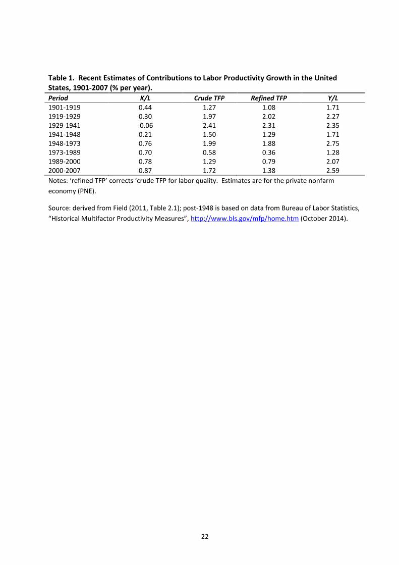
grow th,respectively. M odern research basically confirm sthese findingsand also show sthat T FP

grow th w asby farthe predom inant source oflaborproductivity grow th even w hen refinem entsare

m adetoallow forim provem entsinlaborquality (cf.T able1).

T he context for these estim atesisthe episode oftechnologicaladvance w hich isoften called the

‘second industrialrevolution’ w hich saw the U nited S tatesovertake Britain asthe w orld’sleading

econom y and in the processachieve unprecedented ratesofT FP grow th.1 During the early decadesof

thetw entiethcentury,theU nitedS tatesw asintheforefrontofthedevelopm entofthem ostim portant

new technologiesincluding aviation,the internalcom bustion engine,m assproduction,electricity,and

petrochem icals(M ow ery and R osenberg,2000). Electricity,w hose im pactpeaked in the 1920s(David,

1991),isw idely recognized asone ofhistory’sm ost im portant generalpurpose technologies(GP T s).

Gordon (1999; 2000)described T FP grow th in the period betw een 1891 and 1972 as‘one big w ave’

based on afew m ajortechnology clustersw hich delivered m uch m ore rapid advance than hasbeen

seen since orseem slikely in future. Im portantly,T FP grow th continued to be rapid through the Great

Depression and Field (2003)labeled the 1930sasthe ‘m ost technologically progressive decade’ ofthe

tw entiethcentury.

U nderstanding how and w hy the U nited S tatesw asso successfulin achieving rapid technological

progressat thistim e isobviously im portant,allthe m ore so given current fearsabout ‘secular

stagnation’. A key aspect ofthisisto decide on the m ost appropriate vision ofthe grow th process,a

challenge w hich w asset by Harberger(1998) in hispresidentialaddressto the Am erican Econom ic

Association. Harbergercontrasted the possibility ofa‘yeastprocess’ and a‘m ushroom process’ ofT FP

grow th (orin histerm inology ‘realcostreduction’);the form erw ould be based on acom m on source –

perhapsaGP T w ith m any spillovers-applying acrossm any sectors,w hile the latter w ould entail

m ultipledisparatesources.

Against thisbackground,the m ain contribution ofthispaper isto develop am uch im proved and

extended datasetw hich providesam uch fullerdescription ofthe sectoralpattern ofT FP grow th across

theAm ericaneconom y fortheperiod1899 to1941 andsub-periodsw ithinthoseyears. Com paredw ith

the estim atesin Kendrick (1961),w hich stillcom prise the m ain source available to researchers,our

grow th accounting coversin detailabout 80 percent ratherthan 50 percent ofthe private dom estic

econom y (P DE),w e provide detailed estim atesfor1929 to 1941 ratherthan 1929 to 1937,w e adjust

T FP grow th forlaborquality im provem ent w ithin occupations,w e estim ate the contribution ofcapital

inputson acapital-servicesbasisw here feasible,i.e.,for1929 to 1941,and w e obtain aset ofvalue-

added w eightsw hich allow boththe aggregationofsectoralT FP grow th ratesand also theconstruction

ofdiagram sto illustrate the degree ofinequality ofsectoralcontributionsto totalT FP grow th. O verall,

w e find that contributionsto T FP grow th w ere spread w idely acrossthe Am erican econom y,so w e

perform an additionalgrow th accountingexercise relatingto the directand indirectim plicationsofT FP

1N otonly w as2 percentperyearfarin excessofw hatthe U nited S tatesitselfhad achieved during m ostofthe

nineteenth century,it w asalso w ellahead ofT FP grow th in Britain during and afterthe IndustrialR evolution

w hichneverexceeded0.8percentperyear(Abram ovitzandDavid,2001;Crafts,2004a;M atthew setal.,1982).

2

grow thinelectricalcapitalinthe1920sw henelectricity had itsm axim um im pactasaGP T . W eusethe

resultsofthese investigationsto challenge,orat least to qualify,claim sm ade by David (1991),Field

(2011),Gordon(2000),andHarberger(1998).

T o thisend,w e addressseveralspecificquestions. First,w e considerw hetherthe grow th processw as

‘m ushroom s’ (originating in m ultiple disparate sources),or‘yeast’ (w idespread and originating in one

dom inantsource),orsuperficially yeastbutactually m ushroom s. S econd,w equantify theim pactofthe

technology clustersthat are said to com prise the ‘one big w ave’ ofT FP grow th. T hird,w e re-exam ine

theissueofw hetherthe1930sreally w asthem osttechnologically progressivedecadeofthetw entieth

century. Fourth,w e review the m agnitude and pervasivenessofT FP grow th accruing from investm ent

inelectricm otorsinm anufacturingduringthe1920stoaccountfortheroleofelectricity asaGP T .

Inoutline,ourapproachisasfollow s. W euseconventionalneoclassicalgrow thaccountingassum ptions

taking account oflaborquality in m easuring laborinputs. W e start w ith the estim atesin Kendrick

(1961)for1899-1929 and im prove and extend them w here possible. W e are able to add 5 sectors–

construction,distribution,FIR E (finance,insurance,and realestate),postalservices,and spectator

entertainm ent. W e produce estim atesfor 1929 to 1941 using the N ationalIncom e and P roduct

Accounts(N IP A)to obtain nom inalvalue added atthe industry level(w hich aredeflated usingavailable

price data) and em ploym ent. Capitalinputsfor 1929 to 1941 are constructed using a perpetual

inventory m ethod and investm entdatafrom the BEA’s(2010)fixed assetstables.T he capitalstocksare

then aggregated to the industry levelon the basisofim puted rentalprices.T he result isam easure of

capitalservices,w hichaccurately capturestheinputflow sderived from thecapitalinplace.W ereplace

Kendrick’spre-1929 indicesoflaborinputsand develop new industry levelindicesfor1929 to 1941,

taking changesin the quality oflaborinto account.T he big advantage ofourm ethod forestim ating

laborinputscom pared w ith thatofKendrick(1961)isthatitaccountsforim provem entsin educational

attainm entw ithin occupations. M oreover,since w e now have both capitaland laborinputsm easured

on asim ilarbasisto that ofthe BL S ourT FP estim atesfor1929 to 1941 are com parable w ith the BL S

estim atesforthepost-1948 period.

Having constructed these new grow th accounting estim atesat the sectorallevel,w e use them to

exam inetheconcentrationand persistenceoftheindustry originsofT FP grow th. W eexam ineboththe

rateofT FP grow thand theintensivegrow thcontribution(T FP grow thm ultiplied by shareoftotalvalue

added)ofeach sector. T hisenablesusto construct diagram sforthe P DE in the style ofHarberger

(1998) and thusto see w hether the resulting pictureslook like ‘m ushroom s’ or ‘yeast’. W e also

com pute rank correlationsto exam ine inter-tem poralpersistence ofproductivity perform ance at the

sectorallevel. In orderto pursue the issue ofthe role ofelectrification offactoriesin T FP grow th in

Am erican m anufacturing,w e obtain estim atesofT FP spilloversby replicating the regression analysisin

David (1991)using ournew T FP estim atesand also develop estim atesofelectricalcapitalin use atthe

sectorallevel. T hisperm itsboth grow th accounting w ith tw o typesofcapital(electricaland non-

electrical) and also the construction of Harberger diagram s for electrical and non-electrical

contributionstoT FP grow thinm anufacturingforthe1920s.

T he resultsofthese analysesare quite different from those ofearlierw orkin anum berofim portant

aspects. First,w e estim ate am uch higherrate ofgrow th oflaborquality than did Kendrick(1961);for

1899-1941,ourestim ate isabout 0.8 percent peryearw hile hisw asabout 0.3 percent peryear. An

im m ediate corollary isthatw e estim ate alow errate ofT FP grow th in the P DE at1.3 percentperyear

during 1899-1941 com pared w ith Kendrick’sestim ate of1.7 percent peryear. S econd,w e estim ate

3

that the technology clustersassociated w ith Gordon’s‘one big w ave’ accounted forjust under40 per

centofT FP grow th intheP DEduring1899-1941. T heircontributionrose steadily from 0.3 percentper

yearin 1899-1909 to justunder0.75 percentperyearin 1929-41. T hisisim pressive but possibly less

overw helm ingthan areaderofGordon (2000)m ightim agine. T hird,w e do notagree w ith Field (2003)

(2011)thatthe 1930sw asthe m osttechnologically progressive decade ifthe criterion isT FP grow th in

the P DE;w e estim ate thatT FP grow th w as1.87 percent peryearduring 1929-41 com pared w ith 2.00

percent peryearduring 1948-60 and 2.23 percent peryearduring 1960-73. Fourth,w e find that,

includingboth ow n T FP grow th and T FP spillovers,electricalcapitalcontributed only 28 percentofT FP

grow th in m anufacturing during the 1920sand that thiscontribution varied m ore acrosssectorsthan

did non-electricalT FP grow th,so ourfindingsdo not support the ideaofayeast processbased on

electricity asaGP T asthe best w ay to conceptualize technologicalprogressin m anufacturing at this

tim e. Fifth,w e find that intensive grow th contributionsw ere generally broadly-based w hetherat the

levelofthe P DE orofm anufacturing,w ith the exception ofthe period 1909-19. How ever,w e also find

thatthere isratherlow persistence ofT FP grow th and intensive grow th contributionsbetw een periods

and the econom ichistory literature revealsm ultiple sourcesofT FP grow th. T ogetherw ith ourfindings

on electricity,thisleadsusto conclude thatHarberger’svision thatT FP grow th isreally a‘m ushroom s’

processisprobably righteventhough,superficially,theappearanceis‘yeast-like’.

O urresultstake on added significance in the context ofthe renew ed interest in selective industrial

policy thathasem erged since the financialcrisisof2008 (W arw ick,2013). T hism ightbe thoughtofas

intervening to encourage ashift ofproductive resourcestow ardssectorsw ith prospectsofrapid T FP

grow th. O urinvestigation ofT FP grow th during 1899-1941 underlinesthe dangersofselective policies

favoring‘technologically progressive’ industries. In particular,ourresultssuggestthatT FP grow th over

tim e w ashighly unpredictable,that there w ere m ultiple sourcesofT FP grow th ratherthan afew key

technologies,and that large,unglam oroussectorslike w holesale and retailtrade,w hich can benefit

from but do not originate technologicalprogress,contributed m uch m ore to T FP grow th than exciting

new industrieslike electric m achinery. T hissuggeststhat Harberger(1998)w asright to argue that

ratherthan to try to backw inners,the key role forpolicy isto enable firm sto respond effectively to

changingcircum stancesandnottoobstructcreativedestruction.

1. Key Ideas and Literature Review

A naturalstarting point forconsidering the spread ofproductivity grow th acrosssectorsisthe sem inal

paperby Harberger(1998). T hispaperintroduced agraphicaldevice sim ilarto the L orenz Curve to

display the pattern ofT FP grow th contributionsby industry w hen industriesare ranked by theirT FP

grow th rate from highestto low est;thisisreproduced in Figure 1. Here Figure 1ashow sacase w here

allsectorscontribute to T FP grow th and no industry dom inatesthe grow th processw hile Figure 1b

show sacase w here T FP grow th isnegative in asignificant num ber of sectorsand relatively few

industriesaccountform ostofthetotal.

Harberger used the term inology ofa‘yeast process’ and a‘m ushroom process’ to describe these

patterns.2 A ‘yeast process’ w ould be based on very broad and generalexternalitiesw hereasa

‘m ushroom process’ w ould result from T FP grow th w ith a1001 different causes. How ever,it isalso

possible,asHarbergeracknow ledged,that a‘yeast-like pattern’ m ight be observed w hen disparate

(unconnected)sourcesofT FP grow th happen to be w idespread and sectorsw ith negative T FP grow th

2T heanalogy com esfrom thefactthatyeastcausesbreadtoexpandvery evenly w hereasm ushroom spopup

unpredictably andspasm odically.

4

are absent orat least have little w eight. Harberger’sow n view w asthat the ‘m ushroom ’ diagram

represented theusualconfigurationand heproducedestim atestoillustratethisfortheU nited S tatesin

the period 1948 to 1985 w here the diagram sresem bled Figure 1b ratherthan Figure 1a. M oreover,he

argued thatovertim e differentindustriesdom inated so thatcontributionsw ere notonly concentrated

w ithin each period but exhibited little persistence betw een periods. He thought thism ight be

characteristicofaS chum peterianprocessof‘creativedestruction’. Harbergerdidnotprovideestim ates

forearlierin thetw entiethcentury buthe stated thathe thoughtthatthem ushroom pattern prevailed

then asw elland thatthe 1920sw asthe decade ofcarsand rubbertires,the 1930sw asthe decade of

refrigerators,andthe1940sw asthedecadeofpharm aceuticals(1998,p.5).

It m ay seem thataGeneralP urpose T echnology (GP T ),i.e.one w hich com esto have m any uses,to be

w idely used and to have m any Hicksian and technologicalcom plem entarities(L ipsey,1998) w ould

generateayeastprocessforT FP grow thsim ilartoFigure1. T hisneednotbethecase,how ever.

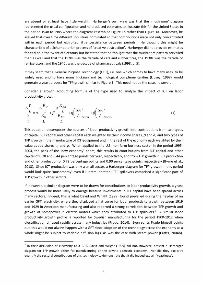
Consider a grow th accounting form ula of the type used to analyze the im pact of ICT on labor

productivity grow th

NICTMICTMICT

ICT

O

O

A

A

A

A

L

KL

K

L

KL

K

L

YL

Y

(1)

T hisequation decom posesthe sourcesoflaborproductivity grow th into contributionsfrom tw o types

ofcapital,ICT capitaland othercapitaleachw eightedby theirincom eshares, and α,and tw otypesof

T FP grow thinthem anufactureofICT equipm entand intherestoftheeconom y eachw eighted by their

value-added shares,η and φ . W hen applied to the U .S .non-farm businesssectorin the period 1995-

2004,the peak ofthe ‘new econom y’ boom ,thisresultsin contributionsfrom ICT capitaland other

capitalof0.78 and0.44 percentagepointsperyear,respectively,andfrom T FP grow thinICT production

and otherproduction of0.72 percentage pointsand 0.90 percentage points,respectively (Byrne et al.,

2013). S ince ICT production w asonly asm allsector,aHarbergerdiagram forT FP grow th in thisperiod

w ould look quite ‘m ushroom y’ even if(unrem unerated)T FP spilloverscom prised asignificant part of

T FP grow thinothersectors.

If,how ever,asim ilardiagram w ere to be draw n forcontributionsto laborproductivity grow th,ayeast

processw ould be m ore likely to em erge because investm entsin ICT capitalhave been spread across

m any sectors. Indeed,thisisw hat David and W right (1999)found prevailed during the heyday ofan

earlierGP T ,electricity,w here they displayed aflat curve forlaborproductivity grow th betw een 1919

and 1929 in Am erican m anufacturing and also reported astrong correlation betw een T FP grow th and

grow th ofhorsepow er in electric m otorsw hich they attributed to T FP spillovers.3 A sim ilar labor

productivity grow th profile isreported for S w edish m anufacturing for the period 1900-1912 w hen

electrification diffused rapidly acrossm any industries(P rado,2014). Even so,asP rado him selfpoints

out,thisw ouldnotalw ayshappenw ithaGP T sinceadoptionofthetechnology acrosstheeconom y asa

w hole m ight be subject to variable diffusion lags,asw asthe case w ith steam pow er(Crafts,2004b).

3In theirdiscussion ofelectricity asaGP T ,David and W right (1999) did not,how ever,present aHarberger

diagram for T FP grow th either for m anufacturing or the private dom estic econom y. N or did they explicitly

quantify thesectoralcontributionsofthistechnology todem onstratethatitdidindeedexplain‘yeastiness’.

5

And in any case,the GP T m ay not be the only gam e in tow n since itsem ergence m ay com e at atim e

w henm yriadothersourcesofproductivity im provem entareavailable.

Although the Harberger-type approach hasgenerally been applied to m anufacturing,thisseem sunduly

restrictive especially given the im portant role that productivity grow th in servicesplayed in the

tw entieth century U nited S tates. T hisisim plicit in the w ell-know n account ofAm erican econom ic

grow th given by Gordon (2000)w ho describes‘one big w ave’ in T FP grow th betw een 1891 and 1972

w ith an acceleration peakingin 1928-1950. He argued thatthisw asdriven by fourtechnology clusters:

electricity,the internalcom bustion engine together w ith derivative inventionssuch asinterstate

highw ays and superm arkets, rearranging m olecules (chem icals and pharm aceuticals), and the

entertainm ent,com m unication and inform ation sector. S urprisingly,Gordon did not attem pt to

quantify thegrow thcontributionofthesefourtechnologiesovertim e.

T he m ostcom prehensive recentdescription ofthe grow th processw hich attem ptsadecom position of

sectoralcontributionsto productivity grow th in the early tw entieth century Am erican econom y isby

Field (2011)w ho drew heavily on the w orkofKendrick(1961). Field em phasized that there w ere big

differencesbetw een the 1920s,in w hich T FP grow th w asdom inated by m anufacturing,and the 1930s

w hen T FP grow th w asspread m ore w idely acrossm uch ofthe econom y. In the period 1919 to 1929,

T FP grow th in m anufacturingw asvery rapid at5.1 percentperyearand exceeded 2 percentperyear

in allbut one 2-digit m anufacturing industry; prim afacie thisdoesnot seem to m atch Harberger’s

caricatureand rapid electrificationoffactoriesatthattim em ightseem toindicatethata‘yeastprocess’

w asatw ork. Intheperiod 1929 to1937,how ever,T FP grow thinm anufacturingfellto1.9 percentper

yearandtherangeofT FP grow thacrossm anufacturingindustriesw asm uchgreater.

An im portant innovation m ade by Field w asto exam ine T FP grow th for the period 1929 to 1941

w hereasKendrick(1961)based hisdisaggregated estim ateson the period 1929 to 1937;it isthe later

end date w hich justifiesthe label‘the m ost technologically progressive decade’. T he rationale for

replacing 1937 by 1941 isthat thisperm itsaview based on ayearw hen econom icrecovery from the

Depression w asm ore com plete.4 Field (2011) provided a 4-sector breakdow n of T FP grow th

contributionsw hich suggeststhat even ifT FP grow th w ithin m anufacturing w as‘yeasty’ in the 1920s

thism ay not be true forthe econom y asaw hole. O n the otherhand,forthe 1930shisem phasison

broadly-based T FP grow thsuggeststhata‘yeast-likepattern’ stem m ingfrom varioussourcesm ay have

prevailed in the econom y ifnot m anufacturing. How ever,to explore these pointsproperly requiresa

4Asnotedby Field(2011),1941 w asthefirstyearsince1929 thatunem ploym entaveragedlessthan10 percent,

m akingitfarpreferableto1937asa(peacetim e)peakyear.S till,1941 isnotideal,asunem ploym entw ashigher(9.9 percent)thanin1929 (3.2 percent).Becauseofthepro-cyclicalnatureofproductivity,FieldarguesthatT FPw ouldhavebeenhigherin1941 hadtheeconom y operatedatfullcapacity,m ainly becauseoftheeffectsoflaborandcapitalhoarding.T oaddressthis,hesuggestsaone-offadjustm entthatraisestheaverageannualgrow thofT FP betw een1929 and1941 from 2.31 to2.78.Inklaaretal.(2011)provideam orecom prehensivetestofthecyclicalnatureofproductivity intheinterw arU S econom y.T hey findrobustevidenceofshort-runincreasingreturnstoscale,onthebasisofw hichthey calculatea‘purified’ m easureoftechnologicalchangew hichconfirm sthat“ thehoardingofproductionfactorsw asthedom inantreasonforthedeclineinm easuredS olow residualT FPinU .S .m anufacturingbetw een1929 and1933.” (Inklaaretal.2011:851)Betw een1933 and1937,how ever,T FPgrew m uchfasterthantechnology,resultingfrom arapidexpansionoftheutilizationoffactorinputs.IntheyearsleadinguptheS econdW orldW arthepotentialbiasbetw eenT FP andtechnology hadvanished. Itshouldalsobenotedthat,althoughunem ploym entin1941 w asabovethe1929 level,thepeacetim eoutputgapm ay havealready closed. Itisw idely acceptedthattheN ew DealraisedtheN AIR U significantly;forexam ple,ColeandO hanianfoundthattheunem ploym entratew asraisedby 6 pecentagepointsw hileHattonandT hom as(2010)estim atedthattheim pactw asprobably evenlarger. T akentogether,thesepointsm aketheadjustm entsuggestedby Fieldhardtojustify andw eprefertousetheraw datafor1941.

6

fulldecom positionbased onappropriatew eightsandafinerbreakdow nthanthebroad sectorsused by

Field.

T hebottom lineisthattheliteraturedoesnotcontainanadequatequantitativeaccountoftheindustry

originsofproductivity grow thduringtheearly tw entiethcentury and thisim pliesthatexistingvisionsof

the grow th processare som ew hat blurred. In particular,it isnot really clearw hetherthe processw as

alw ays‘m ushroom s’,asHarberger w ould expect,or w hether there w asaphase w ith a‘yeast-like

process’ atleastattheheightoftechnologicalprogressivity inthe1930s,asField’saccountsuggests. It

isalso unclearw hetherelectricity asaGP T can be credited w ith prom oting a‘yeast process’ ofT FP

grow thinm anufacturinginthe1920s. W eseektoclarify theseissues.

In theoreticalterm s,then,w e can subdivide the underlying grow th processinto tw o different types:

generalized T FP -grow th,inw hichonedom inantsourceofT FP grow thw orksw ithalargeeffectacrossa

large num berofindustries(ayeast process); and specialized T FP grow th in w hich,at the extrem e,a

source ofT FP grow th w orksjust w ithin one industry (am ushroom process).5 In turn,specialized T FP

grow th canbedividedintotw ocases:universalspecializedT FP grow th,inw hichavery largenum berof

industriesexperienceT FP grow thfrom anindustry-specificsource;and sporadicspecialized T FP -grow th,

inw hichonly alim itednum berofindustriesexperienceT FP grow thfrom anindustry-specificsource.

T hism eansthatthe observation ofayeastpattern can reflectfourdifferentunderlyingprocesses:zero

T FP grow th (universalstagnation),universalspecialized T FP grow th only,generalized T FP grow th only,

and finally,acom bination ofgeneralized T FP grow th and universalspecialized T FP grow th. In the

context of aHarberger diagram ,these processesw ould be observationally equivalent and further

inform ation w ould be required to discrim inate betw een them . O fcourse,observing am ushroom

patternisnotconsistentw ithany ofthesefourunderlyingprocesses.

U sing the above term inology,it isclearthat Harberger’snarrative account ofm ushroom sm ixestw o

differentunderlying processesthatresultin observingeitheram ushroom orayeast pattern.W hen he

m entions‘1001 differentcauses’ ofT FP -grow th,thisappearsvery m uch to referto agrow th processof

universalspecialized T FP -grow th(thevastm ajority ofindustriesexperiencesubstantialindustry-specific

T FP -grow th),w hich actually islikely to lead to observingayeastpattern.W hen Harbergerrem arksthat

the 1920sw ere the decade ofcars,the 1930sofhousehold appliancesand the 1940sofantibiotics,he

appearsto referto agrow th processofsporadicspecialized T FP grow th (asm allnum berofindustries

experience substantialindustry-specific T FP grow th),w hich w ould lead usto expect am ushroom

pattern.

2. Data and Methods

T he definitive study on productivity grow th atthe industry levelinthe U nited S tatesforthe firsthalfof

the tw entieth century isKendrick (1961). Although Kendrick offered substantialdetail,the estim ates

presented inhisbookfallsom ew ay shortofw hatisrequired forafullem piricalevaluationoftheideas

ofFieldandHarberger. Kendrickprovidesestim atesofaverageannualT FP grow thfor1899 to1953 and

forsub-divisionsofthese yearsforthe aggregate ofthe private dom estic econom y and for5 sectors

w hich in turn are divided into 33 industries. T hese sectorscovered 54 percentofthe private dom estic

econom y in 1953. T FP grow th forthe rem aining46 percent(w hich includesconstruction,distribution,

5Aninterm ediatetypeofgrow thw ouldbeaprocessinw hichasourceofT FP grow thhasaneffectonm orethan

oneindustry,butthenum berofindustriesrem ainslim ited.

7

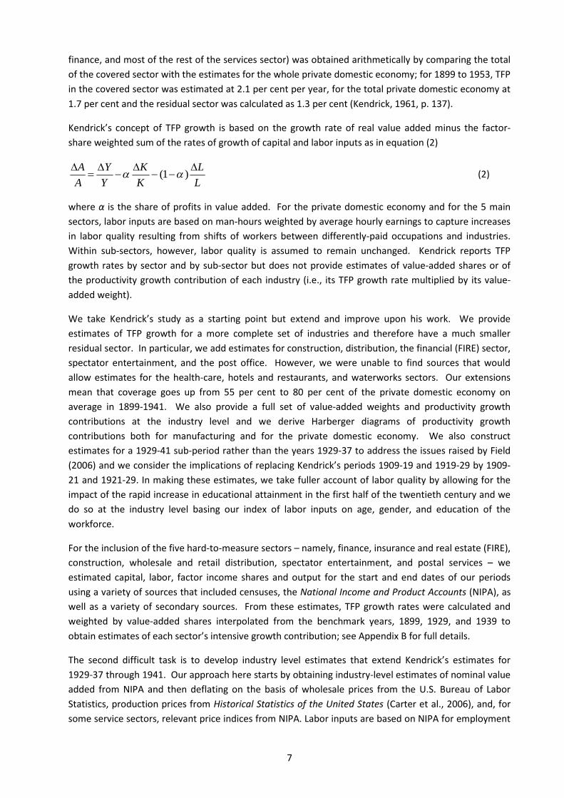
finance,and m ostofthe restofthe servicessector)w asobtained arithm etically by com paringthetotal

ofthecoveredsectorw iththeestim atesforthew holeprivatedom esticeconom y;for1899 to1953,T FP

inthecovered sectorw asestim ated at2.1 percentperyear,forthetotalprivatedom esticeconom y at

1.7 percentandtheresidualsectorw ascalculatedas1.3 percent(Kendrick,1961,p.137).

Kendrick’sconcept ofT FP grow th isbased on the grow th rate ofrealvalue added m inusthe factor-

sharew eightedsum oftheratesofgrow thofcapitalandlaborinputsasinequation(2)

L

L

K

K

Y

Y

A

A

)1( (2)

w here α isthe share ofprofitsin value added. Forthe private dom esticeconom y and forthe 5 m ain

sectors,laborinputsarebased onm an-hoursw eighted by averagehourly earningsto captureincreases

in laborquality resulting from shiftsofw orkersbetw een differently-paid occupationsand industries.

W ithin sub-sectors,how ever,laborquality isassum ed to rem ain unchanged. Kendrick reportsT FP

grow th ratesby sectorand by sub-sectorbut doesnot provide estim atesofvalue-added sharesorof

the productivity grow th contribution ofeach industry (i.e.,itsT FP grow th rate m ultiplied by itsvalue-

addedw eight).

W e take Kendrick’sstudy asastarting point but extend and im prove upon hisw ork. W e provide

estim atesofT FP grow th foram ore com plete set ofindustriesand therefore have am uch sm aller

residualsector. Inparticular,w eaddestim atesforconstruction,distribution,thefinancial(FIR E)sector,

spectatorentertainm ent,and the post office. How ever,w e w ere unable to find sourcesthat w ould

allow estim atesforthe health-care,hotelsand restaurants,and w aterw orkssectors. O urextensions

m ean that coverage goesup from 55 percent to 80 percent ofthe private dom estic econom y on

average in 1899-1941. W e also provide afullset ofvalue-added w eightsand productivity grow th

contributions at the industry level and w e derive Harberger diagram s of productivity grow th

contributionsboth for m anufacturing and for the private dom estic econom y. W e also construct

estim atesfora1929-41 sub-period ratherthan the years1929-37 to addressthe issuesraised by Field

(2006)and w e considerthe im plicationsofreplacingKendrick’speriods1909-19 and 1919-29 by 1909-

21 and 1921-29.In m aking these estim ates,w e take fulleraccount oflaborquality by allow ing forthe

im pactofthe rapid increase in educationalattainm entin the firsthalfofthe tw entieth century and w e

do so at the industry levelbasing ourindex oflaborinputson age,gender,and education ofthe

w orkforce.

Fortheinclusionofthefivehard-to-m easuresectors– nam ely,finance,insuranceandrealestate(FIR E),

construction,w holesale and retaildistribution,spectator entertainm ent,and postalservices– w e

estim ated capital,labor,factorincom e sharesand output forthe start and end datesofourperiods

usingavariety ofsourcesthatincluded censuses,the N ationalIncom eand P roductAccounts(N IP A),as

w ellasavariety ofsecondary sources. From these estim ates,T FP grow th ratesw ere calculated and

w eighted by value-added sharesinterpolated from the benchm ark years,1899,1929,and 1939 to

obtainestim atesofeachsector’sintensivegrow thcontribution;seeAppendix B forfulldetails.

T he second difficult task isto develop industry levelestim atesthat extend Kendrick’sestim atesfor

1929-37 through1941. O urapproachherestartsby obtainingindustry-levelestim atesofnom inalvalue

added from N IP A and then deflating on the basisofw holesale pricesfrom the U .S .Bureau ofL abor

S tatistics,production pricesfrom HistoricalS tatisticsofthe U nited S tates(Carteret al.,2006),and,for

som eservicesectors,relevantpriceindicesfrom N IP A.L aborinputsarebased onN IP A forem ploym ent

8

adjusted forhoursofw ork using Kendrick (1961) and HistoricalS tatisticsand forquality using the

m ethod detailed below . Capitalinputsare estim ated on the basisofcapitalservices. W e estim ate the

industry-levelstock of capitalfor the private dom estic econom y betw een 1929 and 1941 using a

P erpetualInventory M ethod (P IM )and the investm ent and depreciation seriestaken from the BEA’s

FixedAssetstables.6 R entalpricesofassetsattheindustry levelarebased ontheim puted industry rate

ofreturn,theasset-specificrateofdepreciationand capitalgainsand lossesfrom changingassetprices.

T hisallow sthe calculation of ‘capitalcom pensation’ w eightsto aggregate the capitalinput.7 W e

presentfulldetailsinAppendix C.

T hree featuresofthe m ethodsthat w e em ploy deserve som e com m ent. T hese relate to the w ay in

w hich industrialcontributionsto aggregate T FP grow th are m easured,to the w ay in w hich w e m easure

laborquality,andtothesum m ary statisticusedtodescribethe‘yeastiness’ ofproductivity grow th.

Follow ingKendrick(1961),w eem ploy agrow thaccountingtechniquebasedonvalue-addedratherthan

grossoutput. T hisalso m irrorsthe approachesto exam ining contributionsto T FP grow th adopted by

Field (2011)and Harberger(1998). T hisim pliesthatw etakethecontributionto T FP grow thofindustry

jasω j(Δ Aj/Aj) w here ω j isvalue added in industry jdivided by GDP and w e sum these individual

contributionsofalln industriesto obtain T FP grow th forthe aggregate private dom esticeconom y so

that

j

jn

jj

GDP

GDP

A

A

A

A

1

(3)

T hisapproach can be interpreted asm easuring an industry’scapacity to contribute to econom y w ide

productivity but the com ponentsof thisaggregate are not an accurate m easure of disem bodied

technicalchange (O ECD,2001).8 An industry’sintensive grow th contribution (IGC)therefore depends

notonly on itsrate ofT FP grow th butalso on itssizeand itfollow sthatintensive grow th contributions

by industry arenotnecessarily highly correlatedw ithT FP grow thrates.

O urapproach to m easuring laborquality im proveson thatofKendrick,in particular,by taking account

of the im plicationsof the rapid increase in yearsof schooling on the quality of w orkersin each

occupation overtim e but also by allow ing forchangesin gendercom position and experience ofthe

laborforce. O urm ethod also perm itsm easurem ent oflaborquality at the industry level. S o forall

industriesw e conductgrow th accounting w ith m easurem entoflaborinputbased on quality asw ellas

hoursw orked. N otsurprisingly,thism ethod findsahigherrateofgrow thoflaborquality;laborquality

in the private dom esticeconom y during1899-1941 isestim ated to have grow n at0.8 percentperyear

com paredw ithKendrick’sestim ateof0.3 percent.

6N otethatGordon(2016)arguesthattheofficialinvestm entanddepreciationratesfrom theBEA severely

underestim atethegrow thofcapitalinputsfortheperiodbetw een1925 and1945.Inparticular,hequestionsw hetherthedepreciationrates,w hicharefixedovertim e,arerepresentativefortheDepressionera.Appendix Cexplorestheim pactthattheadjustm enttotheofficialdepreciationrates,alongthelinessuggestedby Gordon,w ouldhaveonT FP grow thbetw een1929 and1941.7

Itisnotpossibletousethism ethodtoreplaceKendrick’sestim atesofcapitalinputsforthepre-1929 periodw hichareobtainedusingatraditionalcapitalstocksm ethod. Inparticular,w elackasset-by-industry capitalstocksandasset-specificdepreciationrates. ItshouldbenotedthatthedifferencesinT FP grow thbetw eenthetw om ethodsaregenerally fairly sm all;theim plicationsareexploredinAppendix C.8

Analternativew hichhasthisdesirableproperty istodogrow thaccountingonagrossoutputbasisw heretheuseofinterm ediateinputsisexplicitly takenintoaccountandaggregationisbasedonDom arw eights(cf.Hulten,1978). T hisistoodatadem andingtobeattem ptedhere,giventheavailablehistoricalsources.

9

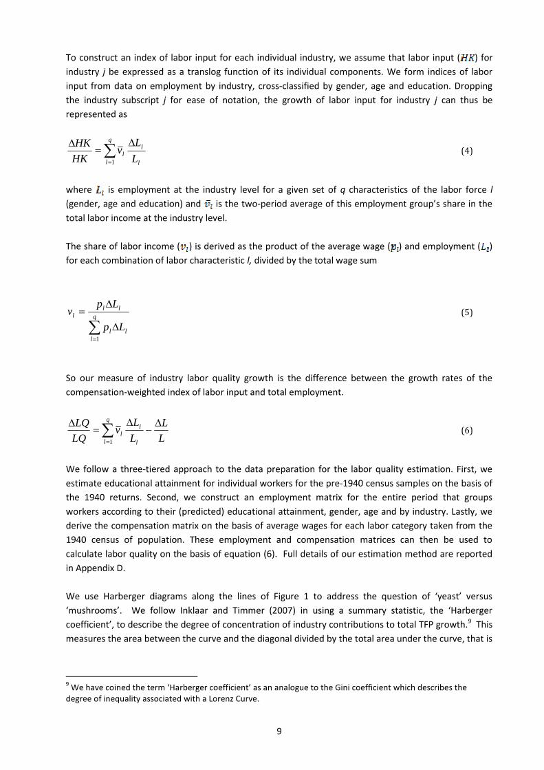
T o construct an index oflaborinput foreach individualindustry,w e assum e that laborinput ( )for

industry jbe expressed asatranslog function ofitsindividualcom ponents.W e form indicesoflabor

input from dataon em ploym ent by industry,cross-classified by gender,age and education.Dropping

the industry subscript jfor ease ofnotation,the grow th oflabor input forindustry jcan thusbe

representedas

l

lq

ll

L

Lv

HK

HK

1

(4)

w here isem ploym ent at the industry levelforagiven set ofq characteristicsofthe laborforce l

(gender,age and education)and isthe tw o-period average ofthisem ploym entgroup’sshare in the

totallaborincom eattheindustry level.

T he share oflaborincom e ( )isderived asthe productofthe average w age ( )and em ploym ent( )

foreachcom binationoflaborcharacteristicl,dividedby thetotalw agesum

l

q

ll

lll

Lp

Lpv

1

(5)

S o ourm easure ofindustry laborquality grow th isthe difference betw een the grow th ratesofthe

com pensation-w eightedindex oflaborinputandtotalem ploym ent.

L

L

L

Lv

LQ

LQ

l

lq

ll

1

(6)

W e follow athree-tiered approach to the datapreparation forthe laborquality estim ation.First,w e

estim ateeducationalattainm entforindividualw orkersforthepre-1940 censussam plesonthebasisof

the 1940 returns. S econd,w e construct an em ploym ent m atrix for the entire period that groups

w orkersaccording to their(predicted)educationalattainm ent,gender,age and by industry.L astly,w e

derive the com pensation m atrix on the basisofaverage w agesforeach laborcategory taken from the

1940 censusof population. T hese em ploym ent and com pensation m atricescan then be used to

calculate laborquality on the basisofequation (6). Fulldetailsofourestim ation m ethod are reported

inAppendix D.

W e use Harberger diagram salong the linesof Figure 1 to addressthe question of ‘yeast’ versus

‘m ushroom s’. W e follow Inklaar and T im m er (2007) in using asum m ary statistic,the ‘Harberger

coefficient’,todescribethedegreeofconcentrationofindustry contributionstototalT FP grow th.9 T his

m easurestheareabetw eenthecurveandthediagonaldividedby thetotalareaunderthecurve,thatis

9W ehavecoinedtheterm ‘Harbergercoefficient’ asananaloguetotheGinicoefficientw hichdescribesthe

degreeofinequality associatedw ithaL orenzCurve.

10

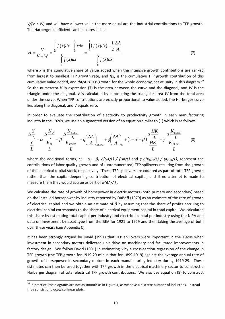
V/(V + W )and w illhave alow ervalue the m ore equalare the industrialcontributionsto T FP grow th.

T heHarbergercoefficientcanbeexpressedas

1

0

1

0

1

0

1

0

1

0

)(

2

1)(

)(

)(

dxxf

A

Adxxf

dxxf

xdxdxxf

WV

VH (7)

w here x isthe cum ulative share ofvalue added w hen the intensive grow th contributionsare ranked

from largest to sm allest T FP grow th rate,and f(x)isthe cum ulative T FP grow th contribution ofthis

cum ulative value added,and dA/A isT FP -grow th forthe w hole econom y,setatunity in thisdiagram .10

S o the num eratorV in expression (7)isthe areabetw een the curve and the diagonal,and W isthe

triangle underthe diagonal.V iscalculated by subtracting the triangularareaW from the totalarea

underthe curve.W hen T FP contributionsare exactly proportionalto value added,the Harbergercurve

liesalongthediagonal,andV equalszero.

In order to evaluate the contribution of electricity to productivity grow th in each m anufacturing

industry inthe1920s,w euseanaugm entedversionofanequationsim ilarto(1)w hichisasfollow s:

L

KL

K

L

HKL

HK

A

A

A

A

L

KL

K

L

KL

K

L

YL

Y

ELEC

ELEC

OELECELEC

ELEC

O

O

1 (8)

w here the additionalterm s,(1 – α – ) Δ (HK/L ) / (HK/L ) and Δ (KEL EC/L ) / (KEL EC/L ),represent the

contributionsoflaborquality grow th and of(unrem unerated)T FP spilloversresulting from the grow th

oftheelectricalcapitalstock,respectively. T heseT FP spilloversarecounted aspartoftotalT FP grow th

rather than the capital-deepening contribution of electricalcapital,and if no attem pt ism ade to

m easurethem they w ouldaccrueaspartofφ (Δ A/A)O .

W e calculate the rate ofgrow th ofhorsepow erin electricm otors(both prim ary and secondary)based

ontheinstalled horsepow erby industry reported by DuBoff(1979)asanestim ateoftherateofgrow th

ofelectricalcapitaland w e obtain an estim ate of by assum ing that the share ofprofitsaccruing to

electricalcapitalcorrespondsto the shareofelectricalequipm entcapitalin totalcapital.W e calculated

thisshare by estim atingtotalcapitalperindustry and electricalcapitalperindustry usingthe N IP A and

dataon investm ent by asset type from the BEA for1921 to 1929 and then taking the average ofboth

overtheseyears(seeAppendix C).

It hasbeen strongly argued by David (1991) that T FP spilloversw ere im portant in the 1920sw hen

investm ent in secondary m otorsdelivered unit drive on m achinery and facilitated im provem entsin

factory design. W e follow David (1991)in estim ating by across-section regression ofthe change in

T FP grow th (the T FP -grow th for1919-29 m inusthat for1899-1919)againstthe average annualrate of

grow th ofhorsepow erin secondary m otorsin each m anufacturing industry during 1919-29. T hese

estim atescan then be used togetherw ith T FP grow th in the electricalm achinery sectorto constructa

Harbergerdiagram oftotalelectricalT FP grow th contributions. W e also use equation (8)to construct

10Inpractice,thediagram sarenotassm oothasinFigure1,asw ehaveadiscretenum berofindustries. Instead

they consistofpiecew iselinearplots.

11

Harberger-type diagram sofcontributionsto laborproductivity grow th follow ing the lead ofDavid and

W right (1999)but in addition distinguishing betw een electricaland non-electricalcontributions. W e

calculatetheequivalentoftheHarbergercoefficient(H*)from am odified versionofequation(7)w hich

is

1

0

1

0

1

0

1

0

1

0

)(

2

1)(

)(

)(

dxxf

L

YL

Y

dxxf

dxxf

xdxdxxf

H (9)

w hereonthisoccasionf(x)isthecum ulativelaborproductivity grow thcontribution.

3. Results

T hissection reportsourestim atesofvalue added w eights,grow th oflaborquality,and T FP grow th at

the industry leveltogetherw ith ourestim atesofintensive grow th contributionsby industry,i.e.,the

sectoraldecom position ofT FP grow th,w hich are derived from them . At the sam e tim e,w e point out

som enotew orthy featuresofthesedata.

Value-added w eightsare reported in T able 2. It isapparent that w holesale & retailtrade and FIR E,

w hich have been added to the m easured sector,are relatively large sectors– taken togetherin the

interw arperiod they are nearly aslarge asm anufacturing. At the sam e tim e,it isalso striking that

m anufacturing accountsforonly about aquarteroftotalvalue added throughout the period. T his

m akesclearboth thatconfiningadiscussion ofproductivity perform ance to thatsectoralonew ould be

potentially quite m isleading and also that strong productivity grow th forthe w hole econom y w ould

norm ally require othersectorsto m ake significant contributions. It isalso w orth noting that farm ing

w asstillquite sizeable w hich suggeststhat,follow ing Kendrick,it isappropriate to base an analysisof

productivity in the m arket econom y prim arily on the perform ance ofthe private dom estic econom y

(P DE)ratherthantheprivatenon-farm dom esticeconom y (P N E).

T able 3 reportsestim atesoflaborquality grow th by industry foreach period. Asw asnoted above,

these estim atesare m ore detailed than Kendrick’sand they also show afasterrate oflaborquality

grow th because they take account ofim provem entsin laborquality w ithin occupationsand sectors

w hichisim portantinaneraofrapidly im provingeducationalattainm ent. Forexam ple,Goldinand Katz

(2008)reportthatw hileonly 10.6 percentofthoseaged 14 to 17 w ere enrolled in high schoolin 1900

by 1938 thishad risen to 67.7 percent. Itisim portantto note thatthe m uch higherrate ofgrow th of

laborquality intheP DEthanintheP N Eisvery largely explainedby theim pactofsectoralreallocationof

labor,w hich m ainly concerned w orkersm oving out ofagriculture,asw ellasby increased educational

attainm ent,w hich provided the m ostim portantcontribution.In addition,the increased average age of

w orkersraised laborquality overthe long run w hile an increase in the proportion offem alesfrom 18

percentatthestartoftheperiodto24 percentattheendlargely offsettheageeffect.11

11T helargenum berofsectorsw ithnegativelaborquality grow thin1899-1909 reflectstendenciesofthe

w orkforcebecom ingyoungerandm orefem aleatatim ew heneducationalattainm entw asrisinglessquickly thaninlaterdecades.

12

T able 3 presentsapicture notonly ofrapid laborquality grow th on average butalso one ofsubstantial

variationbetw eensectorsand overtim e. T hehighestfigure(telephonein1929-41)is1.14 percentper

yearw hilethelow est(leatherproductsin1899-1909)is-0.71 percentperyear. T herangeinsuccessive

sub-periodsis1.64,1.20,0.98,and 1.08,respectively. T hisim pliesthatthe correction factorsforlabor

quality applied to crude T FP w illbe quite variable and that relative sectoralcontributionsto T FP after

these adjustm entsare m ade w illpotentially look quite abit different. Interestingly,and perhaps

contrary to som e priors,the correlationsbetw een labor quality grow th and refined T FP grow th

(reported in T able 4)are quite low acrossour37 sectorsat0.00,-0.03,0.02,0.18,respectively foreach

sub-period,and 0.10 forthew holeperiod,1899-1941. T hefastestlaborquality grow thovertheperiod

asaw holeisfoundinpaper,rubberproducts,andtextiles.

T he ratesofT FP grow th reported in T able 4 are generally low er than those in Kendrick (1961) in

particularbecauseouradjustm entforthegrow thoflaborquality islargerthanhis;over1899-1941 asa

w holew eestim ateT FP grow thintheP DEat1.3 percentperyearcom paredw ith1.7 percentaccording

to Kendrick. O bviously,thisstillrepresentsavery strongperform ance relative eitherto the nineteenth

century orrivalsliketheU nited Kingdom . T hefastestT FP grow thduringtheseyearsw asin1929-41 for

the P DE but not form anufacturing w here T FP grow th w asm uch fasterin the 1920s. It isclearthat

strongperform anceinthe1930sw asrelatively broadly based and involved m uchoftheservicessector,

includingourresidualsector.

During 1899-1941,the top three sectorsin term sofT FP grow th w ere entertainm ent,electricutilities

and transportequipm ent,allofw hichcanbeconsidered partofthe‘second industrialrevolution’. Each

ofthese sectorsm ade regularappearancesin the top 5 throughout the period but afurther9 sectors

featured at least once in the top 5. M ore generally,rank correlation coefficientsforsectoralT FP

perform ance betw een successive periodsw ere quite low (0.4,0.0,and 0.2). T here are 24 observations

(about 16 percent)w ith negative T FP grow th; 13 ofthese w ere for1909-19 w hich m ay have been

affected by W orld W arI. It isnoticeable that the 6 sectorsw hose T FP grow th fellby at least 2.0

percentage pointsbetw een 1899-1909 and 1909-19 show ed an average im provem entin T FP grow th of

4.9 percentagepointsbetw een1909-19 and1919-29.

T able5 displaysestim atesofsectoralintensivegrow thcontributions(IGC). Itisnoticeablethatw iththe

exceptionof1909-19,thesum ofnegative IGC ofm easured sectorsisvery sm all– below 10 percentof

totalT FP grow th in each decade. T he IGC dependsboth on T FP grow th and also on asector’ssize.

Indeed,the sectorw ith the fastest T FP grow th rate neverhad the largest IGC in any period although

rankcorrelationsbetw een T FP grow th and IGC are reasonably high m ostofthe tim e,nam ely,0.6,0.9,

0.4,and 0.8 in successive periods. T o facilitate com parisons,T able 6 providesrankingofsectorsby T FP

grow thandby IGC ineachperiod.

T he top 3 IGC sectorsduring 1899-1941 w ere w holesale and retailtrade,railroads,and foods,none of

w hich w ould be thought ofasexciting new ,technologically progressive industries.12 O verthe w hole

period 1899-1941,w holesale and retailtrade (w ith avalue-added w eight of13.5 per cent),w hich

benefited from im provem entsin transportand com m unicationsand increased store sizes(Field,2011)

but w asnot at the heart ofthe second industrialrevolution,provided the largest IGC but ranked only

24th in T FP grow th. L ikew ise,farm ing w asalarge,unglam oroussector(w ith avalue added of10.1 per

cent)w hich had low T FP -grow th butranked sixth in IGC overthe w hole period,and third in the 1930s,

12T hey w erenotidentifiedby M ow ery andR osenberg(1989)asespecially R & D intensive. T heleadersinthat

respectw erechem icals,petroleum ,andelectricalm achinery.

13

at least partially by benefiting from second industrialrevolution innovationssuch aspesticides,anim al

m edicines,the com bustion engine,and electricity,w hich w asneeded in vast quantitiesforthe Haber-

Bosch processto m ake artificialfertilizer(O lm stead and R hode,2008).M anufacturing’sIGC dom inated

in 1919-29 w hen it accounted forabout 70 percent ofallT FP grow th but thisw asexceptionaland its

average contribution over1899-1941 w as‘only’ about40 percent. T hisw as,how ever,stillw ellabove

itsvalue-added w eightofaboutaquarterofGDP . T he fourtechnologiesthatGordon (2000)identified

asdriving his‘one big w ave’ ofT FP grow th contributed increasingly overthe period,rising from 0.301

percentage pointsin 1899-1909 to 0.742 percentage pointsin 1929-41 w ith an average IGC overthe

w hole period of0.498 percentage points,alm ostasbigasthe contribution ofthe entire m anufacturing

sector(38vs.41 percent).13

4. The Most Technologically Progressive Decade?

Field (2011) repeated his2003 argum ent that the 1930s,defined as1929-41,w ere the m ost

technologically progressive decade ofthe tw entieth century. T hisw asbased on thatperiod havingthe

fastest T FP grow th in the private non-farm econom y (P N E) and also that the 1930ssaw unusually

broadly-based T FP grow th w ith the intensive grow th contribution (IGC) of transport and utilities

com bined w ith w holesale and retailtrade being roughly equalto that ofm anufacturing w ith each

accounting forabout 47 percentofT FP grow th in the P N E. In thissection,w e re-exam ine both these

claim susingthenew estim atesthatw ereportedinsection3.

In T able7,w e reportT FP grow thratesfortheprivatedom esticeconom y (P DE)overthe longtw entieth

century w here,asinField (2011),thepost-1948 estim atesaretakenfrom theBureau ofL aborS tatistics

(2014). Asrem arked insection3 above,w efollow KendrickratherthanField inbasingourcom parisons

ontheP DEratherthantheP N E. W ebelieveourestim atesarecom parablefor1899-1941 w iththoseof

the BL S forpost-1948 in that capitaland laborinputsare estim ated on the sam e basis(but differently

from Kendrickonw hoseestim atesField relied). Itisclearfrom T able7 thatthe1930sdid nothavethe

fastest T FP grow th but w ere below the T FP grow th ofthe periods1948 to 1960 and 1960 to 1973.14

R atherthan singling out the 1930sashaving the highest T FP grow th,it m ay be preferable to see T FP

grow th in the peacetim e Am erican econom y steadily increasing from the 1920sthrough the 1960s

(Gordon2000).

In T able 8,w e re-w ork Field’ssectoraldecom position ofT FP grow th in the P N E w hich com paresthe

1930sw iththe1920s. W eusetheestim atesofT FP grow thandvalue-addedw eightssetoutinsection3

and m id-period rather than end-period w eights,partly because thisisnorm alpractice and partly

because the m anufacturing sector’sw eight increased appreciably asthe Am erican econom y m oved

13W etakethe‘bigw ave’ sectorstobeChem icals,P etroleum & coalproducts,R ubberproducts,Electric

m achinery,Electricutilities,T ransportequipm ent,W holesaleandretailtrade,L ocaltransit,T elephone,andS pectatorentertainm ent.T helatterhasbeenaddedtotheKendrickbigw avesectorsandislargely basedonBakker(2012).14

Iftheperiod1948to1973 isconsidered,asinField(2011),theT FP grow thratefortheP DEis2.12 percentperyearw hichisalsosuperiorto1929-41.Ifthevariableretirem entm ethodproposedby Gordon(2016)isapplied(seefootnote5 aboveandAppendix C,tablesC5 andC6),thentheP DEgrow thratefor1929-1941 reducesfrom1.9 to1.7percentperannum ,eventhoughitstaysthesam eat1.3 percentperannum forthew holeperiod1899-1941.U seofthism ethodw ouldunderm ineField’sclaim thatT FP grow thinthe1930sw asthefastestinthetw entiethcentury. Also,w ithGordon’sm ethod,theHarbergercoefficientincreasesappreciably from 0.35 to0.38w hichw ouldgoagainstField’sview thatthe1930ssaw m orebroadly-basedT FP grow ththanthe1920s,seesection5. How ever,itshouldbenotedthatnoevidenceisavailabletovalidateGordon’sassum ptionsaboutdelayedretirem entofcapital.

14

tow ardsw ar in 1941. In thiscase,our disagreem ent w ith Field (2011) isthat he significantly

understated the contrast betw een the tw o decades.15 O urestim atesshow that,w hereasthe IGC for

m anufacturinginthe1920saccounted for74.1 percentofT FP grow thintheP N E,inthe1930sthishad

fallento 36.0 percentasT FP grow thinm anufacturingalm osthalved. Indeed,during1929 to 1941,w e

estim ate that transport and publicutilitiestogetherw ith w holesale and retailtrade w ere not on apar

w ith m anufacturingbutratheraccounted foram uch largershare ofT FP grow th in the P N E at52.0 per

cent.

How ever,in orderto obtain aclearerpicture the extentto w hich the sectoralpattern ofT FP grow th in

the 1930sdiffered from w hathad gone before,itisim portantto develop aperspective based on aless

coarse decom position ofintensive grow th contributionsand to take alonger-term view . T histask is

undertakeninthefollow ingsectionusingthedeviceoftheHarbergerdiagram .

5. ‘Yeast’ or ‘Mushrooms’?

T he difference betw een ‘yeasty’ and ‘m ushroom y’ patternsofintensive grow th contributions(IGC)w as

review ed in the contextofFigure 1. In Figure 2,w e present Harbergerdiagram sbased on T FP grow th

contributionsobtained from ourdataset forthe period 1899-1941. T o ourknow ledge,thisisthe first

tim e thishasbeen attem pted. In draw ingthese diagram sforthe P DE,w e base them on ouraggregate

m easured sector,i.e.,w e have excluded the residualsector.W e believe thisisappropriate because the

residualsector com prisesan odd assortm ent of sectorsw hich m ay w ellhave experienced quite

differentratesofT FP grow th. Com biningthem islikely to exaggeratethe degree ofyeastinessin 1929-

41 w hentheresidualsector’sT FP grow thw as1.4 percentperyear(T able4).16

T he picturethatem ergesfrom Figure2 isthat1929-41 isquite like notonly the1920sbutalso the first

decade ofthe tw entieth century. In each case,the visualim pression isrelatively ‘yeasty’ and the

Harbergercoefficientsare quite sim ilarw ith 0.35 for1929-41 being m arginally low erthan 0.37 for

1899-1909 butslightly higherthan0.33 for1919-29. Ineachperiod therearefew sectorsw ithnegative

T FP grow thandtheirvalue-addedshareinthem easuredsectorisfairly sm all. Incontrast,1909-19,saw

low er T FP grow th than the other periodsand hasa Harberger coefficient of 0.71,looksvery

‘m ushroom y’ and issom ething ofan outlierw ith negative T FP grow th in m any sectors. Ifthe residual

sectorhad beenincluded asanadditiontotheHarbergerdiagram ,thispicturew ould essentially rem ain

butthedetailsw ould changew ithHarbergercoefficientsof0.42,0.59,0.40,and 0.33 forthesuccessive

periods(and0.30 fortheentireperiod).

Infact,thereseem stobeastronginversecorrelationbetw eenthesizeoftheHarbergercoefficientand

theaggregaterateofT FP grow thasInklaarand T im m er(2007)stressintheirreview oftheevidencefor

them arketsectorinO ECD econom iesaround theturnofthe21st century. Itseem sthatrelatively rapid

T FP grow thistypically associated w itham orebalanced and broadly-based patternacrosssectors. T hat

said,itisw orthnotingthattheHarbergercoefficientsfortheAm ericaneconom y intheinterw arperiod

areabitlow erthanany ofthosereported by Inklaarand T im m er(2007)includingvaluesfortheU nited

S tatesof0.65 and0.52 in1987-95 and1995-2003,respectively.

T hevery sim ilarHarbergercoefficientsforthe1920sand the1930ssuggestthatisprobably bestto see

the argum ent m ade by Field (2011)that the latterdecade saw m ore broadly based T FP grow th asa

15Itshould,how ever,alsobenotedthatourestim ateofT FP grow thintheP N Eat1.82 percentperyearfor1929

to1941 isbelow theBL S estim ateof1.88percentfortheP N Ein1948to1973 reported inT able1.16

T heresidualsectorincludescharities,healthcare,hotels& restaurants,w aterw orksandm iscellaneousservices.

15

com m ent on the dom inance ofm anufacturing in the 1920sbut not in the 1930s. T hisisfurther

reinforced by thecoefficientsofvariationreported inT able5 w hichshow am uchbiggervaluefor1929-

41 thanfor1919-29.

In Figure 3,w e draw Harbergerdiagram sforthe m anufacturing sectorw here coverage isvirtually

com pleteandtheissueofaresidualsectordoesnotarise. Herethestory isevenm ore‘yeasty’ w iththe

sam eexceptionofthe1909-19 decade. How ever,anotabledifferenceisthatthem ost‘yeasty’ decade

in m anufacturing isthe 1920s,the sam e decade that experienced unusually rapid T FP grow th in that

sector. T heHarbergercoefficientsforsuccessiveperiodsare0.34,0.72,0.18,and0.30.

T he sectoralpattern ofT FP grow th for1909-19 isvery different from that ofotherperiods. It seem s

possible that thisreflectsdistortionsfrom W orld W arIand itsafterm ath. T o check on thisw e have

investigated the im plicationsofusing arevised periodization based on 1921 asthe break year. For

industriesw ithinm anufacturingw eobtainedlaborinputandvalueaddeddatafor1909,1921,and1929

from theCensusofM anufacturesand capitalstockestim atesfrom thedatasetconstructed by Inklaaret

al.(2011). W ethenestim ated capitalstockfor1909 by com biningKendrick’sindex ofrealcapitalstock

forthat yearbased on 1929 = 100 w ith the Inklaaret al.dataw hich are in 1929 dollars(fulldetailsof

datasourcescanbefoundinAppendix A).T hepatternthatw eseeconfirm sthefindingsfortheoriginal

periodization.T heHarbergercoefficientsare0.57for1909-21 and0.22 for1921-29.

O verall,thisisclearly not w hat w ould be expected on the basisofHarberger(1998)w hich pointed

readerstow ardsasporadic specialized T FP grow th processform anufacturing (w hich w ould look like

Figure1b)intheinterw arperiod. W hy w asthepictureactually quite‘yeasty’ (likeFigure1aratherthan

Figure 1b) form anufacturing and also forthe P DE? T he answ erseem sto be that severalfactors

sustaineda‘yeast-likepattern’ forIGC by m aintainingpositiveT FP grow thinthevastm ajority ofsectors

ratherthan that there w asa‘yeast process’ atw ork. Considerthe 1930s. In that decade,T FP grow th

representsa com bination of technologicalprogressand cost reductionsassociated w ith exit and

rationalization. Forexam ple,T FP advance on the railroadsw asprom oted by trackclosuresin the face

offinancialpressure (Field,2011,ch.12) w hile the severe dow nturn ofthe early 1930sled to the

perm anentexitofm any low productivity autom obile plants(Bresnahan and R aff,1991). T he large IGC

m adeby w holesaleand retailtradew asbased onthedevelopm entofnationalchainstores,self-service

superm arkets,and investm ent in largerstoreson new sitesw hich replaced earlieroutlets(Bernstein,

1987). T echnologicalprogressw asunderpinned by severalstrong but different clustersincluding

electricity,the internalcom bustion engine,and chem icals(M ow ery and R osenberg,2000). It isfairto

say that thisw asan eraw hen industrialresearch laboratoriesand applied science and engineering in

universitiesw ere becom ing m ore im portant but R &D w asconcentrated in relatively few sectors,

notably,chem icals,electricalm achinery,rubber,and petroleum . Also,the U S w asabig technology

im porterin som e ofthese sectors.In chem icals,forexam ple,itobtained alotofpatentsatthe end of

the First W orld W arbecause ofw artim e expropriations,leading to a20 percent ‘spillover’ increase in

dom estic invention (M oser and Voena2012) and in the 1920salot ofpatentsw ere bought from

abroad.S tandard O ilofN ew Jersey,forexam ple,paid the unprecedented sum of$35 m illion (three

percent ofthe chem icalindustry’s1929 value added and about $390 m illion in dollarsof2013)for

licensingtheentireoilpatentportfolioofIG Farben,theGerm anchem icalscartel(Bakker2013:1801-2;

Enos1962).Duringthe1930s,m any top Germ anscientistsfled to theU nited S tatesand also generated

im portant know ledge spilloversresulting in afurther 31 percent increase in U .S . invention in the

scientists’ respectivedisciplines(M oser,VoenaandW aldinger,2014).

16

P rim a facie,this review points in the direction of a universal specialized T FP grow th process

underpinning forthe yeast pattern that isobserved. O n the otherhand,the experience ofthe 1920s,

w hichw as,ofcourse,theheyday oftheelectrificationofAm ericanfactories,m ightseem topointtothe

im pact ofelectricity asaGP T asa‘yeast process’ that dom inated T FP grow th in m anufacturing during

that decade. T he follow ing section investigatesthishypothesis,w hich isthe strongest candidate fora

yeastprocess.

6. The Impact of Electric Motors on 1920s’ Manufacturing Productivity Growth

T he case forelectricity asaGP T being responsible forabroadly-based (‘yeasty’)pattern ofintensive

grow thcontributionsinAm ericanm anufacturinginthe1920sisbased onT FP spillovers. Devine(1983)

noted severalreasonsw hy such spilloversm ightflow from changesin the design offactoriesfacilitated

by the shift to m achinery w ith unit drive including enhanced flexibility ofconfiguration,im proved

m aterialshandling,greaterfeasibility ofsingle-storey plants,and lighterfactory buildingsallofw hich

w erecapital-saving. Horsepow erinsecondary m otorsinm anufacturinggrew rapidly averaging6.19 per

cent peryearbetw een 1919 and 1929 and 2.87 percent peryearbetw een 1929 and 1939 (DuBoff,

1979).

T o estim ate the size ofthese T FP spilloversw e run sim ilarcross-section regressionsto David (1991)

w hich look at the relationship betw een accelerationsin T FP grow th and grow th ofsecondary m otors

perlaborinput,butuseourestim atesofT FP grow thand alargersam ple ofm anufacturingindustries.17

T heresultsarereported inT able9. W efind evidenceinfavorofT FP spilloversforthe1920sbutcannot

rejectthe nullhypothesisforthe 1930s.18 T hisisperhapsnotsurprisingsince the literature hassingled

out the 1920sasthe period w hen these spilloversw ere substantial. O urresultsforthe 1920sare

som ew hatsim ilarto earlierestim atesbutim ply thatspilloversw ere sm allerand accounted foralow er

proportion ofthe T FP grow th acceleration during the 1920s. Forthe m anufacturing sectorasaw hole,

the im pact ofgrow th in horsepow erin secondary m otorsperlaborinput w as6.19 x 0.203 = 1.26

percentage pointsor about athird ofthe increase in T FP grow th com pared w ith nearly one half

accordingtoDavid(1991).

A decom position ofcontributionsto laborproductivity grow th in m anufacturing in the 1920sbased on

equation (8)isreported in T able 10. Contributionsfrom electricalcapitaldeepening are reported in

colum n 4 and contributionsfrom electricity to T FP grow th are reported in colum n 5;the latterisbased

onT FP spillovers,asestim atedabove,plusow nT FP grow thinthecaseofelectricalm achinery. T hesum

ofthesetw ocom ponentsoftheim pactofelectricity isrecordedincolum n8.

T hree pointsstand out from the data reported in T able 10. First,it isapparent that electrical

contributionsgenerally accountforarelatively sm allshareoflaborproductivity grow th,onaveragejust

underaquarter. S econd,and sim ilarly,T FP grow th attributable to electricity am ountsto lessthan 30

percentofallT FP grow th w hile atthe sam e tim e the coefficientofvariation ofelectricalT FP grow th is

higherthan that ofnon-electricalT FP grow th. T hird,it therefore seem sdifficult to understand the

overall‘yeastiness’ ofm anufacturing productivity grow th in the 1920sasprim arily areflection ofthe

im pactofelectricity asaGP T .

17T hisisquitesim ilarinessencetotheapproachofS tiroh(2002)toinvestigatingT FP spilloversfrom ICT capital

accum ulationinthelatetw entiethcentury.18

T hisrejectsthehypothesisofelectrificationasayeastprocessforT FP grow thinthe1930s.

17

T hisconclusion isreinforced by the Harbergerand Harberger-type diagram sdisplayed in Figure 4 and

the associated Harbergercoefficientssum m arized in T able 11. T hese are 0.30 forboth electricalT FP

grow th and electricalcontributionsto laborproductivity grow th,respectively,com pared w ith 0.18 and

0.17 fortotalT FP grow thand overalllaborproductivity grow th,respectively. T able11 show sthatthese

low Harbergercoefficientsform anufacturingproductivity grow thdonotstem from a‘yeasty’ im pactof

electricity perse but are m ore the result ofbroadly-based non-electricalcontributionsand alack of

correlation betw een these tw o typesof contributions. Although,asnoted in section 1,in som e

circum stancestherem ay be reasonsto beliefthatHarbergercoefficientsforaGP T could be sm allerfor

laborproductivity grow th contributionsthan forT FP grow th contributions,thisdoesnotreally apply to

electricity in the 1920sw here the electricallaborproductivity grow th contribution had ayeastiness

sim ilartothatoftheelectricalT FP grow thcontribution.

In sum ,thisanalysispointsto aratherdifferentinterpretation ofthe ‘yeasty’ Harbergerand Harberger-

type diagram sform anufacturing in the 1920sfrom that w hich areaderofDavid and W right (1999)

w ould have been led to expect. M anufacturing productivity grow th doesnot appearto have been

com pletely dom inated by the pervasive im pact ofelectricity. T he possibility rem ainsopen that T FP

grow thw aslargely sustained by avigorousadvancefrom am ultiplicity ofunconnected sourcesinm any

sectorssuch that it can be seen asacom bination ofgeneralized T FP grow th and universalspecialized

T FP grow th. In otherw ords,w e observe a‘yeast-like pattern’ ratherthan adom inantyeastprocessin

w hich one technology only drove w idespread T FP advance acrossindustries. T he coincidence ofvery

‘yeasty’ productivity contributionsandtheelectricity revolutionm ay bejustthat.19

7. Conclusions

T he research reported in thispaperprovidesasignificantly im proved account ofT FP grow th in the

U nited S tatesbetw een 1899 and 1941. W e have developed the sem inalw ork ofKendrick (1961)by

coveringm oresectorsindetail,by takingbetteraccountoflaborquality,by extendingtheanalysisfrom

1937 to am ore suitable endpointat1941,and by calculating intensive grow th contributionsby sector.

T hislast extension,w hich w eightsT FP grow th by value-added share,also allow susto exam ine the

natureofthegrow thprocessinthestyleofHarberger(1998).

O urgrow thaccountingestim atesfind thatT FP grow thintheP DEaveraged 1.3 percentperyearduring

the yearsfrom 1899 to 1941. T hiscom paresw ith Kendrick’s(1961)estim ate of1.7 percent peryear.

T he difference resultsm ainly from the adjustm ent m ade to crude T FP forlaborquality. W e estim ate

that laborquality grew at 0.8 percent peryearw hich isconsiderably higherthan the 0.3 percent

estim ated by Kendrick(1961). T he m ain reason forthisdifference isthat w e take explicit account of

im provem entsineducationalattainm entw ithinoccupationsw hichw asquitesignificantatatim ew hen

yearsofschoolingw ererisingsteadily.

O urm ethod ofcorrecting T FP forim provem entsin laborquality issim ilarto thatem ployed by the BL S

forthe postw arperiod w hich m eansthat inter-tem poralcom parisonscan be m ade m ore accurately

thanhitherto,especially for1929 to1941 w herew ehavealso beenableto estim atecapitalinputsona

capital-servicesbasis. T hisleadsusto theconclusionthat,despite theclaim sofField (2003),the1930s

w asnotthe ‘m osttechnologically progressive decade ofthe tw entieth century’ since T FP grow th in the

19A sim ilarrem arkm ay beapplicabletothesuggestionby P rado(2014)thattherapiddiffusionofelectricity-

basedtechnology w asresponsiblefora‘yeasty’ Harberger-typediagram inpre-W orldW arIS w edengiventhattheim pactofelectricity isnotquantified.

18

P DE w asbelow that achieved in both 1948-1960 and 1960 to 1973. N evertheless,it isstilltrue that

there w asastrong productivity perform ance during 1929 to 1941;ourestim ate isthat T FP grow th in

theP DEaveragedabout1.9 percentperannum intheseyears.

W e provide adetailed account ofsectoralcontributionsto overallT FP grow th w hich show sthat T FP

grow th w asbroadly based during m ost ofthe period 1899 to 1941. T hism eansthat although the

sectorsw hich Gordon (2000)identified ascom prising the core ofthe ‘one big w ave’ oftechnological

progressm ade asubstantialcontribution averaging just under40 percent ofT FP grow th they did not

com prise adom inantcom ponentofT FP grow th. Electrification,generally thoughtto have been one of

the m ost im portant generalpurpose technologiesin history,accounted foronly 28 percent ofT FP

grow th in Am erican m anufacturing in the 1920sw hen itsim pact peaked. It appearsthat T FP grow th

accruedacrosstheeconom y from m ultipledisparatesources.

T hisleadsusto reject the hypothesisof ayeast processat the heart of Am erican T FP grow th.

N evertheless,ifHarbergerdiagram sare constructed,w ith the exception of1909 to 1919,w e observe

‘yeast-like patterns’ asthe Harbergercurvesare ratherflatand close to the diagonal. T hisisexplained

by therelativeabsenceofsectorsw ithsignificantnegativeT FP grow thcontributionscom pared w iththe

postw arperiodsforw hich Harberger(1998)constructed hischaracteristic‘m ushroom s’ diagram s. W e

observesom ethingquiteclosetouniversal,ratherthansporadic,specializedT FP grow th.

T he vision ofthe grow th processin the Am erican econom y during the early tw entieth century that

em ergesfrom our research hassom e im portant im plications. It w ascharacterized by vigorous

technologicalprogressthat stem m ed from m any different sourcesand w hich,by the 1930s,prom oted

strong T FP grow th in aw ide range ofsectorsgoing w ellbeyond the sectorsusually highlighted in

accountsof the ‘second industrialrevolution’,such aselectricalm achinery and autom obiles,to

distribution and entertainm ent. It seem sreasonable to see thisasthe outcom e ofinstitutionaland

policy settingsthatw eregenerally conducivetoinvestm ent,innovation,andcreativedestruction. S om e

ofthe starperform ersw ere unlikely to have been prom oted by the selective industrialpoliciesofan

interventionist governm ent and w ould certainly nothave been priority sectorsundercentralplanning.

T he m essage isthat strong grow th potentialin the U nited S tatesw asunderpinned by good horizontal

industrialpoliciesw hich ensured that T FP grow th w asresilient even in the traum atic decade ofthe

1930s.

19

References

Abram ovitz,M osesandP aulA.David.2001.“ T w oCenturiesofAm ericanM acroeconom icGrow th:from ExploitationofR esourceAbundancetoKnow ledge-DrivenDevelopm ent.” S tanfordInstituteforEconom icP olicy R esearchDiscussionP aperN o.01-05.

Bakker,Gerben.2012.“ How M otionP icturesIndustrializedEntertainm ent.” JournalofEconom icHistory,72 (4): 1036-1063.

Bakker,Gerben.2013.“ M oney forN othing:How Firm sHaveFinancedR &D-P rojectssincetheIndustrialR evolution.” R esearchP olicy,42(10):1793-1814.

Bernstein,M ichaelA.1987.“ T heR esponseofAm ericanM anufacturingIndustriestotheGreatDepression.” History andT echnology:3(3):225-248.

Bresnahan,T im othy F.andDanielM .G.R aff.1991.“ Intra-Industry Heterogeneity andtheGreatDepression:theAm ericanM otorVehiclesIndustry,1929-1935.” JournalofEconom icHistory 51(2):317-331.

Broadberry,S tephenN .1998.“ How didtheU nitedS tatesandGerm any O vertakeBritain? AS ectoralAnalysisofCom parativeP roductivity L evels.” JournalofEconom icHistory 58(2):375-407.

Bureau ofEconom icAnalysis.1999.FixedR eproducibleT angibleW ealthintheU nitedS tates,1925-1994. W ashingtonDC:Governm entP rintingO ffice.

Bureau ofL aborS tatistics,“ HistoricalM ultifactorP roductivity M easures” ,http://w w w .bls.gov/m fp/hom e.htm (O ctober2014).

Byrne,DavidM .,S tephenD.O liner,andDanielE.S ichel.2013.“ IstheInform ationT echnologyR evolutionO ver?” InternationalP roductivity M onitor25 (S pring):20-36.

Cole,HaroldL .andL eeE.O hanian.2004.“ N ew DealP oliciesandtheP ersistenceoftheGreatDepression:aGeneralEquilibrium Analysis.” JournalofP oliticalEconom y 112:779-816.

Carter,S usanB.,S cottS .Gartner,M ichaelR .Haines,AlanL .O lm stead,R ichardS utch,andGavinW right(Eds.). 2006. HistoricalS tatisticsoftheU nitedS tates:EarliestT im estotheP resent. Cam bridge:Cam bridgeU niversity P ress.

Crafts,N icholas.2004a.“ P roductivity Grow thintheIndustrialR evolution:aN ew Grow thAccountingP erspective.” JournalofEconom icHistory 64(2):521-535.

Crafts,N icholas.2004b.“ S team asaGeneralP urposeT echnology:aGrow thAccountingP erspective.” Econom icJournal114(495):338-351.

David,P aulA.1991.“ Com puterandDynam o:theM odernP roductivity P aradoxinaN ot-T oo-DistantM irror.” InO ECD,T echnology andP roductivity:theChallengeforEconom icP olicy,315-347. P aris:O ECD.

David,P aulA.andGavinW right.1999.“ Early T w entiethCentury P roductivity Grow thDynam ics:anInquiry intotheEconom icHistory of‘O urIgnorance’.” U niversity ofO xfordDiscussionP aperinEconom icandS ocialHistory N o.33.

Devine,W arrenD.1983.“ From S haftstoW ires:HistoricalP erspectiveonElectrification.” JournalofEconom icHistory 43(2):347-372.

20

DuBoff,R ichardB.1979.ElectricP ow erinAm ericanM anufacturing,1889-1959. N ew York:ArnoP ress.

Enos,JohnL .1962.P etroleum P rogressandP rofits:A History ofP rocessInnovation.Cam bridge,M ass.:M IT P ress.

Field,AlexanderJ.2003.“ T heM ostT echnologically P rogressiveDecadeoftheCentury.” Am ericanEconom icR eview 93(4):1399-1413.

Field,AlexanderJ.2011.A GreatL eapForw ard:1930sDepressionandU .S .Econom icGrow th. N ewHaven:YaleU niversity P ress.

Goldin,ClaudiaandL aw renceF.Katz.2008.T heR aceBetw eenEducationandT echnology.Cam bridge,M ass.:HarvardU niversity P ress.

Gordon,R obertJ.1999.“ U .S .Econom icGrow thsince1870:O neBigW ave?” Am ericanEconom icR eview ,89(2):123-128.

Gordon,R obertJ.2000.“ Interpretingthe‘O neBigW ave’ inU .S .L ong-T erm P roductivity Grow th.”In P roductivity,T echnology andEconom icGrow th,editedby BartvanArk,S im onKuipersandGerardKuper,19-65.Dordrecht:Kluw erP ublishers.

Gordon,R obertJ.2016.T heR iseandFallofAm ericanGrow th:T heU .S .S tandardofL ivingsincetheCivilW ar.P rinceton,N J.:P rincetonU niversity P ress.

Harberger,ArnoldC.1998.“ A VisionoftheGrow thP rocess.” Am ericanEconom icR eview 88(1):1-32.

Hatton,T im othy J.andM arkT hom as.2010.“ L abourM arketsintheInterw arP eriodandR ecovery intheU KandtheU S A.” O xfordR eview ofEconom icP olicy 26:463-485.

Hulten,CharlesR .1978.“ Grow thAccountingw ithInterm ediateInputs.” R eview ofEconom icS tudies45(3):511-518.

Inklaar,R obert,deJong,Herm an,andGoum a,R eitze.2011.“ DidT echnology S hocksDrivetheGreatDepression? ExplainingCyclicalM ovem entsinU .S .M anufacturing.” JournalofEconom icHistory,71(4):827-858.

Inklaar,R obertandT im m er,M arcelP .2007.“ O fYeastandM ushroom s:P atternsofIndustry-L evelP roductivity Grow th.” Germ anEconom icR eview 8(2):174-187.

Kendrick,JohnW .1961.P roductivity T rendsintheU nitedS tates. P rinceton,N J.:P rincetonU niversity P ress.

L ipsey,R ichardG.,CliffordT .Bekar,andKennethI.Carlaw .1998.“ W hatR equiresExplanation?” InGeneralP urposeT echnologiesandEconom icGrow th,editedby ElhananHelpm an,15-54.Cam bridge,M ass.:M IT P ress.

M atthew s,R obinC.O .,CharlesH.Feinstein,andJohnC.O dlingS m ee.1982.BritishEconom icGrow th,1856-1973. S tanford,CA.:S tanfordU niversity P ress.

M oser,P etra,andAlessandraVoena.2012.“ Com pulsory L icensing:Evidencefrom T radingw iththeEnem y Act.” Am ericanEconom icR eview ,102(1):396-427.

M oser,P etra,AlessandraVoenaandFabianW aldinger.2014.“ Germ anJew ishEm igresandU SInvention.” Am ericanEconom icR eview ,104(10):322-355.

21

M ow ery,DavidC.andR osenberg,N .1989. T echnology andtheP ursuitofEconom icGrow th.Cam bridge:Cam bridgeU niversity P ress.

M ow ery,DavidC.andN athanR osenberg.2000.“ T w entiethCentury T echnologicalChange.” InT heCam bridgeEconom icHistory oftheU nitedS tates,vol.3.,editedby S tanley L .Engerm anandR obertE.Gallm ann,803-925.Cam bridge:Cam bridgeU niversity P ress.

O ECD.2001.M easuringP roductivity. P aris:O ECD.

O lm stead,AlanL .andP aulW .R hode.2008.CreatingAbundance:BiologicalInnovationandAm ericanAgriculturalDevelopm ent.N ew York:Cam bridgeU niversity P ress.

P rado,S vante.2014.“ YeastorM ushroom s? P roductivity Grow thP atternsacrossS w edishM anufacturingIndustries,1869-1912.” Econom icHistory R eview 67(2):382-408.

S olow ,R obertM .1957.“ T echnicalChangeandtheAggregateP roductionFunction.” R eview ofEconom icsandS tatistics39(3):312-320.

S tiroh,Kevin J.2002."AreICT S pilloversDrivingtheN ew Econom y?",R eview ofIncom eandW ealth,48(1),33-58.

W arw ick,Kenneth(2013),‘BeyondIndustrialP olicy’,O ECD S T IP olicy P aperN o.2.

22

Table 1. Recent Estimates of Contributions to Labor Productivity Growth in the UnitedStates, 1901-2007 (% per year).

Period K/L Crude TFP Refined TFP Y/L

1901-1919 0.44 1.27 1.08 1.711919-1929 0.30 1.97 2.02 2.271929-1941 -0.06 2.41 2.31 2.351941-1948 0.21 1.50 1.29 1.711948-1973 0.76 1.99 1.88 2.751973-1989 0.70 0.58 0.36 1.281989-2000 0.78 1.29 0.79 2.072000-2007 0.87 1.72 1.38 2.59

N otes:‘refinedT FP ’ corrects‘crudeT FP forlaborquality. Estim atesarefortheprivatenonfarm

econom y (P N E).

S ource:derivedfrom Field(2011,T able2.1);post-1948 isbasedondatafrom Bureau ofL aborS tatistics,

“ HistoricalM ultifactorP roductivity M easures” ,http://w w w .bls.gov/m fp/hom e.htm (O ctober2014).

23

Table 2. Industry Value Added as percentage of GDP, United States, 1899-1941.

Industry Value added (percentage of GDP)

1899-1919

1909-1919

1919-1929

1929-1941

1899-1941

Farm ing 12.8 11.1 9.4 7.7 10.1M etals 0.6 0.6 0.6 0.5 0.6AnthraciteCoal 0.3 0.3 0.3 0.2 0.3Bitum inousCoal 0.7 0.7 0.7 0.6 0.7O ilandGas 0.4 0.5 0.7 0.8 0.6N on-m etals 0.4 0.3 0.3 0.2 0.3Foods 4.3 4.5 4.6 5.6 4.8T obacco 0.9 0.9 0.9 1.1 0.9T extiles 1.8 1.8 1.9 1.7 1.8Apparel 1.6 1.5 1.3 1.2 1.4L eatherP roducts 0.9 0.8 0.6 0.5 0.7L um berP roducts 2.3 1.7 1.2 0.8 1.5P aper 0.4 0.5 0.6 0.7 0.6P rintingP ublishing 1.4 1.6 1.7 1.6 1.6Chem icals 0.9 1.0 1.1 1.3 1.1P etroleum ,CoalP roducts 0.6 0.9 1.3 1.2 1.0R ubberP roducts 0.2 0.3 0.4 0.4 0.3S tone,clay,glass 0.7 0.8 0.8 0.8 0.8P rim ary M etals 2.6 2.5 2.4 2.2 2.4FabricatedM etals 1.0 1.2 1.5 1.5 1.3M achinery N on-Electric 2.3 2.2 2.0 1.9 2.1ElectricM achinery 0.4 0.6 0.9 1.0 0.7T ransportEquipm ent 1.0 1.4 1.8 2.0 1.6Furniture 0.5 0.6 0.6 0.6 0.6M iscellaneous 0.9 0.8 0.7 0.6 0.7ElectricU tilities 0.5 1.1 1.7 2.0 1.4M anufacturedGas 0.1 0.1 0.2 0.2 0.2N aturalGas 0.1 0.2 0.2 0.3 0.2Construction* 5.4 4.8 4.2 3.2 4.3W holesale& retailtrade* 13.6 13.5 13.4 13.6 13.5R ailroads 6.2 5.9 5.5 4.4 5.4L ocalT ransit 1.1 1.1 1.0 0.8 1.0R esidualT ransport 1.1 1.2 1.3 1.7 1.3T elephone 0.3 0.5 0.7 0.8 0.6T elegraph 0.1 0.1 0.1 0.1 0.1P ostO ffice* 0.4 0.5 0.5 0.6 0.5FIR E* 4.5 7.9 11.3 10.9 8.8S pectatorEntertainm ent* 0.4 0.4 0.5 0.5 0.5

M anufacturing 24.6 25.5 26.4 26.8 25.8Aggregatem easuredsectors 73.6 76.4 79.2 76.0 76.3Governm entsector 3.4 4.0 4.7 7.7 5.1R esidualsector 23.0 19.6 16.2 16.3 18.7

N ote:benchm arkestim atesw erem adefor1899,1929 and1939 basedonoriginalsources.T heperiodvalues

24

w erethenestim atedby linearadjacent-yearw eightingusingm id-intervalyears,forexam ple:1899-1909 is25/30ofthe1899 w eightand5/30 ofthe1929 w eight;1909-1919 istheaverageofthe1899 and1929 w eights,and1919-1929 is5/30 ofthe1899 w eightand25/30 ofthe1929 w eight.* = sectorm easuredinthispaperbutnotby Kendrick.FIR E= financed,insurance,realestate& businessservices.S ource:seeAppendix A fordetails.

25

Table 3. Growth in Labor Quality by Industry, United States, 1899-1941.

Industry Growth in labor quality (percent per annum)

1899-

1909

1909-

1919

1919-

1929

1929-

1941

1899-

1941

Farm ing 0.00 0.73 0.31 0.48 0.38

M etals 0.16 0.54 0.54 0.44 0.42

AnthraciteCoal 0.19 0.49 0.56 0.51 0.44

Bitum inousCoal 0.19 0.49 0.56 0.51 0.44

O ilandGas -0.05 -0.22 0.73 0.65 0.30

N on-m etals 0.13 0.55 0.14 0.54 0.35

Foods -0.01 0.20 0.36 0.41 0.25

T obacco -0.38 0.10 0.20 0.65 0.17

T extiles 0.52 0.67 0.66 0.71 0.64

Apparel 0.24 0.63 0.40 0.06 0.32

L eatherP roducts -0.71 0.23 0.26 0.31 0.04

L um berP roducts -0.06 0.47 0.46 0.45 0.33

P aper 0.93 0.63 0.67 0.60 0.70

P rintingP ublishing 0.07 0.42 0.39 0.47 0.34

Chem icals -0.09 0.51 0.43 0.62 0.38

P etroleum ,CoalP roducts 0.19 0.61 0.50 0.84 0.55

R ubberP roducts 0.48 0.75 0.56 0.76 0.65

S tone,clay,glass -0.03 0.37 0.57 0.44 0.34

P rim ary M etals 0.05 0.57 0.61 0.47 0.43

FabricatedM etals -0.02 0.45 0.56 0.42 0.35

M achinery N on-Electric 0.02 0.40 0.75 0.54 0.43

ElectricM achinery 0.84 0.48 0.51 0.51 0.58

T ransportEquipm ent -0.20 0.15 0.60 0.60 0.30

Furniture -0.36 0.45 0.23 0.32 0.17

M iscellaneous 0.00 0.44 0.71 0.43 0.40

ElectricU tilities 0.13 0.39 0.40 0.98 0.50

M anufacturedGas -0.19 0.14 0.45 0.71 0.30

N aturalGas -0.19 0.14 0.45 0.71 0.30

Construction* -0.14 0.49 0.15 0.13 0.16

W holesale& retailtrade* -0.04 0.40 0.19 0.09 0.16

R ailroads -0.08 0.53 0.75 0.76 0.50

L ocalT ransit 0.14 0.60 0.60 0.57 0.48

R esidualT ransport 0.14 0.12 0.55 0.49 0.33

T elephone 0.18 0.00 0.80 1.14 0.56

T elegraph -0.06 0.17 -0.19 0.84 0.22

P ostO ffice* 0.30 0.35 0.46 0.44 0.39

FIR E* -0.06 0.99 0.52 0.27 0.42

S pectatorEntertainm ent* 0.21 0.77 0.30 0.23 0.37

26

M anufacturingaverage 0.04 0.42 0.50 0.50 0.37

P DE 0.85 1.12 0.65 0.59 0.79

M em orandum :

KendrickP DE 0.50 0.41 0.17 0.20 0.32

M inim um -0.71 -0.22 -0.19 0.06 0.04

M axim um 0.93 0.99 0.80 1.14 0.70

R ange 1.64 1.20 0.98 1.08 0.67

N otes:

* = sectorm easuredinthispaperbutnotby Kendrick.

S ource:ow ncalculations,seethetextandAppendix D.

27

Table 4. Growth in Total Factor Productivity (TFP) by Industry, United States, 1899-1941.

Industry TFP-growth (percent per annum)

1899-

1909

1909-

1919

1919-

1929

1929-

1941

1899-

1941

Farm ing -0.2 -0.7 1.0 2.5 0.7M etals 1.0 1.8 3.4 0.6 1.7AnthraciteCoal -0.5 0.2 -0.4 0.3 -0.1Bitum inousCoal 1.1 1.5 2.0 1.8 1.6O ilandGas 1.3 1.1 5.0 2.1 2.3N on-m etals 1.5 0.0 5.8 3.6 2.8Foods 0.5 -1.5 4.5 3.7 1.9T obacco 1.5 4.8 4.2 5.8 4.2T extiles 0.7 0.4 2.4 3.3 1.8Apparel 0.5 2.2 3.7 -0.4 1.4L eatherP roducts 0.6 0.3 2.7 -0.1 0.9L um berP roducts -0.4 -1.6 2.1 -1.8 -0.4P aper 1.7 -0.2 4.2 1.1 1.7P rintingP ublishing 3.8 2.7 3.4 0.3 2.5Chem icals 0.8 -1.1 7.1 2.1 2.2P etroleum ,CoalP roducts 0.6 -1.5 8.2 -1.1 1.4R ubberP roducts 1.9 6.8 7.3 1.5 4.2S tone,clay,glass 2.2 0.4 5.3 1.7 2.4P rim ary M etals 2.7 -0.9 5.0 2.4 2.3FabricatedM etals 2.3 1.5 4.2 1.3 2.3M achinery N on-Electric 1.0 0.4 2.3 2.1 1.5ElectricM achinery 0.0 -0.1 3.1 4.6 2.0T ransportEquipm ent 1.3 6.9 7.9 3.5 4.8Furniture -0.5 -0.8 4.0 1.4 1.0M iscellaneous 0.8 -0.9 4.1 1.5 1.4ElectricU tilities 5.1 8.0 2.3 5.1 5.1M anufacturedGas 4.2 4.9 2.9 1.8 3.4N aturalGas 0.1 1.0 0.0 3.7 1.3Construction* 4.4 -1.6 0.8 0.7 1.1W holesale& retailtrade* 1.5 0.0 0.9 3.4 1.6R ailroads 1.9 3.0 1.3 2.6 2.2L ocalT ransit 1.0 2.2 3.6 0.4 1.7R esidualT ransport -1.3 1.4 7.0 5.8 3.3T elephone 4.7 1.9 1.1 1.4 2.2T elegraph 1.5 -1.3 4.4 0.7 1.3

P ostO ffice* 1.4 2.5 0.1 0.4 1.1FIR E* 0.5 -0.6 0.2 -1.3 -0.4S pectatorEntertainm ent* 4.0 10.8 3.2 4.4 5.5

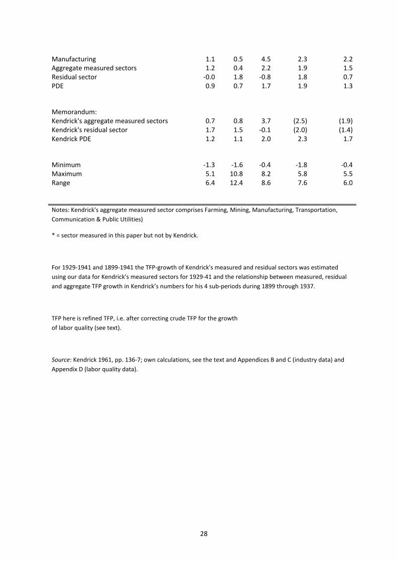
28

M anufacturing 1.1 0.5 4.5 2.3 2.2Aggregatem easuredsectors 1.2 0.4 2.2 1.9 1.5R esidualsector -0.0 1.8 -0.8 1.8 0.7P DE 0.9 0.7 1.7 1.9 1.3

M em orandum :Kendrick'saggregatem easuredsectors 0.7 0.8 3.7 (2.5) (1.9)Kendrick'sresidualsector 1.7 1.5 -0.1 (2.0) (1.4)KendrickP DE 1.2 1.1 2.0 2.3 1.7

M inim um -1.3 -1.6 -0.4 -1.8 -0.4M axim um 5.1 10.8 8.2 5.8 5.5R ange 6.4 12.4 8.6 7.6 6.0

N otes:Kendrick'saggregatem easuredsectorcom prisesFarm ing,M ining,M anufacturing,T ransportation,

Com m unication& P ublicU tilities)

* = sectorm easuredinthispaperbutnotby Kendrick.

For1929-1941 and1899-1941 theT FP -grow thofKendrick'sm easuredandresidualsectorsw asestim ated

usingourdataforKendrick'sm easuredsectorsfor1929-41 andtherelationshipbetw eenm easured,residual

andaggregateT FP grow thinKendrick’snum bersforhis4 sub-periodsduring1899 through1937.

T FP hereisrefined T FP ,i.e.aftercorrectingcrudeT FP forthegrow th

oflaborquality (seetext).

S ource:Kendrick1961,pp.136-7;ow ncalculations,seethetextandAppendicesB andC (industry data)and

Appendix D (laborquality data).

29

Table 5. Intensive Growth Contribution (IGC) by Industry, United States, 1899-1941.

Industry IGC = (VAShare*TFP growth)

1899-

1909

1909-

1919

1919-

1929

1929-

1941

1899-1941

Farm ing -0.025 -0.079 0.097 0.193 0.075M etals 0.006 0.011 0.019 0.003 0.009AnthraciteCoal -0.002 0.001 -0.001 0.001 0.000Bitum inousCoal 0.007 0.010 0.014 0.012 0.010O ilandGas 0.005 0.005 0.033 0.017 0.015N on-m etals 0.006 0.000 0.015 0.007 0.007Foods 0.022 -0.068 0.211 0.206 0.096T obacco 0.013 0.042 0.037 0.062 0.041T extiles 0.013 0.007 0.044 0.058 0.031Apparel 0.008 0.032 0.049 -0.005 0.019L eatherP roducts 0.006 0.002 0.017 0.000 0.005L um berP roducts -0.008 -0.027 0.026 -0.013 -0.006P aper 0.008 -0.001 0.024 0.007 0.010P rintingP ublishing 0.054 0.042 0.058 0.005 0.038Chem icals 0.007 -0.011 0.080 0.028 0.026P etroleum ,CoalP roducts 0.003 -0.013 0.103 -0.013 0.015R ubberP roducts 0.004 0.020 0.028 0.006 0.015S tone,clay,glass 0.016 0.003 0.044 0.015 0.019P rim ary M etals 0.069 -0.023 0.121 0.052 0.054FabricatedM etals 0.022 0.018 0.064 0.020 0.030M achinery N on-Electric 0.022 0.008 0.047 0.039 0.030ElectricM achinery 0.000 0.000 0.028 0.046 0.016T ransportEquipm ent 0.013 0.096 0.142 0.071 0.081Furniture -0.002 -0.005 0.026 0.009 0.006M iscellaneous 0.007 -0.007 0.027 0.010 0.010ElectricU tilities 0.024 0.088 0.040 0.103 0.077M anufacturedGas 0.005 0.007 0.005 0.003 0.006N aturalGas 0.000 0.002 0.000 0.012 0.003Construction* 0.238 -0.075 0.035 0.023 0.043W holesale& retailtrade* 0.209 -0.001 0.123 0.462 0.211R ailroads 0.116 0.175 0.072 0.111 0.111L ocalT ransit 0.011 0.024 0.036 0.003 0.016R esidualT ransport -0.014 0.017 0.094 0.096 0.048T elephone 0.014 0.010 0.008 0.012 0.015T elegraph 0.002 -0.002 0.007 0.001 0.002P ostO ffice* 0.006 0.012 0.001 0.002 0.006FIR E* 0.023 -0.049 0.023 -0.145 -0.032S pectatorEntertainm ent* 0.015 0.048 0.016 0.023 0.026

M anufacturing 0.277 0.115 1.176 0.603 0.537

Aggregatem easured sectors 0.922 0.319 1.812 1.542 1.186

R esidualsector -0.003 0.358 -0.128 0.323 0.128

P DE 0.920 0.677 1.685 1.866 1.314

M ean 0.024 0.008 0.048 0.041 0.031

Coefficientofvariation 2.156 5.2833 0.944 2.211 1.328

30

N otes:

* = sectorm easuredinthispaperbutnotby Kendrick :S ource:derivedfrom T ables3 and5.

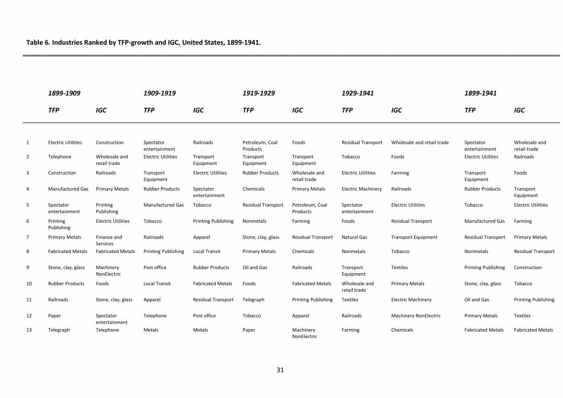
31

Table 6. Industries Ranked by TFP-growth and IGC, United States, 1899-1941.

1899-1909 1909-1919 1919-1929 1929-1941 1899-1941

TFP IGC TFP IGC TFP IGC TFP IGC TFP IGC

1 ElectricU tilities Construction S pectatorentertainm ent

R ailroads P etroleum ,CoalP roducts

Foods R esidualT ransport W holesaleandretailtrade S pectatorentertainm ent

W holesaleandretailtrade

2 T elephone W holesaleandretailtrade

ElectricU tilities T ransportEquipm ent

T ransportEquipm ent

T ransportEquipm ent

T obacco Foods ElectricU tilities R ailroads

3 Construction R ailroads T ransportEquipm ent

ElectricU tilities R ubberP roducts W holesaleandretailtrade

ElectricU tilities Farm ing T ransportEquipm ent

Foods

4 M anufacturedGas P rim ary M etals R ubberP roducts S pectatorentertainm ent

Chem icals P rim ary M etals ElectricM achinery R ailroads R ubberP roducts T ransportEquipm ent

5 S pectatorentertainm ent

P rintingP ublishing

M anufacturedGas T obacco R esidualT ransport P etroleum ,CoalP roducts

S pectatorentertainm ent

ElectricU tilities T obacco ElectricU tilities

6 P rintingP ublishing

ElectricU tilities T obacco P rintingP ublishing N onm etals Farm ing Foods R esidualT ransport M anufacturedGas Farm ing

7 P rim ary M etals FinanceandS ervices

R ailroads Apparel S tone,clay,glass R esidualT ransport N aturalGas T ransportEquipm ent R esidualT ransport P rim ary M etals

8 FabricatedM etals FabricatedM etals P rintingP ublishing L ocalT ransit P rim ary M etals Chem icals N onm etals T obacco N onm etals R esidualT ransport

9 S tone,clay,glass M achineryN onElectric

P ostoffice R ubberP roducts O ilandGas R ailroads T ransportEquipm ent

T extiles P rintingP ublishing Construction

10 R ubberP roducts Foods L ocalT ransit FabricatedM etals Foods FabricatedM etals W holesaleandretailtrade

P rim ary M etals S tone,clay,glass T obacco

11 R ailroads S tone,clay,glass Apparel R esidualT ransport T elegraph P rintingP ublishing T extiles ElectricM achinery O ilandGas P rintingP ublishing

12 P aper S pectatorentertainm ent

T elephone P ostoffice T obacco Apparel R ailroads M achinery N onElectric P rim ary M etals T extiles

13 T elegraph T elephone M etals M etals P aper M achineryN onElectric

Farm ing Chem icals FabricatedM etals FabricatedM etals

32

14 W holesaleandretailtrade

T obacco Bitum inousCoal Bitum inousCoal FabricatedM etals T extiles P rim ary M etals Construction T elephone M achinery

N onElectric

15 N onm etals T ransportEquipm ent

FabricatedM etals T elephone M iscellaneous S tone,clay,glass Chem icals S pectatorentertainm ent

Chem icals Chem icals

16 T obacco T extiles R esidualT ransport M achineryN onElectric

Furniture ElectricU tilities M achineryN onElectric

FabricatedM etals R ailroads S pectator

entertainm ent

17 P ostoffice L ocalT ransit O ilandGas M anufacturedGas Apparel T obacco O ilandGas O ilandGas ElectricM achinery S tone,clay,glass

18 O ilandGas Apparel N aturalGas T extiles L ocalT ransit L ocalT ransit Bitum inousCoal S tone,clay,glass Foods Apparel

19 T ransportEquipm ent

P aper S tone,clay,glass O ilandGas M etals Construction M anufacturedGas T elephone T extiles L ocalT ransit

20 Bitum inousCoal Chem icals M achineryN onElectric

S tone,clay,glass P rintingP ublishing O ilandGas S tone,clay,glass Bitum inousCoal L ocalT ransit ElectricM achinery

21 L ocalT ransit M iscellaneous T extiles L eatherP roducts S pectatorentertainm ent

ElectricM achinery M iscellaneous N aturalGas P aper O ilandGas

22 M etals Bitum inousCoal L eatherP roducts N aturalGas ElectricM achinery R ubberP roducts R ubberP roducts M iscellaneous M etals T elephone

23 M achineryN onElectric

P ostoffice AnthraciteCoal AnthraciteCoal M anufacturedGas M iscellaneous Furniture Furniture Bitum inousCoal R ubberP roducts

24 M iscellaneous M etals N onm etals N onm etals L eatherP roducts L um berP roducts T elephone P aper W holesaleandretailtrade

P etroleum ,Coal

P roducts

25 Chem icals L eatherP roducts W holesaleandretailtrade

ElectricM achinery T extiles Furniture FabricatedM etals N onm etals M achineryN onElectric

Bitum inousCoal

26 T extiles N onm etals ElectricM achinery W holesaleandretailtrade

M achineryN onElectric

P aper P aper R ubberP roducts P etroleum ,CoalP roducts

P aper

27 L eatherP roducts M anufacturedGas P aper P aper ElectricU tilities FinanceandS ervices

Construction P rintingP ublishing Apparel M iscellaneous

28 P etroleum ,CoalP roducts

O ilandGas FinanceandS ervices

T elegraph L um berP roducts M etals T elegraph M anufacturedGas M iscellaneous M etals

29 Apparel R ubberP roducts Farm ing Furniture Bitum inousCoal L eatherP roducts M etals L ocalT ransit T elegraph N onm etals

30 FinanceandS ervices

P etroleum ,CoalP roducts

Furniture M iscellaneous R ailroads S pectatorentertainm ent

P ostoffice M etals N aturalGas Furniture

31 Foods T elegraph M iscellaneous Chem icals T elephone N onm etals L ocalT ransit P ostoffice Construction P ostO ffice

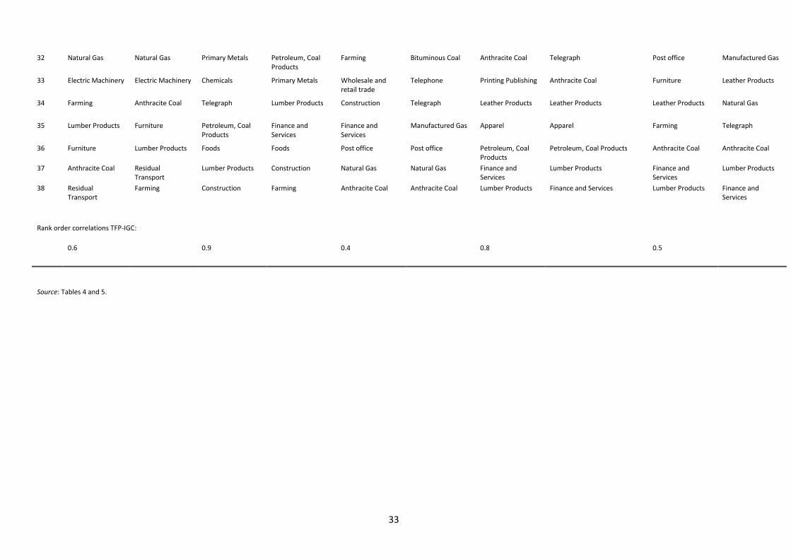
33

32 N aturalGas N aturalGas P rim ary M etals P etroleum ,CoalP roducts

Farm ing Bitum inousCoal AnthraciteCoal T elegraph P ostoffice M anufacturedGas

33 ElectricM achinery ElectricM achinery Chem icals P rim ary M etals W holesaleandretailtrade

T elephone P rintingP ublishing AnthraciteCoal Furniture L eatherP roducts

34 Farm ing AnthraciteCoal T elegraph L um berP roducts Construction T elegraph L eatherP roducts L eatherP roducts L eatherP roducts N aturalGas

35 L um berP roducts Furniture P etroleum ,CoalP roducts

FinanceandS ervices

FinanceandS ervices

M anufacturedGas Apparel Apparel Farm ing T elegraph

36 Furniture L um berP roducts Foods Foods P ostoffice P ostoffice P etroleum ,CoalP roducts

P etroleum ,CoalP roducts AnthraciteCoal AnthraciteCoal

37 AnthraciteCoal R esidualT ransport

L um berP roducts Construction N aturalGas N aturalGas FinanceandS ervices

L um berP roducts FinanceandS ervices

L um berP roducts

38 R esidualT ransport

Farm ing Construction Farm ing AnthraciteCoal AnthraciteCoal L um berP roducts FinanceandS ervices L um berP roducts FinanceandS ervices

R ankordercorrelationsT FP -IGC:

0.6 0.9 0.4 0.8 0.5

S ource:T ables4 and5.

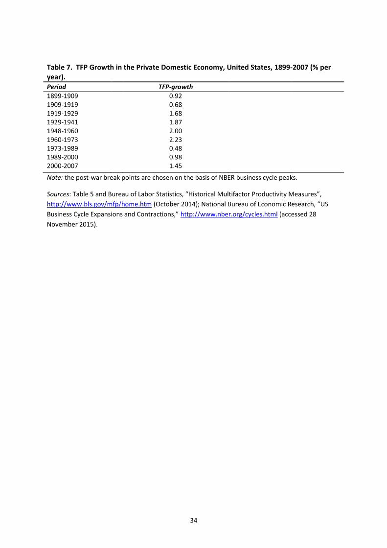
34

Table 7. TFP Growth in the Private Domestic Economy, United States, 1899-2007 (% peryear).Period TFP-growth

1899-1909 0.921909-1919 0.681919-1929 1.681929-1941 1.871948-1960 2.001960-1973 2.231973-1989 0.481989-2000 0.982000-2007 1.45

N ote:thepost-w arbreakpointsarechosenonthebasisofN BER businesscyclepeaks.

S ources:T able5 andBureau ofL aborS tatistics,“ HistoricalM ultifactorP roductivity M easures” ,

http://w w w .bls.gov/m fp/hom e.htm (O ctober2014);N ationalBureau ofEconom icR esearch,“ U S

BusinessCycleExpansionsandContractions,” http://w w w .nber.org/cycles.htm l(accessed28

N ovem ber2015).

35

Table 8. Decomposition of TFP Growth in the United States Private Non-Farm Economy(PNE), 1919-1941.

Panel A: 1919-1929

Field (2011) This study

1929Weight

(%)

TFPGrowth(% p.a.)

IGC(% p.a.)

MidperiodWeight

(%)

TFPGrowth(% p.a.)

IGC(% p.a.)

M anufacturing 32.93 5.12 1.69 30.73 4.45 1.37T ransportandP ublicU tilities 14.10 1.86 0.26 12.66 2.41 0.30W holesaleandR etailT rade 20.30 0.50 0.10 15.66 0.91 0.14

M ining 2.90 3.20 0.09

O ther 32.67 -0.09 -0.03 38.05 -0.39 -0.15

T otalP N E 2.02 1.76

Panel B: 1929-1941

Field (2011) This study

1941Weight

(%)

TFPGrowth(% p.a.)

IGC(% p.a.)

MidperiodWeight

(%)

TFPGrowth(% p.a.)

IGC(% p.a.)

M anufacturing 42.42 2.60 1.10 31.61 2.25 0.71T ransportandP ublicU tilities 12.28 4.60 0.57 12.22 3.30 0.40

W holesaleandR etailT rade 22.23 2.39 0.53 16.10 3.39 0.55

M ining 2.82 1.66 0.05

O ther 23.07 0.48 0.11 37.26 0.31 0.12

T otalP N E 2.31 1.82

N otes:O therisobtainedasaresidualandm iningispartofotherforField(2006);w eightsare% P N E.

M ay notsum tototalduetorounding.

S ources:Field(2011,T ables2.5 and2.10);derivedfrom T ables4 and5.

36

Table 9. Regressions of TFP Spillovers from Electricity Adoption for a Cross-Section of allManufacturing Industries, United States, 1919-1941.

1919-1929 1929-1941

Constant 2.465***(4.02)

-2.662*(-2.42)

HP Grow th 0.203*(2.25)

-0.022(-0.12)

AdjustedR 2 0.18 -0.06N 19 19

N otes:T hedependentvariablesare(T FP grow th1919-29 – T FP grow th1899-19)and(T FP grow th

1929-41 – T FP grow th1919-29)derivedfrom T able4;theindependentvariablesaretheaverage

annualratesofgrow thofhorsepow erinsecondary electricm otorsin1919-29 and1929-39 from

DuBoff(1979).

t-statisticsinparentheses.

* = significantat5 % level

*** = significantat0.1 % level

S ource:ow ncalculations.

37

Table 10. Contributions to Labor Productivity Growth in Manufacturing, United States, 1919-1929 (% per year).

L aborQ ualityGrow th

N on-ElectricalK/L Grow th

N on-ElectricalT FP Grow th

ElectricalK/LGrow th

ElectricalT FPGrow th

L aborP roductivity

Grow th

S um ofN on-Electrical

Contributions

S um ofElectrical

Contributions

Foods 0.2743 0.1501 3.8161 0.0059 0.7222 4.9685 4.2404 0.7281T obacco 0.1508 2.7989 2.4167 0.0011 1.8325 7.2000 5.3664 1.8336T extiles 0.5037 -0.5083 1.7981 0.0083 0.5982 2.4000 1.7935 0.6065Apparel 0.3042 -0.0020 4.2331 0.0020 -0.5374 4.0000 4.5354 -0.5354L eatherP roducts 0.1975 -0.4174 2.3706 0.0174 0.3319 2.5000 2.1507 0.3493L um berP roducts 0.3539 0.4586 -0.2918 0.0414 2.4380 3.0000 0.5207 2.4793P aper 0.5157 0.3666 2.0307 0.0334 2.1536 5.1000 2.9130 2.1870P rintingP ublishing 0.2969 -0.0064 3.4031 0.0064 0.0000 3.7000 3.6936 0.0064Chem icals 0.3338 0.7873 5.6429 0.0127 1.4234 8.2000 6.7639 1.4361P etroleum etc. 0.3870 0.3871 6.2074 0.0129 2.0056 9.0000 6.9815 2.0185R ubberP roducts 0.4335 0.6518 6.0884 0.0482 1.1781 8.4000 7.1736 1.2264S tone,clay,glass 0.4411 0.5778 3.3937 0.0222 1.8653 6.3000 4.4126 1.8874P rim ary M etals 0.4690 0.2777 3.4594 0.0223 1.5716 5.8000 4.2061 1.5939FabricatedM etals 0.4293 0.4910 3.9341 0.0090 0.2366 5.1000 4.8544 0.2456N on-ElecM ach. 0.5763 -0.0099 1.8364 0.1099 0.4872 3.0000 2.4028 0.5972ElectricM achinery 0.3953 0.4960 0.0000 0.0040 3.1047 4.0000 0.8913 3.1087T ransportEqpm t. 0.4580 0.6882 6.4228 0.0118 1.5192 9.1000 7.5691 1.5309Furniture 0.1783 0.0644 2.7529 0.0356 1.2688 4.3000 2.9956 1.3044M iscellaneous 0.5472 0.8893 2.5470 0.0107 1.5059 5.5000 3.9834 1.5166

S tandarddeviation 0.1207 0.6691 1.8545 0.0247 0.8928 2.1147 2.0167 0.8929M ean 0.3813 0.4285 3.2664 0.0218 1.2477 5.3457 4.0762 1.2695Coeff.ofvariation 0.3164 1.5617 0.5677 1.1290 0.7156 0.3956 0.4948 0.7033

N otes:Col8= Col4 + Col5;Col7 = sum ofCols2 through6;Col6 = T FP spilloversexceptforelectricalm achinery w hichincludesow nT FP grow thasw ell.S ource:ow ncalculationsbasedonim plem entingequation(8)

38

Table 11. Harberger Coefficients for Contributions to Productivity Growth in theManufacturing Sector, United States, 1919-1929.

TFP Growth Labor ProductivityGrowth

Electrical 0.30 0.30N on-Electrical 0.22 0.20T otal 0.18 0.17

N otes:Harbergercoefficientsaredefinedasinequations(7)and(9),respectively.

S ource:ow ncalculations.

39

Figures 1a and 1b. Diagram m aticillustrationoftw ohypotheticaldistributionsofintensivegrow th

contributionsby industry versustheindustry’svalue-addedshareinGDP ,rankedby industry T FP -grow th

rate.

S ource:thesetw oim agesaretakenfrom InklaarandT im m er(2007),andarebasedonthediagram

developedinHarberger(1998).

W

W

V

V

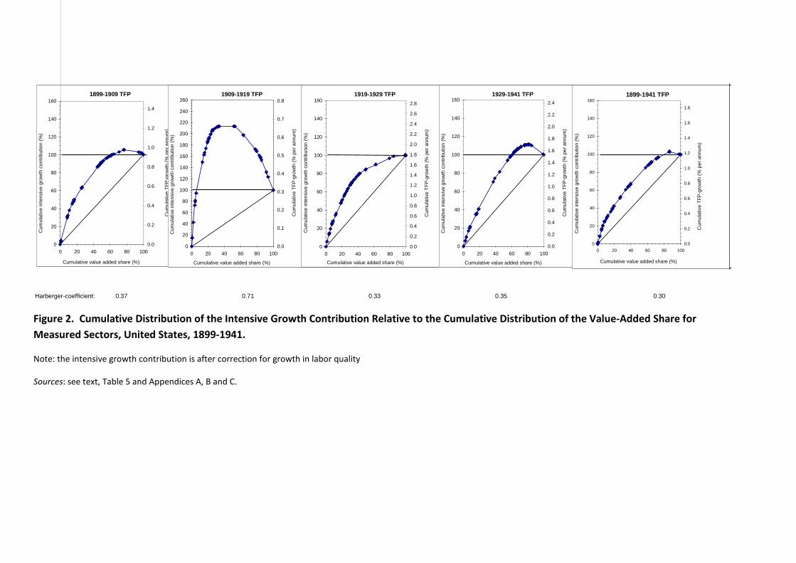
Harberger-coefficient: 0.37 0.71 0.33 0.35 0.30

1899-1909 TFP

0

20

40

60

80

100

120

140

160

0 20 40 60 80 100

Cumulative value added share (%)

Cu

mula

tive

inte

nsi

ve

gro

wth

contr

ibutio

n(%

)

0.0

0.2

0.4

0.6

0.8

1.0

1.2

1.4

Cu

mula

tive

TF

P-g

row

th(%

pe

ran

nu

m)

1909-1919 TFP

0

20

40

60

80

100

120

140

160

180

200

220

240

260

0 20 40 60 80 100

Cumulative value added share (%)

Cum

ula

tive

inte

nsiv

eg

row

thco

ntr

ibution

(%)

0.0

0.1

0.2

0.3

0.4

0.5

0.6

0.7

0.8

Cu

mula

tive

TF

P-g

row

th(%

pe

ran

nu

m)

1919-1929 TFP

0

20

40

60

80

100

120

140

160

0 20 40 60 80 100

Cumulative value added share (%)

Cum

ula

tive

inte

nsiv

egro

wth

contr

ibution

(%)

0.0

0.2

0.4

0.6

0.8

1.0

1.2

1.4

1.6

1.8

2.0

2.2

2.4

2.6

2.8

Cum

ula

tive

TF

P-g

row

th(%

pe

ran

nu

m)

1929-1941 TFP

0

20

40

60

80

100

120

140

160

0 20 40 60 80 100

Cumulative value added share (%)

Cum

ula

tive

inte

nsiv

eg

row

thco

ntr

ibution

(%)

0.0

0.2

0.4

0.6

0.8

1.0

1.2

1.4

1.6

1.8

2.0

2.2

2.4

Cum

ula

tive

TF

P-g

row

th(%

pe

ran

nu

m)

1941-1947 TFP

0

50

100

150

200

250

0 20 40 60 80 100

Cumulative gross output share (%)

Cum

ula

tive

inte

nsiv

eg

row

thco

ntr

ibution

(%)

0.00

0.50

1.00

1.50

2.00

2.50

3.00

3.50

0 20 40 60 80 100 120 140 160

Cumulative gross output / GDP share (%)

Cu

mula

tive

TF

P-g

row

th(%

per

ann

um

)

1899-1941 TFP

0

20

40

60

80

100

120

140

160

0 20 40 60 80 100

Cumulative value added share (%)

Cu

mula

tive

inte

nsiv

eg

row

thcon

trib

utio

n(%

)

0.0

0.2

0.4

0.6

0.8

1.0

1.2

1.4

1.6

1.8

Cu

mula

tive

TF

P-g

row

th(%

pe

ran

nu

m)

Figure 2. Cumulative Distribution of the Intensive Growth Contribution Relative to the Cumulative Distribution of the Value-Added Share for

Measured Sectors, United States, 1899-1941.

N ote:theintensivegrow thcontributionisaftercorrectionforgrow thinlaborquality

S ources:seetext,T able5 andAppendicesA,B andC.

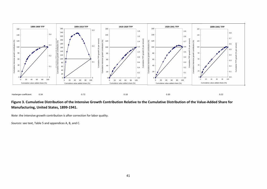
41

Harberger-coefficient: 0.34 0.72 0.18 0.30 0.22

1899-1909 TFP

0

20

40

60

80

100

120

140

160

0 20 40 60 80 100

Cumulative value added share (%)

Cu

mula

tive

inte

nsi

ve

gro

wth

contr

ibutio

n(%

)

0

0.1

0.2

0.3

0.4

Cu

mula

tive

TF

P-g

row

th(%

pe

ran

nu

m)

1909-1919 TFP

0

20

40

60

80

100

120

140

160

180

200

220

240

260

0 20 40 60 80 100

Cumulative value added share (%)

Cum

ula

tive

inte

nsiv

eg

row

thco

ntr

ibution

(%)

0

0.1

0.2

0.3

Cu

mula

tive

TF

P-g

row

th(%

pe

ran

nu

m)

1919-1929 TFP

0

20

40

60

80

100

120

140

160

0 20 40 60 80 100

Cumulative value added share (%)

Cu

mula

tive

inte

nsi

ve

gro

wth

contr

ibutio

n(%

)

0.0

0.2

0.4

0.6

0.8

1.0

1.2

1.4

1.6

1.8

Cum

ula

tive

TF

P-g

row

th(%

per

ann

um

)

1929-1941 TFP

0

20

40

60

80

100

120

140

160

0 20 40 60 80 100

Cumulative value added share (%)

Cum

ula

tive

inte

nsiv

eg

row

thco

ntr

ibution

(%)

0.0

0.1

0.2

0.3

0.4

0.5

0.6

0.7

0.8

0.9

Cum

ula

tive

TF

P-g

row

th(%

pe

ran

nu

m)

1941-1947 TFP

0

20

40

60

80

100

120

0 20 40 60 80 100

Cumulative gross output share (%)

Cum

ula

tive

inte

nsiv

eg

row

thco

ntr

ibution

(%)

0.00

0.50

1.00

1.50

2.00

2.50

3.00

3.50

0 20 40 60 80 100 120 140 160

Cumulative gross output / GDP share (%)

Cu

mula

tive

TF

P-g

row

th(%

per

ann

um

)

1899-1941 TFP

0

20

40

60

80

100

120

140

160

0 20 40 60 80 100

Cumulative value added share (%)

Cu

mula

tive

inte

nsiv

eg

row

thcon

trib

utio

n(%

)

0.0

0.1

0.2

0.3

0.4

0.5

0.6

0.7

0.8

Cu

mula

tive

TF

P-g

row

th(%

per

ann

um

)

Figure 3. Cumulative Distribution of the Intensive Growth Contribution Relative to the Cumulative Distribution of the Value-Added Share for

Manufacturing, United States, 1899-1941.

N ote:theintensivegrow thcontributionisaftercorrectionforlaborquality.

S ources:seetext,T able5 andappendicesA,B,andC.

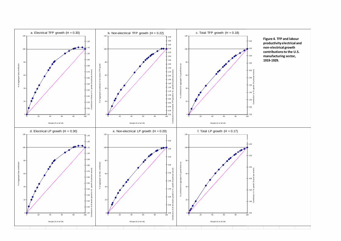
42

0.00

0.10

0.20

0.30

0.40

0.50

0.60

0.70

0.80

0.90

1.00

1.10

1.20

0

20

40

60

80

100

120

0 20 40 60 80 100

Co

ntrib

uti

on

ofb

eta

toY

/Lg

row

th(%

-po

int

pera

nnu

m)

%o

fa

gg

reg

ate

bet

aco

ntri

bu

tion

Weight (% of all VA)

1919-1929,e-T FP contributiontoY/L

H = 0.30

a. Electrical TFP growth (H = 0.30)

0.00

0.20

0.40

0.60

0.80

1.00

1.20

1.40

1.60

1.80

2.00

2.20

2.40

2.60

2.80

3.00

3.20

3.40

3.60

3.80

4.00

0

20

40

60

80

100

120

0 20 40 60 80 100

Co

ntr

ibu

tio

nof

no

n-e

lec

tric

TF

P-g

row

thto

Y/L

gro

wth

(%-p

oin

tp

era

nnu

m)

%o

fag

gre

ga

teco

ntrib

utio

no

fno

n-e

lect

ric

TF

P-g

row

th

Weight (% of all VA)

1919-1929,non-ElectricT FPcontributiontoY

H = 0.22

b. Non-electrical TFP growth (H = 0.22)

0.00

0.50

1.00

1.50

2.00

2.50

3.00

3.50

4.00

4.50

5.00

0

20

40

60

80

100

120

0 20 40 60 80 100

Co

ntrib

utio

nto

Y/L

gro

wth

(%p

oin

tpe

ran

num

)

%c

on

trib

uti

on

toag

gre

gate

Y/L

gro

wth

time

sao

Weight (% of all VA)

Figure 4. TFP and labourproductivity electrical andnon-electrical growthcontributions to the U.S.manufacturing sector,1919-1929.

c. Total TFP growth (H = 0.18)

0.00

0.10

0.20

0.30

0.40

0.50

0.60

0.70

0.80

0.90

1.00

1.10

1.20

1.30

0

20

40

60

80

100

120

0 20 40 60 80 100

Co

ntr

ibuti

on

ofa

llel

ect

ric

gro

wth

toY

/Lgr

ow

th(%

-poi

ntp

er

ann

um

)

%o

fa

gg

reg

ate

bet

aco

ntri

butio

n

Weight (% of all VA)

1919-1929,T otalElectricgrow thcontributiontoY

H = 0.30

d. Electrical LP growth (H = 0.30)

0.00

0.50

1.00

1.50

2.00

2.50

3.00

3.50

4.00

4.50

0

20

40

60

80

100

120

0 20 40 60 80 100

Co

ntr

ibu

tion

ofall

non-e

lect

ric

gro

wth

toY

/Lg

row

th(%

-po

int

pera

nnum

)

%o

fag

gre

ga

ten

onele

c.co

ntr

ibu

tion

Weight (% of all VA)

1919-1929,T otalN on-Electricgrow thcontributiontoY

H = 0.20

e. Non-electrical LP growth (H = 0.20)

0.00

1.00

2.00

3.00

4.00

5.00

6.00

0

20

40

60

80

100

120

0 20 40 60 80 100

Con

trib

uti

on

toY

/Lgr

ow

th(%

po

int

pera

nnu

m)

%c

on

trib

uti

on

toag

gre

gate

Y/L

gro

wth

time

sa

o

Weight (% of all VA)

f. Total LP growth (H = 0.17)

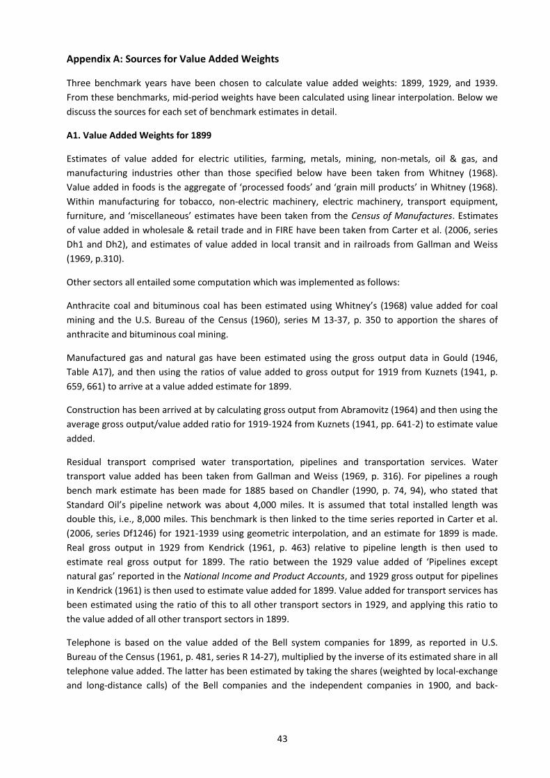
43

Appendix A: Sources for Value Added Weights

T hree benchm ark yearshave been chosen to calculate value added w eights: 1899,1929,and 1939.

From these benchm arks,m id-period w eightshave been calculated usinglinearinterpolation.Below w e

discussthesourcesforeachsetofbenchm arkestim atesindetail.

A1. Value Added Weights for 1899

Estim atesofvalue added for electric utilities,farm ing,m etals,m ining,non-m etals,oil& gas,and

m anufacturing industriesother than those specified below have been taken from W hitney (1968).

Value added in foodsisthe aggregate of‘processed foods’ and ‘grain m illproducts’ in W hitney (1968).

W ithin m anufacturing fortobacco,non-electric m achinery,electric m achinery,transport equipm ent,

furniture,and ‘m iscellaneous’ estim ateshave been taken from the CensusofM anufactures.Estim ates

ofvalue added in w holesale & retailtrade and in FIR E have been taken from Carteretal.(2006,series

Dh1 and Dh2),and estim atesofvalue added in localtransit and in railroadsfrom Gallm an and W eiss

(1969,p.310).

O thersectorsallentailedsom ecom putationw hichw asim plem entedasfollow s:

Anthracite coaland bitum inouscoalhasbeen estim ated using W hitney’s(1968)value added forcoal

m ining and the U .S .Bureau ofthe Census(1960),seriesM 13-37,p.350 to apportion the sharesof

anthraciteandbitum inouscoalm ining.

M anufactured gasand naturalgashave been estim ated using the grossoutput datain Gould (1946,

T able A17),and then using the ratiosofvalue added to grossoutput for1919 from Kuznets(1941,p.

659,661)toarriveatavalueaddedestim atefor1899.

Constructionhasbeenarrived atby calculatinggrossoutputfrom Abram ovitz(1964)and thenusingthe

averagegrossoutput/valueadded ratiofor1919-1924 from Kuznets(1941,pp.641-2)toestim atevalue

added.

R esidual transport com prised w ater transportation,pipelinesand transportation services. W ater

transport value added hasbeen taken from Gallm an and W eiss(1969,p.316).Forpipelinesarough

bench m ark estim ate hasbeen m ade for1885 based on Chandler(1990,p.74,94),w ho stated that

S tandard O il’spipeline netw ork w asabout 4,000 m iles.It isassum ed that totalinstalled length w as

double this,i.e.,8,000 m iles.T hisbenchm arkisthen linked to the tim e seriesreported in Carteret al.

(2006,seriesDf1246)for1921-1939 using geom etricinterpolation,and an estim ate for1899 ism ade.

R ealgrossoutput in 1929 from Kendrick (1961,p. 463) relative to pipeline length isthen used to

estim ate realgrossoutput for1899. T he ratio betw een the 1929 value added of‘P ipelinesexcept

naturalgas’ reported inthe N ationalIncom eand P roductAccounts,and 1929 grossoutputforpipelines

inKendrick(1961)isthenusedtoestim atevalueaddedfor1899.Valueaddedfortransportserviceshas

been estim ated using the ratio ofthisto allothertransport sectorsin 1929,and applying thisratio to

thevalueaddedofallothertransportsectorsin1899.

T elephone isbased on the value added ofthe Bellsystem com paniesfor1899,asreported in U .S .

Bureau oftheCensus(1961,p.481,seriesR 14-27),m ultipliedby theinverseofitsestim atedshareinall

telephonevalueadded.T helatterhasbeenestim ated by takingtheshares(w eighted by local-exchange

and long-distance calls) ofthe Bellcom paniesand the independent com paniesin 1900,and back-

44

projecting thisratio to 1899 taking into account the differentialgrow th rate of the num ber of

telephonesforthetw osystem s.

T elegraph value added com prisesthe ‘Internationaltelegraph industry’ and the ‘dom estic telegraph

industry’. T he form erhasbeen estim ated taking operating revenuesfrom Carteret al.(2006,series

Dg18),and using the 1907 value added/ revenue ratio to estim ate 1899 value added.Forthe latter,

1899 W estern U nion revenuesw ere taken from Carteret al.(2006,seriesDg 16).T o arrive at non –

W estern U nion revenuesthe grow th of thiscategory relative to W estern U nion grow th hasbeen

calculated for1902-1907. T hisratio hasbeen used to extrapolate 1902 non-W estern U nion revenues

backto 1899.T he ratio betw een grossincom e and value added in the telephone industry for1902,as

reported in Departm ent ofCom m erce and L abor,Bureau ofthe Census,Bulletin 17,T elephonesand

T elegraphs,1902 (1905,p.31),hasthenbeenusedtoarriveatanestim atefor1899 valueadded.

P ost O ffice value added istaken asthe sum ofw agesand capitalincom e. T he ratio of1909 w agesas

reported in King (1930,p.364)to totalrevenue asreported in Carteretal.(2006,seriesDg181-9)has

beenused to estim ate1899 w agesbased on1899 revenuefrom Carteretal.(2006,seriesDg181-9). It

hasthenbeenassum edthatincom eofrem uneratedcapitalw asabout0.1 from 1899 revenue.

Value added forspectatorentertainm enthasbeencalculated by extrapolatingthe benchm arkestim ate

for1900 grossoutputfrom Bakker(2012),usingthe grow th rate ofoutputoverthe population grow th

rate betw een1900 and 1909,and m ultiplyingby theaverage fraction ofvalue added overgrossoutput

forlive entertainm ent betw een 1929 and 1941.T he latterhasbeen estim ated from the N IP A by using

the share oflive entertainm entexpenditure in all‘Am usem entsand recreation exceptm otion pictures’

expenditure.

A2. Value Added Weights for 1929

Value added for m ost sectorshasbeen obtained directly from the N ationalIncom e and P roduct

Accountsasreported in Appendix C. Below w e discussthe sectorsforw hich value added could notbe

obtaineddirectly from thissource.

FIR E and w holesale & retailtrade have been taken from Carteret al.(2006,seriesDh2 and Dh25-6).

Construction hasbeen calculated from Abram ovitz(1964). M anufactured gashasbeencalculated from

Kuznets(1941,pp.659-676).

T he w eight ofelectric utilitiesstartsfrom the quantity ofelectricity sold and itsprice asreported in

Bureau oftheCensus(1960,seriesS 80-1)to arriveatthevalueofgrossoutputfor1929.T hisvaluew as

then m ultiplied by the value added / grossoutput ratio calculated for ‘electric light & pow er and

m anufacturedgas’ for1929 from Kuznets(1941,pp.659-676).

N aturalgasisbased on grossoutputfrom Gould (1946)m ultiplied by the ratio ofvalue added to gross

outputforpetroleum andnaturalgastogetherfor1929 from L eontief(1953).

T elephone value added hasbeen calculated from Kuznets(1941,pp.659-670).A second estim ate has

been m ade by usingthe m ethod forcalculatingtelephone value added outlined for1939 in section 1.3

below . T hisestim ate w asslightly lessreliable asfor the ‘Independent T elephone Com panies’ the

geom etric interpolation of‘w agesand salaries’ versusthe use ofrelative factorincom esto estim ate

‘w agesand salaries’ yielded estim atesforvalue added for‘Independent T elephone Com panies’ that

w ere33 percentapart.U singthe averageofthese tw o estim atesyieldsatotalestim ate ofvalue added

45

forthe entire telephone industry thatisonly one percent higherthan the Kuznetsestim ate.T he latter

valuehasthereforebeentaken.

For the ‘Dom estic T elegraph Industry’ the value of interm ediate inputshasbeen calculated by

subtracting ‘w agesand salaries’ from ‘operating expenses’ taken from Bureau ofthe Census(1960,p.

484-5,seriesR 53-67).T hese ‘operatingexpenses’ do notinclude ‘netincom e’ and ‘federalincom e tax’,

so m ust be approxim ately the sum ofw agesand salariesplusinterm ediate inputs. Capitalincom e is

then taken to be ‘operating revenues’ m inus‘operating expenses’. A sim ilarestim ate hasbeen m ade

forthe‘‘InternationalT elegraphIndustry’ from Bureau oftheCensus(1960,p.485-6,seriesR 72-85).

A second estim ate forT elegraph w asm ade based on grossoutput forthe dom esticand international

telegraphindustriesfrom theBureau oftheCensus(1961,p.484)m ultiplied by theratioofvalueadded

togrossoutputfrom Kuznets(1941,pp.659-670).T hisestim ateyieldsavaluethatis2.7 percenthigher.

Astheform erestim ateism oreprecise,thatestim atehasbeentaken.

P ost O ffice value added istaken asthe sum ofw agesand capitalincom e. W agesw ere estim ated by

takingtheratioofthecom pensationofpostm astersasreported inthe AnnualR eportoftheP ostm aster

General(1970,pp.138-141)to allw agesasreported in King (1930,p.364)for1925,and establishing

that thisratio w asfairly stable for1923-25 (fluctuating betw een 10.0 and 11.1 percent ofallw ages),

andthenusingthisratiotoestim ateallw agesfor1929 basedonpostm asters’ com pensationin1929. It

hasthenbeenassum edthatincom eofrem uneratedcapitalw asabout0.1 from 1929 revenue.

ForS pectatorEntertainm ent the value added ofm otion picturesistaken directly from the N ational

Incom e and P roductAccounts.T he value added oflive entertainm enthasbeen estim ated by using the

share oflive entertainm ent expenditure in all‘Am usem ent and recreation,except m otion pictures’

expenditure.

A3. Value Added Weights for 1939

Value added for m ost sectorshasbeen obtained directly from the N ationalIncom e and P roduct

Accountsasreported in Appendix C. Below w e discussthe sectorsforw hichthevalueadded could not

beobtaineddirectly from thissource.

FIR E and w holesale & retailtrade have been taken from Carteret al.(2006,seriesDh27 and Dh25-6).

Constructionvalueaddedhasbeencalculatedfrom Abram ovitz(1964).

T he w eight ofelectric utilitiesstartsfrom the quantity ofelectricity sold and itsprice asreported in

Bureau ofthe Census(1960,seriesS 80-1)to arrive at the value ofgrossoutput.T hisvalue w asthen

m ultiplied by the value added / grossoutput ratio calculated for ‘electric light & pow er and

m anufacturedgas’ for1939 from Kuznets(1941,pp.659-676).

M anufacturedgasisbasedtheestim atefor1938 inKuznets(1941)extrapolatedto1939.

N aturalgasisbased on grossoutputtaken from Gould (1946)m ultiplied by the ratio ofvalue added to

grossoutputforpetroleum andnaturalgastogetherfor1939 from L eontief(1953).

Forthe BellT elephone Com paniesthe value ofinterm ediate inputshasbeen calculated by subtracting

‘w agesand salaries’ from ‘operating expenses’ taken from Bureau ofthe Census(1960,p.481,series

R 14-27).T hese‘operatingexpenses’ donotinclude‘interestexpenses’ and‘federalincom etax’,som ust

be approxim ately the sum ofw agesand salariesplusinterm ediateinputs. Capitalincom e isthentaken

46

to be ‘operating revenues’ m inus‘operating expenses’ plus‘incom e from W estern ElectricCo.’,w hich

equalsthe sum of‘interest expenses’,‘federalincom e tax’ and ‘net incom e’ (Bureau ofthe Census

1960: 481,seriesR 14-27). A sim ilar estim ate hasbeen m ade for the ‘Independent T elephone

Com panies’ from Bureau ofthe Census(1960,p.483,seriesR 28-42),w ith the difference that ‘w ages

and salaries’ arenotavailablefor1939 and hadtobeestim ated.W em adetw oestim ates:oneusingthe

grow th rate of‘w agesand salaries’ betw een 1934 and 1941 and estim ating a1939 value by geom etric

interpolation,and one by using the ratio ofthe factorincom esforthe BellT elephone Com paniesfor

1939.T he estim atesforvalue added using these tw o different ‘w agesand salaries’ estim atesdifferby

only 1.2 percent,andtheaveragehasbeentaken.T otalvalueaddedisthenthesum oftheseestim ates.

A second estim ate hasbeen m ade using the value added estim ate in Kuznets(1941,pp.659-676)for

1938 and m ultiplying it by the grow th rate ofoperating revenue betw een 1938 and 1939 forBelland

independenttelephone com paniestaken from Bureau ofthe Census(1960,p.481-3,seriesR 14-27 and

R 28-42). T hisyieldsavalue added that is4.8 percent low erthan the above estim ate. Asthe second

estim ate isan extrapolation and based on lessinform ation from the actualyear (1939),the first

estim atehasbeentaken.

For the ‘Dom estic T elegraph Industry’ the value of interm ediate inputshasbeen calculated by

subtracting ‘w agesand salaries’ from ‘operating expenses’ taken from Bureau ofthe Census(1960,p.

484-5,seriesR 53-67).T hese ‘operatingexpenses’ do notinclude ‘netincom e’ and ‘federalincom e tax’,

so m ust be approxim ately the sum ofw agesand salariesplusinterm ediate inputs. Capitalincom e is

then taken to be ‘operating revenues’ m inus‘operating expenses’. A sim ilarestim ate hasbeen m ade

forthe‘‘InternationalT elegraphIndustry’ from Bureau oftheCensus(1960,p.485-6,seriesR 72-85).

A second estim atew asm adew iththesecond m ethod used for‘T elephone’,usingthew eighted grow th

rate ofoperating revenuesofthe dom estictelegraph industry and the internationaltelegraph industry

betw een1938 and 1939 from Bureau oftheCensus(1960,p.484)toextrapolateKuznets’svalueadded

from 1938 to 1939.Both estim atesare very close:the firstestim ate isonly 2.6 percenthigherthan the

second.Given that thisfirst estim ate isbased on datafrom the yearitselfand not on extrapolations,

thisfirstestim atehasbeentaken.

P ost O ffice value added istaken asthe sum ofw agesand capitalincom e. W agesw ere estim ated by

takingtheratioofthecom pensationofpostm astersasreported inthe AnnualR eportoftheP ostm aster

General(1970,pp.138-141)to allw agesasreported in King (1930,p.364)for1925,and establishing

that thisratio w asfairly stable for1923-25 (fluctuating betw een 10.0 and 11.1 percent ofallw ages),

andthenusingthisratiotoestim ateallw agesfor1939 basedonpostm asters’ com pensationin1939. It

hasthenbeenassum edthatincom eofrem uneratedcapitalw asabout0.1 from 1939 revenue.

S pectatorEntertainm ent value added hasbeen estim ated using the sam e m ethod and sourcesasfor

1929.

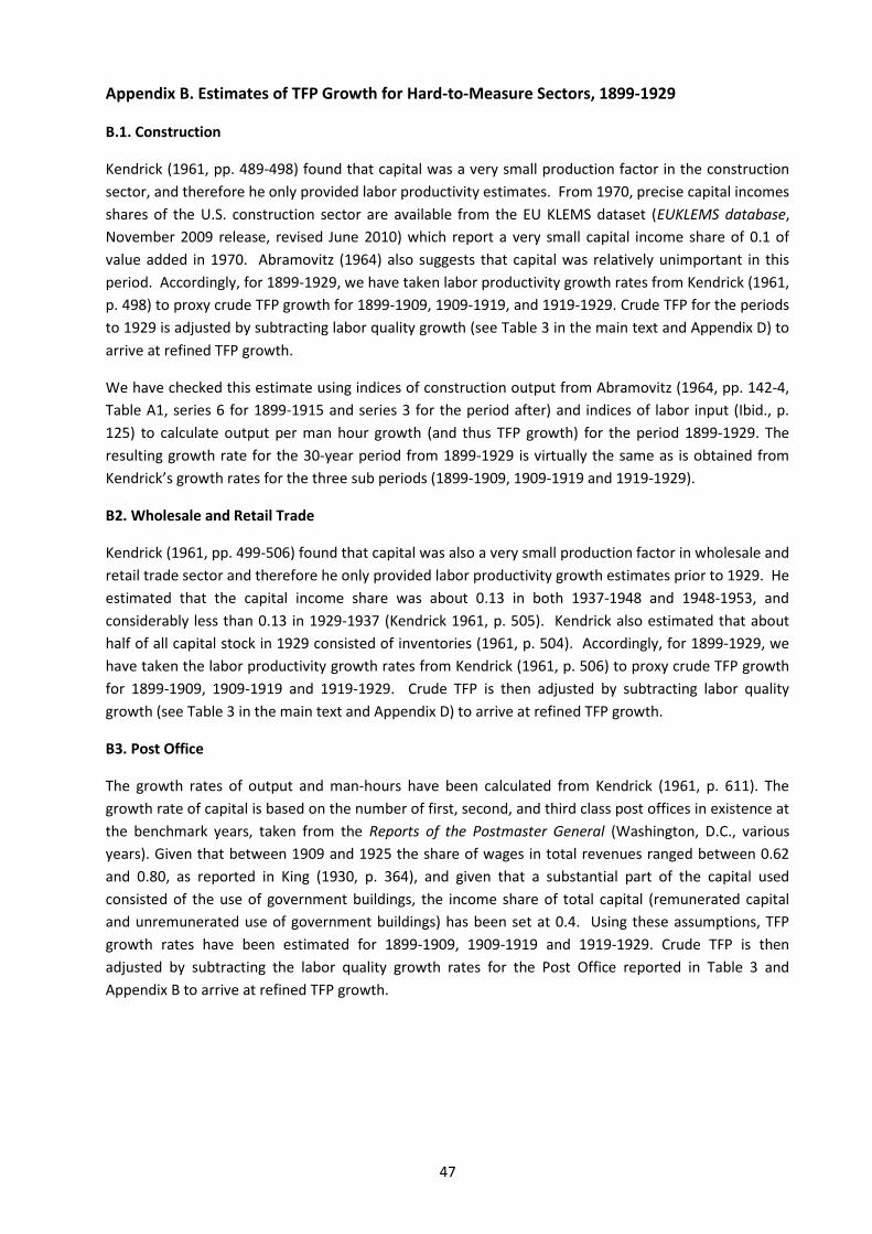
47

Appendix B. Estimates of TFP Growth for Hard-to-Measure Sectors, 1899-1929

B.1. Construction

Kendrick(1961,pp.489-498)found that capitalw asavery sm allproduction factorin the construction

sector,andthereforeheonly providedlaborproductivity estim ates. From 1970,precisecapitalincom es

sharesofthe U .S .construction sectorare available from the EU KL EM S dataset (EU KL EM S database,

N ovem ber2009 release,revised June 2010)w hich report avery sm allcapitalincom e share of0.1 of

value added in 1970. Abram ovitz (1964)also suggeststhat capitalw asrelatively unim portant in this

period. Accordingly,for1899-1929,w ehavetakenlaborproductivity grow thratesfrom Kendrick(1961,

p.498)toproxy crudeT FP grow thfor1899-1909,1909-1919,and 1919-1929.CrudeT FP fortheperiods

to1929 isadjusted by subtractinglaborquality grow th(seeT able3 inthem aintextand Appendix D)to

arriveatrefinedT FP grow th.

W e have checked thisestim ate usingindicesofconstruction outputfrom Abram ovitz (1964,pp.142-4,

T able A1,series6 for1899-1915 and series3 forthe period after)and indicesoflaborinput (Ibid.,p.

125)to calculate output perm an hourgrow th (and thusT FP grow th)forthe period 1899-1929.T he

resulting grow th rate forthe 30-yearperiod from 1899-1929 isvirtually the sam e asisobtained from

Kendrick’sgrow thratesforthethreesubperiods(1899-1909,1909-1919 and1919-1929).

B2. Wholesale and Retail Trade

Kendrick(1961,pp.499-506)foundthatcapitalw asalsoavery sm allproductionfactorinw holesaleand

retailtradesectorandthereforeheonly providedlaborproductivity grow thestim atespriorto1929. He

estim ated that the capitalincom e share w asabout 0.13 in both 1937-1948 and 1948-1953,and

considerably lessthan 0.13 in 1929-1937 (Kendrick1961,p.505). Kendrickalso estim ated that about

halfofallcapitalstockin 1929 consisted ofinventories(1961,p.504). Accordingly,for1899-1929,w e

have taken the laborproductivity grow th ratesfrom Kendrick(1961,p.506)to proxy crude T FP grow th

for1899-1909,1909-1919 and 1919-1929. Crude T FP isthen adjusted by subtracting laborquality

grow th(seeT able3 inthem aintextandAppendix D)toarriveatrefinedT FP grow th.

B3. Post Office

T he grow th ratesofoutput and m an-hourshave been calculated from Kendrick (1961,p.611).T he

grow thrateofcapitalisbased onthenum beroffirst,second,and third classpostofficesinexistenceat

the benchm ark years,taken from the R eportsofthe P ostm asterGeneral(W ashington,D.C.,various

years).Given that betw een 1909 and 1925 the share ofw agesin totalrevenuesranged betw een 0.62

and 0.80,asreported in King (1930,p. 364),and given that asubstantialpart ofthe capitalused

consisted ofthe use ofgovernm ent buildings,the incom e share oftotalcapital(rem unerated capital

and unrem unerated use ofgovernm ent buildings)hasbeen set at 0.4. U sing these assum ptions,T FP

grow th rateshave been estim ated for 1899-1909,1909-1919 and 1919-1929. Crude T FP isthen

adjusted by subtracting the laborquality grow th ratesforthe P ost O ffice reported in T able 3 and

Appendix B toarriveatrefinedT FP grow th.

48

B4. Finance, Insurance, Real Estate, and Business Services (FIRE)

CrudeT FP grow thhasbeenestim ated for1899-1909,1909-1919,and1919-1929 asfollow s.T hegrow th

rate ofoutputhasbeen estim ated by creating an index consistingofone quarterofthe outputgrow th

offinancialinterm ediation,one quarterofthe grow th oflife insurance policies,and one halfofthe

grow th ofrent. T hese w eightsfollow those reported forthe FIR E sectorin CentralS tatisticalO ffice

(1956,pp.364-5).

T he output grow th offinancialinterm ediation hasbeen taken from P hilippon (2014,appendix).T he

index used consistsofthe w eighted average ofP hilippon’slevelindex and 8.48 tim esP hilippon’sflow

index,using P hilippon’sscaling factor(8.48) to m ake the tw o com ponentscom parable. P hilippon’s

series have been taken from the file ‘Data S eries’ for his article published on his w ebsite

http://pages.stern.nyu.edu/~tphilipp/research.htm (accessedon8Decem ber2014).

T hevalueoflifepolicieshasbeentakenfrom Carteretal.(2006),seriesCj715,deflatedtorealvaluesby

using the Bureau ofL aborS tatisticsbased Consum erP rice Index asreported in Carteret al.(2006),

seriesCc1. Consum erexpenditure on rent w astaken from L ebergott (1996),T able A2 and deflated to

realvaluesusingthe residentialrentsindex reported in Carteretal.(2006),seriesCc4.T he grow th rate

oflaborinputsisbased on the num berofm an-hoursreported for‘finance,insurance,realestate’ by

Kendrick (1961,p. 314). T he grow th rate ofthe capitalstock isbased on FIR E tangible assetsin

‘Banking,‘Insurance’ and ‘M iscellaneous’ reported in Goldsm ith (1958),T ablesA1,A7 and A15. Factor

sharesw ere estim ated from Goldsm ith (1958) based on ‘em ployee com pensation’ and ‘non-farm

proprietors’ com pensation’ forlaborand on ‘corporate profits,pre-T ax’ and ‘net interest’ forcapital,

resulting in a0.5 share for both factors. U sing the EU KL EM S datafor 1970 for labor and capital

com pensation in financialinstitutionsand in realestate (EU KL EM S database,N ovem ber2009 release,

revised June 2010),and w eighing each sectorby ahalf,also yieldsfactorincom esof0.5 each.T hese

ratesofcrudeT FP -grow thhavethenbeenadjusted by subtractingthelaborquality grow thratesforthe

FIR EsectorreportedinT able3 andAppendix D toarriveatrefinedT FP grow th.

B5. Spectator entertainment

T FP -grow thforspectatorentertainm enthasbeenestim ated follow ingthem ethodsand sourcessetout

in Bakker(2012)for1900 and 1938,extending the estim atesto 1899 and 1941,and now including the

three interm ediate benchm ark years,1909,1919 and 1929.T he output estim atesare based on the

consum erexpenditure seriesfrom Carteret al.(2006,seriesDh311 and Dh312),the N ationalIncom e

and P roduct Accounts,the Bureau ofL aborS tatisticsAdm ission P rice Index,and severalotherprice

studiesfortheperiod before1929.T helaborestim atesarebasedonthecensususingthesam em ethod

asoutlined for1900 in Bakker(2012).L aborquality hasbeen estim ated using the m ethod outlined in

Appendix D.T he capitalestim atesare based on Bakker(2012),extrapolating the 1900 estim ate by one

yearusingacom posite grow th index ofcapitalproxiesto arrive atan 1899 estim ate,usingthe m ethod

outlined in Bakker(2012)for1900 to arrive at the 1909 estim ate,and for1938 to arrive at a1941

estim ate.Form otion picturesthe annualinvestm entsin new cinem ashave been used to m ake an

estim atefor1929 based onthe1941 estim ate.T he1919 estim atehasbeeninterpolated from the1909

and 1929 estim atesusing the grow th in aggregate cinem aseating capacity and the capitalperseat

deflated by Kuznets’ (1961)capitalgoodsdeflator.L ive capitalfor1929,and for1926 (ayearbefore

talking picturesarrived)hasbeen estim ated assum ing capitalgrew at one fourth the rate ofoutput

(giventhesm allshareoflivecapitalby thistim e,thefindingsarenotvery sensitiveto thisassum ption).

L ive capitalfor1919 hasbeen estim ated by geom etrically interpolating the 1909 and 1926 values.For

49

1929-1941 the resulting stock-based capitalgrow th rate hasbeen m odified to acapitalservices-based

capitalgrow th rate by m ultiplyingby the w eighted difference betw een stock-and service-based capital

grow thestim atesofthe‘M otionpictureandsoundrecordingindustries’ and‘P erform ingarts,spectator

sports,m useum s,and related activities’ from the Bureau ofEconom icAnalysis’ fixed assetstable (see

Appendix C).A detailed statisticalsurvey from 1909 ofallBoston entertainm ent venues,reported by

Jow ett(1974),w asusedtoassesstherelativeim portanceofliveandfilm edentertainm entatthattim e.

Appendix C. Measurement and Sources for Output and Input, 1929-41

Asem phasized by Field (2003),the assessm ent of productivity trendsduring the 1930sishighlysensitive to the choiceofbeginning-and end-point.In orderto preventcyclicaleffectsfrom influencingthe m easurem ent ofproductivity grow th it isbest to choose business-cycle peaksasreference years.Kendrick’s(1961)choice ofcom paring the depressed Am erican econom y in 1937 to the peak-yearof1929 conflictsw ith thisprinciple.Field (2003:1403)arguesinstead that 1941,w ith an unem ploym entrate of9.9 percent,com paresm uch m ore favorably to the fully em ployed econom y of1929 than theyear1937 (14.3 percent unem ploym ent).R egrettably,little productivity dataisavailable – at least notbeyond the totaleconom y trends– forthe early 1940s.T hisled Field (2006)to restrict hisanalysisoftechnologicalchange betw een 1929 and 1941 to a4-sectorbreakdow n ofT FP grow th.Asnoted insection 1,how ever,w e require am uch finer breakdow n in order to fully decom pose the sectoralcontribution to T FP and laborproductivity grow th.T hisappendix describesthe m ethodsand sourcesw hich w e use to develop new ,industry levelestim atesextending beyond Kendrick’soriginal1929-37figures.T hese new estim atesallow usto m easure productivity grow th overthe period suggested byField,1929-41,w hilem atchingthefullsectoraldetailrealizedby Kendrick.

OutputInstead ofestim ating value added on the basisofindustry output lesspurchasesofm aterialsandservices,w e obtain nom inalgrossvalue added by sum m ing overtotalcom pensation,grossoperatingsurplus,andtaxesonproductionlesssubsidies.T hecom ponentsofvalueaddedattheindustry levelarecom piled by the U .S .Bureau ofEconom ic Analysis(BEA,2009)and listed in the N ationalIncom e andP roduct Accounts(N IP A).T able C.1 providesan overview ofthe relevant variables,the exact source-tables,the num berofindustriesdifferentiated,asw ellasthe share ofvalue added covered by eachrespectivevariableintheyear1947.

T heN IP A tablesprovideannualdataattheindustry level,allow ingustoestim atenetoutputforasetof35 (disaggregate)industries,com pletely coveringthe dom esticeconom y.Asillustrated in tableC.1,theN IP A providesfullindustry coverageforthem ostinfluentialvariablesw hich,together,m akeupover80 percentofgrossvalueadded.Fortherem ainingvariablestheBEA suppliesdataatahigherlevelofaggregation,distinguishingbetw eeneither12 separate industries(e.g.proprietors’ incom e)orlistingthe total-econom y value only (e.g.taxeson production lesssubsidies).Forthese variables,w e use thedetailed industry-leveldataforthe com ponentsofvalue added in 1947 – taken from the BEA’s(2011)HistoricalIndustry AccountsData – to distribute the aggregate figuresover our com plete list ofindustries.

T o obtain realvalue added w e deflate the nom inaloutput figuresfor agricultural,m ining,m anufacturing,utilitiesand w holesale trade on the basisofw holesale pricescom piled by the U .S .Bureau ofL aborS tatistics(1943: 4; 1949: 6; 1958: 26,34)supplem ented w ith the production priceslisted intheHistoricalS tatisticsoftheU nitedS tates(HS U S 1975:582-6)and thepriceindex ofelectricalequipm ent com piled by the BEA (2010).Forthe rem aining service sectorsw e apply the relevant priceindicesforpersonalconsum ption expenditure from the N IP A (BEA 1966: table 8.6; BEA 2009: table1.5.4)and Kendrick(1961:543-5,556,583-4).W e aggregate the price deflatorsoverindustrieson thebasisofan annually chained Fisher index,w here nom inalgrossvalue added,previously discussed,servesasw eights.

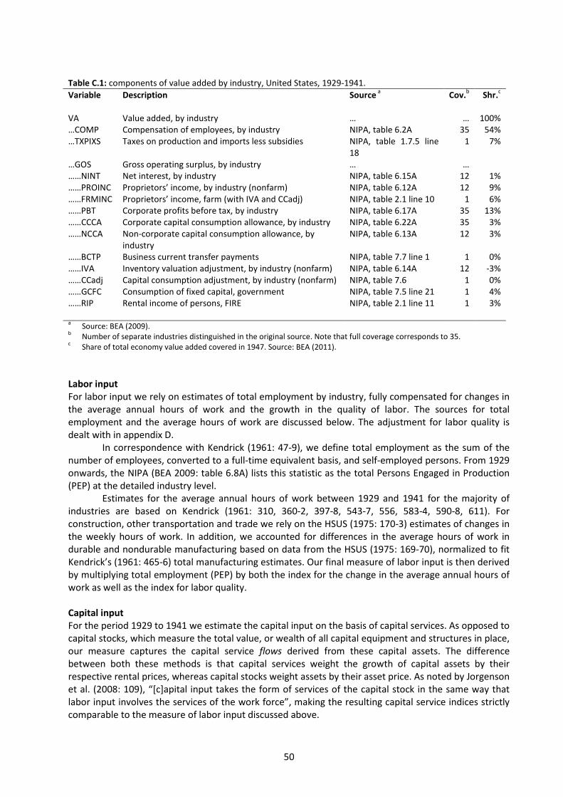
50

Labor inputForlaborinputw erely onestim atesoftotalem ploym entby industry,fully com pensated forchangesinthe average annualhoursof w ork and the grow th in the quality of labor. T he sourcesfor totalem ploym ent and the average hoursofw ork are discussed below .T he adjustm ent forlaborquality isdealtw ithinappendixD.

In correspondence w ith Kendrick(1961:47-9),w e define totalem ploym ent asthe sum ofthenum berofem ployees,converted to afull-tim eequivalentbasis,and self-em ployed persons.From 1929onw ards,the N IP A (BEA 2009:table 6.8A)liststhisstatisticasthe totalP ersonsEngaged in P roduction(P EP )atthedetailedindustry level.

Estim atesforthe average annualhoursofw ork betw een 1929 and 1941 forthe m ajority ofindustriesare based on Kendrick (1961: 310,360-2,397-8,543-7,556,583-4,590-8,611). Forconstruction,othertransportationand tradew erely ontheHS U S (1975:170-3)estim atesofchangesinthe w eekly hoursofw ork.In addition,w e accounted fordifferencesin the average hoursofw ork indurable and nondurable m anufacturing based on datafrom the HS U S (1975:169-70),norm alized to fitKendrick’s(1961:465-6)totalm anufacturingestim ates.O urfinalm easureoflaborinputisthenderivedby m ultiplyingtotalem ploym ent(P EP )by both the index forthe change in the average annualhoursofw orkasw ellastheindex forlaborquality.

Capital inputFortheperiod1929 to1941 w eestim atethecapitalinputonthebasisofcapitalservices.Asopposedtocapitalstocks,w hichm easurethetotalvalue,orw ealthofallcapitalequipm entand structuresinplace,our m easure capturesthe capitalservice flow sderived from these capitalassets. T he differencebetw een both these m ethodsisthat capitalservicesw eight the grow th ofcapitalassetsby theirrespectiverentalprices,w hereascapitalstocksw eightassetsby theirassetprice.Asnotedby Jorgensonet al.(2008:109),“ [c]apitalinput takesthe form ofservicesofthe capitalstockin the sam e w ay thatlaborinputinvolvesthe servicesofthe w orkforce” ,m aking the resulting capitalservice indicesstrictlycom parabletothem easureoflaborinputdiscussedabove.

Table C.1: com ponentsofvalueaddedby industry,U nitedS tates,1929-1941.

Variable Description Sourcea

Cov.b

Shr.c

VA Valueadded,by industry … … 100%… CO M P Com pensationofem ployees,by industry N IP A,table6.2A 35 54%… T X P IX S T axesonproductionandim portslesssubsidies N IP A,table 1.7.5 line

181 7%

… GO S Grossoperatingsurplus,by industry … …… … N IN T N etinterest,by industry N IP A,table6.15A 12 1%… … P R O IN C P roprietors’ incom e,by industry (nonfarm ) N IP A,table6.12A 12 9%… … FR M IN C P roprietors’ incom e,farm (w ithIVA andCCadj) N IP A,table2.1 line10 1 6%… … P BT Corporateprofitsbeforetax,by industry N IP A,table6.17A 35 13%… … CCCA Corporatecapitalconsum ptionallow ance,by industry N IP A,table6.22A 35 3%… … N CCA N on-corporatecapitalconsum ptionallow ance,by

industryN IP A,table6.13A 12 3%

… … BCT P Businesscurrenttransferpaym ents N IP A,table7.7line1 1 0%… … IVA Inventory valuationadjustm ent,by industry (nonfarm ) N IP A,table6.14A 12 -3%… … CCadj Capitalconsum ptionadjustm ent,by industry (nonfarm ) N IP A,table7.6 1 0%… … GCFC Consum ptionoffixedcapital,governm ent N IP A,table7.5 line21 1 4%… … R IP R entalincom eofpersons,FIR E N IP A,table2.1 line11 1 3%

aS ource:BEA (2009).

bN um berofseparateindustriesdistinguished intheoriginalsource.N otethatfullcoveragecorrespondsto35.

cS hareoftotaleconom y valueaddedcoveredin1947.S ource:BEA (2011).

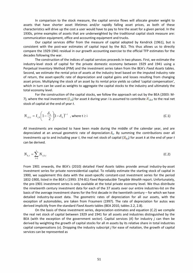
51

In com parison to the stock m easure,the capitalservice flow sw illallocate greaterw eight toassets that have shorter asset lifetim es and/or rapidly falling asset prices, as both of thesecharacteristicsw illdriveupthecostauserw ould haveto pay to hiretheassetforagivenperiod.Inthe1930s,prim e exam plesofassetsthat are underw eighted by the traditionalcapitalstockm easure are:com m unicationequipm ent,officeandaccountingequipm entandtrucks.

O ur capitalservicesdiffer from the m easure ofcapitaladopted by Kendrick (1961),but isconsistent w ith the post-w ar estim atesofcapitalinput by the BL S . T histhusallow susto directlycom pare the 1929-1941 residualin ourgrow th accountingexercise to the officialT FP estim atesforthedecadesfollow ingthew ar.

T heconstructionoftheindicesofcapitalservicesproceedsintw ophases.First,w eestim atetheindustry-levelstock of capitalfor the private dom estic econom y betw een 1929 and 1941 using aP erpetualInventory M ethod (P IM )and the investm entseriestaken from the BEA’sFixed Assetstables.S econd,w e estim ate the rentalprice ofassetsatthe industry levelbased on the im puted industry rateofreturn,the asset-specific rate ofdepreciation and capitalgainsand lossesresulting from changingassetprices.M ultiplyingthe stockofan assetby itsrentalprice yieldsso called ‘capitalcom pensation’,w hich in turn can be used asw eightsto aggregate the capitalstocksto the industry and ultim ately thetotaleconom y level.

Fortheconstruction ofthecapitalstocks,w e follow the approach setoutby theBEA (2003:M -7),w heretherealinvestm ent( )forassetkduringyeariisassum ed tocontribute totherealnet

stockofcapitalattheendofyeart.

it

kk

kitki IN

12

1,,, ,w heret i (C.1)

Allinvestm entsare expected to have been m ade during the m iddle ofthe calendaryear,and aredepreciated at an annualgeom etric rate ofdepreciation . By sum m ing the contributionsoverall

investm entsupto and includingyeart,therealnetstockofcapital( )forassetkattheend ofyeart

canbederived.

t

itkitk NN

1,,, (C.2)

From 1901 onw ards,the BEA’s(2010) detailed Fixed Assetstablesprovide annualindustry-by-assetinvestm ent seriesforprivate nonresidentialcapital.T o reliably estim ate the starting stockofcapitalin1900,w e supplem ent thisdataw ith the asset-specific constant-cost investm ent seriesforthe period1832-1900,listedintheBEA’s(1993:374-81)FixedR eproducibleT angibleW ealthreport.U nfortunately,the pre-1901 investm ent seriesisonly available at the totalprivate econom y level.W e thusdistributethe nineteenth century investm ent dataforeach ofthe 37 assetsoverourentire industries-liston thebasisoftheaverageinvestm entsharesforthefirstdecadeinthetw entiethcentury – forw hichw ehavedetailed industry-by-asset data. T he geom etric ratesof depreciation for allour assets,w ith theexception ofautom obiles,are taken from Fraum eni(1997). T he rate ofdepreciation forautosw asderivedim plicitly from thestandard FixedAssetstables(BEA 2010,tables2.2,2.8).

O n the basisofthese investm entseries,depreciation estim atesand equation (C.2)w e com pilethe realnet stockofcapitalbetw een 1929 and 1941 forallassetsand industriesdistinguished by theBEA (w ith the exception ofthe governm ent sector). Capitalservices(K) forindustry jcan then bederived by w eightingthe grow thofcapitalstocksforallm assetsby itsrelativeshare in totalindustriescapitalcom pensations(v).Dropping the industry subscript jforease ofnotation,the grow th ofcapitalservicescanberepresentedas

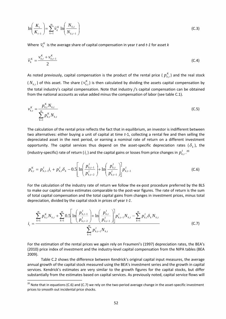
52

1,

,

11

lnlntk

tkm

k

Kk

t

t

N

Nv

K

K(C.3)

W here Kkv istheaverageshareofcapitalcom pensationinyeartandt-1 forassetk

2

1,,K

tkK

tkKk

vvv

(C.4)

Asnoted previously,capitalcom pensation isthe product ofthe rentalprice (K

tkp , )and the realstock

( tkN , )ofthisasset.T he share (K

tkv , )isthen calculated by dividing the assetscapitalcom pensation by

the totalindustry’scapitalcom pensation.N ote that industry j’scapitalcom pensation can be obtainedfrom thenationalaccountsasvalueaddedm inusthecom pensationoflabor(seetableC.1).

m

ktk

Ktk

tkK

tkKtk

Np

Npv

1,,

,,

, (C.5)

T hecalculationoftherentalpricereflectsthefactthatinequilibrium ,aninvestorisindifferentbetw eentw o alternatives:eitherbuying aunit ofcapitalat tim e t-1,collecting arentalfee and then selling thedepreciated asset in the next period,orearning anom inalrate ofreturn on adifferent investm ent

opportunity. T he capitalservicesthusdepend on the asset-specific depreciation rates( k ),the

(industry-specific)rateofreturn( ti )andthecapitalgainsorlossesfrom pricechangesinI

tkp , .20

ItkI

tk

Itk

Itk

Itk

kI

tktI

tkK

tk pp

p

p

ppipp 1,

1,

,

2,

1,

,1,, lnln5.0

(C.6)

Forthe calculation ofthe industry rate ofreturn w e follow the ex-postprocedure preferred by the BL Sto m ake ourcapitalserviceestim atescom parableto the post-w arfigures.T he rate ofreturn isthesumoftotalcapitalcom pensation and the totalcapitalgainsfrom changesin investm entprices,m inustotaldepreciation,dividedby thecapitalstockinpricesofyeart-1.

m

ktk

Itk

m

k

m

ktkk

Itktk

ItkI

tk

Itk

Itk

Itk

m

ktk

Ktk

t

Np

NpNpp

p

p

pNp

i

1,1,

1 1,,,1,

1,

,

2,

1,

1,, lnln5.0

(C.7)

Forthe estim ation ofthe rentalpricesw e again rely on Fraum eni’s(1997)depreciation rates,the BEA’s(2010)priceindex ofinvestm entand theindustry-levelcapitalcom pensationfrom theN IP A tables(BEA2009).

T able C.2 show sthe difference betw een Kendrick’soriginalcapitalinputm easures,the averageannualgrow thofthecapitalstockm easuredusingtheBEA’sinvestm entseriesandthegrow thincapitalservices.Kendrick’sestim atesare very sim ilarto the grow th figuresforthe capitalstocks,but differsubstantially from theestim atesbased oncapitalservices.Aspreviously noted,capitalserviceflow sw ill

20N otethatinequations(C.6)and(C.7)w erely onthetw o-periodaveragechangeintheasset-specificinvestm ent

pricestosm oothoutincidentalpriceshocks.

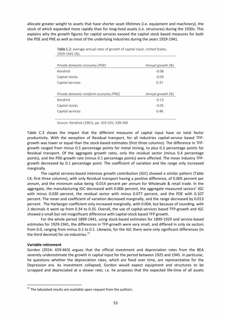
53

allocate greaterw eight to assetsthat have shorterasset lifetim es(i.e.equipm ent and m achinery),thestockofw hich expanded m ore rapidly than forlong-lived assets(i.e.structures)during the 1930s.T hisexplainsw hy the grow th figuresforcapitalservicesexceed the capitalstockbased m easuresforboththeP DEandP N Easw ellasm ostoftheunderlyingindustriesduringtheyears1929-1941.

Table C.2: average annual rates of growth of capital input, United States,1929-1941 (%).

Private domestic economy (PDE) Annual growth (%)

Kendrick -0.08

Capital stocks -0.09

Capital services 0.37

Private domestic nonfarm economy (PNE) Annual growth (%)

Kendrick -0.13

Capital stocks -0.05

Capital services 0.48

Source: Kendrick (1961), pp. 333-335; 338-340

T able C.3 show sthe im pact that the different m easuresof capital input have on total factorproductivity. W ith the exception ofR esidualtransport,for allindustriescapital-service based T FP -grow th w aslow erorequalthan the stock-based estim ates(firstthree colum ns).T he difference in T FP -grow th ranged from m inus0.5 percentage pointsform etalm ining,to plus0.3 percentage pointsforR esidualtransport. O fthe aggregate grow th rates,only the residualsector (m inus0.4 percentagepoints),and the P DE-grow th rate (m inus0.1 percentage points)w ere affected.T he m ean industry T FP -grow th decreased by 0.1 percentage point.T he coefficient ofvariation and the range only increasedm arginally.

T he capitalservices-based intensive grow th contribution (IGC)show ed asim ilarpattern (T ableC4,firstthree colum ns),w ith only R esidualtransporthaving apositive difference,of0.005 percentperannum ,and the m inim um value being -0.014 percent perannum forW holesale & retailtrade.In theaggregate,the m anufacturing IGC decreased w ith 0.006 percent,the aggregate m easured sectors’ IGCw ith m inus0.030 percent,the residualsector w ith m inus0.077 percent,and the P DE w ith 0.107percent.T hem eanand coefficientofvariation decreased m arginally,and the range decreased by 0.013percent. T heHarbergercoefficientonly increasedm arginally,w ith0.004,butbecauseofrounding,w ith2 decim alsit w ent up from 0.34 to 0.35.O verall,the use ofcapital-servicesbased T FP -grow th and IGCshow edasm allbutnotinsignificantdifferencew ithcapital-stockbasedT FP grow th.

Forthe w hole period 1899-1941,using stock-based estim atesfor1899-1929 and service-basedestim atesfor1929-1941,the differencesin T FP -grow th w erevery sm all,and differed in only six sectorsfrom 0.0,rangingfrom m inus0.1 to 0.1.L ikew ise,forthe IGC therew ereonly significantdifferences(inthethirddecim al)forsix industries.21

Variable retirementGordon (2016: 659-663) arguesthat the officialinvestm ent and depreciation ratesfrom the BEAseverely underestim atethegrow thincapitalinputfortheperiod betw een1925 and 1945.Inparticular,he questionsw hetherthe depreciation rates,w hich are fixed overtim e,are representative fortheDepression era. Asinvestm ent collapsed,Gordon w ould expect equipm ent and structuresto bescrapped and depreciated at aslow errate; i.e.he proposesthat the expected life-tim e ofallassets

21T hetabulatedresultsareavailableuponrequestfrom theauthors.

54

should increase substantially during the 1930s.T hislow errate ofdepreciation w ould lead to agreaterincreaseinthecapitalstockthantheestim atesby theBEA w ouldsuggest.

Asacrudeproxy forthesevaryingratesofdepreciation,Gordonsuggestscom paringtheratioofinvestm enttotheofficialcapitalstockforeachyearw iththeaveragefor1925-1972.A low ratio,asw asthecasefor1933,w ould indicateanincreaseintheassetlifetim e,w hereasarelatively highratiow ouldindicateareductioninthetim eproducersholdontotheirageingcapitalassets.

Asarobustnesscheck to our capitalinput estim ates,w e apply the sam e procedure. W eestim ated the ratio ofinvestm ent to stock separately forequipm ent capitaland structures.T he dataw astaken from the BEA’s(2010)Fixed Assets,basic tables2.1,2.2,2.7 and 2.8,lines3 and 37.T heofficialdepreciation ratesdiscussed in the previoussection w ere m ultiplied by the ratio ofinvestm entto capitalin the respective year,relative to the average ofthe period 1925-1972.O n the basisofthesedepreciation ratesw e re-estim ated the capitalstocksand capitalservices.T ablesC.3 and C.4 show theresultingT FP andIGC basedontheserevisedcapitalinputs.

T he effect of the adjustm ent on industry T FP -grow th for 1929-1941 w as negligible orsignificantly negative for allindustries. It varied substantially,from 0.0 percentage-pointsfor CoalM ining,Electric M achinery and Furniture,to m inus0.7 percentage-pointsforO il& Gasm ining andm inus0.5 percentage-pointsforboth M etalM ining,and P etroleum & Coalproducts.T he overalleffecton the T FP -grow th rate ofthe P DE w assubstantial,m inus0.2 percentage-points,w hich constitutesaten percent dow nw ard adjustm ent.T he im pact on the intensive grow th contribution (IGC)w assm allbut significant form any industries,asonly 7 industrieshad no difference at three decim als,and the

change in the IGC w assubstantialforFarm ing,Foods,W holesale & R etailtrade and FIR Ealllargesectors.Forboth T FP and IGC,the m ean decreased and the coefficientofvariation increased by abouttenpercent.T heHarbergercoefficientincreasedappreciably,from 0.35 to0.38.

Forthe w hole period 1899-1941,using standard depreciation based estim atesfor1899-1929and variable retirem entbased estim atesfor1929-1941,the differencesin T FP -grow th w ere very sm all,m inus0.1 or0.0 inm ostsectorsand m inus0.2 inonly onesector,O il& Gas.L ikew ise,fortheIGC therew ere only m arginally significant differences(in the third decim al) for 19 industries,no significantdifferencesin17 industries,andnosignificantdifferenceintheHarbergercoefficient.22

Electrical equipmentT o estim ate the share ofelectricalequipm entassetsin the totalstockofequipm ent– used to m easurethe im pact ofthe installed electricalhorsepow erin m anufacturing in section 6 – w e also com pile anannualseriesofthenom inalnetstockofcapitalforelectricalequipm entandtotalequipm ent.W eapplythe m ethodsdescribed above butfocuson the period 1921 to 1929 instead.23 T he nom inalnetstockofelectricalequipm ent isthe aggregate ofthe nom inalvalue ofthe BEA (2010) assetsEI60 (electricaltransm issions,distribution and industrialapparatus) and EO 70 (electricalequipm ent not elsew hereclassified). T otalequipm ent includeselectricalequipm ent in addition to transportation equipm ent,instrum entsand non-electricalequipm ent.W e estim ate the share ofelectricalequipm ent assetsbydividing the nom inalstockofelectricalequipm ent by the totalstockofequipm ent forthe years1921and1929 andthentakingtheaverageoverboththeseyears.

22T hetabulatedresultsareavailableuponrequestfrom theauthors.

23N otethattheshorterassetlifetim esform achinery andequipm entallow sustosafely estim atetherealand

nom inalstocksfortheseassetsbeginningin1921.T hegreaterrateofdepreciationreducesthesensitivity oftheseassetstotheassum ptionsm aderegardingthepre-1900 rateofinvestm entby individualindustries.

55

Table C3. Comparative growth in Total Factor Productivity (TFP) by industry, using capital stock vs.

capital services and standard depreciation vs. variable retirement, United States, 1929-1941.

Industry TFP-growth (percent per annum)

Effectcapitalservices Effectvariableretirem ent

S tock S erv. Diff. S D VR Diff.

Farm ing 2.6 2.5 -0.1 2.5 2.2 -0.3

M etals 1.1 0.6 -0.5 0.6 0.1 -0.5

AnthraciteCoal 0.4 0.3 0.0 0.3 0.3 0.0

Bitum inousCoal 1.9 1.8 -0.1 1.8 1.8 0.0

O ilandGas 2.1 2.1 0.0 2.1 1.3 -0.7

N on-m etals 3.9 3.6 -0.3 3.6 3.3 -0.3

Foods 3.7 3.7 0.0 3.7 3.5 -0.2

T obacco 5.8 5.8 -0.1 5.8 5.3 -0.5

T extiles 3.4 3.3 -0.1 3.3 3.1 -0.2

Apparel -0.4 -0.4 0.0 -0.4 -0.6 -0.2

L eatherP roducts -0.1 -0.1 0.0 -0.1 -0.2 -0.2

L um berP roducts -1.7 -1.8 0.0 -1.8 -1.9 -0.1

P aper 1.2 1.1 -0.1 1.1 1.0 -0.1

P rintingP ublishing 0.3 0.3 0.0 0.3 0.2 -0.1

Chem icals 2.2 2.1 0.0 2.1 1.9 -0.3

P etroleum ,CoalP roducts -1.2 -1.1 0.1 -1.1 -1.6 -0.5

R ubberP roducts 1.6 1.5 -0.1 1.5 1.4 -0.1

S tone,clay,glass 1.9 1.7 -0.1 1.7 1.5 -0.2

P rim ary M etals 2.3 2.4 0.1 2.4 2.0 -0.3

FabricatedM etals 1.3 1.3 0.0 1.3 1.2 -0.2

M achinery N on-Electric 2.1 2.1 0.0 2.1 2.0 -0.1

ElectricM achinery 4.6 4.6 0.0 4.6 4.6 0.0

T ransportEquipm ent 3.6 3.5 0.0 3.5 3.3 -0.2

Furniture 1.4 1.4 0.0 1.4 1.4 0.0

M iscellaneous 1.9 1.5 -0.3 1.5 1.3 -0.2

ElectricU tilities 5.1 5.1 0.0 5.1 4.7 -0.4

M anufacturedGas 2.0 1.8 -0.2 1.8 1.5 -0.3

N aturalGas 3.7 3.7 -0.1 3.7 3.3 -0.4

Construction* 0.8 0.7 -0.1 0.7 0.4 -0.3

W holesale& retailtrade* 3.5 3.4 -0.1 3.4 3.3 -0.1

R ailroads 2.5 2.6 0.0 2.6 2.4 -0.1

L ocalT ransit 0.5 0.4 -0.1 0.4 0.2 -0.1

R esidualT ransport 5.5 5.8 0.3 5.8 5.6 -0.2

T elephone 1.4 1.4 0.0 1.4 1.2 -0.2

T elegraph 0.8 0.7 -0.1 0.7 0.6 -0.1

P ostO ffice* 0.5 0.4 -0.1 0.4 0.3 -0.1

FIR E* -1.3 -1.3 0.0 -1.3 -1.6 -0.3

S pectatorEntertainm ent* 4.4 4.4 0.0 4.4 4.3 -0.1

56

M anufacturing 2.3 2.3 0.0 2.3 2.0 -0.2

Aggregatem easuredsectors 1.9 1.9 0.0 1.9 1.7 -0.2

R esidualsector 2.3 1.8 -0.4 1.8 1.7 -0.1

P DE 2.0 1.9 -0.1 1.9 1.7 -0.2

M em orandum :Kendrick'saggregatem easuredsectors 2.5 2.5 2.5 2.5Kendrick'sresidualsector 2.0 2.0 2.0 2.0KendrickP DE 2.3 2.3 2.3 2.3

M inim um -1.7 -1.8 0.0 -0.4 -0.4 0.0

M axim um 5.8 5.8 0.0 5.5 5.5 0.0

R ange 7.5 7.6 0.0 6.0 6.0 0.0

N otes:S tock= T FP -grow thrateiscalculatedfrom inputdatathatincludestock-basedestim atesofcapital.

S erv.= T FP -grow thrateiscalculatedfrom inputdatathatincludeservice-basedestim atesofcapital.

Diff.= thedifferencebetw eentheratesinthetw oprecedingcolum ns

S D = T FP -grow thrateiscalculatedfrom inputdatabasedonthestandarddepreciationm ethodusingcapitalservicessetoutinthisappendix.

VR = T FP -grow thrateiscalculatedfrom inputdatabasedonusingbothcapitalservices(assetoutinthisappendix)andthevariableretirem entofcapitalm ethodintroducedby Gordon(2016).

Kendrick'saggregatem easuredsectorcom prisesFarm ing,M ining,M anufacturing,T ransportation,Com m unication& P ublicU tilities)

* = sectorm easuredinthispaperbutnotby Kendrick.

For1929-1941 and1899-1941 theT FP -grow thofKendrick'sm easuredandresidualsectorsw asestim atedusing

ourdataforKendrick'sm easuredsectorsfor1929-41 andtherelationshipbetw eenm easured,residualand

aggregateT FP grow thinKendrick’snum bersforhis4 sub-periodsduring1899 through1937.

T FP hereisrefined T FP ,i.e.aftercorrectingcrudeT FP forthegrow thof

laborquality (seetext).

S ource:Kendrick1961,pp.136-7;ow ncalculations,seethetextandAppendicesB andC (industry data)and

Appendix D (laborquality data).

57

Table C4. Comparative intensive growth contribution by industry, using capital stock vs. capital

services and standard depreciation vs. variable retirement, United States, 1929-1941.

Industry IGC = (VAShare*TFP growth)

Effectcapitalservices Effectvariableretirem ent

S tock S erv. Diff. S D VR Diff.

Farm ing 0.198 0.193 -0.006 0.193 0.168 -0.025

M etals 0.006 0.003 -0.002 0.003 0.001 -0.002

AnthraciteCoal 0.001 0.001 0.000 0.001 0.001 0.000

Bitum inousCoal 0.012 0.012 0.000 0.012 0.012 0.000

O ilandGas 0.017 0.017 0.000 0.017 0.011 -0.006

N on-m etals 0.008 0.007 -0.001 0.007 0.007 -0.001

Foods 0.208 0.206 -0.002 0.206 0.194 -0.012

T obacco 0.063 0.062 -0.001 0.062 0.057 -0.005

T extiles 0.059 0.058 -0.001 0.058 0.054 -0.003

Apparel -0.005 -0.005 0.000 -0.005 -0.007 -0.002

L eatherP roducts 0.000 0.000 0.000 0.000 -0.001 -0.001

L um berP roducts -0.013 -0.013 0.000 -0.013 -0.014 -0.001

P aper 0.008 0.007 0.000 0.007 0.007 -0.001

P rintingP ublishing 0.005 0.005 0.000 0.005 0.003 -0.002

Chem icals 0.029 0.028 0.000 0.028 0.025 -0.003

P etroleum ,CoalP roducts -0.014 -0.013 0.001 -0.013 -0.019 -0.006

R ubberP roducts 0.007 0.006 0.000 0.006 0.006 0.000

S tone,clay,glass 0.016 0.015 -0.001 0.015 0.013 -0.002

P rim ary M etals 0.051 0.052 0.002 0.052 0.045 -0.007

FabricatedM etals 0.020 0.020 0.000 0.020 0.017 -0.003

M achinery N on-Electric 0.039 0.039 0.000 0.039 0.037 -0.002

ElectricM achinery 0.046 0.046 0.000 0.046 0.046 0.000

T ransportEquipm ent 0.072 0.071 -0.001 0.071 0.067 -0.004

Furniture 0.009 0.009 0.000 0.009 0.009 0.000

M iscellaneous 0.012 0.010 -0.002 0.010 0.008 -0.001

ElectricU tilities 0.104 0.103 -0.001 0.103 0.094 -0.009

M anufacturedGas 0.004 0.003 0.000 0.003 0.003 0.000

N aturalGas 0.012 0.012 0.000 0.012 0.011 -0.001

Construction* 0.026 0.023 -0.002 0.023 0.014 -0.009

W holesale& retailtrade* 0.476 0.462 -0.014 0.462 0.451 -0.011

R ailroads 0.111 0.111 0.000 0.111 0.105 -0.006

L ocalT ransit 0.004 0.003 -0.001 0.003 0.002 -0.001

R esidualT ransport 0.091 0.096 0.005 0.096 0.092 -0.004

T elephone 0.012 0.012 0.000 0.012 0.010 -0.002

T elegraph 0.001 0.001 0.000 0.001 0.001 0.000

P ostO ffice* 0.003 0.002 -0.001 0.002 0.002 -0.001

FIR E* -0.143 -0.145 -0.001 -0.145 -0.172 -0.027

S pectatorEntertainm ent* 0.023 0.023 0.000 0.023 0.023 0.000

58

M anufacturing 0.609 0.603 -0.006 0.603 0.546 -0.056

Aggregatem easuredsectors 1.573 1.542 -0.030 1.542 1.380 -0.162

R esidualsector 0.400 0.323 -0.077 0.323 0.299 -0.025

P DE 1.972 1.866 -0.107 1.866 1.679 -0.187

M ean 0.041 0.041 -0.001 0.041 0.036 -0.004

Coefficientofvariation 2.213 2.211 -0.003 2.211 2.431 0.220

M inim um -0.143 -0.145 -0.001 -0.145 -0.172 -0.027

M axim um 0.476 0.462 -0.014 0.462 0.451 -0.011

R ange 0.619 0.607 -0.013 0.607 0.623 0.016

Harbergercoefficient 0.345 0.349 0.004 0.349 0.377 0.028

N otes:S tock= intensivegrow thcontribution(IGC)calculatedfrom inputdatathatincludestock-basedestim atesofcapital.

S erv.= IGC calculatedfrom inputdatathatincludeservice-basedestim atesofcapital.

Diff.= thedifferencebetw eentheIGCsinthetw oprecedingcolum ns

S D = IGC calculatedfrom inputdatabasedonthestandarddepreciationm ethodusingcapitalservicessetoutinthisappendix.

VR = IGC calculatedfrom inputdatabasedonusingbothcapitalservices(assetoutinthisappendix)andthevariableretirem entofcapitalm ethodintroducedby Gordon(2016).

Kendrick'saggregatem easuredsectorcom prisesFarm ing,M ining,M anufacturing,T ransportation,

Com m unication& P ublicU tilities)

* = sectorm easuredinthispaperbutnotby Kendrick.

For1929-1941 and1899-1941 theT FP -grow thofKendrick'sm easuredandresidualsectorsw asestim atedusing

ourdataforKendrick'sm easuredsectorsfor1929-41 andtherelationshipbetw eenm easured,residualand

aggregateT FP grow thinKendrick’snum bersforhis4 sub-periodsduring1899 through1937.

T FP hereisrefined T FP ,i.e.aftercorrectingcrudeT FP forthegrow thof

laborquality (seetext).

S ource:Kendrick1961,pp.136-7;ow ncalculations,seethetextandAppendicesB andC (industry data)and

Appendix D (laborquality data).

59

Appendix D. Labor Quality

D1. Discussion of the Kendrick Labor Quality Estimates

Kendrick (1961: 31-34) assessed the effect of skillchangeson the com position ofthe labor forcebetw een1869 and1957.Insteadofm easuringchangesineducationattainm ent,genderand experiencedirectly,how ever,he m easured the changesin the occupationalstructure.He adjusted laborinput byw eighting the m an-hoursof w ork in separate occupationsand industriesby their average hourlyearningsforagiven base year.Kendrick’sm easure oflaborquality thuscapturestw o effects: (1)therelative shiftsof w orkersbetw een occupations,and (2) the relocation of em ploym ent betw eenindustries.T hefirsteffect,theshiftofw orkersfrom low -payingpositions(e.g.laborers)tobetter-payingjobs(e.g.operativesorclericalstaff),reflectsachange in the potentialoutput perw orker.T he higherearnings(m easured in term sofbase-period com pensation)im ply arise in the m arginalproductivity ofthat w orkerand thusarise in the quality ofthe laborforce – in line w ith the Jorgenson approachdiscussed below .L ikew ise,the shiftofw orkersto better-paying industriesalso show up asan increaseinlaborquality.

Kendrickassum esunder(1)that laborquality w illonly change overtim e ifaw orkertransfersfrom oneoccupationtoanotherorifanindividualjoins(orleaves)thelaborforceinanoccupationthatisbetter (w orse) paid than the nationalaverage. Kendrick (1961: 33) surm isesthat “ the inherentaveragephysicalandm entalcapacity ofthepersonem ployedineachoccupationisconstantovertim e.”T he rapid increase in educationalattainm ent during the late nineteenth and early tw entieth centurycastsseriousdoubt on thisassum ption,how ever. T he average yearsofschooling forcohortsbornbetw een 1880 and 1950 nearly doubled,increasingfrom approxim ately 8 to 14 years(Goldin and Katz,2008: 20; 113; 170). P art of thisincrease in skilltranslated into a shift of em ployeesbetw eenoccupationsand industries,but part also translated into arise ofthe laborquality w ithin occupations.Forinstance,thelikelihood forabluecollarw orkerbornaround 1885 tohaveattended highschoolw assubstantially greaterthan it w asforitscounterpart born only 10 yearsprior,around 1875.T he high-schooleducation gave the blue-collarw orkerbasic know ledge ofchem istry,electricity and algebra,allow ed him to read m anualsand blueprintsand m ade it m uch easierforhim to effectively conversew ith m anagersand otherprofessionals,raising hism arginalproductivity in the process.In addition toundervaluing the im pactofthe rapid increasesin education attainm entduring the late nineteenth andearly tw entieth century,Kendrick’sm ethod ignoresotherdem ographic changesasw ellw hich thusbiaseshislabor quality figuresdow nw ardscom pared to our ow n (see table D.1). Changesin theeducational attainm ent,average age,or experience of the w orkforce and shiftsin the gendercom position are generally considered to be determ ining factorsin the quality oflabor,asw e w illillustratebelow .

60

Table D.1: average annual rates of growth of labor quality, United States,1899-1941 (%).

Kendrick This study

Private domestic economy (PDE) 0.32 0.79

1899-1929 0.36 0.87

1929-1941 0.20 0.59

Private domestic nonfarm economy (PNE) 0.15 0.36

1899-1929 0.16 0.40

1929-1941 0.14 0.27

Source: Kendrick (1961), pp. 333-335; 338-340

D2. Discussion of the Labor Quality Estimates in this Paper

In orderto fully assessthe im pact ofthe substantialinvestm entsin schooling asw ellasthe structuralchangesin the genderand age com position ofthe Am erican w orkforce during the early tw entiethcentury,w e turn to an approach developed by Dale Jorgenson and ZviGriliches(1967). T he keyinnovationintheirw orkw astoadjustthetraditionalm easureoflaborinput– i.e.totalhoursofw orkorem ploym ent – forim provem entsin quality.T he m ain principle behind the laborquality adjustm ent isthe distinction am ongseveraldifferenttypesoflaborinputscharacterized by one orm ore quantifiablefactorsthat affect the productivity potentialofthe w orker(e.g.educationalattainm ent,age,gender).By thenassigningw eightstothesecategories– usually intheform ofaveragew agesand earnings– onecan m easure the change in the productivity ‘potential’ of the w orkforce. T he rationale for thisprocedure isthat differencesin average earningsbetw een the laborcategoriescan be thought ofasreflecting differencesin theirm arginalproductivity.W hen thisnew m easure oflaborinputisused in agrow th accounting fram ew ork,output grow th asaresult ofbettereducated and trained w orkersisascribed to input grow th,rather than productivity or technology grow th (Jorgenson et al.,2008).P reviousstudieshaveshow nthatthisquality adjusted m easurecanaccountforasubstantialpartoftheresidualorT otalFactorP roductivity (T FP )grow thw ithintraditionalgrow thaccountingstudies(Denison,1962; Griliches,1963; Denison and P oullier,1967; Gordon,2010). T herefore,the labor qualityadjustm entallow sforapurerm easure ofboth laborinputasw ellastechnicalchange w ithin agrow thaccountingfram ew ork.

MethodologyT o construct an index oflaborinput foreach individualsector,w e assum e that laborinput ( )for

industry jat tim e t can be expressed asatranslog function ofitsindividualcom ponents(Jorgenson etal.,1999:92-3).W e form indicesoflaborinput from dataon em ploym ent by industry,cross-classifiedby gender,age and education.24 Dropping the industry subscript jforease ofnotation,the grow th oflaborinputforindustry jcanthusberepresentedas

1,

,

11

lnlntl

tlq

l

Ll

t

t

L

Lv

HK

HK(D.1)

24N otethatage,inourestim ateforlaborinput,servesasaproxy for(w ork)experience.W ethusassum ethatanindividualhas

heldajobhisentirelifesinceleavinghigh-schoolorcollege;dependingonhiseducationalattainm ent.

61

W here isem ploym ent at the industry levelforagiven set ofq characteristicsofthe laborforce l(gender,age and education)and isthe average ofthisem ploym ent group’sshare in the totallaborincom e

2

1,,Ltl

LtlL

l

vvv

(D.2)

T he share oflaborincom e ( ) at tim e t isderived asthe product ofthe average w age ( ) and

em ploym ent( )foreachcom binationoflaborcharacteristicl,dividedby thetotalw agesum

tl

n

l

Ll

tiLlL

tl

Lp

Lpv

,1

,

,

(D.3)

Alternatively,the index oflaborinput can also be expressed asthe product ofem ploym ent (L )and anindex oflaborquality (L Q )or,ingrow thterm s,as

111

lnlnlnt

t

t

t

t

t

LQ

LQ

L

L

HK

HK(D.4)

R earranging term sin equation (B.4)and substituting the index forlaborinput by (D.1)w e arrive at adirectm easureofsectorallaborquality grow th

11,

,

11

lnlnlnt

t

tl

tlq

l

Ll

t

t

L

L

L

Lv

LQ

LQ(D.5)

T hechangeinlaborquality thusreflectsthedifferencebetw eenthegrow thratesofthecom pensation-w eightedindexoflaborinputandsectoralem ploym ent.

T he draw backofthisapproach isthat it requireshighly disaggregate dataon em ploym ent andcom pensation,generally not available in the published censusreportsorsecondary sourcesfortheearly tw entieth century.Fortunately,the Integrated P ublic U se M icrodataS eries(IP U M S ) hasm adesam plesfrom thedecennialpopulationcensusespublicly available,providingdetailed recordsfornearly10 m illion individualsbetw een 1900 and 1950 (R ugglesetal,2010).W e utilize the m icrodatafrom thissourcetoconstructourm easureoflaborquality.

U nfortunately,how ever,the 1900-1930 Am erican population censusesdid not inquire intoeither the educationalattainm ent of the generalpopulation or the com pensation ofw orkersandem ployees.T o overcom e these dataissues,w e follow athree-tiered approach to the datapreparationforthelaborquality estim ation.First,w eestim ateeducationalattainm entatthem icrolevelforthepre-1940 censussam pleson the basisofthe1940 returns.S econd,w econstructanem ploym entm atrix forthe entire period that groupsw orkersaccording to their(predicted)educationalattainm ent,gender,age and by industry.L astly,w e derive the com pensation m atrix on the basisofaverage w agesforeachlabor category taken from the 1940 censusofpopulation.25 T hese em ploym ent and com pensationm atricescanthenbeusedtocalculatelaborquality onthebasisofequation(D.5).

Educational attainment

25T he1940 censusw asthefirstcensusofitskindtoaskaboutschooling,laborcom pensationandw orkinghourstoallcitizens

surveyed.Inthew akeofthedepressionthe1940 populationcensusdedicatedasubstantialpartofitsinquiry intotheissueofem ploym entandproductivity.

62

Forthefirststage,w eestim atetheeducationalattainm enty foranindividualionthebasisofhisorheroccupation,gender,age and placeofresidence .O n the basisofthisapproachw etakeboth the long-run changesin the average yearsofschooling asw ellasthe effectsofchangesin the occupationalstructure and the gender/age com position ofthe w orkforce into account.W e define foureducationcategories(see table D.2)and w e predict the likelihood that an individualibelongsto each ofthesespecific educationalcategories(e.g. . T hisprobability should be bounded by 0 and 1,continuousandnonlinear;conditionsw hichareallm etby an(ordered)logitm odel

'

'

1Pr

i

i

x

x

iie

exky

, k = 1, 2, 3 (D.6)

T he right-hand side ofequation (D.6)isacum ulative distribution function w ith m ean 0 and standarddeviation 1.T he coefficientsare estim ated using m axim um likelihood,w hich isthe optim alparam etricestim atorinthiscontext(L ongandFreese2006).26

Table D.2: categorical variables logit and labor quality models.

Logit model Labor quality model

Education: Education:See labor quality model (1) 1-4 years grade school

(2) 5-8 years grade schoolGender: (3) 1-4 years high schoolSee labor quality model (4) 1 or more years college

Occupation: Gender:(1) professional, technical (1) male(2) farmers (owners and managers) (2) female(3) managers, officials, and proprietors(4) clerical staff Age:(5) sales workers (1) 16-17 years(6) craftsmen (2) 18-24 years(7) operatives (3) 25-34 years(8) service workers (household) (4) 35-44 years(9) service workers (other) (5) 45 years and over(10) laborers(11) unemployed/retired Industry:

See main textRegion:(1) South(2) Midwest(3) West(4) Northeast

DataForthe estim ation ofthe logitm odelw e rely exclusively on the 1940 1-percentsam ple included in theIP U M S dataset.T hissam ple islim ited to include only those citizensaged 16 yearsand above,leavingapproxim ately 975,000 observationsforthe logisticregression.T he dataset includesam easure ofthehighestyearofschooling ordegree com pleted.Asillustrated in table D.2,w e reclassify thisvariable toencom passfourdistincteducationalattainm entclasses.T hereasonw ereclassify theeducationvariableistw ofold.First,by treatingitasacategoricalvariableasopposedtoacontinuousvariable(e.g.yearsofeducation),w e avoid the assum ption that the distancesbetw een classesare equal; i.e. that an

26N otethatw eestim atethecum ulativeprobability forthefirstthreeeducationalcategories,sinceallindividualsthatarenot

partofeitherthefirst,secondorthirdcategory w illbepartofthefourthcategory.T hefourthcategory canthusbeim plicitlyderivedand shouldbeexcludedfrom them odel.

63

additionalyearofgrade schoolisidenticalto one additionalyear in college. S econd,w e lim it thenum berofclassesto 4 to ensure thateach classiscovered by asufficientnum berofobservations.T hisisim portant not just forthe estim ation ofeducationalattainm ent,butalso forthe construction ofthecom pensation m atrix.27 Forthe independentvariables,w e follow the literature on U S laborquality andm ark four variablesasim portant predictorsof educationalattainm ent,nam ely: occupation,birthcohort,genderandregion.

Individualsare classified into one ofeleven m ain occupationalgroupsw hich differm arkedly interm softheir average educationalattainm ent. Forinstance,the probability ofaprofessional(e.g.engineers,econom ists)havingattended high schoolw assubstantially greaterthan w asthecase fortheaveragelaborer.T he im portanceofgenderand yearofbirth isillustrated by Goldin and Katz(2008:18-22;170).T hey observearapidincreaseintheaverageyearsofschoolingthroughoutthelatenineteenthand early tw entieth century.Each successive cohort spent asubstantially greaternum berofyearsinschoolcom pared to the previousgeneration.In addition,Goldin and Katz (2008:19)show thatw om engenerally attended schoolforlongerthanm endid throughoutm ostoftheearly tw entiethcentury.T hegendervariable w astaken directly from the IP U M S dataset w hile the yearofbirth w asrounded offtothe nearest decade.T he log ofthe relative distance in decadesto 1930 w asthen taken asthe birthcohort m easure.L astly,the literature pointsto w idespread differencesin state support foreducationand show sthat the rise in both high schoolgraduation ratesasw ellascollege enrollm ent ratesforstatesintheN orthand W estofthecountry w ereconsiderably m oreim pressivethanfortherestofthenation (Goldin and Katz,2008: 271-7). W e incorporate avariable in the m odelthat differentiatesbetw eenthefourm ainregionsofthecountry (seetableD.2).

For the second stage ofthe labor quality estim ation,the construction ofthe em ploym entm atrix,w e rely on the IP U M S 1-percent censussam plesforthe decadesbetw een 1900 and 1950.T oestim ate educationalattainm ent w e include the occupation,birth cohort,genderand region variablesdiscussed earlier,supplem ented by dataontheageoftheindividualand industry inw hichthesubjectisengaged.T he em ploym entsam ple islim ited to include only those citizensbetw een the agesof16 and84,w ho are partofthe laborforce.Forthe em ploym ent-m atrix ourdatasetincludesroughly 3,135,000individualobservations.

Inthethird stageofthedatapreparationw eagainrely onthe1940 sam pleto estim aterelativecom pensation perlaborcategory.Here w e lim itthe sam ple to include only those citizensbetw een theagesof16 and 84 havingw orked atleast48 w eeksin the previousyearand earningan incom e greaterthan 0 (Goldin and Katz,2008).T hese individualsare allocated to the cellsofthe m atrix cross-classifiedby gender,age,education and industry assum m arized in table D.2.Com pensation isreported in thecensusasthe respondent’stotalpre-tax w age and salary incom e forthe previousyear,expressed incurrent dollars.T o obtain totalpersonalincom e,w hich also includesnon-w age incom e,w e m ultipliedthe1940 com pensationfiguresby theindustry specificratio betw eenw ageand salary incom eand totalpersonalincom e taken from the 1950 censusreturns.N onw age incom e generally represented only asm allpartoftotalpersonalincom e,w ith the notable exception ofthe agriculturalsector.T he sam plesforthelogisticregression,thecom pensationm atrix and theem ploym entm atrix areallw eighted by theIP U M S p̀ersonw eight’ variable.

RobustnessIdeally,w e w ould like to allow the w eightsforourlaborquality index to vary overtim e,reflectingpotentialchangesin relative com pensation betw een the laborcategories.U nfortunately,the censusespriorto 1940 did not inquire into eitherw agesorearnings,im peding the accurate m easurem ent oflaborcom pensation forthese earlierdecades.R eassuringly,Goldin and Katz(2008:53-63)dem onstratethat the w age structure observed in 1940 w asfairly typicalforthe prew arperiod.Although they doobserve agradualcom pression ofthe w age distribution forproduction w orkersbetw een 1890 and

27L im itingthenum berofclassesfortheeducationvariableallow sus,forinstance,totestthe‘parallelregressionassum ption’;

m eaningthatforeacheducationclass(grade-school,high-school,college,etc.)thecoefficientsfortheindependentvariables(beta)areidentical.Asitturnsouttheassum ptionisviolated.Hencew eeffectively estim ateseparateregressionsforalleducationclasses,obtainingdifferentbetasforeach.

64

1940,Goldin and Katz conclude that the gap in the skilled/unskilled w age levelfor1920 w asvirtuallyidenticalincom parisonto1940.

O n the basisofGoldin and Katz’s(2010)dataforthe state ofIow aw e can perform am oreconclusivesensitivity checkofourlaborquality figures.T he Iow aS tateCensusP rojectprovidesdetailedcom pensation data,cross-classified by m ost ofthe categoriesthat m ake-up laborinput forthe year1915.Below w e w illcom pare the resultsfrom the third stage ofthe datapreparation – the estim ationofthe com pensation m atrix – forthe 1915 Iow adataand the original1940 censusdata.W e w illthenuse these new estim atesto provide an alternative estim ate oflaborquality forthe first halfofthetw entieth century and decom pose these estim atesto trace the sourcesofdivergence.In addition,w eperform the sam e sensitivity check based on com prehensive incom e datafor1950,taken from theIP U M S dataset.O verall,on the basisofthisevidence presented here w e feelconfidentusingsolely the1940 com pensationfiguresasw eightsfortheconstructionofourlaborquality index.

Table D.3. L aborincom eestim atesforIow aandtheU nitedS tates,1915,1940 and1950.Dependentvariable:log ofincom e

U S 1940(1)

U S 1940(2)

Iow a1940(3)

Iow a1915(4)

U S 1950(5)

Intercept 6.82*** 6.90*** 6.64*** 6.48*** 7.54***

(0.005) (0.003) (0.029) (0.012) (0.009)

Fem aledum m y -0.70*** -0.53*** -0.52*** -0.65*** -0.52***

(0.008) (0.007) (0.071) (0.033) (0.014)

Age16-17dum m y -0.81*** -1.23 -1.21*** -0.96*** -1.30***

(0.019) (0.021) (0.155) (0.043) (0.036)

Age18-24 dum m y -0.35*** -0.44*** -0.53*** -0.54*** -0.29***

(0.004) (0.005) (0.039) (0.017) (0.008)

Age35-44 dum m y 0.24*** 0.29*** 0.28*** 0.10*** 0.15***

(0.003) (0.004) (0.034) (0.017) (0.006)

Age45+ dum m y 0.28*** 0.35*** 0.35*** 0.13*** 0.16***

(0.003) (0.004) (0.032) (0.016) (0.006)

1-4 yrs.gradeschooldum m y -0.34*** -0.46*** -0.28*** -0.30*** -0.22***

(0.006) (0.006) (0.100) (0.025) (0.009)

1-4 yrs.highschooldum m y 0.20*** 0.27*** 0.33*** 0.30*** 0.20***

(0.003) (0.003) (0.028) (0.017) (0.005)

1+ yrs.collegedum m y 0.47*** 0.55*** 0.54*** 0.52*** 0.38***

(0.004) (0.004) (0.038) (0.021) (0.007)

Industry dum m ies YES N O N O N O YES

Interactionterm s YES YES YES YES YES

O bservations 207,436 207,436 3,456 14,403 88,071

AdjustedR -squared 0.50 0.37 0.31 0.26 0.35

R obuststandarderrorsinbrackets;* significantat10% ,** significantat5% ,*** significantat1% .R eferencecategory:m alew orker,aged25 to34,5 to8yearsofgradeschool.

T able D.3 above providesasum m ary ofthe relative com pensation in 1915,1940 and 1950.T he log oftotalcom pensationisregressed againstasetofdum m iesforgender,ageand education.W econtrolledforthe fullrange ofindustriesin oursam ple and included aset ofinteractionsterm sbetw een genderand ourm ain explanatory variables.W e included sam plesfrom 1940 and 1950 forthe w hole ofthe U Sasw ellasthe state ofIow a,w hich,asbefore,are derived from the IP U M S dataset by R uggleset al.(2010).T he1915 dataistakenfrom theIow aS tateCensusP rojectby GoldinandKatz(2010).

65

A draw backofthe 1915 Iow adataisthat Goldin and Katz do not report the industry in w hichthe w orkerw asactive.Consequently,asrelative com pensation by industry isunavailable in the 1915data,w e are unable to fully capture the effectsofthe reallocation oflaborbetw een these industries.T hisreallocation effect turnsout to have had asignificant im pact on overalllabor-quality grow thbetw een1900 and1950,asw ew illshow below .Inaddition,thesolerelianceonincom edatafrom Iow aintroducesabiasinthecom pensationestim ates,asw agesforthedifferentcategoriesw erenotuniformacrossallstates. Iow a m ay not be the m ost representative state for thissensitivity check,butunfortunately itistheonly sourceofm icro-dataonlaborincom ew ehavepriorto1940.

T o tackle these issues,w e include the resultsfrom 5 separate estim ationsin table D.3.Colum n(1)reportsthe fullm odelthatw e have relied on so far,based on the 1940 dataforthe U S asaw hole,includingcontrolsforindustries.W edroptheindustry dum m iesin(2)and restrictthesam pletoIow ain(3).Colum n (4)show sthe resultsbased on the 1915 Iow adatafrom Golden and Katz.T he coefficientsfrom (3)can be directly com pared to the estim atesfrom (4).T he othercolum nscan be used to gaugethe biasintroduced by the exclusion ofindustry specificcom pensation figuresand the sole reliance ondatafrom Iow a.T he finalcolum n (5)show sthe regression based on 1950 censusdataforthe U S asaw hole.T hisregression includesafullsetofindustry dum m iesand interaction term sand can be directlycom paredagainsttheresultsincolum n(1).

L ooking first at colum ns(3)and (4),table D.3 show sthat the gap betw een m ale and fem alew agesinIow aw assignificantly biggerin1915 thanin1940;thelow erand upper95 percentconfidencelim itsforthe fem ale dum m y in m odel(4)are -0.72 and -0.58 respectively.T he estim ate forthe fem aledum m y in(3)clearly fallsoutsidethesebounds.T hereturnstoexperience(proxiedby age)w eresm allerin 1915 than 1940.T he returnsto education w ere roughly equivalentin the 1915 sam ple com pared tothe1940 Iow asam ple;theupperboundsforthehigh schooland collegecoefficientsin(4)are0.33 and0.56 respectively.W ere w e to base ourcom pensation estim ateson 1915 (instead of1940),w e w ouldexpect the effectson ourlaborquality index to be m ixed.Ignoring the interaction term s,the reducedw eight given to fem ale laborin the 1915 w ould dam pen the grow th in laborquality,asw e observe asizable increase in the share ofw om en in the laborforce overthe tw entieth century.S im ilarly,theageingofthew orkforcebetw een1900 and 1950 w ould show alesspronounced positiveeffectonlaborquality grow th.How ever,the increase in the educationalattainm entofthe w orkforce during the earlytw entieth century should have acom parable im pact w hen 1915 w eightsare used.Com paring colum n(5)to colum n (1)w e w ould expect the effect ofboth genderand age on laborquality grow th to beslightly higherbased onthe1950 com pensationw eights,w hiletheeffectofeducationisexpected tobelow er.T he lattercan be inferred from the factthatthe relative spread betw een the coefficientforthehighestandlow esteducationalclassesislow erbasedon1950 datathanfortheoriginal1940 data.

Asw ew illshow below ,ofthethreelaborcharacteristics(age,genderand education)educationisthe driving force behind the grow th in laborquality overthe first halfofthe tw entieth century.T hechange in educationalattainm ent – particularly the rapid rise in the num berofw orkersthat attendedhigh schooloreven college – isalso the m ostim portantfactorm issingfrom Kendrick’s(1961)m easureoflaborquality.T he factthatthe 1940 com pensation w eightsallocated to the foureducationalclassesappearsto be representative forearlieryearsisthusreassuring.Based on identicalsources,Goldin andKatz (1999: 22,45)even show that the returnsto ayearofhigh schooland college education w asgreaterforyoung m en and at least equalforallm en in 1915 com pared to 1940 w hen one adjuststhe1915 Iow adatato cover the nationaleconom y asaw hole. T hisw ould m ean the contribution ofeducation to laborquality grow thw ould com eouteven higherifw ew ould include 1915 com pensationw eightsinto ouranalysis.Goldin and Katz also show thatin 1950,the returnsto education had indeedfallen substantially com pared to the pre-w arera.T his,Goldin and M argo (1992:32)say,“ w asprim arilythe result of a particular confluence of short-run eventsaffecting the dem and for labor and ofinstitutionalchangesbrought about by the w arand the com m and econom y that accom panied it.” T hepostw arfiguresare thuslesslikely to approxim ate the relative com pensation w eightsforthe earlytw entiethcentury.

Aspreviously noted,the 1915 Iow adatasum m arized in table D.3 cannotbe used to determ inew hetherthe 1940 relative w agesby industry are relevantforearlieryears,since the earlierpopulationcensusdoesnot revealw hich industriesthe em ployeesw ere engaged in.Fordataon pre-1940 labor

66

com pensation by industry w e turn to the N ationalIncom e and P roduct Accountsby the BEA (2009),w hich providesaggregate datafrom 1929 onw ards.Com paring the industry-specificw agesin 1929 tothose derived from the 1940 censusrevealsthat,overthe course ofthe 1930s,relative w agesbyindustry did notchangem uch.T hethreew orst-payingindustriesin1940 w ereagriculture,personalandpublic servicesand the lum berindustry.In 1929,agriculture and personalservicesalso recorded thelow est average com pensation per w orker,w hile the lum ber industry ranked asthe seventh w orstpaying em ployer.T he highest average annualcom pensation w asrecorded in the petroleum and coalproductsindustry forboth years.W age datapriorto 1929 isnot readily available forthe entire U Seconom y,butthe 1909 CensusofM anufacturesdoesreportw ages,salariesand personsem ployed forthe m ajor2-digit m anufacturing industries.Com paring 1909 to 1940 w e observe that the textile andlum berm illsconsistently paid the low est w ages,w hile the printing and publishing,petroleum andtransportation equipm ent industriesalw aysranked nearthe top ofthe list ofbest-paying industries.T hisappearsto suggestthattheindustry-specificw agesobserved in1940 areadecentproxy forearlieryears. T he 1940-based com pensation dataisthuslikely to adequately capture the effectsof thereallocationofw orkersbetw eenindustriesonlaborquality.

DecompositionAlthough the coefficientsfrom the incom e regression provide arough overview ofthe changesofrelative com pensation of w orkersbetw een 1915,1940 and 1950,the effect on our labor qualityestim atescan only be properly observed by incorporating the new com pensation m atricesinto ourfullm odel. W e w illre-estim ate laborquality change betw een 1900 and 1950 forthe private dom esticeconom y based on the com pensation w eightsderived on the basisofestim ations(2)through (5)intableD.3 and com parethem toourbaselineestim atefrom colum n(1).T ofully assesstheim pactofthedifferent com pensation w eights– both for the developm ent of labor input asw ellasaggregateproduction – w e should decom pose the laborquality index into itsunderlying constituents.Jorgensonetal.(1999,p.239)suggestabreakdow noftheindex onthebasisofitsdistinctivecharacteristics.T heypropose the construction ofpartialindicesoflaborinputin w hich only asubsetofthe characteristicsisincorporated.T o constructsuch apartialindex,w e sum the num berofw orkersand the correspondingvalue sharesover som e of the characteristicsand construct atranslog index over the rem ainingcharacteristics.

P reviously,w eusedasinglesubscriptltorepresentthecategoriesoflaborinputcross-classifiedby allcharacteristicsexcept forindustry.Below w e use aseparate subscript foreach ofthe individualcharacteristics: tw o sexes,represented by the subscript s; five age-groups,represented by a; foureducationalclasses,representedby e;andthirty-fiveindustries,stillrepresentedby j.Anexam pleofthepartiallaborinputindex forgenderisgivenbelow .

5

1

4

1

35

1

5

1

4

1

35

12

1

1

1

lnln

a e jsaej

a e jsaej

s

Ls

s

s

t

t

t

t

L

L

vHK

HK(D.7)

Equation (D.7)isbased on equation (D.1),the basiclaborinput equation introduced in thisappendix.How ever,now thecom pensation shares solely distinguish betw een thetw o gendercategoriesand is

m ultiplied by the log change in m ale and fem ale w orkersrespectively.T he resulting partiallaborinputindex only reflectschangesin the relative share ofm en and w om en in the w orkforce and ignorestheeffectsoftheothercharacteristics.Asbefore,labor-quality grow thcanstillbederived asthedifferencebetw eenthegrow thratesofthecom pensation-w eighted,partialindexoflaborinputandem ploym ent.

P artialindicesforallfourcharacteristicscan be com puted,w hich are referred to asfirst-orderindices.In addition to these first-orderindices,second-orderindicesoflaborinputcan also be defined.T hese depend on any tw o characteristicsoflaborinput,by adding em ploym entand the corresponding

67

valuesharesoverothercharacteristicsand againconstructingatranslogindex (Jorgensonetal.1999,p.270).S im ilarly,w e can define third-and fourth-orderindices.In ourfullm odel,there are six second-order indices,four third-order indicesand one fourth-order index. T he fourth-order index reflectscom positionalshiftsam ongallcharacteristics,asinequation(D.1).

T hefirstrow intableD.4 reportstheresultsfrom thedecom positionoflabor-quality grow thforthe Am erican laborforce based on the fullU S sam ple for1940,including controlsforindustries.T hefirst colum n in thistable displaysthe annualaverage log grow th overthe entire period,w hile thesubsequent colum nsreport the partial,first orderindicesforeducation (e),age (a),gender(s) andindustry (j)respectively.T hefinalcolum nreportsthesum oftheresidual;i.e.second-,third-andfourth-ordereffects.T he otherrow sin table D.4 report the decom position oflaborquality grow th based onthefourrem ainingcom pensationestim atesintroducedintableD.3.

Table D.4. Contributiontolaborquality grow thfortheprivatedom esticeconom y,U nitedS tates,1900-1950(percentp.annum ).

total educ.(e) age(a) gender(s) industry (j) resid.

U S 1940 (1) 0.83 0.41 0.15 -0.12 0.48 -0.09

U S 1940 (2) 0.52 0.38 0.19 -0.14 … 0.10

Iow a1940 (3) 0.47 0.33 0.20 -0.16 … 0.10

Iow a1915 (4) 0.35 0.28 0.15 -0.15 … 0.08

U S 1950 (5) 0.69 0.34 0.13 -0.12 0.37 -0.04

M ay notsum tototalduetorounding.S ources:seetext.

T he first row in table D.4 show sthat the grow th oflaborquality,at the totaleconom y level,appeared to be driven prim arily by the change in educationalattainm ent and shiftsin the industrialstructure.T he contribution ofeducation w aspositive foralldecadesand show ed arising trend overtim e,reflecting the findingsby Goldin and Katz (2008). T he relocation oflabor from low -skill/low -productivesectors(e.g.agriculture)to high-skillsectors(e.g.tradeand FIR E),reflected anim provem entin the utilization ofthe w orkforce,greatly raising the potentialoutput perw orker.T o alesserextent,the gradualrise in the experience levelofthe Am erican w orkforce,asillustrated by the increase in theaverage age,also positively contributed to labor-quality grow th.In contrast,the risingshare ofw om enin the laborforce tended to depressthe grow th oflaborquality.P articularly the period betw een 1940and1950 – asaresultofthew areffort– observedam arkedincreaseinthenum beroffem alew orkers.

T he resultsfrom estim ation (2)– w here the variationsin incom e betw een industriesare nolongertaken into account – show sam arked drop in the annualaverage grow th oflaborquality.T hereallocation ofw orkersbetw een industriescontributed alittle over0.30 percent perannum to laborquality grow th.N ote thatthe contributionsofthe rem ainingfirstorderindiceschangesslightly asw ell,asthe variationsin incom e am ong individualsisnow attributed to these categoriesinstead ofto thedifferencesin com pensation betw een industries(see table D.3).Ifw e narrow the 1940 sam ple in (3)toinclude com pensation figuresfrom Iow aonly,w e again observe am odest dow nw ard adjustm ent of0.05 percent.Com pared to (2),the difference in annuallaborquality grow th appearsto com e from alow ercontribution ofeducation asaresult ofthe reduced returnsto education w e observed for(3)intableD.3.

T he penultim ate row in table D.4 reportsthe resultsbased on the 1915 Iow asam ple.Ifw ecom pare the estim atesfrom (4)directly to (3),w e see thatusingthe earlierw eightsw ould low erlaborquality grow th by about 0.12 percent per annum . Half of thisdifference com esfrom areducedcontributionofeducationand halffrom alow ercontributionofw orkexperience.T akingthebiasfortheIow a sam ple and the m ism easurem ent of the reallocation of labor into account – observed inestim ations(3)and (2)respectively – w e w ould expectthe average laborquality grow th forthe privatedom estic econom y to be approxim ately 0.70 percent perannum based on the 1915 com pensationw eights.T he laborquality estim atesforthe individualindustriesbased on the 1915 incom e regressionappearto be very sim ilarto ourbaseline findingsasw ell.T he correlation betw een the laborquality

68

estim atesbasedon(1)and(4)forthedisaggregateindustriesm easuredforeachdecadeindividually isastrong0.97.

T he findingson the basisofthe 1950 com pensation w eightsin estim ation (5)paint astrikinglysim ilarpicture.O veralllaborquality grow th isreduced by 0.14 percent perannum com pared to ouroriginalestim atesin the first row oftable D.4.Again,the difference stem sprim arily from areducedcontribution ofeducation and alow erreallocation effect (j).Based on the 1950 com pensation data,annuallaborquality grow th isstillapproxim ately 0.70 percent.O nce again the correlation betw een thelaborquality estim atesfortheindividualindustriesbasedon(1)and(5)isvery high:0.98.

O verall,the m odest difference betw een the laborquality resultsat the totaleconom y levelbased on the 1915,1950 and the original1940 w eightsofapproxim ately 0.12-0.14 percentperannumshow sthatourresultsare quite robust.T hisconclusion isreinforced by the striking sim ilarity betw eenthe disaggregate resultsbased on the tw o setsofw eights.T he benefitsofthe detailed 1940 estim ate,that not only coversthe incom e differencesforthe fullU S sam ple but can also take the reallocationeffectsofthe shiftin em ploym entbetw een industriesinto account,outw eighsthe need to incorporatechangesin the relative incom esovertim e into the analysis.W e preferthe 1940 w eightsoverthe 1950w eightsasthe latterfallsoutside the period w e study in thispaper.T he postw arfiguresare also lesslikely to capture the relative com pensation betw een the labor categoriesfor the early tw entiethcentury,particularly inthecaseoftheeducationalclasses.

Appendix References

Abram ovitz,M oses. 1964. EvidencesofL ongS w ingsinAggregateConstructionsincetheCivilW ar.N ew York: Colum biaU niversity P ress.

Bakker,Gerben.2012.“ How M otionP icturesIndustrializedEntertainm ent.” JournalofEconom icHistory,72(4): 1036-1063.

Bureau ofL aborS tatistics,“ HistoricalM ultifactorP roductivity M easures” ,http://w w w .bls.gov/m fp/hom e.htm (O ctober2014).

Carter,S usanB.,S cottS .Gartner,M ichaelR .Haines,AlanL .O lm stead,R ichardS utch,andGavinW right(Eds.). 2006. HistoricalS tatisticsoftheU nitedS tates:EarliestT im estotheP resent. Cam bridge:Cam bridgeU niversity P ress.

CentralS tatisticalO ffice.1956.N ationalIncom eS tatistics:S ourcesandM ethods. L ondon:HM S O .

Chandler,AlfredD.,Jr.1990.S caleandS cope.T heDynam icsofIndustrialCapitalism . Cam bridge,M ass.:BelknapP ress.

Denison,E.1962.T heS ourcesofEconom icGrow thintheU nitedS tatesandtheAlternativesbeforeU s.N ew York:Com m itteeforEconom icDevelopm ent.

Denison,E.,andJ.P oullier.W hy Grow thR atesDiffer:P ostw arExperienceinN ineW esternCountries.W ashingtonD.C.:BrookingsInstitutionP ress,1967.

Field,AlexanderJ.2003.“ T heM ostT echnologically P rogressiveDecadeoftheCentury,” Am ericanEconom icR eview 93(4):1399-1413.

____.2006.“ T echnologicalChangeandU .S .P roductivity Grow thintheInterw arYears,” JournalofEconom icHistory 66(1):203-236.

Fraum eni,BarbaraM .1997.“ T heM easurem entofDepreciationintheU .S .N ationalIncom eandP roductAccounts,” S urveyofCurrentBusiness,77(7):7-23.

69

Gallm an,R obertE.andT hom asJ.W eiss. 1969."T heS erviceIndustriesintheN ineteenthCentury." InP roductionandP roductivity intheS erviceIndustries,editedby VictorR .Fuchs,287-381. N ewYork: Colum biaU niversity P ress.

Goldin,C.,andL .Katz.1999.“ T heR eturnstoS killintheU nitedS tatesacrosstheT w entiethCentury.”N ationalBureau ofEconom icR esearchW orkingP aper7126:1– 49.

Goldin,C.,andL .Katz.2008.T heR acebetw eenEducationandT echnology.Cam bridge:BelknapP ressofHarvardU niversity P ress.

Goldin,C.,andL .Katz.2010.T he1915 Iow aS tateCensusP roject.ICP S R 28501-v1.AnnArbor,M I:Inter-university Consortium forP oliticalandS ocialR esearch[distributor],2010-12-14.http://doi.org/10.3886/ICP S R 28501.v1

Goldin,C.andR .M argo.1992.“ T heGreatCom pression:T heW ageS tructureintheU nitedS tatesatM id-Century” ,T heQ uarterly JournalofEconom ics,107(1):1-34.

Goldsm ith,R aym ondW .1956,A S tudy ofS avingintheU nitedS tates,Volum eIII,P rinceton:P rincetonU niversity P ress

Goldsm ith,R aym ondW .1958.S tudiesinCapitalForm ationandFinancingIII:FinancialInterm ediariesintheAm ericanEconom y since1900.P rinceton:P rincetonU niversity P ress.

Gordon,R .2010.“ R evisitingU .S .P roductivity Grow thovertheP astCentury w ithaView oftheFuture.”N ationalBureau ofEconom icR esearchW orkingP aper15834:1– 30.

Gordon,R obertJ.2016.T heR iseandFallofAm ericanGrow th:T heU .S .S tandardofL ivingsincetheCivilW ar.P rinceton,N J.:P rincetonU niversity P ress.

Gould,JacobM . 1946.O utputandP roductivity intheElectricandGasU tilities,1899-1942.N ew York:N ationalBureau ofEconom icR esearch.

Griliches,Z.1963.“ T heS ourcesofM easuredP roductivity Grow th:U nitedS tatesAgriculture,1940– 60.”JournalofP oliticalEconom y 71:331– 346.

Jorgenson,D.,F.Gollop,andB.Fraum eni.1999.P roductivity andU S Econom icGrow th,2nded.N ewYork:toExcel.

Jorgenson,D.,andZ.Griliches.1967.“ T heExplanationofP roductivity Change.” R eview ofEconom icS tudies34:249– 283.

Jorgenson,D.,M .Ho,andK.S tiroh.2008.“ A R etrospectiveL ookattheU .S .P roductivity Grow thR esurgence.” JournalofEconom icP erspectives22:3– 24.

Jow ett,GarthS .1974.“ T heFirstM otionP ictureAudiences,’ JournalofP opularFilm ,3 (W inter):39-45.

Kendrick,JohnW .1961,P roductivity T rendsintheU nitedS tates,P rinceton:P rincetonU niversity P ress.

King,W illfordI. 1930.T heN ationalIncom eanditsP urchasingP ow er. N ew York:N ationalBureau ofEconom icR esearch.

Kuznets,S im onS . 1941.N ationalIncom eanditsCom position,1919-1938. N ew York:N ationalBureauofEconom icR esearch.

Kuznets,S im onS .1961.CapitalintheAm ericanEconom y:ItsForm ationandFinancing.P rinceton:P rincetonU niversity P ress.

70

L ebergott,S tanley. 1996. Consum erExpenditures:N ew M easuresandO ldM otives. P rinceton:P rincetonU niversity P ress.

L eontief,W assily W .1953.S tudiesintheS tructureoftheAm ericanEconom y:T heoreticalandEm piricalExplorationsinInput-O utputAnalysis. N ew York:O xfordU niversity P ress.

L ong,J.S cottandFreese,Jerem y (2006).R egressionM odelsforCategoricalDependentVariablesU singS tata.S econdEdition.CollegeS tation,T X :S tataCorpL P .

N ationalBureau ofEconom icR esearch,“ U S BusinessCycleExpansionsandContractions,”http://w w w .nber.org/cycles.htm l(accessed28 N ovem ber2015).

P hilippon,T hom as.2014 “ HastheU S FinanceIndustry Becom eL essEfficient? O ntheT heory andM easurem entofFinancialInterm ediation.” Am ericanEconom icR eview ,forthcom ing.

R uggles,S .,T .Alexander,GenadekK.,R .Goeken,andM .S chroeder.2010.IntegratedP ublicU seM icrodataS eries.5.0.M inneapolis:U niversity ofM innesota.

U .S .Bureau oftheCensus.1913.T hirteenthCensusoftheU nitedS tates,Vol.8.W ashington,D.C.:U .S .Governm entP rintingO ffice.

____.1960.HistoricalS tatisticsoftheU nitedS tates:ColonialT im esto1957.W ashingtonD.C.: U SDepartm entofCom m erce,Bureau oftheCensus.

U .S .Bureau ofEconom icAnalysis.1966.T heN ationalIncom eandP roductAccountsoftheU nitedS tates,1929-1965:S tatisticalT ables,W ashington,D.C.:U .S .Governm entP rintingO ffice.

____.1993.FixedR eproducibleT angibleW ealthintheU nitedS tates,1925-89,W ashington,D.C.:U .S .Governm entP rintingO ffice.

____.2002.FixedAssets,http://w w w .bea.gov/N ational/FAw eb/Index2002.htm (accessedApril4,2014).

____.2003.FixedAssetsandConsum erDurableGoodsintheU nitedS tates,1925– 99,W ashington,D.C.:U .S .Governm entP rintingO ffice.

____.2009.N ationalIncom eandP roductAccounts(accessedJanuary 11,2010).

____.2010.FixedAssets(accessedDecem ber8,2011).

____.2011.“ ValueAddedby Industry,GrossO utputby Industry,Interm ediateInputsby Industry,theCom ponentsofValueAddedby Industry,andEm ploym entby Industry,1947-1997,” HistoricalIndustry AccountsData,http://bea.gov/industry/io_histannual.htm (accessedApril4,2014).

U .S .Bureau ofL aborS tatistics.1943.W holesaleP rices,July-Decem berandYear1942,BulletinN o.736,W ashington,D.C.:U .S .Governm entP rintingO ffice.

____.1949.W holesaleP rices,1947,BulletinN o.947,W ashington,D.C.:U .S .Governm entP rintingO ffice.

____.1958.W holesaleP rices,andP riceIndexes1957,BulletinN o.1235,W ashington,D.C.:U .S .Governm entP rintingO ffice.

U .S .Bureau oftheCensus.1975.HistoricalS tatisticsoftheU nitedS tates,ColonialT im esto1970,W ashington,D.C.:U .S .Governm entP rintingO ffice.

71

W hitney,W .G.1968.T heS tructureoftheAm ericanEconom y intheL ateN ineteenthCentury.Cam bridge,M ass.: HarvardU niversity,P h.D.dissertation.