University of Warwick institutional repository: http://go.warwick.ac.uk/wrap

A Thesis Submitted for the Degree of PhD at the University of Warwick

http://go.warwick.ac.uk/wrap/56768

This thesis is made available online and is protected by original copyright.

Please scroll down to view the document itself.

Please refer to the repository record for this item for information to help you to cite it. Our policy information is available from the repository home page.

JHG 05/2011

Library Declaration and Deposit Agreement

1. STUDENT DETAILS

Please complete the following:

Full name: …………………………………………………………………………………………….

University ID number: ………………………………………………………………………………

2. THESIS DEPOSIT

2.1 I understand that under my registration at the University, I am required to deposit my thesis with the University in BOTH hard copy and in digital format. The digital version should normally be saved as a single pdf file. 2.2 The hard copy will be housed in the University Library. The digital version will be deposited in the University’s Institutional Repository (WRAP). Unless otherwise indicated (see 2.3 below) this will be made openly accessible on the Internet and will be supplied to the British Library to be made available online via its Electronic Theses Online Service (EThOS) service. [At present, theses submitted for a Master’s degree by Research (MA, MSc, LLM, MS or MMedSci) are not being deposited in WRAP and not being made available via EthOS. This may change in future.] 2.3 In exceptional circumstances, the Chair of the Board of Graduate Studies may grant permission for an embargo to be placed on public access to the hard copy thesis for a limited period. It is also possible to apply separately for an embargo on the digital version. (Further information is available in the Guide to Examinations for Higher Degrees by Research.) 2.4 If you are depositing a thesis for a Master’s degree by Research, please complete section (a) below. For all other research degrees, please complete both sections (a) and (b) below:

(a) Hard Copy

I hereby deposit a hard copy of my thesis in the University Library to be made publicly available to readers (please delete as appropriate) EITHER immediately OR after an embargo period of ……….................... months/years as agreed by the Chair of the Board of Graduate Studies. I agree that my thesis may be photocopied. YES / NO (Please delete as appropriate)

(b) Digital Copy

I hereby deposit a digital copy of my thesis to be held in WRAP and made available via EThOS. Please choose one of the following options: EITHER My thesis can be made publicly available online. YES / NO (Please delete as appropriate)

OR My thesis can be made publicly available only after…..[date] (Please give date)

YES / NO (Please delete as appropriate)

OR My full thesis cannot be made publicly available online but I am submitting a separately identified additional, abridged version that can be made available online.

YES / NO (Please delete as appropriate)

OR My thesis cannot be made publicly available online. YES / NO (Please delete as appropriate)

JHG 05/2011

3. GRANTING OF NON-EXCLUSIVE RIGHTS

Whether I deposit my Work personally or through an assistant or other agent, I agree to the following: Rights granted to the University of Warwick and the British Library and the user of the thesis through this agreement are non-exclusive. I retain all rights in the thesis in its present version or future versions. I agree that the institutional repository administrators and the British Library or their agents may, without changing content, digitise and migrate the thesis to any medium or format for the purpose of future preservation and accessibility.

4. DECLARATIONS

(a) I DECLARE THAT:

I am the author and owner of the copyright in the thesis and/or I have the authority of the authors and owners of the copyright in the thesis to make this agreement. Reproduction of any part of this thesis for teaching or in academic or other forms of publication is subject to the normal limitations on the use of copyrighted materials and to the proper and full acknowledgement of its source.

The digital version of the thesis I am supplying is the same version as the final, hard-bound copy submitted in completion of my degree, once any minor corrections have been completed.

I have exercised reasonable care to ensure that the thesis is original, and does not to the best of my knowledge break any UK law or other Intellectual Property Right, or contain any confidential material.

I understand that, through the medium of the Internet, files will be available to automated agents, and may be searched and copied by, for example, text mining and plagiarism detection software.

(b) IF I HAVE AGREED (in Section 2 above) TO MAKE MY THESIS PUBLICLY AVAILABLE

DIGITALLY, I ALSO DECLARE THAT:

I grant the University of Warwick and the British Library a licence to make available on the Internet the thesis in digitised format through the Institutional Repository and through the British Library via the EThOS service.

If my thesis does include any substantial subsidiary material owned by third-party copyright holders, I have sought and obtained permission to include it in any version of my thesis available in digital format and that this permission encompasses the rights that I have granted to the University of Warwick and to the British Library.

5. LEGAL INFRINGEMENTS

I understand that neither the University of Warwick nor the British Library have any obligation to take legal action on behalf of myself, or other rights holders, in the event of infringement of intellectual property rights, breach of contract or of any other right, in the thesis.

Please sign this agreement and return it to the Graduate School Office when you submit your thesis. Student’s signature: ......................................................…… Date: ..........................................................

Determining the Effect of Strain Rate

on the Fracture of Sheet Steel

by

Richard Adrian Beaumont

A thesis submitted in partial fulfilment of the requirements for the degree of

Doctor of Philosophy in Engineering

University of Warwick, Warwick Manufacturing Group

October 2012

Page | ii

Abstract

A key challenge for the automotive industry is to reduce vehicle mass without

compromising on crash safety. To achieve this, it is necessary to model local failure in a

material rather than design to the overly conservative criteria of total elongation to failure.

The current understanding of local fracture is limited to quasi-static loading or strain rates

an order of magnitude too high for automotive crash applications.

This thesis studies the local fracture properties of DP800 sheet steel at the macroscopic

scale from strain rates of to for the first time. Geometries for three stress

states, namely plane-strain, shear and uniaxial tension, were developed to determine a

fracture locus for DP800 steel using optical strain measurement. These geometries were

developed using Finite Element Analysis and validated experimentally for strain rate and

stress state. Thermal imaging was used to determine the effect of strain rate on

temperature rise and its associated effect on fracture. Fractography was used to examine

the specimens’ failure modes at different strain rates.

The geometries were applied to the advanced high strength steel grade DP800. Despite

prior evidence from simple tensile test data, DP800 showed no significant variation in

fracture strain with strain rate in all three stress states. Non-contact thermal

measurements showed that the high strain rate tests ( ) were non-isothermal with

temperature rises of up to being observed. As a result of this it is difficult to

decouple the effect of strain rate from the effect of temperature and requires further

investigation. The test geometries were also applied to the deep draw steel DX54 and the

aluminium alloy AA5754 where a strain rate effect was observed. Both materials are

significantly more ductile than DP800 whish exposed a limitation in the test procedures. At

high fracture strains the stress state deviates from its intended value and can invalidate the

test. Therefore, a method was developed for determining the validity of a test for each

geometry and material from experimental data. The preliminary data from DX54 indicates

significantly greater strain rate sensitivity across one order of magnitude than was

observed in five orders of magnitude in DP800.

Page | iii

Declaration

This thesis is submitted to the University of Warwick in support of my application for the

degree of Doctor of Philosophy. It has been composed by myself and has not been

submitted in any previous application for any degree.

The work presented (including data generated and data analysis) was carried out by the

author.

Page | iv

Acknowledgements

Thanks must go to the University of Warwick, EPSRC and Tata Steel for supporting this

project, in particular my supervisors Professor Richard Dashwood and Dr Iain McGregor. I

was very fortunate to receive their encouragement and assistance, along with technical

help from Dave Norman and Carel ten Horn from Tata Steel.

Much gratitude to the following, whose help was rather necessary: Sanjeev Sharma

(“Ambition is the enemy of success.”), Claus Schley, Neil Reynolds, Dave Williams, Neil

Raath, Ian Dargue, Iain Masters, Sumit Hazra, Dave Cooper, Beth Middleton, Carlos Moreno

and the rest of the Materials and Manufacturing Theme Group.

For services to sanity: Chris Burrows (“A thesis is never finished, only abandoned.”), Mike

Lazenby, Adam Wall and Tom Hill.

Ta Mummy and Daddy.

Page | v

Table of Contents

Abstract ................................................................................................................................ ii

Declaration .......................................................................................................................... iii

Acknowledgements ............................................................................................................. iv

Table of Figures .................................................................................................................... x

Table of Tables ................................................................................................................... xix

Symbols and abbreviations .................................................................................................xx

Abbreviations ..................................................................................................................xx

Greek symbols .................................................................................................................xx

Latin symbols ..................................................................................................................xx

Chapter 1- Introduction ........................................................................................................... 1

1.1 – Background ................................................................................................................. 3

1.1.1 – Fracture locus ....................................................................................................... 3

Stress triaxiality ............................................................................................................ 4

Ratio of principal strains .............................................................................................. 5

Comparison of fracture locus representations ............................................................ 5

1.1.2 – Determining a fracture locus ............................................................................... 6

1.1.3 – Comparison of fracture models ........................................................................... 7

Constant effective strain .............................................................................................. 7

Bao-Wierzbicki ............................................................................................................. 7

Maximum shear stress ................................................................................................. 7

Johnson-Cook ............................................................................................................... 8

Xue-Wierzbicki ............................................................................................................. 8

Wilkins .......................................................................................................................... 8

CrachFEM ..................................................................................................................... 9

Cockcroft-Latham ......................................................................................................... 9

Gurson .......................................................................................................................... 9

GISSMO ........................................................................................................................ 9

Bao-Wierzbicki ........................................................................................................... 10

Overview .................................................................................................................... 10

1.1.4 – Potential strain rate dependency of a fracture locus ........................................ 11

1.2 – Objectives .................................................................................................................. 14

1.3 – Scope of investigation ............................................................................................... 15

1.3.1 – Strain rates ......................................................................................................... 15

1.3.2 – Stress states ....................................................................................................... 15

1.4 – Significance and novelty of work .............................................................................. 16

1.5 – Structure of thesis ..................................................................................................... 18

Page | vi

Chapter 2- Methodology ........................................................................................................ 19

2.1 – Specimen production ................................................................................................ 19

2.2 – Loading ...................................................................................................................... 21

2.2.1 – Low speed .......................................................................................................... 21

2.2.2 – High speed .......................................................................................................... 22

2.3 – Measurement ............................................................................................................ 23

2.3.1 – Load cell ............................................................................................................. 23

2.3.2 – Crosshead displacement .................................................................................... 23

2.3.3 – Extensometer ..................................................................................................... 24

2.3.4 – Strain gauge ....................................................................................................... 24

2.3.5 – Digital image correlation .................................................................................... 24

Coating ....................................................................................................................... 25

Error measurement .................................................................................................... 25

Random noise distribution ......................................................................................... 29

Comparison with an extensometer............................................................................ 30

Scale effects and local measurement ........................................................................ 31

2.3.6 – Shear strain measurement with scribed line ..................................................... 33

2.3.7 – Tensile strain from thickness reduction ............................................................. 34

2.3.8 – Thermal imaging ................................................................................................ 35

2.4 – Finite element analysis .............................................................................................. 37

2.4.1 – Elements ............................................................................................................. 38

2.4.2 – Control................................................................................................................ 39

2.4.3 – Loading ............................................................................................................... 39

2.4.4 – Material .............................................................................................................. 40

Chapter 3 – Plane-strain fracture........................................................................................... 41

3.1 – Introduction .............................................................................................................. 41

3.2 – Low speed specimen ................................................................................................. 43

3.3 – Development of high speed specimen ...................................................................... 45

3.4 – Results ....................................................................................................................... 47

3.4.1 – Identifying fracture location .............................................................................. 53

3.4.2 – Determining strain rate ...................................................................................... 55

3.4.3 – Determining ratio of strains ............................................................................... 57

3.4.4 – Thermal imaging ................................................................................................ 58

3.4.5 – Fractography and microscopy ............................................................................ 62

Chapter 4 – Uniaxial fracture ................................................................................................. 67

4.1 – Introduction .............................................................................................................. 67

4.2 – Development of specimen ........................................................................................ 68

4.2.1 – Low speed .......................................................................................................... 69

Page | vii

Euronorm ................................................................................................................... 69

Plate with hole ........................................................................................................... 70

Comparison of fracture specimens ............................................................................ 73

4.2.2 – High speed .......................................................................................................... 75

4.3 – Results ....................................................................................................................... 77

4.3.1 – Fracture location ................................................................................................ 84

4.3.2 – Determining strain rate ...................................................................................... 85

4.3.3 – Determining ratio of strains ............................................................................... 87

4.3.4 – Comparison of loading machines ....................................................................... 87

4.3.5 – Thermal imaging ................................................................................................ 89

4.3.6 – Fractography and microscopy ............................................................................ 91

Chapter 5 – Shear fracture ..................................................................................................... 94

5.1 – Introduction .............................................................................................................. 94

5.2 – Literature review ....................................................................................................... 94

5.2.1 – Analysis of existing designs ................................................................................ 94

Arcan .......................................................................................................................... 94

Scherzug ..................................................................................................................... 95

Miyauchi ..................................................................................................................... 96

Tarigopula .................................................................................................................. 97

Wierzbicki ................................................................................................................... 99

Peirs .......................................................................................................................... 100

5.3 – Development of geometry for dual phase steel ..................................................... 102

5.3.1 – Finite element analysis of specimens in literature .......................................... 102

5.3.2 – Effect of notch eccentricity .............................................................................. 104

5.3.3 – High strain rate specimen ................................................................................ 107

5.4 – Results ..................................................................................................................... 110

5.4.1 – Fracture location .............................................................................................. 117

5.4.2 – Determining strain rate .................................................................................... 118

5.4.3 – Determining ratio of strains ............................................................................. 119

5.4.4 – Thermal imaging .............................................................................................. 120

5.4.5 – Fractography and microscopy .......................................................................... 123

Chapter 6 – Discussion of methodology .............................................................................. 129

6.1 – Loading .................................................................................................................... 129

6.2 – Measurement of fracture strain ............................................................................. 131

6.2.1 – Applicable range of strains ............................................................................... 132

6.2.2 – Measurement location ..................................................................................... 133

Point ......................................................................................................................... 133

Maximum ................................................................................................................. 134

Page | viii

Average .................................................................................................................... 135

Summary .................................................................................................................. 136

6.2.3 – Effect of frame rate .......................................................................................... 136

6.3 – Measurement of strain rate .................................................................................... 138

6.4 – Measurement of ratio of strains ............................................................................. 140

6.5 – Thermal ................................................................................................................... 141

6.5.1 – Comparison of geometries ............................................................................... 141

6.5.2 – Theoretical adiabatic heating ........................................................................... 143

6.6 – Fractography and microscopy ................................................................................. 146

6.7 – Suitability of specimen geometries ......................................................................... 147

6.7.1 – Experiments ..................................................................................................... 147

Fracture strain .......................................................................................................... 147

Strain rate................................................................................................................. 147

Stress state ............................................................................................................... 149

6.7.2 – Simulation ........................................................................................................ 150

6.8 – Determination of fracture locus .............................................................................. 151

6.9 – Summary of test and analysis procedures .............................................................. 154

6.1 – Scope ................................................................................................................... 154

6.2 – Test geometry ..................................................................................................... 154

6.3 – Specimen preparation ......................................................................................... 155

6.4 – Data acquisition .................................................................................................. 156

6.5 – Strain rate determination ................................................................................... 156

6.6 – Stress state determination .................................................................................. 157

6.7 – Fracture strain ..................................................................................................... 157

Chapter 7 – Discussion of materials ..................................................................................... 158

7.1 – DP800 ...................................................................................................................... 158

7.2 – DX54 ........................................................................................................................ 163

7.3 – AA5754 .................................................................................................................... 166

Chapter 8 – Conclusions ....................................................................................................... 168

8.1 – Conclusions of methodology ................................................................................... 168

8.1.1 – Loading ............................................................................................................. 168

8.1.2 – Measurement of strain .................................................................................... 168

8.1.3 – Measurement of strain rate ............................................................................. 168

8.1.4 – Measurement of stress state ........................................................................... 169

8.1.5 – Thermal analysis ............................................................................................... 169

8.1.6 – Microscopy ....................................................................................................... 170

8.1.7 – Fracture locus ................................................................................................... 170

8.2 – Conclusions of materials ......................................................................................... 170

Page | ix

8.2.1 – DP800 ............................................................................................................... 170

8.2.2 – DX54 and AA5754 ............................................................................................ 172

8.3 – Further work ........................................................................................................... 173

8.3.1 – Range of materials ........................................................................................... 173

Other steels .............................................................................................................. 173

Aluminium ................................................................................................................ 174

8.3.2 – Strain rates and stress states ........................................................................... 175

Strain rate................................................................................................................. 175

Stress state ............................................................................................................... 175

8.3.3 – Manufacturing processes ................................................................................. 177

Specimen production ............................................................................................... 177

Pre-strained material ............................................................................................... 178

Joints ........................................................................................................................ 179

Sheet gauge .............................................................................................................. 179

8.3.4 – Sensitivity analysis............................................................................................ 180

8.3.5 – Fracture locus function .................................................................................... 180

Chapter 9 – References ........................................................................................................ 181

Chapter 10 – Appendices ..................................................................................................... 188

A1 - Derivation of stress triaxiality and alpha values ....................................................... 188

Pure shear .................................................................................................................... 188

Uniaxial tension............................................................................................................ 189

Plane strain .................................................................................................................. 189

A2 – Typical LS-DYNA keyword file .................................................................................. 191

A3 – Octave/Matlab script for determining strain rate and ratio of strains .................... 194

A4 – Octave/Matlab script for determining fracture locus ............................................. 197

Page | x

Table of Figures

Figure 1 – a) EuroNCAP and b) LS-DYNA simulation of frontal impact .................................... 1

Figure 2 – Automotive steel grades and their location in a vehicle ......................................... 2

Figure 3 – Quasi-static fracture locus of a Tata Steel pre-production DP800, plotted as

effective strain against stress triaxiality, adapted from (Tata Steel 2008) .............................. 4

Figure 4 – Quasi-static fracture locus of a Tata Steel pre-production DP800, plotted as

fracture strain against ratio of principal strains, adapted from (Tata Steel 2008) .................. 5

Figure 5 – Comparison of seven fracture models for 12 test geometries in 2024-T351,

adapted from (Wierzbicki, et al. 2005) .................................................................................. 11

Figure 6 – Effect of strain rate on forming limit diagram from a) (Percy and Brown 1980)

and b) (Lee, et al. 2008) ......................................................................................................... 12

Figure 7 – Quasi-static fracture locus of Tata Steel DP800 overlaid with potential effects of

strain rate, uniform change in blue, strain state dependent change in red .......................... 13

Figure 8 – Roughness profiles for a) milled surfaces and b) rolled surfaces, the profiles are

offset vertically in 10 micron increments for clarity .............................................................. 20

Figure 9 – Low speed Instron 5800R testing machine with DIC setup .................................. 21

Figure 10 – Closeup of Instron VHS grips ............................................................................... 22

Figure 11 – High strain rate fracture specimens coated with paint for DIC .......................... 25

Figure 12 – Uncertainty in DIC resulting from translational movement out of plane ........... 26

Figure 13 – Uncertainty in DIC resulting from rotational movement out of plane ............... 28

Figure 14 – Comparison of noise in a DP800 plane-strain fracture specimen a) unloaded b)

frame prior to fracture ........................................................................................................... 30

Figure 15 – Comparison of strain measurement techniques on a DP600 tensile test .......... 31

Figure 16 – Comparison of the effect of ARAMIS facet size on the peak strain of a plane-

strain fracture test ................................................................................................................. 32

Figure 17 - Shear deformation of infintessimal square ........................................................ 33

Page | xi

Figure 18 – Scribed line on a DP600 shear specimen ............................................................ 34

Figure 19 – Three high strain rate fracture specimens coated for thermal imaging on a 10

mm grid .................................................................................................................................. 36

Figure 20 – Comparison of thermal imaging and thermocouple at a) 25.0 °C and b) 28.9 °C

............................................................................................................................................... 37

Figure 21 – Geometry of round bar for plane-strain fracture, adapted from (Hopperstad, et

al. 2003) ................................................................................................................................. 41

Figure 22 – Geometry of a flat-grooved tensile specimen for plane-strain fracture, adapted

from (Li and Wierzbicki 2010) ................................................................................................ 42

Figure 23 – Technical drawing of a plane strain fracture specimen for low strain rate loading

............................................................................................................................................... 43

Figure 24 – Sequence of images from simulation of plane-strain fracture specimen showing

evolution of effective strain map against displacement, only deformable section shown ... 44

Figure 25 – Maximum principal strain plot of simulation of plane-strain fracture specimen

at expected failure point, only deformable section shown ................................................... 45

Figure 26 – Technical drawing of a plane strain fracture specimen for high strain rate

loading.................................................................................................................................... 46

Figure 27 – Graph comparing effective strain and alpha for simulations of low and high

strain rate specimens at expected location of fracture ......................................................... 47

Figure 28 – Effective strain versus displacement for low and high speed plane-strain

fracture simulations and tests ............................................................................................... 48

Figure 29 – Alpha versus displacement for low and high speed plane-strain fracture

simulations and tests ............................................................................................................. 49

Figure 30 – DIC effective strain map of a DP800 plane-strain specimen loaded at 10 s-1 just

prior to fracture ..................................................................................................................... 50

Page | xii

Figure 31 – DIC alpha map of a DP800 plane-strain specimen loaded at 10 s-1 just prior to

fracture .................................................................................................................................. 51

Figure 32 – Graph of fracture strain versus strain rate for DP800 plane-strain fracture tests

............................................................................................................................................... 52

Figure 33 – Graph of alpha versus strain rate for DP800 plane-strain fracture tests ............ 53

Figure 34 – Photograph of fracture of DP800 plane-strain specimen ................................... 54

Figure 35 – High speed photography of crack growth in a low strain rate DP800 plane-strain

fracture specimen .................................................................................................................. 55

Figure 36 – Graph of effective strain versus time with line fitted for constant strain rate for

plane-strain fracture specimen loaded at 0.33 mm.s-1 .......................................................... 56

Figure 37 – Graph of alpha versus time with line fitted for constant alpha for plane-strain

fracture specimen loaded at 0.33 mm.s-1 .............................................................................. 58

Figure 38 – Thermal imaging of DP800 plane-strain fracture loaded at 0.045 s-1 (upper) and

0.45 s-1 (lower) at peak temperature ..................................................................................... 60

Figure 39 - Graph of temperature versus displacement for DP800 plane-strain fracture

loaded at 0.045 s-1 and 0.45 s-1 .............................................................................................. 60

Figure 40 – Stress versus strain for DP steel for temperature range of 25 to 500 °C, from

(Akbarpour and Ekrami 2008) ................................................................................................ 61

Figure 41 – SEM images of fracture surfaces of DP800 plane-strain fracture specimens,

loaded at a) 0.045 s-1 and b) 0.45 s-1 ...................................................................................... 63

Figure 42 – Low resolution image of section through DP800 plane-strain fracture specimen

showing shape of fracture surface ......................................................................................... 64

Figure 43 – SEM images of sections through DP800 plane-strain fracture specimens, loaded

at a) 0.045 s-1 and b) 0.45 s-1 .................................................................................................. 65

Figure 44 – SEM image of section through plane-strain fracture specimen at fracture

surface, 5000x magnification ................................................................................................. 66

Page | xiii

Figure 45 – Geometry for a Euronorm standard tensile dogbone ........................................ 67

Figure 46 – Effective strain contour plot of Euronorm tensile specimen at εvm = 1 .............. 69

Figure 47 – Alpha contour plot of Euronorm tensile specimen at εvm = 1 ............................. 70

Figure 48 – Geometry of low strain rate uniaxial fracture specimen .................................... 71

Figure 49 – a) Effective strain and b) maximum principal contour plot of uniaxial fracture

specimen at εvm = 1, only deformable region shown ............................................................. 72

Figure 50 Alpha contour plot of uniaxial fracture specimen at εvm = 1, only deformable

region shown ......................................................................................................................... 73

Figure 51 – Graph of effective strain and alpha versus grip displacement at expected

fracture location for simulated uniaxial fracture specimens ................................................. 74

Figure 52 – Geometry for a high strain rate uniaxial fracture specimen ............................... 75

Figure 53 – Effective strain contour plot of high strain rate specimen at ε = 1, only

deformable region shown ...................................................................................................... 76

Figure 54 – Alpha contour plot of high strain rate specimen at ε = 1, only deformable region

shown ..................................................................................................................................... 76

Figure 55 – Comparison of effective strain and alpha for high and low strain rate uniaxial

specimens .............................................................................................................................. 77

Figure 56 – Graph comparing simulation and test effective strain versus grip displacement

at low and high strain rate in uniaxial fracture ...................................................................... 78

Figure 57 – Graph comparing simulation and test alpha versus grip displacement at low and

high strain rate in uniaxial fracture ........................................................................................ 79

Figure 58 – DIC effective strain map of a DP800 uniaxial fracture specimen loaded at 0.1 s-1

just prior to fracture .............................................................................................................. 80

Figure 59 – DIC alpha map of a DP800 uniaxial fracture specimen loaded at 0.1 s-1 just prior

to fracture .............................................................................................................................. 81

Page | xiv

Figure 60 – Effective strain and alpha versus position along width of ligature in DP800

uniaxial fracture specimen at location of fracture, specimen loaded at 0.1 s-1, 0 mm

corresponds to the edge of the hole ..................................................................................... 82

Figure 61 – Graph of fracture strain versus strain rate in DP800 uniaxial tension ................ 83

Figure 62 – Graph of alpha versus strain rate in DP800 uniaxial tension .............................. 84

Figure 63 – Crack propagation in a low strain rate uniaxial fracture specimen .................... 85

Figure 64 – Graph of strain versus time with line fitted for constant strain rate for uniaxial

fracture specimen loaded at 2.2 mm.s-1 ................................................................................ 86

Figure 65 – Graph of alpha versus time with line fitted for constant alpha for uniaxial

fracture specimen loaded at 2.2 mm.s-1 ................................................................................ 87

Figure 66 – Comparison of low and high speed test machines with effective strain and alpha

versus time for a DP800 uniaxial fracture specimen loaded at 2.2 mm.s-1 ........................... 88

Figure 67 – Thermal imaging of DP800 uniaxial fracture loaded at 1 s-1 (upper) and 100 s-1

(lower) at peak temperature ................................................................................................. 89

Figure 68 – Graph of temperature versus displacement for DP800 uniaxial fracture loaded

at 1 s-1 and 100 s-1 .................................................................................................................. 90

Figure 69 – SEM images of fracture surfaces of DP800 uniaxial fracture specimens, loaded

at a) 1 s-1 and b) 100 s-1 .......................................................................................................... 92

Figure 70 – SEM images of cross sections of DP800 uniaxial fracture specimens, loaded at a)

1 s-1 and b) 100 s-1 .................................................................................................................. 93

Figure 71 – Technical drawing of modified Arcan specimen for quasi-static shear fracture 95

Figure 72 – Technical drawing of a Scherzug specimen for quasi-static shear fracture ........ 96

Figure 73 – Technical drawing of Miyauchi specimen for quasi-static plastic deformation in

shear ...................................................................................................................................... 97

Figure 74 – Shear specimen placed in fixture for loading, adapted from (Miyauchi 1984) .. 97

Page | xv

Figure 75 – Effective plastic strain versus triaxiality comparing simulations of a shear

specimen, adapted from (Tarigopula, et al. 2008) ................................................................ 98

Figure 76 – Technical drawing of Tarigopula specimen for quasi-static shear plastic

deformation ........................................................................................................................... 99

Figure 77 – Triaxiality versus displacement for low triaxiality specimens, adapted from

(Wierzbicki, et al. 2005) ....................................................................................................... 100

Figure 78 – Technical drawing of a Peirs specimen for split Hopkinson bar high strain rate

shear fracture ....................................................................................................................... 101

Figure 79 – Graph of effective strain and alpha versus grip displacement at expected

fracture locations of five geometries ................................................................................... 103

Figure 80 – Technical drawing of Peirs shear specimen modified for production at WMG 105

Figure 81 – Simulated comparison of effective strain and alpha versus grip displacement for

0.8 and 1.0 mm notch eccentricity in shear fracture specimen .......................................... 106

Figure 82 – Graph of alpha versus position along section through expected fracture location

for shear fracture specimens with eccentricities of 0.8 and 1.0 mm at ε = 0.7................... 106

Figure 83 – Geometry for a high strain rate shear fracture specimen ................................ 107

Figure 84 – a) Effective strain and b) shear strain contour plots of a high strain rate DP800

shear fracture specimen, shown at ε = 1, only deformable region shown ......................... 108

Figure 85 – Alpha contour plot of a high strain rate DP800 shear fracture specimen, shown

at ε = 1, only deformable region shown .............................................................................. 109

Figure 86 – Graph comparing simulated effective strain and alpha versus grip displacement

for low and high speed shear fracture specimens in DP800 ............................................... 110

Figure 87 – Graph comparing simulation and tests strain versus grip displacement at low

and high strain rate in DP800 shear fracture ....................................................................... 111

Figure 88 – Graph comparing simulation and test alpha versus grip displacement at low and

high strain rate in DP800 shear fracture .............................................................................. 112

Page | xvi

Figure 89 – DIC effective strain map of a DP800 shear fracture specimen loaded at 10 s-1,

just prior to fracture ............................................................................................................ 113

Figure 90 – DIC alpha map of a DP800 shear fracture specimen loaded at 10 s-1, just prior to

fracture ................................................................................................................................ 114

Figure 91 – Graph of fracture strain versus strain rate in DP800 shear .............................. 115

Figure 92 – Graph of alpha versus strain rate in DP800 shear ............................................ 116

Figure 93 – High speed photography of shear fracture; 100,000 fps .................................. 117

Figure 94 – Graph of strain versus time with line fitted for constant strain rate for DP800

shear fracture specimen loaded at 30 mm.s-1 ..................................................................... 119

Figure 95 – Graph of alpha versus time with line fitted for constant alpha for DP800 shear

fracture specimen loaded at 30 mm.s-1 ............................................................................... 120

Figure 96 – Thermal imaging of DP800 shear fracture loaded at 1 s-1 (upper) and 100 s-1

(lower) at peak temperature ............................................................................................... 121

Figure 97 – Graph of temperature versus displacement for DP800 shear fracture loaded at 1

and 100 s-1 ............................................................................................................................ 122

Figure 98 – SEM images at 112x magnification of fracture surfaces of DP800 shear fracture,

specimens loaded at a) 1 s-1 and b) 100 s-1 .......................................................................... 124

Figure 99 – SEM image at 1000x magnification of DP800 shear fracture surface, specimen

loaded at 1 s-1 ....................................................................................................................... 125

Figure 100 – SEM images of cross sections of DP800 shear fracture, specimens loaded at a)

1 s-1 and b) 100 s-1 ................................................................................................................ 127

Figure 101 – SEM image at 1500x magnification of DP800 shear fracture, specimen loaded

at 1 s-1 ................................................................................................................................... 128

Figure 102 – Grip velocity versus displacement for two strain rates of DP800 shear fracture

test ....................................................................................................................................... 130

Page | xvii

Figure 103 – Comparison of A) painted and B) etched patterns, adapted from (Tata Steel

2009) .................................................................................................................................... 133

Figure 104 – Graph of DIC effective strain versus frame number from a point for different

facet sizes in a quasi-static DP800 plane-strain fracture specimen ..................................... 134

Figure 105 – Graph of DIC effective strain versus frame number from the maximum of an

area for different facet sizes in a quasi-static DP800 plane-strain fracture specimen ........ 135

Figure 106 – Graph of DIC effective strain versus frame number from an averaged area for

different facet sizes in a quasi-static DP800 plane-strain fracture specimen ..................... 136

Figure 107 – Graph of strain versus time for a uniaxial fracture specimen with a polynomial

trend line .............................................................................................................................. 137

Figure 108 – Graph of strain versus time with line fitted for constant strain rate for uniaxial

fracture specimen loaded at 2.2 mm.s-1 .............................................................................. 139

Figure 109 – Graph of alpha versus time with line fitted for constant alpha for uniaxial

fracture specimen loaded at 2.2 mm.s-1 .............................................................................. 141

Figure 110 – Example of fitting two dimensional fracture locus through example data .... 152

Figure 111 – Specimen geometries for low strain rate fracture testing, a) plane-strain, b)

uniaxial, c) shear .................................................................................................................. 154

Figure 112 – Specimen geometries for high strain rate fracture testing, a) plane-strain, b)

uniaxial, c) shear .................................................................................................................. 155

Figure 113 – DP800 fracture locus as a function of alpha and strain rate a) 3D plot and b)

contour plot ......................................................................................................................... 161

Figure 114 – Comparison of Tata Steel and proposed fracture locus ................................. 162

Figure 115 – Fracture strain versus strain rate in DX54 for (upper) plane-strain, (middle)

uniaxial and (lower) shear .................................................................................................... 164

Figure 116 – Fracture strain versus strain rate in AA5754 under plane-strain .................... 166

Figure 117 – Proposed strain rate insensitive fracture locus for DP800 ............................. 172

Page | xviii

Figure 118 – Engineering stress-strain curves for a) TRIP600 and b) DP600 comparing levels

of pre-strain ......................................................................................................................... 178

Page | xix

Table of Tables

Table 1 – Theoretical calculations of adiabatic temperature rises in high speed DP800

fracture tests ........................................................................................................................ 145

Table 2 – Material constants and residual sum of square error for three-dimensional DP800

fracture locus using polynomial and surface fitting ............................................................ 159

Page | xx

Symbols and abbreviations

Abbreviations

ARAMIS

DIC

A commercial program for DIC

Digital image correlation, an optical measurement technique

DP Dual Phase, a grade of steel

TRIP Transformation Induced Plasticity, a grade of steel

WMG Warwick Manufacturing Group, a department at the University of Warwick

Greek symbols

Ratio of minor to major principal strains, ⁄

True strain, principal axes denoted by subscript

Strain at fracture, typically given as effective strain

Stress triaxiality, ⁄

True stress, principal axes denoted by subscript

Mean stress, average of principal stresses

Stress calculated by Von Mises yield criterion

Latin symbols

Damage parameter

Engineering strain, principals axes denoted by subscript

Engineering stress, principal axes denoted by subscript

Page | 1

Chapter 1- Introduction

Crash worthiness, lightweight design and cost are important drivers in the automotive

industry. There is scope to improve the crash performance of vehicles by optimising the

material choice by using recently developed higher strength steel grades. However, these

can be significantly less ductile than conventional grades. Mild steels typically fracture at

higher strains than those found in crash applications. As such, failure is traditionally found

at joints and other large scale stress raisers (Lanzerath, et al. 2007). For higher strength

steels, it is possible for the ductility to be reduced to the point where failure in the bulk

material becomes significant.

Figure 1 below shows a EuroNCAP frontal impact test and a finite element analysis

simulation of a similar vehicle. It is necessary to verify a vehicle’s crash performance with

physical testing. However, this is expensive and impractical for multiple design iterations.

As such, simulations are used to reduce costs and time to market. This means that it is

becoming increasingly important to be able to predict the potential for local fracture of

sheet steel at high strain rates. Without this capability, simulations lead to overly

conservative designs using the total elongation to failure from a standard tensile test.

Figure 1 – a) EuroNCAP and b) LS-DYNA simulation of frontal impact

b) a)

Page | 2

Figure 2, taken from (Corus Automotive 2009), shows the location in a car where three

different types of steel are typically used. The parts coloured in green are relatively low

strength steels, chosen for formability and surface finish. They are frequently skin panels

and are not intended to carry a significant load under impact.

Figure 2 – Automotive steel grades and their location in a vehicle

The parts coloured red use ultra-high strength steels, like boron steel. These grades are

used in applications such as B-pillars and door beams to prevent intrusion into the

passenger cabin. The low ductility of these grades would imply that is important to

characterise their failure accurately. However, they are typically used in situations where

the global deformation rather than local strain is the limiting factor for safety. For that

reason, the fracture of boron steel is not considered here.

Page | 3

High strength steels like dual-phase or TRIP steels are shown in blue. These have a higher

strength than mild steels but are significantly more ductile than ultra-high strength grades.

This makes them interesting for energy absorption cases, for example a vehicle’s crumple

zone. However, their ductility is reduced compared to conventional grades of steel and it is

necessary to understand their fracture properties in order to simulate the crash

performance of parts safely.

Hydrostatic pressure (Dieter 1988) and stress state (Mackenzie, Hancock and Brown 1977)

strongly influence the fracture strain. However, there is not enough information on the

effect of strain rate.

1.1 – Background

The traditional method for determining a material’s ductility is the tensile test. However,

the total elongation to failure gives an inaccurate measure of ductility. (Lanzerath, et al.

2007) states that this global, load independent, value is not suitable for predicting the risk

of failure from local deformation. Therefore, local strain to failure is important to measure

under different load cases and boundary conditions. This section will discuss fracture loci,

how to determine one and the potential strain rate dependency of fracture.

1.1.1 – Fracture locus

A fracture locus is comparable to a yield locus or a forming limit curve – each shows the

onset of a significant change in the material’s properties. There are several ways of

presenting a fracture locus. It can be described in terms of principal stresses or principal

strains, like yield loci and forming limits respectively. However, a fracture locus is typically

represented as fracture strain against a single variable denoting the stress state of the

material. This variable is either stress triaxiality or the ratio of principal strains. The key

values and merits of these two approaches are discussed below.

Page | 4

Stress triaxiality

Stress triaxiality is one commonly used method of describing the stress/strain state of a

material. It is calculated by dividing the mean stress, or hydrostatic pressure, by the von

Mises stress. As an equation, this is rendered as

. Essentially, this uses a single

number to give a unique representation of a stress state by comparing the hydrostatic and

deviatoric components of stress.

Figure 3 shows a graph of the quasi-static fracture locus of a Tata Steel dual phase (DP)

steel, plotted as fracture strain against stress triaxiality, adapted form (Tata Steel 2008). It

is cropped to approximately the region of interest to this thesis. The rationale behind this

region is considered in Section 1.3.2. Appendix A1 shows the mathematical derivation of

the key points on the x axis. In summary, shear, uniaxial tension and plane-strain are found

at values of ⁄ and √

⁄ respectively.

Figure 3 – Quasi-static fracture locus of a Tata Steel pre-production DP800, plotted as effective strain against stress triaxiality, adapted from (Tata Steel 2008)

0.0

0.2

0.4

0.6

0.8

1.0

0.0 0.1 0.2 0.3 0.4 0.5 0.6 0.7 0.8

Effe

ctiv

e f

ract

ure

str

ain

η

Shear

Uniaxial tension

Plane strain

Page | 5

Ratio of principal strains

A fracture locus is also commonly defined in terms of strain. For this, the ratio of principal

strains,

, is used. Figure 4 is the fracture locus for the same material as shown in the

previous section, in this instance plotted as fracture strain against alpha, adapted from

(Tata Steel 2008). As in the previous section, the graph is cropped to the relevant region

and mathematical derivations of the key points of this curve are shown in Appendix A1. In

summary, shear, uniaxial tension and plane-strain are at values of , and

respectively.

Figure 4 – Quasi-static fracture locus of a Tata Steel pre-production DP800, plotted as fracture strain against ratio of principal strains, adapted from (Tata Steel 2008)

Comparison of fracture locus representations

For this investigation, fracture strain versus alpha is the preferred representation of a

fracture locus. This is because the principal strains, and thus their ratio, are the native

output of both the simulation and live strain measurement technique. It is possible to

convert from one space to another, but this assumes an isotropic material which may

introduce inconsistencies between the simulated and test data.

0.0

0.2

0.4

0.6

0.8

1.0

-1.0 -0.5 0.0

Frac

ture

str

ain

alpha

Shear

Uniaxial tension

Plane strain

Page | 6

1.1.2 – Determining a fracture locus

In the case of both stress triaxiality and alpha, shear and plane-strain are local minima, and

uniaxial tension is a local maximum. (Bao and Wierzbicki 2004) states that simple parabolic

curves for the ranges of to and to - shear to uniaxial tension and

uniaxial tension to plane-strain respectively - were found to be in good agreement with the

test data. (Bao and Wierzbicki 2004) and (Wierzbicki, et al. 2005) used 11 tests ranging

from uniaxial compression to plane-strain tension. This implies that only the minima and

maximum points need to be measured to determine the fracture locus for a similar

material.

(Ebelsheiser, Feucht and Neukamm 2008) took a similar approach for modelling quasi-static

fracture. Whilst several geometries were used, they were clustered around the minima at

shear and plane-strain. This method gives a more accurate shape of the fracture locus but

is not practical for high speed testing due to the large number of experiments required.

Testing to determine the strain rate sensitivity of the fracture of a titanium alloy was

performed by (Peirs, Verleysen and Degrieck 2011). Three geometries were used, targeting

shear, uniaxial tension and plane-strain. These tests were designed to investigate the effect

of strain rate under different stress states, however, it should be possible to build a

fracture locus using this data with the assumption of parabolic shaped curves from (Bao

and Wierzbicki 2004).

(Lanzerath, et al. 2007) investigated fracture in boron steel with tests at uniaxial tension,

plane-strain and biaxial tension. This gives the portion of the fracture locus referred to as

‘ductile fracture’. This covers a smaller range of stress states than the other loci discussed

here as it does not consider shear strain.

Page | 7

1.1.3 – Comparison of fracture models

(Wierzbicki, et al. 2005), (Teng and Wierzbicki 2006) and (Ebelsheiser, Feucht and

Neukamm 2008) compared several different fracture models. These are discussed in terms

of automotive crash below. The purpose of this section is to investigate the quasi-static

fracture models that are currently used in the literature and to select one as a basis for

strain rate dependent fracture modelling.

Constant effective strain

The simplest fracture criterion is constant effective strain. An element is considered to have

failed when the effective strain in it reaches a threshold value . This is a very simple

model and is the only one implemented in most finite element packages. It is calibrated

from a single data point and the choice of this point is arbitrary as the failure level is not

dependent on stress state. Using plane-strain for the fracture strain would give the worst-

case scenario, though it may underestimate the failure in a component. This is undesirable

as it leads to over engineered parts that are thicker and heavier than necessary.

Bao-Wierzbicki

The simplified Bao-Wierzbicki fracture criterion presented in (Teng and Wierzbicki 2006) is

a constant effective strain model with a cut-off value for stress triaxiality as discussed in

(Bao and Wierzbicki 2005). This assumes that a material with ⁄ will not fracture.

As with constant effective strain, it is a very simple model but does not account for the

effect of stress state on fracture strain. In addition, it is not implemented in finite element

packages.

Maximum shear stress

When a ductile fracture occurs in tension, it is possible for the material to fail in the plane

of maximum shear stress. When this occurs in a tensile test, the fracture surface is formed

at to the width or thickness. The failure criterion is similar to the Tresca yield criterion

Page | 8

– the element fails at a limit of ( ) . Only one test is required to calibrate this model

for quasi-static fracture. (Wierzbicki, et al. 2005) found that this fit the data very accurately

for 2024-T351 aluminium alloy. This indicates that this material’s failure is dominated by

shear across a wide range of stress states, whereas it may not be as accurate for a material

with multiple failure modes.

Johnson-Cook

The Johnson-Cook criterion for constant strain rate and temperature is given as

( ). Due to a simple calibration procedure and a table of parameters for several

materials, this model was widely used in literature and in finite element codes, such as LS-

DYNA. It is a monotonic function that is similar to the analytical studies of void expansion

and coalescence. As such, it is only appropriate for use in the high triaxiality region –

uniaxial tension to plane-strain.

Xue-Wierzbicki

The Xue-Wierzbicki model considers both hydrostatic and shear stresses. Damage is

accumulated as the integral of plastic strain divided by a function of stress triaxiality and

the product of shear stresses. It is calibrated with four tests using both round bar and flat

sheet. It produces the correct shape from uniaxial compression to plane strain, though

appears to underestimate the fracture strain in the tensile region.

Wilkins

The Wilkins fracture model calculates damage by integrating two terms over effective

plastic strain. These terms are for hydrostatic pressure – void growth and coalescence –

and shear strain. Fracture occurs when the damage reaches a critical value over a critical

length, which is used to account for mesh size in finite element analysis. It was originally

calibrated with tensile data (Wilkins, Streit and Reaugh 1980). (Wierzbicki, et al. 2005)

found that it could not be reliably calibrated for both low and high triaxiality regions.

Page | 9

CrachFEM

CrachFEM is a commercial plugin for several finite element packages. It considers ductile

and shear fracture as separate phenomena and gives two different failure criteria. The

fracture locus is thus the minimum of these two criteria. Having two criteria enables it to

accurately model materials that have two failure modes. However, for materials that are

dominated by shear fracture, it is similar in shape to the maximum shear stress criterion.

Cockcroft-Latham

(Wierzbicki, et al. 2005) states that fracture occurs when the principal stress, integrated

with respect to plastic strain, reaches a critical value. This is expressed as ∫

.

This criterion is only applicable for compressive strain and is not commonly used.

(Teng and Wierzbicki 2006) has a modified Cockcroft-Latham criterion, given as

.

Good fits were achieved for both compressive and tensile strain by using two different sets

of parameters, though it did not include the range from shear to uniaxial tension.

Gurson

The Gurson fracture criterion is a phenomenological model based on void nucleation and

growth (Zhang, Thaulow and Ødegård 2000). As with the Johnson-Cook model, it is limited

to the high triaxiality range. (Nahshon and Hutchinson 2008) added a term for damage

accumulation in shear. However, this model cannot accurately predict both shear and

plane-strain with one set of parameters.

GISSMO

(Neukamm, et al. 2008) presented an extension to the Johnson-Cook criterion to model a

wider range of stress states, including shear and compression. Essentially, it adds a power

law that, with an exponent of simplifies back to Johnson-Cook. It appears to obtain the

Page | 10

correct shape for shear to biaxial tension. This range was calibrated with four geometries –

shear, uniaxial tension, plane-strain and biaxial tension.

Bao-Wierzbicki

(Bao and Wierzbicki 2004) presented a fracture criteria that applies compression through

to plane-strain tension. It assumes that fracture does not occur in compression beyond the

uniaxial case and fracture between this and shear is modelled as a power law. The ranges

of shear to uniaxial tension and uniaxial tension to plane-strain are parabolic curves. This is

simply fitted to data rather than being a phenomenological model using 11 data points. The

predicted curve is a very good fit.

Overview

Figure 5 shows seven fracture criteria for aluminium alloy 2024-T351. For the stress state

range of this investigation – shear to plane-strain – there are two fracture models that

work well.

Firstly, the maximum shear stress criterion was found to be very accurate and easy to

calibrate. However, it requires the material to fail in shear in all stress cases and this is not

necessarily known before testing. It is a very attractive model for investigating strain rate

dependency as only one test is needed at each strain rate. However, it may be necessary to

do tests at different stress states to ensure that the material does not have a different

failure mechanism at higher strain rates.

The second approach is to use Bao-Wierzbicki’s criterion. Unlike most others, it is not a

phenomenological model. To be confident in the parabolic curves, 11 tests were used. If it

is assumed that other materials will behave in a similar manner, only the minima and

maximum points are needed. This only requires test geometries, which is a manageable

amount for measuring strain rate dependency, while still accounting for a potential change

in fracture mechanism and hence the shape of the fracture locus. Therefore, a derivate of

Page | 11

this fracture criterion for high strain rate testing will be used for the remainder of this

thesis.

Figure 5 – Comparison of seven fracture models for 12 test geometries in 2024-T351, adapted from (Wierzbicki, et al. 2005)

1.1.4 – Potential strain rate dependency of a fracture locus

The effect of strain rate on forming limit diagrams has been previously studied. The results

of (Percy and Brown 1980)and (Lee, et al. 2008) are shown in Figure 6. The first of these

shows the forming limit for a panel steel at two loading speeds – and

The highest strain rates were given as of the order of . It can be

seen that this causes a significant change in the shape of the forming limit diagram. The

limit is lower between plane-strain and biaxial tension but increases towards uniaxial

tension. In comparison, (Lee, et al. 2008) investigated a magnesium alloy, AZ31, at strain

rates of and . This showed a fairly consistent drop in formability across all

Page | 12

stress states. (Kim, et al. 2011) found similar, though less pronounced, behaviour for

DP590 at strain rates of approximately and .

Figure 6 – Effect of strain rate on forming limit diagram from a) (Percy and Brown 1980) and b) (Lee, et al. 2008)

As such, it is hypothesised that there are three ways for a material’s fracture locus to be

strain rate dependent. These are depicted in Figure 7. Firstly, the locus may actually be

strain rate independent. Secondly, there could be a uniform change in the fracture strain.

The effect of a uniform drop in fracture strain for an increase in strain rate is shown in blue.

Finally, the change in fracture strain may be dependent on both the strain rate and strain

state. The red line shows a reduction in fracture strain for shear and uniaxial tension, with

no change for plane-strain.

Page | 13

Figure 7 – Quasi-static fracture locus of Tata Steel DP800 overlaid with potential effects of strain rate, uniform change in blue, strain state dependent change in red

(Hopperstad, et al. 2003) states that there is no strain rate dependency for a structural

steel bar in the range of uniaxial tension to plane-strain. (Panagopoulos and Panagiotakis

1991) investigated the effect of strain rate on the tensile behaviour of aluminium. It was

found that fracture strain increased with strain rate for uniaxial tension.

According to (Huh, Kim and Lim 2008), the fracture strain of dual phase steels increases

with strain rate in the range of to . However, this is global measurement of a

standard tensile test and further work is required to determine the local fracture strain for

different stress states.

(Boyce and Dilmore 2009) tested four high strength steels at strain rates between

and . It was found that while one alloy would lose of tensile

ductility across this range, another would gain . This is in terms of global strain of

round bar material under uniaxial tension, so may not be directly comparable to this work.

However, it raises the point that fracture is potentially sensitive to strain rate and may

increase or decrease.

0.0

0.2

0.4

0.6

0.8

1.0

-1.0 -0.5 0.0

Frac

ture

str

ain

alpha

Page | 14

1.2 – Objectives

The first objective of this work is to determine a quasi-static fracture locus, following a

similar methodology to those discussed in Section 1.1.2. Some existing processes use a

large number of tests to obtain a highly accurate fracture locus. This thesis will use a small

set of stress states to calibrate the locus. Assuming the shape can be modelled as a pair of

parabolic curves, as suggested by (Bao and Wierzbicki 2004), introduces some uncertainty

for a new material. However, it is important to reduce the number of tests required as the

main objective of this thesis is to present suitable specimen geometries for determining a

fracture locus at multiple strain rates.

The quasi-static fracture locus will be based on three target stress states. These are shear,

uniaxial tension and plane-strain, which are the minima and maximum of the fracture

locus. These specimens will be designed using finite element analysis and validated

experimentally for strain rate and stress state. Following on from this, the specimens will

be tested at different strain rates and the effect on fracture strain measured.

The next objective will be to study the thermal behaviour of the geometries at different

strain rates to determine if the temperature rise associated with high strain rate

deformation has an effect on the fracture strain. It is also important to compare the

temperature in the three geometries to validate the specimen design and test

methodology. Fractography will be performed to qualitatively assess if a change in strain

rate causes a change in fracture mechanism.

The final objective of this thesis is to present a method for producing a strain rate

dependent fracture locus. This fracture locus will be a simple mathematical surface fitted to

test data rather than a model based on microscopic scale phenomena. The ultimate

purpose of this thesis is to develop and validate the methodology for strain rate dependent

fracture testing, using the DP800 testing as a baseline.

Page | 15

1.3 – Scope of investigation

1.3.1 – Strain rates

(ten Horn, Carless and van Stijn 2005) and (Huh, Kim and Lim 2008) state that the bulk of

deformation in an automotive crash takes place at strain rates of to while

(Markiewicz, Ducrocq and Drazetic 1998) gives the range as quasi-static to . As

such, the strain rates considered by this work are in the range of to . This

includes the quasi-static state that is currently widely investigated, such as (Wierzbicki, et

al. 2005), and the high strain rates seen in automotive crash applications. Lower strain

rates would be applicable to creep and some specialised forming operations and as such

are not considered here.

1.3.2 – Stress states

As described in Section 1.1.1, three data points can be used to calibrate the fracture locus

in the tensile region between shear, uniaxial tension and plane-strain. The development of

fracture specimens for these conditions is considered in chapters 3 through 5. The rationale

for limiting the investigation to this range is discussed below, with compression at a lower

value of alpha and biaxial tension at a higher value.

Compression fracture testing, such as carried out by (Bao and Wierzbicki 2004), uses

uniaxial compression of short, cylindrical specimens, called the “upsetting test”. An

equivalent test in sheet material is more complicated than in bar due to buckling. This can

be suppressed, as described by (Boger, et al. 2005), with supporting material. However, this

introduces complications arising from correcting the data for friction and resultant forces

on the support walls. Furthermore, this experiment is designed to investigate compressive

plastic flow and the Bauschinger effect – not fracture. As such, there is no practical way to

measure local strains or fracture. In addition, a real-life part such as an automotive crush

Page | 16

can is unlikely to fail in compression. Due to buckling and folding, the strain is largely

tensile.

(Bao and Wierzbicki 2005) described a cut-off value for fracture in compression. Fracture is

possible between pure shear and uniaxial compression, but not in other compressive strain

states. Due to the difficulty in testing in compression and the limited range where fracture

is expected to occur, this thesis does not investigate compressive fracture.

Biaxial tension is typically tested through a bulge test. The standard experimental setup is

quasi-static, though (Ramezani and Ripin 2010) describes a high strain rate bulge test using

a split Hopkinson pressure bar. The setup could be replicated on WMG’s high strain rate

testing equipment, described in Section 2.2.2, though it would be difficult to measure the

local strain with the apparatus in Section 2.3.5. (Ramezani and Ripin 2010) used thickness

reduction of the sheet to measure strain in the sheet. This technique is discussed in 2.3.7 –

Tensile strain from thickness reduction but is not suitable for experiments with an

uncertain strain state and does not allow the evolution of strain to be mapped.

(Bhatnagar, et al. 2007) developed a test fixture to achieve biaxial loading of sheet in

tension. Its design allows for many strain measurement systems to be utilised, such as

extensometers or digital image correlation. This system was not used due to the

complexities of adding the fixture to a high speed testing machine.

1.4 – Significance and novelty of work

(Boyce and Dilmore 2009) stated that mechanical properties at the strain rates of interest

to automotive crash have not been well researched. This is because there is a gap between

the operating velocities of standard low speed tensile testing machines and split Hopkinson

bars. Testing in the range of quasi-static to with a servo-hydraulic machine is

uncommon, particularly for fracture and is therefore an important contribution to the field.

Page | 17

Where data exists in the literature for strain rate dependent fracture properties, it tends to

be limited to uniaxial tension. As such, the approach taken in this thesis of a comprehensive

test program of different stress states at a range of strain rates is novel.

A significant component of the novelty of this thesis is the validation of strain rate and

stress state of the specimens. (Bao and Wierzbicki 2004) and (Tarigopula, et al. 2008)

calculate the stress triaxiality from finite element simulations of the test geometry. This is

based off the assumption that the simulation is accurate from force-displacement curves.

This thesis will measure the ratio of principal strains on the surface of each specimen using

digital image correlation and compare it to the simulated data. Similarly, it is important to

determine the strain rate in each sample. (Li and Lambros 2001) recorded strain rate as the

peak measured. This simple method is not appropriate when the rate substantially

changes. In addition, the existing literature on quasi-static fracture loci does not consider

the difference in strain rate between the geometries. The strain rate of a specimen is

strongly influenced by localised necking and the three geometries in this thesis behave

uniquely. As such, it is necessary and innovative to consistently define the strain rate.

It is not common to use thermal imaging to investigate the effect of strain rate on

temperature and its resultant effect on fracture. (Li and Lambros 2001) used an IR detector

array to measure surface temperature of polymer dumbbell samples at a range of strain

rates. New high speed thermal cameras allow a more detailed analysis of the temperature

as a function of time and spatial distribution. Furthermore, this thesis will compare the

temperature rise in the three different stress states.

This thesis is intended to provide a methodology for determining a strain rate dependent

fracture locus for any suitable material. Fracture is a significant component of

crashworthiness testing. It is hoped that this thesis will lead to the capability to simulate

Page | 18

fracture accurately, with the potential to reduce the cost of designing, building and

operating a vehicle whilst improving crash safety.

1.5 – Structure of thesis

This chapter has discussed the motivation for the thesis, the objectives and limitations to

the area of study. The next chapter will describe the methodology followed to achieve

these objectives and the rationale for the loading and measurement technologies used.

Following this are three chapters, each dedicated to the design, simulation and testing of a

specimen for the three stress states considered by this work, namely plane-strain, uniaxial

tension and shear. The bulk of the literature review is contained in these chapters, where

appropriate to each stress condition.

The next two chapters discuss the methodology and the materials. Whilst the bulk of the

testing was carried out on DP800, some limited testing was performed on other materials

and this is considered here, with recommendations for materials suitable to this test

methodology.

The final chapter is the project’s conclusions, including suggestions for further work in the

field.

Page | 19

Chapter 2- Methodology

2.1 – Specimen production

Sheet steel was provided by Tata Steel for this project, namely dual phase steels DP600 and

DP800 of gauge thickness 1.5 mm. Specimens were produced from this sheet with a Datron

M7HP – a high speed milling machine. This machine has a positioning resolution of 0.5 μm,

which allows for very high precision parts to be made.

As discussed by (Wood, Schley and Beaumont, et al. 2009), high speed machining uses high

spindle speeds and feed rates and achieves a smoother surface than conventional milling.

The surface roughness of a high speed milled edge as measured by a Taylor-Hobson

Talysurf is approximately half of that of conventional milling.

An important factor in testing is the accuracy and repeatability of the specimens produced.

The nominal gauge of the supplied sheet is 1.5 mm. From four measurements per specimen

on 15 specimens, the mean thickness was 1.51 mm with a standard deviation of 0.016. The

nominal gauge width of these specimens was 12.5 mm, while the mean width was 12.6 mm

with a standard deviation of 0.018. As such, these specimens are highly repeatable and

machining tolerances should not have a significant impact on the testing.

The surface roughness profiles of four milled edges are compared to the sheet roughness in

Figure 8. It can be seen that the milled surfaces are comparable to the rolled surfaces. This

indicates that machining the specimens is unlikely to introduce significant stress raisers

that cause premature failure and influence the fracture locus.

(Davies 1981) stated that cold working from punching reduces the expansion of a hole in a

plate and that the ductility can be increased by removing the cold worked material through

machining or heat treatment. (Comstock, Scherrer and Adamczyk 2006) found that the

Page | 20

difference between milled and punched holes is dependent on the work hardening

exponent. The high rate of work hardening in dual phase steels means that punching is not

an appropriate way to produce specimens and that machining will give the best results.

Figure 8 – Roughness profiles for a) milled surfaces and b) rolled surfaces, the profiles are offset vertically in 10 micron increments for clarity

-10

0

10

20

30

40

0 2 4 6 8 10 12

He

igh

t, μ

m

Distance, mm

milled #1

milled #2

milled #3

milled #4

a)

-10

0

10

20

30

40

0 2 4 6 8 10 12

He

igh

t, μ

m

Distance, mm

rolled #1

rolled #2

rolled #3

rolled #4

b)

Page | 21

2.2 – Loading

Two different testing machines were used for low and high rate loading. This does raise the

potential for discrepancies between low and high strain rate results because of the

different machine characteristics and specimen designs but does allow a greater range of

strain rates to be tested. These machines are compared in Section 4.3.4.

2.2.1 – Low speed

For low speed testing, an Instron 5800R universal testing machine was used. It has a

maximum load of 100 kN, which allows for high strength specimens to be tested. The size

of the specimens is limited by the width of the grip faces available, which were 25 mm and

50 mm. The experimental setup of this machine with optical strain measurement is shown

in Figure 9 below.

The crosshead is driven by lead screws with a maximum velocity of 1000 mm min-1, or

approximately 16.7 mm s-1. However, it takes a considerable time to accelerate to the set

speed above 0.3 mm s-1. As a consistent strain rate is desirable, the maximum practical

velocity is significantly reduced from the machine’s theoretical limit.

Figure 9 – Low speed Instron 5800R testing machine with DIC setup

Grips

Camera for live strain

measurement

Specimen

Page | 22

2.2.2 – High speed

The high speed testing was carried out on an Instron VHS. Like the low speed machine, this

has a load limit of 100 kN, allowing high strength specimens to be tested. Its velocity can be

set between 1 mm s-1 at the low end and 20 m s-1 at the high end. This allows a range of

strain rates that have not been tested in the literature. Most fracture testing moves from

quasi-static testing to high strain rates on a split Hopkinson bar. These operate on the order

of , while this servo-hydraulic machine can operate in the range of to .

The machine has a novel method of clamping the specimen, which is shown in Figure 10

below. The lower end of the specimen is rigidly gripped in place, as in a standard tensile

machine. The upper end is in a fixture that is bolted down over a pair of wedges. When the

fixture reaches a certain displacement, these wedges are knocked out and the strain in the

four bolts causes the fixture to clamp on the specimen. The result of this is that the

specimen is loaded at the target velocity and the effect of ramping the velocity is removed.

There is a drop in the crosshead velocity as the grips engage (Wood and Schley 2009) but

this is minimal for the relatively low strength fracture specimens used here.

Figure 10 – Closeup of Instron VHS grips

Page | 23

2.3 – Measurement

2.3.1 – Load cell

The load cell in each of the testing machines is rated to and reads to an accuracy of

(Instron 2005). The frequency response is acceptable for low rate testing below

(Wood and Schley 2009). Above this speed, there are increasingly large

oscillations in the force recorded. When this becomes a problem, a force transducer local

to the specimen is commonly used. This is essentially a strain gauge attached to an elastic

region of the specimen, which is calibrated against the load cell at low speed. However, this

is complicated to set up and may not be necessary as fracture specimens tend to have

shorter gauge lengths than traditional tensile tests. This means that relatively low speeds

are required to reach a specific strain rate. Fracture tests at strain rates of up to

can be reliably measured with a load cell and filtering. In addition, the load is not a vital

measurement to study the effect of strain rate on fracture strain and will be largely used to

estimate the energy to failure. As such, the built-in load cell is adequate.

2.3.2 – Crosshead displacement

The displacement of the crosshead can be measured on both low and high strain rate

systems. This measurement can be inaccurate due to the compliance of the system and

deformation in a specimen outside of the gauge area. An extensometer, as discussed

below, is preferred for the accurate derivation of stress-strain curves. However, it is not

practical to use extensometers with the VHS as the moving grip moves further than an

extensometer’s travel. As such, the crosshead displacement is the only viable method for

comparing force-displacement curves between different strain rates.

Page | 24

2.3.3 – Extensometer

Extensometers are available in a range of sizes, from to gauge length. A

gauge length extensometer with extension is typically used for tensile tests

such as the dog-bones discussed in Section 4.1. They have a very low uncertainty of

strain (Instron 2004) and as such are the preferred measurement for

displacement, particularly as it is local to the specimen rather than to the machine. This

makes comparisons with simulations more accurate. However, it is not possible to use an

extensometer for high strain rate testing as the machine continues to move after the

material’s failure and will overextend an extensometer.

2.3.4 – Strain gauge

Strain gauges are soldered onto a specimen for high strain rate testing (Wood and Schley

2009). They are used because they have a frequency response suitable for high velocity

testing and are disposable, unlike the extensometers used for quasi-static testing.

A strain gauge provides a local strain measurement on the gauge length. However, it is

likely for necking in a standard tensile test to occur outside the strain gauge and the gauge

may delaminate at a lower strain. In addition, while the strain measurement is local, it is

limited by the size of the gauge, which is too large to accurately measure the strain in a

highly localised fracture specimen.

2.3.5 – Digital image correlation

Digital image correlation is an optical technique for measuring strain, which calculates the

deformation of a grid of small facets. These facets are typically 15 pixels across. There must

be random spots of contrasting colour within each facet for the image processing to

determine the strain. For the surface of smooth, featureless materials, such as steel, a

coating must be applied and this is discussed in the following section. This method has

Page | 25

been used previously to measure high local and fracture strains, for example (Tarigopula, et

al. 2008), though it is not yet a common or standard method.

Coating

Figure 11 below shows high rate fracture specimens for shear, plane strain and uniaxial

tension coated for DIC. This coating is made up of two layers of paint. The lower layer is a

solid coat of one colour and the upper layer is a random speckled pattern in a contrasting

colour. There can be some problems with coating high strain specimens, which are

discussed in Section 6.2.1.

Figure 11 – High strain rate fracture specimens coated with paint for DIC

Error measurement

Two dimensional digital image correlation systems have two major sources of systematic

error. They are both related to deviations from the plane on which the system assumes all

parts of the image lie. Translations or rotations of the specimen out of this image plane

Page | 26

distorts the apparent size of a feature and thus introduce a strain in the measurement that

is unrelated to the physical strain of the specimen.

Out of plane translations are most likely to occur during testing from lateral contraction of

a specimen as it is axially strained. The diagram below shows the effect of this.

The lines AB and CD describe a feature of length . In DIC, this feature is a group of pixels

making up a facet that corresponds to a region on the specimen of light and dark patches.

The length is the distance between the camera and the feature’s original position. The

length is the distance that the feature moves out of the measurement plane.

As can be seen in the figure above, the feature subtends a smaller angle at the camera as it

is moved away. This feature will then appear smaller and the DIC software will interpret

this as a compressive strain. To calculate this apparent strain, the translated feature is first

projected onto the original plane, where it has a length of .

A B

C D

Camera

l

m

a

a’

θ1

θ2

Figure 12 – Uncertainty in DIC resulting from translational movement out of plane

Page | 27

These two equations link the feature and its projection’s sizes and their distance from the

camera through the angle subtended at the camera. Rearranging for gives the length of

the projection in terms of the original length and both distances from the camera.

(

)

The apparent strain is thus the difference between original and projected lengths divided

by the original length.

Assuming a measuring distance of and an out of plane translation of ,

this equation gives an apparent strain of or . This translation corresponds

to the material thickness and can be assumed to be a worst case scenario that over-

estimates the uncertainty.

Out of plane rotation will result from the camera not being perfectly aligned with the

specimen. In Figure 13, this is represented as the feature AB being rotated through angle

to AC.

Page | 28

The angle at C =

Using the law of sines;

( )

Expanding ( );

( )

Rearranging for ;

[

]

Camera

A B

C

a

θ2

l

a’

ϕ

Figure 13 – Uncertainty in DIC resulting from rotational movement out of plane

Page | 29

Calculating , projected length of rotated feature;

[

]

As with out of plane translation, the strain is the difference between original and projected

lengths, divided by the original length;

Assuming a measuring distance, , of , a feature size, , of and a rotational

error, , of , the apparent strain is or .

Random noise distribution

The system has a random component of noise. A typical noise pattern is shown in Figure

14a. This is a frame recorded from a DP800 plane-strain fracture specimen before the start

of loading. As such, the actual strain in the specimen is and the noise can be seen to be

approximately , with some points at double this level. However, these points are

typically at the edge of the measurement area or at flaws in the sprayed pattern. These

flaws are where the distribution of paint is such that a facet is mostly or entirely one

colour, which means that it is not possible to accurately measure the shape of the facet.

The flaws range from increased noise to the facet not being calculated at all.

Page | 30

Figure 14b is the frame from the same test prior to failure. It can be seen that the random

noise has very little impact once the specimen has been loaded.

Figure 14 – Comparison of noise in a DP800 plane-strain fracture specimen a) unloaded b) frame prior to fracture

Comparison with an extensometer

Figure 15 shows the engineering stress-strain curve from a DP600 tensile test with five

different measurements of strain. The testing was carried out to ISO standard 6892 (British

Standards Institution 2009). The first measurement is a standard extensometer that is

commonly used for measuring a coupon’s deformation, while the other four are different

DIC measurements. To achieve this, a specimen was spray painted for DIC and then an

extensometer added. The image analysis was performed within the gauge of the

extensometer. The first DIC strain is a virtual extensometer, calculated by measuring the

strain between two points just inside the physical extensometer’s clips. The second DIC

strain is the average strain across the whole surface within the extensometer. The next

measurement is the average strain in the necked region and the last strain is a single point

at the centre of the neck.

It can be seen that all five of the techniques agree on the strain up to the point of necking.

After this point, there are two distinct groups in the DIC measurements, corresponding to

global and local measurements. The virtual extensometer and gauge area are global

Page | 31

measurements and so have a low strain to failure. They do have a slightly higher post-

necking strain than the physical extensometer, most likely because they are operating on a

shorter gauge length. The peak strain measurement is local to the neck and thus reaches

significantly higher strain than is typical for a tensile test.

This shows that DIC can be favourably compared to the standard method of measuring

strain and is able to measure strain beyond necking, up to fracture.

Figure 15 – Comparison of strain measurement techniques on a DP600 tensile test

Scale effects and local measurement

The resolution of the measurement is primarily determined by the resolution of the camera

and the lens used. The choice of camera was fixed as a Photron SA1.1 high speed camera.

This has a resolution of pixels. To avoid scale effects, the same fixed focal

length macro lens was used. This means that the same field of view was used for

0

100

200

300

400

500

600

700

0 10 20 30 40 50 60 70 80

Engi

ne

eri

ng

stre

ss, M

Pa

Engineering strain, %

Extensometer

Virtual extensometer

Gauge area

Peak strain

Page | 32

all tests. Another variable that can affect the strain measurement is the number of pixels

used to build a facet in the DIC software. The graph in Figure 16 below shows strain versus

frame number for a plane-strain fracture specimen.

Figure 16 – Comparison of the effect of ARAMIS facet size on the peak strain of a plane-strain fracture test

Facet sizes ranging from to pixels are shown. The gauge width of this specimen was

, which corresponded to pixels. This means that and

. It can be seen that as the facet size decreases, the measured strain

increases, particularly at high strain. However, facet sizes of pixels and lower appear to

converge. At the smallest size of pixels, there is too much noise in the measurement. As a

compromise between noise and accuracy, the default value of pixels was used for all

specimens.

Further details on measuring fracture strain optically are discussed in Section 6.2.

0

0.05

0.1

0.15

0.2

0.25

0.3

0.35

0.4

0 50 100 150 200

Stra

in

Frame

5px

10px

15px

20px

25px

30px

50px

100px

Page | 33

2.3.6 – Shear strain measurement with scribed line

While DIC has been used previously in similar applications, it is a relatively new technique.

(Miyauchi 1984) used lines drawn perpendicular to the direction of loading to show the

deformation mode. It is also possible to measure the strain of a shearing structure with this

line. When the structure undergoes shear deformation, the shape changes and the size

remains constant. As such, the change in shape of a line drawn across the structure is a

measure of the shear strain in the structure.

Figure 17 - Shear deformation of infintessimal square

√

(

)

(

)

Assuming shear state, normal strains ϵxx, ϵyy and ϵzz, and out of plane shear strains γyz and

γzx are all equal to zero

√

( )

√

( )

This gives the effective strain of the specimen in terms of the shear angle. However, if it is

not a perfect shear state, at least one of ϵxx, ϵyy, ϵzz, γyz or γzx will be non-zero. This equation

δx δy

θ

Page | 34

would then under-estimate the effective strain. Figure 18 shows a scribed line on a DP600

shear specimen. The angle is , which gives a strain of , just prior to failure. This is too

high, according to quasi-static data provided by Tata Steel, which implies that there is a

significant tensile component of strain.

Figure 18 – Scribed line on a DP600 shear specimen

2.3.7 – Tensile strain from thickness reduction

In some circumstances, tensile strain can be calculated from thickness reduction. This was

used by (Hopperstad, et al. 2003) to measure the strain at high strain rate in a round bar,

which noted that material anisotropy caused the bar to tend towards an oval shape as it

deformed. This gave an uncertainty in the measurement of diameter and hence strain.

(Hertzberg 1996) stated that plastic deformation is isochoric. As volume is constant, the

change in area is proportional to the longitudinal strain. However, if it is only possible to

measure in one direction, the stress state of the material must be known in order to

calculate the area. The stress state may be assumed to be the ideal or taken from finite

Page | 35

element analysis but will add an extra source of error. In addition, it is not appropriate for

this work as it is important to measure the stress state itself.

This technique is also limited in the specimen geometries that it is useful for. It requires a

change in cross-sectional area, and as such is not appropriate for shear specimens. It is also

not usable for tensile specimens where the stress state is not constant across the width of

the specimen. As discussed in Chapters 3 and 4, the stress states change, particularly

towards the free edges of the specimen. This means that the area of the fracture surface

will not be related to the fracture strain.

2.3.8 – Thermal imaging

A FLIR SC5200 was used to observe the increase in temperature of high strain rate fracture

specimens. It has an InSb detector, giving it a spectral response of to . This is

classed as short wavelength infra-red.

The emissivity of an opaque material is . For a flat rolled metal, - the ratio of

spectral power reflected by the surface - is evidently high, which gives a low value of

emissivity. The typical values of emissivity are given by (FLIR 2010) for rolled aluminium and

galvanised steel as and respectively. As the FLIR Altair software used to process

the data requires a minimum emissivity of , these materials need to be coated to

correctly record the temperature of the specimen. Furthermore, a highly reflective surface

means that the camera will be detecting the temperature of another object in the

environment rather than the specimen. Figure 19 shows three fracture specimens coated

for thermal imaging. (FLIR 2010) gives the emissivity of black paint as in the

wavelength range of the camera.

Page | 36

Figure 19 – Three high strain rate fracture specimens coated for thermal imaging on a 10 mm grid

To confirm that the software was set up correctly for this material, it was compared to a

thermocouple. Figure 20 shows a specimen with a region heated to two temperatures. For

the left image, the average temperature recorded by the camera in the highlighted box was

compared to on the thermocouple. For the right image, the values are

and respectively. These are both low temperatures compared to those

expected in high rate deformation but demonstrate the high accuracy of the system.

Page | 37

Figure 20 – Comparison of thermal imaging and thermocouple at a) 25.0 °C and b) 28.9 °C

2.4 – Finite element analysis

Finite element analysis is widely used in research and industry. In some cases, such as

(Tarigopula, et al. 2008) and (Wierzbicki, et al. 2005), it is used to determine values such as

stress triaxiality that could not be measured directly on a physical test. This approach will

not be used here as it requires the assumption that the model is accurate. This is risky for

modelling a material up to fracture as a large portion of the deformation will take place

post-necking. The material input to a finite element simulation is typically extrapolated

from pre-necking stress-strain curves. Higher strains are required for crash simulations and

these can be obtained from layered sheet compression tests (Lanzerath, et al. 2007).

However, it is not simple to obtain an accurate flow curve this way as the friction and shear

from the die needs to be accounted for (Becker, Pöhlandt and Lange 1989). (Wierzbicki, et

al. 2005) presented a flow curve extrapolated beyond necking that compared favourably

with a value calculated from area reduction at fracture.

Page | 38

This section will discuss the elements, control, loading and material inputs to a finite

element simulation suitable for designing coupon geometries. A sample file is shown in

Appendix A2.

2.4.1 – Elements

There are two main types of elements – shell and solid.

Shell elements are substantially faster to process (Xiao, Hsiung and Zhao 2008). They are

designed to be plane-stress and as such are intended to be significantly wider than they are

thick. This requirement is to ensure accuracy in bending and folding. However, for tensile

coupons, there is no out of plane loading and smaller elements may be used.

Solid elements give very accurate results as they correctly model stress in all three

directions. However, they are not usually suitable for sheet material as they need to be

approximately cubic to avoid numerical instabilities. This means that their dimensions in-

plane need to be similar to the through-thickness dimension, which increases the number

of elements and hence the processing time. To increase the accuracy in bending, multiple

elements through thickness are required, which increases the computational time further.

Within both shell and solid elements, there are several types available. These are

essentially the number of integration points in the element and the way they are

calculated. An element may be under-integrated or fully integrated. The former has one

integration point at the centre of the element, whereas the latter has one per node. Under-

integrated nodes are faster to process but can be too soft and suffer from hourglass

modes, which is a mathematical instability that results in zero energy deformation. Fully

integrated elements have no hourglassing and are more accurate but are more

computationally expensive and more likely to have negative volumes at large deformations.

Poor quality meshes with triangles or heavily distorted elements can also be overly stiff.

Page | 39

As shell elements are the standard for industrial modelling, they will be used in this thesis

wherever possible to ensure that the techniques developed are compatible. Fully

integrated elements will be used for the improved accuracy.

2.4.2 – Control

Implicit simulations are typically used for low speed deformation while explicit are used for

high speed. This is because explicit calculations have a small time step for the element size,

on the order of , which means that a lot of processor time is required to simulate low

speed deformation. It is possible to run a model at a high velocity as an explicit simulation

and obtain results similar to quasi-static testing, though there are two requirements.

Firstly, the material model needs to be strain rate insensitive, otherwise it will predict the

wrong strain hardening response. Secondly, the kinetic energy of the system needs to

remain lower than of the internal energy (Prior 1994) and (Choi, et al. 2002).

An explicit simulation can be run at a higher time step by mass scaling. The time step is

determined by √( ⁄ ) and thus adding mass to the system can increase the rate at which

the simulation runs. Reducing the stiffness would have the same effect, though it would

also invalidate the results.

Implicit simulations can suffer from non-convergence. As such, this work will use explicit

simulations, run at a higher speed where necessary to reduce the computational time. Solid

elements will be used if there are significant through thickness effects that are not

correctly accounted for by shells.

2.4.3 – Loading

Specimen loading in finite element analysis can be done with either force control or

displacement control. The testing machines are displacement controlled and so that

Page | 40

approach is used here too. The moving grip is assigned an initial velocity and a boundary

prescribed motion.

This velocity is maintained until the strain in the expected fracture location reaches . The

velocity can be a function of time, which would enable a simulation to accurately match the

ramping of velocity in the low speed system and the drop-off associated with the grips

clamping in the high speed system. However, this behaviour is unwanted and assumed to

be negligible, mostly occurring at low strain. Therefore, the loading will be modelled as a

constant velocity.

2.4.4 – Material

There are many different material models available in each finite element package. The

main material being studied here, DP800 steel, is isotropic. This means that the LS-DYNA

material MAT_PIECEWISE_LINEAR_PLASTICITY can be used (Du Bois, et al. 2006). This

model uses Young's modulus with a limiting stress to model elasticity, while plasticity is

modelled by a monotonically increasing curve with 100 samples. Strain rate dependency is

modelled by using a table of plastic flow curves at different strain rates.

Failure can be simulated with this material model. Elements are deleted when they reach a

threshold strain. This corresponds to the constant effective strain discussed in Section

1.1.3. This function will not be used as the fracture strain is not known in advance and it is

useful to study the material behaviour beyond the expected limit.

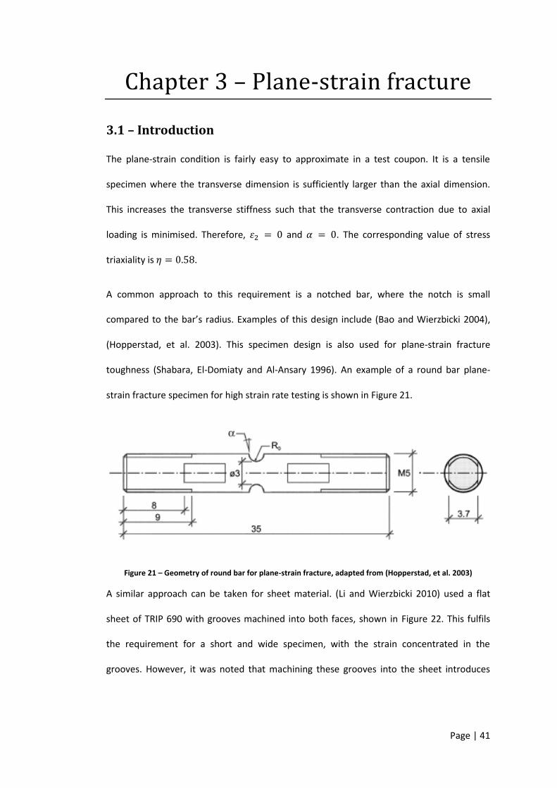
Page | 41

Chapter 3 – Plane-strain fracture

3.1 – Introduction

The plane-strain condition is fairly easy to approximate in a test coupon. It is a tensile

specimen where the transverse dimension is sufficiently larger than the axial dimension.

This increases the transverse stiffness such that the transverse contraction due to axial

loading is minimised. Therefore, and . The corresponding value of stress

triaxiality is .

A common approach to this requirement is a notched bar, where the notch is small

compared to the bar’s radius. Examples of this design include (Bao and Wierzbicki 2004),

(Hopperstad, et al. 2003). This specimen design is also used for plane-strain fracture

toughness (Shabara, El-Domiaty and Al-Ansary 1996). An example of a round bar plane-

strain fracture specimen for high strain rate testing is shown in Figure 21.

Figure 21 – Geometry of round bar for plane-strain fracture, adapted from (Hopperstad, et al. 2003)

A similar approach can be taken for sheet material. (Li and Wierzbicki 2010) used a flat

sheet of TRIP 690 with grooves machined into both faces, shown in Figure 22. This fulfils

the requirement for a short and wide specimen, with the strain concentrated in the

grooves. However, it was noted that machining these grooves into the sheet introduces

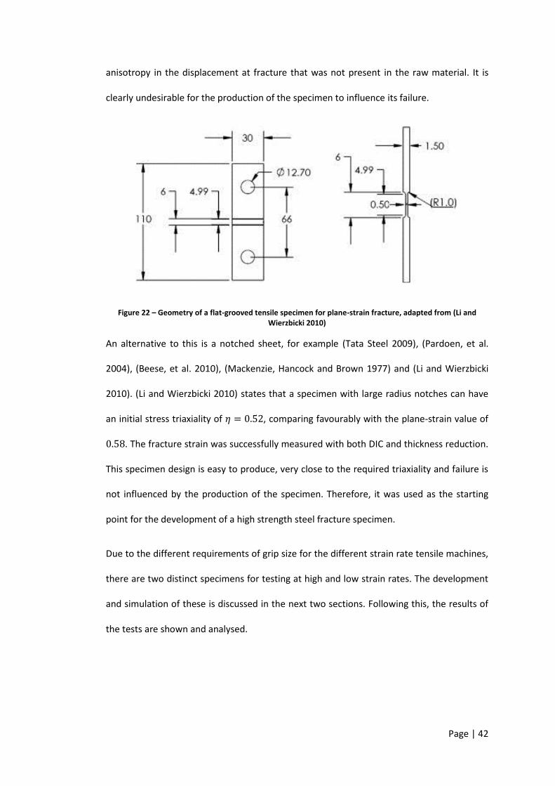
Page | 42

anisotropy in the displacement at fracture that was not present in the raw material. It is

clearly undesirable for the production of the specimen to influence its failure.

Figure 22 – Geometry of a flat-grooved tensile specimen for plane-strain fracture, adapted from (Li and Wierzbicki 2010)

An alternative to this is a notched sheet, for example (Tata Steel 2009), (Pardoen, et al.

2004), (Beese, et al. 2010), (Mackenzie, Hancock and Brown 1977) and (Li and Wierzbicki

2010). (Li and Wierzbicki 2010) states that a specimen with large radius notches can have

an initial stress triaxiality of , comparing favourably with the plane-strain value of

. The fracture strain was successfully measured with both DIC and thickness reduction.

This specimen design is easy to produce, very close to the required triaxiality and failure is

not influenced by the production of the specimen. Therefore, it was used as the starting

point for the development of a high strength steel fracture specimen.

Due to the different requirements of grip size for the different strain rate tensile machines,

there are two distinct specimens for testing at high and low strain rates. The development

and simulation of these is discussed in the next two sections. Following this, the results of

the tests are shown and analysed.

Page | 43

3.2 – Low speed specimen

A plane-strain sheet metal specimen has been used by (Tata Steel 2009). It is a wide

sheet with radius notches. This has been expanded out to for the grips in

the low strain rate testing machine. The technical drawing for this specimen design is

shown below in Figure 23.

Figure 23 – Technical drawing of a plane strain fracture specimen for low strain rate loading

Figure 24 shows a sequence of outputs from an LS-DYNA simulation of this specimen. The

strain initially builds up at the notch tips as they act as a stress raiser. However, it can be

seen that as the strain reaches approximately , a band of strain forms across the gauge

width. By a value of , the peak strain is in the centre of the specimen and growing

outwards. Therefore, the suitability of this specimen for plane-strain fracture is dependent

on the fracture strain under both uniaxial and plane-strain conditions. If the values are

small and close enough, it would be possible for the specimen to crack from the edge of

this notch under uniaxial tension. Plane-strain has a lower fracture strain than uniaxial

tension, so this test is suitable for any material where the fracture strains are above the

point where the strain forms an even band across the gauge width. Using the DP800

simulation as a guideline suggests that the minimum local strain to failure that can be

realistically tested is .

Page | 44

Figure 24 – Sequence of images from simulation of plane-strain fracture specimen showing evolution of effective strain map against displacement, only deformable section shown

Figure 25 shows the same specimen at the expected point of failure with a contour plot of

maximum principal strain. As the stress state in the centre of the specimen is close to the

ideal of plane-strain, this plot is very similar to that of effective strain. In later figures, only

effective strain will be shown, in order to be more comparable with the other stress states.

Page | 45

Figure 25 – Maximum principal strain plot of simulation of plane-strain fracture specimen at expected failure point, only deformable section shown

3.3 – Development of high speed specimen

As with the shear and uniaxial specimens, it is necessary to redesign the specimen to be

suitable for the high strain rate machine. Firstly, one grip needs to be extended for the

machine’s moving grip as described in Section 2.2.2. The extended grip’s length of

allows the high speed tensile loading machine at WMG to reach speeds of approximately

, which gives strains rates of up to . The relationship between grip

velocity and local strain is discussed in Section 3.4.2.

Secondly, design of the specimen is limited by the width of the grips, . To prevent

excessive plastic strain in the grips, the width of the gauge area needs to be reduced.

Standard tensile tests give a ratio of yield to ultimate tensile stress, in engineering stress, of

⁄ . A width of in the gauge area gives a ratio of

⁄ .

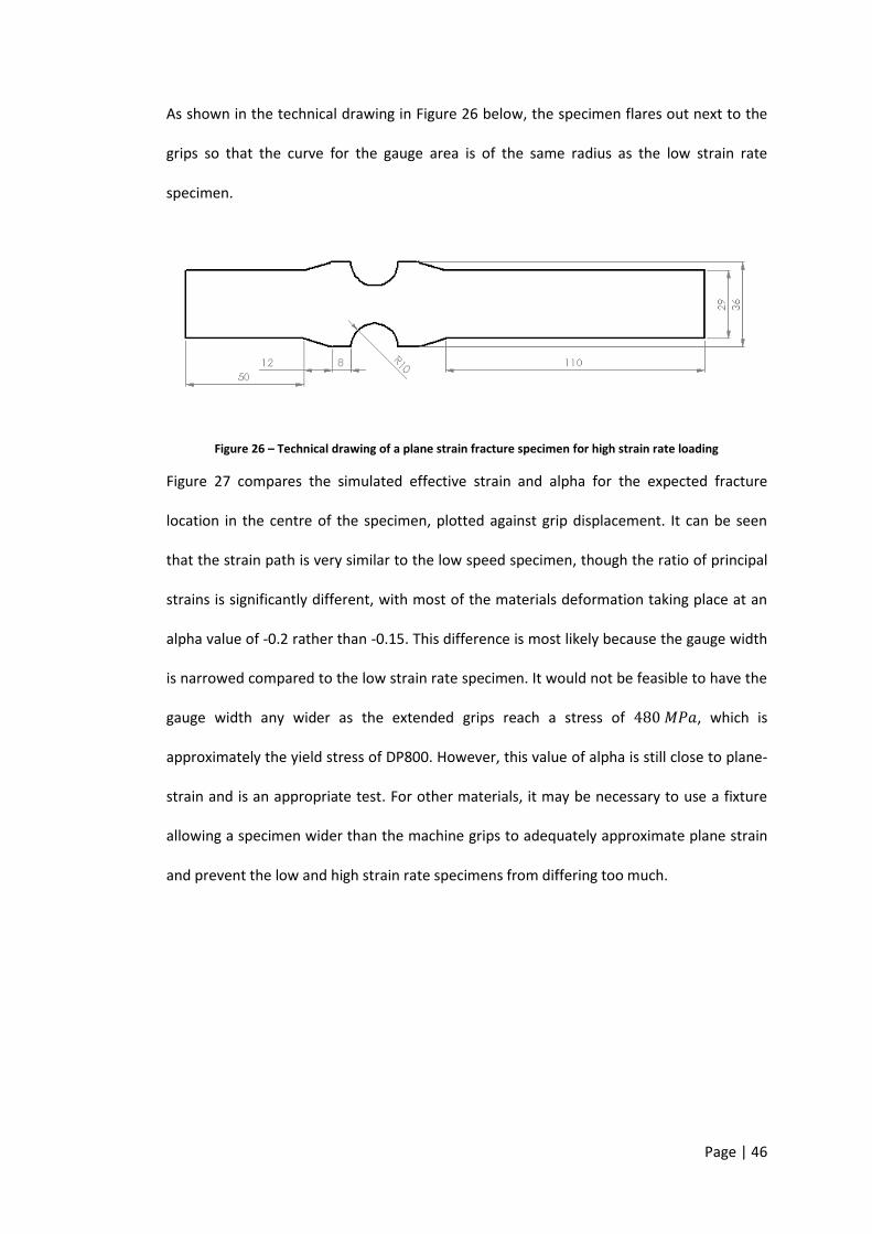
Page | 46

As shown in the technical drawing in Figure 26 below, the specimen flares out next to the

grips so that the curve for the gauge area is of the same radius as the low strain rate

specimen.

Figure 26 – Technical drawing of a plane strain fracture specimen for high strain rate loading

Figure 27 compares the simulated effective strain and alpha for the expected fracture

location in the centre of the specimen, plotted against grip displacement. It can be seen

that the strain path is very similar to the low speed specimen, though the ratio of principal

strains is significantly different, with most of the materials deformation taking place at an

alpha value of -0.2 rather than -0.15. This difference is most likely because the gauge width

is narrowed compared to the low strain rate specimen. It would not be feasible to have the

gauge width any wider as the extended grips reach a stress of , which is

approximately the yield stress of DP800. However, this value of alpha is still close to plane-

strain and is an appropriate test. For other materials, it may be necessary to use a fixture

allowing a specimen wider than the machine grips to adequately approximate plane strain

and prevent the low and high strain rate specimens from differing too much.

Page | 47

Figure 27 – Graph comparing effective strain and alpha for simulations of low and high strain rate specimens at expected location of fracture

3.4 – Results

Strain versus displacement is plotted for low and high speed simulations and tests in Figure

28. Fracture was not modelled, so the simulated strain keeps increasing. As the start of

loading is not defined for the test data, the displacement has been manually adjusted to

make the high speed test intersect the high speed simulation at fracture. The low speed

test was then adjusted to match the curvature of the high speed test. There is clearly a

significant discrepancy between the simulation and test data as the simulation’s strain

increases close to linearly with grip displacement while the test strain has a pronounced

curve. This indicates that at least one of the simulation or test data is inaccurate.

-1.0

-0.9

-0.8

-0.7

-0.6

-0.5

-0.4

-0.3

-0.2

-0.1

0.0

0.0

0.1

0.1

0.2

0.2

0.3

0.3

0.4

0.4

0.5

0.5

0.0 0.5 1.0 1.5 2.0 2.5 3.0 3.5 4.0

alp

ha

Effe

ctiv

e s

trai

n

Displacement, mm

low strain rate von Mises strain high strain rate von Mises strain

low strain rate alpha high strain rate alpha

Page | 48

Figure 28 – Effective strain versus displacement for low and high speed plane-strain fracture simulations and tests

The test data could potentially deviate from the simulation as it is measured on the surface

of the specimen. However, there is no out of plane loading and the simulations did not

show any difference in strain at the different gauss points through thickness. The through

thickness necking would produce an error in the DIC test data, though this error was

calculated in Section 2.3.5 as less than .

It is likely that the simulated data is inaccurate due to post-necking hardening. In the

simulation, this is assumed to linearly extrapolate from the pre-necking behaviour as it is

not possible to measure the post-necking stress. However, the test data indicates that

there are two distinct states to the deformation with a transition at strains of to .

The material model used has data up to the strain of and is extrapolated from there.

The fracture test data implies that there may be a lower rate of strain hardening post-

0.00

0.05

0.10

0.15

0.20

0.25

0.30

0.35

0.40

0.45

0.50

0.0 0.5 1.0 1.5 2.0 2.5 3.0

Effe

ctiv

e s

trai

n

displacement, mm

Low speed simulation High speed simulation

Low speed test High speed test

Page | 49

necking, though this does not account for the discrepancy between test and simulation at

low strain.

Figure 29 is a graph of alpha versus displacement for the same simulations and tests. They

are similar in shape, though the test data has significantly more noise, particularly at low

strain. While the test data is slightly closer to the ideal value of , it follows the same

pattern as the simulation, which implies that the in-plane principal strains are modelled

reasonably well. Both simulation and tests have a flat region which starts increasing in

value towards the ideal at higher displacement and strain. This occurs later in the

simulation, which further indicates that the simulation does not correctly predict the

localisation of strain.

Figure 29 – Alpha versus displacement for low and high speed plane-strain fracture simulations and tests

Figure 30 shows the contour plot of effective strain in a DP800 plane-strain fracture

specimen in the last frame prior to fracture. The peak strain is in the centre of the

specimen and is approximately double the strain at the edge. This behaviour was observed

-1.00

-0.90

-0.80

-0.70

-0.60

-0.50

-0.40

-0.30

-0.20

-0.10

0.00

0.00 0.50 1.00 1.50 2.00 2.50 3.00

Alp

ha

displacement, mm

Low speed simulation High speed simulation

Low speed test High speed test

Page | 50

at all strain rates. The peak strain band is biased towards one side of the specimen, which

occurred in most specimens to a varying degree. One likely cause of this is slight variations

in the angle that the specimen is clamped into the jaws. This is a greater problem with the

high speed testing machine as the upper grip does not have a stop to line the specimen up

with. Another point to consider is that the measurement volume is not necessarily centred

on the specimen. It is intentionally placed a few millimetres away from the edge of the

specimen to avoid edge effects and this distance varies between specimens.

Figure 30 – DIC effective strain map of a DP800 plane-strain specimen loaded at 10 s-1

just prior to fracture

The map of alpha in Figure 31 shows a wide section of the specimen is a consistent strain

state in the range of to alpha. There is some evidence of lateral necking, though it is

mostly confined to approximately from the edge of the notch. As expected, the free

5 mm

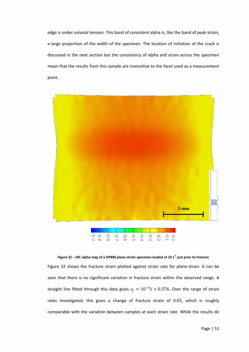
Page | 51

edge is under uniaxial tension. This band of consistent alpha is, like the band of peak strain,

a large proportion of the width of the specimen. The location of initiation of the crack is

discussed in the next section but the consistency of alpha and strain across the specimen

mean that the results from this sample are insensitive to the facet used as a measurement

point.

Figure 31 – DIC alpha map of a DP800 plane-strain specimen loaded at 10 s-1

just prior to fracture

Figure 32 shows the fracture strain plotted against strain rate for plane-strain. It can be

seen that there is no significant variation in fracture strain within the observed range. A

straight line fitted through this data gives . Over the range of strain

rates investigated, this gives a change of fracture strain of , which is roughly

comparable with the variation between samples at each strain rate. While the results do

5 mm

Page | 52

show a general trend of increasing fracture strain with strain rate, the quasi-static fracture

data would give a broadly acceptable estimate of failure under automotive crash

conditions. If this trend continues at higher strain rates, it could produce significant

changes in fracture strain for ballistics and similar events.

Figure 32 – Graph of fracture strain versus strain rate for DP800 plane-strain fracture tests

Alpha versus strain rate is plotted for the same specimens in Figure 33. These results have

lower variation than the fracture strain, indicating that the stress state is not dependent on

the strain, within the tested range. The results are split into two groups as the simulation

predicts – one each of the low and high strain rate specimens. The low rate specimens are

clustered around while the high speed specimens are at . This gap is lower

than may be expected from the curves of alpha versus displacement. The method for

calculating alpha is discussed in greater depth in Sections 3.4.3 and 6.4. In brief, as the data

for alpha versus displacement is not a flat line, a characteristic value is calculated from the

later portion of the test, along with strain rate. Due to through thickness necking, the two

0.00

0.05

0.10

0.15

0.20

0.25

0.30

0.35

0.40

0.45

0.50

0.001 0.01 0.1 1 10 100 1000

Effe

ctiv

e f

ract

ure

str

ain

Strain rate, s-1

Page | 53

geometries tend towards the same stress state and this is reflected by the relatively small

difference in alpha.

Figure 33 – Graph of alpha versus strain rate for DP800 plane-strain fracture tests

3.4.1 – Identifying fracture location

Figure 34 shows a DP800 high rate plane strain fracture specimen. The two halves of the

specimen have been placed together and it can be seen that the fracture surface touches at

the outside edge but not at the centre of the specimen. As discussed previously, there is a

significant change in the stress triaxiality across the width of the specimen from plane

strain in the centre to uniaxial tension at the edge. It is expected from previous work, such

as (Wierzbicki, et al. 2005), that the fracture strain in uniaxial tension is substantially

greater than that of plane strain. As such, the material will deform substantially more at

the edge of the specimen and indicates that the fracture initiated at the centre of the

specimen and the crack grew outwards. This shows that it is correct to take the strain

recorded in the centre of the specimen as the fracture strain.

-1.0

-0.9

-0.8

-0.7

-0.6

-0.5

-0.4

-0.3

-0.2

-0.1

0.0

0.001 0.01 0.1 1 10 100 1000

Rat

io o

f p

rin

cip

le s

trai

ns

Strain rate, s-1

Page | 54

Figure 34 – Photograph of fracture of DP800 plane-strain specimen

It is also possible to corroborate this analysis with a high speed camera. Figure 35 is a series

of four images showing the growth of a crack in an uncoated DP800 plane strain specimen

loaded at . These images were recorded with a Photron SA1.1 at 54,000 frames

per second and a resolution of 320x256. The initial frame at t = 0 s is just prior to fracture.

There is a thin band of light reflected into the camera due to the through-thickness necking

of the specimen. The other three frames, at time steps of , show the crack

opening up in the centre of the specimen and growing outwards.

As the crack initially grows very quickly, it is difficult to determine the precise location of

initiation. The region of high strain and alpha is wide and consistent; therefore the centre

of this region is used for fracture strain, strain rates and alpha measurements. The

rationale for measuring from a single point is discussed in Section 6.2.2

10 mm

Page | 55

Figure 35 – High speed photography of crack growth in a low strain rate DP800 plane-strain fracture specimen

3.4.2 – Determining strain rate

As mentioned previously, the relationship between strain and time is not linear due to

necking through the sheet's thickness. It is therefore not a simple process to determine the

strain rate for a given loading velocity. Strictly speaking, the strain rate is a function of both

loading velocity and time. However, Figure 36 shows that the strain can be roughly divided

into two regions of pre and post necking behaviour. The graph also shows a straight line

fitted through the later portion of the data. It is the gradient of this line that has been used

as the strain rate of the specimen. This was used as it encompasses a greater portion of the

strain and hence damage done to the material.

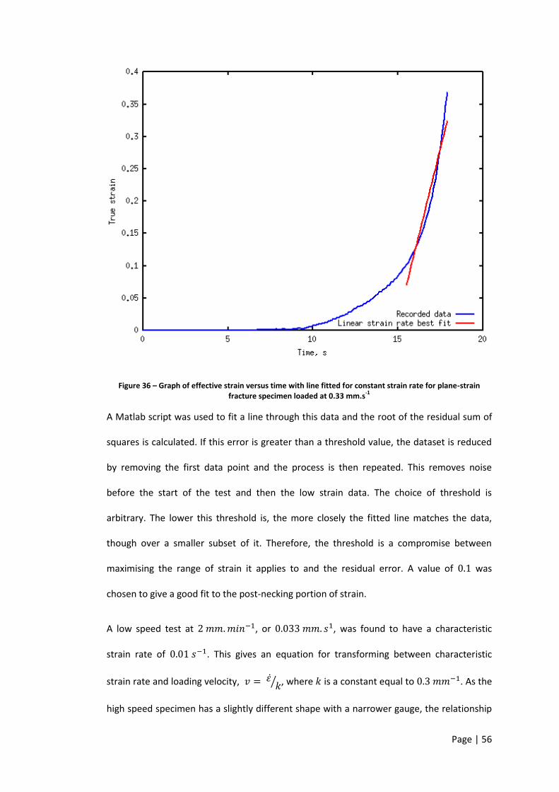
Page | 56

Figure 36 – Graph of effective strain versus time with line fitted for constant strain rate for plane-strain fracture specimen loaded at 0.33 mm.s

-1

A Matlab script was used to fit a line through this data and the root of the residual sum of

squares is calculated. If this error is greater than a threshold value, the dataset is reduced

by removing the first data point and the process is then repeated. This removes noise

before the start of the test and then the low strain data. The choice of threshold is

arbitrary. The lower this threshold is, the more closely the fitted line matches the data,

though over a smaller subset of it. Therefore, the threshold is a compromise between

maximising the range of strain it applies to and the residual error. A value of was

chosen to give a good fit to the post-necking portion of strain.

A low speed test at , or , was found to have a characteristic

strain rate of . This gives an equation for transforming between characteristic

strain rate and loading velocity, ⁄ , where is a constant equal to . As the

high speed specimen has a slightly different shape with a narrower gauge, the relationship

Page | 57

between strain and grip displacement is not the same as the low speed specimen. This can

be seen in Figure 28. A specimen loaded at was found to give a strain rate of

, giving .

3.4.3 – Determining ratio of strains

The value for alpha was recorded for the fracture location. As noted previously, it is not

constant and varies with time. Therefore, a method for determining a characteristic value is

needed. The script that is used to determine the strain rate also calculated this

characteristic value. This is discussed in more detail in Section 6.4.

The output from the script is shown in Figure 37. The data acquisition for the DIC system is

not synchronised with the start of loading for either the low or high speed machines. As

such, there is a variable period at the start of each test’s data that corresponds to zero

strain. For the determination of strain rate in the previous section, this shows as a flat line

of strain versus time, as the noise in the effective strain is low compared to the fracture

strain. However, the noise in the alpha signal is highly dependent on the value of alpha

because it is the ratio of two strains with a fixed error.

At fracture, the effective strain is approximately . An example of the principal strains at

fracture is and , which gives

. If these principal strains are reduced by two orders of magnitude but the

uncertainty is unchanged, the result is . As such, the signal is clear at

higher strains but has very large oscillations at low strain and it is necessary to remove this

region from the calculations to determine the characteristic value of alpha. This is

accomplished using the same region of the data as the strain rate calculation. The graph

below shows a line indicating the average of alpha in this region.

Page | 58

Figure 37 – Graph of alpha versus time with line fitted for constant alpha for plane-strain fracture specimen loaded at 0.33 mm.s

-1

It was noted previously that there is a difference in the values of alpha between the low

and high speed specimens due to the narrower gauge width of the high speed specimen.

The difference in characteristic value is low and there is no significant difference in the

evolution of alpha. This means that the two specimens can be considered equivalent and

the designs are suitable for measuring plane-strain fracture over the range of strain rates of

to .

3.4.4 – Thermal imaging

Thermal imaging was performed as described in Section 2.3.8 at two different strain rates.

These rates were and . This was done to investigate the temperature

rise in the region of transition between isothermal and adiabatic loading and to see if it has

any influence on the fracture behaviour.

Page | 59

While these strain rates are an order of magnitude apart, the change in strain hardening is

relatively low. As the fracture strain has an insignificant strain rate dependency, this means

that there is approximately the same amount of energy involved in the distortion, damage

and eventual fracture of the material. Therefore, the temperature rise of the specimen is

expected to be higher for a higher strain rate as there is less time for the same energy to

dissipate. It is important to determine if this variation in temperature rise is large enough

to influence the fracture strain.

Figure 38 shows the contour plots at peak temperature for the two strain rates and Figure

39 shows the temperature versus time. The contour plots show a cold gap in the centre of

the specimen at the peak temperature, meaning that the peak temperature is recorded

after fracture initiation and during the crack's growth. The heat accumulates during loading

and conducts through to the surface after fracture. This implies that the measured

temperature on the surface is underestimating the temperature in the centre of the

specimen. Also, it is possible that the fracture strain is underestimated, though it is

assumed that both of these effects are negligible as the data for the different specimens is

very consistent within each strain rate.

Figure 39 gives the peak temperatures for the lower speed specimen as approximately

, with the higher speed specimens reaching .

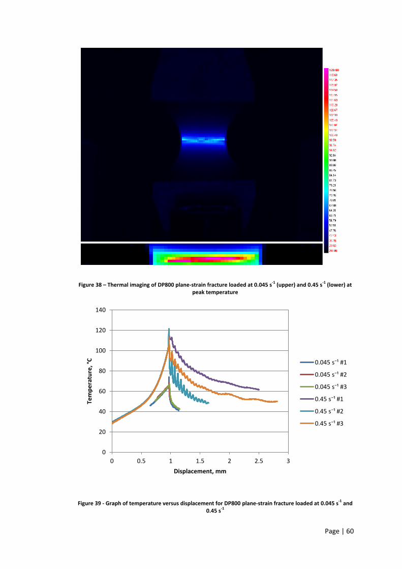
Page | 60

Figure 38 – Thermal imaging of DP800 plane-strain fracture loaded at 0.045 s-1

(upper) and 0.45 s-1

(lower) at peak temperature

Figure 39 - Graph of temperature versus displacement for DP800 plane-strain fracture loaded at 0.045 s-1

and 0.45 s

-1

0

20

40

60

80

100

120

140

0 0.5 1 1.5 2 2.5 3

Tem

pe

ratu

re, °

C

Displacement, mm

0.045 s⁻¹ #1

0.045 s⁻¹ #2

0.045 s⁻¹ #3

0.45 s⁻¹ #1

0.45 s⁻¹ #2

0.45 s⁻¹ #3

Page | 61

The temperature rise from these specimens is low compared to that required for some

thermally activated processes in this grade of steel. (Akbarpour and Ekrami 2008) found

that dynamic strain aging occurred at temperatures above . (Ekrami 2005) stated

that work hardening increases with temperature to and then decreases. These

temperatures indicate transitions in thermally activated processes, which could affect the

fracture strain. Figure 40 below is taken from (Akbarpour and Ekrami 2008) and shows flow

curves at different temperatures for a high bainite volume fraction dual phase steel. It does

suggest a reduction in total elongation to failure as temperature increases from to

, though this does not necessarily extend to a change in local fracture strain.

Figure 40 – Stress versus strain for DP steel for temperature range of 25 to 500 °C, from (Akbarpour and Ekrami 2008)

Page | 62

3.4.5 – Fractography and microscopy

Figure 41a) is a fracture surface of a plane-strain specimen loaded at at

magnification. Figure 41b) is of a specimen loaded at at the same resolution. Both

of these images are at the centre of the specimen – the location of fracture initiation. The

specimens were loaded normal to the plane of the images.

The figure shows that the mechanism of failure does not change between these strain

rates. Both specimens are typical of ductile failure with a rough cup and cone surface from

void initiation and coalescence across the whole surface. Qualitatively, the size of the voids

is reasonably consistent between strain rates, similar to work on the strain rate

dependency of fracture in titanium Ti6Al4V (Peirs, Verleysen and Degrieck 2011). That

research showed very little difference in the fracture surfaces of quasi-statically and

dynamically loaded specimens, concluding that this was the reason for the lack of a

correlation between strain rate and fracture strain.

(Boyce and Dilmore 2009) found that dimple size did not vary with strain rate for four high

strength steels, though reduction in area indicated that the fracture strain could vary from

weak negative correlation to strong positive correlation depending on the steel grade. The

two grades with very little change in reduction in area had radial marks corresponding to

rapid crack growth at low strain rates and no marks at high strain rates. The two remaining

grades showed little morphological change with strain rate, though they had opposite

correlations for reduction in area and strain rate.

It is therefore not simple to conclude whether the similarity of fracture surfaces at different

strain rates in DP800 suggests a lack of strain rate dependency or not. However, in the

absence of significant morphological change due to strain rate, it is assumed that there is

no change in microstructural behaviour that would influence the fracture strain.

Page | 63

Figure 41 – SEM images of fracture surfaces of DP800 plane-strain fracture specimens, loaded at a) 0.045 s-1

and b) 0.45 s

-1

a)

b)

Page | 64

A low resolution image of a section through the specimen shows the shape of the

fracture surface. The loading direction was vertical in the plane of the image. It was seen

previously in Section 3.4.1 that the fracture surface is very rough and does not follow a

straight line in the plane of the sheet. Figure 42 below shows that the fracture surface has

the same sharp changes in direction.

Figure 42 – Low resolution image of section through DP800 plane-strain fracture specimen showing shape of fracture surface

The damage is highly localised to within tens of microns of the fracture surface. Figure 43

shows higher resolution images of this damage at magnification for both strain

rates. The material damage at the higher strain rate reaches further into the material from

the fracture surface. However, this damage is restricted to specific points along the fracture

surface and is not indicative of the energy applied to the whole system. Across most of the

fracture surface, there is very little damage in the bulk material. Figure 44 shows a section

at magnification. The cup and cone failure can be seen and is the same size as that

visible in Figure 41, though there are no voids visible in the rest of the material. This implies

that there are no micromechanical changes that affect the fracture strain.

Page | 65

Figure 43 – SEM images of sections through DP800 plane-strain fracture specimens, loaded at a) 0.045 s-1

and b) 0.45 s

-1

a)

b)

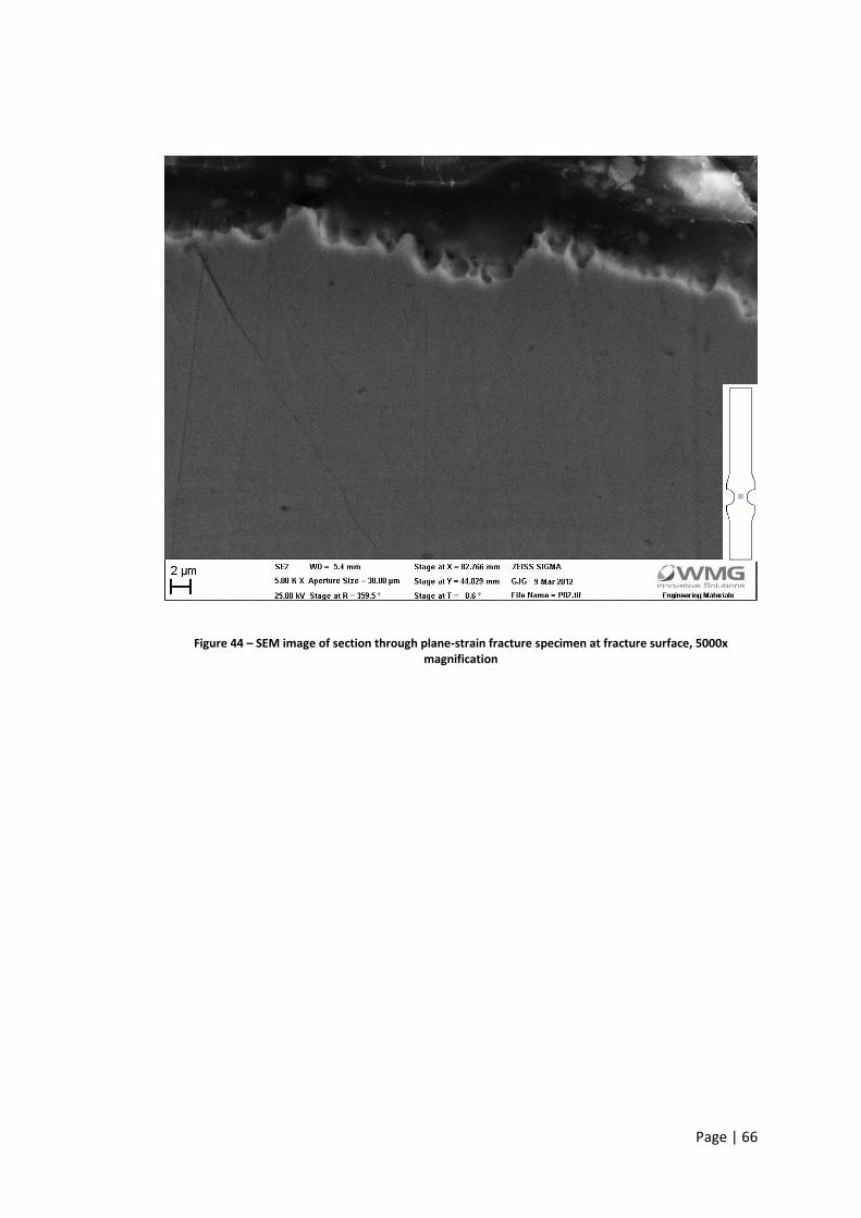
Page | 66

Figure 44 – SEM image of section through plane-strain fracture specimen at fracture surface, 5000x magnification

Page | 67

Chapter 4 – Uniaxial fracture

4.1 – Introduction

Many mechanical properties of metals in uniaxial tension, such as yield and tensile strength

and modulus of elasticity, can be determined with a simple tensile test. The specimen used

for determining the properties of sheet material is commonly known as a ‘dogbone’. A

standard specimen from ISO 6892-1:2009 is shown in Figure 45 below.

Figure 45 – Geometry for a Euronorm standard tensile dogbone

This specimen was used to determine yield, elastic modulus and plastic flow for simulating

fracture specimens in LS-DYNA. However, this was not used to measure fracture properties.

As discussed by (Tarigopula, et al. 2008), these uniaxial tensile tests are unsuitable for high

strain tests due to plastic instabilities. The steels under investigation are sufficiently ductile

for fracture to occur long after necking, meaning that the changing geometry has a

significant effect on the stress state of the material.

(Wierzbicki, et al. 2005) used a round, smooth bar to investigate fracture in the uniaxial

stress triaxiality. This is the equivalent test for bar material and the results show a

significant change in the stress triaxiality as the specimen is deformed. (Jones and Gillis

1984) stated that necking results in a plane-strain state.

Page | 68

This same behaviour was observed in sheet material (Ebelsheiser, Feucht and Neukamm

2008). When triaxiality is plotted against time, there is a flat consistent line for the majority

of the time. However, as is also shown in TRIP700 (Sun, Andrieux and Feucht 2009), the

triaxiality is not consistent for a large portion of the plastic strain. The amount of deviation

from the uniaxial case will depend on the strains at necking and fracture. For a sufficiently

brittle material, this may be an acceptable test. In contrast, DP800 is expected to be quite

ductile and so will have a significant amount of deformation post-necking, leading to a

plane-strain state in a standard dogbone.

(Bao and Wierzbicki 2004) used both smooth round bar and a plate with a hole to measure

uniaxial fracture. The round bar gave a very good value of triaxiality initially but later

increases linearly to a plane-strain state while the flat plate is consistently the correct stress

state up to fracture.

(Tata Steel 2009) used a similar design of specimen, though did not give an indication of its

suitability. Additionally, the specimen normally used for plane-strain forming limits was

used as it has sharp notches that promote cracking from the edge rather than the centre

where necking begins.

4.2 – Development of specimen

The free edge of a material in tension is assumed to be under uniaxial tension. This would

imply that it is simple to design a specimen to fail under uniaxial tension – it simply needs a

stress raiser at a free edge. A notch or hole would fulfil this criterion. However, the

specimen also needs to be designed for measurement. A sharp notch will lead to a very

steep strain gradient in the plane of the sheet. This is undesirable as it will be averaged

over the size of the DIC facet, which will likely underestimate the strain.

Page | 69

4.2.1 – Low speed

Euronorm

The standard low speed tensile test specimen is shown in Figure 46 below. The image is a

contour plot of effective strain at for an FE simulation. The effect of necking and

strain localisation can be clearly seen. A global strain measurement system as is typically

used for mechanical properties is therefore not appropriate for quantifying fracture

properties.

The simulation shows that the neck forms in the centre of the specimen. However, this

rarely occurs in a physical test as necking is an unstable phenomenon (Joun, et al. 2007)

and is influenced by imperfections in the material, loading and geometry. A slight taper can

be machined into a specimen to promote necking at a certain location (García-Garino,

Gabaldón and Goicolea 2006). If this is done, it is necessary to ensure that the specimen is

not damaged in such a way that it prematurely fails.

Figure 46 – Effective strain contour plot of Euronorm tensile specimen at εvm = 1

Necking is commonly studied in finite element simulations. It has been found that necking

can be simulated if the whole specimen, shoulders and grips included as in the figure above

is discretised (Brünig 1998). Adding geometric imperfections to the mesh to prompt

necking is inaccurate due to the large influence of the unknown amplitude of the defect.

However, accurate data for plastic flow is required for an accurate simulation of necking

(Aretz 2007) and this can be difficult to measure at high strain.

Page | 70

Whilst the stress and strain are typically considered to be constant throughout the parallel

length of the specimen, there are inevitably variations. Small variations in the strain field

due to the end connections causes deformation to localise in the centre of a simulated

tensile specimen (Mattos and Chimisso 1997).

The contour plot of alpha at this strain level is shown in Figure 47. In contrast to previous

work (Jones and Gillis 1984), the stress state has not deviated significantly from uniaxial

towards plane-strain as the value of alpha is approximately . It is also unexpected that

the stress state is fairly constant along the specimen – both inside and out the neck. This

suggests that the geometry may be more suitable for studying fracture than previously

thought.

Figure 47 – Alpha contour plot of Euronorm tensile specimen at εvm = 1

Plate with hole

A specimen with a hole in it has been used to improve the ratio of principal strains post-

necking (Tata Steel 2009), (Bao and Wierzbicki 2004). The geometry of such a specimen is

shown in Figure 48. The ratio of hole to plate width can vary from a large hole (Bao and

Wierzbicki 2004) to one half of the width of the plate (Tata Steel 2009). It is assumed that

the stress state at the free edge of the hole is uniaxial tension, thus the size of hole should

be an arbitrary choice. However, (Bao 2004) found that the fracture strain was dependent

on the ratio of sheet thickness to ligature width and that shell elements can only be used to

accurately model such a specimen when the ratio is less than . This means that the

Page | 71

specimen does not necessarily fail under uniaxial tension and that the size of the hole can

be tuned to give different stress states.

Figure 48 – Geometry of low strain rate uniaxial fracture specimen

As the sheet thickness used here is , the minimum ligature width following this

condition would be . A width of has been used here for several reasons. Firstly,

this gives a closer approximation of plane stress, similar to the plane-strain fracture

specimen. It also makes shell simulations more accurate. The second point to consider is

that the hole should not be made so small that the strain gradient is very low and a large

portion of the specimen deforms. A small gauge length is desirable to decrease the loading

speed needed to achieve a given strain rate and to make it easier to locate the point of

necking and fracture prior to testing. This size also makes it possible to have several DIC

facets across the width of the specimen, which is important to measure the strain gradient

accurately.

Figure 49 shows the effective strain and maximum principal strain contour plots of this

geometry at with only the deformable region shown. As with the standard tensile

test, the specimen necks in the centre of the specimen. However, in this instance, necking

is due to the geometry of the specimen and will reliably occur at this location, making it

easier to measure the fracture strain.

Page | 72

Figure 49 – a) Effective strain and b) maximum principal contour plot of uniaxial fracture specimen at εvm = 1, only deformable region shown

Figure 50 shows the alpha contour plot for this specimen at . The necking has

produced a similar stress state to that of the Euronorm specimen, with . The free

edge has not resulted in a pure uniaxial stress state, unless it is confined to a region smaller

than an element. There are regions in the centre of each of the ligatures that are at a

slightly different stress state, with . Due to the shape of a fracture locus, this

region would fracture at a lower strain than the edge. However the strain gradient across

the ligature should be sufficient to crack from the edge of the hole. Nonetheless, it will be

important to identify the location of the crack initiation.

a)

b)

Page | 73

Figure 50 Alpha contour plot of uniaxial fracture specimen at εvm = 1, only deformable region shown

Comparison of fracture specimens

The graph in Figure 51 compares effective strain and alpha for the two low speed uniaxial

specimens. The Euronorm specimen’s displacement has been scaled down by a factor of

to put it on the same range as the plate with a hole due to its large gauge length.

The Euronorm specimen has two distinct regions of strain, pre and post-necking. These

regions have very different strain rates. The plate with a hole, by comparison, has a

significantly more linear strain path. This makes it preferable for producing a specimen with

a constant strain rate.

The Euronorm specimen has the value of alpha closest to the ideal of up to a strain

higher than expected from the literature. However, the plate with a hole has a stress state

that deviates from the ideal only by a small amount, with . This state is

consistent over a much wider range of strains. The Euronorm specimen may be suitable for

a range of materials, however, the local ductility of this material is not known in advance

and so it is more appropriate to choose the specimen design with the most consistent

stress state.

Page | 74

Figure 51 – Graph of effective strain and alpha versus grip displacement at expected fracture location for simulated uniaxial fracture specimens

The location of the neck also makes the plate with a hole a more suitable specimen for

fracture testing. The hole causes the necking and hence location of fracture to be highly

repeatable, which makes it easier to set up the DIC system to capture the area in good

quality. The variable position of the neck in the standard tensile test specimen means that

a larger area has to be measured, increasing the apparent mesh size of the facets because

of the lower number of pixels per millimetre.

As such, the plate with a hole will be used as the low strain rate specimen and a high strain

rate specimen will be derived from it.

-1

-0.9

-0.8

-0.7

-0.6

-0.5

-0.4

-0.3

-0.2

-0.1

0

0.00

0.10

0.20

0.30

0.40

0.50

0.60

0.70

0.80

0.90

1.00

0 0.5 1 1.5 2 2.5

alp

ha

Effe

ctiv

e s

trai

n

displacement, mm

Euronorm von Mises strain Hole von Mises strain

Euronorm alpha Hole alpha

Page | 75

4.2.2 – High speed

Figure 52 below shows the technical drawing for a high strain rate specimen derived from

the low strain rate plate with a hole. Unlike the plane-strain test, the low strain rate

uniaxial specimen was designed for wide grips. This design widens the clamping

regions to match the VHS’s grips and extends the moving end to allow for similar

loading velocities to the high strain rate plane-strain specimen. The geometry of the gauge

area is unchanged.

Figure 52 – Geometry for a high strain rate uniaxial fracture specimen

An effective strain contour plot is shown for this geometry in Figure 53, with the specimen

strained to and only the deformable regions shown. As the strain away from the hole

is low, the extended grip is only elastically deformed. Therefore, the strain distribution

around the hole is unaffected and is identical to the low strain rate specimen.

Page | 76

Figure 53 – Effective strain contour plot of high strain rate specimen at ε = 1, only deformable region shown

The contour plot of alpha at the same displacement is shown below in Figure 54. It can be

seen that the patterns are identical to the low strain rate specimen. The extended grip has

made very little difference beyond the radius to the parallel gauge area. This is because the

grip is sufficiently wider than the ligatures to keep the strain in the grip elastic. Compared

to the gauge area, this is as stiff as the clamped region, making the plastic strain around the

hole symmetrical. Therefore, the unbalanced grips have no impact on the stress state.

Figure 54 – Alpha contour plot of high strain rate specimen at ε = 1, only deformable region shown

The graph in Figure 55 compares the effective strain and alpha against grip displacement

for the low and high strain rate plates with holes. As was apparent from the contour plots

of strain and alpha, these two specimens are very similar. The gradients for both strain and

Page | 77

alpha are essentially identical. The only significant difference is a lag of approximately

for the high strain rate signal. This is because of the time taken for the stress

wave to propagate through the increased length of the moving grip. As these two

specimens produce such similar results, they are suitable for measuring uniaxial fracture

strain across the required range of strain rates.

Figure 55 – Comparison of effective strain and alpha for high and low strain rate uniaxial specimens

4.3 – Results

The graph in Figure 56 compares the effective strain versus time for simulation and test

data at low and high strain rate. The low strain rate sample was loaded at

and the high strain rate sample at . This corresponds to strain rates of

and respectively.

-1

-0.9

-0.8

-0.7

-0.6

-0.5

-0.4

-0.3

-0.2

-0.1

0

0.00

0.10

0.20

0.30

0.40

0.50

0.60

0.70

0.80

0.90

1.00

0 0.5 1 1.5 2 2.5

alp

ha

Effe

ctiv

e s

trai

n

displacement, mm

Low rate von Mises strain High rate von Mises strain

Low rate alpha High rate alpha

Page | 78

While the two tests are very similar, there are two main differences. The first is that there

is a gap in the data for the high strain rate sample at displacement. This is because

of problems with the painted pattern that caused the facets to not be calculated for a few

frames. These problems are more common at higher strain rates due to either strain rate

or thermal dependency of the paint. An alternative coating may solve this, though it has

had little impact on the measurement of fracture strain, strain rate or alpha. The second

discrepancy between the two tests is that the high rate test appears to have a significantly

lower fracture strain than the low rate tests. This will be discussed in more detail later in

this section.

Figure 56 – Graph comparing simulation and test effective strain versus grip displacement at low and high strain rate in uniaxial fracture

The simulation and test data differ significantly. At low displacements, the strain is much

lower in the test data, while at high displacements the gradients are very similar. As with

0.0

0.1

0.2

0.3

0.4

0.5

0.6

0.7

0.8

0.9

1.0

0.0 0.5 1.0 1.5 2.0 2.5

Effe

ctiv

e s

trai

n

displacement, mm

Low rate simulation High rate simulation Low rate test High rate test

Page | 79

the plane-strain test data, this indicates an error in the simulation’s material input and the

test’s grip displacement. This is discussed further in Section 6.7.

Figure 57 compares alpha versus time for the same tests and simulations. As with the

plane-strain specimens, the simulations are overly optimistic. However, the plane-strain

simulations had a higher value of alpha than the test data, while the uniaxial simulations

are lower. There is a large amount of noise in the signal at low displacement and strain,

though there is little for the post-necking region – when displacement is greater than . As

predicted by the simulations, there is very little difference in alpha between the strain

rates.

Figure 57 – Graph comparing simulation and test alpha versus grip displacement at low and high strain rate in uniaxial fracture

-1.0

-0.9

-0.8

-0.7

-0.6

-0.5

-0.4

-0.3

-0.2

-0.1

0.0

0.0 0.5 1.0 1.5 2.0 2.5

alp

ha

displacement, mm

Low rate alpha High rate alpha Low rate test High rate test

Page | 80

A contour plot of effective strain in one side of a DP800 uniaxial fracture specimen loaded

at , corresponding to a strain rate of , is shown in Figure 58. The

loading direction is horizontal in the plane of the page. As expected, the strain is highly

localised to the region around the hole and necking across the width of the specimen is

evident. The shape of the necking typically results in one facet above the narrowest point

and one below. Despite the high strain gradient, no effect from the choice of facet was

observed.

Figure 58 – DIC effective strain map of a DP800 uniaxial fracture specimen loaded at 0.1 s-1

just prior to fracture

Figure 59 shows the contour plot of alpha for the same specimen. Much of the specimen’s

width is in a state half way between uniaxial and plane-strain, with . The edges

are closer to the intended stress state, where , which matches the graph of

alpha versus displacement above. This steep gradient makes it important to locate the

point of fracture initiation as the higher value of alpha at the centre will have a lower

fracture strain than the edge. This means that the crack initiation is a function of the

gradients of the fracture locus and the strain and alpha across the width of the ligature.

3 mm

Page | 81

Figure 59 – DIC alpha map of a DP800 uniaxial fracture specimen loaded at 0.1 s-1

just prior to fracture

The uniaxial specimen is unique in this work in that it is the only specimen where the

fracture initiates at the edge of the material. This presents a unique challenge in

determining if the measured value is accurate. The first problem is in aligning the edge of

the facet with the edge of the hole. The second problem is that the measurement is related

to the size of the facet and may not accurately reflect the conditions at its edge. Figure 60

is a graph of effective strain and alpha versus the position along the width of the ligature in

a DP800 uniaxial fracture specimen loaded at .

The gradient of strain across the width of the specimen is approximately and is

lower closer to the edge of the hole. This means that inaccuracy in the positioning of the

facet and the measurement of the facet itself will not impact the recorded fracture strain

significantly. For example, a worst case offset error of would result in

underestimating the strain by .

The gradient of alpha is much steeper – close to the edge of the hole it is .

Assuming the same inaccuracy in positioning gives an error of in the recorded value of

alpha. This would account for the difference between the expected stress state and the

measured. However, the discrepancy between the simulated and test strain versus strain

3 mm

Page | 82

data indicates that it is the simulation that is inaccurate and not the DIC measurement. As

such, it is assumed that the effects noted here must be minor.

Figure 60 – Effective strain and alpha versus position along width of ligature in DP800 uniaxial fracture specimen at location of fracture, specimen loaded at 0.1 s

-1, 0 mm corresponds to the edge of the hole

Figure 61 and Figure 62 show the fracture strain and alpha plotted against strain rate for

the uniaxial specimen in DP800. As with the plane-strain specimens, there is a general

trend of fracture strain increasing with strain rate. The equation of a straight line fitted

through the data is . The strain rate dependency is similar to that

for plane-strain fracture at , giving a change in strain of across the whole range of

strain rates. This means that the increase in fracture strain in uniaxial tension is also

comparable to the variation within each strain rate. Therefore, the quasi-static fracture

data can be used for an acceptable simulation of crash performance.

-0.60

-0.50

-0.40

-0.30

-0.20

-0.10

0.00

0.00

0.10

0.20

0.30

0.40

0.50

0.60

0.00 0.50 1.00 1.50 2.00 2.50 3.00

alp

ha

Effe

ctiv

e s

trai

n

position across ligature width, mm

von Mises strain alpha

Page | 83

Figure 61 – Graph of fracture strain versus strain rate in DP800 uniaxial tension

As the gauge area is the same for low and high speed specimens, there is no difference

between the low and high speed values of alpha. The stress states measured at do

show a difference, though this is an artefact of the DIC. At this highest strain rate, the

camera must operate at a lower resolution to achieve an appropriate frame rate. A coarser

pattern was painted onto the specimens to match this resolution, which resulted in larger

facets. Though averaging across a larger area does not appear to have had a significant

effect on the fracture strain, the measured stress state was affected. Two of the samples

indicate a stress state approaching plane-strain but this is a failure of measurement rather

than a strain rate dependent change in stress state.

0

0.1

0.2

0.3

0.4

0.5

0.6

0.7

0.001 0.01 0.1 1 10 100 1000

Effe

ctiv

e f

ract

ure

str

ain

Strain rate, s-1

Page | 84

Figure 62 – Graph of alpha versus strain rate in DP800 uniaxial tension

4.3.1 – Fracture location

Figure 63 shows the propagation of a crack in a DP800 uniaxial fracture specimen, loaded

at or . In the first frame, marked , there is a small crack

visible from the back corner of the left side. This is a very stable crack because of the high

strain gradient. By the third frame, , the crack has spread through the sheet

thickness and part of the width. At , the crack has not grown much further.

Therefore, the crack initiates from the edge of the plane perpendicular to the camera. It

does not crack further into the specimen in the region of higher value of alpha, or at the

mid-plane of the sheet thickness. The crack can begin at the surface either facing towards

or away from the camera. However, the crack grows through the thickness of the sheet

much faster than the width. This means that the strain gradient is lower through the sheet

thickness and that the peak strain measured in the DIC system is the correct measure of

the fracture strain.

-1

-0.9

-0.8

-0.7

-0.6

-0.5

-0.4

-0.3

-0.2

-0.1

0

0.001 0.01 0.1 1 10 100 1000

Rat

io o

f p

rin

cip

le s

trai

ns

Strain rate, s-1

Page | 85

Figure 63 – Crack propagation in a low strain rate uniaxial fracture specimen

4.3.2 – Determining strain rate

As with the plane-strain specimen, the uniaxial specimen has a time-dependent strain rate.

However, the geometry for the gauge length is the same for both low and high speed

uniaxial specimens, so there is only one constant of proportionality between grip velocity

and strain rate to calculate. Figure 64 shows strain versus time and the fitted constant

strain rate for a uniaxial fracture specimen loaded at .

Page | 86

This was generated using the Matlab script described in Section 6.3. It can be seen in Figure

61 that the strain rates calculated for this geometry are consistent for each input velocity.

However, the variation within each set is greater at higher velocities.

Figure 64 – Graph of strain versus time with line fitted for constant strain rate for uniaxial fracture specimen loaded at 2.2 mm.s

-1

A specimen loaded at is equivalent to a strain rate of . This means

that the equation for transforming between loading velocity and characteristic strain rate,

⁄ , has the constant . This matches the high strain rate plane-strain

specimen. The strain rate calculation is based on post-necking behaviour in both

specimens, which means that the two different geometries result in a neck with the same

gauge length.

Page | 87

4.3.3 – Determining ratio of strains

The ratio of principal strains was determined with a script in the same manner as the plane-

strain fracture tests. Alpha is very consistent in the region selected for a representative

strain rate, as shown in Figure 65. It starts out at a slightly lower value, closer to the

intended value of at uniaxial tension, though the noise is greater for this period. This

lower region broadly corresponds to pre-necking plastic strain, while the higher region is

post-necking.

Figure 65 – Graph of alpha versus time with line fitted for constant alpha for uniaxial fracture specimen loaded at 2.2 mm.s

-1

4.3.4 – Comparison of loading machines

The uniaxial fracture specimen for a strain rate of was tested on both low and high

speed machines. This corresponds to a loading velocity of or .

Figure 66 shows effective strain and alpha versus time for both machines. The data for the

two machines is synchronised on the x axis such that the high strain portions of the tests

Page | 88

are co-linear. There is a gap in the high speed machine’s data at , though this is an

artefact of the pattern applied to this particular specimen and is not indicative of the

machine’s performance. The two alpha signals are very similar, particularly as the strain

increases and the error in the calculation of alpha decreases.

The major difference between the two machines is in the strain signal. This is particularly

evident from to – the low speed machine has a lower strain. This is because the

machine is still accelerating thus the grip displacement is lower for the same time. The

difference reduces as the machine reaches the correct speed and the material necks.

Figure 66 – Comparison of low and high speed test machines with effective strain and alpha versus time for a DP800 uniaxial fracture specimen loaded at 2.2 mm.s

-1

As the strain rate is measured from the latter portion of the test, the acceleration has little

impact on the recorded results. However, for a suitably strain rate sensitive material, it may

not be appropriate to use such a machine for tests at a higher rate than quasi-static.

-0.6

-0.5

-0.4

-0.3

-0.2

-0.1

0.0

0.0

0.1

0.2

0.3

0.4

0.5

0.6

0.0 0.2 0.4 0.6 0.8 1.0 1.2

alp

ha

Effe

ctiv

e s

trai

n

time, s

static machine strain VHS strain static machine alpha VHS alpha

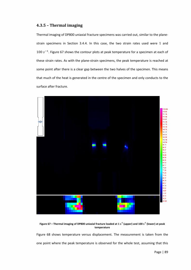
Page | 89

4.3.5 – Thermal imaging

Thermal imaging of DP800 uniaxial fracture specimens was carried out, similar to the plane-

strain specimens in Section 3.4.4. In this case, the two strain rates used were and

. Figure 67 shows the contour plots at peak temperature for a specimen at each of

these strain rates. As with the plane-strain specimens, the peak temperature is reached at

some point after there is a clear gap between the two halves of the specimen. This means

that much of the heat is generated in the centre of the specimen and only conducts to the

surface after fracture.

Figure 67 – Thermal imaging of DP800 uniaxial fracture loaded at 1 s-1

(upper) and 100 s-1

(lower) at peak temperature

Figure 68 shows temperature versus displacement. The measurement is taken from the

one point where the peak temperature is observed for the whole test, assuming that this

Page | 90

corresponds to the peak strain and fracture initiation location. The x axes for the curves

have been adjusted such that the peak temperatures are aligned. The curves for the lower

strain rate are very consistent and the peak temperature recorded is approximately .

The higher strain rate tests are much more variable in both the temperature reached and

the shape of the curve. The peak temperatures for this strain rate range from to

. As with the plane-strain tests, it is assumed that these temperatures are not high

enough to cause a significant change in the mechanical properties of a dual phase steel.

The peak temperature measurement is misleading for the higher strain rate tests because it

is highly dependent on the location chosen and the peak temperature is reached a

considerable time and displacement after fracture. However, it can still be used to

determine broad changes in temperature with strain rate.

Figure 68 – Graph of temperature versus displacement for DP800 uniaxial fracture loaded at 1 s-1

and 100 s-1

0

20

40

60

80

100

120

140

160

0 0.5 1 1.5 2 2.5 3

Tem

pe

ratu

re, °

C

Displacement, mm

1 s⁻¹ #1

1 s⁻¹ #2

1 s⁻¹ #3

100 s⁻¹ #1

100 s⁻¹ #2

100 s⁻¹ #3

Page | 91

4.3.6 – Fractography and microscopy

Figure 69a) shows a fracture surface of a DP800 uniaxial fracture specimen loaded at

at magnification. Figure 69b) is of a specimen loaded at at the same

magnification. Both of these have the hole and thus the crack initiating at the left of the

image.

It is evident that the fracture mechanism does not change between these strain rates.

There is significant necking through the sheet’s thickness as well as across the width.

Similar to the plane-strain specimens, the failure surface is typical of ductile failure with

cups and cones from void coalescence. There is no morphological change in the fracture

surface with strain rate.

Figure 70a) and b) show sections through the same specimens at magnification.

There are two distinct regions on these specimens. The top region is highly polished though

the bottom region is rough from ductile fracture. This is because this section is not in the

same plane as the polished cross section. It is at due to shear bands forming through

the thickness of the sheet. In both specimens, the damage is confined to a short distance of

the fracture surface – approximately . This is because the strain is highly localised

due to the necking and so the majority of the voids nucleate and coalesce in this small

region.

There does appear to be a difference in the amount of damage done to the material

around the fracture surface and the distance from the edge of the specimen to the shear

band. The amount of damage could have increased due to the increased energy applied to

the specimen due to strain hardening. However, it is more likely that the damage varies

through the sheet thickness as these specimens are ground and polished to a smooth finish

rather than to a target depth. As such, it is assumed that there are no strain rate

dependent phenomena that would influence the fracture strain.

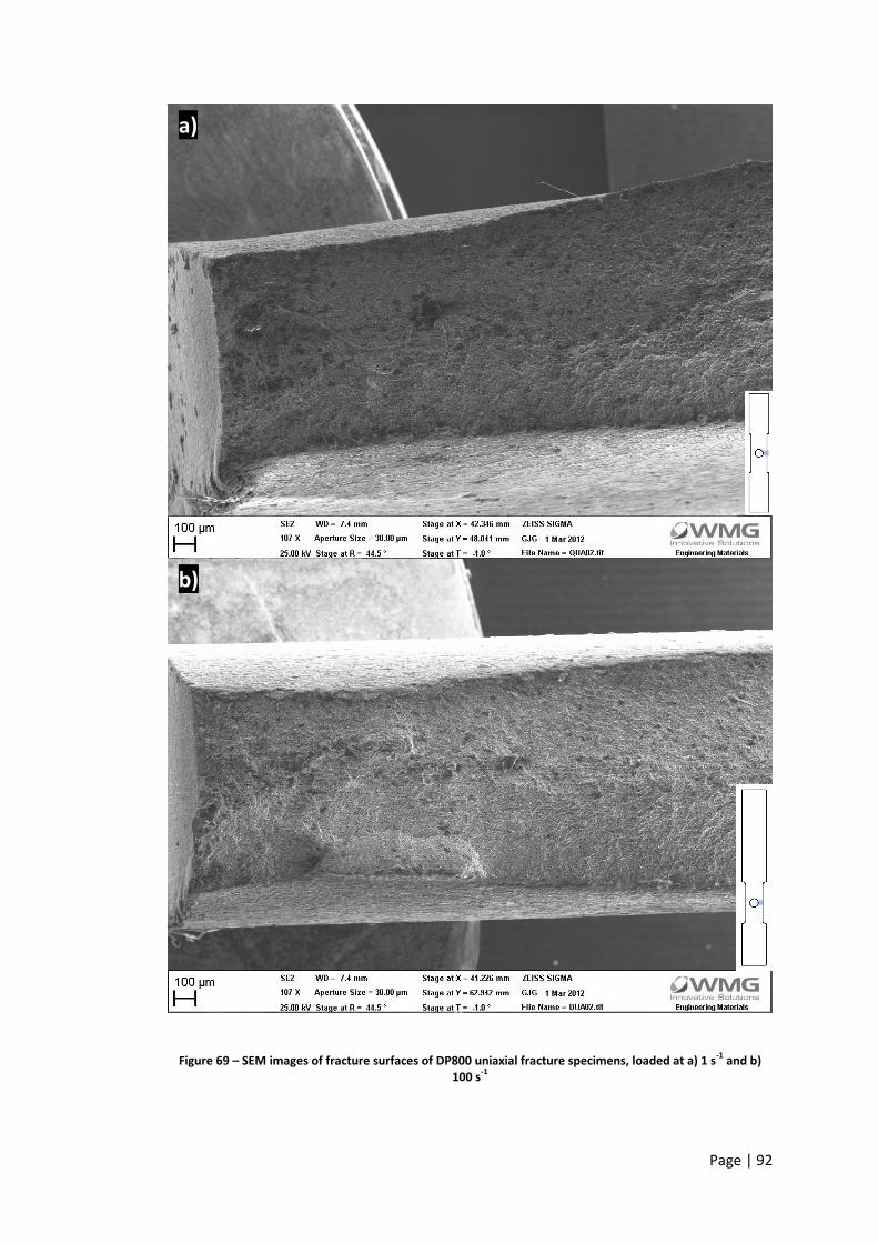
Page | 92

Figure 69 – SEM images of fracture surfaces of DP800 uniaxial fracture specimens, loaded at a) 1 s-1

and b) 100 s

-1

a)

b)

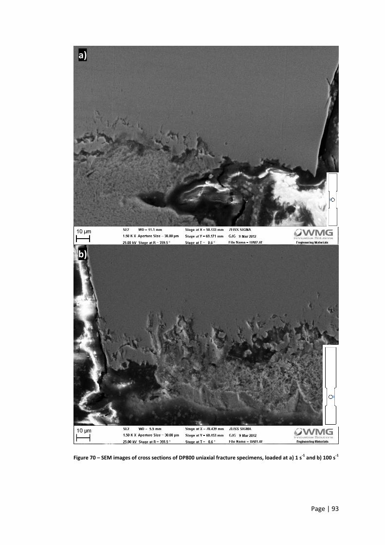
Page | 93

Figure 70 – SEM images of cross sections of DP800 uniaxial fracture specimens, loaded at a) 1 s-1

and b) 100 s-1

a)

b)

Page | 94

Chapter 5 – Shear fracture

5.1 – Introduction

This chapter will discuss the development of a specimen for measuring the fracture strain

of a sheet in shear deformation.

The traditional method for measuring shear properties is through the torsion of a thin wall

cylinder. A low ratio of wall thickness to cylinder diameter gives a strain profile that is

constant through the wall. (Boger, et al. 2005) described a method of rolling and welding

sheet into a tube for torsion testing, though notes that this will alter the material’s

properties. This method is also not suitable for the high speed testing machines at WMG.

Shear specimens for sheet material have been developed for many years for determining

both high strain plastic flow and fracture properties. Several of these designs are studied

below and one suitable for high strength steel fracture developed for low and high strain

rate testing. The results of this testing are then shown and analysed.

5.2 – Literature review

5.2.1 – Analysis of existing designs

Arcan

(Banks-Sills, Arcan and Bui 1983) proposed a geometry for determining KIIc fracture

toughness – a pure shear crack opening. The central portion of the specimen is described

as undergoing “nearly uniform pure shear”, though no experimental validation is provided.

A paper by (Banks-Sills, Arcan and Gabay 1984) discusses the specimen further. Though the

ductility of the material investigated is not explicitly described, a quenched steel of yield

Page | 95

stress and mode I fracture toughness √ is likely to be very brittle,

indicating that this specimen has not been developed for the relatively high fracture strains

found in modern high strength steels. It is also a large and thick specimen and as such is

unlikely to be suitable for testing modern automotive grade steels and gauges without

significant development.

Figure 71 shows a derivation of this specimen for testing at WMG. Finite element analysis

of this design is in Section 5.3.1 along with several other potential designs.

Figure 71 – Technical drawing of modified Arcan specimen for quasi-static shear fracture

Scherzug

Geometries for coupons for several different stress states are shown in (Ebelsheiser, Feucht

and Neukamm 2008). For shear, three tests are proposed. First is the Iosipescu specimen,

which is examined in more detail in (Kumosa and Han 1999). A complex test fixture is

required, which would cause difficulty in testing at high strain rates, and frictional effects

and stress state changes cannot be ignored with high ductility materials. The Arcan

geometry from the previous section is also considered.

A third specimen, the Scherzug, is also shown, though it has the stress state furthest from

pure shear of the three specimens with a value for stress triaxiality of . This may be

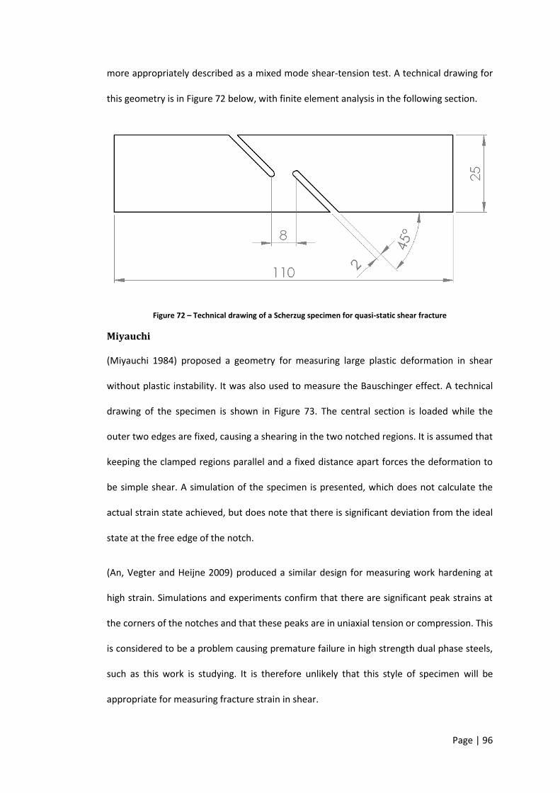
Page | 96

more appropriately described as a mixed mode shear-tension test. A technical drawing for

this geometry is in Figure 72 below, with finite element analysis in the following section.

Figure 72 – Technical drawing of a Scherzug specimen for quasi-static shear fracture

Miyauchi

(Miyauchi 1984) proposed a geometry for measuring large plastic deformation in shear

without plastic instability. It was also used to measure the Bauschinger effect. A technical

drawing of the specimen is shown in Figure 73. The central section is loaded while the

outer two edges are fixed, causing a shearing in the two notched regions. It is assumed that

keeping the clamped regions parallel and a fixed distance apart forces the deformation to

be simple shear. A simulation of the specimen is presented, which does not calculate the

actual strain state achieved, but does note that there is significant deviation from the ideal

state at the free edge of the notch.

(An, Vegter and Heijne 2009) produced a similar design for measuring work hardening at

high strain. Simulations and experiments confirm that there are significant peak strains at

the corners of the notches and that these peaks are in uniaxial tension or compression. This

is considered to be a problem causing premature failure in high strength dual phase steels,

such as this work is studying. It is therefore unlikely that this style of specimen will be

appropriate for measuring fracture strain in shear.

Page | 97

Figure 73 – Technical drawing of Miyauchi specimen for quasi-static plastic deformation in shear

Figure 74 below shows this specimen placed in a fixture for loading. The direction of

loading is left to right.

Figure 74 – Shear specimen placed in fixture for loading, adapted from (Miyauchi 1984)

Tarigopula

(Tarigopula, et al. 2008) presented a geometry for measuring large shear strains in a DP800

grade. It was also studied for fracture and it stated that fracture initiates in the gauge area

rather than at the free edge. A photograph of a fracture specimen appears to show a lack

Page | 98

of tensile crack opening, though a graph of effective plastic strain versus triaxiality shows

that there is a significant tensile component at failure. Figure 75 below is adapted from this

paper and plots effective plastic strain against triaxiality to show the tensile component of

strain from a simulation.

Figure 75 – Effective plastic strain versus triaxiality comparing simulations of a shear specimen, adapted from (Tarigopula, et al. 2008)

Failure occurs at to , equivalent to to . This is described as

being in the low stress triaxiality regime, though at failure it is closer to uniaxial tension

than shear. The graph also shows that the triaxiality changes continuously with strain. An

idealised test would require a constant triaxiality to remove the effect of damage

accumulating under different stress states. As this effect is not understood, this sample is

inappropriate for low or high fracture strain measurement. A technical drawing is shown in

Figure 76 and further analysis is presented in Section 5.3.1.

Page | 99

Figure 76 – Technical drawing of Tarigopula specimen for quasi-static shear plastic deformation

Wierzbicki

(Bao and Wierzbicki 2004) produced a “butterfly” gauge specimen for measuring the

fracture strain of quasi-static shear in AA2024-T351. The central gauge section has a

reduced thickness to concentrate the strain. As noted by (V. Tarigopula, O. Hopperstad, et

al. 2008), this is complex to machine accurately and risks introducing surfaces defects that

could cause premature failure.

It was impossible to locate the point of fracture initiation in shear, so the peak strain in the

cracked region was used as the fracture strain. The strain is taken from a simulation at the

same displacement as the beginning of the load drop-off in a physical test. This requires the

crack to grow quickly for a sharp drop-off to enable an accurate estimate of displacement

at fracture. It also requires the simulation and test to correspond very closely. A local strain

measurement system, such as is discussed in Section 2.3.5, may give a more accurate

measure of strain. However, it may not be appropriate to use the peak strain, depending

on outliers.

Page | 100

A test specimen for combined shear and tensile loading is also presented. Even with a

significant tensile component to the strain, there is no necking evident and the fracture is

clearly a mode II crack. This means that it is not possible to declare a specimen as pure

shear from the lack of necking or crack opening.

A graph of stress triaxiality versus displacement in Figure 77 shows that the triaxiality is

very low initially, though starts to rise halfway through the test. However, it fails at a value

of or , which is still a very close approximation to pure shear with a

corresponding fracture strain of . This is significantly lower than the fracture strain

expected of high strength steels though it could still be appropriate for testing.

Figure 77 – Triaxiality versus displacement for low triaxiality specimens, adapted from (Wierzbicki, et al. 2005)

Due to the complexities of simulating, machining and testing this specimen, it is not

included in the finite element analysis comparison of shear specimens below.

Peirs

(Peirs, Verleysen and Degrieck 2009) presented a geometry for measuring high strain

deformation in shear of a titanium alloy, Ti-6Al-4V, at high strain rates. The technical

Page | 101

drawing for this specimen is shown in Figure 78. This specimen was designed to be

produced from thin, , titanium plate by electrical discharge machining, though it is

easily adaptable to conventional machining processes at WMG. This alloy fails at a

significantly lower strain than that expected of the steel grades considered in this thesis.

However, the stress triaxiality at failure is given as , or . It is also the most

consistently low triaxiality of the different specimens considered here, indicating that it is

the most promising specimen to produce a DP steel fracture specimen from.

Figure 78 – Technical drawing of a Peirs specimen for split Hopkinson bar high strain rate shear fracture

The effect of the eccentricity of the notches is shown with triaxiality plotted against the

position between notch tips and against strain. For eccentricities greater than the

triaxiality is very consistent across the majority of the gauge length. The only significant

deviation is the at either side of the gauge, where the triaxiality tends towards

uniaxial tension at the free edge. However, it is not stated which region the fracture

initiates in.

Page | 102

From the graph of triaxiality versus strain, it can be seen that symmetric notches have a

significantly higher triaxiality that increases over the course of the test, ranging from

to . The lower and more consistent triaxiality from eccentric notches is

preferable for measuring fracture strain in shear.

5.3 – Development of geometry for dual phase steel

There are three stages to developing a specimen for measuring the fracture strain of shear

in a dual phase steel. The first is to study the existing geometries with reference to DP800

material data. The next stage is to develop one of these specimens and then finally modify

it for high strain rate testing.

5.3.1 – Finite element analysis of specimens in literature

The graph in Figure 79 compares five of the specimen geometries discussed in the previous

section. The Wierzbicki specimen was not used due to the difficulty of machining the

reduced through thickness gauge area. They were simulated using data for DP800 steel

rather than their original materials in order to evaluate them for measuring fracture strain

in a high strength, high ductility steel. Each of the geometries has a curve for effective

strain and alpha against the grip displacement, which were taken from one point at the

expected fracture location. The peak strain was used for this location.

There are two requirements for a shear fracture specimen. The first is that the ratio of

principal strains in the fracture location should be close to and consistent. The second

requirement is that the strain should be linear. This was not possible with the plane-strain

and uniaxial specimens due to necking. However, shear strain does not promote necking

and so a linear strain path should be possible.

Page | 103

Figure 79 – Graph of effective strain and alpha versus grip displacement at expected fracture locations of five geometries

The Arcan and Scherzug specimens have the worst stress states with alpha ranging from

to . This is because of the relatively large gauge areas that allow for a significant

tensile component in the loading. As a consequence, the strain paths are not linear and the

specimens are not suitable for high strain shear fracture testing. The Tarigopula specimen

has a fairly linear strain path but a poor stress state comparable to the Scherzug specimen.

The Miyauchi specimen has the best strain path of these specimens. However, the peak

strain is in the corner of the notch, which means that the strain is compressive rather than

-2.0

-1.8

-1.6

-1.4

-1.2

-1.0

-0.8

-0.6

-0.4

-0.2

0.0

0.0

0.1

0.2

0.3

0.4

0.5

0.6

0.7

0.8

0.9

1.0

0.0 1.0 2.0 3.0 4.0 5.0 6.0 7.0 8.0 9.0 10.0

alp

ha

Effe

ctiv

e s

trai

n

displacement, mm

Arcan vM strain Scherzug vM strain Miyauchi vM strain

Tarigopula vM strain Peirs vM strain Arcan alpha

Scherzug alpha Miyauchi alpha Tarigopula alpha

Peirs alpha

Page | 104

shear for the majority of the deformation. The Peirs specimen has a strain path similar to

the Miyauchi and Tarigopula specimens, though its deviation from linearity increases at

higher strains of approximately . The stress state of the Peirs specimen is the closest to

the intended state, , of the specimens investigated here. There is some

compressive strain at lower strains, though this is dependent on the eccentricity of the

notches and can therefore be tuned. This specimen is the most suitable basis for a dual

phase steel shear fracture test due to the stress state. The strain path at high strains could

cause problems with higher ductility materials, though it is not expected to impact the

material studied here.

5.3.2 – Effect of notch eccentricity

The geometry for a shear fracture specimen based on the Peirs design is shown in Figure

80. There have been two changes made to the specimen. The first is that the grips were

extended to to provide a more stable clamping region in the low speed tensile

machine, which should have no effect on the deformation of the specimen. The second

change is that the notches were enlarged to a minimum width of to make the

specimens easier to produce on a milling machine. This changes the shape of the

deformable region of the specimen and therefore can change the mechanical behaviour.

The purpose of this section is to examine the effect of the notch eccentricity on the stress

state of the specimen in DP800 steel. The previous section showed a small compressive

component of strain for an eccentricity of . This agrees with previous work on

titanium Ti-6Al-4V (Peirs, Verleysen and Degrieck 2009), which also showed that symmetric

notches result in a significant tensile component. Therefore, it is necessary to investigate

the adapted design to find the most suitable notch eccentricity.

Page | 105

Figure 80 – Technical drawing of Peirs shear specimen modified for production at WMG

Figure 81 compares the strain and alpha versus grip displacement of simulations of two

notch eccentricities – and . The measurements are taken from the centre of the

peak strain band at the expected fracture location, as with the previous simulations. The

strain path is not affected by the eccentricity until the strain is greater than . After this,

the deviation is not large enough to influence the choice of specimen design.

The effect on the stress state is more significant. The change to the width of the notches

means that for an eccentricity of , alpha ranges from to . In

comparison, an eccentricity of gives alpha as to . As predicted by the

literature, the decreased notch eccentricity results in a measurably worse stress state –

further from shear and closer to uniaxial tension. However, this effect is still small and

neither design results in a flat curve of alpha versus displacement. After a displacement of

, both geometries have a value of alpha that increases linearly with displacement.

As the characteristic stress state of these curves cannot be said to be pure shear, it is more

important to suppress unwanted failure modes in the specimen than to more closely

approximate shear.

Page | 106

Figure 81 – Simulated comparison of effective strain and alpha versus grip displacement for 0.8 and 1.0 mm notch eccentricity in shear fracture specimen

Figure 82 – Graph of alpha versus position along section through expected fracture location for shear fracture specimens with eccentricities of 0.8 and 1.0 mm at ε = 0.7

-1.0

-0.9

-0.8

-0.7

-0.6

-0.5

-0.4

-0.3

-0.2

-0.1

0.0

0.0

0.1

0.2

0.3

0.4

0.5

0.6

0.7

0.8

0.9

1.0

0.0 0.5 1.0 1.5 2.0 2.5 3.0 3.5 4.0

alp

ha

Effe

ctiv

e s

trai

n

displacement, mm

Eccentricity 0.8 mm strain Eccentricity 1.0 mm strain

Eccentricity 0.8 mm alpha Eccentricity 1.0 mm alpha

-1.4

-1.2

-1.0

-0.8

-0.6

-0.4

-0.2

0.0

0.0 0.5 1.0 1.5 2.0 2.5 3.0 3.5

alp

ha

position along section, mm

Eccentricity 0.8 mm Eccentricity 1.0 mm

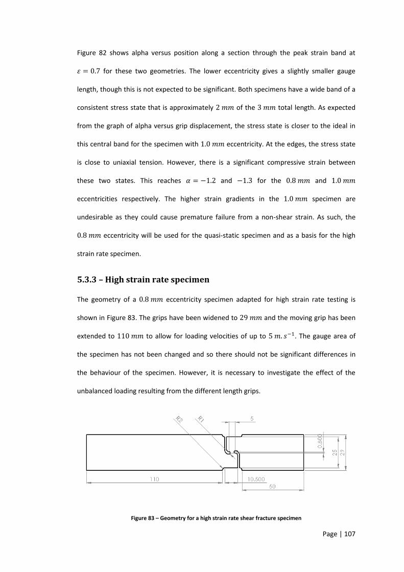
Page | 107

Figure 82 shows alpha versus position along a section through the peak strain band at

for these two geometries. The lower eccentricity gives a slightly smaller gauge

length, though this is not expected to be significant. Both specimens have a wide band of a

consistent stress state that is approximately of the total length. As expected

from the graph of alpha versus grip displacement, the stress state is closer to the ideal in

this central band for the specimen with eccentricity. At the edges, the stress state

is close to uniaxial tension. However, there is a significant compressive strain between

these two states. This reaches and for the and

eccentricities respectively. The higher strain gradients in the specimen are

undesirable as they could cause premature failure from a non-shear strain. As such, the

eccentricity will be used for the quasi-static specimen and as a basis for the high

strain rate specimen.

5.3.3 – High strain rate specimen

The geometry of a eccentricity specimen adapted for high strain rate testing is

shown in Figure 83. The grips have been widened to and the moving grip has been

extended to to allow for loading velocities of up to . The gauge area of

the specimen has not been changed and so there should not be significant differences in

the behaviour of the specimen. However, it is necessary to investigate the effect of the

unbalanced loading resulting from the different length grips.

Figure 83 – Geometry for a high strain rate shear fracture specimen

Page | 108

Figure 84 shows the effective strain and shear strain contour plots for a simulation of this

geometry. As with the previous specimens, the strain is concentrated in the gauge area,

with no significant strain in the extended grip. There is a band of consistent high strain

between the two notch tips. Previous studies in shear fracture show the crack forming

along this line (Wierzbicki, et al. 2005), (Tarigopula, et al. 2008). As such, the centre of this

band is assumed to be the location of fracture and measurements are taken from this

point.

Figure 84 – a) Effective strain and b) shear strain contour plots of a high strain rate DP800 shear fracture specimen, shown at ε = 1, only deformable region shown

Figure 85 shows the alpha contour plot of this simulation at the same strain. There is a

band of consistent stress state through the centre of the specimen, though it is at an angle

20 mm

a)

b)

Page | 109

to the band of strain. This is because there is a significant level of compressive strain at the

notch tips, as discussed in the previous section. Therefore, it is essential that the fracture

initiation occurs at the intersection of these bands for the right fracture strain and stress

state to be recorded.

Figure 85 – Alpha contour plot of a high strain rate DP800 shear fracture specimen, shown at ε = 1, only deformable region shown

The graph in Figure 86 compares the effective strain and alpha versus grip displacement for

the simulations of the low and high strain rate specimens. The strain and alpha signals are

essentially identical for the two specimens. The strain path is slightly different at strains of

and above, though this is small enough to be insignificant. The stress states compare

very favourably after the initial phase of loading. This low strain region is typically

associated with high noise under test conditions and is not included in the calculations for a

representative stress state. Therefore, these geometries are suitable for measuring the

fracture strain in shear of DP800 steel in the strain rate range of to .

20 mm

Page | 110

Figure 86 – Graph comparing simulated effective strain and alpha versus grip displacement for low and high speed shear fracture specimens in DP800

5.4 – Results

Figure 87 compares the effective strain versus grip displacement for low and high strain

rate DP800 shear fracture specimens. The low and high speed tests were loaded at

and respectively. These correspond to strain rates of and . The

displacement values for the tests were offset to be co-linear with the simulations at low

strain and displacement. Above strains of , the tests continue with a linear strain path,

which was not predicted by the simulations. As with the plane-strain and uniaxial

specimens, this implies that the post-necking behaviour of the material has not been

correctly modelled.

-1.0

-0.9

-0.8

-0.7

-0.6

-0.5

-0.4

-0.3

-0.2

-0.1

0.0

0.0

0.1

0.2

0.3

0.4

0.5

0.6

0.7

0.8

0.9

1.0

0.0 0.5 1.0 1.5 2.0 2.5 3.0 3.5 4.0

alp

ha

Effe

ctiv

e s

trai

n

displacement, mm

Low speed von Mises strain High speed von Mises strain

Low speed alpha High speed alpha

Page | 111

Figure 87 – Graph comparing simulation and tests strain versus grip displacement at low and high strain rate in DP800 shear fracture

Alpha versus grip displacement is compared for the same tests and simulations in Figure

88. The general trend is the same for the test and simulations, though the magnitude is

distinctly dissimilar. The simulations show alpha ranging from to approximately ,

though the upper limit is not well defined as the simulation does not take into account

fracture. In comparison, the tests show alpha ranging from to , which means that

there is a much larger tensile component than anticipated.

As with the plane-strain and uniaxial specimens, it is assumed that the discrepancies

between the simulation and test results are due to inaccuracies in the post-necking

material behaviour.

0.0

0.1

0.2

0.3

0.4

0.5

0.6

0.7

0.8

0.9

1.0

0.0 0.5 1.0 1.5 2.0 2.5 3.0 3.5 4.0

Effe

ctiv

e s

trai

n

displacement, mm

Low rate simulation High rate simulation Low rate test High rate test

Page | 112

Figure 88 – Graph comparing simulation and test alpha versus grip displacement at low and high strain rate in DP800 shear fracture

The DIC contour plot of effective strain in a DP800 shear specimen just prior to fracture is

shown in Figure 89. There is a band of consistent strain that is similar to the simulation,

though the experimental data show a more linear distribution of strain around the central

band. The band of strain is consistent across the width and length of the gauge area,

meaning that the results are not sensitive to the choice of facet for measurements. As such,

the central facet was chosen to match the simulation data. The choice of measurement

facet is discussed in more detail in Section 6.2.

The high strain associated with the compression at the notch tips is not seen here due to

distortion of the DIC facets. However, this strain was observed at lower displacements.

There is no plastic strain outside of the gauge area between the notch tips, which was also

predicted by the finite element simulations.

-1.0

-0.9

-0.8

-0.7

-0.6

-0.5

-0.4

-0.3

-0.2

-0.1

0.0

0.0 0.5 1.0 1.5 2.0 2.5 3.0 3.5 4.0

alp

ha

displacement, mm

Low rate simulation High rate simulation Low rate test High rate test

Page | 113

Figure 89 – DIC effective strain map of a DP800 shear fracture specimen loaded at 10 s-1

, just prior to fracture

Figure 90 shows the DIC alpha contour plot of the same specimen and time step. As with

the simulation, there is a band of consistent alpha across the specimen. However, there are

significant differences to the simulated contour plot. The first discrepancy is that the band

is at a much higher value of alpha – closer to uniaxial tension than shear. The other

differences are that the band is much wider and closer to being co-linear with the strain

band than the simulation predicted.

Whilst this implies that the finite element model is inaccurate, the results are much less

sensitive to the choice of measurement facet than anticipated. This is because the bands of

consistent strain and alpha overlap to a much greater extent.

3 mm

Page | 114

Figure 90 – DIC alpha map of a DP800 shear fracture specimen loaded at 10 s-1

, just prior to fracture

The graph in Figure 91 shows fracture strain versus strain rate for the shear specimen in

DP800. There is a downward trend in fracture strain with increasing strain rate. There is a

significant drop in the fracture strain at strain rates of . However, this is not a

change in material behaviour – the discrepancy is due to errors in measurement. A

combination of the stress state, strain rate, local heating and paint ductility lead to

distortion and delamination of the applied pattern. Consequently, the measured fracture

strain is lower than the true fracture strain as the last frame with functioning facets was a

considerable time and displacement away from fracture.

Excluding the results at gives a trend of , while including

those results gives . While this trend of decreasing fracture strain

with increasing strain rate is contrary to the plane-strain and uniaxial specimens, the trend

3 mm

Page | 115

is on the same order as the variation within each strain rate. Across the strain rate range of

quasi-static to , this implies a strain rate dependency of approximately .

Figure 91 – Graph of fracture strain versus strain rate in DP800 shear

A graph of alpha versus strain rate for the same specimens is shown in Figure 92. There are

three discrepancies in the data, occurring at the targeted strain rates of , and .

There is a high level of noise in the data at , as with the fracture strain data.

At strain rates of , the stress state is substantially worse than at other strain rates. The

value of alpha is approximately rather than as with the other rates. This

strain rate was the highest tested on the low speed machine. As a result, there is a

significant effect on the strain path due to acceleration. The strain path becomes non-

linear, unlike the other shear specimens, and so the Matlab script that calculates the

representative strain rate averaged over a smaller portion of the data that is towards the

end of the test. As seen in Figure 88, this means that the value of alpha was averaged over

0

0.1

0.2

0.3

0.4

0.5

0.6

0.7

0.8

0.9

0.01 0.1 1 10 100 1000

Effe

ctiv

e f

ract

ure

str

ain

Strain rate, s-1

Page | 116

a range closer to . Therefore, the recorded value is different to that of other strain

rates, though the stress state versus time shows no significant difference.

The tests at strain rates of show high noise in alpha and are lower than most of

the other tests. As discussed previously, the painted patterns had substantial problems

with distortion and delamination at this strain rate, meaning that the value of alpha was

determined from a portion of the test at low displacements. As shown in Figure 88, this

portion of the test data has the lowest values of alpha, resulting in a lower average at this

strain rate. However, this difference is not thought to be indicative of a change in material

behaviour.

Other than the discrepancies noted here, there is no trend in the data and the stress state

of this material and specimen is assumed to be strain rate insensitive. The two geometries

have the same characteristics for both strain and stress state and so are suitable for

determining the strain rate dependence of fracture.

Figure 92 – Graph of alpha versus strain rate in DP800 shear

-1

-0.9

-0.8

-0.7

-0.6

-0.5

-0.4

-0.3

-0.2

-0.1

0

0.01 0.1 1 10 100 1000

Rat

io o

f p

rin

cip

le s

trai

ns

Strain rate, s-1

Page | 117

5.4.1 – Fracture location

To determine the location of the initiation of fracture in this specimen high speed

photography was used. Figure 93 below shows two consecutive frames recorded at

100,000 frames per second. The first frame is prior to fracture, the second is after fracture.

A thin line from the bottom left to the top right of the gauge area can be seen, indicating

failure. However, the most reliable way to determine the point of failure was from the

elastic recovery in the static grip. This is where the static portion of the specimen rapidly

springs back once the crack has propagated and the load is removed. It is not possible to

observe the crack opening or spreading as in a mode I tensile crack, which implies that this

is a shear in-plane mode II crack.

Figure 93 – High speed photography of shear fracture; 100,000 fps

This confirms that the failure of this specimen doesn’t initiate at the free edge of the

specimen. There are several advantages to this, firstly that the machining process for

producing the specimen hasn’t introduced a defect into the material that would cause

Page | 118

premature failure. This suggests that it may be acceptable to produce shear specimens with

a manufacturing process that does not produce as smooth a finish, potentially allowing a

wider range of materials to be tested. This could include water-jet cutting of ceramics or

thermally sensitive materials. Secondly, it is much easier to measure the strain with DIC as

the facets do not need to be aligned with the edge of the specimen. Finally, this shows that

it is appropriate to measure the fracture strain from the broad central region of even

strain.

5.4.2 – Determining strain rate

The strain rate of the shear specimen was determined using the same Matlab script and

parameters as the plane-strain and uniaxial specimens. This script is discussed in more

detail in Section 6.3. The strain versus time signal was taken from the centre of the band of

consistent strain across the gauge length of the specimen.

Figure 94 shows the output of this script for a DP800 shear fracture specimen loaded at

. This shows the shear specimen has a significantly more linear strain path than

the plane-strain or uniaxial specimens. The line fitted for constant strain rate encompasses

the whole range of strain with very low deviation. This results in an equivalent strain rate

that is relevant to the pre-necking as well as the post-necking strain.

As the low and high speed geometries have the same gauge area, there is only one

equation for transforming between grip velocity and characteristic strain rate for all tested

rates. A specimen loaded at has a characteristic strain rate of , which

means that the constant in the equation ⁄ is equal to .

Page | 119

Figure 94 – Graph of strain versus time with line fitted for constant strain rate for DP800 shear fracture specimen loaded at 30 mm.s

-1

5.4.3 – Determining ratio of strains

The characteristic ratio of principal strains was determined using a Matlab script in the

same manner as the plane-strain and uniaxial specimens. This script uses the same range of

time as the determination of strain rate. For the majority of shear fracture specimens, this

encompasses the entire range of strain from unloaded to fracture.

Figure 95 shows the output of this script for a DP800 shear fracture specimen loaded at

. The change in alpha with loading is more pronounced in shear than in the

other two stress states. After the loading begins at approximately , the stress state

changes from shear at to uniaxial tension at in a fairly linear fashion.

However, no fracture strain dependency was observed. The dependency on time and grip

displacement means that the characteristic alpha in shear does not correspond to

consistent post-necking stress state, as with the plane-strain and uniaxial specimens.

Page | 120

Figure 95 – Graph of alpha versus time with line fitted for constant alpha for DP800 shear fracture specimen loaded at 30 mm.s

-1

5.4.4 – Thermal imaging

DP800 shear fracture specimens at strain rates of and were observed with

thermal imaging. Figure 96 shows the contour plots of temperature for a specimen at each

of these strain rates. The frame shown is that of the highest temperature recorded. Unlike

the plane-strain and uniaxial specimens, the peak temperature is not observed after a clear

gap has formed. This is mostly likely due to the crack opening mode in shear, which does

not result in an obvious separation of the two fracture surfaces. The relatively low

resolution of the thermal camera means that the crack will not be apparent until there is a

significant separation between the two sides of the fracture surface. This may also imply

that the heat is generated more evenly through the thickness of the sheet than the other

two stress states, meaning that less time is required for the peak heat to conduct to the

surface to be detected.

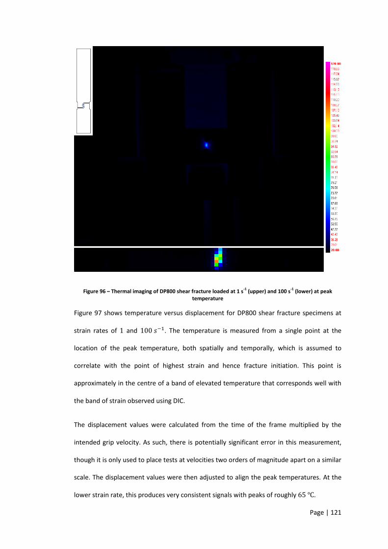
Page | 121

Figure 96 – Thermal imaging of DP800 shear fracture loaded at 1 s-1

(upper) and 100 s-1

(lower) at peak temperature

Figure 97 shows temperature versus displacement for DP800 shear fracture specimens at

strain rates of and . The temperature is measured from a single point at the

location of the peak temperature, both spatially and temporally, which is assumed to

correlate with the point of highest strain and hence fracture initiation. This point is

approximately in the centre of a band of elevated temperature that corresponds well with

the band of strain observed using DIC.

The displacement values were calculated from the time of the frame multiplied by the

intended grip velocity. As such, there is potentially significant error in this measurement,

though it is only used to place tests at velocities two orders of magnitude apart on a similar

scale. The displacement values were then adjusted to align the peak temperatures. At the

lower strain rate, this produces very consistent signals with peaks of roughly .

Page | 122

However, at the higher strain rate, the signal appears to be much more dependent on the

pixel chosen for measurement. The first two specimens show a relatively constant

temperature, while the third has sharp increase and decrease in temperature. The likely

cause for this discrepancy is that the two constant temperatures are probably within some

distance from the fracture location whereas the third signal is closer to the fracture surface

and hence heats and cools more quickly. However, the difference in heat flux does not

change the recorded peak temperature significantly.

The peak temperature at is in the range of to . This is a substantial

increase in temperature compared to the slower strain rate. However, as with the plane-

strain and uniaxial specimens, temperature increases of this magnitude are not considered

high enough to cause significant changes in the fracture behaviour of steel.

Figure 97 – Graph of temperature versus displacement for DP800 shear fracture loaded at 1 and 100 s-1

0

20

40

60

80

100

120

0 0.5 1 1.5 2 2.5 3

tem

pe

ratu

re, °

C

displacement, mm

1 s⁻¹ #1

1 s⁻¹ #2

1 s⁻¹ #3

100 s⁻¹ #1

100 s⁻¹ #2

100 s⁻¹ #3

Page | 123

5.4.5 – Fractography and microscopy

Figure 98 shows the fracture surfaces of DP800 shear fracture specimens loaded at strain

rates of and in subfigures a and b respectively. Both images are at

magnification and the direction of loading is horizontal in the plane of the image. The

centre and one side of each specimen is shown.

The location of fracture initiation is not clear from the fracture surfaces. There is no

evidence of necking, as is expected of shear tests. There is substantial bulging through the

sheet thickness at the edge of the fracture surface due to a high compressive strain in the

plane of the sheet at the notch tips. However, there is no indication that a crack forms

here. A crack formed in this region due to compressive strain would show a crack opening

mode (Cao, et al. 2010), (Landis and Nagy 2000). Likewise, if the crack had formed under

uniaxial tension at the free edge there would be a visible crack opening. The previous two

chapters also indicate that a tensile crack would result in fracture in a plane at to the

sheet thickness. The fracture surface shows no distinguishing features indicating the

fracture location, either through thickness or across the gauge length. As such, the peak

strain recorded in the centre of the band of consistent strain along the gauge length is

assumed to be the fracture strain.

The fracture surface morphology shows two distinct phases mixed randomly across the

fracture surface. However, there is no change in morphology with strain rate. As with the

plane-strain and uniaxial specimens, this implies a lack of strain rate dependency, though it

is not conclusive.

Page | 124

Figure 98 – SEM images at 112x magnification of fracture surfaces of DP800 shear fracture, specimens loaded at a) 1 s

-1 and b) 100 s

-1

a)

b)

Page | 125

A higher magnification of the low strain rate fracture surface at showing the two

phases is in Figure 99. As with the previous images, the direction of loading is horizontal in

the plane of the image. One phase is cups and cones, formed from void nucleation and

growth. They are elongated in the direction of loading, indicating that they are formed in

shear and not tension normal to the plane. These cups are on the order of across,

similar in scale to those of the two tensile specimens. The second phase is comparatively

smoother, though marked with striations in the direction of loading. It is likely the entire

surface was made up of cups and cones at the moment of fracture. However, unlike the

two tensile specimens, the direction of loading is parallel rather than normal to the fracture

surface. Accordingly, the two surfaces rub together after failure, causing this two phase

morphology.

Figure 99 – SEM image at 1000x magnification of DP800 shear fracture surface, specimen loaded at 1 s-1

A fracture surface of a mixed I and III crack mode has a characteristic morphology showing

multiple cracks opening (Hull 1995). This is not observed here, which indicates that while

Page | 126

the plastic stress state is a mixed mode of shear and tension, the failure is dominated by

shear.

Cross sections of both the low and high strain rate specimens are shown in Figure 100.

Subfigure a shows the low strain rate of while b is of the specimen. The

direction of loading is parallel to the rough fracture surface. There are voids up to

from the fracture surface, which correlates with the band of consistent strain that is

approximately across. However, it is surprising to find voids at the outer limit of

this, which is at relatively low strain at failure, and not a greater concentration of voids

closer to the fracture surface. This indicates that the voids may nucleate at low strains but

that higher strains in shear do not cause significant growth and coalescence. The cross

sections do not show any strain rate dependent micromechanical behaviour that would

affect the fracture strain.

Figure 101 shows the low strain rate cross section at a higher magnification of . This

shows that there is a greater concentration of voids within of the fracture surface,

though they are an order of magnitude smaller than those found to be evenly dispersed

across the gauge area. These voids are elongated in the direction of loading. While tensile

and shear voids have similar shapes – they can both be approximated as prolate spheroids

– tensile voids are less elongated and are aligned with the major strain (Bandyopadhyay

1979). The major strain is at to the fracture surface, which means that these voids are

the result of shear rather than tensile strain. Therefore, they are not formed late in the test

as the stress state approaches uniaxial tension and the failure mode is dominated by shear.

Page | 127

Figure 100 – SEM images of cross sections of DP800 shear fracture, specimens loaded at a) 1 s-1

and b) 100 s-1

a)

b)

Page | 128

Figure 101 – SEM image at 1500x magnification of DP800 shear fracture, specimen loaded at 1 s-1

Page | 129

Chapter 6 – Discussion of methodology

6.1 – Loading

Section 4.3.4 compared the low and high speed tensile machines for a uniaxial fracture

specimen with a strain rate of . This corresponds to a loading velocity of

or . It was found that the choice of testing machine had no effect on the

fracture strain that was discernible from the variation between specimens. There was also

no significant change in the stress state of the specimen, indicating that the moving grip of

the high speed machine does not induce any undesirable side loads.

The only noteworthy discrepancy between the two systems was in the strain rate. The

velocity was above the low speed machine’s range where the grip’s acceleration can be

disregarded. Consequently, there was a noticeable lag in the strain at low displacements.

At higher displacements, no lag was observed, meaning that the strain rate calculations for

the two tensile specimens were unaffected as these used the later portion of the test to

calculate a characteristic strain rate. However, the shear specimen was affected at the

highest strain rate on the low speed machine because the strain rate and stress state are

typically calculated from the entire test. At , a higher value of alpha was

calculated that was indicative of a discrepancy in the methodology rather than the material

behaviour.

The graph in Figure 102 compares the grip velocity versus displacement for the shear

fracture specimen in DP800 at two strain rates. The low strain rate is , equivalent to

, while the high strain rate is , with an intended grip velocity of

. There are three important comparisons to make of the different machines.

Page | 130

Figure 102 – Grip velocity versus displacement for two strain rates of DP800 shear fracture test

Firstly, there is a difference in the acceleration of the machines. The low strain rate

displayed here was selected to avoid major discrepancies between the intended and actual

velocities due to acceleration. However, the low speed machine must still accelerate from a

static position while the high speed machine’s grip is moving close to the intended speed

before it engages. However, the acceleration phase of the low speed machine is confined

to very low strain in this instance and does not adversely affect the results.

Secondly, following on from the low speed machine’s acceleration there is a large

overshoot of the target velocity. This is most likely to be related to the machine attempting

to target a displacement that it is lagging due to the low acceleration. As this phase is short

and confined to low strains, it does not affect the results. In comparison, the high speed

0

50

100

150

200

250

300

350

400

450

500

0.00

0.05

0.10

0.15

0.20

0.25

0.30

0.35

0.40

0.45

0.50

0.00 0.50 1.00 1.50 2.00 2.50

hig

h v

elo

city

, m

m.s

-1

low

ve

loci

ty,

mm

.s-1

displacment, mm

0.33 mm.s⁻¹ 300 mm.s⁻¹

Page | 131

machine does not overshoot initially and has a very consistent velocity for the first half of

the test.

In the final phase, the low speed machine approaches the target velocity in the later

portion of the test. In comparison, the high speed machine increases in velocity at higher

displacements. This is due to the servo-hydraulic nature of the machine and its feedback

loop. There is an oscillation in the velocity from the system detecting a slight drop in

velocity and overcorrecting. It may be possible to calibrate the machine to remove this

error, though it is impractical for the range of geometries and strain rates considered here.

The standard for high speed tensile testing on servo-hydraulic systems (British Standards

Institution 2012) states that the time dependent and characteristic strain rates must not

deviate by more than . This is applied to pre-necking strain and so the strain is

proportional to velocity. The tests presented here have satisfied this criterion for velocity

for the range of strain rates from to . However, the two tensile tests, plane-

strain and uniaxial, have a complex relationship between velocity and strain rate and

therefore do no satisfy this limit for strain rate. Discussion of a calculated characteristic

strain rate for these specimens is found in Section 6.3.

This combination of loading machines gives a range of strain rates that has not been widely

explored. Dynamic materials characterisation typically uses Hopkinson bars with minimum

strain rates of . The servo-hydraulic system used here produces fracture data in the

range of to and so is more suitable for automotive crash applications.

6.2 – Measurement of fracture strain

Digital image correlation was used to measure the fracture strain in preference to the other

methods discussed in Chapter 2. Whilst the technique has significant advantages, there are

Page | 132

several points to consider. These are the applicable range of strains, the point of interest,

the effect of frame rate and scale effects, which are discussed below.

6.2.1 – Applicable range of strains

The minimum and maximum measurable strains are governed by different criteria. The

minimum strain is typically a function of the desired signal to noise ratio. While several

factors can influence the noise in a DIC system, noise of was typically observed, as

discussed in Section 2.3.5. While the required signal to noise ratio will be specific to each

situation, a noise level of would imply that the lowest fracture strain that is practical to

measure is approximately . This enables the testing of relatively brittle materials.

In contrast, the maximum recordable strain is dependent on the pattern applied to the

material. Two layers of paint were sprayed on – one solid coat of white paint and one coat

of randomly applied black dots. This was used as it is easy and safe to work with. However,

tests with DX54 showed that its useful range is limited to approximately 100% strain.

Beyond this strain, the paint flakes off and no further measurement is possible. This is

discussed further in Section 7.2. It is possible to measure high strains with a different

coating, such as a pattern etched into the surface of the specimen for measuring high strain

in shear (Tata Steel 2009). Figure 103 compares these two coatings at high strain. However,

while this coating may allow higher strains to be measured, the specimens may not

produce good results at such high strains due to the changing shape and thus stress state of

the specimen. This is discussed in Section 6.7.

Page | 133

Figure 103 – Comparison of A) painted and B) etched patterns, adapted from (Tata Steel 2009)

6.2.2 – Measurement location

The location of measurement of strain and alpha is, to a large extent, determined by the

initiation of fracture. For example, the uniaxial fracture specimen cracks from the edge of

the hole. Coupled with the high strain gradient, this means that the fracture strain must be

measured from this point. However, the shear and plane-strain specimens have large areas

of consistent levels of strain with some uncertainty in the precise location of failure. As

such, the strain and alpha signals can be determined from a point source, or the average or

maximum of an area. These methods are compared below for a quasi-static plane-strain

specimen, where the length of is equivalent to .

Point

Figure 104 shows the graph of effective strain versus frame number for varying DIC facet

sizes in a quasi-static DP800 plane-strain fracture specimen. The facet sizes range from to

. As noted in Section 2.3.5, the general trend is that the measured strain

increases, particularly post-necking, with decreasing facet size. The strains tend to a limit

below facet sizes of , which corresponds to a length of . This length is

related to the necking of the specimen and therefore the limit will vary depending on the

specimen geometry and material. However, as the plane-strain specimen has the shortest

equivalent gauge length, it is a suitable limit to use for all geometries.

Page | 134

The smallest facet size, , results in very high noise. DIC has an exponential decrease

in uncertainty with increasing facet size (Tarigopula, et al. 2008). The facet size is thus a

compromise between uncertainty and accuracy.

Figure 104 – Graph of DIC effective strain versus frame number from a point for different facet sizes in a quasi-static DP800 plane-strain fracture specimen

Maximum

Figure 105 shows the strain signal derived from the maximum strain in a defined region.

The general trend is the same as the measurement from a single point, though the noise

for a facet size of is much larger. The defined region was the band of consistent

strain across the gauge width of the specimen. As such, this method results in a fracture

strain that is very similar to the measurement from a point – approximately compared

to . However, the gradient of the signal, or strain rate, is affected by this method. As

the location of the maximum strain can change in each frame, this signal does not have a

0

0.05

0.1

0.15

0.2

0.25

0.3

0.35

0.4

0 20 40 60 80 100 120 140 160 180

Effe

ctiv

e s

trai

n

frame number

5px 10px 15px 20px 25px 30px 50px 100px

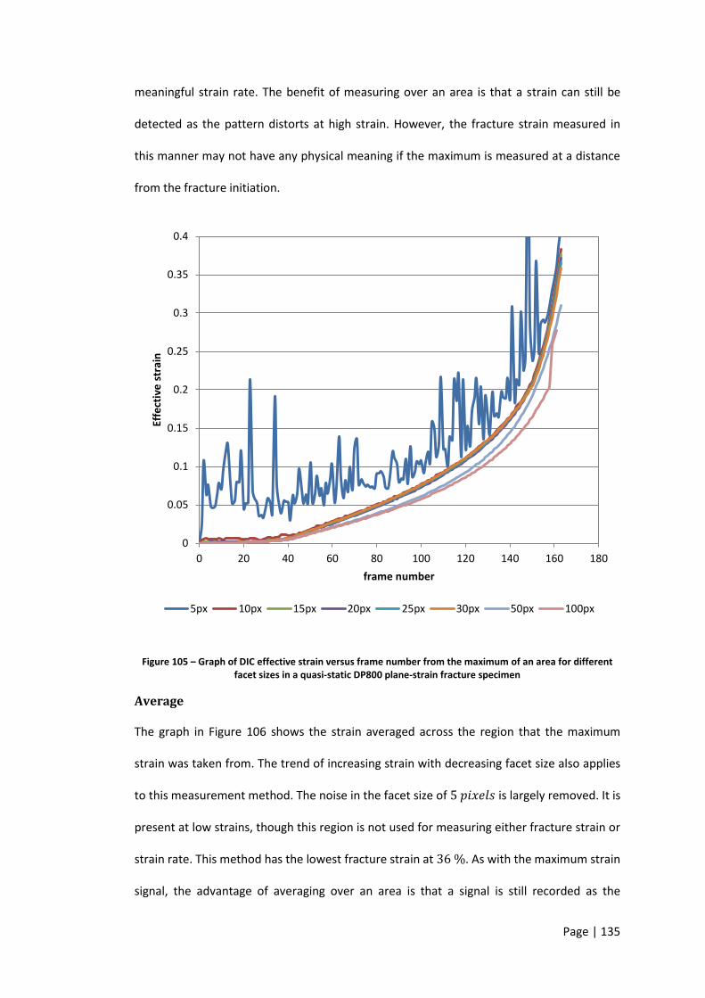
Page | 135

meaningful strain rate. The benefit of measuring over an area is that a strain can still be

detected as the pattern distorts at high strain. However, the fracture strain measured in

this manner may not have any physical meaning if the maximum is measured at a distance

from the fracture initiation.

Figure 105 – Graph of DIC effective strain versus frame number from the maximum of an area for different facet sizes in a quasi-static DP800 plane-strain fracture specimen

Average

The graph in Figure 106 shows the strain averaged across the region that the maximum

strain was taken from. The trend of increasing strain with decreasing facet size also applies

to this measurement method. The noise in the facet size of is largely removed. It is

present at low strains, though this region is not used for measuring either fracture strain or

strain rate. This method has the lowest fracture strain at . As with the maximum strain

signal, the advantage of averaging over an area is that a signal is still recorded as the

0

0.05

0.1

0.15

0.2

0.25

0.3

0.35

0.4

0 20 40 60 80 100 120 140 160 180

Effe

ctiv

e s

trai

n

frame number

5px 10px 15px 20px 25px 30px 50px 100px

Page | 136

pattern distorts. However, this signal is not reliable as it is not local to the fracture

initiation.

Figure 106 – Graph of DIC effective strain versus frame number from an averaged area for different facet sizes in a quasi-static DP800 plane-strain fracture specimen

Summary

The measurements were taken from a single point with a facet size of . This was

used to achieve a good balance of uncertainty and accuracy. It is also important to use a

single point so that the recorded fracture strain is at the location of fracture initiation and

the strain rate and alpha are not averaged across different regions of the specimen.

6.2.3 – Effect of frame rate

Another important point to consider is the effect of the frame rate on the measurement. A

high frame rate will give a more accurate measurement but will require more time to

0

0.05

0.1

0.15

0.2

0.25

0.3

0.35

0.4

0 20 40 60 80 100 120 140 160 180

Effe

ctiv

e s

trai

n

frame number

5px 10px 15px 20px 25px 30px 50px 100px

Page | 137

process. If the frame rate is too low, the final frame prior to fracture may be a significant

time and thus strain from the true fracture point. This will have the effect of

underestimating strain.

For example, strain versus time is shown for a low speed uniaxial specimen in Figure 107

below. Due to necking, the strain rate increases significantly towards the end of the test. A

fifth order polynomial was fitted through this data to accurately match the curve. This

function can be differentiated to obtain the strain rate at any point. Using this, the strain

rate at failure is . This test was recorded at , with images at

intervals. This results in a strain increase per frame of , or . This approximate

ratio of frame rate to grip velocity was used for all tests. Therefore, this value is suitable for

the uncertainty at each strain rate.

Figure 107 – Graph of strain versus time for a uniaxial fracture specimen with a polynomial trend line

This is a significant portion of the overall uncertainty of and larger than the

uncertainties calculated in Section 2.3.5 that are the result of miscalibration of the camera.

It is possible to increase the frame rate for the lower strain rates, which would decrease

y = 1.4495x5 - 3.3026x4 + 3.0213x3 - 0.9242x2 + 0.1069x - 0.0019

0

0.1

0.2

0.3

0.4

0.5

0.6

0 0.2 0.4 0.6 0.8 1 1.2

Effe

ctiv

e s

trai

n

Time, s

Page | 138

the uncertainty for those tests. The only cost of this would be the increased computation

time for these specimens. However, this is not possible for the higher strain rate tests,

particularly at , as the resolution would have to be reduced. This would have the

effect of increasing the facet size, which would reduce the measured fracture strain. The

same ratio of frame rate to grip velocity was used for all tests to reduce the differences

between the low and high strain rate measurements.

6.3 – Measurement of strain rate

While the strain rate of the shear specimen is constant, the strain rate in uniaxial tension

and plane-strain specimens is a function of strain. A characteristic strain rate is required to

study the effect of strain rate on fracture strain. To achieve this consistently, a Matlab

script was written to fit a straight line through the strain versus time data, the gradient of

this line being the strain rate.

It is not appropriate to simply divide the fracture strain by the time to obtain the strain rate

for two reasons. Firstly, the high speed camera is triggered an indeterminate amount of

time before the specimen loading begins, thus the absolute value of time has little

significance. As the plane-strain and uniaxial specimens do not have a linear relationship

between strain and grip displacement or time, it is not easy to identify the start of loading.

This can be seen in Figure 108, a graph of strain versus time for a uniaxial specimen loaded

at . Secondly, averaging the strain in this manner will significantly

underestimate the strain rate. Another option is to record the peak strain rate, however,

this will overestimate the rate for the majority of the test.

The script written to take account of this is written in full in Appendix A3. The function has

four arguments, the first three being vectors for time and strain and alpha respectively. The

fourth argument is optional and used to set the desired least-square error of the fit. This

Page | 139

value defaults to 0.1 if it is not given. The vector for alpha is used in the latter part of the

script, which will be discussed in the next section.

The script's purpose is to fit a straight line through the data and then compare the residual

error against a target threshold. If the fit does not meet the threshold, a smaller subset of

data is used by removing the first data point. This repeats until the threshold is met. The

choice of this threshold is arbitrary. It can be seen in the graph below that if a sufficiently

small range of the data is used, it is possible to fit a straight line with a very low error.

However, this will only account for a small portion of the strain in the specimen. It is

therefore a compromise between the accuracy of the fit and the portion of the test that it

is relevant to. A value of 0.1 was chosen to overestimate the strain rate at the beginning of

its range and underestimate at the end. This fit can be seen in Figure 108 below.

Figure 108 – Graph of strain versus time with line fitted for constant strain rate for uniaxial fracture specimen loaded at 2.2 mm.s

-1

Page | 140

The standard for servo-hydraulic high strain rate tensile testing (British Standards

Institution 2012) states that the time-dependent strain rate must not deviate from the

characteristic strain rate by more than . This is applied to pre-necking strain, while in

comparison, the strains considered in this thesis are largely post-necking. The shear

specimens in Chapter 5 showed no evidence of necking and had linear strain rates that

exceeded this requirement by a substantial margin. However, the two tensile tests –

uniaxial and plane-strain – exhibited necking and hence non-linear strain rates. For these

two geometries, it is not possible to meet this limit and the deviation will increase with the

material’s ductility.

6.4 – Measurement of ratio of strains

As with strain rate, it is necessary to determine a characteristic value for alpha, which is

time dependent. This is performed by the same script that determines the strain rate for a

specimen.

One simple method to obtain the characteristic alpha is to use the value at fracture.

However, it does not automatically follow that this value is the most influential as the

majority of the damage done to the specimen may have been under a different state. To

compensate for this, (Bao and Wierzbicki 2004) used the mean of the stress triaxiality as a

representative value.

The approach used here is to take the mean of alpha for the range of time used to fit the

strain rate. This is shown in Figure 109 for a uniaxial fracture specimen. It can be seen that

this approach removes the influence of noise at the beginning of the test. It also discounts

the value of alpha at low strains and low strain rates. This could give a misleading idea of

the stress state in the specimen with a significantly changing state. However, in the

Page | 141

example below it can be seen that the portion of the test taken as a consistent strain rate is

also the portion of the test that has very little noise in the strain state.

Figure 109 – Graph of alpha versus time with line fitted for constant alpha for uniaxial fracture specimen loaded at 2.2 mm.s

-1

6.5 – Thermal

6.5.1 – Comparison of geometries

Thermal imaging was performed on all three stress states. The peak temperatures reached

were , and for the plane-strain, uniaxial and shear specimens

respectively. As previously noted for each of these specimens, the temperature rise

associated with high strain rates are unlikely to affect the fracture properties.

Temperatures of over have been associated with significant changes in the plastic

flow of high strength steels, which exhibit dynamic strain aging (Akbarpour and Ekrami

2008). A transition from ductile to brittle failure was found in a stainless steel at at

Page | 142

quasi-static loading speeds (Aghaie-Khafri and Zargaran 2010). (Mannan, Samuel and

Rodriguez 1985) likewise found a decrease in ductility measured by reduction in area at

, followed by an increase at for 316 stainless steel. While these temperatures

are markedly higher than those reached in high strain rate testing, it would be useful to

find this transition in DP800 and therefore how likely a higher strain rate test is to reach

this limit.

Furthermore, the temperatures reached in all three stress states are very similar.

Therefore, the different gauge volumes of the specimens have not caused a change in the

localised heating. This rules out thermal effects as a cause of the shear specimens’ slight

increase in fracture strain with strain rate, compared to the tensile specimens’ slight

decrease.

All three specimen geometries showed consistent curves for temperature versus

displacement with increased noise at high strain rate. This may partially be due to the

calculation of the displacement. As the thermal imaging system and VHS data acquisition

are not linked or synchronised, the only information from the thermal camera is

temperature and frame number. The frame number corresponds to a time but this is not a

suitable way of representing tests that are two orders of magnitude apart in velocity. Grip

displacement gives a better comparison and so this was calculated from the time using the

intended grip velocity. There are issues with using a non-local displacement measurement

from the grip, such as compliance of the load train, though this should not be important for

tests within each stress state as they are of similar loads. Section 6.1 showed that the

actual grip velocity is close to the target; though using the intended velocity here is still a

source of uncertainty. Therefore, the graphs of temperature versus displacement have

limited use for analysing the evolution of temperature in the specimen, particularly at

higher strain rates.

Page | 143

6.5.2 – Theoretical adiabatic heating

It is possible to determine an upper limit to the temperature rise of a high strain rate test,

given several assumptions. These can broadly be characterised as measuring the energy in

the system and the amount of material that it is applied to. The temperature rise, , can

be calculated as

⁄ , where is the energy applied and is the mass that it

is applied to. is the specific heat capacity of the material.

The first assumption is that the test is adiabatic. This means that the plastic work that is

converted to heat stays in the specimen for the duration of the tests, with no losses to the

environment. Realistically, there will be conduction from the gauge area through the

specimen and some level of radiation from the surface, as this is how the temperature was

measured in the previous section. However, for a sufficiently high strain rate test, these

effects will be negligible. It is therefore assumed that the higher strain rate that was

measured thermally, , is suitably close to adiabatic. This will slightly overestimate

the energy and hence temperature rise of the system.

The next assumption is that the strain and thermal maps are similar enough to measure a

characteristic gauge area from the strain maps. The thermal camera has a low resolution

compared to the DIC camera. Furthermore, the thermal camera's range does not include

room temperature when calibrated for high strain rate tests. As such, it is difficult to

calibrate the scale of the image against a known length. The temperature rise is a product

of plasticity and it assumed that the heat remains at the point where it is generated for the

duration of the test. Therefore, strain and temperature maps can be considered equivalent

and the gauge area was measured on the DIC strain maps.

This gauge area is then multiplied by the original sheet thickness to obtain the gauge

volume. The accuracy of this assumption is different for each of the specimen geometries.

Page | 144

As the shear specimen does not neck, this will give an accurate measure of the gauge

volume. The thickness was not measured from the fracture surfaces of the tensile

specimens because the necking and hence thickness varies with both strain and position

along gauge width. As such, this assumption will overestimate the mass, particularly in the

plane-strain specimen, reducing the apparent theoretical maximum temperature.

It is also assumed that the plastic strain is isochoric (Hertzberg 1996) and that the standard

density for the material, , may be used. Due to the formation and growth of

voids, this will overestimate the mass at fracture and underestimate the temperature rise.

The growth of voids is dependent on the stress state (Rice and Tracey 1969) and (Liu, et al.

2003). Therefore the density at failure will vary between the specimen geometries.

The energy applied to the system was calculated by integrating force-displacement curves

for each specimen at a strain rate of . It is assumed that nearly all of the plastic

work is converted to heat. The existing literature is divided on this point; some work shows

that the fraction of work that is transformed to heat varies between and ,

dependent on the material, strain rate and plastic strain (Mason, Rosakis and Ravichandran

1994) (Rosakis, et al. 2000). However, another study showed no such dependency in

several metals, including 1018 steel (Kapoor and Nemat-Nasser 1998). It was found that,

within experimental error, of the plastic work was converted to heat and that infra-

red detectors underestimated the temperature of the specimen.

Finally, the specific heat capacity of the material is assumed to be insensitive to

temperature and strain. As the heat capacity of the dual phase steel was not available, the

capacity of iron, , was used (Shackelford 2005).

Table 1 shows calculations of the theoretical maximum temperature rises of adiabatic

DP800 fracture specimens and compares them to the observed temperatures.

Page | 145

Geometry Plane-strain Uniaxial Shear

Length, mm 20 3 3

Width, mm 2.5 3 1.5

Depth, mm 1.5 1.5 1.5

Energy, J 59 21 4.25

Volume, m3 0.0000000750 0.0000000270 0.00000000675

Mass, kg 0.000593 0.000213 0.0000533

Temperature rise, °C 224 222 180

Observed rise, °C 100 120 90

Table 1 – Theoretical calculations of adiabatic temperature rises in high speed DP800 fracture tests

The maximum theoretical temperature rise is similar for all three specimen geometries,

ranging from to . In comparison, the experimentally measured temperature

rises are around to . The shear specimen may reach a slightly lower temperature

than the two tensile geometries, though it is more likely that the variation is within the

experimental and theoretical uncertainties. This means that the work done per unit volume

is fairly consistent despite the different gauge volumes and strains of the three geometries.

The discrepancy between the experimental and theoretical temperature rises may be due

to inaccuracies in the theoretical calculations, the experimental observations or a

combination of the two. The calculations are only intended to be an upper limit and thus

are likely to overestimate the temperature rise. In comparison, the test results will

underestimate the temperature rise due to surface measurements with a time lag from the

generation of heat and an anisotropic and non-adiabatic state. The main point to note is

that the temperature rises associated with high strain rate testing are unlikely to

significantly affect a dual phase steel, even at higher strain rates than those tested here.

However, a material with a meta-stable microstructure, such as the retained austenite in a

TRIP steel, may exhibit a strain rate dependency.

Page | 146

6.6 – Fractography and microscopy

The predicted fracture strain in shear is much higher than measured in testing if a standard

model for fracture derived from void growth, such as Johnson-Cook, is used. Several

methods for correcting this, including the Wilkins and Gurson models, have been

developed by including a separate term for damage accumulation in shear. The assumption

of these models is that fracture can be driven by two different mechanisms. However, it

was seen that the fracture surface of all the specimens was dominated by cup and cone

indicative of ductile failure. The void formation and growth may be due to the significant

tensile component of strain in the shear specimen, though the orientation of the voids with

respect to the major strain implies that they were driven by shear. This means that for

DP800 steel, there is one failure mechanism for the range of shear to plane-strain tension.

A phenomenological fracture model based on the maximum shear stress may therefore be

suitable (Bao and Wierzbicki 2004).

The fracture surface morphology was not found to be dependent on strain rate. The strain

rates tested were and for plane-strain and and for shear and

uniaxial tension. Whilst it is possible that a dependency may exist beyond the range

examined here, the lack of a major strain rate dependency for fracture strain implies that

there is no change in failure mechanism between quasi-static loading and .

Furthermore, sections through the same specimens showed no strain rate effect.

Previous work on the strain rate dependency of fracture in steel showed no correlation

between changes to the fracture surface morphology and changes in the fracture strain as

measured through reduction in area (Boyce and Dilmore 2009). In addition to this, it is

assumed here that failure is catastrophic and therefore the crack propagation is

unimportant. The location and stress state of the crack initiation are critical, though no

strain rate dependency was observed.

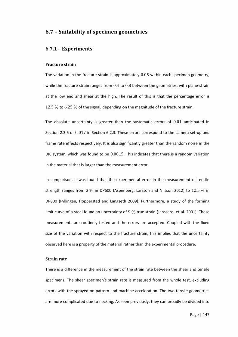
Page | 147

6.7 – Suitability of specimen geometries

6.7.1 – Experiments

Fracture strain

The variation in the fracture strain is approximately within each specimen geometry,

while the fracture strain ranges from to between the geometries, with plane-strain

at the low end and shear at the high. The result of this is that the percentage error is

to of the signal, depending on the magnitude of the fracture strain.

The absolute uncertainty is greater than the systematic errors of anticipated in

Section 2.3.5 or in Section 6.2.3. These errors correspond to the camera set-up and

frame rate effects respectively. It is also significantly greater than the random noise in the

DIC system, which was found to be . This indicates that there is a random variation

in the material that is larger than the measurement error.

In comparison, it was found that the experimental error in the measurement of tensile

strength ranges from in DP600 (Aspenberg, Larsson and Nilsson 2012) to in

DP800 (Fyllingen, Hopperstad and Langseth 2009). Furthermore, a study of the forming

limit curve of a steel found an uncertainty of true strain (Janssens, et al. 2001). These

measurements are routinely tested and the errors are accepted. Coupled with the fixed

size of the variation with respect to the fracture strain, this implies that the uncertainty

observed here is a property of the material rather than the experimental procedure.

Strain rate

There is a difference in the measurement of the strain rate between the shear and tensile

specimens. The shear specimen’s strain rate is measured from the whole test, excluding

errors with the sprayed on pattern and machine acceleration. The two tensile geometries

are more complicated due to necking. As seen previously, they can broadly be divided into

Page | 148

two regions – pre and post-necking. However, the instantaneous strain rate can vary by a

factor of two over these relatively consistent regions. This may cause inaccuracies in the

three dimensional fracture locus for highly strain rate dependent materials, though it is not

practical to design a system that controls the grip velocity accurately and at a high enough

frequency to counter this. It is possible to use a shear test to measure high plastic strain

(Tarigopula, et al. 2008) but this approach is not suitable for characterising a material’s

strain rate dependency for fracture strain. This is because this work has found that the

strain rate dependency can be of opposite sign for shear and tension.

The measurement of strain rate for the two tensile fracture geometries causes a

discrepancy with the measurement of strain rate for plastic flow. The fracture specimens

used the post-necking strain to calculate the strain rate as it encompassed the greater

portion of the material’s deformation and hence damage. However, plastic flow is only

determined for pre-necking strains (British Standards Institution 2012, British Standards

Institution 2009) and so the strain rate is calculated for a different portion of the

deformation. This means that much of the previous work on the strain rate dependency of

fracture is using a drastically different definition of strain rate to the local measurement

used here.

The variation in strain rate for each nominal grip velocity and stress state is low. There is

greater variation in the gap between intended and measured strain rate. This would be

problematic if the fracture strain at a specific strain rate was required for a highly strain

rate sensitive material. The discrepancy can likely be reduced with re-calibration of the

machine for each strain rate and several tests to determine the correct input velocity for a

given strain rate, though this dramatically increases the testing requirements for little gain.

This does not affect the strain rate dependent fracture locus as it is aimed at determining

Page | 149

the effect of strain rate across several orders of magnitude and therefore the discrepancies

of a factor of two do not influence the results.

Stress state

The stress state of the two tensile specimens is very consistent. The uniaxial specimen in

particular produces a nearly horizontal line when plotted as alpha versus grip displacement

when the high initial noise is discounted. This means that the process of averaging the

value over the range of consistent strain rate gives an accurate and repeatable value. In

comparison, the shear specimen has a value of alpha that varies linearly with grip

displacement. This means that the averaging does not give an accurate reflection of the

stress state of the specimen, which ranges from the ideal values of pure shear to uniaxial

tension. Therefore, further development of the shear specimen for ductile materials is

required.

As the plane-strain specimen is the only one of the geometries to have different gauge

volumes for the low and high speed machines, it is the only specimen to have a strain rate

dependent stress state. The variation in alpha for the uniaxial and shear specimens is due

to errors in testing rather than a change in the stress state. These errors were from

problems with the applied pattern and machine acceleration.

The change in stress state at high strain rates in plane-strain is low and unlikely to

significantly affect the parameter fitting of the fracture locus. The uniaxial specimen had no

step change in state but consistently greater noise. This is likely to have a greater impact on

the fracture locus as the assumed polynomial shape will have a significantly higher gradient

at the uniaxial rather than plane-strain state. The shear specimen’s stress state has a

substantial level of noise and systematic errors, though its greatest problem is the

inconsistent stress state. This may reduce confidence in the accuracy of the shear portion

of the fracture locus.

Page | 150

6.7.2 – Simulation

There were discrepancies between the simulations and experimental results for all

specimen geometries. For the plane-strain specimen, the experimental results of local

strain versus grip displacement showed distinct gradients for pre and post-necking, which

was not predicted by the simulation. The uniaxial specimen had lower local strains at all

displacements in tests, thought the gradients of strain versus displacement in test and

simulation matched for post-necking strains. The shear simulations did not predict the

linear strain response that was observed in testing.

There were also differences between the simulations and experiments in terms of the

stress state. The plane-strain tests showed a consistently slightly higher value of alpha than

the simulations, though the shape of alpha versus displacement matched very well. The

uniaxial specimen had a similar response, though this resulted in a stress state that was

further from the ideal than predicted. The simulations of the shear specimen predicted that

alpha would increase linearly with displacement. This was observed in the test results,

though at a much higher gradient.

It is likely that there are inaccuracies in both the test and simulation data. Firstly, the

experimental results are plotted as strain and alpha versus grip displacement. The strain

and alpha values are taken from the DIC system and are assumed to be accurate. However,

the grip displacement was calculated as the DIC and loading machine systems are not

synchronised. The displacement is calculated by multiplying the time of the DIC frame by

the intended test velocity. Section 6.1 showed that the velocity is not constant for either of

the tests machines, which introduces a discrepancy. The displacement values were then

offset to match the simulation as closely as possible at either the start or end of the test.

This was done because the DIC system was not automatically synchronised to the start of

the test. Furthermore, the grip displacement is an inaccurate measurement due to the

Page | 151

compliance of the test machine and the regions of the specimen outside of the gauge area.

Despite these inaccuracies, the grip displacement was used so that tests at different strain

rates could be compared and for a simple comparison between the tests and simulations.

The lower than anticipated strains for a given displacement in the two tensile tests may

therefore be, in part, due to the tightening of the load train. In comparison, the shear

specimen is a lower peak load at than the plane-strain, , and uniaxial, .

This means that the shear specimen is unlikely to cause the same level of strain in the test

machine and thus will have a more accurate grip displacement measurement.

The most probable cause of error in the simulation is the assumption that the material is

isotropic. Tensile tests at , and to the rolling direction showed limited anisotropy

and this is also used in the literature (V. Tarigopula, O. Hopperstad, et al. 2009). However,

this assumption is derived from relatively low global strain measurements. Anisotropy can

by induced by void growth (Hiroshi and Koichi 1988), meaning that an isotropic model may

not be suitable for the high local strains in fracture testing. A model for anisotropic porous

materials (Keralavarma and Benzerga 2010) may result in a more accurate simulation.

6.8 – Determination of fracture locus

A three dimensional fracture locus can be constructed from the experimental results. The

standard quasi-static fracture locus is plotted as fracture strain versus stress state, which is

represented by either triaxiality or the ratio of principal strains. This work adds a third axis

to that graph to show the effect of strain rate. A script was written in GNU Octave/Matlab

to process the data. This script is shown in full in Appendix A4.

The script starts by defining vectors for the strain rate, alpha and fracture strain for each of

the three specimen geometries. The data has been omitted from the appendix for the sake

of clarity. Following this, an estimate of the tensile portion of the static fracture locus is

Page | 152

calculated. It is assumed that the shape of the fracture locus can be approximated as a

second order polynomial (Bao and Wierzbicki 2004). The ideal stress state for the plane-

strain specimen would have given the minimum for the tensile curve, though it was not

practical to obtain this exact state. While the form of the locus may be assumed, there is

not enough test data to accurately model the shape. To produce a curve with the minimum

at the correct stress state, the test data for the two tensile states was mirrored about the

line . A second order polynomial was then fitted through these points. An example of

this is shown in Figure 110 below, using example data rather than test data. The calculation

for the shear curve is performed later in the script.

Figure 110 – Example of fitting two dimensional fracture locus through example data

This fracture locus is calculated from the first entry in the data vectors. This was a quasi-

static result at . It may be more appropriate to select another strain rate,

y = 1.5087x2 + 3E-15x + 0.3291

y = 0.4872x2 + 0.9743x + 1.0716

0

0.1

0.2

0.3

0.4

0.5

0.6

0.7

0.8

0.9

-1.6 -1.4 -1.2 -1 -0.8 -0.6 -0.4 -0.2 0 0.2 0.4

Effe

ctiv

e f

ract

ure

str

ain

alpha

Tensile fracture Shear fracture

Poly. (Tensile fracture) Poly. (Shear fracture)

Page | 153

depending on the material and its strain rate dependency. A more accurate locus may be

obtained by using all of the data from the first strain rate. However, this locus is only used

as an initial estimate for the three dimensional fitting function and so the increased

accuracy was not deemed necessary. An estimate of the strain rate dependency is

calculated by fitting a straight line through the strain rate and fracture strain vectors for the

plane-strain data. For the DP800 steel investigated here, the result is insensitive to the

choice between the plane-strain and uniaxial results.

The three dimensional tensile fracture surface is then calculated using these initial

estimates and the mirrored experimental tensile data. The form of the surface is the static

polynomial with a term added for strain rate dependency. This can be seen in the equation

below, where is the fracture strain, is alpha, is the strain rate and to are

material constants. The fitting procedure works by minimising the residual sum of squares

between the fractures strains predicted by the equation for a given set of constants and

the experimental results.

( ) ( )

The next stage is to calculate the shear fracture surface. The original intention was to have

a uniaxial fracture measurement at the intersection of the shear and tensile modes that

could be used to calibrate both surfaces. However, the uniaxial specimen’s deviation from

the ideal stress state makes this impossible. As such, the next step is to calculate the

fracture strain at for the range of strain rates using the fitted tensile fracture

surface. This calculated data can then be mirrored along with the shear experimental data

about to fit a fracture surface using the same method as the tensile surface. The

output from this script for the DP800 test results is discussed in the next chapter.

Page | 154

6.9 – Summary of test and analysis procedures

6.1 – Scope

The test procedures summarised in this section are intended to characterise the sensitivity

of fracture strain to strain rate of metallic specimens.

6.2 – Test geometry

The test geometries for plane-strain, uniaxial tension and shear at low strain rates are

shown in Figure 111a, b and c respectively. The equivalent specimens for high strain rate

testing are shown in Figure 112.

Figure 111 – Specimen geometries for low strain rate fracture testing, a) plane-strain, b) uniaxial, c) shear

a)

b)

c)

Page | 155

They are appropriate for flat sheet only, with a maximum gauge thickness of 1.5 mm. This is

to ensure a minimum ratio of 2:1 for gauge length to thickness. A higher gauge thickness

may be acceptable but not without a justification of the stress state of the gauge area.

Figure 112 – Specimen geometries for high strain rate fracture testing, a) plane-strain, b) uniaxial, c) shear

6.3 – Specimen preparation

Specimens should be cut from a sheet such that the cut edges are free from defects that

could cause premature failure of the specimen. An maximum size of allowable defect is

hard to define and therefore the cut edges should be comparable in surface roughness to

the as-supplied rolled surface roughness to minimise the risk of failure. As with standard

tensile testing, the specimen production should not distort the geometry or surfaces.

a)

b)

c)

Page | 156

As the preferred strain measurement is digital image correlation, a pattern must be applied

to one surface of the specimen. Therefore, it is necessary to prepare the surface in such a

way that the pattern does not distort before testing or delaminate during testing. For a

painted pattern, the surface of the specimen must be degreased and dried prior to

painting. Other patterns, such as chemical or laser etching, may be less sensitive to the

surface treatment.

A minimum of three specimens should be prepared for each material, geometry and strain

rate combination. If the error in the recorded fracture strain is large compared to the strain

signal, it may be necessary to prepare more samples for a statistically valid measurement.

6.4 – Data acquisition

The rate of data acquisition should be selected such that the sampling does not introduce

excessive errors into the final fracture strain measurement. A maximum strain error of 0.02

per frame was used, though a lower error will be necessary for materials of lower ductility.

This can generally be achieved by using 100 – 200 frames per sample. This means that the

error will approximately scale with ductility and be insensitive to the loading velocity and

strain rate.

6.5 – Strain rate determination

As the strain rate is not constant for materials with significant post-necking strain, a

characteristic strain rate must be calculated. This should correspond to the greatest portion

of damage applied to the material for the smallest deviation from a linear relationship. For

ductile materials, this is likely to be the post-necking portion of strain. To ensure a robust

strain rate measurement, the characteristic strain rate must be determined numerically. It

is suggested to use least-squares residual fitting with a target error. This error may need to

be determined qualitatively for each material and should be reported along with the

characteristic strain rate.

Page | 157

The strain rate must be measured from the time derivative of the strain signal local to the

location of fracture initiation of each test specimen. This requirement means that it is not

appropriate to measure the strain rate from a simulation or non-local strain or

displacement measurement.

6.6 – Stress state determination

As with strain rate, the stress state changes throughout the test and a characteristic state

must be determined for the test. The same least-squares residual fitting should be used. It

was found that the post-necking portion of strain that was chosen for the strain rate

determination resulted in a relatively stable stress state. A different portion of the strain

may be chosen if appropriate. The target residual error must be stated.

As with strain rate, the stress state signal must be taken local to the location of fracture

initiation. A non-local measurement or correlation with simulation may lead to substantial

inaccuracies.

6.7 – Fracture strain

The fracture strain should be measured from a single point at the location of fracture

initiation. High strain gradients make averaged or non-local measurements inaccurate. This

measurement should not be extrapolated, especially for tensile specimens where the non-

linear response increases the inaccuracy of this method. It may be acceptable to highlight

the sensitivity to strain rate using extrapolated data, though this should be stated and the

resulting data should not be used to predict component failure.

Page | 158

Chapter 7 – Discussion of materials

7.1 – DP800

The dual phase steel DP800 was the main focus of this work. As discussed previously, there

were a number of problems in testing. One major issue was with the experimental

technique at the highest strain rate, , which caused high levels of noise in the

uniaxial and shear alpha values and premature failure of the applied pattern in the shear

specimen. A second issue was the inconsistent and high value of alpha in the shear

specimen. The other problems, such as the effect of acceleration on the shear

specimens and the different geometries for low and high speed plane-strain testing, were

minor.

An increase in fracture strain of approximately across the tested strain rate range was

observed for the tensile specimens, along with a decrease of in the shear specimens

for the same range. The initial estimate for the three dimensional fracture locus fitting

procedure agreed with the value for the tensile specimens. This fitting is performed by a

Matlab script, as described in Section 6.8. However, it predicted a much higher strain rate

dependency for the shear portion of the fracture locus, with a decrease in fracture strain of

. The final surface fit reduced this to , which implies that the low fracture strains

measured at due to experimental error do not overly affect the results. The initial

estimates and fitted materials constants, along with the residual sum of squares errors, are

shown in Table 2.

The polynomial coefficients for the tensile portion of the fracture locus are not changed

significantly by the surface fitting procedure. is reduced slightly, giving a lower gradient

and fracture strain, while is increased, which results in a higher minimum fracture strain

under the plane-strain condition. The effect of this, along with the change in strain rate

Page | 159

dependency, is to reduce the residual sum of squares error by a factor of two. This means

that applying a strain rate term to a quasi-static fracture locus can give a reasonable

estimate of the tensile portion. However, a full three-dimensional fitting procedure does

improve the accuracy of the locus.

In comparison, there were significant changes in the shear portion’s polynomial

coefficients. and were initially estimated as and respectively. The

large negative values mean that pure shear at is the local maximum rather than

minimum of the locus. However, the surface fitting procedure changed these parameters

to small positive values. This indicates that the result used for polynomial fitting was

anomalous and a better estimate may be obtained by averaging over several values. In

spite of this, the surface fitting produced a locus that has a minimum at shear, as predicted

by the existing literature. Therefore, the surface fitting is insensitive to poorly calculated

input estimates.

Residuals

Tensile polynomial 1.509 0.000 0.329 0.000122 0.190

Tensile surface 1.238 0.000 0.363 0.000179 0.109

Shear polynomial -0.832 -1.664 0.0488 -0.000433 1.107

Shear surface 0.0794 0.159 0.782 -0.000175 0.491

Table 2 – Material constants and residual sum of square error for three-dimensional DP800 fracture locus using polynomial and surface fitting

As with the tensile portion of the fracture locus, the residual error was reduced by a factor

of 2 by the surface fitting procedure. Nonetheless, the final error is five times larger than

the tensile surface. There are several potential causes for this. Firstly, the fit for the shear

portion used data calculated from the tensile parameters at the intersection point of

Page | 160

. Therefore, the error in the tensile surface will add to the error in the shear

surface. The accuracy of the shear surface fit would be improved by using two or more test

results within the range .

The next potential cause of the high residual error is the shear test itself. The stress state

changes linearly from pure shear to uniaxial tension, unlike the two tensile specimens,

which have a significantly more consistent stress state. It is possible that the low gradient

of the shear portion means that the changing stress state is of little significance. However,

a second specimen in the shear range is required to prove this. Therefore, the high residual

error and low gradient of the locus may be a product of the shear specimen.

Lastly, the assumed form of the fracture locus is a significant cause of residual error. It was

assumed that two parabolic curves were a suitable method for defining a fracture locus

(Bao and Wierzbicki 2004), with an intersection and hence peak at uniaxial tension. If this is

incorrect for DP800, forcing the shear surface to fit the tensile surface at will

dramatically increase the residual error. Another approach using a single curve to define

the fracture locus in the range of with an inflexion point at uniaxial tension

(Zhang, Thaulow and Ødegård 2000) may reduce this error. As with the previous sources of

error, another shear or combined shear-tension specimen is required.

Figure 113 shows the fitted three-dimensional fracture surface as a 3D plot and a contour

plot. On the contour plot in subfigure b, vertical lines indicate a lack of strain rate

sensitivity. It can be seen that the tensile portion of the surface is largely insensitive to

strain rate up to a rate on the order of . In comparison, the shear portion is

insensitive to approximately . After this point, there is a substantial reduction in

the fracture strain due to the measurement errors at .

Page | 161

Figure 113 – DP800 fracture locus as a function of alpha and strain rate a) 3D plot and b) contour plot

a)

b)

Page | 162

There is a discontinuity between the two portions of the fracture surface, which is

particularly evident at the highest strain rates. The causes of this discontinuity are related

to those of the large residual error in the shear surface. This highlights the need for

improved shear and shear-tension specimens, along with a more suitable equation for the

surface. A more suitable equation may involve an alpha dependency for the strain rate

term to blend between the decreasing shear and increasing tensile fracture strains.

Figure 114 below compares the surface fitted fracture locus at strain rates of and

with the commercially fitted quasi-static fracture locus for pre-production

material. It can be seen that the higher strain rate testing has significantly higher noise.

Figure 114 – Comparison of Tata Steel and proposed fracture locus

The discontinuity between the shear and tensile portions of the proposed fracture surface

can be clearly seen here. At the lower strain rate, the shear portion is higher than the

0.0

0.2

0.4

0.6

0.8

1.0

-1.0 -0.5 0.0

Effe

ctiv

e f

ract

ure

str

ain

alpha

Tata Steel fracture locus Proposed fracture locus at 0.01 s⁻¹

Proposed fracture locus at 500 s⁻¹

Page | 163

tensile by . At the higher strain rate, the shear portion is lower than the tensile by

. Due to the opposite signs of the strain rate coefficients for the tensile and shear

surfaces, the discontinuity varies with strain rate.

In comparison to the Tata Steel fracture locus, the proposed locus’ tensile portion has a

lower gradient that results in a substantially lower fracture strain at . However,

the Tata Steel locus has a fracture strain at plane-strain of – far higher than was

observed. This is likely to be a feature of the locus’ equation and suggests that the

complicated function used in CrachFEM is not suitable for dual phase steel. The lower

gradient of the tensile portion of the proposed fracture locus means that the shear portion

is essentially flat. The Tata Steel locus has a shear portion with the form that is expected

from the literature. However, the fracture strain at pure shear is , which is much lower

than the results of the shear test. This implies that the changing stress state of the shear

test used here has an increased fracture strain from the tensile component. Therefore, a

more consistent shear specimen should produce a more pronounced curve in the proposed

fracture locus’ shear surface. The proposed fracture surface, using the current

experimental data, is suitable for tensile strains, though it is more conservative than the

existing locus. It is not currently suitable for shear strains, though this could be improved

with a new shear specimen.

7.2 – DX54

DX54 is a low carbon mild steel that is used in applications where high formability is

required. The fracture strains are therefore much higher than those of DP800 and similar

structural grades of steel. The fracture strains for the three specimen geometries at strain

rates of and are shown in Figure 115.

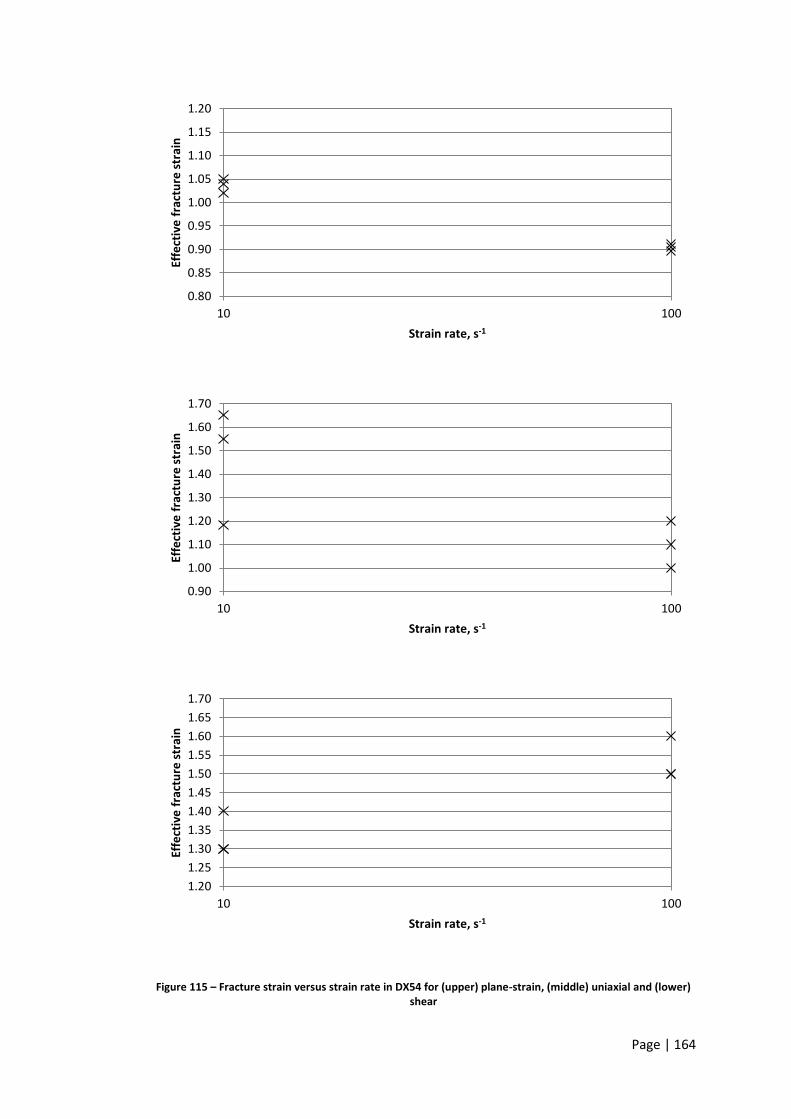
Page | 164

Figure 115 – Fracture strain versus strain rate in DX54 for (upper) plane-strain, (middle) uniaxial and (lower) shear

0.80

0.85

0.90

0.95

1.00

1.05

1.10

1.15

1.20

10 100

Effe

ctiv

e f

ract

ure

str

ain

Strain rate, s-1

0.90

1.00

1.10

1.20

1.30

1.40

1.50

1.60

1.70

10 100

Effe

ctiv

e f

ract

ure

str

ain

Strain rate, s-1

1.20

1.25

1.30

1.35

1.40

1.45

1.50

1.55

1.60

1.65

1.70

10 100

Effe

ctiv

e f

ract

ure

str

ain

Strain rate, s-1

Page | 165

There is a very high level of noise in the uniaxial and shear results because of the high

strains causing delamination and premature failure of the applied random pattern used in

DIC. The strain-time curves were extrapolated to the point of failure, which was identified

by elastic recovery in the static half of the specimen. The noise was highest in the uniaxial

specimen due to the non-linear nature of the strain-time signal. In comparison, the plane-

strain specimen had variation of less than with fracture strains around and at

the low and high strain rates respectively. This suggests that the maximum strain that can

be recorded with the spray-painted DIC pattern is approximately . Higher strains may be

achievable with a different method for applying a random pattern, such as etching.

However, this will exacerbate problems with changing stress states and strain rates.

The strain rates given in Figure 115 are the theoretical rates for the same input velocities as

the DP800 coupons. The characteristic strain rates could not be calculated because of the

strain extrapolation. The characteristic values of alpha are not given for the same reason.

Due to the high noise from the extrapolated data and the fact that only two strain rates

were tested for this material, it is hard to draw firm conclusions on the strain rate

dependency of fracture in DX54. However, Figure 115 shows a reduction in fracture strain

for the two tensile specimens and an increase for shear. The effect is significantly more

pronounced across one order of magnitude than was observed in five orders of magnitude

in DP800. The relative scales of the strain rate dependency for mild and dual phase steels is

the same as those for plastic flow (Kim, et al. 2012). This implies that it may be possible to

predict the strain rate dependency of fracture from plastic flow. It has previously been

found that different grades of steels can have opposite strain rate dependencies for

fracture strain (Boyce and Dilmore 2009). This has been observed here, with DX54’s

fracture strain decreasing in tension at higher strain rates, while the DP800 increases in

ductility. It is assumed that this is due to the different microstructures of the grades and

Page | 166

thus fracture properties cannot be assumed to be comparable across a range of materials.

This means that the strain rate sensitivity must be measured for the appropriate grade.

7.3 – AA5754

AA5754 is a grade of aluminium that is used in structural applications in the automotive

industry. The fracture strain of this material under plane-strain is shown in Figure 116.

Tests were performed at and . As with the DX54 tests, the shear and uniaxial

specimens’ painted DIC patterns delaminated before fracture. In this case, it was not

possible to extrapolate the strain-time signal to the frame of fracture with any degree of

accuracy. The variation in fracture strain at each strain rate is similar to that of DX54 – .

Figure 116 – Fracture strain versus strain rate in AA5754 under plane-strain

The fracture strain of AA5754 increases with strain rate under plane-strain, from to

. Similarly to DX54, the magnitude of this change is much larger than in DP800, though

only a limited number of strain rates were tested. While there is not enough detail to

characterise the strain rate dependency accurately, the general trend is shown.

0

0.1

0.2

0.3

0.4

0.5

0.6

0.7

0.8

0.9

10 100 1000

Effe

ctiv

e f

ract

ure

str

ain

Strain rate

Page | 167

It has previously been shown that the total elongation increases with strain rate for this

aluminium grade (Smerd, et al. 2005). However, as with most aluminium alloys, the strain

rate sensitivity of plastic flow is very low. This means that the magnitude of the strain rate

dependency of fracture is not related to that of plastic flow. Therefore, the previously

noted correlation between DP800 and DX54 does not apply universally, though it may

apply for many grades of steel.

Page | 168

Chapter 8 – Conclusions

8.1 – Conclusions of methodology

A methodology for determining the effect of strain rate on the fracture strain of a high

strength steel under several stress states was presented. The strain rates investigated were

of relevance to automotive crash safety: to and the stress states were shear,

uniaxial and plane-strain tension.

8.1.1 – Loading

This range of strain rates required the use of two loading machines. Traditional high strain

rate testing uses a split Hopkinson bar, typically in the range of . The use of a servo-

hydraulic system allowed the strain rates observed in automotive crash, to , to

be studied. It was found that screw driven quasi-static and servo-hydraulic high speed

machines have different velocity-time characteristics but are broadly comparable.

8.1.2 – Measurement of strain

The local fracture strain was measured using digital image correlation. This was capable of

measuring strains in the range of to . The lower limit is related to the noise of the

system and the upper limit is related to the distortion and delamination of the random

pattern applied to the steel. It is possible to expand this range, though this was not

attempted as it already encompasses a wide range of materials that are of interest to crash

safety.

8.1.3 – Measurement of strain rate

The strain rate was calculated using the local strain measured by DIC from the facet where

the crack initiated. The shear specimen had a linear strain-time relationship, while the two

tensile specimens did not, due to necking. For the uniaxial and plane-strain specimens, it

Page | 169

was necessary to calculate a characteristic strain rate from an approximately linear portion

of the post-necking strain. This resulted in similar grip velocities for all three specimens,

indicating that the equivalent gauge lengths were similar, despite the different geometries

and levels of necking.

8.1.4 – Measurement of stress state

The stress state also had a characteristic value calculated for all three specimens as it is

dependent on the level of strain. A simple average was taken for the same portion of strain

as the strain rate fitting. This was suitable for the uniaxial and plane-strain specimens as

they had a low sensitivity to strain after the initial high noise had dissipated. However, the

shear specimen had a value of alpha that increased linearly with strain and so this

averaging procedure was inaccurate and resulted in a value that is not characteristic of the

variation.

8.1.5 – Thermal analysis

Thermal imaging was performed at two strain rates to measure the temperature rise for

each specimen geometry. It was found that the rise was on the order of despite the

different levels of force and displacement that each geometry was subjected to. Therefore,

the energy per unit volume required for the material to fracture is insensitive to the stress

state. Furthermore, differing strain rate sensitivities for the three stress states are not

caused by unequal heating.

This insensitivity to load and strain implies a potential link to fracture toughness. It may be

that the energy to cause failure in a specimen is a constant and that the change in fracture

strain with stress state and strain rate is a function of the flow stress under these

conditions. However, further work needs to be done to measure the energy local to failure

to examine this.

Page | 170

8.1.6 – Microscopy

Images of the fracture surfaces and sections through tested specimens were taken at

different strain rates. This was to determine if there was a change in fracture mechanism

that was dependent on strain rate, though none was observed.

8.1.7 – Fracture locus

The fracture locus was constructed using a pair of parabolic curves that intersect at

, with minima at and . These values correspond to uniaxial tension,

shear and plane-strain tension respectively. A linear term was added to account for strain

rate sensitivity. The surface for tensile strains had a low residual error and agreed with the

existing quasi-static data. In comparison, the shear fracture surface had a relatively high

residual error and a different form than expected. It is assumed that this is related to an

inconsistent shear specimen and the process of fitting through data predicted from the

tensile curve at the intersection of the two curves. Therefore, it is necessary to improve the

existing shear specimen to obtain a more consistent stress state and to develop an extra

specimen for combined shear-tension. Nonetheless, the existing model is suitable for

simulating fracture under tensile strain at a range of strain rates found in automotive crash

applications.

8.2 – Conclusions of materials

8.2.1 – DP800

DP800 was found to have a fracture strain that increased by across the strain rate

range tested for the uniaxial and plane strain specimens. The shear specimen decreased by

across the same range. This effect is minor and similar in magnitude to the variation in

fracture strain at each strain rate. This variation is larger than can be accounted for by

either the random or systematic errors in the methodology, which indicates that the

Page | 171

fracture strain itself is variable. This is comparable to the variation in forming limit curves.

Further testing is required to see if a statistical form to the variation can be found.

As the strain rate sensitivity for fracture in DP800 is limited, it is not necessary to model the

effect of strain rate. If the strain rate is modelled, it potentially allows a lower factor of

safety to be applied to the fracture and therefore extra weight savings. However, this effect

will be limited in comparison to the spread in the fracture strain at each strain rate. It is

possible to model fracture in DP800 using the previously existing quasi-static data with

some degree of accuracy. This is not the most conservative approach, due to the reduction

in fracture strain in shear at high strain rate. Therefore, to model fracture accurately and

conservatively with a minimum number of tests, it is recommended to perform quasi-static

tests for tension ( ) and high strain rate tests for shear ( ). The

high strain rate to use for shear depends on the application, though is suitable for

automotive crash safety.

An example of this strain rate insensitive fracture locus for DP800 is shown in Figure 117.

As noted previously, there is a discontinuity at and an improved shear specimen

is required to have greater confidence in the left half of the curve. If this locus were shown

with a third axis for strain rate, it would be a horizontal extrude of the curve shown below.

The temperature rises associated with high strain rate loading were not high enough to

significantly affect a dual-phase steel. Likewise, no strain rate dependency for the fracture

mechanism was observed. This is consistent with the lack of strain rate sensitivity in

fracture strain.

Page | 172

Figure 117 – Proposed strain rate insensitive fracture locus for DP800

8.2.2 – DX54 and AA5754

A forming grade of steel, DX54, and a structural grade of aluminium, AA5754, were briefly

tested. Both materials exhibited a much greater response to strain rate. However, further

tests are necessary to establish a strain rate dependency as a limited set of rates was

tested and the high fracture strains required the data to be extrapolated. The DX54 results

imply that a correlation may be found between the magnitude of the effects of strain rate

on the work hardening and the fracture strain. However, no such link was found for the

AA5754. If such a link exists, it may be limited to ferritic steels.

0.0

0.2

0.4

0.6

0.8

1.0

-1.0 -0.5 0.0

Effe

ctiv

e f

ract

ure

str

ain

alpha

Proposed fracture locus

Page | 173

8.3 – Further work

In this section, a range of potential extensions to this investigation are proposed. These

include different materials, loading and manufacturing processes.

8.3.1 – Range of materials

The most obvious extension to this work is to investigate other materials. This could

include other grades of steels or aluminium alloys, both of which are commonly used in

similar automotive applications to dual-phase steels.

Other steels

Boron steels are of significant interest for reducing the mass of some safety-critical

automotive components. (Lanzerath, et al. 2007) states that the conventional ductility of

such grades from global strain measurement is approximately while local fracture

strains are between and , depending on the stress state. These strains are

significantly lower than those found in dual-phase steels, which means that it is even more

important to understand the local fracture properties under crash conditions. As the

fracture strain decreases, the probability of failure in the bulk material rather than at stress

concentrators, such as joints and notches, increases.

Transformation induced plasticity - TRIP- grades of steel are also of interest. These are

typically of similar strength to the dual-phase grades considered in this work. Unlike dual-

phase steels, they have a microstructure that contains meta-stable austenite that

transforms to martensite under loading, which increases the ductility. This transformation,

and hence the ductility, is dependent on several factors, including stress state, strain rate

and temperature (Choi et al. 2009). It is a diffusion-less process involving lattice distortion

(Olson and Owen 1992), meaning that it occurs rapidly and is relevant to high strain rate

loading.

Page | 174

It has previously been found that TRIP steels have an higher elongation to failure with

increasing strain rate (Huh, Kim and Lim 2008) but that higher temperatures make

austenite more stable (Tian, et al. 2006). Simulations have found that less of the austenite

transforms to martensite at higher temperatures and that heat from adiabatic plastic work

has the same effect, through a separate mechanism (Zaera, et al. 2009).

Another point to consider is the paint baking process in the automotive industry. The

elevated temperatures cause a decrease in uniform elongation in TRIP steels

(Durrenberger, Lemoine and Molinari 2011). Furthermore, while TRIP steels bake harden,

unstrained DP steels do not (Zhang, et al. 2008).

In short, while dual-phase steels exhibit low strain rate sensitivity for fracture, TRIP steels

show a much more complicated relationship between temperature, strain rate and

fracture. Therefore, their crash performance cannot accurately be modelled without

further materials characterisation.

Aluminium

A brief study of an aluminium grade, AA5754, was discussed in Section 7.3. A sensitivity to

strain rate for fracture was observed, which is surprising given the existing work showing a

lack of strain rate sensitivity for plastic flow. There is a general trend in the automotive

sector to reduce the weight of vehicles by using composites and lightweight alloys,

including aluminium and magnesium. It is therefore important to characterise the strain

rate dependent fracture properties of these materials in addition to the work presented

here on high strength steel.

Page | 175

8.3.2 – Strain rates and stress states

Strain rate

As discussed in the first chapter, strain rates between and were

investigated and this range was selected for relevance to automotive crash. As discussed in

Chapter 1, rates above or below this range would be of most use to specialised ballistics or

forming and stamping procedures respectively and hence not considered in this work. It is

therefore unlikely to be useful to extend this range, though there is the potential for higher

rate loading to produce higher temperatures. This makes it possible that dual-phase steels

could have a strain rate dependency at higher strain rates.

However, changing strain rates are of considerable interest, particularly for the automotive

sector. Energy absorbing structures experience a high initial strain rate that then reduces,

ideally to zero. For materials with a significant change in fracture strain with strain rate, it

will be necessary to understand the effect of a decelerating load on the fracture locus to

safely reduce the mass of a component.

(Xue 2007) presented a method of damage modelling for fracture initiation. This uses a

damage parameter to track the deterioration of the material. The material is considered to

have fractured when this parameter reaches a value of . As an extension to this work,

damage would be accumulated as the ratio of the plastic work to the fracture strain, both

at a particular set of conditions. This means that when the material is loaded at one rate

and state, the material would fracture when the strain reaches the fracture locus, as

expected.

Stress state

An important extension to this work would be to consider the effect on fracture strain of a

wider range of stress states.

Page | 176

Firstly, an investigation of failure in compression could be important to crash applications.

(Bao and Wierzbicki 2005) discussed a cut-off value of ⁄ beyond which fracture

does not occur. This is represented on a fracture locus by the curve asymptotically

approaching this value. Tests were presented to determine the shape of the curve between

shear and this cut-off point, though they were on bar material rather than sheet.

Considerable work may be required to adapt these specimens to high strain rate sheet.

Secondly, it may be valuable to consider the fracture properties in the region between

plane-strain and biaxial tension. As discussed in Chapter 1, (Bhatnagar, et al. 2007)

produced a fixture to put cruciform sheet specimens under a range of strain states in this

range. This was not considered in this work due to the difficulty in producing a suitable

fixture for high strain rate testing, though would be important for a full understanding of a

material’s dynamic fracture locus.

Uniaxial tension, , is considered to be the local maximum fracture strain and the

intersection between two curves denoting the behaviour of two different failure

mechanisms. The assumption is shared by several models, as shown by (Wierzbicki, et al.

2005). However, (Bao and Wierzbicki 2004) discussed the fracture locus for an aluminium

grade where the transition occurs at , which is given as a change from shear

dominated fracture to void growth. It may be that this transition is determined by the

material’s anisotropy and yield locus shape. As such, it would be useful to produce

specimens to investigate this region closer and determine if there is any strain rate

dependency for the transition in materials where a change in failure mechanism is

identified.

A final point to consider with regards to the stress state is the effect of the stress state

changing during the test. As with strain rates, this work attempted to maintain as

consistent a stress state as possible during each test. However, a real component is likely to

Page | 177

have a varying load and stress state as it deforms. The influence of this is therefore

significant to the understanding of a fracture locus and the ability of a manufacturer to

safely reduce the mass of automotive components.

Damage modelling, as used for changing strain rates, may not be a suitable method for

modelling the effect of non-linear strain paths. Pre-strain in a material not only affects the

level of a forming limit curve, but also shifts the minimum away from plane-strain (Volk, et

al. 2012). As forming limit curves and fracture loci are similar concepts, it is likely that a

material undergoing a complex, non-linear strain path will have a distorted fracture locus.

(Volk, et al. 2012) presented a form of damage modelling for bilinear strain paths in

forming, though the combined effective strain needs to be compared to a FLC for a pre-

strained sample. It is important to understand how this compares to fracture to be able to

simulate the effect of forming operations on crash structures.

8.3.3 – Manufacturing processes

Specimen production

This work has investigated the effect of strain rate on the fracture strain of milled

specimens. However, automotive crash components are rarely milled. The sheet processes

generally used in high volume are stamping and punching, which reduce the ductility of the

material through cold working (Davies 1981). This will be complicated to fully characterise,

as it combines damage modelling at different strain rates and strain paths. In addition, the

effect of damage at the sheet edge due to stamping and trimming will only be captured in

specimens that fail from the edge. The shear and plane-strain specimens should be

unaffected, up to a critical level of edge damage, as they fail from the centre of the

material.

Page | 178

Pre-strained material

In addition to the effect of non-linear strain paths on fracture, there is an effect combined

with strain rate. (Huh, Kim and Lim 2008) investigated the effect of pre-strain on the

mechanical properties of several grades of steel. Figure 118 below shows the plastic flow

for DP600 with three levels of pre-strain and strain rate.

Figure 118 – Engineering stress-strain curves for a) TRIP600 and b) DP600 comparing levels of pre-strain

It is evident that the level of pre-strain has no effect on the hardening of the material but

there is a significant effect on the ductility at strain rates over - . The ductility of the

DP600 was reduced for both and levels of pre-strain loaded at a strain rate of

, though the pre-strained specimens increased in ductility at .

Additionally, these strain measurements are global rather than local strain. As such, it

Page | 179

would be interesting to investigate the effect of pre-strain on the local fracture strain. It is

also necessary to understand this behaviour in order to safely reduce the mass of safety

critical automotive components. According to (Choudhury, Lai and Wong 2006), the

majority of automotive components are stamped and that a typical problem for stamping is

the tearing of the sheet. As the understanding of forming limits for materials and process

simulation improves, the strains achieved in standard parts without tearing will increase.

This means that it is increasingly important to understand the fracture performance of a

range of processed materials and not just as rolled.

Joints

Failure often occurs at stress raisers, such as notches and joints (Lanzerath, et al. 2007). It

has been found that the strength of spot welds and the fracture mechanism is strain rate

sensitive (Langrand and Markiewicz 2010). Likewise, self-piercing rivets have an

exponential decrease in ductility with increasing strain rate (Wood, Schley and Williams, et

al. 2011). This knowledge needs to be combined with the strain rate dependent fracture of

the bulk material in order to accurately simulate component failure. This presents a

challenge as joint failure will lead to rapid changes in strain rate and path.

Sheet gauge

The effect of the sheet gauge has not been studied here, as all of the specimens were

thick. The sheet gauge is known to influence both forming limit curves and

fracture. As the thickness of the sheet increases, the FLC increases linearly, up to a critical

thickness (Banabic 2010). Likewise, the fracture strain increases with sheet thickness for a

plate with a hole (Bao 2004). This is likely to be related to the through-thickness necking

and so specimens with different levels of necking, such as shear and plane-strain may show

different levels of sensitivity to sheet gauge. This is an important consideration as the

Page | 180

improved simulation accuracy offered by local fracture strain measurement may lead to

down-gauging as a way to reduce component mass.

8.3.4 – Sensitivity analysis

The effect of small changes to the specimen geometry was not studied here. It is important

to quantify the effect of specimen variation from manufacturing as it could account for a

significant portion of the variation in the fracture strain. However, it is unlikely to affect the

two tensile specimens as they have relatively large gauge widths. Therefore, a large

variation in the geometry is needed to alter the stress state significantly. In comparison, the

shear specimen has a small gauge area and Section 5.2.1 shows that the shape of a

shearing specimen has a substantial effect on the stress state.

8.3.5 – Fracture locus function

The current fracture locus function is unsuitable for modelling due to the discrepancy

between the shear and tensile surfaces at . This means that a small change in the

stress state of an element leads to a large step change in the predicted fracture strain. This

may be significantly improved by testing with a more consistent shear specimen. However,

it may also be necessary to design a function that removes this gap.

For some materials, a linear strain rate dependency will not be suitable. Alternative strain

rate terms include polynomial, exponential and step functions. Therefore, it is impractical

to design a function that can accurately model all materials and different functions will

need to be developed for dissimilar material classes.

An important step is to implement a user material model for a finite element analysis

package that simulates fracture by deleting elements according to this criterion. This will

allow validation of the fracture locus against component, rather than coupon, testing.

Page | 181

Chapter 9 – References

Aghaie-Khafri, M, and A Zargaran. “High temperature tensile behaviour of a PH stainless steel.” Materials Science and Engineering: A, 2010: 4727-4732.

Akbarpour, M.R, and A Ekrami. “Effect of temperature on flow and work hardening behaviour of high bainite dual phase (HBDP) steels.” Materials Science and Engineering A, 2008: 293-298.

An, Y.G, H Vegter, and J Heijne. “Development of simple shear test for the measurement of work hardening.” Journal of Materials Processing Technology, 2009: 4248-4254.

Aretz, H. “Numerical analysis of diffuse and localized necking in orthotropic sheet materials.” International Journal of Plasticity, 2007: 798-840.

Aspenberg, D, R Larsson, and L Nilsson. “An evaluation of the statistics of steel material model parameters.” Journal of Materials Processing Technology, 2012: 1288-1297.

Banabic, D. Sheet Metal Forming Processes. Springer, 2010.

Bandyopadhyay, S.N. “Stability of void growth in an incompressible solid under uniaxial tension and shear.” Engineering Fracture Mechanics, 1979: 635-643.

Banks-Sills, L, M Arcan, and H Gabay. “A mode II fracture specimen - finite element analysis.” Engineering Fracture Mechanics, 1984: 739-750.

Banks-Sills, L, M Arcan, and H.D Bui. “Toward a pure shear specimen for KIIc determination.” International Journal of Fracture, 1983: 9-14.

Bao, Y. “Dependence of fracture ductility on thickness.” Thin-Walled Structures, 2004: 1211-1230.

Bao, Y, and T Wierzbicki. “On fracture locus in the equivalent strain and stress triaxiality space.” International Journal of Mechanical Sciences, 2004: 81-98.

Bao, Y, and T Wierzbicki. “On the cut-off value of negative triaxiality for fracture.” Engineering Fracture Mechanics, 2005: 1049-1069.

Becker, N, K Pöhlandt, and K Lange. “Improvement of the Plane-Strain Compression Test for Determining FlowCurves.” Manufacturing Technology, 1989: 227-230.

Beese, A.M, M Luo, Y Li, Y Bai, and T Wierzbicki. “Partially coupled anisotropic fracture model for aluminium sheet.” Engineering Fracture Mechanics, 2010: 1128-1152.

Bhatnagar, N, R Bhardwaj, P Selvakumar, and M Brieu. “Development of a biaxial tensile test fixture for reinforced thermoplastic composites.” Polymer Testing, 2007: 154-161.

Boger, R.K, R.H Wagoner, F Barlat, M.G Lee, and K Chung. “Continuous, large strain, tension/compression testing of sheet material.” International Journal of Plasticity, 2005: 2319-2343.

Page | 182

Boyce, B.L, and M.F Dilmore. “The dynamic tensile behavior of tough, ultrahigh-strength steels at strain-rates from 0.0002 s−1 to 200 s−1.” International Journal of Impact Engineering, 2009: 263-271.

British Standards Institution. “26203-2 Metallic materials - Tensile testing at high strain rates.” 2012.

British Standards Institution. “6892-1 Metallic materials. Tensile testing. Method of test at ambient temperature.” 2009.

Brünig, M. “Numerical analysis and modeling of large deformation and necking behaviour of tensile specimens.” Finite Elements in Analysis and Design, 1998: 303-319.

Cao, R, L Li, J.H Chen, and J Zhang. “Study on compression deformation, damage and fracture behavior of TiAl alloys: Part II. Fracture behavior.” Materials Science and Engineering A, 2010: 2468-2477.

Choi, H.-H, S.-M Hwang, Y.H Kang, J Kim, and B.S Kang. “Comparison of Implicit and Explicit Finite-Element Methods for the Hydroforming Process of an Automobile Lower Arm.” International Journal of Advanced Manufacturing Technology, 2002: 407-413.

Choi, K.S, W.N Liu, X Sun, and M.A Khaleel. “Microstructure-based constitutive modeling of TRIP steel: Prediction of ductility and failure modes under different loading conditions.” Acta Materialia, 2009: 2592-2604.

Choudhury, I.A, O.H Lai, and L.T Wong. “PAM-STAMP in the simulation of stamping process of an automotive component.” Simulation Modelling Practice and Theory, 2006: 71-81.

Comstock, R.J, D.K Scherrer, and R.D Adamczyk. “Hole expansion in a variety of sheet steels.” Journal of Materials Engineering and Performance, 2006: 675-683.

Corus Automotive. “Reference: Pocket book of steel.” Tata Steel Automotive web site. 2009. http://www.tatasteelautomotive.com/en/reference/publications/pocket_book_of_steel/ (accessed 05 23, 2012).

Davies, R.G. “Edge cracking in high strength steels.” Journal of Applied Metalworking, 1981: 293-299.

Dieter, G. Mechanical Metallurgy. McGraw-Hill, 1988.

Du Bois, P.A, S Kolling, M Koesters, and T Frank. “Material behaviour of polymers under impact loading.” International Journal of Impact Engineering, 2006: 725-740.

Durrenberger, L, X Lemoine, and A Molinari. “Effects of pre-strain and bake-hardening on the crash properties of a top-hat section.” Journal of Materials Processing Technology, 2011: 1937-1947.

Ebelsheiser, H, M Feucht, and F Neukamm. “On Calibrating Advanced Damage Models Using Sheet Metal Coupon Tests.” LS-DYNA Anwenderforum. Bamberg: DYNAmore GmbH, 2008. H-I-1-10.

Page | 183

Ekrami, A. “High temperature mechanical properties of dual phase steels.” Materials Letters, 2005: 2070-2074.

FLIR. “Photometry Form.” 2010.

Fyllingen, Ø, O.S Hopperstad, and M Langseth. “Robustness study on the behaviour of top-hat thin-walled high-strength steel sections subjected to axial crushing.” International Journal of Impact Engineering, 2009: 12-24.

García-Garino, C, F Gabaldón, and J.M Goicolea. “Finite element simulation of the simple tension test in metals.” Finite Elements in Analysis and Design, 2006: 1187-1197.

Hertzberg, R.W. Deformation and fracture Mechanics of Engineering Materials. John Wiley & Sons, 1996.

Hiroshi, K, and H Koichi. “Anisotropy and softening induced by void growth: A numerical simulation of micro-structural process.” Computers and Structures, 1988: 909-913.

Hopperstad, O.S., T. Børvik, M. Labibes, K. Langseth, and C. Albertini. “On the influence of stress triaxiality and strain rate on the behaviour of a structural steel. Part I. Experiments.” European Journal of Mechanics A/Solids, 2003: 1-13.

Huh, H, S-B Kim, and J-H Lim. “Dynamic tensile characteristics of TRIP-type and DP-type steel sheets for an auto-body.” International Journal of Mechanical Sciences, 2008: 918-931.

Hull, D. “The effect of mixed mode I/III on crack evolution in brittle solids.” International Journal of Fracture, 1995: 59-79.

Instron. 2525-800 Series Load Cells. 2005.

Instron. 2630 Series Strain Gauge Extensometers. 2004.

Janssens, K, F Lambert, S Vanrostenberghe, and M Vermeulen. “Statistical evaluation of the uncertainty of experimentally characterised forming limits of sheet steel.” Journal of Materials Processing Technology, 2001: 174-184.

Jones, S.E, and P.P Gillis. “Analysis of a plane strain neck in a flat sheet.” Mechanics of Materials, 1984: 35-40.

Joun, M, I Choi, J Eom, and M Lee. “Finite element analysis of tensile testing with emphasis on necking.” Computational Materials Science, 2007: 63-69.

Kapoor, R, and S Nemat-Nasser. “Determination of temperature rise during high strain rate deformation.” Mechanics of Materials, 1998: 1-12.

Keralavarma, S.M, and A.A Benzerga. “A constitutive model for plastically anisotropic solids with non-spherical voids.” Journal of the Mechanics and Physics of Solids, 2010: 874-901.

Kim, J-H, D Kim, H.N Han, F Barlat, and M-G L. “Strain rate dependent tensile behavior of advanced high strength steels: Experiment and constitutive modeling.” Materials Science and Engineering, 2012.

Page | 184

Kim, S.B., H. Huh, H.H. Bok, and M.B. Moon. “Forming limit diagram of auto-body steel sheets for high-speed sheet metal forming.” Journal of Materials Processing Technology, 2011: 851-862.

Kumosa, M, and Y Han. “Non-linear finite-element analysis of Iosipescu specimens.” Composites Science and Technology, 1999: 561-573.

Landis, E.N, and E.N Nagy. “Three-dimensional work of fracture for mortar in compression.” Engineering Fracture Mechanics, 2000: 223-234.

Langrand, B, and E Markiewicz. “Strain-rate dependence in spot welds: Non-linear behaviour and failure in pure and combined modes I/II.” International Journal of Impact Engineering, 2010: 792-805.

Lanzerath, H, A Bach, G Oberhofer, and H Gese. “Failure Prediction of Boron Steels in Crash.” SAE World Congress & Exhibition. Detroit: SAE International, 2007.

Lee, Y.S, Y.N Kwon, S.H Kang, S.W Kim, and J.H Lee. “Forming limit of AZ31 alloy sheet and strain rate on warm sheet metal forming.” Journal of Materials Processing Technology, 2008: 431-435.

Li, Y, and T Wierzbicki. “Prediction of plane strain fracture of AHSS sheets with post-initiation softening.” International Journal of Solids and Structures, 2010: 2316-2327.

Li, Z, and J Lambros. “Strain rate effects on the thermomechanical behaviour of polymers.” International Journal of Solids and Structures, 2001: 3549-3562.

Liu, B, X Qiu, Y Huang, K.C Hwang, M Li, and C Liu. “The size effect on void growth in ductile materials.” Journal of the Mechanics and Physics of Solids, 2003: 1171-1187.

Mackenzie, A.C, J.W Hancock, and D.K Brown. “On the influence of state of stress on ductile failure initiation in high strength steels.” Engineering Fracture Mechanics, 1977: 167-188.

Mannan, S.L, K.G Samuel, and P Rodriguez. “Influence of temperature and grain size on the tensile ductility of AISI 316 stainless steel.” Materials Science and Engineering, 1985: 143-149.

Markiewicz, E, P Ducrocq, and P Drazetic. “An inverse approach to determine the constitutive model parameters from axial crushing of thin-walled square tubes.” International Journal of Impact Engineering, 1998: 433-499.

Mason, J.J, A.J Rosakis, and G Ravichandran. “On the strain and strain rate dependence of the fraction of plastic work converted to heat: an experimental study using high speed infrared detectors and the Kolsky bar.” Mechanics of Materials, 1994: 135-145.

Mattos, H.S.C, and F.E.G Chimisso. “Necking of elasto-plastic rods under tension.” International Journal of Non-Linear Mechanics, 1997: 1077-1086.

Miyauchi, K. “Stress-strain Relationship in Simple Shear of In-plane Deformation.” Proceedings of the 13th Biennial Congress of the IDDRG. Melbourne, 1984. 436-443.

Page | 185

Nahshon, K, and J.W Hutchinson. “Modification of the Gurson Model for shear failure.” European Journal of Mechanics - A/Solids, 2008: 1-17.

Neukamm, F, M Feucht, A Haufe, and K Roll. “On closing the constitutive gap between forming and crash simulation.” 10th International LS-DYNA Users Conference. Dearborn, 2008. 1221-1232.

Olson, G.B, and W.S Owen. Martensite. ASM International, 1992.

Panagopoulos, C, and A Panagiotakis. “The effect of strain rate on the tensile behaviour of anodized aluminum.” Materials Letters, 1991: 70-73.

Pardoen, T, F Hachez, B Marchioni, P.H Blyth, and A.G Atkins. “Mode I fracture of sheet metal.” Journal of the Mechanics and Physics of Solids, 2004: 423-452.

Peirs, J, P Verleysen, and J Degrieck. “Experimental study of the influence of strain rate on fracture of Ti6Al4V.” Procedia Engineering, 2011: 2336-2341.

Peirs, J, P Verleysen, and J Degrieck. “Novel pure-shear sheet specimen geometry for dynamic material characterization.” In Workshop in Memory of Prof. J.R. Klepaczko, by A Rusinek and P Chevrier, 89-96. 2009.

Percy, J.H, and R.H Brown. “The Effect of Strain Rate on the Forming Limit Diagram for Sheet Metal.” Manufacturing Technology, 1980: 151-152.

Prior, A.M. “Applications of implicit and explicit finite element techniques to metal forming.” Journal of Materials Processing Technology, 1994: 649-656.

Ramezani, M, and Z.M Ripin. “Combined experimental and numerical analysis of bulge test at high strain rates using split Hopkinson pressure bar apparatus.” Journal of Materials Processing Technology, 2010: 1061-1069.

Rice, J.R, and D.M Tracey. “On the ductile enlargement of voids in triaxial stress fields.” Journal of the Mechanics and Physics of Solids, 1969: 201-217.

Rosakis, P, A.J Rosakis, G Ravichandran, and J Hodowany. “A thermodynamic internal variable model for the partition of plastic work into heat and stored energy in metals.” Journal of the Mechanics and Physics of Solids, 2000: 581-607.

Shabara, M.A.N, A.A El-Domiaty, and M.D Al-Ansary. “Estimation of plane strain fracture toughness from circumferentially bluntly notched round-bar specimens.” Engineering Fracture Mechanics, 1996: 533-541.

Shackelford, J.F. Introduction to Materials Science For Engineers. Pearson Education, 2005.

Smerd, R, S Winkler, C Salisbury, M Worswick, D Lloyd, and M Finn. “High strain rate tensile testing of automotive aluminum alloy sheet.” International Journal of Impact Engineering, 2005: 541-560.

Sun, D-Z, F Andrieux, and M Feucht. “Damage modelling of a TRIP steel for integrated simulation from deep drawing to crash.” 7th European LS-DYNA Conference. Freiburg: DYNAmore GmbH, 2009.

Tarigopula, V, et al. “A Study of Large Plastic Deformations in Dual Phase Steel Using Digital Image Correlation and FE Analysis.” Experimental Mechanics, 2008: 181-196.

Page | 186

Tarigopula, V, O.S Hopperstad, M Langseth, and A.H Clausen. “An evaluation of a combined isotropic-kinematic hardening model for representation of complex strain-path changes in dual-phase steel.” European Journal of Mechanics - A/Solids, 2009: 792-805.

Tata Steel. “Crach Failure Loci DP800 IJTC .” 2008.

—. “Testing methods for fracture modelling.” 2009.

ten Horn, C, S Carless, and I van Stijn. “Influence of material model on crash simulations.” Steels in Cars & Trucks. Wiesbaden, 2005.

Teng, X, and T Wierzbicki. “Evaluation of six fracture models in high velocity perforation.” Engineering Fracture Mechanics, 2006: 1653-1678.

Tian, R, L Li, B.C De Cooman, X-C Wei, and P Sun. “Effect of Temperature and Strain Rate on Dynamic Properties of Low Silicon TRIP Steel.” Journal of Iron and Steel Research International, 2006: 51-56.

Volk, W, H Hoffmann, J Suh, and J Kim. “Failure prediction for nonlinear strain paths in sheet metal forming.” Manufacturing Technology, 2012: 259-262.

Wierzbicki, T, Y Bao, Y-W Lee, and Y Bai. “Calibration and evaluation of seven fracture models.” International Journal of Mechanical Sciences, 2005: 719-743.

Wilkins, M.L, R.D Streit, and J.E Reaugh. Cumulative-strain-damage model of ductile fracture: simulation and prediction of engineering fracture tests. Lawrence Livermore National Laboratory, 1980.

Wood, P.K.C, and C.A Schley. Strain Rate Testing of Metallic Materials and their Modelling for use in CAE based Automotive Crash Simulation Tools (Recommendations and Procedures). Smithers Rapra, 2009.

Wood, P.K.C, C.A Schley, M.A Williams, and A Rusinek. “A model to describe the high rate performance of self-piercing riveted joints in sheet aluminium.” Materials & Design, 2011: 2246-2259.

Wood, P.K.C, C.A Schley, R Beaumont, M.A Williams, A Pearce, and M.A Buckley. “Improved efficiency and quality control in the manufacture and preparation of metallic specimens for high rate tensile testing.” Proceedings of the 7th International Conference on Manufacturing Research (ICMR09). Warwick, 2009.

Xiao, X, C-K Hsiung, and Z Zhao. “Analysis and modeling of flexural deformation of laminated steel.” International Journal of Mechanical Sciences, 2008: 69-82.

Xue, L. “Damage accumulation and fracture initiation in uncracked ductile solds subject to triaxial loading.” International Journal of Solids and Structures, 2007: 5163-5181.

Zaera, R, A Casado, J Fernández-Sáez, A Rusinek, and M.E Angulo. “Influence of strain-induced martensitic transformation on neck formation during dynamic tension of sheet steel.” In Workshop in Memory of Prof. J.R. Klepaczko, by A Rusinek and P Chevrier, 243-250. 2009.

Page | 187

Zhang, J, R Fu, M Zhang, R Liu, X Wei, and L Li. “Bake hardening behaviour of TRIP and DP steels.” Journal of University of Science and Technology Beijing, Mineral, Metallugry, Material, 2008: 132-137.

Zhang, Z.L, C Thaulow, and J Ødegård. “A complete Gurson model approach for ductile fracture.” Engineering Fracture Mechanics, 2000: 155-168.

Page | 188

Chapter 10 – Appendices

A1 - Derivation of stress triaxiality and alpha values

Starting from the basic equation for stress triaxiality

Substitute in the formulae for mean and Von Mises stress

⁄ ( )

√

⁄ *( ) ( )

( ) +

⁄

Assume a two dimensional stress state in sheet material, σ3 = 0, and simplify

⁄ ( )

√

⁄ *

( ) +

⁄

√ ( )

{

}

⁄

Formula for alpha

Pure shear

Assume σ2 = -σ1, ϵ2 = -ϵ1

√ ( )

{

}

⁄

{ }

⁄

Page | 189

Uniaxial tension

Assume σ2 = 0

√ ( )

{ }

⁄

√ ( )

√

⁄

Plane strain

Assume ϵ2 = 0

√ ( )

{

}

⁄

√ ( )

{ }

⁄

Page | 190

√ ( )

√

√

√ √

√

√

Page | 191

A2 – Typical LS-DYNA keyword file

*KEYWORD $ *TITLE Shear fracture specimen $ $ This section imports two files, one containing specimen $ geometry nodes and elements $ The second contains a material model for DP800 $ *INCLUDE shear-geo.key $ *INCLUDE ../../../materials/dp800-static.key $ $ Standard set of control options $ *CONTROL_ACCURACY 1 2 $ *CONTROL_BULK_VISCOSITY 0 0 -1 $ *CONTROL_OUTPUT 1 3 0 0 1e-4 0 1000 5000 0 0 0 0 0 $ *CONTROL_SHELL 20 1 0 1 2 2 1 0 $ *CONTROL_SOLUTION 0 0 0 1000 $ *CONTROL_TERMINATION 1e-1 0 5e-2 0 5 $ *CONTROL_TIMESTEP 0 0.9 0 4.5E-8 0 0 0 0 $ $ Standard set of output options $ *DATABASE_MATSUM 2.0E-4 1 *DATABASE_NODFOR 2.0E-4 1 *DATABASE_NODOUT 2.0E-4 1 *DATABASE_BINARY_D3DRLF 10000

Page | 192

*DATABASE_BINARY_D3DUMP 50000 *DATABASE_BINARY_D3PLOT 2.0E-4 0 0 0 *DATABASE_BINARY_D3THDT 1.0E-5 0 *DATABASE_BINARY_INTFOR 2.0E-4 0 *DATABASE_BINARY_RUNRSF 50000 0 *DATABASE_BINARY_XTFILE 2.0E-4 *DATABASE_EXTENT_BINARY 1 0 5 1 1 1 1 1 0 0 2 2 2 3 2 0 0 0 0.0 0 0 $ $ Two rigid materials for the grips $ Static grip is completely fixed in translation and rotation $ Moving grip is allowed to translate in x $ *MAT_RIGID_TITLE Static grip 10 7.8e-9 210000 0.3 0 0 0 0 1 7 7 0 0 0 0 0 0 $ *MAT_RIGID_TITLE Moving grip 20 7.8e-9 210000 0.3 0 0 0 0 1 5 7 0 0 0 0 0 0 $ $ Standard section for shell elements in metal $ 1.5 mm thick with fully integrated elements $ *SECTION_SHELL_TITLE shell section 1 16 0.833 3 0 0 0 0 1.5 1.5 1.5 1.5 0 0 0 0 $ $ These are standard part cards with the same shell section applied $ The grips have the rigid materials from above $ Deformable part has the DP800 material from include file $ *PART deformable 2 1 99988899 0 0 0 0 0 $ *PART static grip

Page | 193

3 1 10 0 0 0 0 0 $ *PART moving grip 4 1 20 0 0 0 0 0 $ $ These cards define the velocity of the moving grip $ The curve and the initial velocity correspond to $ 100 mm/s in x $ *DEFINE_CURVE 10 0 1.0 1.0 0.0 0.0 0 0.0 100.00000 1.0000000 100.00000 $ $ *BOUNDARY_PRESCRIBED_MOTION_RIGID 4 1 0 10 1.0 0 100000.0 0.0 $ $ *INITIAL_VELOCITY_RIGID_BODY 4 100 0 0 0 0 0 $ *END

Page | 194

A3 – Octave/Matlab script for determining strain rate and ratio

of strains

% Call function with x = time, y = strain, a = alpha, target = maximum least square error

function strain_rate ( x, y, a, target ) % Check for a supplied target and use default in not found if ( ! exist ( "target" ) ) target = 0.1; endif % xval et al are truncated versions of input data, initialised as copies xval = x; yval = y; aval = a; % P contains polynomial coefficients from fitting % S has extra data, including least square error P = 0; S = 0; % Loop over decreasing amounts of data until target is reached for j = 1:(0.88 * size ( x ) )

% Fit polynomial to data, 1 indicates linear fit [ P, S ] = polyfit ( xval, yval, 1 ); % Check against target and break out of loop if reached if ( S.normr < target ) break; endif

% If continuing loop, empty temporary fitting vectors xval = 0; yval = 0; aval = 0; % Fill temporary vectors with data from next sample in vector to the end for k = (j+1):size(x) xval ( k - j ) = x ( k ); yval ( k - j ) = y ( k ); aval ( k - j ) = a ( k ); endfor

Page | 195

endfor % Alpha is calculated as mean of curve for the same portion of data as the linear strain rate % alpha_plot is a vector containing this value % repeated for the number of samples in the reduced data alpha = mean ( aval ); alpha_plot = ones ( size ( aval, 2 ), 1 ) * alpha; % Print message if the least squares error does not reach the target if ( S.normr > target ) printf ( "Target of %f not met\n", target ) endif % Print out fracture strain, strain rate and alpha printf ( "Fracture strain = %f\n", y( end ) ); printf ( "Strain rate = %f\n", P( 1 ) ); printf ("Alpha = %f\n", alpha ); % Create a figure and clear existing data figure(1); clf; % Plot strain versus time plot ( x, y, "b ;Recorded data;", 'LineWidth',2 ) hold on % Plot fitted line using reduced data section and generate y-data % using polyval and the fitted parameters P plot ( xval, polyval ( P, xval ), "r ;Linear strain rate best fit;", 'LineWidth',2 ) % Set up legend and axes labels legend('Location','SouthEast'); xlabel ( "Time, s", 'FontSize',22 ); ylabel ( "True strain", 'FontSize',22 ); hold off % Create a second figure and clear existing data figure(2) clf; % Plot alpha against time

Page | 196

plot ( x, a, "b ;Recorded data;", 'LineWidth',2 ) hold on % Plot average alpha against time for reduced data section plot ( xval, alpha_plot, "r ; Fitted value;", 'LineWidth',2 ) % Set up legend and axes labels legend('Location','SouthEast'); xlabel ( "Time, s", 'FontSize',22 ); ylabel ( "Ratio of principal strains", 'FontSize',22 ); % Set y-axis to limits of -1 and 0 or initial noise will dominate the figure yaxis = axis; yaxis(3) = -1; yaxis(4) = 0; axis ( yaxis ); hold off endfunction

Page | 197

A4 – Octave/Matlab script for determining fracture locus

% This function is called from locus() % Parameters are p = polynomial coefficients fitted at quasi-static % alpha, s_rate, frac = vectors of experimental results % pred_frac is the predicted fracture strain calculated from alpha and s_rate for given p % Return value is residual sum of squares error between predicted and measured strain function err = tensile (p, alpha, s_rate, frac) % Calculate predicted fracture strain from polynomial in terms of alpha % added to linear term for strain rate dependency pred_frac = ((p(1).*(alpha.^2)) + (p(2) .* alpha) + p(3)) + (p(4) * s_rate); % Calculate residual sum of squares err = sum((frac - pred_frac).^2); endfunction % Call this function to determine fracture locus % No parameters as data is included in file % No return value, output is printed function locus() % Column vectors of strain rate, alpha and fracture strain % for each stress state, data is omitted for clarity ps.s_rate = [ ]'; ps.alpha = [ ]'; ps.frac = [ ]'; ua.s_rate = [ ]'; ua.alpha = [ ]'; ua.frac = [ ]'; s.s_rate = [ ]'; s.alpha =[ ]'; s.frac = [ ]'; % Calculate initial polynomial fit at first strain rate % Use the first data for uniaxial, plane-strain and mirror % them around alpha = 0 to get local minimum here % Also create vector for mirrored fracture strain poly_tensile_alpha = [ua.alpha(1) ps.alpha(1) ps.alpha(1)*-1 ua.alpha(1)*-1]; poly_tensile_frac = [ua.frac(1) ps.frac(1) ps.frac(1) ua.frac(1)]; % Fit second order polynomial through mirrored quasi-static % alpha and fracture strain

Page | 198

poly_tensile_val = polyfit(poly_tensile_alpha, poly_tensile_frac, 2); % Fit linear polynomial through plane-strain fracture strain with respect to % strain rate for initial estimate of tensile strain rate dependency % Depending on material, may be more appropriate to choose a uniaxial state poly_ps_val = polyfit(ps.s_rate, ps.frac, 1); % Output the parameters for the initial estimate from polyfit in alpha and strain rate % p(1) to (3) are the coefficients of the alpha polynomial, p(4) is the strain rate term printf ( "tensile poly fit p(1) %f p(2) %f p(3) %f p(4) %f\n", poly_tensile_val(1), poly_tensile_val(2), poly_tensile_val(3), poly_ps_val(1) ); % Concatenate the plane-strain and uniaxial strain rates, alpha and fracture strains % with mirrored data for tensile surface fitting tensile.s_rate = cat (1, ua.s_rate, ps.s_rate, ps.s_rate, ua.s_rate); tensile.alpha = cat(1, ua.alpha, ps.alpha, ps.alpha*-1, ua.alpha*-1); tensile.frac = cat(1, ua.frac, ps.frac, ps.frac, ua.frac); % Concatenate polynomial parameters from quasi-static % fracture locus and plane-strain strain rate tensile.p=cat(1, poly_tensile_val', poly_ps_val(1)); options(2)=1e-12; % Determine parameters for tensile fracture surface % Operates by minimising least-square error % Is allowed to vary the fitted polynomial values % Compares against experimental data for alpha, % strain rate and fracture strain tensile.vars = fmins('tensile', tensile.p, options, 0, tensile.alpha, tensile.s_rate, tensile.frac); % Output the 3D fitted parameters, p(1) to (3) are the alpha polynomial coefficients, % p(4) is the strain rate term printf ( "tensile surface fit p(1) %f p(2) %f p(3) %f p(4) %f \n", tensile.vars(1), tensile.vars(2), tensile.vars(3), tensile.vars(4) ); % Function for tensile fracture surface using fitted parameters tensile_f = @(x, y)(((tensile.vars(1) * (x.^2)) + (tensile.vars(2) * x ) + tensile.vars(3)) + ((tensile.vars(4) * y ) )); % Output residual sum of squares from initial and fitted parameters printf ( "orig resid %f fitted resid %f\n", @tensile(tensile.p, tensile.alpha, tensile.s_rate, tensile.frac), sum((tensile.frac - tensile_f(tensile.alpha, tensile.s_rate)).^2) );

Page | 199

% Determine shear fracture surface % Create a vector for alpha = -0.5 and associated strain rates, data removed for clarity % Calculate corresponding fracture strains using tensile surface equation s_ua.alpha = ones(18, 1) * -0.5; s_ua.s_rate = [ ]'; s_ua.frac = tensile_f(s_ua.alpha, s_ua.s_rate); % Fit a second order polynomial for shear fracture % through shear measurement and calculated uniaxial % mirrored around alpha = -1 to obtain local mimimum poly_shear_alpha = [(2 + s_ua.alpha(1))*-1, (2 + s.alpha(1))*-1, s.alpha(1), s_ua.alpha(1)]; poly_shear_frac = [s_ua.frac(1), s.frac(1), s.frac(1), s_ua.frac(1)]; poly_s_val = polyfit(poly_shear_alpha, poly_shear_frac, 2); % Fit a linear polynomial through the shear fracture and strain rate poly_s_rate = polyfit(s.s_rate, s.frac, 1); % Output initial estimate of parameters from polynomial fitting printf ( "shear poly fit p(1) %f p(2) %f p(3) %f p(4) %f\n", poly_s_val(1), poly_s_val(2), poly_s_val(3), poly_s_rate(1) ); % Fill structure with initial estimates of parameters from polynomial fitting shear.p(1) = poly_s_val(1); shear.p(2) = poly_s_val(2); shear.p(3) = poly_s_val(3); shear.p(4) = poly_s_rate(1) ; % Concatenate the vectors for alpha, strain rate and fracture strain for shear measurement % and uniaxial calculation, mirrored at alpha = -1 shear.s_rate = cat(1, s_ua.s_rate, s.s_rate, s.s_rate, s_ua.s_rate); shear.alpha = cat(1, (2 + s_ua.alpha) * -1, (2 + s.alpha) * -1, s.alpha, s_ua.alpha); shear.frac = cat(1, s_ua.frac, s.frac, s.frac, s_ua.frac); % Determine parameters for shear fracture surface % using same equation and fitting as tensile surface % with new input variables and experimental data shear.vars = fmins('tensile', shear.p, options, 0, shear.alpha, shear.s_rate, shear.frac); % Output fitted parameters printf ( "shear surface fit p(1) %f p(2) %f p(3) %f p(4) %f\n", shear.vars(1), shear.vars(2), shear.vars(3), shear.vars(4) ); % Function for shear fracture surface using fitted parameters

Page | 200

shear_f = @(x, y)(((shear.vars(1) * (x.^2)) + (shear.vars(2) * x )+ shear.vars(3)) + ((shear.vars(4) * (y)) )); % Output residual sums of squares from initial and fitted parameters printf ( "orig resid %f fitted resid %f\n", @tensile(shear.p, shear.alpha, shear.s_rate, shear.frac), sum((shear.frac - shear_f(shear.alpha, shear.s_rate)).^2) ); % Plot fracture surfaces % Clear current figure clf; % Frequency for surface mesh generation alpha_tick = 50; s_rate_tick = 50; % Generate co-ordinate vectors for mesh in % alpha and strain rate % logspace gives log base 10 spaced vector between 10^-2 % and 10^2.69897 tensile_d_alpha = -0.5 : 1 / alpha_tick : 0; shear_d_alpha = -1 : 1 / alpha_tick : -0.5; d_s_rate = logspace(-2, 2.69897, s_rate_tick); % Create mesh for tensile fracture surface from % tensile alpha and strain rate % Calculate fracture strain for this mesh using function % with fitted parameters [tensile_plot_x, tensile_plot_y] = meshgrid(tensile_d_alpha, d_s_rate); tensile_plot_z = tensile_f(tensile_plot_x, tensile_plot_y); % Create mesh and calculate fracture strain for shear % fracture surface [shear_plot_x, shear_plot_y] = meshgrid(shear_d_alpha, d_s_rate); shear_plot_z = shear_f(shear_plot_x, shear_plot_y); % Create a new figure figure(1); % Plot tensile and shear fracture surfaces as a contour plot contourf(tensile_plot_x, tensile_plot_y, tensile_plot_z, 20); hold on;

Page | 201

contourf(shear_plot_x, shear_plot_y, shear_plot_z, 20); % Set axis properties and labels set(gca, 'yscale', 'log') set(gca, 'zscale', 'linear') set(gca, 'zlim', [0 1]) xlabel ("alpha"); ylabel ("strain rate"); zlabel ("fracture strain"); caxis([0.3 0.8]); colorbar; hold off; % Create a new figure figure(2); % Plot tensile and shear fractures as 3D surfaces surf(tensile_plot_x, tensile_plot_y, tensile_plot_z, 'EdgeColor', 'none'); hold on surf(shear_plot_x, shear_plot_y, shear_plot_z, 'EdgeColor', 'none'); % Set axes properties and labels set(gca, 'yscale', 'log') set(gca, 'zscale', 'linear') set(gca, 'zlim', [0 1]) xlabel ("alpha"); ylabel ("strain rate"); zlabel ("fracture strain"); caxis ([0.3 0.8]); colorbar; hold off endfunction