Alpha Power Transformation of Lomax Distribution - ThaiJO
17
Thailand Statistician July 2022; 20(3): 669-685 http://statassoc.or.th Contributed paper Alpha Power Transformation of Lomax Distribution: Properties and Applications Sakthivel Kandaswamy Maruthan* and Nandhini Venkatachalam Department of Statistics, Bharathiar University, Coimbatore, Tamilnadu, India *Corresponding author; e-mail: [email protected] Received: August 12, 2020 Revised: November 2, 2020 Accepted: December 7, 2020 Abstract In this paper, we present a new three-parameter alpha power transformation of Lomax distribution (APTLx). Some statistical properties of the APTLx distribution are obtained including moments, quantiles, entropy, order statistics, and stress-strength analysis and its explicit expressions are derived. Maximum likelihood estimation method is used to estimate the parameters of the distribution. The goodness-of-fit of the proposed model show that the new distribution performs favorably when compare with existing distributions. The application of APTLx distribution is emphasized using a real- life data. ______________________________ Keywords: Alpha power family, probability weighted moments, stochastic ordering, order statistics, MLE. 1. Introduction Lifetime data plays an important role in a wide range of applications such as medicine, engineering, biological science, and public health. Statistical distributions are used to model the life of an item in order to study its important properties. The most popular traditional distributions often not able to characterize and predict most of the interesting data sets. The newly generated families have been broadly studied in several areas as well as yield more flexibility in applications. Generated family of continuous distribution is a new improvement for creating and extending the usual classical distributions. Zografos and Balakrishnan (2009) suggested a gamma generated (gamma-G) family using gamma distribution. Its cumulative distribution function (cdf) is defined as log 1 1 0 1 ; for > 0. Gx x ZB F x x e dx (1) Cordeiro and de Castro (2011) proposed a Kumaraswamy generalized (Kw-G) family of distribution. The cdf of Kw-G distribution is defined as follows: 1 1 ; for , > 0. b a KW G F x G x ab (2) The Lomax distribution, also known as Pareto type II distribution was proposed by Lomax in 1954. It is most commonly used for analyzing business failure life time data, actuarial science, medical
-
Upload
khangminh22 -
Category
Documents
-
view
0 -
download
0
Transcript of Alpha Power Transformation of Lomax Distribution - ThaiJO
Thailand Statistician
July 2022; 20(3): 669-685
http://statassoc.or.th
Contributed paper
Alpha Power Transformation of Lomax Distribution:
Properties and Applications Sakthivel Kandaswamy Maruthan* and Nandhini Venkatachalam Department of Statistics, Bharathiar University, Coimbatore, Tamilnadu, India
*Corresponding author; e-mail: [email protected]
Received: August 12, 2020
Revised: November 2, 2020
Accepted: December 7, 2020
Abstract
In this paper, we present a new three-parameter alpha power transformation of Lomax distribution
(APTLx). Some statistical properties of the APTLx distribution are obtained including moments,
quantiles, entropy, order statistics, and stress-strength analysis and its explicit expressions are derived.
Maximum likelihood estimation method is used to estimate the parameters of the distribution. The
goodness-of-fit of the proposed model show that the new distribution performs favorably when
compare with existing distributions. The application of APTLx distribution is emphasized using a real-
life data.
______________________________ Keywords: Alpha power family, probability weighted moments, stochastic ordering, order statistics, MLE.
1. Introduction
Lifetime data plays an important role in a wide range of applications such as medicine,
engineering, biological science, and public health. Statistical distributions are used to model the life
of an item in order to study its important properties. The most popular traditional distributions often
not able to characterize and predict most of the interesting data sets. The newly generated families
have been broadly studied in several areas as well as yield more flexibility in applications. Generated
family of continuous distribution is a new improvement for creating and extending the usual classical
distributions. Zografos and Balakrishnan (2009) suggested a gamma generated (gamma-G) family
using gamma distribution. Its cumulative distribution function (cdf) is defined as
log 1
1
0
1; for > 0.
G x
xZBF x x e dx
(1)
Cordeiro and de Castro (2011) proposed a Kumaraswamy generalized (Kw-G) family of
distribution. The cdf of Kw-G distribution is defined as follows:
1 1 ; for , > 0.ba
KW GF x G x a b (2)
The Lomax distribution, also known as Pareto type II distribution was proposed by Lomax in
1954. It is most commonly used for analyzing business failure life time data, actuarial science, medical
670 Thailand Statistician, 2022; 20(3): 669-685
and biological sciences, lifetime and reliability modelling. Hassan and Al-Ghamdi (2009) mentioned
that it used for reliability modelling and life testing. Bryson (1974) had suggested the use of this
distribution as an alternative to the exponential distribution when the data are heavy-tailed. Atkinson
and Harrison (1978) used it for modelling the business failure data. Corbellini et al. (2007) used it to
model firm size. Lomax distribution is used as the basis of several generalizations, e.g., Ghitany and
Al-Awadhi (2001) used Lomax distribution as a mixing distribution for the Poisson parameter and
derived a discrete Poisson-Lomax distribution.
A random variable X has the Lomax distribution with two parameters and if it has cdf
given by
1 1 ; for > 0,x
F x x
(3)
where 0 and 0 are the shape and scale parameters, respectively. The corresponding
probability density function (pdf) is
1
1 ; for > 0, > 0, > 0.x
f x x
(4)
In the literature, some extensions of the Lomax distribution are available such as follows:
Marshall-Olkin extended-Lomax distribution by Ghitany et al. (2007), Kumaraswamy-Generalized
Lomax distribution by Shams (2013), Gumbel-Lomax distribution by Tahir et al. (2016), Exponential
Lomax distribution by El-Bassiouny (2015), half-logistic Lomax distribution by Anwar (2018) and
power Lomax distribution by El-Houssainy (2016).
The alpha power transformation (APT) is proposed by Mahadavi and Kundu (2015) in the paper
“A new method of generating distribution with an application to exponential distribution”.
The cdf of APT is given by
;
;
1 if 0, 1
; 1
if 1.
F x
APTF x
F x
(5)
The corresponding pdf is
;
;
log if 0, 1
; 1
if 1.
F x
APT
f xf x
f x
(6)
Based on APT, many new distributions are like alpha power Weibull distribution by Nassar et al.
(2017), denoted by APW with 0, 0, 0. Its cdf is expressed as
1;
;
11 if 0, 1
1;
1 if 1.
xe
APW
x
F x
e
(7)
Malik and Ahmad (2017) introduced two-parameter alpha power Rayleigh distribution (APR),
with 0, 0 if its cdf is given by
Sakthivel Kandaswamy Maruthan et al. 671
2
221
2
22
;
;
1 if 0, 1
1;
1 if 1.
x
e
APR
x
F x
e
(8)
Hassan and Elgarhy (2019) presented a three-parameter alpha power transformed power Lindley
distribution (APTPL) with 0, 0, 0 if its cdf is
1 11
;
;
1; if 0, 1
1
1 1 if 1.1
xxe
APTPL
x
F x
xe
(9)
Some other distributions are available such as alpha power inverted exponential by Unal et al.
(2018), Alpha power transformed Fr�chet by Nasiru et al. (2019), alpha-power transformed Lindley
by Dey et al (2018).
The aim of this paper is to propose and study a new lifetime model called alpha power Lomax
(APTLx) distribution based on APT. The new distribution is very flexible in the sense that it can be
skewed depending upon the special choices of the parameters. This paper is organized as follows: In
Section 2, we introduced the APTLx distribution and presented some illustrations. In Section 3, we
studied some of its structural properties including quantile function, moments, moment generating
function, entropy, order statistics, and stress strength parameter. In Section 4, we discussed the
maximum likelihood estimates (MLEs) of the model parameter. In Section 5, the analysis of real data
sets was illustrated the potentiality of the new model. In Section 6, we concluded the study.
2. APTLx Distribution
The random variable X is said to follow the three-parameter APTLx distribution with the shape
parameter 0 and scale parameter 0, if the cdf of X is given by:
1 1
;
;
1if 0, 1
1
1 1 if 1.
x
APTLxF x
x
(10)
The corresponding pdf of APTLx distribution is
1 1 1
1
;
;
log1 if 0, 1
1
1 if 1.
x
APTLxfx
x
x
(11)
The hazard rate function of APTLx distribution is given by
672 Thailand Statistician, 2022; 20(3): 669-685
1
;
;
1 1
log 1
if 0, 11 1
if 1.
APTLx
xx
h xx
x
(12)
The survival function of APTLx distribution is given by
;
;
1 1
if 0, 11
1 1 if 1.
APTLx
x
S x
x
(13)
The reversed hazard rate function of APTLx distribution is given by
1 1 1
1 1
1
;
;
log 1
if 0, 1
1
1
if 1.
1 1
x
x
APTLx
x
xx
x
(14)
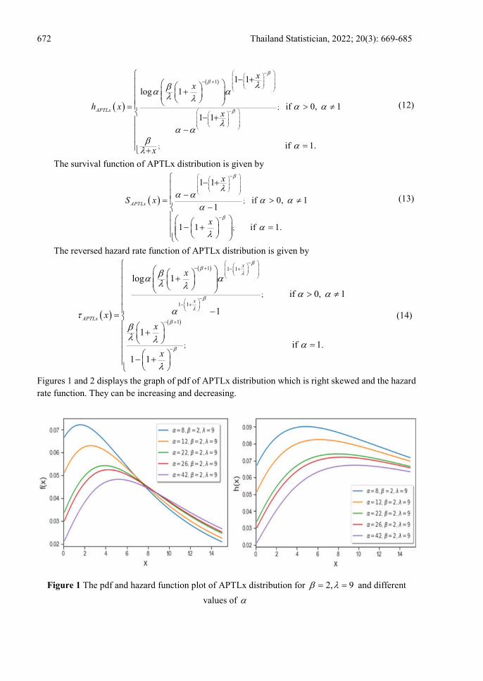
Figures 1 and 2 displays the graph of pdf of APTLx distribution which is right skewed and the hazard
rate function. They can be increasing and decreasing.
Figure 1 The pdf and hazard function plot of APTLx distribution for 2, 9 and different
values of
Sakthivel Kandaswamy Maruthan et al. 673
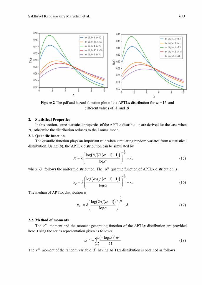
Figure 2 The pdf and hazard function plot of the APTLx distribution for 15 and
different values of and
2. Statistical Properties
In this section, some statistical properties of the APTLx distribution are derived for the case when
, otherwise the distribution reduces to the Lomax model.
2.1. Quantile function
The quantile function plays an important role when simulating random variates from a statistical
distribution. Using (8), the APTLx distribution can be simulated by
1
,log 1 1
log
UX
(15)
where U follows the uniform distribution. The thp quantile function of APTLx distribution is
1
log 1 1.
logp
px
(16)
The median of APTLx distribution is
0.5
1
log 2 1.
logx
(17)
2.2. Method of moments
The thr moment and the moment generating function of the APTLx distribution are provided
here. Using the series representation given as follows
0
log.
!
k k
w
k
w
k
(18)
The thr moment of the random variable X having APTLx distribution is obtained as follows
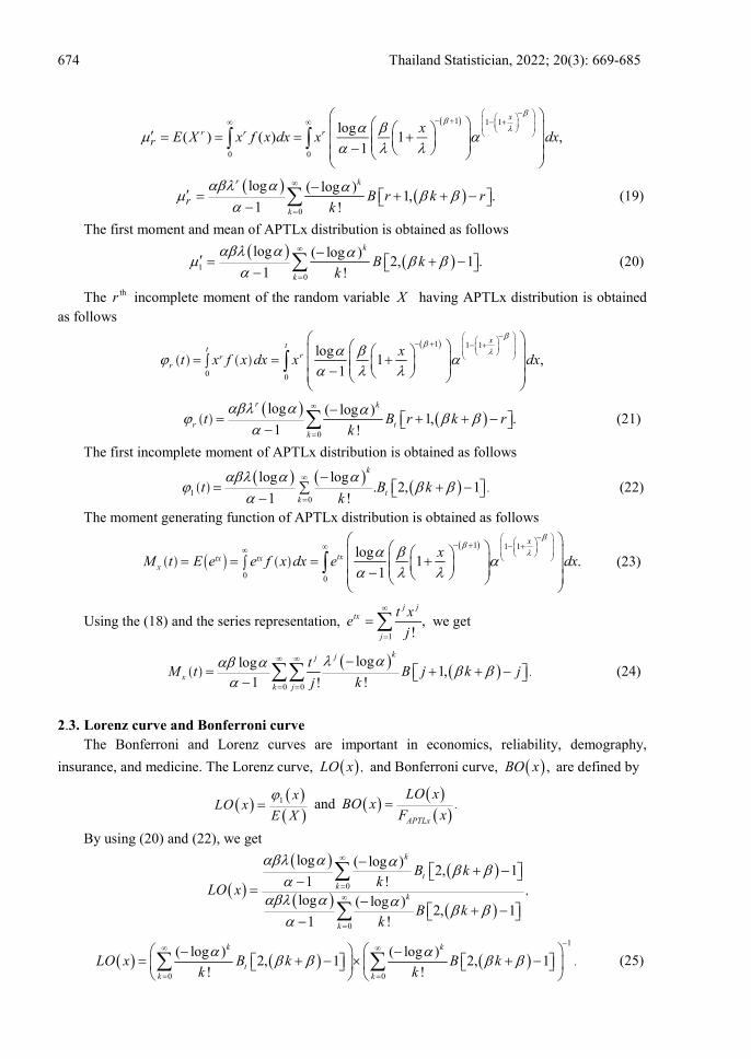
674 Thailand Statistician, 2022; 20(3): 669-685
1 1 1
0 0
log( ) ( ) 1 ,
1
x
r r rr
xE X x f x dx x dx
0
log ( log )1, .
1 !
r k
kr B r k r
k
(19)
The first moment and mean of APTLx distribution is obtained as follows
10
log ( log )2, 1 .
1 !
k
k
B kk
(20)
The thr incomplete moment of the random variable X having APTLx distribution is obtained
as follows
1 1 1
0 0
log1 ,
1
xtt
rrr
xt x f x dx x dx
0
log ( log )1, .
1 !
r k
r tk
t B r k rk
(21)
The first incomplete moment of APTLx distribution is obtained as follows
10
.log log
. 2, 11 !
k
tk
t B kk
(22)
The moment generating function of APTLx distribution is obtained as follows
1 1 1
0 0
log1 .
1
x
txtx txx
xM t E e e f x dx e dx
(23)
Using the (18) and the series representation, 1
,!
j jtx
j
t xe
j
we get
0 0
.loglog
1,1 !!
kjj
xk j
tM t B j k j
kj
(24)
2.3. Lorenz curve and Bonferroni curve
The Bonferroni and Lorenz curves are important in economics, reliability, demography,
insurance, and medicine. The Lorenz curve, ,LO x and Bonferroni curve, ,BO x are defined by
1 xLO x
E X
and
.
APTLx
LO xBO x
F x
By using (20) and (22), we get
0
0
,
log ( log )2, 1
1 !
log ( log )2, 1
1 !
k
tk
k
k
B kk
LO x
B kk
1
0 0
.( log ) ( log )
2, 1 2, 1! !
k k
tk k
LO x B k B kk k
(25)
Sakthivel Kandaswamy Maruthan et al. 675
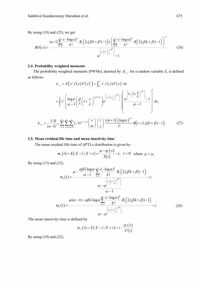
By using (10) and (25), we get
0 0
1 1
1( log ) ( log )
1 2, 1 2, 1! !
.
1
k k
tk k
x
B k B kk k
BO x
(26)
2.4. Probability weighted moments
The probability weighted moments (PWMs), denoted by ,r s for a random variable X, is defined
as follows
, 0
1 1 1
0
1 1
log 11 ,
1 1
s sr rr s
x
r
s
E x f x F x x f x F x dx
x
xx dx
1
, 10 0 0
1 log( 1) 1, ( ) .
!1
i ii sr
s j mr s s
i j m
ms iB r i r
m j i
(27)
2.5. Mean residual life time and mean inactivity time
The mean residual life time of APTLx distribution is given by
1| , 0x
xm t E X t X t t t
S t
where 1
By using (13) and (22),
1
1 1
log ( log )2, 1
1 !,
1
k
tk
xx
B kk
m t t
1
1 1
( log )( 1) log 2, 1
!.
k
tk
xx
B kk
m t t
(28)
The mean inactivity time is defined by
1.|x
xt E X t X t t
F t
By using (10) and (22),
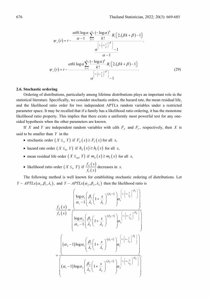
676 Thailand Statistician, 2022; 20(3): 669-685
1
1 1
,
log ( log )2, 1
1 !
1
1
k
tk
xx
B kk
t t
1
1 1
.
( log )log 2, 1
!
1
k
tk
xx
B kk
t t
(29)
2.6. Stochastic ordering
Ordering of distributions, particularly among lifetime distributions plays an important role in the
statistical literature. Specifically, we consider stochastic orders, the hazard rate, the mean residual life,
and the likelihood ratio order for two independent APTLx random variables under a restricted
parameter space. It may be recalled that if a family has a likelihood ratio ordering, it has the monotone
likelihood ratio property. This implies that there exists a uniformly most powerful test for any one-
sided hypothesis when the other parameters are known.
If X and Y are independent random variables with cdfs XF and ,YF respectively, then X is
said to be smaller than Y in the
stochastic order stX Y if X YF x F x for all ,x
hazard rate order hrX Y if X Yh x h x for all ,x
mean residual life order mrlX Y if X Ym x m x for all ,x
likelihood ratio order lrX Y if
X
Y
f x
f xdecreases in .x
The following method is well known for establishing stochastic ordering of distributions. Let
1 1 1, , ,Y APTLx and 2 2 2, ,Y APTLx then the likelihood ratio is
11 1 11
11 11
1 1 1
21 1 12
22 22
2 2 2
log1
1
log1
1
x
X
xY
x
f x
f x
x
11 1 11
112 1 1
1 1
21 1 12
221 2 2
2 2
1 log 1
.
1 log 1
x
x
x
x
Sakthivel Kandaswamy Maruthan et al. 677
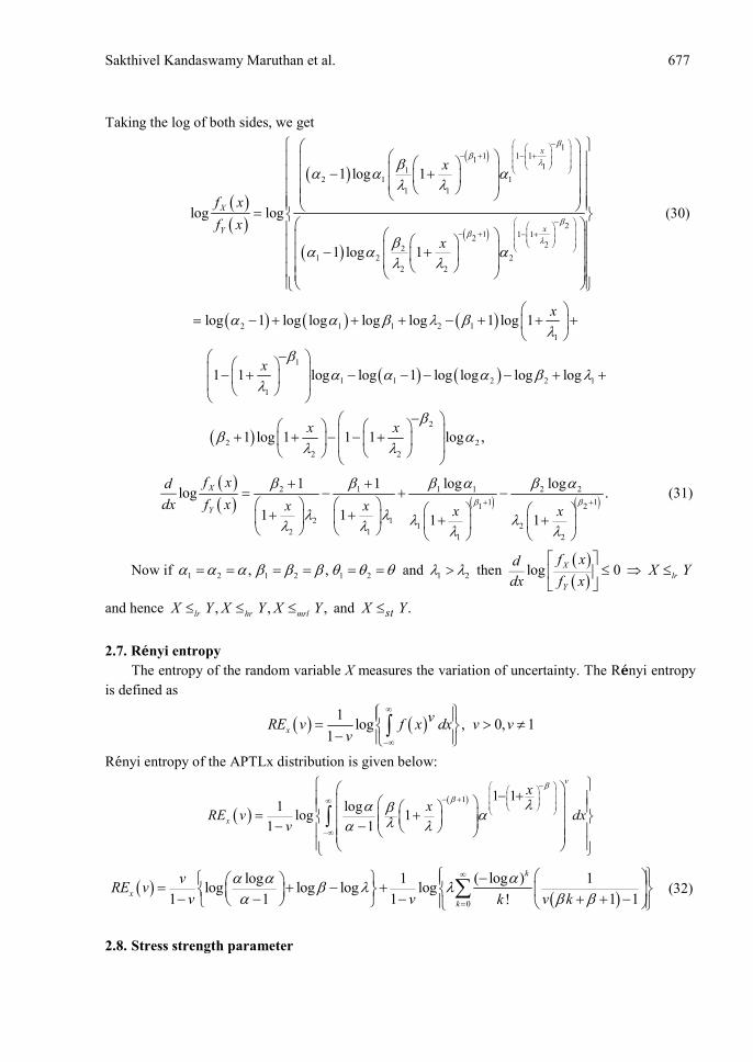
Taking the log of both sides, we get
11 1 11
112 1 1
1 1
21 1 12
221 2 2
2 2
1 log 1
log log
1 log 1
x
X
xY
x
f x
f x
x
(30)
2 1 1 2 1
1
1
1 1 2 2 1
1
2
2 2
2 2
log 1 log log log log 1 log 1
1 1 log log 1 log log log log
1 log 1 1 1 log ,
x
x
x x
2 1 1 1 2 2
1 11 2
2 11 2
2 11 2
1 1 log loglog .
1 1 1 1
X
Y
f xd
dx f x x x x x
(31)
Now if 1 2 1 2 1 2, , and 1 2 then
log 0X
Y
f xd
dx f x
lrX Y
and hence , , ,lr hr mrlX Y X Y X Y and .stX Y
2.7. R�nyi entropy
The entropy of the random variable X measures the variation of uncertainty. The R�nyi entropy
is defined as
1
log , 0, 11
x
vRE v f x dx v vv
Renyi entropy of the APTLx distribution is given below:
1 1 1
1 loglog 1
1 1
v
x
xx
RE v dxv
0
( log )log 1 1log log log log
1 1 1 1 1!
k
xk
vRE v
v v v kk
(32)
2.8. Stress strength parameter
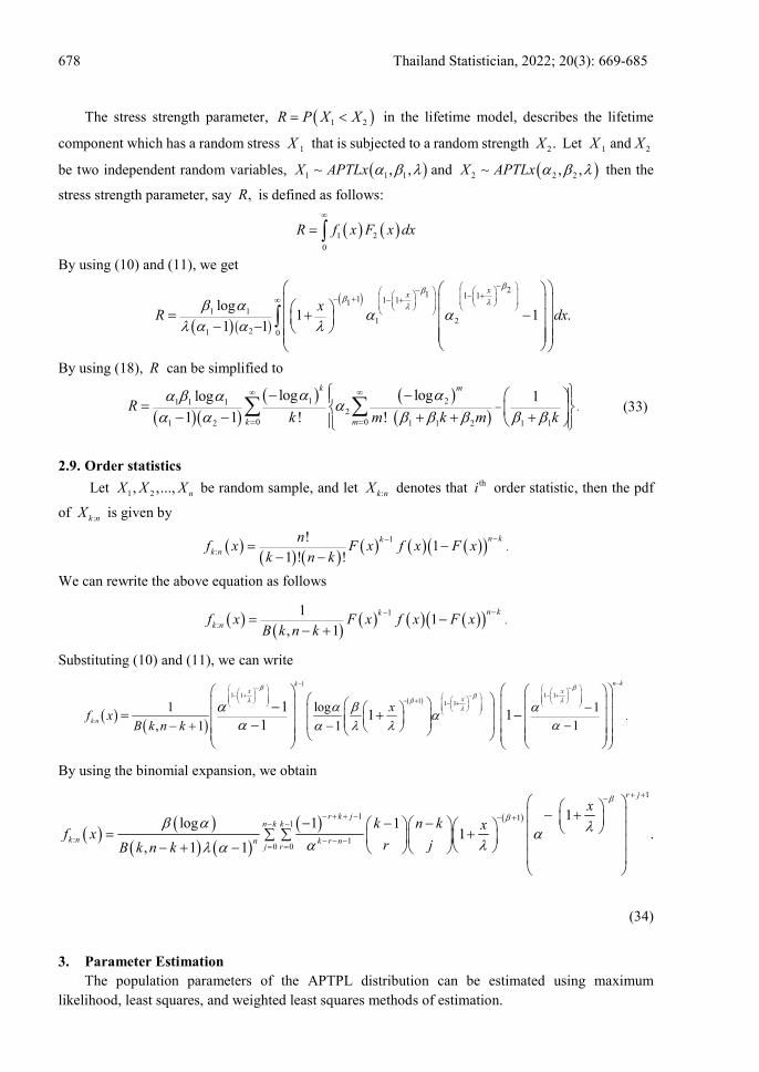
678 Thailand Statistician, 2022; 20(3): 669-685
The stress strength parameter, 1 2R XP X in the lifetime model, describes the lifetime
component which has a random stress 1X that is subjected to a random strength 2.X Let 1X and 2X
be two independent random variables, 1 1 1~ , ,X APTLx and 2 2 2~ , ,X APTLx then the
stress strength parameter, say ,R is defined as follows:
1 2
0
R f x F x dx
By using (10) and (11), we get
2
1 1 11 1 111 1
1 221 0
log1 1 .
1 1
xx
xR dx
By using (18), R can be simplified to
1 21 1 12
0 01 2 1 1 2 1 1
.log loglog 1
1 1 ! !
k m
k m
Rk m k m k
(33)
2.9. Order statistics
Let 1 2, ,..., nX X X be random sample, and let :k nX denotes that thi order statistic, then the pdf
of :k nX is given by
1
: .!
11 ! !
n kk
k n
nf x F x f x F x
k n k
We can rewrite the above equation as follows
1
: .1
1, 1
n kk
k nf x F x f x F xB k n k
Substituting (10) and (11), we can write
1
1 1 1 11 1 1
:.
1 log 1
1, 1 1
11 1
1
n kkx x
x
k n
xf x
B k n k
By using the binomial expansion, we obtain
1
1 11
: 10 0
1log 1 1
1 ., 1 1
r j
r k jn k k
k n n k r nj r
xk n k x
f xr jB k n k
(34)
3. Parameter Estimation
The population parameters of the APTPL distribution can be estimated using maximum
likelihood, least squares, and weighted least squares methods of estimation.
Sakthivel Kandaswamy Maruthan et al. 679
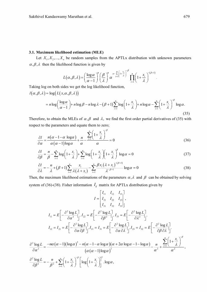
3.1. Maximum likelihood estimation (MLE)
Let 1 2, ,..., nX X X be random samples from the APTLx distribution with unknown parameters
, , then the likelihood function is given by
11
1
1
.log
, , 11
n xi nnii
i
n nx
L
Taking log on both sides we get the log likelihood function,
, , log , , ,l L x
1 1
loglog log log 1 log 1 log 1 log .
1
n ni i
i i
x xn n n n
(35)
Therefore, to obtain the MLEs of , and , we find the first order partial derivatives of (35) with
respect to the parameters and equate them to zero;
1
11 log
01 log
ni
i
x
nl n
(36)
1 1
log 1 log 1 1 log 0n n
i i i
i i
x x xl n
(37)
1
+11 1
1 log 0n n
i ii
i ii
x xxl n
x
(38)
Then, the maximum likelihood estimations of the parameters , and can be obtained by solving
system of (36)-(38). Fisher information ijI matrix for APTLx distribution given by
11 12 13
21 22 23
31 32 33
,
I I I
I I I I
I I I
2 2 2
11 22 332 2 2
2 2 2
12 21 13 31 23 32
, , ,
, , ,
log log log
log log log
L L LI E I E I E
L L LI I E I I E I I E
221
2 2 2 2
11 log 1 log 2 log 1 loglog
,1 log
ni
i
x
n nL n
22
2 21
log1 log 1 .log ,
ni i
i
x xL n
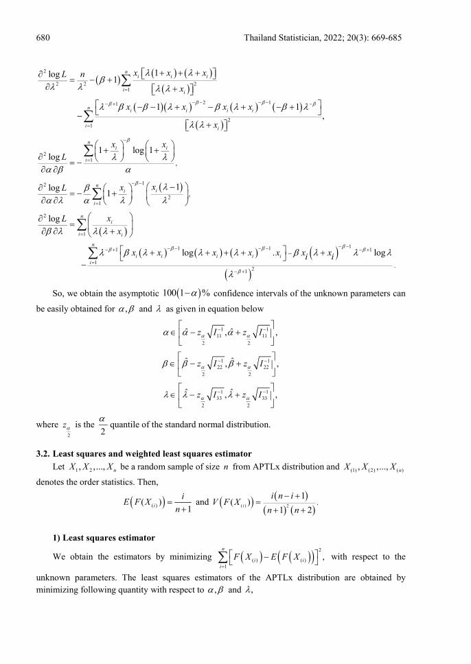
680 Thailand Statistician, 2022; 20(3): 669-685
2
2 2 21
2 11
21
1log1
1 1,
ni i i
i i
ni i i i
ii
x x xL n
x
x x x x
x
21
,
1 log 1log
ni i
i
x x
L
12
21
,1log
1n
ii
i
xxL
2
1
11 11 1
121
.
log
log . log
ni
i i
n
i i i i ii
xL
x
x x x x x x xi i
So, we obtain the asymptotic 100 1 % confidence intervals of the unknown parameters can
be easily obtained for , and as given in equation below
1 111 11
2 2
ˆ ˆ, ,z I z I
1 122 22
2 2
ˆ ˆ, ,z I z I
1 133 33
2 2
ˆ ˆ, ,z I z I
where 2
z is the 2
quantile of the standard normal distribution.
3.2. Least squares and weighted least squares estimator
Let 1 2, ,..., nX X X be a random sample of size n from APTLx distribution and (1) (2) ( ), ,..., nX X X
denotes the order statistics. Then,
( )( )1
i
iE F X
n
and
( ) 2
.1
( )1 2
i
i n iV F X
n n
1) Least squares estimator
We obtain the estimators by minimizing 2
( ) ( )1
,n
i ii
F X E F X
with respect to the
unknown parameters. The least squares estimators of the APTLx distribution are obtained by
minimizing following quantity with respect to , and ,
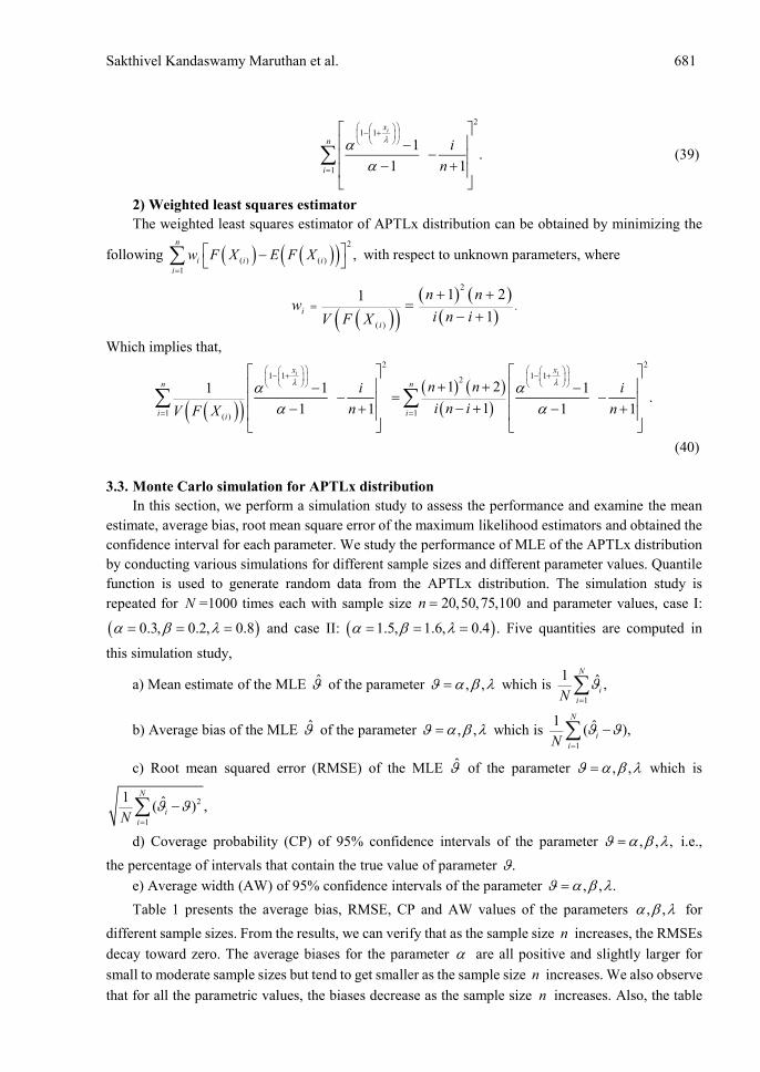
Sakthivel Kandaswamy Maruthan et al. 681
2
1 1
1
1 .
1 1
ix
n
i
i
n
(39)
2) Weighted least squares estimator
The weighted least squares estimator of APTLx distribution can be obtained by minimizing the
following 2
( ) ( )1
,n
i i ii
w F X E F X
with respect to unknown parameters, where
2
( )
.1 21
1i
i
n nw
i n iV F X
Which implies that,
2 2
1 1 1 12
1 1( )
1 21 11 .
11 1 1 1
i ix x
n n
i ii
n ni i
i n in nV F X
(40)
3.3. Monte Carlo simulation for APTLx distribution
In this section, we perform a simulation study to assess the performance and examine the mean
estimate, average bias, root mean square error of the maximum likelihood estimators and obtained the
confidence interval for each parameter. We study the performance of MLE of the APTLx distribution
by conducting various simulations for different sample sizes and different parameter values. Quantile
function is used to generate random data from the APTLx distribution. The simulation study is
repeated for N =1000 times each with sample size 20,50,75,100n and parameter values, case I:
0.3, 0.2, 0.8 and case II: 1.5, 1.6, 0.4 . Five quantities are computed in
this simulation study,
a) Mean estimate of the MLE of the parameter , , which is 1
1 ˆ ,N
iiN
b) Average bias of the MLE of the parameter , , which is 1
1 ˆ( ),N
iiN
c) Root mean squared error (RMSE) of the MLE of the parameter , , which is
2
1
1 ˆ( ) ,N
iiN
d) Coverage probability (CP) of 95% confidence intervals of the parameter , , , i.e.,
the percentage of intervals that contain the true value of parameter .
e) Average width (AW) of 95% confidence intervals of the parameter , , .
Table 1 presents the average bias, RMSE, CP and AW values of the parameters , , for
different sample sizes. From the results, we can verify that as the sample size n increases, the RMSEs
decay toward zero. The average biases for the parameter are all positive and slightly larger for
small to moderate sample sizes but tend to get smaller as the sample size n increases. We also observe
that for all the parametric values, the biases decrease as the sample size n increases. Also, the table
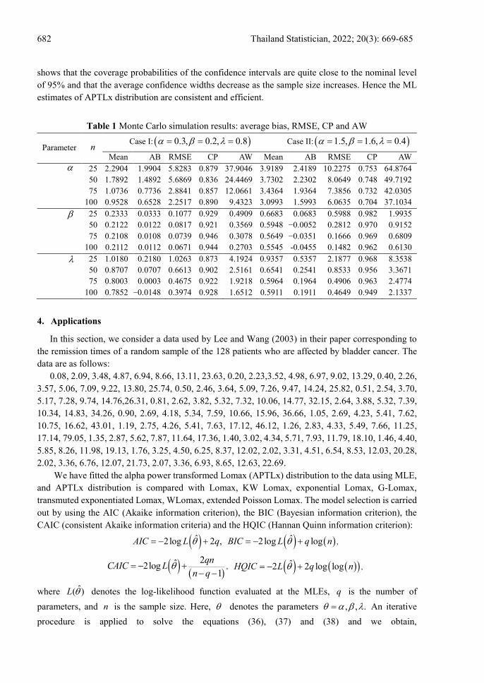
682 Thailand Statistician, 2022; 20(3): 669-685
shows that the coverage probabilities of the confidence intervals are quite close to the nominal level
of 95% and that the average confidence widths decrease as the sample size increases. Hence the ML
estimates of APTLx distribution are consistent and efficient.
Table 1 Monte Carlo simulation results: average bias, RMSE, CP and AW
Parameter n Case I: 0.3, 0.2, 0.8 Case II: 1.5, 1.6, 0.4
Mean AB RMSE CP AW Mean AB RMSE CP AW
25
50
75
100
2.2904
1.7892
1.0736
0.9528
1.9904
1.4892
0.7736
0.6528
5.8283
5.6869
2.8841
2.2517
0.879
0.836
0.857
0.890
37.9046
24.4469
12.0661
9.4323
3.9189
3.7302
3.4364
3.0993
2.4189
2.2302
1.9364
1.5993
10.2275
8.0649
7.3856
6.0635
0.753
0.748
0.732
0.704
64.8764
49.7192
42.0305
37.1034
25
50
75
100
0.2333
0.2122
0.2108
0.2112
0.0333
0.0122
0.0108
0.0112
0.1077
0.0817
0.0739
0.0671
0.929
0.921
0.946
0.944
0.4909
0.3569
0.3078
0.2703
0.6683
0.5948
0.5649
0.5545
0.0683
−0.0052
−0.0351
-0.0455
0.5988
0.2812
0.1666
0.1482
0.982
0.970
0.969
0.962
1.9935
0.9152
0.6809
0.6130
25
50
75
100
1.0180
0.8707
0.8003
0.7852
0.2180
0.0707
0.0003
−0.0148
1.0263
0.6613
0.4675
0.3974
0.873
0.902
0.922
0.928
4.1924
2.5161
1.9218
1.6512
0.9357
0.6541
0.5964
0.5911
0.5357
0.2541
0.1964
0.1911
2.1877
0.8533
0.4906
0.4649
0.968
0.956
0.963
0.949
8.3538
3.3671
2.4774
2.1337
4. Applications
In this section, we consider a data used by Lee and Wang (2003) in their paper corresponding to
the remission times of a random sample of the 128 patients who are affected by bladder cancer. The
data are as follows:
0.08, 2.09, 3.48, 4.87, 6.94, 8.66, 13.11, 23.63, 0.20, 2.23,3.52, 4.98, 6.97, 9.02, 13.29, 0.40, 2.26,
3.57, 5.06, 7.09, 9.22, 13.80, 25.74, 0.50, 2.46, 3.64, 5.09, 7.26, 9.47, 14.24, 25.82, 0.51, 2.54, 3.70,
5.17, 7.28, 9.74, 14.76,26.31, 0.81, 2.62, 3.82, 5.32, 7.32, 10.06, 14.77, 32.15, 2.64, 3.88, 5.32, 7.39,
10.34, 14.83, 34.26, 0.90, 2.69, 4.18, 5.34, 7.59, 10.66, 15.96, 36.66, 1.05, 2.69, 4.23, 5.41, 7.62,
10.75, 16.62, 43.01, 1.19, 2.75, 4.26, 5.41, 7.63, 17.12, 46.12, 1.26, 2.83, 4.33, 5.49, 7.66, 11.25,
17.14, 79.05, 1.35, 2.87, 5.62, 7.87, 11.64, 17.36, 1.40, 3.02, 4.34, 5.71, 7.93, 11.79, 18.10, 1.46, 4.40,
5.85, 8.26, 11.98, 19.13, 1.76, 3.25, 4.50, 6.25, 8.37, 12.02, 2.02, 3.31, 4.51, 6.54, 8.53, 12.03, 20.28,
2.02, 3.36, 6.76, 12.07, 21.73, 2.07, 3.36, 6.93, 8.65, 12.63, 22.69.
We have fitted the alpha power transformed Lomax (APTLx) distribution to the data using MLE,
and APTLx distribution is compared with Lomax, KW Lomax, exponential Lomax, G-Lomax,
transmuted exponentiated Lomax, WLomax, extended Poisson Lomax. The model selection is carried
out by using the AIC (Akaike information criterion), the BIC (Bayesian information criterion), the
CAIC (consistent Akaike information criteria) and the HQIC (Hannan Quinn information criterion):
ˆ2log 2 ,AIC L q ,ˆ2 log logBIC L q n
,2ˆ2log
1
qnCAIC L
n q
,ˆ2 2 log logHQIC L q n
where ˆ( )L denotes the log-likelihood function evaluated at the MLEs, q is the number of
parameters, and n is the sample size. Here, denotes the parameters , , . An iterative
procedure is applied to solve the equations (36), (37) and (38) and we obtain,
Sakthivel Kandaswamy Maruthan et al. 683
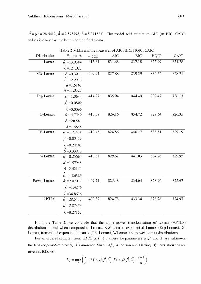
ˆ ˆ ˆˆ( 28.5412, 2.873798, 8.271523). The model with minimum AIC (or BIC, CAIC)
values is chosen as the best model to fit the data.
Table 2 MLEs and the measures of AIC, BIC, HQIC, CAIC
Distribution Estimates log L AIC BIC HQIC CAIC
Lomax =13.9384
=121.023
413.84 831.68 837.38 833.99 831.78
KW Lomax =0.3911
=12.2973
a =1.5162
=11.0323
409.94 827.88 839.29 832.52 828.21
Exp.Lomax =1.0644
=0.0800
=0.0060
414.97 835.94 844.49 839.42 836.13
G-Lomax =4.7540
=20.581
a =1.5858
410.08 826.16 834.72 829.64 826.35
TE-Lomax =1.71418
=0.05456
=0.24401
=3.33911
410.43 828.86 840.27 833.51 829.19
WLomax =0.25661
=1.57945
a =2.42151
b =1.86389
410.81 829.62 841.03 834.26 829.95
Power Lomax =2.07012
=1.4276
=34.8626
409.74 825.48 834.04 828.96 825.67
APTLx =28.5412
=2.87379
=8.27152
409.39 824.78 833.34 828.26 824.97
From the Table 2, we conclude that the alpha power transformation of Lomax (APTLx)
distribution is best when compared to Lomax, KW Lomax, exponential Lomax (Exp.Lomax), G-
Lomax, transmuted exponential Lomax (TE- Lomax), WLomax and power Lomax distributions.
For an ordered sample, from ( , , ),APTL where the parameters , and are unknown,
the Kolmogorov-Smirnov ,nD Cramer-von Mises 2 ,nW Anderson and Darling 2nA tests statistics are
given as follows:
1ˆ ˆ ˆ ˆˆ ˆmax , , , , , , , ,n i ii
i iD F x F x
n n
684 Thailand Statistician, 2022; 20(3): 669-685
2
1
2 1 ˆ ˆ ˆ ˆˆ ˆln , , , ln , , , ,n
n i ii
iA n F x F x
n
(41)
2
2
1
1 2 1 ˆ ˆˆ, , , .12 2
n
n ii
iW F x
n n
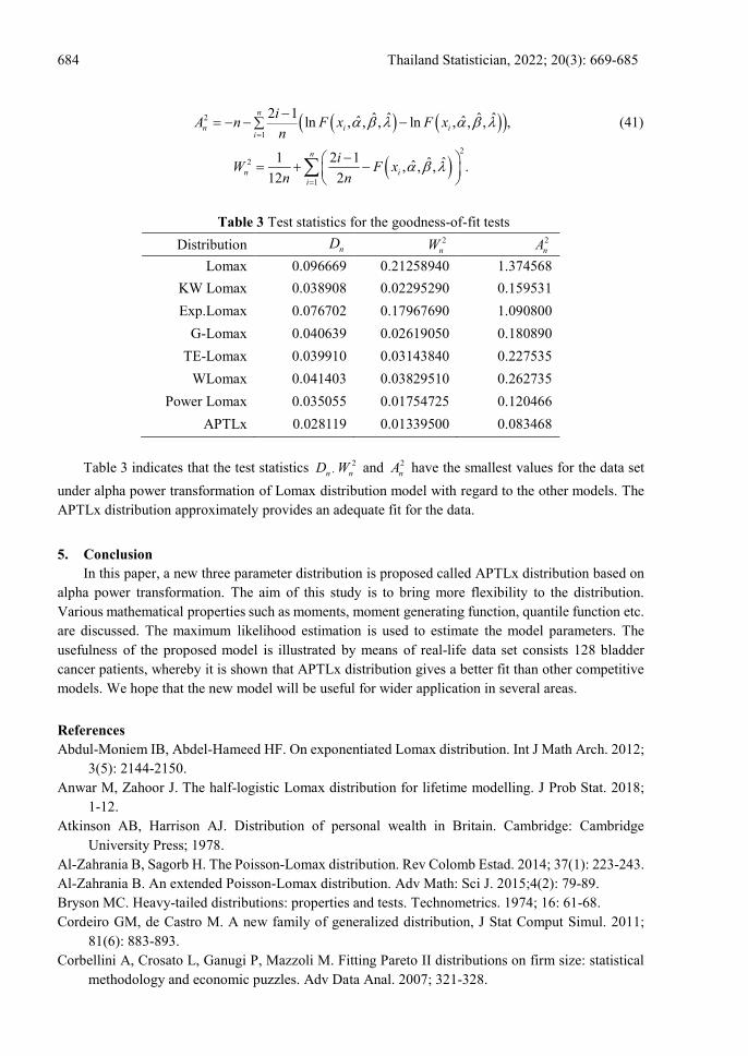
Table 3 Test statistics for the goodness-of-fit tests
Distribution nD 2nW 2
nA
Lomax 0.096669 0.21258940 1.374568
KW Lomax 0.038908 0.02295290 0.159531
Exp.Lomax 0.076702 0.17967690 1.090800
G-Lomax 0.040639 0.02619050 0.180890
TE-Lomax 0.039910 0.03143840 0.227535
WLomax 0.041403 0.03829510 0.262735
Power Lomax 0.035055 0.01754725 0.120466
APTLx 0.028119 0.01339500 0.083468
Table 3 indicates that the test statistics 2,n nD W and 2
nA have the smallest values for the data set
under alpha power transformation of Lomax distribution model with regard to the other models. The
APTLx distribution approximately provides an adequate fit for the data.
5. Conclusion
In this paper, a new three parameter distribution is proposed called APTLx distribution based on
alpha power transformation. The aim of this study is to bring more flexibility to the distribution.
Various mathematical properties such as moments, moment generating function, quantile function etc.
are discussed. The maximum likelihood estimation is used to estimate the model parameters. The
usefulness of the proposed model is illustrated by means of real-life data set consists 128 bladder
cancer patients, whereby it is shown that APTLx distribution gives a better fit than other competitive
models. We hope that the new model will be useful for wider application in several areas.
References
Abdul-Moniem IB, Abdel-Hameed HF. On exponentiated Lomax distribution. Int J Math Arch. 2012;
3(5): 2144-2150.
Anwar M, Zahoor J. The half-logistic Lomax distribution for lifetime modelling. J Prob Stat. 2018;
1-12.
Atkinson AB, Harrison AJ. Distribution of personal wealth in Britain. Cambridge: Cambridge
University Press; 1978.
Al-Zahrania B, Sagorb H. The Poisson-Lomax distribution. Rev Colomb Estad. 2014; 37(1): 223-243.
Al-Zahrania B. An extended Poisson-Lomax distribution. Adv Math: Sci J. 2015;4(2): 79-89.
Bryson MC. Heavy-tailed distributions: properties and tests. Technometrics. 1974; 16: 61-68.
Cordeiro GM, de Castro M. A new family of generalized distribution, J Stat Comput Simul. 2011;
81(6): 883-893.
Corbellini A, Crosato L, Ganugi P, Mazzoli M. Fitting Pareto II distributions on firm size: statistical
methodology and economic puzzles. Adv Data Anal. 2007; 321-328.
Sakthivel Kandaswamy Maruthan et al. 685
Dey S, Sharma VK, Mesfioui M. A new extension of Weibull distribution with application to lifetime
data. Ann Data Sci. 2017; 4(1): 31-61.
Dey S, Alzaatreh A, Zhang C, Kumar D. A new extension of generalized exponential distribution with
application to ozone data. Ozone Sci Eng. 2017; 39(4): 273-285.
Dey S, Ghosh I, Kumar D. Alpha-power transformed Lindley distribution: properties and associated
inference with application to earthquake data. Ann Data Sci. 2018; 1-28.
El-Bassiouny AH, Abdo NF, Shahen HF. Exponential Lomax distribution. Int J Comput Appl. 2015;
121(13): 24-29.
El-Houssainy AR, Hassanein WA, Elhaddad TA. The power Lomax distribution with an application
to bladder cancer data. SpringerPlus. 2016; 5: 1-22.
Ghitany ME, AL-Awadhi SA. Statistical properties of Poisson-Lomax Distribution and its
applications to repeated accident data. J Appl Stat Sci. 2001; 10(4): 365-372.
Ghitany ME, Al-Awadhi FA, Alkhalifan LA. Marshall-Olkin extended Lomax distribution and its
application to censored data. Commun Stat - Theory Methods. 2007; 36: 1855-1866.
Hassan A, Al-Ghamdi AS. Optimum step stress accelerated life testing for Lomax distribution, J Appl
Sci Res. 2009; 5(12): 2153-2164.
Hassan A, Elgrhy M, Mohamd R.E, Alrajhi S. On the alpha power transformed power Lindley
distribution. J Prob Stat. 2019.
Harris CM. The Pareto distribution as a queue service discipline. Oper Res.1968; 16(2): 301-313.
Mahadavi A, Kundu D. A new method of generating distribution with an application to exponential
distribution, Commun Stat- Theory and Methods. 2015; 46(13): 6543-6557.
Malik AS, Ahmad SP. Alpha power Rayleigh distribution and its application to life time data. Int J
Enhanc Res Manag Comput Appl. 2017; 6: 212-219.
Nassar M, Alzaatreh A, Mead M, Abo-Kasem OE. Alpha power Weibull distribution: properties and
application. Commun Stat-Theory and Methods. 2017; 46(20): 10236-10252.
Nasiru S, Mwita PN, Ngesa O. Alpha power transformed Frechet distribution. Appl Math Inf Sci.
2019; 13(1): 129-141.
Shams TM. The Kumaraswamy-generalized Lomax distribution. Middle East J Sci Res. 2013; 17(5):
641-646.
Tahir MH, Cordeiro G.M, Mansoor M, Zubair M. The Weibull-Lomax distribution: properties and
applications. Hacet J Math Stat. 2015; 44(2): 461-480.
Tahir MH, Hussain M, Cordeiro GM, Hamedani GG, Mansoor M, Zubair M. The Gumbel-Lomax
distribution: properties and applications. J Stat Theory Appl. 2016; 15(1): 61-79.
Unal C, Cakmakyaoan S, Ozel G. Alpha power inverted exponential distribution: properties and
applications. Gazi Univ J Sci. 2018; 31(3): 954-965.
Zografos K, Balakrishnan N. On families of beta and generalized gamma-generated distributions and
associated inference. Stat Methodol. 2009; 6: 344-362.