arX

iv:m

ath/

0209

097v

2 [m

ath.

NA

] 17

Sep

200

3

Functions from R2 to R2:

a study in nonlinearity

Nicolau C. Saldanha and Carlos Tomei

February 1, 2008

1 Introduction

Calculus students learn how to draw graphs of functions from R to R and under-graduates studying complex variable learn about geometric properties of functionslike f(z) = z3 and g(z) = ez. Some teachers go further and introduce a few exam-ples of conformal mappings. A picture is worth a thousand words, but more canbe said on their favor: they provide a good exercise in combining theoretical factsin a consistent fashion. Indeed, to obtain the graph of a real function, a studentconsiders its derivatives, asymptotic behavior and some special points, amongother features. Something similar happens in the study of conformal mappings.

In this text, we consider functions from R2 to R2 and along the way assemblea number of tools from undergraduate courses. We describe a graphical represen-tation of such functions and, for functions which are visually too complicated, westill count preimages, in a manner reminiscent of Rouche ’s theorem. Why is itthat such aspects of functions from the plane to the plane are not more familiar?A reason might be the following. Most of the information we compute aboutfunctions from the line to itself, or about holomorphic functions, concerns specialpoints—typically critical points, where the derivative is zero. In the case of func-tions from the plane to the plane, we need to consider critical curves, where theJacobian matrix is not invertible. Such curves are often impossible to describe insimple closed form.

Enter the computer: we should think of the study of a given function fromthe plane to the plane as a description of certain relevant objects, in a way thatthese objects become amenable to numerics. In this sense, the time is ripe forthis new case study in nonlinear theory, in the same way that we feel more at easenowadays with showing students how to evaluate roots of polynomials of degree6, or eigenvalues of 5 × 5 matrices.

The theory should operate on two levels: we should learn enough to getqualitative information about simple examples, and we should be able to derivenumerical procedures to handle general cases. In particular, such procedures

1

should extend our knowledge of the preimages of a point, from mere counting toexplicit computation.

In section 2 we present a representative function F0 which will be our fa-vorite test case throughout the paper; in section 10 some additional examplesare discussed. Some of the tools required for this project belong to the standardcurriculum, others are just ahead. All of them are basic when dealing with non-linear problems. Thus, for example, in section 3, we describe the local behaviorof a function at folds and cusps, special critical points in the domain where theinverse function theorem does not apply. We will compute winding numbers andwill also consider, in section 8, the rotation number of a C1 curve. Some aspectsof covering space theory, presented in sections 5 and 6, will help us fit togetherlocal information. In particular, we will be able to perform compatibility checks,discussed in section 9, which often indicate the presence of yet unknown criticalcurves.

Some theoretical aspects have computational counterparts. For example, un-der appropriate hypothesis, the inverse function theorem asserts that a functionis locally invertible while Newton’s method may be used to actually perform theinversion. More generally, the implicit function theorem verifies the regularityof critical curves and a predictor-corrector method then traces the curve, as insection 4. Similarly, covering space theory is closely related to numerical con-tinuation methods, employed in section 7. Due to space limitations, we handlenumerical aspects rather superficially, providing sketches of arguments and indi-cating more specific literature. Some results are quoted from standard referencesbut we present proofs of a few statements which are harder to find in book form.Senior undergraduates should be able to follow through the arguments.

Together with Iaci Malta, the authors have published more technical texts([13], [14]). The program (in rough form) which generated pictures and com-putations for this paper is available ([1]). Both theoretical and computationalaspects can be extended to the study of functions from a bounded subset of theplane to the plane ([6]). For a more general study of the geometry of functionsbetween two surfaces, see [7].

2 A first example

Our first and favorite example is the function

F0 : R2 → R2(

xy

)

7→

(

x3 − 3xy2 + 2.5x2 − 2.5y2 + x3x2y − y3 − 5xy + y

)

which, in complex notation, can be written as F0(z) = z3 +2.5z2 + z. Due to thepresence of z, F0 is not holomorphic. As every Rouche fan would notice, F0 actson concentric circles centered at the origin according to (at least) three different

2

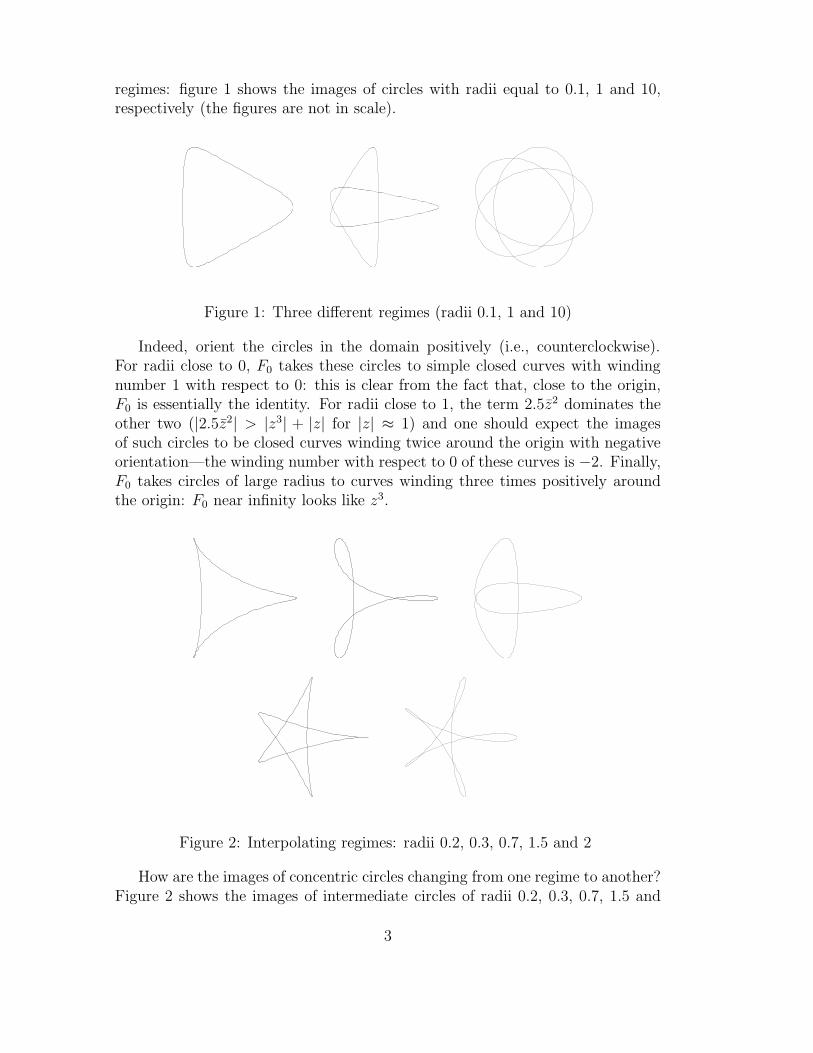
regimes: figure 1 shows the images of circles with radii equal to 0.1, 1 and 10,respectively (the figures are not in scale).

Figure 1: Three different regimes (radii 0.1, 1 and 10)

Indeed, orient the circles in the domain positively (i.e., counterclockwise).For radii close to 0, F0 takes these circles to simple closed curves with windingnumber 1 with respect to 0: this is clear from the fact that, close to the origin,F0 is essentially the identity. For radii close to 1, the term 2.5z2 dominates theother two (|2.5z2| > |z3| + |z| for |z| ≈ 1) and one should expect the imagesof such circles to be closed curves winding twice around the origin with negativeorientation—the winding number with respect to 0 of these curves is −2. Finally,F0 takes circles of large radius to curves winding three times positively aroundthe origin: F0 near infinity looks like z3.

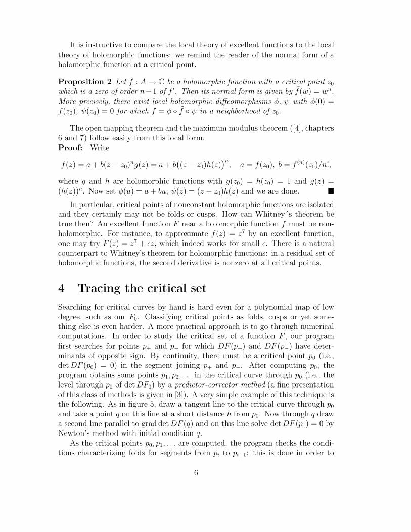
Figure 2: Interpolating regimes: radii 0.2, 0.3, 0.7, 1.5 and 2

How are the images of concentric circles changing from one regime to another?Figure 2 shows the images of intermediate circles of radii 0.2, 0.3, 0.7, 1.5 and

3

2. It may be hard to see in the picture, but there are two small loops in thefirst figure and one in the fourth; the five curves are indeed smooth. We willaddress the formation of these patterns in the sequel. We will draw other, moreinformative pictures and will infer, for example, that the equation F0(z) = 0 hasnine solutions.

3 Local theory

We will use some basic facts of the local theory of functions in the plane, obtainedby Whitney in 1955 ([23]). The subject developed considerably under the name ofsingularity theory after the work of Thom and Mather in the sixties. An excellentreference with emphasis in applications is [9]; a more technical one is [8].

Recall that, for a smooth function F : R2 → R2, a point p is regular ifthe Jacobian DF (p) is an invertible matrix. From the inverse function theorem([11], chap. XVII, §3, pg. 349), after smooth changes of variable in appropriateneighborhoods of a regular point p and its image F (p), the function F takes theform F (x, y) = (x, y); more precisely, there exist local diffeomorphisms Φ and Ψwith F = Φ ◦ F ◦ Ψ as above. Points which are not regular are critical and theyform the critical set C. A critical point pf is a fold point (or, more informally, afold) if, after changing variables near pf and F (pf), F becomes F (x, y) = (x, y2).Also, a critical point pc is a cusp point (or, again, simply a cusp) if changesof variables convert F into F (x, y) = (x, y3 − xy). The formulae for F are thenormal forms of a function at a fold and at a cusp: they imply that in appropriateneighborhoods of folds and cusps, the critical set is a smooth arc consisting offolds and cusps; also, cusps are isolated.

In the same way that the hypothesis of the inverse function theorem guaran-tees a simple normal form of a function near a regular point, there are explicitconditions which characterize folds and cusps. For example, a critical point pf

is a fold of a smooth function F : R2 → R2 if two conditions hold. First, thegradient of detDF should be nonzero at pf , which implies, from the implicit func-tion theorem, that the critical set near pf is a curve. Second, grad detDF (pf)should not be orthogonal to kerDF (pf). There is a similar, more complicatedcharacterization of cusps, which we omit.

A function near a fold behaves in a simple way. All properties describedbelow can be checked by referring to the normal form. In figure 3, a small arcof the critical set and its image under the function F are indicated with thicklines for both types of critical points. Points in the domain with the same imageare indicated by the same label. The thinner lines on both sides of the criticalcurves are taken to thin lines as indicated. Near a fold pf , the function F takespoints to a single side of the image of the critical arc. Thus, a point w nearF (pf) has 0, 1 or 2 preimages near pf , depending on its position with respect tothe image of the critical arc. The image of a curve γ transversal to the critical

4

set at a fold point is generically a nonsingular curve F (γ) tangent to F (C) (twosmooth arcs are transversal at an intersection point if their tangent vectors arelinearly independent). The inverse image of a curve δ transversal to F (C) is acurve tangent to ker(DF ) at C. Only one side of δ actually has preimages (inthe figure, the dotted part of δ is not in the image of F near pf).

A

A

Apf

F(p )f

F( )γ γ

F ( )δ−1

δ 2

0

Figure 3: Local behavior near a fold

Points w near the image F (pc) of a cusp pc may have 1, 2 or 3 preimagesnear pc. Arcs γ1 and γ2 in figure 4 have qualitatively different images: F (γ1)undergoes a loop around F (pc), F (γ2) does not. We also indicate the (nontrivial)preimage of the image of the critical curve near the cusp: notice that it lies toone side of the critical curve. We say that the cusp is effective on that side.

A

B

A

B

AC

C

C

C

B

1

3p F(p )cc

γ

γ

2

1γ

2γF( )

1F( )

Figure 4: Local behavior near a cusp

Whitney defined excellent functions as functions having only folds and cuspsas critical points. The regular points of an excellent function F : R2 → R2 forman open dense subset of the plane and its critical set C is a disjoint union ofisolated smooth curves. It is easy to see from the normal form that cusps forma discrete set and the rest of C consists of arcs of folds. Fortunately, excellentfunctions from the plane to the plane are abundant: this allows us to ignore morecomplicated critical points.

Theorem 1 (Whitney,[23]) In the Cr topology on compact sets (r ≥ 3), theset of excellent functions F : R2 → R2 is residual.

5

It is instructive to compare the local theory of excellent functions to the localtheory of holomorphic functions: we remind the reader of the normal form of aholomorphic function at a critical point.

Proposition 2 Let f : A→ C be a holomorphic function with a critical point z0which is a zero of order n−1 of f ′. Then its normal form is given by f(w) = wn.More precisely, there exist local holomorphic diffeomorphisms φ, ψ with φ(0) =f(z0), ψ(z0) = 0 for which f = φ ◦ f ◦ ψ in a neighborhood of z0.

The open mapping theorem and the maximum modulus theorem ([4], chapters6 and 7) follow easily from this local form.Proof: Write

f(z) = a+ b(z − z0)ng(z) = a+ b

(

(z − z0)h(z))n, a = f(z0), b = f (n)(z0)/n!,

where g and h are holomorphic functions with g(z0) = h(z0) = 1 and g(z) =(h(z))n. Now set φ(u) = a+ bu, ψ(z) = (z − z0)h(z) and we are done. �

In particular, critical points of nonconstant holomorphic functions are isolatedand they certainly may not be folds or cusps. How can Whitney´s theorem betrue then? An excellent function F near a holomorphic function f must be non-holomorphic. For instance, to approximate f(z) = z7 by an excellent function,one may try F (z) = z7 + ǫz, which indeed works for small ǫ. There is a naturalcounterpart to Whitney’s theorem for holomorphic functions: in a residual set ofholomorphic functions, the second derivative is nonzero at all critical points.

4 Tracing the critical set

Searching for critical curves by hand is hard even for a polynomial map of lowdegree, such as our F0. Classifying critical points as folds, cusps or yet some-thing else is even harder. A more practical approach is to go through numericalcomputations. In order to study the critical set of a function F , our programfirst searches for points p+ and p− for which DF (p+) and DF (p−) have deter-minants of opposite sign. By continuity, there must be a critical point p0 (i.e.,detDF (p0) = 0) in the segment joining p+ and p−. After computing p0, theprogram obtains some points p1, p2, . . . in the critical curve through p0 (i.e., thelevel through p0 of detDF0) by a predictor-corrector method (a fine presentationof this class of methods is given in [3]). A very simple example of this technique isthe following. As in figure 5, draw a tangent line to the critical curve through p0

and take a point q on this line at a short distance h from p0. Now through q drawa second line parallel to grad detDF (q) and on this line solve detDF (p1) = 0 byNewton’s method with initial condition q.

As the critical points p0, p1, . . . are computed, the program checks the condi-tions characterizing folds for segments from pi to pi+1: this is done in order to

6

p0 p

1

q

Figure 5: A simple predictor-corrector method

detect cusps (or other singularities). On segments which do not pass this test,the program searches for cusps and validates them with additional tests which wedo not detail. These tests ascertain with considerable robustness and reliabilitythat all critical points on this critical curve are indeed folds or cusps.

What is the critical set of F0? And for that matter, is it even excellent?The left part of figure 6 shows both critical curves Γ1 and Γ2 of the function F0:they are ovals around the origin. The images of the critical curves are on theright: F0(Γ1) is a small curvilinear triangle surrounding the origin and F0(Γ2)is a stellated pentagon. Indeed, numerics confirm that the two critical curveshave 3 and 5 cusps. This is in agreement with the almost polygonal shape ofthe images of circles of radii 0.2 and 1.6 in figure 2. The labels on the outercritical curve Γ2 are of two kinds: capital letters indicate cusps and lower caseletters are preimages of self-intersections of F0(Γ2). The three cusps on Γ1 arenot indicated, but the reader may check that if Γ1 is traversed counterclockwisethen so is F0(Γ1).

A

D

C

E

B

c

a

b

e

dc

b

a

e

d

Γ1

Γ2

A

B

C

D

E

a

c

e

b

d

Y

Y

0

1Y2

Figure 6: The critical curves of F0 and their images

Critical curves are thus described by lists of points, some of them cusps.Outside the known part of the critical set, however, very few points have beenconsidered. Without a labor intensive search, how do we know if we have foundall critical curves of a function? This, in general, is a nontrivial issue and weshall say more about it in section 9.

7

5 Counting preimages

We set the information obtained so far in a more robust setting lest the readerthink that we are letting pictures take control over mathematical reasoning. Webegin by stating without proof a stronger form of the Jordan curve theorem.

Theorem 3 Let γ ⊂ R2 be a simple closed curve. The curve γ is the boundaryof a closed topological disk D. The open set R2 − γ has precisely two connectedcomponents: the interior of D and the complement of D. Furthermore, if γ is apiecewise smooth curve then there exists a homeomorphism from D to the closedunit disk whose restriction to the interior of D is holomorphic.

The first claim is known as the Schoenflies theorem for which a nice proof isgiven in [20]. The second is the standard Jordan theorem (theorem 13.4, chapter8, [16]) and the third is an extension of the Riemann mapping theorem (14.19 in[19]).

We denote by Dγ the closed (topological) disk surrounded by the simple closedcurve γ and by intDγ the corresponding open disk. The lemmas that follow arestandard, but somewhat hard to pinpoint in the literature.

Lemma 4 Let γ be a smooth simple closed curve in R2. Let F : Dγ → R2 be aC0 map which is C1 in intDγ. Assume that F has no critical points in intDγ

and is injective on γ. Then F is a homeomorphism from Dγ to its image F (D).

Proof: For readers acquainted with degree theory, the proof is simpler; we sketcha more elementary argument. Set δ = F (γ): clearly, δ is a simple, closed curve,surrounding a closed (topological) disk Dδ. At every point p ∈ intDγ , F is open,i.e., a small open ball around p is taken bijectively to a small open set aroundF (p): this follows from the inverse function theorem, since F has no criticalpoints in intDγ . Thus, any boundary point of F (Dγ) ought to be in F (γ) = δ.By theorem 3, the compact set F (Dγ) equals either δ or Dδ; on the other hand,F (Dγ) = δ is impossible, since the interior of δ is empty.

We now prove that F is injective: from the arguments above and the injectiv-ity on γ, we only have to show that if p0, p1 ∈ intDγ are such that F (p0) = F (p1)then p0 = p1. Let ζ : [0, 1] → intDγ be a smooth path with ζ(0) = p0, ζ(1) = p1

so that (F ◦ ζ)(0) = (F ◦ ζ)(1). Let H : [0, 1]2 → intDΓ be a smooth functionwith H(0, t) = (F ◦ ζ)(t), H(s, 0) = H(s, 1) = H(1, t): the existence of suchH is ascertained by theorem 3. We now construct ζs : [0, 1] → intDγ so thatF (ζs(t)) = H(s, t): ζs is the solution of the differential equation

ζs(0) = p0, ζ ′s(t) = (DF (ζs(t)))−1∂H

∂t(s, t).

Now ζ1 is constant whence ζ1(1) = p0. But ζs(1) depends continuously on sand satisfies F (ζs(1)) = F (p0) for all s. Therefore ζs(1) = p0 for all s andp1 = ζ0(1) = p0.

8

Since F is a continuous bijection from the compact set Dγ to the Hausdorffspace Dδ, F is a homeomorphism (theorem 5.6, chapter 3, [16]). �

A continuous function F : R2 → R2 is proper if the inverse of any compact setis compact. The reader should have no difficulty in proving that this is equivalentto saying that limp→∞ F (p) = ∞. Our function F0 is proper.

Lemma 5 Let F : R2 → R2 be a proper excellent function. The number ofpreimages under F of any point of R2 is finite.

Proof: By properness, all preimages of a point w belong to a closed disk D. Ifthere are infinitely many of them, they must accumulate at a point p, which, bycontinuity of F , is also a preimage of w. Now, p may not be either regular, afold or a cusp, since the three normal forms do not allow for infinitely many localpreimages, in disagreement with the excellence of F . �

Given a closed set X ⊂ R2, we call the connected components of R2 −X thetiles for X.

Lemma 6 Let F : R2 → R2 be a proper excellent function with critical set C.On each tile A for F (C), the number of preimages of F is a constant.

Proof: By connectivity, it suffices to show that the number of preimages ofpoints near w ∈ A is constant. Let p1, . . . , pk be the (finitely many) preimagesof w. By hypothesis, they are regular points, and thus there are open disjointneighborhoods Vi, i = 1, . . . , k, with pi ∈ Vi and so that F restricts as a home-omorphism from each Vi to an open neighborhood W of w. Thus, points in Whave at least as many preimages as w. Suppose now that for a sequence wj ∈Wconverging to w, the points wj have more preimages than w. For each wj, callone such preimage p∗j 6∈ ∪iVi. By properness, the sequence {p∗j} must accumulateto a point w∞, and, again by continuity, w∞ must be a preimage of w whichdoes not belong to the interior of ∪iVi: this gives rise to a new preimage of w, acontradiction. �

A proper excellent function F : R2 → R2 is nice if the following two conditionshold:

• any point y in F (C) is the image of at most two critical points;

• if q is the image of two critical points p1 and p2 then both are folds and thetangent lines to F (C) at q corresponding to p1 and p2 are distinct.

Points which are images of two critical points are double points. Rather unsur-prisingly, the generic excellent function is nice, but we do not prove this technicalresult. From figure 6, the function F0 is nice. Two distinct tiles A and B forF (C) are adjacent if their boundaries share an arc of F (C). In figure 6, tiles Y0

and Y1 are both adjacent to Y2 but not to each other.

9

Lemma 7 Let F : R2 → R2 be a nice function with critical set C; the numberof preimages of points in adjacent tiles for F (C) differ by two.

Proof: Take w to be the image of a fold p belonging to a common boundary arcof adjacent tiles A and B. Let p1, . . . , pk be the preimages of w, with p = p1. Asin the proof of the previous lemma, we take disjoint open neighborhoods Vi ofp2, . . . , pk not containing p which are taken homeomorphically by F to an openneighborhood W of w. Take points wA ∈ A ∩W , wB ∈ B ∩W : there will bek − 1 preimages of wA and wB in the neighborhoods Vi. Now, from the behaviorof F near p, either wA or wB has two additional preimages close to p. �

How can we obtain the sense of folding, i.e., on which of the two adjacenttiles for F (C) do points have more preimages? One way is to look at images ofcusps: from figure 4, points inside the wedge have more preimages than pointsoutside it.

6 Covering maps and the flower

We now split the domain of a nice function F in regions on which F behaves ina very simple fashion. More precisely, we consider the tiles for F−1(F (C)), theflower of F . Figure 7 shows the flower of F0.

The two critical curves Γ1 and Γ2 are of course part of the flower and are drawnthicker. The labels indicate preimages of special points in the image, given infigure 6. The local behavior at the eight cusps of F0 is in agreement with figure 4.Cusps in Γ1 are effective in the annulus between critical curves and cusps in Γ2

are effective in the region outside Γ2. Notice the five small preimages of F0(Γ1)in the five petal-like tiles for the flower: these are indeed curvilinear triangles, asa zoom would show (one is shown in figure 10).

The tiles for the flower (resp. for F (C)) will be labelled Xi (resp. Yj). Aswe shall see, for many Xi, F is a diffeomorphism from Xi to some Yj , extendingto a homeomorphism between the closures Xi and Yj. For the function F0, forexample, the only exceptions are X0 and X1, indicated in figure 7. It turns outthat each point of Y0 (see figure 6) has 3 preimages, all of them in X0: this isin agreement with lemma 6 and the fact that F0 at infinity looks like z 7→ z3.Furthermore, points in the boundary of Y0 also have 3 preimages in the boundaryof X0 but may have other preimages elsewhere: this can be checked by readingthe labels in figures 6 and 7. Similarly, points in Y1 have 2 preimages in X1. Still,the restrictions F : Xi → Yi, i = 0, 1, are examples of covering maps, a conceptwhose basic properties we now review ([15] and [16] are excellent references).

TakeX and Y to be open nonempty, connected subsets of R2: in our examples,X and Y will be tiles Xi and Yj. The continuous function Π : X → Y is a coveringmap if, for any y ∈ Y , there exists an open neighborhood V ⊂ R2 of y, such that

10

A

D

D

C

AE

AB

C

E

B

E

D

B

C

c

a

c

e

b

d

eb

ad

c

a

b

e

dc

b

a

e

d

X

X0

1

Γ

Γ2

1

Figure 7: The flower F−10 (F0(C))

V ∩ Y is connected and, for any connected component Z of Π−1(V ∩ Y ), therestriction Π : Z → V ∩ Y is a homeomorphism.

Proposition 8 Let F : R2 → R2 be a nice function with critical set C. Let Xi

and Yj be the tiles for the flower F−1(F (C)) and F (C). Then the image of eachtile Xi is a tile Yj, the restriction F : Xi → Yj is a covering map and F : Xi → Yj

is locally injective.

It is not always true that F : Xi → Yj is injective: the boundary may containtwo regular preimages of a double point.Proof: Since F (Xi) ⊆ R2−F (C) is connected, it is contained in a single Yj. Ourproof of lemma 6 shows that the number k of preimages under F in Xi is the samefor any point y ∈ Yj (and therefore k > 0). The remaining argument is standard:given y ∈ Yj, let x1, . . . , xk ∈ Xi be its preimages (lemma 5). These are all regularpoints: by the inverse function theorem there are disjoint open neighborhoods

11

U1, . . . , Uk ⊂ Xi of x1, . . . , xk taken diffeomorphically to V1, . . . , Vk. Take V to bea small ball centered on y contained in V1 ∩ . . . ∩ Vk. This is the neighborhoodof y requested in the definition of covering map. Indeed, since the number ofpreimages is constant, there are no other preimages of V outside U1 ∪ . . . ∪ Uk.

�

From the behavior of F0 near infinity, elements of large absolute value in theimage of F0 have exactly three preimages. Now, by lemmas 6 and 7 (using cuspsto determine the sense of folding, as suggested at the end of section 5), we learnthat the number of preimages in the tiles for F0(C) vary as indicated in the leftpart of figure 8. The origin, which is at the very center of the innermost tile,has 9 preimages. We can actually compute these preimages, as we shall discussin the next section: they are the three conjugate pairs 1.864148 ± 1.450656 i,−0.818866 ± 2.665700 i, 0.204718 ± 0.319589 i and the three real numbers 0,−0.5 and −2.

53

7

δ

=1

=2

=3t

t

t

t

t

t

f

f

f

1

2

3

qω=0

Figure 8: Counting and computing preimages

We shall make use of the so called universal cover of an open subset of theplane, as in following classical result.

Theorem 9 Let X ⊂ R2 be a nonempty connected open set; then there exists acovering map Π : R2 → X.

A sketch of proof could be as follows. Consider X ⊂ C: if X = C or X =C − {z0} set Π(z) = z or Π(z) = z0 + exp(z). Otherwise, take z0 ∈ X and let∆ = {z ∈ C | |z| < 1}: clearly, ∆ and R2 are diffeomorphic. Let F be the(nonempty) class of holomorphic functions f : ∆ → X, f(0) = z0, f

′(0) > 0. InF , there exists a function f0 with maximum derivative at the origin. Existence,uniqueness and the fact that f0 = Π is a covering map follow as in the proof ofthe Riemann mapping theorem in [2] or [19]. With this proof, the theorem aboveis a special case of the uniformization theorem (sections 3.2 and 3.3 of [12]).

12

7 Computing preimages

To compute preimages we use continuation methods, an example of which wenow describe (see [3] for more). Let F : R2 → R2 be a nice function with criticalset C, and take pα to be a regular point with image qα = F (pα). For a pointq sufficiently close to qα, Newton’s method computes the only preimage p of qnear pα by solving F (p) = q, taking pα as the initial iteration. Suppose now thatwe want to compute a preimage of a point qω which is rather far from qα. Wedraw a smooth parametrized arc δ : [0, 1] → R2 with δ(0) = qα, δ(1) = qω andtry to obtain points along a continuous path γ : [0, 1] → R

2 with γ(0) = pα,F (γ(t)) = δ(t). More precisely, set t0 = 0 < t1 < t2 < · · · < tN = 1 and try tocompute γ(ti+1) by solving F (γ(ti+1)) = δ(ti+1) taking γ(ti) as initial conditionfor Newton’s method. If δ does not intersect F (C) and the distances ti+1 − ti aretaken to be sufficiently small then the method is guaranteed to obtain pω = γ(1),a preimage of qω. This follows from the properness of F combined with theNewton-Kantorovich theorem (theorem 12.6.2, page 421, [17]). If δ crosses F (C),this continuation method may fail. For instance, if δ(tf ) = F (pf), where pf isa fold point, as in figure 3, δ(t) belongs to the solid part of δ for t < tf (i.e.,δ(t) belongs to the tile for F (C) adjacent to F (pf) with the larger number ofpreimages) and γ(t) approaches pf when t tends to tf then any continuationmethod ought to fail: the dotted part of δ has no preimage near pf and nocontinuous function γ with the required properties exists.

We now consider the problem of computing all preimages of a point qω 6∈F (C). Assume that there exists qα 6∈ F (C) for which all preimages pα

1 , . . . , pαn

are known. Draw a piecewise smooth arc δ from qα to qω which crosses F (C)transversally at simple images of folds: our strategy is to start with the set ofall preimages of qα and obtain all preimages of qω by an extension of a standardcontinuation method along δ. We may assume by induction that δ is smooth andintersects F (C) exactly once at δ(tf ) = qf . Continuation along δ starting at eachpα

i tries to obtain paths γi with γi(0) = pαi , F (γi(t)) = δ(t). As we saw above,

if δ crosses F (C) from a tile with more preimages to a tile with fewer preimagesthen two of the paths γi will collide at pf and will not be defined for t > tf :that is not a problem for us since the remaining paths will still provide us withall the n − 2 preimages of qω. This scenario is reversed if δ crosses F (C) froma tile with fewer preimages (dotted in figure 3) to a tile with more preimages:two new arcs are born at pf . More precisely, two distinct paths γn+1 and γn+2

from [tf , 1] to R2 exist with γi(tf ) = pf and F (γi(t)) = δ(t) for i = n + 1, n+ 2,t ≥ tf . These paths are quite removed from any of the n preimages γi(tf − ǫ),i = 1, . . . , n, of δ(tf − ǫ) (for a small ǫ > 0) and could not possibly be obtainedfrom these by a (local) continuation method. Also, since the Jacobian DF (pf)is not invertible, pf (which we know, since we previously obtained the criticalcurves) is not acceptable as an initial condition for Newton’s method to solveF (p) = q in p. Instead, we compute a unit generator v for kerDF (pf) and set

13

IV

V

II

I

III

pVIp

f3f2

pf1

Figure 9: Inverting a path

pn+1 = pf +sv, pn+2 = pf −sv (for a small positive real number s) and qi = F (pi)(i = n+1, n+2). From the normal form, each qi is now not too far from δ(tf + ǫ)(for some small ǫ) and can be connected to it by an auxiliary arc δi which doesnot intersect F (C): our continuation method now obtains γi(tf + ǫ) by followingδi, starting with pi. Recall that the preimage of any smooth curve δ crossingF (C) transversally at qf is tangent to v at pf (figure 3).

Let us now go back to our basic example and see how our program obtainsthe nine preimages of 0 under F0. First it computes the critical set C of F0 andits image, presented in figure 6. Next, it obtains the three preimages of a remotepoint qα (see figure 8). This is rather simple: for complex numbers z of largeabsolute value the function F0(z) is similar to z 7→ z3 and the three complexcube roots of qα are good initial conditions for a Newton-like method to solveF0(p

αi ) = qα, i = 1, 2, 3. The three preimages lie in the regions indicated by the

Roman numerals I, II and III in figure 9.

14

A path δ : [0, 4] → R2 from qα = δ(0) to 0 = δ(4) (as in figure 8) wasconstructed as a juxtaposition of four smooth paths defined on intervals withinteger endpoints. The first (0 ≤ t ≤ 1) is the only one that does not crossF0(C). Notice that the number of preimages is increasing along this path.

Three paths γi : [0, 4] → R2, i = 1, 2, 3, were obtained by a continuationmethod starting from γi(0) = pα

i . The path γ1, which is in region I, is presentedin figure 10; γ2 and γ3 are in regions II and III in figure 9. The whole inversionprocedure from γi(0) to γi(4) does not cross a critical curve of F0, and threesolutions to the equation F0(z) = 0 are obtained: γ1(4) ≈ (1.864148, 1.450656),γ2(4) ≈ (−0.818866, 2.665700) and γ3(4) ≈ (−0.818866,−2.665700).

1 (1)

(2)

(3) γγ

γ

1

1

γ1(4)

Figure 10: Zoom on region I of figure 8

The paths obtained by continuation within regions I, II and III do not noticeanything unusual at tf1

, the first intersection between δ and F0(C). As we saw,however, two new arcs γ4 and γ5 are born at the critical point pf1

for whichF0(p) = δ(tf1

). The program identified pf1= γ4(tf1

) = γ5(tf1), which turns out

to lie in the outer critical curve, and obtained by continuation from pf1two new

paths, lying in region IV. Similarly, two new paths are born at tf2from the fold

pf2(they are in region V) and yet two more at tf3

from pf3(in region VI).

These computations rely heavily on the assumption that the critical set of F0

has been correctly identified. This is the same issue raised at the end of section4; we next introduce topological tools to tackle this problem.

8 Rotation numbers

We remind the reader of a few facts concerning winding numbers (for a morecomplete exposition, see [5], sections 17 to 27). For a continuous function φ :

15

[a, b] → R2 and p ∈ R2, p not in the image of φ, define a continuous argumentfunction θp : [a, b] → R such that

φ(t) = |φ(t) − p|(cos θp(t), sin θp(t))

for all t ∈ [a, b]. The argument function is unique up to an additive constant ofthe form 2πn and the angle swept by φ with respect to p, Ap(φ, p) = θp(b)−θp(a),is well defined. Parametrize the standard unit circle by e : [0, 2π] → S1, wheree(t) = (cos t, sin t). For a closed curve c : S1 → R2 with p not in the image of cwe have that W (c, p) = Ap(c ◦ e, p)/(2π) is an integer which we call the windingnumber of c around p.

A homotopy between continuous functions φ0 : [a, b] → R2 and φ1 : [a, b] →R2 is a continuous function Φ : [0, 1] × [a, b] → R2 with Φ(0, t) = φ0(t) andΦ(1, t) = φ1(t). The winding number around p is invariant under homotopyprovided all curves are closed and avoid the point p. More precisely, let Φ :[0, 1] × [a, b] → R2 be a homotopy between φ0 : [a, b] → R2 and φ1 : [a, b] → R2,so that Φ(s, a) = Φ(s, b) for all s, for which p is not in the image of Φ. Then wemust have W (φ0, p) = W (φ1, p) (theorem 25.1 in [5]).

Of special interest will be rotation numbers: we present the basic resultsfollowing [10] and [22]. A parametrized regular closed curve (in short, prc-curve)is a C1 function c : S1 → R2 with (c ◦ e)′(t) 6= 0 for all t ∈ [0, 2π]: the image of cis an oriented curve γ, possibly with self-intersections. The rotation number r(c)is the winding number of c′ around 0: r(c) = W (c′, 0).

Two prc-curves c0 and c1 are equivalent if their images as oriented curves areequal, or, more precisely, if there exists an orientation preserving C1 diffeomor-phism η : S1 → S1 with c0 = c1 ◦ η. Equivalent curves have the same rotationnumber ([22]): this allows the computation of the rotation number of a prc-curvefrom the drawing of its image.

A recipe to compute r(c) = r(γ) is the following. Draw all horizontal andvertical tangent vectors to the oriented curve γ as in figure 11, measure theoriented angles between neighboring vectors (always equal to 0, π/2 or −π/2)add them all up and divide by 2π. In the figure, r(γ) = 1. As another example,denote by eρ a counterclockwise parametrization of the circle of radius ρ aroundthe origin. The curves in figure 1 are thus parametrized by F0 ◦ eρ for variousvalues of ρ. Their rotation numbers are 1, −2 and 3, respectively.

The following result, known as the Umlaufsatz, is somewhat harder to prove.

Theorem 10 (Hopf, [10]) If c is an injective prc-curve then r(c) = ±1.

Proof: Let t0 ∈ S1 be a point maximizing |c(t)|, t ∈ S1. Let ℓ be the linetangent to γ, the image of c, through c(t0). By construction, c(t0) is the onlycommon point between ℓ and γ and γ is a subset of the half-plane defined by ℓcontaining the origin. Without loss, set t0 = 0, ℓ to be the horizontal line y = −1

16

γ

Figure 11: Computing rotation numbers

and (c ◦ e)′(0) = (p, 0) where p > 0: in this case, we show that r(c) = 1. LetT = {(s, t); 0 ≤ s ≤ t ≤ 2π} and ψ : T → R2 be defined by

ψ(s, t) =

(c ◦ e)′(t) for s = t,

−(c ◦ e)′(0) for s = 2π and t = 0,(c ◦ e)(t) − (c ◦ e)(s)min{t− s, 1 + s− t}

otherwise.

Since c is a C1 function, ψ is continuous; injectivity of c implies that ψ is neverzero. The path φ1(t) = ψ(0, t), t ∈ [0, 2π], satisfies φ1(0) = (p, 0), φ1(2π) =(−p, 0) and φ1(t) stays above the horizontal axis, whence φ1 sweeps half a turn:A(φ1, 0) = π. Similarly, for φ2(s) = ψ(s, 2π), s ∈ [0, 2π], we have A(φ2, 0) = π.Juxtapose φ1 and φ2 to define φ12 : [0, 2π] → R2 where φ12(t) = φ1(2t) fort ∈ [0, π] and φ12(t) = φ2(2t − 2π) for t ∈ [π, 2π]: clearly, A(φ12, 0) = 2π. Thefunction ψ can be viewed as a homotopy between (c ◦ e)′ (the restriction of ψ to{(t, t), t ∈ [0, 2π]}) and φ12 (the restriction to {(0, t), t ∈ [0, 2π]} ∪ {(s, 2π), s ∈[0, 2π]}), showing that A((c ◦ e)′, 0) = A(φ12, 0) = 2π and thus r(c) = 1. �

Two prc-curves c0 and c1 can be deformed into each other if there exists acontinuous function H : [0, 1] × [0, 2π] → R2 such that H(s, t) = cs(e(t)) forall s ∈ {0, 1}, t ∈ [0, 2π], ∂H

∂tis continuous and nonzero in [0, 1] × [0, 2π] and

∂H∂t

(s, 0) = ∂H∂t

(s, 2π) for all s ∈ [0, 1]. As the next theorem shows, this is theappropriate concept of deformation on prc-curves, if we want to preserve rotationnumber. For instance, the curves in figure 1 do not admit deformations joiningthem.

Theorem 11 (Graustein and Whitney, [22]) Two prc-curves c0 and c1 canbe deformed into each other if and only if r(c0) = r(c1).

Proof: The invariance of rotation number under deformation is a corollary ofthe invariance of winding number under homotopy: this proves one implication.

Now, let c0 and c1 be prc-curves with r(c0) = r(c1) = n. Reparametrize byarc length and change scale so that |(ci ◦ e)

′(t)| = 1 for all t ∈ [0, 2π], i = 0, 1.Let X : [0, 1] × [0, 2π] → S1 ⊂ R2 be a continuous function with X(i, t) =

17

(ci ◦ e)′(t), X(s, 0) = X(s, 2π) and such that, for any s ∈ [0, 1], the function

t 7→ X(s, t) is not constant: the existence of such X is a standard topological fact,but for completeness we provide an explicit construction. Let θi : [0, 2π] → R beargument functions for (ci ◦e)

′: we have θi(2π)−θi(0) = 2πn for both values of i.For s ∈ [0, 1], consider the segment joining θ0 and θ1: θs(t) = (1−s)θ0(t)+sθ1(t).If n 6= 0, θs is clearly not a constant function and we take X(s, t) = e(θs(t)). Forn = 0, take θ1/2 : [0, 2π] → R to be an arbitrary continuous function withθ1/2(0) = θ1/2(2π) which is not contained is the linear subspace generated by θ0,θ1 and the constant function 1. Define θs, s ∈ [0, 1], by juxtaposing segmentsfrom θ0 to θ1/2 and from there to θ1; take X(s, t) = e(θs(t)). Let

m(s) =1

2π

∫ 2π

0

X(s, t) dt and Y (s, t) = X(s, t) −m(s).

Notice that |m(s)| < 1 and therefore Y (s, t) 6= 0 for all s and t. Also, for anygiven s, the integral of Y (s, t) is 0 so that cs defined by

(cs ◦ e)(t) =

∫ t

0

Y (s, τ) dτ

is a prc-curve. This is the required deformation. �

Two different parametrizations of the same oriented smooth curve γ, yieldingtwo prc-curves, have the same rotation and can therefore be deformed into eachother. We may therefore ask, without ambiguity, whether two smooth curves γ0

and γ1 can be deformed into each other (within the class of prc-curves cs : S1 →R

2): this happens if and only if r(γ0) = r(γ1).

9 Compatibility checks

Suppose that we have detected some critical curves, forming a certain subset C1

of the critical set C of an excellent function F . The propositions in this sectionprovide global compatibility checks on C1, i.e., necessary (but not sufficient)conditions for C1 = C. We start with a technical lemma.

Lemma 12 Let U ⊆ R2 be a connected open set and let γ0, γ1 be positivelyoriented smooth simple closed curves bounding closed topological disks ∆0,∆1 ⊂U . Then γ0 can be deformed to γ1 within U , i.e., the image of the deformationis contained in U .

Proof: Let Π : R2 → U be a covering map (theorem 9) and consider Π−1(∆0).This set is a disjoint union of closed disks: let ∆0 be one of them and γ0 itsboundary. Construct γ1 similarly. Since γs, s = 0, 1, are both simple curves,r(γ0) = r(γ1) = 1 (theorem 10) and therefore γ0 may be deformed to γ1 (theorem11). Composing this deformation with Π yields a deformation from γ0 to γ1

contained in U , as desired. �

18

Proposition 13 Let F : R2 → R2 be an excellent smooth function with criticalset C. Let γ be a positively oriented smooth simple closed curve bounding a closedtopological disk ∆ with ∆ ∩ C = ∅. Then F (γ), the image of γ under F , is asmooth curve and r(F (γ)) = sgn detDF (p) for any p ∈ ∆.

Here sgn(x) is the usual sign function, sgn(x) = 1 (resp. −1) for x > 0 (resp.x < 0).Proof: First notice that the result holds if F is affine and the curve γ is a circle:F (γ) is an ellipse and its orientation is given by sgn detDF (p). Next consider anarbitrary F and p 6∈ C. The affine map F (v) = F (p) + DF (p) · (v − p) is a C1

approximation of F around p: thus there exists ρ0 such that, if γ is a positivelyoriented circle of radius ρ around p, 0 < ρ < ρ0, then |r(F (γ))−r(F (γ))| < 1 (thearguments of the tangent vectors are arbitrarily close for small ρ0). Since rotationnumbers are integers, r(F (γ)) = r(F (γ)). Let now γ0 be arbitrary and γ1 be asmall round circle around some p ∈ ∆: use lemma 12 to deform γ0 to γ1 withinthe connected component of R2 − C containing p. Compose this deformationwith F to conclude that r(F (γ0)) = r(F (γ1)). �

Proposition 14 Let F : R2 → R2 be an excellent smooth function with criticalset C. Let γ0, γ1, . . . , γn be positively oriented smooth simple closed curves bound-ing ∆n, a closed topological disk with n holes with ∆n ∩ C = ∅. Assume γ0 to bethe outer connected component of the boundary of ∆n. Let s = sgn detDF (p),p ∈ ∆n. Then

r(F (γ0)) = r(F (γ1)) + · · ·+ r(F (γn)) − s(n− 1).

In particular, if n = 1, we learn that if r(F (γ0)) = r(F (γ1)), in agreementwith lemma 12.Proof: Construct n smooth disjoint arcs δ1, . . . , δn such that δj crosses γ0 andγj transversally at points pj and pj , respectively, as in figure 12 (a). Construct asimple prc-curve γ in the interior of ∆n −∪iδi close to its boundary, as indicatedin figure 12 (b). From proposition 13, r(F (γ)) = s.

γ1 γ

23

γ

0γ

pp~1 1

p~2

~p3

p2

p3

γ

Figure 12: Adding rotation numbers

On the other hand,

r(F (γ)) = r(F (γ0)) − r(F (γ1)) − · · · − r(F (γn)) + sn.

19

Indeed, the parts of γ close to some γi contribute to r(F (γ)), up to a small error,with r(F (γ0)) − r(F (γ1)) − · · · − r(F (γn)). Similarly, the parts of γ near someδj contribute, again up to a small error, with 0 since arcs on either side of δjessentially cancel their contributions. For each of the 2n intersections betweensome γi and some δj, there are two small arcs of γ which together contributewith half a turn, more precisely, with approximately s/2. Finally, the smallerrors cancel each other since both right and left hand side are integers. �

A cusp q in a closed critical curve Γ is an inner (resp. outer) cusp if it iseffective on the bounded (resp. unbounded) component of R2 − Γ.

Proposition 15 Let F : R2 → R2 be an excellent smooth function with criticalset C. Let A be a closed annulus containing a single critical curve Γ = A ∩ C;set γin and γout to be the positively oriented simple closed components of theboundary of A, assumed to be smooth. Let kin and kout be the number of innerand outer effective cusps on Γ and let sin = sgn detDF (pin), pin ∈ γin andsout = −sin = sgn detDF (pout), pout ∈ γout. Then

r(F (γout)) = r(F (γin)) + sinkin + soutkout.

Proof: Given proposition 14 (with n = 1) we may assume γin and γout to be verynear Γ and for their tangent vectors to be likewise near the tangent vectors toΓ. We first deform γin = γ0 into γ1, a curve which coincides with γout except insmall neighborhoods of cusps. If in the process the tangent vectors to intermediatecurves γs, s ∈ [0, 1], are kept almost parallel to the tangent vectors to Γ, they willnever lie in the kernel of DF (which, due to the normal form at folds, is nevertangent to Γ) and thus F (γs) are all regular and r(F (γ1)) = r(F (γin)).

Let γ2 be a curve which coincides with γ1 everywhere except in the neighbor-hood of a cusp pc, where γ2 coincides with γout. We now compare r(F (γ2)) andr(F (γ1)). The region where γ1 and γ2 do not coincide lies in a small neighborhoodof pc and we may therefore use the normal form at cusps: r(F (γ2))− r(F (γ1)) =sgn detDF (p), where p is in the region where the cusp pc is effective. Repeatingthis process for the other curves yields the desired result. �

As an application, we perform some tests on F0. Suppose that we know thatthe critical set C contains (at least) the curves Γ1 and Γ2 as indicated in figure6. Let DΓ1

and DΓ2be the topological disks bounded by these curves. Consider

four simple, positively oriented closed curves γin,1, γout,1, γin,2, γout,2, on bothsides of the critical curves, as in proposition 15. From the knowledge of theimages of these four curves we learn that r(F0(γin,1)) = 1, r(F0(γout,1)) = −2,r(F0(γin,2)) = −2 and r(F0(γout,1) = 3. Cusps on Γj, j = 1, 2 are effective on theoutside of DΓj

; these values are therefore in agreement with proposition 15.If the rotation number of F0(γin,1) were different from 1, we would learn from

proposition 13 that there had to be additional critical curves in DΓ1. Simi-

larly, proposition 14 would indicate the presence of critical curves in the annulus

20

bounded by Γ1 and Γ2 if the rotation numbers r(F0(γout,1)) and r(F0(γin,2)) weredifferent. Finally, again by proposition 14, r(F0(γout,2)) = 3 is compatible withthe behavior of F0 at infinity.

Given a nice function F and a subset C1 of the critical set C, our criterianever guarantee that C1 = C. There is a more complicated theorem whichprovides necessary and sufficient conditions for the existence of a nice functionF1 coinciding with F in a neighborhood of C1 and having C1 as critical set.Theorem 3.1 in [13] (or theorem 1.6 in [14] for the simpler case of boundedcritical sets) makes use of the ingredients used in this text, combined with anadditional tool from combinatorial topology—Blank-Troyer theory ([18], [21]).Whether C1 is the critical set of F is something that cannot be resolved withoutinvoking completely different methods. The difficulty is already evident in onedimension: how do you know that your favorite numerical method has found allthe roots of, say, the real function f(x) = x? If one is only entitled to a finitenumber of evaluations of a function and its derivatives, one will never know whathappens on very small scales or at very remote points.

10 Other examples

Consider the variation on F0 given by F1(z) = z7 + z4 + z. Now, the z4 termnever dominates, and there is no distinctive intermediate behavior. The criticalset, shown in figure 13, consists of six curves, and from their images it is clearthat each has three outer cusps. Most points in the image have 7 preimages andthe number of preimages of any point ranges from 7 to 11. For the program, bothfunctions are in a sense equally easy to handle.

Figure 13: Critical curves of F1 and their images

Notice that if one of the critical curves had somehow escaped detection thenthe identity from proposition 14 would have indicated that something was miss-ing. More explicitly, we would consider ∆5, a disk with 5 holes: γ0 would bea large positively oriented circle and r(F (γ0)) = 7 (the degree of F1). On the

21

other hand, γi for i = 1, . . . , 5 would be smooth closed curves just outside knowncritical curves; from proposition 15, r(F (γi)) = 2. Here s = 1 (detDF (p) > 0 forlarge p) and n = 5; proposition 14 would give 7 = 2 + 2 + 2 + 2 + 2 − 4 = 6; thefact that this is wrong indicates that at least one critical curve is missing.

The lip is a simpler example: F2(x, y) = (x, y3/3 + (x2 − 1)y), with criticalset C equal to the unit circle and image F2(C) given in figure 14. There exists adiffeomorphism F2 os the plane which coincides with F2 outside a certain circlearound the origin. Thus, the propositions in section 9 would not help us detecttopological lips.

Figure 14: The lip

Our final example is the function F3(x, y) = (x2−y2+20 sin x, 2xy+20 cos y).Both C and F (C) are given in figure 15; the critical set has 17 components andlips abound. Points in the unbounded tile for F (C) have two preimages; theorigin has 10 preimages.

Figure 15: A periodic perturbation of z 7→ z2

22

Acknowledgements:This work was supported by CNPq and Faperj (Brazil).

Address:Departamento de Matematica, PUC-Rio,R. Marques de S. Vicente 225, Rio de Janeiro, RJ 22453-900, Brazil,nicolau@mat.puc-rio.br, tomei@mat.puc-rio.br

References

[1] http://www.mat.puc-rio.br/∼nicolau/2x2/2x2.html.

[2] Ahlfors, L. V., Complex Analysis, McGraw Hill, London, 1981.

[3] Allgower, E. L. and Georg, K., Numerical continuation methods: an intro-duction, Springer-Verlag, New York, 1991.

[4] Bak, J. and Newman, D. J., Complex analysis, UTM, Springer-Verlag, NewYork, 1982.

[5] Chinn, W. G. and Steenrod, N. E., First concepts of topology, New Math-ematical Library, MAA, 1966.

[6] Duczmal, L., Geometria e inversao numerica de funcoes de uma regiaolimitada do plano no plano, Ph. D. Thesis, PUC-Rio, Rio de Janeiro, 1997.

[7] Francis, G. K. and Troyer, S. F., Excellent maps with given folds and cusps,Houston J. of Math. 3 (1977), 165–192.

[8] Golubitsky, M. and Guillemin, V., Stable mappings and their singularities,Graduate Texts in Mathematics 14, Springer-Verlag, New York, 1973.

[9] Golubitsky, M. and Schaeffer, D., Singularities and groups in bifurcationtheory, vol. 1, Applied Mathematical Sciences, 51, Springer-Verlag, NewYork, 1985.

[10] Hopf, H., Uber die Drehung der Tangenten und Sehnen ebener Kurven,Compositio Math. 2 (1935), 50–62.

[11] Lang, S., Analysis I, Addison-Wesley, Reading, MA, 1968.

[12] Lehto, O., Univalent Functions and Teichmuller Spaces, GTM 109,Springer-Verlag, New York, 1987.

[13] Malta, I., Saldanha, N. C. and Tomei, C., Critical Sets of Proper WhitneyFunctions in the Plane, Matematica Contemporanea, SBM, vol. 13 (10thBrazilian Topology Meeting), 181–228 (1997).

23

[14] Malta, I., Saldanha, N. C. and Tomei, C., The numerical inversion of func-tions from the plane to the plane, Mathematics of Computation 65, no.216, 1531–1552 (1996).

[15] Massey, W. S., A basic course in algebraic topology, Graduate Texts inMathematics 127, Springer-Verlag, New York, 1991.

[16] Munkres, J. R., Topology: a first course, Prentice-Hall, Inc., EnglewoodCliffs, NJ, 1975.

[17] Ortega, J. M. and Rheinboldt, W. C., Iterative solution of nonlinear equa-tion in several variables, Academic Press, New York, 1970.

[18] Poenaru, V., Extending immersions of the circle (d’apres Samuel Blank),Expose 342, Seminaire Bourbaki 1967-68, Benjamin, NY, 1969.

[19] Rudin, W., Real and Complex Analysis, Third edition, McGraw-Hill, NewYork, 1987.

[20] Thomassen, C., The Jordan-Schonflies theorem and the classification ofsurfaces Amer. Math. Monthly, 99 , 2, 116–130 (1992).

[21] Troyer, S. F., Extending a boundary immersion to the disk with n holes,Ph. D. Thesis, Northeastern U., Boston, MA, 1973.

[22] Whitney, H., On regular closed curves in the plane, Compositio Math. 4(1937), 276–284.

[23] Whitney, H., On singularities of mappings of Euclidean spaces, I: mappingsof the plane into the plane, Ann. of Math. 62 (1955), 374–410.

24