Simulation methods for the mechanical nonlinearity in MEMS ...
182
Simulation methods for the mechanical nonlinearity in MEMS gyroscopes von der Fakultät für Elektrotechnik und Informationstechnik der Technischen Universität Chemnitz genehmigte Dissertation zur Erlangung des akademischen Grades Doktor-Ingenieur (Dr.-Ing.) vorgelegt von M.Sc. Martin Putnik geboren am 25. Juni 1987 in Freiburg i.Br. eingereicht am 31. Oktober 2018 Gutachter: Prof. Dr.-Ing. habil. Jan Mehner, TU Chemnitz Prof. Dr.-Ing. Dennis Hohlfeld, Universität Rostock Tag der Verteidigung: 1. Juli 2019
-
Upload
khangminh22 -
Category
Documents
-
view
0 -
download
0
Transcript of Simulation methods for the mechanical nonlinearity in MEMS ...
Simulation methodsfor the mechanical nonlinearity
in MEMS gyroscopes
von der Fakultät für Elektrotechnik und Informationstechnikder Technischen Universität Chemnitz
genehmigteDissertation
zur Erlangung des akademischen Grades
Doktor-Ingenieur(Dr.-Ing.)
vorgelegtvon M.Sc. Martin Putnik
geboren am 25. Juni 1987 in Freiburg i.Br.
eingereicht am 31. Oktober 2018
Gutachter:Prof. Dr.-Ing. habil. Jan Mehner, TU Chemnitz
Prof. Dr.-Ing. Dennis Hohlfeld, Universität Rostock
Tag der Verteidigung: 1. Juli 2019
Bibliographische Beschreibung
Putnik, Martin
Simulation methods for the mechanical nonlinearity in MEMS gyroscopes
Dissertation an der Fakultät für Elektrotechnik und Informationstechnikder Technischen Universität Chemnitz,Professur Mikrosysteme und Medizintechnik, Dissertation, 2019
184 Seiten, 67 Abbildungen, 18 Tabellen, 74 Literaturzitate
Kurzreferat:Im Zuge der Miniaturisierung werden mechanische Nichtlinearitäten im-mer wichtiger für die Auslegung und Optimierung von mikromechanischenDrehratensensoren. Die vorliegende Arbeit beschäftigt sich mit neuen Simu-lationsmethoden zur Beschreibung dieser mechanischen Nichtlinearitäten.Die Methoden werden mit Benchmark-Simulationen und Messergebnissenvalidiert. Die Genauigkeit der neuen Simulationsmethoden erlaubt denEinsatz in der Designoptimierung von kommerziellen MEMS Drehratensen-soren.
Schlagworte:MEMS, Gyroskop, Drehratensensor, Frequenzverschiebung, mechanischeNichtlinearitäten, geometrische Nichtlinearitäten, Finite Elemente Methode,Modellordnungsreduktion, Simulation
ii
Abstract
In this thesis, new simulation methods for the mechanical nonlinearitiesin microelectromechanical gyroscopes are developed and validated withbenchmark simulations and experimental results.
The benchmark simulations use transient finite element analysis thatconsider geometric nonlinear effects. Experimental results are from LaserDoppler Vibrometry and electrical measurements on wafer level.
Two different simulation methods, the energy- and stiffness-based ap-proach, are compared with respect to numerical performance and accuracy.
In order to evaluate these methods, four different mechanical structuresare taken into account: a doubly-clamped beam, a gyroscope test structureand two state-of-the-art gyroscopes with 1 and 2 axes.
For the accuracy measurement, the simulated frequency shifts of modesare compared to the true frequency shifts that are developed from eitherbenchmark simulation, Laser Doppler Vibrometry or electrical measurement.
The presented methods allow to predict the frequency shift of modesaccurately and with a minimum of computational cost. Furthermore, themethodologies allow to generate modal reduced order models which arecompatible with common model order reduction in the field. This makesit possible to incorporate mechanical nonlinearity in already establishedreduced order models of gyroscopes.
The simulation and modeling strategies are applicable for generic actuatedstructures that can be also in different fields of study such as the aerospaceand earthquake engineering.
Keywords: MEMS, gyroscope, angular rate sensor, frequency shift, me-chanical nonlinearity, geometric nonlinearity, finite element method, reducedorder modeling, simulation
iii

Contents
Abstract iii
Abbreviations 1
Acknowledgments 3
1 Introduction 51.1 Challenges in developing state-of-the-art MEMS gyroscopes . 7
1.2 Nonlinear effects in structural mechanics . . . . . . . . . . . . 9
1.3 Thesis objective . . . . . . . . . . . . . . . . . . . . . . . . . . . 10
2 Theory 132.1 Structural mechanics . . . . . . . . . . . . . . . . . . . . . . . . 14
2.1.1 Physical picture . . . . . . . . . . . . . . . . . . . . . . . 14
2.1.2 Mathematical description . . . . . . . . . . . . . . . . . 15
2.1.3 Analytical description for simple structures . . . . . . 17
2.1.4 Finite Element formulation . . . . . . . . . . . . . . . . 20
2.2 Model order reduction for MEMS . . . . . . . . . . . . . . . . 25
2.2.1 Modal Superposition . . . . . . . . . . . . . . . . . . . . 26
2.2.2 Other MOR techniques . . . . . . . . . . . . . . . . . . 27
2.3 Oscillators . . . . . . . . . . . . . . . . . . . . . . . . . . . . . . 28
2.3.1 Hardening and softening nonlinearity . . . . . . . . . . 29
2.4 Origin of nonlinearities in MEMS . . . . . . . . . . . . . . . . . 31
2.4.1 Electrostatic . . . . . . . . . . . . . . . . . . . . . . . . . 31
2.4.2 Damping . . . . . . . . . . . . . . . . . . . . . . . . . . . 32
2.4.3 Mechanical . . . . . . . . . . . . . . . . . . . . . . . . . 33
2.5 Description of geometric nonlinearities . . . . . . . . . . . . . 34
2.5.1 Analytical model for a doubly-clamped beam . . . . . 35
2.5.2 Modal description for arbitrary structures . . . . . . . 37
3 Simulation methods 453.1 FE simulation . . . . . . . . . . . . . . . . . . . . . . . . . . . . 46
v
contents
3.2 Transient test bench - NLTFE . . . . . . . . . . . . . . . . . . . 51
3.3 Nonlinear static simulation methods . . . . . . . . . . . . . . . 56
3.4 Energy-based method - NLS . . . . . . . . . . . . . . . . . . . . 57
3.4.1 Simulation approach for the frequency shift of a singlemode . . . . . . . . . . . . . . . . . . . . . . . . . . . . . 58
3.4.2 Simulation approach for the frequency shift of parasiticmodes . . . . . . . . . . . . . . . . . . . . . . . . . . . . 62
3.5 Stiffness-based method - presMA and LinPert . . . . . . . . . 64
3.6 Nonlinear transient ROM simulation - NLTROM . . . . . . . 67
3.6.1 Approach of the model order reduction . . . . . . . . . 68
3.6.2 FE simulation . . . . . . . . . . . . . . . . . . . . . . . . 70
3.6.3 Transient ROM simulation with Look-up table . . . . . 70
4 Results 734.1 Validation of the test bench - NLTFE . . . . . . . . . . . . . . . 74
4.1.1 Laser Doppler Vibrometry . . . . . . . . . . . . . . . . 74
4.1.2 Wafer level test . . . . . . . . . . . . . . . . . . . . . . . 77
4.1.3 Doubly-clamped beam . . . . . . . . . . . . . . . . . . . 78
4.1.4 1-axis gyroscope test structure . . . . . . . . . . . . . . 81
4.1.5 1-axis state-of-the-art MEMS gyroscope . . . . . . . . . 83
4.2 NLS results . . . . . . . . . . . . . . . . . . . . . . . . . . . . . . 88
4.2.1 Doubly-clamped beam . . . . . . . . . . . . . . . . . . . 88
4.2.2 1-axis gyroscope test structure . . . . . . . . . . . . . . 91
4.2.3 1-axis state-of-the-art MEMS gyroscope . . . . . . . . . 96
4.2.4 2-axis state-of-the-art MEMS gyroscope . . . . . . . . . 98
4.3 NLTROM results . . . . . . . . . . . . . . . . . . . . . . . . . . 101
4.3.1 Doubly-clamped beam . . . . . . . . . . . . . . . . . . . 101
4.3.2 1-axis gyroscope test structure . . . . . . . . . . . . . . 102
4.3.3 2-axis state-of-the-art MEMS gyroscope . . . . . . . . . 108
4.4 Prediction of drive and parasitic shifts . . . . . . . . . . . . . . 111
5 Conclusion 1175.1 Outlook . . . . . . . . . . . . . . . . . . . . . . . . . . . . . . . . 120
5.1.1 Technical challenges . . . . . . . . . . . . . . . . . . . . 120
5.1.2 Significance for other fields . . . . . . . . . . . . . . . . 122
vi
contents
A Derivation of the frequency shift of a doubly-clamped beamresonator 125A.1 Out-of-plane higher modes . . . . . . . . . . . . . . . . . . . . 125
A.2 In-plane higher modes . . . . . . . . . . . . . . . . . . . . . . . 127
A.3 Comparison of the effective Duffing coefficient . . . . . . . . . 130
B Notation of the UL and TL formulation 133
C AGC-PLL controller with Hilbert filter 135
D Derivation of the transformation matrix 139D.1 Preparing the modal stiffness for transient simulations . . . . 141
E Pre-stressed modal analysis 143
F Detailed results 145F.1 Validation of the test bench . . . . . . . . . . . . . . . . . . . . 145
F.2 Simulated shifts of the drive mode . . . . . . . . . . . . . . . . 149
F.3 Frame structure . . . . . . . . . . . . . . . . . . . . . . . . . . . 150
Bibliography 153
List of Figures 165
List of Tables 167
Theses 171
Cirriculum Vitae 173
vii

Abbreviations
AGC Automatic Gain Control
APDL Ansys Parametric Design Language
ASIC Application Specific Integrated Circuit
CVD Chemical Vapor Deposition
DoF Degrees of Freedom
ELSTEP Equivalent Linearization using a STiffness Evaluation Procedure
FEM Finite Element Method
FFT Fast Fourier Transform
INP In Plane
LDV Laser Doppler Vibrometry
LHS Left-hand side
LinPert Linear Perturbation analysis
LNM Linear normal mode
LUT Look-up Table
MEMS Micro-electromechanical System
MOR Model Order Reduction
MSE Mean Square Error
NEMS Nano-electromechanical System
NLS NonLinear Static simulation
1
contents
NLTFE NonLinear Transient Finite Element simulation
NLTROM NonLinear Transient Reduced Order Model simulation
NNM Nonlinear normal mode
NOI Node of Interest
ODE Ordinary Differential Equation
OOP Out of Plane
OSR Oversampling Rate
PDE Partial Differential Equation
PLL Phase Locked Loop
POD Proper Orthogonal Decomposition
presMA pre-stressed Modal Analysis
RANSTEP Reduced order Analysis using a Nonlinear STiffness EvaluationProcedure
RHS Right-hand side
ROM Reduced Order Model
SAW Surface Acoustic Wave
SoA State-of-the-Art
SVD Singular Value Decomposition
TL Total Lagrangian formulation
TPWL Trajectory Piecewise Linear
transFE Transient Finite Element method
UL Updated Lagrangian formulation
WLT Wafel Level Test
2
Acknowledgments
The following work has been developed in the time of my Ph.D. with theRobert Bosch GmbH and the Chemnitz University of Technology.
I want to thank all people who contributed to this work. First of all, I wantto thank Prof. Jan Mehner for supervision of the dissertation. His ideas andthe fruitful discussions were very helpful for the overall success of the thesis.Further, I want to thank Prof. Hohlfeld for his contribution as second referee.
I would like to thank Michael Saettler, Mathias Reimann, Dr. Daniel Meiseland Dr. Jochen Franz that gave me the opportunity to work at the RobertBosch GmbH. Furthermore, I would like to thank my former and currentteam leaders, Dr. Axel Franke, Dr. Mirko Hofmann and Dr. Uwe Tellermannfor their support and commitment in the past years and months.
I want to especially thank Dr. Stefano Cardanobile for his supervisionof the thesis within the Robert Bosch GmbH. I’m grateful for his ideas, hiscritical questioning in our discussions and his overall support for this work.
Next, I want to thank Dr. Mateusz Sniegucki, Dr. Matthias Kühnel, Dr.Peter Degenfeld-Schonburg and Cristian Nagel for technical discussions,their support for our publications and for the great time we spent together.
Furthermore, I want to thank
• Dr. Robert Maul and Jörg Hauer for discussions about APDL andtooling with Ansys
• Dr. Steven Kehrberg for his support in the beginning of my Ph.D. andthe measurement data
• Lena Meyer and Axel Hald for their help and for the great time wespent together in the EST4
• the Ph.D. students and alumni in Reutlingen for the monday’s lunchand coffee break, their input about organizational things and everything
• all Ph.D. students in the "Doktorandenarbeitskreis": Regelungstechnik,Simulation, Batterie and Mikrosystemtechnik
3

acknowledgments
• all other EST4 employees that made my days in the past 3 years
Finally, I want to express my gratitude to my family and my girlfriendHannah for their support during the time.
4
1 Introduction
In the past 20 years, micro-electromechanical systems (MEMS) have beenutilized for measuring inertial forces such as acceleration and rotation. In-ertial MEMS have typical length scale of several micrometer to millimeter.With the trends of miniaturization and complexity, nonlinear vibrationsare increasingly relevant for design of these sensors. Specifically, designof actuated MEMS have to consider nonlinear mechanical effects when thedisplacement is beyond the structural width. This includes micro-mirrorsand, most relevant for this thesis, gyroscopes.
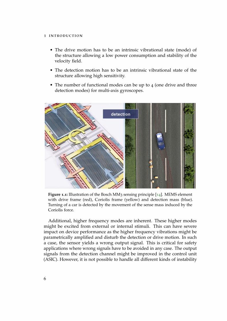
Gyroscopes measure angular rate around a rotation axis. The measure-ment principle is the detection of Coriolis force inside the sensor structure.Sensing Coriolis force requires a moving mass inside the rotating frame.Several concepts exist ranging from spinning wheels over oscillating discsto vibratory gyroscopes. The Coriolis vibratory gyroscope (CVG) is thekey player under state-of-the-art gyroscope concepts [74]. Under cost andrequirement pressure, the automotive engineers have started incorporatingMEMS gyroscopes. Main advantages are the small size, better extendabilityof functionality and optimization of the gyroscope design. A very basic con-cept can be found in various MEMS gyroscopes on the market, e.g. the BoschMM3 ΩZ gyroscope (Figure 1.1). The MEMS element consists of a springmass system which is doubled to suppress sensitivity to linear acceleration.The spring mass system consists of a drive and Coriolis frame and a detectionmass. In operation, the drive frame moves in y-direction. An angular ratearound the z-axis results in a Coriolis force exciting the detection motion(blue arrows in Figure 1.1). The angular rate is determined through thismovement using the capacitive read-out inside the detection mass cells. Theread-out is then processed by an application specific integrated circuit (ASIC)and the result is transfered to the downstream units. The signals from thedetection mass cells are small, typically in the range of a few femto Farad.Thus, even small unintended signals become relevant for the measurementaccuracy.
The structure design has to fulfill different criteria for the functionality ofthe sensor and robustness against external stimuli.
5
1 introduction
• The drive motion has to be an intrinsic vibrational state (mode) ofthe structure allowing a low power consumption and stability of thevelocity field.
• The detection motion has to be an intrinsic vibrational state of thestructure allowing high sensitivity.
• The number of functional modes can be up to 4 (one drive and threedetection modes) for multi-axis gyroscopes.
Figure 1.1: Illustration of the Bosch MM3 sensing principle [14]. MEMS elementwith drive frame (red), Coriolis frame (yellow) and detection mass (blue).Turning of a car is detected by the movement of the sense mass induced by theCoriolis force.
Additional, higher frequency modes are inherent. These higher modesmight be excited from external or internal stimuli. This can have severeimpact on device performance as the higher frequency vibrations might beparametrically amplified and disturb the detection or drive motion. In sucha case, the sensor yields a wrong output signal. This is critical for safetyapplications where wrong signals have to be avoided in any case. The outputsignals from the detection channel might be improved in the control unit(ASIC). However, it is not possible to handle all different kinds of instability
6
1 .1 challenges in developing state-of-the-art mems
gyroscopes
within the ASIC. Optimizing the sensor design is a necessary measure forimproving sensor stability and lowering the error rate.
1.1 Challenges in developing state-of-the-artMEMS gyroscopes
In current development of MEMS gyroscopes, challenges are due to costpressures, the demand for higher performances and better robustness againstexternal stimuli. The cost requirement of the market pushes engineers toshorten their expenses in the development of new sensors. This can beachieved by less iterations in the development process and shorter time-to-market. This drives MEMS engineers to include nonlinear effects in thedesign optimization of gyroscopes. A reliable prediction of the sensor be-haviour can efficiently reduce costs in the development process. Furthermore,new applications of MEMS gyroscopes, such as navigation and augmentedreality, require higher performances. Such performance requirements ask foraccurate predictions of the sensor hardware including the nonlinear effects.In this way, efficient and accurate prediction of the nonlinear effects makesthe development of high-performance gyroscopes possible.
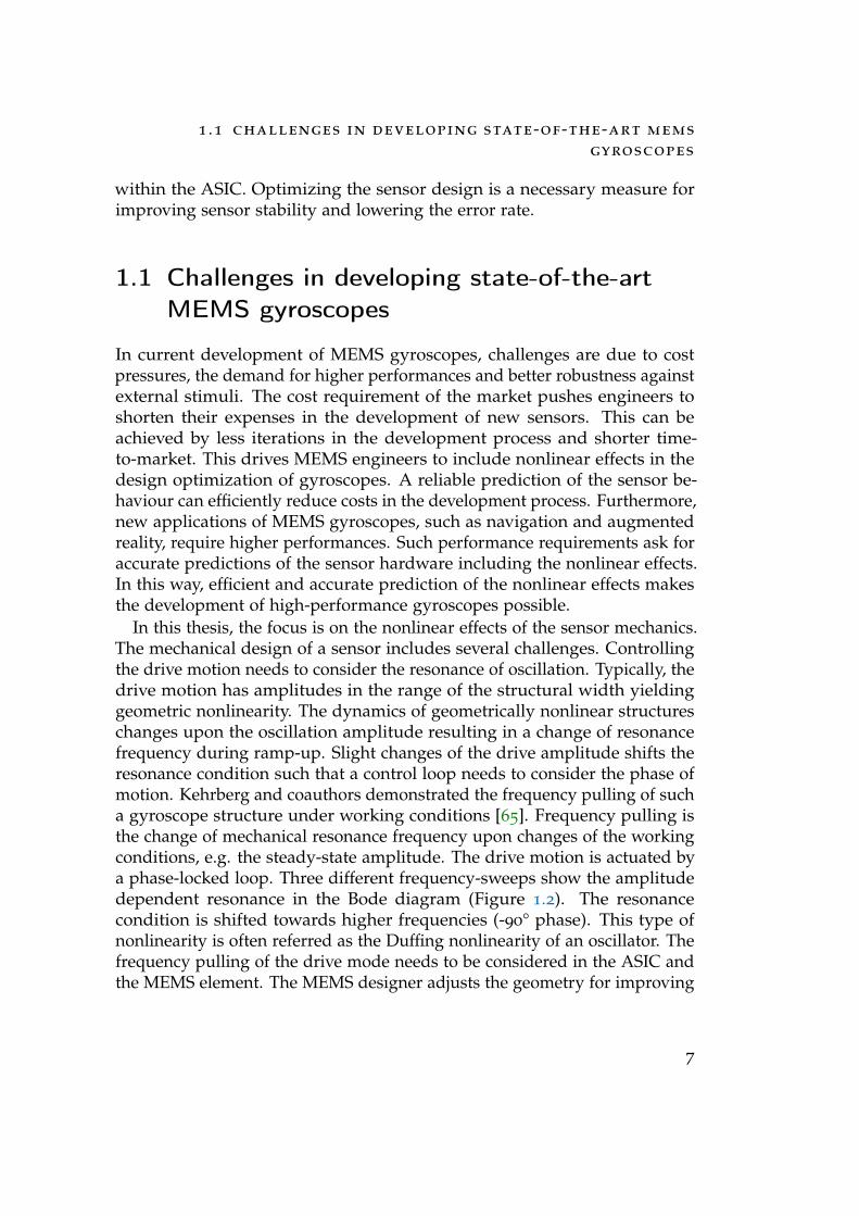
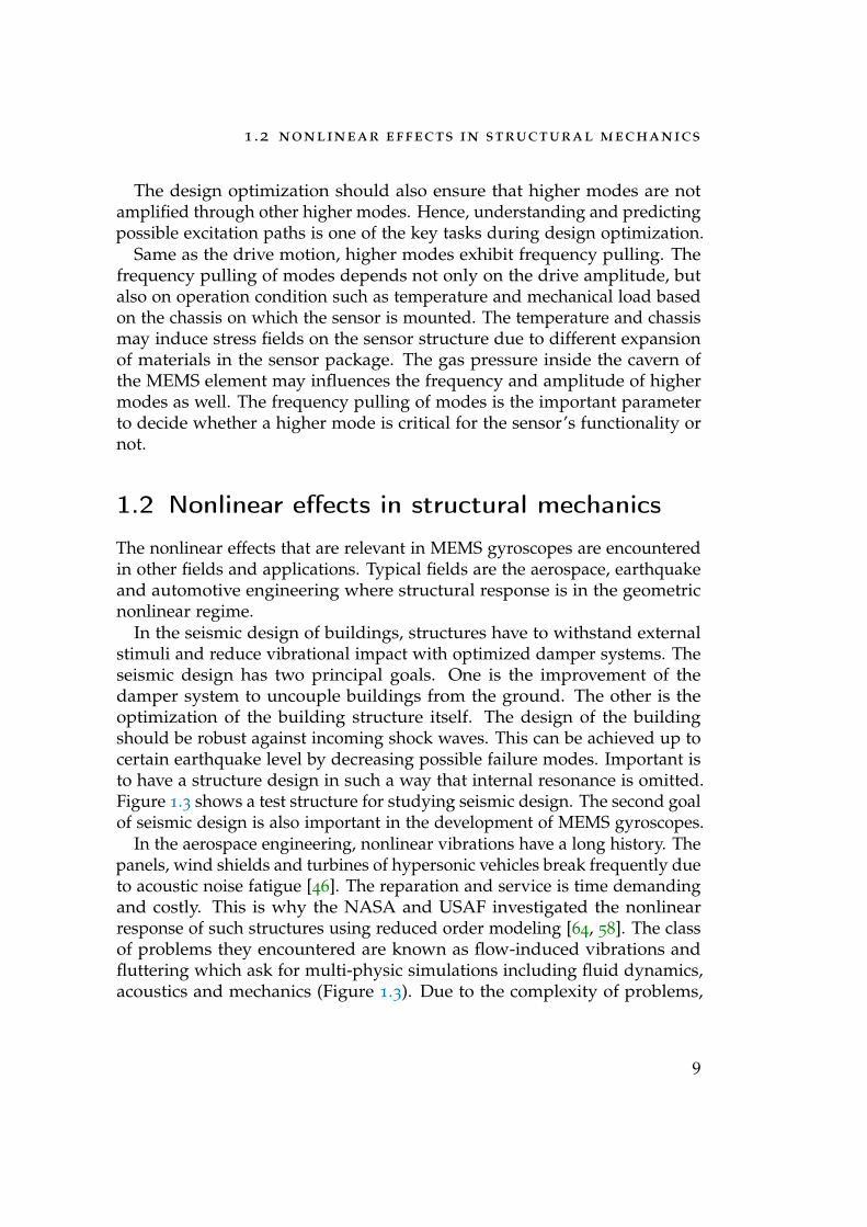
In this thesis, the focus is on the nonlinear effects of the sensor mechanics.The mechanical design of a sensor includes several challenges. Controllingthe drive motion needs to consider the resonance of oscillation. Typically, thedrive motion has amplitudes in the range of the structural width yieldinggeometric nonlinearity. The dynamics of geometrically nonlinear structureschanges upon the oscillation amplitude resulting in a change of resonancefrequency during ramp-up. Slight changes of the drive amplitude shifts theresonance condition such that a control loop needs to consider the phase ofmotion. Kehrberg and coauthors demonstrated the frequency pulling of sucha gyroscope structure under working conditions [65]. Frequency pulling isthe change of mechanical resonance frequency upon changes of the workingconditions, e.g. the steady-state amplitude. The drive motion is actuated bya phase-locked loop. Three different frequency-sweeps show the amplitudedependent resonance in the Bode diagram (Figure 1.2). The resonancecondition is shifted towards higher frequencies (-90° phase). This type ofnonlinearity is often referred as the Duffing nonlinearity of an oscillator. Thefrequency pulling of the drive mode needs to be considered in the ASIC andthe MEMS element. The MEMS designer adjusts the geometry for improving
7
1 introduction
the linearity and decreasing the frequency pulling of the drive motion. TheASIC designer allows enough variation for the resonance condition in thecontrol loop.
ampl
itud
e(µ
m)
phas
e(
)
0
5
10
15
0
-90
-180
2.38 2.40 2.42 2.44 2.46 2.48 2.50 2.52·104
·1042.38 2.40 2.42 2.44 2.46 2.48 2.50 2.52
frequency (Hz)
1
Figure 1.2: Frequency pulling of the drive motion of a MEMS gyroscope.Picture adopted from [65].
Another aspect of geometric nonlinearity is the coupling between vibra-tional modes. The stress inside a geometric nonlinear structure creates forcesonto several modes. Actuation of a single mode can thereby excite othermodes. The amplification of these modes depends on the coupling whichmainly arises from symmetry between the modes. As a rule of thumb, theMEMS engineer has to optimize the gyroscope design such that higher fre-quency modes do not coincide with multiples of the drive mode. Especially,the second and third multiple of the drive mode need to be free from highermodes. These are the 2:1 and 3:1 internal resonances which could exhibit thestrongest parametric gain in the system. Modal coupling can also be betweenthe drive motion and several higher modes (up to 3 higher modes). If theresonance condition for these modes is fulfilled, the system may transferenergy from the drive motion to these higher modes. This excitation pathis complex and has to take interactions between the vibrational modes intoaccount.
8
1 .2 nonlinear effects in structural mechanics
The design optimization should also ensure that higher modes are notamplified through other higher modes. Hence, understanding and predictingpossible excitation paths is one of the key tasks during design optimization.
Same as the drive motion, higher modes exhibit frequency pulling. Thefrequency pulling of modes depends not only on the drive amplitude, butalso on operation condition such as temperature and mechanical load basedon the chassis on which the sensor is mounted. The temperature and chassismay induce stress fields on the sensor structure due to different expansionof materials in the sensor package. The gas pressure inside the cavern ofthe MEMS element may influences the frequency and amplitude of highermodes as well. The frequency pulling of modes is the important parameterto decide whether a higher mode is critical for the sensor’s functionality ornot.
1.2 Nonlinear effects in structural mechanics
The nonlinear effects that are relevant in MEMS gyroscopes are encounteredin other fields and applications. Typical fields are the aerospace, earthquakeand automotive engineering where structural response is in the geometricnonlinear regime.
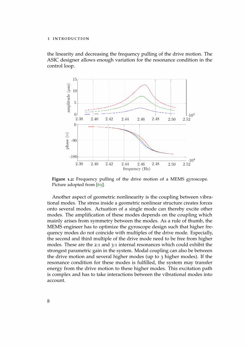
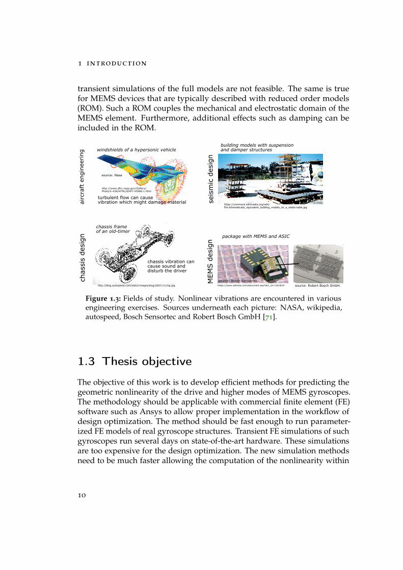
In the seismic design of buildings, structures have to withstand externalstimuli and reduce vibrational impact with optimized damper systems. Theseismic design has two principal goals. One is the improvement of thedamper system to uncouple buildings from the ground. The other is theoptimization of the building structure itself. The design of the buildingshould be robust against incoming shock waves. This can be achieved up tocertain earthquake level by decreasing possible failure modes. Important isto have a structure design in such a way that internal resonance is omitted.Figure 1.3 shows a test structure for studying seismic design. The second goalof seismic design is also important in the development of MEMS gyroscopes.
In the aerospace engineering, nonlinear vibrations have a long history. Thepanels, wind shields and turbines of hypersonic vehicles break frequently dueto acoustic noise fatigue [46]. The reparation and service is time demandingand costly. This is why the NASA and USAF investigated the nonlinearresponse of such structures using reduced order modeling [64, 58]. The classof problems they encountered are known as flow-induced vibrations andfluttering which ask for multi-physic simulations including fluid dynamics,acoustics and mechanics (Figure 1.3). Due to the complexity of problems,
9
1 introduction
transient simulations of the full models are not feasible. The same is truefor MEMS devices that are typically described with reduced order models(ROM). Such a ROM couples the mechanical and electrostatic domain of theMEMS element. Furthermore, additional effects such as damping can beincluded in the ROM.
Figure 1.3: Fields of study. Nonlinear vibrations are encountered in variousengineering exercises. Sources underneath each picture: NASA, wikipedia,autospeed, Bosch Sensortec and Robert Bosch GmbH [71].
1.3 Thesis objective
The objective of this work is to develop efficient methods for predicting thegeometric nonlinearity of the drive and higher modes of MEMS gyroscopes.The methodology should be applicable with commercial finite element (FE)software such as Ansys to allow proper implementation in the workflow ofdesign optimization. The method should be fast enough to run parameter-ized FE models of real gyroscope structures. Transient FE simulations of suchgyroscopes run several days on state-of-the-art hardware. These simulationsare too expensive for the design optimization. The new simulation methodsneed to be much faster allowing the computation of the nonlinearity within
10
1 .3 thesis objective
minutes or hours. Further, the new methods should offer similar accuracy ascompared to the transient FE simulations.
One aspect of the thesis objective is to find proper observables to capturethe type and strength of geometric nonlinearity. The results from the FEsimulation may be further used to build ROMs that allow the calculation offrequency pulling.
The term frequency shift is used in the following for the frequency pullingat a specific amplitude of the drive motion.
The precision of these frequency shifts is used to measure the accuracy ofthe different simulation and modeling approaches. There are several reasonsfor this.
• The frequency shift is an important parameter for the design of MEMSgyroscopes.
• The frequency shift is much more sensitive to the geometric nonlinearityas the structural displacement itself. Similar to the strain energy, theresonance frequency changes drastically upon axial variations of thedisplacements.
• In the community, nonlinear vibrations are characterized by the frequency-energy plot representing the nonlinear normal mode of structures. Thefrequency shift contains information of this frequency-energy relationneglecting branching (bifurcation).
• The frequency shift of higher modes depends on the modal couplingto the actuated mode, i.e. to the drive mode of the gyroscope.
• Finally, the frequency shift is a single number for every mode whichallows a precise valuation of the model quality.
The main challenge in predicting geometric nonlinear structures is that thestiffness depends on the actual displacement of the structure asking for aniterative procedure in the calculation. As the original trajectory is unknownin the beginning of an oscillation, the calculation has to consider the solutionof prior time steps. This is possible in a transient FE simulation where thestiffness is updated in every time step. However, transient FE simulations aretime-consuming and cumbersome for validation and testing of designs. Afruitful strategy is to reduce the number of degrees of freedom (DoFs) usingmodel order reduction. The resulting ROMs may allow transient simulations
11
1 introduction
for the validation and testing. The ultimate goal would be an extremelow-order ROM (1-3D) that allows the use of perturbation techniques. Theresult would be an analytical formula describing the resonance curve, e.g.frequency pulling.
Outline of this thesis
The thesis is organized in three main parts: theory, simulation methods andresults. In the theoretical part, structural mechanics is introduced from thephysical picture. Using variational calculus for mass particles, the FE methodis introduced for arbitrary structures. The common model order reductionfor MEMS is shortly summarized. It will be later used in the part aboutsimulation methods. The origin of nonlinearities in MEMS is shown withthe focus on mechanical nonlinearities. In the end of the theoretical part,geometric nonlinearity is expressed for analytical models and for arbitrarystructures.
In the second part, the different simulation methods that have been devel-oped are described. A nonlinear transient finite element simulation (NLTFE)is used for generating the reference shifts. In this work it is often referredto as the test bench. Specific modes, that are difficult to measure in theexperiment, can be examined with this method. The second method usesnonlinear static simulations to predict the frequency shifts. This methodwill be called nonlinear static simulation (NLS). The NLS is an energy-basedmethod using the strain energy of elements upon static loading. The thirdmethod uses pre-stressed modal analysis for generating ROMs. The fre-quency shifts can be determined by transient simulations of the ROMs. Themethod is called nonlinear transient ROM simulation (NLTROM). It is astiffness-based approach using frequencies and mode shapes from modalanalysis.
In the third part, the simulation methods are benchmarked with four dif-ferent FE models. One is a clamped-clamped beam, the others are gyroscopestructures. These are a single axis gyroscope test structure, a single axisand 2-axis state-of-the-art gyroscope that are currently developed for theautomotive market. Conclusion and outlook are drawn in the last section.The results are summarized and put in context of current literature.
12

2 Theory
Eipot ∝ (δr)2
~Fi,j~Fj,i
ij
δr
p+e−
e− p+
p+je−
e−e−p+j
e− p+i
p+i
interaction mediated by photons
force
atomic scale
macroscopic scale
structural mechanics
continuum
discretization
FEM
1
Structural mechanics describes the macroscopic output of the microscopic interactionsin a solid body. Picture partly taken from [62], page 67.
13
2 theory
2.1 Structural mechanics
2.1.1 Physical picture
The field of structural mechanics is concerned with the macroscopic de-scription of the overall interactions between atoms in a solid body. Atomsfavor periodic orientation in condensed matter. This periodic orientationis called crystal lattice and the reason for a periodic potential leading tophenomena like an electronic and phononic band structure. The phononicbands, such as acoustic and optical bands, are solutions to vibrations withinthe lattice. Light-matter interaction is possible through the optical bandstructure, matter-matter interaction is possible through the acoustic bandstructure. Hence, structural mechanics deals with collective states of theacoustic band structure.
Macroscopic forces of a solid body result from microscopic electromagneticforces between the atoms. The atom cores are in the periodic potential of thelattice which is locally an harmonic potential for each atom core. Thus, smallelongations of the atom cores result in linear forces. For large elongation ofthe atom cores, the local potential is more influenced by the Born repulsionand the electromagnetic interaction between individual charges which giverise to material nonlinearity in structural mechanics. Material fatigue evolvesfrom permanent changes in the crystal lattice.
A simple model of the microscopic interaction is a 2D lattice with effectivevalues for the spring stiffness between the atoms. From this simple model,acoustic and optical solutions can be derived. The acoustic solutions areessential for surface acoustic wave (SAW) filters. Optical solutions areespecially important in quantum and nonlinear optics where light-matterinteraction is studied.
An interesting aspect of the physical picture of structural mechanics isthat interactions between individual charges/ atoms are easy to describeanalytically. In contrast, describing a small volume of solid matter (1023
atoms) results in prohibitive computational cost. The aim of structuralmechanics is to describe this macroscopic output of solid matter efficiently.
In the following, the mathematical description of rigid bodies and particlesis presented. This includes the variational calculus which is later used inthe finite element method (FEM) to allow the description of complex bodydeformations.
14
2 .1 structural mechanics
2.1.2 Mathematical description
The mathematical description of mechanics was key role in the 18th centurybattle over lunar motion [13]. Predicting the orbit of the moon was aprerequisite for determining longitudes of ships and it became especiallyimportant for space missions in the 1960s and 70s. The main actors in thatbattle were the three mathematicians, Clairaut, Euler and d’Alembert. Eachof them aimed for the correct orbit calculation using variational calculus andNewton’s law of gravitation. This part of mechanics became later known asanalytical mechanics.
D’Alembert’s principle
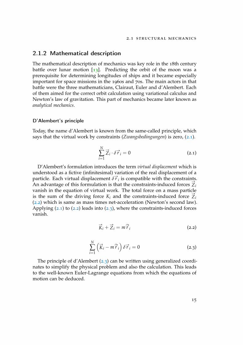
Today, the name d’Alembert is known from the same-called principle, whichsays that the virtual work by constraints (Zwangsbedingungen) is zero, (2.1).
N
∑i=1
ÑZi · δÑr i = 0 (2.1)
D’Alembert’s formulation introduces the term virtual displacement which isunderstood as a fictive (infinitesimal) variation of the real displacement of aparticle. Each virtual displacement δ
Ñr i is compatible with the constraints.An advantage of this formulation is that the constraints-induced forces
ÑZi
vanish in the equation of virtual work. The total force on a mass particleis the sum of the driving force Ki and the constraints-induced force
ÑZi
(2.2) which is same as mass times net-acceleration (Newton’s second law).Applying (2.1) to (2.2) leads into (2.3), where the constraints-induced forcesvanish.
ÑK i +
ÑZi = mÑr i (2.2)
N
∑i=1
(ÑK i −mÑr i
)δ
Ñr i = 0 (2.3)
The principle of d’Alembert (2.3) can be written using generalized coordi-nates to simplify the physical problem and also the calculation. This leadsto the well-known Euler-Lagrange equations from which the equations ofmotion can be deduced.
15
2 theory
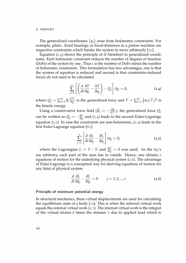
The generalized coordinates qj arise from holonomic constraints. Forexample, plain-, fixed bearings or fixed-distances in a piston machine arerespective constraints which hinder the system to move arbitrarily [51].
Equation (2.4) shows the principle of d’Alembert in generalized coordi-nates. Each holonomic constraint reduces the number of degrees of freedom(DoFs) of the system by one. Thus s is the number of DoFs minus the numberof holonomic constraints. This formulation has two advantages, one is thatthe system of equation is reduced and second is that constraints-inducedforces do not need to be calculated.
s
∑j=1
[(ddt
∂T∂qj− ∂T
∂qj
)−Qj
]δqj = 0, (2.4)
where Qj = ∑Ni=1 Ki
∂Ñr i∂qj
is the generalized force and T = ∑Ni=1
12 mi(
Ñr i)2 is
the kinetic energy.Using a conservative force field (
ÑK i = − ∂V
∂Ñr i
), the generalized force Qj
can be written as Qj = − ∂V∂qj
and (2.4) leads to the second Euler-Lagrangeequation (2.5). In case the constraints are non-holonomic, (2.4) leads to thefirst Euler-Lagrange equation [61]:
s
∑j=1
[ddt
∂L∂qj− ∂L
∂qj
]δqj = 0, (2.5)
where the Lagrangian L = T − V and ∂V∂qj
= 0 was used. As the δqj’sare arbitrary, each part of the sum has to vanish. Hence, one obtains sequations of motion for the underlying physical system (2.6). The advantageof Euler-Lagrange is a conceptual way for deriving equations of motion forany kind of physical system.
ddt
∂L∂qj− ∂L
∂qj= 0 j = 1, 2, ..., s (2.6)
Principle of minimum potential energy
In structural mechanics, these virtual displacements are used for calculatingthe equilibrium state of a body [12]. This is when the internal virtual workequals the external virtual work (2.7). The internal virtual work is the integralof the virtual strains ε times the stresses τ due to applied load which is
16
2 .1 structural mechanics
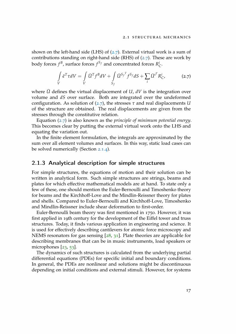
shown on the left-hand side (LHS) of (2.7). External virtual work is a sum ofcontributions standing on right-hand side (RHS) of (2.7). These are work bybody forces f B, surface forces f S f and concentrated forces Ri
C.∫V
εTτdV =∫V
UT f BdV +∫S f
US fT
f S f dS + ∑i
UiTRi
C, (2.7)
where U defines the virtual displacement of U, dV is the integration overvolume and dS over surface. Both are integrated over the undeformedconfiguration. As solution of (2.7), the stresses τ and real displacements Uof the structure are obtained. The real displacements are given from thestresses through the constitutive relation.
Equation (2.7) is also known as the principle of minimum potential energy.This becomes clear by putting the external virtual work onto the LHS andequating the variation out.
In the finite element formulation, the integrals are approximated by thesum over all element volumes and surfaces. In this way, static load cases canbe solved numerically (Section 2.1.4).
2.1.3 Analytical description for simple structures
For simple structures, the equations of motion and their solution can bewritten in analytical form. Such simple structures are strings, beams andplates for which effective mathematical models are at hand. To state only afew of these, one should mention the Euler-Bernoulli and Timoshenko theoryfor beams and the Kirchhoff-Love and the Mindlin-Reissner theory for platesand shells. Compared to Euler-Bernoulli and Kirchhoff-Love, Timoshenkoand Mindlin-Reissner include shear deformation to first-order.
Euler-Bernoulli beam theory was first mentioned in 1750. However, it wasfirst applied in 19th century for the development of the Eiffel tower and trussstructures. Today, it finds various application in engineering and science. Itis used for effectively describing cantilevers for atomic force microscopy andNEMS resonators for gas sensing [28, 31]. Plate theories are applicable fordescribing membranes that can be in music instruments, load speakers ormicrophones [23, 53].
The dynamics of such structures is calculated from the underlying partialdifferential equations (PDEs) for specific initial and boundary conditions.In general, the PDEs are nonlinear and solutions might be discontinuousdepending on initial conditions and external stimuli. However, for systems
17
2 theory
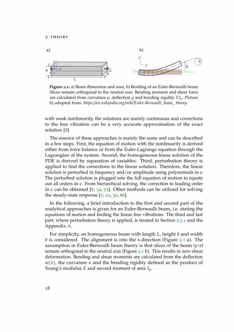
Figure 2.1: a) Beam dimension and axes, b) Bending of an Euler-Bernoulli beam.Slices remain orthogonal to the neutral axis. Bending moment and shear forceare calculated from curvature ρ, deflection g and bending rigidity EIy. Pictureb) adopted from: https://en.wikipedia.org/wiki/Euler-Bernoulli_beam_ theory.
with weak nonlinearity, the solutions are mainly continuous and correctionsto the free vibration can be a very accurate approximation of the exactsolution [8].
The essence of these approaches is mainly the same and can be describedin a few steps. First, the equation of motion with the nonlinearity is derivedeither from force balance or from the Euler-Lagrange equation through theLagrangian of the system. Second, the homogeneous linear solution of thePDE is derived by separation of variables. Third, perturbation theory isapplied to find the corrections to the linear solution. Therefore, the linearsolution is perturbed in frequency and/or amplitude using polynomials in ε.The perturbed solution is plugged into the full equation of motion to equateout all orders in ε. From hierarchical solving, the correction to leading orderin ε can be obtained [8, 32, 72]. Other methods can be utilized for solvingthe steady-state response [7, 21, 30, 66].
In the following, a brief introduction to the first and second part of theanalytical approaches is given for an Euler-Bernoulli beam, i.e. stating theequations of motion and finding the linear free vibrations. The third and lastpart, where perturbation theory is applied, is treated in Section 2.5.1 and theAppendix A.
For simplicity, an homogeneous beam with length L, height h and widthb is considered. The alignment is into the x-direction (Figure 2.1 a). Theassumption in Euler-Bernoulli beam theory is that slices of the beam (y-z)remain orthogonal to the neutral axis (Figure 2.1 b). This results in zero sheardeformation. Bending and shear moments are calculated from the deflectionw(x), the curvature κ and the bending rigidity defined as the product ofYoung’s modulus E and second moment of area Iy.
18
2 .1 structural mechanics
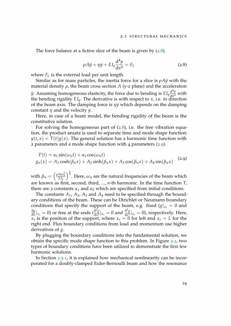
The force balance at a fictive slice of the beam is given by (2.8).
ρAy + ηy + EIyd4ydx4 = FL (2.8)
where FL is the external load per unit length.Similar as for mass particles, the inertia force for a slice is ρAy with the
material density ρ, the beam cross section A (y-z plane) and the acceleration
y. Assuming homogeneous elasticity, the force due to bending is EIyd4ydx4 with
the bending rigidity EIy. The derivative is with respect to x, i.e. in directionof the beam axis. The damping force is ηy which depends on the dampingconstant η and the velocity y.
Here, in case of a beam model, the bending rigidity of the beam is theconstitutive relation.
For solving the homogeneous part of (2.8), i.e. the free vibration equa-tion, the product ansatz is used to separate time and mode shape function:y(t, x) = T(t)g(x). The general solution has a harmonic time function with2 parameters and a mode shape function with 4 parameters (2.9).
T(t) = α1 sin(ωnt) + α2 cos(ωnt)gn(x) = A1 cosh(βnx) + A2 sinh(βnx) + A3 cos(βnx) + A4 sin(βnx)
(2.9)
with βn =(
ρAω2n
EIy
) 14. Here, ωn are the natural frequencies of the beam which
are known as first, second, third, ..., n-th harmonic. In the time function T,there are 2 constants α1 and α2 which are specified from initial conditions.
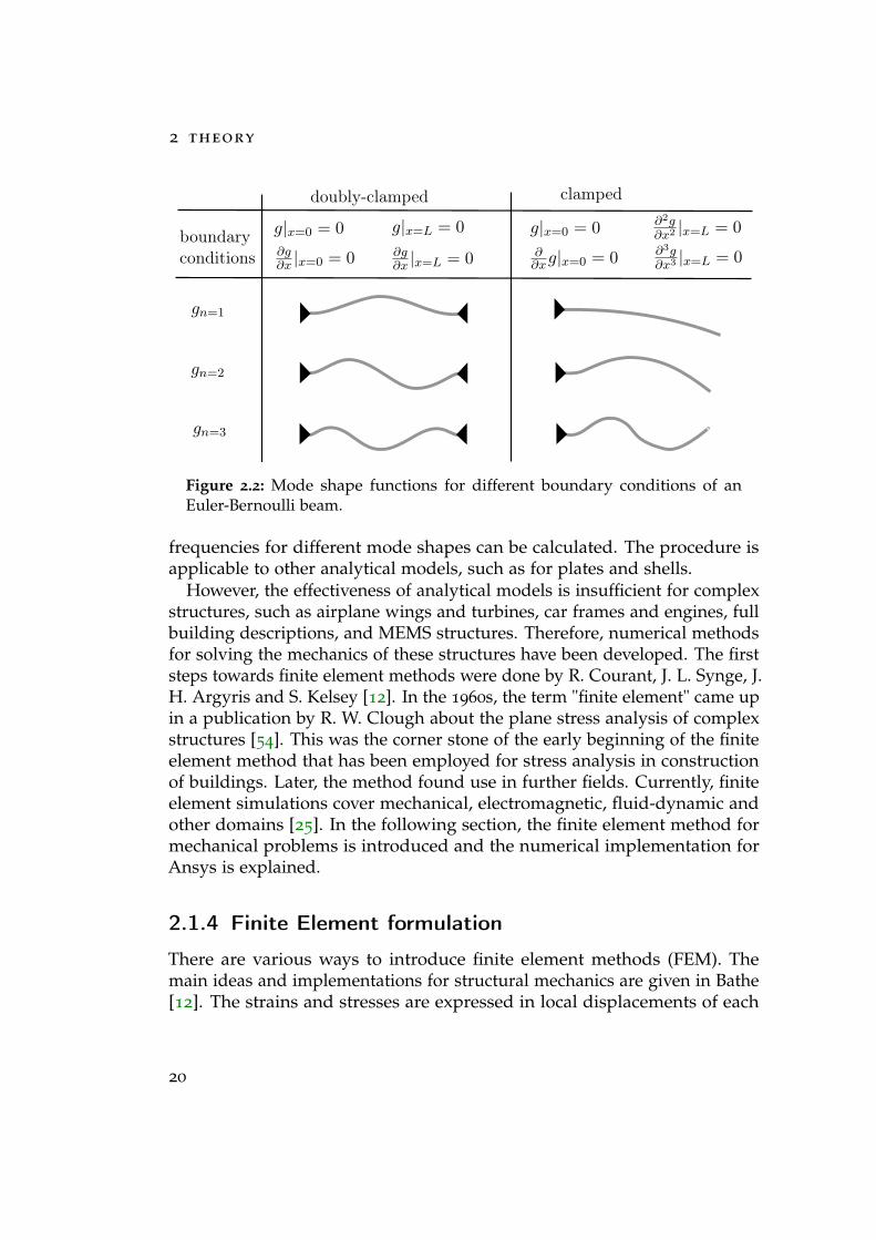
The constants A1, A2, A3 and A4 need to be specified through the bound-ary conditions of the beam. These can be Dirichlet or Neumann boundaryconditions that specify the support of the beam, e.g. fixed (g|xs = 0 and∂g∂x |xs = 0) or free at the ends ( ∂2g
∂x2 |xs = 0 and ∂3g∂x3 |xs = 0), respectively. Here,
xs is the position of the support, where xs = 0 for left and xs = L for theright end. Flux boundary conditions from load and momentum use higherderivatives of g.
By plugging the boundary conditions into the fundamental solution, weobtain the specific mode shape function to this problem. In Figure 2.2, twotypes of boundary conditions have been utilized to demonstrate the first fewharmonic solutions.
In Section 2.5.1, it is explained how mechanical nonlinearity can be incor-porated for a doubly-clamped Euler-Bernoulli beam and how the resonance
19
2 theory
gn=1
gn=2
gn=3
g|x=0 = 0 g|x=L = 0
∂g∂x |x=0 = 0 ∂g
∂x |x=L = 0
g|x=0 = 0
∂∂xg|x=0 = 0 ∂3g
∂x3 |x=L = 0
∂2g∂x2 |x=L = 0
doubly-clamped clamped
boundaryconditions
1
Figure 2.2: Mode shape functions for different boundary conditions of anEuler-Bernoulli beam.
frequencies for different mode shapes can be calculated. The procedure isapplicable to other analytical models, such as for plates and shells.
However, the effectiveness of analytical models is insufficient for complexstructures, such as airplane wings and turbines, car frames and engines, fullbuilding descriptions, and MEMS structures. Therefore, numerical methodsfor solving the mechanics of these structures have been developed. The firststeps towards finite element methods were done by R. Courant, J. L. Synge, J.H. Argyris and S. Kelsey [12]. In the 1960s, the term "finite element" came upin a publication by R. W. Clough about the plane stress analysis of complexstructures [54]. This was the corner stone of the early beginning of the finiteelement method that has been employed for stress analysis in constructionof buildings. Later, the method found use in further fields. Currently, finiteelement simulations cover mechanical, electromagnetic, fluid-dynamic andother domains [25]. In the following section, the finite element method formechanical problems is introduced and the numerical implementation forAnsys is explained.
2.1.4 Finite Element formulation
There are various ways to introduce finite element methods (FEM). Themain ideas and implementations for structural mechanics are given in Bathe[12]. The strains and stresses are expressed in local displacements of each
20
2 .1 structural mechanics
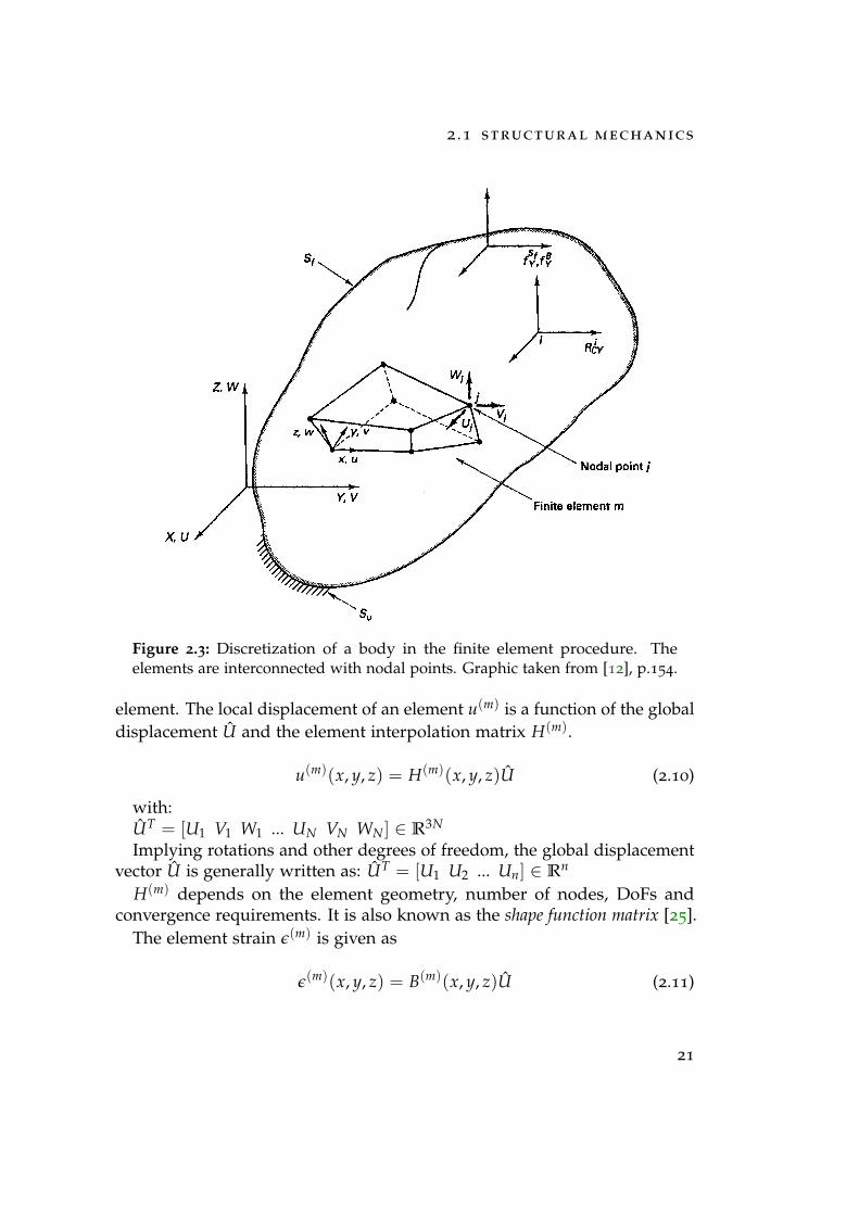
Figure 2.3: Discretization of a body in the finite element procedure. Theelements are interconnected with nodal points. Graphic taken from [12], p.154.
element. The local displacement of an element u(m) is a function of the globaldisplacement U and the element interpolation matrix H(m).
u(m)(x, y, z) = H(m)(x, y, z)U (2.10)
with:UT = [U1 V1 W1 ... UN VN WN] ∈ R3N
Implying rotations and other degrees of freedom, the global displacementvector U is generally written as: UT = [U1 U2 ... Un] ∈ Rn
H(m) depends on the element geometry, number of nodes, DoFs andconvergence requirements. It is also known as the shape function matrix [25].
The element strain ε(m) is given as
ε(m)(x, y, z) = B(m)(x, y, z)U (2.11)
21
2 theory
where the strain-displacement matrix B(m) comes out by differentiation ofH(m) using the respective strain law (engineering strain, logarithmic strain,etc.).
The element stress is calculated from the element strain using the elasticitymatrix C (isotropic, anisotropic). This is the part in structural mechanicswhere the constitutive relation enters the calculation.
τ(m) = C(m)ε(m) + τ(m) (2.12)
with the initial stress τ(m).Using the element formulation, the principle of minimum potential energy
in local coordinates (2.7) reads
∑m
∫V(m)
ε(m)Tτ(m)dV(m) = ∑
m
∫V(m)
u(m)Tf B(m)dV(m)
+∑m
∫S(m)
1 ,...,S(m)q
uS(m)Tf S(m)dS(m) + ∑
iuiT
RiC.
(2.13)
Plugging (2.10), (2.11) and (2.12) into (2.13) yields
∑m
∫V(m)
¯UTB(m)TC(m)B(m)UdV(m) = −∑
m
∫V(m)
¯UTB(m)Tτ(m)dV(m)
+ ∑m
∫V(m)
¯UT H(m)Tf B(m)dV(m)
+ ∑m
∫S(m)
1 ,...,S(m)q
¯UT HS(m)Tf S(m)dSS(m)
+ ¯UTRC
(2.14)
with the global displacement U and the global virtual displacement ¯U.Compared to (2.13), the sum of concentrated nodal forces Ri
C is written asscalar product. One should mention that the initial stress comes in on theright-hand side of (2.14).
¯U can be pulled out. Since ¯U is arbitrary, each line of the vector equationneeds to be fulfilled and the static equilibrium in nodal displacements and
22
2 .1 structural mechanics
forces is obtained (2.15). The hat sign was dropped (U = U).
KU = R (2.15)
with the stiffness matrix
K = ∑m
∫V(m)
B(m)TC(m)B(m)dV(m) (2.16)
and the load vector
R = RB + RS − Ri + RC. (2.17)
The load vector includes concentrated loads RC, and body loads
RB = ∑m
∫V(m)
H(m)Tf B(m)dV(m), (2.18)
surface loadsRS = ∑
m
∫S(m)
1 ,...,S(m)q
HS(m)Tf S(m)dS(m) (2.19)
and loads by initial stress
Ri = ∑m
∫V(m)
B(m)Tτ(m)dV(m). (2.20)
In comparison to nonlinear problems, this assemblage of K is called thedirect stiffness method.
Using d’Alembert (2.3), inertial loads can be added for dynamical prob-lems, i.e.
RB = ∑m
∫V(m)
H(m)T (f B(m) − ρ(m)H(m)U
)dV(m) (2.21)
The inertial force was added as a body force. Furthermore, damping canbe added in the same way. This leads to the general dynamical problem instructural mechanics (2.22).
MU + DU + KU = R (2.22)
23
2 theory
M = ∑m
∫V(m)
ρ(m)H(m)TH(m)dV(m) (2.23)
D = ∑m
∫V(m)
κ(m)H(m)TH(m)dV(m) (2.24)
Usually, the damping matrix is assembled from M and K because theelemental damping κ(m) is not physically given.
All the above holds for linear, infinitesimal displacements where finaland original configurations are same. However, in a large-displacementor large-rotation analysis, strain and stress need to be adjusted due todifference in final and original reference frame. There are two formulations,the total Lagrangian (TL) formulation, where the integration is done over theoriginal (undeformed) configuration V0 and the updated Lagrangian (UL)formulation, where the integration is done over the current configurationV(t). Ansys FE software uses the UL, whereas Comsol Multiphysics usesTL formulation for nonlinear structural problems. These formulations areequivalent. However, the updated formulation yields some simplificationsin the strain, e.g. no terms from initial displacement [12]. For a comparisonbetween the two formulations, the reader is referred to the Appendix B. Inthe following, the main ideas and ingredients of the Ansys-implementationof the UL are briefly summarized.
Numerical implementation for large-displacements in Ansys
Strain ε is implemented using logarithmic/Hencky strain measures wherethe current total strain is given as the sum of the increment and the previousstrain (2.25).
εn = εn−1 + ∆εn (2.25)
The increment ∆εn is approximated from the logarithmic scale of thestretch matrix (2.26).
∆εn = ln(∆Un), (2.26)
where ∆Un is established from ∆F = ∆R∆U and ∆F = FnF−1n−1 using previous
and current deformation gradient. Right polar decomposition is used toisolate the stretch matrix ∆Un from the deformation gradient increment ∆F.
24
2 .2 model order reduction for mems
Furthermore, the strain increment is corrected with the rotation matrix asdescribed by Hughes et al. [25].
Analogously, stress is formulated incremental using Jaumann rate ofCauchy stress. Since the Cauchy stress is not invariant under rotation,Jaumann rate is used for proper application of the constitutive law. This isan objective stress rate with the property of frame-invariance. Here, σ isused as the stress matrix, not to confuse with τ, which is the stress vector.
σij = Cijkldkl + σikωjk + σjkωik, (2.27)
where the first term on the RHS is the constitutive law, i.e. the product ofmaterial constitutive tensor Cijkl and rate of deformation tensor dij due tostraining. Second and third term on RHS are the corrections to rigid bodyrotation due to Jaumann rate formulation.
From this stress rate, the stress stiffening matrix Si is constructed usingthe element shape functions and time step (2.28).
Si =∫V
GTi τiGidV (2.28)
with Gi as the matrix of shape function derivatives evaluated at the config-uration i and τi as the matrix of current Cauchy stresses σi in the globalcoordinate system. The vector τ is constructed from σij with the respectivetime step.
2.2 Model order reduction for MEMS
The idea of model order reduction is to decrease the number of DoFs, butmaintain the accuracy of specific relevant DoFs. In literature, different kindsand techniques of model order reduction (MOR) are available. An overviewis found in [1, 19, 27].
In the field of MEMS, modal and nodal based MOR techniques [59, 9] arecommon. The result of the MOR is a reduced order model (ROM) that can besolved efficiently either via time integration or an algebraic set of equations.MEMS designers benefit from ROMs of their devices as they can treat effectsfrom different domains in one simulation.
For MEMS sensors, the linear normal modes (LNM) offer adequate co-ordinates for a mechanical ROM. Several authors have documented theprocedure and use of LNMs in ROMs for MEMS [19, 20, 26, 35, 34, 43]. In
25
2 theory
literature, MOR via LNMs is known under different terminologies such asmodal superposition, modal truncation or Rayleigh-Ritz method [27]. In thefollowing section, MOR using LNMs is highlighted briefly. Furthermore,several other MOR techniques used in the field are cited.
2.2.1 Modal Superposition
The linear vibration problem is written in the common notation [4, 9, 74,12], where M is the mass matrix, K is the stiffness matrix, D is the dampingmatrix, f is the external force vector and x is the state vector (2.29). Thedimension of this vector equation equals the number of DoFs from the finiteelement formulation.
Mx + Dx + Kx = f (t) (2.29)
In the modal basis, the oscillator equation reads
Mq + Dq + Kq = f (t) (2.30)
The modal vectors and matrices are obtained from the projection of the fullmatrices (2.31).
M = VTMV (same for D and K)x = Vq
q = (VTV)−1VTx
f (t) = VT f (t)
(2.31)
using the projection V with
V = [φ1, φ2, ..., φn] with n < dim(x) (2.32)
It is assumed that V has orthonormal columns where the φi’s are the modeshapes of the free vibration problem, i.e. the eigenvectors to the n low-est eigenvalues of the linear undamped system 2.33. In case the φi’s arenormalized to 1, the third line of (2.31) becomes the simple form q = VTx.
(−λi M + K)φi = 0 i = 1, 2, ..., n (2.33)
with λi = ω2i , where ωi is the angular frequency of oscillation.
The eigenvalue equation (2.33) can be solved numerically in a FE softwaresuch as Ansys. Here, the degree of model reduction is chosen by the number
26
2 .2 model order reduction for mems
of modes (n). The corresponding eigenvectors φi and eigenvalues ω2i are
collected from the modal analysis. The eigenvectors are normalized to massmatrix, such that the modal mass M is identity and the modal stiffnessK becomes diagonal with Kii = ω2
i . The modal damping matrix is eitherconstructed from Rayleigh damping (α, β damping) or from the qualityfactor and the frequency of each mode [57]. Using a time integration scheme,the linear system of ODEs can be computed in Simulink for various stimuliand initial conditions.
In Section 3.6, the procedure to incorporate geometric nonlinearity inthe modal ROM is explained. This allows to handle nonlinear mechanicalsimulations for design validation and testing of various MEMS sensors.Details on the modeling and derivation for that procedure is treated in D.
2.2.2 Other MOR techniques
Other MOR techniques are discussed in literature [1, 27, 59]. The recentdevelopment in the field of MEMS is pointed out here.
One should distinguish between linear and nonlinear systems.In MOR of linear systems, the Krylov subspace methods are widely spread.
In recent years, Bennini, Lienemann and Rudnyi applied the Krylov subspacemethod to MEMS sensors [20, 27, 59].
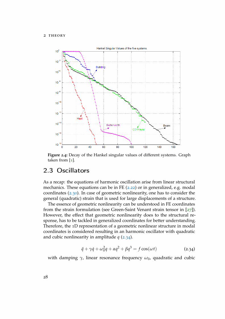
In MOR of nonlinear systems, methods that use snapshots of the system’sstate variables have gained importance. One is the proper orthogonal decom-position (POD) method which generates an optimal basis to the snapshotdata. POD uses singular value decomposition (SVD) to extract the PODmodes. An advantage of SVD-based methods amongst modal superpositionis that the reduction error can be estimated a priori from the singular valuesin the procedure [1, 60]. Antoulas compared the decay of Hankel singularvalues for different systems (Figure 2.4). Error bounds in H∞, L1 and L2 forthe model reduction can be given from the Hankel singular values whichare singular values of the observability and controllability Gramian [1].
A disadvantage of the SVD-based methods is that the exact solution hasto be calculated prior to model reduction. In the design optimization ofMEMS gyroscopes, this solution is neither numerically nor experimentallyaccessible.
The POD method has been applied in various fields, and the applicationto MEMS sensors is most often referred to as the trajectory piecewise linear(TPWL) method [2, 40, 45].
27
2 theory
Figure 2.4: Decay of the Hankel singular values of different systems. Graphtaken from [1].
2.3 Oscillators
As a recap: the equations of harmonic oscillation arise from linear structuralmechanics. These equations can be in FE (2.22) or in generalized, e.g. modalcoordinates (2.30). In case of geometric nonlinearity, one has to consider thegeneral (quadratic) strain that is used for large displacements of a structure.
The essence of geometric nonlinearity can be understood in FE coordinatesfrom the strain formulation (see Green-Saint Venant strain tensor in [27]).However, the effect that geometric nonlinearity does to the structural re-sponse, has to be tackled in generalized coordinates for better understanding.Therefore, the 1D representation of a geometric nonlinear structure in modalcoordinates is considered resulting in an harmonic oscillator with quadraticand cubic nonlinearity in amplitude q (2.34).
q + γq + ω20q + αq2 + βq3 = f cos(ωt) (2.34)
with damping γ, linear resonance frequency ω0, quadratic and cubic
28
2 .3 oscillators
nonlinearity parameter α and β, and a RHS harmonic force with amplitudef .
The Duffing’s equation (2.35) is obtained in case α is zero, which is treatedin many textbooks [8, 32, 33]. This holds for all symmetric structures.
q + γq + ω20q + βq3 = f cos(ωt) (2.35)
The dynamic response of the Duffing oscillator was studied in detail in[15]. Compared to an harmonic oscillator, the Duffing oscillator exhibitsinstability in specific regions of frequency and amplitude. Instability is atypical attribute of the nonlinearity in the equations of motion [8]. For specificinitial conditions and loads (RHS), the solution is either discontinuous ordoes not exist. In this thesis the focus is on the frequency pulling of theresonance frequency of such an oscillator. Frequencies and how they changein the system has to be considered in the design of structural elements aspreviously mentioned.
2.3.1 Hardening and softening nonlinearity
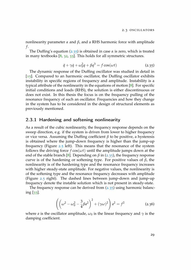
As a result of the cubic nonlinearity, the frequency response depends on thesweep direction, e.g. if the system is driven from lower to higher frequencyor vice versa. Assuming the Duffing coefficient β to be positive, a hysteresisis obtained where the jump-down frequency is higher than the jump-upfrequency (Figure 2.5 left). This means that the resonance of the systemfollows the driving force f cos(ωt) until the amplitude jumps down at theend of the stable branch [8]. Depending on β in (2.35), the frequency responsecurve is of the hardening or softening type. For positive values of β, thenonlinearity is of the hardening type and the resonance frequency increaseswith higher steady-state amplitude. For negative values, the nonlinearity isof the softening type and the resonance frequency decreases with amplitude(Figure 2.5 right). The dashed lines between jump-down and jump-upfrequency denote the instable solution which is not present in steady-state.
The frequency response can be derived from (2.35) using harmonic balanc-ing [33]. ((
ω2 −ω20 −
34
βa2)2
+ (γω)2
)a2 = f 2 (2.36)
where a is the oscillator amplitude, ω0 is the linear frequency and γ is thedamping coefficient.
29
2 theory
Figure 2.5: a) Hysteresis in the frequency amplitude plot for positive β. Increas-ing the forcing frequency yields stronger pulling as compared to decreasingthe forcing frequency. b) Frequency response depending on β. Adopted fromhttps://en.wikipedia.org/wiki/Duffing_equation.
The frequency pulling in steady-state is derived from (2.36). It is thereforeassumed that f and γ are zero, thus the term inside the brackets has to vanish.This results in the quadratic frequency pulling of the Duffing oscillator (2.37).
ω2 = ω20 +
34
βa2
= ω20(1 +
34ω2
0βa2)
(2.37)
where a is the oscillator amplitude, ω0 is the linear frequency. The slopeand sign of the parabola is defined by β.
Using Taylor expansion (2.37) is simplified to (2.38) [18].
ω ≈ ω0(1 + Γa2) (2.38)
with the effective hardening/softening coefficient
Γ =38
β
ω20
. (2.39)
In case α is nonzero in equation (2.34), the effective hardening/softeningcoefficient becomes
Γ =38
β
ω20− 5
12
(α
ω20
)2
. (2.40)
30
2 .4 origin of nonlinearities in mems
The numbers for α and β are defined by the geometry and materialproperties of the structure. However, having different nonlinearities in thesystem, α and β can change. In MEMS, main sources of nonlinearity arefrom the electrostatics, mechanics and fluid dynamics. A short overviewwith the focus on MEMS gyroscopes in given next.
2.4 Origin of nonlinearities in MEMS
2.4.1 Electrostatic
In MEMS sensors, electrostatic fields from sensing or actuating can intro-duce nonlinear forces on the structure which disturb harmonic motion. Anintuitive example is the force on two parallel plates with applied potential,i.e. the force field of a plate capacitor.
A plate capacitor stores the potential energy Wel which depends on capac-itance C (2.42) and voltage U (2.41).
Wel =12
CU2 (2.41)
The capacitance of two parallel plates is given by the geometry and themedium
C = ε0εrAx
(2.42)
where x is the distance between the plates, A is the area of one plate, ε0 =8.854 · 10−12 A s
V m is the vacuum permittivity and εr is the relative permittivityof the material between the plates (for air εr ≈ 1).
The corresponding force in orthogonal direction to the plates is given fromthe gradient of Wel, i.e. from the partial derivative in x (2.43).
Fel,x = −∂Wel∂x
=12
ε0εr Ax2 U2
(2.43)
The initial distance between the plates is assumed to be x0. The absolutedistance is then x = x0 + ∆x with an incremental displacement ∆x << x0.Changing the distance between the plates by ∆x, the force will change by
31
2 theory
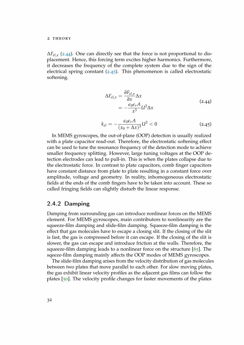
∆Fel,x (2.44). One can directly see that the force is not proportional to dis-placement. Hence, this forcing term excites higher harmonics. Furthermore,it decreases the frequency of the complete system due to the sign of theelectrical spring constant (2.45). This phenomenon is called electrostaticsoftening.
∆Fel,x =∂Fel,x
∂x∆x
= −ε0εr Ax3 U2∆x
(2.44)
kel = −ε0εr A
(x0 + ∆x)3 U2 < 0 (2.45)
In MEMS gyroscopes, the out-of-plane (OOP) detection is usually realizedwith a plate capacitor read-out. Therefore, the electrostatic softening effectcan be used to tune the resonance frequency of the detection mode to achievesmaller frequency splitting. However, large tuning voltages at the OOP de-tection electrodes can lead to pull-in. This is when the plates collapse due tothe electrostatic force. In contrast to plate capacitors, comb finger capacitorshave constant distance from plate to plate resulting in a constant force overamplitude, voltage and geometry. In reality, inhomogeneous electrostaticfields at the ends of the comb fingers have to be taken into account. These socalled fringing fields can slightly disturb the linear response.
2.4.2 Damping
Damping from surrounding gas can introduce nonlinear forces on the MEMSelement. For MEMS gyroscopes, main contributors to nonlinearity are thesqueeze-film damping and slide-film damping. Squeeze-film damping is theeffect that gas molecules have to escape a closing slit. If the closing of the slitis fast, the gas is compressed before it can escape. If the closing of the slit isslower, the gas can escape and introduce friction at the walls. Therefore, thesqueeze-film damping leads to a nonlinear force on the structure [65]. Thesqeeze-film damping mainly affects the OOP modes of MEMS gyroscopes.
The slide-film damping arises from the velocity distribution of gas moleculesbetween two plates that move parallel to each other. For slow moving plates,the gas exhibit linear velocity profiles as the adjacent gas films can follow theplates [50]. The velocity profile changes for faster movements of the plates
32
2 .4 origin of nonlinearities in mems
leading to a frequency dependent in-plane damping force. In MEMS gyro-scopes, slide-film damping mainly affects in-plane modes where the sensorstructure moves parallel to the substrate [50, 65]. Same for electrode struc-tures with large overlap such as comb fingers that have similar geometricproperties as the two parallel plates.
It should be stated that there are other gaseous effects that can lead tononlinear forces and disturb the function of the MEMS sensor [48, 49].
Damping from the sensor material (polysilicon) can be neglected since itis fully elastic until fracturing.
2.4.3 Mechanical
Mechanical nonlinearities can be divided into material, contact, inertial andgeometric nonlinearities.
Material nonlinearity is present when the material matrix is not constant.The reason for material nonlinearity is that materials can change irreversibledue to external influence such as force, temperature or pressure. Thishappens if the material exceeds the elastic regime and becomes inelastic.Common nonlinear materials are ice, rubber and metal featuring plasticity.
Contact nonlinearity is the result of force transduction when the structureis in contact. The contact can be between parts of the sensor structure orbetween surrounding structures and the sensor. The stiffness of contactelements can be included in the tangent stiffness matrix in FE simulations(3.3).
Inertial nonlinearity arises from mass-dependent nonlinear forces in theequation of motion. In the effective model of a cantilever with tip mass, therotation of the tip mass introduces a nonlinear force on the structure whichyields softening for the first mode [31]. The reason is that the cantileverbending mode is softer in the deflected as in the undeflected configuration[65]. In principle, the nonlinear inertial terms can be identified from thetransformation into the rotating part of the structure. Same as for thetransformation into a rotating frame, Euler-, Centrifugal- and Coriolis-forceshave to be introduced in order to correct Newtons law. For simple structures,analytical solutions are developed from the force balance that takes thestationary mass points into account. In this case, mass-dependent terms canbe added in the equation of motion to render the inertial forces from thedynamics. In transient FE simulation, the inertial forces enter as body forcesthat use the velocity of mass points. The velocities are updated as described
33
2 theory
in the integration scheme of the FE solver considering force balance of theglobal motion 3.1. In this way, Euler-, Centrifugal and Coriolis forces areconsidered in a transient FE simulation. Using the spin-softening matrix inthe tangent stiffness, Coriolis forces can be used in static FE simulations aswell (3.3).
Geometric nonlinearity is known from geometry-dependent nonlinearforces of structures. The reason of these forces is that the stiffness matrixdepends on the actual geometry of the structure, i.e. deformation state.Geometric nonlinear forces are quadratic and cubic in amplitude which canresult in softening and stiffening nonlinearity 2.3. For example, a doubly-clamped beam resonator exhibits stiffening nonlinearity due to mid-planestretching. Bending of the doubly-clamped beam results in the extensionof the neutral line which introduces axial forces in the beam. Compared tothe static tuning of a guitar string, the axial stiffness in a doubly-clampedbeam resonator is modulated over deflection amplitude. In general, theeffect that deformation increases the stiffness is called stress-stiffening. Thestress-stiffening has to be considered for thin structures when bendinginduces axial forces such as in beams and plates [26]. A rule of thumb isthat stress-stiffening is present when the bending exceeds the width of thethin structure [8]. Especially, these structures are present in MEMS sensors.MEMS gyroscopes for example use folded-beam suspensions which exhibitstiffening nonlinearity.
Another possibility is that the stiffness reduces upon deflection whichresults in a softening nonlinearity. An example of a structure with softeningnonlinearity is a cantilever beam with tip mass or a cup-spring where theresonance frequency decreases over amplitude [31]. In MEMS gyroscopes, theeffective stiffness of higher modes can decreased over drive mode amplitudeif the two mode shapes combine to a lower stiffness.
2.5 Description of geometric nonlinearities
Nonlinearities stemming from geometry can be derived analytically forsimple structures. For complex structures, however, geometric nonlinearityhas to be derived from the nonlinear strain of an FE model. The reason is thatboundary conditions can be described in closed form for simple structures,such as beams and plates, but not for the more complex structures such asdisk resonators, vibratory gyroscopes and other sensors.
The following shows how geometric nonlinearity can be described for a
34
2 .5 description of geometric nonlinearities
doubly-clamped beam resonator using an analytical relation between axialforce and geometry. From the modulation of axial forces in the resonantbeam, an effective 1D Duffing model can be derived from which the reso-nance frequencies can be obtained.
Then, it is shown how geometric nonlinearity can be described for complexstructures, such as MEMS sensors, using the nonlinear strain in modalcoordinates. From the modal equations of motion, effective Duffing models(also higher-dimensional) can be derived and the resonance frequenciesobtained.
2.5.1 Analytical model for a doubly-clamped beam
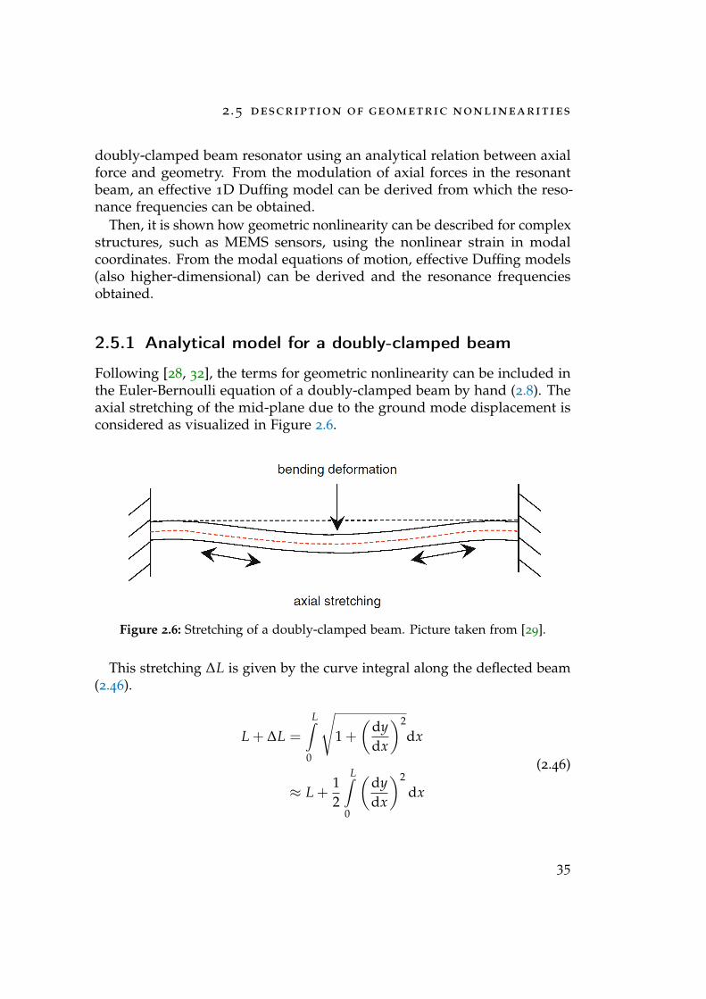
Following [28, 32], the terms for geometric nonlinearity can be included inthe Euler-Bernoulli equation of a doubly-clamped beam by hand (2.8). Theaxial stretching of the mid-plane due to the ground mode displacement isconsidered as visualized in Figure 2.6.
Figure 2.6: Stretching of a doubly-clamped beam. Picture taken from [29].
This stretching ∆L is given by the curve integral along the deflected beam(2.46).
L + ∆L =
L∫0
√1 +
(dydx
)2
dx
≈ L +12
L∫0
(dydx
)2
dx
(2.46)
35
2 theory
In (2.46), the Taylor expansion of the square root function to first order wasused.
The stretching of beams and plates can be related to the axial tension ofthe structure. Thus, the change in axial tension ∆T can be expressed by therelative change of length ∆L/L using Young’s modulus E and cross sectionarea A [32].
∆T = E · A∆LL
(2.47)
The total axial tension T in the beam is given from the constant (initial)tension T0 and the change ∆T (2.48).
T = T0 + ∆T
= T0 +EA2L
L∫0
(dydx
)2
dx(2.48)
Including the axial tension term in (2.8), one obtains (2.49).
ρAy + ηy + EIyd4ydx4 +
T0 +EA2L
L∫0
(dydx
)2
dx
d2ydx2 = FL (2.49)
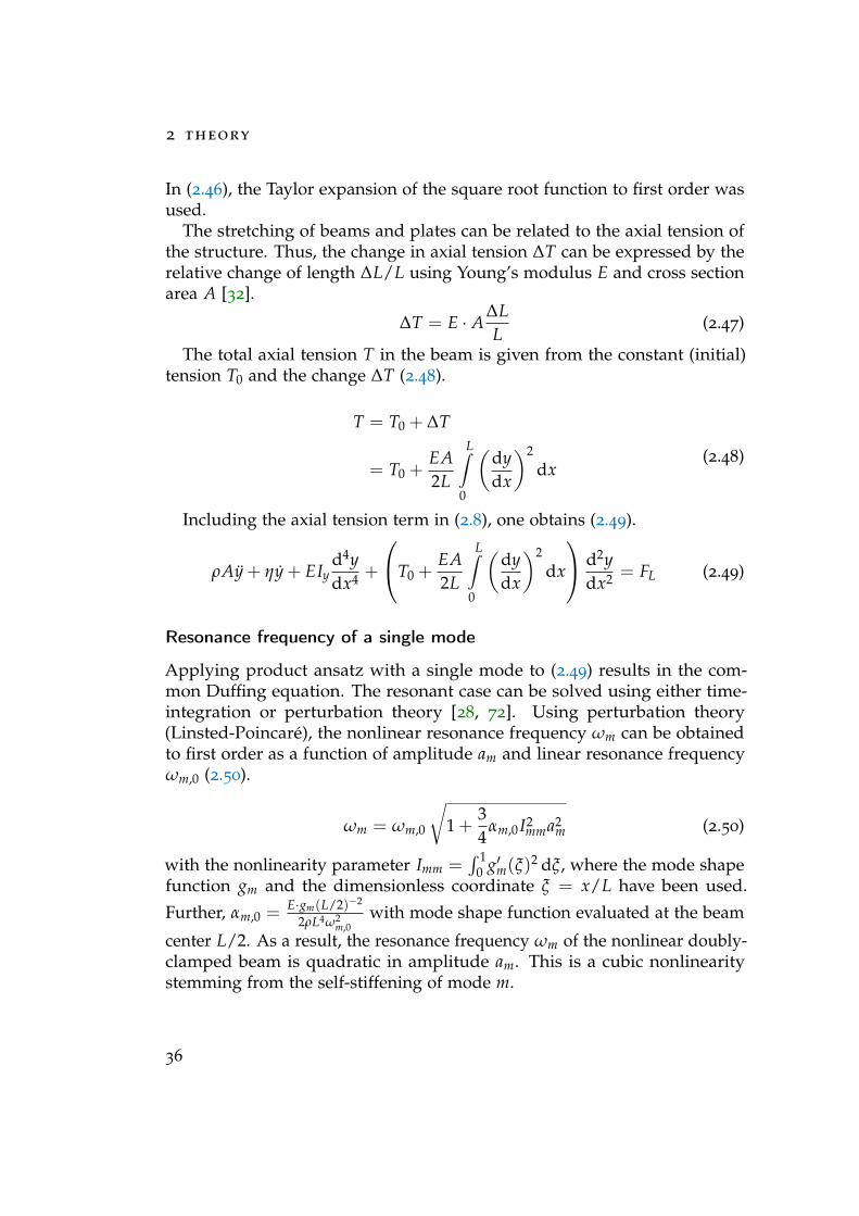
Resonance frequency of a single mode
Applying product ansatz with a single mode to (2.49) results in the com-mon Duffing equation. The resonant case can be solved using either time-integration or perturbation theory [28, 72]. Using perturbation theory(Linsted-Poincaré), the nonlinear resonance frequency ωm can be obtainedto first order as a function of amplitude am and linear resonance frequencyωm,0 (2.50).
ωm = ωm,0
√1 +
34
αm,0 I2mma2
m (2.50)
with the nonlinearity parameter Imm =∫ 1
0 g′m(ξ)2 dξ, where the mode shapefunction gm and the dimensionless coordinate ξ = x/L have been used.
Further, αm,0 = E·gm(L/2)−2
2ρL4ω2m,0
with mode shape function evaluated at the beam
center L/2. As a result, the resonance frequency ωm of the nonlinear doubly-clamped beam is quadratic in amplitude am. This is a cubic nonlinearitystemming from the self-stiffening of mode m.
36
2 .5 description of geometric nonlinearities
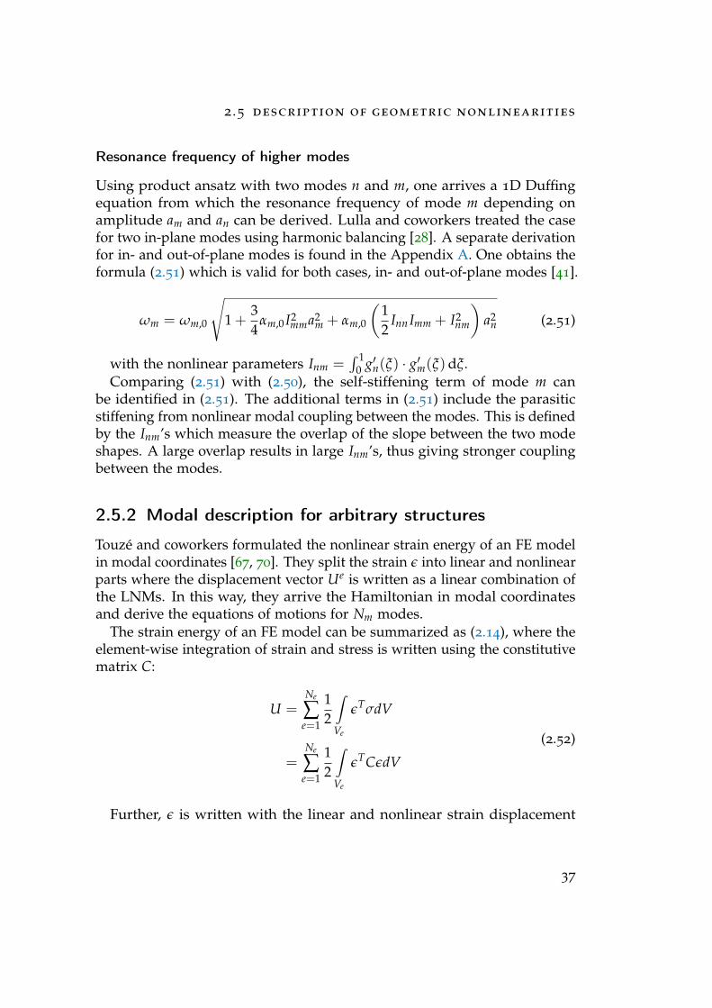
Resonance frequency of higher modes
Using product ansatz with two modes n and m, one arrives a 1D Duffingequation from which the resonance frequency of mode m depending onamplitude am and an can be derived. Lulla and coworkers treated the casefor two in-plane modes using harmonic balancing [28]. A separate derivationfor in- and out-of-plane modes is found in the Appendix A. One obtains theformula (2.51) which is valid for both cases, in- and out-of-plane modes [41].
ωm = ωm,0
√1 +
34
αm,0 I2mma2
m + αm,0
(12
Inn Imm + I2nm
)a2
n (2.51)
with the nonlinear parameters Inm =∫ 1
0 g′n(ξ) · g′m(ξ)dξ.Comparing (2.51) with (2.50), the self-stiffening term of mode m can
be identified in (2.51). The additional terms in (2.51) include the parasiticstiffening from nonlinear modal coupling between the modes. This is definedby the Inm’s which measure the overlap of the slope between the two modeshapes. A large overlap results in large Inm’s, thus giving stronger couplingbetween the modes.
2.5.2 Modal description for arbitrary structures
Touzé and coworkers formulated the nonlinear strain energy of an FE modelin modal coordinates [67, 70]. They split the strain ε into linear and nonlinearparts where the displacement vector Ue is written as a linear combination ofthe LNMs. In this way, they arrive the Hamiltonian in modal coordinatesand derive the equations of motions for Nm modes.
The strain energy of an FE model can be summarized as (2.14), where theelement-wise integration of strain and stress is written using the constitutivematrix C:
U =Ne
∑e=1
12
∫Ve
εTσdV
=Ne
∑e=1
12
∫Ve
εTCεdV
(2.52)
Further, ε is written with the linear and nonlinear strain displacement
37
2 theory
matrix, B0 and B1(Ue) respectively.
ε = B0Ue +12
B1(Ue)Ue (2.53)
Ue is expressed with the mode shapes from a modal analysis with Nm modes.
Ue =Nm
∑p=1
qpΦep (2.54)
Plugging (2.53) and (2.54) into (2.52) yields the strain energy in modalcoordinates with the nonlinear modal coupling coefficients αijk and βijkl.
U =Nm
∑i=1
12
ω2i q2
i +Nm
∑i=1
Nm
∑j=1
Nm
∑k=1
αijkqiqjqk +Nm
∑i=1
Nm
∑j=1
Nm
∑k=1
Nm
∑l=1
βijklqiqjqkql (2.55)
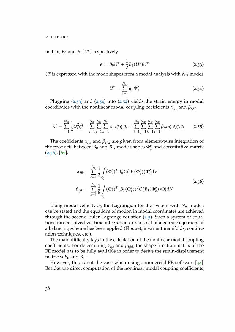
The coefficients αijk and βijkl are given from element-wise integration ofthe products between B0 and B1, mode shapes Φe
p and constitutive matrix(2.56), [67].
αijk =Ne
∑e=1
12
∫Ve
(Φei )
TBT0 C(B1(Φe
j))ΦekdV
βijkl =Ne
∑e=1
18
∫Ve
(Φei )
T(B1(Φej))
TC(B1(Φek))Φ
el dV
(2.56)
Using modal velocity qi, the Lagrangian for the system with Nm modescan be stated and the equations of motion in modal coordinates are achievedthrough the second Euler-Lagrange equation (2.5). Such a system of equa-tions can be solved via time integration or via a set of algebraic equations ifa balancing scheme has been applied (Floquet, invariant manifolds, continu-ation techniques, etc.).
The main difficulty lays in the calculation of the nonlinear modal couplingcoefficients. For determining αijk and βijkl, the shape function matrix of theFE model has to be fully available in order to derive the strain-displacementmatrices B0 and B1.
However, this is not the case when using commercial FE software [44].Besides the direct computation of the nonlinear modal coupling coefficients,
38
2 .5 description of geometric nonlinearities
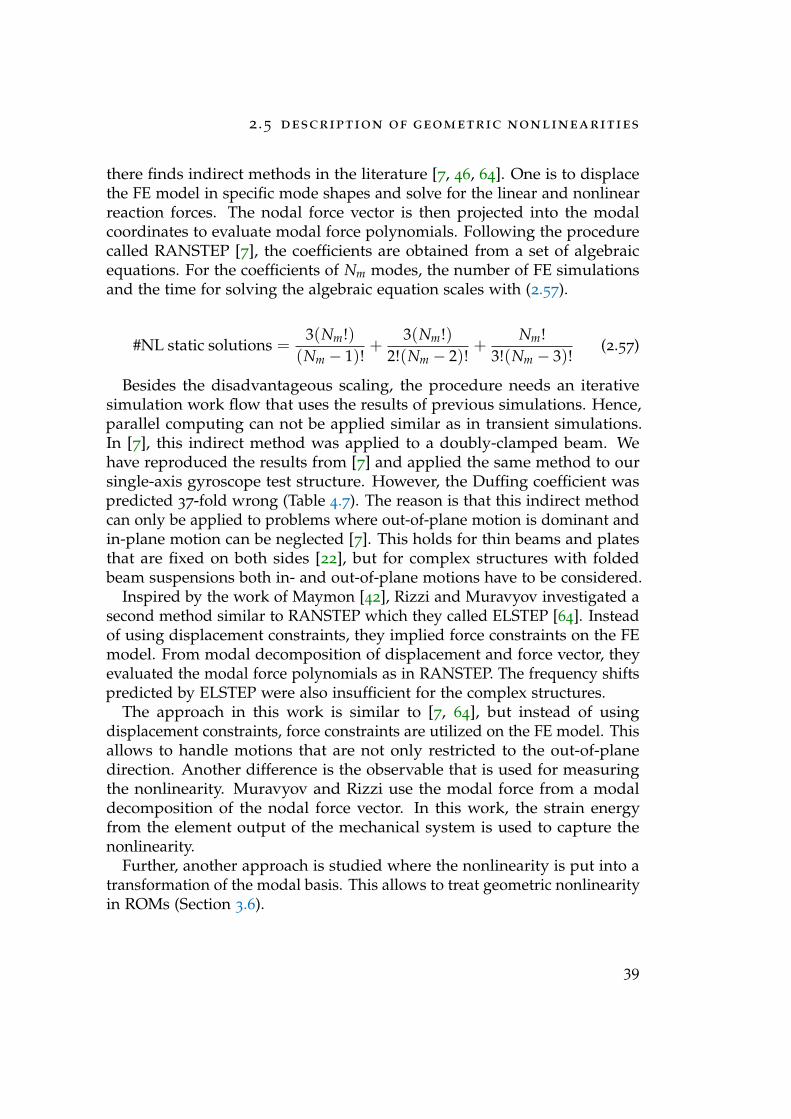
there finds indirect methods in the literature [7, 46, 64]. One is to displacethe FE model in specific mode shapes and solve for the linear and nonlinearreaction forces. The nodal force vector is then projected into the modalcoordinates to evaluate modal force polynomials. Following the procedurecalled RANSTEP [7], the coefficients are obtained from a set of algebraicequations. For the coefficients of Nm modes, the number of FE simulationsand the time for solving the algebraic equation scales with (2.57).
#NL static solutions =3(Nm!)
(Nm − 1)!+
3(Nm!)2!(Nm − 2)!
+Nm!
3!(Nm − 3)!(2.57)
Besides the disadvantageous scaling, the procedure needs an iterativesimulation work flow that uses the results of previous simulations. Hence,parallel computing can not be applied similar as in transient simulations.In [7], this indirect method was applied to a doubly-clamped beam. Wehave reproduced the results from [7] and applied the same method to oursingle-axis gyroscope test structure. However, the Duffing coefficient waspredicted 37-fold wrong (Table 4.7). The reason is that this indirect methodcan only be applied to problems where out-of-plane motion is dominant andin-plane motion can be neglected [7]. This holds for thin beams and platesthat are fixed on both sides [22], but for complex structures with foldedbeam suspensions both in- and out-of-plane motions have to be considered.
Inspired by the work of Maymon [42], Rizzi and Muravyov investigated asecond method similar to RANSTEP which they called ELSTEP [64]. Insteadof using displacement constraints, they implied force constraints on the FEmodel. From modal decomposition of displacement and force vector, theyevaluated the modal force polynomials as in RANSTEP. The frequency shiftspredicted by ELSTEP were also insufficient for the complex structures.
The approach in this work is similar to [7, 64], but instead of usingdisplacement constraints, force constraints are utilized on the FE model. Thisallows to handle motions that are not only restricted to the out-of-planedirection. Another difference is the observable that is used for measuringthe nonlinearity. Muravyov and Rizzi use the modal force from a modaldecomposition of the nodal force vector. In this work, the strain energyfrom the element output of the mechanical system is used to capture thenonlinearity.
Further, another approach is studied where the nonlinearity is put into atransformation of the modal basis. This allows to treat geometric nonlinearityin ROMs (Section 3.6).
39
2 theory
Static model for a single mode
Considering a single mode in (2.55), the potential energy is:
U(q) =12
ω2q2 +13
αq3 +14
βq4 (2.58)
For convenience, the equation is rewritten in nodal form using the ampli-tude x and the stiffness ki (2.59).
E(x) =12
k0x2 +13
k1x3 +14
k2x4 (2.59)
From this energy, the corresponding 1D Duffing equation can be derivedand perturbation techniques such as Linstedt-Poincaré or harmonic balancingcan be applied to derive the resonance frequency [28, 32, 72].
A first order approximation of this nonlinear resonance frequency is givenby the formula of Lifshitz and Kaajakari et al. (2.60).
fnl(x) = f0 + f0
(38
k2
k0− 5
12k2
1k2
0
)x2 (2.60)
where f0 = 12π
√k0m is the frequency of the LNM, i.e. the zero-point frequency,
x is the steady-state amplitude and the coefficients are from the potentialenergy [32, 72].
In practice, one calculates the potential energy for different amplitudes xof the structure using static analysis in FE. Thereby, at least 4 tuples of energyand amplitude are needed to define the coefficients exactly. The amplitudecan either be measured from a single node of the FE model or from modaldecomposition with the LNMs, see 3.4.1.
For many MEMS structures, the nonlinear drive motion is symmetric in x,which means that odd powers of x are suppressed in the potential energy.In this case, the nonlinear resonance frequency reduces to (2.61) and thecalculation of the coefficients is much more efficient.
fnl(x) = f0 + f0 ·38
k2
k0· x2 (2.61)
The linear (2.62) and nonlinear potential energy (2.63) can be accessed bystatic analysis.
Elin =12
k0x2lin (2.62)
40
2 .5 description of geometric nonlinearities
Enl =12
k0x2nl +
14
k2x4nl (2.63)
From this results, the coefficient k0 can be written as (2.64) and k2 as (2.65).Note that Elin and xlin are from a linear static analysis and Enl and xnl arefrom a nonlinear static analysis.
k0 = 2Elin
x2lin
(2.64)
k2
k0=
Enl − 12 k0x2
nl14 k0x4
nl
(2.65)
The numerical implementation of this procedure is found in 3.4.1. In asimilar manner, the coefficients can be constructed for asymmetric structures.
The here presented single mode model is accurate in the limit of weaknonlinearity where the motion is mainly harmonic.
In case, the motion consists of several LNMs, i.e. the modal amplitudeof other modes have to be taken into account, then the nonlinear normalmode (NNM) has to be computed using contributions of the other LNMs[18]. Touzé and coworkers use a rescaling of the coefficients to adjust theeffective stiffening Γ that renders the type and strength of nonlinearity (2.38).
It should be emphasized that MEMS gyroscopes are usually designed towork in the linear regime where the adjustment of Γ can be neglected.
Static model for parasitic modes
The derivation of the static model for parasitic modes starts with the modalrepresentation of the potential energy as in [67].
The potential energy for two arbitrary modes (j and k) is given by:
U(qj, qk) =12
ω2j q2
j + αjjjq3j + β jjjjq4
j
+12
ω2k q2
k + αkkkq3k + βkkkkq4
k
+ αjjkq2j qk + αjkkqjq2
k
+ β jjjkq3j qk + β jjkkq2
j q2k + β jkkkqjq3
k
(2.66)
The bar (α,β) denotes the sum of coefficients with cyclic indices (2.67).
β jjjk = β jjjk + β jjkj + β jkjj + βkjjj (2.67)
41
2 theory
Mode j is considered to be intrinsic nonlinear and mode k to be linear.Hence, the self-stiffening contribution of mode k can be dropped (2.68).
U(qj, qk) =12
ω2j q2
j + αjjjq3j + β jjjjq4
j
+12
ω2k q2
k
+ αjjkq2j qk + αjkkqjq2
k
+ β jjjkq3j qk + β jjkkq2
j q2k + β jkkkqjq3
k
(2.68)
Using the Lagrangian, the equation of motion for mode k can be stated(2.69).
qk + ω2k qk + αjjkq2
j + 2αjkkqjqk + β jjjkq3j + 2β jjkkq2
j qk + 3β jkkkqjq2k = 0
qk +(
ω2k + 2αjkkqj + 2β jjkkq2
j
)qk + 3β jkkkqjq2
k = −αjjkq2j − β jjjkq3
j
(2.69)
The next step is to average over one period Tj =2πωj
(2.70).
qk +(
ω2k + 2β jjkkq2
j
)qk = −αjjkq2
j
qk +(
ω2k + β jjkkq2
j
)qk = −αjjk
12
q2j
(2.70)
where q2j = 1
Tj
∫ Tj0 q2
j cos2(ωjt)dt = 12 q2
j . Further, it was used that oddpowers of qj = qj cos(ωjt) vanish due to symmetry.
The result is a simple formula for the resonance frequency of mode k dueto geometric nonlinearity of mode j (2.71). In case of a MEMS gyroscope,mode j can be the drive mode and mode k can be any parasitic mode that isusually higher in frequency.
ω2NL,k = ω2
k + β jjkkq2j
ωNL,k = ωk
√1 +
β jjkk
ω2k
q2j
= ωk +12
β jjkk
ωkq2
j
(2.71)
42
2 .5 description of geometric nonlinearities
Now, the key in constructing an efficient simulation method for the res-onance frequency of the parasitic mode is to isolate the effective couplingcoefficient β jjkk. This can be done by evaluating the strain energy of thesystem with two modes and subtracting the energy of the single nonlinearmode (2.72).
U(qj, qk)−U(qj) =12
ω2k q2
k + αjjkq2j qk + αjkkqjq2
k
+ β jjjkq3j qk + β jjkkq2
j q2k
(2.72)
The energy difference is a second order polynomial in qk. Note that allterms higher than q2
k were dropped due to small signal approximation ofmode k.
Considering the case that mode j is symmetric in forward and backwarddirection, the odd terms of qj are zero (2.73).
U(qj, qk)−U(qj) =
(12
ω2k + β jjkkq2
j
)q2
k + αjjkq2j qk (2.73)
The quadratic coefficient can be determined for different qj using a secondorder polynomial fit. Finally, the formula for the resonance frequency ofmode k is (2.74), where a(qj) =
12 ω2
k + β jjkkq2j .
ωNL,k = ωk + ωk
(14
a(qj)− a(0)a(0)
)(2.74)
The numerical procedure uses nonlinear static analysis in Ansys and istreated in 3.4.2.
43

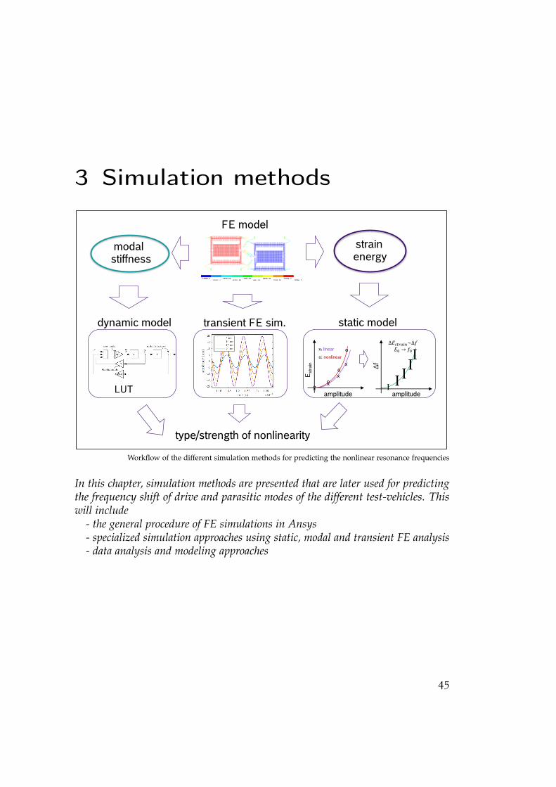
3 Simulation methods
Intern | Automotive Electronics | AE/EST4 | 16.03.2016
© Robert Bosch GmbH 2016. Alle Rechte vorbehalten, auch bzgl. jeder Verfügung, Verwertung, Reproduktion, Bearbeitung, Weitergabe sowie für den Fall von Schutzrechtsanmeldungen.1
amplitude
Estr
ain
x: linear
o: nonlinear
o
o
oo
xx
x
x
amplitude
Δf
II
II
I
Δ𝐸𝑠𝑡𝑟𝑎𝑖𝑛~Δ𝑓𝐸0 → 𝑓0
strainenergy
type/strength of nonlinearity
static modeldynamic model transient FE sim.
LUT
FE model
modal stiffness
Workflow of the different simulation methods for predicting the nonlinear resonance frequencies
In this chapter, simulation methods are presented that are later used for predictingthe frequency shift of drive and parasitic modes of the different test-vehicles. Thiswill include
- the general procedure of FE simulations in Ansys- specialized simulation approaches using static, modal and transient FE analysis- data analysis and modeling approaches
45
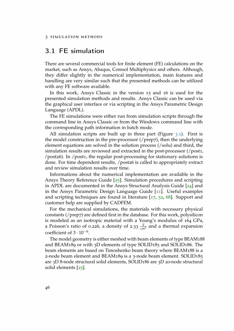
3 simulation methods
3.1 FE simulation
There are several commercial tools for finite element (FE) calculations on themarket, such as Ansys, Abaqus, Comsol Multiphysics and others. Although,they differ slightly in the numerical implementation, main features andhandling are very similar such that the presented methods can be utilizedwith any FE software available.
In this work, Ansys Classic in the version 15 and 16 is used for thepresented simulation methods and results. Ansys Classic can be used viathe graphical user interface or via scripting in the Ansys Parametric DesignLanguage (APDL).
The FE simulations were either run from simulation scripts through thecommand line in Ansys Classic or from the Windows command line withthe corresponding path information in batch mode.
All simulation scripts are built up in three part (Figure 3.1). First isthe model construction in the pre-processor (/prep7), then the underlyingelement equations are solved in the solution process (/solu) and third, thesimulation results are reviewed and extracted in the post-processor (/post1,/post26). In /post1, the regular post-processing for stationary solutions isdone. For time dependent results, /post26 is called to appropriately extractand review simulation results over time.
Informations about the numerical implementation are available in theAnsys Theory Reference Guide [25]. Simulation procedures and scriptingin APDL are documented in the Ansys Structural Analysis Guide [24] andin the Ansys Parametric Design Language Guide [11]. Useful examplesand scripting techniques are found in literature [17, 52, 68]. Support andcustomer help are supplied by CADFEM.
For the mechanical simulations, the materials with necessary physicalconstants (/prep7) are defined first in the database. For this work, polysiliconis modeled as an isotropic material with a Young’s modulus of 164 GPa,a Poisson’s ratio of 0.226, a density of 2.33
gcm3 and a thermal expansion
coefficient of 3 · 10−6.The model geometry is either meshed with beam elements of type BEAM188
and BEAM189 or with 3D elements of type SOLID185 and SOLID186. Thebeam elements are based on Timoshenko beam theory where BEAM188 is a2-node beam element and BEAM189 is a 3-node beam element. SOLID185
are 3D 8-node structural solid elements, SOLID186 are 3D 20-node structuralsolid elements [25].
46
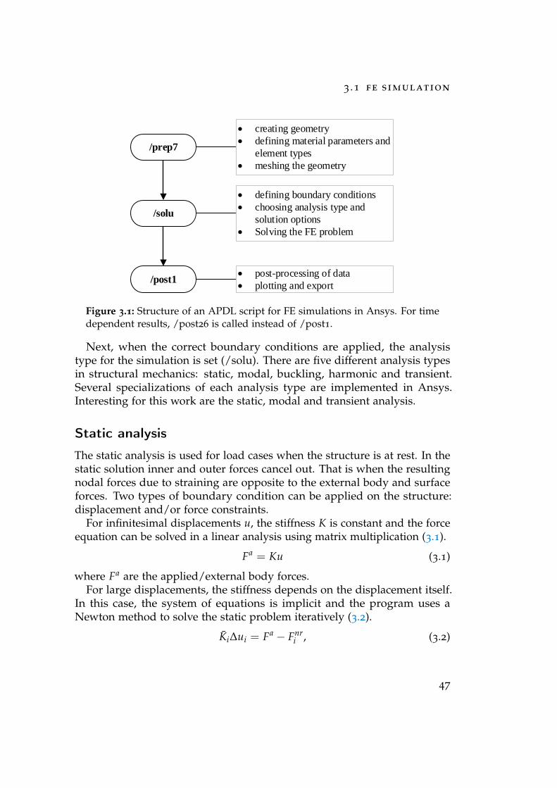
3 .1 fe simulation
/prep7
/solu
/post1
creating geometry
defining material parameters and
element types
meshing the geometry
defining boundary conditions
choosing analysis type and
solution options
Solving the FE problem
post-processing of data
plotting and export
Figure 3.1: Structure of an APDL script for FE simulations in Ansys. For timedependent results, /post26 is called instead of /post1.
Next, when the correct boundary conditions are applied, the analysistype for the simulation is set (/solu). There are five different analysis typesin structural mechanics: static, modal, buckling, harmonic and transient.Several specializations of each analysis type are implemented in Ansys.Interesting for this work are the static, modal and transient analysis.
Static analysis
The static analysis is used for load cases when the structure is at rest. In thestatic solution inner and outer forces cancel out. That is when the resultingnodal forces due to straining are opposite to the external body and surfaceforces. Two types of boundary condition can be applied on the structure:displacement and/or force constraints.
For infinitesimal displacements u, the stiffness K is constant and the forceequation can be solved in a linear analysis using matrix multiplication (3.1).
Fa = Ku (3.1)
where Fa are the applied/external body forces.For large displacements, the stiffness depends on the displacement itself.
In this case, the system of equations is implicit and the program uses aNewton method to solve the static problem iteratively (3.2).
Ki∆ui = Fa − Fnri , (3.2)
47
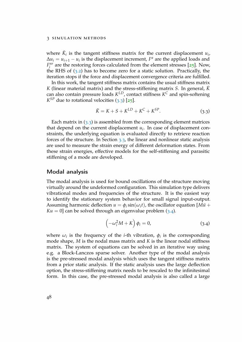
3 simulation methods
where Ki is the tangent stiffness matrix for the current displacement ui,∆ui = ui+1 − ui is the displacement increment, Fa are the applied loads andFnr
i are the restoring forces calculated from the element stresses [25]. Now,the RHS of (3.2) has to become zero for a static solution. Practically, theiteration stops if the force and displacement convergence criteria are fulfilled.
In this work, the tangent stiffness matrix contains the usual stiffness matrixK (linear material matrix) and the stress-stiffening matrix S. In general, Kcan also contain pressure loads KLD, contact stiffness KC and spin-softeningKSP due to rotational velocities (3.3) [25].
K = K + S + KLD + KC + KSP. (3.3)
Each matrix in (3.3) is assembled from the corresponding element matricesthat depend on the current displacement ui. In case of displacement con-straints, the underlying equation is evaluated directly to retrieve reactionforces of the structure. In Section 3.3, the linear and nonlinear static analysisare used to measure the strain energy of different deformation states. Fromthese strain energies, effective models for the self-stiffening and parasiticstiffening of a mode are developed.
Modal analysis
The modal analysis is used for bound oscillations of the structure movingvirtually around the undeformed configuration. This simulation type deliversvibrational modes and frequencies of the structure. It is the easiest wayto identify the stationary system behavior for small signal input-output.Assuming harmonic deflection u = φi sin(ωit), the oscillator equation [Mu +Ku = 0] can be solved through an eigenvalue problem (3.4).(
−ω2i M + K
)φi = 0, (3.4)
where ωi is the frequency of the i-th vibration, φi is the correspondingmode shape, M is the nodal mass matrix and K is the linear nodal stiffnessmatrix. The system of equations can be solved in an iterative way usinge.g. a Block-Lanczos sparse solver. Another type of the modal analysisis the pre-stressed modal analysis which uses the tangent stiffness matrixfrom a prior static analysis. If the static analysis uses the large deflectionoption, the stress-stiffening matrix needs to be rescaled to the infinitesimalform. In this case, the pre-stressed modal analysis is also called a large
48
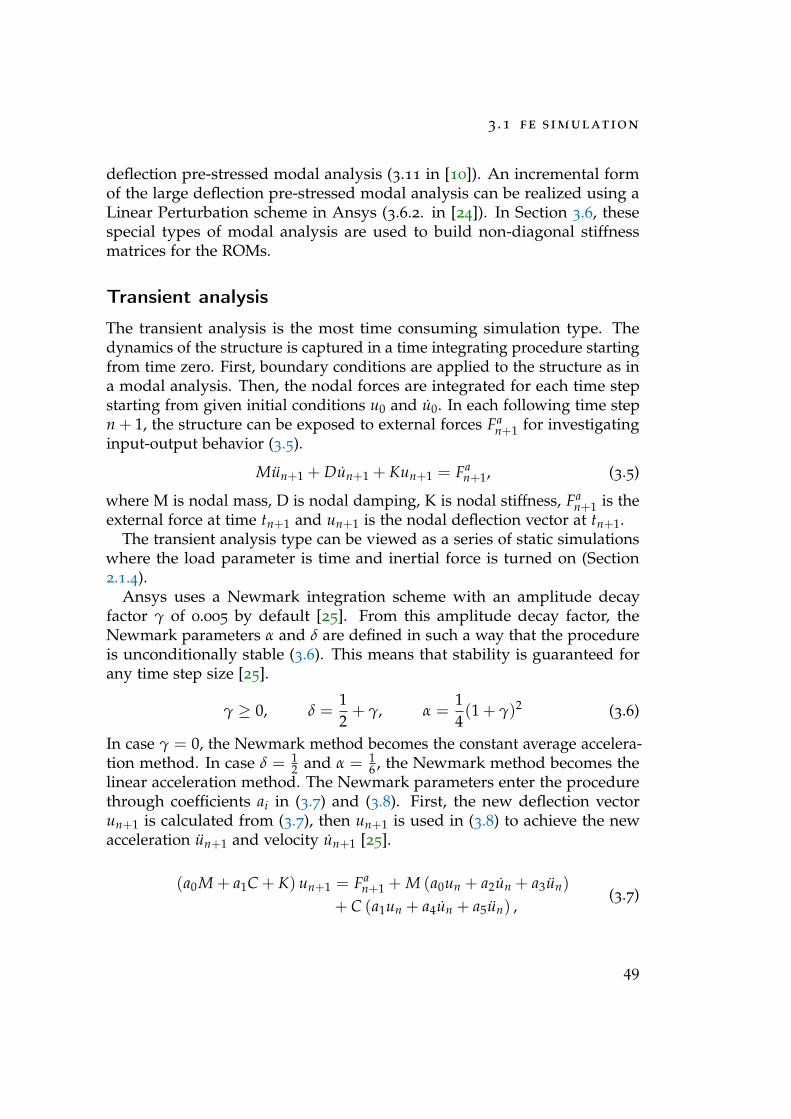
3 .1 fe simulation
deflection pre-stressed modal analysis (3.11 in [10]). An incremental formof the large deflection pre-stressed modal analysis can be realized using aLinear Perturbation scheme in Ansys (3.6.2. in [24]). In Section 3.6, thesespecial types of modal analysis are used to build non-diagonal stiffnessmatrices for the ROMs.
Transient analysis
The transient analysis is the most time consuming simulation type. Thedynamics of the structure is captured in a time integrating procedure startingfrom time zero. First, boundary conditions are applied to the structure as ina modal analysis. Then, the nodal forces are integrated for each time stepstarting from given initial conditions u0 and u0. In each following time stepn + 1, the structure can be exposed to external forces Fa
n+1 for investigatinginput-output behavior (3.5).
Mun+1 + Dun+1 + Kun+1 = Fan+1, (3.5)
where M is nodal mass, D is nodal damping, K is nodal stiffness, Fan+1 is the
external force at time tn+1 and un+1 is the nodal deflection vector at tn+1.The transient analysis type can be viewed as a series of static simulations
where the load parameter is time and inertial force is turned on (Section2.1.4).
Ansys uses a Newmark integration scheme with an amplitude decayfactor γ of 0.005 by default [25]. From this amplitude decay factor, theNewmark parameters α and δ are defined in such a way that the procedureis unconditionally stable (3.6). This means that stability is guaranteed forany time step size [25].
γ ≥ 0, δ =12+ γ, α =
14(1 + γ)2 (3.6)
In case γ = 0, the Newmark method becomes the constant average accelera-tion method. In case δ = 1
2 and α = 16 , the Newmark method becomes the
linear acceleration method. The Newmark parameters enter the procedurethrough coefficients ai in (3.7) and (3.8). First, the new deflection vectorun+1 is calculated from (3.7), then un+1 is used in (3.8) to achieve the newacceleration un+1 and velocity un+1 [25].
(a0M + a1C + K) un+1 = Fan+1 + M (a0un + a2un + a3un)
+ C (a1un + a4un + a5un) ,(3.7)
49
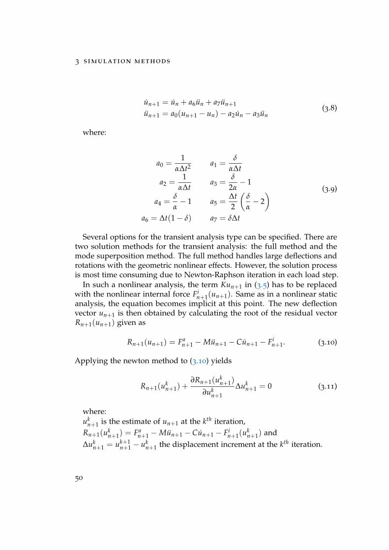
3 simulation methods
un+1 = un + a6un + a7un+1
un+1 = a0(un+1 − un)− a2un − a3un(3.8)
where:
a0 =1
α∆t2 a1 =δ
α∆t
a2 =1
α∆ta3 =
δ
2α− 1
a4 =δ
α− 1 a5 =
∆t2
(δ
α− 2)
a6 = ∆t(1− δ) a7 = δ∆t
(3.9)
Several options for the transient analysis type can be specified. There aretwo solution methods for the transient analysis: the full method and themode superposition method. The full method handles large deflections androtations with the geometric nonlinear effects. However, the solution processis most time consuming due to Newton-Raphson iteration in each load step.
In such a nonlinear analysis, the term Kun+1 in (3.5) has to be replacedwith the nonlinear internal force Fi
n+1(un+1). Same as in a nonlinear staticanalysis, the equation becomes implicit at this point. The new deflectionvector un+1 is then obtained by calculating the root of the residual vectorRn+1(un+1) given as
Rn+1(un+1) = Fan+1 −Mun+1 − Cun+1 − Fi
n+1. (3.10)
Applying the newton method to (3.10) yields
Rn+1(ukn+1) +
∂Rn+1(ukn+1)
∂ukn+1
∆ukn+1 = 0 (3.11)
where:uk
n+1 is the estimate of un+1 at the kth iteration,Rn+1(uk
n+1) = Fan+1 −Mun+1 − Cun+1 − Fi
n+1(ukn+1) and
∆ukn+1 = uk+1
n+1 − ukn+1 the displacement increment at the kth iteration.
50
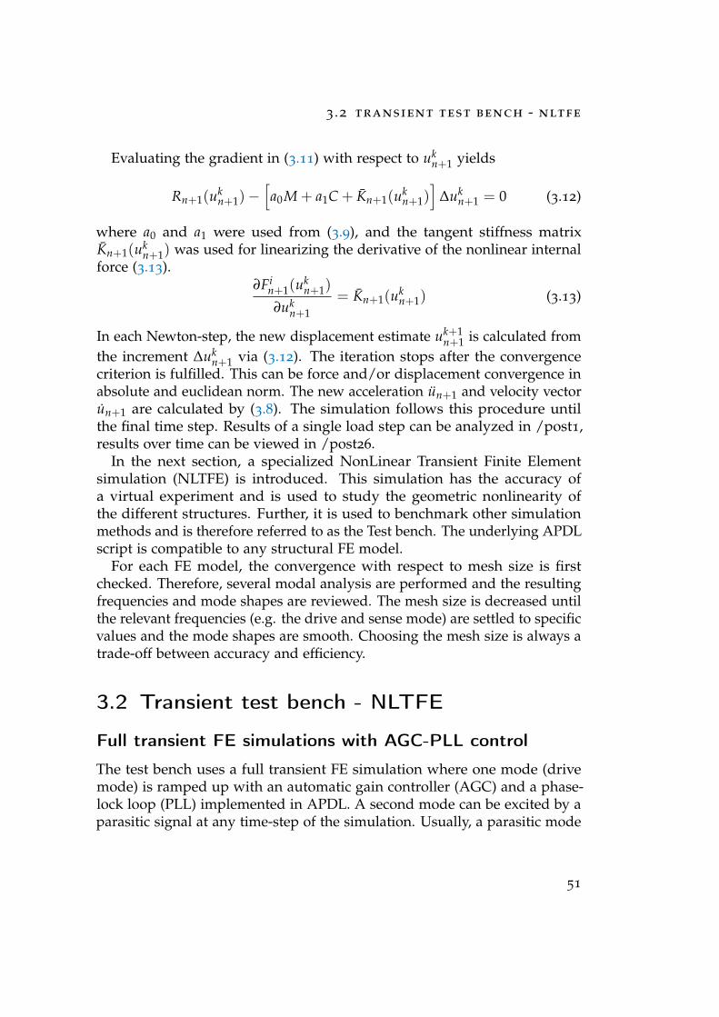
3 .2 transient test bench - nltfe
Evaluating the gradient in (3.11) with respect to ukn+1 yields
Rn+1(ukn+1)−
[a0M + a1C + Kn+1(uk
n+1)]
∆ukn+1 = 0 (3.12)
where a0 and a1 were used from (3.9), and the tangent stiffness matrixKn+1(uk
n+1) was used for linearizing the derivative of the nonlinear internalforce (3.13).
∂Fin+1(u
kn+1)
∂ukn+1
= Kn+1(ukn+1) (3.13)
In each Newton-step, the new displacement estimate uk+1n+1 is calculated from
the increment ∆ukn+1 via (3.12). The iteration stops after the convergence
criterion is fulfilled. This can be force and/or displacement convergence inabsolute and euclidean norm. The new acceleration un+1 and velocity vectorun+1 are calculated by (3.8). The simulation follows this procedure untilthe final time step. Results of a single load step can be analyzed in /post1,results over time can be viewed in /post26.
In the next section, a specialized NonLinear Transient Finite Elementsimulation (NLTFE) is introduced. This simulation has the accuracy ofa virtual experiment and is used to study the geometric nonlinearity ofthe different structures. Further, it is used to benchmark other simulationmethods and is therefore referred to as the Test bench. The underlying APDLscript is compatible to any structural FE model.
For each FE model, the convergence with respect to mesh size is firstchecked. Therefore, several modal analysis are performed and the resultingfrequencies and mode shapes are reviewed. The mesh size is decreased untilthe relevant frequencies (e.g. the drive and sense mode) are settled to specificvalues and the mode shapes are smooth. Choosing the mesh size is always atrade-off between accuracy and efficiency.
3.2 Transient test bench - NLTFE
Full transient FE simulations with AGC-PLL control
The test bench uses a full transient FE simulation where one mode (drivemode) is ramped up with an automatic gain controller (AGC) and a phase-lock loop (PLL) implemented in APDL. A second mode can be excited by aparasitic signal at any time-step of the simulation. Usually, a parasitic mode
51
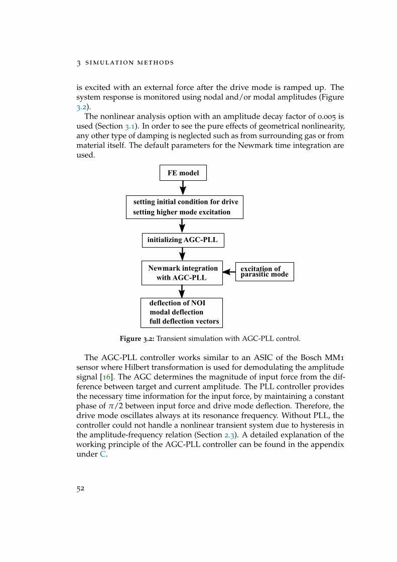
3 simulation methods
is excited with an external force after the drive mode is ramped up. Thesystem response is monitored using nodal and/or modal amplitudes (Figure3.2).
The nonlinear analysis option with an amplitude decay factor of 0.005 isused (Section 3.1). In order to see the pure effects of geometrical nonlinearity,any other type of damping is neglected such as from surrounding gas or frommaterial itself. The default parameters for the Newmark time integration areused.
Figure 3.2: Transient simulation with AGC-PLL control.
The AGC-PLL controller works similar to an ASIC of the Bosch MM1
sensor where Hilbert transformation is used for demodulating the amplitudesignal [16]. The AGC determines the magnitude of input force from the dif-ference between target and current amplitude. The PLL controller providesthe necessary time information for the input force, by maintaining a constantphase of π/2 between input force and drive mode deflection. Therefore, thedrive mode oscillates always at its resonance frequency. Without PLL, thecontroller could not handle a nonlinear transient system due to hysteresis inthe amplitude-frequency relation (Section 2.3). A detailed explanation of theworking principle of the AGC-PLL controller can be found in the appendixunder C.
52
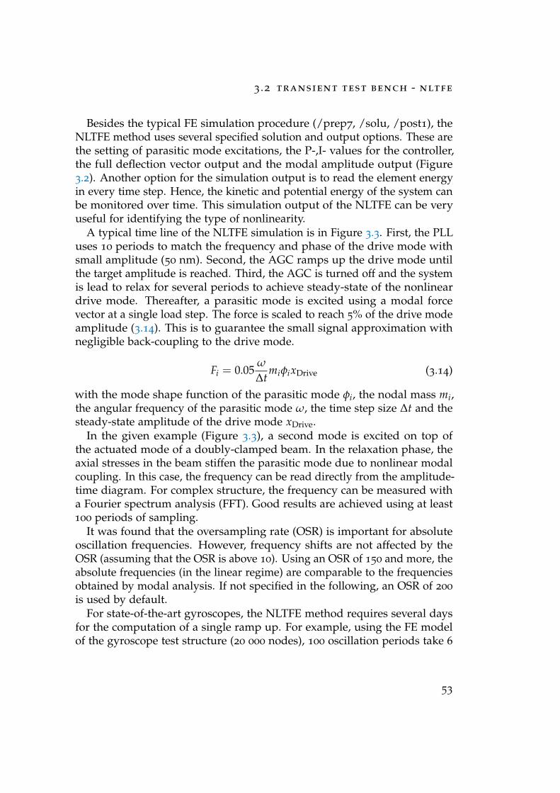
3 .2 transient test bench - nltfe
Besides the typical FE simulation procedure (/prep7, /solu, /post1), theNLTFE method uses several specified solution and output options. These arethe setting of parasitic mode excitations, the P-,I- values for the controller,the full deflection vector output and the modal amplitude output (Figure3.2). Another option for the simulation output is to read the element energyin every time step. Hence, the kinetic and potential energy of the system canbe monitored over time. This simulation output of the NLTFE can be veryuseful for identifying the type of nonlinearity.
A typical time line of the NLTFE simulation is in Figure 3.3. First, the PLLuses 10 periods to match the frequency and phase of the drive mode withsmall amplitude (50 nm). Second, the AGC ramps up the drive mode untilthe target amplitude is reached. Third, the AGC is turned off and the systemis lead to relax for several periods to achieve steady-state of the nonlineardrive mode. Thereafter, a parasitic mode is excited using a modal forcevector at a single load step. The force is scaled to reach 5% of the drive modeamplitude (3.14). This is to guarantee the small signal approximation withnegligible back-coupling to the drive mode.
Fi = 0.05ω
∆tmiφixDrive (3.14)
with the mode shape function of the parasitic mode φi, the nodal mass mi,the angular frequency of the parasitic mode ω, the time step size ∆t and thesteady-state amplitude of the drive mode xDrive.
In the given example (Figure 3.3), a second mode is excited on top ofthe actuated mode of a doubly-clamped beam. In the relaxation phase, theaxial stresses in the beam stiffen the parasitic mode due to nonlinear modalcoupling. In this case, the frequency can be read directly from the amplitude-time diagram. For complex structure, the frequency can be measured witha Fourier spectrum analysis (FFT). Good results are achieved using at least100 periods of sampling.
It was found that the oversampling rate (OSR) is important for absoluteoscillation frequencies. However, frequency shifts are not affected by theOSR (assuming that the OSR is above 10). Using an OSR of 150 and more, theabsolute frequencies (in the linear regime) are comparable to the frequenciesobtained by modal analysis. If not specified in the following, an OSR of 200
is used by default.For state-of-the-art gyroscopes, the NLTFE method requires several days
for the computation of a single ramp up. For example, using the FE modelof the gyroscope test structure (20 000 nodes), 100 oscillation periods take 6
53
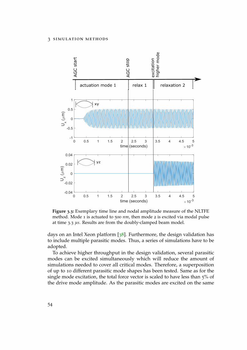
3 simulation methods
AG
C s
top
actuation mode 1 relax 1 relaxation 2
AG
C s
tart
exci
tation
xy
yzhig
her
mod
e
Figure 3.3: Exemplary time line and nodal amplitude measure of the NLTFEmethod. Mode 1 is actuated to 500 nm, then mode 2 is excited via modal pulseat time 3.3 µs. Results are from the doubly-clamped beam model.
days on an Intel Xeon platform [38]. Furthermore, the design validation hasto include multiple parasitic modes. Thus, a series of simulations have to beadopted.
To achieve higher throughput in the design validation, several parasiticmodes can be excited simultaneously which will reduce the amount ofsimulations needed to cover all critical modes. Therefore, a superpositionof up to 10 different parasitic mode shapes has been tested. Same as for thesingle mode excitation, the total force vector is scaled to have less than 5% ofthe drive mode amplitude. As the parasitic modes are excited on the same
54
3 .2 transient test bench - nltfe
structure, special considerations about the choice of theses modes have to betaken into account. Possible interaction between the modes can distort thefrequency measure. Hence, the mode set should include only modes thatare well different in frequency and mode shape.
Nodal and modal amplitude measurement
As output, the test bench stores nodal deflection of several nodes (Figure3.2). These nodes need to be specified prior in the simulation. Due tolimited memory, the full deflection vectors can only be extracted for a smallnumber of load steps. Another option for the deflection output is to use themodal amplitude measure. Therefore, the deflection vector is decomposedinto the LNMs in every time step. The modal amplitudes are achieved bymultiplying a decomposition matrix to the actual deflection vector. Thismatrix uses mode shapes that are normalized to the maximum deflectionof the mode shape. In this way, complex mode shapes can be distinguishedand analyzed.
Data analysis
The simulation results are analyzed with Matlab 2014 and higher. Thefrequency of the modes are either determined directly from the deflectiondata or from the Fourier spectrum of the data. Using nodal amplitudemeasure, the deflection of specific nodes are analyzed in x-,y-,z-directiondepending on the type of motion. In contrast, using modal amplitudemeasure enables to track the deflection of each mode with a single degreeof freedom. This can be advantageous for automated data analysis as thedirection of motion is not important when using modal decomposition.
In the Fourier analysis, modes can be identified by comparing peak po-sition in the spectrum to frequencies from modal analysis. The exact peakpositions are approximated from a quadratic fit where the neighboring datapoints are used (three point fit). This allows to have a higher resolution ofthe frequency (Figure 3.4).
In case a single mode is excited, nodal or modal amplitude over time isused to determine the frequency shift. Thereby, the minimum and maximumelongation of the oscillation are captured by using a parabola fit of theneighboring points. An advantage of the fitting procedure is that even smallfrequency shifts below the sampling frequency of the transient FE simulation
55
3 simulation methods
3.35 3.4 3.45 3.5ampl
itud
e(µ
m)
-0.020
0.02
z(t) of mode 2
frequency (Hz)5.3 5.35 5.4 5.45 5.5 5.55 5.6
Four
ier-
sign
al
10-3
2
4
6
8
10 0.100.200.300.400.500.610.740.891.131.46
ampl. mode 1FFT
p1
p2p3
10-3
104
1
Figure 3.4: Exemplary Fourier spectrum analysis with three point fitting. Thedata is from the second mode of a doubly-clamped beam with different ampli-tudes of mode 1.
can be captured. As an example, the local frequency of a gyro structurehas been calculated from the oscillation period (Figure 3.5). One finds thatduring ramp up of the mode, the local frequency changes drastically dueto excitation impact. Thereafter, the frequency settles into steady-state fromwhich the nonlinear frequency can be extracted. The linear frequency of theoscillation is extracted from the periods before ramp up. The average of localfrequencies is calculated in the marked ranges (Figure 3.5).
3.3 Nonlinear static simulation methods
The nonlinear static simulations can be divided into energy-based andstiffness-based methods. The energy-based method uses linear and nonlinearstatic analysis to retrieve the strain energy in the structure. The stiffness-based method uses the displacement from nonlinear static analysis andperforms a downstream modal analysis to retrieve the stiffness from whicheither a 1D Duffing or a multi-mode model is generated.
56
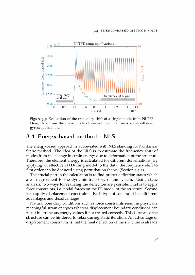
3 .4 energy-based method - nls
frequency frequency at 6 µmat 0 µm
1
Figure 3.5: Evaluation of the frequency shift of a single mode from NLTFE.Here, data from the drive mode of variant 1 of the 1-axis state-of-the-artgyroscope is shown.
3.4 Energy-based method - NLS
The energy-based approach is abbreviated with NLS standing for NonLinearStatic method. The idea of the NLS is to estimate the frequency shift ofmodes from the change in strain energy due to deformation of the structure.Therefore, the element energy is calculated for different deformations. Byapplying an effective 1D Duffing model to the data, the frequency shift tofirst order can be deduced using perturbation theory (Section 2.5.2).
The crucial part in the calculation is to find proper deflection states whichare in agreement to the dynamic trajectory of the system. Using staticanalysis, two ways for realizing the deflection are possible. First is to applyforce constraints, i.e. nodal forces on the FE model of the structure. Secondis to apply displacement constraints. Each type of constraint has differentadvantages and disadvantages.
Natural boundary conditions such as force constraints result in physicallymeaningful strain energies whereas displacement boundary conditions canresult in erroneous energy values if not treated correctly. This is because thestructure can be hindered to relax during static iteration. An advantage ofdisplacement constraints is that the final deflection of the structure is already
57
3 simulation methods
given. If force constraints are used, the deflection has to be measured aftercalculation. In the following, it is described how the actuated and parasiticmode deflections are achieved using either displacement or force constraintsin the static analysis.
3.4.1 Simulation approach for the frequency shift of asingle mode
For the frequency shift of a single mode, the structure is elongated into theconfiguration of that mode. One way to achieve this is by applying a modalforce vector on all nodes of the structure (3.15). This results in deformationsthat are compatible with the dynamics of the nonlinear mode.
Fi,x = miφi,xω2x (3.15)
where Fi,x is the force on node i into global x-direction, mi is the mass ofnode i, ω is the angular frequency of the mode, φi,x is the amplitude of nodei into global x-direction and x is the steady-state amplitude. Same for Fi,yand Fi,z.
Another possibility is to apply force constraints (f-constraints) on thoseparts of the structure which may be undeformed due to high stiffness. Incase of a gyroscopic structure, nodes on the drive frame can be selected forapplying the f-constraints [38]. Using nodal forces on the drive frame, theexact values to reach a specific amplitude are unknown in general. Therefore,reaction forces from a static analysis with displacement constraints can beused a priori.
After boundary conditions are applied to the FE model, the static loadcase is solved using linear solution option. This means that the tangentstiffness matrix contains only the material matrix K (3.3). The strain energyand amplitude of the system are extracted and the coefficient k0 can becalculated from the linear strain energy (Figure 3.6). In a second run, thestatic load case is solved using nonlinear solution option. In this analysis,the tangent stiffness matrix contains the material matrix K and the stress-stiffening matrix S (3.3). Again the strain energy and the amplitude of thesystem are extracted, Enl and xnl respectively.
Using k0 from the linear analysis, the Duffing coefficient k2 can be calcu-
58
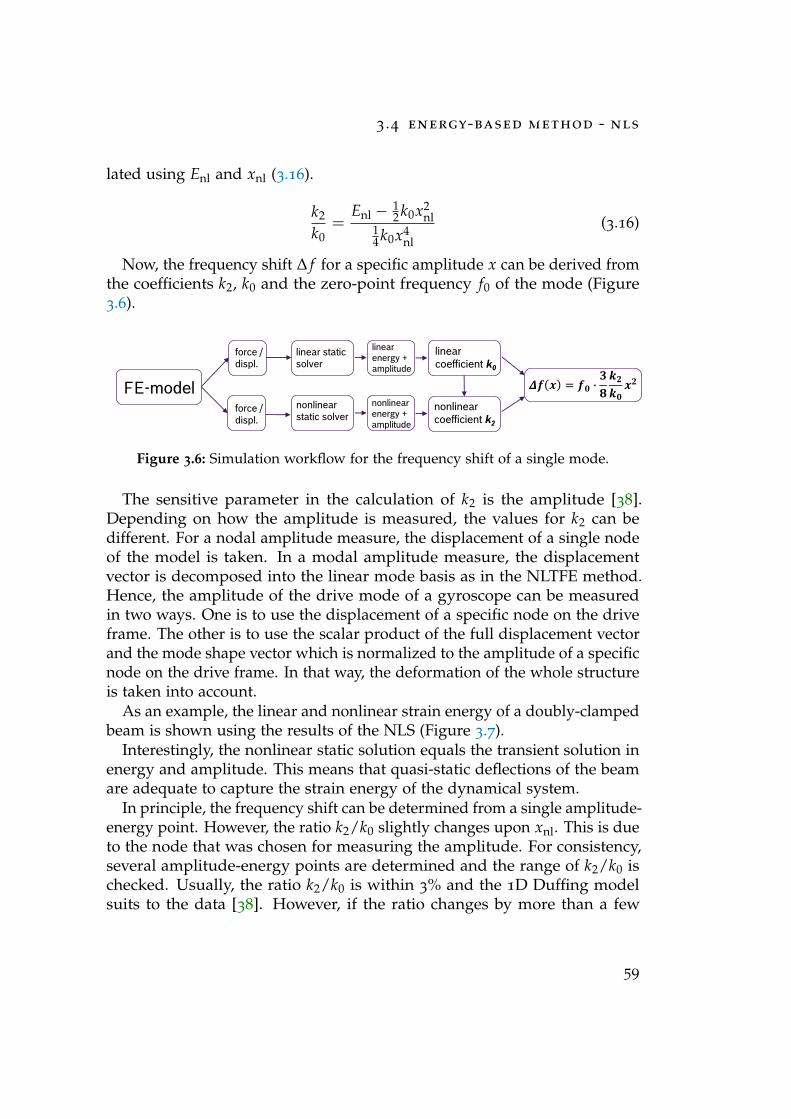
3 .4 energy-based method - nls
lated using Enl and xnl (3.16).
k2
k0=
Enl − 12 k0x2
nl14 k0x4
nl
(3.16)
Now, the frequency shift ∆ f for a specific amplitude x can be derived fromthe coefficients k2, k0 and the zero-point frequency f0 of the mode (Figure3.6).
Header of section
Automotive Electronics | AE/EST4 | 08/11/2016
© Robert Bosch GmbH 2016. All rights reserved, also regarding any disposal, exploitation, reproduction, editing, distribution, as well as in the event of applications for industrial property rights.1
linear
coefficient k0
FE-model
linear static
solver
nonlinear
static solver
𝜟𝒇 𝒙 = 𝒇𝟎 ∙𝟑
𝟖
𝒌𝟐𝒌𝟎
𝒙𝟐
nonlinear
coefficient k2
linear
energy +
amplitude
nonlinear
energy +
amplitude
force /
displ.
force /
displ.
Figure 3.6: Simulation workflow for the frequency shift of a single mode.
The sensitive parameter in the calculation of k2 is the amplitude [38].Depending on how the amplitude is measured, the values for k2 can bedifferent. For a nodal amplitude measure, the displacement of a single nodeof the model is taken. In a modal amplitude measure, the displacementvector is decomposed into the linear mode basis as in the NLTFE method.Hence, the amplitude of the drive mode of a gyroscope can be measuredin two ways. One is to use the displacement of a specific node on the driveframe. The other is to use the scalar product of the full displacement vectorand the mode shape vector which is normalized to the amplitude of a specificnode on the drive frame. In that way, the deformation of the whole structureis taken into account.
As an example, the linear and nonlinear strain energy of a doubly-clampedbeam is shown using the results of the NLS (Figure 3.7).
Interestingly, the nonlinear static solution equals the transient solution inenergy and amplitude. This means that quasi-static deflections of the beamare adequate to capture the strain energy of the dynamical system.
In principle, the frequency shift can be determined from a single amplitude-energy point. However, the ratio k2/k0 slightly changes upon xnl. This is dueto the node that was chosen for measuring the amplitude. For consistency,several amplitude-energy points are determined and the range of k2/k0 ischecked. Usually, the ratio k2/k0 is within 3% and the 1D Duffing modelsuits to the data [38]. However, if the ratio changes by more than a few
59
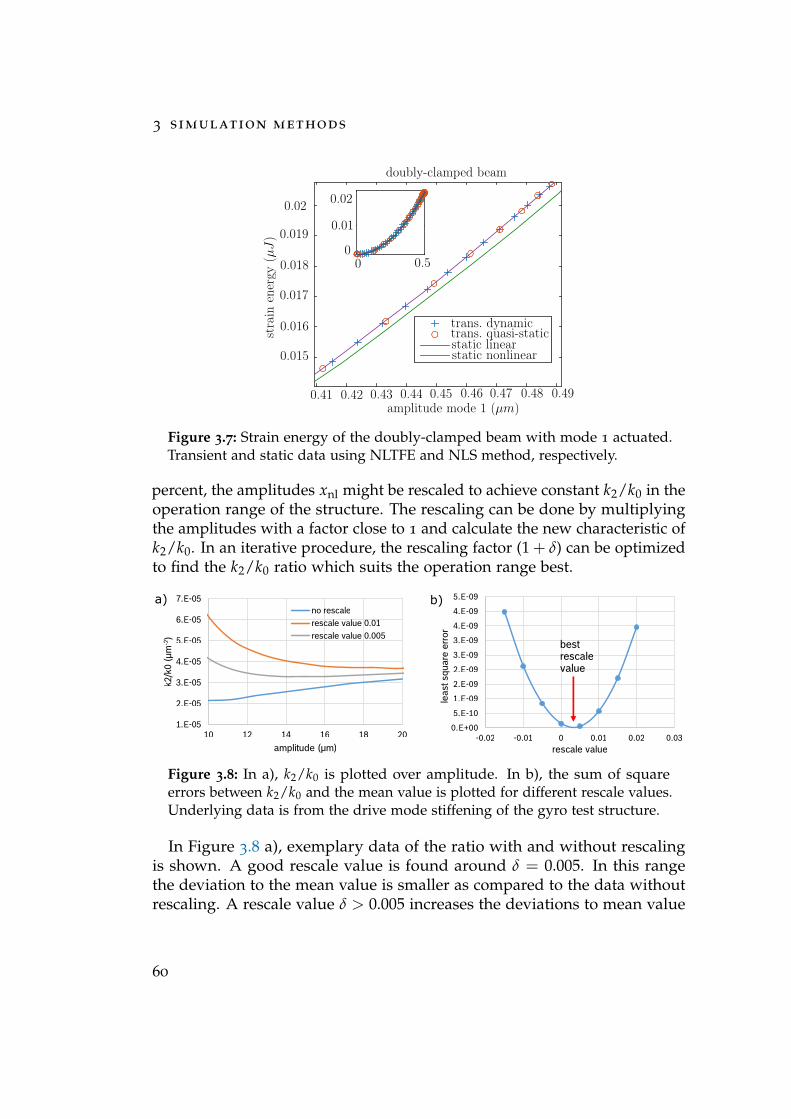
3 simulation methods
doubly-clamped beam
trans. dynamictrans. quasi-staticstatic linearstatic nonlinear
amplitude mode 1 (µm)
stra
inen
ergy
(µJ)
0.02
0.019
0.018
0.017
0.016
0.015
0.41 0.42 0.43 0.44 0.45 0.46 0.47 0.48 0.49
0 0.50
0.01
0.02
1
Figure 3.7: Strain energy of the doubly-clamped beam with mode 1 actuated.Transient and static data using NLTFE and NLS method, respectively.
percent, the amplitudes xnl might be rescaled to achieve constant k2/k0 in theoperation range of the structure. The rescaling can be done by multiplyingthe amplitudes with a factor close to 1 and calculate the new characteristic ofk2/k0. In an iterative procedure, the rescaling factor (1 + δ) can be optimizedto find the k2/k0 ratio which suits the operation range best.
Figure 3.8: In a), k2/k0 is plotted over amplitude. In b), the sum of squareerrors between k2/k0 and the mean value is plotted for different rescale values.Underlying data is from the drive mode stiffening of the gyro test structure.
In Figure 3.8 a), exemplary data of the ratio with and without rescalingis shown. A good rescale value is found around δ = 0.005. In this rangethe deviation to the mean value is smaller as compared to the data withoutrescaling. A rescale value δ > 0.005 increases the deviations to mean value
60
3 .4 energy-based method - nls
again. For automatic calculation of the best rescale value, an optimizationprocedure was implemented that calculates the sum of square errors betweenk2/k0 and the mean value of k2/k0 and converges towards the rescale valuewith the smallest square error sum (Figure 3.8 b)).
It should be emphasized that the presented approach is valid for symmetricmotion [38]. In case of asymmetric motions, a 4-th order polynomial canbe used to fit the amplitude-energy data of the nonlinear static analysis. Inthis way, the coefficient k1 of the quadratic forcing term can be isolated. Thefrequency shift is determined with the formula from Lifshitz and Kaajakari[32, 72] (3.17).
∆ f (x) = f0
(38
k2
k0− 5
12k2
1k2
0
)x2 (3.17)
Displacement and rotation constraints
An alternative to force constraints are displacement constraints. Same aswith force constraints, the displacement can be applied to a part of nodes orto all nodes of the structure. Choosing nodes on stiff parts, e.g. on the driveframe, is convenient for developing dynamic deformation states. It can oftenbe assumed that the stiff parts stay undeformed in dynamic motion. Hence,a linear displacement of these nodes into the direction of motion shouldyield good approximation of the dynamic deflection states. Furthermore, theadvantage is that folded-beams and suspension structures are able to relaxas they are not constraint.
Another possibility is to use the deflection from prior NLTFE simulation.However, the transient FE simulation is computational costly compared tosingle static simulations. Deflection vectors at the minimum and maximumelongation of the system can be extracted, i.e. the quasi-static points ofthe trajectory. These deflections can be used as displacement constraints.Usually, displacements are applied only into the direction of motion. Thishas two reasons, one is that the structure is able to relax and second is thatthe deflection vector might have small deviation to the exact solution orresidual momentum which could give parasitic contributions to the energy.
It was found that displacement constraints by the eigenvector from modalanalysis are not suitable. Constraining all DoFs with the displacement of thelinear mode shape, the structure is not able to relax and the stress-stiffeningis overestimated. To some extend, this issue could be overcome by applyingthe constraints only into a single direction, e.g. into the direction of motion.
61
3 simulation methods
This worked for 1D structures like a cantilever or doubly-clamped beam.However, for certain 2D structures, the displacement into a single directionof the mode shape led to unphysical high strain energies.
If beam elements are used in the model, there is the possibility to constrainrotational degrees of freedom as a part of displacement constraints. However,applying rotational in addition to translational constraint had no significanteffect on resulting energy and deflection.
3.4.2 Simulation approach for the frequency shift ofparasitic modes
The frequency shift of parasitic modes is determined from the strain energyand amplitude of different quasi-static configurations of the actuated andparasitic mode. Therefore, the parasitic mode is supposed to be linear andthe actuated mode is supposed to be nonlinear. This is realized by addinga small perturbation for the parasitic mode on top of the actuated mode.This perturbation is typically about 5% of the amplitude of the actuatedmode. Similarly to the case of a single mode, either force or displacementconstraints can be used.
Force constraints
The inputs are FE model and amplitude tables for the actuated and parasiticmode, xj and xk respectively. From these values, the corresponding forcevectors are defined using (3.15). The sum of actuated and parasitic modeforce is used as constraint in the nonlinear analysis to retrieve energy andamplitudes. For each drive mode force, the parasitic mode force is variedfrom negative to positive values. Since the resulting drive mode amplitudexj may change depending on the force of the parasitic mode, the force vectorof the drive mode can be adjusted in an iteration (Figure 3.9). This is done bylinear scale correction of the drive mode force using the relative differencebetween real and target amplitude. A convergence criterion of 10−4 is usedfor the relative amplitude difference.
The amplitudes are measured by modal decomposition of the static de-formation vector using the LNMs from modal analysis (Section 3.2). Assimulation results, a table with the system’s strain energy and a table withthe corresponding amplitudes of the drive and parasitic mode are achieved(Figure 3.9 b)).
62
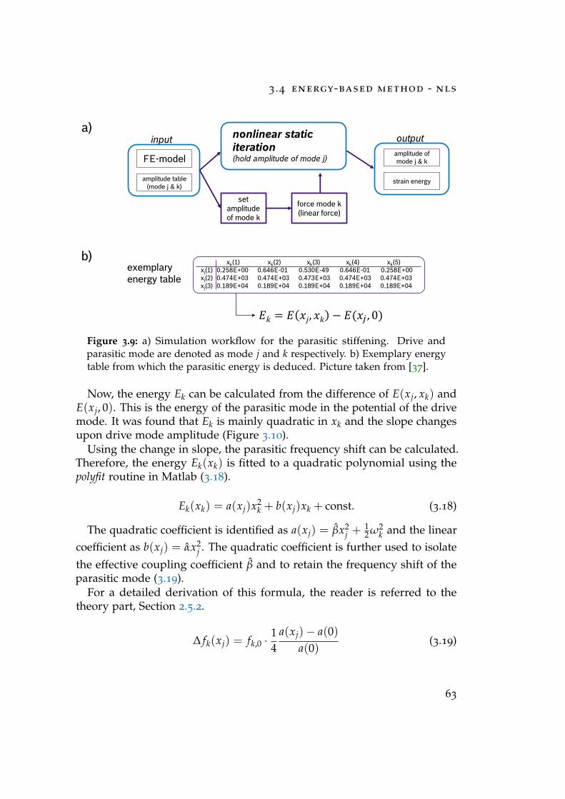
3 .4 energy-based method - nls
Automotive Electronics | AE/EST4 | 08/11/2016
© Robert Bosch GmbH 2016. All rights reserved, also regarding any disposal, exploitation, reproduction, editing, distribution, as well as in the event of applications for industrial property rights.1
amplitude table
(mode j & k)
set
amplitude
of mode k
force mode k
(linear force)
amplitude of
mode j & k
strain energy
FE-model
input outputnonlinear static
iteration (hold amplitude of mode j)
𝐸𝑘 = 𝐸 𝑥𝑗, 𝑥𝑘 − 𝐸(𝑥𝑗 , 0)
xk(1) xk(2) xk(3) xk(4) xk(5)
xj(1) 0.258E+00 0.646E-01 0.530E-49 0.646E-01 0.258E+00
xj(2) 0.474E+03 0.474E+03 0.473E+03 0.474E+03 0.474E+03
xj(3) 0.189E+04 0.189E+04 0.189E+04 0.189E+04 0.189E+04
exemplary
energy table
a)
b)
Figure 3.9: a) Simulation workflow for the parasitic stiffening. Drive andparasitic mode are denoted as mode j and k respectively. b) Exemplary energytable from which the parasitic energy is deduced. Picture taken from [37].
Now, the energy Ek can be calculated from the difference of E(xj, xk) andE(xj, 0). This is the energy of the parasitic mode in the potential of the drivemode. It was found that Ek is mainly quadratic in xk and the slope changesupon drive mode amplitude (Figure 3.10).
Using the change in slope, the parasitic frequency shift can be calculated.Therefore, the energy Ek(xk) is fitted to a quadratic polynomial using thepolyfit routine in Matlab (3.18).
Ek(xk) = a(xj)x2k + b(xj)xk + const. (3.18)
The quadratic coefficient is identified as a(xj) = βx2j +
12 ω2
k and the linearcoefficient as b(xj) = αx2
j . The quadratic coefficient is further used to isolate
the effective coupling coefficient β and to retain the frequency shift of theparasitic mode (3.19).
For a detailed derivation of this formula, the reader is referred to thetheory part, Section 2.5.2.
∆ fk(xj) = fk,0 ·14
a(xj)− a(0)a(0)
(3.19)
63
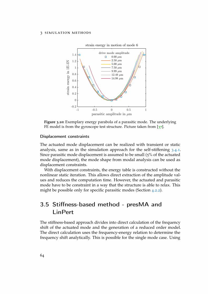
3 simulation methods
Figure 3.10: Exemplary energy parabola of a parasitic mode. The underlyingFE model is from the gyroscope test structure. Picture taken from [37].
Displacement constraints
The actuated mode displacement can be realized with transient or staticanalysis, same as in the simulation approach for the self-stiffening 3.4.1.Since parasitic mode displacement is assumed to be small (5% of the actuatedmode displacement), the mode shape from modal analysis can be used asdisplacement constraints.
With displacement constraints, the energy table is constructed without thenonlinear static iteration. This allows direct extraction of the amplitude val-ues and reduces the computation time. However, the actuated and parasiticmode have to be constraint in a way that the structure is able to relax. Thismight be possible only for specific parasitic modes (Section 4.2.2).
3.5 Stiffness-based method - presMA andLinPert
The stiffness-based approach divides into direct calculation of the frequencyshift of the actuated mode and the generation of a reduced order model.The direct calculation uses the frequency-energy relation to determine thefrequency shift analytically. This is possible for the single mode case. Using
64
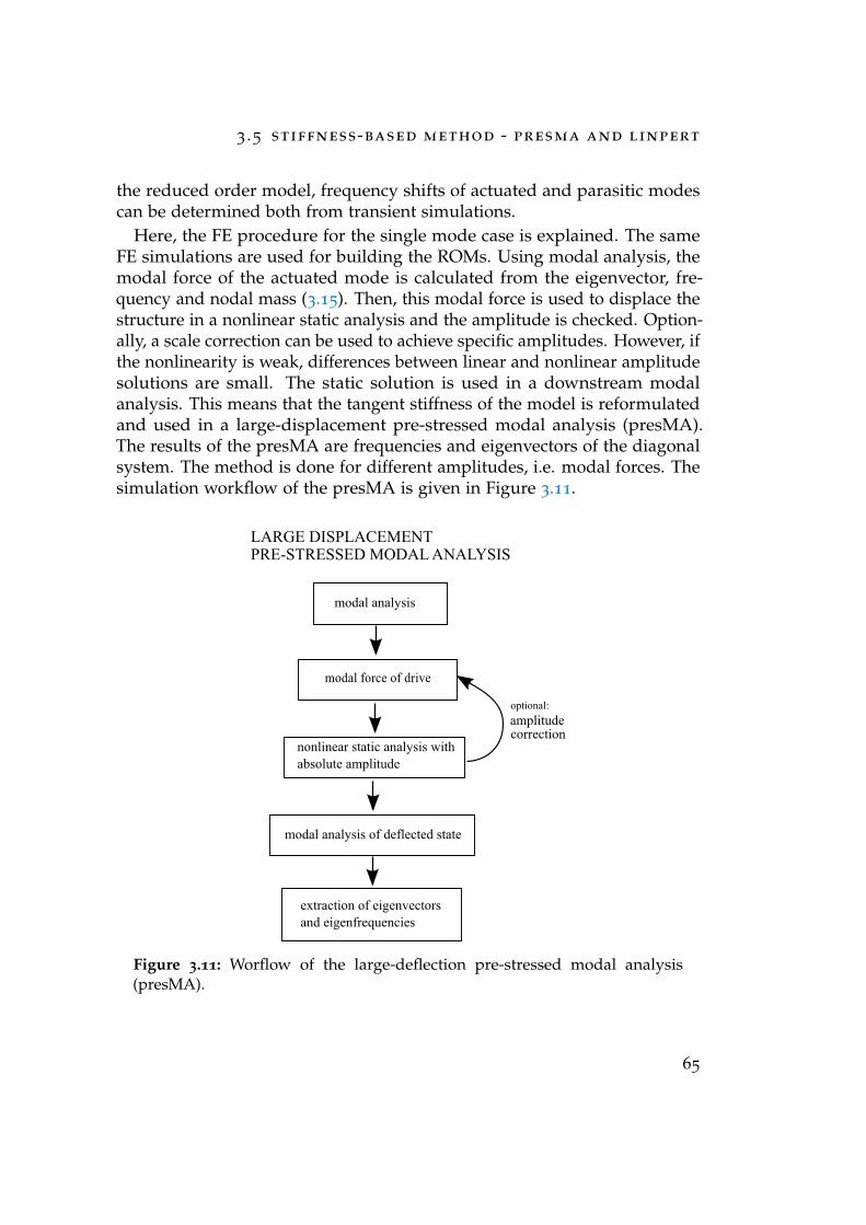
3 .5 stiffness-based method - presma and linpert
the reduced order model, frequency shifts of actuated and parasitic modescan be determined both from transient simulations.
Here, the FE procedure for the single mode case is explained. The sameFE simulations are used for building the ROMs. Using modal analysis, themodal force of the actuated mode is calculated from the eigenvector, fre-quency and nodal mass (3.15). Then, this modal force is used to displace thestructure in a nonlinear static analysis and the amplitude is checked. Option-ally, a scale correction can be used to achieve specific amplitudes. However, ifthe nonlinearity is weak, differences between linear and nonlinear amplitudesolutions are small. The static solution is used in a downstream modalanalysis. This means that the tangent stiffness of the model is reformulatedand used in a large-displacement pre-stressed modal analysis (presMA).The results of the presMA are frequencies and eigenvectors of the diagonalsystem. The method is done for different amplitudes, i.e. modal forces. Thesimulation workflow of the presMA is given in Figure 3.11.
Figure 3.11: Worflow of the large-deflection pre-stressed modal analysis(presMA).
65
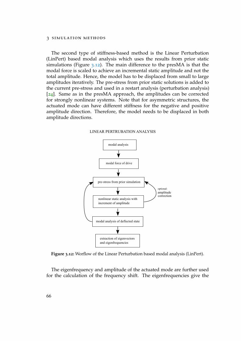
3 simulation methods
The second type of stiffness-based method is the Linear Perturbation(LinPert) based modal analysis which uses the results from prior staticsimulations (Figure 3.12). The main difference to the presMA is that themodal force is scaled to achieve an incremental static amplitude and not thetotal amplitude. Hence, the model has to be displaced from small to largeamplitudes iteratively. The pre-stress from prior static solutions is added tothe current pre-stress and used in a restart analysis (perturbation analysis)[24]. Same as in the presMA approach, the amplitudes can be correctedfor strongly nonlinear systems. Note that for asymmetric structures, theactuated mode can have different stiffness for the negative and positiveamplitude direction. Therefore, the model needs to be displaced in bothamplitude directions.
Figure 3.12: Worflow of the Linear Perturbation based modal analysis (LinPert).
The eigenfrequency and amplitude of the actuated mode are further usedfor the calculation of the frequency shift. The eigenfrequencies give the
66
3 .6 nonlinear transient rom simulation - nltrom
tangent stiffness for the different amplitudes xi of the actuated mode.
ktan(xi) = (2π fi)2, (3.20)
where the frequency fi is from the amplitude xi measured at a referencenode.
Since the force is a 3rd order polynomial of the modal amplitude (generalstrain theory), the stiffness is a 2nd order polynomial. Higher orders are notphysically fro geometric nonlinearity, but can be due to numerical effects.The tangent stiffness is fitted to a parabola using the polyfit routine in Matlab.
ktan(x) = k2,tanx2 + k1,tanx + k0,tan (3.21)
Integration over x yields (3.22).
F =13
k2,tanx3 +12
k1,tanx2 + k0,tanx (3.22)
Comparing (4.8) with the force of the Duffing oscillator results in correc-tions for the linear and quadratic stiffness, k1 and k2 respectively (3.23).
k2 =13
k2,tan
k1 =12
k1,tan
k0 = k0,tan
(3.23)
Inserting the stiffness coefficients (3.23) for the 1D Duffing model into(3.17) yields the frequency shift of the actuated mode.
In [65], the Duffing coefficient was determined from Linear Perturbationbased modal analysis using a correction factor of 4/9. This correction factorwas derived from balancing of the principle harmonic.
3.6 Nonlinear transient ROM simulation -NLTROM
The NonLinear Transient ROM method (NLTROM) uses the FE simulation ofthe previous discussed stiffness-based approaches. The FE results are usedto generate a reduced order model with an amplitude-dependent modal
67
3 simulation methods
stiffness. Using matrix transformation, the mode shapes of the displaced FEmodel can be expressed with the undeflected mode shapes. In this way, themodal stiffness matrix becomes non-diagonal. Modal coupling between thelinear normal modes is described by the off-diagonal entries of the stiffnessmatrix. Transient simulations of the reduced system can be performed inMatlab/Simulink using a look-up table for the amplitude-dependent modalstiffness matrix.
3.6.1 Approach of the model order reduction
The mode shape matrix of the undeflected structure is defined as V0, whereeach column is an eigenvector φi. Similarly, the mode shape matrix of thedeflected structure is defined as Vdefl, which has slightly different eigenvec-tors. A specific transformation T is used to change from the deflected to theundeflected mode shapes (3.24).
T = Q(V+deflV0), (3.24)
where the plus denotes the Moore-Penrose pseudoinverse and the functionQ(..) denotes the orthogonal matrix of the QR decomposition. Using QRdecomposition, an orthogonal matrix is generated from the product of V+
defland V0. Even though, Vdefl and V0 have orthogonal columns, V+
deflV0 is notan orthogonal matrix in general.
The transformation T is used to change the modal stiffness matrix from thedeflected to the undeflected eigenvectors (3.25). An amplitude-dependentmodal stiffness Kdefl,0 is obtained that renders the motion of the structure interms of the zero-point mode shapes. A detailed derivation of the transfor-mation is given in the Appendix D.
Kdefl,0 := TTKdeflT (3.25)
Diagonal mass and damping matrices are invariant under (3.25).For the transient ROM simulation, a look-up table for the stiffness matrices
is incorporated into a linear ROM (Figure 3.13). As damping matrix, aconstant diagonal damping of 50 is used to allow numerical stability. Thesystem is solved in Matlab/Simulink using common time integration (4thorder Runge-Kutta) with two steps for integrating modal accelerations. Thestiffness is evaluated using linear interpolation between the training ampli-tudes of the actuated mode, e.g. the modal amplitude q1. Prior to simulation,continuity of Kdefl,0 with respect to q1 is checked. Further, the linear and
68
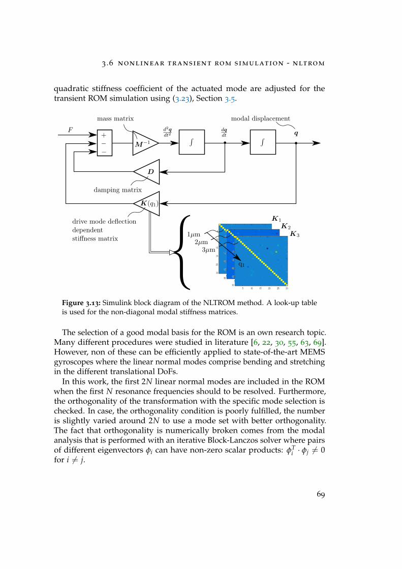
3 .6 nonlinear transient rom simulation - nltrom
quadratic stiffness coefficient of the actuated mode are adjusted for thetransient ROM simulation using (3.23), Section 3.5.
∫ ∫+−−
M−1
D
K(q1)
dqdt q
d2qdt2
F
damping matrix
mass matrix
drive mode deflectiondependentstiffness matrix
modal displacement
q1
K1
K2
K3
relative offdiagonal stiffness of drive mode
deflection of drive [µm]
stiffness
[1 Hz]
1µm2µm
3µm
1
Figure 3.13: Simulink block diagram of the NLTROM method. A look-up tableis used for the non-diagonal modal stiffness matrices.
The selection of a good modal basis for the ROM is an own research topic.Many different procedures were studied in literature [6, 22, 30, 55, 63, 69].However, non of these can be efficiently applied to state-of-the-art MEMSgyroscopes where the linear normal modes comprise bending and stretchingin the different translational DoFs.
In this work, the first 2N linear normal modes are included in the ROMwhen the first N resonance frequencies should to be resolved. Furthermore,the orthogonality of the transformation with the specific mode selection ischecked. In case, the orthogonality condition is poorly fulfilled, the numberis slightly varied around 2N to use a mode set with better orthogonality.The fact that orthogonality is numerically broken comes from the modalanalysis that is performed with an iterative Block-Lanczos solver where pairsof different eigenvectors φi can have non-zero scalar products: φT
i · φj 6= 0for i 6= j.
69
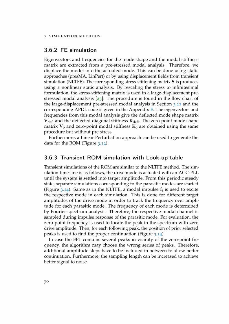
3 simulation methods
3.6.2 FE simulation
Eigenvectors and frequencies for the mode shape and the modal stiffnessmatrix are extracted from a pre-stressed modal analysis. Therefore, wedisplace the model into the actuated mode. This can be done using staticapproaches (presMA, LinPert) or by using displacement fields from transientsimulation (NLTFE). The corresponding stress-stiffening matrix S is producesusing a nonlinear static analysis. By rescaling the stress to infinitesimalformulation, the stress-stiffening matrix is used in a large-displacement pre-stressed modal analysis [25]. The procedure is found in the flow chart ofthe large-displacement pre-stressed modal analysis in Section 3.11 and thecorresponding APDL code is given in the Appendix E. The eigenvectors andfrequencies from this modal analysis give the deflected mode shape matrixVdefl and the deflected diagonal stiffness Kdefl. The zero-point mode shapematrix V0 and zero-point modal stiffness K0 are obtained using the sameprocedure but without pre-stress.
Furthermore, a Linear Perturbation approach can be used to generate thedata for the ROM (Figure 3.12).
3.6.3 Transient ROM simulation with Look-up table
Transient simulations of the ROM are similar to the NLTFE method. The sim-ulation time-line is as follows, the drive mode is actuated with an AGC-PLLuntil the system is settled into target amplitude. From this periodic steadystate, separate simulations corresponding to the parasitic modes are started(Figure 3.14). Same as in the NLTFE, a modal impulse fi is used to excitethe respective mode in each simulation. This is done for different targetamplitudes of the drive mode in order to track the frequency over ampli-tude for each parasitic mode. The frequency of each mode is determinedby Fourier spectrum analysis. Therefore, the respective modal channel issampled during impulse response of the parasitic mode. For evaluation, thezero-point frequency is used to locate the peak in the spectrum with zerodrive amplitude. Then, for each following peak, the position of prior selectedpeaks is used to find the proper continuation (Figure 3.14).
In case the FFT contains several peaks in vicinity of the zero-point fre-quency, the algorithm may choose the wrong series of peaks. Therefore,additional amplitude steps have to be included in between to allow bettercontinuation. Furthermore, the sampling length can be increased to achievebetter signal to noise.
70
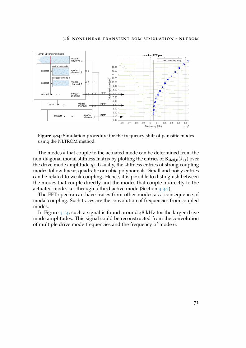
3 .6 nonlinear transient rom simulation - nltrom
Figure 3.14: Simulation procedure for the frequency shift of parasitic modesusing the NLTROM method.
The modes k that couple to the actuated mode can be determined from thenon-diagonal modal stiffness matrix by plotting the entries of Kdefl,0(k, j) overthe drive mode amplitude qj. Usually, the stiffness entries of strong couplingmodes follow linear, quadratic or cubic polynomials. Small and noisy entriescan be related to weak coupling. Hence, it is possible to distinguish betweenthe modes that couple directly and the modes that couple indirectly to theactuated mode, i.e. through a third active mode (Section 4.3.2).
The FFT spectra can have traces from other modes as a consequence ofmodal coupling. Such traces are the convolution of frequencies from coupledmodes.
In Figure 3.14, such a signal is found around 48 kHz for the larger drivemode amplitudes. This signal could be reconstructed from the convolutionof multiple drive mode frequencies and the frequency of mode 6.
71

4 Results
In this chapter, the results of the presented simulation methods are shown. Themethods have been applied to four different structures, a doubly-clamped beam, agyroscope test structure (1 axis) and two different state-of-the-art gyroscopes (1-axisand 2-axes).
The methods are evaluated by the accuracy of predicted frequency shifts and thecomputation performance on state-of-the-art hardware. Benchmark simulations(NLTFE) and experimental data (LDV and WLT) are used as reference. The valida-tion of the NLTFE is shown in the beginning.
73
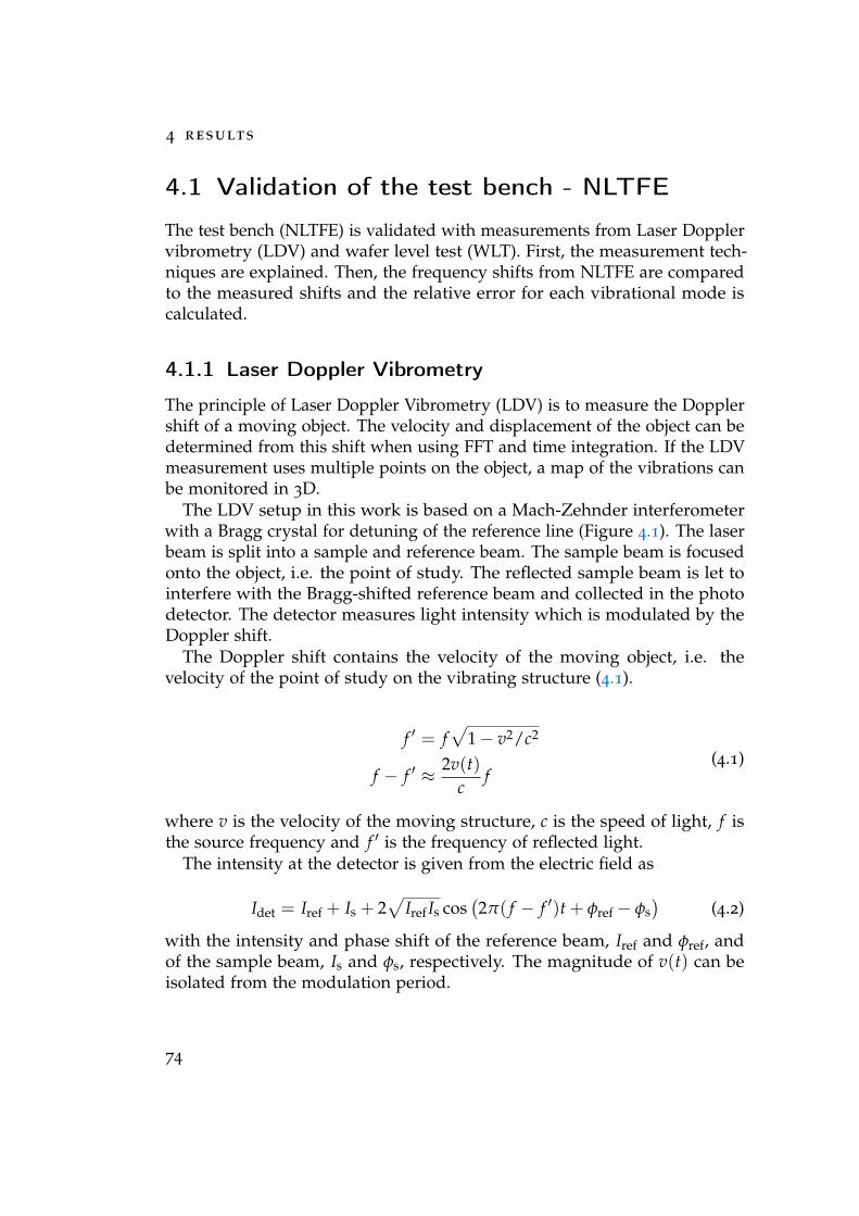
4 results
4.1 Validation of the test bench - NLTFE
The test bench (NLTFE) is validated with measurements from Laser Dopplervibrometry (LDV) and wafer level test (WLT). First, the measurement tech-niques are explained. Then, the frequency shifts from NLTFE are comparedto the measured shifts and the relative error for each vibrational mode iscalculated.
4.1.1 Laser Doppler Vibrometry
The principle of Laser Doppler Vibrometry (LDV) is to measure the Dopplershift of a moving object. The velocity and displacement of the object can bedetermined from this shift when using FFT and time integration. If the LDVmeasurement uses multiple points on the object, a map of the vibrations canbe monitored in 3D.
The LDV setup in this work is based on a Mach-Zehnder interferometerwith a Bragg crystal for detuning of the reference line (Figure 4.1). The laserbeam is split into a sample and reference beam. The sample beam is focusedonto the object, i.e. the point of study. The reflected sample beam is let tointerfere with the Bragg-shifted reference beam and collected in the photodetector. The detector measures light intensity which is modulated by theDoppler shift.
The Doppler shift contains the velocity of the moving object, i.e. thevelocity of the point of study on the vibrating structure (4.1).
f ′ = f√
1− v2/c2
f − f ′ ≈ 2v(t)c
f(4.1)
where v is the velocity of the moving structure, c is the speed of light, f isthe source frequency and f ′ is the frequency of reflected light.
The intensity at the detector is given from the electric field as
Idet = Iref + Is + 2√
Iref Is cos(2π( f − f ′)t + φref − φs
)(4.2)
with the intensity and phase shift of the reference beam, Iref and φref, andof the sample beam, Is and φs, respectively. The magnitude of v(t) can beisolated from the modulation period.
74
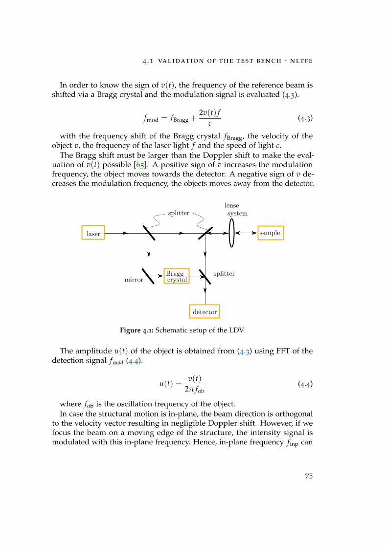
4 .1 validation of the test bench - nltfe
In order to know the sign of v(t), the frequency of the reference beam isshifted via a Bragg crystal and the modulation signal is evaluated (4.3).
fmod = fBragg +2v(t) f
c(4.3)
with the frequency shift of the Bragg crystal fBragg, the velocity of theobject v, the frequency of the laser light f and the speed of light c.
The Bragg shift must be larger than the Doppler shift to make the eval-uation of v(t) possible [65]. A positive sign of v increases the modulationfrequency, the object moves towards the detector. A negative sign of v de-creases the modulation frequency, the objects moves away from the detector.
laser
Braggcrystal
sample
lensesystem
detector
splitter
splitter
mirror
1
Figure 4.1: Schematic setup of the LDV.
The amplitude u(t) of the object is obtained from (4.3) using FFT of thedetection signal fmod (4.4).
u(t) =v(t)
2π fob(4.4)
where fob is the oscillation frequency of the object.In case the structural motion is in-plane, the beam direction is orthogonal
to the velocity vector resulting in negligible Doppler shift. However, if wefocus the beam on a moving edge of the structure, the intensity signal ismodulated with this in-plane frequency. Hence, in-plane frequency finp can
75
4 results
be still evaluated using (4.5).
Idet = Iref + Is,0 + Is,1 cos(2π finpt) + ... (4.5)
The amplitude of oscillation is not accessible in this procedure.
LDV measurement of MEMS gyroscopes
A Polytec Micro System Analyzer 500 is used for the LDV measurements ofthe presented structures. This type of LDV has a scanning option (SLDV)which can resolve 3D images of the mode shape of the vibration usingmultiple measurement points on the object. The Polytec LDV uses a 633 nmHelium-Neon Laser and a Bragg crystal with 40 MHz shift [65].
The drive mode is controlled by an ASIC and external stimuli of thesamples are realized by a piezoelectric shaker setup. The shaker setup allowsexcitations of vibrations between 10 - 200 kHz [65]. The measurements areconducted in air below 1 mbar and the sampling time is adjusted to reacha frequency resolution of 1 Hz. For out-of-plane modes, the scanning LDVmeasurements are used to provide the mode shape. For in-plane modes,stroboscopic measurements are used to identify the mode shape. In order tomeasure the frequency of the drive mode, the gyroscope is actuated with thecomb drive using an ASIC [65]. In general, the drive mode is in-plane andthe LDV measurement is conducted as for in-plane modes.
The frequency of higher modes are measured in the following way. First,the drive mode is set to a specific amplitude and the higher modes are excitedwith a chirp signal at the piezo shaker. Then, the modes are identified witheither SLDV or stroboscopic measurement. Finally, the LDV signal is sampledimmediately after the chirp in order to determine frequency and amplitude.
The oscillation frequencies that are obtained from the LDV are plotted forthe different drive mode amplitudes. Typically, the frequency curve of thedrive mode is quadratic in amplitude.
In this case, the frequency amplitude points are fitted to a quadraticfunction (Figure 4.2).
A polynomial fit seems unphysical around 0 µm. Better is to use thenonlinear function ax2 + b for the curve fitting. This results in physicalmeaningful frequency pulling of the drive mode. In Figure 4.2, the shift is 89
Hz at 15 µm amplitude. Frequency curves of parasitic modes can differ tothe quadratic behaviour. In these cases, the frequency shift is determined fora specific drive mode amplitude without fitting.
76
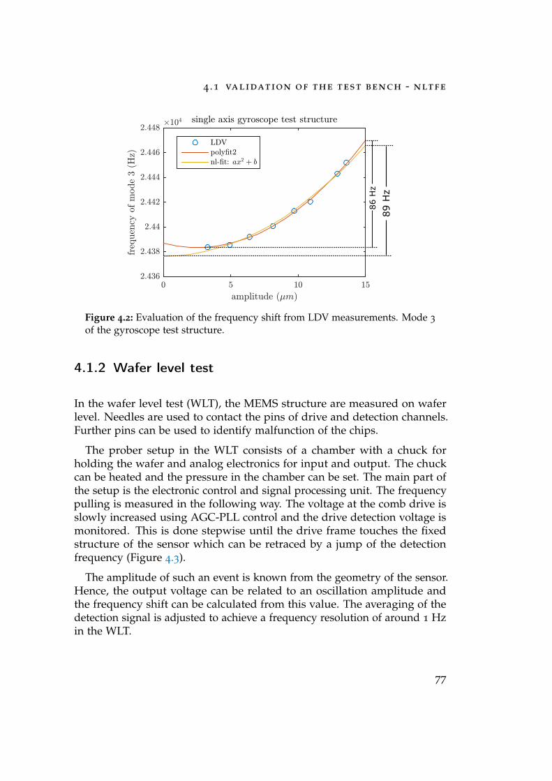
4 .1 validation of the test bench - nltfe
Figure 4.2: Evaluation of the frequency shift from LDV measurements. Mode 3
of the gyroscope test structure.
4.1.2 Wafer level test
In the wafer level test (WLT), the MEMS structure are measured on waferlevel. Needles are used to contact the pins of drive and detection channels.Further pins can be used to identify malfunction of the chips.
The prober setup in the WLT consists of a chamber with a chuck forholding the wafer and analog electronics for input and output. The chuckcan be heated and the pressure in the chamber can be set. The main part ofthe setup is the electronic control and signal processing unit. The frequencypulling is measured in the following way. The voltage at the comb drive isslowly increased using AGC-PLL control and the drive detection voltage ismonitored. This is done stepwise until the drive frame touches the fixedstructure of the sensor which can be retraced by a jump of the detectionfrequency (Figure 4.3).
The amplitude of such an event is known from the geometry of the sensor.Hence, the output voltage can be related to an oscillation amplitude andthe frequency shift can be calculated from this value. The averaging of thedetection signal is adjusted to achieve a frequency resolution of around 1 Hzin the WLT.
77
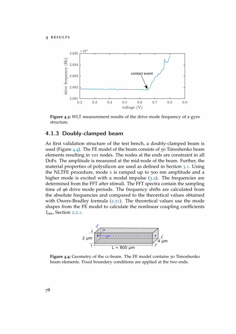
4 results
voltage (V)0.2 0.3 0.4 0.5 0.6 0.7 0.8 0.9
drive
frequency
(Hz)
#104
2.691
2.692
2.693
2.694
2.695
contact event
Figure 4.3: WLT measurement results of the drive mode frequency of a gyrostructure.
4.1.3 Doubly-clamped beam
As first validation structure of the test bench, a doubly-clamped beam isused (Figure 4.4). The FE model of the beam consists of 50 Timoshenko beamelements resulting in 101 nodes. The nodes at the ends are constraint in allDoFs. The amplitude is measured at the mid-node of the beam. Further, thematerial properties of polysilicon are used as defined in Section 3.1. Usingthe NLTFE procedure, mode 1 is ramped up to 500 nm amplitude and ahigher mode is excited with a modal impulse (3.2). The frequencies aredetermined from the FFT after stimuli. The FFT spectra contain the samplingtime of 96 drive mode periods. The frequency shifts are calculated fromthe absolute frequencies and compared to the theoretical values obtainedwith Owers-Bradley formula (2.51). The theoretical values use the modeshapes from the FE model to calculate the nonlinear coupling coefficientsInm, Section 2.5.1.
Figure 4.4: Geometry of the cc-beam. The FE model contains 50 Timoshenkobeam elements. Fixed boundary conditions are applied at the two ends.
78
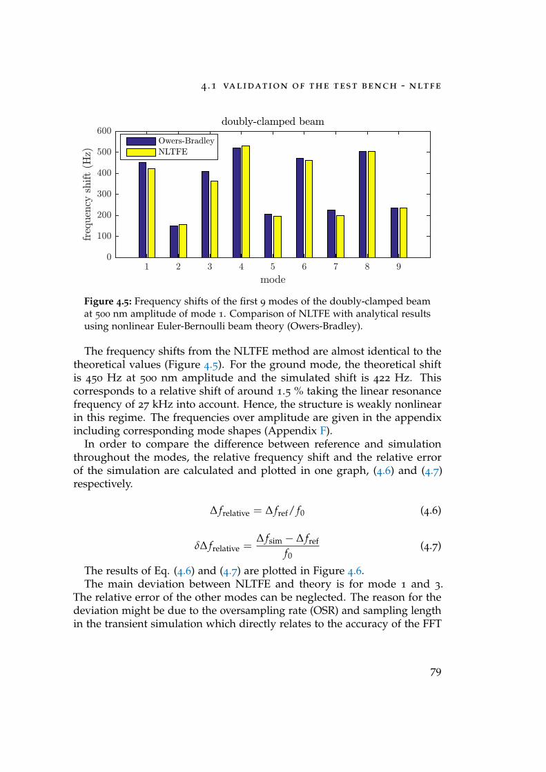
4 .1 validation of the test bench - nltfe
mode1 2 3 4 5 6 7 8 9
freq
uen
cysh
ift
(Hz)
0
100
200
300
400
500
600doubly-clamped beam
Owers-Bradley
NLTFE
Figure 4.5: Frequency shifts of the first 9 modes of the doubly-clamped beamat 500 nm amplitude of mode 1. Comparison of NLTFE with analytical resultsusing nonlinear Euler-Bernoulli beam theory (Owers-Bradley).
The frequency shifts from the NLTFE method are almost identical to thetheoretical values (Figure 4.5). For the ground mode, the theoretical shiftis 450 Hz at 500 nm amplitude and the simulated shift is 422 Hz. Thiscorresponds to a relative shift of around 1.5 % taking the linear resonancefrequency of 27 kHz into account. Hence, the structure is weakly nonlinearin this regime. The frequencies over amplitude are given in the appendixincluding corresponding mode shapes (Appendix F).
In order to compare the difference between reference and simulationthroughout the modes, the relative frequency shift and the relative errorof the simulation are calculated and plotted in one graph, (4.6) and (4.7)respectively.
∆ frelative = ∆ fref/ f0 (4.6)
δ∆ frelative =∆ fsim − ∆ fref
f0(4.7)
The results of Eq. (4.6) and (4.7) are plotted in Figure 4.6.The main deviation between NLTFE and theory is for mode 1 and 3.
The relative error of the other modes can be neglected. The reason for thedeviation might be due to the oversampling rate (OSR) and sampling lengthin the transient simulation which directly relates to the accuracy of the FFT
79
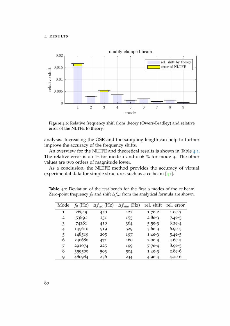
4 results
doubly-clamped beam
mode1 2 3 4 5 6 7 8 9
relativeshift
0
0.005
0.01
0.015
0.02
rel. shift by theory
error of NLTFE
Figure 4.6: Relative frequency shift from theory (Owers-Bradley) and relativeerror of the NLTFE to theory.
analysis. Increasing the OSR and the sampling length can help to furtherimprove the accuracy of the frequency shifts.
An overview for the NLTFE and theoretical results is shown in Table 4.1.The relative error is 0.1 % for mode 1 and 0.06 % for mode 3. The othervalues are two orders of magnitude lower.
As a conclusion, the NLTFE method provides the accuracy of virtualexperimental data for simple structures such as a cc-beam [41].
Table 4.1: Deviation of the test bench for the first 9 modes of the cc-beam.Zero-point frequency f0 and shift ∆ fref from the analytical formula are shown.
Mode f0 (Hz) ∆ fref (Hz) ∆ fsim (Hz) rel. shift rel. error1 26949 450 422 1.7e-2 1.0e-32 53891 151 155 2.8e-3 7.4e-53 74281 410 364 5.5e-3 6.2e-44 145610 519 529 3.6e-3 6.9e-55 148519 205 197 1.4e-3 5.4e-56 240680 471 460 2.0e-3 4.6e-57 291074 225 199 7.7e-4 8.9e-58 359500 503 504 1.4e-3 2.8e-69 480984 236 234 4.9e-4 4.2e-6
80
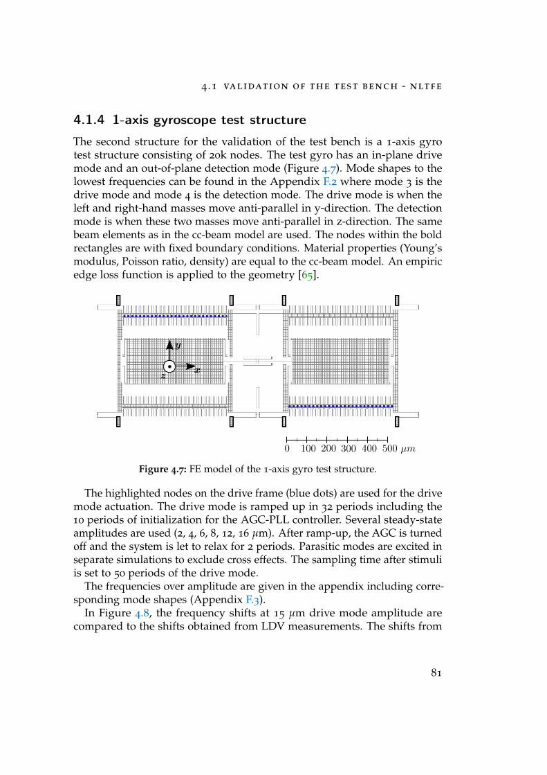
4 .1 validation of the test bench - nltfe
4.1.4 1-axis gyroscope test structure
The second structure for the validation of the test bench is a 1-axis gyrotest structure consisting of 20k nodes. The test gyro has an in-plane drivemode and an out-of-plane detection mode (Figure 4.7). Mode shapes to thelowest frequencies can be found in the Appendix F.2 where mode 3 is thedrive mode and mode 4 is the detection mode. The drive mode is when theleft and right-hand masses move anti-parallel in y-direction. The detectionmode is when these two masses move anti-parallel in z-direction. The samebeam elements as in the cc-beam model are used. The nodes within the boldrectangles are with fixed boundary conditions. Material properties (Young’smodulus, Poisson ratio, density) are equal to the cc-beam model. An empiricedge loss function is applied to the geometry [65].
0 100 200 500 µm300 400
zx
y
1
Figure 4.7: FE model of the 1-axis gyro test structure.
The highlighted nodes on the drive frame (blue dots) are used for the drivemode actuation. The drive mode is ramped up in 32 periods including the10 periods of initialization for the AGC-PLL controller. Several steady-stateamplitudes are used (2, 4, 6, 8, 12, 16 µm). After ramp-up, the AGC is turnedoff and the system is let to relax for 2 periods. Parasitic modes are excited inseparate simulations to exclude cross effects. The sampling time after stimuliis set to 50 periods of the drive mode.
The frequencies over amplitude are given in the appendix including corre-sponding mode shapes (Appendix F.3).
In Figure 4.8, the frequency shifts at 15 µm drive mode amplitude arecompared to the shifts obtained from LDV measurements. The shifts from
81
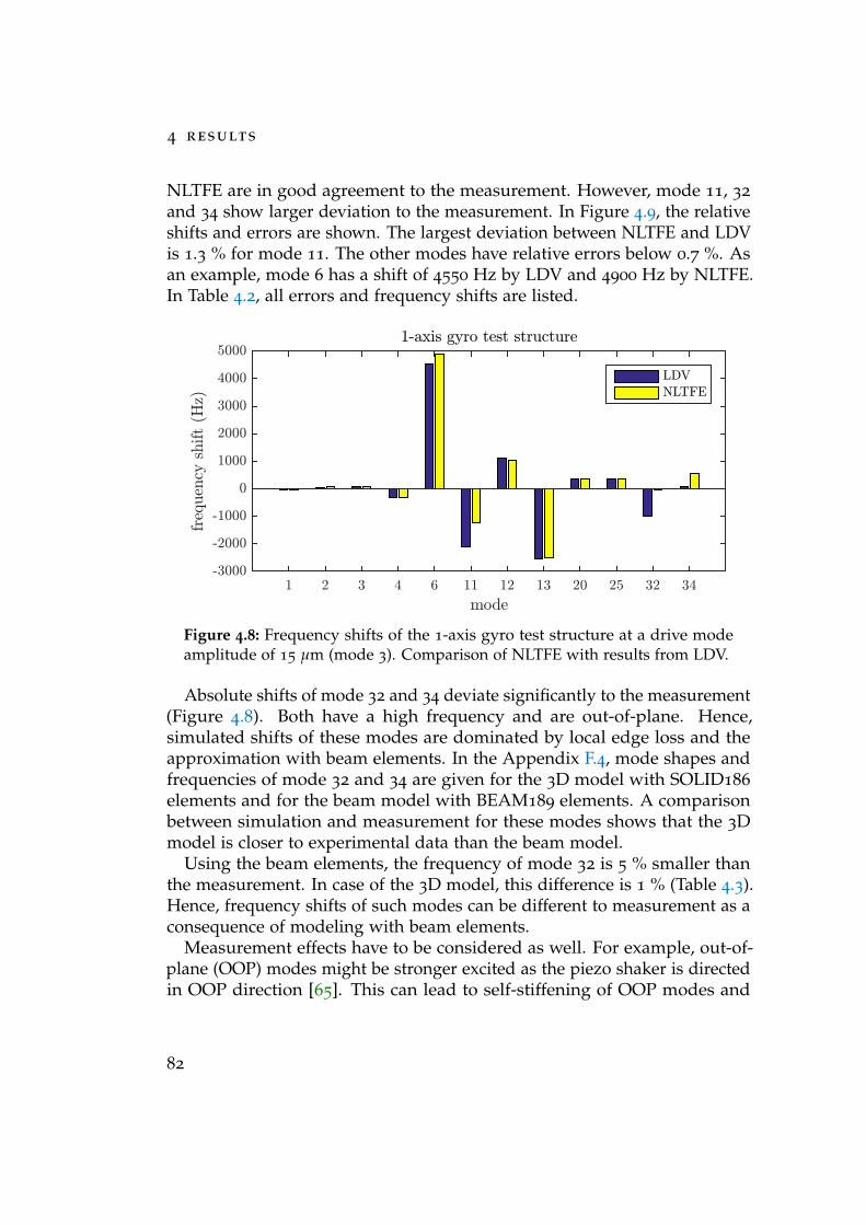
4 results
NLTFE are in good agreement to the measurement. However, mode 11, 32
and 34 show larger deviation to the measurement. In Figure 4.9, the relativeshifts and errors are shown. The largest deviation between NLTFE and LDVis 1.3 % for mode 11. The other modes have relative errors below 0.7 %. Asan example, mode 6 has a shift of 4550 Hz by LDV and 4900 Hz by NLTFE.In Table 4.2, all errors and frequency shifts are listed.
mode1 2 3 4 6 11 12 13 20 25 32 34
frequencyshift(Hz)
-3000
-2000
-1000
0
1000
2000
3000
4000
50001-axis gyro test structure
LDV
NLTFE
Figure 4.8: Frequency shifts of the 1-axis gyro test structure at a drive modeamplitude of 15 µm (mode 3). Comparison of NLTFE with results from LDV.
Absolute shifts of mode 32 and 34 deviate significantly to the measurement(Figure 4.8). Both have a high frequency and are out-of-plane. Hence,simulated shifts of these modes are dominated by local edge loss and theapproximation with beam elements. In the Appendix F.4, mode shapes andfrequencies of mode 32 and 34 are given for the 3D model with SOLID186
elements and for the beam model with BEAM189 elements. A comparisonbetween simulation and measurement for these modes shows that the 3Dmodel is closer to experimental data than the beam model.
Using the beam elements, the frequency of mode 32 is 5 % smaller thanthe measurement. In case of the 3D model, this difference is 1 % (Table 4.3).Hence, frequency shifts of such modes can be different to measurement as aconsequence of modeling with beam elements.
Measurement effects have to be considered as well. For example, out-of-plane (OOP) modes might be stronger excited as the piezo shaker is directedin OOP direction [65]. This can lead to self-stiffening of OOP modes and
82
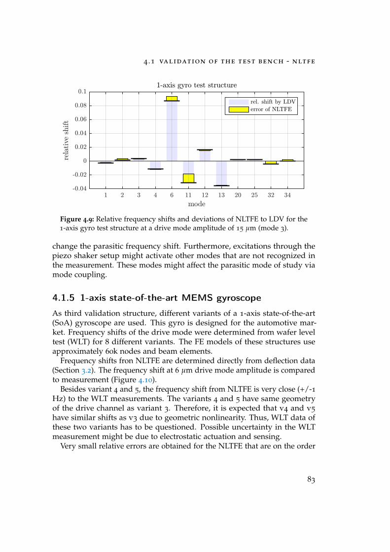
4 .1 validation of the test bench - nltfe
1-axis gyro test structure
mode1 2 3 4 6 11 12 13 20 25 32 34
relativeshift
-0.04
-0.02
0
0.02
0.04
0.06
0.08
0.1
rel. shift by LDV
error of NLTFE
Figure 4.9: Relative frequency shifts and deviations of NLTFE to LDV for the1-axis gyro test structure at a drive mode amplitude of 15 µm (mode 3).
change the parasitic frequency shift. Furthermore, excitations through thepiezo shaker setup might activate other modes that are not recognized inthe measurement. These modes might affect the parasitic mode of study viamode coupling.
4.1.5 1-axis state-of-the-art MEMS gyroscope
As third validation structure, different variants of a 1-axis state-of-the-art(SoA) gyroscope are used. This gyro is designed for the automotive mar-ket. Frequency shifts of the drive mode were determined from wafer leveltest (WLT) for 8 different variants. The FE models of these structures useapproximately 60k nodes and beam elements.
Frequency shifts fron NLTFE are determined directly from deflection data(Section 3.2). The frequency shift at 6 µm drive mode amplitude is comparedto measurement (Figure 4.10).
Besides variant 4 and 5, the frequency shift from NLTFE is very close (+/-1Hz) to the WLT measurements. The variants 4 and 5 have same geometryof the drive channel as variant 3. Therefore, it is expected that v4 and v5
have similar shifts as v3 due to geometric nonlinearity. Thus, WLT data ofthese two variants has to be questioned. Possible uncertainty in the WLTmeasurement might be due to electrostatic actuation and sensing.
Very small relative errors are obtained for the NLTFE that are on the order
83
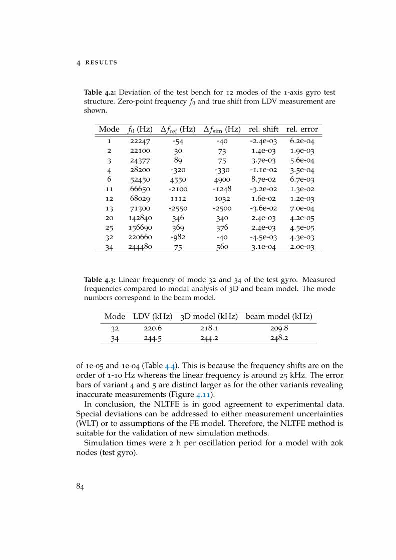
4 results
Table 4.2: Deviation of the test bench for 12 modes of the 1-axis gyro teststructure. Zero-point frequency f0 and true shift from LDV measurement areshown.
Mode f0 (Hz) ∆ fref (Hz) ∆ fsim (Hz) rel. shift rel. error1 22247 -54 -40 -2.4e-03 6.2e-04
2 22100 30 73 1.4e-03 1.9e-03
3 24377 89 75 3.7e-03 5.6e-04
4 28200 -320 -330 -1.1e-02 3.5e-04
6 52450 4550 4900 8.7e-02 6.7e-03
11 66650 -2100 -1248 -3.2e-02 1.3e-02
12 68029 1112 1032 1.6e-02 1.2e-03
13 71300 -2550 -2500 -3.6e-02 7.0e-04
20 142840 346 340 2.4e-03 4.2e-05
25 156690 369 376 2.4e-03 4.5e-05
32 220660 -982 -40 -4.5e-03 4.3e-03
34 244480 75 560 3.1e-04 2.0e-03
Table 4.3: Linear frequency of mode 32 and 34 of the test gyro. Measuredfrequencies compared to modal analysis of 3D and beam model. The modenumbers correspond to the beam model.
Mode LDV (kHz) 3D model (kHz) beam model (kHz)32 220.6 218.1 209.834 244.5 244.2 248.2
of 1e-05 and 1e-04 (Table 4.4). This is because the frequency shifts are on theorder of 1-10 Hz whereas the linear frequency is around 25 kHz. The errorbars of variant 4 and 5 are distinct larger as for the other variants revealinginaccurate measurements (Figure 4.11).
In conclusion, the NLTFE is in good agreement to experimental data.Special deviations can be addressed to either measurement uncertainties(WLT) or to assumptions of the FE model. Therefore, the NLTFE method issuitable for the validation of new simulation methods.
Simulation times were 2 h per oscillation period for a model with 20knodes (test gyro).
84
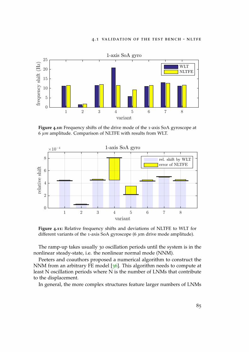
4 .1 validation of the test bench - nltfe
variant1 2 3 4 5 6 7 8
frequencyshift(Hz)
0
5
10
15
20
251-axis SoA gyro
WLT
NLTFE
Figure 4.10: Frequency shifts of the drive mode of the 1-axis SoA gyroscope at6 µm amplitude. Comparison of NLTFE with results from WLT.
1-axis SoA gyro
variant1 2 3 4 5 6 7 8
relativeshift
#10!4
0
2
4
6
8 rel. shift by WLT
error of NLTFE
Figure 4.11: Relative frequency shifts and deviations of NLTFE to WLT fordifferent variants of the 1-axis SoA gyroscope (6 µm drive mode amplitude).
The ramp-up takes usually 30 oscillation periods until the system is in thenonlinear steady-state, i.e. the nonlinear normal mode (NNM).
Peeters and coauthors proposed a numerical algorithm to construct theNNM from an arbitrary FE model [36]. This algorithm needs to compute atleast N oscillation periods where N is the number of LNMs that contributeto the displacement.
In general, the more complex structures feature larger numbers of LNMs
85
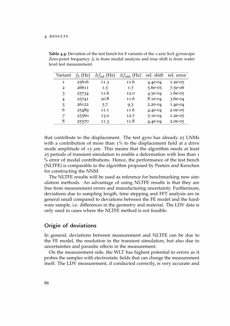
4 results
Table 4.4: Deviation of the test bench for 8 variants of the 1-axis SoA gyroscope.Zero-point frequency f0 is from modal analysis and true shift is from waferlevel test measurement.
Variant f0 (Hz) ∆ fref (Hz) ∆ fsim (Hz) rel. shift rel. error1 25616 11.3 11.6 4.4e-04 1.2e-05
2 26611 1.5 1.7 5.6e-05 7.5e-06
3 25734 11.6 12.0 4.5e-04 1.6e-05
4 25741 20.8 11.6 8.1e-04 3.6e-04
5 26122 5.7 9.3 2.2e-04 1.4e-04
6 25489 11.1 11.6 4.4e-04 2.0e-05
7 25560 13.0 12.7 5.1e-04 1.2e-05
8 25570 11.3 11.8 4.4e-04 2.0e-05
that contribute to the displacement. The test gyro has already 25 LNMswith a contribution of more than 1% to the displacement field at a drivemode amplitude of 15 µm. This means that the algorithm needs at least25 periods of transient simulation to enable a deformation with less than 1
% error of modal contributions. Hence, the performance of the test bench(NLTFE) is comparable to the algorithm proposed by Peeters and Kerschenfor constructing the NNM.
The NLTFE results will be used as reference for benchmarking new sim-ulation methods. An advantage of using NLTFE results is that they arefree from measurement errors and manufacturing uncertainty. Furthermore,deviations due to sampling length, time stepping and FFT analysis are ingeneral small compared to deviations between the FE model and the hard-ware sample, i.e. differences in the geometry and material. The LDV data isonly used in cases where the NLTFE method is not feasible.
Origin of deviations
In general, deviations between measurement and NLTFE can be due tothe FE model, the resolution in the transient simulation, but also due touncertainties and parasitic effects in the measurement.
On the measurement side, the WLT has highest potential to errors as itprobes the samples with electrostatic fields that can change the measurementitself. The LDV measurement, if conducted correctly, is very accurate and
86
4 .1 validation of the test bench - nltfe
the measurement has negligible effect on the state of the sensor. However,the electrostatic control of the drive loop may have parasitic effects on othermodes since it includes direct and alternating voltage signals at the electrodestructures.
Thermal effects of the laser beam can be excluded since exposure timesare small enough.
A secondary effect in the measurement is damping from gas moleculeswhich can yield amplitude dependent forces on the modes. Slide-film andsqueeze-film damping are velocity-dependent and therefore also dependenton the oscillation amplitude, see 2.4.2.
On the simulation side, the FE model and the sampling length of thetransient simulation are main contributors to the uncertainty. The FE modelcontains the average geometry of the structure with an average local edgeloss. However, the chip that was measured by LDV is unique in the way ofmanufacturing. Hence, it deviates to certain extend to the average. Alreadylinear frequencies of the test gyro can differ by 1 %.
Furthermore, the approximation of the 3D model with beam elements canyield inaccuracy in the mode shape and vibrational frequency. Especially forthe higher modes, frequencies of the beam model deviate stronger to the 3Dmodel (Figure F.4).
Another source of errors can be the data analysis, e.g. wrong mode matchor FFT peak selection. Using modal decomposition, the data analysis of theNLTFE is much more reliable.
The roughness and imperfections of the silicon material have a subordinateeffect on accuracy. Such properties were not included in the model. Anexample is the z-asymmetry of the silicon membrane stemming from thelayer growth by chemical vapor deposition (CVD).
87
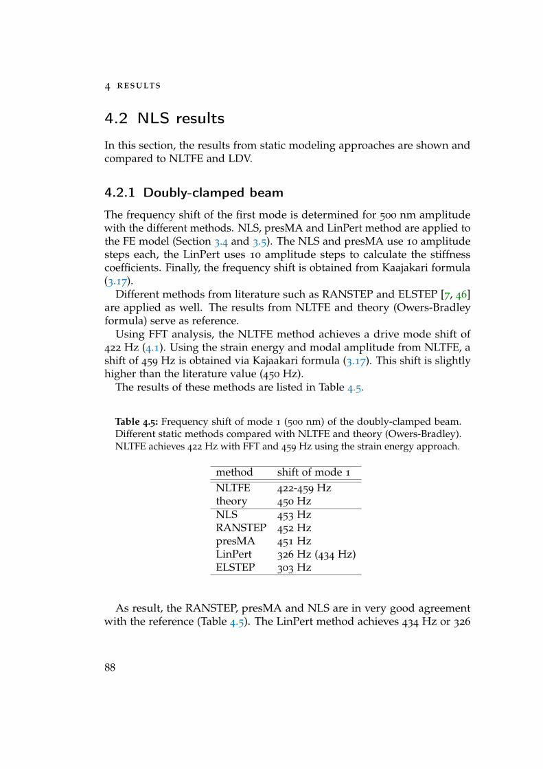
4 results
4.2 NLS results
In this section, the results from static modeling approaches are shown andcompared to NLTFE and LDV.
4.2.1 Doubly-clamped beam
The frequency shift of the first mode is determined for 500 nm amplitudewith the different methods. NLS, presMA and LinPert method are applied tothe FE model (Section 3.4 and 3.5). The NLS and presMA use 10 amplitudesteps each, the LinPert uses 10 amplitude steps to calculate the stiffnesscoefficients. Finally, the frequency shift is obtained from Kaajakari formula(3.17).
Different methods from literature such as RANSTEP and ELSTEP [7, 46]are applied as well. The results from NLTFE and theory (Owers-Bradleyformula) serve as reference.
Using FFT analysis, the NLTFE method achieves a drive mode shift of422 Hz (4.1). Using the strain energy and modal amplitude from NLTFE, ashift of 459 Hz is obtained via Kajaakari formula (3.17). This shift is slightlyhigher than the literature value (450 Hz).
The results of these methods are listed in Table 4.5.
Table 4.5: Frequency shift of mode 1 (500 nm) of the doubly-clamped beam.Different static methods compared with NLTFE and theory (Owers-Bradley).NLTFE achieves 422 Hz with FFT and 459 Hz using the strain energy approach.
method shift of mode 1
NLTFE 422-459 Hztheory 450 HzNLS 453 HzRANSTEP 452 HzpresMA 451 HzLinPert 326 Hz (434 Hz)ELSTEP 303 Hz
As result, the RANSTEP, presMA and NLS are in very good agreementwith the reference (Table 4.5). The LinPert method achieves 434 Hz or 326
88
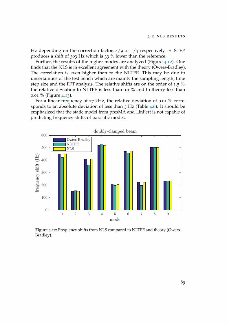
4 .2 nls results
Hz depending on the correction factor, 4/9 or 1/3 respectively. ELSTEPproduces a shift of 303 Hz which is 33 % lower than the reference.
Further, the results of the higher modes are analyzed (Figure 4.12). Onefinds that the NLS is in excellent agreement with the theory (Owers-Bradley).The correlation is even higher than to the NLTFE. This may be due touncertainties of the test bench which are mainly the sampling length, timestep size and the FFT analysis. The relative shifts are on the order of 1.5 %,the relative deviation to NLTFE is less than 0.1 % and to theory less than0.01 % (Figure 4.13).
For a linear frequency of 27 kHz, the relative deviation of 0.01 % corre-sponds to an absolute deviation of less than 3 Hz (Table 4.6). It should beemphasized that the static model from presMA and LinPert is not capable ofpredicting frequency shifts of parasitic modes.
mode1 2 3 4 5 6 7 8 9
freq
uen
cysh
ift
(Hz)
0
100
200
300
400
500
600doubly-clamped beam
Owers-BradleyNLTFENLS
Figure 4.12: Frequency shifts from NLS compared to NLTFE and theory (Owers-Bradley).
89
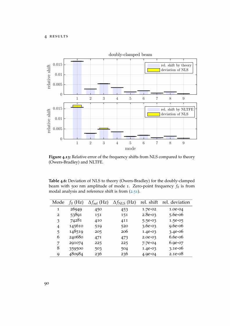
4 results
doubly-clamped beam
1 2 3 4 5 6 7 8 9
relativeshift
0
0.005
0.01
0.015 rel. shift by theory
deviation of NLS
mode1 2 3 4 5 6 7 8 9
relativeshift
0
0.005
0.01
0.015 rel. shift by NLTFE
deviation of NLS
Figure 4.13: Relative error of the frequency shifts from NLS compared to theory(Owers-Bradley) and NLTFE.
Table 4.6: Deviation of NLS to theory (Owers-Bradley) for the doubly-clampedbeam with 500 nm amplitude of mode 1. Zero-point frequency f0 is frommodal analysis and reference shift is from (2.51).
Mode f0 (Hz) ∆ fref (Hz) ∆ fNLS (Hz) rel. shift rel. deviation1 26949 450 453 1.7e-02 1.0e-04
2 53891 151 151 2.8e-03 5.6e-06
3 74281 410 411 5.5e-03 1.5e-05
4 145610 519 520 3.6e-03 9.6e-06
5 148519 205 206 1.4e-03 3.4e-06
6 240680 471 473 2.0e-03 6.6e-06
7 291074 225 225 7.7e-04 6.9e-07
8 359500 503 504 1.4e-03 3.1e-06
9 480984 236 236 4.9e-04 2.1e-08
90
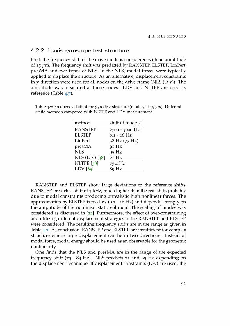
4 .2 nls results
4.2.2 1-axis gyroscope test structure
First, the frequency shift of the drive mode is considered with an amplitudeof 15 µm. The frequency shift was predicted by RANSTEP, ELSTEP, LinPert,presMA and two types of NLS. In the NLS, modal forces were typicallyapplied to displace the structure. As an alternative, displacement constraintsin y-direction were used for all nodes on the drive frame (NLS (D-y)). Theamplitude was measured at these nodes. LDV and NLTFE are used asreference (Table 4.7).
Table 4.7: Frequency shift of the gyro test structure (mode 3 at 15 µm). Differentstatic methods compared with NLTFE and LDV measurement.
method shift of mode 3
RANSTEP 2700 - 3000 HzELSTEP 0.1 - 16 HzLinPert 58 Hz (77 Hz)presMA 91 HzNLS 95 HzNLS (D-y) [38] 71 HzNLTFE [38] 75.4 HzLDV [65] 89 Hz
RANSTEP and ELSTEP show large deviations to the reference shifts.RANSTEP predicts a shift of 3 kHz, much higher than the real shift, probablydue to modal constraints producing unrealistic high nonlinear forces. Theapproximation by ELSTEP is too low (0.1 - 16 Hz) and depends strongly onthe amplitude of the nonlinear static solution. The scaling of modes wasconsidered as discussed in [22]. Furthermore, the effect of over-constrainingand utilizing different displacement strategies in the RANSTEP and ELSTEPwere considered. The resulting frequency shifts are in the range as given inTable 4.7. As conclusion, RANSTEP and ELSTEP are insufficient for complexstructure where large displacement can be in two directions. Instead ofmodal force, modal energy should be used as an observable for the geometricnonlinearity.
One finds that the NLS and presMA are in the range of the expectedfrequency shift (75 - 89 Hz). NLS predicts 71 and 95 Hz depending onthe displacement technique. If displacement constraints (D-y) are used, the
91
4 results
sensor can relax to lower potential energies as compared to modal force. Thisresults in a lower frequency shift.
The LinPert method achieves 77.3 Hz when using 4/9 correction of theDuffing coefficient [65]. This is well within NLTFE and LDV. A shift of 58
Hz is achieved when using 1/3 correction of the Duffing coefficient which islower than the transient FE simulation and the LDV measurement.
The NLTFE is slightly lower than the measurement.Next, the NLS is applied to higher modes of the test gyro using the
procedure as in Section 3.4.2. A tolerance of 10−4 was chosen for the drivemode amplitude. This tolerance corresponds to an amplitude error of lessthan 2 nm at 15 µm. The shift from NLS and NLTFE are compared for 11
parasitic modes (Figure 4.14). The frequency shift of mode 1 and 11 arepredicted with the wrong sign. In this specific case, mode 1 is not critical,whereas mode 11 is much more severe due to a much higher absolute shift(-40 Hz vs -1248 Hz). These deviations can be addressed to the modalcoupling with other higher modes. In the following discussion, mode 1
and 11 are excluded. For specific modes (2 3 6 13 20 25), there finds goodagreement between NLS and NLTFE. For other modes (4 12 32 34), the NLSand NLTFE deviate much stronger.
As result, the maximum deviation of predicted shifts is less than 1.5 % (incomparison to the NLTFE). In average the deviation is around 0.5 %. Themaximum deviation is found for mode 6 which is 1.5 % and 700 Hz in total(NLTFE: 4900 Hz and NLS: 5659 Hz).
All results are listed in Table 4.8.The accuracy of parasitic shifts can be improved when using displacements
from NLTFE in the NLS procedure. Therefore, a transient ramp-up of thedrive mode was performed and the full displacement vectors were extractedfor the minimum and maximum elongation. These displacements were thenused as boundary conditions in the static simulation. The improvement isdiscussed for mode 6. The shift over drive amplitude is given in Figure 4.15.
The NLS predicts a higher frequency shift as compared to the NLTFE andLDV. When using drive mode displacements from prior NLTFE, the shiftof mode 6 is improved and closer to the LDV measurement (Figure 4.15).However, the shift is slightly underestimated similar to the NLS (D-y) inTable 4.7. This is due to the type of constraining. In the static simulation, theFE nodes were only constraint in the y-direction, which results in a relaxationof the x-displacements and slight decrease in the frequency shift.
This hybrid approach is useful for modes that are local and parallel tothe drive mode. If the parasitic mode is orthogonal to the drive mode,
92
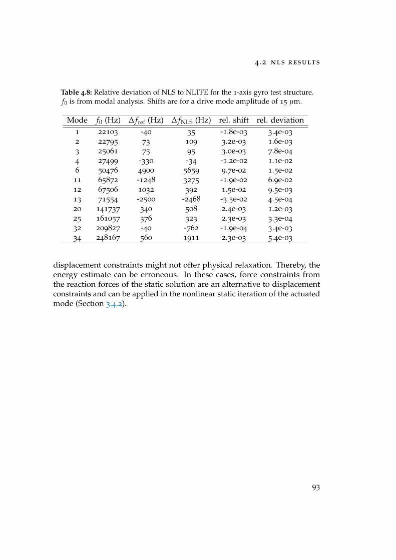
4 .2 nls results
Table 4.8: Relative deviation of NLS to NLTFE for the 1-axis gyro test structure.f0 is from modal analysis. Shifts are for a drive mode amplitude of 15 µm.
Mode f0 (Hz) ∆ fref (Hz) ∆ fNLS (Hz) rel. shift rel. deviation1 22103 -40 35 -1.8e-03 3.4e-03
2 22795 73 109 3.2e-03 1.6e-03
3 25061 75 95 3.0e-03 7.8e-04
4 27499 -330 -34 -1.2e-02 1.1e-02
6 50476 4900 5659 9.7e-02 1.5e-02
11 65872 -1248 3275 -1.9e-02 6.9e-02
12 67506 1032 392 1.5e-02 9.5e-03
13 71554 -2500 -2468 -3.5e-02 4.5e-04
20 141737 340 508 2.4e-03 1.2e-03
25 161057 376 323 2.3e-03 3.3e-04
32 209827 -40 -762 -1.9e-04 3.4e-03
34 248167 560 1911 2.3e-03 5.4e-03
displacement constraints might not offer physical relaxation. Thereby, theenergy estimate can be erroneous. In these cases, force constraints fromthe reaction forces of the static solution are an alternative to displacementconstraints and can be applied in the nonlinear static iteration of the actuatedmode (Section 3.4.2).
93
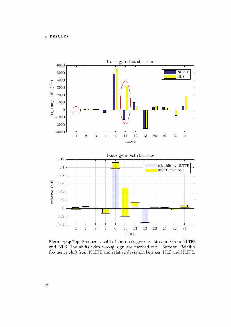
4 results
mode1 2 3 4 6 11 12 13 20 25 32 34
frequency
shift(Hz)
-3000
-2000
-1000
0
1000
2000
3000
4000
5000
60001-axis gyro test structure
NLTFE
NLS
1-axis gyro test structure
mode1 2 3 4 6 11 12 13 20 25 32 34
relativeshift
-0.04
-0.02
0
0.02
0.04
0.06
0.08
0.1
0.12
rel. shift by NLTFE
deviation of NLS
Figure 4.14: Top: Frequency shift of the 1-axis gyro test structure from NLTFEand NLS. The shifts with wrong sign are marked red. Bottom: Relativefrequency shift from NLTFE and relative deviation between NLS and NLTFE.
94
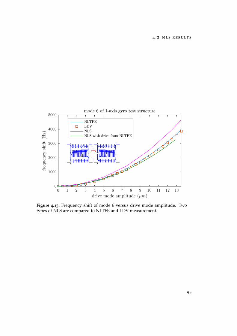
4 .2 nls results
Figure 4.15: Frequency shift of mode 6 versus drive mode amplitude. Twotypes of NLS are compared to NLTFE and LDV measurement.
95
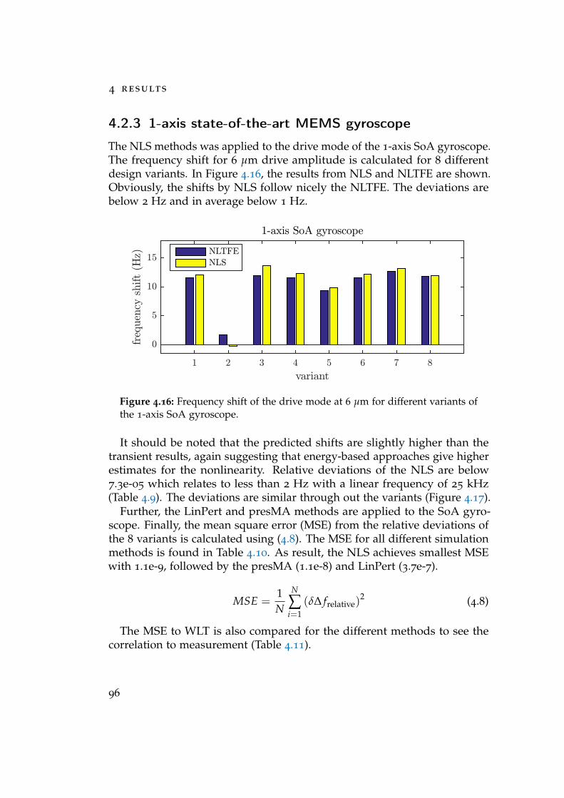
4 results
4.2.3 1-axis state-of-the-art MEMS gyroscope
The NLS methods was applied to the drive mode of the 1-axis SoA gyroscope.The frequency shift for 6 µm drive amplitude is calculated for 8 differentdesign variants. In Figure 4.16, the results from NLS and NLTFE are shown.Obviously, the shifts by NLS follow nicely the NLTFE. The deviations arebelow 2 Hz and in average below 1 Hz.
variant1 2 3 4 5 6 7 8
frequencyshift(Hz)
0
5
10
15
1-axis SoA gyroscope
NLTFE
NLS
Figure 4.16: Frequency shift of the drive mode at 6 µm for different variants ofthe 1-axis SoA gyroscope.
It should be noted that the predicted shifts are slightly higher than thetransient results, again suggesting that energy-based approaches give higherestimates for the nonlinearity. Relative deviations of the NLS are below7.3e-05 which relates to less than 2 Hz with a linear frequency of 25 kHz(Table 4.9). The deviations are similar through out the variants (Figure 4.17).
Further, the LinPert and presMA methods are applied to the SoA gyro-scope. Finally, the mean square error (MSE) from the relative deviations ofthe 8 variants is calculated using (4.8). The MSE for all different simulationmethods is found in Table 4.10. As result, the NLS achieves smallest MSEwith 1.1e-9, followed by the presMA (1.1e-8) and LinPert (3.7e-7).
MSE =1N
N
∑i=1
(δ∆ frelative)2 (4.8)
The MSE to WLT is also compared for the different methods to see thecorrelation to measurement (Table 4.11).
96
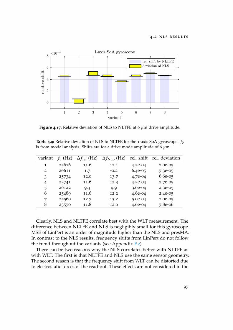
4 .2 nls results
1-axis SoA gyroscope
variant1 2 3 4 5 6 7 8
relativeshift
#10!4
0
2
4
6
8
rel. shift by NLTFE
deviation of NLS
Figure 4.17: Relative deviation of NLS to NLTFE at 6 µm drive amplitude.
Table 4.9: Relative deviation of NLS to NLTFE for the 1-axis SoA gyroscope. f0is from modal analysis. Shifts are for a drive mode amplitude of 6 µm.
variant f0 (Hz) ∆ fref (Hz) ∆ fNLS (Hz) rel. shift rel. deviation1 25616 11.6 12.1 4.5e-04 2.0e-05
2 26611 1.7 -0.2 6.4e-05 7.3e-05
3 25734 12.0 13.7 4.7e-04 6.6e-05
4 25741 11.6 12.3 4.5e-04 2.7e-05
5 26122 9.3 9.9 3.6e-04 2.3e-05
6 25489 11.6 12.2 4.6e-04 2.4e-05
7 25560 12.7 13.2 5.0e-04 2.0e-05
8 25570 11.8 12.0 4.6e-04 7.8e-06
Clearly, NLS and NLTFE correlate best with the WLT measurement. Thedifference between NLTFE and NLS is negligibly small for this gyroscope.MSE of LinPert is an order of magnitude higher than the NLS and presMA.In contrast to the NLS results, frequency shifts from LinPert do not followthe trend throughout the variants (see Appendix F.2).
There can be two reasons why the NLS correlates better with NLTFE aswith WLT. The first is that NLTFE and NLS use the same sensor geometry.The second reason is that the frequency shift from WLT can be distorted dueto electrostatic forces of the read-out. These effects are not considered in the
97
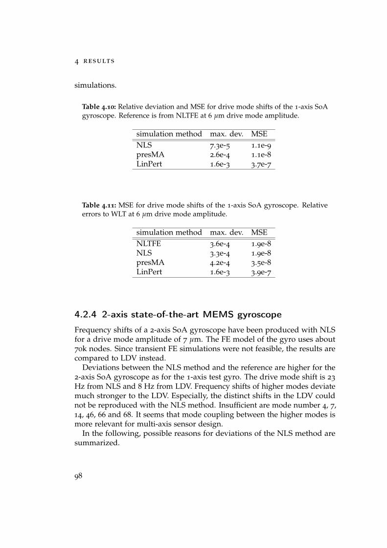
4 results
simulations.
Table 4.10: Relative deviation and MSE for drive mode shifts of the 1-axis SoAgyroscope. Reference is from NLTFE at 6 µm drive mode amplitude.
simulation method max. dev. MSENLS 7.3e-5 1.1e-9presMA 2.6e-4 1.1e-8LinPert 1.6e-3 3.7e-7
Table 4.11: MSE for drive mode shifts of the 1-axis SoA gyroscope. Relativeerrors to WLT at 6 µm drive mode amplitude.
simulation method max. dev. MSENLTFE 3.6e-4 1.9e-8NLS 3.3e-4 1.9e-8presMA 4.2e-4 3.5e-8LinPert 1.6e-3 3.9e-7
4.2.4 2-axis state-of-the-art MEMS gyroscope
Frequency shifts of a 2-axis SoA gyroscope have been produced with NLSfor a drive mode amplitude of 7 µm. The FE model of the gyro uses about70k nodes. Since transient FE simulations were not feasible, the results arecompared to LDV instead.
Deviations between the NLS method and the reference are higher for the2-axis SoA gyroscope as for the 1-axis test gyro. The drive mode shift is 23
Hz from NLS and 8 Hz from LDV. Frequency shifts of higher modes deviatemuch stronger to the LDV. Especially, the distinct shifts in the LDV couldnot be reproduced with the NLS method. Insufficient are mode number 4, 7,14, 46, 66 and 68. It seems that mode coupling between the higher modes ismore relevant for multi-axis sensor design.
In the following, possible reasons for deviations of the NLS method aresummarized.
98
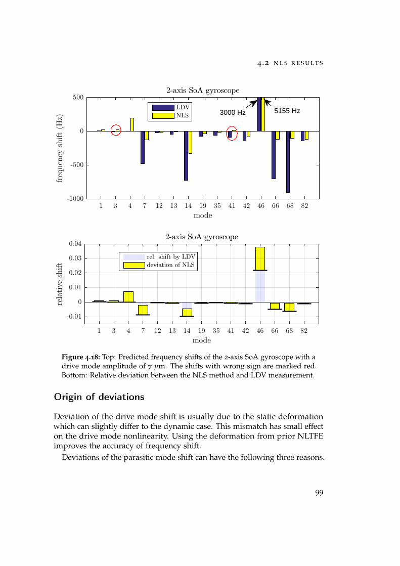
4 .2 nls results
mode1 3 4 7 12 13 14 19 35 41 42 46 66 68 82
frequency
shift(H
z)
-1000
-500
0
5002-axis SoA gyroscope
LDV
NLS 3000 Hz 5155 Hz
2-axis SoA gyroscope
mode1 3 4 7 12 13 14 19 35 41 42 46 66 68 82
rela
tive
shif
t
-0.01
0
0.01
0.02
0.03
0.04
rel. shift by LDV
deviation of NLS
Figure 4.18: Top: Predicted frequency shifts of the 2-axis SoA gyroscope with adrive mode amplitude of 7 µm. The shifts with wrong sign are marked red.Bottom: Relative deviation between the NLS method and LDV measurement.
Origin of deviations
Deviation of the drive mode shift is usually due to the static deformationwhich can slightly differ to the dynamic case. This mismatch has small effecton the drive mode nonlinearity. Using the deformation from prior NLTFEimproves the accuracy of frequency shift.
Deviations of the parasitic mode shift can have the following three reasons.
99
4 results
First, the quasi-static assumption is not fulfilled, the resonance can not becaptured by a 2-mode interaction. Hence, the NLS is only correct in caseswhen the actuated and parasitic mode couple directly. This is when eitherβ00ii or α00i is main contributor to the nonlinearity. Index 0 denotes theactuated mode, e.g. drive mode. The wrong frequency shift of mode 1 and11 of the test gyro can be addressed to the indirect coupling with the drivemode. Second, the actuated mode deformation can deviate to the dynamiccase. This deviation can be overcome by appropriate deformations fromNLTFE simulation. Third, certain combinations of modes can not be properlyconstrained, e.g. two modes that are delocalized and orthogonal. Usually,the model can be constrained properly if one mode is local and the othermode is delocalized over the structure.
100
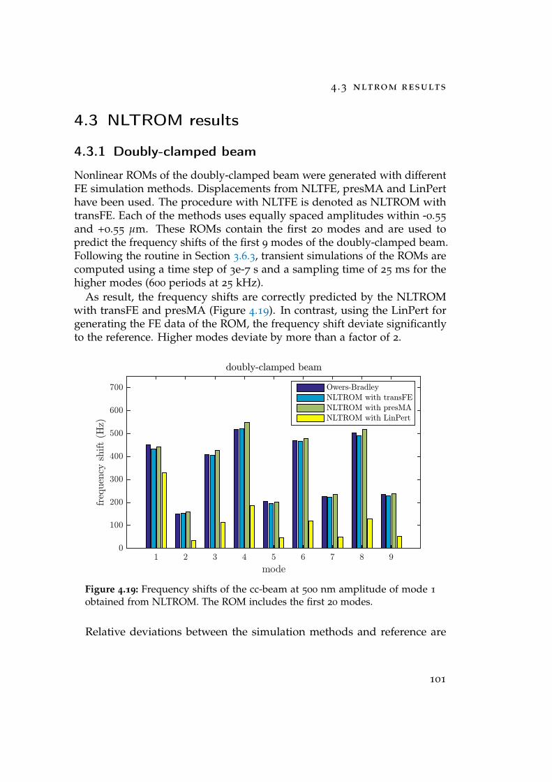
4 .3 nltrom results
4.3 NLTROM results
4.3.1 Doubly-clamped beam
Nonlinear ROMs of the doubly-clamped beam were generated with differentFE simulation methods. Displacements from NLTFE, presMA and LinPerthave been used. The procedure with NLTFE is denoted as NLTROM withtransFE. Each of the methods uses equally spaced amplitudes within -0.55
and +0.55 µm. These ROMs contain the first 20 modes and are used topredict the frequency shifts of the first 9 modes of the doubly-clamped beam.Following the routine in Section 3.6.3, transient simulations of the ROMs arecomputed using a time step of 3e-7 s and a sampling time of 25 ms for thehigher modes (600 periods at 25 kHz).
As result, the frequency shifts are correctly predicted by the NLTROMwith transFE and presMA (Figure 4.19). In contrast, using the LinPert forgenerating the FE data of the ROM, the frequency shift deviate significantlyto the reference. Higher modes deviate by more than a factor of 2.
mode1 2 3 4 5 6 7 8 9
freq
uen
cysh
ift
(Hz)
0
100
200
300
400
500
600
700
doubly-clamped beam
Owers-Bradley
NLTROM with transFE
NLTROM with presMA
NLTROM with LinPert
Figure 4.19: Frequency shifts of the cc-beam at 500 nm amplitude of mode 1
obtained from NLTROM. The ROM includes the first 20 modes.
Relative deviations between the simulation methods and reference are
101
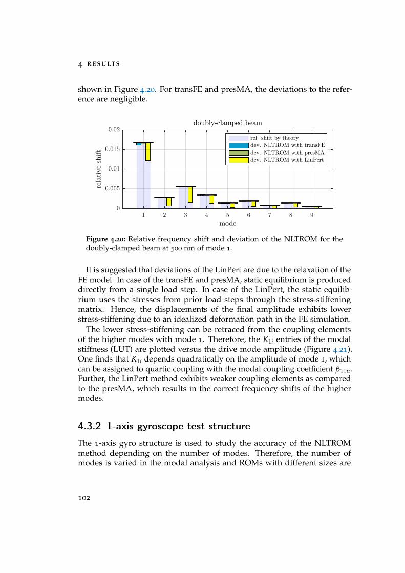
4 results
shown in Figure 4.20. For transFE and presMA, the deviations to the refer-ence are negligible.
doubly-clamped beam
mode1 2 3 4 5 6 7 8 9
relativeshift
0
0.005
0.01
0.015
0.02
rel. shift by theory
dev. NLTROM with transFE
dev. NLTROM with presMA
dev. NLTROM with LinPert
Figure 4.20: Relative frequency shift and deviation of the NLTROM for thedoubly-clamped beam at 500 nm of mode 1.
It is suggested that deviations of the LinPert are due to the relaxation of theFE model. In case of the transFE and presMA, static equilibrium is produceddirectly from a single load step. In case of the LinPert, the static equilib-rium uses the stresses from prior load steps through the stress-stiffeningmatrix. Hence, the displacements of the final amplitude exhibits lowerstress-stiffening due to an idealized deformation path in the FE simulation.
The lower stress-stiffening can be retraced from the coupling elementsof the higher modes with mode 1. Therefore, the K1i entries of the modalstiffness (LUT) are plotted versus the drive mode amplitude (Figure 4.21).One finds that K1i depends quadratically on the amplitude of mode 1, whichcan be assigned to quartic coupling with the modal coupling coefficient β11ii.Further, the LinPert method exhibits weaker coupling elements as comparedto the presMA, which results in the correct frequency shifts of the highermodes.
4.3.2 1-axis gyroscope test structure
The 1-axis gyro structure is used to study the accuracy of the NLTROMmethod depending on the number of modes. Therefore, the number ofmodes is varied in the modal analysis and ROMs with different sizes are
102
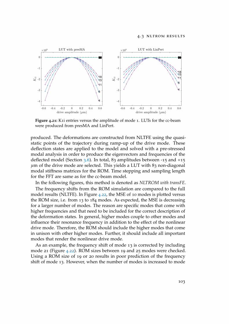
4 .3 nltrom results
Figure 4.21: K1i entries versus the amplitude of mode 1. LUTs for the cc-beamwere produced from presMA and LinPert.
produced. The deformations are constructed from NLTFE using the quasi-static points of the trajectory during ramp-up of the drive mode. Thesedeflection states are applied to the model and solved with a pre-stressedmodal analysis in order to produce the eigenvectors and frequencies of thedeflected model (Section 3.6). In total, 83 amplitudes between -15 and +15
µm of the drive mode are selected. This yields a LUT with 83 non-diagonalmodal stiffness matrices for the ROM. Time stepping and sampling lengthfor the FFT are same as for the cc-beam model.
In the following figures, this method is denoted as NLTROM with transFE.The frequency shifts from the ROM simulation are compared to the full
model results (NLTFE). In Figure 4.22, the MSE of 10 modes is plotted versusthe ROM size, i.e. from 13 to 184 modes. As expected, the MSE is decreasingfor a larger number of modes. The reason are specific modes that come withhigher frequencies and that need to be included for the correct description ofthe deformation states. In general, higher modes couple to other modes andinfluence their resonance frequency in addition to the effect of the nonlineardrive mode. Therefore, the ROM should include the higher modes that comein unison with other higher modes. Further, it should include all importantmodes that render the nonlinear drive mode.
As an example, the frequency shift of mode 13 is corrected by includingmode 21 (Figure 4.22). ROM sizes between 19 and 25 modes were checked.Using a ROM size of 19 or 20 results in poor prediction of the frequencyshift of mode 13. However, when the number of modes is increased to mode
103
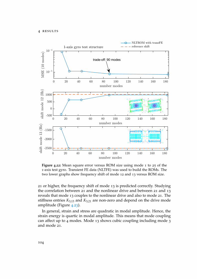
4 results
Figure 4.22: Mean square error versus ROM size using mode 1 to 25 of the1-axis test gyro. Transient FE data (NLTFE) was used to build the ROMs. Thetwo lower graphs show frequency shift of mode 12 and 13 versus ROM size.
21 or higher, the frequency shift of mode 13 is predicted correctly. Studyingthe correlation between 21 and the nonlinear drive and between 21 and 13
reveals that mode 13 couples to the nonlinear drive and also to mode 21. Thestiffness entries K3,13 and K3,21 are non-zero and depend on the drive modeamplitude (Figure 4.23).
In general, strain and stress are quadratic in modal amplitude. Hence, thestrain energy is quartic in modal amplitude. This means that mode couplingcan affect up to 4 modes. Mode 13 shows cubic coupling including mode 3
and mode 21.
104
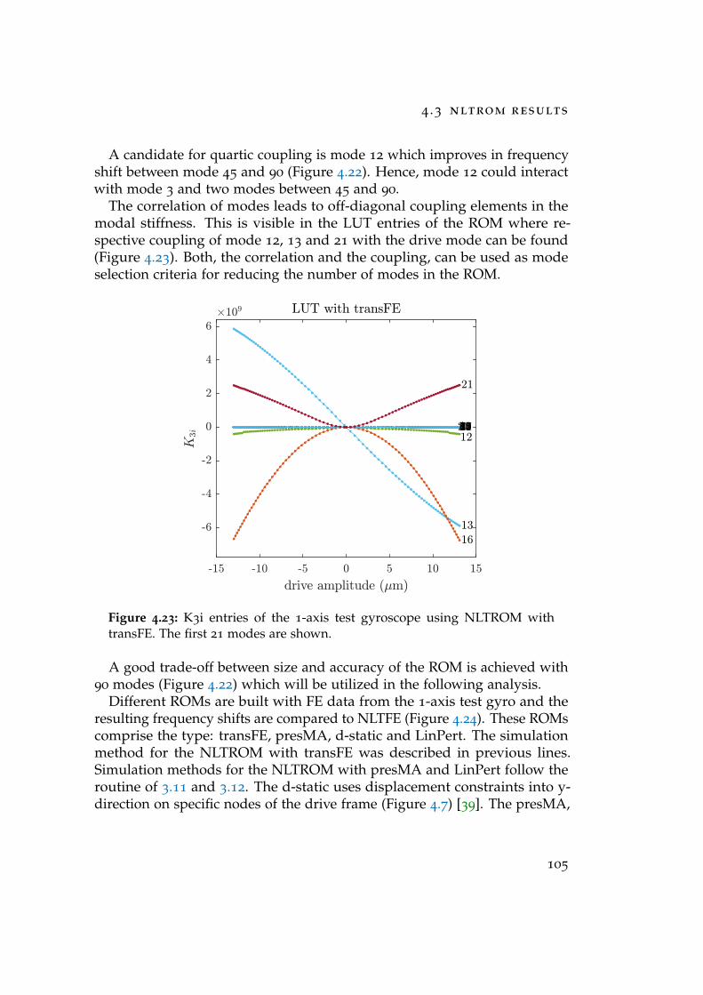
4 .3 nltrom results
A candidate for quartic coupling is mode 12 which improves in frequencyshift between mode 45 and 90 (Figure 4.22). Hence, mode 12 could interactwith mode 3 and two modes between 45 and 90.
The correlation of modes leads to off-diagonal coupling elements in themodal stiffness. This is visible in the LUT entries of the ROM where re-spective coupling of mode 12, 13 and 21 with the drive mode can be found(Figure 4.23). Both, the correlation and the coupling, can be used as modeselection criteria for reducing the number of modes in the ROM.
-15 -10 -5 0 5 10 15
drive amplitude (7m)
-6
-4
-2
0
2
4
6
K3i
#109 LUT with transFE
12456789101112
13
1415
16
17181920
21
Figure 4.23: K3i entries of the 1-axis test gyroscope using NLTROM withtransFE. The first 21 modes are shown.
A good trade-off between size and accuracy of the ROM is achieved with90 modes (Figure 4.22) which will be utilized in the following analysis.
Different ROMs are built with FE data from the 1-axis test gyro and theresulting frequency shifts are compared to NLTFE (Figure 4.24). These ROMscomprise the type: transFE, presMA, d-static and LinPert. The simulationmethod for the NLTROM with transFE was described in previous lines.Simulation methods for the NLTROM with presMA and LinPert follow theroutine of 3.11 and 3.12. The d-static uses displacement constraints into y-direction on specific nodes of the drive frame (Figure 4.7) [39]. The presMA,
105
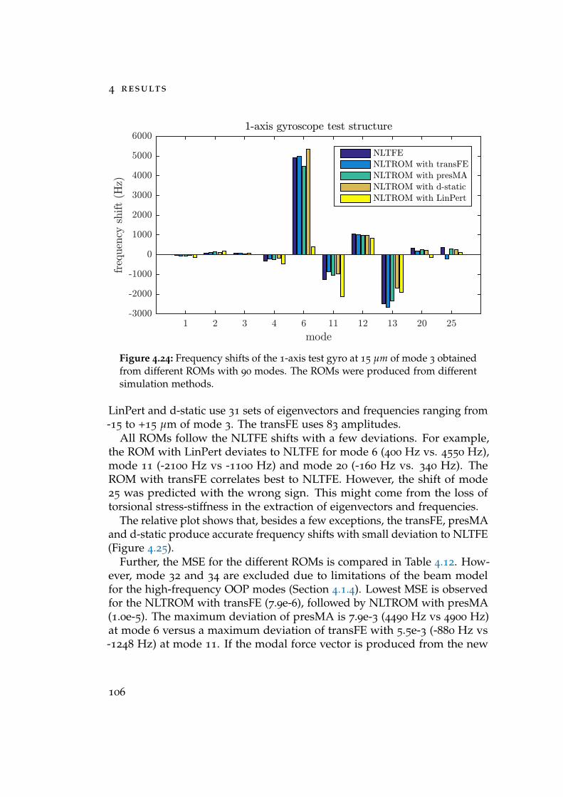
4 results
mode1 2 3 4 6 11 12 13 20 25
frequencyshift(Hz)
-3000
-2000
-1000
0
1000
2000
3000
4000
5000
60001-axis gyroscope test structure
NLTFE
NLTROM with transFE
NLTROM with presMA
NLTROM with d-static
NLTROM with LinPert
Figure 4.24: Frequency shifts of the 1-axis test gyro at 15 µm of mode 3 obtainedfrom different ROMs with 90 modes. The ROMs were produced from differentsimulation methods.
LinPert and d-static use 31 sets of eigenvectors and frequencies ranging from-15 to +15 µm of mode 3. The transFE uses 83 amplitudes.
All ROMs follow the NLTFE shifts with a few deviations. For example,the ROM with LinPert deviates to NLTFE for mode 6 (400 Hz vs. 4550 Hz),mode 11 (-2100 Hz vs -1100 Hz) and mode 20 (-160 Hz vs. 340 Hz). TheROM with transFE correlates best to NLTFE. However, the shift of mode25 was predicted with the wrong sign. This might come from the loss oftorsional stress-stiffness in the extraction of eigenvectors and frequencies.
The relative plot shows that, besides a few exceptions, the transFE, presMAand d-static produce accurate frequency shifts with small deviation to NLTFE(Figure 4.25).
Further, the MSE for the different ROMs is compared in Table 4.12. How-ever, mode 32 and 34 are excluded due to limitations of the beam modelfor the high-frequency OOP modes (Section 4.1.4). Lowest MSE is observedfor the NLTROM with transFE (7.9e-6), followed by NLTROM with presMA(1.0e-5). The maximum deviation of presMA is 7.9e-3 (4490 Hz vs 4900 Hz)at mode 6 versus a maximum deviation of transFE with 5.5e-3 (-880 Hz vs-1248 Hz) at mode 11. If the modal force vector is produced from the new
106
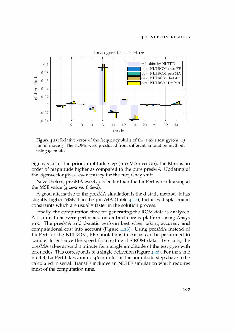
4 .3 nltrom results
1-axis gyro test structure
mode1 2 3 4 6 11 12 13 20 25 32 34
relativeshift
-0.04
-0.02
0
0.02
0.04
0.06
0.08
0.1 rel. shift by NLTFE
dev. NLTROM transFE
dev. NLTROM presMA
dev. NLTROM d-static
dev. NLTROM LinPert
Figure 4.25: Relative error of the frequency shifts of the 1-axis test gyro at 15
µm of mode 3. The ROMs were produced from different simulation methodsusing 90 modes.
eigenvector of the prior amplitude step (presMA-evecUp), the MSE is anorder of magnitude higher as compared to the pure presMA. Updating ofthe eigenvector gives less accuracy for the frequency shift.
Nevertheless, presMA-evecUp is better than the LinPert when looking atthe MSE value (4.2e-2 vs. 8.6e-2).
A good alternative to the presMA simulation is the d-static method. It hasslightly higher MSE than the presMA (Table 4.12), but uses displacementconstraints which are usually faster in the solution process.
Finally, the computation time for generating the ROM data is analyzed.All simulations were performed on an Intel core i7 platform using Ansysv15. The presMA and d-static perform best when taking accuracy andcomputational cost into account (Figure 4.26). Using presMA instead ofLinPert for the NLTROM, FE simulations in Ansys can be performed inparallel to enhance the speed for creating the ROM data. Typically, thepresMA takes around 1 minute for a single amplitude of the test gyro with20k nodes. This corresponds to a single deflection (Figure 4.26). For the samemodel, LinPert takes around 46 minutes as the amplitude steps have to becalculated in serial. TransFE includes an NLTFE simulation which requiresmost of the computation time.
107
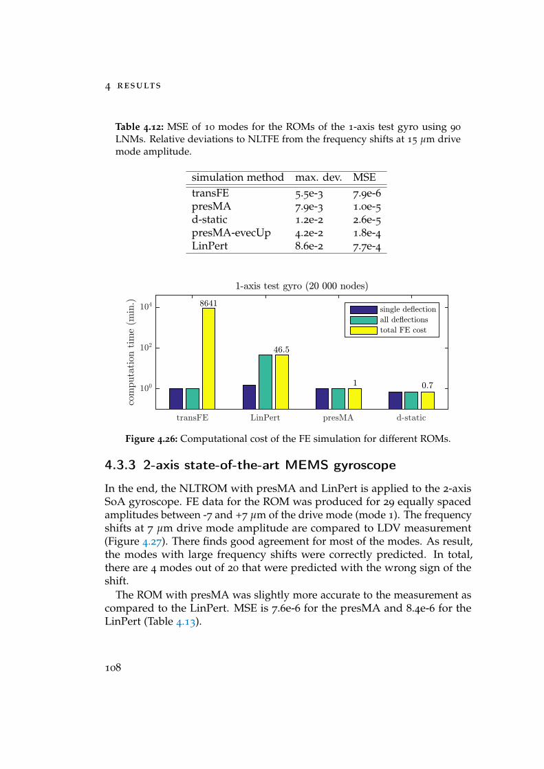
4 results
Table 4.12: MSE of 10 modes for the ROMs of the 1-axis test gyro using 90
LNMs. Relative deviations to NLTFE from the frequency shifts at 15 µm drivemode amplitude.
simulation method max. dev. MSEtransFE 5.5e-3 7.9e-6presMA 7.9e-3 1.0e-5d-static 1.2e-2 2.6e-5presMA-evecUp 4.2e-2 1.8e-4LinPert 8.6e-2 7.7e-4
transFE LinPert presMA d-static
computation
time(m
in.)
100
102
104 8641
46.5
1 0.7
1-axis test gyro (20 000 nodes)
single de.ection
all de.ections
total FE cost
Figure 4.26: Computational cost of the FE simulation for different ROMs.
4.3.3 2-axis state-of-the-art MEMS gyroscope
In the end, the NLTROM with presMA and LinPert is applied to the 2-axisSoA gyroscope. FE data for the ROM was produced for 29 equally spacedamplitudes between -7 and +7 µm of the drive mode (mode 1). The frequencyshifts at 7 µm drive mode amplitude are compared to LDV measurement(Figure 4.27). There finds good agreement for most of the modes. As result,the modes with large frequency shifts were correctly predicted. In total,there are 4 modes out of 20 that were predicted with the wrong sign of theshift.
The ROM with presMA was slightly more accurate to the measurement ascompared to the LinPert. MSE is 7.6e-6 for the presMA and 8.4e-6 for theLinPert (Table 4.13).
108
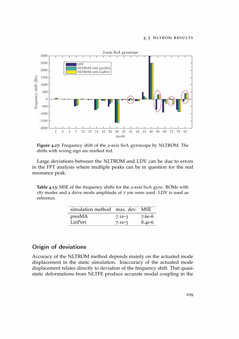
4 .3 nltrom results
mode1 3 4 7 12 13 14 19 23 26 35 41 42 43 46 66 68 73 79 82
frequency
shift(H
z)
-2000
-1500
-1000
-500
0
500
1000
1500
2000
2500
30002-axis SoA gyroscope
LDVNLTROM with presMANLTROM with LinPert
Figure 4.27: Frequency shift of the 2-axis SoA gyroscope by NLTROM. Theshifts with wrong sign are marked red.
Large deviations between the NLTROM and LDV can be due to errorsin the FFT analysis where multiple peaks can be in question for the realresonance peak.
Table 4.13: MSE of the frequency shifts for the 2-axis SoA gyro. ROMs with187 modes and a drive mode amplitude of 7 µm were used. LDV is used asreference.
simulation method max. dev. MSEpresMA 7.1e-3 7.6e-6LinPert 7.1e-3 8.4e-6
Origin of deviations
Accuracy of the NLTROM method depends mainly on the actuated modedisplacement in the static simulation. Inaccuracy of the actuated modedisplacement relates directly to deviation of the frequency shift. That quasi-static deformations from NLTFE produce accurate modal coupling in the
109
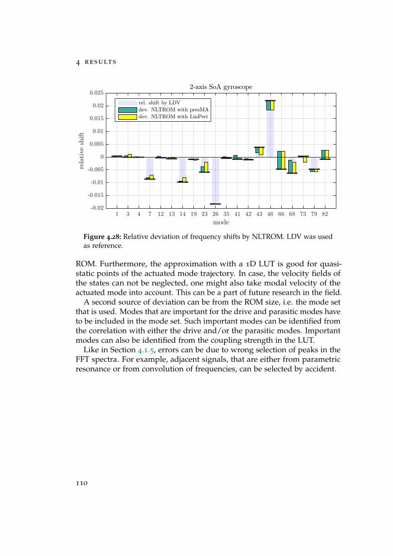
4 results
2-axis SoA gyroscope
mode1 3 4 7 12 13 14 19 23 26 35 41 42 43 46 66 68 73 79 82
rela
tive
shif
t
-0.02
-0.015
-0.01
-0.005
0
0.005
0.01
0.015
0.02
0.025
rel. shift by LDV
dev. NLTROM with presMA
dev. NLTROM with LinPert
Figure 4.28: Relative deviation of frequency shifts by NLTROM. LDV was usedas reference.
ROM. Furthermore, the approximation with a 1D LUT is good for quasi-static points of the actuated mode trajectory. In case, the velocity fields ofthe states can not be neglected, one might also take modal velocity of theactuated mode into account. This can be a part of future research in the field.
A second source of deviation can be from the ROM size, i.e. the mode setthat is used. Modes that are important for the drive and parasitic modes haveto be included in the mode set. Such important modes can be identified fromthe correlation with either the drive and/or the parasitic modes. Importantmodes can also be identified from the coupling strength in the LUT.
Like in Section 4.1.5, errors can be due to wrong selection of peaks in theFFT spectra. For example, adjacent signals, that are either from parametricresonance or from convolution of frequencies, can be selected by accident.
110
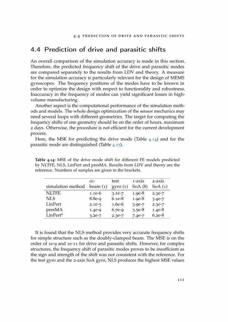
4 .4 prediction of drive and parasitic shifts
4.4 Prediction of drive and parasitic shifts
An overall comparison of the simulation accuracy is made in this section.Therefore, the predicted frequency shift of the drive and parasitic modesare compared separately to the results from LDV and theory. A measurefor the simulation accuracy is particularly relevant for the design of MEMSgyroscopes. The frequency positions of the modes have to be known inorder to optimize the design with respect to functionality and robustness.Inaccuracy in the frequency of modes can yield significant losses in high-volume manufacturing.
Another aspect is the computational performance of the simulation meth-ods and models. The whole design optimization of the sensor mechanics mayneed several loops with different geometries. The target for computing thefrequency shifts of one geometry should be on the order of hours, maximum2 days. Otherwise, the procedure is not efficient for the current developmentprocess.
Here, the MSE for predicting the drive mode (Table 4.14) and for theparasitic mode are distinguished (Table 4.15).
Table 4.14: MSE of the drive mode shift for different FE models predictedby NLTFE, NLS, LinPert and presMA. Results from LDV and theory are thereference. Numbers of samples are given in the brackets.
cc- test 1-axis 2-axissimulation method beam (1) gyro (1) SoA (8) SoA (1)NLTFE 1.1e-6 3.1e-7 1.9e-8 2.3e-7NLS 8.8e-9 6.1e-8 1.9e-8 3.4e-7LinPert 2.1e-5 1.6e-6 3.9e-7 2.3e-7presMA 1.4e-9 6.7e-9 3.5e-8 1.4e-8LinPert* 3.2e-7 2.3e-7 7.4e-7 6.2e-8
It is found that the NLS method provides very accurate frequency shiftsfor simple structure such as the doubly-clamped beam. The MSE is on theorder of 1e-9 and 1e-11 for drive and parasitic shifts. However, for complexstructures, the frequency shift of parasitic modes proves to be insufficient asthe sign and strength of the shift was not consistent with the reference. Forthe test gyro and the 2-axis SoA gyro, NLS produces the highest MSE values
111
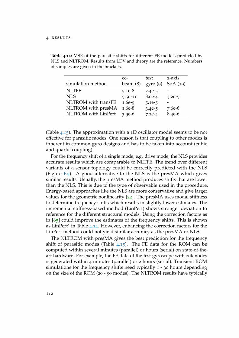
4 results
Table 4.15: MSE of the parasitic shifts for different FE-models predicted byNLS and NLTROM. Results from LDV and theory are the reference. Numbersof samples are given in the brackets.
cc- test 2-axissimulation method beam (8) gyro (9) SoA (19)NLTFE 5.1e-8 2.4e-5 -NLS 5.5e-11 8.0e-4 3.2e-5NLTROM with transFE 1.6e-9 5.1e-5 -NLTROM with presMA 1.6e-8 3.4e-5 7.6e-6NLTROM with LinPert 3.9e-6 7.2e-4 8.4e-6
(Table 4.15). The approximation with a 1D oscillator model seems to be noteffective for parasitic modes. One reason is that coupling to other modes isinherent in common gyro designs and has to be taken into account (cubicand quartic coupling).
For the frequency shift of a single mode, e.g. drive mode, the NLS providesaccurate results which are comparable to NLTFE. The trend over differentvariants of a sensor topology could be correctly predicted with the NLS(Figure F.5). A good alternative to the NLS is the presMA which givessimilar results. Usually, the presMA method produces shifts that are lowerthan the NLS. This is due to the type of observable used in the procedure.Energy-based approaches like the NLS are more conservative and give largervalues for the geometric nonlinearity [22]. The presMA uses modal stiffnessto determine frequency shifts which results in slightly lower estimates. Theincremental stiffness-based method (LinPert) shows stronger deviation toreference for the different structural models. Using the correction factors asin [65] could improve the estimates of the frequency shifts. This is shownas LinPert* in Table 4.14. However, enhancing the correction factors for theLinPert method could not yield similar accuracy as the presMA or NLS.
The NLTROM with presMA gives the best prediction for the frequencyshift of parasitic modes (Table 4.15). The FE data for the ROM can becomputed within several minutes (parallel) or hours (serial) on state-of-the-art hardware. For example, the FE data of the test gyroscope with 20k nodesis generated within 4 minutes (parallel) or 2 hours (serial). Transient ROMsimulations for the frequency shifts need typically 1 - 30 hours dependingon the size of the ROM (20 - 90 modes). The NLTROM results have typically
112
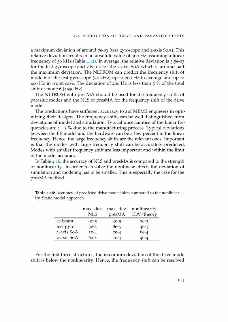
4 .4 prediction of drive and parasitic shifts
a maximum deviation of around 7e-03 (test gyroscope and 2-axis SoA). Thisrelative deviation results in an absolute value of 400 Hz assuming a linearfrequency of 50 kHz (Table 4.12). In average, the relative deviation is 3.5e-03
for the test gyroscope and 2.8e-03 for the 2-axis SoA which is around halfthe maximum deviation. The NLTROM can predict the frequency shift ofmode 6 of the test gyroscope (52 kHz) up to 200 Hz in average and up to400 Hz in worst case. The deviation of 200 Hz is less than 5 % of the totalshift of mode 6 (4550 Hz).
The NLTROM with presMA should be used for the frequency shifts ofparasitic modes and the NLS or presMA for the frequency shift of the drivemode.
The predictions have sufficient accuracy to aid MEMS engineers in opti-mizing their designs. The frequency shifts can be well distinguished fromdeviations of model and simulation. Typical uncertainties of the linear fre-quencies are 1 - 2 % due to the manufacturing process. Typical deviationsbetween the FE model and the hardware can be a few percent in the linearfrequency. Hence, the large frequency shifts are the relevant ones. Importantis that the modes with large frequency shift can be accurately predicted.Modes with smaller frequency shift are less important and within the limitof the model accuracy.
In Table 4.16, the accuracy of NLS and presMA is compared to the strengthof nonlinearity. In order to resolve the nonlinear effect, the deviation ofsimulation and modeling has to be smaller. This is especially the case for thepresMA method.
Table 4.16: Accuracy of predicted drive mode shifts compared to the nonlinear-ity. Static model approach.
max. dev. max. dev. nonlinearityNLS presMA LDV/theory
cc-beam 9e-5 4e-5 2e-3test gyro 3e-4 8e-5 4e-31-axis SoA 1e-4 2e-4 6e-42-axis SoA 6e-4 1e-4 4e-4
For the first three structures, the maximum deviation of the drive modeshift is below the nonlinearity. Hence, the frequency shift can be resolved
113
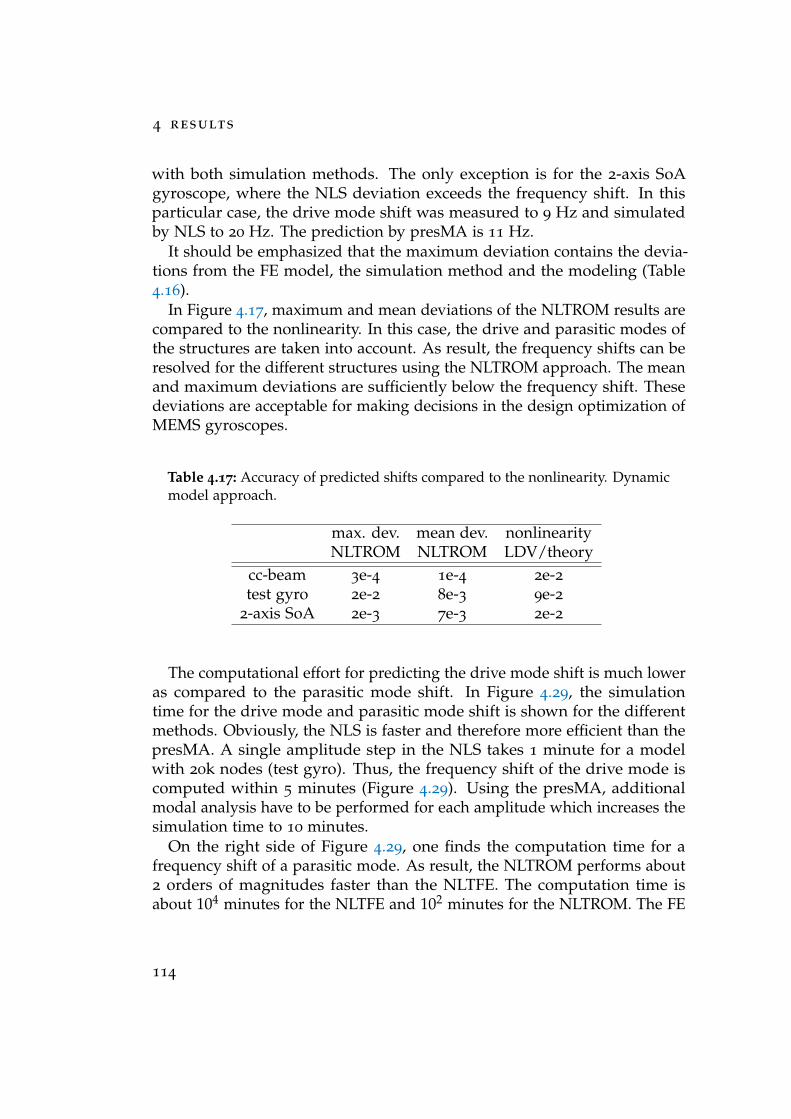
4 results
with both simulation methods. The only exception is for the 2-axis SoAgyroscope, where the NLS deviation exceeds the frequency shift. In thisparticular case, the drive mode shift was measured to 9 Hz and simulatedby NLS to 20 Hz. The prediction by presMA is 11 Hz.
It should be emphasized that the maximum deviation contains the devia-tions from the FE model, the simulation method and the modeling (Table4.16).
In Figure 4.17, maximum and mean deviations of the NLTROM results arecompared to the nonlinearity. In this case, the drive and parasitic modes ofthe structures are taken into account. As result, the frequency shifts can beresolved for the different structures using the NLTROM approach. The meanand maximum deviations are sufficiently below the frequency shift. Thesedeviations are acceptable for making decisions in the design optimization ofMEMS gyroscopes.
Table 4.17: Accuracy of predicted shifts compared to the nonlinearity. Dynamicmodel approach.
max. dev. mean dev. nonlinearityNLTROM NLTROM LDV/theory
cc-beam 3e-4 1e-4 2e-2test gyro 2e-2 8e-3 9e-2
2-axis SoA 2e-3 7e-3 2e-2
The computational effort for predicting the drive mode shift is much loweras compared to the parasitic mode shift. In Figure 4.29, the simulationtime for the drive mode and parasitic mode shift is shown for the differentmethods. Obviously, the NLS is faster and therefore more efficient than thepresMA. A single amplitude step in the NLS takes 1 minute for a modelwith 20k nodes (test gyro). Thus, the frequency shift of the drive mode iscomputed within 5 minutes (Figure 4.29). Using the presMA, additionalmodal analysis have to be performed for each amplitude which increases thesimulation time to 10 minutes.
On the right side of Figure 4.29, one finds the computation time for afrequency shift of a parasitic mode. As result, the NLTROM performs about2 orders of magnitudes faster than the NLTFE. The computation time isabout 104 minutes for the NLTFE and 102 minutes for the NLTROM. The FE
114
4 .4 prediction of drive and parasitic shifts
analysis of the NLTROM takes around 30 minutes and is almost independenton the ROM size (Figure 4.29). Main contributor to the computation cost isthe transient ROM simulation which takes 117, 30 or 5 minutes using 90, 45
or 20 modes, respectively.
LinPert
presMA
NLS
computationtime(min.)
0
5
10
15
single mode nonlinearity
ANSYS
NLTFE
NLTROM90
NLTROM45
NLTROM20
computationtime(min.)
101
102
103
104
parasitic mode nonlinearity
ANSYS
Simulink
Figure 4.29: Computational costs for predicting drive and parasitic frequencyshifts of the 1-axis test gyro (20k nodes). The transient ROM simulations areperformed with different numbers of modes.
115

5 Conclusion
In conclusion, different simulation methods and modeling approaches topredict the frequency shift of modes were investigated. The shifts are dueto the geometric nonlinearity of an actuated mode of the structure. Fourdifferent FE models of real structures were taken into account to evaluatethe accuracy and efficiency of the simulation methods. Namely, a doubly-clamped beam, a gyroscope test structure, a 1-axis and 2-axis state-of-the-artgyroscope.
In the beginning, a test bench in Ansys was implemented for generatingthe reference shifts. Therefore, a nonlinear transient FE simulation (NLTFE)is used to capture the full dynamics. After the actuated mode is ramped up,parasitic modes are excited and evaluated with FFT. Usually, the ramp-uptakes 30 oscillation periods until the system is in steady-state.
Hence, the numerical performance of the test bench (NLTFE) is comparableto the algorithm proposed in literature for constructing the NNM [36, 56].
Next, static simulation methods were investigated that comprise energy-based and stiffness-based approaches in FE. The energy-based approachuses static analysis in Ansys to extract the displacement vector and thecorresponding strain energy. The frequency shift of the deflected mode is de-termined with a 1D Duffing model. The accuracy of the stiffness coefficientsis tuned with an amplitude rescaling. Further, static simulations with 2 de-flected modes were used to determine the frequency shift of parasitic modes.These shifts are due to the dynamic displacement of the actuated mode. Theshifts are calculated from an effective 1D oscillator model that is treatedin Section 2.5.2. The abbreviation NLS is used for the two energy-basedapproaches.
The stiffness-based approach uses a pre-stressed modal analysis of thedeflected structure. The pre-stress is calculated from static FE analysis of theactuated mode. The stiffness-based approach is distinguished between theincremental and absolute static method, LinPert and presMA respectively.The modal stiffness of the actuated mode and the displacement amplitudeswere used to determine the frequency shift from a 1D Duffing model.
The simulation results are further used to generate a modal ROM from
117
5 conclusion
which frequency shifts of parasitic modes can be determined. Therefore, themodal stiffness matrix for each displacement is expressed in terms of theundeflected mode shapes. This is done with matrix transformation usingthe deflected and undeflected mode shapes. The transformed stiffness isthen incorporated into a modal ROM using an amplitude dependent look-uptable (LUT). The frequency shifts are obtained from transient simulations ofthe nonlinear ROM (NLTROM), very similar to the NLTFE. The NLTROMdistinguishes between different variants of the method depending on thedisplacement strategy of the actuated mode. These are the presMA andLinPert. The presMA uses modal forces to displace the structure in a singleload step and the LinPert uses incremental steps of displacements whichinclude results of previous load steps. Further, FE data is generated fromdisplacement constraint static analysis (d-static) and from prior transient FEsimulation (transFE).
The simulation methods were compared to procedures from literature.Rizzi and Muravyov use successive static analysis to determine the modalcoupling coefficients from the modal force polynomials [7]. They studied twoprocedure of that type, one that uses displacement constraints (RANSTEP)and the other that uses force constraints (ELSTEP) on the FE model [5, 64].Gabbay, Bennini and Mehner use the strain energy in modal coordinatesto produce the equations of motion through differentiation [26, 43]. Strainenergy and modal coordinates are thereby extracted from nonlinear static FEanalysis. However, these procedures are restricted to structures where thedominant displacement is out-of-plane. This assumption is true for simplestructures such as beams and plates. For complex structures, usually in- andout-of-plane displacements are large. As a proof of concept, RANSTEP andELSTEP were applied to the drive mode of the test gyro. It was found thatboth methods gave wrong predictions for the frequency shift.
In contrast, the new methods (NLS and presMA) achieved the correctfrequency shift for the drive mode of the test gyro.
Taking the results of all different structures into account, the NLS andpresMA convinced in accuracy and performance for the drive mode shift. Asingle frequency shift is computed within a few minutes which is about twoorders of magnitude faster than the NLTFE. Furthermore, the accuracy ofeach method depends slightly on the design topology.
It turned out that predicting the parasitic frequency shift is much harderas compared to the drive mode shift. Pure static methods, such as the NLS,could accurately predict the parasitic stiffening for simple structures suchas for the doubly-clamped beam. However, the NLS failed in predicting
118
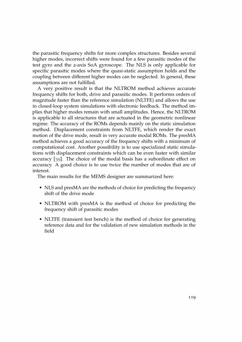
the parasitic frequency shifts for more complex structures. Besides severalhigher modes, incorrect shifts were found for a few parasitic modes of thetest gyro and the 2-axis SoA gyroscope. The NLS is only applicable forspecific parasitic modes where the quasi-static assumption holds and thecoupling between different higher modes can be neglected. In general, theseassumptions are not fulfilled.
A very positive result is that the NLTROM method achieves accuratefrequency shifts for both, drive and parasitic modes. It performs orders ofmagnitude faster than the reference simulation (NLTFE) and allows the usein closed-loop system simulations with electronic feedback. The method im-plies that higher modes remain with small amplitudes. Hence, the NLTROMis applicable to all structures that are actuated in the geometric nonlinearregime. The accuracy of the ROMs depends mainly on the static simulationmethod. Displacement constraints from NLTFE, which render the exactmotion of the drive mode, result in very accurate modal ROMs. The presMAmethod achieves a good accuracy of the frequency shifts with a minimum ofcomputational cost. Another possibility is to use specialized static simula-tions with displacement constraints which can be even faster with similaraccuracy [39]. The choice of the modal basis has a subordinate effect onaccuracy. A good choice is to use twice the number of modes that are ofinterest.
The main results for the MEMS designer are summarized here:
• NLS and presMA are the methods of choice for predicting the frequencyshift of the drive mode
• NLTROM with presMA is the method of choice for predicting thefrequency shift of parasitic modes
• NLTFE (transient test bench) is the method of choice for generatingreference data and for the validation of new simulation methods in thefield
119
5 conclusion
5.1 Outlook
5.1.1 Technical challenges
The presented approaches have been integrated in the development processof MEMS gyroscopes at the Robert Bosch GmbH in Reutlingen. However,there is still ongoing work that concerns numerical performance, accuracyand automation of these methods.
The NLS method is yet not applicable to all higher modes of a structure.The reason is that only 2 modes are considered, the actuated mode and theparasitic mode. Hence, only symmetric coupling βiijj can be captured. Ageneral approach should include at least 3 or 4 modes in order to accountfor the terms βiijk and βijkl. The generalization is not trivial and numericalperformance of the resulting method might be insufficient for the designoptimization.
Considering the data analysis, the time series data of the transient simula-tion was evaluated with Fourier analysis. The peak positions were therebydetermined with a parabola fit of the neighboring points (3-point fit). Theaccuracy could be further improved when using spline interpolation forrendering the peak position. This is also the case, when the frequency ismeasured from the time series data without Fourier transform.
One straight forward way to enhance the numerical performance is to useparallel computation. Especially, methods that rely on independent staticsimulations, such as NLS and presMA, allow parallel computation.
A possible implementation is to use batch jobs in Ansys. The creation ofbatch job files can be done automatically in Matlab. After generating theFE data, the ROM can be built and the transient simulations can be run inparallel using a parfor-loop in Matlab/Simulink.
Further, the numerical performance of the ROM simulation can be im-proved by using analytical expressions for the look-up table (LUT). The LUTentries can be fitted to the amplitude of the actuated mode (polynomial fit).As result, modal coupling coefficients are obtained from which the systemof coupled differential equations can be stated. Transient simulations withfixed coefficients are about twice as fast as compared to the conventionalLUT.
Furthermore, the analytical equations could be efficiently solved withperturbation and continuation techniques. It is highly recommended toinvestigate such analytical procedures as they bypass the transient simulation.This will allow to study nonlinear effects such as frequency pulling, mode
120
5 .1 outlook
coupling and bifurcation conveniently.In this work, the selection of modes for the modal basis of the ROM
were not further discussed. The reader may find deeper information inliterature [6, 3, 63]. The basis selection rule in this work uses twice thenumber of design relevant modes. Such a basis selection rule gave ROMswith accurate frequency shifts of the higher modes. More sophisticated basisselection criteria could take the correlation and coupling between modesinto account. Thereby, a ROM should include all modes with significantcorrelation. Especially, modes that couple to the actuated mode need to beincluded in the basis. Furthermore, higher modes that couple to specificparasitic modes need to be included in the basis. As numerical performancedepends quadratically on the system size, the computation time of frequencyshifts reduces drastically when lowering the size of the modal basis.
Ongoing work concerns the LUT in the NLTROM method. The accuracyof NLTROM might be further increased by using a 2D LUT that accountsfor the modal phase space trajectory of the actuated mode. Therefore, theactuated mode displacement has to be done for different steady-states inorder to consider the modal velocity in the stiffness calculation. Hence, the2D LUT selects the modal stiffness depending on modal amplitude andvelocity. This requires an efficient simulation workflow to generate the FEdata. A starting point can be the workflow given in Figure 5.1. First, a quasi-static displacement field is reached by applying inertial force. From thisdisplacement, the structural constraints are released and a single oscillationperiod is computed using nonlinear transient FE simulation. From each loadsteps of the transient simulation, a pre-stressed modal analysis is performed.This procedure is also known as a multi-frame restart from transient intomodal analysis [25]. The procedure is repeated for different quasi-staticdisplacements in the beginning of the transient simulation. As result, modalstiffness and basis for discrete points on the phase space trajectory of theactuated mode are given (Figure 5.1). The modal stiffness for the LUT can beobtained from interpolation or fitting onto an equidistant grid (Figure 5.2).As a proof of concept, the 2D LUT procedure has been successfully appliedto the doubly clamped beam structure.
The 2D LUT could be further applied to a system where two modes arenonlinear. That can be a micro mirror actuator with two resonant axis on thesame structure. In this case, the LUT selects the modal stiffness dependingon the amplitude of each of the modes, e.g. mode 1 and mode 2 where mode1 describes the motion around the first axis and mode 2 around the secondaxis.
121
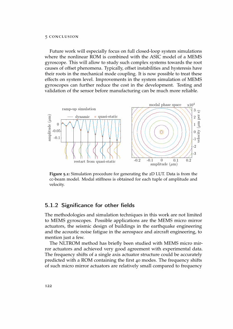
5 conclusion
Future work will especially focus on full closed-loop system simulationswhere the nonlinear ROM is combined with the ASIC model of a MEMSgyroscope. This will allow to study such complex systems towards the rootcauses of offset phenomena. Typically, offset instabilities and hysteresis havetheir roots in the mechanical mode coupling. It is now possible to treat theseeffects on system level. Improvements in the system simulation of MEMSgyroscopes can further reduce the cost in the development. Testing andvalidation of the sensor before manufacturing can be much more reliable.
ampl
itud
e(µ
m)
0
-0.05
-0.1
dynamic quasi-static
amplitude (µm)
velo
city
(µm
per
s)3
2
1
0
-1
-2
-3
-0.2 -0.1 0 0.1 0.2
x104
restart from quasi-static
ramp-up simulationmodal phase space
1
Figure 5.1: Simulation procedure for generating the 2D LUT. Data is from thecc-beam model. Modal stiffness is obtained for each tuple of amplitude andvelocity.
5.1.2 Significance for other fields
The methodologies and simulation techniques in this work are not limitedto MEMS gyroscopes. Possible applications are the MEMS micro mirroractuators, the seismic design of buildings in the earthquake engineeringand the acoustic noise fatigue in the aerospace and aircraft engineering, tomention just a few.
The NLTROM method has briefly been studied with MEMS micro mir-ror actuators and achieved very good agreement with experimental data.The frequency shifts of a single axis actuator structure could be accuratelypredicted with a ROM containing the first 40 modes. The frequency shiftsof such micro mirror actuators are relatively small compared to frequency
122
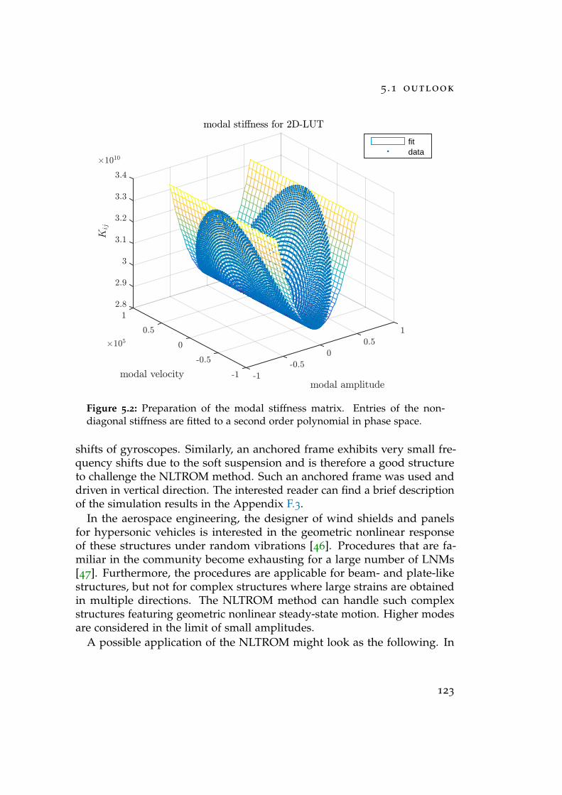
5 .1 outlook
1
modal amplitude
0.5
0
modal sti,ness for 2D-LUT
-0.5
-1-1
-0.5
modal velocity
0
0.5
3.3
3.4
2.9
2.8
3
3.1
3.2
#105
1
#1010
Kij
fitdata
Figure 5.2: Preparation of the modal stiffness matrix. Entries of the non-diagonal stiffness are fitted to a second order polynomial in phase space.
shifts of gyroscopes. Similarly, an anchored frame exhibits very small fre-quency shifts due to the soft suspension and is therefore a good structureto challenge the NLTROM method. Such an anchored frame was used anddriven in vertical direction. The interested reader can find a brief descriptionof the simulation results in the Appendix F.3.
In the aerospace engineering, the designer of wind shields and panelsfor hypersonic vehicles is interested in the geometric nonlinear responseof these structures under random vibrations [46]. Procedures that are fa-miliar in the community become exhausting for a large number of LNMs[47]. Furthermore, the procedures are applicable for beam- and plate-likestructures, but not for complex structures where large strains are obtainedin multiple directions. The NLTROM method can handle such complexstructures featuring geometric nonlinear steady-state motion. Higher modesare considered in the limit of small amplitudes.
A possible application of the NLTROM might look as the following. In
123
5 conclusion
a first step, the dominant nonlinear vibration of an aerospace structure canbe determined. A LUT for the modal stiffness can be efficiently constructedfor this dominant vibration using static FE analysis. The modal couplingcoefficients can be accessed through polynomial fits of the LUT entries. Thisprocedure will be much faster than the RANSTEP and ELSTEP as it bypassesthe iterative procedure to construct the coefficients. The reader is referred tothe amount of static simulations needed with the RANSTEP (2.57).
Another possible application of the NLTROM is in the seismic design ofhouses. Dividing eruptions and traveling waves into different classes, singleROMs for each class of external stimuli can be generated. This is possible,if for each class, there is a dominant vibration excited in the structure. Thespecific building design can be validated through each individual ROM thatcovers possible failure modes.
In general, the NLS and NLTROM procedure are applicable to all actu-ated structures with nonlinear response. The nonlinearity can be from thestructural design or from the material properties. Other nonlinear forcesthat are amplitude- or state-dependent can be covered with the presentedmethodologies as well.
124
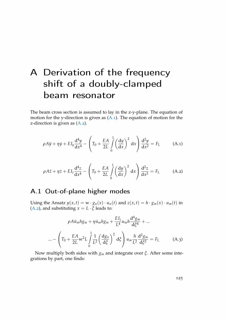
A Derivation of the frequencyshift of a doubly-clampedbeam resonator
The beam cross section is assumed to lay in the z-y-plane. The equation ofmotion for the y-direction is given as (A.1). The equation of motion for thez-direction is given as (A.2).
ρAy + ηy + EIyd4ydx4 −
T0 +EA2L
L∫0
(dydx
)2
dx
d2ydx2 = FL (A.1)
ρAz + ηz + EIzd4zdx4 −
T0 +EA2L
L∫0
(dydx
)2
dx
d2zdx2 = FL (A.2)
A.1 Out-of-plane higher modes
Using the Ansatz y(x, t) = w · gn(x) · un(t) and z(x, t) = h · gm(x) · um(t) in(A.2), and substituting x = L · ξ leads to:
ρAumhgm + ηumhgm +EIz
L4 umhd4gm
dξ4 + ...
...−T0 +
EA2L
w2L1∫
0
1L2
(dgn
dξ
)2
dξ
umhL2
d2gm
dξ2 = FL (A.3)
Now multiply both sides with gm and integrate over ξ. After some inte-grations by part, one finds:
125
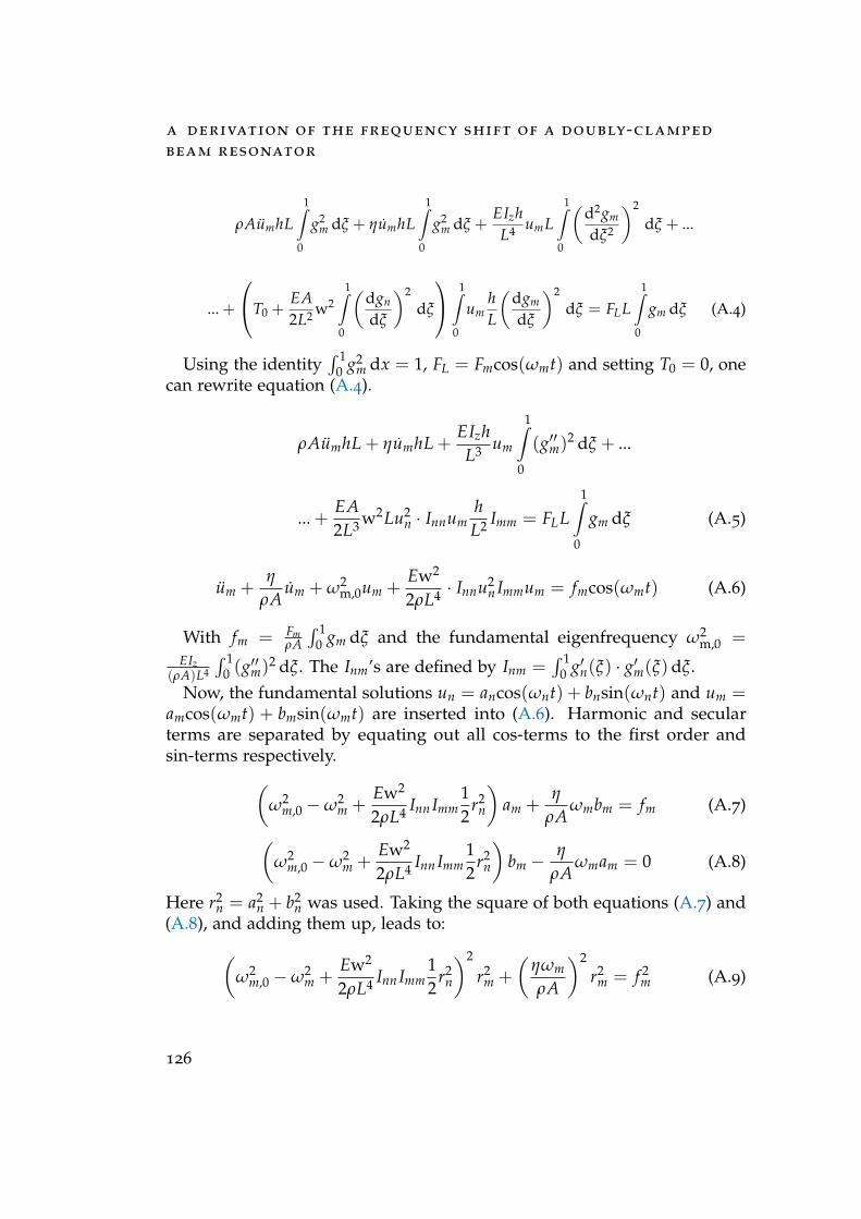
a derivation of the frequency shift of a doubly-clamped
beam resonator
ρAumhL1∫
0
g2m dξ + ηumhL
1∫0
g2m dξ +
EIzhL4 umL
1∫0
(d2gm
dξ2
)2
dξ + ...
... +
T0 +EA2L2 w2
1∫0
(dgn
dξ
)2
dξ
1∫0
umhL
(dgm
dξ
)2
dξ = FLL1∫
0
gm dξ (A.4)
Using the identity∫ 1
0 g2m dx = 1, FL = Fmcos(ωmt) and setting T0 = 0, one
can rewrite equation (A.4).
ρAumhL + ηumhL +EIzhL3 um
1∫0
(g′′m)2 dξ + ...
... +EA2L3 w2Lu2
n · InnumhL2 Imm = FLL
1∫0
gm dξ (A.5)
um +η
ρAum + ω2
m,0um +Ew2
2ρL4 · Innu2n Immum = fmcos(ωmt) (A.6)
With fm = FmρA
∫ 10 gm dξ and the fundamental eigenfrequency ω2
m,0 =EIz
(ρA)L4
∫ 10 (g′′m)2 dξ. The Inm’s are defined by Inm =
∫ 10 g′n(ξ) · g′m(ξ)dξ.
Now, the fundamental solutions un = ancos(ωnt) + bnsin(ωnt) and um =amcos(ωmt) + bmsin(ωmt) are inserted into (A.6). Harmonic and secularterms are separated by equating out all cos-terms to the first order andsin-terms respectively.(
ω2m,0 −ω2
m +Ew2
2ρL4 Inn Imm12
r2n
)am +
η
ρAωmbm = fm (A.7)(
ω2m,0 −ω2
m +Ew2
2ρL4 Inn Imm12
r2n
)bm −
η
ρAωmam = 0 (A.8)
Here r2n = a2
n + b2n was used. Taking the square of both equations (A.7) and
(A.8), and adding them up, leads to:(ω2
m,0 −ω2m +
Ew2
2ρL4 Inn Imm12
r2n
)2
r2m +
(ηωm
ρA
)2
r2m = f 2
m (A.9)
126
a .2 in-plane higher modes
Here r2m = a2
m + b2m was used. Rearranging the terms leads to:
r2m =
f 2m(
ω2m,0 −ω2
m + Ew2
2ρL4 Inn Imm12r2
n
)2r2
m +(
ηωmρA
)2 (A.10)
The maximum amplitude rm can be obtained if the denominator of (A.10)has a minimum. Since damping is low, the η-term can be neglected and theminimum of the denominator is found for:
ωm = ωm,0
√1 +
Ew2
4ρL4ω2m,0
Inn Immr2n (A.11)
ωm = ωm,0
√1 +
E4ρL4ω2
m,0Inn Imm|gn(L/2)|−2A2
n (A.12)
In the last equation rn = Anw|gn(L/2)| was used. For the first fundamental
mode of the presented beam |gn(L/2)|−2 is 0.396.
A.2 In-plane higher modes
In order to derive the in-plane stiffening, the ansatz y(x, t) = w · gn(x) ·un(t) + w · gm(x) · um(t) is used in equation (A.1).
ρAw (umgm + ungn) + ηw (umgm + ungn) + EIywum
(umg(4)m + ung(4)n
)+ ...
...−T0 +
EA2L
w2L∫
0
(umg′m + ung′n
)2 dx
(wumg′′m + wung′′n)
...
... = Fmsin(ωmt) + Fn (A.13)
With g′i as the first derivative of gi with respect to x, g′′i as the second
derivative of gi with respect to x and g(4)i as the fourth derivative of gi withrespect to x. Using the substitution x = Lξ, equation (A.13) becomes:
127
a derivation of the frequency shift of a doubly-clamped
beam resonator
ρAw (umgm + ungn) + ηw (umgm + ungn) +EIyw
L4
(umg(4)m + ung(4)n
)+ ...
...−T0 +
EA2L2 w2
1∫0
(um
dgm
dξ+ un
dgn
dξ
)2
dξ
wL2
(um
d2gm
dξ2 + und2gn
dξ2
)...
... = Fmsin(ωmt) + Fncos(ωnt) (A.14)
The next step is to multiply both sides with gm and integrate over ξ. Dueto the linearity of the integral, the last term on the left hand side can besimplified first.
(T0 +
EA2L2 w2 (u2
m Imm + u2n Inn + 2unum Inm
)) wL2
1∫0
umd2gm
dξ2 gm + und2gn
dξ2 gm dξ...
(A.15)
= −(
T0 +EA2L2 w2 (u2
m Imm + u2n Inn + 2unum Inm
)) wL2 (un Inm + um Imm)
For the characteristic equation of the frequency dependency, the ωm-harmonics are considered to first order. The equation reduces to:
ρAwum + ηwum +EIyw
L4 um
1∫0
g′′2m dξ + ...
... +(
T0 +EA2L2 w2 (u2
m Imm + u2n Inn + 2unum Inm
))· w
L2 (un Inm + um Imm) ...
... = Fmsin(ωmt)1∫
0
gm dξ (A.16)
um +η
ρAum + ω2
m,0um +Ew2
2ρL4
(u2
m Imm + u2n Inn + 2unum Inm
)(un Inm + um Imm) ...
(A.17)... = fmsin(ωmt)
With fm = Fm∫ 1
0 gm dξ and ωm,0 as previous. When entering equa-tion (A.17) with um = amcos(ωmt) + bmsin(ωmt) and un = ancos(ωnt) +
128
a .2 in-plane higher modes
bnsin(ωnt), terms with u3m, u2
mun and umu2n arise. The first order harmonics
are separated from these secular terms as follows:
u3m = a3
mcos3(ωmt)+ b3msin3(ωmt)+ 3amb2
msin2(ωmt)cos(ωmt)+ 3a2mbmsin(ωmt)cos2(ωmt)
= a3m
14(3cos(ωmt) + cos(3ωmt)) + b3
m14(3sin(ωmt) + sin(3ωmt)) + ...
... + 3amb2m
(1− cos2(ωmt)
)cos(ωmt) + 3a2
mbmsin(ωmt)(
1− sin2(ωmt))
u3m/cos(ωmt) =
34
(a2
m + b2m
)am + secular terms
u3m/sin(ωmt) =
34
(b2
m + a2m
)bm + secular terms
u2mun =
(a2
mcos2(ωmt) + b2msin2(ωmt) + 2ambmsin(ωmt)cos(ωmt)
)(ancos(ωnt) + bnsin(ωnt))
u2mun/cos(ωmt) = 0 + secular terms
u2mun/sin(ωmt) = 0 + secular terms
umu2n =
(a2
ncos2(ωnt) + b2nsin2(ωnt) + 2anbnsin(ωnt)cos(ωnt)
)(amcos(ωmt) + bmsin(ωmt))
umu2n/cos(ωmt) =
12
(a2
n + b2n
)am + secular terms
umu2n/sin(ωmt) =
12
(a2
n + b2n
)bm + secular terms
Inserting the terms into (A.17) and separating cos and sin-terms leads to
−ω2mam +
η
ρAωmbm + ω2
m,0am +Ew2
2ρL4
(34
Immr2m +
(12
Inn Imm + I2nm
)r2
n
)am = 0
(A.18)
−ω2mbm −
η
ρAωmam + ω2
m,0bm +Ew2
2ρL4
(34
Immr2m +
(12
Inn Imm + I2nm
)r2
n
)bm = fm
(A.19)
With the same procedure as for out-of-plane stiffening, the characteristic
129
a derivation of the frequency shift of a doubly-clamped
beam resonator
equation for the frequency yields
ωm = ωm,0
√1 +
34
Ew2
2ρL4ω2m,0
I2mmr2
m +Ew2
2ρL4ω2m,0
(12
Inn Imm + I2nm
)r2
n (A.20)
ωm = ωm,0
√1 +
34
αm,0 I2mm A2
m + αm,0
(12
Inn Imm + I2nm
)A2
n (A.21)
With Ai as the physical amplitude of mode i and αi,0 = Egi(L/2)−2
2ρL4ω2i,0
. In the
limit of small amplitudes Am the self-stiffening term 34 αm,0 I2
mm A2m can be
neglected.
ωm = ωm,0
√1 + αm,0
(12
Inn Imm + I2nm
)A2
n (A.22)
Comparing (A.12) with (A.22), one finds that the in-plane stiffening hasan additional contribution from Inm. Since the Inm’s are zero for i 6= j, theformula of (A.22) can be used for both, in- and out-of-plane modes of thebeam.
A.3 Comparison of the effective Duffingcoefficient
The frequency pulling of mode 1 for the doubly-clamped beam can bedetermined from Owers-Bradley formula (A.21) when only the single modecontribution is taken into account. This is given in the following equationon the left hand side. The common notation of the oscillator hardening isin terms of the effective Duffing coefficient (2.38). This is given on the righthand side.
ωn,1 = ωn,0
√1 + 3λI2
nn4ω2
n,0r2
n ≈ ωn,0(1 +3λI2
nn8ω2
n,0r2
n)!= ωn,0(1 +
3β8ω0
x2)
130
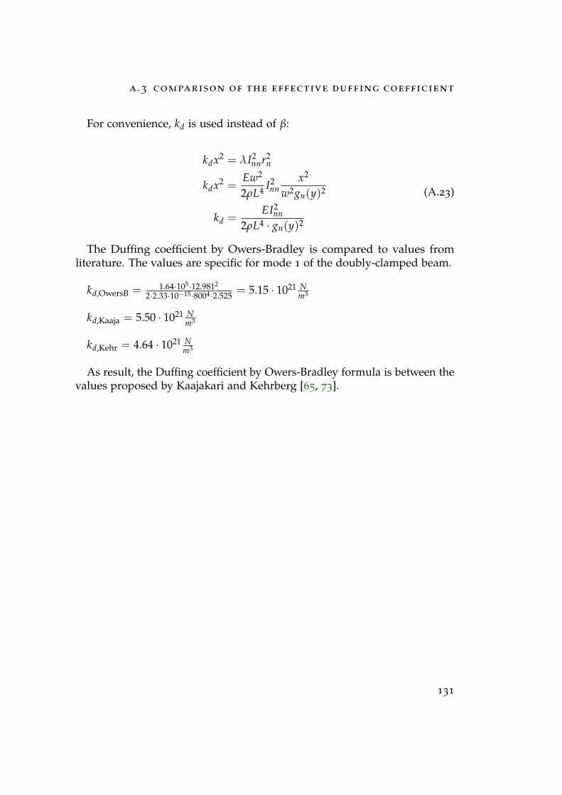
a .3 comparison of the effective duffing coefficient
For convenience, kd is used instead of β:
kdx2 = λI2nnr2
n
kdx2 =Ew2
2ρL4 I2nn
x2
w2gn(y)2
kd =EI2
nn2ρL4 · gn(y)2
(A.23)
The Duffing coefficient by Owers-Bradley is compared to values fromliterature. The values are specific for mode 1 of the doubly-clamped beam.
kd,OwersB = 1.64·105·12.9812
2·2.33·10−15·8004·2.525 = 5.15 · 1021 Nm3
kd,Kaaja = 5.50 · 1021 Nm3
kd,Kehr = 4.64 · 1021 Nm3
As result, the Duffing coefficient by Owers-Bradley formula is between thevalues proposed by Kaajakari and Kehrberg [65, 73].
131

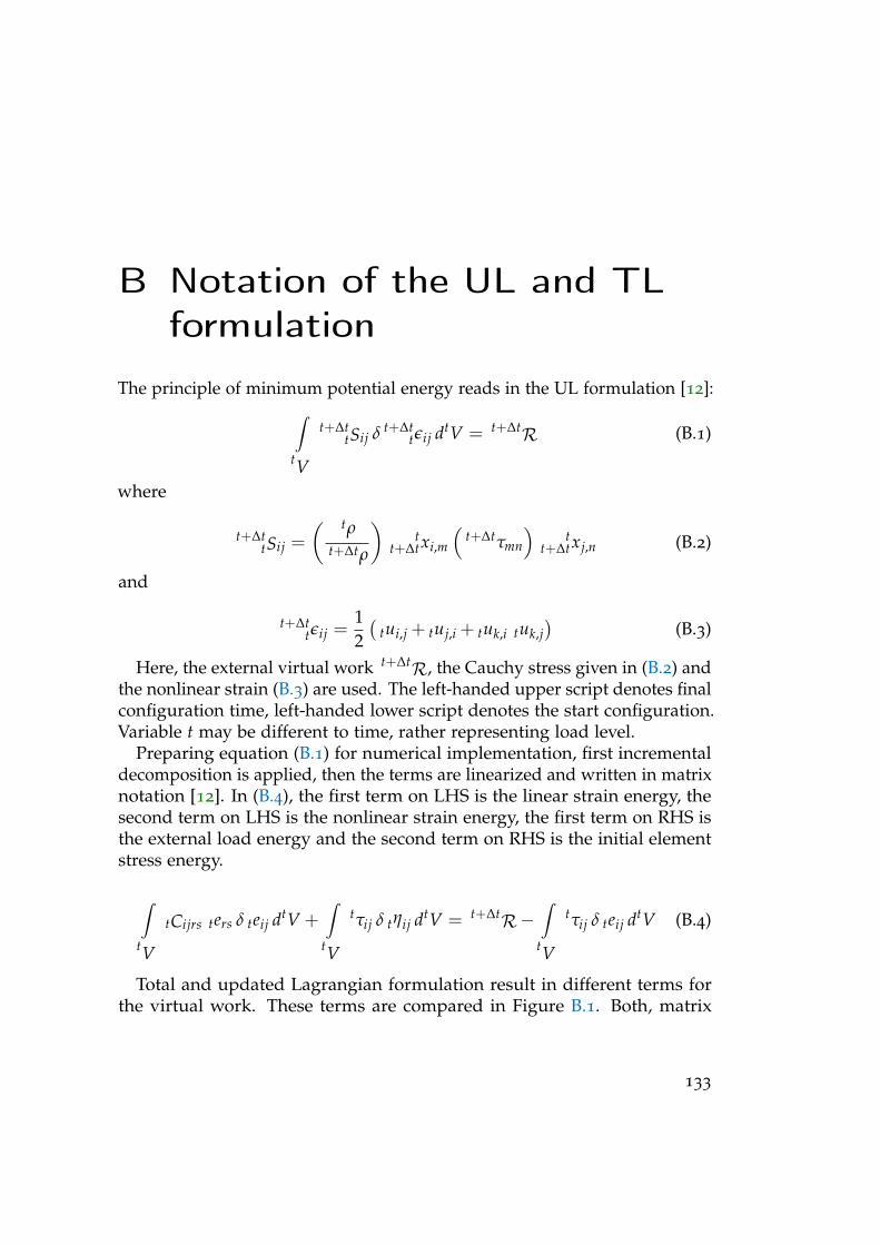
B Notation of the UL and TLformulation
The principle of minimum potential energy reads in the UL formulation [12]:∫tV
t+∆ttSij δ t+∆t
tεij dtV = t+∆tR (B.1)
where
t+∆ttSij =
( tρt+∆tρ
)t
t+∆txi,m
(t+∆tτmn
)t
t+∆txj,n (B.2)
and
t+∆ttεij =
12(
tui,j + tuj,i + tuk,i tuk,j)
(B.3)
Here, the external virtual work t+∆tR, the Cauchy stress given in (B.2) andthe nonlinear strain (B.3) are used. The left-handed upper script denotes finalconfiguration time, left-handed lower script denotes the start configuration.Variable t may be different to time, rather representing load level.
Preparing equation (B.1) for numerical implementation, first incrementaldecomposition is applied, then the terms are linearized and written in matrixnotation [12]. In (B.4), the first term on LHS is the linear strain energy, thesecond term on LHS is the nonlinear strain energy, the first term on RHS isthe external load energy and the second term on RHS is the initial elementstress energy.
∫tV
tCijrs ters δ teij dtV +∫
tV
tτij δ tηij dtV = t+∆tR−∫
tV
tτij δ teij dtV (B.4)
Total and updated Lagrangian formulation result in different terms forthe virtual work. These terms are compared in Figure B.1. Both, matrix
133
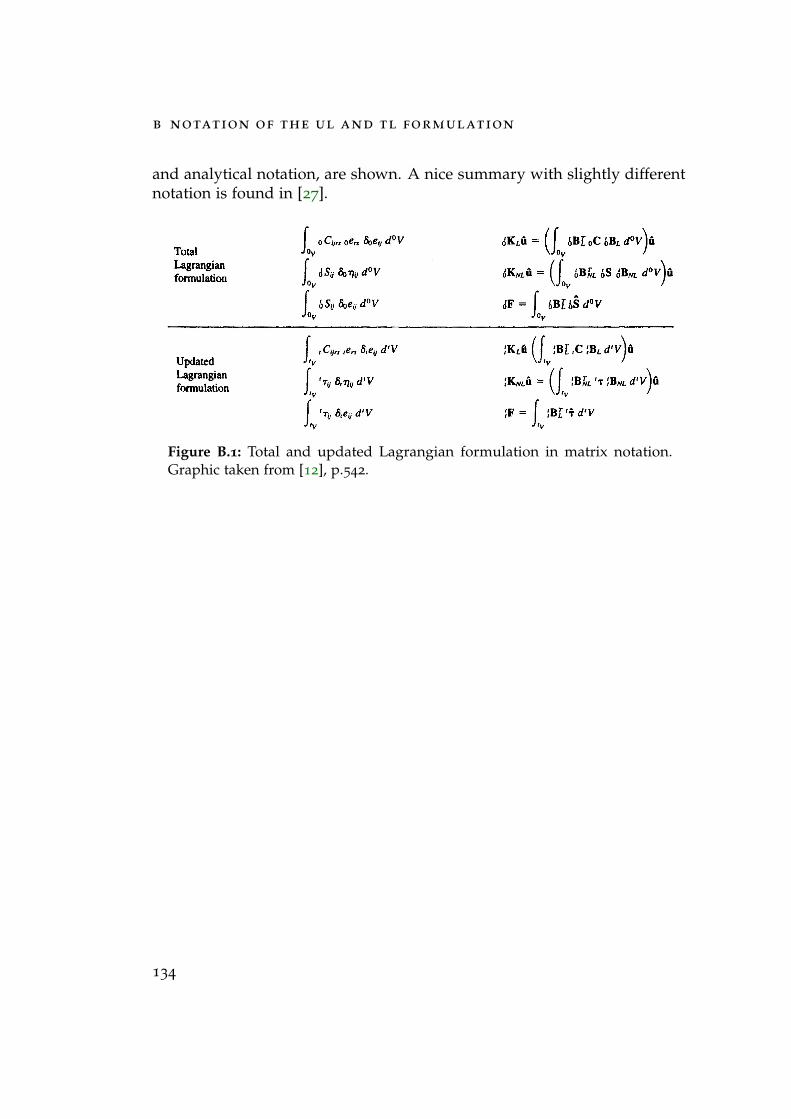
b notation of the ul and tl formulation
and analytical notation, are shown. A nice summary with slightly differentnotation is found in [27].
Figure B.1: Total and updated Lagrangian formulation in matrix notation.Graphic taken from [12], p.542.
134
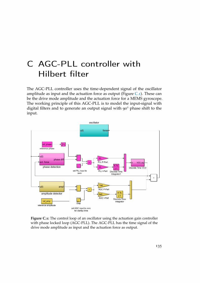
C AGC-PLL controller withHilbert filter
The AGC-PLL controller uses the time-dependent signal of the oscillatoramplitude as input and the actuation force as output (Figure C.1). These canbe the drive mode amplitude and the actuation force for a MEMS gyroscope.The working principle of this AGC-PLL is to model the input-signal withdigital filters and to generate an output signal with 90° phase shift to theinput.
Figure C.1: The control loop of an oscillator using the actuation gain controllerwith phase locked loop (AGC-PLL). The AGC-PLL has the time signal of thedrive mode amplitude as input and the actuation force as output.
135
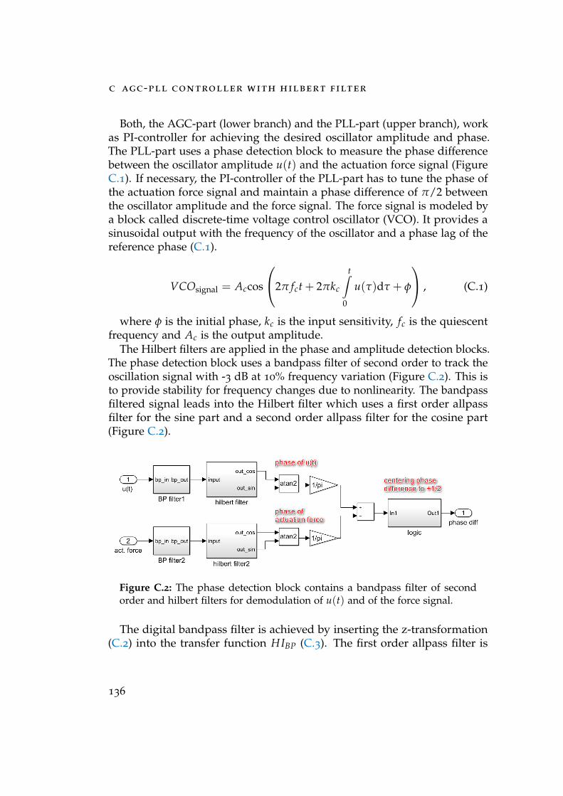
c agc-pll controller with hilbert filter
Both, the AGC-part (lower branch) and the PLL-part (upper branch), workas PI-controller for achieving the desired oscillator amplitude and phase.The PLL-part uses a phase detection block to measure the phase differencebetween the oscillator amplitude u(t) and the actuation force signal (FigureC.1). If necessary, the PI-controller of the PLL-part has to tune the phase ofthe actuation force signal and maintain a phase difference of π/2 betweenthe oscillator amplitude and the force signal. The force signal is modeled bya block called discrete-time voltage control oscillator (VCO). It provides asinusoidal output with the frequency of the oscillator and a phase lag of thereference phase (C.1).
VCOsignal = Accos
2π fct + 2πkc
t∫0
u(τ)dτ + φ
, (C.1)
where φ is the initial phase, kc is the input sensitivity, fc is the quiescentfrequency and Ac is the output amplitude.
The Hilbert filters are applied in the phase and amplitude detection blocks.The phase detection block uses a bandpass filter of second order to track theoscillation signal with -3 dB at 10% frequency variation (Figure C.2). This isto provide stability for frequency changes due to nonlinearity. The bandpassfiltered signal leads into the Hilbert filter which uses a first order allpassfilter for the sine part and a second order allpass filter for the cosine part(Figure C.2).
Figure C.2: The phase detection block contains a bandpass filter of secondorder and hilbert filters for demodulation of u(t) and of the force signal.
The digital bandpass filter is achieved by inserting the z-transformation(C.2) into the transfer function HIBP (C.3). The first order allpass filter is
136
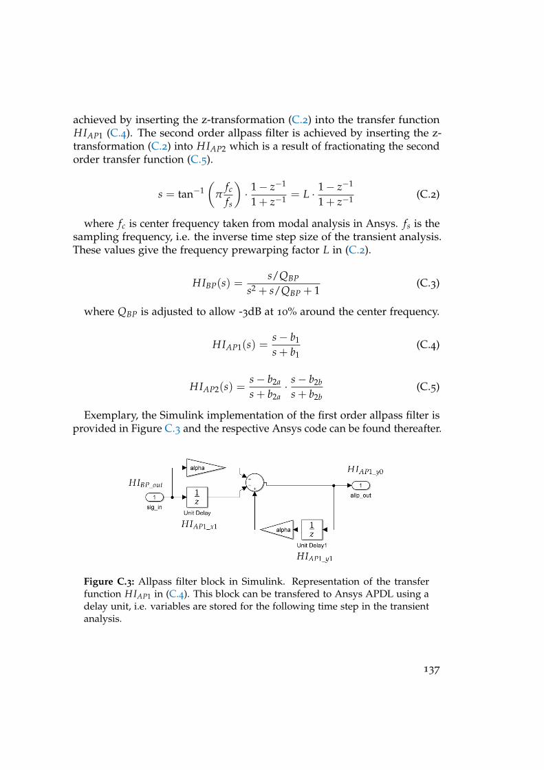
achieved by inserting the z-transformation (C.2) into the transfer functionHIAP1 (C.4). The second order allpass filter is achieved by inserting the z-transformation (C.2) into HIAP2 which is a result of fractionating the secondorder transfer function (C.5).
s = tan−1(
πfc
fs
)· 1− z−1
1 + z−1 = L · 1− z−1
1 + z−1 (C.2)
where fc is center frequency taken from modal analysis in Ansys. fs is thesampling frequency, i.e. the inverse time step size of the transient analysis.These values give the frequency prewarping factor L in (C.2).
HIBP(s) =s/QBP
s2 + s/QBP + 1(C.3)
where QBP is adjusted to allow -3dB at 10% around the center frequency.
HIAP1(s) =s− b1
s + b1(C.4)
HIAP2(s) =s− b2a
s + b2a· s− b2b
s + b2b(C.5)
Exemplary, the Simulink implementation of the first order allpass filter isprovided in Figure C.3 and the respective Ansys code can be found thereafter.
Figure C.3: Allpass filter block in Simulink. Representation of the transferfunction HIAP1 in (C.4). This block can be transfered to Ansys APDL using adelay unit, i.e. variables are stored for the following time step in the transientanalysis.
137
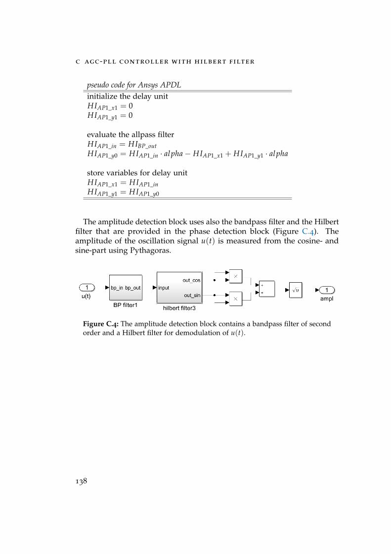
c agc-pll controller with hilbert filter
pseudo code for Ansys APDLinitialize the delay unitHIAP1_x1 = 0HIAP1_y1 = 0
evaluate the allpass filterHIAP1_in = HIBP_outHIAP1_y0 = HIAP1_in · alpha− HIAP1_x1 + HIAP1_y1 · alpha
store variables for delay unitHIAP1_x1 = HIAP1_inHIAP1_y1 = HIAP1_y0
The amplitude detection block uses also the bandpass filter and the Hilbertfilter that are provided in the phase detection block (Figure C.4). Theamplitude of the oscillation signal u(t) is measured from the cosine- andsine-part using Pythagoras.
Figure C.4: The amplitude detection block contains a bandpass filter of secondorder and a Hilbert filter for demodulation of u(t).
138
D Derivation of thetransformation matrix
The NLTROM method uses a transformation T to transform the modalstiffness into a reference basis (3.24). Its derivation is given in the following.
As in Section 3.6, V0 denotes the eigenvector set of the undeflected struc-ture and Vdefl denotes the eigenvector set of the deflected structure. Thestructural deflection is from the actuated mode displacement. Considering aMEMS gyroscope, this can be the drive mode displacement.
Using equation (2.31), the deflected modal amplitude vector qdefl is writtenwith the deflected eigenvector set and the nodal state vector x (D.1). Usingx = V0q0, the deflected modal amplitude vector is expressed in terms of theundeflected modal coordinates (D.1). The undeflected modal basis is hereused as the reference basis.
qdefl = (VTdeflVdefl)
−1VTdeflx
= (VTdeflVdefl)
−1VTdeflV0q0
(D.1)
From this relation, the transformation T is defined:
T := (VTdeflVdefl)
−1VTdeflV0 (D.2)
The modal equation of the deflected system reads:
Mdeflqdefl + Ddeflqdefl + Kdeflqdefl = fdefl(t)
Mdefl(VTdeflVdefl)
−1VTdeflV0q0 + ... = fdefl(t)
MdeflTq0 + ... = fdefl(t)
(D.3)
Multiplying equation (D.3) with TT from the left side yields:
TTMdeflTq0 + TTDdeflTq0 + ˜TTKdeflTq0 = TTfdefl(t)
Mdefl,0q0 + Ddefl,0q0 + Kdefl,0q0 = fdefl,0(t)(D.4)
139
d derivation of the transformation matrix
It is now trivial to see how the deflected modal equation transformsinto the modal equation of the undeflected mode shapes. The new systemmatrices follow from (D.4). The transformation was put into the systemmatrices.
The Matlab implementation of the transformation T uses QR decomposi-tion of the matrix left division of Vdefl with V0. The orthogonal matrix ofthe QR decomposition is represented with the function Q in (D.5).
T = (VTdeflVdefl)
−1VTdeflV0
≈ Q(V+deflV0)
(D.5)
The plus (+) denotes the Moore-Penrose pseudoinverse. This transforma-tion (D.5) is used to change from the deflected to the undeflected eigenvectors.The modal stiffness for a each deflection is transformed into the undeflectedmodal coordinates using Equation (D.6).
TTKdeflT = Kdefl,0 (D.6)
Since mass is unity, the transformed mass matrix is again unity as T isorthogonal. For numerical stability, the damping matrix is a unit matrixmultiplied by a factor of 50. The damping matrix is therefore also invariantunder (D.6).
140
d.1 preparing the modal stiffness for transient simulations
D.1 Preparing the modal stiffness for transientsimulations
The linear and quadratic stiffness of the actuated mode have to be preparedfor the transient ROM simulation. In the transient ROM simulation, modalforces from the stiffness are obtained by multiplication of the q-vector withthe corresponding stiffness matrix (D.6). Instead the physical force is ob-tained from integrating the modal stiffness with respect to modal amplitude.
The factors that arise in the derivative of the actuated mode force (D.7) arecorrected. For simplicity, the index 1 is used for the actuated mode.
F1 = k0q1 + k1q21 + k2q3
1∂F1
∂q1= k0 + 2k1q1 + 3k2q2
1
∂F1
∂q1= k0 + klinq1 + kquadq2
1 =: K11
(D.7)
Without correction, the modal force on the actuated mode yields (D.8).However, the effective Duffing coefficient is three times higher than k2. Thelinear coefficient has doubled. Obviously, time integration of the modal forceF1 tends to overestimate the frequency pulling of this mode.
F1 = K11q1
=(
k0 + klinq1 + kquadq21
)q1
= k0q1 + 2k1q21 + 3k2q3
1
(D.8)
The following correction scheme is applied to the diagonal entries of theactuated mode. The diagonal stiffness of this mode K11 is identified with ∂F1
∂q1.
Fitting the K11 entries to a second order polynomial in amplitude yields thecoefficients k0, klin and kquad. The coefficients are corrected by 1/2 and 1/3,for the linear and quadratic coefficient respectively. The diagonal entries ofthe actuated mode are rewritten by evaluating the corrected polynomial atthe respective amplitudes. For better approximation of the stiffness curve, aforth order polynomial might be beneficial. Therefore, the coefficients haveto be corrected in an analogous manner.
The stiffness coefficients of higher modes may not be adjusted as thecoupling to the actuated mode and to other higher modes is linear in the
141
d derivation of the transformation matrix
modal amplitude (D.9). Thus, modal force Fn is equal to the product ofstiffness and amplitude (D.10). This yields the correct physical force on thehigher mode in the transient ROM simulation.
Fn = k0qn + k1qnq1 + k2qnq21 +
N
∑m 6=n
kmqnqm
∂Fn
∂qn= k0 + k1q1 + k2q2
1 +N
∑m 6=n
kmqm
(D.9)
Fn =∂Fn
∂qnqn (D.10)
In Matlab/Simulink, the stiffness matrices are put into an amplitudedependent look-up table (Section 3.6).
142

143
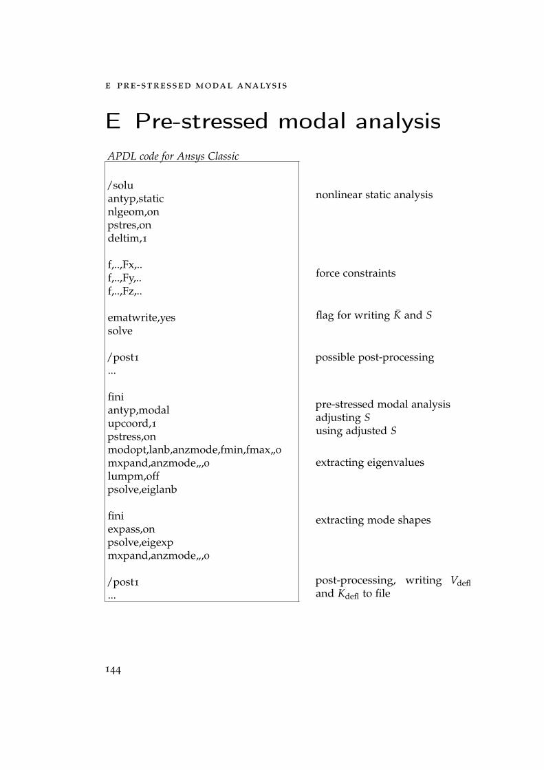
e pre-stressed modal analysis
E Pre-stressed modal analysisAPDL code for Ansys Classic
/soluantyp,staticnlgeom,onpstres,ondeltim,1
f,..,Fx,..f,..,Fy,..f,..,Fz,..
ematwrite,yessolve
/post1...
finiantyp,modalupcoord,1pstress,onmodopt,lanb,anzmode,fmin,fmax„0
mxpand,anzmode„,0lumpm,offpsolve,eiglanb
finiexpass,onpsolve,eigexpmxpand,anzmode„,0
/post1...
nonlinear static analysis
force constraints
flag for writing K and S
possible post-processing
pre-stressed modal analysisadjusting Susing adjusted S
extracting eigenvalues
extracting mode shapes
post-processing, writing Vdefland Kdefl to file
144
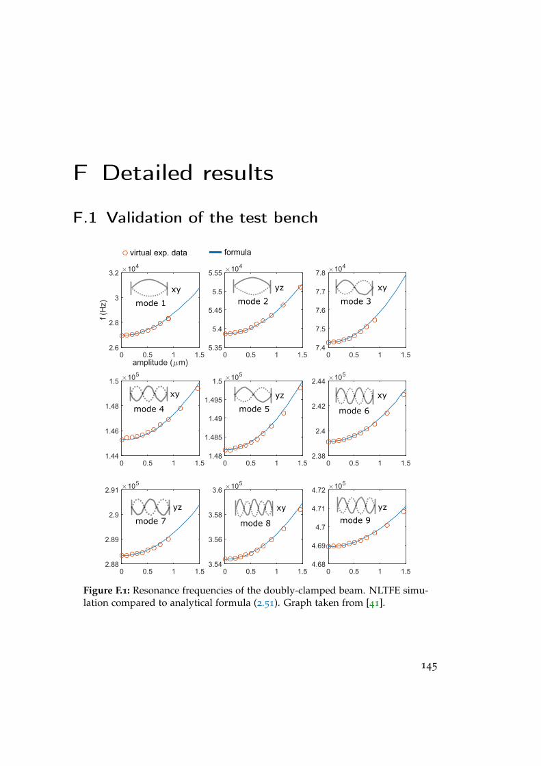
F Detailed results
F.1 Validation of the test bench
mode 1 mode 2
virtual exp. data formula
xy yz
mode 3
xy
mode 4
xy yz xy
mode 5 mode 6
mode 7 mode 8 mode 9
xy yzyz
Figure F.1: Resonance frequencies of the doubly-clamped beam. NLTFE simu-lation compared to analytical formula (2.51). Graph taken from [41].
145
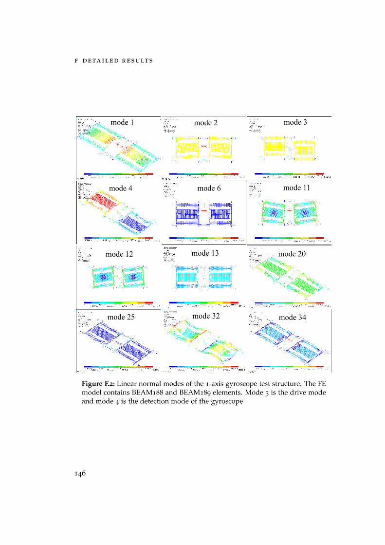
f detailed results
Figure F.2: Linear normal modes of the 1-axis gyroscope test structure. The FEmodel contains BEAM188 and BEAM189 elements. Mode 3 is the drive modeand mode 4 is the detection mode of the gyroscope.
146
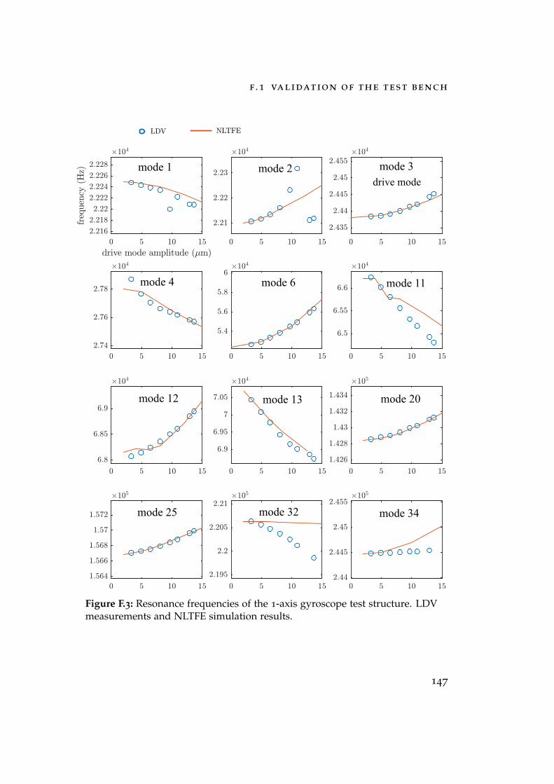
f .1 validation of the test bench
Figure F.3: Resonance frequencies of the 1-axis gyroscope test structure. LDVmeasurements and NLTFE simulation results.
147
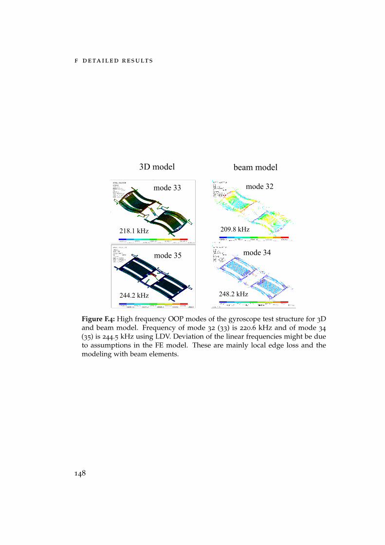
f detailed results
Figure F.4: High frequency OOP modes of the gyroscope test structure for 3Dand beam model. Frequency of mode 32 (33) is 220.6 kHz and of mode 34
(35) is 244.5 kHz using LDV. Deviation of the linear frequencies might be dueto assumptions in the FE model. These are mainly local edge loss and themodeling with beam elements.
148
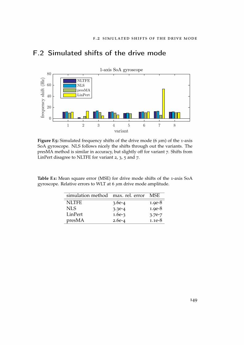
f .2 simulated shifts of the drive mode
F.2 Simulated shifts of the drive mode
variant1 2 3 4 5 6 7 8
frequencyshift(Hz)
0
20
40
60
801-axis SoA gyroscope
NLTFE
NLS
presMA
LinPert
Figure F.5: Simulated frequency shifts of the drive mode (6 µm) of the 1-axisSoA gyroscope. NLS follows nicely the shifts through out the variants. ThepresMA method is similar in accuracy, but slightly off for variant 7. Shifts fromLinPert disagree to NLTFE for variant 2, 3, 5 and 7.
Table F.1: Mean square error (MSE) for drive mode shifts of the 1-axis SoAgyroscope. Relative errors to WLT at 6 µm drive mode amplitude.
simulation method max. rel. error MSENLTFE 3.6e-4 1.9e-8NLS 3.3e-4 1.9e-8LinPert 1.6e-3 3.7e-7presMA 2.6e-4 1.1e-8
149
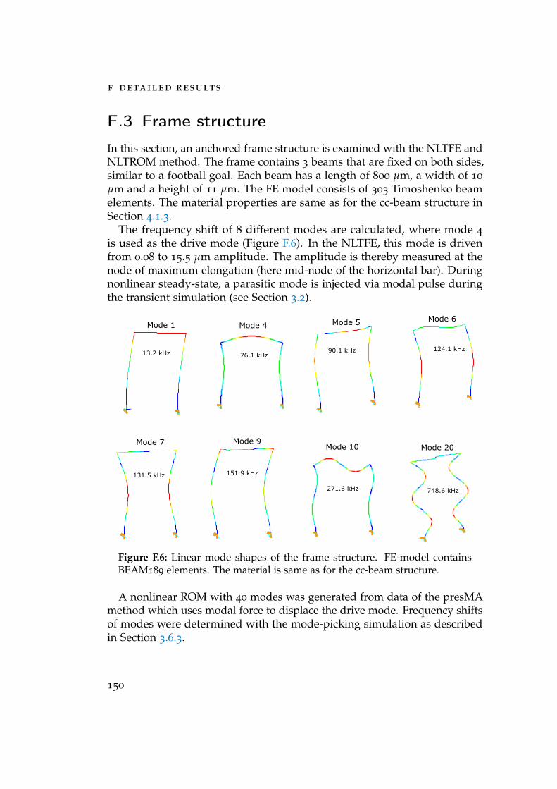
f detailed results
F.3 Frame structure
In this section, an anchored frame structure is examined with the NLTFE andNLTROM method. The frame contains 3 beams that are fixed on both sides,similar to a football goal. Each beam has a length of 800 µm, a width of 10
µm and a height of 11 µm. The FE model consists of 303 Timoshenko beamelements. The material properties are same as for the cc-beam structure inSection 4.1.3.
The frequency shift of 8 different modes are calculated, where mode 4
is used as the drive mode (Figure F.6). In the NLTFE, this mode is drivenfrom 0.08 to 15.5 µm amplitude. The amplitude is thereby measured at thenode of maximum elongation (here mid-node of the horizontal bar). Duringnonlinear steady-state, a parasitic mode is injected via modal pulse duringthe transient simulation (see Section 3.2).
Figure F.6: Linear mode shapes of the frame structure. FE-model containsBEAM189 elements. The material is same as for the cc-beam structure.
A nonlinear ROM with 40 modes was generated from data of the presMAmethod which uses modal force to displace the drive mode. Frequency shiftsof modes were determined with the mode-picking simulation as describedin Section 3.6.3.
150
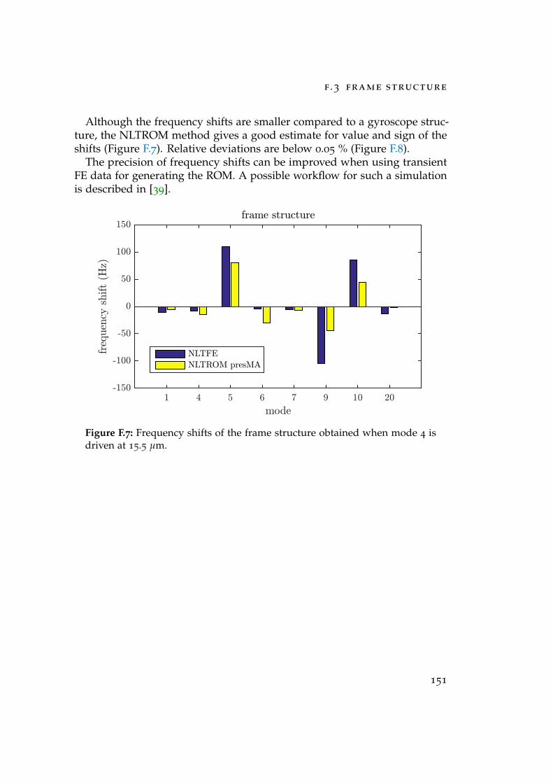
f .3 frame structure
Although the frequency shifts are smaller compared to a gyroscope struc-ture, the NLTROM method gives a good estimate for value and sign of theshifts (Figure F.7). Relative deviations are below 0.05 % (Figure F.8).
The precision of frequency shifts can be improved when using transientFE data for generating the ROM. A possible workflow for such a simulationis described in [39].
mode1 4 5 6 7 9 10 20
frequencyshift(Hz)
-150
-100
-50
0
50
100
150frame structure
NLTFE
NLTROM presMA
Figure F.7: Frequency shifts of the frame structure obtained when mode 4 isdriven at 15.5 µm.
151
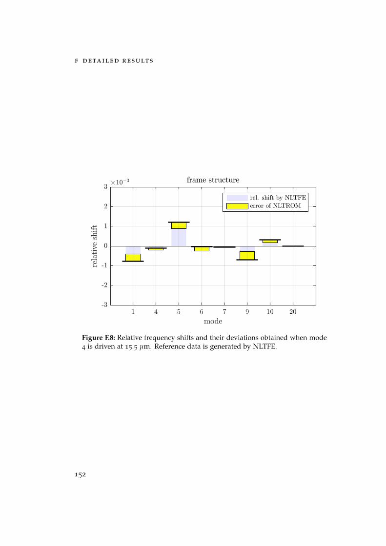
f detailed results
frame structure
mode1 4 5 6 7 9 10 20
relativeshift
#10!3
-3
-2
-1
0
1
2
3
rel. shift by NLTFE
error of NLTROM
Figure F.8: Relative frequency shifts and their deviations obtained when mode4 is driven at 15.5 µm. Reference data is generated by NLTFE.
152
Bibliography
[1] A. C. Antoulas. Approximation of Large-Scale Dynamical Systems. Vol. Ad-vances in Design and Control. SIAM Book Series. Houston, Texas, 2004
(cited on pages 25, 27, 28).
[2] A. K. Gaonkar and S. S. Kulkarni. “Model order reduction for dynamicsimulation of beams with forcing and geometric nonlinearities”. In:Finite Elements in Analysis and Design 76 (Aug. 14, 2013), pp. 50–62. doi:10.1016/j.finel.2013.08.001. url: http://dx.doi.org/10.1016/j.finel.2013.08.001 (cited on page 27).
[3] A. Przekop, G. Xinyun, and Stephen A. Rizzi. “Alternative Modal BasisSelection Procedures for Nonlinear Random Response Simulation”.In: RASD 2010. 10th International Conference on Recent Advances inStructural Dynamic. Southampton, 2008 (cited on page 121).
[4] C. Acar and A. Shkel. MEMS Vibratory Gyroscopes: Structural Approachesto Improve Robustness. MEMS Reference Shelf. Springer US, 2008. isbn:978-0-387-09536-3. url: https : / / books . google . de / books ? id =WgFPvZyApd0C (cited on page 26).
[5] Adam Przekop, Michael A. Stover, and Stephen A. Rizzi. “Nonlin-ear Reduced-Order Simulation Using Stress-Free and Pre-StressedModal Bases”. In: American Institute of Aeronautics and Astronautics. 50thAIAA/ASME/ASCE/AHS/ASC Structures, Structural Dynamics, andMaterials Conference. Palm Springs, 2009 (cited on page 118).
[6] Adam Przekop and Stephen A. Rizzi. “Efficient modal basis selectioncriteria for reduced-order nonlinear simulation”. In: EURODYN 2008
- 7th European Conference on Structural Dynamics. Southhampton,2008 (cited on pages 69, 121).
[7] Alexander A. Muravyov. Determination of Nonlinear Stiffness Coefficientsfor Finite Element Models with Application to the Random Vibration Problem.Technical report 20040086513. Langley Research Center: NASA, 1999
(cited on pages 18, 39, 88, 118).
153
bibliography
[8] Ali H. Nayfeh, Dean T. Mook. Nonlinear Oscillations. Wiley-VCH, 1995.isbn: 978-0-471-12142-8 (cited on pages 18, 29, 34).
[9] Ali H. Nayfeh, Mohammad I. Younis, and Eihab M. Abdel-Rahman.“Reduced-Order Models for MEMS Applications”. In: Nonlinear Dy-namics 41.1 (2005), pp. 211–236. doi: 10.1007/s11071-005-2809-9(cited on pages 25, 26).
[10] ANSYS Inc. Documentation for Release 11.0. CADFEM, 2007 (cited onpage 49).
[11] Inc. Southpointe ANSYS. ANSYS Parametric Design Language Guide.2013. url: http://148.204.81.206/Ansys/150/ANSYS%20Parametric%20DesignLanguage%20Guide.pdf (cited on page 46).
[12] Klaus-Juergen Bathe. Finite Element Procedures. Second Edition. 2014.isbn: 978-0-9790049-5-7 (cited on pages 16, 20, 21, 24, 26, 133, 134).
[13] Siegfried Bodenmann. “The 18th-century battle over lunar motion”.In: Physics Today 63.1 (2010). doi: 10.1063/1.3293410. url: http://physicstoday.scitation.org/doi/pdf/10.1063/1.3293410 (citedon page 15).
[14] Bosch Mobility Solutions. EN | Bosch Working principle of a gyroscopefor ESP. 2014. url: https://www.youtube.com/watch?v=XsjvaYAFN1M(cited on page 6).
[15] M. J. Brennan et al. “On the jump-up and jump-down frequencies ofthe Duffing oscillator”. In: Journal of Sound and Vibration 318.4 (2008),pp. 1250–1261. issn: 0022-460X. doi: http://dx.doi.org/10.1016/j.jsv.2008.04.032. url: http://www.sciencedirect.com/science/article/pii/S0022460X08003805 (cited on page 29).
[16] C. Höppner, O. Krayl und R. Maul. Control system for actuation force intransient Ansys simulations. Research Letter. Gerlingen: Robert BoschGmbH, 2013 (cited on page 52).
[17] Christian Fischer. Potentiale des Finite-Elemente-Programms Ansys bei derSimulation von flexiblen Mehrkörpersystemen. Studienarbeit STUD-283.Stuttgart: Universität Stuttgart, 2008 (cited on page 46).
[18] Cyril Touze. “Normal form theory and nonlinear normal modes: Theo-retical settings and applications”. 91761 Palaiseau Cedex, France, 2012.url: http://www.ensta.fr/~touze (cited on pages 30, 41).
154
bibliography
[19] Denis Gugel. “Ordnungsreduktion in der Mikrosystemtechnik”. PhDthesis. TU Chemnitz, June 15, 2008. 168 pp. (cited on page 25).
[20] Fouad Bennini. “Ordnungsreduktion von elektrostatischen Finite Ele-mente Modellen für die Mikrosystemtechnik”. PhD thesis. TU Chem-nitz, June 4, 2004. 149 pp. (cited on pages 25, 27).
[21] Gaëtan Kerschen (Eds.) Modal Analysis of Nonlinear Mechanical Systems.Vol. 555. International Centre for Mechanical Sciences. Udine: Springer,2014. isbn: 978-3-7091-1790-3 (cited on page 18).
[22] Lorraine C. M. Guerin, Robert J. Kuether, and Matthew S. Allen. “Con-siderations for Indirect Parameter Estimation in Nonlinear ReducedOrder Models”. In: Nonlinear Dynamics, Volume 1: Proceedings of the33rd IMAC, A Conference and Exposition on Structural Dynamics, 2015.Ed. by Gaëtan Kerschen. Cham: Springer International Publishing,2016, pp. 327–342. isbn: 978-3-319-15221-9. doi: 10.1007/978-3-319-15221-9_30. url: https://doi.org/10.1007/978-3-319-15221-9_30(cited on pages 39, 69, 91, 112).
[23] Henry Roy Busby, Jr. “Nonlinear response of a beam and flat plate toperiodic and random loadings”. Dissertation. Los Angeles: Universityof Southern California, 1971 (cited on page 17).
[24] SAS IP. ANSYS Mechanical APDL Structural Analysis Guide. 2013. url:http://148.204.81.206/Ansys/150/ANSYS%20Mechanical%20APDL%20Structural%20Analysis%20Guide.pdf (cited on pages 46, 49, 66).
[25] SAS IP. ANSYS Mechanical APDL Theory Reference. 2013. url: http://148.204.81.206/Ansys/150/ANSYS%20Mechanical%20APDL%20Theory%20Reference.pdf (cited on pages 20, 21, 25, 46, 48, 49, 70, 121).
[26] Jan E. Mehner, Lynn D. Gabbay, and Stephen D. Senturia. “Computer-Aided Generation of Nonlinear Reduced-Order Dynamic Macromod-els—II: Stress-Stiffened Case”. In: Journal of Microelectromechanical Sys-tems 9.2 (June 2000), pp. 270–278 (cited on pages 25, 34, 118).
[27] Jan Lienemann. “Complexity reduction techniques for advanced MEMSactuartors simulation”. PhD thesis. Freiburg: Albert-Ludwig-UniversitätFreiburg, 2006 (cited on pages 25–28, 134).
[28] K. J. Lulla, R. B. Cousins, A. Venkatesan, M. J. Patton, A. D. Armour,C. J. Mellor, J. R. Owers-Bradley. “Nonlinear modal coupling in a high-stress doubly-clamped nanomechanical resonator”. In: New Journal ofPhysics 14 (2012) (cited on pages 17, 35–37, 40).
155
bibliography
[29] Robert J. Kuether and Mathew S. Allen. “Validation of NonlinearReduced Order Models with Time Integration Targeted at NonlinearNormal Modes”. In: Nonlinear Dynamics, Volume 1: Proceedings of the33rd IMAC, A Conference and Exposition on Structural Dynamics, 2015.Ed. by Gaëtan Kerschen. Cham: Springer International Publishing,2016, pp. 363–375. isbn: 978-3-319-15221-9. doi: 10.1007/978-3-319-15221-9_33. url: https://doi.org/10.1007/978-3-319-15221-9_33(cited on page 35).
[30] Robert J. Kuether et al. “Evaluation of Geometrically Nonlinear Reduced-Order Models with Nonlinear Normal Modes”. In: AIAA Journal 53.11
(Sept. 15, 2015), pp. 3273–3285. issn: 0001-1452. doi: 10.2514/1.J053838. url: https://doi.org/10.2514/1.J053838 (visited on07/25/2017) (cited on pages 18, 69).
[31] L. G. Villanueva et al. “Nonlinearity in nanomechanical cantilevers”.In: Phys. Rev. B 87.24304 (2013). doi: 10.1103/PhysRevB.87.024304(cited on pages 17, 33, 34).
[32] Lifshitz R., Cross M. C. Reviews of Nonlinear Dynamics and Complexity.Weinheim: Wiley-VCH, 2008. isbn: 978-3-527-40729-3. url: http://eu.wiley.com/WileyCDA/WileyTitle/productCd-3527407294.html(cited on pages 18, 29, 35, 36, 40, 61).
[33] Louis N. Hand, Janet D. Finch. Analytical mechanics. Cambridge: Cam-bridge University Press, 1998. isbn: 0-521-57327-0 (cited on page 29).
[34] Lynn D. Gabbay, Jan E. Mehner, and Stephen D. Senturia. “Computer-Aided Generation of Nonlinear Reduced-Order Dynamic Macromod-els—I: Non-Stress-Stiffened Case”. In: Journal of MicroelectromechanicalSystems 9.2 (June 2000), pp. 262–269 (cited on page 25).
[35] Lynn Daniel Gabbay. “Computer Aided Macromodeling for MEMS”.PhD thesis. Massachusetts Institute of Technology, June 1998 (cited onpage 25).
[36] M. Peeters et al. “Nonlinear normal modes, Part II: Toward a practicalcomputation using numerical continuation techniques”. In: MechanicalSystems and Signal Processing 23 (2009), pp. 195–216 (cited on pages 85,117).
156
bibliography
[37] M. Putnik et al. “A static approach for the frequency shift of para-sitic excitations in MEMS gyroscopes with geometric nonlinear drivemode”. In: 2017 IEEE International Symposium on Inertial Sensors andSystems (INERTIAL). Mar. 2017, pp. 144–147. doi: 10.1109/ISISS.2017.7935651 (cited on pages 63, 64).
[38] M. Putnik et al. “Simulation and modeling of the drive mode nonlinear-ity in MEMS gyroscopes”. In: 30th Eurosensors Conference. Eurosensors.Budapest: Procedia Engineering, 2016 (cited on pages 54, 58, 59, 61,91).
[39] M. Putnik et al. “Simulation methods for generating reduced ordermodels of MEMS sensors with geometric nonlinear drive motion”. In:2018 IEEE International Symposium on Inertial Sensors and Systems(INERTIAL). Mar. 2018 (cited on pages 105, 119, 151).
[40] Markus Dorwarth et al. “Nonlinear Model Order Reduction for highQ MEMS gyroscopes”. In: International Multi-Conference on Systems,Signals & Devices (SSD). Barcelona: IEEE, 2014. doi: 10.1109/SSD.2014.6808820 (cited on page 27).
[41] Martin Putnik et al. “Stiffening of higher modes in doubly-clampedbeam resonators depending on ground state amplitude”. In: 17th Inter-national Conference on Thermal, Mechanical and Multi-Physics Simulationand Experiments in Microelectronics and Microsystems. EuroSimE. Mont-pellier: IEEE, 2016. doi: 10.1109/EuroSimE.2016.7463301 (cited onpages 37, 80, 145).
[42] Glora Maymon. “Response of geometrically nonlinear elastic struc-tures to acoustic excitation - an engineering oriented computationalprocedure”. In: Computers & Structures 18.4 (1984), pp. 647–652. issn:0045-7949. doi: http://dx.doi.org/10.1016/0045-7949(84)90010-5. url: http://www.sciencedirect.com/science/article/pii/0045794984900105 (cited on page 39).
[43] Jan Mehner. “Modal-Superposition-Based Nonlinear Model OrderReduction for MEMS Gyroscopes”. In: System-Level Modeling of MEMS.Wiley-VCH Verlag GmbH & Co. KGaA, 2013, pp. 291–309. isbn: 978-3-527-64713-2. url: http://dx.doi.org/10.1002/9783527647132.ch12(cited on pages 25, 118).
157
bibliography
[44] C. Mei. Three decades’ interesting experience in nonlinear finite element for-mulation development and aerospace applications. University of Southamp-ton: The Institute of Sound and Vibration Research, 2003 (cited onpage 38).
[45] Michał Rewienski, Jacob White. “A Trajectory Piecewise-Linear Ap-proach to Model Order Reduction and Fast Simulation of Nonlin-ear Circuits and Micromachined Devices”. In: IEEE Transactions onComputer-Aided Design of Integrated Circuits and Systems 22.2 (Feb. 2003),pp. 155–170 (cited on page 27).
[46] Marc P. Mignolet et al. “A review of indirect/non-intrusive reducedorder modeling of nonlinear geometric structures”. In: Journal of Soundand Vibration 332.10 (2013), pp. 2437–2460. issn: 0022-460X. doi: http:/ / dx . doi . org / 10 . 1016 / j . jsv . 2012 . 10 . 017. url: http : / /www.sciencedirect.com/science/article/pii/S0022460X12008188(cited on pages 9, 39, 88, 123).
[47] Alexander A. Muravyov and Stephen A. Rizzi. “Determination of non-linear stiffness with application to random vibration of geometricallynonlinear structures”. In: Computers & Structures 81.15 (2003), pp. 1513–1523. issn: 0045-7949. doi: http://dx.doi.org/10.1016/S0045-7949(03)00145-7. url: http://www.sciencedirect.com/science/article/pii/S0045794903001457 (cited on page 123).
[48] Cristian Nagel et al. “Characterization of temperature gradients onMEMS acceleration sensors”. In: 30th Eurosensors Conference. Eurosen-sors. Budapest: Procedia Engineering, 2016 (cited on page 33).
[49] Cristian Nagel et al. “Effect of Inhomogeneous Temperature Distri-butions on MEMS Inertial Sensors”. In: 13. Chemnitzer FachtagungMikrosystemtechnik, Mikromechanik und Mikroelektronik. Chemnitz, 2016.isbn: 978-3-00-054047-9 (cited on page 33).
[50] Nicolae Lobontiu. “Energy Losses in MEMS and Equivalent ViscousDamping”. In: Dynamics of Microelectromechanical Systems. Boston, MA:Springer US, 2007, pp. 229–298. isbn: 978-0-387-68195-5. doi: 10.1007/978-0-387-68195-5_3. url: http://dx.doi.org/10.1007/978-0-387-68195-5_3 (cited on pages 32, 33).
[51] Nolting, Wolfgang. Grundkurs Theoretische Physik 2 - Analytische Mechanik.9th ed. Vol. 2. Springer Spektrum, 2014. 370 pp. isbn: 978-3-642-41979-9(cited on page 16).
158
bibliography
[52] Inc. PADT. Introduction to the ANSYS Parametric Design Language (APDL):A Guide to the ANSYS Parametric Design Language. Ed. by Jeff Strainand Eric Miller. CreateSpace Independent Publishing Platform, 2013.210 pp. isbn: 978-1-4664-1135-7 (cited on page 46).
[53] Pramod Malatkar. “Nonlinear Vibrations of Cantilever Beams andPlates”. Doctor of Philosophy. Blacksburg, Virginia: Virginia Poly-technic Institute and State University, 2003. 145 pp. url: https://theses.lib.vt.edu/theses/available/etd- 07152003- 164905/unrestricted/Thesis.pdf (visited on 08/03/2016) (cited on page 17).
[54] R. W. Clough. “The Finite Element Method in Plane Stress Analysis”.In: Second ASCE Conference on Electronic Computation. Pittsburgh,1960, pp. 345–378 (cited on page 20).
[55] Stephen A. Rizzi and Adam Przekop. “System identification-guidedbasis selection for reduced-order nonlinear response analysis”. In:Journal of Sound and Vibration 315.3 (2008), pp. 467–485. issn: 0022-460X.doi: http://dx.doi.org/10.1016/j.jsv.2007.12.031. url: http://www.sciencedirect.com/science/article/pii/S0022460X0701005X(cited on page 69).
[56] Robert J. Kuether and Matthew S. Allen. “A numerical approach todirectly compute nonlinear normal modes of geometrically nonlinearfinite element models”. In: Mechanical Systems and Signal Processing 46
(2014). doi: /10.1016/j.ymssp.2013.12.010 (cited on page 117).
[57] Robert Sattler. “Physikalisch basierte Mixed-Level Modellierung vongedämpften elektromechanischen Mikrosystemen”. PhD thesis. München:TU München, 2005. url: https://www.deutsche-digitale-bibliothek.de/binary/X6JACSKWOSCU3Z3ASZTD4YBF347FPXXB/full/1.pdf (citedon page 27).
[58] Robert W. Gordon and Joseph J. Hollkamp. Reduced-order models foracoustic response prediction. Final Report AFRL-RB-WP-TR-2011-3040.Analytical Structural Mechanics Branch Structures Division: Air ForceResearch Laboratory, 2011, p. 224 (cited on page 9).
[59] Evgenii B. Rudnyi and Jan G. Korvink. “Review: Automatic ModelReduction for Transient Simulation of MEMS-based Devices”. In: Sen-sors Update 11.1 (2002), pp. 3–33. issn: 1616-8984. doi: 10.1002/seup.200211105. url: http://dx.doi.org/10.1002/seup.200211105 (citedon pages 25, 27).
159
bibliography
[60] S. Volkwein. “Model reduction using proper orthogonal decomposi-tion”. Skript zur Vorlesung. Konstanz, 2011 (cited on page 27).
[61] Scheck, Florian. Theoretische Physik 1 - Mechanik. 8th ed. Vol. 2. Springer-Verlag Berlin Heidelberg, 2007. 538 pp. isbn: 978-3-540-71377-7 (citedon page 16).
[62] Simon Raphael Eugster. “On the Foundations of Continuum Mechanicsand its Application to Beam Theories”. PhD thesis. Zürich: ETH Zürich,2014. 134 pp. (cited on page 13).
[63] Stephen A. Rizzi and A. Przekop. The Effect of Basis Selection on Static andRandom Acoustic Response Prediction Using a Nonlinear Modal Simulation.TP-2005-213943. Langley Research Center: NASA, 2005, p. 46 (cited onpages 69, 121).
[64] Stephen A. Rizzi and Alexander A. Muravyov. Improved equivalentlinearization implementations using nonlinear stiffness evaluation. TM-2001-210838. Langley Research Center: NASA, 2001 (cited on pages 9, 39,118).
[65] Steven Kehrberg. “Simulation und Charakterisierung der Nichtideal-itäten mikromechanischer Drehratesensoren”. PhD thesis. TU Chem-nitz, Mar. 18, 2015. 191 pp. (cited on pages 7, 8, 32, 33, 67, 75, 76, 81,82, 91, 92, 112, 131).
[66] Suguang Dou and Jakob Sondergaard Jensen. “Optimization of non-linear structural resonance using the incremental harmonic balancemethod”. In: Journal of Sound and Vibration 334 (2015), pp. 239–254. doi:10.1016/j.jsv.2014.08.023 (cited on page 18).
[67] Suguang Dou et al. “Structural optimization for nonlinear dynamicresponse”. In: Proceedings of the Royal Society A (2015). doi: 10.1098/rsta.2014.0408 (cited on pages 37, 38, 41).
[68] Thomas Westermann. Modellbildung und Simulation. Karlsruhe: Springer,2010. 207 pp. isbn: 978-3-642-05460-0. url: http://www.home.hs-karlsruhe.de/~weth0002/buecher/simulation/start.htm (cited onpage 46).
[69] Paolo Tiso. “Optimal second order reduction basis selection for nonlin-ear transient analysis”. In: Modal Analysis Topics, Volume 3: Proceedingsof the 29th IMAC, A Conference on Structural Dynamics, 2011. Ed. byTom Proulx. New York, NY: Springer New York, 2011, pp. 27–39. isbn:
160
bibliography
978-1-4419-9299-4. url: http://dx.doi.org/10.1007/978-1-4419-9299-4_3 (cited on page 69).
[70] C. Touzé, M. Vidrascu, and D. Chapelle. “Direct finite element com-putation of non-linear modal coupling coefficients for reduced-ordershell models”. In: Computational Mechanics 54.2 (Aug. 2014), pp. 567–580. issn: 1432-0924. doi: 10.1007/s00466-014-1006-4. url: https://doi.org/10.1007/s00466-014-1006-4 (cited on page 37).
[71] U.-M. Gomez et al. “New surface micromachined angular rate sensorfor vehicle stabilizing systems in automotive applications”. In: The 13thInternational Conference on Solid-State Sensors, Actuators and Microsystems.TRANSDUCERS’05. Vol. 1. 2005, pp. 184–187 (cited on page 10).
[72] Ville Kaajakari. Nonlinearity in Micromechanical Resonators. 2005. url:http://www.kaajakari.net/%7Eville/research/tutorials/nonlinear_resonators_tutorial.pdf (visited on 01/15/2018) (cited on pages 18,36, 40, 61).
[73] Ville Kaajakari, Tomi Mattila, Aarne Oja, and Heikki Seppä. “Non-linear Limits for Single-Crystal Silicon Microresonators”. In: Journalof Microelectromechanical Systems 13.5 (2004), pp. 715–724 (cited onpage 131).
[74] Volker Kempe. Inertial MEMS - Principles and Practice. Cambridge Press,2011. isbn: 978-0-521-76658-6 (cited on pages 5, 26).
161

List of Figures
1.1 Illustration of the Bosch MM3 sensing principle. . . . . . . . . 6
1.2 Frequency pulling of the drive motion of a MEMS gyroscope. 8
1.3 Fields of study. . . . . . . . . . . . . . . . . . . . . . . . . . . . 10
2.1 a) Beam dimension and axes, b) Bending of an Euler-Bernoullibeam. . . . . . . . . . . . . . . . . . . . . . . . . . . . . . . . . . 18
2.2 Mode shape functions for different boundary conditions of anEuler-Bernoulli beam. . . . . . . . . . . . . . . . . . . . . . . . 20
2.3 Discretization of a body in the finite element procedure. . . . 21
2.4 Decay of the Hankel singular values of different systems. . . 28
2.5 Hysteresis and frequency response depending on β. . . . . . . 30
2.6 Stretching of a doubly-clamped beam. . . . . . . . . . . . . . . 35
3.1 Structure of an APDL script for FE simulations in Ansys. . . . 47
3.2 Transient simulation with AGC-PLL control. . . . . . . . . . . 52
3.3 Exemplary time line and nodal amplitude measure of theNLTFE method. . . . . . . . . . . . . . . . . . . . . . . . . . . . 54
3.4 Exemplary Fourier spectrum analysis with three point fitting. 56
3.5 Evaluation of the frequency shift of a single mode from NLTFE. 57
3.6 Simulation workflow for the frequency shift of a single mode. 59
3.7 Strain energy of the doubly-clamped beam with mode 1 actu-ated. . . . . . . . . . . . . . . . . . . . . . . . . . . . . . . . . . . 60
3.8 k2/k0 ratio versus amplitude. . . . . . . . . . . . . . . . . . . . 60
3.9 Simulation workflow for the parasitic stiffening. . . . . . . . . 63
3.10 Exemplary energy parabola of a parasitic mode. . . . . . . . . 64
3.11 Worflow of the large-deflection pre-stressed modal analysis(presMA). . . . . . . . . . . . . . . . . . . . . . . . . . . . . . . 65
3.12 Worflow of the Linear Perturbation based modal analysis(LinPert). . . . . . . . . . . . . . . . . . . . . . . . . . . . . . . . 66
3.13 Simulink block diagram of the NLTROM method. . . . . . . . 69
3.14 Simulation procedure for the frequency shift of parasitic modesusing the NLTROM method. . . . . . . . . . . . . . . . . . . . 71
163

list of figures
4.1 Schematic setup of the LDV. . . . . . . . . . . . . . . . . . . . . 75
4.2 Evaluation of the frequency shift from LDV measurements. . 77
4.3 WLT measurement results of the drive mode frequency of agyro structure. . . . . . . . . . . . . . . . . . . . . . . . . . . . . 78
4.4 Geometry of the cc-beam. . . . . . . . . . . . . . . . . . . . . . 78
4.5 Frequency shifts of the first 9 modes of the doubly-clampedbeam at 500 nm amplitude of mode 1. . . . . . . . . . . . . . . 79
4.6 Relative frequency shift from theory (Owers-Bradley) andrelative error of the NLTFE to theory. . . . . . . . . . . . . . . 80
4.7 FE model of the 1-axis gyro test structure. . . . . . . . . . . . . 81
4.8 Frequency shifts of the 1-axis gyro test structure at a drivemode amplitude of 15 µm (mode 3). . . . . . . . . . . . . . . . 82
4.9 Relative frequency shifts of NLTFE to LDV for the 1-axis testgyro. . . . . . . . . . . . . . . . . . . . . . . . . . . . . . . . . . 83
4.10 Frequency shifts of the drive mode of the 1-axis SoA gyroscopeat 6 µm amplitude. . . . . . . . . . . . . . . . . . . . . . . . . . 85
4.11 Relative frequency shifts of NLTFE to WLT for the 1-axis SoAgyro. . . . . . . . . . . . . . . . . . . . . . . . . . . . . . . . . . 85
4.12 Frequency shifts from NLS compared to NLTFE and theory(Owers-Bradley). . . . . . . . . . . . . . . . . . . . . . . . . . . 89
4.13 Relative error of the frequency shifts from NLS compared totheory (Owers-Bradley) and NLTFE. . . . . . . . . . . . . . . . 90
4.14 Frequency shift of the 1-axis gyro test structure from NLTFEand NLS. . . . . . . . . . . . . . . . . . . . . . . . . . . . . . . . 94
4.15 Frequency shift of mode 6 versus drive mode amplitude. . . . 95
4.16 Frequency shift of the drive mode at 6 µm for different variantsof the 1-axis SoA gyroscope. . . . . . . . . . . . . . . . . . . . . 96
4.17 Relative deviation of NLS to NLTFE at 6 µm drive amplitude. 97
4.18 Frequency shift of the 2-axis SoA gyroscope from LDV and NLS. 99
4.19 Frequency shifts of the cc-beam at 500 nm amplitude of mode1 obtained from NLTROM. . . . . . . . . . . . . . . . . . . . . 101
4.20 Relative frequency shift and deviation of the NLTROM for thedoubly-clamped beam at 500 nm of mode 1. . . . . . . . . . . 102
4.21 K1i entries versus the amplitude of mode 1. . . . . . . . . . . 103
4.22 Mean square error versus ROM size using mode 1 to 25 of the1-axis test gyro. . . . . . . . . . . . . . . . . . . . . . . . . . . . 104
4.23 K3i entries of the 1-axis test gyro using NLTROM with transFE.105
4.24 Frequency shifts of the 1-axis test gyro at 15 µm of mode 3
obtained from different ROMs. . . . . . . . . . . . . . . . . . . 106
164
list of figures
4.25 Relative error of the frequency shifts of the 1-axis test gyro at15 µm of mode 3. . . . . . . . . . . . . . . . . . . . . . . . . . . 107
4.26 Computational cost of the FE simulation for different ROMs. 108
4.27 Frequency shift of the 2-axis SoA gyroscope by NLTROM. . . 109
4.28 Relative deviation of frequency shifts by NLTROM. . . . . . . 110
4.29 Computational costs for predicting drive and parasitic fre-quency shifts of the 1-axis test gyro (20k nodes). . . . . . . . . 115
5.1 Simulation procedure for generating the 2D LUT. . . . . . . . 122
5.2 Preparation of the modal stiffness matrix. . . . . . . . . . . . . 123
B.1 Total and updated Lagrangian formulation in matrix notation. 134
C.1 Control loop using a tailored AGC-PLL controller. . . . . . . . 135
C.2 Phase detection block of the AGC-PLL. . . . . . . . . . . . . . 136
C.3 Allpass filter block in Simulink. . . . . . . . . . . . . . . . . . . 137
C.4 Amplitude detection block of the AGC-PLL. . . . . . . . . . . 138
F.1 Resonance frequencies of the doubly-clamped beam. . . . . . 145
F.2 Linear normal modes of the 1-axis gyroscope test structure. . 146
F.3 Resonance frequencies of the 1-axis gyroscope test structure. 147
F.4 High frequency OOP modes of the gyroscope test structurefor the 3D and the beam model. . . . . . . . . . . . . . . . . . 148
F.5 Simulated frequency shifts of the drive mode of the 1-axis SoAgyroscope. . . . . . . . . . . . . . . . . . . . . . . . . . . . . . . 149
F.6 Linear mode shapes of the frame structure. . . . . . . . . . . . 150
F.7 Frequency shifts of the frame structure. . . . . . . . . . . . . . 151
F.8 Relative frequency shifts and their deviations using the framestructure. . . . . . . . . . . . . . . . . . . . . . . . . . . . . . . . 152
165

List of Tables
4.1 Deviation of the test bench for the first 9 modes of the cc-beam. 80
4.2 Deviation of the test bench for 12 modes of the 1-axis gyro teststructure. . . . . . . . . . . . . . . . . . . . . . . . . . . . . . . . 84
4.3 Linear frequency of mode 32 and 34 of the test gyro. . . . . . 84
4.4 Deviation of the test bench for 8 variants of the 1-axis SoAgyroscope. . . . . . . . . . . . . . . . . . . . . . . . . . . . . . . 86
4.5 Frequency shift of mode 1 (500 nm) of the doubly-clampedbeam. . . . . . . . . . . . . . . . . . . . . . . . . . . . . . . . . . 88
4.6 Deviation of NLS to theory (Owers-Bradley) for the doubly-clamped beam. . . . . . . . . . . . . . . . . . . . . . . . . . . . 90
4.7 Frequency shift of the gyro test structure (mode 3 at 15 µm). . 91
4.8 Relative deviation of NLS to NLTFE for the 1-axis gyro teststructure. . . . . . . . . . . . . . . . . . . . . . . . . . . . . . . . 93
4.9 Relative deviation of NLS to NLTFE for the 1-axis SoA gyroscope. 97
4.10 Relative deviation and MSE for drive mode shifts of the 1-axisSoA gyroscope. . . . . . . . . . . . . . . . . . . . . . . . . . . . 98
4.11 MSE for drive mode shifts of the 1-axis SoA gyroscope. . . . . 98
4.12 MSE of 10 modes for the ROMs of the 1-axis test gyro using90 LNMs. . . . . . . . . . . . . . . . . . . . . . . . . . . . . . . . 108
4.13 MSE of the frequency shifts for the 2-axis SoA gyro. . . . . . . 109
4.14 MSE of the drive mode shift for different FE models predictedby NLTFE, NLS, LinPert and presMA. . . . . . . . . . . . . . . 111
4.15 MSE of the parasitic shifts for different FE-models predictedby NLS and NLTROM. . . . . . . . . . . . . . . . . . . . . . . . 112
4.16 Accuracy of predicted shifts compared to the nonlinearity(static model). . . . . . . . . . . . . . . . . . . . . . . . . . . . . 113
4.17 Accuracy of predicted shifts compared to the nonlinearity(dynamic model). . . . . . . . . . . . . . . . . . . . . . . . . . . 114
F.1 Mean square error (MSE) for drive mode shifts of the 1-axisSoA gyroscope. . . . . . . . . . . . . . . . . . . . . . . . . . . . 149
167

Versicherung
Hiermit versichere ich, dass ich die vorliegende Arbeit ohne unzulässigeHilfe Dritter und ohne Benutzung anderer als der angegebenen Hilfsmittelangefertigt habe; die aus fremden Quellen direkt oder indirekt übernomme-nen Gedanken sind als solche kenntlich gemacht. Bei der Auswahl undAuswertung des Materials sowie bei der Herstellung des Manuskripts habeich Unterstützungsleistungen von folgenden Personen erhalten:
KEINE
Weitere Personen waren an der Abfassung der vorliegenden Arbeit nichtbeteiligt. Die Hilfe eines Promotionsberaters habe ich nicht in Anspruchgenommen. Weitere Personen haben von mir keine geldwerten Leistungenfür Arbeiten erhalten, die im Zusammenhang mit dem Inhalt der vorgelegtenDissertation stehen.
Die Arbeit wurde bisher weder im Inland noch im Ausland in gleicheroder ähnlicher Form einer anderen Prüfungsbehörde vorgelegt.
Reutlingen, 31. Oktober 2018 Martin PutnikOrt, Datum Unterschrift
169

Theses
1. Mechanical mode coupling due to geometric nonlinearity is relevantfor commercial MEMS.
2. Strain energy and modal stiffness are suitable observables for inves-tigating geometric nonlinearity of complex structures such as MEMSgyroscopes. Methods based on the strain energy generally predicthigher nonlinearity than methods based on the modal stiffness.
3. The simulation precision can be measured by the accuracy of thefrequency shift of modes. Static methods exhibit similar accuracyfor the self-stiffening of modes as transient FE simulations. Modalreduced order models (ROMs) deliver similar accuracy for the parasiticstiffening of modes as transient FE simulations.
4. Analytical formulas for the geometric nonlinear response work forsimple structures such as beams and plates. The generalization ofOwers-Bradley formula works for in- and out-of-plane higher modesof a doubly-clamped beam resonator. The underlying model is a 1DDuffing oscillator with the corresponding stiffness coefficients.
5. Considering the geometric nonlinearity of complex structures such asMEMS gyroscopes, effective 1D models can describe the self-stiffeningcorrectly. These models can be stiffness- or energy-based. However,describing the parasitic stiffening proved to be inaccurate with sucheffective 1D models.
6. Multi-dimensional models correctly predict the nonlinearity of highermodes for complex structures. Theses multi-dimensional models aremodal reduced order models (ROMs) containing a look-up table forthe amplitude-dependent stiffness.
7. The modeling accuracy of these modal ROMs depends on three mainpoints: geometry and approximation level of the FE model, the genera-
171
theses
tion of deformation states for the geometric nonlinear motion and thenumber of DoFs for the model order reduction.
8. Static simulation methods can be used to generate modal ROMs thatcapture the geometric nonlinearity of the structure. The static simu-lations are computationally efficient including modal analysis of thedeformed structure.
9. Transient simulations of these nonlinear ROMs are several orders ofmagnitude faster than transient FE simulations and deliver similaraccuracy.
10. The modal ROMs can be incorporated in full closed-loop system sim-ulations for considering nonlinear mechanical effects of the actuatedstructure. The modal ROMs are compatible with existing develop-ment methods of MEMS and can be utilized in the workflow of designoptimization.
172

Cirriculum Vitae
Personal detailsBirthday and place June 25, 1987 in Freiburg i. Br.Nationality GermanFamily unmarried
Work and Study06/2018 - now Development Engineer for automotive Inertial MEMS
at Robert Bosch GmbH Reutlingen, Germany
04/2015 - 04/2018 PhD at Robert Bosch GmbH Reutlingen, Germanyand TU Chemnitz, Germany
08/2014 - 04/2015 Scientific Assistant at the Department of Physicsat the University of Konstanz, GermanyProject: "New material synthesis and optimization ofSulfur-doped TiO2 Core-Shell Nanostructuresfor organic photovoltaics"
08/2011 - 03/2014 University of Konstanz, GermanyMaster of Science in PhysicsThesis: "Sulfur-doped TiO2 Core-Shell Nanostructuresfor Hybrid Solar Cells"
Civil service09/2007 - 07/2008 Stiftung St. Franziskus Heiligenbronn, Germany
Supervisor of group "Daniel"of the "Förderzentrum Hören und Sprechen"
Reutlingen, October 31, 2018.
173