Contents lists available at SciVerse ScienceDirect

Journal of Sound and Vibration

Journal of Sound and Vibration 331 (2012) 1898–1907

0022-46

doi:10.1

n Corr

E-m

journal homepage: www.elsevier.com/locate/jsvi

Modeling and identification of freeplay nonlinearity

A. Abdelkefi a,n, R. Vasconcellos b, F.D. Marques b, M.R. Hajj a

a Department of Engineering Science and Mechanics, MC 0219, Virginia Polytechnic Institute and State University, Blacksburg, VA 24061, USAb Laboratory of Aeroelasticity, University of S ~ao Paulo, S ~ao Carlos, Brazil

a r t i c l e i n f o

Article history:

Received 24 March 2011

Received in revised form

26 September 2011

Accepted 17 December 2011

Handling Editor: A.V. Metrikinespring. Experimental data and linear analysis are performed to validate the parameters

Available online 11 January 2012

0X/$ - see front matter Published by Elsevier

016/j.jsv.2011.12.021

esponding author. Tel.: þ1 5405773982; fax

ail address: abdes09@vt.edu (A. Abdelkefi).

a b s t r a c t

A nonlinear analysis is performed for the purpose of identification of the pitch freeplay

nonlinearity and its effect on the type of bifurcation of a two degree-of-freedom

aeroelastic system. The databases for the identification are generated from experi-

mental investigations of a pitch-plunge rigid airfoil supported by a nonlinear torsional

of the linearized equations. Based on the periodic responses of the experimental data

which included the flutter frequency and its third harmonics, the freeplay nonlinearity

is approximated by a polynomial expansion up to the third order. This representation

allows us to use the normal form of the Hopf bifurcation to characterize the type of

instability. Based on numerical integrations, the coefficients of the polynomial expan-

sion representing the freeplay nonlinearity are identified.

Published by Elsevier Ltd.

1. Introduction

Nonlinear sources can affect the aeroelastic response of aerospace vehicles and lead to limit cycle oscillations (LCO),chaotic motions, coexisting stable solutions and bifurcations [1–4]. The nonlinearities can arise from unsteadyaerodynamic sources, large structural deflections, and/or partial loss of structural or control integrity [5]. Furthermore,nonlinearities associated with moving surfaces or external stores are inevitable. In these cases, freeplay is one of the mostcommon nonlinearity. Freeplay can arise from worn hinges and loose attachments which are generally related withaircraft aging. The combination of freeplay nonlinearities with the aerodynamic and structural nonlinearities can vary thesystem’s response and change its instability from a supercritical to a subcritical one. These changes can result incatastrophic damages. To that end, many researchers have investigated numerically and experimentally the effects offreeplay nonlinearity on aeroelastic systems [6–11].

Because of the discontinuous representation of freeplay nonlinearity, it is quite difficult to analyse it mathematicallyand include it in numerical simulations. Consequently, there is a need to develop mathematical representations or modelsthat can be used to determine the impact of such nonlinearities on the system’s response. These models can be helpful inthe design stages of varying configurations, development of control strategies and uncertainty quantification of responsecharacteristics.

The objective of this work is to determine whether the representation of a freeplay nonlinearity by a polynomialapproximation is valid for certain responses. This is achieved by performing system identification in a pitch–plunge airfoilusing data from experiments where freeplay nonlinearity is introduced in the torsional spring. The system identification

Ltd.

: þ1 5402314574.

A. Abdelkefi et al. / Journal of Sound and Vibration 331 (2012) 1898–1907 1899

makes use of pitch–plunge governing equations with quasi-steady approximation of the aerodynamic loads. The quasi-steady approximation has been shown to be valid over the range of motions considered in the experiments. Once modeled,the normal form that represents the observed LCO is derived from the governing equations. This form is then used toidentify the type of bifurcation associated with the freeplay nonlinearity of these experiments.

2. Experimental setup

The experimental apparatus has been designed to simulate a typical wing section in a two-dimensional incompressible flow.As shown in Fig. 1, a freeplay nonlinearity (d) that is equal to 2.251 is introduced in the pitch motion. Since the typical section istwo-dimensional, all parameters of the system are defined per unit span and are assumed to be uniformly distributed. The airfoilis composed of a foam-wood made NACA0012 rigid wing that is mounted vertically at the 1/4 of the chord from leading edge byusing an aluminium shaft having a 15 mm diameter. At the edges, the shaft is connected through bearings to the support of theplunge mechanism that is a bi-cantilever beam made of two steel leaf-springs which are of 28 cm long, 2 cm wide, and 0.12 cmthick. The distance between the two cantilever beams is 18.2 cm. The chordwise center of gravity is adjusted by adding a balanceweight to a tube placed inside the wing section at the spanwise position of 19 cm from the leading edge. The torsional pitchstiffness and freeplay mechanism comprises a steel leaf spring inserted tightly into a slot in the main shaft at the top of the wingsection. The free end of the leaf spring is placed into a support that allows for freeplay variations. A picture of the experimentalsetup and a schematic of the freeplay mechanism are presented in Fig. 2(a) and (b), respectively.

The aeroelastic tests were carried out using an open-circuit blower-like wind tunnel with 500 mm �500 mm of testsection and its maximum air velocity of approximately 17.0 m/s. Signals of the rotational motion of the elastic axis werecollected using a USdigital HEDS-9000-T00 encoder. To induce motions of the wing, an initial displacement in the plungewas applied. This process was repeated starting with low speeds of about 2 m/s. It was observed that all disturbances withthe same set of initial displacement would damp at speeds less than 8.4 m/s. Above this speed, limit cycle oscillations(LCOs) were observed as shown in Fig. 3. In addition, we observed that LCO could be initiated at lower speeds than 8.4 m/sif larger initial displacements are introduced. This indicates that the system has a subcritical behavior. We have also

−8 −6 −4 −2 0 2 4 6 8α (deg)

Tor

que

2δ

Fig. 1. Freeplay nonlinearity representation.

Fig. 2. (a) Experimental setup. (b) Pitch freeplay mechanism.

0 1 2 3 4 5−5

0

5

time (s)α

(deg

)

0 1 2 3 4 5−10

0

10

time (s)

α (d

eg)

0 1 2 3 4 5−10

0

10

α (d

eg)

0 1 2 3 4 5

−10

0

10

time (s)

α (d

eg)

0 1 2 3 4 5

−100

10

time (s)

α (d

eg)

Fig. 3. Experimental time histories for different freestream velocities (a) U¼8.44 m/s, (b) U¼8.62 m/s, (c) U¼8.94 m/s, (d) U¼9.10 m/s and

(e) U¼9.42 m/s.

A. Abdelkefi et al. / Journal of Sound and Vibration 331 (2012) 1898–19071900

observed that the pitch angle increases dramatically when the freestream velocity is larger than 9 m/s. In this region, theexperimental results show limit cycle oscillations that have larger amplitudes than the ones observed at freestreamvelocities that are less than 9 m/s. Additionally, the pitch angle became larger than 151 as shown in Fig. 3(d) and (e).Clearly, aerodynamic stall became relatively important. Because the effort here is to determine how freeplay nonlinearitycan be identified. The identification is performed over the region up to a freestream velocity of 9 m/s so that aerodynamicnonlinearities are excluded.

3. Governing equations

We model the wing section as an aeroelastic system that is allowed to move with two degrees of freedom namely theplunge (w) and pitch (a) motions as shown in Fig. 4. The equations of motion governing this system have been derived inmany references [12,13], and are written in the following form:

mT mwxab

mwxab Ia

" #€w

€a

� �þ

cw 0

0 ca

" #_w

_a

� �þ

kw 0

0 kaðaÞ

" #w

a

� �¼�L

M

� �(1)

Fig. 4. Schematic of an aeroelastic system under uniform airflow.

Table 1Parameters of the aeroelastic wing.

Wing geometry and air densitySpan Wing span (m) 0.5

b Wing semi-chord (m) 0.125

a Position of elastic axis relative to the semi-chord �0.5

xa Nondimensional distance between center of

gravity and elastic axis

0.1776

rp Air density (kg/m3) 1.1

Section parameters of the aeroelastic wingper unit span (m)mw Mass of the wing (kg) 1.314

mT Mass of wing and supports (kg) 4.46

Ia Moment of inertia about the elastic axis (kg m2) 0.004836

ca Pitch damping coefficient (kg m2/s) 0.0184

cw Plunge damping coefficient (kg/s) 2.6

ka0 Stiffness in pitch (N m) 1.4228

kw Stiffness in plunge (N/m) 4200

A. Abdelkefi et al. / Journal of Sound and Vibration 331 (2012) 1898–1907 1901

In the above equations, mT is the total mass of the wing with its support structure, mw is the wing mass alone, Ia is the massmoment of inertia about the elastic axis, b is the semi-chord length, xa is the nondimensional distance between the center of massand the elastic axis. Viscous damping forces are described through the coefficients cw and ca for plunge and pitch motions,respectively. Table 1 gives values of the typical section parameters used in the analytical part. In addition, L and M are theaerodynamic lift and moment about the elastic axis and are assumed to be given by the quasi-steady representation:

L¼ rU2bclaaeff (2)

M¼ rU2b2cmaaeff (3)

where U is the freestream velocity and cla and cma are the aerodynamic lift and moment coefficients. The effective angle of attackdue to the instantaneous motion of the airfoil is given by [14].

aeff ¼ aþ_h

Uþ

1

2�a

� �b_aU

(4)

The two spring forces for plunge and pitch motions are represented by kw and ka, respectively. In this experimentalsetup, the sole source of nonlinearity is the freeplay pitch nonlinearity. For the analysis, we approximate the freeplaynonlinearity by a polynomial expansion, i.e, we write

kaðaÞ ¼ ka0þka1aþka2a2þ � � � (5)

To express the equations of motion in state space form, we define the following state of variables:

X¼

X1

X2

X3

X4

266664

377775¼

w

_w

a_a

26666664

37777775

(6)

A. Abdelkefi et al. / Journal of Sound and Vibration 331 (2012) 1898–19071902

The equations of motion are then rewritten as

_X 1 ¼ X2 (7)

_X 2 ¼�Iakw

dX1�c1X2� k1U2

�mwxabka0

d

� �X3�c2X4�N1aðXÞ

_X 3 ¼ X4

_X 4 ¼mwxabkw

dX1�c3X2� k2U2

þka0mT

d

� �X3�c4X4�N2aðXÞ

where

d¼mT Ia�ðmwxabÞ2

c1 ¼ ½IaðcwþrUbclaÞþrUb3mwxacma�=d

c2 ¼ ½IarUb2clað12 �aÞ�mwxabcaþmwxab4rUcmað

12�a�=d

c3 ¼ ½�mwxabðcwþrUbclaÞ�mT cmarUb2�=d

c4 ¼ ½mT ðca�b3rUcmað12 �aÞÞ�mwxab3rUclað

12�a�=d

k1 ¼ ½Iarbclaþmwxab3rcma�=d

k2 ¼�½rb2clamwxaþmTrb2cma�=d

N1a ¼�mwxab½ka1X23þka2X3

3�=d

N2a ¼mT ½ka1X23þka2X3

3�=d

These equations have the following form:

_X ¼ BðUÞXþQ ðX,XÞþCðX,X,XÞ (8)

where Q ðX,XÞ and CðX,X,XÞ are, respectively, the quadratic and cubic vector functions of the state variables which describethe freeplay pitch nonlinearity, and

BðUÞ ¼

0 1 0 0

� Iakw

d �c1 �ðk1U2�

mwxabka0

d Þ �c2

0 0 0 1mwxabkw

d �c3 �ðk2U2þ

ka0mT

d Þ �c4

266664

377775

The matrix BðUÞ has a set of four eigenvalues li, i¼ 1;2, . . . ,4. These eigenvalues are complex conjugates (l2 ¼ l1 andl4 ¼ l3 ). The real parts of these eigenvalues correspond to the damping coefficients and the positive imaginary parts arethe coupled frequencies of the aeroelastic system. The solution of the linear part is asymptotically stable if the real parts ofthe li are negative. In addition, if one of the real parts is positive, the linear system is unstable. The speed, Uf , for which oneeigenvalue has zero real part, corresponds to the onset of the linear instability and is termed as the flutter speed.

4. Linear model vs experimental results

In this section, we validate the coupled natural frequencies and the flutter speed as determined from the analysisagainst the experimental values. The plotted curves in Fig. 5 show the variation of the real parts and the imaginary parts ofthe eigenvalues as function of the freestream velocity. These plots were obtained using the parameters values in Table 1.Using these curves, we determine an analytical value of 8.42 m/s for the flutter speed which is close to the measuredvalues between 8.35 m/s and 8.43 m/s. Values of the coupled natural frequencies and the flutter frequency as predictedfrom the linear analysis of Eq. (8) are shown in the second column of Table 2. Fig. 6 shows plots of the magnitudes of thefrequency response function when the freestream velocity was set to zero and to the flutter speed of 8.4 m/s. Experimentalvalues of the coupled frequencies as well as flutter frequency as determined from these plots and are presented in the thirdcolumn of Table 2. A comparison of the values in the second and third columns of Table 2 shows that the predicted coupledand flutter frequencies are within an acceptable margin of the experimental values. This shows that the values of theparameters of Table 1 are valid for the identification.

0 2 4 6 8 10 12 14

-4

-2

0

2

U (m/s)

Re

(λi)

0 2 4 6 8 10 12 14

-4

-2

0

2

4

Im(λ

i)

U (m/s)

Fig. 5. Variation of (a) the real part of the eigenvalues, (b) imaginary part of the eigenvalues as function of the freestream velocity.

Table 2Comparison between theoretical and experimental results.

Parameter Theoretical

results

Experimental

results

Pitch coupled natural

frequency (Hz) at

U¼0 m/s

2.69 2.80

Plunge coupled natural

frequency (Hz) at

U¼0 m/s

5.02 5.10

Flutter frequency (Hz) 4.73 4.98

Uf (m/s) 8.42 8:35oUf o8:43

A. Abdelkefi et al. / Journal of Sound and Vibration 331 (2012) 1898–1907 1903

5. Identification of the nonlinear torsional spring coefficients

As discussed in Section 3, the freeplay nonlinearity is approximated by a polynomial expansion that includes quadratic,cubic and higher order terms. To identify the terms in this approximation that are mostly associated with the freeplaynonlinearity, we present in Fig. 7 the power spectrum of the measured pitch motion when 8.62 m/s. The spectrum showspeaks at the response frequency of f¼5.85 Hz and its third superharmonic and subharmonic.

The presence of these peaks at 3f and 13f and the absence of strong peaks at 2f and 1

2f indicate that of all terms in theexpansion the cubic term is the most relevant. As such, only cubic nonlinearity, ka2

, is considered to model the freeplaynonlinearity and determine the associated type of bifurcation using the normal form.

Fig. 8 shows the variation of the pitch angle as a function of the cubic nonlinear term ka2 when the freestream velocityU is set to 8.62 m/s. We note that increasing the coefficient of the cubic nonlinearity results in a decrease of the amplitudeof the pitch angle. Therefore, we can easily identify the value of this coefficient to obtain the experimentally measuredvalue of the pitch amplitude. Using this figure, it is concluded that this coefficient should be equal to 380 N m to obtainpitch angle of 8.41.

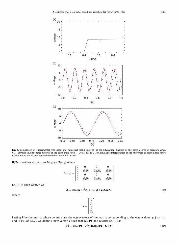
Fig. 9(a) shows the variation of the pitch angle as a function of the freestream velocity when ka2 ¼ 380 N m. The solidcurve presents the analytical results while the red points show the measured values. Fig. 9(b) and (c) shows the timehistories of the pitch angle for 1 s and 0.3 s, respectively, when U¼8.62 m/s. We note that there is a slight shift in thefrequency between the experimental and theoretical results. This behavior is associated with a change in the pitchstiffness that is caused by higher angles of attack which stressed the spring wire as discussed by Conner et al. [9].

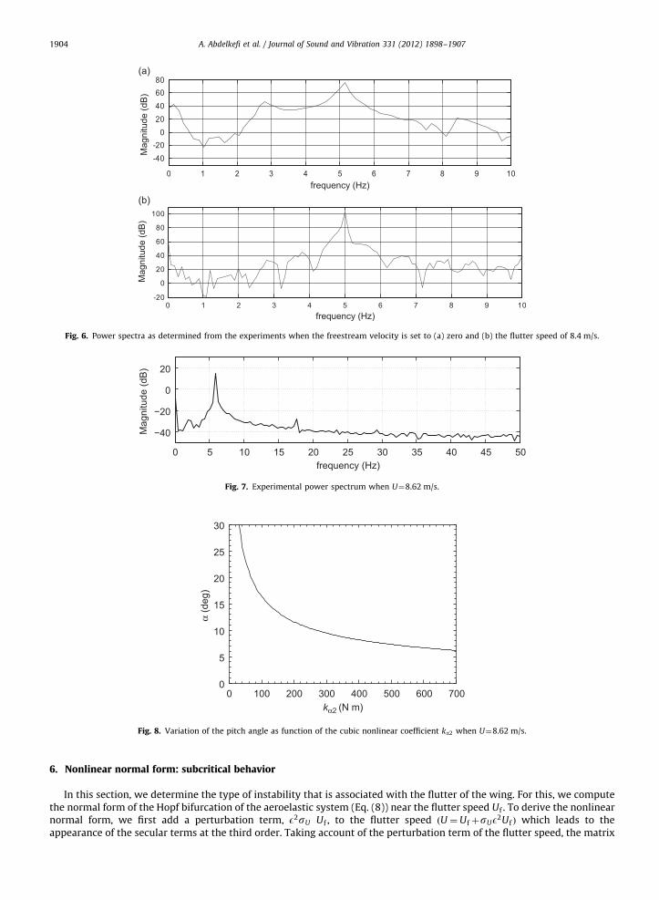
Fig. 6. Power spectra as determined from the experiments when the freestream velocity is set to (a) zero and (b) the flutter speed of 8.4 m/s.

0 5 10 15 20 25 30 35 40 45 50

−40

−20

0

20

frequency (Hz)

Mag

nitu

de (d

B)

Fig. 7. Experimental power spectrum when U¼8.62 m/s.

0 100 200 300 400 500 600 7000

5

10

15

20

25

30

kα2 (N m)

α (d

eg)

Fig. 8. Variation of the pitch angle as function of the cubic nonlinear coefficient ka2 when U¼8.62 m/s.

A. Abdelkefi et al. / Journal of Sound and Vibration 331 (2012) 1898–19071904

6. Nonlinear normal form: subcritical behavior

In this section, we determine the type of instability that is associated with the flutter of the wing. For this, we computethe normal form of the Hopf bifurcation of the aeroelastic system (Eq. (8)) near the flutter speed Uf . To derive the nonlinearnormal form, we first add a perturbation term, E2sU Uf , to the flutter speed ðU ¼UfþsUE2Uf Þ which leads to theappearance of the secular terms at the third order. Taking account of the perturbation term of the flutter speed, the matrix

8.2 8.4 8.6 8.80

5

10

15

20

α (d

eg)

α (d

eg)

α (d

eg)

0.0 0.2 0.4 0.6 0.8 1.0-10

-5

0

5

10

t (s)

0.00 0.05 0.10 0.15 0.20 0.25 0.30-10

-5

0

5

10

t (s)

U (m/s)

Fig. 9. Comparison of experimental (red dots) and numerical (solid line) of (a) the bifurcation diagram of the pitch degree of freedom when

ka2 ¼ 380 N m (b,c) the time histories of the pitch angle for ka2 ¼ 380 N m and U¼8.62 m/s. (For interpretation of the references to color in this figure

legend, the reader is referred to the web version of this article.)

A. Abdelkefi et al. / Journal of Sound and Vibration 331 (2012) 1898–1907 1905

BðUÞ is written as the sum BðUf ÞþE2B1ðUf Þ where

B1ðUf Þ ¼

0 0 0 0

0 �d1Uf �2k1U2f �d2Uf

0 0 0 0

0 �d3Uf �2k2U2f �d4Uf

266664

377775

Eq. (8) is then written as

_X ¼ BðUf ÞXþE2sUB1ðUf ÞXþCðX,X,XÞ (9)

where

C¼

0

C2

0

C4

266664

377775

Letting P be the matrix whose columns are the eigenvectors of the matrix corresponding to the eigenvalues 7 j o1�m1

and 7 jo2 of BðUf Þ, we define a new vector Y such that X¼ PY and rewrite Eq. (9) as

P _Y ¼ BðUf ÞPYþE2sUB1ðUf ÞPYþCðPYÞ (10)

A. Abdelkefi et al. / Journal of Sound and Vibration 331 (2012) 1898–19071906

Multiplying Eq. (10) from the left with the inverse P�1 of P, we obtain

_Y ¼ JYþE2sUKYþP�1CðYÞ (11)

where J¼ P�1BðUf ÞP is a diagonal matrix whose elements are the eigenvalues 7 j o1�m1 and 7 j o2 of BðUf Þ andK¼ P�1B1ðUf ÞP. We note that Y2 ¼ Y1 , Y4 ¼ Y3 , and hence Eq. (11) can be written in component form as

_Y 1 ¼ jo1Y1�m1Y1þE2sU

X5

1

K1iYiþN1ðY,Y,YÞ (12)

_Y 3 ¼ jo2Y3þE2sU

X5

1

K3iYiþN3ðY,Y,YÞ (13)

where the NiðY,Y,YÞ are tri-linear functions of the Y. Because we considered only cubic nonlinearities, the solution of Y1

decays to zero. Consequently, we retain only the non-decaying solution (Y3). Moreover, to compute the normal form of theHopf bifurcation of Eqs. (12) and (13) near U ¼Uf , we follow Nayfeh and Balachandran [15] and search for a third-orderapproximate solution of Eq. (13) in the following form:

Y3 ¼ EY31ðT0,T2ÞþE2Y32ðT0,T2ÞþE3Y33ðT0,T2ÞþOðE4Þ (14)

where Tn ¼ Ent. In terms of the Ti, the time derivative can be expressed as

d

dt¼

qqT0þE2 q

qT2¼D0þE2D2 (15)

Substituting Eqs. (14) and (15) into Eq. (13). These new equations must hold for all values of E, therefore the coefficients of likepowers of E must satisfy these new equations. This leads to two different set of relations corresponding to E and E3 as follows:

Order (E)D0Y31�jo2Y31 ¼ 0 (16)

Order (E3)

D0Y33�jo2Y33 ¼�D2Y31þsUðK33Y31ÞþNðY31,Y31,Y31 ÞþccþNST (17)

where NST stands for terms that do not produce secular terms and cc stands for the complex conjugate of the precedingterms. The solution of Eq. (16) can be expressed as

Y31 ¼ AðT2Þejo2T0 (18)

Substituting Eq. (18) into Eq. (17), eliminating the terms that lead to secular terms, we obtain the modulation equation

D2A¼ sUK33AþaeA2A (19)

The effects of the cubic nonlinearity (ka2) on the system are expressed through the expression of ae. For convenience, we

write Eq. (19) as

D2A¼ bAþaeA2A (20)

where b¼ sUK33.Letting AðT2Þ ¼

12a e igðT2Þ and separating the real and imaginary parts in Eq. (20), we obtain the following nonlinear

normal form of Hopf bifurcation:

a0 ¼ braþ1

4aera

3 (21)

g0 ¼ biþ1

4aeia

2 (22)

where a is the amplitude and g is the shifting angle of the periodic solution. Eq. (21) has generally three equilibriumsolutions which are

a¼ 0, a¼ 7

ffiffiffiffiffiffiffiffiffiffiffiffi�4br

aer

s

a¼0 which corresponds to the fixed points (0,0). The other two solutions are the nontrivial ones. The origin isasymptotically stable for br o0 or br ¼ 0 and aer o0 , unstable for br 40 or br ¼ 0 and aer 40. For the nontrivial solutions,they exist when braer o0. Furthermore, they are stable (supercritical Hopf bifurcation) for br 40 and aer o0 and unstable(subcritical Hopf bifurcation) for br o0 and aer 40. Upon substituting the physical parameters, the expressions of thelinear and nonlinear coefficients of the normal form are given by

br ¼ 1:013sU (23)

aer ¼ 0:00166ka2

A. Abdelkefi et al. / Journal of Sound and Vibration 331 (2012) 1898–1907 1907

Based on the numerical integrations, the cubic nonlinear coefficient ka2 is set equal to 380 N m. Consequently, because(aer 40), this system has a subcritical instability. This result confirms the experimental observation of the existence of(LCO) for larger initial displacements at freestream velocities that are smaller than the flutter speed. The ability to modeland identify the type of bifurcation associated with the freeplay nonlinearity provides a capability that can be used toavoid subcritical responses such as the one observed in these experiments.

7. Conclusion

In this work, we have performed identification of freeplay nonlinearity in a two degree-of-freedom aeroelastic system.The system is composed of a rigid airfoil supported by a nonlinear torsional spring. The databases for the identification aregenerated from experimental data of periodic responses that included the flutter frequency and its third harmonics. Basedon this characterization of the responses, linear and nonlinear analyses that represent the freeplay nonlinearity of thetorsional spring with a polynomial expansion up to the third order were performed. This representation allowed the use ofthe normal form of the Hopf bifurcation to characterize the type of instability of this system. It was determined that theensuing Hopf bifurcation is of the subcritical type. The representative model and identified parameters were validated byintegrating the governing equations and comparing response values from this integration with experimental responses.

Acknowledgment

The authors acknowledge the financial support of the State of S~ao Paulo Research Agency (FAPESP), Brazil (grant 2007/08459-1) and the Coordination for the Improvement of Higher Education Personnel (CAPES), Brazil (grant 0205109).

References

[1] E.H. Dowell, D. Tang, Nonlinear aeroelasticity and unsteady aerodynamics, AIAA Journal 40 (2002) 1697–1707.[2] H.C. Gilliat, T.W. Strganac, A.J. Kurdila, An investigation of internal resonance in aeroelastic systems, Nonlinear Dynamics 31 (2003) 1–22.[3] A. Raghothama, S. Narayanan, Non-linear dynamics of a two-dimensional air foil by incremental harmonic balance method, Journal of Sound and

Vibration 226 (1999) 493–517.[4] L. Liu, Y.S. Wong, B.H.K. Lee, Application of the centre manifold theory in non-linear aeroelasticity, Journal of Sound and Vibration 234 (2000) 641–659.[5] T. O’Neil, Nonlinear aeroelastic response—analyses and experiments, 34th AIAA, Aerospace Sciences Meeting and Exhibit, 1996.[6] M.D. Conner, Nonlinear Aeroelasticity of an Airfoil Section with Control Surface Freeplay, PhD Thesis, Department of Mechanical Engineering and

Materials Science, Duke University, 1996.[7] D.S. Woolston, An investigation of effects of certain types of structural nonlinearities on wing and control surface flutter, Journal of the Aeronautical

Sciences (1957) 9936–9956.[8] B.H.K. Lee, S. Price, E.H. Dowell, Y. Wong, Nonlinear aeroelastic analysis of airfoils: bifurcation and chaos, Progress in Aerospace Sciences 35 (1999)

205–334.[9] M.D. Conner, D.M. Tang, E.H. Dowell, L.N. Virgin, Nonlinear behavior of a typical airfoil section with control surface freeplay: a numerical and

experimental study, Journal of Fluids and Structures 11 (1997) 89–109.[10] R.M.G. Vasconcellos, F.D. Marques, M.H. Hajj, Time series analysis and identification of a nonlinear aeroelastic section, 51st AIAA/ASME/ASCE/AHS/ASC

Structures, Structural Dynamics and Materials Conference, Orlando, FL, April 12–15, 2010.[11] L. Daochun, G. Shijun, X. Jinwu, Aeroelastic dynamic response and control of an airfoil section with control surface nonlinearities, Journal of Sound

and Vibration 239 (2010) 4756–4771.[12] Y.C. Fung, An Introduction to the Theory of Aeroelasticity, Wiley, NY, 1955.[13] E.H. Dowell, A Modern Course in Aeroelasticity, Kluwer, Dordrecht, 1995.[14] T.W. Strganac, J. Ko, D.E. Thompson, A.J. Kurdila, Identification and control of limit cycle oscillations in aeroelastic systems, Proceedings of the 40th

AIAA/ASME/ASCE/AHS/ASC Structures, Structural Dynamics, and Materials Conference and Exhibit, AIAA Paper No. 99-1463, 1999.[15] A.H. Nayfeh, B. Balachandran, Applied Nonlinear Dynamics, Wiley Series in Nonlinear Science, NY, 1994.