Density-based modeling and identification ofbiochemical networks in cell populations

J. Hasenauer1,∗, S. Waldherr1, M. Doszczak2,P. Scheurich2, and F. Allgower1

1Institute of Systems Theory and Automatic ControlUniversity of Stuttgart, Germany

www.ist.uni-stuttgart.de

2Institute of Cell Biology and Immunology,University of Stuttgart, Germany

www.uni-stuttgart.de/izi

∗Corresponding author (hasenauer@ist.uni-stuttgart.de)

February 24, 2010

Abstract

In many biological processes heterogeneity within cell populations is an importantissue. In this work we consider populations where the behavior of every singlecell can be described by a system of ordinary differential equations. Heterogeneityamong individual cells is accounted for by differences in parameter values andinitial conditions. Hereby, parameter values and initial conditions are subject toa distribution function which is part of the model specification. Based on thesingle cell model and the considered parameter distribution, a partial differentialequation model describing the distribution of cells in the state and in the outputspace is derived.

For the estimation of the parameter distribution within the model, we considerexperimental data as obtained from flow cytometric analysis. From these noise-corrupted data a density-based statistical data model is derived. Using this data

1

arX

iv:1

002.

4599

v1 [

q-bi

o.M

N]

24

Feb

2010

model the parameter distribution within the cell population is computed usingconvex optimization techniques.

To evaluate the proposed method, a model for the caspase activation cascadeis considered. It is shown that for known noise properties the unknown parameterdistributions in this model are well estimated by the proposed method.

Keywords: parameter estimation, cell population, kernel-density estimation, flowcytometry, convex optimization

1 Introduction

Most of the modeling performed in the area of systems biology aims at achievinga quantitative description of intracellular pathways. Hence, most available modelsdescribe a ”typical cell” on the basis of experimental data. Unfortunately, experi-mental data are in general obtained using cell population experiments, e.g. westernblotting. If the considered population is highly heterogeneous, meaning that thereis a large cell-cell variability, fitting a single cell model to cell population data canlead to biologically meaningless results. To understand the dynamical behavior ofheterogeneous cell populations it is crucial to develop integrated cell populationmodels.

Modeling on the population scale has already been addressed by Mantzaris(2007) and Munsky et al. (2009). These authors demonstrated that populationscan show a bimodal response if stochasticity in biochemical reactions is considered.But besides stochasticity in biochemical reactions there are other reasons whichcan also lead to heterogeneity in populations. Examples are unequal partition-ing of cellular material at cell division (Mantzaris, 2007), genetic and epigeneticdifferences (Avery, 2006).

For the purpose of this paper, we describe heterogeneity in populations by dif-ferences in parameter values of the model describing the single cell dynamics. Thenetwork structure is assumed to be identical in all cells, as this usually representsthe physical interactions among molecules, which should be independent of thecell’s state. This parametric approach is well suited for genetic and epigeneticdifferences. The distribution of parameter values within the cell population of in-terest is described by a multivariate probability density function, which is part ofthe model specification.

In the following the problem of estimating the parameter distribution func-tion is studied. Therefore, we consider high-throughput experimental methodssuch as flow cytometry, which can be used to measure concentration distributionswithin cell populations by suitable fluorescent labeled antibodies. Classical flowcytometry devices can measure several thousand cells per second.

2

To estimate the parameter distributions, in a first step, an appropriate pop-ulation model has to be found. In the literature mathematical models of cellpopulations are either described as cell ensembles (Waldherr et al., 2009; Munskyet al., 2009), or as a non-linear partial differential equation (PDE) for the distri-bution of the state variables (Mantzaris, 2007; Luzyanina et al., 2009; Tsuchiyaet al., 1966). In case of ensemble models, a differential equation is assigned toeach cell, making an in depth theoretical analysis difficult. PDE models, whichdescribe the time evolution of the distributions of the state variables based on thesingle cell models, are easy to handle from a theoretical point of view but hardto simulate for a large state dimension of the single cell model. Therefore, onlylow dimensional PDE models of populations have been studied in literature so far(Mantzaris, 2007; Luzyanina et al., 2007, 2009).

In this paper a PDE model for the state distribution within a heterogeneouscell population is derived. Given the solution of this PDE the probability densityof measuring a certain output can be determined. As for the estimation only themeasured outputs are required, a numerical method for computing the output dis-tribution is outlined. This methods employs a particle-based approach (Rawlingsand Bakshi, 2006) and classical density estimation (Silverman, 1986).

Based on these efficient computation scheme for the population response anestimation method is developed. A statistical model of the measured output dis-tribution is derived from the single cell measurement obtained at every measure-ment instance. Therefore, again kernel density estimators are used as they havebetter asymptotic properties than commonly used naive estimators (Luzyaninaet al., 2009). Given a model and the output distribution estimated from the mea-surement, a l2-norm minimization is performed over the set of possible parameterdistributions. By employing the model properties and a parameterization of theparameter distribution this optimization problem is convex and can be solved ef-ficiently.

The paper is structured as follows. In Section 2, the problem of estimating theparameter distribution is introduced. In Section 3, we present the statistical modelfor the measured data and the simulation model for state and output distribution.Section 4 gives a short overview of the used identification procedure before inSection 5 the proposed method is applied to a caspase activation model withartificial data.

Notation: Consider the m-dimensional hypersurface S ⊂ Rn. The integral Iof a function f(x), with f : Rn → R, over x ∈ S is written as

I =

∫Sf(x)dS. (1)

Furthermore, the i.th unit vector is denoted by ei.

3

2 Problem statement

For the purpose of this work, a model of a biochemical reaction network in apopulation of M cells is given by the collection of differential equations

x(i) = f(x(i), p(i)), x(i)(0) = x(i)0 ,

y(i) = h(x(i), p(i)), i ∈ {1, . . . ,M}(2)

with state variables x(i)(t) ∈ Rn, measured variables y(i)(t) ∈ Rm, and parametersp(i) ∈ Rq. The index i specifies the individual cells within the population. Theparameters p(i) can be kinetic constants, e.g. reaction rates or binding affinities.The cell-cell interaction of the considered pathway is assumed to be negligible, asit is the case in many in vitro lab experiments.

In the following heterogeneity within the cell population is introduced, modeledby differential parameter values and initial conditions among individual cells. Thedistribution of parameters p(i) and initial conditions x

(i)0 is given by a probability

density function Φ : Rn+q → R+ with∫Rn+q Φ(x0, p)dx0dp = 1. For ease of nota-

tion, we write ξ0 = (xT0 , pT )T . The probability density function Φ is part of the

model specification and the parameters and initial conditions of cell i are subjectto the probability distribution

Pr(ξ(i)0,1 ≤ ξ1, · · · , ξ(i)

0,n+q ≤ ξn+q) =

∫ ξ1

−∞· · ·∫ ξn+q

−∞Φ(ξ)dξ1 · · · dξn+q. (3)

As outlined in Section 1, for the study of cell populations high-throughputcell population measurements are available. Using these experimental techniquesprotein concentrations within thousands of cells can be measured at every mea-surement instance, tk, k = 1, . . . , N . This yields the measurement data

Dk ={(tk, ψ

(i)(tk))}

i∈Ik, k = 1, . . . , N (4)

where ψ(i) is the measured output of the cell i and Ik is the index set of thecells measured at time tk. Note that the cells cannot be tracked over time, andare removed from the population in order to obtain the measurements. Thus,no single-cell time series data are available. On the other hand, the samples areindependent and equally distributed and card(Ik) is assumed to be large, suchthat an approximation of the output distribution is possible.

Like most measurement devices, also high-throughput fluorescence measure-ments are subject to noise. For the rest of the paper, noise consisting of a relativeand an absolute part is considered,

ψ(i)(tk) = diag(η1)y(i)(tk) + η2, (5)

4

in which ψ(i) is the measured output and ηj ∈ Rm is a vector of log-normallydistributed random variables with probability density functions

Θij(η

ij) =

1√2πσijη

ij

exp

{−1

2

(log ηij − µij

σij

)2}, i = 1, 2, j = 1, . . . ,m, (6)

yielding the joint probability density

Θi(ηi) =m∏j=1

Θij(η

ij). (7)

Log-normally distributed random variables are chosen here, since they are a goodmodel for the commonly seen noise distributions of the considered measurementdevice and conserve the positivity of all variables. For notational simplicity themeasurement errors of the different concentrations are assumed to be uncorrelated.This constraint can be removed easily.

Given this setup the problem we are concerned with is:

Problem 1 Given the measurement data Dk, k = 1, . . . , N , the cell populationmodel (2), and the noise model (7), determine the parameter distribution Φ(ξ).

Unfortunately, estimation of Φ(ξ) using a cell population model with a finitenumber of cells and discrete sampled data is fairly difficult as no single cell tra-jectories are available. A far more natural approach would be to use a density de-scription, as the available measurement data can be interpreted as samples drawnfrom the probability density function of the output. This interpretation is alsoquite appealing from a point of modeling as the number of cells considered in astandard lab experiment is of the order of 109 and hence nevertheless too largeto be simulated on an individual basis. In the next chapter a PDE model for theprobability density of the output and a density model for the measurement datais derived.

3 Density-based modeling of heterogeneous cell

populations

As outlined in the previous section, a continuous statistical model for the mea-surement data, as well as for the evolution of the state and output density wouldbe preferable. These two aspects are addressed in the following.

5

3.1 Density model of measurement data

The data collected by the considered measurement devices Dk are samples drawnfrom the distribution of the measured output, as mentioned in Section 2. LetΨ(ψ, tk) be the distribution of the measured outputs ψ(i)(tk) at time tk. As Ψ(ψ, tk)is considered to be a probability density, classical density estimation methods canbe employed for estimating Ψ(ψ, tk) from the given samples Dk.

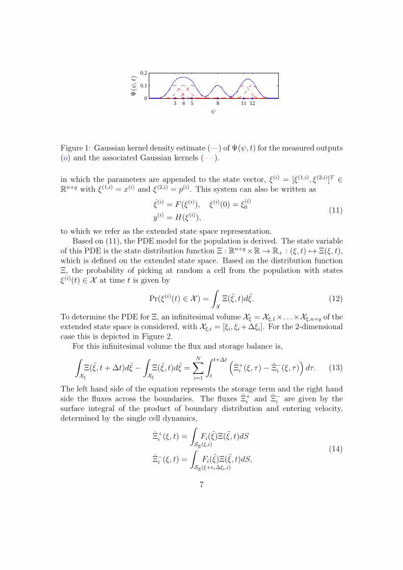
In this work, the problem of determining Ψ(ψ, tk) from Dk is approachedusing kernel density estimators. Kernel density estimators are non-parametricapproaches to estimate probability distributions from sampled data (Silverman,1986). They are widely used and can be thought of as placing probability ”bumps”at each observation, as depicted in Figure 1. These ”bumps” are the kernel func-tion K, with

∫Rm K(ψ)dψ = 1. Note that here only the equations for the one

dimensional case are given. The extension towards higher dimensions is straight-forward and can be found in Silverman (1986). In this work, a Gaussian kernelgiven by

K(ψ − ψ(i), h

)=

1√2πh

exp

{−1

2

(ψ − ψ(i)

h

)2}, (8)

with standard deviation h is used. In this context, h is also called smoothingparameter in the literature (Silverman, 1986).

Given the kernel K an estimator of the probability density for a given set ofsamples Dk is

Ψ(ψ, tk) =1

Mk

∑i∈Ik

K(ψ − ψ(i)(tk), h

), (9)

where Mk is the cardinality of Ik. The selection of the smoothing parameter his crucial and depends strongly on Mk. In this work h is chosen according to theleast-squares cross-validation method (Stone, 1984). As Mk is considered to be oforder 104, it can be assumed that the the estimated output distribution ins closeto the actual output distribution.

3.2 PDE model of density evolution

As outlined previously, a continuous model for the output density is desirablefor the purpose of parameter identification. Therefore, a PDE model for the cellpopulation is derived in the next step.

At first the single cell model is transformed in an extended state space model

ξ(i) =

(f(ξ(1,i), ξ(2,i))

0

), ξ(i)(0) =

(x

(i)0

p(i)

)y(i) = h(ξ(1,i), ξ(2,i))

(10)

6

3 4 5 8 11 120

0.1

0.2

ψ

Ψ(ψ,t)

Figure 1: Gaussian kernel density estimate (—) of Ψ(ψ, t) for the measured outputs(o) and the associated Gaussian kernels (– –).

in which the parameters are appended to the state vector, ξ(i) = [ξ(1,i), ξ(2,i)]T ∈Rn+q with ξ(1,i) = x(i) and ξ(2,i) = p(i). This system can also be written as

ξ(i) = F (ξ(i)), ξ(i)(0) = ξ(i)0

y(i) = H(ξ(i)),(11)

to which we refer as the extended state space representation.Based on (11), the PDE model for the population is derived. The state variable

of this PDE is the state distribution function Ξ : Rn+q×R→ R+ : (ξ, t) 7→ Ξ(ξ, t),which is defined on the extended state space. Based on the distribution functionΞ, the probability of picking at random a cell from the population with statesξ(i)(t) ∈ X at time t is given by

Pr(ξ(i)(t) ∈ X ) =

∫X

Ξ(ξ, t)dξ. (12)

To determine the PDE for Ξ, an infinitesimal volume Xξ = Xξ,1×. . .×Xξ,n+q of theextended state space is considered, with Xξ,i = [ξi, ξi+∆ξi]. For the 2-dimensionalcase this is depicted in Figure 2.

For this infinitesimal volume the flux and storage balance is,∫Xξ

Ξ(ξ, t+ ∆t)dξ −∫Xξ

Ξ(ξ, t)dξ =N∑i=1

∫ t+∆t

t

(Ξ+i (ξ, τ)− Ξ−i (ξ, τ)

)dτ. (13)

The left hand side of the equation represents the storage term and the right handside the fluxes across the boundaries. The fluxes Ξ+

i and Ξ−i are given by thesurface integral of the product of boundary distribution and entering velocity,determined by the single cell dynamics,

Ξ+i (ξ, t) =

∫SΞ(ξ,i)

Fi(ξ)Ξ(ξ, t)dS

Ξ−i (ξ, t) =

∫SΞ(ξ+ei∆ξi,i)

Fi(ξ)Ξ(ξ, t)dS,

(14)

7

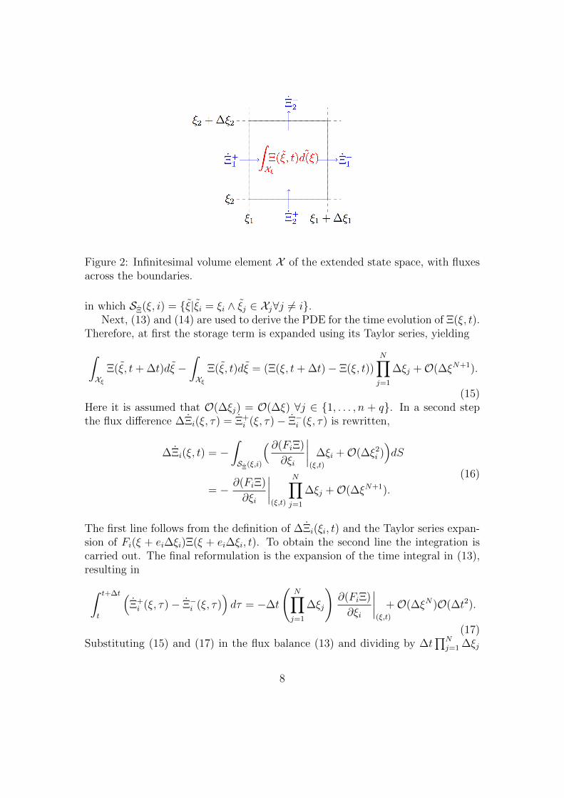
Figure 2: Infinitesimal volume element X of the extended state space, with fluxesacross the boundaries.

in which SΞ(ξ, i) = {ξ|ξi = ξi ∧ ξj ∈ Xj∀j 6= i}.Next, (13) and (14) are used to derive the PDE for the time evolution of Ξ(ξ, t).

Therefore, at first the storage term is expanded using its Taylor series, yielding∫Xξ

Ξ(ξ, t+ ∆t)dξ −∫Xξ

Ξ(ξ, t)dξ = (Ξ(ξ, t+ ∆t)− Ξ(ξ, t))N∏j=1

∆ξj +O(∆ξN+1).

(15)Here it is assumed that O(∆ξj) = O(∆ξ) ∀j ∈ {1, . . . , n + q}. In a second stepthe flux difference ∆Ξi(ξ, τ) = Ξ+

i (ξ, τ)− Ξ−i (ξ, τ) is rewritten,

∆Ξi(ξ, t) = −∫SΞ(ξ,i)

( ∂(FiΞ)

∂ξi

∣∣∣∣(ξ,t)

∆ξi +O(∆ξ2i ))dS

= − ∂(FiΞ)

∂ξi

∣∣∣∣(ξ,t)

N∏j=1

∆ξj +O(∆ξN+1).

(16)

The first line follows from the definition of ∆Ξi(ξi, t) and the Taylor series expan-sion of Fi(ξ + ei∆ξi)Ξ(ξ + ei∆ξi, t). To obtain the second line the integration iscarried out. The final reformulation is the expansion of the time integral in (13),resulting in∫ t+∆t

t

(Ξ+i (ξ, τ)− Ξ−i (ξ, τ)

)dτ = −∆t

(N∏j=1

∆ξj

)∂(FiΞ)

∂ξi

∣∣∣∣(ξ,t)

+O(∆ξN)O(∆t2).

(17)Substituting (15) and (17) in the flux balance (13) and dividing by ∆t

∏Nj=1 ∆ξj

8

then yields,

Ξ(ξ, t+ ∆t)− Ξ(ξ, t) +O(∆ξ)

∆t= −

N∑i=1

∂(FiΞ)

∂ξi

∣∣∣∣ξ

+O(∆t). (18)

Given this the PDE governing the evolution of Ξ(ξ, t) is obtained by taking thelimits ∆ξi → 0 and ∆t→ 0, leading to

∂Ξ

∂t(ξ, t) = −

N∑i=1

∂(FiΞ)

∂ξi(ξ, t), (19)

for sufficiently smooth Ξ(ξ, t). This final equation is somehow what we expected,a transport equation with position dependent transport direction and velocity,according to the single cell dynamics. The initial condition of (22) is the initialdistribution on the extended state space,

Ξ(ξ, 0) = Φ(ξ), ∀ξ ∈ Rn+q+ . (20)

From the state distribution Ξ, the output distribution Υ is computed as theintegral of the state distribution along H(ξ) = y,

Υ(y, t) =

∫SΥ(y)

Ξ(ξ, t)dS, (21)

where SΥ(y) = {ξ|H(ξ) = y}.The resulting partial differential equation system is

∂Ξ

∂t(ξ, t) = −

N∑i=1

∂(FiΞ)

∂ξi(ξ, t), Ξ(ξ, 0) = Φ(ξ)

Υ(y, t) =

∫SΥ(y)

Ξ(ξ, t)dS,

(22)

where Ξ : Rn+q × R → R+ and Υ : Rm × R → R+. This PDE is of first order,quasilinear and known as Liouville’s equation. The solution always exists forsufficiently smooth F (·) (Evans, 1998).

As the measurements are noise corrupted, the distribution of measured outputsΨ(ψ, t) is different from the actual output distribution Υ(y, t). It is defined by

Ψ(ψ, t)=

∫SΨ(ψ)

Υ(y, t)Θ1(η1)Θ2(η2)dS, (23)

where SΨ(ψ) = {[yT , (η1)T , (η2)T ]T |diag(η1)y + η2 = ψ}.

9

3.3 Numerical solution of PDE

In order to study the time evolution of the output distribution Υ(y, t) and themeasured output distribution Ψ(ψ, t) equation (22) has to be solved for given Φ.As Ξ(ξ, t) is defined on the (n+ q)-dimensional space, standard grid based solversare not able to solve (22) for n+q > 3. Theoretically, the methods of characteristicscan be used (Evans, 1998) but for the high dimensional system we are going tostudy, also this method is difficult to apply. Instead, a stochastic method is used,which is known from particle filtering (Rawlings and Bakshi, 2006).

This stochastic integration method is based on a particle description of themodel, which is in our case equivalent to the cell ensemble model (2). To compute

Ψ(ψ, tk), at first a set of samples {(x(i)0 , p

(i))}i=1,...,S, is drawn from Φ(ξ), where S isthe number of samples. For this set of samples the single cell model (9) is simulated,resulting in a set of simulated outputs {(y(i)(t))}i=1,...,S. y(i)(t) is then corruptedby noise according to (5) resulting in {(ψ(i)(t))}i=1,...,S. Given this a numericalapproximation of Ψ(ψ, t) can be determined using the kernel density estimatordescribed in Section 3.1. This numerical stochastic approximation the output of(22) can be shown to converge as S →∞. Hence, the measured output distributionΨ(ψ, tk) can be axproximated also for high dimensional nonlinear systems.

4 Estimation of parameter distributions

As mentioned in Section 2 the problem studied in this work is the estimation ofthe parameter distribution Φ from the data Dk. This problem is approached inthe following by minimizing the l2-norm of the model-data mismatch,

J(

Φ)

=N∑k=1

∣∣∣∣∣∣Ψ(ψ, tk)− Ψ(ψ, tk, Φ)∣∣∣∣∣∣2

2. (24)

in which Ψ(ψ, t, Φ) is the distribution of the measured output ψ obtained by simu-lation with the parameter distribution Φ(ξ). According to the cost J , the optimalparameter distribution Φ∗(ξ) is than given by

Φ∗ = arg minΦ J(Φ)

subject to∫Rn+q

+Φ(ξ)dξ = 1

Φ(ξ) ≥ 0 ∀ξ ∈ Rn+q+ ,

(25)

where the last two constraints enforce that Φ(ξ) is a probability distribution.

Remark 1 In the whole section the measured outputs Ψ(ψ, t) are compared withthe noise corrupted simulated output Ψ(ψ, t, Φ). This is possible as we assume a

10

0

0.5

1

· · ·Λi(p)

· · ·

pmin pmaxpimin pic pimax

p

Λ(p)

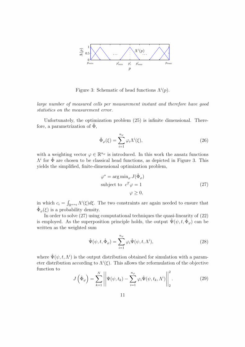
Figure 3: Schematic of head functions Λi(p).

large number of measured cells per measurement instant and therefore have goodstatistics on the measurement error.

Unfortunately, the optimization problem (25) is infinite dimensional. There-fore, a parametrization of Φ,

Φϕ(ξ) =

nϕ∑i=1

ϕiΛi(ξ), (26)

with a weighting vector ϕ ∈ Rnϕ is introduced. In this work the ansatz functionsΛi for Φ are chosen to be classical head functions, as depicted in Figure 3. Thisyields the simplified, finite-dimensional optimization problem,

ϕ∗ = arg minϕ J(Φϕ)

subject to cTϕ = 1

ϕ ≥ 0,

(27)

in which ci =∫Rn+q Λi(ξ)dξ. The two constraints are again needed to ensure that

Φϕ(ξ) is a probability density.In order to solve (27) using computational techniques the quasi-linearity of (22)

is employed. As the superposition principle holds, the output Ψ(ψ, t, Φϕ) can bewritten as the weighted sum

Ψ(ψ, t, Φϕ) =

nϕ∑i=1

ϕiΨ(ψ, t,Λi), (28)

where Ψ(ψ, t,Λi) is the output distribution obtained for simulation with a param-eter distribution according to Λi(ξ). This allows the reformulation of the objectivefunction to

J(

Φϕ

)=

N∑k=1

∣∣∣∣∣∣∣∣∣∣Ψ(ψ, tk)−

nϕ∑i=1

ϕiΨ(ψ, tk,Λi)

∣∣∣∣∣∣∣∣∣∣2

2

. (29)

11

Employing this the optimization problem (27) can finally be written as

ϕ∗ = arg minϕ∑N

k=1 (Akϕ− bk)T W (Akϕ− bk)subject to cTϕ = 1

ϕ ≥ 0,

(30)

where the integral || · ||22 is approximated, e.g. using the trapezoidal rule. Thecolumn vector bk contains hereby the values Ψ(ψ, tk) at the grid points of the dis-cretization. Equivalently, the ith column of Ak contains the values of Ψ(ψ, tk,Λ

i)at the grid points. The matrix W is a constant weighting matrix, determined bythe chosen approximation of || · ||22.

Note that problem (30) is convex. Hence, even in the case of high dimensionalϕ, convergence to the optimal parameter distribution within the considered classof distributions can be guaranteed.

5 Application to the caspase cascade

Programmed cell death, also called apoptosis, is an important physiological processto remove infected, malfunctioning, or no longer needed cells from a multicellularorganism. Pathways to induce apoptosis converge at the caspase activation cascade(Hengartner, 2000). A mathematical model for this network has been proposed byEissing et al. (2004). Here, we consider the caspase activation in response to anexternal death receptor stimulus, e.g. the tumor necrosis factor (TNF). As seenfrom experimental cytotoxicity assays, the cellular response to a TNF stimulus ishighly heterogeneous, with some cells dying and others surviving. To understandthe process at the physiological level it is thus crucial to consider the cellularheterogeneity, using for example cell population modeling.

12

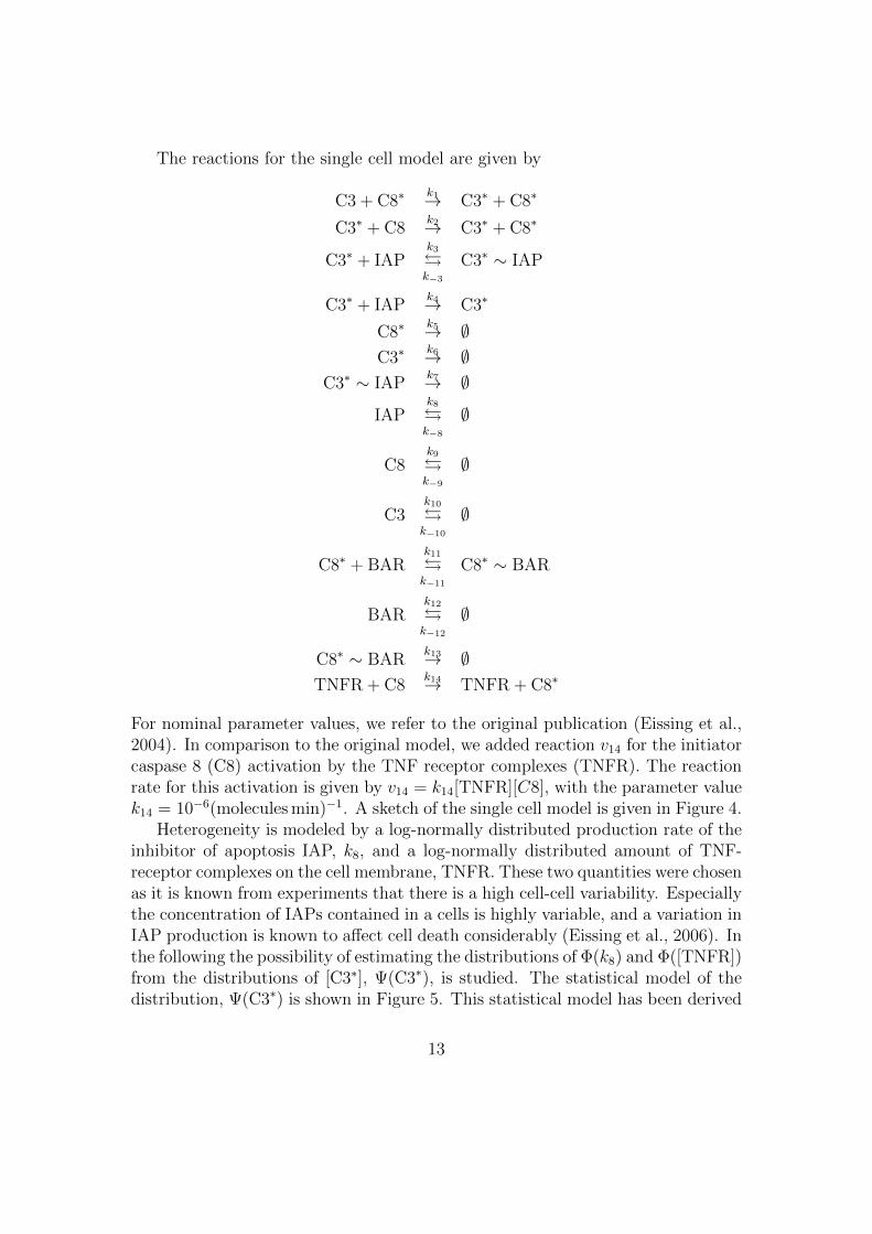
The reactions for the single cell model are given by

C3 + C8∗k1→ C3∗ + C8∗

C3∗ + C8k2→ C3∗ + C8∗

C3∗ + IAPk3

�k−3

C3∗ ∼ IAP

C3∗ + IAPk4→ C3∗

C8∗k5→ ∅

C3∗k6→ ∅

C3∗ ∼ IAPk7→ ∅

IAPk8

�k−8

∅

C8k9

�k−9

∅

C3k10

�k−10

∅

C8∗ + BARk11

�k−11

C8∗ ∼ BAR

BARk12

�k−12

∅

C8∗ ∼ BARk13→ ∅

TNFR + C8k14→ TNFR + C8∗

For nominal parameter values, we refer to the original publication (Eissing et al.,2004). In comparison to the original model, we added reaction v14 for the initiatorcaspase 8 (C8) activation by the TNF receptor complexes (TNFR). The reactionrate for this activation is given by v14 = k14[TNFR][C8], with the parameter valuek14 = 10−6(molecules min)−1. A sketch of the single cell model is given in Figure 4.

Heterogeneity is modeled by a log-normally distributed production rate of theinhibitor of apoptosis IAP, k8, and a log-normally distributed amount of TNF-receptor complexes on the cell membrane, TNFR. These two quantities were chosenas it is known from experiments that there is a high cell-cell variability. Especiallythe concentration of IAPs contained in a cells is highly variable, and a variation inIAP production is known to affect cell death considerably (Eissing et al., 2006). Inthe following the possibility of estimating the distributions of Φ(k8) and Φ([TNFR])from the distributions of [C3∗], Ψ(C3∗), is studied. The statistical model of thedistribution, Ψ(C3∗) is shown in Figure 5. This statistical model has been derived

13

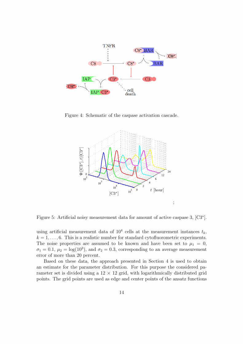
Figure 4: Schematic of the caspase activation cascade.

102

103

104

105 0

24

612

240

t [hour][C3∗]

Ψ([C3∗ ],t)[C3∗ ]

;

Figure 5: Artificial noisy measurement data for amount of active caspase 3, [C3∗].

using artificial measurement data of 104 cells at the measurement instances tk,k = 1, . . . , 6. This is a realistic number for standard cytofluorometric experiments.The noise properties are assumed to be known and have been set to µ1 = 0,σ1 = 0.1, µ2 = log(103), and σ2 = 0.3, corresponding to an average measurementerror of more than 20 percent.

Based on these data, the approach presented in Section 4 is used to obtainan estimate for the parameter distribution. For this purpose the considered pa-rameter set is divided using a 12 × 12 grid, with logarithmically distributed gridpoints. The grid points are used as edge and center points of the ansatz functions

14

0

0.2

0.4

0.6

0.8

1

1.2x 10−3

101 102 103 104

k8

Φ(k

8)

0

0.2

0.4

0.6

0.8

1x 10−2

101 102 103

[TNFR]

Φ([TNFR])

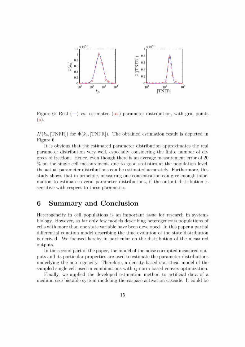
Figure 6: Real (—) vs. estimated (-o-) parameter distribution, with grid points(o).

Λi(k8, [TNFR]) for Φ(k8, [TNFR]). The obtained estimation result is depicted inFigure 6.

It is obvious that the estimated parameter distribution approximates the realparameter distribution very well, especially considering the finite number of de-grees of freedom. Hence, even though there is an average measurement error of 20% on the single cell measurement, due to good statistics at the population level,the actual parameter distributions can be estimated accurately. Furthermore, thisstudy shows that in principle, measuring one concentration can give enough infor-mation to estimate several parameter distributions, if the output distribution issensitive with respect to these parameters.

6 Summary and Conclusion

Heterogeneity in cell populations is an important issue for research in systemsbiology. However, so far only few models describing heterogeneous populations ofcells with more than one state variable have been developed. In this paper a partialdifferential equation model describing the time evolution of the state distributionis derived. We focused hereby in particular on the distribution of the measuredoutputs.

In the second part of the paper, the model of the noise corrupted measured out-puts and its particular properties are used to estimate the parameter distributionsunderlying the heterogeneity. Therefore, a density-based statistical model of thesampled single cell used in combinations with l2-norm based convex optimization.

Finally, we applied the developed estimation method to artificial data of amedium size bistable system modeling the caspase activation cascade. It could be

15

shown that the proposed method yields good estimation results in case of a setupwhich is realistic in terms of noise and amount of available data.

Acknowledgments

The authors acknowledge financial support from the German Federal Ministry ofEducation and Research (BMBF) within the FORSYS-Partner program (grant nr.0315-280A), from the German Research Foundation within the Cluster of Excel-lence in Simulation Technology (EXC 310/1) at the University of Stuttgart, andfrom Center Systems Biology (CSB) at the University Stuttgart.

References

S.V. Avery. Microbial cell individuality and the underlying sources of heterogeneity.Nat. Rev. Microbiol., 4:577–587, 2006.

T. Eissing, H. Conzelmann, E.D. Gilles, F. Allgower, E. Bullinger, and P. Scheurich.Bistability analyses of a caspase activation model for receptor-induced apoptosis. J.of Biol. Chem., 279 (35):36892–36897, 2004.

T. Eissing, S. Waldherr, E. Bullinger, C. Gondro, O. Sawodny, F. Allgower, P. Scheurich,and T. Sauter. Sensitivity analysis of programmed cell death and implications forcrosstalk phenomena during Tumor Necrosis Factor stimulation. In Proc. IEEE Conf.Contr. Appl. (CCA), pages 1746–52, 2006.

L. C. Evans. Partial Differential Equations. American Mathematical Society, June 1998.

M.O. Hengartner. The biochemistry of apoptosis. Nature, 407(6805):770–776, Oct 2000.

T. Luzyanina, D. Roose, T. Schenkel, M. Sester, S. Ehl, A. Meyerhans, and G. Bocharov.Numerical modelling of label-structured cell population growth using CFSE distribu-tion data. Theo. Biol. and Med. Mod., 4(26):1–14, 2007.

T. Luzyanina, D. Roose, and G. Bocharov. Distributed parameter identification forlabel-structured cell population dynamics model using CFSE histogram time-seriesdata. J. Math. Biol., 59:581–603, 2009.

N.V. Mantzaris. From single-cell genetic architecture to cell population dynamics: Quan-titatively decomposing the effects of different population heterogeneity sources for agenetic network with positive feedback architecture. Biophys. J., 92:4271–4288, 2007.

B. Munsky, B. Trinh, and M. Khammash. Listening to the noise: random fluctuationsreveal gene network parameters. Mol. Syst. Biol., 5, 2009.

16

J.B. Rawlings and B.R. Bakshi. Particle filtering and moving horizon estimation. Comp.and Chem. Eng., 30:1529–1541, 2006.

B.W. Silverman. Density Estimation for Statistics and Data Analysis. Monographs onStatistics and Applied Probability. London: Chapman and Hall, 1986.

C.J. Stone. An asymptotically optimal window selection rule for kernel density estima-tion. Annual Statistics, 12:1285–1297, 1984.

H.M. Tsuchiya, A.G. Fredrickson, and R. Aris. Dynamics of microbial cell populations.Adv. Chem. Eng., 6:125–206, 1966.

S. Waldherr, J. Hasenauer, and F. Allgower. Estimation of biochemical network param-eter distributions in cell populations. In Proc. of the 15th IFAC Symp. on Syst. Ident.,pages 1265–1270, 2009.

17