Homotopy types of complements of 2-arrangements in R^4

arX

iv:m

ath/

9712

251v

2 [

mat

h.G

T]

14

Aug

199

8

HOMOTOPY TYPES OF COMPLEMENTS OF

2-ARRANGEMENTS IN R4

DANIEL MATEI AND ALEXANDER I. SUCIU†

Abstract. We study the homotopy types of complements of arrangements ofn transverse planes in R4, obtaining a complete classification for n ≤ 6, andlower bounds for the number of homotopy types in general. Furthermore, weshow that the homotopy type of a 2-arrangement in R4 is not determined bythe cohomology ring, thereby answering a question of Ziegler. The invariantsthat we use are derived from the characteristic varieties of the complement.The nature of these varieties illustrates the difference between real and complexarrangements.

1. Introduction

In [13], Goresky and MacPherson introduced a generalization of the notion ofcomplex hyperplane arrangement. A 2-arrangement in R2d is a finite collectionA of codimension 2 linear subspaces so that, for every subset B ⊆ A, the space⋂H∈B H has even dimension. The main object of study is the complement of the

arrangement, X(A) = R2d \ ⋃H∈A H . Goresky and MacPherson computed the

cohomology groups of X . Bjorner and Ziegler [4] and Ziegler [30] determined thestructure of the cohomology algebraH∗(X ; Z). These results generalize the classicalwork of Arnol’d, Brieskorn, and Orlik and Solomon on the cohomology ring of thecomplement of a complex hyperplane arrangement, see [24]. Unlike the situationobtaining for the Orlik-Solomon algebra, which is completely determined by theintersection lattice, there remained an ambiguity in the relations definingH∗(X ; Z).Even in the simplest case of 2-arrangements in R4, a striking phenomenon occurs,showing that this ambiguity cannot be resolved, [30].

Each 2-arrangement A in R4 is a realization of the uniform matroid U2,n, wheren = |A| is the cardinality of the arrangement. Thus, the intersection lattice of suchan arrangement is uniquely determined by n. Furthermore, the homology groupsof the complement, X , the lower central series quotients of the group G = π1(X),and the Chen groups of G also depend only on n.

On the other hand, the cohomology ring of X is a more subtle invariant. Therelations in H∗(X ; Z) depend on, and are determined by the linking numbers ofthe associated link. Ziegler [30] found a pair of 2-arrangements of four planeswhich have non-isomorphic cohomology rings. His method, which uses an invariantderived from H∗(X ; Z), does not seem, however, to extend beyond n = 4.

In this paper, we introduce new homotopy-type invariants of complements of2-arrangements. These invariants, derived from the Alexander module, work for

1991 Mathematics Subject Classification. Primary 57M05, 57M25, 52B30; Secondary 14M12,20F36.

Key words and phrases. arrangement, line configuration, link, braid, characteristic variety.†Partially supported by N.S.F. grant DMS–9504833.

1

http://arXiv.org/abs/math/9712251v2

2 D. MATEI AND A. SUCIU

arbitrary n. As a first step towards the homotopy classification of 2-arrangements,we prove the following (see Corollary 6.6).

Theorem 1.1. For every integer n ≥ 1, there exist at least p(n − 1) − ⌊n−12 ⌋

different homotopy types of complements of 2-arrangements of n planes in R4, where

p(·) is the partition function, and ⌊·⌋ is the integer part function.

At the end of [30], Ziegler asks whether the cohomology ring determines thehomotopy type of the complement of a 2-arrangement, proposing as a candidatefor a negative answer the remarkable pair of arrangements of 6 planes found byMazurovskiı in [22]. Using successive cablings on Mazurovskiı’s pair, we answerZiegler’s question, as follows (see Theorem 8.4).

Theorem 1.2. For every integer n ≥ 6, there exists a pair of 2-arrangements of nplanes in R4, whose complements have isomorphic cohomology rings, but different

homotopy types.

Rigid isotopy of arrangements implies isotopy of their singularity links. Theconverse is not clear, though, since an isotopy may go outside the class of suchlinks. On the other hand, the classification, up to rigid isotopy, of 2-arrangementsin R4 is equivalent to the classification, also up to rigid isotopy, of configurationsof skew lines in R3. Such configurations were introduced by Viro in [28], and havebeen intensively studied since then, see the survey article by Crapo and Penne [8].The rigid isotopy classification of configurations of n skew lines in R3, was achievedby Viro [28] for n ≤ 5, and by Mazurovskiı [22] for n = 6.

It is readily seen that rigid isotopy of arrangements implies homotopy equivalenceof their complements. The converse is not true. Indeed, as first noted by Viro, thereexist configurations that are not isotopic to their mirror image. But clearly, thecomplements of mirror pairs are diffeomorphic, and thus homotopy equivalent. Thenext result shows that this is the only exception, for n ≤ 6 (see Theorem 9.4).

Theorem 1.3. For 2-arrangements of n ≤ 6 planes in R4, the homotopy types of

complements are in one-to-one correspondence with the rigid isotopy types modulo

mirror images.

This theorem recovers Ziegler’s classification of homotopy types of arrangementsof n = 4 planes. The number of homotopy types from the classification in Theo-rem 1.3, together with the lower bound from Theorem 1.1, are tabulated below.†

n 1 2 3 4 5 6 7

Homotopy types 1 1 1 2 4 11 ?

Lower bound 1 1 1 2 3 5 8

The homotopy-type invariants that we use in our classification of 2-arrangementsare derived from the characteristic varieties of their complements. Given a spaceX with H1(X) ∼= Zn, the kth determinantal ideal of the Alexander module of Xdefines a subvariety, Vk(X), of the complex algebraic torus, (C∗)n, whose mono-mial isomorphism type depends only on the homotopy type of X—in fact, only

†Recently, Borobia and Mazurovskiı [5] achieved the rigid isotopy classification of configurationsof 7 lines. If the assertion of Theorem 1.3 were to hold for n = 7, it would give 37 distinct homotopytypes of complements of arrangements of 7 planes. We have verified this in the particular case ofhorizontal arrangements, for which there are 24 distinct homotopy types.

HOMOTOPY TYPES OF 2-ARRANGEMENTS 3

on π1(X)—see [10, 17]. We call Vk(X) the kth characteristic variety of X . Fromthis variety, we extract in Theorem 5.6 the following homotopy-type invariants forthe space X : the list Σk(X) of codimensions of irreducible components, and thenumber Torsp,k(X) of p-torsion points. These numerical invariants are readily com-putable by standard methods of geometric topology and commutative algebra, andare powerful enough to detect all the differences in homotopy types listed in theabove theorems.

The characteristic varieties of complements of divisors in complex algebraic man-ifolds have been intensively studied recently, see [1, 18, 16, 7, 19, 20]. Deep resultsas to their qualitative nature have been obtained by Arapura [1], who showed thatall the irreducible components of such characteristic varieties are (possibly trans-lated) subtori of a complex algebraic torus. Building on this work, a more precisedescription of the characteristic varieties of complex hyperplane arrangements hasemerged. In all known examples, if X is the complement of such an arrangement,all positive-dimensional subtori of Vk(X) pass through the origin 1 of the torus.

On the other hand, if X is the complement of a 2-arrangement in R4, we findthat the characteristic varieties of X may contain positive-dimensional subtori thatdo not pass through 1. For the non-complex Ziegler arrangement, the varietyV2 contains three subtori of (C∗)4, one of which is translated by (1,−1, 1, 1), seeExample 5.10. But this is still a rather mild qualitative difference. For the in-decomposable Mazurovskiı arrangements, the variety V1 is not even a union oftranslated subtori, see §8. These phenomena may be thought of as manifestationsof the non-complex nature of real arrangements.

The paper is organized as follows.In §2, we review the basic facts about 2-arrangements in R4, and their associated

configurations of lines and singularity links. In §3, we look in detail at some specialclasses of arrangements: the decomposable ones, and the horizontal ones. In §4,we associate several braids to a 2-arrangement, and use these braids to computethe fundamental group of the complement. In §5, we review Alexander modulesand define numerical homotopy-type invariants from the associated characteristicvarieties. In §6, we study the bottom characteristic varieties Vn−2, obtaining acomplete characterization for depth 2, completely decomposable arrangements. In§7, we study the top characteristic varieties V1, and their torsion points. In §8,we study in detail the Mazurovskiı arrangements, and their cablings. Using theresults and techniques from §§6–8, we complete the homotopy-type classification of2-arrangements of 6 planes or less in §9.

Acknowledgment. This work started from an illuminating conversation withGunter Ziegler, who introduced us to [30]. The computational part of the workwas greatly aided by Mathematicar, and by the commutative algebra packageMacaulay 2. Thanks are due to the referee, for many valuable suggestions thathave improved both the substance and the style of the paper.

2. Arrangements, Line Configurations, and Links

In this section we collect some facts about arrangements of transverse planes inR4, and the corresponding configurations of skew lines in R3 and links in S3.

2.1. We start by defining our basic objects of study in a concrete way.


Definition 2.2. A 2-arrangement in R4 is a finite collection A = H1, . . . , Hnof pairwise transverse 2-dimensional vector subspaces of R4. The union of thearrangement is U(A) =

⋃H∈AH . The complement of the arrangement is X(A) =

R4 \ U(A). The link of the arrangement is L(A) = S3 ∩ U(A).

Each plane Hi ∈ A can be written as Hi = kerλi ∩ kerλ′i, for some linear formsλi, λ

′i : R4 → R. The transversality condition means that Hi ∩ Hj = 0, for all

i 6= j. That is, det(λi, λ′i, λj , λ

′j) 6= 0 for i 6= j.

Alternatively, identifying R4 with C2 = (z, w), each plane in A can be writtenas Hi = fi = 0, where fi(z, w) = aiz+ biz+ ciw+ diw, for some ai, bi, ci, di ∈ C.In terms of real coordinates x = Re z, y = Im z, u = Rew, v = Imw, we haveλi(x, y, u, v) = Re fi(x+ i y, u+ i v) and λ′i(x, y, u, v) = Im fi(x+ i y, u+ i v), wherei =

√−1.

With notation as above, let f : C2 → C be the polynomial map in z, z, w, w givenby f = f1 · · · fn. We say that f is a defining polynomial for the arrangement A.Obviously, the union of the arrangement is the zero locus of the defining polynomial.

Example 2.3. The most basic example of a 2-arrangement is a complex arrange-ment. Such an arrangement consists of complex lines through the origin of C2. Anytwo complex arrangements differ by an R-linear change of variables, and thus havediffeomorphic complements. We denote the complex arrangement of n lines by An,and take its defining polynomial to be fn(z, w) = (z − w) · · · (z − nw). The linkL(An) is the n-component Hopf link. The trivial arrangement is A1.

2.4. Let A = H1, . . . , Hn be a 2-arrangement in R4. Its link, L = L1, . . . , Ln,consists of n unknotted circles in S3. The complement of the arrangement, X(A),is homotopy equivalent to the complement of the link, Y (L) = S3 \ L, via radialdeformation. Using this observation, we can compute homotopy-type invariants ofX = X(A) by methods of knot theory.

The homology groups of X depend only on the number of planes in the arrange-ment: H0 = Z, H1 = Zn, H2 = Zn−1, Hk = 0 for k > 2. The cohomology ringof X , on the other hand, also depends on the linking numbers li,j = lk(Li, Lj).Specifically,

H∗(X ; Z) =∧∗

Zn/

(lijeiej + ljkejek + lkiekei = 0) ,

where∧∗

Zn is the exterior algebra on e1, . . . , en. As noted by Ziegler [30], one cancompute the linking numbers of L(A) directly from the defining equations of A.Indeed, if Hi = λi = λ′i = 0, then li,j = sgn(det(λi, λ

′i, λj , λ

′j)).

As shown by Ziegler [30], the complement X fibers over C∗ = C \ 0, with fiberC\n−1 points, and thus X is a K(G, 1) space. Alternatively, since all the linkingnumbers are non-zero, the link L is non-split, and thus Y (L) is aspherical, see [6].It follows that the homotopy type of X is determined by the isomorphism class ofits fundamental group G.

As we shall see in Proposition 4.4, the monodromy of the bundle X → C∗ is acertain (pure) braid automorphism β ∈ Pn−1, and so G is a semidirect product offree groups, G = Fn−1 ⋊β F1. Since β acts trivially on homology, a result of Falk

and Randell [12] implies that the lower central series quotients of G depend only onn, being equal to those of the product Γ = Fn−1 × F1. In fact, since all the linkingnumbers of L are equal to ±1, a result of Massey and Traldi [21] shows that the


1

2

3 4..............................................................................................................................

..............................................

..........................................................................................................

......................................................................... ........... ............................................................................................................................................................................................................................................................................... ..................................................

..........................................................

1

2

3 4..............................................................................................................................

..............................................

..........................................................................................................

......................................................................... ........... .......................................................................................................................................................................................................

............................. ...............................................................................................................................................

Figure 1. Ziegler’s pair: The configurations C+ (left) and C− (right).

1

2

3

4................

...................................................................

................

...................................................................

................

...................................................................

................

...................................................................

................

...................................................................

................

...................................................................

1

2

3

4................

...................................................................

................

...................................................................

................

...................................................................

................

...................................................................

................

...................................................................

...................................................................

................

Figure 2. Ziegler’s pair: The half-braids α+ (left) and α− (right).

lower central series quotients of both G and G/G′′ are equal to the correspondingquotients of Γ and Γ/Γ′′.

2.5. Now let H be an affine hyperplane in R4, generic with respect to A. Theconfiguration of A corresponding to H is the configuration of skew lines in R3

defined as CH(A) = H ∩ U(A). Conversely, given a configuration C of skew lines,one obtains a 2-arrangement, Ap = A(C), by coning at a generic point p, andtranslating p to 0.

Example 2.6. Let A+ and A− be the pair of 2-arrangements considered by Zieglerin [30]. The arrangement A+ is the complex arrangement A4, with defining poly-nomial f+(z, w) = (z − w)(z − 2w)(z − 3w)(z − 4w). The arrangement A− hasdefining polynomial f−(z, w) = (z − w)(z − 2w)(z − 3w)(z − 4w). Projecting ontothe hyperplane v = 1, we get configurations C± = ℓ±1 , ℓ±2 , ℓ3, ℓ4, with equations

ℓ±1 = x− u = y ∓ 1 = 0, ℓ±2 = x− 2u = y ∓ 2 = 0,ℓ3 = x− 3u = y − 3 = 0, ℓ4 = x− 4u = y − 4 = 0.

The two configurations are pictured in Figure 1.

2.7. Finally, let us consider the natural isotopy relation between arrangements,modeled on the similar notion for configurations.

Definition 2.8. Two arrangements A and A′ are called rigidly isotopic if there isan isotopy of R4 connecting A to A′ through arrangements.

The rigid isotopy class of CH(A) does not depend on H , and the rigid isotopyclass of Ap(C) does not depend on p. Therefore, we will denote them simply byC(A) and A(C), respectively. Moreover, rigid isotopy classes of configurations are inone-to-one correspondence with rigid isotopy classes of 2-arrangements. See Crapoand Penne [8] for details and references.

Remark 2.9. Given an arrangement, we can deform it by means of a rigid isotopyso that one of the planes has linking number +1 will all other planes. The analogousprocedure for bringing one of the lines of a configuration on top of all others isexplained in Penne [25].


3. Decomposable and Horizontal Arrangements

In this section we look at arrangements that can be obtained by a sequence ofcabling operations from simpler arrangements, and also at arrangements whose cor-responding configurations are “horizontal”. We consider in more detail the subclassof completely decomposable arrangements, and obtain a normal form for those ofdepth 2.

3.1. Let us start by recalling the following notion from knot theory (see [4]). LetL = L1 ∪ · · · ∪ Ln be a link in S3. The (a, b)-cable of L about the kth componentis the link La, b = L ∪K(a, b), where K(a, b) is an (a, b)-torus link contained inthe boundary of a tubular neighborhood of Lk.

Now let A be a 2-arrangement of n planes in R4, with defining polynomialf = f1 · · · fn. Fix an index 1 ≤ k ≤ n, a positive integer r, and a number ǫ = ±1.Given these data, we define the ǫr-cable about the kth component of A to be thearrangement Akǫr with defining polynomial

f(fk + g1) · · · (fk + gr),

where each gj is a linear form in z, z, w, w, whose coefficients are sufficiently smallwith respect to those of f , and such that sgn(det(fk, gj)) = ǫ, for j = 1, . . . , r.

The cabling operation is well-defined up to rigid isotopy of arrangements. Thereverse operation is called decabling. It is readily seen that the link of Ak±r isthe (r,±r)-cable about the kth component of L(A).

Definition 3.2. A 2-arrangement for which no decabling is possible is called in-

decomposable; otherwise, it is called decomposable. If A is connected to the trivialarrangement A1 by a finite sequence of cabling moves, then A is called completely

decomposable.

Example 3.3. The complex arrangement An is the (n− 1)-cable of A1, and thusis completely decomposable. Its link is the corresponding cable about the unknot.The arrangement A− from Example 2.6 is the (−1)-cable of A3, and thus is alsocompletely decomposable.

3.4. We now define 2-arrangements in R4 corresponding to special collections ofskew lines in R3, variously called join configurations [28], horizontal configurations[22], or spindle configurations [8].

Definition 3.5. A configuration is called horizontal if it is rigidly isotopic to a con-figuration whose lines are stacked one over another in distinct planes, all parallel toa fixed (horizontal) plane. A 2-arrangement which admits an associated horizontalconfiguration is called horizontal.

A horizontal configuration C of n lines determines a permutation τ = τ(C) on1, . . . , n, as follows. Project perpendicularly all lines onto a fixed horizontal plane.Order these n lines in decreasing order of their (necessarily distinct) slopes. Orderthe n horizontal planes containing the lines in increasing order of their verticalheights. For every i ∈ 1, . . . , n, put τi = k if the ith line is contained in the kth

horizontal plane. This defines the permutation τ ∈ Sn.Conversely, every permutation τ ∈ Sn determines a horizontal configuration C(τ)

(see [9, 22]), and thereby a horizontal arrangement A(τ). Explicitly, A(τ) may bedefined as follows.


Proposition 3.6. Let τ ∈ Sn. Choose real numbers ai, bi, 1 ≤ i ≤ n, so that

a1 < · · · < an and bτ1 < · · · < bτn. Then the polynomial

f(z, w) =

n∏

i=1

(z − ai + bi2

w − ai − bi2

w),(3.1)

defines a horizontal 2-arrangement, whose associated permutation is τ .

For horizontal arrangements, the linking numbers have a particularly simpleinterpretation. Namely, if A = A(τ), then li,j = sgn(τiτj).

Example 3.7. In Example 2.6, pick the vertical coordinate to be y = Im z. Thenthe lines of the configurations C± are contained in horizontal planes, parallel tothe plane y = 0. In each case, the ordering given by the slopes is (1, 2, 3, 4). Theordering given by the vertical heights is (1, 2, 3, 4) for C+, and (2, 1, 3, 4) for C−.Thus A+ = A(1234) and A− = A(2134). The defining polynomials correspondingto the choices a = (1, 2, 3, 4), b = (±1,±2, 3, 4) in (3.1) are the polynomials f±

from Example 2.6. All linking numbers l±i,j are equal to +1, except for l−1,2 = −1.

The permutation τ associated to a horizontal arrangement A = A(τ) is notunique. The following result of Mazurovskiı [23] lists various ways in which unique-ness is known to fail.

Proposition 3.8. Two horizontal arrangements, defined by permutations τ and τ ′

in Sn, are rigidly isotopic if:

(a) τ ′ = στσ′, where σ and σ′ are circular permutations of (1, . . . , n); or

(b) τ ′ = τ−1; or

(c) τ ′ = (τ1, . . . , τi−1, τ′i , . . . , τ

′i+s, τi+s+1, . . . , τn), where (τi, . . . , τi+s) is a permu-

tation of m+1, . . . ,m+s+1, and (τ ′i−m, . . . , τ ′i+s−m) = (s+1, . . . , 1)(τi−m, . . . , τi+s −m)(s+ 1, . . . , 1).

Remark 3.9. We do not know whether any two rigidly isotopic horizontal arrange-ments can be connected by a finite sequence of moves of type (a), (b), (c). Thereis another set of moves, introduced by Crapo and Penne, which is conjectured tobe complete for horizontal configurations, see [8], p. 80. At any rate, the preciseenumeration of the cosets of Sn modulo the equivalence relation generated by eitherset of moves seems to be a challenging combinatorial problem.

Example 3.10. We can use moves of type (a) to realize the rigid isotopy fromRemark 2.9 in the case of horizontal arrangements. Indeed, if A = A(τ) for someτ ∈ Sn with τk = n, then we can replace τ by τ ′ = τ(k + 1, . . . , n, 1, . . . , k). Thisyields a new arrangement, A′ = A(τ ′), for which τ ′n = n, and l′i,n = 1 for all i < n.

Example 3.11. An important example of move (c) is as follows. Suppose theblock B = (τi, . . . , τj) is obtained by concatenation of two blocks, B1 and B2, ofconsecutive integers, each block in either increasing order (a positive block), or indecreasing order (a negative block), and so that minB2 = maxB1 + 1. Then theblock B′ = (τ ′i , . . . , τ

′j) is also a concatenation of two blocks of consecutive integers,

B′1 and B′

2. Moreover, B′1 is B2 shifted down by |B1| and B′

2 is B1 shifted up by|B2|. In essence, the move (B1B2) → (B′

1B′2) allows us to flip-and-shift adjacent

blocks of consecutive integers, provided that minB2 = maxB1 + 1.


3.12. We come now to a special class of horizontal arrangements, that can beconstructed inductively from A1 by a sequence of cabling moves. Let A = A(τ),where τ ∈ Sn, and k = τℓ. An ǫr-cabling move on the kth component of A yields anew horizontal arrangement, A(τ ′), where τ ′ ∈ Sn+r is given by

τ ′i =

τi if i /∈ ℓ, . . . , ℓ+ r and τi < k

τi + r if i /∈ ℓ, . . . , ℓ+ r and τi > k

k + ǫ(ℓ− i) + 1−ǫ2 r if i ∈ ℓ, . . . , ℓ+ r.

In other words, an ǫr-cabling move on k shifts all the numbers in τ greater than kby r and replaces k by (k, . . . , k + r) if ǫ = 1 or by (k + r, . . . , k) if ǫ = −1.

Definition 3.13. A horizontal arrangement is called completely decomposable ifthe associated permutation can be obtained from the identity permutation (1) bya finite sequence of cabling moves.

It is apparent from the definitions that the link of a completely decomposablearrangement is obtained from the unknot by successive (1,±1)-cablings.

Example 3.14. All 2-arrangements of up to 5 planes are completely decomposable,except for A(31425), which is indecomposable. Among arrangements of 6 planes,for example, A(K) = A(341256) is completely decomposable, A(314256) is decom-posable but not completely so, and A(241536) is indecomposable.

3.15. We now introduce a measure of the complexity of a completely decomposablearrangement A. Pick a permutation τ such that A = A(τ). Construct a sequenceof permutations connecting τ to the identity permutation, τ = τ0 → τ1 → · · · →τd = (1), as follows. At each step, partition the current permutation into blocks ofconsecutive integers, either in increasing order (positive cablings), or in decreasingorder (negative cablings), and contract each block to a single number (via decablingmoves), renumbering accordingly. Let d(τ) = d.

Definition 3.16. The depth of a completely decomposable arrangement A is

depth(A) = minτ

d(τ) | A is rigidly isotopic to A(τ).

Example 3.17. The only arrangement of depth 0 is the trivial arrangement A1 =A(1). The arrangements of depth 1 are the complex arrangements An = A(1 · · ·n),with n > 1. The arrangement A(21435) is completely decomposable, via the se-quence of permutations (21435) → (123) → (1), and so has depth 2.

For arrangements of depth 2, we single out the following type.

Definition 3.18. Let A(τ) be a depth 2, completely decomposable arrangement.We say that A(τ) is in normal form if τ = (I1, . . . , Ir, J), where I1, . . . , Ir arenegative blocks, J is a positive block, and the following conditions hold:

(i) I1 < · · · < Ir < J ,(ii) 2 ≤ |I1| ≤ · · · ≤ |Ir|,(iii) |I1| ≤ |J | if r = 1.

Proposition 3.19. Every arrangement of depth 2 is rigidly isotopic to a unique

arrangement in normal form.


................

...................................................................

................

...................................................................

...................................................................

................ ................

...................................................................

................

...................................................................

...................................................................

................

................

...................................................................

................

...................................................................

...................................................................

................

Figure 3. The braids α and β associated to A(213).

Proof. Let A be a depth 2 arrangement of n planes. Up to rigid isotopy, we mayassume that A = A(τ), where d(τ) = 2. Applying the type (a) move of Ex-ample 3.10, we may further assume that n is fixed by τ . Then the permutationsequence of A = A(τ) has the following form: τ → (1, . . . , r) → (1). Applyingrepeatedly the type (c) move of Example 3.11, we can push all the positive blocksof τ (including singletons) to the right, packing all of them into a single positiveblock (that will contain n), and also arrange the negative blocks in increasing orderof their sizes from left to the right. In this way, we arrive at the normal formA(I1, . . . , Ir, J) for A. The uniqueness is guaranteed by the conditions imposed onI1, . . . , Ir and |J |.

Thus, we may refer to the normal form of an arrangement of depth 2. As we shallsee in §6, the normal form is a complete homotopy type invariant for complementsof such arrangements.

4. Braids and Fundamental Groups

In this section, we associate to a 2-arrangement of n planes several braids on nstrings, and use these braids to find presentations for the fundamental group of thecomplement.

4.1. Let Bn be Artin’s braid group on n strings, with generators σ1, σ2, . . . , σn−1

and relations σiσjσi = σjσiσj for |i− j| = 1 and σiσj = σjσi for |i− j| > 1, see [2].Also, let ∆n = (σn−1 · · ·σ1)(σn−1 · · ·σ2) · · · (σn−1σn−2)(σn−1) ∈ Bn be “Garside’sbraid”—the half-twist on n strings.

Consider a configuration C = ℓ1, . . . , ℓn of n skew-lines in R3. Associated to C,there is a braid on n strings, α = α(C) ∈ Bn, see Mazurovskiı [22] and Crapo andPenne [8]. The procedure that takes C to α is illustrated in Figures 1 and 2. Setβ = α∆nα∆−1

n . We call α and β, the half-braid, respectively the full-braid of theconfiguration C (or of the arrangement A = A(C)). As is well-known, conjugationby ∆n is the involution σi 7→ σn−i. Thus, the braid β is obtained by concatenatingα with another copy of α, rotated by 180, see Figure 3. Clearly, β is a pure braidin Pn.

The following result of Mazurovskiı [22] and Crapo and Penne [8] establishes thedirect connection between the link and the braid of an arrangement. First recallthe classical theorem of Alexander, according to which every link in S3 is isotopicto the closure of a braid (see [2]).

Proposition 4.2. Let A be a 2-arrangement in R4 and L = L(A) its link. Let

C = C(A) be the associated configuration of skew lines in R3 and β = β(C) its

full-braid. Then L is isotopic to the closure of β.

Let X be the complement of the arrangement A, and G = π1(X) its fundamentalgroup. Recall that X is homotopy equivalent to the complement Y of the link L.


Since L is the closure of β, the group G has Artin presentation

G = 〈x1, . . . , xn | β(xi) = xi, i = 1, . . . , n〉,(4.1)

see [2, 4].

4.3. As mentioned in Remark 2.9, we can bring one of the lines of C, say ℓn, ontop of all the other ones. Discarding ℓn, we get a configuration C of n − 1 skewlines, so that C = C′ ∪ ℓn. It follows that L = L ∪ Ln, where L is the closure ofβ = β(C) ∈ Pn−1. Furthermore, it is readily seen that the half-braid of C is given byι(α) = σ−1

1 · · ·σ−1n−1α, where ι : Bn−1 → Bn is the standard inclusion ι(σi) = σi+1.

We call α and β, the reduced half-braid, respectively the reduced full-braid of thearrangement A = A(C).

It is now apparent that the complement of L in S3 is homotopy equivalent tothe complement of L in the solid torus S1 ×D2 = S3 \ (Ln×D2). These geometricconsiderations lead to the following:

Proposition 4.4. The complement X(A) of a 2-arrangement of n planes in R4

is homotopy equivalent to the total space of a bundle over the circle, with fiber

D2 \ n− 1 points, and monodromy the braid automorphism β.

Thus, X is a K(G, 1), with fundamental group a semidirect product of freegroups, G = Fn−1 ⋊β F1. The Artin representation of β provides a presentation forG, corresponding to this split extension:

G = 〈x1, . . . , xn | x−1n xixn = β(xi), i = 1, . . . , n− 1〉.

Example 4.5. For the complex arrangement An, the half-braid is the half-twistα = ∆n, and the full-braid is the full-twist β = ∆2

n. Since β = ∆2n−1 acts on

Fn−1 by conjugation by x1 · · ·xn−1, the group G is isomorphic to Fn−1×F1, whereF1 = 〈x1 · · ·xn〉.

For a non-complex 2-arrangement, the group G is in general not isomorphic to adirect product, as we shall later see. Nevertheless, we may still use the underlyingidea of Example 4.5, and simplify the presentation of G, by cutting off a full twistfrom β.

Proposition 4.6. Let A be a 2-arrangement of n planes, with reduced half-braid

α. Set ξ = ∆n−1α−1. Then, the fundamental group G of A is isomorphic to

Fn−1 ⋊ξ2 F1, and has presentation

G = 〈x1, . . . , xn | xnxix−1n = ξ2(xi), i = 1, . . . , n− 1〉.(4.2)

Proof. Recall that G1 ⋊φ G2∼= G1 ⋊φ′ G2 if φ′ = γφ±1, where γ ∈ Inn(G1). Thus,

it suffices to show that b differs from ξ−2 by an inner automorphism of Fn−1. Thisfollows from the fact that ∆2

n−1 ∈ Center(Bn−1) ∩ Inn(Fn−1):

b = a∆n−1a∆n−1 = ξ−1∆2n−1ξ

−1 = ∆2n−1ξ

−2.

Remark 4.7. Recall also that G1 ⋊φ G2∼= G1 ⋊φ′ G2 if φ′ = ψφψ−1. We can use

this observation to further simplify the above presentation, by conjugating ξ ∈ Pn−1

by a suitable automorphism of Fn−1. In practice, this will be achieved by eitherchanging the basis of Fn−1, or by conjugating ξ by a suitable braid δ ∈ Bn−1.


................

...................................................................

................

...................................................................

................

...................................................................

................

...................................................................

...................................................................

................

................

...................................................................

................

...................................................................

................

...................................................................

................

...................................................................

...................................................................

................

................

................................................................... ........

........

...................................................................

................

................................................................... ........

........

...................................................................

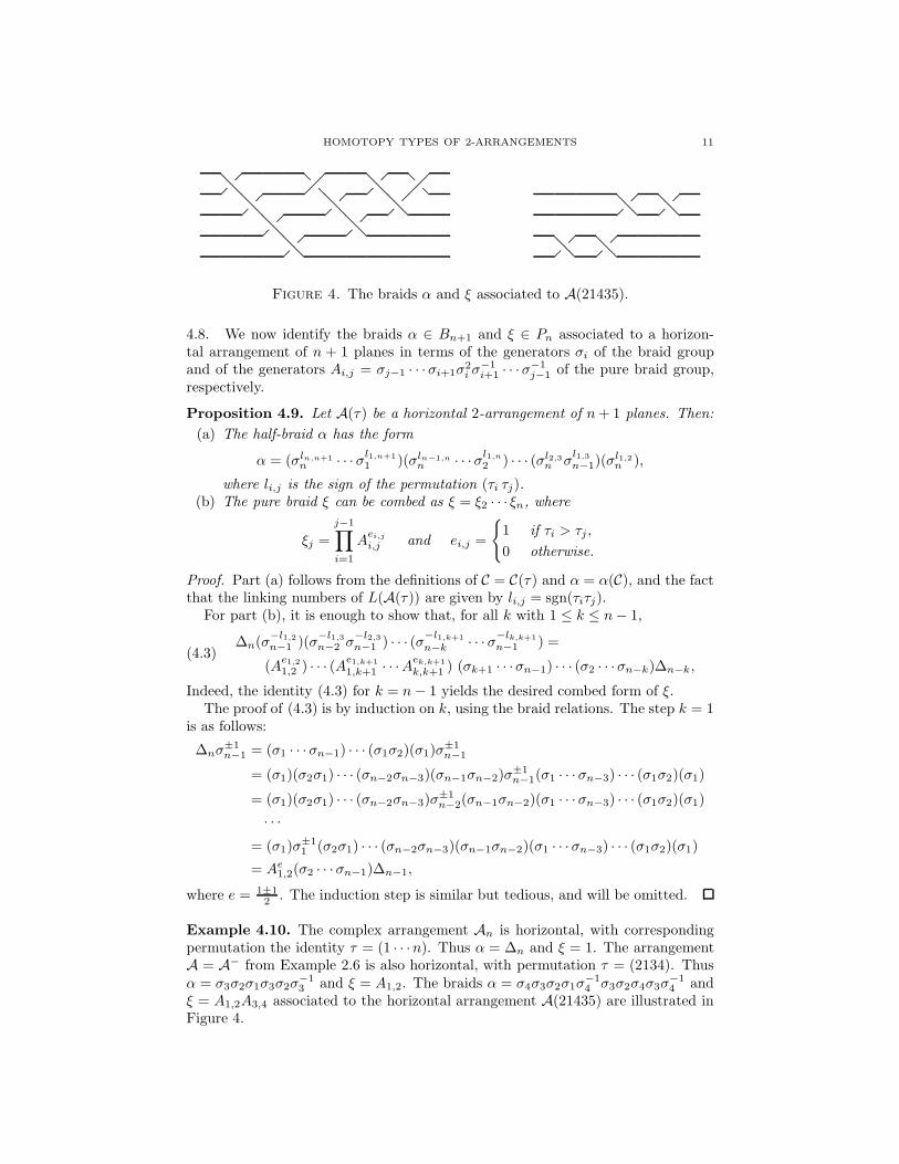
Figure 4. The braids α and ξ associated to A(21435).

4.8. We now identify the braids α ∈ Bn+1 and ξ ∈ Pn associated to a horizon-tal arrangement of n + 1 planes in terms of the generators σi of the braid groupand of the generators Ai,j = σj−1 · · ·σi+1σ

2i σ

−1i+1 · · ·σ−1

j−1 of the pure braid group,respectively.

Proposition 4.9. Let A(τ) be a horizontal 2-arrangement of n+ 1 planes. Then:

(a) The half-braid α has the form

α = (σln,n+1

n · · ·σl1,n+1

1 )(σln−1,nn · · ·σl1,n

2 ) · · · (σl2,3n σ

l1,3

n−1)(σl1,2n ),

where li,j is the sign of the permutation (τi τj).(b) The pure braid ξ can be combed as ξ = ξ2 · · · ξn, where

ξj =

j−1∏

i=1

Aei,j

i,j and ei,j =

1 if τi > τj ,

0 otherwise.

Proof. Part (a) follows from the definitions of C = C(τ) and α = α(C), and the factthat the linking numbers of L(A(τ)) are given by li,j = sgn(τiτj).

For part (b), it is enough to show that, for all k with 1 ≤ k ≤ n− 1,

∆n(σ−l1,2

n−1 )(σ−l1,3

n−2 σ−l2,3

n−1 ) · · · (σ−l1,k+1

n−k · · ·σ−lk,k+1

n−1 ) =

(Ae1,2

1,2 ) · · · (Ae1,k+1

1,k+1 · · ·Aek,k+1

k,k+1 ) (σk+1 · · ·σn−1) · · · (σ2 · · ·σn−k)∆n−k,(4.3)

Indeed, the identity (4.3) for k = n− 1 yields the desired combed form of ξ.The proof of (4.3) is by induction on k, using the braid relations. The step k = 1

is as follows:

∆nσ±1n−1 = (σ1 · · ·σn−1) · · · (σ1σ2)(σ1)σ

±1n−1

= (σ1)(σ2σ1) · · · (σn−2σn−3)(σn−1σn−2)σ±1n−1(σ1 · · ·σn−3) · · · (σ1σ2)(σ1)

= (σ1)(σ2σ1) · · · (σn−2σn−3)σ±1n−2(σn−1σn−2)(σ1 · · ·σn−3) · · · (σ1σ2)(σ1)

· · ·= (σ1)σ

±11 (σ2σ1) · · · (σn−2σn−3)(σn−1σn−2)(σ1 · · ·σn−3) · · · (σ1σ2)(σ1)

= Ae1,2(σ2 · · ·σn−1)∆n−1,

where e = 1±12 . The induction step is similar but tedious, and will be omitted.

Example 4.10. The complex arrangement An is horizontal, with correspondingpermutation the identity τ = (1 · · ·n). Thus α = ∆n and ξ = 1. The arrangementA = A− from Example 2.6 is also horizontal, with permutation τ = (2134). Thusα = σ3σ2σ1σ3σ2σ

−13 and ξ = A1,2. The braids α = σ4σ3σ2σ1σ

−14 σ3σ2σ4σ3σ

−14 and

ξ = A1,2A3,4 associated to the horizontal arrangement A(21435) are illustrated inFigure 4.


5. Determinantal Ideals and Characteristic Varieties

We start this section with a review of the determinantal ideals of the Alexandermodule of a space, following Hillman [15] and Turaev [26, 27]. From the varietiesdefined by these ideals, we extract numerical homotopy-type invariants, that willbe used for the rest of this paper.

5.1. LetX be a connected, finite CW-complex, with basepoint ∗, and fundamental

group π1(X, ∗). Let p : X → X be the universal abelian cover, corresponding to theabelianization homomorphism ab : π1(X, ∗) → H1(X ; Z). The relative homology

group A(X) = H1(X, p−1(∗); Z) has the structure of a (left) module over the group

ring Z[H1(X ; Z)], and is known as the Alexander module of X .Now assume that H1(X,Z) is isomorphic to Zn, the free abelian group on

t1, . . . , tn. A choice of isomorphism, ψ : H1(X)≃−→ Zn, identifies Z[H1(X)] with

Λ = Z[t±11 , . . . , t±1

n ], the ring of Laurent polynomials in n variables, and defines a Λ-module structure on the Alexander module of X , which we will denote by A(X,ψ).From a presentation of the fundamental group, π1(X) = 〈x1, . . . , xq | r1, . . . , rs〉,one gets a presentation for the Alexander module,

ΛsM−→ Λq → A(X,ψ) → 0,

where M =(∂ri/∂xj

)ab

is the abelianized Jacobian matrix of Fox derivatives.

Define the kth determinantal ideal of Aψ(X) to be the ideal Ek(X,ψ) generatedby the codimension k minors of the Alexander matrix M . Clearly, Ek(X,ψ) ⊆Eℓ(X,ψ) if k ≤ ℓ. The determinantal ideals depend only on the homotopy type ofX(in fact, only on its fundamental group), and on the identification ψ : H1(X) → Zn.

If π1(X) has positive deficiency (i.e., admits a presentation with more generatorsthan relations), then E1(X,ψ) is of the form I ·(∆X,ψ), where I is the augmentationideal of Λ, and ∆X,ψ ∈ Λ is the (multi-variable) Alexander polynomial ofX , see [11].

5.2. We now associate to X subvarieties Vk(X,ψ) of the algebraic torus (C∗)n, de-fined by the determinantal ideals Ek(X,ψ), following [10, 17]. The coordinate ringof (C∗)n is ΛC = Λ⊗C, the ring of Laurent polynomials with complex coefficients.Then, for each k ≥ 0, we set

Vk(X,ψ) = (t1, . . . , tn) ∈ (C∗)n | g(t1, . . . , tn) = 0, for all g ∈√Ek(X,ψ) ⊗ C,

where√

a denotes the radical of an ideal a. Clearly, Vk(X,ψ) ⊇ Vℓ(X,ψ) if k ≤ ℓ.

Definition 5.3. Two algebraic subvarieties V and V ′ of (C∗)n are said to have thesame monomial isomorphism type if there exists an automorphism φA : (C∗)n →(C∗)n of the form

φA(ti) = tai1

1 · · · tainn , 1 ≤ i ≤ n,

for some matrix A = (ai,j) ∈ GLn(Z), which maps V into V ′.

Proposition 5.4. The monomial isomorphism type of the subvariety Vk(X,ψ) of

the algebraic torus (C∗)n depends only on the isomorphism type of π1(X), and

not on the identification ψ : H1(X) → Zn. We call Vk(X) = Vk(X,ψ) the kth

characteristic variety of X.


Proof. LetX and Y be connected, finite CW-complexes, and let h : π1(X) → π1(Y )be an isomorphism. Let h∗ : H1(X) → H1(Y ) be the abelianization of h, andset h = ψY h∗ψ

−1X : Zn → Zn. The extension of h to ΛC = CZn restricts to

an isomorphism Ek(X,ψX) ⊗ C → Ek(Y, ψY ) ⊗ C, for each k ≥ 0. Now let φthe (monomial) automorphism of (C∗)n induced by h. Clearly, φ restricts to anisomorphism Vk(X,ψX) → Vk(Y, ψY ).

In other words, for each k ≥ 0, the monomial isomorphism type of Vk(X) is anisomorphism type of π1(X), and thus, a homotopy-type invariant of X . Further-more, if π1(X) has positive deficiency, the Alexander polynomial ∆X = ∆X,ψ iswell-defined up to a monomial change of basis in (C∗)n, and up to multiplication

by a unit cti11 · · · tinn ∈ ΛC. Note that V1(X) = 1 ∪ ∆X = 0, where 1 = (1, . . . , 1)is the origin of the complex torus (C∗)n.

5.5. By themselves, the characteristic varieties are not very practical homotopy-type invariants. We extract from them several numerical invariants that are pow-erful enough for our purposes. For each integer p ≥ 2, let

Ωnp = (ω1, . . . , ωn) ∈ (C∗)n | ωi is a pth root of unitybe the set of p-torsion points of (C∗)n.

Theorem 5.6. The following are isomorphism type invariants of π1(X):

(a) The list Σk(X) of codimensions of irreducible components of Vk(X);(b) The list Σ1,k(X) of codimensions of irreducible components of Vk(X) passing

through 1;

(c) The number Torsp,k(X) =∣∣Ωnp ∩ Vk(X)

∣∣ of p-torsion points of Vk(X).

Proof. By Proposition 5.4, an isomorphism of fundamental groups determines amonomial isomorphism of the corresponding characteristic varieties. Part (a) fol-lows from the fact that an isomorphism of algebraic varieties sends irreducible com-ponents to irreducible components of the same codimension. Part (b) follows fromPart (a), and the fact that a monomial isomorphism fixes 1. Part (c) follows fromthe fact that a monomial isomorphism preserves the set of p-torsion points.

5.7. Now let X = X(A) be the complement of a 2-arrangement of n planes inR4. Recall that X has the homotopy type of a 2-complex (modeled on the Artinpresentation of its fundamental group G), and that H1(X) = Zn. Thus, we candefine the kth characteristic variety of A to be Vk(A) = Vk(X). As we shall see, thedescending tower of characteristic varieties has the form (C∗)n = V0 ⊇ V1 ⊇ · · · ⊇Vn−2 ⊇ Vn−1 ⊇ Vn = ∅, with V1 being a hypersurface in (C∗)n, if n ≥ 3, and Vn−1

consisting of the single point 1, if n ≥ 2. We will focus on the nontrivial ends ofthe tower, namely V1 and Vn−2, which we shall call the top, respectively the bottom

characteristic variety of A.In order to find explicit equations for the characteristic varieties, we need to

choose a particular presentation for G = π1(X). Unless otherwise specified, weshall use the presentation (4.2) associated to the semidirect product structure G =Fn−1 ⋊ξ2 F1 from Proposition 4.6. This presentation yields an identification ψξ :H1(X) → Zn. Let A = A(X,ψξ) be the corresponding Alexander module. Apresentation matrix for A is the (n− 1) × n (Alexander) matrix

M =(tn · id−Θ(ξ2) d1

),


where d1 = (1 − t1 · · · 1 − tn−1)⊤

and Θ : Pn−1 → GLn−1(Λ) is the Gassnerrepresentation of the pure braid group, see Birman [2].

The k×k minors of M generate the determinantal ideal Ek, whose radical,√Ek,

defines the kth characteristic variety Vk = Vk(A). Note that En−1 = I and En = Λ,and so Vn−1 = 1 and Vn = ∅.

Now recall that a link group has deficiency 1, see e.g. [4]. Thus we may definethe Alexander polynomial of A to be ∆A = ∆X,ψξ

. For n = 1, we have ∆A = 1.For n > 1, we have

∆A(t1, . . . , tn) =1

tn − 1det

(tn · id−Θ(ξ2)

),

see Penne [25]. Thus ∆A = 1 for n = 2. For n ≥ 3, the triviality of the Gassner rep-resentation evaluated at 1 implies that 1 ∈ V1(A) and so V1(A) = ∆A(t1, . . . , tn) =0.Remark 5.8. For certain purposes, it is more natural to start from the Artinpresentation (4.1) associated to the semidirect product structure G = Fn−1 ⋊β F1.The resulting presentation, A(X,ψβ), for the Alexander module coincides with theusual presentation of the Alexander module of the link L(A). We will denote theassociated Alexander polynomial by ∆L(A) = ∆X,ψβ

.

Example 5.9. Let An be the arrangement of n ≥ 3 complex lines through theorigin of C2. Recall that ξ = 1 and β = ∆2

n in this case. It is readily seen thatEk = I·(tn−1)n−k−1. Thus V1 = · · · = Vn−2 = tn−1 = 0, and ∆An

= (tn−1)n−2,whereas ∆L(An) = (t1 . . . tn − 1)n−2.

Example 5.10. Let A be the arrangement A− = A(2134). Recall that ξ = A1,2.

The Artin representation of ξ : F3 → F3 is given by ξ(x1) = x1x2x1x−12 x−1

1 ,

ξ(x2) = x1x2x−11 , ξ(x3) = x3. Consider the new basis y1 = x1, y2 = x1x2, y3 = x3

for F3. In this basis, ξ(y1) = y2y1y−12 , ξ(y2) = y2, ξ(y3) = y3, and so the Alexander

matrix is:

M =

t4 − t22 (t2 + 1)(t1 − 1) 0 1 − t1

0 t4 − 1 0 1 − t2

0 0 t4 − 1 1 − t3

.

The determinantal ideals are E1 = I · (t4 − 1)(t4 − t22), and E2 = I · (t4 − 1, t22 −1) + Λ · (t2 + 1)(t1 − 1)(t3 − 1). The characteristic varieties are

V1 = t4 − 1 = 0 ∪ t4 − t22 = 0,V2 = t4 − 1 = t2 + 1 = 0 ∪ t4 − 1 = t2 − 1 = t1 − 1 = 0

∪ t4 − 1 = t2 − 1 = t3 − 1 = 0.Now let A be the arrangement A+ = A(1234). We know from Example 5.9 that

its characteristic varieties are V1 = V2 = t4 − 1 = 0. We plainly see that thecharacteristic varieties of A+ and A− have a different number of components, andso are not isomorphic. Thus, X+ 6≃ X−. In fact, H∗(X+) ≇ H∗(X−), as wasshown by Ziegler [30].

6. Bottom Characteristic Varieties

In this section we study the bottom characteristic varieties Vn−2(A) of arrange-ments of n planes that are obtained from the trivial arrangement by a sequence of


cabling operations. We obtain a complete characterization of these varieties whenthe sequence has length 2.

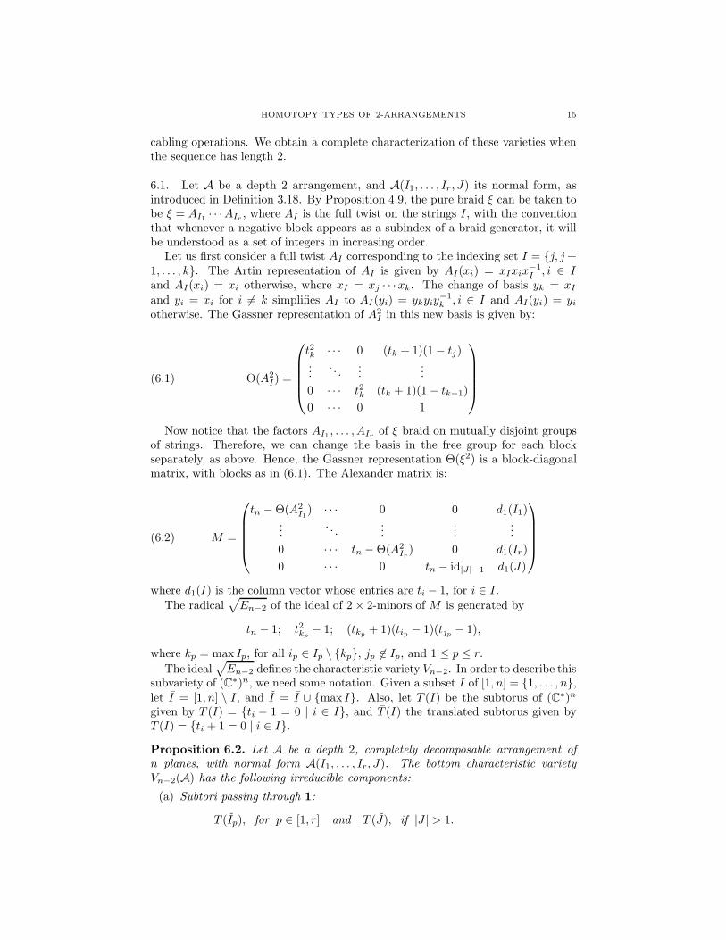
6.1. Let A be a depth 2 arrangement, and A(I1, . . . , Ir, J) its normal form, asintroduced in Definition 3.18. By Proposition 4.9, the pure braid ξ can be taken tobe ξ = AI1 · · ·AIr

, where AI is the full twist on the strings I, with the conventionthat whenever a negative block appears as a subindex of a braid generator, it willbe understood as a set of integers in increasing order.

Let us first consider a full twist AI corresponding to the indexing set I = j, j+1, . . . , k. The Artin representation of AI is given by AI(xi) = xIxix

−1I , i ∈ I

and AI(xi) = xi otherwise, where xI = xj · · ·xk. The change of basis yk = xIand yi = xi for i 6= k simplifies AI to AI(yi) = ykyiy

−1k , i ∈ I and AI(yi) = yi

otherwise. The Gassner representation of A2I in this new basis is given by:

Θ(A2I) =

t2k · · · 0 (tk + 1)(1 − tj)...

. . ....

...

0 · · · t2k (tk + 1)(1 − tk−1)

0 · · · 0 1

(6.1)

Now notice that the factors AI1 , . . . , AIrof ξ braid on mutually disjoint groups

of strings. Therefore, we can change the basis in the free group for each blockseparately, as above. Hence, the Gassner representation Θ(ξ2) is a block-diagonalmatrix, with blocks as in (6.1). The Alexander matrix is:

M =

tn − Θ(A2I1

) · · · 0 0 d1(I1)...

. . ....

......

0 · · · tn − Θ(A2Ir

) 0 d1(Ir)

0 · · · 0 tn − id|J|−1 d1(J)

(6.2)

where d1(I) is the column vector whose entries are ti − 1, for i ∈ I.

The radical√En−2 of the ideal of 2 × 2-minors of M is generated by

tn − 1; t2kp− 1; (tkp

+ 1)(tip − 1)(tjp − 1),

where kp = max Ip, for all ip ∈ Ip \ kp, jp 6∈ Ip, and 1 ≤ p ≤ r.

The ideal√En−2 defines the characteristic variety Vn−2. In order to describe this

subvariety of (C∗)n, we need some notation. Given a subset I of [1, n] = 1, . . . , n,let I = [1, n] \ I, and I = I ∪ max I. Also, let T (I) be the subtorus of (C∗)n

given by T (I) = ti − 1 = 0 | i ∈ I, and T (I) the translated subtorus given byT (I) = ti + 1 = 0 | i ∈ I.

Proposition 6.2. Let A be a depth 2, completely decomposable arrangement of

n planes, with normal form A(I1, . . . , Ir, J). The bottom characteristic variety

Vn−2(A) has the following irreducible components:

(a) Subtori passing through 1:

T (Ip), for p ∈ [1, r] and T (J), if |J | > 1.


(b) Translated subtori:

T (∪p/∈P Ip ∪ n) ∩ T (∪p∈P max Ip), for ∅ 6= P ⊆ [1, r].

Example 6.3. The arrangement A = A(214356) from Example 3.17 is in normalform, with I1 = 2, 1, I2 = 4, 3, and J = 5, 6. The components of V4(A) are:

t6 − 1 = t4 + 1 = t2 + 1 = 0,t6 − 1 = t4 + 1 = t2 − 1 = t1 − 1 = 0,t6 − 1 = t4 − 1 = t3 − 1 = t2 + 1 = 0,t6 − 1 = t5 − 1 = t4 − 1 = t3 − 1 = t2 − 1 = 0,t6 − 1 = t5 − 1 = t4 − 1 = t2 − 1 = t1 − 1 = 0,t6 − 1 = t4 − 1 = t3 − 1 = t2 − 1 = t1 − 1 = 0.

6.4. Let A be a completely decomposable arrangement of depth 2, with normalform A(I1, . . . , Ir, J). Recall that |I1| ≤ · · · ≤ |Ir |. Define

S(A) = |I1|, . . . , |Ir|.Since we also have I1 ≤ · · · ≤ Ir < J , the ordered list S(A), together with thenumber of planes, n = |J | + ∑r

k=1 |Ik|, determines the normal form.Let Σ = Σn−2(A) be the list of codimensions of irreducible components of

Vn−2(A), and Σ1 = Σ1,n−2(A) be the sublist corresponding to components passingthrough 1. From Proposition 6.2, we see that

Σ1 = n+ 1 − |Ip|p=1,...,r if |J | = 1(6.3a)

Σ1 = n+ 1 − |Ip|p=1,...,r ∪ n+ 1 − |J | if |J | > 1(6.3b)

Σ \ Σ1 = r + 1 +∑

p/∈P

(|Ip| − 1)∅(P⊆[1,r](6.3c)

The lists Σ1 and Σ have lengths

d1 = r + ǫJ + 1, d = 2r + r + ǫJ ,(6.4)

where ǫJ = 0 if |J | > 1 and ǫJ = −1 if |J | = 1.

Theorem 6.5. The list S(A) is a complete homotopy-type invariant for depth 2,completely decomposable arrangements A of n planes.

Proof. Let A′ be another completely decomposable arrangement of depth 2, withnormal form A(I ′1, . . . , I

′r , J

′). Assume X(A) ≃ X(A′). Then, by Theorem 5.6,Σ(A) = Σ(A′) and Σ1(A) = Σ1(A′). We want to show that S(A) = S(A′). Thereare four cases to consider, according to the sizes of J and J ′:

• |J | = 1, |J ′| > 1. Then, by (6.4), the system of equations d = d′, d1 = d′1 hasno solution.

• |J | = |J ′| = 1. Then, by (6.3a), Σ1(A) = Σ1(A′) implies S(A) = S(A′).• |J | = |J ′| > 1. Then, (6.3b), Σ1(A) = Σ1(A′) implies S(A) = S(A′).• |J | > |J ′| > 1. Then, by (6.4), r = r′. If r = 1, equation (6.3b) implies

that |I1|, |J | = |I ′1|, |J ′| as unordered lists. But condition (iii) from Def-inition 3.18 and the fact that |J | > |J ′| rule out this possibility. If r > 1,equation (6.3c) implies |J | = n+ r + 2 − max(Σ \ Σ1) − min(Σ \ Σ1). Hence|J | − |J ′| = r − r′ = 0, which again is impossible.


Conversely, assume S(A) = S(A′). Then, as noted above, the normal forms ofA and A′ coincide. By Proposition 3.19, A and A′ are rigidly isotopic, and thusX(A) ≃ X(A′).

Corollary 6.6. The number of homotopy classes of 2-arrangements of n planes

which are completely decomposable of depth at most 2 equals p(n−1)−⌊(n−1)/2⌋,where p(·) is the partition function, and ⌊·⌋ is the integer part function.

Proof. Follows from the Theorem by an elementary counting argument.

7. Top Characteristic Varieties

In this section we study the top characteristic variety V1(A) of a 2-arrangementA, and the number Torsp,1(A) of its p-torsion points, for p a prime number.

7.1. Let us start with a completely decomposable arrangement, A = A(τ). Letτ = τ0 → τ1 → · · · → τd = (1) be the decomposition sequence for τ . Recall thateach permutation in the sequence is partitioned into blocks of consecutive integers.We call such a block B essential if either |B| ≥ 2, or B = τd−1 and |B| > 2.

Theorem 7.2. The top characteristic variety V1(A) of a completely decomposable

arrangement of n planes is the union of an arrangement V(A) of codimension 1subtori of (C∗)n, all passing through 1.

Proof. Choose τ ∈ Sn so that A = A(τ) and depth(A) = d(τ). Let m be thenumber of essential blocks of τ . Recall from §3.12 that L = L(A) is an iterated toruslink, obtained by (1,±1)-cablings on the unknot. Thus, it is a spliced link in thesense of Eisenbud and Neumann [11]. The decomposition sequence of τ correspondsto a minimal splice diagram of L: The (signed) essential blocks B1, . . . , Bm of thepermutations in the sequence correspond to the (signed) nodes vn+1, . . . , vn+m ofthe diagram, and the integers 1, . . . , n to the arrowheads v1, . . . , vn. Then, accordingto [11], Theorem 12.1, the Alexander polynomial of L is given by:

∆L(t1, . . . , tn) =

n+m∏

j=n+1

(tl1,j

1 tl2,j

2 · · · tln,jn − 1)δj−2,

where li,j = ±1 is the linking number of Li with the “virtual component” corre-sponding to vj , and δj is the valency of vj . Thus, each irreducible component ofV1(A) = ∆L = 0 is a codimension 1 subtorus. (It actually can be shown thatV1(A) has precisely m components.)

To compute the number of torsion points on V1(A), we may now use a resultof Bjorner and Ekedahl [3]. Indeed, an arrangement V of codimension 1 subtori in(C∗)n defines an arrangement Vp of hyperplanes in (Zp)

n: To a subtorus ta1

1 · · · tann −

1 = 0 corresponds the hyperplane a1x1 + · · · + anxn = 0 mod p. Proposition 3.2of [3] then implies the following.

Proposition 7.3. The number of p-torsion points on the union U = U(V) of an

arrangement of subtori in (C∗)n is given by:

Torsp(U) = −∑

x∈L\0

µ(0, x)pdim(x),

where L is the intersection lattice of the arrangement Vp, with minimal element

0 = (Zp)n, and Mobius function µ.


Example 7.4. The arrangement A = A(312546) is completely decomposable, ofdepth 3. Its decomposition sequence is (312546) → (2134) → (12) → (1). Proposi-tion 4.9 gives ξ = A1,3A2,3A4,5. The Artin representation of ξ in the basis y1 = x1,

y2 = x1x2, y3 = x1x2x3, y4 = x4, y5 = x4x5 is given by ξ(y1) = y3y−12 y1y2y

−13 ,

ξ(y2) = y3y2y−13 , ξ(y3) = y3, ξ(y4) = y5y4y

−15 , and ξ(y5) = y5. The Alexander

polynomial is ∆A(t1, . . . , t6) = (t6 − 1)(t6 − t25)(t6 − t23)(t6 − t23t−22 ). Proposition 7.3

yields Tors2,1(A) = 32 and Tors3,1(A) = 585.

For an arrangement of depth 2, we can give a more precise description of the topcharacteristic variety, based on formula (6.2) for the Alexander matrix.

Proposition 7.5. Let A be a depth 2 arrangement of n planes, with normal form

A(I1, . . . , Ir, J), and let kq = max Iq, for 1 ≤ q ≤ r. Then:

(a) ∆A(t1, . . . , tn) = (tn − 1)|J|+r−2∏rq=1(tn − t2kq

)|Iq|−1;

(b) V1(A) = t ∈ (C∗)n | (tn − 1)∏rq=1(tn − t2kq

) = 0;(c) Tors2,1(A) = 2n−1 and Torsp,1(A) = pn−r−1(pr+1 − (p− 1)r+1), for p ≥ 3.

7.6. Let L be a link in S3. The Alexander polynomial of a sublink of L, and that ofan (a, b)-cable about L, can be computed from the Alexander polynomial of L, viathe following well-known formulae of Torres and Sumners–Woods, see [11, 15, 26].

Theorem 7.7. Let L = L1 ∪ · · · ∪ Ln be a link in S3. Set T = tl11 · · · tln−1

n−1 , where

li = lk(Li, Ln). Then:

∆L(t1, . . . , tn−1, 1) = (T − 1)∆L\Ln(t1, . . . , tn−1),(7.1a)

Moreover, if L′ = La, b, with gcd(a, b) = 1, then:

∆L′(t1, . . . , tn, tn+1) = (T atbntbn+1 − 1)∆L(t1, . . . , tn−1, t

antn+1).(7.1b)

Corollary 7.8. Let A be an arrangement of n planes, and let Akr be an r-cableabout it. Then:

(a) V1(Ar) = t ∈ (C∗)n+r | t1 · · · tn − 1 = 0 or (t1, . . . , tn) ∈ V1(A);(b) Torsp,1(Ar) = pr−1 Torsp,1(A1).

Proof. Let L = L(A). Recall from §3.1 that L(A1) = L1, 1. By the Sumners-Woods formula (7.1b), we have

∆L(A1)(t1, . . . , tn, tn+1) = (t1 · · · tn+1 − 1)∆L(t1, . . . , tn−1, tntn+1).

After a monomial change of basis, this implies part (a) for r = 1. The general casefollows from the same formula, by induction on r. Part (b) follows immediatelyfrom part (a).

7.9. We conclude this section with a recursion formula for Tors2,1(A). Let ∆L(A)

be the Alexander polynomial of the link L(A). Define the single-variable Alexander

polynomial of A to be ∆A(t) := (t− 1)∆L(A)(t, . . . , t). Furthermore, set

δ(A) =

1 if ∆A(−1) = 0,

0 otherwise.

Example 7.10. The single-variable Alexander polynomial of the complex arrange-

ment An is ∆An(t) = (t− 1)(tn − 1)n−2. Thus, δ(An) = 1+(−1)n

2 .


Theorem 7.11. Let A = H1, . . . , Hn be a 2-arrangement in R4. The number

of 2-torsion points of the top characteristic variety V1(A) is given by the following

formula:

Tors2,1(A) = 2n−1 − 1 + (−1)n

2+ δ(A) +

∑

B∈Γ(A)

δ(B),(7.2)

where Γ(A) is the set of all indecomposable, proper sub-arrangements of A with an

odd number of planes.

Proof. By definition,

Tors2,1(A) =∑

ω∈Ωn2

cω,(7.3)

where Ωn2 = (ω1, . . . , ωn) ∈ (C∗)n | ωi = ±1, and cω = 1 if ∆L(A)(ω) = 0, andcω = 0 otherwise. For ω ∈ Ωn2 , let Aω = Hi ∈ A | ωi = −1. There are severalcases to consider:

• If ω = (−1, . . . ,−1), then Aω = A, and so cω = δ(A).• If ω 6= (−1, . . . ,−1), then Aω is a proper sub-arrangement of A, and so, by

repeated application of Torres’s formula (7.1a), we have

∆L(A)(ω) = ((−1)|Aω| − 1)∆L(Aω)(−1, . . . ,−1).(7.4)

– If |Aω| is even, this formula says that ∆L(A)(ω) = 0, and so cω = 1.

There are 2n−1 − 1+(−1)n

2 such contributions to the sum (7.3).– If |Aω| is odd, and Aω is decomposable, we may write Aω = A′

ω±1,with the cabling done about the last component of A′

ω. Let A′′ω be the

sub-arrangement obtained by deleting the last component of A′ω. Clearly,

|A′′ω | = |Aω | − 2. Formulas (7.1b), and (7.1a) give

∆L(Aω)(−1, . . . ,−1) = −2∆L(A′

ω)(−1, . . . ,−1, 1) = 4∆L(A′′

ω)(−1, . . . ,−1).(7.5)

Hence, δ(Aω) = δ(A′′ω). Iterating this decabling-deletion procedure, we

eventually reach an arrangement B for which the procedure must stop.There are two possibilities:∗ One is B = A3, in which case cω = δ(A3) = 0.∗ The other is B ∈ Γ(A), in which case cω = δ(B). Clearly, any element

of Γ(A) can be reached by the above procedure; thus there are |Γ(A)|such contributions to the sum (7.3).

This completes the proof.

Remark 7.12. Note that 2n−1 − 1 ≤ Tors2,1(A) ≤ 2n. If Tors2,1(A) = 2n−1 − 1,and n ≥ 3, then the top characteristic variety V1(A) is not the union of translatedsubtori of (C∗)n. For, otherwise, at least one of the subtori must be of the formT = ta1

1 · · · tann − 1 = 0, since ∆L(A)(1, . . . , 1) = 0. But the torus T has 2n−1

torsion points of order 2.

Corollary 7.13. If all the proper subarrangements of A are completely decompos-

able, then Tors2,1(A) = 2n−1 − 1+(−1)n

2 + δ(A).

Corollary 7.14. If A is completely decomposable, then Tors2,1(A) = 2n−1.

Proof. The recursion formula (7.5), together with Example 7.10 imply that δ(A) =1+(−1)n

2 , and the conclusion follows from the previous corollary.


Example 7.15. The arrangement A = A(31425) is horizontal, indecomposable,and all its subarrangements are completely decomposable. The (single variable)Alexander polynomial is ∆A(t) = (t − 1)4(4t2 − t + 4), and so δ(A) = 0. FromCorollary 7.13, we get Tors2,1(A) = 16.

Example 7.16. The arrangement A = A(314256) is decomposable, but not com-pletely decomposable, since it has A(31425) as a subarrangement. We have ∆A(t) =(t6 − 1)(t− 1)3(t+ 1)(3t2 − 2t+ 3), and so δ(A) = 1. From Theorem 7.11, we getTors2,1(A) = 32.

Example 7.17. The arrangement A = A(241536) is horizontal, indecomposable,and all its proper subarrangements are completely decomposable. We have ∆A(t) =(t−1)5(5t4+6t2+5), and so δ(A) = 0. From Corollary 7.13, we get Tors2,1(A) = 31.Hence, V1(A) is not a union of translated subtori of (C∗)6.

8. Mazurovskiı’s arrangements

In this section, we study the 2-arrangements associated to Mazurovskiı’s con-figurations. Using their associated cablings, we find infinitely many pairs of ar-rangements whose complements are cohomologically equivalent, but not homotopyequivalent.

8.1. In [22], Mazurovskiı introduced a remarkable pair of configurations of skewlines, K and L, which have the same linking numbers, but are not rigidly isotopic.Let K = A(K) and L = A(L) be the corresponding arrangements of planes. Thearrangement K is horizontal, with associated permutation τ = (341256). Moreover,K is completely decomposable, of depth 3; a minimal decomposition sequence is(341256) → (213) → (12) → (1). The arrangement L is neither horizontal, nordecomposable. Defining polynomials for K and L are given by

fK(z, w) = f(z, w) · (z − 7w),

fL(z, w) = f(z, w) · (z − 6 − 7 i

2w − 3 + 14 i

2w),

where f is the following defining polynomial for A(34125):

f(z, w) = (z − 5 − 5 i

2w +

3 − 5 i

2w)(z − 7 − 10 i

2w +

3 − 10 i

2w)

× (z − 5 − 14 i

2w − 3 + 14 i

2w)(z − 7 − 9 i

2w − 3 + 9 i

2w)(z − 6w).

The half-braids associated to K and L are pictured in Figure 5. We see that thelinking numbers of L(K) are l1,4 = l2,4 = l1,3 = l2,3 = −1, and all other li,j = 1,whereas the linking numbers of L(L) are l1,5 = l2,5 = l1,4 = l2,4 = −1, and allother li,j = 1. The reordering of the components of L(L) that fixes 1, 2, 6 andpermutes 3, 4, 5 to 4, 5, 3 identifies the linking numbers of L(K) and L(L). Thus,H∗(X(K); Z) ∼= H∗(X(L); Z).

8.2. In order to distinguish between the cohomologically equivalent arrangementsK and L, we turn to their characteristic varieties. From Figure 5, we see that thereduced half-braids of K and L are:

αK = σ4σ3σ2σ1σ4σ−13 σ−1

2 σ−14 σ−1

3 σ4, αL = σ4σ2σ−13 σ2σ

−11 σ2σ

−14 σ−1

3 σ2σ4.

The braids ξ = ∆5α−1 ∈ P5 are expressed in terms of the pure braid generators, as

follows. For K, which is horizontal, Proposition 4.9 yields ξK = A1,3A2,3A1,4A2,4.


1

2

3

4

5

6................

...................................................................

................

...................................................................

................

...................................................................

................

...................................................................

................

...................................................................

................

...................................................................

................

...................................................................

................

...................................................................

................

...................................................................

................

...................................................................

...................................................................

................

...................................................................

................

...................................................................

................

...................................................................

................

................

...................................................................

1

2

3

4

5

6................

...................................................................

................

...................................................................

................

...................................................................

................

...................................................................

................

...................................................................

................

...................................................................

................

...................................................................

...................................................................

................

................

...................................................................

...................................................................

................

................

...................................................................

...................................................................

................

...................................................................

................

................

...................................................................

................

...................................................................

Figure 5. Mazurovskiı’s pair: The half-braids αK (top) and αL (bottom).

For L, it is more convenient to work with the conjugate ξ′L = δ−1ξLδ, where

δ = σ1σ3σ−14 . Routine combing of the braid yields ξ′L = A1,3A2,3A4,5A1,4A

−14,5A2,4.

The Artin representation of ξ = ξK in the basis y1 = x1, y2 = x3, y3 = x1x2,y4 = x1x2x3x4, y5 = x5 is given by ξ(y1) = y4y

−13 y1y3y

−14 , ξ(y2) = y3y2y

−13 ,

ξ(y3) = y4y3y−14 , ξ(y4) = y4, and ξ(y5) = y5. The Alexander matrix of K is:

t6 − t24t−23 0 t24t

−23 (t3 + 1)(1 − t1) (t4 + 1)(t1 − 1) 0 t1 − 1

0 t6 − t23 (t4 + t3)(t2 − 1) (1 − t3)(t2 − 1) 0 t2 − 1

0 0 t6 − t24 (t4 + 1)(t3 − 1) 0 t3 − 1

0 0 0 t6 − 1 0 t4 − 1

0 0 0 0 t6 − 1 t5 − 1

An elementary computation shows that the bottom variety V4(K) has 6 irre-ducible components—3 codimension 4 translated subtori of (C∗)6, and 3 codimen-sion 5 subtori passing through 1—given by the following equations:

t6 − 1 = t4 + 1 = t3 + 1 = t2 − 1 = 0,t6 − 1 = t4 + 1 = t3 − 1 = t1 − 1 = 0,t6 − 1 = t5 − 1 = t4 − 1 = t3 + 1 = 0,t6 − 1 = t5 − 1 = t4 − 1 = t3 − 1 = t1 − 1 = 0,t6 − 1 = t5 − 1 = t4 − 1 = t3 − 1 = t2 − 1 = 0,t6 − 1 = t4 − 1 = t3 − 1 = t2 − 1 = t1 − 1 = 0.

The primary decomposition of the ideal E4(L) is much harder to find. Theimplementation in Macaulay 2 [14] of the Eisenbud, Huneke, and Vasconcelos al-gorithm yields such a decomposition, and the result is that V4(L) = V4(K). Thus,the bottom varieties fail to distinguish between the K and L arrangements.

Let us then consider the top varieties. It is readily seen that the Alexanderpolynomial of K is ∆K(t1, . . . , t6) = (t6 − 1)(t6 − t23)(t6 − t24)(t6 − t24t

−23 ), and so


V1(K) is the union of 4 codimension 1 subtori of (C∗)6. Since K is completelydecomposable, Corollary 7.14 implies that Tors2,1(K) = 32.

The Alexander polynomial of L may be computed using Mathematica [29]. Theresult is too long to be displayed here, but suffices to say that it is an irreduciblepolynomial over Z, consisting of 667 monomials. Direct computation shows thatthe single variable Alexander polynomial is ∆L(t) = 3(t− 1)5(3t2− 2t+3)2. Henceδ(L) = 0. Since, as is readily checked, all proper subarrangements of L are com-pletely decomposable, Corollary 7.13 implies that Tors2,1(L) = 31.

Thus, Tors2,1(K) 6= Tors2,1(L). (As noted in Remark 7.12, this arithmetic dif-ference translates into a geometric difference: V1(K) is a union of subtori, whereasV1(L) is not even the union of translated subtori.) Appealing now to Theorem 5.6,we conclude that the complements of K and L are not homotopy equivalent, al-though, as mentioned previously, they are cohomologically isomorphic. This an-swers Ziegler’s question from [30].

8.3. We now use cablings of K and L to show that the above phenomenon happensfor arrangements of n planes, for any n ≥ 6.

Theorem 8.4. Let K and L be Mazurovskiı’s arrangements of 6 transverse planes

in R4. Let Kr and Lr be their r-cables. Then, for each r ≥ 0,

(a) H∗(X(Kr); Z) ∼= H∗(X(Lr); Z);

(b) X(Kr) 6≃ X(Lr).Proof. As noted above, the links of K and L have the same linking numbers. Hence,the links of Kr and Lr have the same linking numbers. This implies that thecomplements of Kr and Lr are cohomologically equivalent.

Although K and L are distinguished by their 2-torsion points, their cables arenot. Indeed, for r ≥ 1, Tors2,1(Kr) = Tors2,1(Lr) = 2r+5, as can be deducedfrom Theorem 7.11 for r = 1, and from Corollary 7.8 for r > 1. Hence, we turnto 3-torsion points. A Mathematica computation shows that Tors3,1(K1) = 35 · 7and Tors3,1(L1) = 33 · 61. From Corollary 7.8, we get

Tors3,1(Kr) = 3r+4 · 7, and Tors3,1(Lr) = 3r+2 · 61,

showing that the respective complements are indeed not homotopy equivalent.

8.5. Mazurovskiı introduced in [22] another interesting configuration of 6 lines,which he called M . Like the L configuration, the M configuration is non-horizontaland indecomposable (they are the only two such configurations of 6 lines, up torigid isotopy and mirror images). But, unlike L, the M configuration does nothave the linking numbers of any horizontal configuration. Let M = A(M) be thecorresponding arrangement. A defining polynomial for it is:

fM(z, w) = (z − (10 − i)w + (9 − 4 i)w)(z − (3 − 4 i)w − (1 + 4 i)w)

× (z − 5 − 10 i

2w +

1 − 10 i

2w)(z − (6 − 5 i)w +

1 − 10 i

2w)

× (z − 21 − 29 i

4w +

1 − 9 i

4w)(z − 6w).

The reduced braids associated to M are:

αM = σ2σ−13 σ1σ2σ

−13 σ−1

4 σ2σ−11 σ−1

2 and ξM = A2,4A1,2A3,4A1,5A3,5.


A Macaulay 2 computation shows that V4(M) consists of sixteen 2-torsion points.A Mathematica computation reveals that the Alexander polynomial of M is anirreducible polynomial over Z, consisting of 317 monomials. The single variableAlexander polynomial is ∆M(t) = (t−1)5(t2− t+1)(t6−5t5− t4−6t3− t2−5t+1),and so δ(M) = 0. Theorem 7.11 gives Tors2,1(M) = 31, the same as for L.(Thus, the top variety of M is not the union of translated subtori.) On the otherhand, a computation yields Tors3,1(L) = 527 and Tors3,1(M) = 421, showing thatX(L) 6≃ X(M).

9. Classification of 2-Arrangements of n ≤ 6 Planes

We start by reviewing the rigid isotopy classification of arrangements of up to 6planes. We then show that the invariants introduced in §5 are powerful enough toclassify up to homotopy the complements of such arrangements.

9.1. As noted in §2.7, rigid isotopy types of 2-arrangements in R4 are in one-to-one correspondence with rigid isotopy types of skew-lines configurations in R3.An important concept introduced by Viro [28] was that of a mirror image of aconfiguration. We now translate this notion to arrangements.

Definition 9.2. An arrangement A′ is called a mirror image of A if there is areflection of R4 sending A to A′. The mirror image of A is unique up to rigidisotopy; we denote it by A. An arrangement A which is not isotopic to A is callednon-mirror.

As shown by Viro, there exist many non-mirror arrangements. For example, thecomplex arrangement, An, and its mirror image under complex conjugation, An,are not rigidly isotopic provided n ≥ 3. Also, an arbitrary arrangement of n linesis non-mirror, provided n ≡ 3 (mod 4).

Viro [28] and Mazurovskiı [22] classified, up to rigid isotopy, all configurations6 lines or less. For up to 5 lines, linking numbers invariants were used. For 6lines, those invariants cannot tell apart the K and L configurations. For that, theMorton trace of the reduced full-braid is used in [22]. Translated to arrangements,the complete list of the 33 rigid isotopy types is as follows:

n = 1 : A(1)

n = 2 : A(12)

n = 3 : A(123)∗

n = 4 : A(1234)∗, A(2134)

n = 5 : A(12345)∗, A(21345)∗, A(21435)∗, A(31425)

n = 6 : A(123456)∗, A(213456)∗, A(321456), A(214356)∗, A(215436)∗,

A(312546), A(341256)∗, A(314256)∗, A(241536), A(L)∗, A(M)∗

where A∗ stands for a non-mirror arrangement A and its mirror image A.

9.3. We now turn to the homotopy classification of complements of arrangements.Clearly, arrangements that are either rigidly isotopic, or mirror images of one an-other, have diffeomorphic (and thus, homotopy equivalent) complements. Thus, ifwe delete from the above list the mirror image A from each pair A∗ = (A,A), weare left with a list 20 arrangements, such that, the complement of any arrangement


n A depth Σn−2 Tors2,1 Tors3,1

1 A(1) 0 0 0 0

2 A(12) 1 0 1 1

3 A(123) 1 1 4 9

4 A(1234) 1 1 8 27

A(2134) 2 2, 32 8 45

5 A(12345) 1 1 16 81

A(21345) 2 2, 3, 4 16 135

A(21435) 2 3, 44 16 171

A(31425) − 511 16 141

6 A(123456) 1 1 32 243

A(213456) 2 2, 3, 5 32 405

A(321456) 2 2, 42 32 405

A(215436) 2 3, 42, 52 32 513

A(214356) 2 3, 42, 53 32 513

K = A(341256) 3 43, 53 32 567

A(312546) 3 4, 56, 6 32 585

A(314256) − 56, 65 32 495

A(241536) − 52, 613 31 513

L − 43, 53 31 527

M − 616 31 421

Table 1. Arrangements of n ≤ 6 planes: Sequence of codimensionsof components of Vn−2—where ik stands for i repeated k times—andnumber of 2- and 3-torsion points on V1.

of n ≤ 6 planes is homotopy equivalent to the complement of one of the arrange-ments in this shorter list. Table 1 shows that there are no repetitions among thehomotopy types of these 20 arrangements. Hence, we have the following.

Theorem 9.4. For 2-arrangements of n ≤ 6 planes in R4, the homotopy types of

complements are in one-to-one correspondence with the rigid isotopy types modulo

mirror images.

References

[1] D. Arapura, Geometry of cohomology support loci for local systems I, J. Alg. Geom. 6 (1997),563–597.

[2] J. Birman, Braids, links and mapping class groups, Annals of Math. Studies, vol. 82, Prince-ton Univ. Press, Princeton, NJ, 1975.

[3] A. Bjorner, T. Ekedahl, Subspace arrangements over finite fields: Cohomological and enu-

merative aspects, Adv. Math. 129 (1997), 159–187.

[4] A. Bjorner, G. Ziegler, Combinatorial stratification of complex arrangements, J. Amer. Math.Soc. 5 (1992), 105–149.

[5] A. Borobia, V. Mazurovskiı, Nonsingular configurations of 7 lines of RP3, J. Knot TheoryRamifications 6 (1997), 751–783.


[6] G. Burde, H. Zieschang, Knots, de Gruyter Stud. Math., vol. 5, de Gruyter, Berlin-New York,1985.

[7] D. Cohen, A. Suciu, Characteristic varieties of arrangements, Math. Proc. Cambridge Phil.Soc., to appear; math.AG/9801048.

[8] H. Crapo, R. Penne, Chirality and the isotopy classification of skew lines in projective 3-space, Adv. Math. 103 (1994), 1–106.

[9] Yu. Drobotukhina, O. Viro, Configurations of skew lines, Leningrad Math. J. 1 (1990), 1027–1050.

[10] W. Dwyer, D. Freed, Homology of free abelian covers, Bull. London Math. Soc. 19 (1987),353–358.

[11] D. Eisenbud, W. Neumann, Three-dimensional link theory and invariants of plane curve

singularities, Annals of Math. Studies, vol. 110, Princeton Univ. Press, Princeton, NJ, 1985.[12] M. Falk, R. Randell, The lower central series of a fiber-type arrangement, Invent. Math. 82

(1985), 77–88.

[13] M. Goresky, R. MacPherson, Stratified Morse theory, Ergeb. Math. Grenzgeb., vol. 14,Springer-Verlag, New York-Berlin-Heidelberg, 1988.

[14] D. Grayson, M. Stillman, Macaulay 2, Version 0.8, November 6, 1996; available athttp://www.math.uiuc.edu/Macaulay2.

[15] J. Hillman, Alexander ideals of links, Lecture Notes in Math., vol 895, Springer-Verlag,New York-Berlin-Heidelberg, 1981.

[16] E. Hironaka, Alexander stratifications of character varieties, Ann. Inst. Fourier (Grenoble)47 (1997), 555–583.

[17] A. Libgober, On the homology of finite abelian coverings, Topology Appl. 43 (1992), 157–166.[18] , Abelian covers of projective plane, In: Proc. in honour of C.T.C. Wall’s 60th birthday

(J.W. Bruce, D. Mond, eds.), Cambridge Univ. Press., to appear.[19] , Characteristic varieties of algebraic curves, preprint; math.AG/9801070.[20] A. Libgober, S. Yuzvinsky, Cohomology of the Orlik-Solomon algebras and local systems,

preprint; math.CO/9806137.[21] W. Massey, L. Traldi, On a conjecture of K. Murasugi, Pacific J. Math. 124 (1986), 193–213.[22] V. Mazurovskiı, Configurations of six skew lines, J. Soviet Math. 52 (1990), 2825–2832.[23] , Configurations of at most 6 lines of RP3, In: Real algebraic geometry (M. Coste,

L. Mahe, M.-F. Roy, eds.), Lecture Notes in Math., vol 1524, Springer-Verlag, New York-Berlin-Heidelberg, 1992, pp. 354–371.

[24] P. Orlik, H. Terao, Arrangements of hyperplanes, Grundlehren Math. Wiss., vol. 300,Springer-Verlag, New York-Berlin-Heidelberg, 1992.

[25] R. Penne, Multi-variable Burau matrices and labeled line configurations, J. Knot TheoryRamifications 4 (1995), 235–262.

[26] V. Turaev, Reidemeister torsion in knot theory, Russian Math. Surveys 41 (1986), 119–182.[27] , Elementary ideals of links and manifolds: symmetry and asymmetry, Leningrad

Math. J. 1 (1990), 1279–1287.[28] O. Viro, Topological problems concerning lines and points of three-dimensional space, Dokl.

Akad. Nauk. SSSR 284 (1985), 1049–1052; English transl., Soviet Math. Dokl. 32 (1985),528–531.

[29] S. Wolfram, The Mathematica book, 3rd ed., Wolfram Media, Champaign, IL, 1996.[30] G. Ziegler, On the difference between real and complex arrangements, Math. Zeit. 212 (1993),

1–11.

Department of Mathematics, Northeastern University, Boston, MA 02115

E-mail address: [email protected]

Department of Mathematics, Northeastern University, Boston, MA 02115

E-mail address: [email protected]

URL: http://www.math.neu.edu/~suciu

Homotopy types of complements of 2-arrangements in R^4

Documents

Transcript of Homotopy types of complements of 2-arrangements in R^4