Certified Numerical Homotopy Tracking
26
CERTIFIED NUMERICAL HOMOTOPY TRACKING CARLOS BELTR ´ AN AND ANTON LEYKIN Abstract. Given a homotopy connecting two polynomial sys- tems we provide a rigorous algorithm for tracking a regular ho- motopy path connecting an approximate zero of the start system to an approximate zero of the target system. Our method uses recent results on the complexity of homotopy continuation rooted in the alpha theory of Smale. Experimental results obtained with the implementation in the numerical algebraic geometry package of Macaulay2 demonstrate the practicality of the algorithm. In particular, we confirm the theoretical results for random linear ho- motopies and illustrate the plausibility of a conjecture by Shub and Smale on a good initial pair. The numerical homotopy continuation methods are the backbone of the area of numerical algebraic geometry; while this area has a rigor- ous theoretic base, its existing software relies on heuristics to perform homotopy tracking. This paper has two main goals: • On one hand, we intend to overview some recent developments in the analysis of complexity of polynomial homotopy contin- uation methods with the view towards a practical implemen- tation. In the last years, there has been much progress in the understanding of this problem. We hereby summarize the main results obtained, writting them in a unified and accesible way. • On the other hand, we present for the first time an implemen- tation of a certified homotopy method which does not rely on heuristic considerations. Experiments with this algorithm are also presented, providing for the first time a tool to study deep conjectures on the complexity of homotopy methods (as Shub & Smale’s conjecture discussed below) and illustrating known –yet somehow surprising – features about these methods, as Date : December 20, 2010. C. Beltr´ an. Departamento de Matem´ aticas, Estad´ ıstica y Computaci´ on, Univer- sidad de Cantabria, Spain ([email protected]). Partially supported by MTM2007-62799 and MTM2010-16051, Spanish Ministry of Science (MICINN).. Anton Leykin. School of Mathematics, Georgia Tech, Atlanta GA, USA ([email protected]). Partially supported by NSF grant DMS-0914802. 1 arXiv:0912.0920v2 [math.NA] 17 Dec 2010
-
Upload
independent -
Category
Documents
-
view
1 -
download
0
Transcript of Certified Numerical Homotopy Tracking
CERTIFIED NUMERICAL HOMOTOPY TRACKING
CARLOS BELTRAN AND ANTON LEYKIN
Abstract. Given a homotopy connecting two polynomial sys-tems we provide a rigorous algorithm for tracking a regular ho-motopy path connecting an approximate zero of the start systemto an approximate zero of the target system. Our method usesrecent results on the complexity of homotopy continuation rootedin the alpha theory of Smale. Experimental results obtained withthe implementation in the numerical algebraic geometry packageof Macaulay2 demonstrate the practicality of the algorithm. Inparticular, we confirm the theoretical results for random linear ho-motopies and illustrate the plausibility of a conjecture by Shub andSmale on a good initial pair.
The numerical homotopy continuation methods are the backbone ofthe area of numerical algebraic geometry; while this area has a rigor-ous theoretic base, its existing software relies on heuristics to performhomotopy tracking. This paper has two main goals:
• On one hand, we intend to overview some recent developmentsin the analysis of complexity of polynomial homotopy contin-uation methods with the view towards a practical implemen-tation. In the last years, there has been much progress in theunderstanding of this problem. We hereby summarize the mainresults obtained, writting them in a unified and accesible way.• On the other hand, we present for the first time an implemen-
tation of a certified homotopy method which does not rely onheuristic considerations. Experiments with this algorithm arealso presented, providing for the first time a tool to study deepconjectures on the complexity of homotopy methods (as Shub& Smale’s conjecture discussed below) and illustrating known–yet somehow surprising – features about these methods, as
Date: December 20, 2010.C. Beltran. Departamento de Matematicas, Estadıstica y Computacion, Univer-sidad de Cantabria, Spain ([email protected]). Partially supported byMTM2007-62799 and MTM2010-16051, Spanish Ministry of Science (MICINN)..Anton Leykin. School of Mathematics, Georgia Tech, Atlanta GA, USA([email protected]). Partially supported by NSF grant DMS-0914802.
1
arX
iv:0
912.
0920
v2 [
mat
h.N
A]
17
Dec
201
0
2 CARLOS BELTRAN AND ANTON LEYKIN
equiprobability of the output in the case of random linear ho-motopy and the average polynomial or quasi–polynomial timeof the algorithms studied by several authors.
Our project constructs a certified homotopy tracking algorithm anddelivers the first practical implementation of a rigorous path-followingprocedure. In particular, the case of a linear homotopy is addressed infull detail in Algorithm 1 of Section 3.3.
The structure of the paper is as follows. In Section 1 we introduce thebasic notations and the general problems that we address. In Section2 we recall the definition of approximate zero, condition number, andNewton’s method, and equip the space of polynomial systems with aHermitian product. In Section 3 the main problem solved in this paperis formulated; we describe a certified algorithm to follow a homotopypath. An overview of approaches to finding all the roots of a system ispresented in Section 4. In Section 5 we give an algorithm to constructa random linear homotopy with good average complexity. In Section 6we discuss the implementation of our algorithm. Section 7 demon-strates the practicality of computation with the developed algorithmand discusses experimental data that could be used to obtain intuition,in particular, with regards to a longstanding conjecture of Shub andSmale.
Acknowledgements. The authors would like to thank Mike Shub forinsightful comments; the second author is grateful to Jan Verscheldefor early discussions of practical certification issues. This work waspartially done while the authors were attending a workshop on theComplexity of Numerical Computation as part of the FoCM Thematicprogram hosted by the Fields Institute, Toronto. We thank that insti-tution for their kind support.
1. Description of the problem
Let n ≥ 1. For a positive integer l ≥ 1, let Pl = Cl[X1, . . . , Xn] bethe vector space of all polynomials of degree at most l with complexcoefficients and unknowns X1, . . . , Xn. Then, for a list of degrees (d) =(d1, . . . , dn) let P(d) = Pd1 × · · · × Pdn . Note that elements in P(d)
are n–tuples f = (f1, . . . , fn) where fi is a polynomial of degree di. Anelement f ∈ P(d) will be seen both as a vector in some high–dimensionalvector space and as a system of n equations with n unknowns.
Problem 1. Assuming f ∈ P(d) has finitely many zeros, find approxi-mately one, several, or all zeros of f in Cn.
CERTIFIED NUMERICAL HOMOTOPY TRACKING 3
It is helpful to consider the homogeneous version of this problem:For a positive integer l ≥ 1, let Hl be the vector space of all ho-mogeneous polynomials of degree l with complex coefficients and un-knowns X0, . . . , Xn. Then, for a list of degrees (d) = (d1, . . . , dn) letH(d) = Hd1 × · · · × Hdn . Note that elements in H(d) are n–tuplesh = (h1, . . . , hn) where hi is a homogeneous polynomial of degree di.An element h ∈ H(d) will be seen both as a vector in some high–dimensional vector space, and as a system of n homogeneous equationswith n+ 1 unknowns. Note that if ζ ∈ Cn+1 is a zero of h ∈ H(d), thenso is λζ, λ ∈ C. Hence, it makes sense to consider zeros of h ∈ H(d) asprojective points ζ ∈ P(Cn+1). Abusing the notation, we will denoteboth a point in P(Cn+1) and a representative of the point in Cn+1 withthe same symbol. Moreover, if necessary, it is implied that the normof this representative equals 1.
Problem 2. Assuming h ∈ H(d) has finitely many zeros, find approxi-mately one, several or all zeros of h in P(Cn+1).
Let d = max{d1, . . . , dn} and D = d1 · · · dn. Note that d is a smallquantity, but in general D is an exponential quantity. We denote byN+1 the complex dimension ofH(d) and P(d) as vector spaces. Namely,
N + 1 =n∑i=1
(n+ didi
).
There is a correspondence between problems 1 and 2. Given f =(f1, . . . , fn) ∈ P(d),
fi =∑
α1+...+αn≤di
aiα1,...,αnXα1
1 · · ·Xαnn ,
we can consider its homogeneous counterpart h = (h1, . . . , hn) ∈ H(d),where
hi =∑
α1+...+αn≤di
aiα1,...,αnXdi−(α1+···+αn)0 Xα1
1 · · ·Xαnn ,
If (η1, . . . , ηn) is a zero of f , then (1, η1, . . . , ηn) is a zero h. Conversely,
if (ζ0, . . . , ζn) ∈ P(Cn+1) is a zero of h and ζ0 6= 0 then(ζ1ζ0, . . . , ζn
ζ0
)is
a zero of f .
2. Preliminaries
2.1. Approximate zeros and Newton’s method. In general, it ishard to describe zeros of f ∈ P(d) or h ∈ H(d) exactly. One may ask for
4 CARLOS BELTRAN AND ANTON LEYKIN
points which are “ε–close” to some zero, but this is not a very stableconcept. The concept of an approximate zero of [24] fixes that gap.
Given f ∈ P(d), consider the Newton operator associated to f ,
N(f)(x) = x−Df(x)−1f(x),
where Df(x) is the n× n derivative matrix of f at x ∈ Cn, also oftencalled the Jacobian (matrix). Note that N(f)(x) is defined as far asDf(x) is an invertible matrix. We will denote
N(f)l(x) = N(f)
l︷ ︸︸ ︷◦ · · · ◦N(f)(x)
namely, the result of l iterations of Newton’s method starting at x.
Definition 1. We say that x ∈ Cn is an approximate zero of f ∈ P(d)
with associated zero η ∈ Cn if N(f)l(x) is defined for all l ≥ 0 and
‖N(f)l(x)− η‖ ≤ ‖x− η‖22l−1
, l ≥ 0.
The homogeneous version of Newton’s method [20] is defined as fol-lows. Let h ∈ H(d) and z ∈ P(Cn+1). Then,
NP(h)(z) = z − (Dh(z) |z⊥)−1 h(z),
where Dh(z) is the n × (n + 1) Jacobian matrix of h at z ∈ P(Cn+1),and
Dh(z) |z⊥is the restriction of the linear operator defined by Dh(z) : Cn+1 → Cn
to the orthogonal complement z⊥ of z. Hence, (Dh(z) |z⊥)−1 is a linearoperator from Cn to z⊥, andNP(h)(z) is defined as far as this operator isinvertible. The reader may check that NP(h)(λz) = λNP(h)(z), namelyNP(h) is a well–defined projective operator. Note that NP(h) may bewritten in a matrix form
NP(h)(z) = z −(Dh(z)
z∗
)−1(h(z)
0
),
which is more comfortable for computations. As before, we denote byNP(h)l(z) the result of l consecutive applications of NP(h) with theinitial point z.
Definition 2. We say that z ∈ P(Cn+1) is an approximate zero ofh ∈ H(d) with associated zero ζ ∈ P(Cn+1) if NP(h)l(z) is defined forall l ≥ 0 and
dR(NP(h)l(z), ζ) ≤ dR(z, ζ)
22l−1, l ≥ 0,
CERTIFIED NUMERICAL HOMOTOPY TRACKING 5
Here dR is the Riemann distance in P(Cn+1), namely
dR(z, z′) = arccos|〈z, z′〉|‖z‖ ‖z′‖
∈ [0, π/2],
where 〈·, ·〉 and ‖ · ‖ are the usual Hermitian product and norm inCn+1. Note that dR(z, z′) = dR(λz, λ′z′) for λ, λ′ ∈ C, namely dR is welldefined in P(Cn+1) × P(Cn+1). The reader familiar with Riemanniangeometry may check that dR(z, z′) is the length of the shortest C1 curvewith extremes z, z′ ∈ P(Cn+1), when P(Cn+1) is endowed with the usualHermitian structure (see [2, Page 226].)
Let f ∈ P(d) and let h ∈ H(d) be the homogeneous counterpartof f . In contrast with the case of exact zeros, it may happen that
z = (z0, . . . , zn) is an approximate zero of h but still(z1z0, . . . , zn
z0
)is not
an approximate zero of f . In Proposition 3 we explain how to fix thatgap.
2.2. The Bombieri-Weyl Hermitian product. In studying Prob-lems 1 and 2, it is very helpful to introduce some geometric and met-ric properties in the vector spaces P(d) and H(d). We recall now theunitarily–invariant Hermitian product in H(d), sometimes called Kost-lan Hermitian product ([2]) or Bombieri-Weyl Hermitian product ([8]).Given two polynomials v, w ∈ Hl,
v =∑
α0+...+αn=l
aα0,...,αnXα00 · · ·Xαn
n ,
w =∑
α0+...+αn=l
bα0,...,αnXα00 · · ·Xαn
n ,
we consider their (Bombieri-Weyl) product
〈v, w〉 =∑
α0+α1+...+αn=l
(l
(α0, . . . , αn)
)−1
aα0,...,αnbα0,...,αn ,
where · is the complex conjugation and(l
(α0, . . . , αn)
)=
l!
α0! · · ·αn!
is the multinomial coefficient.Then, given two elements h = (h1, . . . , hn) and h′ = (h′1, . . . , h
′n) of
H(d), we define
〈h, h′〉 = 〈h1, h′1〉+ · · ·+ 〈hn, h′n〉, ‖h‖ = 〈h, h〉1/2.
This Hermitian product defines a real inner product in H(d) as usual,
〈h, h′〉R = Re (〈h, h′〉) .
6 CARLOS BELTRAN AND ANTON LEYKIN
We also define a Hermitian product and the associated norm in P(d)
as follows: Given f, f ′ ∈ P(d), let h, h′ ∈ H(d) be the homogeneouscounterparts of f, f ′. Then, define
〈f, f ′〉 = 〈h, h′〉, ‖f‖ = ‖h‖.From now on, we will denote by S the unit sphere in H(d) for this norm,namely
S = {h ∈ H(d) : ‖h‖ = 1}.Note that for solving Problem 2, we may restrict our input systemsh ∈ H(d) to h ∈ S, for zeros of a system of equations do not change ifthe system is multiplied by a non–zero scalar number.
2.3. The condition number. The condition number at (h, z) ∈ H(d)×P(Cn+1) is defined as follows
µ(h, z) = ‖h‖ ‖(Dh(z) | z⊥)−1Diag(‖z‖di−1d1/2i )‖,
or µ(h, z) =∞ if Dh(ζ) | z⊥ is not invertible. Here, ‖h‖ is the Bombieri-Weyl norm of h and the second norm in the product is the operatornorm of that linear operator. Note that µ(h, z) is essentially equalto the operator norm of the inverse of the Jacobian Dh(ζ), restrictedto the orthogonal complement of z. The rest of the factors in thisdefinition are normalizing factors which make results look nicer andallow projective computations. See [22] for more details. Sometimes µis denoted µnorm or µproj, but we keep the simplest notation here.
The two following results are versions of Smale’s γ–theorem, andfollow from the study of the condition number in [22, 21].
Proposition 1. [6, Prop. 4.1] Let f ∈ P(d) and let h ∈ H(d) be itshomogeneous counterpart. Let η = (η1, . . . , ηn) ∈ Cn be a zero of f ,and let ζ = (1, η1, . . . , ηn) ∈ P(Cn+1) be the associated zero of h. Letx ∈ Cn satisfy
‖x− η‖ ≤ 3−√
7
d3/2µ(h, ζ).
Then, x is an affine approximate zero of f , with associated zero η.
Proposition 2. [3] Let ζ ∈ P(Cn+1) be a zero of h ∈ H(d) and letz ∈ P(Cn+1) be such that
dR(z, ζ) ≤ u0
d3/2µ(h, ζ), where u0 = 0.17586.
Then z is an approximate zero of h with associated zero ζ.
The following result gives a tool to obtain affine approximate zerosfrom projective ones:
CERTIFIED NUMERICAL HOMOTOPY TRACKING 7
Proposition 3. [6, Prop. 4.5] Let f ∈ P(d) and let h ∈ H(d) be itshomogeneous counterpart. Let η = (η1, . . . , ηn) ∈ Cn be a zero of f ,and let ζ = (1, η1, . . . , ηn) ∈ P(Cn+1) be the associated zero of h. Letz = (z0, . . . , zn) ∈ P(Cn+1) be a projective approximate zero of h withassociated zero ζ, such that
dR(z, ζ) ≤ arctan
(3−√
7
d3/2µ(h, ζ)
).
(dR(z, ζ) ≤ u0d3/2µ(h,ζ)
suffices.)
Let zl = NP(h)l(z), where l ∈ N is such that
l ≥ log2 log2(4(1 + ‖η‖2)).
Let xl =(zl1zl0, . . . , z
ln
zl0
). Then,
‖xl − η‖ ≤ 3−√
7
d3/2µ(f, η).
In particular, xl is an affine approximate zero of f with associated zeroη by Proposition 1.
Thus, if we have a bound on ‖η‖ and a projective approximate zero ofh with associated zero the projective solution ζ, we just need to applyprojective Newton’s operator NP(h) a few times dlog2 log2(4(1+‖η‖2))eto get an affine approximate zero of f with associated zero η. Here,by dλe we mean the smallest integer number greater than λ, λ ∈ R.Thus, a solution to Problem 1 follows from a solution to Problem 2 anda control on the norm of the affine solutions of f ∈ P(d). The lattercan be done either on per case basis or via a probabilistic argument asin [6, Cor. 4.9], where it is proved that for f such that ‖f‖ = 1 andδ ∈ (0, 1), we have ‖η‖ ≤ D
√πn/δ with probability greater than 1− δ.
From now on we center our attention in Problem 2, and we willassume that all the input systems h have unit norm, namely h ∈ S.
3. The homotopy method: A one–root finding algorithm
Let V = {(f, ζ) ∈ S× P(Cn+1) : f(ζ) = 0} be the so–called solutionvariety. Elements in V are pairs (system, solution). Consider theprojection on the first coordinate π : V → S. The condition numberdefined above is an upper bound for the norm of the derivative of thelocal inverse of π near π(f, ζ), see for example [2, Chapter 12]. Inparticular, π is locally invertible near (f, ζ) if µ(f, ζ) <∞.
Let t→ ht ∈ S, 0 ≤ t ≤ T be a C1 curve, and let ζ0 be a solution ofh0. If µ(h0, ζ0) < ∞, then π is locally invertible near h0. Thus, there
8 CARLOS BELTRAN AND ANTON LEYKIN
exists some ε > 0 such that for 0 ≤ t < ε the zero ζ0 can be continuedto a zero ζt of ht in such a way that t→ ζt is a C1 curve. We call thecurve t → (ht, ζt) the lifted curve of t → ht. There are two possiblescenarios:
• Regular: The whole curve t → ht, 0 ≤ t ≤ T can be lifted tot→ (ht, ζt);• Singular: There is some ε ≤ T such that t→ ht can be lifted
for 0 ≤ t < ε, but µ(ht, ζt)→∞ as t→ ε.
Problem 3. Create a homotopy continuation algorithm, a numericalprocedure that follows closely the lifted curve. Namely, in the regularcase such algorithm’s goal is to construct a sequence 0 = t0 < t1 < . . . <tk = T and pairs (gi, zi) ∈ S× P(Cn+1) such that for all i = 0, . . . k wehave gi = hti and zi is an approximate zero associated to the zero ζi ofgi with (g0, ζ0) and (gi, ζi) lying on the same lifted curve.
The homotopy method that we have in mind would solve the problemabove (in the regular case) and would create an infinite sequence {ti}converging to the first singularity on the curve in the singular case.
Remark 1. A homotopy algorithm still may be useful in a singularcase where the curve can be lifted for t ∈ [0, T ), which is the scenario,e.g., of a homotopy curve leading to a singular solution. One may usezi for ti close to T as an empirical approximation of the singular zero.Approximate zeros (defined before) associated to a singular zero mightnot exist, since Newton’s method loses its quadratic convergence near asingularity.
Given a C1 curve t → ht, we denote ht = ddtht. Namely, ht is
the tangent vector to the curve at t. Note that ht depends on theparametrization of the curve, not only on the geometric object (the arcdefined by the curve).
A continuous curve t → ht ∈ S, 0 ≤ t ≤ T is of class C1+Lip if it isof class C1 in [0, T ] (i.e. it has a continuous derivative in (0, T ) and
one–sided derivatives at t = 0 and t = T making h(t) continuous in
[0, T ]), and if the mapping t → ht is a Lipschitz map, namely if thereexists a constant K > 0 such that
‖ht − hs‖ ≤ K|t− s|, ∀ t, s ∈ [0, T ].
By Rademacher’s Theorem, this implies that the second derivative htexists almost everywhere and is bounded by ‖ht‖ ≤ K.
3.1. Explicit construction of the homotopy method. A certifiedhomotopy method and its complexity was shown for the first time in
CERTIFIED NUMERICAL HOMOTOPY TRACKING 9
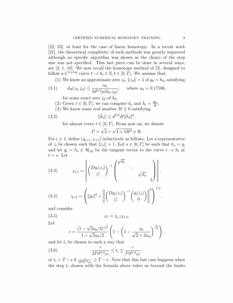
[22, 23], at least for the case of linear homotopy. In a recent work[21], the theoretical complexity of such methods was greatly improvedalthough no specific algorithm was shown as the choice of the stepsize was not specified. This last piece can be done in several ways,see [3, 1, 10]. We now recall the homotopy method of [3], designed tofollow a C1+Lip curve t→ ht ∈ S, t ∈ [0, T ]. We assume that:
(1) We know an approximate zero z0, ‖z0‖ = 1 of g0 = h0, satisfying
(3.1) dR(z0, ζ0) ≤ u0
2d3/2µ(h0, ζ0), where u0 = 0.17586,
for some exact zero ζ0 of h0.(2) Given t ∈ [0, T ], we can compute ht and ht = dht
dt,
(3) We know some real number H ≥ 0 satisfying
(3.2) ‖ht‖ ≤ d3/2H‖ht‖2,
for almost every t ∈ [0, T ]. From now on, we denote
P =√
2 +√
4 + 5H2 ∈ R.For i ≥ 1, define (gi+1, zi+1) inductively as follows. Let a representativeof zi be chosen such that ‖zi‖ = 1. Let s ∈ [0, T ] be such that hs = giand let gi = hs ∈ H(d) be the tangent vector to the curve t → ht att = s. Let
(3.3) χi,1 =
∥∥∥∥∥∥∥∥(Dgi(zi)
z∗i
)−1
√d1
. . . √dn
1
∥∥∥∥∥∥∥∥ ,
(3.4) χi,2 =
‖gi‖2 +
∥∥∥∥∥(Dgi(zi)
z∗i
)−1(gi(zi)
0
)∥∥∥∥∥21/2
,
and consider
(3.5) ϕi = χi,1χi,2.
Let
c =(1−
√2u0/2)
√2
1 +√
2u0/2
(1−
(1− u0√
2 + 2u0
) P√2
),
and let ti be chosen in such a way that
(3.6)c
2Pd3/2ϕi≤ ti ≤
c
Pd3/2ϕi,
or ti = T −s if c2Pd3/2ϕi
≥ T −s. Note that this last case happens when
the step ti chosen with the formula above takes us beyond the limits
10 CARLOS BELTRAN AND ANTON LEYKIN
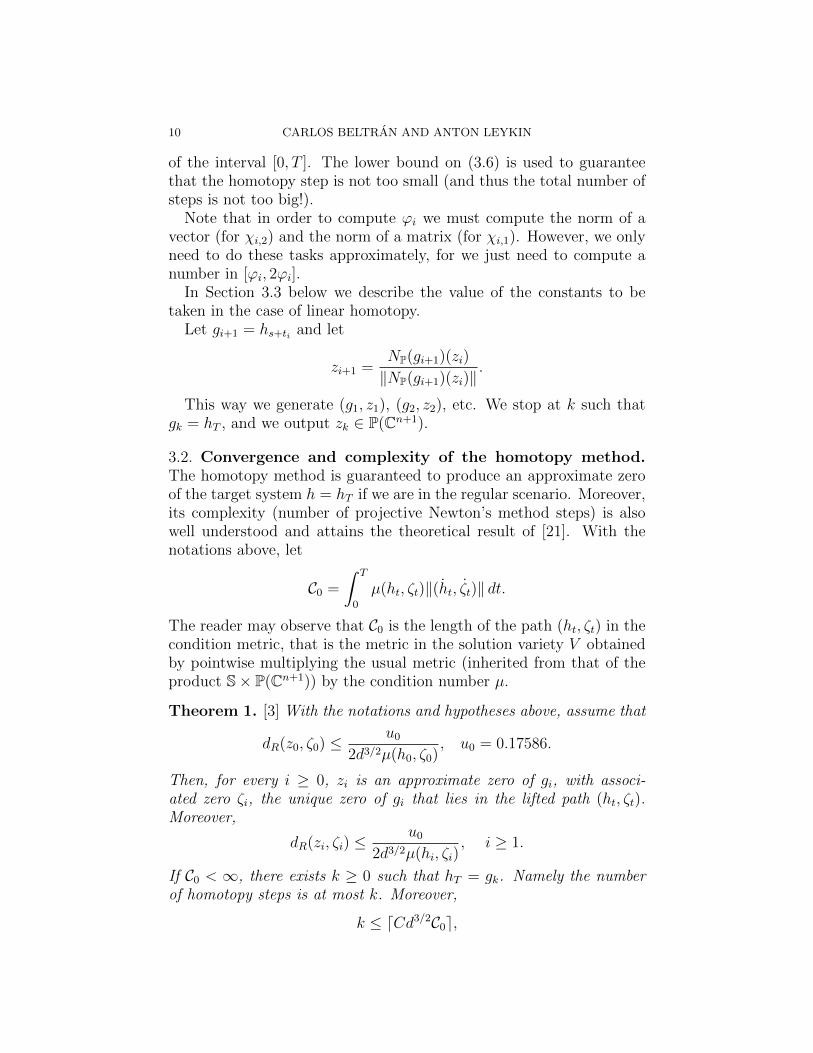
of the interval [0, T ]. The lower bound on (3.6) is used to guaranteethat the homotopy step is not too small (and thus the total number ofsteps is not too big!).
Note that in order to compute ϕi we must compute the norm of avector (for χi,2) and the norm of a matrix (for χi,1). However, we onlyneed to do these tasks approximately, for we just need to compute anumber in [ϕi, 2ϕi].
In Section 3.3 below we describe the value of the constants to betaken in the case of linear homotopy.
Let gi+1 = hs+ti and let
zi+1 =NP(gi+1)(zi)
‖NP(gi+1)(zi)‖.
This way we generate (g1, z1), (g2, z2), etc. We stop at k such thatgk = hT , and we output zk ∈ P(Cn+1).
3.2. Convergence and complexity of the homotopy method.The homotopy method is guaranteed to produce an approximate zeroof the target system h = hT if we are in the regular scenario. Moreover,its complexity (number of projective Newton’s method steps) is alsowell understood and attains the theoretical result of [21]. With thenotations above, let
C0 =
∫ T
0
µ(ht, ζt)‖(ht, ζt)‖ dt.
The reader may observe that C0 is the length of the path (ht, ζt) in thecondition metric, that is the metric in the solution variety V obtainedby pointwise multiplying the usual metric (inherited from that of theproduct S× P(Cn+1)) by the condition number µ.
Theorem 1. [3] With the notations and hypotheses above, assume that
dR(z0, ζ0) ≤ u0
2d3/2µ(h0, ζ0), u0 = 0.17586.
Then, for every i ≥ 0, zi is an approximate zero of gi, with associ-ated zero ζi, the unique zero of gi that lies in the lifted path (ht, ζt).Moreover,
dR(zi, ζi) ≤u0
2d3/2µ(hi, ζi), i ≥ 1.
If C0 < ∞, there exists k ≥ 0 such that hT = gk. Namely the numberof homotopy steps is at most k. Moreover,
k ≤ dCd3/2C0e,
CERTIFIED NUMERICAL HOMOTOPY TRACKING 11
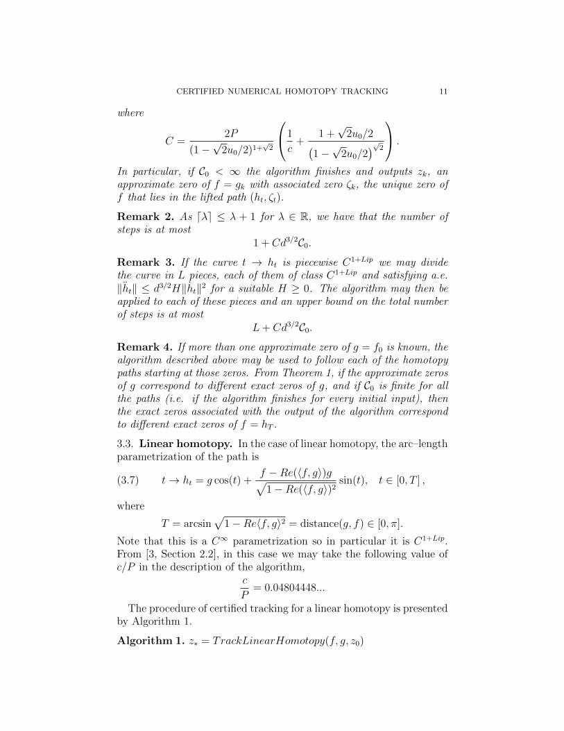
where
C =2P
(1−√
2u0/2)1+√
2
1
c+
1 +√
2u0/2(1−√
2u0/2)√2
.
In particular, if C0 < ∞ the algorithm finishes and outputs zk, anapproximate zero of f = gk with associated zero ζk, the unique zero off that lies in the lifted path (ht, ζt).
Remark 2. As dλe ≤ λ + 1 for λ ∈ R, we have that the number ofsteps is at most
1 + Cd3/2C0.
Remark 3. If the curve t → ht is piecewise C1+Lip we may dividethe curve in L pieces, each of them of class C1+Lip and satisfying a.e.‖ht‖ ≤ d3/2H‖ht‖2 for a suitable H ≥ 0. The algorithm may then beapplied to each of these pieces and an upper bound on the total numberof steps is at most
L+ Cd3/2C0.
Remark 4. If more than one approximate zero of g = f0 is known, thealgorithm described above may be used to follow each of the homotopypaths starting at those zeros. From Theorem 1, if the approximate zerosof g correspond to different exact zeros of g, and if C0 is finite for allthe paths (i.e. if the algorithm finishes for every initial input), thenthe exact zeros associated with the output of the algorithm correspondto different exact zeros of f = hT .
3.3. Linear homotopy. In the case of linear homotopy, the arc–lengthparametrization of the path is
(3.7) t→ ht = g cos(t) +f −Re(〈f, g〉)g√
1−Re(〈f, g〉)2sin(t), t ∈ [0, T ] ,
where
T = arcsin√
1−Re〈f, g〉2 = distance(g, f) ∈ [0, π].
Note that this is a C∞ parametrization so in particular it is C1+Lip.From [3, Section 2.2], in this case we may take the following value ofc/P in the description of the algorithm,
c
P= 0.04804448...
The procedure of certified tracking for a linear homotopy is presentedby Algorithm 1.
Algorithm 1. z∗ = TrackLinearHomotopy(f, g, z0)
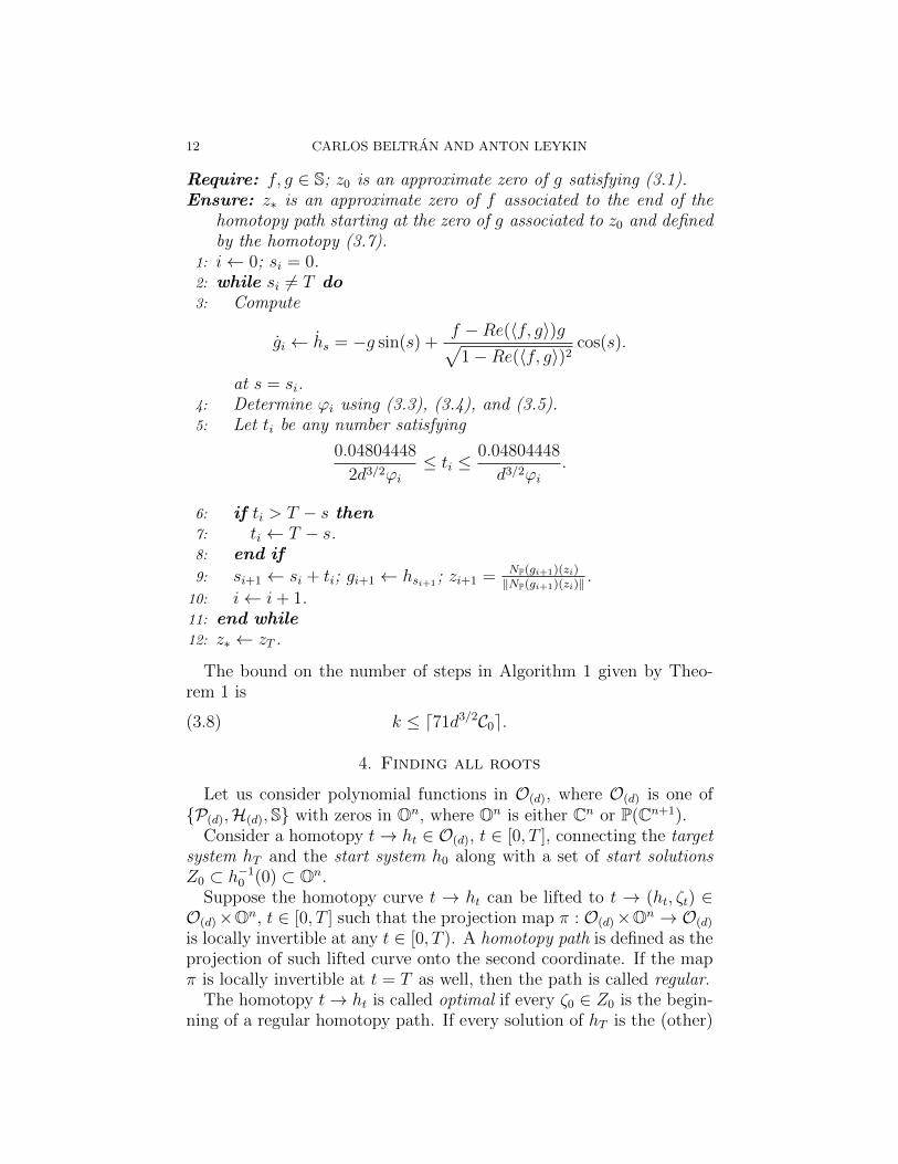
12 CARLOS BELTRAN AND ANTON LEYKIN
Require: f, g ∈ S; z0 is an approximate zero of g satisfying (3.1).Ensure: z∗ is an approximate zero of f associated to the end of the
homotopy path starting at the zero of g associated to z0 and definedby the homotopy (3.7).
1: i← 0; si = 0.2: while si 6= T do3: Compute
gi ← hs = −g sin(s) +f −Re(〈f, g〉)g√
1−Re(〈f, g〉)2cos(s).
at s = si.4: Determine ϕi using (3.3), (3.4), and (3.5).5: Let ti be any number satisfying
0.04804448
2d3/2ϕi≤ ti ≤
0.04804448
d3/2ϕi.
6: if ti > T − s then7: ti ← T − s.8: end if
9: si+1 ← si + ti; gi+1 ← hsi+1; zi+1 = NP(gi+1)(zi)
‖NP(gi+1)(zi)‖ .
10: i← i+ 1.11: end while12: z∗ ← zT .
The bound on the number of steps in Algorithm 1 given by Theo-rem 1 is
(3.8) k ≤ d71d3/2C0e.
4. Finding all roots
Let us consider polynomial functions in O(d), where O(d) is one of{P(d),H(d),S} with zeros in On, where On is either Cn or P(Cn+1).
Consider a homotopy t→ ht ∈ O(d), t ∈ [0, T ], connecting the targetsystem hT and the start system h0 along with a set of start solutionsZ0 ⊂ h−1
0 (0) ⊂ On.Suppose the homotopy curve t → ht can be lifted to t → (ht, ζt) ∈O(d)×On, t ∈ [0, T ] such that the projection map π : O(d)×On → O(d)
is locally invertible at any t ∈ [0, T ). A homotopy path is defined as theprojection of such lifted curve onto the second coordinate. If the mapπ is locally invertible at t = T as well, then the path is called regular.
The homotopy t→ ht is called optimal if every ζ0 ∈ Z0 is the begin-ning of a regular homotopy path. If every solution of hT is the (other)
CERTIFIED NUMERICAL HOMOTOPY TRACKING 13
end of the homotopy path beginning at some ζ0 ∈ Z0 then we call thehomotopy total.
The homotopy method described in Section 3 can also be applied tofollow all homotopy paths of an optimal homotopy in S. Namely, ifwe have a C1+Lip curve t → ht satisfying the hypotheses of Theorem1 and start with approximate zeros Z0 associated to a set of solutionsZ0 ⊂ h−1
0 (0) ⊂ P(Cn+1), then we may perform the algorithm for eachof the initial pairs (h0, z0), z0 ∈ Z0. By Theorem 1, the output will beapproximate zeros associated to ](Z0) distinct solutions of hT .
The area of numerical algebraic geometry (see, e.g., [26]) relies on theability to reliably track optimal homotopies and find all roots of a given0-dimensional polynomial system of equations in O(d). To accomplishthat one has to arrange a total homotopy.
4.1. Total-degree homotopy. For a target system in hT ∈ P(d),(d) = (d1, . . . , dn), define a total degree linear homotopy to be
(4.1) t→ ht = (T − t)h0 + γthT , γ ∈ C∗, t ∈ [0, T ],
where the start system is
(4.2) h0 = (xd11 − 1, . . . , xdnn − 1) ∈ P(d).
There are total degree many, i.e., d1 · · · dn, zeros of h0 that one canreadily write down.
Proposition 4. Assume that hT has a finite number of zeros, and letZ0 be the set of zeros of h0 above. Then for all but finitely many valuesof the constant γ the homotopy (4.1) is total.
If the target system hT ∈ P(d) has total-degree many solutions, then(for a generic γ) the homotopy is optimal.
If the target system hT ∈ P(d) has fewer than total degree manysolutions then:
• some solutions of the target system may be multiple (singular);• in case of On = Cn, some of the homotopy paths may diverge
(to infinity) when approaching t = T .
Remark 5. To compute singular solutions one may track regular ho-motopy paths to t = T − ε for a small ε > 0 (as in Remark 1) and thenuse either singular endgames [26, Section 10.3] or deflation [17, 18].
To avoid diverging paths one may homogenize the homotopy passingfrom P(d) to H(d).
Remark 6. Normalizing an optimal homotopy t → ht with respect tothe Bombieri-Weyl norm brings the system from H(d) to S. In case of a
14 CARLOS BELTRAN AND ANTON LEYKIN
linear homotopy, arc-length re-parametrization enables an applicationof Algorithm 1 for each start solution.
4.2. Other homotopy methods. There are other ways to obtain allsolutions with homotopy continuation that exploit either sparseness orspecial structure of a given polynomial system, here we list a few:
• Polyhedral homotopy continuation based on [13] allows to re-cover all solutions of a sparse polynomial system in the torus(C∗)n.• In many cases presented with a parametric family of polynomial
systems it is enough to solve one system given by a genericchioice of parameters. Then, given another system in the family,the chosen generic system may be used as a start system inthe so-called coefficient-parameter or cheater’s homotopy [26,Chapter 7] recovering all solutions of the latter.• Special homotopies: e.g., Pieri homotopies coming up in Schu-
bert calculus [12] are total and optimal by design.
For the purpose of this paper we assume that some regularization pro-cedure (see Remark 5) has been applied to make these homotopiesoptimal and they are brought to S as in Remark 6 .
5. Random linear homotopy and polynomial time
Suppose, given a regular system f ∈ H(d), we would like to constructan initial pair (g, ζ0) in a random fashion so that every root of f isequally likely to be at the end of the linear homotopy path determinedby this initial pair. A simple solution to this problem would be totake g to be the start system (4.2) of the total-degree homotopy –or its homogenized version – and pick ζ0 from the start solutions withuniform probability distribution on the latter. It has been very recentlyproved by Burgisser and Cucker [1] that this is a pretty good candidatefor the linear homotopy starting pair, as the total average number ofsteps for each path is O(d3Nnd+1) that is O(N log(log(N))), hence closeto polynomial in the input size, mainly when n >> d.
In [5, 6, 7] a probabilistic way to choose the initial pair was proposed.We now center our attention in the most recent of these works [7] whereit is proved that, if the initial pair (g, ζ0) is chosen at random (witha certain probability distribution), then the average number of stepsperformed by the algorithm described in Section 3 is O(d3/2nN), thusalmost linear in the size of the input. It is also proved that in this waywe obtain an approximation of a zero of f , so that each of the zeros off are equiprobable if f has no singular solution. In [8] it is seen that
CERTIFIED NUMERICAL HOMOTOPY TRACKING 15
some higher moments (in particular, the variance) of that algorithmare also polynomial in the size of the input. In this section we describein detail how the process of randomly choosing (g, ζ0) works and werecall the main results of [7, 8].
Given ζ ∈ P(Cn+1), we consider the set
Rζ = {h ∈ H(d) : h(ζ) = 0, Dh(ζ) = 0}.
Note that Rζ is defined as the set of polynomials in H(d) whose co-efficients (in the usual monomial basis) satisfy n2 + 2n linear homo-geneous equalities. Thus, Rζ is a vector subspace of H(d). Moreover,let e0 = (1, 0, . . . , 0)T . Then, Re0 is the set of polynomial systems
h = (h1, . . . , hn) ∈ H(d) such that all the coefficients of hi containing
Xdi0 or Xdi−1
0 are zero, namely
hi = Xdi−20 p2,i(X1, . . . , Xn) +Xdi−3
0 p3,i(X1, . . . , Xn) + · · · ,
where pk,i is a homogeneous polynomial of degree k with unknownsX1, . . . , Xn.
Recall that N + 1 is the (complex) dimension of H(d). The processof choosing (g, ζ0) at random is as follows:
(1) Let (M, l) ∈ Cn2+n × CN+1−n2−n = CN+1 be chosen at randomwith the uniform distribution in
B(CN+1) = {r ∈ CN+1 : ‖r‖2 ≤ 1},
where ‖ · ‖2 is the usual Euclidean norm in CN+1. Thus, M isa (n2 + n)–dimensional complex vector, that we consider as an× (n+ 1) complex matrix. Note that choosing ‖(M, l)‖2 ≤ 1implies that ‖M‖F ≤ 1 and indeed the expected value of ‖M‖2
F
is n2+nN+2
. At this point we can discard l and just keep M . Notethat this procedure is different from just choosing a randommatrix, as it induces a certain distribution in the norm of thematrix which is precisely the one that we are interested in.Hence, choosing (M, l) in the unit ball and then discarding l isnot a fool job!
(2) With probability 1, the choice above has produced a matrixM whose kernel has complex dimension 1. Let ζ0 be a unitnorm element of Ker(M), randomly chosen in Ker(M) withthe uniform distribution (we may just obtain any such ζ0 bysolving Mζ0 = 0 with our preferred method, and then multiplyζ0 by a uniformly chosen random complex number of modulus1). Let V be any unitary matrix such that V ∗ζ0 = e0. Choose
a system h at random in the unit ball (for the Bombieri–Weyl
16 CARLOS BELTRAN AND ANTON LEYKIN
norm) of Re0 . Then, consider h = h ◦ V ∗. (This last procedureis equivalent to choosing a system at random with the uniformdistribution in B(Rζ0) = {h ∈ Rζ0 : ‖h‖ ≤ 1}.)
(3) Let g ∈ H(d) be the polynomial system defined by
g(z) =√
1− ‖M‖2Fh(z) +
〈z, ζ0〉d1−1√d1
. . .
〈z, ζ0〉dn−1√dn
Mz
(4) Let
g =g
‖g‖.
Then, we have chosen (g, ζ0) and the reader may check thatg(ζ0) = 0, so ζ0 is an exact zero of g.
Consider the randomized algorithm defined as follows:
(1) Input f ∈ S(2) Choose (g, ζ0) at random with the process described above(3) Consider the path
t→ ht = g cos(t) +f −Re(〈f, g〉)g√
1−Re(〈f, g〉)2sin(t), t ∈ [0, T ] ,
where T = arcsin√
1−Re〈f, g〉2, and note that h0 = g, hT =f . Use Algorithm 1 to follow the path ht and output an ap-proximate zero of f .
For given f ∈ S, let NS(f) be the expected number of homotopy stepsperformed by this algorithm, on input f ∈ S. We have seen in (3.8)that
NS(f) ≤ d71d3/2C0eThe main theorems of [7, 8] are now summarized as follows.
Theorem 2. If f ∈ S is such that every zero of f is non–singular(thus, f has exactly D = d1 · · · dn projective zeros), then:
• The algorithm above finishes with probability 1 on the choice of(g, ζ0), and• Every zero of f is equally probable as the exact zero associated
with the output of the algorithm (which is an approximate zeroof f).
Assuming f ∈ S is chosen at random with the uniform distribution onS, the expected value and variance of NS(f) satisfy
E(NS(f)) ≤ C1nNd3/2, Var(NS(f)) ≤ C2n
2N2d3 ln(D),
CERTIFIED NUMERICAL HOMOTOPY TRACKING 17
where C1 and C2 are universal constants. One may choose C1 =71π/
√2.
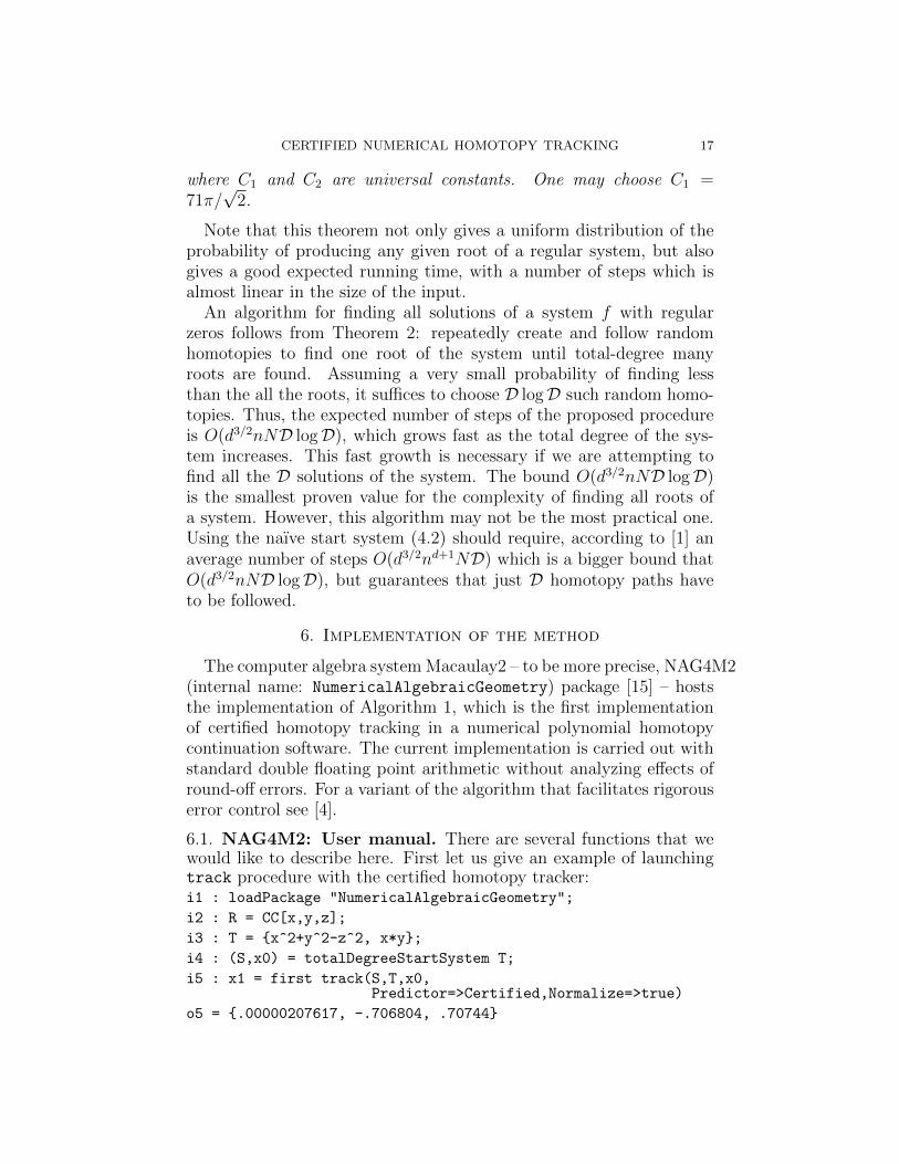
Note that this theorem not only gives a uniform distribution of theprobability of producing any given root of a regular system, but alsogives a good expected running time, with a number of steps which isalmost linear in the size of the input.
An algorithm for finding all solutions of a system f with regularzeros follows from Theorem 2: repeatedly create and follow randomhomotopies to find one root of the system until total-degree manyroots are found. Assuming a very small probability of finding lessthan the all the roots, it suffices to choose D logD such random homo-topies. Thus, the expected number of steps of the proposed procedureis O(d3/2nND logD), which grows fast as the total degree of the sys-tem increases. This fast growth is necessary if we are attempting tofind all the D solutions of the system. The bound O(d3/2nND logD)is the smallest proven value for the complexity of finding all roots ofa system. However, this algorithm may not be the most practical one.Using the naıve start system (4.2) should require, according to [1] anaverage number of steps O(d3/2nd+1ND) which is a bigger bound thatO(d3/2nND logD), but guarantees that just D homotopy paths haveto be followed.
6. Implementation of the method
The computer algebra system Macaulay2 – to be more precise, NAG4M2(internal name: NumericalAlgebraicGeometry) package [15] – hoststhe implementation of Algorithm 1, which is the first implementationof certified homotopy tracking in a numerical polynomial homotopycontinuation software. The current implementation is carried out withstandard double floating point arithmetic without analyzing effects ofround-off errors. For a variant of the algorithm that facilitates rigorouserror control see [4].
6.1. NAG4M2: User manual. There are several functions that wewould like to describe here. First let us give an example of launchingtrack procedure with the certified homotopy tracker:i1 : loadPackage "NumericalAlgebraicGeometry";
i2 : R = CC[x,y,z];
i3 : T = {x^2+y^2-z^2, x*y};
i4 : (S,x0) = totalDegreeStartSystem T;
i5 : x1 = first track(S,T,x0,Predictor=>Certified,Normalize=>true)
o5 = {.00000207617, -.706804, .70744}
18 CARLOS BELTRAN AND ANTON LEYKIN
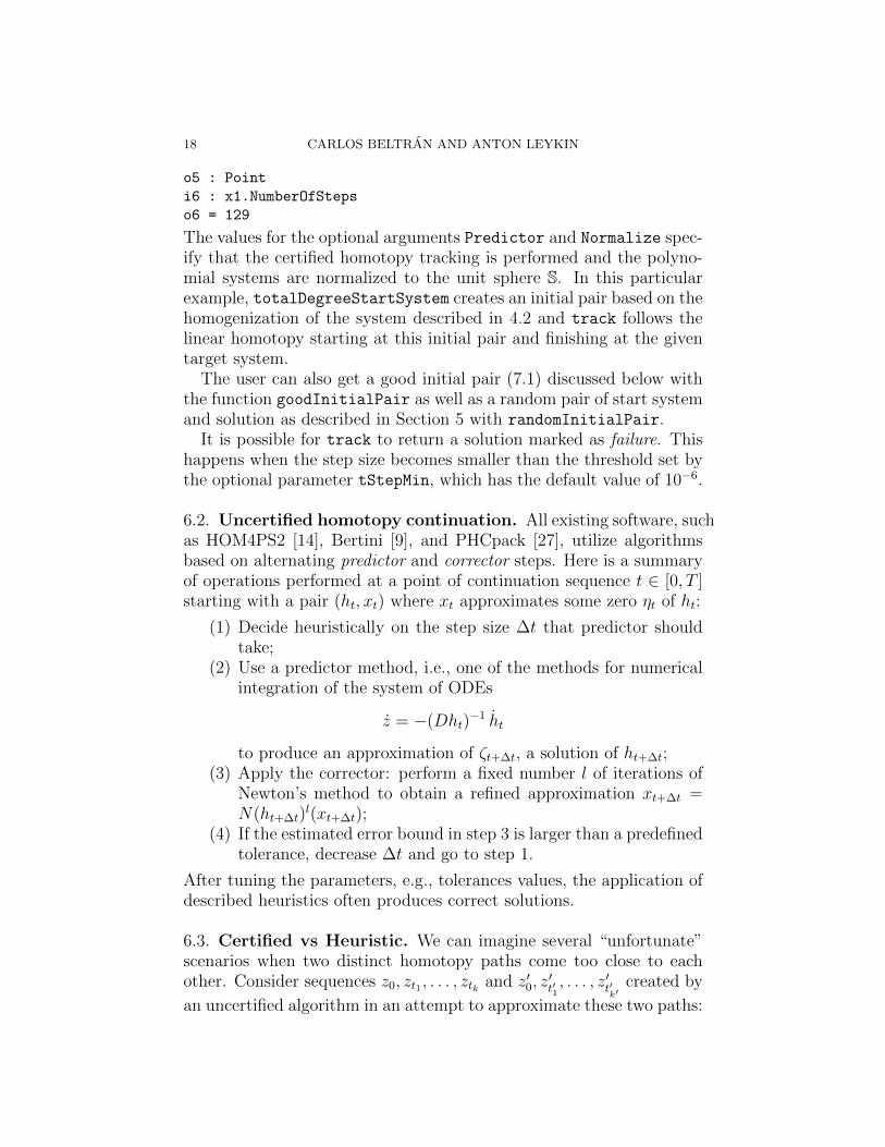
o5 : Point
i6 : x1.NumberOfSteps
o6 = 129
The values for the optional arguments Predictor and Normalize spec-ify that the certified homotopy tracking is performed and the polyno-mial systems are normalized to the unit sphere S. In this particularexample, totalDegreeStartSystem creates an initial pair based on thehomogenization of the system described in 4.2 and track follows thelinear homotopy starting at this initial pair and finishing at the giventarget system.
The user can also get a good initial pair (7.1) discussed below withthe function goodInitialPair as well as a random pair of start systemand solution as described in Section 5 with randomInitialPair.
It is possible for track to return a solution marked as failure. Thishappens when the step size becomes smaller than the threshold set bythe optional parameter tStepMin, which has the default value of 10−6.
6.2. Uncertified homotopy continuation. All existing software, suchas HOM4PS2 [14], Bertini [9], and PHCpack [27], utilize algorithmsbased on alternating predictor and corrector steps. Here is a summaryof operations performed at a point of continuation sequence t ∈ [0, T ]starting with a pair (ht, xt) where xt approximates some zero ηt of ht:
(1) Decide heuristically on the step size ∆t that predictor shouldtake;
(2) Use a predictor method, i.e., one of the methods for numericalintegration of the system of ODEs
z = −(Dht)−1 ht
to produce an approximation of ζt+∆t, a solution of ht+∆t;(3) Apply the corrector: perform a fixed number l of iterations of
Newton’s method to obtain a refined approximation xt+∆t =N(ht+∆t)
l(xt+∆t);(4) If the estimated error bound in step 3 is larger than a predefined
tolerance, decrease ∆t and go to step 1.
After tuning the parameters, e.g., tolerances values, the application ofdescribed heuristics often produces correct solutions.
6.3. Certified vs Heuristic. We can imagine several “unfortunate”scenarios when two distinct homotopy paths come too close to eachother. Consider sequences z0, zt1 , . . . , ztk and z′0, z
′t′1, . . . , z′t′
k′created by
an uncertified algorithm in an attempt to approximate these two paths:
CERTIFIED NUMERICAL HOMOTOPY TRACKING 19
• If there are subsequences in two sequences that approximate apart of the same path then this is referred to as path jumping.• Path crossing happens when the sequences jump from one path
to the other, but there is no common path segment that theyapproximate.
While path jumping can be detected, in principle, a posteriori and thecontinuation rerun with tighter tolerances and smaller step sizes, thepath crossing can not be determined easily.
Path crossing does not result in an incorrect set of target solutions;however, for certain homotopy-based algorithms such as numerical ir-reducible decomposition [25] and applications relying on monodromycomputation such as [16] the order of the target solutions is crucial.Therefore, one not only needs to certify the end points of homotopypaths, but also has to show that the approximating sequences followthe same path from start to finish. The certification of the sequenceproduced in Section 3 provided by Theorem 1 gives such guarantee.
In certain cases the target solutions obtained by means of uncertifiedhomotopy continuation can be rigourously certified after all of them areobtained. For instance, suppose a target system hT ∈ H(d) has distinctregular solutions in P(Cn+1), then there are total degree many of them.Suppose some procedure provides total degree many approximationsto solutions. If a bound on max{µ(hT , ζ) | ζ ∈ h−1
T (0)} is known, thenusing Proposition 2 these approximations may be certified as distinctnumerical zeros, thus certifying that all solutions have been found. Ifno such bound is known, one may still try to prove that the zeros aredifferent by means of Smale’s α–theorem [24] (see [11]). However, theseprocedures do not detect if path crossing has occurred.
7. Experimental results
The developed and implemented algorithm provided us with a chanceto conduct experiments that illuminated several aspects in the complex-ity analysis of solving polynomial systems via homotopy continuation.
7.1. Practicality of certified tracking. Our experiments in this sec-tion were designed to explore how practical the certified tracking pro-vided by Algorithm 1 is. As was already mentioned, the proposed cer-tified procedure makes sense only for a regular homotopy. Moreover, innearly singular examples the certified homotopy is bound to show badperformance due to steps being minuscule at the end of paths, whichis mandated by (3.6).
In the table below we give the data produced by tracking of total-degree homotopy that is optimal for the chosen examples:
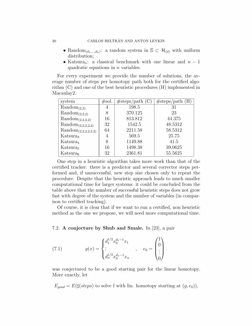
20 CARLOS BELTRAN AND ANTON LEYKIN
• Random(d1,...,dn): a random system in S ⊂ H(d) with uniformdistribution;• Katsuran: a classical benchmark with one linear and n − 1
quadratic equations in n variables.
For every experiment we provide the number of solutions, the av-erage number of steps per homotopy path both for the certified algo-rithm (C) and one of the best heuristic procedures (H) implemented inMacaulay2.
system #sol. #steps/path (C) #steps/path (H)Random(2,2) 4 198.5 31Random(2,2,2) 8 370.125 23Random(2,2,2,2) 16 813.812 44.375Random(2,2,2,2,2) 32 1542.5 48.5312Random(2,2,2,2,2,2) 64 2211.58 58.5312Katsura3 4 569.5 25.75Katsura4 8 1149.88 41.5Katsura5 16 1498.38 39.0625Katsura6 32 2361.81 55.5625
One step in a heuristic algorithm takes more work than that of thecertified tracker: there is a predictor and several corrector steps per-formed and, if unsuccessful, new step size chosen only to repeat theprocedure. Despite that the heuristic approach leads to much smallercomputational time for larger systems: it could be concluded from thetable above that the number of successful heuristic steps does not growfast with degree of the system and the number of variables (in compar-ison to certified tracking).
Of course, it is clear that if we want to run a certified, non heuristicmethod as the one we propose, we will need more computational time.
7.2. A conjecture by Shub and Smale. In [23], a pair
(7.1) g(x) =
d
1/21 xd1−1
0 x1
...
d1/2n xdn−1
0 xn
, e0 =
10...0
.
was conjectured to be a good starting pair for the linear homotopy.More exactly, let
Egood = E(](steps) to solve f with lin. homotopy starting at (g, e0)),
CERTIFIED NUMERICAL HOMOTOPY TRACKING 21
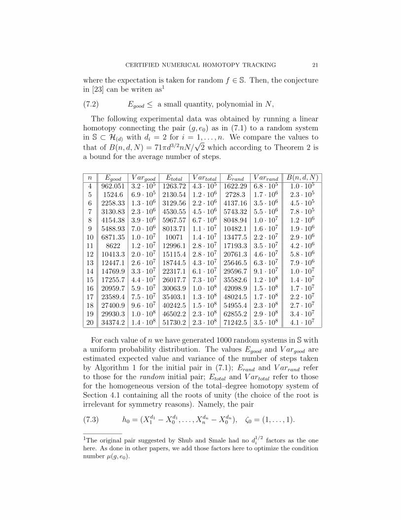
where the expectation is taken for random f ∈ S. Then, the conjecturein [23] can be writen as1
(7.2) Egood ≤ a small quantity, polynomial in N,
The following experimental data was obtained by running a linearhomotopy connecting the pair (g, e0) as in (7.1) to a random systemin S ⊂ H(d) with di = 2 for i = 1, . . . , n. We compare the values to
that of B(n, d,N) = 71πd3/2nN/√
2 which according to Theorem 2 isa bound for the average number of steps.
n Egood V argood Etotal V artotal Erand V arrand B(n, d,N)4 962.051 3.2 · 105 1263.72 4.3 · 105 1622.29 6.8 · 105 1.0 · 105
5 1524.6 6.9 · 105 2130.54 1.2 · 106 2728.3 1.7 · 106 2.3 · 105
6 2258.33 1.3 · 106 3129.56 2.2 · 106 4137.16 3.5 · 106 4.5 · 105
7 3130.83 2.3 · 106 4530.55 4.5 · 106 5743.32 5.5 · 106 7.8 · 105
8 4154.38 3.9 · 106 5967.57 6.7 · 106 8048.94 1.0 · 107 1.2 · 106
9 5488.93 7.0 · 106 8013.71 1.1 · 107 10482.1 1.6 · 107 1.9 · 106
10 6871.35 1.0 · 107 10071 1.4 · 107 13477.5 2.2 · 107 2.9 · 106
11 8622 1.2 · 107 12996.1 2.8 · 107 17193.3 3.5 · 107 4.2 · 106
12 10413.3 2.0 · 107 15115.4 2.8 · 107 20761.3 4.6 · 107 5.8 · 106
13 12447.1 2.6 · 107 18744.5 4.3 · 107 25646.5 6.3 · 107 7.9 · 106
14 14769.9 3.3 · 107 22317.1 6.1 · 107 29596.7 9.1 · 107 1.0 · 107
15 17255.7 4.4 · 107 26017.7 7.3 · 107 35582.6 1.2 · 108 1.4 · 107
16 20959.7 5.9 · 107 30063.9 1.0 · 108 42098.9 1.5 · 108 1.7 · 107
17 23589.4 7.5 · 107 35403.1 1.3 · 108 48024.5 1.7 · 108 2.2 · 107
18 27400.9 9.6 · 107 40242.5 1.5 · 108 54955.4 2.3 · 108 2.7 · 107
19 29930.3 1.0 · 108 46502.2 2.3 · 108 62855.2 2.9 · 108 3.4 · 107
20 34374.2 1.4 · 108 51730.2 2.3 · 108 71242.5 3.5 · 108 4.1 · 107
For each value of n we have generated 1000 random systems in S witha uniform probability distribution. The values Egood and V argood areestimated expected value and variance of the number of steps takenby Algorithm 1 for the initial pair in (7.1); Erand and V arrand referto those for the random initial pair; Etotal and V artotal refer to thosefor the homogeneous version of the total–degree homotopy system ofSection 4.1 containing all the roots of unity (the choice of the root isirrelevant for symmetry reasons). Namely, the pair
(7.3) h0 = (Xd11 −Xd1
0 , . . . , Xdnn −Xdn
0 ), ζ0 = (1, . . . , 1).
1The original pair suggested by Shub and Smale had no d1/2i factors as the one
here. As done in other papers, we add those factors here to optimize the conditionnumber µ(g, e0).
22 CARLOS BELTRAN AND ANTON LEYKIN
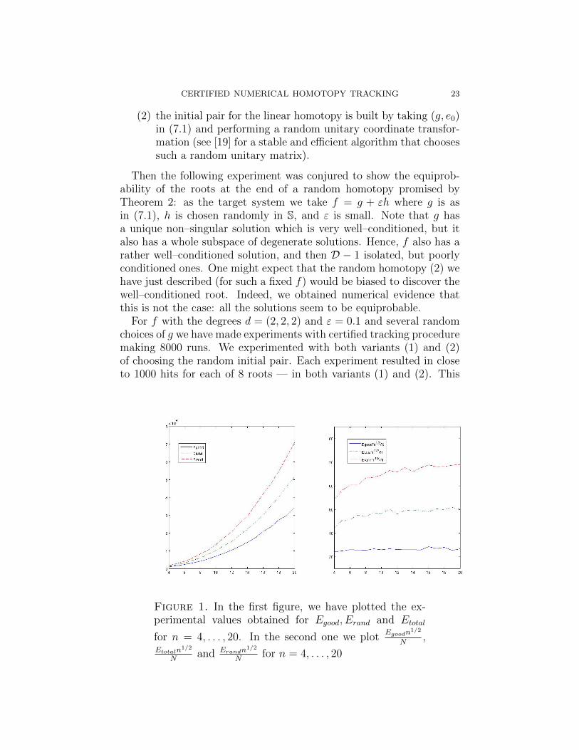
The table above and Figure 1 below suggest two conclusions for thecase of degree two polynomials:
• The random homotopy seems to take approximately doublenumber of steps than the homotopy with initial pair (7.1). Thetotal degree homotopy lies in-between.• The average number of steps in the three cases seem to grow asConstant · N√
nwith Constant ≈ 35, 50, 70 for Egood, Etotal and
Erand respectively.
This experiment thus confirms the conjecture by Shub and Smale andmoreover it suggests a more specific form, suggesting that the samebound given for random homotopy should hold for the conjecturedpair:
(7.4) Egood ≤ CnNd3/2,
with C a constant. We also extend this conjecture to the case of theinitial pair total–degree homotopy pair (h0, ζ0) of Equation (7.3) above:
Etotal ≤ CnNd3/2.
Moreover, as pointed out above, in the case of degree 2 systems, weobtained experimentally a better bound
Egood, Etotal, Erand ≤CN√n,
C a constant. The difference between the experimentally observedvalue and the theoretical bound in the case of randomly chosen initialpairs, respectively O(N/
√n) and O(nN) for (d) = (2, . . . , 2) can be
explained as follows. The proof of the theoretical bound starts bybounding
C0 =
∫ T
0
µ(ht, ζt)‖(ht, ζt)‖ dt ≤√
2
∫ T
0
µ(ht, ζt)2‖ht‖ dt,
which follows from the fact that ‖ζt‖ ≤ µ(ht, ζt)‖ht‖ by the geometricinterpretation of the condition number. This last inequality is notsharp in general, and hence one may expect a better behavior of therandom linear homotopy method than the one given by the theoreticalbound.
7.3. Equiprobable roots via random homotopy. The algorithmconstructing a random homotopy has been implemented in two vari-ants:
(1) as described in Section 5;
CERTIFIED NUMERICAL HOMOTOPY TRACKING 23
(2) the initial pair for the linear homotopy is built by taking (g, e0)in (7.1) and performing a random unitary coordinate transfor-mation (see [19] for a stable and efficient algorithm that choosessuch a random unitary matrix).
Then the following experiment was conjured to show the equiprob-ability of the roots at the end of a random homotopy promised byTheorem 2: as the target system we take f = g + εh where g is asin (7.1), h is chosen randomly in S, and ε is small. Note that g hasa unique non–singular solution which is very well–conditioned, but italso has a whole subspace of degenerate solutions. Hence, f also has arather well–conditioned solution, and then D − 1 isolated, but poorlyconditioned ones. One might expect that the random homotopy (2) wehave just described (for such a fixed f) would be biased to discover thewell–conditioned root. Indeed, we obtained numerical evidence thatthis is not the case: all the solutions seem to be equiprobable.
For f with the degrees d = (2, 2, 2) and ε = 0.1 and several randomchoices of g we have made experiments with certified tracking proceduremaking 8000 runs. We experimented with both variants (1) and (2)of choosing the random initial pair. Each experiment resulted in closeto 1000 hits for each of 8 roots — in both variants (1) and (2). This
Figure 1. In the first figure, we have plotted the ex-perimental values obtained for Egood, Erand and Etotal
for n = 4, . . . , 20. In the second one we plotEgoodn
1/2
N,
Etotaln1/2
Nand Erandn
1/2
Nfor n = 4, . . . , 20
24 CARLOS BELTRAN AND ANTON LEYKIN
appears to show the conclusion of Theorem 2, valid for variant (1), andmoreover extend it to the case of variant (2).
We can state this experimental result in a more precise way, usingShannon’s entropy as suggested in [7]. Assume that we have an al-gorithm that involves some random choice in its input, and that canproduce different outputs x1, . . . , xl. Shannon’s entropy is by definitionthe number
H = −l∑
i=1
pi log2(pi),
where pi is the probability that the output is xi. It is easy to see thatShannon’s entropy of an algorithm is maximal, and equal to log2(l), ifand only if every output is equally probable. The experimental valueof Shannon’s entropy for the random algorithm in all experiments de-scribed above is in the interval [2.99, 3]; the maximum, in this case, islog2 8 = 3.
The exact reason for the modified algorithm (variant (2)) to produceequiprobability of the roots is not understood. This poses a very inter-esting mathematical question, which together with proving (7.4) wouldyield a great progress in the understanding of homotopy methods forsolving systems of polynomial equations.
References
[1] P. Burgisser and F. Cucker, On a problem posed by Steve Smale. Toappear.
[2] L. Blum, F. Cucker, M. Shub, and S. Smale. Complexity and real com-putation, Springer-Verlag, New York, 1998.
[3] C. Beltran. A continuation method to solve polynomial systems, and itscomplexity. Numerische Mathematik. Online first. DOI: 10.1007/s00211-010-0334-3.
[4] Carlos Beltran and Anton Leykin. Robust certified numerical homotopytracking. In preparation, 2010.
[5] C. Beltran and L.M. Pardo. On Smale’s 17th problem: a probabilisticpositive solution. Found. Comput. Math. 8 (2008), no. 1, 1–43.
[6] C. Beltran and L.M. Pardo. Smale’s 17th problem: Average polynomialtime to compute affine and projective solutions. J. Amer. Math. Soc. 22(2009), 363–385.
[7] C. Beltran and L.M. Pardo. Fast linear homotopy to find approximatezeros of polynomial systems. J. Foundations of Computational Mathe-matics. Online first. DOI: 10.1007/s10208-010-9078-9
[8] C. Beltran and M. Shub. A note on the finite variance of the averagingfunction for polynomial system solving. Found. Comput. Math. 10 (2010),115-125.
CERTIFIED NUMERICAL HOMOTOPY TRACKING 25
[9] Daniel J. Bates, Jonathan D. Hauenstein, Andrew J. Sommese, andCharles W. Wampler. Bertini: software for numerical algebraic geom-etry. Available at http://www.nd.edu/∼sommese/bertini.
[10] J-P. Dedieu, G. Malajovich and M. Shub. Adaptavive step size selectionfor homotopy methods to solve polynomial equations. To appear
[11] Jonathan D. Hauenstein and Frank Sottile. ”alphacertified: certifyingsolutions to polynomial systems”. arXiv:1011.1091v1, 2010.
[12] Birkett Huber, Frank Sottile, and Bernd Sturmfels. Numerical Schubertcalculus. J. Symbolic Comput., 26(6):767–788, 1998. Symbolic numericalgebra for polynomials.
[13] Birkett Huber and Bernd Sturmfels. A polyhedral method for solvingsparse polynomial systems. Math. Comp., 64(212):1541–1555, 1995.
[14] T. L. Lee, T. Y. Li, and C. H. Tsai. Hom4ps-2.0: A software packagefor solving polynomial systems by the polyhedral homotopy continuationmethod. Available at http://hom4ps.math.msu.edu/HOM4PS soft.htm.
[15] Anton Leykin. Numerical algebraic geometry for Macaulay2. Preprint:arXiv:0911.1783, 2009.
[16] Anton Leykin and Frank Sottile. Galois groups of Schubert problems viahomotopy computation. Math. Comp., 78(267):1749–1765, 2009.
[17] Anton Leykin, Jan Verschelde, and Ailing Zhao. Newton’s method withdeflation for isolated singularities of polynomial systems. TheoreticalComputer Science, 359(1-3):111–122, 2006.
[18] Anton Leykin, Jan Verschelde, and Ailing Zhao. Higher-order deflationfor polynomial systems with isolated singular solutions. In Algorithms inalgebraic geometry, volume 146 of IMA Vol. Math. Appl., pages 79–97.Springer, New York, 2008.
[19] Francesco Mezzadri How to generate random matrices from the classicalcompact groups. In Notices of the American Mathematical Society 54(2007), no. 5, 592–604.
[20] M. Shub. Some remarks on Bezout’s theorem and complexity theory,From Topology to Computation: Proceedings of the Smalefest (Berkeley,CA, 1990) (New York), Springer, 1993, pp. 443–455.
[21] M. Shub. Complexity of Bezout’s theorem. VI: Geodesics in the condition(number) metric. Found. Comput. Math. 9 (2009), no. 2, 171–178.
[22] M. Shub and S. Smale. Complexity of Bezout’s theorem. I. Geometricaspects, J. Amer. Math. Soc. 6 (1993), no. 2, 459–501.
[23] M. Shub and S. Smale. Complexity of Bezout’s theorem. V. Polynomialtime, Theoret. Comput. Sci. 133 (1994), no. 1, 141–164, Selected papersof the Workshop on Continuous Algorithms and Complexity (Barcelona,1993).
[24] S. Smale. Newton’s method estimates from data at one point, The merg-ing of disciplines: new directions in pure, applied, and computationalmathematics (Laramie, Wyo., 1985), Springer, New York, 1986, pp. 185–196.
[25] A.J. Sommese, J. Verschelde, and C.W. Wampler. Numerical decompo-sition of the solution sets of polynomial systems into irreducible compo-nents. SIAM J. Numer. Anal., 38(6):2022–2046, 2001.

26 CARLOS BELTRAN AND ANTON LEYKIN
[26] Andrew J. Sommese and Charles W. Wampler, II. The numerical solutionof systems of polynomials. World Scientific Publishing Co. Pte. Ltd.,Hackensack, NJ, 2005.
[27] J. Verschelde. Algorithm 795: PHCpack: A general-purposesolver for polynomial systems by homotopy continuation.ACM Trans. Math. Softw., 25(2):251–276, 1999. Available athttp://www.math.uic.edu/∼jan.
[28] K. Zyczkowski and M. Kus. Random unitary matrices. (English sum-mary), J. Phys. A 133 (1994), no. 27, 4235–4245, 1994.